551
✐ ✐ “Compute60” — 2011/12/20 — 14:27 — page i — #1 ✐ ✐ ✐ Doing Mathematics with Scientic WorkPlace R ⃝ & Scientic Notebook R ⃝ Version 6 by Darel Hardy & Carol Walker
| Date post: | 14-Mar-2023 |
| Category: |
Documents |
| Upload: | khangminh22 |
| View: | 0 times |
| Download: | 0 times |
ii
“Compute60” — 2011/12/20 — 14:27 — page i — #1 ii
ii
ii
DoingMathematicswith Scienti c WorkPlace
R⃝
& Scienti c NotebookR⃝
Version 6
by Darel Hardy& Carol Walker
ii
“Compute60” — 2011/12/20 — 14:27 — page ii — #2 ii
ii
ii
Copyright ©2011 by MacKichan So ware, Inc. All rights reserved. No part ofthis book may be reproduced, stored in a retrieval system, or transcribed, in anyform or by any means–electronic, mechanical, photocopying, recording, orotherwise–without the prior written permission of the publisher, MacKichanSo ware, Inc., Poulsbo, Washington, USA. Information in this document issubject to change without notice and does not represent a commitment on thepart of the publisher. e so ware described in this document is furnished undera license agreement and may be used or copied only in accordance with the termsof the agreement. It is against the law to copy the so ware on any medium exceptas speci cally allowed in the agreement.
Printed in the United States of America10 9 8 7 6 5 4 3 2 1
TrademarksScienti c WorkPlace, Scienti c Word, Scienti c Notebook, and EasyMath areregistered trademarks of MacKichan So ware, Inc. EasyMath is the sophisticatedparsing and translating system included in Scienti c WorkPlace, Scienti c Word,and Scienti c Notebook that allows the user to work in standard mathematicalnotation, request computations from the underlying computational system(MuPAD 5 in this version) based on the implied commands embedded in themathematical syntax or via menu, and receive the response in typeset standardnotation or graphic form in the current document. MuPad is a registeredtrademark of SciFace GmbH & Co. KG. Acrobat is a registered trademark ofAdobe Systems, Inc. TEX is a trademark of the American Mathematical Society.pdfTEX is the copyright of Hàn ế ành and is available under the GNUpublic license. VCam is based on VRS, which is a product developed by HassoPlattner Institute of the University of Potsdam. Windows is a registeredtrademark of the Microso Corporation. Macintosh is a registered trademark ofthe Apple Corporation. Linux is a registered trademark of Linus Torvalds. RLMis a registered trademark of Reprise So ware. Activation system licensed underpatent No. 5,490,216. All other brand and product names are trademarks of theirrespective companies.
is document was produced with Scienti c WorkPlace. R⃝
Authors:Darel Hardy and Carol WalkerManuscript Editor: JohnMacKendrickCompositor:MacKichan So ware Inc.Designer: Patti KearneyPrinting and Binding: Malloy Lithographing, Inc.
ii
“Compute60” — 2011/12/20 — 14:27 — page iii — #3 ii
ii
ii
Contents
1 Basic Techniques for Doing Mathematics . . . . . . . . . . . . . . . . . . . 1
Conventions. . . . . . . . . . . . . . . . . . . . . . . . . . . . . . . . . . . . . . . . . . . . . . . . . . . . . . . . 2Inserting Text and Mathematics . . . . . . . . . . . . . . . . . . . . . . . . . . . . . . . 3Basic Guidelines for Computing . . . . . . . . . . . . . . . . . . . . . . . . . . . . . . 7
2 Numbers, Functions, and Units . . . . . . . . . . . . . . . . . . . . . . . . . . . . . . . . 19
Integers and Fractions. . . . . . . . . . . . . . . . . . . . . . . . . . . . . . . . . . . . . . . . . . . . 19Elementary Number eory. . . . . . . . . . . . . . . . . . . . . . . . . . . . . . . . . . . . 21Real Numbers . . . . . . . . . . . . . . . . . . . . . . . . . . . . . . . . . . . . . . . . . . . . . . . . . . . . . . 23Functions and Relations . . . . . . . . . . . . . . . . . . . . . . . . . . . . . . . . . . . . . . . . . 27Complex Numbers. . . . . . . . . . . . . . . . . . . . . . . . . . . . . . . . . . . . . . . . . . . . . . . . 32Units and Measurements . . . . . . . . . . . . . . . . . . . . . . . . . . . . . . . . . . . . . . . . 33Exercises . . . . . . . . . . . . . . . . . . . . . . . . . . . . . . . . . . . . . . . . . . . . . . . . . . . . . . . . . . . . . 36
3 Algebra . . . . . . . . . . . . . . . . . . . . . . . . . . . . . . . . . . . . . . . . . . . . . . . . . . . . . . . . . . . . . . . . 39
Polynomials and Rational Expressions. . . . . . . . . . . . . . . . . . . . . . . 39Substitution . . . . . . . . . . . . . . . . . . . . . . . . . . . . . . . . . . . . . . . . . . . . . . . . . . . . . . . . 47Solving Equations . . . . . . . . . . . . . . . . . . . . . . . . . . . . . . . . . . . . . . . . . . . . . . . . . 48De ning Variables and Functions . . . . . . . . . . . . . . . . . . . . . . . . . . . . . 59Exponents and Logarithms . . . . . . . . . . . . . . . . . . . . . . . . . . . . . . . . . . . . . 65Toolbars and Keyboard Shortcuts . . . . . . . . . . . . . . . . . . . . . . . . . . . . 69Exercises . . . . . . . . . . . . . . . . . . . . . . . . . . . . . . . . . . . . . . . . . . . . . . . . . . . . . . . . . . . . . 70
iii
ii
“Compute60” — 2011/12/20 — 14:27 — page iv — #4 ii
ii
ii
Contents
4 Trigonometry . . . . . . . . . . . . . . . . . . . . . . . . . . . . . . . . . . . . . . . . . . . . . . . . . . . . . . . . 75
Trigonometric Functions. . . . . . . . . . . . . . . . . . . . . . . . . . . . . . . . . . . . . . . . 75Trigonometric Identities. . . . . . . . . . . . . . . . . . . . . . . . . . . . . . . . . . . . . . . . . 80Inverse Trigonometric Functions. . . . . . . . . . . . . . . . . . . . . . . . . . . . . . 83Hyperbolic Functions . . . . . . . . . . . . . . . . . . . . . . . . . . . . . . . . . . . . . . . . . . . . 86Complex Numbers and Complex Functions . . . . . . . . . . . . . . . 89Exercises . . . . . . . . . . . . . . . . . . . . . . . . . . . . . . . . . . . . . . . . . . . . . . . . . . . . . . . . . . . . . 93
5 Function De nitions . . . . . . . . . . . . . . . . . . . . . . . . . . . . . . . . . . . . . . . . . . . . . . 99
Function and Expression Names . . . . . . . . . . . . . . . . . . . . . . . . . . . . . . 99De ning Variables and Functions . . . . . . . . . . . . . . . . . . . . . . . . . . . . .103Handling De nitions . . . . . . . . . . . . . . . . . . . . . . . . . . . . . . . . . . . . . . . . . . . .115Formulas . . . . . . . . . . . . . . . . . . . . . . . . . . . . . . . . . . . . . . . . . . . . . . . . . . . . . . . . . . . .115External Functions . . . . . . . . . . . . . . . . . . . . . . . . . . . . . . . . . . . . . . . . . . . . . . . .119Trigtype Functions. . . . . . . . . . . . . . . . . . . . . . . . . . . . . . . . . . . . . . . . . . . . . . . .122Exercises . . . . . . . . . . . . . . . . . . . . . . . . . . . . . . . . . . . . . . . . . . . . . . . . . . . . . . . . . . . . .124
6 Plotting Curves and Surfaces . . . . . . . . . . . . . . . . . . . . . . . . . . . . . . . . . . .129
Getting Started With 2D Plots . . . . . . . . . . . . . . . . . . . . . . . . . . . . . . . .130Interactive Tools for 2D Plots . . . . . . . . . . . . . . . . . . . . . . . . . . . . . . . . . .138Graph User Settings . . . . . . . . . . . . . . . . . . . . . . . . . . . . . . . . . . . . . . . . . . . . . .1402D Plots of Functions and Expressions . . . . . . . . . . . . . . . . . . . . . .151Creating Animated 2D Plots . . . . . . . . . . . . . . . . . . . . . . . . . . . . . . . . . . .165Creating 3D Plots . . . . . . . . . . . . . . . . . . . . . . . . . . . . . . . . . . . . . . . . . . . . . . . . .171Creating Animated 3D Plots . . . . . . . . . . . . . . . . . . . . . . . . . . . . . . . . . . .189Exercises . . . . . . . . . . . . . . . . . . . . . . . . . . . . . . . . . . . . . . . . . . . . . . . . . . . . . . . . . . . . .196
7 Calculus . . . . . . . . . . . . . . . . . . . . . . . . . . . . . . . . . . . . . . . . . . . . . . . . . . . . . . . . . . . . . . .201
Evaluating Calculus Expressions. . . . . . . . . . . . . . . . . . . . . . . . . . . . . . .201Limits . . . . . . . . . . . . . . . . . . . . . . . . . . . . . . . . . . . . . . . . . . . . . . . . . . . . . . . . . . . . . . . .202Differentiation .. . . . . . . . . . . . . . . . . . . . . . . . . . . . . . . . . . . . . . . . . . . . . . . . . . . .209Inde nite Integration . . . . . . . . . . . . . . . . . . . . . . . . . . . . . . . . . . . . . . . . . . . .226Methods of Integration . . . . . . . . . . . . . . . . . . . . . . . . . . . . . . . . . . . . . . . . . .228De nite Integrals. . . . . . . . . . . . . . . . . . . . . . . . . . . . . . . . . . . . . . . . . . . . . . . . . .231Sequences and Series . . . . . . . . . . . . . . . . . . . . . . . . . . . . . . . . . . . . . . . . . . . . .260Multivariable Calculus. . . . . . . . . . . . . . . . . . . . . . . . . . . . . . . . . . . . . . . . . . .268Exercises . . . . . . . . . . . . . . . . . . . . . . . . . . . . . . . . . . . . . . . . . . . . . . . . . . . . . . . . . . . . .277
iv
ii
“Compute60” — 2011/12/20 — 14:27 — page v — #5 ii
ii
ii
8 Matrix Algebra . . . . . . . . . . . . . . . . . . . . . . . . . . . . . . . . . . . . . . . . . . . . . . . . . . . . . .285
Creating and Editing Matrices . . . . . . . . . . . . . . . . . . . . . . . . . . . . . . . . .286Standard Operations . . . . . . . . . . . . . . . . . . . . . . . . . . . . . . . . . . . . . . . . . . . . .294Row Operations and Echelon Forms. . . . . . . . . . . . . . . . . . . . . . . . .298Equations . . . . . . . . . . . . . . . . . . . . . . . . . . . . . . . . . . . . . . . . . . . . . . . . . . . . . . . . . . .301Matrix Operators. . . . . . . . . . . . . . . . . . . . . . . . . . . . . . . . . . . . . . . . . . . . . . . . . .307Polynomials and Vectors Associated with a Matrix . . . . . . .317Vector Spaces Associated with a Matrix . . . . . . . . . . . . . . . . . . . . .321Normal Forms of Matrices . . . . . . . . . . . . . . . . . . . . . . . . . . . . . . . . . . . . . .326Matrix Decompositions . . . . . . . . . . . . . . . . . . . . . . . . . . . . . . . . . . . . . . . . .334Exercises . . . . . . . . . . . . . . . . . . . . . . . . . . . . . . . . . . . . . . . . . . . . . . . . . . . . . . . . . . . . .337
9 Vector Calculus . . . . . . . . . . . . . . . . . . . . . . . . . . . . . . . . . . . . . . . . . . . . . . . . . . . . .341
Vectors . . . . . . . . . . . . . . . . . . . . . . . . . . . . . . . . . . . . . . . . . . . . . . . . . . . . . . . . . . . . . . .341Gradient, Divergence, Curl, and Related Operators. . . . . .358Plots of Vector Fields and Gradients . . . . . . . . . . . . . . . . . . . . . . . . .363Scalar and Vector Potentials . . . . . . . . . . . . . . . . . . . . . . . . . . . . . . . . . . . .372Matrix-Valued Operators . . . . . . . . . . . . . . . . . . . . . . . . . . . . . . . . . . . . . . . .375Plots of Complex Functions . . . . . . . . . . . . . . . . . . . . . . . . . . . . . . . . . . . .379Exercises . . . . . . . . . . . . . . . . . . . . . . . . . . . . . . . . . . . . . . . . . . . . . . . . . . . . . . . . . . . . .381
10 Differential Equations . . . . . . . . . . . . . . . . . . . . . . . . . . . . . . . . . . . . . . . . . . . .385
Ordinary Differential Equations . . . . . . . . . . . . . . . . . . . . . . . . . . . . . .385Systems . . . . . . . . . . . . . . . . . . . . . . . . . . . . . . . . . . . . . . . . . . . . . . . . . . . . . . . . . . . . . .397Numerical Methods . . . . . . . . . . . . . . . . . . . . . . . . . . . . . . . . . . . . . . . . . . . . . .400Exercises . . . . . . . . . . . . . . . . . . . . . . . . . . . . . . . . . . . . . . . . . . . . . . . . . . . . . . . . . . . . .407
11 Statistics. . . . . . . . . . . . . . . . . . . . . . . . . . . . . . . . . . . . . . . . . . . . . . . . . . . . . . . . . . . . . . .409
Introduction to Statistics . . . . . . . . . . . . . . . . . . . . . . . . . . . . . . . . . . . . . . . .409Measures of Central Tendency. . . . . . . . . . . . . . . . . . . . . . . . . . . . . . . . .411Measures of Dispersion . . . . . . . . . . . . . . . . . . . . . . . . . . . . . . . . . . . . . . . . . .416Distributions and Densities . . . . . . . . . . . . . . . . . . . . . . . . . . . . . . . . . . . .421Families of Continuous Distributions . . . . . . . . . . . . . . . . . . . . . . .423Families of Discrete Distributions . . . . . . . . . . . . . . . . . . . . . . . . . . . .432Random Numbers . . . . . . . . . . . . . . . . . . . . . . . . . . . . . . . . . . . . . . . . . . . . . . . .435Curve Fitting . . . . . . . . . . . . . . . . . . . . . . . . . . . . . . . . . . . . . . . . . . . . . . . . . . . . . . .436Exercises . . . . . . . . . . . . . . . . . . . . . . . . . . . . . . . . . . . . . . . . . . . . . . . . . . . . . . . . . . . . .440
v
ii
“Compute60” — 2011/12/20 — 14:27 — page vi — #6 ii
ii
ii
Contents
12 Applied Modern Algebra. . . . . . . . . . . . . . . . . . . . . . . . . . . . . . . . . . . . . . . . .445
Solving Equations . . . . . . . . . . . . . . . . . . . . . . . . . . . . . . . . . . . . . . . . . . . . . . . . .445Integers Modulo m .. . . . . . . . . . . . . . . . . . . . . . . . . . . . . . . . . . . . . . . . . . . . . .448Other Systems Modulo m.. . . . . . . . . . . . . . . . . . . . . . . . . . . . . . . . . . . . . .454Polynomials Modulo Polynomials . . . . . . . . . . . . . . . . . . . . . . . . . . . .456Linear Programming .. . . . . . . . . . . . . . . . . . . . . . . . . . . . . . . . . . . . . . . . . . . .463Exercises . . . . . . . . . . . . . . . . . . . . . . . . . . . . . . . . . . . . . . . . . . . . . . . . . . . . . . . . . . . . .466
A Menus and Shortcuts for Doing Mathematics . . . . . . . . . . . . .473
Compute Menu .. . . . . . . . . . . . . . . . . . . . . . . . . . . . . . . . . . . . . . . . . . . . . . . . . .473Toolbar and Keyboard Shortcuts for Compute Menu .. .488
B Menus and Shortcuts for Entering Mathematics . . . . . . . . . .489
Entering Mathematics and Text . . . . . . . . . . . . . . . . . . . . . . . . . . . . . . .490Entering Mathematical Objects . . . . . . . . . . . . . . . . . . . . . . . . . . . . . . .491Entering Symbols and Characters . . . . . . . . . . . . . . . . . . . . . . . . . . . . .492Entering Units of Measure . . . . . . . . . . . . . . . . . . . . . . . . . . . . . . . . . . . . . .496
C Customizing the Program for Computing . . . . . . . . . . . . . . . . . .505
Customizing the Toolbars . . . . . . . . . . . . . . . . . . . . . . . . . . . . . . . . . . . . . .506Customizing the Sidebars . . . . . . . . . . . . . . . . . . . . . . . . . . . . . . . . . . . . . . .507Customizing the Compute Settings . . . . . . . . . . . . . . . . . . . . . . . . . .507Customizing the Plot Settings . . . . . . . . . . . . . . . . . . . . . . . . . . . . . . . . .511Automatic Substitution. . . . . . . . . . . . . . . . . . . . . . . . . . . . . . . . . . . . . . . . . .512
D MuPAD Functions and Expressions . . . . . . . . . . . . . . . . . . . . . . . . . .515
Constants . . . . . . . . . . . . . . . . . . . . . . . . . . . . . . . . . . . . . . . . . . . . . . . . . . . . . . . . . . .515Compute Menu Items. . . . . . . . . . . . . . . . . . . . . . . . . . . . . . . . . . . . . . . . . . . .516Functions and Expressions . . . . . . . . . . . . . . . . . . . . . . . . . . . . . . . . . . . . . .522
Index . . . . . . . . . . . . . . . . . . . . . . . . . . . . . . . . . . . . . . . . . . . . . . . . . . . . . . . . . . . . . . . . . . .527
vi
ii
“Compute60” — 2011/12/20 — 14:27 — page vii — #7 ii
ii
ii
Preface
How can it be that mathematics, being after all a product of human thought independent of experience, is so admirably adapted to theobjects of reality? Albert Einstein (1879–1955)
W elcome to Version 6 of Scienti c WorkPlace and Scienti c About Scienti c WorkPlace andScienti c Notebook
Technical Support
Notebook. ese programshave always provided easy text-entry, natural-notation mathematics, powerful symbolic
and numeric computation, and exible output of online, printed, andtypeset documents in aWindows environment. WithVersion 6, thesefeatures are available for Linux and Mac OS/X users as well. With itsentirely newMozilla-based architecture, Version 6 providesmore ex-ibility for your workplace. You can save or export your documents inmultiple formats according to your publication and portability needs.
About Scienti c WorkPlace and Scienti c Notebooke two products Scienti cWorkPlace and Scienti cNotebook pro- New in Version 6
MuPAD 5 computer algebra systemSmoother plotsCustomizable toolbarsOptional sidebarsUndo multiple changes
vide a free-form interface to a computer algebra system that is inte-grated with a scienti c word processor. e essential components ofthis interface are ee-form editing and natural mathematical notation.Scienti cWorkPlace and Scienti c Notebookmake sense out of as manydifferent forms as possible, rather than requiring the user to adhere toa rigid syntax or just one way of writing an expression.
vii
ii
“Compute60” — 2011/12/20 — 14:27 — page viii — #8 ii
ii
ii
Preface
ey are designed to t the needs of a wide range of users, fromthe beginning student trying to solve a linear equation to the profes-sional scientist whowants to produce typeset-quality documents withembedded advanced mathematical calculations. e text editors inScienti c WorkPlace and Scienti c Notebook accept mathematical for-mulas and equations entered in natural notation. e symbolic com-putation system produces mathematical output inside the documentthat is formatted in natural notation, can be edited, and can be useddirectly as input to subsequent mathematical calculations.
e computational components of Scienti c WorkPlace and Sci-enti c Notebook use a MuPAD engine. All versions use standard li-braries furnished by SciFace So ware. Scienti c WorkPlace and Scien-ti c Notebook provide easy, direct access to all themathematics neededby many users. For the user familiar with MuPAD, they also allowaccess to the full range of MuPAD functions and to functions pro-grammed inMuPAD.By providing an interface with little or no learn-ing cost, Scienti c WorkPlace and Scienti c Notebook make symboliccomputation as accessible as any word processor. Students can use Scienti c Notebook as an
experimental mathematics lab and to createclear, well-written homework and reports.
Scienti cWorkPlace and Scienti c Notebook have great potential ineducational settings. In a classroom equipped with appropriate pro-jection equipment, the program’s ease of use and its combination of afree-form scienti c word processor and computational package makeit a natural replacement for the chalkboard. You can use it in the sameways you would a chalkboard and you have the added advantage ofthe computational system. You do not need to erase as you go along,so previous work can be recalled. Class notes can be edited and madeavailable for viewing on line or printed. Scienti c WorkPlace and Sci-enti c Notebook provide a ready laboratory in which students can ex-periment with mathematics to develop new insights and to solve in-teresting problems; they also provide a vehicle for students to produceclear, well-written homework.
is document,DoingMathematics with Scienti c WorkPlace andScienti c Notebook, describes the use of the underlying computer al-gebra system for doing mathematical calculations. In particular, it ex-plains how to use the built-in computer algebra system MuPAD to doa wide range of mathematics without dealing directly with MuPADsyntax.
is document is organized around standard topics in the under-graduate mathematics curriculum. Users can nd the guidance theyneed without going to chapters involving mathematics beyond their
viii
ii
“Compute60” — 2011/12/20 — 14:27 — page ix — #9 ii
ii
ii
current level. e rst four chapters introduce basic procedures forusing the system and cover the content of the standard precalculuscourses. Later chapters cover analytic geometry and calculus, linearalgebra, vector analysis, differential equations, statistics, and appliedmodern algebra. Exercises are provided to encourage users to practicethe ideas presented and to explore possibilities beyond those coveredin this document.
Users with an interest in doing mathematical calculations are ad-vised to read and experiment with the rst ve chapters—Basic Tech-niques for Doing Mathematics; Numbers, Functions, and Units; Alge-bra; Trigonometry; and Function De nitions—which provide a goodfoundation for doing mathematical calculations. You may also nd ithelpful to read parts of the sixth chapter Plotting Curves and Surfacesto get started creating plots. You can approach the remaining chaptersin any order. In addition to the built-in links to MuPAD, users
familiar with MuPAD can now access MuPADdirectly by using Passthru Code to Engine.
Experienced MuPAD users will nd it helpful to read about ac-cessingotherMuPADfunctions and addinguser-de nedMuPADfunc-tions in Appendix D, “MuPAD Functions and Expressions.” You willalsowant to refer to the tables in that chapter that pairMuPADnameswith Scienti c WorkPlace and Scienti c Notebook names for constants,functions, and operations.
For information on the document-editing features of your system,refer to the onlineHelp or to the document,Creating Documents withScienti c Word and Scienti c WorkPlace.
Technical SupportIf you can’t nd the answer to your questions in themanuals or the
online Help, you can obtain technical support from the website at
http://www.mackichan.com/support.htm
or at the Web-based Technical Support forum at
http://www.mackichan.com/forum.htm
You can also contact theTechnical Support staffby email or telephone.We urge you to submit questions by email whenever possible in casethe technical staff needs to obtain your le to diagnose and solve theproblem.
Whenyou contactTechnical Support by email, please provide com-plete information about the problem you’re trying to solve. eymust
ix
ii
“Compute60” — 2011/12/20 — 14:27 — page x — #10 ii
ii
ii
Preface
be able to reproduce theproblemexactly fromyour instructions. Whenyou contact themby telephone, you shouldbe sitting at your computerwith the program running.
Please be prepared to provide the following information any timeyou contact Technical Support:
• e MacKichan So ware product you have installed.
• e version and build numbers of your installation (see Help /About).
• e serial number of your installation (see Help / System Fea-tures).
• e type of hardware and operating system you’re using, (e.g.,Windows 7, Mac OS X Leopard, Ubuntu 10.10, openSUSE11.3, etc.).
• What happened and what you were doing when the problemoccurred.
• e exact wording of any messages that appeared on your com-puter screen.
Tocontact technical support• Contact Technical Support by email or telephone between 8
and 5 Paci c Time:
Internet electronic mail address: [email protected] number: 360-394-6033
Toll-free telephone: 877-SCI-WORD (877-724-9673)Fax number: 360-394-6039
You can learn more about Scienti cWorkPlace and Scienti c Note-book on the MacKichan web site, which is updated regularly to pro-vide the latest technical information about the program. e site alsohouses links to other TEX and LATEX resources. ere is also an un-moderated discussion forum and an unmoderated email list so userscan share information, discuss commonproblems, and contribute tech-nical tips and solutions. You can link to these valuable resources fromthe home page at http://www.mackichan.com.
Darel W. HardyCarol L . Walker
x
ii
“Compute60” — 2011/12/20 — 14:27 — page 1 — #11 ii
ii
ii
1Basic Techniques
for Doing Mathematics
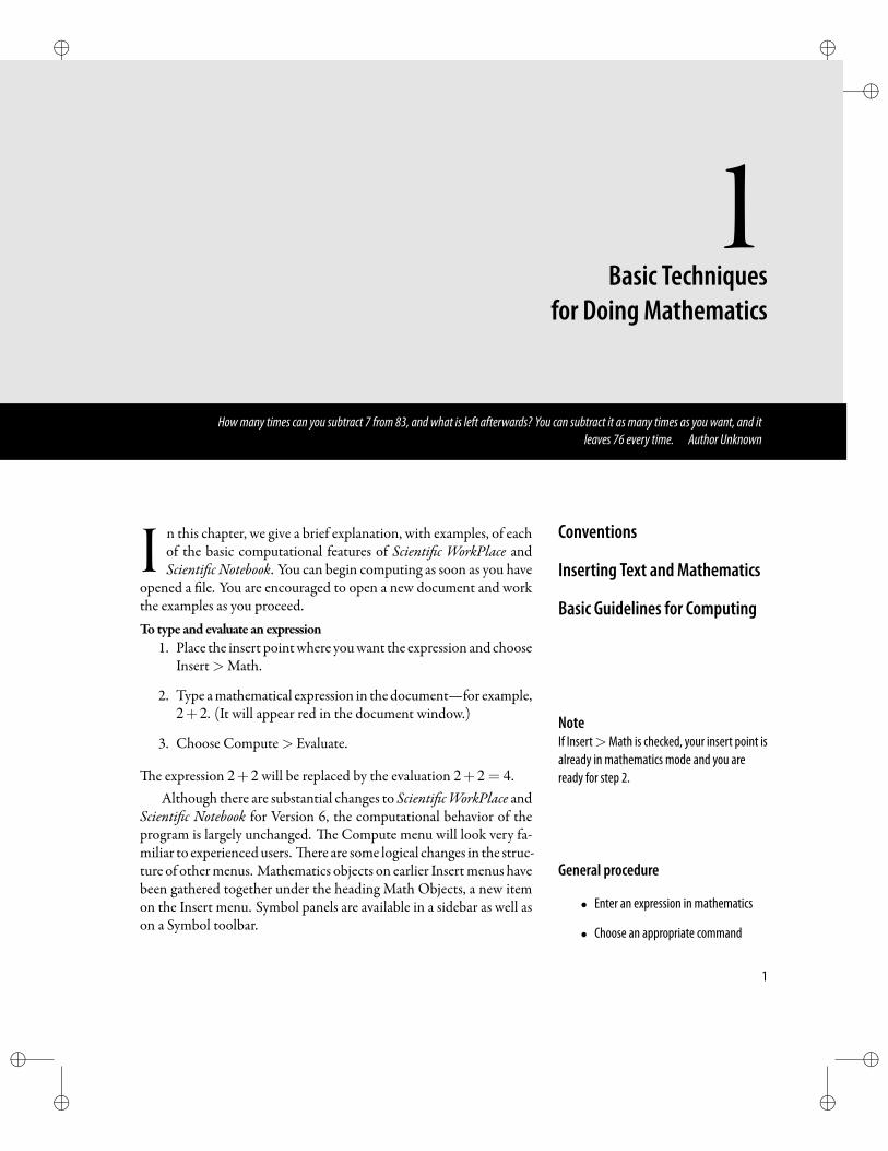
Howmany times can you subtract 7 from 83, and what is left afterwards? You can subtract it as many times as you want, and itleaves 76 every time. Author Unknown
I n this chapter, we give a brief explanation, with examples, of each Conventions
Inserting Text and Mathematics
Basic Guidelines for Computing
of the basic computational features of Scienti c WorkPlace andScienti c Notebook. You can begin computing as soon as you have
opened a le. You are encouraged to open a new document and workthe examples as you proceed.To type and evaluate an expression
1. Place the insert pointwhere youwant the expression and chooseInsert>Math.
2. Type amathematical expression in thedocument—for example,2+2. (It will appear red in the document window.) Note
If Insert>Math is checked, your insert point isalready in mathematics mode and you areready for step 2.
3. Choose Compute> Evaluate.
e expression 2+2 will be replaced by the evaluation 2+2 = 4.Although there are substantial changes to Scienti cWorkPlace and
Scienti c Notebook for Version 6, the computational behavior of theprogram is largely unchanged. e Compute menu will look very fa-miliar to experiencedusers. ere are some logical changes in the struc-ture of othermenus. Mathematics objects on earlier Insertmenus have General procedure
• Enter an expression in mathematics
• Choose an appropriate command
been gathered together under the heading Math Objects, a new itemon the Insert menu. Symbol panels are available in a sidebar as well ason a Symbol toolbar.
1
ii
“Compute60” — 2011/12/20 — 14:27 — page 2 — #12 ii
ii
ii
Chapter 1 | Basic Techniques for Doing Mathematics
ConventionsProgram tools are available frommenus, toolbar buttons, and key-
board shortcuts. Many tools may be invoked in multiple ways to suityour style of work—via menus, toolbar buttons, or the keyboard. Inthis manual, we generally indicate only one of the possible ways of ac-cessing a tool, usually via the menus. Appendices A and B list com-mand shortcuts for doing or entering mathematics.
Understanding the notation and the terms used in our documen-tationwill help you understand the instructions. We assume you’re fa-miliar with the basic procedures and terminology for your operatingsystem. In our manuals, we use the notation and terms listed below.
General Notation• Text like this indicates text you should type exactly as it is shown.
• Text like this indicates information that you must supply, suchas a lename.
• Text like this indicates an expression that is typed inmathemat-ics mode.
• e word choose means to designate a command for the pro-gram to carry out. As with all standard applications, you canchoose a commandwith themouse orwith the keyboard. Com-mandsmay be listed on amenu or shown on a button or in a di-alog box. For example, the instruction “Choose File > Open”means you should rst choose the Filemenu and then from thatmenu, choose the Open command. e instruction “chooseOK” means to click OK with the mouse, or to press Tab to se-lect the OK button and then press Enter.
• e word checkmeans to turn on an option in a dialog box.
Keyboard ConventionsWe also use standard computer conventions to give keyboard in-
structions.
• e names of keys in the instructions match the names shownon most keyboards. Ctrl (Windows) and Cmd (Mac) are syn-onymous, as are Enter (Windows) and Return (Mac), and right
2
ii
“Compute60” — 2011/12/20 — 14:27 — page 3 — #13 ii
ii
ii
Inserting Text and Mathematics
click (Windows) and Cmd+click (Mac). Names of keys are al-ways shown in Windows format. Mac users should substituteMac keys (e.g. Cmd and Return) as appropriate.
• A plus sign (+) between the names of two keys indicates thatyoumust press the rst key and hold it downwhile you press thesecond key. For example, Ctrl+gmeans that you press and holddown theCtrl key, press g, and then release both keys. Similarly,the notation Ctrl+word means that you must hold down theCtrl key, type the word that appears a er the +, then release theCtrl key. Note that if a letter appears capitalized, you shouldtype that letter as a capital.
Inserting Text and MathematicsScienti cWorkPlace and Scienti c Notebook are modal in the sense
that at all times during information entry you are either entering textor mathematics, and the results obtained from keystrokes and otheruser interface actions will differ depending on whether you are enter-ing text or mathematics. us we refer to being in either text mode ormathematics mode. e default state is text mode; it is easy to togglebetween the two modes and it is also easy to determine what modeyou are in. Unless you actively change to mathematics, the programdisplays a “T” on the Standard toolbar and
• Interprets anything you type as text, displaying it in black in theprogram window.
• Displays alphabetic characters as upright, not italicized.
• Inserts a space when you press the spacebar.
When you start the program, the insert point is in text mode. Mathematics modeWhen you switch from text to mathematics,the “T” changes to “M” on the toolbar, and theinsert point changes to red and appearsbetween brackets.
To switch from text tomathematics• Click the “T” on the standard toolbar, or
Choose Insert>Math.
When in mathematics mode, the program
• Displays the insert point between brackets for mathematics.
3
ii
“Compute60” — 2011/12/20 — 14:27 — page 4 — #14 ii
ii
ii
Chapter 1 | Basic Techniques for Doing Mathematics
• Interprets anything you type asmathematics, displaying it in redin the program window.
• Italicizes alphabetic characters and displays numbers upright.
• Automatically formats mathematical expressions, inserting cor-rect spacing around operators such as + and relations such as =. Spacing
Mathematics is automatically spaceddifferently from text as you enter it—forexample, “2+2” rather than “2+2”—soyou do not have to make adjustments.
• Advances the insert point to thenextmathematical objectwhenyou press the spacebar.
To switch frommathematics to text• Click the “M” on the standard toolbar, or
Choose Insert>Text. Text modeWhen you switch frommathematics to text,the “M” changes to “T” and the insert pointchanges to black.
On the screen, mathematics appears in red and text in black. eblinking vertical line on your screen is referred to as the insert point.You may have heard it called the insert cursor, or simply the cursor.
e insert point marks the position where characters or symbols areentered when you type or click a symbol. You can change the positionof the insert point with the arrow keys or by clicking a different screenposition with the mouse. e position of the mouse is indicated bythemouse pointer, which assumes the shape of an I-beam over text andan arrow over mathematics.
Basic GuidelinesYou can type information in a document in either text or mathe-
matics. emathematics that you type is recognized by the underlyingcomputing engine as mathematics, and the text is ignored by the com-puting engine. Text and Mathematics
The state of the Toggle Text/Math buttonre ects the state at the position of the insertpoint.
• Text is entered at the position of the insertion point when theToggle Text/Math button in the Standard toolbar shows T.
• Mathematics is entered at the position of the insert point whenthe Toggle Text/Math button on the Standard toolbar shows ared M.
You can toggle betweenmathematics and text by clicking the Tog-gle Text/Math button or by pressing Ctrl+m or Ctrl+t on the key-board. Entering a mathematics symbol by clicking a button on a tool-bar automatically puts the state inmathematics at theposition inwhichthe symbol is entered. e state remains in mathematics as you type
4
ii
“Compute60” — 2011/12/20 — 14:27 — page 5 — #15 ii
ii
ii
Inserting Text and Mathematics
characters or symbols to the right of existing mathematics, until youeither toggle back into text or move the insert point into text by usingthe mouse or by pressing right arrow, le arrow, or the spacebar.
Choose View>Toolbars if any toolbar youwould like to use doesnot automatically appear above your Document Window.To type a fraction, radical, exponent, or subscript
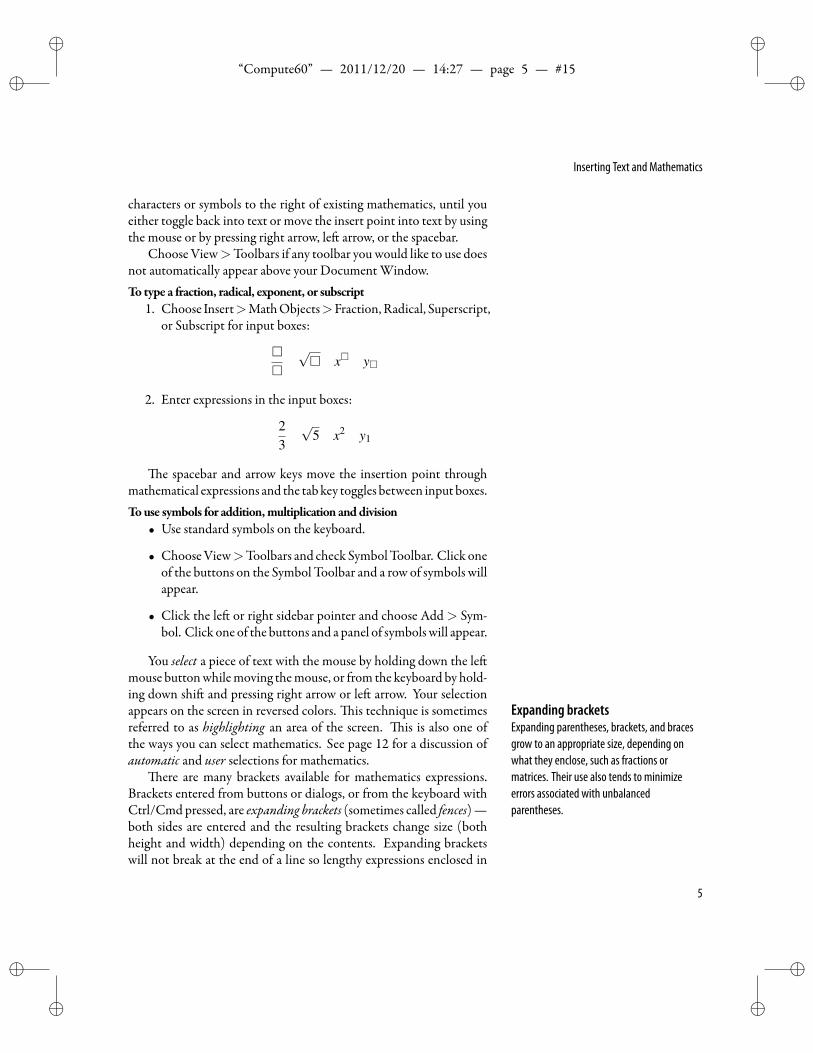
1. Choose Insert>MathObjects>Fraction, Radical, Superscript,or Subscript for input boxes:
√ x y
2. Enter expressions in the input boxes:
23
√5 x2 y1
e spacebar and arrow keys move the insertion point throughmathematical expressions and the tabkey toggles between input boxes.Touse symbols for addition,multiplication anddivision
• Use standard symbols on the keyboard.
• ChooseView>Toolbars and check SymbolToolbar. Click oneof the buttons on the Symbol Toolbar and a row of symbols willappear.
• Click the le or right sidebar pointer and choose Add > Sym-bol. Click one of the buttons and a panel of symbolswill appear.
You select a piece of text with the mouse by holding down the lemouse buttonwhilemoving themouse, or from the keyboard by hold-ing down shi and pressing right arrow or le arrow. Your selectionappears on the screen in reversed colors. is technique is sometimes Expanding brackets
Expanding parentheses, brackets, and bracesgrow to an appropriate size, depending onwhat they enclose, such as fractions ormatrices. Their use also tends to minimizeerrors associated with unbalancedparentheses.
referred to as highlighting an area of the screen. is is also one ofthe ways you can select mathematics. See page 12 for a discussion ofautomatic and user selections for mathematics.
ere are many brackets available for mathematics expressions.Brackets entered from buttons or dialogs, or from the keyboard withCtrl/Cmdpressed, are expanding brackets (sometimes called fences)—both sides are entered and the resulting brackets change size (bothheight and width) depending on the contents. Expanding bracketswill not break at the end of a line so lengthy expressions enclosed in
5
ii
“Compute60” — 2011/12/20 — 14:27 — page 6 — #16 ii
ii
ii
Chapter 1 | Basic Techniques for Doing Mathematics
expanding brackets may need to be displayed. Le and right bracketsentered from the keyboard (without Ctrl/Cmd pressed) act indepen-dently. ey also have xed height. Caution
Mix brackets with care. Although theexpanding parentheses, expanding brackets,and non-expanding brackets from thekeyboard are generally interchangeable (whenproperly matched), the use of nonexpandingor unusual brackets can lead tomisinterpretations. For example, if (2)(3) isentered with the outer parentheses “()”expanding brackets and the inner parentheses“)(” non-expanding parentheses, thenevaluating this non-matched expression gives(2)(3) = 2, which is probably not what isintended!
To insert expandingbrackets in amathematics expression• Choose Insert > Math Objects > Brackets and select the de-
sired brackets from the panel that appears.
Expanding parentheses and square brackets are also available onthe Math toolbar.
Displaying MathematicsMathematics can be centered on a separate line in a display.
y = ax+b
Tocreate a display1. Choose Insert>Math Objects>Display.
2. Type or paste a mathematical expression in the display.Spacing around a displayPressing enter immediately before a displaywill add extra vertical space. If you do not wantthis space, place the insert point immediatelybefore the display and press backspace. (Thisremoves the “new paragraph” symbol.)Pressing enter immediately after a display willadd extra vertical space and cause the nextline to start a new paragraph. If you do notwant this space or indention, place the insertpoint at the start of the next line and pressbackspace. (This removes the “new paragraph”symbol.)
You can begin with an existingmathematical expression and put itinto a display.
Toputmathematics in a display1. Select themathematicswith click anddrag or Shi +right arrow.
2. Choose Insert>Math Objects>Display.
e default environment in a display is mathematics. You can,however, enter text in a display by toggling to text.
Centering Plots, Graphics and TextIf you have text that you wish to center on a separate line, the nat-
ural way to do this operation is with Centered, which you can choosefrom the Section/Body Tag pop-up menu.
If you have a plot or graphic that you wish to center on a separateline, you should choose the Displayed setting in the Layout dialog, asdiscussed in Chapter 6, “Plotting Curves and Surfaces.” To center agroup of plots or graphics, choose the In Line setting in the Layoutdialog and then use Centered.
6
ii
“Compute60” — 2011/12/20 — 14:27 — page 7 — #17 ii
ii
ii
Basic Guidelines for Computing
Basic Guidelines for ComputingWhen you respond to the request, “place the insert point in the ex-
pression,” place the insert point within, or immediately to the right of,the expression. e position immediately to the le of amathematicalexpression is not part of the mathematics.
Evaluating expressionsTo type a mathematics expression for a computation, begin a new
line with the mathematics expression or type the expression immedi-ately to the right of text or a text space. If you type mathematics im-mediately to the right of other mathematics, the expressions may becombined in ways you do not intend. Compute> Evaluate
This sequence of actions insert= 11 to theright of 3+8, resulting in the equation3+8 = 11.
Tocompute the sum3+ 81. Choose Insert>Math
2. Type 3+8
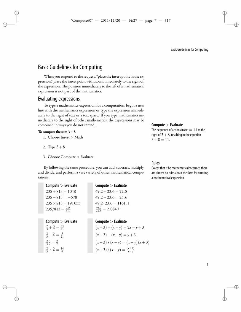
3. Choose Compute> EvaluateRulesExcept that it be mathematically correct, thereare almost no rules about the form for enteringa mathematical expression.
By following the same procedure, you can add, subtract, multiply,and divide, and perform a vast variety of other mathematical compu-tations.
Compute> Evaluate Compute> Evaluate235+813 = 1048 49.2+23.6 = 72.8235−813 =−578 49.2−23.6 = 25.6235×813 = 191055 49.2 ·23.6 = 1161.1235/813 = 235
81349.223.6 = 2.0847
Compute> Evaluate Compute> Evaluate23 +
37 = 23
21 (x+3)+(x− y) = 2x− y+323 −
37 = 5
21 (x+3)− (x− y) = y+323
37 = 2
7 (x+3)∗ (x− y) = (x− y)(x+3)23 ÷
37 = 14
9 (x+3)/(x− y) = (x+3)x−y
7
ii
“Compute60” — 2011/12/20 — 14:27 — page 8 — #18 ii
ii
ii
Chapter 1 | Basic Techniques for Doing Mathematics
One of the few exceptions to the claim of “no rules” is that verticalnotation such as
24+15 and
234−47 and 2 35
used when doingmathematics by hand is not recognized. Write sums,differences, products, and quotients of numbers in natural linear no-tation, such as 24+15 and 235−47 and 24.7/19.5 and 13÷22, ornatural fractional notation, such as 78.9
43.4 and 37 ·
23 .
Certain constants are recognized in their usual forms—such as π ,i, and e—as long as the context is appropriate. On the other hand,they are recognized as arbitrary constants, variables, or indices whenappropriate to the context, helping to provide a completely naturalway for you to type and perform mathematical computations.
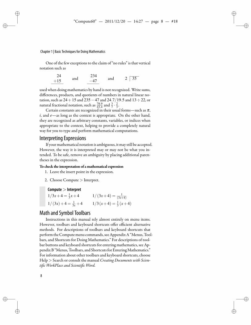
Interpreting ExpressionsIf yourmathematical notation is ambiguous, itmay still be accepted.
However, the way it is interpreted may or may not be what you in-tended. To be safe, remove an ambiguity by placing additional paren-theses in the expression.Tocheck the interpretationof amathematical expression
1. Leave the insert point in the expression.
2. Choose Compute> Interpret.
Compute> Interpret1/3x+4 = 1
3 x+4 1/(3x+4) = 1(3x+4)
1/(3x)+4 = 13x +4 1/3(x+4) = 1
3 (x+4)
Math and Symbol ToolbarsInstructions in this manual rely almost entirely on menu items.
However, toolbars and keyboard shortcuts offer efficient alternativemethods. For descriptions of toolbars and keyboard shortcuts thatperformtheComputemenucommands, seeAppendixA“Menus,Tool-bars, and Shortcuts for Doing Mathematics.” For descriptions of tool-bar buttons and keyboard shortcuts for enteringmathematics, see Ap-pendixB “Menus, Toolbars, and Shortcuts for EnteringMathematics.”For information about other toolbars and keyboard shortcuts, chooseHelp> Search or consult the manualCreating Documents with Scien-ti c WorkPlace and Scienti c Word.
8
ii
“Compute60” — 2011/12/20 — 14:27 — page 9 — #19 ii
ii
ii
Basic Guidelines for Computing
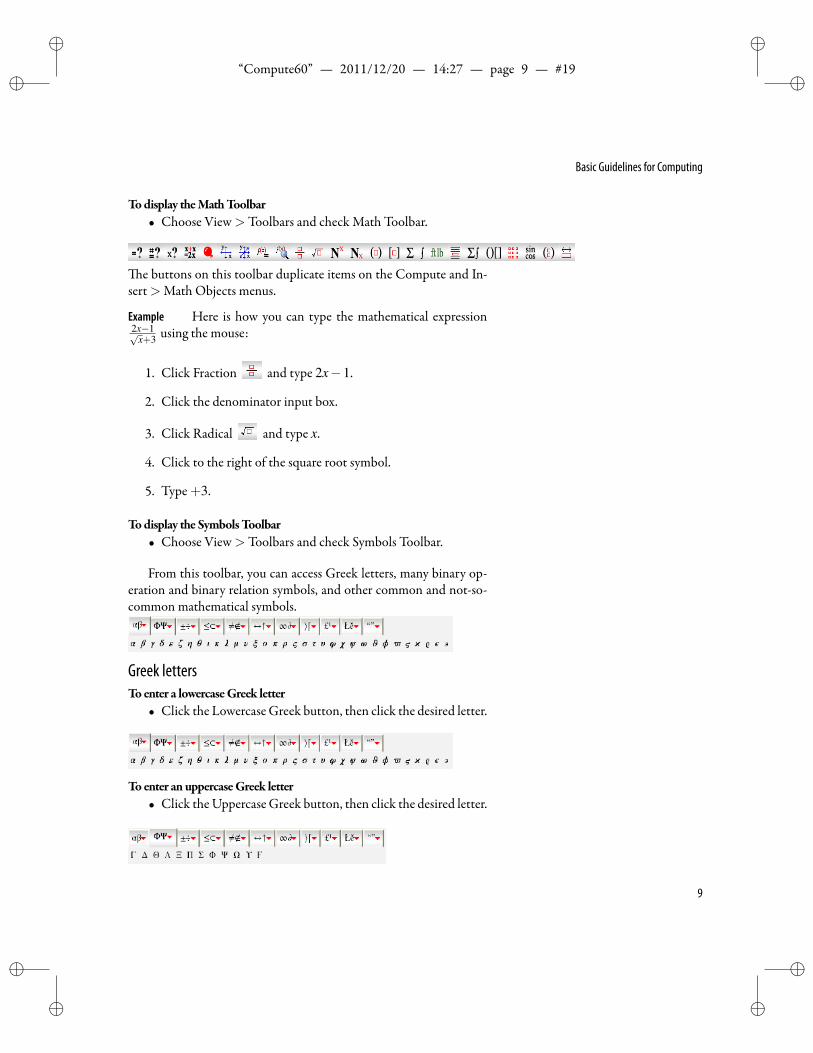
Todisplay theMathToolbar• Choose View>Toolbars and check Math Toolbar.
e buttons on this toolbar duplicate items on the Compute and In-sert>Math Objects menus.
Example Here is how you can type the mathematical expression2x−1√
x+3 using the mouse:
1. Click Fraction and type 2x−1.
2. Click the denominator input box.
3. Click Radical and type x.
4. Click to the right of the square root symbol.
5. Type+3.
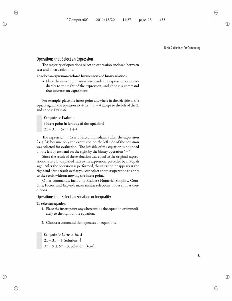
Todisplay the SymbolsToolbar• Choose View>Toolbars and check Symbols Toolbar.
From this toolbar, you can access Greek letters, many binary op-eration and binary relation symbols, and other common and not-so-common mathematical symbols.
Greek lettersToenter a lowercaseGreek letter
• Click the Lowercase Greek button, then click the desired letter.
Toenter anuppercaseGreek letter• Click theUppercase Greek button, then click the desired letter.
9
ii
“Compute60” — 2011/12/20 — 14:27 — page 10 — #20 ii
ii
ii
Chapter 1 | Basic Techniques for Doing Mathematics
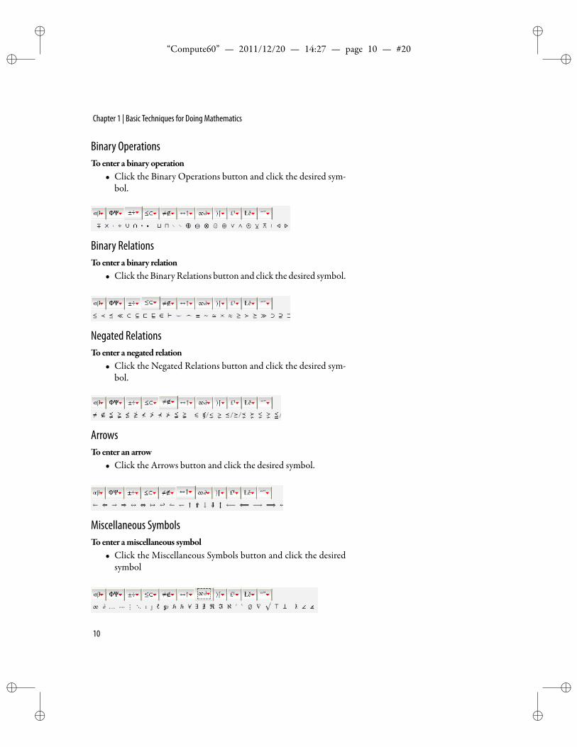
Binary OperationsToenter a binary operation
• Click the Binary Operations button and click the desired sym-bol.
Binary RelationsToenter a binary relation
• Click the Binary Relations button and click the desired symbol.
Negated RelationsToenter a negated relation
• Click the Negated Relations button and click the desired sym-bol.
ArrowsToenter an arrow
• Click the Arrows button and click the desired symbol.
Miscellaneous SymbolsToenter amiscellaneous symbol
• Click the Miscellaneous Symbols button and click the desiredsymbol
10
ii
“Compute60” — 2011/12/20 — 14:27 — page 11 — #21 ii
ii
ii
Basic Guidelines for Computing
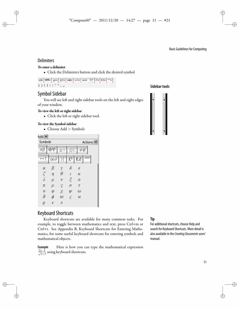
DelimitersToenter a delimiter
• Click the Delimiters button and click the desired symbol
Sidebar tools
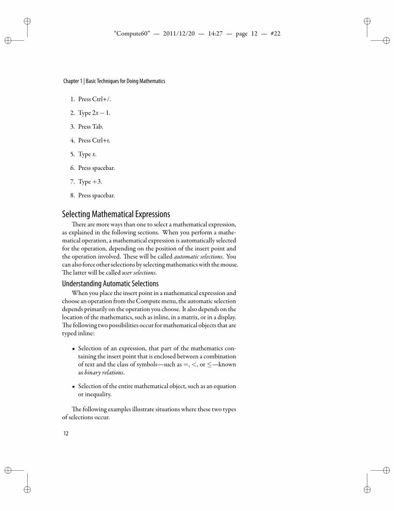
Symbol SidebarYou will see le and right sidebar tools on the le and right edges
of your window.Toview the le or right sidebar
• Click the le or right sidebar tool.
Toview the Symbol sidebar• Choose Add> Symbols
Keyboard ShortcutsKeyboard shortcuts are available for many common tasks. For Tip
For additional shortcuts, choose Help andsearch for Keyboard Shortcuts. More detail isalso available in the Creating Documents users’manual.
example, to toggle between mathematics and text, press Ctrl+m orCtrl+t. See Appendix B, Keyboard Shortcuts for Entering Mathe-matics, for some useful keyboard shortcuts for entering symbols andmathematical objects.
Example Here is how you can type the mathematical expression2x−1√
x+3 using keyboard shortcuts.
11
ii
“Compute60” — 2011/12/20 — 14:27 — page 12 — #22 ii
ii
ii
Chapter 1 | Basic Techniques for Doing Mathematics
1. Press Ctrl+/.
2. Type 2x−1.
3. Press Tab.
4. Press Ctrl+r.
5. Type x.
6. Press spacebar.
7. Type+3.
8. Press spacebar.
Selecting Mathematical Expressionsere are more ways than one to select a mathematical expression,
as explained in the following sections. When you perform a mathe-matical operation, a mathematical expression is automatically selectedfor the operation, depending on the position of the insert point andthe operation involved. ese will be called automatic selections. Youcan also force other selections by selectingmathematicswith themouse.
e latter will be called user selections.
Understanding Automatic SelectionsWhen you place the insert point in amathematical expression and
choose an operation from theComputemenu, the automatic selectiondepends primarily on the operation you choose. It also depends on thelocation of the mathematics, such as inline, in a matrix, or in a display.
e following twopossibilities occur formathematical objects that aretyped inline:
• Selection of an expression, that part of the mathematics con-taining the insert point that is enclosed between a combinationof text and the class of symbols—such as =, <, or≤—knownas binary relations.
• Selection of the entiremathematical object, such as an equationor inequality.
e following examples illustrate situations where these two typesof selections occur.
12
ii
“Compute60” — 2011/12/20 — 14:27 — page 13 — #23 ii
ii
ii
Basic Guidelines for Computing
Operations that Select an Expressione majority of operations select an expression enclosed between
text and binary relations.
To select an expression enclosedbetween text andbinary relations• Place the insert point anywhere inside the expression or imme-
diately to the right of the expression, and choose a commandthat operates on expressions.
For example, place the insert point anywhere in the le side of theequals sign in the equation 2x+3x = 1+4 except to the le of the 2,and choose Evaluate.
Compute> Evaluate(Insert point in le side of the equation)2x+3x = 5x = 1+4
e expression = 5x is inserted immediately a er the expression2x+ 3x, because only the expression on the le side of the equationwas selected for evaluation. e le side of the equation is boundedon the le by text and on the right by the binary operation “=.”
Since the result of the evaluation was equal to the original expres-sion, the resultwas placednext to the expression, precededby an equalssign. A er the operation is performed, the insert point appears at theright end of the result so that you can select another operation to applyto the result without moving the insert point.
Other commands, including Evaluate Numeric, Simplify, Com-bine, Factor, and Expand, make similar selections under similar con-ditions.
Operations that Select an Equation or InequalityTo select an equation
1. Place the insert point anywhere inside the equation or immedi-ately to the right of the equation.
2. Choose a command that operates on equations.
Compute> Solve> Exact2x+3x = 1, Solution: 1
53x+5≤ 5x−3, Solution: [4,∞)
13
ii
“Compute60” — 2011/12/20 — 14:27 — page 14 — #24 ii
ii
ii
Chapter 1 | Basic Techniques for Doing Mathematics
In these cases, the entire mathematical object—that is, the equa-tion or inequality—was selected. e solution is not equal to the se-lection, so it is not presented as a part of the original equation. Note
If the mathematics is not appropriate for theoperation, no action is taken.
e other choices on the Solve submenu and the operationCheckEquality also select an equation.
Selections Inside Displays and MatricesOperations may behave somewhat differently when mathematics
is entered in a display or in amatrix. If you place the insert point insidea display ormatrix, the automatic selection is the entire array of entries,for any operation. Some operations apply to a matrix, and others tothe entries of a matrix or contents of a display. If the operation is notappropriate for either a matrix or its entries or for all the contents of adisplay, you may receive a report of a syntax error.Selections Inside a Display
Inside a one-line display, the automatic selection is the samemath-ematics as outside a display, and the result is generally returned insidethe display.To selectmathematics in a display
• Place the insert point inside the display, and choose a commandthat operates on expressions or equations.
TipPress Enter at the end of a display line to createa new display line.
When you choose Evaluate with the insert point in the le side ofthe displayed equation
2x+3x = 3+5
you get the result2x+3x = 5x = 3+5
and when you choose Evaluate with the insert point in the right sideof the displayed equation you get the result
2x+3x = 3+5 = 8
A multiple-line display, however, behaves like a matrix (see nextsection). Note that multiple line displays are useful for solving sys-tems of equations, or equations with initial-value conditions. Apply-ing Compute> Solve> Exact to the following display yields
5x+2y = 36x− y = 5
Solution:[x = 13
17 ,y =−717
]14
ii
“Compute60” — 2011/12/20 — 14:27 — page 15 — #25 ii
ii
ii
Basic Guidelines for Computing
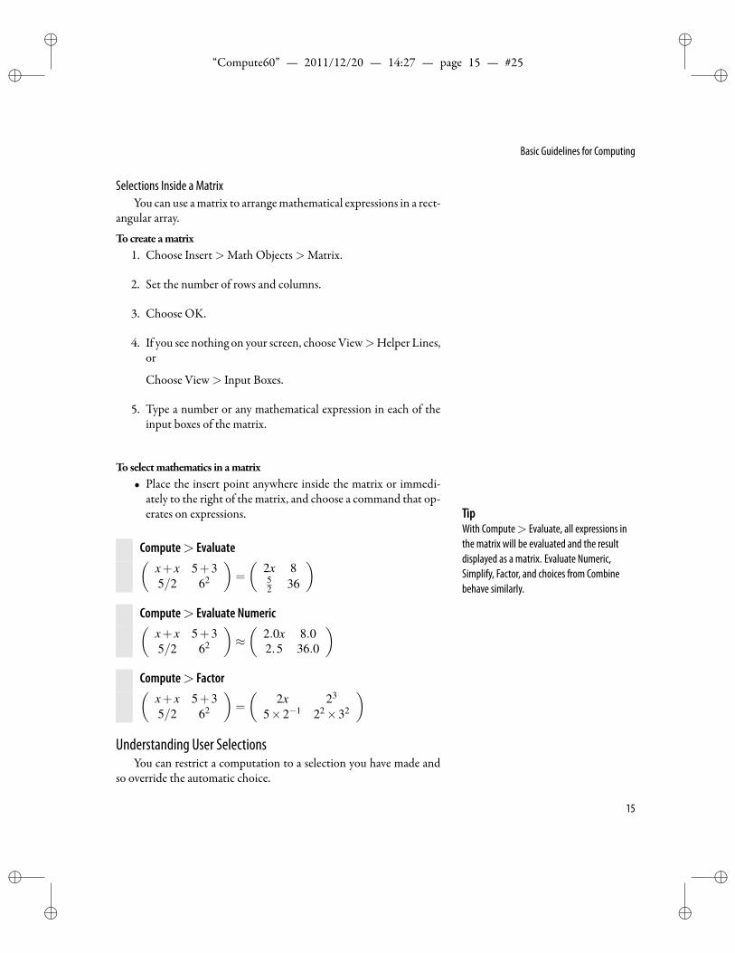
Selections Inside a MatrixYou can use amatrix to arrangemathematical expressions in a rect-
angular array.
Tocreate amatrix1. Choose Insert>Math Objects>Matrix.
2. Set the number of rows and columns.
3. Choose OK.
4. If you see nothing on your screen, choose View>Helper Lines,or
Choose View> Input Boxes.
5. Type a number or any mathematical expression in each of theinput boxes of the matrix.
To selectmathematics in amatrix• Place the insert point anywhere inside the matrix or immedi-
ately to the right of the matrix, and choose a command that op-erates on expressions. Tip
With Compute> Evaluate, all expressions inthe matrix will be evaluated and the resultdisplayed as a matrix. Evaluate Numeric,Simplify, Factor, and choices from Combinebehave similarly.
Compute> Evaluate(x+ x 5+35/2 62
)=
(2x 852 36
)Compute> Evaluate Numeric(
x+ x 5+35/2 62
)≈(
2.0x 8.02.5 36.0
)Compute> Factor(
x+ x 5+35/2 62
)=
(2x 23
5×2−1 22×32
)Understanding User Selections
You can restrict a computation to a selection you have made andso override the automatic choice.
15
ii
“Compute60” — 2011/12/20 — 14:27 — page 16 — #26 ii
ii
ii
Chapter 1 | Basic Techniques for Doing Mathematics
Tomake a user selection• Hold down the le mouse buttonwhilemoving themouse over
the material you want to select, then release the le mouse but-ton.
Your selection is the expression that appears on the screen in re-versed colors. is procedure will o en be referred to as select with themouse.
ere are two options for applying operations to a user selection—operating on a selection displays the result of the operation but leavesthe selection intact, and replacing a selection replaces the selectionwiththe result of the operation. Following are two examples illustrating thebehavior of the system when operating on a selection. e option ofreplacing a selection is referred to as computing in place, and examplesare shown in the following section.Tooperate on a user selection
• Use the mouse to make a selection, and apply an operation.
Compute> Evaluate(2+3 selected)2+3− x : 5
TipWhen you operate on a user selection, theanswer appears to the right of the entireexpression, following a colon.In general, the result of applying an operation to a user selection is
not equal to the entire original expression, so the result is placed at theend of the mathematics, separated by something in text (in this case,a colon). You can use the word-processing capabilities of your systemto put the result where you want it in your document.
Replacing a user selection, an in-place computation, is described inthe following section.
Computing in Place Computing in placeThis “computing in place”— that is, holdingdown the Ctrl key as you choose an operationfrom the Compute menu—is a key feature. Itprovides a convenient way for you tomanipulate expressions into the forms youdesire.
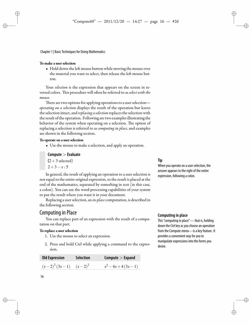
You can replace part of an expression with the result of a compu-tation on that part.To replace a user selection
1. Use the mouse to select an expression.
2. Press and hold Ctrl while applying a command to the expres-sion.
Old Expression Selection Compute> Expand
(x−2)2 (3x−1) (x−2)2 x2−4x+4(3x−1)
16
ii
“Compute60” — 2011/12/20 — 14:27 — page 17 — #27 ii
ii
ii
Basic Guidelines for Computing
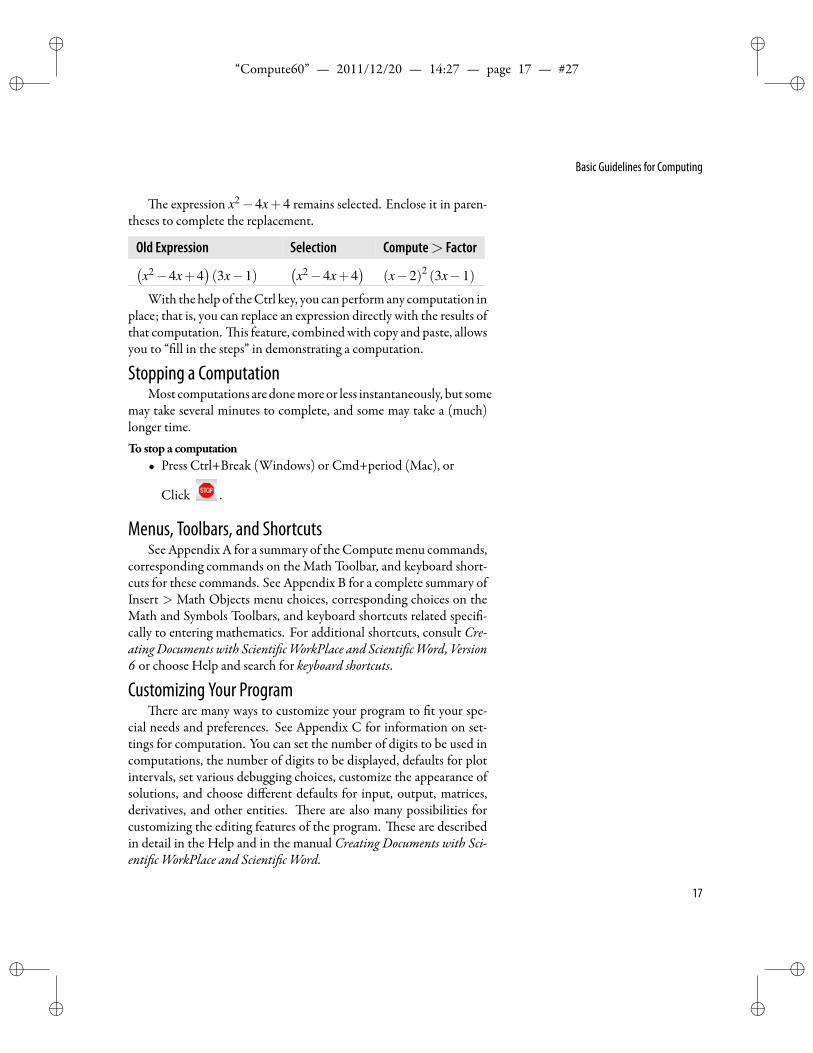
e expression x2−4x+4 remains selected. Enclose it in paren-theses to complete the replacement.
Old Expression Selection Compute> Factor(x2−4x+4
)(3x−1)
(x2−4x+4
)(x−2)2 (3x−1)
With the help of theCtrl key, you canperformany computation inplace; that is, you can replace an expression directly with the results ofthat computation. is feature, combinedwith copy and paste, allowsyou to “ ll in the steps” in demonstrating a computation.
Stopping a ComputationMost computations are donemoreor less instantaneously, but some
may take several minutes to complete, and some may take a (much)longer time.To stop a computation
• Press Ctrl+Break (Windows) or Cmd+period (Mac), or
Click .
Menus, Toolbars, and ShortcutsSeeAppendixA for a summary of theComputemenu commands,
corresponding commands on the Math Toolbar, and keyboard short-cuts for these commands. See Appendix B for a complete summary ofInsert > Math Objects menu choices, corresponding choices on theMath and Symbols Toolbars, and keyboard shortcuts related speci -cally to entering mathematics. For additional shortcuts, consult Cre-atingDocuments with Scienti cWorkPlace and Scienti cWord, Version6 or choose Help and search for keyboard shortcuts.
Customizing Your Programere are many ways to customize your program to t your spe-
cial needs and preferences. See Appendix C for information on set-tings for computation. You can set the number of digits to be used incomputations, the number of digits to be displayed, defaults for plotintervals, set various debugging choices, customize the appearance ofsolutions, and choose different defaults for input, output, matrices,derivatives, and other entities. ere are also many possibilities forcustomizing the editing features of the program. ese are describedin detail in the Help and in the manual Creating Documents with Sci-enti c WorkPlace and Scienti c Word.
17
ii
“Compute60” — 2011/12/20 — 14:27 — page 18 — #28 ii
ii
ii
Chapter 1 | Basic Techniques for Doing Mathematics
Computational Enginee computational engine provided with Scienti cWorkPlace and
Scienti c Notebook version 6 isMuPAD 5. To see if the computationalengine is in active mode, or to deactivate the engine, choose Tools >Preferences > Computation, click Engine tab, and check or uncheckEngine On. ( e path for a Mac is SWPPro > Preferences > Com-putation.)
See AppendixD “MuPADFunctions and Expressions” for a list ofbuilt-in functions and constants, descriptions ofComputemenu com-mands in terms of the native commands of MuPAD, and descriptionsof built-in functions in terms of the MuPAD syntax.
18
ii
“Compute60” — 2011/12/20 — 14:27 — page 19 — #29 ii
ii
ii
2Numbers, Functions, and Units
No human investigation can be called real science if it cannot be demonstrated mathematically. Leonardo da Vinci (1452–1519)
N umbers and functions to be used for computing should be Integers and Fractions
Elementary Number Theory
Real Numbers
Functions and Relations
Complex Numbers
Units and Measurements
entered in mathematics mode and appear red (or gray) onyour screen. If that is not the case, choose Insert > Math
and retype the expression. Units to be used for computing must beentered as a Unit Name (see Units, page 34).Toenter amathematics expression for a computation
• Begin a new line with the mathematics expression, or
Type the expression immediately to the right of text or a textspace.
If you enter mathematics immediately to the right of othermathe-matics, the expressions will be combined in ways you may not intend.A safe way to begin is to press Enter and start on a new line. New in Version 6
Rewrite fraction as mixed numberArithmetic with mixed numbersChoice of letters and fonts for imaginary unitand exponential eOverbar for complex conjugateMore control over thresholds for scienti cnotation
Integers and Fractionse rst examples are centered around rational numbers—that is,
integers and fractions. You will nd examples of many of the sameoperations later in this chapter, using real numbers and then complexnumbers. Similar operations will be illustrated in later chapters with avariety of different mathematical objects.
19
ii
“Compute60” — 2011/12/20 — 14:27 — page 20 — #30 ii
ii
ii
Chapter 2 | Numbers, Functions, and Units
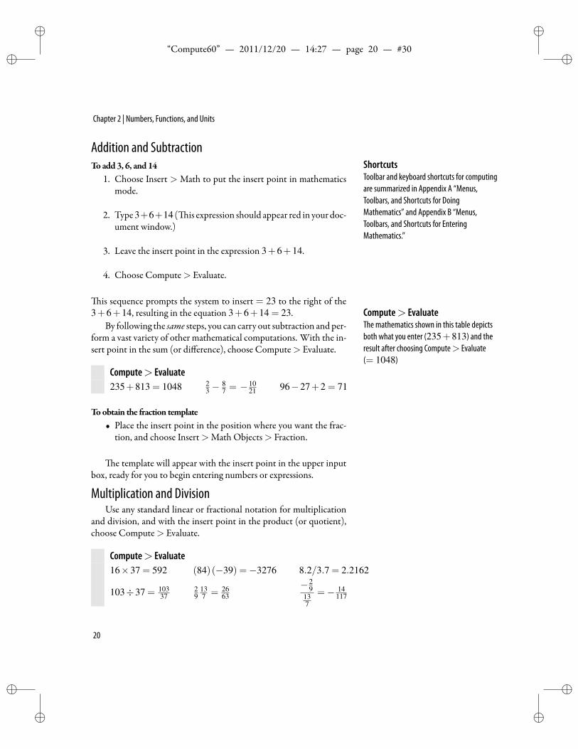
Addition and SubtractionToadd3, 6, and14 Shortcuts
Toolbar and keyboard shortcuts for computingare summarized in Appendix A “Menus,Toolbars, and Shortcuts for DoingMathematics” and Appendix B “Menus,Toolbars, and Shortcuts for EnteringMathematics.”
1. Choose Insert > Math to put the insert point in mathematicsmode.
2. Type3+6+14 ( is expression should appear red in your doc-ument window.)
3. Leave the insert point in the expression 3+6+14.
4. Choose Compute> Evaluate.
is sequence prompts the system to insert = 23 to the right of the3+6+14, resulting in the equation 3+6+14 = 23. Compute> Evaluate
The mathematics shown in this table depictsboth what you enter (235+813) and theresult after choosing Compute> Evaluate(= 1048)
By following the same steps, you can carry out subtraction and per-form a vast variety of other mathematical computations. With the in-sert point in the sum (or difference), choose Compute> Evaluate.
Compute> Evaluate235+813 = 1048 2
3 −87 = − 10
21 96−27+2 = 71
Toobtain the fraction template• Place the insert point in the position where you want the frac-
tion, and choose Insert>Math Objects> Fraction.
e template will appear with the insert point in the upper inputbox, ready for you to begin entering numbers or expressions.
Multiplication and DivisionUse any standard linear or fractional notation for multiplication
and division, and with the insert point in the product (or quotient),choose Compute> Evaluate.
Compute> Evaluate16×37 = 592 (84)(−39) =−3276 8.2/3.7 = 2.2162
103÷37 = 10337
29
137 = 26
63− 2
9137
=− 14117
20
ii
“Compute60” — 2011/12/20 — 14:27 — page 21 — #31 ii
ii
ii
Elementary Number Theory
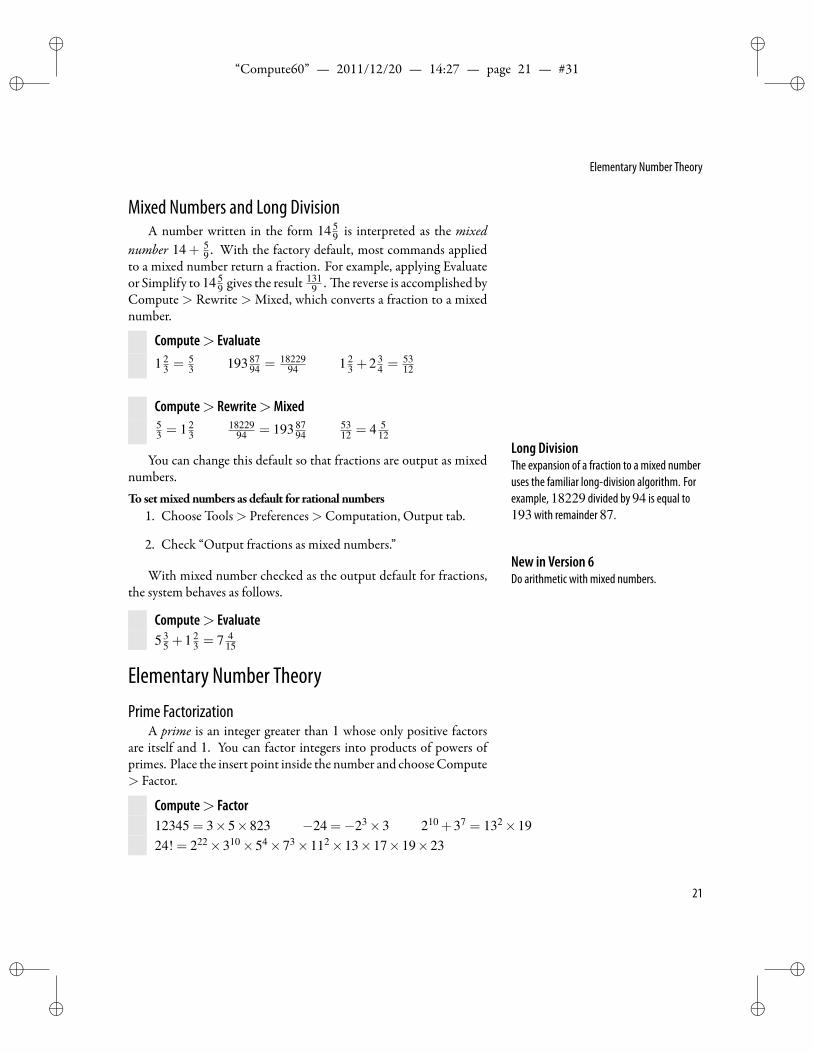
Mixed Numbers and Long DivisionA number written in the form 14 5
9 is interpreted as the mixednumber 14+ 5
9 . With the factory default, most commands appliedto a mixed number return a fraction. For example, applying Evaluateor Simplify to 14 5
9 gives the result 1319 . e reverse is accomplished by
Compute > Rewrite > Mixed, which converts a fraction to a mixednumber.
Compute> Evaluate1 2
3 = 53 193 87
94 = 1822994 1 2
3 +2 34 = 53
12
Compute> Rewrite>Mixed53 = 1 2
318229
94 = 193 8794
5312 = 4 5
12Long DivisionThe expansion of a fraction to a mixed numberuses the familiar long-division algorithm. Forexample, 18229 divided by94 is equal to193with remainder 87.
You can change this default so that fractions are output as mixednumbers.To setmixednumbers as default for rational numbers
1. Choose Tools> Preferences>Computation, Output tab.
2. Check “Output fractions as mixed numbers.”New in Version 6Do arithmetic with mixed numbers.With mixed number checked as the output default for fractions,
the system behaves as follows.
Compute> Evaluate5 3
5 +1 23 = 7 4
15
Elementary Number Theory
Prime FactorizationA prime is an integer greater than 1 whose only positive factors
are itself and 1. You can factor integers into products of powers ofprimes. Place the insert point inside the number and chooseCompute> Factor.
Compute> Factor12345 = 3×5×823 −24 =−23×3 210 +37 = 132×1924! = 222×310×54×73×112×13×17×19×23
21
ii
“Compute60” — 2011/12/20 — 14:27 — page 22 — #32 ii
ii
ii
Chapter 2 | Numbers, Functions, and Units
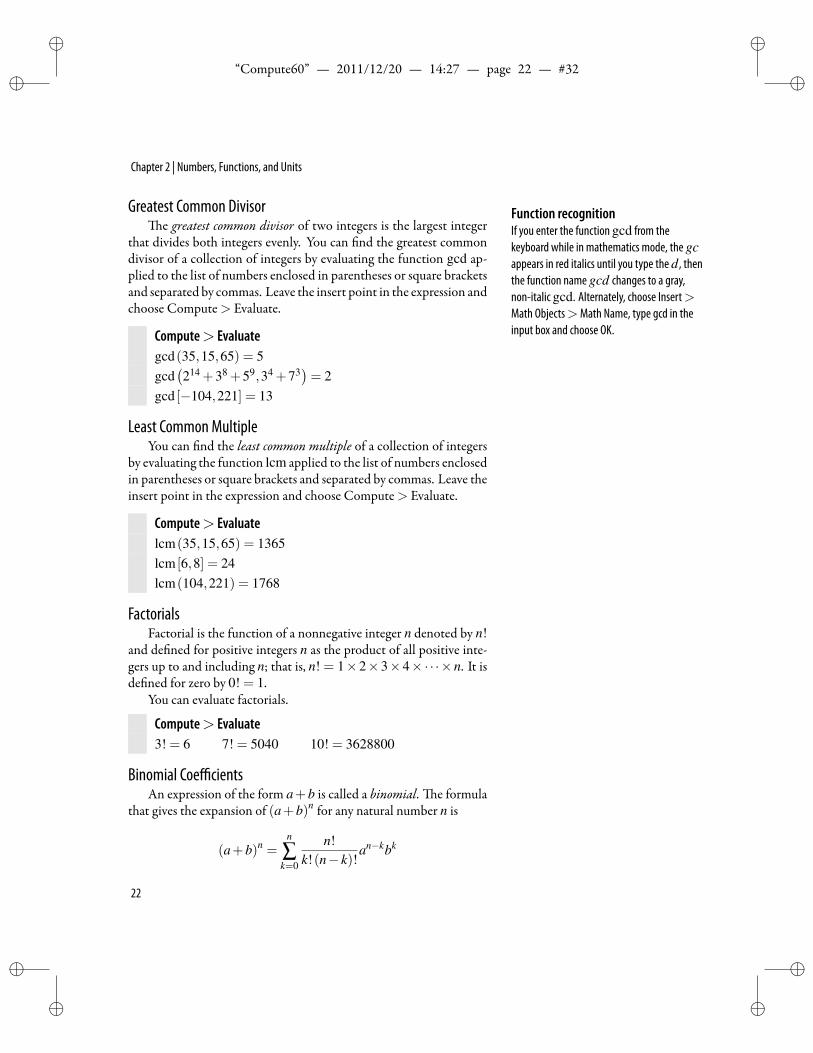
Greatest Common Divisor Function recognitionIf you enter the function gcd from thekeyboard while in mathematics mode, the gcappears in red italics until you type the d, thenthe function name gcd changes to a gray,non-italic gcd. Alternately, choose Insert>Math Objects>Math Name, type gcd in theinput box and choose OK.
e greatest common divisor of two integers is the largest integerthat divides both integers evenly. You can nd the greatest commondivisor of a collection of integers by evaluating the function gcd ap-plied to the list of numbers enclosed in parentheses or square bracketsand separated by commas. Leave the insert point in the expression andchoose Compute> Evaluate.
Compute> Evaluategcd(35,15,65) = 5gcd(214 +38 +59,34 +73
)= 2
gcd [−104,221] = 13
Least Common MultipleYou can nd the least common multiple of a collection of integers
by evaluating the function lcm applied to the list of numbers enclosedin parentheses or square brackets and separated by commas. Leave theinsert point in the expression and choose Compute> Evaluate.
Compute> Evaluatelcm(35,15,65) = 1365lcm [6,8] = 24lcm(104,221) = 1768
FactorialsFactorial is the function of a nonnegative integer n denoted by n!
and de ned for positive integers n as the product of all positive inte-gers up to and including n; that is, n! = 1×2×3×4×·· ·×n. It isde ned for zero by 0! = 1.
You can evaluate factorials.
Compute> Evaluate3! = 6 7! = 5040 10! = 3628800
Binomial CoefficientsAn expression of the form a+b is called a binomial. e formula
that gives the expansion of (a+b)n for any natural number n is
(a+b)n =n
∑k=0
n!k!(n− k)!
an−kbk
22
ii
“Compute60” — 2011/12/20 — 14:27 — page 23 — #33 ii
ii
ii
Real Numbers
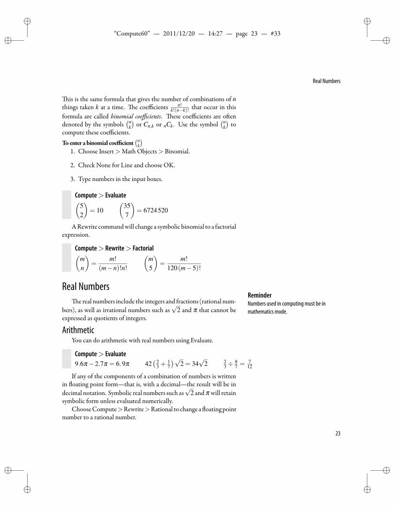
is is the same formula that gives the number of combinations of nthings taken k at a time. e coefficients n!
k!(n−k)! that occur in thisformula are called binomial coefficients. ese coefficients are o endenoted by the symbols
(nk
)or Cn,k or nCk. Use the symbol
(nk
)to
compute these coefficients.Toenter a binomial coefficient
(nk
)1. Choose Insert>Math Objects> Binomial.
2. Check None for Line and choose OK.
3. Type numbers in the input boxes.
Compute> Evaluate(52
)= 10
(357
)= 6724520
ARewrite commandwill change a symbolic binomial to a factorialexpression.
Compute> Rewrite> Factorial(mn
)=
m!(m−n)!n!
(m5
)=
m!120(m−5)!
Real NumbersReminderNumbers used in computing must be inmathematics mode.
e real numbers include the integers and fractions (rational num-bers), as well as irrational numbers such as
√2 and π that cannot be
expressed as quotients of integers.
ArithmeticYou can do arithmetic with real numbers using Evaluate.
Compute> Evaluate9.6π−2.7π = 6.9π 42
( 23 +
17
)√2 = 34
√2 2
3 ÷87 = 7
12
If any of the components of a combination of numbers is writtenin oating point form—that is, with a decimal—the result will be indecimal notation. Symbolic real numbers such as
√2 and π will retain
symbolic form unless evaluated numerically.ChooseCompute>Rewrite>Rational to change a oatingpoint
number to a rational number.
23
ii
“Compute60” — 2011/12/20 — 14:27 — page 24 — #34 ii
ii
ii
Chapter 2 | Numbers, Functions, and Units
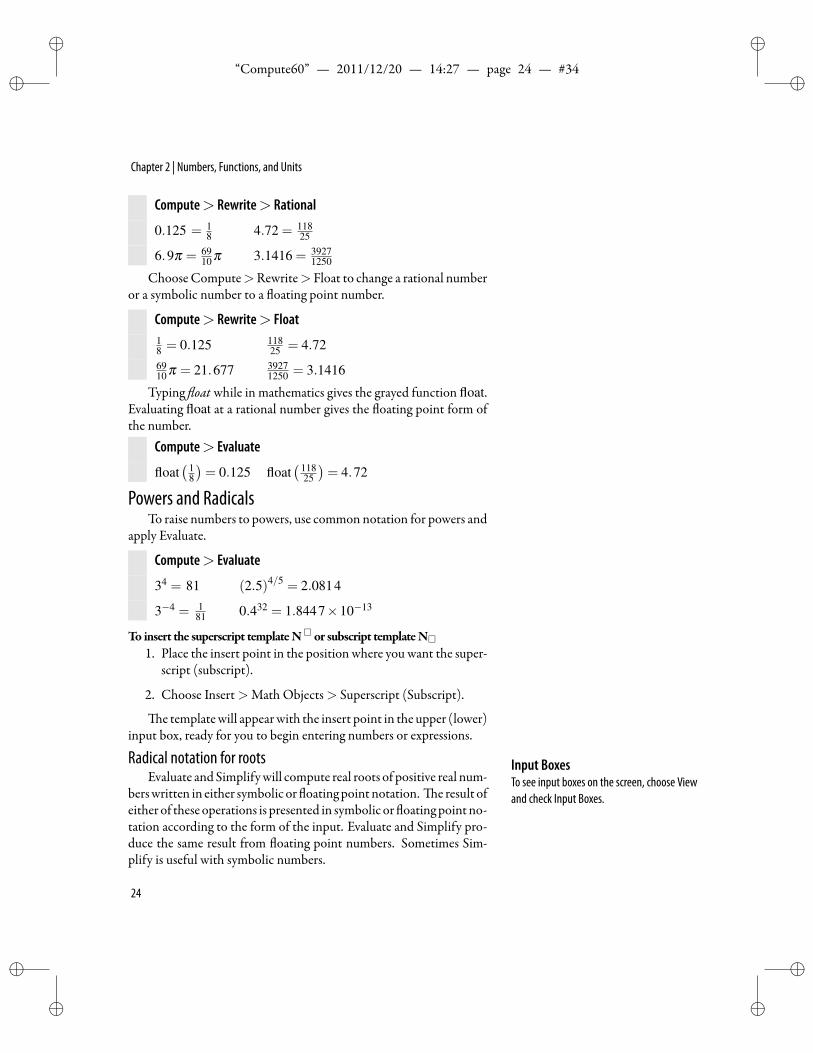
Compute> Rewrite> Rational
0.125 = 18 4.72 = 118
25
6.9π = 6910 π 3.1416 = 3927
1250
ChooseCompute>Rewrite> Float to change a rational numberor a symbolic number to a oating point number.
Compute> Rewrite> Float18 = 0.125 118
25 = 4.726910 π = 21.677 3927
1250 = 3.1416
Typing oat while in mathematics gives the grayed function float.Evaluating float at a rational number gives the oating point form ofthe number.
Compute> Evaluate
float( 1
8
)= 0.125 float
( 11825
)= 4.72
Powers and RadicalsTo raise numbers to powers, use common notation for powers and
apply Evaluate.
Compute> Evaluate
34 = 81 (2.5)4/5 = 2.0814
3−4 = 181 0.432 = 1.8447×10⁻¹³
To insert the superscript templateN or subscript templateN1. Place the insert point in the position where you want the super-
script (subscript).
2. Choose Insert>Math Objects> Superscript (Subscript).
e templatewill appearwith the insert point in the upper (lower)input box, ready for you to begin entering numbers or expressions.
Radical notation for roots Input BoxesTo see input boxes on the screen, choose Viewand check Input Boxes.
Evaluate andSimplifywill compute real roots of positive real num-berswritten in either symbolic or oatingpointnotation. e result ofeither of these operations is presented in symbolic or oatingpointno-tation according to the form of the input. Evaluate and Simplify pro-duce the same result from oating point numbers. Sometimes Sim-plify is useful with symbolic numbers.
24
ii
“Compute60” — 2011/12/20 — 14:27 — page 25 — #35 ii
ii
ii
Real Numbers
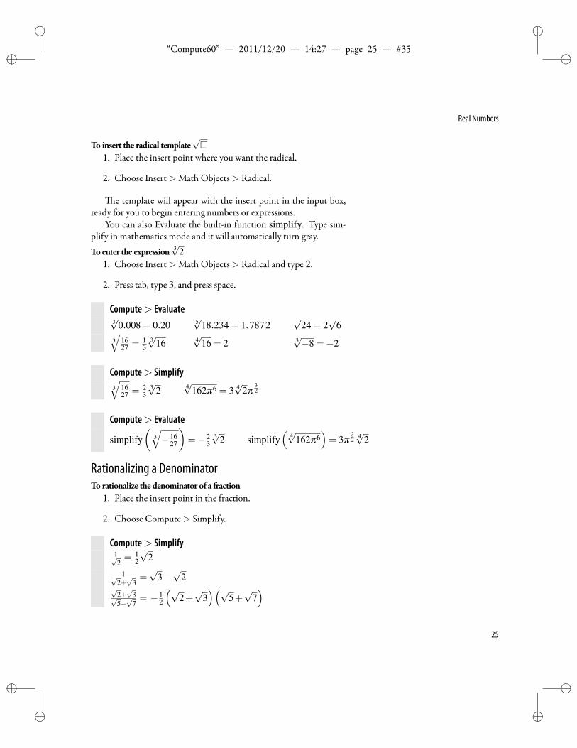
To insert the radical template√
1. Place the insert point where you want the radical.
2. Choose Insert>Math Objects> Radical.
e template will appear with the insert point in the input box,ready for you to begin entering numbers or expressions.
You can also Evaluate the built-in function simplify. Type sim-plify in mathematics mode and it will automatically turn gray.Toenter the expression 3√2
1. Choose Insert>Math Objects> Radical and type 2.
2. Press tab, type 3, and press space.
Compute> Evaluate3√
0.008 = 0.20 5√
18.234 = 1.7872√
24 = 2√
63√
1627 = 1
33√16 4√16 = 2 3
√−8 =−2
Compute> Simplify3√
1627 = 2
33√2 4√162π6 = 3 4√2π 3
2
Compute> Evaluate
simplify(
3√− 16
27
)=− 2
33√2 simplify
(4√162π6
)= 3π 3
24√2
Rationalizing a DenominatorTo rationalize the denominator of a fraction
1. Place the insert point in the fraction.
2. Choose Compute> Simplify.
Compute> Simplify1√2= 1
2
√2
1√2+√
3=√
3−√
2√
2+√
3√5−√
7= − 1
2
(√2+√
3)(√
5+√
7)
25
ii
“Compute60” — 2011/12/20 — 14:27 — page 26 — #36 ii
ii
ii
Chapter 2 | Numbers, Functions, and Units
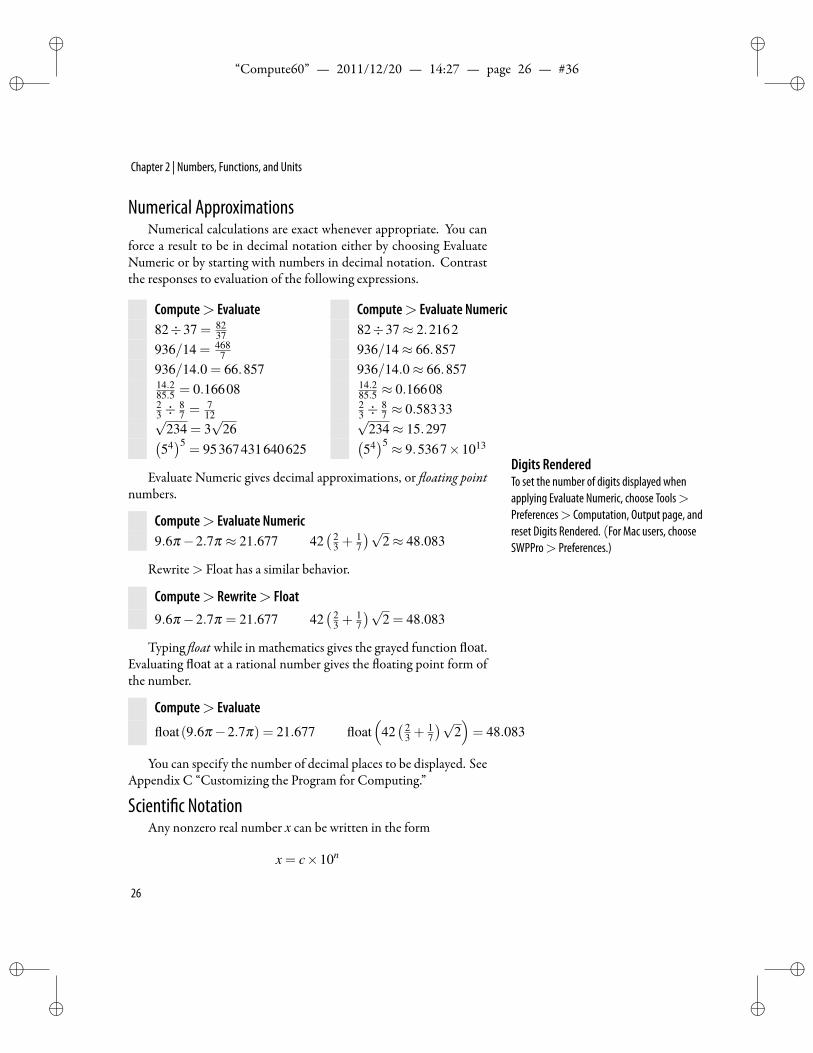
Numerical ApproximationsNumerical calculations are exact whenever appropriate. You can
force a result to be in decimal notation either by choosing EvaluateNumeric or by starting with numbers in decimal notation. Contrastthe responses to evaluation of the following expressions.
Compute> Evaluate Compute> Evaluate Numeric82÷37 = 82
37 82÷37≈ 2.2162936/14 = 468
7 936/14≈ 66.857936/14.0 = 66.857 936/14.0≈ 66.85714.285.5 = 0.16608 14.2
85.5 ≈ 0.1660823 ÷
87 = 7
1223 ÷
87 ≈ 0.58333√
234 = 3√
26√
234≈ 15.297(54)5
= 95367431640625(54)5 ≈ 9.5367×10¹³
Digits RenderedTo set the number of digits displayed whenapplying Evaluate Numeric, choose Tools>Preferences> Computation, Output page, andreset Digits Rendered. (For Mac users, chooseSWPPro> Preferences.)
Evaluate Numeric gives decimal approximations, or oating pointnumbers.
Compute> Evaluate Numeric9.6π−2.7π ≈ 21.677 42
( 23 +
17
)√2≈ 48.083
Rewrite> Float has a similar behavior.
Compute> Rewrite> Float9.6π−2.7π = 21.677 42
( 23 +
17
)√2 = 48.083
Typing oat while in mathematics gives the grayed function float.Evaluating float at a rational number gives the oating point form ofthe number.
Compute> Evaluate
float(9.6π−2.7π) = 21.677 float(
42( 2
3 +17
)√2)= 48.083
You can specify the number of decimal places to be displayed. SeeAppendix C “Customizing the Program for Computing.”
Scienti c NotationAny nonzero real number x can be written in the form
x = c×10n
26
ii
“Compute60” — 2011/12/20 — 14:27 — page 27 — #37 ii
ii
ii
Functions and Relations
with 1≤ |c|< 10 and n an integer. A number in this form is in scien-ti c notation. Following are some examples of scienti c notation:
12 = 1.2×108274.9837 = 8.2749837×10³
0.000001234 = 1.234×10⁻⁶
−54163.02 = −5.416302×10⁴
Towrite a number in scienti c notation1. Enter the number c (in mathematics mode) to as many decimal
places as appropriate.
2. Click the Binary Operations button on the Symbols Toolbar
3. Click× in the symbols palette.
4. Type the number 10.
5. Choose Insert>Math Objects> Superscript and enter the in-teger n in the input box.
e results of a numerical computation are sometimes returned inscienti c notation. is happens when the number of digits exceedsthe setting for Upper reshold for scienti c notation output. SeeAppendix C “Customizing the Program for Computing” for detailson changing this setting.
Functions and RelationsNumbers or expressions to be used for computing should be en-
tered in mathematics mode and appear red on your screen. If that isnot the case, choose Insert>Math to change the expression to math-ematics.
Following are some of the basic built-in functions (absolute value,maximumandminimum, greatest and smallest integer functions), andbuilt-in relations (union, intersection, and difference of sets).
See Absolute Value, page 33 for information on absolute values ofcomplex numbers.
Absolute valuee absolute value of a number z, the distance of z from zero, is
denoted |z|.
27
ii
“Compute60” — 2011/12/20 — 14:27 — page 28 — #38 ii
ii
ii
Chapter 2 | Numbers, Functions, and Units
Toput vertical bars around an expression1. Select the expression. Caution
The vertical lines from the symbol panel ofBinary Relations will not be interpreted asabsolute-value symbols in computations.Although they appear similar, they are not thesame symbols.The keyboard vertical line will work to build anabsolute value, but expanding brackets are lessvulnerable to misinterpretation. Type Ctrl+\for expanding absolute value bars.
2. Choose Insert>Math Objects> Brackets.
3. Click the vertical bracket and click OK.
Tocompute an absolute value1. Place the insert point in an expression between vertical bars.
2. Choose Compute> Evaluate.
Compute> Evaluate|−7|= 7 |−11.3|= 11.3 |43|= 43
Maximum and Minimume functions max and min nd the largest and smallest numbers
in a list of numbers separated by commas and enclosed in brackets.Leave the insert point in the expression and choose Evaluate.
Compute> Evaluate
max(
132 ,−√
63,7.3)= 7.3 min
(132 ,−√
63,7.3)=−3
√7
Toenter functionnames formaximumandminimum1. Choose Insert>Math Objects>Math Name.
2. Select from the list.
Or
1. Choose Insert>Math.
2. Type max or min.Making the symbol toolbar visible
• Choose View> Toolbars
• Check Symbol toolbar
e binary operations join ∨ and meet ∧ also give maximum andminimum.
Compute> Evaluate27∨ 65
2 ∨−14 = 652 27∧ 65
2 ∧−14 =−14
28
ii
“Compute60” — 2011/12/20 — 14:27 — page 29 — #39 ii
ii
ii
Functions and Relations
Toenter vee andwedge symbols formaximumandminimum Integer VariablesThe expression max
−2≤x≤2
(x3−6x+3
)is
not the maximum of the continuouspolynomial function x3−6x+3 on theinterval−2≤ x≤ 2.
1. Click Binary Operations ±+ on the Symbol toolbar
2. Select∨ or∧ from the panel
To nd the maximum or minimum of a nite sequence, enter thelimits on the integer variable as a subscript on max or min, either inthe form of a double inequality such as 1≤ n≤ 10 or as membershipin an interval such as k ∈ [1,10].
Compute> Evaluate Compute> Evaluate Numericmax1≤n≤10 (sinn) = sin8 max1≤n≤10 (sinn)≈ 0.98936
max1≤n≤10 (sin1.5n) = 0.99749 max−2≤x≤2(x3−6x+3
)≈ 8.0
mink∈[1,10] (cosk) = cos3 mink∈[1,10] (cosk)≈−0.98999
mink∈[1,10] (cos2.6k) =−0.99418 mink∈[1,10] (cos2.6k)≈−0.9941
Note that the functions max and min look only at the sequence ofvalues for integer variables. e notations x∈ [−2,2] and−2≤ x≤ 2both indicate that x assumes the range of values in the 5-element set−2,−1,0,1,2. In the last example the maximum is picked fromamong values of x3−6x+3 for x =−2,−1,0,1,2.
Greatest and Smallest Integer FunctionsYou can nd the greatest integer less than or equal to a number by
using the oor function, denoted ⌊z⌋ .Toput oor brackets around an expression
1. Select the expression with click and drag.
1. Choose Insert>Math Objects> Brackets.
2. Select the le oor bracket ⌊ , and click OK.
To nd a greatest integer value1. Place the insert point in an expression between oor brackets.
2. Choose Compute> Evaluate.
Compute> Evaluate⌊5.6⌋= 5
⌊ 435
⌋= 8
⌊−11.3⌋=−12 ⌊π + e⌋= 5
To nd the smallest integer greater than or equal to a number, usethe ceiling function, denoted ⌈z⌉.
29
ii
“Compute60” — 2011/12/20 — 14:27 — page 30 — #40 ii
ii
ii
Chapter 2 | Numbers, Functions, and Units
Toput ceiling brackets around an expression1. Select the expression with click and drag.
2. Choose Insert>Math Objects> Brackets.
3. Select the le ceiling bracket ⌈ , and choose OK.
To nd a smallest integer value1. Place the insert point in a number between ceiling brackets.
2. Choose Compute> Evaluate.
Compute> Evaluate⌈5.6⌉= 6
⌈ 435
⌉= 9
⌈−11.3⌉=−11 ⌈π + e⌉= 6
e oor and ceiling brackets are also available from the Delim-iters tab ⟩⌉ , although these are not expanding brackets.
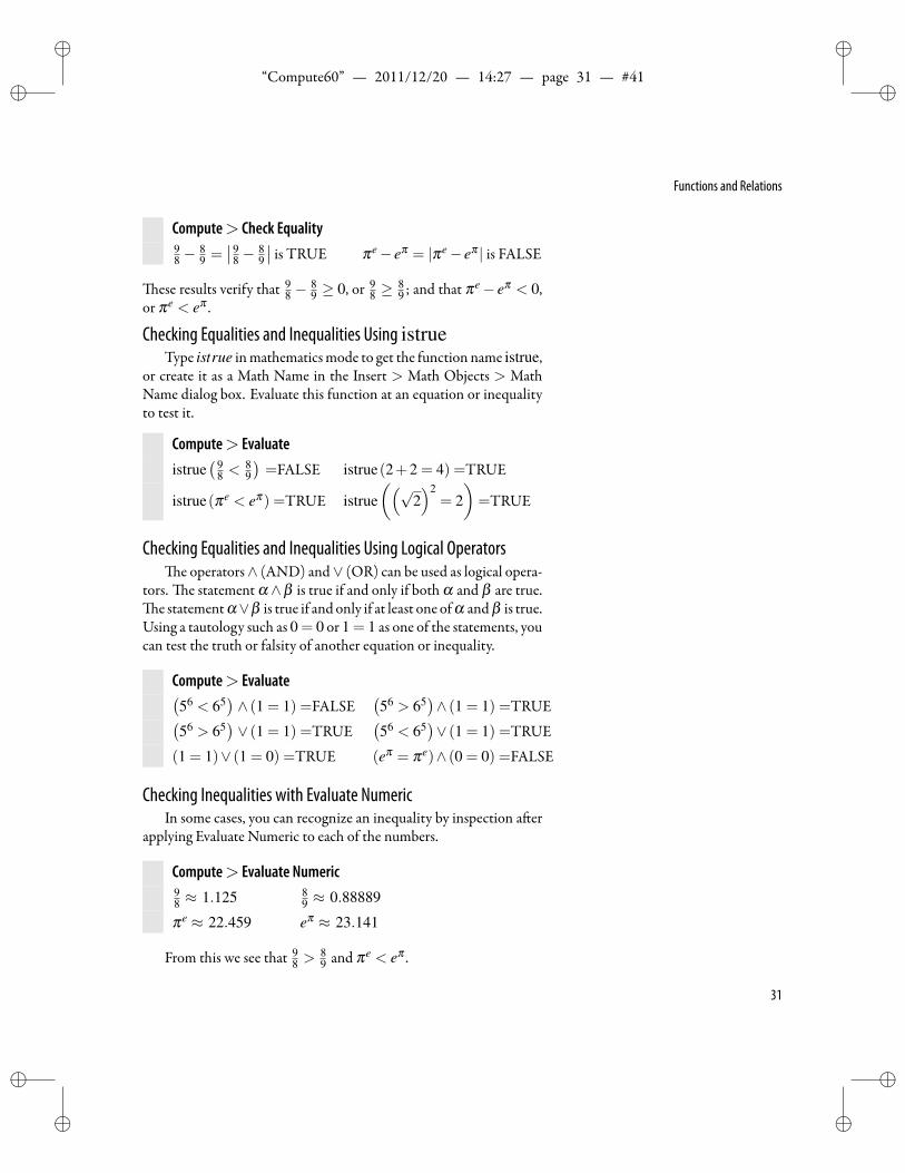
Checking Equality and InequalityYoucanverify equalities and inequalitieswith the commandCheck
Equality orwith the function istrue. ere are three possible responses:true, false, and undecidable. e latter means that the test is inconclu-sive and the equality may be either true or false. e computationalengine may use probabilistic methods to check equality, and there is avery small probability that an equation judged as true is actually false.Some expressions cannot be compared by this method—hence the in-conclusive response.
Checking Equalities and Inequalities using Check EqualityTocheckwhether an equality is true or false
1. Place the insert point in the equation.
2. Choose Check Equality.
Compute> Check Equalityeiπ = −1 is TRUE π = 3.14 is FALSEarcsinsinx = x is FALSE
You can also use Check Equality to check an inequality betweentwo numbers. Set the difference of the two numbers equal to the ab-solute value of the difference, place the insert point in the equation,and choose Check Equality.
30
ii
“Compute60” — 2011/12/20 — 14:27 — page 31 — #41 ii
ii
ii
Functions and Relations
Compute> Check Equality98 −
89 =
∣∣ 98 −
89
∣∣ is TRUE πe− eπ = |πe− eπ | is FALSE
ese results verify that 98 −
89 ≥ 0, or 9
8 ≥89 ; and that πe− eπ < 0,
or πe < eπ .
Checking Equalities and Inequalities Using istrueType istrue inmathematicsmode to get the function name istrue,
or create it as a Math Name in the Insert > Math Objects > MathName dialog box. Evaluate this function at an equation or inequalityto test it.
Compute> Evaluateistrue
( 98 < 8
9
)=FALSE istrue(2+2 = 4) =TRUE
istrue(πe < eπ) =TRUE istrue((√
2)2
= 2)=TRUE
Checking Equalities and Inequalities Using Logical Operatorse operators∧ (AND) and∨ (OR) can be used as logical opera-
tors. e statement α ∧β is true if and only if both α and β are true.e statementα∨β is true if and only if at least one ofα andβ is true.
Using a tautology such as 0 = 0 or 1 = 1 as one of the statements, youcan test the truth or falsity of another equation or inequality.
Compute> Evaluate(56 < 65
)∧ (1 = 1) =FALSE
(56 > 65
)∧ (1 = 1) =TRUE(
56 > 65)∨ (1 = 1) =TRUE
(56 < 65
)∨ (1 = 1) =TRUE
(1 = 1)∨ (1 = 0) =TRUE (eπ = πe)∧ (0 = 0) =FALSE
Checking Inequalities with Evaluate NumericIn some cases, you can recognize an inequality by inspection a er
applying Evaluate Numeric to each of the numbers.
Compute> Evaluate Numeric98 ≈ 1.125 8
9 ≈ 0.88889
πe ≈ 22.459 eπ ≈ 23.141
From this we see that 98 > 8
9 and πe < eπ .
31
ii
“Compute60” — 2011/12/20 — 14:27 — page 32 — #42 ii
ii
ii
Chapter 2 | Numbers, Functions, and Units
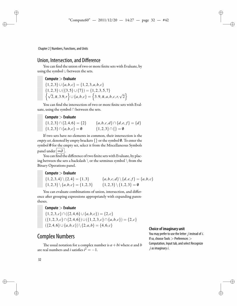
Union, Intersection, and DifferenceYou can nd the union of two ormore nite sets with Evaluate, by
using the symbol∪ between the sets.
Compute> Evaluate1,2,3∪a,b,c= 1,2,3,a,b,c1,2,3∪ (3,5∪7) = 1,2,3,5,7√
2,π,3.9,r∪a,b,c=
3.9,π,a,b,c,r,
√2
You can nd the intersection of two or more nite sets with Eval-uate, using the symbol∩ between the sets.
Compute> Evaluate1,2,3∩2,4,6= 2 a,b,c,d∩d,e, f= d1,2,3∩a,b,c= /0 1,2,3∩= /0
If two sets have no elements in common, their intersection is theempty set, denoted by empty brackets or the symbol /0. To enter thesymbol /0 for the empty set, select it from the Miscellaneous Symbolspanel under ∞∂ .
You can nd the difference of two nite setswithEvaluate, by plac-ing between the sets a backslash \ or the setminus symbol \ from theBinary Operations panel.
Compute> Evaluate1,2,3,4\2,4= 1,3 a,b,c,d\d,e, f= a,b,c1,2,3\a,b,c= 1,2,3 1,2,3\1,2,3= /0
You can evaluate combinations of union, intersection, and differ-ence a er grouping expressions appropriately with expanding paren-theses.
Compute> Evaluate1,2,3,c∩ (2,4,6∪a,b,c) = 2,c(1,2,3,c∩2,4,6)∪ (1,2,3,c∩a,b,c) = 2,c(2,4,6∪a,b,c)\2,a,b= 4,6,c
Choice of imaginary unitYou may prefer to use the letter j instead of i.If so, choose Tools> Preferences>Computation, Input tab, and select Recognizej as imaginary i.
Complex Numberse usual notation for a complex number is a+bi where a and b
are real numbers and i satis es i2 =−1.
32
ii
“Compute60” — 2011/12/20 — 14:27 — page 33 — #43 ii
ii
ii
Units and Measurements
ArithmeticYou can do arithmetic with complex numbers using Evaluate. e
result is the rectangular form a+bi of the complex number.Appearance of imaginary unitYou may prefer a distinguished font for theimaginary i. If so, choose Tools> Preferences> Computation, Entities tab, and checkImaginaryI. If you do not want i recognized asthe imaginary unit, click the Input tab, anduncheck Recognize plain i as imaginary.Choose OK.
Compute> Evaluate√−5 = i
√5 i
1+i =12 +
12 i
(1+ i)(3−2i) = 5+ i (1+ i)÷ (3−2i) = 113 +
513 i
Absolute Valueeabsolute valueof a complexnumbera+bi is givenby |a+bi|=√
a2 +b2. You can compute the absolute value of a complex numberusing Evaluate.
Compute> Evaluate|1+ i|=
√2
∣∣eiπ ∣∣= 1
Complex Conjugatee complex conjugate of a+bi is written (a+bi)∗ or a+bi.
Complex ConjugateTo use overbar notation for complex conjugate,choose Tools> Preferences> Computation,Input tab, and check Overbar accent meansconjugate. Choose OK.
Compute> Evaluate(1+ i)∗ = 1− i 1+ i = 1− i(5−3i)∗ = 5+3i 5−3i = 5+3i
Real and Imaginary PartsYou can nd the real and imaginary parts of a complex number
using the functions Re and Im. Entering functionsWhen you enter the functionsRe and Im inmathematics mode, they will automaticallyturn gray.
Compute> EvaluateRe(1+ i) = 1 Im(5−3i) =−3
SeeComplexNumbers andComplexFunctions, page 89, formoreadvanced topics concerning complex numbers.
Units and Measurementse available units include units from the System of International
Units (SI units), an internationally agreed upon system of coherentunits that is now in use for all scienti c and most technological pur-poses in many countries. SI units are of three kinds: the base, supple-mentary, and derived units. ere are seven base units for the seven di-
33
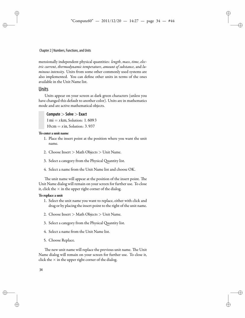
ii
“Compute60” — 2011/12/20 — 14:27 — page 34 — #44 ii
ii
ii
Chapter 2 | Numbers, Functions, and Units
mensionally independent physical quantities: length, mass, time, elec-tric current, thermodynamic temperature, amount of substance, and lu-minous intensity. Units from some other commonly used systems arealso implemented. You can de ne other units in terms of the onesavailable in the Unit Name list.
UnitsUnits appear on your screen as dark green characters (unless you
have changed this default to another color). Units are in mathematicsmode and are active mathematical objects.
Compute> Solve> Exact1mi = xkm, Solution: 1.609310cm = x in, Solution: 3.937
Toenter a unit name1. Place the insert point at the position where you want the unit
name.
2. Choose Insert>Math Objects>Unit Name.
3. Select a category from the Physical uantity list.
4. Select a name from the Unit Name list and choose OK.
e unit name will appear at the position of the insert point. eUnit Name dialog will remain on your screen for further use. To closeit, click the× in the upper right corner of the dialog.To replace a unit
1. Select the unit name you want to replace, either with click anddrag or by placing the insert point to the right of the unit name.
2. Choose Insert>Math Objects>Unit Name.
3. Select a category from the Physical uantity list.
4. Select a name from the Unit Name list.
5. Choose Replace.
e new unit name will replace the previous unit name. e UnitName dialog will remain on your screen for further use. To close it,click the× in the upper right corner of the dialog.
34
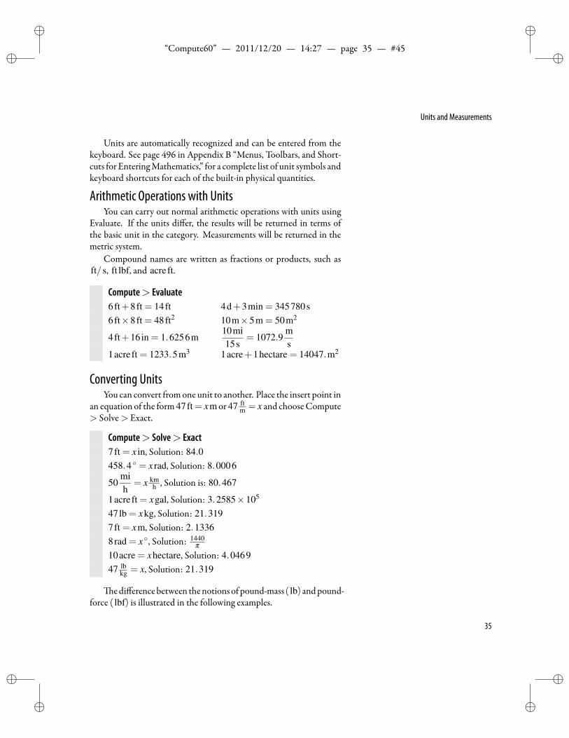
ii
“Compute60” — 2011/12/20 — 14:27 — page 35 — #45 ii
ii
ii
Units and Measurements
Units are automatically recognized and can be entered from thekeyboard. See page 496 in Appendix B “Menus, Toolbars, and Short-cuts for EnteringMathematics,” for a complete list of unit symbols andkeyboard shortcuts for each of the built-in physical quantities.
Arithmetic Operations with UnitsYou can carry out normal arithmetic operations with units using
Evaluate. If the units differ, the results will be returned in terms ofthe basic unit in the category. Measurements will be returned in themetric system.
Compound names are written as fractions or products, such asft/s, ft lbf, and acreft.
Compute> Evaluate6ft+8ft = 14ft 4d+3min = 345780s6ft×8ft = 48ft2 10m×5m = 50m2
4ft+16in = 1.6256m10mi15s
= 1072.9ms
1acreft = 1233.5m3 1acre+1hectare = 14047.m2
Converting UnitsYou can convert fromone unit to another. Place the insert point in
an equation of the form 47ft= xm or 47 ftm = x and chooseCompute
> Solve> Exact.
Compute> Solve> Exact7ft = x in, Solution: 84.0458.4 = x rad, Solution: 8.0006
50mih
= x kmh , Solution is: 80.467
1acreft = xgal, Solution: 3.2585×10⁵
47lb = xkg, Solution: 21.3197ft = xm, Solution: 2.13368rad = x , Solution: 1440
π10acre = xhectare, Solution: 4.046947 lb
kg = x, Solution: 21.319
edifferencebetween thenotionsof pound-mass ( lb) andpound-force ( lbf) is illustrated in the following examples.
35
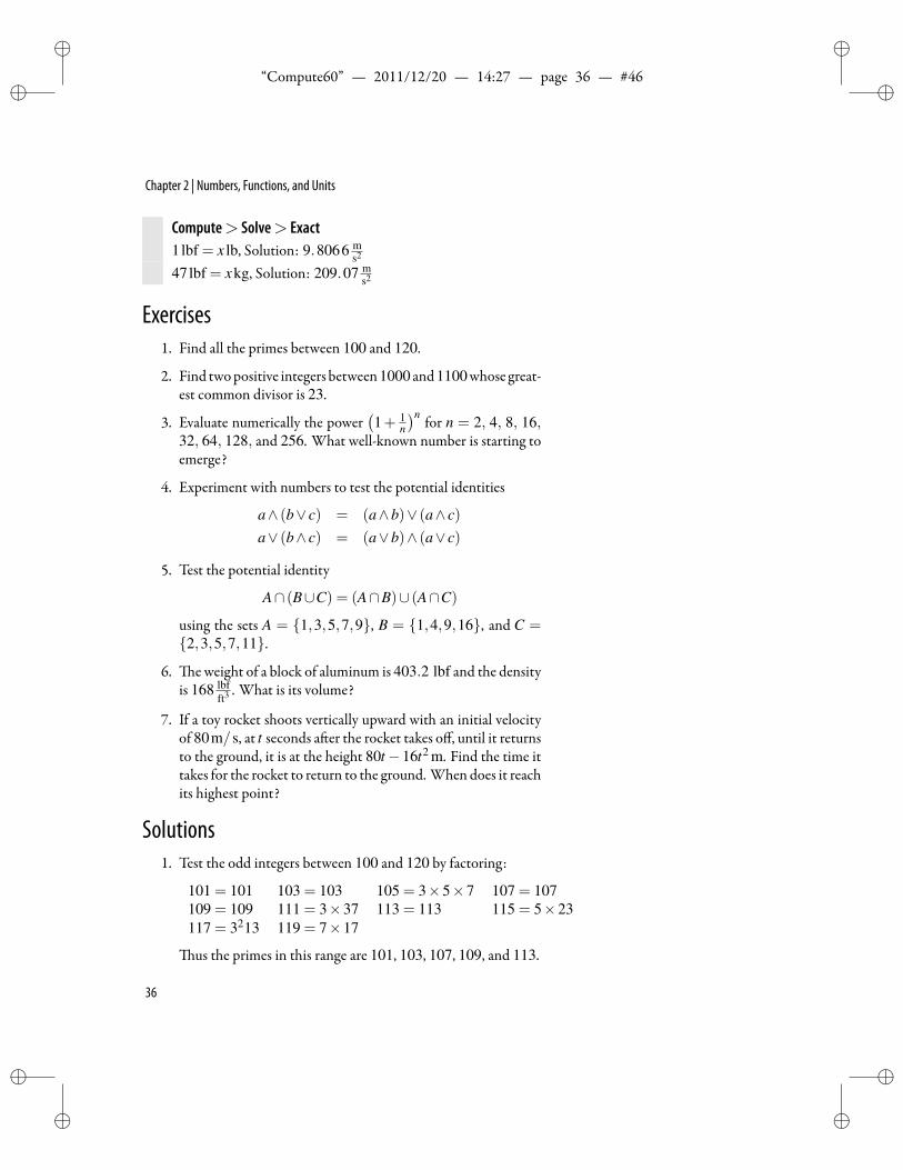
ii
“Compute60” — 2011/12/20 — 14:27 — page 36 — #46 ii
ii
ii
Chapter 2 | Numbers, Functions, and Units
Compute> Solve> Exact1lbf = x lb, Solution: 9.8066 m
s2
47lbf = xkg, Solution: 209.07 ms2
Exercises1. Find all the primes between 100 and 120.
2. Find twopositive integers between1000 and1100whose great-est common divisor is 23.
3. Evaluate numerically the power(1+ 1
n
)n for n = 2, 4, 8, 16,32, 64, 128, and 256. What well-known number is starting toemerge?
4. Experiment with numbers to test the potential identities
a∧ (b∨ c) = (a∧b)∨ (a∧ c)a∨ (b∧ c) = (a∨b)∧ (a∨ c)
5. Test the potential identity
A∩ (B∪C) = (A∩B)∪ (A∩C)
using the sets A = 1,3,5,7,9, B = 1,4,9,16, and C =2,3,5,7,11.
6. e weight of a block of aluminum is 403.2 lbf and the densityis 168 lbf
ft3. What is its volume?
7. If a toy rocket shoots vertically upward with an initial velocityof 80m/s, at t seconds a er the rocket takes off, until it returnsto the ground, it is at the height 80t−16t2 m. Find the time ittakes for the rocket to return to the ground. When does it reachits highest point?
Solutions1. Test the odd integers between 100 and 120 by factoring:
101 = 101 103 = 103 105 = 3×5×7 107 = 107109 = 109 111 = 3×37 113 = 113 115 = 5×23117 = 3213 119 = 7×17
us the primes in this range are 101, 103, 107, 109, and 113.
36
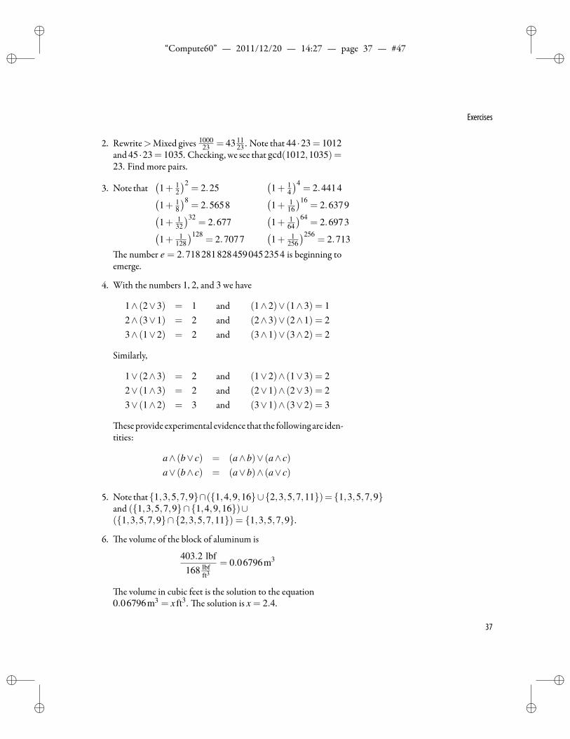
ii
“Compute60” — 2011/12/20 — 14:27 — page 37 — #47 ii
ii
ii
Exercises
2. Rewrite>Mixed gives 100023 = 43 11
23 . Note that 44 ·23 = 1012and 45 ·23= 1035. Checking, we see that gcd(1012,1035) =23. Find more pairs.
3. Note that(1+ 1
2
)2= 2.25
(1+ 1
4
)4= 2.4414(
1+ 18
)8= 2.5658
(1+ 1
16
)16= 2.6379(
1+ 132
)32= 2.677
(1+ 1
64
)64= 2.6973(
1+ 1128
)128= 2.7077
(1+ 1
256
)256= 2.713
e number e = 2.7182818284590452354 is beginning toemerge.
4. With the numbers 1, 2, and 3 we have
1∧ (2∨3) = 1 and (1∧2)∨ (1∧3) = 12∧ (3∨1) = 2 and (2∧3)∨ (2∧1) = 23∧ (1∨2) = 2 and (3∧1)∨ (3∧2) = 2
Similarly,
1∨ (2∧3) = 2 and (1∨2)∧ (1∨3) = 22∨ (1∧3) = 2 and (2∨1)∧ (2∨3) = 23∨ (1∧2) = 3 and (3∨1)∧ (3∨2) = 3
ese provide experimental evidence that the following are iden-tities:
a∧ (b∨ c) = (a∧b)∨ (a∧ c)a∨ (b∧ c) = (a∨b)∧ (a∨ c)
5. Note that1,3,5,7,9∩(1,4,9,16∪2,3,5,7,11)= 1,3,5,7,9and (1,3,5,7,9∩1,4,9,16)∪(1,3,5,7,9∩2,3,5,7,11) = 1,3,5,7,9.
6. e volume of the block of aluminum is
403.2 lbf168 lbf
ft3= 0.06796m3
e volume in cubic feet is the solution to the equation0.06796m3 = x ft3. e solution is x = 2.4.
37
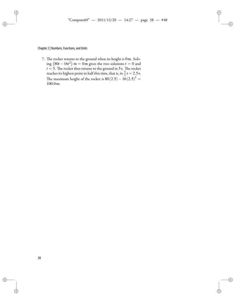
ii
“Compute60” — 2011/12/20 — 14:27 — page 38 — #48 ii
ii
ii
Chapter 2 | Numbers, Functions, and Units
7. e rocket returns to the ground when its height is 0m. Solv-ing(80t−16t2
)m = 0m gives the two solutions t = 0 and
t = 5. e rocket thus returns to the ground in 5s. e rocketreaches its highest point in half this time, that is, in 5
2 s = 2.5s.e maximum height of the rocket is 80(2.5)− 16(2.5)2 =
100.0m.
38
ii
“Compute60” — 2011/12/20 — 14:27 — page 39 — #49 ii
ii
ii
3Algebra
[Algebra's] a merry science. When the animal that we are hunting cannot be caught, we call it X temporarily and continue to huntuntil it is bagged. Jakob Einstein (1850–1912)
A lgebraic operations are generalizations of arithmetic opera- Polynomials and RationalExpressions
Substitution
Solving Equations
De ning Variables and Functions
Exponents and Logarithms
Toolbars and Keyboard Shortcuts
tions. Algebraic expressions are obtained by starting withvariables and constants and combining them using addition,
subtraction, multiplication, division, exponentiation, and roots. esimplest types of algebraic expressions use only addition, subtraction,and multiplication; these are called polynomials. e general form ofa polynomial of degree n in the variable x is
anxn +an−1xn−1 + · · ·+a1x+a0
where a0, a1, . . ., an are constants and an = 0.
Polynomials and Rational ExpressionsYou canperform the usual operations onpolynomials. e general
procedure is as described below.Toworkwith a polynomial expression
1. Enter the expression in mathematics mode and leave the insertpoint in the expression.
2. Apply one of the commands from the Compute menu.
You will nd a variety of useful commands.
39
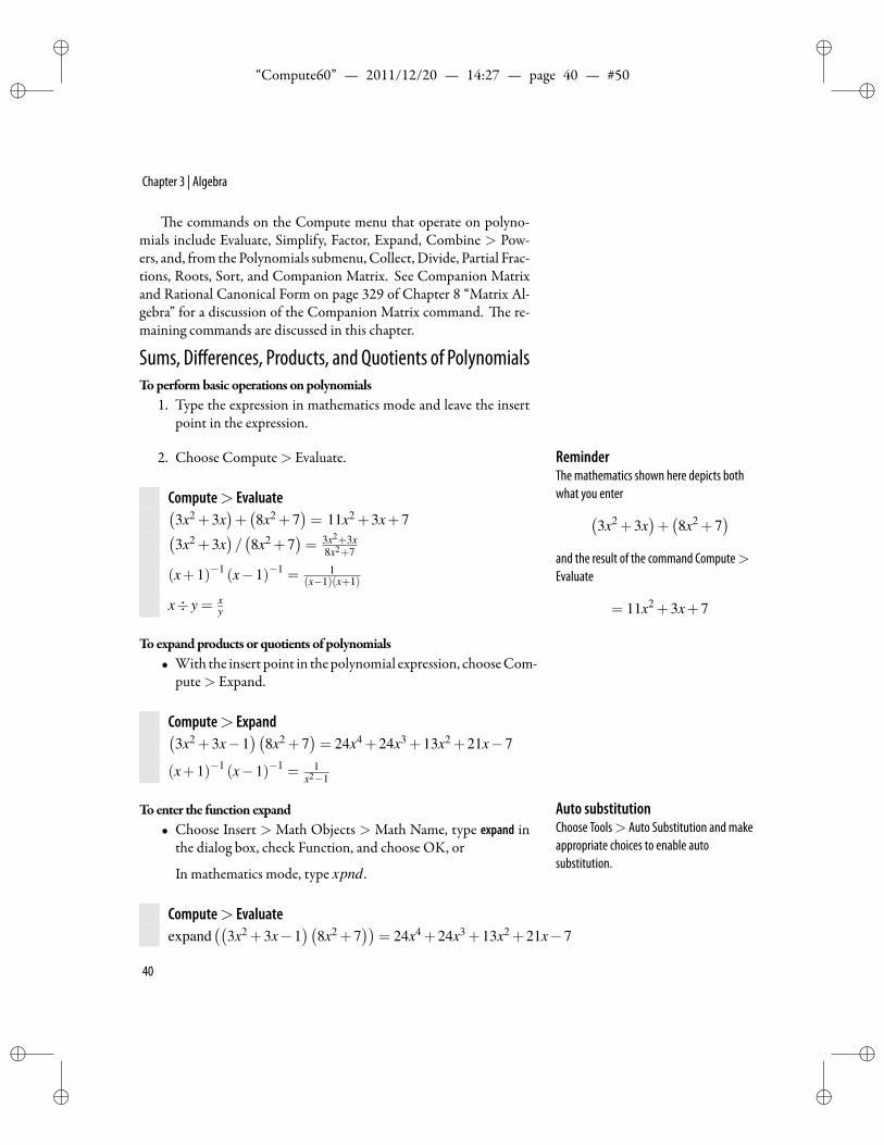
ii
“Compute60” — 2011/12/20 — 14:27 — page 40 — #50 ii
ii
ii
Chapter 3 | Algebra
e commands on the Compute menu that operate on polyno-mials include Evaluate, Simplify, Factor, Expand, Combine > Pow-ers, and, from the Polynomials submenu,Collect, Divide, Partial Frac-tions, Roots, Sort, and Companion Matrix. See Companion Matrixand Rational Canonical Form on page 329 of Chapter 8 “Matrix Al-gebra” for a discussion of the Companion Matrix command. e re-maining commands are discussed in this chapter.
Sums, Differences, Products, and Quotients of PolynomialsToperformbasic operations onpolynomials
1. Type the expression in mathematics mode and leave the insertpoint in the expression.
2. Choose Compute> Evaluate. ReminderThe mathematics shown here depicts bothwhat you enter(
3x2 +3x)+(8x2 +7
)and the result of the command Compute>Evaluate
= 11x2 +3x+7
Compute> Evaluate(3x2 +3x
)+(8x2 +7
)= 11x2 +3x+7(
3x2 +3x)/(8x2 +7
)= 3x2+3x
8x2+7
(x+1)−1 (x−1)−1 = 1(x−1)(x+1)
x÷ y = xy
Toexpandproducts or quotients of polynomials• With the insert point in thepolynomial expression, chooseCom-
pute> Expand.
Compute> Expand(3x2 +3x−1
)(8x2 +7
)= 24x4 +24x3 +13x2 +21x−7
(x+1)−1 (x−1)−1 = 1x2−1
Toenter the function expand Auto substitutionChoose Tools> Auto Substitution and makeappropriate choices to enable autosubstitution.
• Choose Insert > Math Objects > Math Name, type expand inthe dialog box, check Function, and choose OK, or
In mathematics mode, type xpnd.
Compute> Evaluateexpand
((3x2 +3x−1
)(8x2 +7
))= 24x4 +24x3 +13x2 +21x−7
40

ii
“Compute60” — 2011/12/20 — 14:27 — page 41 — #51 ii
ii
ii
Polynomials and Rational Expressions
Division by PolynomialsYou can convert a quotient of polynomials f (x)
g(x) with rational coef-
cients to the form q(x)+ r(x)g(x) , where r(x) and q(x) are polynomials
and degr(x)< degg(x).
Todivide polynomials Polynomials> DivideThis algorithm is the familiar long-divisionalgorithm for polynomials.
1. Enter a quotient of polynomials.
2. Leave the insert point in the expression.
3. Choose Compute> Polynomials>Divide.
Compute> Polynomials> Divide
3x5+3x3−4x2+58x2+7 = 3
64 x−2164 x− 17
28x2+7 + 3
8 x3− 12
5y2−3y+43y−5 = 5
3 y+ 1169(3y−5) +
169
Summation NotationA polynomial in general form can be written in summation nota-
tionn
∑k=0
akxk = anxn +an−1xn−1 + · · ·+a1x+a0
Toenter a polynomial as a summation∑5k=0 akxk
1. Choose Insert>Math Objects>Operator and choose ∑.
2. Choose Insert>Math Objects> Subscript and type k = 0.
3. Press tab and type 5.
4. Press the spacebar and type akxk.
Compute> Evaluate∑5
k=0 akxk = a5x5 +a4x4 +a3x3 +a2x2 +a1x+a0
Sums and Differences of Rational ExpressionsA quotient of two polynomials is called a rational expression.
41
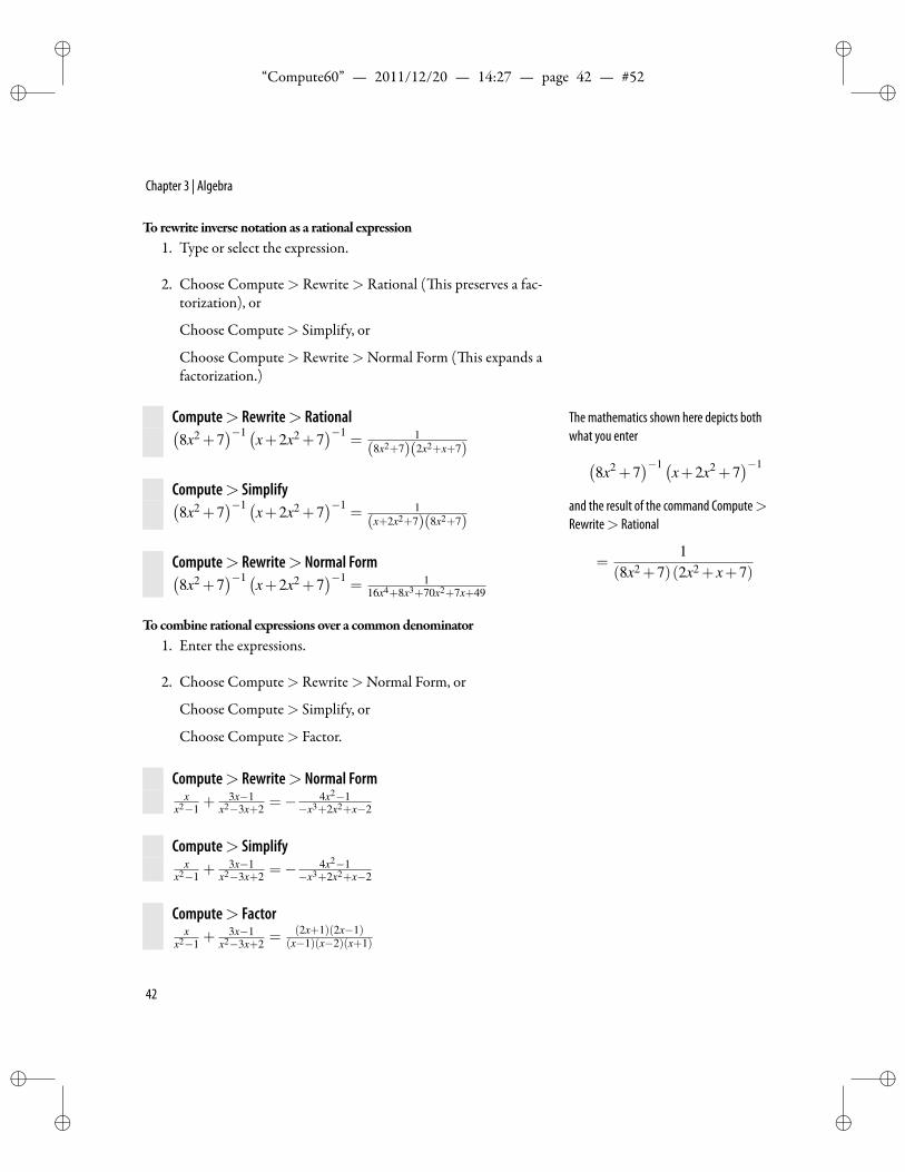
ii
“Compute60” — 2011/12/20 — 14:27 — page 42 — #52 ii
ii
ii
Chapter 3 | Algebra
To rewrite inverse notation as a rational expression1. Type or select the expression.
2. Choose Compute> Rewrite> Rational ( is preserves a fac-torization), or
Choose Compute> Simplify, or
Choose Compute> Rewrite>Normal Form ( is expands afactorization.)
Compute> Rewrite> Rational(8x2 +7
)−1 (x+2x2 +7)−1
= 1(8x2+7)(2x2+x+7)
The mathematics shown here depicts bothwhat you enter(
8x2 +7)−1 (
x+2x2 +7)−1
and the result of the command Compute>Rewrite> Rational
=1
(8x2 +7)(2x2 + x+7)
Compute> Simplify(8x2 +7
)−1 (x+2x2 +7)−1
= 1(x+2x2+7)(8x2+7)
Compute> Rewrite> Normal Form(8x2 +7
)−1 (x+2x2 +7)−1
= 116x4+8x3+70x2+7x+49
Tocombine rational expressions over a commondenominator1. Enter the expressions.
2. Choose Compute> Rewrite>Normal Form, or
Choose Compute> Simplify, or
Choose Compute> Factor.
Compute> Rewrite> Normal Formx
x2−1 +3x−1
x2−3x+2 =− 4x2−1−x3+2x2+x−2
Compute> Simplifyx
x2−1 +3x−1
x2−3x+2 =− 4x2−1−x3+2x2+x−2
Compute> Factorx
x2−1 +3x−1
x2−3x+2 = (2x+1)(2x−1)(x−1)(x−2)(x+1)
42
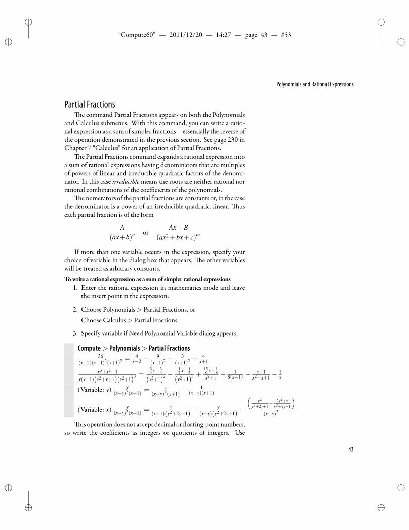
ii
“Compute60” — 2011/12/20 — 14:27 — page 43 — #53 ii
ii
ii
Polynomials and Rational Expressions
Partial Fractionse command Partial Fractions appears on both the Polynomials
and Calculus submenus. With this command, you can write a ratio-nal expression as a sum of simpler fractions—essentially the reverse ofthe operation demonstrated in the previous section. See page 230 inChapter 7 “Calculus” for an application of Partial Fractions.
e Partial Fractions command expands a rational expression intoa sum of rational expressions having denominators that are multiplesof powers of linear and irreducible quadratic factors of the denomi-nator. In this case irreduciblemeans the roots are neither rational norrational combinations of the coefficients of the polynomials.
e numerators of the partial fractions are constants or, in the casethe denominator is a power of an irreducible quadratic, linear. useach partial fraction is of the form
A(ax+b)n or
Ax+B(ax2 +bx+ c)m
If more than one variable occurs in the expression, specify yourchoice of variable in the dialog box that appears. e other variableswill be treated as arbitrary constants.Towrite a rational expression as a sumof simpler rational expressions
1. Enter the rational expression in mathematics mode and leavethe insert point in the expression.
2. Choose Polynomials> Partial Fractions, orChoose Calculus> Partial Fractions.
3. Specify variable if Need Polynomial Variable dialog appears.
Compute> Polynomials> Partial Fractions36
(x−2)(x−1)2(x+1)2 = 4x−2 −
9(x−1)2 − 3
(x+1)2 − 4x+1
x3+x2+1x(x−1)(x2+x+1)(x2+1)
3 =34 x+ 3
4
(x2+1)2 −
12 x− 1
2
(x2+1)3 +
158 x− 1
8x2+1 + 1
8(x−1) −x+1
x2+x+1 −1x
(Variable: y) y(x−y)2(x+1) =
x(x−y)2(x+1)
− 1(x−y)(x+1)
(Variable: x) y(x−y)2(x+1) =
y(x+1)(y2+2y+1)
− y(x−y)(y2+2y+1)
−
(y2
y2+2y+1− 2y2+y
y2+2y+1
)(x−y)2
is operation does not accept decimal or oating-point numbers,so write the coefficients as integers or quotients of integers. Use
43
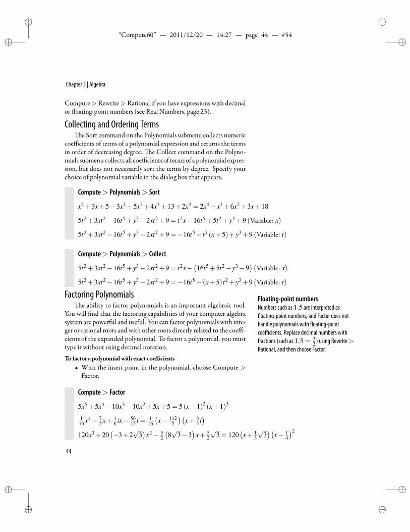
ii
“Compute60” — 2011/12/20 — 14:27 — page 44 — #54 ii
ii
ii
Chapter 3 | Algebra
Compute>Rewrite>Rational if you have expressions with decimalor oating-point numbers (see Real Numbers, page 23).
Collecting and Ordering Termse Sort command on the Polynomials submenu collects numeric
coefficients of terms of a polynomial expression and returns the termsin order of decreasing degree. e Collect command on the Polyno-mials submenu collects all coefficients of terms of a polynomial expres-sion, but does not necessarily sort the terms by degree. Specify yourchoice of polynomial variable in the dialog box that appears.
Compute> Polynomials> Sort
x2 +3x+5−3x3 +5x2 +4x3 +13+2x4 = 2x4 + x3 +6x2 +3x+18
5t2 +3xt2−16t5 + y3−2xt2 +9 = t2x−16t5 +5t2 + y3 +9 (Variable: x)
5t2 +3xt2−16t5 + y3−2xt2 +9 =−16t5 + t2 (x+5)+ y3 +9 (Variable: t)
Compute> Polynomials> Collect
5t2 +3xt2−16t5 + y3−2xt2 +9 = t2x−(16t5 +5t2− y3−9
)(Variable: x)
5t2 +3xt2−16t5 + y3−2xt2 +9 =−16t5 +(x+5) t2 + y3 +9 (Variable: t)
Factoring Polynomials Floating-point numbersNumbers such as 1.5 are interpreted asoating-point numbers, and Factor does nothandle polynomials with oating-pointcoefficients. Replace decimal numbers withfractions (such as 1.5 = 3
2 ) using Rewrite>Rational, and then choose Factor.
e ability to factor polynomials is an important algebraic tool.You will nd that the factoring capabilities of your computer algebrasystem are powerful and useful. You can factor polynomials with inte-ger or rational roots and with other roots directly related to the coeffi-cients of the expanded polynomial. To factor a polynomial, you musttype it without using decimal notation.
To factor a polynomialwith exact coefficients• With the insert point in the polynomial, choose Compute >
Factor.
Compute> Factor
5x5 +5x4−10x3−10x2 +5x+5 = 5(x−1)2 (x+1)3
116 x2− 7
5 x+ 16 ix− 56
15 i = 116
(x− 112
5
)(x+ 8
3 i)
120x3 +20(−3+2
√3)
x2− 52
(8√
3−3)
x+ 52
√3 = 120
(x+ 1
3
√3)(
x− 14
)2
44
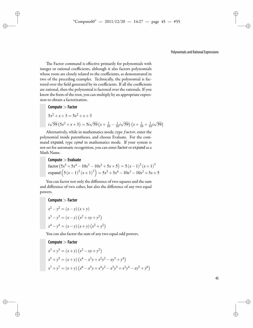
ii
“Compute60” — 2011/12/20 — 14:27 — page 45 — #55 ii
ii
ii
Polynomials and Rational Expressions
e Factor command is effective primarily for polynomials withinteger or rational coefficients, although it also factors polynomialswhose roots are closely related to the coefficients, as demonstrated intwo of the preceding examples. Technically, the polynomial is fac-tored over the eld generated by its coefficients. If all the coefficientsare rational, then the polynomial is factored over the rationals. If youknow the form of the root, you canmultiply by an appropriate expres-sion to obtain a factorization.
Compute> Factor
5x2 + x+3 = 5x2 + x+3
i√
59(5x2 + x+3
)= 5i√
59(x+ 1
10 −1
10 i√
59)(
x+ 110 +
110 i√
59)
Alternatively, while in mathematics mode, type f actor, enter thepolynomial inside parentheses, and choose Evaluate. For the com-mand expand, type xpnd in mathematics mode. If your system isnot set for automatic recognition, you can enter factor or expand as aMath Name.
Compute> Evaluatefactor
(5x5 +5x4−10x3−10x2 +5x+5
)= 5(x−1)2 (x+1)3
expand(
5(x−1)2 (x+1)3)= 5x5 +5x4−10x3−10x2 +5x+5
You can factor not only the difference of two squares and the sumand difference of two cubes, but also the difference of any two equalpowers.
Compute> Factor
x2− y2 = (x− y)(x+ y)
x3− y3 = (x− y)(x2 + xy+ y2
)x4− y4 = (x− y)(x+ y)
(x2 + y2
)You can also factor the sum of any two equal odd powers.
Compute> Factor
x3 + y3 = (x+ y)(x2− xy+ y2
)x5 + y5 = (x+ y)
(x4− x3y+ x2y2− xy3 + y4
)x7 + y7 = (x+ y)
(x6− x5y+ x4y2− x3y3 + x2y4− xy5 + y6
)45
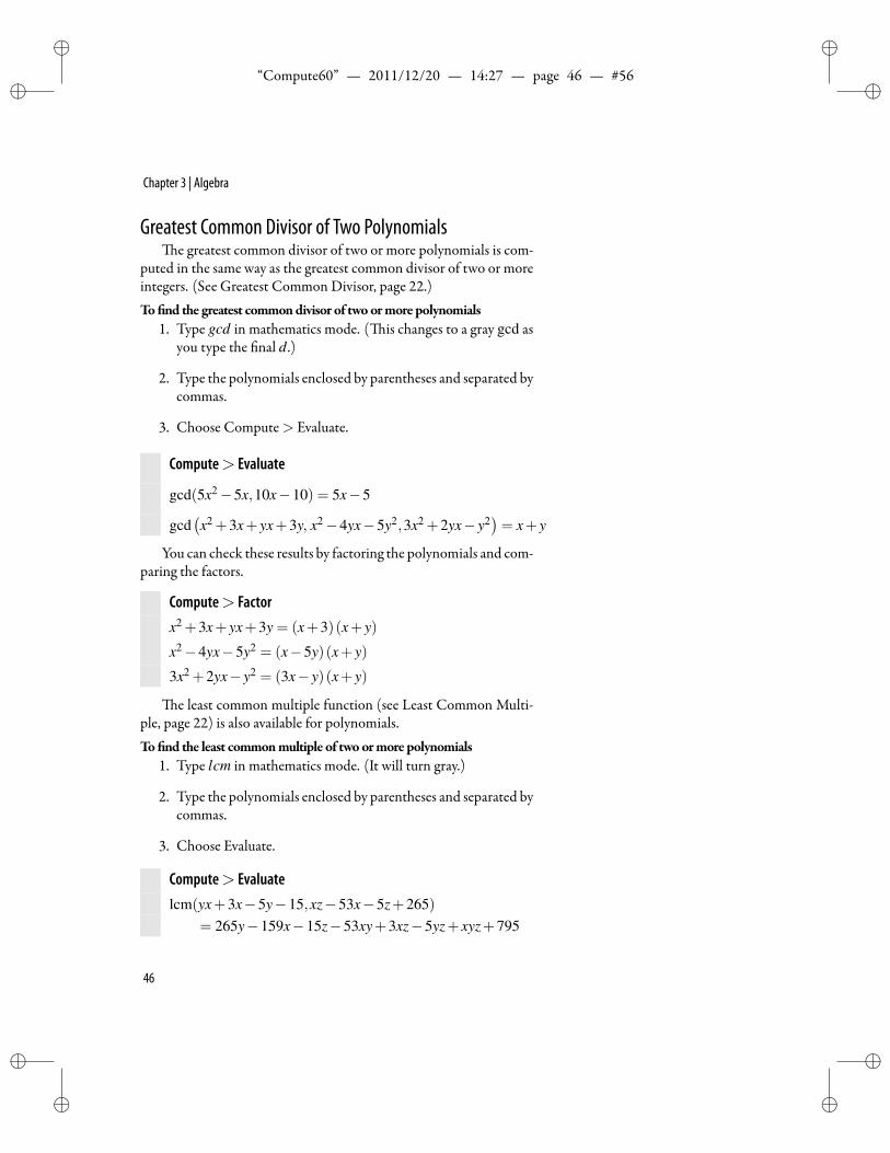
ii
“Compute60” — 2011/12/20 — 14:27 — page 46 — #56 ii
ii
ii
Chapter 3 | Algebra
Greatest Common Divisor of Two Polynomialse greatest common divisor of two or more polynomials is com-
puted in the same way as the greatest common divisor of two or moreintegers. (See Greatest Common Divisor, page 22.)To nd the greatest commondivisor of twoormore polynomials
1. Type gcd in mathematics mode. ( is changes to a gray gcd asyou type the nal d.)
2. Type the polynomials enclosed by parentheses and separated bycommas.
3. Choose Compute> Evaluate.
Compute> Evaluate
gcd(5x2−5x,10x−10) = 5x−5
gcd(x2 +3x+ yx+3y, x2−4yx−5y2,3x2 +2yx− y2
)= x+ y
You can check these results by factoring the polynomials and com-paring the factors.
Compute> Factorx2 +3x+ yx+3y = (x+3)(x+ y)
x2−4yx−5y2 = (x−5y)(x+ y)
3x2 +2yx− y2 = (3x− y)(x+ y)
e least common multiple function (see Least Common Multi-ple, page 22) is also available for polynomials.To nd the least commonmultiple of twoormore polynomials
1. Type lcm in mathematics mode. (It will turn gray.)
2. Type the polynomials enclosed by parentheses and separated bycommas.
3. Choose Evaluate.
Compute> Evaluatelcm(yx+3x−5y−15,xz−53x−5z+265)
= 265y−159x−15z−53xy+3xz−5yz+ xyz+795
46
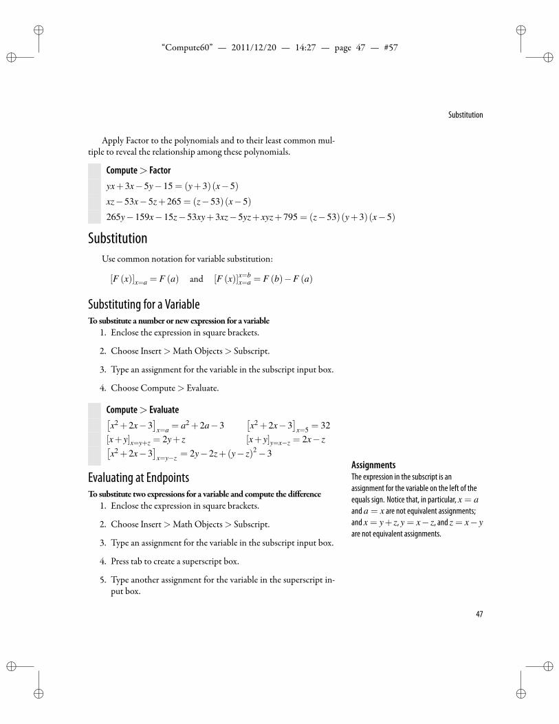
ii
“Compute60” — 2011/12/20 — 14:27 — page 47 — #57 ii
ii
ii
Substitution
Apply Factor to the polynomials and to their least common mul-tiple to reveal the relationship among these polynomials.
Compute> Factoryx+3x−5y−15 = (y+3)(x−5)
xz−53x−5z+265 = (z−53)(x−5)
265y−159x−15z−53xy+3xz−5yz+ xyz+795 = (z−53)(y+3)(x−5)
SubstitutionUse common notation for variable substitution:
[F (x)]x=a = F (a) and [F (x)]x=bx=a = F (b)−F (a)
Substituting for a VariableTo substitute a number or new expression for a variable
1. Enclose the expression in square brackets.
2. Choose Insert>Math Objects> Subscript.
3. Type an assignment for the variable in the subscript input box.
4. Choose Compute> Evaluate.
Compute> Evaluate[x2 +2x−3
]x=a = a2 +2a−3
[x2 +2x−3
]x=5 = 32
[x+ y]x=y+z = 2y+ z [x+ y]y=x−z = 2x− z[x2 +2x−3
]x=y−z = 2y−2z+(y− z)2−3
AssignmentsThe expression in the subscript is anassignment for the variable on the left of theequals sign. Notice that, in particular, x = aand a = x are not equivalent assignments;and x = y+ z, y = x− z, and z = x−yare not equivalent assignments.
Evaluating at EndpointsTo substitute two expressions for a variable and compute the difference
1. Enclose the expression in square brackets.
2. Choose Insert>Math Objects> Subscript.
3. Type an assignment for the variable in the subscript input box.
4. Press tab to create a superscript box.
5. Type another assignment for the variable in the superscript in-put box.
47
ii
“Compute60” — 2011/12/20 — 14:27 — page 48 — #58 ii
ii
ii
Chapter 3 | Algebra
6. Choose Compute> Evaluate.
Compute> Evaluate[x]x=b
x=a = b−a[x2 +2x−3
]x=5x=3 = 20[
x2 +2x−3]x=b
x=a =−a2−2a+b2 +2b
Solving EquationsYoucan solvepolynomial equationsby choosingCompute>Poly-
nomials > Roots or by choosing Compute > Solve. We rst look atexamples for nding roots of polynomials. en we look at the moregeneral problems of solving equations with one or more variables.
Roots of PolynomialsIf zero is obtained when a number is substituted for the variable in
a polynomial, then that number is a root of the polynomial. In otherwords, the roots of a polynomial p(x) are the solutions to the equationp(x) = 0. For example, 1 is a root of x2−1 since
[x2−1
]x=1 = 0. Useful Fact
A number r is a root of a polynomial if andonly if x− r is a factor of that polynomial.
Youcan ndall real and complex roots of a real or complexpolyno-mial with rational coefficients by choosing Compute > Polynomials> Roots.To nd the roots of a polynomial
1. Type the polynomial and leave the insert point in the expres-sion.
2. Choose Compute> Polynomials> Roots.
Compute> Polynomials> Roots
5x2 +2x−3, roots: −1, 35 x2 +1, roots: −i, i
x3− 135 ix2−8x2 + 29
5 ix+ 815 x+6i− 18
5 , roots: 3,5+3i,− 25 i
Youcan simplify complex radical expressionswithRewrite>Rect-angular.
Compute> Rewrite> Rectangular( 52 +
1310 i)− 1
10
√(336+850i) = 2
5 i(−1)
110
√(336+850i)+
( 52 +
1310 i)= 5+3i
You can change settings so that only real roots will be computed.
48
ii
“Compute60” — 2011/12/20 — 14:27 — page 49 — #59 ii
ii
ii
Solving Equations
To nd (only) real roots of a polynomial1. While in mathematics mode, type assume(x, real) and choose
Compute> Evaluate.
2. Place the insert point in the polynomial and choose Compute> Polynomials> Roots.
Compute> Evaluateassume(x, real) = R
Compute> Polynomials> Roots
x3− 135 ix2−8x2 + 29
5 ix+ 815 x+6i− 18
5 , roots: 3
5x2 + x+3, roots: /0
e symbol /0 denotes the empty set, meaning there is no real so-lution.To return to the defaultmode
1. While in mathematics mode, type unassume(x).
2. Choose Compute> Evaluate.
It follows fromtheFundamental eoremofAlgebra that thenum-ber of roots (including complex roots and counting multiplicities) isthe same as the degree of the polynomial. For polynomials with ratio-nal (real or complex) coefficients, the computer algebra system usesthe usual formulas for nding roots symbolically for polynomials ofdegree 4 or less, and it nds the roots numerically for polynomials ofhigher degree. is implementation was dictated by the mathemati-cal phenomenon that there is no general formula in terms of radicalexpressions for the roots of polynomials of degree 5 and higher. Forpolynomials of any degree with oating point or decimal coefficients,the computer algebra system nds the roots numerically.
Second-Degree PolynomialsYou can obtain the familiar quadratic formula for roots of ax2 +
bx+c. e solution includes all cases. e logical symbol∧ is used forAND, so a = 0∧b = 0∧ c = 0 is the case that all three coefficients,a,b,c, are zero. (Interpret this as (a = 0)∧ (b = 0)∧ (c = 0).) esymbol C denotes the set of all complex numbers. e symbol /0 de-notes the empty set; that is, the case when there are no solutions.
49
ii
“Compute60” — 2011/12/20 — 14:27 — page 50 — #60 ii
ii
ii
Chapter 3 | Algebra
Compute> Polynomials> Roots (Variable: x)
ax2 +bx+ c, roots:
−(
b−√−4ac+b2
)2a ,−
(b+√−4ac+b2
)2a
if a = 0
− cb
if a = 0∧b = 0
C if a = 0∧b = 0∧ c = 0/0 if a = 0∧b = 0∧ c = 0
Third- and Fourth-Degree Polynomialse roots of third- and fourth-degree polynomials can be com-
plicated, with multiple embedded radicals in the expressions. To putthose roots in simpler form, youmay want numerical approximations.You get numerical results if you enter at least one coefficient in decimalnotation. You can also get a numerical formdirectly fromthe symbolicone by applying Evaluate Numeric to the matrix of roots. e follow-ing examples show both a symbolic solution and a numerical solution(with Digits Shown in Results set to 6).
Compute> Polynomials> Roots
x3 +3x+1, roots:
3√
12
√5− 1
2 −1
3√
12√
5− 12
1
2 3√
12√
5− 12
− 12
3√
12
√5− 1
2 −12 i√
3
(1
3√
12√
5− 12
+ 3√
12
√5− 1
2
)
1
2 3√
12√
5− 12
− 12
3√
12
√5− 1
2 +12 i√
3
(1
3√
12√
5− 12
+ 3√
12
√5− 1
2
)
x3 +3x+1.0, roots: −0.32219, 0.16109−1.7544i, 0.16109+1.7544i
Substituting the exact roots for x in the polynomial x3 + 3x+ 1gives zero, as it should. ApplyingEvaluate has little effect, but Simplifygives the following result.
Compute> Simplify[x3 +3x+1
]x= 1
2 3√
12√
5− 12− 1
23√
12√
5− 12+
12 i√
3
(1
3√
12√
5− 12+ 3√
12√
5− 12
) = 0
50
ii
“Compute60” — 2011/12/20 — 14:27 — page 51 — #61 ii
ii
ii
Solving Equations
Using the numerical approximations to the roots, you may get avery small, but nonzero, value. To get closer approximations to theroots, increase the number of digits shown in the display of these rootsbymaking changes in the computation output settings. For details, seeAppendix C “Customizing the Program for Computing.”
Compute> Evaluate(−0.322185)3 +3(−0.322185)+1.0 = 1.174312318×10⁻⁶
(−0.32218535462608559291)3 +3(−0.32218535462608559291)+1= 4.870126439×10⁻²¹
Compute> Polynomials> Rootsx4 +3x3−2x2 + x+1.0,
roots: −3.6096,−0.42898,0.51928+0.61332i,0.51928−0.61332ix4−7x3 +2x2 +64x−96, roots: −3, 2, 4, 4
Example e factorization
x3− 83
x2− 53
x+2 =13(x−3)(3x−2)(x+1)
identi es the three roots 3, 23 ,−1, which are precisely the values of the
x-coordinate where the graph of y = x3− 83 x2− 5
3 x+2 crosses the x-axis. e plot depicts this polynomial expression. Chapter 6 “PlottingCurves and Surfaces” tells how to create plots.
2 1 1 2 3 4
20
10
10
x
y
Example e factorization of the complex polynomial
x3− 135
ix2−8x2+295
ix+815
x+6i− 185
=(x−3)(x+ 2
5 i)(x− (5+3i))
displays the three roots 3,− 25 i, 5+3i.
Polynomials of Degree 5 and HigherNumerical approximations are returned for roots of polynomials
of degree 5 and higher. You can change the number of digits shownin the display of these roots by making changes in the Scienti c No-tation Output settings at Tools > Preferences > Computation, Out-put page. For details, see Appendix C “Customizing the Program forComputing.”
51
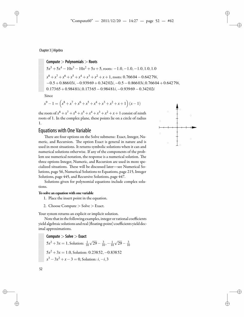
ii
“Compute60” — 2011/12/20 — 14:27 — page 52 — #62 ii
ii
ii
Chapter 3 | Algebra
Compute> Polynomials> Roots5x5 +5x4−10x3−10x2 +5x+5, roots: −1.0,−1.0,−1.0,1.0,1.0
x8 + x7 + x6 + x5 + x4 + x3 + x2 + x+1, roots: 0.76604−0.64279i,−0.5+0.86603i,−0.93969+0.34202i,−0.5−0.86603i,0.76604+0.64279i,0.17365+0.98481i,0.17365−0.98481i,−0.93969−0.34202i
Since
x9−1 =(
x8 + x7 + x6 + x5 + x4 + x3 + x2 + x+1)(x−1)
the roots of x8 +x7 +x6 +x5 +x4 +x3 +x2 +x+1 consist of ninthroots of 1. In the complex plane, these points lie on a circle of radius1.
Equations with One Variableere are four options on the Solve submenu: Exact, Integer, Nu-
meric, and Recursion. e option Exact is general in nature and isused in most situations. It returns symbolic solutions when it can andnumerical solutions otherwise. If any of the components of the prob-lem use numerical notation, the response is a numerical solution. ethree options Integer, Numeric, and Recursion are used in more spe-cialized situations. ese will be discussed later—see Numerical So-lutions, page 56, Numerical Solutions to Equations, page 215, IntegerSolutions, page 445, and Recursive Solutions, page 447.
Solutions given for polynomial equations include complex solu-tions.To solve an equationwith one variable
1. Place the insert point in the equation.
2. Choose Compute> Solve> Exact.
Your system returns an explicit or implicit solution.Note that in the following examples, integer or rational coefficients
yield algebraic solutions and real ( oating-point) coefficients yielddec-imal approximations.
Compute> Solve> Exact5x2 +3x = 1, Solution: 1
10
√29− 3
10 ,−1
10
√29− 3
10
5x2 +3x = 1.0, Solution: 0.23852,−0.83852
x3−3x2 + x−3 = 0, Solution: i,−i,3
52
ii
“Compute60” — 2011/12/20 — 14:27 — page 53 — #63 ii
ii
ii
Solving Equations
When there are multiple roots, only distinct roots are displayed.
Compute> Solve> Exact(x−5)3 (x+1) = 0, Solution: 5,−1
You can solve equations with rational expressions, and equationsinvolving absolute values.
Compute> Solve> Exact14
a+2− 1
a−4= 1, Solution: 5,10
|3x−2|= 5, Solution: 5
3 e2ix + 23 |x ∈ [0,π]
If you want only real roots, rst evaluate assume(x, real). When
you enter these words in mathematics mode, they automatically turnupright and gray. You can also use Insert >Math Objects > MathName to enter assume(x, real). (See Assumptions About Variables,page 111 for more information on the “assume” function.)
Compute> Evaluateassume(x, real) = R
Compute> Solve> Exactx = i, No solution found.x3−3x2 + x−3 = 0, Solution: 3|3x−2|= 5, Solution: −1, 7
3
In general, explicit solutions in terms of radicals for polynomialequations of degree greater than 4 do not exist. In these cases, implicitsolutions are given in terms of roots of a polynomial. When the equa-tion is a polynomial equation with degree 3 or 4, the explicit solutioncan be very complicated—and too large to preview, print, or save. Toavoid this problem, you can set the engine to return large complicatedsolutions in implicit form for smaller degree polynomials as well. SeeAppendix C “Customizing the Program for Computing” for details.
With a setting of 1 for maximum degree, only rational or otherrelatively simple solutions are computed for all polynomials. With asetting of 2 or 3, this behavior occurs for polynomials of degree greaterthan 2.
Compute> Solve> Exact(Maximum Degree set to 1)5x2 +3x = 1, Solution: RootOf
( 35 Z +Z2− 1
5
)x4 + x = 0, Solution: −1,0∪RootOf
(−Z +Z2 +1
)53
ii
“Compute60” — 2011/12/20 — 14:27 — page 54 — #64 ii
ii
ii
Chapter 3 | Algebra
Compute> Solve> Exact(Maximum Degree set to 2 or 3)5x2 +3x = 1, Solution: 1
10
√29− 3
10 ,−1
10
√29− 3
10
x4 + x = 0, Solution: 12 +
12 i√
3, 12 −
12 i√
3,−1,0
x4 + x−1 = 0, Solution: RootOf(Z +Z4−1
)Compute> Solve> Exact(Maximum Degree set to 4)
x4 + x = 0, Solution: 12 +
12 i√
3, 12 −
12 i√
3,−1,0
x4 + x−1 = 0 (Solution too long to display here)
e function solve takes an equation as input. Evaluate solve atan equation and the output is a list of solutions. Tomake the functionname, type solve while inmathematicsmode and it will automaticallygray, or create the name with Insert>Math Objects>Math Name.
Compute> Evaluate
solve(5x2 +3x = 1
)=[
x =− 110
√29− 3
10
],[x = 1
10
√29− 3
10
]Checking the Answer
Substitution provides a convenient way of testing solutions.
Example Check the solutions to several of the preceding equations.
Compute> Evaluate Compute> Simplify[ 14a+2 −
1a−4
]a=5 = 1
[5x2 +3x
]x=− 3
10+1
10√
29 = 1[5x2 +3x
]x=0.23852 = 1.0[
5x2 +3x]
x=−0.83852 = 1.0
Equations with Several VariablesIf there is more than one variable, enter the Variable(s) to Solve
for in the dialog box that opens when you choose Compute > Solve> Exact.
54
ii
“Compute60” — 2011/12/20 — 14:27 — page 55 — #65 ii
ii
ii
Solving Equations
Compute> Solve> Exact
1x+
1y= 1, (Enter x), Solution:
/0 if y = 1− 1
1y−1
if y = 1
1y+
1z+
1x= 1, (Enter z), Solution:
/0 if 1
x +1y = 1
− 11x +
1y−1
if 1
x +1y = 1
1r1
+1r2
=1R
, (Enter R), Solution:
/0 if r1 + r2 = 0
r1r2r1+r2
if r1 + r2 = 0
Systems of EquationsYoucan create a systemof equations either by entering equations in
a one-column matrix or by entering equations in a multi-row display.Tocreate a systemof equations using amatrix
1. Choose Insert>Math Objects>Matrix.
2. Set the number of rows equal to the number of equations.
3. Set the number of columns to 1, and choose OK. TipFrom the Viewmenu, check Helper Lines orInput Boxes to help place equations in a matrixor display.
4. Type the equations in the matrix, one equation to a row.
Tocreate a systemof equations using a display1. Choose Insert>Math Objects>Display.
2. Type the equations in the display, one equation to a row, addingrows as needed with the Enter key.
To solve a systemof equations1. Create a system of equations and leave the insert point in the
system.
2. Choose Compute> Solve> Exact.
3. If a dialog box opens asking Variable(s) to Solve for, type thevariable name(s) in the box, separated by commas.
Following are examples for systems of two equations.
55
ii
“Compute60” — 2011/12/20 — 14:27 — page 56 — #66 ii
ii
ii
Chapter 3 | Algebra
Compute> Solve> Exact2x− y = 5x+3y = 4 , Solution:
[x = 19
7 ,y =37
]x2− y2 = 5x+ y = 1 , Solution: [x = 3,y =−2]
x2−3y = 76x+4y = 9 , Solution:
[x = 1
4
√301− 9
4 ,y =458 −
38
√301],[
x =− 14
√301− 9
4 ,y =38
√301+ 45
8
]When the number of unknowns is larger than the number of equa-
tions, you are asked to specify variables in a dialog box.
Compute> Solve> Exactx+3y = 43x−4z = 7 , Variable(s): x,y
Solution:[x = 4
3 z+ 73 ,y =
59 −
49 z]
2x− y = 1x+3z = 4
w+ x =−3, Variable(s): x,y,z
Solution:[x =−w−3,y =−2w−7,z = 1
3 w+ 73
]Numerical Solutions
You can nd numerical solutions in two ways. You can chooseCompute > Solve > Exact a er entering at least one coefficient inoating-point form—that is, with a decimal.
Compute> Solve> Exactx2 +7x−5.2 = 0, Solution: 0.67732,−7.6773
x3−3.8x−15.6 = 0, Solution: 3.0,−1.5+1.7176i,−1.5−1.7176i
You can choose Compute > Solve > Numeric. is gives all so-lutions, both real and complex, to a polynomial equation or system ofpolynomial equations.
56
ii
“Compute60” — 2011/12/20 — 14:27 — page 57 — #67 ii
ii
ii
Solving Equations
Compute> Solve> Numericx2 +7x−5.2 = 0, Solution: [x = 0.67732] , [x =−7.6773]x3−3.8x−15.6 = 0, Solution: [x =−1.5+1.7176i] , [x =−1.5−1.7176i] , [x = 3.0]
x8 +3x2−1 = 0, Solution: [x =−1.0023+0.63210i], [x =−1.0023−0.63210i],[x = 1.0023+0.63210i], [x = 1.0023−0.63210i], [x =−0.57394],[x = 0.57394], [x =−1.2408i], [x = 1.2408i][x2 + y2 = 5x2− y2 = 1
], Solution: [x =−1.7321,y =−1.4142],
[x =−1.7321,y = 1.4142], [x = 1.7321,y =−1.4142], [x = 1.7321,y = 1.4142]
e choice Compute > Solve > Numeric is particularly usefulwhen solving transcendental equations or systems of transcendentalequations, or when you want to specify a search interval for the solu-tion.To nd anumerical solutionwithin a speci ed range of the variable
1. Add a row to the bottom of the matrix, or
Press Enter to generate a new input box in a display.
2. Write the intervals of your choice, anduse themembership sym-bol∈ to indicate that the variable lies in that interval.
Compute> Solve> Numericx2 + y2 = 5x2− y2 = 1x ∈ (−2,0)y ∈ (0,2)
, Solution: [x =−1.7321,y = 1.4142]
To nd all numerical solutions to a systemof polynomial equations1. Change at least one of the coefficients to oating-point form.
2. Choose Compute> Solve> Exact.
Compute> Solve> Exact
x2 + y2 = 5.0x2− y2 = 1.0
, Solution :
y =−1.4142,x = 1.7321y =−1.4142,x =−1.7321y = 1.4142,x = 1.7321y = 1.4142,x =−1.7321
57
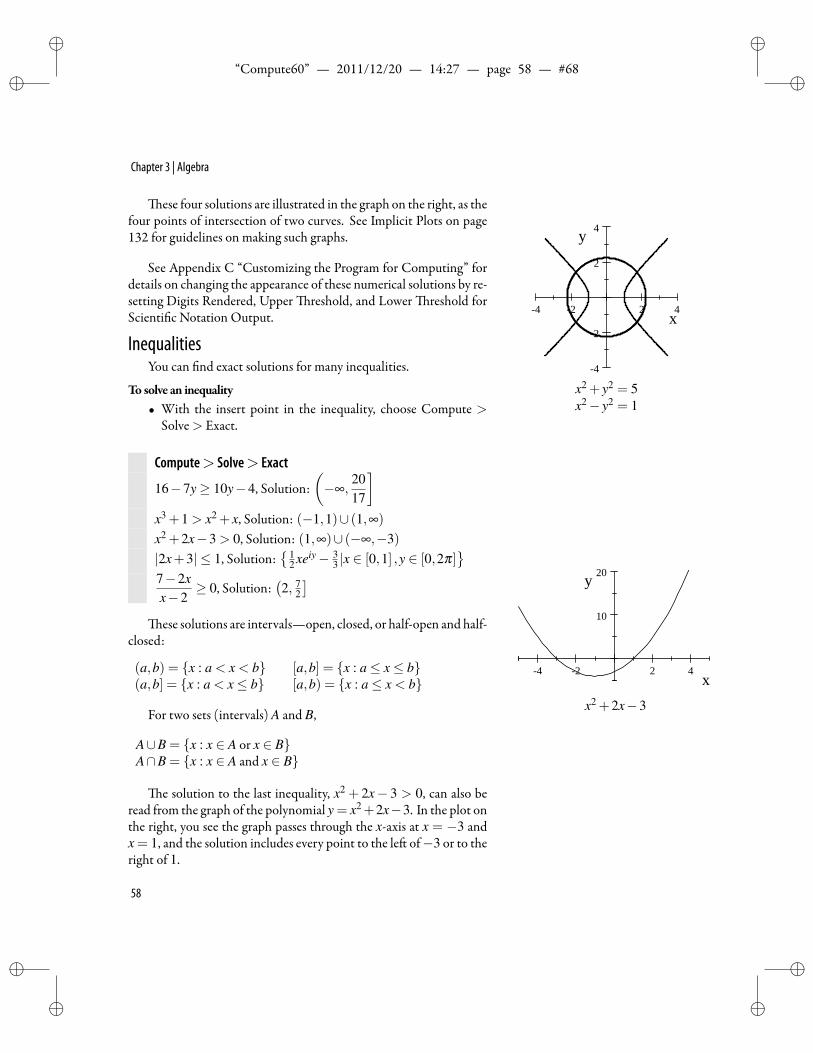
ii
“Compute60” — 2011/12/20 — 14:27 — page 58 — #68 ii
ii
ii
Chapter 3 | Algebra
ese four solutions are illustrated in the graph on the right, as thefour points of intersection of two curves. See Implicit Plots on page132 for guidelines on making such graphs.
4 2 2 4
4
2
2
4
x
y
x2 + y2 = 5x2− y2 = 1
See Appendix C “Customizing the Program for Computing” fordetails on changing the appearance of these numerical solutions by re-setting Digits Rendered, Upper reshold, and Lower reshold forScienti c Notation Output.
InequalitiesYou can nd exact solutions for many inequalities.
To solve an inequality• With the insert point in the inequality, choose Compute >
Solve> Exact.
Compute> Solve> Exact
16−7y≥ 10y−4, Solution:(−∞,
2017
]x3 +1 > x2 + x, Solution: (−1,1)∪ (1,∞)
x2 +2x−3 > 0, Solution: (1,∞)∪ (−∞,−3)|2x+3| ≤ 1, Solution:
12 xeiy− 3
3 |x ∈ [0,1] ,y ∈ [0,2π]
7−2xx−2
≥ 0, Solution:(2, 7
2
]ese solutions are intervals—open, closed, or half-open and half-
closed:
4 2 2 4
10
20
x
y
x2 +2x−3
(a,b) = x : a < x < b [a,b] = x : a≤ x≤ b(a,b] = x : a < x≤ b [a,b) = x : a≤ x < b
For two sets (intervals) A and B,
A∪B = x : x ∈ A or x ∈ BA∩B = x : x ∈ A and x ∈ B
e solution to the last inequality, x2 + 2x− 3 > 0, can also beread from the graph of the polynomial y = x2+2x−3. In the plot onthe right, you see the graph passes through the x-axis at x = −3 andx = 1, and the solution includes every point to the le of−3 or to theright of 1.
58
ii
“Compute60” — 2011/12/20 — 14:27 — page 59 — #69 ii
ii
ii
De ning Variables and Functions
De ning Variables and Functionse De nitions commands enable you to de ne a symbol to be
a mathematical object and to de ne a function using an expressionor a collection of expressions. Four operations on the De ne sub-menu—New De nition, Unde ne, Show De nitions, Clear De ni-tions—are explained brie y in this section for the types of expressionsand functions that occur in precalculus. De ned expressions
The symbol p de ned here represents theexpression x3 +3x2−5x+1. It is not afunction, and in particular, p(2) is not theexpression evaluated at x = 2. In fact, p(2)is interpreted simply as the product 2p =2x3 +6x2−10x+2.
See Chapter 5 “Function De nitions,” for greater detail on theseoperations and other aspects of de nitions. For examples of these op-erations pertinent to topics such as calculus, vector calculus, and ma-trix algebra, see the chapter covering the topic.
Assigning Values to VariablesYou can assign a value to a variable using De nitions>New Def-
inition.Toassign the value 5 to z
1. Type z = 5 in mathematics mode.
2. Choose Compute>De nitions>New De nition.De ned FunctionsDe ning f (y) = ay2 +by+ c de nesthe same function as de ning f (x) = ax2
+bx+ c. The symbol used for the functionargument in making the de nition does notmatter. This point illustrates the subtle butessential difference between expressions andfunctions. In particular, the two expressionsy = x2 +
√x and y = t2 +
√t are
different (because y gets replaced by anexpression in x under the rst de nition and ygets replaced by an expression in t under thesecond de nition). However, the functionsf (x) = x2 +
√x and f (t) = t2 +
√t
are identical.
erea er, until you unde ne the variable, the system recognizesz as 5 and will evaluate the expression 3+ z as 8.
Variables normally have single-character names. (See ValidNamesfor Functions and Expressions or Variables on page 100 for other pos-sibilities.) e value assigned can, however, be any mathematical ex-pression. For example, you could de ne a variable to be any of thefollowing:
• Number: a = 245
• Polynomial: p = x3 +3x2−5x+1
• Rational expression: b = x2−1x2+1
• Matrix: z =[
a bc d
]De ning Functions of One Variable
You follow a similar procedure to de ne a function. Write a func-tionname followedbyparentheses containing the variable, and set thisequal to an expression.
59
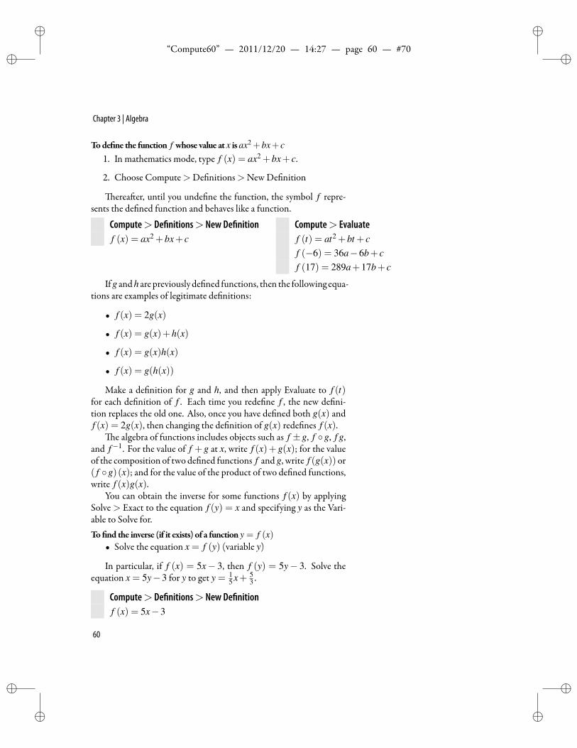
ii
“Compute60” — 2011/12/20 — 14:27 — page 60 — #70 ii
ii
ii
Chapter 3 | Algebra
Tode ne the function f whose value at x isax2 +bx+ c1. In mathematics mode, type f (x) = ax2 +bx+ c.
2. Choose Compute>De nitions>New De nition
erea er, until you unde ne the function, the symbol f repre-sents the de ned function and behaves like a function.
Compute> De nitions> New De nition Compute> Evaluatef (x) = ax2 +bx+ c f (t) = at2 +bt + c
f (−6) = 36a−6b+ cf (17) = 289a+17b+ c
Ifg andh are previously de ned functions, then the following equa-tions are examples of legitimate de nitions:
• f (x) = 2g(x)
• f (x) = g(x)+h(x)
• f (x) = g(x)h(x)
• f (x) = g(h(x))
Make a de nition for g and h, and then apply Evaluate to f (t)for each de nition of f . Each time you rede ne f , the new de ni-tion replaces the old one. Also, once you have de ned both g(x) andf (x) = 2g(x), then changing the de nition of g(x) rede nes f (x).
e algebra of functions includes objects such as f ±g, f g, f g,and f−1. For the value of f +g at x, write f (x)+g(x); for the valueof the composition of two de ned functions f and g, write f (g(x)) or( f g)(x); and for the value of the product of two de ned functions,write f (x)g(x).
You can obtain the inverse for some functions f (x) by applyingSolve > Exact to the equation f (y) = x and specifying y as the Vari-able to Solve for.To nd the inverse (if it exists) of a function y = f (x)
• Solve the equation x = f (y) (variable y)
In particular, if f (x) = 5x− 3, then f (y) = 5y− 3. Solve theequation x = 5y−3 for y to get y = 1
5 x+ 53 .
Compute> De nitions> New De nitionf (x) = 5x−3
60
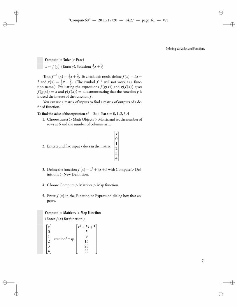
ii
“Compute60” — 2011/12/20 — 14:27 — page 61 — #71 ii
ii
ii
De ning Variables and Functions
Compute> Solve> Exactx = f (y), (Enter y), Solution: 1
5 x+ 35
us f−1 (x) = 15 x+ 5
3 . To check this result, de ne f (x) = 5x−3 and g(x) = 1
5 x + 35 . ( e symbol f−1 will not work as a func-
tion name.) Evaluating the expressions f (g(x)) and g( f (x)) givesf (g(x)) = x and g( f (x)) = x, demonstrating that the function g isindeed the inverse of the function f .
You can use a matrix of inputs to nd a matrix of outputs of a de-ned function.
To nd the value of the expression x2 +3x+5 at x = 0,1, 2,3,41. Choose Insert>MathObjects>Matrix and set the number of
rows at 6 and the number of columns at 1.
2. Enter x and ve input values in the matrix:
x01234
3. De ne the function f (x) = x2+3x+5 withCompute>Def-
initions>New De nition.
4. Choose Compute>Matrices>Map function.
5. Enter f (x) in the Function or Expression dialog box that ap-pears.
Compute>Matrices>Map Function(Enter f (x) for function.)
x01234
, result of map
x2 +3x+5
59
152333
61
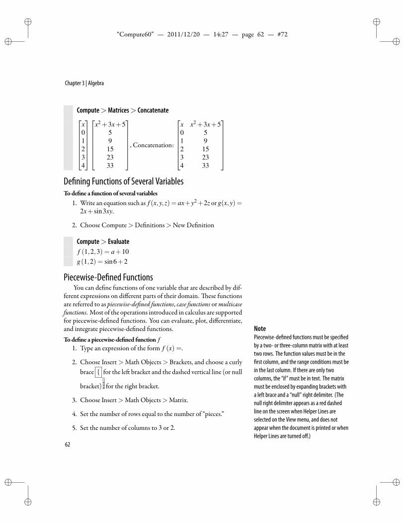
ii
“Compute60” — 2011/12/20 — 14:27 — page 62 — #72 ii
ii
ii
Chapter 3 | Algebra
Compute>Matrices> Concatenatex01234
x2 +3x+5
59
152333
, Concatenation:
x x2 +3x+50 51 92 153 234 33
De ning Functions of Several VariablesTode ne a functionof several variables
1. Write an equation such as f (x,y,z) = ax+y2+2z or g(x,y) =2x+ sin3xy.
2. Choose Compute>De nitions>New De nition
Compute> Evaluatef (1,2,3) = a+10g(1,2) = sin6+2
Piecewise-De ned FunctionsYou can de ne functions of one variable that are described by dif-
ferent expressions on different parts of their domain. ese functionsare referred to as piecewise-de ned functions, case functions ormulticasefunctions. Most of the operations introduced in calculus are supportedfor piecewise-de ned functions. You can evaluate, plot, differentiate,and integrate piecewise-de ned functions. Note
Piecewise-de ned functions must be speci edby a two- or three-columnmatrix with at leasttwo rows. The function values must be in therst column, and the range conditions must bein the last column. If there are only twocolumns, the “if” must be in text. The matrixmust be enclosed by expanding brackets witha left brace and a “null” right delimiter. (Thenull right delimiter appears as a red dashedline on the screen when Helper Lines areselected on the Viewmenu, and does notappear when the document is printed or whenHelper Lines are turned off.)
Tode ne a piecewise-de ned function f1. Type an expression of the form f (x) =.
2. Choose Insert>Math Objects> Brackets, and choose a curlybrace for the le bracket and the dashed vertical line (or null
bracket)... for the right bracket.
3. Choose Insert>Math Objects>Matrix.
4. Set the number of rows equal to the number of “pieces.”
5. Set the number of columns to 3 or 2.
62
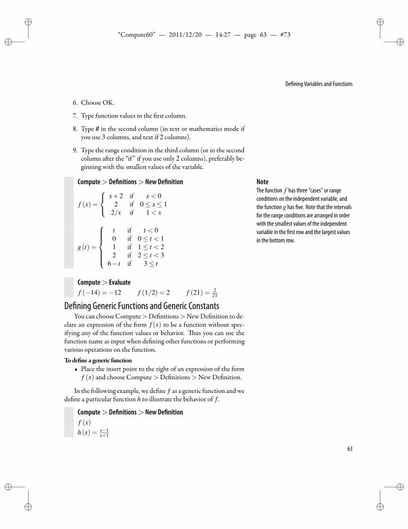
ii
“Compute60” — 2011/12/20 — 14:27 — page 63 — #73 ii
ii
ii
De ning Variables and Functions
6. Choose OK.
7. Type function values in the rst column.
8. Type if in the second column (in text or mathematics mode ifyou use 3 columns, and text if 2 columns).
9. Type the range condition in the third column (or in the secondcolumn a er the “if ” if you use only 2 columns), preferably be-ginning with the smallest values of the variable.
Compute> De nitions> New De nition
f (x) =
x+2 if x < 02 if 0≤ x≤ 1
2/x if 1 < x
g(t) =
t if t < 00 if 0≤ t < 11 if 1≤ t < 22 if 2≤ t < 3
6− t if 3≤ t
NoteThe function f has three “cases” or rangeconditions on the independent variable, andthe function g has ve. Note that the intervalsfor the range conditions are arranged in orderwith the smallest values of the independentvariable in the rst row and the largest valuesin the bottom row.
Compute> Evaluatef (−14) =−12 f (1/2) = 2 f (21) = 2
21
De ning Generic Functions and Generic ConstantsYou can choose Compute>De nitions>NewDe nition to de-
clare an expression of the form f (x) to be a function without spec-ifying any of the function values or behavior. us you can use thefunction name as input when de ning other functions or performingvarious operations on the function.Tode ne a generic function
• Place the insert point to the right of an expression of the formf (x) and choose Compute>De nitions>New De nition.
In the following example, we de ne f as a generic function andwede ne a particular function h to illustrate the behavior of f .
Compute> De nitions> New De nitionf (x)h(x) = x−1
x+1
63
ii
“Compute60” — 2011/12/20 — 14:27 — page 64 — #74 ii
ii
ii
Chapter 3 | Algebra
Compute> Evaluateh( f (x)) = f (x)−1
f (x)+1
f (h(x)) = f( x−1
x+1
)You can choose Compute>De nitions>NewDe nition to de-
clare a character to be a constant.Todeclare a character to be a (generic) constant
• Place the insert point to the right of the character and chooseCompute>De nitions>New De nition.
Compute> De nitions> New De nitiona
Showing and Removing De nitionsA er making de nitions of functions or expressions, you need to Show De nitions
Show De nitions opens a window showing theactive de nitions. In general, the de nedvariables and functions are listed in the orderin which the de nitions were made.Check the Show De nitions list from time totime. If your mathematics is behavingstrangely, this list is a place to look for apossible explanation.
know techniques for keeping track of them, saving them, and deletingthem.Toview the list of currently de ned variables and functions
• Choose Compute>De nitions> Show De nitions.
Example De ne a = b, p = ax, and f (x) = ax. Choose Compute>De nitions> Show De nitions to see the list
f (x) = axp = axa = b
of de ned functions and expressions. Evaluation of p and f (x) pro-duces p = bx and f (x) = bx. Rede ning a with the equation a = cand again evaluating p and f (x) produces p = cx and f (x) = cx.To remove a de nition fromadocument
1. Place the insert point in the equation you wish to unde ne, or CautionIt is easy to forget that a symbol has beende ned to be some expression. If you use thatsymbol later, you can get surprising results. Forexample, if you de ne a = x2, forget aboutit, and later compute f (a) for some functionf that you have just de ned, you are in for asurprise. In complicated computations theerror may not be apparent.
select the name of the function or expression.
2. Choose Compute>De nitions>Unde ne.
Choose Compute > De nitions > Show De nitions to verifythat the de nition has been removed from the list of de ned func-tions and expressions.
64
ii
“Compute60” — 2011/12/20 — 14:27 — page 65 — #75 ii
ii
ii
Exponents and Logarithms
To remove all de nitions fromadocument• Choose Compute>De nitions>Clear De nitions.
If you have worked the preceding examples, you havemade severalde nitions and you should remove them before continuing. De ni-tions that you do not remove remain active as long as a document isopen. As a default, de nitions are saved and then restored when youreopen a document.Tocheck for overlookedde nitions
• Choose Compute>De nitions> Show De nitions
Exponents and LogarithmsYou can work with exponential and logarithmic functions writ-
ten in their natural forms: ex, expx, log5 x, lnx, and so forth. esefunctions are inverses of one another, as exempli ed by the identitieselnx = x and lnex = x.
Exponents and Exponential FunctionsExponential functions are used in modeling many real-life situa-
tions. e laws of exponents are an important feature of these func-tions.
Combining ExponentialsTocombine expressions involving exponential functionswith base e Note
In some cases, the Expand and Combinecommands act as inverses of one another.
• Choose Compute>Combine> Exponentials or Compute>Expand
Compute> Combine> Exponentials Compute> Expand(ex)y = eyx ex+3lny = y3ex
exey = ex+y ex+y = exey
Combining PowersTocombineexpressions involvingexponential functionswith symbolicbase
• Choose Compute>Combine> Powers (or Compute> Sim-plify)
Compute> Combine> Powersaxay = ax+y
65
ii
“Compute60” — 2011/12/20 — 14:27 — page 66 — #76 ii
ii
ii
Chapter 3 | Algebra
Laws of ExponentsYou can demonstrate some of the laws of exponents with some of
the menu commands. ese laws apply for real or complex exponentsand for other expressions as well.
Todemonstrate laws of exponents• Choose a menu command.
Compute> Combine> Powers2x2y = 2x+y
ax
ay = ax−y
10x+310x−3 = 102x
Compute> Combine> Exponentialsexey = ex+y
Compute> Expand2x+y = 2x×2y ax−y = ax
ay
e function exp satis es exp(x) = ex. (Note that exp is a gray Function NameTyping the letters exp in mathematics modeautomatically returns the grayed functionname exp.
Math Name.) Exponential expressions are normally returned to yourdocument in the form e f (x) rather than exp( f (x)), unless the expres-sion f (x) is unusually complicated.
Evaluating Exponential ExpressionsToevaluate an exponential expression
• Choose Compute> Evaluate, or
Choose Compute> Evaluate Numeric
For numerical approximations, use Evaluate Numeric or useoating-point notation. You can change the number of digits shown
in these approximations by changing the number for Digits renderedin the Scienti c Notation Output settings at Tools > Preferences >Computation, Output page. For details, see Appendix C “Customiz-ing the Program for Computing.” In these examples, Digits renderedis set to 5.
Evaluate Evaluate Numerice2 = e2 e2 ≈ 7.3891
e0.0025 = 1.0025 e0.0025 ≈ 1.0025
54 = 625 54 ≈ 625.0
2√
5 = 2√
5 2√
5 ≈ 4.7111
66
ii
“Compute60” — 2011/12/20 — 14:27 — page 67 — #77 ii
ii
ii
Exponents and Logarithms
Logarithms and Logarithmic Functions Function NamesTyping the letters ln in mathematics modeautomatically returns the grayed functionname ln.Similarly, typing the letters log in mathematicsmode returns the grayed function name log.
e function lnx is interpreted as the natural logarithm—that is,the logarithm with base e. Logarithms to other bases are entered witha subscript on the function log. Evaluation gives log5 25 = 2 andlog10 103 = 3. By default, the symbol logx is also interpreted as thenatural logarithm (base e). You can change this default.
Tochange the default for the functionname log frombase e to base 101. Choose Tools> Preferences>Computation, Input page.
2. Click the box to remove the check mark from the line “Base oflog is e (otherwise 10).”
Properties of LogarithmsYou can demonstrate properties of logarithms with Simplify and
Combine. Assume x,y,a,b are positive for the results below.
Evaluate Evaluateassume(x,positive) = (0,∞) assume(a,positive) = (0,∞)
assume(y,positive) = (0,∞) assume(b,positive) = (0,∞)
Compute> Simplifylnxy = y lnxlog38 = 8log3
Compute> Combine> Logslnx+ lny = ln(xy)lna− lnb = ln a
b2ln3 = ln9
Evaluating Logarithmic ExpressionsToevaluate a logarithmic expression
• Choose Compute> Evaluate, or
Choose Compute> Evaluate Numeric
For numerical approximations, use Evaluate Numeric or useoating-point notation. You can change the number of digits shown
in these approximations by changing the number for Digits renderedin the Scienti c Notation Output settings at Tools > Preferences >Computation, Output page. For details, see Appendix C “Customiz-ing the Program for Computing.” In these examples, Digits renderedis set to 5.
67
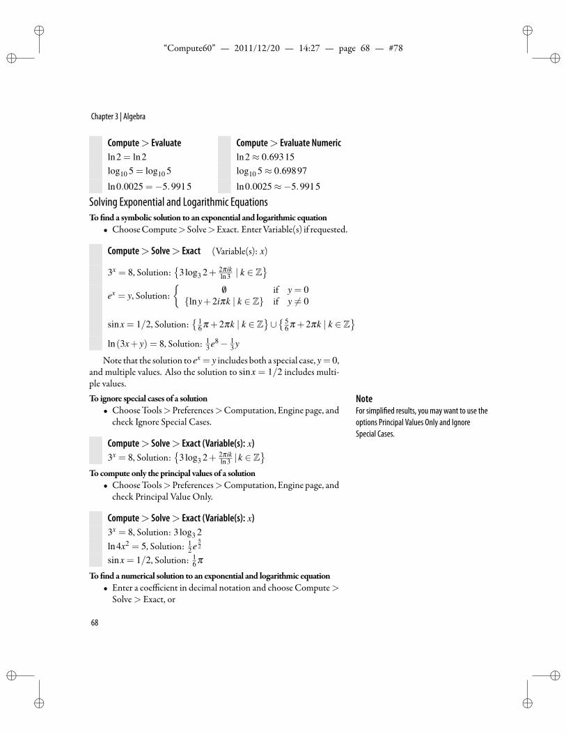
ii
“Compute60” — 2011/12/20 — 14:27 — page 68 — #78 ii
ii
ii
Chapter 3 | Algebra
Compute> Evaluate Compute> Evaluate Numericln2 = ln2 ln2≈ 0.69315log10 5 = log10 5 log10 5≈ 0.69897
ln0.0025 =−5.9915 ln0.0025≈−5.9915
Solving Exponential and Logarithmic EquationsTo nd a symbolic solution to an exponential and logarithmic equation
• ChooseCompute>Solve>Exact. EnterVariable(s) if requested.
Compute> Solve> Exact (Variable(s): x)
3x = 8, Solution:
3log3 2+ 2πikln3 | k ∈ Z
ex = y, Solution:
/0 if y = 0
lny+2iπk | k ∈ Z if y = 0
sinx = 1/2, Solution: 1
6 π +2πk | k ∈ Z∪ 5
6 π +2πk | k ∈ Z
ln(3x+ y) = 8, Solution: 13 e8− 1
3 y
Note that the solution to ex = y includes both a special case, y= 0,and multiple values. Also the solution to sinx = 1/2 includes multi-ple values.To ignore special cases of a solution Note
For simpli ed results, you may want to use theoptions Principal Values Only and IgnoreSpecial Cases.
• ChooseTools>Preferences>Computation, Engine page, andcheck Ignore Special Cases.
Compute> Solve> Exact (Variable(s): x)3x = 8, Solution:
3log3 2+ 2πik
ln3 |k ∈ Z
Tocompute only the principal values of a solution• ChooseTools>Preferences>Computation, Engine page, and
check Principal Value Only.
Compute> Solve> Exact (Variable(s): x)3x = 8, Solution: 3log3 2ln4x2 = 5, Solution: 1
2 e52
sinx = 1/2, Solution: 16 π
To nd anumerical solution to an exponential and logarithmic equation• Enter a coefficient in decimal notation and choose Compute>
Solve> Exact, or
68
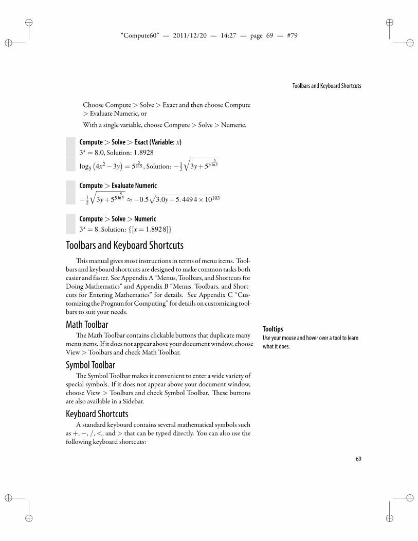
ii
“Compute60” — 2011/12/20 — 14:27 — page 69 — #79 ii
ii
ii
Toolbars and Keyboard Shortcuts
Choose Compute> Solve> Exact and then choose Compute> Evaluate Numeric, or
With a single variable, choose Compute> Solve>Numeric.
Compute> Solve> Exact (Variable: x)3x = 8.0, Solution: 1.8928
log5(4x2−3y
)= 5
5ln5 , Solution: − 1
2
√3y+55
5ln5
Compute> Evaluate Numeric
− 12
√3y+55
5ln5 ≈−0.5
√3.0y+5.4494×10103
Compute> Solve> Numeric3x = 8, Solution: [x = 1.8928]
Toolbars and Keyboard Shortcutsis manual givesmost instructions in terms ofmenu items. Tool-
bars and keyboard shortcuts are designed tomake common tasks botheasier and faster. SeeAppendixA “Menus, Toolbars, and Shortcuts forDoing Mathematics” and Appendix B “Menus, Toolbars, and Short-cuts for Entering Mathematics” for details. See Appendix C “Cus-tomizing theProgram forComputing” for details on customizing tool-bars to suit your needs.
Math Toolbar TooltipsUse your mouse and hover over a tool to learnwhat it does.
e Math Toolbar contains clickable buttons that duplicate manymenu items. If it doesnot appear above yourdocumentwindow, chooseView>Toolbars and check Math Toolbar.
Symbol Toolbare Symbol Toolbarmakes it convenient to enter a wide variety of
special symbols. If it does not appear above your document window,choose View > Toolbars and check Symbol Toolbar. ese buttonsare also available in a Sidebar.
Keyboard ShortcutsA standard keyboard contains several mathematical symbols such
as +,−, /, <, and > that can be typed directly. You can also use thefollowing keyboard shortcuts:
69
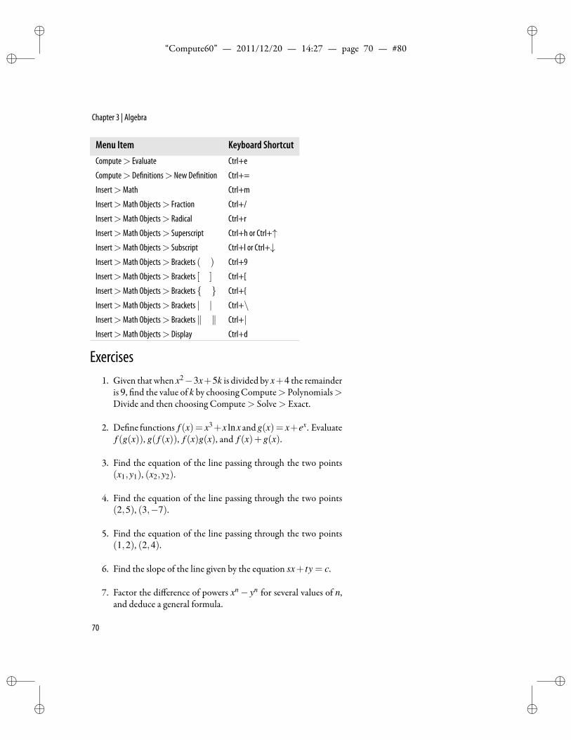
ii
“Compute60” — 2011/12/20 — 14:27 — page 70 — #80 ii
ii
ii
Chapter 3 | Algebra
Menu Item Keyboard ShortcutCompute> Evaluate Ctrl+e
Compute> De nitions> New De nition Ctrl+=
Insert>Math Ctrl+m
Insert>Math Objects> Fraction Ctrl+/
Insert>Math Objects> Radical Ctrl+r
Insert>Math Objects> Superscript Ctrl+h or Ctrl+↑Insert>Math Objects> Subscript Ctrl+l or Ctrl+↓Insert>Math Objects> Brackets ( ) Ctrl+9
Insert>Math Objects> Brackets [ ] Ctrl+[
Insert>Math Objects> Brackets Ctrl+
Insert>Math Objects> Brackets | | Ctrl+\Insert>Math Objects> Brackets ∥ ∥ Ctrl+|Insert>Math Objects> Display Ctrl+d
Exercises1. Given that when x2−3x+5k is divided by x+4 the remainder
is 9, nd the value of k by choosing Compute> Polynomials>Divide and then choosing Compute> Solve> Exact.
2. De ne functions f (x)= x3+x lnx andg(x)= x+ex. Evaluatef (g(x)), g( f (x)), f (x)g(x), and f (x)+g(x).
3. Find the equation of the line passing through the two points(x1,y1), (x2,y2).
4. Find the equation of the line passing through the two points(2,5), (3,−7).
5. Find the equation of the line passing through the two points(1,2), (2,4).
6. Find the slope of the line given by the equation sx+ ty = c.
7. Factor the difference of powers xn− yn for several values of n,and deduce a general formula.
70
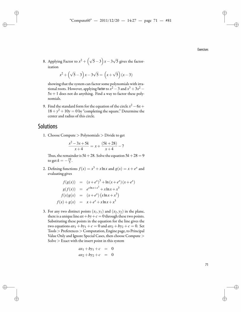
ii
“Compute60” — 2011/12/20 — 14:27 — page 71 — #81 ii
ii
ii
Exercises
8. Applying Factor to x2 +(√
5−3)
x− 3√
5 gives the factor-ization
x2 +(√
5−3)
x−3√
5 =(
x+√
5)(x−3)
showing that the system can factor some polynomials with irra-tional roots. However, applying Factor to x2−3 and x3 +3x2−5x+ 1 does not do anything. Find a way to factor these poly-nomials.
9. Find the standard form for the equation of the circle x2−6x+18+ y2 +10y = 0 by “completing the square.” Determine thecenter and radius of this circle.
Solutions1. Choose Compute> Polynomials>Divide to get
x2−3x+5kx+4
= x+(5k+28)
x+4−7
us, the remainder is 5k+28. Solve the equation 5k+28 = 9to get k =− 19
5 .
2. De ning functions f (x) = x3 + x lnx and g(x) = x+ ex andevaluating gives
f (g(x)) = (x+ ex)3 + ln(x+ ex)(x+ ex)
g( f (x)) = ex lnx+x3+ x lnx+ x3
f (x)g(x) = (x+ ex)(x lnx+ x3)
f (x)+g(x) = x+ ex + x lnx+ x3
3. For any two distinct points (x1,y1) and (x2,y2) in the plane,there is a unique line ax+by+c = 0 through these two points.Substituting these points in the equation for the line gives thetwo equations ax1 + by1 + c = 0 and ax2 + by2 + c = 0. SetTools>Preferences>Computation, Engine page, to PrincipalValue Only and Ignore Special Cases, then choose Compute>Solve> Exact with the insert point in this system
ax1 +by1 + c = 0ax2 +by2 + c = 0
71
ii
“Compute60” — 2011/12/20 — 14:27 — page 72 — #82 ii
ii
ii
Chapter 3 | Algebra
of linear equations, solving for the variables a,b.
Solution:[
a =cy1− cy2
x1y2− x2y1,b =− cx1− cx2
x1y2−y1x2
]Consequently, the equation for the line is
cy1− cy2
x1y2− x2y1x− cx1− cx2
x2y1− x1y2y+ c = 0
or, clearing fractions and collecting coefficients,
(y1− y2)x− (x1− x2)y+(x1y2− y1x2) = 0NoteAn interesting method for nding the equationof a line through two speci ed points usingdeterminants is described in a matrix algebraexercise on page 337.
4. For the points (2,5), (3,−7), the system of equations is
2a+5b+ c = 03a−7b+ c = 0
Choose Compute> Solve> Exact to get
Solution:[a =− 12
29 c,b =− 129 c].
Consequently, the equation for the line is− 1229 cx−
(− 1
29
)cy+
c = 0, or, clearing fractions and simplifying,
−12x+ y+29 = 0.
5. Since thepoint (0,0) lies on the line, youdonot get a unique so-lution to the system of equations for the pair a,b. us, choos-ing Solve + Exact and specifying a,b for the variables gives noresponse. However, specifying a,c for Variable(s) to Solve forgives the solution
[a =−2b,c = 0]
us, the equation for the line is
−2bx+by = 0
or, dividing by b and applying Simplify,
(−2bx+by)1b=−2x+ y = 0
72
ii
“Compute60” — 2011/12/20 — 14:27 — page 73 — #83 ii
ii
ii
Exercises
6. e slope-intercept form of the equation for a line is y = mx+b,where m is the slope and b the y-intercept. If a line is given as alinear equation in the form sx+ ty = c, you can nd the slopeby solving the equation for y. Expand the solution y = − sx−c
t
to get y =ct− s
tx, revealing the slope to be−s
t.
7. Apply Factor to several differences:
x2− y2 = (x− y)(x+ y)
x3− y3 = (x− y)(x2 + xy+ y2
)x4− y4 = (x− y)(x+ y)
(x2 + y2
)x5− y5 = (x− y)
(x4 + x3y+ x2y2 + xy3 + y4
)x6− y6 = (x− y)(x+ y)
(x2 + xy+ y2
)(x2− xy+ y2
)x7−y7 = (x− y)
(x6 + x5y+ x4y2 + x3y3 + x2y4 + xy5 + y6
)A er looking at only these few examples, you might nd it rea-sonable to conjecture that, for n odd,
xn− yn = (x− y)n−1
∑k=0
xn−k−1yk
We leave the general conjecture for you. Experiment.
8. Using the clue from the example that the systemwill factor overroots that appear as coefficients, factor theproduct
√3(x2−3
)to get
√3(x2−3
)=√
3(x−√
3)(
x+√
3). Now you can
divideout the extraneous√
3 to getx2−3=(x−√
3)(
x+√
3).
For thepolynomialx3+3x2−5x+1, chooseCompute>Poly-nomials>Roots to nd the roots:
[1,√
5−2,−√
5−2]. You
can multiply by√
5 to factor this polynomial:
√5(x3 +3x2−5x+1
)=√
5(
x+√
5+2)(
x−√
5+2)(x−1)
en, dividing out the extraneous factor of√
5, you have
x3 +3x2−5x+1 = (x−1)(
x+2+√
5)(
x+2−√
5)
73
ii
“Compute60” — 2011/12/20 — 14:27 — page 74 — #84 ii
ii
ii
Chapter 3 | Algebra
9. To nd the center and radius of the circle
x2−6x+18+ y2 +10y = 0,
rst subtract the constant term 18 from both sides of the equa-tion to get
x2−6x+18+ y2 +10y−18 = 0−18
Simplify each side of the equation. is gives the equation x2−6x+ y2 +10y =−18. Add parentheses to put the equation inthe form (
x2−6x)+(y2 +10y
)=−18.
To complete the squares, add the square of one-half the coeffi-cient of x to both sides. Do the same for the coefficient of y.(
x2−6x+(− 6
2
)2)+(
y2 +10y+( 10
2
)2)=−18+
(− 6
2
)2+( 10
2
)2
Factor the terms(
x2−6x+(−6
2
)2)
and(
y2 +10y+( 10
2
)2):
(x−3)2 +(y+5)2 =−18+(− 6
2
)2+( 10
2
)2
Simplify the right side of the equation to get
(x−3)2 +(y+5)2 = 16.
You can read the solution to this problem from this form of theequation. e center of the circle is (3,−5) and the radius is√
16 = 4.
74
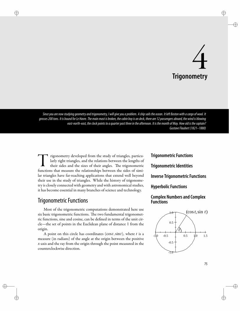
ii
“Compute60” — 2011/12/20 — 14:27 — page 75 — #85 ii
ii
ii
4Trigonometry
Since you are now studying geometry and trigonometry, I will give you a problem. A ship sails the ocean. It left Boston with a cargo of wool. Itgrosses 200 tons. It is bound for Le Havre. The main mast is broken, the cabin boy is on deck, there are 12 passengers aboard, the wind is blowing
east-north-east, the clock points to a quarter past three in the afternoon. It is the month of May. How old is the captain?Gustave Flaubert (1821–1880)
T rigonometry developed from the study of triangles, particu- Trigonometric Functions
Trigonometric Identities
Inverse Trigonometric Functions
Hyperbolic Functions
Complex Numbers and ComplexFunctions
larly right triangles, and the relations between the lengths oftheir sides and the sizes of their angles. e trigonometric
functions that measure the relationships between the sides of simi-lar triangles have far-reaching applications that extend well beyondtheir use in the study of triangles. While the history of trigonome-try is closely connected with geometry and with astronomical studies,it has become essential in many branches of science and technology.
Trigonometric FunctionsMost of the trigonometric computations demonstrated here use
six basic trigonometric functions. e two fundamental trigonomet-ric functions, sine and cosine, can be de ned in terms of the unit cir-cle—the set of points in the Euclidean plane of distance 1 from theorigin.
A point on this circle has coordinates (cos t,sin t), where t is ameasure (in radians) of the angle at the origin between the positivex-axis and the ray from the origin through the point measured in thecounterclockwise direction.
1.0 0.5 0.5 1.0 1.5
1.0
0.5
0.5
1.0
t
cos t, tsin( )
75
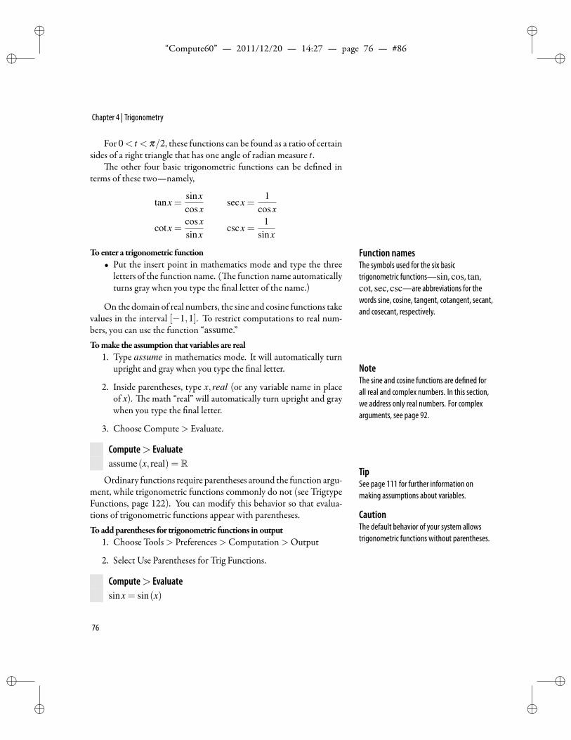
ii
“Compute60” — 2011/12/20 — 14:27 — page 76 — #86 ii
ii
ii
Chapter 4 | Trigonometry
For 0 < t < π/2, these functions can be found as a ratio of certainsides of a right triangle that has one angle of radian measure t .
e other four basic trigonometric functions can be de ned interms of these two—namely,
tanx =sinxcosx
secx =1
cosx
cotx =cosxsinx
cscx =1
sinx
Toenter a trigonometric function Function namesThe symbols used for the six basictrigonometric functions—sin, cos, tan,cot, sec, csc—are abbreviations for thewords sine, cosine, tangent, cotangent, secant,and cosecant, respectively.
• Put the insert point in mathematics mode and type the threeletters of the function name. ( e function name automaticallyturns gray when you type the nal letter of the name.)
On the domain of real numbers, the sine and cosine functions takevalues in the interval [−1,1]. To restrict computations to real num-bers, you can use the function “assume.”Tomake the assumption that variables are real
1. Type assume in mathematics mode. It will automatically turnupright and gray when you type the nal letter. Note
The sine and cosine functions are de ned forall real and complex numbers. In this section,we address only real numbers. For complexarguments, see page 92.
2. Inside parentheses, type x,real (or any variable name in placeof x). e math “real” will automatically turn upright and graywhen you type the nal letter.
3. Choose Compute> Evaluate.
Compute> Evaluateassume(x, real) = R
TipSee page 111 for further information onmaking assumptions about variables.
Ordinary functions require parentheses around the function argu-ment, while trigonometric functions commonly do not (see TrigtypeFunctions, page 122). You can modify this behavior so that evalua-tions of trigonometric functions appear with parentheses. Caution
The default behavior of your system allowstrigonometric functions without parentheses.
Toaddparentheses for trigonometric functions in output1. Choose Tools> Preferences>Computation>Output
2. Select Use Parentheses for Trig Functions.
Compute> Evaluatesinx = sin(x)
76
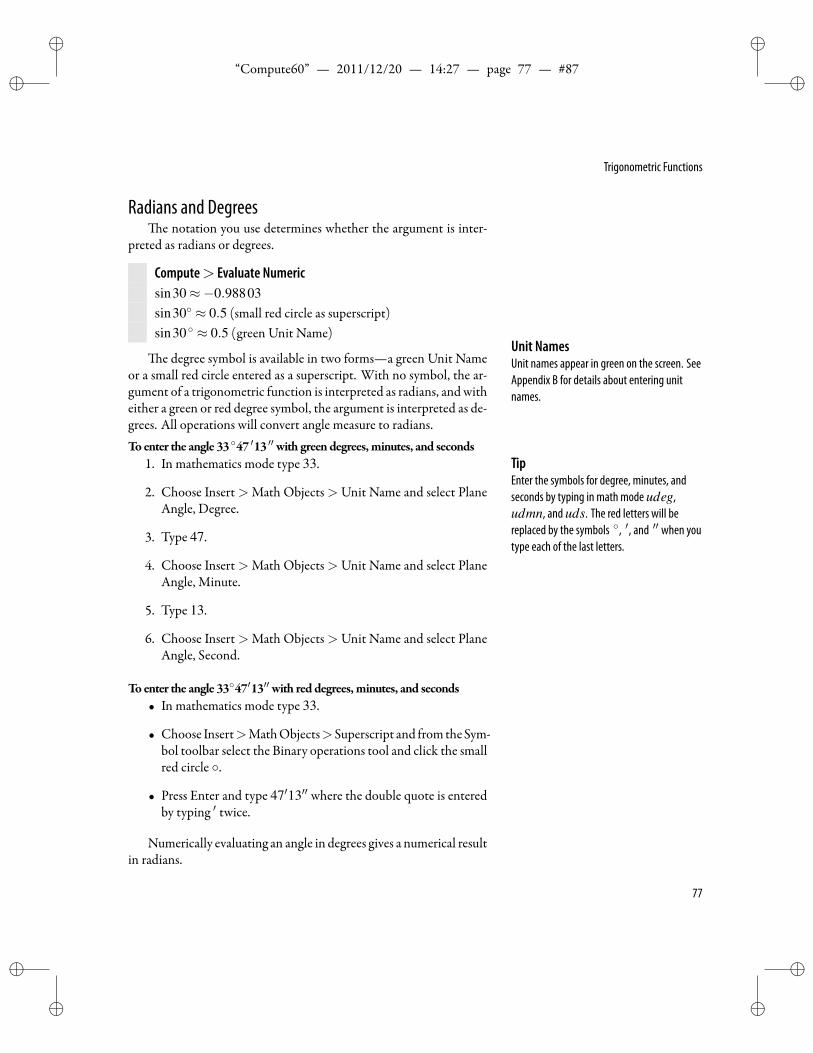
ii
“Compute60” — 2011/12/20 — 14:27 — page 77 — #87 ii
ii
ii
Trigonometric Functions
Radians and Degreese notation you use determines whether the argument is inter-
preted as radians or degrees.
Compute> Evaluate Numericsin30≈−0.98803sin30 ≈ 0.5 (small red circle as superscript)sin30 ≈ 0.5 (green Unit Name)
Unit NamesUnit names appear in green on the screen. SeeAppendix B for details about entering unitnames.
e degree symbol is available in two forms—a green Unit Nameor a small red circle entered as a superscript. With no symbol, the ar-gument of a trigonometric function is interpreted as radians, andwitheither a green or red degree symbol, the argument is interpreted as de-grees. All operations will convert angle measure to radians.Toenter the angle 3347 ′13 ′′ with greendegrees,minutes, and seconds
1. In mathematics mode type 33. TipEnter the symbols for degree, minutes, andseconds by typing in math mode udeg,udmn, and uds. The red letters will bereplaced by the symbols , ′, and ′′ when youtype each of the last letters.
2. Choose Insert>Math Objects>Unit Name and select PlaneAngle, Degree.
3. Type 47.
4. Choose Insert>Math Objects>Unit Name and select PlaneAngle, Minute.
5. Type 13.
6. Choose Insert>Math Objects>Unit Name and select PlaneAngle, Second.
Toenter the angle 3347′13′′ with reddegrees,minutes, and seconds• In mathematics mode type 33.
• Choose Insert>MathObjects>Superscript and fromtheSym-bol toolbar select the Binary operations tool and click the smallred circle .
• Press Enter and type 47′13′′ where the double quote is enteredby typing ′ twice.
Numerically evaluating an angle in degrees gives a numerical resultin radians.
77
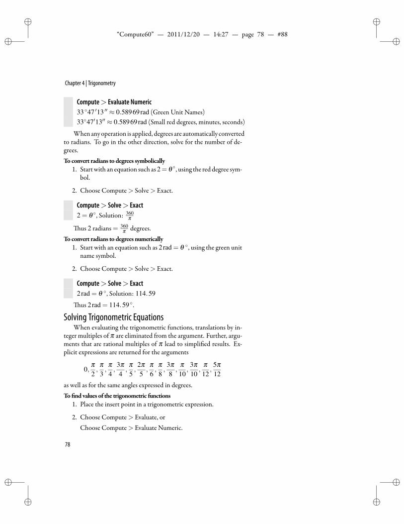
ii
“Compute60” — 2011/12/20 — 14:27 — page 78 — #88 ii
ii
ii
Chapter 4 | Trigonometry
Compute> Evaluate Numeric33 47 ′13 ′′ ≈ 0.58969rad (Green Unit Names)3347′13′′ ≈ 0.58969rad (Small red degrees, minutes, seconds)
Whenanyoperation is applied, degrees are automatically convertedto radians. To go in the other direction, solve for the number of de-grees.Toconvert radians to degrees symbolically
1. Startwith an equation such as2= θ , using the red degree sym-bol.
2. Choose Compute> Solve> Exact.
Compute> Solve> Exact2 = θ , Solution: 360
π
us 2 radians= 360π degrees.
Toconvert radians to degrees numerically1. Start with an equation such as 2rad = θ , using the green unit
name symbol.
2. Choose Compute> Solve> Exact.
Compute> Solve> Exact2rad = θ , Solution: 114.59
us 2rad = 114.59.
Solving Trigonometric EquationsWhen evaluating the trigonometric functions, translations by in-
teger multiples of π are eliminated from the argument. Further, argu-ments that are rational multiples of π lead to simpli ed results. Ex-plicit expressions are returned for the arguments
0,π2,
π3,
π4,
3π4,
π5,
2π5,
π6,
π8,
3π8,
π10
,3π10
,π12
,5π12
as well as for the same angles expressed in degrees.To nd values of the trigonometric functions
1. Place the insert point in a trigonometric expression.
2. Choose Compute> Evaluate, orChoose Compute> Evaluate Numeric.
78
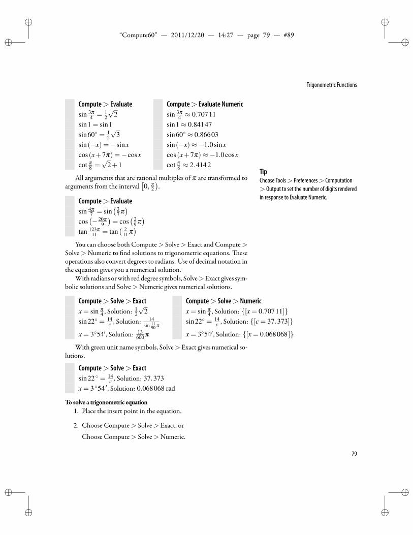
ii
“Compute60” — 2011/12/20 — 14:27 — page 79 — #89 ii
ii
ii
Trigonometric Functions
Compute> Evaluate Compute> Evaluate Numericsin 3π
4 = 12
√2 sin 3π
4 ≈ 0.70711sin1 = sin1 sin1≈ 0.84147sin60 = 1
2
√3 sin60 ≈ 0.86603
sin(−x) =−sinx sin(−x)≈−1.0sinxcos(x+7π) =−cosx cos(x+7π)≈−1.0cosxcot π
8 =√
2+1 cot π8 ≈ 2.4142
TipChoose Tools> Preferences> Computation> Output to set the number of digits renderedin response to Evaluate Numeric.
All arguments that are rational multiples of π are transformed toarguments from the interval
[0, π
2
).
Compute> Evaluatesin 4π
7 = sin( 3
7 π)
cos(− 20π
9
)= cos
( 29 π)
tan 123π11 = tan
( 211 π)
You can choose both Compute> Solve> Exact and Compute>Solve>Numeric to nd solutions to trigonometric equations. eseoperations also convert degrees to radians. Use of decimal notation inthe equation gives you a numerical solution.
With radians orwith red degree symbols, Solve>Exact gives sym-bolic solutions and Solve>Numeric gives numerical solutions.
Compute> Solve> Exact Compute> Solve> Numericx = sin π
4 , Solution: 12
√2 x = sin π
4 , Solution: [x = 0.70711]sin22 = 14
c , Solution: 14sin 11
90 πsin22 = 14
c , Solution: [c = 37.373]
x = 354′, Solution: 13600 π x = 354′, Solution: [x = 0.068068 ]
With green unit name symbols, Solve> Exact gives numerical so-lutions.
Compute> Solve> Exactsin22 = 14
c , Solution: 37.373x = 354 ′, Solution: 0.068068 rad
To solve a trigonometric equation1. Place the insert point in the equation.
2. Choose Compute> Solve> Exact, or
Choose Compute> Solve>Numeric.
79
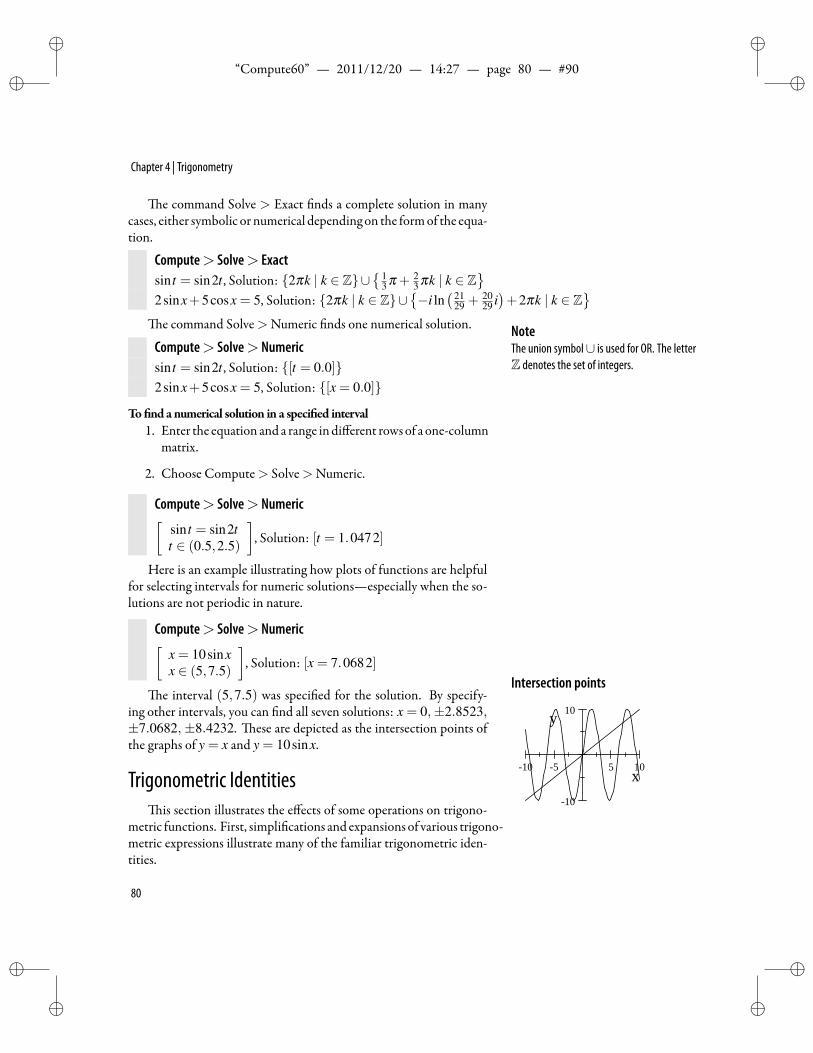
ii
“Compute60” — 2011/12/20 — 14:27 — page 80 — #90 ii
ii
ii
Chapter 4 | Trigonometry
e command Solve > Exact nds a complete solution in manycases, either symbolic or numerical dependingon the formof the equa-tion.
Compute> Solve> Exactsin t = sin2t , Solution: 2πk | k ∈ Z∪
13 π + 2
3 πk | k ∈ Z
2sinx+5cosx = 5, Solution: 2πk | k ∈ Z∪−i ln
( 2129 +
2029 i)+2πk | k ∈ Z
e command Solve>Numeric nds one numerical solution. Note
The union symbol∪ is used for OR. The letterZ denotes the set of integers.
Compute> Solve> Numericsin t = sin2t , Solution: [t = 0.0]2sinx+5cosx = 5, Solution: [x = 0.0]
To nd anumerical solution in a speci ed interval1. Enter the equation and a range indifferent rowsof a one-column
matrix.
2. Choose Compute> Solve>Numeric.
Compute> Solve> Numeric[sin t = sin2tt ∈ (0.5,2.5)
], Solution: [t = 1.0472]
Here is an example illustrating how plots of functions are helpfulfor selecting intervals for numeric solutions—especially when the so-lutions are not periodic in nature.
Compute> Solve> Numeric[x = 10sinxx ∈ (5,7.5)
], Solution: [x = 7.0682]
Intersection points
10 5 5 10
10
10
x
ye interval (5,7.5) was speci ed for the solution. By specify-
ing other intervals, you can nd all seven solutions: x = 0,±2.8523,±7.0682,±8.4232. ese are depicted as the intersection points ofthe graphs of y = x and y = 10sinx.
Trigonometric Identitiesis section illustrates the effects of some operations on trigono-
metric functions. First, simpli cations and expansionsof various trigono-metric expressions illustrate many of the familiar trigonometric iden-tities.
80
ii
“Compute60” — 2011/12/20 — 14:27 — page 81 — #91 ii
ii
ii
Trigonometric Identities
De nitions in terms of Basic Trigonometric FunctionsToexpress a trigonometric function in terms of sine and cosine
• Place the insert point in the function and choose Compute >Rewrite> Sin and Cos.
Compute> Rewrite> Sin and Cossecx = 1
cosx tanx = sinxcosx
cscx = 1sinx cotx = cosx
sinxcosxsinx−2secxcscx = cosxsinx− 2
cosxsinx
Alternatively, for sec and csc, choose Simplify.
Compute> Simplifysecx = 1
cosx cscx = 1sinx
Toexpress a trigonometric function in terms of the sine function1. Place the insert point in the function.
2. Choose Compute> Rewrite> Sin.
Compute> Rewrite> Sincosxsinx−2secxcscx = 2
(2sin2( 12 x)−1)sinx
− sinx(2sin2 ( 1
2 x)−1)
Toexpress a trigonometric function in terms of the cosine function1. Place the insert point in the function.
2. Choose Compute> Rewrite>Cos.
Compute> Rewrite> Coscosxsin2 x =−(cosx)
(cos2 x−1
)Toexpress a trigonometric function in terms of the tangent function
1. Place the insert point in the function.
2. Choose Compute> Rewrite>Tan.
Compute> Rewrite> Tan
sinx =2tan( 1
2 x)tan2( 1
2 x)+1
81
ii
“Compute60” — 2011/12/20 — 14:27 — page 82 — #92 ii
ii
ii
Chapter 4 | Trigonometry
Pythagorean IdentitiesTocomputePythagorean identities
1. Place the insert point in an expression.
2. Choose Compute> Simplify, orCompute> Rewrite> Sin and Cos.
3. Use basic techniques for simplifying such expressions.
Compute> Simplifysin2 x+ cos2 x = 1
Compute> Rewrite> Sin and Cos, Simplifytan2 x− sec2 x = sin2 x
cos2 x −1
cos2 x =−1
Addition FormulasTocompute addition formulas
1. Place the insert point in an expression.
2. Choose Compute> Expand.
Compute> Expandsin(x+ y) = cosxsiny+ cosysinx sin
(x+ π
2
)= cosx
cos(x+ y) = cosxcosy− sinxsiny cos(x− π
2
)= sinx
Combine and Expand act as reverse operations in many cases.
Compute> Combine> Trigonometric Functionscosxsiny+ cosysinx = sin(x+ y)cosxcosy− sinxsiny = cos(x+ y)
Multiple-Angle FormulasYou can obtain multiple-angle formulas with Expand.
To reduce amultiple-angle expression• Place the insert point in the expression and choose Compute>
Expand.
Compute> Expandsin2θ = 2cosθ sinθ cos2θ = cos2 θ − sin2 θtan2θ =− 2tanθ
tan2 θ−1
sin6θ = 6cos5 θ sinθ −20cos3 θ sin3 θ +6cosθ sin5 θ
82
ii
“Compute60” — 2011/12/20 — 14:27 — page 83 — #93 ii
ii
ii
Inverse Trigonometric Functions
Combining and Simplifying Trigonometric Expressions TipThere are many possible forms fortrigonometric expressions. To get expressionsin the form you want, you can experiment withdifferent combinations of commands.
Products and powers of trigonometric functions and hyperbolicfunctions are combined into a sum of trigonometric functions or hy-perbolic functions whose arguments are integral linear combinationsof the original arguments.To simplify sumsof products andpowers of trigonometric expressions
1. Place the insert point in the expression.
2. Choose Compute>Combine>Trigonometric Functions.
Compute> Combine> Trigonometric Functionssinxsiny = 1
2 cos(x− y)− 12 cos(x+ y)
sin2 x = 12 −
12 cos(2x)
sinxcosy = 12 sin(x− y)+ 1
2 sin(x+ y)sin5 xcos5 x = 5
256 sin(2x)− 5512 sin(6x)+ 1
512 sin(10x)
Here is another example where Expand and Combine act as re-verse operations.
Compute> Expand12 cos(x− y)− 1
2 cos(x+ y) = sinxsiny12 sin(x− y)+ 1
2 sin(x+ y) = cosysinx
Simplify also combines and simpli es trigonometric expressions.TipThe inverse trigonometric functions can beentered by typing the function name inmathematics mode or by choosing Insert>Math Objects>Math Name and selectingfrom a list. You can also type the 3-lettertrigonometric name with an exponent of−1.
Compute> Simplifysin3a+4sin3 a = 3sina
Inverse Trigonometric Functionse following typeof question arises frequentlywhenworkingwith
the trigonometric functions: for which angles x is sinx = y? ereare many correct answers to these questions, since the trigonometricfunctions are periodic. e inverse trigonometric functions providesolutions that lie within restricted ranges. e angle returned by thesefunctions is measured in radians, not in degrees.
Inverse function Domain Rangearcsinx or sin−1 x [−1,1]
[−π
2 ,π2
]arccosx or cos−1 x [−1,1] [0,π]arctanx or tan−1 x (−∞,∞)
(−π
2 ,π2
)83
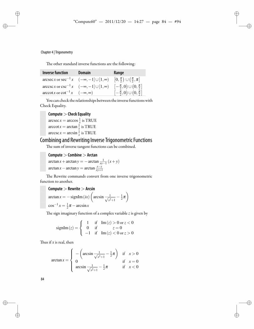
ii
“Compute60” — 2011/12/20 — 14:27 — page 84 — #94 ii
ii
ii
Chapter 4 | Trigonometry
e other standard inverse functions are the following:
Inverse function Domain Rangearcsecx or sec−1 x (−∞,−1]∪ [1,∞)
[0, π
2
)∪(π
2 ,π]
arccscx or csc−1 x (−∞,−1]∪ [1,∞)[−π
2 ,0)∪(0, π
2
]arccotx or cot−1 x (−∞,∞)
[−π
2 ,0)∪(0, π
2
]Youcan check the relationships between the inverse functionswith
Check Equality.
Compute> Check Equalityarcsecx = arccos 1
x is TRUEarccotx = arctan 1
x is TRUEarccscx = arcsin 1
x is TRUE
Combining and Rewriting Inverse Trigonometric Functionse sum of inverse tangent functions can be combined.
Compute> Combine> Arctanarctanx+ arctany =−arctan 1
xy−1 (x+ y)
arctanx− arctany = arctan x−yxy+1
e Rewrite commands convert from one inverse trigonometricfunction to another.
Compute> Rewrite> Arcsin
arctanx =−signIm(ix)(
arcsin 1√x2+1− 1
2 π)
cos−1 x = 12 π− arcsinx
e sign imaginary function of a complex variable z is given by
signIm(z) =
1 if Im(z)> 0 or z < 00 if z = 0−1 if Im(z)< 0 or z > 0
us if x is real, then
arctanx =
−(
arcsin 1√x2+1− 1
2 π)
if x > 0
0 if x = 0arcsin 1√
x2+1− 1
2 π if x < 0
84
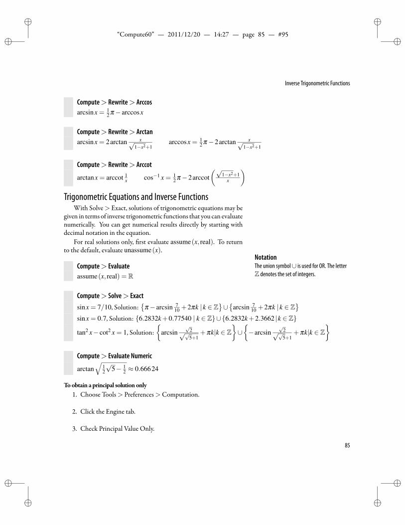
ii
“Compute60” — 2011/12/20 — 14:27 — page 85 — #95 ii
ii
ii
Inverse Trigonometric Functions
Compute> Rewrite> Arccosarcsinx = 1
2 π− arccosx
Compute> Rewrite> Arctanarcsinx = 2arctan x√
1−x2+1arccosx = 1
2 π−2arctan x√1−x2+1
Compute> Rewrite> Arccot
arctanx = arccot 1x cos−1 x = 1
2 π−2arccot(√
1−x2+1x
)Trigonometric Equations and Inverse Functions
With Solve> Exact, solutions of trigonometric equations may begiven in terms of inverse trigonometric functions that you can evaluatenumerically. You can get numerical results directly by starting withdecimal notation in the equation.
For real solutions only, rst evaluate assume(x, real). To returnto the default, evaluate unassume(x).
NotationThe union symbol∪ is used for OR. The letterZ denotes the set of integers.
Compute> Evaluateassume(x, real) = R
Compute> Solve> Exactsinx = 7/10, Solution:
π− arcsin 7
10 +2πk |k ∈ Z∪
arcsin 710 +2πk |k ∈ Z
sinx = 0.7, Solution: 6.2832k+0.77540 | k ∈ Z∪6.2832k+2.3662 |k ∈ Z
tan2 x− cot2 x = 1, Solution:
arcsin√
2√√5+1
+πk|k ∈ Z∪−arcsin
√2√√5+1
+πk|k ∈ Z
Compute> Evaluate Numeric
arctan√
12
√5− 1
2 ≈ 0.66624
Toobtain a principal solutiononly1. Choose Tools> Preferences>Computation.
2. Click the Engine tab.
3. Check Principal Value Only.
85
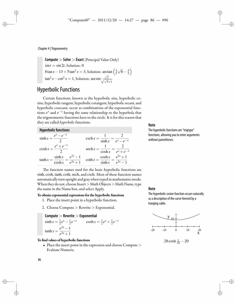
ii
“Compute60” — 2011/12/20 — 14:27 — page 86 — #96 ii
ii
ii
Chapter 4 | Trigonometry
Compute> Solve> Exact (Principal Value Only)sin t = sin2t , Solution: 0
8tanx−13+5tan2 x = 3, Solution: arctan(
45
√6− 4
5
)tan2 x− cot2 x = 1, Solution: arcsin
√2√√5+1
Hyperbolic FunctionsCertain functions, known as the hyperbolic sine, hyperbolic co-
sine, hyperbolic tangent, hyperbolic cotangent, hyperbolic secant, andhyperbolic cosecant, occur as combinations of the exponential func-tions ex and e−x having the same relationship to the hyperbola thatthe trigonometric functions have to the circle. It is for this reason thatthey are called hyperbolic functions.
NoteThe hyperbolic functions are “trigtype”functions, allowing you to enter argumentswithout parentheses.
Hyperbolic functions
sinhx =ex− e−x
2cschx =
1sinhx
=2
ex− e−x
coshx =ex + e−x
2sechx =
1coshx
=2
ex + e−x
tanhx =sinhxcoshx
=e2x−1e2x +1
cothx =coshxsinhx
=e2x +1e2x−1
e function names used for the basic hyperbolic functions aresinh, cosh, tanh, coth, sech, and csch. Most of these function namesautomatically turnupright andgraywhen typed inmathematicsmode.When they donot, choose Insert>MathObjects>MathName, typethe name in the Name box, and select Apply. Note
The hyperbolic cosine function occurs naturallyas a description of the curve formed by ahanging cable.
20 10 0 10 20
10
x
y
28cosh x28 −20
Toobtain exponential expressions for the hyperbolic functions1. Place the insert point in a hyperbolic function.
2. Choose Compute> Rewrite> Exponential.
Compute> Rewrite> Exponentialsinhx = 1
2 ex− 12 e−x coshx = 1
2 ex + 12 e−x
tanhx =e2x−1e2x +1
To nd values of hyperbolic functions• Place the insert point in the expression and choose Compute>
Evaluate Numeric.
86
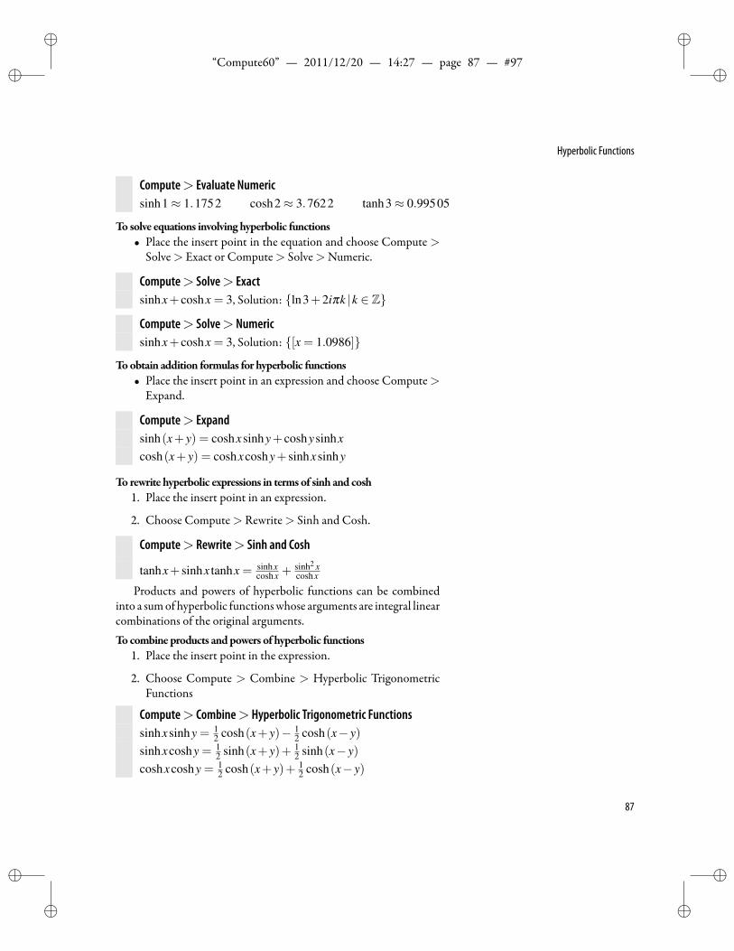
ii
“Compute60” — 2011/12/20 — 14:27 — page 87 — #97 ii
ii
ii
Hyperbolic Functions
Compute> Evaluate Numericsinh1≈ 1.1752 cosh2≈ 3.7622 tanh3≈ 0.99505
To solve equations involving hyperbolic functions• Place the insert point in the equation and choose Compute >
Solve> Exact or Compute> Solve>Numeric.
Compute> Solve> Exactsinhx+ coshx = 3, Solution: ln3+2iπk |k ∈ Z
Compute> Solve> Numericsinhx+ coshx = 3, Solution: [x = 1.0986]
Toobtain addition formulas for hyperbolic functions• Place the insert point in an expression and choose Compute>
Expand.
Compute> Expandsinh(x+ y) = coshxsinhy+ coshysinhxcosh(x+ y) = coshxcoshy+ sinhxsinhy
To rewrite hyperbolic expressions in terms of sinh and cosh1. Place the insert point in an expression.
2. Choose Compute> Rewrite> Sinh and Cosh.
Compute> Rewrite> Sinh and Cosh
tanhx+ sinhx tanhx = sinhxcoshx +
sinh2 xcoshx
Products and powers of hyperbolic functions can be combinedinto a sumof hyperbolic functionswhose arguments are integral linearcombinations of the original arguments.Tocombine products andpowers of hyperbolic functions
1. Place the insert point in the expression.
2. Choose Compute > Combine > Hyperbolic TrigonometricFunctions
Compute> Combine> Hyperbolic Trigonometric Functionssinhxsinhy = 1
2 cosh(x+ y)− 12 cosh(x− y)
sinhxcoshy = 12 sinh(x+ y)+ 1
2 sinh(x− y)coshxcoshy = 1
2 cosh(x+ y)+ 12 cosh(x− y)
87
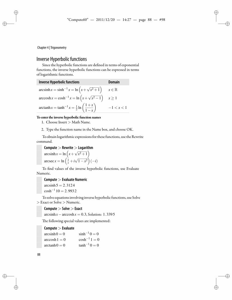
ii
“Compute60” — 2011/12/20 — 14:27 — page 88 — #98 ii
ii
ii
Chapter 4 | Trigonometry
Inverse Hyperbolic functionsSince the hyperbolic functions are de ned in terms of exponential
functions, the inverse hyperbolic functions can be expressed in termsof logarithmic functions.
Inverse Hyperbolic functions Domain
arcsinhx = sinh−1 x = ln(
x+√
x2 +1)
x ∈ R
arccoshx = cosh−1 x = ln(
x+√
x2−1)
x≥ 1
arctanhx = tanh−1 x = 12 ln(
1+ x1− x
)−1 < x < 1
Toenter the inverse hyperbolic functionnames1. Choose Insert>Math Name.
2. Type the function name in the Name box, and choose OK.
Toobtain logarithmic expressions for these functions, use theRewritecommand.
Compute> Rewrite> Logarithmarcsinhx = ln
(x+√
x2 +1)
arcsecx = ln(
1x + i√
1− x2)(−i)
To nd values of the inverse hyperbolic functions, use EvaluateNumeric.
Compute> Evaluate Numericarcsinh5 = 2.3124cosh−1 10 = 2.9932
Tosolve equations involving inversehyperbolic functions, use Solve> Exact or Solve>Numeric.
Compute> Solve> Exactarcsinhx− arccoshx = 0.3, Solution: 1.3395
e following special values are implemented:
Compute> Evaluatearcsinh0 = 0 sinh−1 0 = 0arccosh1 = 0 cosh−1 1 = 0arctanh0 = 0 tanh−1 0 = 0
88
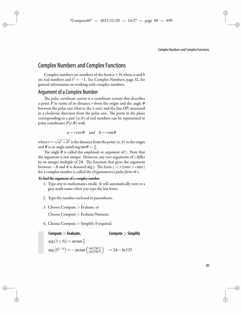
ii
“Compute60” — 2011/12/20 — 14:27 — page 89 — #99 ii
ii
ii
Complex Numbers and Complex Functions
Complex Numbers and Complex FunctionsComplex numbers are numbers of the form a+bi where a and b
are real numbers and i2 = −1. See Complex Numbers, page 32, forgeneral information on working with complex numbers.
Argument of a Complex Numbere polar coordinate system is a coordinate system that describes
a point P in terms of its distance r from the origin and the angle θbetween the polar axis (that is, the x-axis) and the line OP, measuredin a clockwise direction from the polar axis. e point in the planecorresponding to a pair (a,b) of real numbers can be represented inpolar coordinates P(r,θ) with
a = r cosθ and b = r sinθ
where r =√
a2 +b2 is the distance from the point (a,b) to the originand θ is an angle satisfying tanθ = a
b .e angle θ is called the amplitude or argument of z. Note that
the argument is not unique. However, any two arguments of z differby an integer multiple of 2π . e function that gives the argumentbetween −π and π is denoted argz. e form z = r (cos t + isin t)for a complex number is called the (trigonometric) polar form of z.
To nd the argument of a complex number1. Type arg in mathematics mode. It will automatically turn to a
gray math name when you type the last letter.
2. Type the number enclosed in parentheses.
3. Choose Compute> Evaluate, or
Choose Compute> Evaluate Numeric.
4. Choose Compute> Simplify if required.
Compute> Evaluate, Compute> Simplify
arg(3+5i) = arctan 53
arg(52−3i
)=−arctan
(sin(3ln5)cos(3ln5)
)= 2π− ln125
89
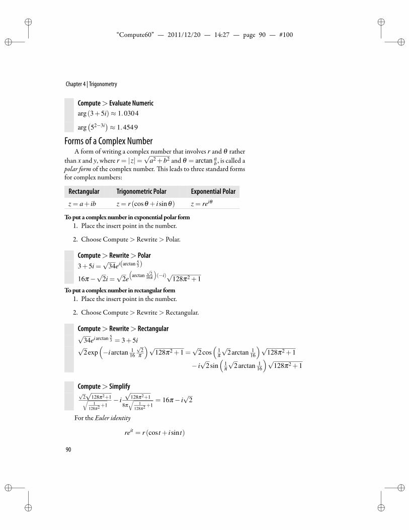
ii
“Compute60” — 2011/12/20 — 14:27 — page 90 — #100 ii
ii
ii
Chapter 4 | Trigonometry
Compute> Evaluate Numericarg(3+5i)≈ 1.0304
arg(52−3i
)≈ 1.4549
Forms of a Complex NumberA form of writing a complex number that involves r and θ rather
than x and y, where r = |z|=√
a2 +b2 and θ = arctan ab , is called a
polar form of the complex number. is leads to three standard formsfor complex numbers:
Rectangular Trigonometric Polar Exponential Polar
z = a+ ib z = r (cosθ + isinθ) z = reiθ
Toput a complex number in exponential polar form1. Place the insert point in the number.
2. Choose Compute> Rewrite> Polar.
Compute> Rewrite> Polar3+5i =
√34ei(arctan 5
3)
16π−√
2i =√
2e(
arctan√
216π
)(−i)√128π2 +1
Toput a complex number in rectangular form1. Place the insert point in the number.
2. Choose Compute> Rewrite> Rectangular.
Compute> Rewrite> Rectangular√
34eiarctan 53 = 3+5i
√2exp
(−iarctan 1
16
√2
π
)√128π2 +1 =
√2cos
(1π√
2arctan 116
)√128π2 +1
− i√
2sin(
1π√
2arctan 116
)√128π2 +1
Compute> Simplify√
2√
128π2+1√1
128π2 +1− i√
128π2+1
8π√
1128π2 +1
= 16π− i√
2
For the Euler identity
reit = r (cos t + isin t)
90
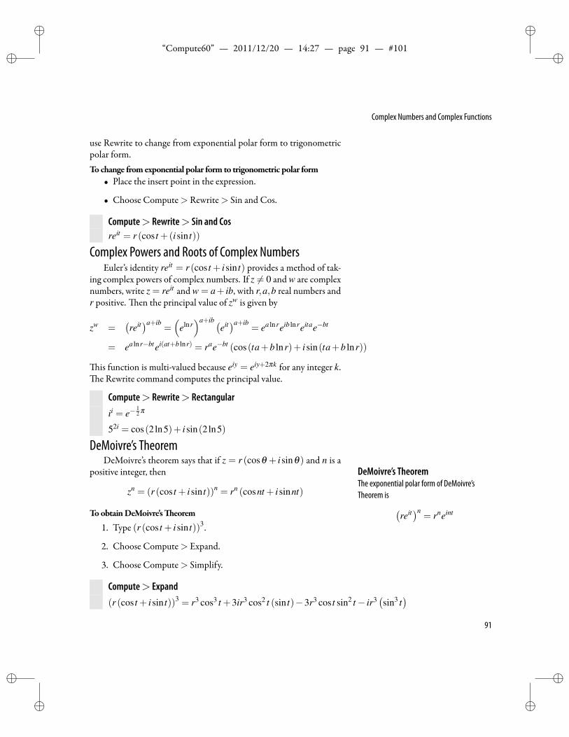
ii
“Compute60” — 2011/12/20 — 14:27 — page 91 — #101 ii
ii
ii
Complex Numbers and Complex Functions
use Rewrite to change from exponential polar form to trigonometricpolar form.Tochange fromexponential polar form to trigonometric polar form
• Place the insert point in the expression.
• Choose Compute> Rewrite> Sin and Cos.
Compute> Rewrite> Sin and Cosreit = r (cos t +(isin t))
Complex Powers and Roots of Complex NumbersEuler’s identity reit = r (cos t + isin t) provides a method of tak-
ing complex powers of complex numbers. If z = 0 and w are complexnumbers, write z = reit and w = a+ ib, with r,a,b real numbers andr positive. en the principal value of zw is given by
zw =(reit)a+ib
=(
elnr)a+ib (
eit)a+ib= ea lnreib lnreitae−bt
= ea lnr−btei(at+b lnr) = rae−bt (cos(ta+b lnr)+ isin(ta+b lnr))
is function is multi-valued because eiy = eiy+2πk for any integer k.e Rewrite command computes the principal value.
Compute> Rewrite> Rectangularii = e−
12 π
52i = cos(2ln5)+ isin(2ln5)
DeMoivre’s TheoremDeMoivre’s theorem says that if z = r (cosθ + isinθ) and n is a
positive integer, then DeMoivre’s TheoremThe exponential polar form of DeMoivre’sTheorem is (
reit)n= rneint
zn = (r (cos t + isin t))n = rn (cosnt + isinnt)
ToobtainDeMoivre's eorem
1. Type (r (cos t + isin t))3.
2. Choose Compute> Expand.
3. Choose Compute> Simplify.
Compute> Expand(r (cos t + isin t))3 = r3 cos3 t +3ir3 cos2 t (sin t)−3r3 cos t sin2 t− ir3
(sin3 t
)91
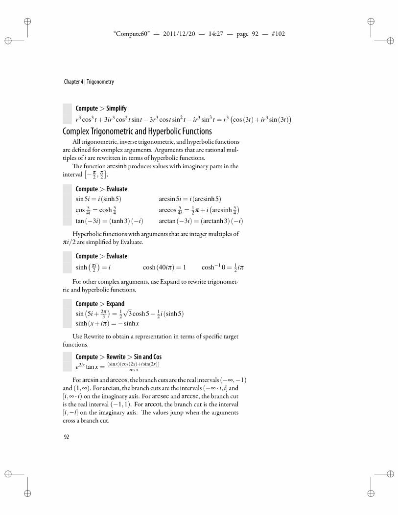
ii
“Compute60” — 2011/12/20 — 14:27 — page 92 — #102 ii
ii
ii
Chapter 4 | Trigonometry
Compute> Simplifyr3 cos3 t +3ir3 cos2 t sin t−3r3 cos t sin2 t− ir3 sin3 t = r3
(cos(3t)+ ir3 sin(3t)
)Complex Trigonometric and Hyperbolic Functions
All trigonometric, inverse trigonometric, andhyperbolic functionsare de ned for complex arguments. Arguments that are rational mul-tiples of i are rewritten in terms of hyperbolic functions.
e function arcsinh produces values with imaginary parts in theinterval
[−π
2 ,π2
].
Compute> Evaluatesin5i = i(sinh5) arcsin5i = i(arcsinh5)
cos 54i = cosh 5
4 arccos 54i =
12 π + i
(arcsinh 5
4
)tan(−3i) = (tanh3)(−i) arctan(−3i) = (arctanh3)(−i)
Hyperbolic functions with arguments that are integermultiples ofπi/2 are simpli ed by Evaluate.
Compute> Evaluatesinh
(πi2
)= i cosh(40iπ) = 1 cosh−1 0 = 1
2 iπ
For other complex arguments, use Expand to rewrite trigonomet-ric and hyperbolic functions.
Compute> Expandsin(5i+ 2π
3
)= 1
2
√3cosh5− 1
2 i(sinh5)sinh(x+ iπ) =−sinhx
Use Rewrite to obtain a representation in terms of speci c targetfunctions.
Compute> Rewrite> Sin and Cose2ix tanx = (sinx)(cos(2x)+isin(2x))
cosx
Forarcsin andarccos, thebranch cuts are the real intervals (−∞,−1)and (1,∞). For arctan, the branch cuts are the intervals (−∞ · i, i] and[i,∞ · i) on the imaginary axis. For arcsec and arccsc, the branch cutis the real interval (−1,1). For arccot, the branch cut is the interval[i,−i] on the imaginary axis. e values jump when the argumentscross a branch cut.
92
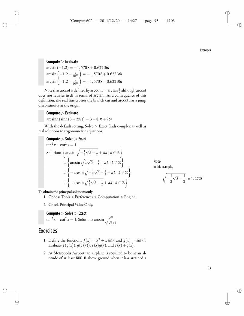
ii
“Compute60” — 2011/12/20 — 14:27 — page 93 — #103 ii
ii
ii
Exercises
Compute> Evaluatearcsin(−1.2) =−1.5708+0.62236i
arcsin(−1.2+ i
1010
)=−1.5708+0.62236i
arcsin(−1.2− i
1010
)=−1.5708−0.62236i
Note that arccot is de nedby arccotx= arctan 1x although arccot
does not rewrite itself in terms of arctan. As a consequence of thisde nition, the real line crosses the branch cut and arccot has a jumpdiscontinuity at the origin.
Compute> Evaluatearcsinh(sinh(3+25i)) = 3−8iπ +25i
With the default setting, Solve > Exact nds complex as well asreal solutions to trigonometric equations.
Compute> Solve> Exacttan2 x− cot2 x = 1
Solution:
arcsin√− 1
2
√5− 1
2 +πk | k ∈ Z
∪
arcsin√
12
√5− 1
2 +πk | k ∈ Z
∪−arcsin
√− 1
2
√5− 1
2 +πk | k ∈ Z
∪−arcsin
√12
√5− 1
2 +πk | k ∈ Z
NoteIn this example,√
−12
√5− 1
2≈ 1.272i
Toobtain the principal solutions only1. Choose Tools> Preferences>Computation> Engine.
2. Check Principal Value Only.
Compute> Solve> Exacttan2 x− cot2 x = 1, Solution: arcsin
√2√√5+1
Exercises1. De ne the functions f (x) = x3 + xsinx and g(x) = sinx2.
Evaluate f (g(x)), g( f (x)), f (x)g(x), and f (x)+g(x).
2. At Metropolis Airport, an airplane is required to be at an al-titude of at least 800 ft above ground when it has attained a
93
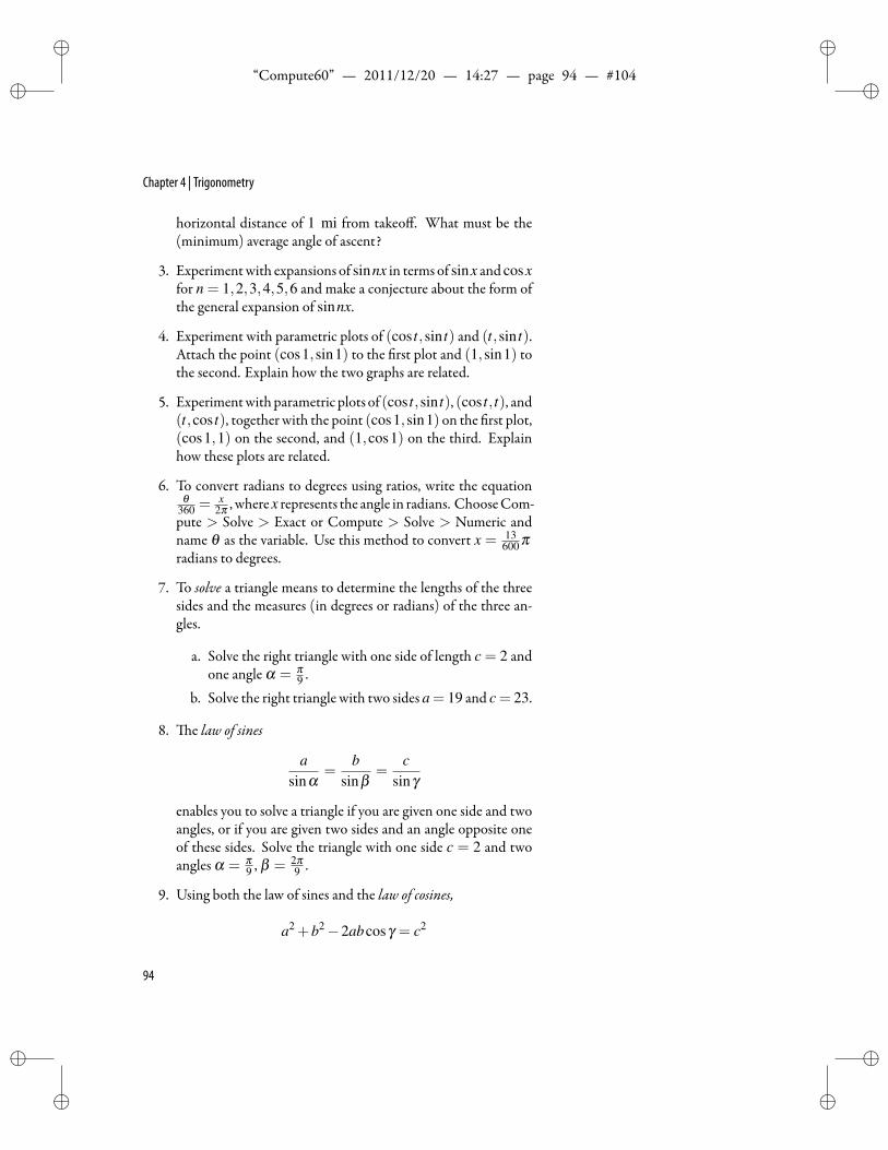
ii
“Compute60” — 2011/12/20 — 14:27 — page 94 — #104 ii
ii
ii
Chapter 4 | Trigonometry
horizontal distance of 1 mi from takeoff. What must be the(minimum) average angle of ascent?
3. Experimentwith expansions of sinnx in terms of sinx and cosxfor n = 1,2,3,4,5,6 and make a conjecture about the form ofthe general expansion of sinnx.
4. Experiment with parametric plots of (cos t,sin t) and (t,sin t).Attach the point (cos1,sin1) to the rst plot and (1,sin1) tothe second. Explain how the two graphs are related.
5. Experimentwithparametric plots of (cos t,sin t), (cos t, t), and(t,cos t), together with the point (cos1,sin1) on the rst plot,(cos1,1) on the second, and (1,cos1) on the third. Explainhow these plots are related.
6. To convert radians to degrees using ratios, write the equationθ
360 =x
2π , wherex represents the angle in radians. ChooseCom-pute > Solve > Exact or Compute > Solve > Numeric andname θ as the variable. Use this method to convert x = 13
600 πradians to degrees.
7. To sol e a triangle means to determine the lengths of the threesides and the measures (in degrees or radians) of the three an-gles.
a. Solve the right triangle with one side of length c = 2 andone angle α = π
9 .b. Solve the right triangle with two sides a = 19 and c = 23.
8. e law of sines
asinα
=b
sinβ=
csinγ
enables you to solve a triangle if you are given one side and twoangles, or if you are given two sides and an angle opposite oneof these sides. Solve the triangle with one side c = 2 and twoangles α = π
9 , β = 2π9 .
9. Using both the law of sines and the law of cosines,
a2 +b2−2abcosγ = c2
94
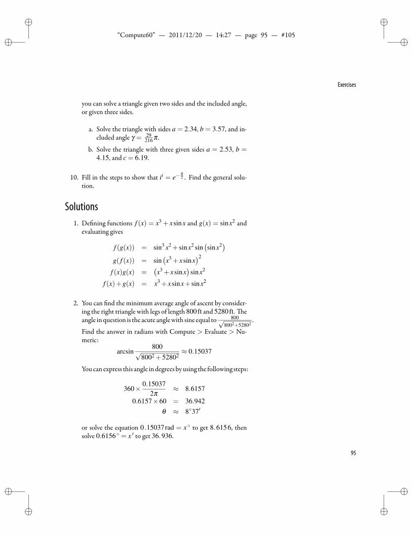
ii
“Compute60” — 2011/12/20 — 14:27 — page 95 — #105 ii
ii
ii
Exercises
you can solve a triangle given two sides and the included angle,or given three sides.
a. Solve the triangle with sides a = 2.34, b = 3.57, and in-cluded angle γ = 29
216 π .
b. Solve the triangle with three given sides a = 2.53, b =4.15, and c = 6.19.
10. Fill in the steps to show that ii = e−π2 . Find the general solu-
tion.
Solutions1. De ning functions f (x) = x3 + xsinx and g(x) = sinx2 and
evaluating gives
f (g(x)) = sin3 x2 + sinx2 sin(sinx2)
g( f (x)) = sin(x3 + xsinx
)2
f (x)g(x) =(x3 + xsinx
)sinx2
f (x)+g(x) = x3 + xsinx+ sinx2
2. You can nd the minimum average angle of ascent by consider-ing the right triangle with legs of length 800ft and 5280ft. eangle inquestion is the acute anglewith sine equal to 800√
8002+52802.
Find the answer in radians with Compute > Evaluate > Nu-meric:
arcsin800√
8002 +52802≈ 0.15037
Youcan express this angle indegrees byusing the following steps:
360× 0.150372π
≈ 8.6157
0.6157×60 = 36.942θ ≈ 837′
or solve the equation 0 .15037rad = x to get 8.6156, thensolve 0.6156 = x ′ to get 36.936.
95
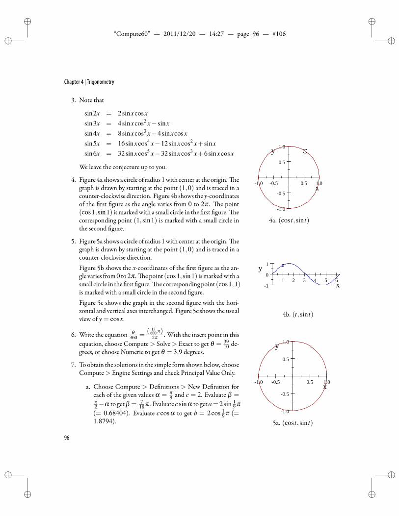
ii
“Compute60” — 2011/12/20 — 14:27 — page 96 — #106 ii
ii
ii
Chapter 4 | Trigonometry
3. Note that
sin2x = 2sinxcosxsin3x = 4sinxcos2 x− sinxsin4x = 8sinxcos3 x−4sinxcosxsin5x = 16sinxcos4 x−12sinxcos2 x+ sinxsin6x = 32sinxcos5 x−32sinxcos3 x+6sinxcosx
We leave the conjecture up to you.
4. Figure 4a shows a circle of radius1with center at the origin. egraph is drawn by starting at the point (1,0) and is traced in acounter-clockwise direction. Figure 4b shows the y-coordinatesof the rst gure as the angle varies from 0 to 2π . e point(cos1,sin1) ismarkedwith a small circle in the rst gure. ecorresponding point (1,sin1) is marked with a small circle inthe second gure.
1.0 0.5 0.5 1.0
1.0
0.5
0.5
1.0
x
y
4a. (cos t,sin t)
1 2 3 4 5 61
0
1
x
y
4b. (t,sin t)
5. Figure 5a shows a circle of radius1with center at the origin. egraph is drawn by starting at the point (1,0) and is traced in acounter-clockwise direction.Figure 5b shows the x-coordinates of the rst gure as the an-gle varies from0 to2π . e point (cos1,sin1) ismarkedwith asmall circle in the rst gure. e correspondingpoint (cos1,1)is marked with a small circle in the second gure.Figure 5c shows the graph in the second gure with the hori-zontal and vertical axes interchanged. Figure 5c shows the usualview of y = cosx.
6. Write the equation θ360 =
( 13600 π)2π . With the insert point in this
1.0 0.5 0.5 1.0
1.0
0.5
0.5
1.0
x
y
5a. (cos t,sin t)
equation, choose Compute> Solve> Exact to get θ = 3910 de-
grees, or choose Numeric to get θ = 3.9 degrees.
7. To obtain the solutions in the simple form shown below, chooseCompute> Engine Settings and check Principal Value Only.
a. Choose Compute > De nitions > New De nition foreach of the given values α = π
9 and c = 2. Evaluate β =π2 −α to getβ = 7
18 π . Evaluatecsinα to geta= 2sin 19 π
(= 0.68404). Evaluate ccosα to get b = 2cos 19 π (=
1.8794).
96
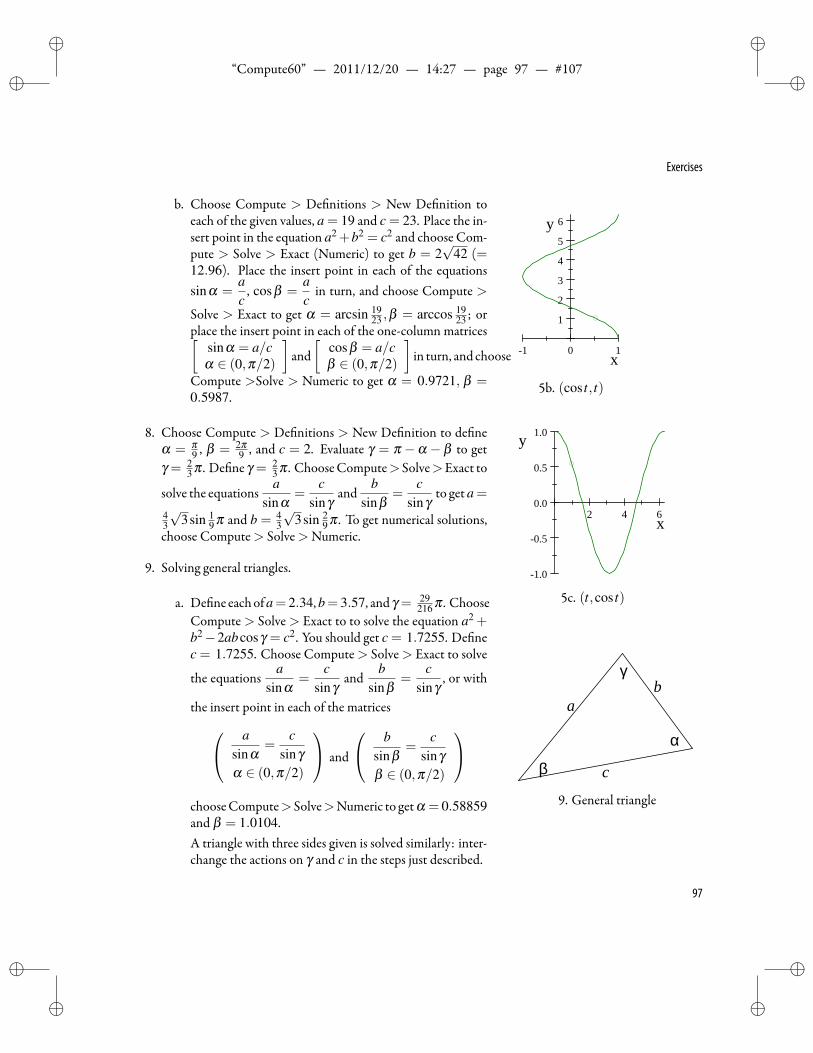
ii
“Compute60” — 2011/12/20 — 14:27 — page 97 — #107 ii
ii
ii
Exercises
b. Choose Compute > De nitions > New De nition toeach of the given values, a = 19 and c = 23. Place the in-sert point in the equation a2+b2 = c2 and choose Com-pute > Solve > Exact (Numeric) to get b = 2
√42 (=
12.96). Place the insert point in each of the equationssinα =
ac, cosβ =
ac
in turn, and choose Compute >
Solve > Exact to get α = arcsin 1923 ,β = arccos 19
23 ; orplace the insert point in each of the one-column matrices[
sinα = a/cα ∈ (0,π/2)
]and[
cosβ = a/cβ ∈ (0,π/2)
]in turn, and choose
Compute >Solve > Numeric to get α = 0.9721, β =0.5987.
1 0 1
1
2
3
4
5
6
x
y
5b. (cos t, t)
2 4 6
1.0
0.5
0.0
0.5
1.0
x
y
5c. (t,cos t)
8. Choose Compute > De nitions > New De nition to de neα = π
9 , β = 2π9 , and c = 2. Evaluate γ = π −α − β to get
γ = 23 π . De ne γ = 2
3 π . ChooseCompute> Solve>Exact to
solve the equationsa
sinα=
csinγ
andb
sinβ=
csinγ
to get a=
43
√3sin 1
9 π and b = 43
√3sin 2
9 π . To get numerical solutions,choose Compute> Solve>Numeric.
9. Solving general triangles.
a. De ne eachofa= 2.34,b= 3.57, and γ = 29216 π . Choose
Compute > Solve > Exact to to solve the equation a2 +b2−2abcosγ = c2. You should get c = 1.7255. De nec = 1.7255. Choose Compute> Solve> Exact to solve
the equationsa
sinα=
csinγ
andb
sinβ=
csinγ
, or with
the insert point in each of the matrices a
c
b
α
β
γ
9. General triangle
asinα
=c
sinγα ∈ (0,π/2)
and
bsinβ
=c
sinγβ ∈ (0,π/2)
chooseCompute>Solve>Numeric to getα = 0.58859and β = 1.0104.A triangle with three sides given is solved similarly: inter-change the actions on γ and c in the steps just described.
97
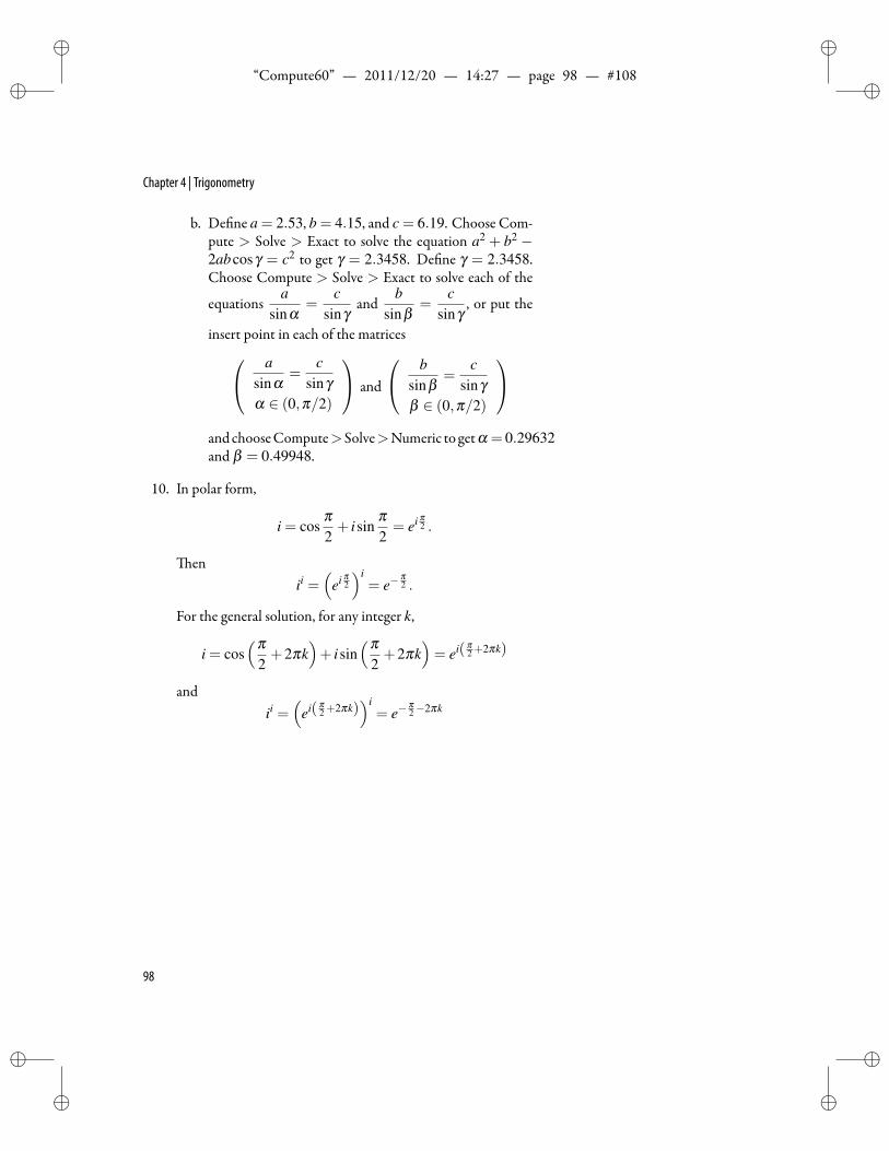
ii
“Compute60” — 2011/12/20 — 14:27 — page 98 — #108 ii
ii
ii
Chapter 4 | Trigonometry
b. De ne a = 2.53, b = 4.15, and c = 6.19. Choose Com-pute > Solve > Exact to solve the equation a2 + b2 −2abcosγ = c2 to get γ = 2.3458. De ne γ = 2.3458.Choose Compute > Solve > Exact to solve each of the
equationsa
sinα=
csinγ
andb
sinβ=
csinγ
, or put the
insert point in each of the matrices asinα
=c
sinγα ∈ (0,π/2)
and
bsinβ
=c
sinγβ ∈ (0,π/2)
and chooseCompute>Solve>Numeric to getα = 0.29632and β = 0.49948.
10. In polar form,
i = cosπ2+ isin
π2= ei π
2 .
enii =
(ei π
2
)i= e−
π2 .
For the general solution, for any integer k,
i = cos(π
2+2πk
)+ isin
(π2+2πk
)= ei( π
2 +2πk)
andii =
(ei( π
2 +2πk))i
= e−π2−2πk
98
ii
“Compute60” — 2011/12/20 — 14:27 — page 99 — #109 ii
ii
ii
5Function De nitions
“Then you should say what youmean,” the March Hare went on. “I do, ” Alice hastily replied; “at least I mean what I say, that's the same thing, youknow.” “Not the same thing a bit!” said the Hatter. “Why, you might just as well say that `I see what I eat' is the same thing as `I eat what I see!' ”
Lewis Carroll (1832–1898), Alice in Wonderland.
D e nitions enable you to de ne a symbol to be a mathemati- Function and Expression Names
De ning Variables and Functions
Handling De nitions
Formulas
External Functions
Trigtype Functions
cal object, and to de ne a function using an expression or acollection of expressions. Function de nition is a powerful
tool. Before elaborating on de nitions, we discuss criteria for namesof functions, constants, and expressions.
Function and Expression NamesAmathematical expression is a collection of valid expression names
combined in amathematically correct way. e notation for a functionconsists of a valid function name followed by a pair of parenthesescontaining a list of variables, called arguments. Trigonometric func-tions and certain others (trigtype functions) do not always require theparentheses around the argument. e argument of a function can New in Version 6
Overbar for complex conjugateDecorated characters as expression namesPassthru Code to Engine
also occur as a subscript.
• Examples ofmathematical expressions: x,a3b−2c, xsiny+3cosz,a1a2−3b1b2
• Examples of ordinary functionnotation: a(x),G(x,y,z), f5 (a,b)
99
ii
“Compute60” — 2011/12/20 — 14:27 — page 100 — #110 ii
ii
ii
Chapter 5 | Function De nitions
Valid Names for Functions and Expressions or VariablesA variable or function name must be either
• A single character (other than a standard constant), withorwith-out a subscript.
Or
• A custom Math Name, with or without a subscript.
Expression names, but not function names, may include decoratedcharacters such as Z.
• Examples of valid expression names include αX , f123, gθ , Ω∞,e2, r (decorated character), Waldo (custom name), John3 (cus-tom name with subscript).
• Examples of valid function names include αX , f123, gθ , Ω∞,e2, sin, Alice (custom name), Lana2 (custom name with sub-script).
• Examples of invalid function names include ∆F (two charac-ters), π , e (standard constants), fab (two-character subscript),r′ (reserved for derivative).
In the example of function names, the subscript on f123 is properly re-garded as the number one hundred twenty-three, not “one, two, three.”
Custom NamesIn general, function or expression names must be single charac-
ters or subscripted characters. However, the system includes a num-ber of prede ned functions with names that appear to bemulticharac-ter—such asgcd, cos, and lcm—but that behave like a single characterin the sense that they can be deleted with a single backspace. You cancreate customnameswith similar behavior that are legitimate functionor expression names.
ere are three types of custom names: Operator, Function, andVariable. When you choose Name Type to be Operator, the customname behaves like ∑ or
∫with regard to Operator Limit Placement.
When you choose Name Type to be Function or Variable, it behaveslike an ordinary character with regard to subscripts and superscripts.Observe the different behaviors of these types for inline and displayedsituations:
100
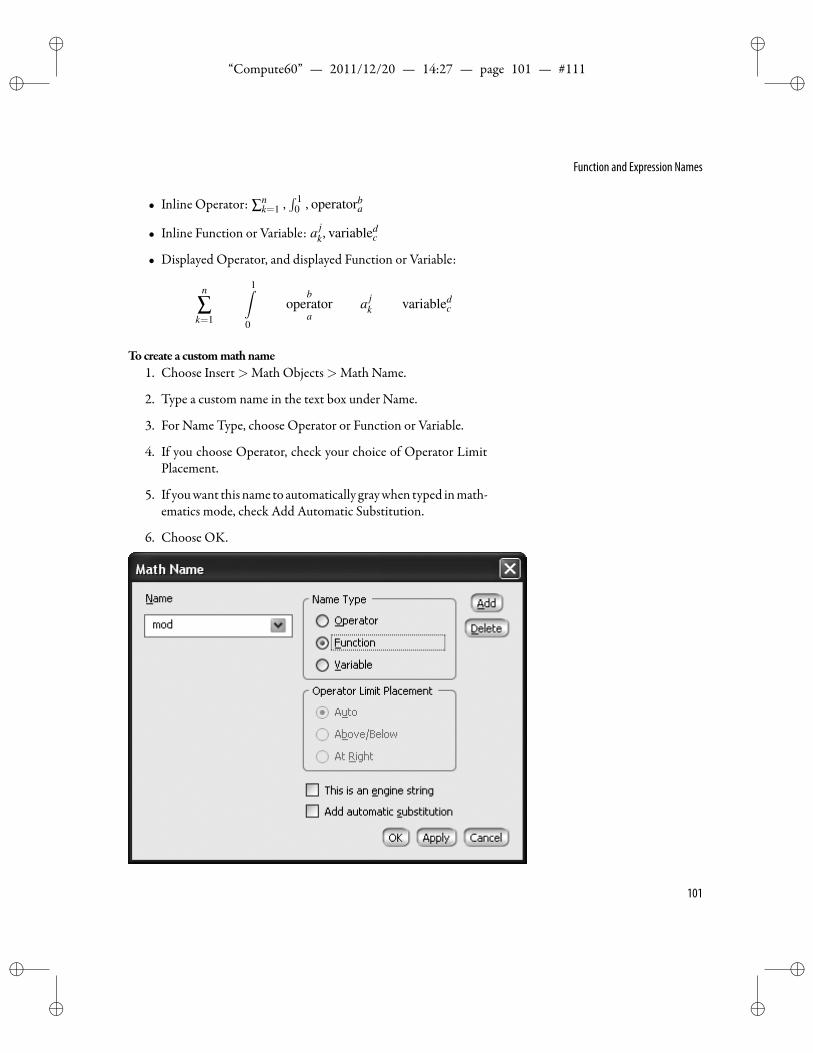
ii
“Compute60” — 2011/12/20 — 14:27 — page 101 — #111 ii
ii
ii
Function and Expression Names
• Inline Operator: ∑nk=1 ,
∫ 10 , operatorb
a
• Inline Function or Variable: a jk, variabled
c
• Displayed Operator, and displayed Function or Variable:
n
∑k=1
1∫0
boperator
aa j
k variabledc
Tocreate a custommathname1. Choose Insert>Math Objects>Math Name.
2. Type a custom name in the text box under Name.
3. For Name Type, choose Operator or Function or Variable.
4. If you choose Operator, check your choice of Operator LimitPlacement.
5. If youwant this name to automatically graywhen typed inmath-ematics mode, check Add Automatic Substitution.
6. Choose OK.
101
ii
“Compute60” — 2011/12/20 — 14:27 — page 102 — #112 ii
ii
ii
Chapter 5 | Function De nitions
e gray custom name appears on the screen at the insert point.You can use this name to de ne a function or expression. You can copyand paste or click and drag this grayed name on the screen, or you canrecreate it with the Math Name dialog.Tocreate a decorated character
1. Type a character.
2. Select the character and choose Edit> Properties>CharacterProperties.
3. Click the desired accent and choose OK.
Compute> De nitions> New De nitiona = 3a = x2 + y2
Compute> De nitions> Evaluateaa = 3x2 +3y2
Automatic SubstitutionWhen automatic substitution is enabled, function names such as
sin, arcsin, and gcd automatically turn graywhen typed inmathemat-ics. For a list of these names, choose Tools>Auto Substitution.Toenable auto substitution inmathematics
• Choose Tools>Auto Substitution and under Enable auto sub-stitution , check In Math.
If automatic substitution is not enabled in mathematics, no func-tion names automatically gray and such names must be selected fromthe Auto Substitution list or created by choosing Insert > Math Ob-jects>Math Name.
You can evoke the automatic substitution behavior with new cus-tom names using the Automatic Substitution dialog.Tomake a customname automatically gray
1. Choose Tools>Auto Substitution.
2. Type the keystrokes that you wish to use. ( is may be an ab-breviated form of the custom name.)
3. Click the Substitution box to place the cursor there and, leavingAuto Substitution open, choose Insert>MathObjects>MathName.
102
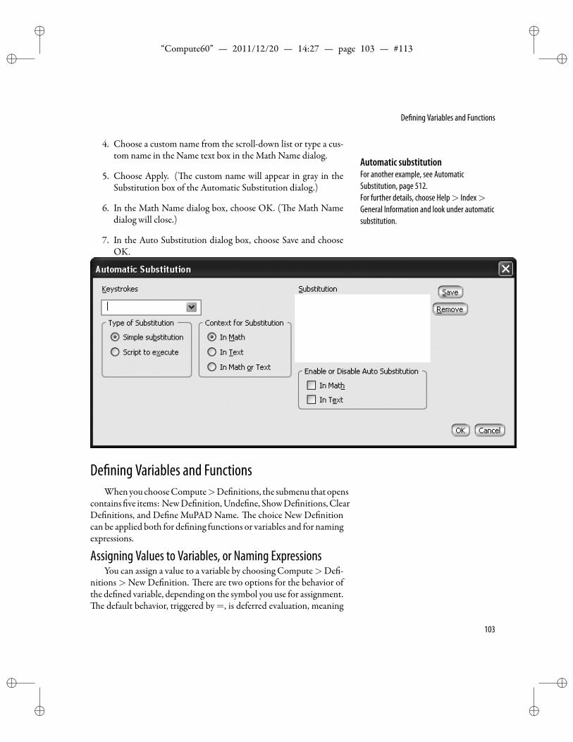
ii
“Compute60” — 2011/12/20 — 14:27 — page 103 — #113 ii
ii
ii
De ning Variables and Functions
4. Choose a custom name from the scroll-down list or type a cus-tom name in the Name text box in the Math Name dialog.
Automatic substitutionFor another example, see AutomaticSubstitution, page 512.For further details, choose Help> Index>General Information and look under automaticsubstitution.
5. Choose Apply. ( e custom name will appear in gray in theSubstitution box of the Automatic Substitution dialog.)
6. In the Math Name dialog box, choose OK. ( e Math Namedialog will close.)
7. In the Auto Substitution dialog box, choose Save and chooseOK.
De ning Variables and FunctionsWhenyouchooseCompute>De nitions, the submenu that opens
contains ve items: NewDe nition,Unde ne, ShowDe nitions,ClearDe nitions, and De ne MuPAD Name. e choice New De nitioncan be applied both for de ning functions or variables and for namingexpressions.
Assigning Values to Variables, or Naming ExpressionsYou can assign a value to a variable by choosing Compute>De -
nitions>New De nition. ere are two options for the behavior ofthe de ned variable, depending on the symbol you use for assignment.
e default behavior, triggered by =, is deferred evaluation, meaning
103
ii
“Compute60” — 2011/12/20 — 14:27 — page 104 — #114 ii
ii
ii
Chapter 5 | Function De nitions
the de nition is stored exactly as you make it. e alternate behavior,triggered by :=, is full evaluation,meaning the de nition that is storedtakes into account earlier de nitions in force that might affect it. SeeFull Evaluation andAssignment page 105 for a discussion of the latteroption.
Deferred Evaluation• Use an equal sign= to make an assignment for deferred evalu-
ation.
Toassign the value 25 to z for deferred evaluation1. Type z = 25 in mathematics.
2. Leave the insert point in the equation.
3. Choose Compute>De nitions>New De nition.
erea er, until you exit the document or unde ne the variable,the system recognizes z as 25. For example, evaluating the expression“3+ z” returns “= 28.”
Another way to describe this operation is to say that an expressionsuch as x2 + sinx can be given a name. Type y = x2 + sinx, leavethe insert point anywhere in the expression, and choose Compute >De nitions>New De nition. Note
These variables or names are single characters.See page 100 for information onmulticharacter names.
Compute> De nitions> New De nitiony = x2 + sinx
Now, whenever you evaluate an expression containing y, every oc-currence of y is replaced by the expression x2 + sinx.
Compute> Evaluatey2 + x3 =
(sinx+ x2
)2+ x3
Functions and expressionsThe symbol p represents the expressionx3−5x+1. It is not a function, so, forexample, p(2) is not the polynomialevaluated at 2, but rather isp(2) = 2p = 2x3−10x+2, theproduct of p and 2.
e value assigned can be anymathematical expression. For exam-ple, you could de ne a variable to be
• A number: a = 245
• A polynomial: p = x3−5x+1
• A quotient of polynomials: b =x2−1x2 +1
• A matrix: z =[
a bc d
]104
ii
“Compute60” — 2011/12/20 — 14:27 — page 105 — #115 ii
ii
ii
De ning Variables and Functions
• An integral: d =∫
x2 sinxdx
You will nd this feature useful for a variety of purposes.
Compound De nitions with Deferred EvaluationIt is legitimate to de ne expressions in terms of other de ned ex-
pressions.Tomake compoundde nitionswith deferred evaluation
• Assign a value to a variable and then use that variable name inthe de nition of a second variable.
Compute> De nitions> New De nitionr = 3p− cq s = nr+q
Compute> Evaluates = q+n(3p− cq)
NoteRede ning r will change the evaluation of s.Full Evaluation and Assignment
With full evaluation, variables previously de ned are evaluated be-fore the de nition is stored. us, de nitions of expressions can de-pend on the order in which they are made.Tomake an assignment symbol for full evaluation
• Type a colon followed by an equals sign :=.
Toassign the value25a to z for full evaluation1. Type z := 25a in mathematics.
2. Leave the insert point in the equation.
3. Choose Compute>De nitions>New De nition.
erea er, until you exit the document or unde ne the variable z,if a has not been previously de ned, the system recognizes z as 25a. Ifa has previously been de ned to be x+ y, then the system recognizesz as 25(x+ y) .
Try the following examples that contrast the two types of assign-ments. A er making the de nitions, choose Compute>De nitions> Show De nitions for each case.
1. Make the assignments a = 1, x := a, y = a, and a = 2 (in thatorder), and evaluate x and y. e result should be x = 1, y = 2.
105
ii
“Compute60” — 2011/12/20 — 14:27 — page 106 — #116 ii
ii
ii
Chapter 5 | Function De nitions
2. Make the assignments a = b, x := a2, y = a2, and a = 6 (inthat order), and evaluate x and y. e result should be x = b2,y = 36.
3. De ne r = 3p−cq and then s= nr+q and t := nr+q. Evalu-ating s and t will then give s= q+n(3p− cq), t = q+n(3p− cq).Now de ne r = x + y. Evaluating s and t will now give s =q+n(x+ y), t = q+n(3p− cq).
Functions of One VariableBy using function notation, you can use the same general proce-
dure to de ne a function as was described for de ning a variable.
Tode ne the function f whose value at x isax2 +bx+ c
1. Type the equation f (x) = ax2 +bx+ c.
2. Place the insert point in the equation.
3. Choose Compute>De nitions>New De nition.
A er following this procedure, the symbol f represents the de-ned function and it behaves like a function.
Compute> De nitions> New De nitionf (x) = ax2 +bx+ c
TipAfter de ning a function, you can make a tableof values for selected points in the domain ofthe function. See Chapter 7 “Calculus,” page205 for examples.
Compute> Evaluatef (t) = at2 +bt + c f ′ (t) = b+2atf (x+h) = c+b(h+ x)+a(h+ x)2
Compound De nitionse algebra of functions includes objects such as f + g, f − g,
f g, f g, and f −1. For the value of f + g at x, write f (x)+ g(x);for the value of the composition of two de ned functions f and g,write f (g(x)) or ( f g)(x); and for the value of the product of twode ned functions, write f (x)g(x). You can obtain the inverse (or in-verse relation) for some functions f (x) by choosingCompute> Solve> Exact with the equation f (y) = x and specifying y as the Variableto Solve for.
106
ii
“Compute60” — 2011/12/20 — 14:27 — page 107 — #117 ii
ii
ii
De ning Variables and Functions
Tomake compoundde nitions1. De ne functions by choosing Compute>De nitions>New
De nition, either as generic functions or in terms of an expres-sion.
2. Combine these functions in standard ways and de ne the re-sulting functions by choosing Compute > De nitions > NewDe nition.
De ne g(x) and h(x). en the following equations are examplesof legitimate de nitions:
• f (x) = 2g(x)
• f (x) = g(x)+h(x)
• f (x) = g(x)h(x)
• f (x) = g(h(x)) or f (x) = (gh)(x)
• f (x) = g(x)/h(x) or f (x) =g(x)h(x)
Once you have de ned both g(x) and f (x) = 2g(x), then chang-ing the de nition of g(x) will change the value of f (x).
Subscripts as Function ArgumentsA subscript can be interpreted either as part of the name of a func-
tion or variable, or as a function argument.Tode ne a subscript as a function argument
1. Place the insert point in an equation such as ai = 3i with asymbolic subscript and choose Compute>De nitions>NewDe nition.
2. In the Interpret Subscript dialog that opens, check A functionargument.
Observe the different behavior in the following examples.
Compute> De nitions> New De nitionai = 3i (subscript a function argument)bi = 3i (subscript a part of the name)
107
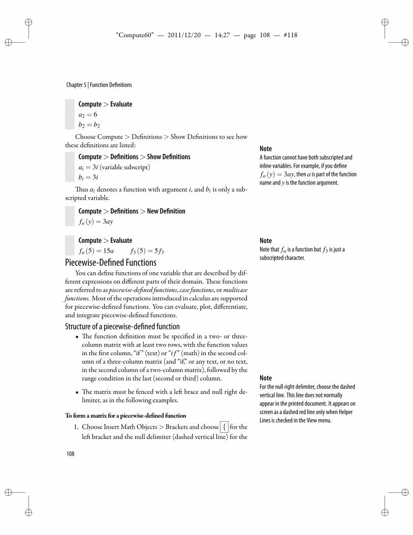
ii
“Compute60” — 2011/12/20 — 14:27 — page 108 — #118 ii
ii
ii
Chapter 5 | Function De nitions
Compute> Evaluatea2 = 6b2 = b2
Choose Compute > De nitions > Show De nitions to see howthese de nitions are listed: Note
A function cannot have both subscripted andinline variables. For example, if you de nefa (y) = 3ay, then a is part of the functionname and y is the function argument.
Compute> De nitions> Show De nitionsai = 3i (variable subscript)bi = 3i
us ai denotes a function with argument i, and bi is only a sub-scripted variable.
Compute> De nitions> New De nitionfa (y) = 3ay
Compute> Evaluatefa (5) = 15a f3 (5) = 5 f3
NoteNote that fa is a function but f3 is just asubscripted character.Piecewise-De ned Functions
You can de ne functions of one variable that are described by dif-ferent expressions on different parts of their domain. ese functionsare referred to as piecewise-de ned functions, case functions, ormulticasefunctions. Most of the operations introduced in calculus are supportedfor piecewise-de ned functions. You can evaluate, plot, differentiate,and integrate piecewise-de ned functions.
Structure of a piecewise-de ned function• e function de nition must be speci ed in a two- or three-
column matrix with at least two rows, with the function valuesin the rst column, “if ” (text) or “i f ” (math) in the second col-umn of a three-column matrix (and “if,” or any text, or no text,in the second column of a two-columnmatrix), followed by therange condition in the last (second or third) column. Note
For the null right delimiter, choose the dashedvertical line. This line does not normallyappear in the printed document. It appears onscreen as a dashed red line only when HelperLines is checked in the Viewmenu.
• e matrix must be fenced with a le brace and null right de-limiter, as in the following examples.
To formamatrix for a piecewise-de ned function
1. Choose Insert Math Objects> Brackets and choose for thele bracket and the null delimiter (dashed vertical line) for the
108
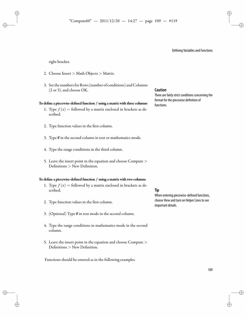
ii
“Compute60” — 2011/12/20 — 14:27 — page 109 — #119 ii
ii
ii
De ning Variables and Functions
right bracket.
2. Choose Insert>Math Objects>Matrix.
3. Set thenumbers forRows (numberof conditions) andColumns(2 or 3), and choose OK. Caution
There are fairly strict conditions concerning theformat for the piecewise de nition offunctions.Tode ne apiecewise-de ned function f using amatrixwith three columns
1. Type f (x) = followed by a matrix enclosed in brackets as de-scribed.
2. Type function values in the rst column.
3. Type if in the second column in text or mathematics mode.
4. Type the range conditions in the third column.
5. Leave the insert point in the equation and choose Compute>De nitions>New De nition.
Tode ne a piecewise-de ned function f using amatrixwith two columns1. Type f (x) = followed by a matrix enclosed in brackets as de-
scribed. TipWhen entering piecewise-de ned functions,choose View and turn on Helper Lines to seeimportant details.
2. Type function values in the rst column.
3. (Optional) Type if in text mode in the second column.
4. Type the range conditions in mathematics mode in the secondcolumn.
5. Leave the insert point in the equation and choose Compute>De nitions>New De nition.
Functions should be entered as in the following examples.
109
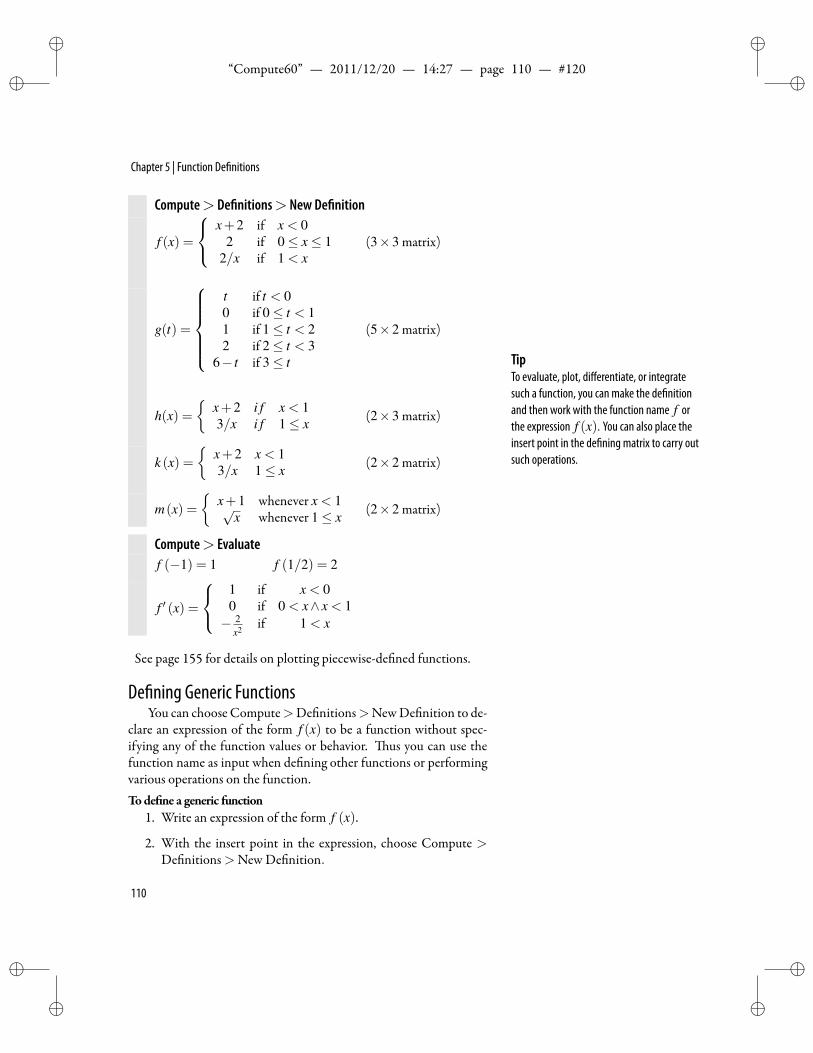
ii
“Compute60” — 2011/12/20 — 14:27 — page 110 — #120 ii
ii
ii
Chapter 5 | Function De nitions
Compute> De nitions> New De nition
f (x) =
x+2 if x < 02 if 0≤ x≤ 1
2/x if 1 < x(3×3 matrix)
g(t) =
t if t < 00 if 0≤ t < 11 if 1≤ t < 22 if 2≤ t < 3
6− t if 3≤ t
(5×2 matrix)
h(x) =
x+2 i f x < 13/x i f 1≤ x (2×3 matrix)
k (x) =
x+2 x < 13/x 1≤ x (2×2 matrix)
m(x) =
x+1 whenever x < 1√x whenever 1≤ x (2×2 matrix)
TipTo evaluate, plot, differentiate, or integratesuch a function, you can make the de nitionand then work with the function name f orthe expression f (x). You can also place theinsert point in the de ning matrix to carry outsuch operations.
Compute> Evaluatef (−1) = 1 f (1/2) = 2
f ′ (x) =
1 if x < 00 if 0 < x∧ x < 1− 2
x2 if 1 < x
See page 155 for details on plotting piecewise-de ned functions.
De ning Generic FunctionsYou can choose Compute>De nitions>NewDe nition to de-
clare an expression of the form f (x) to be a function without spec-ifying any of the function values or behavior. us you can use thefunction name as input when de ning other functions or performingvarious operations on the function.Tode ne a generic function
1. Write an expression of the form f (x).
2. With the insert point in the expression, choose Compute >De nitions>New De nition.
110
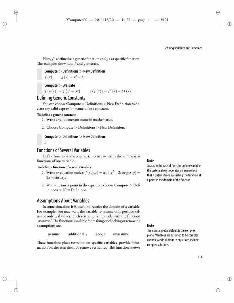
ii
“Compute60” — 2011/12/20 — 14:27 — page 111 — #121 ii
ii
ii
De ning Variables and Functions
Here, f is de ned as a generic function andg as a speci c function.e examples show how f and g interact.
Compute> De nitions> New De nitionf (x) g(x) = x2−3x
Compute> Evaluatef (g(x)) = f
(x2−3x
)g( f (x)) = f 2 (x)−3 f (x)
De ning Generic ConstantsYou can choose Compute>De nitions>NewDe nition to de-
clare any valid expression name to be a constant.Tode ne a generic constant
1. Write a valid constant name in mathematics.
2. Choose Compute>De nitions>New De nition.
Compute> De nitions> New De nitiona
Functions of Several VariablesDe ne functions of several variables in essentially the same way as
functions of one variable. NoteJust as in the case of functions of one variable,the system always operates on expressionsthat it obtains from evaluating the function ata point in the domain of the function.
Tode ne a functionof several variables1. Write an equation such as f (x,y,z) = ax+y2+2z or g(x,y) =
2x+ sin3xy.
2. With the insert point in the equation, choose Compute>Def-initions>New De nition.
Assumptions About VariablesIn some situations it is useful to restrict the domain of a variable.
For example, you may want the variable to assume only positive val-ues or only real values. Such restrictions are made with the function“assume.” e functions available formaking or checking or removingassumptions are Note
The normal global default is the complexplane. Variables are assumed to be complexvariables and solutions to equations includecomplex solutions.
assume additionally about unassume
ese functions place restraints on speci c variables, provide infor-mation on the restraints, or remove restraints. e function assume
111
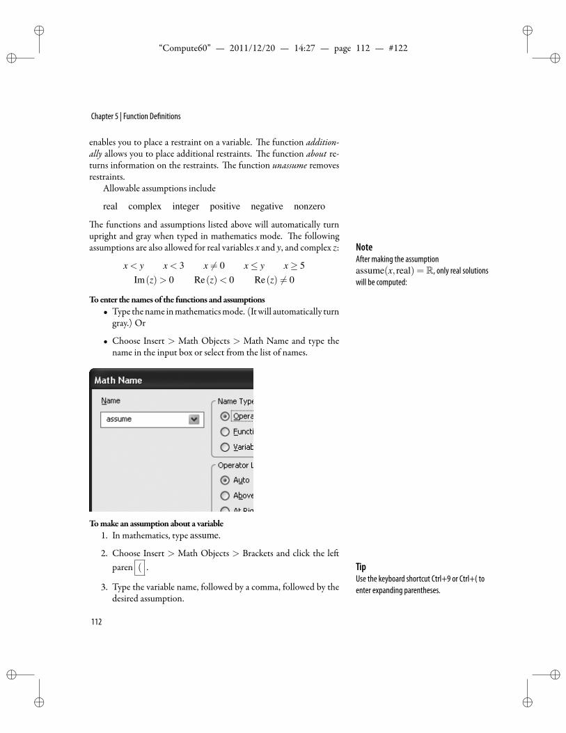
ii
“Compute60” — 2011/12/20 — 14:27 — page 112 — #122 ii
ii
ii
Chapter 5 | Function De nitions
enables you to place a restraint on a variable. e function addition-ally allows you to place additional restraints. e function about re-turns information on the restraints. e function unassume removesrestraints.
Allowable assumptions include
real complex integer positive negative nonzero
e functions and assumptions listed above will automatically turnupright and gray when typed in mathematics mode. e followingassumptions are also allowed for real variables x and y, and complex z: Note
After making the assumptionassume(x, real) = R, only real solutionswill be computed:
x < y x < 3 x = 0 x≤ y x≥ 5Im(z)> 0 Re(z)< 0 Re(z) = 0
Toenter the names of the functions and assumptions• Type thename inmathematicsmode. (Itwill automatically turn
gray.) Or
• Choose Insert > Math Objects > Math Name and type thename in the input box or select from the list of names.
Tomake an assumption about a variable1. In mathematics, type assume.
2. Choose Insert > Math Objects > Brackets and click the leparen ( . Tip
Use the keyboard shortcut Ctrl+9 or Ctrl+( toenter expanding parentheses.3. Type the variable name, followed by a comma, followed by the
desired assumption.
112
ii
“Compute60” — 2011/12/20 — 14:27 — page 113 — #123 ii
ii
ii
De ning Variables and Functions
4. Choose Compute> Evaluate.
Compute> Evaluateassume(x, real) = R
Compute> Solve> Exactx2 =−1, No solution found.x2 = 1, Solution: −1,1
Toplace an additional assumptionon a variablewithout removingpreviousassumptions
1. In mathematics, type additionally. NoteAn additional assumption placed on a variableusing assumewould negate any previousassumption.
2. Choose Insert>Math Objects> Brackets and click ( .
3. Inside the parentheses, type the variable name, followed by acomma, followed by the desired assumption.
4. Choose Compute> Evaluate.
Evaluation of the expressions assume(n,positive) andadditionally(n, integer), followed by evaluation of the expressionabout(n), produces the following output:
Compute> Evaluateassume(n,positive) = (0,∞)
additionally(n, integer) = Z∩ (0,∞)
about(n) = Z∩ (0,∞)
To restrict the domain of a real variable x1. Make the assumption that x is real.
2. Use the function additionally for additional restraints on x.
Compute> Evaluateassume(x, real) = Radditionally(x < 10) = (−∞,10)additionally(x≥−10) = [−10,10)
Compute> Solve> Exactsinx = 0, Solution: −3π,−2π,−π,0,π,2π,3π
Toassume the variablen is positive• Place the insert point in the expression assume(n,positive),
and choose Compute> Evaluate.
113
ii
“Compute60” — 2011/12/20 — 14:27 — page 114 — #124 ii
ii
ii
Chapter 5 | Function De nitions
Toclear the assumptions about a variable• Select the variable and choose Compute > De nitions > Un-
de ne, or
Evaluate unassume(name of variable).
Compute> De nitions> Unde nen
orCompute> Evaluateunassume(n)
A er either procedure, you can check the status of the variable nwith the function about.
Compute> Evaluateabout(n) = n
is response indicates there are no assumptions on the variable n.NoteIf you assume that n is an integer, the systemwill recognize thatn2 is a positive integer.
Compute> Evaluateassume(n, integer) = Zabout
(n2)= Z∩ [0,∞)∣∣n2 +1
∣∣= n2 +1
In the default mode, both real and complex solutions will be com-puted:
Compute> Solve> Exactx4 = 1, Solution: −i,−1, i,1
Assuming x is positive leads to only real positive solutions:
Compute> Evaluateassume(x,positive) = (0,∞)
Compute> Solve> Exactx2 = 1, Solution: 1x4 = 1, Solution: 1
To restrict the domain of a complex variable z• Make assumptions on the real and imaginary parts of z.
Compute> Evaluateassume(Re(z)> 0) = (0,∞)+ iRadditionally(Im(z)< 0) = (0,∞)+ i(−∞,0)
114
ii
“Compute60” — 2011/12/20 — 14:27 — page 115 — #125 ii
ii
ii
Handling De nitions
Handling De nitionsA er making de nitions of functions or expressions, you need to
know techniques for keeping track of them. e choices on the Def-initions submenu are New De nition, Unde ne, Show De nitions,Clear De nitions, and De ne MuPAD Name. e choice Show Def-initions also appears on the Math toolbar as .
Showing De nitionsToview the complete list of currently de ned variables and functions
• Choose Compute>De nitions> Show De nitions.
A window opens showing the active de nitions. e de ned vari-ables and functions are listed in the order inwhich the de nitionsweremade.
Removing and Changing De nitionsTo remove all de nitions
• Choose Compute>De nitions>Clear De nitions.
To remove a single de nition• Select the de ning equation or select the name of the de ned
expression or function and choose Compute > De nitions >Unde ne.
Tochange a de nition• Make anewde nitionusing the same functionor variable name.
You can select the equation or name by placing the insert pointwithin or on the right side of the equation or name that you wish toremove, or you can select the entire equation, expression, or functionnamewith themouse. You can nd the equation or name in the ShowDe nitions window if you do not have a copy readily at hand. Copyan expression from this window into your document, then select theexpression and choose Unde ne.
Formulase Formula dialog provides a way to enter an expression and a
Compute operation. What appears on the screen is the result of the
115
ii
“Compute60” — 2011/12/20 — 14:27 — page 116 — #126 ii
ii
ii
Chapter 5 | Function De nitions
operation and depends upon active de nitions of variables that ap-pear in the formula. Formulas remain active in your document—thatis, changing de nitions of relevant variables changes the data on thescreen.To insert a formula
1. Choose Insert>Math Objects> Formula.
2. Type an expression in the input box. NoteWith Helper Lines on, a Formula appears witha colored background. The default is yellow.3. In theOperation area, select the operation youwant to perform
on the expression. (Click the arrow at the right of the box for alist of available operations.)
4. Choose OK.
e results of the operation will be displayed in your documentwindow.To recognize a formula on the screen fromabackground color
• Choose View and turn on Helper Lines.
Tochange the formula background color1. Choose Tag>Appearance.
2. Check Modify Style Defaults.
3. Under Tag Properties, choose Special Objects.
4. Under Special Objects choose Formula and click Modify.
5. Select background color and choose OK.
6. Choose Save if you wish to make a permanent change in thescreen style, and choose OK.
Example Choose Insert > Math Objects > Formula. In the For-mula box, type a, and under Operations choose evaluate. ChooseOK. e a will appear on your screen at the position of the insertpoint. Now, at any point in your document, de ne a = sinx. evariable a will be replaced by the expression sinx wherever a appearsin the document. Make another de nition for a. e variable a willagain be replaced by the new de nition everywhere a appears in thedocument.
116
ii
“Compute60” — 2011/12/20 — 14:27 — page 117 — #127 ii
ii
ii
Formulas
Example Insert a 2× 2 matrix. With the insert point in the rstinput box, choose Insert>Math Objects> Formula. In the Formulabox, type a. UnderOperations, choose Evaluate. ChooseOK. Repeatfor each matrix entry, typing b, a+ 2b, and (a−b)2, in turn, in theformula box to get the matrix[
a ba+2b (a−b)2
]Now de ne a = sinx and b = cosx. e matrix will be replaced bythe matrix [
sinx cosxsinx+2cosx (sinx− cosx)2
]De ne a = lnx and b = ex. e matrix will then be replaced by thematrix [
lnx ex
lnx+2ex (lnx− ex)2
]
Example Insert a table with 2 columns and 5 rows. Insert formulasx, y, z, and x+ y+ z in the column on the right.
Date Income1/31/96 x2/28/96 y3/31/96 z
Total x+ y+ z
De ne x = 20.56, y = 18.92, z = 23.45 to get the table
Date Income1/31/96 20.562/28/96 18.923/31/96 23.45
Total 62.93
Formulas are useful for writingmultiple choice examinations withvariations enext example outlines away for constructing themman-ually.
e questions in an examination depend on de nitions that aremade globally for each document—they’re not local to each question
117
ii
“Compute60” — 2011/12/20 — 14:27 — page 118 — #128 ii
ii
ii
Chapter 5 | Function De nitions
or variant. is means that you o en should use aMathName insteadof a single character name for variables. A sample question is shown inthe next example. e variables a1 and b1 shown in the next exampleare math names.Toenter aMathName in aFormulawindow
1. Choose Insert>Math Objects> Formula. TipUsing a Math Name (see page 100) instead of asingle character name for each variable avoidscon icts with other de nitions in thedocument.
2. With the insert point in the Formula window, choose Insert>Math Objects>Math Name.
3. Type or select a Math Name and choose OK.
Example You can create an examination with variations by makingdifferent de nitions for the variables such as the a1 and b1 shown inthe following question. Turn on Helper Lines in your document andlook for background color to check that all appropriate entries are for-mulas.
1. For which values of the variable x is a1x−b1 < 0?
a. x < b1/a1
b. x > b1/a1
c. x > b1
d. x < b1
e. None of these
De ne a1= 2 andb1= 5 by placing the insert point in each equa-tion and choosing Compute > De nitions > New De nition. Onyour screen you should see
1. For which values of the variable x is 2x−5 < 0?
a. x < 5/2
b. x > 5/2
c. x > 5
d. x < 5
e. None of these
A erprinting aquiz,makedifferentde nitions for all the variablessuch as a1 and b1 to obtain variations of the quiz.
118
ii
“Compute60” — 2011/12/20 — 14:27 — page 119 — #129 ii
ii
ii
External Functions
External FunctionsYou can access functions available to the computation engine that
do not appear as menu items. ese can be either functions from oneof the libraries of the computation engine or user-de ned functions.
Functionsde nedwith theCompute>De nitions>De neMu-PADNamedialog, with theirMuPADname correspondences, appearin the Show De nitions window but they may not be removed byClear De nitions.
To remove a de nedMuPADfunction• Select the function name and choose Compute > De nitions>Unde ne.
Accessing Functions in MuPAD Librariese following example de nes the function divisors, which com-
putes the divisors of a positive integer.
Toaccess theMuPADfunctiondivisors and toname itD1. Choose Compute>De nitions>De ne MuPAD Name. Caution
Multiple notations for vectors are possible inScienti c WorkPlace and Scienti c Notebook,including row or columnmatrices, andn-tuples enclosed by either parentheses orsquare brackets. However, to work with afunction de ned from the MuPAD libraries, youmust use MuPAD syntax for the functionarguments.
2. Respond to the dialog box as follows:
• MuPAD Name: numlib::divisors(x)
• Scienti c Notebook (WorkPlace) Name: D(x)
• Check “ at is built in to MuPAD” or “is automaticallyloaded”
3. Choose OK.
Compute> EvaluateD(24) = [1,2,3,4,6,8,12,24]
An extensive MuPAD library is included with your system. Hereis a short list of functions from the many examples that are availableusing the De ne MuPAD Name dialog.
119
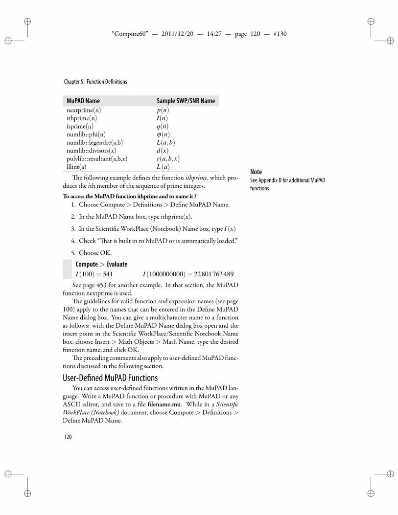
ii
“Compute60” — 2011/12/20 — 14:27 — page 120 — #130 ii
ii
ii
Chapter 5 | Function De nitions
MuPAD Name Sample SWP/SNB Namenextprime(n) p(n)ithprime(n) I(n)isprime(n) q(n)numlib::phi(n) φ(n)numlib::legendre(a,b) L(a,b)numlib::divisors(x) d(x)polylib::resultant(a,b,x) r(a,b,x)lllint(a) L(a)
NoteSee Appendix D for additional MuPADfunctions.
e following example de nes the function ithprime, which pro-duces the ith member of the sequence of prime integers.Toaccess theMuPADfunction ithprime and toname it I
1. Choose Compute>De nitions>De ne MuPAD Name.
2. In the MuPAD Name box, type ithprime(x).
3. In the Scienti c WorkPlace (Notebook) Name box, type I (x)
4. Check “ at is built in to MuPAD or is automatically loaded.”
5. Choose OK.
Compute> EvaluateI (100) = 541 I (1000000000) = 22801763489
See page 453 for another example. In that section, the MuPADfunction nextprime is used.
e guidelines for valid function and expression names (see page100) apply to the names that can be entered in the De ne MuPADName dialog box. You can give a multicharacter name to a functionas follows: with the De ne MuPAD Name dialog box open and theinsert point in the Scienti c WorkPlace/Scienti c Notebook Namebox, choose Insert > Math Objects > Math Name, type the desiredfunction name, and click OK.
e preceding comments also apply to user-de nedMuPADfunc-tions discussed in the following section.
User-De ned MuPAD FunctionsYou can access user-de ned functions written in the MuPAD lan-
guage. Write a MuPAD function or procedure with MuPAD or anyASCII editor, and save to a le lename.mu. While in a Scienti cWorkPlace (Notebook) document, choose Compute > De nitions >De ne MuPAD Name.
120
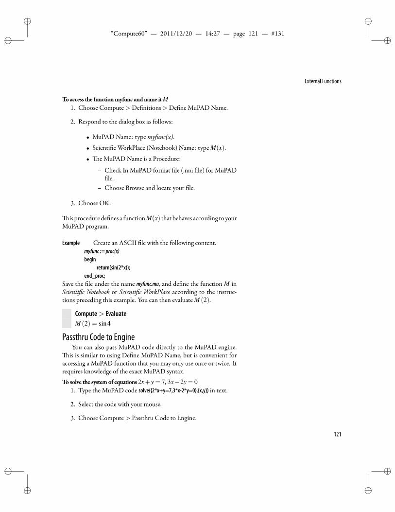
ii
“Compute60” — 2011/12/20 — 14:27 — page 121 — #131 ii
ii
ii
External Functions
Toaccess the functionmyfunc andname itM1. Choose Compute>De nitions>De ne MuPAD Name.
2. Respond to the dialog box as follows:
• MuPAD Name: typemyfunc(x).• Scienti c WorkPlace (Notebook) Name: type M(x).
• e MuPAD Name is a Procedure:
– Check In MuPAD format le (.mu le) for MuPADle.
– Choose Browse and locate your le.
3. Choose OK.
is procedure de nes a functionM(x) that behaves according to yourMuPAD program.
Example Create an ASCII le with the following content.myfunc := proc(x)begin
return(sin(2*x));end_proc;
Save the le under the name myfunc.mu, and de ne the function M inScienti c Notebook or Scienti c WorkPlace according to the instruc-tions preceding this example. You can then evaluate M (2).
Compute> EvaluateM (2) = sin4
Passthru Code to EngineYou can also pass MuPAD code directly to the MuPAD engine.
is is similar to using De ne MuPAD Name, but is convenient foraccessing a MuPAD function that you may only use once or twice. Itrequires knowledge of the exact MuPAD syntax.To solve the systemof equations2x+ y = 7,3x−2y = 0
1. Type the MuPAD code solve(2*x+y=7,3*x-2*y=0,x,y) in text.
2. Select the code with your mouse.
3. Choose Compute> Passthru Code to Engine.
121
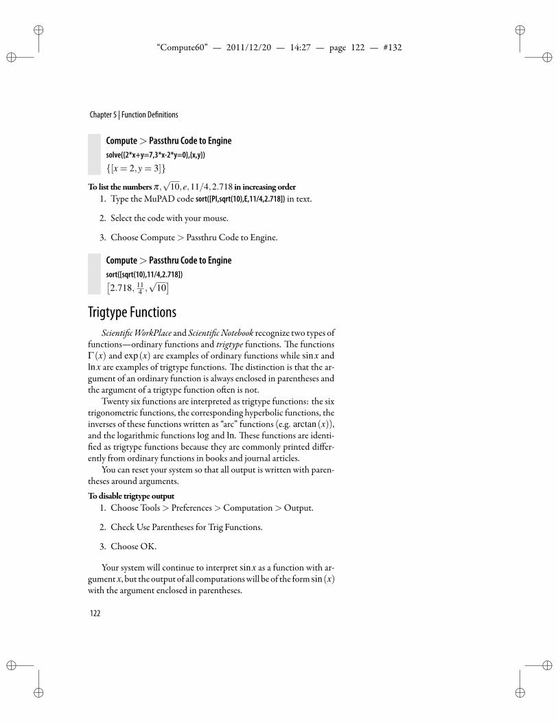
ii
“Compute60” — 2011/12/20 — 14:27 — page 122 — #132 ii
ii
ii
Chapter 5 | Function De nitions
Compute> Passthru Code to Enginesolve(2*x+y=7,3*x-2*y=0,x,y)
[x = 2,y = 3]
To list the numbersπ,√
10,e,11/4,2.718 in increasing order1. Type the MuPAD code sort([PI,sqrt(10),E,11/4,2.718]) in text.
2. Select the code with your mouse.
3. Choose Compute> Passthru Code to Engine.
Compute> Passthru Code to Enginesort([sqrt(10),11/4,2.718])[2.718, 11
4 ,√
10]
Trigtype FunctionsScienti cWorkPlace and Scienti cNotebook recognize two types of
functions—ordinary functions and trigtype functions. e functionsΓ(x) and exp(x) are examples of ordinary functions while sinx andlnx are examples of trigtype functions. e distinction is that the ar-gument of an ordinary function is always enclosed in parentheses andthe argument of a trigtype function o en is not.
Twenty six functions are interpreted as trigtype functions: the sixtrigonometric functions, the corresponding hyperbolic functions, theinverses of these functions written as “arc” functions (e.g. arctan(x)),and the logarithmic functions log and ln. ese functions are identi-ed as trigtype functions because they are commonly printed differ-
ently from ordinary functions in books and journal articles.You can reset your system so that all output is written with paren-
theses around arguments.Todisable trigtype output
1. Choose Tools> Preferences>Computation>Output.
2. Check Use Parentheses for Trig Functions.
3. Choose OK.
Your system will continue to interpret sinx as a function with ar-gumentx, but theoutput of all computationswill be of the form sin(x)with the argument enclosed in parentheses.
122
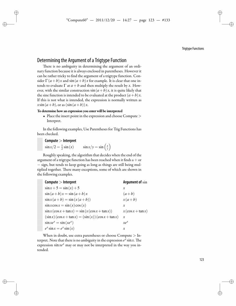
ii
“Compute60” — 2011/12/20 — 14:27 — page 123 — #133 ii
ii
ii
Trigtype Functions
Determining the Argument of a Trigtype Functionere is no ambiguity in determining the argument of an ordi-
nary function because it is always enclosed in parentheses. However itcan be rather tricky to nd the argument of a trigtype function. Con-sider Γ(a+b)x and sin(a+b)x for example. It is clear that one in-tends to evaluate Γ at a+ b and then multiply the result by x. How-ever, with the similar construction sin(a+b)x, it is quite likely thatthe sine function is intended to be evaluated at the product (a+b)x.If this is not what is intended, the expression is normally written asxsin(a+b), or as (sin(a+b))x.Todetermine howan expression you enterwill be interpreted
• Place the insert point in the expression and choose Compute>Interpret.
In the following examples, Use Parentheses for Trig Functions hasbeen checked.
Compute> Interpretsinx/2 = 1
2 sin(x) sinx/y = sin(
xy
)Roughly speaking, the algorithm that decides when the end of the
argument of a trigtype function has been reached when it nds a+ or− sign, but tends to keep going as long as things are still being mul-tiplied together. ere many exceptions, some of which are shown inthe following examples.
Compute> Interpret Argument of sinsinx+5 = sin(x)+5 xsin(a+b)x = sin(a+b)x (a+b)sinx(a+b) = sin(x(a+b)) x(a+b)sinxcosx = sin(x)cos(x) xsinx(cosx+ tanx) = sin(x(cosx+ tanx)) x(cosx+ tanx)(sinx)(cosx+ tanx) = (sin(x))(cosx+ tanx) xsinxex = sin(xex) xex
ex sinx = ex sin(x) x
When in doubt, use extra parentheses or choose Compute > In-terpret. Note that there is no ambiguity in the expression ex sinx. eexpression sinxex may or may not be interpreted in the way you in-tended.
123
ii
“Compute60” — 2011/12/20 — 14:27 — page 124 — #134 ii
ii
ii
Chapter 5 | Function De nitions
Exercises1. De ne a = 5. De ne b = a2. Evaluate b. Now de ne a =
√2.
Guess the value of b and check your answer by evaluation.
2. De ne f (x) = x2 +3x+2. Evaluate
f (x+h)− f (x)h
and simplify the result. Do computing in place to show inter-mediate steps in the simpli cation.
3. De ne f (x) = x2−1, g(x) = 3x+2, h(x) = x2 +3x. Com-pute f +g, ( f +g)h, and f h+gh. Compute ( f +g)h, andf h+gh.
4. Rede ne the function f (x)=max(x2−1,7− x2
)as a piecewise-
de ned function.
5. Experimentwith theEuler phi functionφ(n), which counts thenumber of positive integers k≤ n such that gcd(k,n) = 1. Testthe statement “If gcd(n,m) = 1 then φ(nm) = φ(n)φ(m)”for several speci c choices of n and m. Choose Compute >De nitions > De ne MuPAD Name to open a dialog. Typenumlib::phi(n) as theMuPADName, φ(n) as the Scienti cWork-Place/NotebookName, check at is Built IntoMuPADor au-tomatically loaded, and click OK.
6. Choose Compute > De nitions > De ne MuPAD Name toopen a dialog. De ne d(n) by typing numlib::divisors(n) astheMuPADname, d(n) as the Scienti cWorkPlace/NotebookName, check at isBuilt IntoMuPADor automatically loaded,and click OK. Explain what the function d(n) produces. ( isis an example of a set-valued function, since the function valuesare sets instead of numbers.)
Solutions1. If a = 5 then de ning b = a2 produces b = 25. Now de ne
a =√
2. e value of b is now b = 2.
124
ii
“Compute60” — 2011/12/20 — 14:27 — page 125 — #135 ii
ii
ii
Exercises
2. Evaluate followed by Simplify yields
f (x+h)− f (x)h
=1h
(3h− x2 +(h+ x)2
)= 2x+h+3
Select the expression= f (x+h)− f (x)h and,with theCtrl keydown,
drag the expression to create a copy. Select the expression f (x+h)and, with theCtrl key down, choose Evaluate. Add similar steps(use Factor to rewrite 2xh+h2+3h) until you have the follow-ing:
f (x+h)− f (x)h
=3h+3x+(h+ x)2 +2−
(3x+ x2 +2
)h
=3h+3x+2hx+h2 + x2 +2−3x− x2−2
h
=3h+2hx+h2
h=
h(h+2x+3)h
= h+2x+3
3. e sum is given by ( f +g)(x) = f (x)+g(x) so
( f +g)(x) =(x2−1
)+(3x+2) = x2 +3x+1
e product is given by (( f +g)h)(x) = (( f +g)(x))(h(x))so
(( f +g)h)(x)=(x2 +3x+1
)(x2 +3x
)= x4+6x3+10x2+3x
e sumof theproducts is ( f h+gh)(x)= f (x)h(x)+g(x)h(x)so
( f h+gh)(x) =(x2−1
)(x2 +3x
)+(3x+2)
(x2 +3x
)= x4 +6x3 +10x2 +3x
De ne k (x) = f (x)+g(x) then ( f +g)h = k h so
(( f +g)h)(x) = (k h)(x) =(x2 +3x
)2+1+3x2 +9x
= x4 +6x3 +12x2 +9x+1
Finally, ( f h+gh)(x) = ( f h)(x)+(gh)(x) so that
125
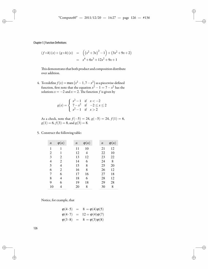
ii
“Compute60” — 2011/12/20 — 14:27 — page 126 — #136 ii
ii
ii
Chapter 5 | Function De nitions
( f h)(x)+(gh)(x) =((
x2 +3x)2−1
)+(3x2 +9x+2
)= x4 +6x3 +12x2 +9x+1
is demonstrates that bothproduct and compositiondistributeover addition.
4. To rede ne f (x)=max(x2−1,7− x2
)as a piecewise-de ned
function, rst note that the equation x2− 1 = 7− x2 has thesolutions x =−2 and x = 2. e function f is given by
g(x) =
x2−1 if x <−27− x2 if −2≤ x≤ 2x2−1 if x > 2
As a check, note that f (−5) = 24, g(−5) = 24, f (1) = 6,g(1) = 6, f (3) = 8, and g(3) = 8.
5. Construct the following table:
n φ(n)1 12 13 24 25 46 27 68 49 610 4
n φ(n)11 1012 413 1214 615 816 817 1618 619 1820 8
n φ(n)21 1222 1023 2224 825 2026 1227 1828 1229 2830 8
Notice, for example, that
φ(4 ·5) = 8 = φ(4)φ(5)φ(4 ·7) = 12 = φ(4)φ(7)φ(3 ·8) = 8 = φ(3)φ(8)
126
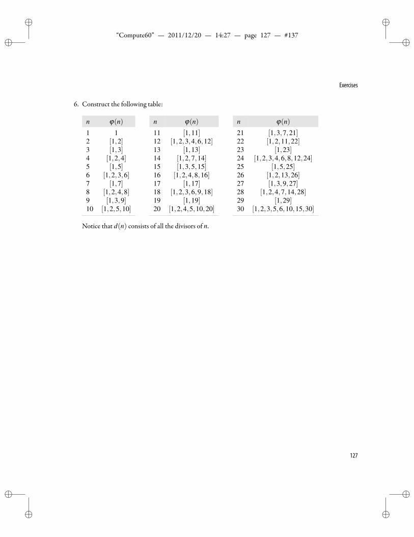
ii
“Compute60” — 2011/12/20 — 14:27 — page 127 — #137 ii
ii
ii
Exercises
6. Construct the following table:
n φ(n)1 12 [1,2]3 [1,3]4 [1,2,4]5 [1,5]6 [1,2,3,6]7 [1,7]8 [1,2,4,8]9 [1,3,9]10 [1,2,5,10]
n φ(n)11 [1,11]12 [1,2,3,4,6,12]13 [1,13]14 [1,2,7,14]15 [1,3,5,15]16 [1,2,4,8,16]17 [1,17]18 [1,2,3,6,9,18]19 [1,19]20 [1,2,4,5,10,20]
n φ(n)21 [1,3,7,21]22 [1,2,11,22]23 [1,23]24 [1,2,3,4,6,8,12,24]25 [1,5,25]26 [1,2,13,26]27 [1,3,9,27]28 [1,2,4,7,14,28]29 [1,29]30 [1,2,3,5,6,10,15,30]
Notice that d(n) consists of all the divisors of n.
127
ii
“Compute60” — 2011/12/20 — 14:27 — page 128 — #138 ii
ii
ii
ii
“Compute60” — 2011/12/20 — 14:27 — page 129 — #139 ii
ii
ii
6Plotting Curves and Surfaces
[The universe] cannot be understood until we have learned the language and can interpret the characters in which it is written. It is written in thelanguage of mathematics, and its characters are triangles, circles and other geometrical gures, without which it is humanly impossible to
understand a single word of it... Galileo Galilei (1564–1642)
T he plotting capabilities of symbolic algebra systems are among Getting Started with 2D Plots
Interactive Tools for 2D Plots
Graph User Settings
2D Plots of Functions andExpressions
Creating Animated 2D Plots
Creating 3D Plots
Creating Animated 3D Plots
their most powerful features. With the system you are using,you can carry out operations interactively. You can plot func-
tions and expressions, examine the results, revise the plot and exam-ine the results of the revision, add multiple functions to the plot, andcarry out a variety of other plotting procedures. is adds an exper-imental dimension to problem solving that was not easily accessiblein the past. In the preceding chapter, several plots were provided toillustrate properties of functions. You will nd yourself creating plotsin many situations to help answer questions about the behavior of dif-ferent functions or families of functions.
In this chapter, you will nd techniques for creating plots, show-ing how to plot lines and curves in the Euclidean plane, and lines,curves, and surfaces in three-dimensional Euclidean space. ese tech-niques use the basic routines Rectangular, Polar, Implicit, and Para-metric fromthePlot 2Dsubmenu, andRectangular,Cylindrical, Spher-ical, Implicit, and Tube from the Plot 3D submenu. e submenus of New in Version 6
Reorient 3D Plots with click and dragInteractive plot tools in document windowSmoother 2D Plots
Plot 2D, Plot 3D, and Calculus also contain a variety of specializedplotting routines for advanced topics in calculus, vector calculus, anddifferential equations. ose plotting options are introduced and dis-cussed elsewhere, along with the related mathematics.
129
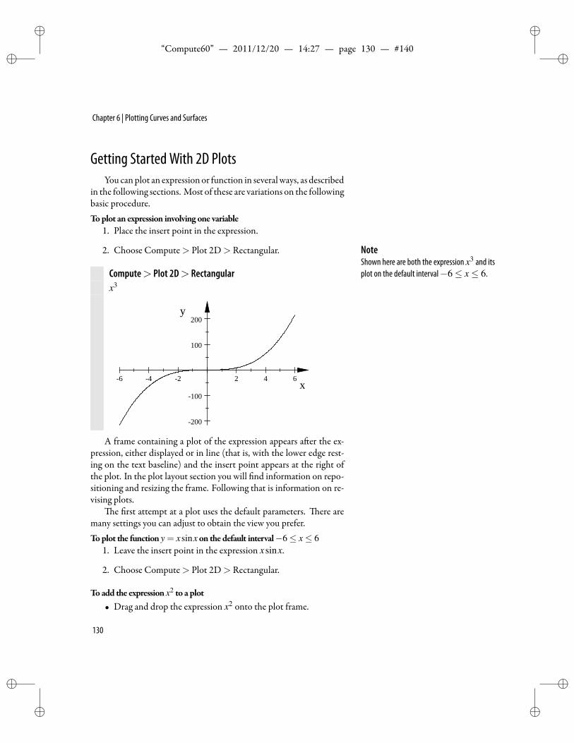
ii
“Compute60” — 2011/12/20 — 14:27 — page 130 — #140 ii
ii
ii
Chapter 6 | Plotting Curves and Surfaces
Getting Started With 2D PlotsYou canplot an expression or function in severalways, as described
in the following sections. Most of these are variations on the followingbasic procedure.Toplot an expression involving one variable
1. Place the insert point in the expression.
2. Choose Compute> Plot 2D> Rectangular. NoteShown here are both the expression x3 and itsplot on the default interval−6≤ x≤ 6.Compute> Plot 2D> Rectangular
x3
6 4 2 2 4 6
200
100
100
200
x
y
A frame containing a plot of the expression appears a er the ex-pression, either displayed or in line (that is, with the lower edge rest-ing on the text baseline) and the insert point appears at the right ofthe plot. In the plot layout section you will nd information on repo-sitioning and resizing the frame. Following that is information on re-vising plots.
e rst attempt at a plot uses the default parameters. ere aremany settings you can adjust to obtain the view you prefer.Toplot the function y = xsinxon the default interval−6≤ x≤ 6
1. Leave the insert point in the expression xsinx.
2. Choose Compute> Plot 2D> Rectangular.
Toadd the expression x2 to a plot• Drag and drop the expression x2 onto the plot frame.
130
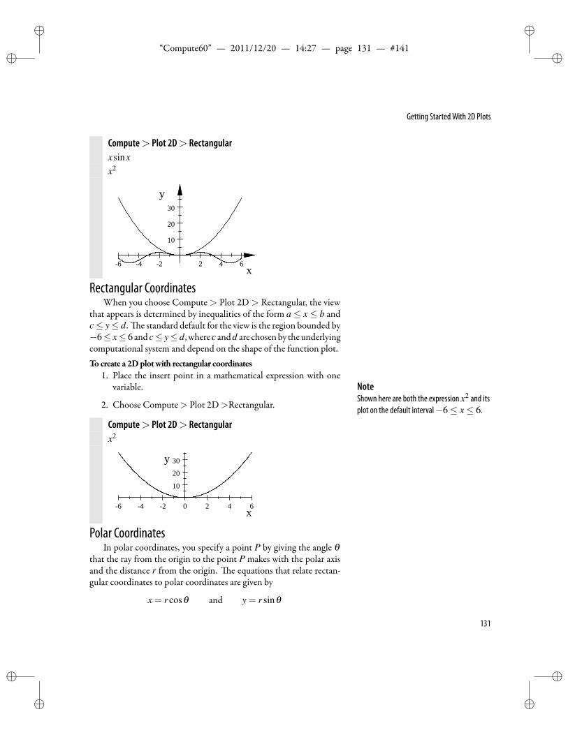
ii
“Compute60” — 2011/12/20 — 14:27 — page 131 — #141 ii
ii
ii
Getting Started With 2D Plots
Compute> Plot 2D> Rectangularxsinxx2
6 4 2 2 4 6
10
20
30
x
y
Rectangular CoordinatesWhen you choose Compute > Plot 2D > Rectangular, the view
that appears is determined by inequalities of the form a≤ x ≤ b andc≤ y≤ d. e standard default for the view is the region bounded by−6≤ x≤ 6 and c≤ y≤ d, where c andd are chosenby theunderlyingcomputational system and depend on the shape of the function plot.Tocreate a 2Dplotwith rectangular coordinates
1. Place the insert point in a mathematical expression with onevariable. Note
Shown here are both the expression x2 and itsplot on the default interval−6≤ x≤ 6.2. Choose Compute> Plot 2D>Rectangular.
Compute> Plot 2D> Rectangularx2
6 4 2 0 2 4 6
10
20
30
x
y
Polar CoordinatesIn polar coordinates, you specify a point P by giving the angle θ
that the ray from the origin to the point P makes with the polar axisand the distance r from the origin. e equations that relate rectan-gular coordinates to polar coordinates are given by
x = r cosθ and y = r sinθ
131
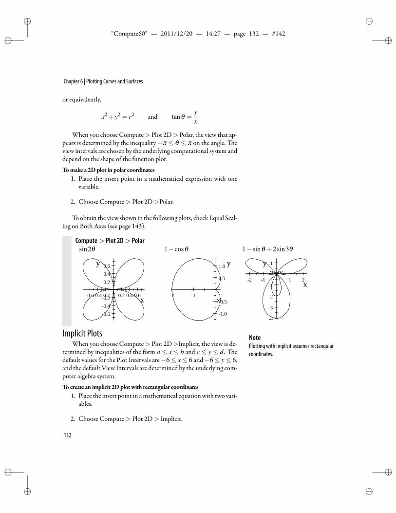
ii
“Compute60” — 2011/12/20 — 14:27 — page 132 — #142 ii
ii
ii
Chapter 6 | Plotting Curves and Surfaces
or equivalently,
x2 + y2 = r2 and tanθ =yx
When you choose Compute> Plot 2D> Polar, the view that ap-pears is determined by the inequality−π ≤ θ ≤ π on the angle. eview intervals are chosen by the underlying computational system anddepend on the shape of the function plot.
Tomake a 2Dplot in polar coordinates1. Place the insert point in a mathematical expression with one
variable.
2. Choose Compute> Plot 2D>Polar.
To obtain the view shown in the following plots, check Equal Scal-ing on Both Axes (see page 143).
Compute> Plot 2D> Polarsin2θ 1− cosθ 1− sinθ +2sin3θ
0.60.40.2 0.2 0.4 0.6
0.60.40.2
0.20.40.6
x
y
2 1
1.0
0.5
0.5
1.0
x
y
2 1 1 2
4
3
2
1
1
x
y
Implicit Plots NotePlotting with Implicit assumes rectangularcoordinates.
When you choose Compute> Plot 2D>Implicit, the view is de-termined by inequalities of the form a ≤ x ≤ b and c ≤ y ≤ d. edefault values for the Plot Intervals are−6≤ x≤ 6 and−6≤ y≤ 6,and the default View Intervals are determined by the underlying com-puter algebra system.
Tocreate an implicit 2Dplotwith rectangular coordinates1. Place the insert point in amathematical equationwith two vari-
ables.
2. Choose Compute> Plot 2D> Implicit.
132
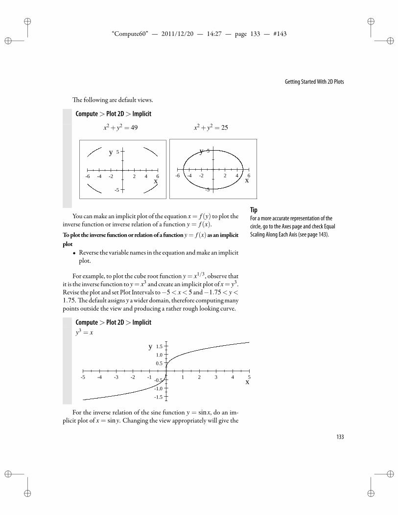
ii
“Compute60” — 2011/12/20 — 14:27 — page 133 — #143 ii
ii
ii
Getting Started With 2D Plots
e following are default views.
Compute> Plot 2D> Implicit
x2 + y2 = 49 x2 + y2 = 25
6 4 2 2 4 6
5
5
x
y
6 4 2 2 4 6
5
5
x
y
TipFor a more accurate representation of thecircle, go to the Axes page and check EqualScaling Along Each Axis (see page 143).
You canmake an implicit plot of the equation x = f (y) to plot theinverse function or inverse relation of a function y = f (x).Toplot the inverse functionor relationof a functiony = f (x)as an implicitplot
• Reverse the variable names in the equation andmake an implicitplot.
For example, to plot the cube root function y = x1/3, observe thatit is the inverse function to y= x3 and create an implicit plot of x= y3.Revise the plot and set Plot Intervals to−5< x< 5 and−1.75< y<1.75. e default assigns y awider domain, therefore computingmanypoints outside the view and producing a rather rough looking curve.
Compute> Plot 2D> Implicity3 = x
5 4 3 2 1 1 2 3 4 5
1.51.00.5
0.51.01.5
x
y
For the inverse relation of the sine function y = sinx, do an im-plicit plot of x = siny. Changing the view appropriately will give the
133
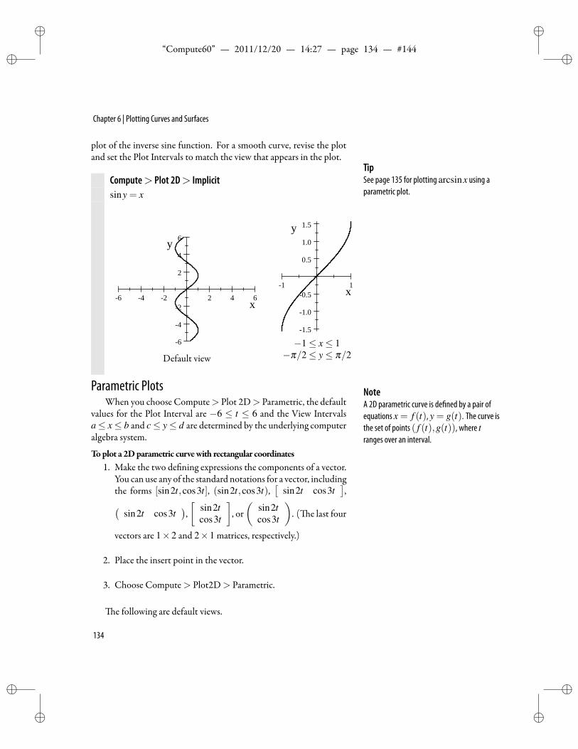
ii
“Compute60” — 2011/12/20 — 14:27 — page 134 — #144 ii
ii
ii
Chapter 6 | Plotting Curves and Surfaces
plot of the inverse sine function. For a smooth curve, revise the plotand set the Plot Intervals to match the view that appears in the plot.
TipSee page 135 for plotting arcsinx using aparametric plot.
Compute> Plot 2D> Implicitsiny = x
6 4 2 2 4 6
6
4
2
2
4
6
x
y
Default view
1 1
1.5
1.0
0.5
0.5
1.0
1.5
x
y
−1≤ x≤ 1−π/2≤ y≤ π/2
Parametric Plots NoteA 2D parametric curve is de ned by a pair ofequations x = f (t), y = g(t). The curve isthe set of points ( f (t),g(t)), where tranges over an interval.
When you choose Compute> Plot 2D> Parametric, the defaultvalues for the Plot Interval are −6 ≤ t ≤ 6 and the View Intervalsa≤ x≤ b and c≤ y≤ d are determined by the underlying computeralgebra system.
Toplot a 2Dparametric curvewith rectangular coordinates1. Make the two de ning expressions the components of a vector.
You can use any of the standard notations for a vector, includingthe forms [sin2t,cos3t], (sin2t,cos3t),
[sin2t cos3t
],(
sin2t cos3t),[
sin2tcos3t
], or(
sin2tcos3t
). ( e last four
vectors are 1×2 and 2×1 matrices, respectively.)
2. Place the insert point in the vector.
3. Choose Compute> Plot2D> Parametric.
e following are default views.
134
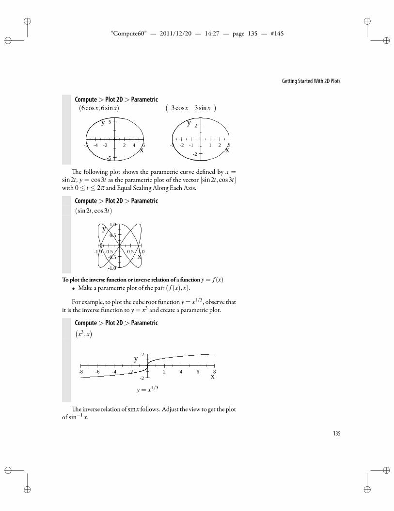
ii
“Compute60” — 2011/12/20 — 14:27 — page 135 — #145 ii
ii
ii
Getting Started With 2D Plots
Compute> Plot 2D> Parametric(6cosx,6sinx)
(3cosx 3sinx
)
6 4 2 2 4 6
5
5
x
y
3 2 1 1 2 3
2
2
x
y
e following plot shows the parametric curve de ned by x =sin2t , y = cos3t as the parametric plot of the vector [sin2t,cos3t]with 0≤ t ≤ 2π and Equal Scaling Along Each Axis.
Compute> Plot 2D> Parametric(sin2t,cos3t)
1.0 0.5 0.5 1.0
1.0
0.5
0.5
1.0
x
y
Toplot the inverse functionor inverse relationof a function y = f (x)• Make a parametric plot of the pair ( f (x),x).
For example, to plot the cube root function y = x1/3, observe thatit is the inverse function to y = x3 and create a parametric plot.
Compute> Plot 2D> Parametric(x3,x
)
8 6 4 2 2 4 6 82
2
x
y
y = x1/3
e inverse relation of sinx follows. Adjust the view to get the plotof sin−1 x.
135
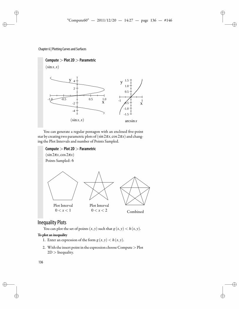
ii
“Compute60” — 2011/12/20 — 14:27 — page 136 — #146 ii
ii
ii
Chapter 6 | Plotting Curves and Surfaces
Compute> Plot 2D> Parametric(sinx,x)
1.0 0.5 0.5 1.0
4
2
2
4
x
y
(sinx,x)
1 1
1.5
1.0
0.5
0.5
1.0
1.5
x
y
arcsinx
You can generate a regular pentagon with an enclosed ve-pointstar by creating two parametric plots of (sin2πx,cos2πx) and chang-ing the Plot Intervals and number of Points Sampled.
Compute> Plot 2D> Parametric(sin2πx,cos2πx)Points Sampled: 6
Plot Interval0 < x < 1
Plot Interval0 < x < 2 Combined
Inequality PlotsYou can plot the set of points (x,y) such that g(x,y)< h(x,y).
Toplot an inequality1. Enter an expression of the form g(x,y)< h(x,y).
2. With the insert point in the expression chooseCompute>Plot2D> Inequality.
136
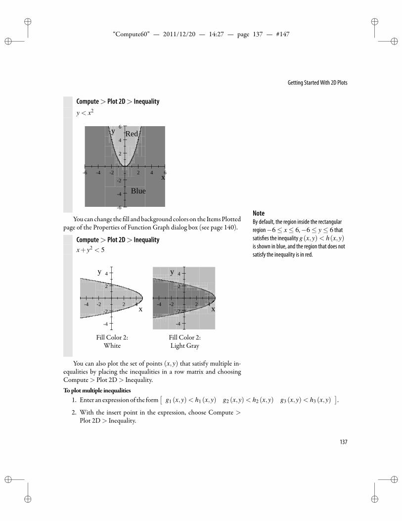
ii
“Compute60” — 2011/12/20 — 14:27 — page 137 — #147 ii
ii
ii
Getting Started With 2D Plots
Compute> Plot 2D> Inequalityy < x2
Blue
Red
6 4 2 2 4 6
6
4
2
2
4
6
x
y
NoteBy default, the region inside the rectangularregion−6≤ x≤ 6,−6≤ y≤ 6 thatsatis es the inequality g(x,y)< h(x,y)is shown in blue, and the region that does notsatisfy the inequality is in red.
Youcan change the ll andbackgroundcolors on the ItemsPlottedpage of the Properties of Function Graph dialog box (see page 140).
Compute> Plot 2D> Inequalityx+ y2 < 5
4 2 2 4
4
2
2
4
x
y
Fill Color 2:White
4 2 2 4
4
2
2
4
x
y
Fill Color 2:Light Gray
You can also plot the set of points (x,y) that satisfy multiple in-equalities by placing the inequalities in a row matrix and choosingCompute> Plot 2D> Inequality.Toplotmultiple inequalities
1. Enter an expressionof the form[
g1 (x,y)< h1 (x,y) g2 (x,y)< h2 (x,y) g3 (x,y)< h3 (x,y)].
2. With the insert point in the expression, choose Compute >Plot 2D> Inequality.
137
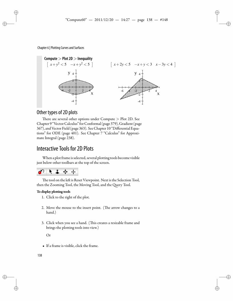
ii
“Compute60” — 2011/12/20 — 14:27 — page 138 — #148 ii
ii
ii
Chapter 6 | Plotting Curves and Surfaces
Compute> Plot 2D> Inequality[x+ y2 < 5 −x+ y2 < 5
] [x+2y < 5 −x+ y < 3 x−3y < 4
]
4 2 2 4
4
2
2
4
x
y
6 4 2 2 4
4
2
2
4
x
y
Other types of 2D plotsere are several other options under Compute > Plot 2D. See
Chapter 9 “VectorCalculus” forConformal (page379),Gradient (page367), andVector Field (page 363). SeeChapter 10 “Differential Equa-tions” for ODE (page 401). See Chapter 7 “Calculus” for Approxi-mate Integral (page 238).
Interactive Tools for 2D PlotsWhenaplot frame is selected, several plotting tools becomevisible
just below other toolbars at the top of the screen.
e tool on the le is Reset Viewpoint. Next is the SelectionTool,then the Zooming Tool, the Moving Tool, and the uery Tool.
Todisplay plotting tools1. Click to the right of the plot.
2. Move the mouse to the insert point. ( e arrow changes to ahand.)
3. Click when you see a hand. ( is creates a resizable frame andbrings the plotting tools into view.)
Or
• If a frame is visible, click the frame.
138
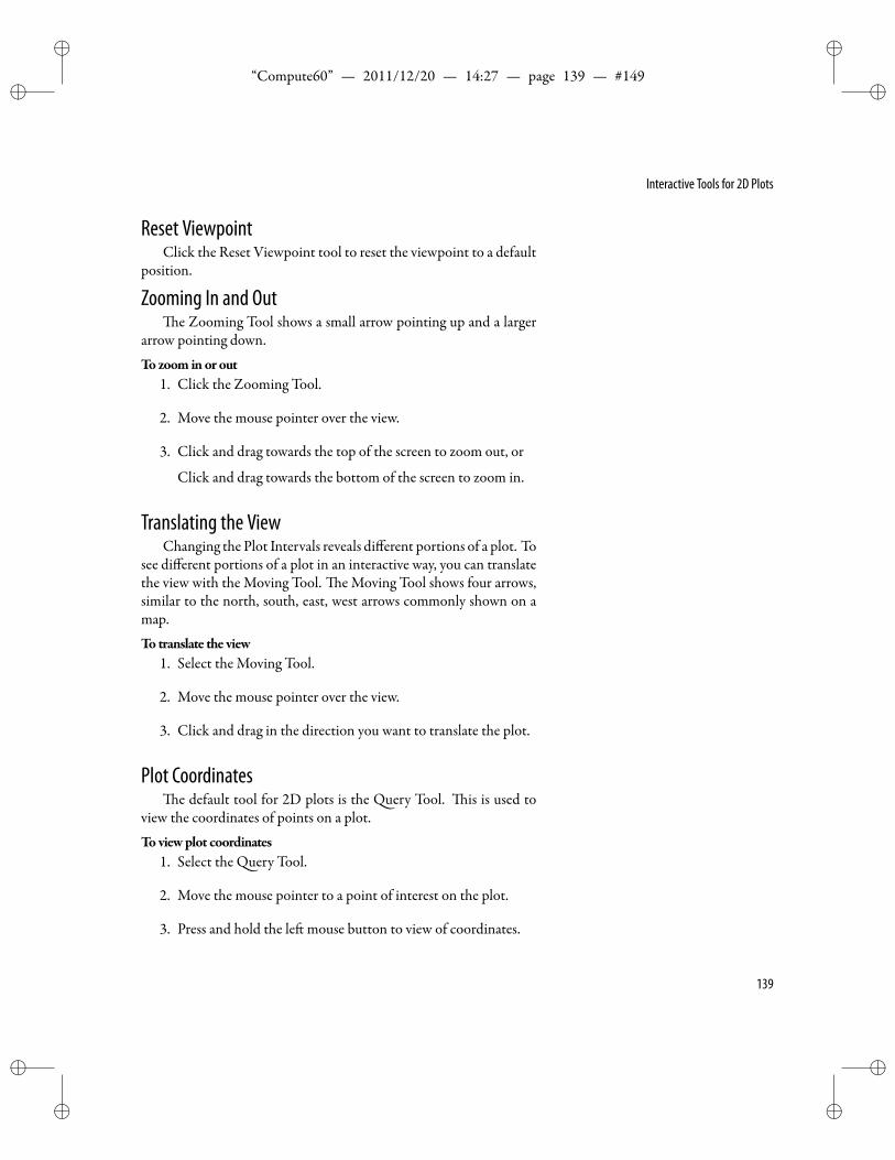
ii
“Compute60” — 2011/12/20 — 14:27 — page 139 — #149 ii
ii
ii
Interactive Tools for 2D Plots
Reset ViewpointClick the Reset Viewpoint tool to reset the viewpoint to a default
position.
Zooming In and Oute Zooming Tool shows a small arrow pointing up and a larger
arrow pointing down.
Tozoom inor out1. Click the Zooming Tool.
2. Move the mouse pointer over the view.
3. Click and drag towards the top of the screen to zoom out, or
Click and drag towards the bottom of the screen to zoom in.
Translating the ViewChanging the Plot Intervals reveals different portions of a plot. To
see different portions of a plot in an interactive way, you can translatethe view with the Moving Tool. e Moving Tool shows four arrows,similar to the north, south, east, west arrows commonly shown on amap.
To translate the view1. Select the Moving Tool.
2. Move the mouse pointer over the view.
3. Click and drag in the direction you want to translate the plot.
Plot Coordinatese default tool for 2D plots is the uery Tool. is is used to
view the coordinates of points on a plot.
Toviewplot coordinates1. Select the uery Tool.
2. Move the mouse pointer to a point of interest on the plot.
3. Press and hold the le mouse button to view of coordinates.
139
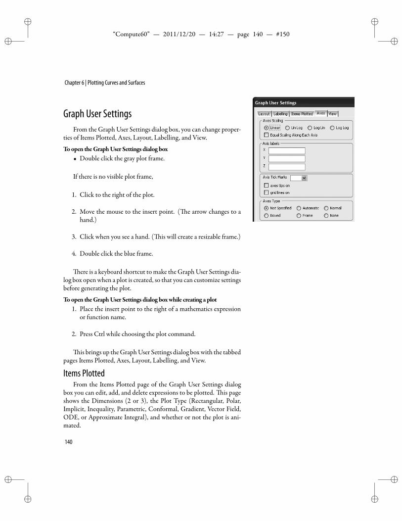
ii
“Compute60” — 2011/12/20 — 14:27 — page 140 — #150 ii
ii
ii
Chapter 6 | Plotting Curves and Surfaces
Graph User SettingsFrom the Graph User Settings dialog box, you can change proper-
ties of Items Plotted, Axes, Layout, Labelling, and View.
Toopen theGraphUser Settings dialog box• Double click the gray plot frame.
If there is no visible plot frame,
1. Click to the right of the plot.
2. Move the mouse to the insert point. ( e arrow changes to ahand.)
3. Click when you see a hand. ( is will create a resizable frame.)
4. Double click the blue frame.
ere is a keyboard shortcut tomake theGraphUser Settings dia-log box openwhen a plot is created, so that you can customize settingsbefore generating the plot.
Toopen theGraphUser Settings dialog boxwhile creating a plot1. Place the insert point to the right of a mathematics expression
or function name.
2. Press Ctrl while choosing the plot command.
is brings up theGraphUser Settings dialog boxwith the tabbedpages Items Plotted, Axes, Layout, Labelling, and View.
Items PlottedFrom the Items Plotted page of the Graph User Settings dialog
box you can edit, add, and delete expressions to be plotted. is pageshows the Dimensions (2 or 3), the Plot Type (Rectangular, Polar,Implicit, Inequality, Parametric, Conformal, Gradient, Vector Field,ODE, or Approximate Integral), and whether or not the plot is ani-mated.
140
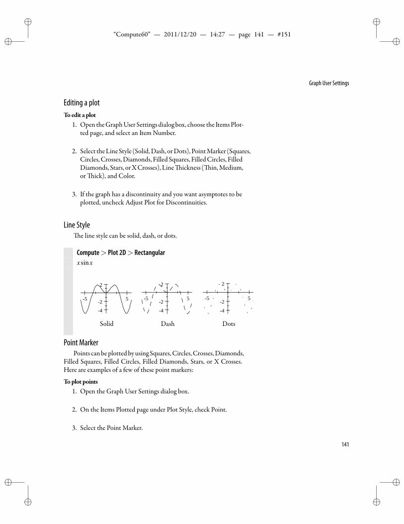
ii
“Compute60” — 2011/12/20 — 14:27 — page 141 — #151 ii
ii
ii
Graph User Settings
Editing a plotToedit a plot
1. Open theGraphUser Settings dialogbox, choose the ItemsPlot-ted page, and select an Item Number.
2. Select theLineStyle (Solid,Dash, orDots), PointMarker (Squares,Circles,Crosses,Diamonds, FilledSquares, FilledCircles, FilledDiamonds, Stars, orXCrosses), Line ickness ( in,Medium,or ick), and Color.
3. If the graph has a discontinuity and you want asymptotes to beplotted, uncheck Adjust Plot for Discontinuities.
Line Stylee line style can be solid, dash, or dots.
Compute> Plot 2D> Rectangularxsinx
5 5
42
2
Solid
5 5
4
2
2
Dash
5 5
4
2
2
Dots
Point MarkerPoints canbeplottedbyusingSquares,Circles,Crosses,Diamonds,
Filled Squares, Filled Circles, Filled Diamonds, Stars, or X Crosses.Here are examples of a few of these point markers:
Toplot points1. Open the Graph User Settings dialog box.
2. On the Items Plotted page under Plot Style, check Point.
3. Select the Point Marker.
141
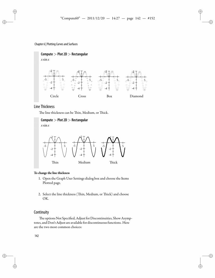
ii
“Compute60” — 2011/12/20 — 14:27 — page 142 — #152 ii
ii
ii
Chapter 6 | Plotting Curves and Surfaces
Compute> Plot 2D> Rectangularxsinx
5 5
4
2
2
Circle
5 5
4
2
2
Cross
5 5
4
2
2
Box
5 5
4
2
2
Diamond
Line Thicknesse line thickness can be in, Medium, or ick.
Compute> Plot 2D> Rectangularxsinx
5 5
4
2
2
in
5 5
4
2
2
Medium
5 5
4
2
2
ick
Tochange the line thickness
1. Open the Graph User Settings dialog box and choose the ItemsPlotted page.
2. Select the line thickness ( in, Medium, or ick) and chooseOK.
Continuitye optionsNotSpeci ed,Adjust forDiscontinuities, ShowAsymp-
totes, andDon’tAdjust are available for discontinuous functions. Hereare the two most common choices:
142
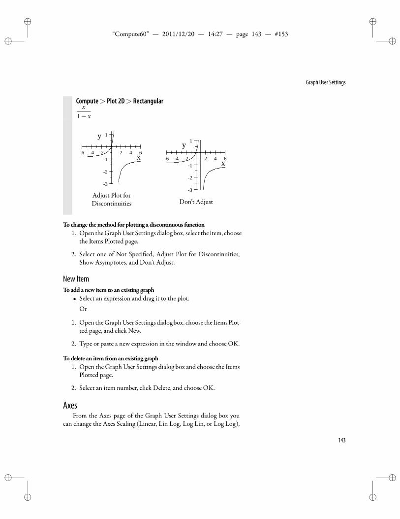
ii
“Compute60” — 2011/12/20 — 14:27 — page 143 — #153 ii
ii
ii
Graph User Settings
Compute> Plot 2D> Rectangularx
1− x
6 4 2 2 4 6
3
2
1
1
x
y
Adjust Plot forDiscontinuities
6 4 2 2 4 6
3
2
1
1
x
y
Don’t Adjust
Tochange themethod for plotting a discontinuous function1. Open theGraphUser Settings dialogbox, select the item, choose
the Items Plotted page.
2. Select one of Not Speci ed, Adjust Plot for Discontinuities,Show Asymptotes, and Don’t Adjust.
New ItemToadd anew item to an existing graph
• Select an expression and drag it to the plot.Or
1. Open theGraphUser Settings dialogbox, choose the ItemsPlot-ted page, and click New.
2. Type or paste a new expression in the window and choose OK.
Todelete an item froman existing graph1. Open the Graph User Settings dialog box and choose the Items
Plotted page.
2. Select an item number, click Delete, and choose OK.
AxesFrom the Axes page of the Graph User Settings dialog box you
can change the Axes Scaling (Linear, Lin Log, Log Lin, or Log Log),
143
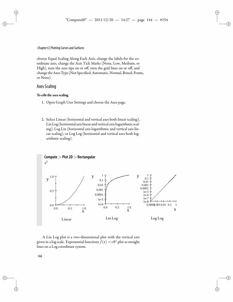
ii
“Compute60” — 2011/12/20 — 14:27 — page 144 — #154 ii
ii
ii
Chapter 6 | Plotting Curves and Surfaces
choose Equal Scaling Along Each Axis, change the labels for the co-ordinate axes, change the Axis Tick Marks (None, Low, Medium, orHigh), turn the axes tips on or off, turn the grid lines on or off, andchange theAxesType (NotSpeci ed,Automatic,Normal, Boxed, Frame,or None).
Axes Scaling
Toedit the axes scaling
1. Open Graph User Settings and choose the Axes page.
2. Select Linear (horizontal and vertical axes both linear scaling),LinLog (horizontal axis linear andvertical axis logarithmic scal-ing), Log Lin (horizontal axis logarithmic and vertical axis lin-ear scaling), or Log Log (horizontal and vertical axes both log-arithmic scaling).
Compute> Plot 2D> Rectangularx2
0.0 0.5 1.00.0
0.5
1.0
x
y
Linear
0.0 0.5 1.01e61e5
0.00010.0010.01
0.11
x
y
Lin Log
0.00010.0010.01 0.1 11e81e71e61e5
0.00010.001
0.010.1
1
x
y
Log Log
A Lin Log plot is a two-dimensional plot with the vertical axisgiven in a log scale. Exponential functions f (x) = cbx plot as straightlines on a Log coordinate system.
144
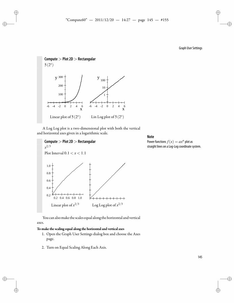
ii
“Compute60” — 2011/12/20 — 14:27 — page 145 — #155 ii
ii
ii
Graph User Settings
Compute> Plot 2D> Rectangular5(2x)
6 4 2 0 2 4 6
100
200
300
x
y
Linear plot of 5(2x)
6 4 2 0 2 4 6
1
10
100
x
y
Lin Log plot of 5(2x)
A Log Log plot is a two-dimensional plot with both the verticaland horizontal axes given in a logarithmic scale.
NotePower functions f (x) = axn plot asstraight lines on a Log-Log coordinate system.
Compute> Plot 2D> Rectangularx2/3
Plot Interval 0.1 < x < 1.1
0.2 0.4 0.6 0.8 1.00.2
0.4
0.6
0.8
1.0
Linear plot of x2/3 Log Log plot of x2/3
Youcan alsomake the scales equal along thehorizontal andverticalaxes.
Tomake the scaling equal along the horizontal and vertical axes1. Open the Graph User Settings dialog box and choose the Axes
page.
2. Turn on Equal Scaling Along Each Axis.
145
ii
“Compute60” — 2011/12/20 — 14:27 — page 146 — #156 ii
ii
ii
Chapter 6 | Plotting Curves and Surfaces
Axes Labelse default labels for the axes are x and y for two-dimensional
plots, or x, y, and z for three-dimensional plots. You can edit the de-fault labels.Toedit the labels for the axes
1. Open the Graph User Settings dialog box and choose the Axespage.
2. Type labels in the axis label boxes.
Axes AppearanceYou can change the appearance of the tick marks and turn on or
off the axes tips and grid lines.Toedit the number of tickmarks shownon the axes
1. Open the Graph User Settings dialog box and choose the Axespage.
2. Edit the number of Axis Tick Marks by selecting None, Low,Normal, or High.
To turn axes tips onor off1. Open the Graph User Settings dialog box and choose the Axes
page.
2. Check or uncheck Axes tips on.
To turn grid lines onor off1. Open the Graph User Settings dialog box and choose the Axes
page. TipThe number of grid lines is determined by thesetting for tick marks (Low, Normal, or High).2. Check or uncheck Grid lines on.
Axes TypeYou can change the axis type to beNot Speci ed, Automatic, Nor-
mal, Boxed, Frame, or None.Toedit the axis type
1. Open the Graph User Settings dialog box and choose the Axespage.
2. Select an Axes Type.
146
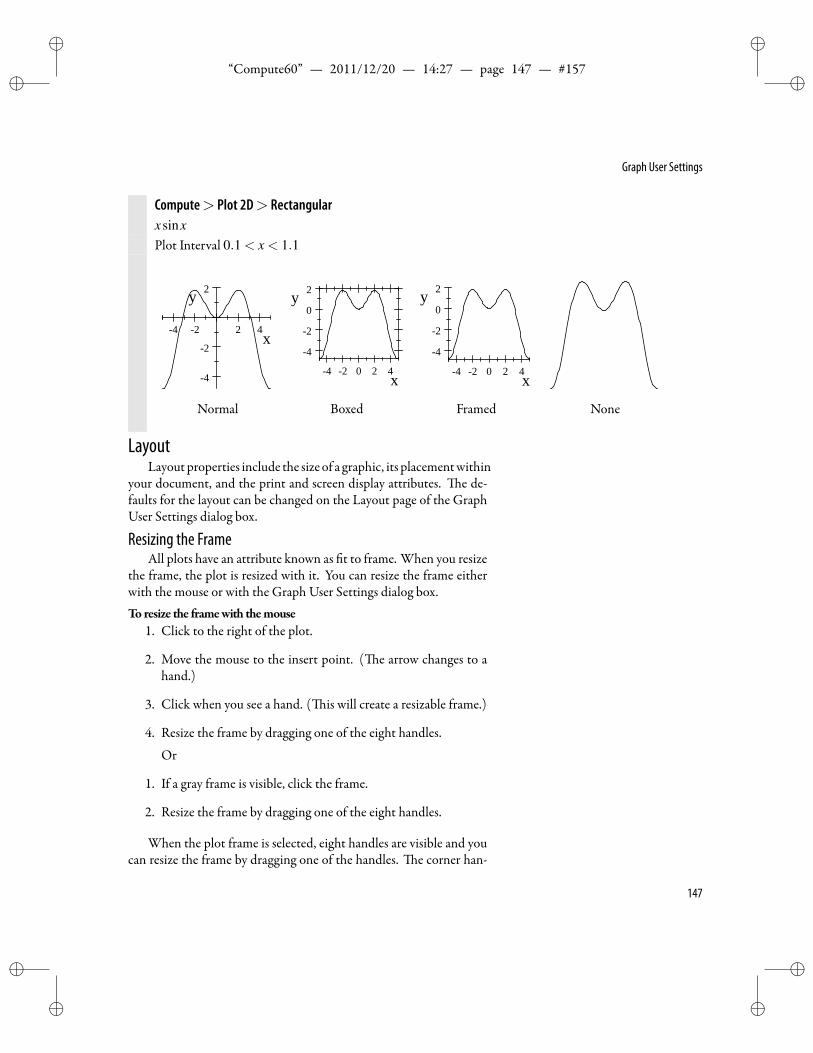
ii
“Compute60” — 2011/12/20 — 14:27 — page 147 — #157 ii
ii
ii
Graph User Settings
Compute> Plot 2D> RectangularxsinxPlot Interval 0.1 < x < 1.1
4 2 2 4
4
2
2
x
y
Normal
4 2 0 2 4
4
2
0
2
x
y
Boxed
4 2 0 2 4
4
2
0
2
x
y
Framed None
LayoutLayoutproperties include the size of a graphic, its placementwithin
your document, and the print and screen display attributes. e de-faults for the layout can be changed on the Layout page of the GraphUser Settings dialog box.
Resizing the FrameAll plots have an attribute known as t to frame. When you resize
the frame, the plot is resized with it. You can resize the frame eitherwith the mouse or with the Graph User Settings dialog box.To resize the framewith themouse
1. Click to the right of the plot.
2. Move the mouse to the insert point. ( e arrow changes to ahand.)
3. Click when you see a hand. ( is will create a resizable frame.)
4. Resize the frame by dragging one of the eight handles.
Or
1. If a gray frame is visible, click the frame.
2. Resize the frame by dragging one of the eight handles.
When the plot frame is selected, eight handles are visible and youcan resize the frame by dragging one of the handles. e corner han-
147
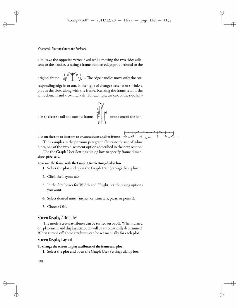
ii
“Compute60” — 2011/12/20 — 14:27 — page 148 — #158 ii
ii
ii
Chapter 6 | Plotting Curves and Surfaces
dles leave the opposite vertex xed while moving the two sides adja-cent to the handle, creating a frame that has edges proportional to the
original frame 5 54. e edge handles move only the cor-
responding edge in or out. Either type of change stretches or shrinks aplot in the view, along with the frame. Resizing the frame retains thesame domain and view intervals. For example, use one of the side han-
dles to create a tall and narrow frame6 6
4
2
2
or use one of the han-
dles on the toporbottomto create a short and fat frame 6 4 2 2 4 65 .e examples in the previous paragraph illustrate the use of inline
plots, one of the two placement options described in the next section.Use the Graph User Settings dialog box to specify frame dimen-
sions precisely.To resize the framewith theGraphUser Settings dialog box
1. Select the plot and open the Graph User Settings dialog box.
2. Click the Layout tab.
3. In the Size boxes for Width and Height, set the sizing optionsyou want.
4. Select desired units (inches, centimeters, picas, or points).
5. Choose OK.
Screen Display Attributesemodel screen attributes can be turned on or off. When turned
on, placement anddisplay attributeswill be automatically determined.When turned off, these attributes can be set manually for each plot.
Screen Display LayoutTochange the screendisplay attributes of the frame andplot
1. Select the plot and open the Graph User Settings dialog box.
148
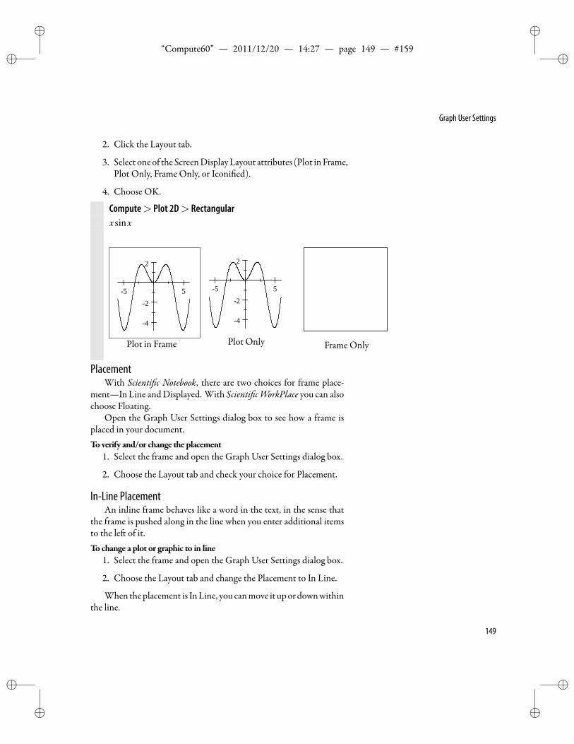
ii
“Compute60” — 2011/12/20 — 14:27 — page 149 — #159 ii
ii
ii
Graph User Settings
2. Click the Layout tab.
3. Select oneof theScreenDisplayLayout attributes (Plot inFrame,Plot Only, Frame Only, or Iconi ed).
4. Choose OK.
Compute> Plot 2D> Rectangularxsinx
5 5
4
2
2
Plot in Frame
5 5
4
2
2
Plot Only Frame Only
PlacementWith Scienti c Notebook, there are two choices for frame place-
ment—In Line andDisplayed. With Scienti cWorkPlace you can alsochoose Floating.
Open the Graph User Settings dialog box to see how a frame isplaced in your document.Toverify and/or change the placement
1. Select the frame and open the Graph User Settings dialog box.
2. Choose the Layout tab and check your choice for Placement.
In-Line PlacementAn inline frame behaves like a word in the text, in the sense that
the frame is pushed along in the line when you enter additional itemsto the le of it.Tochange a plot or graphic to in line
1. Select the frame and open the Graph User Settings dialog box.
2. Choose the Layout tab and change the Placement to In Line.
When theplacement is InLine, you canmove it upordownwithinthe line.
149
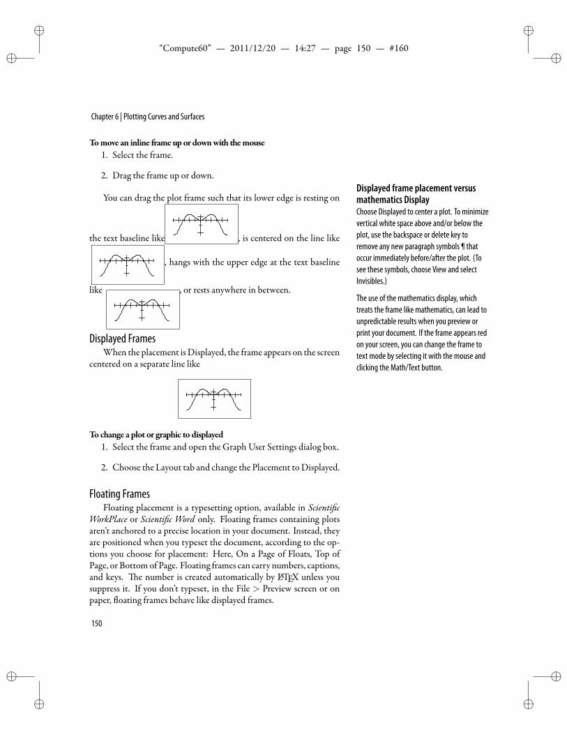
ii
“Compute60” — 2011/12/20 — 14:27 — page 150 — #160 ii
ii
ii
Chapter 6 | Plotting Curves and Surfaces
Tomove an inline frameupor downwith themouse1. Select the frame.
2. Drag the frame up or down.Displayed frame placement versusmathematics DisplayChoose Displayed to center a plot. To minimizevertical white space above and/or below theplot, use the backspace or delete key toremove any new paragraph symbols ¶ thatoccur immediately before/after the plot. (Tosee these symbols, choose View and selectInvisibles.)
The use of the mathematics display, whichtreats the frame like mathematics, can lead tounpredictable results when you preview orprint your document. If the frame appears redon your screen, you can change the frame totext mode by selecting it with the mouse andclicking the Math/Text button.
You can drag the plot frame such that its lower edge is resting on
the text baseline like , is centered on the line like
, hangs with the upper edge at the text baseline
like , or rests anywhere in between.
Displayed FramesWhen the placement isDisplayed, the frame appears on the screen
centered on a separate line like
Tochange a plot or graphic to displayed1. Select the frame and open the Graph User Settings dialog box.
2. Choose the Layout tab and change the Placement toDisplayed.
Floating FramesFloating placement is a typesetting option, available in Scienti c
WorkPlace or Scienti c Word only. Floating frames containing plotsaren’t anchored to a precise location in your document. Instead, theyare positioned when you typeset the document, according to the op-tions you choose for placement: Here, On a Page of Floats, Top ofPage, or Bottomof Page. Floating frames can carry numbers, captions,and keys. e number is created automatically by LATEX unless yousuppress it. If you don’t typeset, in the File > Preview screen or onpaper, oating frames behave like displayed frames.
150
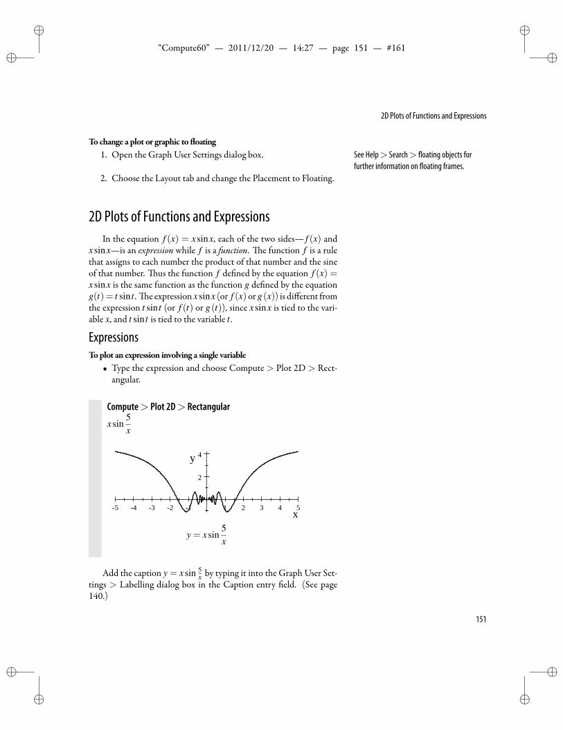
ii
“Compute60” — 2011/12/20 — 14:27 — page 151 — #161 ii
ii
ii
2D Plots of Functions and Expressions
Tochange a plot or graphic to oating1. Open the Graph User Settings dialog box. See Help> Search> oating objects for
further information on oating frames.2. Choose the Layout tab and change the Placement to Floating.
2D Plots of Functions and ExpressionsIn the equation f (x) = xsinx, each of the two sides— f (x) and
xsinx—is an expression while f is a function. e function f is a rulethat assigns to each number the product of that number and the sineof that number. us the function f de ned by the equation f (x) =xsinx is the same function as the function g de ned by the equationg(t) = t sin t . e expression xsinx (or f (x) org(x)) is different fromthe expression t sin t (or f (t) or g(t)), since xsinx is tied to the vari-able x, and t sin t is tied to the variable t .
ExpressionsToplot an expression involving a single variable
• Type the expression and choose Compute > Plot 2D > Rect-angular.
Compute> Plot 2D> Rectangular
xsin5x
5 4 3 2 1 1 2 3 4 5
2
4
x
y
y = xsin5x
Add the caption y = xsin 5x by typing it into the Graph User Set-
tings > Labelling dialog box in the Caption entry eld. (See page140.)
151
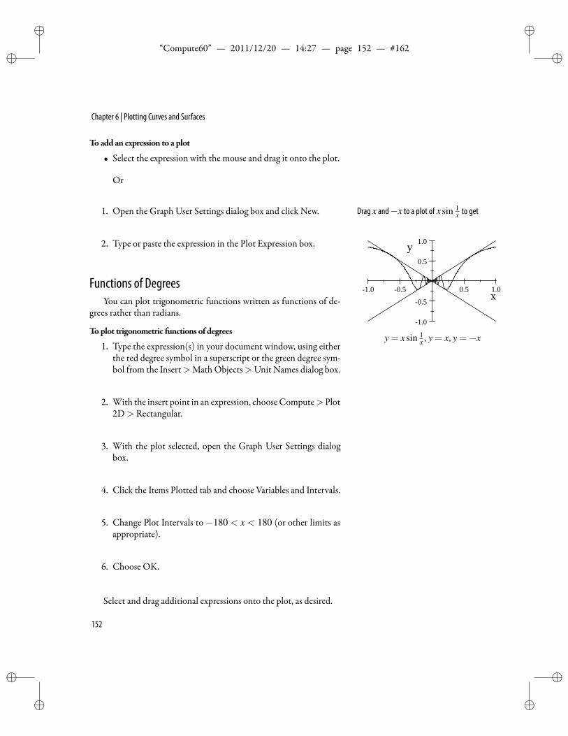
ii
“Compute60” — 2011/12/20 — 14:27 — page 152 — #162 ii
ii
ii
Chapter 6 | Plotting Curves and Surfaces
Toadd an expression to a plot
• Select the expression with the mouse and drag it onto the plot.
Or
1. Open the Graph User Settings dialog box and click New. Drag x and−x to a plot of xsin 1x to get
1.0 0.5 0.5 1.0
1.0
0.5
0.5
1.0
x
y
y = xsin 1x , y = x, y =−x
2. Type or paste the expression in the Plot Expression box.
Functions of DegreesYou can plot trigonometric functions written as functions of de-
grees rather than radians.
Toplot trigonometric functions of degrees
1. Type the expression(s) in your document window, using eitherthe red degree symbol in a superscript or the green degree sym-bol from the Insert>Math Objects>Unit Names dialog box.
2. With the insert point in an expression, chooseCompute>Plot2D> Rectangular.
3. With the plot selected, open the Graph User Settings dialogbox.
4. Click the Items Plotted tab and choose Variables and Intervals.
5. Change Plot Intervals to −180 < x < 180 (or other limits asappropriate).
6. Choose OK.
Select and drag additional expressions onto the plot, as desired.
152
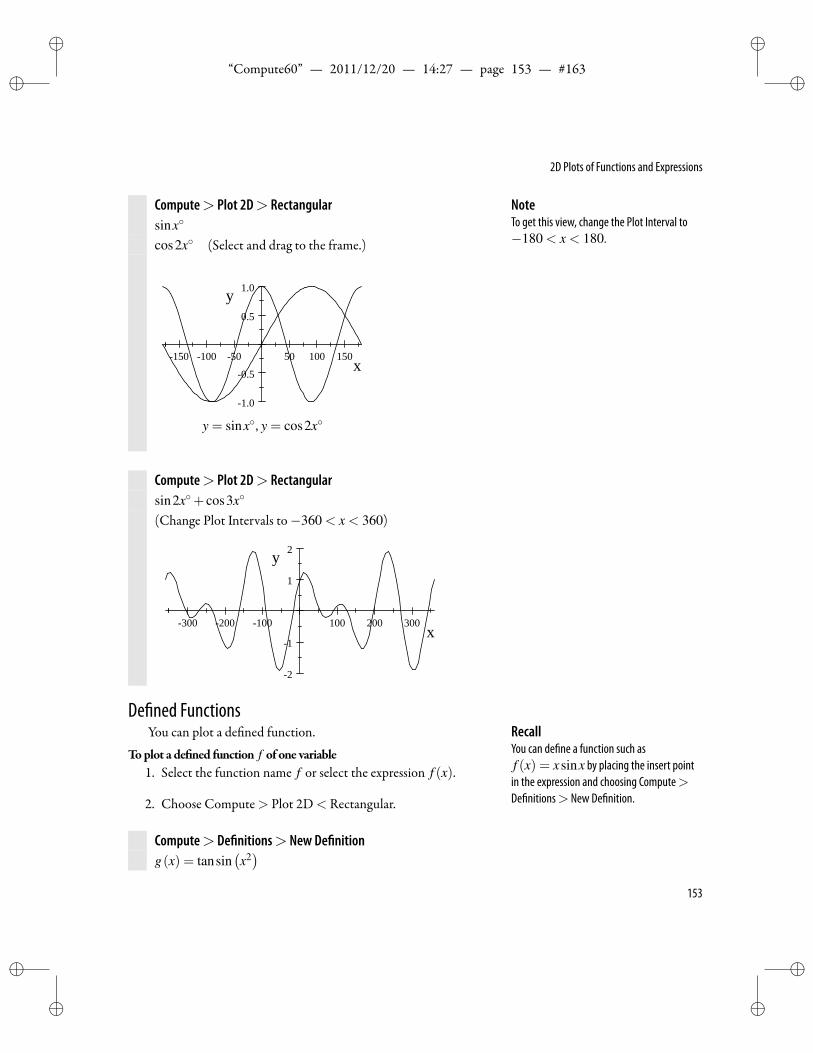
ii
“Compute60” — 2011/12/20 — 14:27 — page 153 — #163 ii
ii
ii
2D Plots of Functions and Expressions
Compute> Plot 2D> Rectangularsinx
cos2x (Select and drag to the frame.)
150 100 50 50 100 150
1.0
0.5
0.5
1.0
x
y
y = sinx, y = cos2x
NoteTo get this view, change the Plot Interval to−180 < x < 180.
Compute> Plot 2D> Rectangularsin2x+ cos3x
(Change Plot Intervals to−360 < x < 360)
300 200 100 100 200 300
2
1
1
2
x
y
De ned FunctionsYou can plot a de ned function. Recall
You can de ne a function such asf (x) = xsinx by placing the insert pointin the expression and choosing Compute>De nitions> New De nition.
Toplot a de ned function f of one variable1. Select the function name f or select the expression f (x).
2. Choose Compute> Plot 2D< Rectangular.
Compute> De nitions> New De nitiong(x) = tansin
(x2)
153
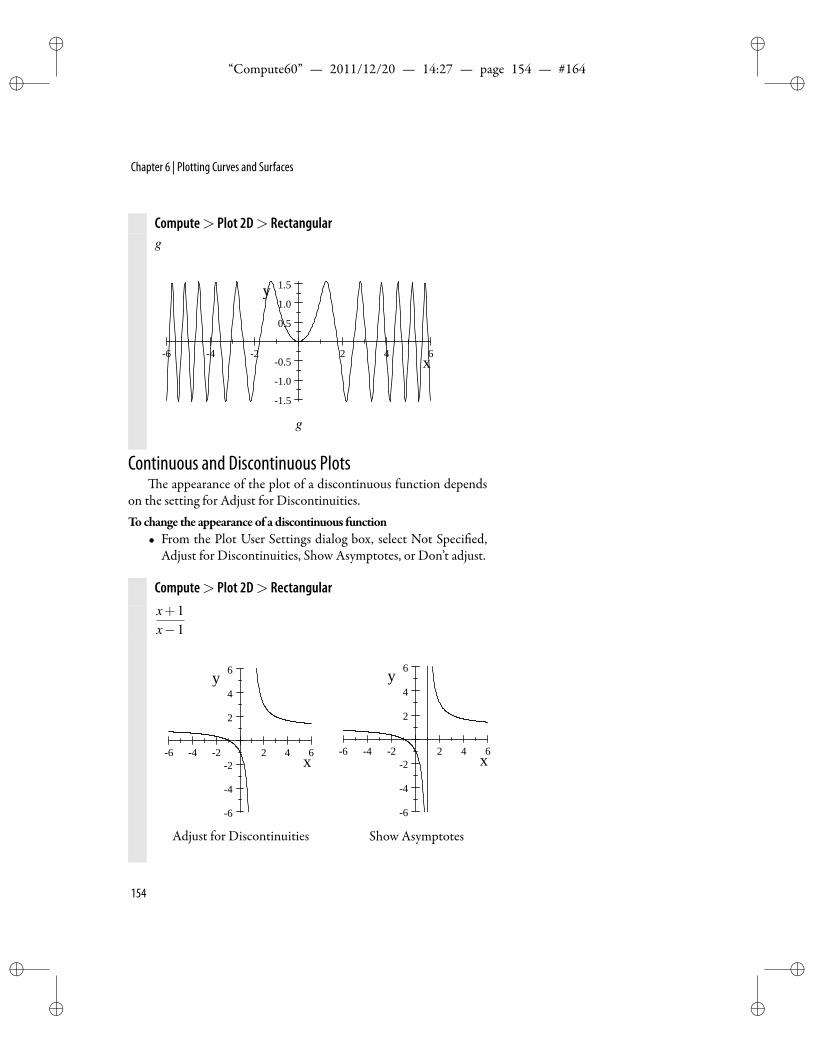
ii
“Compute60” — 2011/12/20 — 14:27 — page 154 — #164 ii
ii
ii
Chapter 6 | Plotting Curves and Surfaces
Compute> Plot 2D> Rectangularg
6 4 2 2 4 6
1.5
1.0
0.5
0.5
1.0
1.5
x
y
g
Continuous and Discontinuous Plotse appearance of the plot of a discontinuous function depends
on the setting for Adjust for Discontinuities.Tochange the appearance of a discontinuous function
• From the Plot User Settings dialog box, select Not Speci ed,Adjust for Discontinuities, Show Asymptotes, or Don’t adjust.
Compute> Plot 2D> Rectangularx+1x−1
6 4 2 2 4 6
6
4
2
2
4
6
x
y
Adjust for Discontinuities
6 4 2 2 4 6
6
4
2
2
4
6
x
y
Show Asymptotes
154
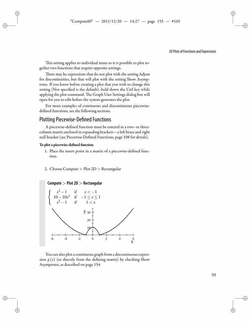
ii
“Compute60” — 2011/12/20 — 14:27 — page 155 — #165 ii
ii
ii
2D Plots of Functions and Expressions
is setting applies to individual items so it is possible to plot to-gether two functions that require opposite settings.
ere may be expressions that do not plot with the setting Adjustfor discontinuities, but that will plot with the setting Show Asymp-totes. If you know before creating a plot that you wish to change thissetting (Not speci ed is the default), hold down the Ctrl key whileapplying the plot command. e Graph User Settings dialog box willopen for you to edit before the system generates the plot.
For more examples of continuous and discontinuous piecewise-de ned functions, see the following sections.
Plotting Piecewise-De ned FunctionsA piecewise-de ned function must be entered in a two- or three-
column matrix enclosed in expanding brackets—a le brace and rightnull bracket (see Piecewise-De ned Functions, page 108 for details).
Toplot a piecewise-de ned function1. Place the insert point in a matrix of a piecewise-de ned func-
tion.
2. Choose Compute> Plot 2D> Rectangular
Compute> Plot 2D> Rectangular x2−1 if x <−110−10x2 if −1≤ x≤ 1
x2−1 if 1 < x
6 4 2 0 2 4 6
10
20
30
x
y
You can also plot a continuous graph from a discontinuous expres-sion g(x) (or directly from the de ning matrix) by checking ShowAsymptotes, as described on page 154.
155
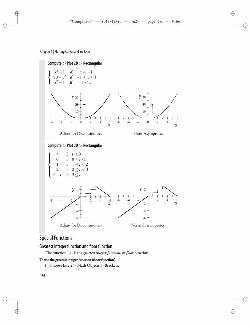
ii
“Compute60” — 2011/12/20 — 14:27 — page 156 — #166 ii
ii
ii
Chapter 6 | Plotting Curves and Surfaces
Compute> Plot 2D> Rectangular x2−1 if x <−120− x2 if −1≤ x≤ 1x2−1 if 1 < x
6 4 2 0 2 4 6
10
20
30
x
y
Adjust for Discontinuities
6 4 2 0 2 4 6
10
20
30
x
y
Show Asymptotes
Compute> Plot 2D> Rectangulart if t < 00 if 0≤ t < 11 if 1≤ t < 22 if 2≤ t < 3
6− t if 3≤ t
6 4 2 2 4 6
6
4
2
2
x
y
Adjust for Discontinuities
6 4 2 2 4 6
6
4
2
2
x
y
Vertical Asymptotes
Special FunctionsGreatest integer function and oor function
e function ⌊x⌋ is the greatest integer function, or oor function.
Touse the greatest integer function ( oor function)1. Choose Insert>Math Objects> Brackets.
156
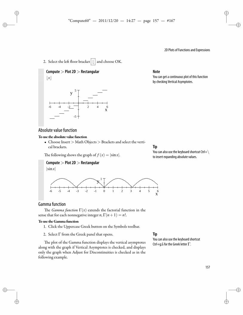
ii
“Compute60” — 2011/12/20 — 14:27 — page 157 — #167 ii
ii
ii
2D Plots of Functions and Expressions
2. Select the le oor bracket ⌊ and choose OK.
Compute> Plot 2D> Rectangular⌊x⌋
6 4 2 2 4 6
5
5
x
y
NoteYou can get a continuous plot of this functionby checking Vertical Asymptotes.
Absolute value functionTouse the absolute value function
• Choose Insert>Math Objects> Brackets and select the verti-cal brackets. Tip
You can also use the keyboard shortcut Ctrl+\to insert expanding absolute values.e following shows the graph of f (x) = |sinx|.
Compute> Plot 2D> Rectangular|sinx|
6 5 4 3 2 1 0 1 2 3 4 5 6
1
x
y
Gamma functione Gamma function Γ(x) extends the factorial function in the
sense that for each nonnegative integer n, Γ(n+1) = n!.Touse theGamma function
1. Click the Uppercase Greek button on the Symbols toolbar.
2. Select Γ from the Greek panel that opens. TipYou can also use the keyboard shortcutCtrl+g,G for the Greek letterΓ.e plot of the Gamma function displays the vertical asymptotes
along with the graph if Vertical Asymptotes is checked, and displaysonly the graph when Adjust for Discontinuities is checked as in thefollowing example.
157
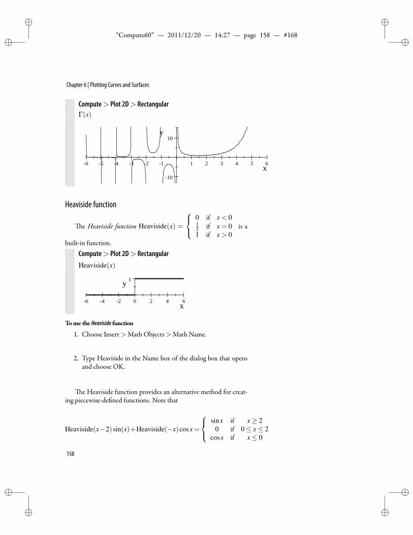
ii
“Compute60” — 2011/12/20 — 14:27 — page 158 — #168 ii
ii
ii
Chapter 6 | Plotting Curves and Surfaces
Compute> Plot 2D> RectangularΓ(x)
6 5 4 3 2 1 1 2 3 4 5 6
10
10
x
y
Heaviside function
e Heaviside function Heaviside(x) =
0 if x < 012 if x = 01 if x > 0
is a
built-in function.Compute> Plot 2D> RectangularHeaviside(x)
6 4 2 0 2 4 6
1
x
y
Touse the Heaviside function
1. Choose Insert>Math Objects>Math Name.
2. Type Heaviside in the Name box of the dialog box that opensand choose OK.
e Heaviside function provides an alternative method for creat-ing piecewise-de ned functions. Note that
Heaviside(x−2)sin(x)+Heaviside(−x)cosx=
sinx if x≥ 20 if 0≤ x≤ 2
cosx if x≤ 0
158
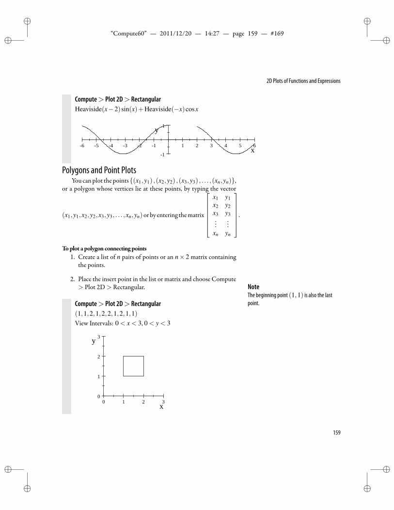
ii
“Compute60” — 2011/12/20 — 14:27 — page 159 — #169 ii
ii
ii
2D Plots of Functions and Expressions
Compute> Plot 2D> RectangularHeaviside(x−2)sin(x)+Heaviside(−x)cosx
6 5 4 3 2 1 1 2 3 4 5 6
1
1
x
y
Polygons and Point PlotsYoucanplot thepoints(x1,y1) ,(x2,y2) ,(x3,y3) , . . . ,(xn,yn),
or a polygon whose vertices lie at these points, by typing the vector
(x1,y1,x2,y2,x3,y3, . . . ,xn,yn)orby entering thematrix
x1 y1x2 y2x3 y3...
...xn yn
.
Toplot a polygon connecting points1. Create a list of n pairs of points or an n× 2 matrix containing
the points.
2. Place the insert point in the list or matrix and choose Compute> Plot 2D> Rectangular. Note
The beginning point (1,1) is also the lastpoint.Compute> Plot 2D> Rectangular
(1,1,2,1,2,2,1,2,1,1)View Intervals: 0 < x < 3, 0 < y < 3
0 1 2 30
1
2
3
x
y
159
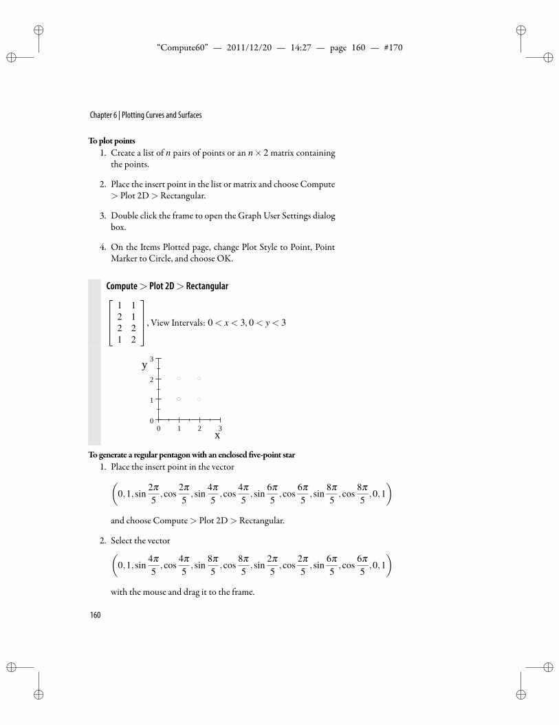
ii
“Compute60” — 2011/12/20 — 14:27 — page 160 — #170 ii
ii
ii
Chapter 6 | Plotting Curves and Surfaces
Toplot points1. Create a list of n pairs of points or an n× 2 matrix containing
the points.
2. Place the insert point in the list or matrix and choose Compute> Plot 2D> Rectangular.
3. Double click the frame to open the Graph User Settings dialogbox.
4. On the Items Plotted page, change Plot Style to Point, PointMarker to Circle, and choose OK.
Compute> Plot 2D> Rectangular1 12 12 21 2
, View Intervals: 0 < x < 3, 0 < y < 3
0 1 2 30
1
2
3
x
y
Togenerate a regular pentagonwith an enclosed ve-point star1. Place the insert point in the vector(
0,1,sin2π5,cos
2π5,sin
4π5,cos
4π5,sin
6π5,cos
6π5,sin
8π5,cos
8π5,0,1
)and choose Compute> Plot 2D> Rectangular.
2. Select the vector(0,1,sin
4π5,cos
4π5,sin
8π5,cos
8π5,sin
2π5,cos
2π5,sin
6π5,cos
6π5,0,1
)with the mouse and drag it to the frame.
160
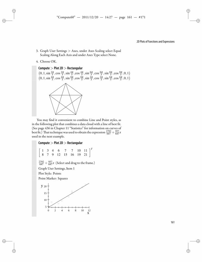
ii
“Compute60” — 2011/12/20 — 14:27 — page 161 — #171 ii
ii
ii
2D Plots of Functions and Expressions
3. Graph User Settings > Axes, under Axes Scaling select EqualScaling Along Each Axis and under Axes Type select None.
4. Choose OK.
Compute> Plot 2D> Rectangular(0,1,sin 2π
5 ,cos 2π5 ,sin 4π
5 ,cos 4π5 ,sin 6π
5 ,cos 6π5 ,sin 8π
5 ,cos 8π5 ,0,1
)(0,1,sin 4π
5 ,cos 4π5 ,sin 8π
5 ,cos 8π5 ,sin 2π
5 ,cos 2π5 ,sin 6π
5 ,cos 6π5 ,0,1
)
You may nd it convenient to combine Line and Point styles, asin the following plot that combines a data cloud with a line of best t.(See page 436 in Chapter 11 “Statistics” for information on curves ofbest t.) at techniquewas used toobtain the expression 2792
647 + 957647 x
used in the next example.
Compute> Plot 2D> Rectangular[1 3 4 6 7 7 10 118 7 9 12 15 16 19 21
]T
2792647 + 957
647 x (Select and drag to the frame.)
Graph User Settings, Item 1Plot Style: PointsPoint Marker: Squares
0 2 4 6 8 10 125
10
15
20
x
y
161
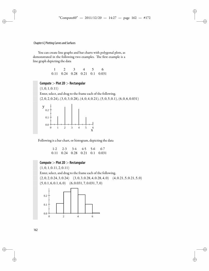
ii
“Compute60” — 2011/12/20 — 14:27 — page 162 — #172 ii
ii
ii
Chapter 6 | Plotting Curves and Surfaces
You can create line graphs and bar charts with polygonal plots, asdemonstrated in the following two examples. e rst example is aline graph depicting the data
1 2 3 4 5 60.11 0.24 0.28 0.21 0.1 0.031
Compute> Plot 2D> Rectangular(1,0,1,0.11)Enter, select, and drag to the frame each of the following.(2,0,2,0.24), (3,0,3,0.28), (4,0,4,0.21), (5,0,5,0.1), (6,0,6,0.031)
0 1 2 3 4 5 60.0
0.1
0.2
x
y
Following is a bar chart, or histogram, depicting the data
1-2 2-3 3-4 4-5 5-6 6-70.11 0.24 0.28 0.21 0.1 0.031
Compute> Plot 2D> Rectangular(1,0,1,0.11,2,0.11)Enter, select, and drag to the frame each of the following.(2,0,2,0.24,3,0.24) (3,0,3,0.28,4,0.28,4,0) (4,0.21,5,0.21,5,0)(5,0.1,6,0.1,6,0) (6,0.031,7,0.031,7,0)
0 2 4 60.0
0.1
0.2
162
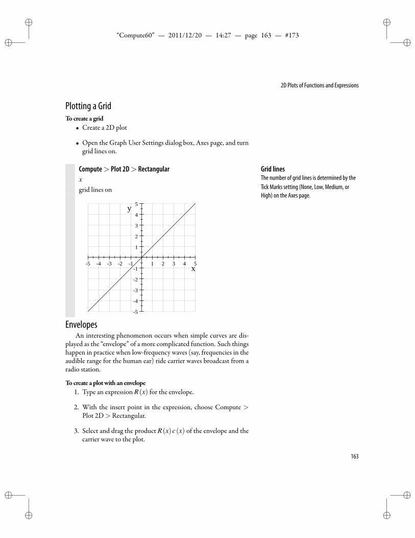
ii
“Compute60” — 2011/12/20 — 14:27 — page 163 — #173 ii
ii
ii
2D Plots of Functions and Expressions
Plotting a GridTocreate a grid
• Create a 2D plot
• Open the Graph User Settings dialog box, Axes page, and turngrid lines on.
Compute> Plot 2D> Rectangularxgrid lines on
5 4 3 2 1 1 2 3 4 5
5
4
3
2
1
1
2
3
4
5
x
y
Grid linesThe number of grid lines is determined by theTick Marks setting (None, Low, Medium, orHigh) on the Axes page.
EnvelopesAn interesting phenomenon occurs when simple curves are dis-
played as the “envelope” of a more complicated function. Such thingshappen in practice when low-frequency waves (say, frequencies in theaudible range for the human ear) ride carrier waves broadcast from aradio station.
Tocreate a plotwith an envelope1. Type an expression R(x) for the envelope.
2. With the insert point in the expression, choose Compute >Plot 2D> Rectangular.
3. Select and drag the product R(x)c(x) of the envelope and thecarrier wave to the plot.
163
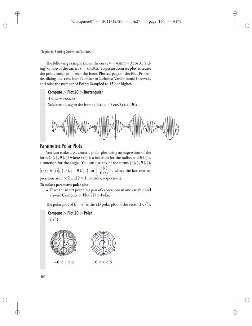
ii
“Compute60” — 2011/12/20 — 14:27 — page 164 — #174 ii
ii
ii
Chapter 6 | Plotting Curves and Surfaces
e following example shows the curve y= 4sinx+3cos3x “rid-ing” on top of the carrier y = sin30x. To get an accurate plot, increasethe point sampled—from the Items Plotted page of the Plot Proper-ties dialog box, raise ItemNumber to 2, chooseVariables and Intervals,and raise the number of Points Sampled to 150 or higher.
Compute> Plot 2D> Rectangular4sinx+3cos3xSelect and drag to the frame (4sinx+3cos3x)sin30x
6 5 4 3 2 1 1 2 3 4 5 6
5
5
x
y
Parametric Polar PlotsYou can make a parametric polar plot using an expression of the
form (r (t) ,θ (t)) where r (t) is a function for the radius and θ (t) isa function for the angle. You can use any of the forms (r (t) ,θ (t)),
[r (t) ,θ (t)],(
r (t) θ (t)), or
[r (t)θ (t)
], where the last two ex-
pressions are 1×2 and 2×1 matrices, respectively.Tomake a parametric polar plot
• Place the insert point in a pair of expressions in one variable andchoose Compute> Plot 2D> Polar.
e polar plot of θ = r2 is the 2D polar plot of the vector(r,r2).
Compute> Plot 2D> Polar(r,r2)
5 5
5
5
x
y
−6 < r < 6
5 5
5
5
x
y
0 < r < 6
164
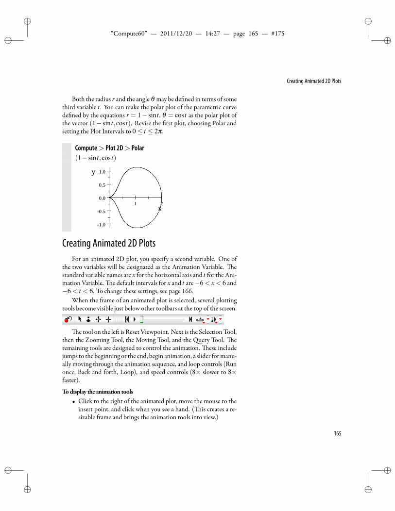
ii
“Compute60” — 2011/12/20 — 14:27 — page 165 — #175 ii
ii
ii
Creating Animated 2D Plots
Both the radius r and the angle θ may be de ned in terms of somethird variable t . You can make the polar plot of the parametric curvede ned by the equations r = 1− sin t , θ = cos t as the polar plot ofthe vector (1− sin t,cos t). Revise the rst plot, choosing Polar andsetting the Plot Intervals to 0≤ t ≤ 2π .
Compute> Plot 2D> Polar(1− sin t,cos t)
1 2
1.0
0.5
0.0
0.5
1.0
x
y
Creating Animated 2D PlotsFor an animated 2D plot, you specify a second variable. One of
the two variables will be designated as the Animation Variable. estandard variable names are x for the horizontal axis and t for the Ani-mation Variable. e default intervals for x and t are−6 < x < 6 and−6 < t < 6. To change these settings, see page 166.
When the frame of an animated plot is selected, several plottingtools become visible just below other toolbars at the top of the screen.
e tool on the le is Reset Viewpoint. Next is the SelectionTool,then the Zooming Tool, the Moving Tool, and the uery Tool. eremaining tools are designed to control the animation. ese includejumps to the beginning or the end, begin animation, a slider formanu-ally moving through the animation sequence, and loop controls (Runonce, Back and forth, Loop), and speed controls (8× slower to 8×faster).
Todisplay the animation tools• Click to the right of the animated plot, move the mouse to the
insert point, and click when you see a hand. ( is creates a re-sizable frame and brings the animation tools into view.)
165
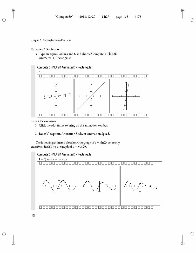
ii
“Compute60” — 2011/12/20 — 14:27 — page 166 — #176 ii
ii
ii
Chapter 6 | Plotting Curves and Surfaces
Tocreate a 2Danimation• Type an expression in x and t , and choose Compute> Plot 2D
Animated> Rectangular.
Compute> Plot 2D Animated> Rectangularxt
Toedit the animation
1. Click the plot.frame to bring up the animation toolbar.
2. Reset Viewpoint, Animation Style, or Animation Speed.
e following animatedplot shows the graphofy= sin2x smoothlytransform itself into the graph of y = cos3x.
Compute> Plot 2D Animated> Rectangular(1− t)sin2x+ t cos3x
166
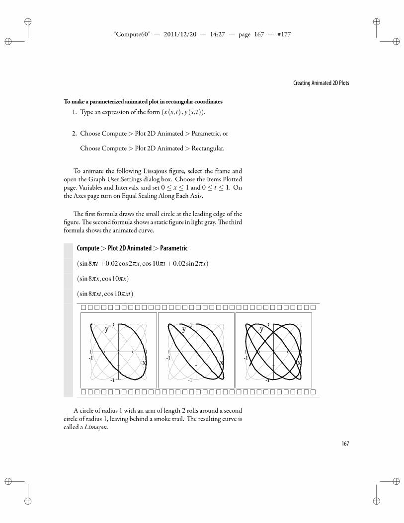
ii
“Compute60” — 2011/12/20 — 14:27 — page 167 — #177 ii
ii
ii
Creating Animated 2D Plots
Tomake a parameterized animatedplot in rectangular coordinates
1. Type an expression of the form (x(s, t) ,y(s, t)).
2. Choose Compute> Plot 2D Animated> Parametric, or
Choose Compute> Plot 2D Animated> Rectangular.
To animate the following Lissajous gure, select the frame andopen the Graph User Settings dialog box. Choose the Items Plottedpage, Variables and Intervals, and set 0 ≤ x ≤ 1 and 0 ≤ t ≤ 1. Onthe Axes page turn on Equal Scaling Along Each Axis.
e rst formula draws the small circle at the leading edge of thegure. e second formula shows a static gure in light gray. e third
formula shows the animated curve.
Compute> Plot 2D Animated> Parametric
(sin8πt +0.02cos2πx,cos10πt +0.02sin2πx)
(sin8πx,cos10πx)
(sin8πxt,cos10πxt)
1 1
1
1
x
y
1 1
1
1
x
y
1 1
1
1
x
y
A circle of radius 1 with an arm of length 2 rolls around a secondcircle of radius 1, leaving behind a smoke trail. e resulting curve iscalled a Limaçon.
167
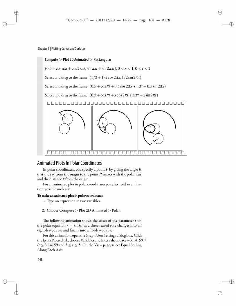
ii
“Compute60” — 2011/12/20 — 14:27 — page 168 — #178 ii
ii
ii
Chapter 6 | Plotting Curves and Surfaces
Compute> Plot 2D Animated> Rectangular
(0.5+ cosπxt + cos2πxt,sinπxt + sin2πxt), 0 < x < 1, 0 < t < 2
Select and drag to the frame: (1/2+1/2cos2πx,1/2sin2πx)
Select and drag to the frame: (0.5+ cosπt +0.5cos2πx,sinπt +0.5sin2πx)
Select and drag to the frame: (0.5+ cosπt + xcos2πt,sinπt + xsin2πt)
Animated Plots In Polar CoordinatesIn polar coordinates, you specify a point P by giving the angle θ
that the ray from the origin to the point P makes with the polar axisand the distance r from the origin.
For an animated plot in polar coordinates you also need an anima-tion variable such as t .
Tomake an animatedplot in polar coordinates1. Type an expression in two variables.
2. Choose Compute> Plot 2D Animated> Polar.
e following animation shows the effect of the parameter t onthe polar equation r = sinθ t as a three-leaved rose changes into aneight-leaved rose and nally into a ve-leaved rose.
For this animation, open theGraphUser Settings dialogbox. Clickthe ItemsPlotted tab, chooseVariables and Intervals, and set−3.14159≤θ ≤ 3.14159 and 3≤ t ≤ 5. On the View page, select Equal ScalingAlong Each Axis.
168
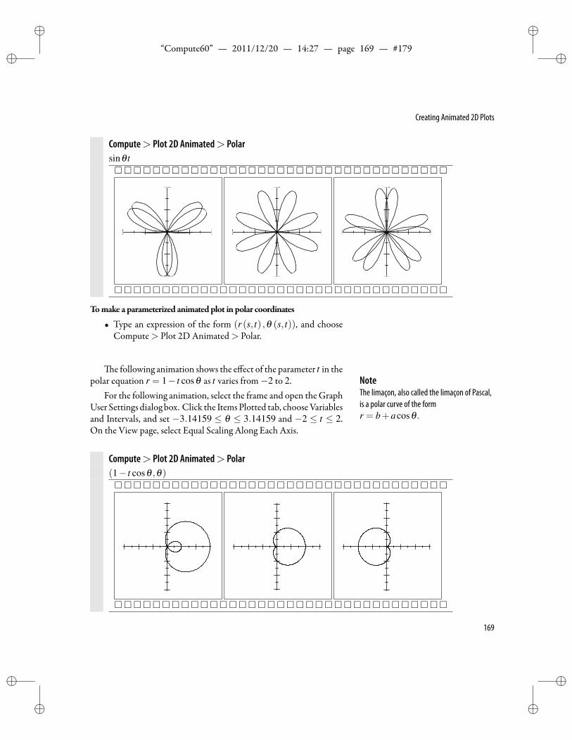
ii
“Compute60” — 2011/12/20 — 14:27 — page 169 — #179 ii
ii
ii
Creating Animated 2D Plots
Compute> Plot 2D Animated> Polarsinθ t
Tomake a parameterized animatedplot in polar coordinates
• Type an expression of the form (r (s, t) ,θ (s, t)), and chooseCompute> Plot 2D Animated> Polar.
e following animation shows the effect of the parameter t in thepolar equation r = 1− t cosθ as t varies from−2 to 2. Note
The limaçon, also called the limaçon of Pascal,is a polar curve of the formr = b+acosθ .
For the following animation, select the frame and open the GraphUser Settings dialog box. Click the ItemsPlotted tab, chooseVariablesand Intervals, and set −3.14159 ≤ θ ≤ 3.14159 and −2 ≤ t ≤ 2.On the View page, select Equal Scaling Along Each Axis.
Compute> Plot 2D Animated> Polar(1− t cosθ ,θ)
169
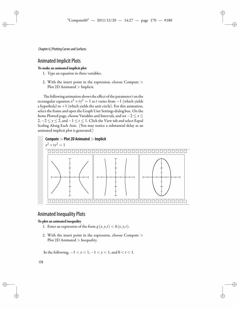
ii
“Compute60” — 2011/12/20 — 14:27 — page 170 — #180 ii
ii
ii
Chapter 6 | Plotting Curves and Surfaces
Animated Implicit PlotsTomake an animated implicit plot
1. Type an equation in three variables.
2. With the insert point in the expression, choose Compute >Plot 2D Animated> Implicit.
e following animation shows the effect of the parameter t on therectangular equation x2 + ty2 = 1 as t varies from −1 (which yieldsa hyperbola) to+1 (which yields the unit circle). For this animation,select the frame and open theGraphUser Settings dialog box. On theItems Plotted page, choose Variables and Intervals, and set−2≤ x≤2,−2≤ y≤ 2, and−1≤ t ≤ 1. Click the View tab and select EqualScaling Along Each Axis. (You may notice a substantial delay as ananimated implicit plot is generated.)
Compute> Plot 2D Animated> Implicitx2 + ty2 = 1
Animated Inequality PlotsToplot an animated inequality
1. Enter an expression of the form g(x,y, t)< h(x,y, t).
2. With the insert point in the expression, choose Compute >Plot 2D Animated> Inequality.
In the following,−1 < x < 1,−1 < y < 1, and 0 < t < 1.
170
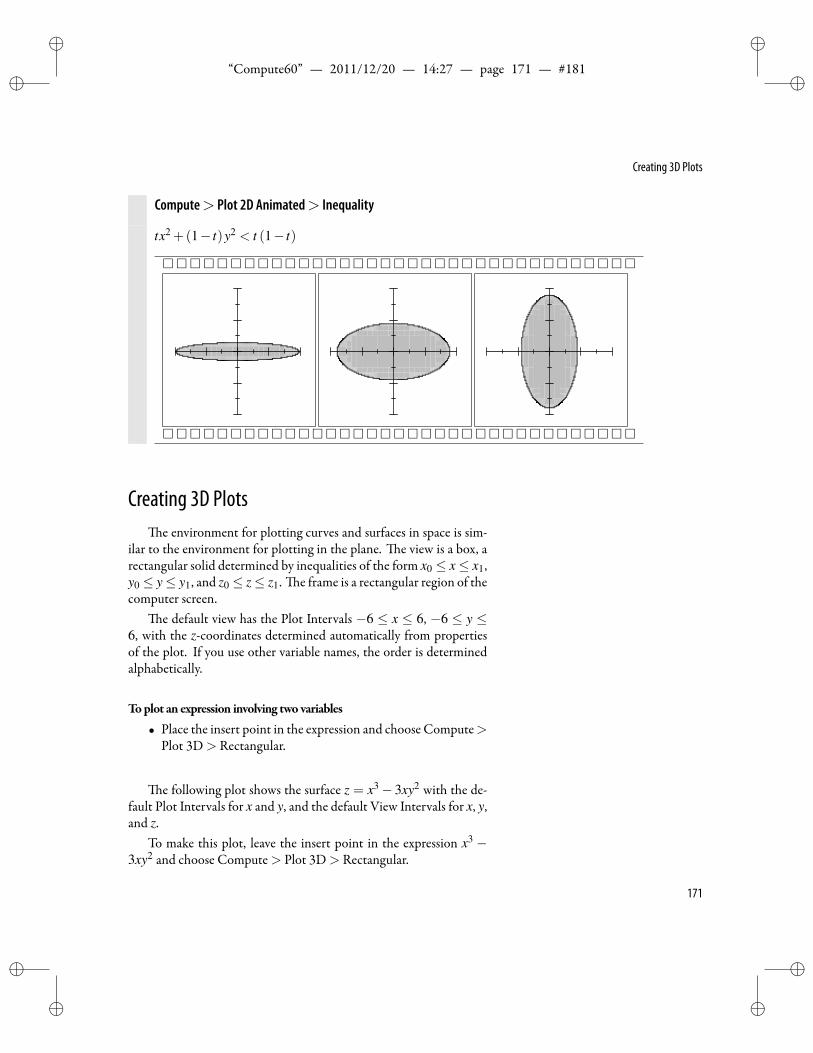
ii
“Compute60” — 2011/12/20 — 14:27 — page 171 — #181 ii
ii
ii
Creating 3D Plots
Compute> Plot 2D Animated> Inequality
tx2 +(1− t)y2 < t (1− t)
Creating 3D Plotse environment for plotting curves and surfaces in space is sim-
ilar to the environment for plotting in the plane. e view is a box, arectangular solid determined by inequalities of the form x0 ≤ x≤ x1,y0 ≤ y≤ y1, and z0 ≤ z≤ z1. e frame is a rectangular region of thecomputer screen.
e default view has the Plot Intervals −6 ≤ x ≤ 6, −6 ≤ y ≤6, with the z-coordinates determined automatically from propertiesof the plot. If you use other variable names, the order is determinedalphabetically.
Toplot an expression involving two variables
• Place the insert point in the expression and choose Compute>Plot 3D> Rectangular.
e following plot shows the surface z = x3− 3xy2 with the de-fault Plot Intervals for x and y, and the default View Intervals for x, y,and z.
To make this plot, leave the insert point in the expression x3 −3xy2 and choose Compute> Plot 3D> Rectangular.
171
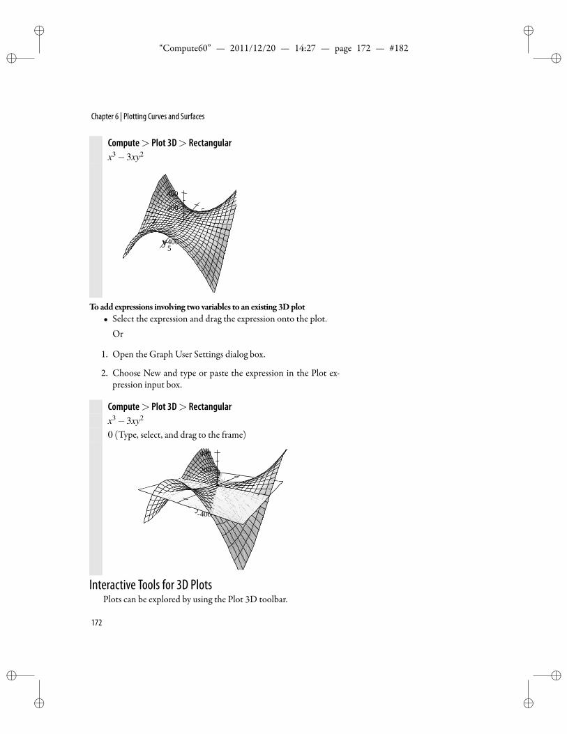
ii
“Compute60” — 2011/12/20 — 14:27 — page 172 — #182 ii
ii
ii
Chapter 6 | Plotting Curves and Surfaces
Compute> Plot 3D> Rectangularx3−3xy2
5
400200
z
y0
0
5x
0
200 5
5
400
Toadd expressions involving two variables to an existing 3Dplot• Select the expression and drag the expression onto the plot.
Or
1. Open the Graph User Settings dialog box.
2. Choose New and type or paste the expression in the Plot ex-pression input box.
Compute> Plot 3D> Rectangularx3−3xy2
0 (Type, select, and drag to the frame)
5
400y200
z 00
5 x0
5
200
5
400
Interactive Tools for 3D PlotsPlots can be explored by using the Plot 3D toolbar.
172
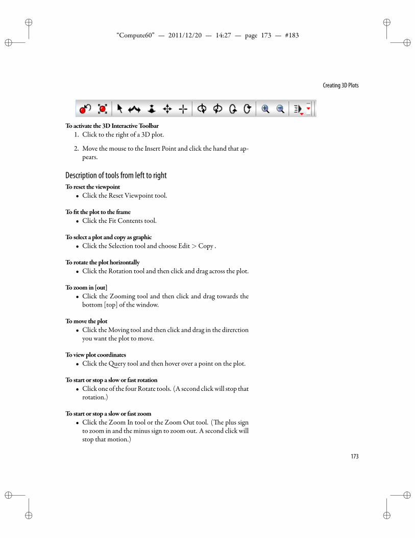
ii
“Compute60” — 2011/12/20 — 14:27 — page 173 — #183 ii
ii
ii
Creating 3D Plots
Toactivate the 3DInteractiveToolbar1. Click to the right of a 3D plot.
2. Move the mouse to the Insert Point and click the hand that ap-pears.
Description of tools from left to rightTo reset the viewpoint
• Click the Reset Viewpoint tool.
To t the plot to the frame• Click the Fit Contents tool.
To select a plot and copy as graphic• Click the Selection tool and choose Edit>Copy .
To rotate the plot horizontally• Click the Rotation tool and then click and drag across the plot.
Tozoom in [out]• Click the Zooming tool and then click and drag towards the
bottom [top] of the window.
Tomove the plot• Click theMoving tool and then click and drag in the direrction
you want the plot to move.
Toviewplot coordinates• Click the uery tool and then hover over a point on the plot.
To start or stop a slowor fast rotation• Click one of the fourRotate tools. (A second clickwill stop that
rotation.)
To start or stop a slowor fast zoom• Click the Zoom In tool or the Zoom Out tool. ( e plus sign
to zoom in and theminus sign to zoom out. A second click willstop that motion.)
173
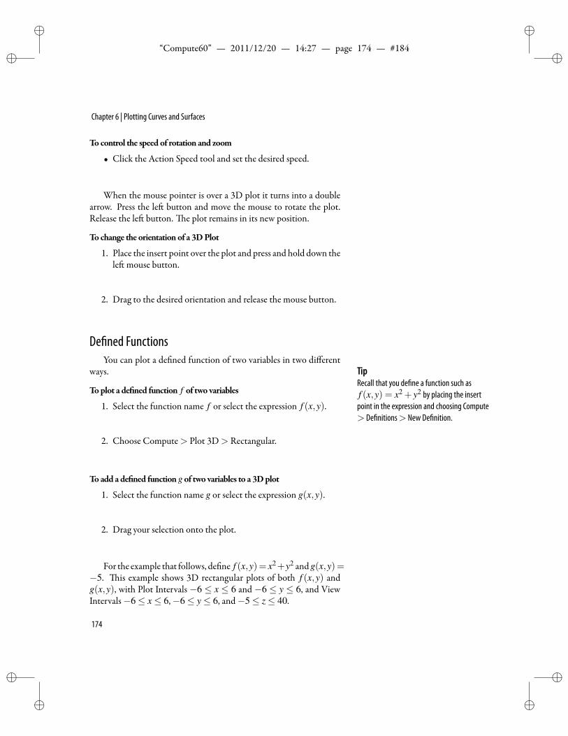
ii
“Compute60” — 2011/12/20 — 14:27 — page 174 — #184 ii
ii
ii
Chapter 6 | Plotting Curves and Surfaces
Tocontrol the speedof rotation and zoom
• Click the Action Speed tool and set the desired speed.
When the mouse pointer is over a 3D plot it turns into a doublearrow. Press the le button and move the mouse to rotate the plot.Release the le button. e plot remains in its new position.
Tochange the orientationof a 3DPlot
1. Place the insert point over the plot and press and hold down thele mouse button.
2. Drag to the desired orientation and release the mouse button.
De ned FunctionsYou can plot a de ned function of two variables in two different
ways. TipRecall that you de ne a function such asf (x,y) = x2 + y2 by placing the insertpoint in the expression and choosing Compute> De nitions> New De nition.
Toplot a de ned function f of two variables
1. Select the function name f or select the expression f (x,y).
2. Choose Compute> Plot 3D> Rectangular.
Toadd ade ned functiongof two variables to a 3Dplot
1. Select the function name g or select the expression g(x,y).
2. Drag your selection onto the plot.
For the example that follows, de ne f (x,y)= x2+y2 andg(x,y)=−5. is example shows 3D rectangular plots of both f (x,y) andg(x,y), with Plot Intervals −6 ≤ x ≤ 6 and −6 ≤ y ≤ 6, and ViewIntervals−6≤ x≤ 6,−6≤ y≤ 6, and−5≤ z≤ 40.
174
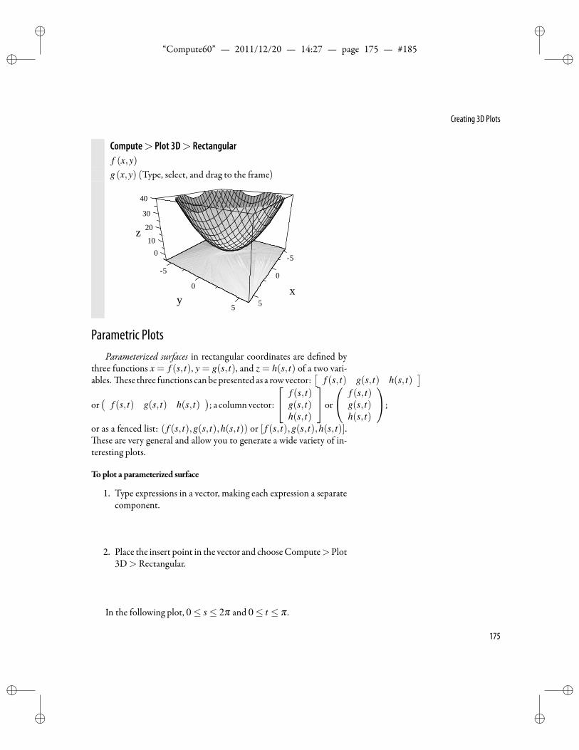
ii
“Compute60” — 2011/12/20 — 14:27 — page 175 — #185 ii
ii
ii
Creating 3D Plots
Compute> Plot 3D> Rectangularf (x,y)g(x,y) (Type, select, and drag to the frame)
010
5
20z
30
40
y0
5
5
x0
5
Parametric PlotsParameterized surfaces in rectangular coordinates are de ned by
three functions x = f (s, t), y = g(s, t), and z = h(s, t) of a two vari-ables. ese three functions canbepresented as a rowvector:
[f (s, t) g(s, t) h(s, t)
]or(
f (s, t) g(s, t) h(s, t)); a columnvector:
f (s, t)g(s, t)h(s, t)
or
f (s, t)g(s, t)h(s, t)
;
or as a fenced list: ( f (s, t),g(s, t),h(s, t)) or [ f (s, t),g(s, t),h(s, t)].ese are very general and allow you to generate a wide variety of in-
teresting plots.
Toplot a parameterized surface
1. Type expressions in a vector, making each expression a separatecomponent.
2. Place the insert point in the vector and chooseCompute>Plot3D> Rectangular.
In the following plot, 0≤ s≤ 2π and 0≤ t ≤ π .
175
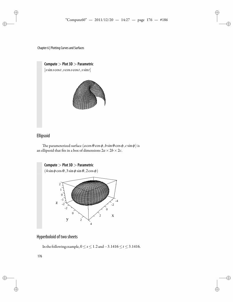
ii
“Compute60” — 2011/12/20 — 14:27 — page 176 — #186 ii
ii
ii
Chapter 6 | Plotting Curves and Surfaces
Compute> Plot 3D> Parametric[ssinscos t,scosscos t,ssin t]
Ellipsoid
e parameterized surface (acosθ cosϕ ,bsinθ cosϕ ,csinϕ) isan ellipsoid that ts in a box of dimensions 2a×2b×2c.
Compute> Plot 3D> Parametric(4sinϕ cosθ ,3sinϕ sinθ ,2cosϕ)
12
20
02
y 22 x
4
4
z
01
2
Hyperboloid of two sheets
In the following example,0≤ s≤ 1.2 and−3.1416≤ t ≤ 3.1416.
176
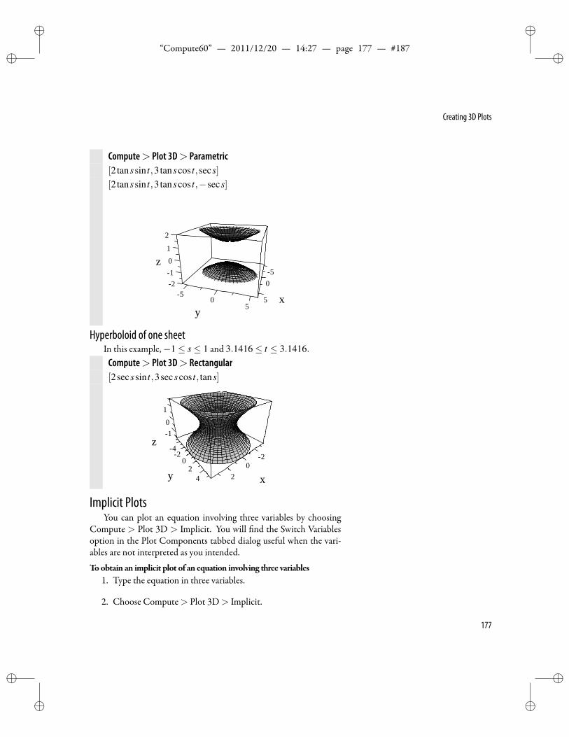
ii
“Compute60” — 2011/12/20 — 14:27 — page 177 — #187 ii
ii
ii
Creating 3D Plots
Compute> Plot 3D> Parametric[2tanssin t,3tanscos t,secs][2tanssin t,3tanscos t,−secs]
50
xy
50
55
210z1
2
Hyperboloid of one sheetIn this example,−1≤ s≤ 1 and 3.1416≤ t ≤ 3.1416.Compute> Plot 3D> Rectangular[2secssin t,3secscos t, tans]
1
01
42
z
y0
24 2
0
x
2
Implicit PlotsYou can plot an equation involving three variables by choosing
Compute > Plot 3D > Implicit. You will nd the Switch Variablesoption in the Plot Components tabbed dialog useful when the vari-ables are not interpreted as you intended.
Toobtain an implicit plot of an equation involving three variables1. Type the equation in three variables.
2. Choose Compute> Plot 3D> Implicit.
177
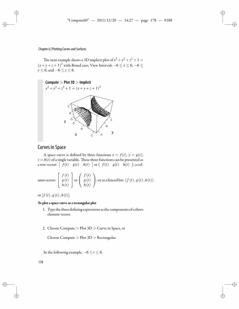
ii
“Compute60” — 2011/12/20 — 14:27 — page 178 — #188 ii
ii
ii
Chapter 6 | Plotting Curves and Surfaces
e next example shows a 3D implicit plot of x2 + y2 + z2 +1 =
(x+ y+ z+1)2 with Boxed axes, View Intervals−6≤ x≤ 6,−6≤y≤ 6, and−6≤ z≤ 6.
Compute> Plot 3D> Implicitx2 + y2 + z2 +1 = (x+ y+ z+1)2
5
y0
5
0
z
x
5
0
5
5
5
Curves in SpaceA space curve is de ned by three functions x = f (t), y = g(t),
z = h(t) of a single variable. ese three functions can be presented asa row vector:
[f (t) g(t) h(t)
]or(
f (t) g(t) h(t)); a col-
umnvector:
f (t)g(t)h(t)
or
f (t)g(t)h(t)
; or as a fenced list: ( f (t) ,g(t) ,h(t))
or [ f (t) ,g(t) ,h(t)].
Toplot a space curve as a rectangular plot
1. Type the threede ning expressions as the components of a three-element vector.
2. Choose Compute> Plot 3D>Curve in Space, or
Choose Compute> Plot 3D> Rectangular.
In the following example,−6≤ t ≤ 6.
178
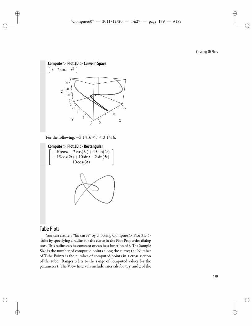
ii
“Compute60” — 2011/12/20 — 14:27 — page 179 — #189 ii
ii
ii
Creating 3D Plots
Compute> Plot 3D> Curve in Space[t 2sin t t2
]
20
10
02
z
30
1 5
00
y x1
52
For the following,−3.1416≤ t ≤ 3.1416.
Compute> Plot 3D> Rectangular −10cos t−2cos(5t)+15sin(2t)−15cos(2t)+10sin t−2sin(5t)
10cos(3t)
Tube PlotsYou can create a “fat curve” by choosing Compute > Plot 3D >
Tube by specifying a radius for the curve in the Plot Properties dialogbox. is radius can be constant or can be a function of t . e SampleSize is the number of computed points along the curve; the Numberof Tube Points is the number of computed points in a cross sectionof the tube. Ranges refers to the range of computed values for theparameter t . e View Intervals include intervals for x, y, and z of the
179
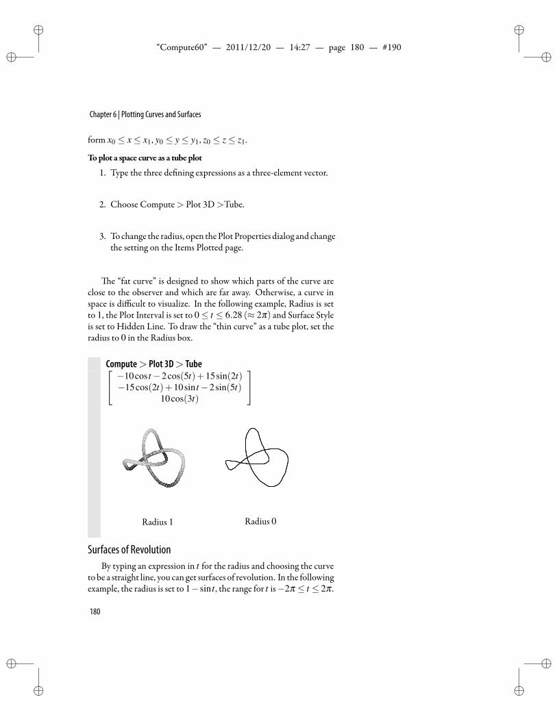
ii
“Compute60” — 2011/12/20 — 14:27 — page 180 — #190 ii
ii
ii
Chapter 6 | Plotting Curves and Surfaces
form x0 ≤ x≤ x1, y0 ≤ y≤ y1, z0 ≤ z≤ z1.
Toplot a space curve as a tube plot
1. Type the three de ning expressions as a three-element vector.
2. Choose Compute> Plot 3D>Tube.
3. To change the radius, open thePlotProperties dialog and changethe setting on the Items Plotted page.
e “fat curve” is designed to show which parts of the curve areclose to the observer and which are far away. Otherwise, a curve inspace is difficult to visualize. In the following example, Radius is setto 1, the Plot Interval is set to 0≤ t ≤ 6.28 (≈ 2π) and Surface Styleis set to Hidden Line. To draw the “thin curve” as a tube plot, set theradius to 0 in the Radius box.
Compute> Plot 3D> Tube −10cos t−2cos(5t)+15sin(2t)−15cos(2t)+10sin t−2sin(5t)
10cos(3t)
Radius 1 Radius 0
Surfaces of RevolutionBy typing an expression in t for the radius and choosing the curve
tobe a straight line, you can get surfaces of revolution. In the followingexample, the radius is set to 1−sin t , the range for t is−2π ≤ t ≤ 2π .
180
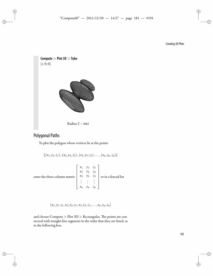
ii
“Compute60” — 2011/12/20 — 14:27 — page 181 — #191 ii
ii
ii
Creating 3D Plots
Compute> Plot 3D> Tube(t,0,0)
Radius 2− sin t
Polygonal PathsTo plot the polygon whose vertices lie at the points
(x1,y1,z1) ,(x2,y2,z2) ,(x3,y3,z3) , . . . ,(xn,yn,zn)
enter the three-column matrix
x1 y1 z1x2 y2 z2x3 y3 z3...
......
xn yn zn
or in a fenced list
(x1,y1,z1,x2,y2,z1,x3,y3,z1, . . . ,xn,yn,zn)
and choose Compute> Plot 3D> Rectangular. e points are con-nected with straight-line segments in the order that they are listed, asin the following box.
181
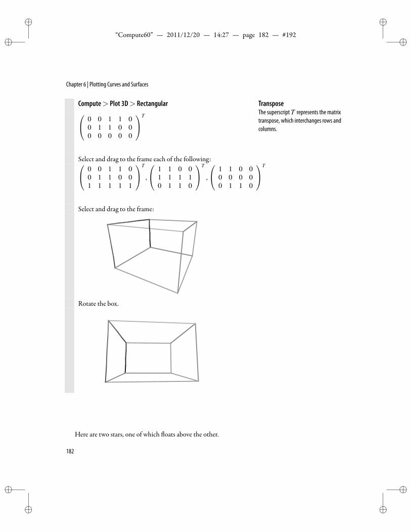
ii
“Compute60” — 2011/12/20 — 14:27 — page 182 — #192 ii
ii
ii
Chapter 6 | Plotting Curves and Surfaces
Compute> Plot 3D> Rectangular 0 0 1 1 00 1 1 0 00 0 0 0 0
T
Select and drag to the frame each of the following: 0 0 1 1 00 1 1 0 01 1 1 1 1
T
,
1 1 0 01 1 1 10 1 1 0
T
,
1 1 0 00 0 0 00 1 1 0
T
Select and drag to the frame:
Rotate the box.
TransposeThe superscriptT represents the matrixtranspose, which interchanges rows andcolumns.
Here are two stars, one of which oats above the other.
182
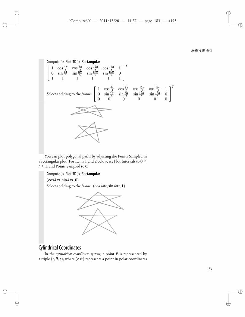
ii
“Compute60” — 2011/12/20 — 14:27 — page 183 — #193 ii
ii
ii
Creating 3D Plots
Compute> Plot 3D> Rectangular 1 cos 4π5 cos 8π
5 cos 12π5 cos 16π
5 10 sin 4π
5 sin 8π5 sin 12π
5 sin 16π5 0
1 1 1 1 1 1
T
Select and drag to the frame:
1 cos 4π5 cos 8π
5 cos 12π5 cos 16π
5 10 sin 4π
5 sin 8π5 sin 12π
5 sin 16π5 0
0 0 0 0 0 0
T
You can plot polygonal paths by adjusting the Points Sampled ina rectangular plot. For Items 1 and 2 below, set Plot Intervals to 0 ≤t ≤ 1, and Points Sampled to 6.
Compute> Plot 3D> Rectangular(cos4πt,sin4πt,0)Select and drag to the frame: (cos4πt,sin4πt,1)
Cylindrical CoordinatesIn the cylindrical coordinate system, a point P is represented by
a triple (r,θ ,z), where (r,θ) represents a point in polar coordinates
183
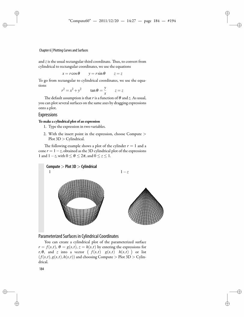
ii
“Compute60” — 2011/12/20 — 14:27 — page 184 — #194 ii
ii
ii
Chapter 6 | Plotting Curves and Surfaces
and z is the usual rectangular third coordinate. us, to convert fromcylindrical to rectangular coordinates, we use the equations
x = r cosθ y = r sinθ z = z
To go from rectangular to cylindrical coordinates, we use the equa-tions
r2 = x2 + y2 tanθ =yx
z = z
e default assumption is that r is a function of θ and z. As usual,you can plot several surfaces on the same axes by dragging expressionsonto a plot.
ExpressionsTomake a cylindrical plot of an expression
1. Type the expression in two variables.
2. With the insert point in the expression, choose Compute >Plot 3D>Cylindrical.
e following example shows a plot of the cylinder r = 1 and acone r = 1− z, obtained as the 3D cylindrical plot of the expressions1 and 1− z, with 0≤ θ ≤ 2π , and 0≤ z≤ 1.
Compute> Plot 3D> Cylindrical1 1− z
Parameterized Surfaces in Cylindrical CoordinatesYou can create a cylindrical plot of the parameterized surface
r = f (s, t), θ = g(s, t), z = h(s, t) by entering the expressions forr,θ , and z into a vector
(f (s, t) g(s, t) h(s, t)
)or list
( f (s, t),g(s, t),h(s, t)) and choosing Compute > Plot 3D > Cylin-drical.
184
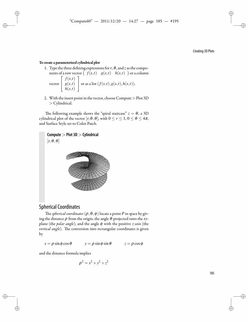
ii
“Compute60” — 2011/12/20 — 14:27 — page 185 — #195 ii
ii
ii
Creating 3D Plots
Tocreate a parameterized cylindrical plot1. Type the three de ning expressions for r, θ , and z as the compo-
nents of a row vector(
f (s, t) g(s, t) h(s, t))or a column
vector
f (s, t)g(s, t)h(s, t)
or as a list ( f (s, t),g(s, t),h(s, t)).
2. With the insert point in the vector, chooseCompute>Plot 3D>Cylindrical.
e following example shows the “spiral staircase” z = θ , a 3Dcylindrical plot of the vector [r,θ ,θ ], with 0 ≤ r ≤ 1, 0 ≤ θ ≤ 4π ,and Surface Style set to Color Patch.
Compute> Plot 3D> Cylindrical[r,θ ,θ ]
Spherical Coordinatese spherical coordinates (ρ,θ ,ϕ) locate a point P in space by giv-
ing the distance ρ from the origin, the angle θ projected onto the xy-plane (the polar angle), and the angle ϕ with the positive z-axis (thevertical angle). e conversion into rectangular coordinates is givenby
x = ρ sinϕ cosθ y = ρ sinϕ sinθ z = ρ cosϕ
and the distance formula implies
ρ2 = x2 + y2 + z2
185
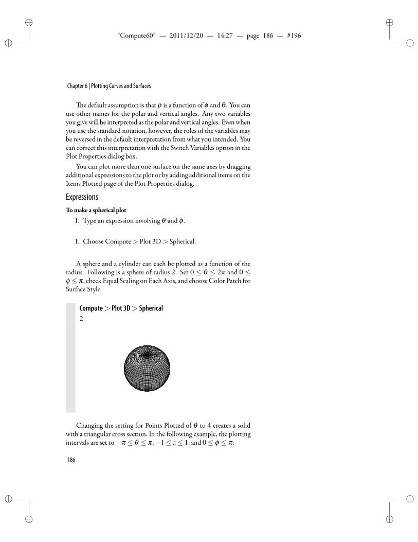
ii
“Compute60” — 2011/12/20 — 14:27 — page 186 — #196 ii
ii
ii
Chapter 6 | Plotting Curves and Surfaces
e default assumption is that ρ is a function of ϕ and θ . You canuse other names for the polar and vertical angles. Any two variablesyou givewill be interpreted as the polar and vertical angles. Evenwhenyou use the standard notation, however, the roles of the variables maybe reversed in the default interpretation fromwhat you intended. Youcan correct this interpretation with the Switch Variables option in thePlot Properties dialog box.
You can plot more than one surface on the same axes by draggingadditional expressions to the plot or by adding additional items on theItems Plotted page of the Plot Properties dialog.
ExpressionsTomake a spherical plot
1. Type an expression involving θ and ϕ .
1. Choose Compute> Plot 3D> Spherical.
A sphere and a cylinder can each be plotted as a function of theradius. Following is a sphere of radius 2. Set 0 ≤ θ ≤ 2π and 0 ≤ϕ ≤ π , check Equal Scaling on EachAxis, and chooseColor Patch forSurface Style.
Compute> Plot 3D> Spherical2
Changing the setting for Points Plotted of θ to 4 creates a solidwith a triangular cross section. In the following example, the plottingintervals are set to−π ≤ θ ≤ π ,−1≤ z≤ 1, and 0≤ ϕ ≤ π .
186
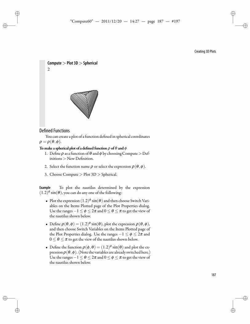
ii
“Compute60” — 2011/12/20 — 14:27 — page 187 — #197 ii
ii
ii
Creating 3D Plots
Compute> Plot 3D> Spherical2
De ned FunctionsYou can create a plot of a function de ned in spherical coordinates
ρ = ρ(θ ,ϕ).Tomake a spherical plot of a de ned functionρ ofθ andϕ
1. De neρ as a function ofθ andϕ by choosingCompute>Def-initions>New De nition.
2. Select the function name ρ or select the expression ρ(θ ,ϕ).
3. Choose Compute> Plot 3D> Spherical.
Example To plot the nautilus determined by the expression(1.2)ϕ sin(θ), you can do any one of the following:
• Plot the expression (1.2)ϕ sin(θ) and then choose SwitchVari-ables on the Items Plotted page of the Plot Properties dialog.Use the ranges−1≤ ϕ ≤ 2π and 0≤ θ ≤ π to get the view ofthe nautilus shown below.
• De ne ρ(θ ,ϕ) = (1.2)ϕ sin(θ), plot the expression ρ(θ ,ϕ),and then choose Switch Variables on the Items Plotted page ofthe Plot Properties dialog. Use the ranges −1 ≤ ϕ ≤ 2π and0≤ θ ≤ π to get the view of the nautilus shown below.
• De ne the function ρ(ϕ ,θ) = (1.2)ϕ sin(θ) and plot the ex-pressionρ(θ ,ϕ). (Note the variables are already switchedhere.)Use the ranges−1≤ θ ≤ 2π and 0≤ ϕ ≤ π to get the view ofthe nautilus shown below.
187
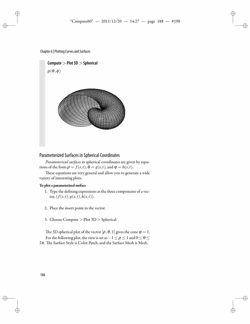
ii
“Compute60” — 2011/12/20 — 14:27 — page 188 — #198 ii
ii
ii
Chapter 6 | Plotting Curves and Surfaces
Compute> Plot 3D> Spherical
ρ(θ ,ϕ)
Parameterized Surfaces in Spherical CoordinatesParameterized surfaces in spherical coordinates are given by equa-
tions of the form ρ = f (s, t), θ = g(s, t), and φ = h(s, t).ese equations are very general and allow you to generate a wide
variety of interesting plots.
Toplot a parameterized surface1. Type the de ning expressions as the three components of a vec-
tor, ( f (s, t),g(s, t),h(s, t)).
2. Place the insert point in the vector.
3. Choose Compute> Plot 3D> Spherical.
e 3D spherical plot of the vector [ρ,θ ,1] gives the cone φ = 1.For the following plot, the view is set as−1≤ ρ ≤ 1 and 0≤ θ ≤
2π . e Surface Style is Color Patch, and the Surface Mesh is Mesh.
188
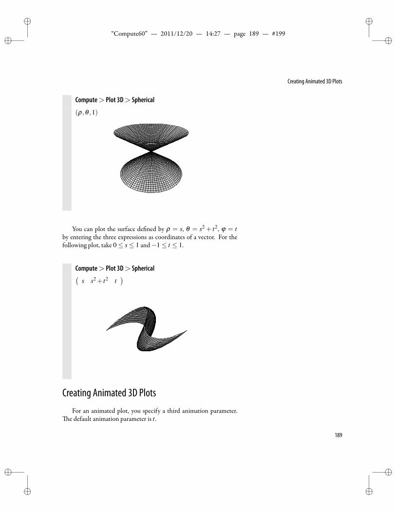
ii
“Compute60” — 2011/12/20 — 14:27 — page 189 — #199 ii
ii
ii
Creating Animated 3D Plots
Compute> Plot 3D> Spherical
(ρ,θ ,1)
You can plot the surface de ned by ρ = s, θ = s2 + t2, φ = tby entering the three expressions as coordinates of a vector. For thefollowing plot, take 0≤ s≤ 1 and−1≤ t ≤ 1.
Compute> Plot 3D> Spherical(s s2 + t2 t
)
Creating Animated 3D PlotsFor an animated plot, you specify a third animation parameter.
e default animation parameter is t .
189
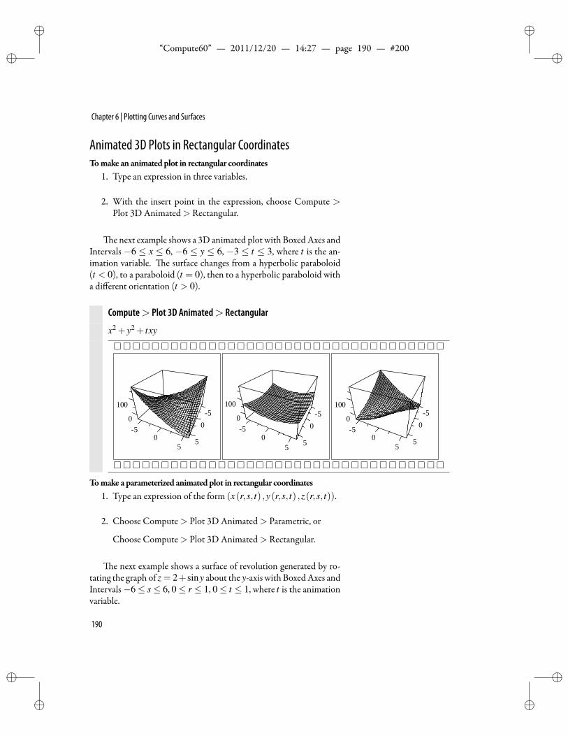
ii
“Compute60” — 2011/12/20 — 14:27 — page 190 — #200 ii
ii
ii
Chapter 6 | Plotting Curves and Surfaces
Animated 3D Plots in Rectangular CoordinatesTomake an animatedplot in rectangular coordinates
1. Type an expression in three variables.
2. With the insert point in the expression, choose Compute >Plot 3D Animated> Rectangular.
e next example shows a 3D animated plot with Boxed Axes andIntervals −6 ≤ x ≤ 6, −6 ≤ y ≤ 6, −3 ≤ t ≤ 3, where t is the an-imation variable. e surface changes from a hyperbolic paraboloid(t < 0), to a paraboloid (t = 0), then to a hyperbolic paraboloid witha different orientation (t > 0).
Compute> Plot 3D Animated> Rectangular
x2 + y2 + txy
550
50
05
100
50
0
100
5 5
50
505
505
0
100
Tomake a parameterized animatedplot in rectangular coordinates
1. Type an expression of the form (x(r,s, t) ,y(r,s, t) ,z(r,s, t)).
2. Choose Compute> Plot 3D Animated> Parametric, or
Choose Compute> Plot 3D Animated> Rectangular.
e next example shows a surface of revolution generated by ro-tating the graph of z = 2+siny about the y-axis with BoxedAxes andIntervals−6≤ s≤ 6, 0≤ r ≤ 1, 0≤ t ≤ 1, where t is the animationvariable.
190
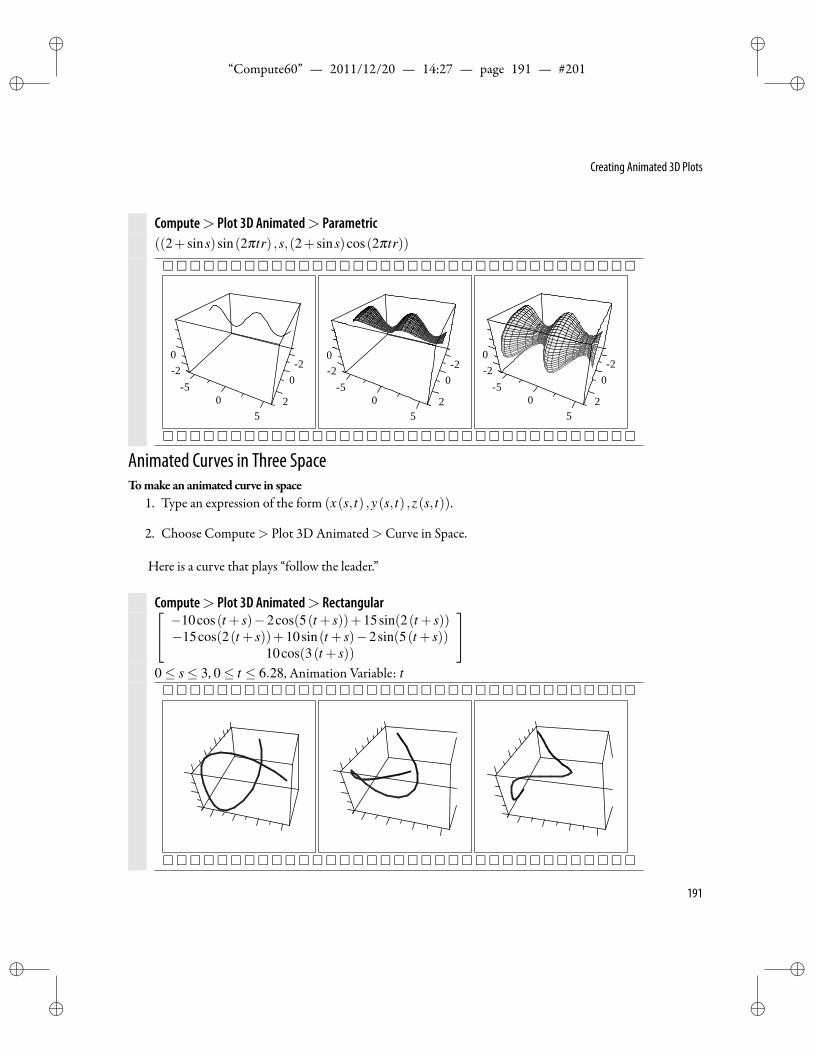
ii
“Compute60” — 2011/12/20 — 14:27 — page 191 — #201 ii
ii
ii
Creating Animated 3D Plots
Compute> Plot 3D Animated> Parametric((2+ sins)sin(2πtr) ,s,(2+ sins)cos(2πtr))
20
0
52
205
0
05
2 20
52
02
5
20
25
0
Animated Curves in Three SpaceTomake an animated curve in space
1. Type an expression of the form (x(s, t) ,y(s, t) ,z(s, t)).
2. Choose Compute> Plot 3D Animated>Curve in Space.
Here is a curve that plays “follow the leader.”
Compute> Plot 3D Animated> Rectangular −10cos(t + s)−2cos(5(t + s))+15sin(2(t + s))−15cos(2(t + s))+10sin(t + s)−2sin(5(t + s))
10cos(3(t + s))
0≤ s≤ 3, 0≤ t ≤ 6.28, Animation Variable: t
191
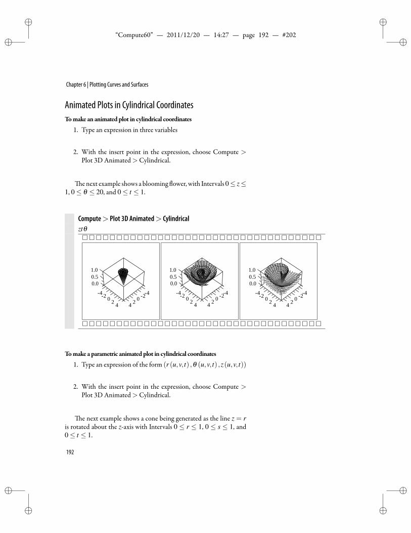
ii
“Compute60” — 2011/12/20 — 14:27 — page 192 — #202 ii
ii
ii
Chapter 6 | Plotting Curves and Surfaces
Animated Plots in Cylindrical CoordinatesTomake an animatedplot in cylindrical coordinates
1. Type an expression in three variables
2. With the insert point in the expression, choose Compute >Plot 3D Animated>Cylindrical.
e next example shows a blooming ower, with Intervals0≤ z≤1, 0≤ θ ≤ 20, and 0≤ t ≤ 1.
Compute> Plot 3D Animated> Cylindricalztθ
0.00.51.0
24 420 20
4 24
0.0
42 0 2 4 4 2 0 24
0.51.0
0.0
4220
4 4 2 0 24
0.51.0
Tomake a parametric animatedplot in cylindrical coordinates
1. Type an expression of the form (r (u,v, t) ,θ (u,v, t) ,z(u,v, t))
2. With the insert point in the expression, choose Compute >Plot 3D Animated>Cylindrical.
e next example shows a cone being generated as the line z = ris rotated about the z-axis with Intervals 0 ≤ r ≤ 1, 0 ≤ s ≤ 1, and0≤ t ≤ 1.
192
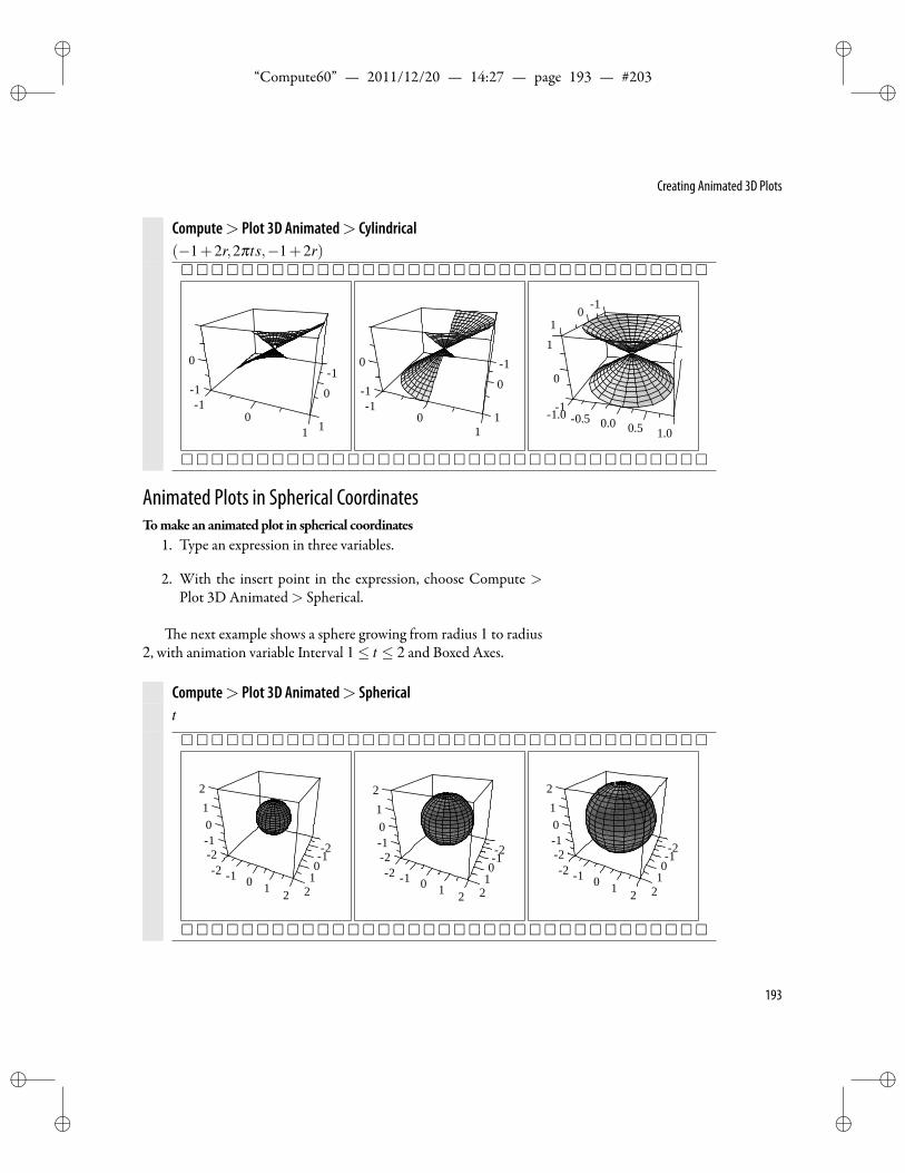
ii
“Compute60” — 2011/12/20 — 14:27 — page 193 — #203 ii
ii
ii
Creating Animated 3D Plots
Compute> Plot 3D Animated> Cylindrical(−1+2r,2πts,−1+2r)
0
0
01
1
11
10
110
0
1
11
101
1
0
0.5 1.00.00.5
11.0
Animated Plots in Spherical CoordinatesTomake an animatedplot in spherical coordinates
1. Type an expression in three variables.
2. With the insert point in the expression, choose Compute >Plot 3D Animated> Spherical.
e next example shows a sphere growing from radius 1 to radius2, with animation variable Interval 1≤ t ≤ 2 and Boxed Axes.
Compute> Plot 3D Animated> Sphericalt
12
01 0 1
122
2210
12
0012
121 2
122101
2
21
001
1 21
2
2210
12
193
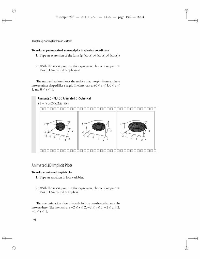
ii
“Compute60” — 2011/12/20 — 14:27 — page 194 — #204 ii
ii
ii
Chapter 6 | Plotting Curves and Surfaces
Tomake anparameterized animatedplot in spherical coordinates
1. Type an expression of the form (ρ (r,s, t) ,θ (r,s, t) ,ϕ (r,s, t))
2. With the insert point in the expression, choose Compute >Plot 3D Animated> Spherical.
e next animation shows the surface that morphs from a sphereinto a surface shaped like a bagel. e Intervals are 0≤ r≤ 1, 0≤ s≤1, and 0≤ t ≤ 1.
Compute> Plot 3D Animated> Spherical(1− t cos2πr,2πs,πr)
212 1 0 1 22
1
212
011 22
1
21
120 1 22
1
Animated 3D Implicit PlotsTomake an animated implicit plot
1. Type an equation in four variables.
2. With the insert point in the expression, choose Compute >Plot 3D Animated> Implicit.
e next animation showahyperboloidon two sheets thatmorphsinto a sphere. e intervals are−2≤ x≤ 2,−2≤ y≤ 2,−2≤ z≤ 2,−1≤ t ≤ 1.
194
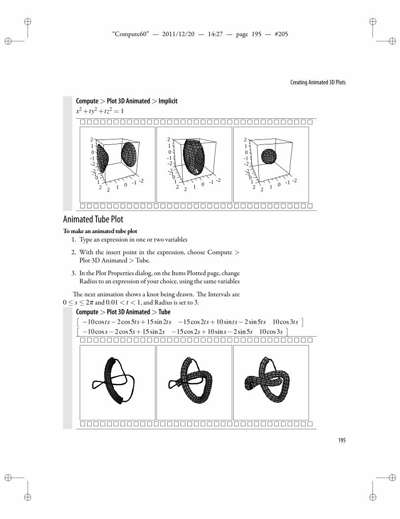
ii
“Compute60” — 2011/12/20 — 14:27 — page 195 — #205 ii
ii
ii
Creating Animated 3D Plots
Compute> Plot 3D Animated> Implicitx2 + ty2 + tz2 = 1
0 1 21
21012
212
20
121012
221012
1012
12
0
211 0
12
12
22
01
Animated Tube PlotTomake an animated tube plot
1. Type an expression in one or two variables
2. With the insert point in the expression, choose Compute >Plot 3D Animated>Tube.
3. In the Plot Properties dialog, on the Items Plotted page, changeRadius to an expression of your choice, using the same variables
e next animation shows a knot being drawn. e Intervals are0≤ s≤ 2π and 0.01 < t < 1, and Radius is set to 3.
Compute> Plot 3D Animated> Tube[−10cos ts−2cos5ts+15sin2ts −15cos2ts+10sin ts−2sin5ts 10cos3ts
][−10coss−2cos5s+15sin2s −15cos2s+10sins−2sin5s 10cos3s
]
195
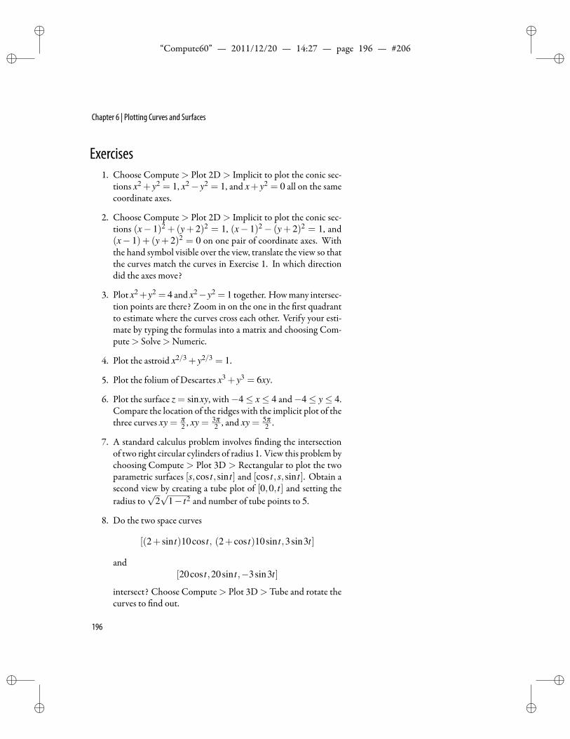
ii
“Compute60” — 2011/12/20 — 14:27 — page 196 — #206 ii
ii
ii
Chapter 6 | Plotting Curves and Surfaces
Exercises1. Choose Compute > Plot 2D > Implicit to plot the conic sec-
tions x2 + y2 = 1, x2− y2 = 1, and x+ y2 = 0 all on the samecoordinate axes.
2. Choose Compute > Plot 2D > Implicit to plot the conic sec-tions (x− 1)2 +(y+ 2)2 = 1, (x− 1)2− (y+ 2)2 = 1, and(x− 1)+ (y+ 2)2 = 0 on one pair of coordinate axes. Withthe hand symbol visible over the view, translate the view so thatthe curves match the curves in Exercise 1. In which directiondid the axes move?
3. Plot x2+y2 = 4 and x2−y2 = 1 together. Howmany intersec-tion points are there? Zoom in on the one in the rst quadrantto estimate where the curves cross each other. Verify your esti-mate by typing the formulas into a matrix and choosing Com-pute> Solve>Numeric.
4. Plot the astroid x2/3 + y2/3 = 1.
5. Plot the folium of Descartes x3 + y3 = 6xy.
6. Plot the surface z = sinxy, with−4≤ x≤ 4 and−4≤ y≤ 4.Compare the location of the ridges with the implicit plot of thethree curves xy = π
2 , xy = 3π2 , and xy = 5π
2 .
7. A standard calculus problem involves nding the intersectionof two right circular cylinders of radius 1. View this problem bychoosing Compute > Plot 3D > Rectangular to plot the twoparametric surfaces [s,cos t,sin t] and [cos t,s,sin t]. Obtain asecond view by creating a tube plot of [0,0, t] and setting theradius to
√2√
1− t2 and number of tube points to 5.
8. Do the two space curves
[(2+ sin t)10cos t, (2+ cos t)10sin t,3sin3t]
and[20cos t,20sin t,−3sin3t]
intersect? Choose Compute> Plot 3D> Tube and rotate thecurves to nd out.
196
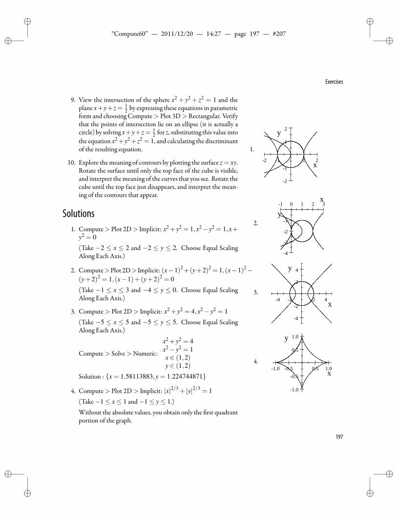
ii
“Compute60” — 2011/12/20 — 14:27 — page 197 — #207 ii
ii
ii
Exercises
9. View the intersection of the sphere x2 + y2 + z2 = 1 and theplane x+y+z = 1
2 by expressing these equations in parametricform and choosing Compute> Plot 3D>Rectangular. Verifythat the points of intersection lie on an ellipse (it is actually acircle) by solving x+y+z = 1
2 for z, substituting this value intothe equation x2+y2+z2 = 1, and calculating the discriminantof the resulting equation. 1.
2 1 1 2
2
1
1
2
x
y
10. Explore themeaning of contours by plotting the surface z = xy.Rotate the surface until only the top face of the cube is visible,and interpret themeaning of the curves that you see. Rotate thecube until the top face just disappears, and interpret the mean-ing of the contours that appear.
2.
1 0 1 2 3
4
3
2
1
x
y
3.4 2 2 4
4
2
2
4
x
y
4.1.0 0.5 0.5 1.0
1.0
0.5
0.5
1.0
x
y
Solutions1. Compute> Plot 2D> Implicit: x2+y2 = 1,x2−y2 = 1,x+
y2 = 0
(Take −2 ≤ x ≤ 2 and −2 ≤ y ≤ 2. Choose Equal ScalingAlong Each Axis.)
2. Compute>Plot 2D> Implicit: (x−1)2+(y+2)2 = 1,(x−1)2−(y+2)2 = 1,(x−1)+(y+2)2 = 0
(Take −1 ≤ x ≤ 3 and −4 ≤ y ≤ 0. Choose Equal ScalingAlong Each Axis.)
3. Compute> Plot 2D> Implicit: x2 + y2 = 4,x2− y2 = 1
(Take −5 ≤ x ≤ 5 and −5 ≤ y ≤ 5. Choose Equal ScalingAlong Each Axis.)
Compute> Solve>Numeric:
x2 + y2 = 4x2− y2 = 1x ∈ (1,2)y ∈ (1,2)
Solution : x = 1.58113883,y = 1.224744871
4. Compute> Plot 2D> Implicit: |x|2/3 + |y|2/3 = 1
(Take−1≤ x≤ 1 and−1≤ y≤ 1.)
Without the absolute values, you obtain only the rst quadrantportion of the graph.
197
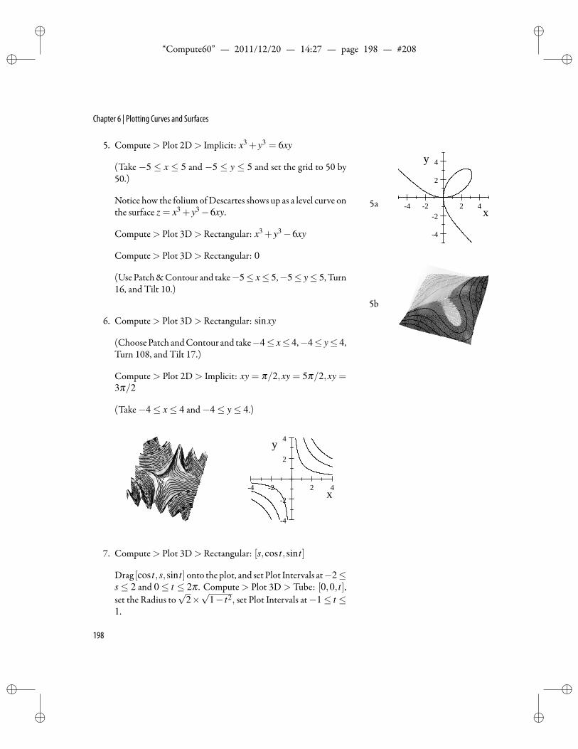
ii
“Compute60” — 2011/12/20 — 14:27 — page 198 — #208 ii
ii
ii
Chapter 6 | Plotting Curves and Surfaces
5. Compute> Plot 2D> Implicit: x3 + y3 = 6xy
(Take −5 ≤ x ≤ 5 and −5 ≤ y ≤ 5 and set the grid to 50 by50.)
5a 4 2 2 4
4
2
2
4
x
y
5b
Notice how the foliumofDescartes shows up as a level curve onthe surface z = x3 + y3−6xy.
Compute> Plot 3D> Rectangular: x3 + y3−6xy
Compute> Plot 3D> Rectangular: 0
(Use Patch&Contour and take−5≤ x≤ 5,−5≤ y≤ 5, Turn16, and Tilt 10.)
6. Compute> Plot 3D> Rectangular: sinxy
(ChoosePatch andContour and take−4≤ x≤ 4,−4≤ y≤ 4,Turn 108, and Tilt 17.)
Compute > Plot 2D > Implicit: xy = π/2,xy = 5π/2,xy =3π/2
(Take−4≤ x≤ 4 and−4≤ y≤ 4.)
4 2 2 4
4
2
2
4
x
y
7. Compute> Plot 3D> Rectangular: [s,cos t,sin t]
Drag [cos t,s,sin t]onto the plot, and set Plot Intervals at−2≤s ≤ 2 and 0 ≤ t ≤ 2π . Compute > Plot 3D > Tube: [0,0, t],set the Radius to
√2×√
1− t2, set Plot Intervals at−1≤ t ≤1.
198
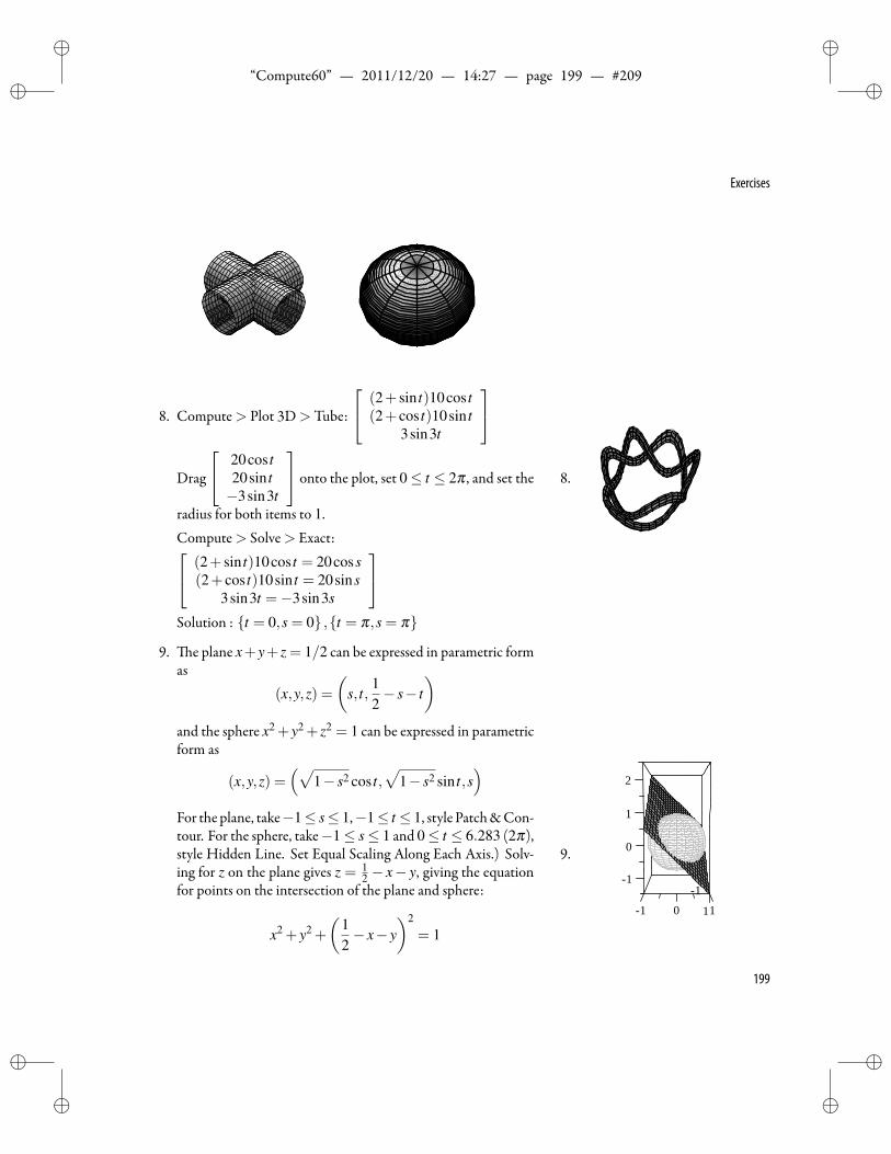
ii
“Compute60” — 2011/12/20 — 14:27 — page 199 — #209 ii
ii
ii
Exercises
8. Compute> Plot 3D>Tube:
(2+ sin t)10cos t(2+ cos t)10sin t
3sin3t
Drag
20cos t20sin t−3sin3t
onto the plot, set 0≤ t ≤ 2π , and set the 8.
radius for both items to 1.Compute> Solve> Exact: (2+ sin t)10cos t = 20coss
(2+ cos t)10sin t = 20sins3sin3t =−3sin3s
Solution : t = 0,s = 0 ,t = π,s = π
9. e plane x+y+ z = 1/2 can be expressed in parametric formas
(x,y,z) =(
s, t,12− s− t
)and the sphere x2 +y2 + z2 = 1 can be expressed in parametricform as
(x,y,z) =(√
1− s2 cos t,√
1− s2 sin t,s)
For the plane, take−1≤ s≤ 1,−1≤ t ≤ 1, style Patch&Con-tour. For the sphere, take−1≤ s≤ 1 and 0≤ t ≤ 6.283 (2π),style Hidden Line. Set Equal Scaling Along Each Axis.) Solv- 9.
01
1
1
1
1
0
2
1
ing for z on the plane gives z = 12 − x− y, giving the equation
for points on the intersection of the plane and sphere:
x2 + y2 +
(12− x− y
)2
= 1
199
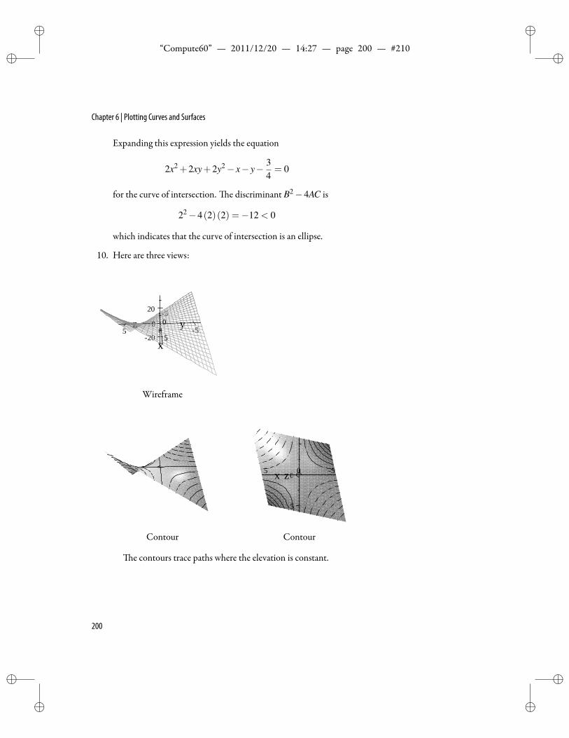
ii
“Compute60” — 2011/12/20 — 14:27 — page 200 — #210 ii
ii
ii
Chapter 6 | Plotting Curves and Surfaces
Expanding this expression yields the equation
2x2 +2xy+2y2− x− y− 34= 0
for the curve of intersection. e discriminant B2−4AC is
22−4(2)(2) =−12 < 0
which indicates that the curve of intersection is an ellipse.
10. Here are three views:
5
20
0z y
x
05
20
055
Wireframe
Contour
y5
x z05
5
0 5
Contour
e contours trace paths where the elevation is constant.
200
ii
“Compute60” — 2011/12/20 — 14:27 — page 201 — #211 ii
ii
ii
7Calculus
Nature laughs at the difficulties of integration. Pierre-Simon de Laplace (1749–1827)
T his chapter covers the standard topics from differential and Evaluating Calculus Expressions
Limits
Differentiation
Inde nite Integration
Methods of Integration
De nite Integrals
Sequences and Series
Multivariate Calculus
integral calculus, including limits, sequences, and series. enotion of a function is fundamental to the study of calculus.
Functions were introduced in Chapter 3 “Algebra,” with a descrip-tion of procedures for naming expressions and functions. Basic in-formation on working with functions and expressions is summarizedin Chapter 5 “Function De nitions,” along with additional informa-tion on storing and retrieving de nitions. In this chapter we assumethat youhave read andunderstandhow tode ne andmanipulate func-tions. We give several examples in this chapter that illustrate connec-tions between calculus and the function plots introduced in Chapter6 “Plotting Curves and Surfaces.”
Evaluating Calculus ExpressionsYou can evaluate calculus expressions in the same manner as ex-
pressions from algebra or trigonometry.New in Version 6Dot notation for derivativesSpecify center of a power seriesSpecify both dependent and independentvariables for implicit differentiation
Tocalculate a derivative or an integral1. Enter a derivative or integral in standard mathematical nota-
tion.
2. Choose Compute> Evaluate.
201
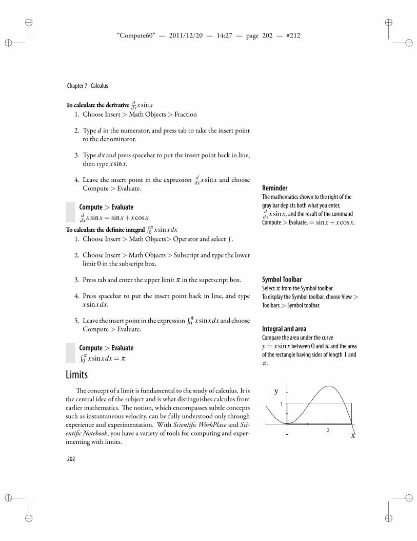
ii
“Compute60” — 2011/12/20 — 14:27 — page 202 — #212 ii
ii
ii
Chapter 7 | Calculus
Tocalculate the derivative ddx xsinx
1. Choose Insert>Math Objects> Fraction
2. Type d in the numerator, and press tab to take the insert pointto the denominator.
3. Type dx and press spacebar to put the insert point back in line,then type xsinx.
4. Leave the insert point in the expression ddx xsinx and choose
Compute> Evaluate. ReminderThe mathematics shown to the right of thegray bar depicts both what you enter,ddx xsinx, and the result of the commandCompute> Evaluate,= sinx+ xcosx.
Compute> Evaluateddx xsinx = sinx+ xcosx
Tocalculate the de nite integral∫ π
0 xsinxdx1. Choose Insert>Math Objects>Operator and select
∫.
2. Choose Insert>Math Objects> Subscript and type the lowerlimit 0 in the subscript box.
3. Press tab and enter the upper limit π in the superscript box. Symbol ToolbarSelectπ from the Symbol toolbar.To display the Symbol toolbar, choose View>Toolbars> Symbol toolbar.
4. Press spacebar to put the insert point back in line, and typexsinxdx.
5. Leave the insert point in the expression∫ π
0 xsinxdx and chooseCompute> Evaluate. Integral and area
Compare the area under the curvey = xsinx between 0 andπ and the areaof the rectangle having sides of length 1 andπ .
2
1
x
y
Compute> Evaluate∫ π0 xsinxdx = π
Limitse concept of a limit is fundamental to the study of calculus. It is
the central idea of the subject and is what distinguishes calculus fromearlier mathematics. e notion, which encompasses subtle conceptssuch as instantaneous velocity, can be fully understood only throughexperience and experimentation. With Scienti c WorkPlace and Sci-enti c Notebook, you have a variety of tools for computing and exper-imenting with limits.
202
ii
“Compute60” — 2011/12/20 — 14:27 — page 203 — #213 ii
ii
ii
Limits
Notation for Limitse limit of f as x approaches a is L, written
limx→a
f (x) = L
if for each number ε > 0 there exists a number δ > 0 such that| f (x)−L|< ϵ whenever 0 < |x−a|< δ . Informally, limx→a f (x) = L, if f (x)
gets close toL as x gets close to a.To nd a limit of the form limx→a f (x)1. Choose Insert>Math and type lim.
2. Choose Insert > Math Objects> Subscript and enter the sub-script x→ a. When you type the name lim, it will turn
from red to gray as you type the third letter.3. Press spacebar to put the insert point back in line, then type a
mathematical expression f (x).
4. Choose Compute> Evaluate.
Compute> Evaluate
limx→1
x2−1x−1 = 2
LimitThe result limx→1
x2−1x−1 = 2 is reasonable
since x = 1 implies x2−1x−1 = x+1, which
is close to 2when x is close to 1.
Limits of rational functions are not always apparent. You cannotevaluate the following expression at x = −3/2, because the denomi-nator is 0 for this value of x. e expression does, however, have a limitat−3/2.
Compute> Evaluate
limx→−3/2
4x4+6x2+19x+6x3+152x3+5x2+5x+3
=− 257
Factoring the numerator and denominator suggests a method forevaluating this limit by direct substitution.
Compute> Factor
4x4 +6x2 +19x+6x3 +15 = (2x+3)(x+1)(2x2−2x+5
)2x3 +5x2 +5x+3 = (2x+3)
(x2 + x+1
)If an expression has a removable singularity, factoring in placemay
allow you to ll in the steps leading to evaluation by direct substitu-tion. is is illustrated in the following example, where the second
203
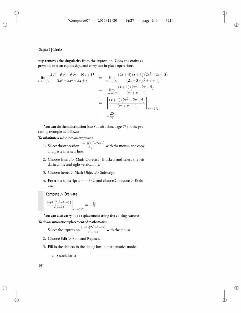
ii
“Compute60” — 2011/12/20 — 14:27 — page 204 — #214 ii
ii
ii
Chapter 7 | Calculus
step removes the singularity from the expression. Copy the entire ex-pression a er an equals sign, and carry out in-place operations.
limx→−3/2
4x4 +6x3 +6x2 +19x+152x3 +5x2 +5x+3
= limx→−3/2
(2x+3)(x+1)(2x2−2x+5
)(2x+3)(x2 + x+1)
= limx→−3/2
(x+1)(2x2−2x+5
)(x2 + x+1)
=
[(x+1)
(2x2−2x+5
)(x2 + x+1)
]x=−3/2
= −257
You can do the substitution (see Substitution, page 47) in the pre-ceding example as follows:To substitute a value into an expression
1. Select the expression(x+1)(2x2−2x+5)
x2+x+1with themouse, and copy
and paste in a new line.
2. Choose Insert > Math Objects> Brackets and select the ledashed line and right vertical line.
3. Choose Insert>Math Objects> Subscript.
4. Enter the subscript x = −3/2, and choose Compute > Evalu-ate.
Compute> Evaluate
(x+1)(2x2−2x+5)x2+x+1
∣∣∣∣x=−3/2
=− 257
You can also carry out a replacement using the editing features.Todo an automatic replacement ofmathematics
1. Select the expression(x+1)(2x2−2x+5)
x2+x+1with the mouse.
2. Choose Edit> Find and Replace.
3. Fill in the choices in the dialog box in mathematics mode.
a. Search for: x
204
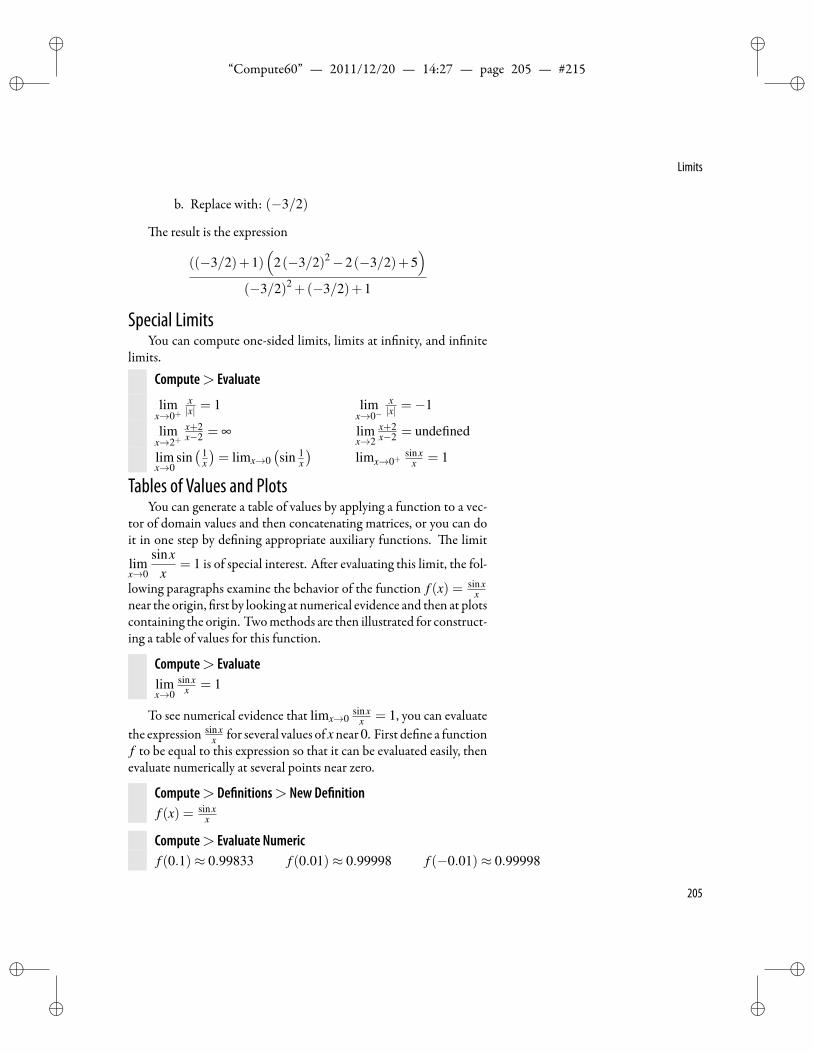
ii
“Compute60” — 2011/12/20 — 14:27 — page 205 — #215 ii
ii
ii
Limits
b. Replace with: (−3/2)
e result is the expression
((−3/2)+1)(
2(−3/2)2−2(−3/2)+5)
(−3/2)2 +(−3/2)+1
Special LimitsYou can compute one-sided limits, limits at in nity, and in nite
limits.
Compute> Evaluate
limx→0+
x|x| = 1 lim
x→0−x|x| =−1
limx→2+
x+2x−2 = ∞ lim
x→2x+2x−2 = undefined
limx→0
sin( 1
x
)= limx→0
(sin 1
x
)limx→0+
sinxx = 1
Tables of Values and PlotsYou can generate a table of values by applying a function to a vec-
tor of domain values and then concatenating matrices, or you can doit in one step by de ning appropriate auxiliary functions. e limit
limx→0
sinxx
= 1 is of special interest. A er evaluating this limit, the fol-
lowing paragraphs examine the behavior of the function f (x) = sinxx
near the origin, rst by looking at numerical evidence and then at plotscontaining the origin. Twomethods are then illustrated for construct-ing a table of values for this function.
Compute> Evaluatelimx→0
sinxx = 1
To see numerical evidence that limx→0sinx
x = 1, you can evaluatethe expression sinx
x for several values of xnear0. First de ne a functionf to be equal to this expression so that it can be evaluated easily, thenevaluate numerically at several points near zero.
Compute> De nitions> New De nitionf (x) = sinx
x
Compute> Evaluate Numericf (0.1)≈ 0.99833 f (0.01)≈ 0.99998 f (−0.01)≈ 0.99998
205
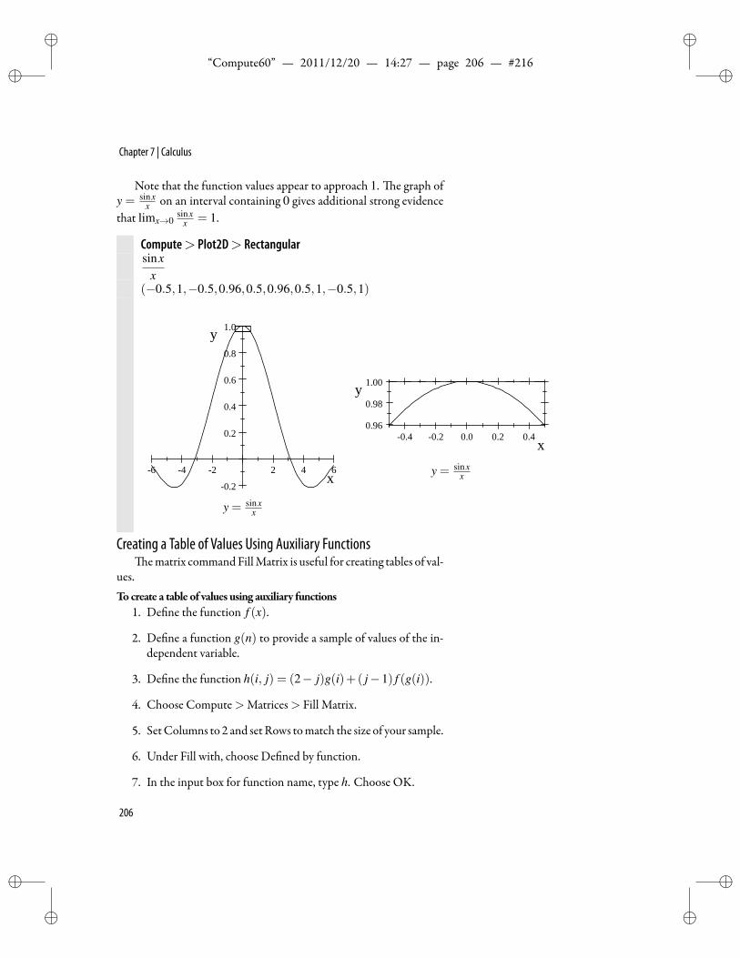
ii
“Compute60” — 2011/12/20 — 14:27 — page 206 — #216 ii
ii
ii
Chapter 7 | Calculus
Note that the function values appear to approach 1. e graph ofy = sinx
x on an interval containing 0 gives additional strong evidencethat limx→0
sinxx = 1.
Compute> Plot2D> Rectangularsinx
x(−0.5,1,−0.5,0.96,0.5,0.96,0.5,1,−0.5,1)
6 4 2 2 4 6
0.2
0.2
0.4
0.6
0.8
1.0
x
y
y = sinxx
0.4 0.2 0.0 0.2 0.40.96
0.98
1.00
x
y
y = sinxx
Creating a Table of Values Using Auxiliary Functionsematrix commandFillMatrix is useful for creating tables of val-
ues.Tocreate a table of values using auxiliary functions
1. De ne the function f (x).
2. De ne a function g(n) to provide a sample of values of the in-dependent variable.
3. De ne the function h(i, j) = (2− j)g(i)+( j−1) f (g(i)).
4. Choose Compute>Matrices> Fill Matrix.
5. SetColumns to 2 and setRows tomatch the size of your sample.
6. Under Fill with, choose De ned by function.
7. In the input box for function name, type h. Choose OK.
206
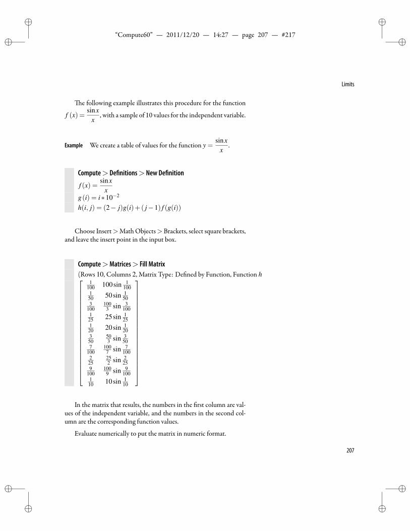
ii
“Compute60” — 2011/12/20 — 14:27 — page 207 — #217 ii
ii
ii
Limits
e following example illustrates this procedure for the function
f (x) =sinx
x, with a sample of 10 values for the independent variable.
Example We create a table of values for the function y =sinx
x.
Compute> De nitions> New De nition
f (x) =sinx
xg(i) = i∗10−2
h(i, j) = (2− j)g(i)+( j−1) f (g(i))
Choose Insert>MathObjects>Brackets, select square brackets,and leave the insert point in the input box.
Compute>Matrices> Fill Matrix(Rows 10, Columns 2, Matrix Type: De ned by Function, Function h
1100 100sin 1
1001
50 50sin 150
3100
1003 sin 3
1001
25 25sin 125
120 20sin 1
203
50503 sin 3
507
1001007 sin 7
1002
25252 sin 2
259
1001009 sin 9
1001
10 10sin 110
In the matrix that results, the numbers in the rst column are val-ues of the independent variable, and the numbers in the second col-umn are the corresponding function values.
Evaluate numerically to put the matrix in numeric format.
207
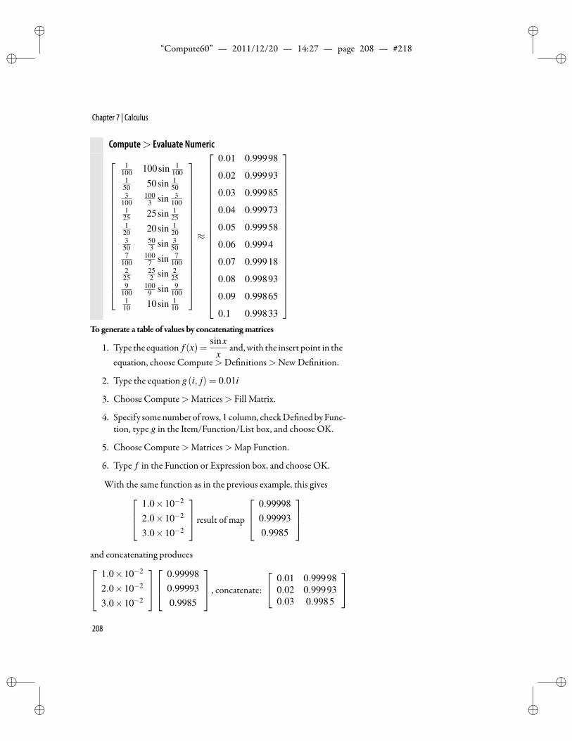
ii
“Compute60” — 2011/12/20 — 14:27 — page 208 — #218 ii
ii
ii
Chapter 7 | Calculus
Compute> Evaluate Numeric
1100 100sin 1
1001
50 50sin 150
3100
1003 sin 3
1001
25 25sin 125
120 20sin 1
203
50503 sin 3
507
1001007 sin 7
1002
25252 sin 2
259
1001009 sin 9
1001
10 10sin 110
≈
0.01 0.99998
0.02 0.99993
0.03 0.99985
0.04 0.99973
0.05 0.99958
0.06 0.9994
0.07 0.99918
0.08 0.99893
0.09 0.99865
0.1 0.99833
Togenerate a table of values by concatenatingmatrices
1. Type the equation f (x)=sinx
xand, with the insert point in the
equation, choose Compute>De nitions>New De nition.
2. Type the equation g(i, j) = 0.01i
3. Choose Compute>Matrices> Fill Matrix.
4. Specify somenumberof rows,1 column, checkDe nedbyFunc-tion, type g in the Item/Function/List box, and choose OK.
5. Choose Compute>Matrices>Map Function.
6. Type f in the Function or Expression box, and choose OK.
With the same function as in the previous example, this gives 1.0×10⁻²
2.0×10⁻²
3.0×10⁻²
result of map
0.999980.999930.9985
and concatenating produces 1.0×10⁻²
2.0×10⁻²
3.0×10⁻²
0.99998
0.999930.9985
, concatenate:
0.01 0.999980.02 0.999930.03 0.9985
208
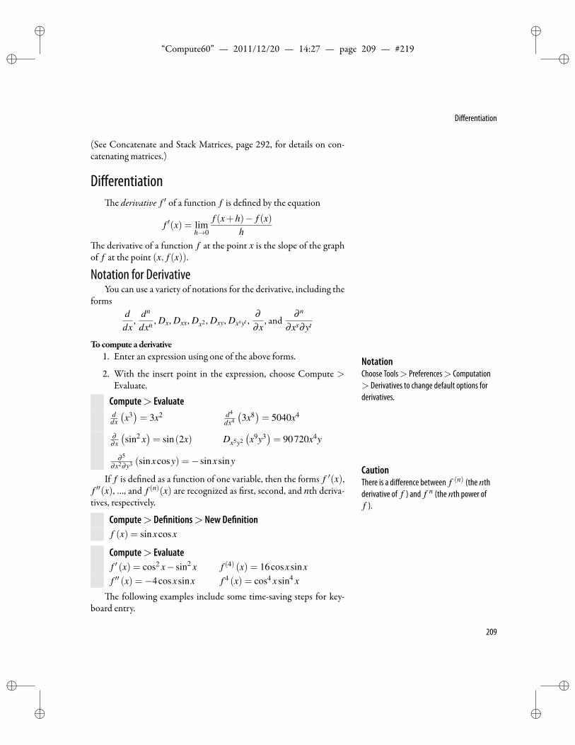
ii
“Compute60” — 2011/12/20 — 14:27 — page 209 — #219 ii
ii
ii
Differentiation
(See Concatenate and Stack Matrices, page 292, for details on con-catenating matrices.)
Differentiatione derivative f ′ of a function f is de ned by the equation
f ′(x) = limh→0
f (x+h)− f (x)h
e derivative of a function f at the point x is the slope of the graphof f at the point (x, f (x)).
Notation for DerivativeYou can use a variety of notations for the derivative, including the
formsddx
,dn
dxn , Dx, Dxx, Dx2 , Dxy, Dxsyt ,∂∂x
, and∂ n
∂xs∂yt
Tocompute a derivative1. Enter an expression using one of the above forms. Notation
Choose Tools> Preferences> Computation> Derivatives to change default options forderivatives.
2. With the insert point in the expression, choose Compute >Evaluate.
Compute> Evaluateddx
(x3)= 3x2 d4
dx4
(3x8)= 5040x4
∂∂x
(sin2 x
)= sin(2x) Dx5y2
(x9y3
)= 90720x4y
∂ 5
∂x2∂y3 (sinxcosy) =−sinxsinyCautionThere is a difference between f (n) (the nthderivative of f ) and f n (the nth power off ).
If f is de ned as a function of one variable, then the forms f ′(x),f ′′(x), …, and f (n)(x) are recognized as rst, second, and nth deriva-tives, respectively.
Compute> De nitions> New De nitionf (x) = sinxcosx
Compute> Evaluatef ′ (x) = cos2 x− sin2 x f (4) (x) = 16cosxsinxf ′′ (x) =−4cosxsinx f 4 (x) = cos4 xsin4 x
e following examples include some time-saving steps for key-board entry.
209
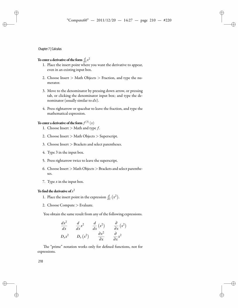
ii
“Compute60” — 2011/12/20 — 14:27 — page 210 — #220 ii
ii
ii
Chapter 7 | Calculus
Toenter a derivative of the form ddx x2
1. Place the insert point where you want the derivative to appear,even in an existing input box.
2. Choose Insert > Math Objects > Fraction, and type the nu-merator.
3. Move to the denominator by pressing down arrow, or pressingtab, or clicking the denominator input box; and type the de-nominator (usually similar to dx).
4. Press rightarrow or spacebar to leave the fraction, and type themathematical expression.
Toenter a derivative of the form f (3) (x)1. Choose Insert>Math and type f .
2. Choose Insert>Math Objects> Superscript.
3. Choose Insert> Brackets and select parentheses.
4. Type 3 in the input box.
5. Press rightarrow twice to leave the superscript.
6. Choose Insert>MathObjects>Brackets and select parenthe-ses.
7. Type x in the input box.
To nd the derivative of x2
1. Place the insert point in the expression ddx
(x2).
2. Choose Compute> Evaluate.
You obtain the same result from any of the following expressions.
dx2
dxddx
x2 ddx
(x2) ∂
∂x
(x2)
Dxx2 Dx(x2) ∂x2
∂x∂∂x
x2
e “prime” notation works only for de ned functions, not forexpressions.
210
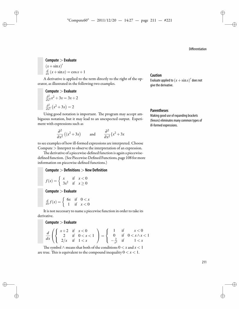
ii
“Compute60” — 2011/12/20 — 14:27 — page 211 — #221 ii
ii
ii
Differentiation
Compute> Evaluate(x+ sinx)′
ddx (x+ sinx) = cosx+1
CautionEvaluate applied to (x+ sinx)′ does notgive the derivative.
A derivative is applied to the term directly to the right of the op-erator, as illustrated in the following two examples.
Compute> Evaluate∂ 2
∂x2 x2 +3x = 3x+2
∂ 2
∂x2
(x2 +3x
)= 2
ParenthesesMaking good use of expanding brackets(fences) eliminates many common types ofill-formed expressions.
Using good notation is important. e program may accept am-biguous notation, but it may lead to an unexpected output. Experi-ment with expressions such as
∂ 2
∂x2
((x2 +3x
)and
∂ 2
∂x2 x2 +3x
to see examples of how ill-formed expressions are interpreted. ChooseCompute> Interpret to observe the interpretation of an expression.
e derivative of a piecewise-de ned function is again a piecewise-de ned function. (SeePiecewise-De nedFunctions, page108 formoreinformation on piecewise-de ned functions.)
Compute> De nitions> New De nition
f (x) =
x if x < 03x2 if x≥ 0
Compute> Evaluate
ddx f (x) =
6x if 0 < x1 if x < 0
It is not necessary to name a piecewise function in order to take itsderivative.
Compute> Evaluate
ddx
x+2 if x < 02 if 0 < x < 1
2/x if 1 < x
=
1 if x < 00 if 0 < x∧ x < 1− 2
x2 if 1 < x
e symbol∧means that both of the conditions 0 < x and x < 1are true. is is equivalent to the compound inequality 0 < x < 1.
211
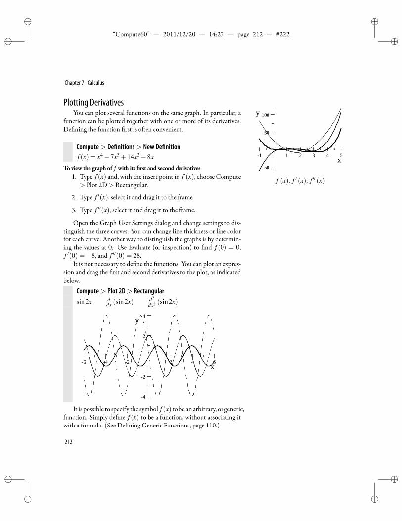
ii
“Compute60” — 2011/12/20 — 14:27 — page 212 — #222 ii
ii
ii
Chapter 7 | Calculus
Plotting DerivativesYou can plot several functions on the same graph. In particular, a
function can be plotted together with one or more of its derivatives.De ning the function rst is o en convenient.
Compute> De nitions> New De nitionf (x) = x4−7x3 +14x2−8x
Toview the graphof f with its rst and secondderivatives1. Type f (x) and, with the insert point in f (x), choose Compute
> Plot 2D> Rectangular.
1 1 2 3 4 5
50
50
100
x
y
f (x), f ′ (x), f ′′ (x)
2. Type f ′(x), select it and drag it to the frame
3. Type f ′′(x), select it and drag it to the frame.
Open the Graph User Settings dialog and change settings to dis-tinguish the three curves. You can change line thickness or line colorfor each curve. Another way to distinguish the graphs is by determin-ing the values at 0. Use Evaluate (or inspection) to nd f (0) = 0,f ′(0) =−8, and f ′′(0) = 28.
It is not necessary to de ne the functions. You can plot an expres-sion and drag the rst and second derivatives to the plot, as indicatedbelow.
Compute> Plot 2D> Rectangularsin2x d
dx (sin2x) d2
dx2 (sin2x)
6 4 2 2 4 6
4
2
2
4
x
y
It is possible to specify the symbol f (x) tobe an arbitrary, or generic,function. Simply de ne f (x) to be a function, without associating itwith a formula. (See De ning Generic Functions, page 110.)
212
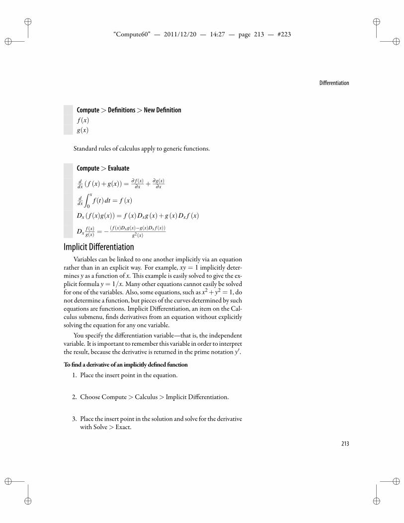
ii
“Compute60” — 2011/12/20 — 14:27 — page 213 — #223 ii
ii
ii
Differentiation
Compute> De nitions> New De nitionf (x)g(x)
Standard rules of calculus apply to generic functions.
Compute> Evaluate
ddx ( f (x)+g(x)) = ∂ f (x)
∂x + ∂g(x)∂x
ddx
∫ x
0f (t)dt = f (x)
Dx ( f (x)g(x)) = f (x)Dxg(x)+g(x)Dx f (x)
Dxf (x)g(x) =−
( f (x)Dxg(x)−g(x)Dx f (x))g2(x)
Implicit DifferentiationVariables can be linked to one another implicitly via an equation
rather than in an explicit way. For example, xy = 1 implicitly deter-mines y as a function of x. is example is easily solved to give the ex-plicit formula y = 1/x. Many other equations cannot easily be solvedfor one of the variables. Also, some equations, such as x2+y2 = 1, donot determine a function, but pieces of the curves determined by suchequations are functions. Implicit Differentiation, an item on the Cal-culus submenu, nds derivatives from an equation without explicitlysolving the equation for any one variable.
You specify the differentiation variable—that is, the independentvariable. It is important to remember this variable in order to interpretthe result, because the derivative is returned in the prime notation y′.
To nd aderivative of an implicitly de ned function
1. Place the insert point in the equation.
2. Choose Compute>Calculus> Implicit Differentiation.
3. Place the insert point in the solution and solve for the derivativewith Solve> Exact.
213
ii
“Compute60” — 2011/12/20 — 14:27 — page 214 — #224 ii
ii
ii
Chapter 7 | Calculus
Compute> Calculus> Implicit Differentiationxy+ sinx = y (Independent variable x, Dependent variable y)Solution: cosx+ y(x)+ xy′ (x) = y′ (x)xyz− x2y = 0 (Independent variable t , Dependent variables x,y,z)Solution: x(t)y(t)z′ (t)−2x(t)y(t)x′ (t)+ x(t)z(t)y′ (t)
+y(t)z(t)x′ (t)− x(t)2 y′ (t) = 0
Note that in the rst example above, y′ = dy/dx. In the secondexample above, x′ = dx/dt , y′ = dy/dt , and z′ = dz/dt .To ignore special cases
• Choose Tools > Preferences > Computation > Engine, andcheck Ignore Special Cases.
Compute> Solve> Exacty+ xy′+ cosx = y′ (Variable(s) to Solve For: y′),Solution: 1
x−1 (−y− cosx)xyz′−2xyx′+ xzy′+ yzx′− x2y′ = 0 (Variable(s) to Solve For: z′)Solution: 1
xy
(2xyx′− xzy′− yzx′+ x2y′
)Use ImplicitDifferentiation combinedwithword processing edit-
ing features to nd the second derivative y′′.
1. Leave the insert point in y′ = − y+cosxx−1 , and choose Compute
>Calculus> Implicit Differentiation. Type x for the Indepen-dent variable and y for the Dependent variable. Choose OK.
is returns the equation
∂y′ (x)∂x
=cosx+ y(x)
(x−1)2 +sinx− y′ (x)
x−1
2. Use editing techniques to replace ∂y′(x)∂x by y′′ and to replace
y′ (x) by− y(x)+cosxx−1 .
3. Apply Compute> Simplify to obtain the following:
y′′ =cosx+ y(x)
(x−1)2 +sinx−
(− y(x)+cosx
x−1
)x−1
=2cosx+2y(x)− sinx+ xsinx
(x−1)2
214
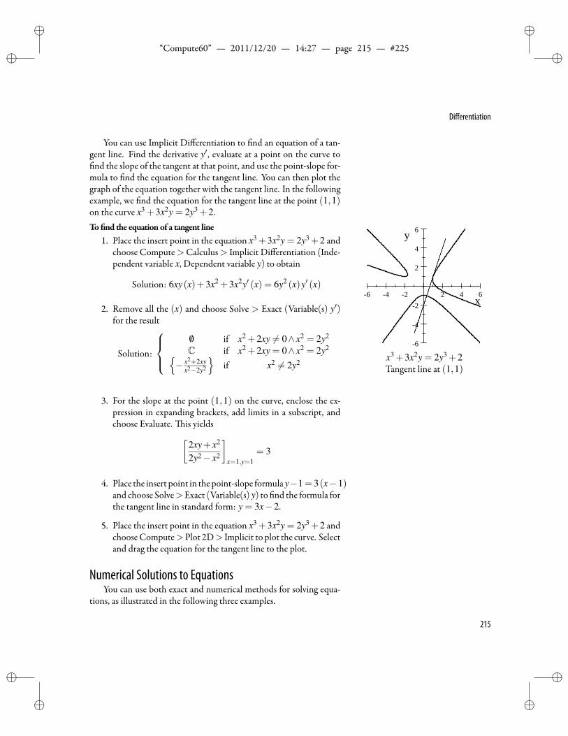
ii
“Compute60” — 2011/12/20 — 14:27 — page 215 — #225 ii
ii
ii
Differentiation
You can use Implicit Differentiation to nd an equation of a tan-gent line. Find the derivative y′, evaluate at a point on the curve tond the slope of the tangent at that point, and use the point-slope for-
mula to nd the equation for the tangent line. You can then plot thegraph of the equation together with the tangent line. In the followingexample, we nd the equation for the tangent line at the point (1,1)on the curve x3 +3x2y = 2y3 +2.To nd the equationof a tangent line
1. Place the insert point in the equation x3 +3x2y = 2y3 +2 andchoose Compute>Calculus> Implicit Differentiation (Inde-pendent variable x, Dependent variable y) to obtain
Solution: 6xy(x)+3x2 +3x2y′ (x) = 6y2 (x)y′ (x)
2. Remove all the (x) and choose Solve > Exact (Variable(s) y′)for the result
Solution:
/0 if x2 +2xy = 0∧ x2 = 2y2
C if x2 +2xy = 0∧ x2 = 2y2− x2+2xy
x2−2y2
if x2 = 2y2
6 4 2 2 4 6
6
4
2
2
4
6
x
y
x3 +3x2y = 2y3 +2Tangent line at (1,1)
3. For the slope at the point (1,1) on the curve, enclose the ex-pression in expanding brackets, add limits in a subscript, andchoose Evaluate. is yields[
2xy+ x2
2y2− x2
]x=1,y=1
= 3
4. Place the insert point in thepoint-slope formulay−1= 3(x−1)and choose Solve>Exact (Variable(s) y) to nd the formula forthe tangent line in standard form: y = 3x−2.
5. Place the insert point in the equation x3 +3x2y = 2y3 +2 andchooseCompute>Plot 2D> Implicit to plot the curve. Selectand drag the equation for the tangent line to the plot.
Numerical Solutions to EquationsYou can use both exact and numerical methods for solving equa-
tions, as illustrated in the following three examples.
215
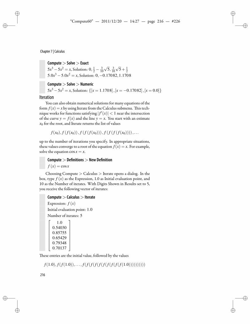
ii
“Compute60” — 2011/12/20 — 14:27 — page 216 — #226 ii
ii
ii
Chapter 7 | Calculus
Compute> Solve> Exact5x3−5x2 = x, Solution: 0, 1
2 −3
10
√5, 3
10
√5+ 1
25.0x3−5.0x2 = x, Solution: 0,−0.17082,1.1708
Compute> Solve> Numeric5x3−5x2 = x, Solution: [x = 1.1708] , [x =−0.17082] , [x = 0.0]
IterationYou can also obtain numerical solutions formany equations of the
form f (x) = x by using Iterate from theCalculus submenu. is tech-nique works for functions satisfying | f ′(x)|< 1 near the intersectionof the curve y = f (x) and the line y = x. You start with an estimatex0 for the root, and Iterate returns the list of values
f (x0), f ( f (x0)) , f ( f ( f (x0))) , f ( f ( f ( f (x0)))) , . . .
up to the number of iterations you specify. In appropriate situations,these values converge to a root of the equation f (x) = x. For example,solve the equation cosx = x.
Compute> De nitions> New De nitionf (x) = cosx
Choosing Compute > Calculus > Iterate opens a dialog. In thebox, type f (x) as the Expression, 1.0 as Initial evaluation point, and10 as the Number of iterates. With Digits Shown in Results set to 5,you receive the following vector of iterates:
Compute> Calculus> IterateExpression: f (x)Initial evaluation point: 1.0Number of iterates: 5
1.00.540300.857550.654290.793480.70137
ese entries are the initial value, followed by the values
f (1.0), f ( f (1.0)), . . . , f ( f ( f ( f ( f ( f ( f ( f ( f ( f (1.0))))))))))
216
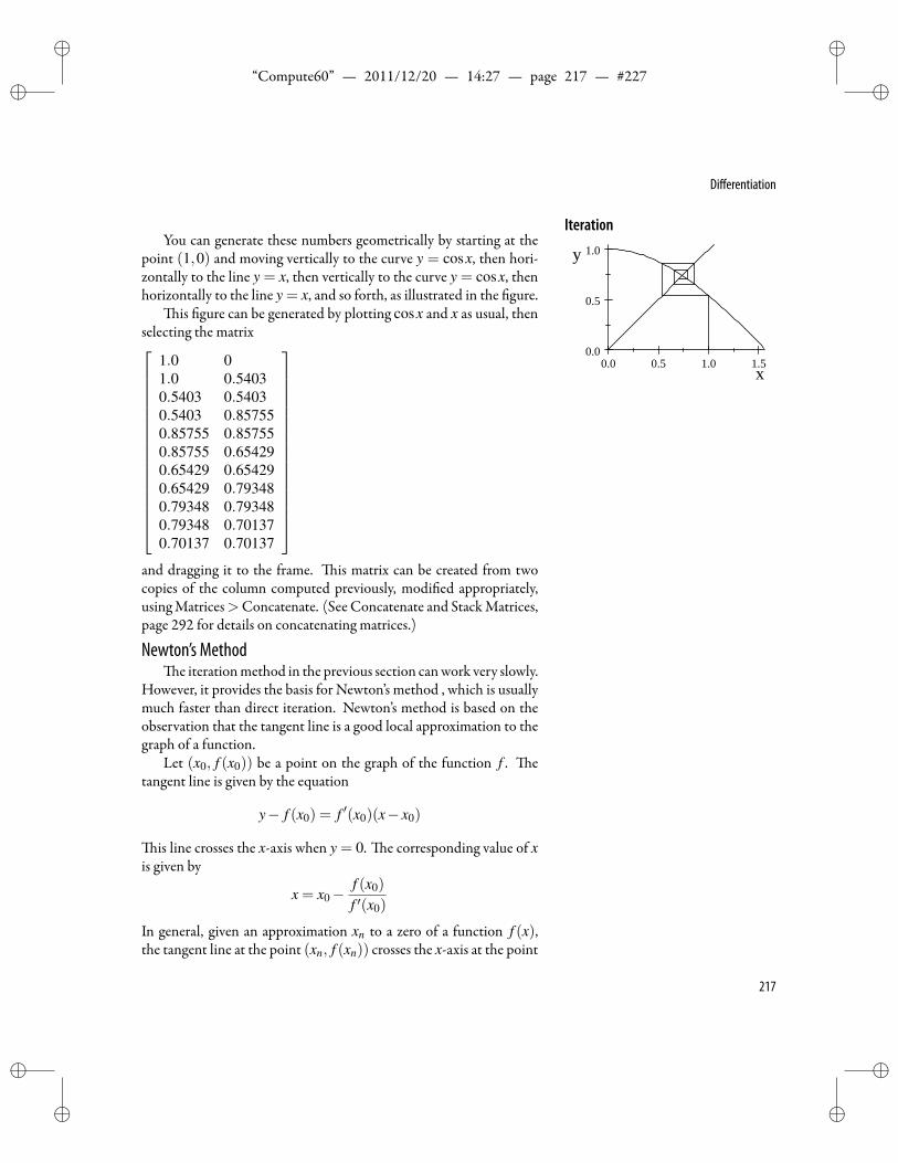
ii
“Compute60” — 2011/12/20 — 14:27 — page 217 — #227 ii
ii
ii
Differentiation
Iteration
0.0 0.5 1.0 1.50.0
0.5
1.0
x
yYou can generate these numbers geometrically by starting at the
point (1,0) and moving vertically to the curve y = cosx, then hori-zontally to the line y = x, then vertically to the curve y = cosx, thenhorizontally to the line y = x, and so forth, as illustrated in the gure.
is gure can be generated by plotting cosx and x as usual, thenselecting the matrix
1.0 01.0 0.54030.5403 0.54030.5403 0.857550.85755 0.857550.85755 0.654290.65429 0.654290.65429 0.793480.79348 0.793480.79348 0.701370.70137 0.70137
and dragging it to the frame. is matrix can be created from twocopies of the column computed previously, modi ed appropriately,usingMatrices>Concatenate. (See Concatenate and StackMatrices,page 292 for details on concatenating matrices.)
Newton’s Methode iterationmethod in the previous section canwork very slowly.
However, it provides the basis for Newton’s method , which is usuallymuch faster than direct iteration. Newton’s method is based on theobservation that the tangent line is a good local approximation to thegraph of a function.
Let (x0, f (x0)) be a point on the graph of the function f . etangent line is given by the equation
y− f (x0) = f ′(x0)(x− x0)
is line crosses the x-axis when y = 0. e corresponding value of xis given by
x = x0−f (x0)
f ′(x0)
In general, given an approximation xn to a zero of a function f (x),the tangent line at the point (xn, f (xn)) crosses the x-axis at the point
217
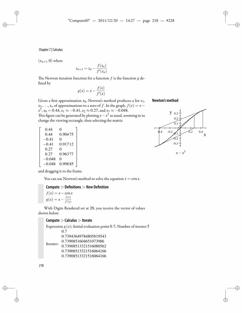
ii
“Compute60” — 2011/12/20 — 14:27 — page 218 — #228 ii
ii
ii
Chapter 7 | Calculus
(xn+1,0) where
xn+1 = xn−f (xn)
f ′(xn)
e Newton iteration function for a function f is the function g de-ned by
g(x) = x− f (x)f ′(x)
Given a rst approximation x0, Newton’s method produces a list x1, Newton’s method
0.4 0.2 0.2 0.4
0.30.20.1
0.10.20.3
x
y
x− x3
x2, . . ., xn of approximations to a zero of f . In the graph, f (x) = x−x3, x0 = 0.44, x1 ≈−0.41, x2 ≈ 0.27, and x3 ≈−0.048.
is gure can be generated by plotting x−x3 as usual, zooming in tochange the viewing rectangle, then selecting the matrix
0.44 00.44 0.90475−0.41 0−0.41 0.91712
0.27 00.27 0.96377−0.048 0−0.048 0.99885
and dragging it to the frame.
You can use Newton’s method to solve the equation x = cosx.
Compute> De nitions> New De nitionf (x) = x− cosx
g(x) = x− f (x)f ′(x)
With Digits Rendered set at 20, you receive the vector of valuesshown below.
Compute> Calculus> IterateExpression g(x); Initial evaluation point 0.7; Number of iterates 5
Iterates:
0.70.739436497848058195430.73908516046510739860.739085133215160805620.739085133215160641660.73908513321516064166
218
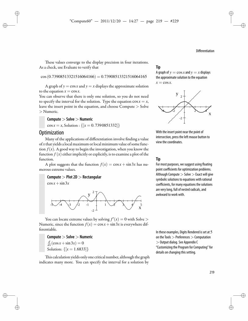
ii
“Compute60” — 2011/12/20 — 14:27 — page 219 — #229 ii
ii
ii
Differentiation
ese values converge to the display precision in four iterations.As a check, use Evaluate to verify that Tip
A graph of y = cosx and y = x displaysthe approximate solution to the equationx = cosx.
4 2 2 4
2
2
x
y
With the insert point near the point ofintersection, press the left mouse button toview the coordinates.
cos(0.73908513321516064166) = 0.73908513321516064165
A graph of y = cosx and y = x displays the approximate solutionto the equation x = cosx.You can observe that there is only one solution, so you do not needto specify the interval for the solution. Type the equation cosx = x,leave the insert point in the equation, and choose Compute > Solve>Numeric.
Compute> Solve> Numericcosx = x, Solution : [x = 0.7390851332]
OptimizationMany of the applications of differentiation involve nding a value
of x that yields a localmaximumor localminimumvalue of some func-tion f (x). A good way to begin the investigation, when you know thefunction f (x) either implicitly or explicitly, is to examine a plot of thefunction. Tip
For most purposes, we suggest using oatingpoint coefficients for optimization problems.Although Compute> Solve> Exact will givesymbolic solutions to equations with rationalcoefficients, for many equations the solutionsare very long, full of nested radicals, andawkward to work with.
A plot suggests that the function f (x) = cosx+ sin3x has nu-merous extreme values.
Compute> Plot 2D> Rectangularcosx+ sin3x
5 4 3 2 1 1 2 3 4 5
2
2
x
y
You can locate extreme values by solving f ′(x) = 0 with Solve >Numeric, since the function f (x) = cosx+ sin3x is everywhere dif-ferentiable.
In these examples, Digits Rendered is set at 5on the Tools> Preferences> Computation> Output dialog. See Appendix C“Customizing the Program for Computing” fordetails on changing this setting.
Compute> Solve> Numericddx (cosx+ sin3x) = 0Solution: [x = 1.6833]
is calculation yields only one critical number, although the graphindicates many more. You can specify the interval for a solution by
219
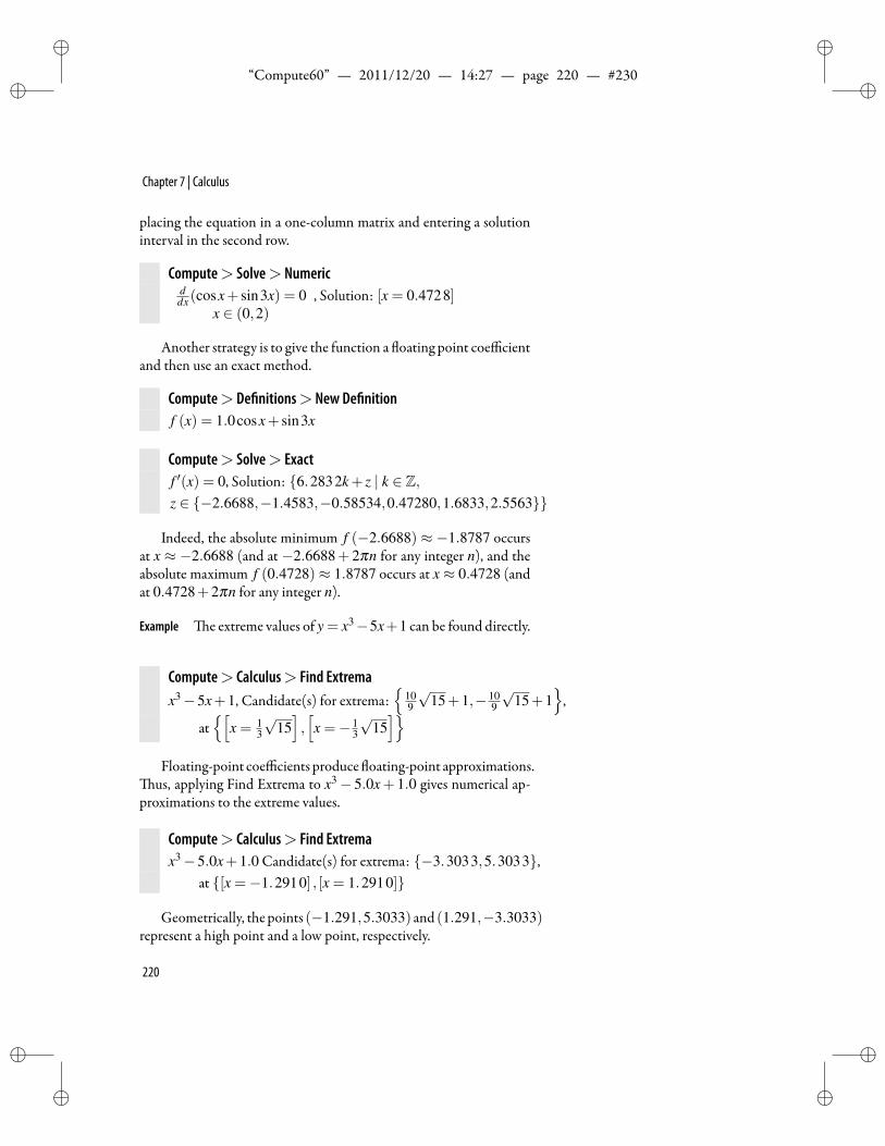
ii
“Compute60” — 2011/12/20 — 14:27 — page 220 — #230 ii
ii
ii
Chapter 7 | Calculus
placing the equation in a one-column matrix and entering a solutioninterval in the second row.
Compute> Solve> Numericddx(cosx+ sin3x) = 0
x ∈ (0,2), Solution: [x = 0.4728]
Another strategy is to give the function a oating point coefficientand then use an exact method.
Compute> De nitions> New De nitionf (x) = 1.0cosx+ sin3x
Compute> Solve> Exactf ′(x) = 0, Solution: 6.2832k+ z | k ∈ Z,z ∈ −2.6688,−1.4583,−0.58534,0.47280,1.6833,2.5563
Indeed, the absolute minimum f (−2.6688) ≈ −1.8787 occursat x ≈ −2.6688 (and at−2.6688+ 2πn for any integer n), and theabsolute maximum f (0.4728)≈ 1.8787 occurs at x ≈ 0.4728 (andat 0.4728+2πn for any integer n).
Example e extreme values of y = x3−5x+1 can be found directly.
Compute> Calculus> Find Extremax3−5x+1, Candidate(s) for extrema:
109
√15+1,− 10
9
√15+1
,
at[
x = 13
√15],[x =− 1
3
√15]
Floating-point coefficients produce oating-point approximations.us, applying Find Extrema to x3− 5.0x+ 1.0 gives numerical ap-
proximations to the extreme values.
Compute> Calculus> Find Extremax3−5.0x+1.0 Candidate(s) for extrema: −3.3033,5.3033,
at [x =−1.2910] , [x = 1.2910]
Geometrically, thepoints (−1.291,5.3033) and (1.291,−3.3033)represent a high point and a low point, respectively.
220
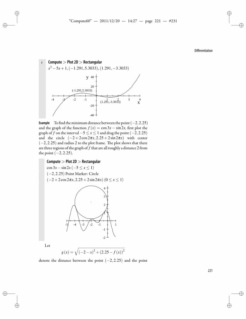
ii
“Compute60” — 2011/12/20 — 14:27 — page 221 — #231 ii
ii
ii
Differentiation
r Compute> Plot 2D> Rectangularx3−5x+1, (−1.291,5.3033), (1.291,−3.3033)
4 3 2 1 1 2 3 4
40
20
20
40
x
y
(1.291,5.3033)
(1.291,3.3033)
Example To nd theminimumdistancebetween thepoint (−2,2.25)and the graph of the function f (x) = cos3x− sin2x, rst plot thegraph of f on the interval−5≤ x≤ 1 and drag the point (−2,2.25)and the circle (−2+2cos2πx,2.25+2sin2πx) with center(−2,2.25) and radius 2 to the plot frame. e plot shows that thereare three regions of the graph of f that are all roughly a distance2 fromthe point (−2,2.25).
Compute> Plot 2D> Rectangularcos3x− sin2x (−5≤ x≤ 1)(−2,2.25) Point Marker: Circle(−2+2cos2πx,2.25+2sin2πx) (0≤ x≤ 1)
5 4 3 2 1 1
2
1
1
2
3
4
Let
g(x) =√(−2− x)2 +(2.25− f (x))2
denote the distance between the point (−2,2.25) and the point
221
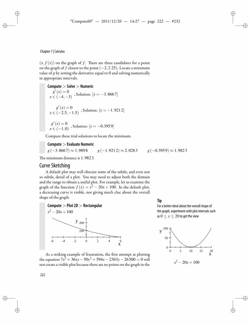
ii
“Compute60” — 2011/12/20 — 14:27 — page 222 — #232 ii
ii
ii
Chapter 7 | Calculus
(x, f (x)) on the graph of f . ere are three candidates for a pointon the graph of f closest to the point (−2,2.25). Locate a minimumvalue of g by setting the derivative equal to 0 and solving numericallyin appropriate intervals.
Compute> Solve> Numericg′ (x) = 0
x ∈ (−4,−3) , Solution: [x =−3.8667]
g′ (x) = 0x ∈ (−2.5,−1.5) , Solution: [x =−1.9212]
g′ (x) = 0x ∈ (−1,0) , Solution: [x =−0.3959]
Compare these trial solutions to locate the minimum.
Compute> Evaluate Numericg(−3.8667)≈ 1.9898 g(−1.9212)≈ 2.0283 g(−0.3959)≈ 1.9823
e minimum distance is 1.9823.
Curve SketchingA default plot may well obscure some of the subtle, and even not
so subtle, detail of a plot. You may need to adjust both the domainand the range to obtain a useful plot. For example, let us examine thegraph of the function f (x) = x2− 20x+ 100. In the default plot,a decreasing curve is visible, not giving much clue about the overallshape of the graph.
TipFor a better ideal about the overall shape ofthe graph, experiment with plot intervals suchas 0≤ x≤ 20 to get the view
0 5 10 15 200
50
100
x
y
x2−20x+100
Compute> Plot 2D> Rectangularx2−20x+100
6 4 2 0 2 4 6
100
200
x
y
As a striking example of frustration, the rst attempt at plottingthe equation 7x2 +36xy−50y2 +594x−2363y−26500 = 0 willnot create a visible plot because there are no points on the graph in the
222
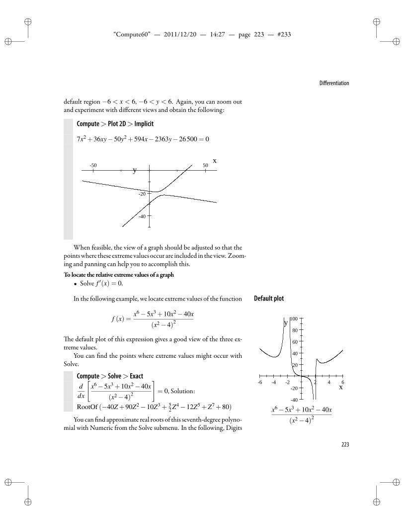
ii
“Compute60” — 2011/12/20 — 14:27 — page 223 — #233 ii
ii
ii
Differentiation
default region −6 < x < 6, −6 < y < 6. Again, you can zoom outand experiment with different views and obtain the following:
Compute> Plot 2D> Implicit
7x2 +36xy−50y2 +594x−2363y−26500 = 0
50 50
40
20
xy
When feasible, the view of a graph should be adjusted so that thepointswhere these extremevalues occur are included in the view. Zoom-ing and panning can help you to accomplish this.To locate the relative extreme values of a graph
• Solve f ′(x) = 0.
In the following example, we locate extreme values of the function Default plot
6 4 2 2 4 6
40
20
20
40
60
80
100
x
y
x6−5x3 +10x2−40x
(x2−4)2
f (x) =x6−5x3 +10x2−40x
(x2−4)2
e default plot of this expression gives a good view of the three ex-treme values.
You can nd the points where extreme values might occur withSolve.
Compute> Solve> Exactddx
[x6−5x3 +10x2−40x
(x2−4)2
]= 0, Solution:
RootOf (−40Z +90Z2−10Z3 + 52 Z4−12Z5 +Z7 +80)
You can nd approximate real roots of this seventh-degree polyno-mial with Numeric from the Solve submenu. In the following, Digits
223
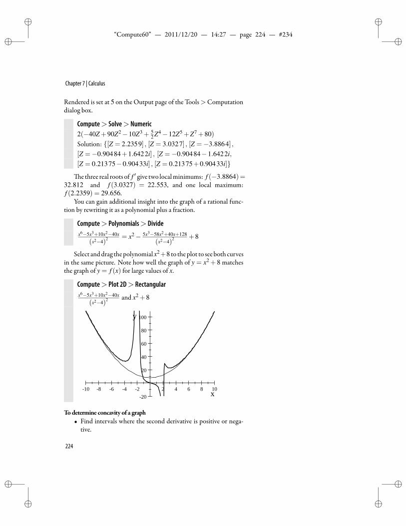
ii
“Compute60” — 2011/12/20 — 14:27 — page 224 — #234 ii
ii
ii
Chapter 7 | Calculus
Rendered is set at 5 on the Output page of the Tools>Computationdialog box.
Compute> Solve> Numeric2(−40Z +90Z2−10Z3 + 5
2 Z4−12Z5 +Z7 +80)Solution: [Z = 2.2359] , [Z = 3.0327] , [Z =−3.8864] ,[Z =−0.90484+1.6422i] , [Z =−0.90484−1.6422i,[Z = 0.21375−0.90433i] , [Z = 0.21375+0.90433i]
e three real roots of f ′ give two localminimums: f (−3.8864)=32.812 and f (3.0327) = 22.553, and one local maximum:f (2.2359) = 29.656.
You can gain additional insight into the graph of a rational func-tion by rewriting it as a polynomial plus a fraction.
Compute> Polynomials> Dividex6−5x3+10x2−40x
(x2−4)2 = x2− 5x3−58x2+40x+128
(x2−4)2 +8
Select anddrag thepolynomialx2+8 to theplot to see both curvesin the same picture. Note how well the graph of y = x2 + 8 matchesthe graph of y = f (x) for large values of x.
Compute> Plot 2D> Rectangularx6−5x3+10x2−40x
(x2−4)2 and x2 +8
10 8 6 4 2 2 4 6 8 1020
20
40
60
80
100
x
y
Todetermine concavity of a graph• Find intervals where the second derivative is positive or nega-
tive.
224
ii
“Compute60” — 2011/12/20 — 14:27 — page 225 — #235 ii
ii
ii
Differentiation
To locate the intervals where the graph of f (x) = x4+3x3−x2−3x is concave upward, evaluate f ′′(x) to obtain f ′′(x)= 12x2+18x−2, and solve the inequality 12x2 +18x−2 > 0.
Compute> Solve> Exact12x2 +18x−2 > 0
Solution:(−∞,− 1
48
√35√
48− 34
)∪(
148
√35√
48− 34 ,∞
)To solve more complicated inequalities or systems of inequalities,
you can set expressions equal to zero and test for sign changes.One way to answer the question of where the graph of
f (x) =x6−5x3 +10x2−40x
(x2−4)2
is concave upward is to nd the sign of the second derivative.
Compute> De nitions> New De nitionf (x) = x6−5x3+10x2−40x
(x2−4)2
ApplyEvaluate andFactor to nd the secondderivative as the quo-tient of two polynomials.
Compute> Evaluate, Compute> Factor
f ′′(x) =2(x8−16x6−5x5+270x4−400x3+320x2−1200x+160)
(x−2)4(x+2)4
Since the denominator is always nonnegative, it is sufficient to in-vestigate the sign of the numerator. Apply Solve > Numeric to theequation
0 = x8−16x6−5x5 +270x4−400x3 +320x2−1200x+160
to nd the real solutions
[x≈ 0.13759] , [x≈ 2.3414]
Compute the value at any point to the le , between, and to the rightof these solutions, using Evaluate Numeric:
f ′′(0) ≈ 1.25f ′′(1) ≈ −21.481
f ′′(2.4) ≈ 40.964
225
ii
“Compute60” — 2011/12/20 — 14:27 — page 226 — #236 ii
ii
ii
Chapter 7 | Calculus
Taking into account the vertical asymptotes, the graph is concaveupward on the intervals (−∞,−2), (−2,0.1376), and (2.3414,∞),and concavedownwardon the intervals (0.13759,2) and (2,2.3414).
Inde nite IntegrationAn antiderivative of a function f (x) is any function g(x) whose
derivative is f (x). If g(x) is an antiderivative of f (x), then g(x)+Cis another antiderivative. In fact, every antiderivative is of the formg(x)+C for some constantC.
e inde nite integral of f (x) is the family of all antiderivatives off (x) and is denoted
∫f (x)dx.
Toevaluate an inde nite integral• Place the insert point anywhere in an integral and choose Eval-
uate.
Compute> Evaluate∫ (2x2 +3x+5
)dx = 1
6 x(4x2 +9x+30
)e system does not automatically return the constant of integra-
tion—o en called the arbitrary constant—so you must remain alert SpacingIt is common, although hardly necessary, toadd a thin space between f (x) and dx in anintegral
∫f (x) dx. The Thin Space (found
under Insert + Spacing + Horizontal Space) isfor readability only, and in no way affects theway in which an integral is interpreted by theunderlying computing engine.
and add the constant when needed. Simply type+C to change from∫ (2x2 +3x+5
)dx =
23
x3 +32
x2 +5x
to ∫ (2x2 +3x+5
)dx =
23
x3 +32
x2 +5x+C
Such constants are needed, for example, if you have a formula for ac-celeration and you want to nd an expression for velocity.
You can evaluate inde nite integrals of piecewise-de ned func-tions. You can de ne a function from a piecewise expression, or workdirectly with the piecewise expression, as shown in the following ex-amples. Turn on Helper Lines to see the null brackets on the right.
Compute> De nitions> New De nition
f (x) =
x if x < 03x2 if x≥ 0
226
ii
“Compute60” — 2011/12/20 — 14:27 — page 227 — #237 ii
ii
ii
Inde nite Integration
Compute> Evaluate∫f (x)dx =
12 x2 if x≤ 0x3 if 0 < x
∫ x if x < 03x2 if x≥ 0 dx =
12 x2 if x≤ 0x3 if 0 < x
Interpreting an Expressione computer algebra system interprets many expressions that
might be considered ambiguous. You can check the interpretationwithout evaluating an expression.
To interpret an expressionwithout evaluation• Place the insert point in the expression and choose Compute>
Interpret.
Compute> Interpretxy/z = xy
z∫
ax3 =∫
ax3 d
sinx/y = sin(
xy
) ∫x3a =
∫x3ad
Even though the interpretations of the integral expressions do notindicate the variable of integration, they show that the expressions areinterpreted as inde nite integrals. If such an expression is evaluated, achoice will be made, generally based on the alphabetical order of thecharacters.
Compute> Evaluate∫ax3 = 1
4 ax4 ∫yx3 = 1
4 x4y∫x3a = 1
4 ax4 ∫x3y = 1
4 x4y
If f is not de ned as a function, then it is treated as a variable orconstant.
Compute> Evaluate∫f = 1
2 f 2∫f (x)dx = 1
2 f x2
In these expressions, f behaves the same as any other variable, andf (x) is interpreted as simply the product of f and x.
227
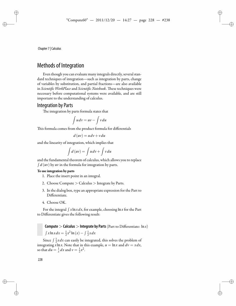
ii
“Compute60” — 2011/12/20 — 14:27 — page 228 — #238 ii
ii
ii
Chapter 7 | Calculus
Methods of IntegrationEven though you can evaluatemany integrals directly, several stan-
dard techniques of integration—such as integration by parts, changeof variables by substitution, and partial fractions—are also availablein Scienti cWorkPlace and Scienti c Notebook. ese techniques werenecessary before computational systems were available, and are stillimportant to the understanding of calculus.
Integration by Partse integration by parts formula states that∫
udv = uv−∫
vdu
is formula comes from the product formula for differentials
d (uv) = udv+ vdu
and the linearity of integration, which implies that∫d (uv) =
∫udv+
∫vdu
and the fundamental theorem of calculus, which allows you to replace∫d (uv) by uv in the formula for integration by parts.
Touse integrationby parts1. Place the insert point in an integral.
2. Choose Compute>Calculus> Integrate by Parts.
3. In the dialog box, type an appropriate expression for the Part toDifferentiate.
4. Choose OK.
For the integral∫
x lnxdx, for example, choosing lnx for the Partto Differentiate gives the following result:
Compute> Calculus> Integrate by Parts (Part to Differentiate: lnx)∫x lnxdx = 1
2 x2 ln(x)−∫ 1
2 xdx
Since∫ 1
2 xdx can easily be integrated, this solves the problem ofintegrating x lnx. Note that in this example, u = lnx and dv = xdx,so that du = 1
x dx and v = 12 x2.
228
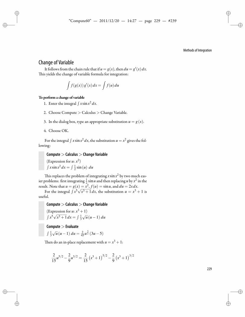
ii
“Compute60” — 2011/12/20 — 14:27 — page 229 — #239 ii
ii
ii
Methods of Integration
Change of VariableIt follows from the chain rule that if u= g(x), then du= g′(x)dx.
is yields the change of variable formula for integration:∫f (g(x))g′(x)dx =
∫f (u)du
Toperforma change of variable1. Enter the integral
∫xsinx2 dx.
2. Choose Compute>Calculus>Change Variable.
3. In the dialog box, type an appropriate substitution u = g(x).
4. Choose OK.
For the integral∫
xsinx2 dx, the substitution u = x2 gives the fol-lowing:
Compute> Calculus> Change Variable(Expression for u: x2)∫
xsinx2 dx =∫ 1
2 sin(u) du
is replaces the problem of integrating xsinx2 by two much eas-ier problems: rst integrating 1
2 sinu and then replacing u by x2 in theresult. Note that u = g(x) = x2, f (u) = sinu, and du = 2xdx.
For the integral∫
x5√
x3 +1dx, the substitution u = x3 + 1 isuseful.
Compute> Calculus> Change Variable(Expression for u: x3 +1)∫
x5√
x3 +1dx =∫ 1
3√
u(u−1) du
Compute> Evaluate∫ 13√
u(u−1) du = 245 u
32 (3u−5)
en do an in-place replacement with u = x3 +1:
215
u5/2− 29
u3/2 =2
15(x3 +1
)5/2− 29(x3 +1
)3/2
229
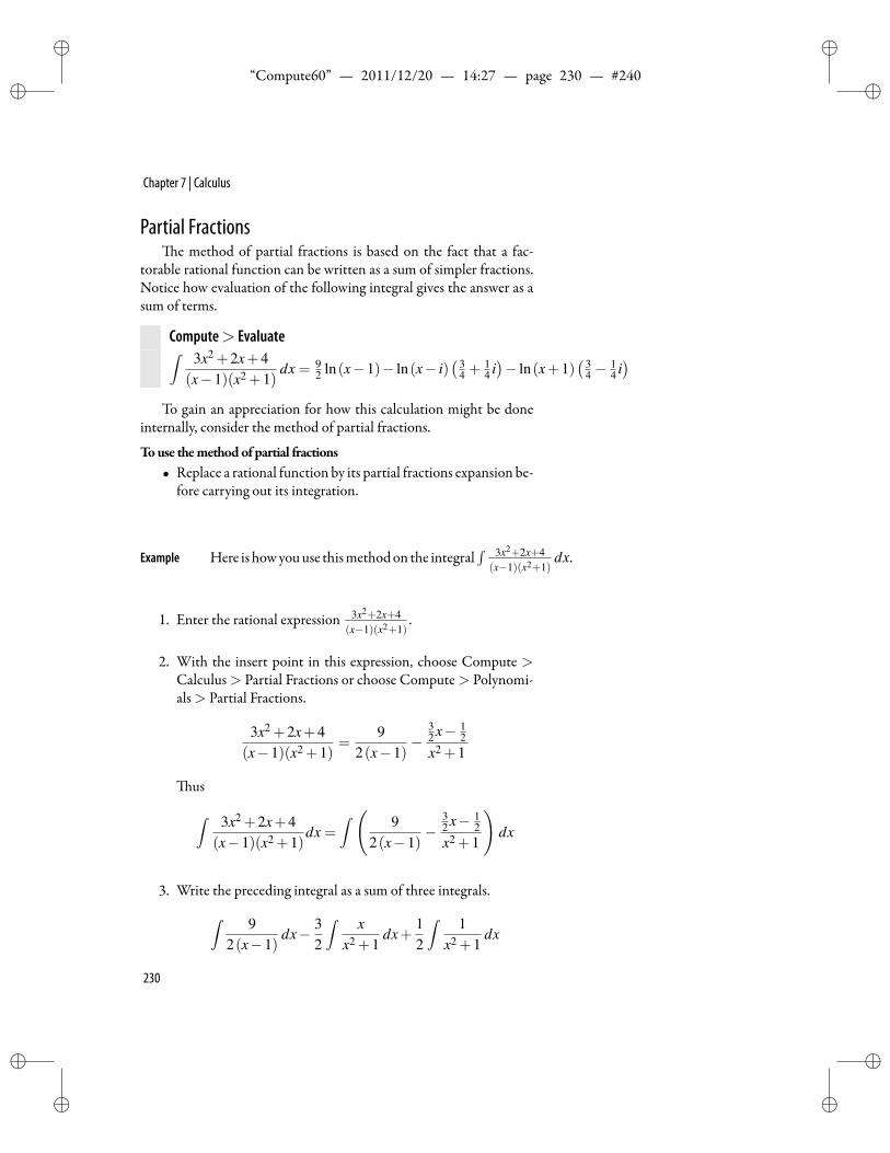
ii
“Compute60” — 2011/12/20 — 14:27 — page 230 — #240 ii
ii
ii
Chapter 7 | Calculus
Partial Fractionse method of partial fractions is based on the fact that a fac-
torable rational function can be written as a sum of simpler fractions.Notice how evaluation of the following integral gives the answer as asum of terms.
Compute> Evaluate∫ 3x2 +2x+4(x−1)(x2 +1)
dx = 92 ln(x−1)− ln(x− i)
( 34 +
14 i)− ln(x+1)
( 34 −
14 i)
To gain an appreciation for how this calculation might be doneinternally, consider the method of partial fractions.
Touse themethodof partial fractions• Replace a rational function by its partial fractions expansion be-
fore carrying out its integration.
Example Here is howyouuse thismethodon the integral∫ 3x2+2x+4
(x−1)(x2+1)dx.
1. Enter the rational expression 3x2+2x+4(x−1)(x2+1)
.
2. With the insert point in this expression, choose Compute >Calculus> Partial Fractions or choose Compute> Polynomi-als> Partial Fractions.
3x2 +2x+4(x−1)(x2 +1)
=9
2(x−1)−
32 x− 1
2x2 +1
us
∫ 3x2 +2x+4(x−1)(x2 +1)
dx =∫ ( 9
2(x−1)−
32 x− 1
2x2 +1
)dx
3. Write the preceding integral as a sum of three integrals.∫ 92(x−1)
dx− 32
∫ xx2 +1
dx+12
∫ 1x2 +1
dx
230
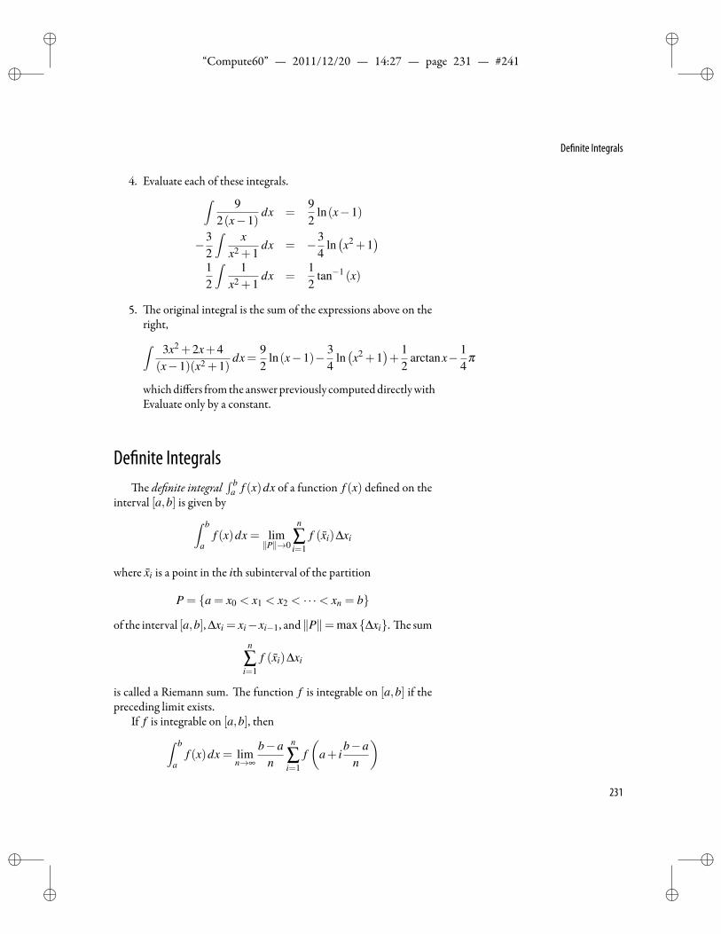
ii
“Compute60” — 2011/12/20 — 14:27 — page 231 — #241 ii
ii
ii
De nite Integrals
4. Evaluate each of these integrals.∫ 92(x−1)
dx =92
ln(x−1)
−32
∫ xx2 +1
dx = −34
ln(x2 +1
)12
∫ 1x2 +1
dx =12
tan−1 (x)
5. e original integral is the sum of the expressions above on theright,∫ 3x2 +2x+4
(x−1)(x2 +1)dx=
92
ln(x−1)− 34
ln(x2 +1
)+
12
arctanx− 14
π
whichdiffers fromthe answerpreviously computeddirectlywithEvaluate only by a constant.
De nite Integralse de nite integral
∫ ba f (x)dx of a function f (x) de ned on the
interval [a,b] is given by∫ b
af (x)dx = lim
∥P∥→0
n
∑i=1
f (xi)∆xi
where xi is a point in the ith subinterval of the partition
P = a = x0 < x1 < x2 < · · ·< xn = b
of the interval [a,b], ∆xi = xi−xi−1, and∥P∥=max∆xi. e sum
n
∑i=1
f (xi)∆xi
is called a Riemann sum. e function f is integrable on [a,b] if thepreceding limit exists.
If f is integrable on [a,b], then∫ b
af (x)dx = lim
n→∞
b−an
n
∑i=1
f(
a+ ib−a
n
)231
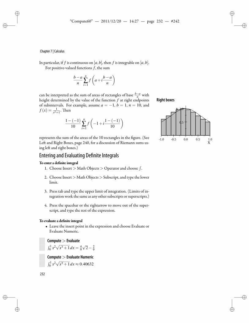
ii
“Compute60” — 2011/12/20 — 14:27 — page 232 — #242 ii
ii
ii
Chapter 7 | Calculus
In particular, if f is continuous on [a,b], then f is integrable on [a,b].For positive-valued functions f , the sum
b−an
n
∑i=1
f(
a+ ib−a
n
)
can be interpreted as the sum of areas of rectangles of base b−an with
height determined by the value of the function f at right endpoints Right boxes
1.0 0.5 0.0 0.5 1.0
0.5
1.0
x
yof subintervals. For example, assume a = −1, b = 1, n = 10, andf (x) = 1
x2+1 . en
1− (−1)10
n
∑i=1
f(−1+ i
1− (−1)10
)
represents the sum of the areas of the 10 rectangles in the gure. (SeeLe and Right Boxes, page 240, for a discussion of Riemann sums us-ing le and right boxes.)
Entering and Evaluating De nite IntegralsToenter a de nite integral
1. Choose Insert>Math Objects>Operator and choose∫.
2. Choose Insert>MathObjects> Subscript, and type the lowerlimit.
3. Press tab and type the upper limit of integration. (Limits of in-tegrationwork the same as any other subscripts or superscripts.)
4. Press the spacebar or the rightarrow to move out of the super-script, and type the rest of the expression.
Toevaluate a de nite integral• Leave the insert point in the expression and choose Evaluate or
Evaluate Numeric.
Compute> Evaluate∫ 10 x2√
x3 +1dx = 49
√2− 2
9
Compute> Evaluate Numeric∫ 10 x2√
x3 +1dx≈ 0.40632
232
ii
“Compute60” — 2011/12/20 — 14:27 — page 233 — #243 ii
ii
ii
De nite Integrals
Integrals involving absolute values or piecewise-de ned functionscan be treated as any other function.
Compute> Evaluate∫ 2−2
∣∣x2−1∣∣ dx = 4
Tounderstand this computation, determine the intervals forwhichx2−1 is positive or negative, and write the integral as a sum of severalintegrals with the absolute value sign removed.
Compute> Solve> Exactx2−1 > 0, Solution: (1,∞)∪ (−∞,−1)
So∣∣x2−1
∣∣= x2−1 forx<−1orx> 1, and∣∣x2−1
∣∣=−(x2−1)=
1− x2 for−1 < x < 1. en you can write the integral as the sum ofthe following three:
∫ 2
−2
∣∣x2−1∣∣ dx=
∫ −1
−2
(x2−1
)dx+
∫ 1
−1
(1− x2) dx+
∫ 2
1
(x2−1
)dx
Compute> Evaluate∫ −1−2(x2−1
)dx = 4
3∫ 1−1(1− x2
)dx = 4
3∫ 2
1(x2−1
)dx = 4
3
You can nd the de nite integral of a piecewise function either byintegrating the expression directly or by de ning a piecewise functionf (x).
Compute> De nitions> New De nition
f (x) =
x2 if x < 0x if x≥ 0
Compute> Evaluate∫ 3−2 f (x)dx = 43
6
∫ 3
−2
(x2 if x < 0x if x≥ 0
)dx = 43
6
To understand this computation, write the integral as a sum of in-tegrals involving ordinary functions. is yields
∫ 3
−2f (x)dx =
∫ 0
−2x2 dx+
∫ 3
0xdx =
83+
92=
436
233
ii
“Compute60” — 2011/12/20 — 14:27 — page 234 — #244 ii
ii
ii
Chapter 7 | Calculus
Methods of Integration with De nite IntegralsMethods thatwere introduced for inde nite integration—integra-
tion by parts, change of variables, and partial fractions—can also beapplied to de nite integrals. See Methods of Integration, page 228for general details about these methods.
To integrate by partswith a de nite integral1. Place the insert point in a de nite integral.
2. Choose Compute>Calculus> Integrate by Parts.
3. Type in the dialog box an appropriate expression for the Part toDifferentiate.
4. Choose OK.
Compute> Calculus> Integrate by Parts(Part to Differentiate: lnx)∫ 2
1 x lnxdx = 2ln2−∫ 2
112 xdx
Touse a change of variableswith a de nite integral1. Place the insert point in a de nite integral.
2. Choose Compute>Calculus>Change Variable.
3. Type in the dialog box an Expression for u, and choose OK.
Compute> Calculus> Change Variable(Expression for u: x3 +1)∫ 2
0 x5√
x3 +1dx =∫ 9
113√
u(u−1) du
is gives an integral that can be computed by elementary meth-ods. Note that the limits have changed to match the new variable.
Touse partial fractionswith a de nite integral• Replace a rational expression with its partial fractions expan-
sion.
Compute> Calculus> Partial Fractions3x2+2x+4(x−1)2 = 8
x−1 +9
(x−1)2 +3
234
ii
“Compute60” — 2011/12/20 — 14:27 — page 235 — #245 ii
ii
ii
De nite Integrals
us∫ 7
3
3x2 +2x+4(x−1)2 dx=
∫ 7
33dx+
∫ 7
3
9
(x−1)2 dx+∫ 7
3
8x−1
dx= 12+3+8ln3
Compute> Evaluate∫ 73 3dx = 12
∫ 73
8x−1 dx = 8ln3∫ 7
39
(x−1)2 dx = 3∫ 7
33x2+2x+4(x−1)2 dx = 8ln3+15
Improper IntegralsIf the proper integral
∫ ba f (x) dx exists for every b≥ a, the limit∫ ∞
af (x) dx = lim
b→∞
∫ b
af (x) dx
de nes an improper integral of the rst kind. e integral is said to con-verge if this limit exists and is nite.Tocompute an improper integral of the rst kind
• Place the insert point in the integral and choose Evaluate orEvaluate Numeric.
Compute> Evaluate∫ ∞1 x−2 dx = 1
∫ ∞1 x−1 dx = ∞∫ ∞
0 e−3x dx = 13
∫ 0−∞ e−3x dx = ∞∫ ∞
−∞ e−x2dx =
√π
∫ ∞0 sinxdx = undefined
Compute> Evaluate Numeric∫ ∞−∞ e−x2
dx≈ 1.7725∫ ∞
0sinxex dx≈ 0.5
A de nite integral for which the integrand has a discontinuity ora place where it is not de ned within the interval of integration is animproper integral of the second kind. e discontinuity may occureither in the interior or at one or both endpoints of the interval ofintegration.Toevaluate an improper integral of the secondkind
1. Place the insert point in the integral.
235
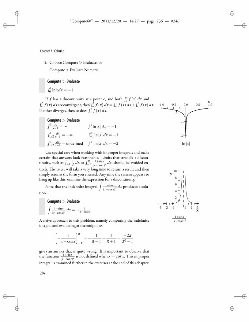
ii
“Compute60” — 2011/12/20 — 14:27 — page 236 — #246 ii
ii
ii
Chapter 7 | Calculus
2. Choose Compute> Evaluate. or
Compute> Evaluate Numeric.
Compute> Evaluate∫ 10 lnxdx =−1
If f has a discontinuity at a point c, and both∫ c
a f (x) dx and∫ bc f (x) dx are convergent, then
∫ ba f (x) dx=
∫ ca f (x) dx+
∫ bc f (x) dx.
If either diverges, then so does∫ b
a f (x) dx.
Compute> Evaluate∫ 31
dxx−1 = ∞
∫ 10 ln |x| dx =−1∫ 1
1/2dx
x−1 =−∞∫ 0−1 ln |x| dx =−1∫ 3
1/2dx
x−1 = undefined∫ 1−1 ln |x| dx =−2
1.0 0.5 0.0 0.5 1.0
10
5
x
y
ln |x|
Use special care when working with improper integrals and makecertain that answers look reasonable. Limits that straddle a discon-tinuity, such as
∫ 1−1
1x2 dx or
∫ π−π
1+sinx(x−cosx)2 dx, should be avoided en-
tirely. e latter will take a very long time to return a result and thensimply returns the form you entered. Any time the system appears tohang up like this, examine the expression for a discontinuity.
Note that the inde nite integral∫
1+sinx(x−cosx)2 dx produces a solu-
tion:
Compute> Evaluate∫1+sinx
(x−cosx)2 dx =− 1x−cosx
A naive approach to this problem, namely computing the inde niteintegral and evaluating at the endpoints,
3 2 1 1 2 3
2
4
6
8
10
x
y
1+sinx(x−cosx)2
[− 1
x− cosx
]π
−π=− 1
π−1− 1
π +1=−2π
π2−1
gives an answer that is quite wrong. It is important to observe thatthe function 1+sinx
(x−cosx)2 is not de ned when x = cosx. is improper
integral is examined further in the exercises at the end of this chapter.
236
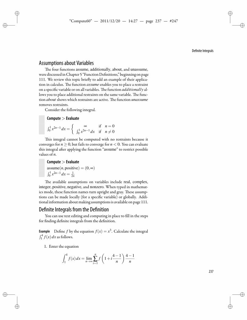
ii
“Compute60” — 2011/12/20 — 14:27 — page 237 — #247 ii
ii
ii
De nite Integrals
Assumptions about Variablese four functions assume, additionally, about, and unassume,
werediscussed inChapter 5 “FunctionDe nitions,” beginningonpage111. We review this topic brie y to add an example of their applica-tion in calculus. e function assume enables you to place a restrainton a speci c variable or on all variables. e function additionally al-lows you to place additional restraints on the same variable. e func-tion about shows which restraints are active. e function unassumeremoves restraints.
Consider the following integral.
Compute> Evaluate
∫ 10 x2n−1 dx =
∞ if n = 0∫ 1
0 x2n−1 dx if n = 0
is integral cannot be computed with no restraints because itconverges for n≥ 0, but fails to converge for n < 0. You can evaluatethis integral a er applying the function “assume” to restrict possiblevalues of n.
Compute> Evaluateassume(n,positive) = (0,∞)∫ 1
0 x2n−1 dx = 12n
e available assumptions on variables include real, complex,integer, positive, negative, and nonzero. When typed in mathemat-ics mode, these function names turn upright and gray. ese assump-tions can be made locally (for a speci c variable) or globally. Addi-tional information aboutmaking assumptions is available onpage 111.
De nite Integrals from the De nitionYou can use text editing and computing in place to ll in the steps
for nding de nite integrals from the de nition.
Example De ne f by the equation f (x) = x3. Calculate the integral∫ 41 f (x)dx as follows.
1. Enter the equation∫ 4
1f (x)dx = lim
n→∞
n
∑i=1
f(
1+ i4−1
n
)4−1
n
237
ii
“Compute60” — 2011/12/20 — 14:27 — page 238 — #248 ii
ii
ii
Chapter 7 | Calculus
2. Select the term to the right of the summation sign.
3. Press and hold down theCtrl key and choose Compute> Eval-uate, then choose Compute> Factor.
4. Select the series.
5. PressCtrl+Evaluate, then chooseCompute>Expand, then addparentheses.
6. With the insert point in the expression, choose Compute >Evaluate.
ese steps produce the following sequence of expressions:∫ 4
1f (x)dx = lim
n→∞
n
∑i=1
f(
1+ i4−1
n
)4−1
n
= limn→∞
n
∑i=1
3(n+3i)3
n4
= limn→∞
(1892n
+1354n2 +
2554
)=
2554
For comparison, you can compute this integral directly:
Compute> Evaluate∫ 4
1x3 dx = 255
4
Pictures of Riemann SumsYou can plot pictures of Riemann sums obtained from midpoints,
le endpoints, or right endpoints of subintervals. e choices areMid-dle Boxes, Le Boxes, Right Boxes, and Le and Right Boxes.
Middle Boxese Riemann sum determined by the midpoints is given by
b−an
n−1
∑i=0
f(
a+b−a
2n+ i
b−an
)which is the sum of the areas of rectangles whose heights are deter-mined by midpoints of subintervals.
238
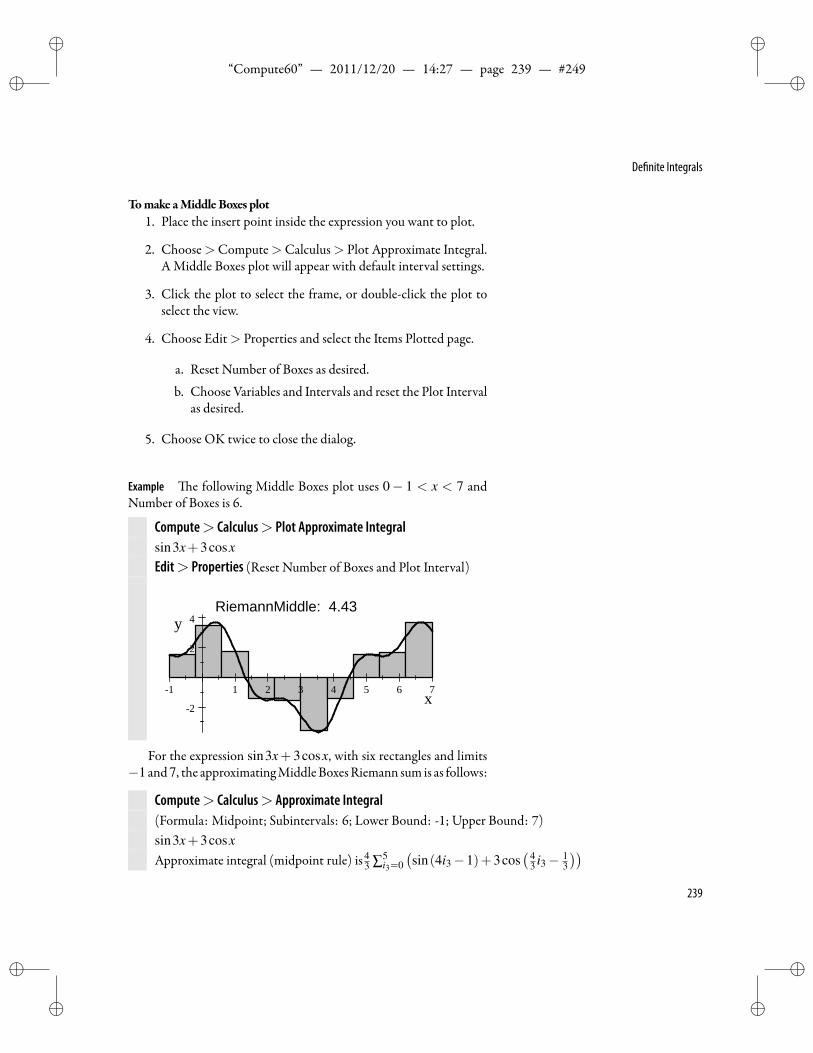
ii
“Compute60” — 2011/12/20 — 14:27 — page 239 — #249 ii
ii
ii
De nite Integrals
Tomake aMiddleBoxes plot1. Place the insert point inside the expression you want to plot.
2. Choose>Compute>Calculus> Plot Approximate Integral.A Middle Boxes plot will appear with default interval settings.
3. Click the plot to select the frame, or double-click the plot toselect the view.
4. Choose Edit> Properties and select the Items Plotted page.
a. Reset Number of Boxes as desired.
b. Choose Variables and Intervals and reset the Plot Intervalas desired.
5. Choose OK twice to close the dialog.
Example e following Middle Boxes plot uses 0− 1 < x < 7 andNumber of Boxes is 6.
Compute> Calculus> Plot Approximate Integralsin3x+3cosxEdit> Properties (Reset Number of Boxes and Plot Interval)
RiemannMiddle: 4.43
1 1 2 3 4 5 6 7
2
2
4
x
y
For the expression sin3x+ 3cosx, with six rectangles and limits−1 and7, the approximatingMiddleBoxesRiemann sum is as follows:
Compute> Calculus> Approximate Integral(Formula: Midpoint; Subintervals: 6; Lower Bound: -1; Upper Bound: 7)sin3x+3cosxApproximate integral (midpoint rule) is 4
3 ∑5i3=0
(sin(4i3−1)+3cos
( 43 i3− 1
3
))239
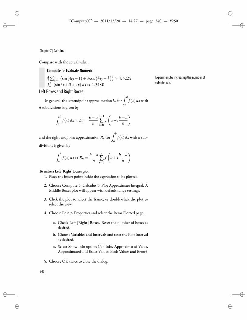
ii
“Compute60” — 2011/12/20 — 14:27 — page 240 — #250 ii
ii
ii
Chapter 7 | Calculus
Compare with the actual value:
Compute> Evaluate Numeric43 ∑5
i3=0(sin(4i3−1)+3cos
( 43 i3− 1
3
))≈ 4.5222∫ 7
−1 (sin3x+3cosx) dx≈ 4.3480
Experiment by increasing the number ofsubintervals.
Left Boxes and Right Boxes
In general, the le endpoint approximationLn for∫ b
af (x)dxwith
n subdivisions is given by
∫ b
af (x)dx≈ Ln =
b−an
n−1
∑i=0
f(
a+ ib−a
n
)
and the right endpoint approximation Rn for∫ b
af (x)dx with n sub-
divisions is given by∫ b
af (x)dx≈ Rn =
b−an
n
∑i=1
f(
a+ ib−a
n
)Tomake aLe [Right]Boxes plot
1. Place the insert point inside the expression to be plotted.
2. Choose Compute>Calculus> Plot Approximate Integral. AMiddle Boxes plot will appear with default range settings.
3. Click the plot to select the frame, or double-click the plot toselect the view.
4. Choose Edit> Properties and select the Items Plotted page.
a. Check Le [Right] Boxes. Reset the number of boxes asdesired.
b. Choose Variables and Intervals and reset the Plot Intervalas desired.
c. Select Show Info option (No Info, Approximated Value,Approximated and Exact Values, Both Values and Error)
5. Choose OK twice to close the dialog.
240
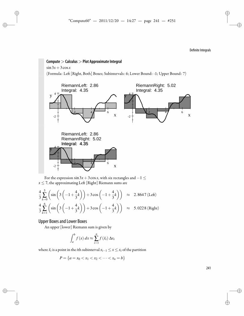
ii
“Compute60” — 2011/12/20 — 14:27 — page 241 — #251 ii
ii
ii
De nite Integrals
Compute> Calculus> Plot Approximate Integralsin3x+3cosx(Formula: Le [Right, Both] Boxes; Subintervals: 6; Lower Bound: -1; Upper Bound: 7)
RiemannLeft: 2.86Integral: 4.35
2 4 62
2
4
x
y
RiemannRight: 5.02Integral: 4.35
2 4 62
2
4
x
y
RiemannLeft: 2.86
Integral: 4.35RiemannRight: 5.02Integral: 4.35
2 4 62
2
4
x
y
For the expression sin3x+3cosx, with six rectangles and−1 ≤x≤ 7, the approximating Le [Right] Riemann sums are
43
5
∑k=0
(sin(
3(−1+
43
k))
+3cos(−1+
43
k))
≈ 2.8647 (Le )
43
6
∑k=1
(sin(
3(−1+
43
k))
+3cos(−1+
43
k))
≈ 5.0228 (Right)
Upper Boxes and Lower BoxesAn upper [lower] Riemann sum is given by∫ b
af (x) dx≈
n
∑i=1
f (xi) ∆xi
where xi is a point in the ith subinterval xi−1 ≤ x≤ xi of the partition
P = a = x0 < x1 < x2 < · · ·< xn = b
241
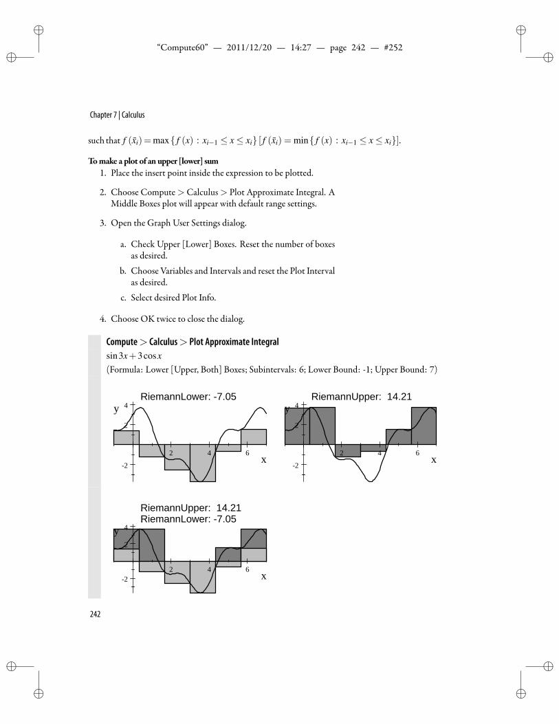
ii
“Compute60” — 2011/12/20 — 14:27 — page 242 — #252 ii
ii
ii
Chapter 7 | Calculus
such that f (xi)=max f (x) : xi−1 ≤ x≤ xi [ f (xi) = min f (x) : xi−1 ≤ x≤ xi].
Tomake a plot of an upper [lower] sum1. Place the insert point inside the expression to be plotted.
2. Choose Compute>Calculus> Plot Approximate Integral. AMiddle Boxes plot will appear with default range settings.
3. Open the Graph User Settings dialog.
a. Check Upper [Lower] Boxes. Reset the number of boxesas desired.
b. Choose Variables and Intervals and reset the Plot Intervalas desired.
c. Select desired Plot Info.
4. Choose OK twice to close the dialog.
Compute> Calculus> Plot Approximate Integralsin3x+3cosx(Formula: Lower [Upper, Both] Boxes; Subintervals: 6; Lower Bound: -1; Upper Bound: 7)
RiemannLower: 7.05
2 4 6
2
2
4
x
yRiemannUpper: 14.21
2 4 6
2
2
4
x
y
RiemannUpper: 14.21..RiemannLower: 7.05
2 4 62
2
4
x
y
242
ii
“Compute60” — 2011/12/20 — 14:27 — page 243 — #253 ii
ii
ii
De nite Integrals
Upper Absolute and Lower Absolute BoxesAn upper [lower] absolute Riemann sum is given by
∫ b
af (x) dx≈
n
∑i=1
f (xi) ∆xi
where xi is a point in the ith subinterval xi−1 ≤ x≤ xi of the partition
P = a = x0 < x1 < x2 < · · ·< xn = b
such that
| f (xi)| = max| f (x)| : xi−1 ≤ x≤ xi[ | f (xi)| = min| f (x)| : xi−1 ≤ x≤ xi].
Tomake a plot of an upper [lower] absolute sum
1. Place the insert point inside the expression to be plotted.
2. Choose Compute>Calculus> Plot Approximate Integral. AMiddle Boxes plot will appear with default range settings.
3. Open the Graph User Settings dialog.
a. CheckUpper [Lower] Absolute Boxes. Reset the numberof boxes as desired.
b. Choose Variables and Intervals and reset the Plot Intervalas desired.
c. Select desired Plot Info.
4. Choose OK twice to close the dialog.
243
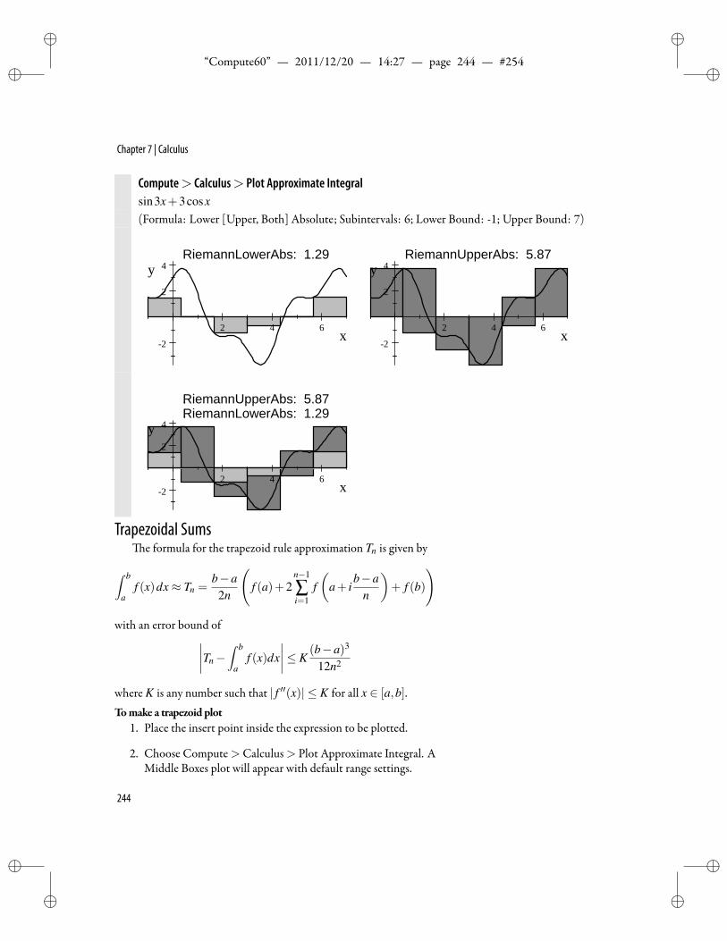
ii
“Compute60” — 2011/12/20 — 14:27 — page 244 — #254 ii
ii
ii
Chapter 7 | Calculus
Compute> Calculus> Plot Approximate Integralsin3x+3cosx(Formula: Lower [Upper, Both] Absolute; Subintervals: 6; Lower Bound: -1; Upper Bound: 7)
RiemannLowerAbs: 1.29
2 4 6
2
2
4
x
yRiemannUpperAbs: 5.87
2 4 6
2
2
4
x
y
RiemannUpperAbs: 5.87..RiemannLowerAbs: 1.29
2 4 62
2
4
x
y
Trapezoidal Sumse formula for the trapezoid rule approximation Tn is given by
∫ b
af (x)dx≈ Tn =
b−a2n
(f (a)+2
n−1
∑i=1
f(
a+ ib−a
n
)+ f (b)
)
with an error bound of∣∣∣∣Tn−∫ b
af (x)dx
∣∣∣∣≤ K(b−a)3
12n2
where K is any number such that | f ′′(x)| ≤ K for all x ∈ [a,b].Tomake a trapezoid plot
1. Place the insert point inside the expression to be plotted.
2. Choose Compute>Calculus> Plot Approximate Integral. AMiddle Boxes plot will appear with default range settings.
244
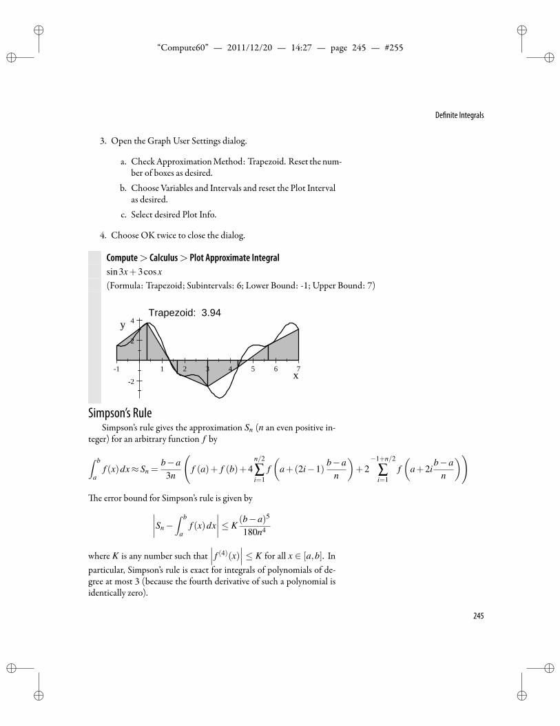
ii
“Compute60” — 2011/12/20 — 14:27 — page 245 — #255 ii
ii
ii
De nite Integrals
3. Open the Graph User Settings dialog.
a. CheckApproximationMethod: Trapezoid. Reset thenum-ber of boxes as desired.
b. Choose Variables and Intervals and reset the Plot Intervalas desired.
c. Select desired Plot Info.
4. Choose OK twice to close the dialog.
Compute> Calculus> Plot Approximate Integralsin3x+3cosx(Formula: Trapezoid; Subintervals: 6; Lower Bound: -1; Upper Bound: 7)
Trapezoid: 3.94
1 1 2 3 4 5 6 7
2
2
4
x
y
Simpson’s RuleSimpson’s rule gives the approximation Sn (n an even positive in-
teger) for an arbitrary function f by
∫ b
af (x)dx≈ Sn =
b−a3n
(f (a)+ f (b)+4
n/2
∑i=1
f(
a+(2i−1)b−a
n
)+2
−1+n/2
∑i=1
f(
a+2ib−a
n
))
e error bound for Simpson’s rule is given by∣∣∣∣Sn−∫ b
af (x)dx
∣∣∣∣≤ K(b−a)5
180n4
where K is any number such that∣∣∣ f (4)(x)∣∣∣ ≤ K for all x ∈ [a,b]. In
particular, Simpson’s rule is exact for integrals of polynomials of de-gree at most 3 (because the fourth derivative of such a polynomial isidentically zero).
245
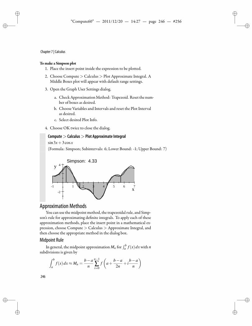
ii
“Compute60” — 2011/12/20 — 14:27 — page 246 — #256 ii
ii
ii
Chapter 7 | Calculus
Tomake a Simpsonplot1. Place the insert point inside the expression to be plotted.
2. Choose Compute>Calculus> Plot Approximate Integral. AMiddle Boxes plot will appear with default range settings.
3. Open the Graph User Settings dialog.
a. CheckApproximationMethod: Trapezoid. Reset thenum-ber of boxes as desired.
b. Choose Variables and Intervals and reset the Plot Intervalas desired.
c. Select desired Plot Info.
4. Choose OK twice to close the dialog.
Compute> Calculus> Plot Approximate Integralsin3x+3cosx(Formula: Simpson; Subintervals: 6; Lower Bound: -1; Upper Bound: 7)
Simpson: 4.33
1 1 2 3 4 5 6 7
2
2
4
x
y
Approximation MethodsYou can use themidpointmethod, the trapezoidal rule, and Simp-
son’s rule for approximating de nite integrals. To apply each of theseapproximation methods, place the insert point in a mathematical ex-pression, choose Compute > Calculus > Approximate Integral, andthen choose the appropriate method in the dialog box.
Midpoint RuleIn general, the midpoint approximation Mn for
∫ ba f (x)dx with n
subdivisions is given by∫ b
af (x)dx≈Mn =
b−an
n−1
∑i=0
f(
a+b−a
2n+ i
b−an
)246
ii
“Compute60” — 2011/12/20 — 14:27 — page 247 — #257 ii
ii
ii
De nite Integrals
with an error bound of∣∣∣∣Mn−∫ b
af (x)dx
∣∣∣∣≤ K(b−a)3
24n2
where K is any number such that | f ′′(x)| ≤ K for all x ∈ [a,b].
Toapproximate∫ b
a f (x) dxusing themidpointmethod
1. Place the insert point in an expression of the form∫ b
a f (x) dx.
2. Choose Compute>Calculus>Approximate Integral.
3. In thedialog that appears, chooseMidpoint and specify thenum-ber of Subintervals.
Or
1. Place the insert point in an expression f (x).
2. Choose Compute>Calculus>Approximate Integral.
3. In the dialog, choose Midpoint, specify the number of Subin-tervals, and specify Lower Bound and Upper Bound.
To obtain the following output, in the dialog that appears, specify10 Subintervals. e system returns a summation that you can evalu-ate numerically.
Compute> Calculus> Approximate Integral∫ π0 xsinxdx Approximate integral (midpoint rule) is
110 π
9∑
i3=0
110 π
(i3 + 1
2
)sin 1
10 π(i3 + 1
2
)For the following output, specify 10 Subintervals, type 0 as Lower
Bound, and type 3.14159 as Upper Bound.
Compute> Calculus> Approximate Integralxsinx Approximate integral (midpoint rule) is
0.314169∑
i4=0(0.31416i4 +0.15708)sin(0.31416i4 +0.15708)
Compare these results with direct computations of the integral.
247
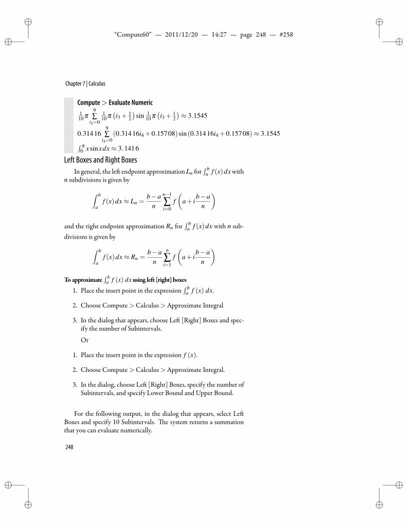
ii
“Compute60” — 2011/12/20 — 14:27 — page 248 — #258 ii
ii
ii
Chapter 7 | Calculus
Compute> Evaluate Numeric1
10 π9∑
i3=0
110 π
(i3 + 1
2
)sin 1
10 π(i3 + 1
2
)≈ 3.1545
0.314169∑
i4=0(0.31416i4 +0.15708)sin(0.31416i4 +0.15708)≈ 3.1545∫ π
0 xsinxdx≈ 3.1416
Left Boxes and Right BoxesIn general, the le endpoint approximationLn for
∫ ba f (x)dx with
n subdivisions is given by
∫ b
af (x)dx≈ Ln =
b−an
n−1
∑i=0
f(
a+ ib−a
n
)
and the right endpoint approximation Rn for∫ b
a f (x)dx with n sub-divisions is given by∫ b
af (x)dx≈ Rn =
b−an
n
∑i=1
f(
a+ ib−a
n
)Toapproximate
∫ ba f (x) dxusing le [right] boxes
1. Place the insert point in the expression∫ b
a f (x) dx.
2. Choose Compute>Calculus>Approximate Integral
3. In the dialog that appears, choose Le [Right] Boxes and spec-ify the number of Subintervals.
Or
1. Place the insert point in the expression f (x).
2. Choose Compute>Calculus>Approximate Integral.
3. In the dialog, choose Le [Right] Boxes, specify the number ofSubintervals, and specify Lower Bound and Upper Bound.
For the following output, in the dialog that appears, select LeBoxes and specify 10 Subintervals. e system returns a summationthat you can evaluate numerically.
248
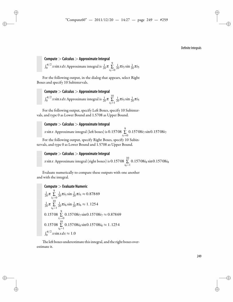
ii
“Compute60” — 2011/12/20 — 14:27 — page 249 — #259 ii
ii
ii
De nite Integrals
Compute> Calculus> Approximate Integral∫ π/20 xsinxdx Approximate integral is 1
20 π9∑
i5=0
120 πi5 sin 1
20 πi5
For the following output, in the dialog that appears, select RightBoxes and specify 10 Subintervals.
Compute> Calculus> Approximate Integral∫ π/20 xsinxdx Approximate integral is 1
20 π10∑
i5=1
120 πi5 sin 1
20 πi5
For the following output, specify Le Boxes, specify 10 Subinter-vals, and type 0 as Lower Bound and 1.5708 as Upper Bound.
Compute> Calculus> Approximate Integral
xsinx Approximate integral (le boxes) is 0.157089∑
i7=00.15708i7 sin0.15708i7
For the following output, specify Right Boxes, specify 10 Subin-tervals, and type 0 as Lower Bound and 1.5708 as Upper Bound.
Compute> Calculus> Approximate Integral
xsinx Approximate integral (right boxes) is 0.1570810∑
i8=10.15708i8 sin0.15708i8
Evaluate numerically to compare these outputs with one anotherand with the integral.
Compute> Evaluate Numeric1
20 π9∑
i5=0
120 πi5 sin 1
20 πi5 ≈ 0.87869
120 π
10∑
i6=1
120 πi6 sin 1
20 πi6 ≈ 1.1254
0.157089∑
i7=00.15708i7 sin0.15708i7 ≈ 0.87869
0.1570810∑
i8=10.15708i8 sin0.15708i8 ≈ 1.1254∫ π/2
0 xsinxdx≈ 1.0
e le boxes underestimate this integral, and the right boxes over-estimate it.
249
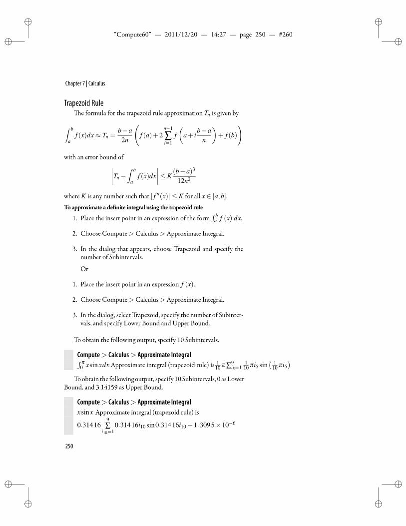
ii
“Compute60” — 2011/12/20 — 14:27 — page 250 — #260 ii
ii
ii
Chapter 7 | Calculus
Trapezoid Rulee formula for the trapezoid rule approximation Tn is given by
∫ b
af (x)dx≈ Tn =
b−a2n
(f (a)+2
n−1
∑i=1
f(
a+ ib−a
n
)+ f (b)
)
with an error bound of∣∣∣∣Tn−∫ b
af (x)dx
∣∣∣∣≤ K(b−a)3
12n2
where K is any number such that | f ′′(x)| ≤ K for all x ∈ [a,b].
Toapproximate a de nite integral using the trapezoid rule
1. Place the insert point in an expression of the form∫ b
a f (x) dx.
2. Choose Compute>Calculus>Approximate Integral.
3. In the dialog that appears, choose Trapezoid and specify thenumber of Subintervals.
Or
1. Place the insert point in an expression f (x).
2. Choose Compute>Calculus>Approximate Integral.
3. In the dialog, select Trapezoid, specify the number of Subinter-vals, and specify Lower Bound and Upper Bound.
To obtain the following output, specify 10 Subintervals.
Compute> Calculus> Approximate Integral∫ π0 xsinxdx Approximate integral (trapezoid rule) is 1
10 π ∑9i5=1
110 πi5 sin
( 110 πi5
)Toobtain the followingoutput, specify 10Subintervals, 0 asLower
Bound, and 3.14159 as Upper Bound.
Compute> Calculus> Approximate Integralxsinx Approximate integral (trapezoid rule) is
0.314169∑
i10=10.31416i10 sin0.31416i10 +1.3095×10⁻⁶
250
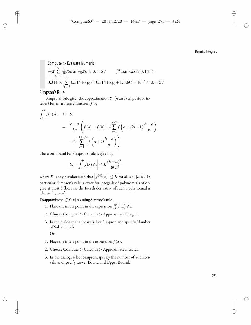
ii
“Compute60” — 2011/12/20 — 14:27 — page 251 — #261 ii
ii
ii
De nite Integrals
Compute> Evaluate Numeric1
10 π9∑
i9=1
110 πi9 sin 1
10 πi9 ≈ 3.1157∫ π
0 xsinxdx≈ 3.1416
0.314169∑
i10=10.31416i10 sin0.31416i10 +1.3095×10⁻⁶ ≈ 3.1157
Simpson’s RuleSimpson’s rule gives the approximation Sn (n an even positive in-
teger) for an arbitrary function f by∫ b
af (x)dx ≈ Sn
=b−a
3n
(f (a)+ f (b)+4
n/2
∑i=1
f(
a+(2i−1)b−a
n
)
+2−1+n/2
∑i=1
f(
a+2ib−a
n
))e error bound for Simpson’s rule is given by∣∣∣∣Sn−
∫ b
af (x)dx
∣∣∣∣≤ K(b−a)5
180n4
where K is any number such that∣∣∣ f (4)(x)∣∣∣ ≤ K for all x ∈ [a,b]. In
particular, Simpson’s rule is exact for integrals of polynomials of de-gree at most 3 (because the fourth derivative of such a polynomial isidentically zero).Toapproximate
∫ ba f (x) dxusing Simpson's rule
1. Place the insert point in the expression∫ b
a f (x) dx.
2. Choose Compute>Calculus>Approximate Integral.
3. In the dialog that appears, select Simpson and specify Numberof Subintervals.Or
1. Place the insert point in the expression f (x).
2. Choose Compute>Calculus>Approximate Integral.
3. In the dialog, select Simpson, specify the number of Subinter-vals, and specify Lower Bound and Upper Bound.
251
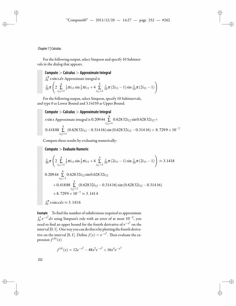
ii
“Compute60” — 2011/12/20 — 14:27 — page 252 — #262 ii
ii
ii
Chapter 7 | Calculus
For the following output, select Simpson and specify 10 Subinter-vals in the dialog that appears.
Compute> Calculus> Approximate Integral∫ π0 xsinxdx Approximate integral is
130 π
(2
4∑
i11=1
15 πi11 sin 1
5 πi11 +45∑
i11=1
110 π (2i11−1)sin 1
10 π (2i11−1)
)For the following output, select Simpson, specify 10 Subintervals,
and type 0 as Lower Bound and 3.14159 as Upper Bound.
Compute> Calculus> Approximate Integral
xsinx Approximate integral is 0.209444∑
i12=10.62832i12 sin0.62832i12+
0.418885∑
i12=1(0.62832i12−0.31416)sin(0.62832i12−0.31416)+ 8.7299×10⁻⁷
Compare these results by evaluating numerically:
Compute> Evaluate Numeric
130 π
(2
4∑
i11=1
15 πi11 sin 1
5 πi11 +45∑
i11=1
110 π (2i11−1)sin 1
10 π (2i11−1)
)≈ 3.1418
0.209444∑
i12=10.62832i12 sin0.62832i12
+0.418885∑
i12=1(0.62832i12−0.31416)sin(0.62832i12−0.31416)
+8.7299×10⁻⁷ ≈ 3.1414∫ π0 xsinxdx≈ 3.1416
Example To nd the number of subdivisions required to approximate∫ 10 e−x2
dx using Simpson’s rule with an error of at most 10−5, youneed to nd an upper bound for the fourth derivative of e−x2
on theinterval [0,1]. Oneway you cando this is byplotting the fourthderiva-tive on the interval [0,1]. De ne f (x) = e−x2
. en evaluate the ex-pression f (4)(x)
f (4)(x) = 12e−x2 −48x2e−x2+16x4e−x2
252
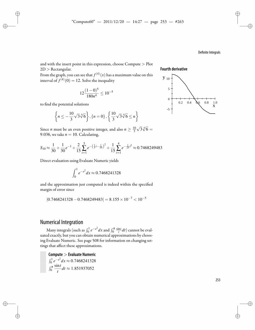
ii
“Compute60” — 2011/12/20 — 14:27 — page 253 — #263 ii
ii
ii
De nite Integrals
and with the insert point in this expression, choose Compute > Plot2D> Rectangular. Fourth derivative
0.2 0.4 0.6 0.8 1.0
5
0
5
10
x
yFrom the graph, you can see that f (4)(x) has amaximum value on thisinterval of f (4)(0) = 12. Solve the inequality
12(1−0)5
180n4 ≤ 10−5
to nd the potential solutionsn≤−10
3
√3 4√6
,n = 0 ,
103
√3 4√6≤ n
Since n must be an even positive integer, and also n ≥ 10
3
√3 4√6 =
9.036, we take n = 10. Calculating,
S10≈1
30+
130
e−1+2
15
5
∑i=1
e−(15 i− 1
10)2+
115
4
∑i=1
e−1
25 i2 ≈ 0.7468249483
Direct evaluation using Evaluate Numeric yields∫ 1
0e−x2
dx≈ 0.7468241328
and the approximation just computed is indeed within the speci edmargin of error since
|0.7468241328−0.7468249483|= 8.155×10⁻⁷ < 10−5
Numerical IntegrationMany integrals (such as
∫ 10 e−x2
dx and∫ π
0sin t
t dt) cannot be eval-uated exactly, but you can obtain numerical approximations by choos-ing Evaluate Numeric. See page 508 for information on changing set-tings that affect these approximations.
Compute> Evaluate Numeric∫ 10 e−x2
dx≈ 0.7468241328∫ π0
sin tt
dt ≈ 1.851937052
253
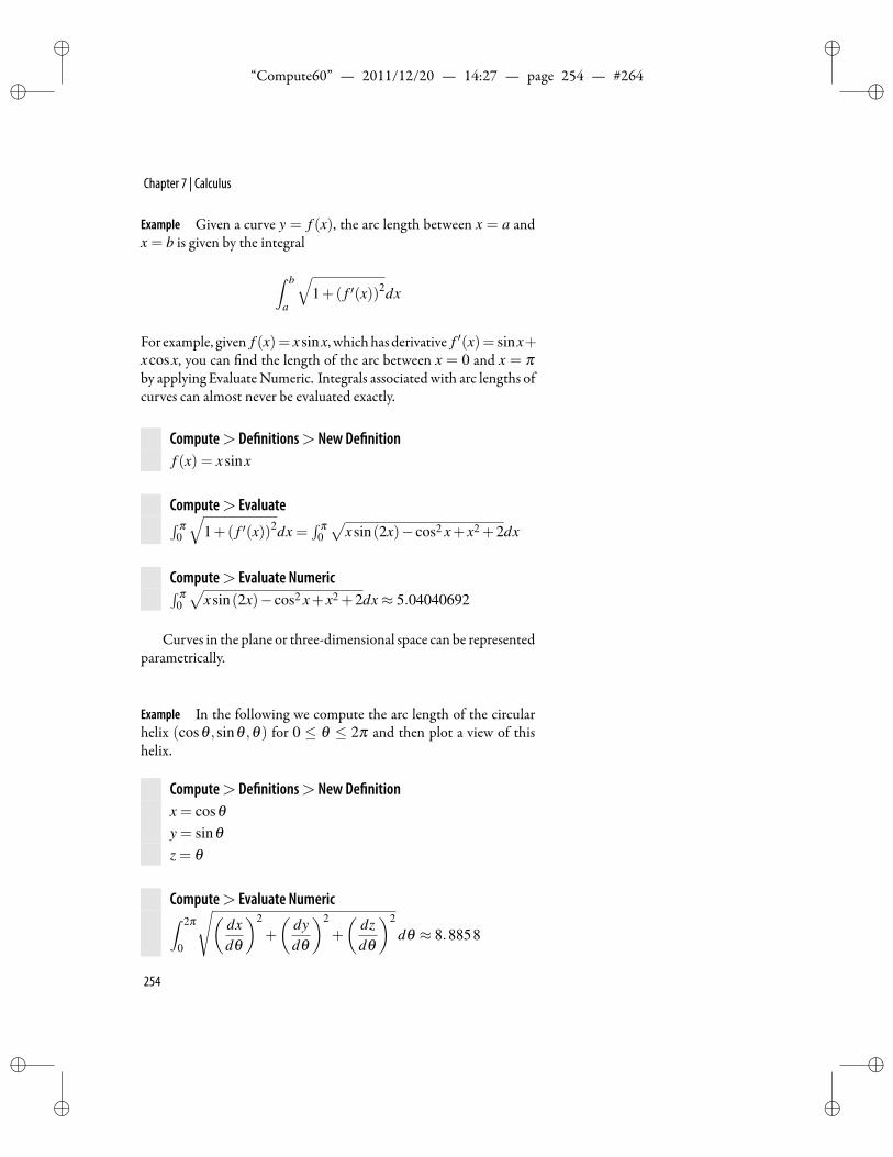
ii
“Compute60” — 2011/12/20 — 14:27 — page 254 — #264 ii
ii
ii
Chapter 7 | Calculus
Example Given a curve y = f (x), the arc length between x = a andx = b is given by the integral
∫ b
a
√1+( f ′(x))2dx
For example, given f (x)= xsinx, whichhas derivative f ′(x)= sinx+xcosx, you can nd the length of the arc between x = 0 and x = πby applying EvaluateNumeric. Integrals associated with arc lengths ofcurves can almost never be evaluated exactly.
Compute> De nitions> New De nitionf (x) = xsinx
Compute> Evaluate∫ π0
√1+( f ′(x))2dx =
∫ π0
√xsin(2x)− cos2 x+ x2 +2dx
Compute> Evaluate Numeric∫ π0
√xsin(2x)− cos2 x+ x2 +2dx≈ 5.04040692
Curves in the plane or three-dimensional space can be representedparametrically.
Example In the following we compute the arc length of the circularhelix (cosθ ,sinθ ,θ) for 0 ≤ θ ≤ 2π and then plot a view of thishelix.
Compute> De nitions> New De nitionx = cosθy = sinθz = θ
Compute> Evaluate Numeric∫ 2π
0
√(dxdθ
)2
+
(dydθ
)2
+
(dzdθ
)2
dθ ≈ 8.8858
254
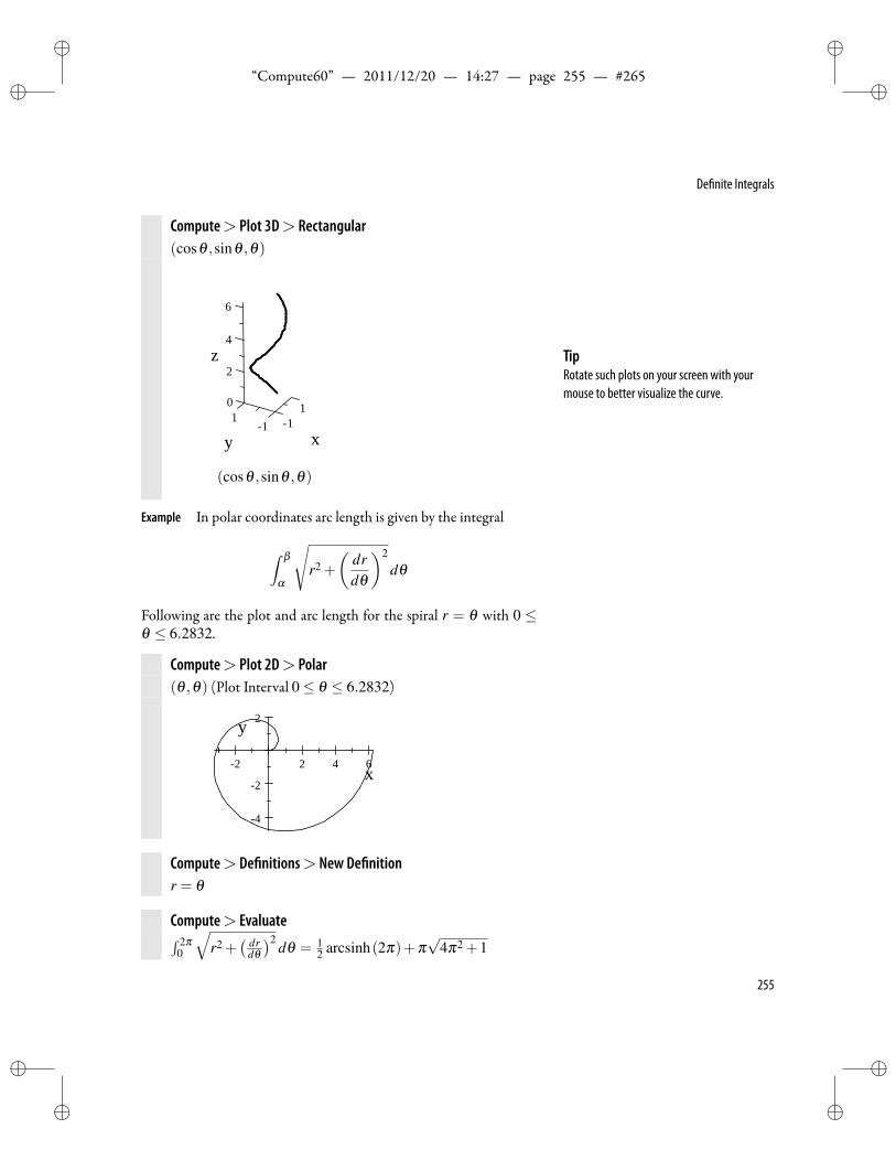
ii
“Compute60” — 2011/12/20 — 14:27 — page 255 — #265 ii
ii
ii
De nite Integrals
Compute> Plot 3D> Rectangular(cosθ ,sinθ ,θ)
10
x1
y
2
11
z4
6
(cosθ ,sinθ ,θ)
TipRotate such plots on your screen with yourmouse to better visualize the curve.
Example In polar coordinates arc length is given by the integral
∫ β
α
√r2 +
(drdθ
)2
dθ
Following are the plot and arc length for the spiral r = θ with 0 ≤θ ≤ 6.2832.
Compute> Plot 2D> Polar(θ ,θ) (Plot Interval 0≤ θ ≤ 6.2832)
2 2 4 6
4
2
2
x
y
Compute> De nitions> New De nitionr = θ
Compute> Evaluate∫ 2π0
√r2 +
( drdθ)2
dθ = 12 arcsinh(2π)+π
√4π2 +1
255
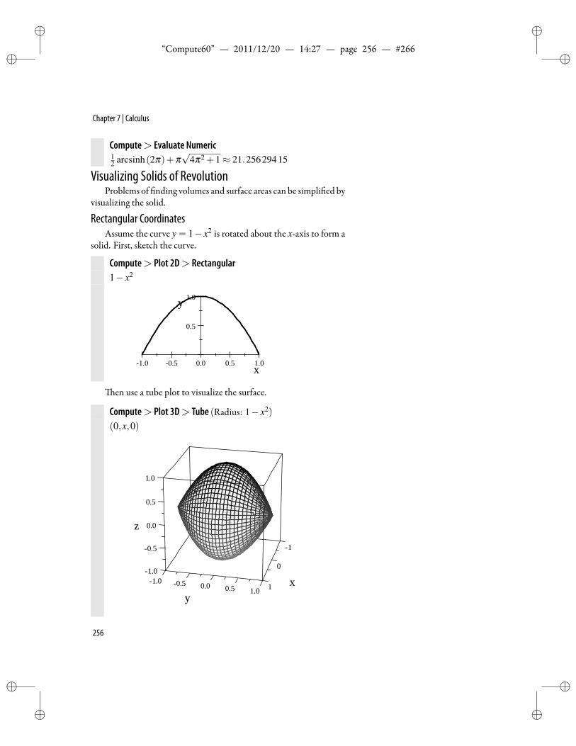
ii
“Compute60” — 2011/12/20 — 14:27 — page 256 — #266 ii
ii
ii
Chapter 7 | Calculus
Compute> Evaluate Numeric12 arcsinh(2π)+π
√4π2 +1≈ 21.25629415
Visualizing Solids of RevolutionProblems of nding volumes and surface areas can be simpli ed by
visualizing the solid.
Rectangular CoordinatesAssume the curve y = 1− x2 is rotated about the x-axis to form a
solid. First, sketch the curve.
Compute> Plot 2D> Rectangular1− x2
1.0 0.5 0.0 0.5 1.0
0.5
1.0
x
y
en use a tube plot to visualize the surface.
Compute> Plot 3D> Tube (Radius: 1− x2)(0,x,0)
1
x
1.0
0.5
z 0.0
0.50.0
y11.0
1.01.0 0.5
0.5
0
256
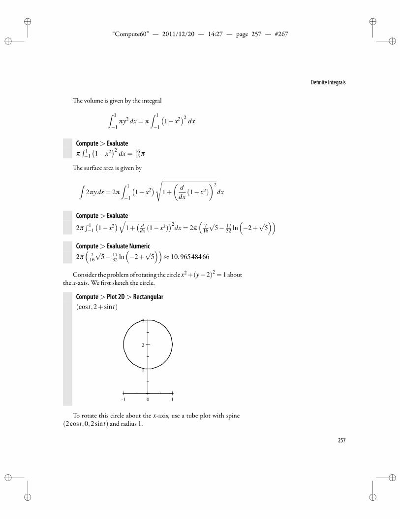
ii
“Compute60” — 2011/12/20 — 14:27 — page 257 — #267 ii
ii
ii
De nite Integrals
e volume is given by the integral
∫ 1
−1πy2 dx = π
∫ 1
−1
(1− x2)2
dx
Compute> Evaluateπ∫ 1−1(1− x2
)2 dx = 1615 π
e surface area is given by
∫2πyds = 2π
∫ 1
−1
(1− x2)√1+
(ddx
(1− x2)
)2
dx
Compute> Evaluate
2π∫ 1−1(1− x2
)√1+( d
dx (1− x2))2
dx = 2π(
716
√5− 17
32 ln(−2+
√5))
Compute> Evaluate Numeric2π(
716
√5− 17
32 ln(−2+
√5))≈ 10.96548466
Consider theproblemof rotating the circlex2+(y−2)2 = 1 aboutthe x-axis. We rst sketch the circle.
Compute> Plot 2D> Rectangular(cos t,2+ sin t)
1 0 1
1
2
3
To rotate this circle about the x-axis, use a tube plot with spine(2cos t,0,2sin t) and radius 1.
257
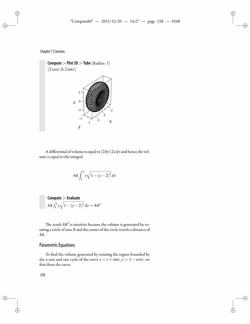
ii
“Compute60” — 2011/12/20 — 14:27 — page 258 — #268 ii
ii
ii
Chapter 7 | Calculus
Compute> Plot 3D> Tube (Radius: 1)(2cos t,0,2sin t)
2
x0
2
y
11
2
z 0
2
Adifferential of volume is equal to (2πy)2xdy and hence the vol-ume is equal to the integral
4π∫ 3
1y√
1− (y−2)2 dy
Compute> Evaluate
4π∫ 3
1 y√
1− (y−2)2 dy = 4π2
e result 4π2 is intuitive because the volume is generated by ro-tating a circle of area π and the center of the circle travels a distance of4π .
Parametric Equations
To nd the volume generated by rotating the region bounded bythe x-axis and one cycle of the curve x = t + sin t , y = 1− cos t , werst draw the curve.
258
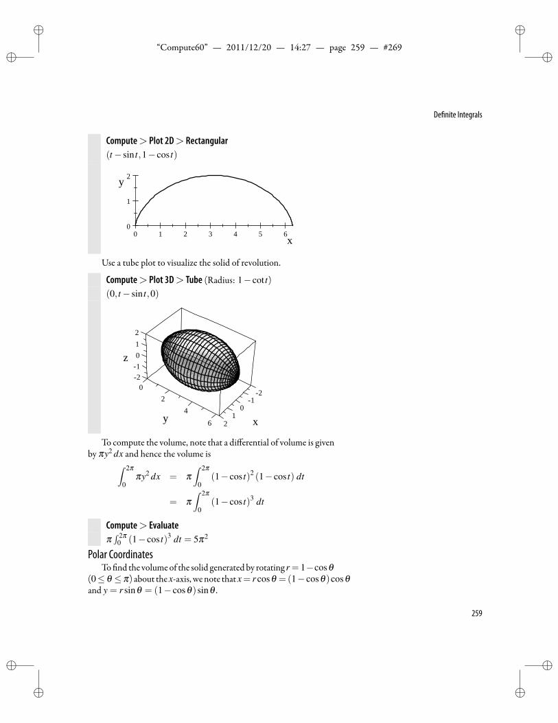
ii
“Compute60” — 2011/12/20 — 14:27 — page 259 — #269 ii
ii
ii
De nite Integrals
Compute> Plot 2D> Rectangular(t− sin t,1− cos t)
0 1 2 3 4 5 60
1
2
x
y
Use a tube plot to visualize the solid of revolution.
Compute> Plot 3D> Tube (Radius: 1− cot t)(0, t− sin t,0)
21
x
2
42
y 6 2
0210z1
10
To compute the volume, note that a differential of volume is givenby πy2 dx and hence the volume is∫ 2π
0πy2 dx = π
∫ 2π
0(1− cos t)2 (1− cos t) dt
= π∫ 2π
0(1− cos t)3 dt
Compute> Evaluateπ∫ 2π
0 (1− cos t)3 dt = 5π2
Polar CoordinatesTo nd the volumeof the solid generated by rotating r = 1−cosθ
(0≤ θ ≤ π) about thex-axis, wenote thatx= r cosθ =(1− cosθ)cosθand y = r sinθ = (1− cosθ)sinθ .
259
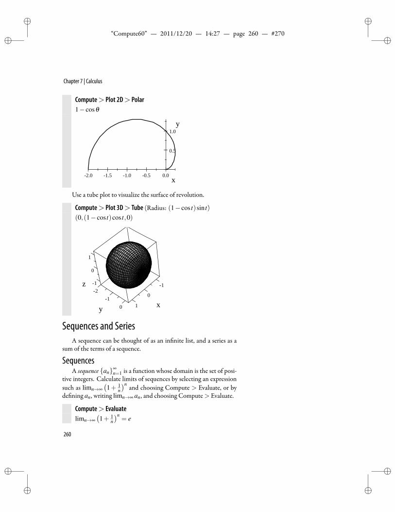
ii
“Compute60” — 2011/12/20 — 14:27 — page 260 — #270 ii
ii
ii
Chapter 7 | Calculus
Compute> Plot 2D> Polar1− cosθ
2.0 1.5 1.0 0.5 0.0
0.5
1.0
x
y
Use a tube plot to visualize the surface of revolution.
Compute> Plot 3D> Tube (Radius: (1− cos t)sin t)(0,(1− cos t)cos t,0)
1
z 1
0
21
y 0 1
0
x
1
Sequences and SeriesA sequence can be thought of as an in nite list, and a series as a
sum of the terms of a sequence.
SequencesA sequence an∞
n=1 is a function whose domain is the set of posi-tive integers. Calculate limits of sequences by selecting an expressionsuch as limn→∞
(1+ 1
n
)n and choosing Compute > Evaluate, or byde ning an, writing limn→∞ an, and choosing Compute> Evaluate.
Compute> Evaluatelimn→∞
(1+ 1
n
)n= e
260
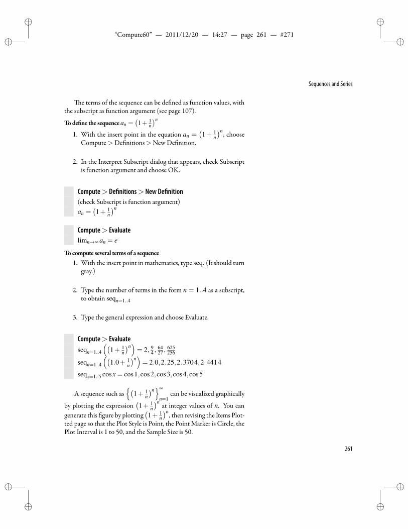
ii
“Compute60” — 2011/12/20 — 14:27 — page 261 — #271 ii
ii
ii
Sequences and Series
e terms of the sequence can be de ned as function values, withthe subscript as function argument (see page 107).
Tode ne the sequencean =(1+ 1
n
)n
1. With the insert point in the equation an =(1+ 1
n
)n, chooseCompute>De nitions>New De nition.
2. In the Interpret Subscript dialog that appears, check Subscriptis function argument and choose OK.
Compute> De nitions> New De nition(check Subscript is function argument)an =
(1+ 1
n
)n
Compute> Evaluatelimn→∞ an = e
Tocompute several terms of a sequence1. With the insert point in mathematics, type seq. (It should turn
gray.)
2. Type the number of terms in the form n = 1..4 as a subscript,to obtain seqn=1..4
3. Type the general expression and choose Evaluate.
Compute> Evaluateseqn=1..4
((1+ 1
n
)n)= 2, 9
4 ,6427 ,
625256
seqn=1..4
((1.0+ 1
n
)n)= 2.0,2.25,2.3704,2.4414
seqx=1..5 cosx = cos1,cos2,cos3,cos4,cos5
A sequence such as(
1+ 1n
)n∞
n=1can be visualized graphically
by plotting the expression(1+ 1
n
)n at integer values of n. You cangenerate this gure by plotting
(1+ 1
n
)n, then revising the Items Plot-ted page so that the Plot Style is Point, the Point Marker is Circle, thePlot Interval is 1 to 50, and the Sample Size is 50.
261
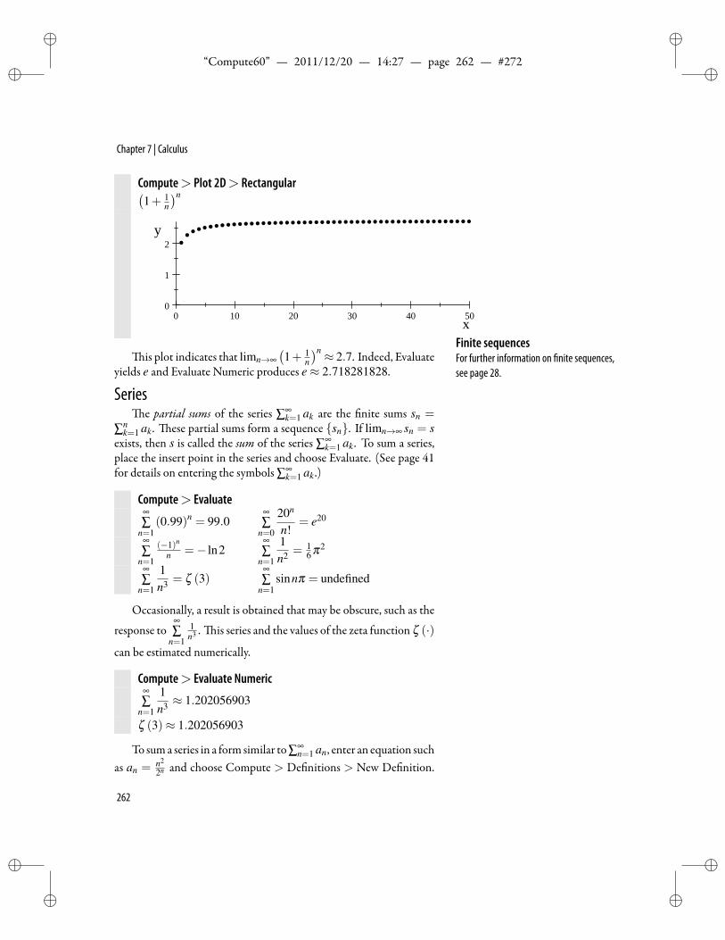
ii
“Compute60” — 2011/12/20 — 14:27 — page 262 — #272 ii
ii
ii
Chapter 7 | Calculus
Compute> Plot 2D> Rectangular(1+ 1
n
)n
0 10 20 30 40 500
1
2
x
y
Finite sequencesFor further information on nite sequences,see page 28.
is plot indicates that limn→∞(1+ 1
n
)n ≈ 2.7. Indeed, Evaluateyields e and Evaluate Numeric produces e≈ 2.718281828.
Seriese partial sums of the series ∑∞
k=1 ak are the nite sums sn =
∑nk=1 ak. ese partial sums form a sequence sn. If limn→∞ sn = s
exists, then s is called the sum of the series ∑∞k=1 ak. To sum a series,
place the insert point in the series and choose Evaluate. (See page 41for details on entering the symbols ∑∞
k=1 ak.)
Compute> Evaluate∞∑
n=1(0.99)n = 99.0
∞∑
n=0
20n
n!= e20
∞∑
n=1
(−1)n
n =− ln2∞∑
n=1
1n2 = 1
6 π2
∞∑
n=1
1n3 = ζ (3)
∞∑
n=1sinnπ = undefined
Occasionally, a result is obtained that may be obscure, such as the
response to∞∑
n=1
1n3 . is series and the values of the zeta function ζ (·)
can be estimated numerically.
Compute> Evaluate Numeric∞∑
n=1
1n3 ≈ 1.202056903
ζ (3)≈ 1.202056903
To suma series in a form similar to∑∞n=1 an, enter an equation such
as an = n2
2n and choose Compute > De nitions > New De nition.
262
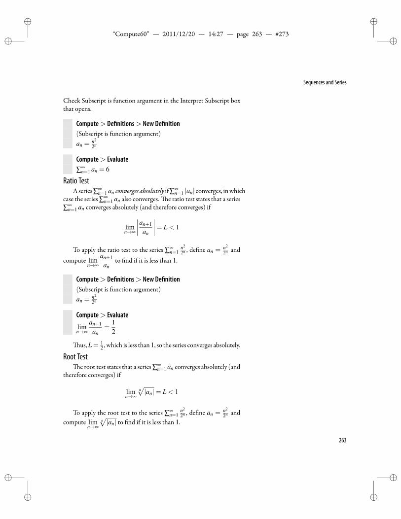
ii
“Compute60” — 2011/12/20 — 14:27 — page 263 — #273 ii
ii
ii
Sequences and Series
Check Subscript is function argument in the Interpret Subscript boxthat opens.
Compute> De nitions> New De nition(Subscript is function argument)an =
n2
2n
Compute> Evaluate∑∞
n=1 an = 6
Ratio TestAseries∑∞
n=1 an con erges absolutely if∑∞n=1 |an| converges, inwhich
case the series ∑∞n=1 an also converges. e ratio test states that a series
∑∞n=1 an converges absolutely (and therefore converges) if
limn→∞
∣∣∣∣an+1
an
∣∣∣∣= L < 1
To apply the ratio test to the series ∑∞n=1
n2
2n , de ne an = n2
2n andcompute lim
n→∞
an+1
anto nd if it is less than 1.
Compute> De nitions> New De nition(Subscript is function argument)an =
n2
2n
Compute> Evaluate
limn→∞
an+1
an=
12
us, L= 12 , which is less than1, so the series converges absolutely.
Root Teste root test states that a series ∑∞
n=1 an converges absolutely (andtherefore converges) if
limn→∞
n√|an|= L < 1
To apply the root test to the series ∑∞n=1
n2
2n , de ne an = n2
2n andcompute lim
n→∞n√|an| to nd if it is less than 1.
263
ii
“Compute60” — 2011/12/20 — 14:27 — page 264 — #274 ii
ii
ii
Chapter 7 | Calculus
Compute> De nitions> New De nition(Subscript is function argument)an =
n2
2n
Compute> Evaluate
limn→∞
n√|an|=
12
us,L= 12 , which is less than1, showing that this series converges
absolutely.
Integral Teste integral test states that a series ∑∞
n=1 an converges absolutelyif there exists a positive decreasing function f such that f (n) = |an|for each positive integer n and∫ ∞
1f (x)dx < ∞
To verify convergence of the series ∑∞n=1
n2
2n using the integral test,
de ne f by f (x) = x2
2x , compute∫ ∞
1
x2
2x dx and determine if it is nite.
Compute> De nitions> New De nitionf (x) = x2
2x
Compute> Evaluate, Compute> Evaluate Numeric∫ ∞
1
x2
2x dx = (ln4+ln2 2+2)2ln3 2
≈ 5.805497209
us, this integral is nite. (Although for f (x) = x2
2x , it is true thatf (1)< f (2)< f (3), you can verify that f is decreasing for x > 3. Infact,
f ′(x) =22x x− 1
2x x2 ln2
is positive only on the interval 0 < x < 2ln2 = 2.8854, so f is decreas-
ing on 3 < x < ∞. Since convergence of a series depends on the tailend of the series only, it is sufficient that the sequence of terms be even-tually decreasing.)
264
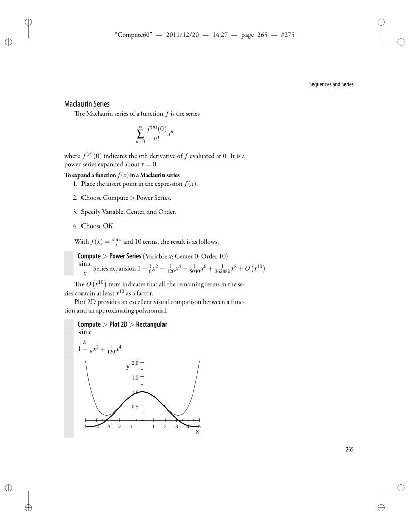
ii
“Compute60” — 2011/12/20 — 14:27 — page 265 — #275 ii
ii
ii
Sequences and Series
Maclaurin Seriese Maclaurin series of a function f is the series
∞
∑n=0
f (n)(0)n!
xn
where f (n)(0) indicates the nth derivative of f evaluated at 0. It is apower series expanded about x = 0.Toexpand a function f (x) in aMaclaurin series
1. Place the insert point in the expression f (x).
2. Choose Compute> Power Series.
3. Specify Variable, Center, and Order.
4. Choose OK.
With f (x) = sinxx and 10 terms, the result is as follows.
Compute> Power Series (Variable x; Center 0; Order 10)sinx
xSeries expansion 1− 1
6 x2 + 1120 x4− 1
5040 x6 + 1362880 x8 +O
(x10)
e O(x10)term indicates that all the remaining terms in the se-
ries contain at least x10 as a factor.Plot 2D provides an excellent visual comparison between a func-
tion and an approximating polynomial.
Compute> Plot 2D> Rectangularsinx
x1− 1
6 x2 + 1120 x4
5 4 3 2 1 1 2 3 4 5
0.5
1.0
1.5
2.0
x
y
265
ii
“Compute60” — 2011/12/20 — 14:27 — page 266 — #276 ii
ii
ii
Chapter 7 | Calculus
To determine which graph corresponds to which equation, evalu-ate one of the expressionswhere the graphs show some separation. Forexample, sin4
4 ≈−0.1892006238, and hence the graph of sinxx is the
one that is negative at x = 4.You can de ne a generic function and reproduce the general for-
mula for a power series.
Compute> De nitions> New De nitionf (x)
Compute> Power Series(Variable x, Center 0, Order 5)f (x) Series expansion f (0)+ x f ′ (0)+ 1
2 x2 f ′′ (0)+ 16 x3 f (3) (0)+ 1
24 x4 f (4) (0)+O(x5)
e following are additional examples of Maclaurin series expan-sions.
Compute> Power Series (Variable x; Center 0; Order 7,10,7 resp.)ex Series expansion 1+ x+ 1
2 x2 + 16 x3 + 1
24 x4 + 1120 x5 + 1
720 x6 +O(x7)
sinx Series expansion x− 16 x3 + 1
120 x5− 15040 x7 + 1
362880 x9 +O(x10)
ex sinx Series expansion x+ x2 + 13 x3− 1
30 x5− 190 x6− 1
630 x7 +O(x8)
Remember that output can be copied and pasted (with ordinaryword-processing tools) to create input for further calculations. In par-ticular, select and delete the +O(xn) expression to convert the seriesinto a polynomial. It is reassuring to note that, if the rst few terms ofthe Maclaurin series for ex are multiplied by the rst few terms of theMaclaurin series for sinx, then the result is the same as the rst fewterms of the Maclaurin series for ex sinx.
Compute> Expand(1+ x+ 1
2 x2 + 16 x3 + 1
24 x4 + 1120 x5
)(x− 1
6 x3 + 1120 x5
)= 1
14400 x10 + 12880 x9− 1
360 x7− 190 x6− 1
30 x5 + 13 x3 + x2 + x
Taylor Seriese Maclaurin series is a special case of the more general Taylor
series. e Taylor series of f expanded about x = a is given by
∞
∑n=0
f (n)(a)n!
(x−a)n
and hence is expanded in powers of x−a and centered about a.
266
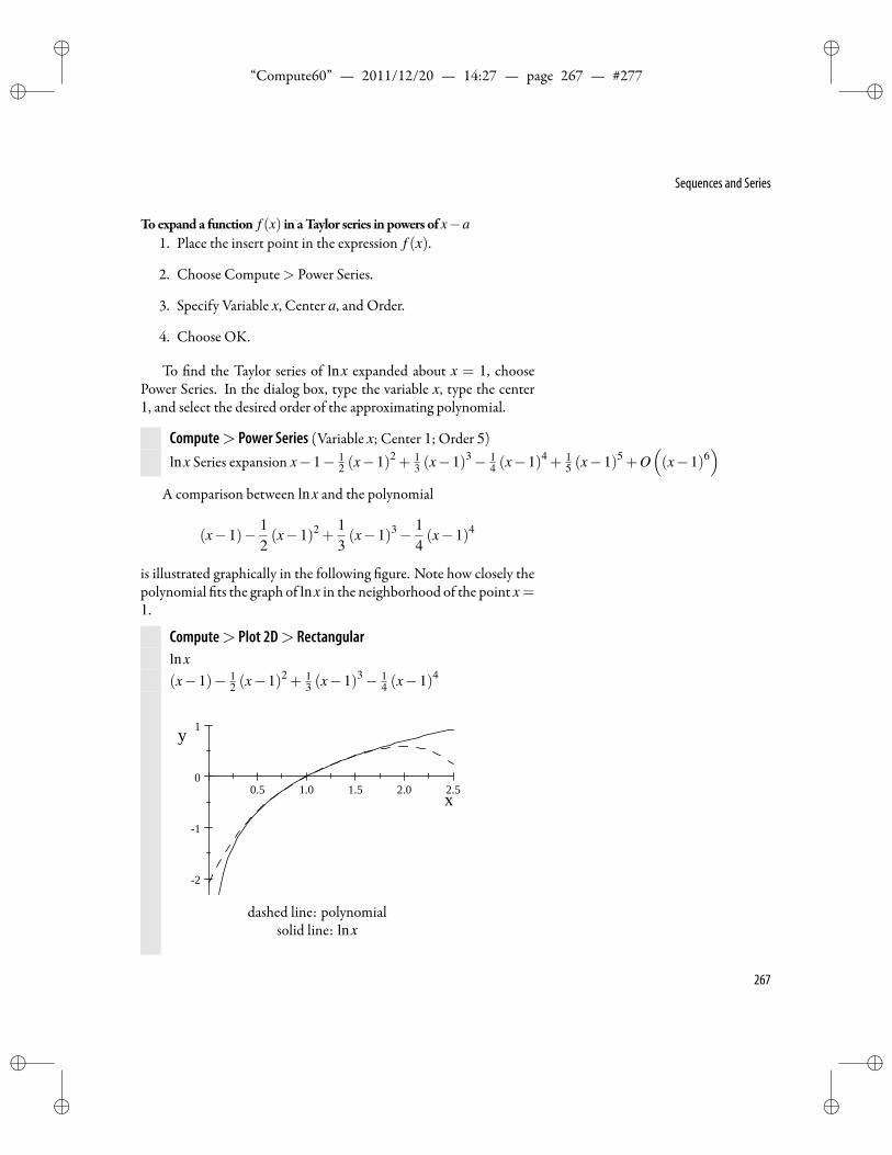
ii
“Compute60” — 2011/12/20 — 14:27 — page 267 — #277 ii
ii
ii
Sequences and Series
Toexpand a function f (x) in aTaylor series in powers of x−a1. Place the insert point in the expression f (x).
2. Choose Compute> Power Series.
3. Specify Variable x, Center a, and Order.
4. Choose OK.
To nd the Taylor series of lnx expanded about x = 1, choosePower Series. In the dialog box, type the variable x, type the center1, and select the desired order of the approximating polynomial.
Compute> Power Series (Variable x; Center 1; Order 5)lnx Series expansion x−1− 1
2 (x−1)2 + 13 (x−1)3− 1
4 (x−1)4 + 15 (x−1)5 +O
((x−1)6
)A comparison between lnx and the polynomial
(x−1)− 12(x−1)2 +
13(x−1)3− 1
4(x−1)4
is illustrated graphically in the following gure. Note how closely thepolynomial ts the graph of lnx in the neighborhood of the point x =1.
Compute> Plot 2D> Rectangularlnx(x−1)− 1
2 (x−1)2 + 13 (x−1)3− 1
4 (x−1)4
0.5 1.0 1.5 2.0 2.5
2
1
0
1
x
y
dashed line: polynomialsolid line: lnx
267
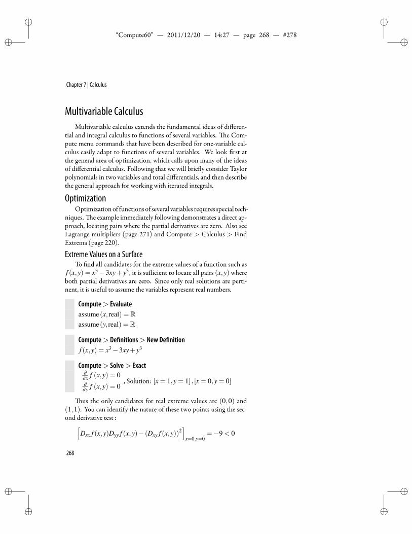
ii
“Compute60” — 2011/12/20 — 14:27 — page 268 — #278 ii
ii
ii
Chapter 7 | Calculus
Multivariable CalculusMultivariable calculus extends the fundamental ideas of differen-
tial and integral calculus to functions of several variables. e Com-pute menu commands that have been described for one-variable cal-culus easily adapt to functions of several variables. We look rst atthe general area of optimization, which calls upon many of the ideasof differential calculus. Following that we will brie y consider Taylorpolynomials in two variables and total differentials, and then describethe general approach for working with iterated integrals.
OptimizationOptimizationof functions of several variables requires special tech-
niques. e example immediately following demonstrates a direct ap-proach, locating pairs where the partial derivatives are zero. Also seeLagrange multipliers (page 271) and Compute > Calculus > FindExtrema (page 220).
Extreme Values on a SurfaceTo nd all candidates for the extreme values of a function such as
f (x,y) = x3−3xy+ y3, it is sufficient to locate all pairs (x,y) whereboth partial derivatives are zero. Since only real solutions are perti-nent, it is useful to assume the variables represent real numbers.
Compute> Evaluateassume(x, real) = Rassume(y, real) = R
Compute> De nitions> New De nitionf (x,y) = x3−3xy+ y3
Compute> Solve> Exact∂∂ x f (x,y) = 0∂∂y f (x,y) = 0
, Solution: [x = 1,y = 1] , [x = 0,y = 0]
us the only candidates for real extreme values are (0,0) and(1,1). You can identify the nature of these two points using the sec-ond derivative test :[
Dxx f (x,y)Dyy f (x,y)− (Dxy f (x,y))2]
x=0,y=0=−9 < 0
268
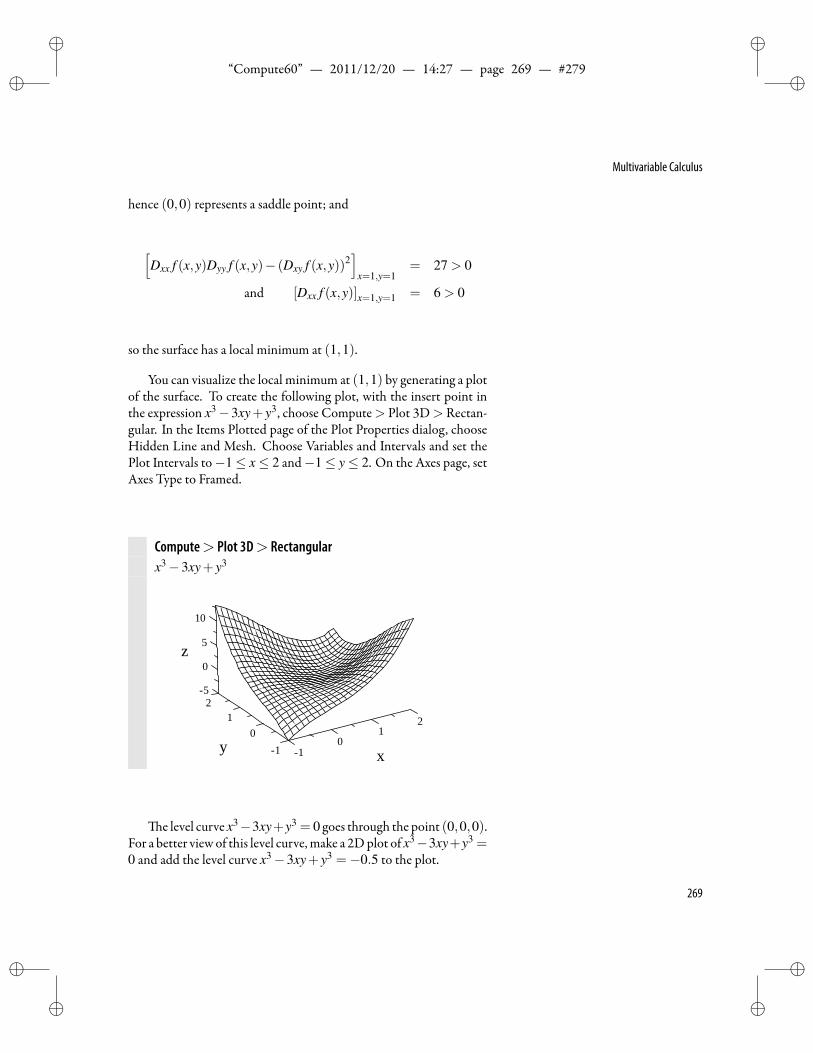
ii
“Compute60” — 2011/12/20 — 14:27 — page 269 — #279 ii
ii
ii
Multivariable Calculus
hence (0,0) represents a saddle point; and
[Dxx f (x,y)Dyy f (x,y)− (Dxy f (x,y))2
]x=1,y=1
= 27 > 0
and [Dxx f (x,y)]x=1,y=1 = 6 > 0
so the surface has a local minimum at (1,1).
You can visualize the local minimum at (1,1) by generating a plotof the surface. To create the following plot, with the insert point inthe expression x3−3xy+y3, choose Compute> Plot 3D> Rectan-gular. In the Items Plotted page of the Plot Properties dialog, chooseHidden Line and Mesh. Choose Variables and Intervals and set thePlot Intervals to−1≤ x≤ 2 and−1≤ y≤ 2. On the Axes page, setAxes Type to Framed.
Compute> Plot 3D> Rectangularx3−3xy+ y3
1 x
12
y 01
01
25
0z 5
10
e level curve x3−3xy+y3 = 0 goes through the point (0,0,0).For a better view of this level curve, make a 2Dplot of x3−3xy+y3 =0 and add the level curve x3−3xy+ y3 =−0.5 to the plot.
269
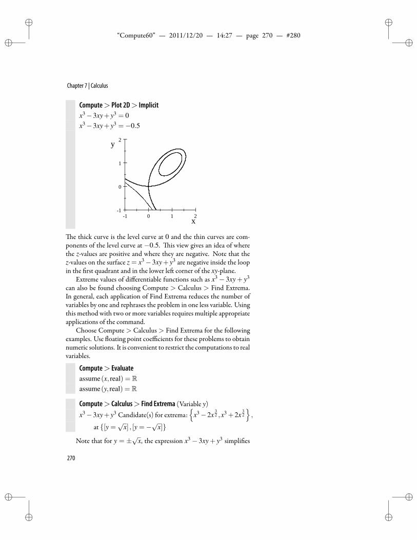
ii
“Compute60” — 2011/12/20 — 14:27 — page 270 — #280 ii
ii
ii
Chapter 7 | Calculus
Compute> Plot 2D> Implicitx3−3xy+ y3 = 0x3−3xy+ y3 =−0.5
1 0 1 21
0
1
2
x
y
e thick curve is the level curve at 0 and the thin curves are com-ponents of the level curve at −0.5. is view gives an idea of wherethe z-values are positive and where they are negative. Note that thez-values on the surface z = x3−3xy+ y3 are negative inside the loopin the rst quadrant and in the lower le corner of the xy-plane.
Extreme values of differentiable functions such as x3− 3xy+ y3
can also be found choosing Compute > Calculus > Find Extrema.In general, each application of Find Extrema reduces the number ofvariables by one and rephrases the problem in one less variable. Usingthis method with two or more variables requires multiple appropriateapplications of the command.
Choose Compute > Calculus > Find Extrema for the followingexamples. Use oating point coefficients for these problems to obtainnumeric solutions. It is convenient to restrict the computations to realvariables.
Compute> Evaluateassume(x, real) = Rassume(y, real) = R
Compute> Calculus> Find Extrema (Variable y)x3−3xy+ y3 Candidate(s) for extrema:
x3−2x
32 ,x3 +2x
32
,
at [y =√
x] , [y =−√
x]
Note that for y = ±√
x, the expression x3− 3xy+ y3 simpli es
270
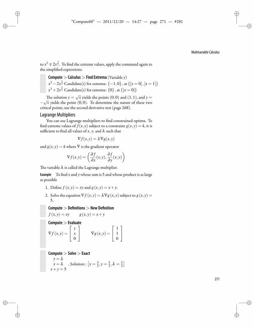
ii
“Compute60” — 2011/12/20 — 14:27 — page 271 — #281 ii
ii
ii
Multivariable Calculus
to x3∓2x32 . To nd the extreme values, apply the command again to
the simpli ed expressions.
Compute> Calculus> Find Extrema (Variable y)x3−2x
32 Candidate(s) for extrema: −1,0 , at [x = 0] , [x = 1]
x3 +2x32 Candidate(s) for extrema: 0 , at [x = 0]
e solution y =√
x yields the points (0,0) and (1,1), and y =−√
x yields the point (0,0). To determine the nature of these twocritical points, use the second derivative test (page 268).
Lagrange MultipliersYou can use Lagrange multipliers to nd constrained optima. To
nd extreme values of f (x,y) subject to a constraint g(x,y) = k, it issufficient to nd all values of x, y, and λ such that
∇ f (x,y) = λ∇g(x,y)
and g(x,y) = k where ∇ is the gradient operator
∇ f (x,y) =(
∂ f∂x
(x,y),∂ f∂y
(x,y))
e variable λ is called the Lagrange multiplier.
Example To nd x and y whose sum is 5 and whose product is as largeas possible
1. De ne f (x,y) = xy and g(x,y) = x+ y.
2. Solve the equation ∇ f (x,y) = λ∇g(x,y) subject to g(x,y) =5.
Compute> De nitions> New De nitionf (x,y) = xy g(x,y) = x+ y
Compute> Evaluate
∇ f (x,y) =
yx0
∇g(x,y) =
110
Compute> Solve> Exacty = λx = λ
x+ y = 5, Solution :
[x = 5
2 ,y =52 ,λ = 5
2
]271
ii
“Compute60” — 2011/12/20 — 14:27 — page 272 — #282 ii
ii
ii
Chapter 7 | Calculus
Example Optimization problems may require numerical solutions ingiven search intervals.
Compute> Evaluate
∇(x+2y) =
120
∇(yex + xey) =
ey + yex
ex + xey
0
Compute> Solve> Numeric1 = λ (yex + ey)2 = λ (ex + xey)
yex + xey = 5x ∈ (0,10)y ∈ (0,10)
λ ∈ (−5,5)
, Solution : [x≈ 1.6665,y≈ 0.45056,λ ≈ 0.25290]
For f (x,y) = x+2y and g(x,y) = yex+xey, these numbers give
g(1.6665,0.45056) ≈ 5.0001f (1.6665,0.45056) ≈ 2.5676
epoint (1.6665,0.45056) gives a possible extremevalue for f (x,y)satisfying the constraint g(x,y) = 5.
Taylor Polynomials in Two VariablesLet z be a function of two variables. e second-degree Taylor
polynomial of z at (a,b) is given by
T2 (x,y) = z(a,b)+Dxz(a,b)(x−a)+Dyz(a,b)(y−b)
+ 12 Dxxz(a,b)(x−a)2 +Dxyz(a,b)(x−a)(y−b)
+ 12 Dyyz(a,b)(y−b)2
Toevaluate a partial derivative of a function z at (a,b)1. Evaluate the partial derivative at (x,y) using an expression such
as∂∂x z(x,y), Dxz(x,y), ∂ 2
∂x2 z(x,y), or Dxyz(x,y).
2. Evaluate at (a,b) using square brackets with the subscript x =a,y = b.
ese steps can be combined into a single step:
272
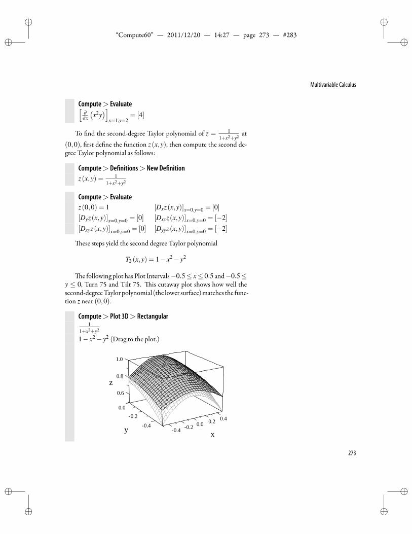
ii
“Compute60” — 2011/12/20 — 14:27 — page 273 — #283 ii
ii
ii
Multivariable Calculus
Compute> Evaluate[∂∂x
(x2y)]
x=1,y=2= [4]
To nd the second-degree Taylor polynomial of z = 11+x2+y2 at
(0,0), rst de ne the function z(x,y), then compute the second de-gree Taylor polynomial as follows:
Compute> De nitions> New De nitionz(x,y) = 1
1+x2+y2
Compute> Evaluatez(0,0) = 1 [Dxz(x,y)]x=0,y=0 = [0][Dyz(x,y)]x=0,y=0 = [0] [Dxxz(x,y)]x=0,y=0 = [−2]
[Dxyz(x,y)]x=0,y=0 = [0] [Dyyz(x,y)]x=0,y=0 = [−2]
ese steps yield the second degree Taylor polynomial
T2 (x,y) = 1− x2− y2
e following plot has Plot Intervals−0.5≤ x≤ 0.5 and−0.5≤y ≤ 0, Turn 75 and Tilt 75. is cutaway plot shows how well thesecond-degreeTaylor polynomial (the lower surface)matches the func-tion z near (0,0).
Compute> Plot 3D> Rectangular1
1+x2+y2
1− x2− y2 (Drag to the plot.)
0.4 x
0.2y
0.2 0.40.00.2
0.6
0.0
0.8z
0.4
1.0
273
ii
“Compute60” — 2011/12/20 — 14:27 — page 274 — #284 ii
ii
ii
Chapter 7 | Calculus
Total DifferentialTo compute the total differential of a function of two variables,
de ne a function u(x,y), represent each differential by a Math Name(du, dx, and dy) so that it will be treated as a variable. en evaluatethe expression
du =∂∂x
u(x,y)dx+∂∂y
u(x,y)dy
A similar procedure produces the total differential of a function ofthree variables.
Compute> De nitions> New De nitionu(x,y) = x3y2
Tocreate the grayed functionnamesdu,dx, anddy1. Choose Insert>Math Objects>Math Name.
2. Type the function name in the Name box and choose OK.
Compute> Evaluatedu = ∂
∂x u(x,y)dx+ ∂∂y u(x,y)dy = 3x2y2 dx+2x3ydy
Iterated IntegralsYou can enter and evaluate iterated integrals. If a ≤ b, f (x) ≤
g(x) for all x ∈ [a,b], and k(x,y) ≥ 0 for all x ∈ [a,b] and all y ∈[ f (x),g(x)], then the iterated integral∫ b
a
∫ g(x)
f (x)k(x,y)dydx
can be interpreted as the volume of the solid bounded by the threeinequalities a≤ x≤ b, f (x)≤ y≤ g(x), and 0≤ z≤ k(x,y).
Example Find the volume of the solid under the surface z = 1+ xyand above the triangle with vertices (1,1), (4,1), and (3,2).
1. Plot the triangle with the given vertices.
2. Find the equations of the bounding lines:y = 1
2 x+ 12
y = 5− xy = 1
274
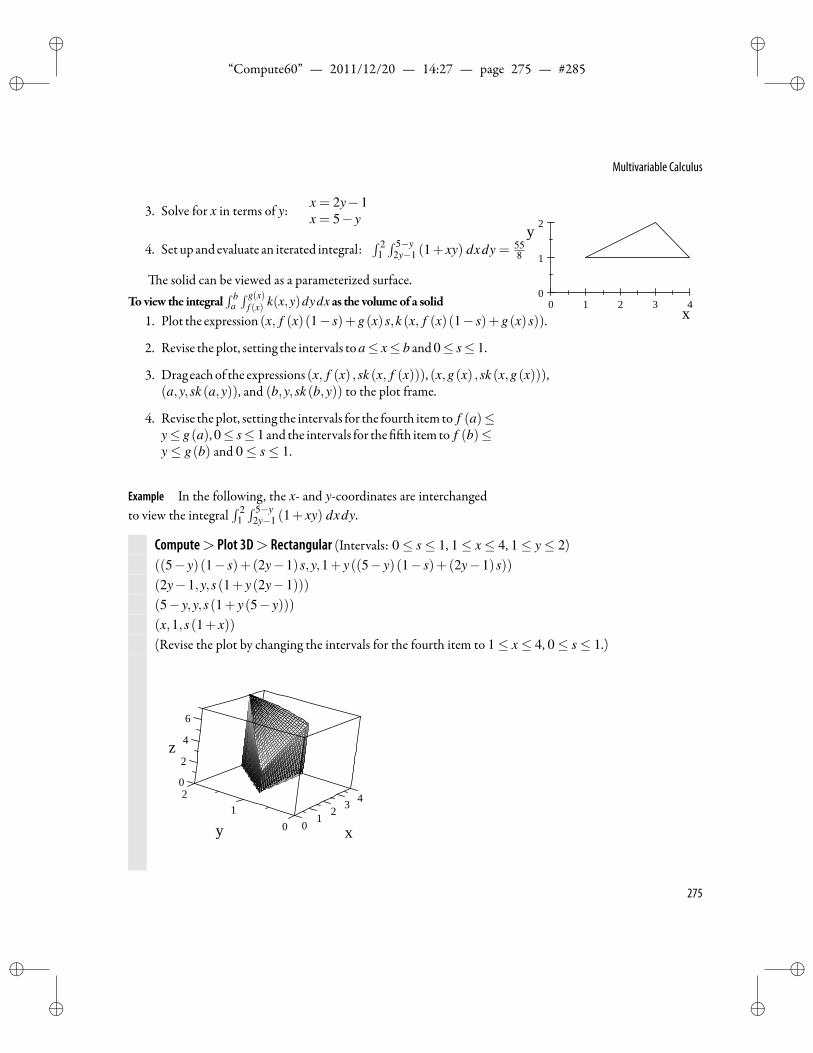
ii
“Compute60” — 2011/12/20 — 14:27 — page 275 — #285 ii
ii
ii
Multivariable Calculus
3. Solve for x in terms of y: x = 2y−1x = 5− y
0 1 2 3 40
1
2
x
y4. Set up and evaluate an iterated integral:
∫ 21∫ 5−y
2y−1 (1+ xy) dxdy = 558
e solid can be viewed as a parameterized surface.Toview the integral
∫ ba∫ g(x)
f (x) k(x,y)dydx as the volumeof a solid1. Plot the expression (x, f (x)(1− s)+g(x)s,k (x, f (x)(1− s)+g(x)s)).
2. Revise the plot, setting the intervals toa≤ x≤ b and0≤ s≤ 1.
3. Drag eachof the expressions (x, f (x) ,sk (x, f (x))), (x,g(x) ,sk (x,g(x))),(a,y,sk (a,y)), and (b,y,sk (b,y)) to the plot frame.
4. Revise theplot, setting the intervals for the fourth itemto f (a)≤y≤ g(a),0≤ s≤ 1 and the intervals for the h itemto f (b)≤y≤ g(b) and 0≤ s≤ 1.
Example In the following, the x- and y-coordinates are interchangedto view the integral
∫ 21∫ 5−y
2y−1 (1+ xy) dxdy.
Compute> Plot 3D> Rectangular (Intervals: 0≤ s≤ 1, 1≤ x≤ 4, 1≤ y≤ 2)((5− y)(1− s)+(2y−1)s,y,1+ y((5− y)(1− s)+(2y−1)s))(2y−1,y,s(1+ y(2y−1)))(5− y,y,s(1+ y(5− y)))(x,1,s(1+ x))(Revise the plot by changing the intervals for the fourth item to 1≤ x≤ 4, 0≤ s≤ 1.)
x
3 4
y
20
2
1
z 4
6
2100
275
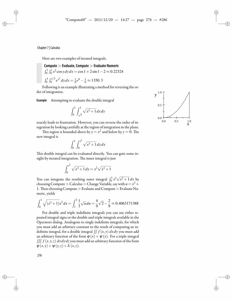
ii
“Compute60” — 2011/12/20 — 14:27 — page 276 — #286 ii
ii
ii
Chapter 7 | Calculus
Here are two examples of iterated integrals.
Compute> Evaluate, Compute> Evaluate Numeric∫ 10∫ x
0 x2 cosydydx = cos1+2sin1−2≈ 0.22324∫ 30∫ x/3
0 ex2dydx = 1
6 e9− 16 ≈ 1350.3
Following is an example illustrating a method for reversing the or-der of integration.
Example Attempting to evaluate the double integral∫ 1
0
∫ 1
√y
√x3 +1dxdy
exactly leads to frustration. However, you can reverse the order of in-tegration by looking carefully at the region of integration in the plane.
0.0 0.5 1.00.0
0.5
1.0
x
y
is region is bounded above by y = x2 and below by y = 0. enew integral is ∫ 1
0
∫ x2
0
√x3 +1dydx
is double integral can be evaluated directly. You can gain some in-sight by iterated integration. e inner integral is just∫ x2
0
√x3 +1dy = x2
√x3 +1
You can integrate the resulting outer integral∫ 1
0 x2√
x3 +1dx bychoosingCompute>Calculus>Change Variable, say with u = x3+1. en choosingCompute>Evaluate andCompute>EvaluateNu-meric, yields∫ 1
0
√(x3 +1)x2 dx =
∫ 2
1
13√
udu =49
√2− 2
9≈ 0.4063171388
For double and triple inde nite integrals you can use either re-peated integral signs or the double and triple integrals available in theOperators dialog. Analogous to single inde nite integrals, for whichyou must add an arbitrary constant to the result of computing an in-de nite integral, for a double integral
∫∫f (x,y) dxdy you must add
an arbitrary function of the form φ (x)+ψ (y). For a triple integral∫∫∫f (x,y,z) dxdydz youmust add an arbitrary function of the form
φ (x,y)+ψ (y,z)+λ (x,z).
276
ii
“Compute60” — 2011/12/20 — 14:27 — page 277 — #287 ii
ii
ii
Exercises
Toenter and evaluate a double or triple integral1. Choose Insert>Math Objects>Operator.
2. Select the double or triple integral and choose OK.
3. Enter the function and the differentials. ( e latter are neces-sary.)
4. With the insert point in the integral, choose Compute> Eval-uate.
5. For a double integral, add an arbitrary function of the formφ (x) + ψ (y); for a triple integral, add φ (x,y) + ψ (y,z) +λ (x,z).
Compute> Evaluate (add “arbitrary functions”)∫∫xydxdy = 1
4 x2y2+ φ (x)+ψ (y)∫∫xsinxcosydxdy = (sinx− xcosx)siny+ φ (x)+ψ (y)∫∫∫xy2zdxdydz = 1
12 x2y3z2 +φ (x,y)+ψ (y,z)+λ (x,z)
Exercises1. Verify the formula d
dx
(x8)= 8x7 by startingwith the de nition
of derivative and choosing submenu items such as Expand andSimplify.
2. Use Newton’s method on the function f (x) = x2 +1, startingwith x0 = 0.5. What conclusions can you draw?
3. Find the equation of one line that is tangent to the graph of
f (x) = x(x−1)(x−3)(x−6)
at two different points.
4. For 0 < k < 1, the elliptic integral E =∫ π/2
0
√1− k sin2 tdt
has no elementary solution. Use a series expansion of the inte-grand to estimate E .
5. Find all the solutions to xy = yx for unequal positive integers xand y.
277
ii
“Compute60” — 2011/12/20 — 14:27 — page 278 — #288 ii
ii
ii
Chapter 7 | Calculus
6. Blood owing through an artery ows fastest at the center ofthe artery, and slowest near thewalls of the arterywhere frictionis a factor. In fact, the velocity is given by the formula v(r) =α(R2− r2), where α is a constant, R is the radius of the artery,and r is the distance from the center.
Set up an integral that gives the total blood ow through anartery. Show that if an artery is constricted to one-half of itsoriginal radius, the blood ow (assuming constant blood pres-sure) is reduced to 1
16 of its original ow.
7. e mass of an object traveling at a velocity v with rest mass m0is given by
m = m0
(1− v2
c2
)−1/2
where c is the speed of light. Use a Maclaurin series expansionto show the increase in mass at low velocities.
8. Evaluate∫
2x cosbxdx.
9. Evaluate∫ π−π
1+ sinx
(x− cosx)2 dx. Hint: Don’t try to do it directly.
10. Evaluate limh→0+∫ ∞
0 sin(x1+h)dx.
11. e Fundamental eorem of Calculus says that if f is contin-uous on a closed interval [a,b], then
a. If g is de ned by g(x) =∫ x
a f (t)dt for x ∈ [a,b], theng′(x) = f (x), and
b. If F is any antiderivative of f , then∫ b
a f (x)dx = F(b)−F(a).
Demonstrate that these twoconditionshold for eachof the threefunctions f (x) = x3, f (x) = xex, and f (x) = sin2 xcosx.
12. e arithmetic-geometric mean of two positive numbers a > bwas de ned by Gauss as follows. Let a0 = a and b0 = b. Givenan and bn, let an+1 be the arithmetic mean of an and bn, andbn+1 the geometric mean of an and bn:
an+1 =an +bn
2and bn+1 =
√anbn
278
ii
“Compute60” — 2011/12/20 — 14:27 — page 279 — #289 ii
ii
ii
Exercises
Usingmathematical induction, you can show that an > an+1 >bn+1 > bn and deduce that both series an and bn are con-vergent, and, in fact, that limn→∞ an = limn→∞ bn.Compute the arithmetic-geometric mean of the numbers 2 and1 to ve decimal places.
13. Two numbers x and y are chosen at random in the unit interval[0,1]. What is the average distance between two suchnumbers?
Solutions1. By de nition,
ddx
(x8) = lim
h→0
(x+h)8− x8
h
= limh→0
8x7h+28x6h2 + · · ·+28x2h6 +8xh7 +h8
h
= limh→0
(8x7 +28x6h+ · · ·+28x2h5 +8xh6 +h7
)= 8x7
2. De ning g by g(x) = x− f (x)/ f ′(x), chooseCompute>Cal-culus> Iterate to obtain
0.5−0.75
0.29167−1.5684−0.46540.84164
If this result seems to be headed nowhere, it is doing so for goodreason. e function f is always positive, so it has no zeroes.Newton’smethod is searching for something that does not exist.
3. It is sufficient to nd three numbers a, b, and m that satisfyf ′(a) = m, f ′(b) = m, and f (b)− f (a)
b−a = m. Put these threeequations inside a 3× 1 matrix and choose Compute > Solve> Exact to get several solutions, including the real solutions[
a =52− 1
2
√21,b =
52− 1
2
√21,m =−8
]279
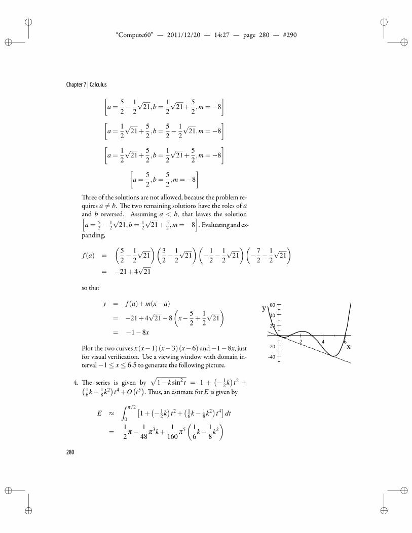
ii
“Compute60” — 2011/12/20 — 14:27 — page 280 — #290 ii
ii
ii
Chapter 7 | Calculus[a =
52− 1
2
√21,b =
12
√21+
52,m =−8
][
a =12
√21+
52,b =
52− 1
2
√21,m =−8
][
a =12
√21+
52,b =
12
√21+
52,m =−8
][
a =52,b =
52,m =−8
]ree of the solutions are not allowed, because the problem re-
quires a = b. e two remaining solutions have the roles of aand b reversed. Assuming a < b, that leaves the solution[a = 5
2 −12
√21,b = 1
2
√21+ 5
2 ,m =−8]. Evaluating and ex-
panding,
f (a) =
(52− 1
2
√21)(
32− 1
2
√21)(−1
2− 1
2
√21)(−7
2− 1
2
√21)
= −21+4√
21
so that
y = f (a)+m(x−a)
= −21+4√
21−8(
x− 52+
12
√21)
= −1−8x
Plot the two curves x(x−1)(x−3)(x−6) and−1−8x, justfor visual veri cation. Use a viewing window with domain in-terval−1≤ x≤ 6.5 to generate the following picture.
2 4 6
40
20
20
40
60
x
y
4. e series is given by√
1− k sin2 t = 1 +(− 1
2 k)
t2 +( 16 k− 1
8 k2)
t4 +O(t5). us, an estimate for E is given by
E ≈∫ π/2
0
[1+(− 1
2 k)
t2 +( 1
6 k− 18 k2) t4]dt
=12
π− 148
π3k+1
160π5(
16
k− 18
k2)
280
ii
“Compute60” — 2011/12/20 — 14:27 — page 281 — #291 ii
ii
ii
Exercises
As a check, k = 1 yields 1.0045 compared with the exact value∫ π/2
0
√1− sin2 tdt = 1
and k = 0 yields 12 π , which agrees precisely with∫ π/2
0dt =
12
π
5. Compute natural logs on both sides and separate variables toget lnx
x = lnyy . Plot lnx
x on the interval 1≤ x ≤ 10. Locate theextreme values of lnx
x by solving ddx
( lnxx
)= 0. Note that 2 is the
only integer between 1 and e, and verify that 24 = 42 is true.
6. e ow is givenby the integral∫ R
0 α(R2−r2)2πrdr = 12 απR4.
If R is reduced by one-half, then R4 is reduced to 116 of the orig-
inal amount.
7. e series expansion is given by
m0
(1− v2
c2
)−1/2
= m0 +1
2c2 v2m0 +3
8c4 v4m0 +O(
v5)
Ifvc
is small, then the model m≈ m0 +12
m0c2 v2 is useful for es-
timating the increased mass.
8. Evaluation yields∫2x cosbxdx =
2x (bsinbx+ cosbx ln2)b2 + ln2 2
9. e integral ∫ π
−π
1+ sinx
(x− cosx)2 dx
is improper, because x− cosx = 0 has a root (≈ 0.73909) be-tween−π and π . Evaluate Numeric gives∫ .739
−π
1+ sinx
(x− cosx)2 dx ≈ 7018.2, and∫ π
.7392
1+ sinx
(x− cosx)2 dx ≈ 5201.4
281
ii
“Compute60” — 2011/12/20 — 14:27 — page 282 — #292 ii
ii
ii
Chapter 7 | Calculus
Change “Digits rendered” to10, in theOutputpageof theTools>Preference>Computationdialog box. Solving cosx= xnu-merically gives x≈ 0.7390851332.
Using this as a limit, Evaluate Numeric gives∫ 0.73908
−π
1+ sinx
(x− cosx)2 dx ≈ 116400.4055 and∫ π
0.73909
1+ sinx
(x− cosx)2 dx ≈ 122772.6822
providing some evidence that both integrals diverge.
10. You obtain the result limh→0+∫ ∞
0 sin(x1+h)dx = 1. is re-sult is reasonable, because the integral f (h) =
∫ ∞0 sin(x1+h)dx
can be viewed as a convergent alternating series for h > 0, andg(y) =
∫ y0 sinxdx = 1− cosy ranges in value between 0 and
2, with an average value of 1.
11. We need to show that for each of the three functions f (x) = x3,f (x) = xex, and f (x) = sin2 xcosx, (a) and (b) hold:
(a) If g is de ned by g(x) =∫ x
a f (t)dt for x ∈ [a,b], theng′(x) = f (x).
(b) If F is any antiderivative of f , then∫ b
a f (x)dx = F(b)−F(a).
For f (x) = x3, g(x) =∫ x
a t3 dt = 14 x4 − 1
4 a4 and g′(x) =ddx
( 14 x4− 1
4 a4)= x3. e antiderivatives of f are of the form
F(x) =∫
x3 dx = 14 x4 +C for different constantsC. Now
F(b)−F(x) =[ 1
4 x4 +C]x=b
x=a =14 b4− 1
4 a4
which is the same as∫ b
a x3 dx = 14 b4− 1
4 a4.
For f (x) = xex, g(x) =∫ x
a tet dt = xex− ex− aea + ea andg′(x) = d
dx (xex− ex−aea + ea) = xex. e antiderivatives of
f are of the form F(x) =∫
xex dx = xex−ex +C for differentconstantsC. Now
F(b)−F(x) = [xex− ex +C]x=bx=a = beb− eb−aea + ea
282
ii
“Compute60” — 2011/12/20 — 14:27 — page 283 — #293 ii
ii
ii
Exercises
which is the same as∫ b
a xex dx = beb− eb−aea + ea.For f (x) = sin2 xcosx,
g(x)=∫ x
asin2 t cos t dt = 1
4 sinx− 14 sina+ 1
12 sin3a− 112 sin3x
and
g′(x) =ddx
( 14 sinx− 1
4 sina+ 112 sin3a− 1
12 sin3x)
= 14 cosx− 1
4 cos3x
To check to see if this is the same as f (x), apply Compute >Combine>TrigonmetricFunctions to the expression sin2 xcosxto see that indeed sin2 xcosx = 1
4 cosx− 14 cos3x. e an-
tiderivatives of f are of the form
F(x) =∫
sin2 xcosxdx = 14 sinx− 1
12 sin3x+C
for different constantsC. Now
F(b)−F(x) =[ 1
4 sinx− 112 sin3x
]x=bx=a
= 14 sinb− 1
4 sina+ 112 sin3a− 1
12 sin3b
while∫ b
asin2 xcosxdx = 1
4 sinb− 14 sina+ 1
12 sin3a− 112 sin3b
12. Since the arithmetic-geometricmean lies between an and bn forall n, we know the arithmetic-geometric mean to ve decimalplaces when these two numbers agree to that many places.
• a1 =2+1
2=
32= 1.5 and b1 =
√2∗1 =
√2 ≈ 1.
41421
• a2 =32 +√
22
= 34 +
12
√2= 1.45711 andb2 =
√32
√2≈
1.45648
• a3 =
32+√
22 +
√32
√2
2=
38+
14
√2+
14
√6 4√2≈ 1.45679
and b3 =
√(34 +
12
√2)√
32
√2≈ 1.45679
283
ii
“Compute60” — 2011/12/20 — 14:27 — page 284 — #294 ii
ii
ii
Chapter 7 | Calculus
13. An average value can be determined by evaluating an integral.e average distance between x and y is given by∫ 1
0
∫ 1
0|x− y| dydx =
13.
is can be veri ed using the following steps:∫ 1
0
∫ 1
0|x− y| dydx =
∫ 1
0
∫ x
0|x− y| dydx+
∫ 1
0
∫ 1
x|x− y| dydx
=∫ 1
0
∫ x
0(x− y) dydx+
∫ 1
0
∫ 1
x(y− x) dydx
=16+
16=
13
284
ii
“Compute60” — 2011/12/20 — 14:27 — page 285 — #295 ii
ii
ii
8Matrix Algebra
One cannot escape the feeling that these mathematical formulas have an independent existence and an intelligence of their own, that they arewiser than we are, wiser even than their discoverers. Heinrich Hertz (1857–1894)
M atrices are used throughoutmathematics and in related elds Creating and Editing Matrices
Standard Operations
Row Operations and EchelonForms
Equations
Matrix Operators
Polynomials and VectorsAssociated with a Matrix
Vector Spaces Associated with aMatrix
Normal Forms of Matrices
Matrix Decompositions
such as physics, engineering, economics, and statistics. ealgebra ofmatrices provides amodel for the study of vector
spaces and linear transformations.A rectangular array of mathematical expressions is called a matrix.
Amatrix with m rows and n columns is called an m×n matrix. Matri-ces are sometimes referred to simply as arrays, and an m× 1 or 1× narray is also called a vector. Several methods for creating matrices aredescribed in the ensuing sections.
Entries in matrices can be real or complex numbers, or mathemat-ical expressions with real or complex coefficients. Most of the choicesfrom the Matrices submenu operate on both real and complex matri-ces. e QR and SVD factorizations discussed later in this chapterassume real matrices.
Matrix entries are identi ed by their row and columnnumber. ematrix can be considered as a function on pairs of positive integers.If the matrix is given a name, this feature can be used to retrieve theentries, with the arguments entered as subscripts.
Compute> De nitions> New De nition
A =
−85 −55 −37−35 97 5079 56 49
New in Version 6Map a function to a matrix
285
ii
“Compute60” — 2011/12/20 — 14:27 — page 286 — #296 ii
ii
ii
Chapter 8 | Matrix Algebra
Compute> EvaluateA2,3 = 50A3,3 = 49
Note that the subscripted row and column numbers are separatedby a comma.
Creating and Editing MatricesYou can create a matrix via the Matrix dialog box or from the Ma-
trices submenu. ere is also a keyboard shortcut, described at the endof this chapter.
Eachmethod involves different choices, as described in the follow-ing paragraphs.Tocreate amatrix
1. Choose Insert>Math Objects>Matrix.
2. Select the number of rows and columns by clicking in the low-est, right-most box you want.
3. Choose OK.
4. Type or copy entries into the input boxes.
e entries can be any valid mathematical expression. Both realand complex numbers are legitimate entries, as well as algebraic ex-pressions. e built-in delimiters have the same appearance as expand-ing brackets on the screen, but they require less horizontal space whentypeset.
Matrix DelimitersYou canmake choices in theViewmenu that affect the appearance
ofmatrices on the screen. Helper Lines and Input Boxes can be shownor hidden. e default is to show them to make it easier to handleentries on the screen. Matrix helper lines and input boxes normally donot appear when you preview or print the document.
It is standard to enclose a matrix in brackets, either built-in oradded manually. ese two options provide the same screen appear-ance andmathematical properties. ey differ only underTypeset—inwhich case, the built-in brackets tmore tightly around thematrix en-tries than added brackets. If you have a matrix without built-in delim-iters, you will generally want to add brackets around it. e result of
286
ii
“Compute60” — 2011/12/20 — 14:27 — page 287 — #297 ii
ii
ii
Creating and Editing Matrices
an operation onmatrices usually appears with the same brackets as theoriginal matrices.
To set the defaultmatrix delimiters1. Choose Tools>Computation>Matrices.
2. Select the desired option: none, [ ], or ( ).
Fill MatrixYou can generate a matrix whose entries are de ned by a function.
Tode ne aHilbertmatrix
1. De ne f (i, j) =1
i+ j−1.
2. ChooseCompute>Matrices>FillMatrix>De nedbyFunc-tion.
3. Type f in the box for the function name.
4. Set rows and columns. (Enter 2 or 3 for the following example.)
5. Choose OK.
Compute>Matrices> Fill Matrix> De ned by FunctionFunction: f[
1 12
12
13
] 1 12
13
12
13
14
13
14
15
2×2 3×3
Tode ne aVandermondematrix
1. De ne the function g(i, j) = x j−1i .
2. ChooseCompute>Matrices>FillMatrix>De nedbyFunc-tion.
3. Type g for the function name.
4. Set the Dimensions and choose OK.
287
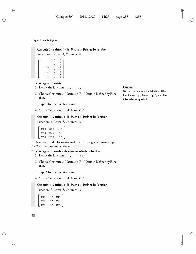
ii
“Compute60” — 2011/12/20 — 14:27 — page 288 — #298 ii
ii
ii
Chapter 8 | Matrix Algebra
Compute>Matrices> Fill Matrix> De ned by FunctionFunction: g, Rows: 4, Columns: 4
1 x1 x21 x3
1
1 x2 x22 x3
2
1 x3 x23 x3
3
1 x4 x24 x3
4
Tode ne a genericmatrix
1. De ne the function a(i, j) = ai, j . CautionWithout the comma in the de nition of thefunction a(i, j), the subscript i j would beinterpreted as a product.
2. ChooseCompute>Matrices>FillMatrix>De nedbyFunc-tion.
3. Type a for the function name.
4. Set the Dimensions and choose OK.
Compute>Matrices> Fill Matrix> De ned by FunctionFunction: a, Rows: 3, Columns: 3 a1,1 a1,2 a1,3
a2,1 a2,2 a2,3a3,1 a3,2 a3,3
You can use the following trick to create a general matrix up to
9×9 with no commas in the subscripts.Tode ne a genericmatrixwith no commas in the subscripts
1. De ne the function b(i, j) = a10i+ j .
2. ChooseCompute>Matrices>FillMatrix>De nedbyFunc-tion.
3. Type b for the function name.
4. Set the Dimensions and choose OK.
Compute>Matrices> Fill Matrix> De ned by FunctionFunction: b, Rows: 3, Columns: 3 a11 a12 a13
a21 a22 a23a31 a32 a33
288
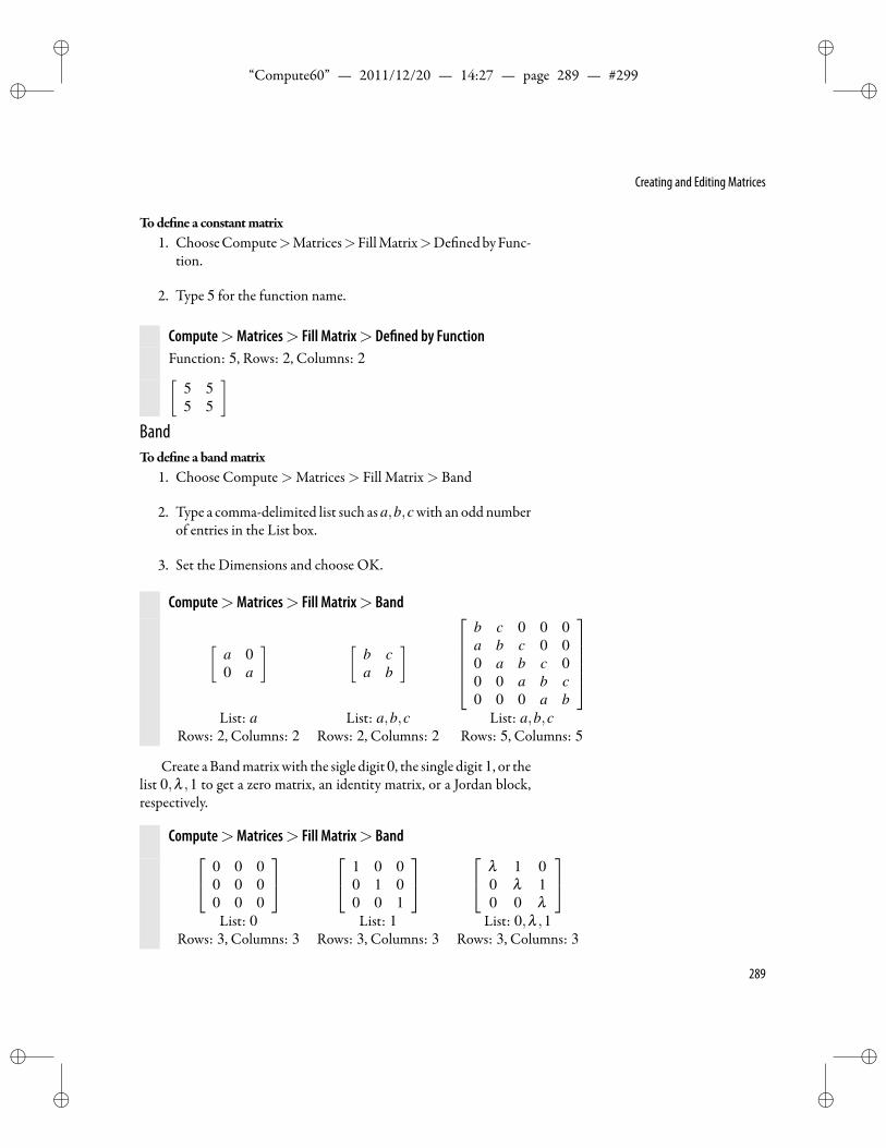
ii
“Compute60” — 2011/12/20 — 14:27 — page 289 — #299 ii
ii
ii
Creating and Editing Matrices
Tode ne a constantmatrix1. ChooseCompute>Matrices>FillMatrix>De nedbyFunc-
tion.
2. Type 5 for the function name.
Compute>Matrices> Fill Matrix> De ned by FunctionFunction: 5, Rows: 2, Columns: 2[
5 55 5
]BandTode ne a bandmatrix
1. Choose Compute>Matrices> Fill Matrix> Band
2. Type a comma-delimited list such as a,b,c with an odd numberof entries in the List box.
3. Set the Dimensions and choose OK.
Compute>Matrices> Fill Matrix> Band
[a 00 a
] [b ca b
] b c 0 0 0a b c 0 00 a b c 00 0 a b c0 0 0 a b
List: a List: a,b,c List: a,b,c
Rows: 2, Columns: 2 Rows: 2, Columns: 2 Rows: 5, Columns: 5
Create aBandmatrixwith the sigle digit0, the single digit1, or thelist 0,λ ,1 to get a zero matrix, an identity matrix, or a Jordan block,respectively.
Compute>Matrices> Fill Matrix> Band 0 0 00 0 00 0 0
1 0 00 1 00 0 1
λ 1 00 λ 10 0 λ
List: 0 List: 1 List: 0,λ ,1
Rows: 3, Columns: 3 Rows: 3, Columns: 3 Rows: 3, Columns: 3
289
ii
“Compute60” — 2011/12/20 — 14:27 — page 290 — #300 ii
ii
ii
Chapter 8 | Matrix Algebra
Revising MatricesYou can add or delete rows, columns, or a full block of rows or
columns from a matrix. e alignment of rows and columns can bereset. Entries in a rectangular block can be deleted or replaced.
Adding Rows and ColumnsToadd rows or columns to amatrix
1. Select the matrix by placing the insert point in a cell of the ma-trix or by placing the insert point at the right of the matrix (butnot outside of any brackets).
2. Choose Edit > Insert Matrix Rows, or Edit > Insert MatrixColumns.
3. Make appropriate choices fromthedialog that appears and chooseOK.
Deleting Rows and ColumnsTodelete a block of rows or columns
1. Select a block of rows or columns with the mouse or withShi +arrow.
2. Press Del.
You can also use the procedure described above to delete entriesfrom a rectangular block that does not include a complete row or col-umn of a matrix.
e choices Insert Row(s) and Insert Column(s) appear on theEdit menu only when a matrix is selected. If they do not appear, repo-sition the insertionpoint or select thematrixwith click anddrag, beingcareful to select only the inside of the matrix—that is, not includingthe exterior Helper Lines.To lengthen a vector represented as ann×1or1×nmatrix
• Place the insert point in the last input box and press Enter.
To shorten a vector represented as ann×1or1×nmatrix• Place the insert point in the last input box and press Backspace.
You can start with a display box, or the input boxes that appearwith the fraction, radical, or bracket buttons, andmake similar changes
290
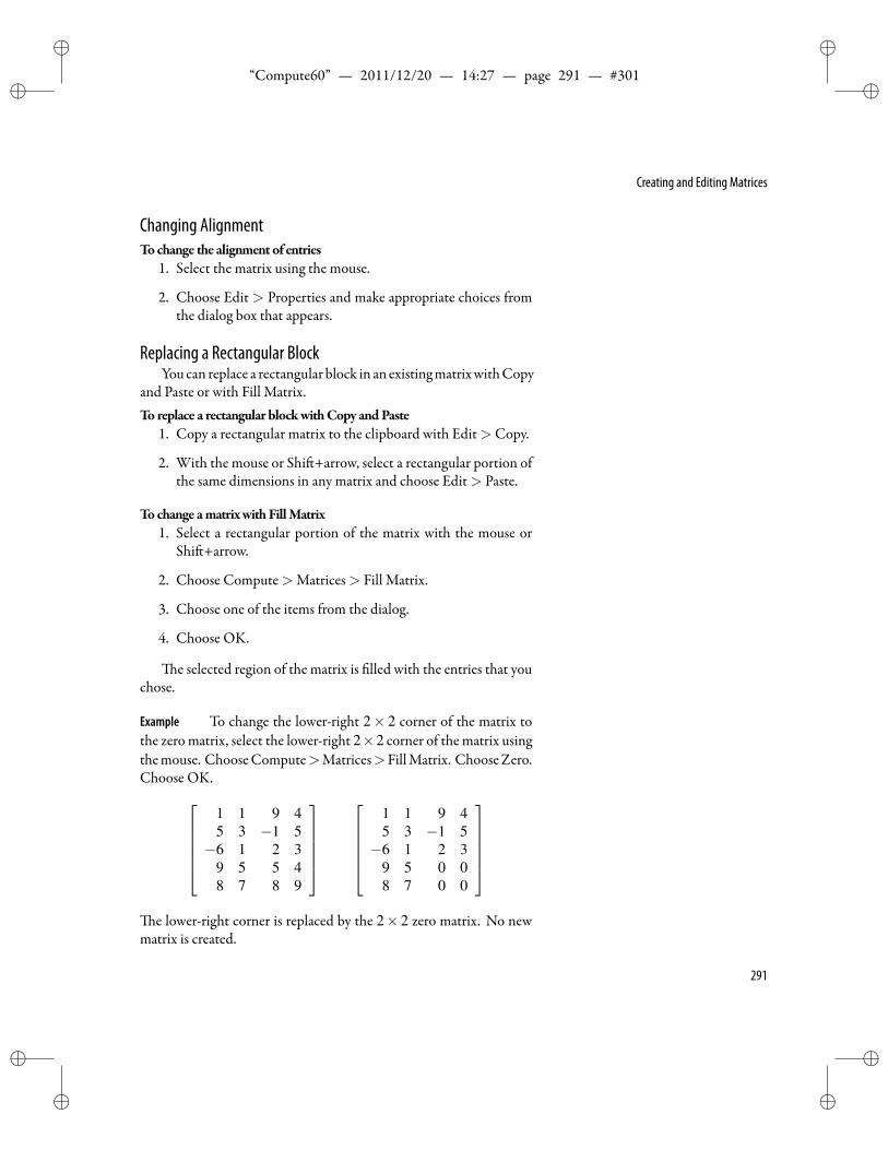
ii
“Compute60” — 2011/12/20 — 14:27 — page 291 — #301 ii
ii
ii
Creating and Editing Matrices
Changing AlignmentTochange the alignment of entries
1. Select the matrix using the mouse.
2. Choose Edit > Properties and make appropriate choices fromthe dialog box that appears.
Replacing a Rectangular BlockYoucan replace a rectangular block in an existingmatrixwithCopy
and Paste or with Fill Matrix.To replace a rectangular blockwithCopy andPaste
1. Copy a rectangular matrix to the clipboard with Edit>Copy.
2. With the mouse or Shi +arrow, select a rectangular portion ofthe same dimensions in any matrix and choose Edit> Paste.
Tochange amatrixwithFillMatrix1. Select a rectangular portion of the matrix with the mouse or
Shi +arrow.
2. Choose Compute>Matrices> Fill Matrix.
3. Choose one of the items from the dialog.
4. Choose OK.
e selected region of the matrix is lled with the entries that youchose.
Example To change the lower-right 2× 2 corner of the matrix tothe zeromatrix, select the lower-right 2×2 corner of thematrix usingthemouse. ChooseCompute>Matrices>FillMatrix. ChooseZero.Choose OK.
1 1 9 45 3 −1 5−6 1 2 3
9 5 5 48 7 8 9
1 1 9 45 3 −1 5−6 1 2 3
9 5 0 08 7 0 0
e lower-right corner is replaced by the 2× 2 zero matrix. No new
matrix is created.
291
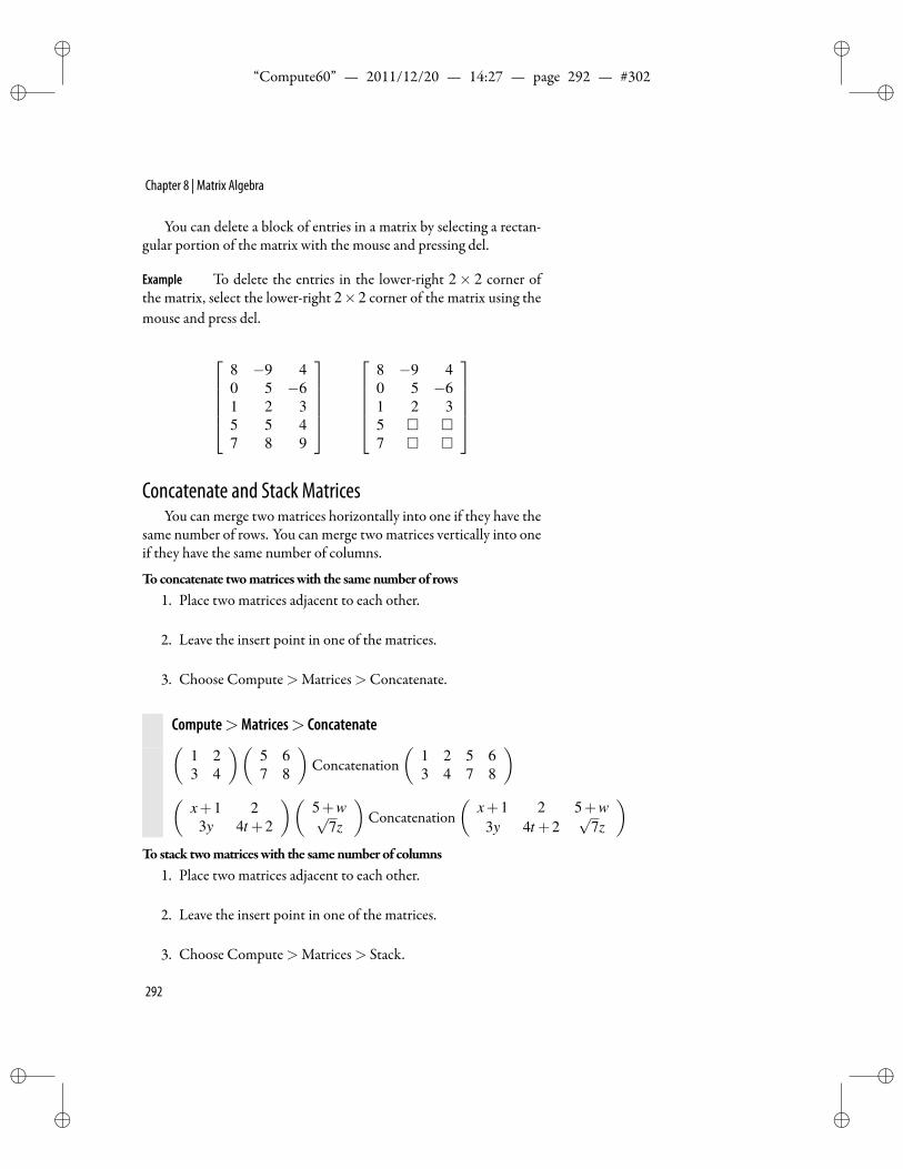
ii
“Compute60” — 2011/12/20 — 14:27 — page 292 — #302 ii
ii
ii
Chapter 8 | Matrix Algebra
You can delete a block of entries in a matrix by selecting a rectan-gular portion of the matrix with the mouse and pressing del.
Example To delete the entries in the lower-right 2× 2 corner ofthe matrix, select the lower-right 2×2 corner of the matrix using themouse and press del.
8 −9 40 5 −61 2 35 5 47 8 9
8 −9 40 5 −61 2 35 7
Concatenate and Stack Matrices
You can merge two matrices horizontally into one if they have thesame number of rows. You can merge two matrices vertically into oneif they have the same number of columns.
Toconcatenate twomatriceswith the samenumber of rows1. Place two matrices adjacent to each other.
2. Leave the insert point in one of the matrices.
3. Choose Compute>Matrices>Concatenate.
Compute>Matrices> Concatenate(1 23 4
)(5 67 8
)Concatenation
(1 2 5 63 4 7 8
)(
x+1 23y 4t +2
)(5+w√
7z
)Concatenation
(x+1 2 5+w
3y 4t +2√
7z
)To stack twomatriceswith the samenumber of columns
1. Place two matrices adjacent to each other.
2. Leave the insert point in one of the matrices.
3. Choose Compute>Matrices> Stack.
292
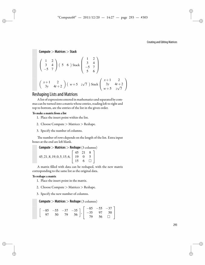
ii
“Compute60” — 2011/12/20 — 14:27 — page 293 — #303 ii
ii
ii
Creating and Editing Matrices
Compute>Matrices> Stack 1 23 4−5 7
( 5 6)Stack
1 23 4−5 75 6
(
x+1 23y 4t +2
)(w+5 z
√7)Stack
x+1 23y 4t +2
w+5 z√
7
Reshaping Lists and Matrices
A list of expressions entered inmathematics and separated by com-mas can be turned into amatrix whose entries, reading le to right andtop to bottom, are the entries of the list in the given order.Tomake amatrix froma list
1. Place the insert point within the list.
2. Choose Compute>Matrices> Reshape.
3. Specify the number of columns.
e number of rows depends on the length of the list. Extra inputboxes at the end are le blank.
Compute>Matrices> Reshape (3 columns)
45,21,8,19,0,5,15,6,
45 21 819 0 515 6
A matrix lled with data can be reshaped, with the new matrix
corresponding to the same list as the original data.To reshape amatrix
1. Place the insert point in the matrix.
2. Choose Compute>Matrices> Reshape.
3. Specify the new number of columns.
Compute>Matrices> Reshape (3 columns)[−85 −55 −37 −35
97 50 79 56
],
−85 −55 −37−35 97 50
79 56
293
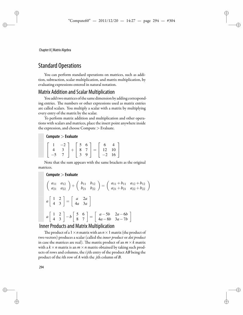
ii
“Compute60” — 2011/12/20 — 14:27 — page 294 — #304 ii
ii
ii
Chapter 8 | Matrix Algebra
Standard OperationsYou can perform standard operations on matrices, such as addi-
tion, subtraction, scalar multiplication, and matrix multiplication, byevaluating expressions entered in natural notation.
Matrix Addition and Scalar MultiplicationYouadd twomatrices of the samedimensionby adding correspond-
ing entries. e numbers or other expressions used as matrix entriesare called scalars. You multiply a scalar with a matrix by multiplyingevery entry of the matrix by the scalar.
To perform matrix addition and multiplication and other opera-tions with scalars and matrices, place the insert point anywhere insidethe expression, and choose Compute> Evaluate.
Compute> Evaluate 1 −24 3−5 7
+ 5 6
8 73 9
=
6 412 10−2 16
Note that the sum appears with the same brackets as the original
matrices.
Compute> Evaluate(a11 a12a21 a22
)+
(b11 b12b21 b22
)=
(a11 +b11 a12 +b12a21 +b21 a22 +b22
)
a[
1 24 3
]=
[a 2a
4a 3a
]
a[
1 24 3
]−b[
5 68 7
]=
[a−5b 2a−6b
4a−8b 3a−7b
]Inner Products and Matrix Multiplication
e product of a 1×n matrix with an n×1 matrix (the product oftwo vectors) produces a scalar (called the inner product or dot productin case the matrices are real). e matrix product of an m× k matrixwith a k×n matrix is an m×n matrix obtained by taking such prod-ucts of rows and columns, the i jth entry of the product AB being theproduct of the ith row of A with the jth column of B.
294
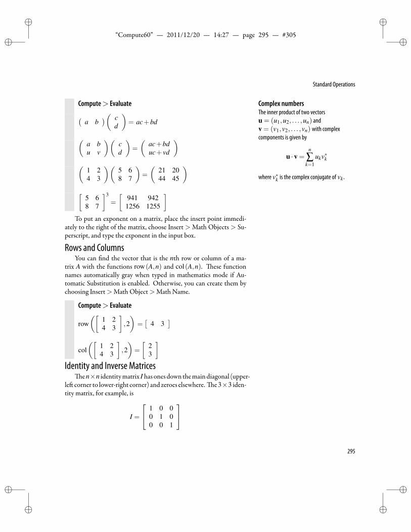
ii
“Compute60” — 2011/12/20 — 14:27 — page 295 — #305 ii
ii
ii
Standard Operations
Compute> Evaluate(a b
)( cd
)= ac+bd
(a bu v
)(cd
)=
(ac+bduc+ vd
)(
1 24 3
)(5 68 7
)=
(21 2044 45
)[
5 68 7
]3
=
[941 9421256 1255
]
Complex numbersThe inner product of two vectorsu = (u1,u2, . . . ,un) andv = (v1,v2, . . . ,vn) with complexcomponents is given by
u ·v =n
∑k=1
ukv∗k
where v∗k is the complex conjugate of vk .
To put an exponent on a matrix, place the insert point immedi-ately to the right of the matrix, choose Insert > Math Objects > Su-perscript, and type the exponent in the input box.
Rows and ColumnsYou can nd the vector that is the nth row or column of a ma-
trix A with the functions row(A,n) and col(A,n). ese functionnames automatically gray when typed in mathematics mode if Au-tomatic Substitution is enabled. Otherwise, you can create them bychoosing Insert>Math Object>Math Name.
Compute> Evaluate
row([
1 24 3
],2)
=[
4 3]
col([
1 24 3
],2)=
[23
]Identity and Inverse Matrices
en×n identitymatrix I has ones down themaindiagonal (upper-le corner to lower-right corner) and zeroes elsewhere. e3×3 iden-tity matrix, for example, is
I =
1 0 00 1 00 0 1
295
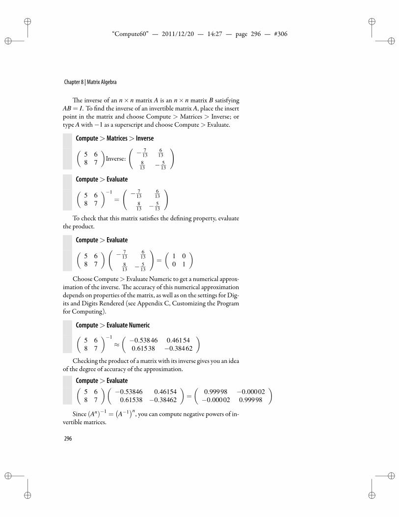
ii
“Compute60” — 2011/12/20 — 14:27 — page 296 — #306 ii
ii
ii
Chapter 8 | Matrix Algebra
e inverse of an n× n matrix A is an n× n matrix B satisfyingAB = I. To nd the inverse of an invertible matrix A, place the insertpoint in the matrix and choose Compute > Matrices > Inverse; ortype A with−1 as a superscript and choose Compute> Evaluate.
Compute>Matrices> Inverse(5 68 7
)Inverse:
(− 7
13613
813 − 5
13
)
Compute> Evaluate(5 68 7
)−1
=
(− 7
136
138
13 − 513
)To check that this matrix satis es the de ning property, evaluate
the product.
Compute> Evaluate(5 68 7
)( − 713
613
813 − 5
13
)=
(1 00 1
)Choose Compute> Evaluate Numeric to get a numerical approx-
imation of the inverse. e accuracy of this numerical approximationdepends on properties of the matrix, as well as on the settings for Dig-its and Digits Rendered (see Appendix C, Customizing the Programfor Computing).
Compute> Evaluate Numeric(5 68 7
)−1
≈(−0.53846 0.461540.61538 −0.38462
)Checking the product of amatrix with its inverse gives you an idea
of the degree of accuracy of the approximation.
Compute> Evaluate(5 68 7
)(−0.53846 0.46154
0.61538 −0.38462
)=
(0.99998 −0.00002−0.00002 0.99998
)Since (An)−1 =
(A−1
)n, you can compute negative powers of in-vertible matrices.
296
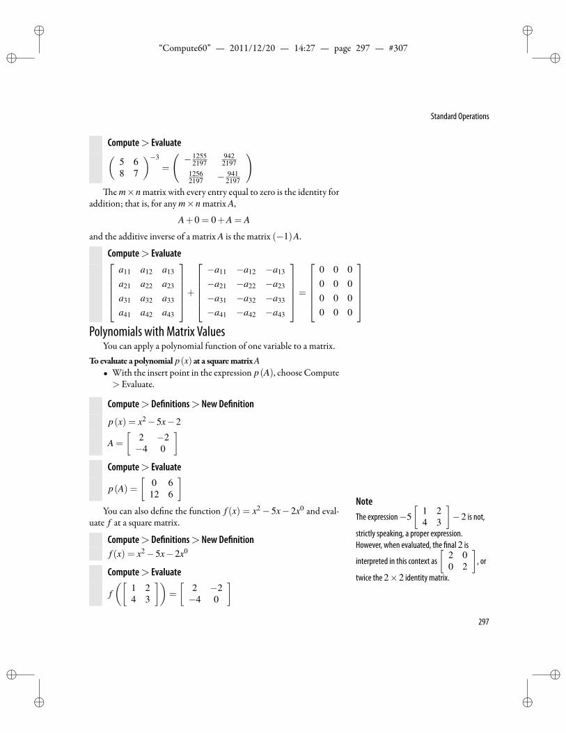
ii
“Compute60” — 2011/12/20 — 14:27 — page 297 — #307 ii
ii
ii
Standard Operations
Compute> Evaluate(5 68 7
)−3
=
(− 1255
21979422197
12562197 − 941
2197
)e m×n matrix with every entry equal to zero is the identity for
addition; that is, for any m×n matrix A,
A+0 = 0+A = A
and the additive inverse of a matrix A is the matrix (−1)A.
Compute> Evaluatea11 a12 a13
a21 a22 a23
a31 a32 a33
a41 a42 a43
+−a11 −a12 −a13
−a21 −a22 −a23
−a31 −a32 −a33
−a41 −a42 −a43
=
0 0 00 0 00 0 00 0 0
Polynomials with Matrix Values
You can apply a polynomial function of one variable to a matrix.Toevaluate a polynomial p(x) at a squarematrixA
• With the insert point in the expression p(A), choose Compute> Evaluate.
Compute> De nitions> New De nition
p(x) = x2−5x−2
A =
[2 −2−4 0
]Compute> Evaluate
p(A) =[
0 612 6
]NoteThe expression−5
[1 24 3
]−2 is not,
strictly speaking, a proper expression.However, when evaluated, the nal 2 is
interpreted in this context as[
2 00 2
], or
twice the 2×2 identity matrix.
You can also de ne the function f (x) = x2− 5x− 2x0 and eval-uate f at a square matrix.
Compute> De nitions> New De nitionf (x) = x2−5x−2x0
Compute> Evaluate
f([
1 24 3
])=
[2 −2−4 0
]297
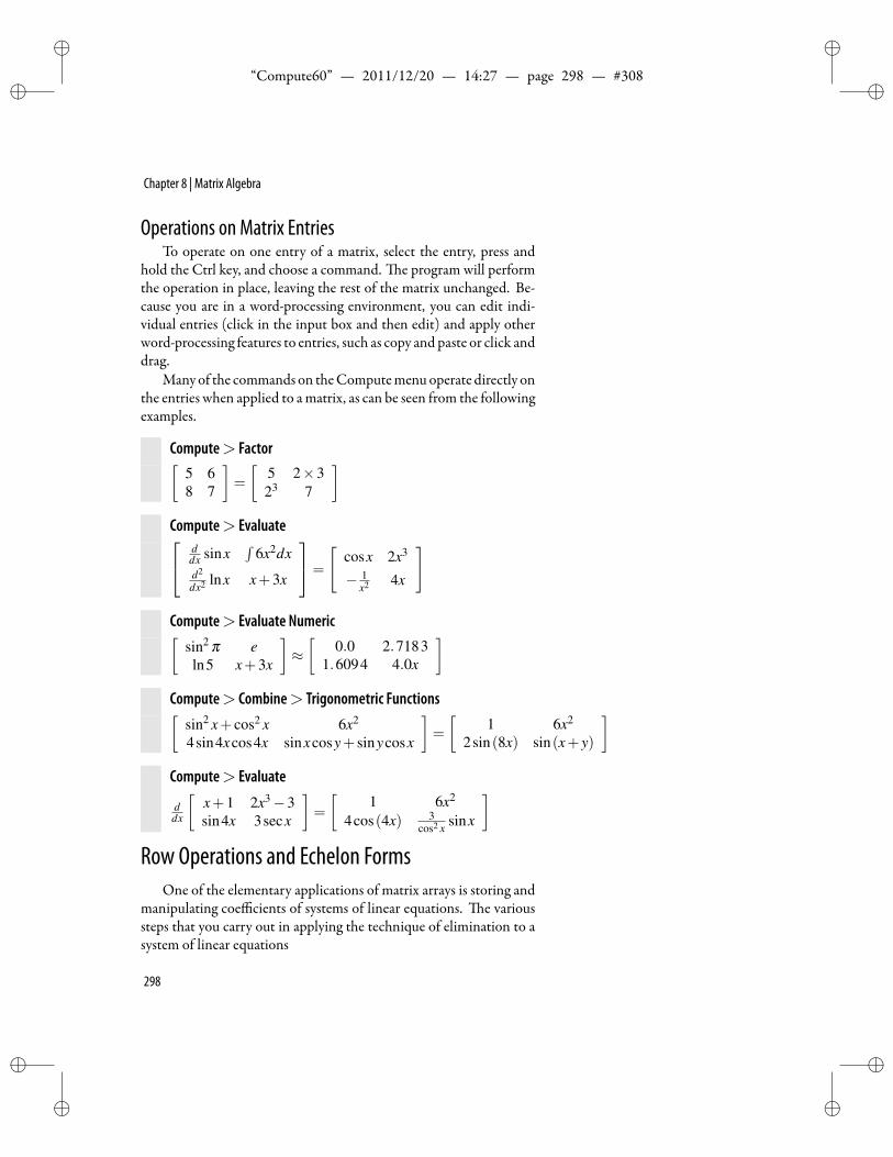
ii
“Compute60” — 2011/12/20 — 14:27 — page 298 — #308 ii
ii
ii
Chapter 8 | Matrix Algebra
Operations on Matrix EntriesTo operate on one entry of a matrix, select the entry, press and
hold the Ctrl key, and choose a command. e program will performthe operation in place, leaving the rest of the matrix unchanged. Be-cause you are in a word-processing environment, you can edit indi-vidual entries (click in the input box and then edit) and apply otherword-processing features to entries, such as copy and paste or click anddrag.
Many of the commands on theComputemenuoperate directly onthe entries when applied to amatrix, as can be seen from the followingexamples.
Compute> Factor[5 68 7
]=
[5 2×323 7
]Compute> Evaluate d
dx sinx∫
6x2dxd2
dx2 lnx x+3x
=
[cosx 2x3
− 1x2 4x
]
Compute> Evaluate Numeric[sin2 π eln5 x+3x
]≈[
0.0 2.71831.6094 4.0x
]Compute> Combine> Trigonometric Functions[
sin2 x+ cos2 x 6x2
4sin4xcos4x sinxcosy+ sinycosx
]=
[1 6x2
2sin(8x) sin(x+ y)
]Compute> Evaluate
ddx
[x+1 2x3−3sin4x 3secx
]=
[1 6x2
4cos(4x) 3cos2 x sinx
]Row Operations and Echelon Forms
One of the elementary applications of matrix arrays is storing andmanipulating coefficients of systems of linear equations. e varioussteps that you carry out in applying the technique of elimination to asystem of linear equations
298
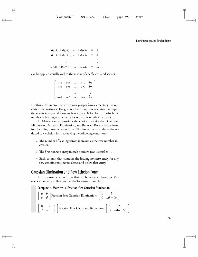
ii
“Compute60” — 2011/12/20 — 14:27 — page 299 — #309 ii
ii
ii
Row Operations and Echelon Forms
a11x1 +a12x2 + . . .+a1nxn = b1
a21x1 +a22x2 + . . .+a2nxn = b2...
......
am1x1 +am2x2 + . . .+amnxn = bm
can be applied equally well to the matrix of coefficients and scalarsa11 a12 . . . a1n b1a21 a22 . . . a2n b2...
... . . ....
...am1 am2 . . . amn bm
For this and numerous other reasons, you perform elementary rowop-erations on matrices. e goal of elementary row operations is to putthe matrix in a special form, such as a row echelon form, in which thenumber of leading zeroes increases as the row number increases.
e Matrices menu provides the choices Fraction-free GaussianElimination, Gaussian Elimination, and Reduced Row Echelon Formfor obtaining a row echelon form. e last of these produces the re-duced row echelon form satisfying the following conditions:
• e number of leading zeroes increases as the row number in-creases.
• e rst nonzero entry in each nonzero row is equal to 1.
• Each column that contains the leading nonzero entry for anyrow contains only zeroes above and below that entry.
Gaussian Elimination and Row Echelon Forme three row echelon forms that can be obtained from the Ma-
trices submenu are illustrated in the following examples.
Compute>Matrices> Fraction-free Gaussian Elimination[a bc d
]Fraction Free Gaussian Elimination:
[a b0 ad−bc
][
8 2 32 −5 8
]Fraction Free Gaussian Elimination:
[8 2 30 −44 58
]299
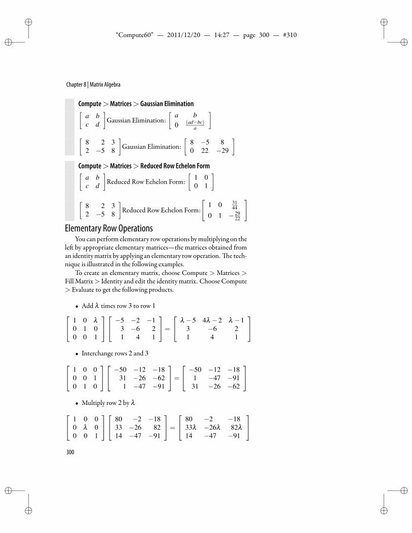
ii
“Compute60” — 2011/12/20 — 14:27 — page 300 — #310 ii
ii
ii
Chapter 8 | Matrix Algebra
Compute>Matrices> Gaussian Elimination[a bc d
]Gaussian Elimination:
[a b0 (ad−bc)
a
][
8 2 32 −5 8
]Gaussian Elimination:
[8 −5 80 22 −29
]Compute>Matrices> Reduced Row Echelon Form[
a bc d
]Reduced Row Echelon Form:
[1 00 1
][
8 2 32 −5 8
]Reduced Row Echelon Form:
[1 0 31
44
0 1 − 2922
]Elementary Row Operations
You can perform elementary row operations bymultiplying on thele by appropriate elementary matrices—the matrices obtained froman identitymatrix by applying an elementary rowoperation. e tech-nique is illustrated in the following examples.
To create an elementary matrix, choose Compute > Matrices >Fill Matrix> Identity and edit the identity matrix. Choose Compute> Evaluate to get the following products.
• Add λ times row 3 to row 1 1 0 λ0 1 00 0 1
−5 −2 −13 −6 21 4 1
=
λ −5 4λ −2 λ −13 −6 21 4 1
• Interchange rows 2 and 3 1 0 0
0 0 10 1 0
−50 −12 −1831 −26 −621 −47 −91
=
−50 −12 −181 −47 −9131 −26 −62
• Multiply row 2 by λ 1 0 0
0 λ 00 0 1
80 −2 −1833 −26 8214 −47 −91
=
80 −2 −1833λ −26λ 82λ14 −47 −91
300
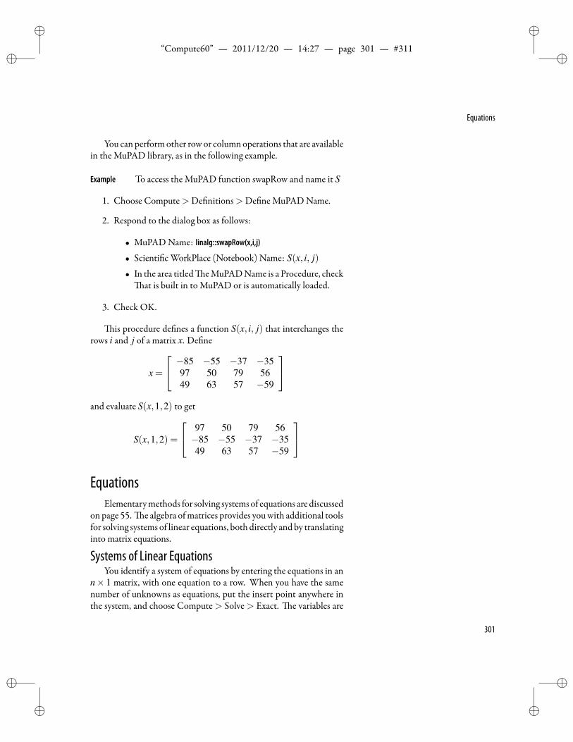
ii
“Compute60” — 2011/12/20 — 14:27 — page 301 — #311 ii
ii
ii
Equations
You can performother rowor columnoperations that are availablein the MuPAD library, as in the following example.
Example To access the MuPAD function swapRow and name it S
1. Choose Compute>De nitions>De ne MuPAD Name.
2. Respond to the dialog box as follows:
• MuPAD Name: linalg::swapRow(x,i,j)
• Scienti c WorkPlace (Notebook) Name: S(x, i, j)
• In the area titled eMuPADName is a Procedure, checkat is built in to MuPAD or is automatically loaded.
3. Check OK.
is procedure de nes a function S(x, i, j) that interchanges therows i and j of a matrix x. De ne
x =
−85 −55 −37 −3597 50 79 5649 63 57 −59
and evaluate S(x,1,2) to get
S(x,1,2) =
97 50 79 56−85 −55 −37 −3549 63 57 −59
EquationsElementarymethods for solving systems of equations are discussed
on page 55. e algebra ofmatrices provides youwith additional toolsfor solving systems of linear equations, both directly and by translatinginto matrix equations.
Systems of Linear EquationsYou identify a system of equations by entering the equations in an
n× 1 matrix, with one equation to a row. When you have the samenumber of unknowns as equations, put the insert point anywhere inthe system, and choose Compute > Solve > Exact. e variables are
301
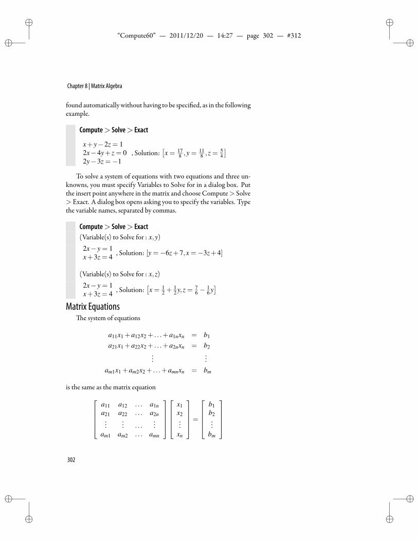
ii
“Compute60” — 2011/12/20 — 14:27 — page 302 — #312 ii
ii
ii
Chapter 8 | Matrix Algebra
found automaticallywithout having to be speci ed, as in the followingexample.
Compute> Solve> Exact
x+ y−2z = 12x−4y+ z = 02y−3z =−1
, Solution:[x = 17
8 ,y =118 ,z =
54
]To solve a system of equations with two equations and three un-
knowns, you must specify Variables to Solve for in a dialog box. Putthe insert point anywhere in thematrix and choose Compute> Solve> Exact. A dialog box opens asking you to specify the variables. Typethe variable names, separated by commas.
Compute> Solve> Exact(Variable(s) to Solve for : x,y)
2x− y = 1x+3z = 4 , Solution: [y =−6z+7,x =−3z+4]
(Variable(s) to Solve for : x,z)
2x− y = 1x+3z = 4 , Solution:
[x = 1
2 +12 y,z = 7
6 −16 y]
Matrix Equationse system of equations
a11x1 +a12x2 + . . .+a1nxn = b1
a21x1 +a22x2 + . . .+a2nxn = b2...
...am1x1 +am2x2 + . . .+amnxn = bm
is the same as the matrix equationa11 a12 . . . a1na21 a22 . . . a2n...
... . . ....
am1 am2 . . . amn
x1x2...
xn
=
b1b2...
bm
302
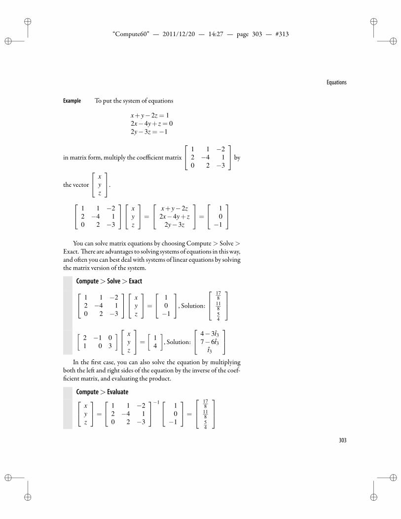
ii
“Compute60” — 2011/12/20 — 14:27 — page 303 — #313 ii
ii
ii
Equations
Example To put the system of equations
x+ y−2z = 12x−4y+ z = 02y−3z =−1
in matrix form, multiply the coefficient matrix
1 1 −22 −4 10 2 −3
by
the vector
xyz
.
1 1 −22 −4 10 2 −3
xyz
=
x+ y−2z2x−4y+ z
2y−3z
=
10−1
You can solve matrix equations by choosing Compute > Solve >
Exact. ere are advantages to solving systems of equations in thisway,and o en you can best deal with systems of linear equations by solvingthe matrix version of the system.
Compute> Solve> Exact 1 1 −22 −4 10 2 −3
xyz
=
10−1
, Solution:
178
11854
[
2 −1 01 0 3
] xyz
=
[14
], Solution:
4−3t37−6t3
t3
In the rst case, you can also solve the equation by multiplying
both the le and right sides of the equation by the inverse of the coef-cient matrix, and evaluating the product.
Compute> Evaluate xyz
=
1 1 −22 −4 10 2 −3
−1 10−1
=
17811854
303
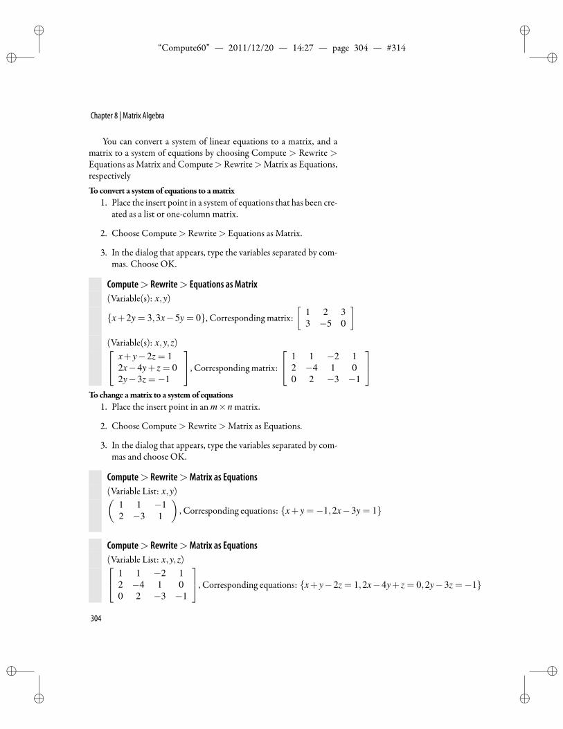
ii
“Compute60” — 2011/12/20 — 14:27 — page 304 — #314 ii
ii
ii
Chapter 8 | Matrix Algebra
You can convert a system of linear equations to a matrix, and amatrix to a system of equations by choosing Compute > Rewrite >Equations as Matrix and Compute>Rewrite>Matrix as Equations,respectivelyToconvert a systemof equations to amatrix
1. Place the insert point in a system of equations that has been cre-ated as a list or one-column matrix.
2. Choose Compute> Rewrite> Equations as Matrix.
3. In the dialog that appears, type the variables separated by com-mas. Choose OK.
Compute> Rewrite> Equations as Matrix(Variable(s): x,y)
x+2y = 3,3x−5y = 0, Corresponding matrix:[
1 2 33 −5 0
](Variable(s): x,y,z) x+ y−2z = 1
2x−4y+ z = 02y−3z =−1
, Corresponding matrix:
1 1 −2 12 −4 1 00 2 −3 −1
Tochange amatrix to a systemof equations
1. Place the insert point in an m×n matrix.
2. Choose Compute> Rewrite>Matrix as Equations.
3. In the dialog that appears, type the variables separated by com-mas and choose OK.
Compute> Rewrite>Matrix as Equations(Variable List: x,y)(
1 1 −12 −3 1
), Corresponding equations: x+ y =−1,2x−3y = 1
Compute> Rewrite>Matrix as Equations(Variable List: x,y,z) 1 1 −2 1
2 −4 1 00 2 −3 −1
, Corresponding equations: x+ y−2z = 1,2x−4y+ z = 0,2y−3z =−1
304
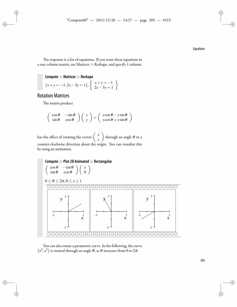
ii
“Compute60” — 2011/12/20 — 14:27 — page 305 — #315 ii
ii
ii
Equations
e response is a list of equations. If you want these equations ina one-column matrix, use Matrices> Reshape, and specify 1 column.
Compute>Matrices> Reshape
x+ y =−1,2x−3y = 1,
x+ y =−12x−3y = 1
Rotation Matrices
e matrix product
(cosθ −sinθsinθ cosθ
)(xy
)=
(xcosθ − ysinθycosθ + xsinθ
)
has the effect of rotating the vector(
xy
)through an angle θ in a
counter-clockwise direction about the origin. You can visualize thisby using an animation.
Compute> Plot 2D Animated> Rectangular(cosθ −sinθsinθ cosθ
)(x0
)0≤ θ ≤ 2π , 0≤ x≤ 1
1 1
1
1
x
y
1 1
1
1
x
y
1 1
1
1
x
y
You can also rotate a parametric curve. In the following, the curve(x2,x3
)is rotated through an angle θ , as θ increases from 0 to 2π .
305
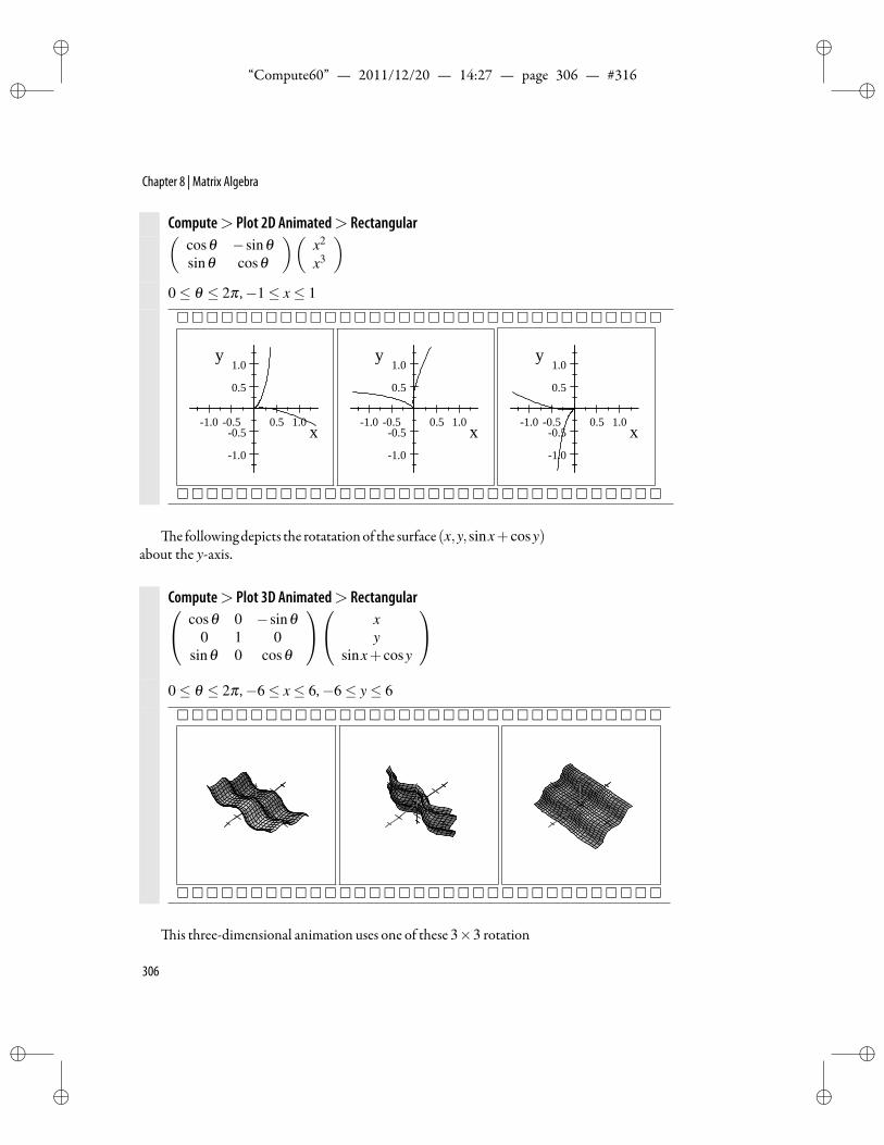
ii
“Compute60” — 2011/12/20 — 14:27 — page 306 — #316 ii
ii
ii
Chapter 8 | Matrix Algebra
Compute> Plot 2D Animated> Rectangular(cosθ −sinθsinθ cosθ
)(x2
x3
)0≤ θ ≤ 2π ,−1≤ x≤ 1
1.0 0.5 0.5 1.0
1.0
0.5
0.5
1.0
x
y
1.0 0.5 0.5 1.0
1.0
0.5
0.5
1.0
x
y
1.0 0.5 0.5 1.0
1.0
0.5
0.5
1.0
x
y
e followingdepicts the rotatationof the surface (x,y,sinx+ cosy)about the y-axis.
Compute> Plot 3D Animated> Rectangular cosθ 0 −sinθ0 1 0
sinθ 0 cosθ
xy
sinx+ cosy
0≤ θ ≤ 2π ,−6≤ x≤ 6,−6≤ y≤ 6
is three-dimensional animation uses one of these 3×3 rotation
306
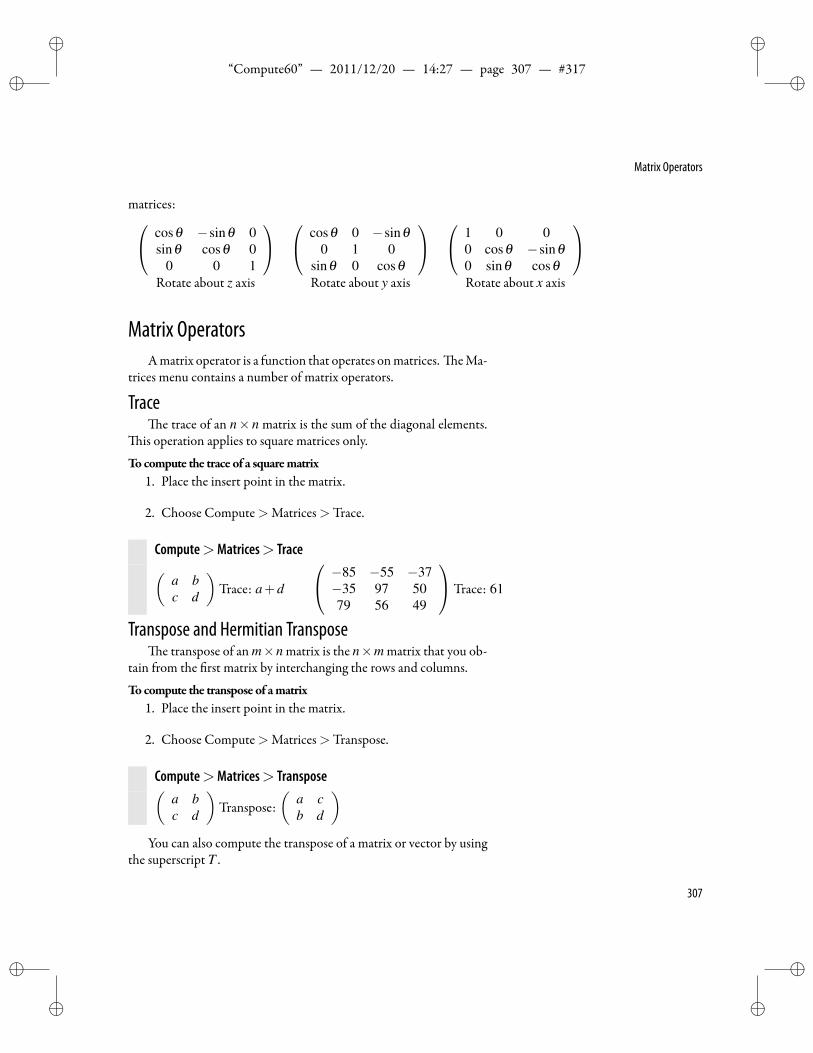
ii
“Compute60” — 2011/12/20 — 14:27 — page 307 — #317 ii
ii
ii
Matrix Operators
matrices: cosθ −sinθ 0sinθ cosθ 0
0 0 1
cosθ 0 −sinθ0 1 0
sinθ 0 cosθ
1 0 00 cosθ −sinθ0 sinθ cosθ
Rotate about z axis Rotate about y axis Rotate about x axis
Matrix OperatorsAmatrix operator is a function that operates onmatrices. eMa-
trices menu contains a number of matrix operators.
Tracee trace of an n× n matrix is the sum of the diagonal elements.
is operation applies to square matrices only.
Tocompute the trace of a squarematrix1. Place the insert point in the matrix.
2. Choose Compute>Matrices>Trace.
Compute>Matrices> Trace(a bc d
)Trace: a+d
−85 −55 −37−35 97 5079 56 49
Trace: 61
Transpose and Hermitian Transposee transpose of an m×n matrix is the n×m matrix that you ob-
tain from the rst matrix by interchanging the rows and columns.
Tocompute the transpose of amatrix1. Place the insert point in the matrix.
2. Choose Compute>Matrices>Transpose.
Compute>Matrices> Transpose(a bc d
)Transpose:
(a cb d
)You can also compute the transpose of a matrix or vector by using
the superscript T .
307
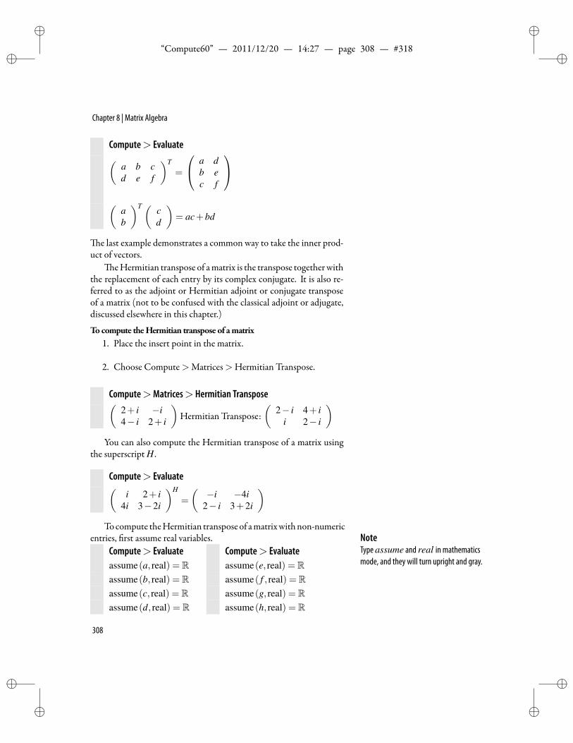
ii
“Compute60” — 2011/12/20 — 14:27 — page 308 — #318 ii
ii
ii
Chapter 8 | Matrix Algebra
Compute> Evaluate(a b cd e f
)T
=
a db ec f
(
ab
)T ( cd
)= ac+bd
e last example demonstrates a common way to take the inner prod-uct of vectors.
eHermitian transpose of amatrix is the transpose togetherwiththe replacement of each entry by its complex conjugate. It is also re-ferred to as the adjoint or Hermitian adjoint or conjugate transposeof a matrix (not to be confused with the classical adjoint or adjugate,discussed elsewhere in this chapter.)
Tocompute theHermitian transpose of amatrix1. Place the insert point in the matrix.
2. Choose Compute>Matrices>Hermitian Transpose.
Compute>Matrices> Hermitian Transpose(2+ i −i4− i 2+ i
)Hermitian Transpose:
(2− i 4+ i
i 2− i
)You can also compute the Hermitian transpose of a matrix using
the superscript H .
Compute> Evaluate(i 2+ i
4i 3−2i
)H
=
(−i −4i
2− i 3+2i
)Tocompute theHermitian transpose of amatrixwithnon-numeric
entries, rst assume real variables. NoteType assume and real in mathematicsmode, and they will turn upright and gray.
Compute> Evaluate Compute> Evaluateassume(a, real) = R assume(e, real) = Rassume(b, real) = R assume( f , real) = Rassume(c, real) = R assume(g, real) = Rassume(d, real) = R assume(h, real) = R
308
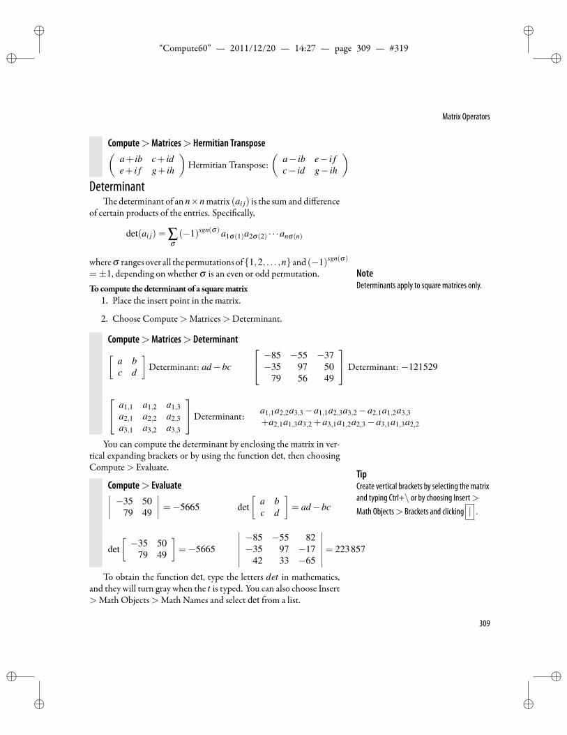
ii
“Compute60” — 2011/12/20 — 14:27 — page 309 — #319 ii
ii
ii
Matrix Operators
Compute>Matrices> Hermitian Transpose(a+ ib c+ ide+ i f g+ ih
)Hermitian Transpose:
(a− ib e− i fc− id g− ih
)Determinant
e determinant of an n×n matrix (ai j) is the sum and differenceof certain products of the entries. Speci cally,
det(ai j) = ∑σ(−1)sgn(σ) a1σ(1)a2σ(2) · · ·anσ(n)
whereσ ranges over all thepermutations of1,2, . . . ,n and (−1)sgn(σ)
=±1, depending on whether σ is an even or odd permutation. NoteDeterminants apply to square matrices only.Tocompute the determinant of a squarematrix
1. Place the insert point in the matrix.
2. Choose Compute>Matrices>Determinant.
Compute>Matrices> Determinant[a bc d
]Determinant: ad−bc
−85 −55 −37−35 97 50
79 56 49
Determinant: −121529
a1,1 a1,2 a1,3a2,1 a2,2 a2,3a3,1 a3,2 a3,3
Determinant: a1,1a2,2a3,3−a1,1a2,3a3,2−a2,1a1,2a3,3+a2,1a1,3a3,2 +a3,1a1,2a2,3−a3,1a1,3a2,2
You can compute the determinant by enclosing the matrix in ver-tical expanding brackets or by using the function det, then choosingCompute> Evaluate.
TipCreate vertical brackets by selecting the matrixand typing Ctrl+\ or by choosing Insert>Math Objects> Brackets and clicking | .
Compute> Evaluate∣∣∣∣ −35 5079 49
∣∣∣∣ =−5665 det[
a bc d
]= ad−bc
det[−35 50
79 49
]=−5665
∣∣∣∣∣∣−85 −55 82−35 97 −17
42 33 −65
∣∣∣∣∣∣= 223857
To obtain the function det, type the letters det in mathematics,and they will turn gray when the t is typed. You can also choose Insert>Math Objects>Math Names and select det from a list.
309
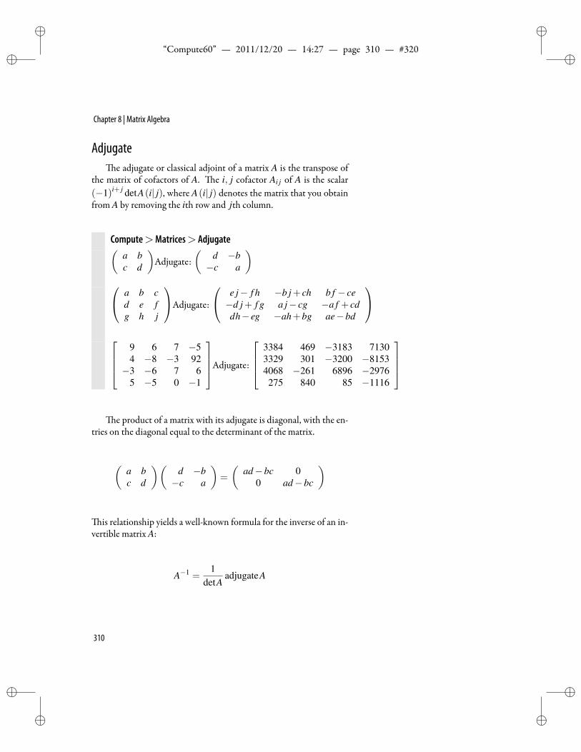
ii
“Compute60” — 2011/12/20 — 14:27 — page 310 — #320 ii
ii
ii
Chapter 8 | Matrix Algebra
Adjugatee adjugate or classical adjoint of a matrix A is the transpose of
the matrix of cofactors of A. e i, j cofactor Ai j of A is the scalar(−1)i+ j detA(i| j), where A(i| j) denotes the matrix that you obtainfrom A by removing the ith row and jth column.
Compute>Matrices> Adjugate(a bc d
)Adjugate:
(d −b−c a
) a b c
d e fg h j
Adjugate:
e j− f h −b j+ ch b f − ce−d j+ f g a j− cg −a f + cddh− eg −ah+bg ae−bd
9 6 7 −54 −8 −3 92−3 −6 7 6
5 −5 0 −1
Adjugate:
3384 469 −3183 71303329 301 −3200 −81534068 −261 6896 −2976275 840 85 −1116
e product of a matrix with its adjugate is diagonal, with the en-tries on the diagonal equal to the determinant of the matrix.
(a bc d
)(d −b−c a
)=
(ad−bc 0
0 ad−bc
)
is relationship yields a well-known formula for the inverse of an in-vertible matrix A:
A−1 =1
detAadjugateA
310
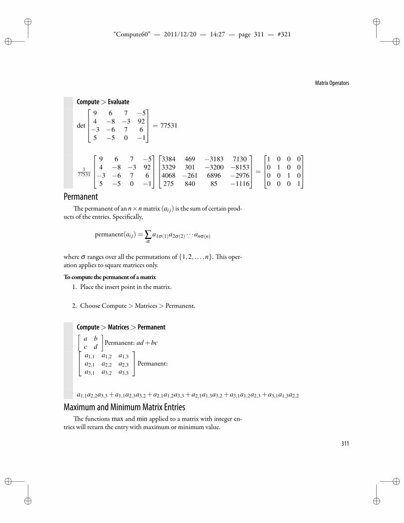
ii
“Compute60” — 2011/12/20 — 14:27 — page 311 — #321 ii
ii
ii
Matrix Operators
Compute> Evaluate
det
9 6 7 −54 −8 −3 92−3 −6 7 65 −5 0 −1
= 77531
177531
9 6 7 −54 −8 −3 92−3 −6 7 65 −5 0 −1
3384 469 −3183 71303329 301 −3200 −81534068 −261 6896 −2976275 840 85 −1116
=
1 0 0 00 1 0 00 0 1 00 0 0 1
Permanent
e permanent of an n×n matrix (ai j) is the sum of certain prod-ucts of the entries. Speci cally,
permanent(ai j) = ∑σ
a1σ(1)a2σ(2) · · ·anσ(n)
where σ ranges over all the permutations of 1,2, . . . ,n. is oper-ation applies to square matrices only.
Tocompute the permanent of amatrix1. Place the insert point in the matrix.
2. Choose Compute>Matrices> Permanent.
Compute>Matrices> Permanent[a bc d
]Permanent: ad +bc a1,1 a1,2 a1,3
a2,1 a2,2 a2,3a3,1 a3,2 a3,3
Permanent:
a1,1a2,2a3,3 +a1,1a2,3a3,2 +a2,1a1,2a3,3 +a2,1a1,3a3,2 +a3,1a1,2a2,3 +a3,1a1,3a2,2
Maximum and MinimumMatrix Entriese functions max and min applied to a matrix with integer en-
tries will return the entry with maximum or minimum value.
311
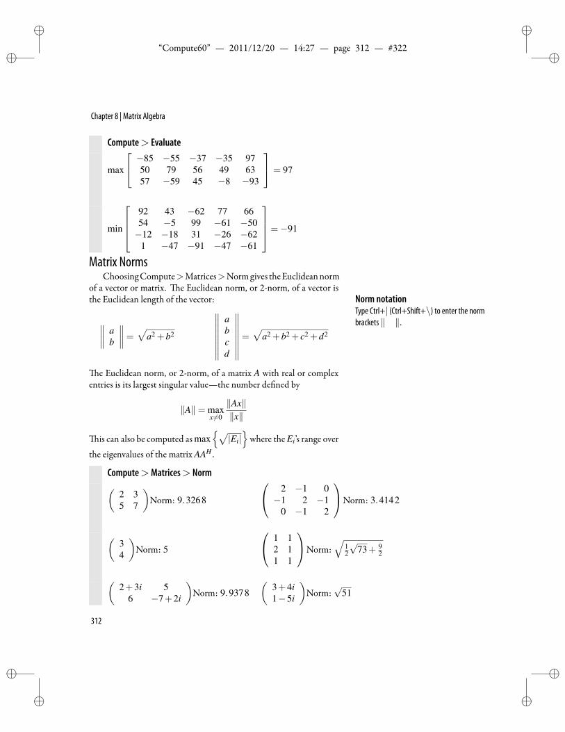
ii
“Compute60” — 2011/12/20 — 14:27 — page 312 — #322 ii
ii
ii
Chapter 8 | Matrix Algebra
Compute> Evaluate
max
−85 −55 −37 −35 9750 79 56 49 6357 −59 45 −8 −93
= 97
min
92 43 −62 77 6654 −5 99 −61 −50−12 −18 31 −26 −62
1 −47 −91 −47 −61
=−91
Matrix NormsChoosingCompute>Matrices>Normgives theEuclideannorm
of a vector or matrix. e Euclidean norm, or 2-norm, of a vector isthe Euclidean length of the vector: Norm notation
Type Ctrl+| (Ctrl+Shift+\) to enter the normbrackets ∥ ∥.∥∥∥∥ a
b
∥∥∥∥= √a2 +b2
∥∥∥∥∥∥∥∥abcd
∥∥∥∥∥∥∥∥=√
a2 +b2 + c2 +d2
e Euclidean norm, or 2-norm, of a matrix A with real or complexentries is its largest singular value—the number de ned by
∥A∥= maxx =0
∥Ax∥∥x∥
is can also be computed as max√|Ei|
where the Ei’s range over
the eigenvalues of the matrix AAH .
Compute>Matrices> Norm(2 35 7
)Norm: 9.3268
2 −1 0−1 2 −1
0 −1 2
Norm: 3.4142
(34
)Norm: 5
1 12 11 1
Norm:√
12
√73+ 9
2
(2+3i 5
6 −7+2i
)Norm: 9.9378
(3+4i1−5i
)Norm:
√51
312
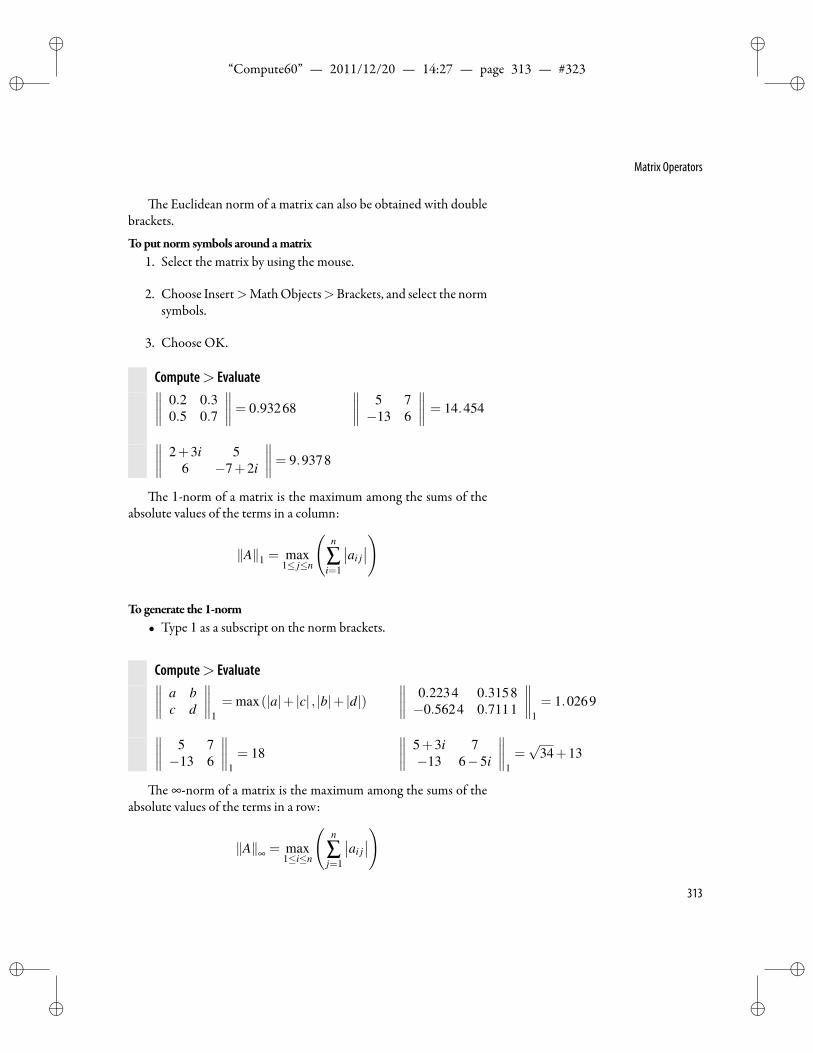
ii
“Compute60” — 2011/12/20 — 14:27 — page 313 — #323 ii
ii
ii
Matrix Operators
e Euclidean norm of a matrix can also be obtained with doublebrackets.
Toput norm symbols around amatrix1. Select the matrix by using the mouse.
2. Choose Insert>MathObjects>Brackets, and select the normsymbols.
3. Choose OK.
Compute> Evaluate∥∥∥∥ 0.2 0.30.5 0.7
∥∥∥∥= 0.93268∥∥∥∥ 5 7−13 6
∥∥∥∥ = 14.454
∥∥∥∥ 2+3i 56 −7+2i
∥∥∥∥= 9.9378
e 1-norm of a matrix is the maximum among the sums of theabsolute values of the terms in a column:
∥A∥1 = max1≤ j≤n
(n
∑i=1
∣∣ai j∣∣)
Togenerate the 1-norm• Type 1 as a subscript on the norm brackets.
Compute> Evaluate∥∥∥∥ a bc d
∥∥∥∥1= max(|a|+ |c| , |b|+ |d|)
∥∥∥∥ 0.2234 0.3158−0.5624 0.7111
∥∥∥∥1= 1.0269
∥∥∥∥ 5 7−13 6
∥∥∥∥1= 18
∥∥∥∥ 5+3i 7−13 6−5i
∥∥∥∥1=√
34+13
e ∞-norm of a matrix is the maximum among the sums of theabsolute values of the terms in a row:
∥A∥∞ = max1≤i≤n
(n
∑j=1
∣∣ai j∣∣)
313
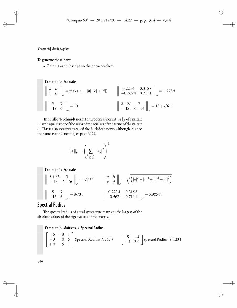
ii
“Compute60” — 2011/12/20 — 14:27 — page 314 — #324 ii
ii
ii
Chapter 8 | Matrix Algebra
Togenerate the∞-norm
• Enter ∞ as a subscript on the norm brackets.
Compute> Evaluate∥∥∥∥ a bc d
∥∥∥∥∞= max(|a|+ |b| , |c|+ |d|)
∥∥∥∥ 0.2234 0.3158−0.5624 0.7111
∥∥∥∥∞= 1.2735
∥∥∥∥ 5 7−13 6
∥∥∥∥∞= 19
∥∥∥∥ 5+3i 7−13 6−5i
∥∥∥∥∞= 13+
√61
eHilbert-Schmidt norm (or Frobenius norm) ∥A∥F of amatrixA is the square root of the sumsof the squares of the terms of thematrixA. is is also sometimes called the Euclidean norm, although it is notthe same as the 2-norm (see page 312).
∥A∥F =
∑1≤ j≤n1≤i≤n
∣∣ai j∣∣2 1
2
Compute> Evaluate∥∥∥∥ 5+3i 7−13 6−5i
∥∥∥∥F=√
313∥∥∥∥ a b
c d
∥∥∥∥F=
√(|a|2 + |b|2 + |c|2 + |d|2
)∥∥∥∥ 5 7−13 6
∥∥∥∥F= 3√
31∥∥∥∥ 0.2234 0.3158−0.5624 0.7111
∥∥∥∥F= 0.98569
Spectral Radiuse spectral radius of a real symmetric matrix is the largest of the
absolute values of the eigenvalues of the matrix.
Compute>Matrices> Spectral Radius 5 −3 1−3 0 51.0 5 4
Spectral Radius: 7.7627[
5 −4−4 3.0
]Spectral Radius: 8.1231
314
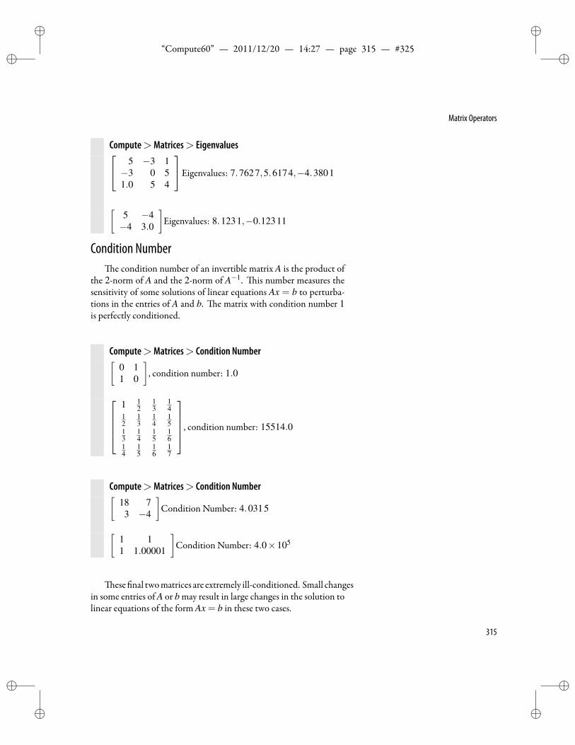
ii
“Compute60” — 2011/12/20 — 14:27 — page 315 — #325 ii
ii
ii
Matrix Operators
Compute>Matrices> Eigenvalues 5 −3 1−3 0 51.0 5 4
Eigenvalues: 7.7627,5.6174,−4.3801
[5 −4−4 3.0
]Eigenvalues: 8.1231,−0.12311
Condition Numbere condition number of an invertible matrix A is the product of
the 2-norm of A and the 2-norm of A−1. is number measures thesensitivity of some solutions of linear equations Ax = b to perturba-tions in the entries of A and b. e matrix with condition number 1is perfectly conditioned.
Compute>Matrices> Condition Number[0 11 0
], condition number: 1.0
1 1
213
14
12
13
14
15
13
14
15
16
14
15
16
17
, condition number: 15514.0
Compute>Matrices> Condition Number[18 73 −4
]Condition Number: 4.0315
[1 11 1.00001
]Condition Number: 4.0×10⁵
ese nal twomatrices are extremely ill-conditioned. Small changesin some entries of A or b may result in large changes in the solution tolinear equations of the form Ax = b in these two cases.
315
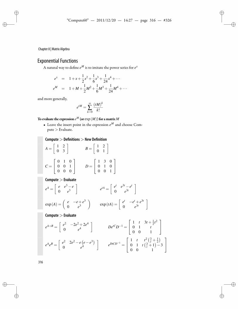
ii
“Compute60” — 2011/12/20 — 14:27 — page 316 — #326 ii
ii
ii
Chapter 8 | Matrix Algebra
Exponential FunctionsA natural way to de ne eM is to imitate the power series for ex
ex = 1+ x+12
x2 +16
x3 +1
24x4 + · · ·
eM = 1+M+12
M2 +16
M3 +1
24M4 + · · ·
and more generally,
etM =∞
∑k=0
(tM)k
k!
Toevaluate the expression eM (or exp(M)) for amatrixM• Leave the insert point in the expression eM and choose Com-
pute> Evaluate.
Compute> De nitions> New De nition
A =
[1 20 3
]B =
[1 20 1
]
C =
0 1 00 0 10 0 0
D =
1 3 00 1 00 0 1
Compute> Evaluate
eA =
[e e3− e0 e3
]etA =
[et e3t − et
0 e3t
]
exp(A) =(
e −e+ e3
0 e3
)exp(tA) =
[et −et + e3t
0 e3t
]Compute> Evaluate
eA+B =
[e2 −2e2 +2e4
0 e4
]DetCD−1 =
1 t 3t + 12 t2
0 1 t0 0 1
eAeB =
[e2 2e2− e
(e− e3
)0 e4
]eDtCD−1
=
1 t t2( 3
t +12
)0 1 t
( 3t +1
)−3
0 0 1
316
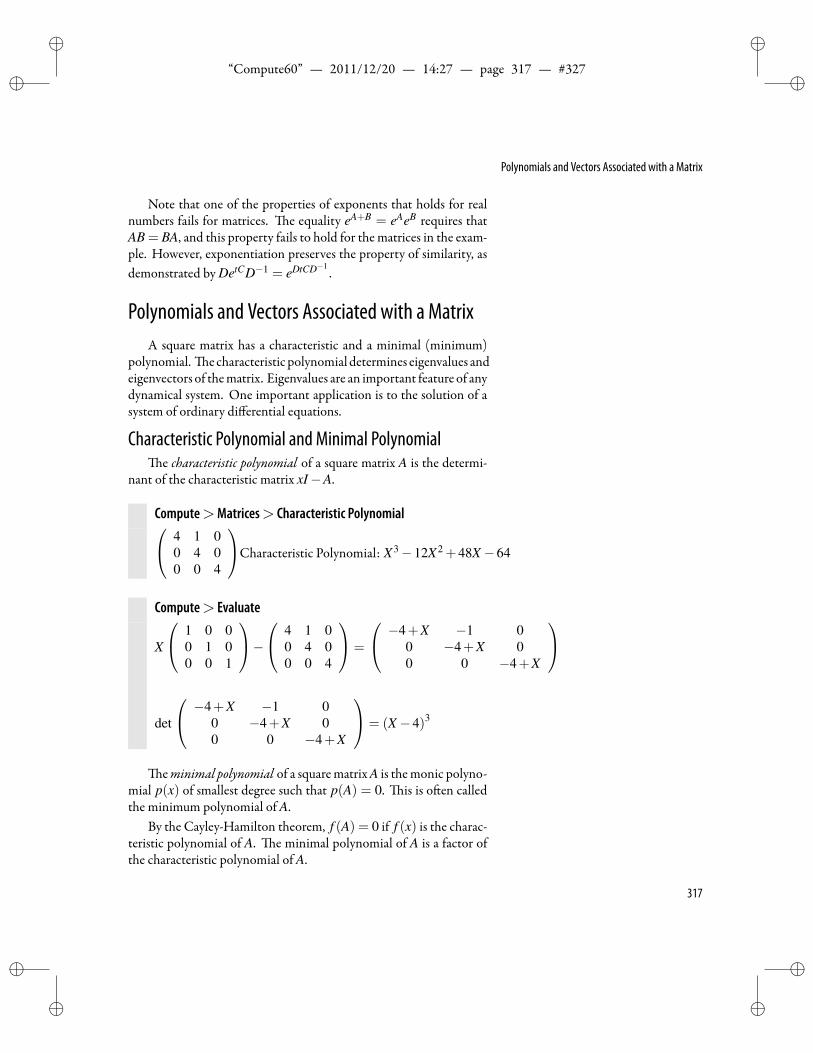
ii
“Compute60” — 2011/12/20 — 14:27 — page 317 — #327 ii
ii
ii
Polynomials and Vectors Associated with a Matrix
Note that one of the properties of exponents that holds for realnumbers fails for matrices. e equality eA+B = eAeB requires thatAB = BA, and this property fails to hold for thematrices in the exam-ple. However, exponentiation preserves the property of similarity, asdemonstrated by DetCD−1 = eDtCD−1
.
Polynomials and Vectors Associated with a MatrixA square matrix has a characteristic and a minimal (minimum)
polynomial. e characteristic polynomial determines eigenvalues andeigenvectors of thematrix. Eigenvalues are an important feature of anydynamical system. One important application is to the solution of asystem of ordinary differential equations.
Characteristic Polynomial and Minimal Polynomiale characteristic polynomial of a square matrix A is the determi-
nant of the characteristic matrix xI−A.
Compute>Matrices> Characteristic Polynomial 4 1 00 4 00 0 4
Characteristic Polynomial: X3−12X2 +48X−64
Compute> Evaluate
X
1 0 00 1 00 0 1
− 4 1 0
0 4 00 0 4
=
−4+X −1 00 −4+X 00 0 −4+X
det
−4+X −1 00 −4+X 00 0 −4+X
= (X−4)3
eminimal polynomial of a squarematrix A is themonic polyno-mial p(x) of smallest degree such that p(A) = 0. is is o en calledthe minimum polynomial of A.
By the Cayley-Hamilton theorem, f (A) = 0 if f (x) is the charac-teristic polynomial of A. e minimal polynomial of A is a factor ofthe characteristic polynomial of A.
317
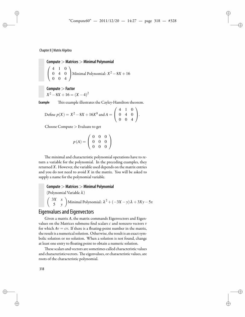
ii
“Compute60” — 2011/12/20 — 14:27 — page 318 — #328 ii
ii
ii
Chapter 8 | Matrix Algebra
Compute>Matrices>Minimal Polynomial 4 1 00 4 00 0 4
Minimal Polynomial: X2−8X +16
Compute> FactorX2−8X +16 = (X−4)2
Example is example illustrates the Cayley-Hamilton theorem.
De ne p(X) = X2−8X +16X0 and A =
4 1 00 4 00 0 4
.
Choose Compute> Evaluate to get
p(A) =
0 0 00 0 00 0 0
e minimal and characteristic polynomial operations have to re-
turn a variable for the polynomial. In the preceding examples, theyreturned X . However, the variable used depends on the matrix entriesand you do not need to avoid X in the matrix. You will be asked tosupply a name for the polynomial variable.
Compute>Matrices>Minimal Polynomial(Polynomial Variable λ )(
3X x5 y
)Minimal Polynomial: λ 2 +(−3X− y)λ +3Xy−5x
Eigenvalues and EigenvectorsGiven a matrix A, the matrix commands Eigenvectors and Eigen-
values on the Matrices submenu nd scalars c and nonzero vectors vfor which Av = cv. If there is a oating-point number in the matrix,the result is a numerical solution. Otherwise, the result is an exact sym-bolic solution or no solution. When a solution is not found, changeat least one entry to oating point to obtain a numeric solution.
ese scalars and vectors are sometimes called characteristic valuesand characteristicvectors. e eigenvalues, or characteristic values, areroots of the characteristic polynomial.
318
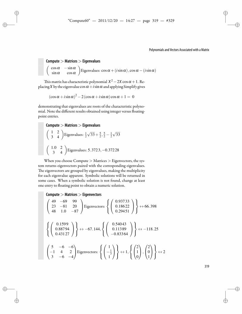
ii
“Compute60” — 2011/12/20 — 14:27 — page 319 — #329 ii
ii
ii
Polynomials and Vectors Associated with a Matrix
Compute>Matrices> Eigenvalues(cosα −sinαsinα cosα
)Eigenvalues: cosα +(isinα) ,cosα− (isinα)
is matrix has characteristic polynomial X2−2X cosα +1. Re-placingX by the eigenvaluecosα+ isinα and applyingSimplify gives
(cosα + isinα)2−2(cosα + isinα)cosα +1 = 0
demonstrating that eigenvalues are roots of the characteristic polyno-mial. Note the different results obtained using integer versus oating-point entries.
Compute>Matrices> Eigenvalues(1 23 4
)Eigenvalues: 1
2
√33+ 5
2 ,52 −
12
√33
(1.0 23 4
)Eigenvalues: 5.3723,−0.37228
When you choose Compute > Matrices > Eigenvectors, the sys-tem returns eigenvectors paired with the corresponding eigenvalues.
e eigenvectors are grouped by eigenvalues, making the multiplicityfor each eigenvalue apparent. Symbolic solutions will be returned insome cases. When a symbolic solution is not found, change at leastone entry to oating point to obtain a numeric solution.
Compute>Matrices> Eigenvectors 49 −69 9923 −81 2048 1.0 −87
Eigenvectors:
0.93733
0.186220.29451
↔ 66.398
0.1599
0.887940.43127
↔−67.144,
0.54043
0.11389−0.83364
↔−118.25
5 −6 −6−1 4 23 −6 −4
Eigenvectors:
1− 1
31
↔ 1,
2
10
,
201
↔ 2
319
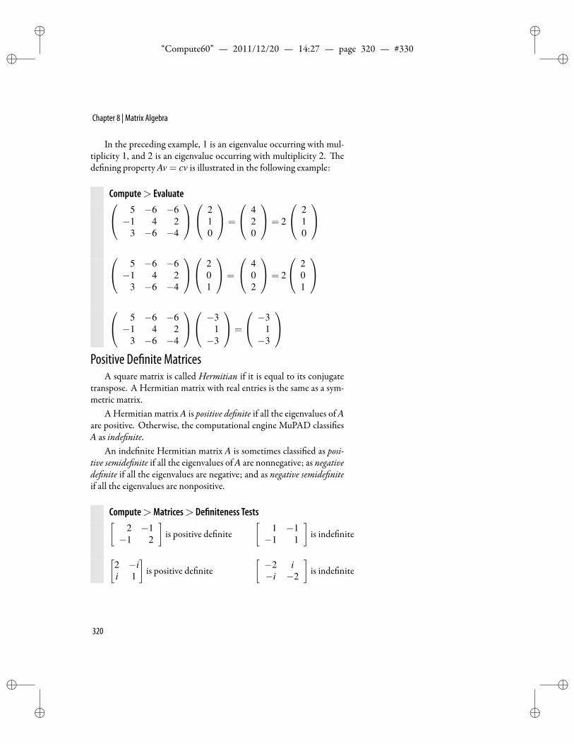
ii
“Compute60” — 2011/12/20 — 14:27 — page 320 — #330 ii
ii
ii
Chapter 8 | Matrix Algebra
In the preceding example, 1 is an eigenvalue occurring with mul-tiplicity 1, and 2 is an eigenvalue occurring with multiplicity 2. ede ning property Av = cv is illustrated in the following example:
Compute> Evaluate 5 −6 −6−1 4 2
3 −6 −4
210
=
420
= 2
210
5 −6 −6−1 4 2
3 −6 −4
201
=
402
= 2
201
5 −6 −6−1 4 2
3 −6 −4
−31−3
=
−31−3
Positive De nite Matrices
A square matrix is called Hermitian if it is equal to its conjugatetranspose. A Hermitian matrix with real entries is the same as a sym-metric matrix.
A Hermitian matrix A is positive de nite if all the eigenvalues of Aare positive. Otherwise, the computational engine MuPAD classi esA as inde nite.
An inde nite Hermitian matrix A is sometimes classi ed as posi-tive semide nite if all the eigenvalues of A are nonnegative; as negativede nite if all the eigenvalues are negative; and as negative semide niteif all the eigenvalues are nonpositive.
Compute>Matrices> De niteness Tests[2 −1−1 2
]is positive de nite
[1 −1−1 1
]is inde nite
[2 −ii 1
]is positive de nite
[−2 i−i −2
]is inde nite
320
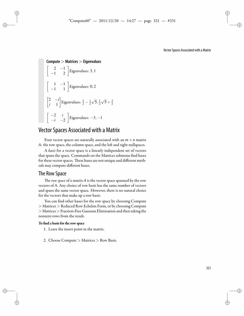
ii
“Compute60” — 2011/12/20 — 14:27 — page 321 — #331 ii
ii
ii
Vector Spaces Associated with a Matrix
Compute>Matrices> Eigenvalues[2 −1−1 2
]Eigenvalues: 3,1
[1 −1−1 1
]Eigenvalues: 0,2
[2 −ii 1
]Eigenvalues: 3
2 −12
√5, 1
2
√5+ 3
2
[−2 i−i −2
]Eigenvalues: −3,−1
Vector Spaces Associated with a MatrixFour vector spaces are naturally associated with an m× n matrix
A: the row space, the column space, and the le and right nullspaces.A basis for a vector space is a linearly independent set of vectors
that spans the space. Commands on the Matrices submenu nd basesfor these vector spaces. ese bases are not unique and differentmeth-ods may compute different bases.
The Row Spacee row space of a matrix A is the vector space spanned by the row
vectors of A. Any choice of row basis has the same number of vectorsand spans the same vector space. However, there is no natural choicefor the vectors that make up a row basis.
You can nd other bases for the row space by choosing Compute>Matrices>Reduced Row Echelon Form, or by choosing Compute>Matrices>Fraction-FreeGaussianElimination and then taking thenonzero rows from the result.
To nd abasis for the row space1. Leave the insert point in the matrix.
2. Choose Compute>Matrices> Row Basis.
321
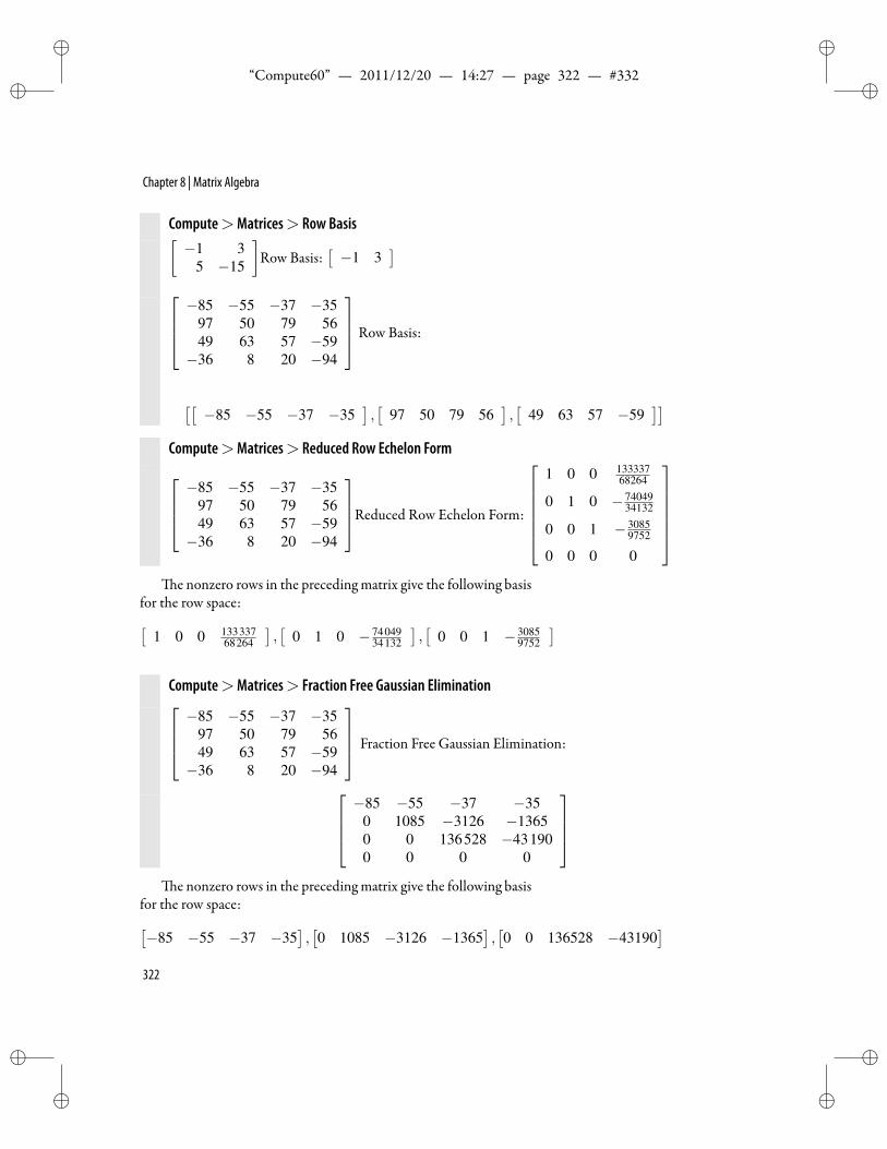
ii
“Compute60” — 2011/12/20 — 14:27 — page 322 — #332 ii
ii
ii
Chapter 8 | Matrix Algebra
Compute>Matrices> Row Basis[−1 3
5 −15
]Row Basis:
[−1 3
]−85 −55 −37 −35
97 50 79 5649 63 57 −59−36 8 20 −94
Row Basis:
[[−85 −55 −37 −35
],[
97 50 79 56],[
49 63 57 −59]]
Compute>Matrices> Reduced Row Echelon Form−85 −55 −37 −35
97 50 79 5649 63 57 −59−36 8 20 −94
Reduced Row Echelon Form:
1 0 0 133337
68264
0 1 0 − 7404934132
0 0 1 − 30859752
0 0 0 0
e nonzero rows in the preceding matrix give the following basis
for the row space:[1 0 0 133337
68264
],[
0 1 0 − 7404934132
],[
0 0 1 − 30859752
]Compute>Matrices> Fraction Free Gaussian Elimination−85 −55 −37 −35
97 50 79 5649 63 57 −59−36 8 20 −94
Fraction Free Gaussian Elimination:
−85 −55 −37 −35
0 1085 −3126 −13650 0 136528 −431900 0 0 0
e nonzero rows in the preceding matrix give the following basis
for the row space:[−85 −55 −37 −35
],[0 1085 −3126 −1365
],[0 0 136528 −43190
]322
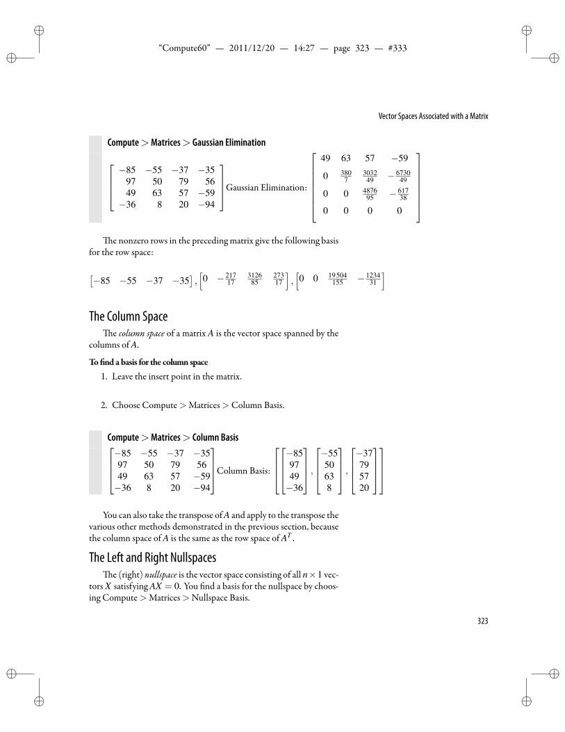
ii
“Compute60” — 2011/12/20 — 14:27 — page 323 — #333 ii
ii
ii
Vector Spaces Associated with a Matrix
Compute>Matrices> Gaussian Elimination
−85 −55 −37 −35
97 50 79 5649 63 57 −59−36 8 20 −94
Gaussian Elimination:
49 63 57 −59
0 3807
303249 − 6730
49
0 0 487695 − 617
38
0 0 0 0
e nonzero rows in the preceding matrix give the following basis
for the row space:
[−85 −55 −37 −35
],[0 − 217
17312685
27317
],[0 0 19504
155 − 123431
]
The Column Spacee column space of a matrix A is the vector space spanned by the
columns of A.
To nd abasis for the column space
1. Leave the insert point in the matrix.
2. Choose Compute>Matrices>Column Basis.
Compute>Matrices> Column Basis−85 −55 −37 −3597 50 79 5649 63 57 −59−36 8 20 −94
Column Basis:
−859749−36
,−5550638
,−37795720
You can also take the transpose of A and apply to the transpose thevarious other methods demonstrated in the previous section, becausethe column space of A is the same as the row space of AT .
The Left and Right Nullspacese (right) nullspace is the vector space consisting of all n×1 vec-
tors X satisfying AX = 0. You nd a basis for the nullspace by choos-ing Compute>Matrices>Nullspace Basis.
323
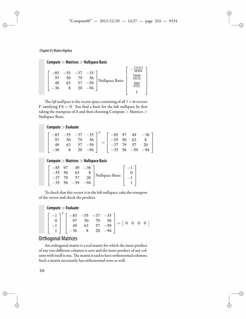
ii
“Compute60” — 2011/12/20 — 14:27 — page 324 — #334 ii
ii
ii
Chapter 8 | Matrix Algebra
Compute>Matrices> Nullspace Basis−85 −55 −37 −35
97 50 79 5649 63 57 −59−36 8 20 −94
Nullspace Basis:
− 133337
68264740493413230859752
1
e le nullspace is the vector space consisting of all 1×m vectors
Y satisfying YA = 0. You nd a basis for the le nullspace by rsttaking the transpose of A and then choosing Compute>Matrices>Nullspace Basis.
Compute> Evaluate−85 −55 −37 −35
97 50 79 5649 63 57 −59−36 8 20 −94
T
=
−85 97 49 −36−55 50 63 8−37 79 57 20−35 56 −59 −94
Compute>Matrices> Nullspace Basis−85 97 49 −36−55 50 63 8−37 79 57 20−35 56 −59 −94
Nullspace Basis:
−1
0−1
1
To check that this vector is in the le nullspace, take the transpose
of the vector and check the product.
Compute> Evaluate−1
0−1
1
T −85 −55 −37 −35
97 50 79 5649 63 57 −59−36 8 20 −94
=[
0 0 0 0]
Orthogonal MatricesAn orthogonal matrix is a real matrix for which the inner product
of any two different columns is zero and the inner product of any col-umnwith itself is one. ematrix is said tohaveorthonormal columns.Such a matrix necessarily has orthonormal rows as well.
324
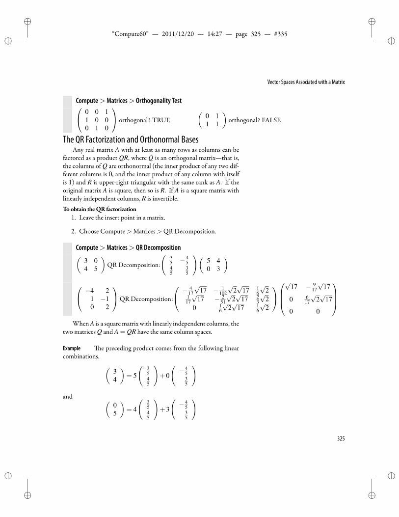
ii
“Compute60” — 2011/12/20 — 14:27 — page 325 — #335 ii
ii
ii
Vector Spaces Associated with a Matrix
Compute>Matrices> Orthogonality Test 0 0 11 0 00 1 0
orthogonal? TRUE(
0 11 1
)orthogonal? FALSE
The QR Factorization and Orthonormal BasesAny real matrix A with at least as many rows as columns can be
factored as a product QR, where Q is an orthogonal matrix—that is,the columns of Q are orthonormal (the inner product of any two dif-ferent columns is 0, and the inner product of any column with itselfis 1) and R is upper-right triangular with the same rank as A. If theoriginal matrix A is square, then so is R. If A is a square matrix withlinearly independent columns, R is invertible.Toobtain theQR factorization
1. Leave the insert point in a matrix.
2. Choose Compute>Matrices>QR Decomposition.
Compute>Matrices> QR Decomposition(3 04 5
)QR Decomposition:
(35 − 4
545
35
)(5 40 3
) −4 2
1 −10 2
QR Decomposition:
− 417
√17 − 1
102
√2√
17 16
√2
117
√17 − 2
51
√2√
17 23
√2
0 16
√2√
17 16
√2
√
17 − 917
√17
0 617
√2√
17
0 0
When A is a squarematrix with linearly independent columns, the
two matrices Q and A = QR have the same column spaces.
Example e preceding product comes from the following linearcombinations. (
34
)= 5
(3545
)+0
(− 4
535
)
and (05
)= 4
(3545
)+3
(− 4
535
)
325
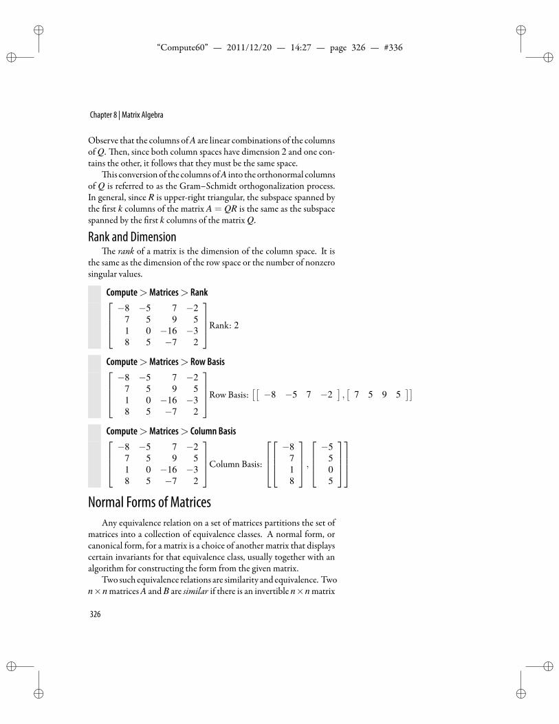
ii
“Compute60” — 2011/12/20 — 14:27 — page 326 — #336 ii
ii
ii
Chapter 8 | Matrix Algebra
Observe that the columns of A are linear combinations of the columnsof Q. en, since both column spaces have dimension 2 and one con-tains the other, it follows that they must be the same space.
is conversionof the columnsofA into theorthonormal columnsof Q is referred to as the Gram–Schmidt orthogonalization process.In general, since R is upper-right triangular, the subspace spanned bythe rst k columns of the matrix A = QR is the same as the subspacespanned by the rst k columns of the matrix Q.
Rank and Dimensione rank of a matrix is the dimension of the column space. It is
the same as the dimension of the row space or the number of nonzerosingular values.
Compute>Matrices> Rank−8 −5 7 −2
7 5 9 51 0 −16 −38 5 −7 2
Rank: 2
Compute>Matrices> Row Basis−8 −5 7 −2
7 5 9 51 0 −16 −38 5 −7 2
Row Basis:[[−8 −5 7 −2
],[
7 5 9 5]]
Compute>Matrices> Column Basis−8 −5 7 −2
7 5 9 51 0 −16 −38 5 −7 2
Column Basis:
−8
718
,−5
505
Normal Forms of MatricesAny equivalence relation on a set of matrices partitions the set of
matrices into a collection of equivalence classes. A normal form, orcanonical form, for a matrix is a choice of another matrix that displayscertain invariants for that equivalence class, usually together with analgorithm for constructing the form from the given matrix.
Two such equivalence relations are similarity and equivalence. Twon×n matrices A and B are similar if there is an invertible n×n matrix
326
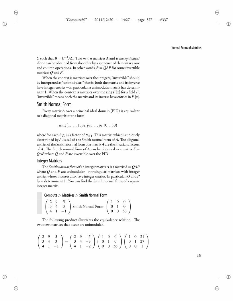
ii
“Compute60” — 2011/12/20 — 14:27 — page 327 — #337 ii
ii
ii
Normal Forms of Matrices
C such that B =C−1AC. Two m×n matrices A and B are equivalentif one can be obtained from the other by a sequence of elementary rowand column operations. In other words, B = QAP for some invertiblematrices Q and P.
When the context ismatrices over the integers, “invertible” shouldbe interpreted as “unimodular;” that is, both thematrix and its inversehave integer entries—in particular, a unimodular matrix has determi-nant 1. When the context is matrices over the ring F [x] for a eld F ,“invertible”means both thematrix and its inverse have entries in F [x].
Smith Normal FormEvery matrix A over a principal ideal domain (PID) is equivalent
to a diagonal matrix of the form
diag(1, . . . ,1, p1, p2, . . . , pk,0, . . . ,0)
where for each i, pi is a factor of pi+1. is matrix, which is uniquelydetermined by A, is called the Smith normal form of A. e diagonalentries of the Smith normal formof amatrixA are the invariant factorsof A. e Smith normal form of A can be obtained as a matrix S =QAP where Q and P are invertible over the PID.
Integer Matricese Smith normal form of an integermatrix A is amatrix S =QAP
where Q and P are unimodular—nonsingular matrices with integerentries whose inverses also have integer entries. In particular, Q and Phave determinant 1. You can nd the Smith normal form of a squareinteger matrix.
Compute>Matrices> Smith Normal Form 2 9 53 4 34 1 −1
Smith Normal Form:
1 0 00 1 00 0 56
e following product illustrates the equivalence relation. e
two new matrices that occur are unimodular.
2 9 53 4 34 1 −1
=
2 9 −53 4 −34 1 −2
1 0 00 1 00 0 56
1 0 210 1 270 0 1
327
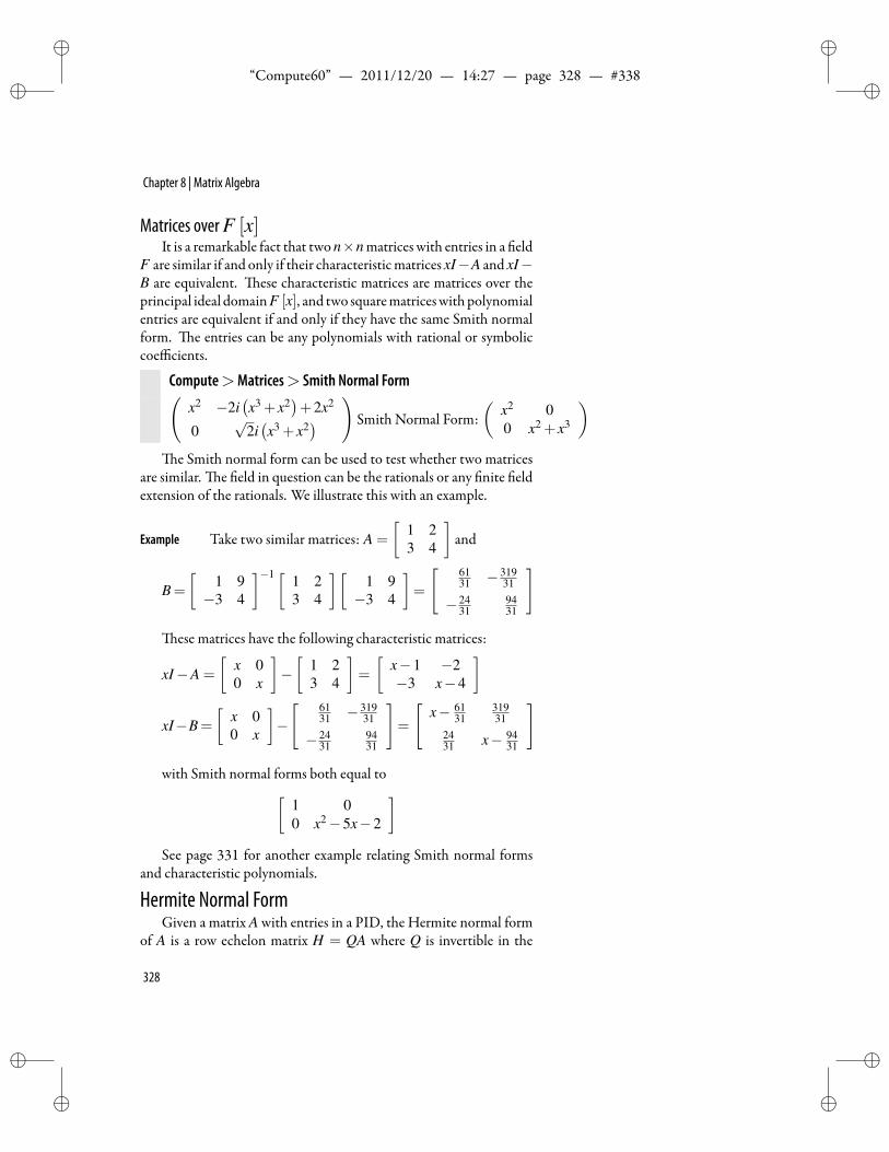
ii
“Compute60” — 2011/12/20 — 14:27 — page 328 — #338 ii
ii
ii
Chapter 8 | Matrix Algebra
Matrices overF [x]It is a remarkable fact that two n×n matrices with entries in a eld
F are similar if and only if their characteristicmatrices xI−A and xI−B are equivalent. ese characteristic matrices are matrices over theprincipal ideal domainF [x], and two squarematriceswithpolynomialentries are equivalent if and only if they have the same Smith normalform. e entries can be any polynomials with rational or symboliccoefficients.
Compute>Matrices> Smith Normal Form(x2 −2i
(x3 + x2
)+2x2
0√
2i(x3 + x2
) )Smith Normal Form:
(x2 00 x2 + x3
)e Smith normal form can be used to test whether two matrices
are similar. e eld in question can be the rationals or any nite eldextension of the rationals. We illustrate this with an example.
Example Take two similar matrices: A =
[1 23 4
]and
B=
[1 9−3 4
]−1 [ 1 23 4
][1 9−3 4
]=
[ 6131 − 319
31
− 2431
9431
]
ese matrices have the following characteristic matrices:
xI−A =
[x 00 x
]−[
1 23 4
]=
[x−1 −2−3 x−4
]
xI−B=
[x 00 x
]−
[ 6131 − 319
31
− 2431
9431
]=
[x− 61
3131931
2431 x− 94
31
]
with Smith normal forms both equal to[1 00 x2−5x−2
]See page 331 for another example relating Smith normal forms
and characteristic polynomials.
Hermite Normal FormGiven a matrix A with entries in a PID, the Hermite normal form
of A is a row echelon matrix H = QA where Q is invertible in the
328
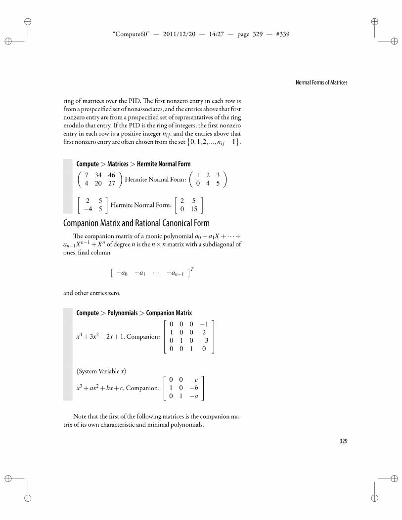
ii
“Compute60” — 2011/12/20 — 14:27 — page 329 — #339 ii
ii
ii
Normal Forms of Matrices
ring of matrices over the PID. e rst nonzero entry in each row isfromaprespeci ed set of nonassociates, and the entries above that rstnonzero entry are from a prespeci ed set of representatives of the ringmodulo that entry. If the PID is the ring of integers, the rst nonzeroentry in each row is a positive integer ni j , and the entries above thatrst nonzero entry are o en chosen from the set
0,1,2, ...,ni j−1
.
Compute>Matrices> Hermite Normal Form(7 34 464 20 27
)Hermite Normal Form:
(1 2 30 4 5
)[
2 5−4 5
]Hermite Normal Form:
[2 50 15
]Companion Matrix and Rational Canonical Form
e companion matrix of a monic polynomial a0 + a1X + · · ·+an−1Xn−1 +Xn of degree n is the n×n matrix with a subdiagonal ofones, nal column
[−a0 −a1 · · · −an−1
]Tand other entries zero.
Compute> Polynomials> Companion Matrix
x4 +3x2−2x+1, Companion:
0 0 0 −11 0 0 20 1 0 −30 0 1 0
(System Variable x)
x3 +ax2 +bx+ c, Companion:
0 0 −c1 0 −b0 1 −a
Note that the rst of the following matrices is the companion ma-
trix of its own characteristic and minimal polynomials.
329
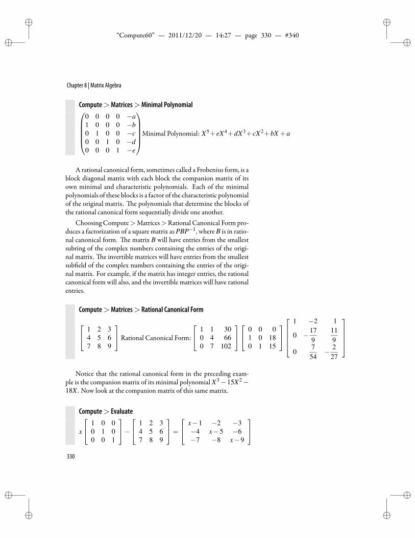
ii
“Compute60” — 2011/12/20 — 14:27 — page 330 — #340 ii
ii
ii
Chapter 8 | Matrix Algebra
Compute>Matrices>Minimal Polynomial0 0 0 0 −a1 0 0 0 −b0 1 0 0 −c0 0 1 0 −d0 0 0 1 −e
Minimal Polynomial: X5+ eX4+dX3+ cX2+bX +a
A rational canonical form, sometimes called a Frobenius form, is ablock diagonal matrix with each block the companion matrix of itsown minimal and characteristic polynomials. Each of the minimalpolynomials of these blocks is a factor of the characteristic polynomialof the original matrix. e polynomials that determine the blocks ofthe rational canonical form sequentially divide one another.
Choosing Compute>Matrices>Rational Canonical Form pro-duces a factorization of a square matrix as PBP−1, where B is in ratio-nal canonical form. e matrix B will have entries from the smallestsubring of the complex numbers containing the entries of the origi-nal matrix. e invertible matrices will have entries from the smallestsub eld of the complex numbers containing the entries of the origi-nal matrix. For example, if the matrix has integer entries, the rationalcanonical form will also, and the invertible matrices will have rationalentries.
Compute>Matrices> Rational Canonical Form
1 2 34 5 67 8 9
Rational Canonical Form:
1 1 300 4 660 7 102
0 0 01 0 180 1 15
1 −2 1
0 −179
119
0754
− 227
Notice that the rational canonical form in the preceding exam-
ple is the companion matrix of its minimal polynomial X3−15X2−18X . Now look at the companion matrix of this same matrix.
Compute> Evaluate
x
1 0 00 1 00 0 1
− 1 2 3
4 5 67 8 9
=
x−1 −2 −3−4 x−5 −6−7 −8 x−9
330
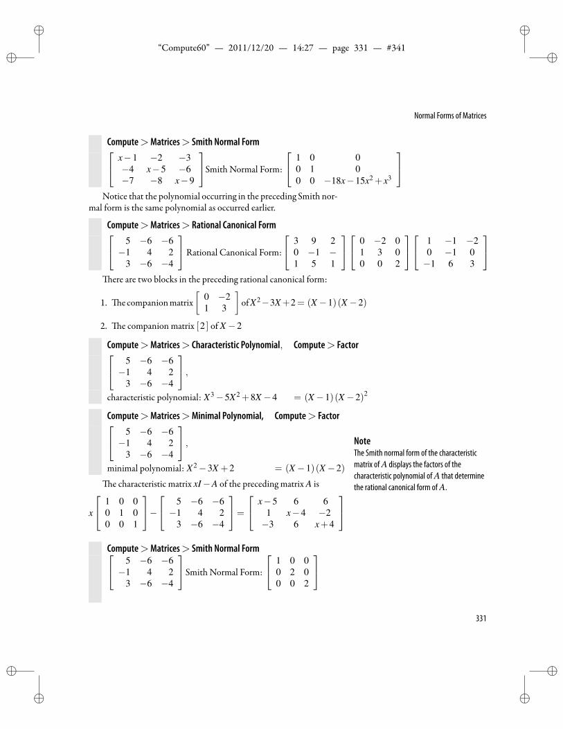
ii
“Compute60” — 2011/12/20 — 14:27 — page 331 — #341 ii
ii
ii
Normal Forms of Matrices
Compute>Matrices> Smith Normal Form x−1 −2 −3−4 x−5 −6−7 −8 x−9
Smith Normal Form:
1 0 00 1 00 0 −18x−15x2 + x3
Notice that the polynomial occurring in the preceding Smith nor-
mal form is the same polynomial as occurred earlier.
Compute>Matrices> Rational Canonical Form 5 −6 −6−1 4 2
3 −6 −4
Rational Canonical Form:
3 9 20 −1 −1 5 1
0 −2 01 3 00 0 2
1 −1 −20 −1 0−1 6 3
ere are two blocks in the preceding rational canonical form:
1. e companionmatrix[
0 −21 3
]ofX2−3X+2= (X−1)(X−2)
2. e companion matrix [2 ] of X−2
Compute>Matrices> Characteristic Polynomial, Compute> Factor 5 −6 −6−1 4 2
3 −6 −4
,characteristic polynomial: X3−5X2 +8X−4 = (X−1)(X−2)2
Compute>Matrices>Minimal Polynomial, Compute> Factor 5 −6 −6−1 4 2
3 −6 −4
,minimal polynomial: X2−3X +2 = (X−1)(X−2)
NoteThe Smith normal form of the characteristicmatrix of A displays the factors of thecharacteristic polynomial of A that determinethe rational canonical form of A.e characteristic matrix xI−A of the preceding matrix A is
x
1 0 00 1 00 0 1
− 5 −6 −6−1 4 2
3 −6 −4
=
x−5 6 61 x−4 −2−3 6 x+4
Compute>Matrices> Smith Normal Form 5 −6 −6−1 4 2
3 −6 −4
Smith Normal Form:
1 0 00 2 00 0 2
331
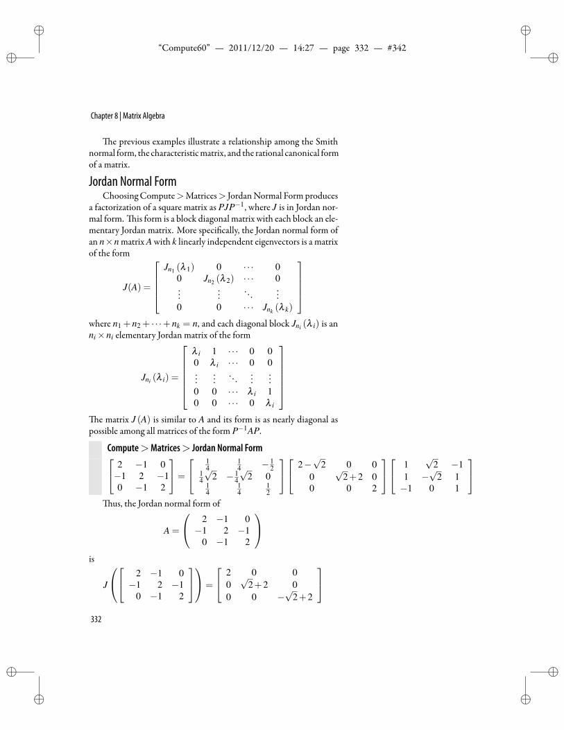
ii
“Compute60” — 2011/12/20 — 14:27 — page 332 — #342 ii
ii
ii
Chapter 8 | Matrix Algebra
e previous examples illustrate a relationship among the Smithnormal form, the characteristicmatrix, and the rational canonical formof a matrix.
Jordan Normal FormChoosingCompute>Matrices> JordanNormal Formproduces
a factorization of a square matrix as PJP−1, where J is in Jordan nor-mal form. is form is a block diagonal matrix with each block an ele-mentary Jordan matrix. More speci cally, the Jordan normal form ofan n×n matrix A with k linearly independent eigenvectors is a matrixof the form
J(A) =
Jn1 (λ 1) 0 · · · 0
0 Jn2 (λ 2) · · · 0...
.... . .
...0 0 · · · Jnk (λ k)
where n1 + n2 + · · ·+ nk = n, and each diagonal block Jni (λ i) is anni×ni elementary Jordan matrix of the form
Jni (λ i) =
λ i 1 · · · 0 00 λ i · · · 0 0...
.... . .
......
0 0 · · · λ i 10 0 · · · 0 λ i
e matrix J (A) is similar to A and its form is as nearly diagonal as
possible among all matrices of the form P−1AP.
Compute>Matrices> Jordan Normal Form 2 −1 0−1 2 −10 −1 2
=
14
14 − 1
214
√2 − 1
4
√2 0
14
14
12
2−√
2 0 00
√2+2 0
0 0 2
1√
2 −11 −
√2 1
−1 0 1
us, the Jordan normal form of
A =
2 −1 0−1 2 −1
0 −1 2
is
J
2 −1 0−1 2 −1
0 −1 2
=
2 0 00√
2+2 00 0 −
√2+2
332
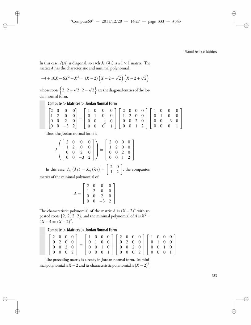
ii
“Compute60” — 2011/12/20 — 14:27 — page 333 — #343 ii
ii
ii
Normal Forms of Matrices
In this case, J(A) is diagonal, so each Jni (λ i) is a 1× 1 matrix. ematrix A has the characteristic and minimal polynomial
−4+10X−6X2 +X3 = (X−2)(
X−2−√
2)(
X−2+√
2)
whose roots
2, 2+√
2, 2−√
2
are thediagonal entries of the Jor-dan normal form.
Compute>Matrices> Jordan Normal Form2 0 0 01 2 0 00 0 2 00 0 −3 2
=
1 0 0 00 1 0 00 0 − 1
3 00 0 0 1
2 0 0 01 2 0 00 0 2 00 0 1 2
1 0 0 00 1 0 00 0 −3 00 0 0 1
us, the Jordan normal form is
J
2 0 0 01 2 0 00 0 2 00 0 −3 2
=
2 0 0 01 2 0 00 0 2 00 0 1 2
In this case, Jn1 (λ 1) = Jn2 (λ 2) =
[2 01 2
], the companion
matrix of the minimal polynomial of
A =
2 0 0 01 2 0 00 0 2 00 0 −3 2
e characteristic polynomial of the matrix A is (X−2)4 with re-
peated roots 2, 2, 2, 2, and the minimal polynomial of A is X2−4X +4 = (X−2)2.
Compute>Matrices> Jordan Normal Form2 0 0 00 2 0 00 0 2 00 0 0 2
=
1 0 0 00 1 0 00 0 1 00 0 0 1
2 0 0 00 2 0 00 0 2 00 0 0 2
1 0 0 00 1 0 00 0 1 00 0 0 1
e preceding matrix is already in Jordan normal form. Its mini-
mal polynomial is X−2 and its characteristic polynomial is (X−2)4,
333
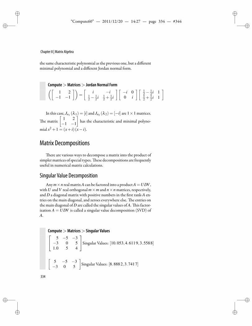
ii
“Compute60” — 2011/12/20 — 14:27 — page 334 — #344 ii
ii
ii
Chapter 8 | Matrix Algebra
the same characteristic polynomial as the previous one, but a differentminimal polynomial and a different Jordan normal form.
Compute>Matrices> Jordan Normal Form([1 2−1 −1
])=
[i −i
12 −
12 i 1
2 +12 i
][−i 00 i
][ 12 −
12 i 1
12 +
12 i 1
]
In this case, Jn1 (λ 1) = [i] and Jn2 (λ 2) = [−i] are 1×1 matrices.
e matrix[
1 2−1 −1
]has the characteristic and minimal polyno-
mial x2 +1 = (x+ i)(x− i).
Matrix Decompositions
ere are various ways to decompose a matrix into the product ofsimplermatrices of special types. ese decompositions are frequentlyuseful in numerical matrix calculations.
Singular Value DecompositionAny m×n realmatrix A can be factored into a product A =UDV ,
withU andV real orthogonal m×m and n×n matrices, respectively,and D a diagonal matrix with positive numbers in the rst rank-A en-tries on the main diagonal, and zeroes everywhere else. e entries onthemain diagonal of D are called the singular values of A. is factor-ization A = UDV is called a singular value decomposition (SVD) ofA.
Compute>Matrices> Singular Values 5 −5 −3−3 0 51.0 5 4
Singular Values: [10.053,4.6119,3.5588]
[5 −5 −3−3 0 5
]Singular Values: [8.8882,3.7417]
334
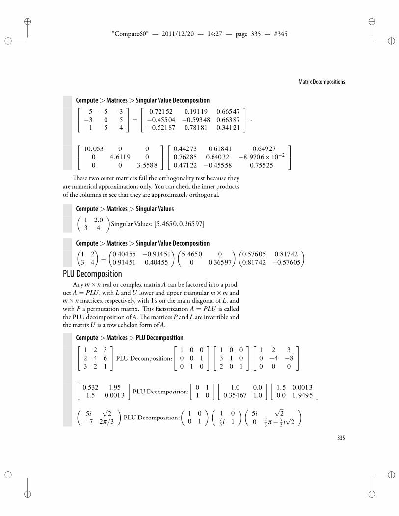
ii
“Compute60” — 2011/12/20 — 14:27 — page 335 — #345 ii
ii
ii
Matrix Decompositions
Compute>Matrices> Singular Value Decomposition 5 −5 −3−3 0 5
1 5 4
=
0.72152 0.19119 0.66547−0.45504 −0.59348 0.66387−0.52187 0.78181 0.34121
· 10.053 0 0
0 4.6119 00 0 3.5588
0.44273 −0.61841 −0.649270.76285 0.64032 −8.9706×10⁻²
0.47122 −0.45558 0.75525
ese two outer matrices fail the orthogonality test because they
are numerical approximations only. You can check the inner productsof the columns to see that they are approximately orthogonal.
Compute>Matrices> Singular Values(1 2.03 4
)Singular Values: [5.4650,0.36597]
Compute>Matrices> Singular Value Decomposition(1 23 4
)=
(0.40455 −0.914510.91451 0.40455
)(5.4650 0
0 0.36597
)(0.57605 0.817420.81742 −0.57605
)PLU Decomposition
Any m× n real or complex matrix A can be factored into a prod-uct A = PLU , with L and U lower and upper triangular m×m andm× n matrices, respectively, with 1’s on the main diagonal of L, andwith P a permutation matrix. is factorization A = PLU is calledthe PLU decomposition of A. e matrices P and L are invertible andthe matrixU is a row echelon form of A.
Compute>Matrices> PLU Decomposition 1 2 32 4 63 2 1
PLU Decomposition:
1 0 00 0 10 1 0
1 0 03 1 02 0 1
1 2 30 −4 −80 0 0
[
0.532 1.951.5 0.0013
]PLU Decomposition:
[0 11 0
][1.0 0.0
0.35467 1.0
][1.5 0.00130.0 1.9495
](
5i√
2−7 2π/3
)PLU Decomposition:
(1 00 1
)(1 075 i 1
)(5i
√2
0 23 π− 7
5 i√
2
)335
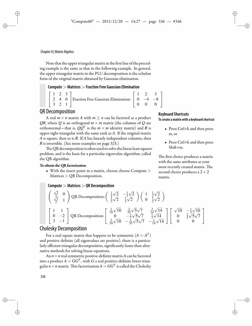
ii
“Compute60” — 2011/12/20 — 14:27 — page 336 — #346 ii
ii
ii
Chapter 8 | Matrix Algebra
Note that theupper triangularmatrix in the rst line of the preced-ing example is the same as that in the following example. In general,the upper triangular matrix in the PLU decomposition is the echelonform of the original matrix obtained by Gaussian elimination.
Compute>Matrices> Fraction Free Gaussian Elimination 1 2 32 4 63 2 1
Fraction Free Gaussian Elimination:
1 2 30 −4 −80 0 0
QR Decomposition Keyboard Shortcuts
To create a matrix with a keyboard shortcut
• Press Ctrl+k and then pressm, or
• Press Ctrl+k and then pressShi +m.
e rst choice produces a matrixwith the same attributes as yourmost recently created matrix. esecond choice produces a 2×2matrix.
A real m× n matrix A with m ≥ n can be factored as a productQR, where Q is an orthogonal m×m matrix (the columns of Q areorthonormal—that is, QQT is the m×m identity matrix) and R isupper-right triangular with the same rank as A. If the original matrixA is square, then so is R. If A has linearly independent columns, thenR is invertible. (See more examples on page 325.)
eQRdecomposition is o enused to solve the linear least squaresproblem, and is the basis for a particular eigenvalue algorithm, calledthe QR algorithm.Toobtain theQR factorization
• With the insert point in a matrix, choose choose Compute >Matrices>QR Decomposition.
Compute>Matrices> QR Decomposition( √2
2 0√2
2 1
)QR Decomposition:
( 12
√2 − 1
2
√2
12
√2 1
2
√2
)(1 1
2
√2
0 12
√2
) 1 1
0 −23 −1
QR Decomposition:
110
√10 3
35
√5√
7 314
√14
0 − 17
√5√
7 17
√14
310
√10 − 1
35
√5√
7 − 114
√14
√10 − 15
√10
0 25
√5√
70 0
Cholesky Decomposition
For a real square matrix that happens to be symmetric (A = AT )and positive de nite (all eigenvalues are positive), there is a particu-larly efficient triangular decomposition, signi cantly faster than alter-native methods for solving linear equations.
An n×n real symmetric positive-de nitematrix A can be factoredinto a product A = GGT , with G a real positive-de nite lower trian-gular n×n matrix. is factorization A=GGT is called theCholesky
336
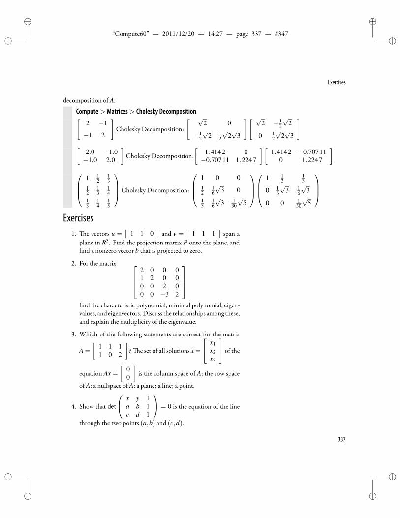
ii
“Compute60” — 2011/12/20 — 14:27 — page 337 — #347 ii
ii
ii
Exercises
decomposition of A.
Compute>Matrices> Cholesky Decomposition[2 −1
−1 2
]Cholesky Decomposition:
[ √2 0
− 12
√2 1
2
√2√
3
][ √2 − 1
2
√2
0 12
√2√
3
][
2.0 −1.0−1.0 2.0
]Cholesky Decomposition:
[1.4142 0−0.70711 1.2247
][1.4142 −0.70711
0 1.2247
]
1 12
13
12
13
14
13
14
15
Cholesky Decomposition:
1 0 012
16
√3 0
13
16
√3 1
30
√5
1 12
13
0 16
√3 1
6
√3
0 0 130
√5
Exercises
1. e vectors u =[
1 1 0]and v =
[1 1 1
]span a
plane in R3. Find the projection matrix P onto the plane, andnd a nonzero vector b that is projected to zero.
2. For the matrix 2 0 0 01 2 0 00 0 2 00 0 −3 2
nd the characteristic polynomial, minimal polynomial, eigen-
values, and eigenvectors. Discuss the relationships among these,and explain the multiplicity of the eigenvalue.
3. Which of the following statements are correct for the matrix
A =
[1 1 11 0 2
]? e set of all solutions x =
x1x2x3
of the
equation Ax =
[00
]is the column space of A; the row space
of A; a nullspace of A; a plane; a line; a point.
4. Show that det
x y 1a b 1c d 1
= 0 is the equation of the line
through the two points (a,b) and (c,d).
337
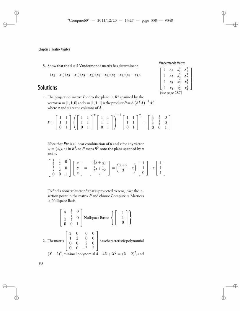
ii
“Compute60” — 2011/12/20 — 14:27 — page 338 — #348 ii
ii
ii
Chapter 8 | Matrix Algebra
Vandermonde Matrix1 x1 x2
1 x31
1 x2 x22 x3
2
1 x3 x23 x3
3
1 x4 x24 x3
4
(see page 287)
5. Show that the 4×4 Vandermonde matrix has determinant
(x2− x1)(x3− x1)(x3− x2)(x1− x4)(x2− x4)(x4− x3) .
Solutions1. e projection matrix P onto the plane in R3 spanned by the
vectorsu= [1,1,0] andv= [1,1,1] is theproductP=A(AT A
)−1 AT ,where u and v are the columns of A.
P=
1 11 10 1
1 11 10 1
T 1 11 10 1
−1 1 11 10 1
T
=
12
12 0
12
12 0
0 0 1
Note that Pw is a linear combination of u and v for any vectorw = (x,y,z) in R3, so P maps R3 onto the plane spanned by uand v.
12
12 0
12
12 0
0 0 1
x
yz
=
12 x+ 1
2 y12 x+ 1
2 yz
=
(x+ y
2− z) 1
10
+z
111
To nd a nonzero vector b that is projected to zero, leave the in-sertion point in the matrix P and choose Compute>Matrices>Nullspace Basis.
12
12 0
12
12 0
0 0 1
Nullspace Basis:
−1
10
2. ematrix
2 0 0 01 2 0 00 0 2 00 0 −3 2
has characteristic polynomial
(X−2)4, minimal polynomial 4−4X +X2 = (X−2)2, and
338
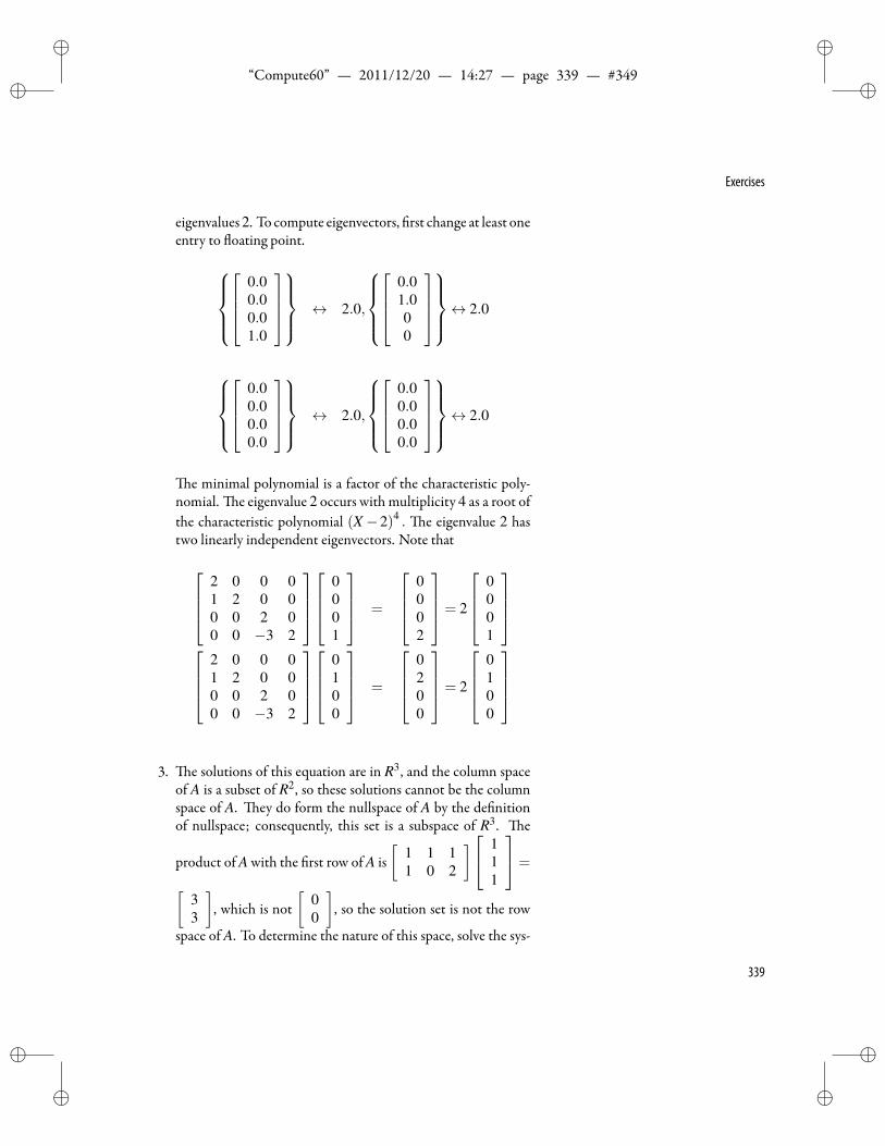
ii
“Compute60” — 2011/12/20 — 14:27 — page 339 — #349 ii
ii
ii
Exercises
eigenvalues2. To compute eigenvectors, rst change at least oneentry to oating point.
0.00.00.01.0
↔ 2.0,
0.01.000
↔ 2.0
0.00.00.00.0
↔ 2.0,
0.00.00.00.0
↔ 2.0
e minimal polynomial is a factor of the characteristic poly-nomial. e eigenvalue 2 occurs with multiplicity 4 as a root ofthe characteristic polynomial (X−2)4 . e eigenvalue 2 hastwo linearly independent eigenvectors. Note that
2 0 0 01 2 0 00 0 2 00 0 −3 2
0001
=
0002
= 2
0001
2 0 0 01 2 0 00 0 2 00 0 −3 2
0100
=
0200
= 2
0100
3. e solutions of this equation are in R3, and the column spaceof A is a subset of R2, so these solutions cannot be the columnspace of A. ey do form the nullspace of A by the de nitionof nullspace; consequently, this set is a subspace of R3. e
product of A with the rst row of A is[
1 1 11 0 2
] 111
=[33
], which is not
[00
], so the solution set is not the row
space of A. To determine the nature of this space, solve the sys-
339
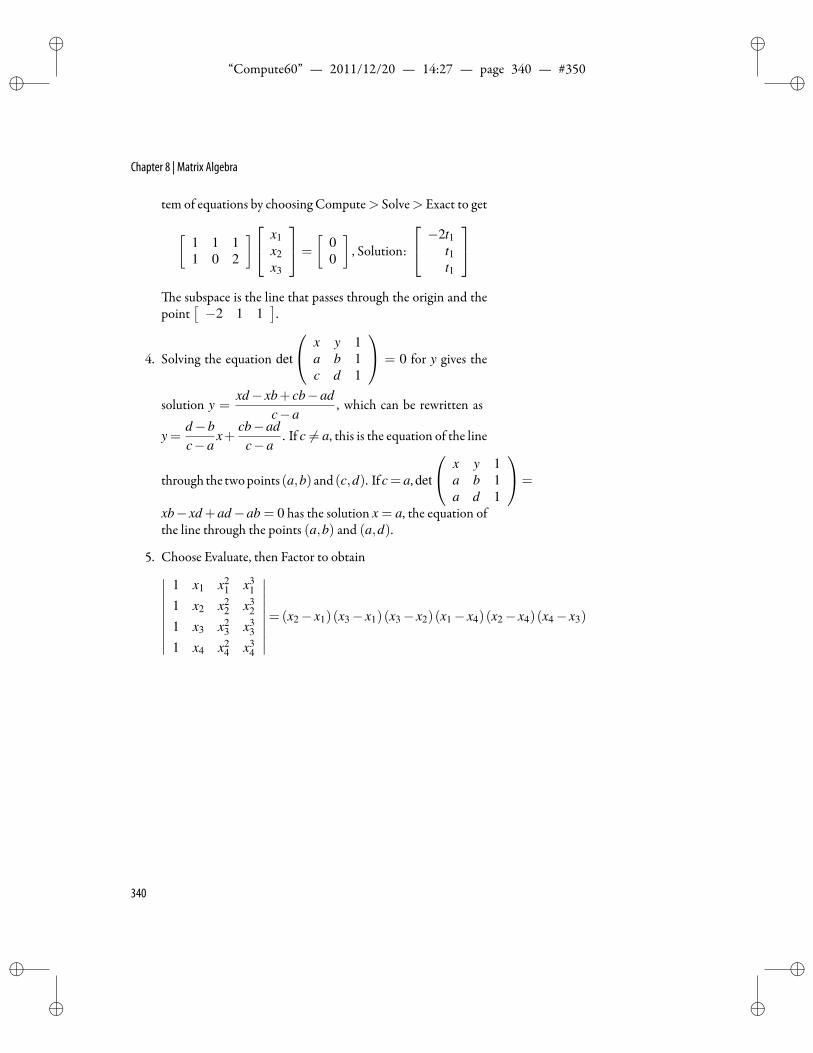
ii
“Compute60” — 2011/12/20 — 14:27 — page 340 — #350 ii
ii
ii
Chapter 8 | Matrix Algebra
tem of equations by choosing Compute> Solve> Exact to get
[1 1 11 0 2
] x1x2x3
=
[00
], Solution:
−2t1t1t1
e subspace is the line that passes through the origin and the
point[−2 1 1
].
4. Solving the equation det
x y 1a b 1c d 1
= 0 for y gives the
solution y =xd− xb+ cb−ad
c−a, which can be rewritten as
y =d−bc−a
x+cb−ad
c−a. If c = a, this is the equation of the line
through the twopoints (a,b) and (c,d). Ifc= a,det
x y 1a b 1a d 1
=
xb− xd+ad−ab = 0 has the solution x = a, the equation ofthe line through the points (a,b) and (a,d).
5. Choose Evaluate, then Factor to obtain∣∣∣∣∣∣∣∣∣1 x1 x2
1 x31
1 x2 x22 x3
2
1 x3 x23 x3
3
1 x4 x24 x3
4
∣∣∣∣∣∣∣∣∣=(x2− x1)(x3− x1)(x3− x2)(x1− x4)(x2− x4)(x4− x3)
340
ii
“Compute60” — 2011/12/20 — 14:27 — page 341 — #351 ii
ii
ii
9Vector Calculus
The calculus is the greatest aidwe have to the application of physical truth in the broadest sense of theword. William Fogg Osgood (1864–1943)
V ector calculus is the calculus of functions that assign vectors Vectors
Gradient, Divergence, Curl, andRelated Operators
Plots of Vector Fields andGradients
Scalar and Vector Potentials
Matrix-Valued Operators
Plots of Complex Functions
to points in space. It is concerned with differentiation andintegration of vector elds, primarily in 3-dimensional Eu-
clidean space.Vector calculus operations are of particular importance in solving
physical problems. ey can be applied to problems such as ndingthe work done by a force eld in moving an object along a curve ornding the rate of uid ow across a surface.
Vectorse term vector is used to indicate a quantity that has both mag-
nitude and direction. A vector is o en represented by an arrow or adirected line segment. e length of the arrow represents the magni-tude of the vector and the arrow points in its direction. Two directedline segments are considered equivalent if they have the same lengthand point in the same direction. In other words, a vector v can bethought of as a set of equivalent directed line segments.
A two-dimensional vector is an ordered pair a = (a1,a2) of realnumbers. A three-dimensional vector is anordered triplea=(a1,a2,a3)of real numbers. More generally, an n-dimensional vector is an orderedn-tuplea=(a1,a2, . . . ,an)of real numbers. e numbersa1,a2, . . . ,anare called the components of a.
341
ii
“Compute60” — 2011/12/20 — 14:27 — page 342 — #352 ii
ii
ii
Chapter 9 | Vector Calculus
Notation for VectorsYou can represent vectors in any of the following ways.
• n-tupleswithinparentheses or square brackets: (2,−1,0), (x1,x2,x3),[3,2,1], [x1,x2,x3]
• 1× n matrices:[
1 2 3],[
5 −1 3 17 −8 2],[
x1 x2 x3 x4]
• n×1 matrices:
10−1
,[
35−4
],(
x1x2
)
is exibility allows you to use the output of previous work asinput, without undue worry about the shape of the output. For pur-poses of clear exposition, you will nd it preferable to use consistentnotation for vectors. Calculations involving vectors
Although vectors may be represented invarious ways, the result of an operation onvectors will be returned in matrix form.
Tocreate a vector inmatrix form1. Choose Insert>Math Objects>Matrix.
2. Set the number of rows (or columns) to 1 and the number ofcolumns (or rows) to the dimension of the vector.
3. Type the values for the components in the input boxes.
4. Select the vectorwith themouse and choose Insert>MathOb-jects> Brackets and click a le bracket to enclose the vector inexpanding brackets.
Tocreate a vector in list form1. Choose Insert>MathObjects>Brackets and click a le bracket.
2. With the insert point inside the expanding brackets, type thevector components, separated by commas.
Plots of vectors in 2D and 3DToplot the vectora =
1. De ne a =(
3 2).
2. Place the insert point in the expression xa.
3. Choose Compute> Plot 2D> Rectangular.
342
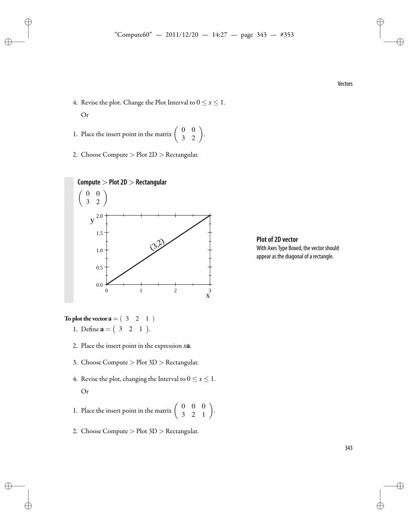
ii
“Compute60” — 2011/12/20 — 14:27 — page 343 — #353 ii
ii
ii
Vectors
4. Revise the plot. Change the Plot Interval to 0≤ x≤ 1.
Or
1. Place the insert point in the matrix(
0 03 2
).
2. Choose Compute> Plot 2D> Rectangular.
Compute> Plot 2D> Rectangular(0 03 2
)
0 1 2 30.0
0.5
1.0
1.5
2.0
x
y
(3,2) Plot of 2D vectorWith Axes Type Boxed, the vector shouldappear as the diagonal of a rectangle.
Toplot the vectora = ( 3 2 1 )
1. De ne a =(
3 2 1).
2. Place the insert point in the expression xa.
3. Choose Compute> Plot 3D> Rectangular.
4. Revise the plot, changing the Interval to 0≤ x≤ 1.
Or
1. Place the insert point in the matrix(
0 0 03 2 1
).
2. Choose Compute> Plot 3D> Rectangular.
343
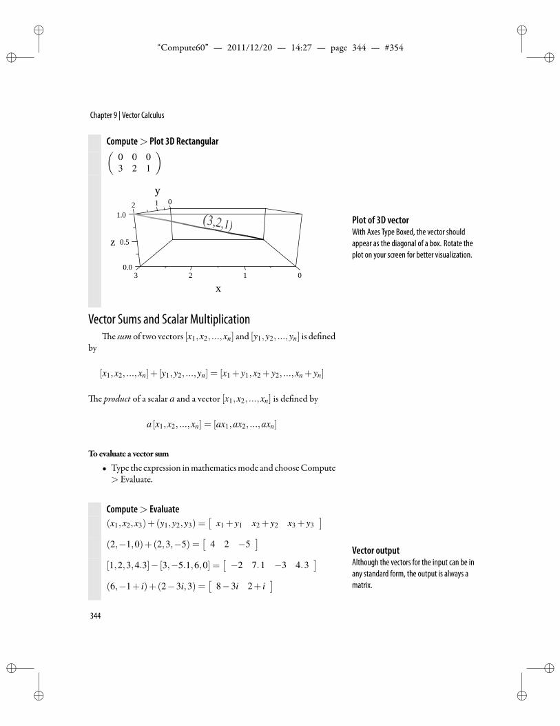
ii
“Compute60” — 2011/12/20 — 14:27 — page 344 — #354 ii
ii
ii
Chapter 9 | Vector Calculus
Compute> Plot 3D Rectangular(0 0 03 2 1
)
1.0
z 0.5
0.0
1y
02
x0123
Plot of 3D vectorWith Axes Type Boxed, the vector shouldappear as the diagonal of a box. Rotate theplot on your screen for better visualization.
Vector Sums and Scalar Multiplicatione sum of two vectors [x1,x2, ...,xn] and [y1,y2, ...,yn] is de ned
by
[x1,x2, ...,xn]+ [y1,y2, ...,yn] = [x1 + y1,x2 + y2, ...,xn + yn]
e product of a scalar a and a vector [x1,x2, ...,xn] is de ned by
a [x1,x2, ...,xn] = [ax1,ax2, ...,axn]
Toevaluate a vector sum
• Type the expression inmathematicsmode and chooseCompute> Evaluate.
Compute> Evaluate(x1,x2,x3)+(y1,y2,y3) =
[x1 + y1 x2 + y2 x3 + y3
](2,−1,0)+(2,3,−5) =
[4 2 −5
][1,2,3,4.3]− [3,−5.1,6,0] =
[−2 7.1 −3 4.3
](6,−1+ i)+(2−3i,3) =
[8−3i 2+ i
]Vector outputAlthough the vectors for the input can be inany standard form, the output is always amatrix.
344
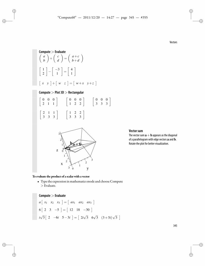
ii
“Compute60” — 2011/12/20 — 14:27 — page 345 — #355 ii
ii
ii
Vectors
Compute> Evaluate(ab
)+
(cd
)=
(a+ cb+d
)[
12
]−[−31
]=
[41
][
x y]+[
w z]=[
w+ x y+ z]
Compute> Plot 3D> Rectangular[0 0 02 1 1
] [0 0 01 2 2
] [0 0 03 3 3
][
2 1 13 3 3
] [1 2 23 3 3
]
01
0
x
b
1
az
32
y
2
2
a + b
13 0
3Vector sumThe vector suma+b appears as the diagonalof a parallelogramwith edge vectors a andb.Rotate the plot for better visualization.
Toevaluate the product of a scalarwith a vector• Type the expression inmathematicsmode and chooseCompute> Evaluate.
Compute> Evaluate
a[
x1 x2 x3]=[
ax1 ax2 ax3]
6[
2 3 −5]=[
12 18 −30]
i√
3[
2 −6i 5−3i]=[
2i√
3 6√
3 (3+5i)√
3]
345
ii
“Compute60” — 2011/12/20 — 14:27 — page 346 — #356 ii
ii
ii
Chapter 9 | Vector Calculus
Dot Producte dot product (or inner product) of two vectors (a1,a2, ...,an)
and (b1,b2, ...,bn) with real entries is de ned by
(a1,a2, ...,an) · (b1,b2, ...,bn) = a1b1 +a2b2 + · · ·+anbn
and the inner product of two vectors with complex entries is de nedby Complex Conjugate
To use overbar notation for complex conjugate,choose Tools> Preferences> Computation> Input and check “Overbar accent meansconjugate.”
(a1,a2, ...,an) · (b1,b2, ...,bn) = a1b∗1 +a2b∗2 + · · ·+anb∗n
where b∗ = x− iy is the complex conjugate of b = x+ iy. For realnumbers b, it is clear that b∗ = b, so these two de nitions are consis-tent. e dot product can also be obtained by matrix multiplication:
(a1,a2, ...,an)·(b1,b2, ...,bn)=[
a1 a2 ... an]
b∗1b∗2...
b∗n
=
a1a2...
an
T
b∗1b∗2...
b∗n
Toenter the dot used for the dot product
• Select · from the Binary Operations tab ±÷ .
Tocompute a dot product1. Type the expression.
2. With the insert point in the expression, choose Compute >Evaluate.
Compute> Evaluate(1,2,3) · (3,2,1) = 10[3x,−1,5] · [1,1,1] = 3x+4(1+2i,−3i) · (5,1− i) = 8+7i(
1+2i −3i)( 5
(1− i)∗
)= 8+7i
e standard default on variables returns complex solutions. Youcan change this default with the function assume.
346
ii
“Compute60” — 2011/12/20 — 14:27 — page 347 — #357 ii
ii
ii
Vectors
Compute> Evaluate(u,v,w) · (x,y,z) = ux∗+ vy∗+wz∗
assume(u, real) = Rassume(v, real) = Rassume(w, real) = Rassume(x, real) = Rassume(y, real) = Rassume(z, real) = R(u,v,w) · (x,y,z) = ux+ vy+wz
NoteType assume, real, and complex inmathematics mode, and they will turn uprightand gray.
For the following examples of dot products with n = 3, de ne
a =[
1 2 3], b =
10−1
, c = [3,2,1] , d = (2,−1,0)
by placing the insert point in each equation and choosingCompute>De nitions>New De nition.
Compute> Evaluatea · c = 10 a ·b =−2 c ·d = 4
Cross Producte cross product of three-dimensional vectorsa=(a1,a2,a3) and
b = (b1,b2,b3) is de ned by
a×b = (a2b3−a3b2,a3b1−a1b3,a1b2−a2b1)
Toenter the cross used for the cross product• Select× from the Binary Operations panel under ±÷ .
Tocompute a cross product• Place the insert point in the cross product and chooseCompute> Evaluate.
For the following examples, use the vectors a =[
1 2 3],
b =
10−1
, c = [3,2,1], and d = (2,−1,0) de ned in the previ-
ous section.
347
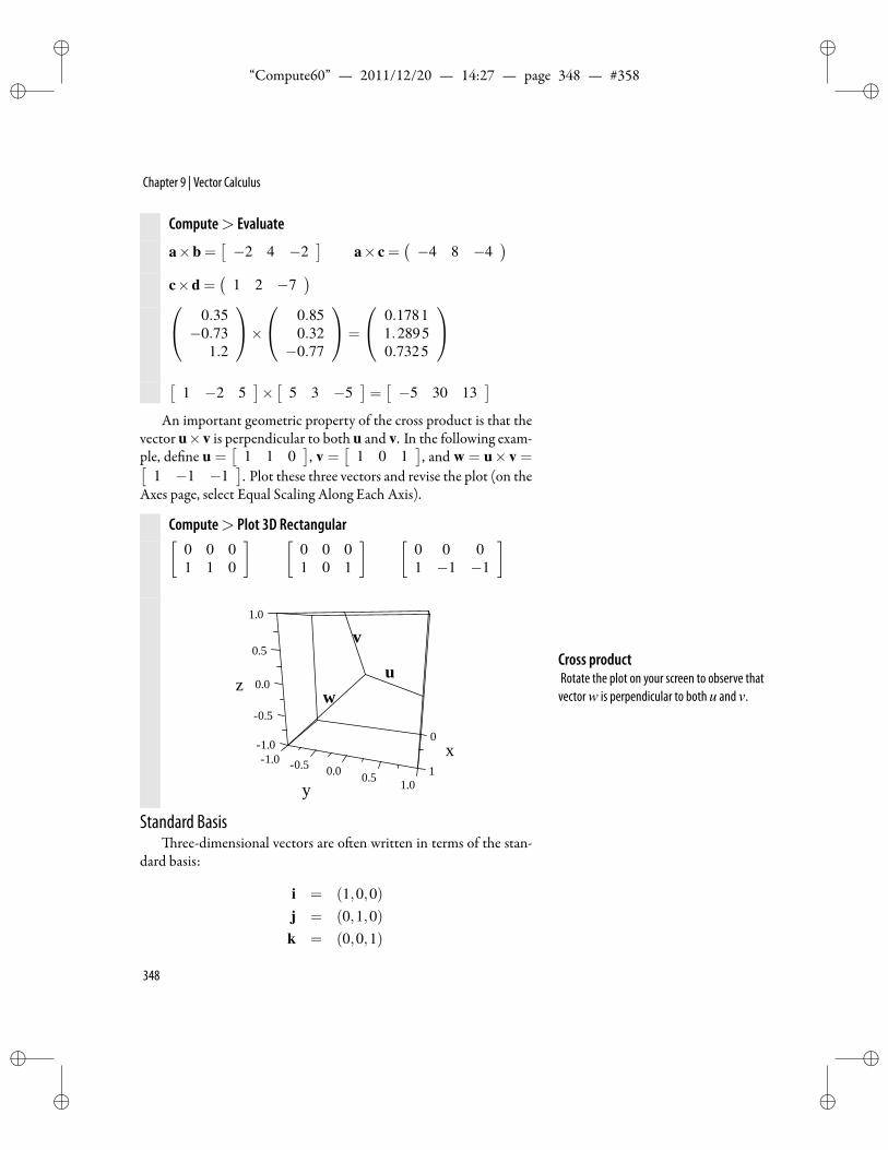
ii
“Compute60” — 2011/12/20 — 14:27 — page 348 — #358 ii
ii
ii
Chapter 9 | Vector Calculus
Compute> Evaluate
a×b =[−2 4 −2
]a× c =
(−4 8 −4
)c×d =
(1 2 −7
) 0.35−0.73
1.2
× 0.85
0.32−0.77
=
0.17811.28950.7325
[
1 −2 5]×[
5 3 −5]=[−5 30 13
]An important geometric property of the cross product is that the
vector u×v is perpendicular to both u and v. In the following exam-ple, de ne u =
[1 1 0
], v =
[1 0 1
], and w = u× v =[
1 −1 −1]. Plot these three vectors and revise the plot (on the
Axes page, select Equal Scaling Along Each Axis).
Compute> Plot 3D Rectangular[0 0 01 1 0
] [0 0 01 0 1
] [0 0 01 −1 −1
]
1.0
w
0
u0.0
1.0 x
0.5
v
z
0.5
1.0
0.0
0.5
0.5
y1
1.0
Cross productRotate the plot on your screen to observe thatvectorw is perpendicular to both u and v.
Standard Basisree-dimensional vectors are o en written in terms of the stan-
dard basis:
i = (1,0,0)j = (0,1,0)k = (0,0,1)
348
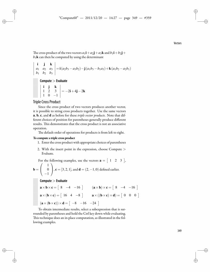
ii
“Compute60” — 2011/12/20 — 14:27 — page 349 — #359 ii
ii
ii
Vectors
e cross product of the two vectors a1i+a2j+a3k and b1i+b2j+b3k can then be computed by using the determinant∣∣∣∣∣∣
i j ka1 a2 a3b1 b2 b3
∣∣∣∣∣∣= i(a2b3−a3b2)−j(a1b3−b1a3)+k(a1b2−a2b1)
Compute> Evaluate∣∣∣∣∣∣i j k1 2 31 0 −1
∣∣∣∣∣∣=−2i+4j−2k
Triple Cross ProductSince the cross product of two vectors produces another vector,
it is possible to string cross products together. Use the same vectorsa, b, c, and d as before for these triple vector products. Note that dif-ferent choices of position for parentheses generally produce differentresults. is demonstrates that the cross product is not an associativeoperation.
e default order of operations for products is from le to right.Tocompute a triple cross product
1. Enter the cross product with appropriate choices of parentheses
2. With the insert point in the expression, choose Compute >Evaluate.
For the following examples, use the vectors a =[
1 2 3],
b =
10−1
, c = [3,2,1], and d = (2,−1,0) de ned earlier.
Compute> Evaluate
a×b× c =[
8 −4 −16]
(a×b)× c =[
8 −4 −16]
a× (b× c) =[
16 4 −8]
a× ((b× c)×d) =[
0 0 0]
(a× (b× c))×d =[−8 −16 −24
]To obtain intermediate results, select a subexpression that is sur-
rounded by parentheses and hold the Ctrl key down while evaluating.is technique does an in-place computation, as illustrated in the fol-
lowing examples.
349
ii
“Compute60” — 2011/12/20 — 14:27 — page 350 — #360 ii
ii
ii
Chapter 9 | Vector Calculus
Ctrl+Compute> Evaluate Compute> Evaluate
a× (b× c) = a×
2−42
a×
2−42
=(
16 4 −8)
(a×b)× c =(−2 4 −2
)× c
(−2 4 −2
)× c =
(8 −4 −16
)Triple Scalar Product Tip
Whenmixing cross products with scalarproducts, use parentheses for clarity. Asalways, careful and consistent use ofmathematical notation is in order. Wheneverin doubt, add an extra set of parentheses toclarify an expression.
A triple scalar product is the dot product of one vector with thecross product of two vectors.Tocompute a triple scalar product
1. Enter the triple scalar productwith appropriate choices of paren-theses.
2. With the insert point in the expression, choose Compute >Evaluate. Caution
(1,0,1) · (1,2,3)× (3,2,1) is notinterpreted as a triple scalar product, but as theproduct of the scalar (1,0,1) · (1,2,3) =4with the vector (3,2,1).
Ctrl+Evaluate, Compute> Evaluate(1,0,1) · ((1,2,3)× (3,2,1)) =−8((1,0,1)× (1,2,3)) · (3,2,1) =−8
(1,0,1) · (1,2,3)× (3,2,1) =(
12 8 4)
To nd the volumeof theparallelepiped spannedby the vectorsA,B, andC VolumeThe volume of the parallelepiped spanned bythree vectorsA,B, andC is equal to|A · (B×C)|.
• Evaluate the absolute valueof the triple scalar productA·(B×C).
Toplot the parallelepiped spannedby the vectorsA,B, andC1. De ne each of the vectors A, B, andC.
2. With the insert point in the expression sA+ tB, choose Com-pute> Plot 3D> Rectangular.
3. Revise the plot intervals to 0≤ s≤ 1 and 0≤ t ≤ 1.
4. Select and drag to the plot each of the expressions sA+tC, sB+tC, A+ sB+ tC, sA+B+ tC, and sA+ tB+C.
Compute> De nitions> New De nitionA = [0,1,1] B = [1,0,1] C = [1,1,0]
The volume of a parallelipiped does notdepend on the order in which the triple scalarproduct is computed.
Compute> Evaluate|A · (B×C)|= 2 |B · (C×A)|= 2 |C · (A×B)|= 2
350
ii
“Compute60” — 2011/12/20 — 14:27 — page 351 — #361 ii
ii
ii
Vectors
Compute> Plot 3D> RectangularsA+ tB (0≤ s≤ t , 0≤ s≤ 1)sA+ tC, sB+ tC, A+ sB+ tC, sA+B+ tC, sA+ tB+C
2
2
1
x
0
2y
z
1
0
1
0
TipAny three-dimensional object can be rotatedon the screen to view the back side.
e triple product (a1,a2,a3)·[(b1,b2,b3)× (c1,c2,c3)] can alsobe interpreted as the determinant Volume of a parallelepiped
It is clear from this equation that if all thevertices of a parallelepiped have integercoordinates, then the volume is also an integer.
∣∣∣∣∣∣a1 a2 a3b1 b2 b3c1 c2 c3
∣∣∣∣∣∣ = a1b2c3−a1b3c2−b1a2c3
+b1a3c2 + c1a2b3− c1a3b2
Vector NormsYou can compute vector norms ∥v∥n for vectors v = (v1, ...,vk)
and positive integers n and for ∞, where
∥v∥n =
(k
∑i=1|vi|n
)1/n
∥v∥∞ = max(|vi|)
with entries vi either real or complex, as illustrated by the followingexamples.
Tocompute a vector norm1. Select the vector, choose Insert > Math Objects > Brackets,
and choose the norm symbols. Choose OK. Norm symbolType Ctrl+| to enter the norm symbol ∥ ∥ .
2. Choose Insert > Subscript, and type a positive integer or thesymbol ∞.
351
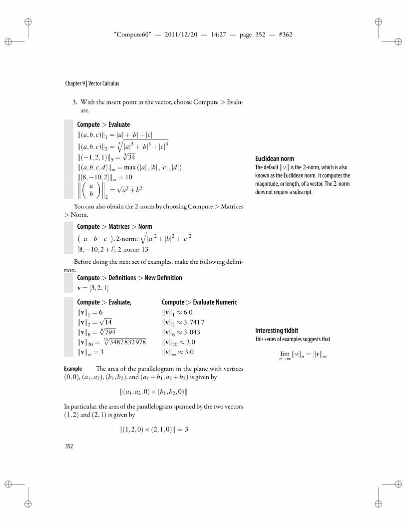
ii
“Compute60” — 2011/12/20 — 14:27 — page 352 — #362 ii
ii
ii
Chapter 9 | Vector Calculus
3. With the insert point in the vector, choose Compute> Evalu-ate.
Compute> Evaluate∥(a,b,c)∥1 = |a|+ |b|+ |c|
∥(a,b,c)∥3 =3√|a|3 + |b|3 + |c|3
∥(−1,2,1)∥5 =5√
34∥(a,b,c,d)∥∞ = max(|a| , |b| , |c| , |d|)∥[8,−10,2]∥∞ = 10∥∥∥∥( a
b
)∥∥∥∥2=√
a2 +b2
Euclidean normThe default ∥v∥ is the 2-norm, which is alsoknown as the Euclidean norm. It computes themagnitude, or length, of a vector. The 2-normdoes not require a subscript.
You can also obtain the 2-norm by choosingCompute>Matrices>Norm.
Compute>Matrices> Norm(a b c
), 2-norm:
√|a|2 + |b|2 + |c|2
[8,−10,2+ i], 2-norm: 13
Before doing the next set of examples, make the following de ni-tion.
Compute> De nitions> New De nitionv = [3,2,1]
Compute> Evaluate, Compute> Evaluate Numeric∥v∥1 = 6 ∥v∥1 ≈ 6.0∥v∥2 =
√14 ∥v∥2 ≈ 3.7417
∥v∥6 =6√
794 ∥v∥6 ≈ 3.043∥v∥20 =
20√
3487832978 ∥v∥20 ≈ 3.0∥v∥∞ = 3 ∥v∥∞ ≈ 3.0
Interesting tidbitThis series of examples suggests that
limn→∞∥v∥n = ∥v∥∞
Example e area of the parallelogram in the plane with vertices(0,0), (a1,a2), (b1,b2), and (a1 +b1,a2 +b2) is given by
∥(a1,a2,0)× (b1,b2,0)∥
In particular, the area of the parallelogram spanned by the two vectors(1,2) and (2,1) is given by
∥(1,2,0)× (2,1,0)∥= 3
352
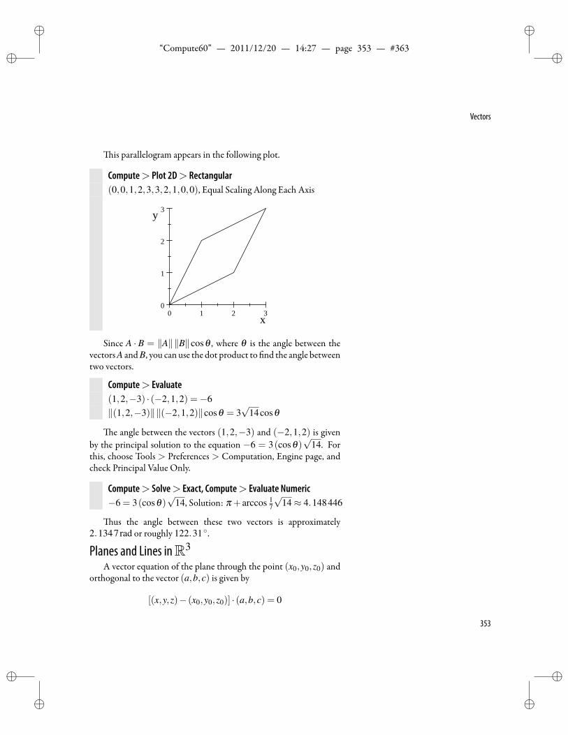
ii
“Compute60” — 2011/12/20 — 14:27 — page 353 — #363 ii
ii
ii
Vectors
is parallelogram appears in the following plot.
Compute> Plot 2D> Rectangular(0,0,1,2,3,3,2,1,0,0), Equal Scaling Along Each Axis
0 1 2 30
1
2
3
x
y
Since A · B = ∥A∥∥B∥cosθ , where θ is the angle between thevectors A and B, you can use the dot product to nd the angle betweentwo vectors.
Compute> Evaluate(1,2,−3) · (−2,1,2) =−6∥(1,2,−3)∥∥(−2,1,2)∥cosθ = 3
√14cosθ
e angle between the vectors (1,2,−3) and (−2,1,2) is givenby the principal solution to the equation −6 = 3(cosθ)
√14. For
this, choose Tools > Preferences > Computation, Engine page, andcheck Principal Value Only.
Compute> Solve> Exact, Compute> Evaluate Numeric−6 = 3(cosθ)
√14, Solution: π + arccos 1
7
√14≈ 4.148446
us the angle between these two vectors is approximately2.1347rad or roughly 122.31 .
Planes and Lines inR3
A vector equation of the plane through the point (x0,y0,z0) andorthogonal to the vector (a,b,c) is given by
[(x,y,z)− (x0,y0,z0)] · (a,b,c) = 0
353
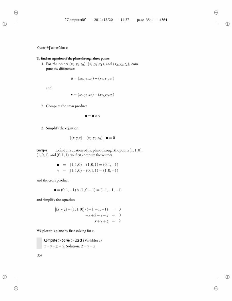
ii
“Compute60” — 2011/12/20 — 14:27 — page 354 — #364 ii
ii
ii
Chapter 9 | Vector Calculus
To nd an equationof the plane through three points1. For the points (x0,y0,z0), (x1,y1,z1), and (x2,y2,z2), com-
pute the differences
u = (x0,y0,z0)− (x1,y1,z1)
and
v = (x0,y0,z0)− (x2,y2,z2)
2. Compute the cross product
n = u×v
3. Simplify the equation
[(x,y,z)− (x0,y0,z0)] ·n = 0
Example To ndan equationof theplane through thepoints (1,1,0),(1,0,1), and (0,1,1), we rst compute the vectors
u = (1,1,0)− (1,0,1) = (0,1,−1)v = (1,1,0)− (0,1,1) = (1,0,−1)
and the cross product
n = (0,1,−1)× (1,0,−1) = (−1,−1,−1)
and simplify the equation
[(x,y,z)− (1,1,0)] · (−1,−1,−1) = 0−x+2− y− z = 0
x+ y+ z = 2
We plot this plane by rst solving for z.
Compute> Solve> Exact (Variable: z)x+ y+ z = 2, Solution: 2− y− x
354
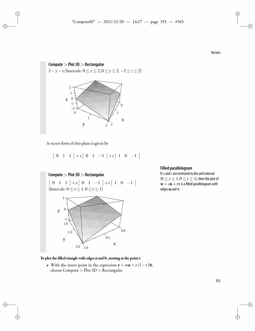
ii
“Compute60” — 2011/12/20 — 14:27 — page 355 — #365 ii
ii
ii
Vectors
Compute> Plot 3D> Rectangular2− y− x (Intervals: 0≤ x≤ 2, 0≤ y≤ 2,−2≤ z≤ 2)
2 2
1
z
0
x1
0
y
12
0
1
2
A vector form of this plane is given by
[0 1 1
]+ s[
0 1 −1]+ t[
1 0 −1]
Filled parallelogramIf s and t are restricted to the unit interval(0≤ s≤ 1, 0≤ t ≤ 1), then the plot ofw+ su+ tv is a lled parallelogramwithedgesu and v.
Compute> Plot 3D> Rectangular[0 1 1
]+ s[
0 1 −1]+ t[
1 0 −1]
(Intervals: 0≤ s≤ 1, 0≤ t ≤ 1)
1.02.0
0.0
xy
1.50.5
0
11.0
z
1
Toplot the lled trianglewith edgesa andb, starting at the point c
• With the insert point in the expression c + sta + s(1− t)b,choose Compute> Plot 3D> Rectangular.
355
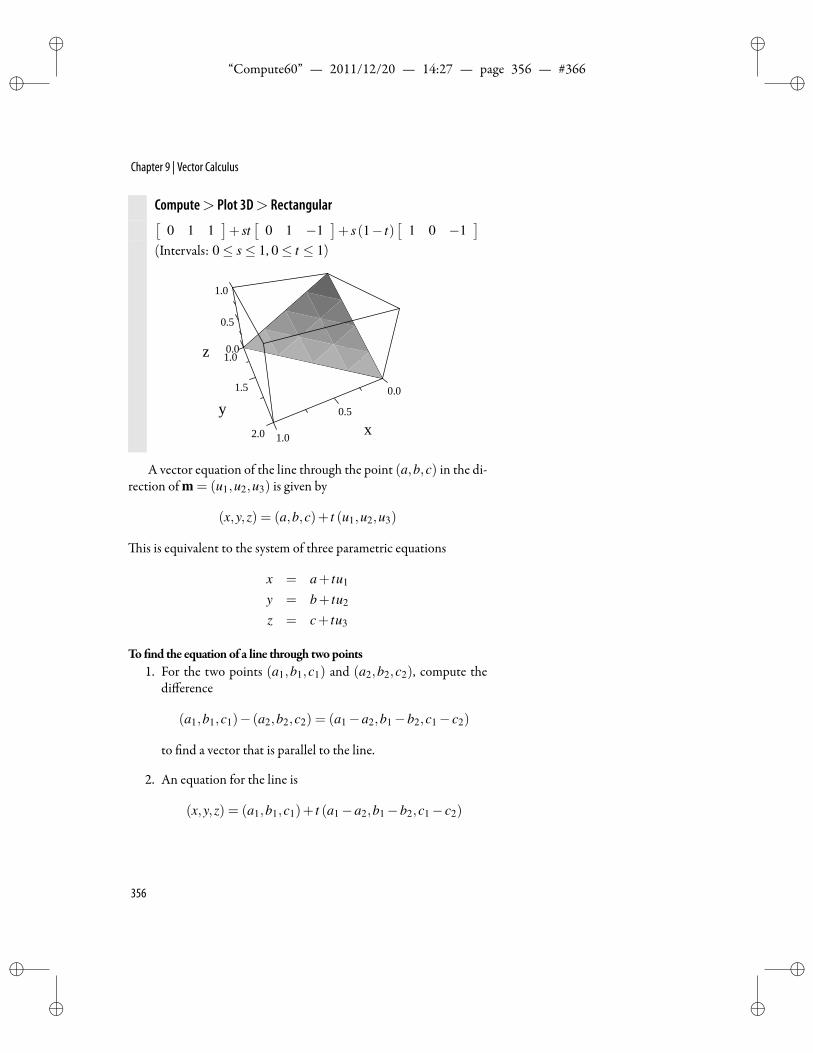
ii
“Compute60” — 2011/12/20 — 14:27 — page 356 — #366 ii
ii
ii
Chapter 9 | Vector Calculus
Compute> Plot 3D> Rectangular[0 1 1
]+ st
[0 1 −1
]+ s(1− t)
[1 0 −1
](Intervals: 0≤ s≤ 1, 0≤ t ≤ 1)
0.0
0.0z
0.5
1.0
y
1.0
x
1.5
0.5
2.0 1.0
A vector equation of the line through the point (a,b,c) in the di-rection of m = (u1,u2,u3) is given by
(x,y,z) = (a,b,c)+ t (u1,u2,u3)
is is equivalent to the system of three parametric equations
x = a+ tu1
y = b+ tu2
z = c+ tu3
To nd the equationof a line through twopoints1. For the two points (a1,b1,c1) and (a2,b2,c2), compute the
difference
(a1,b1,c1)− (a2,b2,c2) = (a1−a2,b1−b2,c1− c2)
to nd a vector that is parallel to the line.
2. An equation for the line is
(x,y,z) = (a1,b1,c1)+ t (a1−a2,b1−b2,c1− c2)
356
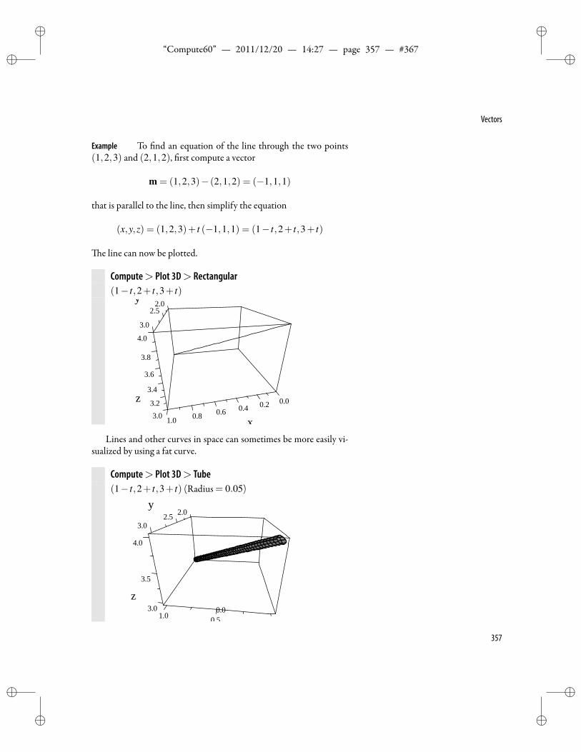
ii
“Compute60” — 2011/12/20 — 14:27 — page 357 — #367 ii
ii
ii
Vectors
Example To nd an equation of the line through the two points(1,2,3) and (2,1,2), rst compute a vector
m = (1,2,3)− (2,1,2) = (−1,1,1)
that is parallel to the line, then simplify the equation
(x,y,z) = (1,2,3)+ t (−1,1,1) = (1− t,2+ t,3+ t)
e line can now be plotted.
Compute> Plot 3D> Rectangular(1− t,2+ t,3+ t)
2.0
3.8
3.6
z3.4
3.2
1.0 0.83.0 0.6 0.4
x
0.2 0.0
y2.5
4.0
3.0
Lines and other curves in space can sometimes be more easily vi-sualized by using a fat curve.
Compute> Plot 3D> Tube(1− t,2+ t,3+ t) (Radius= 0.05)
2.0y
2.5
x
3.01.0
0.00.5
3.5
z
3.0
4.0
357
ii
“Compute60” — 2011/12/20 — 14:27 — page 358 — #368 ii
ii
ii
Chapter 9 | Vector Calculus
Gradient, Divergence, Curl, and Related Operatorsree operations are of particular importance in vector calculus:
• gradient: measures the rate and direction of change in a scalareld; the gradient of a scalar eld is a vector eld.
• divergence: measures a vector eld’s tendency to originate fromor converge upon a given point.
• curl: measures a vector eld’s tendency to rotate about a point;the curl of a vector eld is another vector eld.
e operators gradient, divergence, curl, and the Laplacian are im-plemented with their usual notation ∇, ∇·, ∇×, and ∇ ·∇, respec-tively, followed by Evaluate. ey also appear as special commandson the Vector Calculus menu. Directional derivatives have a similarimplementation.
To enter the nabla symbol ∇ select the nabla from the Miscella-neous Symbols tab ∞∂ .
GradientIf f (x1,x2, . . . ,xn) is a scalar function of n variables, then the vec-
tor(∂ f∂x1
(c1,c2, . . . ,cn) ,∂ f∂x2
(c1,c2, . . . ,cn) , . . . ,∂ f
∂xn1(c1,c2, . . . ,cn)
)is the gradient of f at the point (c1,c2, . . . ,cn) and is denoted ∇ f .For n = 3, the vector ∇ f at (a,b,c) is normal to the level surfacef (x,y,z) = f (a,b,c) at the point (a,b,c). Potential energy and force
In physics, f represents potential energy, and∇ f represents force.
Tocompute the gradient of a function f (x,y,z)1. Place the insert point in the expression ∇ f (x,y,z).
2. Choose Compute> Evaluate.
Or
1. Place the insert point in the expression f (x,y,z).
2. Choose Compute> Vector Calculus>Gradient.
358
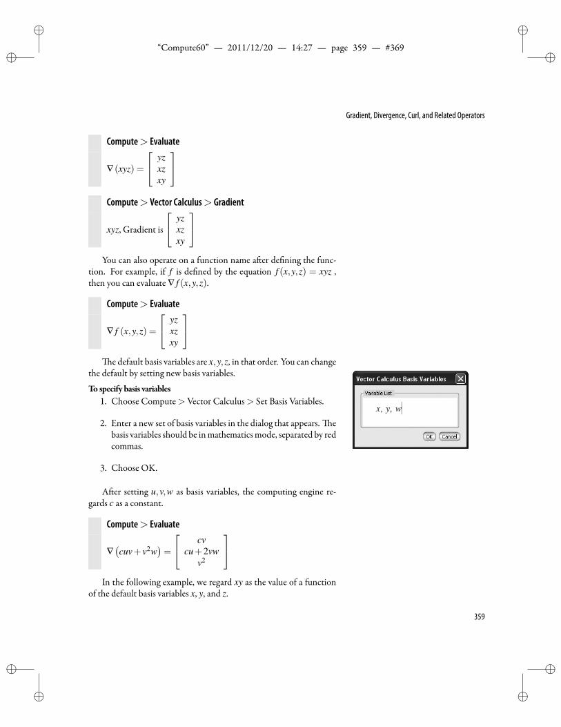
ii
“Compute60” — 2011/12/20 — 14:27 — page 359 — #369 ii
ii
ii
Gradient, Divergence, Curl, and Related Operators
Compute> Evaluate
∇(xyz) =
yzxzxy
Compute> Vector Calculus> Gradient
xyz, Gradient is
yzxzxy
You can also operate on a function name a er de ning the func-
tion. For example, if f is de ned by the equation f (x,y,z) = xyz ,then you can evaluate ∇ f (x,y,z).
Compute> Evaluate
∇ f (x,y,z) =
yzxzxy
e default basis variables are x,y,z, in that order. You can change
the default by setting new basis variables.
To specify basis variables1. Choose Compute> Vector Calculus> Set Basis Variables.
2. Enter a new set of basis variables in the dialog that appears. ebasis variables should be inmathematicsmode, separated by redcommas.
3. Choose OK.
A er setting u,v,w as basis variables, the computing engine re-gards c as a constant.
Compute> Evaluate
∇(cuv+ v2w
)=
cvcu+2vw
v2
In the following example, we regard xy as the value of a function
of the default basis variables x, y, and z.
359
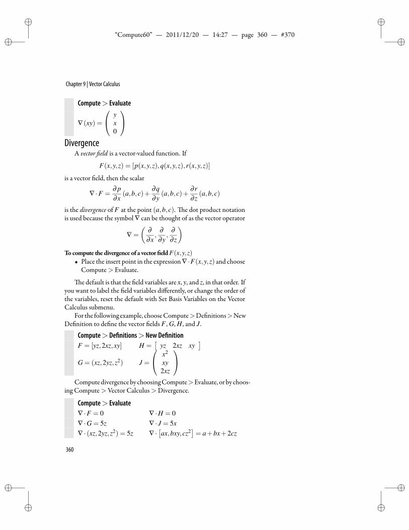
ii
“Compute60” — 2011/12/20 — 14:27 — page 360 — #370 ii
ii
ii
Chapter 9 | Vector Calculus
Compute> Evaluate
∇(xy) =
yx0
Divergence
A vector eld is a vector-valued function. If
F(x,y,z) = [p(x,y,z),q(x,y,z),r(x,y,z)]
is a vector eld, then the scalar
∇ ·F =∂ p∂x
(a,b,c)+∂q∂y
(a,b,c)+∂ r∂ z
(a,b,c)
is the divergence of F at the point (a,b,c). e dot product notationis used because the symbol ∇ can be thought of as the vector operator
∇ =
(∂∂x
,∂∂y
,∂∂ z
)Tocompute the divergence of a vector eldF(x,y,z)
• Place the insert point in the expression ∇ ·F(x,y,z) and chooseCompute> Evaluate.
e default is that the eld variables are x, y, and z, in that order. Ifyou want to label the eld variables differently, or change the order ofthe variables, reset the default with Set Basis Variables on the VectorCalculus submenu.
For the following example, chooseCompute>De nitions>NewDe nition to de ne the vector elds F , G, H , and J.
Compute> De nitions> New De nitionF = [yz,2xz,xy] H =
[yz 2xz xy
]G = (xz,2yz,z2) J =
x2
xy2xz
Computedivergenceby choosingCompute>Evaluate, or by choos-
ing Compute> Vector Calculus>Divergence.
Compute> Evaluate∇ ·F = 0 ∇ ·H = 0∇ ·G = 5z ∇ · J = 5x∇ · (xz,2yz,z2) = 5z ∇ ·
[ax,bxy,cz2
]= a+bx+2cz
360
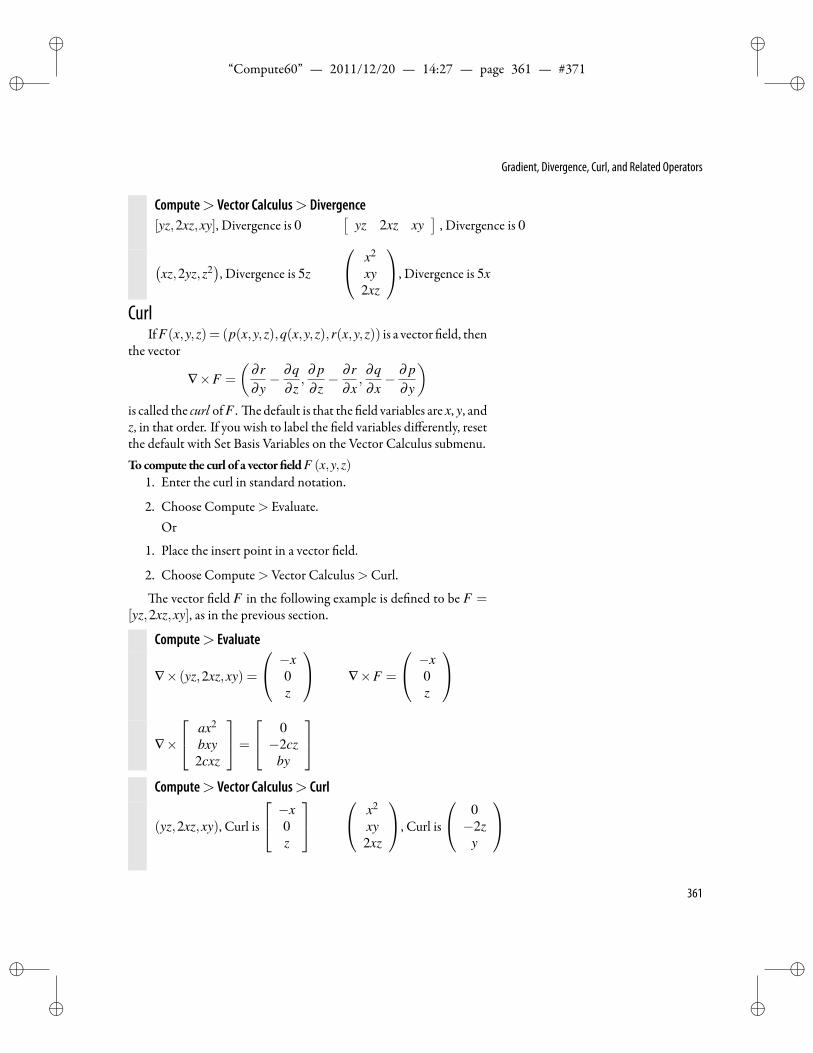
ii
“Compute60” — 2011/12/20 — 14:27 — page 361 — #371 ii
ii
ii
Gradient, Divergence, Curl, and Related Operators
Compute> Vector Calculus> Divergence[yz,2xz,xy], Divergence is 0
[yz 2xz xy
], Divergence is 0
(xz,2yz,z2
), Divergence is 5z
x2
xy2xz
, Divergence is 5x
CurlIfF(x,y,z) = (p(x,y,z),q(x,y,z),r(x,y,z)) is a vector eld, then
the vector
∇×F =
(∂ r∂y− ∂q
∂ z,
∂ p∂ z− ∂ r
∂x,
∂q∂x− ∂ p
∂y
)is called the curl of F . e default is that the eld variables are x, y, andz, in that order. If you wish to label the eld variables differently, resetthe default with Set Basis Variables on the Vector Calculus submenu.Tocompute the curl of a vector eldF (x,y,z)
1. Enter the curl in standard notation.
2. Choose Compute> Evaluate.Or
1. Place the insert point in a vector eld.
2. Choose Compute> Vector Calculus>Curl.
e vector eld F in the following example is de ned to be F =[yz,2xz,xy], as in the previous section.
Compute> Evaluate
∇× (yz,2xz,xy) =
−x0z
∇×F =
−x0z
∇×
ax2
bxy2cxz
=
0−2cz
by
Compute> Vector Calculus> Curl
(yz,2xz,xy), Curl is
−x0z
x2
xy2xz
, Curl is
0−2z
y
361
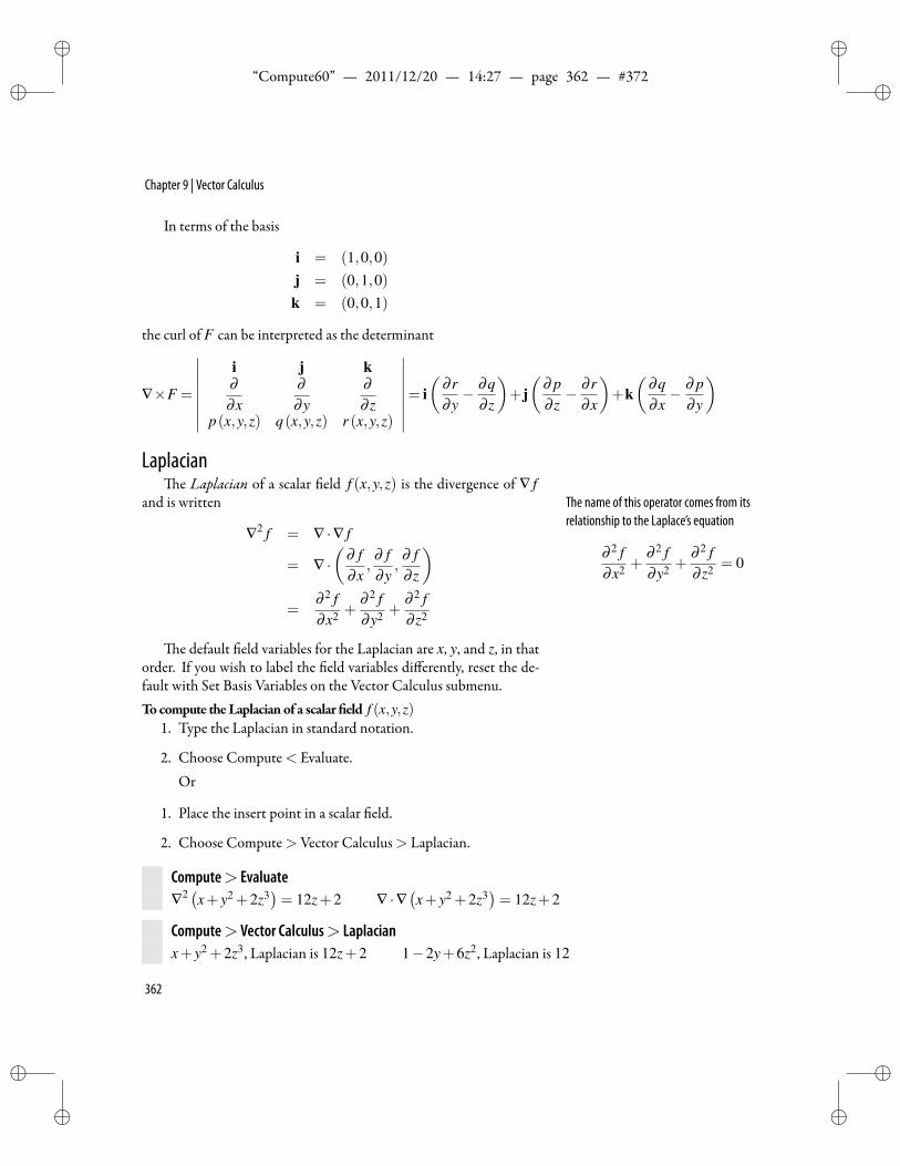
ii
“Compute60” — 2011/12/20 — 14:27 — page 362 — #372 ii
ii
ii
Chapter 9 | Vector Calculus
In terms of the basis
i = (1,0,0)j = (0,1,0)k = (0,0,1)
the curl of F can be interpreted as the determinant
∇×F =
∣∣∣∣∣∣∣∣i j k∂∂x
∂∂y
∂∂ z
p(x,y,z) q(x,y,z) r (x,y,z)
∣∣∣∣∣∣∣∣= i(
∂ r∂y− ∂q
∂ z
)+j(
∂ p∂ z− ∂ r
∂x
)+k(
∂q∂x− ∂ p
∂y
)
Laplaciane Laplacian of a scalar eld f (x,y,z) is the divergence of ∇ f
and is written The name of this operator comes from itsrelationship to the Laplace’s equation
∂ 2 f∂x2 +
∂ 2 f∂y2 +
∂ 2 f∂ z2 = 0
∇2 f = ∇ ·∇ f
= ∇ ·(
∂ f∂x
,∂ f∂y
,∂ f∂ z
)=
∂ 2 f∂x2 +
∂ 2 f∂y2 +
∂ 2 f∂ z2
e default eld variables for the Laplacian are x, y, and z, in thatorder. If you wish to label the eld variables differently, reset the de-fault with Set Basis Variables on the Vector Calculus submenu.Tocompute theLaplacian of a scalar eld f (x,y,z)
1. Type the Laplacian in standard notation.
2. Choose Compute< Evaluate.Or
1. Place the insert point in a scalar eld.
2. Choose Compute> Vector Calculus> Laplacian.
Compute> Evaluate∇2 (x+ y2 +2z3
)= 12z+2 ∇ ·∇
(x+ y2 +2z3
)= 12z+2
Compute> Vector Calculus> Laplacianx+ y2 +2z3, Laplacian is 12z+2 1−2y+6z2, Laplacian is 12
362
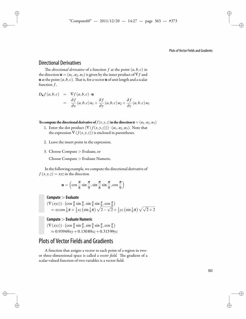
ii
“Compute60” — 2011/12/20 — 14:27 — page 363 — #373 ii
ii
ii
Plots of Vector Fields and Gradients
Directional Derivativese directional derivative of a function f at the point (a,b,c) in
the direction u = (u1,u2,u3) is given by the inner product of ∇ f andu at the point (a,b,c). at is, for a vectoru of unit length and a scalarfunction f ,
Du f (a,b,c) = ∇ f (a,b,c) ·u
=∂ f∂x
(a,b,c)u1 +∂ f∂y
(a,b,c)u2 +∂ f∂ z
(a,b,c)u3
Tocomputethedirectionalderivativeof f (x,y,z) inthedirectionu=(u1,u2,u3)
1. Enter the dot product (∇( f (x,y,z))) · (u1,u2,u3). Note thatthe expression ∇( f (x,y,z)) is enclosed in parentheses.
2. Leave the insert point in the expression.
3. Choose Compute> Evaluate, or
Choose Compute> Evaluate Numeric.
In the following example, we compute the directional derivative off (x,y,z) = xyz in the direction
u =(
cosπ8
sinπ9,sin
π8
sinπ9,cos
π9
)Compute> Evaluate(∇(xyz)) ·
(cos π
8 sin π9 ,sin π
8 sin π9 ,cos π
9
)= xycos 1
9 π + 12 xz(sin 1
9 π)√
2−√
2+ 12 yz(sin 1
9 π)√√
2+2
Compute> Evaluate Numeric(∇(xyz)) ·
(cos π
8 sin π9 ,sin π
8 sin π9 ,cos π
9
)≈ 0.93969xy+0.13089xz+0.31599yz
Plots of Vector Fields and GradientsA function that assigns a vector to each point of a region in two-
or three-dimensional space is called a vector eld. e gradient of ascalar-valued function of two variables is a vector eld.
363
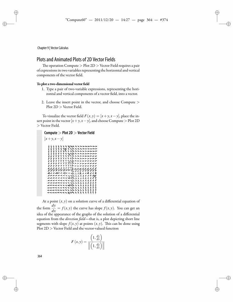
ii
“Compute60” — 2011/12/20 — 14:27 — page 364 — #374 ii
ii
ii
Chapter 9 | Vector Calculus
Plots and Animated Plots of 2D Vector Fieldse operation Compute> Plot 2D>Vector Field requires a pair
of expressions in two variables representing the horizontal and verticalcomponents of the vector eld.
Toplot a two-dimensional vector eld1. Type a pair of two-variable expressions, representing the hori-
zontal and vertical components of a vector eld, into a vector.
2. Leave the insert point in the vector, and choose Compute >Plot 2D> Vector Field.
To visualize the vector eld F(x,y) = [x+ y,x− y], place the in-sert point in the vector [x+ y,x− y], and chooseCompute>Plot 2D> Vector Field.
Compute> Plot 2D> Vector Field[x+ y,x− y]
6 4 2 2 4 6
6
4
2
2
4
6
x
y
At a point (x,y) on a solution curve of a differential equation of
the formdydx
= f (x,y) the curve has slope f (x,y). You can get anidea of the appearance of the graphs of the solution of a differentialequation from the direction eld—that is, a plot depicting short linesegments with slope f (x,y) at points (x,y). is can be done usingPlot 2D> Vector Field and the vector-valued function
F (x,y) =
(1, dy
dx
)∥∥∥(1, dy
dx
)∥∥∥364
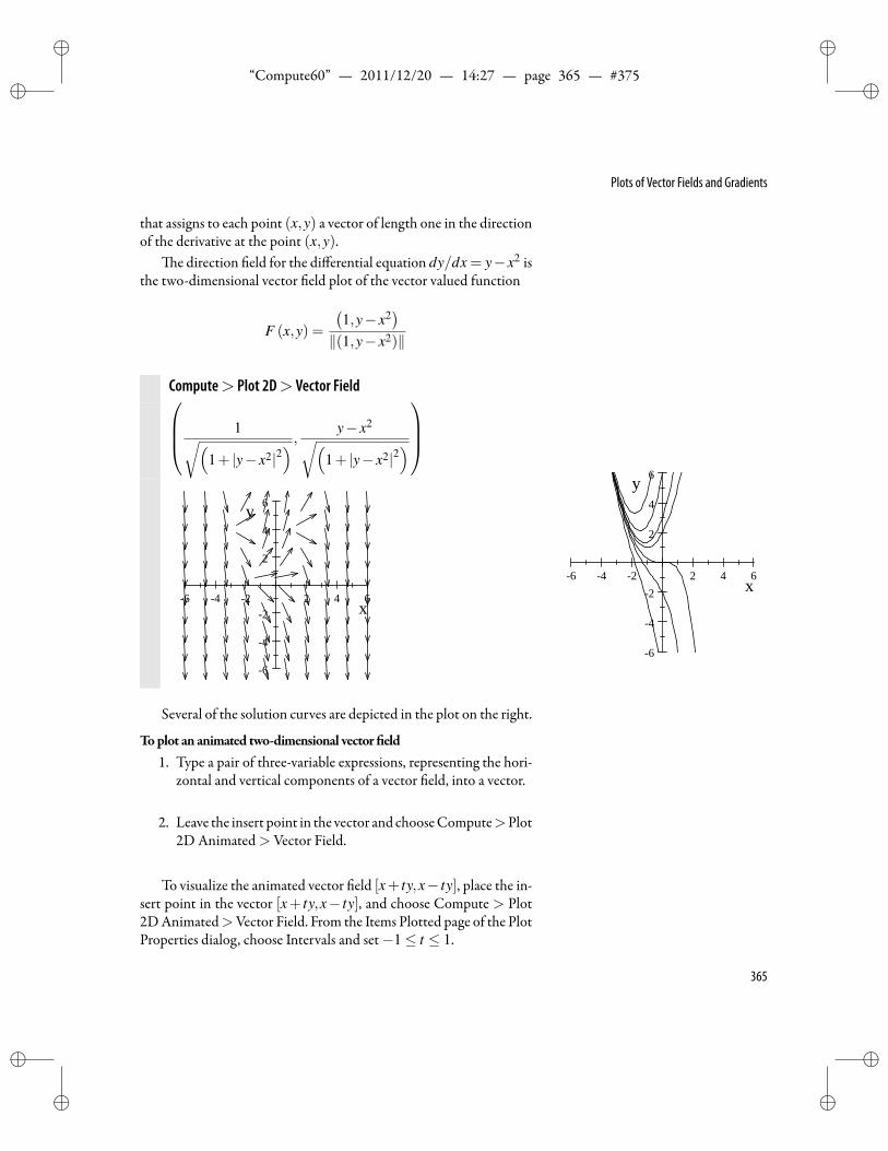
ii
“Compute60” — 2011/12/20 — 14:27 — page 365 — #375 ii
ii
ii
Plots of Vector Fields and Gradients
that assigns to each point (x,y) a vector of length one in the directionof the derivative at the point (x,y).
e direction eld for the differential equation dy/dx = y−x2 isthe two-dimensional vector eld plot of the vector valued function
F (x,y) =
(1,y− x2
)∥(1,y− x2)∥
Compute> Plot 2D> Vector Field 1√(1+ |y− x2|2
) , y− x2√(1+ |y− x2|2
)
6 4 2 2 4 6
6
4
2
2
4
6
x
y
6 4 2 2 4 6
6
4
2
2
4
6
x
y
Several of the solution curves are depicted in the plot on the right.
Toplot an animated two-dimensional vector eld1. Type a pair of three-variable expressions, representing the hori-
zontal and vertical components of a vector eld, into a vector.
2. Leave the insert point in the vector and chooseCompute>Plot2D Animated> Vector Field.
To visualize the animated vector eld [x+ ty,x− ty], place the in-sert point in the vector [x+ ty,x− ty], and choose Compute > Plot2DAnimated>Vector Field. From the Items Plotted page of the PlotProperties dialog, choose Intervals and set−1≤ t ≤ 1.
365
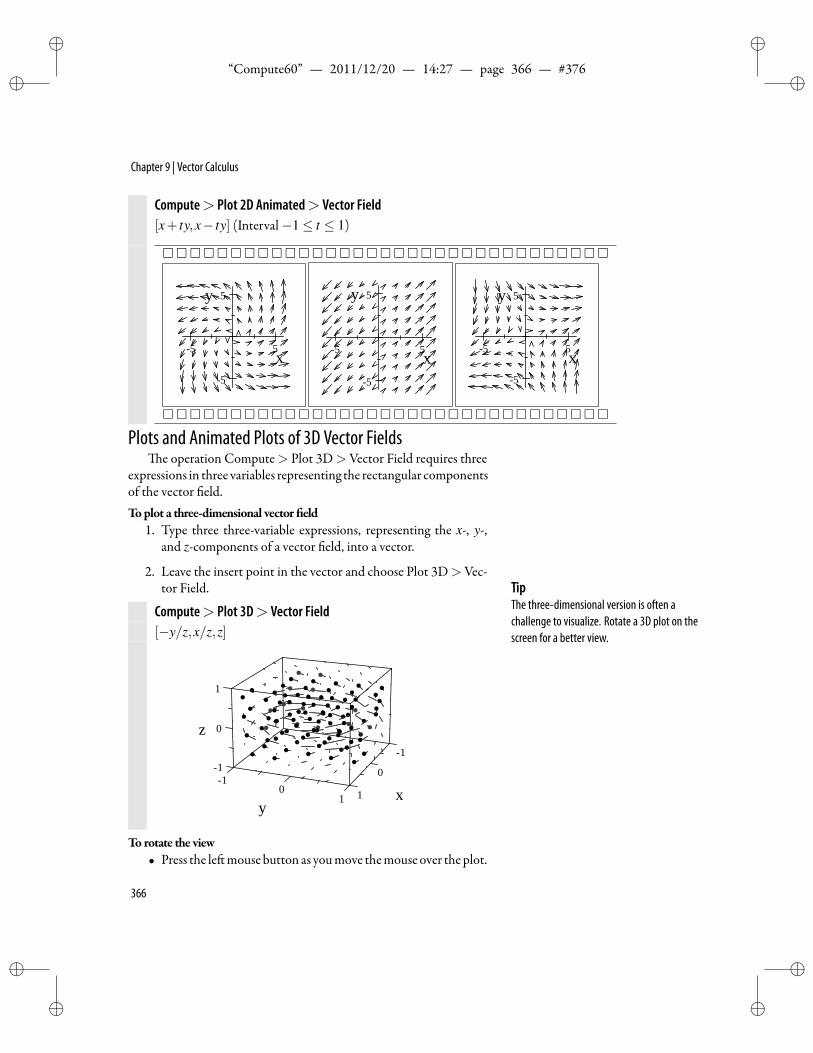
ii
“Compute60” — 2011/12/20 — 14:27 — page 366 — #376 ii
ii
ii
Chapter 9 | Vector Calculus
Compute> Plot 2D Animated> Vector Field[x+ ty,x− ty] (Interval−1≤ t ≤ 1)
5 5
5
5
x
y
5 5
5
5
x
y
5 5
5
5
x
y
Plots and Animated Plots of 3D Vector Fields
e operation Compute> Plot 3D>Vector Field requires threeexpressions in three variables representing the rectangular componentsof the vector eld.Toplot a three-dimensional vector eld
1. Type three three-variable expressions, representing the x-, y-,and z-components of a vector eld, into a vector.
2. Leave the insert point in the vector and choose Plot 3D>Vec-tor Field. Tip
The three-dimensional version is often achallenge to visualize. Rotate a 3D plot on thescreen for a better view.
Compute> Plot 3D> Vector Field[−y/z,x/z,z]
1
x0
y
1
1
0z
1
0 11
To rotate the view• Press the le mouse button as youmove themouse over the plot.
366
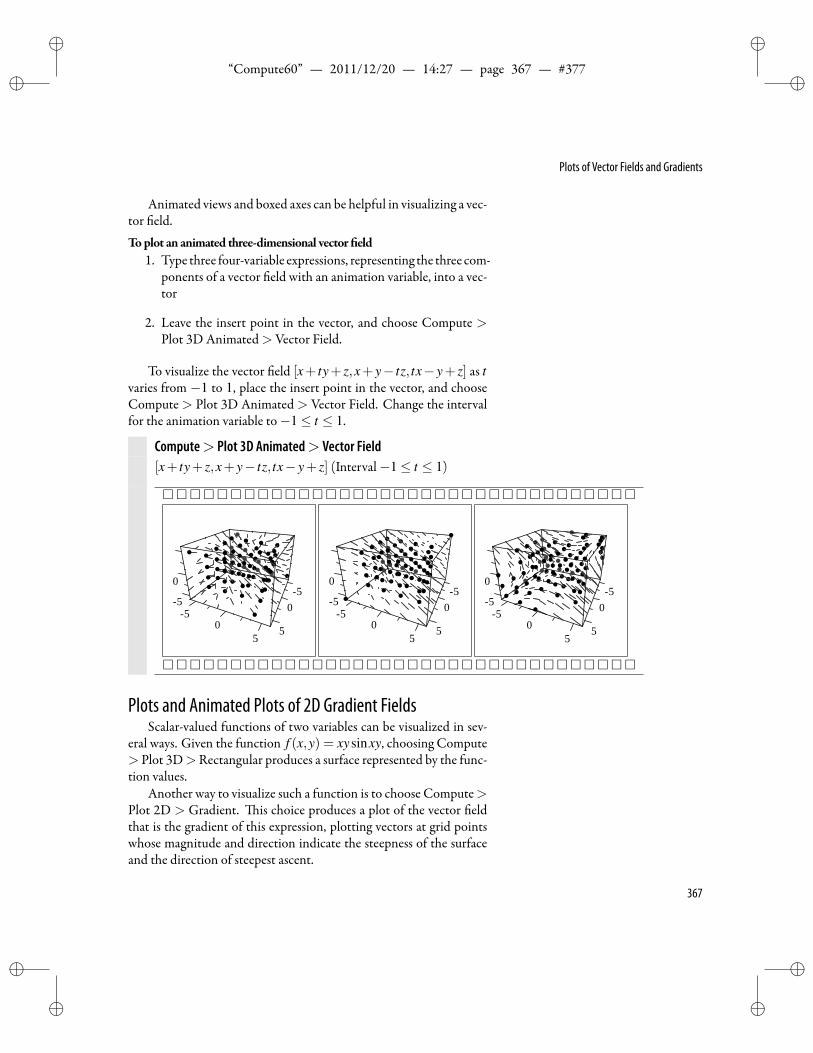
ii
“Compute60” — 2011/12/20 — 14:27 — page 367 — #377 ii
ii
ii
Plots of Vector Fields and Gradients
Animated views and boxed axes can be helpful in visualizing a vec-tor eld.Toplot an animated three-dimensional vector eld
1. Type three four-variable expressions, representing the three com-ponents of a vector eld with an animation variable, into a vec-tor
2. Leave the insert point in the vector, and choose Compute >Plot 3D Animated> Vector Field.
To visualize the vector eld [x+ ty+ z,x+ y− tz, tx− y+ z] as tvaries from −1 to 1, place the insert point in the vector, and chooseCompute > Plot 3D Animated > Vector Field. Change the intervalfor the animation variable to−1≤ t ≤ 1.
Compute> Plot 3D Animated> Vector Field[x+ ty+ z,x+ y− tz, tx− y+ z] (Interval−1≤ t ≤ 1)
55 0
0
50 5
5
55
0
5 00 5
5
55 0
0
50 5
5
Plots and Animated Plots of 2D Gradient FieldsScalar-valued functions of two variables can be visualized in sev-
eral ways. Given the function f (x,y) = xysinxy, choosing Compute> Plot 3D>Rectangular produces a surface represented by the func-tion values.
Another way to visualize such a function is to choose Compute>Plot 2D > Gradient. is choice produces a plot of the vector eldthat is the gradient of this expression, plotting vectors at grid pointswhose magnitude and direction indicate the steepness of the surfaceand the direction of steepest ascent.
367
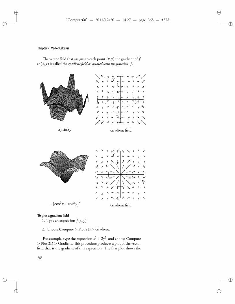
ii
“Compute60” — 2011/12/20 — 14:27 — page 368 — #378 ii
ii
ii
Chapter 9 | Vector Calculus
e vector eld that assigns to each point (x,y) the gradient of fat (x,y) is called the gradient eld associated with the function f .
xysinxy
3 2 1 1 2 3
3
2
1
1
2
3
x
y
Gradient eld
−(cos2 x+ cos2 y
)2
2 1 1 2
2
1
1
2
x
y
Gradient eld
Toplot a gradient eld1. Type an expression f (x,y).
2. Choose Compute> Plot 2D>Gradient.
For example, type the expression x2 + 2y2, and choose Compute> Plot 2D>Gradient. is procedure produces a plot of the vectoreld that is the gradient of this expression. e rst plot shows the
368

ii
“Compute60” — 2011/12/20 — 14:27 — page 369 — #379 ii
ii
ii
Plots of Vector Fields and Gradients
relative steepness, the second is the surface, and the third shows thecontour lines.
Compute> Plot 2D> Gradientx2 +2y2
6 4 2 2 4 6
6
4
2
2
4
6
Gradient eld
Compute> Plot 3D> Rectangularx2 +2y2
Turn: 0 Tilt: 0Contour
Toplot an animated gradient eld1. Type an expression f (x,y, t).
369
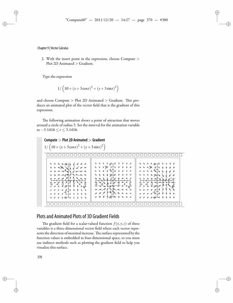
ii
“Compute60” — 2011/12/20 — 14:27 — page 370 — #380 ii
ii
ii
Chapter 9 | Vector Calculus
2. With the insert point in the expression, choose Compute >Plot 2D Animated>Gradient.
Type the expression
1/(
10+(x+3cos t)2 +(y+3sin t)2)
and choose Compute > Plot 2D Animated > Gradient. is pro-duces an animated plot of the vector eld that is the gradient of thisexpression.
e following animation shows a point of attraction that movesaround a circle of radius 3. Set the interval for the animation variableto−3.1416≤ t ≤ 3.1416.
Compute> Plot 2D Animated> Gradient
1/(
10+(x+3cos t)2 +(y+3sin t)2)
6 4 2 2 4 6
6
4
2
2
4
6
x
y
6 4 2 2 4 6
6
4
2
2
4
6
x
y
6 4 2 2 4 6
6
4
2
2
4
6
x
y
Plots and Animated Plots of 3D Gradient Fieldse gradient eld for a scalar-valued function f (x,y,z) of three
variables is a three-dimensional vector eld where each vector repre-sents the direction ofmaximal increase. e surface represented by thefunction values is embedded in four-dimensional space, so you mustuse indirect methods such as plotting the gradient eld to help youvisualize this surface.
370
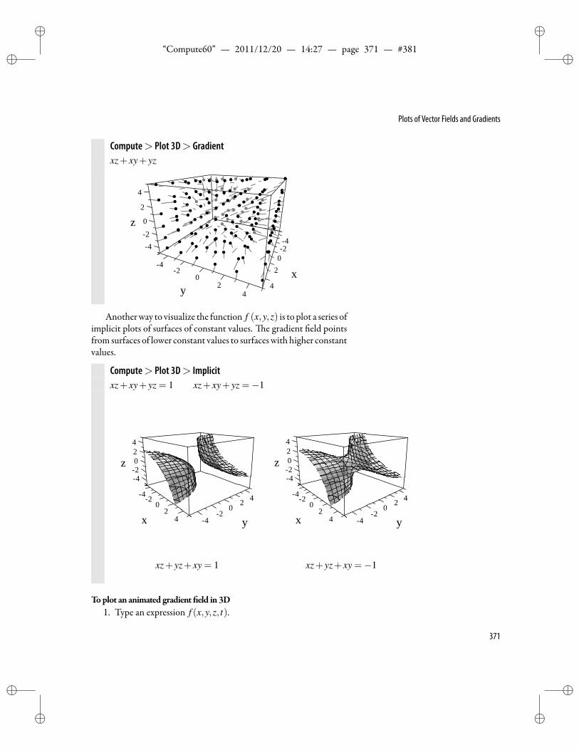
ii
“Compute60” — 2011/12/20 — 14:27 — page 371 — #381 ii
ii
ii
Plots of Vector Fields and Gradients
Compute> Plot 3D> Gradientxz+ xy+ yz
42
04
x
2z
4
0
2
22
4
y0
442
Anotherway to visualize the function f (x,y,z) is to plot a series ofimplicit plots of surfaces of constant values. e gradient eld pointsfrom surfaces of lower constant values to surfaceswith higher constantvalues.
Compute> Plot 3D> Implicitxz+ xy+ yz = 1 xz+ xy+ yz =−1
2x
0
z
4
42
20
24
4 42
2 4
y0
xz+ yz+ xy = 1
420z
42
42
x0 0
42
y2
42
4
xz+ yz+ xy =−1
Toplot an animated gradient eld in 3D1. Type an expression f (x,y,z, t).
371
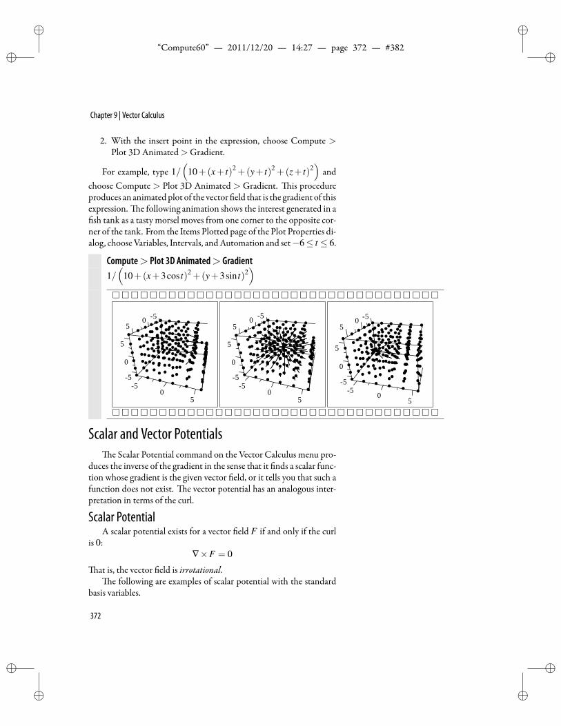
ii
“Compute60” — 2011/12/20 — 14:27 — page 372 — #382 ii
ii
ii
Chapter 9 | Vector Calculus
2. With the insert point in the expression, choose Compute >Plot 3D Animated>Gradient.
For example, type 1/(
10+(x+ t)2 +(y+ t)2 +(z+ t)2)
andchoose Compute > Plot 3D Animated > Gradient. is procedureproduces an animatedplot of the vector eld that is the gradient of thisexpression. e following animation shows the interest generated in ash tank as a tasty morsel moves from one corner to the opposite cor-
ner of the tank. From the Items Plotted page of the Plot Properties di-alog, chooseVariables, Intervals, andAutomation and set−6≤ t ≤ 6.
Compute> Plot 3D Animated> Gradient1/(
10+(x+3cos t)2 +(y+3sin t)2)
50
0
0
55
5
5
5
50
55
0
0
5
5
5
50
55
0
0
5
5
5
Scalar and Vector Potentialse Scalar Potential command on the Vector Calculus menu pro-
duces the inverse of the gradient in the sense that it nds a scalar func-tion whose gradient is the given vector eld, or it tells you that such afunction does not exist. e vector potential has an analogous inter-pretation in terms of the curl.
Scalar PotentialA scalar potential exists for a vector eld F if and only if the curl
is 0:∇×F = 0
at is, the vector eld is irrotational.e following are examples of scalar potential with the standard
basis variables.
372
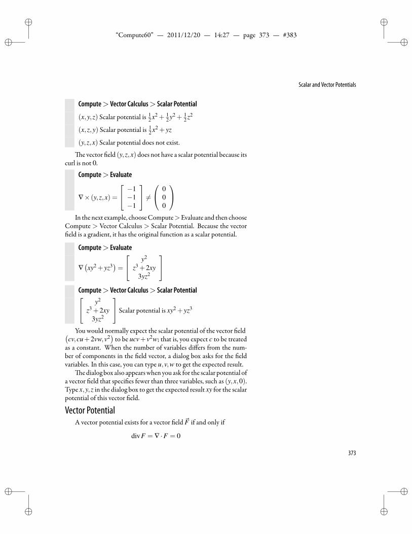
ii
“Compute60” — 2011/12/20 — 14:27 — page 373 — #383 ii
ii
ii
Scalar and Vector Potentials
Compute> Vector Calculus> Scalar Potential
(x,y,z) Scalar potential is 12 x2 + 1
2 y2 + 12 z2
(x,z,y) Scalar potential is 12 x2 + yz
(y,z,x) Scalar potential does not exist.
e vector eld (y,z,x) does not have a scalar potential because itscurl is not 0.
Compute> Evaluate
∇× (y,z,x) =
−1−1−1
= 0
00
In the next example, chooseCompute>Evaluate and then choose
Compute > Vector Calculus > Scalar Potential. Because the vectoreld is a gradient, it has the original function as a scalar potential.
Compute> Evaluate
∇(xy2 + yz3
)=
y2
z3 +2xy3yz2
Compute> Vector Calculus> Scalar Potential y2
z3 +2xy3yz2
Scalar potential is xy2 + yz3
You would normally expect the scalar potential of the vector eld(cv,cu+2vw,v2
)to be ucv+v2w; that is, you expect c to be treated
as a constant. When the number of variables differs from the num-ber of components in the eld vector, a dialog box asks for the eldvariables. In this case, you can type u,v,w to get the expected result.
e dialog box also appearswhen you ask for the scalar potential ofa vector eld that speci es fewer than three variables, such as (y,x,0).Type x,y,z in the dialog box to get the expected result xy for the scalarpotential of this vector eld.
Vector PotentialA vector potential exists for a vector eld F if and only if
divF = ∇ ·F = 0
373
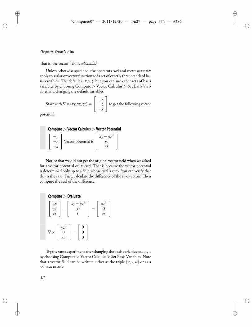
ii
“Compute60” — 2011/12/20 — 14:27 — page 374 — #384 ii
ii
ii
Chapter 9 | Vector Calculus
at is, the vector eld is solenoidal.Unless otherwise speci ed, the operators curl and vector potential
apply to scalar or vector functions of a set of exactly three standard ba-sis variables. e default is x,y,z, but you can use other sets of basisvariables by choosing Compute > Vector Calculus > Set Basis Vari-ables and changing the default variables.
Start with ∇×(xy,yz,zx) =
−y−z−x
to get the following vector
potential.
Compute> Vector Calculus> Vector Potential −y−z−x
Vector potential is
xy− 12 z2
yz0
Notice that we did not get the original vector eld when we askedfor a vector potential of its curl. at is because the vector potentialis determined only up to a eld whose curl is zero. You can verify thatthis is the case. First, calculate the difference of the two vectors. encompute the curl of the difference.
Compute> Evaluate xyyzzx
− xy− 1
2 z2
yz0
=
12 z2
0xz
∇×
12 z2
0xz
=
000
Try the same experiment a er changing thebasis variables tou,v,wby choosing Compute>Vector Calculus> Set Basis Variables. Notethat a vector eld can be written either as the triple (u,v,w) or as acolumn matrix.
374
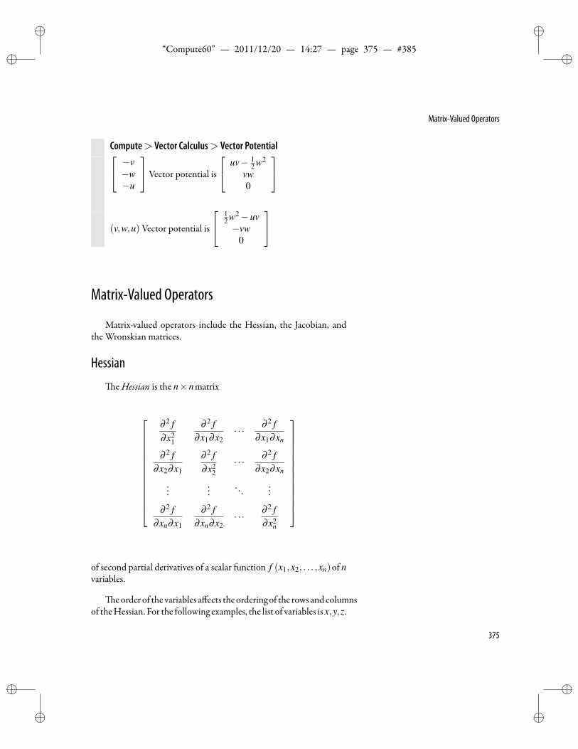
ii
“Compute60” — 2011/12/20 — 14:27 — page 375 — #385 ii
ii
ii
Matrix-Valued Operators
Compute> Vector Calculus> Vector Potential −v−w−u
Vector potential is
uv− 12 w2
vw0
(v,w,u) Vector potential is
12 w2−uv−vw
0
Matrix-Valued Operators
Matrix-valued operators include the Hessian, the Jacobian, andthe Wronskian matrices.
Hessian
eHessian is the n×nmatrix
∂ 2 f∂x2
1
∂ 2 f∂x1∂x2
· · · ∂ 2 f∂x1∂xn
∂ 2 f∂x2∂x1
∂ 2 f∂x2
2· · · ∂ 2 f
∂x2∂xn
......
. . ....
∂ 2 f∂xn∂x1
∂ 2 f∂xn∂x2
· · · ∂ 2 f∂x2
n
of second partial derivatives of a scalar function f (x1,x2, . . . ,xn)of nvariables.
e order of the variables affects theorderingof the rows and columnsof theHessian. For the following examples, the list of variables is x,y,z.
375
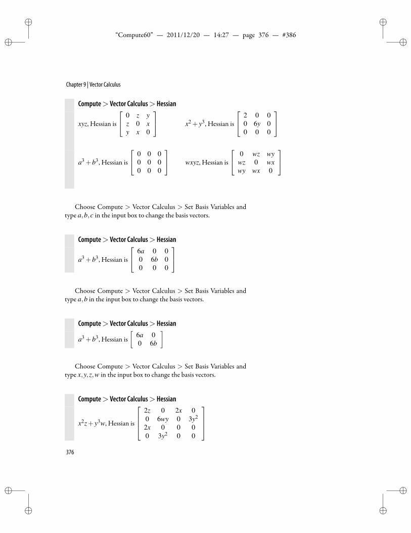
ii
“Compute60” — 2011/12/20 — 14:27 — page 376 — #386 ii
ii
ii
Chapter 9 | Vector Calculus
Compute> Vector Calculus> Hessian
xyz, Hessian is
0 z yz 0 xy x 0
x2 + y3, Hessian is
2 0 00 6y 00 0 0
a3 +b3, Hessian is
0 0 00 0 00 0 0
wxyz, Hessian is
0 wz wywz 0 wxwy wx 0
Choose Compute > Vector Calculus > Set Basis Variables andtype a,b,c in the input box to change the basis vectors.
Compute> Vector Calculus> Hessian
a3 +b3, Hessian is
6a 0 00 6b 00 0 0
Choose Compute > Vector Calculus > Set Basis Variables and
type a,b in the input box to change the basis vectors.
Compute> Vector Calculus> Hessian
a3 +b3, Hessian is[
6a 00 6b
]
Choose Compute > Vector Calculus > Set Basis Variables andtype x,y,z,w in the input box to change the basis vectors.
Compute> Vector Calculus> Hessian
x2z+ y3w, Hessian is
2z 0 2x 00 6wy 0 3y2
2x 0 0 00 3y2 0 0
376
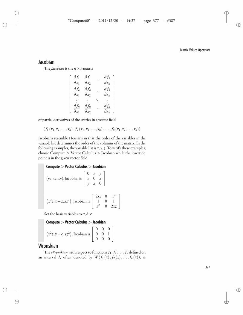
ii
“Compute60” — 2011/12/20 — 14:27 — page 377 — #387 ii
ii
ii
Matrix-Valued Operators
Jacobiane Jacobian is the n×nmatrix
∂ f1
∂x1
∂ f1
∂x2· · · ∂ f1
∂xn
∂ f2
∂x1
∂ f2
∂x2· · · ∂ f2
∂xn...
.... . .
...∂ fn
∂x1
∂ fn
∂x2· · · ∂ fn
∂xn
of partial derivatives of the entries in a vector eld
( f1 (x1,x2, . . . ,xn) , f2 (x1,x2, . . . ,xn) , . . . , fn (x1,x2, . . . ,xn))
Jacobians resemble Hessians in that the order of the variables in thevariable list determines the order of the columns of the matrix. In thefollowing examples, the variable list is x,y,z. To verify these examples,choose Compute > Vector Calculus > Jacobian while the insertionpoint is in the given vector eld.
Compute> Vector Calculus> Jacobian
(yz,xz,xy), Jacobian is
0 z yz 0 xy x 0
(x2z,x+ z,xz2
), Jacobian is
2xz 0 x2
1 0 1z2 0 2xz
Set the basis variables to a,b,c.
Compute> Vector Calculus> Jacobian
(x2z,y+ c,yz2
), Jacobian is
0 0 00 0 10 0 0
Wronskian
eWronskianwith respect to functions f1, f2, . . . , fn de ned onan interval I, o en denoted by W ( f1 (x) , f2 (x) , . . . , fn (x)), is
377
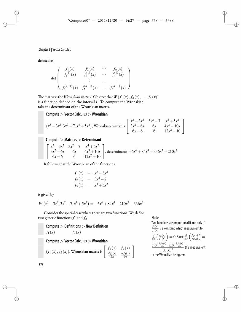
ii
“Compute60” — 2011/12/20 — 14:27 — page 378 — #388 ii
ii
ii
Chapter 9 | Vector Calculus
de ned as
det
f1 (x) f2 (x) · · · fn (x)
f (1)1 (x) f (1)2 (x) · · · f (1)n (x)...
... · · ·...
f (n−1)1 (x) f (n−1)
2 (x) · · · f (n−1)n (x)
ematrix is theWronskianmatrix. Observe thatW ( f1 (x) , f2 (x) , . . . , fn (x))
is a function de ned on the interval I. To compute the Wronskian,take the determinant of the Wronskian matrix.
Compute> Vector Calculus>Wronskian
(x3−3x2,3x2−7,x4 +5x2
), Wronskian matrix is
x3−3x2 3x2−7 x4 +5x2
3x2−6x 6x 4x3 +10x6x−6 6 12x2 +10
Compute>Matrices> Determinant x3−3x2 3x2−7 x4 +5x2
3x2−6x 6x 4x3 +10x6x−6 6 12x2 +10
, determinant: −6x6 +84x4−336x3−210x2
It follows that the Wronskian of the functions
f1 (x) = x3−3x2
f2 (x) = 3x2−7f3 (x) = x4 +5x2
is given by
W(x3−3x2,3x2−7,x4 +5x2)=−6x6 +84x4−210x2−336x3
Consider the special casewhere there are two functions. Wede netwo generic functions f1 and f2. Note
Two functions are proportional if and only iff2(x)f1(x)
is a constant, which is equivalent to
ddx
(f2(x)f1(x)
)= 0. Since d
dx
(f2(x)f1(x)
)=
f1(x)∂ f2(x)
∂x − f2(x)∂ f1(x)
∂x( f1(x))
2 this is equivalent
to the Wronskian being zero.
Compute> De nitions> New De nitionf1 (x) f2 (x)
Compute> Vector Calculus>Wronskian
( f1 (x) , f2 (x)), Wronskian matrix is
[f1 (x) f2 (x)∂ f1(x)
∂x∂ f2(x)
∂x
]
378
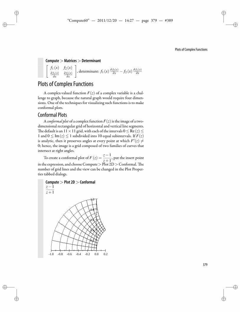
ii
“Compute60” — 2011/12/20 — 14:27 — page 379 — #389 ii
ii
ii
Plots of Complex Functions
Compute>Matrices> Determinant[f1 (x) f2 (x)∂ f1(x)
∂x∂ f2(x)
∂x
], determinant: f1 (x)
∂ f2(x)∂x − f2 (x)
∂ f1(x)∂x
Plots of Complex FunctionsA complex-valued function F(z) of a complex variable is a chal-
lenge to graph, because the natural graph would require four dimen-sions. One of the techniques for visualizing such functions is to makeconformal plots.
Conformal PlotsA conformal plot of a complex function F(z) is the image of a two-
dimensional rectangular grid of horizontal and vertical line segments.e default is an 11×11 grid, with each of the intervals 0≤Re(z)≤
1 and 0 ≤ Im(z) ≤ 1 subdivided into 10 equal subintervals. If F(z)is analytic, then it preserves angles at every point at which F ′(z) =0; hence, the image is a grid composed of two families of curves thatintersect at right angles.
To create a conformal plot of F (z) =z−1z+1
, put the insert point
in the expression, and chooseCompute>Plot 2D>Conformal. enumber of grid lines and the view can be changed in the Plot Proper-ties tabbed dialogs.
Compute> Plot 2D> Conformalz−1z+1
1.0 0.8 0.6 0.4 0.2 0.0 0.2
0.2
0.4
0.6
0.8
1.0
379
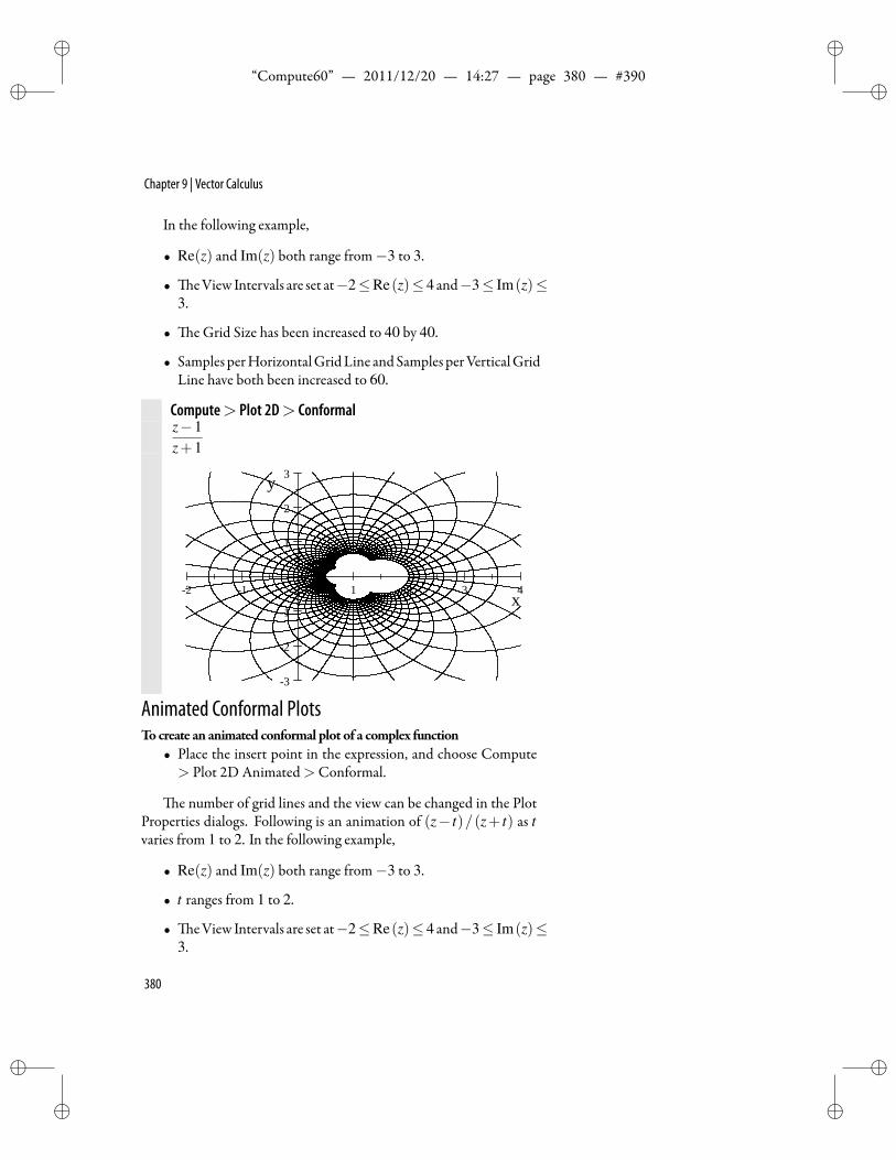
ii
“Compute60” — 2011/12/20 — 14:27 — page 380 — #390 ii
ii
ii
Chapter 9 | Vector Calculus
In the following example,
• Re(z) and Im(z) both range from−3 to 3.
• eView Intervals are set at−2≤Re(z)≤ 4 and−3≤ Im(z)≤3.
• e Grid Size has been increased to 40 by 40.
• Samples perHorizontalGridLine andSamples perVerticalGridLine have both been increased to 60.
Compute> Plot 2D> Conformalz−1z+1
2 1 1 2 3 4
3
2
1
1
2
3
x
y
Animated Conformal PlotsTocreate an animated conformal plot of a complex function
• Place the insert point in the expression, and choose Compute> Plot 2D Animated>Conformal.
e number of grid lines and the view can be changed in the PlotProperties dialogs. Following is an animation of (z− t)/(z+ t) as tvaries from 1 to 2. In the following example,
• Re(z) and Im(z) both range from−3 to 3.
• t ranges from 1 to 2.
• eView Intervals are set at−2≤Re(z)≤ 4 and−3≤ Im(z)≤3.
380
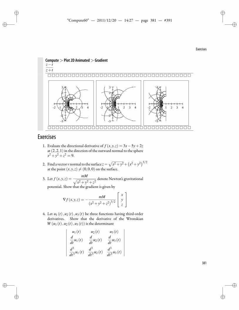
ii
“Compute60” — 2011/12/20 — 14:27 — page 381 — #391 ii
ii
ii
Exercises
Compute> Plot 2D Animated> Gradientz− tz+ t
2 1 1 2 3 4
3
2
1
1
2
3
2 1 1 2 3 4
3
2
1
1
2
3
2 1 1 2 3 4
3
2
1
1
2
3
Exercises1. Evaluate the directional derivative of f (x,y,z) = 3x−5y+2z
at (2,2,1) in the direction of the outward normal to the spherex2 + y2 + z2 = 9.
2. Find a vectorvnormal to the surface z=√
x2 + y2+(x2 + y2
)3/2
at the point (x,y,z) = (0,0,0) on the surface.
3. Let f (x,y,z) =mM√
x2 + y2 + z2denote Newton’s gravitational
potential. Show that the gradient is given by
∇ f (x,y,z) =− mM
(x2 + y2 + z2)3/2
xyz
4. Let u1 (t) ,u2 (t) ,u3 (t) be three functions having third-order
derivatives. Show that the derivative of the WronskianW (u1 (t) ,u2 (t) ,u3 (t)) is the determinant∣∣∣∣∣∣∣∣∣∣∣
u1 (t) u2 (t) u3 (t)ddt
u1 (t)ddt
u2 (t)ddt
u3 (t)
d3
dt3 u1 (t)d3
dt3 u2 (t)d3
dt3 u3 (t)
∣∣∣∣∣∣∣∣∣∣∣381
ii
“Compute60” — 2011/12/20 — 14:27 — page 382 — #392 ii
ii
ii
Chapter 9 | Vector Calculus
In other words, the derivative of W (u1 (t) ,u2 (t) ,u3 (t)) maybe obtained by rst differentiating the elements in the last rowof theWronskianmatrix of (u1 (t) ,u2 (t) ,u3 (t)) and then tak-ing the derivative of the resulting matrix.
5. Starting with the function f (x,y) = sinxy, observe connec-tions between the surface z = f (x,y), the gradient of f (x,y),and the vector eld of ∇ f (x,y).
6. Observe the vector eldof (sinxy,cosxy) anddescribe the ow.Is there a function g(x,y) whose gradient is (sinxy,cosxy)?
Solutions1. e directional derivative is givenbyDu f (x,y,z))=∇ f (x,y,z)·
u, where u is a unit vector in the direction of the outward nor-mal to the sphere x2 + y2 + z2 = 9. e vector
∇(x2 + y2 + z2)=
2x2y2z
is normal to the sphere x2 + y2 + z2 = 9, and at (2,2,1) thisnormal is (4,4,2). A unit vector in the same direction is givenby
u =
442
÷∥∥∥∥∥∥ 4
42
∥∥∥∥∥∥= 16
442
=
2/32/31/3
Hence, ∇ f (x,y,z) ·u evaluated at (2,2,1) is− 2
3 .
2. A normal vector is given by
∇(√
x2 + y2 +(x2 + y2)3/2− z
)=
x√
x2+y2+3x
√x2 + y2
y√x2+y2
+3y√
x2 + y2
−1
=
1√(x2 + y2)
(x(1+3x2 +3y2) ,y(1+3x2 +3y2) ,−√(x2 + y2)
)Hence, any scalar multiple of[
x(1+3x2 +3y2) ,y(1+3x2 +3y2) ,−√(x2 + y2)
]382
ii
“Compute60” — 2011/12/20 — 14:27 — page 383 — #393 ii
ii
ii
Exercises
is also normal to the given surface.
3. Evaluate the expression
∇
(mM√
x2 + y2 + z2
)=
−Mm x
(x2+y2+z2)32
−Mm y
(x2+y2+z2)32
−Mm z
(x2+y2+z2)32
=− mM
(x2 + y2 + z2)3/2
xyz
is gives the Newtonian gravitational force between two ob-jects of masses m and M, with one object at the origin and theother at the point (x,y,z).
4. Evaluate each of ddt
∣∣∣∣∣∣∣u1 (t) u2 (t) u3 (t)
ddt u1 (t) d
dt u2 (t) ddt u3 (t)
d2
dt2 u1 (t) d2
dt2 u2 (t) d2
dt2 u3 (t)
∣∣∣∣∣∣∣ and
∣∣∣∣∣∣∣u1 (t) u2 (t) u3 (t)
ddt u1 (t) d
dt u2 (t) ddt u3 (t)
d3
dt3 u1 (t) d3
dt3 u2 (t) d3
dt3 u3 (t)
∣∣∣∣∣∣∣. Each gives
u1 (t)∂u2 (t)
∂ t∂ 3u3 (t)
∂ t3 −u1 (t)∂u3 (t)
∂ t∂ 3u2 (t)
∂ t3 − ∂u1 (t)∂ t
u2 (t)∂ 3u3 (t)
∂ t3
+∂u1 (t)
∂ tu3 (t)
∂ 3u2 (t)∂ t3 +
∂ 3u1 (t)∂ t3 u2 (t)
∂u3 (t)∂ t
− ∂ 3u1 (t)∂ t3 u3 (t)
∂u2 (t)∂ t
.
5. e surface z= sinxy has ridges along the hyperbolas xy= π2 +
2nπ and valleys along the hyperbolas xy= 3π2 +2nπ in the rst
quadrant. e gradient ∇sinxy = (ycosxy,xcosxy) producesa vector eld whose vectors show the steepness of the surfacez= sinxy. Note that plotting the gradient of f (x,y) is the sameas plotting the vector eld of ∇ f (x,y). e ridges and valleysare indicated by vectors of zero length.
383
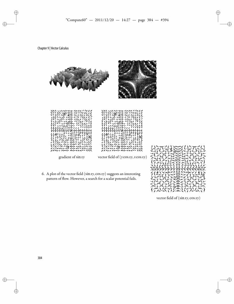
ii
“Compute60” — 2011/12/20 — 14:27 — page 384 — #394 ii
ii
ii
Chapter 9 | Vector Calculus
41
2
x
z10
24
02 2
y4
4 2
40
4
y
4
224 z
x20
4 2 2 4
4
2
2
4
x
y
gradient of sinxy
4 2 2 4
4
2
2
4
x
y
vector eld of (ycosxy,xcosxy)
6. A plot of the vector eld (sinxy,cosxy) suggests an interestingpattern of ow. However, a search for a scalar potential fails.
4 2 2 4
4
2
2
4
x
y
vector eld of (sinxy,cosxy)
384
ii
“Compute60” — 2011/12/20 — 14:27 — page 385 — #395 ii
ii
ii
10Differential Equations
Everything should be made as simple as possible, but not simpler. Albert Einstein (1879–1955)
A differential equation is an equation that includes differen- Ordinary Differential Equations
Systems
Numerical Methods
tials or derivatives of an unknown function. A solution to adifferential equation is any function that satis es the given
equation. us f (x) = sinx is a solution to the differential equationy′′+y = 0, because if y = sinx, then y′ = cosx and y′′ =−sinx, andhence y′′+ y = sinx− sinx = 0. Differential equations are encoun-tered in the study of problems in both pure and applied mathematics,in the sciences, in engineering, and in business and the social sciences.
Ordinary Differential EquationsWith the choices on the Solve ODE submenu you will be able to
nd closed-form solutions to many differential equations. e solu-tion is generally returned as an equation in y(x) and x (or whatevervariables were speci ed) with any arbitrary constants represented asC1,C2, ...,Cn.To solve a differential equation
1. Type the differential equation using standardmathematical no-tation.
2. With the insert point in the equation, chooseCompute>SolveODE> Exact, Laplace, Numeric, or Series.
385
ii
“Compute60” — 2011/12/20 — 14:27 — page 386 — #396 ii
ii
ii
Chapter 10 | Differential Equations
To solve a differential equationwith initial condition(s)1. Place the differential equation in a one-column matrix or in a
display, with initial condition(s) in separate rows.
2. Place the insert point in the equation and, choose Compute>Solve ODE>Numeric.
ese different choices are explained inmore detail in the next fewsections.
Exact SolutionsTwo methods, Exact and Laplace, return exact solutions to a lin-
ear differential equation. Laplace, which as its name suggests, uses theLaplace transform to derive solutions, works for either homogeneousor nonhomogeneous linear differential equations with constant coef-cients. Initial conditions are displayed in the solution. Exact is more
general in the sense that is works for some nonlinear differential equa-tions as well.
Exact MethodTo solve a differential equationby theExactmethod
1. Place the insert point in the differential equation.
2. Choose Compute> Solve ODE> Exact.
When a notation is used for differentiation that names the inde-pendent variable, the variable is taken from context.
Compute> Solve ODE> Exactdydx = xyODE Solution:
C1e
12 x2
To check this result, de ne y(x) = e12 x2
C1. Replace y by y(x) inthe differential equation and evaluate both sides.
Compute> Evaluatedy(x)
dx = xC1e12 x2
xy(x) = xC1e12 x2
For any given number C1, the solution describes a curve. SinceC1 may, in general, take on in nitely many values, there is an in -nite family of solution curves—or a one-parameter family of solutioncurves—for this equation.
When a prime indicates differentiation, the independent variablewill be named if it is unambiguous; otherwise, a variable name must
386
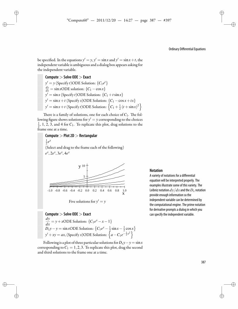
ii
“Compute60” — 2011/12/20 — 14:27 — page 387 — #397 ii
ii
ii
Ordinary Differential Equations
be speci ed. In the equations y′ = y, y′ = sinx and y′ = sinx+ t , theindependent variable is ambiguous and a dialog box appears asking forthe independent variable.
Compute> Solve ODE> Exacty′ = y (Specify t)ODE Solution: C1etdydx = sinxODE solution: C1− cosxy′ = sinx (Specify t)ODE Solution: C1 + t sinxy′ = sinx+ t (Specify x)ODE Solution: C1− cosx+ txy′ = sinx+ t (Specify t)ODE Solution:
C1 +
12 (t + sinx)2
ere is a family of solutions, one for each choice of C1. e fol-
lowing gure shows solutions for y′ = y corresponding to the choices12 , 1, 2, 3, and 4 for C1. To replicate this plot, drag solutions to theframe one at a time.
Compute> Plot 2D> Rectangular12 ex
(Select and drag to the frame each of the following)ex, 2ex, 3ex, 4ex
1.0 0.8 0.6 0.4 0.2 0.0 0.2 0.4 0.6 0.8 1.0
5
10
x
y
Five solutions for y′ = y
NotationA variety of notations for a differentialequation will be interpreted properly. Theexamples illustrate some of this variety. TheLeibniz notationdy/dx and theDx notationprovide enough information so theindependent variable can be determined bythe computational engine. The prime notationfor derivative prompts a dialog in which youcan specify the independent variable.Compute> Solve ODE> Exact
dydx
= y+ xODE Solution: C1ex− x−1
Dxy− y = sinxODE Solution:
C1ex− 12 sinx− 1
2 cosx
y′+ xy = ax, (Specify x)ODE Solution:
a−C1e−12 x2
Following is a plot of three particular solutions forDxy−y= sinxcorresponding to C1 = 1,2,3. To replicate this plot, drag the secondand third solutions to the frame one at a time.
387

ii
“Compute60” — 2011/12/20 — 14:27 — page 388 — #398 ii
ii
ii
Chapter 10 | Differential Equations
Compute> Plot 2D> Rectangularex− 1
2 cosx− 12 sinx
2ex− 12 cosx− 1
2 sinx (Select and drag to the frame)3ex− 1
2 cosx− 12 sinx (Select and drag to the frame)
1.0 0.8 0.6 0.4 0.2 0.0 0.2 0.4 0.6 0.8 1.0
2
4
6
x
y
ree solutions for Dx y− y = sinx
TipThe three solutions can be distinguished byevaluation at 0. For example, the solutionwithC1 = 1 crosses the y-axis at y = 1/2.
Compute> Solve ODE> Exacty′′+ y = x2 (specify x), ODE solution:
x2−C1 sinx+C2 cosx−2
e following plot shows three solutions generatedwith constants
(C1,C2) = (1,1), (C1,C2) = (5,1), and (C1,C2) = (1,5). To repli-cate this plot, drag the second and third solutions to the frame one ata time.
Compute> Plot 2D> Rectangularsinx+ cosx+ x2−25sinx+ cosx+ x2−2 (Select and drag to the frame)sinx+5cosx+ x2−2 (Select and drag to the frame)
3 2 1 1 2 3 4
5
5
10
x
y
ree solutions to y ′′+ y = x2
TipThe particular solutiony(x) = sinx+5cosx+ x2−2 is theone whose graph crosses the y-axis at y = 3.
388
ii
“Compute60” — 2011/12/20 — 14:27 — page 389 — #399 ii
ii
ii
Ordinary Differential Equations
Compute> Solve ODE> Exactxy′− y = x2 (specify x), ODE solution:
x2 +C1x
d2ydx2 +
dydx = x+ y, ODE solution:
C1e−x( 1
2√
5+ 12)− x+C1ex( 1
2√
5− 12)−1
Laplace Method
Laplace transforms solve eitherhomogeneousornonhomogeneouslinear systems in which the coefficients are all constants. Initial con-ditions appear explicitly in the solution.To solve a differential equationby theLaplacemethod
• Place the insert point in the differential equation and chooseCompute> Solve ODE> Laplace.
Compute> Solve ODE> Laplacedydx
= y, ODE Solution (Laplace): C1ex
y′+ y = x+ sinx, (Specify x), ODE Solution (Laplace)x− 1
2 cosx+ 12 sinx+C1e−x−1
e following examples compare exact and Laplace solutions. In
each case, the ODE Independent Variable is x.
Compute> Solve ODE> Exacty′ = sinx, ODE Solution: C1− cosxy′ = y+ x, ODE Solution: C1ex− x−1Dxy = cosx, ODE Solution: C1 + sinx
Compute> Solve ODE> Laplacey′ = sinx, ODE Solution (Laplace): C2− cosxy′ = y+ x, ODE Solution (Laplace): −x−1,C1ex− x−1Dxy = cosx, ODE Solution (Laplace): C1 + sinx
Series SolutionsFor many applications requiring a solution to a differential equa-
tion, a few terms of a Taylor series solution are sufficient.To nd aTaylor series solution to a differential equation
1. Type the differential equation in standard mathematical nota-tion.
2. With the insert point in the equation, chooseCompute>SolveODE> Series.
389
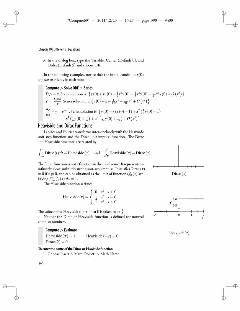
ii
“Compute60” — 2011/12/20 — 14:27 — page 390 — #400 ii
ii
ii
Chapter 10 | Differential Equations
3. In the dialog box, type the Variable, Center (Default 0), andOrder (Default 5) and choose OK.
In the following examples, notice that the initial condition y(0)appears explicitly in each solution.
Compute> Solve ODE> SeriesDxy = y, Series solution is:
y(0)+ xy(0)+ 1
2 x2y(0)+ 16 x3y(0)+ 1
24 x4y(0)+O(x5)
y′ =sinx
x, Series solution is:
y(0)+ x− 1
18 x3 + 1600 x5 +O
(x7)
dydx
+ y = e−x2, Series solution is:
y(0)− x(y(0)−1)+ x2
( 12 y(0)− 1
2
)−x3
( 16 y(0)+ 1
6
)+ x4
( 124 y(0)+ 1
24
)+O
(x5)
Heaviside and Dirac FunctionsLaplace and Fourier transforms interact closely with theHeaviside
unit-step function and the Dirac unit-impulse function. e Diracand Heaviside functions are related by∫ x
−∞Dirac(t)dt =Heaviside(x) and
ddx
Heaviside(x)=Dirac(x)
eDirac function is not a function in the usual sense. It represents anin nitely short, in nitely strongunit-area impulse. It satis esDirac(x)= 0 if x = 0, and can be obtained as the limit of functions fn (x) sat-isfying
∫ ∞−∞ fn (x) dx = 1.
Dirac(x)
e Heaviside function satis es
Heaviside(x) =
0 if x < 012 if x = 01 if x > 0
e value of the Heaviside function at 0 is taken to be 12 .
Neither the Dirac or Heaviside function is de ned for nonrealcomplex numbers.
2 1 0 1 2
0.5
1.0
x
y
Heaviside(x)Compute> EvaluateHeaviside(π) = 1 Heaviside(−e) = 0Dirac(2) = 0
Toenter the nameof theDirac orHeaviside function1. Choose Insert>Math Objects>Math Name.
390
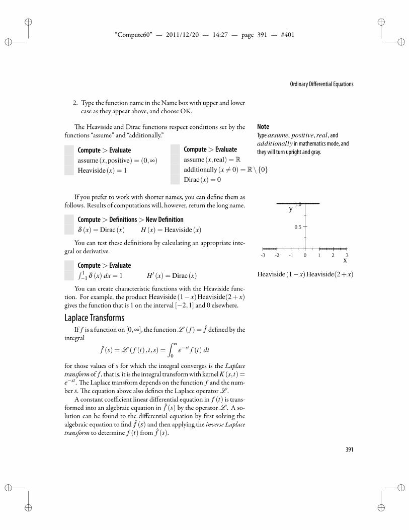
ii
“Compute60” — 2011/12/20 — 14:27 — page 391 — #401 ii
ii
ii
Ordinary Differential Equations
2. Type the function name in theName box with upper and lowercase as they appear above, and choose OK.
e Heaviside and Dirac functions respect conditions set by the NoteType assume, positive, real, andadditionally in mathematics mode, andthey will turn upright and gray.
functions “assume” and “additionally.”
Compute> Evaluateassume(x,positive) = (0,∞)
Heaviside(x) = 1
Compute> Evaluateassume(x, real) = Radditionally(x = 0) = R\0Dirac(x) = 0
If you prefer to work with shorter names, you can de ne them asfollows. Results of computations will, however, return the long name.
Compute> De nitions> New De nitionδ (x) = Dirac(x) H (x) = Heaviside(x)
You can test these de nitions by calculating an appropriate inte-gral or derivative.
Compute> Evaluate∫ 1−1 δ (x) dx = 1 H ′ (x) = Dirac(x)
3 2 1 0 1 2 3
0.5
1.0
x
y
Heaviside(1− x)Heaviside(2+ x)
You can create characteristic functions with the Heaviside func-tion. For example, the product Heaviside(1− x)Heaviside(2+ x)gives the function that is 1 on the interval [−2,1] and 0 elsewhere.
Laplace TransformsIf f is a function on [0,∞], the functionL ( f ) = f de ned by the
integral
f (s) = L ( f (t) , t,s) =∫ ∞
0e−st f (t) dt
for those values of s for which the integral converges is the Laplacetransformof f , that is, it is the integral transformwithkernelK (s, t)=e−st . e Laplace transform depends on the function f and the num-ber s. e equation above also de nes the Laplace operator L .
A constant coefficient linear differential equation in f (t) is trans-formed into an algebraic equation in f (s) by the operator L . A so-lution can be found to the differential equation by rst solving thealgebraic equation to nd f (s) and then applying the in erse Laplacetransform to determine f (t) from f (s).
391
ii
“Compute60” — 2011/12/20 — 14:27 — page 392 — #402 ii
ii
ii
Chapter 10 | Differential Equations
Expressions involving exponentials, polynomials, trigonometrics(sin, cos, sinh, cosh) with linear arguments, and Bessel functions(BesselJ, BesselI) with linear arguments can be transformed.
e Laplace transform also recognizes derivatives and integrals,the Heaviside unit-step function Heaviside(x), and the Dirac-deltaunit impulse function Dirac(x).
Computing Laplace TransformsTocompute theLaplace transformof an expression
• With the insert point in the expression, choose Compute >Transforms> Laplace.
Compute> Transforms> Laplacet , Laplace Transform is: 1
s2
t3/2− et + sinhat , Laplace Transform is: 3√
π4s5/2 − a
a2−s2 − 1s−1
You can also compute a Laplace transform using the symbol L .Tocompute aLaplace transformusing the symbolL
1. From the Miscellaneous Symbols panel, choose L .
2. Choose Insert>Math Objects> Brackets.
3. Click ( , and choose OK.
4. Inside the parentheses, type an expression in the variable t .
5. Choose Compute> Evaluate. TipThe default variable of integration is t and thedefault transform variable is s. The computingengine evaluates a Laplace transform with t asinput variable and produces a solution usingthe variable s.
Compute> Evaluate
L (t) = 1s2 L
(t3)= 6
s4 L (3sin t) = 3s2+1
To compute the Laplace transform of an expression E with variable of inte-gration x and transformvariable y
1. Place the insert point in L (E,x,y).
2. Choose Compute> Evaluate.
You can use other variable names by specifying the variable of in-tegration and the transform variable as in the following examples.
Compute> EvaluateL (x,x,y) = 1
y2 L(x3,x,s
)= 6
s4 L(e2πw,w,u
)=− 1
2π−u
392
ii
“Compute60” — 2011/12/20 — 14:27 — page 393 — #403 ii
ii
ii
Ordinary Differential Equations
Computing Inverse Laplace TransformsTocompute the inverseLaplace transformof an expression
1. Place the insert point in the expression.
2. Choose Compute>Transforms> Inverse Laplace.
Compute> Transforms> Inverse Laplace2s3 , Is Laplace Transform of t2
1s+α , Is Laplace Transform of e−at
1, Is Laplace Transform of Dirac(t)TipThe default variable for the inverse transformis s, and the default output variable is t . Theinverse Laplace transform will interpretcorrectly an expression with the variable s asinput.
You can also compute an inverse Laplace transform by evaluatingan expression of the form L −1 ( f (s)).
Tocompute an inverseLaplace transformusing the symbolL• With the insert point in the expression L −1 ( f (s)), choose
Compute> Evaluate.
Compute> EvaluateL −1
(1s2
)= t L −1
(6s4
)= t3 L −1
(3
s2+1
)= 3sin t
For other variable names, the variable of integration and the trans-form variable must be speci ed, as in the following examples.
Compute> EvaluateL −1
(2s3 ,s,x
)= x2 L −1
( 1x+α ,x,y
)= e−αy L −1 (1,a,b) = Dirac(b)
If the range of parameters must be restricted, use the functions as-sume and additionally.
e following two examples demonstrate the use of the Laplacetransform to solve a differential equation.
Example In order to solve the problem
f ′ (t)+a f (t) = 0, f (0) = b
de ne f (t) as a generic function and a and b as generic constants.en evaluate both sides of the equation:
L(
f ′ (t)+a f (t))= L (0)
393
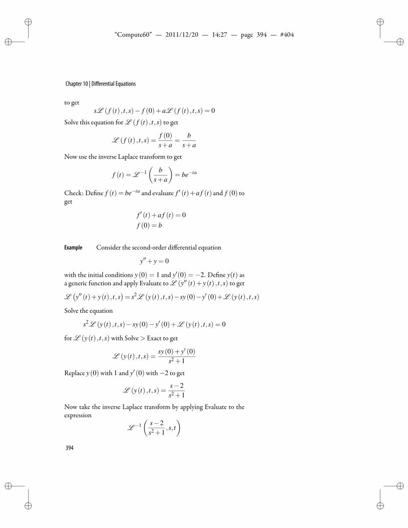
ii
“Compute60” — 2011/12/20 — 14:27 — page 394 — #404 ii
ii
ii
Chapter 10 | Differential Equations
to getsL ( f (t) , t,s)− f (0)+aL ( f (t) , t,s) = 0
Solve this equation for L ( f (t) , t,s) to get
L ( f (t) , t,s) =f (0)s+a
=b
s+a
Now use the inverse Laplace transform to get
f (t) = L −1(
bs+a
)= be−ta
Check: De ne f (t) = be−ta and evaluate f ′ (t)+a f (t) and f (0) toget
f ′ (t)+a f (t) = 0f (0) = b
Example Consider the second-order differential equation
y′′+ y = 0
with the initial conditions y(0) = 1 and y′(0) = −2. De ne y(t) asa generic function and apply Evaluate to L (y′′ (t)+ y(t) , t,s) to get
L(y′′ (t)+ y(t) , t,s
)= s2L (y(t) , t,s)−sy(0)−y′ (0)+L (y(t) , t,s)
Solve the equation
s2L (y(t) , t,s)− sy(0)− y′ (0)+L (y(t) , t,s) = 0
for L (y(t) , t,s) with Solve> Exact to get
L (y(t) , t,s) =sy(0)+ y′ (0)
s2 +1
Replace y(0) with 1 and y′ (0) with−2 to get
L (y(t) , t,s) =s−2s2 +1
Now take the inverse Laplace transform by applying Evaluate to theexpression
L −1(
s−2s2 +1
,s, t)
394
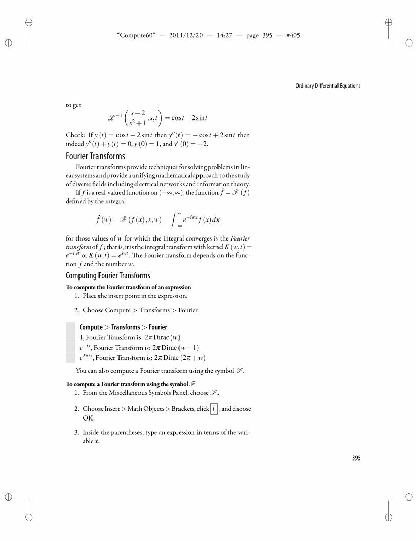
ii
“Compute60” — 2011/12/20 — 14:27 — page 395 — #405 ii
ii
ii
Ordinary Differential Equations
to get
L −1(
s−2s2 +1
,s, t)= cos t−2sin t
Check: If y(t) = cos t − 2sin t then y′′(t) = −cos t + 2sin t thenindeed y′′(t)+ y(t) = 0, y(0) = 1, and y′ (0) =−2.
Fourier TransformsFourier transforms provide techniques for solving problems in lin-
ear systems andprovide aunifyingmathematical approach to the studyof diverse elds including electrical networks and information theory.
If f is a real-valued function on (−∞,∞), the function f =F ( f )de ned by the integral
f (w) = F ( f (x) ,x,w) =∫ ∞
−∞e−iwx f (x)dx
for those values of w for which the integral converges is the Fouriertransformof f ; that is, it is the integral transformwithkernelK (w, t)=e−iwt or K (w, t) = eiwt . e Fourier transform depends on the func-tion f and the number w.
Computing Fourier TransformsTocompute theFourier transformof an expression
1. Place the insert point in the expression.
2. Choose Compute>Transforms> Fourier.
Compute> Transforms> Fourier1, Fourier Transform is: 2π Dirac(w)e−ix, Fourier Transform is: 2π Dirac(w−1)e2πix, Fourier Transform is: 2π Dirac(2π +w)
You can also compute a Fourier transform using the symbol F .
Tocompute a Fourier transformusing the symbolF1. From the Miscellaneous Symbols Panel, choose F .
2. Choose Insert>MathObjects>Brackets, click ( , and chooseOK.
3. Inside the parentheses, type an expression in terms of the vari-able x.
395
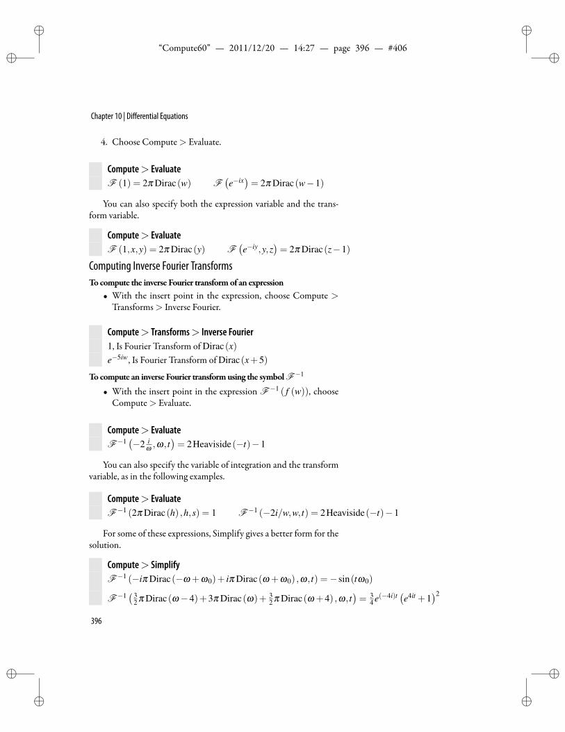
ii
“Compute60” — 2011/12/20 — 14:27 — page 396 — #406 ii
ii
ii
Chapter 10 | Differential Equations
4. Choose Compute> Evaluate.
Compute> EvaluateF (1) = 2π Dirac(w) F
(e−ix
)= 2π Dirac(w−1)
You can also specify both the expression variable and the trans-form variable.
Compute> EvaluateF (1,x,y) = 2π Dirac(y) F
(e−iy,y,z
)= 2π Dirac(z−1)
Computing Inverse Fourier TransformsTocompute the inverse Fourier transformof an expression
• With the insert point in the expression, choose Compute >Transforms> Inverse Fourier.
Compute> Transforms> Inverse Fourier1, Is Fourier Transform of Dirac(x)e−5iw, Is Fourier Transform of Dirac(x+5)
Tocompute an inverse Fourier transformusing the symbolF−1
• With the insert point in the expression F−1 ( f (w)), chooseCompute> Evaluate.
Compute> EvaluateF−1
(−2 i
ω ,ω, t)= 2Heaviside(−t)−1
You can also specify the variable of integration and the transformvariable, as in the following examples.
Compute> EvaluateF−1 (2π Dirac(h) ,h,s) = 1 F−1 (−2i/w,w, t) = 2Heaviside(−t)−1
For some of these expressions, Simplify gives a better form for thesolution.
Compute> SimplifyF−1 (−iπ Dirac(−ω +ω0)+ iπ Dirac(ω +ω0) ,ω , t) =−sin(tω0)
F−1( 3
2 π Dirac(ω−4)+3π Dirac(ω)+ 32 π Dirac(ω +4) ,ω, t
)= 3
4 e(−4i)t(e4it +1
)2
396
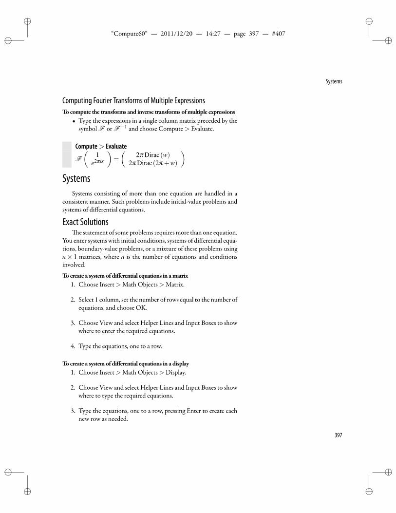
ii
“Compute60” — 2011/12/20 — 14:27 — page 397 — #407 ii
ii
ii
Systems
Computing Fourier Transforms of Multiple ExpressionsTocompute the transforms and inverse transformsofmultiple expressions
• Type the expressions in a single column matrix preceded by thesymbol F or F−1 and choose Compute> Evaluate.
Compute> Evaluate
F
(1
e2πix
)=
(2π Dirac(w)
2π Dirac(2π +w)
)Systems
Systems consisting of more than one equation are handled in aconsistent manner. Such problems include initial-value problems andsystems of differential equations.
Exact Solutionse statement of some problems requiresmore than one equation.
You enter systems with initial conditions, systems of differential equa-tions, boundary-value problems, or a mixture of these problems usingn× 1 matrices, where n is the number of equations and conditionsinvolved.
Tocreate a systemof differential equations in amatrix1. Choose Insert>Math Objects>Matrix.
2. Select 1 column, set the number of rows equal to the number ofequations, and choose OK.
3. Choose View and select Helper Lines and Input Boxes to showwhere to enter the required equations.
4. Type the equations, one to a row.
Tocreate a systemof differential equations in a display1. Choose Insert>Math Objects>Display.
2. Choose View and select Helper Lines and Input Boxes to showwhere to type the required equations.
3. Type the equations, one to a row, pressing Enter to create eachnew row as needed.
397
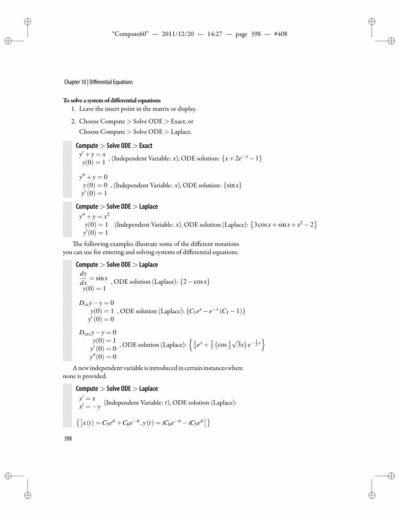
ii
“Compute60” — 2011/12/20 — 14:27 — page 398 — #408 ii
ii
ii
Chapter 10 | Differential Equations
To solve a systemof differential equations1. Leave the insert point in the matrix or display.
2. Choose Compute> Solve ODE> Exact, orChoose Compute> Solve ODE> Laplace.
Compute> Solve ODE> Exacty′+ y = xy(0) = 1 , (Independent Variable: x), ODE solution: x+2e−x−1
y′′+ y = 0y(0) = 0
y′ (0) = 1, (Independent Variable: x), ODE solution: sinx
Compute> Solve ODE> Laplacey′′+ y = x2
y(0) = 1y′(0) = 1
(Independent Variable: x), ODE solution (Laplace):
3cosx+ sinx+ x2−2
e following examples illustrate some of the different notationsyou can use for entering and solving systems of differential equations.
Compute> Solve ODE> Laplacedydx
= sinx
y(0) = 1, ODE solution (Laplace): 2− cosx
Dxxy− y = 0y(0) = 1
y′ (0) = 0, ODE solution (Laplace): C1ex− e−x (C1−1)
Dxxxy− y = 0y(0) = 1
y′ (0) = 0y′′(0) = 0
, ODE solution (Laplace):
13 ex + 2
3
(cos 1
2
√3x)
e−12 x
Anew independent variable is introduced in certain instanceswherenone is provided.
Compute> Solve ODE> Laplacey′ = xx′ =−y (Independent Variable: t), ODE solution (Laplace):
[x(t) =C5eit +C6e−it ,y(t) = iC6e−it − iC5eit
]398
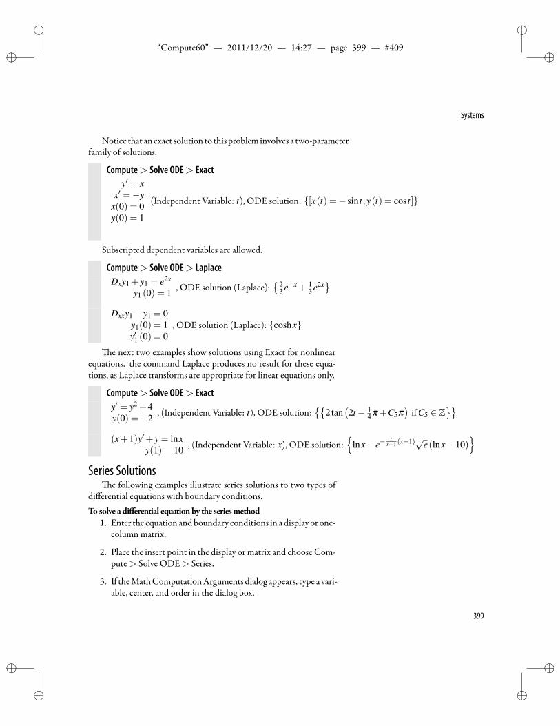
ii
“Compute60” — 2011/12/20 — 14:27 — page 399 — #409 ii
ii
ii
Systems
Notice that an exact solution to this problem involves a two-parameterfamily of solutions.
Compute> Solve ODE> Exacty′ = x
x′ =−yx(0) = 0y(0) = 1
(Independent Variable: t), ODE solution: [x(t) =−sin t,y(t) = cos t]
Subscripted dependent variables are allowed.
Compute> Solve ODE> LaplaceDxy1 + y1 = e2x
y1 (0) = 1 , ODE solution (Laplace): 2
3 e−x + 13 e2x
Dxxy1− y1 = 0
y1(0) = 1y′1 (0) = 0
, ODE solution (Laplace): coshx
e next two examples show solutions using Exact for nonlinearequations. the command Laplace produces no result for these equa-tions, as Laplace transforms are appropriate for linear equations only.
Compute> Solve ODE> Exacty′ = y2 +4y(0) =−2 , (Independent Variable: t), ODE solution:
2tan
(2t− 1
4 π +C5π)
ifC5 ∈ Z
(x+1)y′+ y = lnxy(1) = 10 , (Independent Variable: x), ODE solution:
lnx− e−
tx+1 (x+1)√e(lnx−10)
Series Solutions
e following examples illustrate series solutions to two types ofdifferential equations with boundary conditions.To solve a differential equationby the seriesmethod
1. Enter the equation andboundary conditions in a display or one-column matrix.
2. Place the insert point in the display or matrix and choose Com-pute> Solve ODE> Series.
3. If theMathComputationArguments dialog appears, type a vari-able, center, and order in the dialog box.
399
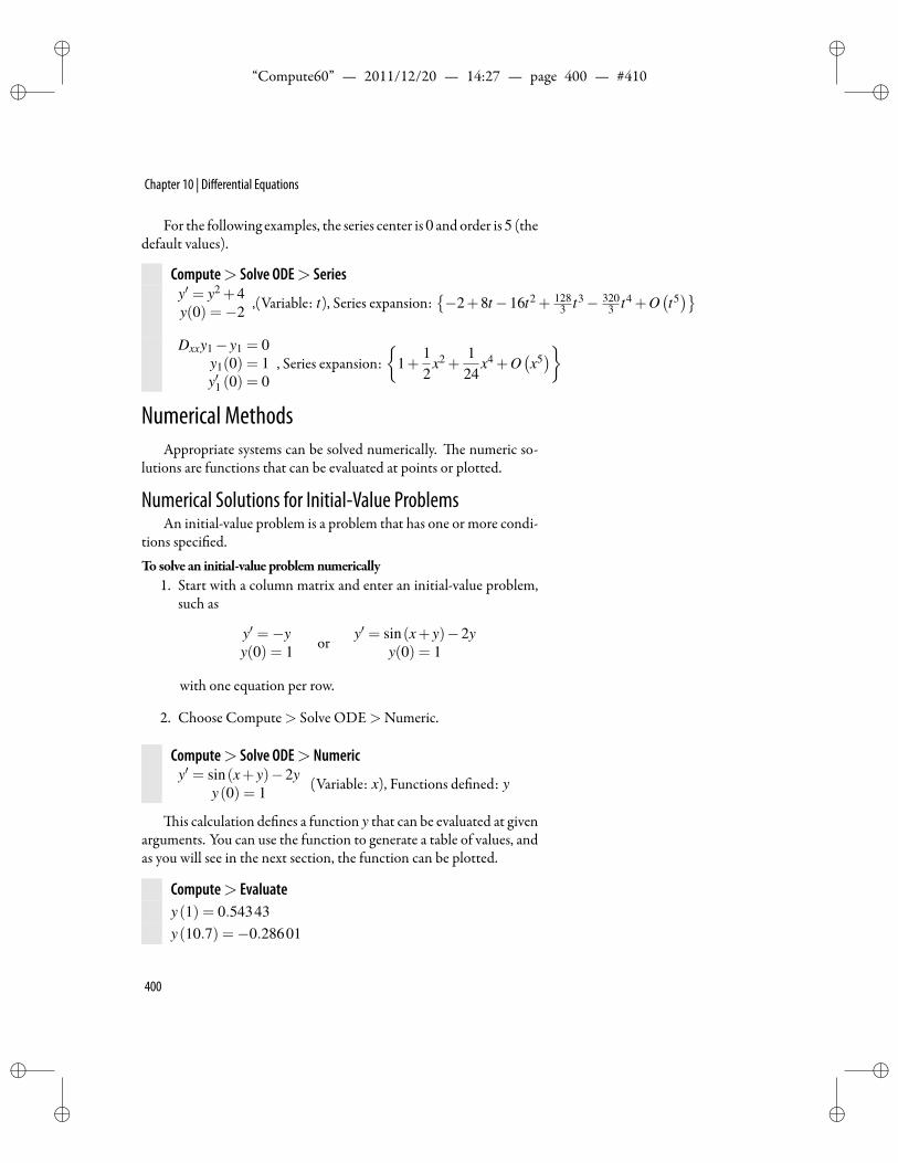
ii
“Compute60” — 2011/12/20 — 14:27 — page 400 — #410 ii
ii
ii
Chapter 10 | Differential Equations
For the following examples, the series center is 0 and order is 5 (thedefault values).
Compute> Solve ODE> Seriesy′ = y2 +4y(0) =−2 ,(Variable: t), Series expansion:
−2+8t−16t2 + 128
3 t3− 3203 t4 +O
(t5)
Dxxy1− y1 = 0y1(0) = 1y′1 (0) = 0
, Series expansion:
1+12
x2 +124
x4 +O(x5)
Numerical MethodsAppropriate systems can be solved numerically. e numeric so-
lutions are functions that can be evaluated at points or plotted.
Numerical Solutions for Initial-Value ProblemsAn initial-value problem is a problem that has one or more condi-
tions speci ed.To solve an initial-value problemnumerically
1. Start with a column matrix and enter an initial-value problem,such as
y′ =−yy(0) = 1 or y′ = sin(x+ y)−2y
y(0) = 1
with one equation per row.
2. Choose Compute> Solve ODE>Numeric.
Compute> Solve ODE> Numericy′ = sin(x+ y)−2y
y(0) = 1 (Variable: x), Functions de ned: y
is calculation de nes a function y that can be evaluated at givenarguments. You can use the function to generate a table of values, andas you will see in the next section, the function can be plotted.
Compute> Evaluatey(1) = 0.54343y(10.7) =−0.28601
400
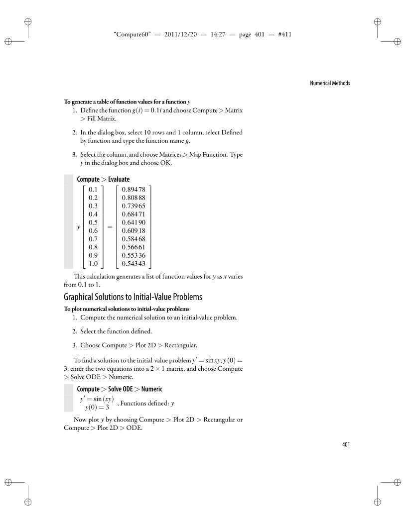
ii
“Compute60” — 2011/12/20 — 14:27 — page 401 — #411 ii
ii
ii
Numerical Methods
Togenerate a table of function values for a function y1. De ne the functiong(i)= 0.1i and chooseCompute>Matrix
> Fill Matrix.
2. In the dialog box, select 10 rows and 1 column, select De nedby function and type the function name g.
3. Select the column, and chooseMatrices>MapFunction. Typey in the dialog box and choose OK.
Compute> Evaluate
y
0.10.20.30.40.50.60.70.80.91.0
=
0.894780.808880.739650.684710.641900.609180.584680.566610.553360.54343
is calculation generates a list of function values for y as x varies
from 0.1 to 1.
Graphical Solutions to Initial-Value ProblemsToplot numerical solutions to initial-value problems
1. Compute the numerical solution to an initial-value problem.
2. Select the function de ned.
3. Choose Compute> Plot 2D> Rectangular.
To nd a solution to the initial-value problem y′ = sinxy, y(0) =3, enter the two equations into a 2× 1 matrix, and choose Compute> Solve ODE>Numeric.
Compute> Solve ODE> Numericy′ = sin(xy)
y(0) = 3 , Functions de ned: y
Now plot y by choosing Compute > Plot 2D > Rectangular orCompute> Plot 2D>ODE.
401
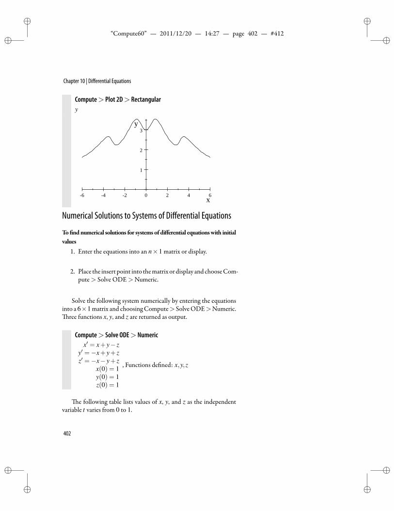
ii
“Compute60” — 2011/12/20 — 14:27 — page 402 — #412 ii
ii
ii
Chapter 10 | Differential Equations
Compute> Plot 2D> Rectangulary
6 4 2 0 2 4 6
1
2
3
x
y
Numerical Solutions to Systems of Differential Equations
To ndnumerical solutions for systemsof differential equationswith initialvalues
1. Enter the equations into an n×1 matrix or display.
2. Place the insert point into thematrix ordisplay and chooseCom-pute> Solve ODE>Numeric.
Solve the following system numerically by entering the equationsinto a 6×1 matrix and choosingCompute> SolveODE>Numeric.
ree functions x, y, and z are returned as output.
Compute> Solve ODE> Numericx′ = x+ y− z
y′ =−x+ y+ zz′ =−x− y+ z
x(0) = 1y(0) = 1z(0) = 1
, Functions de ned: x,y,z
e following table lists values of x, y, and z as the independentvariable t varies from 0 to 1.
402
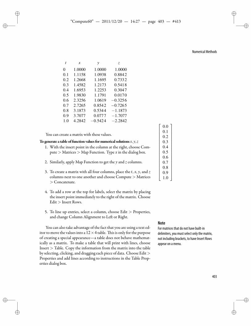
ii
“Compute60” — 2011/12/20 — 14:27 — page 403 — #413 ii
ii
ii
Numerical Methods
t x y z
0 1.0000 1.0000 1.00000.1 1.1158 1.0938 0.88420.2 1.2668 1.1695 0.73320.3 1.4582 1.2173 0.54180.4 1.6953 1.2253 0.30470.5 1.9830 1.1791 0.01700.6 2.3256 1.0619 −0.32560.7 2.7265 0.8542 −0.72650.8 3.1873 0.5344 −1.18730.9 3.7077 0.0777 −1.70771.0 4.2842 −0.5424 −2.2842
You can create a matrix with these values.
Togenerate a table of function values for numerical solutions x,y,z1. With the insert point in the column at the right, choose Com-
pute>Matrices>Map Function. Type x in the dialog box.
0.00.10.20.30.40.50.60.70.80.91.0
2. Similarly, apply Map Function to get the y and z columns.
3. To create a matrix with all four columns, place the t , x, y, and zcolumns next to one another and choose Compute>Matrices>Concatenate.
4. To add a row at the top for labels, select the matrix by placingthe insert point immediately to the right of the matrix. ChooseEdit> Insert Rows.
5. To line up entries, select a column, choose Edit > Properties,and change Column Alignment to Le or Right.
NoteFor matrices that do not have built-indelimiters, you must select only the matrix,not including brackets, to have Insert Rowsappear on a menu.
You can also take advantage of the fact that you are using a text ed-itor tomove the values into a 12×4 table. is is only for the purposeof creating a special appearance—a table does not behave mathemat-ically as a matrix. To make a table that will print with lines, chooseInsert > Table. Copy the information from the matrix into the tableby selecting, clicking, and dragging each piece of data. Choose Edit>Properties and add lines according to instructions in the Table Prop-erties dialog box.
403
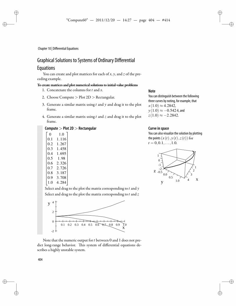
ii
“Compute60” — 2011/12/20 — 14:27 — page 404 — #414 ii
ii
ii
Chapter 10 | Differential Equations
Graphical Solutions to Systems of Ordinary DifferentialEquations
You can create and plot matrices for each of x, y, and z of the pre-ceding example.Tocreatematrices andplot numerical solutions to initial-value problems
1. Concatenate the columns for t and x. NoteYou can distinguish between the followingthree curves by noting, for example, thatx(1.0)≈ 4.2842,y(1.0)≈−0.5424, andz(1.0)≈−2.2842.
2. Choose Compute> Plot 2D> Rectangular.
3. Generate a similar matrix using t and y and drag it to the plotframe.
4. Generate a similar matrix using t and z and drag it to the plotframe.
Compute> Plot 2D> Rectangular
0 1.00.1 1.1160.2 1.2670.3 1.4580.4 1.6950.5 1.980.6 2.3260.7 2.7260.8 3.1870.9 3.7081.0 4.284
Select and drag to the plot the matrix corresponding to t and ySelect and drag to the plot the matrix corresponding to t and z
0.1 0.2 0.3 0.4 0.5 0.6 0.7 0.8 0.9 1.0
2
0
2
4
x
y
Curve in spaceYou can also visualize the solution by plottingthe points (x(t) ,y(t) ,z(t)) fort = 0,0.1, . . . ,1.0.
122
1
x0.5
0.0
0
z3
0.5
1
y 41.0
Note that the numeric output for t between 0 and 1 does not pre-dict long-range behavior. is system of differential equations de-scribes a highly unstable system.
404
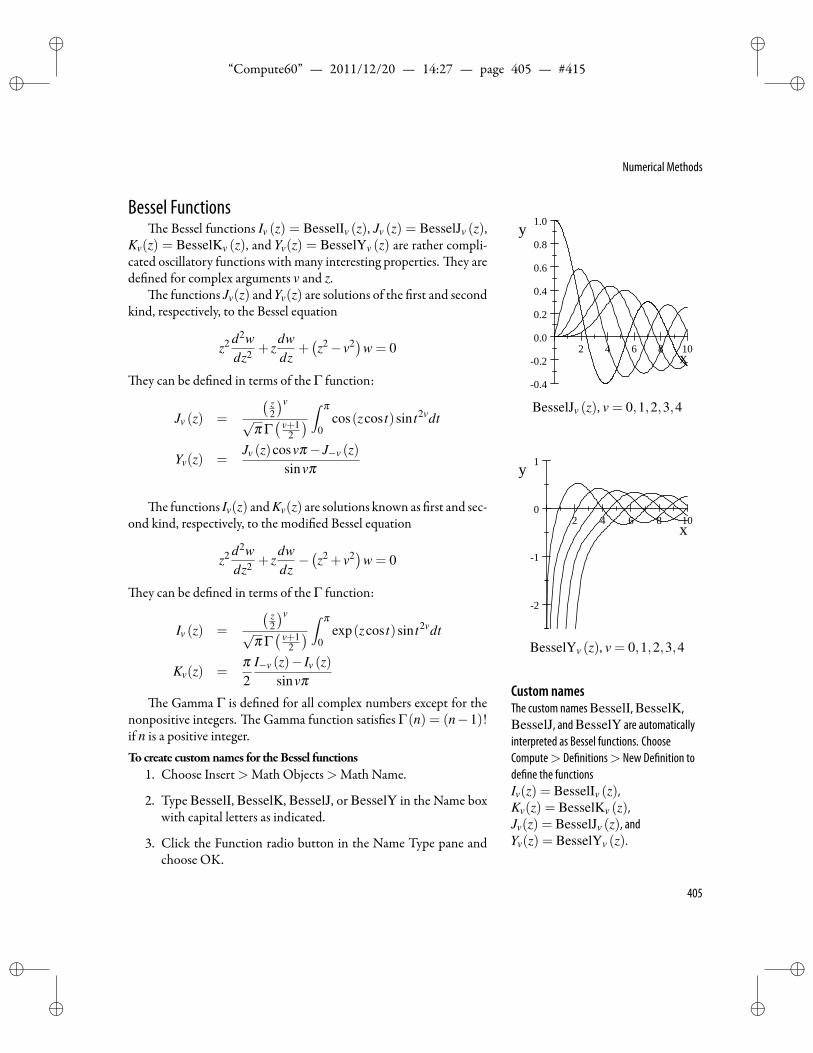
ii
“Compute60” — 2011/12/20 — 14:27 — page 405 — #415 ii
ii
ii
Numerical Methods
Bessel Functionse Bessel functions Iv (z) = BesselIv (z), Jv (z) = BesselJv (z),
Kv(z) = BesselKv (z), and Yv(z) = BesselYv (z) are rather compli-cated oscillatory functions with many interesting properties. ey arede ned for complex arguments v and z.
e functions Jv(z) andYv(z) are solutions of the rst and secondkind, respectively, to the Bessel equation
z2 d2wdz2 + z
dwdz
+(z2− v2)w = 0
ey can be de ned in terms of the Γ function:
2 4 6 8 10
0.4
0.2
0.0
0.2
0.4
0.6
0.8
1.0
x
y
BesselJv (z), v = 0,1,2,3,4
2 4 6 8 10
2
1
0
1
x
y
BesselYv (z), v = 0,1,2,3,4
Jv (z) =
( z2
)v
√π Γ( v+1
2
) ∫ π
0cos(zcos t)sin t2vdt
Yv(z) =Jv (z)cosvπ− J−v (z)
sinvπ
e functions Iv(z) and Kv(z) are solutions known as rst and sec-ond kind, respectively, to the modi ed Bessel equation
z2 d2wdz2 + z
dwdz−(z2 + v2)w = 0
ey can be de ned in terms of the Γ function:
Iv (z) =
( z2
)v
√π Γ( v+1
2
) ∫ π
0exp(zcos t)sin t2vdt
Kv(z) =π2
I−v (z)− Iv (z)sinvπ
Custom namesThe custom namesBesselI,BesselK,BesselJ, andBesselY are automaticallyinterpreted as Bessel functions. ChooseCompute> De nitions> New De nition tode ne the functionsIv(z) = BesselIv (z),Kv(z) = BesselKv (z),Jv(z) = BesselJv (z), andYv(z) = BesselYv (z).
e Gamma Γ is de ned for all complex numbers except for thenonpositive integers. e Gamma function satis es Γ(n) = (n−1)!if n is a positive integer.Tocreate customnames for theBessel functions
1. Choose Insert>Math Objects>Math Name.
2. Type BesselI, BesselK, BesselJ, or BesselY in the Name boxwith capital letters as indicated.
3. Click the Function radio button in the Name Type pane andchoose OK.
405
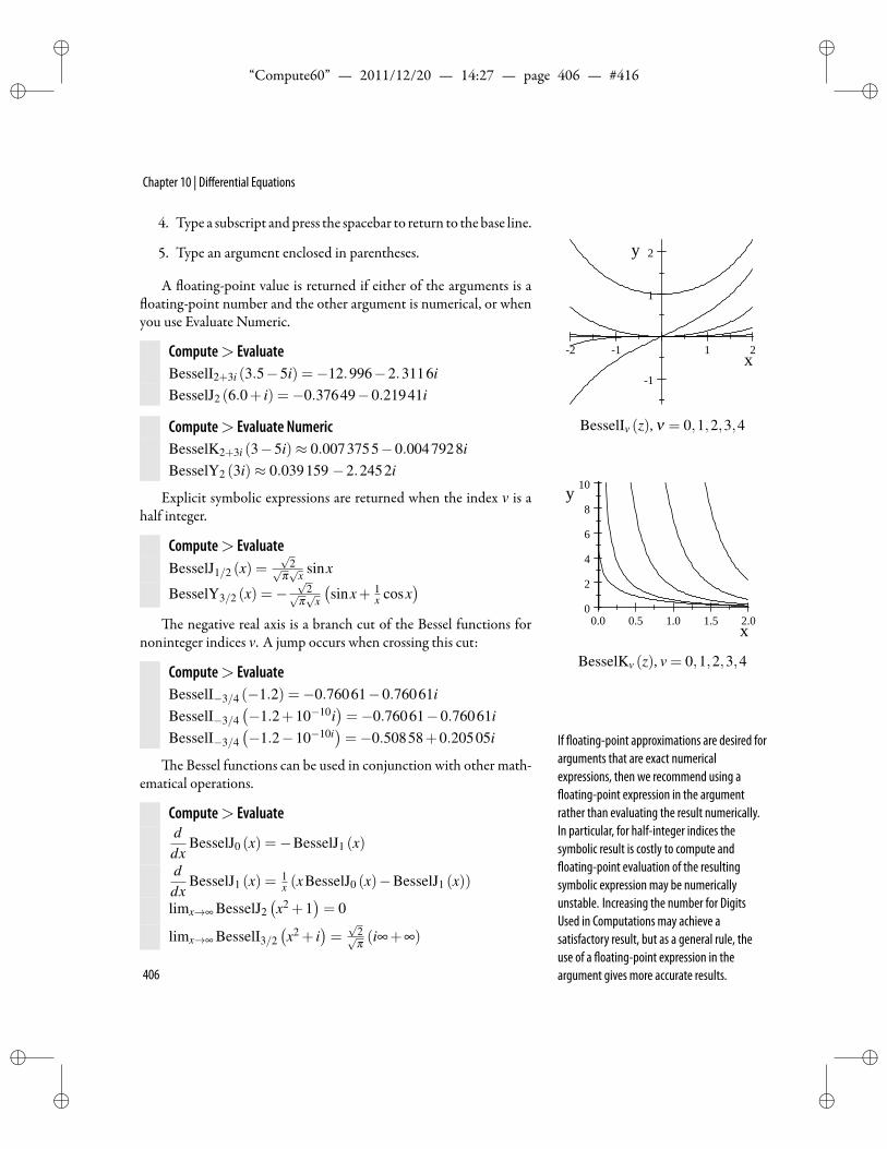
ii
“Compute60” — 2011/12/20 — 14:27 — page 406 — #416 ii
ii
ii
Chapter 10 | Differential Equations
4. Type a subscript andpress the spacebar to return to the base line.
5. Type an argument enclosed in parentheses.
A oating-point value is returned if either of the arguments is aoating-point number and the other argument is numerical, or when
you use Evaluate Numeric.
Compute> EvaluateBesselI2+3i (3.5−5i) =−12.996−2.3116iBesselJ2 (6.0+ i) =−0.37649−0.21941i
2 1 1 2
1
1
2
x
y
BesselIv (z), ν = 0,1,2,3,4
0.0 0.5 1.0 1.5 2.00
2
4
6
8
10
x
y
BesselKv (z), v = 0,1,2,3,4
Compute> Evaluate NumericBesselK2+3i (3−5i)≈ 0.0073755−0.0047928iBesselY2 (3i)≈ 0.039159 −2.2452i
Explicit symbolic expressions are returned when the index v is ahalf integer.
Compute> EvaluateBesselJ1/2 (x) =
√2√
π√
x sinx
BesselY3/2 (x) =−√
2√π√
x
(sinx+ 1
x cosx)
e negative real axis is a branch cut of the Bessel functions fornoninteger indices v. A jump occurs when crossing this cut:
Compute> EvaluateBesselI−3/4 (−1.2) =−0.76061−0.76061iBesselI−3/4
(−1.2+10−10i
)=−0.76061−0.76061i
BesselI−3/4(−1.2−10−10i
)=−0.50858+0.20505i If oating-point approximations are desired for
arguments that are exact numericalexpressions, then we recommend using aoating-point expression in the argumentrather than evaluating the result numerically.In particular, for half-integer indices thesymbolic result is costly to compute andoating-point evaluation of the resultingsymbolic expression may be numericallyunstable. Increasing the number for DigitsUsed in Computations may achieve asatisfactory result, but as a general rule, theuse of a oating-point expression in theargument gives more accurate results.
e Bessel functions can be used in conjunction with other math-ematical operations.
Compute> Evaluateddx
BesselJ0 (x) =−BesselJ1 (x)
ddx
BesselJ1 (x) = 1x (xBesselJ0 (x)−BesselJ1 (x))
limx→∞ BesselJ2(x2 +1
)= 0
limx→∞ BesselI3/2(x2 + i
)=√
2√π (i∞+∞)
406
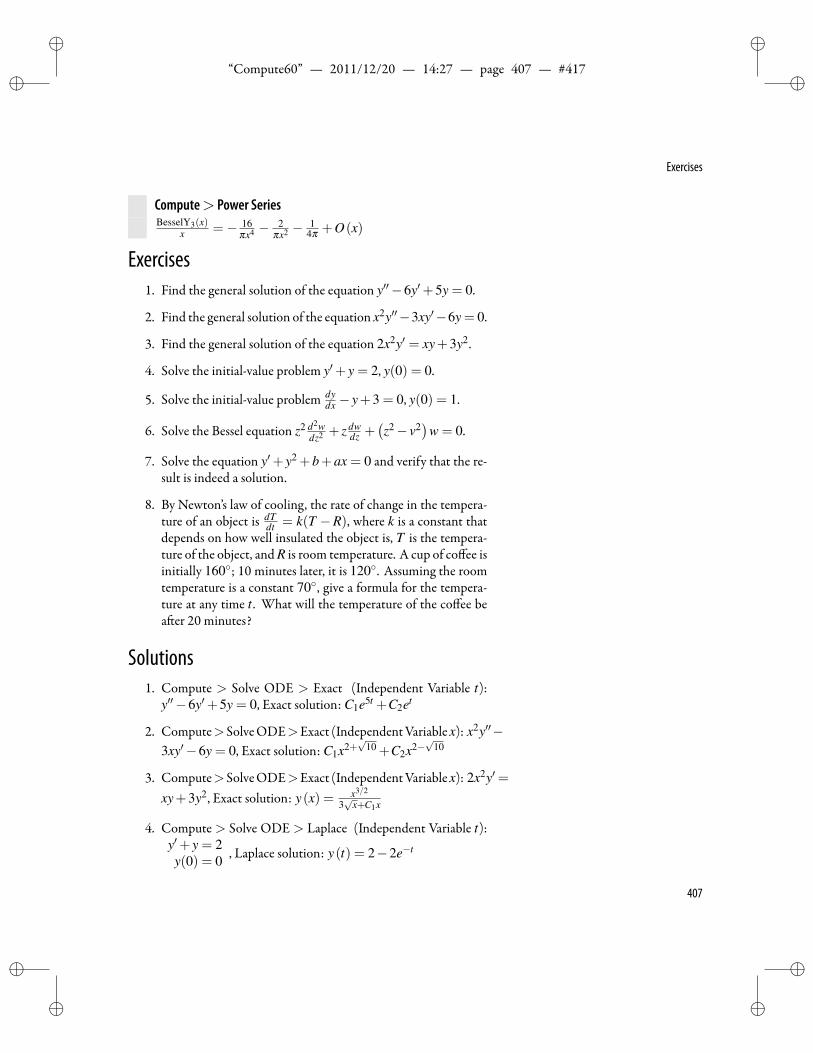
ii
“Compute60” — 2011/12/20 — 14:27 — page 407 — #417 ii
ii
ii
Exercises
Compute> Power SeriesBesselY3(x)
x =− 16πx4 − 2
πx2 − 14π +O(x)
Exercises1. Find the general solution of the equation y′′−6y′+5y = 0.
2. Find the general solution of the equation x2y′′−3xy′−6y = 0.
3. Find the general solution of the equation 2x2y′ = xy+3y2.
4. Solve the initial-value problem y′+ y = 2, y(0) = 0.
5. Solve the initial-value problem dydx − y+3 = 0, y(0) = 1.
6. Solve the Bessel equation z2 d2wdz2 + z dw
dz +(z2− v2
)w = 0.
7. Solve the equation y′+ y2 +b+ax = 0 and verify that the re-sult is indeed a solution.
8. By Newton’s law of cooling, the rate of change in the tempera-ture of an object is dT
dt = k(T −R), where k is a constant thatdepends on how well insulated the object is, T is the tempera-ture of the object, and R is room temperature. A cup of coffee isinitially 160; 10 minutes later, it is 120. Assuming the roomtemperature is a constant 70, give a formula for the tempera-ture at any time t . What will the temperature of the coffee bea er 20 minutes?
Solutions1. Compute > Solve ODE > Exact (Independent Variable t):
y′′−6y′+5y = 0, Exact solution: C1e5t +C2et
2. Compute>SolveODE>Exact (IndependentVariablex): x2y′′−3xy′−6y = 0, Exact solution: C1x2+
√10 +C2x2−
√10
3. Compute>SolveODE>Exact (IndependentVariablex): 2x2y′=xy+3y2, Exact solution: y(x) = x3/2
3√
x+C1x
4. Compute > Solve ODE > Laplace (Independent Variable t):y′+ y = 2y(0) = 0 , Laplace solution: y(t) = 2−2e−t
407
ii
“Compute60” — 2011/12/20 — 14:27 — page 408 — #418 ii
ii
ii
Chapter 10 | Differential Equations
5. Compute > Solve ODE > Exact:dydx − y+3 = 0
y(0) = 1Exact
solution: y(x) = 3−2ex
6. Compute>SolveODE>Exact: z2 d2wdz2 +z dw
dz +(z2− v2
)w=
0, Exact solution: C31 BesselJv (z)+C32 BesselYv (z).
7. Compute> Solve ODE> Exact: y′+ y2 +b+ax = 0, Exact
solution: −C29 AiryAi
(− 1
ab+ax3√
1a,1
)+AiryBi
(− 1
ab+ax3√
1a,1
)
AiryBi
(− 1
ab+ax3√
1a,0
)3√
1a+C29 AiryAi
(− 1
ab+ax3√
1a,0
)3√
1a
r
Compute>De nitions>New De nition: y(x) =
−C29 AiryAi
(− 1
ab+ax3√
1a,1
)+AiryBi
(− 1
ab+ax3√
1a,1
)
AiryBi
(− 1
ab+ax3√
1a,0
)3√
1a+C29 AiryAi
(− 1
ab+ax3√
1a,0
)3√
1a
Compute> Evaluate, Simplify: y′ (x)+y(x)2+b+ax = b−
1a
AiryBi
(− 1
a 3√
1a(b+ax),0
)3√
1a
2 (b+ax)+ 1aC29
AiryAi
− 1
a 3√
1a(b+ax),0
3√
1a
2 (b+ax)
AiryBi
(− 1
a 3√
1a(b+ax),0
)3√
1a+C29 AiryAi
(− 1
a 3√
1a(b+ax),0
)3√
1a
+ax = 0.
8. Compute > Solve ODE > Exact: dTdt = k (T −70), Exact so-
lution: T (t) = 70+ ektC1
Compute > Solve > Exact: 160 =C1e0 +70120 =C1ek10 +70
, Solution:k = 1
10 ln 59 ,C1 = 90
Compute>De nitions>NewDe nition: C1 = 90, k= 1
10 ln 59
Compute>De nitions>NewDe nition: T (t)= 70+ektC1
Compute> Evaluate: T (t) = 90e1
10 t ln 59 +70
Compute> Evaluate Numeric: T (20) = 97.778
408
ii
“Compute60” — 2011/12/20 — 14:27 — page 409 — #419 ii
ii
ii
11Statistics
Statistics: the mathematical theory of ignorance. Morris Kline (1908–1992)
S tatistics is the science and art of obtaining and analyzing quan- Introduction to Statistics
Measures of Central Tendency
Measures of Dispersion
Distributions and Densities
Families of ContinuousDistributions
Families of Discrete Distributions
Random Numbers
Curve Fitting
titative data in order to make sound inferences in the face ofuncertainty. e word statistics is used to refer both to a set of
quantitative data and to a eld of study. e eld includes the devel-opment and application of effective methods for obtaining and usingquantitative data.
Introduction to StatisticsYou can perform statistical operations on data using the various
itemson theStatistics submenu. In addition to themenu items, a num-ber of the standard statistical distribution functions and densities areavailable, either built in or de nable.
e items Mean, Median, Mode, Moment, uantile, Mean De-viation, Standard Deviation, and Variance on the Statistics submenutake a single argument that can be presented as a list of data or as ama-trix. e result of an operation is a number or, in the case of a matrixor vector, a number for each column.
e items Correlation, Covariance, and Fit Curve to Data on theStatistics submenu take a single argument that must be a matrix. Forthe multiple regression curve- tting commands, the columns must belabeledwith variable names. e choiceCompute> Statistics>Ran-dom Numbers allows you to get random samples from standard fam-ilies of distributions.
409
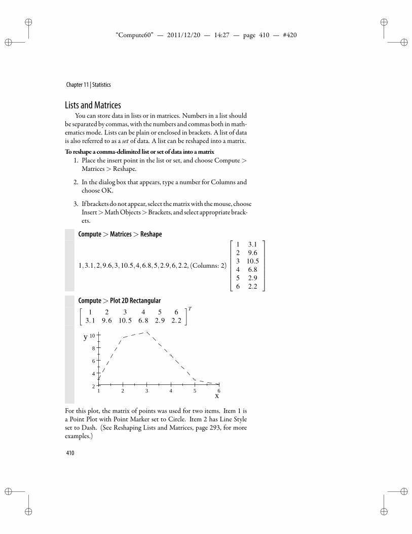
ii
“Compute60” — 2011/12/20 — 14:27 — page 410 — #420 ii
ii
ii
Chapter 11 | Statistics
Lists and MatricesYou can store data in lists or in matrices. Numbers in a list should
be separated by commas, with the numbers and commas both inmath-ematics mode. Lists can be plain or enclosed in brackets. A list of datais also referred to as a set of data. A list can be reshaped into a matrix.To reshape a comma-delimited list or set of data into amatrix
1. Place the insert point in the list or set, and choose Compute>Matrices> Reshape.
2. In the dialog box that appears, type a number for Columns andchoose OK.
3. If brackets donot appear, select thematrixwith themouse, chooseInsert>MathObjects>Brackets, and select appropriate brack-ets.
Compute>Matrices> Reshape
1,3.1,2,9.6,3,10.5,4,6.8,5,2.9,6,2.2, (Columns: 2)
1 3.12 9.63 10.54 6.85 2.96 2.2
Compute> Plot 2D Rectangular[
1 2 3 4 5 63.1 9.6 10.5 6.8 2.9 2.2
]T
1 2 3 4 5 62
4
6
8
10
x
y
For this plot, the matrix of points was used for two items. Item 1 isa Point Plot with Point Marker set to Circle. Item 2 has Line Styleset to Dash. (See Reshaping Lists and Matrices, page 293, for moreexamples.)
410
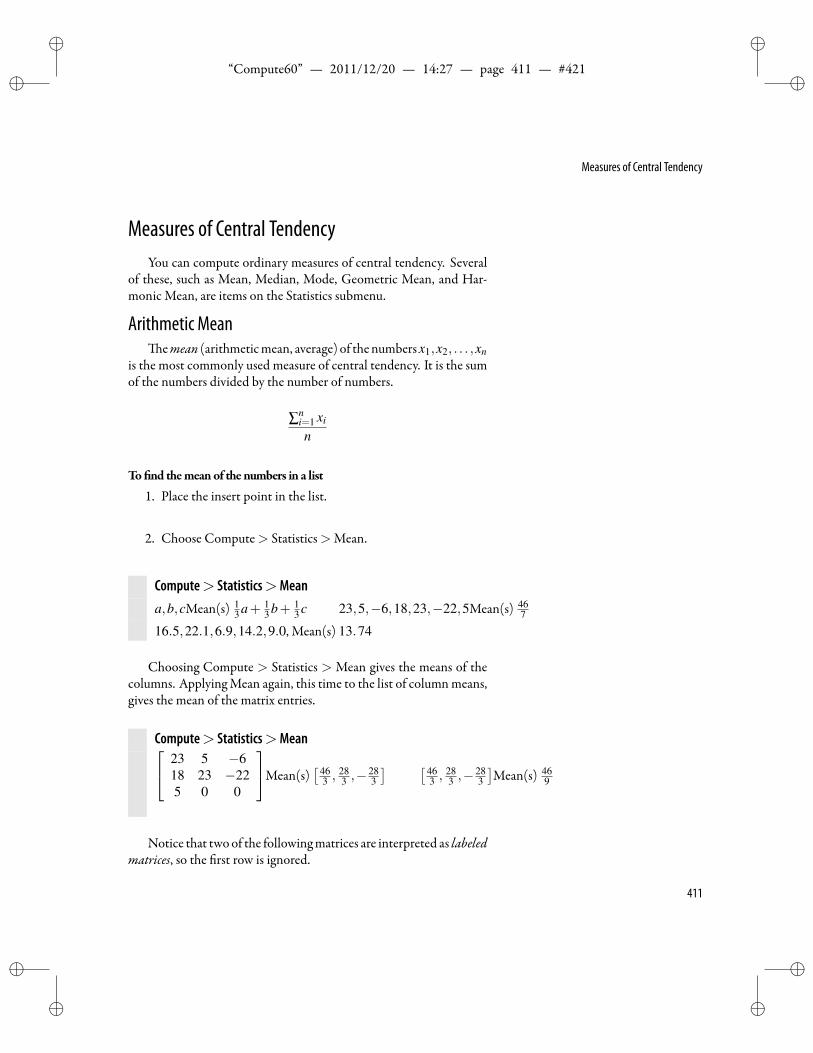
ii
“Compute60” — 2011/12/20 — 14:27 — page 411 — #421 ii
ii
ii
Measures of Central Tendency
Measures of Central TendencyYou can compute ordinary measures of central tendency. Several
of these, such as Mean, Median, Mode, Geometric Mean, and Har-monic Mean, are items on the Statistics submenu.
Arithmetic Meanemean (arithmeticmean, average) of thenumbers x1,x2, . . . ,xn
is the most commonly used measure of central tendency. It is the sumof the numbers divided by the number of numbers.
∑ni=1 xi
n
To nd themeanof the numbers in a list
1. Place the insert point in the list.
2. Choose Compute> Statistics>Mean.
Compute> Statistics>Meana,b,cMean(s) 1
3 a+ 13 b+ 1
3 c 23,5,−6,18,23,−22,5Mean(s) 467
16.5,22.1,6.9,14.2,9.0, Mean(s) 13.74
Choosing Compute > Statistics > Mean gives the means of thecolumns. ApplyingMean again, this time to the list of columnmeans,gives the mean of the matrix entries.
Compute> Statistics>Mean 23 5 −618 23 −225 0 0
Mean(s)[ 46
3 ,283 ,−
283
] [ 463 ,
283 ,−
283
]Mean(s) 46
9
Notice that twoof the followingmatrices are interpreted as labeledmatrices, so the rst row is ignored.
411
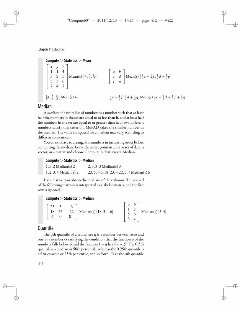
ii
“Compute60” — 2011/12/20 — 14:27 — page 412 — #422 ii
ii
ii
Chapter 11 | Statistics
Compute> Statistics>Meanx y z1 1 43 2 55 3 67 4 7
Mean(s)[4, 5
2 ,112
] a bc df g
Mean(s)[ 1
2 c+ 12 f , 1
2 d + 12 g]
[4, 5
2 ,112
]Mean(s) 4
[ 12 c+ 1
2 f , 12 d + 1
2 g]Mean(s) 1
4 c+ 14 d + 1
4 f + 14 g
MedianAmedian of a nite list of numbers is a number such that at least
half the numbers in the set are equal to or less than it, and at least halfthe numbers in the set are equal to or greater than it. If two differentnumbers satisfy this criterion, MuPAD takes the smaller number asthe median. e value computed for a median may vary according todifferent conventions.
You do not have to arrange the numbers in increasing order beforecomputing the median. Leave the insert point in a list or set of data, avector, or a matrix and choose Compute> Statistics>Median.
Compute> Statistics>Median1,5,2 Median(s) 2 2,3,3,3 Median(s) 31,2,3,4 Median(s) 2 23,5,−6,18,23,−22,5,7 Median(s) 5
For a matrix, you obtain the medians of the columns. e secondof the followingmatrices is interpreted as a labeledmatrix, and the rstrow is ignored.
Compute> Statistics>Median 23 5 −618 23 −225 0 0
Median(s) [18,5,−6]
a b1 25 63 4
Median(s) [3,4]
Quantilee qth quantile of a set, where q is a number between zero and
one, is a number Q satisfying the condition that the fraction q of thenumbers falls below Q and the fraction 1−q lies above Q. e 0.5thquantile is a median or 50th percentile, whereas the 0.25th quantile isa rst quartile or 25th percentile, and so forth. Take the qth quantile
412
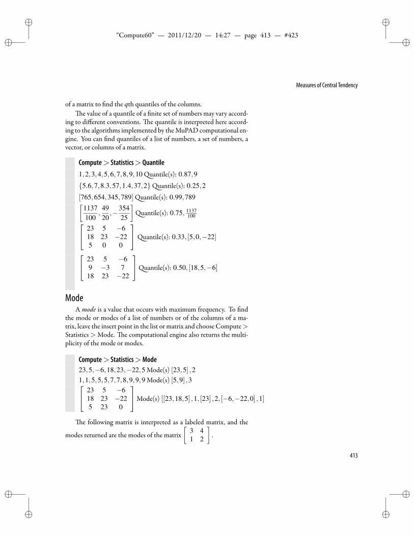
ii
“Compute60” — 2011/12/20 — 14:27 — page 413 — #423 ii
ii
ii
Measures of Central Tendency
of a matrix to nd the qth quantiles of the columns.e value of a quantile of a nite set of numbers may vary accord-
ing to different conventions. e quantile is interpreted here accord-ing to the algorithms implemented by theMuPAD computational en-gine. You can nd quantiles of a list of numbers, a set of numbers, avector, or columns of a matrix.
Compute> Statistics> Quantile1,2,3,4,5,6,7,8,9,10 uantile(s): 0.87,9
5.6,7,8.3,57,1.4,37,2 uantile(s): 0.25,2
[765,654,345,789] uantile(s): 0.99,789[1137100
,4920
,−35425
]uantile(s): 0.75, 1137
100 23 5 −618 23 −225 0 0
uantile(s): 0.33, [5,0,−22]
23 5 −69 −3 7
18 23 −22
uantile(s): 0.50, [18,5,−6]
ModeA mode is a value that occurs with maximum frequency. To nd
the mode or modes of a list of numbers or of the columns of a ma-trix, leave the insert point in the list ormatrix and choose Compute>Statistics > Mode. e computational engine also returns the multi-plicity of the mode or modes.
Compute> Statistics>Mode23,5,−6,18,23,−22,5 Mode(s) [23,5] ,21,1,5,5,5,7,7,8,9,9,9 Mode(s) [5,9] ,3 23 5 −6
18 23 −225 23 0
Mode(s) [[23,18,5] ,1, [23] ,2, [−6,−22,0] ,1]
e following matrix is interpreted as a labeled matrix, and the
modes returned are the modes of the matrix[
3 41 2
].
413
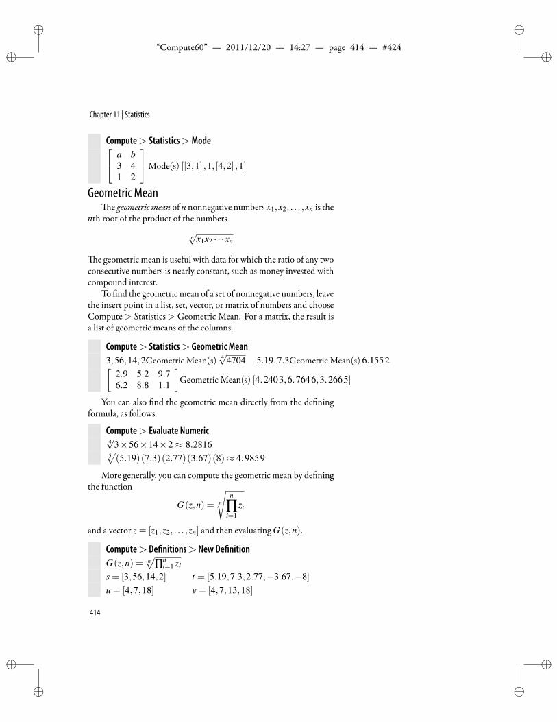
ii
“Compute60” — 2011/12/20 — 14:27 — page 414 — #424 ii
ii
ii
Chapter 11 | Statistics
Compute> Statistics>Mode a b3 41 2
Mode(s) [[3,1] ,1, [4,2] ,1]
Geometric Meane geometric mean of n nonnegative numbers x1,x2, . . . ,xn is the
nth root of the product of the numbers
n√
x1x2 · · ·xn
e geometric mean is useful with data for which the ratio of any twoconsecutive numbers is nearly constant, such as money invested withcompound interest.
To nd the geometric mean of a set of nonnegative numbers, leavethe insert point in a list, set, vector, or matrix of numbers and chooseCompute > Statistics > Geometric Mean. For a matrix, the result isa list of geometric means of the columns.
Compute> Statistics> Geometric Mean3,56,14,2Geometric Mean(s) 4
√4704 5.19,7.3Geometric Mean(s) 6.1552[
2.9 5.2 9.76.2 8.8 1.1
]Geometric Mean(s) [4.2403,6.7646,3.2665]
You can also nd the geometric mean directly from the de ningformula, as follows.
Compute> Evaluate Numeric4√
3×56×14×2≈ 8.28165√(5.19)(7.3)(2.77)(3.67)(8)≈ 4.9859
More generally, you can compute the geometric mean by de ningthe function
G(z,n) = n
√n
∏i=1
zi
and a vector z = [z1,z2, . . . ,zn] and then evaluating G(z,n).
Compute> De nitions> New De nitionG(z,n) = n
√∏n
i=1 zi
s = [3,56,14,2] t = [5.19,7.3,2.77,−3.67,−8]u = [4,7,18] v = [4,7,13,18]
414
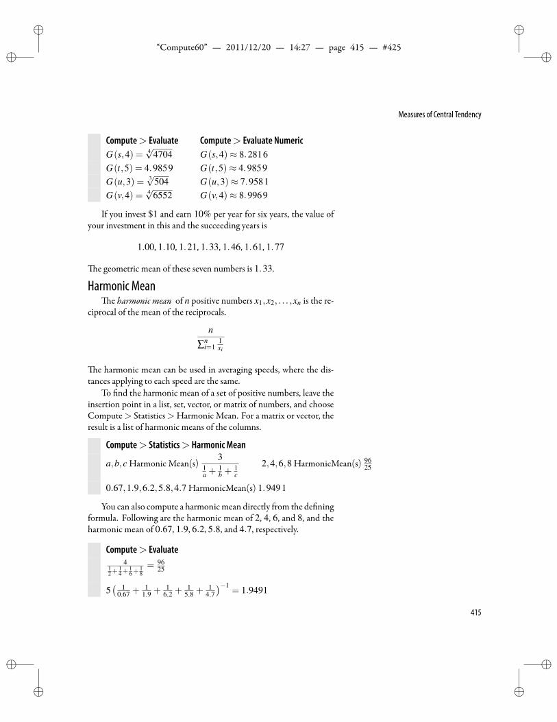
ii
“Compute60” — 2011/12/20 — 14:27 — page 415 — #425 ii
ii
ii
Measures of Central Tendency
Compute> Evaluate Compute> Evaluate NumericG(s,4) = 4
√4704 G(s,4)≈ 8.2816
G(t,5) = 4.9859 G(t,5)≈ 4.9859G(u,3) = 3√504 G(u,3)≈ 7.9581G(v,4) = 4√6552 G(v,4)≈ 8.9969
If you invest $1 and earn 10% per year for six years, the value ofyour investment in this and the succeeding years is
1.00, 1.10, 1.21, 1.33, 1.46, 1.61, 1.77
e geometric mean of these seven numbers is 1.33.
Harmonic Meane harmonic mean of n positive numbers x1,x2, . . . ,xn is the re-
ciprocal of the mean of the reciprocals.
n
∑ni=1
1xi
e harmonic mean can be used in averaging speeds, where the dis-tances applying to each speed are the same.
To nd the harmonic mean of a set of positive numbers, leave theinsertion point in a list, set, vector, or matrix of numbers, and chooseCompute> Statistics>Harmonic Mean. For a matrix or vector, theresult is a list of harmonic means of the columns.
Compute> Statistics> Harmonic Mean
a,b,c Harmonic Mean(s)3
1a +
1b +
1c
2,4,6,8 HarmonicMean(s) 9625
0.67,1.9,6.2,5.8,4.7 HarmonicMean(s) 1.9491
You can also compute a harmonicmean directly from the de ningformula. Following are the harmonic mean of 2, 4, 6, and 8, and theharmonic mean of 0.67, 1.9, 6.2, 5.8, and 4.7, respectively.
Compute> Evaluate4
12+
14+
16+
18= 96
25
5( 1
0.67 +1
1.9 +1
6.2 +1
5.8 +1
4.7
)−1= 1.9491
415
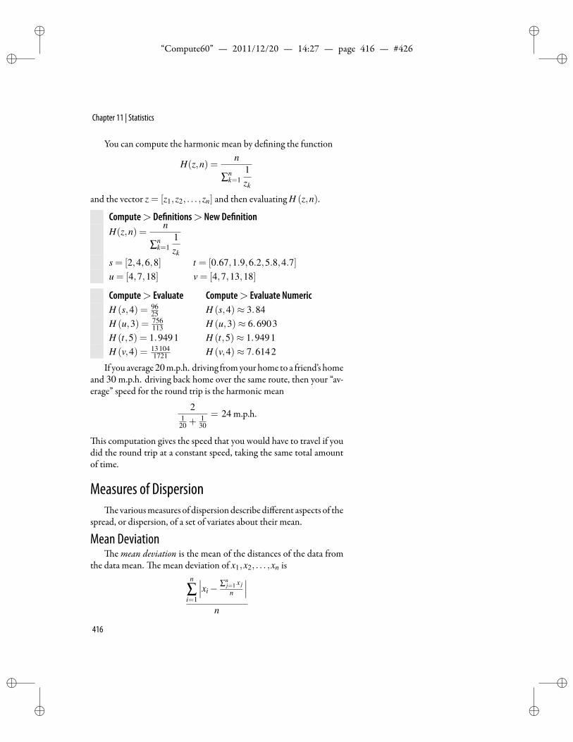
ii
“Compute60” — 2011/12/20 — 14:27 — page 416 — #426 ii
ii
ii
Chapter 11 | Statistics
You can compute the harmonic mean by de ning the function
H(z,n) =n
∑nk=1
1zk
and the vector z = [z1,z2, . . . ,zn] and then evaluating H (z,n).
Compute> De nitions> New De nitionH(z,n) =
n
∑nk=1
1zk
s = [2,4,6,8] t = [0.67,1.9,6.2,5.8,4.7]u = [4,7,18] v = [4,7,13,18]
Compute> Evaluate Compute> Evaluate NumericH (s,4) = 96
25 H (s,4)≈ 3.84H (u,3) = 756
113 H (u,3)≈ 6.6903H (t,5) = 1.9491 H (t,5)≈ 1.9491H (v,4) = 13104
1721 H (v,4)≈ 7.6142
If you average20m.p.h. driving fromyourhome to a friend’s homeand 30 m.p.h. driving back home over the same route, then your “av-erage” speed for the round trip is the harmonic mean
21
20 +130
= 24 m.p.h.
is computation gives the speed that you would have to travel if youdid the round trip at a constant speed, taking the same total amountof time.
Measures of Dispersione variousmeasures of dispersiondescribe different aspects of the
spread, or dispersion, of a set of variates about their mean.
Mean Deviatione mean deviation is the mean of the distances of the data from
the data mean. e mean deviation of x1,x2, . . . ,xn isn
∑i=1
∣∣∣xi−∑n
j=1 x j
n
∣∣∣n
416
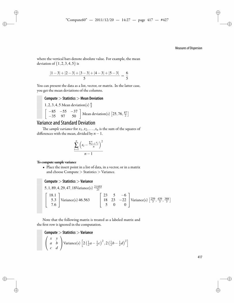
ii
“Compute60” — 2011/12/20 — 14:27 — page 417 — #427 ii
ii
ii
Measures of Dispersion
where the vertical bars denote absolute value. For example, the meandeviation of 1,2,3,4,5 is
|1−3|+ |2−3|+ |3−3|+ |4−3|+ |5−3|5
=65
You can present the data as a list, vector, or matrix. In the latter case,you get the mean deviations of the columns.
Compute> Statistics>Mean Deviation1,2,3,4,5 Mean deviation(s) 6
5[−85 −55 −37−35 97 50
]Mean deviation(s)
[25,76, 87
2
]Variance and Standard Deviation
e sample variance for x1,x2, . . . ,xn is the sum of the squares ofdifferences with the mean, divided by n−1.
n
∑i=1
(xi−
∑nj=1 x j
n
)2
n−1
Tocompute sample variance• Place the insert point in a list of data, in a vector, or in a matrix
and choose Compute> Statistics> Variance.
Compute> Statistics> Variance5,1,89,4,29,47,18Variance(s) 21055
21 18.15.37.6
Variance(s) 46.563
23 5 −618 23 −22
5 0 0
Variance(s)[ 259
3 , 4393 , 388
3
]
Note that the following matrix is treated as a labeled matrix andthe rst row is ignored in the computation.
Compute> Statistics> Variance x ya bc d
Variance(s)[2( 1
2 a− 12 c)2,2( 1
2 b− 12 d)2]
417
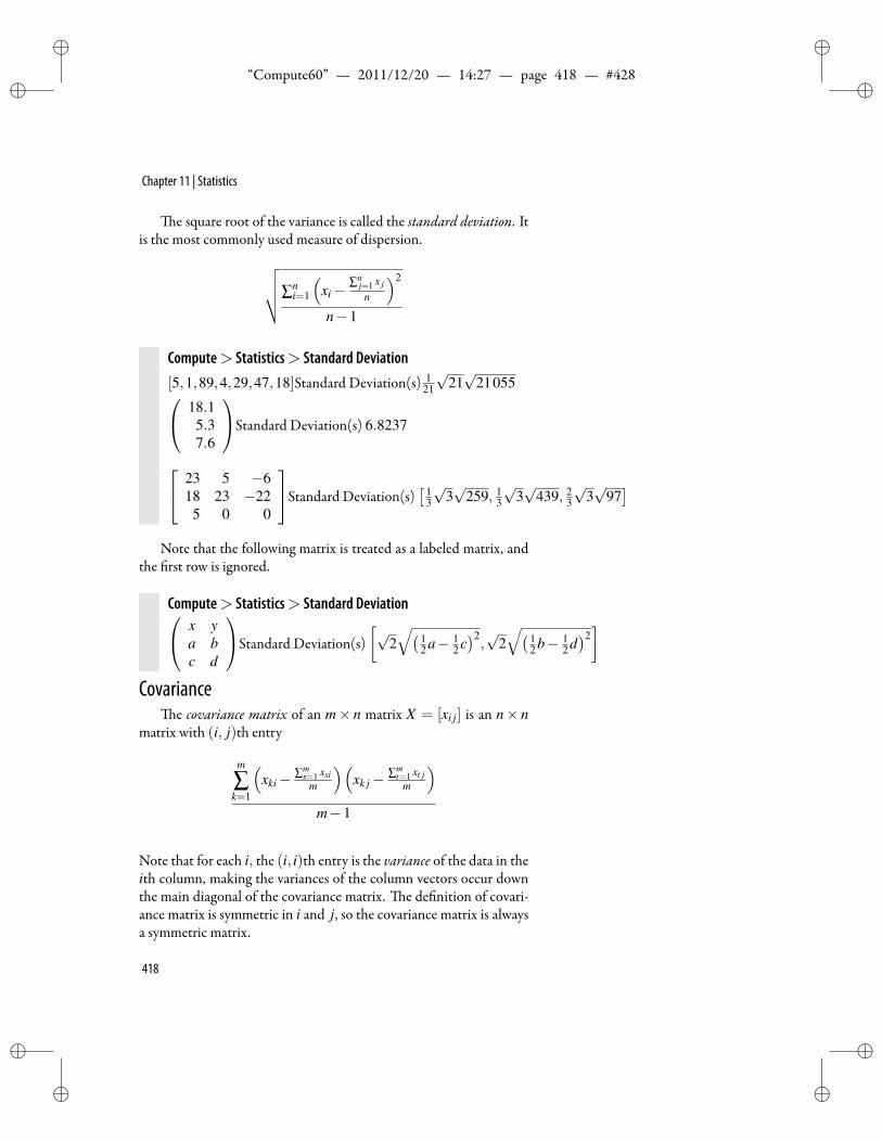
ii
“Compute60” — 2011/12/20 — 14:27 — page 418 — #428 ii
ii
ii
Chapter 11 | Statistics
e square root of the variance is called the standard deviation. Itis the most commonly used measure of dispersion.√√√√∑n
i=1
(xi−
∑nj=1 x j
n
)2
n−1
Compute> Statistics> Standard Deviation[5,1,89,4,29,47,18]Standard Deviation(s) 1
21
√21√
21055 18.15.37.6
Standard Deviation(s) 6.8237
23 5 −618 23 −225 0 0
Standard Deviation(s)[ 1
3
√3√
259, 13
√3√
439, 23
√3√
97]
Note that the following matrix is treated as a labeled matrix, andthe rst row is ignored.
Compute> Statistics> Standard Deviation x ya bc d
Standard Deviation(s)[√
2√( 1
2 a− 12 c)2,√
2√( 1
2 b− 12 d)2]
Covariancee co ariance matrix of an m× n matrix X = [xi j] is an n× n
matrix with (i, j)th entry
m
∑k=1
(xki−
∑ms=1 xsi
m
)(xk j−
∑mt=1 xt j
m
)m−1
Note that for each i, the (i, i)th entry is the variance of the data in theith column, making the variances of the column vectors occur downthe main diagonal of the covariance matrix. e de nition of covari-ance matrix is symmetric in i and j, so the covariance matrix is alwaysa symmetric matrix.
418
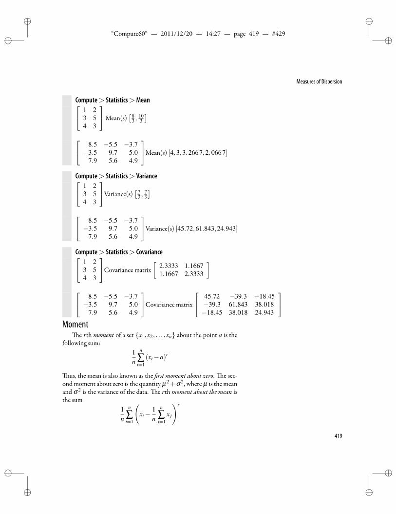
ii
“Compute60” — 2011/12/20 — 14:27 — page 419 — #429 ii
ii
ii
Measures of Dispersion
Compute> Statistics>Mean 1 23 54 3
Mean(s)[ 8
3 ,103
] 8.5 −5.5 −3.7−3.5 9.7 5.0
7.9 5.6 4.9
Mean(s) [4.3,3.2667,2.0667]
Compute> Statistics> Variance 1 23 54 3
Variance(s)[ 7
3 ,73
] 8.5 −5.5 −3.7−3.5 9.7 5.0
7.9 5.6 4.9
Variance(s) [45.72,61.843,24.943]
Compute> Statistics> Covariance 1 23 54 3
Covariance matrix[
2.3333 1.16671.1667 2.3333
] 8.5 −5.5 −3.7−3.5 9.7 5.0
7.9 5.6 4.9
Covariance matrix
45.72 −39.3 −18.45−39.3 61.843 38.018−18.45 38.018 24.943
Moment
e rth moment of a set x1,x2, . . . ,xn about the point a is thefollowing sum:
1n
n
∑i=1
(xi−a)r
us, the mean is also known as the rst moment about zero. e sec-ondmoment about zero is the quantity µ2+σ2, where µ is themeanand σ2 is the variance of the data. e rthmoment about the mean isthe sum
1n
n
∑i=1
(xi−
1n
n
∑j=1
x j
)r
419
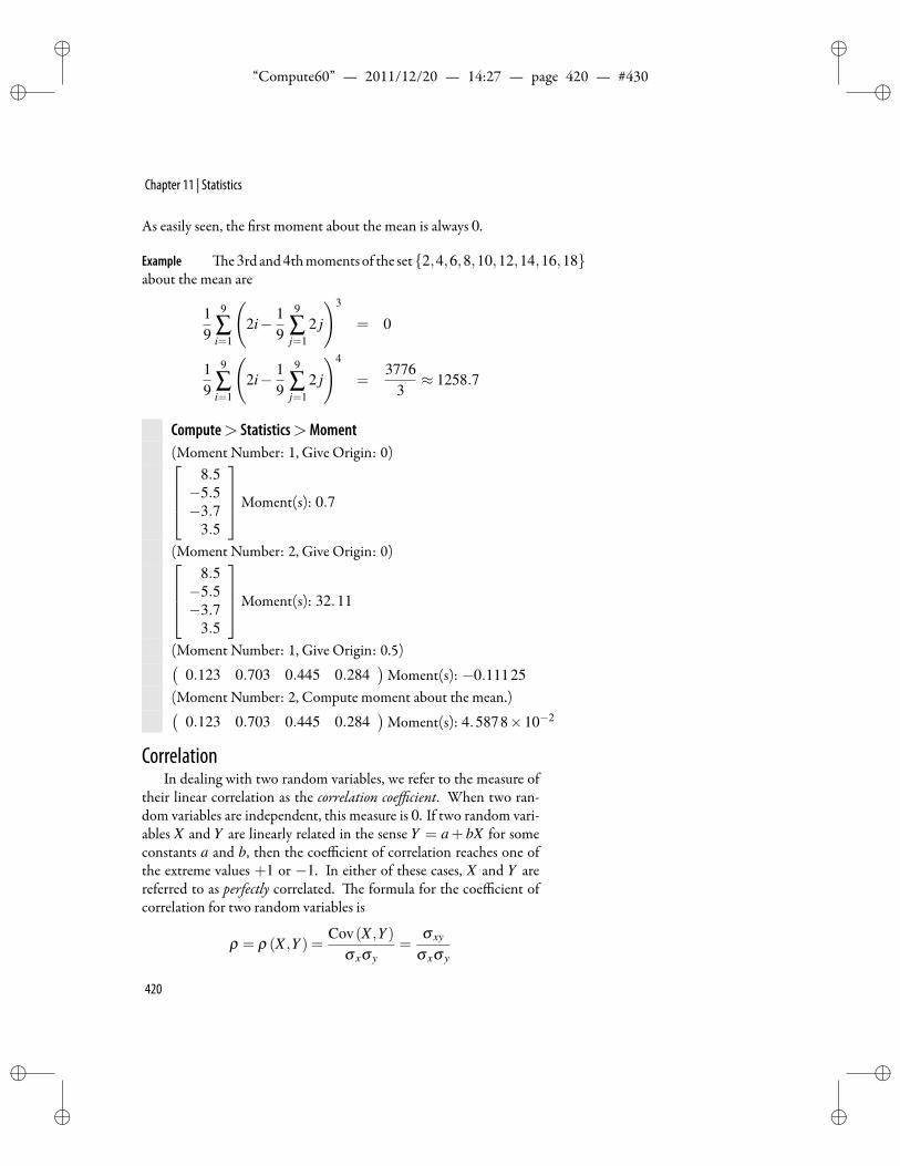
ii
“Compute60” — 2011/12/20 — 14:27 — page 420 — #430 ii
ii
ii
Chapter 11 | Statistics
As easily seen, the rst moment about the mean is always 0.
Example e3rd and4thmoments of the set2,4,6,8,10,12,14,16,18about the mean are
19
9
∑i=1
(2i− 1
9
9
∑j=1
2 j
)3
= 0
19
9
∑i=1
(2i− 1
9
9
∑j=1
2 j
)4
=3776
3≈ 1258.7
Compute> Statistics>Moment(Moment Number: 1, Give Origin: 0)
8.5−5.5−3.7
3.5
Moment(s): 0.7
(Moment Number: 2, Give Origin: 0)8.5−5.5−3.7
3.5
Moment(s): 32.11
(Moment Number: 1, Give Origin: 0.5)(0.123 0.703 0.445 0.284
)Moment(s): −0.11125
(Moment Number: 2, Compute moment about the mean.)(0.123 0.703 0.445 0.284
)Moment(s): 4.5878×10⁻²
CorrelationIn dealing with two random variables, we refer to the measure of
their linear correlation as the correlation coefficient. When two ran-dom variables are independent, this measure is 0. If two random vari-ables X and Y are linearly related in the sense Y = a+ bX for someconstants a and b, then the coefficient of correlation reaches one ofthe extreme values +1 or −1. In either of these cases, X and Y arereferred to as perfectly correlated. e formula for the coefficient ofcorrelation for two random variables is
ρ = ρ (X ,Y ) =Cov(X ,Y )
σ xσ y=
σ xy
σ xσ y
420
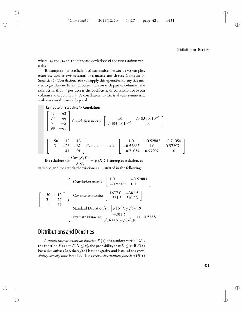
ii
“Compute60” — 2011/12/20 — 14:27 — page 421 — #431 ii
ii
ii
Distributions and Densities
where σ x and σ y are the standard deviations of the two random vari-ables.
To compute the coefficient of correlation between two samples,enter the data as two columns of a matrix and choose Compute >Statistics>Correlation. You can apply this operation to any size ma-trix to get the coefficient of correlation for each pair of columns: thenumber in the i, j position is the coefficient of correlation betweencolumn i and column j. A correlation matrix is always symmetric,with ones on the main diagonal.
Compute> Statistics> Correlation43 −6277 6654 −599 −61
Correlation matrix:[
1.0 7.4831×10⁻²
7.4831×10⁻² 1.0
]
−50 −12 −1831 −26 −621 −47 −91
Correlation matrix:
1.0 −0.52883 −0.71054−0.52883 1.0 0.97297−0.71054 0.97297 1.0
e relationship
Cov(X ,Y )σ xσ y
= ρ (X ,Y ) among correlation, co-
variance, and the standard deviations is illustrated in the following:
−50 −1231 −261 −47
Correlation matrix:[
1.0 −0.52883−0.52883 1.0
]
Covariance matrix:[
1677.0 −381.5−381.5 310.33
]Standard Deviation(s):
[√1677, 7
3
√3√
19]
Evaluate Numeric:−381.5√
1677× 73
√3√
19≈−0.52881
Distributions and DensitiesA cumulative distribution function F (x) of a random variable X is
the function F (x) = P(X ≤ x), the probability that X ≤ x. If F(x)has a derivative f (x), then f (x) is nonnegative and is called the prob-ability density function of x. e in erse distribution function G(α)
421
ii
“Compute60” — 2011/12/20 — 14:27 — page 422 — #432 ii
ii
ii
Chapter 11 | Statistics
satis es G(F (x)) = x and F (G(α)) = α . e names for these func-tions are obtained by adding Dist, Den, or Inv to the name of the dis-tribution. For example, NormalDist, NormalDen, and NormalInvare the three functions for the normal distribution. ese functionnames will automatically turn gray when typed in mathematics mode.
Cumulative Distribution FunctionsA cumulative distribution function is a nondecreasing function
de ned on the interval (−∞,∞), with values in the interval [0,1]. ede nition of a distribution function generally describes only the val-ues where the function is positive, the implicit assumption being thatthe distribution function is zero up to that point. For discrete cumu-lative distribution functions, the de nition also gives only the valueswhere the function changes, the implicit assumption being that thecumulative distribution function is a step function. Commonly, def-initions of these functions are stated only for integers. e de nitionof a density function also generally describes only the values where thefunction is positive, the implicit assumption being that the function iszero elsewhere.
ese distribution and density functions satisfy the relationships
f (x) =ddx
F(x) and F(x) =∫ x
−∞f (u)du
Also note that the cumulative distribution function satis es
limx→∞
F(x) = 1 and limx→−∞
F(x) = 0.
In Scienti c WorkPlace and Scienti c Notebook, cumulative distribu-tion functions are named FunctionDist, and the density functions arenamed FunctionDen. For example, the probability density functionsfor the normal distributions are called NormalDen.
You can compute with several families of distributions: Normal,Cauchy, Student’s t, Chi-Square, F, Exponential, Weibull, Gamma,Beta, Uniform, Binomial, Poisson, and Hypergeometric.
Inverse Distribution FunctionsFor a distribution function F mapping (−∞,∞) into [0,1], the in-
verse distribution functionG performs the corresponding inverse map-ping from (a subset of ) [0,1] into (−∞,∞); that is, G(F (x)) = x andF (G(α)) = α . Equivalently, Prob[X ≤ G(α)] = F(x) = α . Note
422
ii
“Compute60” — 2011/12/20 — 14:27 — page 423 — #433 ii
ii
ii
Families of Continuous Distributions
that the value that is exceeded with probability α is given by the func-tion G(1−α). is function is also of interest.
Prob [X ≤ G(1−α)] = F(x) = 1−α = 1−Prob [X ≤ G(α)]
When cumulative distribution functions are named FunctionDist,then the inverse cumulative distribution functions arenamedFunctionInv.For example, NormalInv is the name of the inverse cumulative distri-bution function for the normal distribution.
Distribution TablesDepending on the particular family of distributions, the distribu-
tion tables in statistics books list function values for selected parame-ters of one of the functions described earlier—either the cumulativedistribution, the inverse cumulative distribution, or the probabilitydensity function. With access to these functions, not only can youcompute the tabular entries easily and accurately, but you can also ndthe corresponding values directly for any variables and parameters toany degree of accuracy you wish.
Families of Continuous Distributionse relationship of the various distribution, inverse distribution,
and density functions to the entries in standard statistical tables is ex-plained in the following sections for each of the families of distribu-tions available.
Gamma Functione Gamma function Γ(t) that appears in the de nition of the
Student’s t distribution and the gamma distribution is the continu-ous function Γ(t) =
∫ ∞0 e−xxt−1dx de ned for positive real numbers
t . e Gamma function satis es
Γ(1) = 1 and Γ(t +1) = tΓ(t)
and for positive integers k, it is the familiar factorial function
Γ(k) = (k−1)!
eGamma function symbol Γ is recognized as a function. For exam-ple, place the insert point in the expression Γ(5) and choose Evaluateto get Γ(5) = 24. Note that 24 = 4×3×2×1. (See page 157 for aplot of the Gamma function.)
423
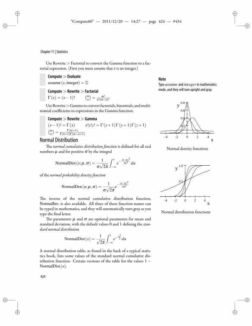
ii
“Compute60” — 2011/12/20 — 14:27 — page 424 — #434 ii
ii
ii
Chapter 11 | Statistics
Use Rewrite> Factorial to convert the Gamma function to a fac-torial expression. (First you must assume that x is an integer.)
Compute> Evaluateassume(x, integer) = Z
NoteType assume and integer in mathematicsmode, and they will turn upright and gray.Compute> Rewrite> Factorial
Γ(x) = (x−1)!(m
n
)= m!
n!(m−n)!
UseRewrite>Gammato convert factorials, binomials, andmulti-nomial coefficients to expressions in the Gamma function.
Compute> Rewrite> Gamma(x−1)! = Γ(x) x!y!z! = Γ(x+1)Γ(y+1)Γ(z+1)(m
n
)= Γ(m+1)
Γ(n+1)Γ(m−n+1)4 2 0 2 4
0.2
0.4
0.6
0.8
x
y
Normal density functions
4 2 0 2 4
0.5
1.0
x
y
Normal distribution functions
Normal Distributione normal cumulative distribution function is de ned for all real
numbers µ and for positive σ by the integral
NormalDist(x; µ,σ) =1
σ√
2π
∫ x
−∞e−
(u−µ)2
2σ2 du
of the normal probability density function
NormalDen(u; µ,σ) =1
σ√
2πe−
(u−µ)2
2σ2
e inverse of the normal cumulative distribution function,NormalInv, is also available. All three of these function names canbe typed in mathematics, and they will automatically turn gray as youtype the nal letter.
e parameters µ and σ are optional parameters for mean andstandard deviation, with the default values 0 and 1 de ning the stan-dard normal distribution
NormalDist(x) =1√2π
∫ x
−∞e−
u22 du
A normal distribution table, as found in the back of a typical statis-tics book, lists some values of the standard normal cumulative dis-tribution function. Certain versions of the table list the values 1−NormalDist(x).
424
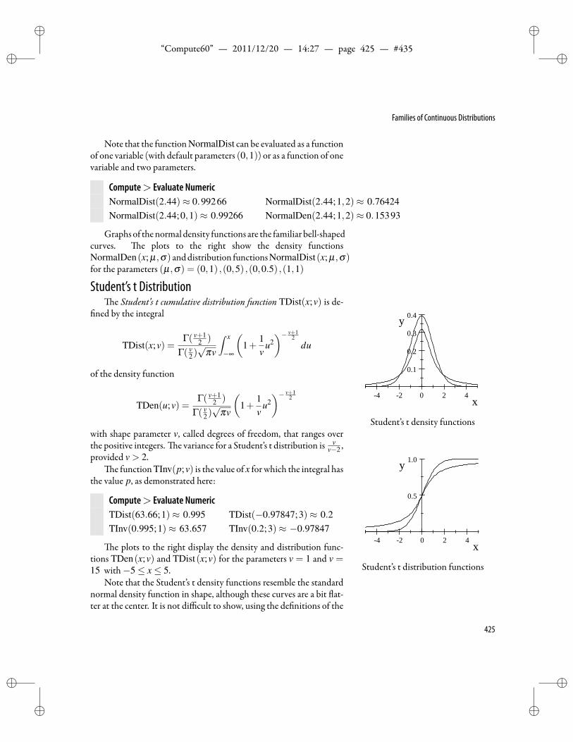
ii
“Compute60” — 2011/12/20 — 14:27 — page 425 — #435 ii
ii
ii
Families of Continuous Distributions
Note that the function NormalDist can be evaluated as a functionof one variable (with default parameters (0,1)) or as a function of onevariable and two parameters.
Compute> Evaluate NumericNormalDist(2.44)≈ 0.99266 NormalDist(2.44;1,2)≈ 0.76424NormalDist(2.44;0,1)≈ 0.99266 NormalDen(2.44;1,2)≈ 0.15393
Graphsof thenormal density functions are the familiar bell-shapedcurves. e plots to the right show the density functionsNormalDen(x; µ ,σ) anddistribution functionsNormalDist(x; µ,σ)for the parameters (µ,σ) = (0,1) ,(0,5) ,(0,0.5) ,(1,1)
Student’s t Distributione Student’s t cumulative distribution function TDist(x;v) is de-
ned by the integral
TDist(x;v) =Γ( v+1
2 )
Γ( v2)√
πv
∫ x
−∞
(1+
1v
u2)− v+1
2du
of the density function
TDen(u;v) =Γ( v+1
2 )
Γ( v2)√
πv
(1+
1v
u2)− v+1
2
with shape parameter v, called degrees of freedom, that ranges over
4 2 0 2 4
0.1
0.2
0.3
0.4
x
y
Student’s t density functions
4 2 0 2 4
0.5
1.0
x
y
Student’s t distribution functions
the positive integers. e variance for a Student’s t distribution is vv−2 ,
provided v > 2.e function TInv(p;v) is the value of x for which the integral has
the value p, as demonstrated here:
Compute> Evaluate NumericTDist(63.66;1)≈ 0.995 TDist(−0.97847;3)≈ 0.2TInv(0.995;1)≈ 63.657 TInv(0.2;3)≈ −0.97847
e plots to the right display the density and distribution func-tions TDen(x;v) and TDist(x;v) for the parameters v = 1 and v =15 with−5≤ x≤ 5.
Note that the Student’s t density functions resemble the standardnormal density function in shape, although these curves are a bit at-ter at the center. It is not difficult to show, using the de nitions of the
425
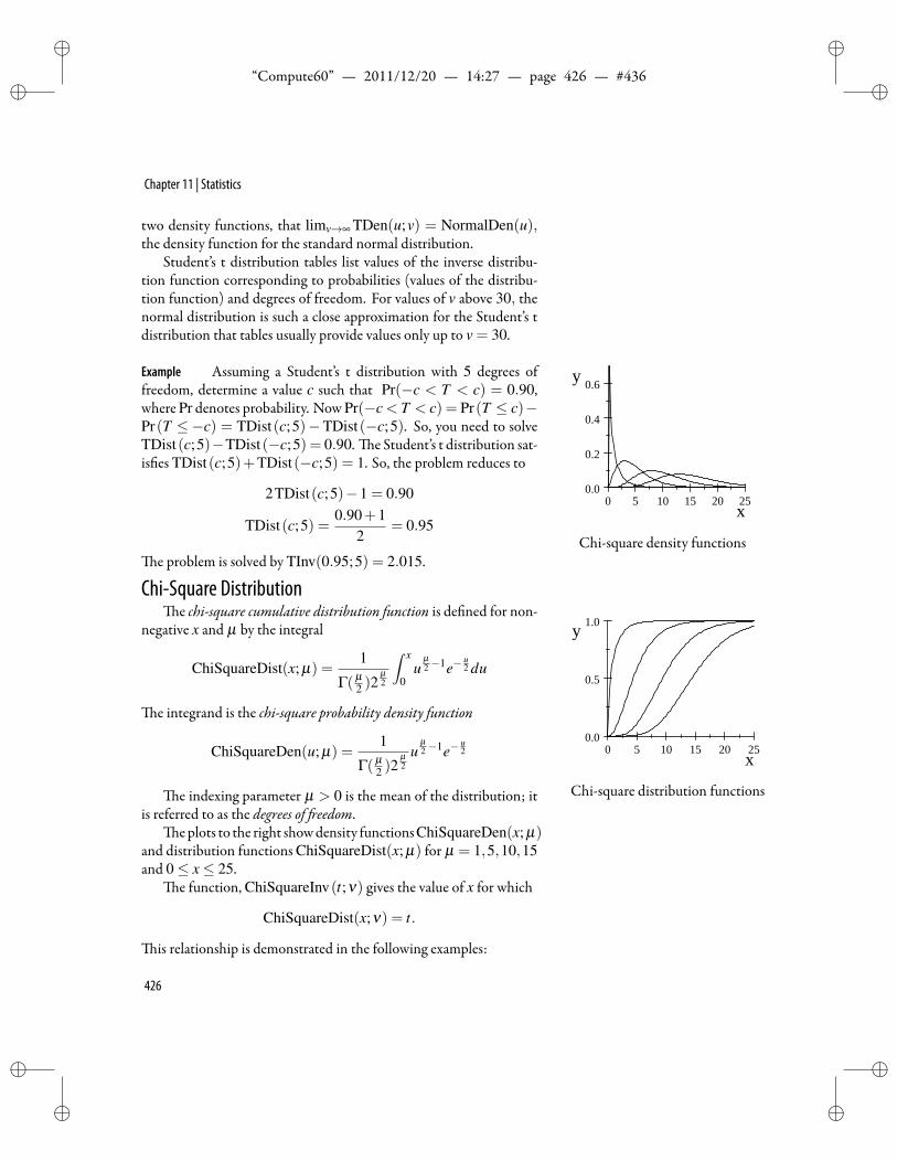
ii
“Compute60” — 2011/12/20 — 14:27 — page 426 — #436 ii
ii
ii
Chapter 11 | Statistics
two density functions, that limv→∞ TDen(u;v) = NormalDen(u),the density function for the standard normal distribution.
Student’s t distribution tables list values of the inverse distribu-tion function corresponding to probabilities (values of the distribu-tion function) and degrees of freedom. For values of v above 30, thenormal distribution is such a close approximation for the Student’s tdistribution that tables usually provide values only up to v = 30.
Example Assuming a Student’s t distribution with 5 degrees offreedom, determine a value c such that Pr(−c < T < c) = 0.90,where Pr denotes probability. Now Pr(−c < T < c) = Pr(T ≤ c)−Pr(T ≤−c) = TDist(c;5)−TDist(−c;5). So, you need to solveTDist(c;5)−TDist(−c;5) = 0.90. e Student’s t distribution sat-is es TDist(c;5)+TDist(−c;5) = 1. So, the problem reduces to
2TDist(c;5)−1 = 0.90
TDist(c;5) =0.90+1
2= 0.95
e problem is solved by TInv(0.95;5) = 2.015.
0 5 10 15 20 250.0
0.2
0.4
0.6
x
y
Chi-square density functions
0 5 10 15 20 250.0
0.5
1.0
x
y
Chi-square distribution functions
Chi-Square Distributione chi-square cumulative distribution function is de ned for non-
negative x and µ by the integral
ChiSquareDist(x; µ) =1
Γ( µ2 )2
µ2
∫ x
0u
µ2−1e−
u2 du
e integrand is the chi-square probability density function
ChiSquareDen(u; µ) =1
Γ( µ2 )2
µ2
uµ2−1e−
u2
e indexing parameter µ > 0 is the mean of the distribution; itis referred to as the degrees of eedom.
e plots to the right showdensity functionsChiSquareDen(x; µ)and distribution functions ChiSquareDist(x; µ) for µ = 1,5,10,15and 0≤ x≤ 25.
e function, ChiSquareInv(t;ν) gives the value of x for which
ChiSquareDist(x;ν) = t.
is relationship is demonstrated in the following examples:
426
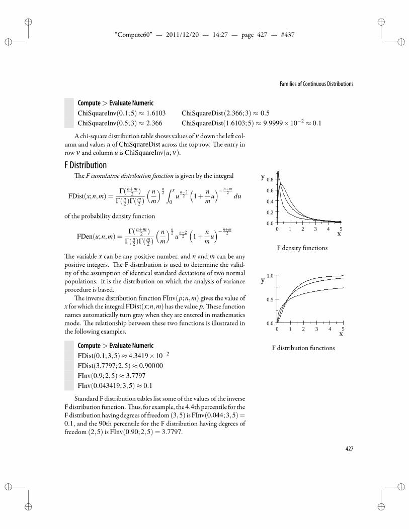
ii
“Compute60” — 2011/12/20 — 14:27 — page 427 — #437 ii
ii
ii
Families of Continuous Distributions
Compute> Evaluate NumericChiSquareInv(0.1;5)≈ 1.6103 ChiSquareDist(2.366;3)≈ 0.5ChiSquareInv(0.5;3)≈ 2.366 ChiSquareDist(1.6103;5)≈ 9.9999×10⁻² ≈ 0.1
Achi-square distribution table shows values ofν down the le col-umn and values u of ChiSquareDist across the top row. e entry inrow ν and column u is ChiSquareInv(u;ν).
F Distributione F cumulative distribution function is given by the integral
FDist(x;n,m) =Γ( n+m
2 )
Γ( n2)Γ(
m2 )
( nm
) n2∫ x
0u
n−22
(1+
nm
u)− n+m
2du
of the probability density function
FDen(u;n,m) =Γ( n+m
2 )
Γ( n2)Γ(
m2 )
( nm
) n2
un−2
2
(1+
nm
u)− n+m
2
e variable x can be any positive number, and n and m can be any
0 1 2 3 4 50.0
0.2
0.4
0.6
0.8
x
y
F density functions
0 1 2 3 4 50.0
0.5
1.0
x
y
F distribution functions
positive integers. e F distribution is used to determine the valid-ity of the assumption of identical standard deviations of two normalpopulations. It is the distribution on which the analysis of varianceprocedure is based.
e inverse distribution function FInv(p;n,m) gives the value ofx for which the integral FDist(x;n,m)has the value p. ese functionnames automatically turn gray when they are entered in mathematicsmode. e relationship between these two functions is illustrated inthe following examples.
Compute> Evaluate NumericFDist(0.1;3,5)≈ 4.3419×10⁻²
FDist(3.7797;2,5)≈ 0.90000FInv(0.9;2,5)≈ 3.7797FInv(0.043419;3,5)≈ 0.1
Standard F distribution tables list some of the values of the inverseFdistribution function. us, for example, the4.4thpercentile for theF distribution having degrees of freedom (3,5) isFInv(0.044;3,5) =0.1, and the 90th percentile for the F distribution having degrees offreedom (2,5) is FInv(0.90;2,5) = 3.7797.
427
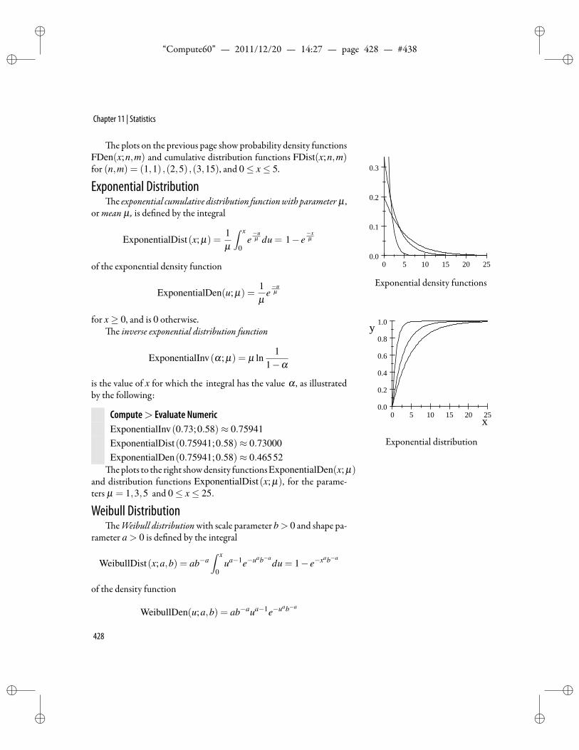
ii
“Compute60” — 2011/12/20 — 14:27 — page 428 — #438 ii
ii
ii
Chapter 11 | Statistics
e plots on the previous page show probability density functionsFDen(x;n,m) and cumulative distribution functions FDist(x;n,m)for (n,m) = (1,1) ,(2,5) ,(3,15), and 0≤ x≤ 5.
Exponential Distributione exponential cumulative distribution functionwith parameter µ ,
ormean µ , is de ned by the integral
ExponentialDist(x; µ) =1µ
∫ x
0e−uµ du = 1− e
−xµ
of the exponential density function 0 5 10 15 20 250.0
0.1
0.2
0.3
Exponential density functions
0 5 10 15 20 250.0
0.2
0.4
0.6
0.8
1.0
x
y
Exponential distribution
ExponentialDen(u; µ) =1µ
e−uµ
for x≥ 0, and is 0 otherwise.e in erse exponential distribution function
ExponentialInv(α; µ) = µ ln1
1−α
is the value of x for which the integral has the value α , as illustratedby the following:
Compute> Evaluate NumericExponentialInv(0.73;0.58)≈ 0.75941ExponentialDist(0.75941;0.58)≈ 0.73000ExponentialDen(0.75941;0.58)≈ 0.46552eplots to the right showdensity functionsExponentialDen(x; µ)
and distribution functions ExponentialDist(x; µ), for the parame-ters µ = 1,3,5 and 0≤ x≤ 25.
Weibull DistributioneWeibull distributionwith scale parameter b > 0 and shape pa-
rameter a > 0 is de ned by the integral
WeibullDist(x;a,b) = ab−a∫ x
0ua−1e−uab−a
du = 1− e−xab−a
of the density function
WeibullDen(u;a,b) = ab−aua−1e−uab−a
428
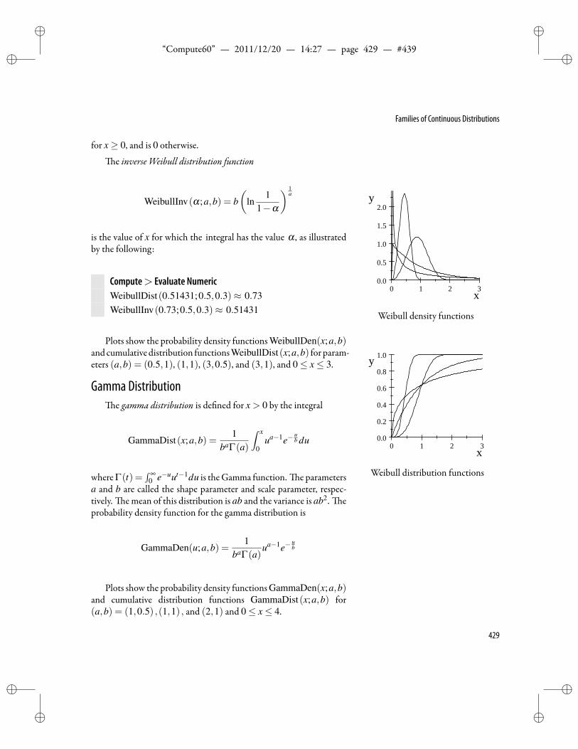
ii
“Compute60” — 2011/12/20 — 14:27 — page 429 — #439 ii
ii
ii
Families of Continuous Distributions
for x≥ 0, and is 0 otherwise.
e in erse Weibull distribution function
WeibullInv(α;a,b) = b(
ln1
1−α
) 1a
is the value of x for which the integral has the value α , as illustratedby the following:
Compute> Evaluate NumericWeibullDist(0.51431;0.5,0.3)≈ 0.73WeibullInv(0.73;0.5,0.3)≈ 0.51431
0 1 2 30.0
0.5
1.0
1.5
2.0
x
y
Weibull density functions
0 1 2 30.0
0.2
0.4
0.6
0.8
1.0
x
y
Weibull distribution functions
Plots show the probability density functions WeibullDen(x;a,b)and cumulative distribution functionsWeibullDist(x;a,b) for param-eters (a,b) = (0.5,1), (1,1), (3,0.5), and (3,1), and 0≤ x≤ 3.
Gamma Distributione gamma distribution is de ned for x > 0 by the integral
GammaDist(x;a,b) =1
baΓ(a)
∫ x
0ua−1e−
ub du
where Γ(t) =∫ ∞
0 e−uut−1du is theGamma function. e parametersa and b are called the shape parameter and scale parameter, respec-tively. e mean of this distribution is ab and the variance is ab2. eprobability density function for the gamma distribution is
GammaDen(u;a,b) =1
baΓ(a)ua−1e−
ub
Plots show the probability density functions GammaDen(x;a,b)and cumulative distribution functions GammaDist(x;a,b) for(a,b) = (1,0.5) ,(1,1) , and (2,1) and 0≤ x≤ 4.
429
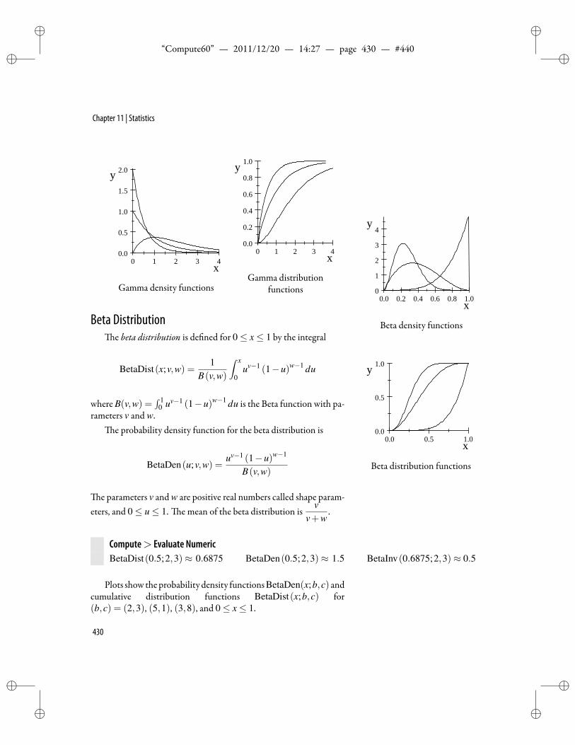
ii
“Compute60” — 2011/12/20 — 14:27 — page 430 — #440 ii
ii
ii
Chapter 11 | Statistics
0 1 2 3 40.0
0.5
1.0
1.5
2.0
x
y
Gamma density functions
0 1 2 3 40.0
0.2
0.4
0.6
0.8
1.0
x
y
Gamma distributionfunctions
Beta Distributione beta distribution is de ned for 0≤ x≤ 1 by the integral
0.0 0.2 0.4 0.6 0.8 1.00
1
2
3
4
x
y
Beta density functions
0.0 0.5 1.00.0
0.5
1.0
x
y
Beta distribution functions
BetaDist(x;v,w) =1
B(v,w)
∫ x
0uv−1 (1−u)w−1 du
where B(v,w) =∫ 1
0 uv−1 (1−u)w−1 du is the Beta function with pa-rameters v and w.
e probability density function for the beta distribution is
BetaDen(u;v,w) =uv−1 (1−u)w−1
B(v,w)
e parameters v and w are positive real numbers called shape param-eters, and 0≤ u≤ 1. e mean of the beta distribution is
vv+w
.
Compute> Evaluate NumericBetaDist(0.5;2,3)≈ 0.6875 BetaDen(0.5;2,3)≈ 1.5 BetaInv(0.6875;2,3)≈ 0.5
Plots show theprobability density functionsBetaDen(x;b,c) andcumulative distribution functions BetaDist(x;b,c) for(b,c) = (2,3), (5,1), (3,8), and 0≤ x≤ 1.
430
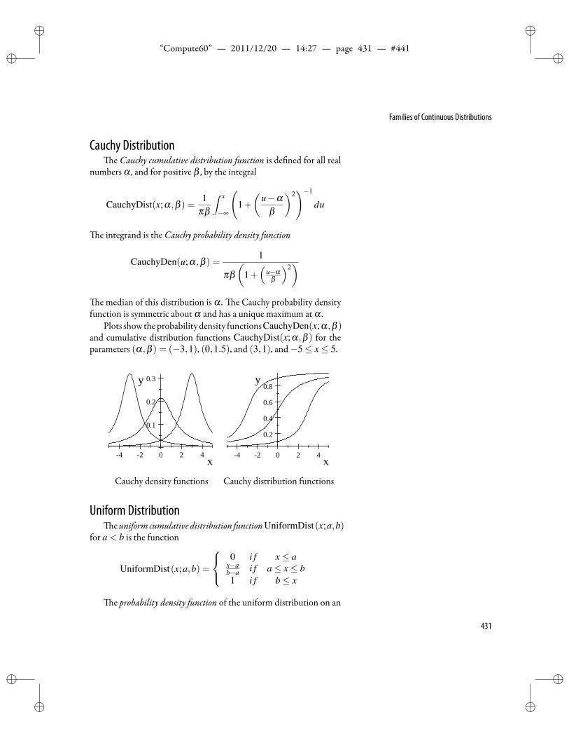
ii
“Compute60” — 2011/12/20 — 14:27 — page 431 — #441 ii
ii
ii
Families of Continuous Distributions
Cauchy Distributione Cauchy cumulative distribution function is de ned for all real
numbers α , and for positive β , by the integral
CauchyDist(x;α,β ) =1
πβ
∫ x
−∞
(1+(
u−αβ
)2)−1
du
e integrand is the Cauchy probability density function
CauchyDen(u;α,β ) =1
πβ(
1+(
u−αβ
)2)
e median of this distribution is α . e Cauchy probability densityfunction is symmetric about α and has a unique maximum at α .
Plots show theprobability density functionsCauchyDen(x;α,β )and cumulative distribution functions CauchyDist(x;α,β ) for theparameters (α,β ) = (−3,1), (0,1.5), and (3,1), and−5≤ x≤ 5.
4 2 0 2 4
0.1
0.2
0.3
x
y
Cauchy density functions
4 2 0 2 4
0.2
0.4
0.6
0.8
x
y
Cauchy distribution functions
Uniform Distributioneuniform cumulative distribution functionUniformDist(x;a,b)
for a < b is the function
UniformDist(x;a,b) =
0 i f x≤ a
x−ab−a i f a≤ x≤ b1 i f b≤ x
e probability density function of the uniform distribution on an
431
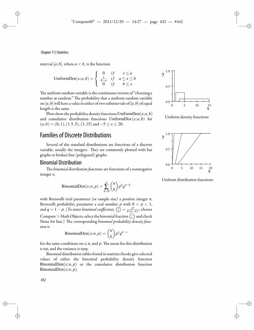
ii
“Compute60” — 2011/12/20 — 14:27 — page 432 — #442 ii
ii
ii
Chapter 11 | Statistics
interval [a,b], where a < b, is the function
UniformDen(x;a,b) =
0 i f x≤ a1
b−a i f a≤ x≤ b0 i f b≤ x
e uniform random variable is the continuous version of “choosing a
0 5 10 150.0
0.5
1.0
x
y
Uniform density functions
0 5 10 15 200.0
0.5
1.0
x
y
Uniform distribution functions
number at random.” e probability that a uniform random variableon [a,b]will have a value in either of two subintervals of [a,b] of equallength is the same.
Plots showtheprobability density functionsUniformDen(x;a,b)and cumulative distribution functions UniformDist(x;a,b) for(a,b) = (0,1), (1.5,5), (3,15) and−5≤ x≤ 20.
Families of Discrete DistributionsSeveral of the standard distributions are functions of a discrete
variable, usually the integers. ey are commonly plotted with bargraphs or broken line (polygonal) graphs.
Binomial Distributione binomial distribution functions are functions of a nonnegative
integer x,
BinomialDist(x;n, p) =x
∑k=0
(nk
)pkqn−k
with Bernoulli trial parameter (or sample size) a positive integer n,Bernoulli probability parameter a real number p with 0 < p < 1,and q = 1− p. (To enter binomial coefficients,
(nk
)= n!
k!(n−k)! , choose
Compute>MathObjects, select the binomial fraction()and check
None for line.) e corresponding binomial probability density func-tion is
BinomialDen(x;n, p) =(
nk
)pxqn−x
for the same conditions on x, n, and p. e mean for this distributionis np, and the variance is npq.
Binomial distribution tables found in statistics books give selectedvalues of either the binomial probability density functionBinomialDen(x;n, p) or the cumulative distribution functionBinomialDist(x;n, p).
432
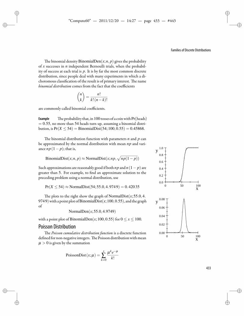
ii
“Compute60” — 2011/12/20 — 14:27 — page 433 — #443 ii
ii
ii
Families of Discrete Distributions
e binomial density BinomialDen(x;n, p) gives the probabilityof x successes in n independent Bernoulli trials, when the probabil-ity of success at each trial is p. It is by far the most common discretedistribution, since people deal with many experiments in which a di-chotomous classi cation of the result is of primary interest. e namebinomial distribution comes from the fact that the coefficients(
nk
)=
n!k!(n− k)!
are commonly called binomial coefficients.
Example eprobability that, in100 tosses of a coinwithPr(heads)= 0.55, no more than 54 heads turn up, assuming a binomial distri-bution, is Pr(X ≤ 54) = BinomialDist(54;100,0.55) = 0.45868.
e binomial distribution function with parameters n and p canbe approximated by the normal distribution with mean np and vari-ance np(1− p); that is,
BinomialDist(x;n, p)≈ NormalDist(x;np,√
np(1− p))
Such approximations are reasonably good if both np and n(1− p) aregreater than 5. For example, to nd an approximate solution to thepreceding problem using a normal distribution, use
Pr(X ≤ 54)≈ NormalDist(54;55.0,4.9749) = 0.42035 0 50 1000.0
0.2
0.4
0.6
0.8
1.0
x
y
0 50 1000.00
0.02
0.04
0.06
0.08
x
ye plots to the right show the graph of NormalDist(x;55.0,4.
9749)with apoint plot ofBinomialDist(x;100,0.55), and the graphof
NormalDen(x;55.0,4.9749)
with a point plot of BinomialDen(x;100,0.55) for 0≤ x≤ 100.
Poisson Distributione Poisson cumulative distribution function is a discrete function
de ned fornon-negative integers. e Poissondistributionwithmeanµ > 0 is given by the summation
PoissonDist(x; µ) =x
∑k=0
µke−µ
k!
433
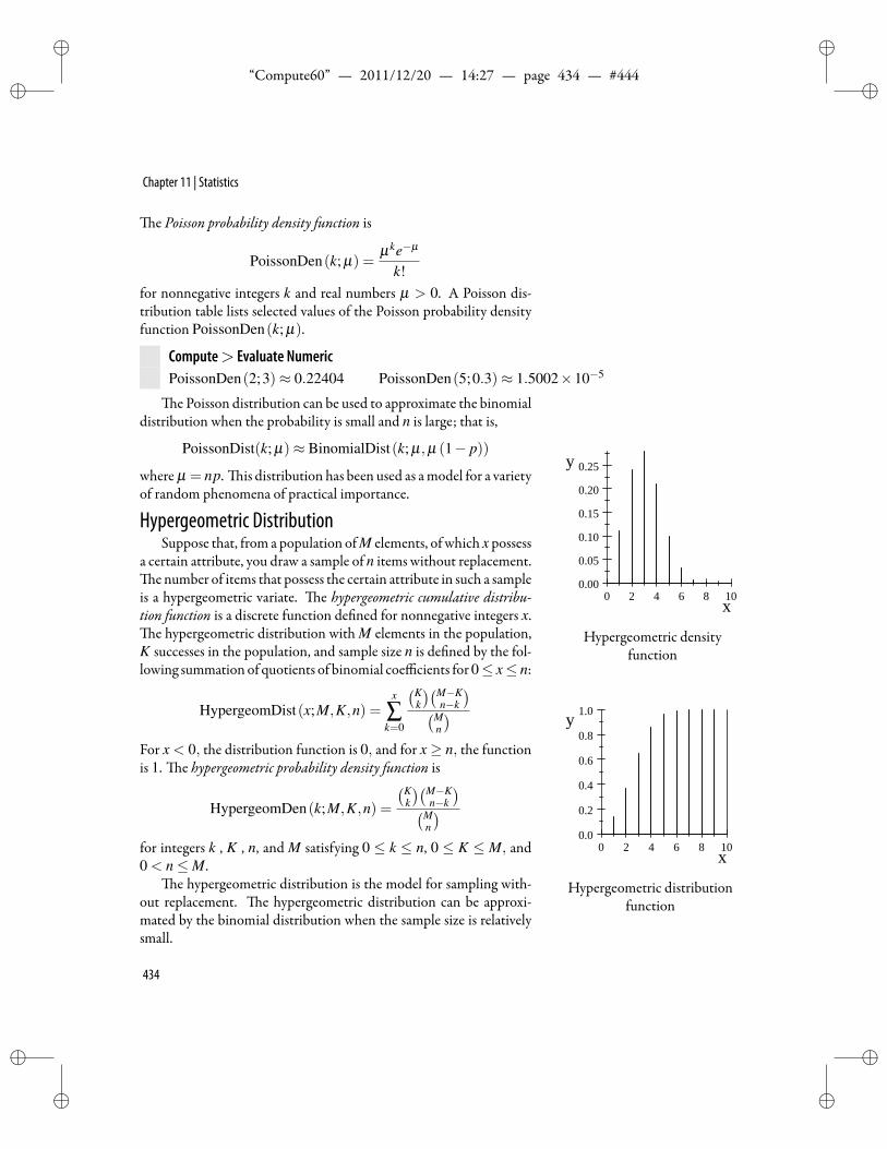
ii
“Compute60” — 2011/12/20 — 14:27 — page 434 — #444 ii
ii
ii
Chapter 11 | Statistics
e Poisson probability density function is
PoissonDen(k; µ) =µke−µ
k!for nonnegative integers k and real numbers µ > 0. A Poisson dis-tribution table lists selected values of the Poisson probability densityfunction PoissonDen(k; µ).
Compute> Evaluate NumericPoissonDen(2;3)≈ 0.22404 PoissonDen(5;0.3)≈ 1.5002×10⁻⁵
e Poisson distribution can be used to approximate the binomialdistribution when the probability is small and n is large; that is,
PoissonDist(k; µ)≈ BinomialDist(k; µ ,µ (1− p))
where µ = np. is distribution has been used as amodel for a varietyof random phenomena of practical importance.
Hypergeometric DistributionSuppose that, from a population of M elements, of which x possess
a certain attribute, you draw a sample of n items without replacement.e number of items that possess the certain attribute in such a sample
is a hypergeometric variate. e hypergeometric cumulative distribu-tion function is a discrete function de ned for nonnegative integers x.
e hypergeometric distribution with M elements in the population,K successes in the population, and sample size n is de ned by the fol-lowing summation of quotients of binomial coefficients for0≤ x≤ n:
0 2 4 6 8 100.00
0.05
0.10
0.15
0.20
0.25
x
y
Hypergeometric densityfunction
0 2 4 6 8 100.0
0.2
0.4
0.6
0.8
1.0
x
y
Hypergeometric distributionfunction
HypergeomDist(x;M,K,n) =x
∑k=0
(Kk
)(M−Kn−k
)(Mn
)For x < 0, the distribution function is 0, and for x≥ n, the functionis 1. e hypergeometric probability density function is
HypergeomDen(k;M,K,n) =
(Kk
)(M−Kn−k
)(Mn
)for integers k , K , n, and M satisfying 0 ≤ k ≤ n, 0 ≤ K ≤ M, and0 < n≤M.
e hypergeometric distribution is the model for sampling with-out replacement. e hypergeometric distribution can be approxi-mated by the binomial distribution when the sample size is relativelysmall.
434
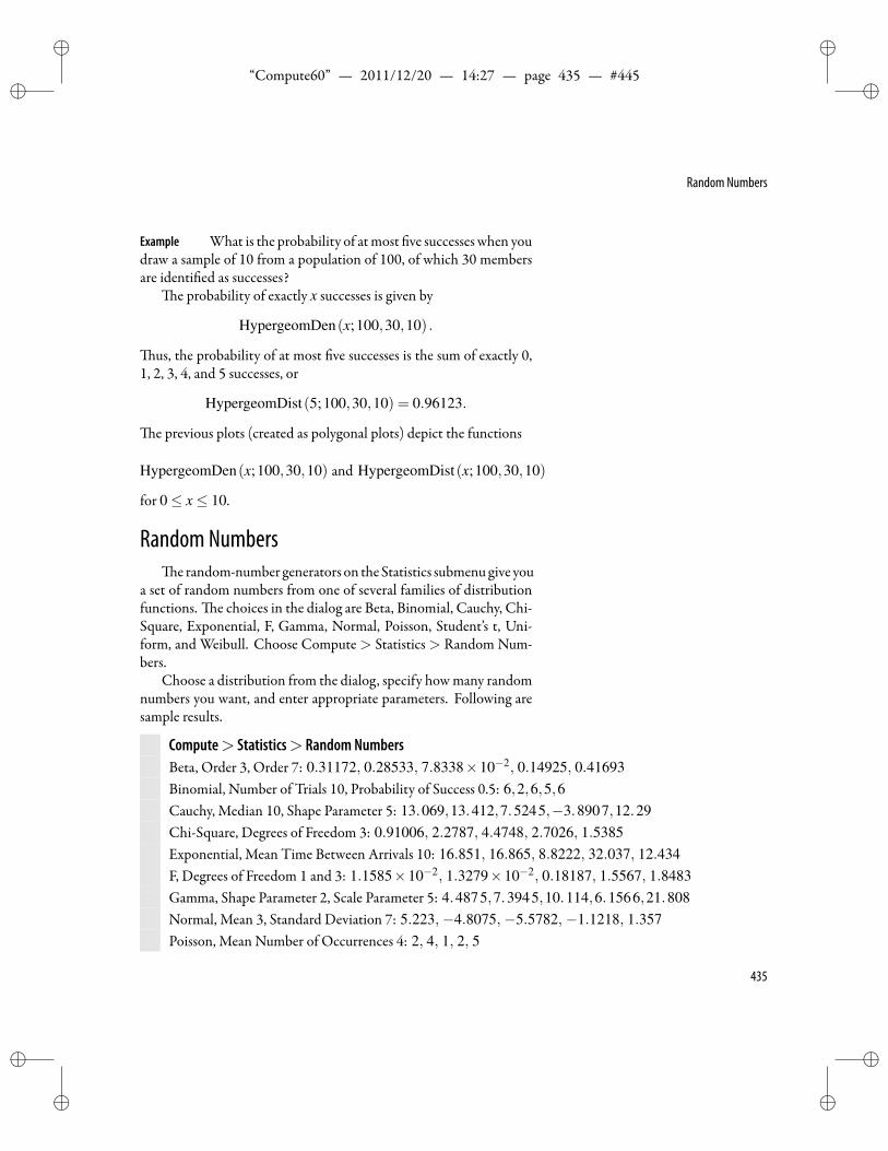
ii
“Compute60” — 2011/12/20 — 14:27 — page 435 — #445 ii
ii
ii
Random Numbers
Example What is the probability of atmost ve successes when youdraw a sample of 10 from a population of 100, of which 30 membersare identi ed as successes?
e probability of exactly x successes is given by
HypergeomDen(x;100,30,10) .
us, the probability of at most ve successes is the sum of exactly 0,1, 2, 3, 4, and 5 successes, or
HypergeomDist(5;100,30,10) = 0.96123.
e previous plots (created as polygonal plots) depict the functions
HypergeomDen(x;100,30,10) and HypergeomDist(x;100,30,10)
for 0≤ x≤ 10.
Random Numberse random-number generators on theStatistics submenugive you
a set of random numbers from one of several families of distributionfunctions. e choices in the dialog are Beta, Binomial, Cauchy, Chi-Square, Exponential, F, Gamma, Normal, Poisson, Student’s t, Uni-form, and Weibull. Choose Compute > Statistics > Random Num-bers.
Choose a distribution from the dialog, specify howmany randomnumbers you want, and enter appropriate parameters. Following aresample results.
Compute> Statistics> Random NumbersBeta, Order 3, Order 7: 0.31172, 0.28533, 7.8338×10⁻², 0.14925, 0.41693Binomial, Number of Trials 10, Probability of Success 0.5: 6,2,6,5,6Cauchy, Median 10, Shape Parameter 5: 13.069,13.412,7.5245,−3.8907,12.29Chi-Square, Degrees of Freedom 3: 0.91006, 2.2787, 4.4748, 2.7026, 1.5385Exponential, Mean Time Between Arrivals 10: 16.851, 16.865, 8.8222, 32.037, 12.434F, Degrees of Freedom 1 and 3: 1.1585×10⁻², 1.3279×10⁻², 0.18187, 1.5567, 1.8483Gamma, Shape Parameter 2, Scale Parameter 5: 4.4875,7.3945,10.114,6.1566,21.808Normal, Mean 3, Standard Deviation 7: 5.223,−4.8075,−5.5782,−1.1218, 1.357Poisson, Mean Number of Occurrences 4: 2, 4, 1, 2, 5
435
ii
“Compute60” — 2011/12/20 — 14:27 — page 436 — #446 ii
ii
ii
Chapter 11 | Statistics
Compute> Statistics> Random NumbersStudent’s t, Degrees of Freedom 7: −3.6549×10⁻²,−0.35357,1.3031,−1.1615,1.1861Uniform, Lower End of Range 0, Upper End of Range 20: 5.6016, 16.744, 10.275, 14.057, 10.136Weibull, Shape Parameter 5, Scale Parameter 3: 2.2615,3.0731,3.0868,3.8504,2.4592
Curve FittingYou have the tools to do general curve tting in an intuitive man-
ner. Choose Compute > Statistics > Fit Curve to Data and make achoice in the dialog box.
• For straight-line ts, choose Multiple Regression or MultipleRegression (no constant).
• For best ts by polynomials, choose Polynomial of Degree [ ].
Linear RegressionMultiple Regression calculates linear-regression equations with
keyed or labeled data matrices. e result is an equation expressingthe variable at the head of the rst column as a linear combination ofthe variables heading the remaining columns, plus a constant (that ismissing if Multiple Regression (no constant) was chosen).
e equation produced is the best t to the data in the least-squaressense.
Compute> Statistics> Fit Curve to Data>Multiple Regression(Location of Dependent Variable: First Column)
y x0 1.1
0.5 1.51 1.9
1.5 2.4
Regression is: y = 1.159x−1.2493
Compute> Statistics> Fit Curve to Data>Multiple Regression(Location of Dependent Variable: First Column)
z x y1 0 1.12 0.5 1.14 1 1.95 1.5 1.9
Regression is: z = 2.0x+1.25y−0.375
436
ii
“Compute60” — 2011/12/20 — 14:27 — page 437 — #447 ii
ii
ii
Curve Fitting
e choice Multiple Regression (no constant) gives the followinglinear equations:
Compute> Statistics> Fit Curve to Data>Multiple Regression(no constant; Location of Dependent Variable: First Column)
u v0 1.1
0.5 1.51 1.9
1.5 2.42 2.9
Regression is: u = 0.56733v
z x y1 0 1.12 0.5 1.14 1 1.95 1.5 1.97 2 2.9
Regression is: z = 2.1829x+0.91245y
x ya bc d
Regression is: x = y1.0(ab+ cd)
b2 +d2
Polynomial FitPolynomial of Degree [ ] calculates polynomial equations from la-
beled or unlabeled two-column data matrices. e result is a polyno-mial of the speci ed degree that is the best t to the data in the least-squares sense. For the polynomial t, the x column appears rst.
To nd the best t by a polynomial of second degree to the setof points (0,0.64) ,(0.5,0.09) ,(1,0.04) ,(1.5,0.49) ,(2,1.44), re-move the parentheses and convert the entries into a two-column ma-trix. To make this conversion, place the insert point in the list andchoose Compute>Matrices> Reshape; then specify two columns.
Compute>Matrices> Reshape(2 columns)
0,0.64,0.5,0.09,1,0.04,1.5,0.49,2,1.44,
0 0.64
0.5 0.091 0.04
1.5 0.492 1.44
437
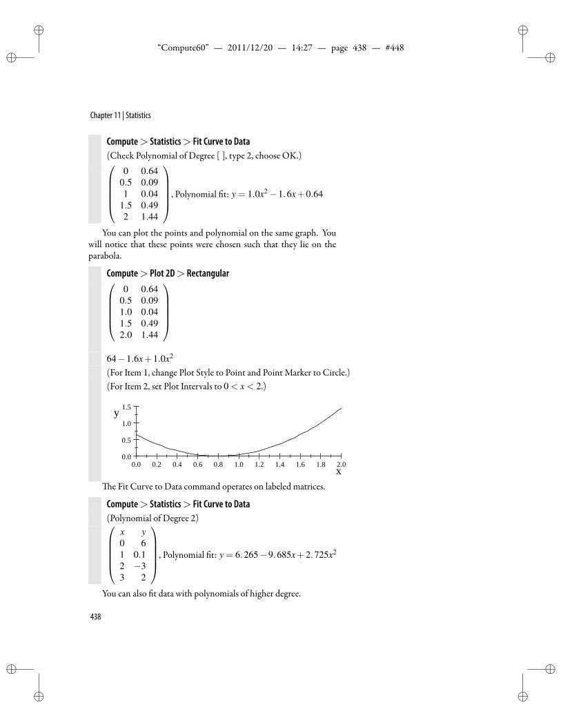
ii
“Compute60” — 2011/12/20 — 14:27 — page 438 — #448 ii
ii
ii
Chapter 11 | Statistics
Compute> Statistics> Fit Curve to Data(Check Polynomial of Degree [ ], type 2, choose OK.)
0 0.640.5 0.091 0.04
1.5 0.492 1.44
, Polynomial t: y = 1.0x2−1.6x+0.64
You can plot the points and polynomial on the same graph. Youwill notice that these points were chosen such that they lie on theparabola.
Compute> Plot 2D> Rectangular0 0.64
0.5 0.091.0 0.041.5 0.492.0 1.44
64−1.6x+1.0x2
(For Item 1, change Plot Style to Point and Point Marker to Circle.)(For Item 2, set Plot Intervals to 0 < x < 2.)
0.0 0.2 0.4 0.6 0.8 1.0 1.2 1.4 1.6 1.8 2.00.0
0.5
1.0
1.5
x
y
e Fit Curve to Data command operates on labeled matrices.
Compute> Statistics> Fit Curve to Data(Polynomial of Degree 2)
x y0 61 0.12 −33 2
, Polynomial t: y = 6.265−9.685x+2.725x2
You can also t data with polynomials of higher degree.
438
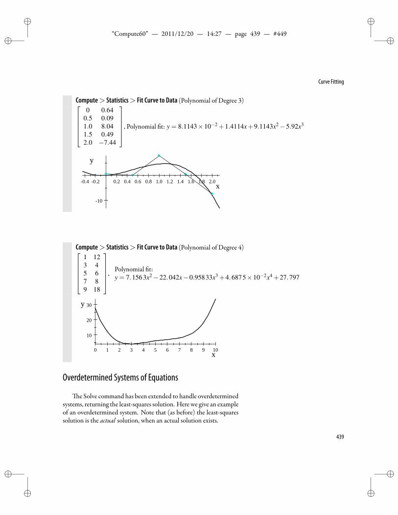
ii
“Compute60” — 2011/12/20 — 14:27 — page 439 — #449 ii
ii
ii
Curve Fitting
Compute> Statistics> Fit Curve to Data (Polynomial of Degree 3)0 0.64
0.5 0.091.0 8.041.5 0.492.0 −7.44
, Polynomial t: y = 8.1143×10⁻² +1.4114x+9.1143x2−5.92x3
0.4 0.2 0.2 0.4 0.6 0.8 1.0 1.2 1.4 1.6 1.8 2.0
10
x
y
Compute> Statistics> Fit Curve to Data (Polynomial of Degree 4)1 123 45 67 89 18
, Polynomial t:y = 7.1563x2−22.042x−0.95833x3 +4.6875×10−2x4 +27.797
0 1 2 3 4 5 6 7 8 9 10
10
20
30
x
y
Overdetermined Systems of Equations
e Solve command has been extended to handle overdeterminedsystems, returning the least-squares solution. Here we give an exampleof an overdetermined system. Note that (as before) the least-squaressolution is the actual solution, when an actual solution exists.
439
ii
“Compute60” — 2011/12/20 — 14:27 — page 440 — #450 ii
ii
ii
Chapter 11 | Statistics
Compute> Solve> Exact1 23 45 67 8
[ xy
]=
37
1115
, Solution:[
11
]
It is easy tomultiply both sides of amatrix equation byAT to checkthat, when you “solve” AX = B, you are actually getting the solutionof(AT A
)X = AT B. Here,
A =
1 23 45 67 8
, X =
[xy
], B =
371115
.Compute> Evaluate
AT A =
[84 100
100 120
]
AT B =
[184220
]is calculation gives the following equation, which has an exact
solution.
Compute> Solve> Exact[84 100100 120
][xy
]=
[184220
], Solution:
[11
]Exercises
1. Consider a normal randomvariable withmean 50 and standarddeviation 10, and a random sample of size 80 from which weare to compute the values of X , the sample mean. What is theprobability of getting a value of X as low as 46?
2. Suppose a workingwidget deteriorates very little with age. atis, a widget that has been running for some timewill have nearlythe same failure probability during the following hour as it hadduring its rst hour of operation. en, the failure times have anexponential distribution P(T ≤ t) of the form 1−e−
xµ . Given
440
ii
“Compute60” — 2011/12/20 — 14:27 — page 441 — #451 ii
ii
ii
Exercises
that the widget has a mean life of 5 years, what is the probabil-ity that the widget will have a lifetime exceeding 7.5 years? Ifthe widget is guaranteed for 2 years, what percentage of suchwidgets can be expected to need replacement while under war-ranty?
3. A widget has a mean life of 5 years with a standard deviationof 2 years. Assuming a normal distribution, what is the prob-ability that the widget will have a lifetime exceeding 7.5 years?If the widget is guaranteed for 2 years, what percentage of suchwidgets can be expected to need replacement while under war-ranty?
4. e mean of a continuous distribution with probability densityfunction f (u) is the integral
∫ ∞−∞ u f (u)du = µ of the product
of the variable and the probability density function. e vari-ance is the integral
∫ ∞−∞ (u−µ)2 f (u)du. Find the mean and
variance for each of the continuous distributions discussed inthis chapter.
5. emeanof adiscrete distributionwithprobability density func-tion f (u) is the sum ∑∞
−∞ u f (u) = µ , and the variance is
∞
∑−∞
(u−µ)2 f (u) = σ2.
Find the mean and variance for the discrete distributions dis-cussed in this chapter. If the probability density function for adistribution is f (n) =
( 12
)n, what is the mean of the distribu-
tion? What is the variance?
6. A die is cast until a 4 appears. What is the probability that itmust be cast more than 5 times?
7. A telephone switchboard handles 600 calls on average during asingle rush hour. e board canmake amaximumof 20 connec-tions per minute. Use the Poisson distribution to evaluate theprobability that the board will be overtaxed during any givenminute of a rush hour.
8. Find the probability that x2 ≤ 4 for a normal distribution withmean 1 and standard deviation 1.
441
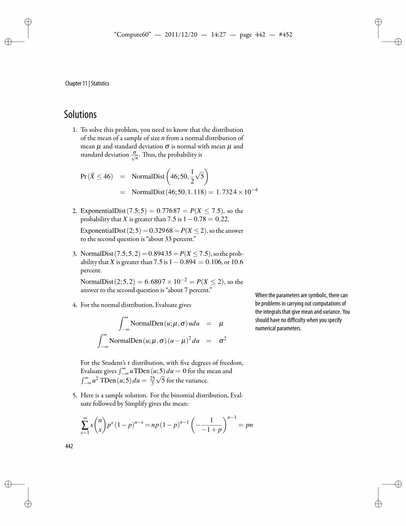
ii
“Compute60” — 2011/12/20 — 14:27 — page 442 — #452 ii
ii
ii
Chapter 11 | Statistics
Solutions1. To solve this problem, you need to know that the distribution
of the mean of a sample of size n from a normal distribution ofmean µ and standard deviation σ is normal with mean µ andstandard deviation σ√
n . us, the probability is
Pr(X ≤ 46) = NormalDist(
46;50,12
√5)
= NormalDist(46;50,1.118) = 1.7324×10⁻⁴
2. ExponentialDist(7.5;5) = 0.77687 = P(X ≤ 7.5), so theprobability that X is greater than 7.5 is 1−0.78 = 0.22.
ExponentialDist(2;5) = 0.32968=P(X ≤ 2), so the answerto the second question is “about 33 percent.”
3. NormalDist(7.5;5,2)= 0.89435=P(X ≤ 7.5), so theprob-ability that X is greater than 7.5 is 1− 0.894 = 0.106, or 10.6percent.
NormalDist(2;5,2) = 6.6807× 10−2 = P(X ≤ 2), so theanswer to the second question is “about 7 percent.”
When the parameters are symbolic, there canbe problems in carrying out computations ofthe integrals that give mean and variance. Youshould have no difficulty when you specifynumerical parameters.
4. For the normal distribution, Evaluate gives∫ ∞
−∞NormalDen(u; µ,σ)udu = µ∫ ∞
−∞NormalDen(u; µ ,σ)(u−µ)2 du = σ2
For the Student’s t distribution, with ve degrees of freedom,Evaluate gives
∫ ∞−∞ uTDen(u;5)du = 0 for the mean and∫ ∞
−∞ u2 TDen(u;5)du = 253
√5 for the variance.
5. Here is a sample solution. For the binomial distribution, Eval-uate followed by Simplify gives the mean:
∞
∑x=1
x(
nx
)px (1− p)n−x = np(1− p)n−1
(− 1−1+ p
)n−1
= pn
442
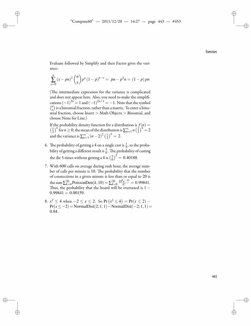
ii
“Compute60” — 2011/12/20 — 14:27 — page 443 — #453 ii
ii
ii
Exercises
Evaluate followed by Simplify and then Factor gives the vari-ance:
n
∑x=0
(x− pn)2(
nx
)px (1− p)n−x = pn− p2n = (1− p) pn
( e intermediate expression for the variance is complicatedand does not appear here. Also, you need to make the simpli -cations (−1)2n = 1 and (−1)2n+1 =−1. Note that the symbol(n
x
)is a binomial fraction, rather than amatrix. To enter a bino-
mial fraction, choose Insert > Math Objects > Binomial, andchoose None for Line.)
If the probability density function for a distribution is f (n) =( 12
)n forn≥ 0, themean of the distribution is∑∞n=1 n
( 12
)n= 2
and the variance is ∑∞n=1 (n−2)2 ( 1
2
)n= 2.
6. e probability of getting a 4 on a single cast is 16 , so the proba-
bility of getting a different result is 56 . e probability of casting
the die 5 times without getting a 4 is( 5
6
)5= 0.40188.
7. With 600 calls on average during rush hour, the average num-ber of calls per minute is 10. e probability that the numberof connections in a given minute is less than or equal to 20 isthe sum∑20
k=0 PoissonDen(k,10)=∑20k=0
10ke−10
k! = 0.99841.us, the probability that the board will be overtaxed is 1−
0.99841 = 0.00159.
8. x2 ≤ 4 when −2 ≤ x ≤ 2. So Pr(x2 ≤ 4
)= Pr(x ≤ 2)−
Pr(x≤−2)=NormalDist(2;1,1)−NormalDist(−2;1,1)=0.84.
443

ii
“Compute60” — 2011/12/20 — 14:27 — page 444 — #454 ii
ii
ii
ii
“Compute60” — 2011/12/20 — 14:27 — page 445 — #455 ii
ii
ii
12Applied Modern Algebra
[On the concept of group:] ... what a wealth, what a grandeur of thought may spring fromwhat slight beginnings.Henry Frederick Baker (1866–1956)
A pplied modern algebra provides techniques for sending and Solving Equations
Integers Modulo m
Other Systems Modulo m
Polynomials ModuloPolynomials
Linear Programming
receiving con dential messages, for assuring that recordingsalways sound perfect, and for packing a lot of data into a very
small space. is chapter includes an introduction to some of the un-derlying computational tools that make such applications possible.
Solving EquationsMany techniques in applied modern algebra are designed to solve
equations, from integer equations to polynomial equations to matrixequations. In this section, we describe a few of the methods that canbe applied to such problems.
Integer Solutionse solver can be restricted to the domain of integers. Choose
Compute > Solve > Integer to nd integer roots of polynomial ex-pressions with rational coefficients, and integer solutions to equationsof the same type.To nd integer roots or integer solutions to an equation
1. Place the insert point in an expression or equation.
2. Choose Compute> Solve> Integer.
445
ii
“Compute60” — 2011/12/20 — 14:27 — page 446 — #456 ii
ii
ii
Chapter 12 | Applied Modern Algebra
Compute> Solve> Integer41x+421x2−165x3−4x4 +4x5−105, Solution: −7,3,52x2−11x+15 = 3x2−16x+21, Solution: 2,3
Continued FractionsA simple continued action is an expression of the form
a0 +1
a1 +1
a2+1
a3+1
a4+1
a5+..
where a0 is an integer and a1,a2, . . . are positive integers. ere canbe either an in nite or a nite number of terms ai. A number is ra-tional if and only if it can be expressed as a simple nite continuedfraction. You can nd rational approximations to irrational numbersby expanding the irrational as a simple continued fraction, then trun-cating the continued fraction to obtain a rational.
Continued fractions have been utilized within computer algo-rithms for computing rational approximations to real numbers, as wellas solving indeterminate equations. Connections have been establish-ed between continued fractions and chaos theory.
Use theMuPADcommand contfrac to construct a continued frac-tion of the real numerical expression x to n signi cant digits.Tode ne a continued fractions command
1. Choose Compute>De nitions>De ne MuPAD Name.
2. In the MuPAD Name box, type numlib::contfrac(x,n).
3. In the Scienti c WorkPlace (Notebook) Name box, type r (x,n).
4. Check “ at is built in to MuPAD or is automatically loaded”and choose OK.
Use the continued fractions command to generate continued frac-tions.
Compute> Evaluater (π,10) = 3+ 1
7+ 115+ 1
1+ 1292+ 1
1+ 11+..
e twodots at thebottom indicate an in nite continued fraction.However, you can easily truncate the continued fraction.
446
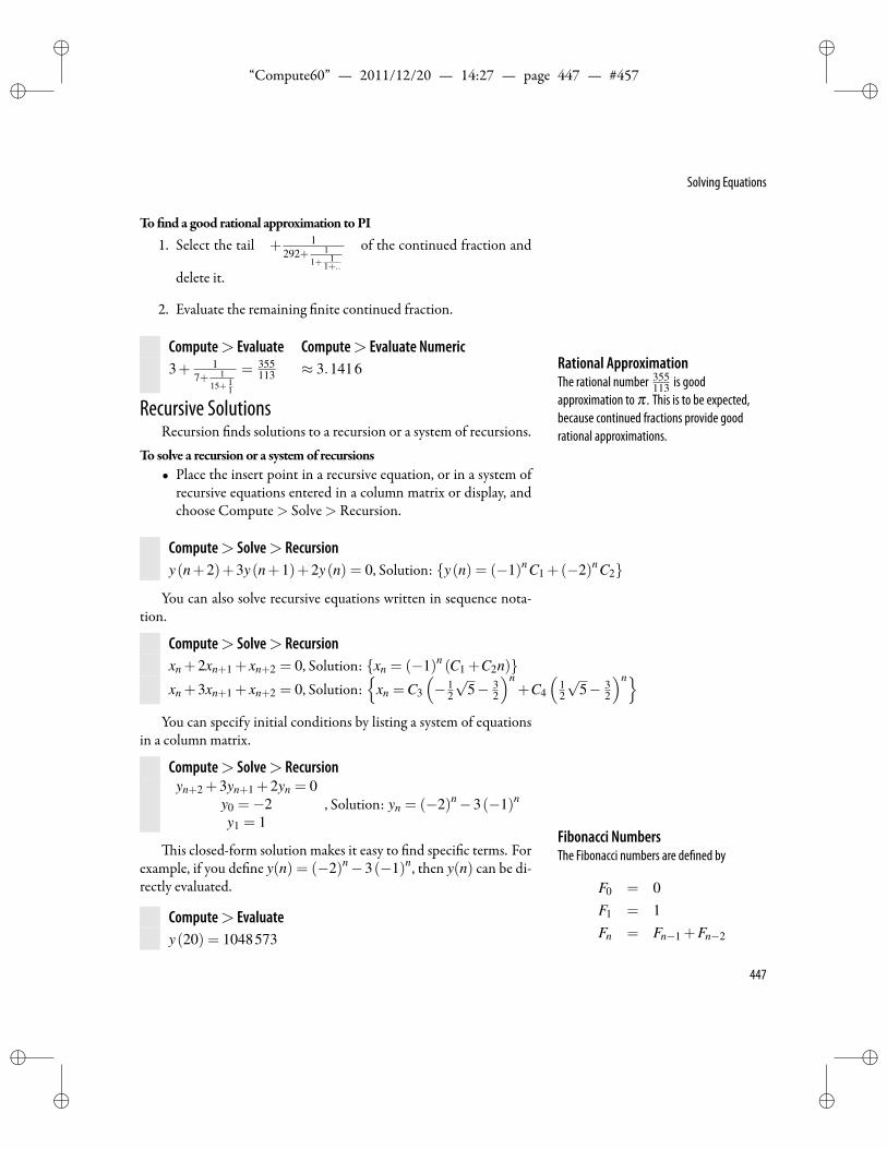
ii
“Compute60” — 2011/12/20 — 14:27 — page 447 — #457 ii
ii
ii
Solving Equations
To nd a good rational approximation toPI1. Select the tail + 1
292+ 11+ 1
1+..
of the continued fraction and
delete it.
2. Evaluate the remaining nite continued fraction.
Compute> Evaluate Compute> Evaluate Numeric3+ 1
7+ 115+ 1
1
= 355113 ≈ 3.1416 Rational Approximation
The rational number 355113 is good
approximation toπ . This is to be expected,because continued fractions provide goodrational approximations.
Recursive SolutionsRecursion nds solutions to a recursion or a system of recursions.
To solve a recursionor a systemof recursions• Place the insert point in a recursive equation, or in a system of
recursive equations entered in a column matrix or display, andchoose Compute> Solve> Recursion.
Compute> Solve> Recursiony(n+2)+3y(n+1)+2y(n) = 0, Solution: y(n) = (−1)n C1 +(−2)n C2
You can also solve recursive equations written in sequence nota-tion.
Compute> Solve> Recursionxn +2xn+1 + xn+2 = 0, Solution: xn = (−1)n (C1 +C2n)xn +3xn+1 + xn+2 = 0, Solution:
xn =C3
(− 1
2
√5− 3
2
)n+C4
(12
√5− 3
2
)nYou can specify initial conditions by listing a system of equations
in a column matrix.
Compute> Solve> Recursionyn+2 +3yn+1 +2yn = 0
y0 =−2y1 = 1
, Solution: yn = (−2)n−3(−1)n
Fibonacci NumbersThe Fibonacci numbers are de ned by
F0 = 0F1 = 1Fn = Fn−1 +Fn−2
is closed-form solution makes it easy to nd speci c terms. Forexample, if you de ne y(n) = (−2)n−3(−1)n, then y(n) can be di-rectly evaluated.
Compute> Evaluatey(20) = 1048573
447
ii
“Compute60” — 2011/12/20 — 14:27 — page 448 — #458 ii
ii
ii
Chapter 12 | Applied Modern Algebra
Integers Modulo me Euclidean algorithm for integers leads to the notion of con-
gruence of two integers modulo a given integer. Mod FunctionThe mod function is a function of twovariables, with the function written betweenthe two variables. This usage is similar to thecommon usage of+, which is also a functionof two variables with the function valuesexpressed as a+b, rather than the usualfunctional notation+(a,b).
Two integers a and b are congruent modulo m if and only if a−b is a multiple of m, in which case we write a ≡ b (modm). us,15 ≡ 33 (mod9), because 15− 33 = −18 is a multiple of 9. Givenintegersa andm, themod function is givenbyamodm= b if andonlyif a≡ b (modm) and 0≤ b≤ m−1; hence, amodm is the smallestnonnegative residue of a modulo m.
e underlying computer algebra system does not understand thecongruence notation a≡ b(modm), but it does understand the func-tion notation amodm. is section shows how to translate problemsin algebra and number theory into language that will be handled cor-rectly by the computational engine.
Traditionally the congruence notation a ≡ b (modm) is writtenwith the modm enclosed inside parentheses since the modm clari esthe expression a≡ b. In this context, the expression b (modm) neverappearswithout the precedinga≡. On the other hand, themod func-tion is usually written in the form amodm without parentheses.Toevaluate themod function
• Place the insert point in the expressionamodb and chooseCom-pute> Evaluate.
Compute> Evaluate23mod14 = 9
In terms of the oor function ⌊x⌋, the mod function is given by
amodm = a−⌊a/m⌋m
Compute> Evaluate23−
⌊ 2314
⌋14 = 9
Multiplication Tables Modulo mYou can make tables that display the products modulo m of pairs
of integers from the set 0,1,2, . . . ,m−1.Toget amultiplication tablemodulomwithm=6
1. Type the equation g(i, j) = (i−1)( j−1) and choose Com-pute>De nitions>New De nition.
448
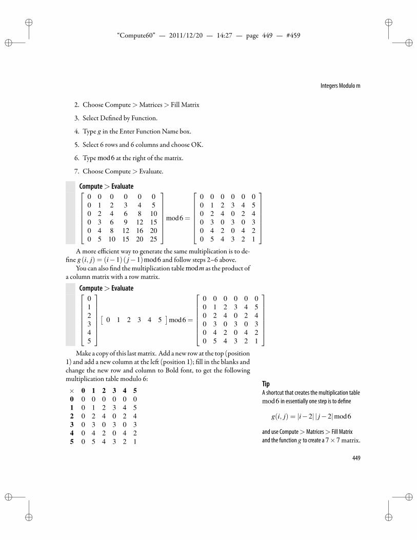
ii
“Compute60” — 2011/12/20 — 14:27 — page 449 — #459 ii
ii
ii
Integers Modulo m
2. Choose Compute>Matrices> Fill Matrix
3. Select De ned by Function.
4. Type g in the Enter Function Name box.
5. Select 6 rows and 6 columns and choose OK.
6. Type mod6 at the right of the matrix.
7. Choose Compute> Evaluate.
Compute> Evaluate0 0 0 0 0 00 1 2 3 4 50 2 4 6 8 100 3 6 9 12 150 4 8 12 16 200 5 10 15 20 25
mod6 =
0 0 0 0 0 00 1 2 3 4 50 2 4 0 2 40 3 0 3 0 30 4 2 0 4 20 5 4 3 2 1
A more efficient way to generate the same multiplication is to de-
ne g(i, j) = (i−1)( j−1)mod6 and follow steps 2–6 above.You can also nd themultiplication table modm as the product of
a column matrix with a row matrix.
Compute> Evaluate012345
[
0 1 2 3 4 5]
mod6 =
0 0 0 0 0 00 1 2 3 4 50 2 4 0 2 40 3 0 3 0 30 4 2 0 4 20 5 4 3 2 1
Make a copy of this lastmatrix. Add a new row at the top (position
1) and add a new column at the le (position 1); ll in the blanks andchange the new row and column to Bold font, to get the followingmultiplication table modulo 6:
TipA shortcut that creates the multiplication tablemod6 in essentially one step is to de ne
g(i, j) = |i−2| | j−2|mod6
and use Compute>Matrices> Fill Matrixand the functiong to create a7×7 matrix.
× 0 1 2 3 4 50 0 0 0 0 0 01 0 1 2 3 4 52 0 2 4 0 2 43 0 3 0 3 0 34 0 4 2 0 4 25 0 5 4 3 2 1
449
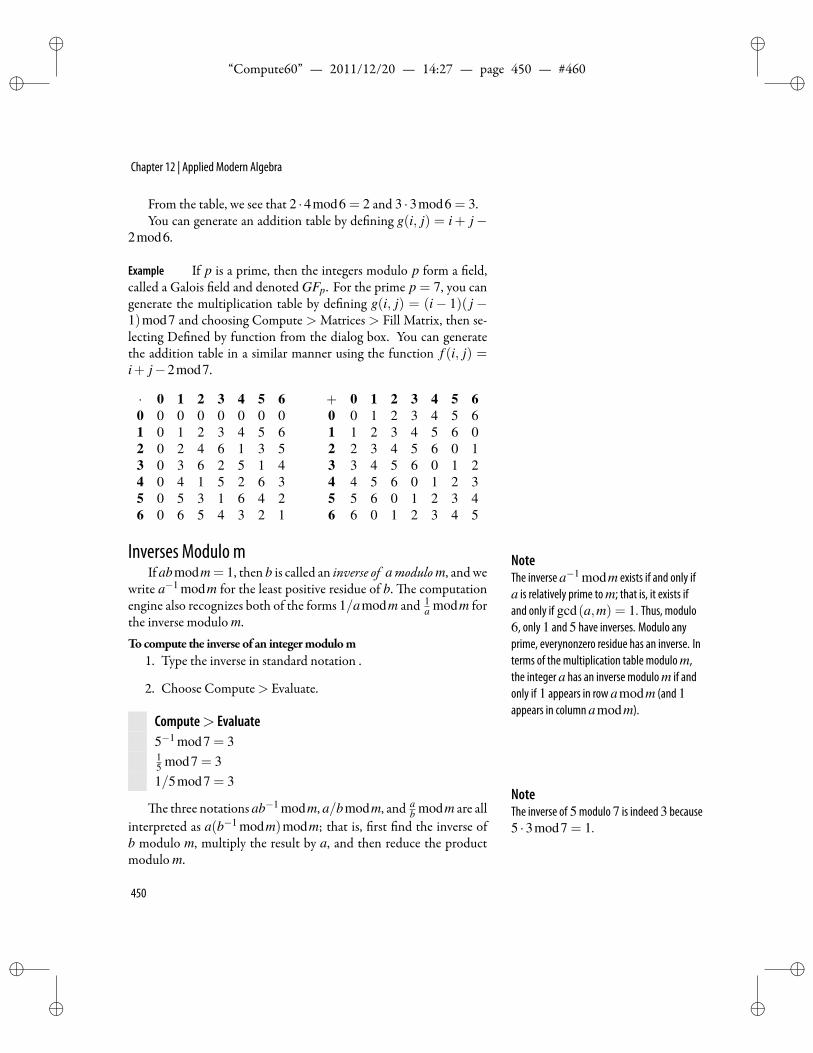
ii
“Compute60” — 2011/12/20 — 14:27 — page 450 — #460 ii
ii
ii
Chapter 12 | Applied Modern Algebra
From the table, we see that 2 ·4mod6 = 2 and 3 ·3mod6 = 3.You can generate an addition table by de ning g(i, j) = i+ j−
2mod6.
Example If p is a prime, then the integers modulo p form a eld,called a Galois eld and denoted GFp. For the prime p = 7, you cangenerate the multiplication table by de ning g(i, j) = (i− 1)( j−1)mod7 and choosing Compute > Matrices > Fill Matrix, then se-lecting De ned by function from the dialog box. You can generatethe addition table in a similar manner using the function f (i, j) =i+ j−2mod7.
· 0 1 2 3 4 5 60 0 0 0 0 0 0 01 0 1 2 3 4 5 62 0 2 4 6 1 3 53 0 3 6 2 5 1 44 0 4 1 5 2 6 35 0 5 3 1 6 4 26 0 6 5 4 3 2 1
+ 0 1 2 3 4 5 60 0 1 2 3 4 5 61 1 2 3 4 5 6 02 2 3 4 5 6 0 13 3 4 5 6 0 1 24 4 5 6 0 1 2 35 5 6 0 1 2 3 46 6 0 1 2 3 4 5
Inverses Modulo m NoteThe inverse a−1 modm exists if and only ifa is relatively prime tom; that is, it exists ifand only if gcd(a,m) = 1. Thus, modulo6, only 1 and 5 have inverses. Modulo anyprime, everynonzero residue has an inverse. Interms of the multiplication table modulom,the integera has an inverse modulom if andonly if 1 appears in row amodm (and 1appears in column amodm).
If abmodm = 1, then b is called an in erse of amodulom, and wewrite a−1 modm for the least positive residue of b. e computationengine also recognizes both of the forms 1/amodm and 1
a modm forthe inverse modulo m.Tocompute the inverse of an integermodulom
1. Type the inverse in standard notation .
2. Choose Compute> Evaluate.
Compute> Evaluate5−1 mod7 = 315 mod7 = 31/5mod7 = 3
NoteThe inverse of 5modulo7 is indeed3 because5 ·3mod7 = 1.
e three notations ab−1 modm, a/bmodm, and ab modm are all
interpreted as a(b−1 modm)modm; that is, rst nd the inverse ofb modulo m, multiply the result by a, and then reduce the productmodulo m.
450
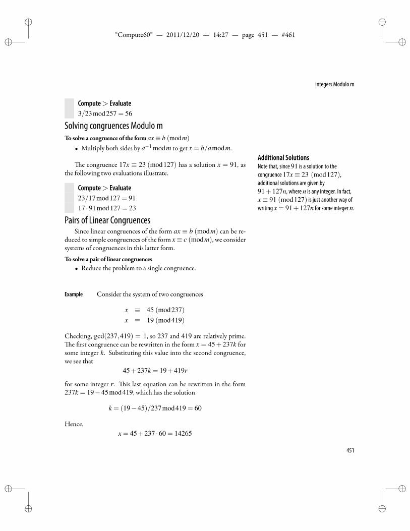
ii
“Compute60” — 2011/12/20 — 14:27 — page 451 — #461 ii
ii
ii
Integers Modulo m
Compute> Evaluate3/23mod257 = 56
Solving congruences Modulo mTo solve a congruence of the formax≡ b (modm)
• Multiply both sides by a−1 modm to get x = b/amodm.Additional SolutionsNote that, since91 is a solution to thecongruence17x≡ 23 (mod127),additional solutions are given by91+127n, where n is any integer. In fact,x≡ 91 (mod127) is just another way ofwriting x = 91+127n for some integern.
e congruence 17x ≡ 23 (mod127) has a solution x = 91, asthe following two evaluations illustrate.
Compute> Evaluate23/17mod127 = 9117 ·91mod127 = 23
Pairs of Linear CongruencesSince linear congruences of the form ax ≡ b (modm) can be re-
duced to simple congruences of the form x≡ c (modm), we considersystems of congruences in this latter form.
To solve a pair of linear congruences• Reduce the problem to a single congruence.
Example Consider the system of two congruences
x ≡ 45 (mod237)x ≡ 19 (mod419)
Checking, gcd(237,419) = 1, so 237 and 419 are relatively prime.e rst congruence can be rewritten in the form x = 45+237k for
some integer k. Substituting this value into the second congruence,we see that
45+237k = 19+419r
for some integer r. is last equation can be rewritten in the form237k = 19−45mod419, which has the solution
k = (19−45)/237mod419 = 60
Hence,x = 45+237 ·60 = 14265
451
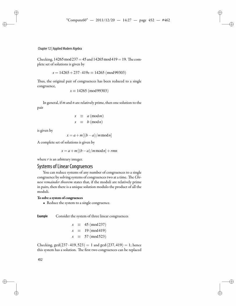
ii
“Compute60” — 2011/12/20 — 14:27 — page 452 — #462 ii
ii
ii
Chapter 12 | Applied Modern Algebra
Checking,14265mod237= 45 and14265mod419= 19. e com-plete set of solutions is given by
x = 14265+237 ·419s≡ 14265 (mod99303)
us, the original pair of congruences has been reduced to a singlecongruence,
x≡ 14265 (mod99303)
In general, if m and n are relatively prime, then one solution to thepair
x ≡ a (modm)
x ≡ b (modn)
is given byx = a+m [(b−a)/mmodn]
A complete set of solutions is given by
x = a+m [(b−a)/mmodn]+ rmn
where r is an arbitrary integer.
Systems of Linear CongruencesYou can reduce systems of any number of congruences to a single
congruence by solving systems of congruences two at a time. eChi-nese remainder theorem states that, if the moduli are relatively primein pairs, then there is a unique solution modulo the product of all themoduli.To solve a systemof congruences
• Reduce the system to a single congruence.
Example Consider the system of three linear congruences
x ≡ 45 (mod237)x ≡ 19 (mod419)x ≡ 57 (mod523)
Checking, gcd(237 · 419,523) = 1 and gcd(237,419) = 1; hencethis system has a solution. e rst two congruences can be replaced
452
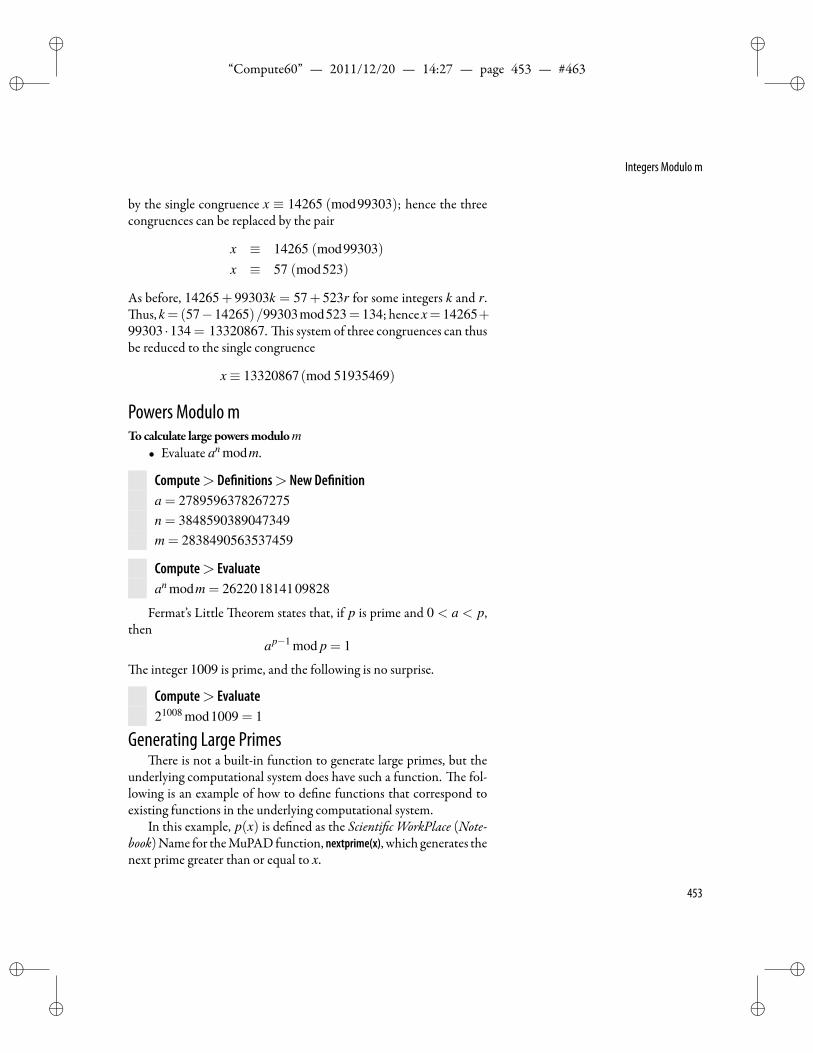
ii
“Compute60” — 2011/12/20 — 14:27 — page 453 — #463 ii
ii
ii
Integers Modulo m
by the single congruence x ≡ 14265 (mod99303); hence the threecongruences can be replaced by the pair
x ≡ 14265 (mod99303)x ≡ 57 (mod523)
As before, 14265+ 99303k = 57+ 523r for some integers k and r.us, k=(57−14265)/99303mod523= 134; hence x= 14265+
99303 ·134 = 13320867. is system of three congruences can thusbe reduced to the single congruence
x≡ 13320867(mod 51935469)
Powers Modulo mTocalculate large powersmodulom
• Evaluate an modm.
Compute> De nitions> New De nitiona = 2789596378267275n = 3848590389047349m = 2838490563537459
Compute> Evaluatean modm = 262201814109828
Fermat’s Little eorem states that, if p is prime and 0 < a < p,then
ap−1 mod p = 1
e integer 1009 is prime, and the following is no surprise.
Compute> Evaluate21008 mod1009 = 1
Generating Large Primesere is not a built-in function to generate large primes, but the
underlying computational system does have such a function. e fol-lowing is an example of how to de ne functions that correspond toexisting functions in the underlying computational system.
In this example, p(x) is de ned as the Scienti c WorkPlace (Note-book)Name for theMuPADfunction, nextprime(x), which generates thenext prime greater than or equal to x.
453
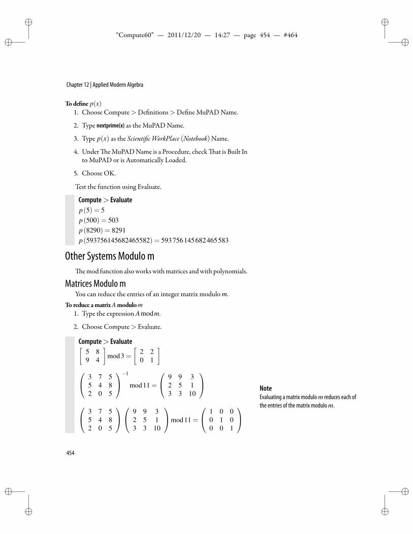
ii
“Compute60” — 2011/12/20 — 14:27 — page 454 — #464 ii
ii
ii
Chapter 12 | Applied Modern Algebra
Tode ne p(x)1. Choose Compute>De nitions>De ne MuPAD Name.
2. Type nextprime(x) as the MuPAD Name.
3. Type p(x) as the Scienti c WorkPlace (Notebook) Name.
4. Under eMuPADName is a Procedure, check at is Built Into MuPAD or is Automatically Loaded.
5. Choose OK.
Test the function using Evaluate.
Compute> Evaluatep(5) = 5p(500) = 503p(8290) = 8291p(593756145682465582) = 593756145682465583
Other Systems Modulo memod function alsoworkswithmatrices andwith polynomials.
Matrices Modulo mYou can reduce the entries of an integer matrix modulo m.
To reduce amatrixAmodulom1. Type the expression Amodm.
2. Choose Compute> Evaluate.
Compute> Evaluate[5 89 4
]mod3 =
[2 20 1
] 3 7 5
5 4 82 0 5
−1
mod11 =
9 9 32 5 13 3 10
3 7 5
5 4 82 0 5
9 9 32 5 13 3 10
mod11 =
1 0 00 1 00 0 1
NoteEvaluating a matrix modulom reduces each ofthe entries of the matrix modulom.
454
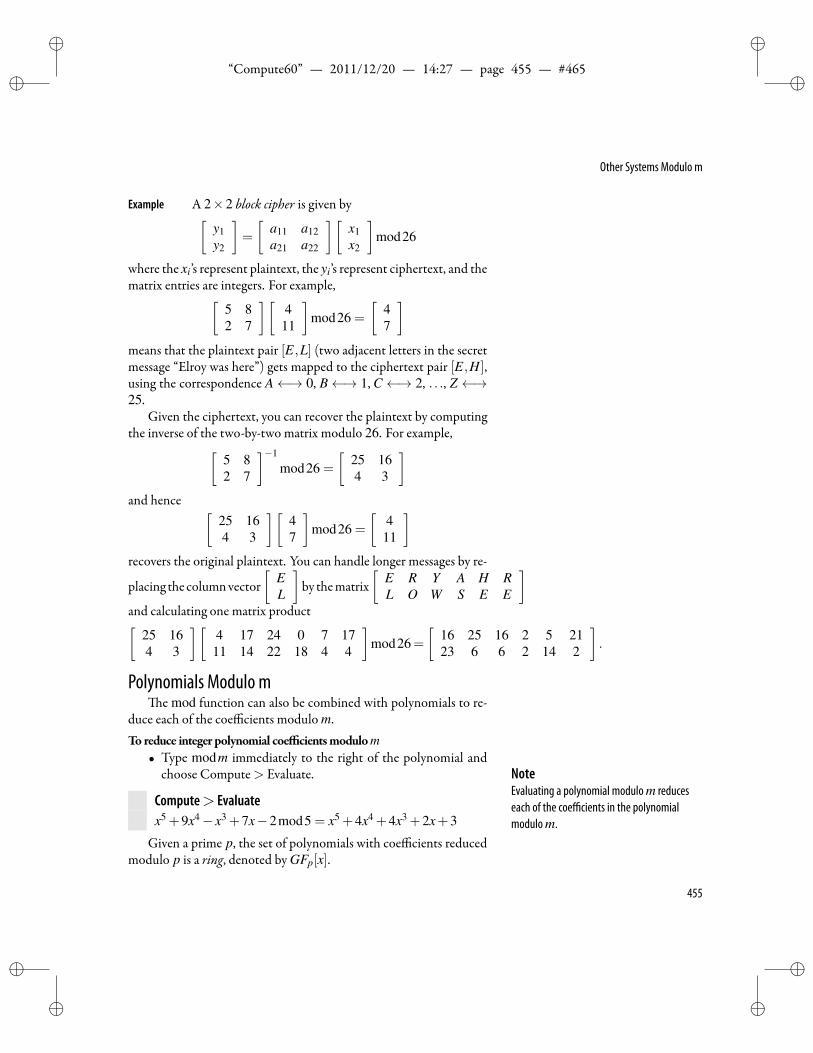
ii
“Compute60” — 2011/12/20 — 14:27 — page 455 — #465 ii
ii
ii
Other Systems Modulo m
Example A 2×2 block cipher is given by[y1y2
]=
[a11 a12a21 a22
][x1x2
]mod26
where the xi’s represent plaintext, the yi’s represent ciphertext, and thematrix entries are integers. For example,[
5 82 7
][411
]mod26 =
[47
]means that the plaintext pair [E,L] (two adjacent letters in the secretmessage “Elroy was here”) gets mapped to the ciphertext pair [E,H],using the correspondence A←→ 0, B←→ 1, C←→ 2, . . ., Z ←→25.
Given the ciphertext, you can recover the plaintext by computingthe inverse of the two-by-two matrix modulo 26. For example,[
5 82 7
]−1
mod26 =
[25 164 3
]and hence [
25 164 3
][47
]mod26 =
[411
]recovers the original plaintext. You can handle longer messages by re-
placing the columnvector[
EL
]by thematrix
[E R Y A H RL O W S E E
]and calculating one matrix product[
25 164 3
][4 17 24 0 7 1711 14 22 18 4 4
]mod26=
[16 25 16 2 5 2123 6 6 2 14 2
].
Polynomials Modulo me mod function can also be combined with polynomials to re-
duce each of the coefficients modulo m.To reduce integer polynomial coefficientsmodulom
• Type modm immediately to the right of the polynomial andchoose Compute> Evaluate. Note
Evaluating a polynomial modulom reduceseach of the coefficients in the polynomialmodulom.
Compute> Evaluatex5 +9x4− x3 +7x−2mod5 = x5 +4x4 +4x3 +2x+3
Given a prime p, the set of polynomials with coefficients reducedmodulo p is a ring, denoted by GFp[x].
455
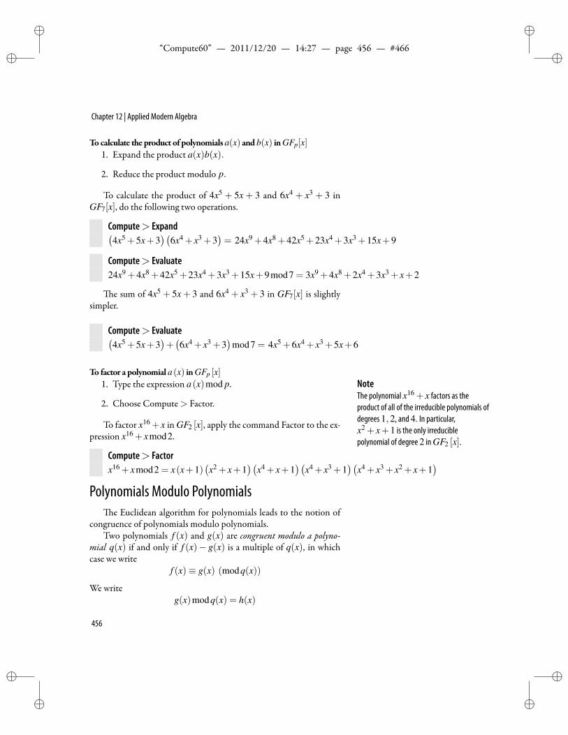
ii
“Compute60” — 2011/12/20 — 14:27 — page 456 — #466 ii
ii
ii
Chapter 12 | Applied Modern Algebra
Tocalculate the product of polynomialsa(x) andb(x) inGFp[x]1. Expand the product a(x)b(x).
2. Reduce the product modulo p.
To calculate the product of 4x5 + 5x + 3 and 6x4 + x3 + 3 inGF7[x], do the following two operations.
Compute> Expand(4x5 +5x+3
)(6x4 + x3 +3
)= 24x9 +4x8 +42x5 +23x4 +3x3 +15x+9
Compute> Evaluate24x9 +4x8 +42x5 +23x4 +3x3 +15x+9mod7 = 3x9 +4x8 +2x4 +3x3 + x+2
e sum of 4x5 + 5x+ 3 and 6x4 + x3 + 3 in GF7[x] is slightlysimpler.
Compute> Evaluate(4x5 +5x+3
)+(6x4 + x3 +3
)mod7 = 4x5 +6x4 + x3 +5x+6
To factor a polynomiala(x) inGFp [x]1. Type the expression a(x)mod p. Note
The polynomial x16 + x factors as theproduct of all of the irreducible polynomials ofdegrees 1,2, and 4. In particular,x2 + x+1 is the only irreduciblepolynomial of degree2 inGF2 [x].
2. Choose Compute> Factor.
To factor x16 + x in GF2 [x], apply the command Factor to the ex-pression x16 + xmod2.
Compute> Factorx16 + xmod2 = x(x+1)
(x2 + x+1
)(x4 + x+1
)(x4 + x3 +1
)(x4 + x3 + x2 + x+1
)Polynomials Modulo Polynomials
e Euclidean algorithm for polynomials leads to the notion ofcongruence of polynomials modulo polynomials.
Two polynomials f (x) and g(x) are congruent modulo a polyno-mial q(x) if and only if f (x)− g(x) is a multiple of q(x), in whichcase we write
f (x)≡ g(x) (modq(x))
We writeg(x)modq(x) = h(x)
456
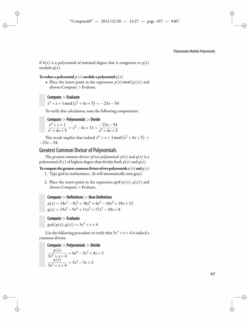
ii
“Compute60” — 2011/12/20 — 14:27 — page 457 — #467 ii
ii
ii
Polynomials Modulo Polynomials
if h(x) is a polynomial of minimal degree that is congruent to g(x)modulo q(x).
To reduce a polynomial p(x)modulo a polynomialq(x)• Place the insert point in the expression p(x)mod(q(x)) and
choose Compute> Evaluate.
Compute> Evaluatex4 + x+1mod
(x2 +4x+5
)=−23x−54
To verify this calculation, note the following computation:
Compute> Polynomials> Dividex4 + x+1
x2 +4x+5= x2−4x+11+
−23x−54x2 +4x+5
is result implies that indeed x4 + x+ 1mod(x2 +4x+5
)=
−23x−54.
Greatest Common Divisor of Polynomialse greatest common divisor of two polynomials p(x) and q(x) is a
polynomial d(x) of highest degree that divides both p(x) and q(x).Tocomputethegreatestcommondivisoroftwopolynomials p(x)andq(x)
1. Type gcd in mathematics. (It will automatically turn gray.)
2. Place the insert point in the expression gcd(p(x) ,q(x)) andchoose Compute> Evaluate.
Compute> De nitions> New De nitionp(x) = 18x7−9x5 +36x4 +4x3−16x2 +19x+12q(x) = 15x5−9x4 +11x3 +17x2−10x+8
Compute> Evaluategcd(p(x),q(x)) = 3x3 + x+4
Use the following procedure to verify that 3x3 + x+4 is indeed acommon divisor.
Compute> Polynomials> Dividep(x)
3x3 + x+4= 6x4−5x2 +4x+3
q(x)3x3 + x+4
= 5x2−3x+2
457
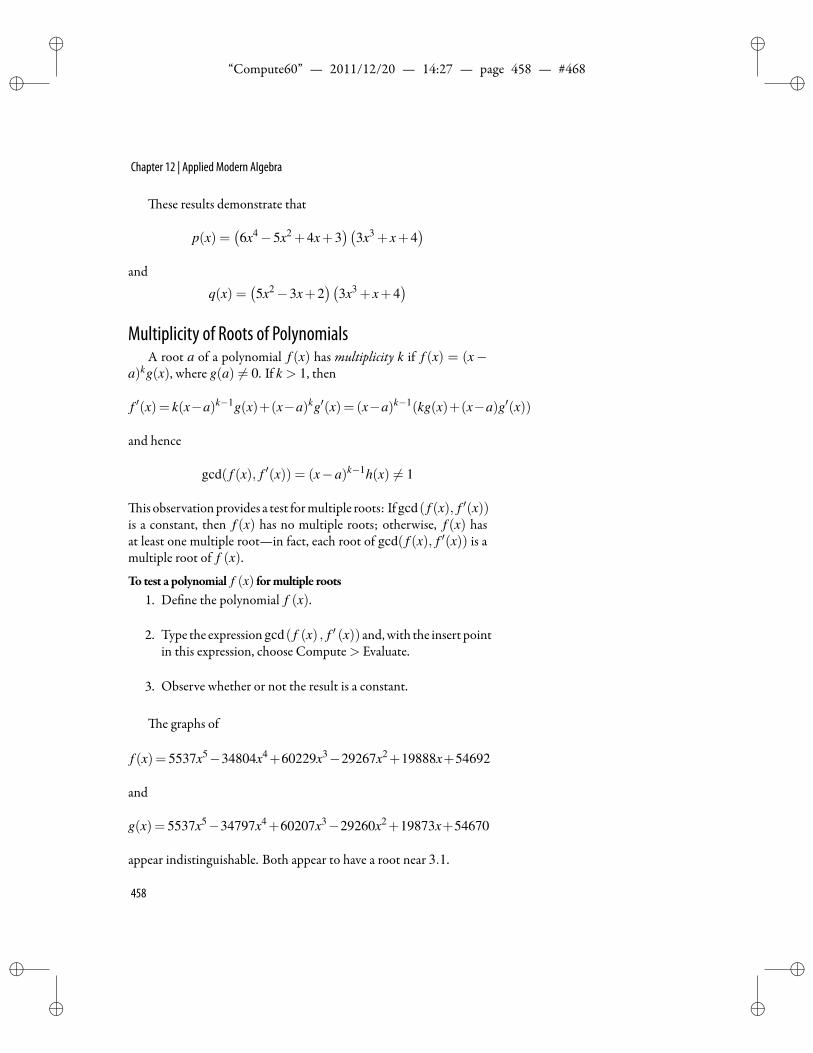
ii
“Compute60” — 2011/12/20 — 14:27 — page 458 — #468 ii
ii
ii
Chapter 12 | Applied Modern Algebra
ese results demonstrate that
p(x) =(6x4−5x2 +4x+3
)(3x3 + x+4
)and
q(x) =(5x2−3x+2
)(3x3 + x+4
)Multiplicity of Roots of Polynomials
A root a of a polynomial f (x) has multiplicity k if f (x) = (x−a)kg(x), where g(a) = 0. If k > 1, then
f ′(x)= k(x−a)k−1g(x)+(x−a)kg′(x)= (x−a)k−1(kg(x)+(x−a)g′(x))
and hence
gcd( f (x), f ′(x)) = (x−a)k−1h(x) = 1
is observationprovides a test formultiple roots: Ifgcd( f (x), f ′(x))is a constant, then f (x) has no multiple roots; otherwise, f (x) hasat least one multiple root—in fact, each root of gcd( f (x), f ′(x)) is amultiple root of f (x).
To test a polynomial f (x) formultiple roots1. De ne the polynomial f (x).
2. Type the expressiongcd( f (x) , f ′ (x)) and,with the insert pointin this expression, choose Compute> Evaluate.
3. Observe whether or not the result is a constant.
e graphs of
f (x)= 5537x5−34804x4+60229x3−29267x2+19888x+54692
and
g(x)= 5537x5−34797x4+60207x3−29260x2+19873x+54670
appear indistinguishable. Both appear to have a root near 3.1.
458
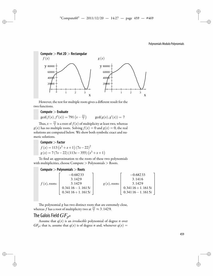
ii
“Compute60” — 2011/12/20 — 14:27 — page 459 — #469 ii
ii
ii
Polynomials Modulo Polynomials
Compute> Plot 2D> Rectangularf (x) g(x)
1 2 3
20000
40000
60000
80000
x
y
1 2 3
20000
40000
60000
80000
x
y
However, the test for multiple roots gives a different result for thetwo functions.
Compute> Evaluategcd( f (x), f ′(x)) = 791
(x− 22
7
)gcd(g(x),g′(x)) = 7
us, x = 227 is a root of f (x) of multiplicity at least two, whereas
g(x) has no multiple roots. Solving f (x) = 0 and g(x) = 0, the realsolutions are computed below. We show both symbolic exact and nu-meric solutions.
Compute> Factorf (x) = 113
(x3 + x+1
)(7x−22)2
g(x) = 7(7x−22)(113x−355)(x3 + x+1
)To nd an approximation to the roots of these two polynomials
with multiplicities, choose Compute> Polynomials> Roots.
Compute> Polynomials> Roots
f (x), roots:
−0.68233
3.14293.1429
0.34116−1.1615i0.34116+1.1615i
g(x), roots:
−0.68233
3.14163.1429
0.34116+1.1615i0.34116−1.1615i
e polynomial g has two distinct roots that are extremely close,whereas f has a root of multiplicity two at 22
7 ≈ 3.1429.
The Galois FieldGFpn
Assume that q(x) is an irreducible polynomial of degree n overGFp; that is, assume that q(x) is of degree n and, whenever q(x) =
459
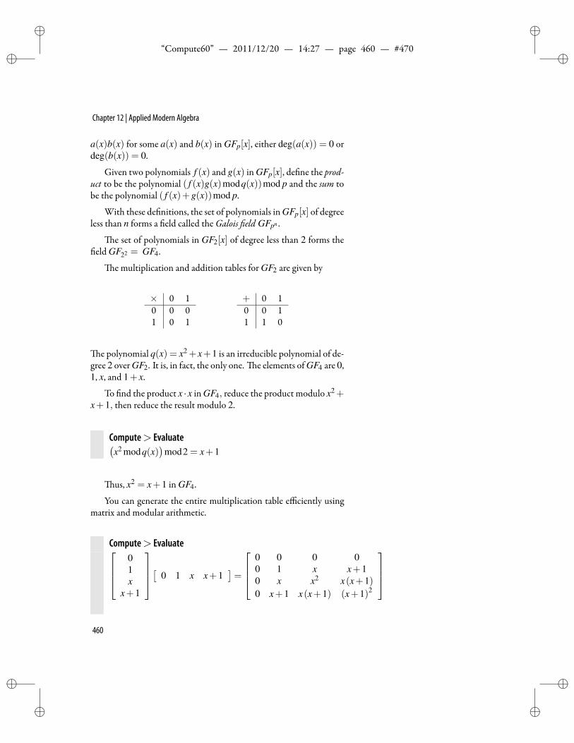
ii
“Compute60” — 2011/12/20 — 14:27 — page 460 — #470 ii
ii
ii
Chapter 12 | Applied Modern Algebra
a(x)b(x) for some a(x) and b(x) in GFp[x], either deg(a(x)) = 0 ordeg(b(x)) = 0.
Given two polynomials f (x) and g(x) in GFp[x], de ne the prod-uct to be the polynomial ( f (x)g(x)modq(x))mod p and the sum tobe the polynomial ( f (x)+g(x))mod p.
With these de nitions, the set of polynomials in GFp[x] of degreeless than n forms a eld called theGalois eld GFpn .
e set of polynomials in GF2[x] of degree less than 2 forms theeld GF22 = GF4.
e multiplication and addition tables for GF2 are given by
× 0 10 0 01 0 1
+ 0 10 0 11 1 0
e polynomial q(x) = x2+x+1 is an irreducible polynomial of de-gree 2 over GF2. It is, in fact, the only one. e elements of GF4 are 0,1, x, and 1+ x.
To nd the product x ·x in GF4, reduce the product modulo x2+x+1, then reduce the result modulo 2.
Compute> Evaluate(x2 modq(x)
)mod2 = x+1
us, x2 = x+1 in GF4.
You can generate the entire multiplication table efficiently usingmatrix and modular arithmetic.
Compute> Evaluate01x
x+1
[ 0 1 x x+1]=
0 0 0 00 1 x x+10 x x2 x(x+1)0 x+1 x(x+1) (x+1)2
460
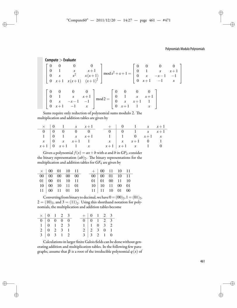
ii
“Compute60” — 2011/12/20 — 14:27 — page 461 — #471 ii
ii
ii
Polynomials Modulo Polynomials
Compute> Evaluate0 0 0 00 1 x x+10 x x2 x(x+1)0 x+1 x(x+1) (x+1)2
modx2 + x+1 =
0 0 0 00 1 x x+10 x −x−1 −10 x+1 −1 x
0 0 0 00 1 x x+10 x −x−1 −10 x+1 −1 x
mod2 =
0 0 0 00 1 x x+10 x x+1 10 x+1 1 x
Sums require only reduction of polynomial sums modulo 2. e
multiplication and addition tables are given by
× 0 1 x x+10 0 0 0 01 0 1 x x+1x 0 x x+1 1
x+1 0 x+1 1 x
+ 0 1 x x+10 0 1 x x+11 1 0 x+1 xx x x+1 0 1
x+1 x+1 x 1 0
Given a polynomial f (x) = ax+b with a and b in GF2, considerthe binary representation (ab)2. e binary representations for themultiplication and addition tables for GF4 are given by
× 00 01 10 1100 00 00 00 0001 00 01 10 1110 00 10 11 0111 00 11 01 10
+ 00 11 10 1100 00 01 10 1101 01 00 11 1010 10 11 00 0111 11 10 01 00
Converting frombinary todecimal, wehave0=(00)2,1=(01)2,2 = (10)2, and 3 = (11)2. Using this shorthand notation for poly-nomials, the multiplication and addition tables become
× 0 1 2 30 0 0 0 01 0 1 2 32 0 2 3 13 0 3 1 2
+ 0 1 2 30 0 1 2 31 1 0 3 22 2 3 0 13 3 2 1 0
Calculations in larger niteGalois elds can be donewithout gen-erating addition and multiplication tables. In the following few para-graphs, assume that β is a root of the irreducible polynomial q(x) of
461
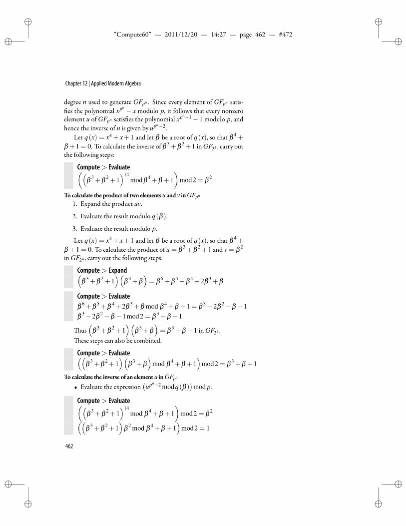
ii
“Compute60” — 2011/12/20 — 14:27 — page 462 — #472 ii
ii
ii
Chapter 12 | Applied Modern Algebra
degree n used to generate GFpn . Since every element of GFpn satis-es the polynomial xpn − x modulo p, it follows that every nonzero
element u of GFpn satis es the polynomial xpn−1−1 modulo p, andhence the inverse of u is given by upn−2.
Let q(x) = x4 + x+ 1 and let β be a root of q(x), so that β 4 +
β +1 = 0. To calculate the inverse of β 3 +β 2 +1 in GF24 , carry outthe following steps:
Compute> Evaluate((β 3 +β 2 +1
)14modβ 4 +β +1
)mod2 = β 2
Tocalculate the product of two elementsu and v inGFpn
1. Expand the product uv.
2. Evaluate the result modulo q(β ).
3. Evaluate the result modulo p.
Let q(x) = x4 + x+ 1 and let β be a root of q(x), so that β 4 +
β +1 = 0. To calculate the product of u = β 3 +β 2 +1 and v = β 2
in GF24 , carry out the following steps.
Compute> Expand(β 3 +β 2 +1
)(β 3 +β
)= β 6 +β 5 +β 4 +2β 3 +β
Compute> Evaluateβ 6 +β 5 +β 4 +2β 3 +β mod β 4 +β +1 = β 3−2β 2−β −1β 3−2β 2−β −1mod2 = β 3 +β +1
us(
β 3 +β 2 +1)(
β 3 +β)= β 3 +β +1 in GF24 .
ese steps can also be combined.
Compute> Evaluate((β 3 +β 2 +1
)(β 3 +β
)mod β 4 +β +1
)mod2 = β 3 +β +1
Tocalculate the inverse of an elementu inGFpn
• Evaluate the expression(upn−2 modq(β )
)mod p.
Compute> Evaluate((β 3 +β 2 +1
)14mod β 4 +β +1
)mod2 = β 2((
β 3 +β 2 +1)
β 2 mod β 4 +β +1)
mod2 = 1
462
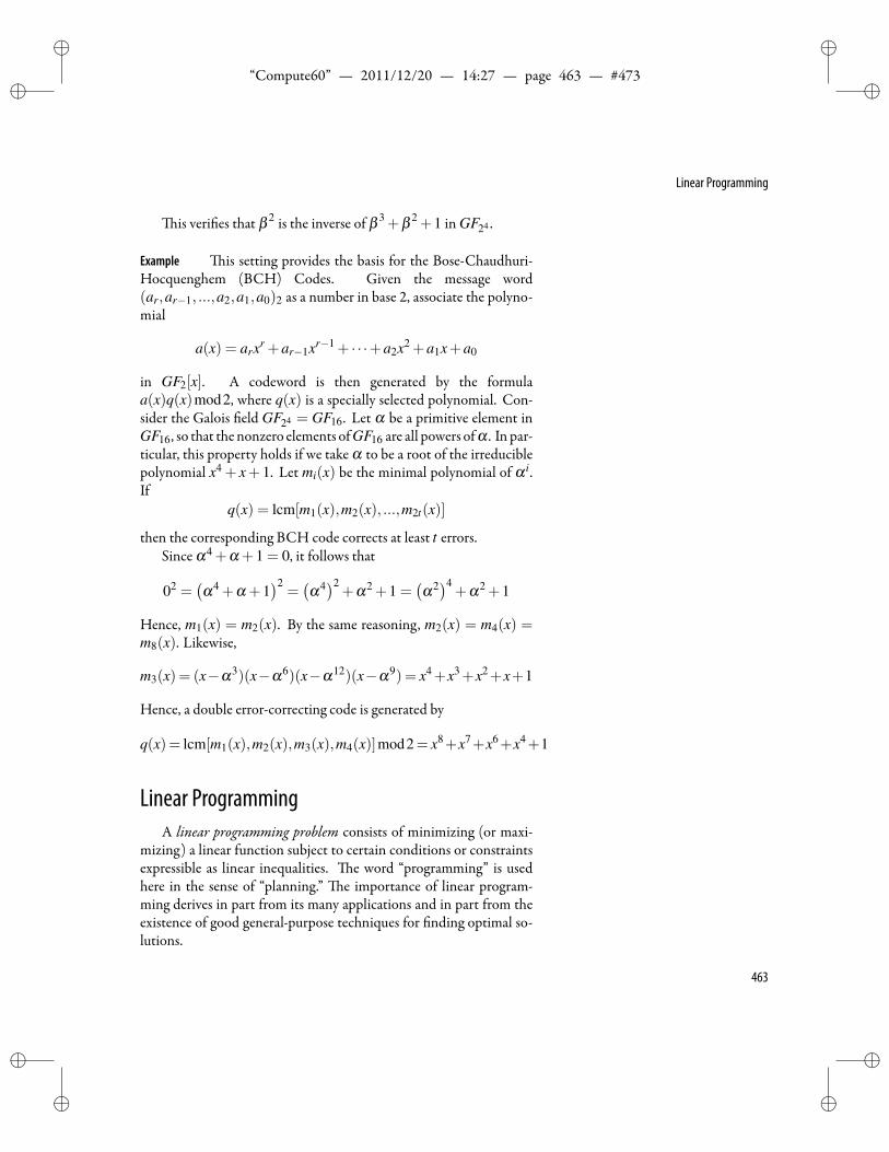
ii
“Compute60” — 2011/12/20 — 14:27 — page 463 — #473 ii
ii
ii
Linear Programming
is veri es that β 2 is the inverse of β 3 +β 2 +1 in GF24 .
Example is setting provides the basis for the Bose-Chaudhuri-Hocquenghem (BCH) Codes. Given the message word(ar,ar−1, ...,a2,a1,a0)2 as a number in base 2, associate the polyno-mial
a(x) = arxr +ar−1xr−1 + · · ·+a2x2 +a1x+a0
in GF2[x]. A codeword is then generated by the formulaa(x)q(x)mod2, where q(x) is a specially selected polynomial. Con-sider the Galois eld GF24 = GF16. Let α be a primitive element inGF16, so that the nonzero elements ofGF16 are all powers ofα . In par-ticular, this property holds if we take α to be a root of the irreduciblepolynomial x4 + x+ 1. Let mi(x) be the minimal polynomial of α i.If
q(x) = lcm[m1(x),m2(x), ...,m2t(x)]
then the corresponding BCH code corrects at least t errors.Since α4 +α +1 = 0, it follows that
02 =(α4 +α +1
)2=(α4)2
+α2 +1 =(α2)4
+α2 +1
Hence, m1(x) = m2(x). By the same reasoning, m2(x) = m4(x) =m8(x). Likewise,
m3(x) = (x−α3)(x−α6)(x−α12)(x−α9) = x4+x3+x2+x+1
Hence, a double error-correcting code is generated by
q(x)= lcm[m1(x),m2(x),m3(x),m4(x)]mod2= x8+x7+x6+x4+1
Linear ProgrammingA linear programming problem consists of minimizing (or maxi-
mizing) a linear function subject to certain conditions or constraintsexpressible as linear inequalities. e word “programming” is usedhere in the sense of “planning.” e importance of linear program-ming derives in part from its many applications and in part from theexistence of good general-purpose techniques for nding optimal so-lutions.
463
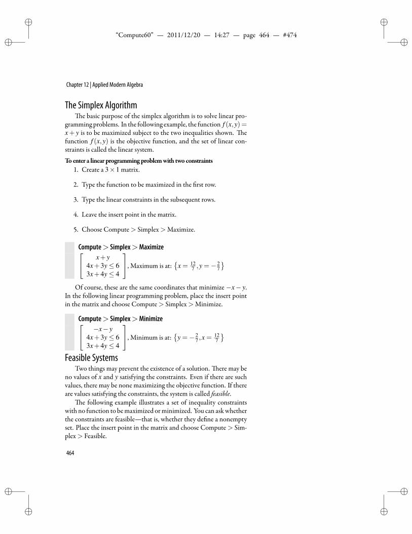
ii
“Compute60” — 2011/12/20 — 14:27 — page 464 — #474 ii
ii
ii
Chapter 12 | Applied Modern Algebra
The Simplex Algorithme basic purpose of the simplex algorithm is to solve linear pro-
grammingproblems. In the following example, the function f (x,y)=x+ y is to be maximized subject to the two inequalities shown. efunction f (x,y) is the objective function, and the set of linear con-straints is called the linear system.
Toenter a linear programmingproblemwith two constraints1. Create a 3×1 matrix.
2. Type the function to be maximized in the rst row.
3. Type the linear constraints in the subsequent rows.
4. Leave the insert point in the matrix.
5. Choose Compute> Simplex>Maximize.
Compute> Simplex>Maximize x+ y4x+3y≤ 63x+4y≤ 4
, Maximum is at:
x = 127 ,y =−
27
Of course, these are the same coordinates that minimize−x− y.
In the following linear programming problem, place the insert pointin the matrix and choose Compute> Simplex>Minimize.
Compute> Simplex>Minimize −x− y4x+3y≤ 63x+4y≤ 4
, Minimum is at:
y =− 27 ,x =
127
Feasible Systems
Two things may prevent the existence of a solution. ere may beno values of x and y satisfying the constraints. Even if there are suchvalues, there may be none maximizing the objective function. If thereare values satisfying the constraints, the system is called feasible.
e following example illustrates a set of inequality constraintswith no function to bemaximized orminimized. You can askwhetherthe constraints are feasible—that is, whether they de ne a nonemptyset. Place the insert point in the matrix and choose Compute> Sim-plex> Feasible.
464
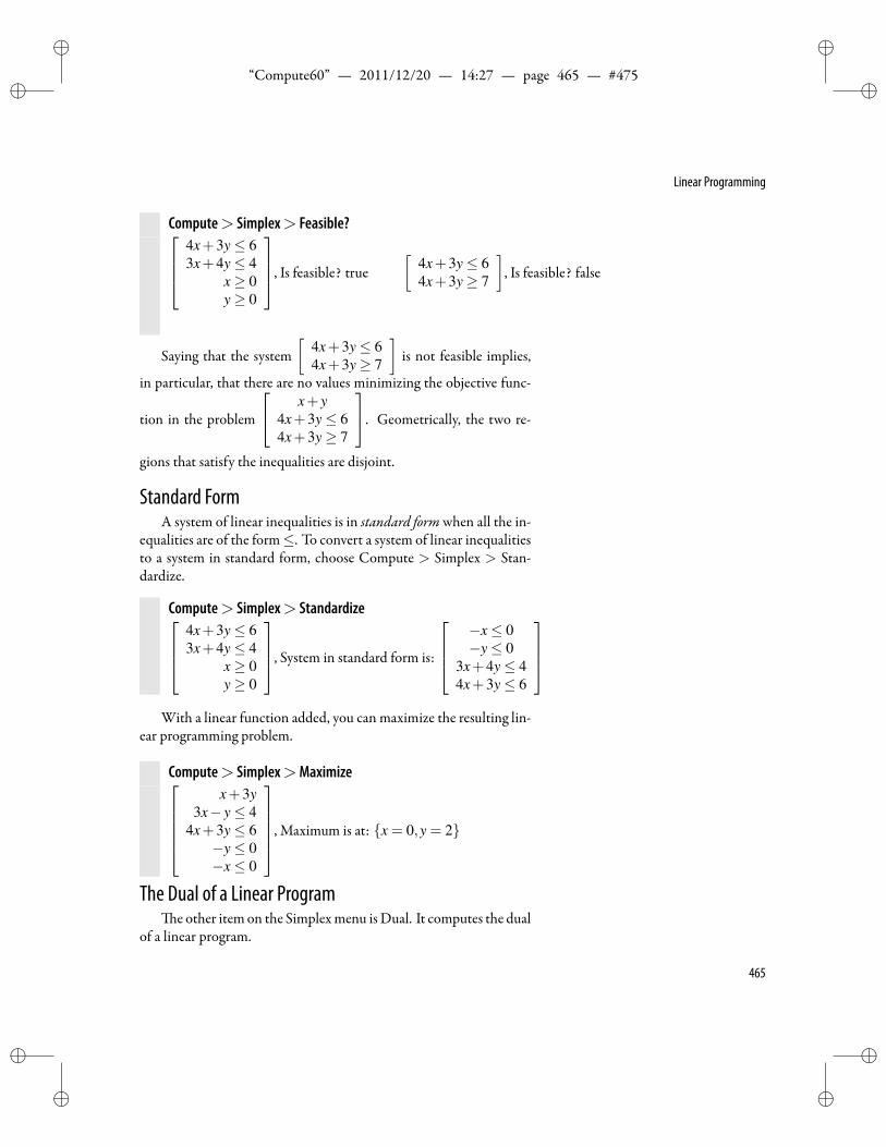
ii
“Compute60” — 2011/12/20 — 14:27 — page 465 — #475 ii
ii
ii
Linear Programming
Compute> Simplex> Feasible?4x+3y≤ 63x+4y≤ 4
x≥ 0y≥ 0
, Is feasible? true[
4x+3y≤ 64x+3y≥ 7
], Is feasible? false
Saying that the system[
4x+3y≤ 64x+3y≥ 7
]is not feasible implies,
in particular, that there are no values minimizing the objective func-
tion in the problem
x+ y4x+3y≤ 64x+3y≥ 7
. Geometrically, the two re-
gions that satisfy the inequalities are disjoint.
Standard FormA system of linear inequalities is in standard formwhen all the in-
equalities are of the form≤. To convert a system of linear inequalitiesto a system in standard form, choose Compute > Simplex > Stan-dardize.
Compute> Simplex> Standardize4x+3y≤ 63x+4y≤ 4
x≥ 0y≥ 0
, System in standard form is:
−x≤ 0−y≤ 0
3x+4y≤ 44x+3y≤ 6
With a linear function added, you can maximize the resulting lin-
ear programming problem.
Compute> Simplex>Maximizex+3y
3x− y≤ 44x+3y≤ 6−y≤ 0−x≤ 0
, Maximum is at: x = 0,y = 2
The Dual of a Linear Programe other item on the Simplexmenu isDual. It computes the dual
of a linear program.
465
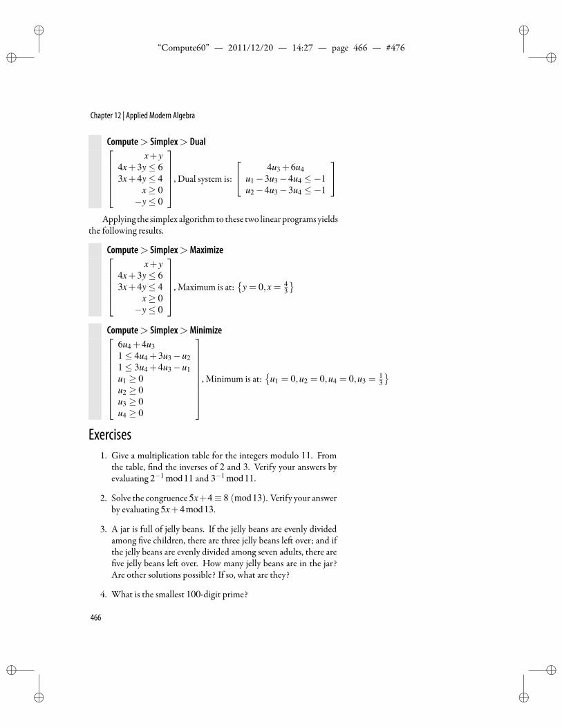
ii
“Compute60” — 2011/12/20 — 14:27 — page 466 — #476 ii
ii
ii
Chapter 12 | Applied Modern Algebra
Compute> Simplex> Dualx+ y
4x+3y≤ 63x+4y≤ 4
x≥ 0−y≤ 0
, Dual system is:
4u3 +6u4u1−3u3−4u4 ≤−1u2−4u3−3u4 ≤−1
Applying the simplex algorithmto these two linear programs yields
the following results.
Compute> Simplex>Maximizex+ y
4x+3y≤ 63x+4y≤ 4
x≥ 0−y≤ 0
, Maximum is at:
y = 0,x = 43
Compute> Simplex>Minimize
6u4 +4u31≤ 4u4 +3u3−u21≤ 3u4 +4u3−u1u1 ≥ 0u2 ≥ 0u3 ≥ 0u4 ≥ 0
, Minimum is at:
u1 = 0,u2 = 0,u4 = 0,u3 =
13
Exercises1. Give a multiplication table for the integers modulo 11. From
the table, nd the inverses of 2 and 3. Verify your answers byevaluating 2−1 mod11 and 3−1 mod11.
2. Solve the congruence 5x+4≡ 8 (mod13). Verify your answerby evaluating 5x+4mod13.
3. A jar is full of jelly beans. If the jelly beans are evenly dividedamong ve children, there are three jelly beans le over; and ifthe jelly beans are evenly divided among seven adults, there areve jelly beans le over. How many jelly beans are in the jar?
Are other solutions possible? If so, what are they?
4. What is the smallest 100-digit prime?
466
ii
“Compute60” — 2011/12/20 — 14:27 — page 467 — #477 ii
ii
ii
Exercises
5. If p is the smallest 100-digit prime, what is 2p−1 mod p? Whatis 2(p−1)/2 mod p? What about 2(p−1)/4 mod p?
6. e matrix M =
1 1 11 2 41 4 9
is used as a block cipher mod-
ulo 26 to scramble letters in a message, three letters at a time.Assume A←→ 0, B←→ 1, C←→ 2, and so forth. Descram-ble the ciphertext FKBHRTMTU.
7. Find an irreducible polynomial of degree 3. Use this polyno-mial to describe how to calculate sums and products in the eldGF27.
8. A barge company transports bales of hay and barrels of beer upthe Mississippi River. e company charges $2.30 for each baleof hay and $3.00 for each barrel of beer. e bales of hay average75 pounds and take up 5 cubic feet of space; the barrels of beerweigh 100 pounds and take up 4 cubic feet of space. A bargeis limited to a payload of 150,000 pounds and 8,000 cubic feet.Howmuch beer and howmuch hay should a barge transport tomaximize the shipping charges?
9. eRiemannHypothesis states that all of thenontrivial zeros ofthe Riemann zeta function lie on the line Re(s) = 1
2 . Visualizethe Riemann zeta function along Re(s) = 1
2 by drawing a curvein three-dimensional space.
10. Let Z30 denote the integers modulo 30. Write Z30 as a (dis-joint) union of groups.
Solutions1. De ne the function f (i, j) = i j. ChooseCompute>Matrices
> Fill Matrix with 10 rows and 10 columns, and use the func-tion f to generate a matrix. en, reduce the matrix mod11 toget the following:
467
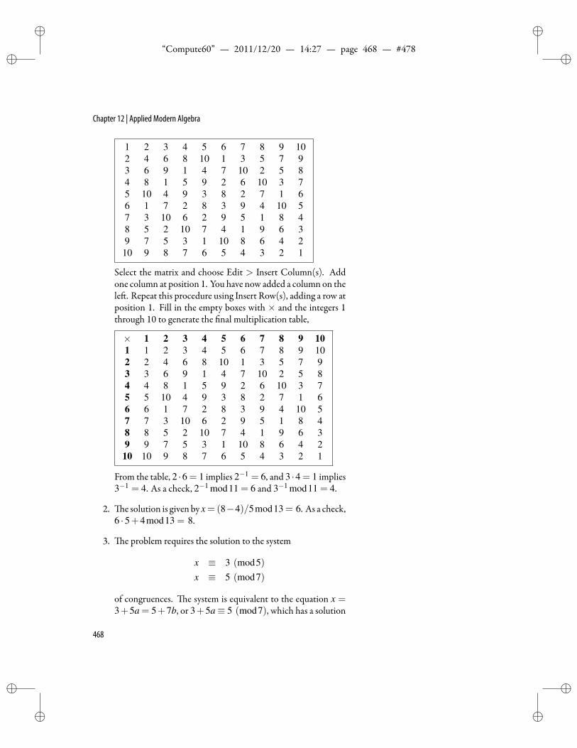
ii
“Compute60” — 2011/12/20 — 14:27 — page 468 — #478 ii
ii
ii
Chapter 12 | Applied Modern Algebra
1 2 3 4 5 6 7 8 9 102 4 6 8 10 1 3 5 7 93 6 9 1 4 7 10 2 5 84 8 1 5 9 2 6 10 3 75 10 4 9 3 8 2 7 1 66 1 7 2 8 3 9 4 10 57 3 10 6 2 9 5 1 8 48 5 2 10 7 4 1 9 6 39 7 5 3 1 10 8 6 4 210 9 8 7 6 5 4 3 2 1
Select the matrix and choose Edit > Insert Column(s). Addone column at position 1. You have now added a column on thele . Repeat this procedure using Insert Row(s), adding a row atposition 1. Fill in the empty boxes with × and the integers 1through 10 to generate the nal multiplication table,
× 1 2 3 4 5 6 7 8 9 101 1 2 3 4 5 6 7 8 9 102 2 4 6 8 10 1 3 5 7 93 3 6 9 1 4 7 10 2 5 84 4 8 1 5 9 2 6 10 3 75 5 10 4 9 3 8 2 7 1 66 6 1 7 2 8 3 9 4 10 57 7 3 10 6 2 9 5 1 8 48 8 5 2 10 7 4 1 9 6 39 9 7 5 3 1 10 8 6 4 210 10 9 8 7 6 5 4 3 2 1
From the table, 2 ·6 = 1 implies 2−1 = 6, and 3 ·4 = 1 implies3−1 = 4. As a check, 2−1 mod11 = 6 and 3−1 mod11 = 4.
2. e solution is given by x= (8−4)/5mod13= 6. As a check,6 ·5+4mod13 = 8.
3. e problem requires the solution to the system
x ≡ 3 (mod5)x ≡ 5 (mod7)
of congruences. e system is equivalent to the equation x =3+5a = 5+7b, or 3+5a≡ 5 (mod7), which has a solution
468
ii
“Compute60” — 2011/12/20 — 14:27 — page 469 — #479 ii
ii
ii
Exercises
a = (5−3)/5mod7 = 6, which means x = 3+5a = 33 jellybeans. Other possible solutions are x = 33+ 35n, where n isany positive integer.
4. De ne the function nextp as indicated in this chapter. ennextp(1099) produces a number with lots of zeroes that ends in289. e prime p can be written as p = 1099 +289.
5. Note that 2p−1 mod p = 1 and 2(p−1)/2 mod p = 1, whereas2(p−1)/4 mod p produces another number with lots of zeroesthat ends in 288. More precisely, 2(p−1)/4 ≡ −1mod p. iscongruence illustrates the fact that, if p is a prime, then x2 ≡1 (mod p) has only two solutions, x ≡ 1 (mod p) and x ≡−1 (mod p).
6. We have
1 1 11 2 41 4 9
−1
mod26 =
24 5 245 18 324 3 25
. e
ciphertext F K B H R T M T U has a numerical equivalent of[5,10,1,7,17,19,12,19,20]. Picking three at a time, we get 24 5 24
5 18 324 3 25
5 7 1210 17 191 19 20
mod26=
12 7 50 8 20
19 18 13
e vector [12,0,19,7,8,18,5,20,13] corresponds to theplain-
text M A T H I S F U N, or MATH IS FUN.
7. De ning g(x) = x3 + x+ 1, we see that g(1)mod3 = 0, andhence g(x) is not irreducible (since it has a root in GF3). How-ever, if f (x)= x3+2x+1, then f (0)mod3= 1, f (1)mod3=1, and f (2)mod3 = 1, and hence f (x) is irreducible. (If f (x)were reducible, it would have a linear factor, and hence a root.)An element ofGF27 can be thought of as a polynomial of degreeless than 3 with coefficients in GF3. Given the eld elements2x2 + x+2 and 2x+1, the product is((
2x2 + x+2)(2x+1)mod x3 +2x+1
)mod3 = x2 +1,
and the sum is given by(2x2 + x+2
)+(2x+1)mod3 = 2x2.
469
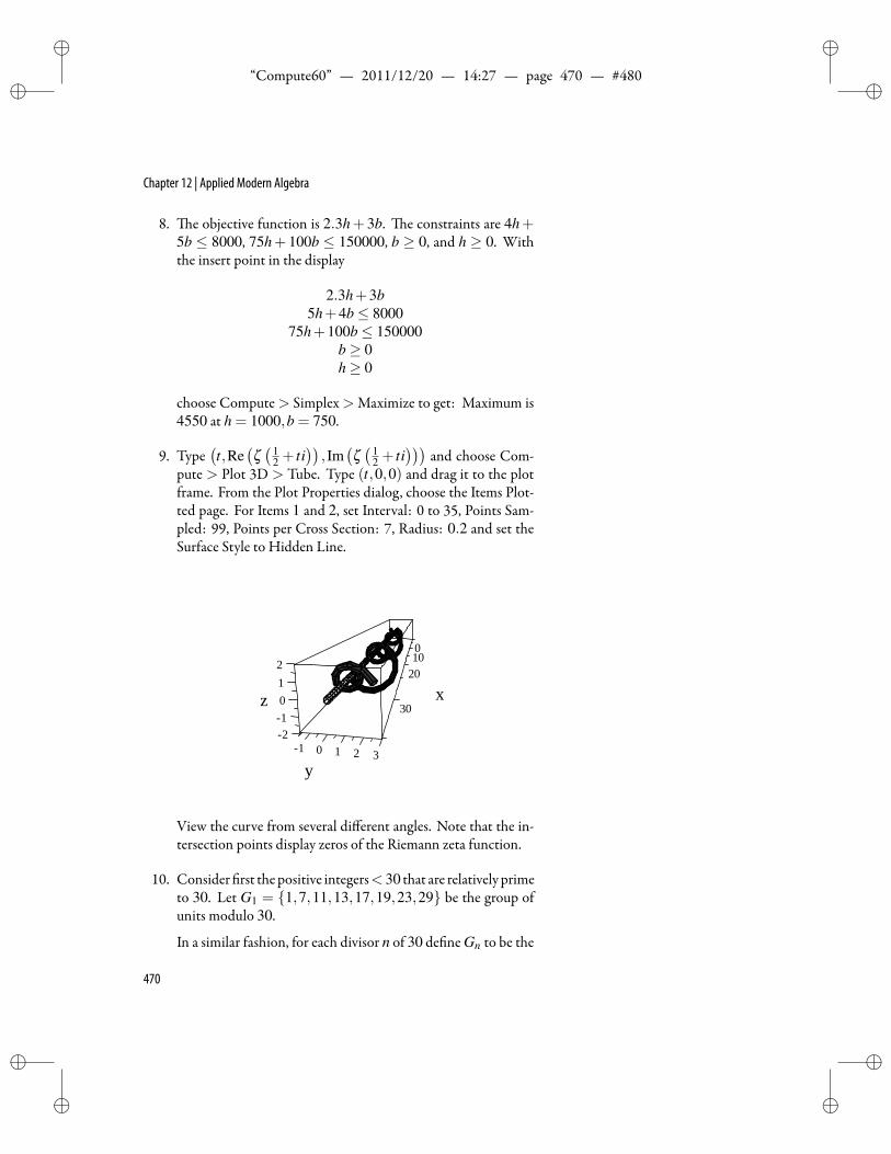
ii
“Compute60” — 2011/12/20 — 14:27 — page 470 — #480 ii
ii
ii
Chapter 12 | Applied Modern Algebra
8. e objective function is 2.3h+ 3b. e constraints are 4h+5b ≤ 8000, 75h+ 100b ≤ 150000, b ≥ 0, and h ≥ 0. Withthe insert point in the display
2.3h+3b5h+4b≤ 8000
75h+100b≤ 150000b≥ 0h≥ 0
choose Compute> Simplex>Maximize to get: Maximum is4550 at h = 1000,b = 750.
9. Type(t,Re
(ζ( 1
2 + ti))
, Im(ζ( 1
2 + ti)))
and choose Com-pute > Plot 3D > Tube. Type (t,0,0) and drag it to the plotframe. From the Plot Properties dialog, choose the Items Plot-ted page. For Items 1 and 2, set Interval: 0 to 35, Points Sam-pled: 99, Points per Cross Section: 7, Radius: 0.2 and set theSurface Style to Hidden Line.
100
x20
30
y3201
21
2
z 01
1
View the curve from several different angles. Note that the in-tersection points display zeros of the Riemann zeta function.
10. Consider rst thepositive integers< 30 that are relatively primeto 30. Let G1 = 1,7,11,13,17,19,23,29 be the group ofunits modulo 30.
In a similar fashion, for each divisor n of 30 de ne Gn to be the
470
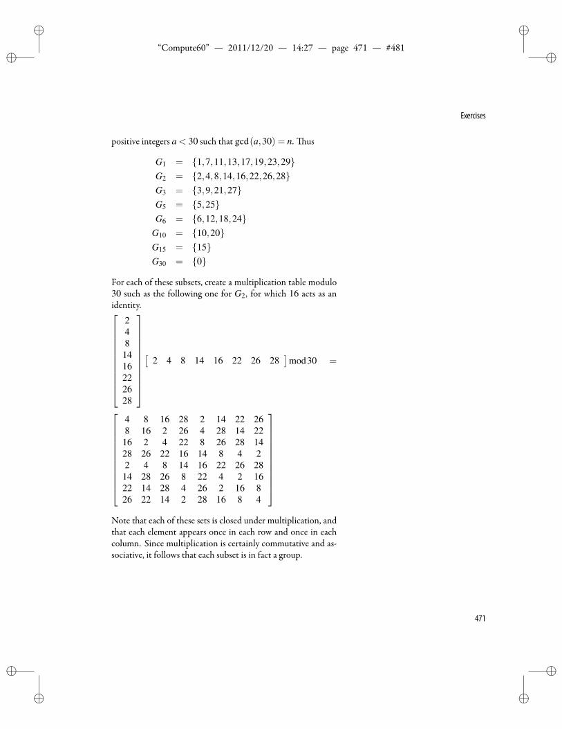
ii
“Compute60” — 2011/12/20 — 14:27 — page 471 — #481 ii
ii
ii
Exercises
positive integers a < 30 such that gcd(a,30) = n. us
G1 = 1,7,11,13,17,19,23,29G2 = 2,4,8,14,16,22,26,28G3 = 3,9,21,27G5 = 5,25G6 = 6,12,18,24
G10 = 10,20G15 = 15G30 = 0
For each of these subsets, create a multiplication table modulo30 such as the following one for G2, for which 16 acts as anidentity.
248
1416222628
[
2 4 8 14 16 22 26 28]
mod30 =
4 8 16 28 2 14 22 268 16 2 26 4 28 14 22
16 2 4 22 8 26 28 1428 26 22 16 14 8 4 22 4 8 14 16 22 26 28
14 28 26 8 22 4 2 1622 14 28 4 26 2 16 826 22 14 2 28 16 8 4
Note that each of these sets is closed under multiplication, andthat each element appears once in each row and once in eachcolumn. Since multiplication is certainly commutative and as-sociative, it follows that each subset is in fact a group.
471

ii
“Compute60” — 2011/12/20 — 14:27 — page 472 — #482 ii
ii
ii
ii
“Compute60” — 2011/12/20 — 14:27 — page 473 — #483 ii
ii
ii
AMenus and Shortcuts for
Doing Mathematics
If I feel unhappy, I do mathematics to become happy. If I am happy, I do mathematics to keep happy. Alfréd Rényi (1921–1970)
T his appendix summarizes information about the Compute Compute Menu
Toolbar and Keyboard Shortcutsfor Compute Menu Commands
menu, corresponding commands on the Math Toolbar, andkeyboard shortcuts for these commands. Details and exam-
ples are given in the main text.
Compute Menu• Calculus > Approximate Integral Apply approximation
methods Le , Right, Le and Right, Middle, Lower, Upper,Lower andUpper, LowerAbsolute,UpperAbsolute, Lower andUpper Absolute, Trapezoid, or Simpson for approximating def-inite integrals by a mathematical expression.
• Calculus>Change Variables Simpli es an inde nite in-tegral: specify a substitution and get the result of the substitu-tion.
• Calculus > Find Extrema Given a mathematical expres- New in Version 6Compute> Passthru Code to MuPADCompute> Rewrite>Mixed
sion, returns candidates for extrema.
• Calculus > Implicit Differentiation Given an equationand a differentiation variable, performs differentiation.
473
ii
“Compute60” — 2011/12/20 — 14:27 — page 474 — #484 ii
ii
ii
Appendix A | Menus and Shortcuts for Doing Mathematics
• Calculus> Integrate by Parts Simpli es an inde nite in-tegral: specify the part to be differentiated and invoke the inte-gration by parts method.
• Calculus > Iterate Find numerical approximations to aroot of an equation f (x) = x, starting with your estimate of aroot.
• Calculus > Partial Fractions Writes a factorable rationalfunction as a sum of simpler fractions. (Same as Polynomials>Partial Fractions)
• Calculus > Plot Approximate Integral Plot pictures ofRiemann sumsobtained frommidpoints, le endpoints, or rightendpoints of subintervals.
• Check Equality Verify equalities and inequalities. ereare three possible responses: true, false, and undecidable.
• Combine>Arctan Combines or simpli es expressions in-volving inverse tangent functions.
• Combine> Exponentials Combines or simpli es expres-sions involving exponential functions with base e.
• Combine>Hyperbolic Trigonometric Functions Prod-ucts and powers of hyperbolic trigonometric functions are com-bined into a sum of hyperbolic functions whose arguments areintegral linear combinations of the original arguments.
• Combine > Logs Combines or simpli es expressions in-volving logarithmic functions with base e.
• Combine > Powers Combines or simpli es expressionsinvolving exponential functions with arbitrary base.
• Combine>TrigonometricFunctions Products andpow-ers of trigonometric functions are combined into a sumof trigo-nometric functions whose arguments are integral linear combi-nations of the original arguments.
• De nitions> Clear De nitions Removes all active user-de ned de nitions from a document.
474
ii
“Compute60” — 2011/12/20 — 14:27 — page 475 — #485 ii
ii
ii
Compute Menu
• De nitions>De ne MuPAD Name Allows users to ac-cess functions available to the computation engine that do notappear as menu items, either functions from one of the librariesof the computation engine or user-de ned functions.
• De nitions>NewDe nition Allows users to de ne newfunctions and variables for computation.
• De nitions > Show De nitions Provides a list of all ac-tive user-de ned de nitions in a document.
• De nitions > Unde ne Removes a selected user-de nedde nition from a document.
• Evaluate Evaluate yields symbolic or numerical results, de-pending on the input.
• Evaluate Numeric Evaluates and gives numerical results.
• Expand Expandpolynomial and rational products, trigono-metric and exponential expressions.
• Factor Factorpolynomials and rational, trigonometric andexponential expressions.
• Interpret Shows the interpretation of possibly ambiguousexpressions as made by the computing engine.
• Matrices>Adjugate Produces the adjugate or classical ad-joint of a square matrix A, namely, the transpose of the matrixof cofactors of A.
• Matrices>CharacteristicPolynomial Produces the char-acteristic polynomial of a square matrix A, namely, the determi-nant of the characteristic matrix xI−A.
• Matrices>CholeskyDecomposition Factors a real square,symmetric, andpositive de nitematrixA as a productA=GGT ,with G a real positive-de nite lower triangular square matrix.
• Matrices>Column Basis Produces a basis for the vectorspace spanned by the columns of a matrix.
• Matrices > Concatenate Merges two matrices with thesame number of rows horizontally into one matrix.
475
ii
“Compute60” — 2011/12/20 — 14:27 — page 476 — #486 ii
ii
ii
Appendix A | Menus and Shortcuts for Doing Mathematics
• Matrices > Condition Number Produces the conditionnumber of an invertible matrix A, the product of the 2-norm ofA and the 2-norm of A−1. is numbermeasures the sensitivityof some solutions of linear equations Ax = b to perturbationsin the entries of A and b.
• Matrices>De nitenessTests Determineswhether aHer-mitianmatrix (a square matrix equal to its conjugate transpose)is positive de nite, positive semide nite, negative de nite, ornegative semide nite.
• Matrices > Determinant Produces the determinant of asquare matrix.
• Matrices> Eigenvalues Produces a list of eigenvalues of asquare matrix, that is, the roots of its characteristic polynomial.
e results are symbolic or numerical approximations depend-ing on the matrix entries.
• Matrices > Eigenvectors Produces a list of eigenvectorspaired with eigenvalues of a square matrix, that is, the roots ofits characteristic polynomial. Given amatrixA, these are a scalarc and a vector v with Av = cv. e results are symbolic or nu-meric depending on the matrix entries.
• Matrices> Fill Matrix Create a matrix: choose from ma-trix types Band, De ned by Function, Identity, Jordan Block,Random (integers between -1000 and 1000), and Zero ( lledwith zeroes).
• Matrices>Fraction-FreeGaussianElimination Elemen-tary row operations are used to reduce a matrix of integers torow echelon form with integer entries.
• Matrices > Gaussian Elimination Elementary row oper-ations are used to reduce a matrix to row echelon form. e re-sults are symbolic or numeric depending on the matrix entries.
• Matrices>Hermite Normal Form Produces, from a ma-trix A with integer entries, a row echelonmatrix H = QA whereQ is invertible in the ring of matrices over the integers.
• Matrices>Hermitian Transpose Produces, from a com-plex matrix, the Hermitian transpose.
476
ii
“Compute60” — 2011/12/20 — 14:27 — page 477 — #487 ii
ii
ii
Compute Menu
• Matrices > Inverse Produces the inverse of a square, in-vertible matrix.
• Matrices> JordanNormalForm Produces a factorizationof a square matrix as PJP−1, where J is in Jordan normal form.
• Matrices>MapFunction Applies a function (either built-in or user de ned) to the entries of a matrix or vector.
• Matrices > Minimal Polynomial Computes the monicminimal polynomial of a square matrix.
• Matrices > Norm Computes the 2-norm, or Euclideannorm, of a matrix A with real or complex entries. is is thenumber de ned by ∥A∥ = maxx =0 ∥Ax∥/∥x∥. In the specialcase A is a vector, this is the Euclidean length of the vector.
• Matrices > Nullspace Basis Finds a basis for the vectorspace consisting of all vectors X satisfying AX = 0.
• Matrices > Orthogonality Test Tests a real matrix to de-termine if the inner product of any twodifferent columns is zeroand the inner product of every columnwith itself is one, and re-ports true or false.
• Matrices > Permanent Computes the sum of certainproducts of the entries of a square matrix (ai j), namely,permanent(ai j) = ∑σ a1σ(1)a2σ(2) · · ·anσ(n) where σ rangesover all the permutations of 1,2, . . . ,n.
• Matrices > PLU Decomposition Factors a real matrix Ainto a product A = PLU , with L and U real lower and uppertriangularmatrices with 1’s on themain diagonal of L, andwithP a permutationmatrix. ematricesP andL are invertible andthe matrixU is a row echelon form of A.
• Matrices>QR Decomposition Factors a real m×n ma-trix A with m ≥ n as a product QR, where Q is an orthogonalm×mmatrix andR is upper-right triangularwith the same rankas A. If the original matrix A is square, then so is R. If A has lin-early independent columns, then R is invertible.
• Matrices> Random Matrix Creates a matrix of integers.Set dimensions and the range of random entries. Select amatrixtype—unrestricted, symmetric, antisymmetric, or triangular.
477
ii
“Compute60” — 2011/12/20 — 14:27 — page 478 — #488 ii
ii
ii
Appendix A | Menus and Shortcuts for Doing Mathematics
• Matrices > Rank Reports the dimension of the vectorspace generated by the columns of a matrix.
• Matrices > Rational Canonical Form Produces a blockdiagonal matrix with each block the companion matrix of itsown minimum and characteristic polynomials.
• Matrices>ReducedRowEchelonForm Produces a row-equivalent matrix in row echelon form in which the numberof leading zeros increases as the row number increases; the rstnonzero entry in each nonzero row is equal to 1; and each col-umn that contains the leading nonzero entry for any row con-tains only zeros above and below that entry.
• Matrices> Reshape Creates a matrix of speci ed dimen-sions from a list. Also changes dimensions of a matrix.
• Matrices>Row Basis Produces a set of vectors that forma basis for the vector space spanned by the rows of a matrix.
• Matrices>SingularValueDecomposition Factors anm×n real matrix A can into a product A =UDV , withU andV realorthogonal m×m and n×n matrices, respectively, and D a di-agonalmatrix with positive numbers in the rst rank(A) entrieson the main diagonal, and zeros everywhere else.
• Matrices > Singular Values Computes the nonnegativescalars a for which there exist two nonzero vectors u and v sothat Av = au and AHu = av, where AH is the complex conju-gate transpose of a complex matrix. ese singular values ap-pear as entries on the main diagonal of the diagonal matrix inthe singular value decomposition of A.
• Matrices> Smith Normal Form Given a matrix A over aprincipal ideal domain (in particular, a matrix of integers), pro-duces an equivalent diagonal matrix of the form diag(1, . . . ,1,p1, p2, . . . , pk,0, . . . ,0) where for each i, pi is a factor of pi+1.
• Matrices > Spectral Radius Computes the largest of theabsolute values of the eigenvalues of a square matrix.
• Matrices>Stack Merges twomatriceswith the samenum-ber of columns vertically into one matrix.
478
ii
“Compute60” — 2011/12/20 — 14:27 — page 479 — #489 ii
ii
ii
Compute Menu
• Matrices > Trace Computes the sum of the diagonal ele-ments of a square matrix.
• Matrices>Transpose Interchanges the rows and columnsof a matrix.
• Passthru Code to Engine Allows users to enter and sendMuPAD code directly to the compute engine.
• Plot 2D > Approximate Integral Plots an expression to-getherwithpictures ofRiemann sumsobtained frommidpoints,le endpoints, or right endpoints of subintervals.
• Plot 2D > Conformal Given a complex function F(z),maps a two-dimensional grid from the plane into a second(curved) grid determined by the images of the original grid linesunder F . Yields a set of curves in the plane with the propertythat they also intersect at right angles at the points where F isanalytic.
• Plot 2D > Gradient Plots a rectangular array of arrowsthat describe the gradient of an expression f (x,y).
• Plot 2D> Implicit Plots the graph of an equation in rect-angular coordinates.
• Plot 2D> Inequality Plots points in the plane that satisfya given inequality of the form f (x)< g(x) or f (x)> g(x).
• Plot 2D>ODE Plots a function f given as the numericalsolution to an ordinary differential equation.
• Plot2D>Parametric Plots a parametric curve (x(t) ,y(t))in rectangular coordinates.
• Plot2D>Polar Plots the polar graphof f (θ)or the polargraph of a parametric curve (r (t) ,θ (t)).
• Plot 2D > Rectangular Plots the graph of an expressionf (x) in rectangular coordinates. Also plots the graph of a para-metric curve (x(t) ,y(t)) in rectangular coordinates.
• Plot 2D > Vector Field Given an equation of the formF (x,y) = [u(x,y) ,v(x,y)], plots a vector eld in rectangularcoordinates.
479
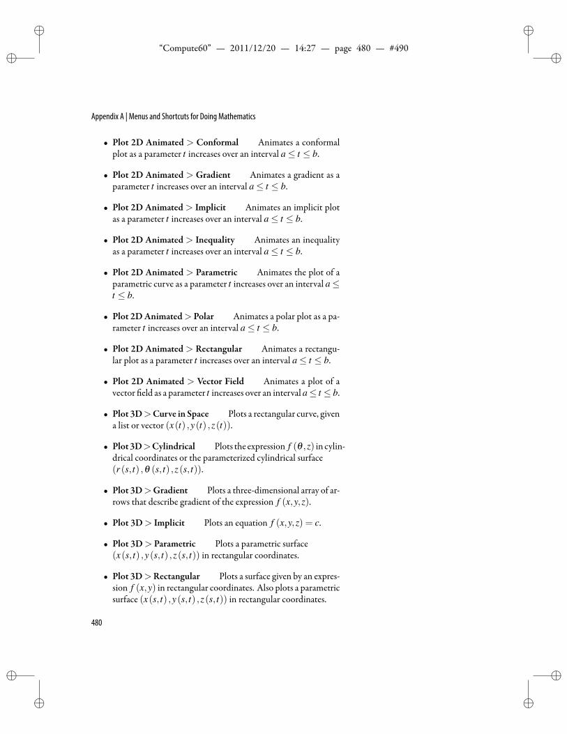
ii
“Compute60” — 2011/12/20 — 14:27 — page 480 — #490 ii
ii
ii
Appendix A | Menus and Shortcuts for Doing Mathematics
• Plot 2D Animated > Conformal Animates a conformalplot as a parameter t increases over an interval a≤ t ≤ b.
• Plot 2D Animated > Gradient Animates a gradient as aparameter t increases over an interval a≤ t ≤ b.
• Plot 2D Animated > Implicit Animates an implicit plotas a parameter t increases over an interval a≤ t ≤ b.
• Plot 2D Animated > Inequality Animates an inequalityas a parameter t increases over an interval a≤ t ≤ b.
• Plot 2D Animated > Parametric Animates the plot of aparametric curve as a parameter t increases over an interval a≤t ≤ b.
• Plot 2DAnimated> Polar Animates a polar plot as a pa-rameter t increases over an interval a≤ t ≤ b.
• Plot 2D Animated > Rectangular Animates a rectangu-lar plot as a parameter t increases over an interval a≤ t ≤ b.
• Plot 2D Animated > Vector Field Animates a plot of avector eld as a parameter t increases over an interval a≤ t ≤ b.
• Plot 3D>Curve in Space Plots a rectangular curve, givena list or vector (x(t) ,y(t) ,z(t)).
• Plot3D>Cylindrical Plots the expression f (θ ,z) in cylin-drical coordinates or the parameterized cylindrical surface(r (s, t) ,θ (s, t) ,z(s, t)).
• Plot 3D>Gradient Plots a three-dimensional array of ar-rows that describe gradient of the expression f (x,y,z).
• Plot 3D> Implicit Plots an equation f (x,y,z) = c.
• Plot 3D> Parametric Plots a parametric surface(x(s, t) ,y(s, t) ,z(s, t)) in rectangular coordinates.
• Plot 3D>Rectangular Plots a surface given by an expres-sion f (x,y) in rectangular coordinates. Also plots a parametricsurface (x(s, t) ,y(s, t) ,z(s, t)) in rectangular coordinates.
480
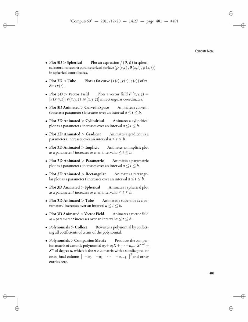
ii
“Compute60” — 2011/12/20 — 14:27 — page 481 — #491 ii
ii
ii
Compute Menu
• Plot 3D>Spherical Plot an expression f (θ ,ϕ) in spheri-cal coordinates or a parameterized surface (ρ (s, t) ,θ (s, t) ,ϕ (s, t))in spherical coordinates.
• Plot 3D>Tube Plots a fat curve (x(t) ,y(t) ,z(t)) of ra-dius r (t).
• Plot 3D > Vector Field Plots a vector eld F (x,y,z) =[u(x,y,z) ,v(x,y,z) ,w(x,y,z)] in rectangular coordinates.
• Plot 3DAnimated>Curve in Space Animates a curve inspace as a parameter t increases over an interval a≤ t ≤ b.
• Plot 3D Animated > Cylindrical Animates a cylindricalplot as a parameter t increases over an interval a≤ t ≤ b.
• Plot 3D Animated > Gradient Animates a gradient as aparameter t increases over an interval a≤ t ≤ b.
• Plot 3D Animated > Implicit Animates an implicit plotas a parameter t increases over an interval a≤ t ≤ b.
• Plot 3D Animated > Parametric Animates a parametricplot as a parameter t increases over an interval a≤ t ≤ b.
• Plot 3D Animated > Rectangular Animates a rectangu-lar plot as a parameter t increases over an interval a≤ t ≤ b.
• Plot 3DAnimated> Spherical Animates a spherical plotas a parameter t increases over an interval a≤ t ≤ b.
• Plot 3D Animated> Tube Animates a tube plot as a pa-rameter t increases over an interval a≤ t ≤ b.
• Plot 3DAnimated>Vector Field Animates a vector eldas a parameter t increases over an interval a≤ t ≤ b.
• Polynomials>Collect Rewrites a polynomial by collect-ing all coefficients of terms of the polynomial.
• Polynomials>CompanionMatrix Produces the compan-ionmatrix of amonic polynomiala0+a1X+· · ·+an−1Xn−1+Xn of degree n, which is the n×n matrix with a subdiagonal ofones, nal column
[−a0 −a1 · · · −an−1
]T and otherentries zero.
481
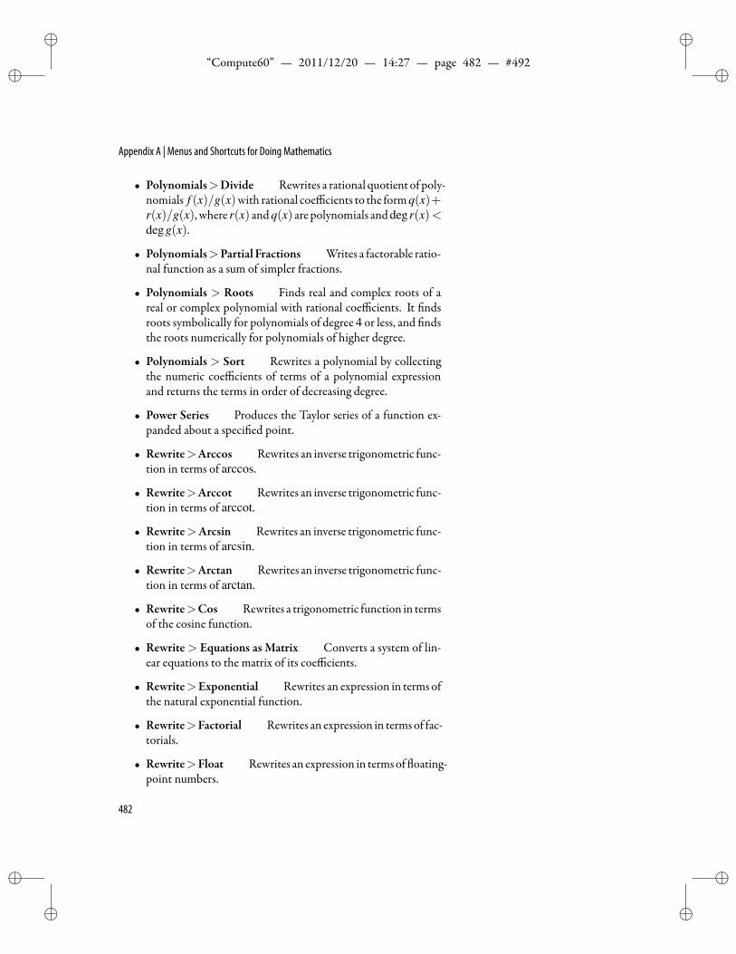
ii
“Compute60” — 2011/12/20 — 14:27 — page 482 — #492 ii
ii
ii
Appendix A | Menus and Shortcuts for Doing Mathematics
• Polynomials>Divide Rewrites a rational quotient of poly-nomials f (x)/g(x)with rational coefficients to the formq(x)+r(x)/g(x), where r(x) andq(x) are polynomials anddegr(x)<degg(x).
• Polynomials>Partial Fractions Writes a factorable ratio-nal function as a sum of simpler fractions.
• Polynomials > Roots Finds real and complex roots of areal or complex polynomial with rational coefficients. It ndsroots symbolically for polynomials of degree 4 or less, and ndsthe roots numerically for polynomials of higher degree.
• Polynomials > Sort Rewrites a polynomial by collectingthe numeric coefficients of terms of a polynomial expressionand returns the terms in order of decreasing degree.
• Power Series Produces the Taylor series of a function ex-panded about a speci ed point.
• Rewrite>Arccos Rewrites an inverse trigonometric func-tion in terms of arccos.
• Rewrite>Arccot Rewrites an inverse trigonometric func-tion in terms of arccot.
• Rewrite>Arcsin Rewrites an inverse trigonometric func-tion in terms of arcsin.
• Rewrite>Arctan Rewrites an inverse trigonometric func-tion in terms of arctan.
• Rewrite>Cos Rewrites a trigonometric function in termsof the cosine function.
• Rewrite> Equations as Matrix Converts a system of lin-ear equations to the matrix of its coefficients.
• Rewrite>Exponential Rewrites an expression in terms ofthe natural exponential function.
• Rewrite>Factorial Rewrites an expression in termsof fac-torials.
• Rewrite>Float Rewrites an expression in termsof oating-point numbers.
482
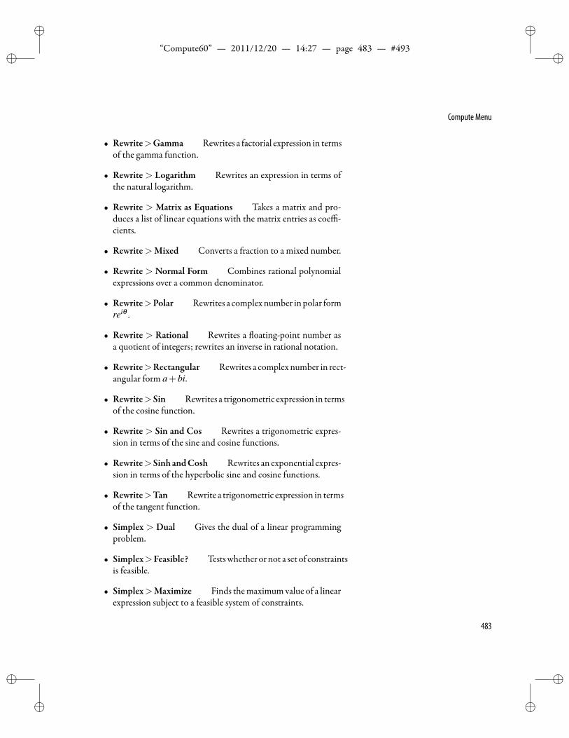
ii
“Compute60” — 2011/12/20 — 14:27 — page 483 — #493 ii
ii
ii
Compute Menu
• Rewrite>Gamma Rewrites a factorial expression in termsof the gamma function.
• Rewrite > Logarithm Rewrites an expression in terms ofthe natural logarithm.
• Rewrite > Matrix as Equations Takes a matrix and pro-duces a list of linear equations with the matrix entries as coeffi-cients.
• Rewrite>Mixed Converts a fraction to a mixed number.
• Rewrite > Normal Form Combines rational polynomialexpressions over a common denominator.
• Rewrite>Polar Rewrites a complexnumber inpolar formreiθ .
• Rewrite > Rational Rewrites a oating-point number asa quotient of integers; rewrites an inverse in rational notation.
• Rewrite>Rectangular Rewrites a complexnumber in rect-angular form a+bi.
• Rewrite>Sin Rewrites a trigonometric expression in termsof the cosine function.
• Rewrite > Sin and Cos Rewrites a trigonometric expres-sion in terms of the sine and cosine functions.
• Rewrite>SinhandCosh Rewrites an exponential expres-sion in terms of the hyperbolic sine and cosine functions.
• Rewrite>Tan Rewrite a trigonometric expression in termsof the tangent function.
• Simplex > Dual Gives the dual of a linear programmingproblem.
• Simplex>Feasible? Testswhether ornot a set of constraintsis feasible.
• Simplex>Maximize Finds themaximumvalue of a linearexpression subject to a feasible system of constraints.
483
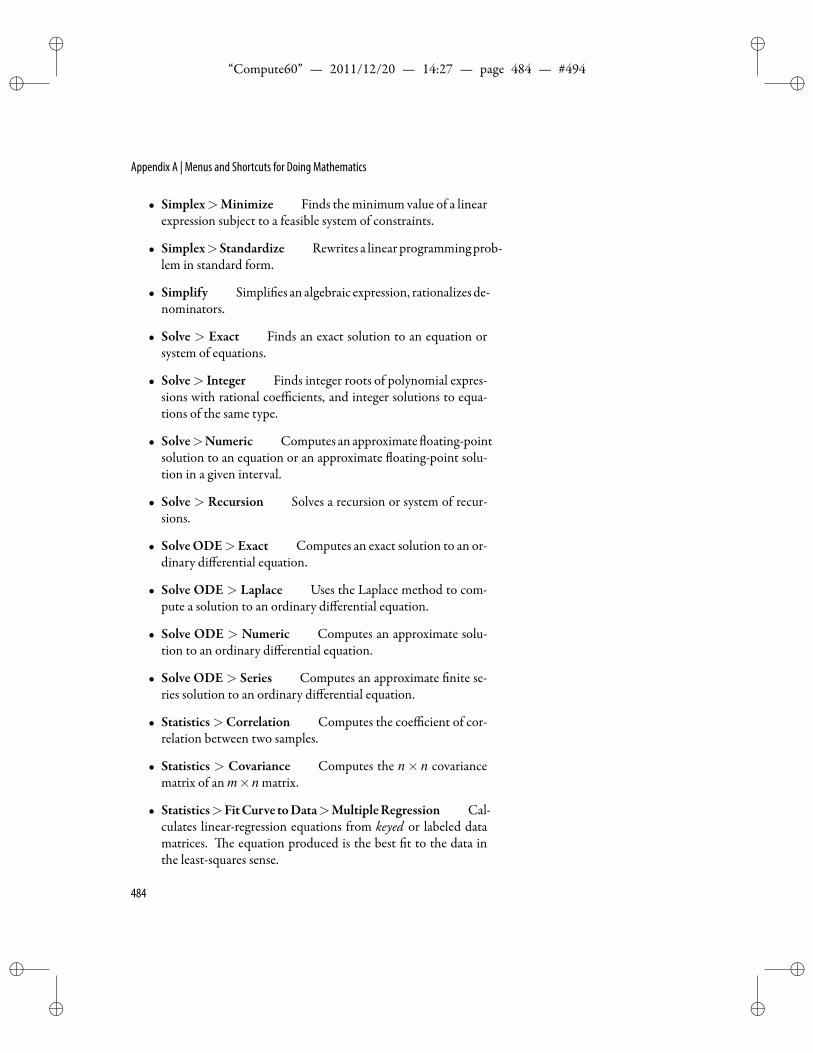
ii
“Compute60” — 2011/12/20 — 14:27 — page 484 — #494 ii
ii
ii
Appendix A | Menus and Shortcuts for Doing Mathematics
• Simplex>Minimize Finds theminimum value of a linearexpression subject to a feasible system of constraints.
• Simplex>Standardize Rewrites a linear programmingprob-lem in standard form.
• Simplify Simpli es an algebraic expression, rationalizes de-nominators.
• Solve > Exact Finds an exact solution to an equation orsystem of equations.
• Solve> Integer Finds integer roots of polynomial expres-sions with rational coefficients, and integer solutions to equa-tions of the same type.
• Solve>Numeric Computes an approximate oating-pointsolution to an equation or an approximate oating-point solu-tion in a given interval.
• Solve > Recursion Solves a recursion or system of recur-sions.
• SolveODE>Exact Computes an exact solution to an or-dinary differential equation.
• Solve ODE > Laplace Uses the Laplace method to com-pute a solution to an ordinary differential equation.
• Solve ODE > Numeric Computes an approximate solu-tion to an ordinary differential equation.
• Solve ODE> Series Computes an approximate nite se-ries solution to an ordinary differential equation.
• Statistics>Correlation Computes the coefficient of cor-relation between two samples.
• Statistics > Covariance Computes the n× n covariancematrix of an m×n matrix.
• Statistics>FitCurve toData>MultipleRegression Cal-culates linear-regression equations from keyed or labeled datamatrices. e equation produced is the best t to the data inthe least-squares sense.
484

ii
“Compute60” — 2011/12/20 — 14:27 — page 485 — #495 ii
ii
ii
Compute Menu
• Statistics>FitCurve toData>Polynomial ofDegreen Cal-culates polynomial equations from labeled or unlabeled two-columndatamatrices. e result is a polynomial of the speci eddegree that is the best t to the data in the least-squares sense.
• Statistics > Geometric Mean Calculates the nth root ofthe product of numbers in a comma delimited list or a vector,and calculates the nth roots of the products of numbers incolumns of an n×m matrix for n≥ 2.
• Statistics>Harmonic Mean Calculates the reciprocal ofthe mean of the reciprocals of numbers in a comma delimitedlist or a vector, and calculates the harmonic means for columnsof an n×m matrix for n≥ 2.
• Statistics > Mean Calculates the arithmetic mean, or av-erage, of numbers in a comma delimited list or a vector, and cal-culates the arithmeticmeans of numbers in columns of ann×mmatrix for n≥ 2.
• Statistics > Mean Deviation Calculates the mean of thedistances of the data from the data mean for data in a commadelimited list or in a vector, and calculates the mean deviationsof data in columns of an n×m matrix for n≥ 2.
• Statistics>Median Calculates a number such that at leasthalf the numbers in a data set are equal to or less than it, and atleast half the numbers in the data set are equal to or greater thanit for data in a commadelimited list or in a vector, and calculatesthe medians of data in columns of an n×m matrix for n≥ 2.
• Statistics>Mode Finds the valueor values that occurwithmaximum frequency in a data set, and also gives themultiplicityof each of the modes for data in a comma delimited list or in avector, and calculates the modes of data in columns of an n×mmatrix for n≥ 2.
• Statistics > Moment Computes the 1st, 2nd, and highermoments about themean or about a speci ed point for data in acomma delimited list or in a vector, and calculates themomentsof data in columns of an n×m matrix for n≥ 2.
485
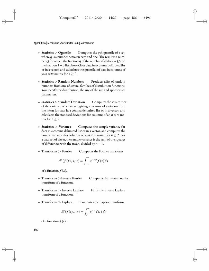
ii
“Compute60” — 2011/12/20 — 14:27 — page 486 — #496 ii
ii
ii
Appendix A | Menus and Shortcuts for Doing Mathematics
• Statistics> uantile Computes the qth quantile of a set,where q is a number between zero and one. e result is a num-ber Q for which the fraction q of the numbers falls below Q andthe fraction1−q lies aboveQ for data in a commadelimited listor in a vector, and calculates the quantiles of data in columns ofan n×m matrix for n≥ 2.
• Statistics>RandomNumbers Produces a list of randomnumbers from one of several families of distribution functions.You specify the distribution, the size of the set, and appropriateparameters.
• Statistics>StandardDeviation Computes the square rootof the variance of a data set, giving a measure of variation fromthe mean for data in a comma delimited list or in a vector, andcalculates the standard deviations for columns of an n×m ma-trix for n≥ 2.
• Statistics > Variance Computes the sample variance fordata in a comma delimited list or in a vector, and computes thesample variances for columns of an n×m matrix for n≥ 2. Fora data set of size n, the sample variance is the sum of the squaresof differences with the mean, divided by n−1.
• Transforms> Fourier Computes the Fourier transform
F ( f (x) ,x,w) =∫ ∞
−∞e−iwx f (x)dx
of a function f (x).
• Transforms> InverseFourier Computes the inverseFouriertransform of a function.
• Transforms > Inverse Laplace Finds the inverse Laplacetransform of a function.
• Transforms> Laplace Computes the Laplace transform
L ( f (t) , t,s) =∫ ∞
0e−st f (t) dt
of a function f (t).
486
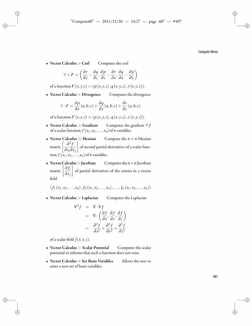
ii
“Compute60” — 2011/12/20 — 14:27 — page 487 — #497 ii
ii
ii
Compute Menu
• Vector Calculus>Curl Computes the curl
×F =
(∂ r∂y− ∂q
∂ z,
∂ p∂ z− ∂ r
∂x,
∂q∂x− ∂ p
∂y
)of a function F (x,y,z) = (p(x,y,z) ,q(x,y,z) ,r (x,y,z)).
• Vector Calculus>Divergence Computes the divergence
·F =∂ p∂x
(a,b,c)+∂q∂y
(a,b,c)+∂ r∂ z
(a,b,c)
of a function F (x,y,z) = (p(x,y,z) ,q(x,y,z) ,r (x,y,z)).
• Vector Calculus > Gradient Computes the gradient fof a scalar function f (x1,x2, . . . ,xn)of n variables.
• Vector Calculus > Hessian Compute the n× n Hessian
matrix[
∂ 2 f∂xi∂x j
]of second partial derivatives of a scalar func-
tion f (x1,x2, . . . ,xn)of n variables.
• VectorCalculus> Jacobian Computes the n×n Jacobian
matrix[
∂ fi
∂x j
]of partial derivatives of the entries in a vector
eld
( f1 (x1,x2, . . . ,xn) , f2 (x1,x2, . . . ,xn) , . . . , fn (x1,x2, . . . ,xn))
• Vector Calculus> Laplacian Computes the Laplacian
∇2 f = ∇ ·∇ f
= ∇ ·(
∂ f∂x
,∂ f∂y
,∂ f∂ z
)=
∂ 2 f∂x2 +
∂ 2 f∂y2 +
∂ 2 f∂ z2
of a scalar eld f (x,y,z).
• Vector Calculus > Scalar Potential Computes the scalarpotential or informs that such a function does not exist.
• Vector Calculus> Set Basis Variables Allows the user toenter a new set of basis variables.
487

ii
“Compute60” — 2011/12/20 — 14:27 — page 488 — #498 ii
ii
ii
Appendix A | Menus and Shortcuts for Doing Mathematics
• VectorCalculus>Vector Potential Computes the vectorpotential of a vector elds. e vector potential of a vector eldsis a vector eld whose curl is the given vector eld.
• VectorCalculus>Wronskian Computes theWronskian,the determinate of the n× n matrix
[f (i−1)
j (x)], of a vector
eld ( f1 (x) , f2 (x) , . . . , fn (x)).
Toolbar and Keyboard Shortcuts for Compute Menu
Math Toolbar and Keyboard ShortcutsTooltips identify the buttons on the toolbars in the program win-
dow. To see the button name, hold the mouse pointer on a toolbarbutton for several seconds until the tooltip appears.
Following areMathToolbar andkeyboard shortcuts for commandson the Compute menu.
Button Compute Menu Keyboard Shortcut
Evaluate Ctrl+e
Evaluate Numeric
De nitions>New De nition Ctrl+=
De nitions> Show De nitions
Interpret Ctrl+shi +/ or Ctrl+?
Solve> Exact
Simplify
Expand
Plot 2D> Rectangular
Plot 3D> Rectangular
488
ii
“Compute60” — 2011/12/20 — 14:27 — page 489 — #499 ii
ii
ii
BMenus and Shortcuts for
Entering Mathematics
Time is the most valuable thing a man can spend. Theophrastus (372 BC–287 BC)
K eyboard shortcuts are available for many common tasks. e Entering Mathematics and Text
Entering Mathematical Objects
Entering Symbols and Characters
Entering Units of Measure
keyboard shortcuts for performing basic mathematical oper-ations and entering symbols, characters, and the most com-
mon mathematical objects are faster to use than the mouse. e listson the following pages summarize shortcuts related speci cally to en-tering mathematics. For many additional shortcuts, consult CreatingDocuments with Scienti c WorkPlace and Scienti c Word, Version 6 orchoose Help and search for keyboard shortcuts.
We use standard computer conventions to give keyboard instruc-tions. e names of keys in the instructions match the names shownon most keyboards. Ctrl (Windows) and Cmd (Mac) are synony-mous, as are Enter (Windows) and Return (Mac). Names of keys arealways shown in Windows format. Mac users should substitute Mackeys (e.g., Cmd and Return) as appropriate.
A plus sign (+) between the names of two keys indicates that youmust press the rst key and hold it down while you press the secondkey. For example, Ctrl+gmeans that you press and hold down theCtrlkey, press g, and then release both keys.
Entering mathematics is straightforward. Working right in theprogramwindow, youuse familiar notation to entermathematical char-acters, symbols, and objects into your document. Simple commandslet you create displayed or inline mathematics.
Editing mathematics is equally straightforward. You can use stan-dard clipboard and drag-and-drop operations to cut, copy, paste, and
489
ii
“Compute60” — 2011/12/20 — 14:27 — page 490 — #500 ii
ii
ii
Appendix B | Menus and Shortcuts for Entering Mathematics
delete selections. You can also use the search and replace features tolocate or change mathematical information.
Entering Mathematics and TextDuring information entry you are either entering text or mathe-
matics, and the results obtained from keystrokes and other user inter-face actions will differ depending on whether you are entering text ormath. us we refer to being in either text mode or math mode. edefault state is text mode; it is easy to toggle between the two modesand it is also easy to determine what mode you are in.
When you toggle to mathematics, the Math/Text button changesto an “M” and the program
• Displays the insert point between brackets for mathematics.
• Interprets anything you type asmathematics, displaying it in redin the program window.
• Italicizes alphabetic characters and displays numbers upright.
• Automatically formats mathematical expressions, inserting cor-rect spacing around operators such as + and relations such as =.
• Advances the insert point to thenextmathematical objectwhenyou press the spacebar.
To switch from text tomathematics from the keyboard• Press Ctrl+m.
Subsequent editing inmathmodewill continue until you press thespacebar at the end of math. Subsequent editing in text mode willenter text objects.
To switch from text tomathematics from the Insertmenu• Choose Insert>Math.
Subsequent editing will enter math objects.
To switch frommathematics to text from the keyboard• Press Spacebar once or twice.
490
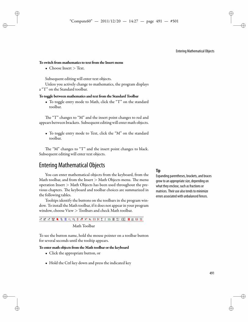
ii
“Compute60” — 2011/12/20 — 14:27 — page 491 — #501 ii
ii
ii
Entering Mathematical Objects
To switch frommathematics to text from the Insertmenu• Choose Insert>Text.
Subsequent editing will enter text objects.Unless you actively change to mathematics, the program displays
a “T” on the Standard toolbar.
To toggle betweenmathematics and text from the StandardToolbar• To toggle entry mode to Math, click the “T” on the standard
toolbar.
e “T” changes to “M” and the insert point changes to red andappears between brackets. Subsequent editingwill entermath objects.
• To toggle entry mode to Text, click the “M” on the standardtoolbar.
e “M” changes to “T” and the insert point changes to black.Subsequent editing will enter text objects.
Entering Mathematical ObjectsTipExpanding parentheses, brackets, and bracesgrow to an appropriate size, depending onwhat they enclose, such as fractions ormatrices. Their use also tends to minimizeerrors associated with unbalanced fences.
You can enter mathematical objects from the keyboard, from theMath toolbar, and from the Insert>Math Objects menu. e menuoperation Insert > Math Objects has been used throughout the pre-vious chapters. e keyboard and toolbar choices are summarized inthe following tables.
Tooltips identify the buttons on the toolbars in the program win-dow. To install theMath toolbar, if it does not appear in your programwindow, choose View>Toolbars and check Math toolbar.
Math Toolbar
To see the button name, hold the mouse pointer on a toolbar buttonfor several seconds until the tooltip appears.
Toentermath objects from theMath toolbar or the keyboard• Click the appropriate button, or
• Hold the Ctrl key down and press the indicated key
491
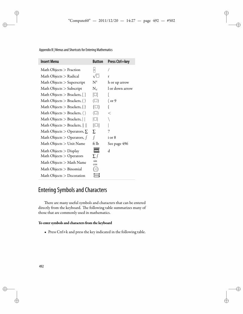
ii
“Compute60” — 2011/12/20 — 14:27 — page 492 — #502 ii
ii
ii
Appendix B | Menus and Shortcuts for Entering Mathematics
Insert Menu Button Press Ctrl+key
Math Objects> Fraction /
Math Objects> Radical√ r
Math Objects> Superscript Nx h or up arrowMath Objects> Subscript Nx l or down arrowMath Objects> Brackets, [ ] [] [Math Objects> Brackets, ( ) () ( or 9Math Objects> Brackets, Math Objects> Brackets, ⟨ ⟩ ⟨⟩ <
Math Objects> Brackets, | | || \Math Objects> Brackets, ∥ ∥ ∥∥ |Math Objects>Operators, ∑ ∑ 7Math Objects>Operators,
∫ ∫i or 8
Math Objects>Unit Name lb See page 496
Math Objects>Display dMath Objects>Operators ∑
∫Math Objects>Math Name sin
cos
Math Objects> Binomial()
Math Objects>Decoration
Entering Symbols and Characters
ere are many useful symbols and characters that can be entereddirectly from the keyboard. e following table summarizes many ofthose that are commonly used in mathematics.
Toenter symbols and characters from the keyboard
• Press Ctrl+k and press the key indicated in the following table.
492
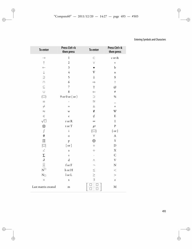
ii
“Compute60” — 2011/12/20 — 14:27 — page 493 — #503 ii
ii
ii
Entering Symbols and Characters
To enter Press Ctrl+kthen press To enter Press Ctrl+k
then press
→ 1 ⊂ c or &↑ 2 ∨ v← 3 • b↓ 4 ∇ n⊇ 5 ⇓ $∩ 6 ⇒ !⊆ 7 ⇑ @∪ 8 ⇐ #() 9 or 0 or ( or ) ⊃ %≡ - ∼= _= = ± +≈ w ℵ W∈ e /∈ E√ r or R ∞ I⊗
t or T ℘ P∫i or
/0 o ∀ A∏ p
⊕S
[] [ or ] ⋄ D∠ a ÷ X∑ s · C∂ d ∧ V f or F ¬ N
N h or H ≤ <
N l or L ≥ >
× x ∃ z
Last matrix created m[
]M
493
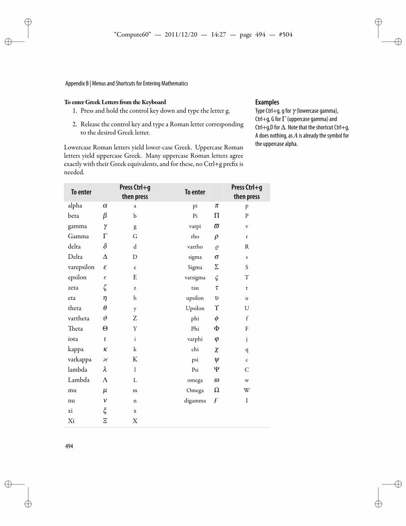
ii
“Compute60” — 2011/12/20 — 14:27 — page 494 — #504 ii
ii
ii
Appendix B | Menus and Shortcuts for Entering Mathematics
ToenterGreekLetters from theKeyboard ExamplesType Ctrl+g, g for γ (lowercase gamma),Ctrl+g, G forΓ (uppercase gamma) andCtrl+g,D for∆. Note that the shortcut Ctrl+g,A does nothing, asA is already the symbol forthe uppercase alpha.
1. Press and hold the control key down and type the letter g.
2. Release the control key and type a Roman letter correspondingto the desired Greek letter.
Lowercase Roman letters yield lower-case Greek. Uppercase Romanletters yield uppercase Greek. Many uppercase Roman letters agreeexactly with their Greek equivalents, and for these, no Ctrl+g pre x isneeded.
To enterPress Ctrl+gthen press To enter
Press Ctrl+gthen press
alpha α a pi π p
beta β b Pi Π P
gamma γ g varpi ϖ v
Gamma Γ G rho ρ r
delta δ d varrho ϱ R
Delta ∆ D sigma σ s
varepsilon ε e Sigma Σ S
epsilon ϵ E varsigma ς T
zeta ζ z tau τ t
eta η h upsilon υ u
theta θ y Upsilon ϒ U
vartheta ϑ Z phi ϕ f
eta Θ Y Phi Φ F
iota ι i varphi φ j
kappa κ k chi χ q
varkappa κ K psi ψ c
lambda λ l Psi Ψ C
Lambda Λ L omega ω w
mu µ m Omega Ω W
nu ν n digamma 𝟋 I
xi ξ xXi Ξ X
494
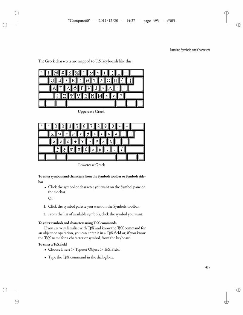
ii
“Compute60” — 2011/12/20 — 14:27 — page 495 — #505 ii
ii
ii
Entering Symbols and Characters
e Greek characters are mapped to U.S. keyboards like this:
Uppercase Greek
Lowercase Greek
Toenter symbols andcharacters fromtheSymbols toolbarorSymbols side-bar
• Click the symbol or character you want on the Symbol pane onthe sidebar.Or
1. Click the symbol palette you want on the Symbols toolbar.
2. From the list of available symbols, click the symbol you want.
Toenter symbols and characters usingTeXcommandsIf you are very familiar with TEX and know the TEX command for
an object or operation, you can enter it in a TEX eld or, if you knowthe TEX name for a character or symbol, from the keyboard.Toenter aTeX eld
• Choose Insert>Typeset Object>TeX Field.
• Type the TEX command in the dialog box.
495
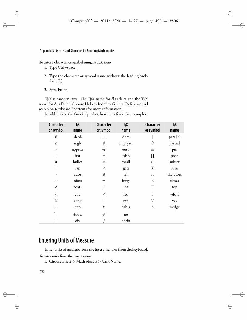
ii
“Compute60” — 2011/12/20 — 14:27 — page 496 — #506 ii
ii
ii
Appendix B | Menus and Shortcuts for Entering Mathematics
Toenter a character or symbol using itsTeXname1. Type Ctrl+space.
2. Type the character or symbol name without the leading back-slash (\).
3. Press Enter.
TEX is case-sensitive. e TEX name for δ is delta and the TEXname for ∆ is Delta. Choose Help> Index>General Reference andsearch on Keyboard Shortcuts for more information.
In addition to the Greek alphabet, here are a few other examples.
Characteror symbol
TEXname
Characteror symbol
TEXname
Characteror symbol
TEXname
ℵ aleph . . . dots ∥ parallel∠ angle /0 emptyset ∂ partial≈ approx e euro ± pm⊥ bot ∃ exists ∏ prod• bullet ∀ forall ⊂ subset∩ cap ≥ geq ∑ sum· cdot ∈ in ∴ therefore· · · cdots ∞ in y × timesc/ cents
∫int ⊤ top
circ ≤ leq... vdots
∼= cong ∓ mp ∨ vee∪ cup ∇ nabla ∧ wedge. . . ddots = ne÷ div /∈ notin
Entering Units of MeasureEnter units ofmeasure fromthe Insertmenuor fromthekeyboard.
Toenter units from the Insertmenu1. Choose Insert>Math objects>Unit Name.
496
ii
“Compute60” — 2011/12/20 — 14:27 — page 497 — #507 ii
ii
ii
Entering Units of Measure
2. When theUnitName dialog box appears, select ameasurementcategory and a unit, then click Apply.
Units are automatically recognized and can be entered from thekeyboard. Following the general guidelines given below, and a tableof unit pre xes, are tables giving speci c keyboard shortcuts for eachof the built-in physical quantities.
Toenter units from the keyboard1. Choose Insert>Math.
2. Type ‘u’ followed by the unit symbol, with the exceptions:
• Type ‘mc’ for ‘micro’ in place of µ whichwill appear in theunit symbol.
• Type ‘uhr’ for the hour symbol h.
• Type ’uda’ for the day symbol d.
• Type ’use’ for the second symbol s.
• Type ‘ume’ for the meter symbol m.
• Type ‘uan’ for the angstrom symbol A.
• Type ‘uCo’ for the Coulomb symbol C.
• Type ‘uTe’ for the Tesla symbol T.
• Type ‘uli’ for the Liter symbol l.
• Type ‘ohm’ (a er the pre x) for the symbols for ohm (andits derivatives) Ω.
• Type ‘ucel’ and ‘u f ahr’ for degrees Celsius C and de-grees Fahrenheit F, respectively.
• Type ‘udeg’ for the degree symbol (plane angle) .
• Type ‘udmn’ and ‘uds’ for (degree) minute ′ and (degree)second ′′, respectively.
Autorecognition is case sensitive, so type upper case where indi-cated. e unit symbol should turn greenwhen you type the last char-acter.
497
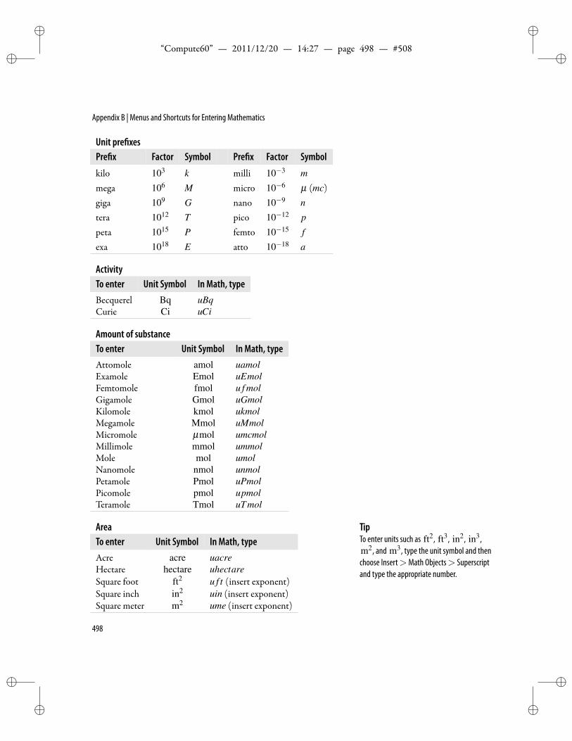
ii
“Compute60” — 2011/12/20 — 14:27 — page 498 — #508 ii
ii
ii
Appendix B | Menus and Shortcuts for Entering Mathematics
Unit pre xesPre x Factor Symbol Pre x Factor Symbol
kilo 103 k milli 10−3 m
mega 106 M micro 10−6 µ (mc)giga 109 G nano 10−9 n
tera 1012 T pico 10−12 p
peta 1015 P femto 10−15 f
exa 1018 E atto 10−18 a
ActivityTo enter Unit Symbol In Math, typeBecquerel Bq uBqCurie Ci uCi
Amount of substanceTo enter Unit Symbol In Math, typeAttomole amol uamolExamole Emol uEmolFemtomole fmol u f molGigamole Gmol uGmolKilomole kmol ukmolMegamole Mmol uMmolMicromole µmol umcmolMillimole mmol ummolMole mol umolNanomole nmol unmolPetamole Pmol uPmolPicomole pmol upmolTeramole Tmol uT mol
AreaTo enter Unit Symbol In Math, typeAcre acre uacreHectare hectare uhectareSquare foot ft2 u f t (insert exponent)Square inch in2 uin (insert exponent)Square meter m2 ume (insert exponent)
TipTo enter units such as ft2, ft3, in2, in3,m2, and m3, type the unit symbol and thenchoose Insert>Math Objects> Superscriptand type the appropriate number.
498
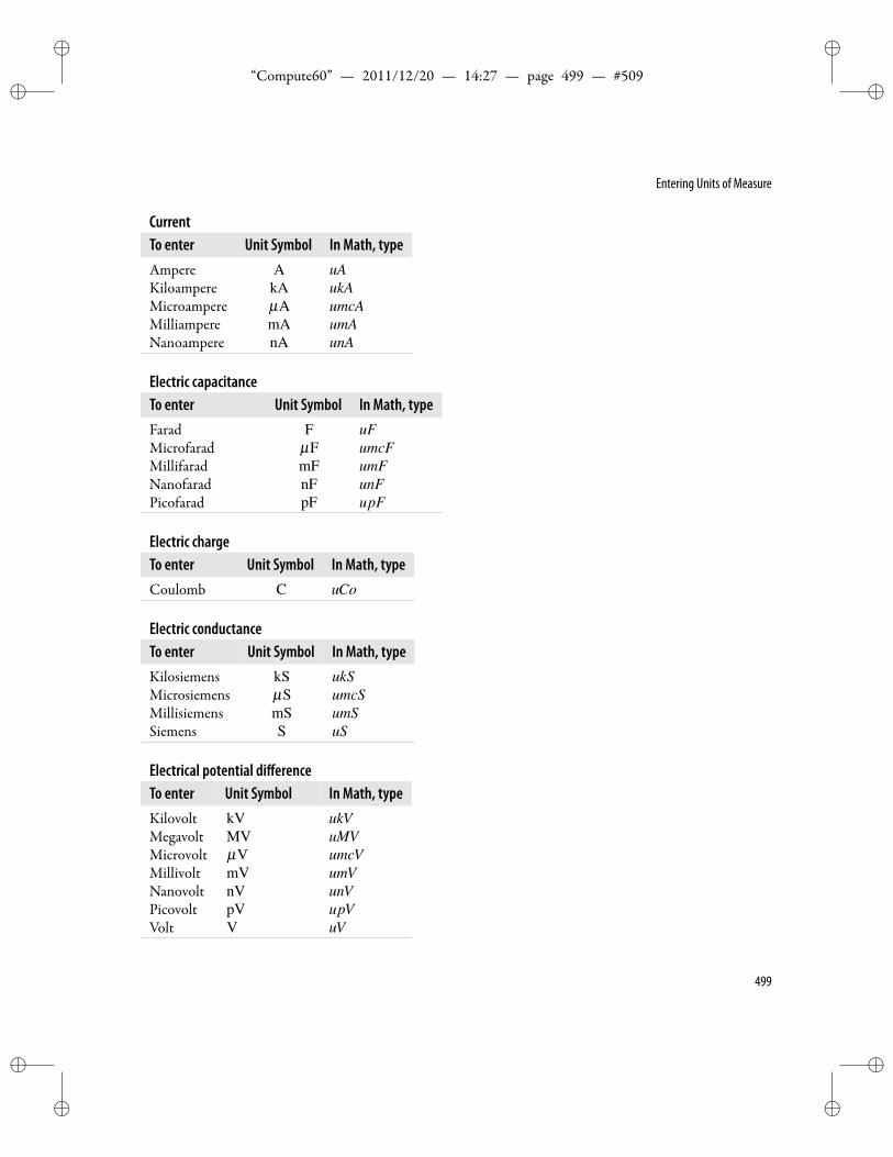
ii
“Compute60” — 2011/12/20 — 14:27 — page 499 — #509 ii
ii
ii
Entering Units of Measure
CurrentTo enter Unit Symbol In Math, typeAmpere A uAKiloampere kA ukAMicroampere µA umcAMilliampere mA umANanoampere nA unA
Electric capacitanceTo enter Unit Symbol In Math, typeFarad F uFMicrofarad µF umcFMillifarad mF umFNanofarad nF unFPicofarad pF upF
Electric chargeTo enter Unit Symbol In Math, typeCoulomb C uCo
Electric conductanceTo enter Unit Symbol In Math, typeKilosiemens kS ukSMicrosiemens µS umcSMillisiemens mS umSSiemens S uS
Electrical potential differenceTo enter Unit Symbol In Math, typeKilovolt kV ukVMegavolt MV uMVMicrovolt µV umcVMillivolt mV umVNanovolt nV unVPicovolt pV upVVolt V uV
499
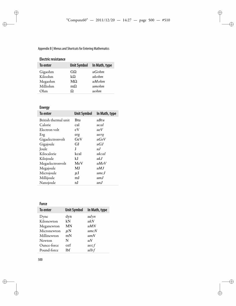
ii
“Compute60” — 2011/12/20 — 14:27 — page 500 — #510 ii
ii
ii
Appendix B | Menus and Shortcuts for Entering Mathematics
Electric resistanceTo enter Unit Symbol In Math, typeGigaohm GΩ uGohmKiloohm kΩ ukohmMegaohm MΩ uMohmMilliohm mΩ umohmOhm Ω uohm
EnergyTo enter Unit Symbol In Math, typeBritish thermal unit Btu uBtuCalorie cal ucalElectron volt eV ueVErg erg uergGigaelectronvolt GeV uGeVGigajoule GJ uGJJoule J uJKilocalorie kcal ukcalKilojoule kJ ukJMegaelectronvolt MeV uMeVMegajoule MJ uMJMicrojoule µJ umcJMillijoule mJ umJNanojoule nJ unJ
ForceTo enter Unit Symbol In Math, typeDyne dyn udynKilonewton kN ukNMeganewton MN uMNMicronewton µN umcNMillinewton mN umNNewton N uNOunce-force ozf uoz fPound-force lbf ulb f
500
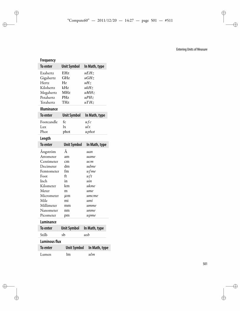
ii
“Compute60” — 2011/12/20 — 14:27 — page 501 — #511 ii
ii
ii
Entering Units of Measure
FrequencyTo enter Unit Symbol In Math, typeExahertz EHz uEHzGigahertz GHz uGHzHertz Hz uHzKilohertz kHz ukHzMegahertz MHz uMHzPetahertz PHz uPHzTerahertz THz uT Hz
IlluminanceTo enter Unit Symbol In Math, typeFootcandle fc u f cLux lx ulxPhot phot uphot
LengthTo enter Unit Symbol In Math, type
Ångström A uanAttometer am uameCentimeter cm ucmDecimeter dm udmeFemtometer fm u f meFoot ft u f tInch in uinKilometer km ukmeMeter m umeMicrometer µm umcmeMile mi umiMillimeter mm ummeNanometer nm unmePicometer pm upme
LuminanceTo enter Unit Symbol In Math, typeStilb sb usb
Luminous uxTo enter Unit Symbol In Math, typeLumen lm ulm
501
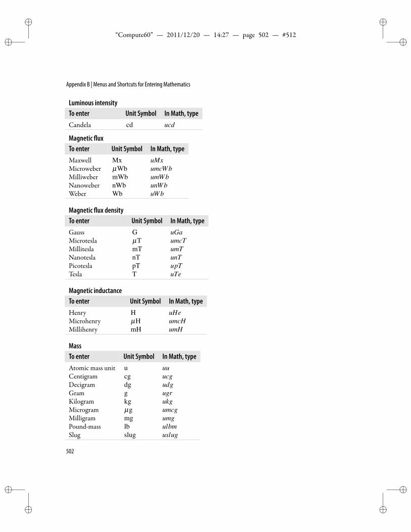
ii
“Compute60” — 2011/12/20 — 14:27 — page 502 — #512 ii
ii
ii
Appendix B | Menus and Shortcuts for Entering Mathematics
Luminous intensityTo enter Unit Symbol In Math, typeCandela cd ucd
Magnetic uxTo enter Unit Symbol In Math, typeMaxwell Mx uMxMicroweber µWb umcWbMilliweber mWb umWbNanoweber nWb unWbWeber Wb uWb
Magnetic ux densityTo enter Unit Symbol In Math, typeGauss G uGaMicrotesla µT umcTMillitesla mT umTNanotesla nT unTPicotesla pT upTTesla T uTe
Magnetic inductanceTo enter Unit Symbol In Math, typeHenry H uHeMicrohenry µH umcHMillihenry mH umH
MassTo enter Unit Symbol In Math, typeAtomic mass unit u uuCentigram cg ucgDecigram dg udgGram g ugrKilogram kg ukgMicrogram µg umcgMilligram mg umgPound-mass lb ulbmSlug slug uslug
502
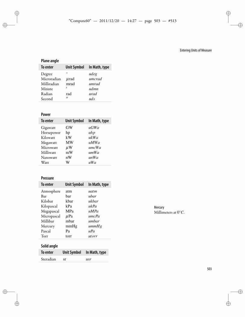
ii
“Compute60” — 2011/12/20 — 14:27 — page 503 — #513 ii
ii
ii
Entering Units of Measure
Plane angleTo enter Unit Symbol In Math, typeDegree udegMicroradian µrad umcradMilliradian mrad umradMinute ′ udmnRadian rad uradSecond ′′ uds
PowerTo enter Unit Symbol In Math, typeGigawatt GW uGWaHorsepower hp uhpKilowatt kW ukWaMegawatt MW uMWaMicrowatt µW umcWaMilliwatt mW umWaNanowatt nW unWaWatt W uWa
PressureTo enter Unit Symbol In Math, typeAtmosphere atm uatmBar bar ubarKilobar kbar ukbarKilopascal kPa ukPaMegapascal MPa uMPaMicropascal µPa umcPaMillibar mbar umbarMercury mmHg ummHgPascal Pa uPaTorr torr utorr
MercuryMillimeters at 0C.
Solid angleTo enter Unit Symbol In Math, typeSteradian sr usr
503
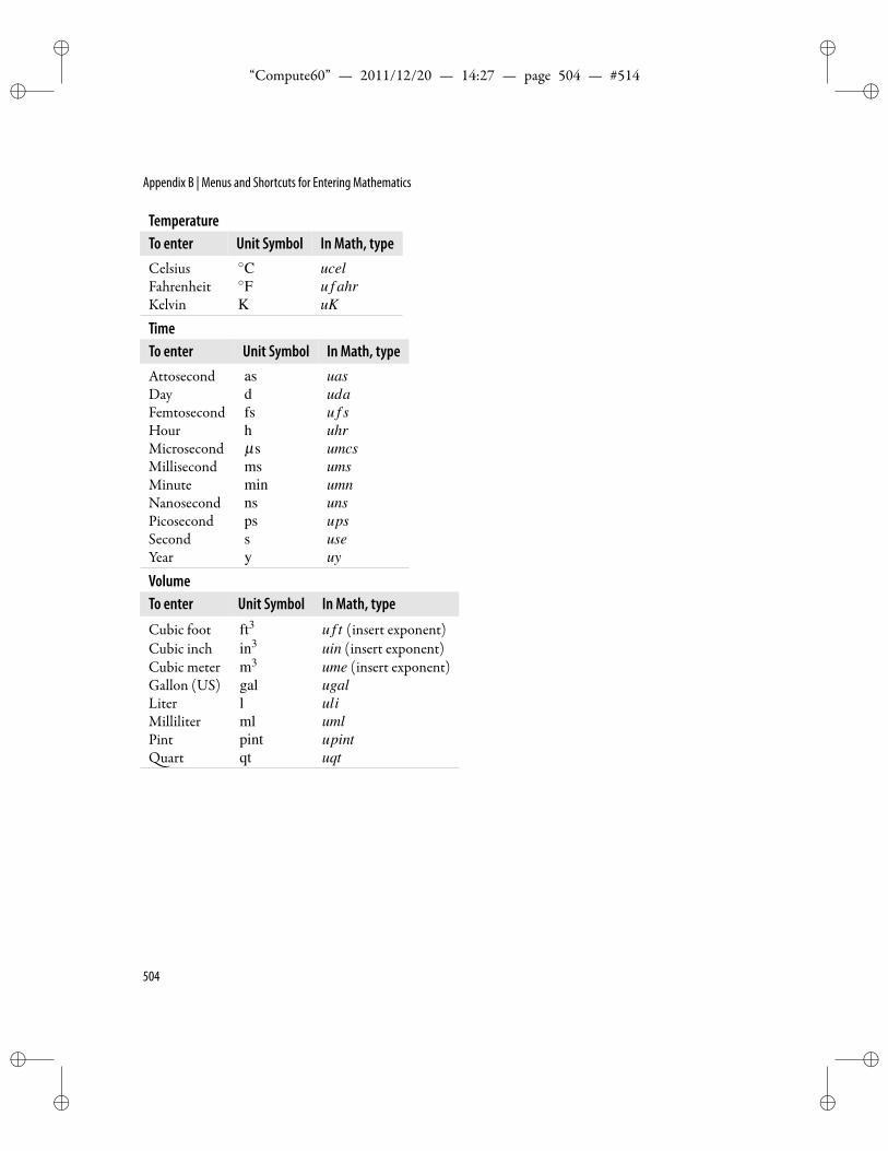
ii
“Compute60” — 2011/12/20 — 14:27 — page 504 — #514 ii
ii
ii
Appendix B | Menus and Shortcuts for Entering Mathematics
TemperatureTo enter Unit Symbol In Math, typeCelsius C ucelFahrenheit F u f ahrKelvin K uK
TimeTo enter Unit Symbol In Math, typeAttosecond as uasDay d udaFemtosecond fs u f sHour h uhrMicrosecond µs umcsMillisecond ms umsMinute min umnNanosecond ns unsPicosecond ps upsSecond s useYear y uy
VolumeTo enter Unit Symbol In Math, type
Cubic foot ft3 u f t (insert exponent)Cubic inch in3 uin (insert exponent)Cubic meter m3 ume (insert exponent)Gallon (US) gal ugalLiter l uliMilliliter ml umlPint pint upint
uart qt uqt
504
ii
“Compute60” — 2011/12/20 — 14:27 — page 505 — #515 ii
ii
ii
CCustomizing the Program
for Computing
Wherever there is number, there is beauty. Proclus Diadochus (412–485)
T he program window has an updated look with streamlined Customizing the Toolbars
Customizing the Sidebars
Customizing the ComputeSettings
Customizing the Plot Settings
Automatic Subsitution
layouts for the toolbars and symbol panels. As before, amouse-activated tooltip gives the name of each toolbar button and
panel symbol. Most tools work the same way they did in earlier ver-sions. e Version 6 system offers a number of ways to customize itsfeatures.
Use Preferences in the Tools menu to customize the universal andlocal settings. e Computation choices replace the previous Com-putation Setup and Engine Setup. You will nd some new features inthese dialogs.
You cande ne automatic substitution sequences for text andmath-ematics, thus speeding the entry of the text and mathematical expres-sions you usemost o enwith an enhanced automatic substitution fea-ture.
You can enter content quicklywith fragments. WithVersion 6 youcan create fragments containing XHTML code, TEX code, graphics,or anything else that can go on the clipboard. Fragments are no longerlimited to TEX strings. Fragments and many other text editing short-cuts are documented in themanualCreatingDocuments with Scienti cWorkPlace and Scienti c Word, as well as in the Help.
505
ii
“Compute60” — 2011/12/20 — 14:27 — page 506 — #516 ii
ii
ii
Appendix C | Customizing the Program for Computing
Customizing the Toolbarse Version 6 program window has three customizable toolbars.
• e Standard toolbar contains buttons for invoking commonle operations and the text boxes for tag lists.
• e Editing toolbar buttons invoke ordinary editing tools.
• e Math toolbar buttons insert mathematical objects directlyinto your document or open dialog boxes so that you can makeadditional speci cations. Certainbuttons invoke commoncom-putational operations.
e Symbol toolbar has palettes of buttons for adding a wide vari-ety of symbols to your documents. With the exception of those on theSymbol toolbar, the buttons on the toolbars are identical in functionto commands on the menus. Point the mouse at each toolbar buttonfor a few seconds to display a brief tooltip that identi es the button.As with menu commands, buttons that appear dimmed are unavail-able.
e default screen displays the rst three of these toolbars.
Toaddor remove toolbars1. Choose View>Toolbars.
2. Check or uncheck the desired toolbars.
Tocustomize a toolbar1. Place the insert point in one of the toolbars and click the right
button.
2. Choose Customize Toolbars.
3. Click and drag buttons from the panel to a toolbar.
With the Customize toolbar dialog box open, you can also adda new toolbar, restore the default set of toolbars, drag a button to adifferent position on a toolbar, or drag a button from one toolbar toanother. You can show icons only, icons and text, or text only. eicons can be small or normal.
506
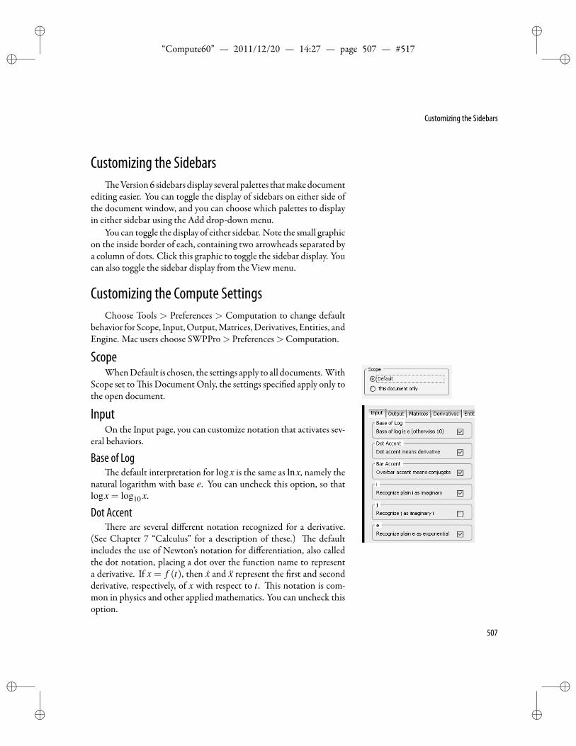
ii
“Compute60” — 2011/12/20 — 14:27 — page 507 — #517 ii
ii
ii
Customizing the Sidebars
Customizing the SidebarseVersion6 sidebars display several palettes thatmakedocument
editing easier. You can toggle the display of sidebars on either side ofthe document window, and you can choose which palettes to displayin either sidebar using the Add drop-down menu.
You can toggle the display of either sidebar. Note the small graphicon the inside border of each, containing two arrowheads separated bya column of dots. Click this graphic to toggle the sidebar display. Youcan also toggle the sidebar display from the View menu.
Customizing the Compute SettingsChoose Tools > Preferences > Computation to change default
behavior for Scope, Input,Output,Matrices,Derivatives, Entities, andEngine. Mac users choose SWPPro> Preferences>Computation.
ScopeWhenDefault is chosen, the settings apply to all documents. With
Scope set to is Document Only, the settings speci ed apply only tothe open document.
InputOn the Input page, you can customize notation that activates sev-
eral behaviors.
Base of Loge default interpretation for logx is the same as lnx, namely the
natural logarithm with base e. You can uncheck this option, so thatlogx = log10 x.
Dot Accentere are several different notation recognized for a derivative.
(See Chapter 7 “Calculus” for a description of these.) e defaultincludes the use of Newton’s notation for differentiation, also calledthe dot notation, placing a dot over the function name to representa derivative. If x = f (t), then x and x represent the rst and secondderivative, respectively, of x with respect to t . is notation is com-mon in physics and other applied mathematics. You can uncheck thisoption.
507
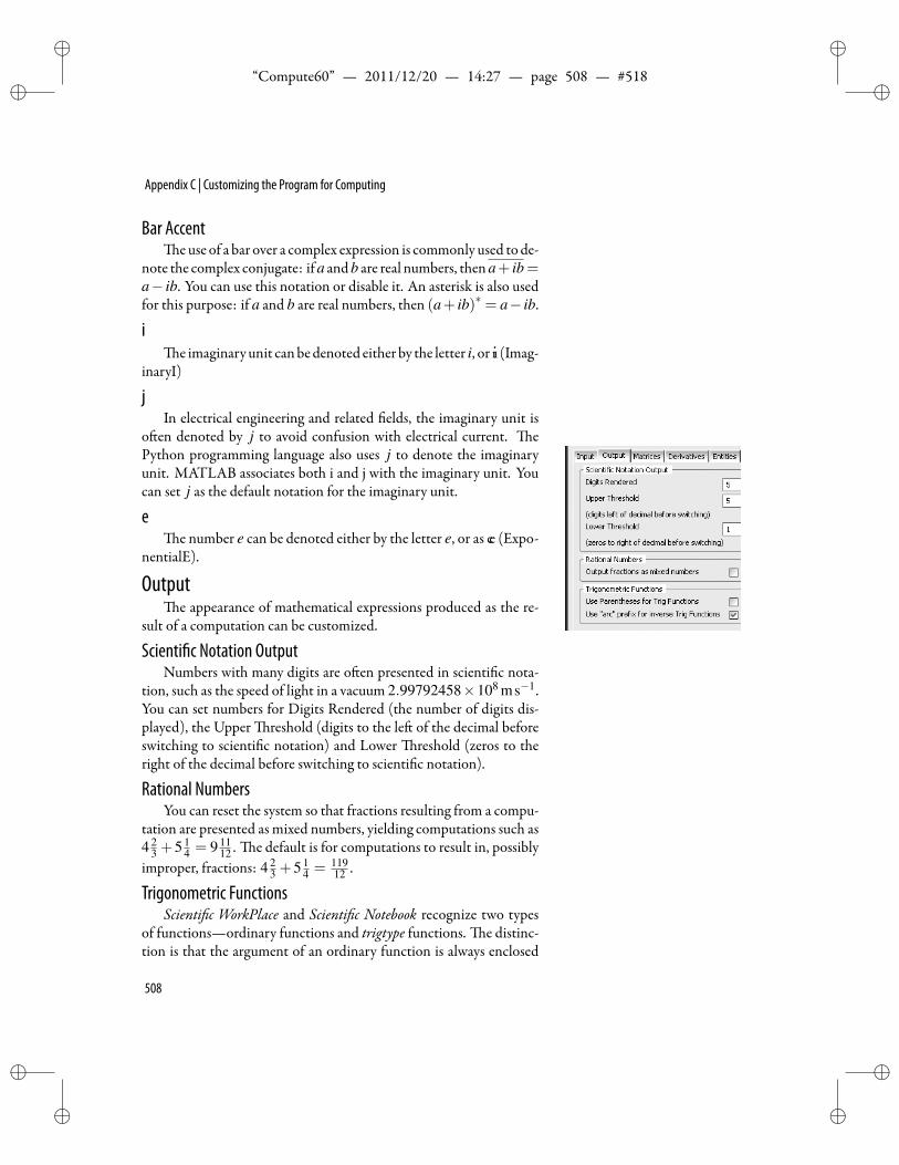
ii
“Compute60” — 2011/12/20 — 14:27 — page 508 — #518 ii
ii
ii
Appendix C | Customizing the Program for Computing
Bar Accente use of a bar over a complex expression is commonly used to de-
note the complex conjugate: ifa andb are real numbers, thena+ ib=a− ib. You can use this notation or disable it. An asterisk is also usedfor this purpose: if a and b are real numbers, then (a+ ib)∗ = a− ib.
ie imaginary unit canbedenoted either by the letter i, or .ıı (Imag-
inaryI)
jIn electrical engineering and related elds, the imaginary unit is
o en denoted by j to avoid confusion with electrical current. ePython programming language also uses j to denote the imaginaryunit. MATLAB associates both i and j with the imaginary unit. Youcan set j as the default notation for the imaginary unit.
ee number e can be denoted either by the letter e, or as ee (Expo-
nentialE).
Outpute appearance of mathematical expressions produced as the re-
sult of a computation can be customized.
Scienti c Notation OutputNumbers with many digits are o en presented in scienti c nota-
tion, such as the speed of light in a vacuum 2.99792458×10⁸ ms−1.You can set numbers for Digits Rendered (the number of digits dis-played), the Upper reshold (digits to the le of the decimal beforeswitching to scienti c notation) and Lower reshold (zeros to theright of the decimal before switching to scienti c notation).
Rational NumbersYou can reset the system so that fractions resulting from a compu-
tation are presented as mixed numbers, yielding computations such as4 2
3 +5 14 = 9 11
12 . e default is for computations to result in, possiblyimproper, fractions: 4 2
3 +5 14 = 119
12 .
Trigonometric FunctionsScienti c WorkPlace and Scienti c Notebook recognize two types
of functions—ordinary functions and trigtype functions. e distinc-tion is that the argument of an ordinary function is always enclosed
508
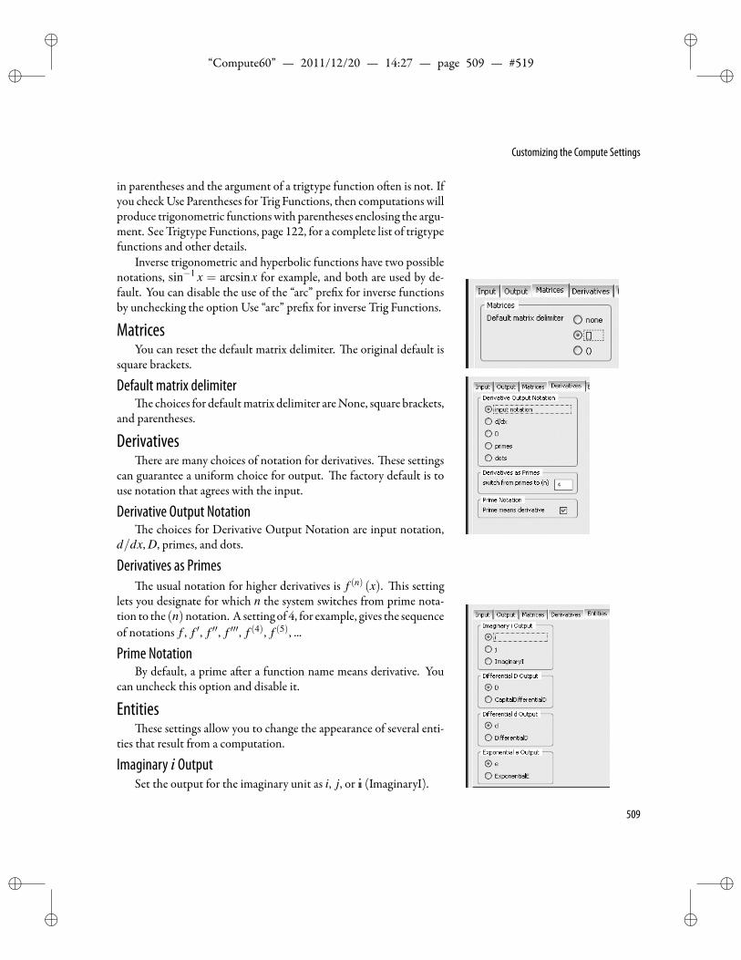
ii
“Compute60” — 2011/12/20 — 14:27 — page 509 — #519 ii
ii
ii
Customizing the Compute Settings
in parentheses and the argument of a trigtype function o en is not. Ifyou checkUse Parentheses for Trig Functions, then computations willproduce trigonometric functionswith parentheses enclosing the argu-ment. See Trigtype Functions, page 122, for a complete list of trigtypefunctions and other details.
Inverse trigonometric and hyperbolic functions have two possiblenotations, sin−1 x = arcsinx for example, and both are used by de-fault. You can disable the use of the “arc” pre x for inverse functionsby unchecking the option Use “arc” pre x for inverse Trig Functions.
MatricesYou can reset the default matrix delimiter. e original default is
square brackets.
Default matrix delimitere choices for defaultmatrix delimiter areNone, square brackets,
and parentheses.
Derivativesere are many choices of notation for derivatives. ese settings
can guarantee a uniform choice for output. e factory default is touse notation that agrees with the input.
Derivative Output Notatione choices for Derivative Output Notation are input notation,
d/dx, D, primes, and dots.
Derivatives as Primese usual notation for higher derivatives is f (n) (x). is setting
lets you designate for which n the system switches from prime nota-tion to the (n)notation. A setting of 4, for example, gives the sequenceof notations f , f ′, f ′′, f ′′′, f (4), f (5), ...
Prime NotationBy default, a prime a er a function name means derivative. You
can uncheck this option and disable it.
Entitiesese settings allow you to change the appearance of several enti-
ties that result from a computation.
Imaginary i OutputSet the output for the imaginary unit as i, j, or .ıı (ImaginaryI).
509
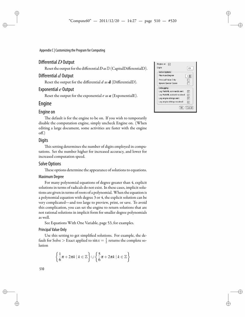
ii
“Compute60” — 2011/12/20 — 14:27 — page 510 — #520 ii
ii
ii
Appendix C | Customizing the Program for Computing
DifferentialD OutputReset theoutput for thedifferentialD asD (CapitalDifferentialD).
Differentiald OutputReset the output for the differential d as dd (DifferentialD).
Exponential e OutputReset the output for the exponential e as ee (ExponentialE).
EngineEngine on
e default is for the engine to be on. If you wish to temporarilydisable the computation engine, simply uncheck Engine on. (Whenediting a large document, some activities are faster with the engineoff.)
Digitsis setting determines the number of digits employed in compu-
tations. Set the number higher for increased accuracy, and lower forincreased computation speed.
Solve Optionsese options determine the appearance of solutions to equations.
Maximum DegreeFor many polynomial equations of degree greater than 4, explicit
solutions in terms of radicals do not exist. In these cases, implicit solu-tions are given in terms of roots of a polynomial. When the equation isa polynomial equation with degree 3 or 4, the explicit solution can bevery complicated—and too large to preview, print, or save. To avoidthis complication, you can set the engine to return solutions that arenot rational solutions in implicit form for smaller degree polynomialsas well.
See Equations With One Variable, page 53, for examples.
Principal Value OnlyUse this setting to get simpli ed solutions. For example, the de-
fault for Solve > Exact applied to sinx = 12 returns the complete so-
lution 16
π +2πk | k ∈ Z∪
56
π +2πk | k ∈ Z
510

ii
“Compute60” — 2011/12/20 — 14:27 — page 511 — #521 ii
ii
ii
Customizing the Plot Settings
With Principal Value Only checked, the solution returned is
16
π
Ignore Special CasesUse this setting to get simpli ed solutions. For example, the de-
fault for Solve> Exact applied to ex = y (variable x) returns the solu-tion
lny+2iπk | k ∈ Z if y = 0/0 if y = 0
With Ignore Special Cases checked, the solution returned is
lny+2iπk | k ∈ Z
Note thatwithboth Ignore SpecialCases andPrincipalValueOnlychecked the solution returned is simply lny.
DebuggingYou can investigate possible syntax errors in mathematics being
sent to or returned by the computing engine by creating logs of theprocess.
Customizing the Plot SettingsChoose Tools > Preferences > Plots to change the settings for
Axes, Layout, Labelling, and View.
Axese Axes Scaling options are Linear, Lin Log, Log Lin, and Log
Log. e option Lin Log uses linear scaling along the horizontal axisand logarithmic scaling along the vertical axis. Log Lin uses logarith-mic scaling along the horizontal axis and linear scaling along the ver-tical axis.
Check Equal Scaling Along Each Axis for plotting geometric ob-jects, such as circles, where youwant the scaling to be the same onbothaxes.
You can change the axis labels to other letters of names. e AxisTick Marks can be None, Low, Normal, or High. Arrow tips at thepositive ends of the axes can be turned on or off. You can turn onGridLine for 2D plots.
e Axes Type choices are Not Speci ed, Automatic, Normal,Boxed, Frame, or None.
511
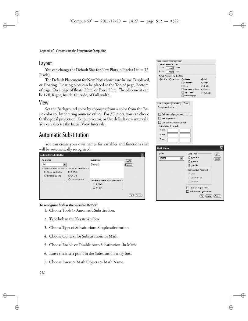
ii
“Compute60” — 2011/12/20 — 14:27 — page 512 — #522 ii
ii
ii
Appendix C | Customizing the Program for Computing
LayoutYou can change theDefault Size forNewPlots in Pixels (1in= 75
Pixels).eDefaultPlacement forNewPlots choices are In line,Displayed,
or Floating. Floating plots can be placed at the Top of page, Bottomof page, On a page of oats, Here, or Force Here. e placement canbe Le , Right, Inside, Outside, of Full width.
ViewSet the Background color by choosing from a color from the Ba-
sic colors or by entering numeric values. For 3D plots, you can checkOrthogonal projection, Keep up vector, or Use default view intervals.You can also set the Initial View Intervals.
Automatic SubstitutionYou can create your own names for variables and functions that
will be automatically recognized.
To recognizebob as the variableRobert1. Choose Tools>Automatic Substitution.
2. Type bob in the Keystrokes box
3. Choose Type of Substitution: Simple substitution.
4. Choose Context for Substitution: In Math.
5. Choose Enable or Disable Auto Substitution: In Math.
6. Leave the insert point in the Substitution entry box.
7. Choose Insert>Math Objects>Math Name.
512
ii
“Compute60” — 2011/12/20 — 14:27 — page 513 — #523 ii
ii
ii
Automatic Substitution
8. Type Robert in the Name box.
9. Choose Name Type: Variable.
10. Check is is an engine string.
11. Check Add automatic substitution.
12. Choose Apply. ( e name ‘Robert’ should appear in the Sub-stitution Box in the Automatic Substitution box.)
13. In the Automatic Substitution dialog, choose Save.
Compute> De nitions> New De nition(In mathematics, type bob.)Robert = 17
Compute> EvaluateRobert2 = 289
For additional examples and information about automatic substi-tution, see Automatic Substitution, page 102, choose Help> Search,or consult the manual Creating Documents with Scienti c WorkPlaceand Scienti c Word.
513

ii
“Compute60” — 2011/12/20 — 14:27 — page 514 — #524 ii
ii
ii
ii
“Compute60” — 2011/12/20 — 14:27 — page 515 — #525 ii
ii
ii
DMuPAD Functionsand Expressions
There is nothing so troublesome to mathematical practice ... than multiplications, divisions, square and cubical extractionsof great numbers ... I began therefore to consider ... how I might remove those hindrances. John Napier (1550–1617)
Constants
Compute Menu Items
Functions and Expressions
C onstants and functions are available either as items on theCompute menu or through evaluating mathematical expres-sions. ere are alsomany built-in functions and expressions.
MuPAD equivalents are given for all of these and, where needed, abrief description of the constant, function, or expression.
e two menu items Compute > De nitions > De ne MuPADName and Compute > Passthru to Engine offer additional ways totake advantage of the computational capabilities of MuPAD. is ap-pendix concludes with a brief discussion of each of these items.
ConstantsCommon constants can be expressed in ordinary mathematical
notation. See page 507 in Appendix C “Customizing the Programfor Computing” for some choices for the appearance of some of theconstants.
If a name such as gamma does not automatically gray when typedin mathematics, then choose Insert > Math Objects > Math Nameand select or type the name.
515
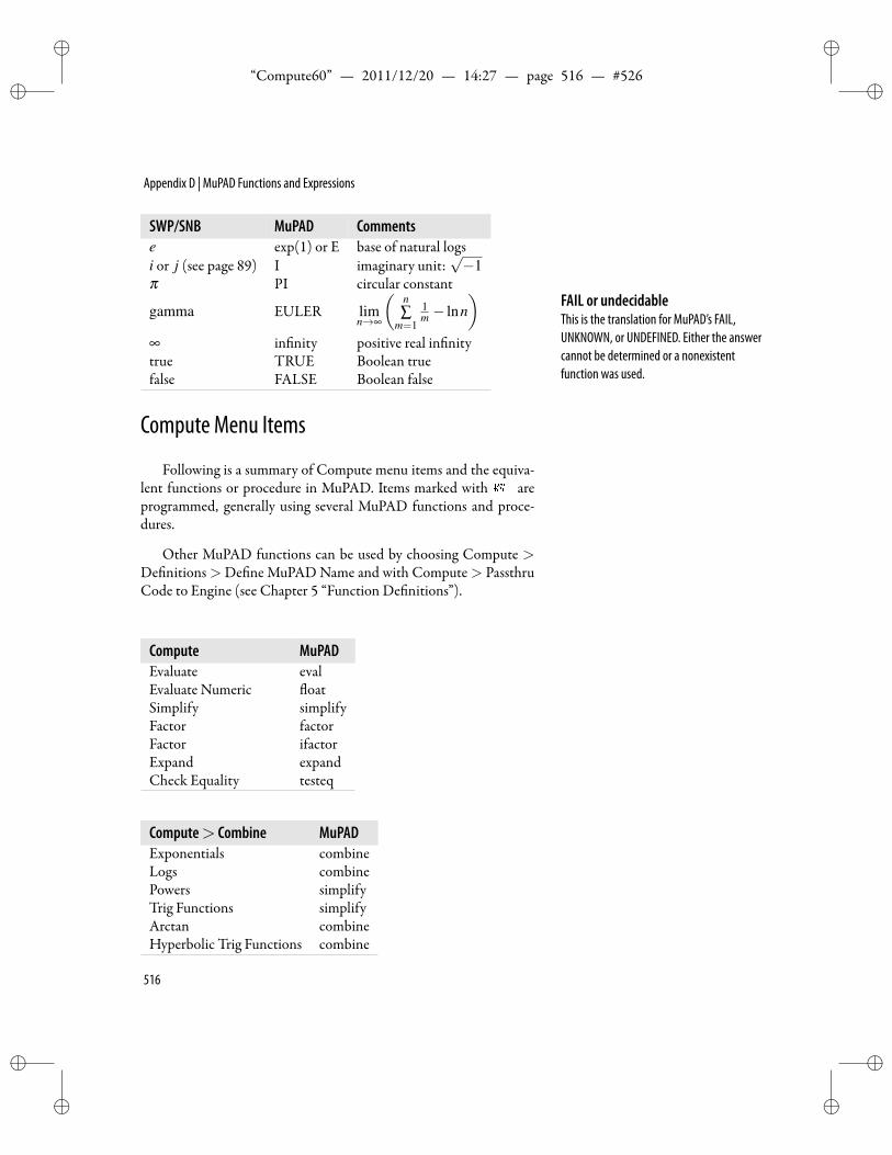
ii
“Compute60” — 2011/12/20 — 14:27 — page 516 — #526 ii
ii
ii
Appendix D | MuPAD Functions and Expressions
SWP/SNB MuPAD Commentse exp(1) or E base of natural logsi or j (see page 89) I imaginary unit:
√−1
π PI circular constant
gamma EULER limn→∞
(n∑
m=1
1m − lnn
)∞ in nity positive real in nitytrue TRUE Boolean truefalse FALSE Boolean false
FAIL or undecidableThis is the translation for MuPAD’s FAIL,UNKNOWN, or UNDEFINED. Either the answercannot be determined or a nonexistentfunction was used.
Compute Menu Items
Following is a summary of Compute menu items and the equiva-lent functions or procedure in MuPAD. Items marked with areprogrammed, generally using several MuPAD functions and proce-dures.
Other MuPAD functions can be used by choosing Compute >De nitions>De ne MuPAD Name and with Compute> PassthruCode to Engine (see Chapter 5 “Function De nitions”).
Compute MuPADEvaluate evalEvaluate Numeric oatSimplify simplifyFactor factorFactor ifactorExpand expandCheck Equality testeq
Compute> Combine MuPADExponentials combineLogs combinePowers simplifyTrig Functions simplifyArctan combineHyperbolic Trig Functions combine
516
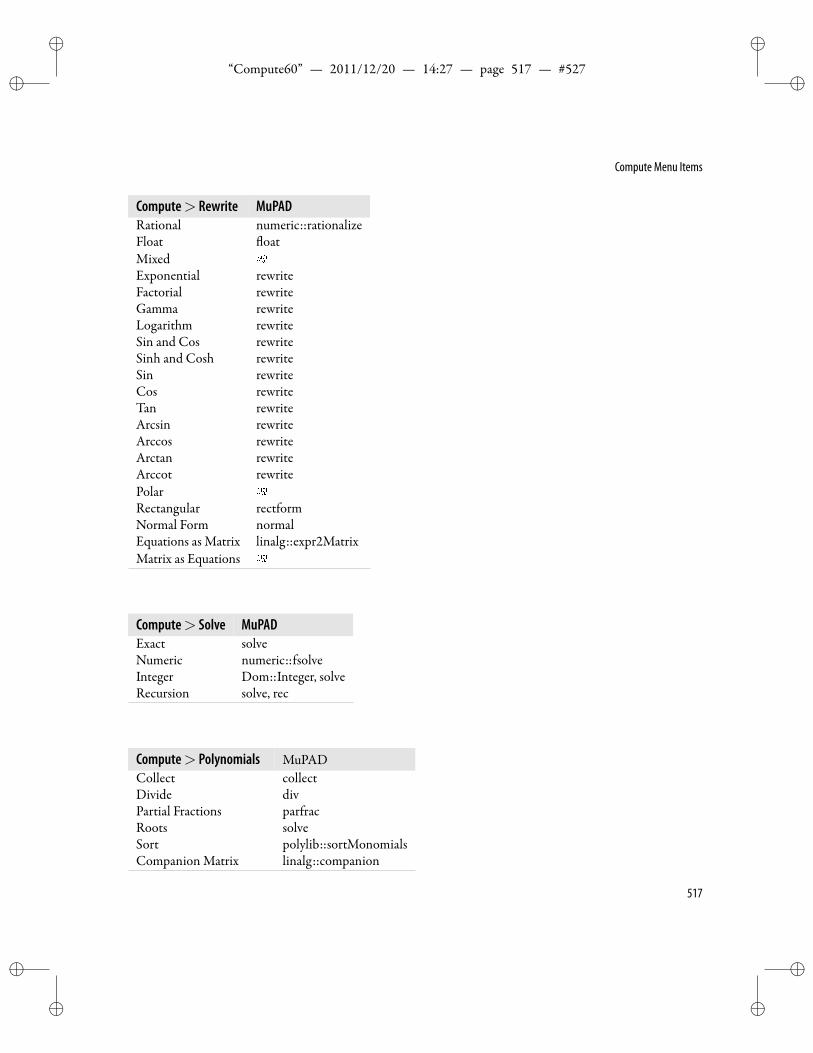
ii
“Compute60” — 2011/12/20 — 14:27 — page 517 — #527 ii
ii
ii
Compute Menu Items
Compute> Rewrite MuPADRational numeric::rationalizeFloat oatMixedExponential rewriteFactorial rewriteGamma rewriteLogarithm rewriteSin and Cos rewriteSinh and Cosh rewriteSin rewriteCos rewriteTan rewriteArcsin rewriteArccos rewriteArctan rewriteArccot rewritePolarRectangular rectformNormal Form normalEquations as Matrix linalg::expr2MatrixMatrix as Equations
Compute> Solve MuPADExact solveNumeric numeric::fsolveInteger Dom::Integer, solveRecursion solve, rec
Compute> Polynomials MuPADCollect collectDivide divPartial Fractions parfracRoots solveSort polylib::sortMonomialsCompanion Matrix linalg::companion
517
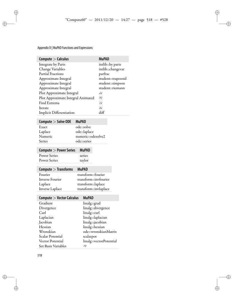
ii
“Compute60” — 2011/12/20 — 14:27 — page 518 — #528 ii
ii
ii
Appendix D | MuPAD Functions and Expressions
Compute> Calculus MuPADIntegrate by Parts intlib::by partsChange Variables intlib::changevarPartial Fractions parfracApproximate Integral student::trapezoidApproximate Integral student::simpsonApproximate Integral student::riemannPlot Approximate IntegralPlot Approximate Integral AnimatedFind ExtremaIterateImplicit Differentiation diff
Compute> Solve ODE MuPADExact ode::solveLaplace ode::laplaceNumeric numeric::odesolve2Series ode::series
Compute> Power Series MuPADPower Series seriesPower Series taylor
Compute> Transforms MuPADFourier transform::fourierInverse Fourier transform::invfourierLaplace transform::laplaceInverse Laplace transform::invlaplace
Compute> Vector Calculus MuPADGradient linalg::gradDivergence linalg::divergenceCurl linalg::curlLaplacian linalg::laplacianJacobian linalg::jacobianHessian linalg::hessianWronskian ode::wronskianMatrixScalar Potential scalarpotVector Potential linalg::vectorPotentialSet Basis Variables
518
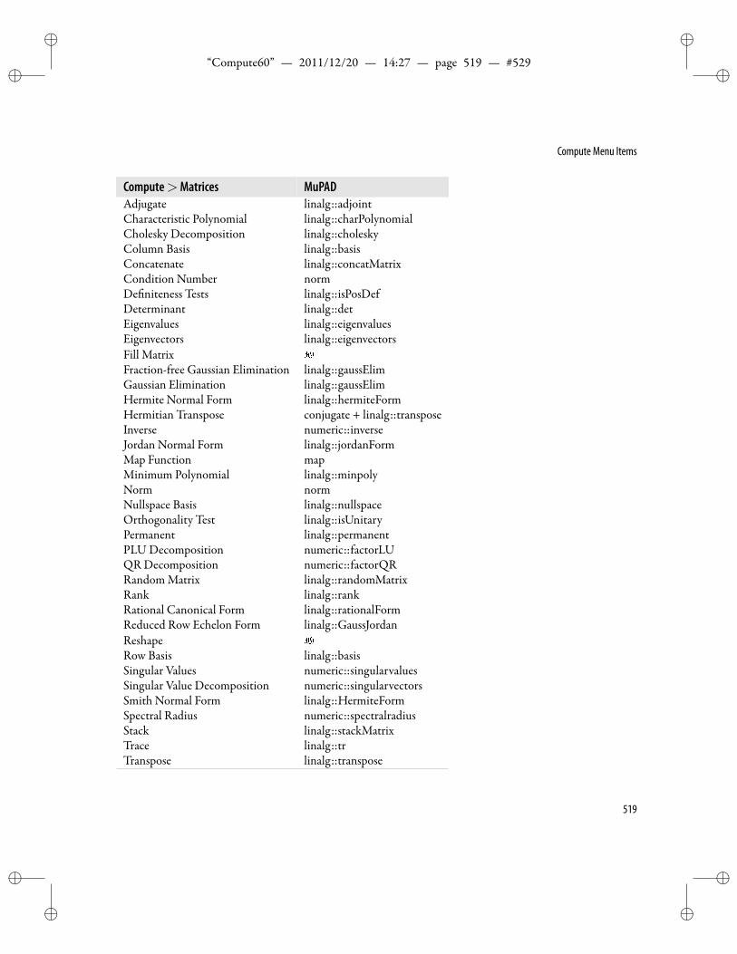
ii
“Compute60” — 2011/12/20 — 14:27 — page 519 — #529 ii
ii
ii
Compute Menu Items
Compute>Matrices MuPADAdjugate linalg::adjointCharacteristic Polynomial linalg::charPolynomialCholesky Decomposition linalg::choleskyColumn Basis linalg::basisConcatenate linalg::concatMatrixCondition Number normDe niteness Tests linalg::isPosDefDeterminant linalg::detEigenvalues linalg::eigenvaluesEigenvectors linalg::eigenvectorsFill MatrixFraction-free Gaussian Elimination linalg::gaussElimGaussian Elimination linalg::gaussElimHermite Normal Form linalg::hermiteFormHermitian Transpose conjugate + linalg::transposeInverse numeric::inverseJordan Normal Form linalg::jordanFormMap Function mapMinimum Polynomial linalg::minpolyNorm normNullspace Basis linalg::nullspaceOrthogonality Test linalg::isUnitaryPermanent linalg::permanentPLU Decomposition numeric::factorLUQR Decomposition numeric::factorQRRandom Matrix linalg::randomMatrixRank linalg::rankRational Canonical Form linalg::rationalFormReduced Row Echelon Form linalg::GaussJordanReshapeRow Basis linalg::basisSingular Values numeric::singularvaluesSingular Value Decomposition numeric::singularvectorsSmith Normal Form linalg::HermiteFormSpectral Radius numeric::spectralradiusStack linalg::stackMatrixTrace linalg::trTranspose linalg::transpose
519
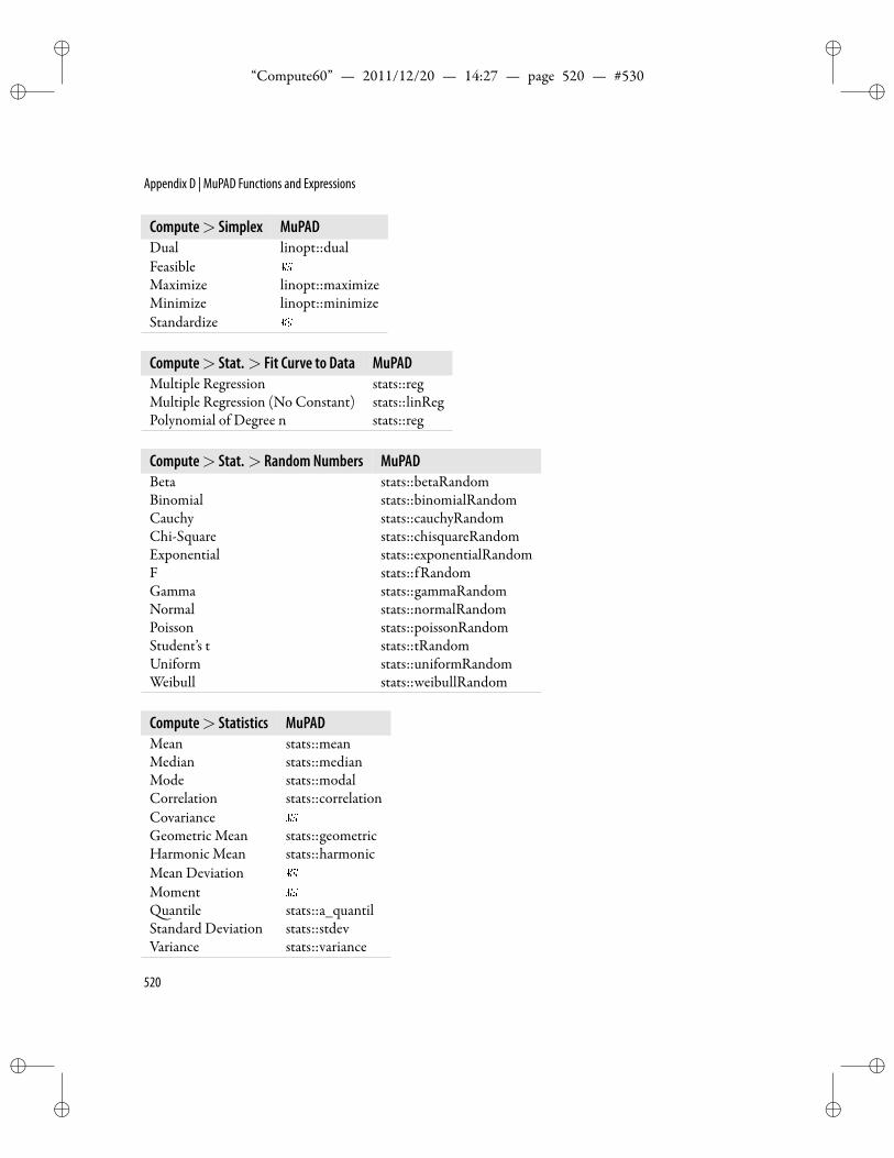
ii
“Compute60” — 2011/12/20 — 14:27 — page 520 — #530 ii
ii
ii
Appendix D | MuPAD Functions and Expressions
Compute> Simplex MuPADDual linopt::dualFeasibleMaximize linopt::maximizeMinimize linopt::minimizeStandardize
Compute> Stat.> Fit Curve to Data MuPADMultiple Regression stats::regMultiple Regression (No Constant) stats::linRegPolynomial of Degree n stats::reg
Compute> Stat.> Random Numbers MuPADBeta stats::betaRandomBinomial stats::binomialRandomCauchy stats::cauchyRandomChi-Square stats::chisquareRandomExponential stats::exponentialRandomF stats::fRandomGamma stats::gammaRandomNormal stats::normalRandomPoisson stats::poissonRandomStudent’s t stats::tRandomUniform stats::uniformRandomWeibull stats::weibullRandom
Compute> Statistics MuPADMean stats::meanMedian stats::medianMode stats::modalCorrelation stats::correlationCovarianceGeometric Mean stats::geometricHarmonic Mean stats::harmonicMean DeviationMoment
uantile stats::a_quantilStandard Deviation stats::stdevVariance stats::variance
520
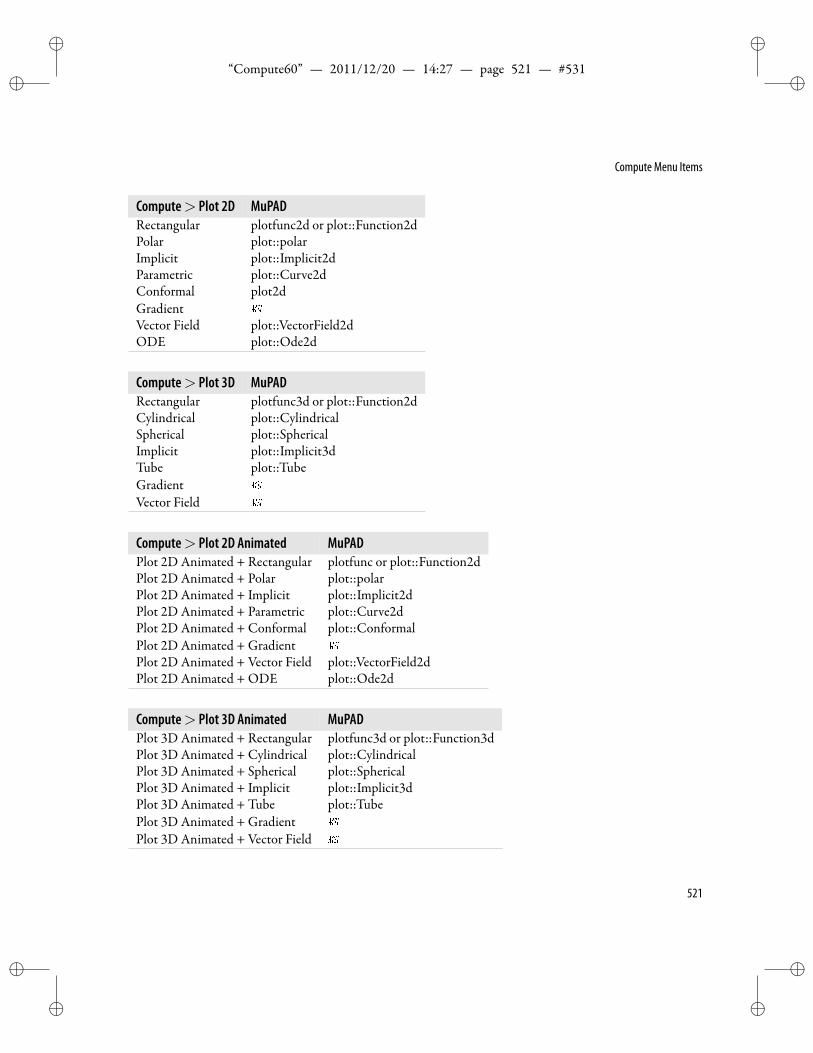
ii
“Compute60” — 2011/12/20 — 14:27 — page 521 — #531 ii
ii
ii
Compute Menu Items
Compute> Plot 2D MuPADRectangular plotfunc2d or plot::Function2dPolar plot::polarImplicit plot::Implicit2dParametric plot::Curve2dConformal plot2dGradientVector Field plot::VectorField2dODE plot::Ode2d
Compute> Plot 3D MuPADRectangular plotfunc3d or plot::Function2dCylindrical plot::CylindricalSpherical plot::SphericalImplicit plot::Implicit3dTube plot::TubeGradientVector Field
Compute> Plot 2D Animated MuPADPlot 2D Animated + Rectangular plotfunc or plot::Function2dPlot 2D Animated + Polar plot::polarPlot 2D Animated + Implicit plot::Implicit2dPlot 2D Animated + Parametric plot::Curve2dPlot 2D Animated + Conformal plot::ConformalPlot 2D Animated + GradientPlot 2D Animated + Vector Field plot::VectorField2dPlot 2D Animated + ODE plot::Ode2d
Compute> Plot 3D Animated MuPADPlot 3D Animated + Rectangular plotfunc3d or plot::Function3dPlot 3D Animated + Cylindrical plot::CylindricalPlot 3D Animated + Spherical plot::SphericalPlot 3D Animated + Implicit plot::Implicit3dPlot 3D Animated + Tube plot::TubePlot 3D Animated + GradientPlot 3D Animated + Vector Field
521
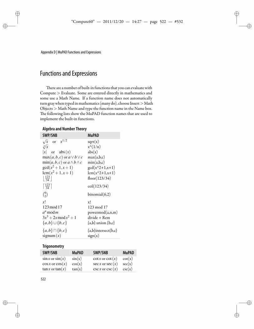
ii
“Compute60” — 2011/12/20 — 14:27 — page 522 — #532 ii
ii
ii
Appendix D | MuPAD Functions and Expressions
Functions and Expressions
ere are a number of built-in functions that you can evaluatewithCompute > Evaluate. Some are entered directly in mathematics andsome use a Math Name. If a function name does not automaticallyturn graywhen typed inmathematics (manydo), choose Insert>MathObjects>Math Name and type the function name in the Name box.
e following lists show the MuPAD function names that are used toimplement the built-in functions.
Algebra and Number TheorySWP/SNB MuPAD√
x or x1/2 sqrt(x)n√
x x^(1/n)|x| or abs(x) abs(x)max(a,b,c) or a∨b∨ c max(a,b,c)min(a,b,c) or a∧b∧ c min(a,b,c)gcd(x2 +1,x+1) gcd(x^2+1,x+1)lcm(x2 +1,x+1) lcm(x^2+1,x+1)⌊ 123
34
⌋oor(123/34)⌈ 123
34
⌉ceil(123/34)(6
2
)binomial(6,2)
x! x!123mod17 123 mod 17an modm powermod(a,n,m)3x3 +2xmodx2 +1 divide + Rema,b∪b,c a,b union b,c
a,b∩b,c a,bintersectb,csignum(x) sign(x)
TrigonometrySWP/SNB MuPAD SWP/SNB MuPADsinx or sin(x) sin(x) cotx or cot(x) cot(x)cosx or cos(x) cos(x) secx or sec(x) sec(x)tanx or tan(x) tan(x) cscx or csc(x) csc(x)
522
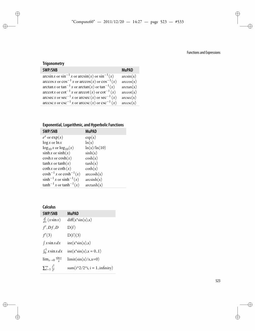
ii
“Compute60” — 2011/12/20 — 14:27 — page 523 — #533 ii
ii
ii
Functions and Expressions
TrigonometrySWP/SNB MuPADarcsinx or sin−1 x or arcsin(x) or sin−1(x) arcsin(x)arccosx or cos−1 x or arccos(x) or cos−1(x) arccos(x)arctanx or tan−1 x or arctan(x) or tan−1(x) arctan(x)arccotx or cot−1 x or arccot(x) or cot−1 (x) arccot(x)arcsecx or sec−1 x or arcsec(x) or sec−1 (x) arcsec(x)arccscx or csc−1 x or arccsc(x) or csc−1 (x) arccsc(x)
Exponential, Logarithmic, and Hyperbolic FunctionsSWP/SNB MuPADex or exp(x) exp(x)logx or lnx ln(x)log10 x or log10(x) ln(x)/ln(10)sinhx or sinh(x) sinh(x)coshx or cosh(x) cosh(x)tanhx or tanh(x) tanh(x)cothx or coth(x) coth(x)cosh−1 x or cosh−1(x) arccosh(x)sinh−1 x or sinh−1(x) arcsinh(x)tanh−1 x or tanh−1(x) arctanh(x)
CalculusSWP/SNB MuPADddx (xsinx) diff(x*sin(x),x)
f ′,D f ,D D(f )
f ′(3) D(f )(3)∫xsinxdx int(x*sin(x),x)∫ 1
0 xsinxdx int(x*sin(x),x = 0..1)
limx→0sinx
x limit(sin(x)/x,x=0)
∑∞i=1
i22i sum(i^2/2^i, i = 1..in nity)
523
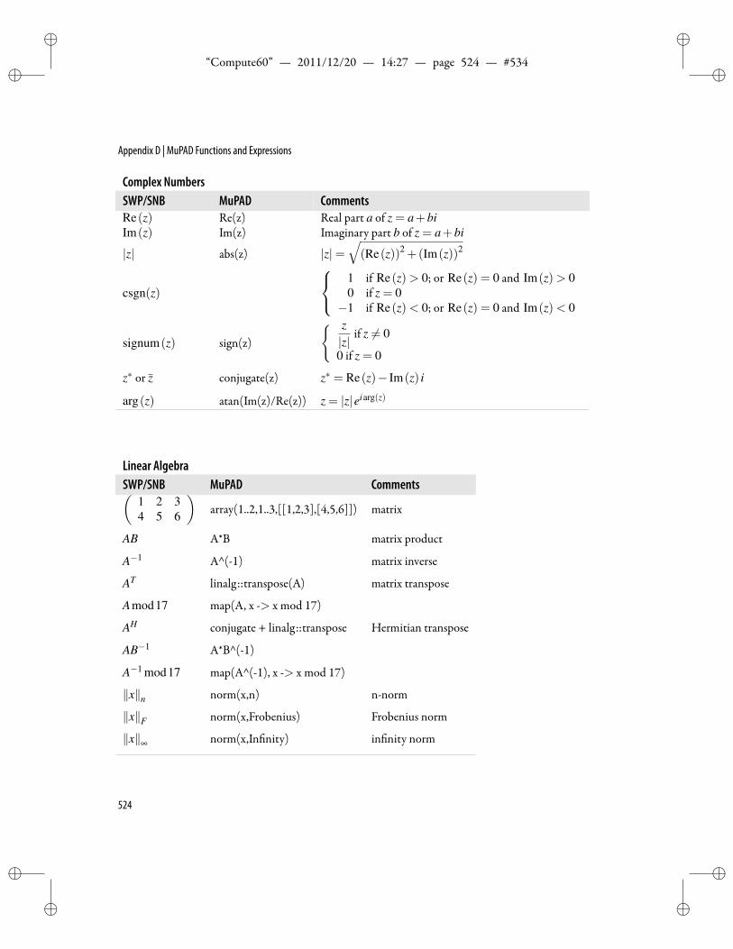
ii
“Compute60” — 2011/12/20 — 14:27 — page 524 — #534 ii
ii
ii
Appendix D | MuPAD Functions and Expressions
Complex NumbersSWP/SNB MuPAD CommentsRe(z) Re(z) Real part a of z = a+biIm(z) Im(z) Imaginary part b of z = a+bi
|z| abs(z) |z|=√(Re(z))2 +(Im(z))2
csgn(z)
1 if Re(z)> 0; or Re(z) = 0 and Im(z)> 00 if z = 0−1 if Re(z)< 0; or Re(z) = 0 and Im(z)< 0
signum(z) sign(z)
z|z|
if z = 0
0 if z = 0
z∗ or z conjugate(z) z∗ = Re(z)− Im(z) i
arg(z) atan(Im(z)/Re(z)) z = |z|eiarg(z)
Linear AlgebraSWP/SNB MuPAD Comments(
1 2 34 5 6
)array(1..2,1..3,[[1,2,3],[4,5,6]]) matrix
AB A*B matrix product
A−1 A^(-1) matrix inverse
AT linalg::transpose(A) matrix transpose
Amod17 map(A, x -> x mod 17)
AH conjugate + linalg::transpose Hermitian transpose
AB−1 A*B^(-1)
A−1 mod17 map(A^(-1), x -> x mod 17)
∥x∥n norm(x,n) n-norm
∥x∥F norm(x,Frobenius) Frobenius norm
∥x∥∞ norm(x,In nity) in nity norm
524
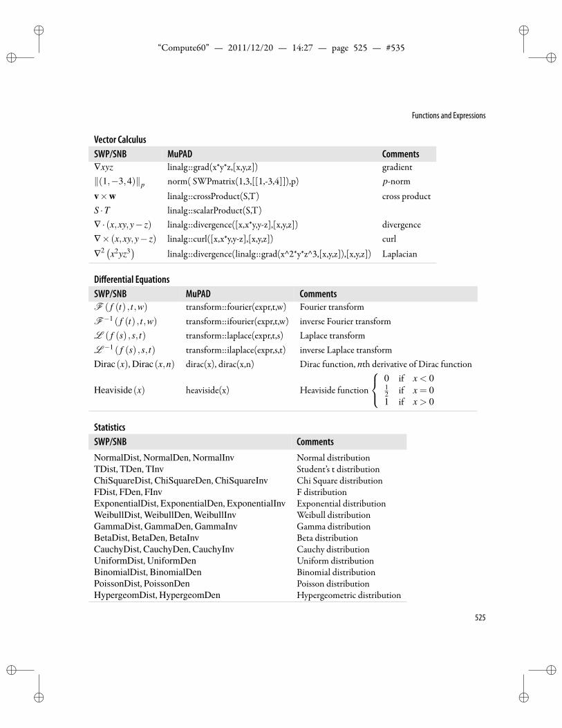
ii
“Compute60” — 2011/12/20 — 14:27 — page 525 — #535 ii
ii
ii
Functions and Expressions
Vector CalculusSWP/SNB MuPAD Comments∇xyz linalg::grad(x*y*z,[x,y,z]) gradient∥(1,−3,4)∥p norm( SWPmatrix(1,3,[[1,-3,4]]),p) p-normv×w linalg::crossProduct(S,T) cross productS ·T linalg::scalarProduct(S,T)∇ · (x,xy,y− z) linalg::divergence([x,x*y,y-z],[x,y,z]) divergence∇× (x,xy,y− z) linalg::curl([x,x*y,y-z],[x,y,z]) curl
∇2 (x2yz3)
linalg::divergence(linalg::grad(x^2*y*z^3,[x,y,z]),[x,y,z]) Laplacian
Differential EquationsSWP/SNB MuPAD CommentsF ( f (t) , t,w) transform::fourier(expr,t,w) Fourier transformF−1 ( f (t) , t,w) transform::ifourier(expr,t,w) inverse Fourier transformL ( f (s) ,s, t) transform::laplace(expr,t,s) Laplace transformL −1 ( f (s) ,s, t) transform::ilaplace(expr,s,t) inverse Laplace transformDirac(x), Dirac(x,n) dirac(x), dirac(x,n) Dirac function, nth derivative of Dirac function
Heaviside(x) heaviside(x) Heaviside function
0 if x < 012 if x = 01 if x > 0
StatisticsSWP/SNB CommentsNormalDist, NormalDen, NormalInv Normal distributionTDist, TDen, TInv Student’s t distributionChiSquareDist, ChiSquareDen, ChiSquareInv Chi Square distributionFDist, FDen, FInv F distributionExponentialDist, ExponentialDen, ExponentialInv Exponential distributionWeibullDist, WeibullDen, WeibullInv Weibull distributionGammaDist, GammaDen, GammaInv Gamma distributionBetaDist, BetaDen, BetaInv Beta distributionCauchyDist, CauchyDen, CauchyInv Cauchy distributionUniformDist, UniformDen Uniform distributionBinomialDist, BinomialDen Binomial distributionPoissonDist, PoissonDen Poisson distributionHypergeomDist, HypergeomDen Hypergeometric distribution
525
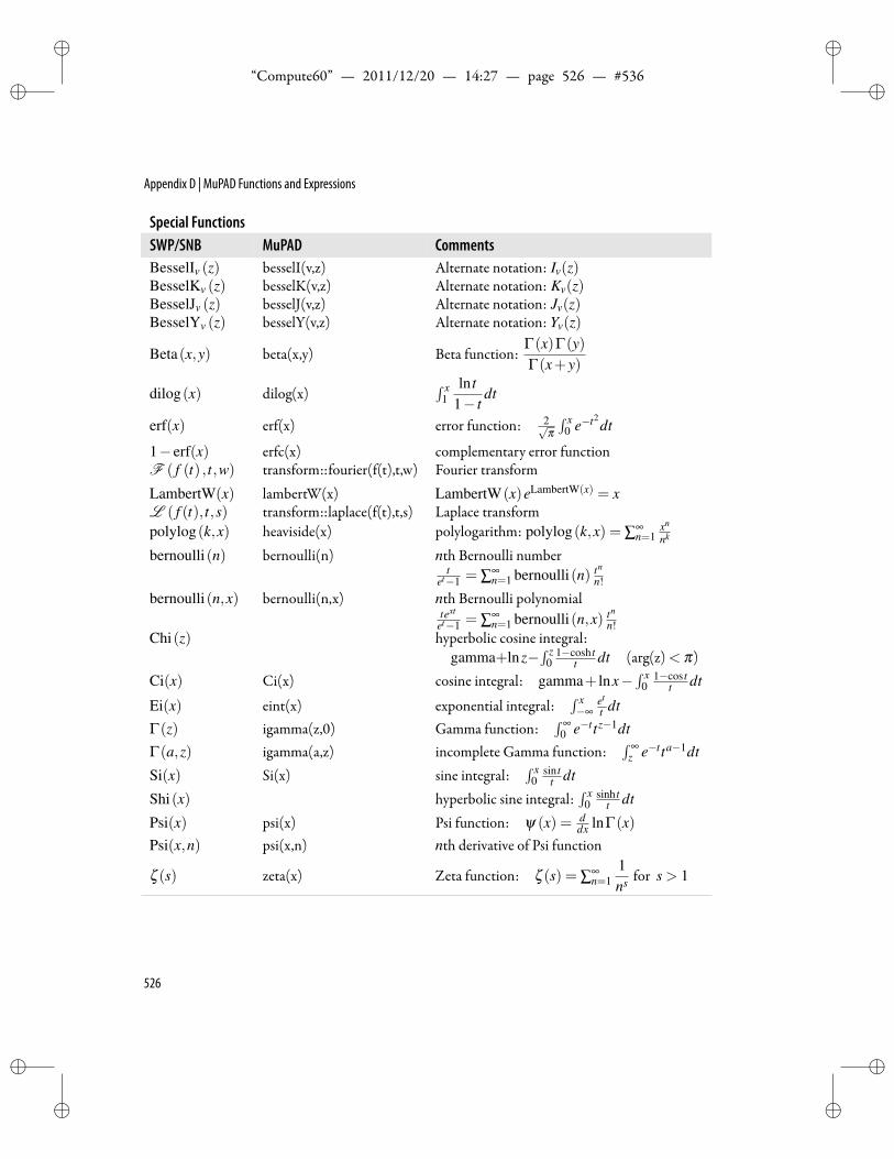
ii
“Compute60” — 2011/12/20 — 14:27 — page 526 — #536 ii
ii
ii
Appendix D | MuPAD Functions and Expressions
Special FunctionsSWP/SNB MuPAD CommentsBesselIv (z) besselI(v,z) Alternate notation: Iv(z)BesselKv (z) besselK(v,z) Alternate notation: Kv(z)BesselJv (z) besselJ(v,z) Alternate notation: Jv(z)BesselYv (z) besselY(v,z) Alternate notation: Yv(z)
Beta(x,y) beta(x,y) Beta function:Γ(x)Γ(y)Γ(x+ y)
dilog(x) dilog(x)∫ x
1ln t
1− tdt
erf(x) erf(x) error function: 2√π∫ x
0 e−t2dt
1− erf(x) erfc(x) complementary error functionF ( f (t) , t,w) transform::fourier(f(t),t,w) Fourier transformLambertW(x) lambertW(x) LambertW(x)eLambertW(x) = xL ( f (t), t,s) transform::laplace(f(t),t,s) Laplace transformpolylog(k,x) heaviside(x) polylogarithm: polylog(k,x) = ∑∞
n=1xn
nk
bernoulli(n) bernoulli(n) nth Bernoulli numbert
et−1 = ∑∞n=1 bernoulli(n) tn
n!
bernoulli(n,x) bernoulli(n,x) nth Bernoulli polynomialtext
et−1 = ∑∞n=1 bernoulli(n,x) tn
n!Chi(z) hyperbolic cosine integral:
gamma+lnz−∫ z
01−cosh t
t dt (arg(z)< π)Ci(x) Ci(x) cosine integral: gamma+ lnx−
∫ x0
1−cos tt dt
Ei(x) eint(x) exponential integral:∫ x−∞
et
t dt
Γ(z) igamma(z,0) Gamma function:∫ ∞
0 e−ttz−1dt
Γ(a,z) igamma(a,z) incomplete Gamma function:∫ ∞
z e−tta−1dt
Si(x) Si(x) sine integral:∫ x
0sin t
t dt
Shi(x) hyperbolic sine integral:∫ x
0sinh t
t dt
Psi(x) psi(x) Psi function: ψ (x) = ddx lnΓ(x)
Psi(x,n) psi(x,n) nth derivative of Psi function
ζ (s) zeta(x) Zeta function: ζ (s) = ∑∞n=1
1ns for s > 1
526
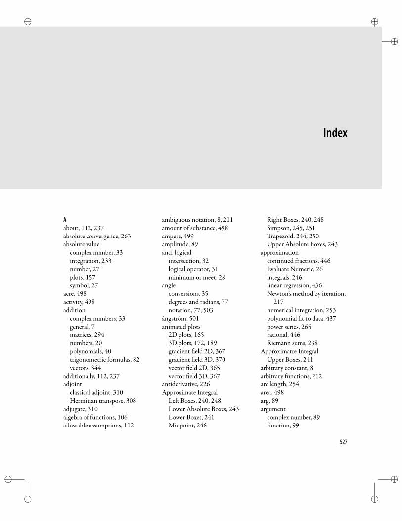
ii
“Compute60” — 2011/12/20 — 14:27 — page 527 — #537 ii
ii
ii
Index
Aabout, 112, 237absolute convergence, 263absolute value
complex number, 33integration, 233number, 27plots, 157symbol, 27
acre, 498activity, 498addition
complex numbers, 33general, 7matrices, 294numbers, 20polynomials, 40trigonometric formulas, 82vectors, 344
additionally, 112, 237adjoint
classical adjoint, 310Hermitian transpose, 308
adjugate, 310algebra of functions, 106allowable assumptions, 112
ambiguous notation, 8, 211amount of substance, 498ampere, 499amplitude, 89and, logical
intersection, 32logical operator, 31minimum or meet, 28
angleconversions, 35degrees and radians, 77notation, 77, 503
ångström, 501animated plots
2D plots, 1653D plots, 172, 189gradient eld 2D, 367gradient eld 3D, 370vector eld 2D, 365vector eld 3D, 367
antiderivative, 226Approximate Integral
Le Boxes, 240, 248Lower Absolute Boxes, 243Lower Boxes, 241Midpoint, 246
Right Boxes, 240, 248Simpson, 245, 251Trapezoid, 244, 250Upper Absolute Boxes, 243
approximationcontinued fractions, 446Evaluate Numeric, 26integrals, 246linear regression, 436Newton’s method by iteration,
217numerical integration, 253polynomial t to data, 437power series, 265rational, 446Riemann sums, 238
Approximatre IntegralUpper Boxes, 241
arbitrary constant, 8arbitrary functions, 212arc length, 254area, 498arg, 89argument
complex number, 89function, 99
527
ii
“Compute60” — 2011/12/20 — 14:27 — page 528 — #538 ii
ii
ii
Index
ordinary and trigtypefunctions, 123
arithmetic mean, 411arithmetic-geometric mean, 278arrows, 10assigning values to variables, 47,
59assignment
deferred evaluation, 104de ning variables, 103full evaluation, 105
assumeassumptions about variables,
111calculus example, 237real, 49
asymptotes, 141atmosphere, 503automatic selection, 12automatic substitution, 102, 512average, 411Axes Scaling, 511Axes Type
2D plots, 144, 146axis scaling, 143
Bband matrix, 289bar, 503bar chart, 162base of log, 67, 507basic guidelines, 7basis
column space, 323nullspaces, 323orthonormal, 325rank of matrix, 326row space, 321variables, 359
BCH code, 463
becquerel, 498Bernoulli
number, 526polynomial, 526
Bessel functions, 392, 405beta
distribution, 430function, 526
binaryoperations, 10relations, 10, 12representation, 461
binomialcoefficients, 22, 432distribution, 432Rewrite Factorial, 23
block cipher, 455blood ow problem, 278brackets
built-in delimiters, 286choosing and entering, 5expanding, 6
British thermal unit, 500
CCalculus, see calculus
Approximate Integral, 246Change Variable, 229Change Variables, 234Find Extrema, 220, 270Implicit Differentiation, 111,
213Integrate by Parts, 228, 234Iterate, 216Partial Fractions, 230, 234Plot Approx. Integral, 238
calculus, seeCalculusde nite integral, 231derivative, 209evaluate expression, 201
inde nite integral, 226limit, 202Newton’s method, 217plotting derivatives, 212
calorie, 500candela, 502carrier waves, 163case function, 62, 108Cauchy distribution, 431Cayley-Hamilton theorem, 317ceiling function, 29celsius, 504center
graphics, 6mathematics, 6text, 6
chain rule, 213Change from i to j, 508Change Variable, 229characteristic
matrix, 328polynomial, 317value, 318vector, 318
Check Equality, 30chi-square distribution, 426Chinese remainder theorem, 452Cholesky Decomposition, 336circle center and radius, 74Clear De nitions, 115code word, 463coefficient of correlation, 420cofactor, 310Collect, 44column
matrix, 290select, 15space, 323
CombineArctan, 84
528
ii
“Compute60” — 2011/12/20 — 14:27 — page 529 — #539 ii
ii
ii
Index
Exponentials, 65Hyperbolic Trig Functions, 87Logs, 67Powers, 65Trig Functions, 83
companion matrix, 329completing a square, 71complex conjugate, 33, 346, 508complex numbers
absolute value, 33argument, 89assume, 112basic operations, 32complex conjugate, 33complex powers and roots, 91form, 89imaginary unit i or j, 32polar form, 90real and imaginary part, 33rectangular form, 33, 90trigonometric form, 90
complex or real default, 49components, 341composition of functions, 106compound units, 35Compute menu, 516computing, 7computing in place, 16Concatenate, 208, 292concave upward, 225Condition Number, 315conformal plot, 379congruence
inverse modulo m, 450matrix modulo m, 454modulo m, 448modulo polynomial, 456polynomials modulo
polynomials, 456solving linear congruences,
451conjugate, 33conjugate transpose, 308constant of integration, 226constants
generic constants, 111MuPAD constants, 515π, i,e, 8
constrained optimaFind Extrema, 270Lagrange multipliers, 271
constraints, 463conventions, 2correlation, 420cosecant, 76cosine, 75cotangent, 76coulomb, 499covariance, 418cross product, 347cubic meter, 504cumulative distribution function,
421curie, 498curl, 361current, 499cursor, 4curve tting, 436, 437curve sketching, 222curves in space
polygonal paths, 181rectangular plot, 178tube plots, 179
custom name, 100custom settings
Change from i to j, 32imaginary unit, 32input, 507scope, 507sidebars, 507
toolbars, 506customer support, ixcustomizing computation
settings, see Settingscylindrical coordinates, 184
Ddata
2D plots, 1593D plots, 181convert list to matrix, 293, 410tting curves to data, 436
random numbers, 435reshape lists and matrices, 293
day, 504decimal notation, 23deferred evaluation, 104De ne MuPAD Name, 446de ned function
2D plots, 1533D plots, 174valid names, 100
de nite integralmidpoint rule, 246notation, 232Simpson’s rule, 245, 251trapezoid rule, 244, 250using the de nition, 237
De niteness Tests, 320de nition, see assignment
deferred evaluation, 104de ning a variable, 59full evaluation, 105function of one variable, 106function of several variables,
111generic constant, 111generic function, 110, 212making a de nition, 59remove a de nition, 115
529
ii
“Compute60” — 2011/12/20 — 14:27 — page 530 — #540 ii
ii
ii
Index
subscripted function, 107valid names, 100
De nitions, see de nitionClear De nitions, 115De ne MuPAD Name, 119New De nition, 59, 103, 106,
107Show De nitions, 115Unde ne, 115
degreesdegrees and radians, 77keyboard shortcut, 503notation and behavior, 77plot trig functions, 152unit names, 504
delimiters, 11DeMoivre’s theorem, 91derivative
2D plot, 212de nition, 209directional, 363implicit, 213notation, 202, 209, 507, 509piecewise-de ned functions,
211Descartes, folium, 196determinant, 309difference of sets, 32differential, 274differential equations
Bessel functions, 392, 405direction eld, 364exact method, 386graphical solutions, 401initial-value problems, 400,
401Laplace method, 389linear, 386numerical solutions, 400, 402ordinary, 385
series solutions, 389Solve ODE, 400systems of equations, 402
digits in computations, 510Digits Rendered, 508Digits rendered, 66, 67Dirac function, 390direction, 356direction eld, 364directional derivative, 363discontinuities, 142display, 14
graphics, 6mathematics, 6text, 6
distribution, see statisticscontinuous distributions, 423discrete distributions, 432function, 421tables, 423
divergence, 360divide
division, 20divisors, 119general, 7integers, 21polynomials, 41
domain, 111dot product, 294, 308, 346double integral, 276double-angle formulas, 82dual of a linear program, 465dyne, 500
Ee, 8, 508, 515echelon forms, 298Eigenvalues, 318Eigenvectors, 318electric
capacitance, 499charge, 499conductance, 499potential difference, 499resistance, 500
electron volt, 500elementary
Jordan matrix, 332matrix, 300number theory, 21row operations, 300
ellipsoid, 176elliptic integral, 277email technical support, ixempty set, 32, 49energy, 500Engine settings
Debugging, 511Engine on, 18Ignore Special Cases, 68Maximum Degree, 510Principal Value Only, 68
envelope, 163equality
Check Equality, 30logical operators, 31
equations, trigonometry, 78equivalent matrices, 327erf, 526erg, 500error function, 526Euclidean
algorithm for polynomials,456
norm, 312, 314plane, 75
Euler identity, 90Evaluate
add numbers, 20at endpoints, 47, 204
530
ii
“Compute60” — 2011/12/20 — 14:27 — page 531 — #541 ii
ii
ii
Index
calculus expression, 201expression, 7matrices, 294multiply numbers, 20polynomial, 40series, 262
Evaluate Numeric, 26evaluation
deferred evaluation, 103full evaluation, 103, 105
exact solutions, 52exp, 66Expand
complex trigonometricfunctions, 92
polynomial, 40expanding brackets, 5exponential distribution, 428exponential equations, 68exponential function
complex numbers, 90laws of exponents, 66matrices, 316notation, 65
exponential integral, 526exponents, 5, 24expressions
naming expressions, 103plotting expressions, 151valid names, 100
external functions, 119extreme values
Find Extrema, 220, 270Lagrange multipliers, 271on a curve, 219on a surface, 268
FF distribution, 427Factor
integer, 21polynomial, 44
factorial, 22, 423fahrenheit, 504farad, 499feasible system, 464fence, 5Fermat’s little theorem, 453Fill Matrix
Band, 289example, 206
Find Extrema, 220nite eld, 459oating point, 23, 26oor function, 448greatest integer, 29
foot, 501footcandle, 501force, 500Formula, 115Fourier transform, 395fraction
mixed number, 21notation, 8rationalize denominator, 25template, 5
frequency, 501Frobenius form, 330Frobenius norm, 314full evaluation, 105function name, 99
subscripts as functionarguments, 107
valid names, 100functions, see distributions
absolute value, 33algebra and number theory,
522assume real, 49beta function, 430
built-in, 522calculus, 523ceiling, 29complex numbers, 524de ning case functions, 108de ning generic functions, 110de nitions, 59differential equations, 525oor, 29
Gamma, 423greatest integer, 29Im, 33inverse, 60istrue, 31linear algebra, 524menu items, 516MuPAD , 522notation, 99piecewise de nition, 108plotting, 151Re, 33smallest integer, 29special functions, 526statistics, 525step, 29tables of equivalents, 515trigonometry, 522trigtype, 122valid names, 100vector calculus, 525
fundamental theoremalgebra, 49calculus, 278
Ggallon, 504Galois eld
integers mod p, 450inverse, 462irreducible polynomial, 459
531
ii
“Compute60” — 2011/12/20 — 14:27 — page 532 — #542 ii
ii
ii
Index
product, 462Γ, 526gamma, 515gamma distribution, 429Gamma function
de nition, 526plot, 157statistics, 423
gauss, 502Gaussian Elimination, 299gcd
integers, 22polynomials, 46, 457
generic constants, 111generic functions, 110, 212Geometric Mean, 414GF16, 462GF4, 460GFpn , 460gradient
eld, 367optimization, 271vector calculus, 358
gram, 502Gram-Schmidt
orthogonalization, 326Graph User Settings, 140graphical solutions
initial-value problems, 401systems of ODEs, 404
greatest common divisorintegers, 22polynomials, 46
greatest integer function, 29Greek letters, 9green unit symbol, 77grid, 163
HHarmonic Mean, 415
Heaviside function, 158, 390hectare, 498help
additional information, xdiscussion forum, xtechnical support, ix
henry, 502Hermite Normal Form, 328Hermitian Transpose, 308hertz, 501Hessian, 375highlight, 5Hilbert matrix, 287Hilbert-Schmidt norm, 314histogram, 162horsepower, 503hour, 504hyperbolic
cosine integral, 526function inverse, 88functions, 86sine integral, 526
hyperboloid, 176hypergeometric distribution, 434
Ii, 8, 509Ignore Special Cases, 68, 511ill-formed expressions, 211illuminance, 501imaginary
part, 33unit, 32, 508
ImplicitPlot 2D, 132Plot 3D, 177
Implicit Differentiation, 213improper integrals
de nite integrals, 235example, 236, 278
in-place computations, 16, 203inch, 501inde nite integral, 226index symbol, 8inequality
numbers, 30plot, 136solve, 58
∞-norm, 313initial conditions, 386initial-value problems, 400inline plots, 148inner product
matrices, 294parallelepiped volume, 350using transpose, 308vectors, 346
input settingsBase of Log, 67Input page, 507
Insert, seeMath ObjectsMath, 1, 4, 20Math Objects, 492Text, 4, 20
insert point, 4integer
modulo m, 448restraint, 112solutions, 445
integrable function, 231integral
blood ow problem, 278change of variable, 234computing volumes, 274de nite, 231improper, 235inde nite, 226integration by parts, 234iterated, 274notation, 202
532
ii
“Compute60” — 2011/12/20 — 14:27 — page 533 — #543 ii
ii
ii
Index
numerical integration, 253partial fractions, 234piecewise-de ned functions,
226integral test, 264integral transform, 391Integrate by Parts, 228interactive plot tools, 138interchange matrix rows, 301Interpret, 8, 211, 227intersection, 32inverse
distribution function, 422function, 60function plot, 135hyperbolic functions, 88matrices, 296modulo m, 450trigonometric functions, 83
inverse function, 106irreducible polynomial, 459irrotational, 372Is prime, 119istrue, 31iterated integral
de nite integrals, 274inde nite integrals, 276
iterationNewton iteration function,
218solving equations, 216
Ithprime, 120
JJacobian, 377join, 28, 31Jordan Normal Form, 332joule, 500
Kkelvin, 504
keyboard conventions, 2keyboard shortcuts
algebra, 69common tasks, 11entering units, 34, 497Greek characters, 494matrix, 336symbols and characters, 492TeX commands, 495
kilogram, 502
LLagrange multiplier, 271Laplace method, 389Laplace transform, 391Laplacian, 362law of cosines, 94law of sines, 94layout properties, 147lcm
integers, 22polynomials, 46
least common multipleintegers, 22polynomials, 46
least positive residue, 450least-squares solution, 439Le Boxes, 240, 244, 245, 248length
units of length, 501vector, 312
level curve, 269limit, 202
at in nity, 205in nite, 205notation, 203one-sided, 205
linegraph, 162style, 141
vector equation, 356linear programming, see Simplex
constraints, 464dual, 465objective function, 464standard form, 465
linear regression, 436list of data, 410liter, 504local maximum, 219local minimum, 219local minimum and maximum on
a surface, 268logarithmic function, 65logarithms
base, 67notation, 67
logical operators, 31long division
integers, 21polynomials, 41
Lower Absolute Boxes, 243Lower Boxes, 241lumen, 501luminance, 501luminous ux, 501luminous intensity, 502lux, 501
MMacKichan So ware, ixMaclaurin series, 265magnetic
ux, 502ux density, 502
inductance, 501, 502making assumptions about
variables, 237mass, 502Math Name, 100
533
ii
“Compute60” — 2011/12/20 — 14:27 — page 534 — #544 ii
ii
ii
Index
Math ObjectsBinomial, 23Brackets, 6, 62Display, 6, 55Formula, 115Fraction, 5, 20Math Name, 100Matrix, 15, 55Operator, 41, 202Radical, 5, 25Subscript, 5, 24Superscript, 5, 24Unit Name, 34
Math toolbar, 9Math/Text button, 4mathematics mode, 4, 490Matrices, seematrix
Adjugate, 310Characteristic Polynomial, 317Cholesky Decomposition, 336Column Basis, 323Concatenate, 292Condition Number, 315De niteness Tests, 320Determinant, 309Eigenvalues, 315, 318Eigenvectors, 318Fraction-Free Gaussian
Elimination, 299Gaussian Elimination, 299Hermite Normal Form, 328Hermitian Transpose, 308Inverse, 295Jordan Normal Form, 332Minimal Polynomial, 317Norm, 312, 352Nullspace Basis, 323Orthogonality Test, 324Permanent, 311PLU Decomposition, 335
QR Decomposition, 325, 336Rank, 326Rational Canonical Form, 329Reduced Row Echelon Form,
299Reshape, 293, 410Row Basis, 321Singular Value
Decomposition, 334Singular Values, 334Smith Normal Form, 327Spectral Radius, 314Stack, 292Trace, 307Transpose, 307
matrix, seeMatricesaddition, 294additive inverse, 297adjugate, 310algebra, 285alignment, 291brackets, 286classical adjoint, 310cofactor, 310column space, 323companion matrix, 329convert equations to matrix,
304convert matrix to equations,
304de nition, 285deleting rows and columns,
290determinant, 309echelon forms, 298elementary, 300elementary row operations,
300entries, 285equations, 302
equivalence, 327exponential functions, 316Frobenius form, 330identity, 295insert rows and columns, 290inverse, 296Jordan form, 332matrix equations, 302matrix multiplication, 294maximum entry, 311minimum entry, 311modulo m, 454normal form, 327, 328notation, 286nullspace, 323operations on entries, 298orthogonal, 325, 336orthonormal columns, 325polynomial expressions, 297positive de nite, 320powers, 294, 296product, 294projection matrix, 338rational canonical form, 330replacing a block of cells, 291row operations, 298row space, 321scalar multiplication, 294screen appearance, 286, 287similar, 326swap rows, 301transpose, 307unitary, 334
matrix operatoradjugate, 310condition number, 315determinant, 309Euclidean norm, 312exponential function, 316Hermitian transpose, 308
534
ii
“Compute60” — 2011/12/20 — 14:27 — page 535 — #545 ii
ii
ii
Index
Hilbert-Schmidt (Frobenius)norm, 314
∞-norm, 313maximum and minimum, 311norm, 3121-norm, 313permanent, 311trace, 307transpose, 307
maximumdegree, 53, 510nite sequence, 29
join, 28matrix entries, 311numbers, 28optimization, 219
maxwell, 502Mean
Geometric Mean, 414Harmonic Mean, 415Mean, 411
Mean Deviation, 416Median, 412meet, 28, 31meter, 501methods of integration
change of variable, 229, 234integration by parts, 228, 234partial fractions, 230, 234
Middle Boxes, 238midpoint rule, 246mile, 501minimal polynomial, 317minimum
nite sequence, 29matrix entries, 311meet, 28numbers, 28optimization, 219polynomial, 317
minute, 503, 504miscellaneous symbols, 10mixed number, 21mixed number output, 508mod function, 448mode, 413modern algebra, 445modulo, 448mole, 498moment, 419mouse pointer, 4multicase function, 62, 108multiple choice examination
formula, 118multiple integral, 274Multiple Regression, 436multiple roots, 458multiple-angle formulas, 82multiplication
general, 7inner product, 294matrices, 294matrices by scalars, 294numbers, 20polynomials, 40vector cross product, 347vector dot product, 346vector with scalar, 345
multiplicity of a root, 458multivariable calculus, 268MuPAD
constants, 515engine, 18functions, 119, 516swapRow, 301
Nnabla symbol, 358naming expressions
de nitions, 103
valid names, 100naming functions
subscripts as arguments, 107valid names, 100
natural linear notation, 8negated relations, 10negative, 112New De nition
assignment, 103function, 60, 106function and expression
names, 100variables, 59
newton, 500Newton iteration function, 218Newton’s method, 217, 218nextprime, 119, 453no rules, 7nonzero, 112Norm, 312normal distribution, 424notation, 2null delimiter, 108nullspace, 323number theory
lcm and gcd, 22prime numbers, 21
numbersbasic operations, 23complex numbers, 32mathematics mode, 19mixed numbers, 21real numbers, 23symbolic, 23
numericalintegration, 253results, 26solutions to ODEs, 400
Oobjective function, 464
535
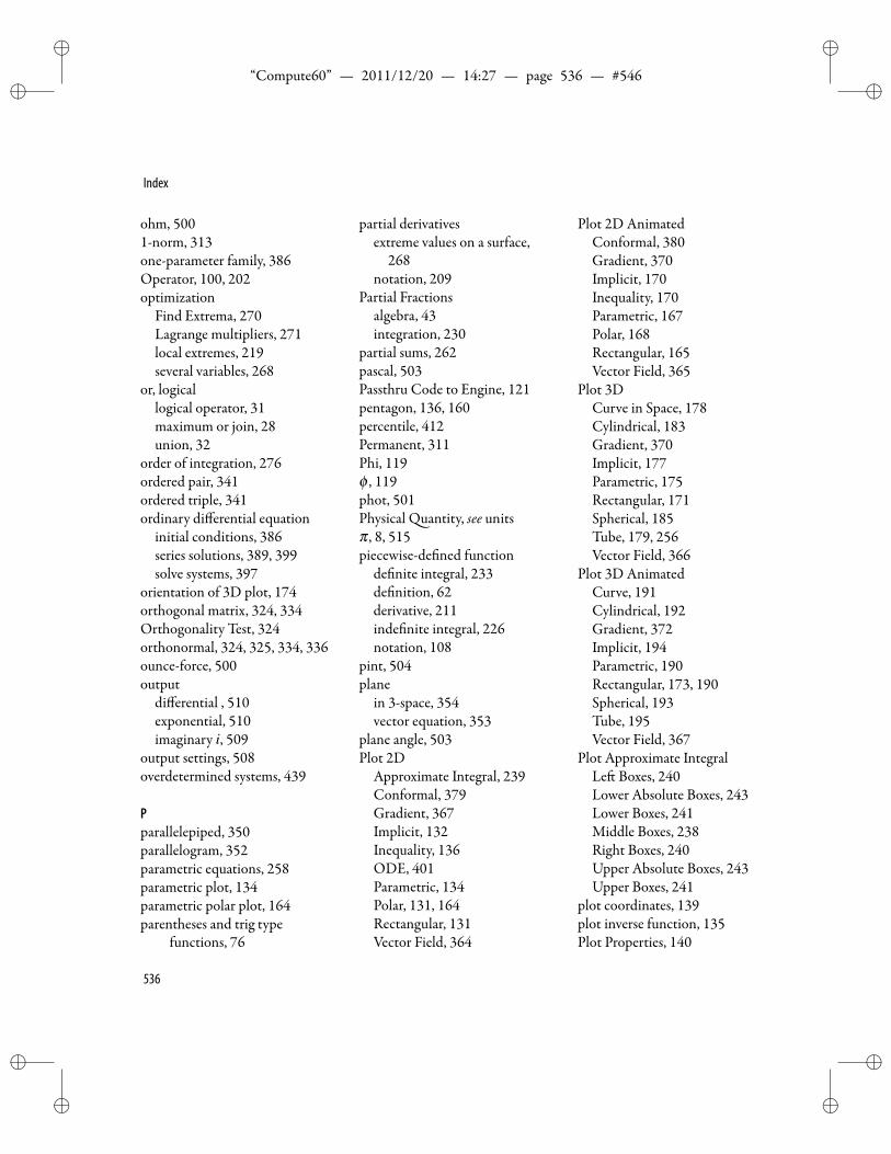
ii
“Compute60” — 2011/12/20 — 14:27 — page 536 — #546 ii
ii
ii
Index
ohm, 5001-norm, 313one-parameter family, 386Operator, 100, 202optimization
Find Extrema, 270Lagrange multipliers, 271local extremes, 219several variables, 268
or, logicallogical operator, 31maximum or join, 28union, 32
order of integration, 276ordered pair, 341ordered triple, 341ordinary differential equation
initial conditions, 386series solutions, 389, 399solve systems, 397
orientation of 3D plot, 174orthogonal matrix, 324, 334Orthogonality Test, 324orthonormal, 324, 325, 334, 336ounce-force, 500output
differential , 510exponential, 510imaginary i, 509
output settings, 508overdetermined systems, 439
Pparallelepiped, 350parallelogram, 352parametric equations, 258parametric plot, 134parametric polar plot, 164parentheses and trig type
functions, 76
partial derivativesextreme values on a surface,
268notation, 209
Partial Fractionsalgebra, 43integration, 230
partial sums, 262pascal, 503Passthru Code to Engine, 121pentagon, 136, 160percentile, 412Permanent, 311Phi, 119ϕ , 119phot, 501Physical uantity, see unitsπ , 8, 515piecewise-de ned function
de nite integral, 233de nition, 62derivative, 211inde nite integral, 226notation, 108
pint, 504plane
in 3-space, 354vector equation, 353
plane angle, 503Plot 2D
Approximate Integral, 239Conformal, 379Gradient, 367Implicit, 132Inequality, 136ODE, 401Parametric, 134Polar, 131, 164Rectangular, 131Vector Field, 364
Plot 2D AnimatedConformal, 380Gradient, 370Implicit, 170Inequality, 170Parametric, 167Polar, 168Rectangular, 165Vector Field, 365
Plot 3DCurve in Space, 178Cylindrical, 183Gradient, 370Implicit, 177Parametric, 175Rectangular, 171Spherical, 185Tube, 179, 256Vector Field, 366
Plot 3D AnimatedCurve, 191Cylindrical, 192Gradient, 372Implicit, 194Parametric, 190Rectangular, 173, 190Spherical, 193Tube, 195Vector Field, 367
Plot Approximate IntegralLe Boxes, 240Lower Absolute Boxes, 243Lower Boxes, 241Middle Boxes, 238Right Boxes, 240Upper Absolute Boxes, 243Upper Boxes, 241
plot coordinates, 139plot inverse function, 135Plot Properties, 140
536
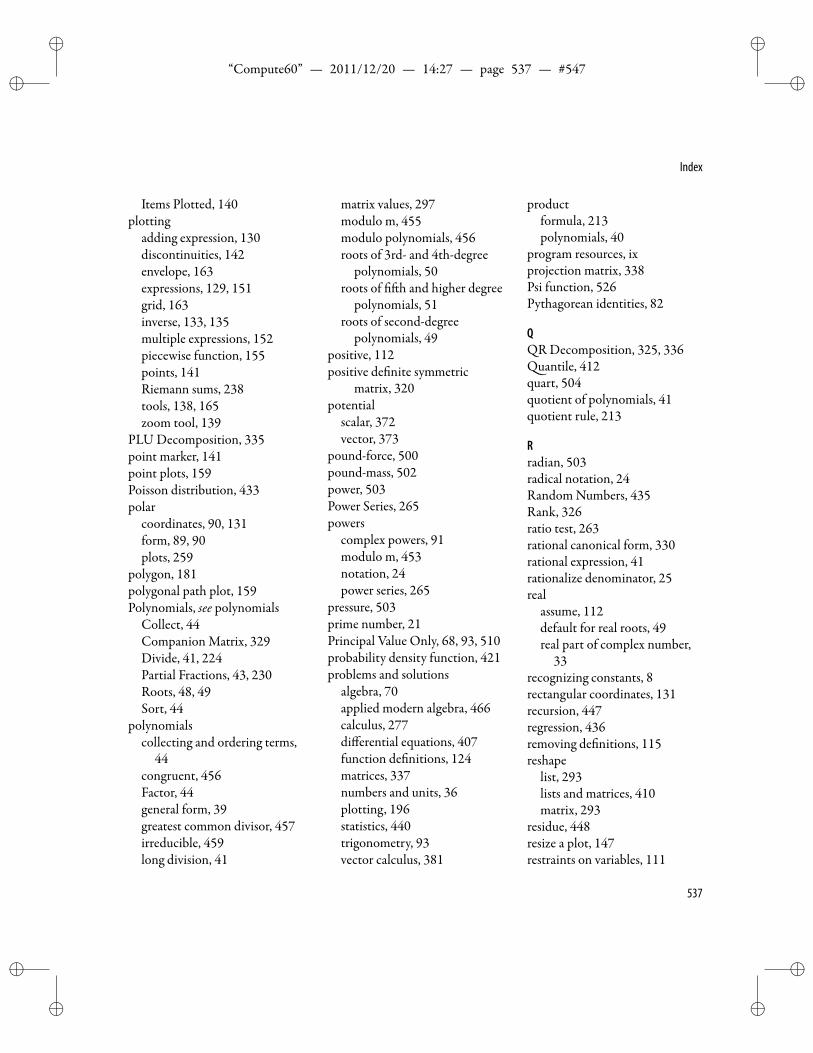
ii
“Compute60” — 2011/12/20 — 14:27 — page 537 — #547 ii
ii
ii
Index
Items Plotted, 140plotting
adding expression, 130discontinuities, 142envelope, 163expressions, 129, 151grid, 163inverse, 133, 135multiple expressions, 152piecewise function, 155points, 141Riemann sums, 238tools, 138, 165zoom tool, 139
PLU Decomposition, 335point marker, 141point plots, 159Poisson distribution, 433polar
coordinates, 90, 131form, 89, 90plots, 259
polygon, 181polygonal path plot, 159Polynomials, see polynomials
Collect, 44Companion Matrix, 329Divide, 41, 224Partial Fractions, 43, 230Roots, 48, 49Sort, 44
polynomialscollecting and ordering terms,
44congruent, 456Factor, 44general form, 39greatest common divisor, 457irreducible, 459long division, 41
matrix values, 297modulo m, 455modulo polynomials, 456roots of 3rd- and 4th-degree
polynomials, 50roots of h and higher degree
polynomials, 51roots of second-degree
polynomials, 49positive, 112positive de nite symmetric
matrix, 320potential
scalar, 372vector, 373
pound-force, 500pound-mass, 502power, 503Power Series, 265powers
complex powers, 91modulo m, 453notation, 24power series, 265
pressure, 503prime number, 21Principal Value Only, 68, 93, 510probability density function, 421problems and solutions
algebra, 70applied modern algebra, 466calculus, 277differential equations, 407function de nitions, 124matrices, 337numbers and units, 36plotting, 196statistics, 440trigonometry, 93vector calculus, 381
productformula, 213polynomials, 40
program resources, ixprojection matrix, 338Psi function, 526Pythagorean identities, 82
QQR Decomposition, 325, 336
uantile, 412quart, 504quotient of polynomials, 41quotient rule, 213
Rradian, 503radical notation, 24Random Numbers, 435Rank, 326ratio test, 263rational canonical form, 330rational expression, 41rationalize denominator, 25real
assume, 112default for real roots, 49real part of complex number,
33recognizing constants, 8rectangular coordinates, 131recursion, 447regression, 436removing de nitions, 115reshape
list, 293lists and matrices, 410matrix, 293
residue, 448resize a plot, 147restraints on variables, 111
537
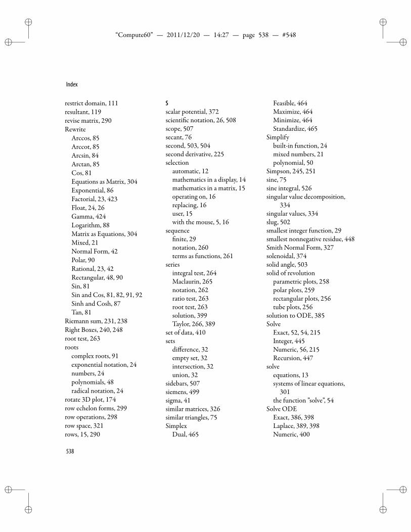
ii
“Compute60” — 2011/12/20 — 14:27 — page 538 — #548 ii
ii
ii
Index
restrict domain, 111resultant, 119revise matrix, 290Rewrite
Arccos, 85Arccot, 85Arcsin, 84Arctan, 85Cos, 81Equations as Matrix, 304Exponential, 86Factorial, 23, 423Float, 24, 26Gamma, 424Logarithm, 88Matrix as Equations, 304Mixed, 21Normal Form, 42Polar, 90Rational, 23, 42Rectangular, 48, 90Sin, 81Sin and Cos, 81, 82, 91, 92Sinh and Cosh, 87Tan, 81
Riemann sum, 231, 238Right Boxes, 240, 248root test, 263roots
complex roots, 91exponential notation, 24numbers, 24polynomials, 48radical notation, 24
rotate 3D plot, 174row echelon forms, 299row operations, 298row space, 321rows, 15, 290
Sscalar potential, 372scienti c notation, 26, 508scope, 507secant, 76second, 503, 504second derivative, 225selection
automatic, 12mathematics in a display, 14mathematics in a matrix, 15operating on, 16replacing, 16user, 15with the mouse, 5, 16
sequencenite, 29
notation, 260terms as functions, 261
seriesintegral test, 264Maclaurin, 265notation, 262ratio test, 263root test, 263solution, 399Taylor, 266, 389
set of data, 410sets
difference, 32empty set, 32intersection, 32union, 32
sidebars, 507siemens, 499sigma, 41similar matrices, 326similar triangles, 75Simplex
Dual, 465
Feasible, 464Maximize, 464Minimize, 464Standardize, 465
Simplifybuilt-in function, 24mixed numbers, 21polynomial, 50
Simpson, 245, 251sine, 75sine integral, 526singular value decomposition,
334singular values, 334slug, 502smallest integer function, 29smallest nonnegative residue, 448Smith Normal Form, 327solenoidal, 374solid angle, 503solid of revolution
parametric plots, 258polar plots, 259rectangular plots, 256tube plots, 256
solution to ODE, 385Solve
Exact, 52, 54, 215Integer, 445Numeric, 56, 215Recursion, 447
solveequations, 13systems of linear equations,
301the function ”solve”, 54
Solve ODEExact, 386, 398Laplace, 389, 398Numeric, 400
538
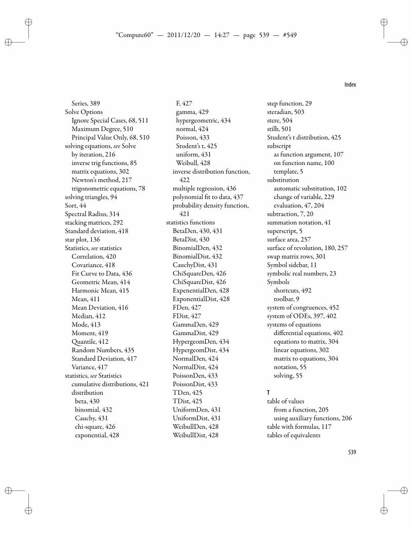
ii
“Compute60” — 2011/12/20 — 14:27 — page 539 — #549 ii
ii
ii
Index
Series, 389Solve Options
Ignore Special Cases, 68, 511Maximum Degree, 510Principal Value Only, 68, 510
solving equations, see Solveby iteration, 216inverse trig functions, 85matrix equations, 302Newton’s method, 217trigonometric equations, 78
solving triangles, 94Sort, 44Spectral Radius, 314stacking matrices, 292Standard deviation, 418star plot, 136Statistics, see statistics
Correlation, 420Covariance, 418Fit Curve to Data, 436Geometric Mean, 414Harmonic Mean, 415Mean, 411Mean Deviation, 416Median, 412Mode, 413Moment, 419
uantile, 412Random Numbers, 435Standard Deviation, 417Variance, 417
statistics, see Statisticscumulative distributions, 421distributionbeta, 430binomial, 432Cauchy, 431chi-square, 426exponential, 428
F, 427gamma, 429hypergeometric, 434normal, 424Poisson, 433Student’s t, 425uniform, 431Weibull, 428
inverse distribution function,422
multiple regression, 436polynomial t to data, 437probability density function,
421statistics functions
BetaDen, 430, 431BetaDist, 430BinomialDen, 432BinomialDist, 432CauchyDist, 431ChiSquareDen, 426ChiSquareDist, 426ExpenentialDen, 428ExponentialDist, 428FDen, 427FDist, 427GammaDen, 429GammaDist, 429HypergeomDen, 434HypergeomDist, 434NormalDen, 424NormalDist, 424PoissonDen, 433PoissonDist, 433TDen, 425TDist, 425UniformDen, 431UniformDist, 431WeibullDen, 428WeibullDist, 428
step function, 29steradian, 503stere, 504stilb, 501Student’s t distribution, 425subscript
as function argument, 107on function name, 100template, 5
substitutionautomatic substitution, 102change of variable, 229evaluation, 47, 204
subtraction, 7, 20summation notation, 41superscript, 5surface area, 257surface of revolution, 180, 257swap matrix rows, 301Symbol sidebar, 11symbolic real numbers, 23Symbols
shortcuts, 492toolbar, 9
system of congruences, 452system of ODEs, 397, 402systems of equations
differential equations, 402equations to matrix, 304linear equations, 302matrix to equations, 304notation, 55solving, 55
Ttable of values
from a function, 205using auxiliary functions, 206
table with formulas, 117tables of equivalents
539
ii
“Compute60” — 2011/12/20 — 14:27 — page 540 — #550 ii
ii
ii
Index
compute menu items, 516functions, 522
tables of units, 497tangent function, 76tangent line, 215, 277tautology, 31Taylor polynomials
one variable, 267two variables, 272
Taylor series, 266technical support, ixtechniques of integration
change of variable, 229, 234integration by parts, 228, 234partial fractions, 230, 234
telephone MacKichan, ixtemperature, 504tesla, 502test for multiple roots, 458Text/Math button, 4three-dimensional vector, 341time, 504Toggle Text/Math button, 4toll-free number, ixtorr, 503total differential, 274Trace, 307Transforms
Fourier, 395, 396Inverse Fourier, 396Inverse Laplace, 393Laplace, 391
translate view, 139Transpose, 307trapezoid rule, 244, 250trigonometric
form of z, 89inverse functions, 83
trigonometryidentities, 80
simplifying expressions, 83solution of triangles, 94solving trigonometric
equations, 78trigonometric functions, 75
trigtype functionsargument defaults, 123parentheses, 76
triple cross product, 349troubleshooting, ixTube, 256tube plot, 179two-dimensional vector, 3412-norm, 312, 352
Uunassume, 112Unde ne, 115uniform distribution, 431union, 32unit circle, 75Unit Name, 34unit pre xes, 498unitary matrix, 334units
activity, 498amount of substance, 498angle, 503area, 498arithmetic operations, 35compound names, 35converting, 35current, 499degree, 77electric capacitance, 499electric charge, 499electric conductance, 499electric resistance, 500electrical potential difference,
499
energy, 500force, 500frequency, 501illuminance, 501keyboard shortcuts, 497length, 501luminance, 501luminous ux, 501magnetic ux, 502magnetic ux density, 502magnetic inductance, 501, 502mass, 502physical units, 33plane angle, 503power, 503pressure, 503solid angle, 503temperature, 504time, 504volume, 504
Upper Absolute Boxes, 243Upper Boxes, 241user selection, 16user-de ned
functions, 106
Vvalid names for de nitions, 100Vandermonde matrix, 287variables
deferred evaluation, 105de nitions, 59full evaluation, 105making assumptions, 111, 237valid names, 100
Variance, 417, 418vector
components, 341cross product, 347de nition, 341
540
ii
“Compute60” — 2011/12/20 — 14:27 — page 541 — #551 ii
ii
ii
Index
dot product, 294, 346inner product, 294, 346length, 312matrix notation, 285norm, 351notation, 342product with scalar, 345sum, 344triple cross product, 349triple scalar product, 350
Vector CalculusCurl, 361Divergence, 360Gradient, 358Hessian, 375Jacobian, 377Laplacian, 362Scalar Potential, 373
Set Basis Variables, 359, 362,374
Vector Potential, 374Wronskian, 378
vector calculus, 341vector equation
line, 356plane, 353
vector elddivergence, 360plot, 363solenoidal, 374
vector spacecolumn space, 323nullspaces, 323row space, 321
vertical notation, 8View Intervals
Plot 3D, 171volt, 499volume
iterated integral, 274surface of revolution, 257units, 504
Wwatt, 503weber, 501, 502Weibull distribution, 428Wronskian, 377
Yyear, 504
Zzeta function, 262, 526zoom in and out, 139
541


