DOMESTIC VIOLENCE IN OHIO 2004 Ohio Office of Criminal Justice Services 1970 W. Broad Street, 4th Floor Columbus, Ohio 43223 Toll-Free: (800) 448-4842 Telephone: (614) 466-7782 Fax: (614) 466-0308 www.ocjs.ohio.gov State of Ohio Office of Criminal Justice Services The opinions, findings, and conclusions or recommendations expressed in this publication are those of the author(s) and do not necessarily reflect the views of the Department of Justice. This project was supported by Award No. 2005-JG-EOR-6329 awarded by the Bureau of Justice Assistance, Office of Justice Programs, U.S. Department of Justice, and administered by the Ohio Office of Criminal Justice Services.
The opinions, findings, and conclusions or recommendations expressed in this publication are those of the author(s) and do not necessarily reflect the views of the Department of Justice. This project was supported by Award No. 2005-JG-EOR-6329 awarded by the Bureau of Justice Assistance, Office of Justice Programs, U.S. Department of Justice, and administered by the Ohio Office of Criminal Justice Services.
DOMESTIC VIOLENCE IN OHIO, 2004
Report to the Ohio Office of Criminal Justice Services
Danielle C. Payne Michael D. Maltz
Ruth Peterson Lauren Krivo
Criminal Justice Research Center
and Department of Sociology The Ohio State University
City Size by Relationship .................................................................................................... 266
Census Data: Poverty, Income, and Race .......................................................................... 322 III. ADDITIONAL ANALYSES................................................................................................ 377
• there are two general age patterns of domestic violence—one in which the victim and
suspect are both in their early 20s, and another in which the suspect is an older teenager
who victimizes a person in their mid-30s;
• the frequency of domestic violence tapers off as the suspect ages, thus confirming the
general age distribution of crime.
We hope that such findings reveal the value of OIBRS data, even if they point to areas in need of
improvement.
6
I. INTRODUCTION AND SCOPE
The goal of this report is to provide a snapshot of the crime of domestic violence in Ohio
in 2004, as reported to the police. It is not a complete picture for three reasons. First, not all cases
of domestic violence are reported to the police, since victims are often reluctant to “call the
cops” to report being victimized by persons in their own household. Second, the analysis is based
on data collected by the Ohio Incident-Based Reporting System (OIBRS), which does not (yet)
capture the data from all police departments in the state. And third, even among those police
departments that do report OIBRS data, not all of them have been able to report for all 12 months
of 2004. Despite these reporting problems, we feel that this provides a useful picture of the state
of the problem. Moreover, it will be more useful as time goes on, since analyses of the problem
in subsequent years can be compared with this as a benchmark.
All in all, there were 168 separate jurisdictions that reported domestic violence crimes
through OIBRS in 2004. However, upon then taking out the cases for the Ohio State Highway
Patrol and assigning small agencies such as airports, universities, and parks to their respective
cities, we now have 160 places in the data base.1 The majority of incidents (36,455 of 42,409
cases, or 86%) involved the commission of a single crime, 11.4% of incidents involved two
crimes, and just 2.6% of incidents involved three or more crimes. A majority (88%) of these
single-crime cases also involved a single offender and a single victim. Because of this prevalence
of single-offender-single-victim cases, we focus on these cases in our report. Among the one-on-
one incidents there were 32 homicides, which are detailed in a separate section. In addition to
cases specifically determined to be domestic violence, we have broadened the scope somewhat to
1 We can’t get populations for the areas where the highway patrol operates, because it’s not technically a Census-defined “place.” Also, if we create counties for the zip codes where the highway patrol operates, there will be just one or two crimes per zip code, which will make the computed rates extremely misleading. Therefore, we decided to delete all cases for the Ohio State Highway Patrol.
7
include rape cases; that is, because (as we will document) domestic violence is a crime whose
victims are predominantly women, we included another crime whose victims are predominantly
women.
Many analysts have documented the benefits of using graphs to present data (Cleveland
2004; Few 2004; Robbins 2005; Tufte 1990, 1983). Since our goal has been to make our findings
accessible to the greatest number of people, we have made extensive use of charts and graphs in
this report to present our findings.
The report is organized as follows. Section II describes the overall characteristics of one-
on-one domestic violence incidents, in particular the relationships between victims and suspects2
in terms of their respective ages, races, and sexes. Section III describes some of the
characteristics of incidents involving homicide, rape, and domestic violence cases with single
suspects and multiple victims. Section IV provides an overview of the results and suggestions for
future work in this area, which is followed by our references. An appendix (Section VI)
describes the data-related problems we encountered in this project, along with suggestions for
improving the quality of the data.
2 Throughout this report we use the term “suspect” instead of “offender” to identify the alleged perpetrator, since the report is taken by the police at the point of identification (or arrest) of the involved parties and before any adjudication of guilt.
8
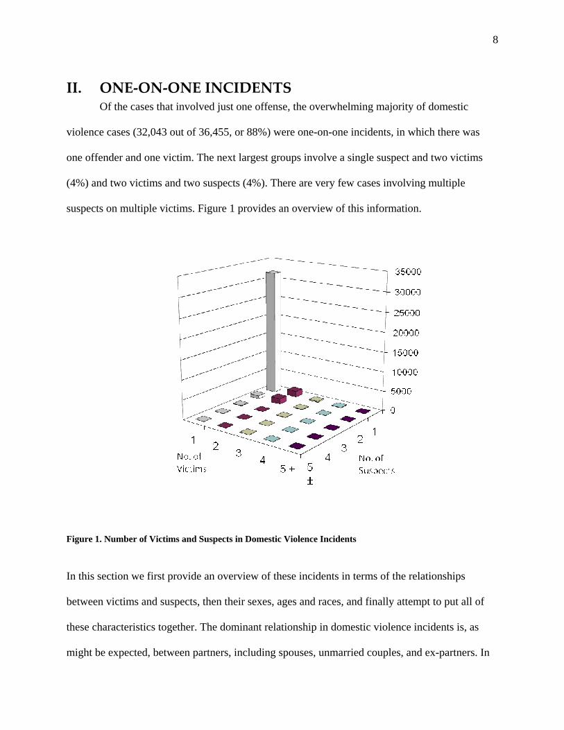
II. ONE‐ON‐ONE INCIDENTS Of the cases that involved just one offense, the overwhelming majority of domestic
violence cases (32,043 out of 36,455, or 88%) were one-on-one incidents, in which there was
one offender and one victim. The next largest groups involve a single suspect and two victims
(4%) and two victims and two suspects (4%). There are very few cases involving multiple
suspects on multiple victims. Figure 1 provides an overview of this information.
Figure 1. Number of Victims and Suspects in Domestic Violence Incidents
In this section we first provide an overview of these incidents in terms of the relationships
between victims and suspects, then their sexes, ages and races, and finally attempt to put all of
these characteristics together. The dominant relationship in domestic violence incidents is, as
might be expected, between partners, including spouses, unmarried couples, and ex-partners. In
9
addition, most incidents involve individuals of the opposite sex, the dominant age difference is a
few years, and most incidents involve individuals of the same race. This would suggest that the
most frequent domestic violence incident would involve opposite-sex partners of the same race
and about the same age, which happens to be the case.
Relationships
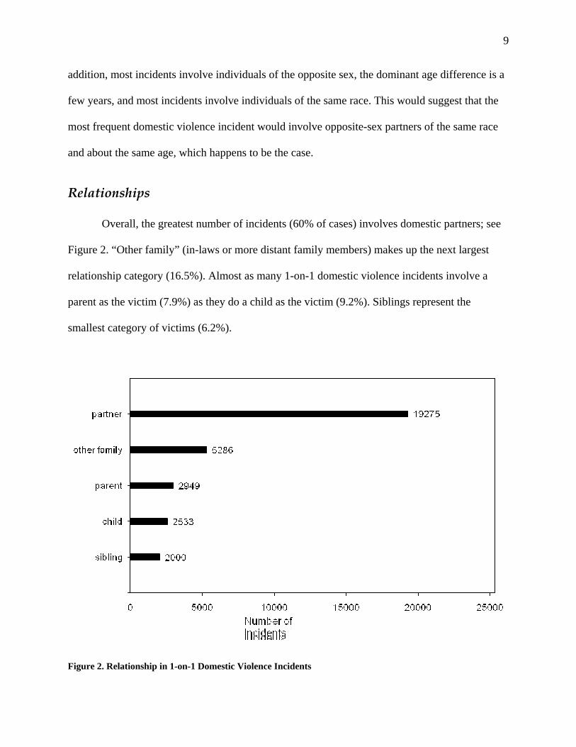
Overall, the greatest number of incidents (60% of cases) involves domestic partners; see
Figure 2. “Other family” (in-laws or more distant family members) makes up the next largest
relationship category (16.5%). Almost as many 1-on-1 domestic violence incidents involve a
parent as the victim (7.9%) as they do a child as the victim (9.2%). Siblings represent the
smallest category of victims (6.2%).
Figure 2. Relationship in 1-on-1 Domestic Violence Incidents
10
Relationships and Age
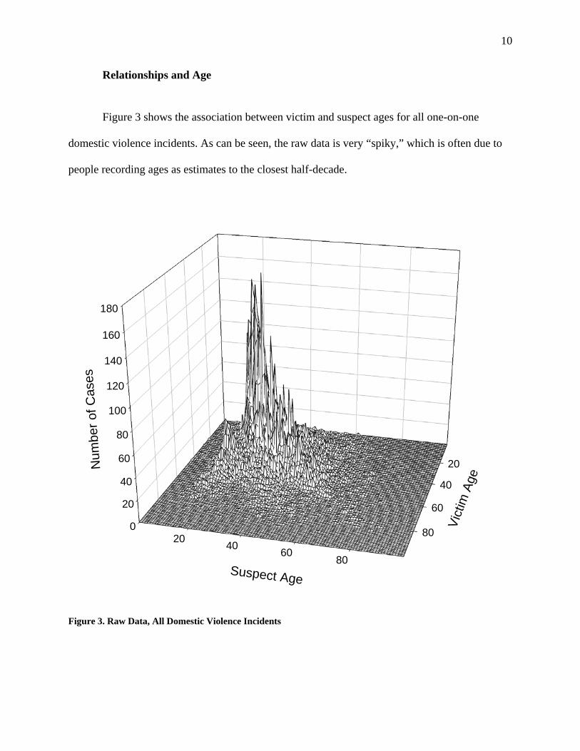
Figure 3 shows the association between victim and suspect ages for all one-on-one
domestic violence incidents. As can be seen, the raw data is very “spiky,” which is often due to
people recording ages as estimates to the closest half-decade.
0
20
40
60
80
100
120
140
160
180
20
40
60
8020 40 6080
Num
ber o
f Cas
es
Vict
im A
ge
Suspect Age
Figure 3. Raw Data, All Domestic Violence Incidents
11
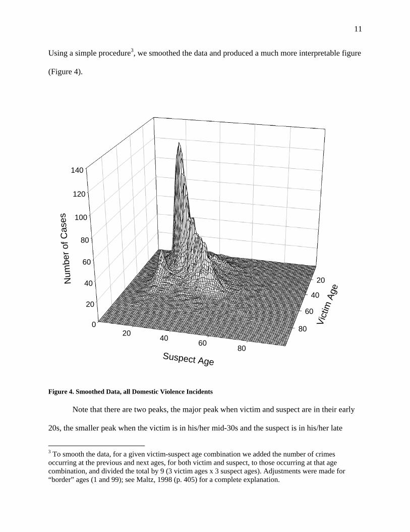
Using a simple procedure3, we smoothed the data and produced a much more interpretable figure
(Figure 4).
0
20
40
60
80
100
120
140
20
40
60
8020 40 6080
Num
ber o
f Cas
es
Vict
im A
ge
Suspect Age
Figure 4. Smoothed Data, all Domestic Violence Incidents
Note that there are two peaks, the major peak when victim and suspect are in their early
20s, the smaller peak when the victim is in his/her mid-30s and the suspect is in his/her late
3 To smooth the data, for a given victim-suspect age combination we added the number of crimes occurring at the previous and next ages, for both victim and suspect, to those occurring at that age combination, and divided the total by 9 (3 victim ages x 3 suspect ages). Adjustments were made for “border” ages (1 and 99); see Maltz, 1998 (p. 405) for a complete explanation.
12
teens. Obviously, these are (at least) two different behavioral patterns at work here.
Disaggregating the age data by relationship and by age provides additional insight into the nature
Figure 5. Age Difference between Suspect and Victim by Relationship
When we look at the age difference between suspect and victim within these relationship
types (Figure 5), we see that the bulk of partner, sibling, and other family domestic violence
incidents occurred between persons of the same age group (either the same age or within 4 years
of one another). Thus, the blue, pink, and brown peaks on the left side of the chart indicate the
number of cases for these three relationship types that involve suspects and victims within one or
two years apart in age. The turquoise and red lines represent parent and child relationship cases,
13
and here we see that the largest number of cases for these occur for age differences between
roughly 17 and 30 years apart, which is what we would expect.4
Looking even more closely at how victim and suspect ages vary by relationship
categories (see Figure 6), we can see that, for partner cases, there is a great deal of difference
when sex of the actors is taken into account. As would be expected, the greatest number of cases
are opposite-sex cases, reflecting the relatively small numbers of same-sex relationships – note
that the vertical scales on the upper and lower graphs are different. In addition, there are about 6
times as many male-on-female incidents as F-on-M incidents (16,089 vs. 2731). And as with
other crimes, the frequency of occurrence tapers off as the actors grow older. Although there are
hardly enough cases to evidence a true pattern, the age patterns in the same-sex partner cases
appear to show that the suspects are by and large younger than their victim partners.
4 There were 145 parent or child incidents where the age difference is less than 5 (within the circle in the lower left-hand corner in Figure 5), which indicates a problem with data from some jurisdictions which have likely incorrectly entered either the relationship or age data for the victim or suspect. Users of the data need to be aware of this shortcoming when performing analyses. This issue also arises in subsequent visual presentations of data that examine age and relationship.
14
0
1
2
3
4
20
40
60
8020 40 60 80
Num
ber o
f Cas
es
Vict
im A
ge
Suspect Age
Partner, M-on-M
0
1
2
3
4
20
40
60
8020 40 60 80
Num
ber o
f Cas
es
Vict
im A
ge
Suspect Age
Partner, F-on-F
0
20
40
60
80
100
20
40
60
802040
6080
Num
ber o
f Cas
es
Vict
im A
geSuspect Age
Partner, M-on-F
0
20
40
60
80
100
20
40
60
8020 40 60 80
Num
ber o
f Cas
es
Vict
im A
ge
Suspect Age
Partner, F-on-M
Figure 6. Victim and Suspect Ages by Sex for Partner Victims
Figure 7 shows the age-sex differences when the victim is a child of the suspect. In this
case the number of cases is about the same for all four sex combinations. In addition, note that,
unlike the partner cases, all four graphs are on the same scale. This indicates that victims of
either sex are (allegedly) victimized equally by suspects of both sexes. Note also that some of the
incidents in all four graphs lie above the diagonal, meaning that the age of the suspect (parent) is
15
greater than the age of the victim (child). While the number of cases is relatively small in
number, it shows that OIBRS data has inaccuracies. Unfortunately, it is impossible to tell if the
ages were reversed (meaning that the victim was a child, so the age of the victim is actually the
suspect’s age and vice versa) or if the relationship was misspecified (and the victim was the
parent and not the child). In the first case, the data point belongs to this graph with the ages
reversed; in the second case the data point belongs to the chart with the parent as victim.
16
0
1
2
3
4
5
20
40
60
8020 4060
80
Num
ber o
f Cas
es
Vict
im A
geSuspect Age
Child, M-on-F
0
1
2
3
4
5
20
40
60
8020 4060
80
Num
ber o
f Cas
es
Vict
im A
ge
Suspect Age
Child, F-on-M
0
1
2
3
4
5
20
40
60
8020 4060
80
Num
ber o
f Cas
es
Vict
im A
ge
Suspect Age
Child, M-on-M
0
1
2
3
4
5
20
40
60
8020 4060
80
Num
ber o
f Cas
es
Vict
im A
ge
Suspect Age
Child, F-on-F
Figure 7. Victim and Suspect Ages by Sex for Child Victims
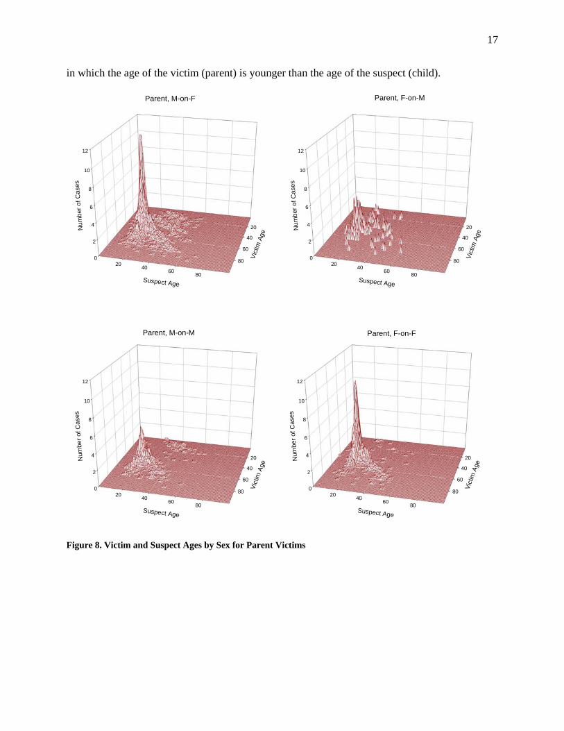
When the parent is the victim (Figure 8), we get a different picture. In this case the
dominant situation is a female victim, with male and female suspects about equal in number. As
might be expected, when the victim was male, males were more likely than females to be
suspects. And as with child victims, there were many incorrect and ambiguous cases of incidents
17
in which the age of the victim (parent) is younger than the age of the suspect (child).
0
2
4
6
8
10
12
20
40
60
8020 4060
80
Num
ber o
f Cas
es
Vict
im A
ge
Suspect Age
Parent, M-on-F
0
2
4
6
8
10
12
20
40
60
8020 40 6080
Num
ber o
f Cas
es
Vict
im A
ge
Suspect Age
Parent, M-on-M
0
2
4
6
8
10
12
20
40
60
8020 40 6080
Num
ber o
f Cas
es
Vict
im A
ge
Suspect Age
Parent, F-on-F
0
2
4
6
8
10
12
20
40
60
8020 4060
80
Num
ber o
f Cas
es
Vict
im A
ge
Suspect Age
Parent, F-on-M
Figure 8. Victim and Suspect Ages by Sex for Parent Victims
18
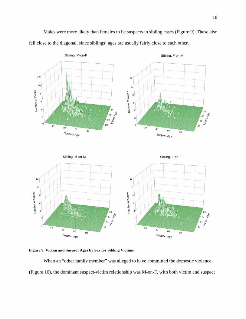
Males were more likely than females to be suspects in sibling cases (Figure 9). These also
fell close to the diagonal, since siblings’ ages are usually fairly close to each other.
0
2
4
6
8
10
12
20
40
60
8020 40 6080
Num
ber o
f Cas
es
Vict
im A
ge
Suspect Age
Sibling, M-on-M
0
2
4
6
8
10
12
20
40
60
8020 4060
80N
umbe
r of C
ases
Vict
im A
ge
Suspect Age
Sibling, F-on-M
0
2
4
6
8
10
12
20
40
60
8020 40 6080
Num
ber o
f Cas
es
Vict
im A
ge
Suspect Age
Sibling, F-on-F
0
2
4
6
8
10
12
20
40
60
8020 4060
80
Num
ber o
f Cas
es
Vict
im A
ge
Suspect Age
Sibling, M-on-F
Figure 9. Victim and Suspect Ages by Sex for Sibling Victims
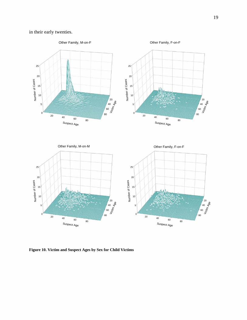
When an “other family member” was alleged to have committed the domestic violence
(Figure 10), the dominant suspect-victim relationship was M-on-F, with both victim and suspect
19
in their early twenties.
0
5
10
15
20
25
20
40
60
8020 40 60 80
Num
ber o
f Cas
es
Vict
im A
ge
Suspect Age
Other Family, M-on-F
0
5
10
15
20
25
20
40
60
8020 4060
80
Num
ber o
f Cas
es
Vict
im A
ge
Suspect Age
Other Family, F-on-F
0
5
10
15
20
25
20
40
60
8020 40 60 80
Num
ber o
f Cas
es
Vict
im A
ge
Suspect Age
Other Family, M-on-M
0
5
10
15
20
25
20
40
60
8020 4060 80
Num
ber o
f Cas
es
Vict
im A
ge
Suspect Age
Other Family, F-on-F
Figure 10. Victim and Suspect Ages by Sex for Child Victims
20
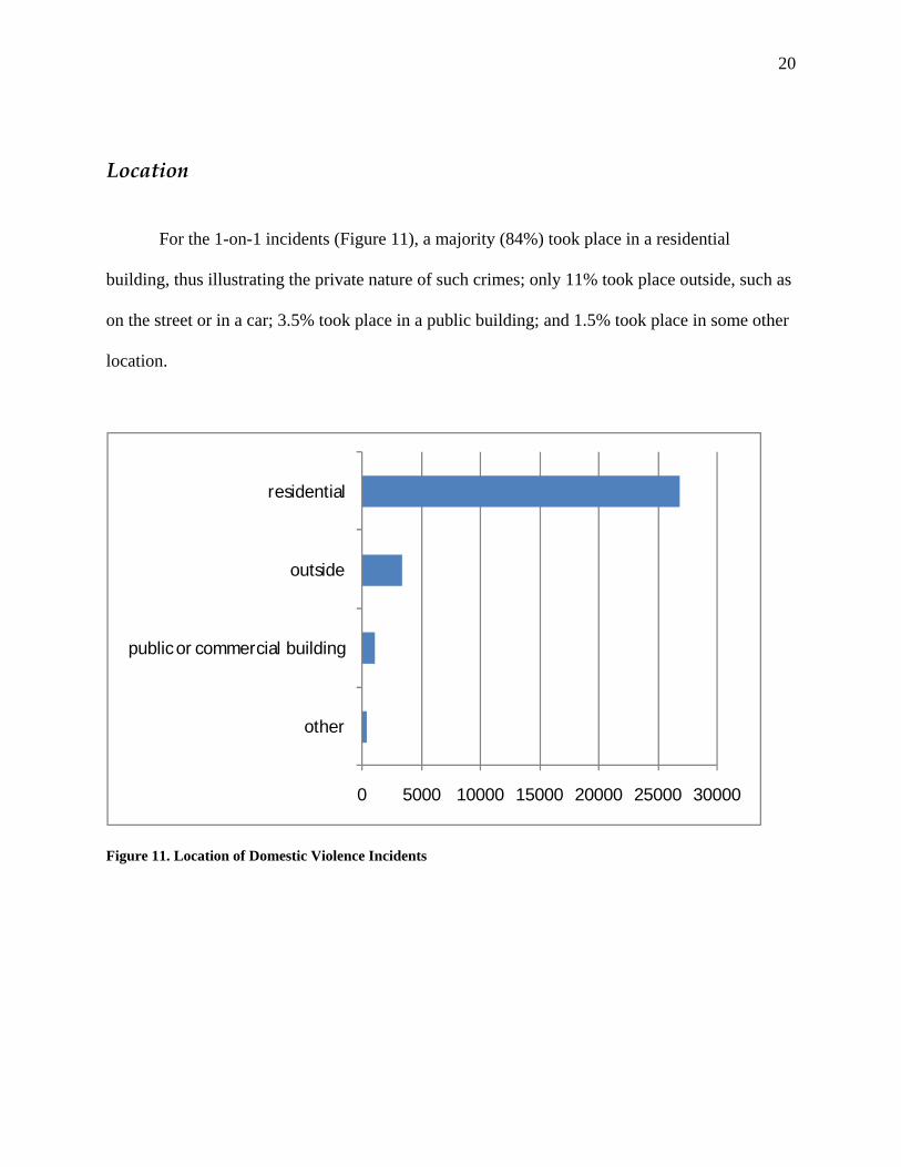
Location
For the 1-on-1 incidents (Figure 11), a majority (84%) took place in a residential
building, thus illustrating the private nature of such crimes; only 11% took place outside, such as
on the street or in a car; 3.5% took place in a public building; and 1.5% took place in some other
location.
0 5000 10000 15000 20000 25000 30000
other
public or commercial building
outside
residential
Figure 11. Location of Domestic Violence Incidents
21
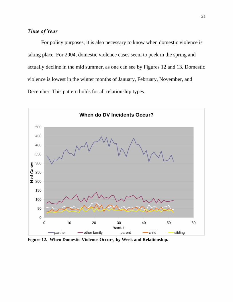
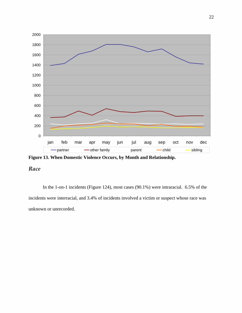
Time of Year
For policy purposes, it is also necessary to know when domestic violence is
taking place. For 2004, domestic violence cases seem to peek in the spring and
actually decline in the mid summer, as one can see by Figures 12 and 13. Domestic
violence is lowest in the winter months of January, February, November, and
December. This pattern holds for all relationship types.
When do DV Incidents Occur?
0
50
100
150
200
250
300
350
400
450
500
0 10 20 30 40 50 60Week #
N o
f Cas
es
partner other family parent child sibling Figure 12. When Domestic Violence Occurs, by Week and Relationship.
22
0
200
400
600
800
1000
1200
1400
1600
1800
2000
jan feb mar apr may jun jul aug sep oct nov dec
partner other family parent child sibling
Figure 13. When Domestic Violence Occurs, by Month and Relationship.
Race
In the 1-on-1 incidents (Figure 124), most cases (90.1%) were intraracial. 6.5% of the
incidents were interracial, and 3.4% of incidents involved a victim or suspect whose race was
unknown or unrecorded.
23
0% 20% 40% 60% 80% 100%
other, N = 46
black on black, N =13015
white on white, N =15801
partner
other family
parent
child
sibling
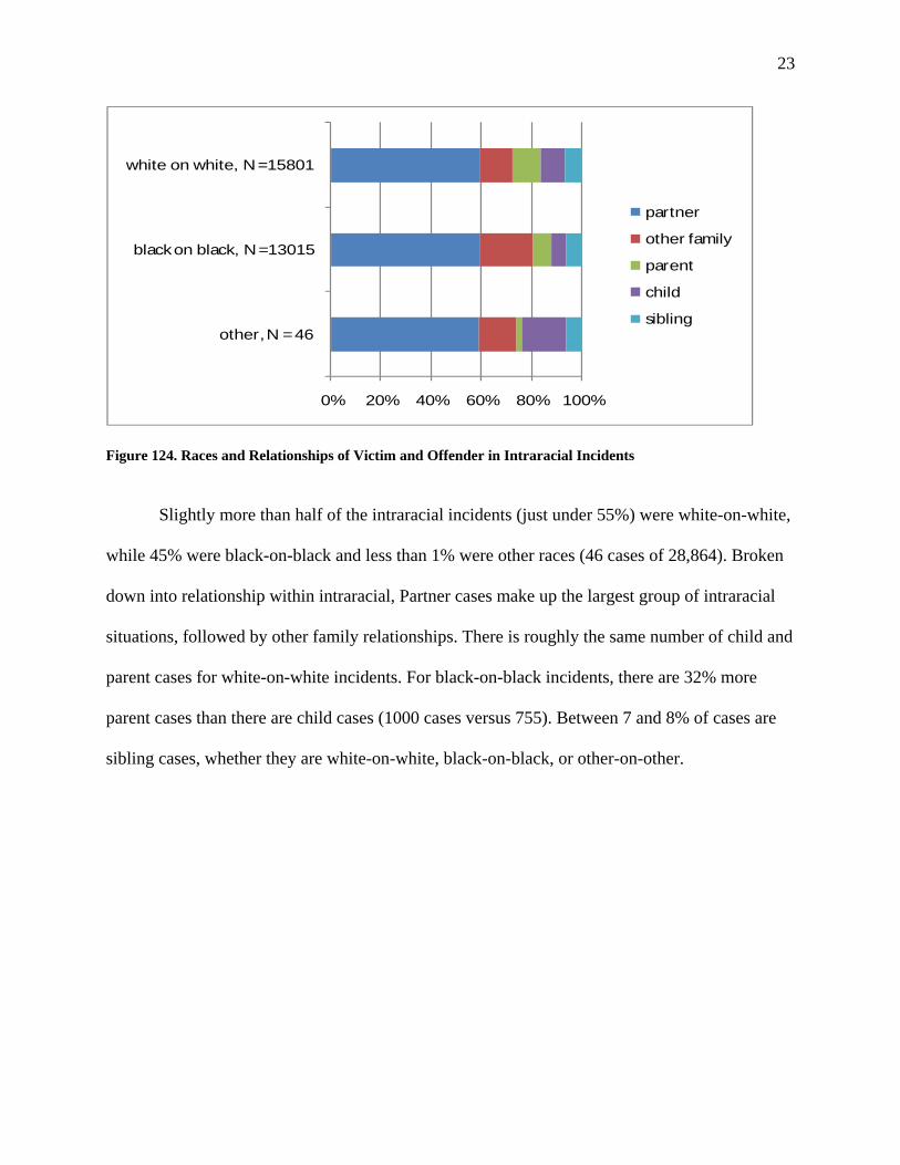
Figure 124. Races and Relationships of Victim and Offender in Intraracial Incidents
Slightly more than half of the intraracial incidents (just under 55%) were white-on-white,
while 45% were black-on-black and less than 1% were other races (46 cases of 28,864). Broken
down into relationship within intraracial, Partner cases make up the largest group of intraracial
situations, followed by other family relationships. There is roughly the same number of child and
parent cases for white-on-white incidents. For black-on-black incidents, there are 32% more
parent cases than there are child cases (1000 cases versus 755). Between 7 and 8% of cases are
sibling cases, whether they are white-on-white, black-on-black, or other-on-other.
24
0% 20% 40% 60% 80% 100%
other, N = 87
white on black, N = 355
black on white, N = 1643
partner
other family
parent
child
sibling
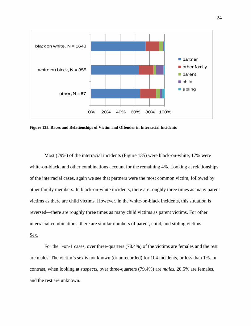
Figure 135. Races and Relationships of Victim and Offender in Interracial Incidents
Most (79%) of the interracial incidents (Figure 135) were black-on-white, 17% were
white-on-black, and other combinations account for the remaining 4%. Looking at relationships
of the interracial cases, again we see that partners were the most common victim, followed by
other family members. In black-on-white incidents, there are roughly three times as many parent
victims as there are child victims. However, in the white-on-black incidents, this situation is
reversed—there are roughly three times as many child victims as parent victims. For other
interracial combinations, there are similar numbers of parent, child, and sibling victims.
Sex.
For the 1-on-1 cases, over three-quarters (78.4%) of the victims are females and the rest
are males. The victim’s sex is not known (or unrecorded) for 104 incidents, or less than 1%. In
contrast, when looking at suspects, over three-quarters (79.4%) are males, 20.5% are females,
and the rest are unknown.
25
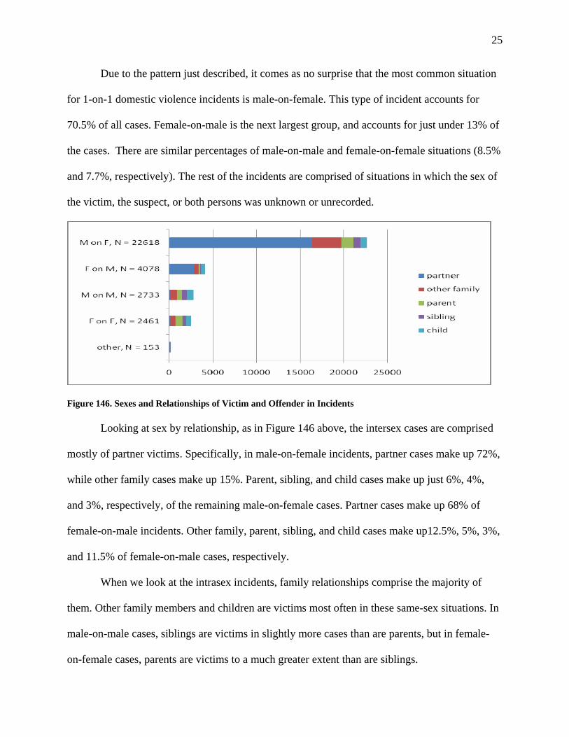
Due to the pattern just described, it comes as no surprise that the most common situation
for 1-on-1 domestic violence incidents is male-on-female. This type of incident accounts for
70.5% of all cases. Female-on-male is the next largest group, and accounts for just under 13% of
the cases. There are similar percentages of male-on-male and female-on-female situations (8.5%
and 7.7%, respectively). The rest of the incidents are comprised of situations in which the sex of
the victim, the suspect, or both persons was unknown or unrecorded.
Figure 146. Sexes and Relationships of Victim and Offender in Incidents
Looking at sex by relationship, as in Figure 146 above, the intersex cases are comprised
mostly of partner victims. Specifically, in male-on-female incidents, partner cases make up 72%,
while other family cases make up 15%. Parent, sibling, and child cases make up just 6%, 4%,
and 3%, respectively, of the remaining male-on-female cases. Partner cases make up 68% of
female-on-male incidents. Other family, parent, sibling, and child cases make up12.5%, 5%, 3%,
and 11.5% of female-on-male cases, respectively.
When we look at the intrasex incidents, family relationships comprise the majority of
them. Other family members and children are victims most often in these same-sex situations. In
male-on-male cases, siblings are victims in slightly more cases than are parents, but in female-
on-female cases, parents are victims to a much greater extent than are siblings.
26
Sociodemographic Characteristics
Population We were able to acquire population size descriptions from the Inter-University
Consortium on Political and Social Research (ICPSR) at the University of Michigan. This allows
us to compare domestic violence rates in cities of different sizes. When we do this, we notice
some interesting patterns (Figure 157).
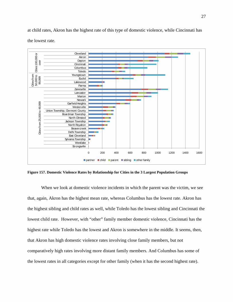
City Size by Relationship Before discussing these patterns in detail, it should be noted that the data we present here
are reported rates, that is, the number of incidents of domestic violence reported to the police in
a city divided by the city’s population, then multiplied by 100,000. Not all domestic violence
incidents are reported, and the rate of reporting them varies considerably with the demographic
composition of the city. According to a Bureau of Justice Statistics study (“Intimate Partner
Violence in the United States,” available at http://www.ojp.usdoj.gov/bjs/pub/pdf/ipvus.pdf),
reporting ranges from about 47 to 67 percent, depending on the sex, race, and ethnicity of the
victim. In addition, police policies with respect to reporting domestic violence, the presence or
absence of domestic violence shelters, and other factors also affect the rates. Therefore, the
figures presented herein should not be taken as definitive. Rather, they should be seen as a
benchmark against which to gauge rates in subsequent years, since the demographic and
programmatic factors mentioned above normally do not change much from year to year.
For the six cities with 100,000 or more population, Cleveland has the highest mean rate
of partner domestic violence, while Toledo has the lowest partner rate. However, when we look
27
at child rates, Akron has the highest rate of this type of domestic violence, while Cincinnati has
the lowest rate.
0 200 400 600 800 1000 1200 1400 1600
StrongsvilleWestlake
Sylvania TownshipEast ClevelandDelhi Township
BeavercreekNorth Royalton
Jackson TownshipNorth Olmsted
Boardman TownshipUnion Township, Clermont County
WestervilleGarfield Heights
NewarkMarion
LancasterZanesville
ParmaLakewood
EuclidYoungstown
ToledoColumbusCincinnati
DaytonAkron
Cleveland
Citie
s fro
m 2
5,00
0 to
49,
999
Citie
s fro
m
50,0
00 to
99
,999
Citie
s 100
,000
or
over
partner child parent sibling other family
Figure 157. Domestic Violence Rates by Relationship for Cities in the 3 Largest Population Groups
When we look at domestic violence incidents in which the parent was the victim, we see
that, again, Akron has the highest mean rate, whereas Columbus has the lowest rate. Akron has
the highest sibling and child rates as well, while Toledo has the lowest sibling and Cincinnati the
lowest child rate. However, with “other” family member domestic violence, Cincinnati has the
highest rate while Toledo has the lowest and Akron is somewhere in the middle. It seems, then,
that Akron has high domestic violence rates involving close family members, but not
comparatively high rates involving more distant family members. And Columbus has some of
the lowest rates in all categories except for other family (when it has the second highest rate).
28
Upon examining the mean rates across the four places with populations between 50,000
and 99,999, it seems that Youngstown has the highest rate for almost all relationship types
(except for child rates, but even here it is very close to Euclid’s rate).
Turning to mid-sized cities (with populations between 25,000 and 49,999), Zanesville has
the highest partner domestic violence rate of this group (a rate of more than 750 per 100,000
persons), while Westlake has the lowest partner rate (6.34 per 100,000 persons). Strongsville has
no partner domestic violence incidents, only child incidents. Zanesville also has the highest
domestic violence rate for children, siblings, and other family members; the only category for
which this city does not have the highest rate is for parent domestic violence (but it has the
second highest). Lancaster and Marion have some of the highest rates for all types of domestic
violence. Newark also has high rates, except for other family domestic violence—for this type of
DV, Newark’s rate is lower than seven other places.
For cities in the next population group (between 10,000 and 24,999 persons), Piqua
(Figure 168) has a much higher rate of domestic violence than others in this group -- and higher
than all larger cities as well. As noted earlier, it may be due to sociodemographic characteristics
of the municipality, to municipal policies with respect to shelters, or to police policies with
respect to reporting of domestic violence incidents.
29
0 200 400 600 800 1000 1200 1400 1600 1800
Fairview ParkBay VillageBrecksville
Genoa TownshipPoland Township
Hudson CitySolon
LyndhurstSylvania
Broadview HeightsAthens
AvonAshland
Avon LakeNorth Canton
AmherstNew PhiladelphiaCopley Township
MaumeeLiberty Township
BereaPickerington
Brook ParkPerkins Township
Franklin Township, Summit CountyPierce Township
PataskalaUrbana
SharonvilleForest Park
Franklin CityCirclevilleRiverside
CelinaSpringfield Township, Summit County
WashingtonGalionPiqua
partner child parent sibling other family
Figure 168. Domestic Violence Rates by Relationship for Cities with Populations Between 10,000 and 24,999
Among cities with populations from 2,500 to 9,999, we see that Windham has the highest
rate of domestic violence, higher even than Piqua (Figure 179). Aside from the standard
explanation given in the previous paragraph, there is a statistical one as well. The larger the
population, the more stable the rates tend to be; and conversely, the smaller the population, the
30
more volatile the rates tend to be. What may be at play here is that type of phenomenon; to
explain further, note that a crime count of 10 in one year is likely to be followed by a crime
count of 8 the next year – reduction by 2 crimes produces a 20 percent drop -- but a crime count
of 1000 in one year is highly unlikely to be followed by a crime count of 800 the next year.
0 500 1000 1500 2000 2500
Richland Township, Belmont CountyPowell
Milton Township, Mahoning CountyCanfield
Medina TownshipHighland HeightsMayfield Village
LouisvilleNewton Township, Trumbull CountyMontville Township, Medina County
Hubbard TownshipCheviot
Sugarcreek TownshipGerman Township
Munroe FallsDeer Park
Beaver TownshipSunburyTipp CityArchboldWauseon
New AlbanyDelta
BellbrookHillsboro
WintersvilleGrandview Heights
FredericktownNew Lexington
Plain CityLake Township, Wood County
ColdwaterNorthwoodUhrichsville
HeathWapakoneta
SwantonEast Palestine
LoganMount Gilead
Mt. HealthyCovingtonMt. OrabLockland
UniontownWoodlawn
North BaltimoreMontpelier
Windham
partner child parent sibling other family
Figure 179. Domestic Violence Rates by Relationship for Cities with Populations Between 2,500 and 9,999
31
This phenomenon is probably more apparent in the smaller jurisdictions and counties depicted in
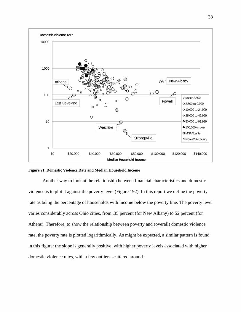
Figure 21. Domestic Violence Rate and Median Household Income
Another way to look at the relationship between financial characteristics and domestic
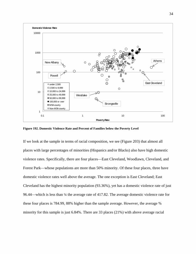
violence is to plot it against the poverty level (Figure 192). In this report we define the poverty
rate as being the percentage of households with income below the poverty line. The poverty level
varies considerably across Ohio cities, from .35 percent (for New Albany) to 52 percent (for
Athens). Therefore, to show the relationship between poverty and (overall) domestic violence
rate, the poverty rate is plotted logarithmically. As might be expected, a similar pattern is found
in this figure: the slope is generally positive, with higher poverty levels associated with higher
domestic violence rates, with a few outliers scattered around.
34
1
10
100
1000
10000
0.1 1 10 100
Domestic Violence Rate
Poverty Rate
under 2,5002,500 to 9,99910,000 to 24,99925,000 to 49,99950,000 to 99,999100,000 or overMSA countyNon-MSA county
East Cleveland
Strongsville
Westlake
New Albany
Powell
Athens
Figure 192. Domestic Violence Rate and Percent of Families below the Poverty Level
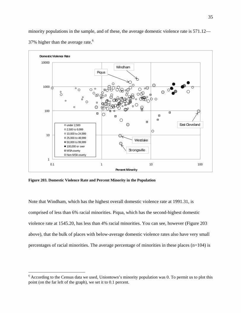
If we look at the sample in terms of racial composition, we see (Figure 203) that almost all
places with large percentages of minorities (Hispanics and/or Blacks) also have high domestic
violence rates. Specifically, there are four places—East Cleveland, Woodlawn, Cleveland, and
Forest Park—whose populations are more than 50% minority. Of these four places, three have
domestic violence rates well above the average. The one exception is East Cleveland; East
Cleveland has the highest minority population (93.36%), yet has a domestic violence rate of just
96.44—which is less than ¼ the average rate of 417.82. The average domestic violence rate for
these four places is 784.99, 88% higher than the sample average. However, the average %
minority for this sample is just 6.84%. There are 33 places (21%) with above average racial
35
minority populations in the sample, and of these, the average domestic violence rate is 571.12—
37% higher than the average rate.6
1
10
100
1000
10000
0.1 1 10 100
Domestic Violence Rate
Percent Minority
under 2,5002,500 to 9,99910,000 to 24,99925,000 to 49,99950,000 to 99,999100,000 or overMSA countyNon-MSA county
East Cleveland
WindhamPiqua
Strongsville
Westlake
Figure 203. Domestic Violence Rate and Percent Minority in the Population
Note that Windham, which has the highest overall domestic violence rate at 1991.31, is
comprised of less than 6% racial minorities. Piqua, which has the second-highest domestic
violence rate at 1545.20, has less than 4% racial minorities. You can see, however (Figure 203
above), that the bulk of places with below-average domestic violence rates also have very small
percentages of racial minorities. The average percentage of minorities in these places (n=104) is
6 According to the Census data we used, Uniontown’s minority population was 0. To permit us to plot this point (on the far left of the graph), we set it to 0.1 percent.
36
just 4.44%. However, even among the places with above-average domestic violence rates (n=56),
the average percentage of racial minorities is still just 11.30%.
37
III. ADDITIONAL ANALYSES
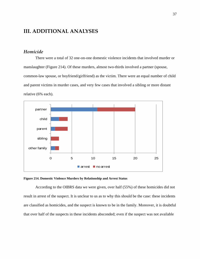
Homicide There were a total of 32 one-on-one domestic violence incidents that involved murder or
manslaughter (Figure 214). Of these murders, almost two-thirds involved a partner (spouse,
common-law spouse, or boyfriend/girlfriend) as the victim. There were an equal number of child
and parent victims in murder cases, and very few cases that involved a sibling or more distant
relative (6% each).
0 5 10 15 20 25
other family
sibling
parent
child
partner
arrest no arrest
Figure 214. Domestic Violence Murders by Relationship and Arrest Status
According to the OIBRS data we were given, over half (55%) of these homicides did not
result in arrest of the suspect. It is unclear to us as to why this should be the case: these incidents
are classified as homicides, and the suspect is known to be in the family. Moreover, it is doubtful
that over half of the suspects in these incidents absconded; even if the suspect was not available
38
at the time of the officer taking the initial report, OIBRS permits updating (in the case of, e.g.,
subsequent arrests) for up to two years after the initial report.7
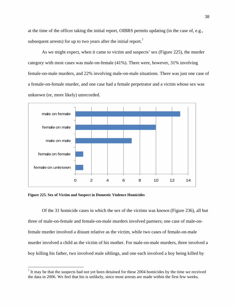
As we might expect, when it came to victim and suspects’ sex (Figure 225), the murder
category with most cases was male-on-female (41%). There were, however, 31% involving
female-on-male murders, and 22% involving male-on-male situations. There was just one case of
a female-on-female murder, and one case had a female perpetrator and a victim whose sex was
unknown (or, more likely) unrecorded.
0 2 4 6 8 10 12 14
female on unknown
female on female
male on male
female on male
male on female
Figure 225. Sex of Victim and Suspect in Domestic Violence Homicides
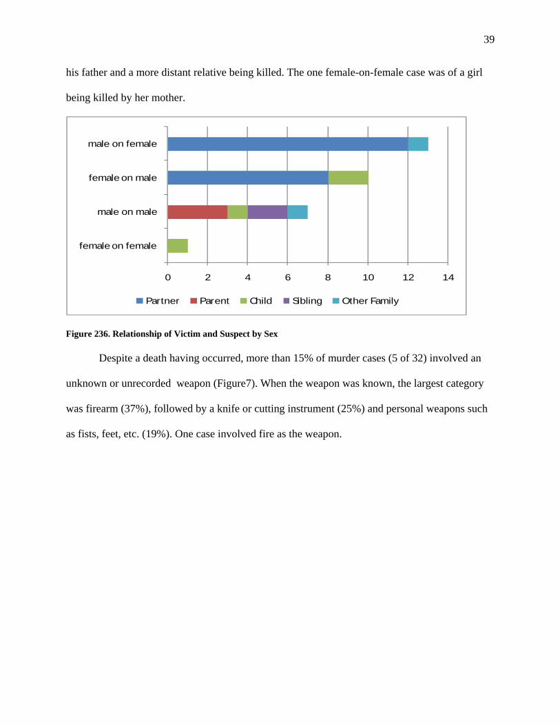
Of the 31 homicide cases in which the sex of the victims was known (Figure 236), all but
three of male-on-female and female-on-male murders involved partners; one case of male-on-
female murder involved a distant relative as the victim, while two cases of female-on-male
murder involved a child as the victim of his mother. For male-on-male murders, three involved a
boy killing his father, two involved male siblings, and one each involved a boy being killed by
7 It may be that the suspects had not yet been detained for these 2004 homicides by the time we received the data in 2006. We feel that his is unlikely, since most arrests are made within the first few weeks.
39
his father and a more distant relative being killed. The one female-on-female case was of a girl
being killed by her mother.
0 2 4 6 8 10 12 14
female on female
male on male
female on male
male on female
Partner Parent Child Sibling Other Family
Figure 236. Relationship of Victim and Suspect by Sex
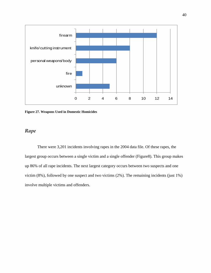
Despite a death having occurred, more than 15% of murder cases (5 of 32) involved an
unknown or unrecorded weapon (Figure7). When the weapon was known, the largest category
was firearm (37%), followed by a knife or cutting instrument (25%) and personal weapons such
as fists, feet, etc. (19%). One case involved fire as the weapon.
40
0 2 4 6 8 10 12 14
unknown
fire
personal weapons/body
knife/cutting instrument
firearm
Figure 27. Weapons Used in Domestic Homicides
Rape
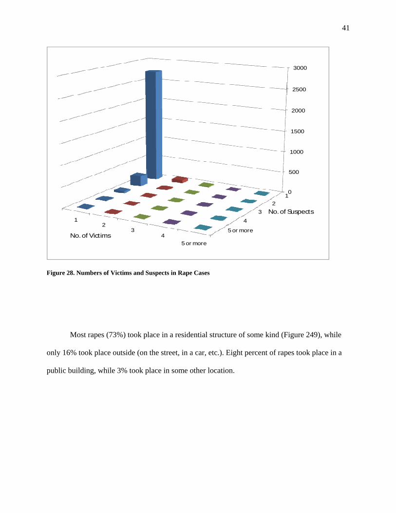
There were 3,201 incidents involving rapes in the 2004 data file. Of these rapes, the
largest group occurs between a single victim and a single offender (Figure8). This group makes
up 86% of all rape incidents. The next largest category occurs between two suspects and one
victim (8%), followed by one suspect and two victims (2%). The remaining incidents (just 1%)
involve multiple victims and offenders.
41
12
34
5 or more
0
500
1000
1500
2000
2500
3000
12
34
5 or moreNo. of Victims
No. of Suspects
Figure 28. Numbers of Victims and Suspects in Rape Cases
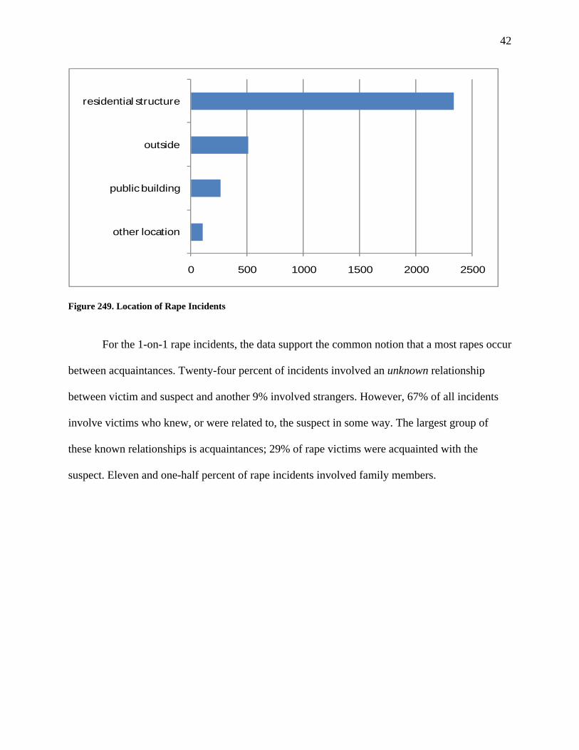
Most rapes (73%) took place in a residential structure of some kind (Figure 249), while
only 16% took place outside (on the street, in a car, etc.). Eight percent of rapes took place in a
public building, while 3% took place in some other location.
42
0 500 1000 1500 2000 2500
other location
public building
outside
residential structure
Figure 249. Location of Rape Incidents
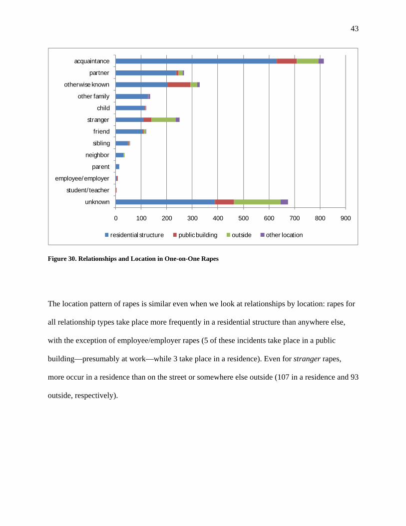
For the 1-on-1 rape incidents, the data support the common notion that a most rapes occur
between acquaintances. Twenty-four percent of incidents involved an unknown relationship
between victim and suspect and another 9% involved strangers. However, 67% of all incidents
involve victims who knew, or were related to, the suspect in some way. The largest group of
these known relationships is acquaintances; 29% of rape victims were acquainted with the
suspect. Eleven and one-half percent of rape incidents involved family members.
43
0 100 200 300 400 500 600 700 800 900
unknown
student/ teacher
employee/employer
parent
neighbor
sibling
friend
stranger
child
other family
otherwise known
partner
acquaintance
residential structure public building outside other location
Figure 30. Relationships and Location in One-on-One Rapes
The location pattern of rapes is similar even when we look at relationships by location: rapes for
all relationship types take place more frequently in a residential structure than anywhere else,
with the exception of employee/employer rapes (5 of these incidents take place in a public
building—presumably at work—while 3 take place in a residence). Even for stranger rapes,
more occur in a residence than on the street or somewhere else outside (107 in a residence and 93
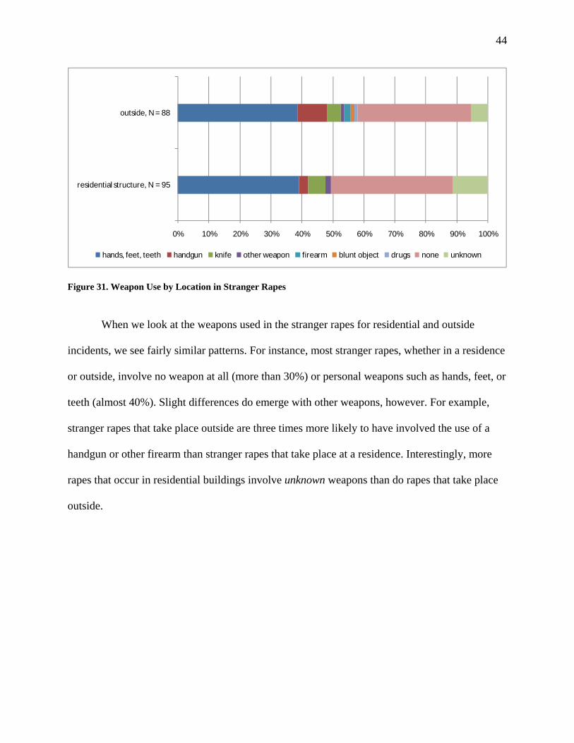
Figure 31. Weapon Use by Location in Stranger Rapes
When we look at the weapons used in the stranger rapes for residential and outside
incidents, we see fairly similar patterns. For instance, most stranger rapes, whether in a residence
or outside, involve no weapon at all (more than 30%) or personal weapons such as hands, feet, or
teeth (almost 40%). Slight differences do emerge with other weapons, however. For example,
stranger rapes that take place outside are three times more likely to have involved the use of a
handgun or other firearm than stranger rapes that take place at a residence. Interestingly, more
rapes that occur in residential buildings involve unknown weapons than do rapes that take place
outside.
45
One‐on‐Many Incidents It is often difficult to perform a detailed analysis in cases with multiple victims and/or
suspects. Each individual victim may have a different relationship with each individual suspect,
so parsing the cases on the basis of relationships can be misleading. For example, if one wanted
to determine the extent to which twenty-year-olds victimize their parents, the data could be
searched for 20-year-old suspects and victims whose relationship to the suspects is either “PA”
(parent) or “SP” stepparent). But suppose that the parents are taking care of the suspect’s
children, who are also victimized by the suspect; then this is also a case of child abuse. Questions
then arise as to how to count this incident: as parental abuse, as child abuse, as both (therefore
double-counting this incident), or as a new category of parent-and-child abuse?
Moreover, this situation assumes that the data are accurate, which is unfortunately not
always the case. In 2004 there were 1300 one-on-many incidents. Among these we found 312
(24 percent) in which a parent or stepparent was named as a victim. Of these, there were 28 (9
percent) in which the victim was older than the supposed parent. This points out one of the key
concerns that we have about using OIBRS data: training. It would appear most likely that the
persons filling out the OIBRS form may have entered the relationship of the suspect to the victim
rather than the opposite. It may be that simpler wording would help: that is, rather than having
the officer respond to the query, “Relationship of Victim to Suspect __________,”8 it might be
better to have the officer respond to a query of the form, “The Victim is __________ of/to the
Suspect.”
Despite this, we can perform some simple analyses of the data. Figure 252 depicts the age
distribution of suspects in incidents with more than one victim, for all such cases and for cases in
8 We have not seen any of the forms that officers fill out, and thus cannot verify if our conjecture about the nature of OIBRS or other police forms is correct.
46
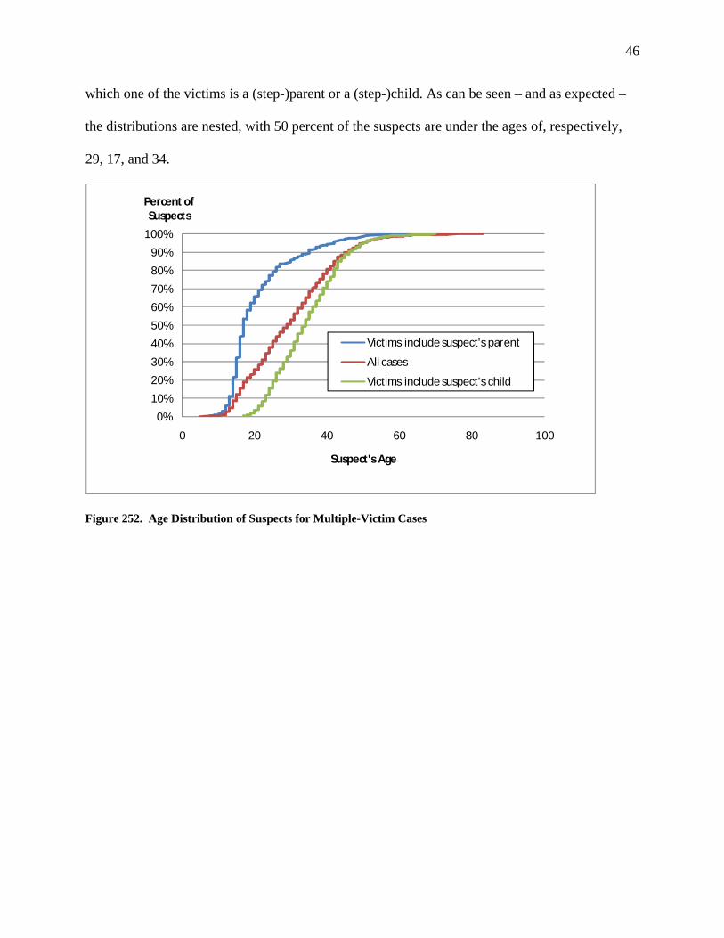
which one of the victims is a (step-)parent or a (step-)child. As can be seen – and as expected –
the distributions are nested, with 50 percent of the suspects are under the ages of, respectively,
29, 17, and 34.
0%10%20%30%40%50%60%70%80%90%
100%
0 20 40 60 80 100
Percent of Suspects
Suspect's Age
Victims include suspect's parent
All cases
Victims include suspect's child
Figure 252. Age Distribution of Suspects for Multiple-Victim Cases
47
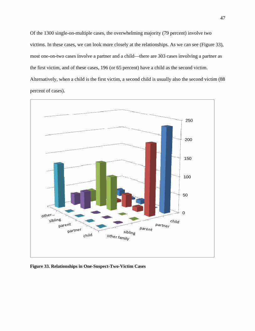
Of the 1300 single-on-multiple cases, the overwhelming majority (79 percent) involve two
victims. In these cases, we can look more closely at the relationships. As we can see (Figure 33),
most one-on-two cases involve a partner and a child—there are 303 cases involving a partner as
the first victim, and of these cases, 196 (or 65 percent) have a child as the second victim.
Alternatively, when a child is the first victim, a second child is usually also the second victim (88
percent of cases).
0
50
100
150
200
250
Figure 33. Relationships in One-Suspect-Two-Victim Cases
48
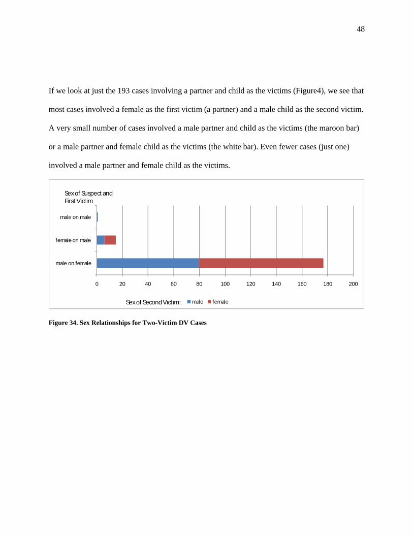
If we look at just the 193 cases involving a partner and child as the victims (Figure4), we see that
most cases involved a female as the first victim (a partner) and a male child as the second victim.
A very small number of cases involved a male partner and child as the victims (the maroon bar)
or a male partner and female child as the victims (the white bar). Even fewer cases (just one)
involved a male partner and female child as the victims.
0 20 40 60 80 100 120 140 160 180 200
male on female
female on male
male on male
male female
Sex of Suspect and First Victim
Sex of Second Victim:
Figure 34. Sex Relationships for Two-Victim DV Cases
49
IV. CONCLUSIONS AND RECOMMENDATIONS
In this report we provide the reader with an overview of the characteristics of domestic
violence in the State of Ohio. We hope that this will become a template for subsequent analyses,
and that the template will be revised as additional years’ data allow for the development of
trends.
We have attempted to provide a context for the nature and extent of domestic violence in
different places by tying it to sociodemographic characteristics: population size, race and
ethnicity, and income and poverty. While this may provide a partial explanation of variation in
domestic violence rates, it should be stressed that other factors may play an even more important
part. In particular, the extent to which domestic violence support services are available in the
community9, the policies of the police department with respect to reporting and making arrests in
domestic violence incidents, the extent of immigrants in the community (Erez 2000), and the
extent of community trust in the police can all have profound effects on the domestic violence
statistics that we use to gauge the problem.
In a previous report on domestic violence (Payne et al. 2006) we noted the deficiencies in
reporting; this report does the same (see the Appendix). As in the earlier report, we strongly
recommend that location information be made available; this would permit an analysis based on
the characteristics of the census tract in which the incident occurred, which would provide a
better understanding of the community dynamics involved. While some of this may be inferred
9 Dugan et al (1999) note that the availability of domestic violence support services has contributed markedly “to the reduction in the intimate partner homicide rate, most prominently to the rate at which women kill their male partners” (p.208).
50
from the jurisdictional analyses performed in Section II above, a more detailed look could be of
greater value for policy purposes.
This report gives an indication of the nature and extent of domestic violence at one point
in time. It would be of great benefit for policy purposes if this could be tracked over time, to see
how it changes in different jurisdictions (with different policy initiatives).
51
V. REFERENCES
Cleveland, William S. 1994. The Elements of Graphing Data. Summit, NJ: Hobart Press. Dugan, Laura, Daniel S. Nagin, and Richard Rosenfeld. 1999. “Explaining the Decline in
Intimate Partner Homicide: The Effects of Changing Domesticity, Women's Status, and Domestic Violence Status.” Homicide Studies 3:3: 187-214.
Erez, Edna. 2000. “Immigration, Culture Conflict and Domestic Violence/Woman Battering.”
Crime Prevention and Community Safety 2, 27–36. Few, Stephen. 2004. Show Me the Numbers: Designing Tables and Graphs to Enlighten.
Oakland, CA: Analytics Press. Maltz, Michael D. 1998. “Visualizing Homicide: A Research Note.” Journal of Quantitative
Criminology 14: 397-410. Payne, Danielle, Michael Maltz, Lauern Krivo, and Ruth Peterson. 2006. Crime in Ohio:
Analyses of OIBRS Data. Ohio Office of Criminal Justice Services. Available at http://www.ocjs.ohio.gov/research/OIBRS%20Final%20Report%20011906-osu.pdf.
Robbins, Naomi. 2005. Creating More Effective Graphs. Hoboken, NJ: John Wiley and Sons,
Inc. Tufte, Edward. 1983. The Visual Display of Quantitative Information. Cheshire, CN: Graphics