Socio.d~¢on. Plan. Sci Vol. 16, No. 5, pp. 195-207, 1982 0038--0121/82/050195-13503.00/0 Printed in Great Britain Pergamon Press Ltd. DYNAMIC APPRAISAL OF INFRASTRUCTURE INVESTMENTS ARTURO J. BENCOSME and JARIR S. DAJANI Program in Infrastructure Planning and Management, Department of Civil Engineering, Stanford University, Stanford, CA 94305, U.S.A. (Received 19 February 1982) Abstract--The assessment of the reciprocal impacts of infrastructure investments and their socio-economic environment requires that a number of such aspects be simultaneouslyconsidered. Some of those aspects. however, have not been traditionallyincorporatedin such assessments due (in part) to the limitations inherent in the techniques utilized in current practice. This paper presents a conceptual framework for the use of dynamic simulation in the assessment of packages of infrastructure investments. The concepts are then applied to case studies involving the evaluationof coordinatedsets of infrastructure projects in rural areas. 1. INTRODUCTION The provision of different elements of physical in- frastructure is generally considered to be an important phase of development. The expansion of water supply facilities, for example, can lower the cost of agricultural production, and can foster urban growth in those areas where water is a limiting factor. Similarly, investments in the transportation network can improve access to social services and economic opportunities, and increase the mobility of people and goods. Part of the complexity of infrastructure project ap- praisal results because the effects of introducing in- frastructure improvements into a region can be far reaching. A priori appraisal methods must be compre- hensive enough to include all of the expected important effects of these improvements. The complexity of the task is exacerbated because of reciprocal effects between the socio-economic environment and the infrastructure. Current practice in the appraisal of infrastructure in- vestments, as reported in Refs. [1-3], admits the exis- tence of these complexities, but does little to accomodate them in the analysis [4]. Reciprocal interactions between the socio-economic environment and the infrastructure are usually ignored in quantitative appraisal but they are sometimes considered in qualitative impact assessment studies. Quantitative analyses are based on forecasts of the expected effects of a project on the affected area; often the underlying forecasting scheme pre-determines the outcome of the appraisal. Current practice frequently uses forecasting methods which preclude some variables or relationships that are central to the situation being appraised, with a consequent possibility of obtaining misleading or even erroneous results, conclusions, and choices. A CONCEPTUAL FRAMEWORK It has been suggested by Carnemark [5] that the socio- economic assessment of infrastructure projects in developmental contexts should involve the consideration of eight important factors: (i) distribution of benefits, (ii) relative magnitude of cost savings, (iii) social engineer- ing, (iv) delivery systems, (v) complementary invest- ments and activities, (vi) institutional issues, (vii) design standards, and (viii) construction techniques. While each of the elements on Carnemark's list appear reasonable, questions remain regarding the methods to be used in order to guarantee that all of these factors can be analyzed in a quantitative manner. Furthermore, while the eight factors listed above reflect most of the im- portant policy issues that generally need to be addressed, these factors should be considered in a dynamic context, i.e. the dynamics of the reciprocal effects of infrastruc- ture developments and their socio-economic environ- ment need to be explicitly included in the analysis. It is demonstrated herein that a failure to include such factors could significantly alter the outcome of the infrastructure project appraisal process. In searching for an appraisal scheme that reflects the aforementioned dynamic reciprocal interactions, Ben- cosme [6], departing from the work of MaciarMlo [7], developed a project evaluation scheme which (i) is specifically oriented towards the analysis of the cumula- tive impacts of infrastructure investments, and (ii) pro- vides a conceptual framework which is capable of ac- comodating the analysis of the eight factors listed above. The proposed conceptual framework views the study area as a "system", i.e. a set of interrelated elements. The elements are grouped into two sub-systems: the infrastructure sub-system, and the socio-economic environment. The interrelationships a.mong these ele- ments are classified into two types: short-ruri and long- run interactions. The two sub-sets interact directly through short run interactions, which, in turn, provide the basis for long-adjustments in both sub-sets. This conceptual scheme is depicted in Fig. 1, which employs the following conventions: the boxes represent the elements; the dashed arrows indicate short-run in- teractions. These interactions result in instantaneous situations (i.e. situations not directly dependent of the past history of the system), which are represented by the circles. Continuous arrows represent long-run adjust- ment mechanisms. These arrows go from the circles back to the boxes. The two sub-systems are not connected directly, but rather through the short-run/long-run paths which provide the linkages among them. The following prototypical situation is used in order to facilitate the discussion of the conceptual framework described above. Consider the case in which a develop- ment plan for a rural area in a developing region needs to be assessed; the issue concerns whether or not to finance certain projects which are under consideration, Assume that the plan includes two infrastructure prolects: a rural road and an irrigation facility, and that the area is part of a region in which little previous development has taken 195
Transcript
Socio.d~¢on. Plan. Sci Vol. 16, No. 5, pp. 195-207, 1982 0038--0121/82/050195-13503.00/0 Printed in Great Britain Pergamon Press Ltd.
DYNAMIC APPRAISAL OF INFRASTRUCTURE INVESTMENTS
ARTURO J. BENCOSME and JARIR S. DAJANI
Program in Infrastructure Planning and Management, Department of Civil Engineering, Stanford University, Stanford, CA 94305, U.S.A.
(Received 19 February 1982)
Abstract--The assessment of the reciprocal impacts of infrastructure investments and their socio-economic environment requires that a number of such aspects be simultaneously considered. Some of those aspects. however, have not been traditionally incorporated in such assessments due (in part) to the limitations inherent in the techniques utilized in current practice. This paper presents a conceptual framework for the use of dynamic simulation in the assessment of packages of infrastructure investments. The concepts are then applied to case studies involving the evaluation of coordinated sets of infrastructure projects in rural areas.
1. INTRODUCTION
The provision of different elements of physical in- frastructure is generally considered to be an important phase of development. The expansion of water supply facilities, for example, can lower the cost of agricultural production, and can foster urban growth in those areas where water is a limiting factor. Similarly, investments in the transportation network can improve access to social services and economic opportunities, and increase the mobility of people and goods.
Part of the complexity of infrastructure project ap- praisal results because the effects of introducing in- frastructure improvements into a region can be far reaching. A priori appraisal methods must be compre- hensive enough to include all of the expected important effects of these improvements. The complexity of the task is exacerbated because of reciprocal effects between the socio-economic environment and the infrastructure. Current practice in the appraisal of infrastructure in- vestments, as reported in Refs. [1-3], admits the exis- tence of these complexities, but does little to accomodate them in the analysis [4]. Reciprocal interactions between the socio-economic environment and the infrastructure are usually ignored in quantitative appraisal but they are sometimes considered in qualitative impact assessment studies. Quantitative analyses are based on forecasts of the expected effects of a project on the affected area; often the underlying forecasting scheme pre-determines the outcome of the appraisal. Current practice frequently uses forecasting methods which preclude some variables or relationships that are central to the situation being appraised, with a consequent possibility of obtaining misleading or even erroneous results, conclusions, and choices.
A CONCEPTUAL FRAMEWORK
It has been suggested by Carnemark [5] that the socio- economic assessment of infrastructure projects in developmental contexts should involve the consideration of eight important factors: (i) distribution of benefits, (ii) relative magnitude of cost savings, (iii) social engineer- ing, (iv) delivery systems, (v) complementary invest- ments and activities, (vi) institutional issues, (vii) design standards, and (viii) construction techniques. While each of the elements on Carnemark's list appear reasonable, questions remain regarding the methods to be used in order to guarantee that all of these factors can be
analyzed in a quantitative manner. Furthermore, while the eight factors listed above reflect most of the im- portant policy issues that generally need to be addressed, these factors should be considered in a dynamic context, i.e. the dynamics of the reciprocal effects of infrastruc- ture developments and their socio-economic environ- ment need to be explicitly included in the analysis. It is demonstrated herein that a failure to include such factors could significantly alter the outcome of the infrastructure project appraisal process.
In searching for an appraisal scheme that reflects the aforementioned dynamic reciprocal interactions, Ben- cosme [6], departing from the work of MaciarMlo [7], developed a project evaluation scheme which (i) is specifically oriented towards the analysis of the cumula- tive impacts of infrastructure investments, and (ii) pro- vides a conceptual framework which is capable of ac- comodating the analysis of the eight factors listed above.
The proposed conceptual framework views the study area as a "system", i.e. a set of interrelated elements. The elements are grouped into two sub-systems: the infrastructure sub-system, and the socio-economic environment. The interrelationships a.mong these ele- ments are classified into two types: short-ruri and long- run interactions. The two sub-sets interact directly through short run interactions, which, in turn, provide the basis for long-adjustments in both sub-sets.
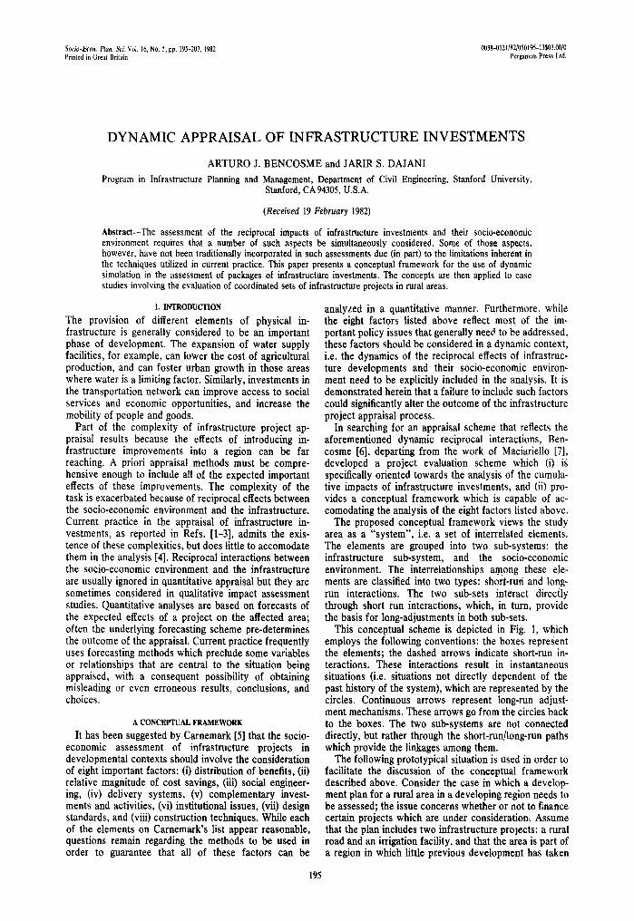
This conceptual scheme is depicted in Fig. 1, which employs the following conventions: the boxes represent the elements; the dashed arrows indicate short-run in- teractions. These interactions result in instantaneous situations (i.e. situations not directly dependent of the past history of the system), which are represented by the circles. Continuous arrows represent long-run adjust- ment mechanisms. These arrows go from the circles back to the boxes. The two sub-systems are not connected directly, but rather through the short-run/long-run paths which provide the linkages among them.
The following prototypical situation is used in order to facilitate the discussion of the conceptual framework described above. Consider the case in which a develop- ment plan for a rural area in a developing region needs to be assessed; the issue concerns whether or not to finance certain projects which are under consideration, Assume that the plan includes two infrastructure prolects: a rural road and an irrigation facility, and that the area is part of a region in which little previous development has taken
195
196 A. J. BENCOSME and J. S. DAJANI
ENVIRONMENT
SUB-SYSTEM
Environment Demand Adjustment
\ \
,~UTI LI ZAT I ONJ
/
SUB-SYSTEM I
I Infrastructure Supply
Adjustment
Fig. 1. Conceptual framework.
place. Let the corresponding investments be 2.5 and 5.0 million dollars, respectively. The following additional assumptions are made concerning the interactions be- tween the proposed projects and their socio-economic environment:
(1) It is assumed in this example that the road will be used mostly by traffic which did not exist before its construction, since, by definition, a penetration road is one which opens up new lands for use.
(2) The road will require maintenance in order to keep it operational. Maintenance, in turn, is dependent on the volume of traffic flow using it.
(3) The new land opened up by the road is assumed to produce a single argicultural commodity.
(4) Agricultural production is partly dependent upon irrigation which is assumed to affect production only by improving the productivity of the land.
(5) The increase in land productivity has two effects on the system: It increases both agricultural production and .road usage. The latter is due to the increase in the amount of cargo moved through the penetration road.
(6) In- and out-migration may occur, and will depend only on (i) the relative per capita income of the study area as compared to competing areas, and (ii) the popu- lation holding capacity of the area, which is assumed to be dependent on the amount of available agricultural land in the area.
(7) The demand for irrigation water depends on the quantity of cultivated land.
(8) The area of cultivated land is also dependent upon the supply of agricultural labor, and the latter is assumed to be equal to a fixed fraction of the population in the study area.
The interactions assumed above describe a rather icomplex set of cross linkages within the system. It is further assumed that enough capital is available for work on these lands, and that market conditions for the agri- cultural produce of the area are described by a horizon- tal, time inv~iant demand curve. It is, of course, pos- sible to rerax both of these assumptions in a more complex application of this methodology. Although the number of variables in the system representing this situ-
ation is small, the complexity of interactions is such that the future behavior of the system is not intuitively obvious.
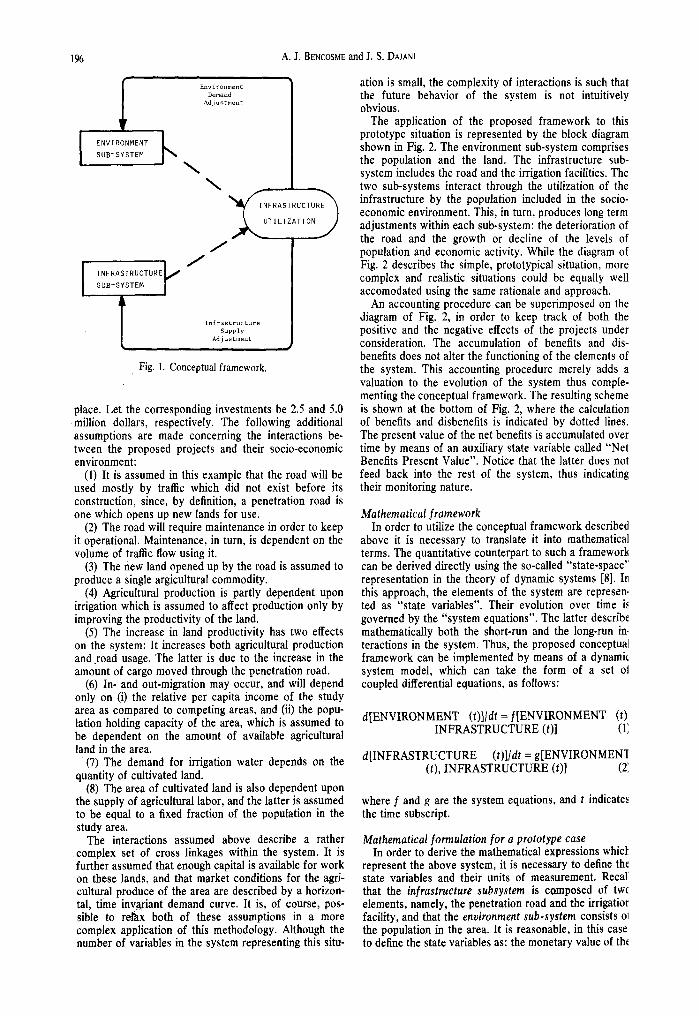
The application of the proposed framework to this prototype situation is represented by the block diagram shown in Fig. 2. The environment sub-system comprises the population and the land. The infrastructure sub- system includes the road and the irrigation facilities. The two sub-systems interact through the utilization of the infrastructure by the population included in the socio- economic environment. This, in turn, produces long term adjustments within each sub-system: the deterioration of the road and the growth or decline of the levels of population and economic activity. While the diagram of Fig. 2 describes the simple, prototypical situation, more complex and realistic situations could be equally well accomodated using the same rationale and approach.
An accounting procedure can be superimposed on the diagram of Fig. 2, in order to keep track of both the positive and the negative effects of the projects under consideration. The accumulation of benefits and dis- benefits does not alter the functioning of the elements of the system. This accounting procedure merely adds a valuation to the evolution of the system thus comple- menting the conceptual framework. The resulting scheme is shown at the bottom of Fig. 2, where the calculation of benefits and disbenefits is indicated by dotted lines. The present value of the net benefits is accumulated over time by means of an auxiliary state variable called "Net Benefits Present Value". Notice that the latter does not feed back into the rest of the system, thus indicating their monitoring nature.
Mathematical framework In order to utilize the conceptual framework described
above it is necessary to translate it into mathematical terms. The quantitative counterpart to such a framework can be derived directly using the so-called "state-space" representation in the theory of dynamic systems [8]. I~ this approach, the elements of the system are represen. ted as "state variables". Their evolution over time is governed by the "system equations". The latter describe mathematically both the short-run and the long-run in. teractions in the system. Thus, the proposed conceptual framework can be implemented by means of a dynami( system model, which can take the form of a set ot coupled differential equations, as follows:
where [ and g are the system equations, and t indicates the time subscript.
Mathematical [ormulation [or a prototype case In order to derive the mathematical expressions whict
represent the above system, it is necessary to define the state variables and their units of measurement. Recall that the in[rastructure subsystem is composed of two elements, namely, the penetration road and the irrigatior facility, and that the environment sub-system consists ol the population in the area. It is reasonable, in this case to define the state variables as: the monetary value of th(
Dynamic appraisal of infrastructure investments
MIGRATION
I " Environment Sub-system
Adjustment INFRASTRUCTURE UTILIZATION ++
I t I
[POPULATION "~-.~ ...~, 1| ~ 'I
I I I ~ Agl ic.l r ' - - , ' / Lal or J._ ~ I | AVAILABLE I ' ~ J~ "--//A~=i~'\ w
LAND ~ t ~'~-~-~- ~ " I L _ I - - i / > / -.,, F : ) , \ - ( I , ,e I CAPITAL I~ "~I""~""I~ / ~ .~. ,~Fk / " '
f f ~ , - ' 7 " / i . . . . I ' ' I ENVIRONMENT SUB-SYSTEM ' ~ I L C°sts / I~',NI
Fig. 2. Application of the conceptual framework to the prototype case.
197
road and irrigation facilities and the number of people residing in the area.
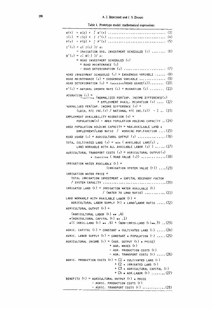
Let the three state variables described above, i.e. ACCUMULATED ROAD VALUE, ACCUMULATED VALUE OF IRRIGATION SYSTEM, AND POPU- LATION, be represented by R, I and P respectively. The rates of change in these variables at any time (t) are thus d[R(t)]/dt, d[I(t)]ldt, and d[P(t)]ldt, respectively. In- tegrating over time, the value of each of these three variables is given by eqns (3), (4), and (5) respectively. These equations, as well as all other system equations, are given in Table 1. The values of variables at t = 0 indicate initial conditions.
In the proposed conceptual framework, the long-run interactions are time-lagged adjustment mechanisms. Within the infrastructure subsystem it is assumed that only the road will have long-run adjustment mechanisms, as indicated in ~qns (6) and (7). Although the investment in road construction is an exogeneous variable (eqn 8), the cost of maintaining the road in operational condition is dependent upon the degree of deterioration, which in turn depends on the actual volume of traffic. Both road deterioration and maintenance are assumed to be effects of previous road usage (eqns 9 and 10). The environment
subsystem, on the other hand, could beassumed to react to the usage of infrastructure in a variety of ways. Nevertheless, only one adaptive socio-economic mechanism will be considered, namely, migration (eqn 11). The migration phenomenon is assumed to depend on (i) the migrants' perception of the difference between their net per capita income and the going average net per capita income in competing areas; and (ii) the availability of employment (eqns 12-15).
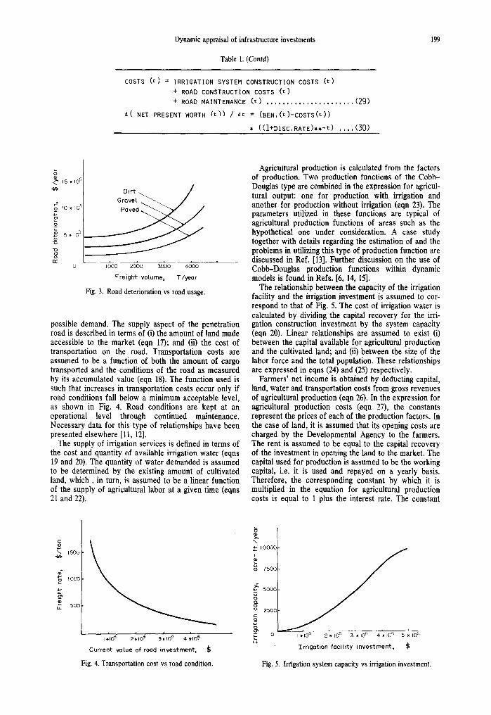
The road deterioration function is assumed to be as shown in Fig. 3. The shape of the curve indicates that road usage will significantly affect the process of normal road deterioration only when it is larger than a certain value. For levels of road utilization lower than this value, it is assumed that a fixed deterioration rate takes place. Empirical evidence for this type of relationship can be found in the transportation economics literature; see, e.g. Refs. [9, 10].
Recall that short-run interactions directly determine the utilization of the infrastructure subsystem by its environment. The demand for road use is defined to be equal to the quantity of agricultural production to be transported out of the region (eqn 16). It is assumed that road capacity is equal to or greater than the maximum
d( NET PRESENT WORTH ( t ) ) / dt = (BEN,( t ) -COSTS(t ) )
* ( (~+DISC,RATE)**- t ) . . . . (~0)
199
15.105
IO * 105
0
~. 5 * 105
OC 1000 2000 ?~300 4000
Freight votume, T /year
Fig. 3. Road deterioration vs road usage.
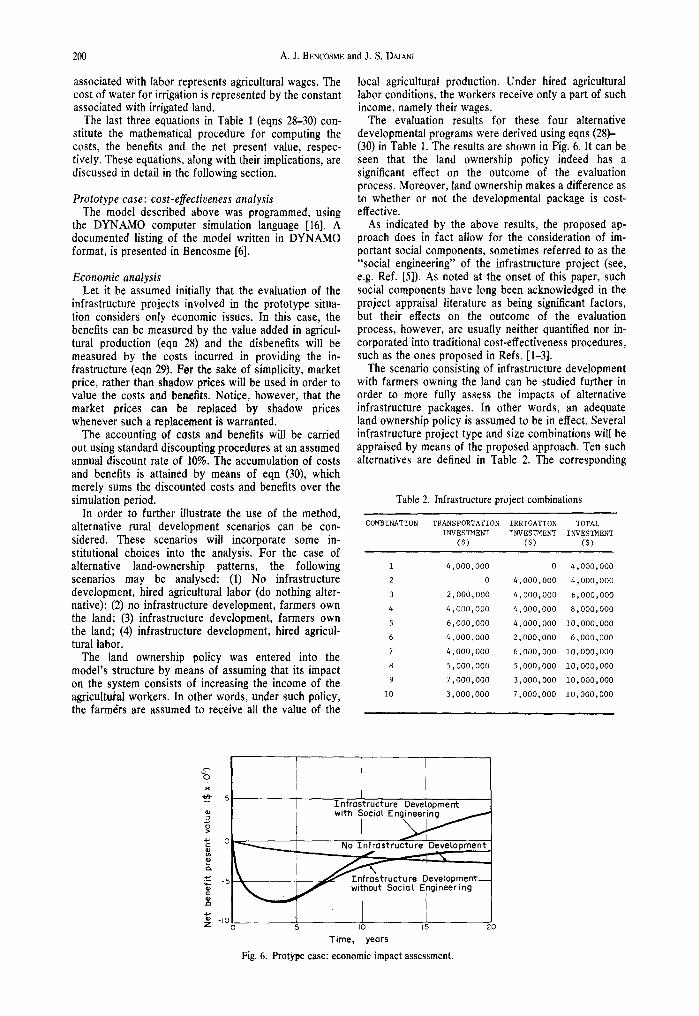
possible demand. The supply aspect of the penetration road is described in terms of (i) the amount of land made accessible to the market (eqn 17); and (ii) the cost of transportation on the road. Transportation costs are assumed to be a function of both the amount of cargo transported and the conditions of the road as measured by its accumulated value (eqn 18). The function used is such that increases in transportation costs occur only if road conditions fall below a minimum acceptable level, as shown in Fig. 4. Road conditions are kept at an operational level through continued maintenance. Necessary data for this type of relationships have been presented elsewhere [11, 12].
The supply of irrigation services is defined in terms of the cost and quantity of available irrigation water (eqns 19 and 20). The quantity of water demanded is assumed to be determined by the existing amount of cultivated land, which, in turn, is assumed to be a linear function of the supply of agricultural labor at a given time (eqns 21 and 22).
15(30 t
IOOO
if- 5°° I
i i . ~ i I*106 2.106 3~106 4 ~e106
Current vatue of road investment,
Fig. 4. Transportation cost vs road condition.
Agricultural production is calculated from the factors of production. Two production functions of the Cobb- Douglas type are combined in the expression for agricul- tural output: one for production with irrigation and another for production without irrigation (eqn 23). The parameters utilized in these functions are typical of agricultural production functions of areas such as the hypothetical one under consideration. A case study together with details regarding the estimation of and the problems in utilizing this type of production function are discussed in Ref. [13]. Further discussion on the use of Cobb-Douglas production functions within dynamic models is found in Refs. [6, 14, 15].
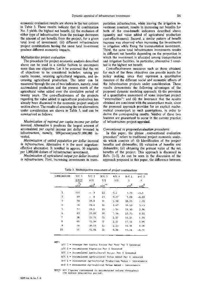
The relationship between the capacity of the irrigation facility and the irrigation investment is assumed to cor- respond to that of Fig. 5. The cost of irrigation water is calculated by dividing the capital recovery for the irri- gation construction investment by the system capacity (eqn 20). Linear relationships are assumed to exist (i) between the capital available for agricultural production and the cultivated land; and (ii) between the size of the labor force and the total population. These relationships are expressed in eqns (24) and (25) respectively.
Farmers' net income is obtained by deducting capital, land, water and transportation costs from gross revenues of agricultural production (eqn 26). In the expression for agricultural production costs (eqn 27), the. constants represent the prices of each of the production factors. In the case of land, it is assumed that its opening costs are charged by the Developmental Agency to the farmers. The rent is assumed to be equal to the capital recovery of the investment in opening the land to the market. The capital used for production is assumed to be the working capital, i.e. it is used and repayed on a yearly basis. Therefore, the corresponding constant by which it is multiplied in the equation for agricultural production costs is equal to 1 plus the interest rate. The constant
~ I O00O
7500
~ 5O0O
250C
E o I-4 I~106 2~106 5~106 4~106 5.106
Trrigation fac i l i ty investment , $
Fig. 5. Irrigation system capacity vs irrigation investment.
200 A. J. BENCOSME and J. S. DMANI
associated with labor represents agricultural wages. The cost of water for irrigation is represented by the constant associated with irrigated land.
The last three equations in Table 1 (eqns 28-30) con- stitute the mathematical procedure for computing the costs, the benefits and the net present value, respec- tively. These equations, along with their implications, are discussed in detail in the following section.
Prototype case: cost-effectiveness analysis The model described above was programmed, using
the DYNAMO computer simulation language [16]. A documented listing of the model written in DYNAMO format, is presented in Bencosme [6].
Economic analysis Let it be assumed initially that the evaluation of the
infrastructure projects involved in the prototype situa- tion considers only economic issues. In this case, the benefits can be measured by the value added in agricul- tural production (eqn 28) and the disbenefits will be measured by the costs incurred in providing the in- frastructure (eqn 29). Fer the sake of simplicity, market price, rather than shadow prices will be used in order to value the costs and benefits. Notice, however, that the market prices can be replaced by shadow prices whenever such a replacement is warranted.
The accounting of casts and benefits will be carried out using standard discounting procedures at an assumed annual discount rate of 10%. The accumulation of costs and benefits is attained by means of eqn (30), which merely sums the discounted costs and benefits over the simulation period.
In order to further illustrate the use of the method, alternative rural development scenarios can be con- sidered. These scenarios will incorporate some in- stitutional choices into the analysis. For the case of alternative land-ownership patterns, the following scenarios may be analysed: (1) No infrastructure development, hired agricultural labor (do nothing alter- native); (2) no infrastructure development, farmers own the land; (3) infrastructure development, farmers own the land; (4) infrastructure development, hired agricul- tural labor.
The land ownership policy was entered into the model's structure by means of assuming that its impact on the system consists of increasing the income of the agricultui'al workers. In other words, under such policy, the farmers are assumed to receive all the value of the
local agricultural production. Under hired agricultural labor conditions, the workers receive only a part of such income, namely their wages.
The evaluation results for these four alternative developmental programs were derived using eqns (28)- (30) in Table 1. The results are shown in Fig. 6. It can be seen that the land ownership policy indeed has a significant effect on the outcome of the evaluation process. Moreover, land ownership makes a difference as to whether or not the developmental package is cost- effective.
As indicated by the above results, the proposed ap- proach does in fact allow for the consideration of im- portant social components, sometimes referred to as the "social engineering" of the infrastructure project (see, e.g. Ref. [5]). As noted at the onset of this paper, such social components have long been acknowledged in the project appraisal literature as being significant factors, but their effects on the outcome of the evaluation process, however, are usually neither quantified nor in- corporated into traditional cost-effectiveness procedures, such as the ones proposed in Refs. [1-3].
The scenario consisting of infrastructure development with farmers owning the land can be studied further in order to more fully assess the impacts of alternative infrastructure packages. In other words, an adequate land ownership policy is assumed to be in effect. Several infrastructure project type and size combinations will be appraised by means of the proposed approach. Ten such alternatives are defined in Table 2. The corresponding
Table 2. Infrastructure project combinations
COMBINATION TRANSPORTATION IRRIGATION TOTAL INVESTMENT INVESTMENT INVESTMENT
($) ($) ($)
1 4,000,000 0 4,000,000
2 0 4,000,000 4,000,000
3 2,000,000 4,000,000 6,000,000
4 4,000,000 4,000,000 8,000,000
5 6,000,000 4,000,000 I0,000,000
6 4,000,000 2,000,000 6,000,000
7 4,000,000 6,000,000 i0,000,000
8 5,000,000 5,000,000 i0,000,000
9 7,000,000 3,000,000 i0,000,000
I0 3,000,000 7,000,000 i0,000,000
O x
o>
Z
-5
-IO O
In f ras t ruc tu re Devetopme nt with Social E n ~
No I n f r a s t r u c t u r e DeveLopment
5 i0 15 20
Time, years
Fig. 6. Protype case: economic impact assessment.
Dynamic appraisal of infrastructure investments 201
economic evaluation results are shown in the last column in Table 3. These results indicate that (i) combination No. 5 yields the highest net benefit, (ii) the exclusion of either type of infrastructure from the package decreases the amount of net benefits from the project, for a given total level of investment; (iii) different infrastructure project combinations having the same total investment produce different economic impacts.
Multiobjective project evaluation The procedure for project economic analysis described
above can be used in a similar fashion to encompass more than one objective. Let it be assumed that the set of objectives to be considered includes: raising per capita income, retaining agricultural migrants, and in- creasing agricultural production. The latter can be measured through the use of two indicators, namely, total accumulated production and the present worth of the agricultural value added over the simulation period of twenty years. The cost-effectiveness of the projects regarding the value added in agricultural production has already been discussed in the economic project analysis section above. The results of assessing the ten alternatives under consideration are shown in Table 3, and can be summarized as follows:
Maximization o[ regional per capita income per dollar invested. Alternative 6 produces the largest amount of accumulated per capital income per dollar invested in infrastructure, namely, $89/person/year/$1,000,000 in- vested.
Maximization o[ settled population per dollar invested in infrastructure. Alternative 4 is the most migration- effective alternative. It resulted in approx. 30 migrants per 1,000,000 dollars of infrastructure investment.
Maximization of agricultural output per dollar invested in infrastructure. First, increasing investments in trans-
portation infrastructure, while leaving the irrigation in- vestment constant, results in increasing net benefits for both of the cost-benefit indicators described above (quantity and value added of agricultural production cost-effectiveness). Second, a similar pattern of benefit increase was observed when increasing the investments in irrigation while fixing the transportation investment. Third, the same total infrastructure investments results in different net benefits depending on the proportion in which the investment is allocated among transportation and irrigation facilities. In particular, alternative 5 resul- ted in the highest net benefit.
Cost-effectiveness measures such as those obtained for each of the three objectives can provide inputs for policy making, since they represent a quantitative measure of the different social and economic effects of the infrastructure projects under consideration. These results demonstrate the following advantages of the proposed dynamic modeling approach: (i) the provision of a quantitative assessment of some important project "externalities"; and (ii) the insurance that the results obtained are consistent with the assumptions made, since the proposed approach provides for an explicit mathe- matical counterpart to such assumptions, in order to derive the corresponding results. Neither of these two features are guaranteed to occur in the current practice of infrastructure project appraisal.
Conventional vs proposed-evaluation procedures In this paper, the phr~tse , conventional evaluation
procedure" refers to traditional project economic analy- sis which consists of: (i) Identification of the project benefits and disbenefits; (ii) valuation of benefits and disbenefits; (iii) obtaining the present value of the net benefits of the project. This approach is discussed in Refs. [1-3]. As can be seen in the discussion of the approach proposed in this paper, the difference between
Table 3. Multiobjective assessment of project combinations
COMBINATION B/C i B/C 2 B/C 3 B/C 4 B-C i B-C 2
S/P/! P/$ T/$ $/$ $ $
xl~ 3 xlO 6 xlO -4 xl06 xl06
i I00 9 12 0.i 2.75 -3.5
2 40 6 13 0.17 7.09 -6.03
3 70 29.0 31 1.18 18.15 1.30
4 76 29.6 31 1.47 18.59 3.43
5 72 29.1 30 1.54 18.30 3.96
6 89 25.07 28 1.16 12.73 0.85
7 58 23.31 25 1.17 16.53 1.59
8 65 25.98 27 1.37 17.52 2.99
9 76 30.11 31 1.53 16.58 3.38
i0 51 21.04 22 0,98 15.26 -0.22
SEPS Vol. 16, No. 5--B
KEY: B/C i = Average Per Capita Income Per Year Per $ Invested
B/C 2 = Accumulated Migration Per $ Invested
B/C 3 = Accumulated Agricultural Output Per $ Invested
B/C 4 = Accumulated Agricultural Value Added Per $ Invested
B-C I = Discounted Agricultural Production Value ~ Investments
B-C 2 = Discounted Agricultural Value Added - Investments
NOTE: All figures correspond to accumulated values throughout the entire simulation period.
202 A. J. BENCOSME and J. S. D~AN]
the two approaches lies in the form in which the benefits and disbenefits are derived and forecasted, and in the type of benefits and disbenefits considered. While the conventional approach forecasts economic variables only, one at a time, the proposed approach can simul- taneously forecast social and economic variables, with due consideration to the cross-linkages among them.
In order to illustrate the differences between the two methods, the model for the prototype situation described above will be used. It is sufficient, for the purposes of this discussion, to assume that the only difference be- tween the two procedures lies in the variables being considered, and not in the forecasting procedure. Specifically, it will be assumed that no income-triggered migration is included in the conventional approach, since this is one of the "externalities' of the project, which are not usually incorporated into conventional analyses.
The different outputs of the model with and without the income-migration linkage are presented in Fig. 7. In this figure, the results based on the proposed approach, which makes explicit use of the income triggered migra- tion, are represented by curves 1 and 2, and curves 3 and 4 shows the results that are obtained based on the more conventional approach. It can be seen from this figure, that the conventional approach is unable to discriminate between a project which has the land ownership com- ponent and one which does not, since curves 3 and 4 are coincident. Furthermore, it can be inferred that the decision could be significantly altered by the inclusion of income-triggered migration in the analysis, as indicated by curves 1 and 2.
As pointed out by Weiss [4], the current state of the art of economic project evaluation poses more questions than answers when planners attempt to assess the project impacts on the socio-economic environment. Alternatively, the approach proposed herein addresses one of these unresolved questions, namely, that of quan- titatively including project externalities in the analysis. The above prototype application, with a reduced number of socio-economic and infrastructural variables, illus- trates the usefulness of the proposed approach for in- corporating key variables from different disciplines into the economic analysis of infrastructure projects.
Other social components, such as labor training, agri- cultural extension, agricultural industrial development, and so forth, can be included in more complex ap- plications. Their impact on evaluation results can be analysed using the dynamic modeling approach in the same fashion as the land ownership policy impact analy- sis was demonstrated above. Project engineering design standards and alternative construction techniques could also be evaluated in a similar manner.
APPLICATION CASE: AN AGRICULTURAL
BEVELOVMENT PROGRAM 1N VENEZUELA
The setting This section deals with the application of the dynamic
modeling approach to the appraisal of infrastructure investments in the Andes Region of Venezuela. This region is defined as the geographic space encompassing the Venezuelan Andes range and its corresponding piedmonts. The Andes region is located in the South- West corner of Venezuela. The responsibility for plan- ning, promoting and coordinating the development of this area has been assigned to CORPOANDES (Corporaci6n para el Desarrollo de la Regi6n de los Andes).
The Venezuelan Andes is appropriately described as a backward region [17]. One of the major problems in the development of this region arises from the circumstance that it is part of an oil exporting developing country, where a low priority is being placed on areas with a seemingly low relative economic potential. Agriculture and related industries, together with some tourism and education, represent the major development potential of the region. The region under consideration has an area of approximately 70,000km 2 (about 7.5% of the area of Venezuela). The region's population of about 1.8 million people represents 13.5% of the total for the country. Its contribution to the gross national product has remained at about 4-5%, for the past 10 yr.
This region has achieved a certain degree of develop- ment during the past decades. The rate of growth and the level of development, however, could both be increased if the region received a bigger share of the country's developmental effort. The use of this area as a case study will focus on the potential use of infrastructure invest-
x
Z
-I0 10 15 20
Time, years Ke._~y: I - Inf rastructure Devetopment with Sociat Engineering
( I n c o m e - triggered migration is considered ). 2 - Some as I, wi~:hout Sociat Engineering. 3 - Same asl, no income-triggered migration considered. 4 - Same as2, no income-triggered migration considered.
Fig. 7. Comparison of results: conventional vs dynamic modeling approach.
Dynamic appraisal of infrastructure investments 203
ments, as a major developmental activity. Attention is devoted here to examining the relationships between agricultural infrastructure, agricultural industries, and regional development, since most previous regional stu- dies have agreed that the key to the development of the region lies in attaining successful interactions among these three activities. (See, e.g. Refs. [17-21].)
The high valley agricultural infrastructure plan As one of its specific efforts, CORPOANDES
promotes the development of the agricultural sector by means of packages of projects which are directed toward particular planning areas. One such package is "The High Valley Agricultural Development Program" (Pro- grama de Desarrollo Agr~cola de los Valles Altos) [22]. The area consists of thirty valleys located at the up- stream end of the corresponding river basins. Within this Program, each comprehensive set of projects consists of irrigation, drainage, economic production, and ground transportation projects; agricultural price policies; agri- cultural extension services, agricultural credit services; land use policies; social organization of the farmers; and incentives for industrial processing of the produce.
The role of infrastructure in the High Valleys areas is directed toward the opening to the market of lands with high agricultural potential. Irrigation projects are expec- ted to make it feasible to utilize the opened lands for profitable agricultural production, and future trans- portation infrastructure will allow producers to reach market areas. In addition, agricultural produce storage facilities will be provided wherever they are needed. Other urban facilities are included in a currently ongoing regional urban infrastructure program.
Thus, the High Valleys Program is expected to trans- form stagnated areas into self-sustaining and growing communities. One question that can be asked is whether or not these expectations are realistic. A second question regards the extent to which, and the conditions under which, the above mentioned infrastructure investments would in fact contribute to the social and economic growth of the region is general, and of the High Valleys in particular.
Modeling socio.economic impacts A detailed description of a model developed for the
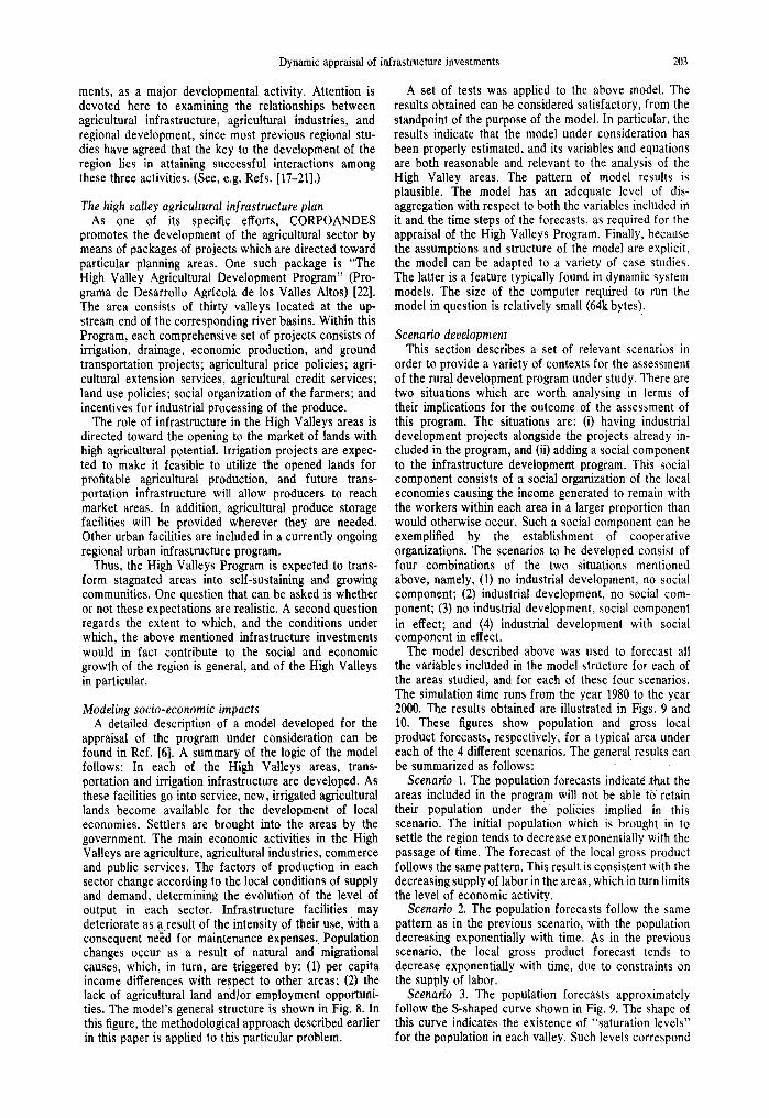
appraisal of the program under consideration can be found in Ref. [6]. A summary of the logic of the model follows: In each of the High Valleys areas, trans- portation and irrigation infrastructure are developed. As these facilities go into service, new, irrigated agricultural lands become available for the development of local economies. Settlers are brought into the areas by the government. The main economic activities in the High Valleys are agriculture, agricultural industries, commerce and public services. The factors of production in each sector change according to the local conditions of supply and demand, determining the evolution of the level of output in each sector. Infrastructure facilities may deteriorate as a result of the intensity of their use, with a consequent need for maintenance expenses, Population changes occur as a result of natural and migrational causes, which, in turn, are triggered by: (1) per capita income differences with respect to other areas; (2) the lack of agricultural land and/0r employment opportuni- ties. The model's general structure is shown in Fig. 8. In this figure, the methodological approach described earlier in this paper is applied to this particular problem.
A set of tests was applied to the above model. The results obtained can be considered satisfactory, from the standpoint of the purpose of the model. In particular, the results indicate that the model under consideration has been properly estimated, and its variables and equations are both reasonable and relevant to the analysis of the High Valley areas. The pattern of model results is plausible. The model has an adequate level of dis- aggregation with respect to both the variables included in it and the time steps of the forecasts, as required for the appraisal of the High Valleys Program. Finally, because the assumptions and structure of the model are explicit, the model can be adapted to a variety of case studies. The latter is a feature typically found in dynamic system models. The size of the computer required to run the model in question is relatively small (64k bytes).
Scenario development This section describes a set of relevant scenarios in
order to provide a variety of contexts for the assessment of the rural development program under study. There are two situations which are worth analysing in terms of their implications for the outcome of the assessment of this program. The situations are: (i) having industrial development projects alongside the projects already in- cluded in the program, and (ii) adding a social component to the infrastructure development program. This social component consists of a social organization of the local economies causing the income generated to remain with the workers within each area in a larger proportion than would otherwise occur. Such a social component can be exemplified by the establishment of cooperative organizations. The scenarios to be developed consist of four combinations of the two situations mentioned above, namely, (1) no industrial development, no social component; (2) industrial development, no social com- ponent; (3) no industrial development, social component in effect; and (4) industrial development with social component in effect.
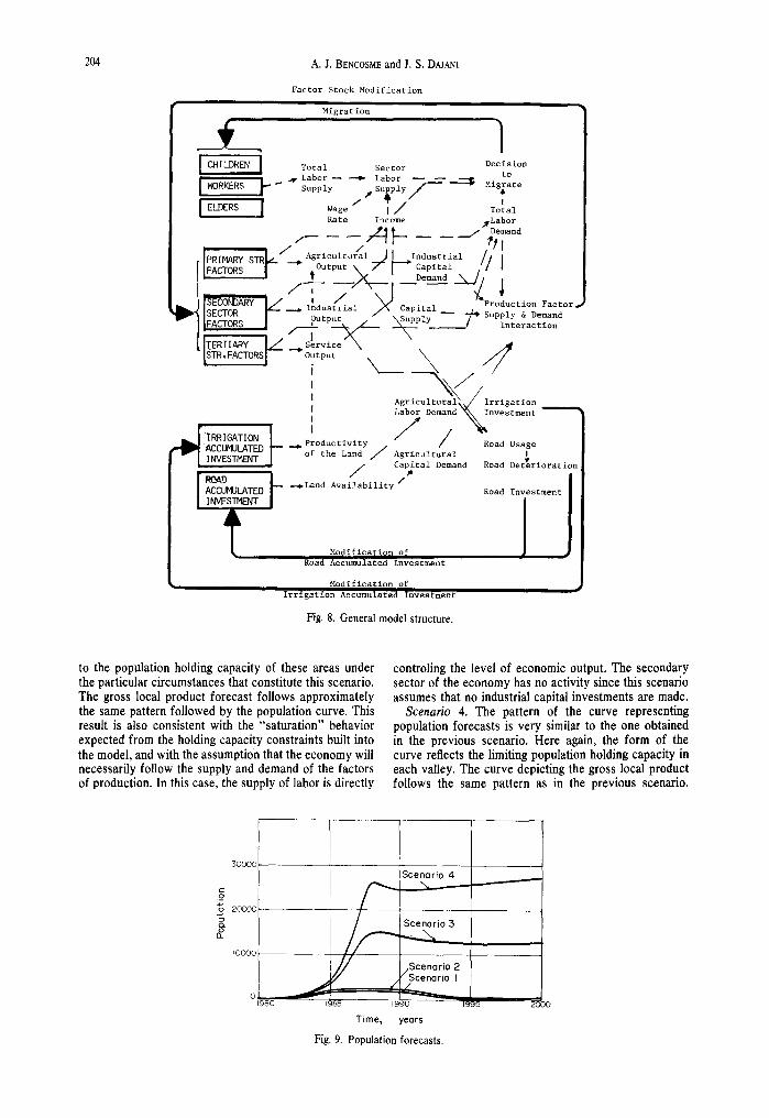
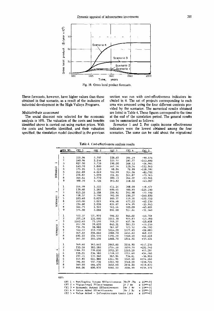
The model described above was used to forecast all the variables included in the model structure for each of the areas studied, and for each of these four scenarios. The simulation time runs from the year 1980 to the year 2000. The results obtained are illustrated in Figs. 9 and 10. These figures show population and gross local product forecasts, respectively, for a typical area under each of the 4 different scenarios. The general results can be summarized as follows:
Scenario 1. The population forecasts indicate.that the areas included in the program will not be able to retain their population under the policies implied in this scenario. The initial population which is brought in to settle the region tends to decrease exponentially with the passage of time. The forecast of the local gross product follows the same pattern. This result is consistent with the decreasing supply of labor in the areas, which in turn limits the level of economic activity.
Scenario 2. The population forecasts follow the same pattern as in the previous scenario, with the population decreasing exponentially with time. As in the previous scenario, the local gross product forecast tends to decrease exponentially with time, due to constraints on the supply of labor.
Scenario 3. The population forecasts approximately follow the S-shaped curve shown in Fig. 9. The shape of this curve indicates the existence of "saturation levels" for the population in each valley. Such levels correspond
204 A.J. BENCOSME and J. S. D~JAN]
Factor Stock Modification
Migration
I CHILDREN I Total Sector Labor -- ---~ Labor
T~
l Decision
to 1 Migrate
I Total
Rate Income .~Labor ~ ~ ~." Demand
/ r 7 1 " - - ~ - - /'#1 r . . . . . . . . . . i . / Ag ricultur/al J I Industrial / ' I | ~ . ~ o.~.- -- Output \ 7 ~ ~ Capital // [ , -- . . . . d \ h •
)SECONDARY I / - ' - / . " ~ . . . Production Factor, __~ inaustrial uapltal ~i~ ISECTOR P ~ - /~ . . . . . . -- --/~ Supply & Demand I FACTORs I ~ 'p~/ /_.__ . ~ e . e -~' # I n t . . . . t i o n
I Agr icultural~. / irrlgat ion I Labor D .... d%l .... truant
- tmRmAT,ON | . / / ~CCIMII 6T~r~ ~ -'~ Productivity / / Road Usage r mvl INVES~ I o the Land / Agricultural I
~r / / Capital D .... d Road Det~riorati~[
ROAD F --~Land Availability / ACCUMULATED I INVESTMENT
t Modification of Road Accumulated Investment
Road Investment
1. Modification of
Irrigation Accumulated Investment
Fig. 8. General model structure.
to the population holding capacity of these areas under the particular circumstances that constitute this scenario. The gross local product forecast follows approximately the same pattern followed by the population curve. This result is also consistent with the "saturation" behavior expected from the holding capacity constraints built into the model, and with the assumption that the economy will necessarily follow the supply and demand of the factors of production. In this case, the supply of labor is directly
controling the level of economic output. The secondary sector of the economy has no activity since this scenario assumes that no industrial capital investments are made.
Scenario 4. The pattern of the curve representing population forecasts is very similar to the one obtained in the previous scenario. Here again, the form of the curve reflects the limiting population holding capacity in each valley. The curve depicting the gross local product follows the same pattern as in the previous scenario.
3000C
c 0 4-, o 2000~
O. £
IO00(
0 1980 1985
T ime, years
Fig. 9. Population forecasts.
Scenario 4
Scenario 3
Scenario 2 /Scenario I
35 2C
Dynamic appraisal of infrastructure investments 205
90
~ ~o
o
1980 1985 1990 1990
Time, yeors
Fig . 10. Gross local product forecasts.
2000
These forecasts, however, have higher values than those obtained in that scenario, as a result of the inclusion of industrial development in the High Valleys Programs.
Multiattribute assessment The social discount rate selected for the economic
analysis is 10%. The valuation of the costs and benefits identified above is carried out using market prices. With the costs and benefits identified, and their valuation specified, the simulation model described in the previous
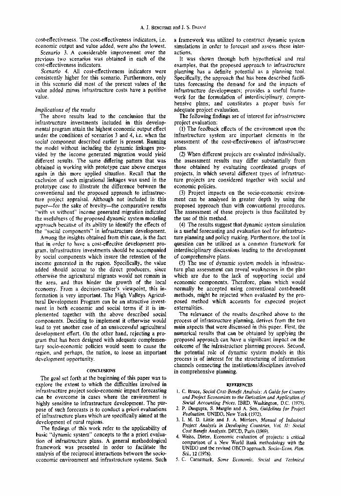
section was run with cost-effectiveness indicators in- cluded in it. The set of projects corresponding to each area was assessed using the four different contexts pro- vided by the scenarios. The numerical results obtained are listed in Table 4. These figures correspond to the time at the end of the simulation period. The general results can be summarized as follows:
Scenarios 1 and 2. Per capita income effectiveness indicators were the lowest obtained among the four scenarios. The same, can be said about the migrational
CEI i = Per/Caplta Income Effectiveness [Br/P /Br x 10"*-9] CEI 2 = Migrational Effectiveness [P / Br x i0"*-6] CEI 3 = Economic Output Effectiveness [Br / Br x 10"*-3] CEI 4 = Value Added Effectiveness [Br / Br x 10"*-3] CEI 5 = Value Added - Infrastructure Costs [Brs x 10"*+6]
A. J. BENCOSME and J. S. DAJANI
cost-effectiveness. The cost-effectiveness indicators, i.e. economic output and value added, were also the lowest.
Scenario 3. A considerable improvement over the previous two scenarios was obtained in each of the cost-effectiveness indicators.
Scenario 4. All cost-effectiveness indicators were consistently higher for this scenario. Furthermore, only in this scenario did most of the present values of the value added minus infrastructure costs have a positive value.
Implications of the results The above results lead to the conclusion that the
infrastructure investments included in this develop- mental program attain the highest economic output effect under the conditions of scenarios 3 and 4, i.e. when the social component described earlier is present. Running the model without including the dynamic linkages pro- vided by the income generated migration would yield different results. The same differing pattern that was obtained in working with prototype case above emerges again in this more applied situation. Recall that the exclusion of such migrational linkages was used in the prototype case to illustrate the difference between the conventional and the proposed approach to infrastruc- ture project appraisal. Although not included in this paper--for the sake of brevity--the comparative results "with vs without" income generated migration indicated the usefulness of the proposed dynamic system modeling approach because of its ability to identify the effects of the "social components" in infrastructure development.
Among the insights obtained from this case, is the fact that in order to have a cost-effective development pro- gram, infrastructure investments should be accompanied by social components which insure the retention of the income generated in the region. Specifically, the value added should accrue to the direct producers, since otherwise the agricultural migrants would not remain in the area, and thus hinder the growth of the local economy. From a decision-maker's viewpoint, this in- formation is very important. The High Valleys Agricul- tural Development Program can be an attractive invest- ment in both economic and social terms if it is im- plemented together with the above described social components. Deciding to implement it otherwise would lead to yet another case of an unsuccessful agricultural development effort. On the other hand, rejecting a pro- gram that has been designed with adequate complemen- tary socio-economic policies would seem to cause the region, and perhaps, the nation, to loose an important development opportunity.
CONCLUSIONS
The goal set forth at the beginning of this paper was to explore the extent to which the difficulties involved in infrastructure project socio-economic impact forecasting can be overcome in cases where the environment is highly sensitive to infrastructure development. The pur- pose of such forecasts is to conduct a priori evaluations of infrastructure plans which are specifically aimed at the development of rural regions.
The findings of this work refer to the applicability of basic "dynamic system" concepts to the a priori evalua- tion of infrastructure plans. A general methodological framework was presented in order to facilitate the analysis of the reciprocal interactions between the socio- economic environment and infrastructure systems. Such
a framework was utilized to construct dynamic system simulations in order to forecast and assess these inter- actions.
It was shown through both hypothetical and real examples, that the proposed approach to infrastructure planning has a definite potential as a planning tool. Specifically, the approach that has been described facili- tates forecasting the demand for and the impacts of infrastructure developments; provides a useful frame- work for the formulation of interdisciplinary, compre- hensive plans; and constitutes a proper basis for adequate project evaluation.
The following findings are of interest for infrastructure project evaluation:
(1) The feedback effects of the environment upon the infrastructure system are important elements in the assessment of the cost-effectiveness of infrastructure plans.
(2) When different projects are evaluated individually, the assessment results may differ substantially from those obtained by evaluating coordinated groups of projects, in which several different types of infrastruc- ture projects are considered together with social and economic policies.
(3) Project impacts on the socio-economic environ- ment can be analysed in greater depth by using the proposed approach than with conventional procedures. The assessment of these projects is thus facilitated by the use of this method.
(4) The results suggest that dynamic system simulation is a useful forecasting and evaluation tool for infrastruc- ture planning and policy making. Furthermore, the tool in question can be utilized as a common framework for interdisciplinary discussions leading to the development of comprehensive plans.
(5) The use of dynamic system models in infrastruc- ture plan assessment can reveal weaknesses in the plan which are due to the lack of supporting social and economic components. Therefore, plans which would normally be accepted using conventional cost-benefit methods, might be rejected when evaluated by the pro- posed method which accounts for expected project externalities.
The relevance of the results described above to the process of infrastructure planning, derives from the two main aspects that were discussed in this paper. First, the numerical results that can be obtained by applying the proposed approach can have a significant impact on the outcome of the infrastructure planning process. Second, the potential role of dynamic system models in this process is of interest for the structuring of information channels connecting the institutions/disciplines involved in comprehensive planning.
REFERENCES 1. C. Bruce, Social Cost-Benefit Analysis: A Guide for Country
and Project Economists to the Derivation and Application of Social Accounting Prices. IBRD, Washington, D.C. (1975).
2. P. Dasgupta, S. Marglin and A. Sen, Guidelines [or Project Evaluation. UNIDO, New York (1972),
3. I. M. D. Little and J. A. Mirrlees, Manual o/ Industrial Project Analysis in Developing Countries, Vol. II: Social Cost Ben~t Analysis. DECD, Paris (1%9).
4. Weiss, Dieter, Economic evaluation of projects: a critical comparison of a New World Bank methodology with the UNIDO and the revised OECD approach. Socio-Econ. Plan. Sci., 12 (1978).
5. C. Carnemark, Some Economic, Social and Technical
Dynamic appraisal of infrastructure investments 207
Aspects oy Rural Roads. Paper presented at the United Nations (ESCAP) Workshop on Rural Roads. Dacca (1979).
6. Bencosme, Arturo, Infrastructure planning for regional development: a dynamic modeling approach. Ph.D. Thesis. Stanford University (1979).
7. J. A. Maciariello, Dynamic Benefit Cost Analysis, Policy Evaluation in a l)yanmic Urban Simulation Model. Lexing- ton Books, Lexington, Mass. (1975).
8. F. Cortes, A. Przeworski and J. Sprague, System Analysis for Social Scientists. Wiley, New York (1974).
9. C. H. Oglesby and M. J. Altenhofen, Economics of design standards for low volume rural roads. HRB Rep. 63 (1969).
10. J. W. Hodges, J. Rolt and T. E. Jones, The Kenya road transport cost study: research on road deterioration. U.K. Transport and Road Research Lab., TRRL Rep. LR 673 (1975).
i1. R. M. Soberman, Transport Technology for Developing Regions, MIT Press, Cambridge, Mass. (1%6).
12. H. Hide, S. W. Abaynayaka, I. Sayer and R. J. Wyatt, The Kenya road transport cost study: research on vehicle operating costs. U.K. Transport and Road Research Lab., TRRL Rep. LR 672 (1975).
13. P. A. Yotopoulos and J. B. Nugent, Economics of Develop- ment: Empirical Investigations. Harper-Row Publishers, New York (1976).
14. S. K. Schuck, Migration, income and public policy in a three region economy: a simulation model for Peru. Ph.D. Thesis. Stanford University (1977).
15. H. Ervick, The causal structure and implicit assumptions of alternative production functions. Darmouth Systems Dynamics Group, Rep. DSD-19 (1974).
16. A. Pugh III, DYNAMO User's Manual, 5th Ed. MIT Press, Cambridge, Mass. (1976).
17. CORPOANDES, Plan de la Region de los Andes (1977). 18. CORPOANDES, La Subregion Chama-Moeoties (1971). 19. CORPOANDES, La Subregion Grita-Torbes (1972). 20. CORPOANDES, La Subregion Motatan-Cenizo (1971). 21. CORPOANDES, Programa Altos Llanos Occidentales
(1971). 22. CORPOANDES, Pragrama de Desarrollo Agricola de Valles
Altos de la Region Andina: Fundamentos y Methodologia (Agricultural Development Program for the High Valleys of the Andean Region: Foundations and Methodology) (1978).