Dynamical Scaling Implications of Ferrari, Pr¨ ahofer, and Spohn’s Remarkable Spatial Scaling Results for Facet-Edge Fluctuations T.L. Einstein 1, 2, * and Alberto Pimpinelli 1, 3, † 1 Department of Physics, University of Maryland, College Park, Maryland 20742-4111, USA 2 Condensed Matter Theory Center, University of Maryland, College Park, Maryland 20742-4111, USA 3 Rice Quantum Institute, Rice University, Houston, Texas 77005, USA (Dated: December 18, 2013) Spurred by theoretical predictions from Spohn and coworkers [Phys. Rev. E 69, 035102(R) (2004)], we rederived and extended their result heuristically as well as investigated the scaling properties of the associated Langevin equation in curved geometry with an asymmetric potential. With experimental colleagues we used STM line scans to corroborate their prediction that the fluctuations of the step bounding a facet exhibit scaling properties distinct from those of isolated steps or steps on vicinal surfaces. The correlation functions was shown to go as t 0.15(3) decidedly different from the t 0.26(2) behavior for fluctuations of isolated steps. From the exponents, we were able to categorize the universality, confirming the prediction that the non-linear term of the KPZ equation, long known to play a central role in non-equilibrium phenomena, can also arise from the curvature or potential-asymmetry contribution to the step free energy. We also considered, with modest Monte Carlo simulations, a toy model to show that confinement of a step by another nearby step can modify as predicted the scaling exponents of the step’s fluctuations. This paper is an expansion of a celebratory talk at the 95 th Rutgers Statistical Mechanics Conference, May 2006. I. INTRODUCTION Fluctuations of steps on surfaces play a central role in determining their impact on surface processes and the evolution of surface morphology. In the past nearly-two decades, the step continuum model has allowed several successful quantitative correlations of direct observations of step fluctuations with kinetic and thermodynamic de- scriptions of nanoscale structural evolution [1–5], bridg- ing from the atomistic and nanoscale to the mesoscale. For steps on flat or vicinal (misoriented modestly from a facet orientation) surfaces, there are two well-defined scaling behaviors for temporal correlations, correspond- ing to cases B and A, conserved and non-conserved dy- namics, respectively, in the framework of dynamic critical phenomena [6]. Several examples of both behaviors have been observed experimentally in physical systems [1, 2, 7] and numerically in Monte Carlo simulations [8–10]. For complex structures where mass transport is lim- ited by geometry, the fundamental question of how fluc- tuations behave in a constrained environment becomes experimentally accessible. These issues become particu- larly important for smaller structures, especially nanos- tructures, where issues of finite volume (shape effects and volume conservation) become non-negligible [11, 12]. Al- though the step can still be viewed as a 1D interface obeying a Langevin-type equation of motion, not only local deformation but global effects must be considered when calculating the step chemical potential. These con- siderations alter the equation of motion, including the noise term, resulting in different universality classes of dynamic scaling [13] (see Table II below). * [email protected]† [email protected]Thus, it was especially enlightening and inspiring to read of a well-defined intermediate scaling regime in Fer- rari, Pr¨ ahofer, and Spohn’s stimulating paper [14] (here- after FPS) (as well as related works [15–17]), in which they computed the scaling of equilibrium fluctuations of an atomic ledge bordering a crystalline facet surrounded by rough regions of the equilibrium crystal shape in their examination of a 3D Ising corner (Fig. 1). We refer to this boundary edge as the “shoreline” since it is the edge of an island-like region–the crystal facet–surrounded by a “sea” of steps. FPS derive an intriguing exact result, concerning how the width w of shoreline fluctuations scales as a function of the linear size of the facet. This length corresponds to the length of a step or the linear dimension of an island (or its circumference). This length is often called L [18, 19] and other times ‘ [20] (while ‘ has a closely related but slightly different meaning in Ref. [14]). To prevent any possible confusion, we denote this length by the Polish crossed L, L, in this paper, following the notation used in a ceremonial presentation on this subject [21]. We anticipate that w ∼ L α , (1) where the value of roughness exponent α depends on the mode of mass transport and the geometry of the step. For the step that serves as the border a two-dimensional (2D) island on a high-symmetry crystal plane, one ex- pects (and finds in physical and numerical experiments) that w ∼ L 1/2 , i.e. α =1/2, since this step performs a random walk [22]. FPS show that, as we quipped in the title of our paper [20], “a crystal facet is not an island”. Indeed, they find that instead of the expected random-walk behavior, w ∼ L 1/3 , (2) arXiv:1312.4910v1 [cond-mat.stat-mech] 17 Dec 2013
Transcript
Dynamical Scaling Implications of Ferrari, Prahofer, and Spohn’s Remarkable SpatialScaling Results for Facet-Edge Fluctuations
T.L. Einstein1, 2, ∗ and Alberto Pimpinelli1, 3, †
1Department of Physics, University of Maryland, College Park, Maryland 20742-4111, USA2Condensed Matter Theory Center, University of Maryland, College Park, Maryland 20742-4111, USA
3Rice Quantum Institute, Rice University, Houston, Texas 77005, USA(Dated: December 18, 2013)
Spurred by theoretical predictions from Spohn and coworkers [Phys. Rev. E 69, 035102(R)(2004)], we rederived and extended their result heuristically as well as investigated the scalingproperties of the associated Langevin equation in curved geometry with an asymmetric potential.With experimental colleagues we used STM line scans to corroborate their prediction that thefluctuations of the step bounding a facet exhibit scaling properties distinct from those of isolatedsteps or steps on vicinal surfaces. The correlation functions was shown to go as t0.15(3) decidedlydifferent from the t0.26(2) behavior for fluctuations of isolated steps. From the exponents, we wereable to categorize the universality, confirming the prediction that the non-linear term of the KPZequation, long known to play a central role in non-equilibrium phenomena, can also arise from thecurvature or potential-asymmetry contribution to the step free energy. We also considered, withmodest Monte Carlo simulations, a toy model to show that confinement of a step by another nearbystep can modify as predicted the scaling exponents of the step’s fluctuations. This paper is anexpansion of a celebratory talk at the 95th Rutgers Statistical Mechanics Conference, May 2006.
I. INTRODUCTION
Fluctuations of steps on surfaces play a central role indetermining their impact on surface processes and theevolution of surface morphology. In the past nearly-twodecades, the step continuum model has allowed severalsuccessful quantitative correlations of direct observationsof step fluctuations with kinetic and thermodynamic de-scriptions of nanoscale structural evolution [1–5], bridg-ing from the atomistic and nanoscale to the mesoscale.For steps on flat or vicinal (misoriented modestly froma facet orientation) surfaces, there are two well-definedscaling behaviors for temporal correlations, correspond-ing to cases B and A, conserved and non-conserved dy-namics, respectively, in the framework of dynamic criticalphenomena [6]. Several examples of both behaviors havebeen observed experimentally in physical systems [1, 2, 7]and numerically in Monte Carlo simulations [8–10].
For complex structures where mass transport is lim-ited by geometry, the fundamental question of how fluc-tuations behave in a constrained environment becomesexperimentally accessible. These issues become particu-larly important for smaller structures, especially nanos-tructures, where issues of finite volume (shape effects andvolume conservation) become non-negligible [11, 12]. Al-though the step can still be viewed as a 1D interfaceobeying a Langevin-type equation of motion, not onlylocal deformation but global effects must be consideredwhen calculating the step chemical potential. These con-siderations alter the equation of motion, including thenoise term, resulting in different universality classes ofdynamic scaling [13] (see Table II below).
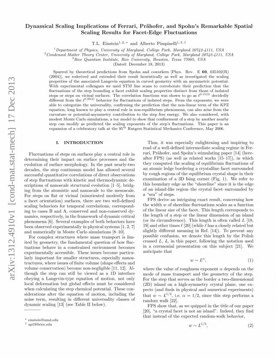
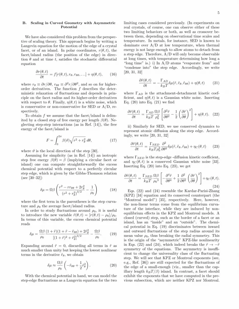
Thus, it was especially enlightening and inspiring toread of a well-defined intermediate scaling regime in Fer-rari, Prahofer, and Spohn’s stimulating paper [14] (here-after FPS) (as well as related works [15–17]), in whichthey computed the scaling of equilibrium fluctuations ofan atomic ledge bordering a crystalline facet surroundedby rough regions of the equilibrium crystal shape in theirexamination of a 3D Ising corner (Fig. 1). We refer tothis boundary edge as the “shoreline” since it is the edgeof an island-like region–the crystal facet–surrounded bya “sea” of steps.
FPS derive an intriguing exact result, concerning howthe width w of shoreline fluctuations scales as a functionof the linear size of the facet. This length corresponds tothe length of a step or the linear dimension of an island(or its circumference). This length is often called L [18,19] and other times ` [20] (while ` has a closely related butslightly different meaning in Ref. [14]). To prevent anypossible confusion, we denote this length by the Polishcrossed L, L, in this paper, following the notation usedin a ceremonial presentation on this subject [21]. Weanticipate that
w ∼ Lα, (1)
where the value of roughness exponent α depends on themode of mass transport and the geometry of the step.For the step that serves as the border a two-dimensional(2D) island on a high-symmetry crystal plane, one ex-pects (and finds in physical and numerical experiments)
that w ∼ L1/2, i.e. α = 1/2, since this step performs arandom walk [22].
FPS show that, as we quipped in the title of our paper[20], “a crystal facet is not an island”. Indeed, they findthat instead of the expected random-walk behavior,
i.e. α = 1/3, for a crystal facet. They prove that the
origin of the unusual L1/3 scaling lies in the step-step in-teractions between the facet ledge and the neighboringsteps under conditions of conserved volume. Note thatthis value of α is intermediate between α = 1/2 for iso-lated steps and α = 0 (w ∼ ln( L))) [23] for a step on avicinal surface, i.e. in a step train.
FPS’s formidable calculation is based on the use offree spinless fermions, transfer matrices, random-matrixproperties, Airy functions, and specific models; as apurely static result, it does not address the question ofthe time behavior of step fluctuations, which are easierto measure experimentally.
This article is an expansion of a celebratory talk [21]which described the impact of FPS on our research,in particular the results found in three publications[19, 20, 24]. In Section II we summarize highlights of FPSthat motivated and underpinned our subsequent work. InSection III we describe the relevant correlation functions.Next we present a heuristic derivation extending the rea-soning of Pimpinelli et al. [18] that leads to the dynamicscaling of shoreline fluctuations, as well as the static re-sult of FPS. Then we present a more formal analysisof scaling for curved steps in an asymmetric potential.In Section IV we describe experiments using scanningtunneling microscopy (STM) that demonstrate the novelscaling behavior in a physical system. In Section V wepresent Monte Carlo results for a toy model that showsin a simple system the effect of a neighboring step onthe fluctuations of a step. The Conclusion section offerssome final remarks.
FIG. 1. Simple-cubic crystal corner viewed from the 111direction, from Refs. [14–17].
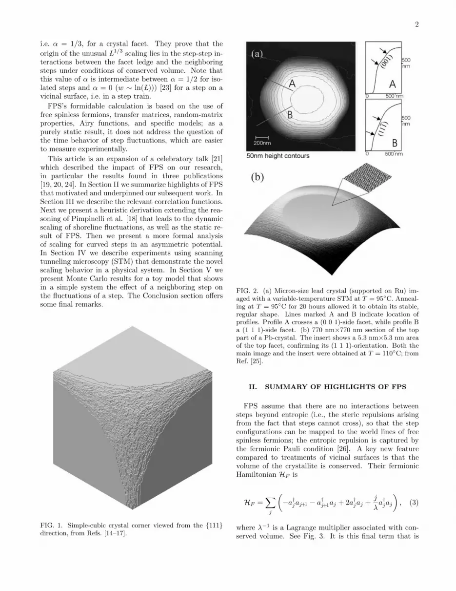
FIG. 2. (a) Micron-size lead crystal (supported on Ru) im-aged with a variable-temperature STM at T = 95C. Anneal-ing at T = 95C for 20 hours allowed it to obtain its stable,regular shape. Lines marked A and B indicate location ofprofiles. Profile A crosses a (0 0 1)-side facet, while profile Ba (1 1 1)-side facet. (b) 770 nm×770 nm section of the toppart of a Pb-crystal. The insert shows a 5.3 nm×5.3 nm areaof the top facet, confirming its (1 1 1)-orientation. Both themain image and the insert were obtained at T = 110C; fromRef. [25].
II. SUMMARY OF HIGHLIGHTS OF FPS
FPS assume that there are no interactions betweensteps beyond entropic (i.e., the steric repulsions arisingfrom the fact that steps cannot cross), so that the stepconfigurations can be mapped to the world lines of freespinless fermions; the entropic repulsion is captured bythe fermionic Pauli condition [26]. A key new featurecompared to treatments of vicinal surfaces is that thevolume of the crystallite is conserved. Their fermionicHamiltonian HF is
HF =∑j
(−a†jaj+1 − a
†j+1aj + 2a†jaj +
j
λa†jaj
), (3)
where λ−1 is a Lagrange multiplier associated with con-served volume. See Fig. 3. It is this final term that is
3
new in their treatment. Its asymmetry is key to the novelbehavior they find. They then derive an exact result forthe step density in terms of Jj , the Bessel function of in-teger order j, and its derivative. Near the shoreline theyfind
limλ→∞
λ1/3ρλ(λ1/3x) = −x(Ai(x))2 + (Ai′(x))2, (4)
where ρλ is the step density (for the particular value ofλ).
The presence of the Airy function Ai results from theasymmetric potential implicit in HF and preordains ex-ponents involving 1/3. The variance of the wandering ofthe shoreline, the top fermionic world line in Fig. 3 anddenoted by b, is given by
Var[bλ(t)− bλ(0)] ∼= λ2/3g(λ−2/3t) (5)
where t is the fermionic “time” along the step; g(s) ∼2|s| for small s (diffusive meandering) and ∼ 1.6264 −2/s2 for large s. They then set λ to a scaling parameter` = (4N/1.202 . . .)1/3, where 1.202 . . . is Apery’s constantand N is the number of atoms in the crystal, as in Fig. 1.They find
Var[b`(`τ + x)− b`(`τ)] ∼= (A`)2/3g(A1/3`−2/3x
), (6)
where A = (1/2)b′′∞ [27]. This leads to the central resultthat the width w ∼ `1/3. Furthermore, the fluctuationsare non-Gaussian. They also show that near the shore-line, the deviation of the equilibrium crystal shape fromthe facet plane takes on the Gruber-Mullins-Pokrovsky-Talapov [28] form −(r − r0)3/2, where r is the lateraldistance from the facet center and r0 is the radius of thefacet.
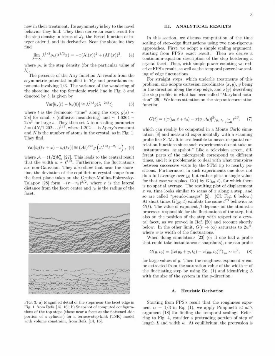
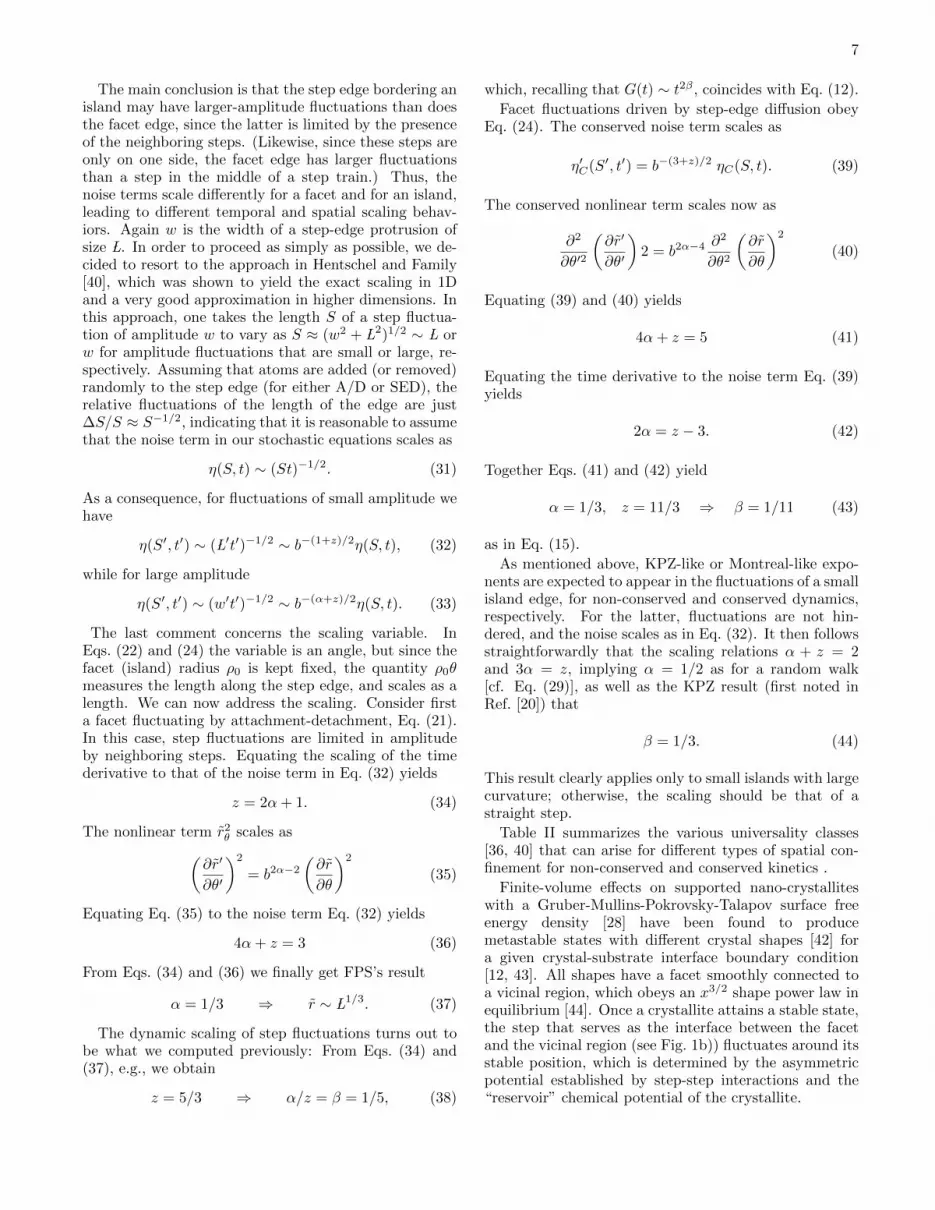
FIG. 3. a) Magnified detail of the steps near the facet edge inFig. 1, from Refs. [15, 16]; b) Snapshot of computed configura-tions of the top steps (those near a facet at the flattened sideportion of a cylinder) for a terrace-step-kink (TSK) modelwith volume constraint, from Refs. [14, 16].
III. ANALYTICAL RESULTS
In this section, we discuss computation of the timescaling of step-edge fluctuations using two non-rigorousapproaches. First, we adopt a simple scaling argument,starting from FPS’s exact result. Then we derive acontinuum-equation description of the step bordering acrystal facet. Then, with simple power counting we red-erive FPS’s result, as well as the temporal power-law scal-ing of edge fluctuations.
For straight steps, which underlie treatments of thisproblem, one adopts cartesian coordinates (x, y), y beingin the direction along the step edge, and x(y) describingthe step profile, in what has been called “Maryland nota-tion” [29]. We focus attention on the step autocorrelationfunction
G(t) = 〈[x(y0, t+ t0)− x(y0, t0)]2〉y0,t0 ∼t→0
t2β , (7)
which can readily be computed in a Monte Carlo simu-lation [8] and measured experimentally with a scanningprobe like STM. It is less feasible to measure spatial cor-relation functions since such experiments do not take aninstantaneous “snapshot.” Like a television screen, dif-ferent parts of the micrograph correspond to differenttimes, and it is problematic to deal with what transpiresbetween successive visits by the STM tip to nearby po-sitions. Furthermore, in such experiments one does notdo a full average over y0 but rather picks a single value;for that case we replace G(t) by G(y0, t), for which thereis no spatial average. The resulting plot of displacementx vs. time looks similar to scans of x along a step, andso are called “pseudo-images” [2]. (Cf. Fig. 6 below.)At short times G(y0, t) exhibits the same t2β behavior asG(t). The value of exponent β depends on the atomisticprocesses responsible for the fluctuations of the step, butalso on the position of the step with respect to a crys-tal facet, as we proved in Ref. [20] and recount shortlybelow. In the other limit, G(t → ∞) saturates to 2w2,where w is width of the fluctuations.
When doing simulations [23] (or if one had a probethat could take instantaneous snapshots), one can probe
for large values of y. Then the roughness exponent α canbe extracted from the saturation value of the width w ofthe fluctuating step by using Eq. (1) and identifying Lwith the size of the system in the y-direction.
A. Heuristic Derivation
Starting from FPS’s result that the roughness expo-nent α = 1/3 in Eq. (1), we apply Pimpinelli et al.’sargument [18] for finding the temporal scaling: Refer-ring to Fig. 4, consider a protruding portion of step oflength L and width w. At equilibrium, the protrusion is
4
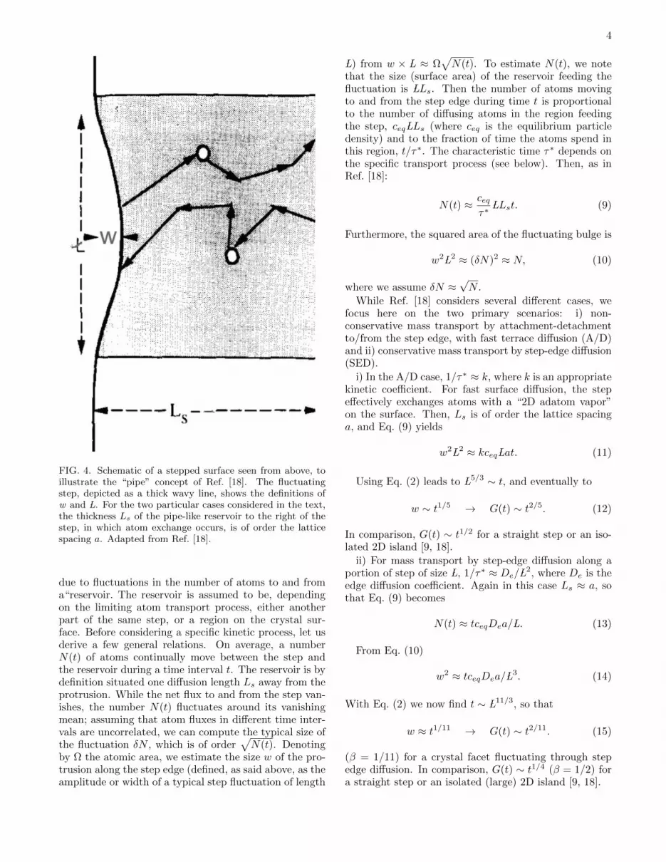
FIG. 4. Schematic of a stepped surface seen from above, toillustrate the “pipe” concept of Ref. [18]. The fluctuatingstep, depicted as a thick wavy line, shows the definitions ofw and L. For the two particular cases considered in the text,the thickness Ls of the pipe-like reservoir to the right of thestep, in which atom exchange occurs, is of order the latticespacing a. Adapted from Ref. [18].
due to fluctuations in the number of atoms to and froma“reservoir. The reservoir is assumed to be, dependingon the limiting atom transport process, either anotherpart of the same step, or a region on the crystal sur-face. Before considering a specific kinetic process, let usderive a few general relations. On average, a numberN(t) of atoms continually move between the step andthe reservoir during a time interval t. The reservoir is bydefinition situated one diffusion length Ls away from theprotrusion. While the net flux to and from the step van-ishes, the number N(t) fluctuates around its vanishingmean; assuming that atom fluxes in different time inter-vals are uncorrelated, we can compute the typical size ofthe fluctuation δN , which is of order
√N(t). Denoting
by Ω the atomic area, we estimate the size w of the pro-trusion along the step edge (defined, as said above, as theamplitude or width of a typical step fluctuation of length
L) from w × L ≈ Ω√N(t). To estimate N(t), we note
that the size (surface area) of the reservoir feeding thefluctuation is LLs. Then the number of atoms movingto and from the step edge during time t is proportionalto the number of diffusing atoms in the region feedingthe step, ceq LLs (where ceq is the equilibrium particledensity) and to the fraction of time the atoms spend inthis region, t/τ∗. The characteristic time τ∗ depends onthe specific transport process (see below). Then, as inRef. [18]:
N(t) ≈ ceqτ∗
LLst. (9)
Furthermore, the squared area of the fluctuating bulge is
w2 L2 ≈ (δN)2 ≈ N, (10)
where we assume δN ≈√N .
While Ref. [18] considers several different cases, wefocus here on the two primary scenarios: i) non-conservative mass transport by attachment-detachmentto/from the step edge, with fast terrace diffusion (A/D)and ii) conservative mass transport by step-edge diffusion(SED).
i) In the A/D case, 1/τ∗ ≈ k, where k is an appropriatekinetic coefficient. For fast surface diffusion, the stepeffectively exchanges atoms with a “2D adatom vapor”on the surface. Then, Ls is of order the lattice spacinga, and Eq. (9) yields
w2 L2 ≈ kceq Lat. (11)
Using Eq. (2) leads to L5/3 ∼ t, and eventually to
w ∼ t1/5 → G(t) ∼ t2/5. (12)
In comparison, G(t) ∼ t1/2 for a straight step or an iso-lated 2D island [9, 18].
ii) For mass transport by step-edge diffusion along aportion of step of size L, 1/τ∗ ≈ De/ L2, where De is theedge diffusion coefficient. Again in this case Ls ≈ a, sothat Eq. (9) becomes
N(t) ≈ tceqDea/ L. (13)
From Eq. (10)
w2 ≈ tceqDea/ L3. (14)
With Eq. (2) we now find t ∼ L11/3, so that
w ≈ t1/11 → G(t) ∼ t2/11. (15)
(β = 1/11) for a crystal facet fluctuating through stepedge diffusion. In comparison, G(t) ∼ t1/4 (β = 1/2) fora straight step or an isolated (large) 2D island [9, 18].
5
B. Scaling in Curved Geometry with AsymmetricPotential
We have also considered this problem from the perspec-tive of scaling theory. This approach begins by writing aLangevin equation for the motion of the edge of a crystalfacet, or of an island. In polar coordinates, r(θ, t), thefacet/island radius (the position of the edge) in direc-tion θ and at time t, satisfies the stochastic differentialequation
∂r(θ, t)
∂t= f [r(θ, t), rθ, rθθ, . . .] + η(θ, t), (16)
where rθ ≡ ∂r/∂θ, rθθ ≡ ∂2r/∂θ2, and so on for higher-order derivatives. The function f describes the deter-ministic relaxation of fluctuations and depends in prin-ciple on the facet radius and its higher-order derivativeswith respect to θ. Finally, η(θ, t) is a white noise, whichis conservative or non-conservative for SED or A/D, re-spectively.
To obtain f we assume that the facet/island is delim-ited by a closed step of free energy per length β(θ). Ne-glecting step-step interactions (as in Ref. [14]), the freeenergy of the facet/island is
F =
∫ 2π
0
β(ϑ)√r2 + r2θ dθ, (17)
where ϑ is the local direction of the step [30].Assuming for simplicity (as in Ref. [14]) an isotropic
step free energy β(θ) = β (implying a circular facet orisland) one can compute straightforwardly the excesschemical potential with respect to a perfectly circularstep edge, which is given by the Gibbs-Thomson relation(see [30–32])
δµ = Ωβ
(r2 − rrθθ + 2r2θ
(r2 + r2θ)3/2
− 1
ρ0
)(18)
where the first term in the parentheses is the step curva-ture and ρ0 the average facet/island radius.
In order to study fluctuations around ρ0, it is usefulto introduce the new variable r(θ, t) = [r(θ, t) − ρ0]/ρ0.In terms of this variable, the excess chemical potentialreads
δµ =Ωβ
ρ0
(1 + r)(1 + r − rθθ) + 2r2θ
[(1 + r)2 + r2θ ]3/2
− Ωβ
ρ0. (19)
Expanding around r = 0, discarding all terms in r asmuch smaller than unity but keeping the lowest nonlinearterms in the derivative rθ, we obtain
δµ ≈ Ωβ
ρ0
(−rθθ +
1
2r2θ
). (20)
With the chemical potential in hand, we can model thestep-edge fluctuations as a Langevin equation for the two
limiting cases considered previously. (In experiments onreal crystals, of course, one can observe either of thesetwo limiting behaviors or both, as well as crossover be-tween them, depending on observational time scales andtemperature. In metals, for instance, SED is known todominate over A/D at low temperature, when thermalenergy is not large enough to allow atoms to detach froma step edge. Therefore, A/D will only become observableat long times, with temperature determining how long a“long time” is.) i) In A/D atoms “evaporate from” and“condense into” the step edge. Accordingly, we write[20, 31, 32]
∂r(θ, t)
∂t= −ΓAD
kBTδµ(r, rθ, rθθ) + η(θ, t) (21)
where ΓAD is the attachment-detachment kinetic coef-ficient, and η(θ, t) is a Gaussian white noise. InsertingEq. (20) into Eq. (21) we find
∂r(θ, t)
∂t=
ΓADkBT
Ωβ
ρ30
[∂2r
∂θ2− 1
2
(∂r
∂θ
)2]
+ η(θ, t). (22)
ii) Similarly for SED, we use conserved dynamics torepresent atomic diffusion along the step edge. Accord-ingly, we write [20, 31, 32]
∂r(θ, t)
∂t=
ΓSEDkBTρ20
∂2
∂θ2δµ(r, rθ, rθθ) + ηC(θ, t) (23)
where ΓSED is the step-edge -diffusion kinetic coefficient,and ηC(θ, t) is a conserved Gaussian white noise [33].Inserting Eq. (20) into Eq. (23), we get
∂r(θ, t)
∂t=
ΓSEDkBT
Ωβ
ρ03
[−∂
4r
∂θ4+
1
2
∂2
∂θ2
(∂r
∂θ
)2]
+ηC(θ, t).
(24)Eqs. (22) and (24) resemble the Kardar-Parisi-Zhang
(KPZ) [34] equation and its conserved counterpart (the“Montreal model”) [35], respectively. Here, however,the non-linear terms come from the equilibrium curva-ture of the interface, while they are induced by non-equilibrium effects in the KPZ and Montreal models. Aclosed (curved) step, such as the border of a facet or anisland, has an “inside” and an “outside”. The chemi-cal potential in Eq. (19) discriminates between inwardand outward fluctuations of the step radius around itsmean value ρ0, thus breaking the radial symmetry. Thisis the origin of the “asymmetric” KPZ-like nonlinearityin Eqs. (22) and (24), which indeed breaks the r → −rsymmetry of the equations. The asymmetry is insuffi-cient to change the universality class of the fluctuatingstep. We will see that KPZ or Montreal exponents (see,e.g., Ref. [36]) are still expected for the fluctuations ofthe edge of a small-enough (viz., smaller than the cap-illary length kBT/β) island. In contrast, a facet shouldexhibit the exponents that we have computed in the pre-vious subsection, which are neither KPZ nor Montreal.
6
The difference stems from the interactions of the factedge with the neighboring steps, which limit the ampli-tude of the fluctuations and change the character of thenoise term in Eqs. (22) and (24). In the previous subsec-tion, the effect of interactions was implicitly introducedthrough the assumption that the exponent α = 1/3. Inthe following, we derive the latter, too, using a scaling ar-gument. Step-step interactions constitute another sourceof asymmetry at a facet edge, since steps are only presenton one side of the fluctuating step. We will investigatethe interaction-induced asymmetry in Section 5.
To illustrate how our scaling arguments work, we firstconsider fluctuations of a straight step in the A/D case.(The rescaling in angle assumes that the angle is small, sothat it essentially parametrizes distance along the arc.)The step-edge fluctuations (in the A/D case) obey thelinear equation [31, 32]
∂x(y, t)
∂t=
ΓADΩβ
kBT
∂2x
∂y2+ η(y, t). (25)
Rather than simply solving this linear equation, weuse it to illustrate the scaling argument. Assume thatthe linear size L along the step edge is dilated by a factorb, L′ = b L (where primed variables denote rescaled quan-tities). Scaling implies that the width w of a fluctuationvaries as w ∼ Lα, so that w′ = bαw. (See, e.g., Ref. [36].)The typical time needed to develop a fluctuation of size L scales as t ∼ Lz, so that t′ = bzt. The time derivativein Eq. (25) scales then as
∂x′(y′, t′)
∂t′= bα−z
∂x(y, t)
∂t, (26)
while the Laplacian term scales as
∂2x′(y′, t′)
∂y′2= bα−2
∂2x(y, t)
∂y2. (27)
Then equating the scaling exponents of b in Eqs. (26) and(27) yields z = 2.
The scaling exponent α depends on the scaling behav-ior of the noise term in the problem of interest. If the stepis isolated, the step edge should be treated as a 1D inter-face. Then, since η(y1, t1)η(y2, t2) = δ(y1− y2)δ(t1− t2),the noise term scales as
η′(y′, t′) = b−(1+z)/2 η(y, t). (28)
Equating the scaling exponents of b in Eqs. (26) and(28) and using z = 2 gives the random-walk value
α = 1/2. (29)
These results are tabulated in the first line of Table I.The second line gives analogous results for the SED case.
If the step is inside a train, as on a vicinal surface,then Eq. (25) must be replaced by a similar second-orderequation for the surface profile z = z(x, y). With x andy chosen so that they are perpendicular and parallel to
the average step direction, respectively, the Laplacian inEq. (25) is replaced by second derivatives of z with re-spect to x and y with different coefficients, reflecting thatthe stiffness of a vicinal surface differs in directions par-allel and perpendicular to the steps. The scaling of theseterms, however, does not change with respect to Eq. (27).The important point is that in this case the fluctuationstake on a 2D character, so that the noise term scales as
η′(x′, y′, t′) = b−(2+z)/2 η(x, y, t). (30)
Equating the scaling exponents of b in Eqs. (26) and (28)and using z = 2 now yields α = 0, corresponding to theexpected logarithmic scaling [23] w ∼ ln L.
We turn now to the topic of primary concern, the scal-ing behavior of nonlinear Eqs. (22) and (24) for a facetedge, for which the nonlinearity dominates the scaling.This nonlinearity comes from the curvature of the stepedge (Gibbs-Thomson effect), but the fluctuation spec-trum may differ differ in a subtle way from the analogousterm in the KPZ equation. The latter is an equationfor a growing interface, which roughens during growth.Because of the nonlinear term, the noise-induced rough-ening of the interface cannot be captured by a simplepower-counting argument such as we used for the linearEq. (25). Indeed, except for the 1D case, the scaling ofthe KPZ equations is still an open problem. Here, we areaddressing equilibrium fluctuations of the interface; wecan expect that their scaling will differ from the growthcase. In fact, the different physical situations representedby an island edge and by a facet shoreline suggest that thenoise term has to be treated differently in the two cases.Ultimately, the difference stems from the fact that, un-like the boundary step of a facet, an island edge is freeto fluctuate, the amplitude w of its fluctuations beinglimited only by the size of the island. Because of the hin-drance of neighboring steps, the fluctuations of a facetare constrained to smaller amplitudes than those of anisland of comparable size. As noted above, the non-linearterm becomes important only for small (relative to thecapillary length) islands. However, the radius of an is-land has to be larger than a minimum value in order forthe island to be stable [37]. More details can be foundelsewhere [24, 38, 39].
Class ∂/∂t L ∇2,4 NL KPZ Noise α z
Isolated A/D α−z α−2 – −(1+z)/2 1/2 2
Isolated SED α−z α−4 – −(3+z)/2 1/2 4
Train A/D α−z α−2 – −(2+z)/2 0 (ln) 2
Asym A/D α−z α−2 2α−2 −(1+z)/2 1/3 5/3
Asym SED α−z α−4 2α−4 −(3+z)/2 1/3 11/3
TABLE I. Summary of exponents resulting from scaling ar-guments for the evolution, [linear] relaxation, and noise termsof the relevant Langevin equations, as well as the nonlinearKPZ term for facet edges. The deduced values of the rough-ness exponent α and the dynamic exponent z are then listed.See text for details.
7
The main conclusion is that the step edge bordering anisland may have larger-amplitude fluctuations than doesthe facet edge, since the latter is limited by the presenceof the neighboring steps. (Likewise, since these steps areonly on one side, the facet edge has larger fluctuationsthan a step in the middle of a step train.) Thus, thenoise terms scale differently for a facet and for an island,leading to different temporal and spatial scaling behav-iors. Again w is the width of a step-edge protrusion ofsize L. In order to proceed as simply as possible, we de-cided to resort to the approach in Hentschel and Family[40], which was shown to yield the exact scaling in 1Dand a very good approximation in higher dimensions. Inthis approach, one takes the length S of a step fluctua-tion of amplitude w to vary as S ≈ (w2 + L2)1/2 ∼ L orw for amplitude fluctuations that are small or large, re-spectively. Assuming that atoms are added (or removed)randomly to the step edge (for either A/D or SED), therelative fluctuations of the length of the edge are just∆S/S ≈ S−1/2, indicating that it is reasonable to assumethat the noise term in our stochastic equations scales as
η(S, t) ∼ (St)−1/2. (31)
As a consequence, for fluctuations of small amplitude wehave
η(S′, t′) ∼ ( L′t′)−1/2 ∼ b−(1+z)/2η(S, t), (32)
while for large amplitude
η(S′, t′) ∼ (w′t′)−1/2 ∼ b−(α+z)/2η(S, t). (33)
The last comment concerns the scaling variable. InEqs. (22) and (24) the variable is an angle, but since thefacet (island) radius ρ0 is kept fixed, the quantity ρ0θmeasures the length along the step edge, and scales as alength. We can now address the scaling. Consider firsta facet fluctuating by attachment-detachment, Eq. (21).In this case, step fluctuations are limited in amplitudeby neighboring steps. Equating the scaling of the timederivative to that of the noise term in Eq. (32) yields
z = 2α+ 1. (34)
The nonlinear term r2θ scales as(∂r′
∂θ′
)2
= b2α−2(∂r
∂θ
)2
(35)
Equating Eq. (35) to the noise term Eq. (32) yields
4α+ z = 3 (36)
From Eqs. (34) and (36) we finally get FPS’s result
α = 1/3 ⇒ r ∼ L1/3. (37)
The dynamic scaling of step fluctuations turns out tobe what we computed previously: From Eqs. (34) and(37), e.g., we obtain
z = 5/3 ⇒ α/z = β = 1/5, (38)
which, recalling that G(t) ∼ t2β , coincides with Eq. (12).
Facet fluctuations driven by step-edge diffusion obeyEq. (24). The conserved noise term scales as
η′C(S′, t′) = b−(3+z)/2 ηC(S, t). (39)
The conserved nonlinear term scales now as
∂2
∂θ′2
(∂r′
∂θ′
)2 = b2α−4
∂2
∂θ2
(∂r
∂θ
)2
(40)
Equating (39) and (40) yields
4α+ z = 5 (41)
Equating the time derivative to the noise term Eq. (39)yields
2α = z − 3. (42)
Together Eqs. (41) and (42) yield
α = 1/3, z = 11/3 ⇒ β = 1/11 (43)
as in Eq. (15).
As mentioned above, KPZ-like or Montreal-like expo-nents are expected to appear in the fluctuations of a smallisland edge, for non-conserved and conserved dynamics,respectively. For the latter, fluctuations are not hin-dered, and the noise scales as in Eq. (32). It then followsstraightforwardly that the scaling relations α + z = 2and 3α = z, implying α = 1/2 as for a random walk[cf. Eq. (29)], as well as the KPZ result (first noted inRef. [20]) that
β = 1/3. (44)
This result clearly applies only to small islands with largecurvature; otherwise, the scaling should be that of astraight step.
Table II summarizes the various universality classes[36, 40] that can arise for different types of spatial con-finement for non-conserved and conserved kinetics .
Finite-volume effects on supported nano-crystalliteswith a Gruber-Mullins-Pokrovsky-Talapov surface freeenergy density [28] have been found to producemetastable states with different crystal shapes [42] fora given crystal-substrate interface boundary condition[12, 43]. All shapes have a facet smoothly connected toa vicinal region, which obeys an x3/2 shape power law inequilibrium [44]. Once a crystallite attains a stable state,the step that serves as the interface between the facetand the vicinal region (see Fig. 1b)) fluctuates around itsstable position, which is determined by the asymmetricpotential established by step-step interactions and the“reservoir” chemical potential of the crystallite.
8
Geom. A/D α 2β z SED α 2β z
Free lM21(EW) 1
212
2 lC41
12
14
4
Sym-cfn lM22 0 0 2 lC4
2 0 0 4
Asy-cfn KYP [41] 13
25
53
nC41
13
211
113
KPZ nN21
12
23
32
nM42
23
25
103
TABLE II. Summary of the dynamical scaling universalityclasses for crystallite steps. The geometries included are: Free= an isolated step or island edge, Sym-cfn = steps symmet-rically confined by the nearby steps as in a step bunch, andAsy-cfn = steps confined by an asymmetric potential, esp. afacet edge. The KPZ class is included for comparison. In theunderlying Langevin equation (cf. Ref. [36]), l or n indicateswhether the equation is linear or non-linear (has a KPZ term).C or N indicates whether the deterministic part and the noiseare conservative or non-conservative; M denotes mixed, withthe former conservative but the noise not. The superscript (2or 4) indicates the power of ∇ in the linear conservative term,while the subscript gives the dimensionality of the indepen-dent variable. From Ref. [19].
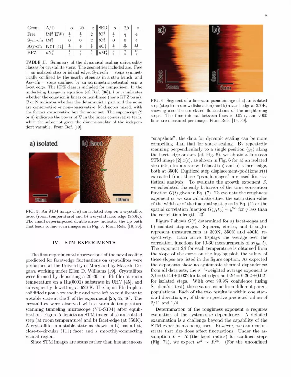
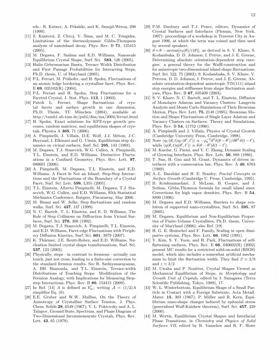
FIG. 5. An STM image of a) an isolated step on a crystallitefacet (room temperature) and b) a crystal facet edge (350K).The small superimposed double-arrow indicates the tip paththat leads to line-scan images as in Fig. 6. From Refs. [19, 39].
IV. STM EXPERIMENTS
The first experimental observations of the novel scalingpredicted for facet-edge fluctuations on crystallites wereperformed at the University of Maryland by Masashi De-gawa working under Ellen D. Williams [19]. Crystalliteswere formed by depositing a 20–30 nm Pb film at roomtemperature on a Ru(0001) substrate in UHV [45], andsubsequently dewetting at 620 K. The liquid Pb dropletssolidified upon slow cooling and were left to equilibrate toa stable state at the T of the experiment [25, 45, 46]. Thecrystallites were observed with a variable-temperaturescanning tunneling microscope (VT-STM) after equili-bration. Figure 5 depicts an STM image of a) an isolatedstep (at room temperature) and b) facet-edge (at 350K).A crystallite in a stable state as shown in b) has a flat,close-to-circular (111) facet and a smoothly-connectingvicinal region.
Since STM images are scans rather than instantaneous
FIG. 6. Segment of a line-scan pseudoimage of a) an isolatedstep (step from screw dislocation) and b) a facet-edge at 350K,showing also the correlated fluctuations of the neighboringsteps. The time interval between lines is 0.02 s, and 2000lines are measured per image. From Refs. [19, 39].
“snapshots”, the data for dynamic scaling can be morecompelling than that for static scaling. By repeatedlyscanning perpendicularly to a single position (y0) alongthe facet-edge or step (cf. Fig. 5), we obtain a line-scanSTM image [2] x(t), as shown in Fig. 6 for a) an isolatedstep (step from a screw dislocation) and b) a facet-edge,both at 350K. Digitized step displacement-positions x(t)extracted from these “pseudoimages” are used for sta-tistical analysis. To evaluate the growth exponent β,we calculated the early behavior of the time correlationfunction G(t) given in Eq. (7). To evaluate the roughnessexponent α, we can calculate either the saturation valueof the width w of the fluctuating step as in Eq. (1) or thespatial correlation function G(y, t0) ∼ y2α for y less thanthe correlation length [23].
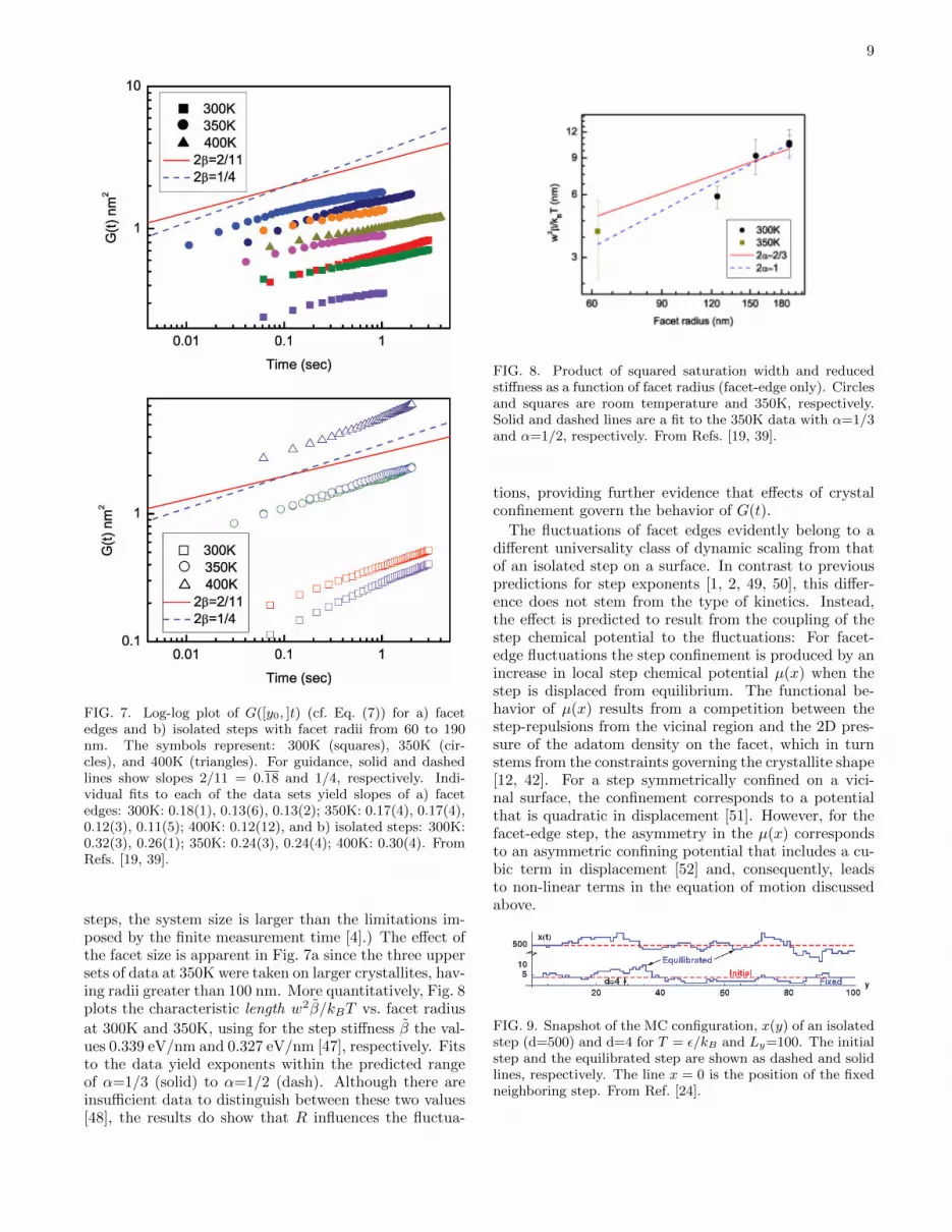
Figure 7 shows G(t) determined for a) facet-edges andb) isolated step-edges. Squares, circles, and trianglesrepresent measurements at 300K, 350K and 400K, re-spectively. Each curve displays the average over thecorrelation functions for 10-30 measurements of x(y0, t).The exponent 2β for each temperature is obtained fromthe slope of the curve on the log-log plot; the values ofthese slopes are listed in the figure caption. As expectedthe exponents show no systematic thermal dependence:from all data sets, the σ−2-weighted average exponent is2β = 0.149±0.032 for facet-edges and 2β = 0.262±0.021for isolated steps. With over 99.9% confidence (usingStudent’s t-test), these values come from different parentpopulations. Each of the two results is within one stan-dard deviation, σ, of their respective predicted values of2/11 and 1/4.
Determination of the roughness exponent α requiresevaluation of the system-size dependence. A detailedexamination is a challenge beyond the capability of theSTM experiments being used. However, we can demon-strate that size does affect fluctuations. Under the as-sumption L ∼ R (the facet radius) for confined steps(Fig. 7a), we expect w2 ∼ R2α. (For the unconfined
9
FIG. 7. Log-log plot of G([y0, ]t) (cf. Eq. (7)) for a) facetedges and b) isolated steps with facet radii from 60 to 190nm. The symbols represent: 300K (squares), 350K (cir-cles), and 400K (triangles). For guidance, solid and dashedlines show slopes 2/11 = 0.18 and 1/4, respectively. Indi-vidual fits to each of the data sets yield slopes of a) facetedges: 300K: 0.18(1), 0.13(6), 0.13(2); 350K: 0.17(4), 0.17(4),0.12(3), 0.11(5); 400K: 0.12(12), and b) isolated steps: 300K:0.32(3), 0.26(1); 350K: 0.24(3), 0.24(4); 400K: 0.30(4). FromRefs. [19, 39].
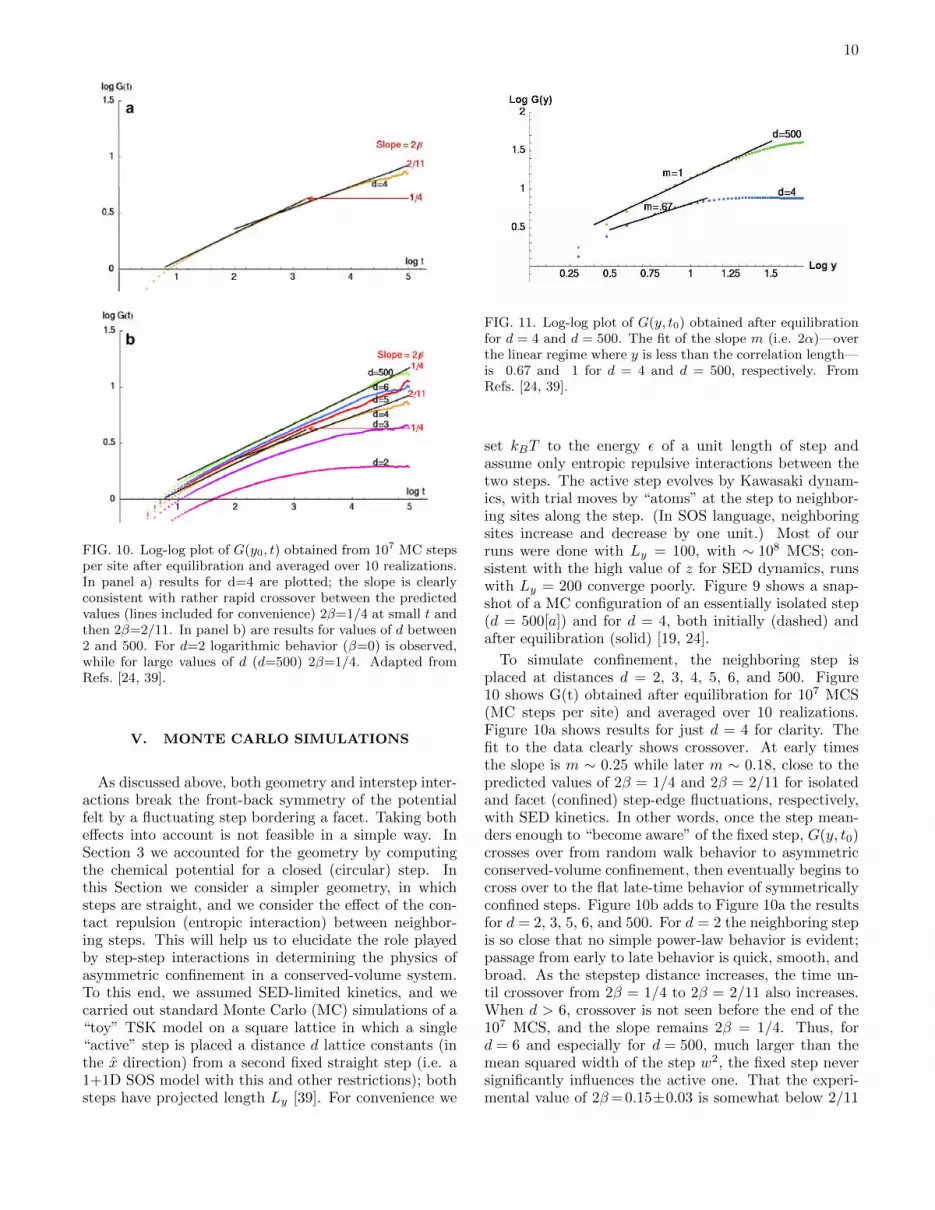
steps, the system size is larger than the limitations im-posed by the finite measurement time [4].) The effect ofthe facet size is apparent in Fig. 7a since the three uppersets of data at 350K were taken on larger crystallites, hav-ing radii greater than 100 nm. More quantitatively, Fig. 8plots the characteristic length w2β/kBT vs. facet radius
at 300K and 350K, using for the step stiffness β the val-ues 0.339 eV/nm and 0.327 eV/nm [47], respectively. Fitsto the data yield exponents within the predicted rangeof α=1/3 (solid) to α=1/2 (dash). Although there areinsufficient data to distinguish between these two values[48], the results do show that R influences the fluctua-
FIG. 8. Product of squared saturation width and reducedstiffness as a function of facet radius (facet-edge only). Circlesand squares are room temperature and 350K, respectively.Solid and dashed lines are a fit to the 350K data with α=1/3and α=1/2, respectively. From Refs. [19, 39].
tions, providing further evidence that effects of crystalconfinement govern the behavior of G(t).
The fluctuations of facet edges evidently belong to adifferent universality class of dynamic scaling from thatof an isolated step on a surface. In contrast to previouspredictions for step exponents [1, 2, 49, 50], this differ-ence does not stem from the type of kinetics. Instead,the effect is predicted to result from the coupling of thestep chemical potential to the fluctuations: For facet-edge fluctuations the step confinement is produced by anincrease in local step chemical potential µ(x) when thestep is displaced from equilibrium. The functional be-havior of µ(x) results from a competition between thestep-repulsions from the vicinal region and the 2D pres-sure of the adatom density on the facet, which in turnstems from the constraints governing the crystallite shape[12, 42]. For a step symmetrically confined on a vici-nal surface, the confinement corresponds to a potentialthat is quadratic in displacement [51]. However, for thefacet-edge step, the asymmetry in the µ(x) correspondsto an asymmetric confining potential that includes a cu-bic term in displacement [52] and, consequently, leadsto non-linear terms in the equation of motion discussedabove.
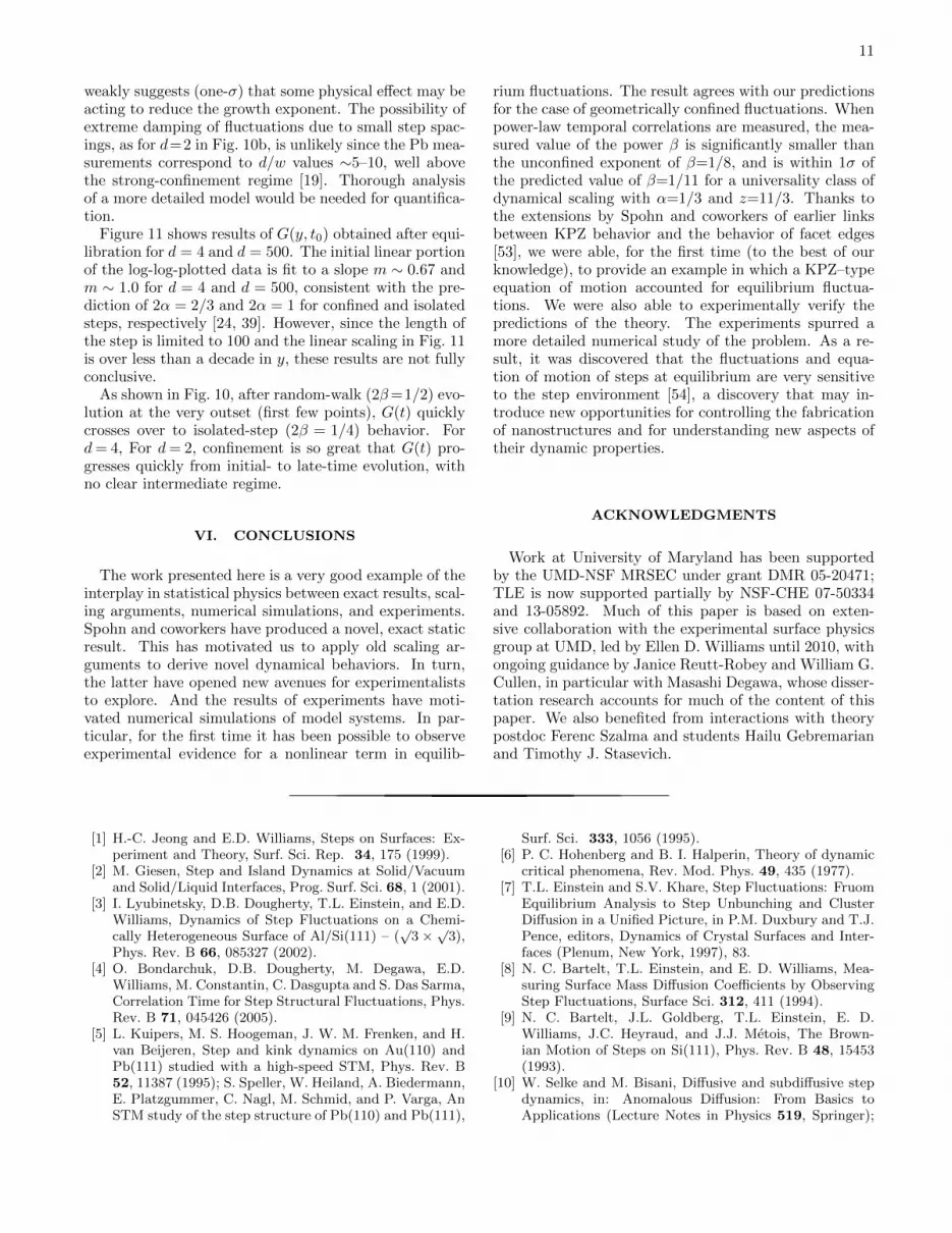
FIG. 9. Snapshot of the MC configuration, x(y) of an isolatedstep (d=500) and d=4 for T = ε/kB and Ly=100. The initialstep and the equilibrated step are shown as dashed and solidlines, respectively. The line x = 0 is the position of the fixedneighboring step. From Ref. [24].
10
FIG. 10. Log-log plot of G(y0, t) obtained from 107 MC stepsper site after equilibration and averaged over 10 realizations.In panel a) results for d=4 are plotted; the slope is clearlyconsistent with rather rapid crossover between the predictedvalues (lines included for convenience) 2β=1/4 at small t andthen 2β=2/11. In panel b) are results for values of d between2 and 500. For d=2 logarithmic behavior (β=0) is observed,while for large values of d (d=500) 2β=1/4. Adapted fromRefs. [24, 39].
V. MONTE CARLO SIMULATIONS
As discussed above, both geometry and interstep inter-actions break the front-back symmetry of the potentialfelt by a fluctuating step bordering a facet. Taking botheffects into account is not feasible in a simple way. InSection 3 we accounted for the geometry by computingthe chemical potential for a closed (circular) step. Inthis Section we consider a simpler geometry, in whichsteps are straight, and we consider the effect of the con-tact repulsion (entropic interaction) between neighbor-ing steps. This will help us to elucidate the role playedby step-step interactions in determining the physics ofasymmetric confinement in a conserved-volume system.To this end, we assumed SED-limited kinetics, and wecarried out standard Monte Carlo (MC) simulations of a“toy” TSK model on a square lattice in which a single“active” step is placed a distance d lattice constants (inthe x direction) from a second fixed straight step (i.e. a1+1D SOS model with this and other restrictions); bothsteps have projected length Ly [39]. For convenience we
FIG. 11. Log-log plot of G(y, t0) obtained after equilibrationfor d = 4 and d = 500. The fit of the slope m (i.e. 2α)—overthe linear regime where y is less than the correlation length—is 0.67 and 1 for d = 4 and d = 500, respectively. FromRefs. [24, 39].
set kBT to the energy ε of a unit length of step andassume only entropic repulsive interactions between thetwo steps. The active step evolves by Kawasaki dynam-ics, with trial moves by “atoms” at the step to neighbor-ing sites along the step. (In SOS language, neighboringsites increase and decrease by one unit.) Most of ourruns were done with Ly = 100, with ∼ 108 MCS; con-sistent with the high value of z for SED dynamics, runswith Ly = 200 converge poorly. Figure 9 shows a snap-shot of a MC configuration of an essentially isolated step(d = 500[a]) and for d = 4, both initially (dashed) andafter equilibration (solid) [19, 24].
To simulate confinement, the neighboring step isplaced at distances d = 2, 3, 4, 5, 6, and 500. Figure10 shows G(t) obtained after equilibration for 107 MCS(MC steps per site) and averaged over 10 realizations.Figure 10a shows results for just d = 4 for clarity. Thefit to the data clearly shows crossover. At early timesthe slope is m ∼ 0.25 while later m ∼ 0.18, close to thepredicted values of 2β = 1/4 and 2β = 2/11 for isolatedand facet (confined) step-edge fluctuations, respectively,with SED kinetics. In other words, once the step mean-ders enough to “become aware” of the fixed step, G(y, t0)crosses over from random walk behavior to asymmetricconserved-volume confinement, then eventually begins tocross over to the flat late-time behavior of symmetricallyconfined steps. Figure 10b adds to Figure 10a the resultsfor d = 2, 3, 5, 6, and 500. For d = 2 the neighboring stepis so close that no simple power-law behavior is evident;passage from early to late behavior is quick, smooth, andbroad. As the stepstep distance increases, the time un-til crossover from 2β = 1/4 to 2β = 2/11 also increases.When d > 6, crossover is not seen before the end of the107 MCS, and the slope remains 2β = 1/4. Thus, ford = 6 and especially for d = 500, much larger than themean squared width of the step w2, the fixed step neversignificantly influences the active one. That the experi-mental value of 2β=0.15±0.03 is somewhat below 2/11
11
weakly suggests (one-σ) that some physical effect may beacting to reduce the growth exponent. The possibility ofextreme damping of fluctuations due to small step spac-ings, as for d=2 in Fig. 10b, is unlikely since the Pb mea-surements correspond to d/w values ∼5–10, well abovethe strong-confinement regime [19]. Thorough analysisof a more detailed model would be needed for quantifica-tion.
Figure 11 shows results of G(y, t0) obtained after equi-libration for d = 4 and d = 500. The initial linear portionof the log-log-plotted data is fit to a slope m ∼ 0.67 andm ∼ 1.0 for d = 4 and d = 500, consistent with the pre-diction of 2α = 2/3 and 2α = 1 for confined and isolatedsteps, respectively [24, 39]. However, since the length ofthe step is limited to 100 and the linear scaling in Fig. 11is over less than a decade in y, these results are not fullyconclusive.
As shown in Fig. 10, after random-walk (2β=1/2) evo-lution at the very outset (first few points), G(t) quicklycrosses over to isolated-step (2β = 1/4) behavior. Ford= 4, For d= 2, confinement is so great that G(t) pro-gresses quickly from initial- to late-time evolution, withno clear intermediate regime.
VI. CONCLUSIONS
The work presented here is a very good example of theinterplay in statistical physics between exact results, scal-ing arguments, numerical simulations, and experiments.Spohn and coworkers have produced a novel, exact staticresult. This has motivated us to apply old scaling ar-guments to derive novel dynamical behaviors. In turn,the latter have opened new avenues for experimentaliststo explore. And the results of experiments have moti-vated numerical simulations of model systems. In par-ticular, for the first time it has been possible to observeexperimental evidence for a nonlinear term in equilib-
rium fluctuations. The result agrees with our predictionsfor the case of geometrically confined fluctuations. Whenpower-law temporal correlations are measured, the mea-sured value of the power β is significantly smaller thanthe unconfined exponent of β=1/8, and is within 1σ ofthe predicted value of β=1/11 for a universality class ofdynamical scaling with α=1/3 and z=11/3. Thanks tothe extensions by Spohn and coworkers of earlier linksbetween KPZ behavior and the behavior of facet edges[53], we were able, for the first time (to the best of ourknowledge), to provide an example in which a KPZ–typeequation of motion accounted for equilibrium fluctua-tions. We were also able to experimentally verify thepredictions of the theory. The experiments spurred amore detailed numerical study of the problem. As a re-sult, it was discovered that the fluctuations and equa-tion of motion of steps at equilibrium are very sensitiveto the step environment [54], a discovery that may in-troduce new opportunities for controlling the fabricationof nanostructures and for understanding new aspects oftheir dynamic properties.
ACKNOWLEDGMENTS
Work at University of Maryland has been supportedby the UMD-NSF MRSEC under grant DMR 05-20471;TLE is now supported partially by NSF-CHE 07-50334and 13-05892. Much of this paper is based on exten-sive collaboration with the experimental surface physicsgroup at UMD, led by Ellen D. Williams until 2010, withongoing guidance by Janice Reutt-Robey and William G.Cullen, in particular with Masashi Degawa, whose disser-tation research accounts for much of the content of thispaper. We also benefited from interactions with theorypostdoc Ferenc Szalma and students Hailu Gebremarianand Timothy J. Stasevich.
[1] H.-C. Jeong and E.D. Williams, Steps on Surfaces: Ex-periment and Theory, Surf. Sci. Rep. 34, 175 (1999).
[2] M. Giesen, Step and Island Dynamics at Solid/Vacuumand Solid/Liquid Interfaces, Prog. Surf. Sci. 68, 1 (2001).
[3] I. Lyubinetsky, D.B. Dougherty, T.L. Einstein, and E.D.Williams, Dynamics of Step Fluctuations on a Chemi-cally Heterogeneous Surface of Al/Si(111) – (
√3 ×√
3),Phys. Rev. B 66, 085327 (2002).
[4] O. Bondarchuk, D.B. Dougherty, M. Degawa, E.D.Williams, M. Constantin, C. Dasgupta and S. Das Sarma,Correlation Time for Step Structural Fluctuations, Phys.Rev. B 71, 045426 (2005).
[5] L. Kuipers, M. S. Hoogeman, J. W. M. Frenken, and H.van Beijeren, Step and kink dynamics on Au(110) andPb(111) studied with a high-speed STM, Phys. Rev. B52, 11387 (1995); S. Speller, W. Heiland, A. Biedermann,E. Platzgummer, C. Nagl, M. Schmid, and P. Varga, AnSTM study of the step structure of Pb(110) and Pb(111),
Surf. Sci. 333, 1056 (1995).[6] P. C. Hohenberg and B. I. Halperin, Theory of dynamic
critical phenomena, Rev. Mod. Phys. 49, 435 (1977).[7] T.L. Einstein and S.V. Khare, Step Fluctuations: Fruom
Equilibrium Analysis to Step Unbunching and ClusterDiffusion in a Unified Picture, in P.M. Duxbury and T.J.Pence, editors, Dynamics of Crystal Surfaces and Inter-faces (Plenum, New York, 1997), 83.
[8] N. C. Bartelt, T.L. Einstein, and E. D. Williams, Mea-suring Surface Mass Diffusion Coefficients by ObservingStep Fluctuations, Surface Sci. 312, 411 (1994).
[9] N. C. Bartelt, J.L. Goldberg, T.L. Einstein, E. D.Williams, J.C. Heyraud, and J.J. Metois, The Brown-ian Motion of Steps on Si(111), Phys. Rev. B 48, 15453(1993).
[10] W. Selke and M. Bisani, Diffusive and subdiffusive stepdynamics, in: Anomalous Diffusion: From Basics toApplications (Lecture Notes in Physics 519, Springer);
12
eds.: R. Kutner, A. Pekalski, and K. Sznajd-Weron, 298(1999).
[11] Z. Kuntova, Z. Chvoj, V. Sıma, and M. C. Tringides,Limitations of the thermodynamic Gibbs-Thompsonanalysis of nanoisland decay, Phys. Rev. B 71, 125415(2005).
[12] M. Degawa, F. Szalma and E.D. Williams, NanoscaleEquilibrium Crystal Shape, Surf. Sci. 583, 126 (2005).
[13] Hailu Gebremariam Bantu, Terrace Width Distributionand First Passage Probabilities for Interacting Steps,Ph.D. thesis, U. of Maryland (2005).
[14] P.L. Ferrari, M. Prahofer, and H. Spohn, Fluctuations ofan atomic ledge bordering a crystalline facet, Phys. Rev.E 69, 035102(R) (2004).
[15] P.L. Ferrari and H. Spohn, Step Fluctuations for aFaceted Crystal, J. Stat. Phys. 113, 1 (2003).
[16] Patrik L. Ferrari, Shape fluctuations of crys-tal facets and surface growth in one dimension,Ph.D. Thesis, TU Munchen (2004), available athttp://tumb1.ub.tum.de/publ/diss/ma/2004/ferrari.html.
[17] H. Spohn, Exact solutions for KPZ-type growth pro-cesses, random matrices, and equilibrium shapes of crys-tals, Physica A 369, 71 (2006).
[18] A. Pimpinelli, J. Villain, D.E. Wolf, J.J. Metois, J.C.Heyraud, I. Elkinani and G. Uimin, Equilibrium step dy-namics on vicinal surfaces, Surf. Sci. 295, 143 (1993).
[19] M. Degawa, T.J. Stasevich, W.G. Cullen, A. Pimpinelli,T.L. Einstein, and E.D. Williams, Distinctive Fluctu-ations in a Confined Geometry, Phys. Rev. Lett. 97,080601 (2006).
[20] A. Pimpinelli, M. Degawa, T.L. Einstein, and E.D.Williams, A Facet Is Not an Island: Step-Step Interac-tions and the Fluctuations of the Boundary of a CrystalFacet, Surf. Sci. Lett. 598, L355 (2005).
[21] T.L. Einstein, Alberto Pimpinelli, M. Degawa, T.J. Sta-sevich, W.G. Cullen, and E.D. Williams, 95th StatisticalMechanics Conference, Rutgers, Piscataway, May 2006.
[22] M. Bisani and W. Selke, Step fluctuations and randomwalks, Surf. Sci. 437, 137 (1999).
[23] N. C. Bartelt, T. L. Einstein, and E. D. Williams, TheRole of Step Collisions on Diffraction from Vicinal Sur-faces, Surf. Sci. 276, 308 (1992).
[24] M. Degawa, T.J. Stasevich, A. Pimpinelli, T.L. Einstein,and E.D. Williams, Facet-edge Fluctuations with Periph-ery Diffusion Kinetics, Surf. Sci. 601, 3979 (2007).
[25] K. Thurmer, J.E. Reutt-Robey, and E.D. Williams, Nu-cleation limited crystal shape transformations, Surf. Sci.537, 123 (2003).
[26] Physically, steps—in contrast to fermions—actually cantouch, just not cross, leading to a finite-size correction tothe standard fermion results. See R. Sathiyanarayanan,A. BH. Hamouda, and T.L. Einstein, Terrace-widthDistributions of Touching Steps: Modification of theFermion Analogy, with Implications for Measuring Step-step Interactions, Phys. Rev. B 80, 153415 (2009).
[27] In Ref. [14] A is defined as b′′∞; writing A = (1/2)Asimplifies Eq. (6).
[28] E.E. Gruber and W.W. Mullins, On the Theory ofAnisotropy of Crystalline Surface Tension, J. Phys.Chem. Solids 28, 6549 (1967); V. L. Pokrovsky and A. L.Talapov, Ground State, Spectrum, and Phase Diagram ofTwo-Dimensional Incommensurate Crystals, Phys. Rev.Lett. 42, 65 (1979).
[29] P.M. Duxbury and T.J. Pence, editors, Dynamics ofCrystal Surfaces and Interfaces (Plenum, New York,1997): proceedings of a workshop in Traverse City in Au-gust 1996, at which the term was coined and then usedby several speakers.
[30] ϑ= θ − arctan[rθ(θ)/r(θ)], as derived in S. V. Khare, S.Kodambaka, D. D. Johnson, I. Petrov, and J. E. Greene,Determining absolute orientation-dependent step ener-gies: a general theory for the Wulff-construction andfor anisotropic two-dimensional island shape fluctuations,Surf. Sci. 522, 75 (2003); S. Kodambaka, S. V. Khare, V.Petrova, D. D. Johnson, I. Petrov, and J. E. Greene, Ab-solute orientation-dependent anisotropic TiN(111) islandstep energies and stiffnesses from shape fluctuation anal-yses, Phys. Rev. B 67, 035409 (2003).
[31] S. V. Khare, N. C. Bartelt, and T. L. Einstein, Diffusionof Monolayer Adatom and Vacancy Clusters: LangevinAnalysis and Monte Carlo Simulations of Their BrownianMotion, Phys. Rev. Lett. 75, 2148 (1995); Brownian Mo-tion and Shape Fluctuations of Single Layer Adatom andVacancy Clusters on Surfaces: Theory and Simulations,Phys. Rev. B 54, 11752 (1996).
[32] A. Pimpinelli and J. Villain, Physics of Crystal Growth(Cambridge University Press, Cambridge, 1998).
while 〈η(θ, t)η(θ′, t′)〉 ∝ δ(θ − θ′)δ(t− t′).[34] M. Kardar, G. Parisi, and Y. C. Zhang, Dynamic Scaling
of Growing Interfaces, Phys. Rev. Lett. 56, 889 (1986).[35] T. Sun, H. Guo and M. Grant, Dynamics of driven in-
terfaces with a conservation law, Phys. Rev. A 40, 6763(1989).
[36] A.-L. Barabasi and H. E. Stanley, Fractal Concepts inSurface Growth (Cambridge U. Press, Cambridge, 1995).
[37] B. Krishnamachari, J. McLean, B. Cooper, and J.Sethna, Gibbs-Thomson formula for small island sizes:Corrections for high vapor densities, Phys. Rev. B 54,8899 (1996).
[38] M. Degawa and E.D. Williams, Barriers to shape evo-lution of supported nano-crystallites, Surf. Sci. 595, 87(2005).
[39] M. Degawa, Equilibrium and Non-Equilibrium Proper-ties of Finite-Volume Crystallites, Ph.D. thesis, Univer-sity of Maryland (2006); also Ref. [19].
[40] H. G. E. Hentschel and F. Family, Scaling in open dissi-pative systems, Phys. Rev. Lett. 66, 1982 (1991).
[41] Y. Kim, S. Y. Yoon, and H. Park, Fluctuations of self-flattening surfaces, Phys. Rev. E 66, 040602(R) (2002)present MC results for a restricted solid-on-solid (RSOS)model, which also includes a somewhat artificial mecha-nism to limit the fluctuation width. They find β ' 2/9and z ' 3/2.
[42] M. Uwaha and P. Nozieres, Crystal Shapes Viewed asMechanical Equilibrium of Steps, in Morphology andGrowth Unit of Crystals, edited by I. Sunagawa (TerraScientific Publishing, Tokyo, 1989), 17.
[43] W. L. Winterbottom, Equilibrium Shape of a Small Par-ticle in Contact with a Foreign Substrate, Acta Metall.Mater. 15, 303 (1967); P. Muller and R. Kern, Equi-librium nano-shape changes induced by epitaxial stress(generalised Wulf-Kaishew theorem), Surf. Sci. 457, 229(2000).
[44] M. Wortis, Equilibrium Crystal Shapes and InterfacialPhase Transitions, in Chemistry and Physics of SolidSurfaces VII, edited by R. Vanselow and R. F. Howe
(Springer, Berlin, 1988), 367; P. Nozieres, Shape andGrowth of Crystals, in Solids far from Equilibrium, editedby C. Godreche (Cambridge U. Press, Cambridge, 1992),1; S. Balibar, H. Alles, and A.Ya. Parshin, The surfaceof helium crystals, Rev. Mod. Phys. 77, 317 (2005); A.Pavlovska et al., Surf. Sci. 326, 101 (1995); C. Rottman,M. Wortis, J.C. Heyraud, and J.J. Metois, Equilib-rium Shapes of Small Lead Crystals: Observation ofPokrovsky-Talapov Critical Behavior, Phys. Rev. Lett.52, 1009 (1984).
[45] K. Arenhold, S. Surnev, H.P. Bonzel, and P. Wynblatt,Step energetics of Pb(111) vicinal surfaces from facetshape, Surf. Sci. 424, 271 (1999); C. Bombis, A. Emu-ndts, M. Nowicki, and H.P. Bonzel, Absolute surface freeenergies of Pb, Surf. Sci. 511, 83 (2002); M. Nowicki etal., New J. Phys. 4, 60 (2002).
[46] K. Thurmer, J.E. Reutt-Robey, E.D. Williams, M.Uwaha, A. Emundts, and H.P. Bonzel, Step Dynamicsin 3D Crystal Shape Relaxation, Phys. Rev. Lett. 87,186102 (2001).
[47] N. Akutsu and Y. Akutsu, Statistical mechanical calcu-lation of anisotropic step stiffness of a two-dimensionalhexagonal lattice-gas model with next-nearest-neighbourinteractions: application to Si(111) surface, J. Phys.-Cond. Mat. 11, 6635 (1999); M. Nowicki, C. Bombis,A. Emundts, and H. P. Bonzel, Absolute step and kinkformation energies of Pb derived from step rougheningof two-dimensional islands and facets, Phys. Rev. B 67,075405 (2003).
[48] Direct experimental observation, e.g. of the spatial corre-lation function on a quenched crystallite, would be neededto obtain α for facet-edge fluctuations.
[49] T. Ihle, C. Misbah, and O. Pierre-Louis, Equilibrium stepdynamics on vicinal surfaces revisited, Phys. Rev. B 58,2289 (1998); S.V. Khare and T.L. Einstein, Unified viewof step-edge kinetics and fluctuations, Phys. Rev. B 57,4782 (1998); M. Ondrejcek, M. Rajappan, W. Swiech,and C. P. Flynn, Step fluctuation studies of surface dif-fusion and step stiffness for the Ni(111) surface, Phys.Rev. B 73, 035418 (2006).
[50] E. Le Goff, L. Barbier, and B. Salanon, Timespace heightcorrelations of thermally fluctuating 2-d systems. Appli-cation to vicinal surfaces and analysis of STM images ofCu(1 1 5), Surf. Sci. 531, 337 (2003); M. Ondrejcek, W.Swiech, G. Yang, and C.P. Flynn, Crossover from bulkto surface diffusion in the fluctuations of step edges onPt(111), Phil. Mag. Lett. 84, 69, 417 (2004); M. On-drejcek, W. Swiech, M. Rajappan, and C. P. Flynn,Fluctuation spectroscopy of step edges on Pt(111) andPd(111), Phys. Rev. B 72, 085422 (2005).
[51] N. C. Bartelt, T.L. Einstein, and E. D. Williams, TheInfluence of Step-Step Interactions on Step Wandering,Surf. Sci. Lett. 240, L591 (1990).
[52] T. J. Stasevich, Hailu Gebremariam, T.L. Einstein, M.Giesen, C. Steimer, and H. Ibach, Low-Temperature Ori-entation Dependence of Step Stiffness on 111 Surfaces,Phys. Rev. B 71, 245414 (2005).
[53] J. D. Shore and D. J. Bukman, Coexistence point in thesix-vertex model and the crystal shape of fcc materials,Phys. Rev. Lett. 72, 604 (1994); J. Neergaard and M.den Nijs, Crossover Scaling Functions in One Dimen-sional Dynamic Growth Models, Phys. Rev. Lett. 74,730 (1995).
[54] C. Tao, T. J. Stasevich, T.L. Einstein, and E. D.Williams, Step Fluctuations on Ag(111) Surfaces withC60, Phys. Rev. B 73, 125436 (2006).