This article was downloaded by: [CSIRO Library Services]On: 11 December 2012, At: 16:20Publisher: RoutledgeInforma Ltd Registered in England and Wales Registered Number: 1072954 Registered office: Mortimer House,37-41 Mortimer Street, London W1T 3JH, UK

Applied EconomicsPublication details, including instructions for authors and subscription information:http://www.tandfonline.com/loi/raec20

Economic and conservation implications of a variableeffort penalty system in effort-controlled fisheriesSean Pascoe a , James Innes a , Ana Norman-López a , Chris Wilcox b & Natalie Dowling ba Wealth from Oceans Flagship, CSIRO Marine and Atmospheric Research, EcoSciencesPrecinct, PO Box 2583, Brisbane, QLD 4001, Australiab Wealth from Oceans Flagship, CSIRO Marine and Atmospheric Research, Castray Esplanade,Hobart 7000, AustraliaVersion of record first published: 21 Nov 2012.

To cite this article: Sean Pascoe , James Innes , Ana Norman-López , Chris Wilcox & Natalie Dowling (2013): Economicand conservation implications of a variable effort penalty system in effort-controlled fisheries, Applied Economics, 45:27,3880-3890

To link to this article: http://dx.doi.org/10.1080/00036846.2012.736941

PLEASE SCROLL DOWN FOR ARTICLE

Full terms and conditions of use: http://www.tandfonline.com/page/terms-and-conditions

This article may be used for research, teaching, and private study purposes. Any substantial or systematicreproduction, redistribution, reselling, loan, sub-licensing, systematic supply, or distribution in any form toanyone is expressly forbidden.

The publisher does not give any warranty express or implied or make any representation that the contentswill be complete or accurate or up to date. The accuracy of any instructions, formulae, and drug doses shouldbe independently verified with primary sources. The publisher shall not be liable for any loss, actions, claims,proceedings, demand, or costs or damages whatsoever or howsoever caused arising directly or indirectly inconnection with or arising out of the use of this material.

Applied Economics, 2013, 45, 3880–3890

Economic and conservation

implications of a variable effort penalty

system in effort-controlled fisheries

Sean Pascoea,*, James Innesa, Ana Norman-Lopeza, Chris Wilcoxb

and Natalie Dowlingb

aWealth from Oceans Flagship, CSIRO Marine and Atmospheric Research,

EcoSciences Precinct, PO Box 2583, Brisbane, QLD 4001, AustraliabWealth from Oceans Flagship, CSIRO Marine and Atmospheric Research,

Castray Esplanade, Hobart 7000, Australia

Bycatch of threatened, endangered or protected species by commercial fishers is a

universal problem. Technical solutions are often applied that may impose inefficiencies

across the fleet, even in periods or areas when the risk of bycatch is low. These may

include gear specifically designed to avoid the bycatch which may also reduce the targeted

catch, or designation of marine protected areas that exclude fishing from whole areas. In

this article, we examine the effectiveness of a variable penalty system that can provide

incentives for fishers to redirect their effort away from problem areas. The system is

examined using a case study of fishery, which is currently subjected to gear and closure

controls to limit bycatch of turtles and seabirds. An alternative incentive-based

management policy using a series of differential hook penalties has been proposed as a

flexible tool to discourage vessels operating in certain areas. The effects of various hook

penalties and closures in key areas on fishing effort in those areas and elsewhere as well as

vessel economic performance are assessed using a location choice model. The results

suggest that incentive-based approaches may result in lower costs to industry than

closures provided some level of residual bycatch is acceptable.

Keywords: effort controls; location choice; bycatch; decrementation systems; fisheries

JEL Classification: Q22; Q57; C31; D21

I. Introduction

Increased understanding of the spatial structure of marine

ecosystems and the factors that influence the spatial distribu-

tion of both commercial fish species, charismatic noncommer-

cial species and marine biodiversity, in general, has resulted in

increased interest in the use of spatial management techniques,

particularly – but not exclusively – Marine Protected Areas

(MPAs) (Gray, 1997; Wilen, 2004). In Australia, as elsewhere,

conservation-driven spatial management measures arising

from marine bioregional planning are increasingly affecting

fisheries through closure of areas to fishing (Kearney et al.,

2012). MPAs are becoming a favoured management strategy

for the conservation of marine biodiversity within Australia

(Manson and Die, 2001). In creating MPAs, however, there is

often a trade off between biodiversity benefits and negative

economic impacts on the affected fisheries (Manson and Die,

2001).

Spatial management, especially closures, are also often

implemented in order to prevent bycatch of particular species,

especially charismatic species such as seabirds (Pascoe et al.,

2011), seals (Smith et al., 2010) and other marine mammals

(Murray et al., 2000). An alternative approach is to use

incentive-based management systems to create appropriate

incentives for fishers to avoid the bycatch (Pascoe et al., 2010).

One such system had been developed for the Australian

*Corresponding author. E-mail: sean.pascoe@csiro.au

Applied Economics ISSN 0003–6846 print/ISSN 1466–4283 online � 2013 Taylor & Francis 3880http://www.tandfonline.com

http://dx.doi.org/10.1080/00036846.2012.736941

Dow

nloa

ded

by [

CSI

RO

Lib

rary

Ser

vice

s] a

t 16:

20 1

1 D

ecem

ber

2012

Eastern Tuna and Billfish Fishery (ETBF) with the intentionof providing incentives to avoid fishing in areas where bycatch

may be a problem without necessarily closing these areas.

Of considerable concern in the fishery is bycatch of highlyvulnerable species such as turtles, sharks and seabirds,

particularly flesh-footed shearwaters and albatross. The loca-

tion of effort deployment has different implications for catchesof these bycatch species. Technical measures have been

introduced that have reduced bycatch, but not sufficiently tosatisfy conservation objectives for the fishery. Closures have

been introduced in some areas of the fishery to protect seabirds

at considerable cost to the industry (Pascoe et al., 2011).Until recently, the fishery was managed through an

Individual Transferable Effort (ITE) unit system expressed interms of total number of hooks that can be deployed over the

year. Under the ITE system, a facility was introduced to

potentially influence the distribution of effort using ‘hookdecrements’ (termed sub-area factors in the management plan),

which are differential decrement rates of an operator’s effort

allocation depending on where they fish. As opposed to directcontrols, this approach relied on an incentive-based approach

to drive the spatial distribution of effort, as it effectively varied

the Value Per Hook (VPH) employed. This system was neverfully implemented (due to the pending move to individual

transferable quotas in March 2011), although its potential as aflexible approach to divert fishing effort as required was

considered advantageous (Pascoe et al., 2009).The concept of hook decrements is similar to that of the

individual habitat quota (Holland and Schnier, 2006). These

are spatial management instruments where different effortpenalties are applied to different areas based on the expected

level of damage created by fishing in those areas. These quotas

are tradeable, allowing vessels to adjust their fishing activitiesto minimize their own damage. Fishers consume their quota

based on where and when they fish, with the penalty system

providing incentives to either operate in areas where lessdamage will be incurred, or adopt fishing gear that will have a

lower impact. In the proposed ETBF management system, the

rate at which effort quota is consumed depends on where andwhen they fish. Areas and/or seasons with the potential for

high levels of bycatch of species of concern will attract a highpenalty rate (e.g. three hooks of quota for each hook actually

set), whereas other areas with little bycatch may attract a much

lower rate (e.g. decremented 1.1 hooks per hook set), reflectingthe difference in impact.

The effectiveness of such a system will largely be dependenton the degree to which fishers respond to changing incentives

created by the policy. The spatial hook penalty effectively

reduces the VPH associated with fishing in a particular area,making other areas potentially more attractive. This will

encourage fishers who are able to fish elsewhere, while those

who chose to continue fishing in the affected area are still ableto do so, but the total effort quota consumed will be increased

(potentially resulting in overall lower levels of fishing effort).Of key importance to managers will be the level of incentive

required to achieve a given objective, the likely locations to

which that displaced effort will shift, and the expected effect onfishery economics at a variety of levels from vessel profits to

economic activity in a port to fishery revenue as a whole.In this study, a nested multinomial logit model is estimated

to determine the importance of catch VPH on the location

choice of fishers in the ETBF. From this, the effects of varying

effective VPH on effort levels through inducing hook penalties

in both high effort and low effort areas is examined. The

impact on economic performance is also considered through

estimating the proportional changes in total fishery revenue

and fuel costs. We demonstrate that spatial incentive-based

approaches offer a less-expensive (to the fishing industry)

alternative to closures where effort reduction rather than

elimination is required to achieve conservation objectives.

II. The ETBF

The ETBF is a tropical tuna and billfish fishery targeting fish

in the boundary current off the east of Australia from the tip

of Cape York to the South Australia–Victoria border (Fig. 1).

The principal target species are yellowfin tuna (Thunnus

albacares), albacore tuna (Thunnus alalunga), broadbill sword-

fish (Xiphias gladius), bigeye tuna (Thunnus obesus) and striped

marlin (Tetrapturus audax) with the total catch of these five

species averaging around 6000 tonnes over recent years, with

an average total value of around $40m (Evans, 2007; ABARE,

2009a; ABARES, 2011).The Eastern Tuna and Billfish Fishery Management Plan

2005 introduced a system of Statutory Fishing Rights (SFRs)

in the form of individual transferable effort quotas based on

the number of hooks employed by each vessel, and a

corresponding total allowable effort level (total number of

hooks that can be deployed in the fishery). Although devel-

oped in 2005 (and amended in 2007), SFRs were only allocated

in August 2009, with the first season under effort management

commenced on 1 November 2009. Hook decrementation rates

were set at a uniform level of 1 (one) across the fishery pending

further investigation into the effects of differential rates. The

intention of a variable decrementation rate was largely to

address issues of bycatch of seabirds, turtles and other

protected species, with different issues occurring in different

areas to different degrees. In March 2011, the SFRs were

converted to Individual Transferable Quotas (ITQs), with total

allowable catches imposed on the main species, and area

closures and technical measures retained to deal with bycatch

issues.Our study focuses on fishing patterns prior to the definition

of SFRs as effort units to avoid obfuscation of behaviour as a

result of the new (and changing) policy initiatives. Fishing

effort is expended disproportionally over the range of the

fishery (Fig. 1a), suggesting both heterogeneity in the charac-

teristics of fishing locations, and fishers responding to this

heterogeneity in their location choice. Most fishing effort is

expended inshore in the southern and northern extremes of the

fishery, although fishing effort extends offshore in the central

part of the fishery. The fleet is relatively homogeneous across

the fishery in terms of average vessel size and engine power

(Table 1), although within each region there is a mix of smaller

and larger vessels. The smaller vessels are more limited in their

range, tending to predominantly fish inshore.

The largest single port is Mooloolaba (Table 1), located on

the Sunshine Coast, north of Brisbane. For practical reasons,

the analysis was limited to vessels fishing out of Mooloolaba.

These vessels have a similar distribution of effort to the fishery

Effects of variable penalty systems in effort-controlled fisheries 3881

Dow

nloa

ded

by [

CSI

RO

Lib

rary

Ser

vice

s] a

t 16:

20 1

1 D

ecem

ber

2012

as a whole (Fig. 1b). Vessels operating out of the southern-

most ports also operate in the southern bluefin tuna fishery.

Hence, their share of total trips in the ETBF is substantially

lower than those of the Mooloolaba fleet.

III. Modelling Fisher Location Choice

Models of fisher location choice have largely been driven by

the increasing use of marine protected areas (Haynie and

Layton, 2010; Smith et al., 2010; Dowling et al., 2011; van

Putten et al., 2012). Closing areas to fishing forces fishers to

either move elsewhere or cease fishing. In the modelling of

spatial dynamics, several assumptions have been proposed.

For example, the distribution of fishing effort could be

assumed to move towards areas of highest catches

(i.e. reflecting differences in revenues assuming constant

costs) (Maury and Gascuel, 1999), highest catch rates modified

for distance to port (i.e. taking into consideration revenues and

costs implicitly (Sampson, 1991) or greatest profit (Bockstael

and Opaluch, 1984; Haynie and Layton, 2010).1

A method that allows for heterogeneity in both fishing

activity and fisher characteristics is discrete choice modelling

or the Random Utility Model (RUM) (McFadden, 1974,

1981).2 The key feature of the RUM is that it models discrete

decisions with no requisite assumption of homogeneity

amongst individuals. Rational decision makers are assumed

to make decisions that maximize their level of utility subject to

any constraints. In the case of effort allocation in fisheries,

utility is assumed to relate to profitability (subject to any

constraints the fisher may face), and location choice is based

on the expected profitability at each alternative location.

Fig. 1. Distribution of total fishing days, 2003–2008: (a) all vessels; (b) Mooloolaba vessels

Table 1. Characteristics of the vessels by general region (2003–2008)

Share of total Length Power Hooks deployed per shot

Region Boats Trips (%) Mean SD Mean SD Mean SD

North Queensland 12 13 21.3 3.8 418.0 46.8 611.4 187.4Central Queensland 5 1 19.9 2.6 347.2 131.0 1046.4 57.9Mooloolaba 59 46 22.1 3.4 368.0 126.2 1148.7 221.6Brisbane and Gold Coast 7 4 20.1 3.9 244.1 130.5 1024.0 184.4Northern and Central NSW 13 5 17.5 2.4 347.2 125.5 939.2 174.5Sydney, Newcastle, Wollongong 15 10 21.0 2.7 357.3 100.6 1039.9 135.9Southern NSW 79 21 21.7 5.4 349.5 145.3 996.0 254.7

1 A review of drivers of fisher behaviour and modelling approaches is given by van Putten et al. (2012).2 Recently, increasing attention has also been paid to the development of state dependent dynamic programming models to estimate fisherbehaviour (Gillis et al., 1995a, b; Costello and Polasky, 2008; Poos et al., 2010; Dowling et al., 2011). These have an additional advantage inquota-based fisheries in that they also allow for the opportunity cost of using quota to be taken into account, so that the decision when aswell as where to fish can be modelled (Costello and Polasky, 2008; Dowling et al., 2011). Others (Smith, 2005; Zhang and Smith, 2011) haveused a mixed logit modelling approach to capture both state dependency and heterogeneity in fisher decision making with regard to locationchoice.

3882 S. Pascoe et al.

Dow

nloa

ded

by [

CSI

RO

Lib

rary

Ser

vice

s] a

t 16:

20 1

1 D

ecem

ber

2012

The method is probabilistic in nature, in that the model

estimates the probability of a fisher operating in a given area

based on the characteristics of the area (e.g. average revenue

per unit effort, distance from port, etc) and the characteristics

of the fisher.

Numerous studies have been undertaken in fisheries utiliz-

ing a RUM approach to estimate fisher location choice

(Bockstael and Opaluch, 1984; Eales and Wilen, 1986; Holland

and Sutinen, 1999, 2000; Curtis and Hicks, 2000; Smith, 2002;

Wilen et al., 2002; Hutton et al., 2004; Pradhan and Leung,

2004; Marchal et al., 2009; Smith et al., 2010; Ran et al., 2011;

Schnier and Felthoven, 2011; Andersen et al., 2012; Tidd et al.,

2012). Most of these studies have employed multinomial logit

techniques to estimate the model.

Multinomial logit and nested multinomial logit models

As in most economic-based choice models, utility is assumed

to derive from an individual’s choice, while the choice itself is

assumed to be made on the basis of expected utility derived

from the characteristics of the option chosen. Different

decisions of individuals are treated as independent over time

(Smith, 2002). Utility is typically defined as a (linear) combi-

nation of a set of explanatory variables that together are

surmised to form (for the most part) the nonrandom compo-

nents of the utility, and a stochastic error component (thereby

giving the term ‘random utility model’)

Uij ¼ �jzi, j þ "ij ð1Þ

where for a given person time-event, i, (such as a fishing trip)

choice j (i.e. fishing location) is made. The explanatory

variables zij can be comprised of attributes of the choice,

xij, and characteristics of the individual, wi, while �j is the

parameter vector to be estimated.The basic multinomial logit model assumes that all choices

are Independent of Irrelevant Alternatives (IIA). However,

alternatives in close proximity to each other most likely share

the same, or similar, characteristics, and the IIA assumption is

likely to be invalid. The nested multinomial logit (NL) model

overcomes this by partially relaxing the IIA assumption

allowing for some correlation between sub-sets of alternatives

(Hensher et al., 2005). The NL is a structural model of the

interdependent decisions of where to fish (Smith, 2002).

Several levels of choice may be specified, such as the decision

to fish or not to fish, the general fishing zone (if fishing) and

then area within that fishing zone, and the NL allows for

different variances at these different nodes (Smith, 2002).The choice probability of the NL model is defined as the

conditional probability of area j in zone k (i.e. j kj ) j is given by

Prð j kÞ�� ¼ expð�0jzj kj ÞP

j2k expð�0jzj kj Þ¼

expð�0jzj kj Þ

expKkð2Þ

and

Kk ¼ lnXj2k

expð�0jzj kj Þ

" #ð3Þ

where Kk is the inclusive value for zone k, representing the

composite utility of the choices within the branch (Holland

and Sutinen, 1999).

The probability of choosing a particular zone k is given by

PrðkÞ ¼expð�kKkÞPk expð�kKkÞ

ð4Þ

where �k is the inclusive value variable relating to zone k. The

unconditional probability of fishing in any particular area j is

given by PrðkÞ � Prð j kÞ�� .

IV. Data

Individual shot level logbook data were available covering the

period 2003–2008. In this context, a shot denotes one discrete

fishing event where the long-line gear, consisting of a long

(several kilometres), horizontally strung line of baited hooks is

deployed overboard and subsequently left to catch fish until

retrieved several hours later. Information was available on

catch by species, fishing area (latitude and longitude), trip

length, as well as vessel characteristics (vessel length, power,

hooks deployed per shot). Vessels either fished for 1, 2 or 3

days per trip (steaming time was not included in the data set,

only active fishing time), with most trips being of 2 fishing days

duration (Table 2). Only one shot per day was taken. Distance

(great circle nautical miles) to port was estimated for each

fishing trip location (defined by the latitude and longitude of

each shot). Once in an area, distance travelled in multi-shot

trips was relatively small (Table 2).Only vessels operating from Mooloolaba were used in the

model estimation as this was the main port, and the objective

of the study was to estimate the potential effects of a hook

decrementation system rather than model the fishery per se.

Data were aggregated to a trip level, with the number of days

fished with each trip retained as a variable. The total distance

travelled (return trip) was used as a measure of distance to

allow for multi-day trips.Price information for the key species was derived from the

Australian Bureau of Agricultural and Resource Economics

(ABARE) fisheries and commodity statistics (ABARE, 2008,

2009a, b). Weekly diesel price information was available from

the West Australia Fuelwatch website.3 While these data

related to Western Australia, a consistent series of east coast

data at a weekly level were not available. The diesel fuel prices

Table 2. Distance to home port by trip length

Distance travelled (nautical miles)

Trip length(days)

Number oftrips

Home tofirst shot

First tosecond

Secondto third

1 6710 193.412 18 554 263.81 31.773 1631 135.89 27.02 25.01

Total 26 895

3www.fuelwatch.wa.gov.au/.

Effects of variable penalty systems in effort-controlled fisheries 3883

Dow

nloa

ded

by [

CSI

RO

Lib

rary

Ser

vice

s] a

t 16:

20 1

1 D

ecem

ber

2012

were adjusted by the off-road rebate ($0.381 per litre) in place

over the period of the data, and the weekly price series

converted to an index. All prices were converted to real

(2007–2008) values using the consumer price index.For the purposes of the model, each trip was allocated to a

1o square location (an area of 60� 60 Nautical Miles (NM))

based on their latitude and longitude. For trips that straddled

two or more areas, the middle area was used to represent the

trip (this happened very rarely as most trips between shots

were less around 30 NM, see Table 2). Areas with low

observed effort levels (Fig. 1) were amalgamated with adjacent

low effort areas, resulting in a total of 50 fishing areas. Vessels

that did not fish in a given week were also included, allocated

to an additional cell representing a no-fishing option.The key variables used in the analysis were the expected

average VPH in each area, and the average distance from each

area to the home port (Mooloolaba) multiplied by the fuel

price index as a proxy indicator of fishing costs (on the

assumption that both distance and fuel prices influenced the

decision). The distance from home port to each exact location

fished within an area was averaged across all observations for

that area, rather than using the distance to the mid point of the

area, as this better reflected where the activity was taking place

within the area. A second variable was estimated by dividing

the average distance (multiplied by fuel prices) by the average

number of days fished per trip by vessels operating in those

areas, reflecting that distances further away may be compen-

sated partially by a longer fishing trip (Holland and Sutinen,

1999). The level of fishing effort (in number of trips) in each

cell in the previous week and the previous year were also

derived on the basis that fishers may use the activities of others

in determining their decisions (e.g. avoiding areas with recent

high density of fishing activities). The coefficient of variation

in VPH was also included as a variable to capture any risk

seeking or aversion behaviour. A negative parameter value on

this variable would reflect risk aversion, while a positive

parameter would reflect risk seeking behaviour (Holland and

Sutinen, 1999).The average VPH deployed from each trip was estimated

using the price and catch data, and the average of these for

each area for each week was used to represent the expected

revenue from fishing in a particular location. As the location

choice model estimation is based on expected, rather than

realized, revenues, a separate model of expected VPH was

estimated with sea surface temperature in each cell, change in

sea surface temperature and recent catch rates in the cells as

the key covariates.The key individual vessel characteristics included in the

location choice model involved the size of the vessel and its

previous fishing activity. Smaller vessels are believed less likely

to undertake trips offshore than their larger counterparts,

mainly as they have a lower capacity for storage and lower fuel

reserves. To allow for this, the distance variable (multiplied by

price) was divided by the length of the vessel, with an a priori

expectation that the sign of the coefficient for this variable

would be negative (i.e. the probability of fishing further from

the port decreases as the vessel length decreases, and vice

versa). Many other studies have found that past behaviour is

also a key factor in determining future effort allocation

(Holland and Sutinen, 1999, 2000; Hutton et al., 2004). The

location fished in the previous week and also in the same week

of the previous year was included for each vessel as dummy

variables. This resulted in the loss of data for weeks in which

the vessel did not fish the previous week,4 or in that week of

the previous year. Also, the first year (2003) of the data was

excluded as a lag of 1 year was required. The final data set used

for the analysis involved 3511 trips.

V. Results

Expected VPH

The expected VPH was estimated as a log-linear function of

recent and pervious catch rate values, as well as current and

changes in sea surface temperature. The model was estimated

as a frontier ‘production’ function to allow for differences in

site characteristics (e.g. seamounts, currents) to be captured as

inefficiency terms. A truncated normal inefficiency distribution

was found to be the most appropriate. Ideally, spatial

autocorrelation should also have been considered, but in any

given time period fishing effort was generally dispersed, such

that activity in adjacent cells was rare and hence attempts at

developing models with spatial autocorrelation considered

were unsuccessful due to insufficient contiguous data. The

coefficients of the model are as expected (Table 3), with

expectations based on recent (last week) and historic (last year)

catch rates, and sea surface temperature. Change in sea surface

temperature was not significant. The values of expected

average VPH used in the location choice model was derived

from this model based on the characteristics of the cell, and

adjusted using the cell-specific ‘inefficiency’ estimate.

Nested multinomial model

The location choice model was estimated as a nested multi-

nomial logit model with three levels (Fig. 2). The first level

Table 3. Model results for expected VPH

Estimate SE z-value

Constant 3.604 0.357 10.094***log(VPHt�1) 0.126 0.012 10.101***log(VPHt�52) 0.037 0.012 2.987**log(SSTt) �0.615 0.112 �5.478***log(SSTt/SSTt�1) 0.396 0.325 1.218Y2005 �0.161 0.033 �4.820***Y2006 �0.240 0.036 �6.704***Y2007 �0.254 0.037 �6.918***Y2008 �0.174 0.037 �4.682***

Model diagnostics�2 1.955 0.317 6.166***� 0.943 0.009 102.026***� �2.716 0.704 �3.859***

Note: *** and ** denote significance at the 1 and 5% levels,respectively.

4Other studies have used a dummy variable to identify data for vessels that did not fish the previous week (Holland and Sutinen, 1999,2000).

3884 S. Pascoe et al.

Dow

nloa

ded

by [

CSI

RO

Lib

rary

Ser

vice

s] a

t 16:

20 1

1 D

ecem

ber

2012

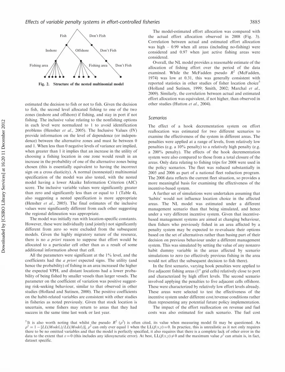
estimated the decision to fish or not to fish. Given the decision

to fish, the second level allocated fishing to one of the two

zones (inshore and offshore) if fishing, and stay in port if not

fishing. The inclusive value relating to the nonfishing options

in each level were normalized to 1 to avoid identification

problems (Hensher et al., 2005). The Inclusive Values (IV)

provide information on the level of dependence (or indepen-

dence) between the alternative zones and must lie between 0

and 1. When less than 0 negative levels of variance are implied,

when greater than 1 it implies that an increase in the utility of

choosing a fishing location in one zone would result in an

increase in the probability of one of the alternative zones being

chosen (this is essentially equivalent to having the incorrect

sign on a cross elasticity). A normal (nonnested) multinomial

specification of the model was also tested, with the nested

model having a lower Akaike Information Criterion (AIC)

score. The inclusive variable values were significantly greater

than zero and significantly less than or equal to 1 (Table 4),

also suggesting a nested specification is more appropriate

(Hensher et al., 2005). The final estimates of the inclusive

values were significantly different from each other suggesting

the regional delineation was appropriate.The model was initially run with location-specific constants.

However, these were individually (and jointly) not significantly

different from zero so were excluded from the subsequent

models. Given the highly migratory nature of the resource,

there is no a priori reason to suppose that effort would be

allocated to a particular cell other than as a result of some

additional information about that cell.

All the parameters were significant at the 1% level, and the

coefficients had the a priori expected signs. The utility (and

hence the probability) of fishing in an area increased the higher

the expected VPH, and distant locations had a lower proba-

bility of being fished by smaller vessels than larger vessels. The

parameter on the coefficient of variation was positive suggest-

ing risk-seeking behaviour, similar to that observed in other

studies (Holland and Sutinen, 2000). The positive coefficients

on the habit-related variables are consistent with other studies

in fisheries as noted previously. Given that stock location is

uncertain, some fishers may return to areas that they had

success in the same time last week or last year.

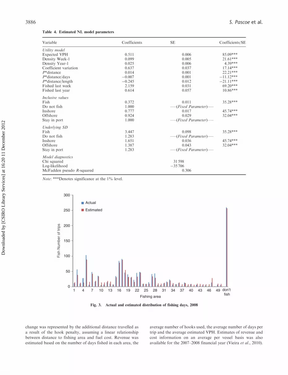
The model-estimated effort allocation was compared with

the actual effort allocation observed in 2008 (Fig. 3).

Correlation between actual and estimated effort allocation

was high – 0.99 when all areas (including no-fishing) were

considered and 0.97 when just active fishing areas were

considered.Overall, the NL model provides a reasonable estimate of the

allocation of fishing effort over the period of the data

examined. While the McFadden pseudo R2 (McFadden,

1974) was low at 0.31, this was generally consistent with

reported statistics in other studies of fisher location choice5

(Holland and Sutinen, 1999; Smith, 2002; Marchal et al.,

2009). Similarly, the correlation between actual and estimated

effort allocation was equivalent, if not higher, than observed in

other studies (Hutton et al., 2004).

Scenarios

The effect of a hook decrementation system on effort

reallocation was estimated for two different scenarios to

examine the effectiveness of the system in different areas. The

penalties were applied at a range of levels, from relatively low

penalties (e.g. a 10% penalty) to a relatively high penalty (e.g.

a 200% penalty). The effects of the hook decrementation

system were also compared to those from a total closure of the

areas. Only data relating to fishing trips for 2008 were used in

the policy scenarios. The fleet was reduced substantially in

2005 and 2006 as part of a national fleet reduction program.

The 2008 data reflects the current fleet situation, so provides a

more meaningful basis for examining the effectiveness of the

incentive-based system.A further set of simulations were undertaken assuming that

‘habits’ would not influence location choice in the affected

areas. The NL model was estimated under a different

management scenario than that being simulated, and hence

under a very different incentive system. Given that incentive-

based management systems are aimed at changing behaviour,

then fishers who previously fished in an area affected by a

penalty system may be expected to re-evaluate their options

based on the set of alternatives rather than basing part of their

decision on previous behaviour under a different management

system. This was simulated by setting the value of any nonzero

habit dummy variable in the areas affected by scenario

simulations to zero (so effectively previous fishing in the area

would not affect the subsequent decision to fish there).

In the first scenario, varying hook penalties were applied to

five adjacent fishing areas (1o grid cells) relatively close to port

and characterized by high effort levels. The second scenario

involved applying the penalties to five adjacent cells offshore.

These were characterized by relatively low effort levels already.

These areas were selected to test the effectiveness of the

incentive system under different cost/revenue conditions rather

than representing any potential future policy implementation.

The impact of the effort reallocation on revenue and fuel

costs was also estimated for each scenario. The fuel cost

Fish Don’t Fish

Don’t Fish

Don’t Fish

Inshore Offshore

Fishing area Fishing area

Fig. 2. Structure of the nested multinomial model

5 It is also worth noting that whilst the pseudo R2 (�2) is often cited, its value when measuring model fit may be questioned. As�2 ¼ 1� ½LLðModel1Þ=LLðModel2Þ�, �

2 can only ever equal 1 when the LL(�|x,y)¼ 0. In practice, this is unrealistic as it not only requiresthere to be no omitted variables and that the model is perfectly specified, it also requires that there is a complete lack of other error in thedata to the extent that "¼ 0 (this includes any idiosyncratic error). At best, LL(�|x,y) 6¼ 0 and the maximum value �2 can attain is, in fact,dataset specific.

Effects of variable penalty systems in effort-controlled fisheries 3885

Dow

nloa

ded

by [

CSI

RO

Lib

rary

Ser

vice

s] a

t 16:

20 1

1 D

ecem

ber

2012

change was represented by the additional distance travelled as

a result of the hook penalty, assuming a linear relationship

between distance to fishing area and fuel cost. Revenue was

estimated based on the number of days fished in each area, the

average number of hooks used, the average number of days per

trip and the average estimated VPH. Estimates of revenue and

cost information on an average per vessel basis was also

available for the 2007–2008 financial year (Vieira et al., 2010).

Table 4. Estimated NL model parameters

Variable Coefficients SE Coefficients/SE

Utility modelExpected VPH 0.511 0.006 85.09***Density Week-1 0.099 0.005 21.61***Density Year-1 0.025 0.006 4.39***Coefficient variation 0.637 0.037 17.14***P*distance 0.014 0.001 22.21***P*distance/days �0.007 0.001 �11.12***P*distance/length �0.245 0.012 �21.11***Fished last week 2.159 0.031 69.20***Fished last year 0.614 0.057 10.86***

Inclusive valuesFish 0.372 0.011 35.28***Do not fish 1.000 —–(Fixed Parameter)—–Inshore 0.777 0.017 45.74***Offshore 0.924 0.029 32.04***Stay in port 1.000 —–(Fixed Parameter)—–

Underlying SDFish 3.447 0.098 35.28***Do not fish 1.283 —–(Fixed Parameter)—–Inshore 1.651 0.036 45.74***Offshore 1.387 0.043 32.04***Stay in port 1.283 —–(Fixed Parameter)—–

Model diagnosticsChi squared 31 598Log-likelihood �35 706McFadden pseudo R-squared 0.306

Note: ***Denotes significance at the 1% level.

0

50

100

150

200

250

300

1 4 7 10 13 16 19 22 25 28 31 34 37 40 43 46 49 don’t fish

Fishing area

Actual

Estimated

Fis

h N

umbe

r of

trip

s

Fig. 3. Actual and estimated distribution of fishing days, 2008

3886 S. Pascoe et al.

Dow

nloa

ded

by [

CSI

RO

Lib

rary

Ser

vice

s] a

t 16:

20 1

1 D

ecem

ber

2012

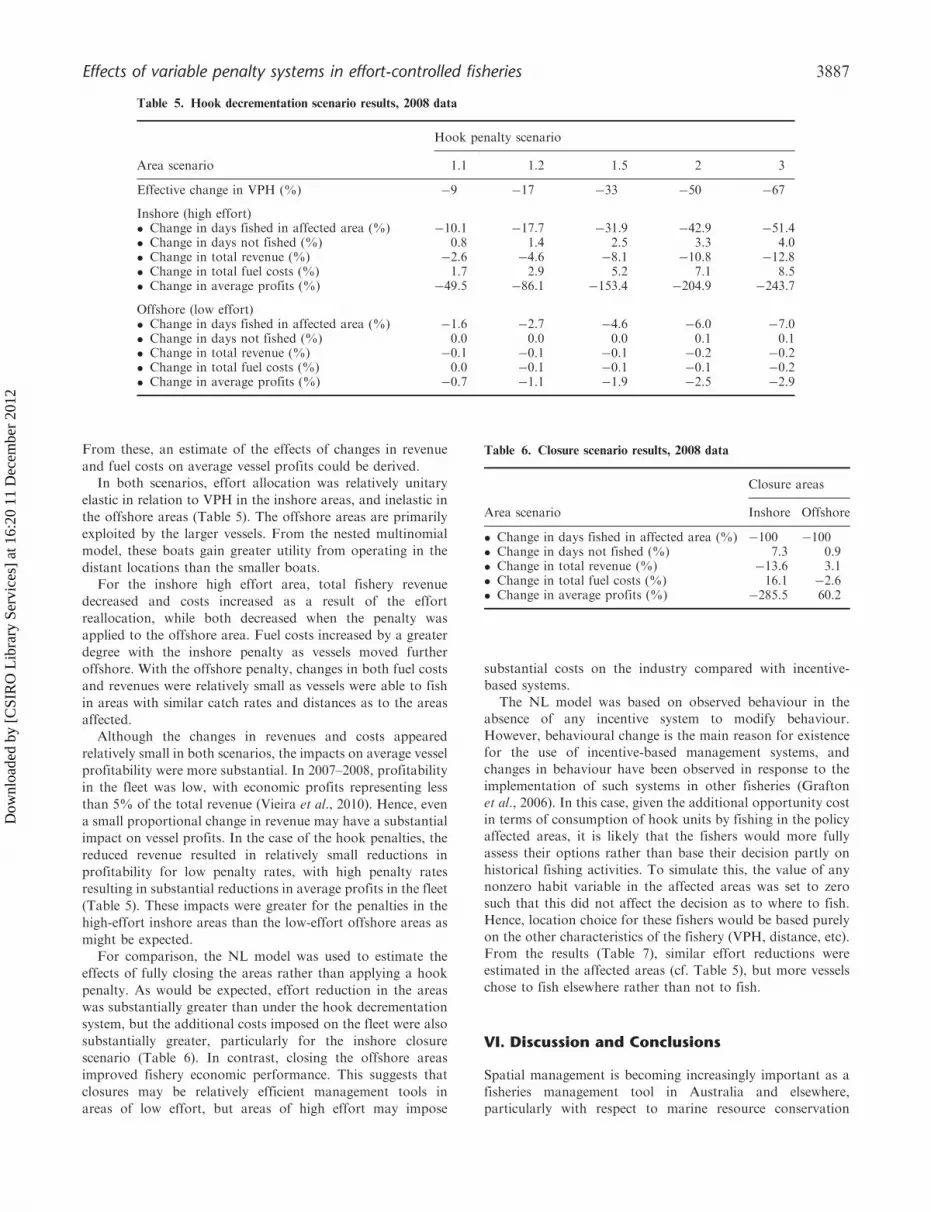
From these, an estimate of the effects of changes in revenue

and fuel costs on average vessel profits could be derived.In both scenarios, effort allocation was relatively unitary

elastic in relation to VPH in the inshore areas, and inelastic in

the offshore areas (Table 5). The offshore areas are primarily

exploited by the larger vessels. From the nested multinomial

model, these boats gain greater utility from operating in the

distant locations than the smaller boats.For the inshore high effort area, total fishery revenue

decreased and costs increased as a result of the effort

reallocation, while both decreased when the penalty was

applied to the offshore area. Fuel costs increased by a greater

degree with the inshore penalty as vessels moved further

offshore. With the offshore penalty, changes in both fuel costs

and revenues were relatively small as vessels were able to fish

in areas with similar catch rates and distances as to the areas

affected.Although the changes in revenues and costs appeared

relatively small in both scenarios, the impacts on average vessel

profitability were more substantial. In 2007–2008, profitability

in the fleet was low, with economic profits representing less

than 5% of the total revenue (Vieira et al., 2010). Hence, even

a small proportional change in revenue may have a substantial

impact on vessel profits. In the case of the hook penalties, the

reduced revenue resulted in relatively small reductions in

profitability for low penalty rates, with high penalty rates

resulting in substantial reductions in average profits in the fleet

(Table 5). These impacts were greater for the penalties in the

high-effort inshore areas than the low-effort offshore areas as

might be expected.For comparison, the NL model was used to estimate the

effects of fully closing the areas rather than applying a hook

penalty. As would be expected, effort reduction in the areas

was substantially greater than under the hook decrementation

system, but the additional costs imposed on the fleet were also

substantially greater, particularly for the inshore closure

scenario (Table 6). In contrast, closing the offshore areas

improved fishery economic performance. This suggests that

closures may be relatively efficient management tools in

areas of low effort, but areas of high effort may impose

substantial costs on the industry compared with incentive-based systems.

The NL model was based on observed behaviour in theabsence of any incentive system to modify behaviour.

However, behavioural change is the main reason for existencefor the use of incentive-based management systems, and

changes in behaviour have been observed in response to the

implementation of such systems in other fisheries (Graftonet al., 2006). In this case, given the additional opportunity cost

in terms of consumption of hook units by fishing in the policyaffected areas, it is likely that the fishers would more fully

assess their options rather than base their decision partly on

historical fishing activities. To simulate this, the value of anynonzero habit variable in the affected areas was set to zero

such that this did not affect the decision as to where to fish.Hence, location choice for these fishers would be based purely

on the other characteristics of the fishery (VPH, distance, etc).From the results (Table 7), similar effort reductions were

estimated in the affected areas (cf. Table 5), but more vessels

chose to fish elsewhere rather than not to fish.

VI. Discussion and Conclusions

Spatial management is becoming increasingly important as a

fisheries management tool in Australia and elsewhere,particularly with respect to marine resource conservation

Table 5. Hook decrementation scenario results, 2008 data

Hook penalty scenario

Area scenario 1.1 1.2 1.5 2 3

Effective change in VPH (%) �9 �17 �33 �50 �67

Inshore (high effort)� Change in days fished in affected area (%) �10.1 �17.7 �31.9 �42.9 �51.4� Change in days not fished (%) 0.8 1.4 2.5 3.3 4.0� Change in total revenue (%) �2.6 �4.6 �8.1 �10.8 �12.8� Change in total fuel costs (%) 1.7 2.9 5.2 7.1 8.5� Change in average profits (%) �49.5 �86.1 �153.4 �204.9 �243.7

Offshore (low effort)� Change in days fished in affected area (%) �1.6 �2.7 �4.6 �6.0 �7.0� Change in days not fished (%) 0.0 0.0 0.0 0.1 0.1� Change in total revenue (%) �0.1 �0.1 �0.1 �0.2 �0.2� Change in total fuel costs (%) 0.0 �0.1 �0.1 �0.1 �0.2� Change in average profits (%) �0.7 �1.1 �1.9 �2.5 �2.9

Table 6. Closure scenario results, 2008 data

Closure areas

Area scenario Inshore Offshore

� Change in days fished in affected area (%) �100 �100� Change in days not fished (%) 7.3 0.9� Change in total revenue (%) �13.6 3.1� Change in total fuel costs (%) 16.1 �2.6� Change in average profits (%) �285.5 60.2

Effects of variable penalty systems in effort-controlled fisheries 3887

Dow

nloa

ded

by [

CSI

RO

Lib

rary

Ser

vice

s] a

t 16:

20 1

1 D

ecem

ber

2012

(Pascoe et al., 2009). In most countries, spatial management

has largely focused on marine protected areas (Wilen, 2004),

although there are a range of alternative spatial management

tools that may achieve the desired conservation outcomes

without a total closure of a fishing area. The hook

decrementation system examined in this study shares similar

characteristics to an individual habitat quota system, in that

spatial penalties can be assigned to effort expended in

particular areas to encourage movement elsewhere (Holland

and Schnier, 2006).The results of the analysis suggest that a hook decrementa-

tion program is likely to be more successful in terms of effort

reallocation when the penalties are applied to high effort areas

than low effort areas. The attraction to the latter is fairly

limited (hence the low level of effort), so making these areas

less attractive is likely to have less of an impact. Conversely,

high effort areas are attractive either due to their high VPH or

low costs of access. In the case of the scenario examined above,

the effort in the inshore areas was driven by both the low

access cost and the VPH, which was also high relative to more

offshore areas. Altering the effective VPH (i.e. increasing the

opportunity cost of the hook quota consumed) in these areas

resulted in a reduction in fishing effort in the affected area

without the need to fully close it.

Several forms of bycatch problems exist in the fishery, both

in inshore and offshore waters. Interactions with turtles, while

occurring across the fishery, are highest in areas close to

nesting beaches, particularly in the northern part of the

fishery. Interactions with seabirds occur in the central offshore

zone (fleshfooted shearwater) near their main nesting islands

(Pascoe et al., 2011) and southern inshore zone (albatross).

These areas are generally characterized by high effort levels as

they also correspond to key tuna grounds at certain times of

the year. Given this, a hook decrementation approach may

have helped reduce fishing effort in the key interaction areas,

although from the model results a high penalty may be needed

to have been imposed to result in a substantial effort

reduction.

A potential downside of the use of incentives rather than

more blunt instruments (closures) is that there is greater

uncertainty about the conservation outcomes. We have

assumed that achieving effort reduction is sufficient to realize

conservation benefits. However, if the relationship is non-

linear, substantial effort reduction may be required to achieve

conservation objectives, and in some cases a closure may be

unavoidable. However, in other cases, conservation objectives

may be achievable even with some residual bycatch, and hence

a decrementation system may be preferable to a closure in

these circumstances.Only a hook penalty was examined in the analysis.

Potentially, hook ‘rewards’ could also be applied to attract

effort to particular areas. The Faroe Islands’ individual

transferable effort quota system provides incentives for vessels

to fish in offshore areas by allowing each quota day to equal 3

fishing days in these areas (i Jakupsstovu et al., 2007).

Similarly, a hook penalty of less than 1 could be applied in

areas where bycatch was relatively low to encourage fishing in

these areas.

The model has several limitations. Heterogeneity in risk

preferences has not been considered, and this has been shown

to affect location choice elsewhere (Mistiaen and Strand, 2000;

Zhang and Smith, 2011). The analysis treats each trip as an

independent event, and the location choice is based on the

prevailing conditions only. While this is seen as an advantage

of the NL approach in most cases (Smith, 2002), with an effort

quota, trips are not completely independent as hook units used

in one trip results in less quota being available for use in the

subsequent trips. In such a case, the response to the hook

penalties may be greater than estimated using the model as the

opportunity cost of using the additional hook units in the

penalty areas is not fully considered (Dowling et al., 2011).

Despite the potential model limitations, the model results

suggest that a hook decrementation system has potential as a

spatial management tool to redirect fishing effort from

sensitive areas to less sensitive areas. However, high penalties

may need to be applied to encourage effort reallocation. For

some areas, closures may still be considered necessary if

bycatch rates are unacceptable even at lower fishing effort

levels. Closures are effective as a conservation tool, but as seen

from the model results, may impose substantial costs on the

Table 7. Hook decrementation scenario results if habits change, 2008 data

Hook penalty scenario

Area scenario 1.1 1.2 1.5 2 3

Effective change in VPH (%) �9 �17 �33 �50 �67

Inshore (high effort)� Change in days fished in affected area (%) �10.4 �18.1 �32.1 �42.8 �50.9� Change in days not fished (%) 0.5 0.9 1.6 2.2 2.6� Change in total revenue (%) �1.9 �3.3 �5.7 �7.5 �8.9� Change in total fuel costs (%) 1.2 2.0 3.6 4.7 5.6� Change in average profits (%) �35.4 �61.1 �107.5 �142.3 �168.0

Offshore (low effort)� Change in days fished in affected area (%) �1.6 �2.8 �4.8 �6.2 �7.2� Change in days not fished (%) 0.0 0.0 0.0 0.1 0.1� Change in total revenue (%) �0.1 �0.1 �0.1 �0.2 �0.2� Change in total fuel costs (%) 0.0 �0.1 �0.1 �0.1 �0.2� Change in average profits (%) �0.7 �1.1 �1.9 �2.5 �2.9

3888 S. Pascoe et al.

Dow

nloa

ded

by [

CSI

RO

Lib

rary

Ser

vice

s] a

t 16:

20 1

1 D

ecem

ber

2012

fishery, even if effort can reallocate. However, in many cases,

effort reduction rather than total exclusion may be sufficient to

achieve the conservation objective, and a hook decrementation

system allows the level of effort reduction to be ‘fine tuned’

through changing the penalty structure.

Acknowledgements

The work was undertaken as part of an AFMA/FRDC-funded

project ‘Predicting the impact of hook decrements on the

distribution of fishing effort in the ETBF’. The authors would

also like to thank the reviewers who provided valuable

comments.

References

ABARE (2008) Australian Commodity Statistics 2007, ABARE,Canberra.

ABARE (2009a) Australian Fisheries Statistics 2008, ABARE,Canberra.

ABARE (2009b) Statistical tables, Australian Commodities, 16,377–414.

ABARES (2011) Australian Fisheries Statistics 2010, AustralianBureau of Agricultural and Resource Economics andSciences, Canberra.

Andersen, B. S., Ulrich, C., Eigaard, O. R. and Christensen, A.-S.(2012) Short-term choice behaviour in a mixed fishery:investigating metier selection in the Danish gillnet fishery,ICES Journal of Marine Science, 69, 131–43.

Bockstael, N. E. and Opaluch, J. J. (1984) Behavioral modelingand fisheries management, Marine Resource Economics, 1,105–15.

Costello, C. and Polasky, S. (2008) Optimal harvesting ofstochastic spatial resources, Journal of EnvironmentalEconomics and Management, 56, 1–18.

Curtis, R. and Hicks, R. L. (2000) The cost of sea turtlepreservation: the case of Hawaii’s pelagic longliners,American Journal of Agricultural Economics, 82, 1191–7.

Dowling, N. A., Wilcox, C., Mangel, M. and Pascoe, S. (2011)Assessing opportunity and relocation costs of marine pro-tected areas using a behavioural model of longline fleetdynamics, Fish and Fisheries, 13, 139–57.

Eales, J. and Wilen, J. E. (1986) An examination of fishinglocation choice in the pink shrimp fishery, Marine ResourceEconomics, 2, 331–51.

Evans, S. K. (2007) Eastern Tuna and Billfish Fishery DataSummary 2005–2006, Australian Fisheries ManagementAuthority, Canberra.

Gillis, D. M., Peterman, R. M. and Pitkitch, E. K. (1995a)Implications of trip regulations for high-grading: a model ofthe behaviour of fishermen, Canadian Journal of Fisheries andAquatic Sciences, 52, 402–15.

Gillis, D. M., Pitkitch, E. K. and Peterman, R. M. (1995b)Dynamic discarding decisions: foraging theory for high-grading in a trawl fishery, Behavioural Ecology, 6, 146–54.

Grafton, R. Q., Arnason, R., Bjørndal, T., Campbell, D.,Campbell, H. F., Clark, C. W., Connor, R., Dupont, D. P.,Hannesson, R., Hilborn, R., Kirkley, J. E., Kompas, T., Lane,D. E.,Munro, G. R., Pascoe, S., Squires, D., Steinshamn, S. I.,Turris, B. R. and Weninger, Q. (2006) Incentive-basedapproaches to sustainable fisheries, Canadian Journal ofFisheries and Aquatic Sciences, 63, 699–710.

Gray, J. S. (1997) Marine biodiversity: patterns, threats andconservation needs, Biodiversity and Conservation, 6, 153–75.

Haynie, A. C. and Layton, D. F. (2010) An expected profit modelfor monetizing fishing location choices, Journal ofEnvironmental Economics and Management, 59, 165–76.

Hensher, D. A., Rose, J. and Greene, W. (2005) Applied ChoiceAnalysis: A Primer, Cambridge University Press, Cambridge.

Holland, D. and Schnier, K. E. (2006) Individual habitat quotasfor fisheries, Journal of Environmental Economics andManagement, 51, 72–92.

Holland, D. S. and Sutinen, J. G. (1999) An empirical model offleet dynamics in New England trawl fisheries, CanadianJournal of Fisheries and Aquatic Sciences, 56, 253–64.

Holland, D. S. and Sutinen, J. G. (2000) Location choice in NewEngland trawl fisheries: old habits die hard, Land Economics,76, 133–49.

Hutton, T., Mardle, S., Pascoe, S. and Clark, R. A. (2004)Modelling fishing location choice within mixed fisheries:English North Sea beam trawlers in 2000 and 2001, ICESJournal of Marine Science, 61, 1443–52.

i Jakupsstovu, S. H., Cruz, L. R., Maguire, J. J. and Reinert, J.(2007) Effort regulation of the demersal fisheries at the FaroeIslands: a 10-year appraisal, ICES Journal Marine Science,64, 730–7.

Kearney, R., Buxton, C. D. and Farebrother, G. (2012)Australia’s no-take marine protected areas: appropriateconservation or inappropriate management of fishing?,Marine Policy, 36, 1064–71.

Manson, F. J. and Die, D. J. (2001) Incorporating commercialfishery information into the design of marine protected areas,Ocean and Coastal Management, 44, 517–30.

Marchal, P., Lallemand, P. and Stokes, K. (2009) The relativeweight of traditions, economics, and catch plans in NewZealand fleet dynamics, Canadian Journal of Fisheries andAquatic Sciences, 66, 291–311.

Maury, O. and Gascuel, D. (1999) SHADYS (‘simulateurhalieutique de dynamiques spatiales’), a GIS based numericalmodel of fisheries. Example application: the study of amarine protected area, Aquatic Living Resources, 12, 77–88.

McFadden, D. (1974) Conditional logit analysis of qualitativechoice behavior, in Frontiers in Econometrics (Ed.)P. Zarembka, Academic Press, New York, pp. 105–42.

McFadden, D. (1981) Econometric models of probabilistic choice,in Structural Analysis of Discrete Data with EconometricsApplications (Eds) C. F. Manski and D. McFadden, MITPress, Cambridge, pp. 198–272.

Mistiaen, J. A. and Strand, I. E. (2000) Locationchoice of commercial fishermen with heterogeneous riskpreferences, American Journal of Agricultural Economics, 82,1184–90.

Murray, K. T., Read, A. J. and Solow, A. R. (2000) The useof time/area closures to reduce bycatches of harbourporpoises: lessons from the Gulf of Maine sink gillnetfishery, Journal of Cetacean Research and Management, 2,135–41.

Pascoe, S., Bustamante, R., Wilcox, C. and Gibbs, M. (2009)Spatial fisheries management: a framework for multi-objective qualitative assessment, Ocean and CoastalManagement, 52, 130–8.

Pascoe, S., Innes, J., Holland, D., Fina, M., Thebaud, O.,Townsend, R., Sanchirico, J., Arnason, R., Wilcox, C. andHutton, T. (2010) Use of incentive-based managementsystems to limit bycatch and discarding, InternationalReview of Environmental and Resource Economics, 4, 123–61.

Pascoe, S., Wilcox, C. and Donlan, C. J. (2011) Biodiversityoffsets: a cost-effective interim solution to seabird bycatch infisheries?, PLoS ONE, 6, e25762.

Poos, J.J., Bogaards, J.A., Quirijns, F.J., Gillis, D.M. andRijnsdorp, A.D. (2010) Individual quotas, fishing effortallocation, and over-quota discarding in mixed fisheries,ICES Journal of Marine Science, 67, 323–33.

Effects of variable penalty systems in effort-controlled fisheries 3889

Dow

nloa

ded

by [

CSI

RO

Lib

rary

Ser

vice

s] a

t 16:

20 1

1 D

ecem

ber

2012

Pradhan, N. C. and Leung, P.-S. (2004) Modeling trip choicebehavior of the longline fishers in Hawaii, Fisheries Research,68, 209–24.

Ran, T., Keithly, W. R. and Kazmierczak, R. F. (2011) Locationchoice behavior of Gulf of Mexico shrimpers under dynamiceconomic conditions, Journal of Agricultural and AppliedEconomics, 43, 29–42.

Sampson, D. B. (1991) Fishing tactics and fish abundance, andtheir influence on catch rates, ICES Journal of MarineScience, 48, 291–301.

Schnier, K. E. and Felthoven, R. G. (2011) Accounting for spatialheterogeneity and autocorrelation in spatial discrete choicemodels: implications for behavioral predictions, LandEconomics, 87, 382–402.

Smith, M. D. (2002) Two econometric approaches for predictingthe spatial behavior of renewable resource harvesters, LandEconomics, 78, 522–38.

Smith, M. D. (2005) State dependence and heterogeneity in fishinglocation choice, Journal of Environmental Economics andManagement, 50, 319–40.

Smith, M. D., Lynham, J., Sanchirico, J. N. and Wilson, J. A.(2010) Political economy of marine reserves: understanding

the role of opportunity costs, Proceedings of the NationalAcademy of Sciences, 107, 18300–5.

Tidd, A. N., Hutton, T., Kell, L. T. and Blanchard, J. L. (2012)Dynamic prediction of effort reallocation in mixed fisheries,Fisheries Research, 125–126, 243–53.

van Putten, I. E., Kulmala, S., Thebaud, O., Dowling, N., Hamon,K. G., Hutton, T. and Pascoe, S. (2012) Theories andbehavioural drivers underlying fleet dynamics models, Fishand Fisheries, 13, 216–35.

Vieira, S., Perks, C., Mazur, K., Curtotti, R. and Li, M. (2010)Impact of the structural adjustment package on the profit-ability of Commonwealth fisheries, ABARE ResearchReport 10.01, ABARE, Canberra.

Wilen, J. E. (2004) Spatial management of fisheries, MarineResource Economics, 19, 7–19.

Wilen, J. E., Smith, M. D., Lockwood, D. and Botsford, F. W.(2002) Avoiding surprises: incorporating fisherman behaviorinto management models, Bulletin of Marine Science, 70,553–75.

Zhang, J. and Smith, M. (2011) Heterogeneous response to marinereserve formation: a sorting model approach, Environmentaland Resource Economics, 49, 311–25.

3890 S. Pascoe et al.

Dow

nloa

ded

by [

CSI

RO

Lib

rary

Ser

vice

s] a

t 16:

20 1

1 D

ecem

ber

2012