Page 1
Meixia Tao @ SJTU
Principles of Communications
Chapter 4: Analog-to-Digital Conversion
Selected from: Chapter 7.1 – 7.4 of Fundamentals of Communications Systems, Pearson Prentice Hall
2005, by Proakis & Salehi
1
Page 2
Meixia Tao @ SJTU
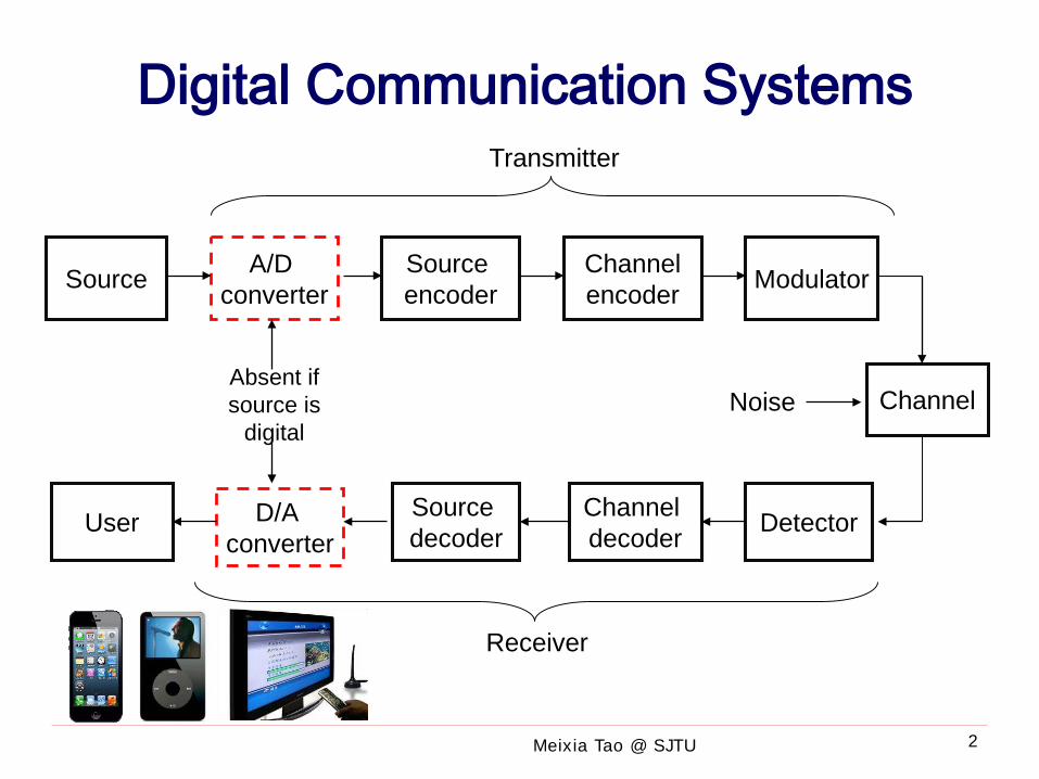
Digital Communication Systems
Source A/D converter
Source encoder
Channelencoder Modulator
Channel
DetectorChannel decoder
Source decoder
D/A converter
User
Transmitter
Receiver
Absent if source is
digitalNoise
2
Page 3
Meixia Tao @ SJTU
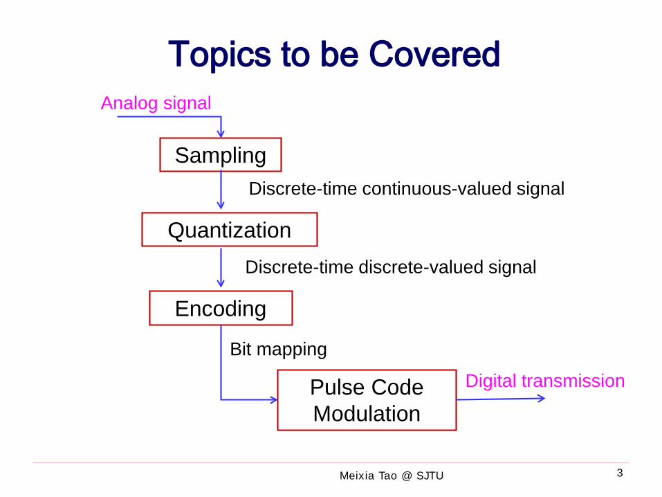
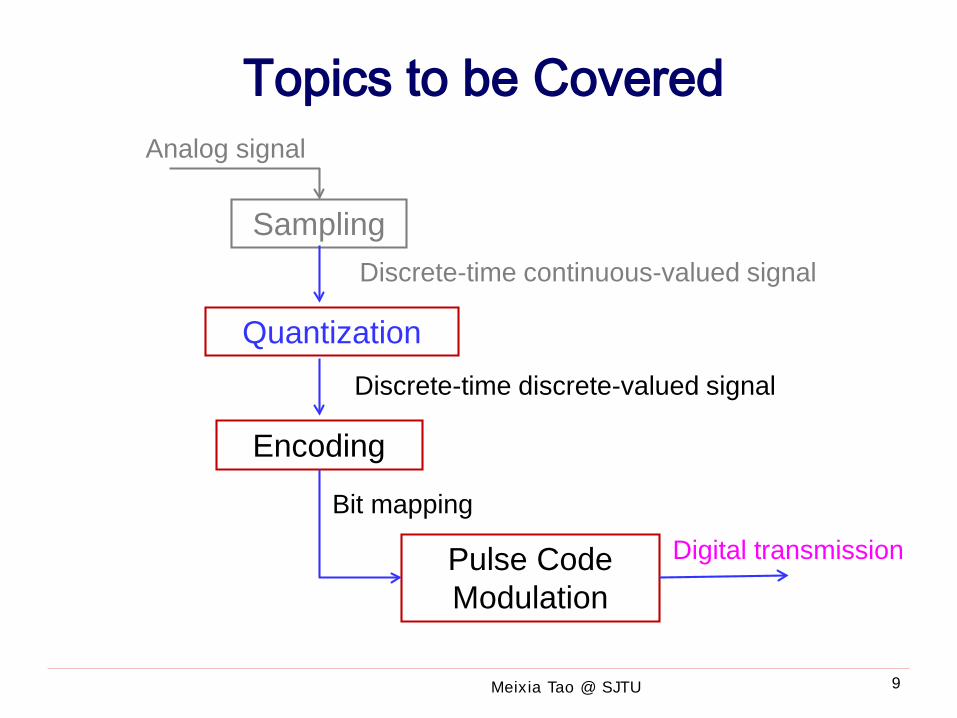
Topics to be Covered
Sampling
Quantization
Encoding
Pulse Code Modulation
Analog signal
Discrete-time continuous-valued signal
Discrete-time discrete-valued signal
Bit mapping
Digital transmission
3
Page 4
Meixia Tao @ SJTU
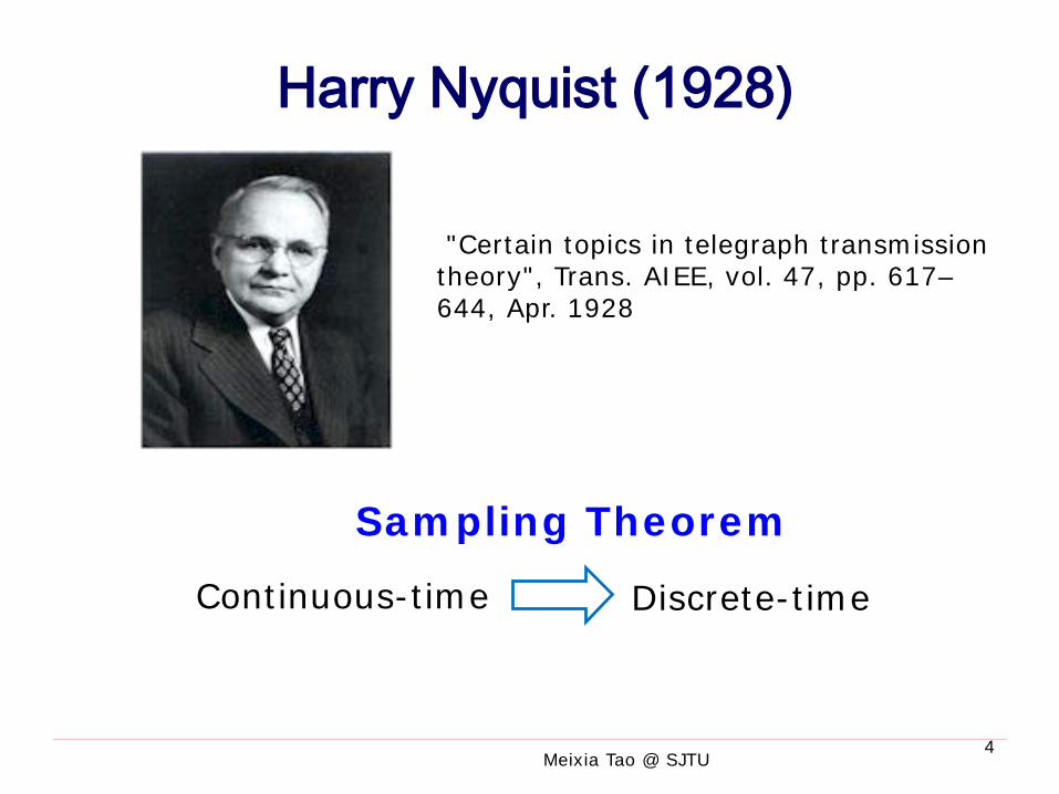
Harry Nyquist (1928)
Continuous-time Discrete-time
Sampling Theorem
"Certain topics in telegraph transmission theory", Trans. AIEE, vol. 47, pp. 617–644, Apr. 1928
4
Page 5
Meixia Tao @ SJTU
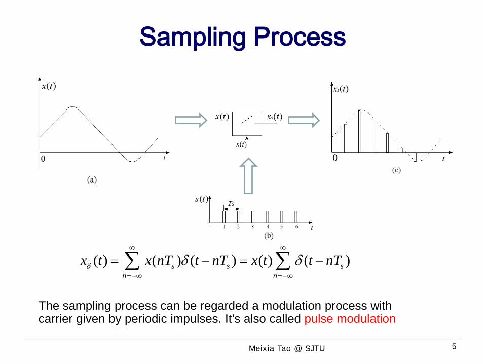
Sampling Process
( ) ( ) ( ) ( ) ( )s s sn n
x t x nT t nT x t t nTδ δ δ∞ ∞
=−∞ =−∞
= − = −∑ ∑
The sampling process can be regarded a modulation process with carrier given by periodic impulses. It’s also called pulse modulation
5
Page 6
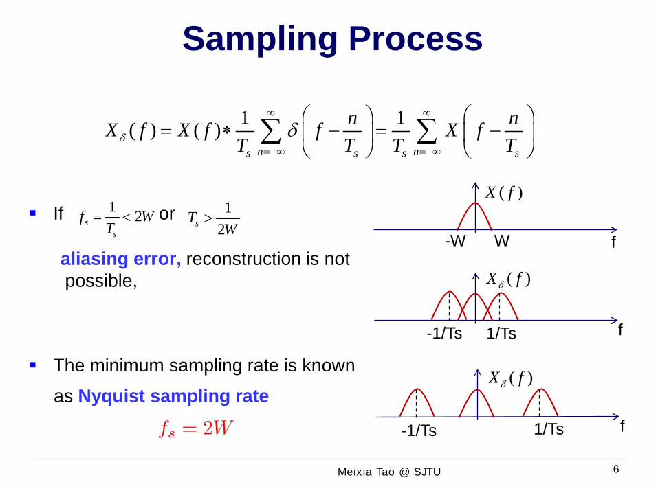
Meixia Tao @ SJTU
If or
The minimum sampling rate is known
as Nyquist sampling rate
1 1( ) ( )n ns s s s
n nX f X f f X fT T T Tδ δ
∞ ∞
=−∞ =−∞
= ∗ − = −
∑ ∑
W-W f
( )X f
f1/Ts-1/Ts
( )X fδ
12sTW
>
aliasing error, reconstruction is not possible,
1 2ss
f WT
= <
Sampling Process
f1/Ts-1/Ts
( )X fδ
6
Page 7
Meixia Tao @ SJTU
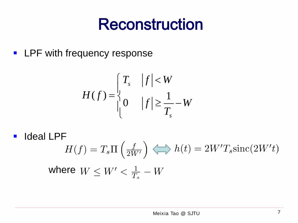
Reconstruction LPF with frequency response
Ideal LPF
where
( ) 10
s
s
T f WH f
f WT
<= ≥ −
7
Page 8
Meixia Tao @ SJTU
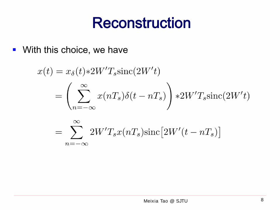
Reconstruction With this choice, we have
8
Page 9
Meixia Tao @ SJTU
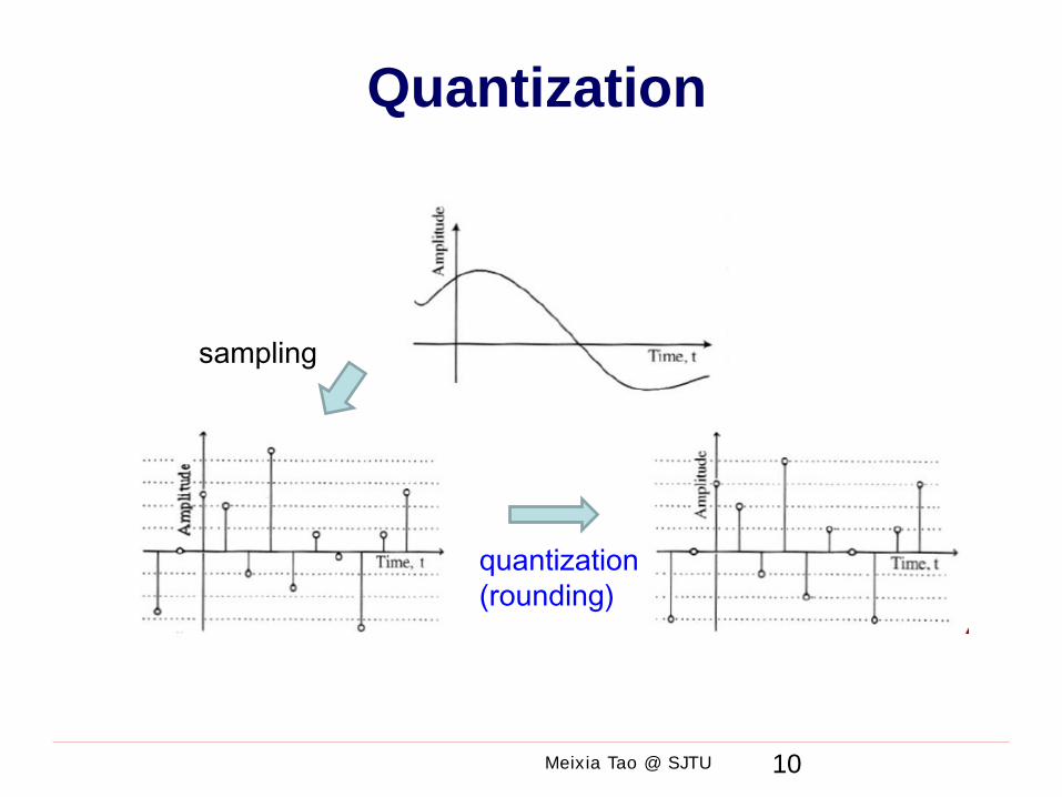
Topics to be Covered
Sampling
Quantization
Encoding
Pulse Code Modulation
Analog signal
Discrete-time continuous-valued signal
Discrete-time discrete-valued signal
Bit mapping
Digital transmission
9
Page 10
Meixia Tao @ SJTU
Quantization
quantization (rounding)
sampling
10
Page 11
Meixia Tao @ SJTU
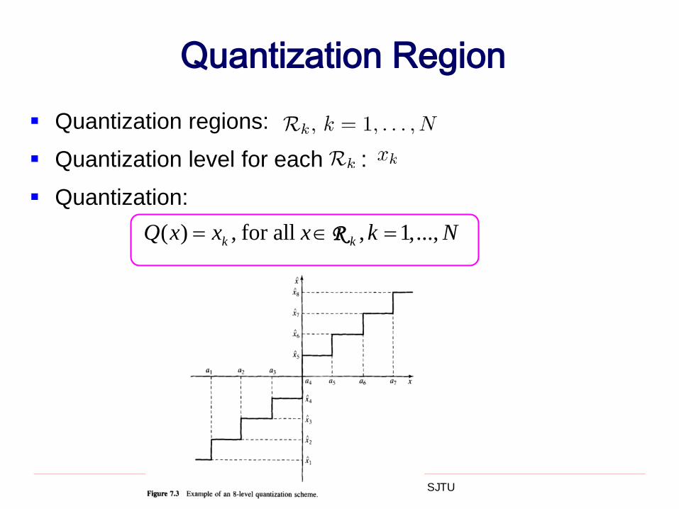
Quantization Region Quantization regions:
Quantization level for each :
Quantization: ( ) , for all , 1,...,k kQ x x x k N= ∈ =R
Page 12
Meixia Tao @ SJTU
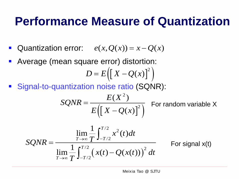
Performance Measure of Quantization
Quantization error:
Average (mean square error) distortion:
Signal-to-quantization noise ratio (SQNR):
( , ( )) ( )e x Q x x Q x= −
[ ]( )2( )D E X Q x= −
[ ]( )2
2
( )( )
E XSQNRE X Q x
=−
( )
/2 2
/2
/2 2
/2
1lim ( )
1lim ( ) ( ( ))
T
TT
T
TT
x t dtTSQNR
x t Q x t dtT
−→∞
−→∞
=−
∫
∫
For random variable X
For signal x(t)
Page 13
Meixia Tao @ SJTU
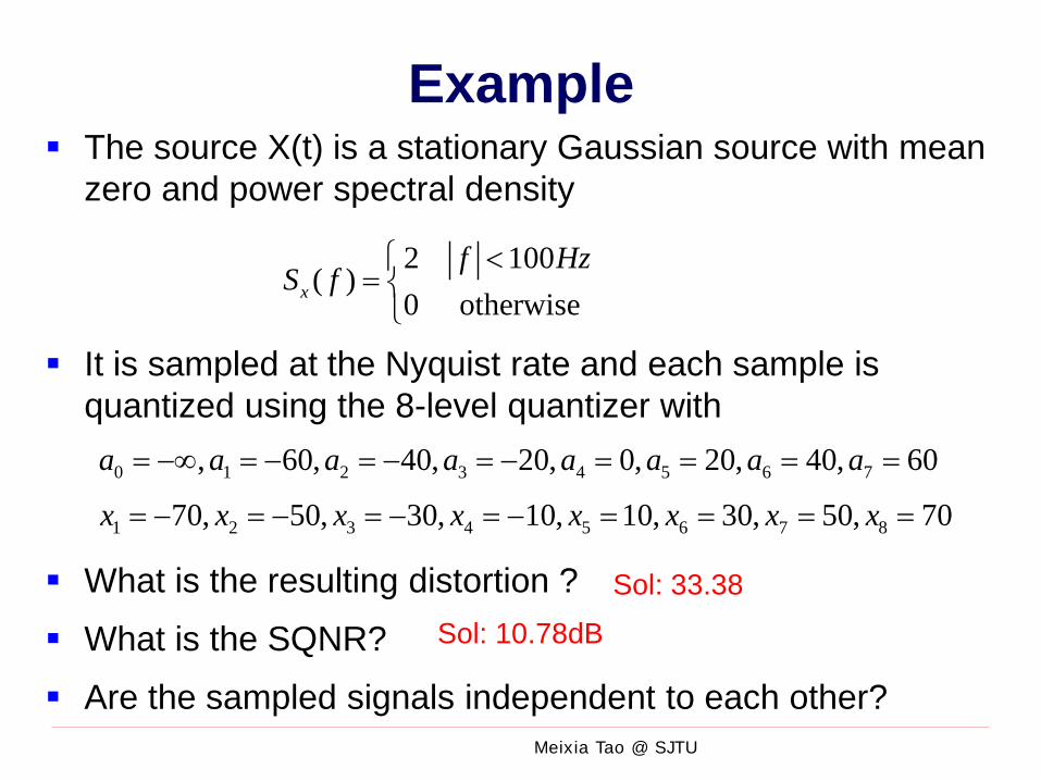
Example The source X(t) is a stationary Gaussian source with mean
zero and power spectral density
It is sampled at the Nyquist rate and each sample is quantized using the 8-level quantizer with
What is the resulting distortion ?
What is the SQNR?
Are the sampled signals independent to each other?
2 100( )
0 otherwisexf Hz
S f <
=
0 1 2 3 4 5 6 7, 60, 40, 20, 0, 20, 40, 60a a a a a a a a= −∞ = − = − = − = = = =
1 2 3 4 5 6 7 870, 50, 30, 10, 10, 30, 50, 70x x x x x x x x= − = − = − = − = = = =
Sol: 33.38
Sol: 10.78dB
Page 14
Meixia Tao @ SJTU
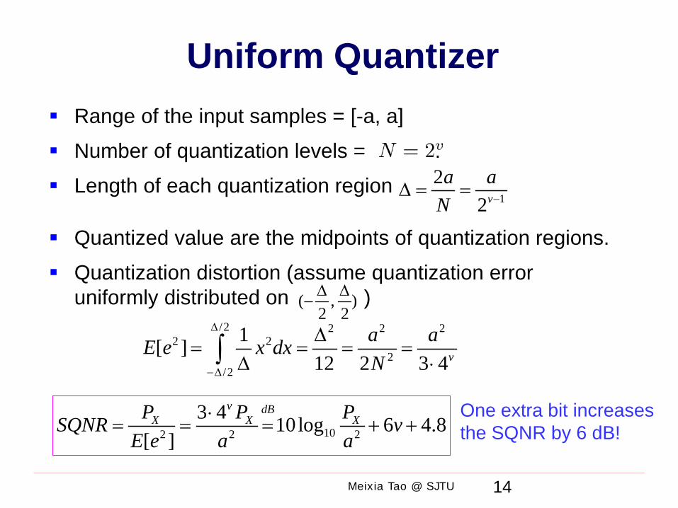
Uniform Quantizer Range of the input samples = [-a, a]
Number of quantization levels = .
Length of each quantization region
Quantized value are the midpoints of quantization regions.
Quantization distortion (assume quantization error uniformly distributed on )
1
22v
a aN −∆ = =
( , )2 2∆ ∆
−/2 2 2 2
2 22
/2
1[ ]12 2 3 4v
a aE e x dxN
∆
−∆
∆= = = =
∆ ⋅∫
102 2 2
3 4 10log 6 4.8[ ]
v dBX X XP P PSQNR v
E e a a⋅
= = = + +One extra bit increases the SQNR by 6 dB!
14
Page 15
Meixia Tao @ SJTU
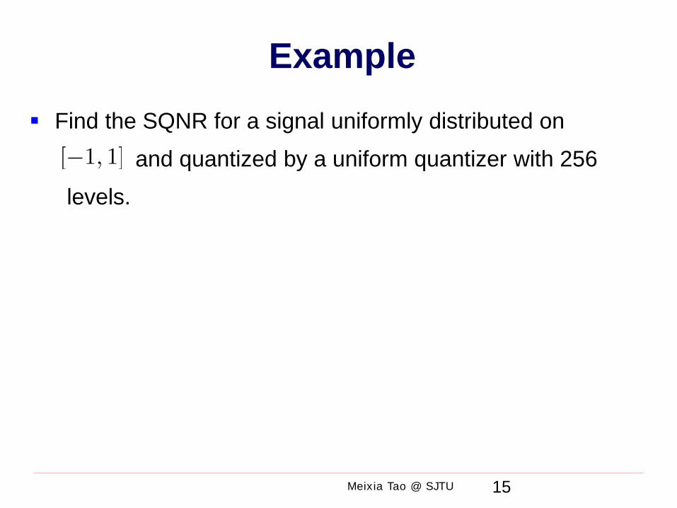
Example Find the SQNR for a signal uniformly distributed on
and quantized by a uniform quantizer with 256
levels.
15
Page 16
Meixia Tao @ SJTU
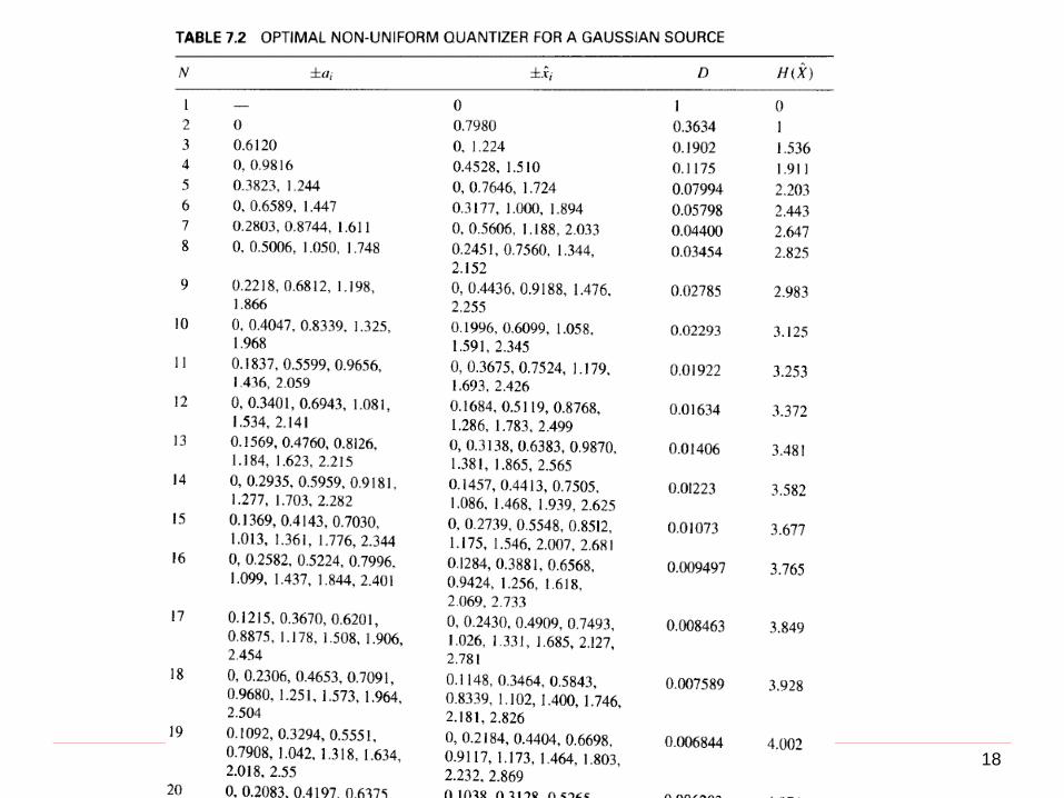
Nonuniform Quantizer By relaxing the condition that the quantization regions be of
equal length, we can minimize the distortion with less constraints
The resulting quantizer will perform better than a uniform quantizer
16
Page 17
Meixia Tao @ SJTU
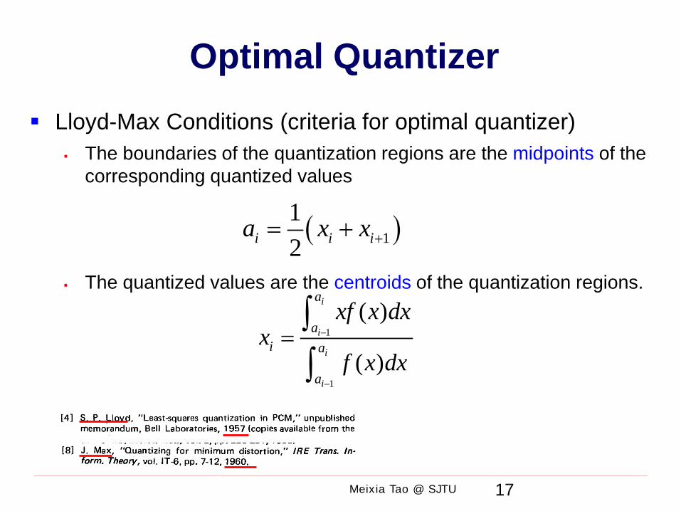
Optimal Quantizer Lloyd-Max Conditions (criteria for optimal quantizer)
The boundaries of the quantization regions are the midpoints of the corresponding quantized values
The quantized values are the centroids of the quantization regions.
( )112i i ia x x += +
1
1
( )
( )
i
i
i
i
a
ai a
a
xf x dxx
f x dx−
−
=∫∫
17
Page 18
Meixia Tao @ SJTU 18
Page 19
Meixia Tao @ SJTU
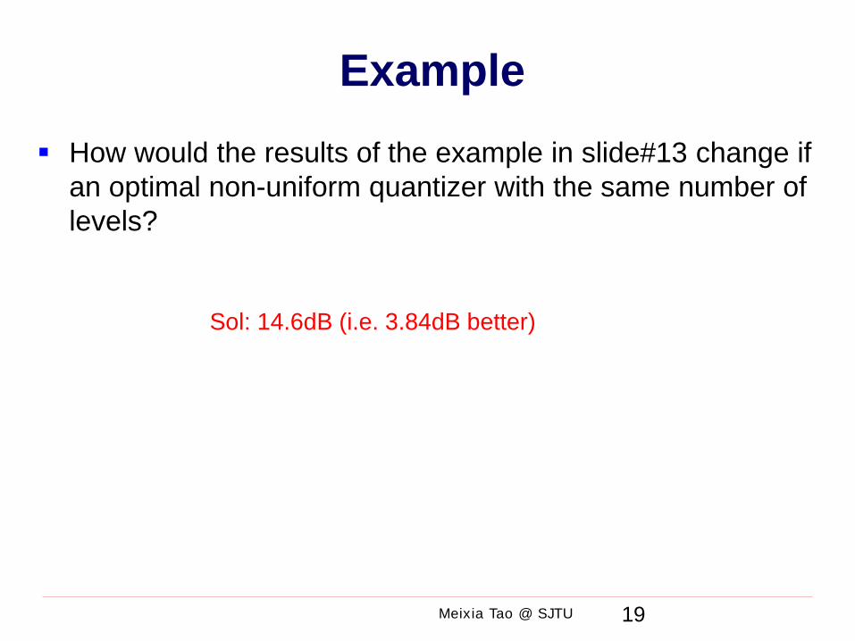
Example How would the results of the example in slide#13 change if
an optimal non-uniform quantizer with the same number of levels?
Sol: 14.6dB (i.e. 3.84dB better)
19
Page 20
Meixia Tao @ SJTU
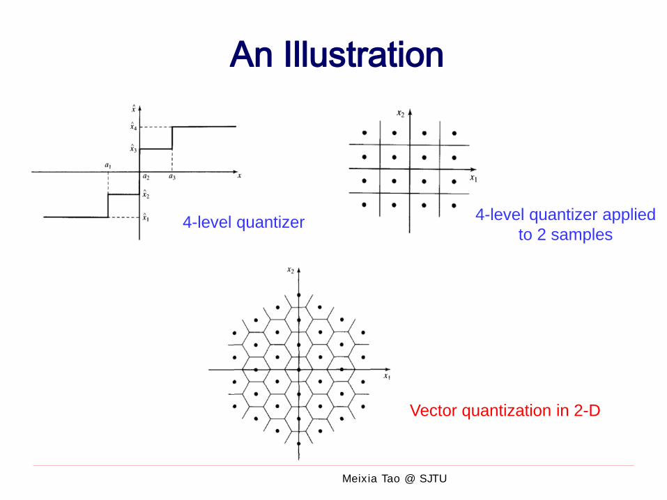
Vector Quantization Scalar quantization
Each sample is quantized individually
Vector quantization: Take blocks of source outputs of length n, and design the quantizer
in the n-dim Euclidean space, rather than doing the quantization based on single samples in an one-dim space
20
Page 21
Meixia Tao @ SJTU
An Illustration
4-level quantizer 4-level quantizer applied to 2 samples
Vector quantization in 2-D
Page 22
Meixia Tao @ SJTU
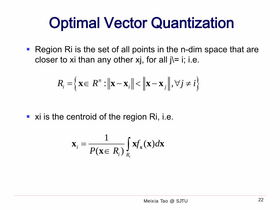
Optimal Vector Quantization Region Ri is the set of all points in the n-dim space that are
closer to xi than any other xj, for all j\= i; i.e.
xi is the centroid of the region Ri, i.e.
{ }: ,ni i jR R j i= ∈ − < − ∀ ≠x x x x x
1 ( )( )
i
ii R
f dP R
=∈ ∫ xx x x x
x
22
Page 23
Meixia Tao @ SJTU
Application of Quantizer Application of quantizer:
ADC in digital communication Channel feedback in FDD cellular networks
More reading: Allen Gersho, "Quantization", IEEE Communications Society
Magazine, pp. 16–28, Sept. 1977.
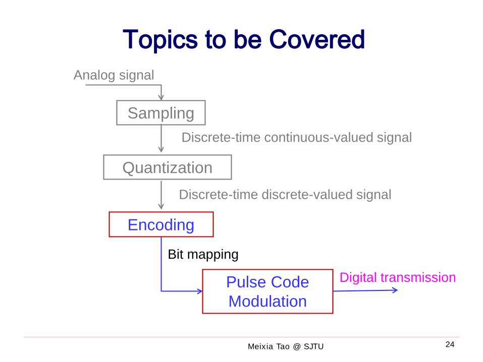
Page 24
Meixia Tao @ SJTU
Topics to be Covered
Sampling
Quantization
Encoding
Pulse Code Modulation
Analog signal
Discrete-time continuous-valued signal
Discrete-time discrete-valued signal
Bit mapping
Digital transmission
24
Page 25
Meixia Tao @ SJTU
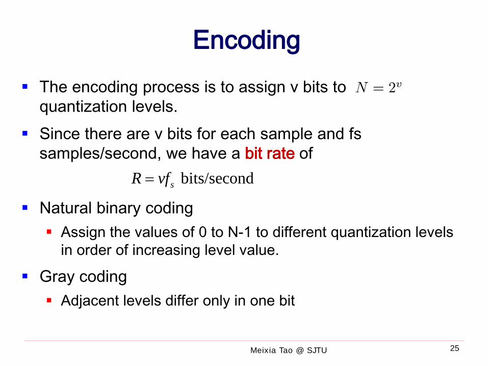
Encoding The encoding process is to assign v bits to
quantization levels. Since there are v bits for each sample and fs
samples/second, we have a bit rate of
Natural binary coding Assign the values of 0 to N-1 to different quantization levels
in order of increasing level value.
Gray coding Adjacent levels differ only in one bit
bits/secondsR vf=
25
Page 26
Meixia Tao @ SJTU
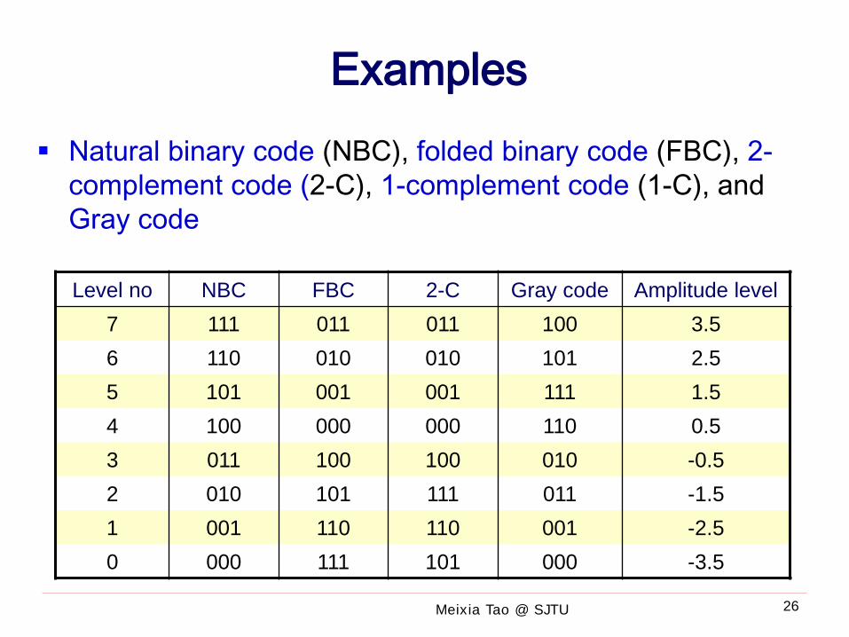
Examples Natural binary code (NBC), folded binary code (FBC), 2-
complement code (2-C), 1-complement code (1-C), and Gray code
Level no NBC FBC 2-C Gray code Amplitude level7 111 011 011 100 3.56 110 010 010 101 2.55 101 001 001 111 1.54 100 000 000 110 0.53 011 100 100 010 -0.52 010 101 111 011 -1.51 001 110 110 001 -2.50 000 111 101 000 -3.5
26
Page 27
Meixia Tao @ SJTU
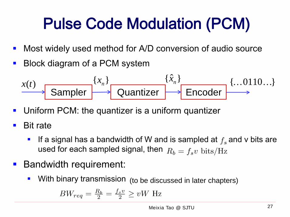
Most widely used method for A/D conversion of audio source Block diagram of a PCM system
Uniform PCM: the quantizer is a uniform quantizer Bit rate
If a signal has a bandwidth of W and is sampled at and v bits are used for each sampled signal, then
Bandwidth requirement: With binary transmission
Pulse Code Modulation (PCM)
Sampler Quantizer Encoder( )x t { }nx ˆ{ }nx { 0110 }
(to be discussed in later chapters)
27
Page 28
Meixia Tao @ SJTU
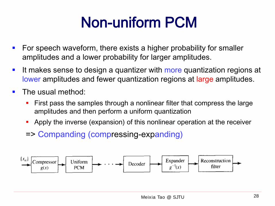
Non-uniform PCM For speech waveform, there exists a higher probability for smaller
amplitudes and a lower probability for larger amplitudes. It makes sense to design a quantizer with more quantization regions at
lower amplitudes and fewer quantization regions at large amplitudes. The usual method:
First pass the samples through a nonlinear filter that compress the large amplitudes and then perform a uniform quantization
Apply the inverse (expansion) of this nonlinear operation at the receiver
=> Companding (compressing-expanding)
28
Page 29
Meixia Tao @ SJTU
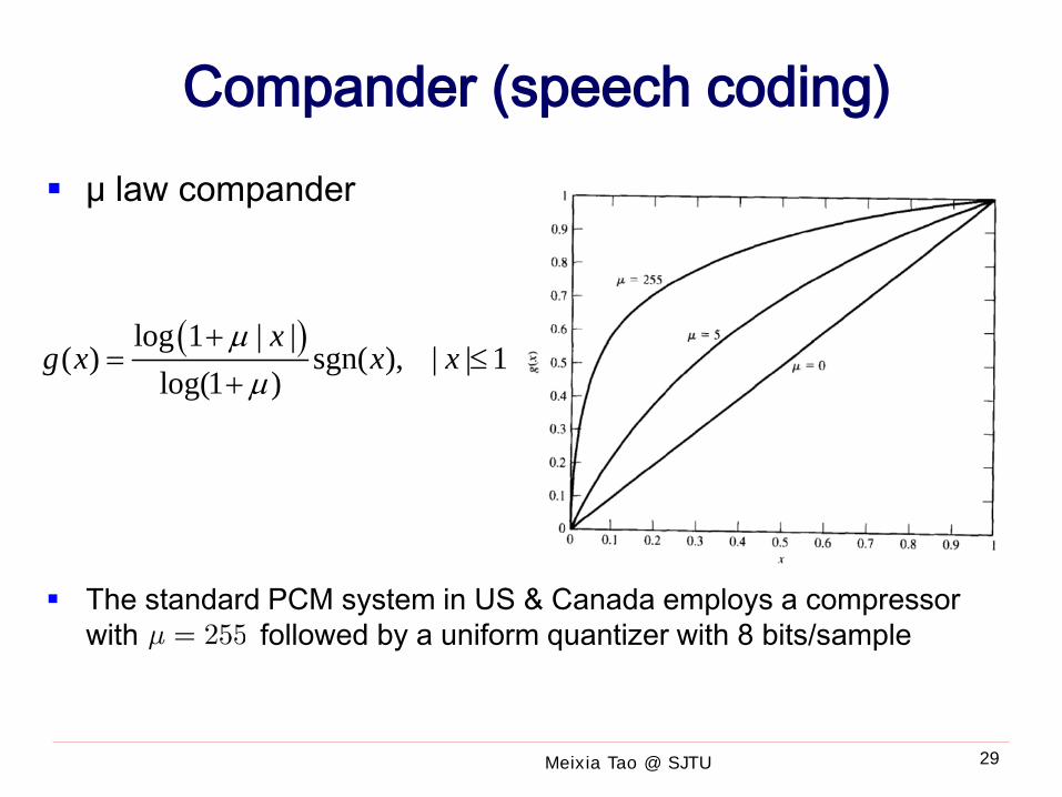
Compander (speech coding) μ law compander
The standard PCM system in US & Canada employs a compressor with followed by a uniform quantizer with 8 bits/sample
( )log 1 | |( ) sgn( ), | | 1
log(1 )x
g x x xµµ
+= ≤
+
29
Page 30
Meixia Tao @ SJTU
Compander A law compander
1 log | |( ) sgn( ), | | 11 log
A xg x x xA
+= ≤
+
81
8486
1
x
y
21
41
81
1
6.87=A
30
Page 31
Meixia Tao @ SJTU
Differential PCM (DPCM) For a bandlimited random process, the sampled values are usually
correlated random variables This correlation can be exploited to improve the performance Differential PCM: quantize the difference between two adjacent
samples. As the difference has small variation, to achieve a certain level of
performance, fewer bits are required
31
Page 32
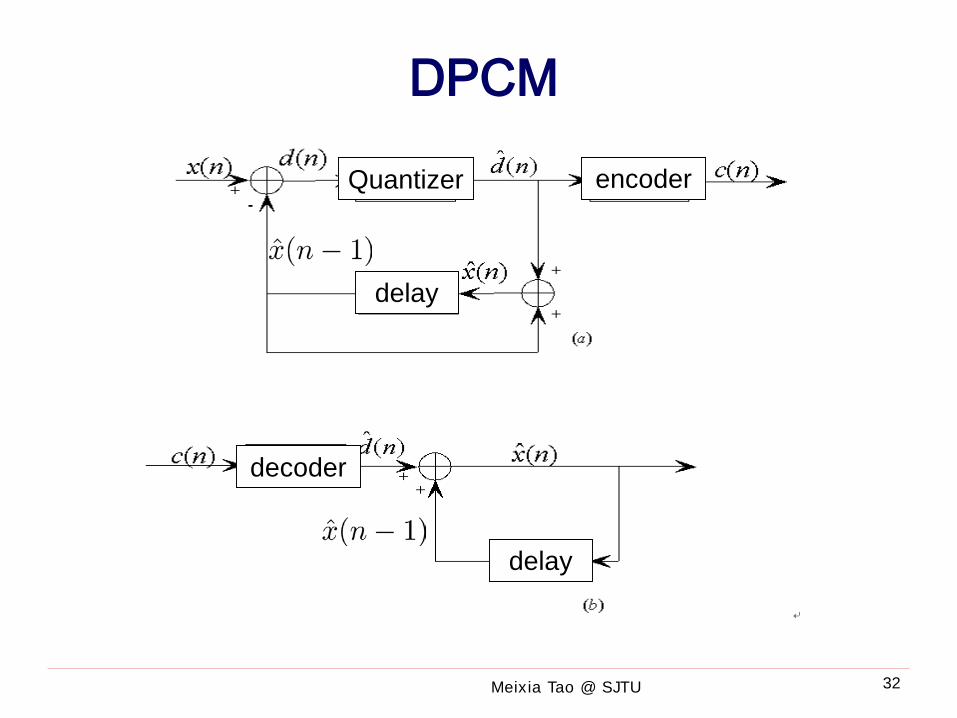
Meixia Tao @ SJTU
DPCM
Quantizer
delay
delay
encoder
decoder
32
Page 33
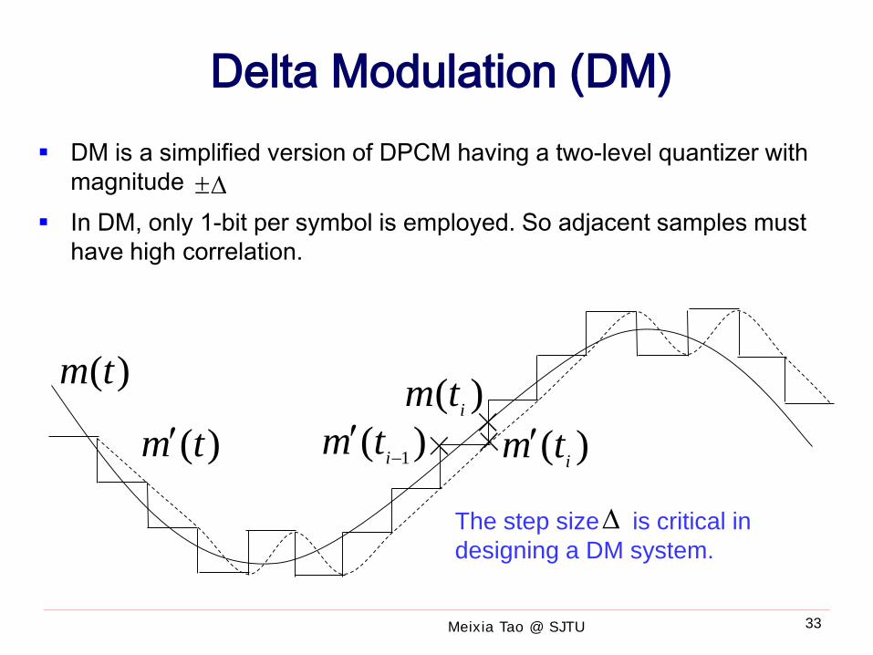
Meixia Tao @ SJTU
Delta Modulation (DM) DM is a simplified version of DPCM having a two-level quantizer with
magnitude In DM, only 1-bit per symbol is employed. So adjacent samples must
have high correlation.
±∆
×××)( 1−
′itm )( itm′
)( itm)(tm
)(tm′
∆The step size is critical in designing a DM system.
33
Page 34
Meixia Tao @ SJTU
Step Size
34
Page 35
Meixia Tao @ SJTU
Suggested Reading Chapter 7.1 – 7.4 of Fundamentals of Communications
Systems, Pearson Prentice Hall 2005, by Proakis & Salehi
35