Estimating Maximum Surface Winds from Hurricane Reconnaissance Measurements

MARK D. POWELL AND ERIC W. UHLHORN

NOAA/Atlantic Oceanographic and Meteorological Laboratory/Hurricane Research Division, Miami, Florida

JEFFREY D. KEPERT

Centre for Australian Weather and Climate Research, Bureau of Meteorology, Melbourne, Victoria, Australia

(Manuscript received 2 November 2007, in final form 19 October 2008)

ABSTRACT

Radial profiles of surface winds measured by the Stepped Frequency Microwave Radiometer (SFMR) are

compared to radial profiles of flight-level winds to determine the slant ratio of the maximum surface wind

speed to the maximum flight-level wind speed, for flight altitude ranges of 2–4 km. The radius of maximum

surface wind is found on average to be 0.875 of the radius of the maximum flight-level wind, and very few

cases have a surface wind maximum at greater radius than the flight-level maximum. The mean slant re-

duction factor is 0.84 with a standard deviation of 0.09 and varies with storm-relative azimuth from a max-

imum of 0.89 on the left side of the storm to a minimum of 0.79 on the right side. Larger slant reduction

factors are found in small storms with large values of inertial stability and small values of relative angular

momentum at the flight-level radius of maximum wind, which is consistent with Kepert’s recent boundary

layer theories. The global positioning system (GPS) dropwindsonde-based reduction factors that are assessed

using this new dataset have a high bias and substantially larger RMS errors than the new technique. A new

regression model for the slant reduction factor based upon SFMR data is presented, and used to make

retrospective estimates of maximum surface wind speeds for significant Atlantic basin storms, including

Hurricanes Allen (1980), Gilbert (1988), Hugo (1989), Andrew (1992), and Mitch (1998).

1. Introduction

Motivated by the difficulty of obtaining measure-

ments of the peak surface wind in hurricanes, several

methods have been formulated to estimate surface winds

from flight-level reconnaissance wind measurements

(e.g., Powell 1980; Powell and Black 1990; Franklin

et al. 2003; Dunion et al. 2003). Aircraft flight levels

near 3 km are of particular interest since that altitude

is typically flown in mature hurricanes and is too high

to directly invoke boundary layer models (Powell et al.

1999). The aforementioned papers focused on reduc-

tion factors (Fr) based on the ratio of the surface wind to

the flight-level wind speed, with the surface wind either

directly below the location of the flight-level wind mea-

surement, or along the sloping global positioning system

dropwindsonde (GPS sonde) trajectory, the inward dis-

placement of which is normally substantially less than

the eyewall slope.1 A summary of the vertical and slant

reduction factor terminology to be used in this paper is

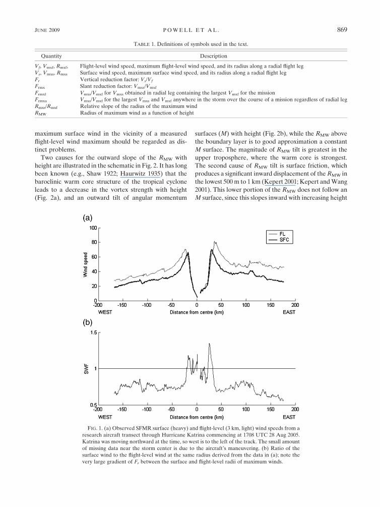
included in Table 1. A transect of simultaneous 10-m

and flight-level wind speeds through Hurricane Katrina

is shown in Fig. 1, in which the surface radii of maxi-

mum winds (Rmxs) are each located 5–6 km inward of

the corresponding flight-level radii of maximum winds

(Rmxf). This outward slope of the radius of maximum wind

(RMW) with height results in very large radial gradients

of Fr near the RMW, with the risk of significant errors

in estimates of the operationally important maxi-

mum surface wind speed (Vmxs). Indeed, these data

imply that (i) estimating the surface wind directly

beneath a flight-level estimate and (ii) estimating the

Corresponding author address: Dr. Mark Powell, FSU-COAPS,

2035 E. Paul Dirac Dr., 200 RM Johnson Bldg., Tallahassee, FL

32306-2840.

E-mail: mark.powell@noaa.gov

1 Although the maximum inflow speed can reach 2–3 times the

GPS sonde fall speed of 12 m s21, the maximum inflow occurs in a

thin layer near the surface, and thus leads to only a modest inward

displacement of the GPS sonde. Even in intense storms, the inward

displacement of a GPS sonde trajectory is small; see, for example,

Kepert (2006a, Fig. 4).

868 W E A T H E R A N D F O R E C A S T I N G VOLUME 24

DOI: 10.1175/2008WAF2007087.1

� 2009 American Meteorological Society

maximum surface wind in the vicinity of a measured

flight-level wind maximum should be regarded as dis-

tinct problems.

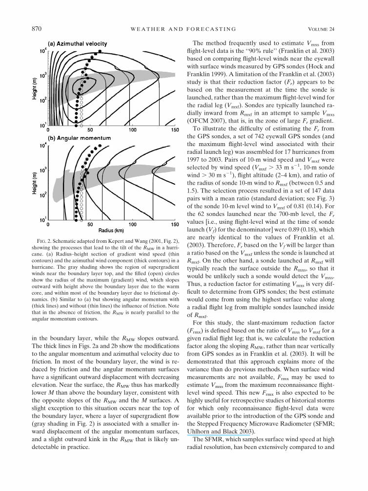
Two causes for the outward slope of the RMW with

height are illustrated in the schematic in Fig. 2. It has long

been known (e.g., Shaw 1922; Haurwitz 1935) that the

baroclinic warm core structure of the tropical cyclone

leads to a decrease in the vortex strength with height

(Fig. 2a), and an outward tilt of angular momentum

surfaces (M) with height (Fig. 2b), while the RMW above

the boundary layer is to good approximation a constant

M surface. The magnitude of RMW tilt is greatest in the

upper troposphere, where the warm core is strongest.

The second cause of RMW tilt is surface friction, which

produces a significant inward displacement of the RMW in

the lowest 500 m to 1 km (Kepert 2001; Kepert and Wang

2001). This lower portion of the RMW does not follow an

M surface, since this slopes inward with increasing height

TABLE 1. Definitions of symbols used in the text.

Quantity Description

Vf, Vmxf, Rmxf, Flight-level wind speed, maximum flight-level wind speed, and its radius along a radial flight leg

Vs, Vmxs, Rmxs Surface wind speed, maximum surface wind speed, and its radius along a radial flight leg

Fr Vertical reduction factor: Vs/Vf

Frmx Slant reduction factor: Vmxs/Vmxf

Frmxl Vmxs/Vmxf for Vmxs obtained in radial leg containing the largest Vmxf for the mission

Frmxa Vmxs/Vmxf for the largest Vmxs and Vmxf anywhere in the storm over the course of a mission regardless of radial leg

Rmxs/Rmxf Relative slope of the radius of the maximum wind

RMW Radius of maximum wind as a function of height

FIG. 1. (a) Observed SFMR surface (heavy) and flight-level (3 km, light) wind speeds from a

research aircraft transect through Hurricane Katrina commencing at 1708 UTC 28 Aug 2005.

Katrina was moving northward at the time, so west is to the left of the track. The small amount

of missing data near the storm center is due to the aircraft’s maneuvering. (b) Ratio of the

surface wind to the flight-level wind at the same radius derived from the data in (a); note the

very large gradient of Fr between the surface and flight-level radii of maximum winds.

JUNE 2009 P O W E L L E T A L . 869

in the boundary layer, while the RMW slopes outward.

The thick lines in Figs. 2a and 2b show the modifications

to the angular momentum and azimuthal velocity due to

friction. In most of the boundary layer, the wind is re-

duced by friction and the angular momentum surfaces

have a significant outward displacement with decreasing

elevation. Near the surface, the RMW thus has markedly

lower M than above the boundary layer, consistent with

the opposite slopes of the RMW and the M surfaces. A

slight exception to this situation occurs near the top of

the boundary layer, where a layer of supergradient flow

(gray shading in Fig. 2) is associated with a smaller in-

ward displacement of the angular momentum surfaces,

and a slight outward kink in the RMW that is likely un-

detectable in practice.

The method frequently used to estimate Vmxs from

flight-level data is the ‘‘90% rule’’ (Franklin et al. 2003)

based on comparing flight-level winds near the eyewall

with surface winds measured by GPS sondes (Hock and

Franklin 1999). A limitation of the Franklin et al. (2003)

study is that their reduction factor (Fr) appears to be

based on the measurement at the time the sonde is

launched, rather than the maximum flight-level wind for

the radial leg (Vmxf). Sondes are typically launched ra-

dially inward from Rmxf in an attempt to sample Vmxs

(OFCM 2007), that is, in the zone of large Fr gradient.

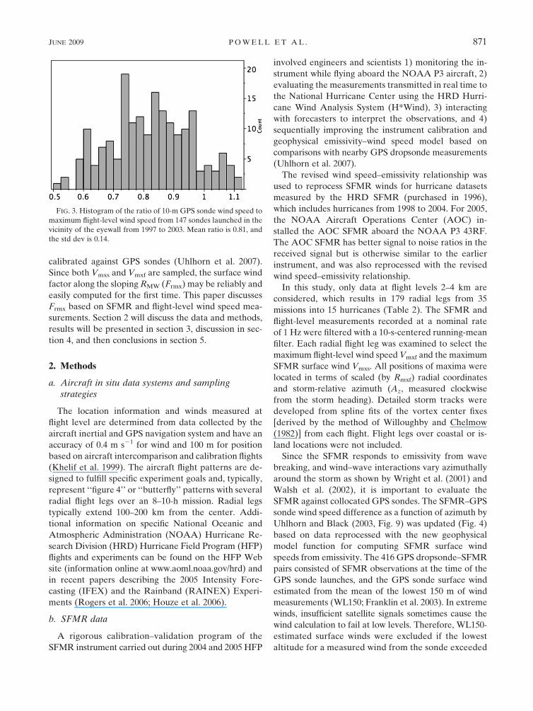
To illustrate the difficulty of estimating the Fr from

the GPS sondes, a set of 742 eyewall GPS sondes (and

the maximum flight-level wind associated with their

radial launch leg) was assembled for 17 hurricanes from

1997 to 2003. Pairs of 10-m wind speed and Vmxf were

selected by wind speed (Vmxf . 33 m s21, 10-m sonde

wind . 30 m s21), flight altitude (2–4 km), and ratio of

the radius of sonde 10-m wind to Rmxf (between 0.5 and

1.5). The selection process resulted in a set of 147 data

pairs with a mean ratio (standard deviation; see Fig. 3)

of the sonde 10-m level wind to Vmxf of 0.81 (0.14). For

the 62 sondes launched near the 700-mb level, the Fr

values [i.e., using flight-level wind at the time of sonde

launch (Vf) for the denominator] were 0.89 (0.18), which

are nearly identical to the values of Franklin et al.

(2003). Therefore, Fr based on the Vf will be larger than

a ratio based on the Vmxf unless the sonde is launched at

Rmxf. On the other hand, a sonde launched at Rmxf will

typically reach the surface outside the Rmxs, so that it

would be unlikely such a sonde would detect the Vmxs.

Thus, a reduction factor for estimating Vmxs is very dif-

ficult to determine from GPS sondes; the best estimate

would come from using the highest surface value along

a radial flight leg from multiple sondes launched inside

of Rmxf.

For this study, the slant-maximum reduction factor

(Frmx) is defined based on the ratio of Vmxs to Vmxf for a

given radial flight leg; that is, we calculate the reduction

factor along the sloping RMW, rather than near vertically

from GPS sondes as in Franklin et al. (2003). It will be

demonstrated that this approach explains more of the

variance than do previous methods. When surface wind

measurements are not available, Frmx may be used to

estimate Vmxs from the maximum reconnaissance flight-

level wind speed. This new Frmx is also expected to be

highly useful for retrospective studies of historical storms

for which only reconnaissance flight-level data were

available prior to the introduction of the GPS sonde and

the Stepped Frequency Microwave Radiometer (SFMR;

Uhlhorn and Black 2003).

The SFMR, which samples surface wind speed at high

radial resolution, has been extensively compared to and

FIG. 2. Schematic adapted from Kepert and Wang (2001, Fig. 2),

showing the processes that lead to the tilt of the RMW in a hurri-

cane. (a) Radius–height section of gradient wind speed (thin

contours) and the azimuthal wind component (thick contours) in a

hurricane. The gray shading shows the region of supergradient

winds near the boundary layer top, and the filled (open) circles

show the radius of the maximum (gradient) wind, which slopes

outward with height above the boundary layer due to the warm

core, and within most of the boundary layer due to frictional dy-

namics. (b) Similar to (a) but showing angular momentum with

(thick lines) and without (thin lines) the influence of friction. Note

that in the absence of friction, the RMW is nearly parallel to the

angular momentum contours.

870 W E A T H E R A N D F O R E C A S T I N G VOLUME 24

calibrated against GPS sondes (Uhlhorn et al. 2007).

Since both Vmxs and Vmxf are sampled, the surface wind

factor along the sloping RMW (Frmx) may be reliably and

easily computed for the first time. This paper discusses

Frmx based on SFMR and flight-level wind speed mea-

surements. Section 2 will discuss the data and methods,

results will be presented in section 3, discussion in sec-

tion 4, and then conclusions in section 5.

2. Methods

a. Aircraft in situ data systems and samplingstrategies

The location information and winds measured at

flight level are determined from data collected by the

aircraft inertial and GPS navigation system and have an

accuracy of 0.4 m s21 for wind and 100 m for position

based on aircraft intercomparison and calibration flights

(Khelif et al. 1999). The aircraft flight patterns are de-

signed to fulfill specific experiment goals and, typically,

represent ‘‘figure 4’’ or ‘‘butterfly’’ patterns with several

radial flight legs over an 8–10-h mission. Radial legs

typically extend 100–200 km from the center. Addi-

tional information on specific National Oceanic and

Atmospheric Administration (NOAA) Hurricane Re-

search Division (HRD) Hurricane Field Program (HFP)

flights and experiments can be found on the HFP Web

site (information online at www.aoml.noaa.gov/hrd) and

in recent papers describing the 2005 Intensity Fore-

casting (IFEX) and the Rainband (RAINEX) Experi-

ments (Rogers et al. 2006; Houze et al. 2006).

b. SFMR data

A rigorous calibration–validation program of the

SFMR instrument carried out during 2004 and 2005 HFP

involved engineers and scientists 1) monitoring the in-

strument while flying aboard the NOAA P3 aircraft, 2)

evaluating the measurements transmitted in real time to

the National Hurricane Center using the HRD Hurri-

cane Wind Analysis System (H*Wind), 3) interacting

with forecasters to interpret the observations, and 4)

sequentially improving the instrument calibration and

geophysical emissivity–wind speed model based on

comparisons with nearby GPS dropsonde measurements

(Uhlhorn et al. 2007).

The revised wind speed–emissivity relationship was

used to reprocess SFMR winds for hurricane datasets

measured by the HRD SFMR (purchased in 1996),

which includes hurricanes from 1998 to 2004. For 2005,

the NOAA Aircraft Operations Center (AOC) in-

stalled the AOC SFMR aboard the NOAA P3 43RF.

The AOC SFMR has better signal to noise ratios in the

received signal but is otherwise similar to the earlier

instrument, and was also reprocessed with the revised

wind speed–emissivity relationship.

In this study, only data at flight levels 2–4 km are

considered, which results in 179 radial legs from 35

missions into 15 hurricanes (Table 2). The SFMR and

flight-level measurements recorded at a nominal rate

of 1 Hz were filtered with a 10-s-centered running-mean

filter. Each radial flight leg was examined to select the

maximum flight-level wind speed Vmxf and the maximum

SFMR surface wind Vmxs. All positions of maxima were

located in terms of scaled (by Rmxf) radial coordinates

and storm-relative azimuth (Az, measured clockwise

from the storm heading). Detailed storm tracks were

developed from spline fits of the vortex center fixes

[derived by the method of Willoughby and Chelmow

(1982)] from each flight. Flight legs over coastal or is-

land locations were not included.

Since the SFMR responds to emissivity from wave

breaking, and wind–wave interactions vary azimuthally

around the storm as shown by Wright et al. (2001) and

Walsh et al. (2002), it is important to evaluate the

SFMR against collocated GPS sondes. The SFMR–GPS

sonde wind speed difference as a function of azimuth by

Uhlhorn and Black (2003, Fig. 9) was updated (Fig. 4)

based on data reprocessed with the new geophysical

model function for computing SFMR surface wind

speeds from emissivity. The 416 GPS dropsonde–SFMR

pairs consisted of SFMR observations at the time of the

GPS sonde launches, and the GPS sonde surface wind

estimated from the mean of the lowest 150 m of wind

measurements (WL150; Franklin et al. 2003). In extreme

winds, insufficient satellite signals sometimes cause the

wind calculation to fail at low levels. Therefore, WL150-

estimated surface winds were excluded if the lowest

altitude for a measured wind from the sonde exceeded

FIG. 3. Histogram of the ratio of 10-m GPS sonde wind speed to

maximum flight-level wind speed from 147 sondes launched in the

vicinity of the eyewall from 1997 to 2003. Mean ratio is 0.81, and

the std dev is 0.14.

JUNE 2009 P O W E L L E T A L . 871

150 m. Differences were bin averaged in 308 sectors and

fit as shown in Fig. 4 together with the number of samples

and the standard deviation of the differences in each bin.

A harmonic fit to the differences results in

SFMR�GPS 5 2.02 cos(Az 1 27). (1)

We apply Eq. (1) to correct the SFMR wind mea-

surements for nonwind sources of roughness related to

storm regions where windsea wave breaking is influ-

enced by swell. In the right-rear quadrant of the storm,

the swell and wind are propagating (moving) in the

same direction, which causes the swell to grow and leave

less foam (fewer breaking waves), hence resulting in

negative differences. In the left-front quadrant, the

swells may propagate against or across the wind, which

leads to more breaking and more foam generation than

wind seas alone (positive differences).

3. Statistical results and physical interpretation

Radial leg wind maxima pairs were analyzed to un-

derstand the dependence of Frmx on storm characteristics

that may be computed from flight-level quantities and

other storm information. In particular, we establish an

observational and theoretical basis for the location of the

surface maximum wind relative to the maximum at flight

level, and the relationship of Frmx to Rmxf, eyewall slope,

flight-level angular momentum, inertial stability, storm-

relative azimuth, and storm motion. To gain further in-

sight into the relationship between maximum surface

and flight-level winds, observed characteristics are then

compared to simulations from the Kepert and Wang

(2001) tropical cyclone boundary layer model. An Frmx

model is developed through screening regression, and

evaluated against other methods that have been used to

estimate surface winds from flight-level wind measure-

ments. Finally, we will revisit significant Atlantic basin

hurricanes to provide updated estimates of intensity.

a. Distribution of Frmx and Rmxs

When examining all 179 radial legs in our dataset, the

mean Frmx is 0.8346 with a standard deviation of 0.09.

Considerable variability exists about the mean Frmx in

Fig. 5 but the scatter is much less than that for Fr (0.19)

reported by Franklin et al. (2003). The low Frmx outliers

of 0.5 and 0.6 are both from Hurricane Ophelia on 11

September of 2005. Ophelia was characterized by a

relatively flat radial profile of flight-level wind speed, so

the large (.80 km) values of Rmxf were based on rather

subtle maxima. The high Frmx values . 1.05 are from

two legs in Hurricane Ivan on 7 and 9 September 2005,

and one leg in Hurricane Frances on 31 August 2004,

and are associated with small (,30 km) values of Rmxf.

Franklin et al. (2003) have associated low and high

values of Fr with stratiform and enhanced convective

activities, respectively. However, Kepert (2001) and

Kepert and Wang (2001) have shown that Fr may vary

spatially in idealized boundary layer models that do not

contain representations of convective processes. Rather,

the hurricane boundary layer dynamics are such that

horizontal advection of angular momentum2 plays an

important role in determining the wind structure. In

particular, the eyewall is associated with a marked ra-

dial gradient of angular momentum that, coupled with

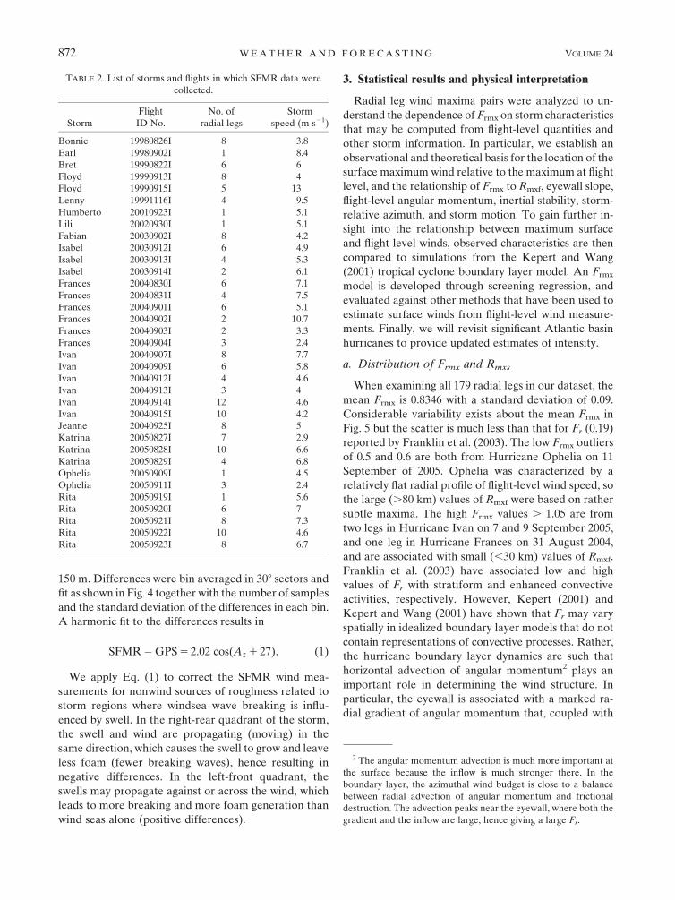
TABLE 2. List of storms and flights in which SFMR data were

collected.

Storm

Flight

ID No.

No. of

radial legs

Storm

speed (m s21)

Bonnie 19980826I 8 3.8

Earl 19980902I 1 8.4

Bret 19990822I 6 6

Floyd 19990913I 8 4

Floyd 19990915I 5 13

Lenny 19991116I 4 9.5

Humberto 20010923I 1 5.1

Lili 20020930I 1 5.1

Fabian 20030902I 8 4.2

Isabel 20030912I 6 4.9

Isabel 20030913I 4 5.3

Isabel 20030914I 2 6.1

Frances 20040830I 6 7.1

Frances 20040831I 4 7.5

Frances 20040901I 6 5.1

Frances 20040902I 2 10.7

Frances 20040903I 2 3.3

Frances 20040904I 3 2.4

Ivan 20040907I 8 7.7

Ivan 20040909I 6 5.8

Ivan 20040912I 4 4.6

Ivan 20040913I 3 4

Ivan 20040914I 12 4.6

Ivan 20040915I 10 4.2

Jeanne 20040925I 8 5

Katrina 20050827I 7 2.9

Katrina 20050828I 10 6.6

Katrina 20050829I 4 6.8

Ophelia 20050909I 1 4.5

Ophelia 20050911I 3 2.4

Rita 20050919I 1 5.6

Rita 20050920I 6 7

Rita 20050921I 8 7.3

Rita 20050922I 10 4.6

Rita 20050923I 8 6.7

2 The angular momentum advection is much more important at

the surface because the inflow is much stronger there. In the

boundary layer, the azimuthal wind budget is close to a balance

between radial advection of angular momentum and frictional

destruction. The advection peaks near the eyewall, where both the

gradient and the inflow are large, hence giving a large Fr.

872 W E A T H E R A N D F O R E C A S T I N G VOLUME 24

the frictionally forced inflow, can produce supergradient

winds in the upper boundary layer and maintain rela-

tively strong winds near the surface. This process ex-

plains the observed high Fr without the need to invoke

additional processes (e.g., convective transport). Similar

processes would be expected to operate near outer wind

maxima, but probably to a lesser degree. Kepert (2006a,b)

analyzed the boundary layer flow in the intense Hurricanes

Georges and Mitch of 1998 and found strong quantita-

tive and qualitative agreement with the model results

for these storms through the depth of the boundary

layer. The boundary layer dynamics associated with wind

maxima also generate a frictionally forced updraft

(Eliassen 1971; Kepert 2001; Kepert and Wang 2001).

Thus, it appears that the physical cause for the statistical

relationship between high values of Fr and strong ver-

tical motion found by Franklin et al. (2003) may be that

both are associated with the local wind maximum,

rather than that the high Fr values are caused by the

convective vertical motion.

Values of Frmx were found to be negatively correlated

(Fig. 6) with Rmxf and also to be higher on the left side of

the storm than on the right. Kepert (2001) developed a

linear analytical model of the tropical cyclone boundary

layer, from which he derives a nonlinear analytical ex-

pression for the surface wind reduction factor Fr:

Fr 5(x2 1 2x 1 2)

(2x2 1 3x 1 2), (2)

where

x 5 CDVg

ffiffiffiffiffiffi2

KI

r, (3)

where CD is the drag coefficient, VG is the gradient wind,

K is the boundary layer mean vertical diffusivity, and I is

the inertial stability. Other things being equal, the in-

ertial stability at the RMW will be higher for a smaller

RMW, so (2) predicts that Frmx will be larger for a smaller

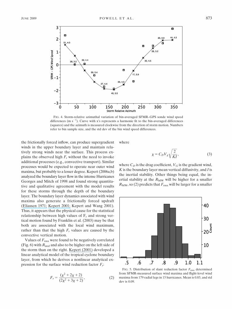
FIG. 4. Storm-relative azimuthal variation of bin-averaged SFMR–GPS sonde wind speed

differences (m s21). Curve with x’s represents a harmonic fit to the bin-averaged differences

(squares) and the azimuth is measured clockwise from the direction of storm motion. Numbers

refer to bin sample size, and the std dev of the bin wind speed differences.

FIG. 5. Distribution of slant reduction factor Frmx determined

from SFMR-measured surface wind maxima and flight-level wind

maxima from 179 radial legs in 15 hurricanes. Mean is 0.83, and std

dev is 0.09.

JUNE 2009 P O W E L L E T A L . 873

RMW, consistent with the negative correlation shown in

Fig. 6. The left–right asymmetry in Frmx found here was

first predicted by Kepert (2001) and Kepert and Wang

(2001), and subsequently found in Franklin et al.’s

(2003) observational analysis. Case studies of individual

storms by Kepert (2006a) and Schwendike and Kepert

(2008) have also shown the presence of this asymmetry.

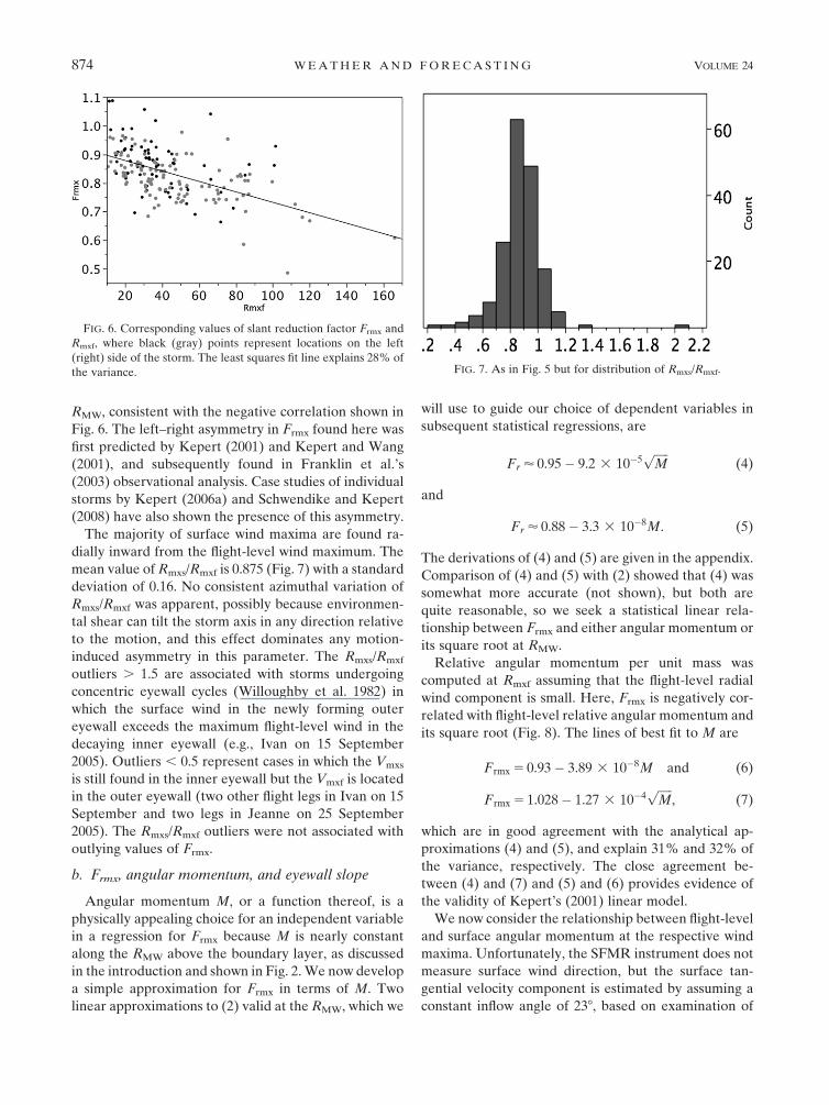
The majority of surface wind maxima are found ra-

dially inward from the flight-level wind maximum. The

mean value of Rmxs/Rmxf is 0.875 (Fig. 7) with a standard

deviation of 0.16. No consistent azimuthal variation of

Rmxs/Rmxf was apparent, possibly because environmen-

tal shear can tilt the storm axis in any direction relative

to the motion, and this effect dominates any motion-

induced asymmetry in this parameter. The Rmxs/Rmxf

outliers . 1.5 are associated with storms undergoing

concentric eyewall cycles (Willoughby et al. 1982) in

which the surface wind in the newly forming outer

eyewall exceeds the maximum flight-level wind in the

decaying inner eyewall (e.g., Ivan on 15 September

2005). Outliers , 0.5 represent cases in which the Vmxs

is still found in the inner eyewall but the Vmxf is located

in the outer eyewall (two other flight legs in Ivan on 15

September and two legs in Jeanne on 25 September

2005). The Rmxs/Rmxf outliers were not associated with

outlying values of Frmx.

b. Frmx, angular momentum, and eyewall slope

Angular momentum M, or a function thereof, is a

physically appealing choice for an independent variable

in a regression for Frmx because M is nearly constant

along the RMW above the boundary layer, as discussed

in the introduction and shown in Fig. 2. We now develop

a simple approximation for Frmx in terms of M. Two

linear approximations to (2) valid at the RMW, which we

will use to guide our choice of dependent variables in

subsequent statistical regressions, are

Fr ’ 0.95� 9.2 3 10�5ffiffiffiffiffiMp

(4)

and

Fr ’ 0.88� 3.3 3 10�8M. (5)

The derivations of (4) and (5) are given in the appendix.

Comparison of (4) and (5) with (2) showed that (4) was

somewhat more accurate (not shown), but both are

quite reasonable, so we seek a statistical linear rela-

tionship between Frmx and either angular momentum or

its square root at RMW.

Relative angular momentum per unit mass was

computed at Rmxf assuming that the flight-level radial

wind component is small. Here, Frmx is negatively cor-

related with flight-level relative angular momentum and

its square root (Fig. 8). The lines of best fit to M are

Frmx 5 0.93� 3.89 3 10�8M and (6)

Frmx 5 1.028� 1.27 3 10�4ffiffiffiffiffiMp

, (7)

which are in good agreement with the analytical ap-

proximations (4) and (5), and explain 31% and 32% of

the variance, respectively. The close agreement be-

tween (4) and (7) and (5) and (6) provides evidence of

the validity of Kepert’s (2001) linear model.

We now consider the relationship between flight-level

and surface angular momentum at the respective wind

maxima. Unfortunately, the SFMR instrument does not

measure surface wind direction, but the surface tan-

gential velocity component is estimated by assuming a

constant inflow angle of 238, based on examination of

FIG. 6. Corresponding values of slant reduction factor Frmx and

Rmxf, where black (gray) points represent locations on the left

(right) side of the storm. The least squares fit line explains 28% of

the variance. FIG. 7. As in Fig. 5 but for distribution of Rmxs/Rmxf.

874 W E A T H E R A N D F O R E C A S T I N G VOLUME 24

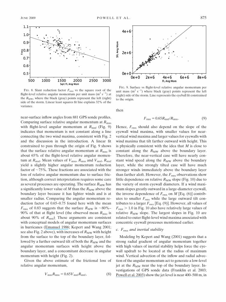
near-surface inflow angles from 881 GPS sonde profiles.

Comparing surface relative angular momentum at Rmxs

with flight-level angular momentum at Rmxf (Fig. 9)

indicates that momentum is not constant along a line

connecting the two wind maxima, consistent with Fig. 2

and the discussion in the introduction. A linear fit

constrained to pass through the origin of Fig. 9 shows

that the surface relative angular momentum at Rmxs is

about 65% of the flight-level relative angular momen-

tum at Rmxf. Mean values of Vmxs, Rmxs and Vmxf, Rmxf

yield a slightly higher angular momentum reduction

factor of ;75%. These fractions are associated with the

loss of relative angular momentum due to surface fric-

tion, although correct interpretation requires some care

as several processes are operating. The surface RMW has

a significantly lower value of M than the RMW above the

boundary layer because it has lighter winds and is at

smaller radius. Comparing the angular momentum re-

duction factor of 0.65–0.75 found here with the mean

Frmx of 0.83 suggests that the surface RMW is ;80%–

90% of that at flight level (the observed mean Rmxs is

about 90% of Rmxf). These arguments are consistent

with conceptual models of angular momentum surfaces

in hurricanes (Emanuel 1986; Kepert and Wang 2001;

see also Fig. 2 above), with increases of RMW with height

from the surface to the top of the boundary layer, fol-

lowed by a further outward tilt of both the RMW and the

angular momentum surfaces with height above the

boundary layer, and a concomitant decrease in angular

momentum with height (Fig. 2).

Given the above estimate of the frictional loss of

relative angular momentum,

VmxsRmxs 5 0.65VmxfRmxf, (8)

then

Frmx 5 0.65Rmxf/Rmxs. (9)

Hence, Frmx should also depend on the slope of the

eyewall wind maxima, with smaller values for near-

vertical wind maxima and larger values for eyewalls with

wind maxima that tilt farther outward with height. This

is physically consistent with the idea that M is close to

constant along the RMW above the boundary layer.

Therefore, the near-vertical case will have nearly con-

stant wind speed along the RMW above the boundary

layer, while the strongly tilted case will have much

stronger winds immediately above the boundary layer

than farther aloft. However, the Frmx observations show

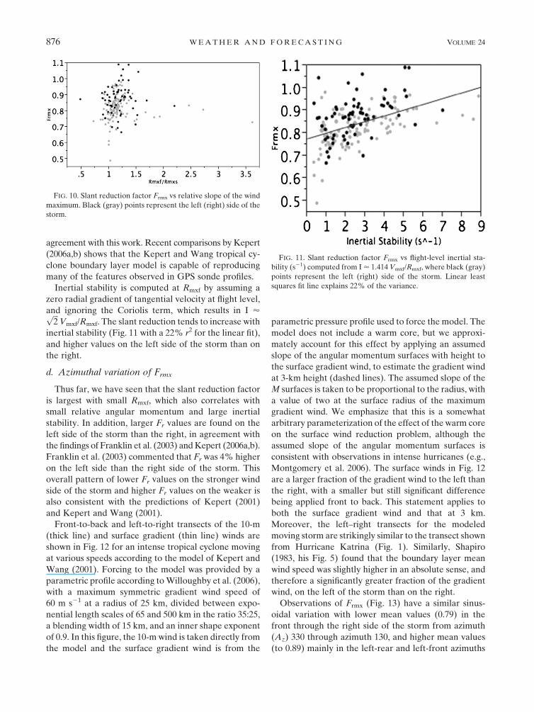
little dependence on relative RMW slope (Fig. 10) due to

the variety of storm eyewall diameters. If a wind maxi-

mum slopes greatly outward in a large-diameter eyewall,

the inverse dependence of Frmx on M [Eq. (6)] contrib-

utes to smaller Frmx while the large outward tilt con-

tributes to a larger Frmx [Eq. (9)]. However, all values of

Frmx . 1.0 in Fig. 10 also have relatively large values of

relative RMW slope. The largest slopes in Fig. 10 are

related to outer flight-level wind maxima associated with

concentric eyewall processes mentioned earlier.

c. Frmx and inertial stability

Modeling by Kepert and Wang (2001) suggests that a

strong radial gradient of angular momentum together

with high values of inertial stability helps force the eye-

wall updraft to be located at the radius of maximum

wind. Vertical advection of the inflow and radial advec-

tion of the angular momentum act to generate a low-level

jet at the RMW near the top of the boundary layer. In-

vestigations of GPS sonde data (Franklin et al. 2003;

Powell et al. 2003) show the jet level is near 400–500 m, in

FIG. 8. Slant reduction factor Frmx vs the square root of the

flight-level relative angular momentum per unit mass (m2 s21) at

the RMW, where the black (gray) points represent the left (right)

side of the storm. Linear least squares fit line explains 32% of the

variance.

FIG. 9. Surface vs flight-level relative angular momentum per

unit mass (m2 s21) where black (gray) points represent the left

(right) side of the storm. Line represents the eyeball fit constrained

to the origin.

JUNE 2009 P O W E L L E T A L . 875

agreement with this work. Recent comparisons by Kepert

(2006a,b) shows that the Kepert and Wang tropical cy-

clone boundary layer model is capable of reproducing

many of the features observed in GPS sonde profiles.

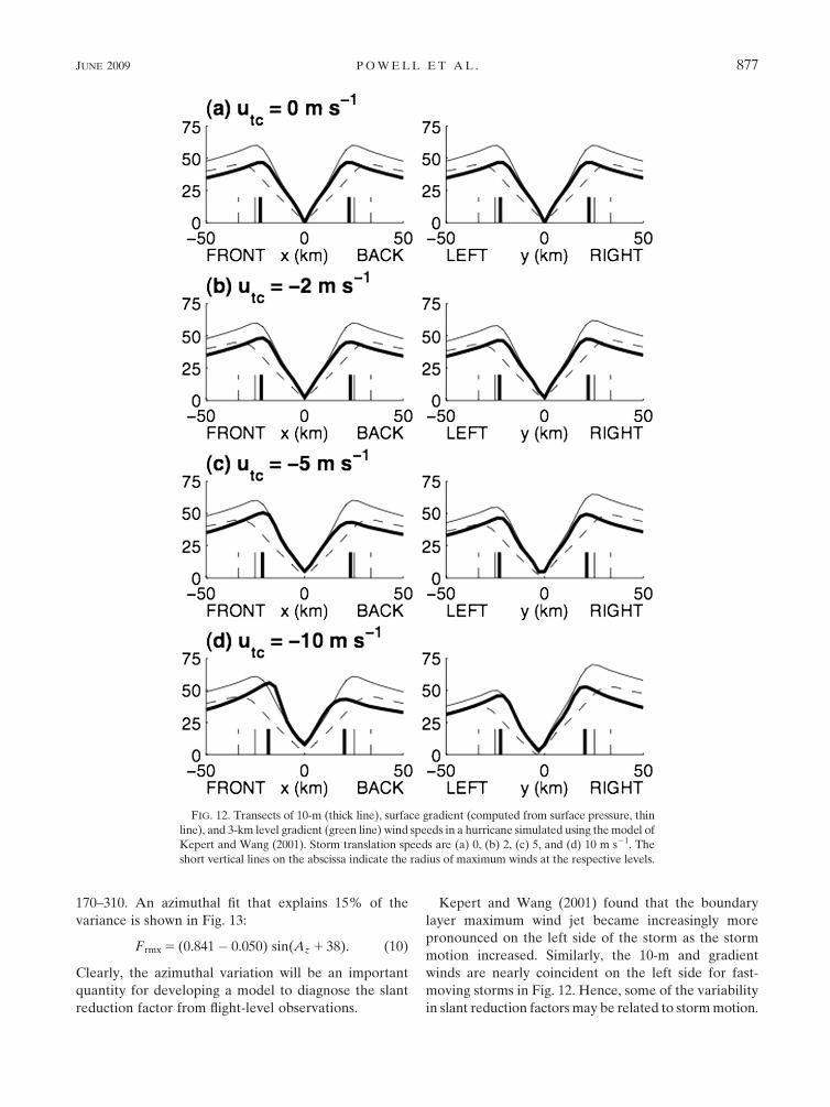
Inertial stability is computed at Rmxf by assuming a

zero radial gradient of tangential velocity at flight level,

and ignoring the Coriolis term, which results in I ’ffiffiffi2p

Vmxf/Rmxf. The slant reduction tends to increase with

inertial stability (Fig. 11 with a 22% r2 for the linear fit),

and higher values on the left side of the storm than on

the right.

d. Azimuthal variation of Frmx

Thus far, we have seen that the slant reduction factor

is largest with small Rmxf, which also correlates with

small relative angular momentum and large inertial

stability. In addition, larger Fr values are found on the

left side of the storm than the right, in agreement with

the findings of Franklin et al. (2003) and Kepert (2006a,b).

Franklin et al. (2003) commented that Fr was 4% higher

on the left side than the right side of the storm. This

overall pattern of lower Fr values on the stronger wind

side of the storm and higher Fr values on the weaker is

also consistent with the predictions of Kepert (2001)

and Kepert and Wang (2001).

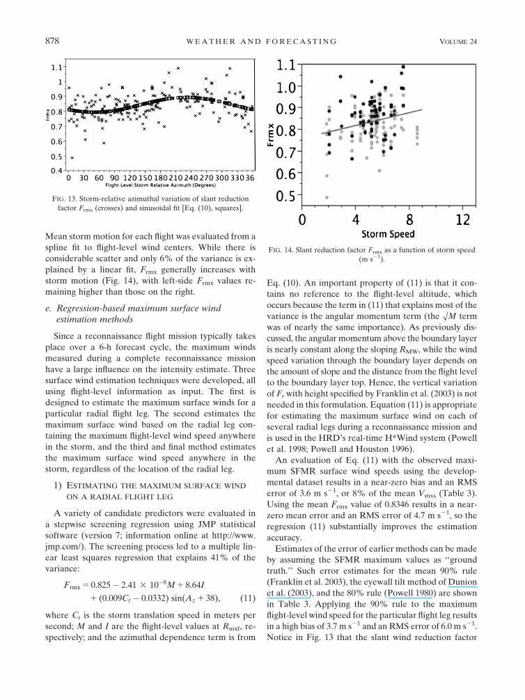
Front-to-back and left-to-right transects of the 10-m

(thick line) and surface gradient (thin line) winds are

shown in Fig. 12 for an intense tropical cyclone moving

at various speeds according to the model of Kepert and

Wang (2001). Forcing to the model was provided by a

parametric profile according to Willoughby et al. (2006),

with a maximum symmetric gradient wind speed of

60 m s21 at a radius of 25 km, divided between expo-

nential length scales of 65 and 500 km in the ratio 35:25,

a blending width of 15 km, and an inner shape exponent

of 0.9. In this figure, the 10-m wind is taken directly from

the model and the surface gradient wind is from the

parametric pressure profile used to force the model. The

model does not include a warm core, but we approxi-

mately account for this effect by applying an assumed

slope of the angular momentum surfaces with height to

the surface gradient wind, to estimate the gradient wind

at 3-km height (dashed lines). The assumed slope of the

M surfaces is taken to be proportional to the radius, with

a value of two at the surface radius of the maximum

gradient wind. We emphasize that this is a somewhat

arbitrary parameterization of the effect of the warm core

on the surface wind reduction problem, although the

assumed slope of the angular momentum surfaces is

consistent with observations in intense hurricanes (e.g.,

Montgomery et al. 2006). The surface winds in Fig. 12

are a larger fraction of the gradient wind to the left than

the right, with a smaller but still significant difference

being applied front to back. This statement applies to

both the surface gradient wind and that at 3 km.

Moreover, the left–right transects for the modeled

moving storm are strikingly similar to the transect shown

from Hurricane Katrina (Fig. 1). Similarly, Shapiro

(1983, his Fig. 5) found that the boundary layer mean

wind speed was slightly higher in an absolute sense, and

therefore a significantly greater fraction of the gradient

wind, on the left of the storm than on the right.

Observations of Frmx (Fig. 13) have a similar sinus-

oidal variation with lower mean values (0.79) in the

front through the right side of the storm from azimuth

(Az) 330 through azimuth 130, and higher mean values

(to 0.89) mainly in the left-rear and left-front azimuths

FIG. 10. Slant reduction factor Frmx vs relative slope of the wind

maximum. Black (gray) points represent the left (right) side of the

storm.

FIG. 11. Slant reduction factor Frmx vs flight-level inertial sta-

bility (s21) computed from I ’ 1.414 Vmxf/Rmxf, where black (gray)

points represent the left (right) side of the storm. Linear least

squares fit line explains 22% of the variance.

876 W E A T H E R A N D F O R E C A S T I N G VOLUME 24

170–310. An azimuthal fit that explains 15% of the

variance is shown in Fig. 13:

Frmx 5 (0.841� 0.050) sin(Az 1 38). (10)

Clearly, the azimuthal variation will be an important

quantity for developing a model to diagnose the slant

reduction factor from flight-level observations.

Kepert and Wang (2001) found that the boundary

layer maximum wind jet became increasingly more

pronounced on the left side of the storm as the storm

motion increased. Similarly, the 10-m and gradient

winds are nearly coincident on the left side for fast-

moving storms in Fig. 12. Hence, some of the variability

in slant reduction factors may be related to storm motion.

FIG. 12. Transects of 10-m (thick line), surface gradient (computed from surface pressure, thin

line), and 3-km level gradient (green line) wind speeds in a hurricane simulated using the model of

Kepert and Wang (2001). Storm translation speeds are (a) 0, (b) 2, (c) 5, and (d) 10 m s21. The

short vertical lines on the abscissa indicate the radius of maximum winds at the respective levels.

JUNE 2009 P O W E L L E T A L . 877

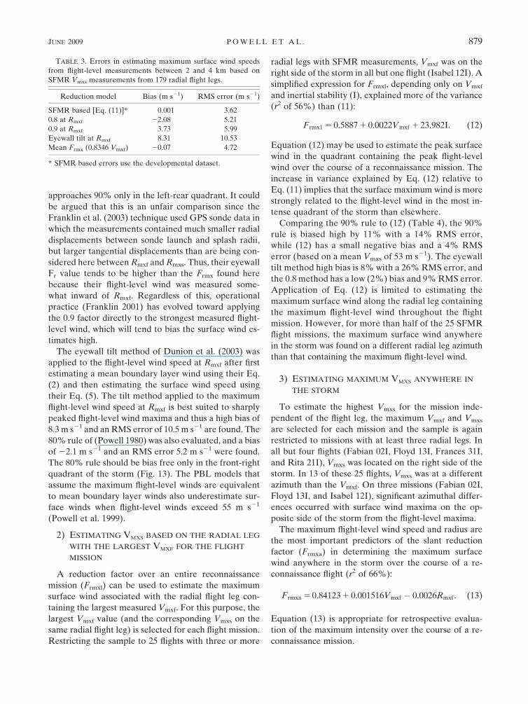
Mean storm motion for each flight was evaluated from a

spline fit to flight-level wind centers. While there is

considerable scatter and only 6% of the variance is ex-

plained by a linear fit, Frmx generally increases with

storm motion (Fig. 14), with left-side Frmx values re-

maining higher than those on the right.

e. Regression-based maximum surface windestimation methods

Since a reconnaissance flight mission typically takes

place over a 6-h forecast cycle, the maximum winds

measured during a complete reconnaissance mission

have a large influence on the intensity estimate. Three

surface wind estimation techniques were developed, all

using flight-level information as input. The first is

designed to estimate the maximum surface winds for a

particular radial flight leg. The second estimates the

maximum surface wind based on the radial leg con-

taining the maximum flight-level wind speed anywhere

in the storm, and the third and final method estimates

the maximum surface wind speed anywhere in the

storm, regardless of the location of the radial leg.

1) ESTIMATING THE MAXIMUM SURFACE WIND

ON A RADIAL FLIGHT LEG

A variety of candidate predictors were evaluated in

a stepwise screening regression using JMP statistical

software (version 7; information online at http://www.

jmp.com/). The screening process led to a multiple lin-

ear least squares regression that explains 41% of the

variance:

Frmx 5 0.825� 2.41 3 10�8M 1 8.64I

1 (0.009Ct � 0.0332) sin(Az 1 38), (11)

where Ct is the storm translation speed in meters per

second; M and I are the flight-level values at Rmxf, re-

spectively; and the azimuthal dependence term is from

Eq. (10). An important property of (11) is that it con-

tains no reference to the flight-level altitude, which

occurs because the term in (11) that explains most of the

variance is the angular momentum term (the OM term

was of nearly the same importance). As previously dis-

cussed, the angular momentum above the boundary layer

is nearly constant along the sloping RMW, while the wind

speed variation through the boundary layer depends on

the amount of slope and the distance from the flight level

to the boundary layer top. Hence, the vertical variation

of Fr with height specified by Franklin et al. (2003) is not

needed in this formulation. Equation (11) is appropriate

for estimating the maximum surface wind on each of

several radial legs during a reconnaissance mission and

is used in the HRD’s real-time H*Wind system (Powell

et al. 1998; Powell and Houston 1996).

An evaluation of Eq. (11) with the observed maxi-

mum SFMR surface wind speeds using the develop-

mental dataset results in a near-zero bias and an RMS

error of 3.6 m s21, or 8% of the mean Vmxs (Table 3).

Using the mean Frmx value of 0.8346 results in a near-

zero mean error and an RMS error of 4.7 m s21, so the

regression (11) substantially improves the estimation

accuracy.

Estimates of the error of earlier methods can be made

by assuming the SFMR maximum values as ‘‘ground

truth.’’ Such error estimates for the mean 90% rule

(Franklin et al. 2003), the eyewall tilt method of Dunion

et al. (2003), and the 80% rule (Powell 1980) are shown

in Table 3. Applying the 90% rule to the maximum

flight-level wind speed for the particular flight leg results

in a high bias of 3.7 m s21 and an RMS error of 6.0 m s21.

Notice in Fig. 13 that the slant wind reduction factor

FIG. 13. Storm-relative azimuthal variation of slant reduction

factor Frmx (crosses) and sinusoidal fit [Eq. (10), squares].

FIG. 14. Slant reduction factor Frmx as a function of storm speed

(m s21).

878 W E A T H E R A N D F O R E C A S T I N G VOLUME 24

approaches 90% only in the left-rear quadrant. It could

be argued that this is an unfair comparison since the

Franklin et al. (2003) technique used GPS sonde data in

which the measurements contained much smaller radial

displacements between sonde launch and splash radii,

but larger tangential displacements than are being con-

sidered here between Rmxf and Rmxs. Thus, their eyewall

Fr value tends to be higher than the Frmx found here

because their flight-level wind was measured some-

what inward of Rmxf. Regardless of this, operational

practice (Franklin 2001) has evolved toward applying

the 0.9 factor directly to the strongest measured flight-

level wind, which will tend to bias the surface wind es-

timates high.

The eyewall tilt method of Dunion et al. (2003) was

applied to the flight-level wind speed at Rmxf after first

estimating a mean boundary layer wind using their Eq.

(2) and then estimating the surface wind speed using

their Eq. (5). The tilt method applied to the maximum

flight-level wind speed at Rmxf is best suited to sharply

peaked flight-level wind maxima and thus a high bias of

8.3 m s21 and an RMS error of 10.5 m s21 are found. The

80% rule of (Powell 1980) was also evaluated, and a bias

of 22.1 m s21 and an RMS error 5.2 m s21 were found.

The 80% rule should be bias free only in the front-right

quadrant of the storm (Fig. 13). The PBL models that

assume the maximum flight-level winds are equivalent

to mean boundary layer winds also underestimate sur-

face winds when flight-level winds exceed 55 m s21

(Powell et al. 1999).

2) ESTIMATING VMXS BASED ON THE RADIAL LEG

WITH THE LARGEST VMXF FOR THE FLIGHT

MISSION

A reduction factor over an entire reconnaissance

mission (Frmxl) can be used to estimate the maximum

surface wind associated with the radial flight leg con-

taining the largest measured Vmxf. For this purpose, the

largest Vmxf value (and the corresponding Vmxs on the

same radial flight leg) is selected for each flight mission.

Restricting the sample to 25 flights with three or more

radial legs with SFMR measurements, Vmxf was on the

right side of the storm in all but one flight (Isabel 12I). A

simplified expression for Frmxl, depending only on Vmxf

and inertial stability (I), explained more of the variance

(r2 of 56%) than (11):

Frmx1 5 0.5887 1 0.0022Vmxf 1 23.982I. (12)

Equation (12) may be used to estimate the peak surface

wind in the quadrant containing the peak flight-level

wind over the course of a reconnaissance mission. The

increase in variance explained by Eq. (12) relative to

Eq. (11) implies that the surface maximum wind is more

strongly related to the flight-level wind in the most in-

tense quadrant of the storm than elsewhere.

Comparing the 90% rule to (12) (Table 4), the 90%

rule is biased high by 11% with a 14% RMS error,

while (12) has a small negative bias and a 4% RMS

error (based on a mean Vmxs of 53 m s21). The eyewall

tilt method high bias is 8% with a 26% RMS error, and

the 0.8 method has a low (2%) bias and 9% RMS error.

Application of Eq. (12) is limited to estimating the

maximum surface wind along the radial leg containing

the maximum flight-level wind throughout the flight

mission. However, for more than half of the 25 SFMR

flight missions, the maximum surface wind anywhere

in the storm was found on a different radial leg azimuth

than that containing the maximum flight-level wind.

3) ESTIMATING MAXIMUM VMXS ANYWHERE IN

THE STORM

To estimate the highest Vmxs for the mission inde-

pendent of the flight leg, the maximum Vmxf and Vmxs

are selected for each mission and the sample is again

restricted to missions with at least three radial legs. In

all but four flights (Fabian 02I, Floyd 13I, Frances 31I,

and Rita 21I), Vmxs was located on the right side of the

storm. In 13 of these 25 flights, Vmxs was at a different

azimuth than the Vmxf. On three missions (Fabian 02I,

Floyd 13I, and Isabel 12I), significant azimuthal differ-

ences occurred with surface wind maxima on the op-

posite side of the storm from the flight-level maxima.

The maximum flight-level wind speed and radius are

the most important predictors of the slant reduction

factor (Frmxa) in determining the maximum surface

wind anywhere in the storm over the course of a re-

connaissance flight (r2 of 66%):

Frmxa 5 0.84123 1 0.001516Vmxf � 0.0026Rmxf. (13)

Equation (13) is appropriate for retrospective evalua-

tion of the maximum intensity over the course of a re-

connaissance mission.

TABLE 3. Errors in estimating maximum surface wind speeds

from flight-level measurements between 2 and 4 km based on

SFMR Vmxs measurements from 179 radial flight legs.

Reduction model Bias (m s21) RMS error (m s21)

SFMR based [Eq. (11)]* 0.001 3.62

0.8 at Rmxf 22.08 5.21

0.9 at Rmxf 3.73 5.99

Eyewall tilt at Rmxf 8.31 10.53

Mean Frmx (0.8346 Vmxf) 20.07 4.72

* SFMR based errors use the developmental dataset.

JUNE 2009 P O W E L L E T A L . 879

The increase in variance explained by Eq. (13) rela-

tive to Eq. (12) is probably due to the fact that the

azimuth of the maximum wind may vary with height in

the storm due to asymmetric friction (Kepert 2001;

Kepert and Wang 2001; Kepert 2006a,b; Schwendike

2005) and to environmental shear (e.g., Frank and Ritchie

2001; Jones 1995). Considering that the maximum flight-

level and surface winds may appear in different quadrants

in this regression, as they do in nature, thus reduces the

amount of random scatter. The greater amount of var-

iance explained in Eq. (13) is a most useful property, as

the maximum surface wind, anywhere in the storm, is

highly important parameter for operational forecasting

and warning.

Estimation from Eq. (13) of the peak Vmxs of all radial

legs within the storm is relevant to estimation of the

maximum surface wind in a storm for operational and

historical retrospective analysis applications. Based on

the developmental data, Eq. (13) results in an RMS error

of , 5%. Evaluation of other methods (Table 5) suggests

that the 90% rule has a high bias (RMS) of 9% (12%),

while the eyewall tilt method bias (RMS) is 26% high

(28%), and the 0.8 method is 4% low (10%). Also in-

cluded in Table 5 is the official ‘‘best track’’ (BT) esti-

mate of the maximum wind from the National Hurricane

Center based on tropical cyclone reports available from

the NHC Web site (information online at http://www.

nhc.noaa.gov/pastall.shtml). The BT estimates are very

similar to the 90% method and are the basis for the

historical record in the Hurricane Database (HURDAT)

file (Jarvinen et al. 1988). This analysis is only valid for

flight-level reductions in which the aircraft is flying

within the 2–4-km altitude range, which is the common

altitude for mature hurricanes. In tropical storms and

weaker hurricanes, reconnaissance flights are often con-

ducted at altitudes , 1.5 km, and surface wind reduction

factors are closer to 80% (Franklin et al. 2003).

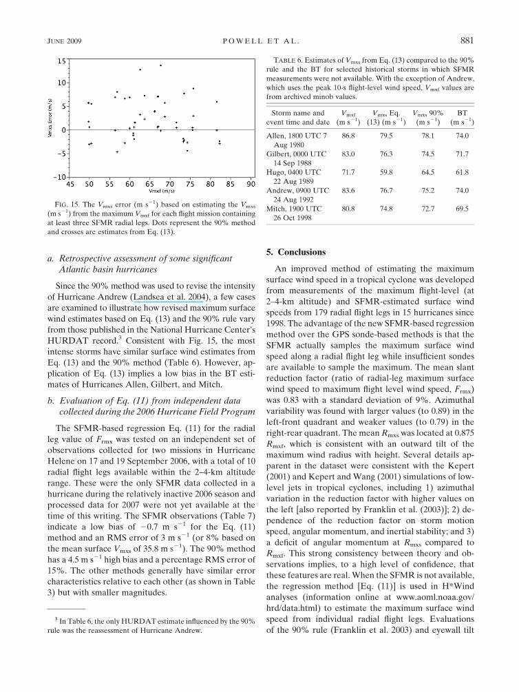
It is apparent from Fig. 15 that the 90% method, and

by implication portions of the recent historical record,

are biased high for Vmxf , 75 m s21. Application of (13)

to flight-level measurements in historical storms would

provide an assessment of the impact of the bias on

the historical record, but the 4.6 m s21 bias in the 90%

method (; one-half a Saffir–Simpson scale category)

suggests that hurricane activity is overestimated for

categories weaker than a moderate category 4 hurri-

cane, provided the reconnaissance aircraft were flying

above 2 km. The transition of the SFMR to operational

reconnaissance will make the 90% method obsolete for

future operational estimates of surface winds in Atlantic

hurricanes within aircraft range. The SFMR measure-

ments and (13) can be used to help calibrate satellite

hurricane intensity estimation methods (e.g., Olander

and Velden 2007). The resulting updated satellite tech-

niques could then be applied to improve intensity esti-

mates for all tropical cyclone basins. These techniques

may then be applied in reanalysis efforts to improve the

historical record.

4. Discussion

Equation (11) has been implemented in H*Wind to

estimate the maximum surface wind speed from an

aircraft radial flight leg when reconnaissance measure-

ments are available at the 2–4-km level. Installation of

new SFMR units on the fleet of U.S. Air Force hurricane

aircraft commenced in 2007 so future use of reduction

factors will be limited to flights on which the instrument

is not available. The Frmx fit in Eq. (11) provides an

improved estimate of the surface wind speed on a par-

ticular flight leg for cases in which the SFMR is not

available. Equations (12) and (13) will be especially

useful for improving estimates of the maximum surface

wind from available flight-level observations in signifi-

cant historical hurricanes. Additional studies are in

progress to use Eqs. (12) and (13) to calibrate estimates

of intensity from pattern recognition techniques applied

to historical satellite imagery (C. Velden, S. Mullins,

and P. Black 2007, personal communication). For cases

in which the reconnaissance aircraft is flying below

2 km (typically tropical storms and weaker hurricanes),

Dunion et al. (2003) found a strong correlation of flight-

level wind speeds with mean boundary layer winds

measured by GPS sondes. In those cases, the Fr values

described in Franklin et al. (2003) may be adequate but

await confirmation using SFMR data.

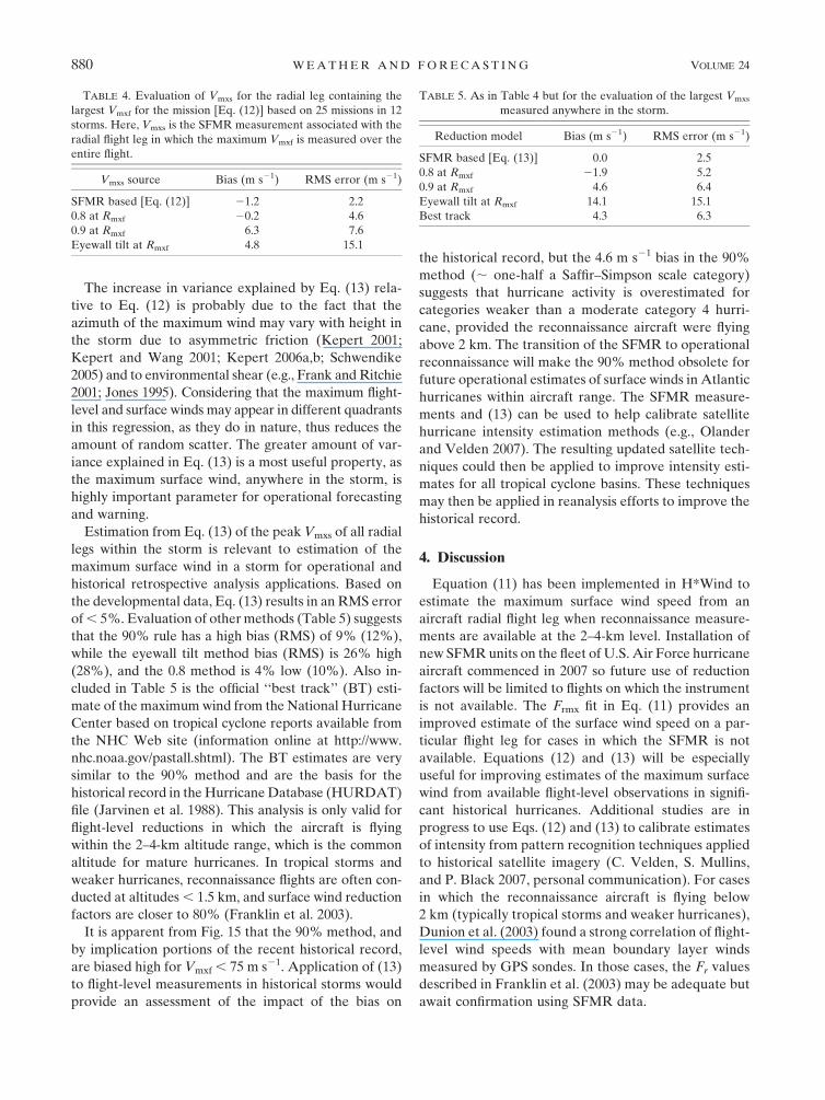
TABLE 4. Evaluation of Vmxs for the radial leg containing the

largest Vmxf for the mission [Eq. (12)] based on 25 missions in 12

storms. Here, Vmxs is the SFMR measurement associated with the

radial flight leg in which the maximum Vmxf is measured over the

entire flight.

Vmxs source Bias (m s21) RMS error (m s21)

SFMR based [Eq. (12)] 21.2 2.2

0.8 at Rmxf 20.2 4.6

0.9 at Rmxf 6.3 7.6

Eyewall tilt at Rmxf 4.8 15.1

TABLE 5. As in Table 4 but for the evaluation of the largest Vmxs

measured anywhere in the storm.

Reduction model Bias (m s21) RMS error (m s21)

SFMR based [Eq. (13)] 0.0 2.5

0.8 at Rmxf 21.9 5.2

0.9 at Rmxf 4.6 6.4

Eyewall tilt at Rmxf 14.1 15.1

Best track 4.3 6.3

880 W E A T H E R A N D F O R E C A S T I N G VOLUME 24

a. Retrospective assessment of some significantAtlantic basin hurricanes

Since the 90% method was used to revise the intensity

of Hurricane Andrew (Landsea et al. 2004), a few cases

are examined to illustrate how revised maximum surface

wind estimates based on Eq. (13) and the 90% rule vary

from those published in the National Hurricane Center’s

HURDAT record.3 Consistent with Fig. 15, the most

intense storms have similar surface wind estimates from

Eq. (13) and the 90% method (Table 6). However, ap-

plication of Eq. (13) implies a low bias in the BT esti-

mates of Hurricanes Allen, Gilbert, and Mitch.

b. Evaluation of Eq. (11) from independent datacollected during the 2006 Hurricane Field Program

The SFMR-based regression Eq. (11) for the radial

leg value of Frmx was tested on an independent set of

observations collected for two missions in Hurricane

Helene on 17 and 19 September 2006, with a total of 10

radial flight legs available within the 2–4-km altitude

range. These were the only SFMR data collected in a

hurricane during the relatively inactive 2006 season and

processed data for 2007 were not yet available at the

time of this writing. The SFMR observations (Table 7)

indicate a low bias of 20.7 m s21 for the Eq. (11)

method and an RMS error of 3 m s21 (or 8% based on

the mean surface Vmxs of 35.8 m s21). The 90% method

has a 4.5 m s21 high bias and a percentage RMS error of

15%. The other methods generally have similar error

characteristics relative to each other (as shown in Table

3) but with smaller magnitudes.

5. Conclusions

An improved method of estimating the maximum

surface wind speed in a tropical cyclone was developed

from measurements of the maximum flight-level (at

2–4-km altitude) and SFMR-estimated surface wind

speeds from 179 radial flight legs in 15 hurricanes since

1998. The advantage of the new SFMR-based regression

method over the GPS sonde-based methods is that the

SFMR actually samples the maximum surface wind

speed along a radial flight leg while insufficient sondes

are available to sample the maximum. The mean slant

reduction factor (ratio of radial-leg maximum surface

wind speed to maximum flight level wind speed, Frmx)

was 0.83 with a standard deviation of 9%. Azimuthal

variability was found with larger values (to 0.89) in the

left-front quadrant and weaker values (to 0.79) in the

right-rear quadrant. The mean Rmxs was located at 0.875

Rmxf, which is consistent with an outward tilt of the

maximum wind radius with height. Several details ap-

parent in the dataset were consistent with the Kepert

(2001) and Kepert and Wang (2001) simulations of low-

level jets in tropical cyclones, including 1) azimuthal

variation in the reduction factor with higher values on

the left [also reported by Franklin et al. (2003)]; 2) de-

pendence of the reduction factor on storm motion

speed, angular momentum, and inertial stability; and 3)

a deficit of angular momentum at Rmxs compared to

Rmxf. This strong consistency between theory and ob-

servations implies, to a high level of confidence, that

these features are real. When the SFMR is not available,

the regression method [Eq. (11)] is used in H*Wind

analyses (information online at www.aoml.noaa.gov/

hrd/data.html) to estimate the maximum surface wind

speed from individual radial flight legs. Evaluations

of the 90% rule (Franklin et al. 2003) and eyewall tilt

FIG. 15. The Vmxs error (m s21) based on estimating the Vmxs

(m s21) from the maximum Vmxf for each flight mission containing

at least three SFMR radial legs. Dots represent the 90% method

and crosses are estimates from Eq. (13).

TABLE 6. Estimates of Vmxs from Eq. (13) compared to the 90%

rule and the BT for selected historical storms in which SFMR

measurements were not available. With the exception of Andrew,

which uses the peak 10-s flight-level wind speed, Vmxf values are

from archived minob values.

Storm name and

event time and date

Vmxf

(m s21)

Vmxs Eq.

(13) (m s21)

Vmxs 90%

(m s21)

BT

(m s21)

Allen, 1800 UTC 7

Aug 1980

86.8 79.5 78.1 74.0

Gilbert, 0000 UTC

14 Sep 1988

83.0 76.3 74.5 71.7

Hugo, 0400 UTC

22 Aug 1989

71.7 59.8 64.5 61.8

Andrew, 0900 UTC

24 Aug 1992

83.6 76.7 75.2 74.0

Mitch, 1900 UTC

26 Oct 1998

80.8 74.8 72.7 69.5

3 In Table 6, the only HURDAT estimate influenced by the 90%

rule was the reassessment of Hurricane Andrew.

JUNE 2009 P O W E L L E T A L . 881

(Dunion et al. 2003) flight-level wind reduction methods

indicate overestimates of 4 and 8 m s21, respectively,

when applied to individual flight leg observations. For

the purposes of estimating the maximum surface wind

speed anywhere in the storm over an entire reconnais-

sance mission, Eq. (13) is appropriate. When applied to

the maximum flight-level values observed over a flight

mission, the 90% method shows a bias of 4.6 m s21,

which suggests a high bias in the recent historical record.

Underestimates of intensity are suggested for some

extreme storms in the historical record that occurred

before the advent of GPS sondes or the SFMR. The

regression method of Eq. (13) can be applied to reassess

historical surface wind speed estimates during the era of

aircraft reconnaissance, and is also applicable to cali-

bration of satellite intensity estimation techniques.

Acknowledgments. We appreciate the efforts of our

colleagues at HRD, NOAA’s Aircraft Operations Cen-

ter, and NHC, who persisted in exhaustive evaluations

and calibrations of the SFMR during the 2005 Hurricane

Field Program. Russell St. Fleur of the University of

Miami Cooperative Institute for Marine and Atmo-

spheric Studies helped assemble the eyewall GPS sonde

dataset. We appreciate the suggestions of Jason Dunion

and John Kaplan of HRD who provided internal re-

views of the manuscript, as well as the three anony-

mous reviewers who made very helpful suggestions.

This research was supported by the 2005 SFMR initia-

tive, the NOAA 2006 Hurricane Supplemental, and the

Army Corps of Engineers Hurricane Katrina Interagency

Performance Evaluation Task Force.

APPENDIX

Derivation of Eqs. (4) and (5)

Equation (2) repeats Kepert’s (2001) theoretical ex-

pression for the surface wind reduction factor Fr in

terms of the dimensionless quantity x defined in (3). At

the RMW, the radial gradient of VG is zero and the

Coriolis parameter is negligible, so I ’ffiffiffi2p

VG/RMW and

x 5 CD

ffiffiffiffiffiffiffiffiffiffiffiffiffiffiffiffiffiM

ffiffiffi2p

/Kp

, where M 5 VG RMW is the relative

angular momentum. Here, Frmx can be written in terms

of M by substituting this RMW value for x into (2). We

then approximate Frmx as a first-order Taylor series inffiffiffiffiffiMp

:

Frmx(ffiffiffiffiffiMp

) ’ Frxm(ffiffiffiffiffiffiffiM0

p)

1 (ffiffiffiffiffiMp

�ffiffiffiffiffiffiffiM0

p)›Frmx/›

ffiffiffiffiffiMp

M5M0j .

Performing the differentiation, substituting in a typical

eyewall value of M0 5 2 3 106 m2 s22 (e.g., RMW 5 40

km, VG 5 50 m s21; see also Fig. 8) and reasonable

values of CD 5 0.002 and K 5 50 m2 s21, gives

Frmx ’ 0.95� 9.2 3 10�5ffiffiffiffiffiMp

,

which is (4). The derivation of (5) is similar, except that

the Taylor series is expanded in terms of M rather thanffiffiffiffiffiMp

. Comparison of the two approximations with (2)

showed that the one inffiffiffiffiffiMp

is a better approximation to

(2) (not shown), but both are quite reasonable. Hence, it

is appropriate to seek a linear relationship between Frmx

and either angular momentum or its square root at RMW.

REFERENCES

Dunion, J. P., C. W. Landsea, S. H. Houston, and M. D. Powell,

2003: A reanalysis of the surface winds for Hurricane Donna

of 1960. Mon. Wea. Rev., 131, 1992–2011.

Eliassen, A., 1971: On the Ekman layer in a circular vortex. J.

Meteor. Soc. Japan, 49, 784–789.

Emanuel, K. A., 1986: An air–sea interaction theory for tropical

cyclones. Part I: Steady-state maintenance. J. Atmos. Sci., 43,

585–604.

Frank, W. M., and E. A. Ritchie, 2001: Effects of vertical wind

shear on the intensity and structure of numerically simulated

hurricanes. Mon. Wea. Rev., 129, 2249–2269.

Franklin, J. L., 2001: Guidance for reduction of flight-level ob-

servations and interpretation of GPS dropwindsonde data.

NHC Internal Document. [Available from National Hurri-

cane Center, 11691 SW 17th St., Miami, FL 33166-2149.]

——, M. L. Black, and K. Valde, 2003: GPS dropwindsonde wind

profiles in hurricanes and their operational implications. Wea.

Forecasting, 18, 32–44.

Haurwitz, B., 1935: The height of tropical cyclones and the ‘‘eye’’

of the storm. Mon. Wea. Rev., 63, 45–49.

Hock, T. R., and J. L. Franklin, 1999: The NCAR GPS drop-

windsonde. Bull. Amer. Meteor. Soc., 80, 407–420.

Houze, R. A., Jr., and Coauthors, 2006: The hurricane rainband

and intensity change experiment: Observations and modeling

of Hurricanes Katrina, Ophelia, and Rita. Bull. Amer. Meteor.

Soc., 87, 1503–1521.

Jarvinen, B. R., C. J. Neumann, and M. A. S. Davis, 1988: A

tropical cyclone data tape for the North Atlantic basin, 1886–

1983: Contents, limitations, and uses. NWS Tech. Memo NWS

NHC 22, 21 pp.

Jones, S. C., 1995: The evolution of vortices in vertical shear. Part I:

Initially barotropic vortices. Quart. J. Roy. Meteor. Soc., 121,

821–851.

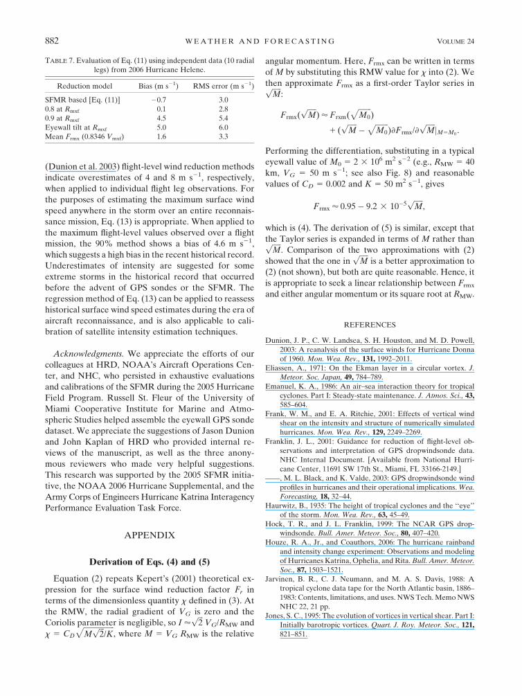
TABLE 7. Evaluation of Eq. (11) using independent data (10 radial

legs) from 2006 Hurricane Helene.

Reduction model Bias (m s21) RMS error (m s21)

SFMR based [Eq. (11)] 20.7 3.0

0.8 at Rmxf 0.1 2.8

0.9 at Rmxf 4.5 5.4

Eyewall tilt at Rmxf 5.0 6.0

Mean Frmx (0.8346 Vmxf) 1.6 3.3

882 W E A T H E R A N D F O R E C A S T I N G VOLUME 24

Kepert, J. D., 2001: The dynamics of boundary layer jets within the

tropical cyclone core. Part I: Linear theory. J. Atmos. Sci., 58,

2469–2484.

——, 2006a: Observed boundary layer wind structure and balance

in the hurricane core. Part I: Hurricane Georges. J. Atmos.

Sci., 63, 2169–2193.

——, 2006b: Observed boundary layer wind structure and balance

in the hurricane core. Part II: Hurricane Mitch. J. Atmos. Sci.,

63, 2194–2211.

——, and Y. Wang, 2001: The dynamics of boundary layer jets

within the tropical cyclone core. Part II: Nonlinear enhance-

ment. J. Atmos. Sci., 58, 2485–2501.

Khelif, D., S. P. Burns, and C. A. Friehe, 1999: Improved wind

measurements on research aircraft. J. Atmos. Oceanic Tech-

nol., 16, 860–875.

Landsea, C. W., J. L. Franklin, C. J. McAdie, J. L. Beven II, J. M.

Gross, B. R. Jarvinen, J. P. Dunion, and P. Dodge, 2004: A

reanalysis of Hurricane Andrew’s (1992) intensity. Bull. Amer.

Meteor. Soc., 85, 1699–1712.

Montgomery, M. T., M. M. Bell, S. D. Aberson, and M. L. Black,

2006: Hurricane Isabel (2003): New insights into the physics of

intense storms. Part I. Bull. Amer. Meteor. Soc., 87, 1335–1347.

OFCM, 2007: National Hurricane Operations Plan. FCM-P12-

2007, Office of the Federal Coordinator for Meteorological

Services and Supporting Research, Washington, DC, 193 pp.

[Available online at www.ofcm.gov/nhop/07/pdf/entire-nhop07.

pdf.]

Olander, T., and C. Velden, 2007: The advanced Dvorak tech-

nique: Continued development of an objective scheme to es-

timate tropical cyclone intensity using geostationary infrared

satellite imagery. Wea. Forecasting, 22, 287–298.

Powell, M. D., 1980: Evaluations of diagnostic marine boundary-

layer models applied to hurricanes. Mon. Wea. Rev., 108, 757–

766.

——, and P. G. Black, 1990: The relationship of hurricane recon-

naissance flight-level wind measurements to winds measured

by NOAA’s oceanic platforms. J.Wind Eng. Indust. Aerodyn.,

36, 381–392.

——, and S. H. Houston, 1996: Hurricane Andrew’s landfall in

south Florida. Part II: Surface wind fields and potential real-

time applications. Wea. Forecasting, 11, 329–349.

——, S. H. Houston, L. R. Amat, and N. Morisseau-Leroy, 1998:

The HRD real-time hurricane wind analysis system. J. Wind

Eng. Indust. Aerodyn., 77/78, 53–64.

——, T. A. Reinhold, and R. D. Marshall, 1999: GPS sonde in-

sights on boundary layer wind structure in hurricanes. Wind

Engineering into the 21st Century, A. Larsen, G. L. Larose,

and F. M. Livesey, Eds., Taylor and Francis, 307–314.

——, P. J. Vickery, and T. A. Reinhold, 2003: Reduced drag co-

efficient for high wind speeds in tropical cyclones. Nature, 422,

279–283.

Rogers, R., and Coauthors, 2006: The Intensity Forecasting Ex-

periment (IFEX): A NOAA multi-year field program for

improving tropical cyclone intensity forecasts. Bull. Amer.

Meteor. Soc., 87, 1523–1537.

Schwendike, J., 2005: The boundary layer winds in Hurricanes

Danielle (1998) and Isabel (2003). Diplomarbeit in Meteo-

rology, Freie Universitat, Berlin, Germany, 255 pp.

——, and J. A. Kepert, 2008: The boundary layer winds in Hur-

ricanes Danielle (1998) and Isabel (2003). Mon. Wea. Rev.,

136, 3168–3192.

Shapiro, L., 1983: The asymmetric boundary layer flow under a

translating hurricane. J. Atmos. Sci., 40, 1984–1998.

Shaw, N., 1922: The birth and death of cyclones. Geophys. Mem., 2,

213–227.

Uhlhorn, E. W., and P. G. Black, 2003: Verification of remotely

sensed sea surface winds in hurricanes. J. Atmos. Oceanic

Technol., 20, 99–116.

——, ——, J. L. Franklin, M. Goodberlet, J. Carswell, and A. S.

Goldstein, 2007: Hurricane surface wind measurements from

an operational Stepped Frequency Microwave Radiometer.

Mon. Wea. Rev., 135, 3070–3085.

Walsh, E. J., and Coauthors, 2002: Hurricane directional wave

spectrum spatial variation at landfall. J. Phys. Oceanogr., 32,1667–1684.

Willoughby, H. E., and M. B. Chelmow, 1982: Objective deter-

mination of hurricane tracks from aircraft observations. Mon.

Wea. Rev., 110, 1298–1305.

——, J. A. Clos, and M. G. Shoreibah, 1982: Concentric eye walls,

secondary wind maxima, and the evolution of the hurricane

vortex. J. Atmos. Sci., 39, 395–411.

——, R. W. R. Darling, and M. E. Rahn, 2006: Parametric repre-

sentation of the primary hurricane vortex. Part II: A new

family of sectionally continuous profiles. Mon. Wea. Rev., 134,

1102–1120.

Wright, C. W., and Coauthors, 2001: Hurricane directional wave

spectrum spatial variation in the open ocean. J. Phys. Oce-

anogr., 31, 2472–2488.

JUNE 2009 P O W E L L E T A L . 883