arX

iv:1

111.

2057

v1 [

astr

o-ph

.GA

] 8

Nov

201

1

F Turnoff Distribution in the Galactic Halo Using Globular

Clusters as Proxies

Matthew Newby1, Heidi Jo Newberg1, Jacob Simones1,2, Nathan Cole1, Matthew

Monaco1

ABSTRACT

F turnoff stars are important tools for studying Galactic halo substructure

because they are plentiful, luminous, and can be easily selected by their photo-

metric colors from large surveys such as the Sloan Digital Sky Survey (SDSS).

We describe the absolute magnitude distribution of color-selected F turnoff stars,

as measured from SDSS data, for eleven globular clusters in the Milky Way halo.

We find that the Mg distribution of turnoff stars is intrinsically the same for all

clusters studied, and is well fit by two half Gaussian functions, centered at µ =

4.18, with a bright-side σ = 0.36, and with a faint-side σ = 0.76. However, the

color errors and detection efficiencies cause the observed σ of the faint-side Gaus-

sian to change with magnitude due to contamination from redder main sequence

stars (40% at 21st magnitude). We present a function that will correct for this

magnitude-dependent change in selected stellar populations, when calculating

stellar density from color-selected turnoff stars. We also present a consistent set

of distances, ages and metallicities for eleven clusters in the SDSS Data Release

7. We calculate a linear correction function to Padova isochrones so that they

are consistent with SDSS globular cluster data from previous papers. We show

that our cluster population falls along the Milky Way Age-Metallicity Relation-

ship (AMR), and further find that isochrones for stellar populations on the AMR

have very similar turnoffs; increasing metallicity and decreasing age conspire to

produce similar turnoff magnitudes and colors for all old clusters that lie on the

AMR.

Subject headings: Galaxy: halo — (Galaxy:) globular clusters: general — Galaxy:

structure — methods: data analysis — stars: statistics — Surveys

1Dept. of Physics, Applied Physics and Astronomy, Rensselaer Polytechnic Institute Troy, NY 12180;

newbym2@rpi.edu, heidi@rpi.edu

2School of Physics and Astronomy, University of Minnesota, Minneapolis, MN 55455

– 2 –

1. Introduction

During the past decade, Galactic stars from the Sloan Digital Sky Survey (SDSS) have

been used not only to discover substructure, but also to trace the density of the smooth

components of the Galaxy: the disks and spheroid. Because the sample of stars is large and

the colors of stars are well measured, it has been possible to use the statistical distributions

of star magnitudes to infer the distances to Milky Way substructure, without the need

to know the absolute magnitude of every star. In an early application of this technique

(Newberg et al. 2002), an estimate of the most common absolute magnitude of very blue F

turnoff stars in the Sagittarius dwarf spheroidal galaxy was compared with the most common

absolute magnitude of similar stars in the tidal debris stream to determine the distance to

the tidal stream. Even though there is a two magnitude spread in the absolute magnitudes

of stars near the turnoff, these stars were used as distance indicators to discover stellar

substructure and to estimate the distance to it.

Later studies such as Belokurov et al. (2006); Juric et al. (2008) used photometric par-

allax of a larger color selection of the stars in the sample, assuming they were overwhelmingly

main sequence stars, to measure the shape of the major components of the Milky Way or

to discover substructures. Some searches for stellar halo substructure (Rockosi et al. 2002;

Grillmair & Dionatos 2006a,b; Grillmair & Johnson 2006; Grillmair 2006, 2009) have used a

matched filter technique to discover stars that have been tidally stripped from dwarf galaxies

and globular clusters.

Since the Newberg et al. (2002) paper, Newberg & Yanny have continued to use the

apparent magnitude of the turnoff stars in a discovered Milky Way substructure to es-

timate the distances to discovered overdensities of stars (Yanny et al. 2003; Freese et al.

2004; Newberg & Yanny 2006; Newberg et al. 2007; Willett et al. 2009; Yanny et al. 2009;

Newberg et al. 2010). Sometimes the assumed absolute magnitude for F turnoff stars is the

same as was calculated for the Sagittarius dwarf galaxy, and sometimes it is adjusted slightly

based on available information about the stellar population of the substructure being stud-

ied. In general, the distance to the structure under study is estimated from the peak of the

apparent magnitude distribution of the bluest main sequence stars.

This technique was improved in Cole et al. (2008), in which a maximum likelihood

technique for measuring the spatial distribution of tidal debris from the Sagittarius dwarf

galaxy was described. In this paper, the distribution of magnitudes for F turnoff stars with

0.1 < (g − r)0 < 0.3 was represented by a Gaussian with center Mg0 = 4.2 and dispersion

σg0 = 0.6. QSOs were eliminated from the sample with (u − g)0 > 0.4. This distribution is

approximately the same as the distribution of similarly selected F turnoff stars for three glob-

ular clusters measured by Newberg & Yanny (2006), except that Newberg & Yanny (2006)

– 3 –

fit a slightly larger tail on the faint side of the peak than the bright side of the peak. With

the maximum likelihood technique, the star number counts expected for a particular stream

and smooth halo model (assuming a single absolute magnitude value for all turnoff stars)

were broadened in the g0 direction by the absolute magnitude distribution for the turnoff

stars, before the number counts were compared with the data. Using this method, one could

estimate the depth of the tidal debris stream along the line of sight, and could make a more

accurate fit to the smooth distribution of stars in the stellar halo.

Implicit in all of these studies has been the assumption that the absolute magnitude

distribution of F turnoff stars is well represented by a single Gaussian distribution with a

fixed peak and width. One might expect that the actual distribution might be a function of

age and metallicity of the stellar component. In fact, the distribution might be different as

a function of distance along a tidal debris stream, and different across the stellar halo and

disks. To effectively use F turnoff stars as standard candles, one should study the variation

in the distribution of F turnoff star absolute magnitudes as a function of stellar population.

In this paper, we analyze eleven globular clusters in the Galactic halo, and find that the

peak of the distribution of absolute magnitudes of F turnoff stars is typically Mg = 4.18,

and that the asymmetric distribution can be approximated by a half Gaussian on the bright

side with a width of σ = 0.36, and a half Gaussian on the faint side with a width of σ =

0.76. This distribution is surprisingly similar for all of the globular clusters studied, which

range in age from 9.5 to 13.5 Gyr and from [Fe/H]= −1.17 to [Fe/H]= −2.30. We explain

this surprising result by showing that it is consistent with the age-metallicity relationship for

Galactic stars. Older clusters should have fainter, redder turnoffs. However, older clusters

also contain fewer metals, which pushes the turnoff brighter and bluer. Although the color

of the turnoff varies slightly from cluster to cluster, the absolute magnitude of the turnoff

only shifts about 0.1 magnitudes from the mean.

Although we find the turnoff magnitude to be similar for the clusters studied, observa-

tional effects may considerably change the properties of turnoff star distributions. As one

samples stars to the limit of the survey, the photometric errors increase. Although these

photometric errors are small compared to the uncertainty with which we know the absolute

magnitude of a single F turnoff star, they can be large compared to the width of our color

selection box. For bright magnitudes, the actual colors of most of the stars selected are

actually within the color range selected. For magnitudes near the survey limit, some stars

that should be selected are randomly measured with colors that are too red or too blue,

and a larger number of stars that are too red or too blue are randomly scattered into our

selection range. The largest flux into and out of the color selection range is on the red side of

the range, and primarily broadens the measured width on the faint side of the peak absolute

– 4 –

magnitude as one approaches the survey limit.

The results of this paper will make it possible to make more accurate measurements of

the intrinsic density of F turnoff stars in the Milky Way’s stellar halo. We present a function

that can be used to estimate the observed width on the faint side of the absolute magnitude

distribution. We also provide numbers for the fractional increase in the number counts as

stars leak into the color box at distances where G main sequence stars are near the survey

limit; and the fractional decrease in the number counts as F turnoff stars reach the survey

limit and the large color errors scatter them out of the color selection range.

2. Globular Cluster Data Selection

Our analysis used photometric data from eleven globular clusters, taken from the SDSS

database’s seventh data release (DR7; Abazajian et al. 2009). There are a total of seventeen

globular clusters within the SDSS DR7 footprint, but five clusters (NGC 2419, NGC 7006,

Pal3, Pal 4, and Pal 14) were eliminated because they are too distant, and one (Pal 1) was

eliminated because there were too few stars to obtain accurate measures of the F turnoff

star distribution using SDSS data. A list of all clusters studied in this investigation can be

found in Table 1.

To determine the limits in right ascension and declination for selecting stars for each

field, we used the SDSS SkyServer’s Navigate tool.1 The image field of view was expanded

so that the cluster was clearly visible, then expanded further until a sizable background

distribution was also contained within this view. In general, the entire field of view spanned

a rectangle with sides of lengths between 6 and 8 times the apparent radius of the cluster.

The bounds of this rectangle were then used as the right ascension and declination limits in

the Casjobs data query.

Within these limits, we selected all objects classified as STAR, and that had (u− g)0 >

0.4. The latter requirement was designed to avoid possible contamination from quasars

(Yanny et al. 2000). By selecting from the database of “STAR”s, we ensured that we ob-

tained only one instance of each object. We extracted the extinction-corrected (denoted by

the subscript ‘0’) point-spread-function (PSF) apparent magnitudes with errors. We deter-

mined rclus, the radius within which the majority of the stars belong to the globular cluster,

and rcut, the radius outside of which there is little contamination from cluster stars, by vi-

sual inspection of the data. Stars with rclus < r < rcut were removed from the data set. An

1Located at http://cas.sdss.org/dr7/en/tools/chart/navi.asp

– 5 –

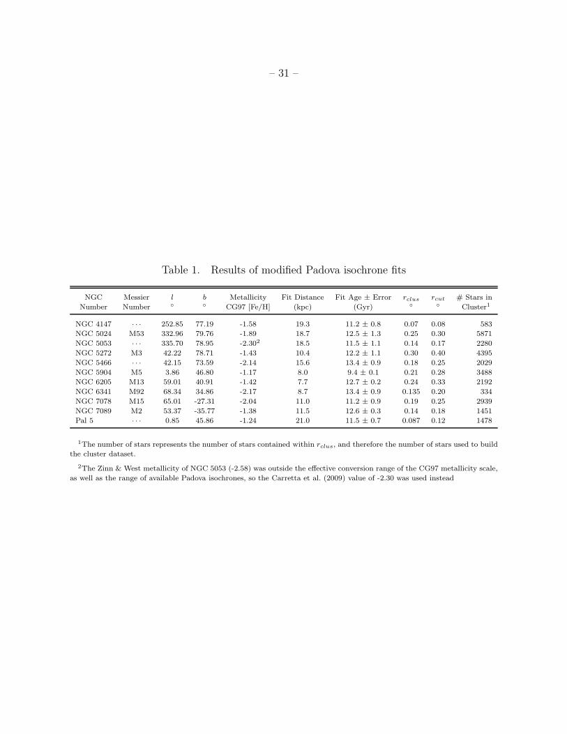
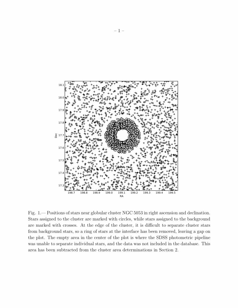
example is shown in Figure 1. The rclus and rcut values used for each cluster are included in

Table 1.

The following clusters are listed in Table 1, but were excluded in some of our analyses:

NGC 5053 has a very low Zinn & West metallicity ([Fe/H ]ZW84 ∼-2.58) which falls

outside the range of the Carretta & Gratton (1997) conversion scale, and is also below the

minimum metallicity value for which Padova isochrones can be generated. In the newer

work of Carretta et al. (2009), an [Fe/H ] of -2.30 is found, which is within the range of

the Padova isochrones (Girardi et al. 2000; Marigo et al. 2008), and therefore we use this

metallicity value for our analysis. To indicate status as a potential outlier, results for NGC

5053 are plotted using a red-dotted series in figures showing turnoff stars properties.

M15 (NGC 7078) is a ‘core-collapsed’ cluster, and so has a very compact core. It

may also have different dynamics and stellar distributions than standard globular clusters

(Haurberg et al. 2010). The SDSS photometric pipeline does not attempt to deblend crowded

star fields, and so information on M15 in SDSS is highly biased towards stars found on the

edges of the cluster. We do not expect this cluster to necessarily be consistent with the other

clusters, but we include it in analysis anyway. We indicate M15’s status as potential outlier

in figures showing turnoff star properties by plotting it with a red dotted series.

NGC 4147 contains only slightly more stars than M92, (583 versus 334) but they are

more concentrated around the turnoff due to a lack of stars below Mg = 6.5. This lack

of stars is due to SDSS crowded-field photometry detection efficiency problems at fainter

magnitudes (see Section 4). We attempt to analyze NGC 4147 with other clusters later in

our analysis, but we expect errors to be large due to the low number of data points available.

In figures showing turnoff star properties, a blue dotted series is used for NGC 4147 to

indicate it’s low star counts and high expected errors.

Cluster M92 (NGC 6341) fell on the edge of the SDSS DR7 footprint, and relatively few

stars were observed in the cluster. The number of cluster stars was large enough to produce

a fiducial fit with large bins in magnitude (0.5 magnitudes). Therefore we were able to fit

a modified Padova isochrone to this cluster. However, as there are so few M92 stars in our

data, especially close to the turnoff, that M92 was omitted from the turnoff analysis.

3. Isochrone Fitting to Determine Cluster Distances

In order to convert our observed apparent magnitudes to absolute magnitudes, we rely on

the measured distances to each globular cluster. Since we would like to study the effects of age

– 6 –

and metallicity on the absolute magnitudes of the turnoff stars, we would like measurements

of these quantities that are as accurate and as uniform as possible for our sample of globular

clusters. In this section, we assemble the spectroscopically determined metallicities ([Fe/H ])

from a single group of authors; measurements were obtained from Zinn & West (1984) and

then converted to more modern Carretta & Gratton scale using the conversion provided in

(Carretta & Gratton 1997). Using these metallicities, we then fit ages and distances to the

clusters in a consistent fashion using Padova isochrones.

The Padova theoretical isochrones were fit to fiducial sequences determined from data

for eleven clusters found in SDSS. Stars in each cluster were separated into g0 bins, then

the mean and standard deviation (σg−r) of the (g − r)0 distribution in each bin was found.

Any stars in the g0 bin with a (g − r)0 value beyond 2σg−r from the mean were rejected,

and then the (g − r)0 mean and σg−r of the remaining population was found. The (g − r)0mean and average Mg value were accepted as a point on the fiducial sequence once the

entire bin was within 2σg−r of the current mean. Isochrones were then fit to the fiducial

sequences using distance and age as free parameters, while metallicity was held constant at

the spectroscopically determined value.

In our initial attempts to use this technique to determine cluster properties, we found

that Padova isochrones that are good fits to both the main sequence and the subgiant

branch require unreasonably high ages (>15 Gyr) for most clusters. The lack of agreement

between theoretical isochrones and cluster data has been explored by previous authors. Using

eclipsing binary stars in the Hyades open cluster, Pinsonneault et al. (2003) showed that

theoretical isochrones do not match true star populations; there are discrepancies in mass,

luminosity, temperature, and radius. In the second paper in the series, Pinsonneault et al.

(2004) uses Hipparcos parallax data for the Hyades cluster to further calibrate theoretical

isochrones, finding that offsets in color indexes are sufficient to bring a theoretical isochrone

in line with real main sequence data. In the fourth and final paper of the series An et al.

(2007) fits isochrones to Galactic open clusters using color corrections in (B − V )0 as a

function of Mv, while using Cepheid variables as calibration points. In An et al. (2009),

updated Yale Rotating Evolutionary Code with MARCS model atmospheres were used to

produce ugriz isochrones which were fit to main sequences of five globular clusters, producing

ages and distances to these clusters.

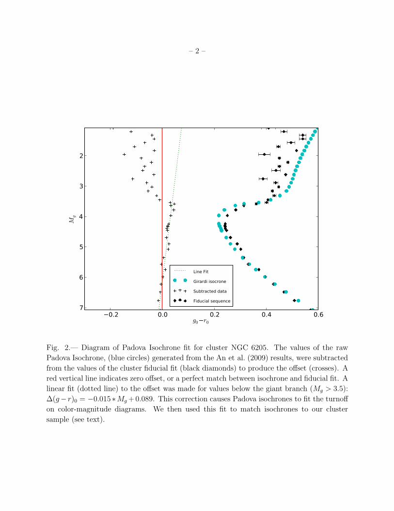
Using similar techniques, we seek to calibrate Padova ugriz isochrones to the An et al.

(2009) results. Comparing a Padova isochrone generated from the An et al. (2009) derived

age and distance for globular cluster NGC 6205 with our derived fiducial fit, we find that

the difference between the theoretical isochrone and the data is very nearly linear along the

main sequence (Figure 2). Therefore, we apply a linear color correction function in (g− r)0,

– 7 –

holding Mg as the independent variable, to the Padova isochrone to bring it into agreement

with our fiducial fit. We fit only to the main sequence and subgiant branch, and ignored

the giant branch (∼ Mg > 3.5), as the linear trend was no longer valid brighter than the

subgiant branch. We also did not fit to the lower main sequence, as our data does not extend

to fainter absolute magnitudes. Our color-correction functional fit is given by the following

equation:

∆(g − r) = −0.015 ∗Mg + 0.089 (1)

This function was applied to all of the colors in the model isochrones and then these

models were fit to our fiducial sequences derived from the data. For each cluster, we first

chose a Padova isochrone that, modified by Equation 1, appeared to fit the fiducial sequence

well. We then chose additional isochrones, identical except for age, which was varied about

our “by eye” best fit in increments of 0.2 Gyrs. A Gaussian function was fit to the residuals

of these isochrones fits, and the mean of this Gaussian was taken as the best fit age.

Errors in our fit ages were determined through a Hessian matrix method by comparing

the residuals in the isochrone fit. In the limit of a single fit parameter (age), the Hessian

error method reduces to:

σ =

(

R2(t+ 2h) +R2(t− 2h)− 2R2(t)

8h2

)−1

2

(2)

Where R2(t) is the residual of the isochrone fit at age t, and h = 0.2 is the step size

in the age determination method. Using Equation 2, we were able to determine the age fit

errors for each cluster through the use of three isochrones: the isochrone of best fit age, and

two isochrones generated at the best fit age ±0.4 Gyr.

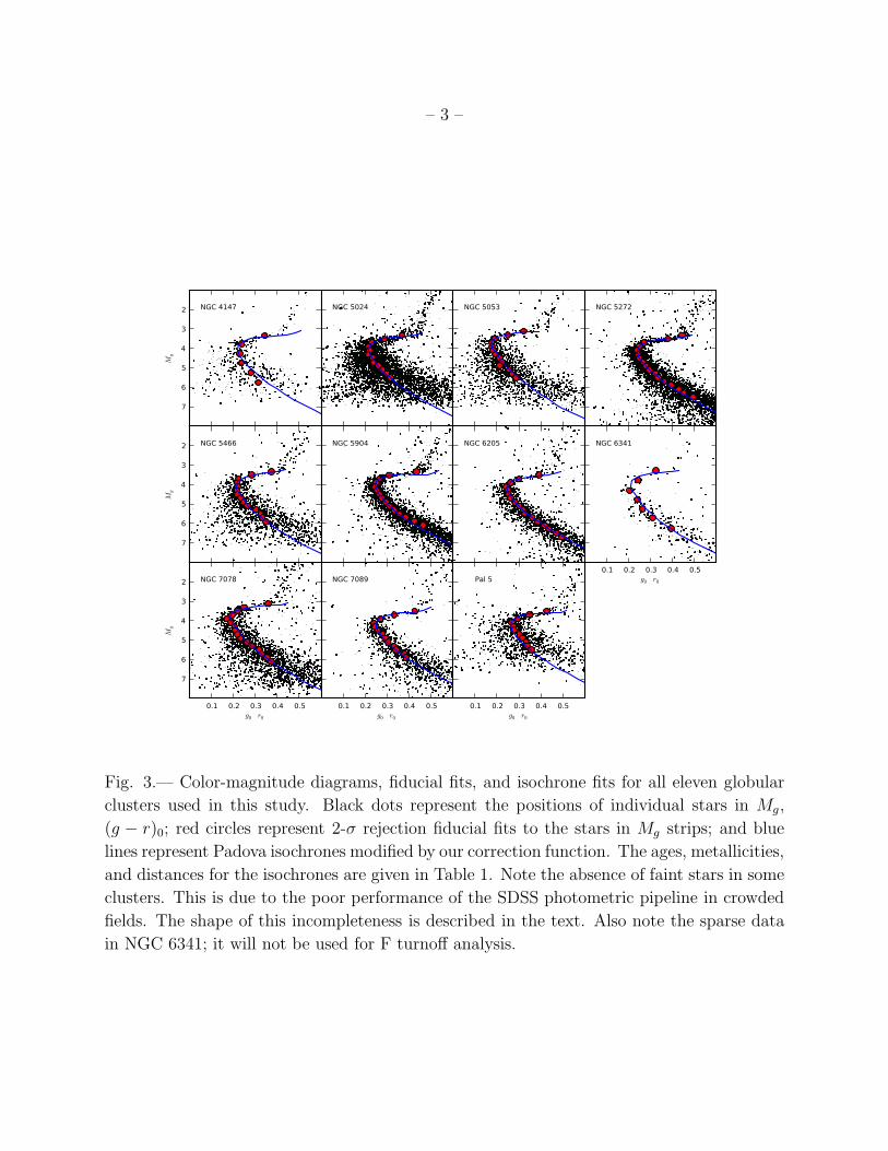
Padova isochrones fit using our correction function produce a consistent set of metal-

licities, ages, and distances to our globular cluster sample, as presented in Table 1. Cluster

color-magnitude diagrams, fiducial fits, and modified isochrone fits are shown in Figure 3.

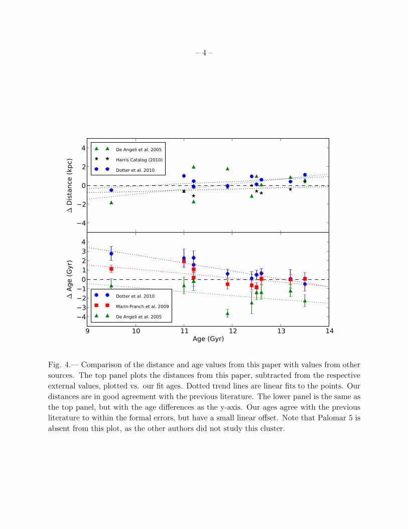
We compare our distance fits to distances in three other sources (De Angeli et al. (2005),

Harris, et al. (1997) and Dotter et al. (2010)), and compare our ages to other isochrone-

derived ages (De Angeli et al. (2005), Marın-Franch et al. (2009), and Dotter et al. (2010)),

in Figure 4. Our distances appear to be in excellent agreement with other sources. Our

ages agree to within the formal errors for each cluster, but appear to have a small linear

systematic offset. The ages are a very close match around 13 Gyr, but are a Gyr or two

higher for ages of 10 Gyr, so our age scale is slightly more compressed than the ages in the

– 8 –

comparison sources.

4. Detection Efficiency for Stars in SDSS Globular Clusters

It is clear from Figure 3 that the cluster data is incomplete at fainter absolute mag-

nitudes, especially amongst the farther clusters: Pal 5, and NGC 4147, NGC 5024 and

NGC 5053. This incompleteness begins at a brighter magnitude than is expected from the

SDSS detection efficiency for stars (Newberg et al. 2002). The poorer detection efficiency in

globular clusters is due to difficulty in detecting faint sources in highly crowded star fields,

and in particular the poor performance of the SDSS photometric pipeline in this regime

(Adelman-McCarthy et al. 2008). For sufficiently crowded fields, the code cannot deblend

and resolve faint stars, since they are washed out by much brighter stars.

To quantify the cluster detection efficiency, we examined nearby clusters with relatively

complete CMDs and compared them to the farther, incomplete CMDs under the assumption

that there are similar absolute magnitude distributions for the stars in nearby and distant

clusters. We select stars from the CMDs in a rectangular box with bounds 3.567 < Mg0 <

7.567, 0.0 < (g − r)0 < 0.8, and a color cut of (u − g)0 < 0.4, to coincide with areas of

completeness in the near clusters (specifically 18.0 < g0 < 22.0 for NGC 6205) that are

incomplete for the more distant clusters. We choose three nearby clusters, NGC 6205, NGC

5904, and NGC 5272, and found that their normalized Mg0 histograms in our box are, in fact,

similar. Therefore, we average them to create a reference absolute magnitude distribution for

cluster stars. We assume that this histogram represents the true magnitude distribution of

globular clusters, then compare the normalized histograms of the four most distant clusters

(NGC 4147, NGC 5024, NGC 5053, and Pal 5) to this reference. To make the normalizations

comparable across the incompleteness of the farther clusters, we took the average difference

of the first five bins (which showed a similar rising trend in all of our clusters) and scaled

the entire histogram by this value, thereby scaling the clusters by matching initial trends.

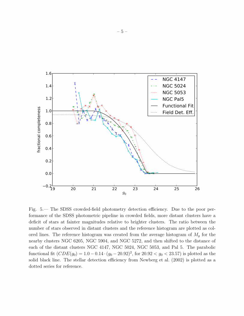
To quantify the detection efficiency in our globular clusters, we fit the ratios between

the reference histogram and the distant cluster histograms using a parabolic function. We

expect these globular clusters to have the same intrinsic absolute magnitude distribution as

the bright clusters, but are missing faint stars that were lost to the crowded-field photometry.

The histogram residuals and functional fit can be seen in Figure 5, and the resulting function

is given empirically as:

– 9 –

CDE(g0) =

1.0 if g0 < 20.92

0.0 if g0 > 23.57

1.0− 0.14 · (g0 − 20.92)2 otherwise

(3)

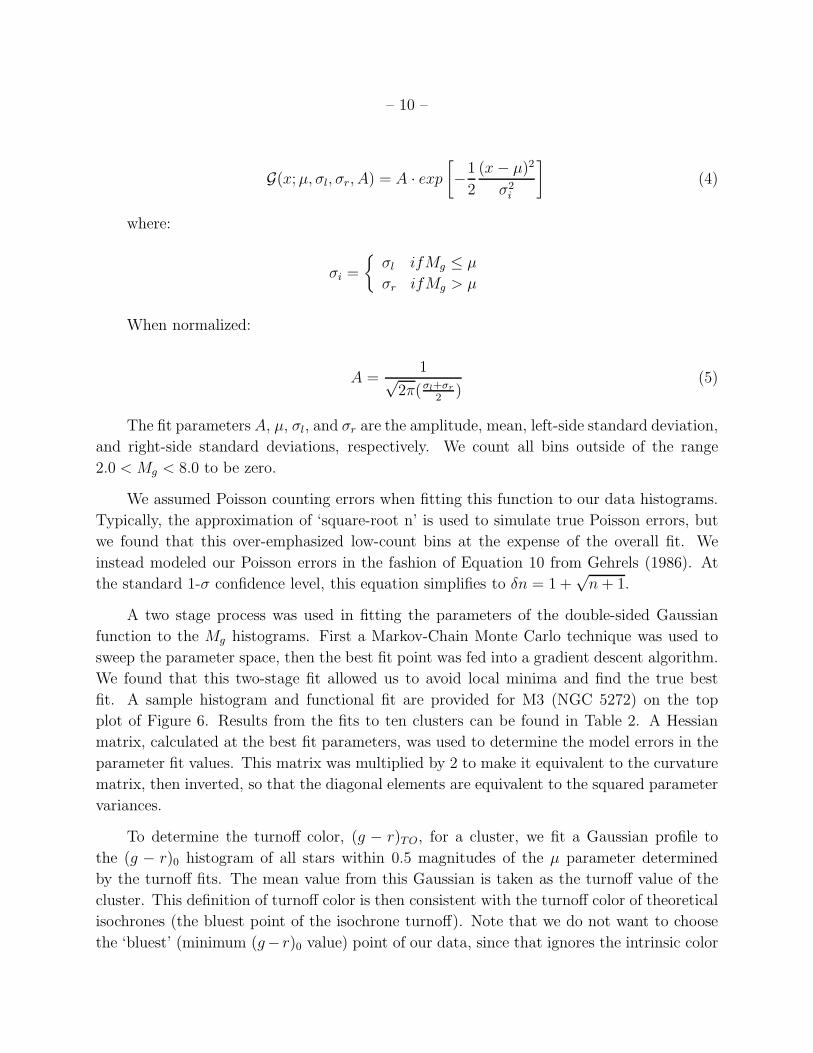
We can use this function to reconstruct incomplete cluster star distributions, and to

model the effect of SDSS crowded-field photometry at farther distances. Errors in the pa-

rameter fits in Equation 3 are 0.14 ± 0.001, 20.92 ± 0.007.

5. Absolute Magnitude Distribution of F Turnoff Stars

5.1. Fitting the Turnoff

We are now prepared to characterize the absolute magnitude distribution of F turnoff

stars in old stellar populations. We select stars in the F turnoff region (0.1 < (g−r)0 < 0.3),

which is the color range used in the photometric F turnoff density searches in Cole et al.

(2008), and the range originally chosen in Newberg et al. (2002) to include stars redder than

most blue horizontal branch stars, but bluer than the turnoff of Milky Way disk stars. We

then build a histogram in Mg from the cluster data, using a bin size of 0.2 magnitudes over

the range 2.0 < Mg < 8.0, which minimizes potential contamination from non-cluster stars.

We then divide each bin by the cluster detection efficiency for the g0 that corresponds to

the bin’s Mg, thereby rebuilding the component of each cluster lost due to the detection

efficiency.

We subtract from this histogram the expected number of field stars in each magnitude

bin, as determined from the sky area around each cluster, scaled to the sky area of cluster

data. If the cluster lies on the edge of the SDSS footprint, or where sections of the clusters

were unresolved by SDSS, the areas with no data were excluded from the area used in scaling

the background bins. The magnitude histogram for the background was divided by the field

stellar detection efficiency (Newberg et al. 2002) as a function of apparent magnitude.

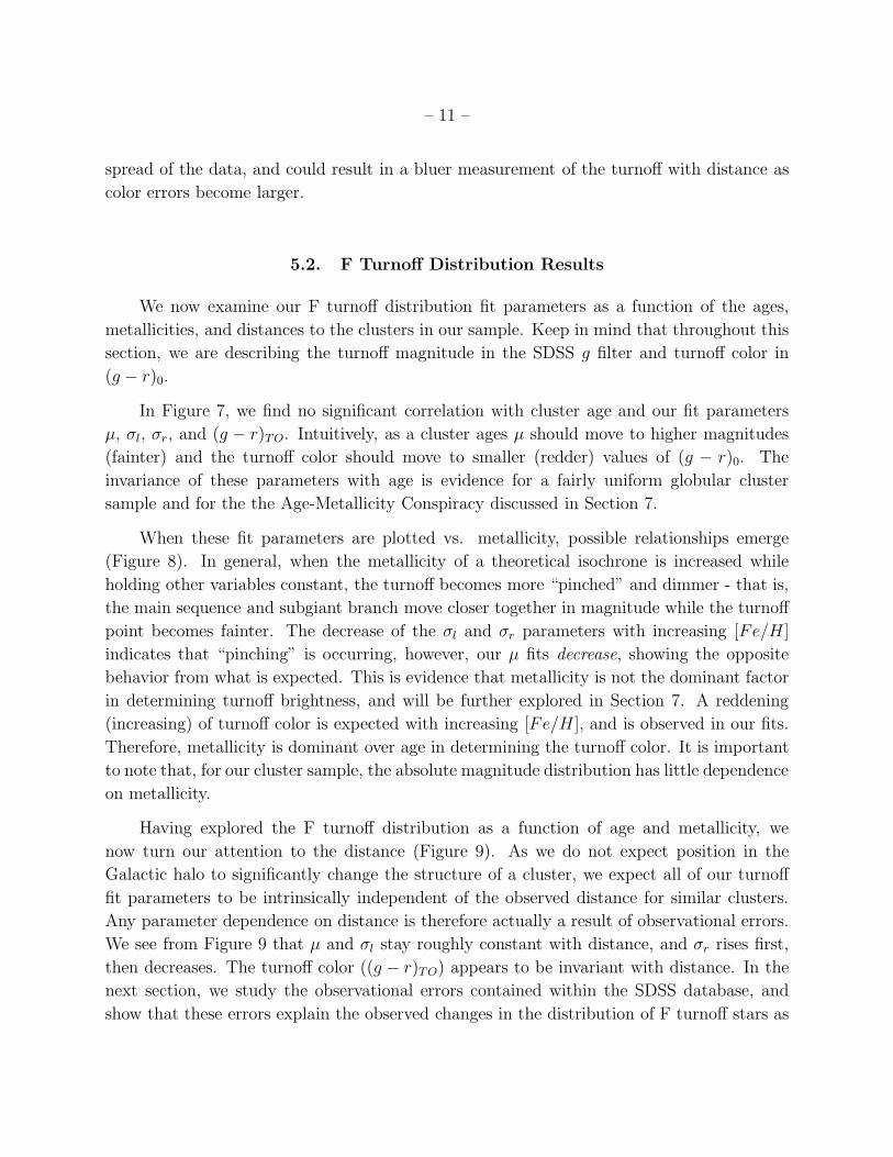
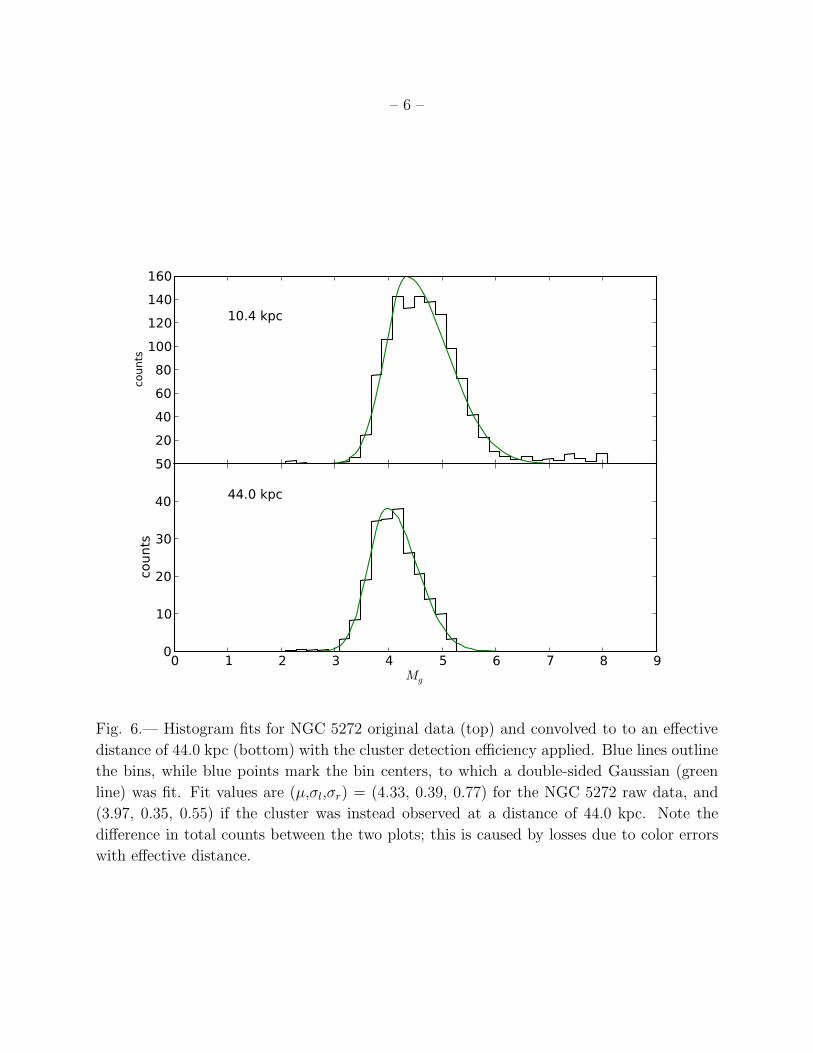
The top panel in Figure 6 shows the distribution of turnoff star Mg absolute magnitudes

in globular cluster NGC 5272. We fit each SDSS cluster histogram with a ‘double-sided’

Gaussian distribution, where the standard deviation is different on each side of the mean.

This choice provides a good fit to the data using a simple, well-known function. We have no

theoretical motivation behind our choice of fitting function; however, this function appears

to effectively match the form of our data without over-determining the system. The form of

our fit function is given by:

– 10 –

G(x;µ, σl, σr, A) = A · exp[

−1

2

(x− µ)2

σ2i

]

(4)

where:

σi =

σl ifMg ≤ µ

σr ifMg > µ

When normalized:

A =1√

2π(σl+σr

2)

(5)

The fit parameters A, µ, σl, and σr are the amplitude, mean, left-side standard deviation,

and right-side standard deviations, respectively. We count all bins outside of the range

2.0 < Mg < 8.0 to be zero.

We assumed Poisson counting errors when fitting this function to our data histograms.

Typically, the approximation of ‘square-root n’ is used to simulate true Poisson errors, but

we found that this over-emphasized low-count bins at the expense of the overall fit. We

instead modeled our Poisson errors in the fashion of Equation 10 from Gehrels (1986). At

the standard 1-σ confidence level, this equation simplifies to δn = 1 +√n+ 1.

A two stage process was used in fitting the parameters of the double-sided Gaussian

function to the Mg histograms. First a Markov-Chain Monte Carlo technique was used to

sweep the parameter space, then the best fit point was fed into a gradient descent algorithm.

We found that this two-stage fit allowed us to avoid local minima and find the true best

fit. A sample histogram and functional fit are provided for M3 (NGC 5272) on the top

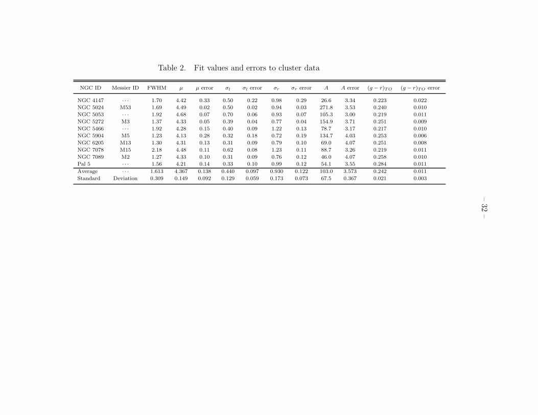
plot of Figure 6. Results from the fits to ten clusters can be found in Table 2. A Hessian

matrix, calculated at the best fit parameters, was used to determine the model errors in the

parameter fit values. This matrix was multiplied by 2 to make it equivalent to the curvature

matrix, then inverted, so that the diagonal elements are equivalent to the squared parameter

variances.

To determine the turnoff color, (g − r)TO, for a cluster, we fit a Gaussian profile to

the (g − r)0 histogram of all stars within 0.5 magnitudes of the µ parameter determined

by the turnoff fits. The mean value from this Gaussian is taken as the turnoff value of the

cluster. This definition of turnoff color is then consistent with the turnoff color of theoretical

isochrones (the bluest point of the isochrone turnoff). Note that we do not want to choose

the ‘bluest’ (minimum (g− r)0 value) point of our data, since that ignores the intrinsic color

– 11 –

spread of the data, and could result in a bluer measurement of the turnoff with distance as

color errors become larger.

5.2. F Turnoff Distribution Results

We now examine our F turnoff distribution fit parameters as a function of the ages,

metallicities, and distances to the clusters in our sample. Keep in mind that throughout this

section, we are describing the turnoff magnitude in the SDSS g filter and turnoff color in

(g − r)0.

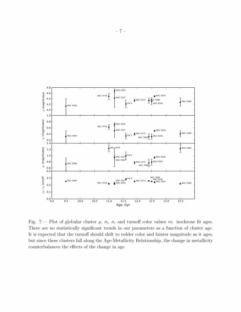
In Figure 7, we find no significant correlation with cluster age and our fit parameters

µ, σl, σr, and (g − r)TO. Intuitively, as a cluster ages µ should move to higher magnitudes

(fainter) and the turnoff color should move to smaller (redder) values of (g − r)0. The

invariance of these parameters with age is evidence for a fairly uniform globular cluster

sample and for the the Age-Metallicity Conspiracy discussed in Section 7.

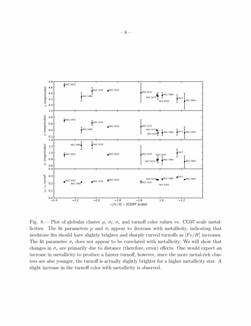
When these fit parameters are plotted vs. metallicity, possible relationships emerge

(Figure 8). In general, when the metallicity of a theoretical isochrone is increased while

holding other variables constant, the turnoff becomes more “pinched” and dimmer - that is,

the main sequence and subgiant branch move closer together in magnitude while the turnoff

point becomes fainter. The decrease of the σl and σr parameters with increasing [Fe/H ]

indicates that “pinching” is occurring, however, our µ fits decrease, showing the opposite

behavior from what is expected. This is evidence that metallicity is not the dominant factor

in determining turnoff brightness, and will be further explored in Section 7. A reddening

(increasing) of turnoff color is expected with increasing [Fe/H ], and is observed in our fits.

Therefore, metallicity is dominant over age in determining the turnoff color. It is important

to note that, for our cluster sample, the absolute magnitude distribution has little dependence

on metallicity.

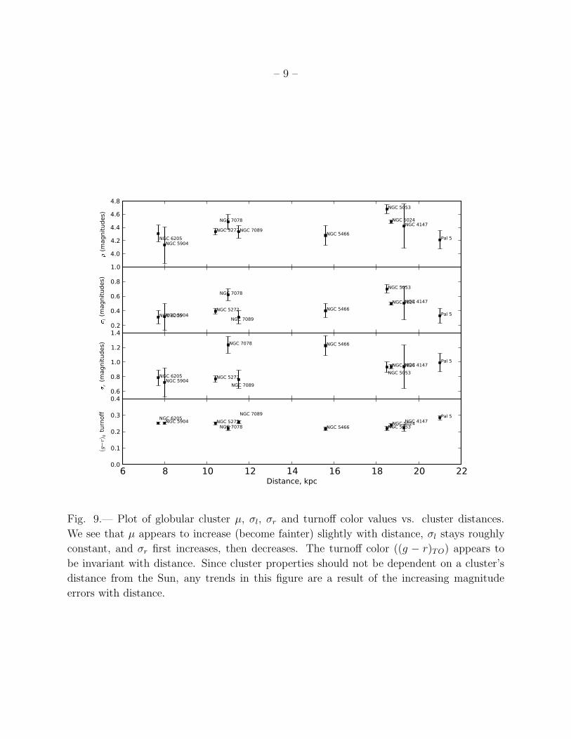
Having explored the F turnoff distribution as a function of age and metallicity, we

now turn our attention to the distance (Figure 9). As we do not expect position in the

Galactic halo to significantly change the structure of a cluster, we expect all of our turnoff

fit parameters to be intrinsically independent of the observed distance for similar clusters.

Any parameter dependence on distance is therefore actually a result of observational errors.

We see from Figure 9 that µ and σl stay roughly constant with distance, and σr rises first,

then decreases. The turnoff color ((g − r)TO) appears to be invariant with distance. In the

next section, we study the observational errors contained within the SDSS database, and

show that these errors explain the observed changes in the distribution of F turnoff stars as

– 12 –

a function of distance.

6. Observational Effects of SDSS Errors

6.1. Photometric Errors in SDSS Star Colors

Photometric errors widen the observed magnitude and color distributions of turnoff

stars in globular clusters as plotted in color-magnitude diagrams, by an increasing amount

with fainter magnitudes. We now examine the photometric errors in the SDSS database

and extrapolate the observational biases that result from these errors. SDSS forgoes the

conventional “Pogson” logarithmic definition of magnitude in favor of the “asinh magnitude”

system described in Lupton et al. (1999). These systems are virtually identical at high signal-

to-noise, but in the low signal-to-noise regime asinh magnitudes are well-behaved and have

non-infinite errors. The two magnitude systems do not differ noticeably in magnitude or

magnitude error until fainter than 24th magnitude (signal-to-noise ∼2.0), so our analysis

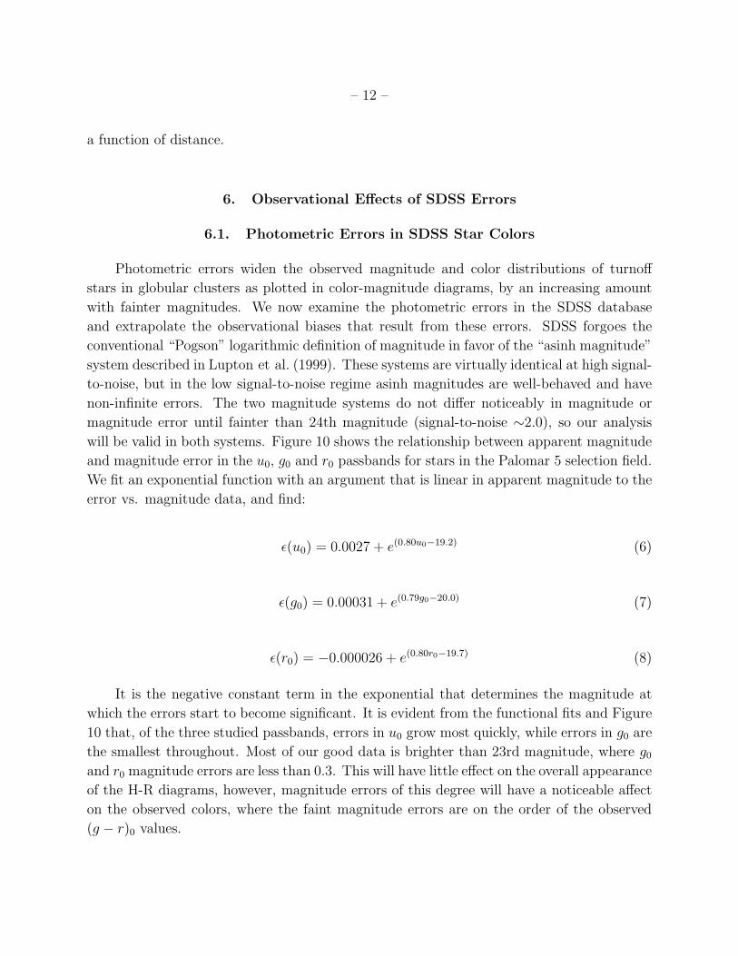
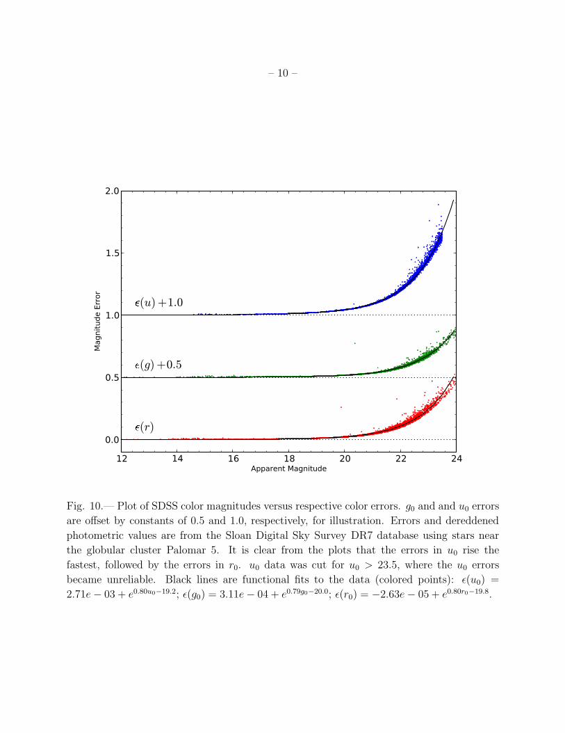
will be valid in both systems. Figure 10 shows the relationship between apparent magnitude

and magnitude error in the u0, g0 and r0 passbands for stars in the Palomar 5 selection field.

We fit an exponential function with an argument that is linear in apparent magnitude to the

error vs. magnitude data, and find:

ǫ(u0) = 0.0027 + e(0.80u0−19.2) (6)

ǫ(g0) = 0.00031 + e(0.79g0−20.0) (7)

ǫ(r0) = −0.000026 + e(0.80r0−19.7) (8)

It is the negative constant term in the exponential that determines the magnitude at

which the errors start to become significant. It is evident from the functional fits and Figure

10 that, of the three studied passbands, errors in u0 grow most quickly, while errors in g0 are

the smallest throughout. Most of our good data is brighter than 23rd magnitude, where g0and r0 magnitude errors are less than 0.3. This will have little effect on the overall appearance

of the H-R diagrams, however, magnitude errors of this degree will have a noticeable affect

on the observed colors, where the faint magnitude errors are on the order of the observed

(g − r)0 values.

– 13 –

6.2. F Turnoff Contamination

Since F turnoff stars are selected through color cuts, we expect SDSS color errors to cause

the turnoff to be contaminated by misidentified non-turnoff stars. We took cluster NGC 6205

as a reference data set, as the relatively low distance (7.7 kpc) implies minimal photometric

magnitude errors near the turnoff. Cluster NGC 6205 color errors do not become noticeable

until Mg = 7.0 (g0 = 21.43); at our absolute magnitude limit of Mg = 8.0 (g0 = 22.43),

the magnitude errors are close to 0.1 in g0 and 0.15 in r0, resulting in a maximum color

error at Mg = 8.0 equal to 0.18. From Figure 3, we see that NGC 6205 stars between

7.0 < Mg < 8.0 are sufficiently red that even for the maximum color error, these stars are

statistically unlikely to to be detected in the turnoff color cut. We therefore can assume that

NGC 6205 will be illustrative as an example of a cluster with an uncontaminated turnoff.

In order to understand how the errors affect a cluster with increasing distance, we must

first define a process that will allow us to view a cluster as though it were observed by

SDSS at a farther distance, taking into account the increasing magnitude errors as apparent

magnitudes increase. We first choose a new ‘effective distance’ (deff) to observe the cluster

at, and then perform a ‘distance shift’ on each star for each of u0, g0 and r0; the magnitude

of each star is increased by an amount equivalent to observing the cluster at deff instead of

the original distance (d0). The magnitude error associated with the new magnitude is then

derived from the appropriate error equation (Equations 6, 7 and 8). The original magnitude

error is then subtracted in quadrature from the new magnitude error to produce the relative

increase in error. The new magnitude value is then modified by the relative increase in

error: we select a random value from a Gaussian distribution with a mean equivalent to the

new magnitude, and with a standard deviation equal to the relative increase in error. This

random value produces the new shifted magnitude, equivalent to observing the star at deff ,

including the effects of SDSS magnitude errors.

Having defined the distance shift process, we then separate the NGC 6205 cluster data

into three color bins and examine bin cross-contamination as the distance increases. The

three color bins are: the primary ‘yellow’ turnoff bin 0.1 < (g − r)0 < 0.3, the ‘red’ star bin

((g − r)0 > 0.3) and the ‘blue’ star bin ((g − r)0 < 0.1). Each of these bins were treated as

separate data sets. We then performed distance shifts on each bin at 1.0 kpc steps, up to a

maximum deff of 80.0 kpc. At each step we reinforced the (u − g)0 color cut, then counted

the number of stars that remained in their origin bin, and the number that had leaked into

other color bins due to color errors. We performed this process 100 times with the NGC

6205 cluster data, and averaged the results to smooth out potential random errors. We then

repeated this process, but included the field stellar detection efficiency in our calculations in

order to represent the actual observed turnoff population.

– 14 –

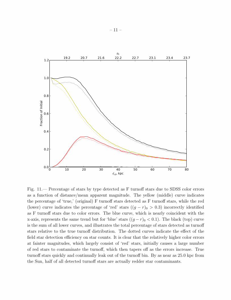
Figure 11 illustrates the composition of the selected turnoff stars (0.1 < (g−r)0 < 0.3) as

a fraction of the original ‘true’ turnoff count, and as a function of distance. This calculation

assumed 100% detection efficiency for the shifted stars. The results of applying the field

stellar detection efficiency is shown by the dotted lines. The trends in this figure are color-

coded by the bin of origin; the black trend is a sum of all lower curves, and represents the

total number of stars detected as turnoff stars for a given distance. Readily apparent from

Figure 11 is the quick influx of ‘red’ stars into the turnoff between distances of (10.0-20.0

kpc), and the constant loss of true turnoff stars with distance.

Red G stars that lie just below the turnoff are on the densely populated main sequence,

and have (g − r)0 values just above our turnoff color cut of 0.3. Even slight color error

perturbations will tend to shift some these stars into the turnoff color cut, resulting in

significant ‘red’ star contamination at relatively low halo distances. It is clear from Figure

11 that this is a rapid effect that occurs at fairly low distances (10.0-20.0 kpc), but as

the errors continue to increase it becomes just as likely for a red G star to jump over the

turnoff selection box as it is to land in it, thereby causing the red star contamination to stop

increasing around 20.0 kpc.

It is interesting to note that the (u − g)0 color cut causes some suppression of the red

contamination effect. Since red stars are fainter and farther down the main sequence, they

have higher measured magnitudes and magnitude errors than true turnoff stars. As the

u0 passband has the highest associated magnitude errors, faint stars with large errors are

perturbed more in (u− g)0 than in (g− r)0. Therefore, faint red stars with large color errors

may be perturbed beyond the (u − g)0 cut and subsequently removed from the data set,

even if errors would place that star in the (g− r)0 cut for the turnoff. The (u− g)0 cut then

serves to remove some of the red contamination stars from the turnoff selection.

As the errors increase, true F turnoff stars can only leak out of the turnoff selection box.

Since there are very few bluer ((g − r)0 < 0.1) A-type stars or redder subgiants in globular

clusters, and these in any event are bright, few A stars leak into the F turnoff star selection

due to errors in color. Around the distance that the red star contamination stops (∼25.0

kpc), the number of stars in the turnoff selection box is comprised of roughly 60% true F

turnoff stars and 40% redder G star contamination. As distances increase, the fraction of

true turnoff stars in the color selection range decreases to 50%, and the total number of stars

selected as turnoff stars decreases. This is a significant effect that has never been accounted

for in previous research papers.

So that future authors may compensate for these effects, we provide analytical functions

for the F turnoff dissipation and the red star contamination. These fits are to the 100%

detection efficiency case (solid curves in Figure 11), representing the effect caused by color

– 15 –

errors only. We represent the F turnoff dissipation with a 4th-order polynomial function in

deff , and fit the red contamination with a similar function of 7th-order, with the coefficients

given by ay and ar (where a = (a0, a1, a2, ...), subscripts corresponding to order of term),

respectively:

ay = (1.06,−0.031, 0.00020, 2.54× 10−6,−2.67× 10−8) (9)

ar = (0.016,−0.020, 0.0066,−0.00043, 1.26× 10−5,−1.92× 10−7, 1.47× 10−9,−4.54× 10−12)

(10)

These functions are valid in the range of 0.0 < deff < 80.0, that is, the range of the

distance shifts used in the above analysis.

6.3. Effects of Magnitude Errors on the Turnoff Absolute Magnitude

Distribution

In order to study the effects of SDSS errors on our measured fit parameters, we performed

distance shifts (see previous section) on the u0, g0 and r0 magnitudes of each cluster at varying

deff steps, to a maximum of 44.0 kpc. At every deff , we applied the (u− g)0 < 0.4 color cut

to remove stars that would have been removed as if we had selected this data from the SDSS

database.

At each distance shift we took into account the background subtraction and detection

losses. Since distance shifts must be performed on a dataset of individual stars, while the

correction functions must be applied to histogrammed data, we performed the distance shift

before background subtraction and detection efficiency correction could occur. In order

to keep the background subtraction consistent with a new, effectively more distant cluster

data set, we applied an equivalent distance shift to the background prior to binning and

subtraction. This reproduces the effect of subtracting the background prior to the shift. We

then divided by the cluster detection efficiency, but with the parabola center shifted with

the cluster to the new magnitude. If we did not shift the detection efficiency function before

dividing, it would be applied to the wrong portion of the cluster histogram, since the cluster

has been shifted to higher magnitudes.

Before performing the functional fit to our shifted data, we apply one of three observa-

tional biases to our Mg histogram: The cluster detection efficiency detailed in Section 4, the

stellar detection efficiency described in Newberg et al. (2002), and 100% detection efficiency

– 16 –

(in which no correction is applied). The first bias system reveals the evolution with increas-

ing distance of globular cluster turnoff distributions as observed in SDSS data. The second

bias system will produce the evolution of non-cluster turnoff distributions as a function of

distance. The final system reveals the evolution of turnoff distributions if no detection bias

is applied, that is, if all of the stars originally detected in a cluster continue to be detected

as the distances increase.

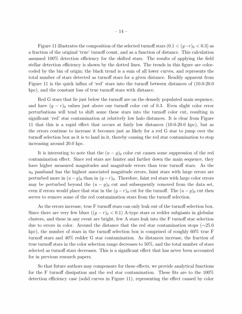
All ten clusters fit in Section 5 were distance shifted to increasingly greater deff values,

using the methods outlined above. At each deff , a new set of fit parameters for the observed

absolute magnitude distribution were evaluated using the methods described above. An

example of the histogram and fit of cluster M3 (NGC 5272), shifted to a deff of 44.0 kpc, is

presented in the lower plot of Figure 6.

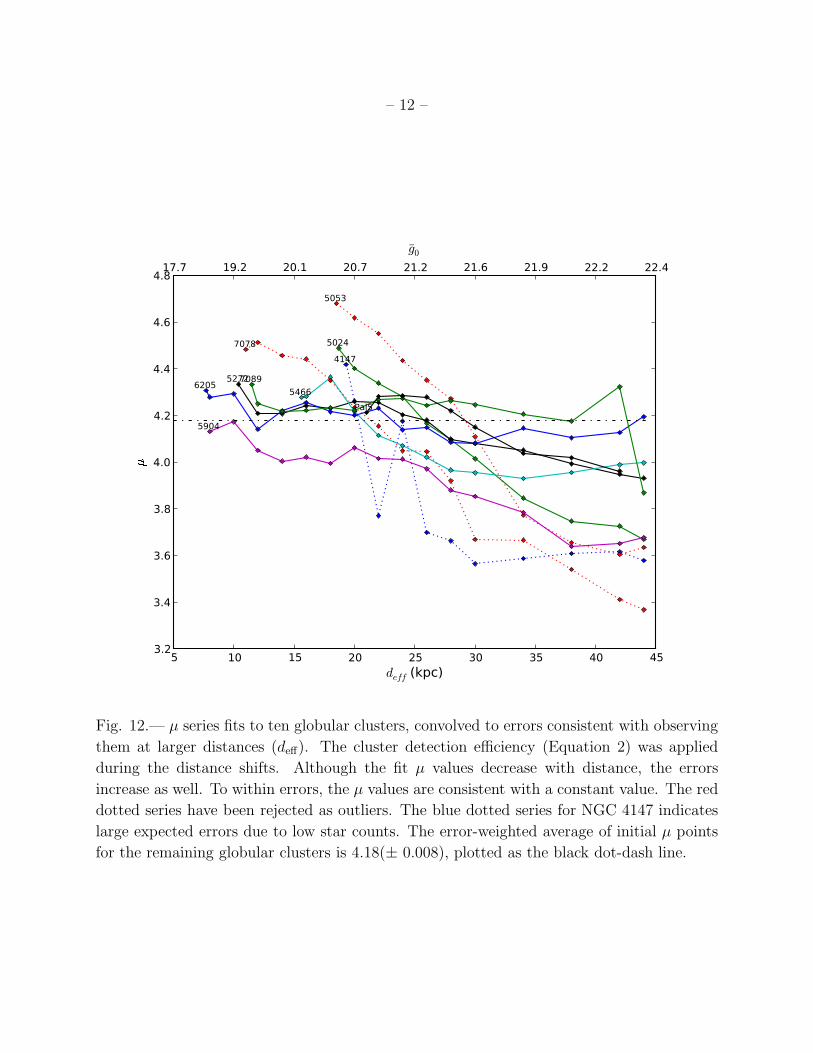
We present the results of the distance shifted fits for the parameters µ, σl, and σr in

Figures 12, 13, and 14 respectively. NGC 5053 and M15 (NGC 7078) are plotted with a red

dotted series to indicate their status as expected outliers, while NGC 4147 is plotted with a

blue dotted series to indicate that it contains few stars and therefore the fits contain large

errors.

6.4. Observed vs. Intrinsic Absolute Magnitude Distribution of F Turnoff

Stars

It is important to note that all of the clusters studied, including suspected outliers, have

similar µ and σl values despite differences in distance, age and metallicity. Although we see

differences in σr, we have shown these are due to photometric errors, and not differences in

the absolute magnitude distribution of turnoff stars in globular clusters. This implies that

the halo cluster population is intrinsically similar throughout. In the next section we will

show that this similarity is related to the Age-Metallicity Relationship.

In Figure 15 we show a series of fits to the turnoff star magnitude distribution for

nearby cluster NGC 6205 at increasing effective distances, including the effects of the cluster

detection efficiency. From this plot, the most obvious effect is the loss of stars with distance;

however, one can see that these losses balance to cause σl to stay constant throughout, and

µ shifts slightly to the left (brighter magnitudes) as the detection efficiency cuts in with

distance.

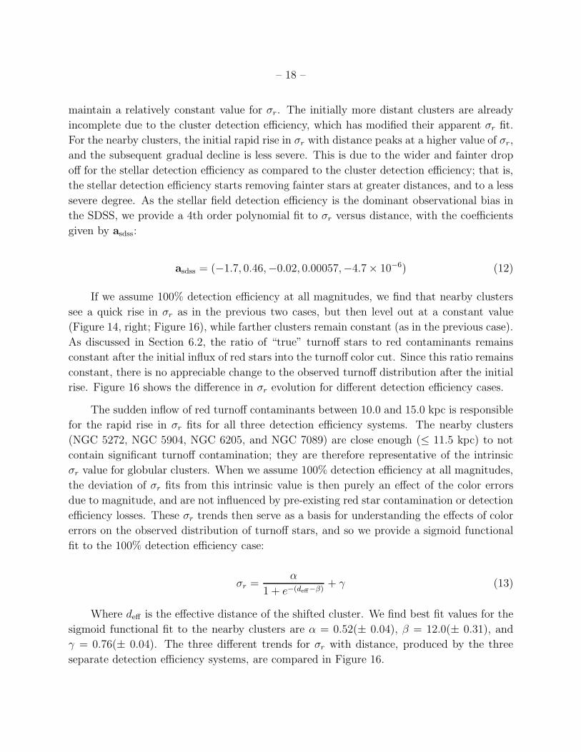
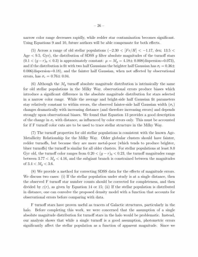
We find that µ is approximately constant with distance, regardless of the applied de-

tection efficiency bias. From the plot of µ vs deff (Figure 12), we see that µ values decrease

slowly with increasing distance; however, µ fit errors increase quickly with distance due to

– 17 –

the loss of turnoff stars. Within the fit errors, µ is adequately described by a constant value.

The error-weighted constant-value fit to µ gives µ = 4.18(± 0.008), with a cluster dispersion

of 0.073. We also provide a linear fit to µ with distance, and find that a slope of zero (which

would imply a constant value) is within the one-σ errors:

µ(deff) = −0.011(±0.02)deff + 4.39(±0.57) (11)

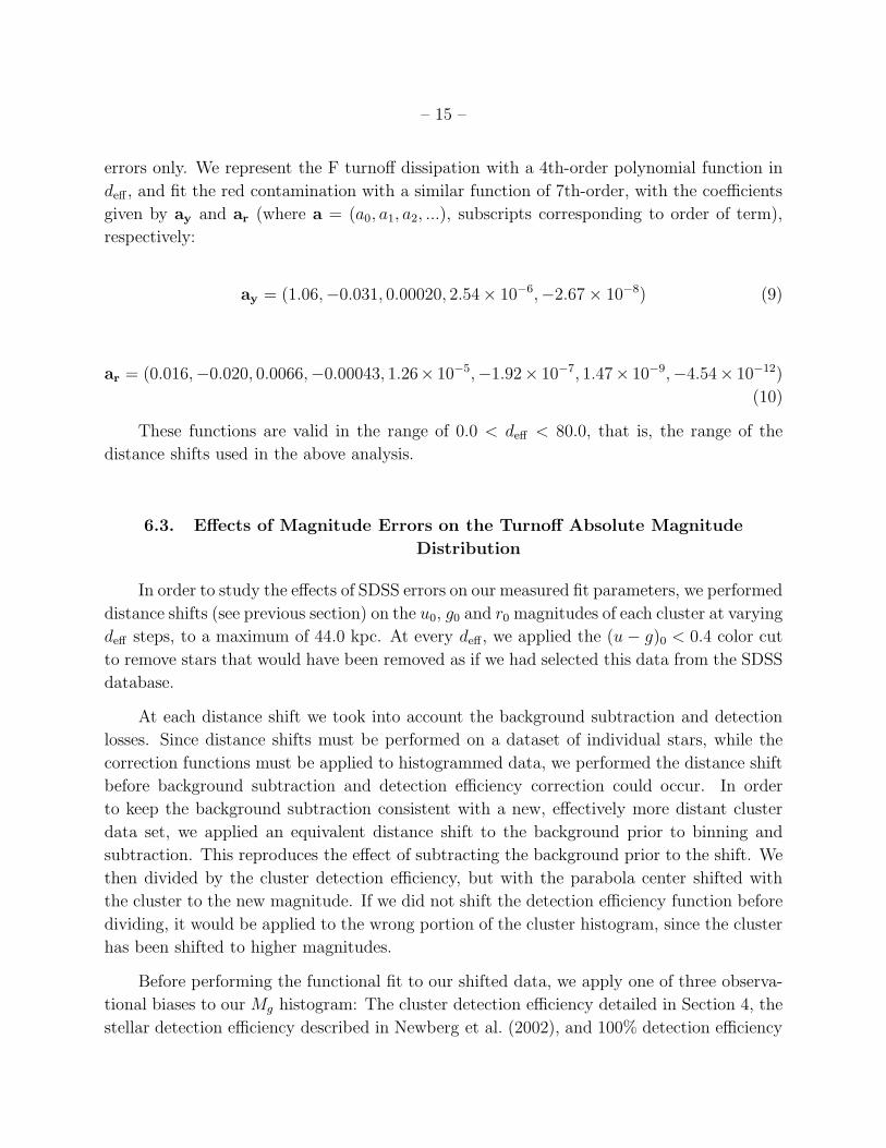
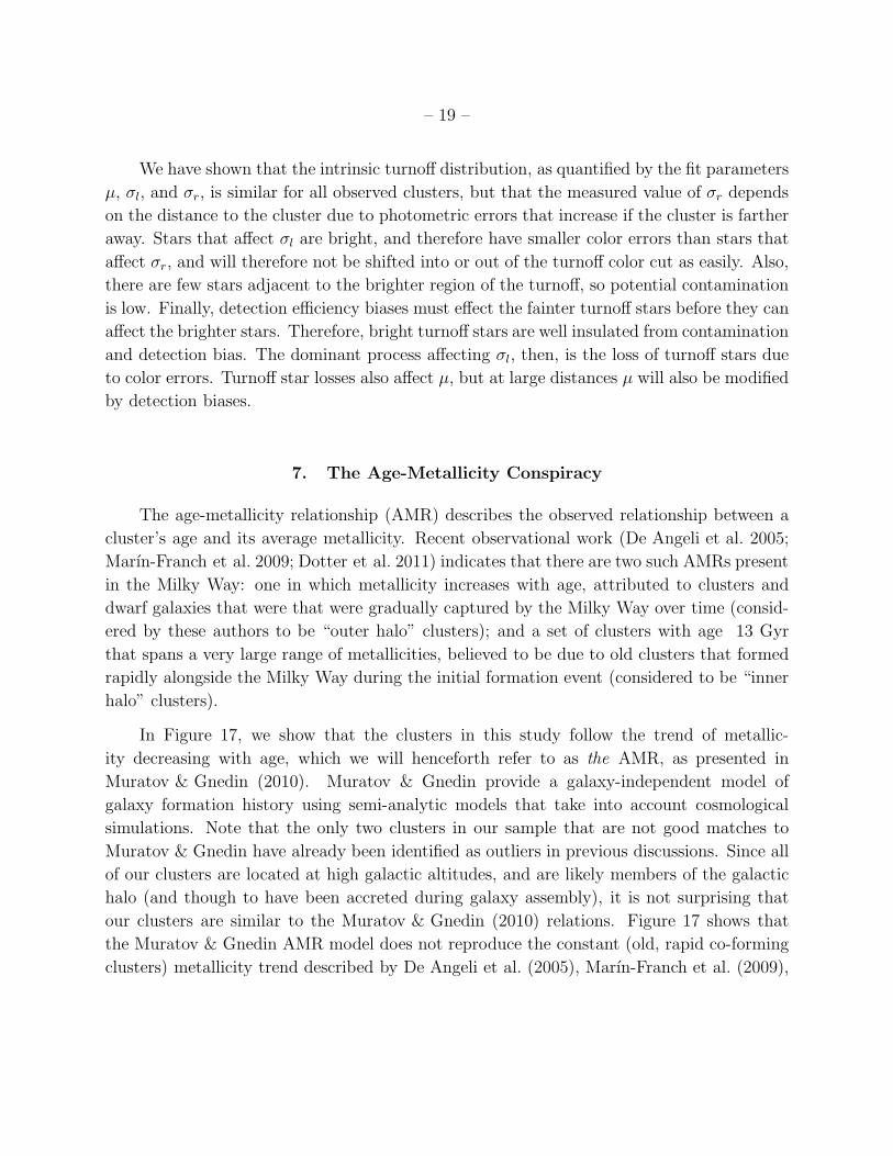
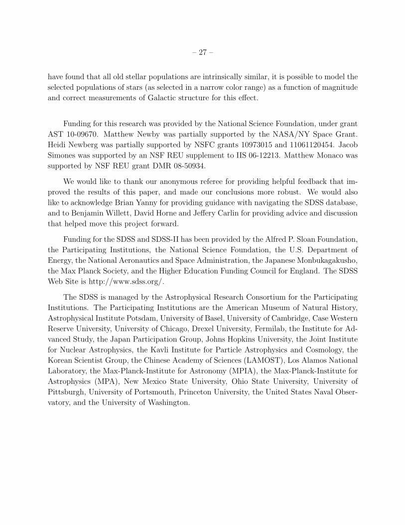
We find that σl values also stay constant with distance, regardless of the applied de-

tection efficiency, to within calculated errors (Figure 13). It is also apparent that the two

expected outlier clusters NGC 5053 and NGC 7078 have σl behaviors that differ from the

other clusters. An error-weighted average to the σl values, excluding the two outliers, give

σl = 0.36(± 0.006), with a cluster dispersion of 0.18.

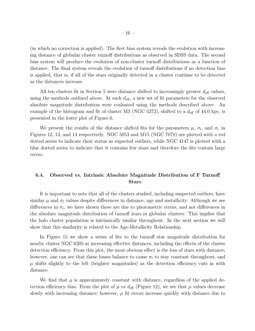
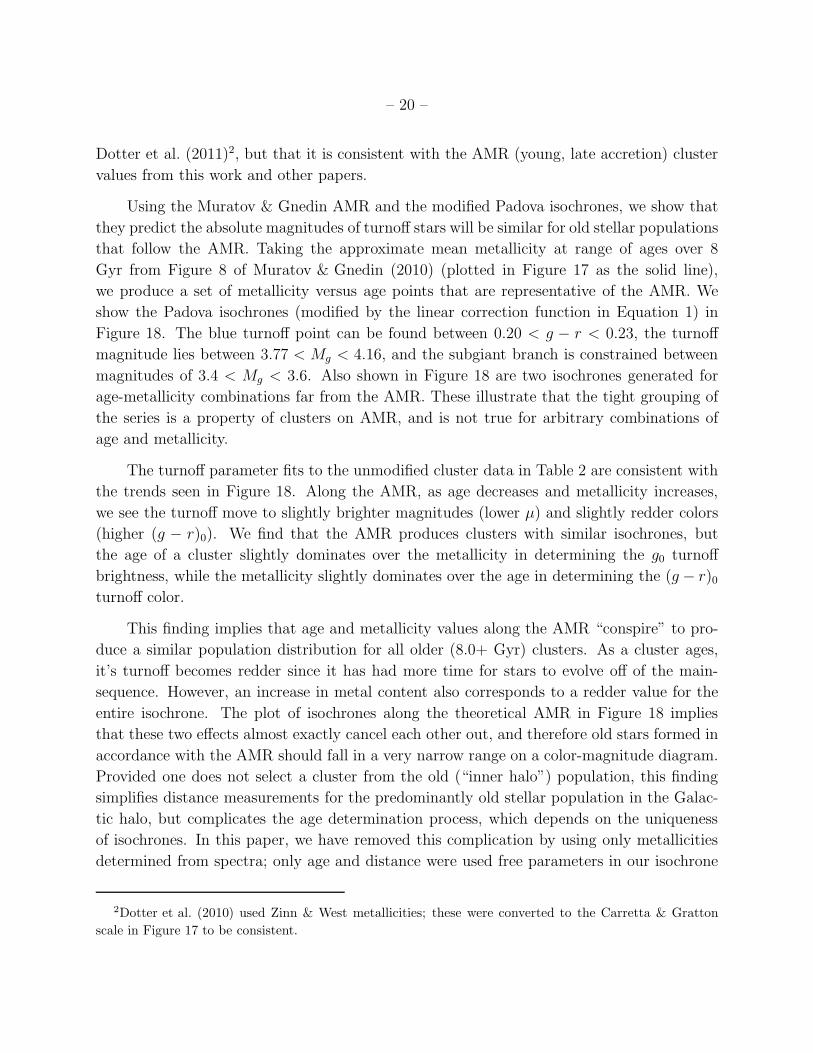
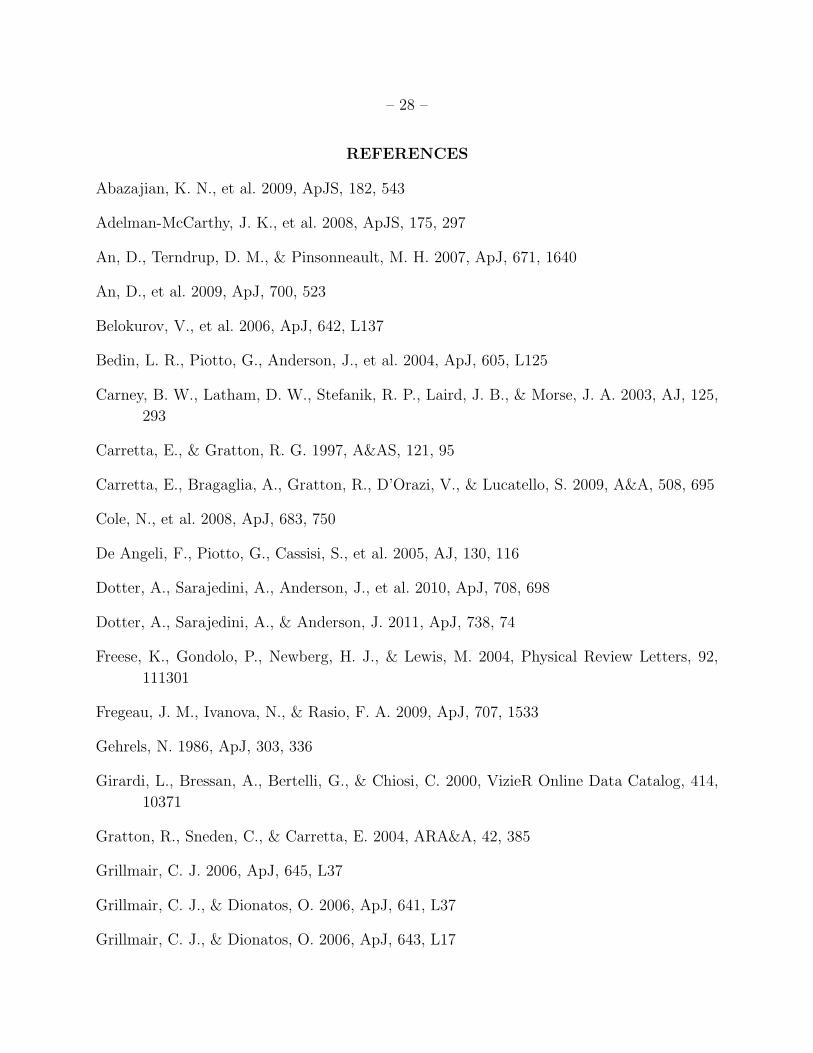
The values of σr do not stay constant with the distance shifts for any of our three

detection efficiency cases. Because of increasing color errors with distance, all but the nearest

turnoff star populations are contaminated by redder main-sequence stars, as described in

Section 6.2. These redder stars enter the turnoff histograms on the fainter (> µ) side, thereby

widening the overall distribution and increasing σr while leaving the other two parameters

unchanged. The nearest clusters (NGC 5272, NGC 5904, NGC 6205, NGC 7089; excluding

the core-collapsed NGC 7078) are near enough that they do not exhibit significant red main-

sequence contamination, and are consistent with each other. We report that these nearby,

uncontaminated clusters are representative of the “true” globular cluster distribution, with

a σr fit of 0.76(± 0.04), equivalent to the fit value of γ, below.

When we apply the SDSS detection efficiency for globular clusters, we find that all of

our clusters show the same behavior as a function of distance (Figure 14, left). The initial,

quick rise in σr with distance is due to a large influx of red main-sequence stars due to

color errors. If the cluster is observed at even farther distances, σr is reduced due to the

cluster detection efficiency removing increasingly larger portions of the faint edge of the

turnoff. This consistent series in σr is evidence that the observed spread in initial cluster

σr values is not a real feature of the clusters, but is instead an observational bias due to

the incompleteness of SDSS crowded-field photometry at faint magnitudes. In Figure 16, we

show a fit to the variation of σr with distance.

In order to see what happens to the distribution of of turnoff stars as a function of dis-

tance for SDSS field stars, we also apply the SDSS stellar detection efficiency when distance

shifting the cluster. We find that the nearby clusters (NGC 5272, NGC 5904, NGC 6205,

NGC 7089, and NGC 5466) follow a similar pattern as in the cluster detection efficiency

system, while the initially more distant clusters (NGC 4147, NGC 5024, NGC 5053, Pal 5)

– 18 –

maintain a relatively constant value for σr. The initially more distant clusters are already

incomplete due to the cluster detection efficiency, which has modified their apparent σr fit.

For the nearby clusters, the initial rapid rise in σr with distance peaks at a higher value of σr,

and the subsequent gradual decline is less severe. This is due to the wider and fainter drop

off for the stellar detection efficiency as compared to the cluster detection efficiency; that is,

the stellar detection efficiency starts removing fainter stars at greater distances, and to a less

severe degree. As the stellar field detection efficiency is the dominant observational bias in

the SDSS, we provide a 4th order polynomial fit to σr versus distance, with the coefficients

given by asdss:

asdss = (−1.7, 0.46,−0.02, 0.00057,−4.7× 10−6) (12)

If we assume 100% detection efficiency at all magnitudes, we find that nearby clusters

see a quick rise in σr as in the previous two cases, but then level out at a constant value

(Figure 14, right; Figure 16), while farther clusters remain constant (as in the previous case).

As discussed in Section 6.2, the ratio of “true” turnoff stars to red contaminants remains

constant after the initial influx of red stars into the turnoff color cut. Since this ratio remains

constant, there is no appreciable change to the observed turnoff distribution after the initial

rise. Figure 16 shows the difference in σr evolution for different detection efficiency cases.

The sudden inflow of red turnoff contaminants between 10.0 and 15.0 kpc is responsible

for the rapid rise in σr fits for all three detection efficiency systems. The nearby clusters

(NGC 5272, NGC 5904, NGC 6205, and NGC 7089) are close enough (≤ 11.5 kpc) to not

contain significant turnoff contamination; they are therefore representative of the intrinsic

σr value for globular clusters. When we assume 100% detection efficiency at all magnitudes,

the deviation of σr fits from this intrinsic value is then purely an effect of the color errors

due to magnitude, and are not influenced by pre-existing red star contamination or detection

efficiency losses. These σr trends then serve as a basis for understanding the effects of color

errors on the observed distribution of turnoff stars, and so we provide a sigmoid functional

fit to the 100% detection efficiency case:

σr =α

1 + e−(deff−β)+ γ (13)

Where deff is the effective distance of the shifted cluster. We find best fit values for the

sigmoid functional fit to the nearby clusters are α = 0.52(± 0.04), β = 12.0(± 0.31), and

γ = 0.76(± 0.04). The three different trends for σr with distance, produced by the three

separate detection efficiency systems, are compared in Figure 16.

– 19 –

We have shown that the intrinsic turnoff distribution, as quantified by the fit parameters

µ, σl, and σr, is similar for all observed clusters, but that the measured value of σr depends

on the distance to the cluster due to photometric errors that increase if the cluster is farther

away. Stars that affect σl are bright, and therefore have smaller color errors than stars that

affect σr, and will therefore not be shifted into or out of the turnoff color cut as easily. Also,

there are few stars adjacent to the brighter region of the turnoff, so potential contamination

is low. Finally, detection efficiency biases must effect the fainter turnoff stars before they can

affect the brighter stars. Therefore, bright turnoff stars are well insulated from contamination

and detection bias. The dominant process affecting σl, then, is the loss of turnoff stars due

to color errors. Turnoff star losses also affect µ, but at large distances µ will also be modified

by detection biases.

7. The Age-Metallicity Conspiracy

The age-metallicity relationship (AMR) describes the observed relationship between a

cluster’s age and its average metallicity. Recent observational work (De Angeli et al. 2005;

Marın-Franch et al. 2009; Dotter et al. 2011) indicates that there are two such AMRs present

in the Milky Way: one in which metallicity increases with age, attributed to clusters and

dwarf galaxies that were that were gradually captured by the Milky Way over time (consid-

ered by these authors to be “outer halo” clusters); and a set of clusters with age 13 Gyr

that spans a very large range of metallicities, believed to be due to old clusters that formed

rapidly alongside the Milky Way during the initial formation event (considered to be “inner

halo” clusters).

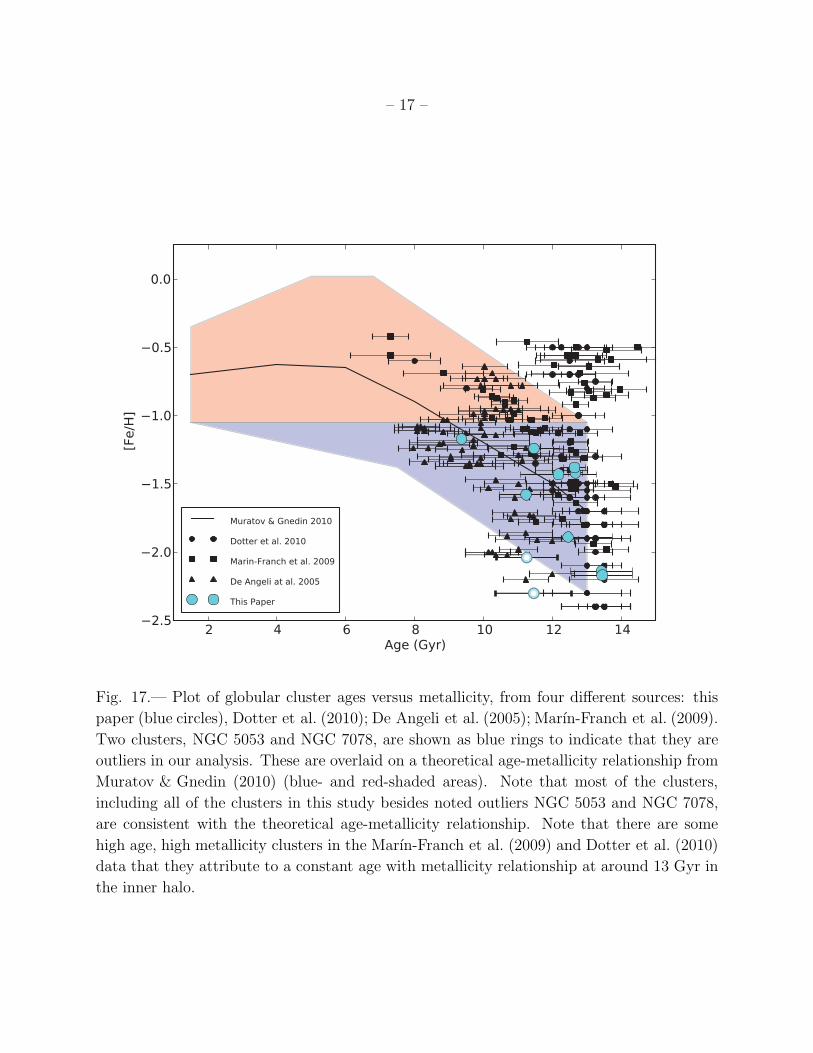
In Figure 17, we show that the clusters in this study follow the trend of metallic-

ity decreasing with age, which we will henceforth refer to as the AMR, as presented in

Muratov & Gnedin (2010). Muratov & Gnedin provide a galaxy-independent model of

galaxy formation history using semi-analytic models that take into account cosmological

simulations. Note that the only two clusters in our sample that are not good matches to

Muratov & Gnedin have already been identified as outliers in previous discussions. Since all

of our clusters are located at high galactic altitudes, and are likely members of the galactic

halo (and though to have been accreted during galaxy assembly), it is not surprising that

our clusters are similar to the Muratov & Gnedin (2010) relations. Figure 17 shows that

the Muratov & Gnedin AMR model does not reproduce the constant (old, rapid co-forming

clusters) metallicity trend described by De Angeli et al. (2005), Marın-Franch et al. (2009),

– 20 –

Dotter et al. (2011)2, but that it is consistent with the AMR (young, late accretion) cluster

values from this work and other papers.

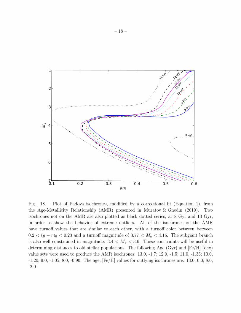
Using the Muratov & Gnedin AMR and the modified Padova isochrones, we show that

they predict the absolute magnitudes of turnoff stars will be similar for old stellar populations

that follow the AMR. Taking the approximate mean metallicity at range of ages over 8

Gyr from Figure 8 of Muratov & Gnedin (2010) (plotted in Figure 17 as the solid line),

we produce a set of metallicity versus age points that are representative of the AMR. We

show the Padova isochrones (modified by the linear correction function in Equation 1) in

Figure 18. The blue turnoff point can be found between 0.20 < g − r < 0.23, the turnoff

magnitude lies between 3.77 < Mg < 4.16, and the subgiant branch is constrained between

magnitudes of 3.4 < Mg < 3.6. Also shown in Figure 18 are two isochrones generated for

age-metallicity combinations far from the AMR. These illustrate that the tight grouping of

the series is a property of clusters on AMR, and is not true for arbitrary combinations of

age and metallicity.

The turnoff parameter fits to the unmodified cluster data in Table 2 are consistent with

the trends seen in Figure 18. Along the AMR, as age decreases and metallicity increases,

we see the turnoff move to slightly brighter magnitudes (lower µ) and slightly redder colors

(higher (g − r)0). We find that the AMR produces clusters with similar isochrones, but

the age of a cluster slightly dominates over the metallicity in determining the g0 turnoff

brightness, while the metallicity slightly dominates over the age in determining the (g − r)0turnoff color.

This finding implies that age and metallicity values along the AMR “conspire” to pro-

duce a similar population distribution for all older (8.0+ Gyr) clusters. As a cluster ages,

it’s turnoff becomes redder since it has had more time for stars to evolve off of the main-

sequence. However, an increase in metal content also corresponds to a redder value for the

entire isochrone. The plot of isochrones along the theoretical AMR in Figure 18 implies

that these two effects almost exactly cancel each other out, and therefore old stars formed in

accordance with the AMR should fall in a very narrow range on a color-magnitude diagram.

Provided one does not select a cluster from the old (“inner halo”) population, this finding

simplifies distance measurements for the predominantly old stellar population in the Galac-

tic halo, but complicates the age determination process, which depends on the uniqueness

of isochrones. In this paper, we have removed this complication by using only metallicities

determined from spectra; only age and distance were used free parameters in our isochrone

2Dotter et al. (2010) used Zinn & West metallicities; these were converted to the Carretta & Gratton

scale in Figure 17 to be consistent.

– 21 –

fits.

8. Application to SDSS Data

In this paper we have described the SDSS photometric errors and the resulting effects

on observed F turnoff distributions (0.1 < (g − r)0 < 0.3). In this section we will provide

a method by which SDSS observations can be corrected for these effects. If we sum the

polynomials whose coefficients are presented in Equation 9 and Equation 10, we will produce

a function that describes the ratio of stars selected as turnoff stars to the number of actual

turnoff stars present, as a function of distance

ε(r) =n(r)

n0

=7

∑

i=0

(ayi(r) + ari(r))ri (14)

where r is the distance to the stellar population. Note that this equation assumes a (u− g)0cut to the data; if this cut is not performed, then additional stars will be included in the

data set and this equation will not be valid. Instead, the following equation should be used:

ε(r) =n(r)

n0=

7∑

i=0

(byi + bri)ri (15)

byi = (1.02,−0.011,−0.00043, 9.7× 10−6,−5.5× 10−8) (16)

bri = (0.034,−0.039, 0.011,−0.00071, 2.0×10−5,−2.9×10−7, 2.1×10−9,−6.4×10−12) (17)

For simple density searches that ignore F turnoff distribution statistics, dividing the

observed density at a given distance by ε(r) is sufficient to correct data for missing turnoff

stars due to magnitude errors. For example, if one measures the number of background-

corrected F turnoff stars in a section of the Sagittarius tidal debris stream at a distance of

45 kpc, that number should be corrected for completeness (if necessary) and then divided

by ε(45 kpc) in order to produce the true number of turnoff stars in that field.

For statistical models that seek to quantify F turnoff star densities in the Galactic halo,

a more complicated correction method is required. In Cole et al. (2008), the authors sought

to map the Sagittarius tidal debris stream by performing a maximum likelihood fit of a

statistical model to F turnoff stars taken from the SDSS data. They include the effect of

the turnoff star distribution by convolving a normalized Gaussian, representing the turnoff

star distribution (mean=4.2, σ =0.6), with a halo density model in which all of the turnoff

stars have the same absolute magnitude (Mg =4.2). A correction for the stellar detection

efficiency is subsequently applied.

– 22 –

We seek to modify the methods of Cole et al. (2008) by incorporating our results into

their analysis. In order to include the turnoff star distribution presented in this paper, the

turnoff distribution in the density convolution must be changed from a symmetrical Gaussian

(N in that paper) to the double-sided Gaussian, G(g0;µ, σl, σr, A) presented in Equations

4 and 5, with a σr given by Equation 13. Note that we use the 100% detection efficiency

function for σr, as the stellar detection efficiency is applied subsequent to the turnoff con-

volution. The normalization for G must be adjusted for the fact that turnoff stars are lost

(and a smaller number of G stars are gained) at farther distances. To account for the turnoff

dissipation and contamination, the distribution G should be multiplied by ε(g). Putting

this together, we produce a convolution recipe which provides a statistical description of the

Galactic halo turnoff population, including the effects of the double-sided Gaussian magni-

tude distribution and the effects of dissipation and contamination with distance. Equation

14 in Cole et al. (2008) is replaced by:

ρ(g0,Ω) =

∫

∞

−∞

dg ε (r(g, µ)) ρµ(g,Ω)G (g0 − g;µ, σl, σr(r(g, µ))) (18)

where ρ represents a density function of magnitude and solid angle (Ω), ρµ(g,Ω) is the model

turnoff density function, in which all stars are assumed to be at absolute magnitude µ (4.18),

ε is Equation 14, and G is Equation 4 with Equation 13 as the input for σr. ε and σr are

both functions of r, which is equal to the distance (r = 10g0−µ−10

5 ).

Using these examples as templates, and with the information contained in the rest of

this paper, future authors should be able to adapt our results to correct their models for

observational biases due to turnoff magnitude errors. Future authors must be prepared to

compensate for three mechanisms that cause turnoff star incompleteness and misidentifi-

cation: The combined effects of dissipation and contamination, given by Equation 14; the

SDSS stellar field detection efficiency, given in Newberg et al. (2002); and the intrinsic mag-

nitude distribution of turnoff stars within the Galactic halo, as discussed in Section 6 and

this section.

9. Discussion

9.1. Effects of Abundance Variation

Recent observational studies (Pritzl et al. 2005; Roederer 2009) (see also reviews by

Gratton et al. 2004 and McWilliam 1997) indicate that both outer halo globular clusters

and halo field stars have similar alpha-element abundances, consistent with an average [α/Fe]

value of 0.3. This is strong evidence that halo clusters and field stars share a similar

– 23 –

formation history, and it is therefore reasonable to assume that they share similar population

distributions and photometric properties. These studies also find that halo clusters and stars

are chemically distinct from dwarf spheroidal galaxies (Venn et al. 2004) and the galactic

disk, including stars in the thick disk. While thick disk stars can be removed from SDSS

photometric data through magnitude and color cuts, dwarf spheroidal stars may be present

in the halo due to tidal disruptions of infalling dwarfs. If significantly different [α/Fe] affect

the photometric properties of a population, disrupted dwarf spheroidal galaxies may pose a

problem for our technique. However, the success of Cole et al. (2008) in mapping segments

the Sagittarius tidal stream with a similar technique is evidence that that dwarf galaxy

turnoff star distributions are not significantly different from those in the globular clusters in

this study.

The set of globular clusters in this study are limited to old, metal poor galactic halo

clusters, with a maximum metallicity of [Fe/H]= −1.17 and a minimum age of 9.5 Gyr

(NGC 5904). Figure 18 indicates that our results can be extended to an age of at least 8.0

Gyr. From Figure 17 we see that our entire cluster sample falls within the “metal poor”

(blue) region of the Muratov & Gnedin AMR. While our results are well-suited to our goal

of describing the old, metal-poor halo of the Milky Way, we have not tested how far it can be

extrapolated to stellar populations less than 8 Gyr old or more metal-rich than NGC 5904.

The results of this paper may not apply to globular clusters with age and metallicity

values that fall far from the Milky Way AMR. Our results may not apply to stellar pop-

ulations in other galaxies, which have differing assembly histories and potentially different

age-metallicity relationships. Indeed, the two unusual globular clusters that fall outside of

the AMR in Figure 17, are the two clusters that differ from each other in turnoff magnitude

(Figure 11).

Recently, multiple star formation periods have been detected in globular clusters (Milone et al.

2008; Bedin et al. 2004; Piotto et al. 2007) (see review by Piotto (2009)). We do not expect

multiple stellar populations to significantly affect our results, however, certain clusters with

several separate, strongly visible main sequences (such as M54) may be poorly described by

our results.

Above average helium enrichment has been proposed as a potential mechanism for

producing separations in multiple-population cluster main sequences (Piotto et al. 2007;

Milone et al. 2008; Pasquini et al. 2011). Due to the difficulty of measuring He enrichment,

the complete effects of enrichment are still under investigation (see preliminary work by Val-

carce at al. 2011, and Milone & Merlo 2008), but it is thought that it will result in slightly

brighter subgiant branches and slightly bluer turnoffs, since He is less opaque than H. If the

He abundances have only a small effects on photometry, they will not significantly influence

– 24 –

our results.

9.2. Potential Influence of Binaries

Binary stars present in globular clusters have the potential to bias color-magnitude

diagrams towards brighter, redder values, as detailed in (Romani & Weinberg 1991). The

maximum increase in brightness occurs when the binaries are of the same spectroscopic type,

2.5 ∗ log(2) ≈ 0.75 magnitude, and the maximum increase in “reddening,” which serves to

widen the color-magnitude diagram towards redder values, can shift colors by as much as

0.05 magnitudes. Depending on the binary fraction (f), this effect could introduce significant

biases when determining population statistics of a globular cluster.

The binary fraction in old globular clusters is generally low, around a few percent to

20%, with the binaries being concentrated near the cluster’s center (Sollima et al. 2007;

Fregeau et al. 2009), although a select few globular clusters have f values as high as 50%.

The primary result of Monte-Carlo simulations in Fregeau et al. (2009) is that “True” bi-

nary fractions are likely to remain constant with age, implying that we can also rule out

age-dependent biases on cluster f values. Carney et al. (2003) studied the binary fractions

of metal-poor ([Fe/H] ≤ -1.4) field red giants and dwarfs, and found them to be 16%±4%

and 17%±2%, respectively, which is on the high end of a typical globular cluster f . Glob-

ular clusters also feature apparent binaries, which are stars that appear as binaries due to

crowding, which become more likely as one looks closer to the densely-packed cluster cores.

Due to the poor performance of the SDSS photometric pipeline in crowded fields, the

centers of globular clusters are absent from the database, and therefore are not present

in this study. If binaries are concentrated towards a cluster’s center as in Sollima et al.

(2007); Fregeau et al. (2009), then this “disadvantage” serves to reduce the potential bias

that binaries would have on our results, and will also greatly reduce the number of apparent

binaries in our data.

The effect of a binary population is to shift the observed turnoff to brighter magnitudes,

and to increase the spread in magnitudes. We ran an experiment in which we generated

1000 stars with magnitudes given by a double-sided Gaussian with µ = 4.2, σl = 0.36

and σr = 0.76, and with colors given by a standard Gaussian with a µ(g−r) = 0.25 and

σ(g−r) = 0.025. We then randomly selected 20% of these stars and shifted them brighter by

0.75 magnitudes and redder by 0.05 magnitudes, which should produce a larger effect than

we would expect from the binary fraction of a typical halo globular cluster. We found that

the 20% binary population had a new magnitude fit of µ = 4.22, σl = 0.55 and σr = 0.75,

– 25 –

and a color fit of µ(g−r) = 0.26 and σ(g−r) = 0.03. The variations in these values are all within

the errors of the fitting process, except for σl in the magnitude fit. It is possible that the

quantity σl is sensitive to to the binary fractions typically found in halo globular clusters, in

the sense that a large binary fraction could produce a larger σl. The spread in σl values in

our accepted sample is low (Figure 13), so we do not expect that the effect of binaries has

changed our results significantly. A future study could potentially use a more rigorous study

of binary fraction effects to see if the binary fraction is directly correlated to the value of σl.

We expect the results of this paper to provide a close approximation of the F turnoff

absolute magnitude distribution in old, metal poor stars in the Milky Way halo, as observed

by SDSS. These results should also be a reasonable approximation of small dwarf galaxy

turnoff distributions. We do not expect the results to be applicable to young, relatively

metal-rich stellar populations, to populations that are outliers on the AMR, or to populations

that are outside of the Milky Way.

10. Conclusions

In this paper we analyze SDSS data for 11 globular clusters in the halo of the Milky Way,

and draw conclusions about the intrinsic and observed absolute magnitude distributions of

F turnoff stars. The major conclusions are:

(1) The completeness as a function of magnitude in SDSS stellar data is different in

crowded fields such as globular clusters than in typical star fields. This incompleteness begins

at brighter magnitudes and falls off more steeply than the standard stellar detection efficiency

reported in Newberg et al. (2002). We calculated an approximate parabolic function to

describe this crowded-field incompleteness, as presented in Equation 3.

(2) We calculated a linear correction to the turnoff region of Padova isochrones in SDSS

colors in order to place them on an age scale that is consistent with determinations from other

authors. The findings of An et al. (2009) were used as a basis for this function. Without

this correction, Padova ugriz isochrones imply ages greater than the current measured age

of the universe. We find the appropriate correction to be ∆(g − r) = −0.015 ∗Mg + 0.089,

valid for 3.5 < Mg < 8.0.

(3) Using our Padova isochrone correction, a uniformly determined set of metallicity

([Fe/H ]), distance (kpc), and age (Gyr) measurements were calculated for 11 globular clus-

ters observed in the Sloan Digital Sky Survey. These results are collected in Table 1.

(4) As color errors increase with distance, the fraction of F turnoff stars detected in a

– 26 –

narrow color range decreases rapidly, while redder star contamination becomes significant.

Using Equations 9 and 10, future authors will be able compensate for both effects.

(5) Across a range of old stellar populations (−2.30 < [Fe/H ] < −1.17, dex; 13.5 <

Age < 9.5, Gyr), the distribution of SDSS g filter absolute magnitudes of the turnoff stars

(0.1 < (g− r)0 < 0.3) is approximately constant: µ = Mg = 4.18± 0.008(dispersion=0.073),

and if the distribution is fit with two half Gaussians the brighter half Gaussian has σl = 0.36±0.006(dispersion=0.18), and the fainter half Gaussian, when not affected by observational

errors, has σr = 0.76± 0.04.

(6) Although the Mg turnoff absolute magnitude distribution is intrinsically the same

for old stellar populations in the Milky Way, observational errors produce biases which

introduce a significant difference in the absolute magnitude distribution for stars selected

in a narrow color range. While the average and bright-side half Gaussian fit parameters

stay relatively constant to within errors, the observed fainter-side half Gaussian width (σr)

changes dramatically with increasing distance (and therefore increasing errors) and depends

strongly upon observational biases. We found that Equation 13 provides a good description

of the change in σr with distance, as influenced by color errors only. This must be accounted

for if F turnoff color cuts are to be used to trace stellar structure in the Milky Way.

(7) The turnoff properties for old stellar populations is consistent with the known Age-

Metallicity Relationship for the Milky Way. Older globular clusters should have fainter,

redder turnoffs, but because they are more metal-poor (which tends to produce brighter,

bluer turnoffs) the turnoff is similar for all older clusters. For stellar populations at least 8.0

Gyr old, the turnoff color ranges from 0.20 < (g − r)0 < 0.23, the turnoff magnitudes range

between 3.77 < Mg < 4.16, and the subgiant branch is constrained between the magnitudes

of 3.4 < Mg < 3.6.

(8) We provide a method for correcting SDSS data for the effects of magnitude errors.

We discuss two cases: (i) If the stellar population under study is at a single distance, then

the observed F turnoff star number counts should be corrected for completeness, and then

divided by ε(r), as given by Equation 14 or 15; (ii) If the stellar population is distributed

in distance, one can convolve the proposed density model with a function that accounts for

observational errors before comparing with data.

F turnoff stars have proven useful as tracers of Galactic structures, particularly in the

halo. Before completing this work, we were concerned that the assumption of a single

absolute magnitude distribution for turnoff stars in the halo would be problematic. Instead,

our analysis shows that while a single turnoff is a good assumption, photometric errors

significantly affect the stellar population as a function of apparent magnitude. Since we

– 27 –

have found that all old stellar populations are intrinsically similar, it is possible to model the

selected populations of stars (as selected in a narrow color range) as a function of magnitude

and correct measurements of Galactic structure for this effect.

Funding for this research was provided by the National Science Foundation, under grant

AST 10-09670. Matthew Newby was partially supported by the NASA/NY Space Grant.

Heidi Newberg was partially supported by NSFC grants 10973015 and 11061120454. Jacob

Simones was supported by an NSF REU supplement to IIS 06-12213. Matthew Monaco was

supported by NSF REU grant DMR 08-50934.

We would like to thank our anonymous referee for providing helpful feedback that im-

proved the results of this paper, and made our conclusions more robust. We would also

like to acknowledge Brian Yanny for providing guidance with navigating the SDSS database,

and to Benjamin Willett, David Horne and Jeffery Carlin for providing advice and discussion

that helped move this project forward.

Funding for the SDSS and SDSS-II has been provided by the Alfred P. Sloan Foundation,

the Participating Institutions, the National Science Foundation, the U.S. Department of

Energy, the National Aeronautics and Space Administration, the Japanese Monbukagakusho,

the Max Planck Society, and the Higher Education Funding Council for England. The SDSS

Web Site is http://www.sdss.org/.

The SDSS is managed by the Astrophysical Research Consortium for the Participating

Institutions. The Participating Institutions are the American Museum of Natural History,

Astrophysical Institute Potsdam, University of Basel, University of Cambridge, Case Western

Reserve University, University of Chicago, Drexel University, Fermilab, the Institute for Ad-

vanced Study, the Japan Participation Group, Johns Hopkins University, the Joint Institute

for Nuclear Astrophysics, the Kavli Institute for Particle Astrophysics and Cosmology, the

Korean Scientist Group, the Chinese Academy of Sciences (LAMOST), Los Alamos National

Laboratory, the Max-Planck-Institute for Astronomy (MPIA), the Max-Planck-Institute for

Astrophysics (MPA), New Mexico State University, Ohio State University, University of

Pittsburgh, University of Portsmouth, Princeton University, the United States Naval Obser-

vatory, and the University of Washington.

– 28 –

REFERENCES

Abazajian, K. N., et al. 2009, ApJS, 182, 543

Adelman-McCarthy, J. K., et al. 2008, ApJS, 175, 297

An, D., Terndrup, D. M., & Pinsonneault, M. H. 2007, ApJ, 671, 1640

An, D., et al. 2009, ApJ, 700, 523

Belokurov, V., et al. 2006, ApJ, 642, L137

Bedin, L. R., Piotto, G., Anderson, J., et al. 2004, ApJ, 605, L125

Carney, B. W., Latham, D. W., Stefanik, R. P., Laird, J. B., & Morse, J. A. 2003, AJ, 125,

293

Carretta, E., & Gratton, R. G. 1997, A&AS, 121, 95

Carretta, E., Bragaglia, A., Gratton, R., D’Orazi, V., & Lucatello, S. 2009, A&A, 508, 695

Cole, N., et al. 2008, ApJ, 683, 750

De Angeli, F., Piotto, G., Cassisi, S., et al. 2005, AJ, 130, 116

Dotter, A., Sarajedini, A., Anderson, J., et al. 2010, ApJ, 708, 698

Dotter, A., Sarajedini, A., & Anderson, J. 2011, ApJ, 738, 74

Freese, K., Gondolo, P., Newberg, H. J., & Lewis, M. 2004, Physical Review Letters, 92,

111301

Fregeau, J. M., Ivanova, N., & Rasio, F. A. 2009, ApJ, 707, 1533

Gehrels, N. 1986, ApJ, 303, 336

Girardi, L., Bressan, A., Bertelli, G., & Chiosi, C. 2000, VizieR Online Data Catalog, 414,

10371

Gratton, R., Sneden, C., & Carretta, E. 2004, ARA&A, 42, 385

Grillmair, C. J. 2006, ApJ, 645, L37

Grillmair, C. J., & Dionatos, O. 2006, ApJ, 641, L37

Grillmair, C. J., & Dionatos, O. 2006, ApJ, 643, L17

– 29 –

Grillmair, C. J., & Johnson, R. 2006, ApJ, 639, L17

Grillmair, C. J. 2009, ApJ, 693, 1118

Gunn, J. E., et al. 1998, AJ, 116, 3040

Harris, W. E. et al. 1997, AJ, 114, 1030

Haurberg, N. C., Lubell, G. M. G., Cohn, H. N., Lugger, P. M., Anderson, J., Cool, A. M.,

& Serenelli, A. M. 2010, ApJ, 722, 158

Juric, M., et al. 2008, ApJ, 673, 864

Lupton, R. H., Gunn, J. E., & Szalay, A. S. 1999, AJ, 118, 1406

Marigo, P., Girardi, L., Bressan, A., Groenewegen, M. A. T., Silva, L., & Granato, G. L.

2008, A&A, 482, 883

Marın-Franch, A., Aparicio, A., Piotto, G., et al. 2009, ApJ, 694, 1498

McWilliam, A. 1997, ARA&A, 35, 503

Milone, A. P., Bedin, L. R., Piotto, G., et al. 2008, ApJ, 673, 241

Milone, L. A., & Merlo, D. C. 2008, Boletin de la Asociacion Argentina de Astronomia La

Plata Argentina, 51, 121

Muratov, A. L., & Gnedin, O. Y. 2010, ApJ, 718, 1266

Newberg, H. J., et al. 2002, ApJ, 569, 245

Newberg, H. J., & Yanny, B. 2006, Journal of Physics Conference Series, 47, 195

Newberg, H. J., Yanny, B., Cole, N., Beers, T. C., Re Fiorentin, P., Schneider, D. P., &

Wilhelm, R. 2007, ApJ, 668, 221

Newberg, H. J., Willett, B. A., Yanny, B., & Xu, Y. 2010, ApJ, 711, 32

Pasquini, L., Mauas, P., Kaufl, H. U., & Cacciari, C. 2011, A&A, 531, A35

Pinsonneault, M. H., Terndrup, D. M., Hanson, R. B., & Stauffer, J. R. 2003, ApJ, 598, 588

Pinsonneault, M. H., Terndrup, D. M., Hanson, R. B., & Stauffer, J. R. 2004, ApJ, 600, 946

Piotto, G., Bedin, L. R., Anderson, J., et al. 2007, ApJ, 661, L53

– 30 –

Piotto, G. 2009, arXiv:0902.1422

Pritzl, B. J., Venn, K. A., & Irwin, M. 2005, AJ, 130, 2140

Rockosi, C. M., et al. 2002, AJ, 124, 349

Roederer, I. U. 2009, AJ, 137, 272

Romani, R. W., & Weinberg, M. D. 1991, ApJ, 372, 487

Sollima, A., Beccari, G., Ferraro, F. R., Fusi Pecci, F., & Sarajedini, A. 2007, MNRAS, 380,

781

Valcarce, A. A. R., Catelan, M., & Sweigart, A. V. 2011, Revista Mexicana de Astronomia

y Astrofisica Conference Series, 40, 257

Venn, K. A., Irwin, M., Shetrone, M. D., et al. 2004, AJ, 128, 1177

Willett, B. A., Newberg, H. J., Zhang, H., Yanny, B., & Beers, T. C. 2009, ApJ, 697, 207

Yanny, B., et al. 2000, ApJ, 540, 825

Yanny, B., et al. 2003, ApJ, 588, 824

Yanny, B., et al. 2009, ApJ, 700, 1282

Zinn, R., & West, M. J. 1984, ApJS, 55, 45

This preprint was prepared with the AAS LATEX macros v5.2.

– 31 –

Table 1. Results of modified Padova isochrone fits

NGC Messier l b Metallicity Fit Distance Fit Age ± Error rclus rcut # Stars in

Number Number CG97 [Fe/H] (kpc) (Gyr) Cluster1

NGC 4147 · · · 252.85 77.19 -1.58 19.3 11.2 ± 0.8 0.07 0.08 583

NGC 5024 M53 332.96 79.76 -1.89 18.7 12.5 ± 1.3 0.25 0.30 5871

NGC 5053 · · · 335.70 78.95 -2.302 18.5 11.5 ± 1.1 0.14 0.17 2280

NGC 5272 M3 42.22 78.71 -1.43 10.4 12.2 ± 1.1 0.30 0.40 4395

NGC 5466 · · · 42.15 73.59 -2.14 15.6 13.4 ± 0.9 0.18 0.25 2029

NGC 5904 M5 3.86 46.80 -1.17 8.0 9.4 ± 0.1 0.21 0.28 3488

NGC 6205 M13 59.01 40.91 -1.42 7.7 12.7 ± 0.2 0.24 0.33 2192

NGC 6341 M92 68.34 34.86 -2.17 8.7 13.4 ± 0.9 0.135 0.20 334

NGC 7078 M15 65.01 -27.31 -2.04 11.0 11.2 ± 0.9 0.19 0.25 2939

NGC 7089 M2 53.37 -35.77 -1.38 11.5 12.6 ± 0.3 0.14 0.18 1451

Pal 5 · · · 0.85 45.86 -1.24 21.0 11.5 ± 0.7 0.087 0.12 1478

1The number of stars represents the number of stars contained within rclus, and therefore the number of stars used to build

the cluster dataset.

2The Zinn & West metallicity of NGC 5053 (-2.58) was outside the effective conversion range of the CG97 metallicity scale,

as well as the range of available Padova isochrones, so the Carretta et al. (2009) value of -2.30 was used instead

–32

–

Table 2. Fit values and errors to cluster data

NGC ID Messier ID FWHM µ µ error σl σl error σr σr error A A error (g − r)TO (g − r)TO error

NGC 4147 · · · 1.70 4.42 0.33 0.50 0.22 0.98 0.29 26.6 3.34 0.223 0.022

NGC 5024 M53 1.69 4.49 0.02 0.50 0.02 0.94 0.03 271.8 3.53 0.240 0.010

NGC 5053 · · · 1.92 4.68 0.07 0.70 0.06 0.93 0.07 105.3 3.00 0.219 0.011

NGC 5272 M3 1.37 4.33 0.05 0.39 0.04 0.77 0.04 154.9 3.71 0.251 0.009

NGC 5466 · · · 1.92 4.28 0.15 0.40 0.09 1.22 0.13 78.7 3.17 0.217 0.010

NGC 5904 M5 1.23 4.13 0.28 0.32 0.18 0.72 0.19 134.7 4.03 0.253 0.006

NGC 6205 M13 1.30 4.31 0.13 0.31 0.09 0.79 0.10 69.0 4.07 0.251 0.008

NGC 7078 M15 2.18 4.48 0.11 0.62 0.08 1.23 0.11 88.7 3.26 0.219 0.011

NGC 7089 M2 1.27 4.33 0.10 0.31 0.09 0.76 0.12 46.0 4.07 0.258 0.010

Pal 5 · · · 1.56 4.21 0.14 0.33 0.10 0.99 0.12 54.1 3.55 0.284 0.011

Average · · · 1.613 4.367 0.138 0.440 0.097 0.930 0.122 103.0 3.573 0.242 0.011

Standard Deviation 0.309 0.149 0.092 0.129 0.059 0.173 0.073 67.5 0.367 0.021 0.003

– 1 –

198.7 198.8 198.9 199.0 199.1 199.2 199.3 199.4 199.5RA

17.3

17.4

17.5

17.6

17.7

17.8

17.9

18.0

18.1

Dec

Fig. 1.— Positions of stars near globular cluster NGC 5053 in right ascension and declination.

Stars assigned to the cluster are marked with circles, while stars assigned to the background

are marked with crosses. At the edge of the cluster, it is difficult to separate cluster stars

from background stars, so a ring of stars at the interface has been removed, leaving a gap on

the plot. The empty area in the center of the plot is where the SDSS photometric pipeline

was unable to separate individual stars, and the data was not included in the database. This

area has been subtracted from the cluster area determinations in Section 2.

– 2 –

0.2 0.0 0.2 0.4 0.6g0r0

2

3

4

5

6

7

Mg

Line Fit

Girardi isocrone

Subtracted data

Fiducial sequence

Fig. 2.— Diagram of Padova Isochrone fit for cluster NGC 6205. The values of the raw

Padova Isochrone, (blue circles) generated from the An et al. (2009) results, were subtracted

from the values of the cluster fiducial fit (black diamonds) to produce the offset (crosses). A

red vertical line indicates zero offset, or a perfect match between isochrone and fiducial fit. A

linear fit (dotted line) to the offset was made for values below the giant branch (Mg > 3.5):

∆(g− r)0 = −0.015 ∗Mg+0.089. This correction causes Padova isochrones to fit the turnoff

on color-magnitude diagrams. We then used this fit to match isochrones to our cluster

sample (see text).

– 3 –

2

3

4

5

6

7

Mg

NGC 4147 NGC 5024 NGC 5053 NGC 5272

2

3

4

5

6

7

Mg

NGC 5466 NGC 5904 NGC 6205

0.1 0.2 0.3 0.4 0.5g0r0

NGC 6341

0.1 0.2 0.3 0.4 0.5g0r0

2

3

4

5

6

7

Mg

NGC 7078

0.1 0.2 0.3 0.4 0.5g0r0

NGC 7089

0.1 0.2 0.3 0.4 0.5g0r0

Pal 5

Fig. 3.— Color-magnitude diagrams, fiducial fits, and isochrone fits for all eleven globular

clusters used in this study. Black dots represent the positions of individual stars in Mg,

(g − r)0; red circles represent 2-σ rejection fiducial fits to the stars in Mg strips; and blue

lines represent Padova isochrones modified by our correction function. The ages, metallicities,

and distances for the isochrones are given in Table 1. Note the absence of faint stars in some

clusters. This is due to the poor performance of the SDSS photometric pipeline in crowded

fields. The shape of this incompleteness is described in the text. Also note the sparse data

in NGC 6341; it will not be used for F turnoff analysis.

– 4 –

−4

−2

0

2

4

∆ D

ista

nce

(kp

c)

De Angeli et al. 2005

Harris Catalog (2010)

Dotter et al. 2010

9 10 11 12 13 14Age (Gyr)

−4−3−2−1

01234

∆ A

ge (

Gyr)

Dotter et al. 2010

Marin-Franch et al. 2009

De Angeli et al. 2005

Fig. 4.— Comparison of the distance and age values from this paper with values from other

sources. The top panel plots the distances from this paper, subtracted from the respective

external values, plotted vs. our fit ages. Dotted trend lines are linear fits to the points. Our

distances are in good agreement with the previous literature. The lower panel is the same as

the top panel, but with the age differences as the y-axis. Our ages agree with the previous

literature to within the formal errors, but have a small linear offset. Note that Palomar 5 is

absent from this plot, as the other authors did not study this cluster.

– 5 –

19 20 21 22 23 24 25 26g0

0.2

0.0

0.2

0.4

0.6

0.8

1.0

1.2

1.4

1.6

frac

tiona

l com

plet

enes

s

NGC 4147NGC 5024NGC 5053NGC Pal5Functional FitField Det. Eff.

Fig. 5.— The SDSS crowded-field photometry detection efficiency. Due to the poor per-

formance of the SDSS photometric pipeline in crowded fields, more distant clusters have a

deficit of stars at fainter magnitudes relative to brighter clusters. The ratio between the

number of stars observed in distant clusters and the reference histogram are plotted as col-

ored lines. The reference histogram was created from the average histogram of Mg for the

nearby clusters NGC 6205, NGC 5904, and NGC 5272, and then shifted to the distance of

each of the distant clusters NGC 4147, NGC 5024, NGC 5053, and Pal 5. The parabolic

functional fit (CDE(g0) = 1.0− 0.14 · (g0− 20.92)2, for 20.92 < g0 < 23.57) is plotted as the

solid black line. The stellar detection efficiency from Newberg et al. (2002) is plotted as a

dotted series for reference.

– 6 –

20406080

100120140160

coun

ts

10.4 kpc

0 1 2 3 4 5 6 7 8 9Mg

0

10

20

30

40

50

coun

ts

44.0 kpc

Fig. 6.— Histogram fits for NGC 5272 original data (top) and convolved to to an effective

distance of 44.0 kpc (bottom) with the cluster detection efficiency applied. Blue lines outline

the bins, while blue points mark the bin centers, to which a double-sided Gaussian (green

line) was fit. Fit values are (µ,σl,σr) = (4.33, 0.39, 0.77) for the NGC 5272 raw data, and

(3.97, 0.35, 0.55) if the cluster was instead observed at a distance of 44.0 kpc. Note the

difference in total counts between the two plots; this is caused by losses due to color errors

with effective distance.

– 7 –

9.0 9.5 10.0 10.5 11.0 11.5 12.0 12.5 13.0 13.5Age, Gyr

0.0

0.1

0.2

0.3

0.4

(g

r)0 tu

rnof

f

NGC 4147 NGC 5024NGC 5053NGC 5272

NGC 5466NGC 5904 NGC 6205

NGC 7078

NGC 7089Pal 5

0.6

0.8

1.0

1.2

1.4

r (m

agni

tude

s)

NGC 4147 NGC 5024NGC 5053

NGC 5272

NGC 5466

NGC 5904NGC 6205

NGC 7078

NGC 7089

Pal 5

0.2

0.4

0.6

0.8

1.0

l (m

agni

tude

s)

NGC 4147 NGC 5024

NGC 5053

NGC 5272 NGC 5466NGC 5904 NGC 6205

NGC 7078

NGC 7089Pal 5

4.0

4.2

4.4

4.6

4.8

(mag

nitu

des)

NGC 4147NGC 5024

NGC 5053

NGC 5272NGC 5466

NGC 5904NGC 6205

NGC 7078

NGC 7089Pal 5

Fig. 7.— Plot of globular cluster µ, σl, σr and turnoff color values vs. isochrone fit ages.

There are no statistically significant trends in our parameters as a function of cluster age.

It is expected that the turnoff should shift to redder color and fainter magnitude as it ages,

but since these clusters fall along the Age-Metallicity Relationship, the change in metallicity

counterbalances the effects of the change in age.

– 8 –

2.4 2.2 2.0 1.8 1.6 1.4 1.2<[Fe/H]> (CG97 scale)

0.0

0.1

0.2

0.3

0.4

(g

r)0 tu

rnof

f

NGC 4147NGC 5024NGC 5053

NGC 5272

NGC 5466

NGC 5904

NGC 6205NGC 7078

NGC 7089Pal 5

0.6

0.8

1.0

1.2

1.4

r (m

agni

tude

s)

NGC 4147NGC 5024NGC 5053

NGC 5272

NGC 5466

NGC 5904

NGC 6205

NGC 7078

NGC 7089

Pal 5

0.2

0.4

0.6

0.8

1.0

l (m

agni

tude

s)

NGC 4147NGC 5024

NGC 5053

NGC 5272NGC 5466NGC 5904

NGC 6205

NGC 7078

NGC 7089 Pal 5

4.0

4.2

4.4

4.6

4.8

(mag

nitu

des)

NGC 4147NGC 5024

NGC 5053

NGC 5272NGC 5466

NGC 5904NGC 6205

NGC 7078

NGC 7089Pal 5

Fig. 8.— Plot of globular cluster µ, σl, σr and turnoff color values vs. CG97 scale metal-

licities. The fit parameters µ and σl appear to decrease with metallicity, indicating that

isochrone fits should have slightly brighter and sharply curved turnoffs as [Fe/H ] increases.

The fit parameter σr does not appear to be correlated with metallicity; We will show that

changes in σr are primarily due to distance (therefore, error) effects. One would expect an

increase in metallicity to produce a fainter turnoff, however, since the more metal-rich clus-

ters are also younger, the turnoff is actually slightly brighter for a higher metallicity star. A

slight increase in the turnoff color with metallicity is observed.

– 9 –

6 8 10 12 14 16 18 20 22Distance, kpc

0.0

0.1

0.2

0.3

0.4

(g

r)0 tu

rnof

f

NGC 4147NGC 5024NGC 5053NGC 5272

NGC 5466NGC 5904NGC 6205

NGC 7078

NGC 7089 Pal 5

0.6

0.8

1.0

1.2

1.4

r (m

agni

tude

s)

NGC 4147NGC 5024NGC 5053

NGC 5272

NGC 5466

NGC 5904NGC 6205

NGC 7078

NGC 7089

Pal 5

0.2

0.4

0.6

0.8

1.0

l (m

agni

tude

s)

NGC 4147NGC 5024

NGC 5053

NGC 5272 NGC 5466NGC 5904NGC 6205

NGC 7078

NGC 7089Pal 5

4.0

4.2

4.4

4.6

4.8

(mag

nitu

des)

NGC 4147NGC 5024

NGC 5053

NGC 5272NGC 5466

NGC 5904NGC 6205

NGC 7078

NGC 7089Pal 5

Fig. 9.— Plot of globular cluster µ, σl, σr and turnoff color values vs. cluster distances.

We see that µ appears to increase (become fainter) slightly with distance, σl stays roughly

constant, and σr first increases, then decreases. The turnoff color ((g − r)TO) appears to

be invariant with distance. Since cluster properties should not be dependent on a cluster’s

distance from the Sun, any trends in this figure are a result of the increasing magnitude

errors with distance.

– 10 –

12 14 16 18 20 22 24Apparent Magnitude

0.0

0.5

1.0

1.5

2.0

Mag

nitu

de E

rror

(u) +1.0

(g) +0.5

(r)

Fig. 10.— Plot of SDSS color magnitudes versus respective color errors. g0 and and u0 errors

are offset by constants of 0.5 and 1.0, respectively, for illustration. Errors and dereddened

photometric values are from the Sloan Digital Sky Survey DR7 database using stars near

the globular cluster Palomar 5. It is clear from the plots that the errors in u0 rise the

fastest, followed by the errors in r0. u0 data was cut for u0 > 23.5, where the u0 errors

became unreliable. Black lines are functional fits to the data (colored points): ǫ(u0) =

2.71e− 03 + e0.80u0−19.2; ǫ(g0) = 3.11e− 04 + e0.79g0−20.0; ǫ(r0) = −2.63e− 05 + e0.80r0−19.8.

– 11 –

0 10 20 30 40 50 60 70 80deff, kpc

0.0

0.2

0.4

0.6

0.8

1.0

1.2

Frac

tion

of In

itial

19.2 20.7 21.6 22.2 22.7 23.1 23.4 23.7g0

Fig. 11.— Percentage of stars by type detected as F turnoff stars due to SDSS color errors

as a function of distance/mean apparent magnitude. The yellow (middle) curve indicates

the percentage of ‘true,’ (original) F turnoff stars detected as F turnoff stars, while the red

(lower) curve indicates the percentage of ‘red’ stars ((g − r)0 > 0.3) incorrectly identified

as F turnoff stars due to color errors. The blue curve, which is nearly coincident with the

x-axis, represents the same trend but for ‘blue’ stars ((g− r)0 < 0.1). The black (top) curve

is the sum of all lower curves, and illustrates the total percentage of stars detected as turnoff

stars relative to the true turnoff distribution. The dotted curves indicate the effect of the

field star detection efficiency on star counts. It is clear that the relatively higher color errors

at fainter magnitudes, which largely consist of ‘red’ stars, initially causes a large number

of red stars to contaminate the turnoff, which then tapers off as the errors increase. True

turnoff stars quickly and continually leak out of the turnoff bin. By as near as 25.0 kpc from

the Sun, half of all detected turnoff stars are actually redder star contaminants.

– 12 –

5 10 15 20 25 30 35 40 45deff (kpc)

3.2

3.4

3.6

3.8

4.0

4.2

4.4

4.6

4.8

4147

5024

5053

52725466

5904

6205

7078

7089

Pal5

17.7 19.2 20.1 20.7 21.2 21.6 21.9 22.2 22.4g0

Fig. 12.— µ series fits to ten globular clusters, convolved to errors consistent with observing

them at larger distances (deff). The cluster detection efficiency (Equation 2) was applied

during the distance shifts. Although the fit µ values decrease with distance, the errors

increase as well. To within errors, the µ values are consistent with a constant value. The red

dotted series have been rejected as outliers. The blue dotted series for NGC 4147 indicates

large expected errors due to low star counts. The error-weighted average of initial µ points

for the remaining globular clusters is 4.18(± 0.008), plotted as the black dot-dash line.

– 13 –

5 10 15 20 25 30 35 40 45deff (kpc)

0.0

0.1

0.2

0.3

0.4

0.5

0.6

0.7

l

41475024

5053

5272 5466

59046205

7078

7089Pal5

17.7 19.2 20.1 20.7 21.2 21.6 21.9 22.2 22.4g0

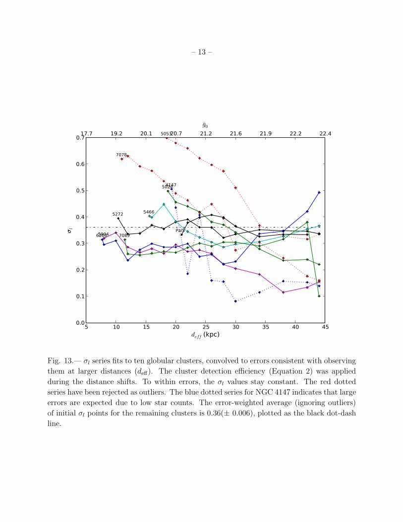
Fig. 13.— σl series fits to ten globular clusters, convolved to errors consistent with observing

them at larger distances (deff). The cluster detection efficiency (Equation 2) was applied

during the distance shifts. To within errors, the σl values stay constant. The red dotted

series have been rejected as outliers. The blue dotted series for NGC 4147 indicates that large

errors are expected due to low star counts. The error-weighted average (ignoring outliers)

of initial σl points for the remaining clusters is 0.36(± 0.006), plotted as the black dot-dash

line.

– 14 –

5 10 15 20 25 30 35 40 45deff (kpc)

0.4

0.6

0.8

1.0

1.2

r

414750245053

5272

5466

5904

6205

7078

7089

Pal5

17.8 19.3 20.2 20.8 21.3 21.7 22.0 22.3 22.6g0

5 10 15 20 25 30 35 40 45deff (kpc)

0.7

0.8

0.9

1.0

1.1

1.2

1.3

1.4

1.5

1.6

r5272

5466

5904

6205

7078

7089

17.8 19.3 20.2 20.8 21.3 21.7 22.0 22.3 22.6g0

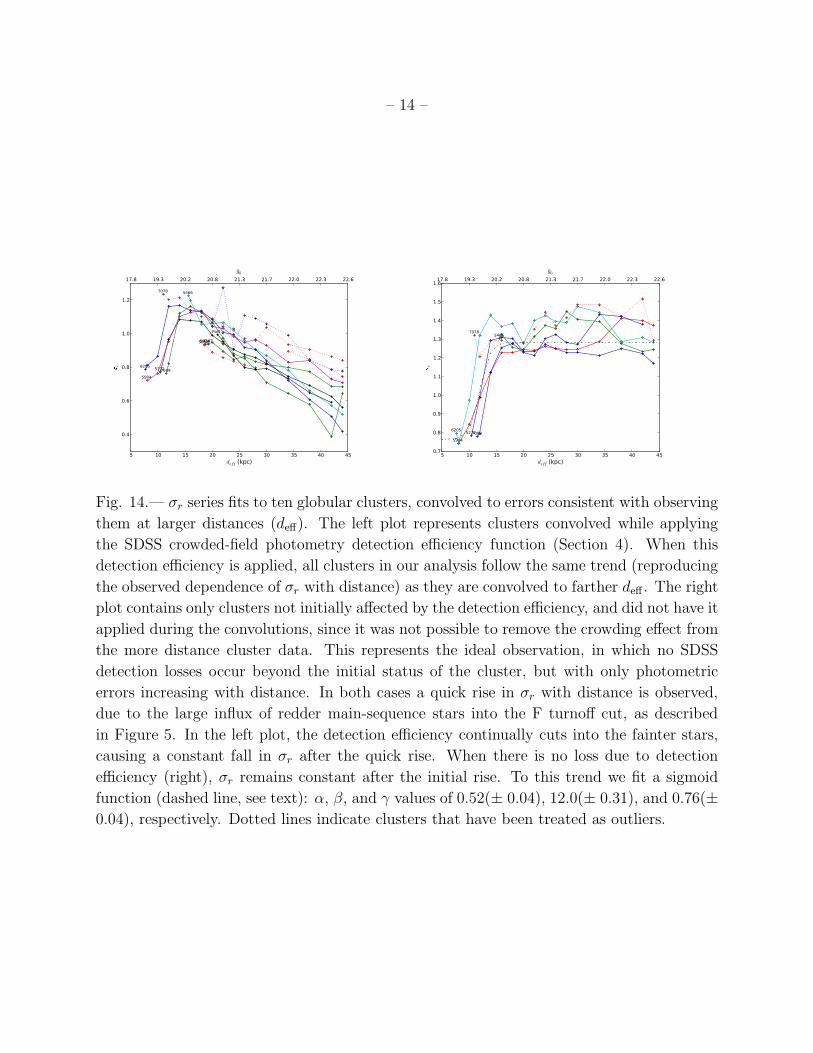
Fig. 14.— σr series fits to ten globular clusters, convolved to errors consistent with observing

them at larger distances (deff). The left plot represents clusters convolved while applying

the SDSS crowded-field photometry detection efficiency function (Section 4). When this

detection efficiency is applied, all clusters in our analysis follow the same trend (reproducing

the observed dependence of σr with distance) as they are convolved to farther deff . The right

plot contains only clusters not initially affected by the detection efficiency, and did not have it

applied during the convolutions, since it was not possible to remove the crowding effect from

the more distance cluster data. This represents the ideal observation, in which no SDSS

detection losses occur beyond the initial status of the cluster, but with only photometric

errors increasing with distance. In both cases a quick rise in σr with distance is observed,

due to the large influx of redder main-sequence stars into the F turnoff cut, as described

in Figure 5. In the left plot, the detection efficiency continually cuts into the fainter stars,

causing a constant fall in σr after the quick rise. When there is no loss due to detection

efficiency (right), σr remains constant after the initial rise. To this trend we fit a sigmoid

function (dashed line, see text): α, β, and γ values of 0.52(± 0.04), 12.0(± 0.31), and 0.76(±0.04), respectively. Dotted lines indicate clusters that have been treated as outliers.

– 15 –

0 2 4 6 8 10Mg

0

10

20

30

40

50

60

coun

ts

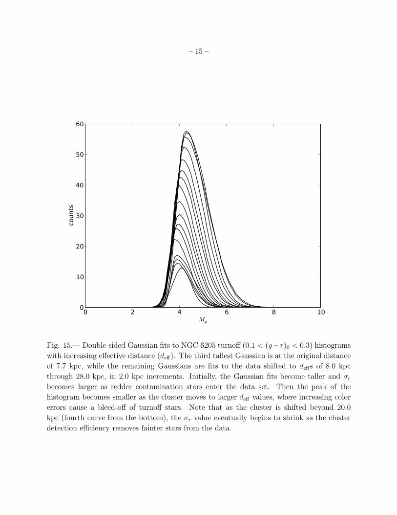
Fig. 15.— Double-sided Gaussian fits to NGC 6205 turnoff (0.1 < (g−r)0 < 0.3) histograms

with increasing effective distance (deff). The third tallest Gaussian is at the original distance

of 7.7 kpc, while the remaining Gaussians are fits to the data shifted to deffs of 8.0 kpc

through 28.0 kpc, in 2.0 kpc increments. Initially, the Gaussian fits become taller and σr

becomes larger as redder contamination stars enter the data set. Then the peak of the

histogram becomes smaller as the cluster moves to larger deff values, where increasing color

errors cause a bleed-off of turnoff stars. Note that as the cluster is shifted beyond 20.0

kpc (fourth curve from the bottom), the σr value eventually begins to shrink as the cluster

detection efficiency removes fainter stars from the data.

– 16 –

5 10 15 20 25 30 35 40 45deff

0.6

0.7

0.8

0.9

1.0

1.1

1.2

1.3

1.4

r

17.7 19.2 20.1 20.7 21.2 21.6 21.9 22.2 22.4g0

No detection loss

With sigmoidal detection efficiency

With cluster detection efficiency

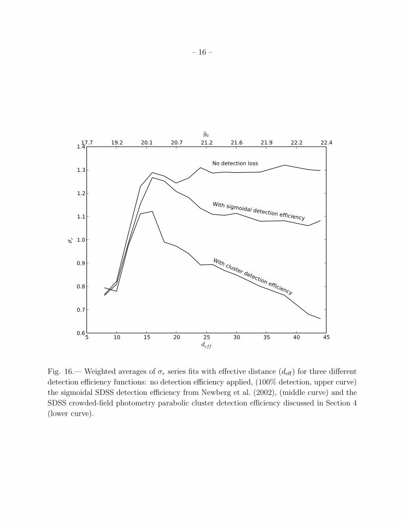
Fig. 16.— Weighted averages of σr series fits with effective distance (deff) for three different

detection efficiency functions: no detection efficiency applied, (100% detection, upper curve)

the sigmoidal SDSS detection efficiency from Newberg et al. (2002), (middle curve) and the

SDSS crowded-field photometry parabolic cluster detection efficiency discussed in Section 4

(lower curve).

– 17 –

Fig. 17.— Plot of globular cluster ages versus metallicity, from four different sources: this

paper (blue circles), Dotter et al. (2010); De Angeli et al. (2005); Marın-Franch et al. (2009).

Two clusters, NGC 5053 and NGC 7078, are shown as blue rings to indicate that they are

outliers in our analysis. These are overlaid on a theoretical age-metallicity relationship from

Muratov & Gnedin (2010) (blue- and red-shaded areas). Note that most of the clusters,

including all of the clusters in this study besides noted outliers NGC 5053 and NGC 7078,

are consistent with the theoretical age-metallicity relationship. Note that there are some

high age, high metallicity clusters in the Marın-Franch et al. (2009) and Dotter et al. (2010)

data that they attribute to a constant age with metallicity relationship at around 13 Gyr in

the inner halo.

– 18 –

0.1 0.2 0.3 0.4 0.5 0.6g -r

1

2

3

4

5

6

7

Mg

8 Gyr

9 G

yr

10 G

yr

11 G

yr12 G

yr

13 G

yr

13 G

yr

8 Gyr

0 0

Fig. 18.— Plot of Padova isochrones, modified by a correctional fit (Equation 1), from

the Age-Metallicity Relationship (AMR) presented in Muratov & Gnedin (2010). Two

isochrones not on the AMR are also plotted as black dotted series, at 8 Gyr and 13 Gyr,

in order to show the behavior of extreme outliers. All of the isochrones on the AMR

have turnoff values that are similar to each other, with a turnoff color between between

0.2 < (g − r)0 < 0.23 and a turnoff magnitude of 3.77 < Mg < 4.16. The subgiant branch

is also well constrained in magnitude: 3.4 < Mg < 3.6. These constraints will be useful in

determining distances to old stellar populations. The following Age (Gyr) and [Fe/H] (dex)

value sets were used to produce the AMR isochrones: 13.0, -1.7; 12.0, -1.5; 11.0, -1.35; 10.0,

-1.20; 9.0, -1.05; 8.0, -0.90. The age, [Fe/H] values for outlying isochrones are: 13.0, 0.0; 8.0,

-2.0