Ferromagnetism in Armchair Graphene Nanoribbon

Hsiu-Hau Lin∗Department of Physics, National Tsing-Hua University, Hsinchu 300, Taiwan andPhysics Division, National Center for Theoretical Sciences, Hsinchu 300, Taiwan

Toshiya Hikihara†Department of Physics, Hokkaido University, Sapporo 060-0810, Japan

Horng-Tay Jeng‡Institute of Physics, Academia Sinica, Nankang, Taipei 11529, Taiwan and

Department of Physics, National Tsing-Hua University, Hsinchu 300, Taiwan

Bor-Luen Huang and Chung-Yu MouDepartment of Physics, National Tsing-Hua University, Hsinchu 300, Taiwan

Xiao HuWPI Center for Materials Nanoarchitectonics, National Institute for Materials Science, Tsukuba 305-0047, Japan

(Dated: January 27, 2009)

Due to the weak spin-orbit interaction and the peculiar relativistic dispersion in graphene, thereare exciting proposals to build spin qubits in graphene nanoribbons with armchair boundaries.However, the mutual interactions between electrons are neglected in most studies so far and thusmotivate us to investigate the role of electronic correlations in armchair graphene nanoribbon byboth analytical and numerical methods. Here we show that the inclusion of mutual repulsions leadsto drastic changes and the ground state turns ferromagnetic in a range of carrier concentrations. Ourfindings highlight the crucial importance of the electron-electron interaction and its subtle interplaywith boundary topology in graphene nanoribbons. Furthermore, since the ferromagnetic propertiessensitively depends on the carrier concentration, it can be manipulated at ease by electric gates.The resultant ferromagnetic state with metallic conductivity is not only surprising from an academicviewpoint, but also has potential applications in spintronics at nanoscale.

PACS numbers: 73.22.-f, 72.80.Rj, 75.70.Ak

I. INTRODUCTION

Graphene,1 a single hexagonal layer of carbon atoms intwo dimensions (2D), is the building block for graphiticmaterials ranging from 0D fullerenes to 1D nanotubes,and also the commonly seen 3D graphite. Since itwas generally believed that the two-dimensional latticeshould not exist at finite temperature, graphene had of-ten been used as a toy model and viewed as an aca-demic material until its recent discovery in laboratory.2The honeycomb structure gives rise to linear dispersion,making electrons and holes in graphene massless as inrelativistic theories.3,4 Therefore, most studies focus onthe electronic and transport properties arisen from thispeculiar band structure,5,6,7,8,9 such as the half-integerquantum Hall effect5,6 due to the π Berry phase, thequantization of minimal conductivity where carriers arealmost absent5 and so on.

One of the potential applications of graphene is torealize fast electronics at nanoscale, making graphenenanoribbons (GNRs) a natural building block for thesedevices. Since the electronic structure sensitively de-pends on the transverse width and also the edge topology,there are intensive investigations10,11,12,13,14 on narrowGNRs with width less than 10 nm. Although GNRs have

been successfully fabricated by lithography15 down to thewidths of 20 nm, the roughness of the edges remains large(about 5 nm or larger). As a result, theoretical predic-tions may not be applicable and limit the fundamentaland practical applications. A recent breakthrough offabricating GNRs came from chemical methods.16 It israther remarkable that the width of the GNRs can befabricated in a controlled way down to 10 nm. In ad-dition, the edges of these GNRs are ultra smooth withpossibly well-defined zigzag or armchair shapes, suitablefor building electric junctions at molecular scale.

As the transverse width shrinks, the quantum fluctu-ations become important and results/predictions frommean-field theories shall be checked carefully. Mean-while, since the open boundaries of GNR play a crucialrole at nanoscale, the interplay between the Coulombinteraction and the edge morphology will lead to richphysics. For instance, it has been revealed that theCoulomb interaction gives rise to edge moments in zigzagGNR.17,18,19 Furthermore, Son, Cohen, and Louie20 haveshown that, in the presence of external electric field inthe transverse direction, the system turns half metal-lic with magnetic properties controlled by the externalelectric field. Their results not only show that the elec-tronic spin degrees of freedom can be manipulated by

arX

iv:0

901.

4177

v1 [

cond

-mat

.mes

-hal

l] 2

7 Ja

n 20

09

2

the electric fields, but also bring up the possibility to ex-plore spintronics21,22,23 at the nanometer scale based ongraphene.

Inspired by these discoveries, we investigate the effectof Coulomb interaction in armchair GNR as schemati-cally shown in Fig. 1. Note that the edges are hydro-genated so that the dangling σ bonds are saturated andonly the π bands remain active in low energy.20 By com-bining analytical weak-coupling analysis, numerical den-sity matrix renormalization-group (DMRG) method, andthe first-principles calculations, we show that armchairGNR exhibits an interesting carrier-mediated ferromag-netism upon appropriate doping. Even though only πbands are active in low-energy, in appropriate dopingregimes, the armchair edges give rise to both itinerantBloch and localized Wannier orbitals. As will be ex-plained later, these localized orbitals are direct conse-quences of quantum interferences in armchair GNR andform flat bands with zero velocity. The carrier-mediatedferromagnetism can thus be understood in two steps:Electronic correlations in the flat band generate intrinsicmagnetic moments first, then the itinerant Bloch elec-trons mediate ferromagnetic exchange coupling amongthem. As a result, the magnetic properties of armchairGNR sensitively depend on the doping and thus can bemanipulated easily by the external electric fields.

Though the ferromagnetic state in armchair GNRstems from the flat-band states which are partially filled,the mechanism is different from the “flat-band ferromag-netism” proposed by Mielke and Tasaki.24,25,26 The keyto Mielke-Tasaki ferromagnetism is the finite overlap ofadjacent Wannier orbitals in the flat band: the finiteoverlaps generate exchange coupling among these orbitalsand lead to the flat-band ferromagnetism. However, theWannier orbital in armchair GNR (shown in Fig. 1) haszero overlap with its adjacent neighbors. The flat bandalone only accounts for the existence of the magnetic mo-ments and the ferromagnetic order sets in only when itin-erant carriers are present. A similar mechanism of ferro-magnetism has been argued for the Hubbard model in akind of frustrated lattice.27,28

In the following, we will elaborate in details how thecarrier-mediated ferromagnetism emerges (upon appro-priate doping) in the armchair GNR. In Sec. II, we startwith the Hubbard model and solve the band structureby the method of generalized Bloch theorem. In Sec.III, we integrate out the gapped modes and explore theground state properties in weak coupling. We first showhow the local moments in the flat band form from theCoulomb interaction. We also demonstrate the crucialrole of itinerant carriers in dispersive bands, which medi-ate the indirect exchange coupling among the local mo-ments and give rise to the ferromagnetic ground state.Indeed, without those carriers, the ferromagnetism disap-pears and only Curie-like susceptibility remains in arm-chair GNR. In Sec. IV, we employ the technique of non-Abelian DMRG to investigate the ferromagnetic groundstate in intermediate coupling. It is remarkable that the

1

x........

1

2

Ly

y

2 Lx

....

−1 0 1

−2

0

2

E /

t

k / π −1 0 1

−2

0

2

E /

t

k / π

(a)

(b) (c)

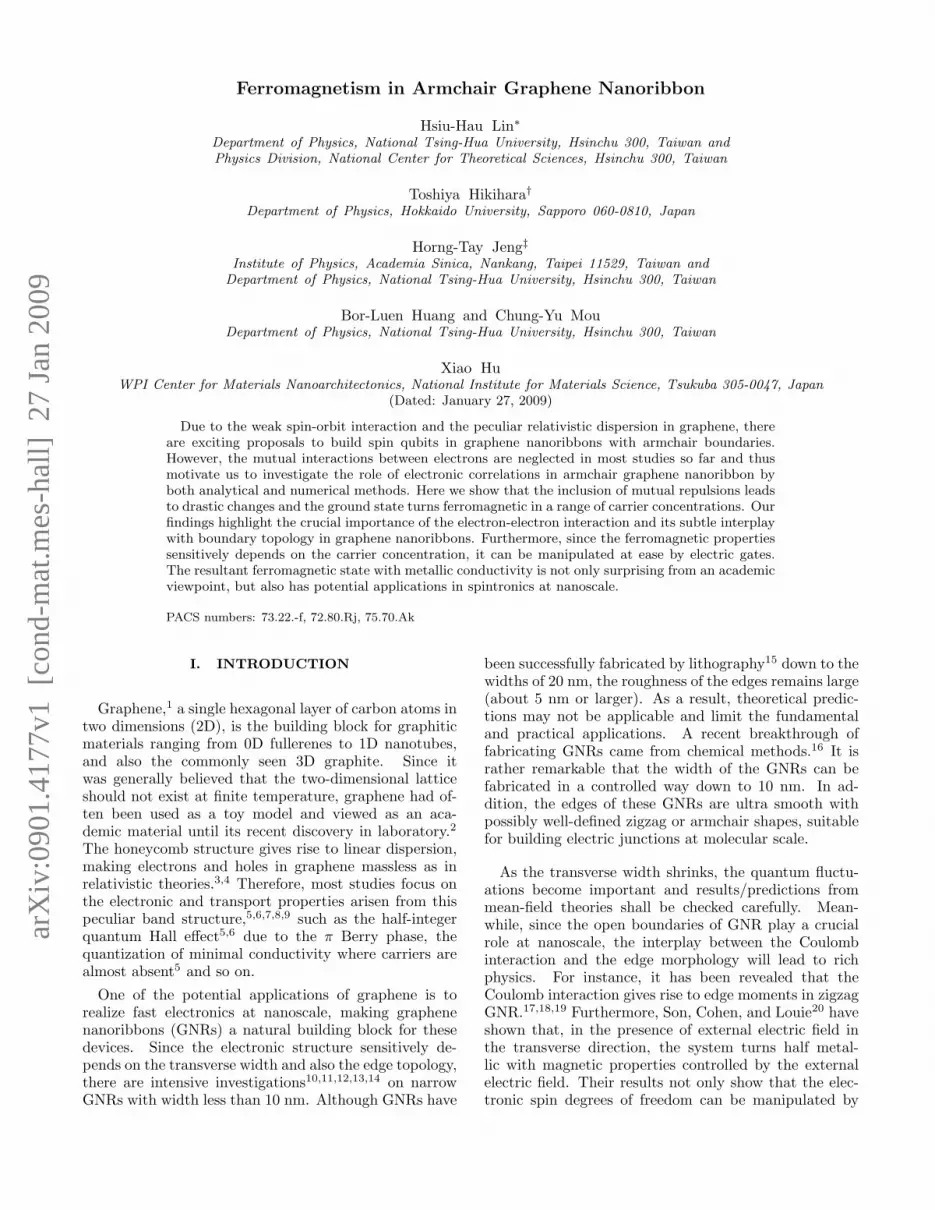
FIG. 1: (Color online) (a) Armchair GNR of Lx = 4 andLy = 5. Open edges are present at y = 1 and Ly. The solidcircles and squares represent sublattice A and B respectively.The shaded circles show the amplitudes of a local Wannierorbital of E = t at x = 2, with opposite signs indicated bylight/dark colors. Band structures for the infinitely long GNRwith (b) Ly = 5 and (c) Ly = 7 clearly show the pair of flatbands at E = ±t.

numerical results agree with the weak-coupling analy-sis pretty well. In Sec. V, the realistic band structureand the long-range Coulomb interactions are included viathe first-principles calculations. It is rather unexpectedthat the flat band is robust even when the realistic bandstructure is taken into account. Ferromagnetism appearsaround the same doping regime as predicted by eitherweak-coupling or DMRG approaches. Finally, in the lastsection, we discuss the robustness of our predictions andalso their connections to practical experiments.

II. HUBBARD MODEL FOR ARMCHAIRNANORIBBON

To understand the carrier-mediated flat-band ferro-magnetism in the armchair GNR, we start with the Hub-bard Hamiltonian,

H = −t∑〈r,r′〉,α

[c†α(r)cα(r′) + H.c.] + U∑r

n↑(r)n↓(r),(1)

where t is the hopping amplitude on the honeycomb net-work, U > 0 is the on-site repulsion, α =↑, ↓ is the spinindex. The lattice points r = (x, y,Λ) are labeled by in-teger indices (x, y) in longitudinal and transverse direc-tions and the additional sublattice index Λ = A,B. Thetransverse integer index y = 1, 2, ..., Ly defines the widthof the ribbon while x = 1, 2, ..., Lx defines the length.The sum

∑〈r,r′〉 is taken only for nearest-neighbor (NN)

3

bonds.The values of t reported in the literature29,30,31 range

from 2.4-2.7 eV for nanotubes, while t ' 3 eV is typicalin graphites. Although an accurate value of U is not yetknown in GNRs, the estimate from polyacetylene, U '6-10 eV,32,33 might serve as a reasonable guess. Thus,we expect the ratio U/t to be of order one.

Let us try to obtain the band structure of the armchairGNR within the tight-binding model first. For conve-nience, we consider the infinite length Lx →∞ in the fol-lowing. Since the system is translational invariant alongthe x-direction, the hopping Hamiltonian simplifies afterthe partial Fourier transformation,

c(r) =1√Lx

∑k

eik[x+δ(y)]c(k,y). (2)

We omit the spin index α for a while. The shorthandnotation y = (y,Λ) is defined to label the sites within aunit cell. The geometric phases arisen from the underly-ing honeycomb structure are

δ(y) = 2/3, for y=even and Λ = A,

δ(y) = 0, for y=even and Λ = B,

δ(y) = 1/6, for y=odd and Λ = A,

δ(y) = 1/2, for y=odd and Λ = B. (3)

The hopping Hamiltonian simplifies to decoupled two-legladders with finite length Ly labeled by momentum k inthe x-direction,

Ht =∑k

Ψ†(k)H(k)Ψ(k), (4)

where Ψ(k) = [c(k, y;A), c(k, y;B)] is the fermion opera-tor for sublattices A and B and thus has 2Ly components.The reduced hopping Hamiltonian H(k) is a 2Ly × 2Lymatrix. It is rather interesting that H(k) can be castedinto supersymmetric (SUSY) form34,35,36

H(k) =(

0 Q†

Q 0

). (5)

The submatrix that connects opposite sublattices is thesupercharge operator,

Q =

t∗2 t1 0 0 ... 0t1 t∗2 t1 0 ... 00 t1 t∗2 t1 ... 0. . . . ... .0 0 0 0 ... t∗2

, (6)

where the complex hopping amplitudes are t1 = −teik/6and t2 = −teik/3. One should not be surprised by thecomplex hopping amplitudes that come from the corre-sponding geometric phases kδ(y).

To solve the wave function, let us introduce a 2Ly-component spinor,

Φ(y) =[ϕA(y)ϕB(y)

], (7)

where ϕA/B(y) are the wave functions on sublattices A/B.Making use of the SUSY form in Eq. (5), the coupledHarper equations are

Q ϕA = EϕB, Q†ϕB = EϕA. (8)

It is known that the solution for E 6= 0 is supersymmetricand can be solved by combining the two Harper equationstogether Q†Q ϕA = E2ϕA. Once the eigenstate ϕA isobtained, the wave function on the other sublattice isϕB = 1

EQϕA. Thus, the remaining task is to diagonalizethe matrix Q†Q. Note that the above trick only works forE 6= 0 eigenstates while the E = 0 states can be obtainedby finding the null space of Q and Q† alone.

Before digging into details, we would like to make somegeneral remarks. It is clear that, for each solution ϕA, wecan construct two wave functions on the other sublatticeϕB by two choices of eigenenergies E = ±|E|. As a result,the energy spectrum is symmetric about E = 0 and totalwave functions of opposite energies E = ±|E| only differby an overall minus sign on one of the sublattices (butnot on the other).

With this general picture in mind, we now turn to theexplicit form of the matrix Q†Q, that can be worked outby straightforward algebra

Q†Q =

V0 − T2 T1 T2 0 0 0 ... 0T1 V0 T1 T2 0 0 ... 0T2 T1 V0 T1 T2 0 ... 00 T2 T1 V0 T1 T2 ... 0. . . . . . ... .0 0 0 0 ... T2 T1 V0 − T2

,

(9)where V0 = 3t2, T1 = 2t2 cos(k/2) and T2 = t2. This ma-trix resembles the hopping Hamiltonian of a finite chainwith the site potential V0, nearest-neighbor hopping T1

and next-nearest-neighbor one T2. The eigenfunction sat-isfies

T2[ϕA(y + 2) + ϕA(y − 2)] + T1[ϕA(y + 1) + ϕA(y − 1)]+V0ϕA(y) = E2ϕA(y), (10)

where y = 1, 2, ..., Ly with the appropriate boundary con-ditions

ϕA(0) = 0, ϕA(Ly + 1) = 0, (11)ϕA(−1) = −ϕA(1), ϕA(Ly + 2) = −ϕA(Ly). (12)

The first two boundary conditions arise from the openends of the effective two-leg ladder and the last two con-straints comes from the change of the potential at the endsites. Note that the usual plane-wave solutions satisfy thebulk Harper equation in Eq. (10). Thus, we only need toform appropriate linear combination of these plane-wavesolutions to match the boundary conditions. In the casewe study here, the eigenstate is the simple combinationof opposite momentum states with a relative minus sign,i.e. the wave function takes the usual sine form,

ϕA(y) = sin(qmy), (13)

4

where the magnitude of transverse momentum is quan-tized, qm = mπ/(Ly + 1) with m = 1, 2, ..., Ly. From theeigenstates, it is straightforward to compute the corre-sponding dispersions for each band,

E = ±[V0 + 2T1 cos qm + 2T2 cos 2qm]1/2

= ±t[1 + 4 cos(k/2) cos qm + 4 cos2 qm]1/2. (14)

With the wave function on sublattice A and the energydispersion, we can obtain the wave function on sublat-tice B by the supercharge operator as described before.However, a closer look would ensure us that the full wavefunction on the armchair GNR is far simpler than we ex-pected.

The simplification arises from the fact that the super-charges Q and Q† commute. As a result, the matrixQ†Q = QQ† share the same eigenstates as the matricesQ and Q†. It is straightforward to show that the wavefunction ϕA(y) is also an eigenstate of Q with complexeigenvalue,

QϕA = (t∗2 + 2t1 cos qm)ϕA = |E|eiθ(k)ϕA, (15)

where the phase θ(k) = θ(k, qm) of the complex eigen-value is

eiθ(k) =t∗2 + 2t1 cos qm

|E|. (16)

Therefore, the wave function on the sublattice B is aduplicate of ϕA with a momentum-dependent phase shift,

ϕB(y) = ±eiθ(k) sin(qmy). (17)

The ± signs arise from the signs of the energy, corre-sponding to antibonding and bonding bands respectively.Finally, after attaching appropriate renormalization fac-tor, the full eigenstate wave function is labeled by thequantum number k = (k, qm, s), including the longitu-dinal momentum k, the transverse momentum qm andantibonding/bonding index s = ±1. The explicit form ofthe wave function is

Φk(y) =1√

Ly + 1

[sin(qmy)

seiθ(k) sin(qmy),

]. (18)

Note that the dependence of the longitudinal momentumk only appears through the relative phase θ(k) betweenwave functions on two sublattices. This simple analyticalform of the eigenstates allows us to map the armchairGNR to effective theory in the low-energy limit and studythe correlation effects analytically.

For the width of odd Ly, the transverse momentumgoes through the particular value qm = π/2, renderingthe energy dispersion completely flat at energy E = ±tin the whole Brillouin zone. To obtain the wave function,we only need to evaluate the phase shift, eiθF± = [t∗2 +2t1 cos(π/2)]/t = −e−ik/3. Therefore, the wave functionsfor the flat bands E = ±t are

ΦF±(y) =1√

Ly + 1

[sin(πy/2)

∓e−ik/3 sin(πy/2)

]. (19)

Since all states with different momentum k are exactlydegenerate, it is possible to construct the local Wannierorbital with the same energy,

ΨF±(r) = δx,x0

1√Ly + 1

[sin(πy/2)∓ sin(πy/2)

]. (20)

Note that the momentum-dependent phase shift θF± =−k/3 cancels the relative geometric phase k[δ(y,B) −δ(y,A)] leading to extremely simple local Wannier orbitalat x = x0. Repeatedly applying the lattice displacementoperator Tx on one Wannier orbital, all orbitals at dif-ferent locations can be constructed. Since [Tx, Ht] = 0,all the orbitals share the same energy and form a flatband. This is the one-dimensional analog of the Landaulevel degeneracy for two-dimensional electrons in mag-netic field. The peculiar edge topology at nanoscale re-places the role of the magnetic field in 2D and quenchesthe kinetic energy of the carriers.

At first sight, it is rather counterintuitive that the localWannier orbital cannot move around by quantum hop-ping. The static nature is due to perfect destructivequantum interferences which make hopping amplitudesfrom different sites cancel each other. Thus, the openboundaries of armchair shape play a crucial role for thebirth of the Wannier orbitals. Furthermore, since thewave function is not zero only at odd y coordinates (seeFig. 1), it is clear that the adjacent orbitals have zerooverlap. Thus, the Mielke-Tasaki mechanism does notwork to couple neighboring orbitals magnetically.

Let us concentrate on the flat-band regimes E = ±t forthe armchair GNR with odd Ly. Due to the particle-holesymmetry for the Hubbard model, the low-energy physicsis dictated by the doping level disregarding whether it iselectron or hole doped. Thus, it is convenient to intro-duce the positive-definite doping level xd ≡ |〈n〉 − 1|,where 〈n〉 is the average electron number per site. Thelower and upper bounds of the doping rate xd for theflat-band regime are obtained from the Fermi momentakm of the dispersive bands intersecting the flat band.For those dispersive bands, the Fermi momentum sat-isfies cos(km/2) + cos(qm) = 0, which leads to km =2π − 2qm, where m = Ly, Ly − 1, ..., (Ly + 3)/2: thereare (Ly − 1)/2 pairs of Fermi points crossing the flatband. Thus, the system is in the flat-band regime forxd,min < xd < xd,max, where

xd,min =1πLy

∑m

km =14− 1

4Ly,

xd,max = xd,min +1Ly

=14

+3

4Ly. (21)

Therefore, the flat-band regime shrinks as the transversewidth increases and eventually goes to zero in the two-dimansional limit. This trend highlights the importanceof finite transverse width of the system and why the flat-band physics is no longer the dominant player in 2D. Inthe following, we will try to write down the effective fieldtheory for both the flat and dispersive bands in weakcoupling.

5

III. WEAK-COUPLING ANALYSIS

Even though we have derived the analytical form ofwave functions in armchair GNR, it is still quite compli-cated to write down the effective field theory. In the flat-band regime, after integrating out gapped bands, thereremains a flat band with intersecting dispersive bands.Note that the lattice fermion can be decomposed intoeigenstates,

cα(x, y,Λ) =1√Lx

∑k

eikx∑m,s

φms(y)cmsα(k), (22)

where the extra geometric factor is included in the mod-ified wave function φms(y) = eikδ(y)Φms(y). In thelow-energy limit, one can approximate all intersectingbands with linear dispersions, the above expansion isthen greatly simplified.

Let us work out the chiral-field expansion in the flat-band regime at E = t as an example. In that case, theeffective low-energy theory is described by the flat bandand the intersecting dispersive bands of the antibondingsector s = 1. Thus, the lattice fermion can be decom-posed into the flat-band and pairs of chiral field opera-tors,

cα(r) ' φF (y)ψFα(x) +∑m

∑P

eiPkmxφPm(y)ψPmα(x),

(23)

where P = R/L = +/− represents the chirality. Themodified (including the geometric phases) wave functionfor the flat-band orbital is

φF (y) =1√

Ly + 1

[sin(πy/2)− sin(πy/2)

], (24)

and those for the right/left-moving plane waves at Fermipoint ±km are

φPm(y) =1√

Ly + 1

[eiPkmδA sin(qmy)

eiPkm[2/3+δB ] sin(qmy)

], (25)

where the shorthand notation is introduced δA/B =δ(y,A/B). Substituting the chiral-field expansion intothe lattice Hamiltonian, one can easily derive the effec-tive field theory in the flat-band regimes.

Since the density of states is divergent for the flat band,the dispersive bands can be dropped to the leading orderapproximation. The effective Hamiltonian, keeping theflat band only, is rather simple,

HF = UF∑x

nF↑(x)nF↓(x), (26)

where nFα(x) is the number density of each spin flavorand UF is the effective on-site interaction for the flat-bandorbitals, which can be computed by projection onto theflat band,

UF = U∑y

|φF (y)|2|φF (y)|2 =U

Ly + 1. (27)

Note that the kinetic energy is quenched in the flat bandand thus the ground state contains no quantum fluctua-tions. To avoid the cost of UF , the ground state consistsof the maximum number of singly-occupied Wannier or-bitals, which leads to local magnetic moments. Sincethere is no overlap between adjacent orbitals, these mag-netic moments are free and give rise to a large ground-state degeneracy.

To lift the large degeneracy of the ground state, inter-action with the itinerant carriers in the dispersive bandsmust be included. While the effective Hamiltonian forthe interaction contains other terms, the terms to play akey role are the exchange interactions which couple thelocal moments and the itinerant carriers,

HJ =∑x,m

−Jm SF (x) · Sm(x), (28)

where SF (x) is the spin density operator for the localmoments and Sm(x) = SRm(x) + SLm(x) is the spin den-sity of itinerant carriers in the crossing band m. Theexchange integral is given by,

JPm = 2∑y,y′

φ∗F (y)φF (y′)φPm(y)φ∗Pm(y′)Vy,y′ . (29)

Using Eqs. (24) and (25), we obtain the exchange integraldue to the on-site interaction Vy,y′ = δy,y′U ; it has arather simple form,

Jm = 2U∑y

|φF (y)|2|φPm(y)|2

=2U

(Ly + 1)2∑y=odd

2 sin2(qmy) =U

Ly + 1. (30)

The subscript P = R/L is dropped because the couplingstrength does not depend on the chirality. Thus, the on-site interaction induces a ferromagnetic coupling betweenthe local moments in the flat band and the itinerant spinsin the dispersive bands.

The exchange coupling Jm tends to align the local mo-ments from the flat band because it does not cause anyextra kinetic energy. The ferromagnetically aligned mo-ments act back on the itinerant carriers and induce fi-nite polarization in the dispersive bands. The interactingHamiltonian HF + HJ therefore shows interesting two-step flat-band ferromagnetism – electronic correlationsin the flat band give rise to local moments without directexchange coupling, while the presence of gapless itiner-ant carriers mediates the ferromagnetic order. The sig-nificant feature of the armchair GNR is that, even withinthe one-orbital Hubbard model without any magnetic im-purity nor additional localized levels, the electronic cor-relations give rise to both local moments and itinerantcarriers simultaneously due to the peculiar topology ofthe open edges.

It is also interesting to consider the finite-size effectarisen from the length Lx of the armchair GNR. If one

6

0 0.2 0.4 0.6 0.8

0

0.5∆

Ene

rgy

diffe

renc

e

Doping rate

: = 1δ: = 2δ: = 3δ

/ tSSS

xd

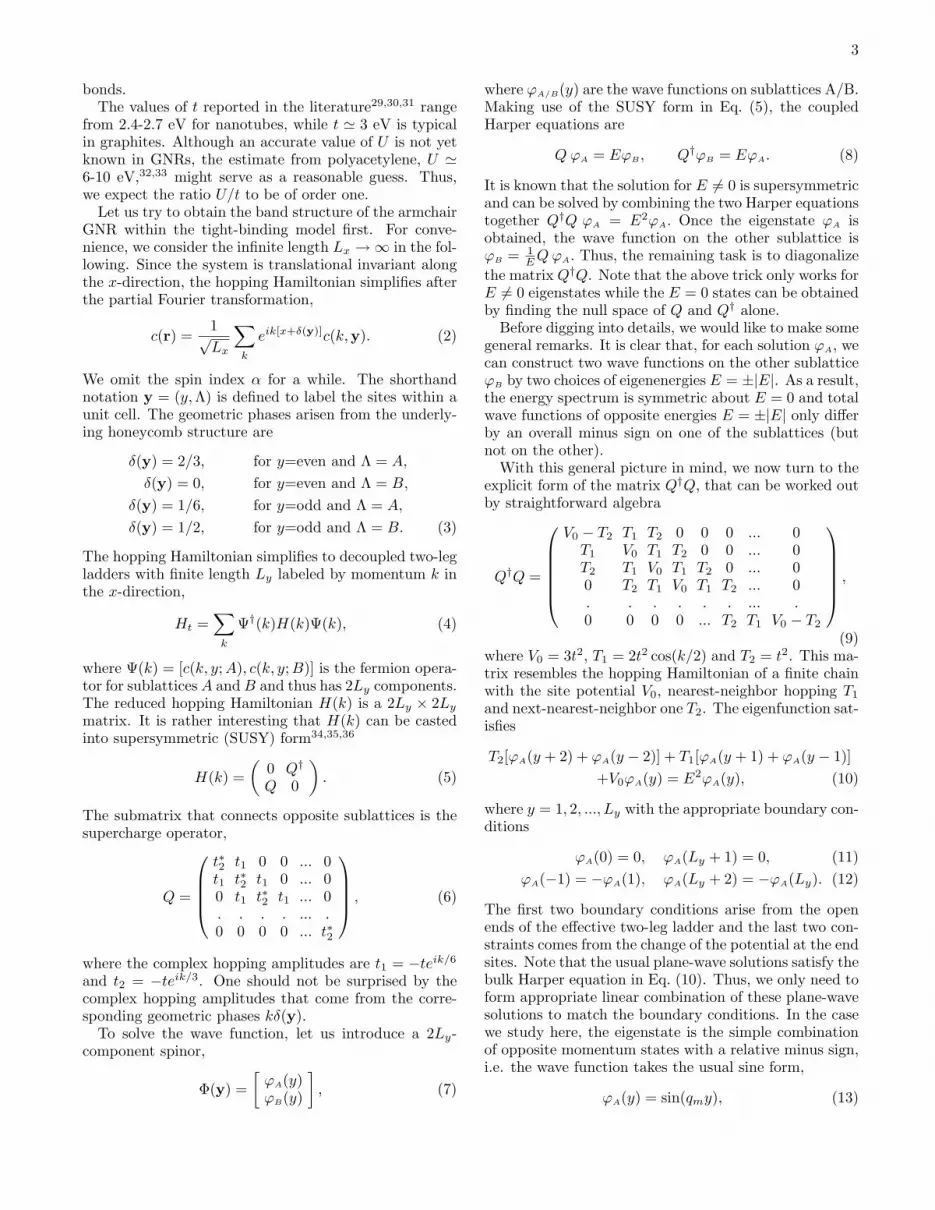
FIG. 2: (Color online) Doping dependence of the energy dif-ference ∆(xd, δS) between higher-spin and lowest-spin statesin the armchair GNR with Lx = 2 and Ly = 5 for U/t = 4.The squares, triangles, and diamonds represent the data forδS = S − S0 = 1, 2, and 3, respectively.

TABLE I: Energy difference per unit cell ∆(xd) between theferromagnetic ground state and the paramagnetic one in thearmchair GNR with Lx = 2 and Ly = 5 for the flat-bandregime. Here S is the total spin of the ground state and thehopping amplitude is chosen t = 3 eV.

xd S U/t = 2 U/t = 4 U/t = 8

0.25 3/2 -44 meV -54 meV -57 meV

0.30 2 -115 meV -111 meV -87 meV

0.35 3/2 -48 meV -52 meV -34 meV

imposes the periodic boundary conditions along the x-direction, the system becomes a short segment of arm-chair nanotube. In this case, only when the quantizedmomenta kx = 2lπ/Lx (l = 0, 1, ..., Lx − 1) coincidewith the Fermi points ±km, the gapless itinerant car-riers are present and the ferromagnetic ground stateis realized. For open boundary conditions with finiteLx, the situation is much more complicated; kx is nolonger good quantum number and the band structurecan be deformed by finite Lx. However, from numeri-cal calculations for the tight-binding Hamiltonian Ht, wehave found that the energy spectrum around the flat-band level E = ±t is not affected by finite Lx andcan be accurately approximated by the quantization rulekx = lπ/(Lx + 1) (l = 1, 2, ..., Lx). When the quantizedmomenta kx coincide with the Fermi points km, ferro-magnetism sets in with the help of these gapless itinerantcarriers. Therefore, depending on specific choice of Lx,the ground state of the armchair GNR in the flat-bandregime can be ferromagnetic or Curie-like paramagnetic.

x

yU t/ = 4

x

yU t/ = 0+

0 10 200

0.1

0.2

= 1

2

3

4

5

6

7

8

9

10

11

12

13

14

15

16

17

18

19

20

i

spin

pol

ariz

atio

n

site index i

: = 8: = 4: = 2: = 0+

U t/U t/U t/U t/

(a)

(b) (c)

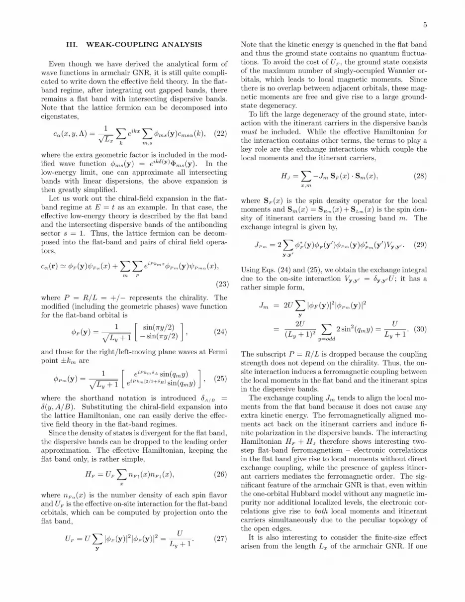
FIG. 3: (Color online) Spin polarization profile 〈Sz(r)〉 ofthe ferromagnetic ground state for the armchair GNR withLx = 2 and Ly = 5. It is at the optimal doping x∗d = 0.30with the interaction strength (a) U/t = 4. (b) U/t = 0+. Thevalues of 〈Sz(r)〉 are represented by the areas of the shadedcircles. It is remarkable that the profiles with intermediateand weak interaction strength are almost identical. (c) Thevalues of 〈Sz(r)〉 at each site for U/t = 0+, 2, 4, 8 representedby solid circles, squares, triangles and diamonds.

IV. NON-ABELIAN DENSITY MATRIXRENORMALIZATION GROUP

To check the validity of the weak-coupling scenario andsee whether it survives for the realistic coupling regime,we choose the non-Abelian DMRG method.37 It is im-portant to emphasize that, to look for the higher-spinground state, the non-Abelian approach is more powerfuland convenient compared to the conventional DMRG38,39

because the former makes the full use of the spin SU(2)symmetry. Employing the non-Abelian DMRG method,we can compute the energy difference between the higher-spin (ferromagnetic) state and the lowest-spin (paramag-netic) state,

∆(xd, δS) ≡ E0(xd, S)− E0(xd, S0), (31)

where E0(xd, S) is the lowest energy in the subspace withthe doping rate xd and the total spin S. Furthermore,δS ≡ S − S0, where S0 = 0, 1/2 denotes the lowest spindepending on whether the number of carriers is even orodd. The calculation is performed for the system withLy = 5 and Lx = 2, for which the quantized momentakx = lπ/3 coincide with the Fermi points of the dispersivebands and therefore the weak-coupling theory predictsthe ferromagnetic ground state. The number of SU(2)multiplets kept is up to 450, typically corresponding to1000-3000 U(1) states. The truncation error is of order10−5 or less, and the results are extrapolated to the limitof zero truncation error.

Figure 2 shows the energy difference ∆(xd, δS) as afunction of the doping rate xd and the spin δS forU/t = 4. We do find numerically the ferromagnetic

7

(higher-spin) ground state in the flat-band regime, xd =0.25, 0.30, 0.35.40 The results with U/t = 2, 8 (not shownhere) also show a similar doping-rate dependence, sup-porting the ferromagnetism for the flat-band regime.

Collecting all data for ∆(xd, δS) together, we can de-termine the ground state at each doping level and its en-ergy gain per unit cell, ∆(xd), which is the energy differ-ence between the higher-spin ferromagnetic ground stateand the paramagnetic one with lowest spin,

∆(xd) =1Lx

[E0(xd)− E0(xd, S0)], (32)

where E0(xd) is the ground state energy at doping levelxd. The results for the flat-band regime (0.2 < xd < 0.4for Ly = 5) and U/t = 2, 4, 8 are summarized in Table I.The optimal doping occurs at x∗d = 0.3 as predicted bythe weak-coupling theory. Thus, the non-Abelian DMRGresults support the carrier-mediated ferromagnetism pre-dicted from the analytical approach in weak couplingeven when the interaction strength is in the intermediateregime.

To further verify the role of the flat band, we also calcu-late the profile of spin density in the ground state. Sincethe interaction strength is now larger than the hoppingamplitude, one may guess any peculiar feature in theband structure should be suppressed. Figure 3 showsthe results at the optimal doping xd = 0.3 with totalspin S = 2. Remarkably, the spin polarization for finiteU/t = 4 has a similar profile to that in the weak-couplinglimit U → 0+ obtained from the eigen-wavefunctions ofthe tight-binding model Ht. The result clearly indicatesthat the flat-band orbitals still play a significant rolein the ferromagnetic ground state for finite U/t. Thephysical picture developed in weak coupling thus appliesrather well and extends smoothly to the intermediate-and strong-coupling regime.

As the momentum kx is discretized in the system withfinite Lx, it is important to see how the properties ofthe system change depending on Lx. For armchair GNR,the large unit cell and peculiar nature of the flat-bandstates lead to slow convergence of the DMRG calculationand make it difficult to treat the system with larger Lx,unfortunately.41 Nevertheless, we have performed numer-ical calculation for other one-dimensional-lattice modelswhich have essentially the same band structure as thatof armchair GNR. We have then found that the modelswith larger number of unit cells indeed exhibits the itin-erant ferromagnetism with the properties expected fromthe weak-coupling theory in Sec. III, even including thepeculiar finite-size effect. The results will be reportedelsewhere.42 Furthermore, we also emphasize that, aswe will see in Sec. V, the first-principles calculation forinfinite-length armchair GNR also shows the itinerantferromagnetism for the flat-band regime, in accordancewith the weak-coupling prediction. These observationssupport that the carrier-mediated ferromagnetism foundin this section would survive for larger Lx and connectto the thermodynamic limit Lx →∞.

G X-5

-4

-3

-2

-1

0

1

2

3

4

5

Ene

rgy

(eV

)

0.1 0.2 0.3 0.4 0.5hole (e/carbon)

−40−35−30−25−20−15−10

−50

E(F

erro

)−E

(Par

a) (

meV

/cel

l)

0.0

0.2

0.4

0.6

0.8

1.0

1.2

mag

netic

mom

ent (

muB

/cel

l)

(c)

(b)

(a)

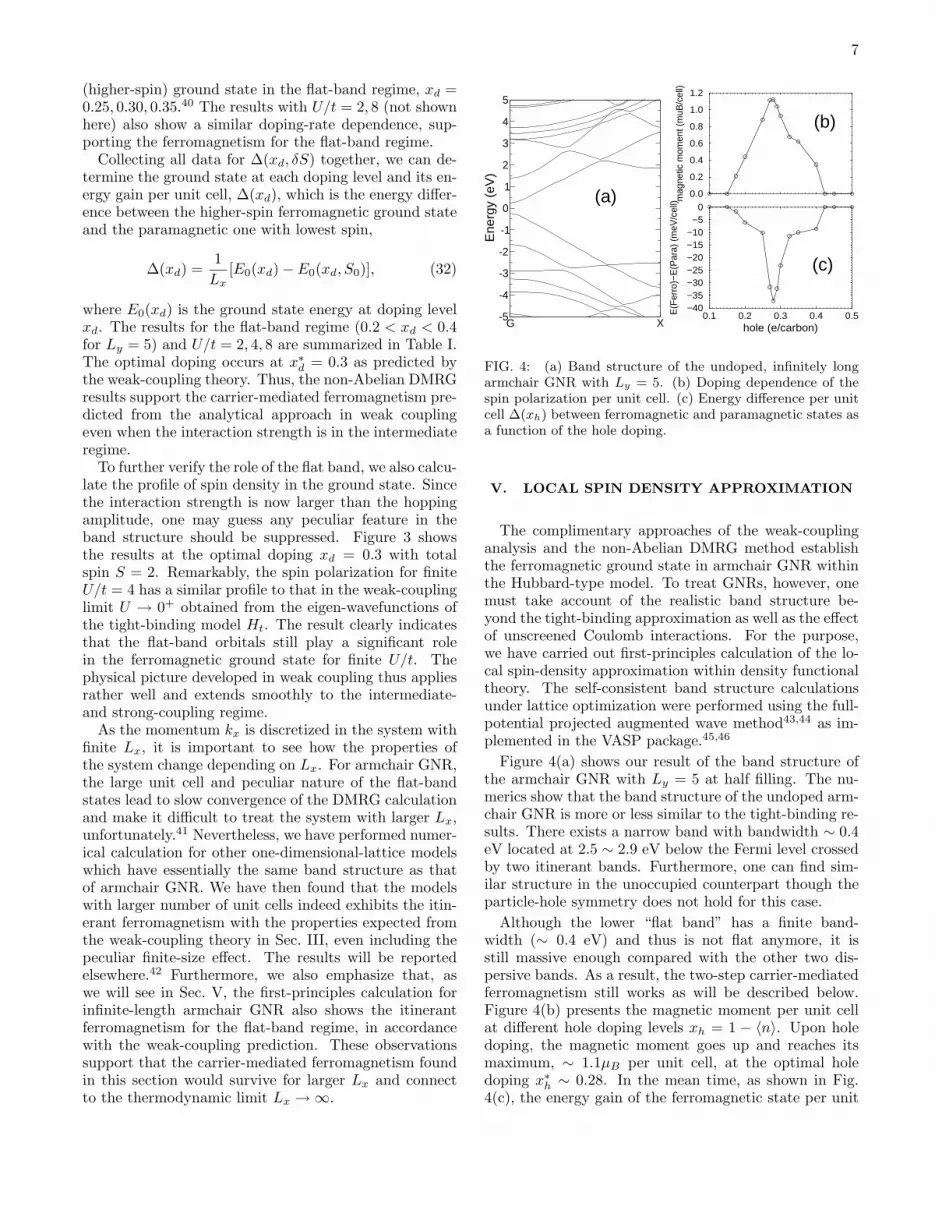
FIG. 4: (a) Band structure of the undoped, infinitely longarmchair GNR with Ly = 5. (b) Doping dependence of thespin polarization per unit cell. (c) Energy difference per unitcell ∆(xh) between ferromagnetic and paramagnetic states asa function of the hole doping.

V. LOCAL SPIN DENSITY APPROXIMATION

The complimentary approaches of the weak-couplinganalysis and the non-Abelian DMRG method establishthe ferromagnetic ground state in armchair GNR withinthe Hubbard-type model. To treat GNRs, however, onemust take account of the realistic band structure be-yond the tight-binding approximation as well as the effectof unscreened Coulomb interactions. For the purpose,we have carried out first-principles calculation of the lo-cal spin-density approximation within density functionaltheory. The self-consistent band structure calculationsunder lattice optimization were performed using the full-potential projected augmented wave method43,44 as im-plemented in the VASP package.45,46

Figure 4(a) shows our result of the band structure ofthe armchair GNR with Ly = 5 at half filling. The nu-merics show that the band structure of the undoped arm-chair GNR is more or less similar to the tight-binding re-sults. There exists a narrow band with bandwidth ∼ 0.4eV located at 2.5 ∼ 2.9 eV below the Fermi level crossedby two itinerant bands. Furthermore, one can find sim-ilar structure in the unoccupied counterpart though theparticle-hole symmetry does not hold for this case.

Although the lower “flat band” has a finite band-width (∼ 0.4 eV) and thus is not flat anymore, it isstill massive enough compared with the other two dis-persive bands. As a result, the two-step carrier-mediatedferromagnetism still works as will be described below.Figure 4(b) presents the magnetic moment per unit cellat different hole doping levels xh = 1 − 〈n〉. Upon holedoping, the magnetic moment goes up and reaches itsmaximum, ∼ 1.1µB per unit cell, at the optimal holedoping x∗h ∼ 0.28. In the mean time, as shown in Fig.4(c), the energy gain of the ferromagnetic state per unit

8

G X-5

-4

-3

-2

-1

0

1

2

3

4

5En

ergy

(eV)

majority spinminority spin

(a)

(c)

(b)

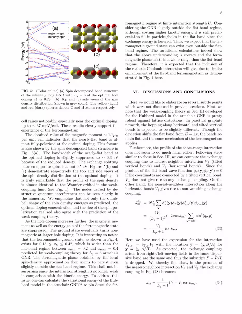
FIG. 5: (Color online) (a) Spin decomposed band structureof the infinitely long GNR with Ly = 5 at the optimal holedoping x∗h ' 0.28. (b) Top and (c) side views of the spindensity distribution (shown in grey color). The yellow (light)and red (dark) spheres denote C and H atoms respectively.

cell raises noticeably, especially near the optimal doping,up to ∼ 37 meV/cell. These results clearly support theemergence of the ferromagnetism.

The obtained value of the magnetic moment ∼ 1.1µBper unit cell indicates that the nearly-flat band is al-most fully-polarized at the optimal doping. This featureis also shown by the spin decomposed band structure inFig. 5(a). The bandwidth of the nearly-flat band atthe optimal doping is slightly suppressed to ∼ 0.3 eVbecause of the reduced density. The exchange splittingbetween opposite spins is about 0.5 eV. Figures 5(b) and(c) demonstrate respectively the top and side views ofthe spin density distribution at the optimal doping. Itis truly remarkable that the profile of the spin densityis almost identical to the Wannier orbital in the weak-coupling limit (see Fig. 1). The nodes caused by de-structive quantum interferences can be seen clearly inthe numerics. We emphasize that not only the dumb-bell shape of the spin density emerges as predicted, theoptimal doping concentration and the size of the spin po-larization realized also agree with the prediction of theweak-coupling theory.

As the hole doping increases further, the magnetic mo-ment as well as the energy gain of the ferromagnetic stateare suppressed. The ground state eventually turns non-magnetic at larger hole doping. It is interesting to noticethat the ferromagnetic ground state, as shown in Fig. 4,exists for 0.15 ≤ xh ≤ 0.42, which is wider than theflat-band regime between xmin = 0.2 and xmax = 0.4predicted by weak-coupling theory for Ly = 5 armchairGNR. The ferromagnetic phase obtained by the localspin-density approximation then seems to persist evenslightly outside the flat-band regime. This shall not besurprising since the interaction strength is no longer weakin comparison with the kinetic energy. To address thisissue, one can calculate the variational energy of the Hub-bard model in the armchair GNR47 to pin down the fer-

romagnetic regime at finite interaction strength U . Con-sidering the GNR slightly outside the flat-band regime,although costing higher kinetic energy, it is still prefer-ential to fill in particles/holes in the flat band since theexchange energy is lowered. Thus, we expect that the fer-romagnetic ground state can exist even outside the flat-band regime. The variational calculations indeed showthat the above understanding is correct and the ferro-magnetic phase exists in a wider range than the flat-bandregime. Therefore, it is expected that the inclusion ofthe realistic Coulomb interaction will give rise to similarenhancement of the flat-band ferromagnetism as demon-strated in Fig. 4 here.

VI. DISCUSSIONS AND CONCLUSIONS

Here we would like to elaborate on several subtle pointswhich were not discussed in previous sections. First, wenote that the weak-coupling theory in Sec. III developedfor the Hubbard model in the armchair GNR is prettyrobust against lattice distortions. In practical graphitenetwork, the hopping along horizontal and tilted verticalbonds is expected to be slightly different. Though thedeviation shifts the flat band from E = ±t, the bands re-main flat and the same mechanism of the ferromagnetismapplies.

Furthermore, the profile of the short-range interactiondoes not seem to do much harm either. Following stepssimilar to those in Sec. III, we can compute the exchangecoupling due to nearest-neighbor interaction V⊥ (tiltedvertical bonds) and V‖ (horizontal bonds). Since theproduct of the flat-band wave function φF (y)φF (y′) = 0if the coordinates are connected by a tilted vertical bond,V⊥ does not give rise to any exchange coupling. On theother hand, the nearest-neighbor interaction along thehorizontal bonds V‖ gives rise to non-vanishing exchangecoupling,

JV‖m = 2V‖

∑y

φ∗F (y)φF (y)φ∗Pm(y)φPm(y)

=2V‖

(Ly + 1)2(−2 cos km)

∑y=odd

sin2(qmy)

= −V‖

Ly + 1cos km. (33)

Here we have used the expression for the interactionVy,y′ = δy,y′V‖ with the notation y = (y,B/A) fory = (y,A/B). As expected, the exchange couplingsarisen from right-/left-moving fields in the same disper-sive band are the same and thus the subscript P = R/Lis dropped. We thereby find that, in the presence ofthe nearest-neighbor interaction V⊥ and V‖, the exchangecoupling in Eq. (28) becomes

Jm =1

Ly + 1(U − V‖ cos km). (34)

9

Since V⊥, V‖ < U is often expected, the exchange cou-pling is still ferromagnetic and the picture does notchange.

The above calculations can be generalized tothe screened short-ranged interaction. Suppose thespatial profile of the screened interaction goes asexp(−x/ξ)/

√x2 + l20, where l0 is a short-range cutoff

(comparable to the lattice constant) and ξ is the lengthscale of the short-ranged interaction. Ignoring the com-plicated form factor due to detail orbital overlapping,the exchange coupling takes the general form Jm(x) ∼exp(−x/ξ) cos(kmx)/x. As expected, the exchange cou-pling decreases as the distance is far apart. Furthermore,the oscillatory factor cos(kmx) makes the couplings to thedispersive bands with different signs and tends to canceleach other. It will further suppress the effects of theexchange coupling beyond the nearest neighbors. Thistrend is in agreement with our first-principles calcula-tions where the true long-ranged Coulomb interaction isincluded.

To realize the flat-band ferromagnetism in armchairGNR, the crucial challenge lies in how to achieve the ap-propriate doping level. One of graphene’s superior prop-erties is its pronounced ambipolar electric field effect.2,5,6By applying gate voltages, the charge carriers can betuned between electrons and holes with concentration upto 1013 cm−2. Even so, it is unlikely that the exter-

nal gate voltage alone can pour enough electrons/holesinto the system to reach the flat-band regime. An-other route to dope GNR is via chemical doping. It wasdemonstrated8 that the chemical dopants in the substratecan markably change the carrier density. Perhaps thecombination of both methods can be even more efficient.

In conclusion, by combining the weak-coupling anal-ysis, the non-Abelian DMRG technique, and the first-principles calculations, we show how ferromagnetism oc-curs in armchair GNR – electronic correlations give riseto magnetic moments in the flat band and the itinerantcarriers in the dispersive bands mediate ferromagneticcoupling between these uncoupled moments. Recently,there are proposals48,49 to use GNR to build transistorsand spin qubits. While these proposals take care of manyrealistic issues, the electronic correlations are ignored.Our study here show that electronic correlations in GNRcan bring up surprises such as the carrier-mediated flat-band ferromagnetism. Therefore, it is crucially impor-tant to include the correlation effects when we try torealize these proposals into devices.

We acknowledge Leon Balents, Greg Fiete, YukitoshiMotome and Tsutomu Momoi for valuable discussionsand comments. HHL, HTJ, BLH and CYM appreciatesfinancial supports from National Science Council in Tai-wan. The hospitality of KITP in Santa Barbara is alsogreatly appreciated.

∗ Electronic address: hsiuhau@phys.nthu.edu.tw† Electronic address: hikihara@phys.sci.hokudai.ac.jp‡ Electronic address: jeng@phys.sinica.edu.tw1 A. K. Geim and K. S. Novosselov, Nature Mat. 6, 183

(2007) and references therein.2 K. S. Novoselov, A. K. Geim, S. V. Morozov, D. Jiang,

Y. Zhang, S. V. Dubonos, V. Grigorieva and A. A. Firsov,Science 306, 666 (2004).

3 G. W. Semenoff, Phys. Rev. Lett. 53, 2449 (1984).4 F. D. M. Haldane, Phys. Rev. Lett. 61, 2015 (1988).5 K. S. Novoselov, A. K. Geim, S. V. Morozov, D. Jiang, M.

I. Katsnelson, I. V. Grigorieva, S. V. Dubonos and A. A.Firsov, Nature 438, 197 (2005).

6 Y. Zhang, Y.-W. Tan, H. L. Stormer and P. Kim, Nature438, 201 (2005).

7 C. Berger, Z. Song, X. Li, X. Wu, N. Brown, C. Naud, D.Mayou, T. Li, J. Hass, A. N. Marchenkov, E. H. Conrad,P. N. First, W. A. de Heer, Science 312, 1191 (2006).

8 T. Ohta, A. Bostwick, T. Seyller, K. Horn and E. Roten-berg, Science 313, 951 (2006).

9 A. Bostwick, T. Ohta, T. Seyller, K. Horn and E. Roten-berg, Nature Phys. 3, 36 (2007).

10 Y.-W. Son, M. L. Cohen and S. G. Louie, Phys. Rev. Lett.97, 216803 (2006).

11 V. Barone, O. Hod and G. E. Scuseria, Nano Lett. 6, 2748(2006).

12 D. A. Areshkin, D. Gunlycke and C. T. White, Nano Lett.7, 204 (2007).

13 G. C. Liang, N. Neophytou, D. E. Nikonov and M. S. Lund-strom, IEEE Trans. Electron. Dev. 54, 677 (2007).

14 K. Nakada, M. Fujita, G. Dresslhaus and M. S. Dressel-haus, Phys. Rev. B 54, 17954 (1996).

15 M. Y. Han, B. Ozyilmaz, Y. B. Zhang and P. Kim, Phys.Rev. Lett. 98, 206805 (2007).

16 X. Li, X. Wang, L. Zhang, S. Lee and H. Dai, Science 319,1229 (2008).

17 M. Fujita, K. Wakabayashi, K. Nakada, and K. Kusakabe,J. Phys. Soc. Jpn. 65, 1920 (1996).

18 S. Okada and A. Oshiyama, Phys. Rev. Lett. 87, 146803(2001).

19 T. Hikihara, X. Hu, H.-H. Lin, and C.-Y. Mou, Phys. Rev.B 68, 035432 (2003).

20 Y.-W Son, M. L. Cohen and S. G. Louie, Nature 444, 347(2006).

21 S. A. Wolf, D. D. Awschalom, R. A. Buhrman, J. M.Daughton, S. von Molnar, M. L. Roukes, A. Y. Chtchelka-nova, and D. M. Treger, Science 294, 1488 (2001).

22 I. Zutic, J. Fabian and S. Das Sarma, Rev. Mod. Phys. 76,323 (2004).

23 A. H. MacDonald, P. Schiffer and N. Samarth, Nature Mat.4, 195 (2005).

24 A. Mielke and H. Tasaki, Commun. Math. Phys. 158, 341(1993).

25 H. Tasaki, Prog. Theor. Phys. 99, 489 (1998).26 A. Tanaka and H. Tasaki, Phys. Rev. Lett. 98, 116402

(2007)27 A. Tanaka and T. Idogaki, J. Phys. Soc. Jpn. 67, 401

(1998).28 Precisely, the situation considered in Ref. 27 is different

from ours; the model discussed in Ref. 27 leads to a ferro-

10

magnetic state in the weak-coupling limit when a disper-sive band touches a flat band being at the bottom of thewhole band structure. On the other hand, in the armchairGNR, the dispersive bands intersect with the flat bandwhich lies inside the band structure.

29 J. W. Mintmire, B. I. Dunlap and C. T. White, Phys. Rev.Lett. 68, 631-634 (1992).

30 J. W. G. Wildoer, L. C. Venema, A. G. Rinzler, R. E.Smalley and C. Dekker, Nature 391, 59 (1998).

31 T. W. Odom, J. L. Huang, P. Kim and C. M. Lieber, Na-ture 391, 62 (1998).

32 D. Baeriswyl and K. Maki, Phys. Rev. B 31, 6633 (1985).33 E. Jeckelmann and D. Baeriswyl, Synt. Met. 65, 211

(1994).34 B.-L. Huang, S.-T. Wu and C.-Y. Mou, Phys. Rev. B 70,

205408 (2004).35 T. Pereg-Barnea and H.-H. Lin, Europhys. Lett. 69, 791

(2005).36 H. Zheng, Z. F. Wang, T. Luo, Q. W. Shi and J. Chen,

Phys. Rev. B 75, 165414 (2007).37 I.-P. McCulloch and M. Gulacsi, Europhys. Lett. 57, 852

(2002).38 S. R. White, Phys. Rev. Lett. 69, 2863 (1992).39 S. R. White, Phys. Rev. B 48, 10345 (1993).40 The high-spin ground state with δS = 1 for xd = 0.6 seen

in Fig. 2 is due to an intersection of two dispersive bandsat a high-doping rate [see Fig. 1 (b)] and does not lead toa bulk ferromagnetism in the thermodynamic limit.

41 In the lattice geometry of armchair GNR, rather large unitcells consisting of 2Ly sites are connected via (Ly − 1)/2bonds, resulting in a rapid increase of the number of siteswith Lx and a loose connection between unit cells. Further-more, for the flat-band regime, there are many low-lyingstates with extremely small energy scale, especially for thecases of Lx where the itinerant electron at the flat-bandlevel is absent. These facts lead to a very slow convergenceof the DMRG calculation and require a large number ofkept DMRG states for achieving accurate results.

42 T. Hikihara, H.-H. Lin, and C.-Y. Mou, in preparation. Inthe work, we study several lattice models which exhibit thecarrier-mediated flat-band ferromagnetism. For instance,from the calculation of up to Lx = 8 unit cells, we havefound that the Hubbard model in a two-leg ladder latticewith diagonal hoppings has the ferromagnetic ground statefor the cases of Lx where the itinerant electrons at the flat-band level are present, while it does not for the other Lx

having no itinerant state at flat-band level.43 P. E. Blochl, Phys. Rev. B 50, 17953 (1994).44 G. Kresse and J. Joubert, Phys. Rev. B 59, 1758 (1999).45 G. Kresse and J. Hafner, Phys. Rev. B 48, 13115 (1993).46 G. Kresse and J. Furthmuller, Phys. Rev. B 54, 11169

(1996).47 Y.-C. Lee and H.-H. Lin, to appear in J. Phys.: Conf.

Series (unpublished).48 A. Rycerz, J. Tworzydlo and C. W. J. Beenakker, Nature

Phys. 3, 172 (2007).49 B. Trauzettel, D. V. Bulaev, D. Loss and G. Burkard, Na-

ture Phys. 3, 192 (2007).