Projektbereich B Discussion Paper No. B–166 Hedging of Contingent Claims under Incomplete Information by HansF¨ollmer *) Martin Schweizer *) October 1990 *) Financial support by Deutsche Forschungsgemeinschaft, Sonderforschungsbereich 303 at the University of Bonn, is gratefully acknowledged. (in: M. H. A. Davis and R. J. Elliott (eds.), “Applied Sto- chastic Analysis”, Stochastics Monographs, Vol. 5, Gordon and Breach, London/New York (1991), 389–414)
Transcript
Projektbereich BDiscussion Paper No. B–166
Hedging of Contingent Claims
under Incomplete Information
by
Hans Follmer ∗)
Martin Schweizer ∗)
October 1990
∗) Financial support by Deutsche Forschungsgemeinschaft,Sonderforschungsbereich 303 at the University of Bonn, isgratefully acknowledged.
(in: M. H. A. Davis and R. J. Elliott (eds.), “Applied Sto-chastic Analysis”, Stochastics Monographs, Vol. 5, Gordonand Breach, London/New York (1991), 389–414)
Hedging of Contingent Claims
under Incomplete Information
Hans Follmer and Martin Schweizer
Universitat Bonn
Institut fur Angewandte Mathematik
Wegelerstraße 6
D – 5300 Bonn 1
West Germany
2
1. Introduction
Consider a financial market where the price fluctuation of stocks is given by
a stochastic process X = (Xt)0≤t≤T on some probability space (Ω,F , P ). If this
market is complete then any contingent claim, viewed as a random variable on
(Ω,F , P ), can be generated by a dynamic portfolio strategy based on the underly-
ing stock process X. This was the basic economic insight behind the Black-Scholes
formula for option pricing.
In the absence of arbitrage opportunities, there is an equivalent probability
measure P ∗ ≈ P such that X is a martingale under P ∗; this implies that X is a
semimartingale under the basic measure P . From a mathematical point of view,
completeness now means that any contingent claim H can be represented as a
stochastic integral of the semimartingaleX. The integrand in such a representation
provides a sequential hedging strategy which is self-financing, and which creates
the random amount H(ω) at the terminal time T without any risk; cf. [7], [8].
Thus, the a priori risk as measured for example by the variance of H, is reduced
to 0 by a suitable dynamic strategy.
In the incomplete case, a general claim is not necessarily a stochastic integral
of X. From an economic point of view, this means that such a claim will have
an intrinsic risk. We can only hope to reduce the a priori risk to this minimal
component. Thus, the problem is to characterize and to construct those strategies
which minimize the risk. For the martingale case P = P ∗, the notion of a risk-
minimizing strategy was introduced in [6]. In this context, it was shown that
a unique risk-minimizing strategy exists, and that it can be constructed using
the Kunita-Watanabe projection technique in the space M2 of square-integrable
martingales.
In this paper we consider the general case P ≈ P ∗ where X is no longer
a martingale, but only a semimartingale under the given measure P . Here the
problem of reducing risk becomes more delicate. In [11], risk-minimization was
defined in a local sense, and the construction of such strategies was reduced to a
stochastic optimality equation. The problem of solving this equation is equivalent
to a projection problem in the space S2 of semimartingales. Section 2 gives an
introduction to these questions; it is based on the results in [6], [11], [12], [13]. Here
we restrict the discussion to the case where the semimartingale X has continuous
paths , and we put more emphasis on the projection problem in S2.
It seems natural to use a Girsanov transformation in order to shift this prob-
lem back to the space M2 where the standard projection technique can be used.
But this needs some care: In the incomplete case, the equivalent martingale mea-
3
sure is no longer unique, and one has to make an appropriate choice P of the
martingale measure in order to determine the optimal strategy in terms of P . In
section 3 we introduce the notion of a minimal martingale measure P ≈ P and
discuss its existence and uniqueness. The idea is that we want to preserve the
structure of P as far as possible under the constraint that X becomes a martin-
gale under P . In the class of all equivalent martingale measures, this minimal
modification of the basic measure P can also be characterized in terms of the
relative entropy H(.|P ). We show how the optimal strategy can be computed in
terms of the minimal martingale measure P .
In section 4 we discuss the case where incompleteness is due to incomplete
information. We assume that the claim H admits an Ito representation as a
stochastic integral with respect to some large filtration (Ft)0≤t≤T . But in con-
structing a dynamic strategy, we can only use a smaller filtration (Ft)0≤t≤T ,
where Ft specifies the information available to us at time t. We show how the
unique optimal strategy can be constructed by projecting the Ito integrand down
to the filtration (Ft). We also discuss the question to which extent this strategy
is robust under an equivalent change of measure.
In section 5 we analyze the special case where incompleteness is due to a
random fluctuation in the variance. As an example, consider the standard Black-
Scholes model whereX is a geometric Brownian motion, and suppose that there is a
random jump of the variance at some fixed time t0. This example was introduced in
[8]; for a martingale measure P = P ∗, the corresponding strategy was investigated
in [10]. Our attempt to understand its probabilistic structure from a more general
point of view led to the projection results described in sections 4 and 5.
2. Minimizing Risk in an Incomplete Market
Let X = (Xt)0≤t≤T be a stochastic process with continuous paths on some
probability space (Ω,F , P ) with a right-continuous filtration (Ft)0≤t≤T . The pro-
cess X is supposed to describe the price fluctuation of a given stock. In order to
keep the notation simple we assume that X is real-valued, but the extension of
what follows to the multi-dimensional case is straightforward. We assume that X
belongs to the space S2 of semimartingales; cf. [2]. For the Doob-Meyer decom-
position
(2.1) X = X0 +M +A
of X into a local martingale M = (Mt)0≤t≤T and a predictable process A =
(At)0≤t≤T with paths of bounded variation, this amounts to the integrability con-
4
dition
(2.2) E[X2
0 + 〈X〉T + |A|2T]<∞.
Here 〈X〉 = 〈M〉 denotes the pathwise defined quadratic variation process of X
resp. M , and |A| = (|A|t)0≤t≤T is the total variation of A. In particular,
(2.3) M is a square-integrable martingale under P .
Consider a contingent claim at time T given by a random variable
(2.4) H ∈ L2(Ω,FT , P ).
In order to hedge against this claim, we want to use a portfolio strategy which
involves the stock X and a riskless bond Y ≡ 1, and which yields the random
payoff H at the terminal time T . Let ξt and ηt denote the amounts of stock and
bond, respectively, held at time t. We assume that the process ξ = (ξt)0≤t≤T is
predictable while η = (ηt)0≤t≤T is allowed to be adapted; cf. [6] for the underlying
motivation. The value of the resulting portfolio at time t is given by
(2.5) Vt = ξtXt + ηt (0 ≤ t ≤ T ),
the cost accumulated up to time t by
(2.6) Ct = Vt −∫ t
0
ξsdXs (0 ≤ t ≤ T ).
We only admit strategies (ξ, η) such that the processes V = (Vt)0≤t≤T and C =
(Ct)0≤t≤T are square-integrable, have right-continuous paths and satisfy
(2.7) VT = H P − a.s.
We also require the integrability condition
(2.8) E
∫ T
0
ξ2sd〈X〉s +
(∫ T
0
|ξs|d|A|s)2 <∞;
this ensures that the process of stochastic integrals in (2.6) is well defined and be-
longs to the space S2 of semimartingales. Such strategies will be called admissible.
Suppose that our claim H admits an Ito representation of the form
(2.9) H = H0 +
∫ T
0
ξHs dXs P − a.s.
5
where ξH satisfies (2.8). Then we can use the strategy defined by
(2.10) ξ := ξH , η := V − ξ ·X , Vt := H0 +
∫ t
0
ξHs dXs (0 ≤ t ≤ T ).
This strategy is clearly admissible. Moreover, it is self-financing, i.e.,
(2.11) Ct = CT = H0 (0 ≤ t ≤ T ).
Thus, the Ito representation (2.9) leads to a strategy which produces the claim H
from the initial amount C0 = H0. No further cost arises, and no risk is involved.
Let us now introduce the standard assumption which excludes arbitrage op-
portunities, namely the existence of an equivalent martingale measure P ∗. More
precisely, we assume that P ∗ ≈ P is a probability measure on (Ω,F) such that
(2.12)dP ∗
dP∈ L2(Ω,F , P )
and
(2.13) X is a martingale under P ∗.
Then the strategy in (2.10) can be identified as follows:
(2.14) Vt = E∗[H|Ft] (0 ≤ t ≤ T ),
and ξH is obtained as the Radon-Nikodym derivative
(2.15) ξH =d〈V,X〉d〈X〉
where 〈V,X〉 is the covariance process associated to V and X. Thus, the strategy
can be identified in terms of P ∗ and does not depend on the specific choice of the
initial measure P ≈ P ∗.So far we have summarized the well-known mathematical construction of
hedging strategies in a complete financial market model where every contingent
claim is attainable, i.e., admits a representation (2.9); cf. [7], [8] . In that ideal
case, hedging allows complete elimination of the risk involved in handling an op-
tion. In the incomplete case this is no longer possible. A typical claim will carry
an intrinsic risk, and the problem consists in finding a dynamic portfolio strategy
which reduces the actual risk to that intrinsic component. Let us first consider
the case P = P ∗ where X is already a martingale under the initial measure P .
6
In this context, the following criterion of risk-minimization was introduced in [6]:
We look for an admissible strategy which minimizes, at each time t, the remaining
risk
(2.16) E[(CT − Ct)2|Ft]
over all admissible continuations of this strategy from time t on; cf. [6] for a
detailed definition. H is attainable if and only if this remaining risk can be reduced
to 0, since this is equivalent to (2.11). But for a general contingent claim (2.4),
the cost process associated to a risk-minimizing strategy will no longer be self-
financing. Instead, it will be mean-self-financing in the sense that
E[CT − Ct|Ft] = 0 (0 ≤ t ≤ T ).
In other words, the cost process C associated to a risk-minimizing strategy is a
martingale. In [6] the existence of a unique risk-minimizing strategy is shown. In
order to describe it, consider the Kunita-Watanabe decomposition
(2.17) H = H0 +
∫ T
0
ξHs dXs + LHT
with H0 ∈ L2(Ω,F0, P ), where
(2.18) LH = (LHt )0≤t≤T is a square-integrable martingale orthogonal to X.
The risk-minimizing strategy is now given by
(2.19) ξ := ξH , η := V − ξ ·X
with
(2.20) Vt := H0 +
∫ t
0
ξHs dXs + LHt (0 ≤ t ≤ T ).
In the present martingale case, the process V can also be computed directly as a
right-continuous version of the martingale
(2.21) Vt = E[H|Ft] (0 ≤ t ≤ T ).
In particular, ξH is given by (2.15). Thus, the problem is solved by using a well-
known projection technique in the spaceM2 of square-integrable martingales: we
simply project the martingale V associated to H on the martingale X.
7
Let us now consider the general incomplete case where P ≈ P ∗, but where P
itself is no longer a martingale measure. Here the situation becomes more subtle,
and we are going to face a projection problem which is no longer standard. In
[11] a criterion of local risk-minimization is introduced. A strategy is called locally
risk-minimizing if, for any t < T , the remaining risk (2.16) is minimal under all
infinitesimal perturbations of the strategy at time t. This definition is made precise
in terms of the differentiation of semimartingales, and it is shown to be essentially
equivalent to the following property of the associated cost process C = (Ct)0≤t≤T :
(2.22) C is a square-integrable martingale orthogonal to M under P ;
cf. [11], [12], [13]. This motivates the following
(2.23) Definition. An admissible strategy (ξ, η) is called optimal if the associated
cost process C satisfies condition (2.22).
In discrete time, a unique optimal strategy does exist, and it can be deter-
mined by a sequential regression procedure running backwards from time T to time
0; cf. [11]. In continuous time, the construction of such a strategy becomes more
difficult. We start with the observation that an optimal strategy corresponds to a
decomposition (2.17) of the claim where LH is now orthogonal to the martingale
component M of X.
(2.24) Proposition. The existence of an optimal strategy is equivalent to a
decomposition
(2.25) H = H0 +
∫ T
0
ξHs dXs + LHT
with H0 ∈ L2(Ω,F0, P ), where ξH satisfies (2.8) and
(2.26) LH = (LHt )0≤t≤T is a square-integrable martingale orthogonal to M .
For such a decomposition, the associated optimal strategy (ξ, η) is given by (2.19)
and (2.20).
Proof. For a decomposition (2.25) with (2.26), the cost process associated
to the strategy (ξ, η) defined by (2.19) and (2.20) is given by
Ct = H0 + LHt (0 ≤ t ≤ T ),
and so (ξ, η) is optimal. Conversely, an optimal strategy leads to the decomposition
H = CT +
∫ T
0
ξsdXs
= C0 +
∫ T
0
ξsdXs + (CT − C0),
8
and so we have (2.25) with ξH = ξ, LHt = Ct − C0 (0 ≤ t ≤ T ) and H0 = C0.
Thus, the problem of minimizing risk is reduced to finding the representation
(2.25) and (2.26). This is of course analogous to (2.17) and (2.18). But if X is not
a martingale, we can no longer use directly the usual Kunita-Watanabe projection
technique.
(2.27) Remark. One possible approach is to use as a starting point the Kunita-
Watanabe decomposition
(2.28) H = NH0 +
∫ T
0
µHs dMs + (NHT −NH
0 )
of H with respect to the square-integrable martingale M , where NH = (NHt )0≤t≤T
is a square-integrable martingale orthogonal to M . Consider a decomposition
H = H0 +
∫ T
0
ξsdXs + LT
as in (2.25), and introduce the Kunita-Watanabe decomposition
∫ T
0
ξsdAs = N ξ0 +
∫ T
0
µξsdMs + (N ξT −N ξ
0 )
where N ξ = (N ξt )0≤t≤T is a square-integrable martingale orthogonal to M . This
leads to
H = (H0 +N ξ0 ) +
∫ T
0
(ξs + µξs)dMs + (LT +N ξT −N ξ
0 ).
But (2.28) is unique, and so an optimal strategy must satisfy the optimality equa-
tion
(2.29) ξ + µξ = µH .
One can now focus on this equation and analyze existence and uniqueness of its
solution. This is the approach taken in [11], [12].
In the next section we use a different method to study the uniqueness of
the decomposition (2.25) and of the corresponding optimal strategy, and at the
same time its robustness under an equivalent change of measure. In the complete
case, the optimal strategy can be computed in terms of the unique equivalent
martingale measure P ∗. Thus, it does not depend on the specific choice of the
measure P ≈ P ∗. In our present situation, the question becomes obviously more
delicate. To begin with, the martingale measure P ∗ is no longer unique [9], and it
9
has been shown in [6] how different martingale measures P ∗ may lead to different
strategies. But it turns out that there is a minimal martingale measure P ≈ P
such that the optimal strategy for P can be computed in terms of P . In this
partial sense, robustness will extend to our present case.
3. The Minimal Martingale Measure
Recall that the notion of a martingale measure P ∗ ≈ P was defined by prop-
erties (2.12) and (2.13). Such a martingale measure is determined by the right-
continuous square-integrable martingale G∗ = (G∗t )0≤t≤T with
G∗t = E
[dP ∗
dP
∣∣∣∣Ft]
(0 ≤ t ≤ T ).
Under P ∗, the Doob-Meyer decomposition of M is given by M = X −X0 + (−A).
But the theory of the Girsanov transformation shows that the predictable process
of bounded variation can also be computed in terms of G∗:
−At =
∫ t
0
1
G∗s−d〈M,G∗〉s (0 ≤ t ≤ T );
cf. [2], VII.49. Since 〈M,G∗〉 ¿ 〈M〉 = 〈X〉, the process A must be absolutely
continuous with respect to the variance process 〈X〉 of X, i.e.,
(3.1) At =
∫ t
0
αsd〈X〉s (0 ≤ t ≤ T )
for some predictable process α = (αt)0≤t≤T .
(3.2) Definition. A martingale measure P ≈ P will be called minimal if
(3.3) P = P on F0,
and if any square-integrable P -martingale which is orthogonal to M under P
remains a martingale under P :
(3.4) L ∈M2 and 〈L,M〉 = 0 =⇒ L is a martingale under P
Let us now look at the question of existence and uniqueness.
(3.5) Theorem. 1) The minimal martingale measure P is uniquely determined.
10
2) P exists if and only if
(3.6) Gt = exp
(−∫ t
0
αsdMs −1
2
∫ t
0
α2sd〈X〉s
)(0 ≤ t ≤ T )
is a square-integrable martingale under P ; in that case, P is given bydP
dP= GT .
3) The minimal martingale measure preserves orthogonality: Any L ∈ M2
with 〈L,M〉 = 0 under P satisfies 〈L,X〉 = 0 under P .
Proof. 1) Let G∗ = (G∗t )0≤t≤T be the square-integrable martingale associ-
ated to a martingale measure P ∗ ≈ P . Then
G∗t = G∗0 +
∫ t
0
βs dMs + Lt (0 ≤ t ≤ T )
where L is a square-integrable martingale under P orthogonal to M , and β =
(βt)0≤t≤T is a predictable process with
(3.7) E
[∫ T
0
β2s d〈M〉
]<∞.
Under P ∗, the predictable process of bounded variation in the Doob-Meyer de-
composition of M is given by
∫ t
0
1
G∗s−d〈G∗,M〉s =
∫ t
0
1
G∗s−·βs d〈X〉s.
But X = X0 +M +A is assumed to be a martingale under P ∗, and so we get
(3.8) α = − β
G∗−;
since G∗ > 0 P -a.s. due to P ∗ ≈ P and since 〈M〉 = 〈X〉, (3.7) implies
(3.9)
∫ T
0
α2s d〈X〉s <∞ P − a.s.
Now suppose that P ∗ is minimal. Then G∗0 = 1 due to (3.3), and L is a martingale
under P ∗ due to (3.4). This implies 〈L,G∗〉 = 0, and so we get
〈L〉 = 〈L,G∗〉 = 0,
11
hence L ≡ 0. Thus, G∗ solves the stochastic equation
(3.10) G∗t = 1 +
∫ t
0
G∗s− ·(−αs) dMs.
Since M is continuous and 〈M〉 = 〈X〉, we obtain G∗ = G, hence uniqueness.
2) Due to (3.9), the process G is well-defined by (3.6). But in general, it
is only a local martingale under P . If G corresponds to a martingale measure,
then this local martingale is in fact a square-integrable martingale. Conversely,
suppose that the process G has this property; we want to show that the associated
martingale measure P is indeed minimal. Consider a martingale L ∈ M2 with
〈L,M〉 = 0 under P . Since G solves (3.10), we get 〈L, G〉 = 0, and so L is a local
martingale under P . But since L is a square-integrable martingale under P , we
have
sup0≤t≤T
|Lt| ∈ L2(Ω,F , P ),
hence
sup0≤t≤T
|Lt| ∈ L1(Ω,F , P ),
since GT ∈ L2(Ω,F , P ). Thus, the local martingale L is in fact a martingale under
P .
3) Let us show that L from above also satisfies 〈L,X〉 = 0 under P . Recall
the definition of the process
[Y, Z] := 〈Y c, Zc〉+∑
s
∆Ys ·∆Zs
for two semimartingales Y and Z; cf. [4], 12.6. Since X and A are continuous, we
have〈L,X〉 = 〈Lc, X〉+ 〈Ld, X〉
= 〈Lc, X〉= [L,X]
= [L,M ] + [L,A]
= [L,M ]
under P . But since M is continuous,
[L,M ] = 〈Lc,M〉 = 〈L,M〉 = 0
under P , and this implies that [L,M ] = 0 also under P ; cf. [2], Theorem VIII.20.
12
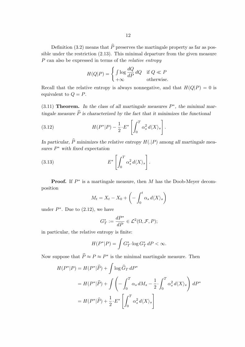
Definition (3.2) means that P preserves the martingale property as far as pos-
sible under the restriction (2.13). This minimal departure from the given measure
P can also be expressed in terms of the relative entropy
H(Q|P ) =
∫log
dQ
dPdQ if Q¿ P
+∞ otherwise.
Recall that the relative entropy is always nonnegative, and that H(Q|P ) = 0 is
equivalent to Q = P .
(3.11) Theorem. In the class of all martingale measures P ∗, the minimal mar-
tingale measure P is characterized by the fact that it minimizes the functional
(3.12) H(P ∗|P )− 1
2·E∗
[∫ T
0
α2s d〈X〉s
].
In particular, P minimizes the relative entropy H(.|P ) among all martingale mea-
sures P ∗ with fixed expectation
(3.13) E∗[∫ T
0
α2s d〈X〉s
].
Proof. If P ∗ is a martingale measure, then M has the Doob-Meyer decom-
position
Mt = Xt −X0 +
(−∫ t
0
αs d〈X〉s)
under P ∗. Due to (2.12), we have
G∗T :=dP ∗
dP∈ L2(Ω,F , P );
in particular, the relative entropy is finite:
H(P ∗|P ) =
∫G∗T ·logG∗T dP <∞.
Now suppose that P ≈ P ≈ P ∗ is the minimal martingale measure. Then
H(P ∗|P ) = H(P ∗|P ) +
∫log GT dP
∗
= H(P ∗|P ) +
∫ (−∫ T
0
αs dMs −1
2·∫ T
0
α2s d〈X〉s
)dP ∗
= H(P ∗|P ) +1
2·E∗
[∫ T
0
α2s d〈X〉s
]
13
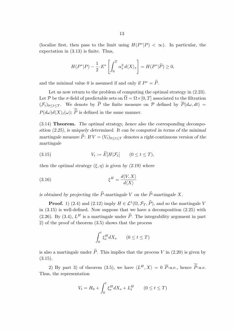
(localize first, then pass to the limit using H(P ∗|P ) < ∞). In particular, the
expectation in (3.13) is finite. Thus,
H(P ∗|P )− 1
2·E∗
[∫ T
0
α2s d〈X〉s
]= H(P ∗|P ) ≥ 0,
and the minimal value 0 is assumed if and only if P ∗ = P .
Let us now return to the problem of computing the optimal strategy in (2.23).
Let P be the σ-field of predictable sets on Ω = Ω×[0, T ] associated to the filtration
(Ft)0≤t≤T . We denote by P the finite measure on P defined by P (dω, dt) =
P (dω)d〈X〉t(ω); P is defined in the same manner.
(3.14) Theorem. The optimal strategy, hence also the corresponding decompo-
sition (2.25), is uniquely determined. It can be computed in terms of the minimal
martingale measure P : If V = (Vt)0≤t≤T denotes a right-continuous version of the
martingale
(3.15) Vt := E[H|Ft] (0 ≤ t ≤ T ),
then the optimal strategy (ξ, η) is given by (2.19) where
(3.16) ξH =d〈V,X〉d〈X〉
is obtained by projecting the P -martingale V on the P -martingale X.
Proof. 1) (2.4) and (2.12) imply H ∈ L1(Ω,FT , P ), and so the martingale V
in (3.15) is well-defined. Now suppose that we have a decomposition (2.25) with
(2.26). By (3.4), LH is a martingale under P . The integrability argument in part
2) of the proof of theorem (3.5) shows that the process
∫ t
0
ξHs dXs (0 ≤ t ≤ T )
is also a martingale under P . This implies that the process V in (2.20) is given by
(3.15).
2) By part 3) of theorem (3.5), we have 〈LH , X〉 = 0 P -a.e., hence P -a.e.
Thus, the representation
Vt = H0 +
∫ t
0
ξHs dXs + LHt (0 ≤ t ≤ T )
14
of the P -martingale V implies that ξH can be identified as the Radon-Nikodym
derivative in (3.16).
The representation (3.15) and (3.16) of the optimal strategy in terms of P
also provides a natural approach to its existence. We can start with the Kunita-
Watanabe decomposition of H under the minimal martingale measure P . Then we
have to ensure that the resulting processes ξH and V resp. η fit into the preceding
framework. If we insist on the space S2, then we need additional integrability
conditions on H and A. A more flexible alternative would be to localize both the
definitions and the arguments in the preceding discussion.
In the next section we consider a situation where a different approach can be
used. We suppose that the model is complete with respect to some larger filtration,
and we show how the decomposition (2.25) with respect to the given filtration can
be derived by projection. In particular, we obtain existence and uniqueness of the
optimal strategy.
4. Incomplete Information
In this section we consider a situation which would be complete if we had
more information. The information accessible to us is described by the filtration
(Ft)0≤t≤T . We are going to suppose that the claim H is attainable with respect
to some larger filtration. Only at the terminal time T , but not at times t < T , all
the information relevant to the claim will be available to us. So let (Ft)0≤t≤T be
a right-continuous filtration such that
(4.1) Ft ⊆ Ft ⊆ F (0 ≤ t ≤ T ).
Our basic assumption is that the Doob-Meyer decomposition
(4.2) X = X0 +M +A
of the semimartingale X ∈ S2 in (2.1) with respect to (Ft) is still valid with respect
to (Ft). In other words, we assume that
(4.3) M is a martingale with respect to (Ft)0≤t≤T ,
although it is adapted to the smaller filtration (Ft). A class of examples will be
given in section 5.
Now suppose that H in (2.4) is attainable with respect to the large filtration
(Ft), i.e.,
(4.4) H = H0 +
∫ T
0
ξHs dXs
15
where H0 is F0-measurable, and where the process ξH = (ξHt )0≤t≤T is predictable
with respect to (Ft). Let us specify our integrability assumptions. We assume
that the (Ft)-semimartingale
H0 +
∫ t
0
ξHs dXs (0 ≤ t ≤ T )
associated to H belongs to the space S2. This amounts to the condition
(4.5) E
H2
0 +
∫ T
0
(ξHs
)2
d〈X〉s +
(∫ T
0
|ξHs |d|A|s)2 <∞.
Let P denote the σ-field of predictable sets on Ω associated to the filtration (Ft).Recall from section 3 the measure P , and note that (4.5) implies ξH ∈ L2(Ω, P, P ).
(4.6) Theorem. Suppose that H satisfies (4.4) and (4.5). Then H admits the
representation
(4.7) H = H0 +
∫ T
0
ξHs dXs + LHT
with H0 := E[H0
∣∣F0
], where
(4.8) ξH := E[ξH∣∣∣P]
is the conditional expectation of ξH with respect to P and P , and where LH =
(LHt )0≤t≤T is the square-integrable (Ft)-martingale orthogonal to M associated
to
(4.9) LHT := H0 −H0 +
∫ T
0
(ξHs − ξHs )dXs ∈ L2(Ω,FT , P ).
Proof. 1) Let us first show that all components in (4.7) are square-integrable.
Since ξH ∈ L2(Ω,P, P ), we obtain
(4.10)
∫ T
0
ξHs dMs ∈ L2(Ω,FT , P ).
(4.5) implies ξH · α ∈ L1(Ω, P, P ), hence ξH · α ∈ L1(Ω,P, P ), and so we have
(4.11)
∫ T
0
|ξHs | · |αs|d〈X〉s ∈ L1(Ω,FT , P ),
16
and in particular
(4.12)
∫ T
0
ξHs dAs ∈ L1(Ω,FT , P ).
In order to obtain ∫ T
0
ξHs dAs ∈ L2(Ω,FT , P ),
we show that
(4.13)
∣∣∣∣∣E[ZT
∫ T
0
ξHs dAs
]∣∣∣∣∣ ≤ c · ‖ZT ‖2
for any bounded FT -measurable ZT with L2-norm ‖ZT ‖2. Let (Zt)0≤t≤T denote
a right-continuous version with left limits of the martingale E[ZT |Ft] (0 ≤ t ≤ T ),
and put Z∗ := sup0≤t≤T
|Zt|. By predictable projection (cf. [2], VI.45, VI.57),
∣∣∣∣∣E[ZT
∫ T
0
ξHs dAs
]∣∣∣∣∣ =
∣∣∣∣∣E[∫ T
0
Zs− · ξHs · αsd〈X〉s]∣∣∣∣∣
=
∣∣∣∣∣E[∫ T
0
Zs− · ξHs · αsd〈X〉s]∣∣∣∣∣
≤ E[Z∗∫ T
0
|ξHs | · |αs|d〈X〉s]
≤ ‖Z∗‖2 ·∥∥∥∥∥
∫ T
0
|ξHs | · |αs|d〈X〉s∥∥∥∥∥
2
≤ c · ‖ZT ‖2;
in the last step we use (4.5) and Doob’s inequality for the supremum of a square-
integrable martingale.
2) Clearly, H0 − H0 ∈ L2(Ω, F0, P ) is orthogonal to all square-integrable
stochastic integrals of M with respect to the filtration (Ft), hence in particular
with respect to the filtration (Ft). Thus, it only remains to show
E
[(∫ T
0
(ξHs − ξHs )dXs
)·(∫ T
0
µsdMs
)]= 0,
resp.
(4.14)
E
[(∫ T
0
ξHs dXs
)·(∫ T
0
µsdMs
)]= E
[(∫ T
0
ξHs dXs
)·(∫ T
0
µsdMs
)],
17
say for all bounded P-measurable processes µ = (µt)0≤t≤T ; this will imply that
the martingale LH is orthogonal to M . We decompose the left side of (4.14) into
E
[(∫ T
0
ξHs dMs
)·(∫ T
0
µsdMs
)]= E
[∫ T
0
ξHs · µsd〈X〉s]
and
E
[(∫ T
0
ξHs dAs
)·(∫ T
0
µsdMs
)]= E
[∫ T
0
ξHs ·(∫ s
0
µudMu
)· αsd〈X〉s
];
the second identity follows by predictable projection. But it is now clear that ξH
can be replaced by ξH in each of the two parts, and this yields (4.14).
The representation (4.7), together with the equivalence in proposition (2.24),
leads to the following
(4.15) Corollary. There exists a unique optimal strategy given by (2.19) and
(2.20).
We have seen in (3.14) how the optimal strategy (ξ, η) is determined by the
minimal martingale measure P . In our present context, its component ξ = ξH can
also be computed directly from ξH as a conditional expectation with respect to P .
(4.16) Theorem. The optimal strategy is given by (2.19) and (2.20) where
(4.17) ξH = E[ξH∣∣∣P]
is the conditional expectation of ξH with respect to P under the measure P asso-
ciated to the minimal martingale measure P .
Proof. Decomposing if necessary, we may assume ξH ≥ 0. We want to show
(4.18) E
[∫ T
0
ξHs · ϑsd〈X〉s]
= E
[∫ T
0
ξHs · ϑsd〈X〉s]
for any nonnegative P-measurable process ϑ = (ϑt)0≤t≤T . The left side equals
E
[GT
∫ T
0
ξHs · ϑsd〈X〉s],
18
and by predictable projection, this is equal to
E
[∫ T
0
Gs · ξHs · ϑsd〈X〉s].
But here we can replace ξH by ξH since (Gt · ϑt)0≤t≤T is P-measurable, and this
implies (4.18).
5. Incompleteness due to a Random Variance
As our basic probability space we take a standard diffusion model on C[0, T ]
together with an additional source of randomness, given by a probability space
(S,S, µ), which will affect the variance of the diffusion. Let F be the natural
product σ-field on
Ω = C[0, T ]× S,
define Xt(ω) = ω0(t) for ω = (ω0, η) ∈ Ω, and let (Ft)0≤t≤T denote the right-
continuous filtration generated by the process X = (Xt)0≤t≤T . Let β = (βt)0≤t≤Tand σ(η) = (σt(·, η))0≤t≤T (η ∈ S) be measurable adapted processes on C[0, T ]
such that the stochastic differential equation
(5.1) dXt = σt(X, η)dWt + βt(X)dt,
with fixed initial value X0 = x0, where W = (Wt) is a Wiener process, has a
unique weak solution for any η ∈ S. Let Pη be the corresponding distribution on
C[0, T ]; we assume that the mapping η 7→ Pη is measurable with respect to S.
Under suitable bounds on the processes σ(η) and β, the diffusion model
(5.2) (C[0, T ], Pη) is complete
for any η ∈ S, i.e., any square-integrable contingent claim can be written as a
stochastic integral of the coordinate process.
Let P be the probability measure on (Ω,F) associated to µ and to the map
η 7→ Pη by P (dω0, dη) = µ(dη)Pη(dω0). We assume that X is a semimartingale of
class S2 under P ; this amounts to the condition
(5.3)
∫
S
µ(dη)Eη
∫ T
0
σ2s(·, η)ds+
(∫ T
0
|βs| · σ−2s ds
)2 <∞.
19
In particular,
(5.4) Mt := Xt −X0 −∫ t
0
βs(X)ds (0 ≤ t ≤ T )
is a square-integrable martingale under P , with variance process 〈M〉 = 〈X〉 given
by
(5.5) 〈X〉t(ω) =
∫ t
0
σ2s(X(ω), η)ds (0 ≤ t ≤ T ).
P is concentrated on the measurable set of paths in C[0, T ] which admit a quadratic
variation along a suitable sequence of partitions of [0, T ]; cf. [5]. This shows that
the left side of (5.5) can be defined to be Ft-measurable. Thus, the σ-field Ftreveals through (5.5) the partial information σ2
s(X, η) (0 ≤ s ≤ t) about η. In
particular, (5.4) yields the Doob-Meyer decomposition
(5.6) Xt = X0 +Mt +
∫ t
0
αsd〈X〉s (0 ≤ t ≤ T )
of X with respect to the filtration (Ft), where α = (αt)0≤t≤T can be chosen
as a P-measurable version of the process (βt · σ−2t )0≤t≤T , due to the pathwise
reconstruction of the process σ2.
In general, the model (Ω,F , P ) is incomplete with respect to the filtration
(Ft); cf. the explicit example below. But consider the larger right-continuous
filtration (Ft)0≤t≤T obtained by adding the full information about the second
coordinate η already at the initial time 0. The conditional model (Ω, P [·|F0](η))
can be identified with the complete model (C[0, T ], Pη). This implies that
(5.7) P is complete with respect to (Ft),
i.e., any square-integrable H ∈ L2(Ω,FT , P ) can be written as
(5.8) H = H0 +
∫ T
0
ξHs dXs
with H0 ∈ L2(Ω, F0, P ) and a P-measurable process ξH = (ξHt )0≤t≤T . Since
the martingale M defined in (5.4) is also a martingale with respect to the larger
filtration (Ft), condition (4.3) is satisfied, and we can apply the results of sec-
tion 4. Under the integrability condition (4.5) on α, theorem (4.6) leads to the
representation
(5.9) H = H0 +
∫ T
0
ξHs dXs + LHT
20
with H0 := E[H0], where
(5.10) ξH := E[ξH∣∣∣P]
is the conditional expectation of ξH with respect to P and P , and where LH =
(LHt )0≤t≤T is the square-integrable (Ft)-martingale associated to
(5.11) LHT := H0 −H0 +
∫ T
0
(ξHs − ξHs )dXs ∈ L2(Ω,FT , P ).
Due to corollary (4.15), we obtain in particular the following
(5.12) Theorem. The strategy defined by (5.10) and (2.19) is optimal.
Under further bounds on σ(η) and β, the process
Gt = exp
(−∫ t
0
αsdMs −1
2
∫ t
0
α2sd〈X〉s
)(0 ≤ t ≤ T )
is a square-integrable martingale, and so the minimal martingale measure P is well
defined. In that case, theorem (4.16) shows that the optimal strategy can also be
computed in terms of P . In particular, it does not depend on our initial choice of
the drift process β.
Since our model is incomplete, the martingale measure is not unique. In fact,
any distribution ν ≈ µ on (S,S) composed with the conditional distribution of P
with respect to η induces a martingale measure; the minimal martingale measure
is characterized by the condition ν = µ.
(5.13) Example. In order to illustrate the general projection method, let us con-
sider the standard Black-Scholes model, but with a random jump of the diffusion
parameter at time t0. In the martingale case P = P ∗, this example was introduced
by Harrison and Pliska in [8] and analyzed in detail by S. Muller in [10]. In the
notation of this section, we take S = +,− and µ(+) = p. For η ∈ S and
t0 ∈ (0, T ), define the piecewise constant function
σt(η) = σ0I[0,t0)(t) + σηI[t0,T ](t) (0 ≤ t ≤ T )
with fixed parameters σ0, σ+, σ− > 0. Let Pη be the distribution of the solution
of the stochastic differential equation
dXt = σt(η) · XtdWt + γ ·Xt dt
21
with some drift parameter γ ∈ IR. Any contingent claim can be written as a
stochastic integral with respect to the larger filtration (Ft):
(5.14) H = H+0 IB +H−0 IBc +
∫ T
0
(ξ+s IB + ξ−s IBc)dXs
where H±0 and ξ± denote the usual Black-Scholes values and strategies for a known
variance σ(±), and where B = η = +. The decomposition (5.9) with respect to