Journal of Mechanics, Vol. 28, No. 2, June 2012 329
HOMOGENIZATION THEORY APPLIED TO UNSATURATED SOLID-LIQUID MIXTURE
K.-F. Liu * Y.-H. Wu Y.-C. Hsu
Department of Civil engineering National Taiwan University
Taipei, Taiwan 10617, R.O.C.
ABSTRACT
In this study, we present theoretical derivation of seepage flow in unsaturated and static soil using Homogenization theory. The derivation started in the microscopic scale in the soil. The representative elementary volume (REV) in the soil is set to be one order larger than the scale of characteristic length of pore. Solids in the REV are assumed to be rigid and cohesionless. The liquid velocity in the pore is slow. By no-slip boundary condition on the solid boundary in REV, we could obtain the microscopic flow conditions. Using spatial ensemble average under the microscopic scale, we obtain the relation between water content, pressure head and velocities in macroscopic scale. This macroscopic averaged equation is validated to be equal to Richards’ equation.
It is well accepted concept that landslide together with enough water can form debris flows. But the mechanism for landslides and occurrence of debris flows are different. Landslide is a bulky motion of a soil where particle displacement is important. How-ever, debris flow is a flowing process where strain rate is important. This means that as the motion changes from landslides to debris flows, the modeling of these physics must be changed. Furthermore, if we consider these phenomena from scales of particles, the major difference would be the interactions between solids and solids as well as solids and fluid in the pore scale.
From the continuum point of view, there are many theories used to interpret the flowing properties of de-bris flow. An extensive review was given by Ancey [1]. Many theories are validated useful and practical in certain domains. However, most of these theories can be used either when bulk material is almost station-ary (such as soil) or has large movement (such as debris flows and avalanches). In the aspect of landslide modeling, Iverson et al. [2] gave a review for models involving the effect of pore pressures and granular tem-perature in the mobilization of debris-flow. In the same paper, they assessed the relationship between Coulomb failure and liquefaction, and considered the role of granular temperature and soil volume change in an infinite-slope formulation. Iverson [3] used a mul-tiple time-scale approach together with Richards’ equa-tion to develop a mathematical model to evaluate ef-
fects of rainfall infiltration on landslide occurrence and acceleration. The model provided a tool to assess the possibility of landslide triggered by rainfall and post- failure motion. But this approach still used the con-tinuum concept to model sliding process macroscopi-cally. From the authors’ knowledge, no theory has accounted for the transition from a pile of stationary mass to debris flows. To tackle this problem, we shall start from a theory that is accurate at a condition close to initiation of solid motion.
As the continuum motion is actually the result from small scale motion, there should be methods to examine the small scale motion and then transfer small scale motion to that of continuum. In such small scale, one should be able to visualize how particles start from dry and stationary state to fully saturated but stationary state, and then start to move.
Homogenization theory [4], which based on the mul-tiple-scale perturbation method together with spatial average technique, is adapted in our problem. It has been applied to porous medium flow and used to derive the averaged seepage flow in pores under saturated and static soil [4] successfully. As the first attempt to study the initiation mechanism of debris-flow, we shall apply homogenization theory on unsaturated soil. Therefore, in this study, we only consider the case of solids in static and start by deriving the unsteady flow motion of liquid in the unsaturated pore as the first step towards our goal.
Under the assumption of static solids, we shall ig-nore the effect of solid-air interaction. Without any
330 Journal of Mechanics, Vol. 28, No. 2, June 2012
assumption of constitutive law for the water-soil mix-ture, we begin to derive seepage flow condition in the representative element volume (REV from here on) under the microscopic length scale - the scale of pores. Then we use ensemble average to obtain the averaged flow condition in the macroscopic scale - the scale of total soil-water mixture. Using our formulation, we can obtain the Richards’ equation [5] by theoretical derivation. Since the original Richards’ equation was derived based on the semi-empirical Darcy’s law, this can be a support for our formulation.
2. INTRODUCTION TO HOMOGENIZATION THEORY
Homogenization theory is a method to obtain motion equations by using multiple-scale perturbation method together with ensemble average in smaller scales. There are two different characteristic length scales in our problem. The characteristic length scale of a typical pore in soil is defined as the microscopic char-acteristic length l. On the other hand, the characteris-tic length scale of bulk soil is the macroscopic length L. Using these two scales, we define the small parameter as
1 ,l
L (1)
where l and L are micro- and macro-scopic characteris-tic length scales respectively. With this small pa-rameter defined in Eq. (1), the multiple-scale func-tional dependence for spatial and temporary independ-ent variables as
0 1 2( , , , ...)i i i ix x x x (2)
and
0 1 2( , , ,...) ,t t t t (3)
where the subscript index i indicates three major direc-tions in Cartesian coordinates, i {x, y, z}
and x1ix0i,
x2i2x0i, ... and t1t0, t2 = 2t0, ..., etc. Physical dependant variables are also expanded in as
20 1 2( , ) ( , ) ( , ) ( , ) ... . ,i i i ix t x t x t x t (4)
where dependent variable (xi,t) can represent velocity, pressure or other perturbed physical variables. Sub-stituting Eqs. (2), (3) and (4) into the governing equa-tions of the problem of interest, we can solve the mi-croscopic solution with the boundary conditions. Then we use the spatial ensemble average over a REV to obtain the averaged physical variable representing the macroscopic property. The ensemble average is defined as
( )
( )( )( )
1,
| |k
kkk
d
(5)
where | (k) | is the total volume of kth-order REV.
( )k is the volume average of in the kth-order REV.
( )k represents the (k 1)th-order property and is the
function of macroscopic independent variables x(k + 1)i, x(k + 2)i, …, etc. The volume (k) can also be a function of time in an unsaturated soil. Then the physical properties of the solid-liquid mixture can be found us-ing these averaged results with boundary conditions under macroscopic scale.
3. GOVERNING EQUATIONS
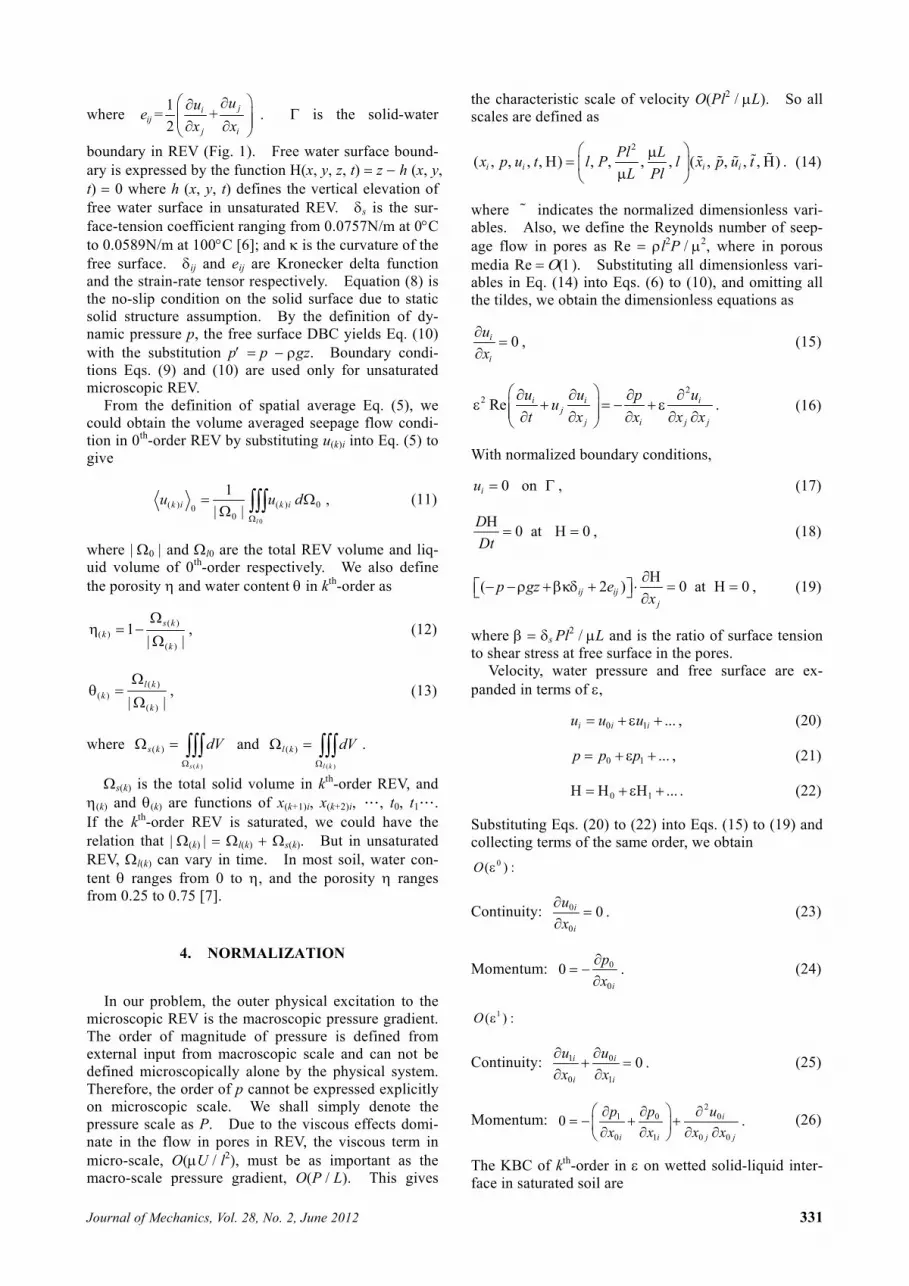
In this study, our goal is to derive the seepage flow condition in unsaturated soil under static solid structure. We consider the pores in soil are large enough for water to form a free surface (Fig. 1). Besides, solids itself in soil is assumed to be rigid, and water is considered in-compressible. If solid structure is stationary, we only need the governing equations for water, which are the continuity and Navier-Stokes equations.
0 , , , ,i
i
ui j x y z
x
(6)
2
, , , ,i i ij
j i j j
u u p uu i j x y z
t x x x x
(7)
where p p gz. and are the density and dy-namic viscosity of water, which are all constants. g is the gravitational acceleration. p is dynamic pressure where p is total pressure.
For boundary conditions, we need them for different scales. At microscopic scale, there are kinematic boundary conditions (KBC) at free surface and solid-water interface, and a dynamic boundary condi-tion (DBC) at free surface.
0 on , , , ,iu i j x y z (8)
0 at free surface
( , , , ) ( , , ) 0 ,
D
Dtx y z t z h x y t
(9)
( ) 2 0 at free surface
0 , , , ,
s ij ijj
p gz ex
i j x y z
(10)
Fig. 1 Definition of free surface of water, solid and solid-liquid boundary in the REV. All bounda-ries and free surface are three dimensional
Journal of Mechanics, Vol. 28, No. 2, June 2012 331
where 1
= +2
jiij
j i
uue
x x
. is the solid-water
boundary in REV (Fig. 1). Free water surface bound-ary is expressed by the function H(x, y, z, t) z h (x, y, t) 0 where h (x, y, t) defines the vertical elevation of free water surface in unsaturated REV. s is the sur-face-tension coefficient ranging from 0.0757N/m at 0C to 0.0589N/m at 100C [6]; and is the curvature of the free surface. ij and eij are Kronecker delta function and the strain-rate tensor respectively. Equation (8) is the no-slip condition on the solid surface due to static solid structure assumption. By the definition of dy-namic pressure p, the free surface DBC yields Eq. (10) with the substitution p p gz. Boundary condi-tions Eqs. (9) and (10) are used only for unsaturated microscopic REV.
From the definition of spatial average Eq. (5), we could obtain the volume averaged seepage flow condi-tion in 0th-order REV by substituting u(k)i into Eq. (5) to give
0
( ) ( ) 000
1,
| |l
k i k iu u d
(11)
where | 0 | and l0 are the total REV volume and liq-
uid volume of 0th-order respectively. We also define the porosity and water content in kth-order as
( )( )
( )
1 ,| |
s kk
k
(12)
( )( )
( )
,| |
l kk
k
(13)
where ( )
( )
s k
s k dV
and ( )
( )
l k
l k dV
.
s(k) is the total solid volume in kth-order REV, and
(k) and (k) are functions of x(k+1)i, x(k+2)i, …, t0, t1…. If the kth-order REV is saturated, we could have the relation that | (k) | l(k) s(k). But in unsaturated REV, l(k)
can vary in time. In most soil, water con-tent ranges from 0 to , and the porosity ranges from 0.25 to 0.75 [7].
4. NORMALIZATION
In our problem, the outer physical excitation to the microscopic REV is the macroscopic pressure gradient. The order of magnitude of pressure is defined from external input from macroscopic scale and can not be defined microscopically alone by the physical system. Therefore, the order of p cannot be expressed explicitly on microscopic scale. We shall simply denote the pressure scale as P. Due to the viscous effects domi-nate in the flow in pores in REV, the viscous term in micro-scale, O(U / l2), must be as important as the macro-scale pressure gradient, O(P / L). This gives
the characteristic scale of velocity O(Pl2 / L). So all scales are defined as
2
( , , , , ) , , , , ( , , , , ) .i i i i
Pl Lx p u t l P l x p u t
L Pl
(14)
where indicates the normalized dimensionless vari-ables. Also, we define the Reynolds number of seep-age flow in pores as Re l2P / 2, where in porous media Re . Substituting all dimensionless vari-ables in Eq. (14) into Eqs. (6) to (10), and omitting all the tildes, we obtain the dimensionless equations as
0 ,i
i
u
x
(15)
22 Re .i i i
jj i j j
u u p uu
t x x x x
(16)
With normalized boundary conditions,
0 on ,iu (17)
0 at 0 ,D
Dt
(18)
( 2 ) 0 at 0 ,ij ijj
p gz ex
(19)
where s Pl2 / L and is the ratio of surface tension to shear stress at free surface in the pores.
Velocity, water pressure and free surface are ex-panded in terms of ,
0 1 ... ,i i iu u u (20)
0 1 ... ,p p p (21)
0 1 ... . (22)
Substituting Eqs. (20) to (22) into Eqs. (15) to (19) and collecting terms of the same order, we obtain
0( ) :O
Continuity: 0
0
0 .i
i
u
x
(23)
Momentum: 0
0
0 .i
p
x
(24)
1( ) :O
Continuity: 1 0
0 1
0 .i i
i i
u u
x x
(25)
Momentum: 2
1 0 0
0 1 0 0
0 .i
i i j j
p p u
x x x x
(26)
The KBC of kth-order in on wetted solid-liquid inter-face in saturated soil are
332 Journal of Mechanics, Vol. 28, No. 2, June 2012
0 1 ... 0 for .i i iu u x (27)
In unsaturated soil, KBC of different orders at free sur-face are
0( ) :O
0 00 0 0
0 0
0 , 0 .jj
u z ht x
(28)
1( ) :O
1 1 0 0 0 00 1 1
0 0 1 1 0 0
0 0
0 ,
0 .
ii i
i i i
uu u
t x x t z xz h
(29)
Dynamic boundary conditions at free surface are 0( ) :O
20 0
0 0 0,00 0 0
0 0
2( ) 0 ,
0 .
ijk k j
p gz ex x x
z h
(30)
1( ) :O
20 1 0
0 0 0,00 0 0 1
2 21 0
1 10 0 1 0
01,0 0,1
0
1 0 1 001
0 0 0 0
2( )
2( ) 2( )
2
ij ijk k j j
k k k k
ij ij ijj
i j
j i
p gz ex x x x
p gzx x x x
e ex
h u h up
z z x x
0
0
0 0
0 ,
0 ,
jx
z h
(31)
where ,( ) mi niij m n
nj mj
u ue
x x
. Equations (23) to (31)
are all the equations and boundary conditions needed in the present problem.
5. UNSTEADY FLOW IN UNSATURATED SOIL
In the whole solid-water mixture, there must be sat-urated and unsaturated REV. We first derive the flow condition for saturated REV, and then continue to un-saturated REV. From Eq. (24), we obtain
0 0 1 2( , , ...., ) .i ip p x x t (32)
This implies 0th-order pressure depends on macroscopic pressure effect for 0th-order REV. To solve u0i, we combine Eq. (32) with Eq. (26) to obtain
20 1 0
1 2 0 1 21 0 0 0
( , , ...) ( , , , ...) ,ii i i i i
i i j j
p p ux x x x x
x x x x
(33)
where the two terms on RHS of Eq. (33) depends on microscopic variable xoi
and higher order macroscopic variables x1i. But the LHS of Eq. (33) only depends on macroscopic variables. Therefore, LHS simply equals a constant under the variable x0i. So Eq. (33) is a linear equation in x0i, and the two terms on RHS are linearly related to the LHS term p0 / x1i. It is also proved from Auriault [4] and Mei and Auriault [8] that the solution form of u0i and p1
from Eq. (33) can be formally represented by
0 00 1 1
1 1
and ,i ij jj j
p pu K p A p
x x
(34a,b)
due to the linearity of Eq. (33). Kij and Aj are the 2nd and 1st-order tensors representing the geometrical prop-erties in the 0th-order REV, and they depend on micro-scopic variables, x0i. 1p
is the function of x1i, x2i, ,
t, and is a constant representing macroscopic pressure effect for 0th-order pressure. Physically Kij can be regarded as hydraulic conductivity. Substituting Eqs. (34a) and (34b) into Eqs. (23) and (26), we obtain
0
0 ,ij
i
K
x
(35)
2
0 0 0
,j ijij
i k k
A K
x x x
(36)
and with the assumption that macroscopic pressure gra dient is not zero, p0 /x1i 0; otherwise, the solution would be trivial. So that boundary conditions for wa-ter in saturated REV become
0 for .ij iK x (37)
For unsaturated REVs, by substituting Eqs. (34a) and (34b) into Eqs. (28) and (29), the free surface boundary conditions become
0 0 0
0 1 0
0 ,jkk j
pK
t x x
(38)
20 0 0
0 0 20 0 1 00
0 .jk ik
i j k jk
K K pp gz
x x x xx
(39)
Equations (35) to (37) are a boundary-value-problem for solving Kij and Aj in saturated REV. For specific cases such as sample formed with many identical glass balls, it is possible to define and then solve the whole set of equations. However, generally it is difficult to define the solid boundary in the microscopic REV without any knowledge for the solid structure. Due to the complex composition of heterogeneous materials in nature, one often obtain Kij and Aj through experimental or computational methods [9].
Journal of Mechanics, Vol. 28, No. 2, June 2012 333
In saturated REV, substituting Eq. (34a) into Eq. (25) and applying ensemble average in a saturated REV, we find
0
1 00 0
0 0 1 1
10 .
| |l
iij
i i j
u pd K
x x x
(40)
Using Gauss theorem to the first term on LHS of Eq. (40), we obtain
01 0
0 1 1
1,
| |REV
REV i i iji jS
pQ u n dS K
x x
(41)
where QREV is averaged net volume flux for a REV; SREV
represents all the wet surfaces of REV and depends on microscopic variables x0i; u1i ni is the normal volume flux through the saturated REV surfaces;
0ijK is the averaged hydraulic conductivity in microscopic REV, and it can be regarded as the representative hydraulic conductivity in the macro-scale. Equation (41) only depends on macroscopic variables.
Since solid matrix is assumed to be rigid and fixed spatially, the net total volume flux for a saturated REV through all control surfaces must be zero, so
0 .REV
i i
S
u n dS (42)
By substituting the perturbed velocity, Eq. (20), into Eq. (42), we find
20 1 ( ) 0 .
REV REV
i i i i
S S
u n dS u n dS O (43)
From the principle of perturbation theory, terms of dif-ferent orders are independent. So integrations at dif-ferent orders in Eq. (43) must all be zero. This implies that QREV in Eq. (41) in saturated REV is also zero. Furthermore, if the soil is isotropic and homogeneous on the macro-scale, we could simplify
0ijK to Kij, where K is a constant. With these conditions, Eq. (41) becomes
2
0
1 1
0 .i i
p
x x
(44)
Equation (44) is the macroscopic averaged 1st-order continuity in saturated, isotropic and homogeneous soil. The result is the same as in Mei and Auriault [8]. If we have macroscopic boundary conditions of some specified problem, we could apply these boundary con-ditions to Eq. (44) to obtain the pressure distribution p0. Then substituting this solved p0
back to Eq. (34a), we could obtain microscopic velocity of seepage condition of the specified problem.
For unsaturated REV, we apply ensemble average to Eq. (23) to yield
0
0 00
0 0 00
10 .
| |l
i i
i i
u ud
x x
(45)
With Divergence theorem, Eq. (45) becomes
00 0
0 00
10 ,
| |i
i ii S
uu n dS
x
(46)
where S is the boundary surface of water in 0th-order REV. There are three different kinds of boundaries. They are water-solid interface S, water-air interface SH and water area on boundary of a REV SREV, respectively. Separating RHS of Eq. (46) for different kinds of inter-faces, we obtain
REV
0 0 0 0 0 0
0 0 0 ,
i i i i i i
S S S
i i
S
u n dS u n dS u n dS
u n dS
(47)
where ni is the unit normal vector of each surface. With no-slip condition, the last term on RHS of Eq. (47) is zero. Before discussing the first term in RHS of Eq. (47), we divide the free surface kinematic boundary condition, Eq. (38), by | 0 H0 | to yield
0 0
0 0 0 1
10 ,
| |jk j
k
pK n
t x
(48)
where 0
0 0 0
1
| |j
j
nx
is unit normal vector of free
surface. The subscript zero of the operator 0 means taking gradient with respect to 0th-order spatial inde-pendent variables x0, y0 and z0. From Eq. (34a), the second term in Eq. (48) is u0i ni and physically is the normal flux at the free surface. So it can be expressed as
00
0 0 0
1, on .
| |i iu n S
t
(49)
Finally, substituting Eq. (49) into Eq. (47), we obtain
REV
00 0 0
0 0 0
10 .
| |i i
S S
dS u n dSt
(50)
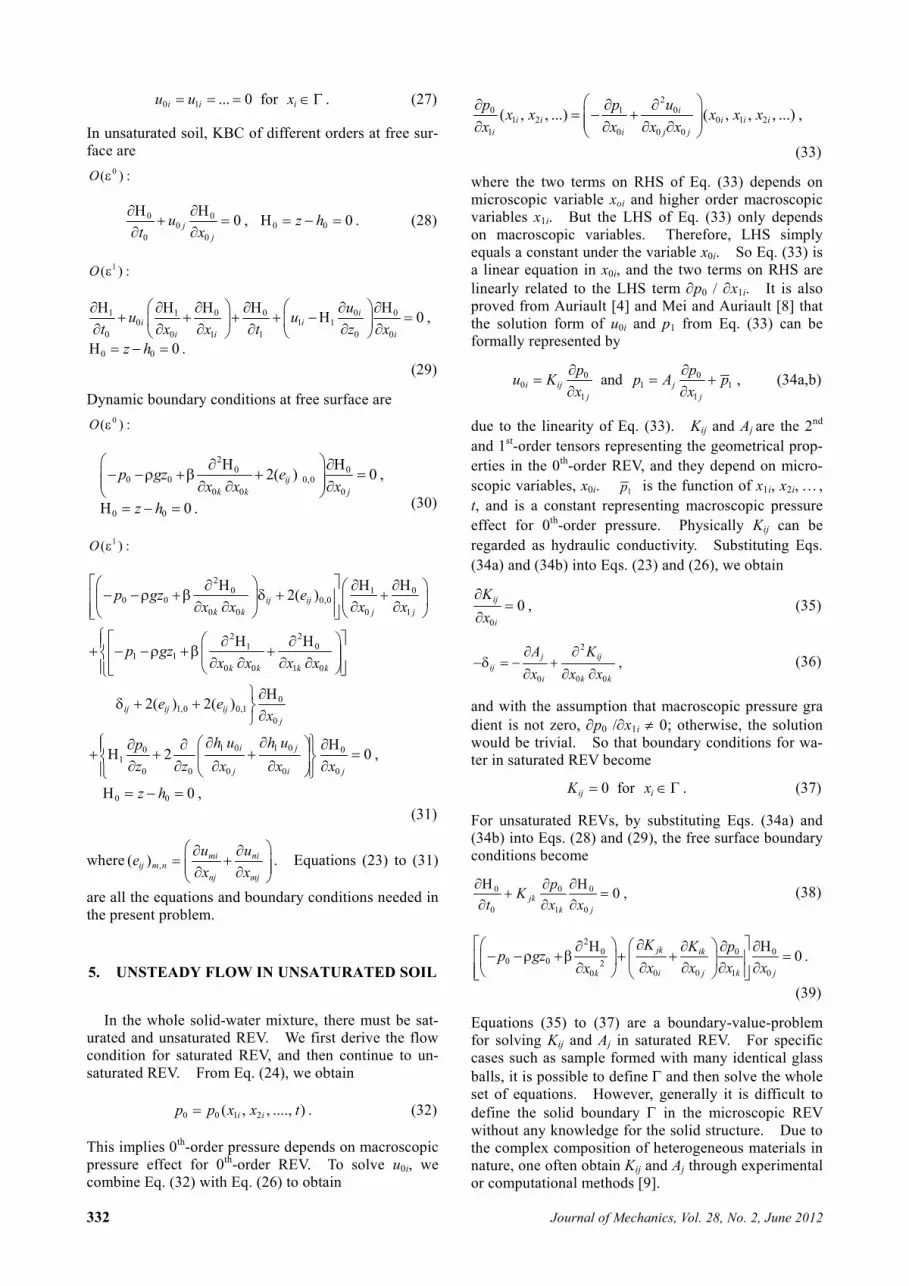
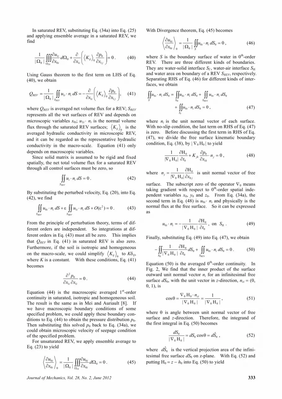
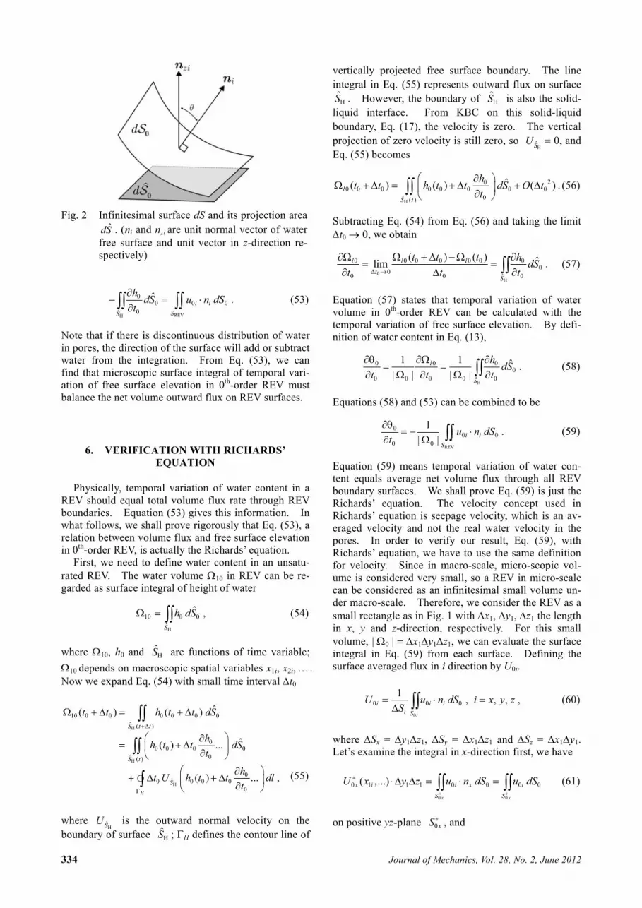
Equation (50) is the averaged 0th-order continuity. In Fig. 2, We find that the inner product of the surface outward unit normal vector ni for an infinitesimal free surface dS0, with the unit vector in z-direction, nzi
(0, 0, 1), is
0 0
0 0 0 0
1cos ,
| | | |zin
(51)
where is angle between unit normal vector of free surface and z-direction. Therefore, the integrand of the first integral in Eq. (50) becomes
00 0
0 0
ˆcos ,| |
dSdS dS
(52)
where 0ˆdS
is the vertical projection area of the infini-
tesimal free surface dS0 on z-plane. With Eq. (52) and putting H0 z h0 into Eq. (50) to yield
334 Journal of Mechanics, Vol. 28, No. 2, June 2012
Fig. 2 Infinitesimal surface dS and its projection area ˆdS . (ni and nzi are unit normal vector of water
free surface and unit vector in z-direction re-spectively)
REV
00 0 0
0ˆ
ˆ .i i
SS
hdS u n dS
t
(53)
Note that if there is discontinuous distribution of water in pores, the direction of the surface will add or subtract water from the integration. From Eq. (53), we can find that microscopic surface integral of temporal vari-ation of free surface elevation in 0th-order REV must balance the net volume outward flux on REV surfaces.
6. VERIFICATION WITH RICHARDS’ EQUATION
Physically, temporal variation of water content in a REV should equal total volume flux rate through REV boundaries. Equation (53) gives this information. In what follows, we shall prove rigorously that Eq. (53), a relation between volume flux and free surface elevation in 0th-order REV, is actually the Richards’ equation.
First, we need to define water content in an unsatu-rated REV. The water volume 10 in REV can be re-garded as surface integral of height of water
10 0 0
ˆ
ˆ ,S
h dS
(54)
where 10, h0 and S are functions of time variable;
10 depends on macroscopic spatial variables x1i, x2i, . Now we expand Eq. (54) with small time interval t0
10 0 0 0 0 0 0
ˆ ( )
00 0 0 0
0ˆ ( )
0ˆ0 0 0 0
0
ˆ( ) ( )
ˆ( ) ...
( ) ... ,H
S t t
S t
S
t t h t t dS
hh t t dS
t
ht U h t t dl
t
(55)
where S
U
is the outward normal velocity on the boundary of surface S ; H defines the contour line of
vertically projected free surface boundary. The line integral in Eq. (55) represents outward flux on surface S . However, the boundary of S is also the solid- liquid interface. From KBC on this solid-liquid boundary, Eq. (17), the velocity is zero. The vertical projection of zero velocity is still zero, so
SU
0, and
Eq. (55) becomes
200 0 0 0 0 0 0 0
0ˆ ( )
ˆ( ) ( ) ( ) .l
S t
ht t h t t dS O t
t
(56)
Subtracting Eq. (54) from Eq. (56) and taking the limit t0 0, we obtain
0
0 0 0 0 0 0 00
00 0 0ˆ
( ) ( ) ˆlim .l l l
tS
t t t hdS
t t t
(57)
Equation (57) states that temporal variation of water volume in 0th-order REV can be calculated with the temporal variation of free surface elevation. By defi-nition of water content in Eq. (13),
0 0 00
0 0 0 0 0ˆ
1 1 ˆ .| | | |
l
S
hdS
t t t
(58)
Equations (58) and (53) can be combined to be
REV
00 0
0 0
1.
| |i i
S
u n dSt
(59)
Equation (59) means temporal variation of water con-tent equals average net volume flux through all REV boundary surfaces. We shall prove Eq. (59) is just the Richards’ equation. The velocity concept used in Richards’ equation is seepage velocity, which is an av-eraged velocity and not the real water velocity in the pores. In order to verify our result, Eq. (59), with Richards’ equation, we have to use the same definition for velocity. Since in macro-scale, micro-scopic vol-ume is considered very small, so a REV in micro-scale can be considered as an infinitesimal small volume un-der macro-scale. Therefore, we consider the REV as a small rectangle as in Fig. 1 with x1, y1, z1 the length in x, y and z-direction, respectively. For this small volume, | 0 | x1y1z1, we can evaluate the surface integral in Eq. (59) from each surface. Defining the surface averaged flux in i direction by U0i.
0
0 0 0
1, , , ,
i
i i ii S
U u n dS i x y zS
(60)
where Sx = y1z1, Sy = x1z1 and Sz = x1y1. Let’s examine the integral in x-direction first, we have
0 0
0 1 1 1 0 0 0 0( ,...)x x
x i i x i
S S
U x y z u n dS u dS
(61)
on positive yz-plane 0xS , and
Journal of Mechanics, Vol. 28, No. 2, June 2012 335
0 0
0 1 1 1 0 0 0 0( ,...)x x
x i i x i
S S
U x y z u n dS u dS
(62)
on negative yz-plane 0xS . So the net flux in x-direc-
tion is
0 0
0 0 0 1 1 1 0 1 1 1
0 1 1 1 1 2 0 1
01 1 1 1
1
( ,...) ( ,...)
( , , , , ..) ( ,...)
( ) .
x x
i x x i x i
S S
x i x i
x
u n dS U x y z U x y z
U x x y z x U xU
x y z O xx
Then
0
00 0 1 1 1 1
1
00 1
1
( )
| | ( ) ,
x
xi x
S
x
Uu n dS x y z O x
x
UO x
x
(63)
where | 0 | x1y1z1. Similarly, in y and z-di-rection, we could also obtain
0
00 0 0 1
1
| | ( ) ,y
yi y
S
Uu n dS O y
y
(64)
and
0
00 0 0 1
1
| | ( ) .z
zi z
S
Uu n dS O z
z
(65)
With Eqs. (63) to (65) and omitting small terms, Eq. (59) becomes
0 0
0 1
, , , .i
i
Ui x y z
t x
(66)
Finally, the velocity solution, Eq. (34a), is used in Eq. (66) to reach
0
0 00
0 1 1
1, , , .,
i
ij ii i jS
pK n dS i j x y z
t x S x
(67)
Defining
0
0
1ˆ
j
i jii S
K K dSS
as the surface averaged micro hydraulic conductivity Kij in three directions under macro-scale. Equation (67) becomes
0 0
0 1 1
ˆ .ii i
pK
t x x
(68)
Equation (68) interprets the temporal variation of water content in a REV is equivalent to negative divergence of macroscopic pressure gradient multiplying by hy-draulic conductivity. Equation (68) is exactly the Richards’ equation [5].
7. CONCLUSION AND DISCUSSION
Without any constitutive assumption for unsaturated solid-liquid mixture, we successfully use homogeniza-tion theory to obtain the equation governs water content variation. The derived result is proved to be the Rich-ards’ equation. From this result, we can conclude that homogenization theory can be used to describe water motion in the problem of unsteady and unsaturated sol-id-liquid mixtures. Therefore, this result can be a sound foundation for studying the initiation of solids under unsteady and unsaturated solid-liquid mixture.
ACKNOWLEDGEMENTS
We gratefully appreciate National Science Council (Grant No. NSC 96-2625-Z-002-006-MY3) in Taiwan for supporting this research. Valuable and useful comments and suggestions from reviewers are also ac-knowledged.
REFERENCES
1. Ancey, C., “Plasticity and Geophysical Flows: A Review,” Journal of Non-Newtonian Fluid Me-chanics, 142, pp. 435 (2007).
2. Iverson, R. M., Reid, M. E. and LaHusen, R. G., “Debris-Flow Mobilization from Landslide,” An-nual Review of Earth and Planetary Sciences, 25, pp. 85138 (1997).
3. Iverson, R. M., “Landslide Triggering by Rain Infiltration,” Water Resources Research, 36, pp. 18971910 (2000).
4. Auriault, J.-L., “Heterogenous Medium. is an Equivalent Macroscopic Description Possible?,” International Journal of Engineering Science, 29, pp. 785795 (1991).
5. Richards, L. A., “Capillary Conduction of Liquids Through Porous Mediums,” Physics, 1, pp. 318333 (1931)
6. White, F. M., Viscous Fluid Flow, 3rd Ed., McGraw Hill (2006).
7. Chow, V. T., Maidment, D. R. and Mays, L. W., Applied Hydrology, McGraw-Hill (1998).
8. Mei, C. C. and Auriault, J.-L., “The Effect of Weak Inertia on Flow Through a Porous Medium,” Journal of Fluid Mechanics, 222, pp. 647663 (1991).
9. Mei, C. C. and Vernescu, B., Homogenization Methods for Multiscale Mechanics, World Scien-tific (2010).
(Manuscript received January 20, 2011, accepted for publication October 13, 2011.)