RIVER RESEARCH AND APPLICATIONS

River Res. Applic. (2011)

Published online in Wiley Online Library(wileyonlinelibrary.com) DOI: 10.1002/rra.1597

LANDSCAPE-LEVEL MODEL TO PREDICT SPAWNING HABITAT FOR LOWERCOLUMBIA RIVER FALL CHINOOK SALMON (ONCORHYNCHUS TSHAWYTSCHA)†

D. SHALLIN BUSCH,a* MINDI SHEER,a KELLY BURNETT,b PAUL MCELHANYa and TOM COONEYc

a Northwest Fisheries Science Center, National Oceanic and Atmospheric Administration, 2725 Montlake Blvd. E, Seattle, WA 98112, USAb USDA Forest Service, Pacific Northwest Research Station, 3200 SW Jefferson Way, Corvallis, OR 97331, USA

c Northwest Fisheries Science Center, National Oceanic and Atmospheric Administration, 1201 NE Lloyd Blvd., Suite 1001, Portland, OR 97232, USA

ABSTRACT

We developed an intrinsic potential (IP) model to estimate the potential of streams to provide habitat for spawning fall Chinook salmon(Oncorhynchus tshawytscha) in the Lower Columbia River evolutionarily significant unit. This evolutionarily significant unit is a threatenedspecies, and both fish abundance and distribution are reduced from historical levels. The IP model focuses on geomorphic conditions that leadto the development of a habitat that fish use and includes three geomorphic channel parameters: confinement, width and gradient. We foundthat the amount of potential habitat for each population does not correlate with current, depressed, total population abundance. However,reaches currently used by spawners have high IP, and IP model results correlate well with results from the complex Ecosystem Diagnosisand Treatment model. A disproportionately large amount of habitat with the best potential is currently inaccessible to fish because of an-thropogenic barriers. Sensitivity analyses indicate that uncertainty in the relationship between channel width and habitat suitability has thelargest influence on model results and that model form influences model results more for some populations than for others. Published in2011 by John Wiley & Sons, Ltd.

key words: Chinook salmon; habitat modeling; intrinsic potential; digital elevation model; Lower Columbia River (USA)

Received 8 June 2011; Revised 16 August 2011; Accepted 18 August 2011

INTRODUCTION

Chinook salmon (Oncorhynchus tshawytscha) is an anadro-mous species with a spawning distribution around the PacificRim from Russia’s Kamchatka peninsula to California’sCentral Valley. In the western USA, it is an ecologicallyand culturally important species (Lichatowich, 1999; Gendeet al., 2002; Moore, 2006). Dams and other barriers(e.g. culverts) on waterways, urbanisation and agricultural,forestry, hatchery and fishery practices have negativelyaffected population abundances and freshwater habitats ofChinook salmon over the past two centuries (Fulton, 1968;Lichatowich, 1999; Sheer and Steel, 2006). In response toboth declining abundances and habitat alterations, the currentspawning distribution of many Chinook salmon populationshas contracted from its historical state (Nickelson andLawson, 1998; McElhany et al., 2007). Consequently, nineevolutionarily significant units (ESUs; Waples, 1991) ofChinook salmon have been listed under the US EndangeredSpecies Act as either threatened or endangered. This has

*Correspondence to: D. S. Busch, Northwest Fisheries Science Center, Na-tional Oceanic and Atmospheric Administration, 2725 Montlake Blvd. E,Seattle, WA 98112, USA.E-mail: Shallin.Busch@noaa.gov†This article is a US Government work and is in the public domain in theUSA.

Published in 2011 by John Wiley & Sons, Ltd.

prompted the increased regulation of land use and fishingactivities and the development of recovery plans designed toprotect and recover the listed ESUs.The protection and the restoration of listed salmon ESUs

rely, in part, on the knowledge of historical fish distributionand habitat quality. Historical data are patchy, limited to thelargest waterways and subject to much regional variabilityin amount, type and quality (Myers et al., 2006). Currentfish distribution is an insufficient proxy for historical distri-bution because of declines in fish abundance, habitat qualityand habitat accessibility. Researchers have developed re-gional models to identify areas with high potential as usablesalmonid habitat and to estimate how much habitat was his-torically available for fish. Burnett et al. (2007) recently for-malised a model, called intrinsic potential (IP), to estimatethe potential of stream reaches to act as habitat for salmo-nids. IP models can be comprehensively applied to largeregions because they use relatively high-resolution, spatiallyextensive digital elevation and climate data that are publiclyavailable. They differ from previous fish habitat suitabilitymodels (e.g. McMahon, 1982; Schamberger et al., 1982;Lee and Terrell, 1987) in attempting to estimate the potentialto provide habitat and not the actual condition of habitat. IPmodels yield quantitative estimates of potential habitat byevaluating geomorphic characteristics that shape fine-scale

D. S. BUSCH ET AL.

habitat features off which fish cue. Published IP modelsexist for the Oregon Coast coho salmon (Oncorhynchuskisutch) and steelhead (Oncorhynchus mykiss) ESUs(Burnett et al., 2007) and the Northern CaliforniaChinook and coho salmon and steelhead ESUs (Agrawalet al., 2005). Results from IP models have been used for avariety of management purposes, including defining popu-lation boundaries of coho salmon and evaluating culvertrepair and replacement programs in Oregon (Dent et al.,2005; Lawson et al., 2007).Regulators, managers, policy makers and biologists con-

cerned with the Lower Columbia River fall Chinook sal-mon, a threatened ESU, have shown great interest in IPmodels given their ability to generate region-wide estimatesof habitat potential (Sheer et al., 2009). To meet this man-agement need, here we develop an IP model to estimate his-torical potential of habitat for the Lower Columbia River fallChinook salmon ESU, providing an example of soundmodel development and testing. Because we lack historicalfish density data with which to validate the model, we com-pare results of our IP model with three types of data: (i)current population abundance, (ii) field and expert-opinion-based maps on the current distribution of spawningfall Chinook salmon in Washington and Oregon and (iii)results from the Ecosystem Diagnosis and Treatment(EDT) model (Blair et al., 2009), a complex model thatpredicts salmon performance primarily as a function offreshwater habitat and is used by many salmon recoveryplanners in the Pacific Northwest to prioritise habitat restor-ation and preservation actions.

METHODS

Study area

The Lower Columbia River Chinook ESU consists of 22independent populations of Lower Columbia RiverChinook salmon (Myers et al., 2006). It encompasses23 042 km2 of watershed habitat, a major mainstem riverand estuary (Columbia River), and a series of manmadereservoirs. Fall-run Chinook salmon in the ESU carry outmost of their freshwater life cycle in estuaries and the down-stream portions of waterways near estuaries, mostly in main-stems and tributaries off mainstems (Myers et al., 2006);they largely avoid the upstream extents of accessible water-ways used by spring-run Chinook salmon (Healey, 1991).Because of this difference between runs, we developed theIP model only for fall Chinook salmon, the primary life-history type in the ESU (Myers et al., 2006). We focussedmodel development on tributary watersheds only, excludingthe mainstem Columbia River and its estuary from consider-ation. We chose to model spawning habitat because more isknown about the habitat preferences of spawners than of

Published in 2011 by John Wiley & Sons, Ltd.

rearing juveniles and because rearing juveniles use so manydifferent habitat types, including portions of the mainstemColumbia. However, the overlap in the freshwater habitatchosen by spawners and juveniles is likely great (Healey,1991), especially when considered at the reach scale.

Spawner stream networks

We modelled the total stream network (1:24 000) in theLower Columbia River Chinook ESU and its associatedgeomorphic features from 10m drainage-enforced digitalelevation models, using techniques that are well describedin the literature (Jenson and Domingue, 1988; Tarbotonet al., 1991; Montgomery and Foufoula-Georgiou, 1993;Clarke and Burnett, 2003; Miller, 2003; Clarke et al., 2008;M. Sheer, D. S. Busch, T. Beechie, D. Miller, K. Burnett,in preparation). From the modelled total stream network,we created two stream networks to represent the physicalhabitat available to spawning fall Chinook salmon: thehistorical spawner stream network, which includes thehabitat fish had access to before anthropogenic barriers tofish passage (e.g. dams), and the current spawner streamnetwork, which includes all habitat in the historical spawnerstream network minus those areas blocked by anthropogenicbarriers. The data set of anthropogenic barriers we used wasdeveloped by Sheer and Steel (2006) and updated with morerecent barriers data sources (Oregon Department of Fish andWildlife, 2009; S. VanderPloeg, Washington Department ofFish and Wildlife, Vancouver, Washington, personal com-munication, 2009). We identified the extent of the historicalspawner stream network by incorporating boundaries that re-flect physical barriers to spawners (McElhany et al., 2003;Myers et al., 2006; Sheer and Steel, 2006; M. Sheer, D. S.Busch, T. Beechie, E. Gilbert, D. Miller, in preparation).The lower and upper extents of the historical spawner

stream network were refined using two exclusion thresholds:tidal influence and elevation. The tidal influence thresholdcaptures spawners’ aversion to laying eggs in brackish water,locations with substantial tidally driven water level fluctua-tions (near the mouth of the Columbia River), or highly silteddepositional floodplains. We defined tidally influencedreaches as those (i) ≤3.5m above mean sea level within theColumbia River tidal reversal zone (lower 95 km), (ii) in thetributary mouth adjacent to the Columbia River estuaryand (iii) in the floodplain and downstream of the lowermostpoints of documented (current) spawning (Sherwood andCreager, 1990; Mikhailova, 2008; J. Burke, NOAA North-west Fisheries Science Center, Seattle, Washington, un-published data; D. Rawding, Washington Department ofFish and Wildlife, Vancouver, Washington, unpublisheddata). We verified this lower-limit threshold against statemaps of the distribution of spawning fall Chinook salmonand specific stream locations demarked as a documented

River Res. Applic. (2011)

DOI: 10.1002/rra

INTRINSIC POTENTIAL MODEL FOR SPAWNING FALL CHINOOK SALMON

lower limit to spawning (Washington Department of Fish andWildlife, 2006; Oregon Department of Fish and WildlifeNatural Resource Inventory Management Project, 2009; S.VanderPloeg, Washington Department of Fish and Wildlife,Vancouver, Washington, personal communication, 2009).The historical upper elevation threshold captures fall

Chinook spawners’ use of reaches lower in tributary water-sheds and was applied because our initial map overpredictedthe upper extent of habitat historically accessible (Fulton,1968; Fulton, 1970; Washington Department of Fish andWildlife, 2006; D. Rawding, Washington Department ofFish and Wildlife, Vancouver, Washington, personal com-munication, 2009; J. Rodgers, Oregon Department of Fishand Wildlife, Portland, Oregon, personal communication,2009; Oregon Department of Fish and Wildlife Natural Re-source Inventory Management Project, 2009). By examin-ing historical information and general limits to currentdistribution in unblocked streams, we found that the eleva-tion contour of 350m best reflects the natural uppermost ex-tent of fall Chinook salmon.The factors that limit the distribution of fall-run Chinook

salmon to the lower portions of watersheds are currently un-known but are potentially related to the degree of sexual ma-turity when fish enter freshwater systems and access toupstream areas. We considered elevation as an acceptablesurrogate for the variety of factors that influence the distri-bution of fall-run Chinook salmon. We limited the upper-most extent of the spatial distribution of spawning fallChinook also by natural waterfalls (typically ≥3–4.6m tall;Sheer and Steel, 2006), reach gradients that are too steep forfish to navigate beyond (>16%; Washington Department ofFish and Wildlife, 2000; Myers et al., 2006; Steel et al.,2007) and the minimum accessible channel width for fallChinook salmon (inaccessible reaches are <4m duringseasonal low flow). We exclude one natural waterfall in MillCreek that was destroyed in the 1950s to allow fish passage.The locations of natural barriers were checked against thepublished and the unpublished (Washington state only) statedistributions of spawning fall Chinook (Washington Depart-ment of Fish and Wildlife, 2006; Oregon Department ofFish and Wildlife Natural Resource Inventory ManagementProject, 2009).Our historical spawner stream network includes lakes,

ponds and reservoirs—features that fall Chinook salmontypically do not use for spawning (Healey, 1991). We didnot attempt to estimate the historical condition of reachescurrently in manmade lakes and reservoirs. Instead, we as-sume these have the highest potential to provide spawninghabitat. Although perfect potential may not fully reflect his-torical reality, our approach is precautionary because it doesnot discount areas that may have been suitable for spawners.Natural lakes and ponds were treated the same way, and al-though we know these are unsuitable for spawning, they

Published in 2011 by John Wiley & Sons, Ltd.

make up a small portion of the stream network (23 kmacross all watersheds, an average of 2 km per watershed).Stream reach is the unit of analysis for the IP model. We

divided our stream network into reaches using an algorithmdeveloped by Miller (2003), which segments streams intogeomorphically homogeneous reaches based on tributaryjunctions and gradient transitions. Reach length increaseslower in the watershed due to reduced geomorphic variation.The mean and the median length of the reaches in the histor-ical spawner stream network are 121 and 84m, respectively(range, 10–3197m). We estimated the channel width ofeach reach using a regression developed by Steel and Sheer(2003); this regression uses basin drainage area (km2) andmean annual precipitation (mm) as predictors of channelwidth (Miller et al., 1996; Davies et al., 2007; Hall et al.,2007). Large mainstem channels are not well characterisedby the regression, so we estimated their widths manuallyusing topographic distinctions from the digital elevationmodels and other hydrologic data sources. The mean andthe median channel widths of the reaches in the historicalspawner stream network are 12 and 6m, respectively (range,4–1200m; the length of historical spawner stream networkwith channel width x< 10m= 2387 km, 10m< x< 20m=871 km, 20m< x< 100m= 777 km, x> 100m= 96 km).

IP model

Our IP model was informed by IP models for salmonidsfrom California and Oregon (Agrawal et al., 2005; Burnettet al., 2007) and other broad-scale models that predict habi-tat suitability for Chinook salmon (Cooney et al., 2007;Steel et al., 2007). It characterises Chinook salmon spawn-ing habitat by three geomorphic variables: channel confine-ment, channel width and channel gradient. These variablesinfluence the physical processes that shape channel form.To relate these variables to fish use, we combined an under-standing of fluvial geomorphology with a series of assump-tions about the habitat features that Chinook salmon prefer:(i) mainstems (Healey, 1991), (ii) side channels (Beechieet al., 2006a, 2006b; Hall et al., 2007), (iii) pool–riffle andforced pool–riffle habitat (Montgomery et al., 1999) and(iv) gravel substrate (Healey, 1991). For each of the threegeomorphic channel variables, we defined specific pointsin the relationship between habitat characteristics and suit-ability score and interpolate between these along straightlines connecting the points (Figure S1). Channel confine-ment, width and gradient were modelled from 10-m digitalelevation models during the delineation of the modelledstream network, using methods detailed elsewhere (Clarkeand Burnett, 2003; Miller, 2003; Clarke et al., 2008; M.Sheer, D. S. Busch, T. Beechie, E. Gilbert, D. Miller, inpreparation). We used Spearman’s rank to test for

River Res. Applic. (2011)

DOI: 10.1002/rra

D. S. BUSCH ET AL.

correlation among model input variables, log transformingall data sets before analysis.

Channel confinement. Chinook salmon typically usecomplex channel forms for spawning (Geist and Dauble,1998). Channel confinement—the ratio of valley (e.g.floodplain) width to bankfull channel width—influencesthe types of channel that a stream can form, with higherratios having more complex channel forms (Beechie et al.,2006a; Cooney et al., 2007; Hall et al., 2007). Complexchannel forms are more likely to have side channel habitat,which contributes to succ\essful reproduction and thussuitability because of its importance during juvenilerearing (Beechie et al., 2006a). Channel confinementinfluences the interaction between surface and subsurfaceflows. When channels are complex, there is greaterpotential for interstitial flow pathways between surfacewater and hyporheic groundwater; microhabitat with highintergravel flow is preferred spawning habitat for salmon(Geist and Dauble, 1998; Poole et al., 2008). Variability inconstraint can benefit salmonids: the upwelling ofhyporheic groundwater into a channel is higher inunconfined reaches when upstream of confined reaches(Baxter and Hauer, 2000). Finally, unconstrained reachesare less prone to debris flows from hillslopes, reducing thepotential for a channel to scour (Montgomery andBuffington, 1997).The transition between confined and unconfined reaches

dominates the habitat suitability curve for channel

Table I. Relationship between channel confinement, width andgradient and habitat suitability score for the Lower ColumbiaRiver fall Chinook salmon IP model and relationships used in thesensitivity analysis

Model Sensitivity analysis

Value Score Value Score

Channel confinement <1 0 <1 01 0.25 1 0–0.75

5.06a 0–0.75>8.87 1 >4–8.87 1

Channel width (m) <4 0 0–5 0–0.2515–20 0.25–1

>20 1 >20 1

Channel gradient (%) <2 1 0 0.5–14–7 0.05 1–2 1

4–7 0.05–0.25>7 0 >7 0

aOnly used when the value from 4 to 8.87 is >5.06.

Published in 2011 by John Wiley & Sons, Ltd.

confinement (Table 1, Figure S1a). Evidence from the fieldsuggests that when valley confinement is greater than ap-proximately 4, channels are unconfined (Hall et al., 2007).However, data collected in the field differ from data on con-finement from digital elevation models (constrained: ratio5.06; unconstrained: ratio> 8.87; Clarke et al., 2008). Weused the modelled threshold for channel confinement,assigning the suitability score of 0.25 at the channel confine-ment ratio of one and the suitability score of one at the chan-nel confinement ratio of 8.87 and greater. This relationshipindicates that reaches with higher confinement values arelikely to provide higher-quality habitat for spawning fish.By definition, channel confinement cannot be less than 1.

Channel width. In general, fall Chinook salmon spawn inwide reaches that are complex and have side channels(Beechie et al., 2006a; Hall et al., 2007). Fall Chinooksalmon rarely spawn in small channels: field data fromwestern Washington suggest that fall Chinook spawning isinfrequent in reaches less than 3 to 5m wide (Montgomeryet al., 1999; Washington Department of Fish and Wildlife,2000; Washington Department of Fish and Wildlife, 2001;Beechie et al., 2006b; Steel et al., 2007). Spawning habitatsnear complex rearing habitat are likely to be the mostproductive. Such complex rearing habitats can develop inlarger channels that have the power to erode forestedfloodplains and thus migrate. When migrating channels arenot tightly confined by valley width, they form meandering,braided or island-braided reaches, off-channel ponds andoxbow lakes (Hall et al., 2007). Small channels lack thestream power to erode forested floodplains and to generatethese features (Beechie et al., 2006a).The habitat suitability curve for bankfull channel width

(Figure S1b) is defined by the break between channels thatare too small to migrate (<15m) and are wide enough to mi-grate (>20m; Beechie et al., 2006a). Large channels(>20m) are given a suitability score of one, and channelsuitability is assumed to decline with decreasing channelwidth. Channels ≤4 m wide are assumed unsuitable forspawners; this value is at the lower end of the range of chan-nel widths reported as suitable for spawners (WashingtonDepartment of Fish and Wildlife, 2000; Washington Depart-ment of Fish and Wildlife, 2001; Beechie et al., 2006b; Steelet al., 2007).

Channel gradient. Fall Chinook salmon spawn in gravel inpool–riffle and forced pool–riffle habitat (Geist and Dauble,1998; Montgomery et al., 1999). Reaches with pool–rifflemorphologies usually have gravel as bed material(Montgomery and Buffington, 1997), sufficient to supportspawning Chinook salmon. Reaches with gradientsbetween 0% and 1% are typically pool–riffle (Lunettaet al., 1997; Montgomery and Buffington, 1997). Withadequate large wood, channels between 1% and 2%

River Res. Applic. (2011)

DOI: 10.1002/rra

INTRINSIC POTENTIAL MODEL FOR SPAWNING FALL CHINOOK SALMON

gradient will be pool–riffle and forced pool–riffle (Lunettaet al., 1997; Montgomery and Buffington, 1997). Thepotential for forced pool–riffle habitats to form in wood-loaded channels extends to reaches with gradients up to 4%(Lunetta et al., 1997; Rapp and Abbe, 2003).Three points define the channel gradient habitat suitability

curve (Figure S1c). Given the model assumption that largewood was historically not a limiting factor in LowerColumbia watersheds, we deem that channels from 0% to2% gradient will form pool–riffle/forced pool–riffle habitatideal for spawning salmon (suitability score = 1). A gradientof 4% marks the upper boundary at which forced pool–rifflehabitat can form; we used this value as the point at whichhabitat suitability is at its lowest (0.05). Reaches with gradi-ents between 2% and 4% are of intermediate but decreasingsuitability. Chinook salmon have been found spawning inreaches up to 7% gradient (Montgomery et al., 1999; Sheerand Steel, 2006; Cooney et al., 2007), indicating that pock-ets of potential habitat can occur in high gradient reaches.We give channel gradients between 4% and 7% a very lowsuitability score (0.05; Hall et al., 2007).

Model form and output. We combined suitability scores forthe three model parameters using the geometric mean as perBurnett et al. (2007) and referred to the geometric mean asthe reach IP score [reach IP score = (channel confinementsuitability score � channel width suitability score �channel gradient suitability score)1/3]. For many analyses,reaches were grouped into five categories by their IPscore: very low (x≤ 0.2), low (0.2< x≤ 0.4), moderate(0.4< x≤ 0.6), high (0.6< x≤ 0.8) and very high(x> 0.8). We multiplied reach IP score with reach lengthto scale reach length by its potential, which we calledreach IP. Summing reach IP for all reaches in an area ofinterest determines the area’s IP: IP of area ofinterest =Σ(reach IP score � reach length). For example,historical population IP is calculated by summing the IP ofall reaches in the population’s historical spawner streamnetwork. To calculate the amount of high and very highpotential habitat available to a population, we consideredthe reaches with IP scores >0.6, and to calculate theamount of very high potential habitat available to apopulation, we considered reaches with IP scores >0.8.All values of length are expressed in kilometres.

Sensitivity analysis. We used a Monte Carlo approach toexplore the sensitivity of our model results to the form ofthe parameter suitability curves by varying the curvesacross a range consistent with an understanding about thehabitat use of spawning fish (Table 1, Figure S1). For eachparameter curve, we developed 1000 variants, with thelocation and suitability score of each inflection pointassigned as a random number from a uniform distributionwithin the bounds discussed in the next paragraph. Data

Published in 2011 by John Wiley & Sons, Ltd.

from all streams with Lower Columbia River fall Chinooksalmon populations were run through each model variant.To understand the influence of variation in each parametercurve on model output, we introduced variation to eachparameter curve singly, called a one-at-a-time (OAT)analysis (McElhany et al., 2010). We also introducedvariation to all parameter curves simultaneously. Theseexercises yield a distribution of IP estimates for theLower Columbia River fall Chinook salmon populationsthat incorporates a wider range of information on thegeomorphic conditions that produce habitat used byspawning fall Chinook salmon than the singular form of theIP model presented earlier.To conduct the sensitivity analysis, we imposed variation

on each parameter suitability curve as follows:

• Channel confinement. We explored uncertainty in the suit-ability of confined reaches and the breakpoint between un-confined and confined reaches (Table 1). To do the former,we varied the suitability of confined reaches from 0 to0.75. To do the latter, we varied the breakpoint for con-finement between values defined with field (4; Cooneyet al., 2007; Hall et al., 2007) and modelled data (8.87;Clarke et al. 2008) and defined an end point of constrainedreaches (5.06; Clarke et al., 2008).

• Channel width. Uncertainty in the suitability of narrowreaches was incorporated by varying the start point ofthe channel width curve and the suitability of the startpoint. We added an additional inflection point to bettercapture the intermediate suitability of reaches between15 and 20m (Beechie et al., 2006a).

• Channel gradient. Uncertainty in the suitability of <1%and 4% to 7% gradient reaches was incorporated by vary-ing their suitability scores. We varied the suitability of 0%gradient reaches from 0.5 to 1, which alters the start pointof the gradient suitability curve. Suitability scores forreaches between 4% and 7% are constant; we varied thisset point between 0.05 and 0.25.

We examined the sensitivity of IP model outputs to itsinputs through three sets of analysis. For each population,we determined whether two estimates from the singularform of the IP model—the population IP and the ratio ofpopulation IP to the length of the historical spawner streamnetwork—were included in the 10th–90th percentile of dis-tributions from the Monte Carlo variants when all curveswere varied together and OAT. We used Levene’s test to as-sess, across populations by parameters and across param-eters by population, the homogeneity of variance in thedistributions of the Monte Carlo variants (OATs and allcurves varied together) for the IP and the ratio of populationIP to the length of the historical spawner stream network. Toexplore whether the Monte Carlo variants with all curves

River Res. Applic. (2011)

DOI: 10.1002/rra

D. S. BUSCH ET AL.

varied together were sensitive to the possible ranges of geo-morphic input data, we regressed the length of the historicalspawner stream network against the standard deviation fromthe Monte Carlo variants and against the difference betweenthe estimates from the singular form of the IP model and themean from the Monte Carlo variants.

Comparison data sets and analyses

Population abundance data. To assess the performance ofour model, we conducted linear regressions of abundanceof returning spawners (from the 14 populations with timeseries of abundance) against estimates of (i) the length ofstream in the current spawner stream network (e.g. belowanthropogenic barriers) available to each population, (ii)the population IP of reaches in the current spawner streamnetwork, (iii) the population IP of reaches in the currentspawner stream network with high or very high IP scoresand (iv) the population IP of reaches in the currentspawner stream network with very high IP scores. Currentabundance was calculated as the geometric mean ofnatural-origin spawners (e.g. excludes hatchery-origin fish)from years 2001–2005 as reported by the NorthwestFisheries Science Center (Ford et al., 2007). Differences inthe amount of variation in population abundance explainedby the four regressions give insight into whetherpopulation IP in the current spawner stream network is abetter predictor of current abundance than the length ofstream in the current spawner stream network available toeach population and whether the amount of high and/orvery high potential habitat is a better predictor of currentabundance than population IP in the current spawnerstream network. The latter comparison addresses whethermany reaches of marginal potential might produce thesame number of spawners as few reaches of high potential.All data were log transformed before analysis to achievenormality.

ODFW/WDFW spawner distribution. No spatially explicit,reach-level data on the current or historical spawningabundance of fall Chinook salmon are available to validateour model. In the absence of extensive spatially referencedfield surveys per watershed and fine-scale historical maps,state maps of current fish distribution are the most consistentsource against which to compare IP model results(Washington Department of Fish and Wildlife, 2006; D.Rawding, Washington Department of Fish and Wildlife,Vancouver, Washington, personal communication, 2009;J. Rodgers, Oregon Department of Fish and Wildlife,Portland, Oregon, personal communication, 2009; OregonDepartment of Fish and Wildlife Natural ResourceInventory Management Project, 2009). We compared WDFWand ODFW’s spawner distribution Geographic InformationSystem (GIS) maps and data with results of the IP model

Published in 2011 by John Wiley & Sons, Ltd.

when using the current spawner stream network, whichexcludes reaches above anthropogenic barriers. We did sobecause the state fish distribution maps do not extend aboveanthropogenic barriers. If the IP model matched the WDFW/ODFW assignments perfectly, then reaches with spawnerswould be scored by the IP model as good potential (high–very high IP score) and reaches unused by fish but accessiblewould be scored as poor potential (very low–moderate IPscore). We expected some disagreement between the data setsbecause the state spawner distribution maps and our IP mapsrepresent somewhat different stream networks, resulting inmore small to medium tributaries in the IP database than thatin the WDFW and ODFW fish distribution maps (M. Sheer,unpublished data). For a separate analysis, we used a chi-squared test to assess if WDFW/ODFW spawning reaches areassigned a different distribution of the five IP score categories(very low to very high) than those assigned to all reaches inthe historical spawner stream network.

EDT information. The EDT model (Mobrand Biometrics,Inc.) was created to provide information for developingand implementing watershed plans and has been applied inthe Pacific Northwest to aid in salmon management (Blairet al., 2009; McElhany et al., 2010). The quantitativeportion of this model analyses environmental informationto understand the habitat capacity of watersheds and toevaluate ecosystem status and functioning. This analyticalmodel is highly complex, using many equations for itscalculations and taking input on a large number ofenvironmental variables (Blair et al., 2009; McElhanyet al., 2010). One output of the EDT model is reach-levelestimates of historical spawner capacity. These estimatesof historical capacity are based on intrinsic features of thereaches but incorporate some aspects of current habitatcondition for both the mainstem Columbia River and theestuary.The EDT model was run on 3–19 EDT-defined reaches

for nine Lower Columbia fall Chinook salmon populations(Clackamas, Coweeman, Elochoman, Kalama, Lewis,Lower Cowlitz, Sandy, Toutle and Washougal Rivers).These reaches, mainly in river mainstems, were deemedsuitable salmon habitat by the model’s developers. We usedEDT’s estimate of the number of spawners in each of thesereaches at population equilibrium (Neq), a measure that con-siders both productivity (the rate of population increase) andcapacity (the number of spawners a reach can support), tocompare how habitat suitability ratings from this complexmodel differ from scores generated by our simple IP model.We conducted linear regressions of (i) the Neq of each EDTreach against its IP and (ii) the population Neq against itspopulation IP. Because EDT reaches are longer than thereaches used for IP analyses, each EDT reach containedmany reaches from our stream network. To calculate the

River Res. Applic. (2011)

DOI: 10.1002/rra

INTRINSIC POTENTIAL MODEL FOR SPAWNING FALL CHINOOK SALMON

IP of an EDT reach, we summed the IP of all IP reaches con-tained within it. In this analysis, population IP is for the his-torical spawner stream network, as our intention is tocompare the models’ representations of historical potentialhabitat. All data sets were log transformed before analysisto achieve normality.

RESULTS

IP model

Input data. All correlations between the three geomorphicinput variables were significant but weak (Table 2).Because of the limited strength of the correlation amongvariables, we assumed that channel constraint, width andgradient contributed semi-independently to the IP modelresults for fall Chinook salmon spawning.

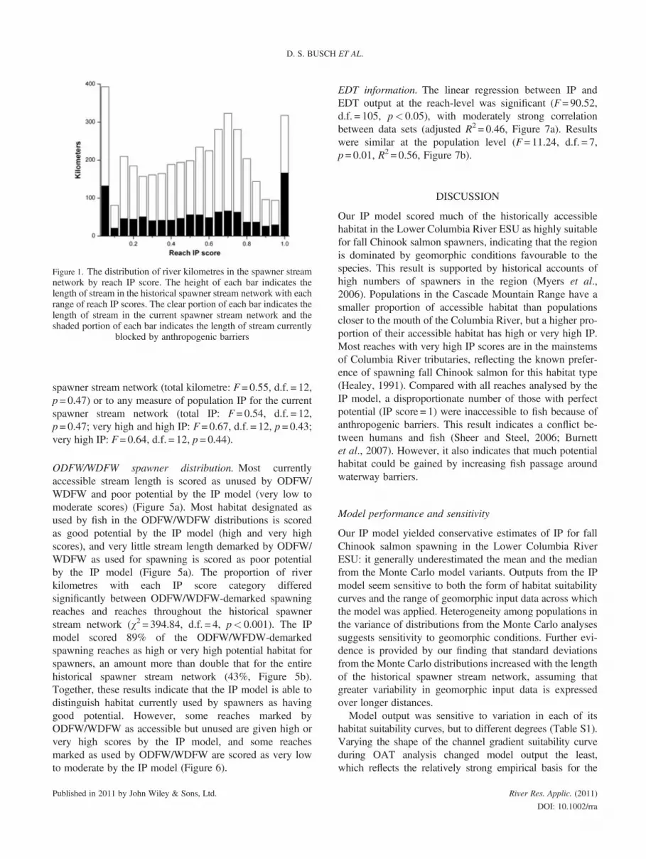
Distribution of IP scores. The distribution of IP scores forthe historical spawner stream network peaked at <0.05,0.65> x≥ 0.8 and >0.95 (Figures 1 and S2). More thanhalf (52%) of all reaches with an IP score of 1 and 26% ofall reaches in the historical spawner stream network areblocked by anthropogenic barriers (Figure 1). Of thestream length scored as very high potential, 16% isflooded by reservoirs.The proportion of reaches with each IP score varies across

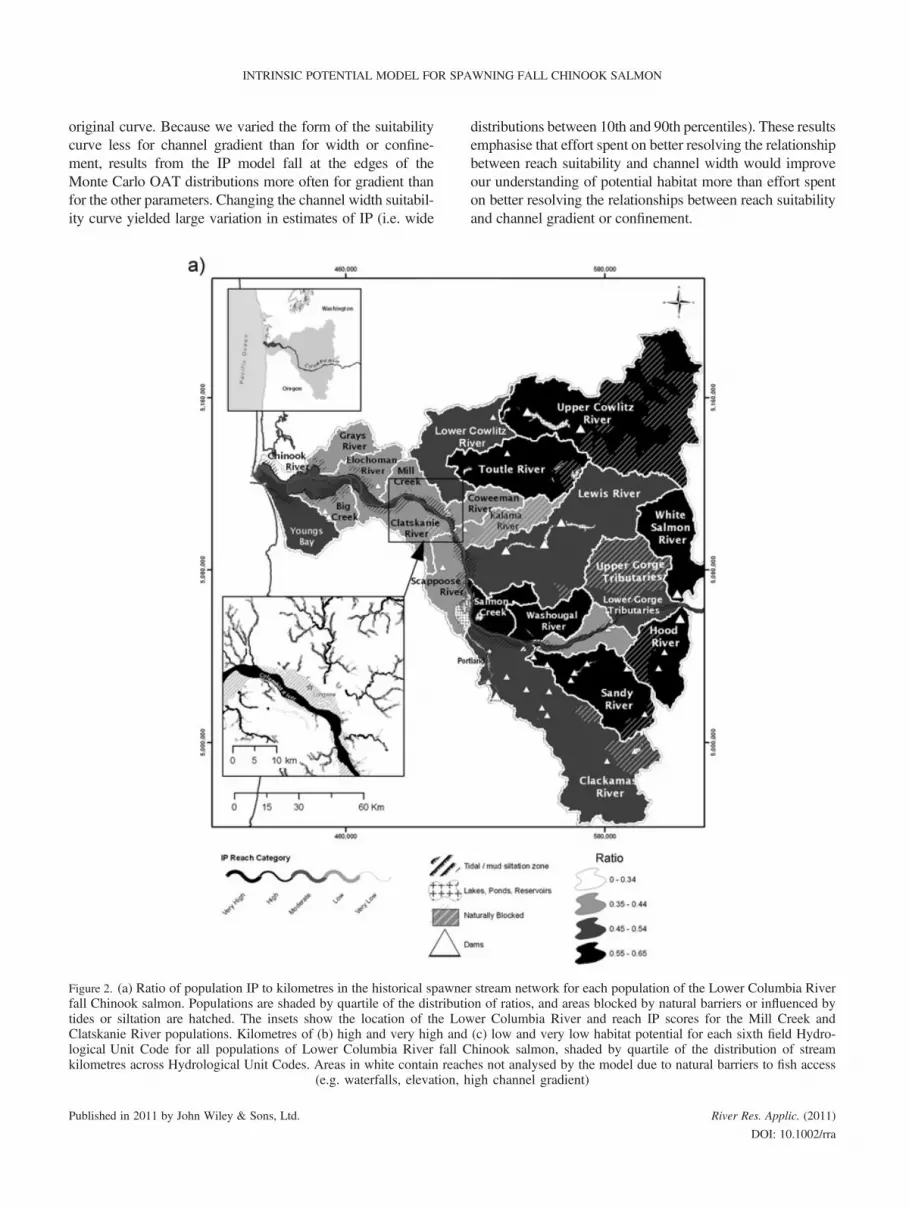
populations (Figures 2 and 3). In general, populations nearthe mouth of the Columbia River have a lower ratio of popu-lation IP to kilometres in the historical spawner stream net-work and more kilometres of reaches with poor (very lowand low) and good (high and very high) IP scores than popu-lations in the Cascade Mountain Range. This is likely due tobarriers to accessibility in the Cascade Mountain Range anddifferences between the areas in landscape characteristics(Figure 2, Table S1). On average, 66% of the kilometres ina watershed were included in the historical spawner streamnetwork (SD� 22%, min = 23%, max = 100%). The meanratio of population IP to kilometres in the historic spawnerstream network was 47% (SD� 10%, min = 22%, max =64%; Table S1). All of the very high potential habitat wasin mainstem reaches (57% in reaches 10–25m wide, 43%in reaches >25m wide; both percentages exclude reachesin reservoirs and lakes).

Table II. Results from correlations between geomorphic variablesincluded in the IP model

d.f. p r

Width vs. confinement 34 027 <0.01 �0.21Gradient vs. width 34 027 <0.01 �0.37Gradient vs. confinement 34 027 <0.01 �0.49

Published in 2011 by John Wiley & Sons, Ltd.

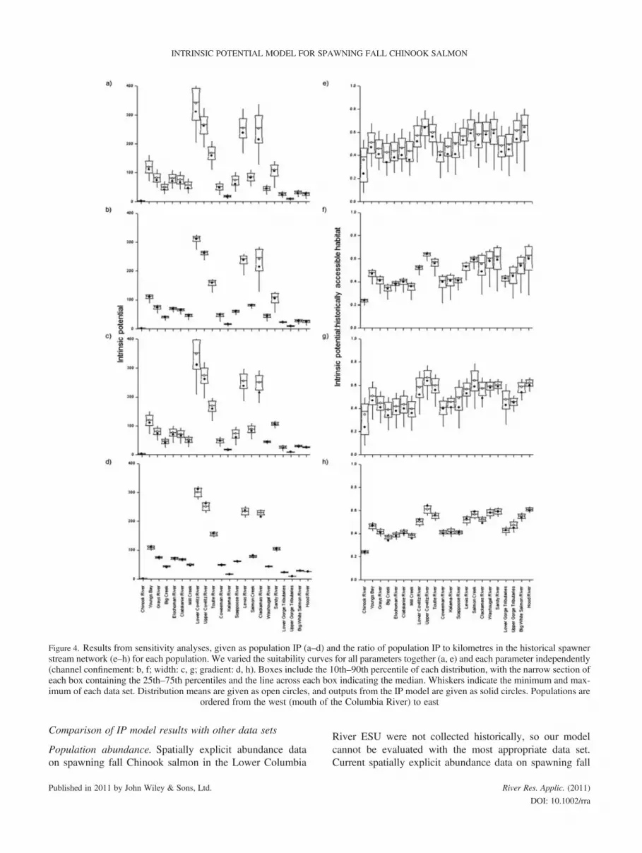
Sensitivity analysis. The Monte Carlo–based sensitivityanalyses indicated that IP model outputs were sensitive tovariation in each input parameter (Figure 4; Table S1). Foreach population, variance in the distributions of both thepopulation IP and the ratio of population IP to the lengthof the historical spawning stream network differedsignificantly among the OATs and when all curves werevaried together (Levene’s test, F> 363, d.f. = 3, 3996,p< 0.0001). The heterogeneity of variance also existedacross populations for each OAT and when all curves werevaried together (Levene’s test, F> 36, d.f. = 21, 21 978,p< 0.0001).When all habitat suitability curves were varied together,

outputs from the IP model typically underestimated themean and the median from the Monte Carlo variants butremained in the 10th–90th percentile range for every popu-lation (Figures 4a and 4e). After log transforming to normal-ise regression residuals, longer lengths of the historicalspawner stream network were typically associated withlarger standard deviations from the Monte Carlo variants(Table S1, columns All) for the population IP (F= 561.55,d.f. = 20, p< 0.0001, R2 = 0.96) and the ratio of populationIP to the length of the historical spawning stream network(F= 5.32, d.f. = 20, p< 0.03, R2 = 0.21), although thestrength of the latter relationship is weak. After log trans-forming, the difference between the output from the singularform of the IP model and the mean from the Monte Carlovariants also increased with the length of the historicalspawner stream network for population IP (F= 38.72,d.f. = 20, p< 0.0001, R2 = 0.66) but not for the ratio of popu-lation IP to the length of the historical spawning stream net-work (F= 2.57, d.f. = 20, p = 0.13, R2 = 0.11).Variation in the Monte Carlo distributions for each popu-

lation was less when habitat suitability curves were variedOAT than when all curves were varied together (Figure 4;Table S1). When habitat suitability curves for channel widthand confinement were varied OAT, IP model outputs wereless than or equal to the mean and median from the MonteCarlo variants for each population. In contrast, when habitatsuitability curves for channel gradient were varied, IP modeloutputs exceeded the mean from the Monte Carlo variantsfor six populations. Distributions of the OAT Monte Carlovariants were typically narrower when varying habitat suit-ability curves for channel gradient than for either confine-ment or width; our IP model outputs were outside the10th–90th percentiles for the most populations with the gra-dient OAT analysis (seven for population IP and four for thepopulation ratio).

Comparison data sets and analyses

Population abundance. Current population abundance wasnot linearly related to the length of stream in the current

River Res. Applic. (2011)

DOI: 10.1002/rra

Figure 1. The distribution of river kilometres in the spawner streamnetwork by reach IP score. The height of each bar indicates thelength of stream in the historical spawner stream network with eachrange of reach IP scores. The clear portion of each bar indicates thelength of stream in the current spawner stream network and theshaded portion of each bar indicates the length of stream currently

blocked by anthropogenic barriers

D. S. BUSCH ET AL.

spawner stream network (total kilometre: F= 0.55, d.f. = 12,p= 0.47) or to any measure of population IP for the currentspawner stream network (total IP: F= 0.54, d.f. = 12,p= 0.47; very high and high IP: F= 0.67, d.f. = 12, p = 0.43;very high IP: F= 0.64, d.f. = 12, p = 0.44).

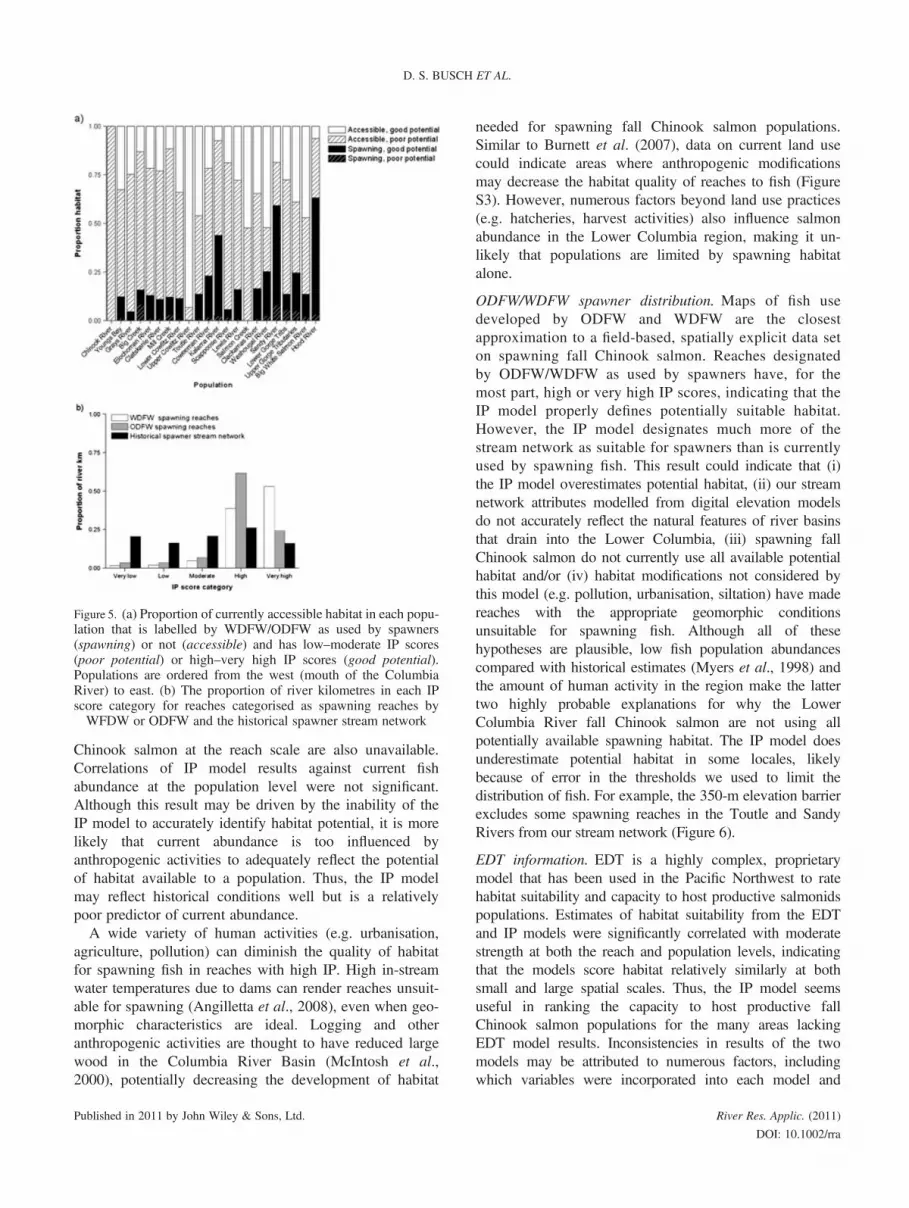
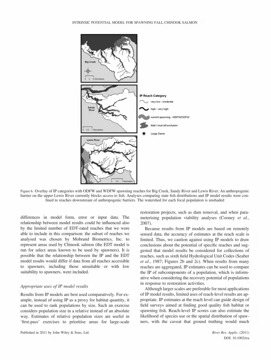
ODFW/WDFW spawner distribution. Most currentlyaccessible stream length is scored as unused by ODFW/WDFW and poor potential by the IP model (very low tomoderate scores) (Figure 5a). Most habitat designated asused by fish in the ODFW/WDFW distributions is scoredas good potential by the IP model (high and very highscores), and very little stream length demarked by ODFW/WDFW as used for spawning is scored as poor potentialby the IP model (Figure 5a). The proportion of riverkilometres with each IP score category differedsignificantly between ODFW/WDFW-demarked spawningreaches and reaches throughout the historical spawnerstream network (w2 = 394.84, d.f. = 4, p< 0.001). The IPmodel scored 89% of the ODFW/WFDW-demarkedspawning reaches as high or very high potential habitat forspawners, an amount more than double that for the entirehistorical spawner stream network (43%, Figure 5b).Together, these results indicate that the IP model is able todistinguish habitat currently used by spawners as havinggood potential. However, some reaches marked byODFW/WDFW as accessible but unused are given high orvery high scores by the IP model, and some reachesmarked as used by ODFW/WDFW are scored as very lowto moderate by the IP model (Figure 6).

Published in 2011 by John Wiley & Sons, Ltd.

EDT information. The linear regression between IP andEDT output at the reach-level was significant (F= 90.52,d.f. = 105, p< 0.05), with moderately strong correlationbetween data sets (adjusted R2 = 0.46, Figure 7a). Resultswere similar at the population level (F= 11.24, d.f. = 7,p= 0.01, R2 = 0.56, Figure 7b).

DISCUSSION

Our IP model scored much of the historically accessiblehabitat in the Lower Columbia River ESU as highly suitablefor fall Chinook salmon spawners, indicating that the regionis dominated by geomorphic conditions favourable to thespecies. This result is supported by historical accounts ofhigh numbers of spawners in the region (Myers et al.,2006). Populations in the Cascade Mountain Range have asmaller proportion of accessible habitat than populationscloser to the mouth of the Columbia River, but a higher pro-portion of their accessible habitat has high or very high IP.Most reaches with very high IP scores are in the mainstemsof Columbia River tributaries, reflecting the known prefer-ence of spawning fall Chinook salmon for this habitat type(Healey, 1991). Compared with all reaches analysed by theIP model, a disproportionate number of those with perfectpotential (IP score = 1) were inaccessible to fish because ofanthropogenic barriers. This result indicates a conflict be-tween humans and fish (Sheer and Steel, 2006; Burnettet al., 2007). However, it also indicates that much potentialhabitat could be gained by increasing fish passage aroundwaterway barriers.

Model performance and sensitivity

Our IP model yielded conservative estimates of IP for fallChinook salmon spawning in the Lower Columbia RiverESU: it generally underestimated the mean and the medianfrom the Monte Carlo model variants. Outputs from the IPmodel seem sensitive to both the form of habitat suitabilitycurves and the range of geomorphic input data across whichthe model was applied. Heterogeneity among populations inthe variance of distributions from the Monte Carlo analysessuggests sensitivity to geomorphic conditions. Further evi-dence is provided by our finding that standard deviationsfrom the Monte Carlo distributions increased with the lengthof the historical spawner stream network, assuming thatgreater variability in geomorphic input data is expressedover longer distances.Model output was sensitive to variation in each of its

habitat suitability curves, but to different degrees (Table S1).Varying the shape of the channel gradient suitability curveduring OAT analysis changed model output the least,which reflects the relatively strong empirical basis for the

River Res. Applic. (2011)

DOI: 10.1002/rra

INTRINSIC POTENTIAL MODEL FOR SPAWNING FALL CHINOOK SALMON

original curve. Because we varied the form of the suitabilitycurve less for channel gradient than for width or confine-ment, results from the IP model fall at the edges of theMonte Carlo OAT distributions more often for gradient thanfor the other parameters. Changing the channel width suitabil-ity curve yielded large variation in estimates of IP (i.e. wide

Figure 2. (a) Ratio of population IP to kilometres in the historical spawnefall Chinook salmon. Populations are shaded by quartile of the distributitides or siltation are hatched. The insets show the location of the LowClatskanie River populations. Kilometres of (b) high and very high andlogical Unit Code for all populations of Lower Columbia River fall Ckilometres across Hydrological Unit Codes. Areas in white contain reach

(e.g. waterfalls, elevation, h

Published in 2011 by John Wiley & Sons, Ltd.

distributions between 10th and 90th percentiles). These resultsemphasise that effort spent on better resolving the relationshipbetween reach suitability and channel width would improveour understanding of potential habitat more than effort spenton better resolving the relationships between reach suitabilityand channel gradient or confinement.

r stream network for each population of the Lower Columbia Riveron of ratios, and areas blocked by natural barriers or influenced byer Columbia River and reach IP scores for the Mill Creek and(c) low and very low habitat potential for each sixth field Hydro-hinook salmon, shaded by quartile of the distribution of streames not analysed by the model due to natural barriers to fish accessigh channel gradient)

River Res. Applic. (2011)

DOI: 10.1002/rra

Figure 2. Continued

D. S. BUSCH ET AL.

On the basis of the sensitivity analysis, outputs from theIP model may be quite useful for distinguishing differencesamong populations when engaging in ESU-wide planningactivities for and monitoring of the Lower Columbia Riverfall Chinook salmon. For most populations, the models arelikely appropriate for characterising the sub-watershed vari-ability necessary to address within-population concerns.However, IP model estimates for some populations (e.g.Clackamas River) seem to be particularly sensitive to model

Figure 3. Proportion of river kilometres in each IP score category and the entire watershed for the Lower Columbia River fall Chinook salmopopulations. Populations are ordered from the west (mouth of the Columbia River) to east

Published in 2011 by John Wiley & Sons, Ltd. River Res. Applic. (2011

DOI: 10.1002/r

form, raising caution about using the IP model as a manage-ment tool in specific locales. Although we considered the IPmodel satisfactory for many applications regarding theLower Columbia River fall Chinook salmon, we see valuein managers considering the range of results from the MonteCarlo runs. For example, managers could evaluate whetherusing the mean or the median of the Monte Carlo output dis-tributions rather than point estimates from the IP modelwould change the outcome of decisions that consider IP.

n

)

ra

Figure 4. Results from sensitivity analyses, given as population IP (a–d) and the ratio of population IP to kilometres in the historical spawnerstream network (e–h) for each population. We varied the suitability curves for all parameters together (a, e) and each parameter independently(channel confinement: b, f; width: c, g; gradient: d, h). Boxes include the 10th–90th percentile of each distribution, with the narrow section ofeach box containing the 25th–75th percentiles and the line across each box indicating the median. Whiskers indicate the minimum and max-imum of each data set. Distribution means are given as open circles, and outputs from the IP model are given as solid circles. Populations are

ordered from the west (mouth of the Columbia River) to east

INTRINSIC POTENTIAL MODEL FOR SPAWNING FALL CHINOOK SALMON

Comparison of IP model results with other data sets

Population abundance. Spatially explicit abundance dataon spawning fall Chinook salmon in the Lower Columbia

Published in 2011 by John Wiley & Sons, Ltd.

River ESU were not collected historically, so our modelcannot be evaluated with the most appropriate data set.Current spatially explicit abundance data on spawning fall

River Res. Applic. (2011)

DOI: 10.1002/rra

Figure 5. (a) Proportion of currently accessible habitat in each popu-lation that is labelled by WDFW/ODFW as used by spawners(spawning) or not (accessible) and has low–moderate IP scores(poor potential) or high–very high IP scores (good potential).Populations are ordered from the west (mouth of the ColumbiaRiver) to east. (b) The proportion of river kilometres in each IPscore category for reaches categorised as spawning reaches byWFDW or ODFW and the historical spawner stream network

D. S. BUSCH ET AL.

Chinook salmon at the reach scale are also unavailable.Correlations of IP model results against current fishabundance at the population level were not significant.Although this result may be driven by the inability of theIP model to accurately identify habitat potential, it is morelikely that current abundance is too influenced byanthropogenic activities to adequately reflect the potentialof habitat available to a population. Thus, the IP modelmay reflect historical conditions well but is a relativelypoor predictor of current abundance.A wide variety of human activities (e.g. urbanisation,

agriculture, pollution) can diminish the quality of habitatfor spawning fish in reaches with high IP. High in-streamwater temperatures due to dams can render reaches unsuit-able for spawning (Angilletta et al., 2008), even when geo-morphic characteristics are ideal. Logging and otheranthropogenic activities are thought to have reduced largewood in the Columbia River Basin (McIntosh et al.,2000), potentially decreasing the development of habitat

Published in 2011 by John Wiley & Sons, Ltd.

needed for spawning fall Chinook salmon populations.Similar to Burnett et al. (2007), data on current land usecould indicate areas where anthropogenic modificationsmay decrease the habitat quality of reaches to fish (FigureS3). However, numerous factors beyond land use practices(e.g. hatcheries, harvest activities) also influence salmonabundance in the Lower Columbia region, making it un-likely that populations are limited by spawning habitatalone.

ODFW/WDFW spawner distribution. Maps of fish usedeveloped by ODFW and WDFW are the closestapproximation to a field-based, spatially explicit data seton spawning fall Chinook salmon. Reaches designatedby ODFW/WDFW as used by spawners have, for themost part, high or very high IP scores, indicating that theIP model properly defines potentially suitable habitat.However, the IP model designates much more of thestream network as suitable for spawners than is currentlyused by spawning fish. This result could indicate that (i)the IP model overestimates potential habitat, (ii) our streamnetwork attributes modelled from digital elevation modelsdo not accurately reflect the natural features of river basinsthat drain into the Lower Columbia, (iii) spawning fallChinook salmon do not currently use all available potentialhabitat and/or (iv) habitat modifications not considered bythis model (e.g. pollution, urbanisation, siltation) have madereaches with the appropriate geomorphic conditionsunsuitable for spawning fish. Although all of thesehypotheses are plausible, low fish population abundancescompared with historical estimates (Myers et al., 1998) andthe amount of human activity in the region make the lattertwo highly probable explanations for why the LowerColumbia River fall Chinook salmon are not using allpotentially available spawning habitat. The IP model doesunderestimate potential habitat in some locales, likelybecause of error in the thresholds we used to limit thedistribution of fish. For example, the 350-m elevation barrierexcludes some spawning reaches in the Toutle and SandyRivers from our stream network (Figure 6).

EDT information. EDT is a highly complex, proprietarymodel that has been used in the Pacific Northwest to ratehabitat suitability and capacity to host productive salmonidspopulations. Estimates of habitat suitability from the EDTand IP models were significantly correlated with moderatestrength at both the reach and population levels, indicatingthat the models score habitat relatively similarly at bothsmall and large spatial scales. Thus, the IP model seemsuseful in ranking the capacity to host productive fallChinook salmon populations for the many areas lackingEDT model results. Inconsistencies in results of the twomodels may be attributed to numerous factors, includingwhich variables were incorporated into each model and

River Res. Applic. (2011)

DOI: 10.1002/rra

Figure 6. Overlay of IP categories with ODFW and WDFW spawning reaches for Big Creek, Sandy River and Lewis River. An anthropogenicbarrier on the upper Lewis River currently blocks access to fish. Analyses comparing state fish distributions and IP model results were con-

fined to reaches downstream of anthropogenic barriers. The watershed for each focal population is unshaded

INTRINSIC POTENTIAL MODEL FOR SPAWNING FALL CHINOOK SALMON

differences in model form, error or input data. Therelationship between model results could be influenced alsoby the limited number of EDT-rated reaches that we wereable to include in this comparison: the subset of reaches weanalysed was chosen by Mobrand Biometrics, Inc. torepresent areas used by Chinook salmon (the EDT model isrun for select areas known to be used by spawners). It ispossible that the relationship between the IP and the EDTmodel results would differ if data from all reaches accessibleto spawners, including those unsuitable or with lowsuitability to spawners, were included.

Appropriate uses of IP model results

Results from IP models are best used comparatively. For ex-ample, instead of using IP as a proxy for habitat quantity, itcan be used to rank populations by size. Such an exerciseconsiders population size in a relative instead of an absoluteway. Estimates of relative population sizes are useful in‘first-pass’ exercises to prioritise areas for large-scale

Published in 2011 by John Wiley & Sons, Ltd.

restoration projects, such as dam removal, and when para-meterising population viability analyses (Cooney et al.,2007).Because results from IP models are based on remotely

sensed data, the accuracy of estimates at the reach scale islimited. Thus, we caution against using IP models to drawconclusions about the potential of specific reaches and sug-gested that model results be considered for collections ofreaches, such as sixth field Hydrological Unit Codes (Seaberet al., 1987; Figures 2b and 2c). When results from manyreaches are aggregated, IP estimates can be used to comparethe IP of subcomponents of a population, which is inform-ative when considering the recovery potential of populationsin response to restoration activities.Although larger scales are preferable for most applications

of IP model results, limited uses of reach-level results are ap-propriate. IP estimates at the reach level can guide design offield surveys aimed at finding good quality fish habitat orspawning fish. Reach-level IP scores can also estimate thelikelihood of species use or the spatial distribution of spaw-ners, with the caveat that ground truthing would much

River Res. Applic. (2011)

DOI: 10.1002/rra

Figure 7. Linear regression between (a) EDT-estimated equilibriumabundance in each EDT-defined reach and IP of those reaches and(b) EDT-estimated equilibrium abundance of 9 populations and IP

of those populations

D. S. BUSCH ET AL.

improve these estimates. Finally, the IP scores of individualreaches can be considered together to identify longer streamsections that might support spawning aggregations or popu-lation segments.Estimates of IP from our IP model are not based on

stream area: reach width is factored into IP only by its influ-ence on reach IP score via the width suitability curve, andreach depth is not considered at all. Because results maynot reflect the area of habitat available in a reach, IP modelsshould not be used to estimate absolute habitat capacities orspawner abundances—whether current or historical. The IPmodel could be used as a starting point to address absolutehabitat capacities or spawner abundances if quantitativerelationships were established between the reach IP scoreand the proportion of a reach that is used for spawning.Developing such relationships would likely require data on

Published in 2011 by John Wiley & Sons, Ltd.

reach depth and other characteristics (e.g. channel type,wood load), which may be difficult to generate from re-motely sensed data. IP is, however, helpful for partitioningestimates of historical abundance from a region into esti-mates of historical abundance per population (LowerColumbia Fish Recovery Board, 2010).Because overestimation of potential habitat can lead to

nonachievable restoration and protection goals (Geistet al., 2000), evidence that the IP model may overestimatepotential habitat should not be dismissed readily. Thiscaution is especially relevant in the Lower Columbia Riverregion, given its reduced habitat quality due to anthropo-genic activities not captured by the IP model. Wherepossible, we recommend that managers consider data on fishuse, threats to wild salmon populations (e.g. road density,proximity to hatcheries) and intrinsic factors not includedin the model that can affect habitat suitability. For example,information about whether watershed hydrographs aredominated by rain or snow melt could inform habitat suit-ability estimates, as rain-on-snow events increase the poten-tial of redds to fail due to scouring (Montgomery et al.,1999; Steel et al., 2007). In addition, given the correlationbetween fish use and channel form (Beechie et al., 2006a,2006b; Hall et al., 2007), information on channel type (e.g. island-braided, meandering, strait) could help refine esti-mates of habitat suitable for spawners: reaches designatedas highly suitable by the IP model but with a rarely usedchannel type (e.g. straight) could be considered of lowervalue when planning restoration activities.

CONCLUSIONS

We outlined the rationale and processes for developing an IPmodel, using fall Chinook salmon as a case study. Althoughthe methods we presented are transferable to other speciesand locales, the model we developed is specific to fallChinook salmon in the Lower Columbia River ESU. Furtherresearch would be needed to ascertain the validity of applyingthis model to fall Chinook salmon in other regions, differentruns of Chinook salmon or non-Chinook salmonid species,and potentially to modify the model to suit the new region,run type or species.It is impossible to fully validate this IP model because the

historical data needed to do so do not, and most likely willnever, exist. However, this model is built on principles ofgeomorphology and fish habitat utilisation that are wellunderstood. In addition, our IP model (i) assigns veryhigh/high potential scores to reaches that WDFW andODFW designate as spawning habitat and (ii) generatesresults that agree with those from a more complex model,EDT. The sensitivity analyses indicate that model output issensitive to the shape of the parameter curves and that theresults from our IP model are conservative estimates, not

River Res. Applic. (2011)

DOI: 10.1002/rra

INTRINSIC POTENTIAL MODEL FOR SPAWNING FALL CHINOOK SALMON

always indicative of the central tendency from likely modelforms. Thus, we recommend that those basing managementon IP model results consider whether using the mean or me-dian of the distributions from the Monte Carlo runs wouldchange their decisions.

ACKNOWLEDGEMENTS

T. Beechie, H. Imaki, J. Myers, D. Rawding and the partici-pants of the November 2008 State of the IP workshop inPortland, Oregon, contributed ideas helpful in the develop-ment of this model and manuscript. Greg Blair of IFC Inter-national, Inc., graciously provided the EDT output used inthis study. DSB was supported by a National ResearchCouncil post-doctoral fellowship.

REFERENCES

Agrawal A, Schick RS, Bjorkstedt EP, Szerlong RG, Goslin MN, SpenceBC, Williams TH, Burnett KM. 2005. Predicting the potential for histor-ical coho, Chinook, and steelhead habitat in Northern California. U.S.Dept. Commerce, NOAA Tech. Memo. NMFS-SWFSC-379.

Angilletta MJJ, Steel EA, Bartz KK, Kingsolver JG, Scheuerell MD,Beckman BR, Crozier LG. 2008. Big dams and salmon evolution:changes in thermal regimes and their potential evolutionary conse-quences. Evolutionary Applications 1: 286–299.

Baxter CV, Hauer FR. 2000. Geomorphology, hyporheic exchange, andselection of spawning habitat by bull trout (Salvelinus confluentus).Canadian Journal of Fisheries and Aquatic Science 57: 1470–1481.

Beechie T, Liermann M, Pollack MM, Baker S, Davies J. 2006a. Channelpattern and river-floodplain dynamics in forested mountain river systems.Geomorphology 78: 124–141.

Beechie TJ, Greene CM, Holsinger L, Beamer EM. 2006b. Incorporatingparameter uncertainty into evaluation of spawning habitat limitationson Chinook salmon (Oncorhynchus tshawytscha) populations. CanadianJournal of Fisheries and Aquatic Science 63: 1242–1250.

Blair GR, Lestelle LC, Mobrand LE. 2009. The Ecosystem Diagnosis andTreatment model: a tool for assessing salmonid performance potentialbased on habitat conditions. In Pacific salmon environment and life his-tory models: advancing science for sustainable salmon in the future,Knudson E (ed). American Fisheries Society: Bethesda, Maryland,USA; 464, 289–309.

Burnett KM, Reeves GH, Miller DJ, Clarke S, Vance-Borland K,Christiansen K. 2007. Distribution of salmon-habitat potential relativeto landscape characteristics and implications for conservation. EcologicalApplications 17: 66–80.

Clarke SE, Burnett KM. 2003. Comparison of digital elevation models foraquatic data development. Photogrammetric Engineering and RemoteSensing 69: 1367–1375.

Clarke S, Burnett KM, Miller DJ. 2008. Modeling streams and hydrogeo-morphic attributes in Oregon from digital and field data. Journal of theAmerican Water Resources Association 44: 459–477.

Cooney T, McClure M, Baldwin C, Carmicheal R, Hassmer P, Howell P,McCullough D, Schaller H, Spruell P, Petrosky C, Utter F. 2007. Viabil-ity criteria for application to Interior Columbia basin salmonid ESUs. U.S. Dept. Commerce, NOAA Tech. Memo. NMFS-NWFSC-Draft.

Davies JR, Lagueux KM, Sanderson B, Beechie TJ. 2007. Modeling streamchannel characteristics from drainage-enforced DEMs in Puget Sound,Washington, USA. Journal of the American Water Resources Associ-ation 43: 414–426.

Published in 2011 by John Wiley & Sons, Ltd.

Dent L, Herstrom A, Gilbert E. 2005. A spatial evaluation of habitat accessconditions and Oregon plan fish passage improvement projects in the Coastalcoho ESU. Oregon Plan Assessment Part 4J OP Technical Report 2.

Ford MJ, Sands NJ, McElhany P, Kope RG, Simmons D, Dygert P. 2007.Analyses to support a review of an ESA jeopardy consultation on fisher-ies impacting Lower Columbia tule Chinook salmon. National MarineFisheries Service, Northwest Fisheries Science Center, ConservationBiology Division; National Marine Fisheries Service, Northwest Re-gional Office, Sustainable Fisheries Division.

Fulton LA. 1968. Spawning areas and abundance of Chinook salmon(Oncorhynchus tshawytscha) in the Columbia River basin — past andpresent. U.S. Fish and Wildlife Service, Special Scientific Report -Fisheries No. 571.

Fulton LA. 1970. Spawning areas and abundance of steelhead trout andcoho, sockeye, and chum salmon in the Columbia River Basin — pastand present. National Marine Fisheries Service.

Geist DR, Dauble DD. 1998. Redd site selection and spawning habitat useby fall Chinook salmon: the importance of geomorphic features in largerivers. Environmental Management 22: 655–669.

Geist DR, Jones J, Murray CJ, Dauble DD. 2000. Suitability criteria ana-lyzed at the spatial scale of redd clusters improved estimates of fallChinook salmon (Oncorhynchus tshawytscha) spawning habitat usein the Hanford Reach, Columbia River. Canadian Journal of Fisheriesand Aquatic Science 57: 1636–1646.

Gende SM, Edwards RT, Willson MF, Wipfli MS. 2002. Pacific salmon inaquatic and terrestrial ecosystems. Bioscience 52: 917–928.

Hall JE, Holzer DM, Beechie TJ. 2007. Predicting river floodplain and lat-eral channel migration for salmon habitat conservation. Journal of theAmerican Water Resources Association 43: 1–12.

Healey MC. 1991. Life history of Chinook salmon (Oncorhynchustshawytscha). In Pacific salmon life histories, Groot C, Margolis L (eds).UBC Press: Vancouver, Canada; 564, 313–393.

Jenson SK, Domingue JO. 1988. Extracting topographic structure fromdigital elevation data for geographic information system analysis. Photo-grammetric Engineering and Remote Sensing 54: 1593–1600.

Lawson PW, Bjorkstedt EP, Chilcote MW, Huntington CW, Mills JS,Moore KMS, Nickelson TE, Reeves GH, Stout HA, Wainwright TC,Weitkamp LA. 2007. Identification of historical populations of coho salmon(Oncorhynchus kisutch) in the Oregon Coast Evolutionarily Significant Unit.U.S. Dept. Commerce, NOAA Tech. Memo. NMFS-NWFSC-79.

Lee LA, Terrell JW. 1987. Habitat suitability index models: flathead catfish.U.S. Fish and Wildlife Service Biological Report 82(10.152).

Lichatowich JA. 1999. Salmon without rivers: a history of the Pacific salm-on crisis. Island Press: Washington, D.C., USA; 336.

Lower Columbia Fish Recovery Board. 2010. Washington LowerColumbia salmon recovery and fish and wildlife subbasin plan.

Lunetta RS, Cosentino BL, Montgomery DR, Beamer EM, Beechie T.1997. GIS-based evaluation of salmon habitat in the Pacific Northwest.Photogrammetric Engineering and Remote Sensing 63: 1219–1229.

McElhany P, Backman T, Busack C, Heppell S, Kolmes S, Maule A, MyersJ, Rawding D, Shively D, Steel A, Steward C, Whitesel T. 2003. Interimreport on viability criteria for Willamette and Lower Columbia BasinPacific salmonids. U.S. Dept. Commerce, NOAA Tech. Memo. NMFS-NWFSC-Draft.

McElhany P, Chilcote M, Myers J, Beamesderfer R. 2007. Viability status ofOregon salmon and steelhead populations in the Willamette and LowerColumbia basins, reviewdraft.U.S.Dept. Commerce,NOAA-NMFS-NWFSC.

McElhany P, Steel EA, Avery K, Yoder N, Busack C, Thompson B. 2010.Dealing with uncertainty in ecosystem models: lessons from a complexsalmon model. Ecological Applications 20: 465–482.

McIntosh BA, Sedell JR, Thurow RF, Clarke SE, Chandler GL. 2000. His-torical changes in pool habitats in the Columbia River Basin. EcologicalApplications 10: 1478–1496.

River Res. Applic. (2011)

DOI: 10.1002/rra

D. S. BUSCH ET AL.

McMahon TE. 1982. Habitat suitability index models: creek chub. U.S.Fish Wildlife Service. FWS/OBS-82/10.4.

Mikhailova M. 2008. Hydrological and morphological features of rivermouths of different types (the Columbia Estuary and the Fraser Deltaas examples). Environmental Research, Engineering and Management4: 4–12.

Miller DJ. 2003. Programs for DEM Analysis. In Landscape Dynamics andForest Management: General Technical Report RMRS-GTR-101CD.USDA Forest Service, Rocky Mountain Research Station: Fort Collins,CO, USA.

Miller SN, Guertin DP, Goodrich DC. 1996. Linking GIS and geomorpho-logic research at Walnut Gulch Experimental Watershed. Proceedings ofthe American Water Resources Association Symposium on GIS andWater Resources, Ft. Lauderdale, FL. Available online: http://www.awra.org/proceedings/gis32/index.html [accessed 8 August 2011].

Montgomery DR, Buffington JM. 1997. Channel-reach morphology inmountain drainage basins. Geological Society of America Bulletin 109:596–611.

Montgomery DR, Foufoula-Georgiou E. 1993. Channel network sourcerepresentation using digital elevation models. Water Resources Research29:3925–3934.

Montgomery DR, Beamer EM, Pess GR, Quinn TP. 1999. Channel typeand salmonid spawning distribution and abundance. Canadian Journalof Fisheries and Aquatic Science 56: 377–387.

Moore JW. 2006. Animal ecosystem engineers in streams. Bioscience 56:237–246.

Myers JM, Kope RG, Bryant GJ, Teel DJ, Lierheimer LJ, Wainwright TC,Grant WS, Waknitz FW, Neely K, Lindley S, Waples RS. 1998. Statusreview of Chinook salmon from Washington, Idaho, Oregon, andCalifornia. U.S. Dept. of Commerce, NOAA Tech. Memo., NMFS-NWFSC-35.

Myers JM, Busack C, Rawding D, Marshall AR, Teel DJ, Van Doornik DM,Maher MT. 2006. Historical population structure of Pacific salmonids inthe Willamette River and lower Columbia River basins. U.S. Dept. ofCommerce, NOAA Tech. Memo., NMFS-NWFSC-73.

Nickelson TE, Lawson PW. 1998. Population viability of coho salmon,Oncorhynchus kisutch, in Oregon coastal basins: application of a habitat-based life cycle model.Canadian Journal of Fisheries and Aquatic Science55: 2383–2392.

Oregon Department of Fish and Wildlife. 2009. Oregon fish passage bar-riers. Available online: http://nrimp.dfw.state.or.us/nrimp/default.aspx?pn=fishbarrierdata [accessed 2 March 2009].

Oregon Department of Fish and Wildlife Natural Resource Inventory Man-agement Project. 2009. Oregon fish habitat distribution.

Published in 2011 by John Wiley & Sons, Ltd.

Poole GC, O’Daniel SJ, Jones KL, Woessner WW, Bernhardt ES, HeltonAM, Stanford JA, Boer BR, Beechie TJ. 2008. Hydrologic spirals: therole of multiple interactive flow paths in stream ecosystems. RiverResearch and Applications 24: 1018–1031.

Rapp CF, Abbe TB. 2003. A framework for delineating channel migrationzones. Washington State Department of Ecology Publication #03-06-027.

Schamberger M, Farmer AH, Terrell JW. 1982. Habitat suitability indexmodels: introduction. U.S. Fish and Wildlife Service. FWS/OBS-82/10.

Seaber PR, Kapinos FP, Knapp GL. 1987. Hydrologic unit maps. U.S. Geo-logical Survey Water-Supply Paper 2294.

Sheer MB, Steel EA. 2006. Lost watersheds: barriers, aquatic habitat connec-tivity, and salmon persistence in the Willamette and Lower Columbia Riverbasins. Transactions of the American Fisheries Society 135: 1654–1669.

Sheer MB, Busch DS, Gilbert E, Bayer JM, Lanigan S, Schei JL, BurnettKM, Miller D. 2009. Development and management of fish intrinsic po-tential data and methodologies: State of the IP 2008 summary report.Pacific Northwest Aquatic Monitoring Partnership Series 2009–004.

Sherwood CR, Creager JS. 1990. Sedimentary geology of the ColumbiaRiver estuary. Progress in Oceanography 24: 15–79.

Steel EA, Sheer MB. 2003. Appendix I: Broad-Scale Habitat Analyses toEstimate Fish Densities for Viability Criteria. In Interim Report on Via-bility Criteria for Willamette and Lower Columbia Basin Pacific Salmo-nids. Willamette/Lower Columbia Technical Recovery Team,NOAANorthwest Fisheries Science Center, Seattle, WA.

Steel A, Fullerton A, Caras Y, Sheer M, Olson P, Jensen D, Burke J, MaherM, Miller D, McElhany P. 2007. The Lewis River case study: final re-port. NOAA Northwest Fisheries Science Center, Seattle, WA.

Tarboton DG, Bras RL, Rodriguez-Iturbe I. 1991. On the extraction ofchannel networks from digital elevation data. Hydrological Processes5: 81–100.

Waples RS. 1991. Pacific salmon, Oncorhynchus spp., and the definition of“species” under the Endangered Species Act. Marine Fisheries Review53: 11–22.

Washington Department of Fish and Wildlife. 2000. Fish passage barrierand surface water diversion screening assessment and prioritization man-ual. Environmental Restoration Division; Salmon Screening, Habitat En-hancement, and Restoration Section.

Washington Department of Fish and Wildlife. 2001. Salmon and steelheadhabitat inventory and assessment program: Determining presumed and poten-tial habitat for anadromous salmonids in the Lower Columbia region.

Washington Department of Fish and Wildlife. 2006. Salmon and steelheadhabitat inventory and assessment program: unpublished data on fish pas-sage barriers (1:24,000), physical stream segments, and fish distributionfor Watershed Inventory Areas (WRIA) 24–29.

River Res. Applic. (2011)

DOI: 10.1002/rra