117
Introduction to Empirical Research: An Overview of Methods and Research Design Choices Andreas Warntjen 2014/15
Introduction to Empirical Research: An Overview of Methods and Research Design Choices
Andreas Warntjen
2014/15
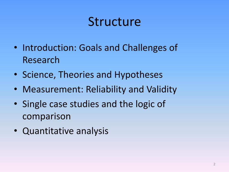
Structure
• Introduction: Goals and Challenges of Research
• Science, Theories and Hypotheses
• Measurement: Reliability and Validity
• Single case studies and the logic of comparison
• Quantitative analysis
2

Introduction
• Goals of research
• Evaluating policy
• Challenges for research
• Validity
3
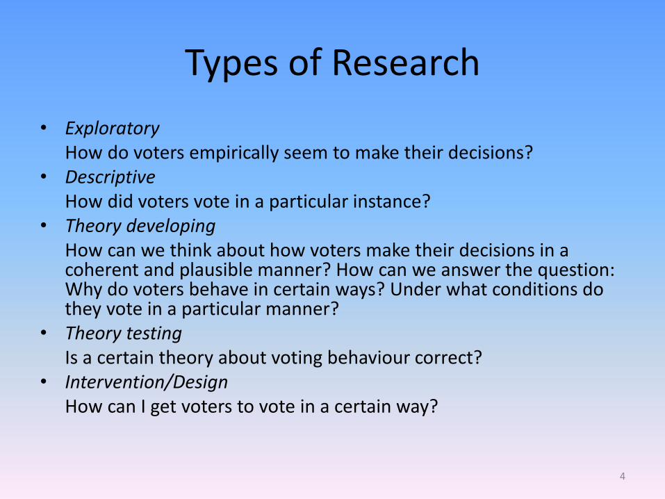
Types of Research
• Exploratory How do voters empirically seem to make their decisions? • Descriptive How did voters vote in a particular instance? • Theory developing How can we think about how voters make their decisions in a
coherent and plausible manner? How can we answer the question: Why do voters behave in certain ways? Under what conditions do they vote in a particular manner?
• Theory testing Is a certain theory about voting behaviour correct? • Intervention/Design How can I get voters to vote in a certain way?
4
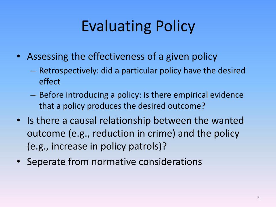
Evaluating Policy
• Assessing the effectiveness of a given policy
– Retrospectively: did a particular policy have the desired effect
– Before introducing a policy: is there empirical evidence that a policy produces the desired outcome?
• Is there a causal relationship between the wanted outcome (e.g., reduction in crime) and the policy (e.g., increase in policy patrols)?
• Seperate from normative considerations
5
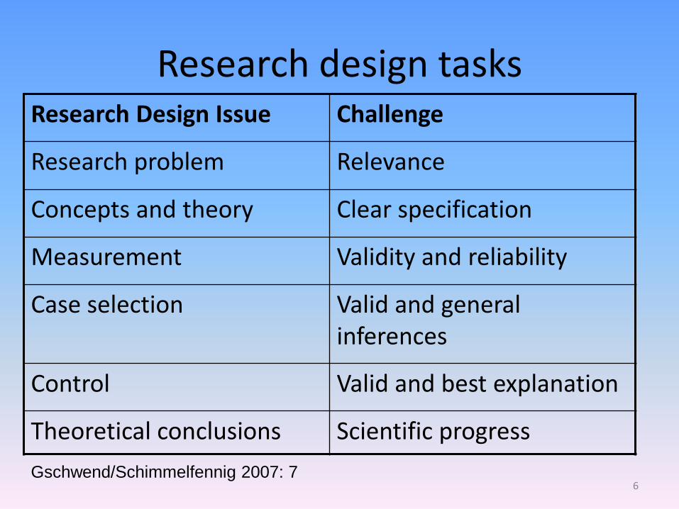
Research design tasks Research Design Issue Challenge
Research problem Relevance
Concepts and theory Clear specification
Measurement Validity and reliability
Case selection Valid and general inferences
Control Valid and best explanation
Theoretical conclusions Scientific progress
Gschwend/Schimmelfennig 2007: 7 6
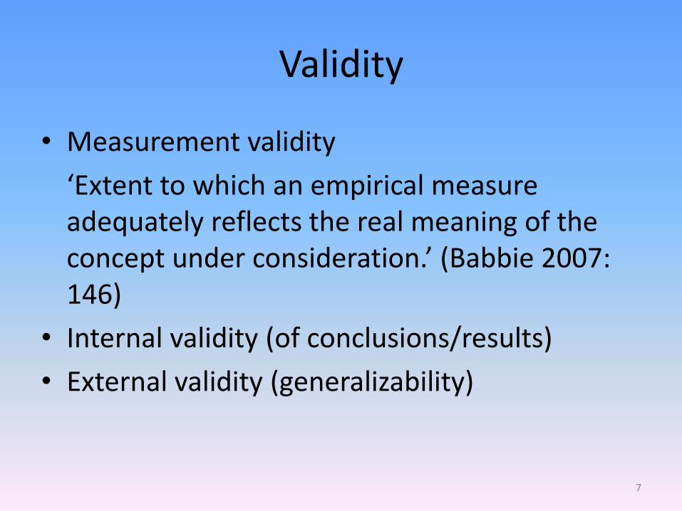
Validity
• Measurement validity
‘Extent to which an empirical measure adequately reflects the real meaning of the concept under consideration.’ (Babbie 2007: 146)
• Internal validity (of conclusions/results)
• External validity (generalizability)
7

Any questions?
8

Further readings
Babbie, Earl (2007) The practice of social research. Wadsworth Gschwend, Thomas and Frank Schimmelfennig (2007), ‘Designing Research in Political Science’, in: Gschwend and Schimmelfennig (eds.) Research Design in Political Science, Houndmills, Palgrave Macmillan
De Vaus, David (2001) Research Design in Social Research. London, Sage, Ch. 1 (The Context of Design)
Johnson and Reynolds (2008) Political Science Research Methods. Washington, CQ Press, Ch. 3 (The Building Blocks of Social Scientific Research: Hypotheses, Concepts and Variables)
Pollock, Philipp (2011) Essentials of Political Analysis. Washington, CQ Press, Ch. 3 (Proposing Explanations, Framing Hypotheses, and Making Comparisons)
9
Session 1
• What is ‘science’?
• What is ‘theory’ and what is it good for
• Formulating hypotheses
• Validity
10
What is this thing called science?
Exercises:
1. Read the newspaper article. What is the difference between this text and a scientific one?
2. What is the difference between
a) A scientific conclusion
b) A personal political opinion
c) The ‘collective wisdom’ on a certain topic
11
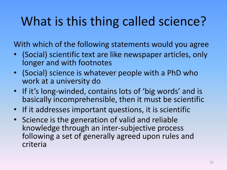
What is this thing called science?
With which of the following statements would you agree • (Social) scientific text are like newspaper articles, only
longer and with footnotes • (Social) science is whatever people with a PhD who
work at a university do • If it’s long-winded, contains lots of ‘big words’ and is
basically incomprehensible, then it must be scientific • If it addresses important questions, it is scientific • Science is the generation of valid and reliable
knowledge through an inter-subjective process following a set of generally agreed upon rules and criteria
12
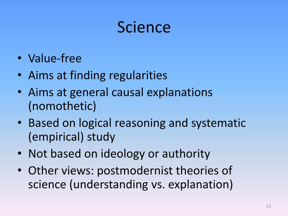
Science
• Value-free
• Aims at finding regularities
• Aims at general causal explanations (nomothetic)
• Based on logical reasoning and systematic (empirical) study
• Not based on ideology or authority
• Other views: postmodernist theories of science (understanding vs. explanation)
13
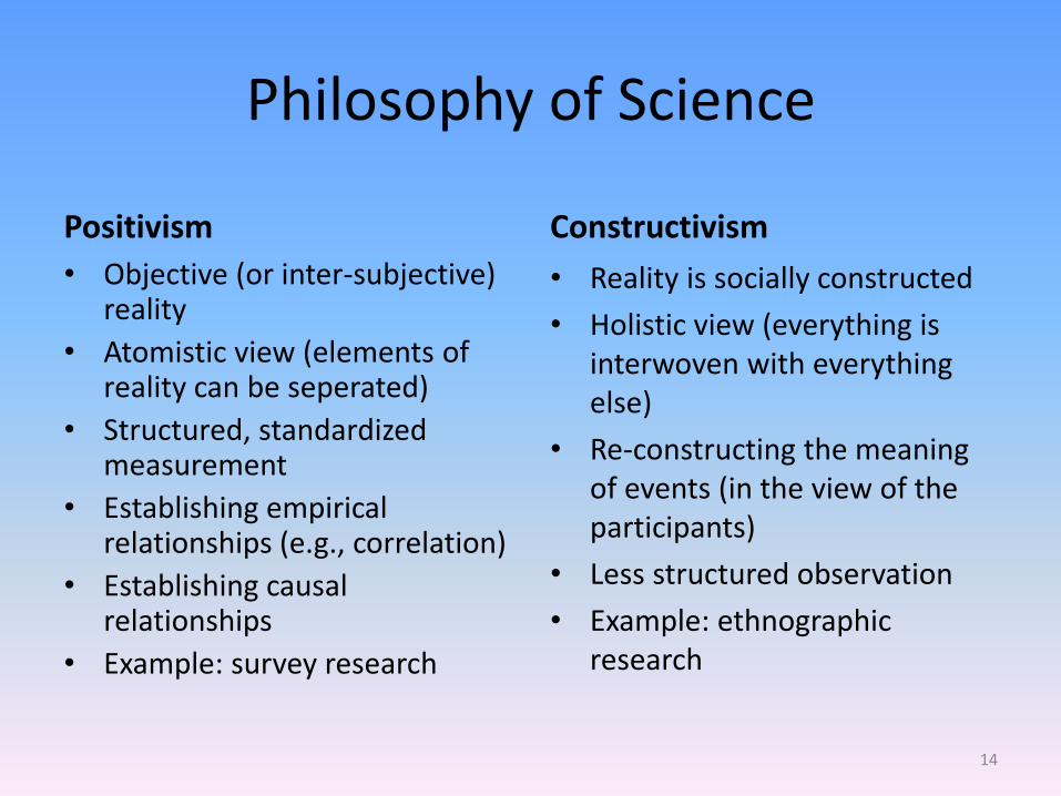
Philosophy of Science
Positivism
• Objective (or inter-subjective) reality
• Atomistic view (elements of reality can be seperated)
• Structured, standardized measurement
• Establishing empirical relationships (e.g., correlation)
• Establishing causal relationships
• Example: survey research
Constructivism
• Reality is socially constructed
• Holistic view (everything is interwoven with everything else)
• Re-constructing the meaning of events (in the view of the participants)
• Less structured observation
• Example: ethnographic research
14
Exercise
• What is the difference between the following images?
• Are any of them true representations of reality?
• Is any of them ‘truer’ than the other?
15

16

17
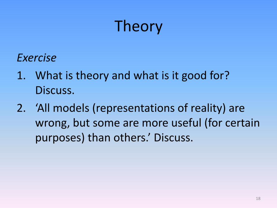
Theory
Exercise
1. What is theory and what is it good for? Discuss.
2. ‘All models (representations of reality) are wrong, but some are more useful (for certain purposes) than others.’ Discuss.
18
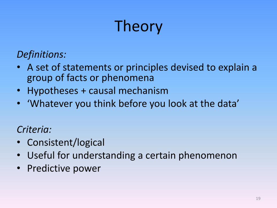
Theory
Definitions: • A set of statements or principles devised to explain a
group of facts or phenomena • Hypotheses + causal mechanism • ‘Whatever you think before you look at the data’ Criteria: • Consistent/logical • Useful for understanding a certain phenomenon • Predictive power
19
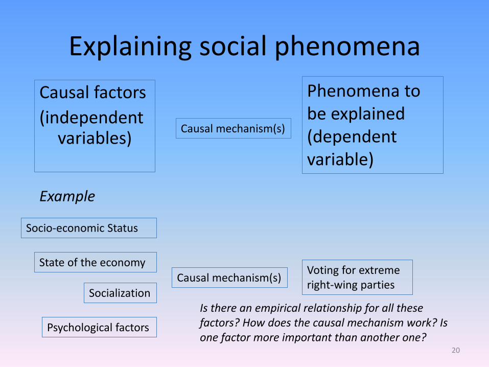
Explaining social phenomena
Causal factors
(independent variables)
Causal mechanism(s)
Phenomena to be explained (dependent variable)
Voting for extreme right-wing parties
Example
Socio-economic Status
Socialization
State of the economy
Causal mechanism(s)
Psychological factors
Is there an empirical relationship for all these factors? How does the causal mechanism work? Is one factor more important than another one?
20
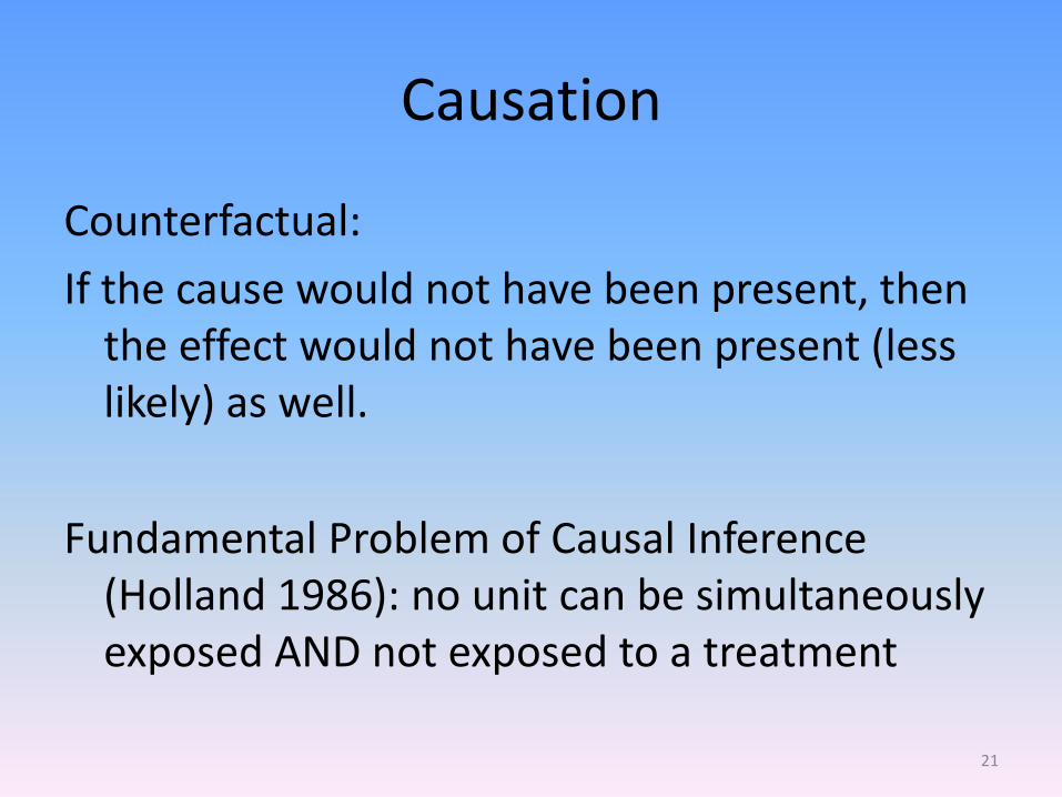
Causation
Counterfactual:
If the cause would not have been present, then the effect would not have been present (less likely) as well.
Fundamental Problem of Causal Inference (Holland 1986): no unit can be simultaneously exposed AND not exposed to a treatment
21
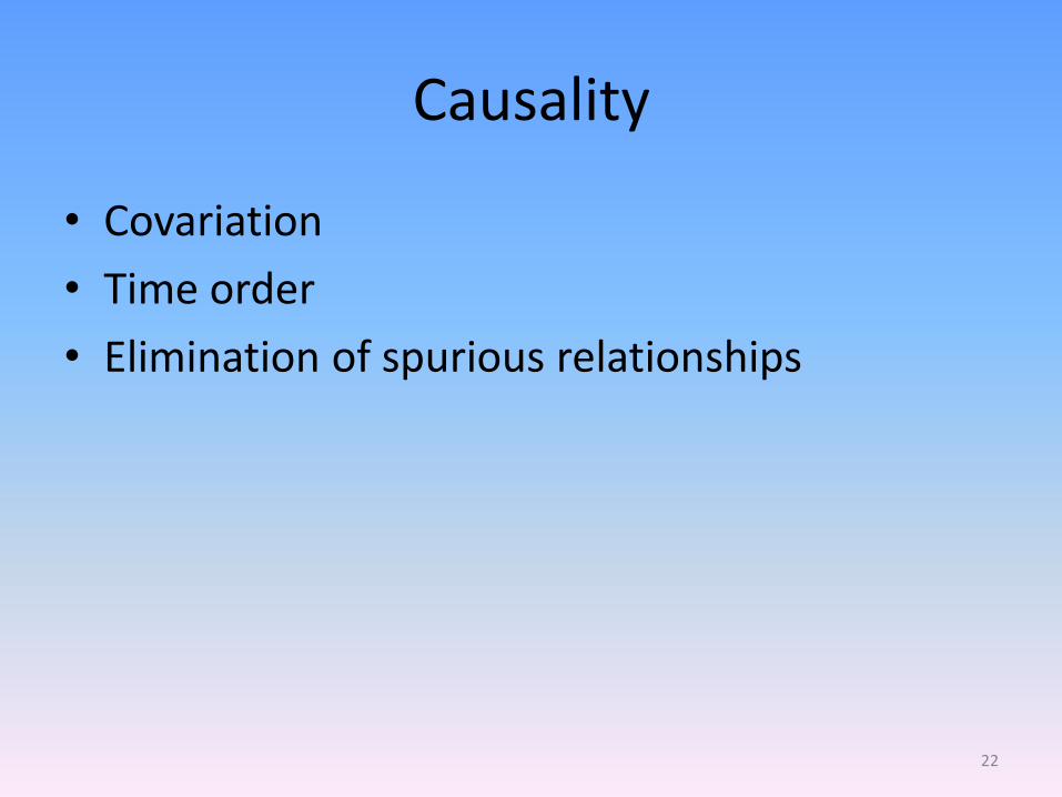
Causality
• Covariation
• Time order
• Elimination of spurious relationships
22
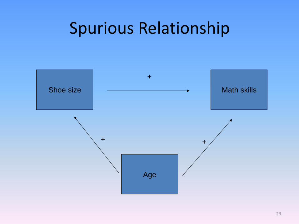
Spurious Relationship
Shoe size Math skills
Age
+
+ +
23
Experiments
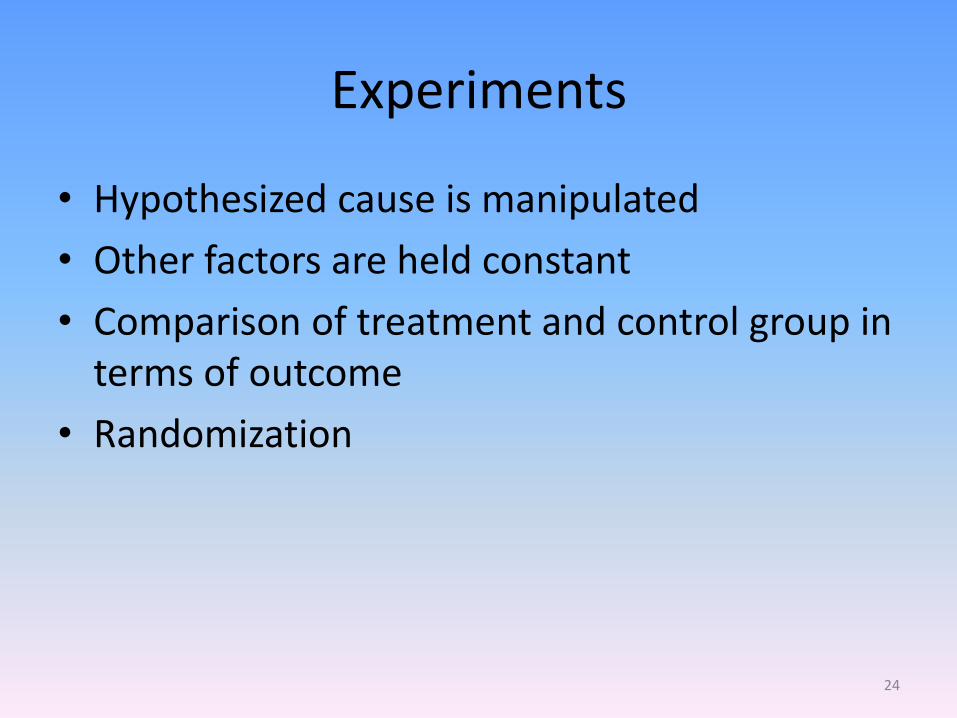
• Hypothesized cause is manipulated
• Other factors are held constant
• Comparison of treatment and control group in terms of outcome
• Randomization
24
Formulating Hypotheses
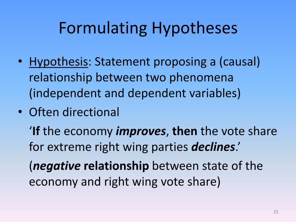
• Hypothesis: Statement proposing a (causal) relationship between two phenomena (independent and dependent variables)
• Often directional
‘If the economy improves, then the vote share for extreme right wing parties declines.’
(negative relationship between state of the economy and right wing vote share)
25
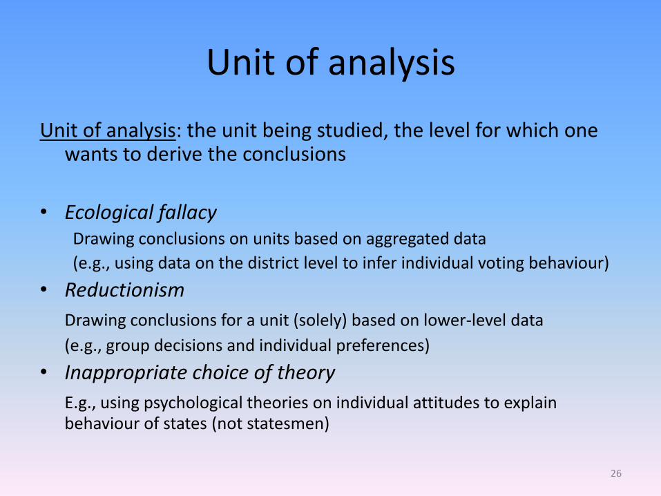
Unit of analysis
Unit of analysis: the unit being studied, the level for which one wants to derive the conclusions
• Ecological fallacy Drawing conclusions on units based on aggregated data
(e.g., using data on the district level to infer individual voting behaviour)
• Reductionism
Drawing conclusions for a unit (solely) based on lower-level data
(e.g., group decisions and individual preferences)
• Inappropriate choice of theory
E.g., using psychological theories on individual attitudes to explain behaviour of states (not statesmen)
26

Any questions?
27
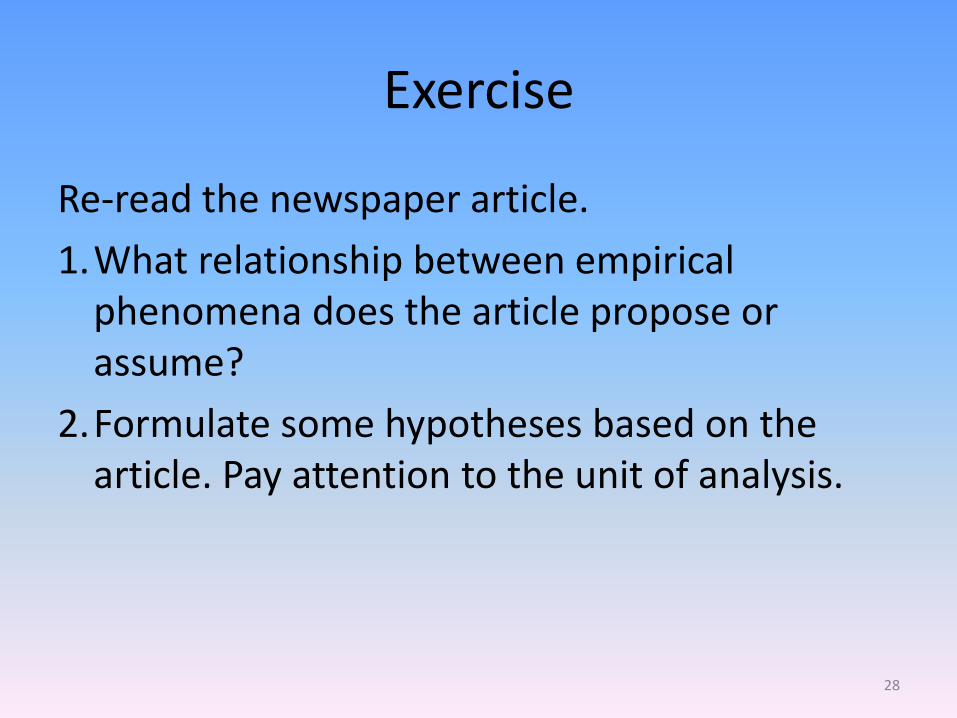
Exercise
Re-read the newspaper article.
1.What relationship between empirical phenomena does the article propose or assume?
2.Formulate some hypotheses based on the article. Pay attention to the unit of analysis.
28
Further readings
Chalmers, Alan (2013) What is this thing called science? Maidenhead, McGraw-Hill
Gerring, John (2012) Social Science Methodology. Cambridge, Cambridge University Press, Ch. 2
Johnson and Reynolds (2008) Political Science Research Methods. Washington, CQ Press, Ch. 2 (Studying Politics Scientifically) and Ch. 3 (The Building Blocks of Social Scientific Research: Hypotheses, Concepts and Variables)
Pollock, Philipp (2011) Essentials of Political Analysis. Washington, CQ Press, Ch. 3 (Proposing Explanations, Framing Hypotheses, and Making Comparisons)
29

Session 2
Measurement:
• Conceptualization and Operationalization
• Data collection
• Reliability and Validity
30
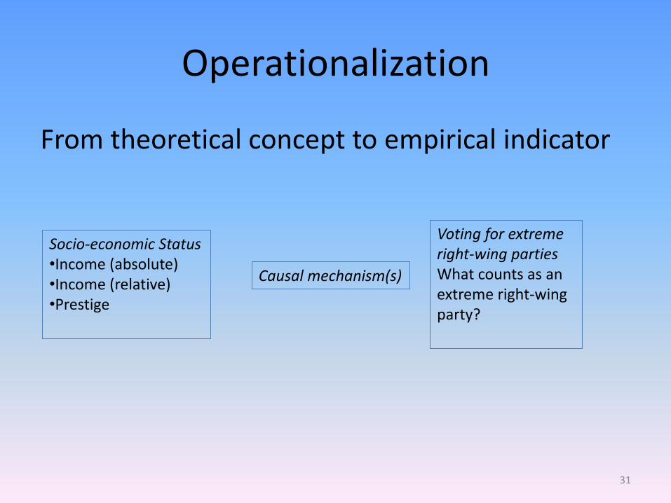
Operationalization
From theoretical concept to empirical indicator
Voting for extreme right-wing parties What counts as an extreme right-wing party?
Socio-economic Status •Income (absolute) •Income (relative) •Prestige
Causal mechanism(s)
31

Conceptualization and operationalization
32
Concept
Aspect/Construct 1 Indicator 1
Indicator 2
Indicator 3
Indicator 4
Indicator 5
Indicator 6
Abstract (usually unobservable) Concrete and observable
Aspect/Construct 2
Aspect/Construct 3
Conceptualization
(definition of concept) Operationalization
(choice of indictors/observations)
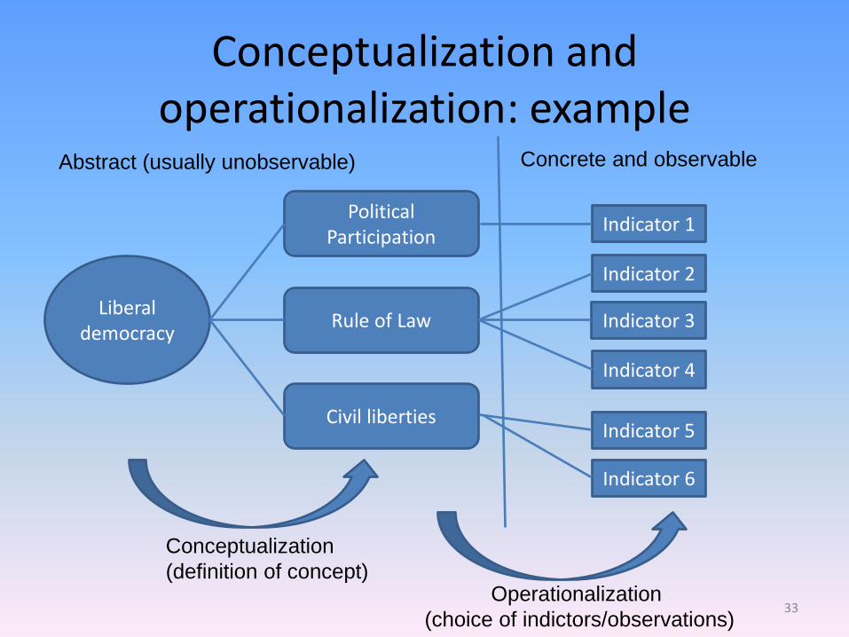
Conceptualization and operationalization: example
33
Liberal democracy
Political Participation
Indicator 1
Indicator 2
Indicator 3
Indicator 4
Indicator 5
Indicator 6
Abstract (usually unobservable) Concrete and observable
Rule of Law
Civil liberties
Conceptualization
(definition of concept) Operationalization
(choice of indictors/observations)
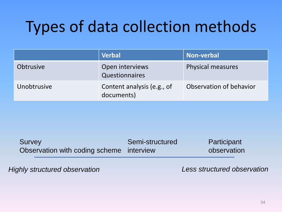
Types of data collection methods
Verbal Non-verbal
Obtrusive Open interviews Questionnaires
Physical measures
Unobtrusive Content analysis (e.g., of documents)
Observation of behavior
Highly structured observation Less structured observation
Survey
Observation with coding scheme
Semi-structured
interview
Participant
observation
34
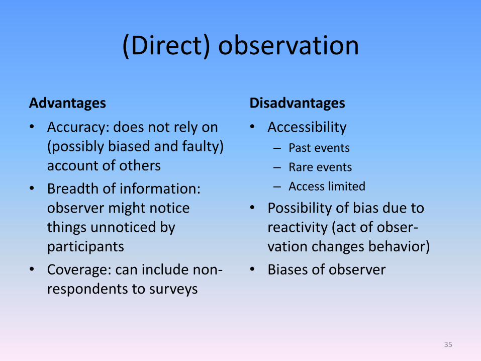
(Direct) observation
Advantages
• Accuracy: does not rely on (possibly biased and faulty) account of others
• Breadth of information: observer might notice things unnoticed by participants
• Coverage: can include non-respondents to surveys
Disadvantages
• Accessibility – Past events
– Rare events
– Access limited
• Possibility of bias due to reactivity (act of obser-vation changes behavior)
• Biases of observer
35
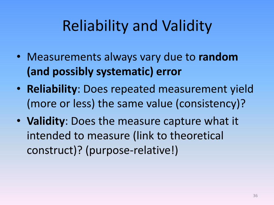
Reliability and Validity
• Measurements always vary due to random (and possibly systematic) error
• Reliability: Does repeated measurement yield (more or less) the same value (consistency)?
• Validity: Does the measure capture what it intended to measure (link to theoretical construct)? (purpose-relative!)
36
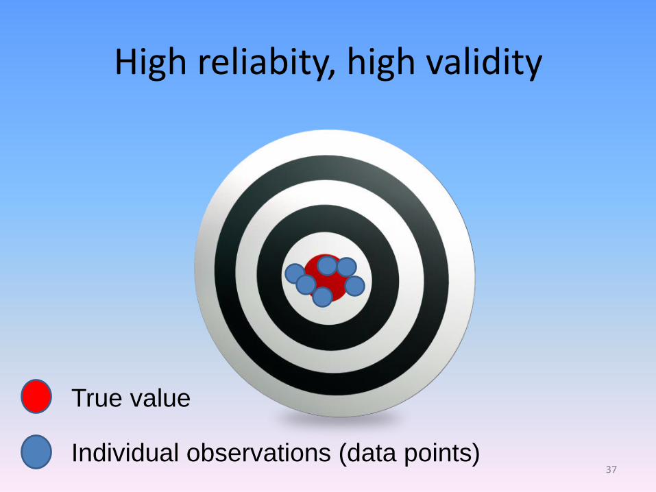
High reliabity, high validity
True value
Individual observations (data points) 37
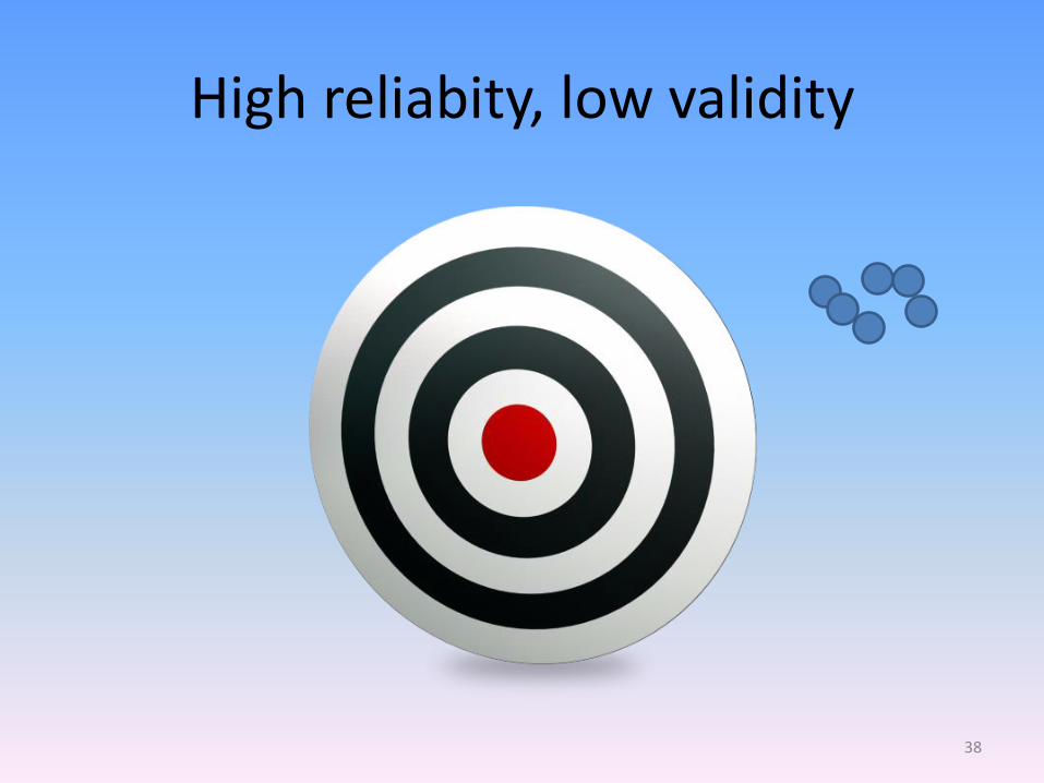
High reliabity, low validity
38

Low reliabity, low validity
39
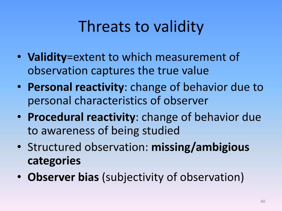
Threats to validity
• Validity=extent to which measurement of observation captures the true value
• Personal reactivity: change of behavior due to personal characteristics of observer
• Procedural reactivity: change of behavior due to awareness of being studied
• Structured observation: missing/ambigious categories
• Observer bias (subjectivity of observation)
40

Any questions?
41
Exercise
1. Conceptualize and operationalize your dependent variable.
2. Conceptualize and operationalize (one of your) independent variable(s).
3. Compare the advantages and disadvantages of at least two ways of measuring one of your variables.
42

Further readings
Gerring, John (2012) Social Science Methodology. Cambridge, Cambridge University Press, Ch. 5 (Concepts)
Johnson and Reynolds (2008) Political Science Research Methods. Washington, CQ Press, Ch. 4 (Measurement)
Pollock, Philipp (2011) Essentials of Political Analysis. Washington, CQ Press, Ch. 1 (Definition and Measurement)
43
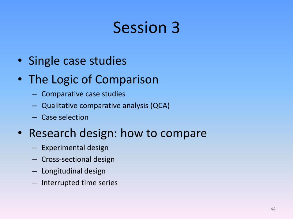
Session 3
• Single case studies
• The Logic of Comparison – Comparative case studies
– Qualitative comparative analysis (QCA)
– Case selection
• Research design: how to compare – Experimental design
– Cross-sectional design
– Longitudinal design
– Interrupted time series
44
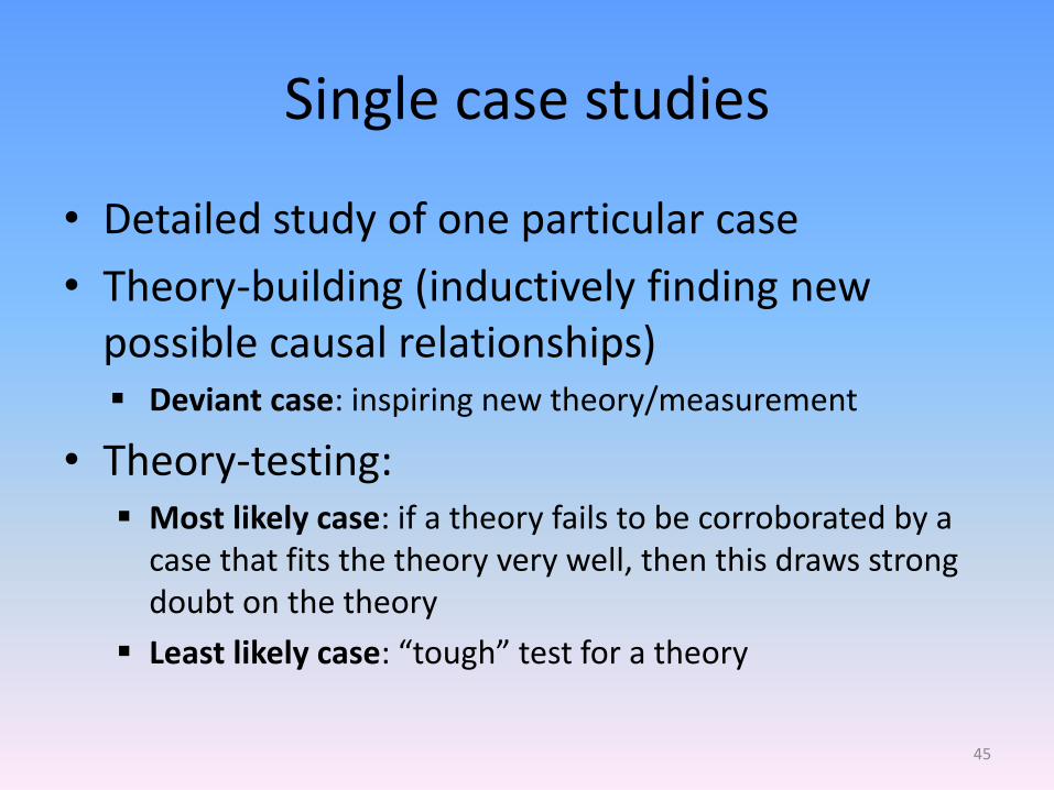
Single case studies
• Detailed study of one particular case
• Theory-building (inductively finding new possible causal relationships) Deviant case: inspiring new theory/measurement
• Theory-testing: Most likely case: if a theory fails to be corroborated by a
case that fits the theory very well, then this draws strong doubt on the theory
Least likely case: “tough” test for a theory
45
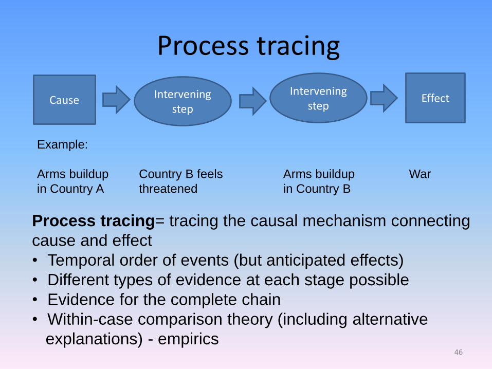
Process tracing
Cause Intervening step
Intervening step
Effect
Process tracing= tracing the causal mechanism connecting
cause and effect
• Temporal order of events (but anticipated effects)
• Different types of evidence at each stage possible
• Evidence for the complete chain
• Within-case comparison theory (including alternative
explanations) - empirics
Example:
Arms buildup Country B feels Arms buildup War
in Country A threatened in Country B
46
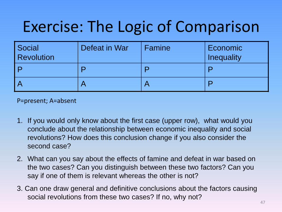
Exercise: The Logic of Comparison Social
Revolution
Defeat in War Famine Economic
Inequality
P P P P
A A A P
P=present; A=absent
1. If you would only know about the first case (upper row), what would you
conclude about the relationship between economic inequality and social
revolutions? How does this conclusion change if you also consider the
second case?
2. What can you say about the effects of famine and defeat in war based on
the two cases? Can you distinguish between these two factors? Can you
say if one of them is relevant whereas the other is not?
3. Can one draw general and definitive conclusions about the factors causing
social revolutions from these two cases? If no, why not? 47
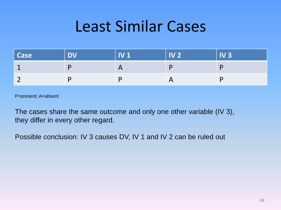
Least Similar Cases
Case DV IV 1 IV 2 IV 3
1 P A P P
2 P P A P
P=present; A=absent
The cases share the same outcome and only one other variable (IV 3),
they differ in every other regard.
Possible conclusion: IV 3 causes DV, IV 1 and IV 2 can be ruled out
48
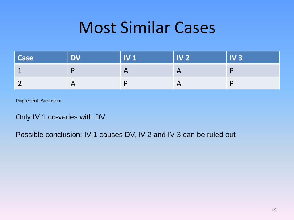
Most Similar Cases
Case DV IV 1 IV 2 IV 3
1 P A A P
2 A P A P
P=present; A=absent
Only IV 1 co-varies with DV.
Possible conclusion: IV 1 causes DV, IV 2 and IV 3 can be ruled out
49

Causal analysis
• A single disconfirming case can falsify a deterministic theory
• Comparison:
– Deterministic relationship of a single necessary or sufficient condition to a cause
– All possible causes have to be included in the analysis
– Empirical cases have to cover all possibilities
50
Necessary condition
Democracies
Universe of
cases Economically
developed countries
Necessary condition: all cases that exhibit the outcome of interest
(e.g. democracies) also have the same condition (e.g. are economically
developed). Democracies (outcome/effect) are a subset of
economically advanced countries (condition). All democracies are
economically advanced countries, but not all economically advanced
countries are democracies. 51

Sufficient condition
Economically developed countries
Universe of
cases Democracies
Sufficient condition: all cases that have the condition (e.g. are
economically developed) exhibit the outcome of interest (e.g. are
democracies. Economically developed countries (condition) are a
subset of democracies (outcome/effect). All economically developed
countries are democracies, but not all democracies are economically
developed.
52

Case study methods
Advantages
• High construct validity (measurement)
• Generation of new theories
• Tracing the causal mechanism
Disadvantages
• Potential indeterminacy
• Selection bias
• Lack of Representativeness
• Low external validity (generalizability)
Source: Bennett (2007)
53

Any questions?
54

Configurational Comparative Methods
• Systematic cross-case comparison
• Integrating case knowledge/context in the process
• Focus on configurations (combinations of conditions and outcomes)
• Establishing necessary and sufficient conditions
• Allows for complexity (combinations of conditions) and equifinality (several conditions are necessary/sufficient)
• Usually applied to small to medium N
• (Crisp set) Qualitative comparative analysis (QCA, csQCA) for binary variables
• Extensions: Fuzzy sets (fsQCA) or multiple value QCA (mvQCA)
55
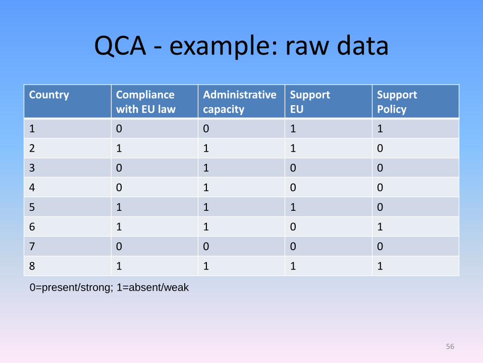
QCA - example: raw data
Country Compliance with EU law
Administrative capacity
Support EU
Support Policy
1 0 0 1 1
2 1 1 1 0
3 0 1 0 0
4 0 1 0 0
5 1 1 1 0
6 1 1 0 1
7 0 0 0 0
8 1 1 1 1
0=present/strong; 1=absent/weak
56
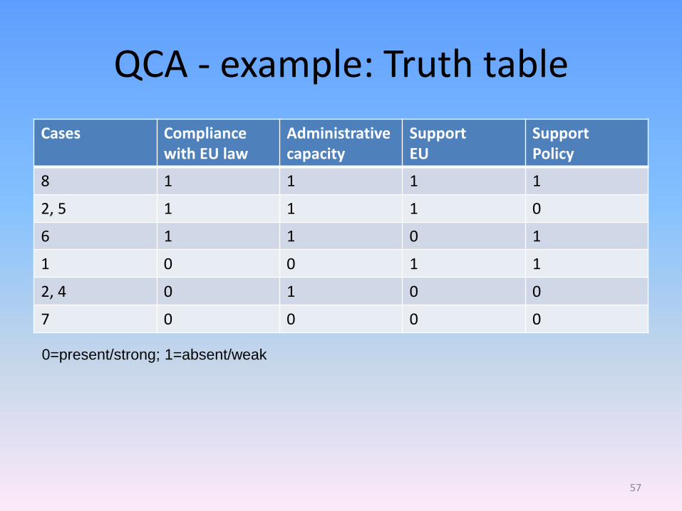
QCA - example: Truth table
Cases Compliance with EU law
Administrative capacity
Support EU
Support Policy
8 1 1 1 1
2, 5 1 1 1 0
6 1 1 0 1
1 0 0 1 1
2, 4 0 1 0 0
7 0 0 0 0
0=present/strong; 1=absent/weak
57
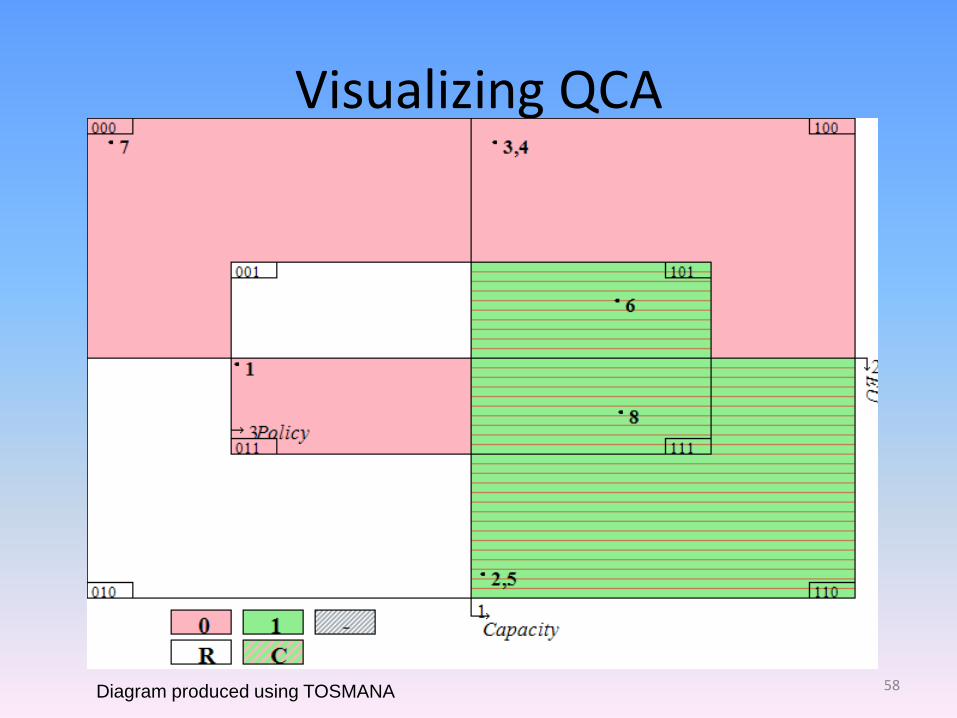
Visualizing QCA
Diagram produced using TOSMANA 58

Example: Result
CAPACITY * EU + CAPACITY * POLICY -> COMPLIANCE CAPITAL/small letters=PRESENT/absent
*=logical AND
+=logical OR
Compliance is present when either administrative capacity AND support for the EU OR administrative capacity AND support for the proposed policy are present.
Administrative capacity is a necessary condition, but it is only sufficient in combination with support for the EU or support for the policy
59

Configurational methods
Strenghts
• Possible combination of comparison and case knowledge
• Allowing for complexity
• Allowing for equifinality
• Allowing for asymmetry
Pitfalls
• Sensitivity to cases and conditions included
• Use of simplifying assumptions to reach parsimonious results
• Does not show causal mechanism
• Does not include temporal order
60

Any questions?
61

Case selection: positive relationship
Cause
Absent Present
Outcome Present Cases A, B, C
Absent Cases D, E, F
There is a positive relationship between cause and outcome
62
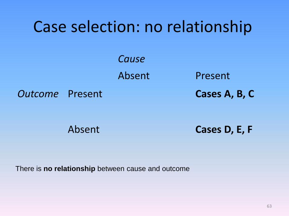
Case selection: no relationship
Cause
Absent Present
Outcome Present Cases A, B, C
Absent Cases D, E, F
There is no relationship between cause and outcome
63
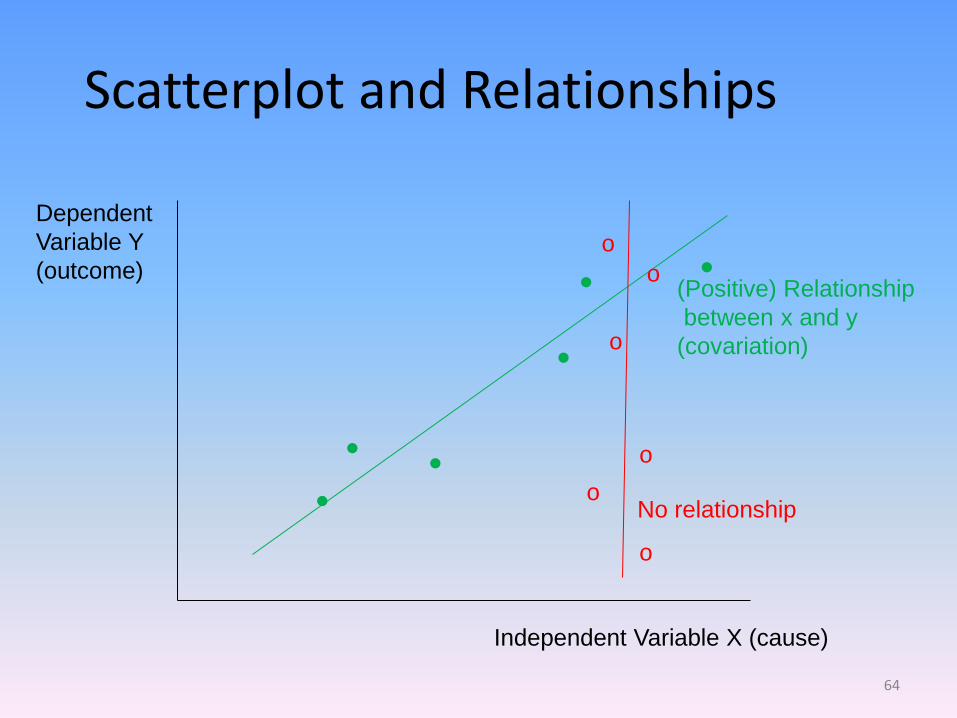
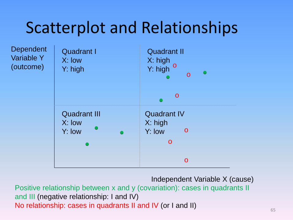
Scatterplot and Relationships
Independent Variable X (cause)
Dependent
Variable Y
(outcome) (Positive) Relationship
between x and y
(covariation)
No relationship ●
●
●
●
● ●
o
o
o
o
o
o
64
Scatterplot and Relationships
Independent Variable X (cause)
Dependent
Variable Y
(outcome)
Positive relationship between x and y (covariation): cases in quadrants II
and III (negative relationship: I and IV)
No relationship: cases in quadrants II and IV (or I and II)
Quadrant I
X: low
Y: high
Quadrant II
X: high
Y: high
Quadrant III
X: low
Y: low
Quadrant IV
X: high
Y: low
●
●
●
●
● ●
●
●
●
●
● ●
o
o
o
o
o
o
65

Choosing Cases on the Dependent Variable
Cause
Absent Present
Outcome Present Cases A, B, C
Absent Assumption:
D, E, F
Alternative:
D, E, F
66
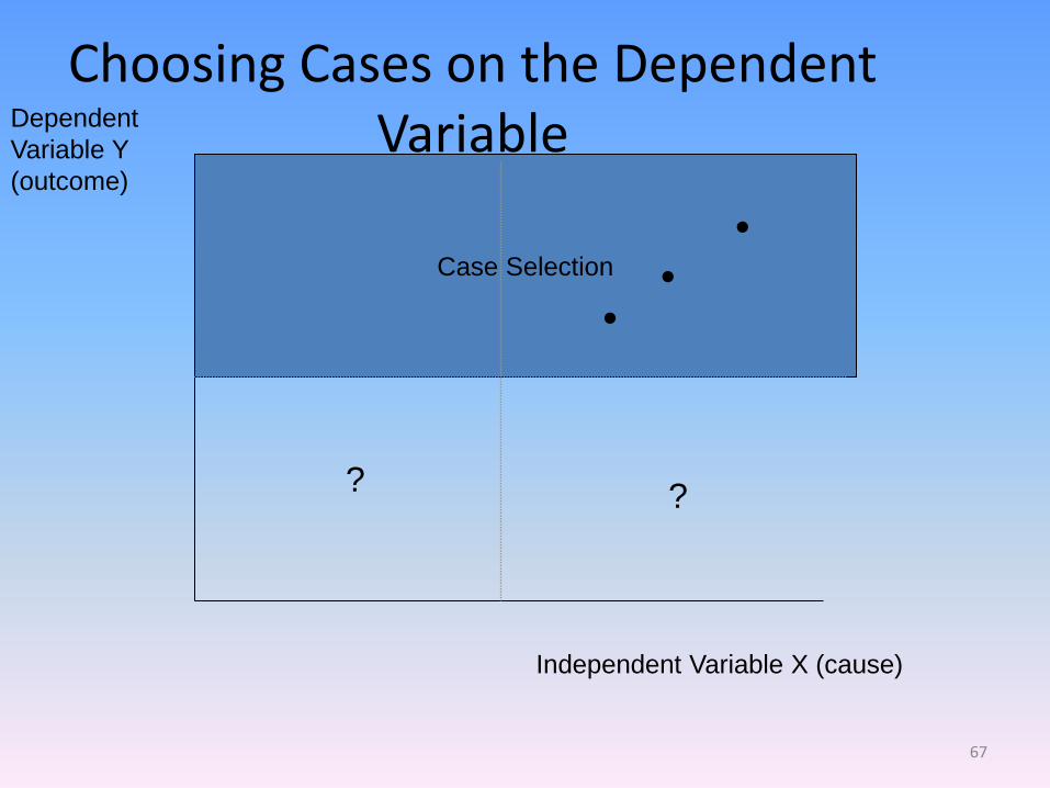
Case Selection
Choosing Cases on the Dependent Variable
Independent Variable X (cause)
Dependent
Variable Y
(outcome)
? ?
●
●
●
67

Any questions?
68
Research design
• Experimental design
• Cross-sectional design
• Longitudinal design
• Interrupted time series
69
Experiments I
• Hypothesized cause is manipulated
• Other factors are held constant
• Comparison of treatment and control group in terms of outcome
• Randomization
70
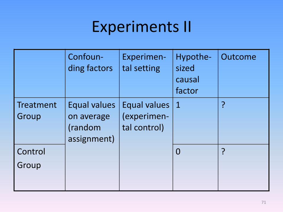
Experiments II
Confoun-ding factors
Experimen-tal setting
Hypothe-sized causal factor
Outcome
Treatment Group
Equal values on average (random assignment)
Equal values (experimen-tal control)
1 ?
Control
Group
0 ?
71
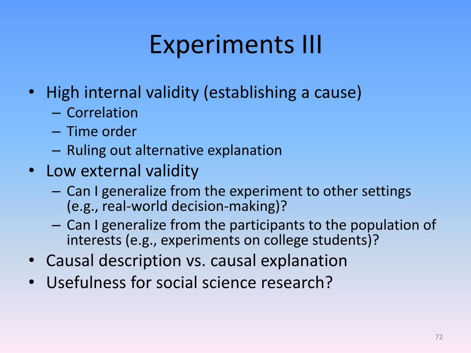
Experiments III
• High internal validity (establishing a cause) – Correlation – Time order – Ruling out alternative explanation
• Low external validity – Can I generalize from the experiment to other settings
(e.g., real-world decision-making)? – Can I generalize from the participants to the population of
interests (e.g., experiments on college students)?
• Causal description vs. causal explanation • Usefulness for social science research?
72
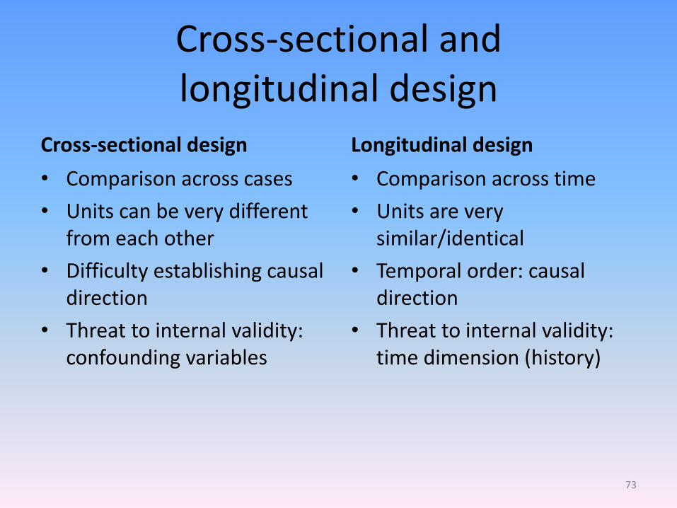
Cross-sectional and longitudinal design
Cross-sectional design
• Comparison across cases
• Units can be very different from each other
• Difficulty establishing causal direction
• Threat to internal validity: confounding variables
Longitudinal design
• Comparison across time
• Units are very similar/identical
• Temporal order: causal direction
• Threat to internal validity: time dimension (history)
73

Any questions?
74
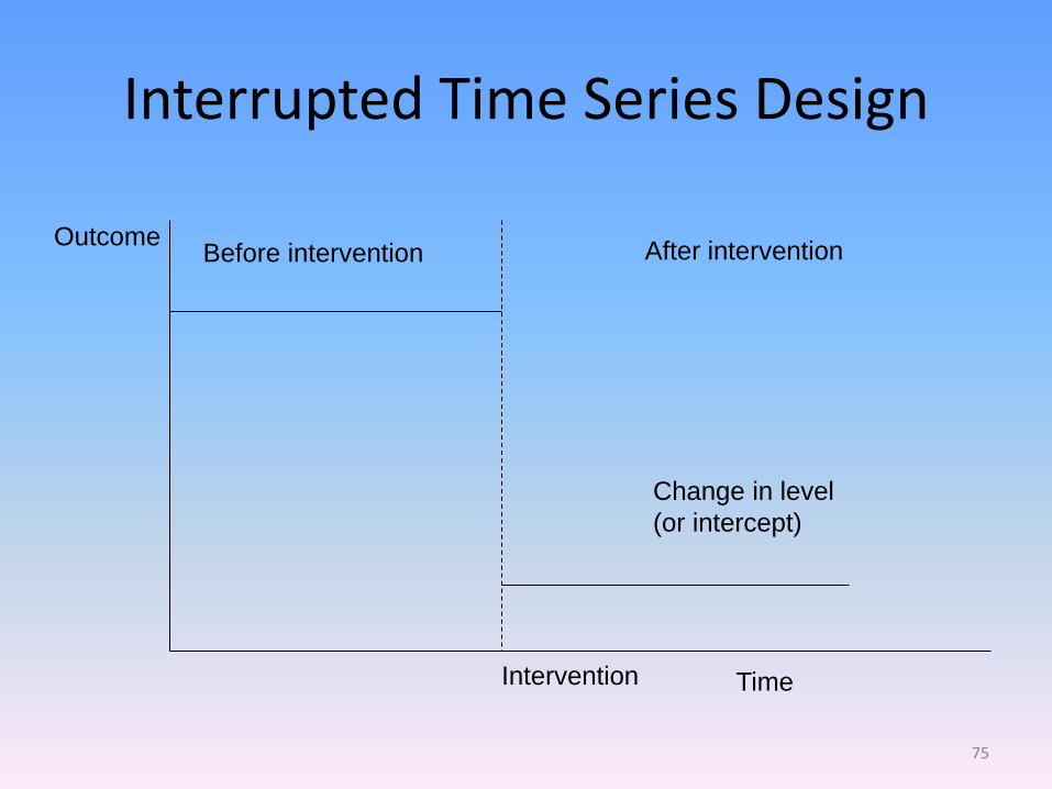
Interrupted Time Series Design
Outcome
Time
Before intervention After intervention
Intervention
Change in level
(or intercept)
75
Interrupted Time Series Design
Outcome
Time
Before intervention After intervention
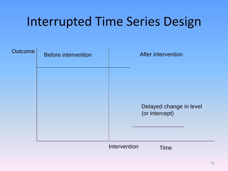
Intervention
Delayed change in level
(or intercept)
76
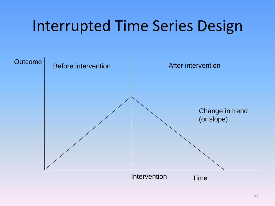
Interrupted Time Series Design
Outcome
Time
Before intervention After intervention
Intervention
Change in trend
(or slope)
77
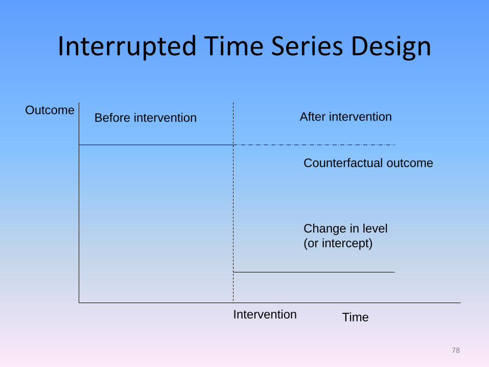
Interrupted Time Series Design
Outcome
Time
Before intervention After intervention
Intervention
Change in level
(or intercept)
Counterfactual outcome
78
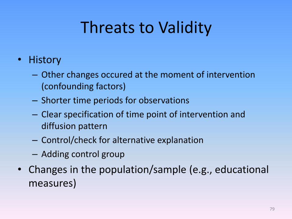
Threats to Validity
• History
– Other changes occured at the moment of intervention (confounding factors)
– Shorter time periods for observations
– Clear specification of time point of intervention and diffusion pattern
– Control/check for alternative explanation
– Adding control group
• Changes in the population/sample (e.g., educational measures)
79

Interrupted Time Series Design
Outcome
Time
Before intervention After intervention
Intervention
Change in trend
(or slope)
Control group
Treatment group
80
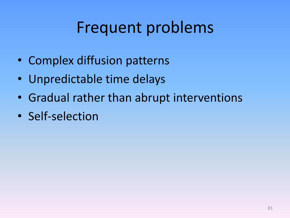
Frequent problems
• Complex diffusion patterns
• Unpredictable time delays
• Gradual rather than abrupt interventions
• Self-selection
81

Any questions?
82
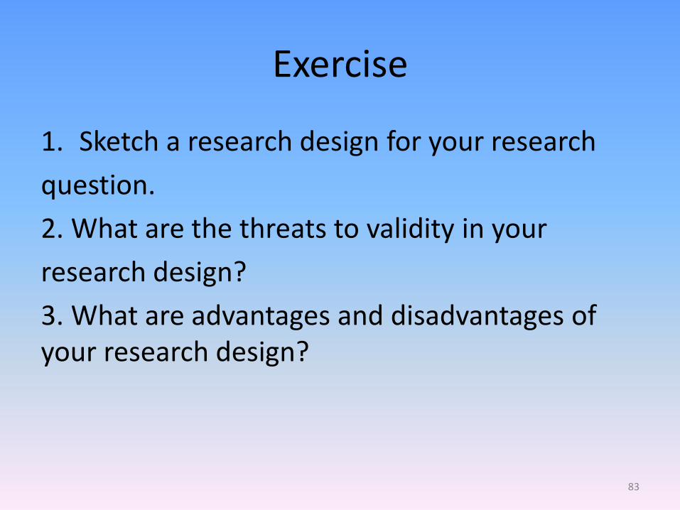
Exercise
1. Sketch a research design for your research
question.
2. What are the threats to validity in your
research design?
3. What are advantages and disadvantages of your research design?
83
Further readings
Bennett, Andrew (2002) Case Study Methods: Design, Use, and Comparative Advantages, in: Sprinz and Yael Wolinsky (eds.) Cases, Numbers, Models: International Relations Research Methods, Ann Arbor, University of Michigan Press
De Vaus, David (2001) Research Design in Social Research. London, Sage
Geddes, Barbara (2003). Paradigms and Sandcastles. Theory Building and Research Design in Comparative Politics. Ann Arbor, University of Michigan Press
Gerring, John (2013) Social Science Methodology. Cambridge, Cambridge University Press, Ch. 10 (Causal strategies)
Rihoux, Benoit and Ragin, Charles (2008) Configurational Comparative Methods: Qualitative Comparative Analysis and Related Methods. London, Sage
Rohlfing, Ingo (2012) Case studies and Causal Inference. Houndmills, MacMillan
84
Session 4
• Quantitative Analysis
• Comparing Methods
85
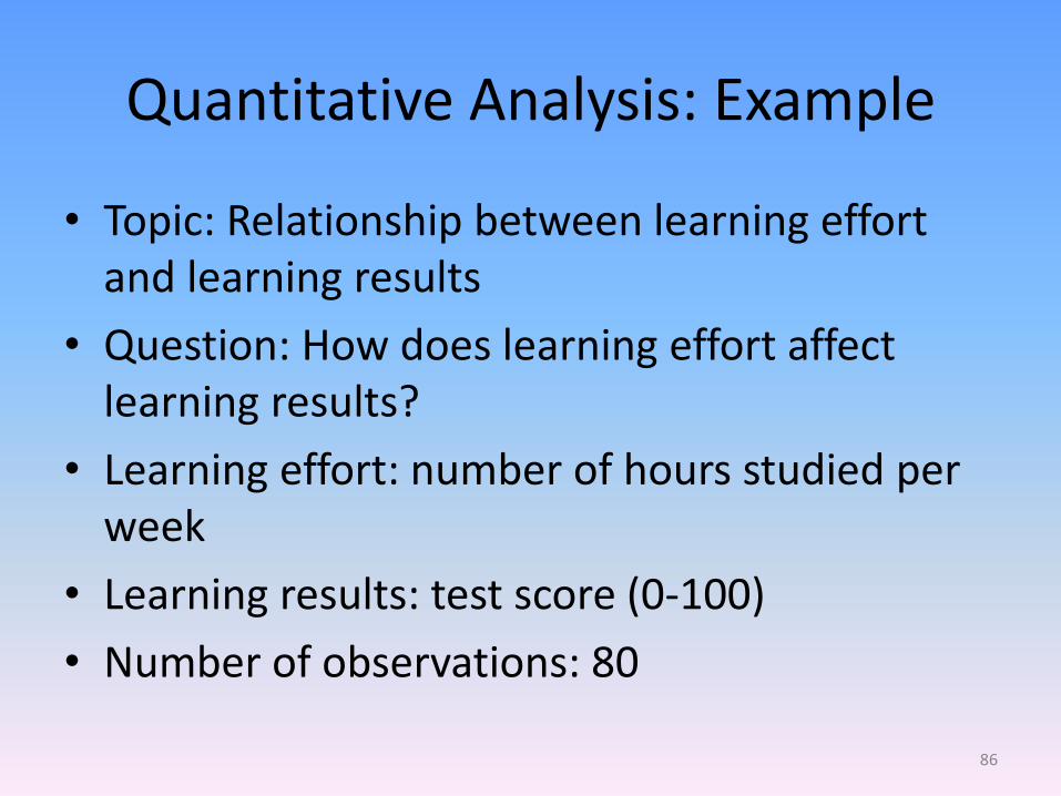
Quantitative Analysis: Example
• Topic: Relationship between learning effort and learning results
• Question: How does learning effort affect learning results?
• Learning effort: number of hours studied per week
• Learning results: test score (0-100)
• Number of observations: 80
86
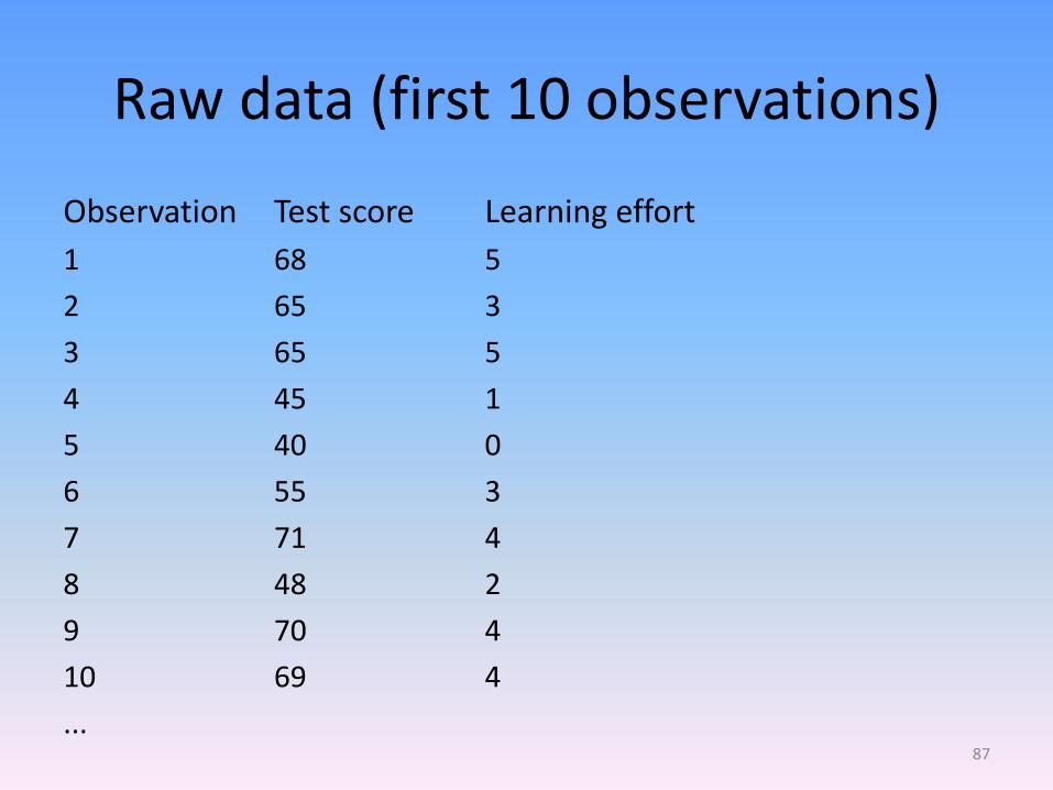
Raw data (first 10 observations)
Observation Test score Learning effort
1 68 5
2 65 3
3 65 5
4 45 1
5 40 0
6 55 3
7 71 4
8 48 2
9 70 4
10 69 4
...
87
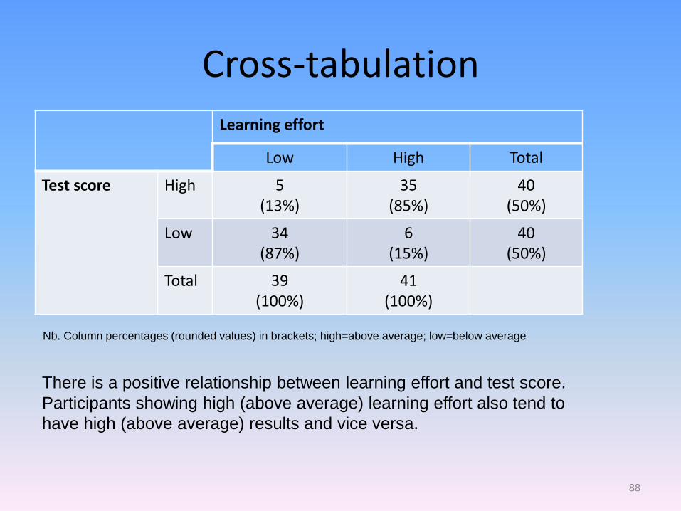
Cross-tabulation
Learning effort
Low High Total
Test score High 5 (13%)
35 (85%)
40 (50%)
Low 34 (87%)
6 (15%)
40 (50%)
Total 39 (100%)
41 (100%)
Nb. Column percentages (rounded values) in brackets; high=above average; low=below average
There is a positive relationship between learning effort and test score.
Participants showing high (above average) learning effort also tend to
have high (above average) results and vice versa.
88
02
04
06
08
0
Ave
rag
e te
st score
Low High
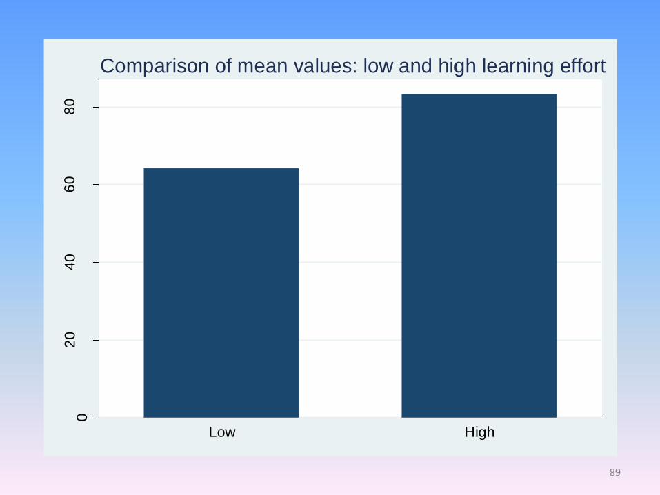
Comparison of mean values: low and high learning effort
89
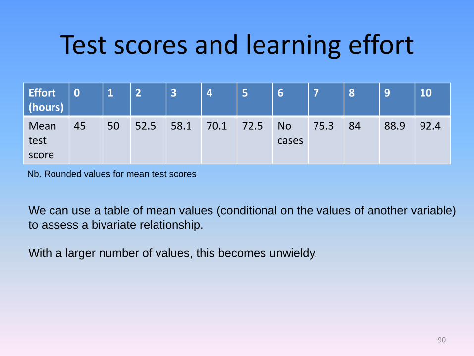
Test scores and learning effort
Effort (hours)
0 1 2 3 4 5 6 7 8 9 10
Mean test score
45 50 52.5 58.1 70.1 72.5 No cases
75.3
84 88.9 92.4
We can use a table of mean values (conditional on the values of another variable)
to assess a bivariate relationship.
With a larger number of values, this becomes unwieldy.
Nb. Rounded values for mean test scores
90
02
04
06
08
01
00
Test sco
re (
0-1
00
)
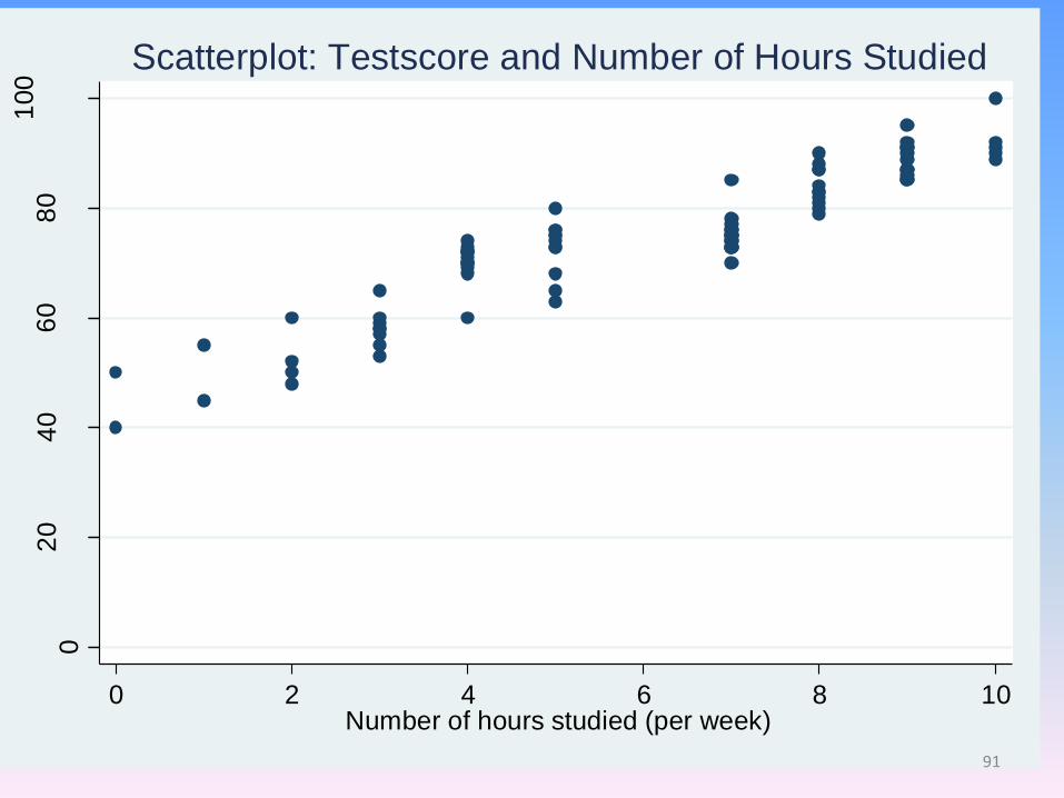
0 2 4 6 8 10Number of hours studied (per week)
Scatterplot: Testscore and Number of Hours Studied
91
40
50
60
70
80
90
Ave
rag
e te
st score
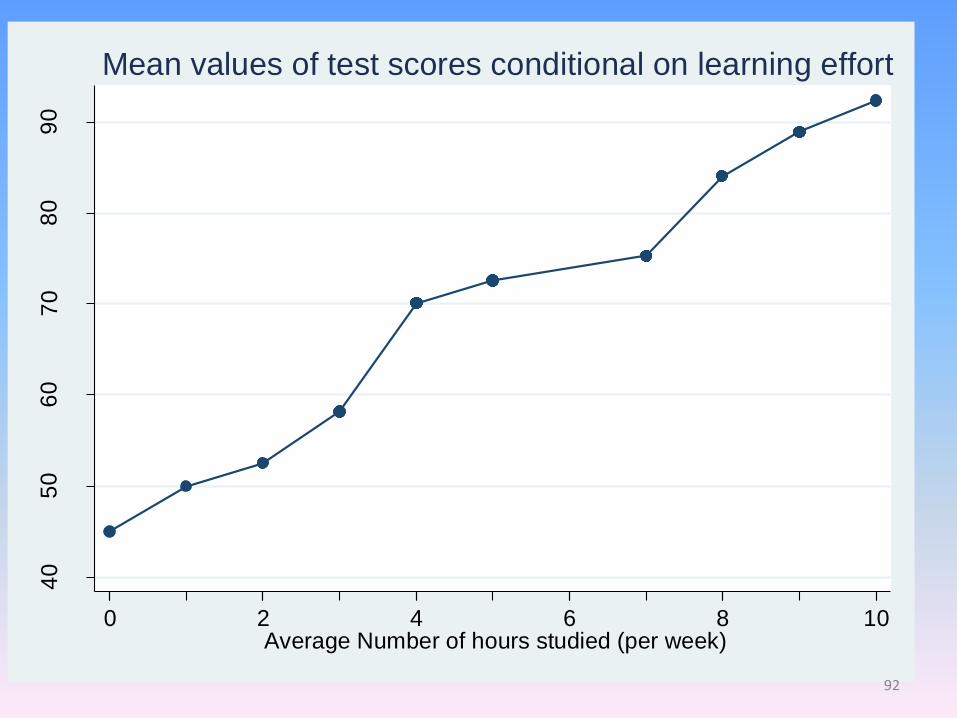
0 2 4 6 8 10Average Number of hours studied (per week)
Mean values of test scores conditional on learning effort
92
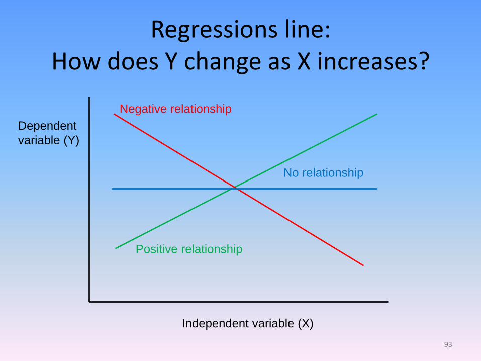
Regressions line: How does Y change as X increases?
Dependent
variable (Y)
Independent variable (X)
Negative relationship
Positive relationship
No relationship
93

02
04
06
08
01
00
Test sco
re
0 2 4 6 8 10Number of hours studied (per week)
Scatterplot with regression line
Constant (α)
(x-variable=0)
Coefficient (β)
(slope)
Regression line (red line)
Example:
Test score=Constant+Coeffizient *Learning effort
In general:
Y=α+β*X
Determining the regression line via ordinary least
squares
94
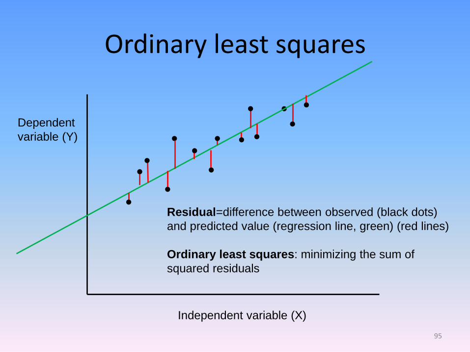
Ordinary least squares
Dependent
variable (Y)
Independent variable (X)
●
●
Residual=difference between observed (black dots)
and predicted value (regression line, green) (red lines)
Ordinary least squares: minimizing the sum of
squared residuals
●
●
●
●
●
●
● ● ● ●
●
●
95
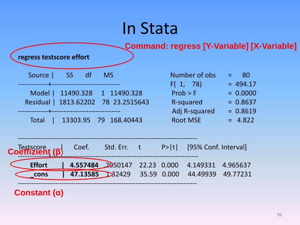
regress testscore effort Source | SS df MS Number of obs = 80 -------------+------------------------------ F( 1, 78) = 494.17 Model | 11490.328 1 11490.328 Prob > F = 0.0000 Residual | 1813.62202 78 23.2515643 R-squared = 0.8637 -------------+------------------------------ Adj R-squared = 0.8619 Total | 13303.95 79 168.40443 Root MSE = 4.822 ------------------------------------------------------------------------------ Testscore | Coef. Std. Err. t P>|t| [95% Conf. Interval] -------------+---------------------------------------------------------------- Effort | 4.557484 .2050147 22.23 0.000 4.149331 4.965637 _cons | 47.13585 1.32429 35.59 0.000 44.49939 49.77231 ------------------------------------------------------------------------------
In Stata Command: regress [Y-Variable] [X-Variable]
Coeffizient (β)
Constant (α)
96

Result Regression analysis
• Description
Test score=47,1+4,6*effort
Every additional hour of learning typically yields an
increase of 4.6 points in the test scores.
• Prediction (6 hours learning, no cases in the data set but within the range of values we observe)
47,1+4,6*6=74,7
We can expect 6 hours of learning per week to result in a
test score of 74.7.
97
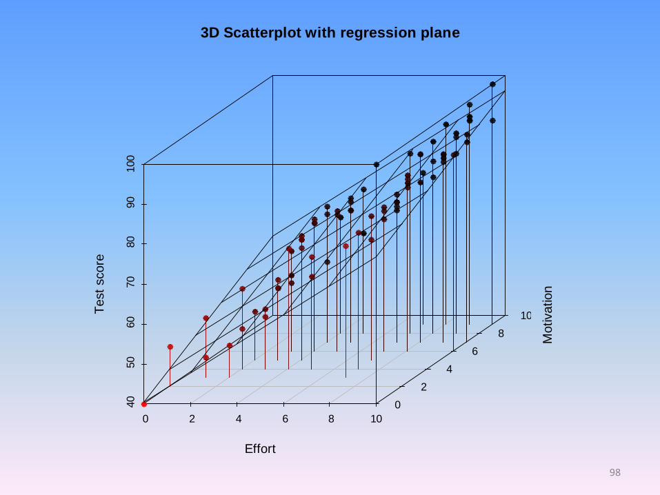
3D Scatterplot with regression plane
0 2 4 6 8 10
40
50
60
70
80
90
100
0
2
4
6
8
10
Effort
Motivation
Test
score
98
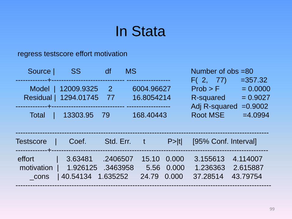
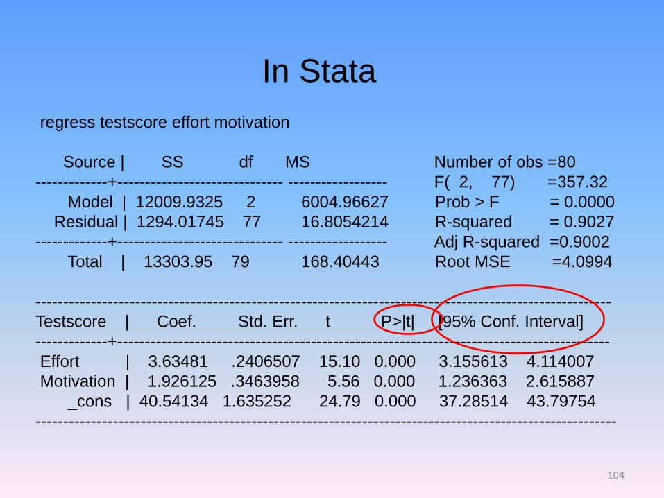
regress testscore effort motivation
Source | SS df MS Number of obs =80
-------------+------------------------------ ------------------ F( 2, 77) =357.32
Model | 12009.9325 2 6004.96627 Prob > F = 0.0000
Residual | 1294.01745 77 16.8054214 R-squared = 0.9027
-------------+------------------------------ ------------------ Adj R-squared =0.9002
Total | 13303.95 79 168.40443 Root MSE =4.0994
--------------------------------------------------------------------------------------------------------
Testscore | Coef. Std. Err. t P>|t| [95% Conf. Interval]
-------------+-----------------------------------------------------------------------------------------
effort | 3.63481 .2406507 15.10 0.000 3.155613 4.114007
motivation | 1.926125 .3463958 5.56 0.000 1.236363 2.615887
_cons | 40.54134 1.635252 24.79 0.000 37.28514 43.79754
---------------------------------------------------------------------------------------------------------
In Stata
99

Addressing uncertainty
• Drawing repeated samples from a population will yield different values (e.g., mean values, regression coefficients)
• Random sampling allows us to make inferences from our sample to the population
100
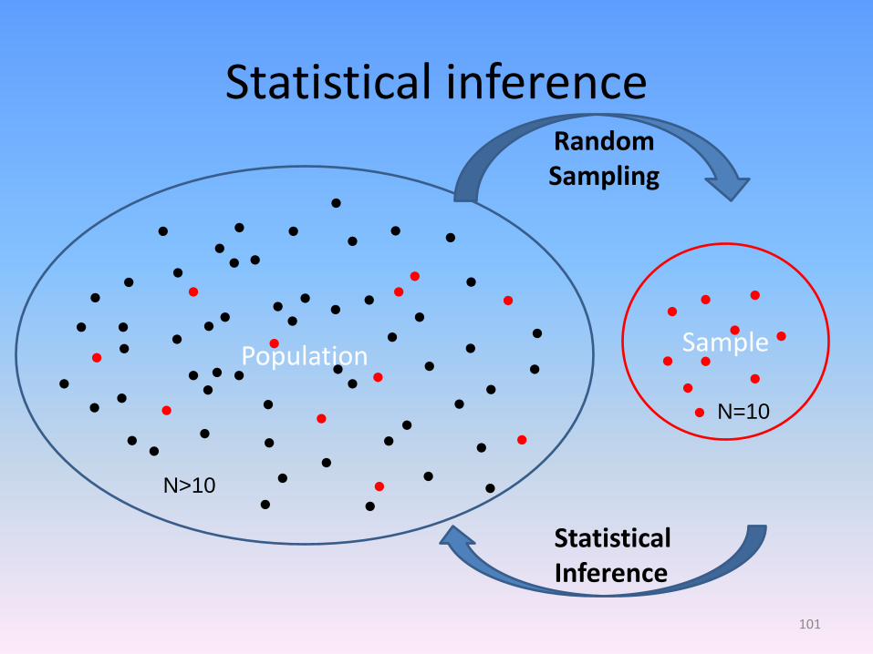
Statistical inference
Population ●
●
●
●
●
●
●
●
●
●
●
●
●
●
●
●
●
●
●
●
●
●
●
● ●
●
●
●
●
●
●
●
● ●
●
●
Random Sampling
Sample ●
●
●
● ●
● ●
●
●
●
Statistical Inference
N=10
N>10
●
●
● ●
●
● ●
●
●
●
●
●
●
●
●
●
●
●
●
●
●
●
●
● ●
●
●
● ●
● ●
101

Adressing uncertainty
• Confidence interval=interval of values for which x percent of samples would include the value of interest (e.g., the regression coefficient) if we would keep drawing samples from the same population
• P-value=probability of obtaining a value (e.g., regression coefficient) at least as extreme as the one in your sample data, assuming the truth of the null hypothesis (usually: no effect).
102
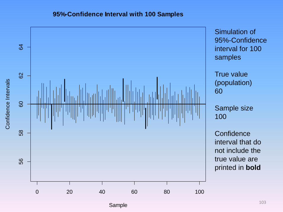
0 20 40 60 80 100
56
58
60
62
64
95%-Confidence Interval with 100 Samples
Sample
Confidence I
nte
rvals
Simulation of
95%-Confidence
interval for 100
samples
True value
(population)
60
Sample size
100
Confidence
interval that do
not include the
true value are
printed in bold
103
regress testscore effort motivation
Source | SS df MS Number of obs =80
-------------+------------------------------ ------------------ F( 2, 77) =357.32
Model | 12009.9325 2 6004.96627 Prob > F = 0.0000
Residual | 1294.01745 77 16.8054214 R-squared = 0.9027
-------------+------------------------------ ------------------ Adj R-squared =0.9002
Total | 13303.95 79 168.40443 Root MSE =4.0994
--------------------------------------------------------------------------------------------------------
Testscore | Coef. Std. Err. t P>|t| [95% Conf. Interval]
-------------+-----------------------------------------------------------------------------------------
Effort | 3.63481 .2406507 15.10 0.000 3.155613 4.114007
Motivation | 1.926125 .3463958 5.56 0.000 1.236363 2.615887
_cons | 40.54134 1.635252 24.79 0.000 37.28514 43.79754
---------------------------------------------------------------------------------------------------------
In Stata
104
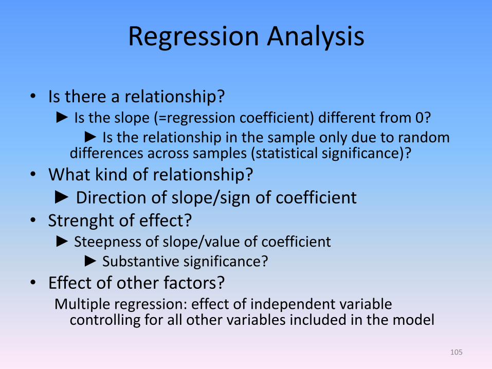
Regression Analysis
• Is there a relationship? ► Is the slope (=regression coefficient) different from 0? ► Is the relationship in the sample only due to random
differences across samples (statistical significance)?
• What kind of relationship? ► Direction of slope/sign of coefficient • Strenght of effect?
► Steepness of slope/value of coefficient ► Substantive significance?
• Effect of other factors? Multiple regression: effect of independent variable
controlling for all other variables included in the model
105
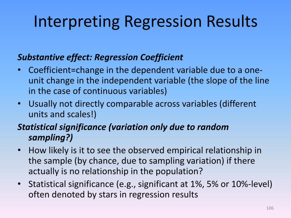
Interpreting Regression Results
Substantive effect: Regression Coefficient
• Coefficient=change in the dependent variable due to a one-unit change in the independent variable (the slope of the line in the case of continuous variables)
• Usually not directly comparable across variables (different units and scales!)
Statistical significance (variation only due to random sampling?)
• How likely is it to see the observed empirical relationship in the sample (by chance, due to sampling variation) if there actually is no relationship in the population?
• Statistical significance (e.g., significant at 1%, 5% or 10%-level) often denoted by stars in regression results
106

Example of
published
results of
a regression
analysis (Gabel
1998: 346)
Reference:
Gabel, M. (1998)
Public Support for
European Integra-
tion - An empirical
test of five
theories, Journal of
Politics, Vol. 60,
No. 2, pp. 333-354
Regression coefficients
(stars denote the level
of statistical
significance)
107

02
46
81
0
4 6 8 10Independent variable (x)
Observations Regression line (all obs.)
Regression line (w/o outlier)
Regression diagnostics: outlier
The regression line is heavily
Influenced by just one observation.
Excluding the outlier drastically
changes the conclusions.
outlier
108
02
04
06
08
01
00
Dep
en
de
nt va
ria
ble
(y)
-10 -5 0 5 10Independent variable (x)
Observations Regression line (OLS)
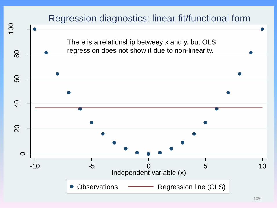
Regression diagnostics: linear fit/functional form
There is a relationship betweey x and y, but OLS
regression does not show it due to non-linearity.
109
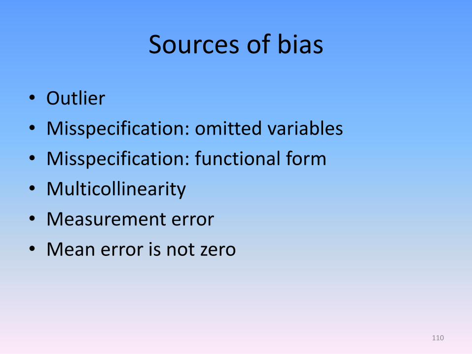
Sources of bias
• Outlier
• Misspecification: omitted variables
• Misspecification: functional form
• Multicollinearity
• Measurement error
• Mean error is not zero
110
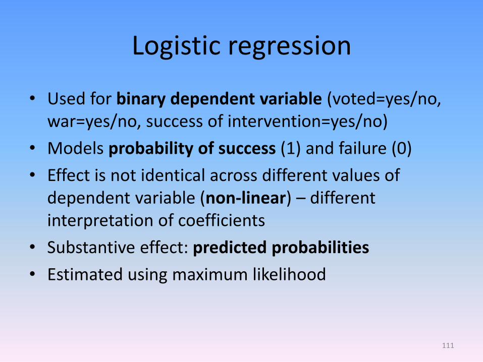
Logistic regression
• Used for binary dependent variable (voted=yes/no, war=yes/no, success of intervention=yes/no)
• Models probability of success (1) and failure (0)
• Effect is not identical across different values of dependent variable (non-linear) – different interpretation of coefficients
• Substantive effect: predicted probabilities
• Estimated using maximum likelihood
111
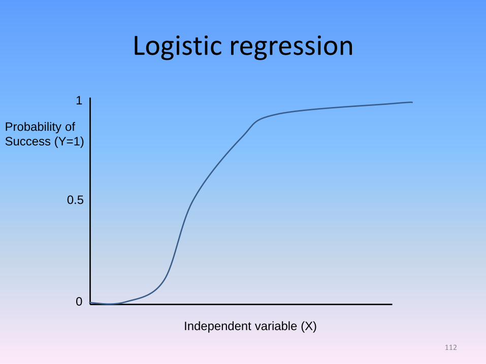
Logistic regression
Probability of
Success (Y=1)
Independent variable (X)
1
0
0.5
112
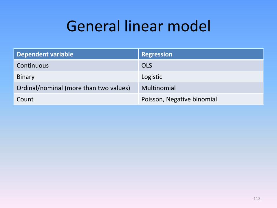
General linear model
Dependent variable Regression
Continuous OLS
Binary Logistic
Ordinal/nominal (more than two values) Multinomial
Count Poisson, Negative binomial
113
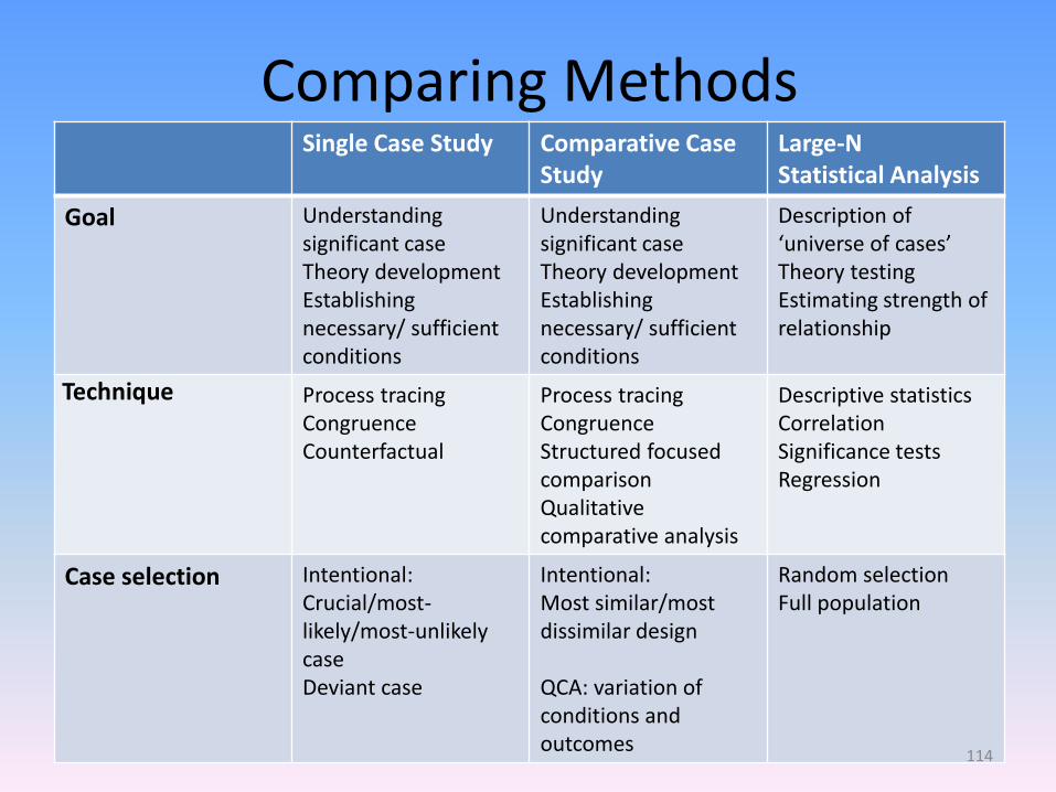
Comparing Methods Single Case Study Comparative Case
Study Large-N Statistical Analysis
Goal Understanding significant case Theory development Establishing necessary/ sufficient conditions
Understanding significant case Theory development Establishing necessary/ sufficient conditions
Description of ‘universe of cases’ Theory testing Estimating strength of relationship
Technique Process tracing Congruence Counterfactual
Process tracing Congruence Structured focused comparison Qualitative comparative analysis
Descriptive statistics Correlation Significance tests Regression
Case selection Intentional: Crucial/most-likely/most-unlikely case Deviant case
Intentional: Most similar/most dissimilar design QCA: variation of conditions and outcomes
Random selection Full population
114

Comparing Methods Single Case Study Comparative Case
Study Large-N Statistical Analysis
Advantage Identifying new/omitted variables or hypotheses High level of construct validity Capturing complex relationships (path dependency, multiple interaction effects) Identifying causal mechanisms
Identifying new/omitted variables or hypotheses High level of construct validity Capturing complex relationships (path dependency, multiple interaction effects) Identifying causal mechanisms
Description of frequency of occurrences Generalizability of findings Established standards of evidence and inference Explicit operationalization
Disadvantage Selection and confirmation bias Limited generalizability of results Establishing relative magnitude of effects Potential indeterminacy
Selection and confirmation bias Limited generalizability of results Establishing relative magnitude of effects
Construct validity
Source: adopted from Bennett (2007) and Braumoeller and Sartori (2007) 115

Any questions?
116
Further readings
Berk, Richard (2004) Regression. A constructive critique. London, Sage
Best, Henning and Wolf, Christof (2014) The SAGE Handbook of Regression Analysis and Causal Inference. London, Sage
Braumoeller, Bear and Sartori, Anne (2007) The Promise and Perils of Statistics in International Relations, in Sprinz and Wolinsky-Nahmias, Models, Numbers and Cases. Ann Arbor, University of Michigan Press
Agresti, Alan and Barbara Finlay (2013) Statistical Methods for the Social Sciences. Upper Saddle River, Pearson
Fox, John (1991) Regression diagnostics. London, Sage
Fox, John (2008) Applied Regression Analysis and Generalized Linear Models. London, Sage
Gailmard, Sean (2014) Statistical Modeling and Inference for Social Science. Cambridge, Cambridge University Press
Pollock, Philipp (2011) Essentials of Political Analysis. Washington, CQ Press
Wooldridge, Jeffrey (2013) Introductory Econometrics. London, Thomson Learning
117


