Page 1
STAT II-LAVC-DENARO 1
Lecture NotesLecture NotesLecture NotesLecture Notes
Part IPart IPart IPart I
Introduction to terminologyIntroduction to terminologyIntroduction to terminologyIntroduction to terminology
DataDataDataData---- Who, What, When, Where, and Who, What, When, Where, and Who, What, When, Where, and Who, What, When, Where, and Why?Why?Why?Why?
Page 2
STAT II-LAVC-DENARO 2
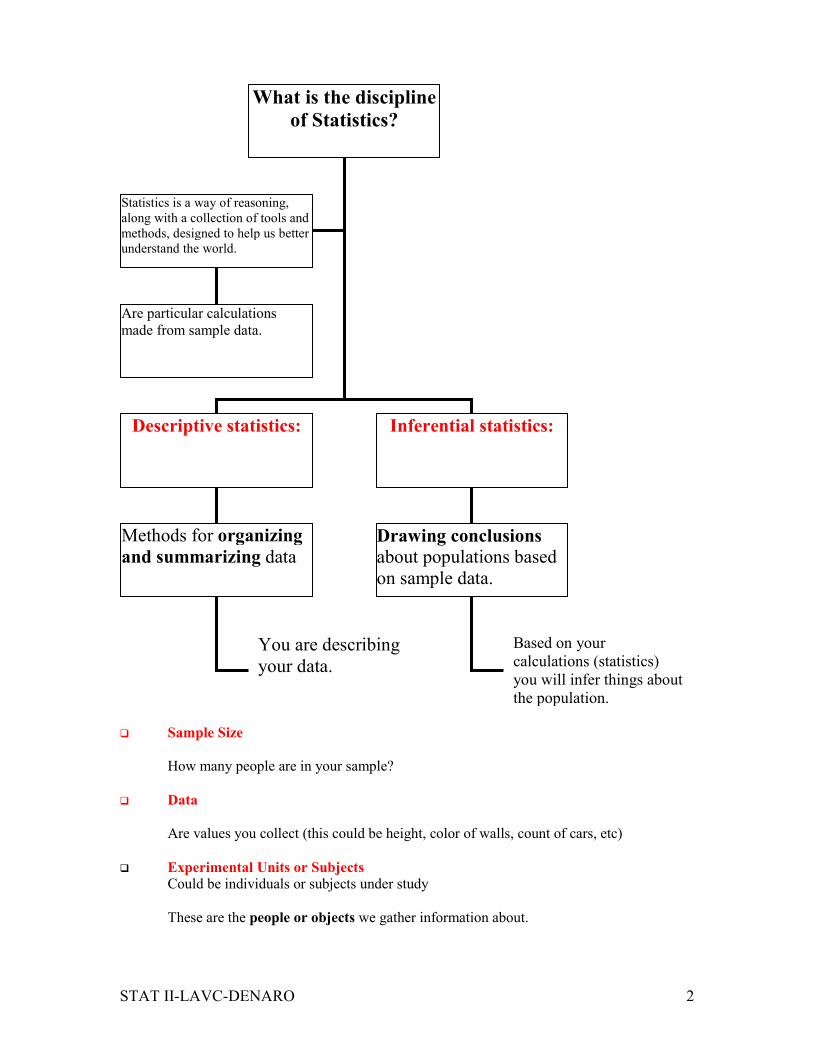
� Sample Size
How many people are in your sample?
� Data
Are values you collect (this could be height, color of walls, count of cars, etc)
� Experimental Units or Subjects Could be individuals or subjects under study
These are the people or objects we gather information about.
What is the discipline
of Statistics?
Descriptive statistics:
Inferential statistics:
Statistics is a way of reasoning,
along with a collection of tools and
methods, designed to help us better
understand the world.
Methods for organizing
and summarizing data
Drawing conclusions about populations based
on sample data.
Based on your
calculations (statistics)
you will infer things about
the population.
You are describing
your data.
Are particular calculations
made from sample data.
Page 3
STAT II-LAVC-DENARO 3
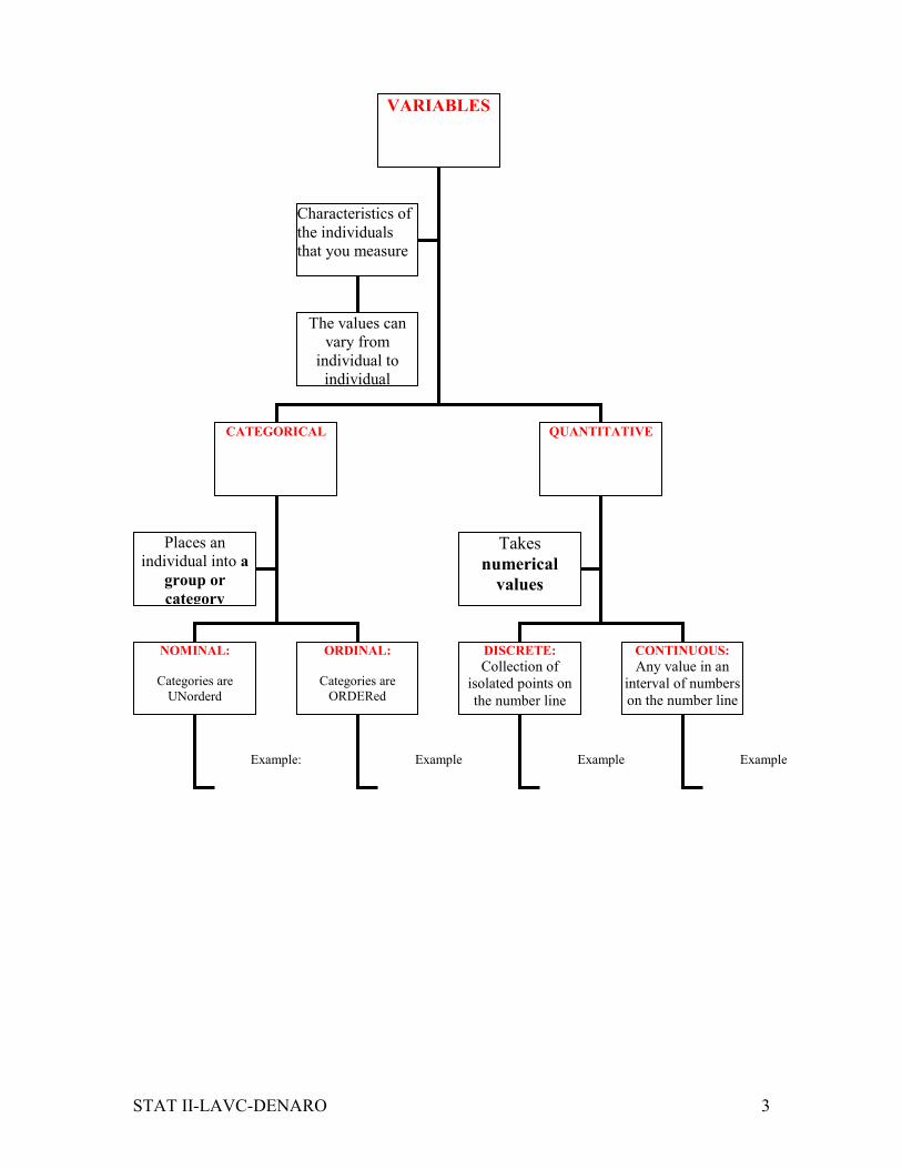
VARIABLES
CATEGORICAL QUANTITATIVE
NOMINAL:
Categories are
UNorderd
ORDINAL:
Categories are
ORDERed
DISCRETE:
Collection of
isolated points on
the number line
CONTINUOUS:
Any value in an
interval of numbers
on the number line
Example: Example Example Example
Characteristics of
the individuals
that you measure
The values can
vary from
individual to
individual
Places an
individual into a
group or
category
Takes
numerical
values
Page 4
STAT II-LAVC-DENARO 4
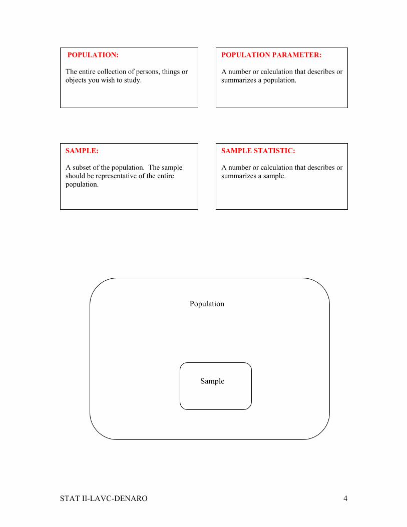
POPULATION:
The entire collection of persons, things or
objects you wish to study.
SAMPLE:
A subset of the population. The sample
should be representative of the entire
population.
POPULATION PARAMETER:
A number or calculation that describes or
summarizes a population.
SAMPLE STATISTIC:
A number or calculation that describes or
summarizes a sample.
Population
Sample
Page 5
STAT II-LAVC-DENARO 5
Lecture NotesLecture NotesLecture NotesLecture Notes
Part IIPart IIPart IIPart II
Displaying and describing Displaying and describing Displaying and describing Displaying and describing Categorical DataCategorical DataCategorical DataCategorical Data
Page 6
STAT II-LAVC-DENARO 6
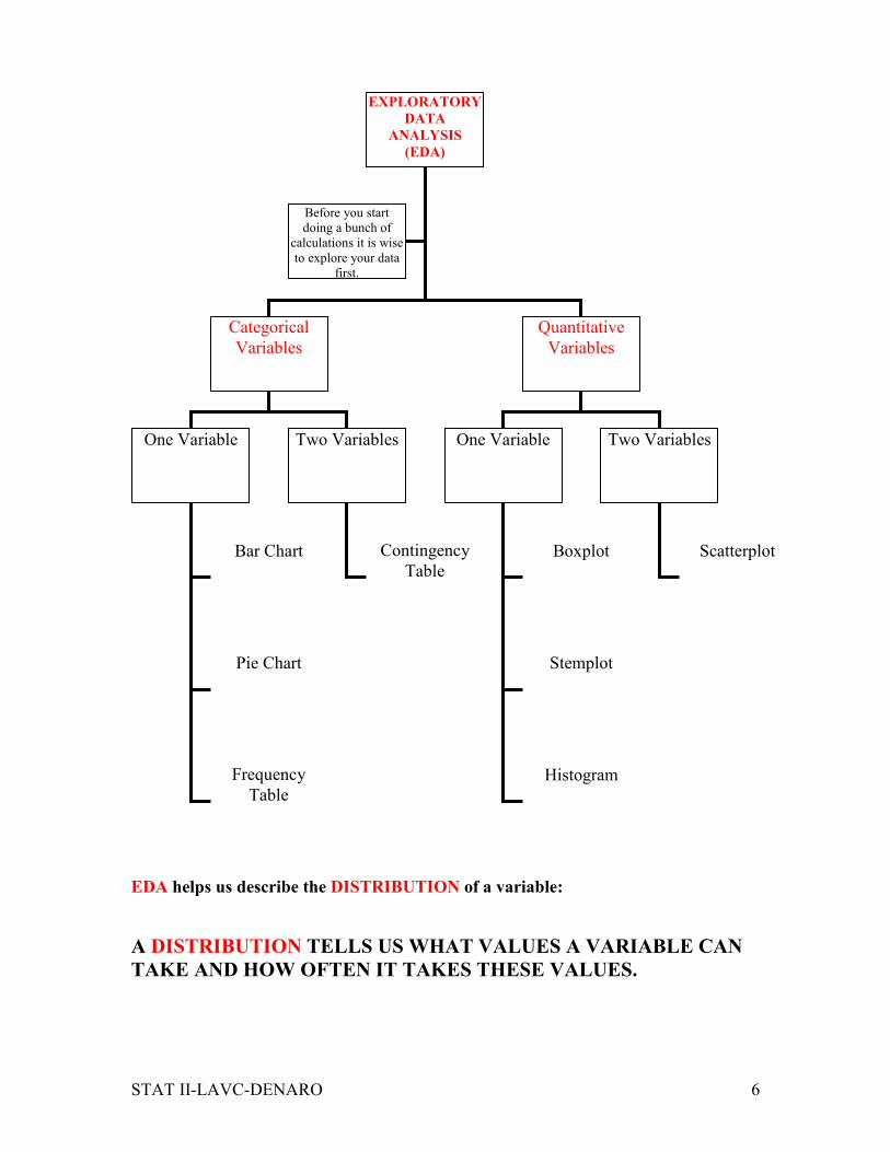
EDA helps us describe the DISTRIBUTION of a variable:
A DISTRIBUTION TELLS US WHAT VALUES A VARIABLE CAN
TAKE AND HOW OFTEN IT TAKES THESE VALUES.
EXPLORATORY
DATA
ANALYSIS
(EDA)
Categorical
Variables
Quantitative
Variables
Before you start
doing a bunch of
calculations it is wise
to explore your data
first.
One Variable Two Variables One Variable
Bar Chart
Pie Chart
Contingency
Table
Boxplot
Stemplot
Two Variables
Histogram
Scatterplot
Frequency
Table
Page 7
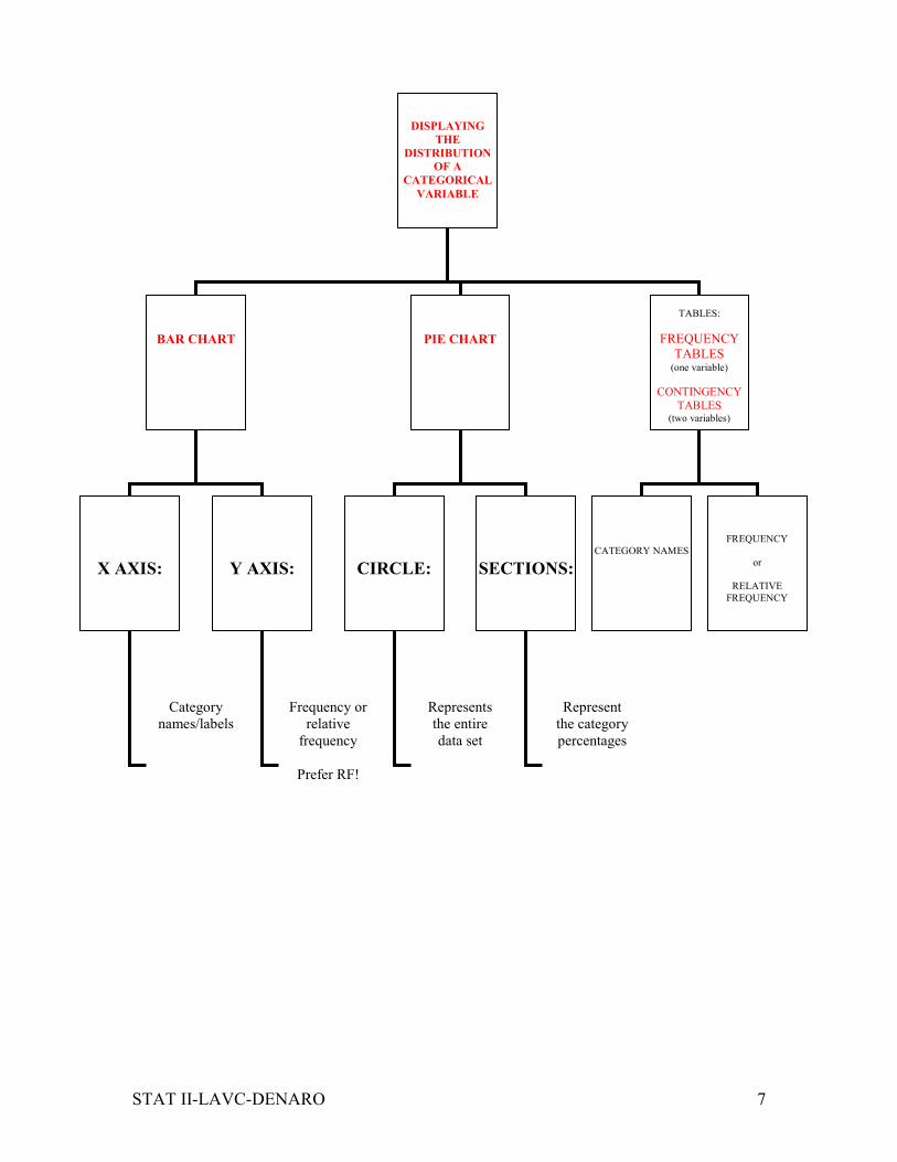
STAT II-LAVC-DENARO 7
DISPLAYING
THE
DISTRIBUTION OF A
CATEGORICAL
VARIABLE
BAR CHART
PIE CHART
X AXIS:
Y AXIS:
CIRCLE:
SECTIONS:
TABLES:
FREQUENCY
TABLES (one variable)
CONTINGENCY
TABLES (two variables)
CATEGORY NAMES
FREQUENCY
or
RELATIVE
FREQUENCY
Category
names/labels
Frequency or
relative
frequency
Prefer RF!
Represents
the entire
data set
Represent
the category
percentages
Page 8
STAT II-LAVC-DENARO 8
Ex:
An article in the Winter 2003 issue of Chance magazine reported on the Houston
Independent School District’s magnet schools programs. Of the 1755 qualified
applicants, 931 were accepted, 298 were waitlisted, and 526 were turned away for lack of
space.
1. What is the variable of interest?
2. Find the relative frequency distribution of the decisions made
3. Make an appropriate display of these data
4. Interpret your graph.
Page 9
STAT II-LAVC-DENARO 9
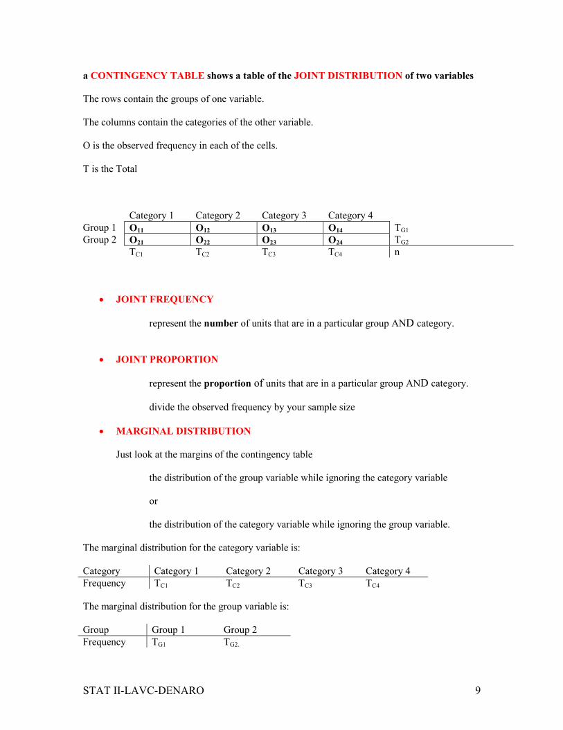
a CONTINGENCY TABLE shows a table of the JOINT DISTRIBUTION of two variables
The rows contain the groups of one variable.
The columns contain the categories of the other variable.
O is the observed frequency in each of the cells.
T is the Total
Category 1 Category 2 Category 3 Category 4
Group 1 O11 O12 O13 O14 TG1
Group 2 O21 O22 O23 O24 TG2
TC1 TC2 TC3 TC4 n
• JOINT FREQUENCY
represent the number of units that are in a particular group AND category.
• JOINT PROPORTION
represent the proportion of units that are in a particular group AND category.
divide the observed frequency by your sample size
• MARGINAL DISTRIBUTION
Just look at the margins of the contingency table
the distribution of the group variable while ignoring the category variable
or
the distribution of the category variable while ignoring the group variable.
The marginal distribution for the category variable is:
Category Category 1 Category 2 Category 3 Category 4
Frequency TC1 TC2 TC3 TC4
The marginal distribution for the group variable is:
Group Group 1 Group 2
Frequency TG1 TG2.
Page 10
STAT II-LAVC-DENARO 10
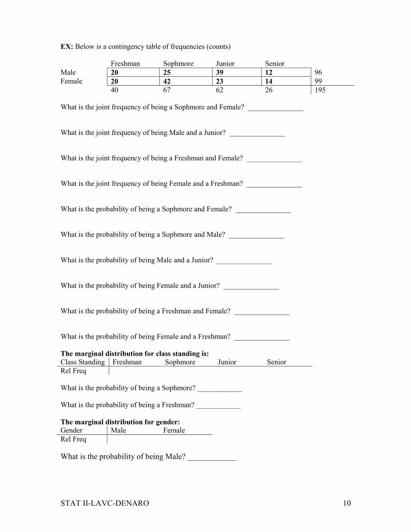
EX: Below is a contingency table of frequencies (counts)
Freshman Sophmore Junior Senior
Male 20 25 39 12 96
Female 20 42 23 14 99
40 67 62 26 195
What is the joint frequency of being a Sophmore and Female? _______________
What is the joint frequency of being Male and a Junior? _______________
What is the joint frequency of being a Freshman and Female? _______________
What is the joint frequency of being Female and a Freshman? _______________
What is the probability of being a Sophmore and Female? _______________
What is the probability of being a Sophmore and Male? _______________
What is the probability of being Male and a Junior? _______________
What is the probability of being Female and a Junior? _______________
What is the probability of being a Freshman and Female? _______________
What is the probability of being Female and a Freshman? _______________
The marginal distribution for class standing is: Class Standing Freshman Sophmore Junior Senior
Rel Freq
What is the probability of being a Sophmore? ____________
What is the probability of being a Freshman? ____________
The marginal distribution for gender: Gender Male Female
Rel Freq
What is the probability of being Male? ____________
Page 11
STAT II-LAVC-DENARO 11
Lecture NotesLecture NotesLecture NotesLecture Notes
Part IIIPart IIIPart IIIPart III
Displaying and describing Displaying and describing Displaying and describing Displaying and describing Quantitative DataQuantitative DataQuantitative DataQuantitative Data
Page 12
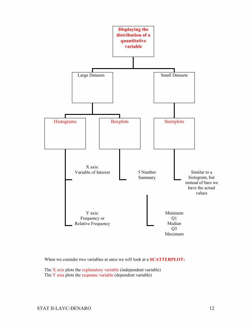
STAT II-LAVC-DENARO 12
When we consider two variables at once we will look at a SCATTERPLOT:
The X axis plots the explanatory variable (independent variable)
The Y axis plots the response variable (dependent variable)
Displaying the
distribution of a
quantitative
variable
Large Datasets Small Datasets
Histograms Boxplots Stemplots
X axis:
Variable of Interest
Y axis:
Frequency or
Relative Frequency
5 Number
Summary
Minimum
Q1
Median
Q3
Maximum
Similar to a
histogram, but
instead of bars we
have the actual
values
Page 13
STAT II-LAVC-DENARO 13
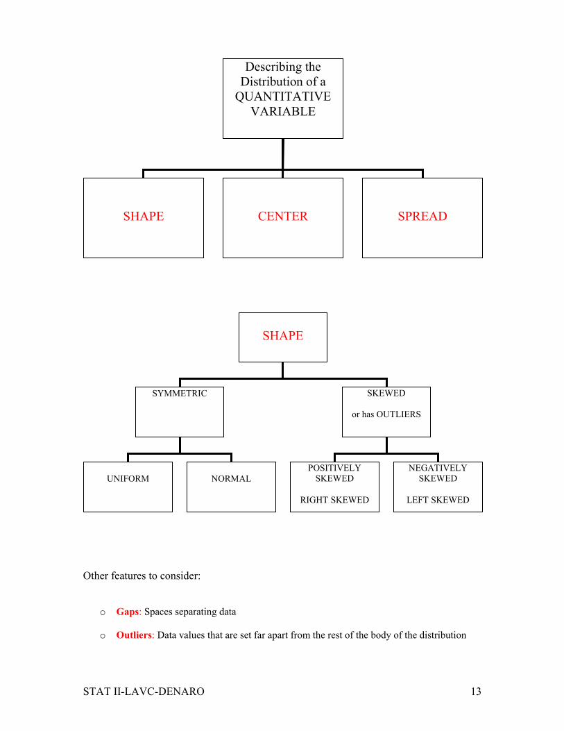
Other features to consider:
o Gaps: Spaces separating data
o Outliers: Data values that are set far apart from the rest of the body of the distribution
Describing the
Distribution of a
QUANTITATIVE
VARIABLE
SHAPE
CENTER
SPREAD
SHAPE
SYMMETRIC SKEWED
or has OUTLIERS
UNIFORM
NORMAL
POSITIVELY
SKEWED
RIGHT SKEWED
NEGATIVELY
SKEWED
LEFT SKEWED
Page 14
STAT II-LAVC-DENARO 14
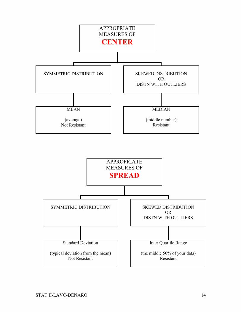
APPROPRIATE
MEASURES OF
CENTER
SYMMETRIC DISTRIBUTION
SKEWED DISTRIBUTION
OR
DISTN WITH OUTLIERS
MEAN
(average)
Not Resistant
MEDIAN
(middle number)
Resistant
APPROPRIATE
MEASURES OF
SPREAD
SYMMETRIC DISTRIBUTION
SKEWED DISTRIBUTION
OR
DISTN WITH OUTLIERS
Standard Deviation
(typical deviation from the mean)
Not Resistant
Inter Quartile Range
(the middle 50% of your data)
Resistant
Page 15
STAT II-LAVC-DENARO 15
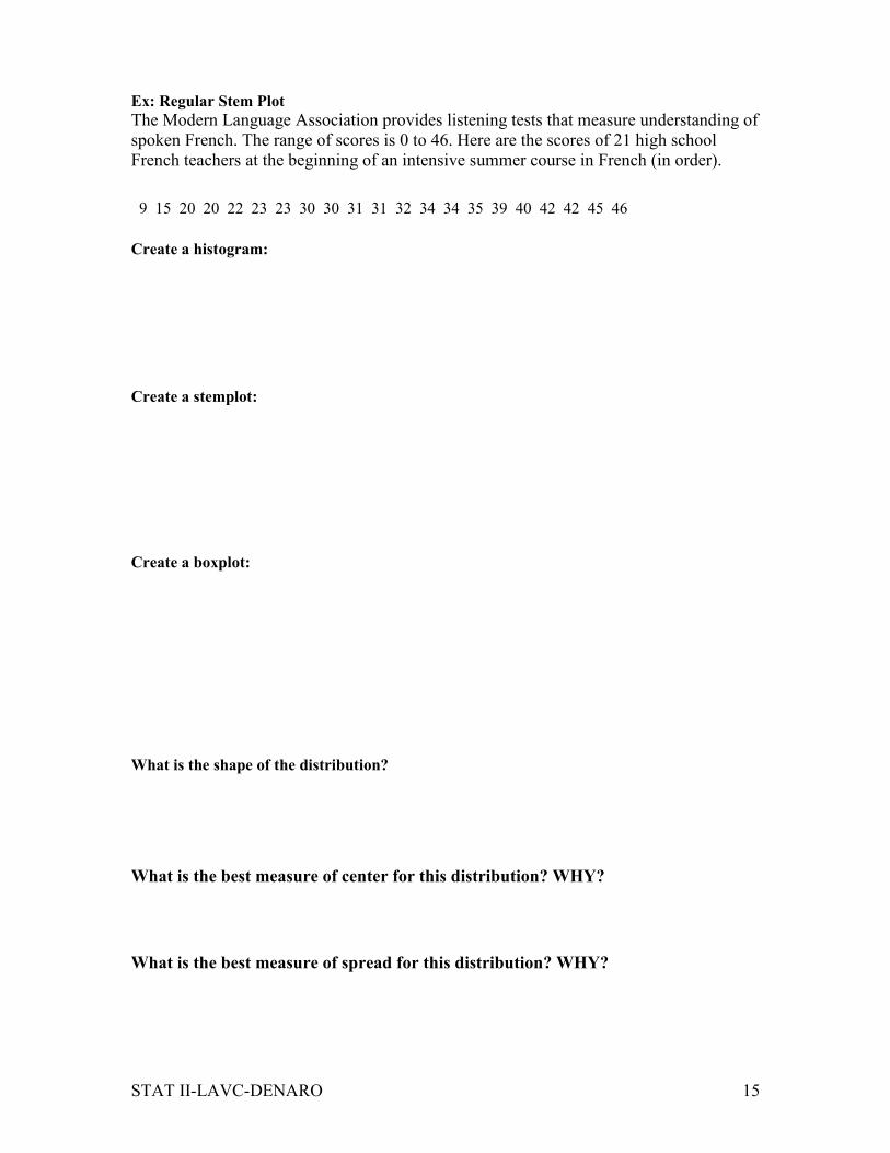
Ex: Regular Stem Plot
The Modern Language Association provides listening tests that measure understanding of
spoken French. The range of scores is 0 to 46. Here are the scores of 21 high school
French teachers at the beginning of an intensive summer course in French (in order).
9 15 20 20 22 23 23 30 30 31 31 32 34 34 35 39 40 42 42 45 46
Create a histogram:
Create a stemplot:
Create a boxplot:
What is the shape of the distribution?
What is the best measure of center for this distribution? WHY?
What is the best measure of spread for this distribution? WHY?
Page 16
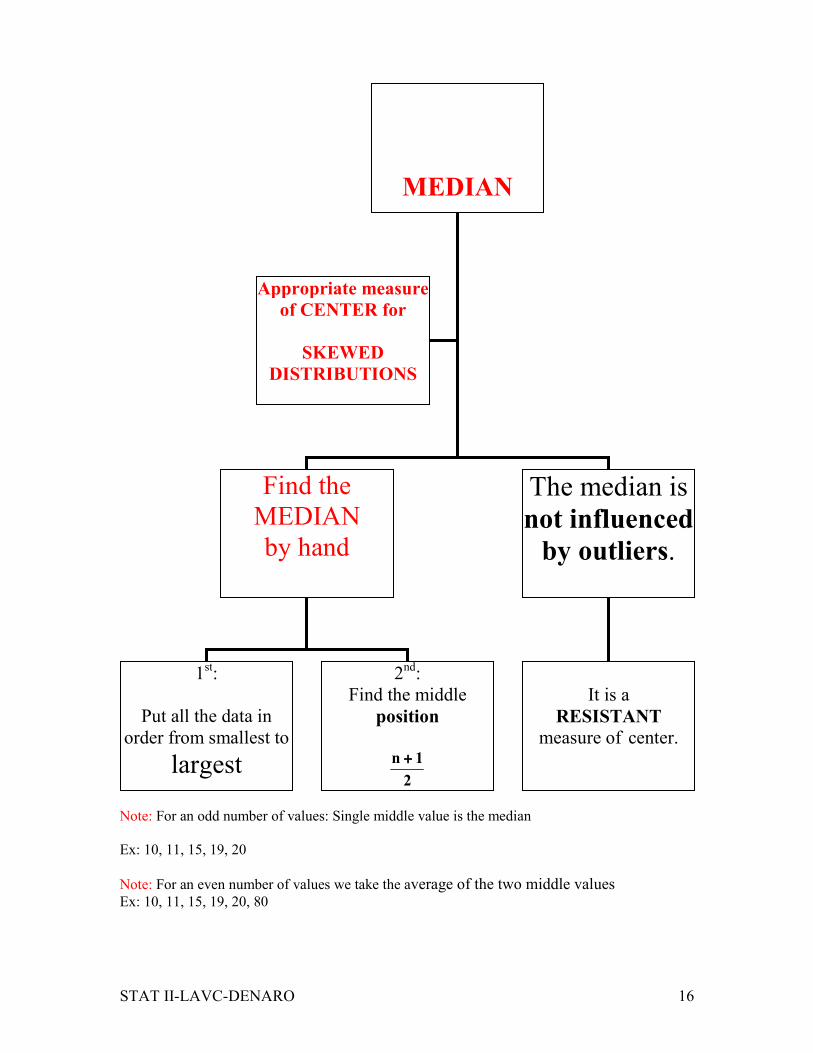
STAT II-LAVC-DENARO 16
Note: For an odd number of values: Single middle value is the median
Ex: 10, 11, 15, 19, 20
Note: For an even number of values we take the average of the two middle values Ex: 10, 11, 15, 19, 20, 80
MEDIAN
Find the
MEDIAN
by hand
The median is
not influenced
by outliers.
It is a
RESISTANT measure of center.
Appropriate measure
of CENTER for
SKEWED
DISTRIBUTIONS
1st:
Put all the data in
order from smallest to largest
2nd:
Find the middle
position
2
1n ++++
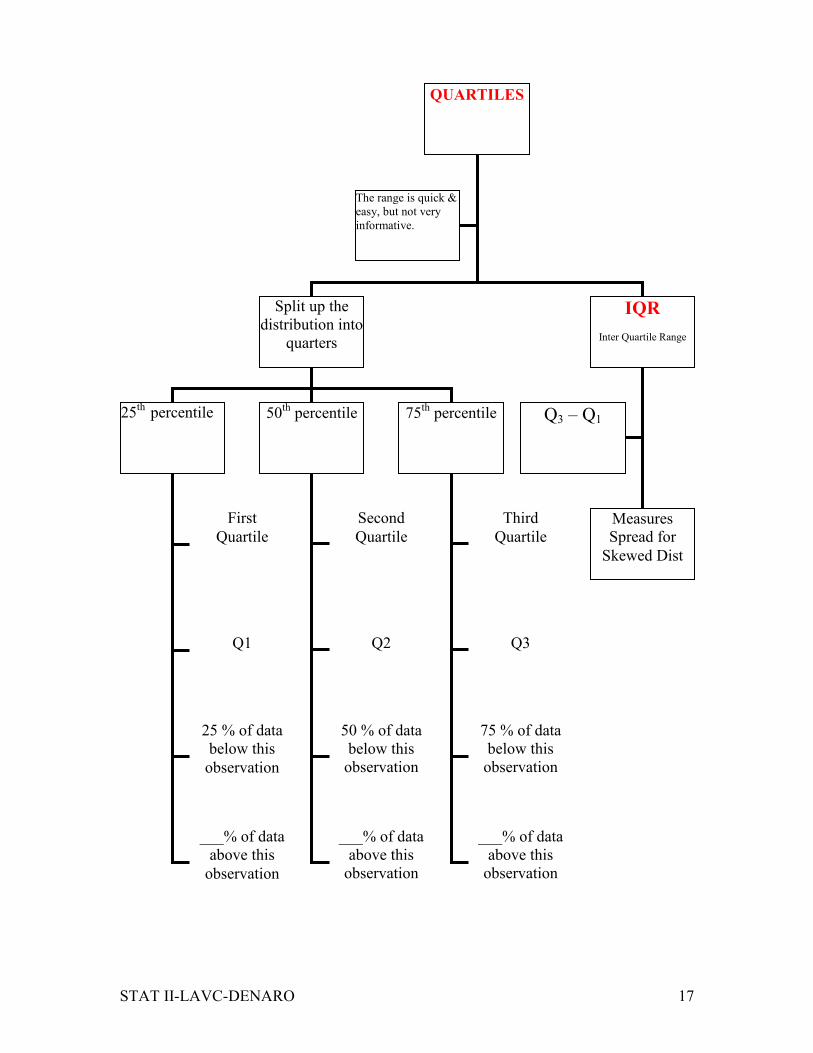
Page 17
STAT II-LAVC-DENARO 17
QUARTILES
Split up the
distribution into
quarters
IQR
Inter Quartile Range
25th
percentile
50th percentile 75
th percentile
The range is quick &
easy, but not very informative.
First
Quartile
Q1
25 % of data
below this
observation
___% of data
above this
observation
Second
Quartile
Q2
50 % of data
below this
observation
___% of data
above this
observation
Third
Quartile
Q3
75 % of data
below this
observation
___% of data
above this
observation
Q3 – Q1
Measures
Spread for
Skewed Dist
Page 18
STAT II-LAVC-DENARO 18
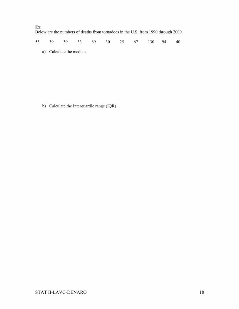
Ex: Below are the numbers of deaths from tornadoes in the U.S. from 1990 through 2000.
53 39 39 33 69 30 25 67 130 94 40
a) Calculate the median.
b) Calculate the Interquartile range (IQR)
Page 19
STAT II-LAVC-DENARO 19
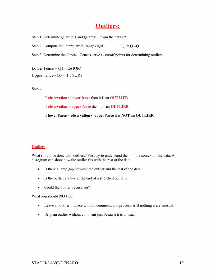
Outliers:
Step 1: Determine Quartile 1 and Quartile 3 from the data set.
Step 2: Compute the Interquartile Range (IQR) IQR= Q3-Q1
Step 3: Determine the Fences. Fences serve as cutoff points for determining outliers
Lower Fence = Q1- 1.5(IQR)
Upper Fence= Q3 + 1.5(IQR)
Step 4:
If observation < lower fence then it is an OUTLIER
If observation > upper fence then it is an OUTLIER
If lower fence < observation < upper fence it is NOT an OUTLIER
Outliers
What should be done with outliers? First try to understand them in the context of the data. A
histogram can show how the outlier fits with the rest of the data:
• Is there a large gap between the outlier and the rest of the data?
• Is the outlier a value at the end of a stretched out tail?
• Could the outlier be an error?
What you should NOT do:
• Leave an outlier in place without comment, and proceed as if nothing were unusual.
• Drop an outlier without comment just because it is unusual.
Page 20
STAT II-LAVC-DENARO 20
Ex: The data set below is the case prices (in dollars) of wines produced by a vineyard in
Napa Valley.
150 135 90 122 128 67 142 140 128 132 127 140 129
Page 21
STAT II-LAVC-DENARO 21
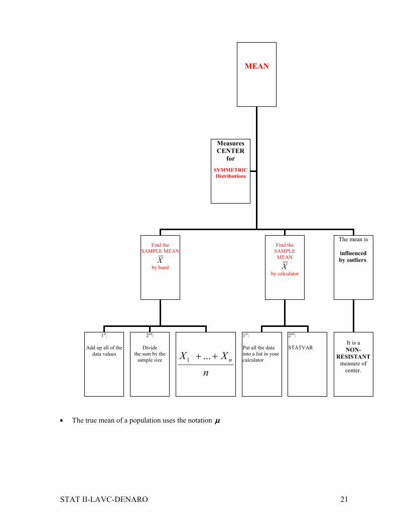
• The true mean of a population uses the notation µµµµ
MEAN
Find the SAMPLE MEAN
X
by hand
Find the SAMPLE
MEAN
X
by calculator
The mean is
influenced by outliers.
It is a
NON-
RESISTANT measure of
center.
Measures
CENTER
for
SYMMETRIC Distributions
1st:
Add up all of the
data values
2nd:
Divide
the sum by the
sample size
1st:
Put all the data
into a list in your
calculator
2nd:
STATVAR
n
XX n++ ...1
Page 22
STAT II-LAVC-DENARO 22
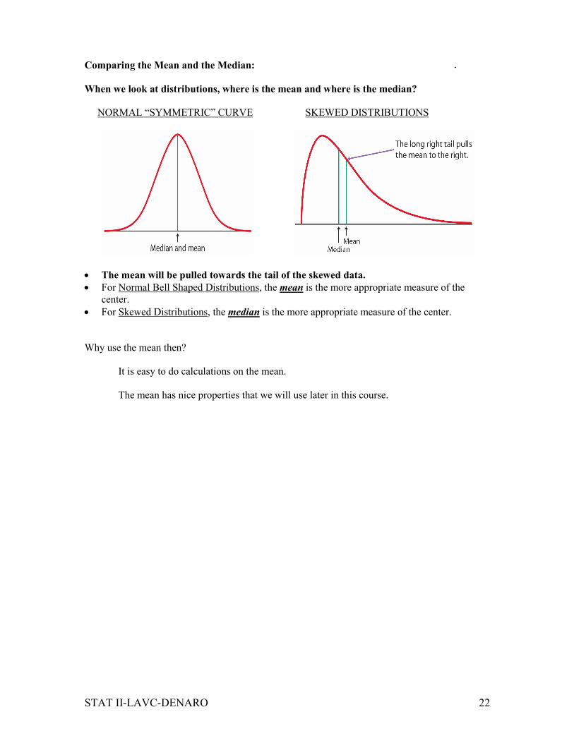
Comparing the Mean and the Median:
When we look at distributions, where is the mean and where is the median?
NORMAL “SYMMETRIC” CURVE SKEWED DISTRIBUTIONS
• The mean will be pulled towards the tail of the skewed data.
• For Normal Bell Shaped Distributions, the mean is the more appropriate measure of the
center.
• For Skewed Distributions, the median is the more appropriate measure of the center.
Why use the mean then?
It is easy to do calculations on the mean.
The mean has nice properties that we will use later in this course.
Page 23
STAT II-LAVC-DENARO 23
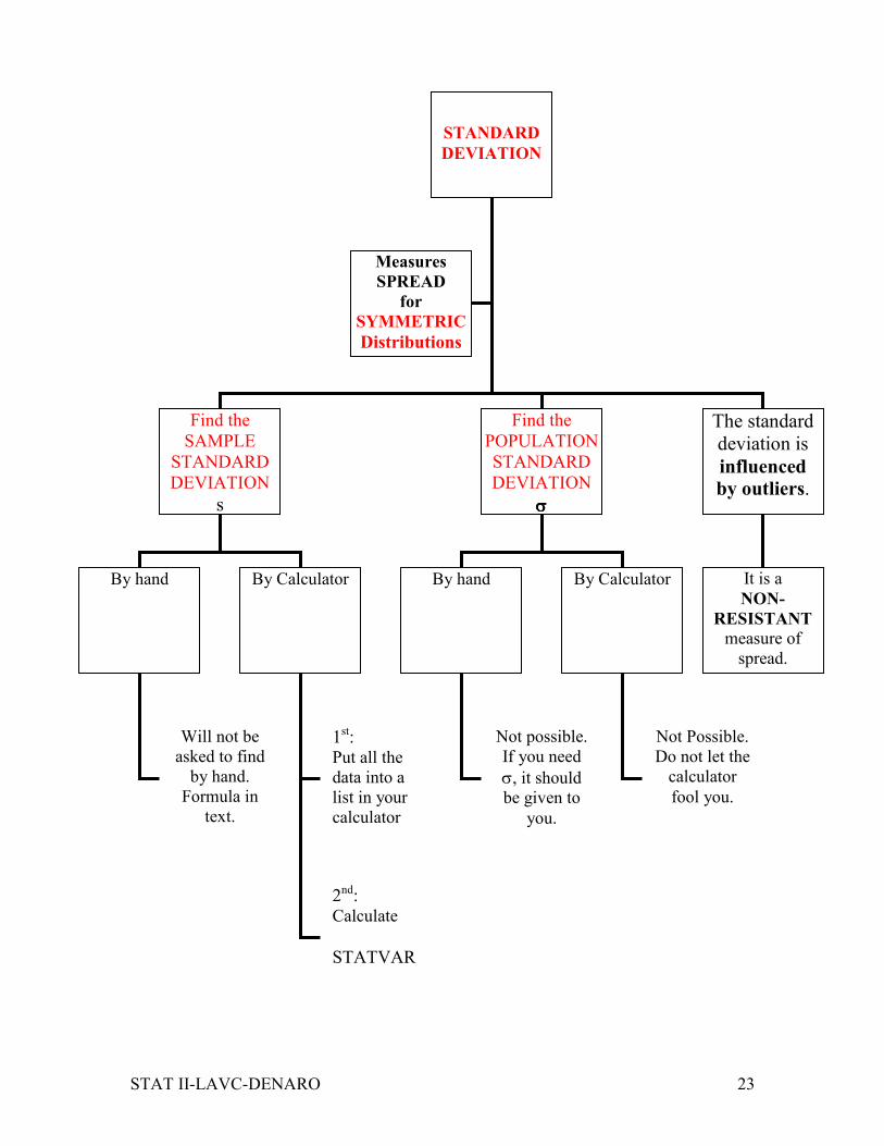
STANDARD
DEVIATION
Find the
SAMPLE
STANDARD
DEVIATION
s
Find the
POPULATION
STANDARD
DEVIATION
σσσσ
The standard
deviation is
influenced by outliers.
It is a
NON-
RESISTANT measure of
spread.
Measures
SPREAD
for
SYMMETRIC
Distributions
By hand By hand By Calculator By Calculator
Will not be
asked to find
by hand.
Formula in
text.
1st: Put all the
data into a
list in your
calculator
2nd: Calculate
STATVAR
Not possible.
If you need
σ, it should be given to
you.
Not Possible.
Do not let the
calculator
fool you.
Page 24
STAT II-LAVC-DENARO 24
Variance is the standard deviation squared.
Standard Deviation is the positive square root of the variance
It is a distance measure so it has to be positive
It is the “typical” distance of the datapoints to the mean.
A standard deviation of zero means ________________________.
Values that are very close together have a small standard deviation.
Values that are very far apart have a large standard deviation.
Ex: 1, 2, 3, 4, 5 Calculate the standard deviation
Ex: 1, 1, 1, 1, 1 Calculate the standard deviation
NOTATION:
Sample Mean X
Population Mean µ
Sample Standard deviation s
Sample Variance s2
Population Standard deviation σσσσ
Population Variance σσσσ2222
Page 25
STAT II-LAVC-DENARO 25
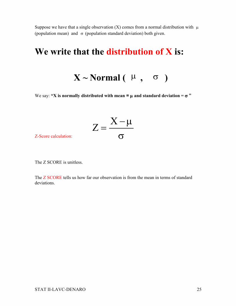
Suppose we have that a single observation (X) comes from a normal distribution with µ
(population mean) and σ (population standard deviation) both given.
We write that the distribution of X is:
X ~ Normal ( µ , σ )
We say: “X is normally distributed with mean = µ µ µ µ and standard deviation = σ σ σ σ ”
Z-Score calculation: σ
µ−=X
Z
The Z SCORE is unitless.
The Z SCORE tells us how far our observation is from the mean in terms of standard
deviations.
Page 26
STAT II-LAVC-DENARO 26
Ex: Two friends are training for the Boston marathon. James is training on a hilly jogging
loop. For the general population of runners, the time to complete this loop follows a normal
distribution with a mean of 167 minutes and standard deviation 25 minutes. Rob is training
on a flat jogging route. The time to complete this flat route follows a normal distribution
with a mean of 143 minutes and standard deviation 20 minutes. If it takes James 91 minutes
to complete his loop, and it takes Rob 86 minutes to complete his loop, who is in better
condition?
Draw a picture for each of the distributions.
What is the Z-Score for each runner?
Who is in better condition?
Page 27
STAT II-LAVC-DENARO 27
Lecture NotesLecture NotesLecture NotesLecture Notes
Part IVPart IVPart IVPart IV
Linear RegressionLinear RegressionLinear RegressionLinear Regression
Scatterplots, correlations, and Scatterplots, correlations, and Scatterplots, correlations, and Scatterplots, correlations, and associationsassociationsassociationsassociations
Regression WisdomRegression WisdomRegression WisdomRegression Wisdom
Page 28
STAT II-LAVC-DENARO 28
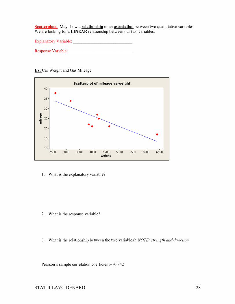
Scatterplots: May show a relationship or an association between two quantitative variables.
We are looking for a LINEAR relationship between our two variables.
Explanatory Variable: ____________________________
Response Variable: ______________________________
Ex: Car Weight and Gas Mileage
weight
mileage
650060005500500045004000350030002500
40
35
30
25
20
15
10
Scatterplot of mileage vs weight
1. What is the explanatory variable?
2. What is the response variable?
3. What is the relationship between the two variables? NOTE: strength and direction
Pearson’s sample correlation coefficient= -0.842
Page 29
STAT II-LAVC-DENARO 29
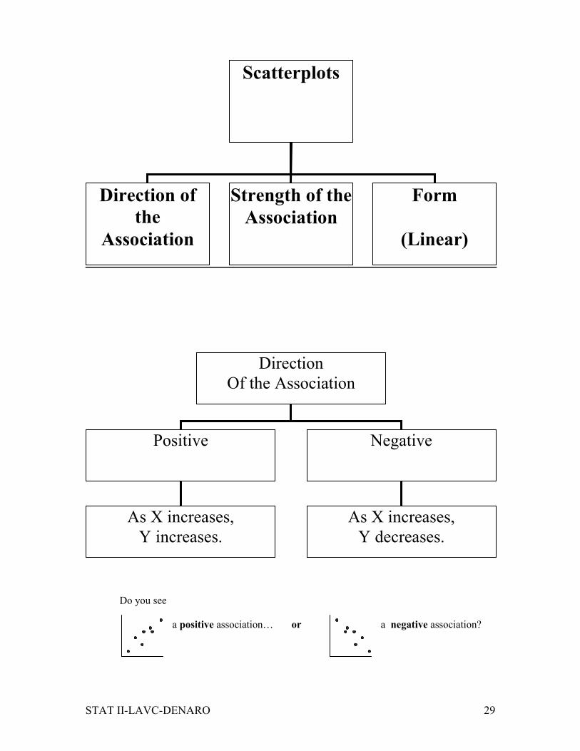
Do you see
a positive association… or a negative association?
Scatterplots
Direction of
the
Association
Strength of the
Association
Form
(Linear)
Direction
Of the Association
Positive Negative
As X increases,
Y increases.
As X increases,
Y decreases.
Page 30
STAT II-LAVC-DENARO 30
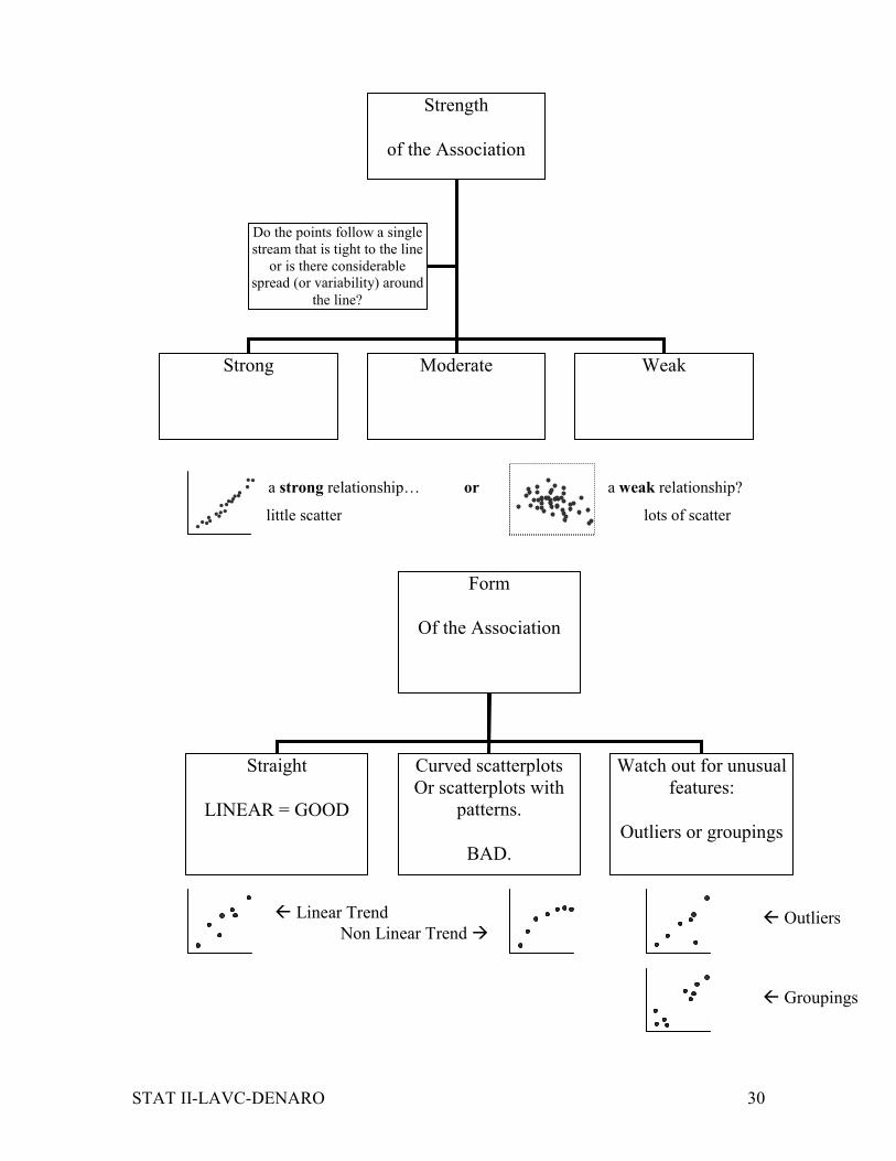
a strong relationship… or a weak relationship?
Strength
of the Association
Strong Moderate Weak
Do the points follow a single
stream that is tight to the line
or is there considerable
spread (or variability) around
the line?
Form
Of the Association
Straight
LINEAR = GOOD
Curved scatterplots
Or scatterplots with
patterns.
BAD.
Watch out for unusual
features:
Outliers or groupings
little scatter lots of scatter
� Groupings
� Linear Trend
Non Linear Trend � � Outliers
Page 31
STAT II-LAVC-DENARO 31
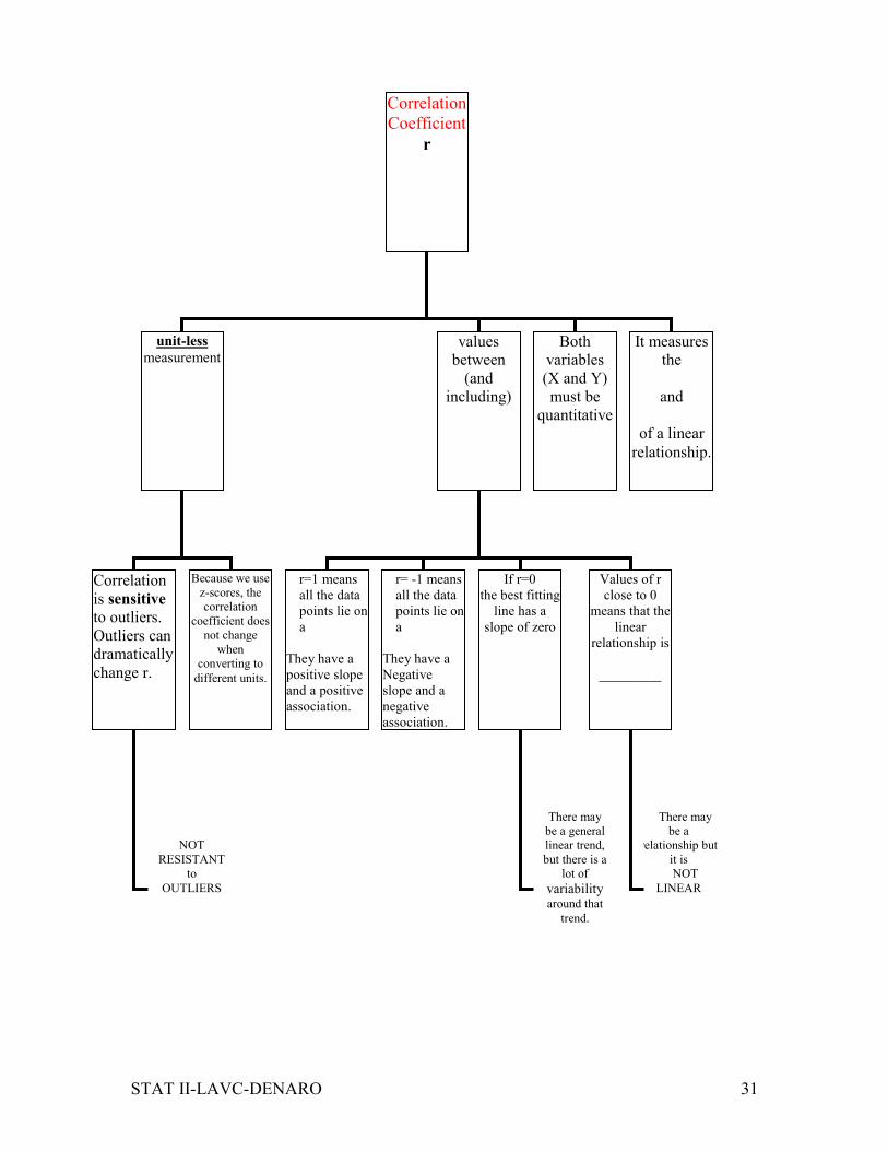
Correlation
Coefficient
r
unit-less
measurement values
between
(and
including)
Both
variables
(X and Y)
must be
quantitative
It measures
the
and
of a linear
relationship.
r=1 means
all the data
points lie on
a
They have a
positive slope
and a positive
association.
r= -1 means
all the data
points lie on
a
They have a
Negative
slope and a
negative
association.
If r=0
the best fitting
line has a
slope of zero
Values of r
close to 0
means that the
linear
relationship is
_________
Correlation
is sensitive
to outliers.
Outliers can
dramatically
change r.
Because we use
z-scores, the
correlation
coefficient does
not change
when
converting to
different units.
There may
be a general
linear trend,
but there is a
lot of
variability around that
trend.
There may
be a
relationship but
it is
NOT
LINEAR
NOT
RESISTANT
to
OUTLIERS
Page 32
STAT II-LAVC-DENARO 32
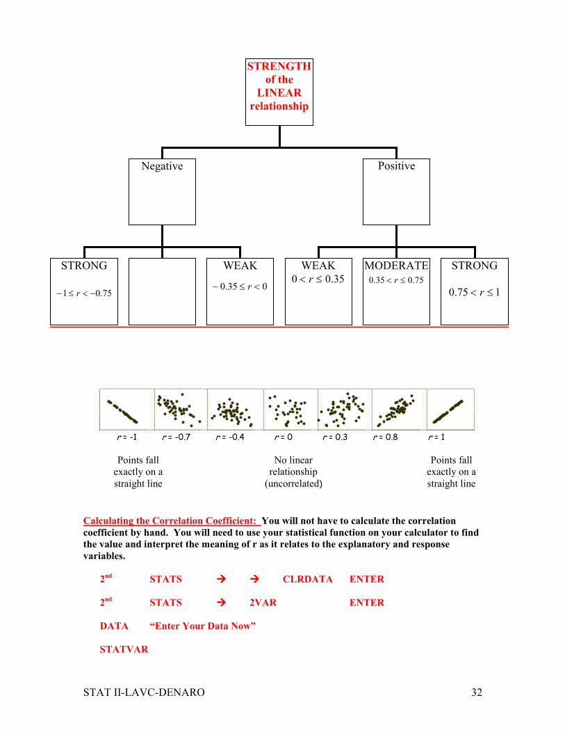
r = -1 r = -0.7 r = -0.4 r = 0 r = 0.3 r = 0.8 r = 1
Calculating the Correlation Coefficient: You will not have to calculate the correlation
coefficient by hand. You will need to use your statistical function on your calculator to find
the value and interpret the meaning of r as it relates to the explanatory and response
variables.
2nd STATS ���� ���� CLRDATA ENTER
2nd STATS ���� 2VAR ENTER
DATA “Enter Your Data Now”
STATVAR
STRENGTH
of the
LINEAR
relationship
Negative Positive
STRONG
75.01 −<≤− r
WEAK
035.0 <≤− r
WEAK
35.00 ≤< r
MODERATE
75.035.0 ≤< r
STRONG
175.0 ≤< r
Points fall
exactly on a
straight line
Points fall
exactly on a
straight line
No linear
relationship
(uncorrelated)
Page 33
STAT II-LAVC-DENARO 33
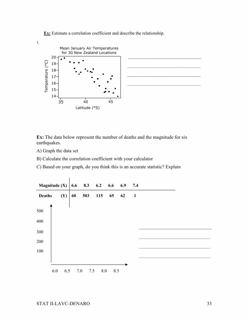
Ex: Estimate a correlation coefficient and describe the relationship.
1.
______________________________
______________________________________
______________________________________
______________________________________
Ex: The data below represent the number of deaths and the magnitude for six
earthquakes.
A) Graph the data set
B) Calculate the correlation coefficient with your calculator
C) Based on your graph, do you think this is an accurate statistic? Explain
Magnitude (X) 6.6 8.3 6.2 6.6 6.9 7.4
Deaths (Y) 60 503 115 65 62 1
500
400
______________________________ 300
_____________________________________
200 _____________________________________
100 _____________________________________
6.0 6.5 7.0 7.5 8.0 8.5
4540 35
20
19
18
17
16
15
14
Latitude (°S)
Mean January Air Temperatures
for 30 New Zealand Locations
Temperature (°C)
Page 34
STAT II-LAVC-DENARO 34
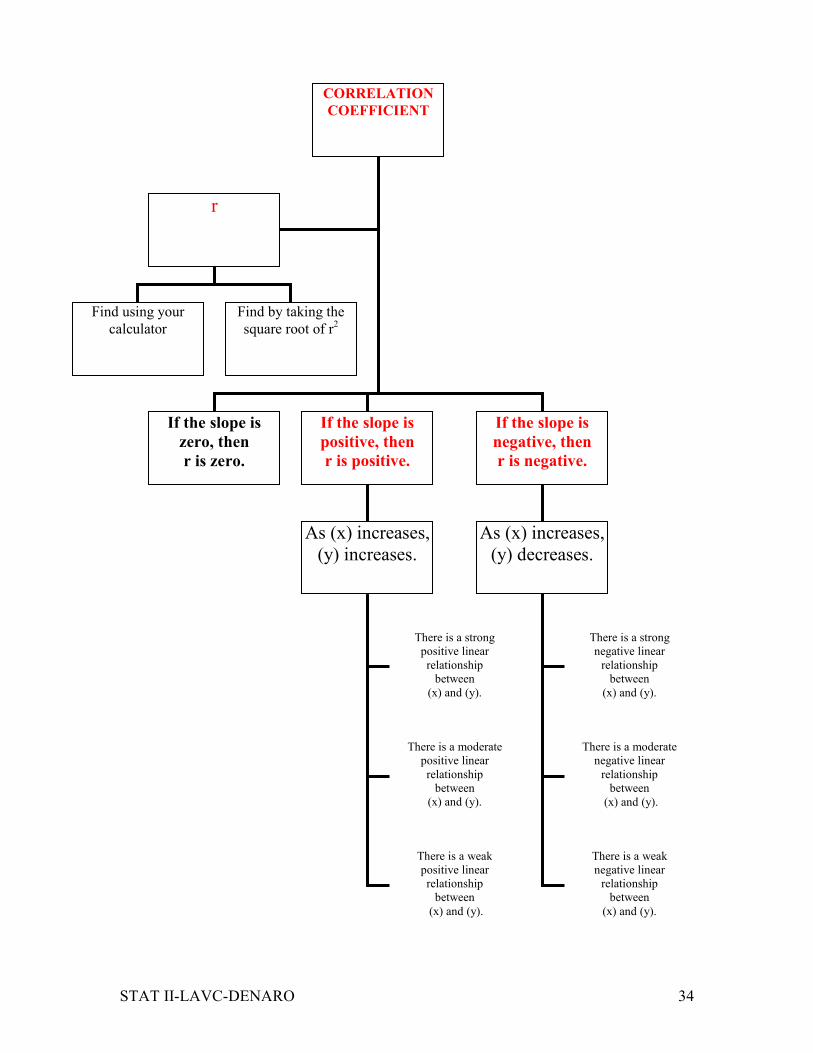
CORRELATION
COEFFICIENT
If the slope is
zero, then
r is zero.
If the slope is
positive, then
r is positive.
If the slope is
negative, then
r is negative.
r
Find using your
calculator
Find by taking the
square root of r2
As (x) increases,
(y) increases.
There is a strong
positive linear
relationship
between
(x) and (y).
There is a moderate
positive linear
relationship
between
(x) and (y).
There is a weak
positive linear
relationship
between
(x) and (y).
As (x) increases,
(y) decreases.
There is a strong
negative linear
relationship
between
(x) and (y).
There is a moderate
negative linear
relationship
between
(x) and (y).
There is a weak
negative linear
relationship
between
(x) and (y).
Page 35
STAT II-LAVC-DENARO 35
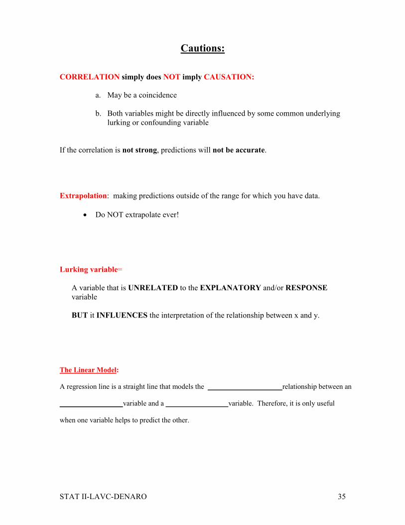
Cautions:
CORRELATION simply does NOT imply CAUSATION:
a. May be a coincidence
b. Both variables might be directly influenced by some common underlying
lurking or confounding variable
If the correlation is not strong, predictions will not be accurate.
Extrapolation: making predictions outside of the range for which you have data.
• Do NOT extrapolate ever!
Lurking variable=
A variable that is UNRELATED to the EXPLANATORY and/or RESPONSE
variable
BUT it INFLUENCES the interpretation of the relationship between x and y.
The Linear Model:
A regression line is a straight line that models the relationship between an
variable and a variable. Therefore, it is only useful
when one variable helps to predict the other.
Page 36
STAT II-LAVC-DENARO 36
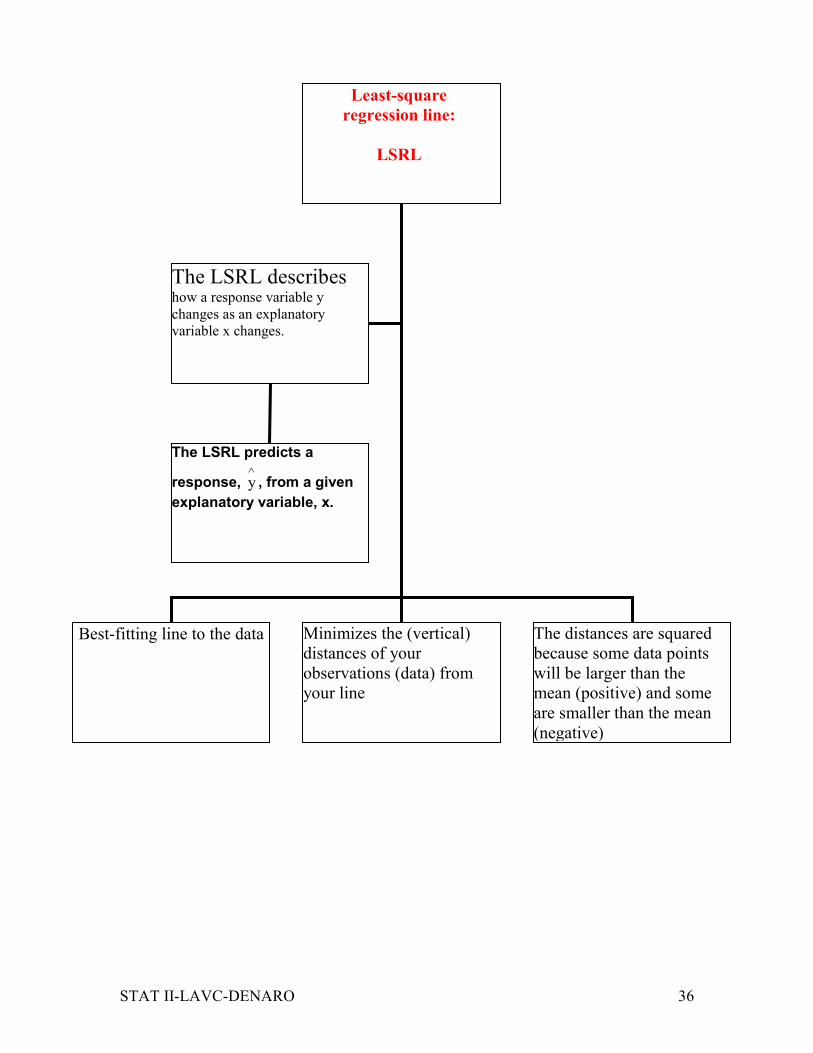
Least-square
regression line:
LSRL
Best-fitting line to the data Minimizes the (vertical)
distances of your
observations (data) from
your line
The distances are squared
because some data points
will be larger than the
mean (positive) and some
are smaller than the mean
(negative)
The LSRL describes how a response variable y
changes as an explanatory
variable x changes.
The LSRL predicts a
response, y∧, from a given
explanatory variable, x.
Page 37
STAT II-LAVC-DENARO 37
Lecture NotesLecture NotesLecture NotesLecture Notes
Part VPart VPart VPart V
Regression WisdomRegression WisdomRegression WisdomRegression Wisdom
Page 38
STAT II-LAVC-DENARO 38
Residuals
For every
given value of X
We have a
True/observed
data value for y
We have a
predicted value for
y
e = error
Difference between
observed y and
predicted y
Observed – Predicted
It is a “model”
which is not perfect
Some of the data points
might be above the line,
and some might be
below the line.
OVER-
PREDICTIONS
UNDER-
PREDICTIONS
Page 39
STAT II-LAVC-DENARO 39
Ex: Scatterplot of Systolic Blood Pressure versus Weight (Sample of 12 American Adults).
Weight
SBP
220210200190180170160
170
160
150
140
130
Scatterplot of SBP vs Weight
Pearson correlation of SBP and Weight = 0.971
The regression equation is: y = 1.1 + 0.764(x)
1) Suppose we know that one person in the sample weighs 188 pounds and has a systolic blood pressure of
136.
2) Predict the SBP for a person weighing 188 pounds using your regression model.
3) Find the residual.
Page 40
STAT II-LAVC-DENARO 40
Ex:
LSRL
Slope-Intercept Form
b a The Least Squares
Regression Line always
passes through the point
( x , y ).
xy ab +=ˆ
b = xay − a = r
sx
sy
When ___x____ is 0,
___y___ is equal
to ____b___
Increasing ____X_____
by 1, is associated with
increasing ____Y_____
by _________a______.
Increasing ____X_____
by 1, is associated with
decreasing ____Y_____
by _________a______.
Page 41
STAT II-LAVC-DENARO 41
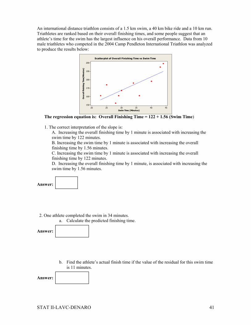
An international distance triathlon consists of a 1.5 km swim, a 40 km bike ride and a 10 km run.
Triathletes are ranked based on their overall finishing times, and some people suggest that an
athlete’s time for the swim has the largest influence on his overall performance. Data from 10
male triathletes who competed in the 2004 Camp Pendleton International Triathlon was analyzed
to produce the results below:
Swim Time (Minutes)
Overall Finishing Time(M
inutes)
454035302520
200
190
180
170
160
150
Scatterplot of Overall Finishing Time vs Swim Time
The regression equation is: Overall Finishing Time = 122 + 1.56 (Swim Time)
1. The correct interpretation of the slope is:
A. Increasing the overall finishing time by 1 minute is associated with increasing the
swim time by 122 minutes.
B. Increasing the swim time by 1 minute is associated with increasing the overall
finishing time by 1.56 minutes.
C. Increasing the swim time by 1 minute is associated with increasing the overall
finishing time by 122 minutes.
D. Increasing the overall finishing time by 1 minute, is associated with increasing the
swim time by 1.56 minutes.
Answer:
2. One athlete completed the swim in 34 minutes.
a. Calculate the predicted finishing time.
Answer:
b. Find the athlete’s actual finish time if the value of the residual for this swim time
is 11 minutes.
Answer:
Page 42
STAT II-LAVC-DENARO 42
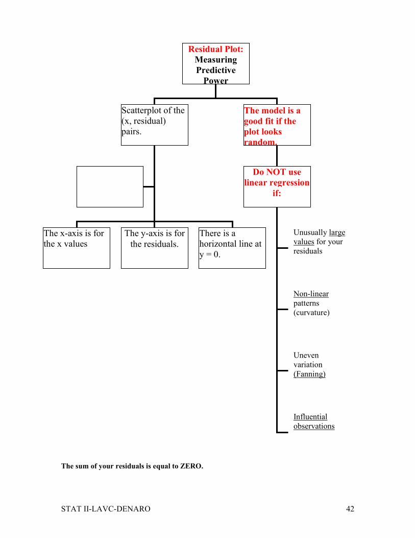
The sum of your residuals is equal to ZERO.
Residual Plot:
Measuring
Predictive
Power
Scatterplot of the
(x, residual)
pairs.
The model is a
good fit if the
plot looks
random.
The x-axis is for
the x values
The y-axis is for
the residuals.
There is a
horizontal line at
y = 0.
Do NOT use
linear regression
if:
Unusually large
values for your
residuals
Non-linear
patterns
(curvature)
Uneven
variation
(Fanning)
Influential
observations
Page 43
STAT II-LAVC-DENARO 43
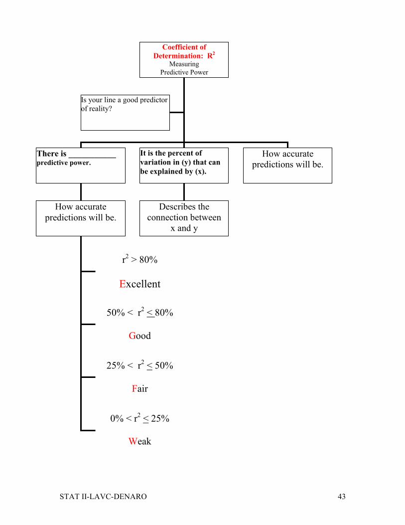
Coefficient of
Determination: R2 Measuring
Predictive Power
There is ___________ predictive power.
It is the percent of
variation in (y) that can
be explained by (x).
How accurate
predictions will be.
Is your line a good predictor
of reality?
How accurate
predictions will be.
r2 > 80%
Excellent
50% < r2 < 80%
Good
25% < r2 < 50%
Fair
0% < r2 < 25%
Weak
Describes the
connection between
x and y
Page 44
STAT II-LAVC-DENARO 44
Example: Does more education result in more crime? Education was measured as the percentage of residents aged at least 25 in the county who had at
least a high school degree. Crime rate was measured as the number of crimes in Florida County
in the past year per 1000 residents. The correlation coefficient between these variables is 0.67.
a) What is the coefficient of determination?
b) Give the definition and describe the strength of the predictive power based on the
guidelines above.
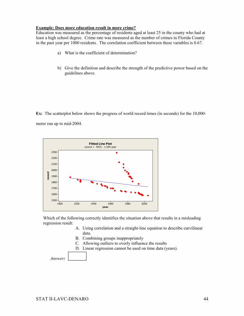
Ex: The scatterplot below shows the progress of world record times (in seconds) for the 10,000-
meter run up to mid-2004.
year
record
200019801960194019201900
2300
2200
2100
2000
1900
1800
1700
1600
1500
Fitted Line Plotrecord = 4915 - 1.594 year
Which of the following correctly identifies the situation above that results in a misleading
regression result:
A. Using correlation and a straight-line equation to describe curvilinear
data.
B. Combining groups inappropriately
C. Allowing outliers to overly influence the results
D. Linear regression cannot be used on time data (years).
Answer:
Page 45
STAT II-LAVC-DENARO 45
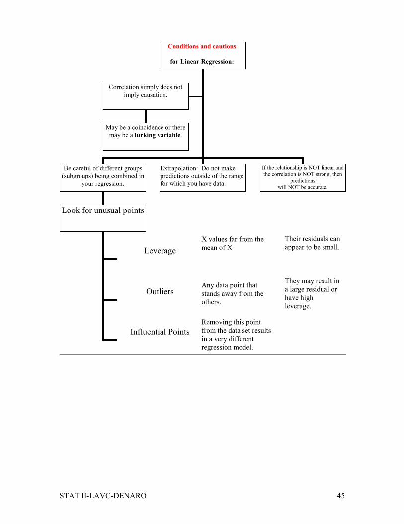
Conditions and cautions
for Linear Regression:
Be careful of different groups
(subgroups) being combined in
your regression.
Extrapolation: Do not make
predictions outside of the range
for which you have data.
Correlation simply does not
imply causation.
Look for unusual points
Leverage
Outliers
Influential Points
May be a coincidence or there
may be a lurking variable.
If the relationship is NOT linear and
the correlation is NOT strong, then
predictions
will NOT be accurate.
X values far from the
mean of X
Any data point that
stands away from the
others.
Removing this point
from the data set results
in a very different
regression model.
Their residuals can
appear to be small.
They may result in
a large residual or
have high
leverage.
Page 46
STAT II-LAVC-DENARO 46
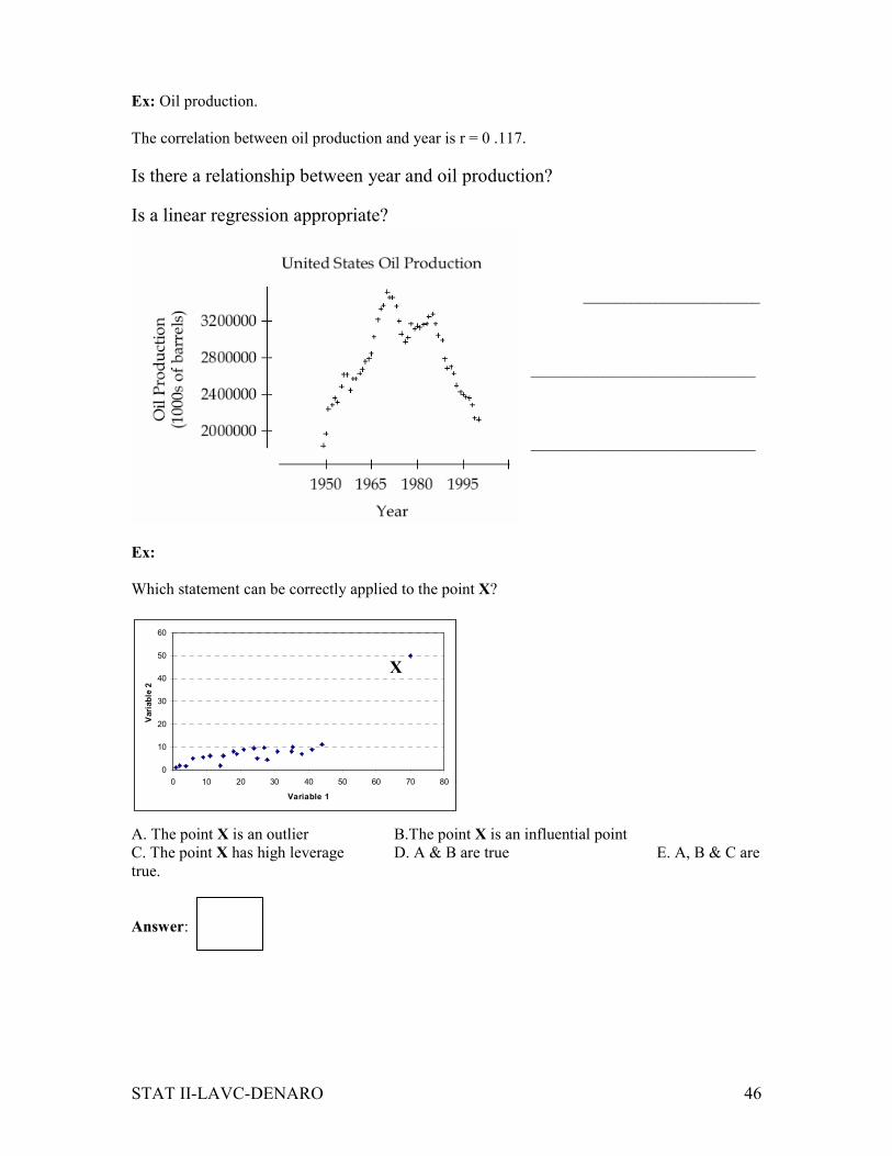
0
10
20
30
40
50
60
0 10 20 30 40 50 60 70 80
Variable 1
Variable 2
Ex: Oil production.
The correlation between oil production and year is r = 0 .117.
Is there a relationship between year and oil production?
Is a linear regression appropriate?
______________________
____________________________
____________________________
Ex:
Which statement can be correctly applied to the point X?
X
A. The point X is an outlier B.The point X is an influential point
C. The point X has high leverage D. A & B are true E. A, B & C are
true.
Answer:
Page 47
STAT II-LAVC-DENARO 47
Lecture NotesLecture NotesLecture NotesLecture Notes
Part VPart VPart VPart VIIII
All About TestingAll About TestingAll About TestingAll About Testing
Page 48
STAT II-LAVC-DENARO 48
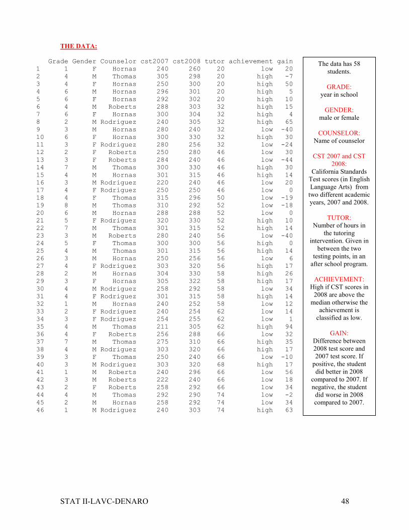
THE DATA:
Grade Gender Counselor cst2007 cst2008 tutor achievement gain
1 1 F Hornas 240 260 20 low 20
2 4 M Thomas 305 298 20 high -7
3 4 F Hornas 250 300 20 high 50
4 6 M Hornas 296 301 20 high 5
5 6 F Hornas 292 302 20 high 10
6 4 M Roberts 288 303 32 high 15
7 6 F Hornas 300 304 32 high 4
8 2 M Rodriguez 240 305 32 high 65
9 3 M Hornas 280 240 32 low -40
10 6 F Hornas 300 330 32 high 30
11 3 F Rodriguez 280 256 32 low -24
12 2 F Roberts 250 280 46 low 30
13 3 F Roberts 284 240 46 low -44
14 7 M Thomas 300 330 46 high 30
15 4 M Hornas 301 315 46 high 14
16 3 M Rodriguez 220 240 46 low 20
17 4 F Rodriguez 250 250 46 low 0
18 4 F Thomas 315 296 50 low -19
19 8 M Thomas 310 292 52 low -18
20 6 M Hornas 288 288 52 low 0
21 5 F Rodriguez 320 330 52 high 10
22 7 M Thomas 301 315 52 high 14
23 3 M Roberts 280 240 56 low -40
24 5 F Thomas 300 300 56 high 0
25 4 M Thomas 301 315 56 high 14
26 3 M Hornas 250 256 56 low 6
27 4 F Rodriguez 303 320 56 high 17
28 2 M Hornas 304 330 58 high 26
29 3 F Hornas 305 322 58 high 17
30 4 M Rodriguez 258 292 58 low 34
31 4 F Rodriguez 301 315 58 high 14
32 1 M Hornas 240 252 58 low 12
33 2 F Rodriguez 240 254 62 low 14
34 3 F Rodriguez 254 255 62 low 1
35 4 M Thomas 211 305 62 high 94
36 4 F Roberts 256 288 66 low 32
37 7 M Thomas 275 310 66 high 35
38 4 M Rodriguez 303 320 66 high 17
39 3 F Thomas 250 240 66 low -10
40 3 M Rodriguez 303 320 68 high 17
41 1 M Roberts 240 296 66 low 56
42 3 M Roberts 222 240 66 low 18
43 2 F Roberts 258 292 66 low 34
44 4 M Thomas 292 290 74 low -2
45 2 M Hornas 258 292 74 low 34
46 1 M Rodriguez 240 303 74 high 63
The data has 58
students.
GRADE:
year in school
GENDER:
male or female
COUNSELOR:
Name of counselor
CST 2007 and CST
2008:
California Standards
Test scores (in English
Language Arts) from
two different academic
years, 2007 and 2008.
TUTOR:
Number of hours in
the tutoring
intervention. Given in
between the two
testing points, in an
after school program.
ACHIEVEMENT:
High if CST scores in
2008 are above the
median otherwise the
achievement is
classified as low.
GAIN:
Difference between
2008 test score and
2007 test score. If
positive, the student
did better in 2008
compared to 2007. If
negative, the student
did worse in 2008
compared to 2007.
Page 49
STAT II-LAVC-DENARO 49
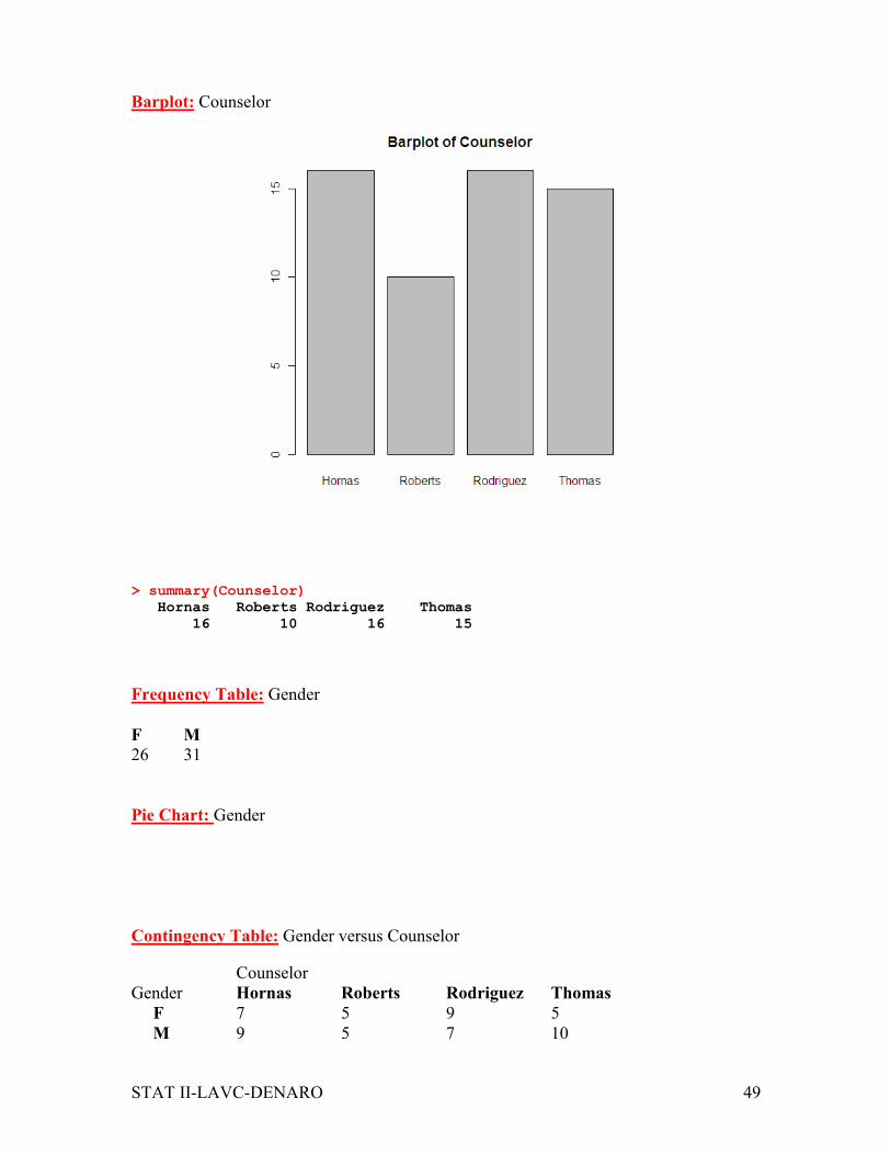
Barplot: Counselor
> summary(Counselor)
Hornas Roberts Rodriguez Thomas
16 10 16 15
Frequency Table: Gender
F M 26 31
Pie Chart: Gender
Contingency Table: Gender versus Counselor
Counselor
Gender Hornas Roberts Rodriguez Thomas
F 7 5 9 5
M 9 5 7 10
Page 50
STAT II-LAVC-DENARO 50
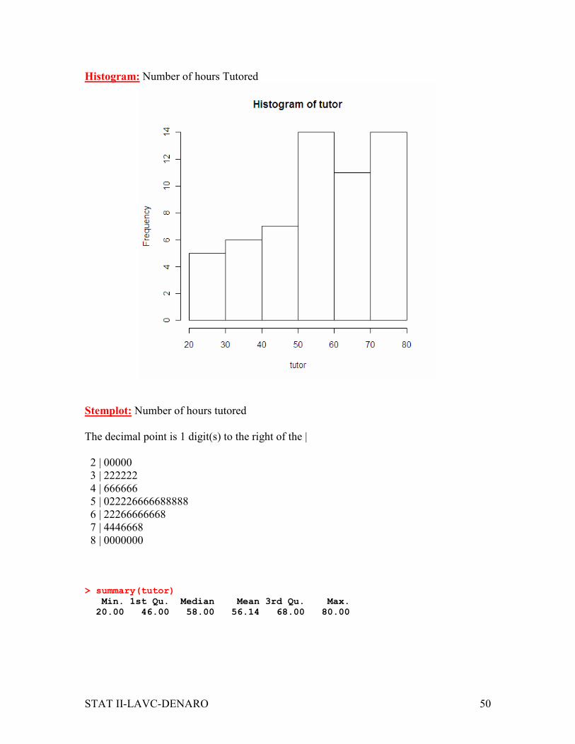
Histogram: Number of hours Tutored
Stemplot: Number of hours tutored
The decimal point is 1 digit(s) to the right of the |
2 | 00000
3 | 222222
4 | 666666
5 | 022226666688888
6 | 22266666668
7 | 4446668
8 | 0000000
> summary(tutor)
Min. 1st Qu. Median Mean 3rd Qu. Max.
20.00 46.00 58.00 56.14 68.00 80.00
Page 51
STAT II-LAVC-DENARO 51
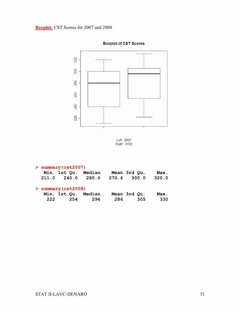
Boxplot: CST Scores for 2007 and 2008
> summary(cst2007)
Min. 1st Qu. Median Mean 3rd Qu. Max.
211.0 240.0 280.0 270.4 300.0 320.0
> summary(cst2008)
Min. 1st Qu. Median Mean 3rd Qu. Max.
222 254 296 286 305 330
Page 52
STAT II-LAVC-DENARO 52
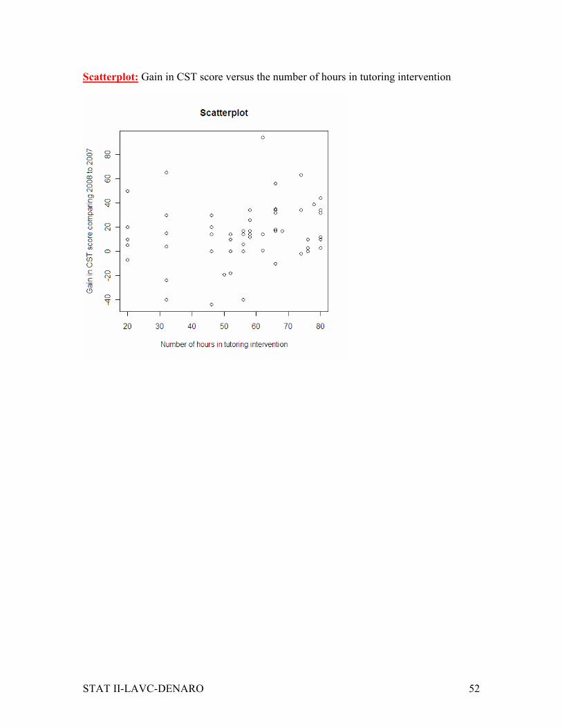
Scatterplot: Gain in CST score versus the number of hours in tutoring intervention
Page 53
STAT II-LAVC-DENARO 53
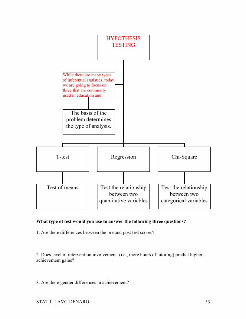
What type of test would you use to answer the following three questions?
1. Are there differences between the pre and post test scores?
2. Does level of intervention involvement (i.e., more hours of tutoring) predict higher
achievement gains?
3. Are there gender differences in achievement?
HYPOTHESIS
TESTING
T-test
Regression
Chi-Square
While there are many types
of inferential statistics, today
we are going to focus on
three that are commonly
used in education and
The basis of the
problem determines
the type of analysis.
Test of means
Test the relationship
between two
quantitative variables
Test the relationship
between two
categorical variables
Page 54
STAT II-LAVC-DENARO 54
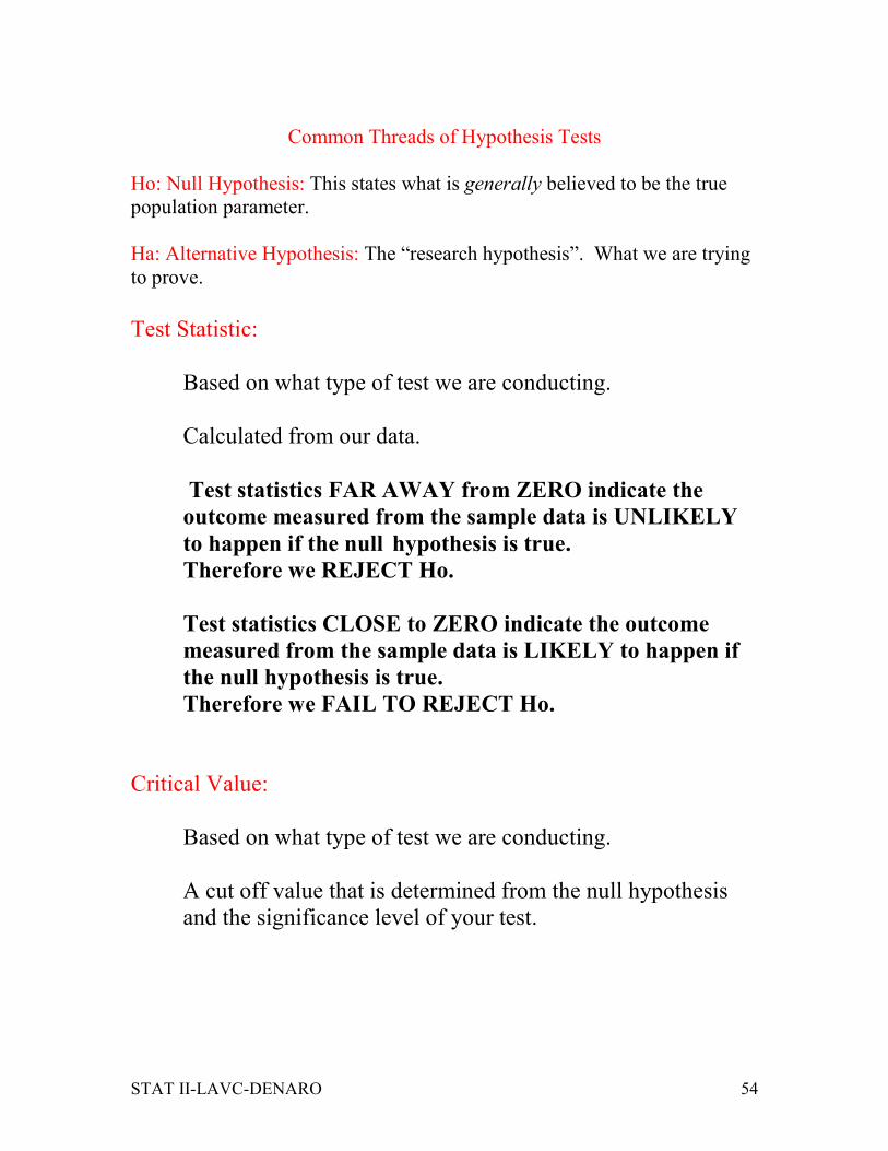
Common Threads of Hypothesis Tests
Ho: Null Hypothesis: This states what is generally believed to be the true
population parameter.
Ha: Alternative Hypothesis: The “research hypothesis”. What we are trying
to prove.
Test Statistic:
Based on what type of test we are conducting.
Calculated from our data.
Test statistics FAR AWAY from ZERO indicate the
outcome measured from the sample data is UNLIKELY
to happen if the null hypothesis is true.
Therefore we REJECT Ho.
Test statistics CLOSE to ZERO indicate the outcome
measured from the sample data is LIKELY to happen if
the null hypothesis is true.
Therefore we FAIL TO REJECT Ho.
Critical Value:
Based on what type of test we are conducting.
A cut off value that is determined from the null hypothesis
and the significance level of your test.
Page 55
STAT II-LAVC-DENARO 55
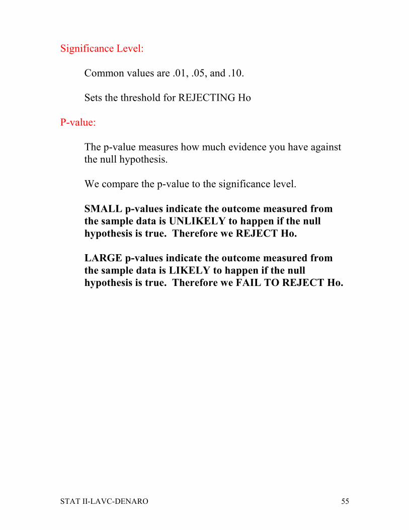
Significance Level:
Common values are .01, .05, and .10.
Sets the threshold for REJECTING Ho
P-value:
The p-value measures how much evidence you have against
the null hypothesis.
We compare the p-value to the significance level.
SMALL p-values indicate the outcome measured from
the sample data is UNLIKELY to happen if the null
hypothesis is true. Therefore we REJECT Ho.
LARGE p-values indicate the outcome measured from
the sample data is LIKELY to happen if the null
hypothesis is true. Therefore we FAIL TO REJECT Ho.
Page 56
STAT II-LAVC-DENARO 56
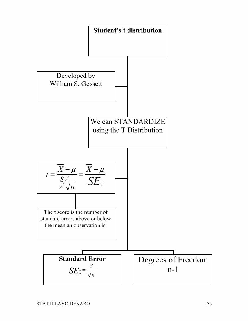
Student’s t distribution
We can STANDARDIZE
using the T Distribution
Developed by
William S. Gossett
Standard Error
n
SSE x
=
Degrees of Freedom
n-1
SE x
X
nS
Xt
µµ −=
−=
The t score is the number of
standard errors above or below
the mean an observation is.
Page 57
STAT II-LAVC-DENARO 57
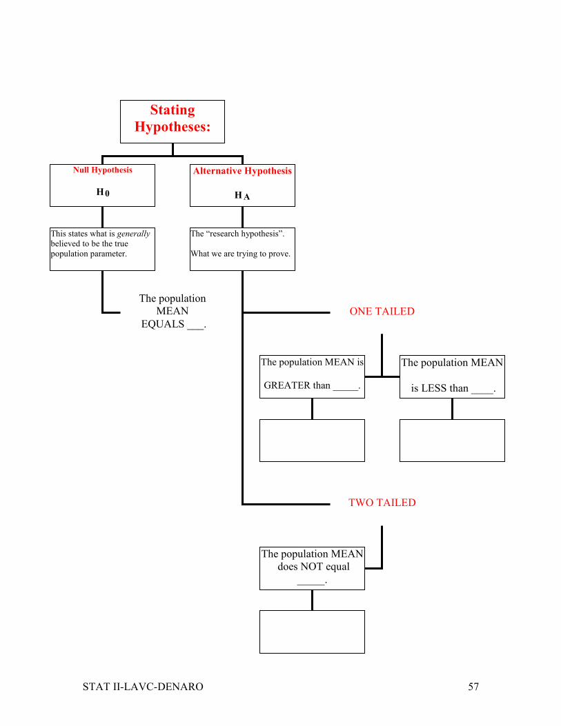
Stating
Hypotheses:
Null Hypothesis
H0
Alternative Hypothesis
HA
This states what is generally
believed to be the true
population parameter.
The population
MEAN
EQUALS ___.
The “research hypothesis”.
What we are trying to prove.
ONE TAILED
TWO TAILED
The population MEAN is
GREATER than _____.
The population MEAN
is LESS than ____.
The population MEAN
does NOT equal
_____.
Page 58
STAT II-LAVC-DENARO 58
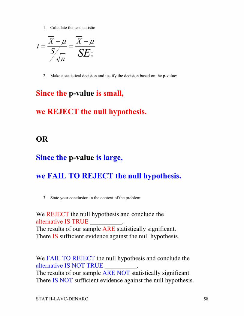
1. Calculate the test statistic
SE x
X
nS
Xt
µµ −=
−=
2. Make a statistical decision and justify the decision based on the p-value:
Since the p-value is small,
we REJECT the null hypothesis.
OR
Since the p-value is large,
we FAIL TO REJECT the null hypothesis.
3. State your conclusion in the context of the problem:
We REJECT the null hypothesis and conclude the
alternative IS TRUE __________.
The results of our sample ARE statistically significant.
There IS sufficient evidence against the null hypothesis.
We FAIL TO REJECT the null hypothesis and conclude the
alternative IS NOT TRUE __________.
The results of our sample ARE NOT statistically significant.
There IS NOT sufficient evidence against the null hypothesis.
Page 59
STAT II-LAVC-DENARO 59
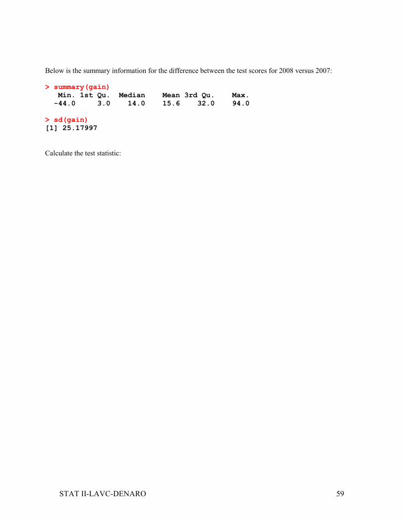
Below is the summary information for the difference between the test scores for 2008 versus 2007:
> summary(gain)
Min. 1st Qu. Median Mean 3rd Qu. Max.
-44.0 3.0 14.0 15.6 32.0 94.0
> sd(gain)
[1] 25.17997
Calculate the test statistic:
Page 60
STAT II-LAVC-DENARO 60
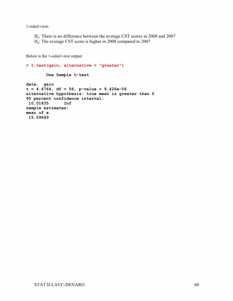
1-sided t-test:
Ho: There is no difference between the average CST scores in 2008 and 2007
Ha: The average CST score is higher in 2008 compared to 2007
Below is the 1-sided t-test output:
> t.test(gain, alternative = "greater")
One Sample t-test
data: gain
t = 4.6764, df = 56, p-value = 9.426e-06
alternative hypothesis: true mean is greater than 0
95 percent confidence interval:
10.01835 Inf
sample estimates:
mean of x
15.59649
Page 61
STAT II-LAVC-DENARO 61
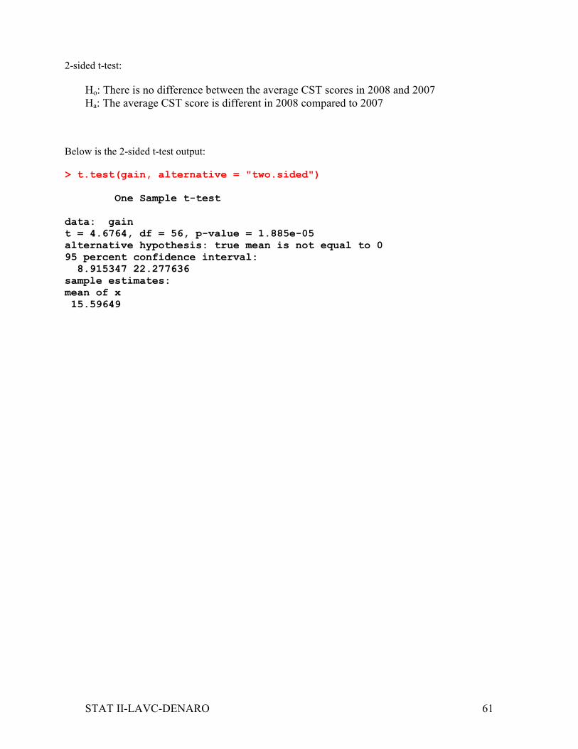
2-sided t-test:
Ho: There is no difference between the average CST scores in 2008 and 2007
Ha: The average CST score is different in 2008 compared to 2007
Below is the 2-sided t-test output:
> t.test(gain, alternative = "two.sided")
One Sample t-test
data: gain
t = 4.6764, df = 56, p-value = 1.885e-05
alternative hypothesis: true mean is not equal to 0
95 percent confidence interval:
8.915347 22.277636
sample estimates:
mean of x
15.59649
Page 62
STAT II-LAVC-DENARO 62
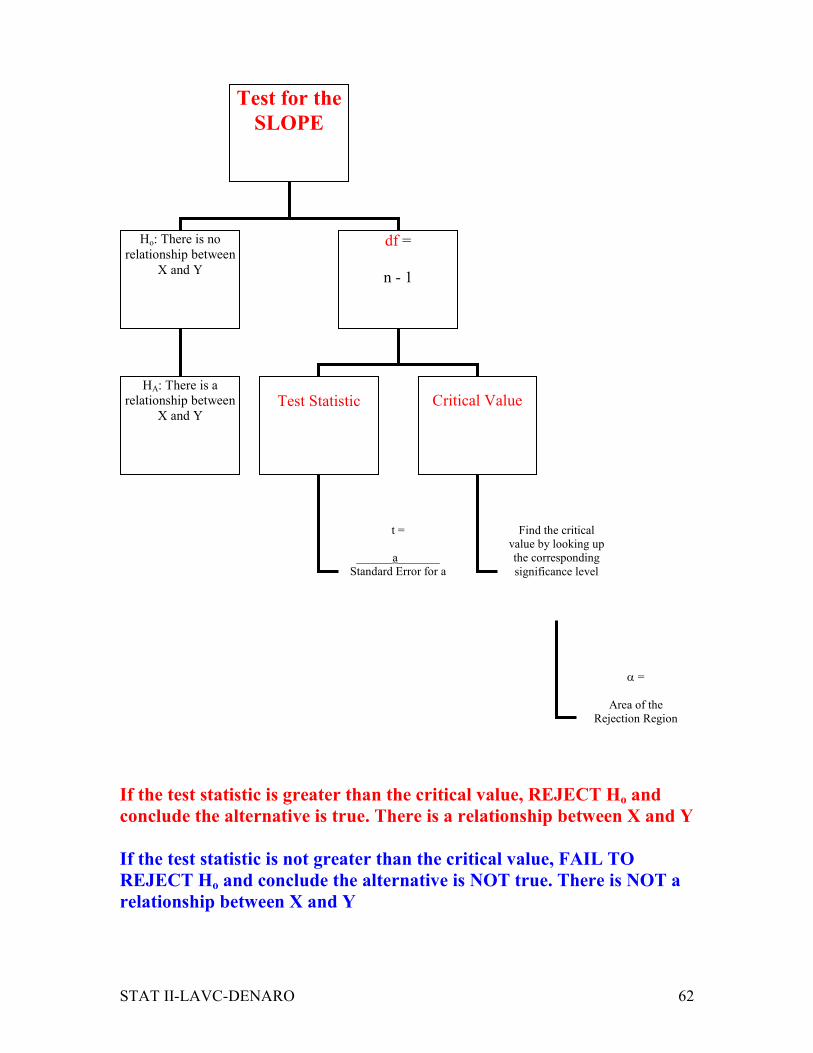
If the test statistic is greater than the critical value, REJECT Ho and
conclude the alternative is true. There is a relationship between X and Y
If the test statistic is not greater than the critical value, FAIL TO
REJECT Ho and conclude the alternative is NOT true. There is NOT a
relationship between X and Y
Test for the
SLOPE
Ho: There is no
relationship between
X and Y
df =
n - 1
Test Statistic
Critical Value
HA: There is a
relationship between
X and Y
t =
______a_______
Standard Error for a
Find the critical
value by looking up
the corresponding
significance level
α =
Area of the
Rejection Region
Page 63
STAT II-LAVC-DENARO 63
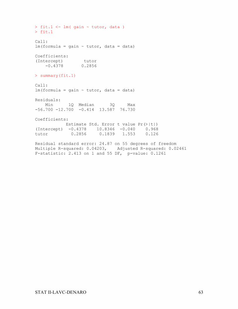
> fit.1 <- lm( gain ~ tutor, data )
> fit.1
Call:
lm(formula = gain ~ tutor, data = data)
Coefficients:
(Intercept) tutor
-0.4378 0.2856
> summary(fit.1)
Call:
lm(formula = gain ~ tutor, data = data)
Residuals:
Min 1Q Median 3Q Max
-56.700 -12.700 -0.414 13.587 76.730
Coefficients:
Estimate Std. Error t value Pr(>|t|)
(Intercept) -0.4378 10.8346 -0.040 0.968
tutor 0.2856 0.1839 1.553 0.126
Residual standard error: 24.87 on 55 degrees of freedom
Multiple R-squared: 0.04203, Adjusted R-squared: 0.02461
F-statistic: 2.413 on 1 and 55 DF, p-value: 0.1261
Page 64
STAT II-LAVC-DENARO 64
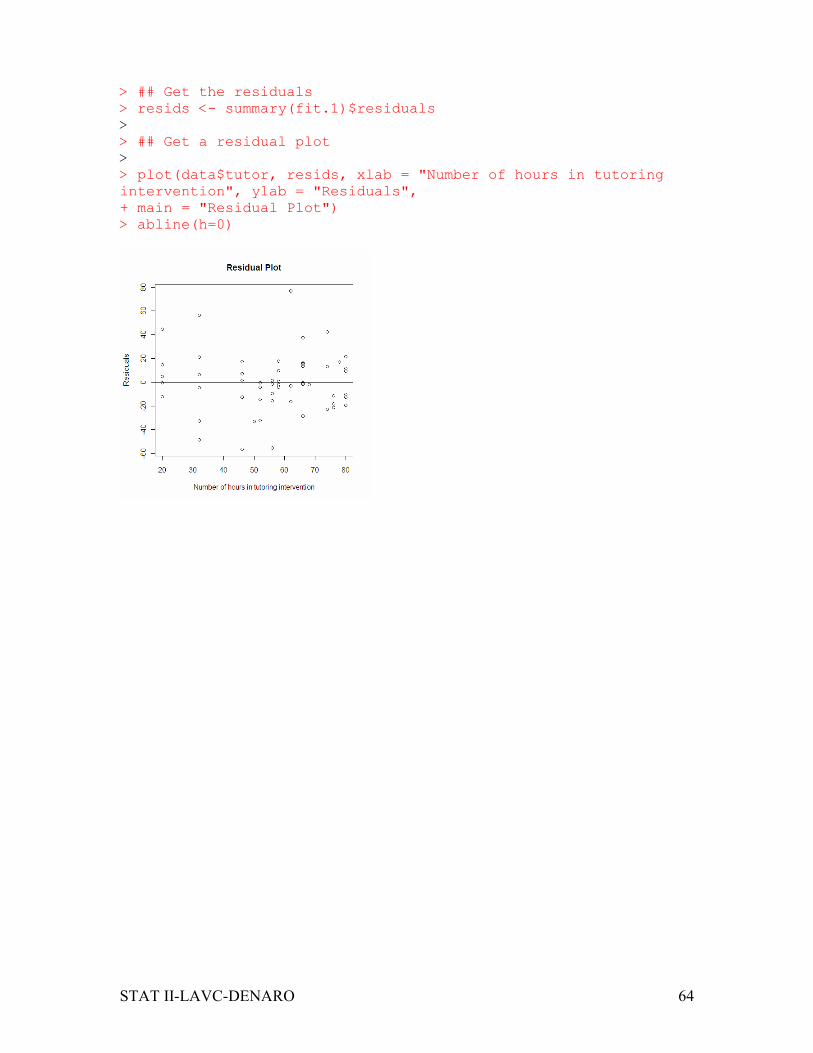
> ## Get the residuals
> resids <- summary(fit.1)$residuals
>
> ## Get a residual plot
>
> plot(data$tutor, resids, xlab = "Number of hours in tutoring
intervention", ylab = "Residuals",
+ main = "Residual Plot")
> abline(h=0)
Page 65
STAT II-LAVC-DENARO 65
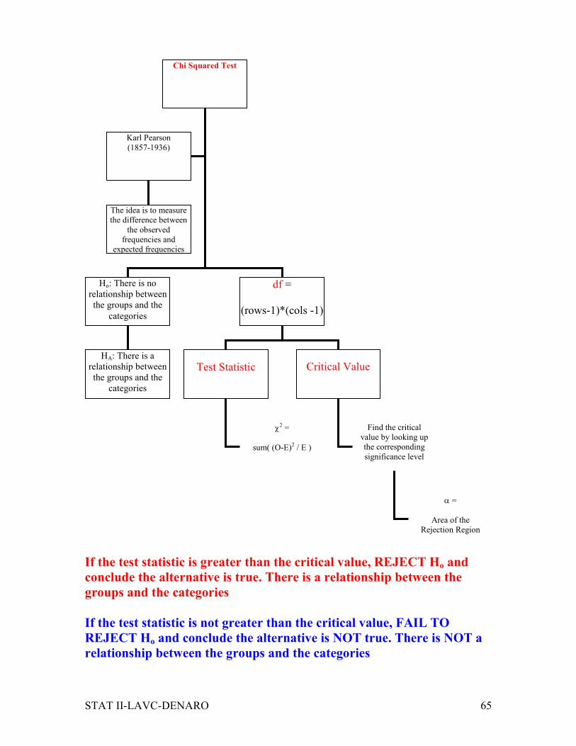
If the test statistic is greater than the critical value, REJECT Ho and
conclude the alternative is true. There is a relationship between the
groups and the categories
If the test statistic is not greater than the critical value, FAIL TO
REJECT Ho and conclude the alternative is NOT true. There is NOT a
relationship between the groups and the categories
Chi Squared Test
Ho: There is no
relationship between
the groups and the
categories
df =
(rows-1)*(cols -1)
Karl Pearson
(1857-1936)
Test Statistic
Critical Value
The idea is to measure
the difference between
the observed
frequencies and
expected frequencies
HA: There is a
relationship between
the groups and the
categories
χ2 =
sum( (O-E)2 / E )
Find the critical
value by looking up
the corresponding
significance level
α =
Area of the
Rejection Region
Page 66
STAT II-LAVC-DENARO 66
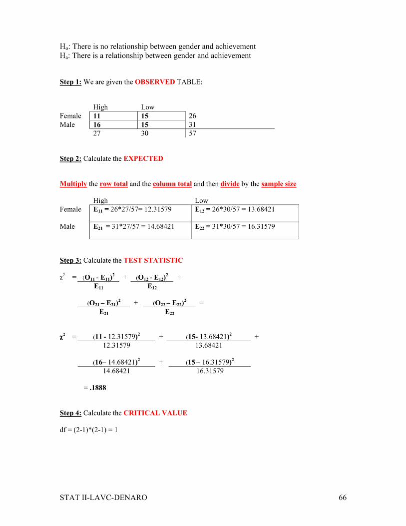
Ho: There is no relationship between gender and achievement
Ha: There is a relationship between gender and achievement
Step 1: We are given the OBSERVED TABLE:
High Low
Female 11 15 26
Male 16 15 31
27 30 57
Step 2: Calculate the EXPECTED
Multiply the row total and the column total and then divide by the sample size
High Low
Female E11 = 26*27/57= 12.31579
E12 = 26*30/57 = 13.68421
Male E21 = 31*27/57 = 14.68421
E22 = 31*30/57 = 16.31579
Step 3: Calculate the TEST STATISTIC
χ2 = (O11 - E11)
2 + (O12 - E12)
2 +
E11 E12
(O21 – E21)2 + (O22 – E22)
2 =
E21 E22
χχχχ2 = (11 - 12.31579)
2 + (15- 13.68421)
2 +
12.31579 13.68421
(16– 14.68421)2 + (15 – 16.31579)
2
14.68421 16.31579
= .1888
Step 4: Calculate the CRITICAL VALUE
df = (2-1)*(2-1) = 1
Page 67
STAT II-LAVC-DENARO 67
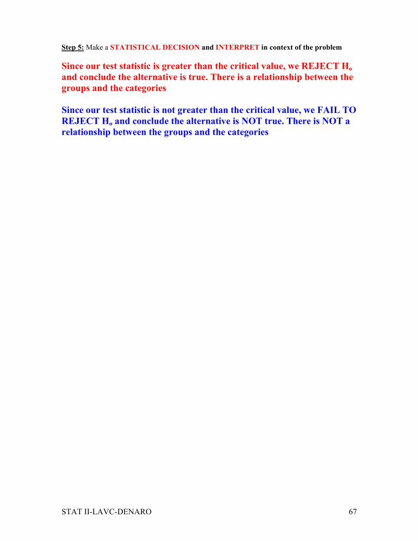
Step 5: Make a STATISTICAL DECISION and INTERPRET in context of the problem
Since our test statistic is greater than the critical value, we REJECT Ho
and conclude the alternative is true. There is a relationship between the
groups and the categories
Since our test statistic is not greater than the critical value, we FAIL TO
REJECT Ho and conclude the alternative is NOT true. There is NOT a
relationship between the groups and the categories


![Computer Organization [R18A0505] LECTURE NOTES](https://static.documents.pub/doc/80x56/631656291e5d335f8d09f4a5/computer-organization-r18a0505-lecture-notes.jpg)