RESERVES ASSESSMENT AND EVALUATION OF

AN ONSHORE OILFIELD

BY

AnajembaUgochukwu Christopher (3207773)

OgboliChukwudiCharles (3206391

Woodward Joseph (3212270

(Group 6)

London South Bank University

1

RESERVES ASSESSMENT AND EVALUATION OF

AN ONSHORE OILFIELD

AnajembaUgochukwu Christopher (3207773)

Charles (3206391)

Woodward Joseph (3212270)

28 DECEMBER 2013

London South Bank University

RESERVES ASSESSMENT AND EVALUATION OF

2

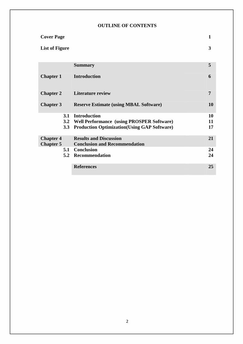
OUTLINE OF CONTENTS

Cover Page 1

List of Figure 3 Summary

5

Chapter 1 Introduction

6

Chapter 2

Literature review 7

Chapter 3 Reserve Estimate (using MBAL Software)

10

3.1 Introduction 10 3.2

3.3 Well Performance (using PROSPER Software) Production Optimization(Using GAP Software)

11 17

Chapter 4 Results and Discussion 21 Chapter 5 Conclusion and Recommendation

5.1 Conclusion 24 5.2 Recommendation

24

References 25

3

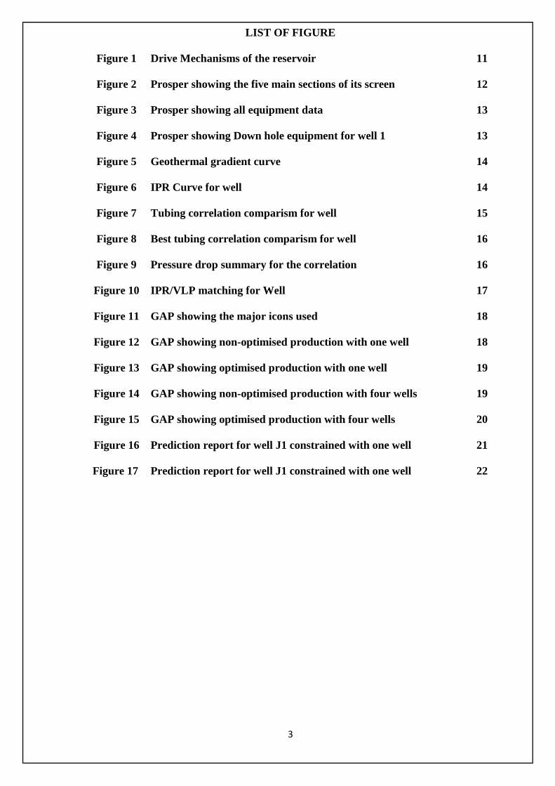
LIST OF FIGURE

Figure 1 Drive Mechanisms of the reservoir

11

Figure 2 Prosper showing the five main sections of its screen

12

Figure 3 Prosper showing all equipment data

13

Figure 4 Prosper showing Down hole equipment for well 1

13

Figure 5 Geothermal gradient curve

14

Figure 6 IPR Curve for well

14

Figure 7 Tubing correlation comparism for well

15

Figure 8 Best tubing correlation comparism for well

16

Figure 9 Pressure drop summary for the correlation

16

Figure 10 IPR/VLP matching for Well 17

Figure 11 GAP showing the major icons used

18

Figure 12

GAP showing non-optimised production with one well

18

Figure 13

GAP showing optimised production with one well

19

Figure 14 GAP showing non-optimised production with four wells 19

Figure 15 GAP showing optimised production with four wells 20

Figure 16

Prediction report for well J1 constrained with one well

21

Figure 17 Prediction report for well J1 constrained with one well

22

4

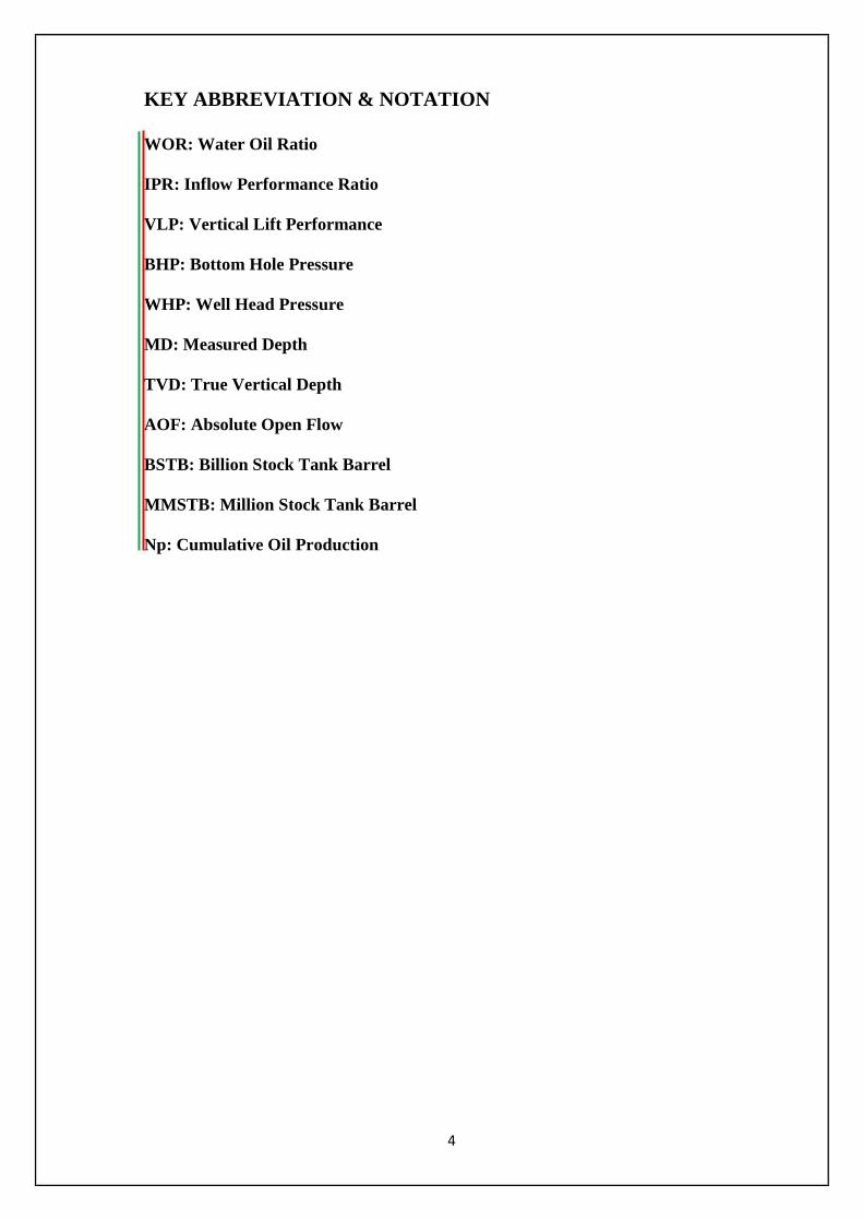
KEY ABBREVIATION & NOTATION

WOR: Water Oil Ratio

IPR: Inflow Performance Ratio

VLP: Vertical Lift Performance

BHP: Bottom Hole Pressure

WHP: Well Head Pressure

MD: Measured Depth

TVD: True Vertical Depth

AOF: Absolute Open Flow

BSTB: Billion Stock Tank Barrel

MMSTB: Million Stock Tank Barrel

Np: Cumulative Oil Production

5

SUMMARY

In this study, the Integration Production Modelling (IPM) was used to calculate different important parameters for "a mature onshore oilfield" that has been in production for 13years using (GAP, PROSPER &MBAL). A systematic reservoir engineering investigation which is extremely important for the development of an oil field is conducted to get insight information of the reservoir and production system. In the present work, MBAL software calculation is used to estimate the total oil in place of the mature oilfield which is 7162.59MMSTB. In January 2010, the cumulative production of the field is 60.157MMSTB with a production rate of 7499.925STB/day for each of the four wells used. Thus the amount of reserves after the 8years of management period is 7102.433MMSTB and hence forth, the recoverable of this reserve is 4616.58MMSTB based on the drive mechanism of 65%. PROSPER is most common software for the petroleum industry which can assist the production or reservoir engineer to predict tubing and pipeline hydraulics and temperatures with accuracy and speed that is also used to compare the measured oil rate. The production optimization depends upon several parameters such as well stimulation, tubing size, flow line size, chock size, separator pressure and average reservoir pressure. The impacts of each parameter are also observed to identify any bottle-neck in the production system. GAP analysis approach has been followed in conducting the system analysis to optimize production of mature oilfield. Different separator pressure is also investigated because it has a great influence in the flow period and flow rate. From the study, it is found that with the increase of separator pressure the flow period decreases i.e. the recovery of oil decreases. Various types of production tubing inner diameter is also used to find the great influence on the flow period and flow rate of oil. In this case, when production tubing inner diameter decreases then the oil flow rate also decreases but flow period of oil production increases i.e. recovery of oil increases.

The essence of this project is to evaluate the current reserves and propose the best way to manage the development of the field initially using the available facilities (not exceeding the production capacity of 30000 STB/day) and also considering a maximum of 10 new wells in production for 8 more years more.

6

1.0 Chapter 1

1.1 Objectives

To evaluate the current reserves and propose the best way to manage the development of the field initially using the available facilities (not exceeding the production capacity of 30000 STB/day) and also considering a maximum of 10 new wells in production for 8 more years more.

1.2 Introduction

There has been a mature oilfield onshore that have been in production 13years (from 1989 to 2002). The facilities for the development of the field is minimal and limited to the maximum processing capacity of 30000 STB/day, producing currently at a pressure 250 psig about 8km from main Centre Oil.

Reserve estimation and well performance study are essential studies in the field of petroleum engineering. Gas or oil recovery depends on well performance. So a well performance study is important for a production engineer for the depletion of the oil reservoir. Reserve estimation is important to decide whether the reservoir is economically viable or not. If a large amount of oil in place is present and the well performance is also good, then the reservoir is going to be on production.

This project will focus on production simulation of the mature oilfield using a commercial software and reserve estimation by MBAL software. The reservoir characteristics like permeability, porosity, reservoir pressure, and other relevant information were given for the evaluation as provided from the field analysis and these data are used in the reserve estimation and production optimization to predict reservoir performance of the oilfield.

The well deliverability test data and the well completion configuration data will be used to analyse the production scenario by PROSPER software. The analysis is helpful for the prediction of reservoir and well performance of this gas field. The overall performance of any well depends upon the combination of the well inflow performance, downhole conduit flow performance and surface flow performance. The eight production optimization depends upon several parameters i.e. well stimulation, tubing size, flow line size, chock size, separator pressure and average reservoir pressure. The impacts of each parameter have been observed to identify any bottle-neck in the production system. GAP analysis approach has been followed in conducting the system analysis to optimize production of the mature onshore oilfield.

7

Chapter 2

2.0 Literature Overview:

2.1 Inflow performance of a well:

The ability of a well to lift up the fluid represents its inflow performance. Success of a design for lifting fluids depends upon the accuracy of predicting a fluid flow into the well bore from the reservoir.

Inflow performance of a well with the flowing well pressure Pwf above bubble point pressure can be easily evaluated using the Dupuit’s solution for a single well located in a centre of a drainage area which produces at a steady state conditions (often called Darcy’s equation):

q=[2πkh(Pe-Pwf)]/[µBln (re/rw)+S]…………………………………(1)

According to which the productivity index PI has a constant value:

PI= q/(Pe-Pwf) =2πkh/[µB. 1/ ln (re/rw)+S] ……………………….(2)

As follows from (2), PI depends on the reservoir / fluid properties and therefore is one of important characteristics of a well’s inflow performance.

If Pi is known, then evaluation of the expected production rate under specified flowing well pressure Pwf is straightforward:

q = PI. (Pe- Pwf)

In case of a single phase flow, the relation between the production rate q and the pressure drop (∆P), which is called the inflow performance ratio, or IPR – curve is a straight line. As follows slope of the IPR curve is inversely proportional to the PI value, i.e.

Slope = 1/PI

Following the straight line to the point corresponding to the zero value of the bottom hole flowing well pressure Pwf =0, we can evaluate a theoretical limit of flow called absolute open flow (AOF).

8

2.2 IPR- Curve: Generalized form

Here we will consider a more general case when the reservoir pressure is higher than the bubble point pressure while the flowing well pressure can take any value (i.e. above or below the point pressure).

Due to the fact that the reservoir pressure is higher than bubble point pressure and IPR curve will consist of 2 parts i.e.

� Linear part for Pwf>Pb � Curved (Vogel’s type curve) part for Pwf<Pb

Note that both parts coincide at Pwf = Pb and q0 =q*, where q* is unknown.

Moreover, at this point both parts should have the same productivity index which means that derivatives to both parts at this point should have the same value.

2.3 Constructing IPR-Curve:

In performing a system analysis on a well, it is necessary to have a good test data on the well so that the reservoir capability can be predicted. In order to construct the IPR-curve, a well test data consisting of the measured average reservoir pressure, the flowing well pressure and the corresponding production rate are needed.

2.4 Back pressure IPR-curve:

Another technique for evaluating the non-linear IPR curve at two-phase flow is based on so called back pressure equation:

q=C. (Pr*2 – Pwf*2)*n

which can be used for both gas and saturated oil wells.

Here n usually takes value:

0.5 < n < 1.0

2.5 Fetkovich:

The fetkovich equation is modified from the Darcy equation which allows for the two phase flow below the bubble point. The Fetkovich equation can be expressed as

Q = J (Pr - Pb) + J’ ( Pr*2 – Pwf*2)

2.6 Multi-rate Fetkovich

9

This method uses a non-linear regression to fit the Fetkovich model for up to 10 test point. The model is expressed as

Q = C ((Pr*2 – Pwf*2)/1000)*n

In Prosper, the fit values of C and n are posted on the IPR plot.

2.7 Multi-rate Jones

This method uses a non-linear regression to fit for up to 10 test point for the Jones model

(Pr – Pwf) = aQ*2 + bQ*2

10

Chapter 3

Reserve Estimate (Using MBAL Software)

3.1 Introductions.

Petroleum Experts develop the Integrated Production Modelling software (IPM). IPM models the complete oil or gas production system including reservoir, wells and the surface network.

The IPM suite of tools: GAP- PROPSER- MBAL is fully integrated technologies and GAP which provides the integration between the MBAL reservoir elements and surface network.

Reserve estimation is an essential study in the field of petroleum engineering. Gas or oil recovery depends on well performance. So a well performance study is important for a production engineer for the depletion of the oil reservoir. Reserve estimation is important to decide whether the reservoir is economically viable or not. If a large amount of oil in place is present and the well performance is also good then the reservoir is going to be on production and profitable.

Gap is used as the master controller to access instances of PROSPER and MBAL. Integration of the well and reservoir elements provides the ability to understand the dynamic interactions of the complete petroleum engineering system. The value of well re-design and well stimulation efforts can easily be evaluated in context of the complete petroleum engineering system.

During a prediction, MBAL passes the evolving reservoir fluids to the Gap well elements. GAP uses the evolving reservoir fluids to capture well stability phenomena during a prediction enabling well contingency planning strategies to be developed.

Gap's scheduling power provides the ability to automatically develop well completion and drilling schedules that are required to meet a given overall flow objective. Drilling queues, walkovers, etc., can automatically be activated based on an objective function being set at any level in a given system.

Predicting measured reality is the ultimate goal of integrated studies and GAP offers a Model Validation utility to interrogate the system response. The model validation utility enables well model performance to be updated based on latest test data ensuring consistent model prediction ability.

This study will focus on the well evaluation and production simulation of a mature oilfield reserve estimation by using MBAL software. These data are used in the reserve estimation and production performance analysis of the field.

The production and pressure data are used to calculate oil in place by MBAL software.

The study uses PVT properties, production data and flowing well head pressure data. Well testing and production simulation were conducted to achieve a clear scenario about the well performance and oil in place of the gas field.

11

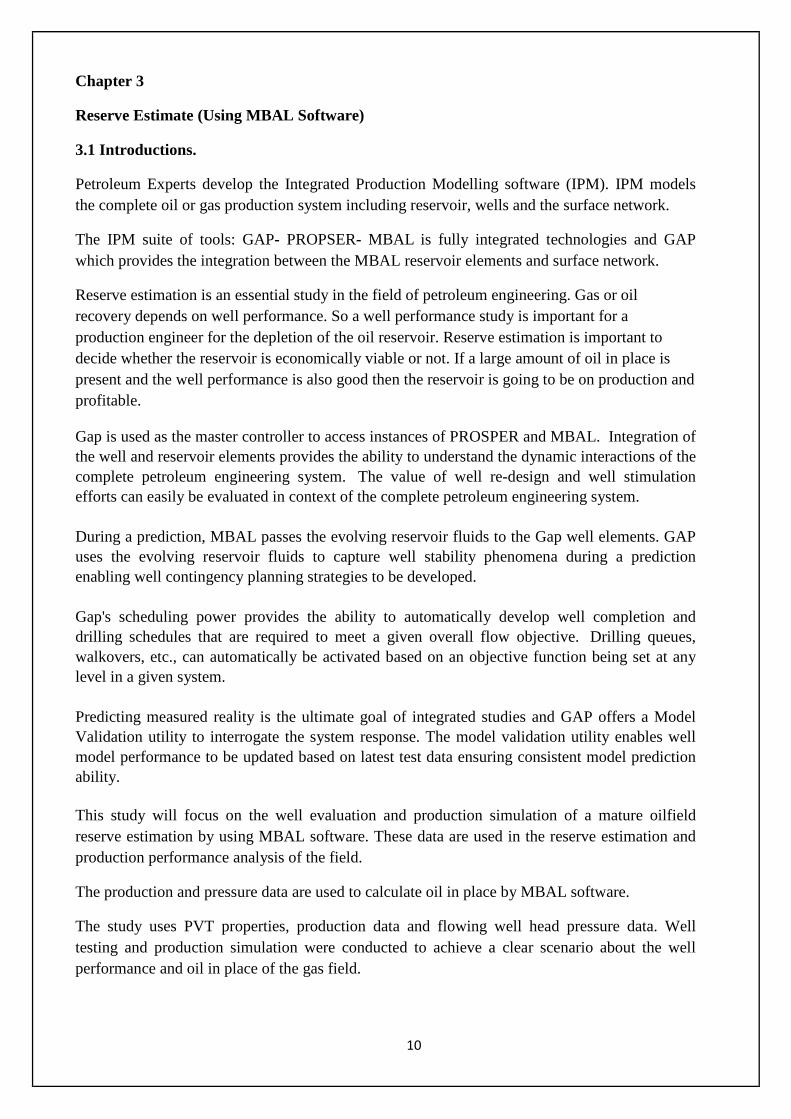
Figure-1, Drive Mechanisms of the reservoir

Looking at the three drive mechanisms: Fluid expansion, PV compressibility and water influx present in this reservoir, it could be seen that drive mechanism from Figure 1 that is most active is Fluid expansion which has a value of approximately 0.6

Well Performance (Using PROSPER Software)

3.2 Introduction

Prosper is one of the most common software for the petroleum industry. It is the petroleum Experts Limited’s advance Production and systems performance analysis software. Prosper can assist the production or reservoir engineer to predict tubing and pipeline hydraulics and temperatures with accuracy and speed. Prospers powerful sensitivity calculation features enables existing designs to be optimized and the effects of future changes in the system parameters to be assessed.

Prosper is a fundamental element in the Integrated Production Model (IPM) as defined by Petroleum Experts, linking to GAP, the production network optimization program for gathering system modelling and MBAL, the reservoir engineering and modelling tool for making fully integrated total system modelling and production forecasting.

The objective of this section is to set up prosper model for a oil well, input the PVT values, draw the phase diagram, draw the down hole, construct the IPR , matching the model to a well test and

12

performing the calculation of well performance, gradient transverse and vertical lift performance curves.

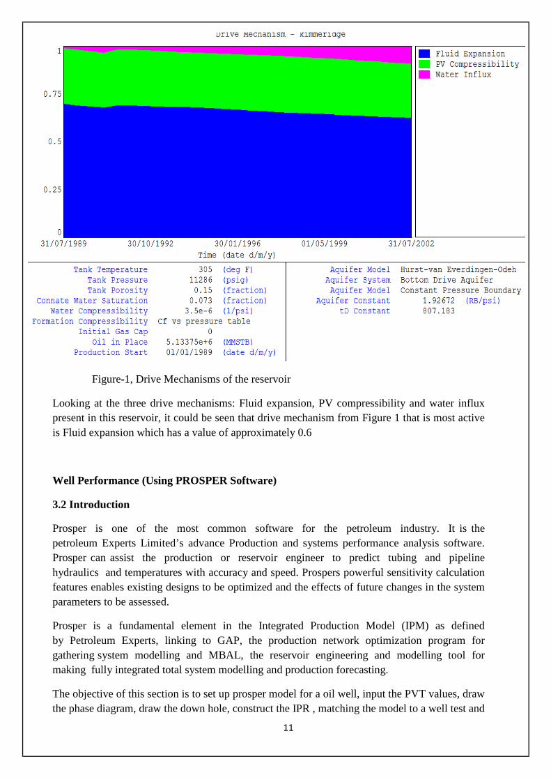
The PROSPER main screen is divided in to 5main sections. They are

• Options/summary • PVT Data • Equipment Data

• IPR Data • Analysis Summary

Figure-2, Prosper showing the five main sections of its screen

In this section, all equipment data are provided to the Prosper as follows.

• Deviation Survey • Surface Equipment

• Downhole Equipment • Geo-Thermal Gradient • Average Heat capacities

Option/Summary PVT Data

IPR Data

Equipment Data

Analysis Summary

13

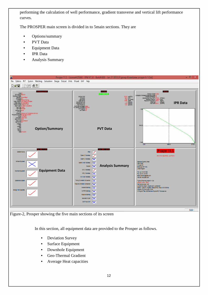
Figure-3, Prosper showing all equipment data

For this process, no surface equipment data are provided. The overall heat transfer coefficient was assumed to be 8.0 BTU/h/ft2/Fwhich was used to compute the geothermal gradient. Average heat capacities are taken as default value given by the Prosper.

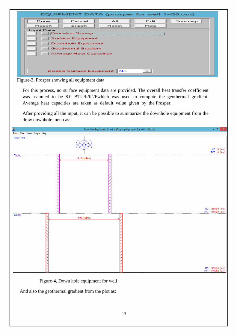
After providing all the input, it can be possible to summarize the downhole equipment from the draw downhole menu as:

Figure-4, Down hole equipment for well

And also the geothermal gradient from the plot as:

14

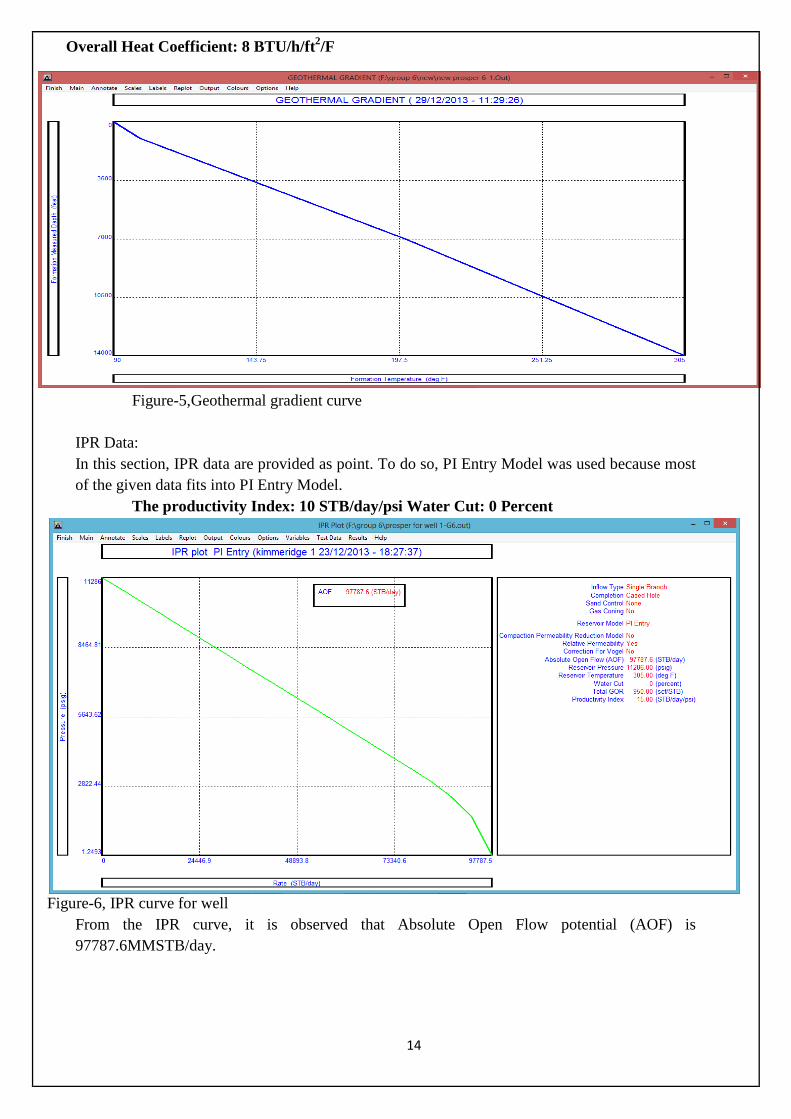
Overall Heat Coefficient: 8 BTU/h/ft2/F

Figure-5,Geothermal gradient curve

IPR Data: In this section, IPR data are provided as point. To do so, PI Entry Model was used because most of the given data fits into PI Entry Model.

The productivity Index: 10 STB/day/psi Water Cut: 0 Percent

Figure-6, IPR curve for well From the IPR curve, it is observed that Absolute Open Flow potential (AOF) is 97787.6MMSTB/day.

15

Matching of the Model to a Test

The matching process consists of two main steps:

- Matching of the VLP: The multiphase flow correction will be tuned in order to match

a down hole pressure measurement.

- Matching of the IPR: The IPR will be turned so that the intersection of VLP/IPR will

match the production rate as per well test.

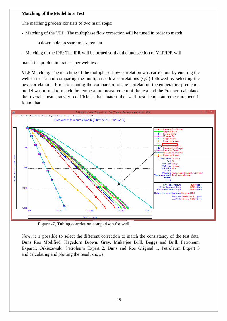
VLP Matching: The matching of the multiphase flow correlation was carried out by entering the well test data and comparing the multiphase flow correlations (QC) followed by selecting the best correlation. Prior to running the comparison of the correlation, thetemperature prediction model was turned to match the temperature measurement of the test and the Prosper calculated the overall heat transfer coefficient that match the well test temperaturemeasurement, it found that

Figure -7, Tubing correlation comparison for well

Now, it is possible to select the different correction to match the consistency of the test data. Duns Ros Modified, Hagedorn Brown, Gray, Mukerjee Brill, Beggs and Brill, Petroleum Expart1, Orkiszewski, Petroleum Expart 2, Duns and Ros Original 1, Petroleum Expert 3 and calculating and plotting the result shows.

16

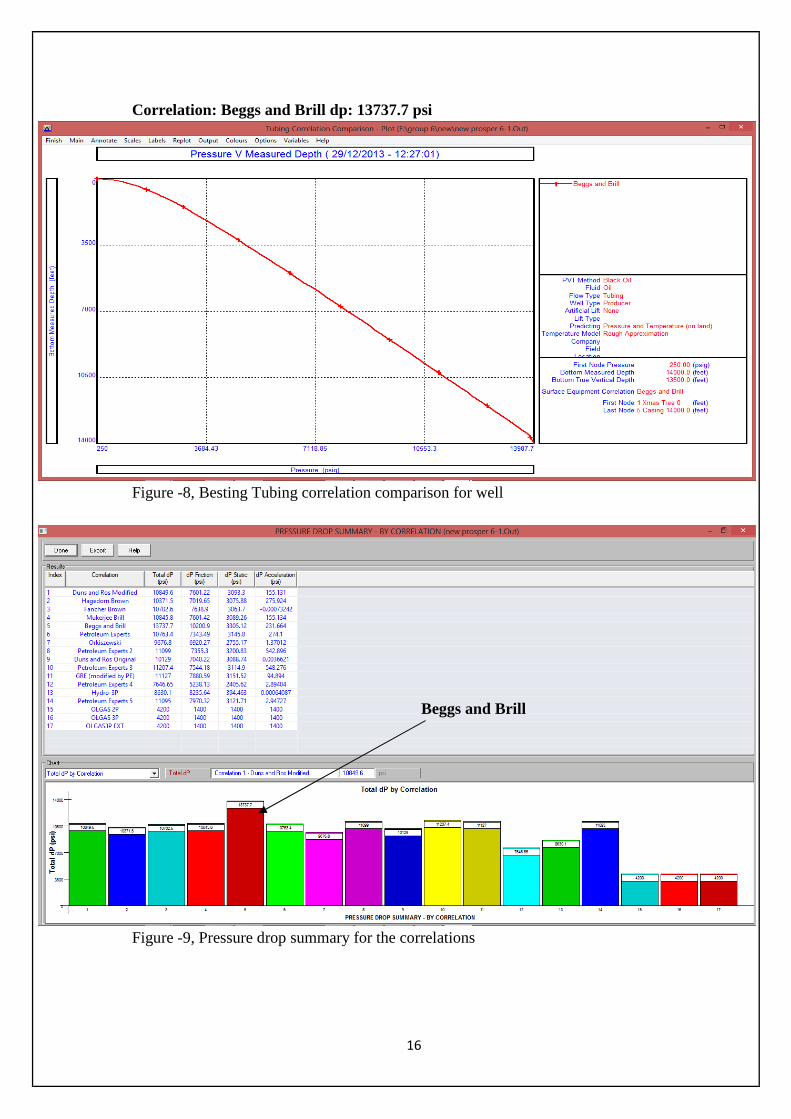
Correlation: Beggs and Brill dp: 13737.7 psi

Figure -8, Besting Tubing correlation comparison for well

Figure -9, Pressure drop summary for the correlations

Beggs and Brill

17

Matching the correlation to the test:

Once chosen the best correlation, it is possible to adjust the correlation to best fit the downhole pressure measurement. Prosper does this using a non-linear regression technique which applies multipliers to the gravity and friction components of the pressure drop prediction by multiphase flow correlation.

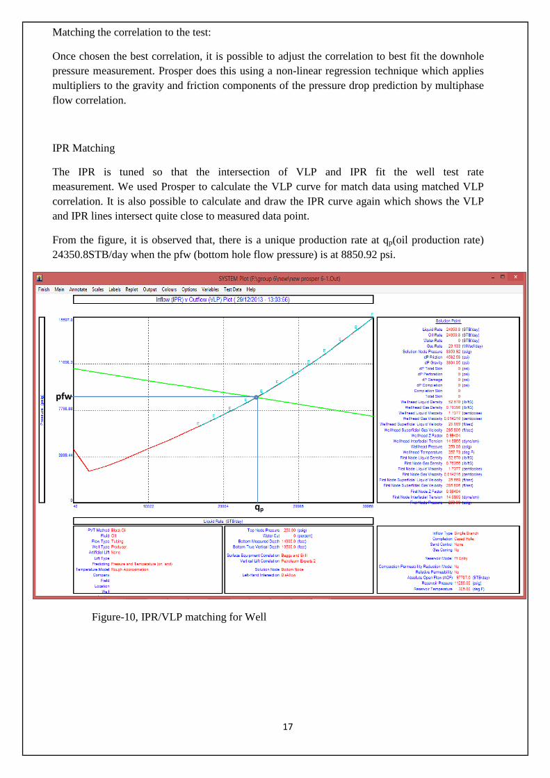
IPR Matching

The IPR is tuned so that the intersection of VLP and IPR fit the well test rate measurement. We used Prosper to calculate the VLP curve for match data using matched VLP correlation. It is also possible to calculate and draw the IPR curve again which shows the VLP and IPR lines intersect quite close to measured data point.

From the figure, it is observed that, there is a unique production rate at qp(oil production rate) 24350.8STB/day when the pfw (bottom hole flow pressure) is at 8850.92 psi.

Figure-10, IPR/VLP matching for Well

qp

pfw

18

3.3 Production Optimization(Using GAP Software)

Introduction:

Petroleum experts general allocation package is an extremely powerful and useful tool offered to the petroleum engineering community. Some of the tasks GAP can achieve are:

Complete surface production/injection network modelling.

In creating the gap model the following icons on the toolbars were mostly used. Icons such as

well, tank, joint, link/pipe and separator.

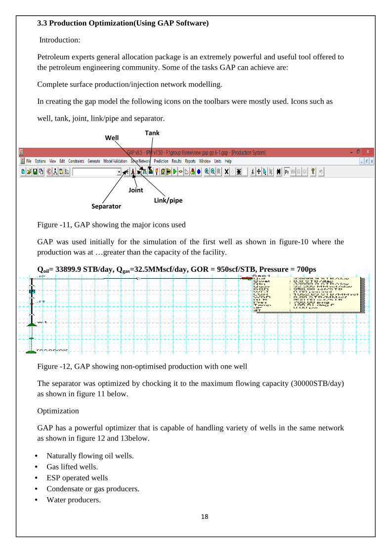
Figure -11, GAP showing the major icons used

GAP was used initially for the simulation of the first well as shown in figure-10 where the production was at …greater than the capacity of the facility.

Qoil= 33899.9 STB/day, Qgas=32.5MMscf/day, GOR = 950scf/STB, Pressure = 700ps

Figure -12, GAP showing non-optimised production with one well

The separator was optimized by chocking it to the maximum flowing capacity (30000STB/day) as shown in figure 11 below.

Optimization

GAP has a powerful optimizer that is capable of handling variety of wells in the same network as shown in figure 12 and 13below.

• Naturally flowing oil wells. • Gas lifted wells.

• ESP operated wells • Condensate or gas producers.

• Water producers.

Separator

Joint

Link/pipe

Well Tank

19

• Water or gas injectors.

• PCP wells. • HSP wells.

• The optimizer controls production rates using well head chokes, ESP operating frequencies or allocating lift gas to maximize the hydrocarbon production while honouring constraints at the gathering system, well and reservoir levels.

• Allocation of production.

• Predictions (production forecast). • GAP models both production and injection systems simultaneously, containing oil, gas

condensate and/or water well to generate production profiles. • GAP’s powerful optimization engine can for example allocate gas for gas lift wells, alter the

frequency of ESP pumps or sets well head chokes for naturally flowing wells to maximize revenue or oil production while honouring constraints at any level.

• GAP can also model and optimize injection network associated with the production system (both together).

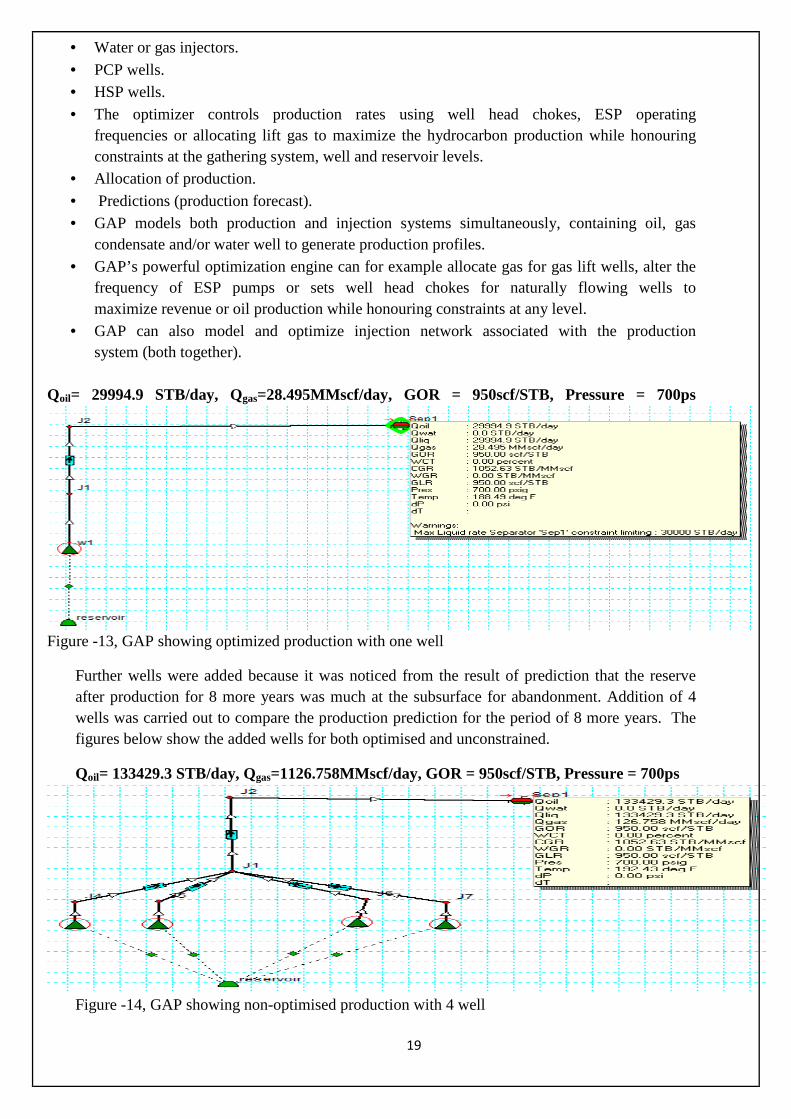
Qoil= 29994.9 STB/day, Qgas=28.495MMscf/day, GOR = 950scf/STB, Pressure = 700ps

Figure -13, GAP showing optimized production with one well

Further wells were added because it was noticed from the result of prediction that the reserve after production for 8 more years was much at the subsurface for abandonment. Addition of 4 wells was carried out to compare the production prediction for the period of 8 more years. The figures below show the added wells for both optimised and unconstrained.

Qoil= 133429.3 STB/day, Qgas=1126.758MMscf/day, GOR = 950scf/STB, Pressure = 700ps

Figure -14, GAP showing non-optimised production with 4 well

20

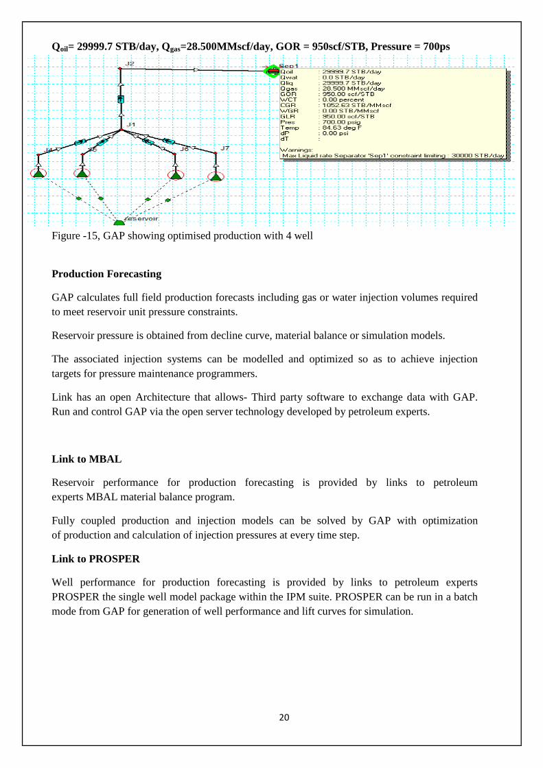
Qoil= 29999.7 STB/day, Qgas=28.500MMscf/day, GOR = 950scf/STB, Pressure = 700ps

Figure -15, GAP showing optimised production with 4 well

Production Forecasting

GAP calculates full field production forecasts including gas or water injection volumes required to meet reservoir unit pressure constraints.

Reservoir pressure is obtained from decline curve, material balance or simulation models.

The associated injection systems can be modelled and optimized so as to achieve injection targets for pressure maintenance programmers.

Link has an open Architecture that allows- Third party software to exchange data with GAP. Run and control GAP via the open server technology developed by petroleum experts.

Link to MBAL

Reservoir performance for production forecasting is provided by links to petroleum experts MBAL material balance program.

Fully coupled production and injection models can be solved by GAP with optimization of production and calculation of injection pressures at every time step.

Link to PROSPER

Well performance for production forecasting is provided by links to petroleum experts PROSPER the single well model package within the IPM suite. PROSPER can be run in a batch mode from GAP for generation of well performance and lift curves for simulation.

21

Chapter 4

4.1 Result and Discussion

Considering the recoverable oil after production for 8 more years, it shows that the oil reserve was 479MMSTB for one and four wells respectively when it was constrained. There was no clear difference for the amount of oil produced per day from the separator with increasing number of wells. This is a clear indication that the addition of more wells will incur more expenses and it is therefore not economically advisable to add more wells since it is obvious from our result, addition of more wells will noteffectan appreciable increase in production beyond the capacity of the facility. The prediction was done initially for single well and then four wells to compare the production history of the two as shown in table 1 below.

Table-1 showing the cumulative oil and gas constrained and unconstrained wells 1 well without

constrain 1 well with constrain

4 wells without constrain

4 wells with constrain

Cumulative oil production (MMSTB/day)

319.62 283.284 1015.048 283.123

Cumulative gas production (MMscf/day)

146547.406 19663.936 509446.297 129589.434

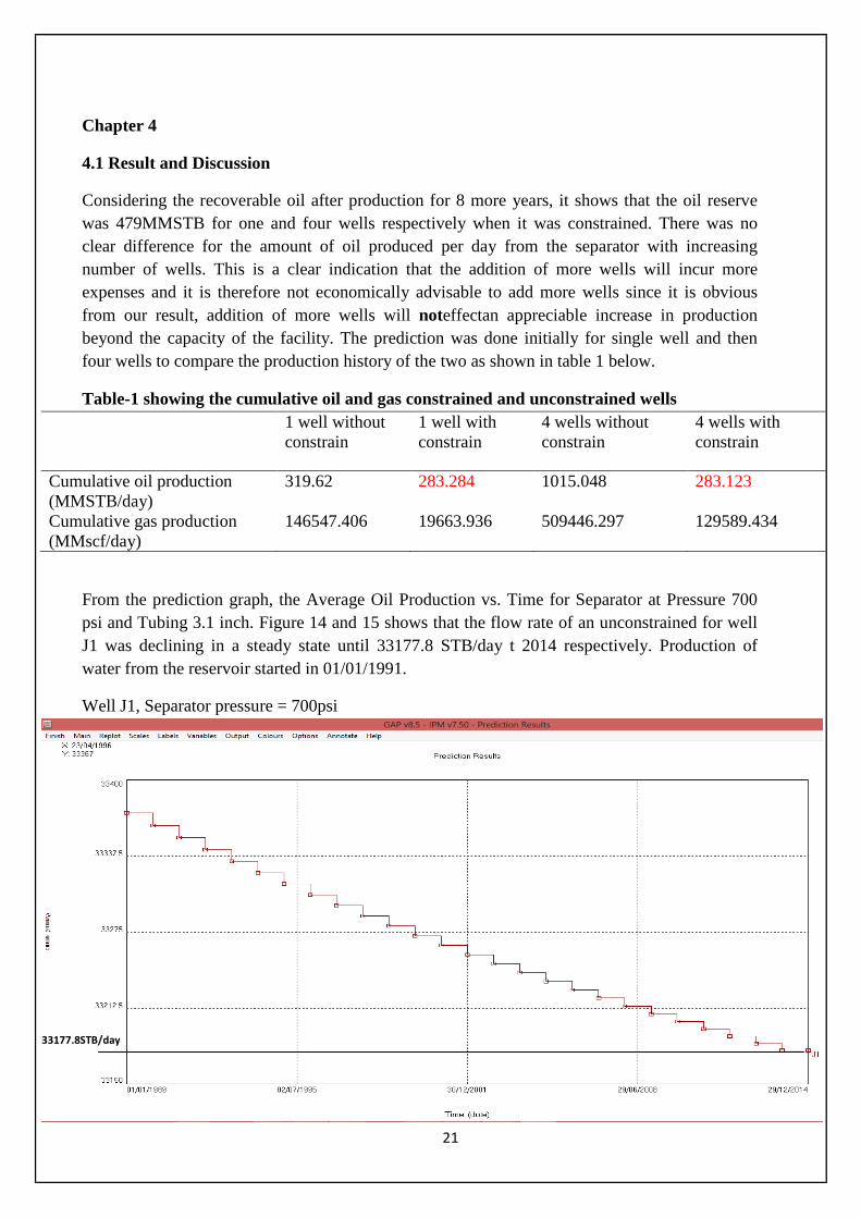
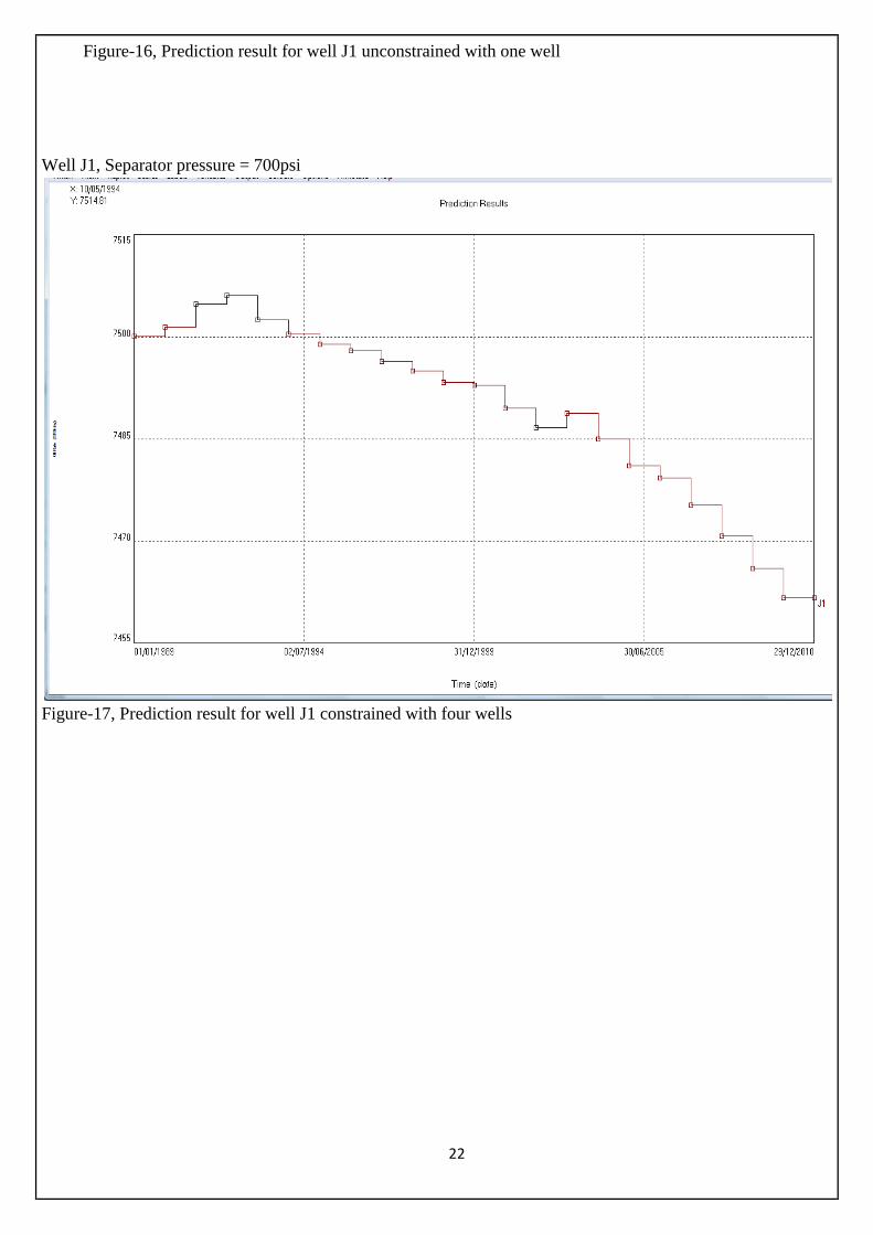
From the prediction graph, the Average Oil Production vs. Time for Separator at Pressure 700 psi and Tubing 3.1 inch. Figure 14 and 15 shows that the flow rate of an unconstrained for well J1 was declining in a steady state until 33177.8 STB/day t 2014 respectively. Production of water from the reservoir started in 01/01/1991.

Well J1, Separator pressure = 700psi

33177.8STB/day

22

Figure-16, Prediction result for well J1 unconstrained with one well

Well J1, Separator pressure = 700psi

Figure-17, Prediction result for well J1 constrained with four wells

23

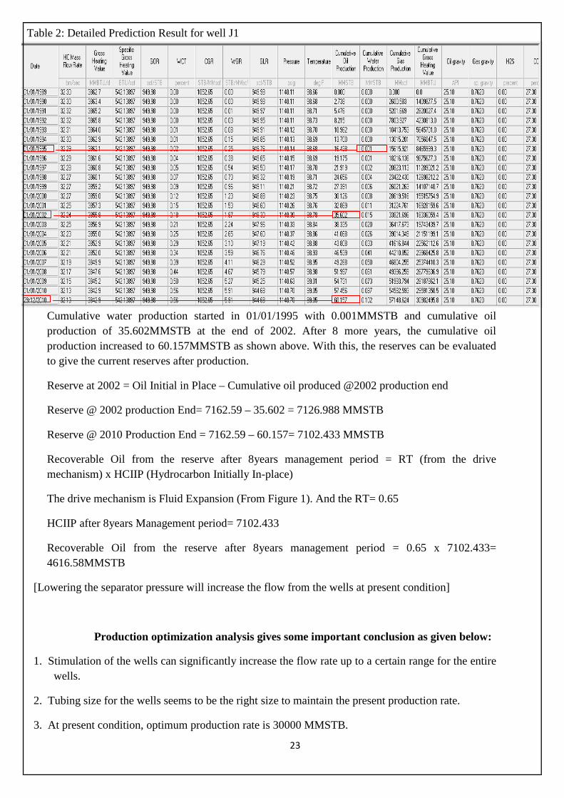
Table 2: Detailed Prediction Result for well J1

Cumulative water production started in 01/01/1995 with 0.001MMSTB and cumulative oil production of 35.602MMSTB at the end of 2002. After 8 more years, the cumulative oil production increased to 60.157MMSTB as shown above. With this, the reserves can be evaluated to give the current reserves after production.

Reserve at 2002 = Oil Initial in Place – Cumulative oil produced @2002 production end

Reserve @ 2002 production End= 7162.59 – 35.602 = 7126.988 MMSTB

Reserve @ 2010 Production End = 7162.59 – 60.157= 7102.433 MMSTB

Recoverable Oil from the reserve after 8years management period = RT (from the drive mechanism) x HCIIP (Hydrocarbon Initially In-place)

The drive mechanism is Fluid Expansion (From Figure 1). And the RT= 0.65

HCIIP after 8years Management period= 7102.433

Recoverable Oil from the reserve after 8years management period = 0.65 x 7102.433= 4616.58MMSTB

[Lowering the separator pressure will increase the flow from the wells at present condition]

Production optimization analysis gives some important conclusion as given below:

1. Stimulation of the wells can significantly increase the flow rate up to a certain range for the entire wells.

2. Tubing size for the wells seems to be the right size to maintain the present production rate.

3. At present condition, optimum production rate is 30000 MMSTB.

24

Chapter 5

5.0 Conclusions

After critical evaluation of the reserves from the available field data given, it wasobserved that increase in the number of wells supplying a particular separator under constrain will effect no change in the liquid rate at the separator (since the separator was producing at 3000STB/DAY). It is expected that the addition of more wells was meant to increase the liquid rate at the separator but the restraining factor as to the limitation of the project hindered the usefulness of adding more wells and hence would be rather an economic waste of the companies resources. Addition of more wells is of little advantage because it will lead to pressure maintenance and also emergency shutdown of some wells in case of emergency purpose which will not stop the company’s production during maintenance processes.

The original oil in place 7162.59MMSTB from the gap shows the actual volume of oil in place when the project was awarded to our company. After critical evaluation and further production at the rate of 7499.9STB/day for each of the four wells used in the period of 8years, 7102.433MMSTB was remaining.

Since the addition of more wells will effect no change in liquid production, we recommended that addition of an extra separator will enhance the recovery of more liquid from the reservoir. This because we still have a reserve of 7102.433 MMSTB at the end of the 8 years management period. This will aid maximum recovery.

Recommendation

Since the separator is constrained to produce at 30000 STB/day, it was noticed that adding more wells will not affect the production at separator but only reduce the production at the wells which add up to the separator production.

Therefore adding 1 or 2 wells will help reduce the pressure on one well, but then the financial implication should be considered.

From the foregoing its very clear that at the current facility production at the end of the 13 years period put with 8 years management period, there is still large quantity of oil reserve (7102.433 MMSTB).

Hence a better way of exploiting the reserve for maximum recovery should be put in place.

The capacity of the separator should be increased to accommodate a higher value (beyond the 30000STB constraint) of oil from the well

Also an additional separator should be added for maximum recovery over the period of time.

25

Reference

� Petroleum Engineering Design and Practice 2 Lectures. � Dr J.D Bell, Introduction to Petroleum Geology Lecture Notes, � Maria Ceteno Assignment (IPM) Integrated Production Modelling. � http://www.petex.com/products/?id=71accessed 13th January, 2013. � http://www.addenergy.no/well-engineering/integrated-production-modelling-

article1149-517.htmlaccessed 17th December, 2012.