Laboratory Course Neutron Scattering Experiment Manuals Thomas Brückel, Gernot Heger, Dieter Richter, Georg Roth and Reiner Zorn (Editors) Mitglied der Helmholtz-Gemeinschaft RWTH Aachen University Münster
Transcript
Schl
üsse
ltec
hnol
ogie
nK
ey T
echn
olog
ies
28
Laboratory Course
Neutron ScatteringExperiment Manuals
Thomas Brückel, Gernot Heger, Dieter Richter, Georg Roth and Reiner Zorn (Editors)
Schriften des Forschungszentrums JülichReihe Schlüsseltechnologien / Key Technologies Band / Volume 28
Forschungszentrum Jülich GmbHJülich Centre For Neutron Science (JCNS)
Thomas Brückel, Gernot Heger, Dieter Richter, Georg Roth and Reiner Zorn (Editors)
Neutron Scattering
Experiment Manuals of the JCNS Laborator Course held at Forschungszentrum Jülich and the research reactor FRM II of TU Munich In cooperation with RWTH Aachen and University of Münster
Schriften des Forschungszentrums JülichReihe Schlüsseltechnologien / Key Technologies Band / Volume 28
ISSN 1866-1807 ISBN 978-3-89336-726-9
Bibliographic information published by the Deutsche Nationalbibliothek.The Deutsche Nationalbibliothek lists this publication in the Deutsche Nationalbibliografie; detailed bibliographic data are available in the Internet at http://dnb.d-nb.de.
Schriften des Forschungszentrums JülichReihe Schlüsseltechnologien / Key Technologies Band / Volume 28
ISSN 1866-1807ISBN 978-3-89336-726-9
The complete volume ist freely available on the Internet on the Jülicher Open Access Server (JUWEL) at http://www.fz-juelich.de/zb/juwel
Neither this book nor any part of it may be reproduced or transmitted in any form or by any means, electronic or mechanical, including photocopying, microfilming, and recording, or by any information storage and retrieval system, without permission in writing from the publisher.
1 PUMA – Thermal Triple Axis Spectrometer O. Sobolev, A. Teichert,
N. Jünke
2 SPODI – High-resolution powder diffractometer M. Hoelzel, A. Senyshyn
3 HEiDi – Hot Single Crystal Diffractometer for Structure Analysis with Neutrons
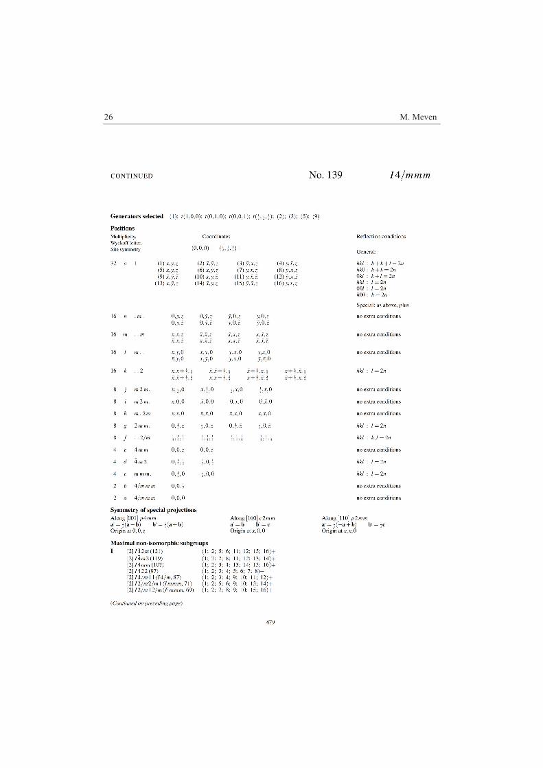
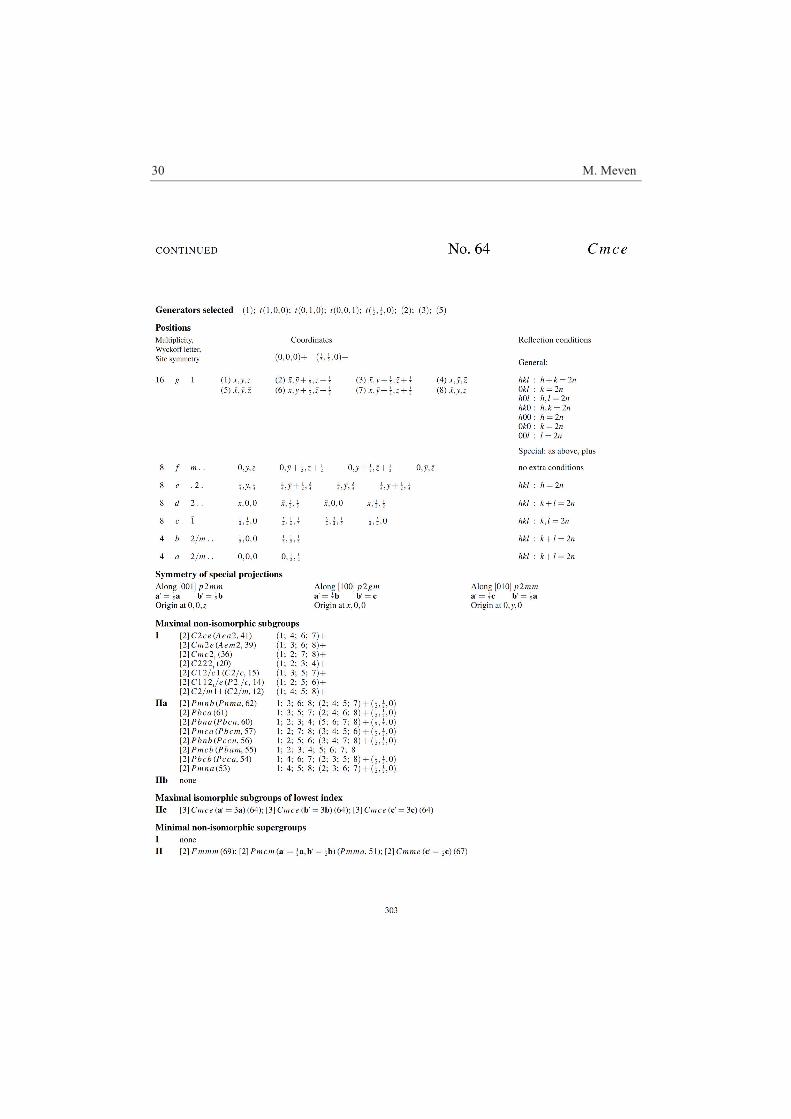
M. Meven
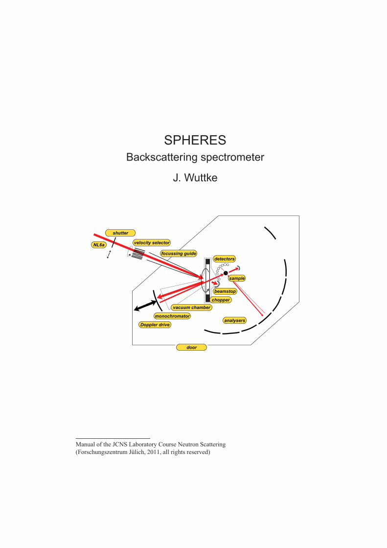
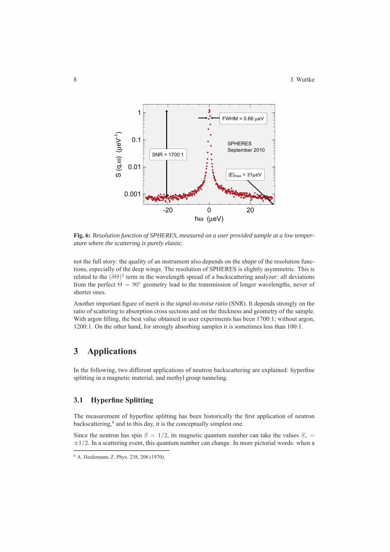
4 SPHERES – Backscattering spectrometer J. Wuttke
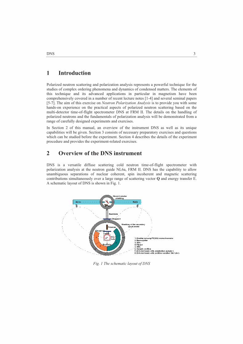
5 DNS – Neutron Polarization Analysis Y. Su
6 J-NSE – Neutron spin echo spectrometer O. Holderer, M. Zamponi, M. Monkenbusch
7 KWS-1/-2 – Small Angle Neutron Scattering H. Frielinghaus, M.-S. Appavou
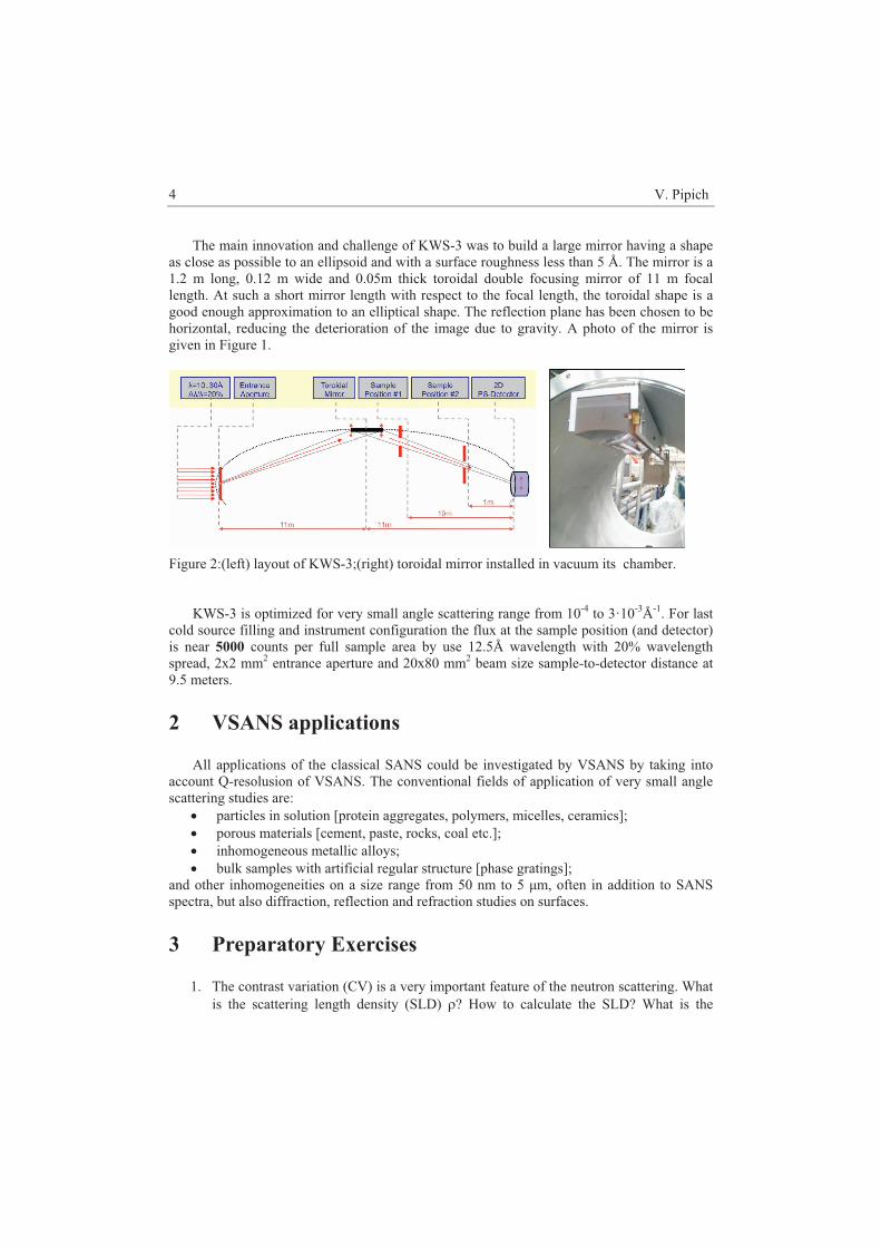
8 KWS-3 – Very Small Angle Neutron Scattering Diffractometer with Focusing Mirror
V. Pipich
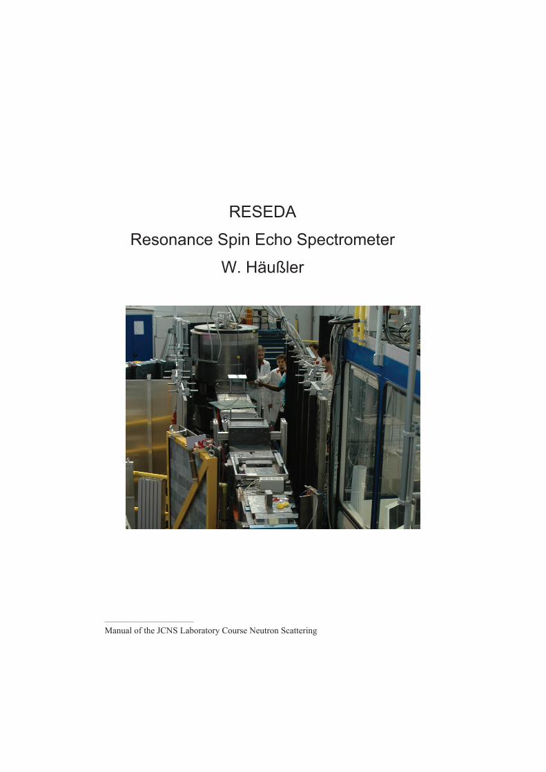
9 RESEDA – Resonance Spin Echo Spectrometer W. Häußler
10 TREFF – Reflectometer S. Mattauch, U. Rücker
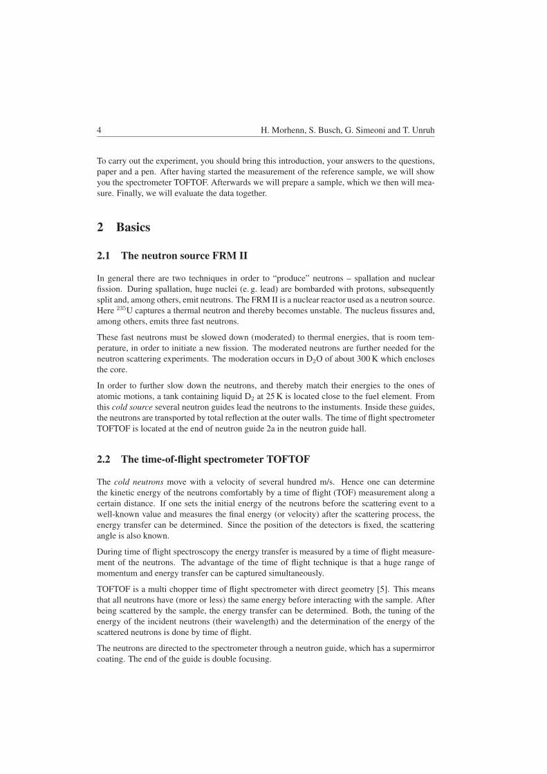
11 TOFTOF – Time-of-flight spectrometer H. Morhenn, S. Busch, G. Simeoni, T. Unruh
________________________
Manual of the JCNS Laboratory Course Neutron Scattering (Forschungszentrum Jülich, 2011, all rights reserved)
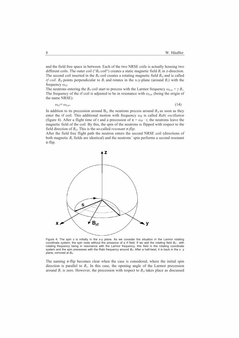
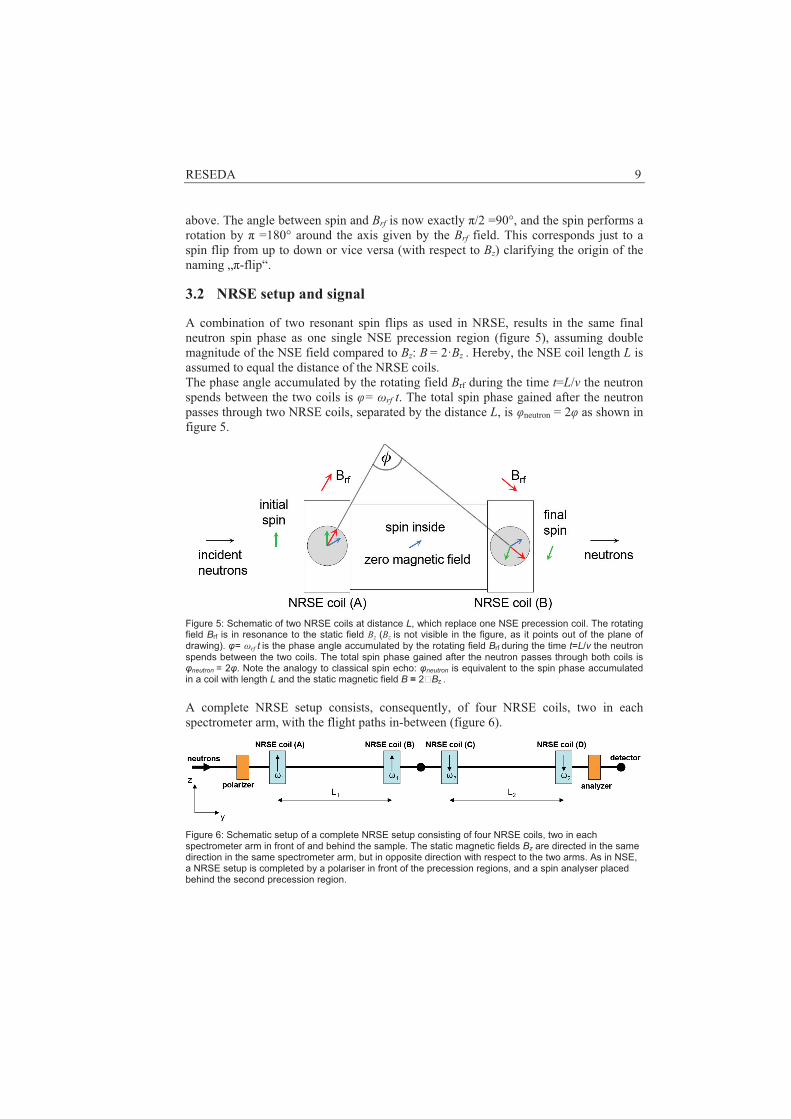
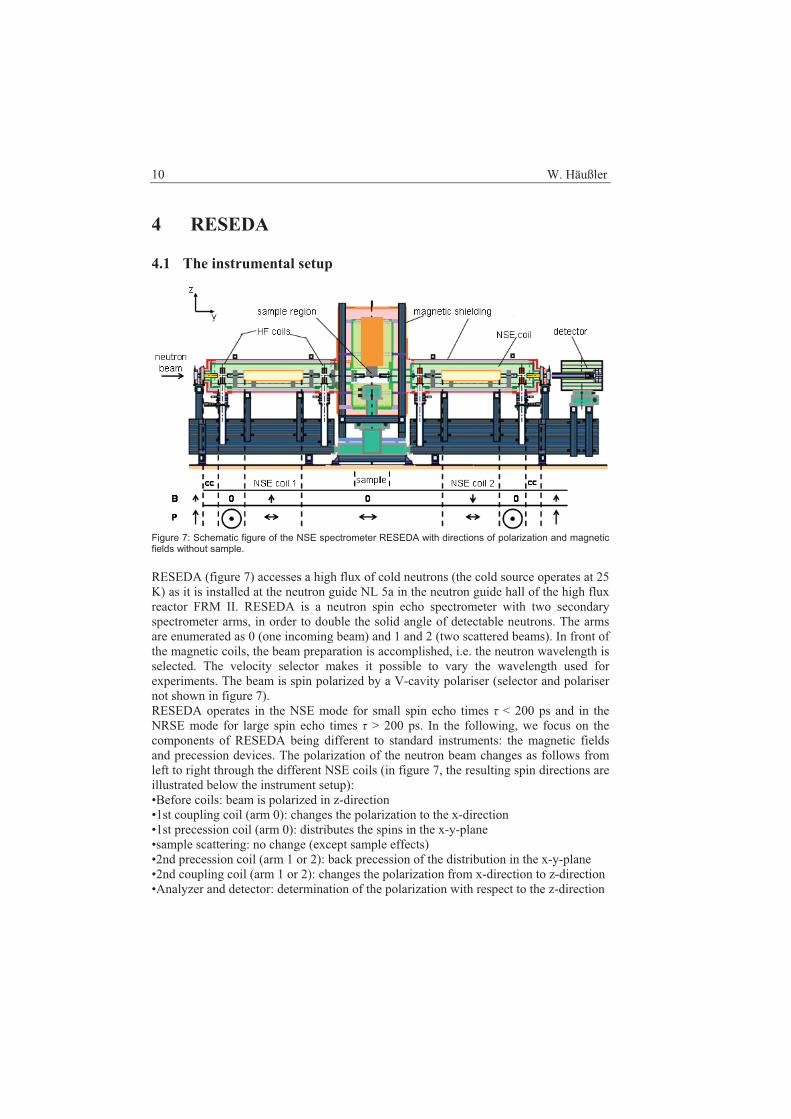
1. Introduction Excitations in crystals can be described using formalism of dispersion relations of the normal modes or quasi-particles (phonons, magnons, etc.). These relations contain the most detailed information on the intermolecular interactions in solids. The result of a neutron scattering experiment is the distribution of neutrons that have undergone an energy exchange �� = Ei - Ef, and a wave vector transfer, Q = ki – kf , after scattering by the sample.:
���
��� �
),(
4),(
4),2(
ddd2
��
��
��� QQ inc
inccoh
coh
i
f SSkk
N (1)
coh is coherent scattering cross section, inc is incoherent scattering cross section. They are constants that can be found in tables (http://www.ncnr.nist.gov/resources/n-lengths/). S(Q,�) functions depend only on the structure and dynamics of the sample and do not depend on the interaction between neutrons and the sample. Sinc(Q,�) reflects individual motions of atoms. Scoh(Q,�) provides the information on the structure and collective excitations in the sample.
The triple axis spectrometer is designed for measuring the Scoh(Q,�) in monocrystals. Therefore this function is of special interest for us and is considered in more detail in the theoretical sections of the first volume (lecture manuscripts).
Energy transfer �� = Ei - Ef
Momentum transfer
f0 kkQ �
��22
�
mEk
�2cos222
fifi kkkkQ ��
If ki = kf
���� sin4sin2 ikQ
4 O. Sobolev, A. Teichert, N.Jünke
2. Elastic scattering and Structure of Crystals
In the case of coherent elastic scattering, when � = 0 (ki = kf ) only neutrons, that fulfil the Brags law are scattered by the sample:
n� = 2dhklsin�hkl, (2) where � is a wavelength of neutron, dhkl is a distance between crystal planes described by corresponding Miller indexes hkl. �hkl denotes the angle between incoming (outgoing) scattering beam and the (hkl) plane. For the analysis of the scattering processes in crystals it is convenient to use the concept of the reciprocal space. For an infinite three dimensional lattice, defined by its primitive vectors a1, a2 and a3, its reciprocal lattice can be determined by generating three reciprocal primitive vectors, through the formulae:
213
21
312
31
321
32
aaaaag
aaaaag
aaaaag
���
���
���
�
�
2
2
2
3
2
1 �
(3)
Note the denominator is the scalar triple product. Geometrically, the scalar triple product a1(a2�a3) is the volume of the parallelepiped defined by the three vectors. Let us imagine the lattice of points given by the vectors g1, g2 and g3 such that � is an arbitrary linear combination of these vectors:
321 ggg� lkh �� , (4)
where h,k,l are integers. Every point of the reciprocal lattice, characterized by � corresponds in the position space to the equidistant set of planes with Miller indices (h,k,l) perpendicular to the vector �. These planes are separated by the distance
hklhkld
��2
(6)
The Brag’s condition for diffraction can be expressed in the following vector form:
Q = �hkl (7) A useful construction for work with wave vectors in reciprocal space is the Brillouin
zone (BZ). The BZ is the smallest unit in reciprocal space over which physical quantities such as phonon or electron dispersions repeat themselves. It is constructed by drawing vectors from one reciprocal lattice points to another and then constructing lines perpendicular to these vectors at the midpoints. The smallest enclosed volume is the BZ.
PUMA 5
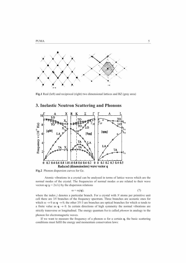
Fig.1 Real (left) and reciprocal (right) two dimensional lattices and BZ (gray area) 3. Inelastic Neutron Scattering and Phonons
Fig.2 Phonon dispersion curves for Ge.
Atomic vibrations in a crystal can be analysed in terms of lattice waves which are the
normal modes of the crystal. The frequencies of normal modes � are related to their wave vectors q (q = 2�/�) by the dispersion relations
� = �j(q), (7) where the index j denotes a particular branch. For a crystal with N atoms per primitive unit cell there are 3N branches of the frequency spectrum. Three branches are acoustic ones for which � � 0 as q � 0; the other 3N-3 are branches are optical branches for which � tends to a finite value as q � 0. In certain directions of high symmetry the normal vibrations are strictly transverse or longitudinal. The energy quantum �� is called phonon in analogy to the phonon for electromagnetic waves. If we want to measure the frequency of a phonon � for a certain q, the basic scattering conditions must fulfil the energy and momentum conservation laws:
6 O. Sobolev, A. Teichert, N.Jünke
)()(2
22 q������ fi
nfi kk
mEE (9)
Q = ki – kf = G � q
When the above conditions are fulfilled, the function Scoh(Q,�) shows a peak. We can held Q constant and vary ki (kf) to measure intensity of scattered neutrons at different energy transfers. In order to keep Q, and thus q, constant while varying ki, the scattering angle must change as well as the relative orientation of the crystal with respect to kf. The intensity of neutrons scattered by phonon is proportional to the square of the dynamical structure factor F(Q):
� � � � 2
)exp(exp)(~),( 2 � ���
�
��
��� qr
qeQQQ iW
mbFS k
jcoh , (10)
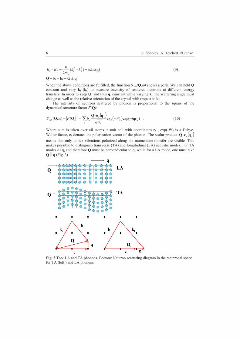
Where sum is taken over all atoms in unit cell with coordinates rk , exp(-W) is a Debye-Waller factor, ek denotes the polarization vector of the phonon. The scalar product � �jqeQ �� means that only lattice vibrations polarized along the momentum transfer are visible. This makes possible to distinguish transverse (TA) and longitudinal (LA) acoustic modes. For TA modes e�q, and therefore Q must be perpendicular to q, while for a LA mode, one must take Q�� q (Fig. 3)
Fig. 3 Top: LA and TA phonons. Bottom: Neutron scattering diagram in the reciprocal space for TA (left ) and LA phonons
PUMA 7
4. Triple Axis Spectrometer PUMA The three-axis instrument is the most versatile instrument for use in inelastic scattering because it allows one to probe nearly any coordinates in energy and momentum space in a precisely controlled manner. The three axes correspond to the axes of rotation of the monochromator (axis1), the sample (axis2), and the analyzer (axis3). The monochromator crystal selects neutrons with a certain energy from the white neutron beam emanating from the reactor. The monochromatic beam is then scattered off from the sample (second axis). The neutrons scattered by the sample can have a different energy from those incident on the sample. The energy of these scattered neutrons is then determined by the analyzer crystal (third axis). All three angles (�M, �S, �A) can vary during an experiment, the sample table and analyzer are equipped with air pads, so that they can glide over the “Tanzboden” (dancing floor). Below, we describe in detail each component of a triple-axis spectrometer. Monochromator A crystal monochromator is used to select neutrons with a specific wavelength. Neutrons with this wavelength interact with the sample and are scattered off at a similar (elastic) or different wavelength (inelastic). The energy of the neutrons both incident on and scattered from the sample is determined by Bragg reflection from the monochromator and analyzer crystals, respectively. For a specific Bragg plane (hkl) characterized by an interplanar spacing dhkl, the crystal is rotated about a vertical axis. A pyrolytic graphite with d002 = 3.35 Å (PG(002)) and a copper with d220 = 1.28 Å (Cu(220)) monochromators are available at PUMA. The angular range of the monochromator 2�M is of 15o - 115°. The PG(002) is usually used for energies below 50meV (�>1.3Å). For higher incident energies the Cu(220) can be used. Sample table The sample table from the company Huber provides a possibility to vary independently both 2�s and �S. It is equipped with a goniometer moving the sample in the three translation axes x, y and z and tilting. The tilt angle is ±15°. Single crystal experiments can be performed with an Euler cradle at PUMA. The sample environment includes magnets, pressure cells, cryostats and high temperature furnace. Analyzer Like the monochromator, the PG(002) analyzer consist of 20x5 separate analyzer crystal plates are mounted in an aluminum frame. There is an option to measure with the flat or horisontaly and verticaly focused analyser. The angular range of the analysator 2�M is of -130o - 130°. Detector and monitor The detector consists of five counter tubes which are filled with a 3He pressure of 5 bar. To be able to monitor the neutron flux incident on the sample, a low-efficiency neutron counter monitor is usually placed before the sample. Such a monitor is required so that flux variation caused by, for example, the reactor power fluctuations and the change in reflectivity of the monochromator with neutron wavelength can be automatically corrected for.
Additional components like slits or collimators are used to define the beam cross section. Collimators (�1- �4) are used for the improvement of the resolution and to specify the beam divergence. They consist of multiple parallel arranged Gd2O3 coated foils with a defined angle to the beam. The angular divergence of the collimator in the horizontal plane � is defined by the distance between foils �d and the length of the collimator l (tan � = �d / l). Different collimators with a horizontal divergence between 10’ and 60’ are available at the instrument.
One of the problems of the TAS method is the possible presence of higher harmonics in the neutron beam. Higher harmonics arise from higher order (hkl) in Bragg’s law (2). This means that if the monochromator (analyzer) crystal is set to reflect neutrons with a wavelength of � from a given (hkl) plane, it will also reflect neutrons with wavelength �/n. This leads to the appearance of several types of spurious peaks in the observed signal. Different filters are used to eliminate the high-order neutrons and to reduce the background. There are a sapphire filter (Al2O3) and an erbium filter (Er) at PUMA. They are installed in front of the monochromator. Sapphire filter is used wavelengths ��> 1 Å and reduce the background inducing by the epithermal neutrons. Erbium filter is suitable as �/2 filter for � between 0.5 and 1Å as well as �/3 filter for � between 0.7 and 1.6Å.
PUMA 9
Components Axis PUMAs notation
Description
Monochromator M �M mth Monochromator Theta 2�M mtt Monochromator 2Theta mtx, mty Monochromator Translation x-, y- direction mgx, mgy Monochromator Goniometer x-, y- direction mfh, mfv Monochromator Focus horizontal, vertical Sample S �S psi Sample Theta 2�S phi Sample 2Theta stx, sty, stz Sample Translation x-, y-, z- direction sgx, sgy Sample Goniometer x-, y- direction Analyzer A �A ath Analyzer Theta 2�A att Analyzer 2Theta atx, aty Analyzer Translation x-, y- direction agx, agy Analyzer Goniometer x-, y- direction afh Analyzer Focus horizontal Collimators alpha1 – alpha4 Collimation 5. Experiment Procedure The aim of the experiment is to measure acoustic phonons in a germanium sample. The phonons will be measured for [110] (LA) and [001] (TA) directions in [220] BZ. The experimental procedure shall contain the following steps: Sample alignment It is very difficult to align a sample with triple axis spectrometer, if the sample orientation is absolutely unknown. A sample must be pre-aligned, this means that the vertical axis of the sample must be known and roughly perpendicular to the ‘Tanzboden’. Than we shall do the following steps: - Inform the control program of the spectrometer about a scattering plane of the sample. One must set two reciprocal vectors (in our case [110] and [001]) laying in the scattering plane. - Drive spectrometer (�M, 2�M, �S, 2�S, �A, 2�A,) to the position corresponding to [220] reflection. - Scan �S and find the Brag’s peak. - Scan corresponding goniometer axes to maximize intensity of the peak. - Do the same for other reflection [004]. - Change the offset of the �S so that the nominal �S values correspond to intensity maxima for the above reflections. Phonons measurements For our measurements we will chose the const-kf configuration with kf = 2.662 Å-1 (Ef = 14.68 meV). This means that we will scan the energy transfer �� = Ei – Ef by varying incident energy Ei (ki). We are going to use PG(002) monochromator.
10 O. Sobolev, A. Teichert, N.Jünke
For LA phonon we will do constant-Q scans in the energy transfer range �� = 0 – 21 meV (0 – 8 THz) for the following points: Q(r.l.u.) = (2.1, 2.1, 0), (2.2, 2.2, 0), (2.3, 2.3, 0), (2.4, 2.4, 0), (2.5, 2.5, 0), (2.6, 2.6, 0), (2.7, 2.7, 0), (2.75, 2.75, 0). For TA phonon we will do constant-Q scans in the energy transfer range �� = 0 – 15 meV (0 – 3.6 THz) for the following points: Q(r.l.u.) = (2, 2, 0.2), (2, 2, 0.3), (2, 2, 0.4), (2, 2, 0.5), (2, 2, 0.7), (2, 2, 0.8), (2, 2, 0.9), (2, 2, 1).
PUMA 11
Fig 5 Elements of PUMA
a) PG Analyzer b) Soller collimator
c) Sample table d) Shutter, filters and collimators
e) Analyzer and Detector f) Detector, consists of 5 3He tubes
12 O. Sobolev, A. Teichert, N.Jünke
6. Preparatory Exercises
1. Calculate angles �M, 2�M, �S, 2�S, �A, 2�A for the reflections [220] and [002] of germanium (cubic-diamond, a = 5.66 Å), supposing that kf = 2.662 Å-1 = const, minichromator is PG(002). 2. Before doing a scan it is important to check that all point in Q - �� space are accessible, instrument angles do not exceed high or low limits. Also, an experimental scientist must be sure that the moving instrument will not hit walls or any equipment. Calculate instrument parameters (�M, 2�M, �S, 2�S, �A, 2�A) for the momentum transfers Q (r.l.u.) = (2.1, 2.1, 0), (2.75, 2.75, 0) and energy transfers �� = 0 and 21 meV. This can be done using an online triple-axis simulator: http://www.ill.eu/instruments-support/computing-for-science/cs-software/all-software/vtas/ 7. Experiment-Related Exercises
1. Plot obtained spectra for each Q as a function of energy (THz). Fit the spectra with Gaussian function and find centers of the phopon peaks. The obtained phonon energies plot as a function of q.
2. Why triple-axis spectrometer is the best instrument to study excitations in single crystals?
3. During this practicum we do not consider some problems that are very important for planning experiments with a triple axis instrument such as resolution and intensity zones [2]. Persons who have a strong interest to the triple-axis spectroscopy should study these topics by oneself. Advanced students should be able to explain our choice of Brillouin zone and parameters of scans for the phonon measurements.
Useful formula and conversions 1 THz = 4.1.4 meV n� = 2dhklsin�hkl,
hklhkld
��2
f0 kkQ �
�2cos222fifi kkkkQ ��
If ki = kf (elastic scattering) ���� sin4sin2 ikQ
E [meV] = 2.072 k2 [Å-1]
PUMA 13
References [1] Ch. Kittel, Einführung in die Festkörperphysik, Oldenburg, 14th ed., 2006 [2] G. Shirane, S.M. Shapiro, J.M. Tranquada, Neutron Scattering with a Triple-Axis Spektrometer, Cambridge University Press, 2002 [4] G. Eckold, P. Link, J. Neuhaus, Physica B, 276-278 (2000) 122- 123 [5] B.N.Brockhouse and P.K. Iyengar, Physikal Review 111 (1958) 747-754 [6] http://www.ill.eu/instruments-support/computing-for-science/cs-software/all-software/vtas/
14 O. Sobolev, A. Teichert, N.Jünke
Contact PUMA Phone: + 49 89 289 14914 Web: http://www.frm2.tum.de/wissenschaftliche-nutzung/spektrometrie/puma/index.html Oleg Sobolev Georg-August Universität Göttingen Institut für Physikalische Chemie Aussenstelle am FRM II Phone: + 49 89 289 14754 Email: [email protected]
Anke Teichert Georg-August Universität Göttingen Institut für Physikalische Chemie Aussenstelle am FRM II Phone: + 49 89 289 14756 Email: [email protected] Norbert Jünke Forschungsneutronenquelle Heinz Maier-Leibnitz ZWE FRM II Phone: + 49 89 289 14761 Email: [email protected]
________________________
Manual of the JCNS Laboratory Course Neutron Scattering Forschungsneutronenquelle Heinz Maier-Leibnitz (FRM II) and Forschungszentrum Jülich, 2011
SPODI
High-resolution powder diffractometer
M. Hoelzel and A. Senyshyn
2 M. Hoelzel, A. Senyshyn
Contents
1 Applications of neutron powder diffraction ........................................... 3
2 Basics of Powder Diffraction.................................................................... 4
3 Information from powder diffraction experiments ............................. 10
4 Evaluation of Powder Diffraction Data ................................................ 11
5 Comparison between Neutron and X-ray diffraction ......................... 13
6 Setup of the high-resolution neutron powder diffractometer SPODI at FRM II...................................................................................................... 15
7 Experiment: Phase- and structure analysis of lead titanate at various temperatures ............................................................................................ 17
Powder diffraction reveals information on the phase composition of a sample and the structural details of the phases. In particular, the positions of the atoms (crystallographic structure) and the ordering of magnetic moments (magnetic structure) can be obtained. In addition to the structural parameters, also some information on the microstructure (crystallite sizes/microstrains) can be obtained. The knowledge of the structure is crucial to understand structure – properties – relationships in any material. Thus, neutron powder diffraction can provide valuable information for the optimisation of modern materials.
Typical applications:
Material Task
Lithium-ion battery materials Positions of Li atoms, structural changes/phase transitions at the electrodes during operation, diffusion pathways of Li atoms
Hydrogen storage materials Positions of H atoms, phase transformations during hydrogen absorption/desorption
Ionic conductors for fuel cells positions of O/N atoms, thermal displacement parameters of the atoms and disorder at different temperatures,
diffusion pathways of O/N atoms
Shape memory alloys stress-induced phase transformations, stress-induced texture development
materials with CMR effect magnetic moment per atom at different temperatures
catalysers Structural changes during the uptake of sorbents
Piezoelectric ceramics Structural changes during poling in electric field, positions of O atoms
Nickel superalloys Phase transformations at high temperatures, lattice mismatch of phases
magnetic shape memory alloys Magneto-elastic effects, magnetic moment per atom at different temperatures and magnetic fields
4 M. Hoelzel, A. Senyshyn
2 Basics of Powder Diffraction
Diffraction can be regarded as detection of interference phenomena resulting from coherent elastic scattering of neutron waves from crystalline matter. Crystals can be imagined by a three-dimensional periodic arrangement of unit cells. The unit cell is characterised by the lattice parameters (dimensions and angles) and the positions of atoms or molecules.
For diffraction experiments the probe should have a wavelength comparable to interatomic distances: this is possible for X-rays, electrons or neutrons.
Structure factor The structure factor describes the intensity of Bragg reflections with Miller indexes (hkl), based on the particular atomic arrangement in the unit cell
� ���
�n
jjjjhkl RHiTbF
12exp
���
where
Fhkl: structure factor of Bragg reflection with Miller indexes hkl. n: number of atoms in unit cell
bj: scattering lengths (in case of neutron scattering) or atomic form factor (in case of X-ray diffraction) of atom j Tj: Debye Waller factor of atom j The scalar product H Rj consists of the reciprocal lattice vector H and the vector Rj, revealing the fractional atomic coordinates of atom j in the unit cell.
jjj
j
j
j
j lzkyhxzyx
lkh
RH ������
���
�
����
���
�
�
��
Thus, the structure factor can also be given as follows:
� ���
���n
jjjjjjhkl lzkyhxTbF
1exp
SPODI 5
The intensity of a Bragg reflection is proportional to the square of the absolute value of the structure factor: 2
hklFI �
Debye-Waller Factor The Debye-Waller Factor describes the decrease in the intensity of Bragg reflections due to atomic thermal vibrations.
� ����
����� jj uQQT ��
21exp)(
vector uj reflects the thermal displacements of atom j
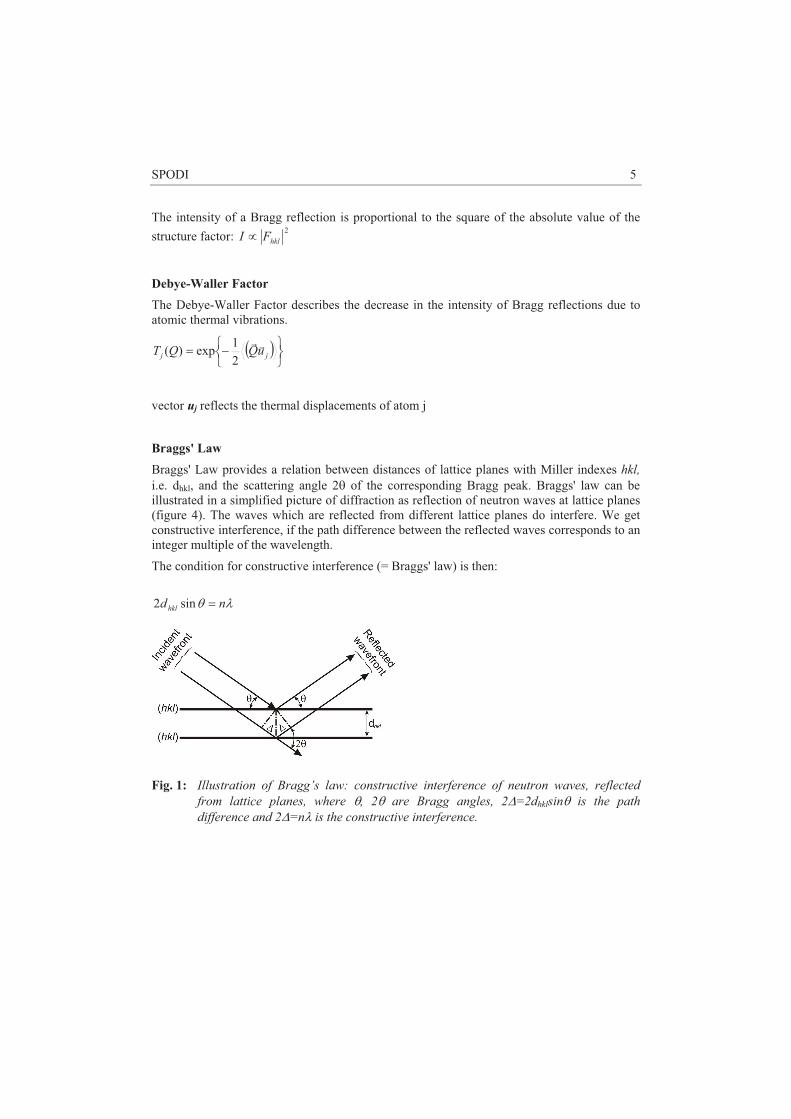
Braggs' Law Braggs' Law provides a relation between distances of lattice planes with Miller indexes hkl, i.e. dhkl, and the scattering angle 2� of the corresponding Bragg peak. Braggs' law can be illustrated in a simplified picture of diffraction as reflection of neutron waves at lattice planes (figure 4). The waves which are reflected from different lattice planes do interfere. We get constructive interference, if the path difference between the reflected waves corresponds to an integer multiple of the wavelength.
The condition for constructive interference (= Braggs' law) is then:
�� ndhkl �sin2
Fig. 1: Illustration of Bragg’s law: constructive interference of neutron waves, reflected
from lattice planes, where �, 2� are Bragg angles, 2�=2dhklsin� is the path difference and 2�=n� is the constructive interference.
6 M. Hoelzel, A. Senyshyn
Applying Bragg’s law one can derive the lattice spacings (“d-values“) from the scattering angle positions of the Bragg peaks in a constant-wavelength diffraction experiment. With the help of d-values a qualitative phase analysis can be carried out.
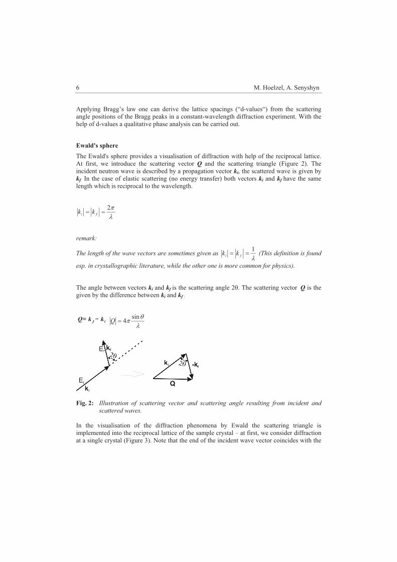
Ewald's sphere The Ewald's sphere provides a visualisation of diffraction with help of the reciprocal lattice. At first, we introduce the scattering vector Q and the scattering triangle (Figure 2). The incident neutron wave is described by a propagation vector ki, the scattered wave is given by kf. In the case of elastic scattering (no energy transfer) both vectors ki and kf have the same length which is reciprocal to the wavelength.
��2
�� fi kk
remark:
The length of the wave vectors are sometimes given as �1
�� fi kk (This definition is found
esp. in crystallographic literature, while the other one is more common for physics).
The angle between vectors ki and kf is the scattering angle 2�. The scattering vector Q is the given by the difference between ki and kf :
Q= k f � ki �
�� sin4�Q
Fig. 2: Illustration of scattering vector and scattering angle resulting from incident and
scattered waves. In the visualisation of the diffraction phenomena by Ewald the scattering triangle is implemented into the reciprocal lattice of the sample crystal – at first, we consider diffraction at a single crystal (Figure 3). Note that the end of the incident wave vector coincides with the
SPODI 7
origin of the reciprocal lattice. Ewald revealed the following condition for diffraction: we have diffraction in the direction of kf, if its end point (equivalently: the end point of scattering vector Q) lies at a reciprocal lattice point hkl. All possible kf, which fulfil this condition, describe a sphere with radius ����, the so called Ewald's sphere. Thus we obtain a hkl reflection if the reciprocal lattice point hkl is on the surface of the Ewald's sphere.
Fig. 3: Illustration of diffraction using the Ewald's sphere.
Here, the radius of Ewald's sphere is given by 1/� (For��2
�ik we obtain a radius of ����).
We receive the following condition for diffraction: the scattering vector Q should coincide with a reciprocal lattice vector Hhkl (x 2�):
hklHQ��
�2� ; xxxhkl clbkahH ����
��� ; hkl
xhklhkl d
dH 1��
�
From this diffraction condition based on the reciprocal lattice we can derive Bragg's law:
����
��� ����� sin22sin42 hklhkl
hkl dd
HQ��
The Ewald's sphere is a very important tool to visualize the method of single crystal diffraction: At a random orientation of a single crystalline sample a few reciprocal lattice points might match the surface of Ewald's sphere, thus fulfil the condition for diffraction. If we rotate the crystal, we rotate the reciprocal lattice with respect to the Ewald's sphere. Thus by a stepwise rotation of the crystal we receive corresponding reflections.
8 M. Hoelzel, A. Senyshyn
Powder Diffraction in Debye-Scherrer Geometry In a polycrystalline sample or a powder sample we assume a random orientation of all crystallites. Correspondingly, we have a random orientation of the reciprocal lattices of the crystallites. The reciprocal lattice vectors for the same hkl, i.e. Hhkl, describe a sphere around the origin of the reciprocal lattice. In the picture of Ewald's sphere we observe diffraction effect, if the surface of the Ewald's sphere intersects with the spheres of Hhkl vectors. For a sufficient number of crystallites in the sample and a random distribution of grain orientations, the scattered wave vectors (kf) describe a cone with opening angle 2� with respect to the incident beam ki.
In the so called Debye-Scherrer Geometry a monochromatic beam is scattered at a cylindrical sample. The scattered neutrons (or X-rays) are collected at a cylindrical detector in the scattering plane. The intersection between cones (scattered neutrons) and a cylinder (detector area) results in segments of rings (= Debye-Scherrer rings) on the detector. By integration of the data along the Debye-Scherrer rings one derives the conventional constant-wavelength powder diffraction pattern, i.e. intensity as a function of the scattering angle 2�.
0 20 40 60 80 100 120 140 160 18
Rel
ativ
e in
tens
ity
Bragg angle, 2� (deg)
Fig. 4: Illustration of powder diffraction in Debye-Scherrer Geometry. On the left: cones of
neutrons scattered from a polycrystalline sample are detected in the scattering plane. On the right: resulting powder diffraction pattern.
SPODI 9
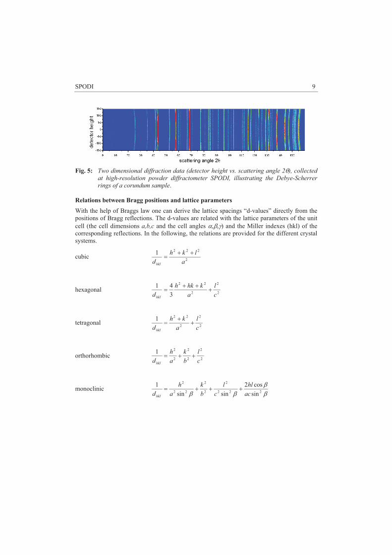
Fig. 5: Two dimensional diffraction data (detector height vs. scattering angle 2�), collected
at high-resolution powder diffractometer SPODI, illustrating the Debye-Scherrer rings of a corundum sample.
Relations between Bragg positions and lattice parameters With the help of Braggs law one can derive the lattice spacings “d-values” directly from the positions of Bragg reflections. The d-values are related with the lattice parameters of the unit cell (the cell dimensions a,b,c and the cell angles � ! ") and the Miller indexes (hkl) of the corresponding reflections. In the following, the relations are provided for the different crystal systems.
cubic 2
2221a
lkhdhkl
���
hexagonal 2
2
2
22
341
cl
akhkh
dhkl
���
�
tetragonal 2
2
2
221cl
akh
dhkl
��
�
orthorhombic 2
2
2
2
2
21cl
bk
ah
dhkl
���
monoclinic !!
!! 222
2
2
2
22
2
sincos2
sinsin1
achl
cl
bk
ah
dhkl
����
10 M. Hoelzel, A. Senyshyn
3 Information from powder diffraction experiments
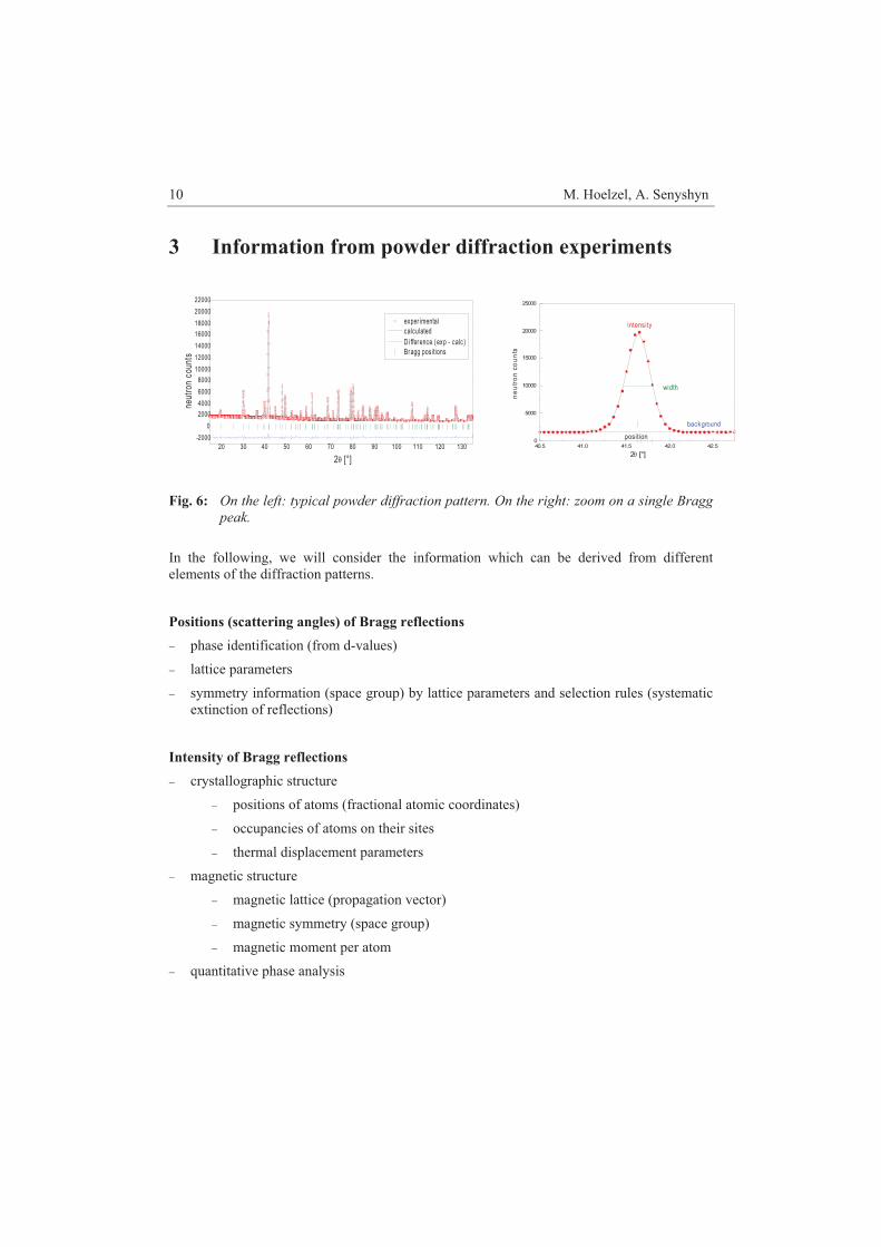
Fig. 6: On the left: typical powder diffraction pattern. On the right: zoom on a single Bragg
peak.
In the following, we will consider the information which can be derived from different elements of the diffraction patterns.
� symmetry information (space group) by lattice parameters and selection rules (systematic extinction of reflections)
Intensity of Bragg reflections � crystallographic structure
� positions of atoms (fractional atomic coordinates)
� occupancies of atoms on their sites
� thermal displacement parameters
� magnetic structure
� magnetic lattice (propagation vector)
� magnetic symmetry (space group)
� magnetic moment per atom
� quantitative phase analysis
20 30 40 50 60 70 80 90 100 110 120 130-2000
02000400060008000
10000120001400016000180002000022000
exper imental calculated D ifference (exp - calc) Bragg positions
neut
ron
coun
ts
2� [°]
40.5 41.0 41.5 42.0 42.50
5000
10000
15000
20000
25000
intensity
background
position
neut
ron
coun
ts
2� [°]
width
SPODI 11
� preferred orientation effects
Profiles of reflections The reflection profiles result in a convolution of the instrumental resolution function with broadening effects of the sample
� microstructural information
� microstrains
� crystallite sizes
Modulation/Profile of Background � short range order
� disorder
� amorphous contents
4 Evaluation of Powder Diffraction Data The methods of data treatment can be classified in analysis of phase composition or phase transformation, structure solution and structure refinement.
Qualitative phase analysis is based on the determination of d-values and relative intensities (in particular intensities of strong reflections have to be considered). The phase identification is supported by crystallographic data bases (ICDD, ISCD), literature data and information from other methods (for instance, analysis of the chemical composition). Such kind of phase analysis is however typically carried out with X-ray diffraction.
The majority of neutron powder diffraction studies is based on experiments at various temperatures to investigate phase transformation behaviour as a function of temperature. There is an increasing demand for parametric studies, i.e. diffraction studies under various environmental conditions (temperature, electric or magnetic field, mechanical stress, gas atmosphere...) with particular attention to reaction pathways/reaction kinetics. This kind of investigations require in general high-intensity powder diffraction.
Powder diffraction data can be used either for phase identification or for the refinement of structural parameters, such as lattice parameters, fractional atomic coordinates, atomic occupancies and atomic displacement parameters by the full profile Rietveld analysis. In the Rietveld method, the full diffraction pattern is calculated by a structure model, taking into account the above mentioned structural parameters, as well as reflection profile parameters, instrumental parameters and background parameters. Using least-squares method, the experimental data can be fitted to the model in a stepwise refinement of the parameters. The
12 M. Hoelzel, A. Senyshyn
complexity of the structures is directly dependent on the instrument specification, in particular, high-resolution powder diffractometers are designed for structure refinements on complex systems.
Besides structure refinement, also structure solution can be done based on powder diffraction patterns by various methods.
Fig. 7: Data treatment of a measurement on a lead zirconate titanate sample, carried out at 5 K at diffractometer SPODI (FRM II): Diffraction pattern including experimental
SPODI 13
data, calculated data by Rietveld fit, Bragg reflection positions of the phases (space groups CC and Cm) and difference plot (between experimental and calculated data). - zoom into the diffraction pattern, highlighting a superlattice reflection of the CC phase. - structure model of the CC phase, view in the [001]c direction - structure model of the CC phase, view in the [010]c direction. In particular, the superstructure in the tiltings of oxygen octahedra can be seen. M. Hinterstein et. al, Journal of Applied Physics 108, 1 (2010).
5 Comparison between Neutron and X-ray diffraction
I) X-rays are scattered at electrons, neutrons are scattered at nuclei In case of X-ray scattering, the scattering power of an atom (described by the atomic form factor f) is proportional to the number of electrons.
Neutrons are scattered at nuclei. Thus the interaction (described by the scattering length b) varies between different isotopes of an element. Scattering length of neighbouring elements in the periodic system can be very different.
implications: Localisation of light elements next to heavier ones X-ray diffraction is a powerful tool to determine the positions of heavy atoms, but the localisation of light atoms in the vicinity of much heavier atoms is often difficult or related with high uncertainties. Neutron diffraction is advantageous to localise light atoms such as H, D, Li, C, N, O.
Localisation of neighbouring elements in the periodic table Neighbouring elements in the periodic table can hardly be distinguished by means of X-ray diffraction. Neutrons are advantageous for such cases: examples: Mn – Fe - Co – Ni or O – N.
Q-dependence of intensities Since the size of electron clouds is comparable to the wavelength, the atomic form factor depends on sin���#or#Q$#Therefore the intensities of X-ray reflections decrease significantly for increasing Q (increasing scattering angles 2���.
As the range of the neutron–nuclei–interaction is by orders of magnitude smaller than the wavelengths of thermal neutrons, scattering lengths do not depend on Q. As a consequence, neutron diffraction patterns do not show a decrease of Bragg reflection intensities for higher scattering angles, enabling the analysis of larger Q-ranges. In particular, neutron diffraction is advantageous for the analysis of thermal displacement parameters.
14 M. Hoelzel, A. Senyshyn
II) neutrons interact weakly with matter implications: sample volume The flux from neutron sources much lower compared to X-ray tubes or even synchrotrons. In addition, neutrons interact weakly with matter. Therefore, much larger sample amounts are required compared to X-ray diffraction (“grams instead of milligrams”). On the other hand this weak interaction results in much higher penetration depths of neutrons, compared to laboratory X-ray diffractometers. Thus, polycrystalline bulk samples can be investigated. Furthermore, using large sample volumes avoids possible problems due to preferred orientation effects. In principle, bulk samples can also be investigated with high-energy synchrotron radiation. Anyhow in special cases the very low scattering angles related to low wavelength (in high-energy synchrotron studies) can cause difficulties.
Sample environments The large penetration depths of neutrons facilitate the usage of sample environments like cryostat, furnaces, magnets... In general neutron scattering experiments are more powerful applying high or low temperatures. On the other hand, the small sample volume required for synchrotron studies gives better possibilities for high-pressure experiments.
III) neutrons exhibit a magnetic moment Though neutrons do not have an electric charge, the internal charge distribution due to its three quarks along with the spin result in a magnetic moment of the neutron.
implications: magnetic scattering The interaction between the magnetic moment of the neutron and a possible magnetic moment of an atom results in a magnetic scattering contribution, incidentally in the same order of magnitude as the nuclear scattering contribution. The magnetic scattering contribution can be easily detected by means of neutron diffraction. In synchrotron diffraction studies, possible magnetic scattering events are by several orders of magnitude weaker than the Thomson scattering.
SPODI 15
6 Setup of the high-resolution neutron powder diffractometer SPODI at FRM II
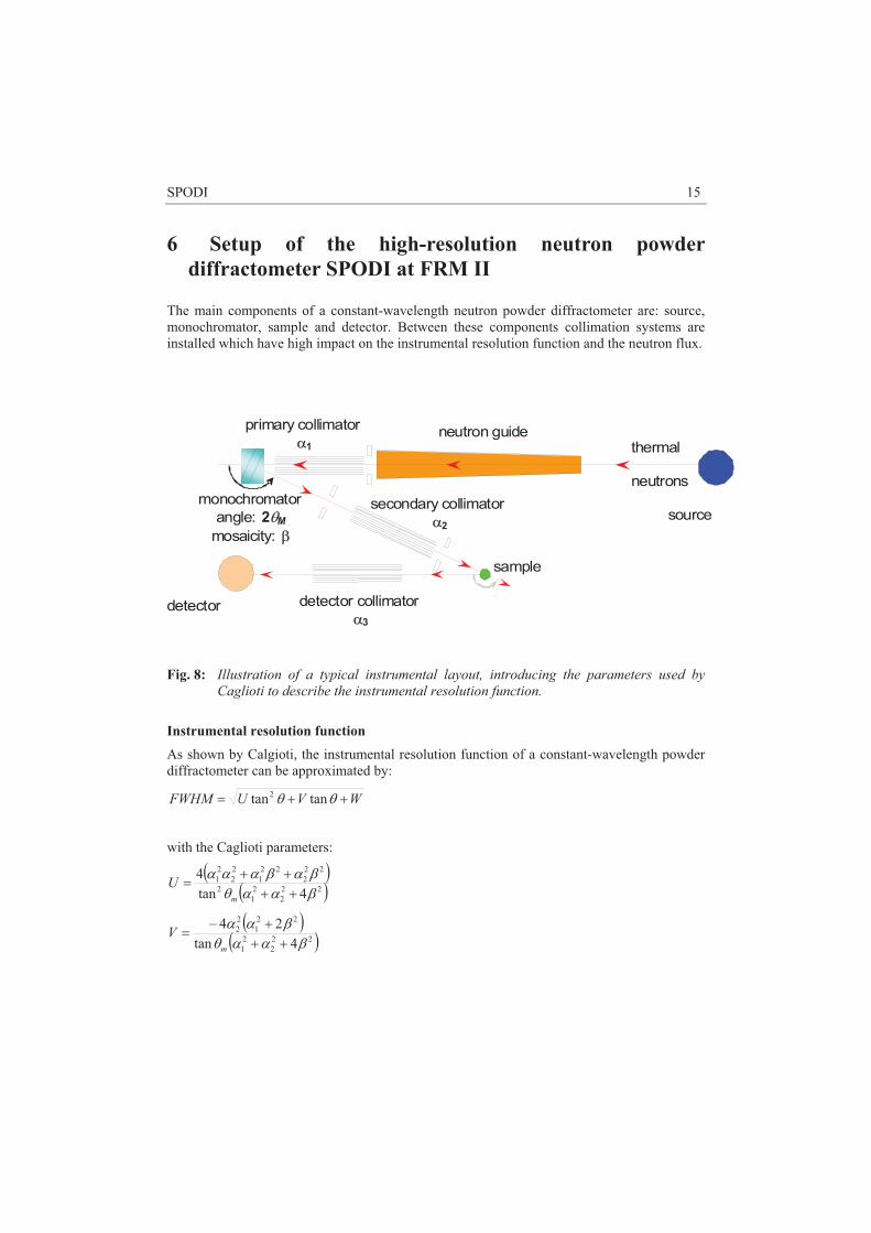
The main components of a constant-wavelength neutron powder diffractometer are: source, monochromator, sample and detector. Between these components collimation systems are installed which have high impact on the instrumental resolution function and the neutron flux.
thermal
neutrons
neutron guide
monochromator angle: 2�M
mosaicity: !
secondary collimator �2
sample
detector
primary collimator �1
detector collimator�3
source
Fig. 8: Illustration of a typical instrumental layout, introducing the parameters used by
Caglioti to describe the instrumental resolution function. Instrumental resolution function As shown by Calgioti, the instrumental resolution function of a constant-wavelength powder diffractometer can be approximated by:
WVUFWHM ��� �� tantan2
with the Caglioti parameters:
� �� �22
221
2
222
221
22
21
4tan4
!���!�!���
����
�m
U
� �� �22
221
221
22
4tan24
!���!����
���
m
V
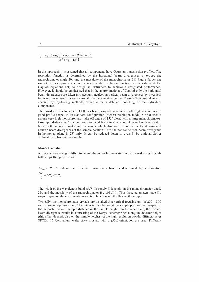
16 M. Hoelzel, A. Senyshyn
� �� �22
221
23
22
223
22
23
21
22
21
44!��
��!��������
�����W
in this approach it is assumed that all components have Gaussian transmission profiles. The resolution function is determined by the horizontal beam divergences �% #�� #�& the monochromator angle 2�m and the mosaicity of the monochromator !#�(Figure 8). As the impact of these parameters on the instrumental resolution function can be estimated, the Caglioti equations help to design an instrument to achieve a designated performance. However, it should be emphasised that in the approximations of Caglioti only the horizontal beam divergences are taken into account, neglecting vertical beam divergences by a vertical focusing monochromator or a vertical divergent neutron guide. Those effects are taken into account by ray-tracing methods, which allow a detailed modelling of the individual components.
The powder diffractometer SPODI has been designed to achieve both high resolution and good profile shape. In its standard configuration (highest resolution mode) SPODI uses a unique very high monochromator take-off angle of 155° along with a large monochromator-to-sample distance of 5 meters. An evacuated beam tube of about 4 m in length is located between the monochromator and the sample which also controls both vertical and horizontal neutron beam divergences at the sample position. Thus the natural neutron beam divergence in horizontal plane is 25’ only. It can be reduced down to even 5’ by optional Soller collimators in front of the sample.
Monochromator At constant-wavelength diffractometers, the monochromatisation is performed using crystals followings Bragg's equation:
�� �sin2 hkld , where the effective transmission band is determined by a derivative
MM ���� cot��
�
The width of the wavelength band ���� �strongly �depends on the monochromator angle 2�m and the mosaicity of the monochromator !#or#��m��. Thus these parameters have �a major impact on the instrumental resolution function and the flux on the sample.
Typically, the monochromator crystals are installed at a vertical focusing unit of 200 – 300 mm, allowing optimization of the intensity distribution at the sample position with respect to the monochromator – sample distance or the sample height. On the other hand, the vertical beam divergence results in a smearing of the Debye-Scherrer rings along the detector height (this effect depends also on the sample height). At the high-resolution powder diffractometer SPODI, 15 Germanium wafer-stack crystals with a (551)-orientation are used. Different
SPODI 17
wavelengths between 1.0 and 2.6 Å can easily be selected by rotation of the monochromator unit (without changing the monochromator take-off angle 2�m), i.e. by selecting different (hkl) reflection planes. In general, large wavelengths are advantageous to investigate structures exhibiting large d-values. This is the case for large unit cells, but in particular for magnetic ordering. With decreasing wavelengths, larger Q-values can be achieved. Thus, with lower wavelengths, more reflections can be observed in the same scattering angle range. Low wavelengths are in particular advantageous for the analysis of thermal displacement parameters or static disorder phenomena.
Detector array At constant-wavelength diffractometers the data are collected in an angle-dispersive manner at equidistant 2� points. Detector systems based on 3He have been most commonly used due to their very high efficiency. Now, the world wide shortage of 3He demands and promotes the development of alternatives, in particular scintillator based systems.
Classical high-resolution powder diffractometers, such as D2B (ILL), SPODI (FRM II), BT1 (NIST), ECHIDNA (ANSTO) use multidetector/multicollimator systems. The data are collected by 3He tubes while the beam divergence is limited by Soller collimators. Such systems enable high Q-resolution over a broad scattering angle regime, while the resolution does not depend on the sample diameter. On the other hand, a multidetector concept requires a data collection by stepwise positioning of the detector array to collect the full diffraction pattern. Therefore, kinetic measurements are not feasible due to the fact that the sample must not change during the collection of a pattern.
The detector array of SPODI consists of 80 3He tubes, which are position sensitive in the vertical direction. Thus, two-dimensional raw data are obtained, which allow to rapid check for sample crystallinity, alignment and possible preferred orientation effects. The conventional diffraction patterns (intensity vs. scattering angle 2�) are derived from the two-dimensional raw data by integration along the Debye-Scherrer rings.
7 Experiment: Phase- and structure analysis of lead titanate at various temperatures
samples Lead zirconate titanates PbZr1-xTixO3 („PZT“) exhibit piezo-, pyro- and ferroelectric properties. Piezoelectricity describes the generation of an electric polarisation as a consequence of a mechanical deformation – or the other way round the development of a macroscopic strain by an electric field. The crystallographic condition of piezoelectricity is the lack of an inversion center: as the balance points of negative and positive charge do not coincide the displacements of the ions in the electric field results in a polarization. Pyroelectricity refers to a spontaneous polarization of a material as a function of temperature.
18 M. Hoelzel, A. Senyshyn
Ferroelectrics are special pyroelectric materials, in which the polarization can be switched by an electric field, resulting in a ferroelectric hysteresis.
The electromechanical properties of PbZr1-xTixO3 can be understood by their phase transformation behaviour. At high temperatures they exhibit the perovskite structure with simple cubic symmetry (space group Pm-3m). Because of its symmetry (inversion center) this phase is not piezoelectric but paraelectric. During cooling, titanium-rich samples undergo a phase transition to a tetragonal phase (space group P4mm). This phase transformation is accompanied by atomic displacements. In particular, the Ti4+/Zr4+ are shifted in the opposite direction than O2- ions, resulting in a dipole moment or a spontaneous polarisation. The material exhibits ferroelectric behaviour, with a polar axis in the direction of the pseudocubic c-axis, i.e. [001]c . Zirconium rich samples undergo a phase transition towards a rhombohedral phase (space group R3m) during cooling. In this case, the atomic displacements result in a polar axis in direction [111]c with respect to the parent pseudocubic lattice. Materials PbZr1-xTixO3 with compositions (Zr/Ti ratios) close to the so called morphotropic phase boundary between rhombohedral and tetragonal phase, show the highest piezoelectric response, i.e. the largest macroscopic strain as a function of the applied electric field. These compositions are therefore most interesting for technological applications. The piezoelectric properties can be modified further by adding doping elements to substitute Pb2+ or Ti4+/Zr4+ ions.
Fig. 9: Structure models of the paraelectric cubic phase and the ferroelectric rhombohedral
and tetragonal phases.
Pm3m�
P4mmR3m
Pb2+
Zr4+/ Ti4+ O2-
SPODI 19
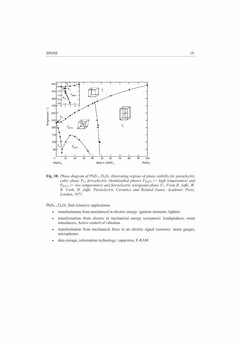
Fig. 10: Phase diagram of PbZr1-xTixO3, illustrating regions of phase stability for paraelectric
cubic phase PC, ferroelectric rhomboedral phases FR(HT) (= high temperature) and FR(LT) (= low temperature) and ferroelectric tetragonal phase FT. From B. Jaffe, W. R. Cook, H. Jaffe, Piezoelectric Ceramics and Related Issues, Academic Press, London, 1971.
PbZr1-xTixO3, find extensive applications
' transformation from mechanical in electric energy: ignition elements, lighters
' transformation from electric in mechanical energy (actuators): loudspeakers, sonar transducers, Active control of vibration
' transformation from mechanical force in an electric signal (sensors): strain gauges, microphones
' data storage, information technology: capacitors, F-RAM
20 M. Hoelzel, A. Senyshyn
Experiment In the frame of the practical course, the temperature-dependent phase transformation behavior of a PbZr1-xTixO3 with a composition on the tetragonal side should be investigated. Diffraction patterns at different temperature steps between room temperature and 600 °C will be collected with a vacuum high-temperature furnace. The structural changes at different temperatures will be investigated by an analysis of the lattice parameters. Based on the experimental data, the relations between the structural changes and the corresponding physical properties can be discussed.
Following experimental procedures will be carried out ' sample preparation, filling the sample material into a sample can, adjustment of the
sample stick, installation of the sample stick into the furnace
' short test measurement to check the sample adjustment and data quality
' editing a program to run the data collection at various temperatures and starting the scans
' data reduction: Derivation of diffraction patterns from the two-dimensional raw data
' data analysis: analysis of the lattice parameter changes as a function of temperature
' discussing the results with respect to structure – properties relationships
SPODI 21
References
[1] V. K. Pecharsky, P. Y. Zavalij, Fundamentals of Powder Diffraction and structural Characterisation of Materials (2003)
[2] G. L. Squires, Introduction to the Theory of Thermal Neutron Scattering, Dover Reprints (1978)
[3] C. Kittel, Einführung in die Festkörperphysik, 10. Edition, Oldenbourg (1993)
[4] H. Dachs, Neutron Diffraction, Springer Verlag (1978)
[5] H. Ibach und H. Lüth, Festkörperphysik, Einführung in die Grundlagen, 6. Edition, Springer Verlag (2002)
[6] J.R.D. Copley, The Fundamentals of Neutron Powder Diffraction (2001), http://www.nist.gov/public_affairs/practiceguides/SP960-2.pdf
[7] A. D. Krawitz, Introduction to Diffraction in Materials Science and Engineering
[8] W. Kleber, Einführung in die Kristallographie, Oldenbourg (1998)
[9] B. Jaffe, W. R. Cook, H. Jaffe, Piezoelectric Ceramics and Related Issues, Academic Press, London, 1971.
22 M. Hoelzel, A. Senyshyn
Contact
SPODI Phone: 089/289-14826 Web: http://www.frm2.tum.de/wissenschaftliche- nutzung/diffraktion/spodi/index.html Markus Hölzel Forschungsneutronenquelle Heinz Maier-Leibnitz (FRM II) Technische Universität München Phone: 089/289-14314 e-Mail: [email protected] Anatoliy Senyshyn Forschungsneutronenquelle Heinz Maier-Leibnitz (FRM II) Technische Universität München Phone: 089/289-14316 e-Mail: [email protected]
________________________
Manual of the JCNS Laboratory Course Neutron Scattering (Forschungszentrum Jülich, 2011, all rights reserved)
HEiDi
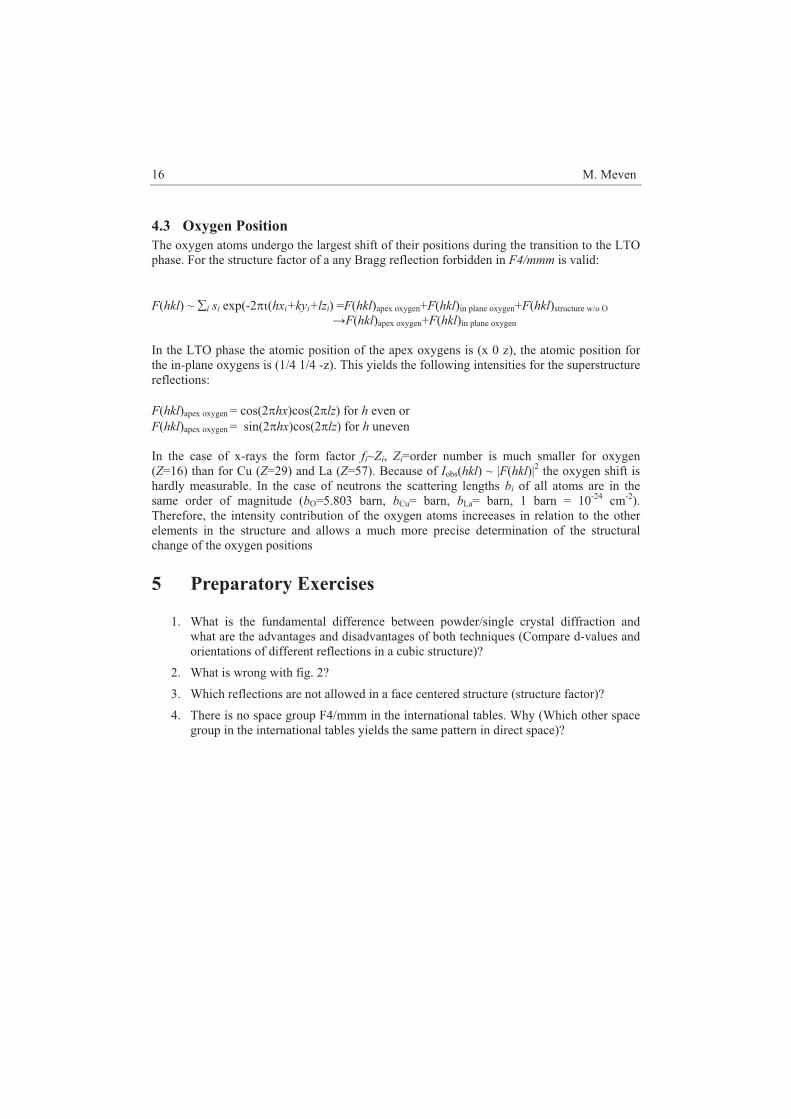
Hot Single Crystal Diffractometer for Structure Analysis with Neutrons
2 Crystallographic Basics ....................................................................3 3 Structure Determination with Diffraction..................................................5 3.1 Introduction ...............................................................................................5 3.2 Comparison of X-ray and Neutron Radiation............................................7 3.3 Special Effects ...........................................................................................8 3.4 Summary of Theory of Method ...............................................................10 3.5 From Measurement to Model ..................................................................10
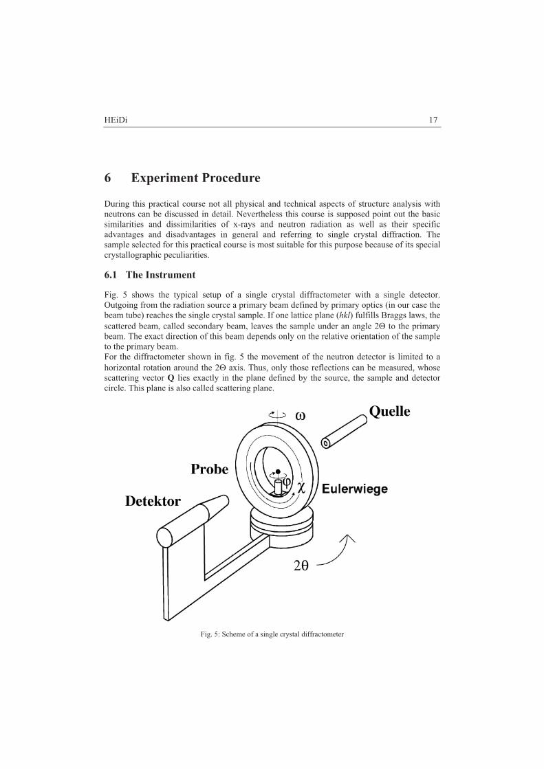
6 Experiment Procedure....................................................................17 6.1 The Instrument.........................................................................................17 6.2 Sequence of measurement in Theory.......................................................19 6.3 and in Practice .........................................................................................20 6.4 Data analysis............................................................................................21
Many properties of solid matter like their mechanical, thermal, optical, electrical and magnetic properties depend strongly on their atomic structure. Therefore, a good understanding of the physical properties needs not only the knowledge about the particles inside (atoms, ions, molecules) but also about their spatial arrangement. For most cases diffraction is the tool to answer questions about the atomic and/or magnetic structure of a system. Beyond this, neutron diffraction allows to answer questions where other techniques fail.
2 Crystallographic Basics
In the ideal case a complete solid matter consists of small identical units (same content, same size, same orientation like sugar pieces in a box). These units are called unit cells. A solid matter made of these cells is called a single crystal. The shape of a unit cell is equivalent to a parallelepiped that is defined by its base vectors a1, a2 und a3 and that can be described by its lattice constants a, b, c; �, * and + (pic. 1). Typical lengths of the edges of such cells are between a few and a few ten Ångström (1Å=10–10 m). The combination of various restrictions of the lattice constants between a � b � c; ��� *� � +�� 90° (triclinic) and a = b = c; ���*� = +� = 90° (cubic) yields seven crystal systems. The request to choose the system with the highest symmetry to describe the crystal structure yields fourteen Bravais lattices, seven primitive and seven centered lattices.
Fig. 1: Unit cell with |a1|=a, |a2|=b, |a3|=c, �)�*)�+
Each unit cell contains one or more particles i. The referring atomic positions xi=xi*a1 + yi*a2 + zi*a3 are described in relative coordinates 0 � xi; yi; zi < 1. The application of different symmetry operations (mirrors, rotations, glide mirrors, screw axes) on the atoms in one cell yield the 230 different space groups (see [1]). The description of a crystal using identical unit cells allows the representation as a threedimensional lattice network. Each lattice point can be described as the lattice vector t = u*a1 + v*a2 + w*a3; u, v, w 2 Z. From this picture we get the central word for diffraction in crystals; the lattice plane or diffraction plane. The orientations of these planes in the crystal are described by the so called Miller indices h, k and l with h, k, l 2 Z (see pic. 2). The reciprocal base vectors a*1, a*2, a*3 create the reciprocal space with: a*i * aj = 3ij with 3ij=1 for i=j and 3ij=0 for i�� j. Each point Q=h*a*1 + k*a*2 + l*a*3 represents the normal vector of
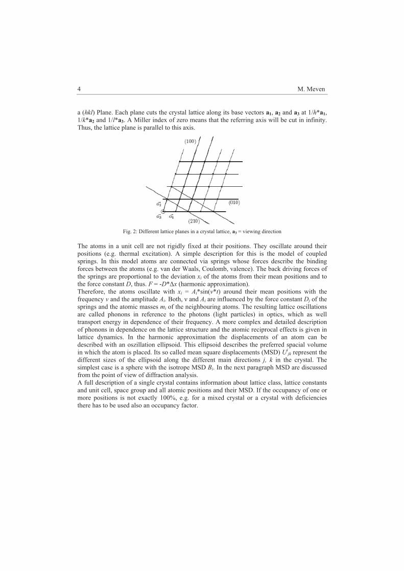
4 M. Meven
a (hkl) Plane. Each plane cuts the crystal lattice along its base vectors a1, a2 and a3 at 1/h*a1, 1/k*a2 and 1/l*a3. A Miller index of zero means that the referring axis will be cut in infinity. Thus, the lattice plane is parallel to this axis.
Fig. 2: Different lattice planes in a crystal lattice, a3 = viewing direction The atoms in a unit cell are not rigidly fixed at their positions. They oscillate around their positions (e.g. thermal excitation). A simple description for this is the model of coupled springs. In this model atoms are connected via springs whose forces describe the binding forces between the atoms (e.g. van der Waals, Coulomb, valence). The back driving forces of the springs are proportional to the deviation xi of the atoms from their mean positions and to the force constant D, thus. F = -D*�x (harmonic approximation). Therefore, the atoms oscillate with xi = Ai*sin(�*t) around their mean positions with the frequency � and the amplitude Ai. Both, � and Ai are influenced by the force constant Dj of the springs and the atomic masses mi of the neighbouring atoms. The resulting lattice oscillations are called phonons in reference to the photons (light particles) in optics, which as well transport energy in dependence of their frequency. A more complex and detailed description of phonons in dependence on the lattice structure and the atomic reciprocal effects is given in lattice dynamics. In the harmonic approximation the displacements of an atom can be described with an oszillation ellipsoid. This ellipsoid describes the preferred spacial volume in which the atom is placed. Its so called mean square displacements (MSD) Ui
jk represent the different sizes of the ellipsoid along the different main directions j, k in the crystal. The simplest case is a sphere with the isotrope MSD Bi. In the next paragraph MSD are discussed from the point of view of diffraction analysis. A full description of a single crystal contains information about lattice class, lattice constants and unit cell, space group and all atomic positions and their MSD. If the occupancy of one or more positions is not exactly 100%, e.g. for a mixed crystal or a crystal with deficiencies there has to be used also an occupancy factor.
HEiDi 5
3 Structure Determination with Diffraction 3.1 Introduction Diffraction means coherent elastic scattering of a wave on a crystal. Because of the quantum mechanical wave/particle dualism x-rays as well as neutron beams offer the requested wave properties: Electrons: E = h�; ��= c/� Neutrons: Ekin = 1/2 * mn*v2 = h� = p2/2mn; ��= h/p; p ~4(mn kB T) h: Planck’s constant; �: oscillation frequency; �: wavelength; c: light speed; p: impact; mn: neutron mass; kB: Boltzmann constant; T: temperature Only the cross section partners are different (x-rays: scattering on the electron shell of the atoms, neutrons: core (and magnetic) scattering) as explained in detail below. In scattering experiments informations about structural properties are hidden in the scattering intensities I. In the following pages we will discuss only elastic scattering (�in=�out). The cross section of the radiation with the crystal lattice can be described as following: Parallel waves of the incoming radiation with constant � are diffracted by lattice planes which are ordered parallel with a constant distance of d. This is very similar to a light beam reflected by a mirror. The angle of the diffracted beam is equal to the angle of the incoming beam, thus the total angle between incoming and outgoing beam is 25 (see fig. 3).
Fig. 3: Scattering on lattice planes
The overlap of all beams diffracted by a single lattice plane results in constructive interference only if the combination of the angle 5, lattice plane distance d and wavelength ��meet Braggs law:
2d sin5 = � The largest distance dhkl = |Q| of neighboured parallel lattice planes in a crystal is never larger than the largest lattice constant dhkl � max(a; b; c). Therefore, it can only be a few Å�or less. For a cubic unit cell (a = b = c; � = * = + = 90°) this means: dhkl = a/4 (h2+k2+l2) With increasing scattering angle also the indices (hkl) increase while the lattice plane distances shrink with a lower limit of dmin = �/2. Therefore, scattering experiments need wavelengths � in the same order of magnitude of the lattice constants or below. This is equal to x-ray energies of about 10 keV or neutron energies about 25 meV (thermal neutrons).
6 M. Meven
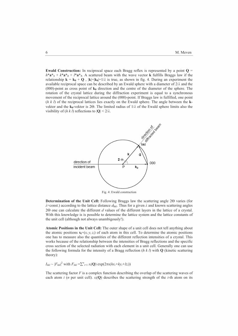
Ewald Construction: In reciprocal space each Bragg reflex is represented by a point Q = h*a*1 + k*a*2 + l*a*3. A scattered beam with the wave vector k fulfills Braggs law if the relationship k = k0 + Q , |k|=|k0|=1/� is true, as shown in fig. 4. During an experiment the available reciprocal space can be described by an Ewald sphere with a diameter of 2/� and the (000)-point as cross point of k0 direction and the centre of the diameter of the sphere. The rotation of the crystal lattice during the diffraction experiment is equal to a synchronous movement of the reciprocal lattice around the (000)-point. If Braggs law is fulfilled, one point (h k l) of the reciprocal lattices lies exactly on the Ewald sphere. The angle between the k-vektor and the k0-vektor is 25. The limited radius of 1/� of the Ewald sphere limits also the visibility of (h k l) reflections to |Q| < 2/�.
Fig. 4: Ewald construction Determination of the Unit Cell: Following Braggs law the scattering angle 25 varies (for �=const.) according to the lattice distance dhkl. Thus for a given � and known scattering angles 25 one can calculate the different d values of the different layers in the lattice of a crystal. With this knowledge is is possible to determine the lattice system and the lattice constants of the unit cell (although not always unambigously!). Atomic Positions in the Unit Cell: The outer shape of a unit cell does not tell anything about the atomic positions xi=(xi yi zi) of each atom in this cell. To determine the atomic positions one has to measure also the quantities of the different reflection intensities of a crystal. This works because of the relationship between the intensities of Bragg reflections and the specific cross section of the selected radiation with each element in a unit cell. Generally one can use the following formula for the intensity of a Bragg reflection (h k l) with Q (kinetic scattering theory): Ihkl ~ |Fhkl|2 with Fhkl =�n
i=1 si(Q) exp(2�6(hxi+kyi+lzi)) The scattering factor F is a complex function describing the overlap of the scattering waves of each atom i (n per unit cell). si(Q) describes the scattering strength of the i-th atom on its
Q
HEiDi 7
position xi in dependence of the scattering vector Q, which depends on the character of cross section as described below. In this context one remark concerning statistics: For measurements of radiation the statistical error is the square root of the number of measured events, e.g. x-ray or neutron particles. Thus, 100 events yield an error of 10% while 10,000 events yield an error of only 1%! Mean Square Displacements (MSD): Thermal movement of atoms around their average positions reduce the Bragg intensities during a diffraction experiment. The cause for this effect is the reduced probability density and therefore reduced cross section probability at the average positions. For higher temperatures (above a few Kelvin) the MSD Bi of the atoms increase linearly to the temperature T, this means B ~ T. Near a temperature of 0 K the MSD become constant with values larger than zero (zero point oscillation of the quantum mechanical harmonic oscillator). Thus, the true scattering capability si of the i-th atom in a structure has to be corrected by an angle-dependent factor (the so called Debye-Waller factor): si(Q) � si(Q) * exp(-Bi(sin 5Q/�)2) This Debye-Waller factor decreases with increasing temperatures and yields an attenuation of the Bragg reflection intensities. At the same time this factor becomes significantly smaller with larger sin5(�~|Q|. Therefore, especially reflections with large indices loose a lot of intensity. The formula for anisotropic oscillations around their average positions looks like this: si(Q) � si(Q) * exp(-2�2(Ui
11 h2a*2 + Ui22 k2b*2 + Ui
33 l2c*2 + + 2Ui
13 hl a*c* + 2Ui12 hk a*b* + 2Ui
23kl b*c*)) The transformation between B and Ueq (from the Uij calculated isotropic MSD for a sphere with identical volume) yields B = 8�2Ueq. For some structures the experimentally determined MSD are significantly larger than from the harmonic calculations of the thermal movement of the atoms expected. Such deviations can have different reasons: Static local deformations like point defects, mixed compounds, anharmonic oscillations or double well potentials where two energetically equal atomic positions are very near to each other and therefore distribute the same atom over the crystal with a 50%/50% chance to one or the other position. In all those cases an additional contribution to the pure Debye-Waller factor can be found which yields an increased MSD. Therefore in the following text only the term MSD will be used to avoid misunderstandings.
3.2 Comparison of X-ray and Neutron Radiation
X-Ray Radiation interacts as electromagnetic radiation only with the electron density in a crystal. This means the shell electrons of the atoms as well as the chemical binding. The scattering capability s (atomic form factor f(sin5(�)) of an atom depends on the number Z of its shell electrons (f(sin(5=0)/�) =Z). To be exact, f(sin(5)/�) is the Fourier transform of the radial electron density distribution ne(r): f(sin(5)/�)=s ��0 4�2ne(r) sin(μr)/μr dr with μ=4�sin(5)/�,�Heavy atoms with many electrons contribute much stronger to reflection intensities (I~Z2) than light atoms with less electrons. The reason for the sin5(�-dependence of f is the diameter of the electron shell, which has the same order of magnitude as the
8 M. Meven
wavelength �. Because of this there is no pointlike scattering centre. Thus, for large scattering angles the atomic form factors vanish and also the reflection intensities relying on them. The atomic form factors are derived from theoretical spherical electron density functions (e. g. Hartree-Fock). The resulting f(sin5(�)-curves of all elements (separated for free atoms and ions) are listed in the international tables. Their analytical approximation can be described by seven coefficients (c; ai; bi; 1� i � 3) , see [1]. Neutron Radiation radiation interacts with the cores and the magnetic moments of atoms. The analogon to the x-ray form factor (the scattering length b) is therefore not only dependent on the element but the isotope. At the same time b-values of elements neighboured in the periodic table can differ significantly. Nevertheless, the scattering lengths do not differ around several orders of magnitude like in the case of the atomic form factors f . Therefore, in a compound with light and heavy atoms the heavy atoms do not dominate necessarily the Bragg intensities. Furthermore the core potential with a diameter about 10-15Å is a pointlike scattering centre and thus the scattering lengths bn become independent of the Bragg angle and sin5(� respectively. This results in large intensities even at large scattering angles. The magnetic scattering lengths bm can generate magnetic Bragg intensities comparable in their order of magnitude to the intensities of core scattering. On the other hand side the magnetic scattering lengths are strongly dependent on the sin5(� value due to the large spacial distribution of magnetic fields in a crystal. Therefore, it is easy to measure magnetic structures with neutrons and to separate them from the atomic structure. Comparison: In summary in the same diffraction experiment the different character of x-ray and neutron radiation yield different pieces of information that can be combined. x-rays yield electron densities in a crystal while neutron scattering reveals the exact atomic positions. This fact is important because for polarised atoms the core position and the centre of gravity of electron densities are not identical any more. In compounds with light an heavy atoms structural changes driven by light elements need additional diffraction experiments with neutrons to reveal their influence and accurate atomic positions respectively. One has to take into account also that for x-rays intensitied depend twice on sin5(�. Once bye the atomic form factor f, and twice by the temperature dependent Debye-Waller factor (see above). The first dependence vanishes if using neutron diffraction with b=const. and decouples the structure factors from the influence of the MSD. In general this yields much more accurate MSD Uij especially for the light atoms and might be helpful to reveal double well potentials.
3.3 Special Effects
From the relation I~|F|2 one can derive that the scattering intensities of a homogenous illuminated sample increases with its volume. But there are other effects than MSD that can attenuate intensities. These effects can be absorption, extinction, polarization and the Lorentz factor: Absorption can be described by the Lambert-Beer law: I = I0 exp(-μx) , μ/cm-1 = linear absorption coefficient, x/cm = mean path through sample The linear absorption coefficient is an isotropic property of matter and depends on the wavelength and kind of radiation. For x-rays penetration depths are only a few millimetre or
HEiDi 9
below (e.g. for silicon with μMoK�=1.546 mm-1, μCuK�=14.84 mm-1 with penetration depths of 3 mm and 0.3 mm respectively). This limits transmission experiments to sample diameter of typically below 0.3 mm. To correct bias of intensities due to different scattering paths through the sample one has to measure accurately the sample size in all directions. Even for sphere liek samples the mean path lenghts depend on 257 In addition the sample environment must have an extraordinary small absorption Thermal neutrons have for most elements a penetration depth of several centimeters. Thus, sample diameters of several millimeters and large and complex sample environments (furnaces, magnets, etc.) can be used. On the other hand side one needs sufficiently large samples for neutron diffraction which is often a delicate problem. Extinction reduces also radiation intensities. But the character is completely different form that of absorption. In principle extinction can be explained quite easily by taking into account that each diffracted beam can be seen as a new primary beam for the neighbouring lattice planes. Therefore, the diffracted beam becomes partially backscattered towards the direction of the very first primary beam (Switch from kinetic to dynamic scattering theory!). Especially for very strong reflections this effect can reduce intensities dramatically (up to 50% and more). Condition for this effect is a merely perfect crystal. Theoretical models which include a quantitative description of the extinction effect were developed from Zachariasen (1962) and Becker and Coppens [2, 3, 4, 5, 6]. These models base on an ideal spherical mosaic crystal with a very perfect single crystal (primary Extinction) or different mosaic blocks with almost perfect alignment (secundary Extinction) to describe the strength of the extinction effect. In addition, it is possible to take into account anisotropic extinction effect if the crystal quality is also anisotropic. Nowadays extinction correction is included in most refinement programs [7]. In general extinction is a problem of sample quality and size and therefore more commonly a problem for neutron diffraction and not so often for x-ray diffraction with much smaller samples and larger absorption. Polarisation: X-ray radiation is electromagnetic radiation. Therefore, the primary beam of an x-ray tube is not polarized. The radiation hits the sample under an diffraction angle of 5 where it can be separated into two waves of same intensity, firstly with an electrical field vector parallel E|| and secondly perpendicular E� towards the 5-axis. Whilst the radiation with E|| will not be attenuated the radiation with E� undergoes an attenuation with E� � cos(25) E�. The polarization factor P for the attenuation has then the following formula (I ~ E2): P = (1+cos(25)2)/2 Additional optical components like monochromator crystals also have an impact on the polarization and have to be taken into account accordingly. Lorentz factor: The Lorentz factor L is a purely geometrical factor. It describes that during an �- and 5-scan respectively of Bragg reflections towards higher 25 values for the same angular speed ��/�t an effectively elongated stay of the sample in the reflection position results.: L = 1/sin(25)
10 M. Meven
This has to be taken into account for any kind of radiation in an diffraction experiment.
3.4 Summary of Theory of Method
The different interactions of x-ray and neutron radiation with the atoms in a crystal make neutrons in general the better choice for a diffraction experiment. But on the other hand one has to take into account the available flux of x-rays and neutrons respectively. The flux of modern neutron sources like the Heinz Maier-Leibnitz neutron source (FRM II) is spread around a broad spectrum of neutron energies. In a sharp band of energies/wavelengths, e.g. �/�<10-3, there is the flux of neutrons several order of magnitude smaller than the flux of x-rays of a corresponding synchtrotron source or x-ray tube in the laboratory. The reason for this is the fact that in an x-ray tube most x-rays are generated in a small energy band, the characteristic lines of the tube target (K�, K*, etc.). Additional metal foil used as filter allow to cut off unwanted characteristic lines which yields quasi monochromatic radiation of a single wavelength. To use neutrons around a small energy band one has to use monochromator crystals. This reduces significantly the number of available neutrons for the diffraction experiment. Thus, the weak flux of neutrons and the weak cross section of neutrons with matter has to be compensated with large sample sizes of several millimeters. For the same reason the monochromatization of the neutrons is normally chosen to be not too sharp (resolution about �/�10-2 for neutrons, �/�10-5 – 10-6 for synchrotron).
3.5 From Measurement to Model
To get a structural model from the experimentally collected integral Bragg intensities one needs several steps in advance. Firstly on has to make sure that all reflections are measured properly (no shading, no �/2-contamination, no Umweganregung (Renninger-effect) ). Damaged reflections have to be excluded from further treatment. During data refinement not only the quantities of the relative intensities but also their errors are taken into account. The total statistical error of an integral intensity Iobs of a single reflection is calculated as following: ' = Iobs + Ibackground + (k Itotal)2 The part 8
' = Itotal, Itotal = Iobs + Ibackground refers to the error caused by counting statistics. It contains as well the effective intensity Iobs as well as the contribution of the background. But there are other effects that influence the reproducibility of a measurement (and thus the total error), e.g. specific errors of the instrumental adjustment. Those errors are collected in the so called McCandlish-Factor k and contribute to the total error. Therefore, the total error cannot drop below the physically correct limit of the experiment and thus the impact of strong reflections does not become exaggerated in the refinement. The determination of k is done by measurent the same set of reflections several times during an experiment (the so called standard reflections). The mean variation of the averaged value represents k. In addition, the repeated measurement of standard reflections offers the opportunity to notice unwanted changes during experiment like structural changes or release from the sample holder.
HEiDi 11
To make sure the comparisability of all reflections with each other, all intensities and errors are normalized to the same time of measurement (or monitor count rate) and undergo the Lorentz and (in the x-ray case) polarization correction. Finally in advance of the data refinement there can be done an numerical (e.g. with DataP, [8]) or an empirical absoprtion if necessary. The quality of a measurement is checked in advance of the data refinement by comparing symmetry equivalent reflections and systematic extinctions to confirm the Laue group and space group symmetry. The result is written as internal R-value: Rint = (�k=1
m(�j=1n
k (<Ik>- Ij)2))/ (�k=1�j=1n
k(Ij2)k)
Rint represents the mean error of a single reflection j of a group k of nk symmetry equivalent reflections, corresponding to its group and the total number m of all symmetrically independent groups. Therefore Rint is also a good mark to check the absorption correction. After these preliminary steps one can start the final data refinement. At the beginning one has to develop a structural model. The problem with that is that we measure only the absolut values |Fhkl| and not the complete structure factor Fhkl = |Fhkl|exp(69) including its phase 9. Therefore, generally the direct fouriertransform of the reflection information Fhkl from reciprocal space into the density information 0 in the direct space (electron density for x-rays, probability density of atomic cores for neutrons) with 0(x) ~ �h�k�l Fhkl exp(-2�(hx+ky+lz)) not possible. This can be done only by direct methods like patterson, heavy atom method or anomal dispersion for x-rays. In the so called refinement program a given structural model (space group, lattice constants, atomic form factors, MSD, etc.) are compared with the experimental data and fitted. In a leas squares routine those programs try to optimize (typically over several cycles) the free parameters to reduce the difference between the calculated structure factors Fcalc and intensities |Fcalc|2 respectively and the experimentally found Fobs and |Fobs|2 respectively. To quantisize the quality of measurement there are several values in use: 1. unweighted R-value: Ru = �hkl |Fobs
2-Fcalc2|/�hkl Fobs
2 This value gives the alignment of the whole number of reflections without their specific errors. 2. weighted R-value: Rw = (�hkl w (Fobs
2-Fcalc2)2)/�hkl w Fobs
4 This value represents the alignment of the whole number of reflections including their specific errors or weights (w~1/ 2). Sometimes weights are adopted in a way to suppress unwanted influence of the refinement algorithm by weak or badly defined reflections. Be aware that such corrections have to be done extremely carefully because otherwise the refinement adopts the data to the selected structural model and not the model to the experimental data! 3. Goodness of Fit S: S2 =(�hkl w (Fobs
2-Fcalc2)/(nhkl-reflections - nfree parameter)
S should have a value near one if the weighting scheme and the structure model fit to the experimental data set.
12 M. Meven
4 Sample Section
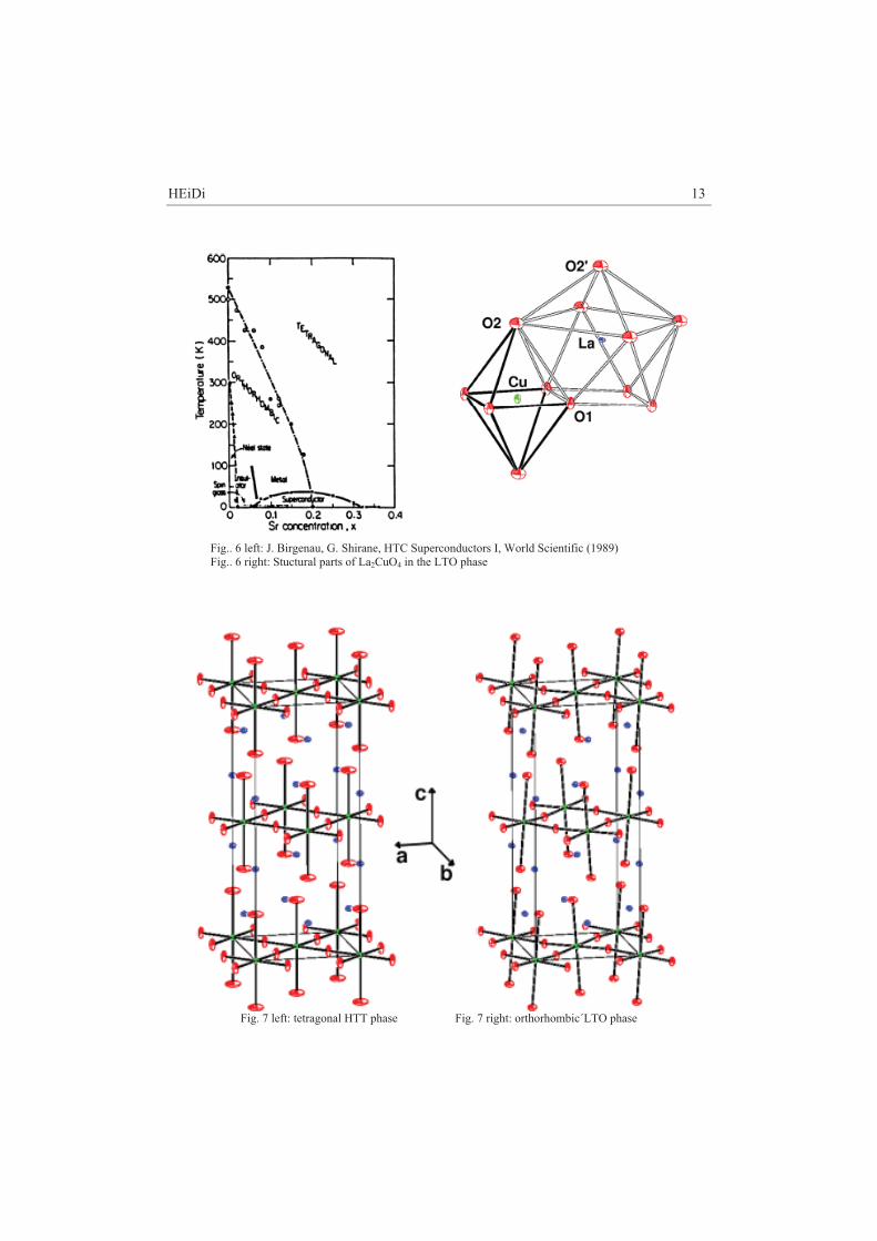
4.1 Introduction La2-xSrxCuO4 is one of the cuprate superconductors with K2NiF4- structure for whose discovery the noble prize was granted in 1988 (Bednorz and Müller [9]) . Pure La2CuO4 is an isolator. Doping with earth alcali metals (Ca2+, Sr2+, Ba2+) on the La3+ lattice positions generates in dependence of the degree of doping superconductivity. Sr doping of x=0.15 yields a maximum Tc of 38 K. Pure La2CuO4 undergoes at Tt-o=530 K a structural phase transition from the tetragonal high temperature phase (HTT) F4/mmm: a=b=5.384 Å, c=13.204 Å, �=*=+=90° at T=540 K to the orthorhombic low temperature phase (LTO) Abma: a=5.409 Å, b=5.357 Å, c=13.144 Å, �=*=+=90° at room temperature. The phase transition temperature Tt-o drops for La2-xSrxCuO4 with increased doping and disappears above x=0.2.
HEiDi 13
Fig.. 6 left: J. Birgenau, G. Shirane, HTC Superconductors I, World Scientific (1989) Fig.. 6 right: Stuctural parts of La2CuO4 in the LTO phase
4.2 Twinning During the transition into the low temperature phase the CuO6 octahedrons are tilted around their [010] axis. Thus, the two axes of identical length in the HTT phase, a1 and a2, are not equal in the LTO phase anymore. Instead, the longer one becomes the new a axis, the shorter one becomes the b axis. Whether a1 or a2 becomes the new a axis depends only on the real structure of the crystal, for instance grain boundaries or point defects. Therefore, one can find two equivalent crystallographic space groups in the LTO phase: Abma (a1 � a, a2 � b) and Bmab (a1 � b, a2 � a) For the structure factors in the LTO is valid: FAbma(hkl)=FBmab(khl)
Fig. 8 (a) orthorhombic distortion with twinning correspondint to a (1-10) mirroring (b) corresponding reciprocal lattice (c) Overlay of (110)- and (1-10)-mirroring in reciprocal space In the HTT phase only reflections with h, k, l of equal parity (g for even, u for uneven) are allowed - (uuu) and (ggg). They are called in the following main structrure reflections. In the LTO phase additional reflections occur, called super structure reflections: In the Abma-Structure (ugg), l�0 and (guu), in the Bmab structure (gug), l�0 and(ugu). Forbidden in both the HTT and the LTO phase are (uug), (ggu), (ug0) and (gu0). These extinction rules will become important later.
HEiDi 15
In the real structure of the crystal there exist four domain types in total. They are separated into two pairs with the couple Abma1/Bmab1 (I/II) with the (1-10) mirror plane as grain boundary and the couple Abma2/Bmab2 (III/IV) with the (110) mirror plane as grain boundary (fig. 8). The following overlaps of reflections result from this twinning: - No splitting of the (00l) reflections, - triple splitting of the (hh0) reflections - fourfold splitting of the (h00) reflections. An equal distribution of the volumetric portion of each single domain yields a ratio of intensities of 1:2:1 for the triple splitting. The distance � between the centre and the side peaks of a (hkl) reflex gives because of (a+b)/2 = a1/2 an information about the orthorhombic a/b splitting. For the triple splitting of a (hh0) reflex is valid: � = 90°-2arctan(b/a) Thus, although the real crystal is twinned, one can quantify the orthorhombic distortion. The intensity contribution of the single domains corresponding to the whole intensity of a reflection can be described (taking into account the incoherent overlap of single intensities and the volumetric portions VA1 to VB2 of the domains) as follows: Iobs(hkl) = IAbma1(hkl) + IBmab1(hkl) + IAbma2(hkl) + IBmab2(khl) or Vtotal|Fobs(hkl)|2=VA1|FAbma1(hkl)|2 +VB1|FBmab1(hkl)|2 + VA2|FAbma2(hkl)|2 +VB2|FBmab2(hkl)|2
with � being the relative portion of the volume of Abma domains to the crystal.. Because of the extinction rules in the LTO phase for the super structure reflections is valid: Iobs(hkl) ~ �|FAbma(hkl)|2 for Abma and Iobs(hkl) ~ (1-��|FAbma(khl)|2 for Bmab. Thus, one can classify directly intensities to the volumetric portions of the domain types Abma and Bmab respectively. Therefore, by using one single additional parameter � to describe the relation between the twins in the structure one can determine the orthorhombic single crystal structure! This holds true although the Bragg reflections contain contributions of up to four different domains.
16 M. Meven
4.3 Oxygen Position The oxygen atoms undergo the largest shift of their positions during the transition to the LTO phase. For the structure factor of a any Bragg reflection forbidden in F4/mmm is valid: F(hkl) ~ �i si exp(-2�6(hxi+kyi+lzi) =F(hkl)apex oxygen+F(hkl)in plane oxygen+F(hkl)structure w/o O �F(hkl)apex oxygen+F(hkl)in plane oxygen In the LTO phase the atomic position of the apex oxygens is (x 0 z), the atomic position for the in-plane oxygens is (1/4 1/4 -z). This yields the following intensities for the superstructure reflections: F(hkl)apex oxygen = cos(2�hx)cos(2�lz) for h even or F(hkl)apex oxygen = sin(2�hx)cos(2�lz) for h uneven In the case of x-rays the form factor fi~Zi, Zi=order number is much smaller for oxygen (Z=16) than for Cu (Z=29) and La (Z=57). Because of Iobs(hkl) ~ |F(hkl)|2 the oxygen shift is hardly measurable. In the case of neutrons the scattering lengths bi of all atoms are in the same order of magnitude (bO=5.803 barn, bCu= barn, bLa= barn, 1 barn = 10-24 cm-2). Therefore, the intensity contribution of the oxygen atoms increeases in relation to the other elements in the structure and allows a much more precise determination of the structural change of the oxygen positions
5 Preparatory Exercises
1. What is the fundamental difference between powder/single crystal diffraction and what are the advantages and disadvantages of both techniques (Compare d-values and orientations of different reflections in a cubic structure)?
2. What is wrong with fig. 2?
3. Which reflections are not allowed in a face centered structure (structure factor)?
4. There is no space group F4/mmm in the international tables. Why (Which other space group in the international tables yields the same pattern in direct space)?
HEiDi 17
6 Experiment Procedure
During this practical course not all physical and technical aspects of structure analysis with neutrons can be discussed in detail. Nevertheless this course is supposed point out the basic similarities and dissimilarities of x-rays and neutron radiation as well as their specific advantages and disadvantages in general and referring to single crystal diffraction. The sample selected for this practical course is most suitable for this purpose because of its special crystallographic peculiarities.
6.1 The Instrument
Fig. 5 shows the typical setup of a single crystal diffractometer with a single detector. Outgoing from the radiation source a primary beam defined by primary optics (in our case the beam tube) reaches the single crystal sample. If one lattice plane (hkl) fulfills Braggs laws, the scattered beam, called secondary beam, leaves the sample under an angle 25 to the primary beam. The exact direction of this beam depends only on the relative orientation of the sample to the primary beam. For the diffractometer shown in fig. 5 the movement of the neutron detector is limited to a horizontal rotation around the 25 axis. Thus, only those reflections can be measured, whose scattering vector Q lies exactly in the plane defined by the source, the sample and detector circle. This plane is also called scattering plane.
Fig. 5: Scheme of a single crystal diffractometer
18 M. Meven
To direct the secondary beam towards the detector position one has to orient the sample around the three axes �, : and 9. These three axes allow a virtually random orientation of the crystal in the primary beam. During the experiment the sample has to stay exactly in the cross point of all four axes (25, �)�: and 9) and the primary beam. Additionally, for 25 = ���: = 9 = 0° the primary beam direction and the : axis on one hand side and the 25-, �- and 9-axes on the other hand side are identical while the angle between the primary beam and the 25-is exactly 90°. Because of the four rotational axes (25, �)�:, 9) this kind of single crystal diffractometer is often called four circle diffractometer. Another often used geometry - the so called �-Geometrie - will not be discussed in detail here. Further details of the experimental setup: 1. Beam source and primary optics: The primary beam is generated by a suitable source (x-rays: x-ray tube, synchrotron; neutrons: nuclear fission, spallation source). The primary optics defines the path of the beam to the sample in the Eulerian cradle. Furthermore, the primary optics defines the beam diameter using slits to make it fit to the sample size for homogeneous illumination. This homogeneity is very important because the quality of the data refinement relies on the comparison of the intensity ratios between the different reflections measured during an experiment. Wrong ratios caused by inhomogeneous illumination can yield wrong structural details! Other components of the primary optics are collimators defining beam divergence and filters or monochromators which define the wavelength � of the radiation. 2. Sample and sample environment: The sample position is fixed by the centre of the Eulerian cradle which is defined by the cross point of the axes �)�: and 9. As described above, the cradle itself has in combination with the �-circle the task to orient the sample according to the observed reflection in a way that it hits the detector. The sample itself is mounted on a goniometer head. This head allows the adjustment of the sample in all three directions x; y; z, via microscope or camera. To avoid scattering from the sample environment and goniometer head the sample is usually connected to the head via a thin glass fibre (x-rays) or aluminum pin (neutrons). This reduces significantly background scattering. For experiments at high or low temperatures adjustable cooling or heating devices can be mounted into the Eulerian cradle. 3. Secondary optics and detector: The 25 arm of the instrument hold the detector which – in the ideal case – catches only radiation scattered from the sample and transforms it to an electrical signal. There exists a variety of detectors, single detectors and position sensitive 1D and 2D detectors. Area detectors have a large sensitive area that allows the accurate observation of spatial distribution of radiation. Other components of the secondary optics are slits and collimators or analyser (as optional units). They fulfil the task to shield the detector from unwanted radiation like scattering from sample environment, scattering in air, wrong wavelengths or flourescence
HEiDi 19
6.2 Sequence of measurement in Theory
1. Centering: In advance of the planned scientific program (profile analysis, Bragg data collection) the orientation of the sample in relation to the coordinate system of the diffractometer has to be determined. First of all the sample has to be centered optically to assure a homogeneous illumination of the sample. Afterwards, a reflection search routine has to be started to optimize the intensity of a found reflection by moving several angles after each other. In many cases there are some structural informations like the unit cell and hkl values of strong reflections available from previous studies, e.g. from powder diffraction, thus, one can limit the reflection search to 25 values around these strong reflections to spare some time and to classify manually the found reflections with the correct indices. 2. Determination of orienting matrix and lattice constants: The comparison of the Q vectors of the found and centered reflections yields generally one or more suggestions for a suitable unit cell. This is done by a least squares routine minimizing the error bars between the calculated and measured Q vectors. This method allows to determine accurately the orientation matrix Mo = (a* b* c*)T of the sample relative to the coordinate system of the diffractometer and the lattice constants of the unit cell. On HEiDi the axes are defined as following: x=primary beam, z || 25 axis, y=z x x. A proposed unit cell is only acceptable if all experimentally found reflections can be indexed with integer hkl , this means Q = (h k l)*Mo. In addition the found reflection intensities I offer a course check, e.g. whether extinction rules are followed or intensities of symmetrically identical reflections are identical. 3. Profile analyses and scan types: During profile analysis reflex profiles are analysed via so called � scans. During this scan the sample is turned for n steps around a center position �0. This scan makes different crystallites in one large sample visible. In addition one has to take into account that even in perfectly grown crystals there are grain boundaries and slight mismatches of the crystallites. These mosaic blocks are perfect crystals whose orientations are misaligned only a few tenths of a degree or less. By the way, the axis position 25(2=5� is called the bisecting orientation of the Eulerian cradle. As long as the vertical aperture is large enough, a rotation of the crystal around a �0, that is equivalent to the ideal 50 Bragg angle of a reflex allows to catch the intensity portion of each crystallite in the sample in the neutron detector on the fixed 25 position, even those that can only be found for slightly differing �. Therefore, a crystal with large mosaicity gives measurable intensities over a broader � area than a perfect crystal. Thus it gives a broader reflex profile. Also the tearing and cracking of a crystal creates broad but unregular profiles. Beside the crystal quality also the instrumental resolution limits the measurable profile widths in the following sense: The divergence of a primary beam in real experiment is limited, for instance to 0.2°. If a reflection fulfills Bragg’s Law at 5) the total divergence is a convolution of the divergence of the primary beam and the mosaicity/divergence of the sample. Thus, the reflection profile will never be sharper than the divergence of the primary beam itself. In addition one has to take into account that for larger diffraction angles a fixed detector window will not be sufficient to catch the whole reflection intensities during a rocking scan.
20 M. Meven
For a given spectrum �/� of the primary beam, with increasing scattering angle 5 angular range 5 increases with sin(5(2)=tan(5)*�/� for which all wavelengths in the interval �±�/' fulfilling Bragg’s law are distributed. Because of the limited width of the detector window this yields a cut off of intensities for larger scattering angles for �-scans. To compensate this cut off effect it is necessary to begin at a certain 25-angle to move the detector window with the �-angle.. This can be done by so called �/25-scans. The start position of this 25�range depends on the primary beam divergence and sample quality and has to be checked individually for each sample. 4. Collection of Bragg reflections: If a sample was found good after the described preliminary studies one can start with the Bragg data collection. In this data collection all (or selected) reflections in a given 25 intervall are collected automatically. The usual strategy follows the rule „Only as many as necessary“. This means the following: On one hand side the quality of the measured reflections has to fulfil certain standards (like small standard deviations and a good shape of the profiles) to reach an acceptable accuracy. On the other side there is only a limited amount of time available for each reflection due to the huge number of them (up to several thousands). and the limited beam time. A rule of thumb is therefore to measure about 10 non symmetry equivalent reflections for each free parameter used in the data refinement to get the correct structure. To achieve this goal a typical algorithm is to do a prescan with tmin per point of measurement in combination with a given larger (e.g. I/ =4 and 25%, respectively) and a smaller (e.g. I/ =20 and 5%, respectively) relative error limit. tmin is chosen in a way that the statistics of strong reflections is fine already after the prescan. Weak reflections are also noticed in the prescan and stored as weak reflections without additional treatment. Reflections in between get an additional chance to improve their statistics by performing a second scan with a limited amount of time up to tmax- tmin. This method avoids to spend unreasonable beam time to weak reflections which will not help to improve the quality of the structure model.
6.3 and in Practice
1. Adjust optically the sample in the neutron beam : Alignment of the sample in the rotational centre of the instrument. This is necessary for a homogeneous illumination of the sample for all possible orientations.
2. Search for Bragg reflections and center them, ‚ “Reflex centering”: Sample and detector position are controlled by a special diffractometer software. The main goal is to find suitable angular positions for the detector first and afterwards for the sample to get a measurable signal. Afterwards the orientation of the sample in the Eulerian cradle have to be optimized for maximum intensity.
3. Analyse profiles of selected reflections: Study different reflex profiles and reveal the impact of twinning
4. Determine the orthorhombic lattice parameters a, b and c: Estimate the misalignment of a and b in reference to a1/2 in the real tetragonal cell.
HEiDi 21
5. Determine the average tetragonal unit cell: The centering of different reflections allows the calculation of all lattice constants including the averaged tetragonal parameters.
6. Observe super structure reflections: Measuring pairs of (hkl)/(khl) allows the estimation of the volumetric contribution of each single domain to the whole crystal.
7. Select measurement parameters for Bragg data collection: In order to optimize the number and statistical quality of collected Bragg reflections suitable scan parameters (time/step, no. of steps, stepwidths, etc.) have to be determined.
8. Collect a Bragg data set
6.4 Data analysis
After having measured a Bragg data set one has to do the final step, the alignment of model and measurement: 1. Data Reduction: In this process the measured reflection profiles are analysed and
reduced to a simple list of all measured reflections and their integrated intensities including error bars and some other useful information. This so-called hkl-list is the base for the next step:
2. Structure refinement: Here the measured hkl-list and our structure model are combined to determine structural details like atomic positions and mean square displacements.
7 Experiment-Related Exercises
1. Why is the optical adjustment of the sample so important?
2. How large is the a/b-splitting at room temperature (=|a-b|/(a+b))?
3. What is the benefit/enhancement of studying the room temperature structure with neutrons instead of X-rays?
22 M. Meven
References
[1] Th. Hahn (ed.), Space-group symmetry, International Tables for Crystallography Vol. A, Kluver Academic Publishers (2006).
[2] W.H. Zachariasen, Acta Cryst. 18 703 (1965).
[3] W.H. Zachariasen, Acta Cryst. 18 705 (1965).
[4] P. Coppens and W.C. Hamilton, Acta Cryst. A 26 71-83 (1970).
[5] P.J. Becker and P. Coppens, Acta Cryst. A 30 129-147 (1974).
[6] P.J. Becker and P. Coppens, Acta Cryst. A 30 148-153 (1974).
[7] U.H. Zucker, E. Perrenthaler, W.F. Kuhs, R. Bachmann and H. Schulz J. of Appl. Crystallogr., 16 358 (1983).
[8] P. Coppens, W.C. Hamilton, S. Wilkins, M.S. Lehmann and Savariault, Datap, http://www.ill.fr/data treat/diftreat.html#single (1999).
[9] J. Bednorz and K. Müller, Z. Phys. B 64 189 (1986).
Literature N.W. Ashcroft and N.D. Mermin, Festkörperphysik, Oldenbourg 2001.
H. Ibach and H. Lüth, Festkörperphysik, Einführung in die Grundlagen, 6. Edition Springer 2002.
C. Kittel, Einführung in die Festkörperphysik, 10. Edition, Oldenbourg 1993.
W. Borchardt-Ott, Kristallographie. Eine Einführung für Naturwissenschaftler, 6. Auflage Springer 2002.
W. Kleber, Einführung in die Kristallographie, Oldenbourg 1998
H. Dachs, Neutron Diffraction, Springer (1978)
D.J. Dyson, X-Ray and Electron Diffraction Studies in Material Science, Maney Pub 2004.
C. Giacovazzo, Fundamentals of Crystallography, 2nd Ed., Oxford University Press 2002.
L.A. Aslanov, Crystallographic Instrumentation, Oxford University Press 1998.
M.T. Dove, Structure and Dynamics. An Atomic View of Materials, Oxford University Press 2003. W. Clegg, Crystal Structure Analysis. Principles and Practice, Oxford University Press 2001.
Neutron backscattering spectrometers are used to measure inelastic scattering with very highenergy resolution. What does this mean?
In inelastic scattering, scattering intensity is measured as function of the energy exchangedbetween the scattered neutron and the sample. As in other areas of physics, a data set of the formintensity-versus-energy is called a spectrum. An instrument that resolves inelastic scattering istherefore called a spectrometer.
While elastic scattering experiments yield information about structure or texture of a sample,inelastic scattering is used to investigate its dynamics. Specifically, inelastic neutron scatteringyields information about the thermal motion of atomic nuclei.
The most common instrument for inelastic neutron scattering is the triple-axis spectrometer. Itis routinely used to measure phonon and magnon dispersions, with energy exchanges of theorder of meV. In contrast, the high resolution of a backscattering spectrometer allows to resolvevery small energy shifts of the order of μeV. By the time-energy uncertainty relation, smallenergy means long times. Hence, backscattering addresses relatively slow nuclear motion —much slower than the lattice vibrations typically seen in triple-axis spectrometry.
What processes take place on the energy or time scale made accessible by neutron backscatter-ing? For instance the following:
• hyperfine splitting of nuclear spin orientations in a magnetic field,• rotations or hindered reorientations of molecules or molecular side groups,• quantum tunneling,• hydrogen diffusion in solids,• relaxation (molecular rearrangements) in viscous liquids,• innermolecular rearrangements in polymers.
During your lab course day, you will use the backscattering spectrometer SPHERES (SPec-trometer for High Energy RESolution) to study one example of these applications.
2 Spectrometer Physics
2.1 Energy Selection by Backscattering
In crystal spectrometers, neutron energies are selected by Bragg reflection from crystals, ac-cording to the Bragg condition
nλn = 2dhkl sinΘ (1)
where dhkl is the distance of lattice planes [hkl], and Θ is the glancing angle of reflectionfrom these planes. The index n indicates that along with a fundamental wavelength λ1, integerfractions λn = λ1/n are transmitted as well. To suppress these unwanted higher orders, ex-perimental setups include either a mechanical neutron velocity selector (Fig. 1), or a berylliumfilter.
In practice, the parameters d and Θ on the right-hand side of Eq. (1) are not sharp: Imperfec-tions of the crystal lead to a distribution of lattice constants, characterized by a width δd. Andsimilarly, imperfections of the neutron optics (inevitable because the incoming beam, the sam-ple, and the detector all have finite size) lead to a distribution of reflection angles, characterizedby a width δΘ. By differentiating the Bragg equation (1), one obtains the relative width of thewavelength distribution reflected by a crystal monochromator:
δλ
λ=
δd
d+ cotΘ δΘ. (2)
In usual crystal spectrometers, the second term is the dominant one. However, by choosingΘ = 90◦, the prefactor cotΘ can be sent to zero. This is the fundamental idea of the backscatter-ing spectrometer. If a monochromator crystal is used in backscattering geometry, with Θ � 90◦,then the reflected wavelength distribution is in first order insensitive to the geometric imperfec-tion δΘ; it depends only on the crystal imperfection δd and on a second-order (δΘ)2 term.
The monochromator of SPHERES is made of silicon crystals in (111) orientation (Fig. 2).The backscattered wavelength is λ = 2d111 = 6.27 A, corresponding to a neutron energy of2.08 meV. The crystals are cut from wafers produced by the semiconductor industry. Theyare perfectly monocrystalline, so that their intrinsic resolution1 of δd/d � 10−6 is actuallytoo good because it does not match the spectrometer’s second-order geometric imperfection(δΘ)2 � 10−4. As a remedy, the crystals are glued to a spherical support so that the resultingstrain induces a lattice constant gradient of the order δd/d � 10−4.
1 In perfect crystals, the intrinsic resolution δd/d is limited by primary extinction: Say, each crystalline layer hasa reflectivity of about 10−6. Then only about 106 layers contribute to the Bragg reflection. This limits δλ/λ toabout 10−6.
SPHERES 5
Fig. 2: The monochromator of SPHERES consists of hexagonal Si(111) wafers of 750 μmthickness, glued onto a spherical support made of carbon fiber.
Fig. 3: The analyzers of SPHERES are made of the same Si(111) as the monochromator. Forsmall scattering angles, they are shaped as rings; for large scattering angles, they are approxi-mately rectangular sections of a sphere.
2.2 Spectrometer Layout
In a crystal spectrometer, a monochromator is used to send a neutron beam with a narrowenergy distribution Ei±δE onto the sample. After the sample, a second monochromator, calledanalyzer, is used to select a narrow energy distributionEf±δE out of the scattered spectrum. InSPHERES, we actually have a huge array of analyzers (Fig. 3), covering a solid angle of about2.5, which is 20% of 4π. These analyzers send energy-selected neutrons towards 16 differentdetectors, depending on the scattering angle ϑ.
Fig. 4 shows the complete layout of SPHERES. The incoming beam is pre-monochromatizedby a mechanical velocity selector. Then, it is transported by a focussing neutron guide into theinstrument housing where it hits a rotating chopper. The chopper rotor (Fig. 5) carries mosaiccrystals made of pyrolitic graphite on half of its circumference. When the incoming neutrons hit
6 J. Wuttke
NL6a
shutter
velocity selector
focussing guide
choppervacuum chamber
detectors
beamstop
sample
monochromator
Doppler driveanalysers
door
Fig. 4: Layout of the Julich backscattering spectrometer SPHERES at FRM II.
Fig. 5: Schematic front view of the chopper rotor of SPHERES. The red bands indicate themosaic crystals that deflect the incident beam towards the monochromator.
these crystals, they undergo a Bragg reflection towards the monochromator.2 Otherwise, theyare transmitted towards a beamstop.
The backscattering monochromator selects a neutron band Ei ± δE as described above. Neu-trons within this band are sent back towards the chopper. When they reach the chopper, therotor has turned by 60◦: the mosic crystals have moved out of the way; the neutrons comingfrom the monochromator are transmitted towards the sample.
The sample scatters neutrons into 4π. About 20% of this is covered by analyzers. If a scatteredneutron hits an analyzer and fullfills the backscattering Bragg condition, it is sent back towardsthe sample. It traverses the sample3 and reaches a detector. To discriminate energy-selectedneutrons from neutrons that are directly scattered from the sample into a detector, the time ofarrival is put in relation to the chopper phase.
2 As a side effect, the Bragg deflection by rotating mosaic crystals achieves a favorable phase-space transform(PST): the incoming wavevector distribution is spread in angle, but compressed in modulus. This results in ahigher spectral flux in the acceptance range of the monochromator.3 Of course not all neutrons are transmitted: some are lost, some are scattered into a wrong detector. This inac-curacy is inevitable in neutron backscattering. We strive to keep it small by using rather thin samples with typicaltransmissions of 90% to 95%.
SPHERES 7
While the primary spectrometer (everything before the sample) is mainly in vacuum, the sec-ondary spectrometer is not. To minimize neutron losses in the secondary spectrometer, theentire instrument housing can be flooded with argon. For the labcourse, we preferentially re-move the argon so that participants can accede the housing. However, since refilling takes atleast one full day, time constraints may prevent us from doing so. In this case, a video will beshown to present the interior of the spectrometer.
2.3 Measuring Spectra
So far we have introduced a static arrangement with fixed energies Ei = Ef . Such an arrange-ment is actually used to measure the fraction of elastic versus total scattering, called the Debye-Waller factor for coherent scattering and the Lamb-Mossbauer factor for incoherent scattering.More often, however, one wants to measure full spectra S(Q, ω). Therefore, one must find away to modify the energy transfer
�ω = Ei −Ef . (3)
This can be done using the Doppler effect: The monochromator is mounted on a linear drivethat performs a cyclic motion. In the monochromator’s rest frame, the backscattered energy isalways the value E0 = 2.08 meV given by the lattice constant of Si(111). Depending on themonochromator’s velocity v, the value in the laboratory frame is
Ei(v) =mn
2(v0 + v)2 (4)
where v0 = 631 m/s is the neutron velocity at E0 = mn/2 v20. The Doppler drive of SPHERES
has a linear amplitude of ±75 mm and achieves a velocity amplitude of ±4.7 m/s, resulting inan energy range
−30.7 μeV < �ω < 30.9 μeV. (5)
This is called the dynamic range of the spectrometer.
When a scattered neutron is detected, its time of flight is traced back to the moment when ithas been backscattered by the monochromator. From the recorded trace of the linear drive, themonochromator velocity at that moment is infered, ω is computed from (4) and (3), and the cor-responding histogram channel is incremented. To determine S(Q, ω), one needs to normalize tothe time spent in channel ω. This normalization is routinely done by the instrument’s raw-datareduction program SLAW.
2.4 Instrument Characteristics
The performance of a spectrometer can be characterized by its resolution function. To obtainthe resolution function, one measures the spectrum of a purely elastic scatterer. Fig. 6 shows theresult of a resolution measurement from a user experiment on SPHERES. Note the logarithmicintensity scale.
Conventionally, the resolution of an instrument is characterized by the full width at half max-imum (FWHM). For SPHERES, a typical value is 0.65 μeV. Note however that the FWHM is
8 J. Wuttke
-20 0 20hω (μeV)
0.001
0.01
0.1
1S
(q,ω
) (μ
eV-1
)FWHM = 0.66 μeV
SNR > 1700:1
|E|max = 31μeV
SPHERESSeptember 2010
Fig. 6: Resolution function of SPHERES, measured on a user provided sample at a low temper-ature where the scattering is purely elastic.
not the full story: the quality of an instrument also depends on the shape of the resolution func-tions, especially of the deep wings. The resolution of SPHERES is slightly asymmetric. This isrelated to the (δΘ)2 term in the wavelength spread of a backscattering analyzer: all deviationsfrom the perfect Θ = 90◦ geometry lead to the transmission of longer wavelengths, never ofshorter ones.
Another important figure of merit is the signal-to-noise ratio (SNR). It depends strongly on theratio of scattering to absorption cross sections and on the thickness and geometry of the sample.With argon filling, the best value obtained in user experiments has been 1700:1; without argon,1200:1. On the other hand, for strongly absorbing samples it is sometimes less than 100:1.
3 Applications
In the following, two different applications of neutron backscattering are explained: hyperfinesplitting in a magnetic material, and methyl group tunneling.
3.1 Hyperfine Splitting
The measurement of hyperfine splitting has been historically the first application of neutronbackscattering,4 and to this day, it is the conceptually simplest one.
Since the neutron has spin S = 1/2, its magnetic quantum number can take the values Sz =±1/2. In a scattering event, this quantum number can change. In more pictorial words: when a
4 A. Heidemann, Z. Phys. 238, 208 (1970).
SPHERES 9
neutron is scattered, it may or may not undergo a spin flip.
As angular momentum is conserved, a change of Sz must be accompanied by an oppositechange of the magnetic quantum number Iz of the nucleus by which the neutron is scattered,ΔIz = −ΔSz . Therefore, spin-flip scattering is only possible if the sample contains nuclei withnonzero spin I .
Nuclei with nonzero spin quantum number I possess a magnetic moment
μ = IgμN (6)
with the nuclear magneton
μN =e�
2mp
= 3.153 · 10−8 eV/T. (7)
The g factor is different for each nucleus.5
A local magnetic field B leads to a splitting of energy levels,
E = IzgμNB, (8)
called hyperfine splitting. Consequently spin-flip scattering is accompanied by an energy ex-change ΔE = ±gμNB. By measuring the neutron energy gain or loss ±ΔE, one can accuratelydetermine the local field B in ferromagnetic or antiferromagnetic materials.
3.2 Molecular Rotation and Quantum Tunneling
Rotational motion of molecules or molecular side groups is one of the most important applica-tions of neutron backscattering. Here, we specialize on the rotation of methyl (CH3) groups.We consider these groups as stiff, with fixed6 CH bond length 1.097 A and HCH angle 106.5.◦
The only degree of freedom is then a rotation around the RC bond that connects the methylgroup to the remainder R of the molecule. This RC bond coincides with the symmetry axis ofthe CH3 group. The rotational motion can therefore be described by a wave function ψ thatdepends on one single coordinate, the rotation angle φ.
The Schrdinger equation is {B
∂2
∂φ2− V (φ) + E
}ψ(φ) = 0. (9)
For free rotation (V = 0), solutions that possess the requested periodicity are sine and cosinefunctions of argument Jφ, with integer J . Accordingly, the energy levels are E = BJ2.
Given the value B = 670 μeV, it is obvious that free rotor excitations occur only far outsidethe dynamic range of neutron backscattering. Conversely, if we observe an inelastic signalfrom methyl groups on a backscattering spectrometer, then we must conclude that V �= 0: the
5 Tabulation: http://ie.lbl.gov/toipdf/mometbl.pdf.6 Ignoring the variations of empirical values, which are of the order of ±0.004 A and ±1.5◦.
10 J. Wuttke
methyl group rotation is hindered by a rotational potential. This potential can be caused by theremainder R of the molecule as well as by neighbouring molecules.
Due to the symmetry of the CH3 group, the Fourier expansion of V (φ) contains only sine andcosine functions with argument 3mφ, with integer m. In most applications, it is sufficient toretain only one term,
V (φ).= V3 cos(3φ). (10)
The strength of the potential can then be expressed by the dimensionless number V3/B. In thefollowing we specialize to the case of a strong potential, V3/B � 10, which is by far the mostfrequent one.
In a strong potential of form (10), the CH3 group has three preferential orientations, separatedby potential walls. The motion of the CH3 group consists mainly of small excursions from thepreferred orientations, called librations. Essentially, they are harmonic vibrations.
At low temperatures, almost exclusively the vibrational ground state is occupied. Yet reorien-tational motion beyond librations is possible by means of quantum mechanical tunneling: thewave functions of the three localised pocket states ψm (m = 1, 2, 3) have nonzero overlap.Therefore, the ground state is a linear combination of pocket states.7 Periodicity and threefoldsymmetry allow three such combinations: a plain additive one
ψ1 + ψ2 + ψ3, (11)
and two superpositions with phase rotations
ψ1 + e±i2π/3ψ2 + e±i4π/3ψ3. (12)
In the language of group theory, state (11) has symmetry A, the degenerate states (12) arelabelled Ea, Eb. It is found that A is the ground state. The tunneling splitting �ωt betweenthe states A and E is determined by the overlap integral 〈ψm|V |ψn〉 (m �= n). It dependsexponentially on the height of the potential wall. Provided it falls into the dynamic range ofneutron scattering, it leads to a pair of inelastic lines at at ±�ωt.
With rising temperatures, the occupancy of excited vibrational levels increase. This facilitatestransitions between A and E sublevels and results in a decrease of �ωt and a broadening of theinelastic lines.
Upon further temperature increase, thermal motion of neighbouring molecules causes so strongpotential fluctuations that the picture of quantum tunneling is no longer applicable. Instead, themotion between different pocket states can be described as stochastic jump diffusion.
Let pm(t) be the probability of being in pocket state m (m = 1, 2, 3). Assume that jumpsbetween the three main orientations occur with a constant rate τ−1. Then, the pm obye rateequations
d
dtpm(t) =
1
τ
{−pm +
∑n �=m
1
2pn
}. (13)
7 This is an extremely simplified outline of the theory. In a serious treatment, to get all symmetry requirementsright, one must also take into account the nuclear spins of the H atoms. See W. Press, Single-Particle Rotations inMolecular Crystals, Springer: Berlin 1981.
SPHERES 11
The stationary equilibrium solution is just pm = 1/3 for all m. When perturbed, the systemrelaxes into equilibrium with a time dependence of exp(−t/τ ). Explicit solution of the lineardifferential equation system (13) yields τ = 2τ/3.
According to a fundamental theorem of statistical mechanics (the fluctation dissipation theo-rem), the relaxation by which a slightly perturbed system returns into equilibrium has the sametime dependence as the pair correlation function in equilibrium. Therefore, we can employ thesolution of (13) to write down the self-correlation function of the protons that constitute ourmethyl group. Fourier transform yields then the incoherent scattering function
S(q, ω) = a(q)δ(ω) + b(q)Γ
ω2 + Γ2. (14)
The first term describes elastic scattering. The second term, the Fourier transform of the expo-nential exp(−t/τ ), is a Lorentzian with linewidth Γ = τ−1; such broadening of the elastic lineis often called quasielastic.
4 Preparatory Exercises
1. Relate the relative wavelength spread δλ/λ to the relative energy spread δE/E.
2. In SPHERES, useable detectors are located at scattering angles 2θ ranging from 12.5◦
to 134◦. Calculate the corresponding wavenumbers in A−1. Recommendation: use thefollowing constants in atomic units: �c = 1973 eVA and mnc
2 = 940 MeV.
3. Convert dynamic range and resolution of SPHERES into GHz. To make contact withoptical spectroscopy, you might also wish to convert into cm−1.
4. Empirically, it is found that the centre of the resolution function can be fitted by a Gaus-sian a exp(−E2/2/σ2). Derive an expression that relates the Gaussian standard deviationσ to the FWHM.
5. Note that the above mentioned fit applies only to the very centre of the resolution function.How does a Gaussian look like on the lin-log representation of Fig. 6? And a Lorentzian?
6. In SPHERES, the distance sample-analyzer is 2 m. Calculate the time neutrons need fora round trip sample-analyzer-sample, and deduce the rotation frequency of the chopper.
7. Assume that the monochromator motion is perfectly sinusoidal. Sketch how the measur-ing time per energy channel varies with �ω.
8. Draw a sketch of the expected backscattering spectrum S(q, ω) of a ferromagnetic mate-rial with I �= 0.
9. Assume a hyperfine splitting of ΔE = 2 μeV. To which temperature do you have tocool the sample to observe a 10% difference between the probabilities of energy gain andenergy loss scattering?
10. How do you expect ΔE to evolve when the sample is heated towards the Curie or Neeltemperature?
12 J. Wuttke
11. Calculate the moment of inertia, I =∑
mr2⊥, of a methyl group. Verify that the rota-tional constant B = �
2/(2I) has a value of about 670 μeV.
12. Expand V (φ) around a potential minimum, and compare the resulting Schrodinger equa-tion with that of a harmonic oscillator. Show that the splitting of oscillator levels is of theorder of meV.
13. Draw a coordinate system energy-versus-angle. Sketch V (φ), the harmonic approxima-tion, the ground state’s ψ(φ), and the lowest oscillator energy levels. What does thatimply for the validity of the oscillator approximation?
14. Sketch the expected spectra for different temperatures.
5 Experiment Procedure
5.1 The experiment itself
After an initial discussion, the group chooses which experiment to perform: hyperfine splitting,methyl group tunneling, or participation in an ongoing research project. For a given chemicalcomposition, the group computes the sample thickness that yields 90% transmission. Depend-ing on the group’s interest, a sample is prepared, or a standard sample is used. The tutor showshow to insert the sample in the instrument’s cryostat. Using the instrument’s graphical userinterface, starting a measurement is rather trivial. Log entries are written to the instrument logwiki.
5.2 Raw data reduction
The program SLAW is used to convert raw neutron counts into S(Q, ω). It is parametrized bya script, called Slawfile. The tutor provides a sample script, which is then modified toconvert the results of the current experiment.
SLAW can save S(Q, ω) in a variety of output formats. Most relevant are plain tabular formatsrecttab and spectab, and a self-documenting format y08 required by our standard data-analysis software FRIDA.
5.3 Data evaluation
In a first approach, labcourse participants should analyse plain tabular data using whatever all-purpose data-analysis software they are used to.
1. Plot a representative selection (choose a few Q) of measured spectra.
2. Determine the FWHM of the elastic line, and of the inelastic lines if there are any.
3. Try to fit these lines with a Gaussian, with a Lorentzian, with a squared Lorentzian.
SPHERES 13
4. Summarize the temperature dependence of the spectra.
For a more quantitative analysis, it is necessary to convolute a theoretical model with a measuredresolution function. This can be done with the data-analysis package FRIDA. For a tutorial, referto the SPHERES wiki.8
8 Follow the link at http://www.jcns.info/jcns_spheres.
Polarized neutron scattering and polarization analysis represents a powerful technique for the studies of complex ordering phenomena and dynamics of condensed matters. The elements of this technique and its advanced applications in particular in magnetism have been comprehensively covered in a number of recent lecture notes [1-4] and several seminal papers [5-7]. The aim of this exercise on Neutron Polarization Analysis is to provide you with some hands-on experience on the practical aspects of polarized neutron scattering based on the multi-detector time-of-flight spectrometer DNS at FRM II. The details on the handling of polarized neutrons and the fundamentals of polarization analysis will be demonstrated from a range of carefully designed experiments and exercises.
In Section 2 of this manual, an overview of the instrument DNS as well as its unique capabilities will be given. Section 3 consists of necessary preparatory exercises and questions which can be studied before the experiment. Section 4 describes the details of the experiment procedure and provides the experiment-related exercises.
2 Overview of the DNS instrument
DNS is a versatile diffuse scattering cold neutron time-of-flight spectrometer with polarization analysis at the neutron guide NL6a, FRM II. DNS has the capability to allow unambiguous separations of nuclear coherent, spin incoherent and magnetic scattering contributions simultaneously over a large range of scattering vector Q and energy transfer E. A schematic layout of DNS is shown in Fig. 1.
Fig. 1 The schematic layout of DNS
4 Y. Su
DNS has a number of unique features such as wide-angle polarization analysis, a large position-sensitive detector array and a high frequency double disc chopper system. With its compact design and the powerful double-focusing PG(002) monochromator, DNS is optimized as a high intensity instrument with medium resolution. The monochromatic neutron beams with the wavelength ranging from 2.4 to 6 � are available at DNS. Newly constructed polarizer and polarization analyzers, both using m = 3 Schärpf bender-type focusing supermirrors, perform very well. A polarized neutron flux as high as 5 � 106 n/(s�cm2) has been achieved at 4.74 Å. The polarization rate of the incident neutron beams is nearly 96%. The wide-angle polarization analysis in the horizontal scattering plane is achieved via using 24 units of polarization analyzers simultaneously. The neutron spins are manipulated using a Mezei-type �-flipper, followed by a set of orthogonal XYZ-coils situated around the sample position for providing guide fields. In addition to high polarized flux, the unique strength of DNS lies on its extreme versatility. DNS can be operated in a number of modes for a wide range of samples. There are three polarization analysis (PA) modes at DNS: uniaxial-PA for separation of coherent and spin-incoherent scattering in non-magnetic samples; longitudinal-PA for separation of magnetic scattering in paramagnetic and antiferromagnetic samples; vector-PA for the determination of complex magnetic structures. Time-of-flight spectroscopy is another important application at DNS. The installation of 128 position-sensitive 3He tubes of 1m height and half inch diameter has just been completed at DNS, and the commissioning is expected soon. This will increase the covered solid angle up to 1.9 sr. DNS will be running with a double disc chopper system with the frequency up to 300 Hz. The setup with two phase-controlled choppers would allow to eliminate high-order (e.g. �/2) background or to select only high orders. DNS is targeted as a high count-rate cold neutron time-of-flight spectrometer with medium resolution. DNS is thus ideal for the studies of spin dynamics in many novel magnetic materials. The technical details of DNS are shown in Table 1.
Table 1 The technical details of the DNS instrument
Typical scientific applications at DNS are the studies of complex magnetic correlations, such as in highly frustrated magnets and strongly correlated electrons, as well as the structures of soft condensed matter systems, such as the nanoscale confined polymers and proteins, via polarization analysis. The exploration of unusual magnetic properties can also be efficiently undertaken on single-crystal samples by reciprocal space mapping. Fig. 2(a) shows an example of the measured magnetic diffuse scattering patterns in frustrated spin-ice pyrochlore compound (Ho1-xYx)2Ti2O7, due to in-plane magnetic correlations as determined by the spin-flip scattering of the initial Pz polarization [8]. In addition to the separation of magnetic cross section from nuclear and spin-incoherent ones, polarization analysis can also be used to explore possible anisotropy of spin correlations in complex materials. Polarized powder diffraction carried out at DNS is complementary to standard neutron powder diffraction and may be extremely useful for magnetic structure refinements, particularly in case of small magnetic moments by improving the signal to background ratio. Fig. 2(b) shows the magnetic and nuclear scattering of iron-based superconductor Sr2CrO3FeAs measured at DNS via polarization analysis and the corresponding Rietveld refinements [9]. Fig. 2(c) shows the magnetic diffuse scattering derived with the same approach on the {Mo72Fe30} molecule magnet [10]. DNS also represents a powerful instrument for the soft condensed matter
6 Y. Su
community for the separation of nuclear coherent scattering from often dominating spin incoherent scattering background in hydrogenous materials.
(a)
(b)
(c) Fig. 2 Examples of the scientific applications at DNS: (a) peculiar magnetic diffuse scattering patterns observed on the frustrated spin-ice pyrochlore compound (Ho1-xYx)2Ti2O7 via polarization analysis [8]; (b) magnetic and nuclear scattering of iron-based superconductor Sr2CrO3FeAs at 3.5 K as measured (blue) at DNS via polarization analysis and the Rietveld refinements (red) [9]; (c) differential magnetic scattering cross section measured at 1.5 K and the theoretical simulation with the three-sublattice spin model of the {Mo72Fe30} molecule magnet [10].
DNS 7
3 Preparatory Exercises
The practical aspects and the experimental setup of DNS with respect to polarization analysis have been addressed and discussed in great details in the lecture [1]. Therefore, it is strongly recommended to go through the relevant sections of the lecture notes thoroughly before the exercises. Try to answer the following general questions would greatly improve your understandings:
1. What is the Larmor precession? How to calculate the Larmor frequency (�L)?
2. How neutron spins would respond to changing magnetic fields? What are adiabatic and non-adiabatic behaviour?
3. How to produce polarized neutrons and how to analyze the spin state of the neutrons after the scattering process?
4. What is the spin flipper? How does it work?
5. What is the flipping ratio? What is the polarization rate of the neutron beams?
6. What are nuclear coherent, spin incoherent, isotopic incoherent and magnetic scattering processes? Whether and how the spin states of the scattered neutrons would be changed in those scattering processes?
(a)
(b)
Fig. 3 Preparatory exercises
In addition to these general questions, the following exercises are provided:
1. How strong the magnetic fields Hy should be provided in the coil of length L = 100 mm to perform 90° turn for neutrons with �=4 Å? (see Fig. 3(a))
2. A magnetic field H changes its space direction by 90° over a distance of L = 20 mm (as shown in Fig. 3(b)). How strong H should be to provide adiabatic evolution of the neutron spins guided by such fields? The neutrons wavelength is �=4 Å.
8 Y. Su
4 Experiment Procedure and Experiment-related Exercises
4.1 Manipulating neutron spins
After the DNS instrument and its major instrument components are briefly introduced by the tutor, the first task for students is to learn how to manipulate neutrons spins via the Larmor precession and properly set guide fields. The following experiments are planned:
1 Alignment of the �-flipper and z-compensation field coils for the incident neutrons with �=4.74 Å
1 Alignment of the magnetic guide fields at the sample position along three orthogonal directions via XYZ-coils
1 Measurement of the flipping ratio and the polarization rate of the incident neutron beams at DNS
In addition, the following exercises are provided:
1. For neutrons with a wavelength �=4.74 Å and a flight path of 10 mm through the flipper coil, how strong the flipping field would be required to achieve a �-flip?
2. The measured flipping ratio (R) is 25, what is the polarization rate (P) of the incident neutron beams?
4.2 Demonstration of the principle of neutron polarization analysis
The principle of neutron polarization analysis will be demonstrated here by the measurement of various standard samples. The following samples are planned,
1 (002) Bragg reflection of pyrolytic graphite: nuclear coherent scattering
1 A prototypical antiferromagnet: magnetic scattering
The students are expected to perform the experiment to measure the spin-flip and non-spin-flip scattering intensities of each sample via wide-angle polarization analyzers at DNS. The basic rules for the separation of different scattering cross-sections can thus be derived. The students will be encouraged to compare the results obtained at DNS to those reported in the seminal work by R.M. Moon [5].
The polarization efficiency can never achieve 100% due to polarization losses by depolarizations in the polarizer, the analyzer and the guide fields and the imperfections of the polarizer, the analyzer and the flipper. This would always lead to a finite flipping ratio even for an ideal non-spin-flip scatter. The correction for finite flipping ratio thus becomes an
DNS 9
important and always necessary practical issue in order to obtain a precise separation. Therefore, the following exercise related to the flipping ratio correction is provided,
1. The measured flipping ratio from an ideal isotopic incoherent scatter Ni0.89Cr0.11 is 20, the spin-flip scattering intensity is I== and the non-spin-flip scattering intensity is I=>, how to calculated the corrected intensities for I== and I=> by taking into account the finite flipping ratio?
4.3 Case studies
In the final part, two case studies will be provided for students to maser neutron polarization analysis via the measurements on two real samples. The first one is the separation of nuclear coherent scattering from incoherent scattering in heavy water D2O [11]. The second case study is the measurement of magnetic ordering in the novel superconducting compound via the XYZ-method [9]. The following exercises are provided,
1. How to separate nuclear coherent scattering from spin-incoherent scattering in soft condensed matter?
2. How to obtain the magnetic scattering cross section via the XYZ-method? Which necessary corrections need to be done for a precise separation?
10 Y. Su
References
[1] W. Schweika, Polarized Neutron Scattering and Polarization Analysis, in Lecture Notes on Laboratory Course Neutron Scattering, Eds. Th. Brückel, G. Heger, D. Richter, G. Roth and R. Zorn (Forschungszentrum Jülich, 2010)
[2] J. Schweiza, Polarized Neutron and Polarization Analysis, in Neutron Scattering from Magnetic Materials, Ed. T. Chatterji (Elsevier, Amsterdam, 2006)
[3] P.J. Brown, Spherical Neutron Polarimetry, in Neutron Scattering from Magnetic Materials, Ed. T. Chatterji (Elsevier, Amsterdam, 2006)
[4] L.P. Regnault, Inelastic Neutron Polarization Analysis, in Neutron Scattering from Magnetic Materials, Ed. T. Chatterji (Elsevier, Amsterdam, 2006)
spektrometrie/dns/index.html Yixi Su Juelich Centre for Neutron Science JCNS-FRM II Forschungszentrum Juelich GmbH Outstation at FRM II Phone: 089/289-10714 e-Mail: [email protected] Web: http://www2.fz-juelich.de/iff/Su_Y/ Wouter Borghols Juelich Centre for Neutron Science JCNS-FRM II Forschungszentrum Juelich GmbH Outstation at FRM II Phone: 089/289-10716 e-Mail: [email protected]
J-NSENeutron spin echo spectrometer
O. Holderer, M. Zamponi and M. Monkenbusch
Manual of the JCNS Laboratory Course Neutron Scattering(Forschungszentrum Julich, 2011, all rights reserved)
Aim of the experiment is to study the dynamics of a polymer chain in solution with NeutronSpin Echo spectroscopy (NSE), the technique which offers the highest energy resolution inneutron scattering. The technique is well suited for soft matter systems where the molecules ornanoscopic structures like membranes or micelles exhibit fluctuating Brownian motions, drivenby the thermal energy. NSE is able to analyze these fluctuations on the nanosecond and nanome-ter time- and lengthscale.
In this neutron course experiment PEP (poly(ethylene propylene)) with a molecular weight of70 kg/mol is dissolved in deuterated decane with a concentration of 3 %. The dynamics of thepolymer in solution will be studied here at room temperature. The results will be interpreted interms of the Zimm model which allows to draw conclusions about the internal motions of thepolymer chains.
2 Neutron Spin Echo Spectroscopy
The neutron spin echo technique uses the neutron spin as an indicator of the individual velocitychange the neutron suffered when scattered by the sample. Due to this trick the instrumentaccepts a broad wavelength band and at the same time is sensitive to velocity changes down to10−5. However the information carried by the spins can only be retrieved modulo an integernumber of spin precessions as intensity modulation proportional to the cosine of a precessionangle difference. The measured signal is the cosine transform I(Q, t) of the scattering functionS(Q,ω). All spin manipulations only serve to establish this special type of velocity analysis.For details see Reference [1].
Due to the intrinsic Fourier transform property of the NSE instrument it is especially suited forthe investigation of relaxation-type motions that contribute at least several percent to the entirescattering intensity at the momentum transfer of interest. In those cases the Fourier transformproperty yields the desired relaxation function directly without numerical transformation andtedious resolution deconvolution. The resolution of the NSE may be corrected by a simpledivision.
For a given wavelength the Fourier time range is limited to short times (about 3 ps for the FRMII-setup) by the lower limit of the field integral and to long times by the maximum achievablefield integral J =
∫Bdl. The lower limit results from the lowest field values that are needed as
“guide” field in order to prevent neutrons from depolarization effects. The upper limit resultseither from the maximum field that can be produced by the main solenoid, powersupply andcooling combination or by the maximum field integral inhomogeniety (→ variation of preces-sion angle between different paths within the neutron beam) that can be tolerated respectivelycorrected for, depending which condition applies first. The Fourier time is proportional to J ·λ3.The J-NSE may achieve a J = 0.5 Tm corresponding to t = 48 ns at λ = 8 A.
The instrument itself (see Figure 1) consists mainly of two large water-cooled copper solenoidsthat generate the precession field. The precession tracks are limited by the π/2-flippers in frontof the entrance respectively exit of the first and second main solenoids and the π-flipper nearthe sample position. The embedding fields for the flippers are generated by Helmholtz-type coil
4 O. Holderer, M. Zamponi and M. Monkenbusch
pairs around the flipper locations. After leaving the last flipper the neutrons enter an analyzercontaining 60 (30 x 30 cm2) magnetized CoTi supermirrors located in a solenoid set. Thesemirrors reflect only neutrons of one spin direction into the multidetector. By the addition ofcompensating loops the main coils and the analyzer coil are designed such that the mutualinfluence of the different spectrometer components is minimized.
Fig. 1: Working principle of the NSE spectrometer [2].
Depending on its velocity, each neutron undergoes a number of precessions in the first solenoidbefore hitting the sample. The second solenoid after the scattering process rewinds exactly theseprecessions for elastically scattered neutrons, whereas inelastically scattered neutrons collect adifferent phase angle of rotation, ΔΨ � Δv/v2 γ J , with γ = 2π×2913.06598×10−4 s−1 T−1.
The distribution of velocity changes Δv of the neutrons suffer during scattering at the sample–in terms of it’s cos-Fourier transform– is measured as polarization of the neutron beam at theend of the second solenoid after the last π/2-flipper. The small velocity changes are propor-tional to the small energy changes �ω, ω being the frequency of the Fourier transform. Thetime parameter (Fourier time) is proportional to λ3J and here in first instance is controlled bythe current setting of the main coils (i.e. J). The polarization then is determined by scanningthe magnetic field in one of the main coils slightly with the so called phase coil. If first andsecond arm are symmetric, a maximum of the polarization is measured, if the phase of the spinsis shifted by 180 degree by variation of the field of one coil, one gets to a minimum of intensity.With a 360 degree variation one gets to the next maximum and so on. These oscillations areshown in Figure 2. The amplitude of this echo is normalized to the difference between maxi-mum intensity (up-value), where all flippers are switched off, and the minimum intensity whereonly the π-flipper is switched on (down-value). Assuming that this normalization accounts forall imperfections of the polarization analysis in the instrument, the result yields the desired de-gree of polarization reduction due to inelastic/quasielastic scattering of the sample. Since thethus determined polarization reduction also contains the effects due to field integral inhomoge-niety a further renormalization step is needed, which is equivalent to a resolution deconvolutionin a spectroscopic instrument as e.g. the backscattering spectrometer. In order to be able toperform this resolution correction the same experimental and data treatment procedure has tobe carried out with an elastic scatterer.
J-NSE 5
The scattering vector Q is determined by the angle 2θ of the second arm of the spectrometer withrespect to the first one by Q = 4π/λ sin(θ). The Fourier time t is proportional to the magneticfield of the main solenoids. At a given scattering vector Q, the magnetic field is successivelyincreased and an echo group is recorded for each setting to obtain I(Q, t) as a function of t.
Fig. 2: Echo group measured with the NSE instrument.
2.1 Separation of coherent and incoherent scattering
By the use of polarized neutrons it is possible to separate the coherent and spin incoherent partof the scattering, since the incoherent scattering changes the polarisation to −1/3. For differentscattering vectors Q the scattering intensity is measured, once in the spin-up configuration andonce in the spin-down setup. In the spin-up configuration all spin flippers are switched off andthe longitudinal, in forward direction (i.e. parallel to the magnetic field) polarized beam canpass through the spectrometer. The analyzer in front of the detector transmits those polarizedneutrons. The measured intensity at the detector in this configuration is the maximum possibleintensity. In the spin-down configuration only the π flipper at the sample position is switched on,which rotates the neutron spin orientation by 180◦. The spin direction is now against the mag-netic field direction and in the ideal case the analyzer completly absorbs the neutrons, so thatthe minimal possible detector intensity is measured. Omitting background effects and assumingperfect flipping ratio (ratio spin-up/spin-down = ∞ in the direct beam) coherent and incoherent
6 O. Holderer, M. Zamponi and M. Monkenbusch
scattering contributions can be separated as follow (with Up: detector intensity in the diffrac-tion run with all flippers off, Down: detector intensity in the diffraction run with only π flipperat sample position on, Icoh: coherent scattered intensity, Iinc: incoherent scattered intensity)
Up+Down = Icoh + Iinc (1)
Up−Down = Icoh − 1/3 ∗ Iinc (2)
which givesUp = Icoh + 1/3Iinc (3)
Down = 2/3Iinc (4)
respectively
Iinc = 3/2Down (5)
Icoh = Up− 1/2Down (6)
To include nonideal flipping ratio and background count rate the calculation is more difficult.
3 Polymer dynamics
There are different models to describe the dynamics of large molecules. A nice overview isgiven in the book ”Neutron Spin Echo in Polymer Systems”, which is also available online [3].
The conformation of a linear polymer chain follows a random walk, this means a chain segmentof length l can move freely around the neighboring segment (within the limitation of chemicalbonds). With a set of segment vectors rn = Rn − Rn−1, where Rn is the position vector ofsegment n, the distance between segments which are n steps apart follows a Gaussian distribu-tion [3]:
Φ(R, n) =
(3
2πnl2
)3/2
exp
(− 3R2
2nl2
)(7)
with l the segment length.
By summing up the scattering amplitudes of the centres of the segments of a polymer chainwith the correct phases, one obtains the scattering function of the polymer chain (see Lectureon Dynamics of Macromolecules for more details):
Fig. 3: Time development of I(Q, t)/I(Q, 0) (here denoted S(Q, t) for a Gaussian chain in theRouse model.
A snapshot of the chain, i.e. the static structure factor, is obtained for t = 0. One gets the wellknown Debye funktion:
I(Q) = NfDebye(Q2R2
g) (9)
fDebye(x) =2
x2(e−x − 1 + x) (10)
with Rg the radius of gyration of the chain. In Figure 3 the Debye function and its time evolutionis displayed.
3.1 Rouse dynamics
In the Rouse model the Gausssian polymer chain is described as beads connected by springs.The springs correspond to the entropic forces between the beads and the distance between thebeads corresponds to the segment length of the polymer. The polymer chain is in a heat bath.The Rouse model describes the movement of the single chain segments of such a polymer chainas Brownian movement. Thermally activated fluctuations (by the stochastic force fn(t) with< fn(t) >= 0), friction force (with friction coefficient ζ) and the entropic force determine therelaxation of polymer chains.
The movement of the chain segments is described by a Langevin equation:
ζdRn
dt+
∂U
∂Rn
= fn(t) (11)
8 O. Holderer, M. Zamponi and M. Monkenbusch
3kTl
Δ2x
ζ v DR
Fig. 4: Polymer chain in the Rouse model [3] as Gaussian chain with beads connected bysprings.
The Langevin equation can be solved and one can calculate with equation 8 the intermediatescattering function, which is measured by NSE (for details, see the lecture on “Dynamics ofMacromolecules”):
I(Q, t) = exp(−Q2Dt)Iintern(Q, t) (12)
with a diffusive part with a relaxation rate proportional to Q2 and the part describing the internalrelaxation, which can be written for QRG >> 1:
Iintern(Q, t) =12
Q2l2
∫ ∞
0
du exp(−u−√(ΓQt)h(u/
√(ΓQt))) (13)
with the relaxation rateΓQ =
kBT
12ζQ4l2 (14)
andh(u) =
2
π
∫dx cos(xu)(1− e−x2
)/x2 (15)
Note that the local relaxation rate depends on Q4. When I(Q, t)/I(Q, 0) is plotted against theRouse variable
√ΓQt, all curves collapse onto a master curve if the Rouse model holds.
With this model e.g. the dynamic of short polymers in the melt can be described. With increas-ing molecular weight other effects like the constraints imposed by mutual entanglements of thepolymer chains become important, which are described in the reptation model by DeGennes(Nobel prize 1991). In this experiment polymers in solution, not in the melt, are considered.The Rouse model then needs to be extended by hydrodynamic interactions as will be describedin the following section.
J-NSE 9
3.2 Zimm dynamics
Polymers in solution can be described by the Zimm model, where hydrodynamic interactionbetween the chain segments mediated by the solvent are dominant. Moving chain segmentsexert forces on other segments due to the flow of the surrounding solvent. Within some approx-imations the system can be described by a Langevin equation analogous to that of the Rousemodel which includes the friction coefficient ξ = 6πηaseg with η the viscosity of the solvent.The diffusion of a chain segment depends on its hydrodynamic radius aseg. More details can befound in literature [3].
In general the intermediate scattering function for polymers in solution is
I(Q, t)
I(Q, 0)= F
(kB T Q3 t
6 π η
)(16)
with a function F (x) which depends on the polymer conformation and the quality of the sol-vent. The relaxation rate ΓQ = kB T Q3/(6 π η) is mainly determined by the viscosity of thesolvent. Internal dynamics is dominant at higher scattering vectors Q, where also the typical Q3
dependence of the relaxation rate can be observed. At smaller scattering vectors the contributionfrom the center of mass diffusion is more prominent so that rather a Q2 dependence of the relax-ation rate is expected (see below). For not too small Q values and long polymer chains, wherethe end-to-end distance of the chain segments follow Gaussian statistics (Gaussian chain), thefunction F (x) can be written as:
F (x) =
∞∫0
exp(−u− x2/3 2
π
∞∫0
cos(y u x−2/3)
y2
×[1− exp
(− y2/3√
2
)]dy
)du (17)
This more complex function can be approximated by a stretched exponential function over awide Q range:
F (x) � exp(−( x
b
)β )(18)
with the parameters b � 1.354 and β � 0.85. For the evaluation of this experiment thisapproximation of F (x) can be used.
3.3 Center of mass diffusion
With NSE spectroscopy the movements on length scales in the order of nanometer and timescales in the order of nanoseconds can be observed. This matches e.g. the center of mass dif-fusion of macromolecules in solution or micelles. The mean square displacement of a particleis < r2(t) >= 6D0t with the diffusion constant D0 = kBT/(6πηRG), where RG is the hydro-dynamic particle radius and η the viscosity (Stokes-Einstein-relation). The dynamic structurefactor which is measured by NSE is then
I(Q, t)/I(Q, 0) = exp(−1/6 < r2(t) > Q2
)= exp
(−D0tQ2)
(19)
A simple diffusion therefore has a quadratic dependence on the scattering vector Q.
10 O. Holderer, M. Zamponi and M. Monkenbusch
4 Preparatory Exercises
1. How fast do neutrons with a wavelength of 8 A fly?
2. What is the value of the earth’s magnetic field?
3. What is the magnetic field at the surface of a common permanent magnet?
4. How many mm fall neutrons on their way from the entrance of the spectrometer to thedetector (about 7 m) due to gravity?
5. How many precessions does a neutron of λ = 8 A perform in the main coils if the Fouriertime is set to 20 ns? (Angle Ψ = γ/v
∫Bdl with γ = 2π · 2913.06598× 104(s · T )−1.
5 Experiment Procedure
5.1 The experiment itself
First, the function of the key components of the neutron spin-echo spectrometer will beexplained and demonstrated.
The generation of the ”Spin Echo” will be demonstrated with an auxiliary phase coil, woundaround one of the main precession coils with a simple wire. With a laboratory DC-powersupplyconnected to this coil, the magnetic field inside this main coil is slightly varied. A fullysymmetrical setup with identical magnetic path integrals in both main coils results in amaximum count rate at the detector. Increasing the current in the auxiliary coil from this pointresults in an additional phase shift of the neutron spin and thus the intensity varies from themaximum to a minimum and further to the next maximum and so on. In this way, the echogroup is scanned.
The experimental sample under investigation is a polymer chain (PEP, polyethylenepropylene)with a molecular weight of 70 kg/mol in solution (deuterated decane). The PEP concentrationis 3 wt %. The first experiment with the sample is to measure the elastic scattering by recordingthe spin-up and spin-down intensity at the detector.
• The coherent and incoherent scattering of the sample shall be extracted from this readingand plotted versus the scattering vector Q.
The dynamics of the sample is measured. For some selected scattering vectors Q, a series ofFourier times is measured for the sample, for a background sample containing everything butthe objects under investigation, in this case the pure deuterated solvent (d-decane), and for anelastic scatterer as reference.
J-NSE 11
5.2 Data reduction
Each Fourier time is determined by measuring 2-3 oscillations of the echo bunch and fitting thetheoretical curve (a cosine oscillation with a gaussian envelope) to the points. In short, the nor-malized amplitude of the fitted curve is the degree of polarization wanted in this measurement.This procedure is done with a program called echodet, which creates the files containing theintermediate scattering function I(Q, t).
5.3 Data evaluation
The I(Q, t) vs. t is contained in the files b XXXXX as ascii-data.
• Read in the data with some data treatment program (e.g. qtiKWS9).
• Fit the data with a model function. First use a simple exponential function I(Q, t) =A exp (−Γt) and determine the relaxation rate Γ. For diffusion like behaviour with theStokes-Einstein diffusion coefficient, Γ = DQ2 should be valid. Plot Γ/Q2 to check thevalidity of the model. It also allows for the determiation of the hydrodynamic radius ofthe particle assuming a viscosity of d-decane of η = 0.954× 10⁻³ kg/(m s).
• Use a stretched exponential function as model function: I(Q, t) = A exp (−[Γt]β) anddetermine the relaxation rate Γ and the stretching exponent β. The Zimm model wouldpredict that the rate depends on the viscosity η as Γ = kBT/(6πη)Q
3. Which is theviscosity of d-decane? Does the Q-dependence of the model describes that of the datacorrectly (i.e. is Γ/Q3 = const.)?
6 Experiment-Related Exercises
Data evaluation (the bullet points in section 5):
1. Separate coherent and incoherent scattering from elastic scan (diffrun) and plot it.
2. Evaluate the data containing I(Q, t) vs t with the models as described in the previoussection and discuss the results.
General questions:
1. Why are no iron yoke magnets used in the construction of a NSE spectrometer?
2. What is the maximum field inside the main precession coils of the J-NSE?
3. What determines the resolution of the spin echo spectrometer?
4. How does the signal look like if the scattering is spin-incoherent? (Hint: in this case 2/3of all neutron spins get flipped in the scattering process.)
12 O. Holderer, M. Zamponi and M. Monkenbusch
5. What is the measured effect of the spin echo spectrometer?
6. What is measured finally?
J-NSE 13
References
[1] F. Mezei, editor. Neutron Spin Echo, Proceedings Grenoble 1979, volume 128 of LectureNotes in Physics. Springer, 1980.
[2] D. Richter M. Monkenbusch, R. Schatzler. Nucl. Instr. Meth. in Phys. Res. A, 399:301–323,1997.
[3] D. Richter, M. Monkenbusch, A. Arbe, and J. Colmenero. Adv. Polym. Sci., 174:1–221,2005.
14 O. Holderer, M. Zamponi and M. Monkenbusch
Contact
J-NSEPhone: 089/289-14903
Web: http://www.jcns.info/jcns_nse
Olaf Holderer
Julich Centre for Neutron Science, Outstation at the FRM IIForschungszentrum Julich GmbH
Manual of the JCNS Laboratory Course Neutron Scattering
(Forschungszentrum Julich, 2011, all rights reserved)
2 H. Frielinghaus, M.-S. Appavou
Contents
1 Introduction 3
2 The Protein Lysozyme in Water 3
3 The Diblock Copolymer POO10-PEO10 3
4 The Measurement at KWS-1 and/or KWS-2 4
5 Evaluation of the Scattering Data: Absolute Calibration 4
6 Evaluation of Lysozyme Scattering Curves 4
7 Theoretical Background for Cylindrical Micelles 5
8 Evaluation of the POO10-PEO10 Scattering Curves 6
9 Preparatory Exercises 7
Contact 9
KWS-1 & KWS-2 3
Fig. 1: Representation of the protein
lysozyme, which has a very compact form.
Fig. 2: Schematic representation of a
cylindrical micelle, which is composed of
amphiphilic polymers.
1 Introduction
The objective of this lab course is to clarify the essential concepts of small-angle neutron scat-
tering. Structures are only visible by a scattering experiment if there is an appropriate contrast.
For neutrons one often uses the exchange of 1H by 2H, i.e. deuterium. The scattering length
density difference is responsible for the contrast of a small-angle neutron scattering experiment.
We will investigate the protein Lysozyme in heavy water (Fig. 1) to obtain the information about
the typical distance of the molecules. A second example is a micellar solution of the amphiphilic
polymer POO10-PEO10 in heavy water (Fig. 2). The chosen contrast makes only the core of the
micelle visible. The core is very compact because of the hydrophobic interaction. The aim of
this second part is to determine the radius of the cylindrical structure.
2 The Protein Lysozyme in Water
For this part of the experiment a Lysozyme solution of 0.02g per ml of water must be prepared.
We will use deuterium oxide to prepare the solution of ca. 1ml. We will weigh exactly 0.02g of
Lysozyme and put it into a new Packard glas. With an Eppendorf pipette we will add exactly
1 ml D2O. These pipettes are extremely accurate with respect to the volume. From the solu-
tion about 0.5 to 0.6ml are transferred to Hellma quartz cuvettes, which are 1mm thick. The
experimental part in the chemistry lab is finished.
3 The Diblock Copolymer POO10-PEO10
This polymer is an amphiphilic diblock copolymer. It consists of the monomers octyl-oxide and
ethylene oxide. The monomers were consecutively polymerized and are now forming polymers.
4 H. Frielinghaus, M.-S. Appavou
The POO-block has a molar mass of 10kg/mol. The symmetrical polymer has about the same
molecular weight in the PEO block. The PEO is deuterated in this polymer. Using heavy water
especially the contrast of the POO-hydrophobic block to PEO and D2O is highlighted. This
means that in the scattering experiment the micelle core will be particularly well visible, the
corona will be not. Because these polymers are very expensive, a 0.1% solution is available for
the scattering experiment.
4 The Measurement at KWS-1 and/or KWS-2
These two solutions are now being measured in the small-angle neutron scattering instrument
KWS-1 (or KWS-2). The wavelength of neutrons is set to 7A. The collimation is fixed to 8m.
The samples are placed as close as possible to the detector, to measure the largest Q values
possible. Both samples will be measured at detector distances 2m and 8m. The offset between
the sample position and the detector of about 30cm leads to effective detector distances of about
1.7m and 7.7m.
The sample holder will be filled with the two samples. In addition, the empty beam and a
plexiglass plate are measured for absolute calibration. For a good statistical measurement the
following times are set: 8m detector distance for 20min, and 2m detector distance 10min. The
total measuring time for the 4 positions will be about 2 hours. The measurement is typically
started before lunch, and can be evaluated in the afternoon. It is quite likely that an internal
employee will start separate measurements during the afternoon until the next morning in order
to use the valuable measuring time overnight.
5 Evaluation of the Scattering Data: Absolute Calibration
The measured data is raw data at first and describes the intensity on the detector. The data has
to be corrected for the effectiveness of the different detector channels. Then the empty beam
measurement is deducted to account for the zero effect of the instrument. Then the intensities
are expressed as absolute units using Eq. 5.5 and are radially averaged, because for the isotropic
scattering samples, the intensity does not depend on the polar angle. To perform all these
steps we will be using a software available in our institute, called QtiKWS. However, since the
understanding of the Eq. 5.5, as such, is more important than the exact technical understanding
of the evaluation, the results are produced relatively quickly by the software, namely, dΣ/dΩ as
a function of the scattering vector Q for our samples. This data will be provided for the students
to do the final evaluation. In the following, this evaluation is described.
6 Evaluation of Lysozyme Scattering Curves
The position of the maximum Qmax provides information on the typical distance of the proteins
in solution. This can be calculated to � = 2π/Qmax. Knowing the weight of the protein in
water (0.02g/cm3) there is an alternative way to calculate the average distance. The molar
KWS-1 & KWS-2 5
mass of the protein is 1.43 × 10⁴g/mol. The number density of the protein is therefore n/V =0.02g/cm3/(1.43× 104g/mol) = 1.40 × 10⁻⁶mol/cm3 = 8.42 × 10⁻⁷A−3. For a simple cubic
packing the typical distance is given by � = 3√V/n. For a hexagonal packing the typical
distance is � = 6√2 3√V/n. Both calculated distances are to be compared with the measured
one.
7 Theoretical Background for Cylindrical Micelles
Now a formula for the macroscopic scattering cross section of an infinitely long cylinder with
a finite radius will be discussed. This cylinder is assumed to be infinitely long, because the
experimental Q-window is not sufficient to observe the entire particle as a whole.
So our scattering formula does not have a Guinier region for the entire cylinder. Moreover, the
question about the orientation of the cylinder arises, because this particle is no longer isotropic.
Simple sample preparations (like in the case of the lab course) do not impose a preferred ori-
entation of the particles and they are oriented arbitrarily and therefore scatter isotropically. The
presented macroscopic scattering cross section was calculated with an orientational average,
which however will not be discussed in detail. One finds:
dΣ
dΩ(Q) = (Δρ)2 · φcyl · Acyl ·
π
Q·
(2J1(QR)
QR
)2
(1)
You get individual factors with the following meanings: (a) contrast, (b) the concentration of
the cylinders, (c) the cross-sectional area of the cylinder, (d) a form factor part for infinitely
long cylinders and (e) a form factor part of the shape of the cross-sectional area, which is
simply a circle. Since the Guinier region of the entire cylinder slides out of the Q-window, the
observable particle volume is reduced to a cross section Acyl of the cylinder. In addition, the
total form factor can be expressed as the product of two terms. This is possible if the entire
structure can be expressed as a convolution of two simpler structures. In this case, this is an
infinitely thin infinitely long cylinder and a flat disk perpendicular thereto. The convolution is
a cylinder with a finite cross section. The infinitely long cylinder is described by the term π/Q.
While having strong oscillations for finite lengths, in the limiting case this factor yields just a
power law – similar to the Porod-law. The orientation-averaged disc has a rather complicated
expression with a first-order Bessel function. The first zero is at Q = 3.832/R. This factor can
also be regarded as a separate form factor with its own Guinier region. In this case, eq. 1 would
be written as follows:
dΣ
dΩ(Q) = (Δρ)2 · φcyl · Acyl ·
π
Q· exp
(−1
4Q2R2
)(2)
These two principal areas of Guinier regions derive from a scale separation. On the one hand,
the cylinder is very long, and the first Guinier region disappears at very low Q. On the other
hand, one finds a Guinier region of a circular disk of radius R in our Q-window. Both Guinier
regions are clearly separated in reciprocal space. It is just that the observed Guinier region is
covered by an additional form factor for an infinitely long, infinitely thin cylinder. The radius of
6 H. Frielinghaus, M.-S. Appavou
Fig. 3: Measured scattering curve of POO10-PEO10 micelles. The bright green data are mea-
sured at a longer wavelength, and are not intended to be repeated in the lab course. Here you
can see, however, the Q−1 behavior, which clearly speaks for the cylindrical shape of the mi-
celle core. The dark green and blue dots are measured in the lab course. The sharp drop of the
curve at about 0.1A−1 shows the Guinier region of the cylinder cross section. This is evaluated
in further detail. Two minima and maxima follow at higher scattering vectors Q before the
incoherent background is noticeable. Black data points, shows the curve without background
(moved down to clarify the distinction).
the cylinder can be determined from scattering data, when plotting ln(Q×dΣ/dΩ) as a function
of Q2.
8 Evaluation of the POO10-PEO10 Scattering Curves
The entire scattering curve is first plotted in a log-log representation (Fig. 3). While in the
shown diagram, the curve is measured to even smaller Q, the larger Q values suffice for the
lab course ranging from about 0.006 up to 0.2A−1. We see a strong drop in intensity at about
0.01A−1. In this area the Guinier region of the cylinder cross section is found. Note that the
contrast was chosen in a way, such that only the micelle core is visible. At higher Q two min-
ima and maxima are found, which describe the sharp boundary of the micelle core. These two
oscillations become clearly visible when the incoherent background is subtracted. It will be suf-
ficient for the lab course to calculate the average of seven data points from the highest scattering
vectors and subtract it. The quality of the measurement is only visible in this representation.
The basis for our further analysis is the Guinier-plot (Fig. 4). In the Gunier-plot ln(Q×dΣ/dΩ)is plotted against Q2. On the one hand, the data points show no significant slope for the smallest
Q. On the other hand the examined Q values cannot be too big, because then the Guinier
KWS-1 & KWS-2 7
Fig. 4: Guinier plot for cylindrical cross section. The first data points of the 8m, 7A mea-
surement indicate no slope. The data points for larger Q values than 0.02A−1 are neglected.
analysis is no longer valid. From the slope of the regression one can extract the diameter of the
cylinder cross section (see Eq. 2). This is in the range of 120A. For the validity of the Guinier
assumption, the product of the highest Q value taken and the obtained radius can be calculated.
This yields 0.02A−1 × 120A= 2.4. This value is not much larger than√4. Therefore, the
Guinier approximation is a good estimate for the cylinder diameter. The measurement error of
the obtained radius is to be specified.
Alternatively, the first minimum Qmin in Fig. 4 can be used for calculating the cylinder cross
section. The radius is calculated according to R = 3.832/Qmin. The two different radii are to
be compared. Is the Guinier condition QR < 2 well enough fulfilled? Which result is more
precise?
9 Preparatory Exercises
(I) Lysozyme in D2O
The first sample of the Neutron Lab Course at the SANS instrument KWS-1 (KWS-2) will
be Lysozyme in heavy water (D2O). This protein is rather globular (diameter ca. 5 nm). The
Coulomb interactions of this charged molecule lead to liquid-like short-range-ordering. This
will be observed in the SANS scattering experiment by a correlation peak. Simple estimations
will be made now:
1. Give the connection between the number density φ and the unit cell parameter assuming
a simple cubic lattice!
2. The chemical concentration c is usually given in g/L or mg/ml. The molar mass of the
8 H. Frielinghaus, M.-S. Appavou
molecule is 14307g/mol. What is the connection between the chemical concentration and
the number density?
3. The correlation peak appears at a scattering vector Qmax. How would it relate to the unit
cell parameter of a simple cubic lattice? What is the dependence of Qmax as a function of
the chemical concentration c?
4. If the packing of the globules was fcc (face centered cubic) or hexagonal (with arbitrary
layer order) the system is more dense by a factor of6√2. What would be the function
Qmax(c)?
(II) Cylindrical Micelles in D2O
The Q-dependence of the scattering curve will be evaluated in two different ways to obtain the
diameter of the cylinders.
1. The Taylor expansion for small scattering vectors Q yields the following functional form
I(Q) ∝ Q−1 · exp(−14R2Q2). What would you plot in a simple graph to obtain a linear
dependence? Which role does the radius R play in this graph?
2. Knowing that the formula occurs from a Taylor expansion with the parameter x = QRaround the point x = 0, what would be criterion for a good approximation? (Don’t argue
too mathematically!)
3. As for many compact (and monodisperse) bodies the scattering curve shows oscillations.
The first minimum of such a curve also indicates the radius of the cylindrical micelle.
Mathematical calculations yield Qmin = 3.832/R. This is another example for connec-
tions in real space to reciprocal space. Where does the name reciprocal space come from?
4. The mathematical form of an ideal, infinitely long cylinder with a radius R would predict
a zero intensity for the Qmin-value. Why would we observe a finite intensity nonetheless?
Ultra small angle (USANS) and small angle neutron scattering (SANS) experiments are performed by two different types of instruments to cover a combined Q-range from 10-5Å-1 up to 1Å-1. Double crystal diffractometers are used for USANS experiments, whereas the "standard" SANS experiment is performed using a pinhole camera. In principle, the Q-range of both instrument classes overlaps. Typical USANS instruments like S18 (ILL) or PCD (NIST) may reach maximum Q-vectors of 5�10-3Å-1. The disadvantage of these instruments is that they do not allow taking a full area image on a 2D position sensitive detector. On the other hand, the well-known pinhole instrument D11 at Institut Laue-Langevin (France) reaches a minimum Q-vector of 3�10-4Å-1 by use of largest possible wavelength 22Å and sample-to-detector distances (>40 m). But the required instrumental settings push both types of instruments to their limits, mainly due to signal-to-noise level and the reduced flux at sample position. The use of neutron lenses as additional elements of a pinhole SANS instrument has been tested to overcome this intensity problem [1]. An alternative design is realized by the KWS-3 instrument [2]. The principle of this instrument is a one-to-one image of an entrance aperture onto a 2D position-sensitive detector by neutron reflection from a double-focusing elliptical mirror. It permits to perform SANS studies with a scattering wave vector resolution between 10-4 and 10-3Å-1 with considerable intensity advantages over conventional pinhole-SANS instruments and double crystal diffractometers. Therefore it perfectly bridges the "Q-gap" between USANS and SANS: Very Small Angle Scattering (VSANS). The increasing need for these intermediate Q-vectors arises from the growing interest in biological and colloidal samples, which partially deal with length scales in the ?m range. An investigation of the multilevel structures in partially crystalline polymer solutions performed using a combination of those three above depicted types of SANS instruments can be found in [3].
Figure 1: Focused VSANS fills space between USANS (double crystal diffractometer) and classical SANS instruments.
4 V. Pipich
The main innovation and challenge of KWS-3 was to build a large mirror having a shape as close as possible to an ellipsoid and with a surface roughness less than 5 Å. The mirror is a 1.2 m long, 0.12 m wide and 0.05m thick toroidal double focusing mirror of 11 m focal length. At such a short mirror length with respect to the focal length, the toroidal shape is a good enough approximation to an elliptical shape. The reflection plane has been chosen to be horizontal, reducing the deterioration of the image due to gravity. A photo of the mirror is given in Figure 1.
Figure 2:(left) layout of KWS-3;(right) toroidal mirror installed in vacuum its chamber. KWS-3 is optimized for very small angle scattering range from 10-4 to 3·10-3Å-1. For last cold source filling and instrument configuration the flux at the sample position (and detector) is near 5000 counts per full sample area by use 12.5Å wavelength with 20% wavelength spread, 2x2 mm2 entrance aperture and 20x80 mm2 beam size sample-to-detector distance at 9.5 meters.
2 VSANS applications
All applications of the classical SANS could be investigated by VSANS by taking into account Q-resolusion of VSANS. The conventional fields of application of very small angle scattering studies are:
and other inhomogeneities on a size range from 50 nm to 5 �m, often in addition to SANS spectra, but also diffraction, reflection and refraction studies on surfaces.
3 Preparatory Exercises
1. The contrast variation (CV) is a very important feature of the neutron scattering. What is the scattering length density (SLD) 0? How to calculate the SLD? What is the
KWS-3 5
definition of the scattering contrast �0? How to carry out the contrast variation experiment in case of an aqueous solution of particles?
2. The standard Q-range of KWS-3 is from 10-4 to 3·10-3Å-1. What the size of particles could be investigated in this Q-range? What are the form factor P(Q) and structure factor S(Q)? In which case the scattering intensity d@/d(Q) could be represented as a product of the structure factor and form factor d@/d(Q)= d@/d(0)�P(Q)�S(Q)? What is the physical “content” of the forward scattering d@/d(0) [I(0)]?
3. The standard wavelength at KWS-3 is 12.5Å. What are disadvantages of this wavelength? What should we correctly select before sample preparation?
4. What is the difference between pine-hole SANS and focused SANS? Why the beam size at KWS-3 is 16cm2? Could you estimate the length of a pine-hole SANS instrument with Q-resolution from 10-4 to 3·10-3Å-1 and the beam-size 16cm2?
4 Experiment Procedure
Within the frame of this practicum we will explore aquaeous solution of monodisperse polystyrene (PS) microspheres with diameter 8000Å and the initial concentration 1% of particles in H2O. In future, this sample will be used at KWS-3 as “a standard sample” to check the performance of instrument, absolute calibration, instrument resolution. In Table 1 there is collected information about PS microspheres obtained from the producer; additionally all necessary information about H2O and D2O is listed there. Table 1. Parameters of used components
Polystyrene Spheres H2O D2O
Scattering Length Density [Å-2] 1.41·10-8 -0.56·10-8 6.50·10-8
Density, 20°C [g/cm3] 1.05 1.0 1.05
Radius [Å] 4000±45
The contrast variation is proposed to proceed simply by step-by-step adding of D2O to the initial H2O solution of spheres. To estimate how much of D2O we should add, the simulation of the forward scattering should be done as function of D2O concentration:
d@d
0� � ASpheresVSpheres 0Spheres � 0Water� �2, where VSpheres is volume of PS spheres, 0Spheres SLD of PS spheres, 0Water SLD of D2O/H2O mixture, ASpheres volume fraction of PS spheres in D2O/H2O mixture. We could rewrite the above mentioned equation in terms of A0 and AD2O, the volume fraction of PS spheres in the initial H2O solution and volume fraction of D2O in D2O/H2O mixture respectively:
In Figure 3 the forward scattering d@ d 0� � as a function of AD2O and A is plotted. At the starting point of the experiment (AD2O=0) we have PS spheres in pure H2O and maximal
6 V. Pipich
volume fraction of spheres ASpheres = A0 = 1%. Minimum of the plotted curve corresponds to the matching point of PS spheres in water. In Table 2 seven points around matching concentration are labeled with “CV” mark. In case of CV, from the scattering curves of above-mentioned samples we need to extract only “integral” parameter forward scattering to extract information about minimum of the forward scattering, and plot it as function of D2O content.
Figure 3. Forward scattering as a function of AD2O and A.
Figure 4: Expected results. (Left) the scattering signal in case of AD2O=0.04 and 0.76. In the amplified inset is the small angle part of the calculated scattering curves. In case of AD2O=0.04 there is clear suppression of the forward scattering due to the hard sphere interactions. Calculated scattering curve in case of the sample with AD2O= 0.76 shows no interaction term. Red curve is pure form factor of PS spheres without taking into account instrumental resolution function. (Right) Ration between AD2O=0.04 and AD2O=0.76 is plotted here. So the forward scattering and form factor of both sample are the same, and in case of AD2O=0.76 sample S(Q) =1, therefore this ratio is the structure factor of AD2O=0.04 sample.
KWS-3 7
Next step is the investigation PS spheres in case of sample with D2O content 76% [PS content 0.25%]. This point is located at the local maximum (see Figure 3). At this level of the dilution the structure factor is definitely undetectable. Please read carefully caption of Figure 4 to understand the logic of planned experiment.
Table 2. Samples for practicum; CV: samples for the contrast variation; FF, SF: sample for form and structure factor determination.
All samples listed in Table 2 we will measure with (Sample) and without (Sample-DB) beamstop. The first one should be measured much longer than the second one. Additionally the empty cell [with (EC) and without (EC-DB) beamstop] and the black current (BC) run will be measured and used for data reduction of all datasets.
What to measure? ISample, ISample-DB, IEC, IEC-DB, IBC [counts per current pixel, normalized by monitor] Sample transmission: T ISample�DB IEC �DB
Empty cell and black current subtraction: I (ISample � IBC ) �T� (IEC � IBC ) Absolute calibration:
d@d
Q� � I(Q)d� T� DD � IEC �DB �(Q)
where d sample thickness, T sample transmission, DD detector efficiency, � solid angle per current pixel, <IEC-DB> counts on sample.
8 V. Pipich
6 Experiment-Related Exercises
Within our “one-day-experiment” at KWS-3 it would be nice to get as much as possible information about above mentioned sample, like:
a) the form factor P(Q) of PS spheres from sample with AD2O=0.76; “real” radius R and polydispersity of the PS microspheres;
b) the structure factor S(Q) in case of AD2O=0.04 and decide about the interactions between spheres: could we neglect the structure factor S(Q) during data analysis?
c) the scattering length density of PS spheres by H2O/D2O contrast variation. At matching point, the SLD of microspheres and water are equal. Polystyrene in microspheres is amorphous or crystalline?
KWS-3 9
References
[1] Eskilden, M. R. et al., Nature 391, 563 (2000);
Frielinghaus, H. et al., J. Appl. Cryst. 42, 681 (2009);
[2] Alefeld, B. et al., Physica B 283, 330 (2000);
Kentzinger, E. et al., Physica B 350, e779 (2004);
Goerigk, G. et al., J. Appl. Cryst. 44, 337 (2011);
[3] Radulescu A. et al., Macromolecules 39, 6142 (2006)
10 V. Pipich
Contact
Phone: 089/289-14325 Web: http://www.jcns.info/jcns_kws3 Vitaliy Pipich Jülich Centre for Neutron Science JCNS Forschungszentrum Jülich GmbH Outstation at FRM II Phone: 089/289-10710 e-Mail: [email protected] Web: http:// iffwww.iff.kfa-juelich.de/~pipich/
________________________
Manual of the JCNS Laboratory Course Neutron Scattering
Neutrons are well suited as probes for investigating matter non-destructively, due to their large penetration depth caused by their vanishing electric charge. The energy E of a neutron with mass m corresponds to a temperature T and a velocity v:
, (1)
where kB is the Boltzmann constant. Then the wavelength of the neutron is given by:
with Planck`s constant h. In neutron scattering mainly cold (E E 0.1 10meV, T E 1 120K , � E 30 3Å), thermal (E E 5 100meV, T E 60 1000K, � E 4 1Å) and hot (E E 100 500meV, T E 1000 6000K, � E 1 0.4 Å) neutrons are used. The energy range as well as the wavelength of neutrons allows investigations of dynamics and structures of a broad range of samples. The so-called elastic neutron scattering (no energy transfer) provides the possibility to observe the structures of the studied samples. Inelastic neutron scattering (with energy transfer) and quasi-elastic scattering (with a small energy transfer) experiments provide information on the dynamics in the sample. The fact that a neutron is a spin 1/2 particle bears another great advantage of neutron scattering: The corresponding magnetic moment of � = 0.966 · 10-26 J/T makes them sensitive to electro-magnetic interactions and allows to polarize neutrons by using magnetic fields in polarization devices. In neutron spin echo (NSE), the spin of the neutron is used, in order to analyze the energy transfer in quasi-elastic scattering experiments. NSE provides high energy resolution being typically in the �eV to neV range when using cold neutrons. The NSE energy resolution does not depend on the wavelength spread of the incident beam, as opposed to other types of spectrometers.
2 Neutron Spin Echo
2.1 Elastic Scattering
The NSE technique is based on the Larmor precession of polarized neutrons. To understand the basic principle, we first assume two uniform DC magnetic fields B1 and B2 located before and after the sample position, respectively (figure 1). We also assume elastic scattering at the sample (no energy change). An initially polarized neutron beam
E 32
kBT 12
mv2
� h
mv
4 W. Häußler
passes through the magnetic fields before and after being scattered at the sample. The spin of the neutrons must be aligned perpendicular to the magnetic fields (in
Figure 1: Basic principle of a NSE instrument (P: polariser, B1,2: static, homogeneous magnetic fields, A: analyzer). The arrows indicate the neutron spins, which precess with the Larmor frequency. The region around the sample is located in a zero magnetic field region. figure 1 the magnetic field points in z-direction, whereas the neutron spin points in x-direction). Then, the neutron spin precesses inside the magnetic field with the Larmor frequency �Lar = �B, where � = 2.916 kHz/Gauss is the neutron’s gyromagnetic ratio. The total precession phase of the neutron after passing through B1 is proportional to the time t the neutron spends in the magnetic field. t only depends on the neutron’s velocity v and the length of the magnetic field L1. The phase of the neutron spin �1(v) after the first magnetic field can be written as:
. (2)
Figure 2: Polarization Px after the first magnetic field as a function of the length of the magnetic field L1. The positions 1 to 4 (1’ to 4’) correspond to the positions 1 to 4 (1’ to 4’) in figure 1. The polarization is analyzed in x-direction. It is calculated from the average over all neutrons as follows:
(3)
with a distribution of neutron velocities f(v). Due to different neutron velocities, the envelope of the polarization decreases, if � increases (figure 2). The shape of the
F1(v) � Lart + L1B1
v
Px cosF dvG f (v)cos + L1B1
v%$#
"!�
RESEDA 5
measured polarization Px is called „spin rotation group“. As equation (10) shows, � can be varied either by scanning through B1 or by varying L1. In figure 2, Px is shown at various length values l according to the positions shown in figure (1). In practice, B1 is scanned and L1 is kept constant, because it is easy to be technically realized. After passing the second magnetic field B2 behind the sample, which is antiparallel to B1, the spin phase can be written as:
(4)
As shown in figure 1 the antiparallel field B2 leads to a back precession of the neutron spin, denoted by the negative sign in equation (4).
Figure 3: Spin echo group measured at RESEDA. The spin echo point represents the point where the magnitude of the magnetic field integrals and, consequently, the number of precessions in both magnetic field regions are equal. In the ideal case, the polarization reaches the value 1 in the spin echo point. In the case of L1B1 = L2B2 the total spin phase of the neutron vanishes (� = 0). According to equation (3) this leads to a polarization of Px = 1. Varying one of the magnetic field integrals L1B1 or L2B2 and measuring for each set of field integrals the polarization renders the so-called spin echo group. Figure 3 shows a spin echo group measured at RESEDA. Here, the magnitude of the magnetic field B1 is varied, whereas B2, L1 and L2 are fixed. The center point, where L1B1 = L2B2 and the polarization Px reaches its maximum, is called the spin echo point. At both sides of the spin echo group, the polarization decreases, as the envelope of the spin echo group equals the envelope of the spin rotation.
F(v) F1(v)�F2 (v) + L1B1
v�
L2B2
v%$#
"!�
6 W. Häußler
2.2 Inelastic and quasi-elastic scattering
In the case of inelastic scattering the kinetic energy and, consequently, the velocity of the neutrons changes. Equation (4) then reads:
(5)
where v1 and v2 are the neutron velocities before and after scattering, respectively. The scattering of neutrons by the sample is described by the scattering function S(q,�) quantifying the probability that a neutron is scattered by the sample with a momentum transfer q and an energy transfer � (both are usually given in units of �). For quasi-elastic scattering processes the energy transfer � is small compared to the energy of the incident neutrons. We assume an energy transfer distribution, which is symmetrically distributed around � = 0. Then, the averaged neutron velocity after scattering v2 equals the averaged neutron velocity before scattering v1. Regarding equation (5) with respect to v1 = v2 the spin echo point can still be found for L1B1 = L2B2 = BL. The energy transfer on the sample given by the energy difference between incoming and outgoing neutrons is:
(6)
For small velocity changes dv =(v1-v2) << v1 equation (5) can be written as:
. (7)
Equation (6) then gives:
. (8)
Note that we assume identical field integrals in both spectrometer arms, that means: all formula assume that measurements are performed at the spin echo point. Combining equations (7 and 8) leads to:
(9)
where the spin echo time is the proportionality constant between energy transfer and spin phase. Equation (10) describes the basic principle of NSE data evaluation. The energy transfer due to scattering is measured directly by the spin phase � of the neutron. The energy transfer may be quite small, but is still detectable at large spin echo times. Thus, the energy resolution increases with increasing spin echo time according to equation (9). The final NSE signal PNSE measured in an NSE experiment, using equations (3 and 5), is given by
F(v) F1(v)�F2 (v) + L1B1
v1
�L2B2
v2
%$#
"!�
F(v) + BL 1v1
�1v2
%$#
"!� + BL 1
v1
�1
v1 � dv%$#
"!�H + BL dv
v12
���
12
m(v1 � dv)2 �12
mv12 H mv1dv
�F
+ �m
BLv1
3 � I ��
RESEDA 7
(10)
In this expression, a normalization is applied to account for possible changes of the neutron polarization by the scattering process itself. Equation (10) shows that the NSE signal PNSE is proportional to the cosine fourier transformation of the scattering function S(q,�). In order to obtain full information about S(q,�), PNSE has to be measured at several values of . In general, quasi-elastic processes lead to a decrease of polarization. We note here that, in practice, the determination of the polarization in the spin echo point is accomplished by slight variation of the field integrals B1 and B2 and fitting of an appropriate theoretical expression to the measured values.
2.3 Example
Imagine moving particles inside a liquid sample. Each scattered neutron loses or gains energy through the interaction with such a particle. This will result in different velocities for the incoming and outgoing neutrons. The strength of the NSE technique is to detect small energy changes of individual neutrons. To illustrate this fact, imagine a velocity distribution symmetric around the mean velocity v1, with only two kinds of neutrons namely one sort with speed v1 v and a second sort with speed v1 + v with v < v1 representing an arbitrary momentum transfer. If we now have a sample inside of which the first sort is scattered with the probability of 100 % into the other sort and vice versa, the measured polarization at the end of the spectrometer will differ from 1, since only the wrong number of precessions for each neutron takes place. The first sort is too fast and the second one too slow to precess back to the initial position. Our assumption will be that S(q,�) corresponds to a Lorentzian line
(11)
which then, using equation (10), gives for the measured polarization signal an exponential decay :
(12)
From the � dependence of PNSE() it is possible to determine the linewidth parameter
of the scattering process and its lifetime .
3 Neutron Resonance Spin Echo
3.1 NRSE coils
In the Neutron Resonance Spin Echo (NRSE) method each precession coil of NSE is replaced by a setup of two so-called neutron resonance spin flipper coils (NRSE coils)
PNSE d�G S(q,� )cos(�� )
d�G S(q,� )
S(q,� )S(q,� 0)
S(q,� ) JJ2 �� 2
PNSE cosF e�J� I e�� /�0
� 0 J�1
8 W. Häußler
and the field free space in between. Each of the two NRSE coils is actually housing two different coils. The outer coil (“B0 coil“) creates a static magnetic field Bz in z-direction. The second coil inserted in the B0 coil creates a rotating magnetic field Brf and is called rf coil. Brf points perpendicular to Bz and rotates in the x-y-plane (around Bz) with the frequency �rf. The neutrons entering the B0 coil start to precess with the Larmor frequency �Lar = � Bz. The frequency of the rf coil is adjusted to be in resonance with �Lar (being the origin of the name NRSE):
�rf � �Lar. (14)
In addition to its precession around Bz, the neutrons precess around Brf as soon as they enter the rf coil. This additional motion with frequency �R is called Rabi oscillation (figure 4). After a flight time of t and a precession of � = �R · t, the neutrons leave the magnetic field of the coil. By this, the spin of the neutrons is flipped with respect to the field direction of Brf. This is the so-called resonant �-flip. After the field free flight path the neutron enters the second NRSE coil (directions of both magnetic Bz fields are identical) and the neutrons´ spin performs a second resonant �-flip.
Figure 4: The spin s is initially in the x-y plane. As we consider the situation in the Larmor rotating coordinate system, the spin rests without the presence of a rf field. If we add the rotating field Brf , with rotating frequency being in resonance with the Larmor frequency, this field in the rotating coordinate system and the spin precesses with the Rabi frequency around Brf. After a half-twist, it is back in the x y plane, mirrored at Brf. The naming �-flip becomes clear when the case is considered, where the initial spin direction is parallel to Bz. In this case, the opening angle of the Larmor precession around Bz is zero. However, the precession with respect to Brf takes place as discussed
RESEDA 9
above. The angle between spin and Brf is now exactly �/2 =90°, and the spin performs a rotation by � =180° around the axis given by the Brf field. This corresponds just to a spin flip from up to down or vice versa (with respect to Bz) clarifying the origin of the naming „�-flip“.
3.2 NRSE setup and signal
A combination of two resonant spin flips as used in NRSE, results in the same final neutron spin phase as one single NSE precession region (figure 5), assuming double magnitude of the NSE field compared to Bz: B = 2·Bz . Hereby, the NSE coil length L is assumed to equal the distance of the NRSE coils. The phase angle accumulated by the rotating field Brf during the time t=L/v the neutron spends between the two coils is �= �rf t. The total spin phase gained after the neutron passes through two NRSE coils, separated by the distance L, is �neutron = 2� as shown in figure 5.
Figure 5: Schematic of two NRSE coils at distance L, which replace one NSE precession coil. The rotating field Brf is in resonance to the static field Bz (Bz is not visible in the figure, as it points out of the plane of drawing). �= �rf t is the phase angle accumulated by the rotating field Brf during the time t=L/v the neutron spends between the two coils. The total spin phase gained after the neutron passes through both coils is �neutron = 2�. Note the analogy to classical spin echo: �neutron is equivalent to the spin phase accumulated in a coil with length L and the static magnetic field B = 2�Bz . A complete NRSE setup consists, consequently, of four NRSE coils, two in each spectrometer arm, with the flight paths in-between (figure 6).
Figure 6: Schematic setup of a complete NRSE setup consisting of four NRSE coils, two in each spectrometer arm in front of and behind the sample. The static magnetic fields Bz are directed in the same direction in the same spectrometer arm, but in opposite direction with respect to the two arms. As in NSE, a NRSE setup is completed by a polariser in front of the precession regions, and a spin analyser placed behind the second precession region.
10 W. Häußler
4 RESEDA
4.1 The instrumental setup
Figure 7: Schematic figure of the NSE spectrometer RESEDA with directions of polarization and magnetic fields without sample. RESEDA (figure 7) accesses a high flux of cold neutrons (the cold source operates at 25 K) as it is installed at the neutron guide NL 5a in the neutron guide hall of the high flux reactor FRM II. RESEDA is a neutron spin echo spectrometer with two secondary spectrometer arms, in order to double the solid angle of detectable neutrons. The arms are enumerated as 0 (one incoming beam) and 1 and 2 (two scattered beams). In front of the magnetic coils, the beam preparation is accomplished, i.e. the neutron wavelength is selected. The velocity selector makes it possible to vary the wavelength used for experiments. The beam is spin polarized by a V-cavity polariser (selector and polariser not shown in figure 7). RESEDA operates in the NSE mode for small spin echo times < 200 ps and in the NRSE mode for large spin echo times > 200 ps. In the following, we focus on the components of RESEDA being different to standard instruments: the magnetic fields and precession devices. The polarization of the neutron beam changes as follows from left to right through the different NSE coils (in figure 7, the resulting spin directions are illustrated below the instrument setup): •Before coils: beam is polarized in z-direction •1st coupling coil (arm 0): changes the polarization to the x-direction •1st precession coil (arm 0): distributes the spins in the x-y-plane •sample scattering: no change (except sample effects) •2nd precession coil (arm 1 or 2): back precession of the distribution in the x-y-plane •2nd coupling coil (arm 1 or 2): changes the polarization from x-direction to z-direction •Analyzer and detector: determination of the polarization with respect to the z-direction
RESEDA 11
The neutrons are counted in 3He detectors. RESEDA uses four points of an echo group to analyze the polarization. These four points are separated by a �/2-rotation of the spin phase. The measured signals do not necessarily correspond to the exact maximum or minimum of the amplitude. Nevertheless this method allows to obtain the polarization in a short measurement time with good statistics and without knowing the exact phase of the neutron spin. The measurements of the phase of the neutron spin may be disturbed by external magnetic stray fields. Therefore, the spectrometer arms and sample region of RESEDA is surrounded by a double Mu-metal shielding (very high permeability of �r � 10000) which compensates small stray fields.
4.2 The samples under study
At RESEDA, quasi-elastic dynamics in the spin echo time range 1.5 ps to 2 ns is routinely studied. In the laboratory course, two samples will be used. A standard elastically scattering sample is used to verify the operation of the instrument, and, in particular, to check the polarization of the spin rotation signal and the spin echo signal. The quasi-elastic measurements are performed on a magnetically scattering sample which exhibits helical magnetic ordering (figure 8) below the temperature of 28.5 K. The quasi-elastic dynamics are studied slightly above this temperature.
Figure 8: Schematic magnetic ordering structure of MnSi below 28.5 K. The spins form a helix with wavelength K (therefore the name „helical phase“). a is the lattice spacing of the MnSi crystal.
5 Preparatory Exercises
1. Read this instruction carefully.
2. Calculate the energy and velocity of the neutrons accessible at RESEDA (cold source!). Calculate the time the neutrons need to pass the spectrometer arms (total length 8 m).
3. Look up the typical value of the earth‘s magnetic field. Calculate the precession frequency of the neutron spin in this field (gyromagnetic ratio!). Conclude with 2. on the spin phase accumulated at RESEDA, if there was no mu-metal shielding.
12 W. Häußler
4. Understand the function of the instrumental set up and the NSE- and NRSE- method. What is the so-called „rotating wave approximation“?
5. Calculate the envelope of a spin rotation and spin echo group. Assume a Gaussian wavelength distribution of 13% width (FWHM) provided by the selector. Are the envelopes equal? If yes, why?
6. Calculate the spin phase �1(v) assuming BL = 100 Gm (neutron wavelength 5 Å). Calculate the final spin phase �(v), if the neutron is scattered inelastically with an energy transfer of 0.01 meV. Discuss the sign of the energy transfer given in equation (6).
7. Calculate the polarization in the case of quasielastic scattering with S(q,�) given by a Lorentzian function with line width = 0.01 meV (neutron wavelength 5 Å).
8. Look up the nuclear and magnetic structure of MnSi. Which q-value corresponds to the largest magnetic structure? At which scattering angle are neutrons detected, when being scattered with this q-value (neutron wavelength 5 Å).
9. Which dynamics are detected in the experiment with MnSi temperature fixed to T=29 K? Plot the expected S(q,�) curve.
6 Experiment Procedure
6.1 The experiment itself
You will have a guided tour on the instrument. You watch all components with the tutor, especially the precession devices.
You follow the tutor fixing the sample container at the sample stick and putting it to the sample position.
The experiment involves the following preparations:
•Sample assembly and alignment •Cooling down the cryostat and verification of the temperature control. •Check of the instrument set up (slits, cryostat, measurement angles, wavelength etc.) •At low temperature, search for the magnetic peak of MnSi •Resolution measurement at the lowest temperature •Analysis and interpretation of data The quasi-elastic data are acquired by means of a scan over night. The length and number of measurements will have to be adjusted to the available time, it may be necessary to use some measurements of the preceding groups. Questions are welcome...!
RESEDA 13
Contact
Phone: 089/289-14874 Web: http://www.frm2.tum.de/wissenschaftliche-nutzung/spektrometrie/reseda/index.html Wolfgang Häußler Forschungsneutronenquelle Heinz Maier-Leibnitz (FRM II) und Physik Department E21 Technische Universität München Phone: 089/289-14921 e-Mail: [email protected]
TREFFReflectometer
S. Mattauch and U. Rucker
Manual of the JCNS Laboratory Course Neutron Scattering(Forschungszentrum Julich, 2011, all rights reserved)
Fig. 1: Sketch of the reflectometer TREFF@NOSPEC in top view.
1 Introduction
The neutron reflectometry TREFF@NOSPEC at the neutron guide NL5-S is part of the neutronguide laboratory at the research reactor FRM II in Garching. TREFF is a joint facility of JCNSand the neutron optics group of FRM II. It is used for the investigation of magnetic layeredstructures as well as neutron optical components for the installation and improvement of neutronscattering instruments.
Figure 1 depicts the neutron reflectometer TREFF in the neutron guide hall of the FRM II re-search reactor. Essentially, it consists out of a double monochromator, the collimation path, thesample table with several stages of translation and rotation and, finally, the scattering arm witha position sensitive detector. The distance between the collimation slits is 1820mm and 450mmbetween the second slit and the centre of rotation of the sample table. For this experiment thewavelength is set to 𝜆=4.73 A.
2 Preparatory Exercises
The following questions will be asked during the practical course at TREFF:
1. In the sketch (Figure 1 of the instrument you will find a Be-filter and a NG (neutronguide) between the MC1 and MC2. What are they used for?
4 S. Mattauch and U. Rucker
Fig. 2: This drawing should help you to solve question 5.
2. In the introduction the used wavelength was given with 𝜆=4.73 A. Which other wave-length are possible and how do you achieve these?
3. Depict a reflectivity curve of a substrate only
4. Depict a reflectivity curve of a substrate plus a layer
5. Calculate the divergence of a beam passing two slits S1 and S2 in a distance of L (seeFigure 2)
6. Calculate the angle of collimation of the neutron beam to sufficiently resolve reflectivityoscillations of a 80nm thick monolayer on a substrate. What slit sizes follow for thisreflectometer
3 Experiment Procedure
The aim of this experiment is the investigation of a nickel monolayer deposited on a glasssubstrate with unknown composition. Using neutron reflectometry the thickness of the nickellayer should be determined.
1. Perform a reflectivity experiment on the sample’s back side and analyse the critical angle.To get sufficient collimation of the neutron beam, 0.6mm slit size for S1 and S2 shouldbe taken.
2. Take the reflectivity curve of the Ni-monolayer system with the suitable collimation an-gles, so speaking the slit size for S1 and S2 calculated in the section before
3. Do like 3) but with a slit size of 3mm for S1 and S2.
3.1 The experiment itself
We (in the end it will be you) will mount the sample on the sample table and pre-align it withan appropriate tool (what could it be) parallel to the neutron beam. After some alignment scans
TREFF 5
with the neutron beam we will measure the reflectivity curve step by step of the sample (seechapter Experiment Procedure).
3.2 Data reduction
The instrument saves the number of counts as a function of scattering angle.
3.3 Data evaluation
For systems such as multilayers the scattered intensity is determined by the difference in thepotential of each layer (contrast). The potential is given by the scattering length density𝜌𝑠𝑙𝑑 =
∑𝑗 𝑏𝑗𝜌𝑗 with the scattering lengths 𝑏𝑗 and the particle number densities 𝜌𝑗 . The index
j runs over all kind of atoms of the layer. The scattering length density is comparable to theoptical density in light optics.The refraction index of each layer is given by
𝑛 ≫ 1− 𝜆2
2𝑝𝜌𝑠𝑙𝑑 = 1− 𝑑
.With the angle of total external reflection Θ𝑐 ∼
√2𝛿, which is usually small, it follows
𝑘𝑐,𝑧 = 𝑘 sin(𝑞𝑐) ≫ 𝑘𝑞𝑐 =2𝑝
𝜆
√2𝜆2
2𝑝𝜌𝑠𝑙𝑑 =
√4𝑝𝜌𝑠𝑙𝑑
for the critical wave vector. For a monolayer system the reflected amplitude of each interface𝑟𝑓,1 and 𝑟𝑓,2 can be calculated by the Fresnel formulae (Equation 16 in chapter 12 of thelectures book).Neglecting roughness at the sample surface and at the interface between layer and substrate,for the amplitude at the surface one gets
𝑟𝑓,1 =𝑘𝑧,𝑣𝑎𝑐 − 𝑘𝑧,𝑙𝑎𝑦𝑘𝑧,𝑣𝑎𝑐 + 𝑘𝑧,𝑙𝑎𝑦
and at the interface 𝑟𝑓,2 =𝑘𝑧,𝑙𝑎𝑦 − 𝑘𝑧,𝑠𝑢𝑏𝑘𝑧,𝑙𝑎𝑦 + 𝑘𝑧,𝑠𝑢𝑏
.The superposition of both amplitudes yields the reflected amplitude of a monolayer sample
𝑅 = [𝑟𝑓,1 + 𝑟𝑓,2 exp(2𝑖𝑘𝑧,𝑙𝑎𝑦𝑑)]exp(−2𝑖𝑘𝑧,𝑣𝑎𝑐𝑑)
[1 + 𝑟𝑓,1𝑟𝑓,2 exp(2𝑖𝑘𝑧,𝑙𝑎𝑦𝑑)]
with the film thickness d. The reflected intensity is given by re mean square of R. For𝑘𝑧,𝑣𝑎𝑐 > 3𝑘𝑐,𝑧 the intensity can be calculated in Born approximation by
∣𝑅∣2 ≫ 𝑝2
𝑘4𝑧,𝑣𝑎𝑐
[𝜌2𝑠𝑙𝑑,𝑙𝑎𝑦 + (𝜌𝑠𝑙𝑑,𝑙𝑎𝑦 − 𝜌𝑠𝑙𝑑,𝑠𝑢𝑏)
2 + 2𝜌𝑠𝑙𝑑,𝑙𝑎𝑦(𝜌𝑠𝑙𝑑,𝑙𝑎𝑦 − 𝜌𝑠𝑙𝑑,𝑠𝑢𝑏) cos(2𝑘𝑧,𝑣𝑎𝑐𝑑)]
6 S. Mattauch and U. Rucker
4 Experiment-Related Exercises
1. calculate from the reflectivity curve of the glass substrate the scattering length density𝜌𝑠𝑙𝑑,𝑠𝑢𝑏
2. Describe the differences and explain them between the measurement of the Ni monolayerwith the 3mm slit and the slit size you have calculated.
3. Calculate the scattering length density 𝜌𝑠𝑙𝑑,𝑠𝑢𝑏 of the Ni monolayer using:molar volume 𝑉𝑁𝑖=6.59 cm3 mol−1
Avogadro number 𝑁𝐿=6.02 1023 mol−1
coherent scattering volume 𝑏𝑁𝑖=10.3 fm
4. Determination of the thickness d of the Ni monolayer using the reflectivity formula inBorn approximation. At first, estimate d based on the distance of the fringes of the reflec-tivity (see Data evaluation chapter).
5 Questions to be answered before the experiment 13
6 Questions to be answered during the experiment 14
7 Constants 15
References 16
Contact 17
TOFTOF 3
Fig. 1: Neutron time-of-flight spectrum of pentafluorotoluene, taken from [4]. Elastic scatteringhappens at energy transfer zero, quasielastic scattering in a region of approximately 0±1meV,inelastic scattering at larger energy transfers.
1 Introduction
Scattering experiments are carried out in order to obtain information about the structure anddynamics of the studied systems (e. g. crystals, liquids, nanoparticles). Optical microscopesare simpler to understand and operate but their resolution is limited by the wavelength of light.There are only few techniques which give access to the length scale of molecules and atoms.Of those, one of the most important is scattering.
There are several kinds of scattering experiments, depending on the subject matter. In thisexperiment we want to introduce you to quasielastic neutron scattering (QENS). Quasielas-tic scattering is referring to a broadening of the elastic line in a spectrum. The extend of thisbroadening is approximately 1 meV. Whereas in inelastic scattering (which will not be furtherdiscussed in this experiment), discrete maxima or bands appear clearly separated from the elas-tic line. While one can gain information about the structure or periodic motions (i. e. phonons)of the sample using diffraction or inelastic scattering, respectively, it is possible to analysenon-periodic motions (e. g. diffusion) with quasielastic scattering.
Prior to the experiment, you should read and understand these instructions, since you won’thave much time to do so during the experiment. Along with this you should also work outthe question section. In the following, we will first follow the path of the neutrons from thesource over the sample to the detector. Afterwards, the theory of scattering will be roughlyintroduced, so that one can understand which information can be obtained from the scatteredneutrons. Thereon the specific experiment will be explained.
4 H. Morhenn, S. Busch, G. Simeoni and T. Unruh
To carry out the experiment, you should bring this introduction, your answers to the questions,paper and a pen. After having started the measurement of the reference sample, we will showyou the spectrometer TOFTOF. Afterwards we will prepare a sample, which we then will mea-sure. Finally, we will evaluate the data together.
2 Basics
2.1 The neutron source FRM II
In general there are two techniques in order to “produce” neutrons – spallation and nuclearfission. During spallation, huge nuclei (e. g. lead) are bombarded with protons, subsequentlysplit and, among others, emit neutrons. The FRM II is a nuclear reactor used as a neutron source.Here 235U captures a thermal neutron and thereby becomes unstable. The nucleus fissures and,among others, emits three fast neutrons.
These fast neutrons must be slowed down (moderated) to thermal energies, that is room tem-perature, in order to initiate a new fission. The moderated neutrons are further needed for theneutron scattering experiments. The moderation occurs in D2O of about 300 K which enclosesthe core.
In order to further slow down the neutrons, and thereby match their energies to the ones ofatomic motions, a tank containing liquid D2 at 25 K is located close to the fuel element. Fromthis cold source several neutron guides lead the neutrons to the instuments. Inside these guides,the neutrons are transported by total reflection at the outer walls. The time of flight spectrometerTOFTOF is located at the end of neutron guide 2a in the neutron guide hall.
2.2 The time-of-flight spectrometer TOFTOF
The cold neutrons move with a velocity of several hundred m/s. Hence one can determinethe kinetic energy of the neutrons comfortably by a time of flight (TOF) measurement along acertain distance. If one sets the initial energy of the neutrons before the scattering event to awell-known value and measures the final energy (or velocity) after the scattering process, theenergy transfer can be determined. Since the position of the detectors is fixed, the scatteringangle is also known.
During time of flight spectroscopy the energy transfer is measured by a time of flight measure-ment of the neutrons. The advantage of the time of flight technique is that a huge range ofmomentum and energy transfer can be captured simultaneously.
TOFTOF is a multi chopper time of flight spectrometer with direct geometry [5]. This meansthat all neutrons have (more or less) the same energy before interacting with the sample. Afterbeing scattered by the sample, the energy transfer can be determined. Both, the tuning of theenergy of the incident neutrons (their wavelength) and the determination of the energy of thescattered neutrons is done by time of flight.
The neutrons are directed to the spectrometer through a neutron guide, which has a supermirrorcoating. The end of the guide is double focusing.
TOFTOF 5
���� ��������
� � � � � �
�������
������
2θ = 7.5�
2θ = 140�
Fig. 2: Schematic drawing of TOFTOF. Following the neutron guide, first are choppers 1 & 2which work together with 6 & 7 as velocity selector. Choppers 3 & 4 remove higher orders, 5is the frame overlap chopper. The time needed for the neutrons to get from the sample to thedetectors encodes their energy.
The primary spectrometer consists of seven rotating chopper discs which are placed in evacuatedvessels (colored green on the cover page). The discs are made of carbon fibre composites andare coated with neutron-absorbing boron. On opposing sides, slits have been manufactured intothe discs through which neutrons can pass. The first and last pair of choppers rotate in oppositedirection each.
The incoming white neutron beam is pulsed by the first pair of choppers (pulsing choppers).The short neutron pulse consists of fast and slow neutrons. Thus the pulse spreads along theway to the last chopper pair. These last two choppers (monochromating choppers) select anarrow range of wavelengths out of the pulse. The third and fourth chopper filter out higherorders (higher order removal choppers).
The fifth chopper is the frame overlap chopper. After the scattering process some neutrons flytowards the detectors. It is essential that all scattered neutrons of one pulse are detected beforethe neutrons from the next pulse arrive. The overlap of slow neutrons from a pulse with fastneutrons of the following pulse inside the secondary spectrometer is called frame overlap. Theframe-overlap-chopper blocks out several pulses, in order to avoid such an overlap.
A good energy resolution can be achieved with a high rotational speed of the chopper discs (upto 16000 revolutions/minute). The energy resolution of the spectrometer can be changed con-tinuously in the range from roughly 5μeV to 5 meV (Fig. 3). By defining the energy uncertaintyone can modify the time of observation in the range from roughly 1 ps to 1 ns.
The intensity of the incident neutron beam is recorded with a monitor, which is located betweenthe primary spectrometer and the sample. A ionization chamber is used as a monitor, filled withfissile matter (235U). The incoming neutrons trigger a fission and the high-energy nuclear fissionproducts generate a clear voltage pulse, due to their high ionization density.
After passing the monitor, the neutrons hit the sample. Most of the neutrons are transmittedand reach the beamstop, but about 10 % of the neutrons are scattered in all possible directions.Some neutrons move towards the detectors and enter the flight chamber, which occupies thespace between the sample and detectors. The chamber is filled with argon in order to avoidunwanted scattering with air molecules.
6 H. Morhenn, S. Busch, G. Simeoni and T. Unruh
Fig. 3: Calculated energy resolution of the TOFTOF spectrometer shown for several chopperrotation speeds as function of the initial neutron wavelength. The chopper rotation speeds aregiven in rounds per minute (rpm) [5].
Altogether 1000 3He-detectors (40 cm long and 3 cm in diameter) are placed tangential to theDebye-Scherrer-circles and also tangential to an imaginary spherical surface with a radius of4 m around the position of the sample. Thus the flightpath from the sample to the detectorsis 4 m long. The scattering angle 2θ covers a region from 7.5◦ to 140◦. The detection of thescattered neutrons inside the 3He-detectors occurs via a (n,p)-reaction. Hereby the neutrons areregistered and tagged with a time stamp. The amount of detected neutrons is saved in time offlight bins for each detector in raw data files.
3 Theory
3.1 Cross sections
The probability that a neutron is scattered by a nucleus is denoted by the scattering cross sectionσ. It depends on:
1. the element
2. the isotope
3. the relative spin orientation of neutron and nucleus
Imagine a single crystal. The scattering cross section of every nucleus i can be decomposedinto σ±Δσi where σ is the average over the whole crystal. This averaged part of the scatteringcross section is called the coherent scattering cross section: scattered neutrons which can bedescribed by this part of the scattering cross section “see” a regular lattice and interfere to aregular scattering pattern.
Table 1: Coherent and incoherent scattering cross sections as well as absorption cross sectionsof some selected nuclei or elements in their natural isotope composition, 1 barn = 100 fm2.Source: [2].
Fig. 4: Schematic representation of a scattering experiment. ki,f,t are the wave vectors of theinitial (incoming), final (scattered) and transmitted neutrons, respectively. Q is the scatteringvector.
In contrast, the Δσ are distributed randomly throughout the crystal and the scattering of theneutrons which can be described by the Δσ does not interfere to a special pattern. This effectis attributed to an artificial quantity, the incoherent scattering cross section.
The proton (1H) has the biggest incoherent cross section of all nuclei we study normally (about80 barn, cf. Tab. 1). For practical purposes, the big difference between the incoherent scatteringcross section of the proton and the deuteron (2H) is of enormous importance. Using isotopeexchange, i. e. (partial) deuteration of molecules, specific parts of the sample can be masked.
Vanadium scatters at the employed wavelengths also mainly incoherently although not as strongas the proton.
3.2 Principle of a scattering experiment
At a scattering experiment, two important values are recorded (cf. Fig. 4):
• The scattering vector Q is defined as the difference between the wave vector kf of the
8 H. Morhenn, S. Busch, G. Simeoni and T. Unruh
scattered wave (f as “final”) and the wave vektor ki of the incident wave (i as “initial”).The momentum gained or lost during the scattering process can be calculated by
Δp = �Q = �(kf − ki) . (1)
However, the momentum transfer is commonly not noted. Instead, the scattering vectoris commonly stated in units of inverse Angstrom.
• The energy transfer ΔE is defined as the energy of the neutron after Ef and before Ei thescattering process:
ΔE = �ω = �(ωf − ωi) =�2(|kf |2 − |ki|2)
2mn
. (2)
The energy transfer is measured in meV. Often, ω is written incorrectly instead of �ω.
The absolute value of the wave vectors k is defined as |k| = 2π/λ, with an refractive indexn ≈ 1 (which is a very good approximation for neutrons). However, the scattering vectorcannot be measured directly, only the wave vector of the incident and scattered neutrons. Usingthe law of cosine one obtains a general equation for converting ki and kf to Q:
|Q|2 = |ki|2 + |kf |2 − 2|ki||kf | cos(2θ) . (3)
In the case of elastic scattering, the energy transfer is zero. Hence |ki| = |kf | simplifies theequation to
Q =4π
λsin
(2θ
2
)(4)
where Q = |Q|. Roughly speaking a distance d in direct space corresponds to a Q value
Q =2π
d. (5)
Therefore one can extract information about the physical configuration of the nuclei in thesample by analysing the intensity of the elastic scattering as a function of Q (the diffractogram),cf. Fig. 6. Furthermore the intensity at a certain value of Q as a function of energy (a spectrum)provides information about the motion of the nuclei (see Fig. 6).
3.3 Correlation & scattering functions
The motions of the nuclei – and hence of the molecules – can be described using correlationfunctions. It can be shown that these correlation functions are what is measured with scatteringmethods.
The pair correlation function Gpair(r, t) gives the probability to find a particle j at time t at theplace r if this or another particle i was at time t = 0 at the origin r = 0, as shown in Fig. 5. Thepair correlation function is
Gpair(r, t) =1
N
N∑i=1
N∑j=1
∫〈δ{r−Ri(0)} · δ{r+ r−Rj(t)}〉 dr , (6)
TOFTOF 9
Fig. 5: Left: Pair correlation, right: self correlation. In the case of pair correlation, the secondparticle may be a different one than the first one but it doesn’t have to.
with the number of particles N , an integration variable r and the place Rj(t) of particle j attime t. The angle brackets 〈〉 denote an ensemble average.
The self correlation function or auto correlation function Gself(r, t) gives the probability to findone particle at time t at place r if this very particle was at time t = 0 at the place r = 0, seeagain Fig. 5. It is defined as
Gself(r, t) =1
N
N∑i=1
∫〈δ{r−Ri(0)} · δ{r+ r−Ri(t)}〉 dr . (7)
In the following, we will assume that the samples are powder samples (i. e. not single crystals,so for example liquids) and will therefore use the absolute value of r, r, instead of the vector.
It is possible to calculate the pair and self correlation function from the scattered intensities.Roughly, the calculation is as follows:
Looking at the momentum and energy change of the neutrons during the scattering process,one obtains the double differential scattering cross section which can be seen as the sum of acoherent and an incoherent part:
d2σ
dΩdE ′ =kfki
N
4π
(σcohScoh(Q,ω) + σincSinc(Q,ω)
). (8)
It denotes the probability that a neutron is scattered into the solid angle dΩ with an energychange dE ′. N is the number of scattering nuclei and S(Q,ω) is called the scattering function.
The Fourier transform in time and space of the coherent scattering function Scoh(Q,ω) is noth-ing but the pair correlation function Gpair(r, t) and the Fourier transform in time and space ofSinc(Q,ω) is the self correlation function Gself(r, t).
Three functions are important:
1. the correlation function G(r, t)
2. the intermediate scattering function I(Q, t) which is the Fourier transform (from r to Q)of G(r, t)
3. the scattering function S(Q,ω) which is the Fourier transform (from t to ω) of I(Q, t)
10 H. Morhenn, S. Busch, G. Simeoni and T. Unruh
All of them exist in two versions, considering pairs of particles (pair correlation function) oronly one particle (self correlation function).
For the intermediate scattering function I(Q, t) one can obtain further expressions – for a paircorrelation
Icoh(Q, t) =1
N
N∑i=1
N∑j=1
⟨e−iQri(0)eiQrj(t)
⟩(9)
and for the self correlation function
Iinc(Q, t) =1
N
N∑i=1
⟨e−iQri(0)eiQri(t)
⟩. (10)
At neutron spin echo spectrometers, the intermediate scattering function is measured – all otherneutron scattering spectrometers, including TOFTOF, measure the scattering function.
If a scatterer performs several motions simultaneously (but independently from each other), theresulting incoherent scattering function is a convolution in energy space of the single scatteringfunctions, for example
If two scatterers perform two motions independently from each other and both cause incoher-ent scattering, the recorded total incoherent scattering function is simply the sum of the twoscattering functions, for example
Stotal(Q,ω) = Ssolute(Q,ω) + Ssolvent(Q,ω) , (13)
which is also a sum after Fourier transform to the intermediate scattering function.
This decomposition of the scattering functions into parts is very important.
Due to the limited number of supporting points it is not possible to obtain the correlation func-tion by numerical Fourier transform of the measured scattering function. Therefore, one pro-ceeds the other way round: After inventing a plausible correlation function, one performs aFourier transform of this theoretical function to a scattering function and checks if this candescribe the data.
The hereby obtained theoretical scattering function Stheor(Q,ω) is fitted to the measured scatter-ing function Smeas(Q,ω) after convolving the theoretical scattering function with the measuredinstrumental resolution. The instrumental resolution is often determined using a vanadium sam-ple which is a static, incoherent scatterer.
4 Experiment
4.1 The system
In this experiment we will study the diffusive motions of molecules, mainly of n-alkanes.
TOFTOF 11
Alkanes are rather simple chemical compounds, consisting only of carbon and hydrogen, whichare linked together by single bonds. By analyzing this system we want to learn more about themechanism of molecular self-diffusion.
As already mentioned, the observation time of the instrument can be modified in the pico- tonanosecond time scale. In this experiment, we want to probe the dynamics in this regime,therefore we will perform resolution resolved experiments at temperatures above the meltingpoint. The main questions that we want to answer are: Can we observe long-time diffusion?How can we describe the dynamics that are faster than long-range diffusion?
4.2 Modelling the motions
Molecules in general are by far too complex to come up with a scattering function which de-scribes all the motions correctly. Therefore, very simplified models are used. Assuming that themolecule itself is rigid and moves as a whole, one obtains the scattering function
Sdiffusion(Q,ω) =1
π
|Γd(Q)|ω2 + Γd(Q)2
, (14)
a Lorentzian with a Q-dependent width |Γd(Q)|. If the diffusion follows exactly Fick’s law, oneobtains
|Γd(Q)| = �D ·Q2 (15)
with the diffusion coefficient D which is normally given in m2/s.
Is the line width too big at small Q, this can be a sign of confinement: the molecule cannotescape from a cage formed by the neighboring molecules. Is the line width too small at highQ, this can be a sign of jump diffusion which should rather be named stop-and-go diffusion: themolecule sits for some time at a certain place, then diffuses for a while, gets trapped again, . . .
Try to fit the data with one Lorentzian. If this model does not describe the data satisfactorily, theassumption of a rigid molecule was probably not justified. In this case, also an internal motionhas to be regarded – one localized motion corresponds to the scattering function
Sintern(Q,ω) = A0(Q) · δ(ω) + (1− A0(Q)) · 1π
|Γi|ω2 + Γ2
i
, (16)
that is the sum of a delta-function and a Lorentzian (confer also figure 6). While the Q-independent |Γi| gives the frequency of the motion, the elastic incoherent structure factor EISFA0(Q) describes the geometry of the motion – in first approximation the size.
As we assume that the molecule performs a local motion and long-range diffusion simultane-ously but independently from each other, we have to convolve the two functions with each other.The result is the sum of two Lorentzians:
S(Q,ω) = F (Q) ·{A0(Q)
π
|Γd(Q)|ω2 + Γd(Q)2
+1− A0(Q)
π
|Γd(Q)|+ |Γi|ω2 + (|Γd(Q)|+ |Γi|)2
}. (17)
12 H. Morhenn, S. Busch, G. Simeoni and T. Unruh
4.3 The experiment itself
We might either produce a sample together or fill an existing sample into the aluminium hollowcylindrical container or a flat aluminium container. This sample is then measured at TOFTOFwith a vanadium standard and the empty aluminum container. The length and number of mea-surements will have to be adjusted to the available time, it will be necessary to use some mea-surements of the preceding groups.
You will do all sample changes in the presence of a tutor who explains the procedure in detail.
4.4 Data reduction
The instrument saves the number of counts as a function of scattering angle and time-of-flight,N(2θ, tof). The next step is the data reduction which applies several corrections and transformsto get rid of many instrument-specific properties of the data and convert them to a scatteringfunction S(Q,ω).
Data reduction (and later on also data evaluation) is done with the program FRIDA [6]. Insidean X Terminal window, start FRIDA by entering ida. The question “Load file ?” has to beanswered by simply pressing “Enter”. You can get an overview of the available commands inFRIDA by entering hc or looking into the online manual [3].
As you can see there, the routine to load TOFTOF data is started with rtof. The values insquare brackets are default values proposed by the program, they can be accepted by pressing“Enter”. You can find all the commands you have to enter in the online manual – they make theprogram do the following:
While reading the raw data N(2θ, tof), all the given runs will be added up (which means thatyou will have to do this procedure for one sample temperature at a time) and normalized to themonitor counts. This is followed by the calculation of the energy transfer from the time-of-flightso that one obtains S(2θ, ω). The time-of-flight when the neutrons arrive which were scatteredelastically by the vanadium is set as energy transfer zero for each detector independently.
Now that the x-axis is energy transfer, FRIDA can correct for the neutron energy dependentefficiency of the detectors which was given by the manufacturer. Also the differences in sensi-tivity between the detectors will be corrected. To do that, all scattered intensities are normalizedto the elastically scattered intensity of the vanadium standard. As vanadium is an incoherentscatterer, it should scatter the same intensity in all directions. The only effect which causesdeviations from an isotropic scattering is the Debye-Waller-factor (DWF) which is well-knownand can be corrected by the program as well.
4.5 Data evaluation
To get an impression how much coherent and incoherent scattering the sample produces andto check the existence of Bragg peaks, diffraction patterns have to be produced. To makediffraction patterns, stop here and extract the intensity at ω = 0. Should you find Bragg peaks,delete all spectra which contain intensity from these peaks before continuing.
TOFTOF 13
Fig. 6: Left: Neutron diffraction patterns of solid pentafluortoluene at 100 K (λi = 6 A), takenfrom [4]. If the scattering vector is a reciprocal lattice vector, the positive interference ofneutron waves yields a maximum in the scattered intensity. The sharp features in the diffractionpattern indicate an ordered lattice. Right: The spectra S(Q,ω) of pentafluortoluene (◦) andvanadium (–) at a momentum transfer of Q = 1.1 A−1, cf. also [4]. The solid sample showsonly an internal motion, can therefore be described by equation 16.
To look at the dynamics, the next step is to calculate the momentum transfer Q from the scat-tering angle 2θ and the energy transfer ω using equation (3). During this step, we obtain about1000 spectra with relatively low statistics each and a varying value of Q as the energy transfervaries. To get a better statistics and to have spectra which have the same Q for all values ofenergy transfer, the 1000 spectra are grouped into about 20 spectra of constant Q in the sameroutine.
These spectra S(Q,ω) contain information about sample and sample container. Therefore,the spectra of the empty sample container are subtracted. To do so, the same data reductionprocedure has to be repeated with the empty container as “sample”.
We want to use the spectra of vanadium as a measure of the instrumental resolution. Thismeans that the whole procedure has to be done one more time with vanadium as “sample” (andas “vanadium”).
Fit the spectra with the functions given in section 4.2, a single Lorentzian and a sum ofLorentzians. As the theoretical functions have to be convolved with the experimental reso-lution, the program will ask for the converted and grouped spectra of vanadium.
The numbers shown in brackets are the reduced χ2 which is a measure for the quality of the fit,the other numbers are the fitted values of the parameters. Judge the fit quality by the reducedχ2 and by visually inspecting the fits together with the data. Plot the parameters as a functionof Q or Q2 and determine the diffusion coefficient.
If you measured the sample at different temperatures, repeat the procedure for all of them.
5 Questions to be answered before the experiment
1. Do you expect the vanadium sample to be activated by the neutron beam? What about thealuminum container with the real sample? (2 min)
14 H. Morhenn, S. Busch, G. Simeoni and T. Unruh
2. The vanadium standard sample at TOFTOF is a hollow cylinder with an outer diameterof 22.5 mm and a height of 65 mm. The wall thickness is 0.6 mm. Which fraction of theneutrons that hit the vanadium will be scattered? How big is the transmission?
3. Why do the samples measured at TOFTOF mostly have a transmission of about 90 %?How can the transmission be adjusted? (3 min)
4. The substance to be measured is filled in a gap between the inner and the outer cylinderof the sample container. The inner diameter of the outer cylinder is always 22.5 mm,the inner cylinder can be chosen to have either 22.1 mm or 22.3 mm outer diameter. Theheight of the cylinders is 65 mm. How large is the sample volume for the two differentinner cylinders? Which inner cylinder would you use? (5 min)
5. Take a look into the FRIDA online manual [3]. Find the pages where it is explained howto read TOFTOF data and how to fit a model. (10 min)
6. Please note where this handout could need improvement. (5 min)
6 Questions to be answered during the experiment
During the experiment, we will divide the group for some time into two: One is evaluating thedata at the computer while the other solves these problems. After some time, the two groupswill switch.
1. When measuring water-based samples, H2O is most often replaced by D2O when thewater is not the subject of the study. Why? The signal of the solvent has to be subtratcedin both cases! (2 min)
2. Why is the sample container made of aluminum? (2 min)
3. The Vanadium standard sample at TOFTOF (hollow cylinder, 2 cm outer diameter,0.6 mm thickness) is a “7% scatterer”, meaning that it transmits 93% of the neutrons.In the moment, TOFTOF has 1000 neutron detectors with an active area of 40x3 cm eachin 4 m distance from the sample. Estimate the efficiency of the monitor detector using theMonitor rate and Signal Rate given by the control program. (5 min)
4. To calculate the energy of neutrons in meV with a well-known wavelength given in A,one can use a formula
E ≈ a
λ2. (18)
Determine a numerical value for a. How big is the initial energy Ei of the neutrons in thecurrent experiment? (5 min)
5. What is the maximal energy transfer from the neutron to the sample? (1 min)
6. What is the maximal energy transfer from the sample to the neutron? (1 min)
7. Draw at least six scattering triangles (as shown in Fig. 4) for these points in the dynamicalrange:
TOFTOF 15
ΔE = Ef −Ei
Q = | �Q|
• Elastic scattering with a scattering angle of 7.5◦; with a scattering angle of 140◦ (thefirst & last detector at TOFTOF)
• Same scattering angles with neutron energy gain
• Same scattering angles with neutron energy loss
(6 min)
8. Locate those points in this dynamic range plot:
and determine which area in this plot is accessible in the current scattering experiment.(5 min)
9. How can you distinguish coherent and incoherent scattering in the diffraction pattern?Which information can you extract from the spectra when they are caused by coherent orincoherent scattering, respectively? (2 min)
10. Why do we measure Vanadium? (three reasons; for one it is important that Vanadiumscatters neutrons incoherently, for two it is important that the Vanadium signal does nothave a quasielastic broadening) (6 min)
11. Assume that the scatterers in your sample are partially trapped. They diffuse inside a“cage” until they find a hole through which they can escape. How do the intermediatescattering function I(Q, t) and the scattering function S(Q,ω) look like? (5 min)
7 Constants
mn = 1.675 · 10−27 kg (19)
h = 6.626 · 10−34 J · s = 4.136 · 10−15 eV · s (20)
� = 1.055 · 10−34 J · s = 6.582 · 10−16 eV · s (21)
e = 1.602 · 10−19 C (22)
16 H. Morhenn, S. Busch, G. Simeoni and T. Unruh
References
[1] S. Konig, W. Pfeiffer, T. Bayerl, D. Richter, and E. Sackmann, Journal de Physique II 2,1589 (1992).
[2] National Institute of Standards and Technology, “Neutron scattering lengths and cross sec-tions” (1992) http://www.ncnr.nist.gov/resources/n-lengths/list.html.
[3] L. C. Pardo Soto, S. Busch, and F. Kargl: “FRIDA online manual” (2008) http://iffwww.iff.kfa-juelich.de/˜wuttke/doku/doku.php?id=frida:frida1:frida-1.
[4] C. Smuda, G. Gemmecker, and T. Unruh, Journal of Chemical Physics 128, 194502 (2008).
[5] T. Unruh, Jurgen Neuhaus, and Winfried Petry, Nucl. Instrum. Methods Phys. Res. A 580,1414 (2007).
[6] J. Wuttke and F. Kargl, “FRIDA data analysis version 1.2” (2006) http://sourceforge.net/projects/frida.
Schriften des Forschungszentrums Jülich Reihe Schlüsseltechnologien / Key Technologies
1. Soft Matter From Synthetic to Biological Materials Lecture manuscripts of the 39th IFF Spring School March 3 – 14, 2008 Jülich, Germany edited by J.K.G. Dhont, G. Gompper, G. Nägele, D. Richter, R.G. Winkler (2008), c. 1000 pages ISBN: 978-3-89336-517-3
2. Structural analysis of diblock copolymer nanotemplates using grazing incidence scattering by D. Korolkov (2008), III, 167 pages ISBN: 978-3-89336-522-7
3. Thermal Nonequilibrium Thermal forces in fluid mixtures Lecture Notes of the 8th International Meeting on Thermodiffusion, 9 – 13 June 2008, Bonn, Germany edited by S. Wiegand, W. Köhler (2008), 300 pages ISBN: 978-3-89336-523-4
4. Synthesis of CMR manganites and ordering phenomena in complex transition metal oxides by H. Li (2008), IV, 176 pages ISBN: 978-3-89336-527-2
5. Neutron Scattering Lectures of the JCNS Laboratory Course held at the Forschungszentrum Jülich and the research reactor FRM II of TU Munich edited by R. Zorn, Th. Brückel, D. Richter (2008), ca. 500 pages ISBN: 978-3-89336-532-6
6. Ultrafast Magnetization Dynamics by S. Woodford (2008), 130 pages ISBN: 978-3-89336-536-4
7. Role of Surface Roughness inTribology: from Atomic to Macroscopic Scale by C. Yang (2008), VII, 166 pages ISBN: 978-3-89336-537-1
8. Strahl- und Spindynamik von Hadronenstrahlen in Mittelenergie-Ringbeschleunigern von A. Lehrach (2008), II, 171 Seiten ISBN: 978-3-89336-548-7
9. Phase Behaviour of Proteins and Colloid-Polymer Mixtures by C. Gögelein (2008), II, 147 pages ISBN: 978-3-89336-555-5
Schriften des Forschungszentrums Jülich Reihe Schlüsseltechnologien / Key Technologies
10. Spintronics – From GMR to Quantum Information Lecture Notes of the 40th IFF Spring School March 9 – 20, 2009 Jülich, Germany edited by St. Blügel, D. Bürgler, M. Morgenstern, C. M. Schneider, R. Waser (2009), c. 1000 pages ISBN: 978-3-89336-559-3
11. ANKE / PAX Workshop on SPIN Physics JINR, Dubna, Russia / June 22. – 26, 2009 Org. Committee: A. Kacharava, V. Komarov, A. Kulikov, P. Lenisa, R. Rathmann, H. Ströher (2009), CD-ROM ISBN: 978-3-89336-586-9
12. Entwicklung einer Nanotechnologie-Plattform für die Herstellung Crossbar-basierter Speicherarchitekturen von M. Meier (2009), 135 Seiten ISBN: 978-3-89336-598-2
13. Electronic Oxides – Correlation Phenomena, Exotic Phases and Novel Functionalities Lecture Notes of the 41st IFF Spring School March 8 – 19, 2010 Jülich, Germany edited by St. Blügel, T. Brückel, R. Waser, C.M. Schneider (2010), ca. 1000 pages ISBN: 978-3-89336-609-5
14. 4th Georgian-German School and Workshop in Basic Science Tbilisi, Georgia / May 3 – 7, 2010 Org. Committee: E. Abrosimova, R. Botchorishvili, A. Kacharava, M. Nioradze, A. Prangishvili, H. Ströher (2010); CD-ROM ISBN: 978-3-89336-629-3
15. Neutron Scattering Lectures of the JCNS Laboratory Course held at Forschungszentrum Jülich and the research reactor FRM II of TU Munich edited by Th. Brückel, G. Heger, D. Richter, G. Roth and R. Zorn (2010), ca 350 pages ISBN: 978-3-89336-635-4
16. Ab initio investigations of magnetic properties of ultrathin transition-metal films on 4d substrates by A. Al-Zubi (2010), II, 143 pages ISBN: 978-3-89336-641-5
17. Investigation of a metal-organic interface realization and understanding of a molecular switch by O. Neucheva (2010), 134 pages ISBN: 978-3-89336-650-7
Schriften des Forschungszentrums Jülich Reihe Schlüsseltechnologien / Key Technologies
18. Reine Spinströme in lateralen Spinventilen, in situ Erzeugung und Nachweis von J. Mennig (2010), V, 95 Seiten ISBN: 978-3-89336-684-2
19. Nanoimprint Lithographie als Methode zur chemischen Oberflächen-strukturierung für Anwendungen in der Bioelektronik von S. Gilles (2010), II, 169 Seiten ISBN: 978-3-89336-686-6
20. Macromolecular Systems in Soft- and Living-Matter Lecture Notes of the 42nd IFF Spring School 2011 February 14 – 25, 2011 Jülich, Germany edited by Jan K.G. Dhont, Gerhard Gompper, Peter R.Lang, Dieter Richter, Marisol Ripoll, Dieter Willbold, Reiner Zorn (2011), ca. 1000 pages ISBN: 978-3-89336-688-0
21. The spin structure of magnetic nanoparticles and in magnetic nanostructures by S. Disch (2011), V, 342 pages ISBN: 978-3-89336-704-7
22. Element-selective and time-resolved magnetic investigations in the extreme ultraviolet range by P. Grychtol (2011), xii, 144 pages ISBN: 978-3-89336-706-1
23. Spin-Transfer Torque Induced Dynamics of Magnetic Vortices in
Nanopillars by V. Sluka (2011), 121 pages ISBN: 978-3-89336-717-7
24. Adsorption von Phthalocyaninen auf Edelmetalloberflächen
von I. Kröger (2011), vi, 206 Seiten ISBN: 978-3-89336-720-7
25. Time-Resolved Single Molecule FRET Studies on Folding/Unfolding
Transitions and on Functional Conformational Changes of Phospho-glycerate Kinase by T. Rosenkranz (2011), II, 139 pages ISBN: 978-3-89336-721-4
26. NMR solution structures of the MIoK1 cyclic nucleotide-gated ion channel
binding domain by S. Schünke (2011), VI, (getr. pag.) ISBN: 978-3-89336-722-1
Schriften des Forschungszentrums Jülich Reihe Schlüsseltechnologien / Key Technologies
27. Neutron Scattering Lectures of the JCNS Laboratory Course held at Forschungszentrum Jülich and the research reactor FRM II of TU Munich edited by Th. Brückel, G. Heger, D. Richter, G. Roth and R. Zorn (2011), ca 350 pages ISBN: 978-3-89336-725-2
28. Neutron Scattering Experiment Manuals of the JCNS Laborator Course held at Forschungszentrum Jülich and the research reactorFRM II of TU Munich edited by Th. Brückel, G. Heger, D. Richter, G. Roth and R. Zorn (2011), ca. 180 pages ISBN: 978-3-89336-726-9
Schl
üsse
ltec
hnol
ogie
nK
ey T
echn
olog
ies
28
Laboratory Course
Neutron ScatteringExperiment Manuals
Thomas Brückel, Gernot Heger, Dieter Richter, Georg Roth and Reiner Zorn (Editors)