BIT 34 (1994), 62-79. ON INTEGRATING VERTEX SINGULARITIES USING EXTRAPOLATION TERJE O. ESPELID Department of lnformatics, University of Beroen, N-5020 Bergen, Norway Dedicated to Carl-Erik Fr6berg on the occasion of his 75th birthday. Abstract. A new approach to the integration of vertex singularities is described. This approach is based on a non-uniform subdivision of the region of integration and the technique fits well to the subdivision strategy used in many adaptive algorithms. A nice feature with this approach is that it can be used in any dimension and on any region of integration which can be subdivided into subregions of the same form. The strategy can be applied both to vertex singularities and internal point singularities. In the latter case this can be done without an initial subdivision of the region in order to put the singular point in a vertex. It turns out that the technique has excellent numerical stability properties. Subject Classification: AMS(MOS) 65D30, 65B05. Keywords: adaptive, cubature, singularity, extrapolation, stability. 1. Introduction. In 1976 J. N. Lyness [6] published the first paper which addresses the problem of finding the error functional expansions in multidimensional quadrature with a sin- gular integrand function. Knowing at least the existence of such expansions is essential in order to compute such integrals effectively. Since 1976 several related papers have appeared, some giving expansions for different regions and others giving expansions for different types (or combinations) of singular behavior [3, 4, 5, 7, 8, 9, 10, 11]. A common feature for these expansions is that they are based on a uniform subdivision of the region, applying the same rule on each subregion. In this paper we will investigate an idea which applies extrapolation on a sequence of estimates produced through a non-uniform subdivision of the initial region. In 1975, [t 2], Squire suggested a "partition" approach to several problem classes. One of the examples was integration of a vertex singularity over a square. No theory was presented and no discussion of the methods stability/work was given. We will This work was supported by The Norwegian Research Council for Science and the Humanities. Received September 1992. Revised March 1993
Transcript
BIT 34 (1994), 62-79.
ON INTEGRATING VERTEX SINGULARITIES USING EXTRAPOLATION
TERJE O. ESPELID
Department of lnformatics, University of Beroen, N-5020 Bergen, Norway
Dedicated to Carl-Erik Fr6berg on the occasion of his 75th birthday.
Abstract.
A new approach to the integration of vertex singularities is described. This approach is based on a non-uniform subdivision of the region of integration and the technique fits well to the subdivision strategy used in many adaptive algorithms. A nice feature with this approach is that it can be used in any dimension and on any region of integration which can be subdivided into subregions of the same form. The strategy can be applied both to vertex singularities and internal point singularities. In the latter case this can be done without an initial subdivision of the region in order to put the singular point in a vertex. It turns out that the technique has excellent numerical stability properties.
In 1976 J. N. Lyness [6] published the first paper which addresses the problem of
finding the error functional expansions in multidimensional quadra ture with a sin- gular integrand function. Knowing at least the existence of such expansions is essential in order to compute such integrals effectively. Since 1976 several related papers have appeared, some giving expansions for different regions and others giving expansions for different types (or combinat ions) of singular behavior [3, 4, 5,
7, 8, 9, 10, 11]. A c o m m o n feature for these expansions is that they are based on a uniform subdivision of the region, applying the same rule on each subregion.
In this paper we will investigate an idea which applies extrapolat ion on a sequence of estimates produced through a non-uniform subdivision of the initial region. In
1975, [ t 2], Squire suggested a "part i t ion" approach to several problem classes. One of the examples was integration of a vertex singularity over a square. N o theory was presented and no discussion of the methods stability/work was given. We will
This work was supported by The Norwegian Research Council for Science and the Humanities. Received September 1992. Revised March 1993
ON INTEGRATING VERTEX SINGULARITIES USING EXTRAPOLATION 63
present this idea as a series approach and modify it by including a tail correction to that series. The motivation for this approach is that adaptive software, when applied to such a problem, will produce a non-uniform subdivision, and an extrapolation technique based on available information would be very powerful for such prob- lems.
We will concentrate on vertex singularities associated with homogeneous fun- ctions. The idea presented is generally applicable to any dimension and any region which can be subdivided into subregions of the same form, e.g. hypercubes, simpli- ces, etc. We will use the triangle as the basic region when we present the ideas; however, it is straightforward to apply the same technique for other regions and dimensions.
In the next section we develop the basic error expansion for an approximation to an integral involving a homogeneous function over a triangle. Then we will review some results about uniform subdivisions of the region and the corresponding error expansions. Next, two alternative ways of generating sequences in order to apply extrapolation is presented. Finally we give some examples and make some conclud- ing remarks.
2. Homogeneous functions: basic error expansion.
A function f (x , y) is said to be homogeneous of degree e (about the origin) if
f(2x, 2y) = U f (x , y) for V2 > 0.
We will use the notation introduced by J. N. Lyness, [9], and denote such a function f~(x, y). (Note: We choose to present these ideas in two dimensions. A generalisation to N dimensions is straightforward.)
Define r = (x 2 + y2)1/2 and 0 = arctan (y/x). Then the following are 6 examples of homogeneous functions (about the origin):
Note the following simple rules: f , fp is of homogeneous degree e + fl and (f~)P is of homogeneous degree aft.
Suppose we want to integrate over the triangle
Tz:0_<x, O < _ y a n d x + y < 1.
64 TERJE O. ESPELID
Define
fo(fo ) (1) l rz( f ) = f (x , y)dy dx = f (x , y)dxdy. 2
With f equal to the function given in the first 3 examples (with a, b > 0 in the cases 1. and 2.) we have a corner singularity at the origin in T2 due to the homogeneous function involved. The integration problem is well defined as long as 7 > - 2 and it becomes more difficult as the degree ~ approaches - 2. In the examples 4 and 5 we have Hr lder discontinuous functions at the origin (assuming cd > 0 in case 4.). Example 6 gives a function with line singularities along both axes and a corner singularity at the origin.
In this paper we will discuss how to compute numerical estimates to integration problems of type (1), where the function involved has a corner singularity at the origin due to a function of homogeneous degree ~. We will assume that the function, f , is a product of a homogeneous function f ,(x, y) and a function g(x, y) which is regular in T2.
f (x , y) = f~(x, y) g(x, y), with ~ > - 2.
Furthermore we assume that the origin is the only point in T2 where f is non- analytic. Thus problems of type 6. are not treated in this work. We may expand g(x, y) in Taylor series about the origin, using p terms and a remainder term
Suppose that the original triangle T2 has been subdivided a number of times (e.g. in an adaptive algorithm) in such a way that we have a collection of triangles. We assume that in this collection there is one triangle only with the origin as a vertex with corners: (0, 0), (0, h) and (h, 0). Thus this triangle is a simple h-scaling of T2 and will be denoted T2(h). Define go = g(0, 0), then we have
Ir2~h~(f,g) = go y)dxdy + f~+l(x, y)dxdy + r(x, y)dxdy. l = 1 2(h) 2(h)
Changing variables in each one of these integrals to x = uh and y = vh moves all integrals to T2. Using the fact that we are dealing with homogeneous functions (about the origin) gives
Suppose furthermore that we use a fixed cubature rule Q on a triangle T, based on L evaluation points
L
Q r ( f ) = ~ wlf(xt, y,). I = l
ON INTEGRATING VERTEX SINGULARITIES USING EXTRAPOLATION 6 5
REMARK. Here we assume that ~ = 1 w~ equals the area of the triangle T (Q has degree of precision at least 0), and that the evaluation points (xz, Yz) have been translated to T. Applying this rule on f over Tz(h) then gives
Here we have used the fact that the functions f , +t are of homogeneous degree c~ + l and that applying Q over Tz(h ) is a simple h-scaling of Tz. Thus the area and the weights w~ must be scaled by a factor h 2. Subtracting (2) from (3) we get the error expansion
al = QT2(f~+l) -- Ir2(f~+~), l = 1 ,2 , . . . p -- 1.
These results are easy to generalize: having an N-dimensional region RN (e.g. a hyperrectangle or a simplex) with the origin as the singular vertex and a function f = f , 9 with c~ > - N , then we get the error over an h-scaled region RN(h)
One of the extrapolation schemes will be based on the basic error expansion given in (5). This means that we will concentrate the work on eliminating the terms from the major error source, that is the integration over RN(h). The error contribution from the rest of the original region RN has to be kept under control and we will show how it will influence the extrapolation process and the final global estimate of I ( f ) .
3. Uniform subdivisions.
Let Q be a rule designed for the triangle, then a n m 2 copy of such a rule (Qt")) can be found by subdividing T2 in m 2 equal subtriangles using the lines x = integer/m, y = integer/m and x + y = integer/re. Applying a properly scaled version of Q on each subtriangle then gives a compound rule Qtm)(f). This procedure can be
66 TERJE O. ESPELID
generalized to an N-simplex. Similarly an N-cube can be subdivided into m N subcubes of equal volume and the same rule used on each of these subcubes gives a compound rule Q~") for the cube.
THEOREM 1. (N-cube: Lyness, 1976, [6]) Let f be of the form
(7) f ( x l , x2 , . . . , XN) = r ~ rb(O)z(r)g(x)
where (r, O) are hyperspherical coordinates of x and eb, z and g are analytical functions; and let Q be an integration rule for the cube Cu of degree at least O. Then
At Cllog m Bz (8) Q t ' ~ ( f ) - l ( f ) ~ ~ m,+t+N + Y" m,+t+N + ~1~'-~"
l>_O l>_O l
The C-coefficients vanish ~ ~ is non-integer; some of the B-coefficients may vanish depending on the degree of precision and symmetry of Q.
A similar theorem is true for the N-simplex (Lyness and Monegato, 1980, [10]). Extrapolation is a natural choice once an expansion of type (8) is known.
Defining h = 1/m then the A-terms in (8) and the a-terms in (5) become similar (except that in general the constants Az ~ at). Note that the z(r) term is not present in the discussion in the previous section. However, such a term may be included and the result (5) will still be valid, but with different coefficients at. (An expansion ofz(r) = z(O) + r z'(O) + (r~/2)z"(O) + . . . , assuming z(0) ~ 0, may be used. The terms in this sequence are of homogeneous degree 0, 1, 2 . . . . and will involve different powers of h when applied over RN(h)).
Thus integration over the region RN(h), containing the vertex singularity, contrib- utes only to the A-terms in (8). We know from [6] that all the other subregions contribute to the A-terms as well, in addition to being responsible for the C- and B-terms in this expansion. This observation shows that the basis for Theorem 1 may be changed slightly: one may apply a different rule over the region RN(1/m) than on the other subregions in the uniform subdivision. This fact may prove useful since it is cheap to use a higher degree rule on the singular subregion in each such subdivision and the effect may be a substantial reduction of the size of the IAI-constants in the error expansion and thus potentially fewer extrapolation steps.
In [5] different sequences of subdivisions are discussed with respect to the cost/stability problem when linear extrapolation is used. The geometric sequence mj = 2 j turns out to have good stability properties but is hardly practical in higher dimensions (N > 2) due u to the fact that mj applications of Q is necessary in order to compute Qt"J}. The cheapest m-sequence is the harmonic sequence mj = j + 1; however, Lyness demonstrates that this sequence may lead to a severe loss of significance if many extrapolation steps are needed. The potential loss depends on the number of extrapolation steps and N + ~ through the exponent sequence in the error expansion for the problem at hand.
ON INTEGRATING VERTEX SINGULARITIES USING EXTRAPOLATION
4. The series approach.
67
Suppose that we try to solve the initial problem (1) by an adaptive strategy which repeatedly subdivides the region considered to represent the most difficult part of the integration problem. At any time the triangle collection will contain only one triangle with the origin as a vertex, namely T2(h). At a given time we may have replaced this triangle in the collection k times. Define (with hi = I/2/)
~Ii = Ir2th)(f~g), i = 0,1 . . . . . k, (9) ( U , = I i _ l - - I i , i = 1,2 . . . . . k.
One possible method to compute Io is a series approach combined with extrapola- tion. Define
= Ui 0o) ZL , o,,
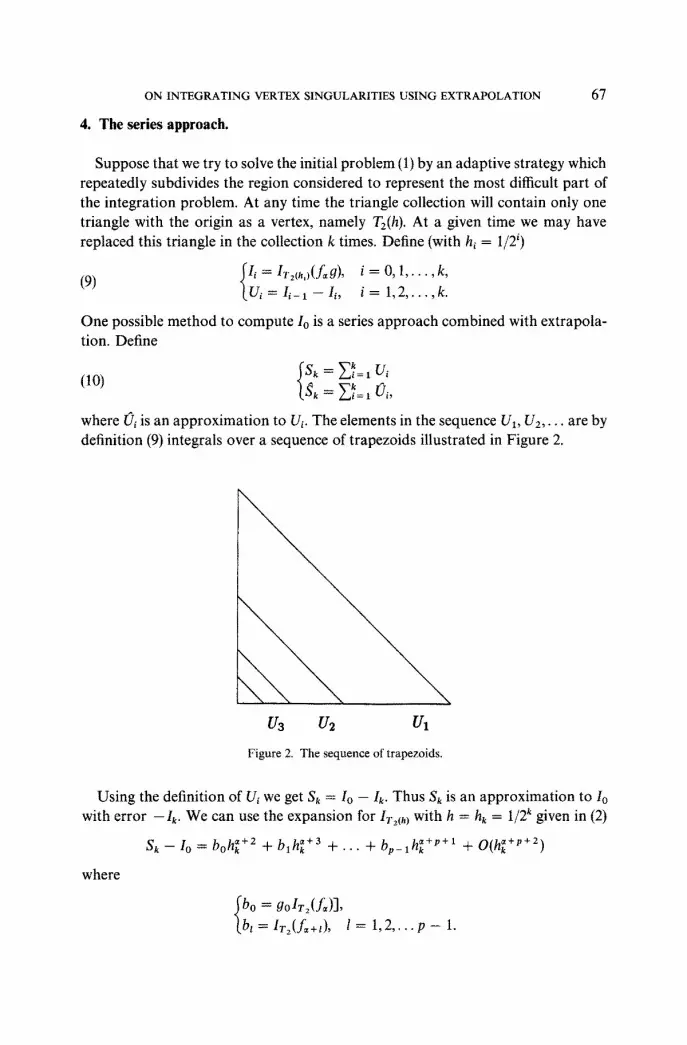
where 0~ is an approximation to Ui. The elements in the sequence U1, U2 . . . . are by definition (9) integrals over a sequence of trapezoids illustrated in Figure 2.
U3 U2 U1
Figure 2. The sequence of trapezoids.
Using the definition of Ui we get Sk = Io - Ik. Thus Sk is an approximation to lo with error --I~. We can use the expansion for ITs(h) with h = hk = 1/2 k given in (2)
S k - - Io I, In at + 2 = uO¢l. k "Jr" blh~ +3 + + b p _ t ,~+p+l • "" l " k + O ( h ~ + p + 2 )
where
bo = golr2(f~)],
b l= l r2 ( f~+~) , l = 1,2 . . . . p - - 1 .
68 TERJE O. ESPELID
Ux can be expressed as an integral over a trapezoid say, Tr, of the function f In fact this is true for all Ui's, and all these trapezoids are simply hi - a-scalings of Tr. Thus we can make use of the homogeneous function property and find, using standard procedures, that
b'~+2 C /,,~ + 3 hot+p+ I U i -~. Co,, i_ 1 -~- t t , i _ l --~ . . . + C p - l , , i - 1 -~ O(h~_+P+2) ,
where
co = 9olr,(f~) cz=Irr( f ,+t) , I = 1,2 . . . . p - 1.
This demonstrates that the series given in (10) will approach a geometric series asymptotically and that
UI+I/U~ "~ 1/2 ~+2 < 1, since ~ > - 2 .
Thus Io = ~ = l U i , but the convergence may become very slow if ~ ~ - 2 . In practice we have to approximate Ui; e.g. dividing this trapezoid into three congruent triangles is one possible strategy. Sk is an approximation to Io giving
k __ h h~t+P +1 (11 ) Sk - - to = 2 (~fi Ui) + boh~ +2 + bxh~, +3 + . . . + '~ 'p- l"k '[- O(h~+p+2) •
i = l
By standard linear extrapolation we may use (11) to eliminate the (k - 1) first terms in the sum of h-powers. Define
where Ev~ = t)t -- Ut. The b~}:s are just linear combinations of the b~'s and still independent of h. The coefficients that effect the Ev,'s are given by the relations
ON INTEGRATING VERTEX SINGULARITIES USING EXTRAPOLATION 69
below (can be shown using (12)):
floj = 1, j = O , 1 . . . . . k - l ; f l i j=O, i = 1,2 . . . . . k , j = O , 1 . . . . . i - 1;
flij = fllj-I + ( f l l j -1 -- fli 1 , j -1 ) /n j , i = 1,2 . . . . . k - 1,j = i, i + 1 . . . . . k - 1.
We can thus give a tableau for these coefficients, once ~ is known and a maximum value of k is given
1 1 1 . . . 1 1 ]
L 0 f l~ 312 . . . fl~k-2 fl~k-1 0 0 fl22 " ' " f12,k-2 f l2 .k - I
. . . . . .
0 0 0 . . . 0 fl~-l,k-1 0 0 0 . . . 0 0
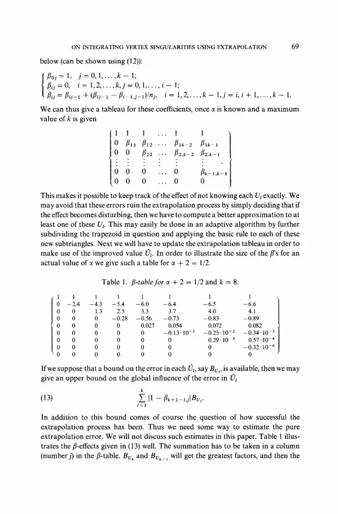
This makes it possible to keep track of the effect of not knowing each U~ exactly. We may avoid that these errors ruin the extrapolation process by simply deciding that if the effect becomes disturbing, then we have to compute a better approximation to at least one of these U~. This may easily be done in an adaptive algorithm by further subdividing the trapezoid in question and applying the basic rule to each of these new subtriangles. Next we will have to update the extrapolation tableau in order to make use of the improved value C~. In order to illustrate the size of the fl's for an actual value of ~ we give such a table for c¢ + 2 = 1/2.
If we suppose that a bound on the error in each 0 l, say Be,, is available, then we may give an upper bound on the global influence of the error in L]
k
(13) ~ [1 - flk+l_t,s[Bvv l = I
In addition to this bound comes of course the question of how successful the extrapolation process has been. Thus we need some way to estimate the pure extrapolation error. We will not discuss such estimates in this paper. Table 1 illus- trates the fl-effects given in (13) well. The summation has to be taken in a column (number j) in the fl-table. Bv~ and Bv~l will get the greatest factors, and then the
7 0 TERJE O. ESPELID
effect of the extrapolation on the following errors will decrease rapidly. Further- more we see that the fl-table indicates row-wise convergence. This implies that moving along the last row in the S-tableau will increase the fl-effect on Bvk, but the effect will soon become practically constant. The same observation seems to be true for all rows in the fl-table.
Suppose that we are not satisfied with any of the approximations offered by (12). Then we have two alternatives: (A) Either compute an improved value for, say, 0~, if necessary recompute the extrapolation tableau, and then check if finished, or (B) take another extrapolation step: compute Sk,o = Uk + l and then the next row in the extrapolation tableau.
The important observation is that the extrapolation process reduces the influence of the h-series, but the effect of using 0l as an approximation to Ul enters the extrapolated value through the fl-terms and therefore will increase.
It is not essential, in order for this technique to work, that we have used the same compound rule on each trapezoid involved. The important idea is to have a good approximation and this may be reflected in the choice of rules and/or subdivisions of these subregions. (13) shows that the effect can be monitored and the approximation improved. However, if we use the same compound rule, Q', on each trapezoid, then we can say a little more about the Ev,-effect. We make use of the homogeneous property and get
p 1
= ~lr l i_ 1 -~- v ~,~i_ i / 1=0
where we have
This means that
eo = g(O, O) [Q~'r(f~) - Irr(f~)]'
et = Q'~r(f~+~)--ITr(L+l), l = 1,2 . . . . p - - 1.
k p - 1 k k
Z Ev, 2 el E / a c t + l + 2 o' tact+P+ = , , / - 1 + E , " i - 1 2) , i = 1 / = 0 i = 1 i = t
giving, with 71 = 1/2~+t+2,
k p - 1 p - 1
2 E v , = ~ e , / ( 1 - 7 ~ ) - 2 h~ + ' + 2 e , / ( 1 - y , ) + O ( e p ) . i = 1 / = 0 1=0
Putting this expression into (11) shows that we get a modified hk-series which will be eliminated next, term by term through the extrapolation. In addition we get a contribution
p - 1
et/(1 -- ?t). / = 0
Since we expect that e~ is strongly decreasing with increasing 1, we can look at this
O N I N T E G R A T I N G V E R T E X S I N G U L A R I T I E S U S I N G E X T R A P O L A T I O N 7 1
sum as a "constant" added to I o in (11). This can be observed in the tableau as convergence to the "wrong" answer.
5. Series with tail-correction.
If we use the rule Q to estimate It, then Qt = QT2~h,)(f~g) is an estimate of the tail
li = ~ l > i Ul. Define
i
T i o = Q i + ~ UI, i = 0 , 1 , 2 . . . . . k. / = 1
In this way each T~o = Qt + St- 1.o is an approximation to Io and we have according to (4)
As in the series approach we face two different alternatives if we are not satisfied with the global approximation: (A) Either compute a better value for Ui and update the T-tableau. This can easily be done directly in the last row of this tableau. Just pick the appropriate row in the fl-table, then recompute Tks, estimate the new errors and finally decide what to do next. Or (B), take a new extrapolation step: put hk + 1 = hk/2, compute Ok + 1 and Qk + ~ in order to create a new row in the T-tableau
T~+~,0 = T~o + (Q~+~ - Q~) + 0~+~.
In order to compare the series approach and this tail correction approach we see that the coefficients in the h-series are given by
at = QT~(f~+~) -- IT~(f~+l)
b l = IT~(f~+t).
Thus it is reasonable to expect that the tail correction approach will turn out to be more efficient than the series approach since there is a low cost associated with this correction and we can expect latl << Ibtl. Furthermore we can expect that la~+xl << la~l, at least for 1 < degree of precision of Q. This means that the h- extrapolation in the tail case will be more efficient than one normally will experience
72 TERJE O. ESPELID
with such expansions. Finally we note that the extrapolation is identical in the two approaches and therefore the linear combinations of at and bt will be the same.
We will conclude this section by observing that the result (14) can be generalized to an N-dimensional simplex and an N-dimensional rectangle with the same notation, by simply replacing the number 2 by the dimension N
The definitions of Qi and 0i are obvious and at is given by (6). The extrapolation will be identical, just change nl = 2 N+~ - 1 to get the sequence of denominators.
Observe furthermore that TkR is indeed itself a quadrature formula which can be written
k k
(18) Tkk = ~ 71k'0~ + ~ 61k'Qt. /=1 l=0
Here Qt and (l~ represent quadratures over different regions, while the coefficients contain the information about the strength of the singularity. Thus this formula resembles what one finds in cubatures developed for integrals involving weight functions: (1) information about the weight function enters the quadrature coef- ficients, and (2) most of the evaluation points will appear as a cluster near the singular point.
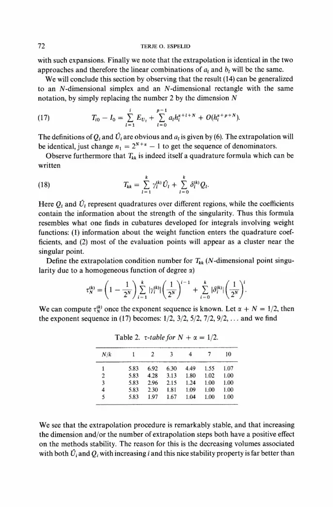
Define the extrapolation condition number for Tkk (N-dimensional point singu- larity due to a homogeneous function of degree c~)
i=1 i=0
We can compute r~ ) once the exponent sequence is known. Let c~ + N = 1/2, then the exponent sequence in (17) becomes: 1/2, 3/2, 5/2, 7/2, 9/2, . . . and we find
We see that the extrapolation procedure is remarkably stable, and that increasing the dimension and/or the number of extrapolation steps both have a positive effect on the methods stability. The reason for this is the decreasing volumes associated with both (Jr and Qt with increasing i and this nice stability property is far better than
ON INTEGRATING VERTEX SINGULARITIES USING EXTRAPOLATION 73
what one finds in uniform subdivision strategies, Lyness [5], even with the geometric m-sequence. Note that the non-uniform method only deals with some of the terms in the error expansion given in Theorem 1, and we have the possibility to choose rules of high degree combined with adaptive strategies in the computation of U.
Discussing the work involved is more complex in general. We see that k extrapola- tion steps involves (k + 1) applications of the rule Q to singular regions and k 0 approximations. The cost of computing 0 to sufficient precision, e.g. using an adaptive strategy, depends both on the geometry and the choice of basic rule. The region associated with ~3 may in the N-cube case be cut into N different hyper- rectangles. Thus at least N applications of the basic rule is necessary for each tS"-term. The quality of the rule and the problem at hand will determine whether more subdivisions are necessary.
These ideas can easily be extended to handle problems involving a logarithmic singularity too: e.g. f = f, z(r)log(9#)9. Here 9# is a homogeneous function of degree fl around the origin and the effect on the expansion (17) will be that the constants a~ will be replaced by al °) + log (h)al 1). Linear extrapolation may be applied assuming that each exponent appears twice. If the logarithm appears in an integer power then we get a polynomial in log (h) of degree equal to that power.
In the next section we will give some examples where we apply these techniques.
6. Numerical examples.
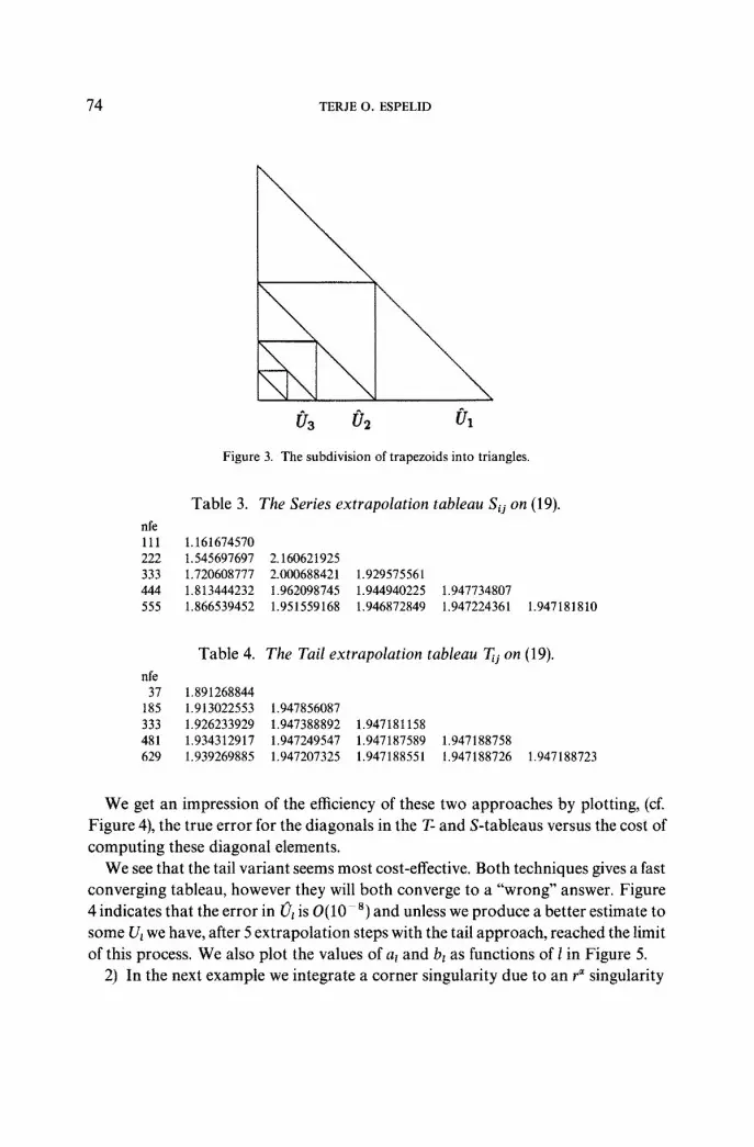
In this section we will demonstrate, on a few examples, how efficient the new approach may be. We will not compare these techniques with extrapolation schemes based on the uniform approach (8) due to the fact that such a comparison will depend both on the problem, the choice of rule(s), Q, in both techniques and the choice of extrapolation technique. For this illustrative purpose we will apply the basic rule Q (degree 13, using 37 nodes) implemented in DCUTRI, [1], and further- more subdivide each trapezoid in three congruent triangles (in fact use the subdivi- sion produced by DCUTRI) and then use Q on each of these triangles; see Figure 3.
All computations have been performed on a SUN Sparc station 2 in double precision arithmetic.
1) In the first example we treat a problem with a strong vertex singularity in the origin combined with a nice function 9(x, y)
In order to illustrate the two different techniques we give the Series tableau in Table 3 and the Tail tableau in Table 4. The number of function evaluations (nfe) is in both tables given in the left column.
74 TERJE O. ESPELID
Figure 3. The subdivision of trapezoids into triangles.
Table 3. The Series extrapolation tableau Sij on (19). nfe 111 1,161674570 222 1,545697697 2,160621925 333 1,720608777 2.000688421 1.929575561 444 1.813444232 1.962098745 1.944940225 1.947734807 555 1,866539452 1.951559168 1.946872849 1.947224361 1.947181810
Table 4. The Tail extrapolation tableau T~j on (19). nfe
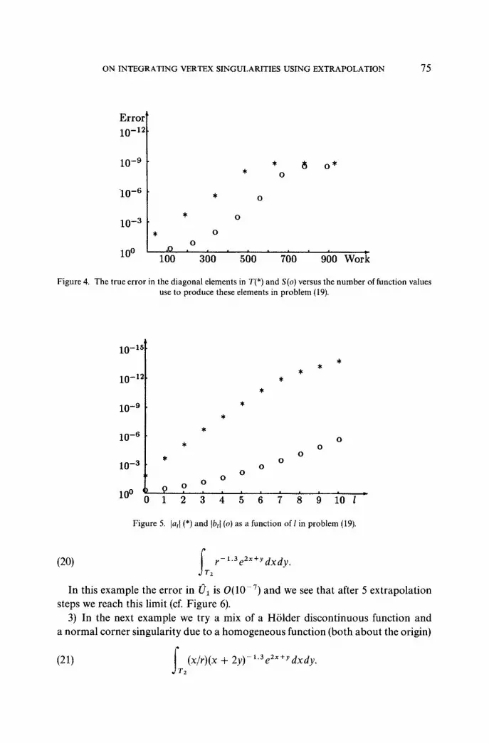
We get an impression of the efficiency of these two approaches by plotting, (cf. Figure 4), the true error for the diagonals in the T- and S-tableaus versus the cost of computing these diagonal elements.
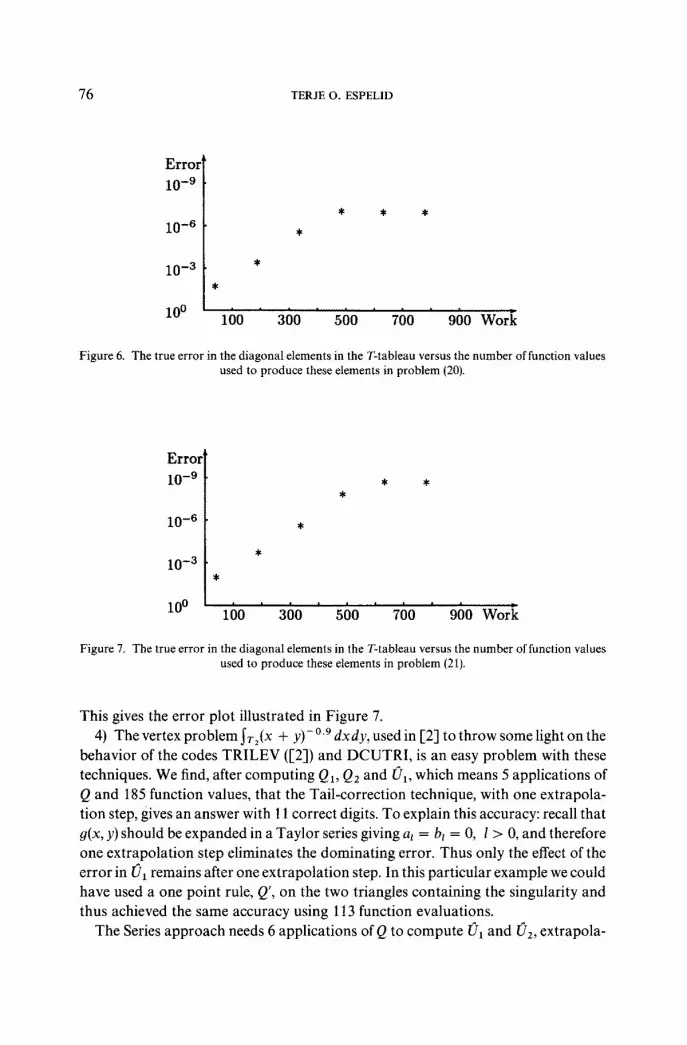
We see that the tail variant seems most cost-effective. Both techniques gives a fast converging tableau, however they will both converge to a "wrong" answer. Figure 4 indicates that the error in Ot is O(10 8) and unless we produce a better estimate to some Uz we have, after 5 extrapolation steps with the tail approach, reached the limit of this process. We also plot the values of at and bt as functions of 1 in Figure 5.
2) In the next example we integrate a corner singularity due to an r ~ singularity
O N I N T E G R A T I N G VERTEX S I N G U L A R I T I E S U S I N G E X T R A P O L A T I O N 75
Error 10-12
10-9
10 -6
10-3
10 o
0
0
* 8 o * 0
, O
O ,O m i t
100 360 ' 560 760 960 W o r k
Figure 4. The true error in the diagonal elements in T(*) and S(o) versus the number of function values use to produce these elements in problem (19).
10-12
10-1;
10 - 9
10-8
10-3
lOS 0
0 0
0 0
0
O O
9 o
Figure 5. Ja~[ (*) and tb, I (o) as a function of l in problem (19).
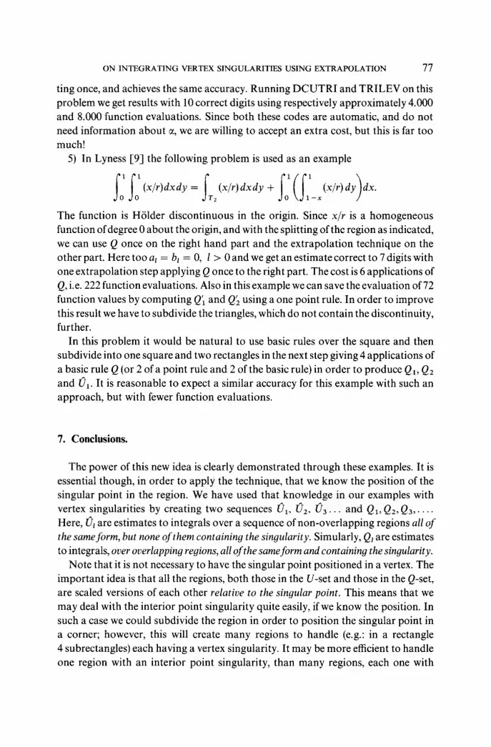
t ' (20) ---IT2 r - 1.3 e2X +y dxdy.
In this example the error in 01 is 0(10-7) and we see that after 5 extrapolation steps we reach this limit (cf. Figure 6).
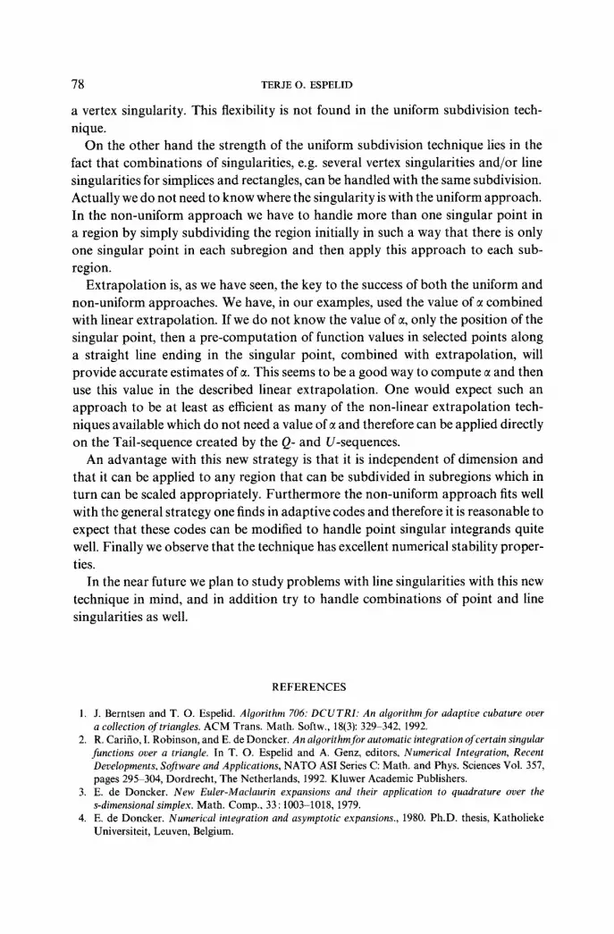
3) In the next example we try a mix of a H61der discontinuous function and a normal corner singularity due to a homogeneous function (both about the origin)
(21) ~ (x/r)(x + 2y)- t.3 e2X+Y dxdy" J~ r2
76 TERJE O. ESPELID
Error ~ 10-9
10-6
i 0 - 3
i o o 1 0 0 ' 3 0 0 ' 5 ( ' ) 0 ' 7 ( ) 0 ' 900 Work
Figure 6. The true error in the diagonal elements in the T-tableau versus the number of function values used to produce these elements in problem (20).
Error 10 - 9
10-6
10-3
i0 o 160 360 560 760 960 Wori Figure 7. The true error in the diagonal elements in the T-tableau versus the number of function values
used to produce these elements in problem (21).
This gives the error plot illustrated in Figure 7. 4) The vertex problem ~r2 (x + y)- o.9 dx dy, used in [2] to throw some light on the
behavior of the codes TRILEV ([2]) and DCUTRI, is an easy problem with these techniques. We find, after computing Q1, Q~ and 0, , which means 5 applications of Q and 185 function values, that the Tail-correction technique, with one extrapola- tion step, gives an answer with 11 correct digits. To explain this accuracy: recall that g(x, y) should be expanded in a Taylor series giving a~ = bz = 0, l > 0, and therefore one extrapolation step eliminates the dominating error. Thus only the effect of the error in 01 remains after one extrapolation step. In this particular example we could have used a one point rule, Q', on the two triangles containing the singularity and thus achieved the same accuracy using 113 function evaluations.
The Series approach needs 6 applications of Q to compute 01 and 02, extrapola-
ON INTEGRATING VERTEX SINGULARITIES USING EXTRAPOLATION 77
ting once, and achieves the same accuracy. Running DCUTRI and TRILEV on this problem we get results with 10 correct digits using respectively approximately 4.000 and 8.000 function evaluations. Since both these codes are automatic, and do not need information about a, we are willing to accept an extra cost, but this is far too much!
5) In Lyness [9] the following problem is used as an example
f] f] (x/r)dxdY= fr2(x/r)dxdy + f] (f]_ (x/r)dy)dx" The function is H61der discontinuous in the origin. Since x/r is a homogeneous function of degree 0 about the origin, and with the splitting of the region as indicated, we can use Q once on the right hand part and the extrapolation technique on the other part. Here too at = b~ = 0, I > 0 and we get an estimate correct to 7 digits with one extrapolation step applying Q once to the right part. The cost is 6 applications of Q, i.e. 222 function evaluations. Also in this example we can save the evaluation of 72 function values by computing Q~ and Q~ using a one point rule. In order to improve this result we have to subdivide the triangles, which do not contain the discontinuity, further.
In this problem it would be natural to use basic rules over the square and then subdivide into one square and two rectangles in the next step giving 4 applications of a basic rule Q (or 2 of a point rule and 2 of the basic rule) in order to produce Q1, Q2 and 01. It is reasonable to expect a similar accuracy for this example with such an approach, but with fewer function evaluations.
7. Conclusions.
The power of this new idea is clearly demonstrated through these examples. It is essential though, in order to apply the technique, that we know the position of the singular point in the region. We have used that knowledge in our examples with vertex singularities by creating two sequences U1, U2, U3. . . and Q1, Q2,Qa . . . . . Here, 0z are estimates to integrals over a sequence of non-overlapping regions all of the same form, but none of them containing the singularity. Simularly, Qt are estimates to integrals, over overlapping regions, all of the same form and containing the singularity.
Note that it is not necessary to have the singular point positioned in a vertex. The important idea is that all the regions, both those in the U-set and those in the Q-set, are scaled versions of each other relative to the singular point. This means that we may deal with the interior point singularity quite easily, if we know the position. In such a case we could subdivide the region in order to position the singular point in a corner; however, this will create many regions to handle (e.g.: in a rectangle 4 subrectangles) each having a vertex singularity. It may be more efficient to handle one region with an interior point singularity, than many regions, each one with
78 TERJE O. ESPELID
a vertex singularity. This flexibility is not found in the uniform subdivision tech- nique.
On the other hand the strength of the uniform subdivision technique ties in the fact that combinations of singularities, e.g. several vertex singularities and/or line singularities for simplices and rectangles, can be handled with the same subdivision. Actually we do not need to know where the singularity is with the uniform approach. In the non-uniform approach we have to handle more than one singular point in a region by simply subdividing the region initially in such a way that there is only one singular point in each subregion and then apply this approach to each sub- region.
Extrapolation is, as we have seen, the key to the success of both the uniform and non-uniform approaches. We have, in our examples, used the value of ~ combined with linear extrapolation. If we do not know the value of ~, only the position of the singular point, then a pre-computation of function values in selected points along a straight line ending in the singular point, combined with extrapolation, will provide accurate estimates of ~. This seems to be a good way to compute ~ and then use this value in the described linear extrapolation. One would expect such an approach to be at least as efficient as many of the non-linear extrapolation tech- niques available which do not need a value of~ and therefore can be applied directly on the Tail-sequence created by the Q- and U-sequences.
An advantage with this new strategy is that it is independent of dimension and that it can be applied to any region that can be subdivided in subregions which in turn can be scaled appropriately. Furthermore the non-uniform approach fits well with the general strategy one finds in adaptive codes and therefore it is reasonable to expect that these codes can be modified to handle point singular integrands quite well. Finally we observe that the technique has excellent numerical stability proper- ties.
In the near future we plan to study problems with line singularities with this new technique in mind, and in addition try to handle combinations of point and line singularities as well.
REFERENCES
1. J. Berntsen and T. O. Espelid. Algorithm 706: DCUTRI: An algorithm for adaptive cubature over a collection of triangles. ACM Trans. Math. Softw., 18(3): 329-342, 1992.
2. R. Carifio, I. Robinson, and E. de Doncker. An algorithm for automatic integration of certain singular functions over a triangle. In T. O. Espelid and A. Genz, editors, Numerical Integration, Recent Developments, Software and Applications, NATO ASI Series C: Math. and Phys. Sciences Vol. 357, pages 295-304, Dordrecht, The Netherlands, 1992. Kluwer Academic Publishers.
3. E. de Doncker. New Euler-Maclaurin expansions and their application to quadrature over the s-dimensional simplex. Math. Comp., 33: 1003-1018, 1979.
4. E. de Doncker. Numerical integration and asymptotic expansions., 1980. Ph.D. thesis, Katholieke Universiteit, Leuven, Belgium.
ON INTEGRATING VERTEX SINGULARITIES USING EXTRAPOLATION 79
5. J. N. Lyness. Applications of extrapolation techniques to multidimensional quadrature of some integrandfunctions with a singularity. J. Comp. Phys., 20(3) : 346-364, 1976.
6. J. N. Lyness. An error functional expansion for n-dimensional quadrature with an integrand function singular at a point. Math. Comp., 30(133): 1 23, 1976.
7. J.N. Lyness. Quadrature over a simplex: Part 1. A representation for the integrand function. SIAM d. Numer. Anal., 15(1): 122-133, 1978.
8. J. N. Lyness, Quadrature over a simplex: Part 2. A representation for the error functional. SIAM J. Numer. Anal., 15(5): 870-887, 1978.
9. J. N. Lyness. On handling singularities in finite elements. In T. O. Espelid and A. Genz, editors, Numerical Integration, Recent Developments, Software and Applications, NATO ASI Series C: Math. and Phys. Sciences Vol. 357, pages 219-233, Dordrecht, The Netherlands, 1992. Kluwer Academic Publishers.
10. J. N. Lyness and G. Monegato. Quadrature error functional expansions for the simplex when the integrand function has singularities at vertices. Math. Comp., 34(149): 213-225, 1980.
11. A. Sidi. Euler-McLaurin expansions for integrals over triangles ofjunctions having algebraic~logarith- mic singularities along an edge. J. Approx. Th., 39(1):39-53, t983.
12. W. Squire. Partition-extrapolation methods for numerical quadratures. Int. J. Comp. Math., 5(1): 81- 91, 1975.