On the Integration of Differential Fractions

François BoulierUniversité Lille 1

Villeneuve d’Ascq, FranceFrancois.Boulier@univ-lille1.fr

François Lemaire∗

Université Lille 1Villeneuve d’Ascq, France

Francois.Lemaire@lifl.fr

Georg RegensburgerRICAM

Linz, AustriaGeorg.Regensburger@oeaw.ac.at

Markus Rosenkranz†

University of KentCanterbury, United Kingdom

M.Rosenkranz@kent.ac.uk

ABSTRACTIn this paper, we provide a differential algebra algorithm forintegrating fractions of differential polynomials. It is notrestricted to differential fractions that are the derivativesof other differential fractions. The algorithm leads to newtechniques for representing differential fractions, which mayhelp converting differential equations to integral equations(as for example used in parameter estimation).

Categories and Subject DescriptorsI.1.1 [Symbolic and Algebraic Manipulation]: Expres-sions and Their Representation—simplification of expres-sions; I.1.2 [Symbolic and Algebraic Manipulation]:Algorithms—algebraic algorithms

KeywordsDifferential algebra, differential fractions, integration

1. INTRODUCTIONIn this paper we present an algorithm that solves the fol-

lowing problem in differential algebra: Given a differentialfraction F , i.e., a fraction P/Q where P and Q are differ-ential polynomials, and a derivation δ, compute a finite se-quence F1, F2, F3, . . . , Ft of differential fractions such that

F = F1 + δ F2 + δ2 F3 + · · ·+ δt Ft , (1)

the differential fractions δ` F` have rank less than or equalto F (the result is thus ranking dependent) and the δ` differ-ential operators are as much “factored out” as possible. In

∗The first two authors acknowledge partial support by theFrench ANR-10-BLAN-0109 LEDA project.†The fourth author acknowledges partial support by the EP-SRC First Grant EP/I037474/1.

Permission to make digital or hard copies of all or part of this work forpersonal or classroom use is granted without fee provided that copies arenot made or distributed for profit or commercial advantage and that copiesbear this notice and the full citation on the first page. To copy otherwise, torepublish, to post on servers or to redistribute to lists, requires prior specificpermission and/or a fee.ISSAC’13, June 26–29, 2013, Boston, Massachusetts, USA.Copyright 2013 ACM 978-1-4503-2059-7/13/06 ...$15.00.

particular, if there exists some differential fraction G suchthat F = δ G, then F1 = 0: the algorithm recognizes firstintegrals.

This work originated from our attempts to generalize theconstruction of integro-differential polynomials [14] to thecase of several independent and dependent variables. Theresults presented here constitute the most important stepin this construction: the decomposition of an arbitrary dif-ferential polynomial—or differential fraction—into a totalderivative and a remainder (see Example 1 with iterated

= false). For ordinary differential polynomials, such a de-composition is described in [1]. See also [8, 2] and the recentdissertation [12] for further references.1

If the remainder is zero, the given differential fraction F isrecognized to be the total derivative of another differentialfraction G, so the latter appears as a first integral of F .Algorithms for determining such first integrals are known(see [15, 16]), and one such algorithm is implemented inMaple via the function DEtools[firint].

Handling differential fractions rather than polynomialsmay be very important for the range of application of Al-gorithms 3 and 4 since differential equations may be mucheasier to integrate when multiplied, or divided, by an inte-grating factor. Beyond its theoretical interest, the algorithmpresented in this paper may also be useful in practice:

1. Sometimes (though not always), a differential fractionis shorter in the representation (1) than in expandedform. Thus our algorithm provides new facilities forrepresenting differential equations.

2. The representation (1) may also be more convenientthan the expanded form if one wants to convert dif-ferential equations to integral equations. This may bea very important feature for the problem of estimat-ing parameters of dynamical systems from their input-output behaviour (see Example 5).

The paper is organized as follows: In Section 2, we re-view some standard definitions for differential polynomialsand generalize them to differential fractions. In Section 3,the main result of this paper is stated and proved (Algo-rithm 3 and Proposition 6). In Section 4, we describe animplementation along with a few worked-out examples.

1The authors would like to thank the reviewers for pointingout these references.

2. BASICS OF DIFFERENTIAL ALGEBRAThis paper is concerned with differential fractions, i.e.,

fractions of differential polynomials. A key problem withsuch fractions is to reduce them, which requires computingthe gcd of multivariate polynomials, which is possible when-ever the base field is computable.

The reference books are [13] and [11]. A differential ring Ris a ring endowed with finitely many, say m, derivationsδ1, . . . , δm, i.e., unary operations satisfying the following ax-ioms, for all a, b ∈ R:

δ(a+ b) = δ(a) + δ(b) , δ(a b) = δ(a) b+ a δ(b) ,

and which commute pairwise. To each derivation δi an in-dependent variable xi is associated such that δi xj = 1 ifi = j and 0 otherwise. The set of independent variables isdenoted by X = {x1, . . . , xm}. The derivations generate acommutative monoid w.r.t. composition denoted by

Θ = {δa11 · · · δ

amm | a1, . . . , am ∈ N} ,

where N stands for the nonnegative integers. The elementsof Θ are called derivation operators. If θ = δa1

1 · · · δamm is

a derivation operator then ord(θ) = a1 + · · · + am denotesits order, with ai being the order of θ w.r.t. derivation δi(or xi).

In order to form differential polynomials, one introduces aset U = {u1, . . . , un} of n differential indeterminates. Themonoid Θ acts on U , giving the infinite set ΘU of deriva-tives. For readability, we often index derivations by letterslike δx and δy, denoting also the corresponding derivativesby these subscripts, so uxy denotes δx δy u.

For applications, it is crucial that one can also handleparametric differential equations. Parameters are nothingbut symbolic constants, i.e., symbols whose derivatives arezero. Let C denote the set of constants.

The differential fractions considered in this paper are ra-tios of differential polynomials taken from the differentialring R = Z[X ∪ C ]{U } = Z[X ∪ C ∪ ΘU ]. A differen-tial fraction is said to be reduced if its numerator and de-nominator do not have any common factor. A differentialpolynomial (respectively a differential fraction) is said to benumeric if it is an element of Z (resp. of Q). It is said to be acoefficient if it is an element of Z[X ∪C ] (resp. of Q(X ∪C )).The elements of X ∪ C ∪ΘU are called variables.

A ranking is a total ordering on ΘU that satisfies the twofollowing axioms:

1. v ≤ θv for every v ∈ ΘU and θ ∈ Θ,

2. v < w ⇒ θv < θw for every v, w ∈ ΘU and θ ∈ Θ.

Rankings are well-orderings, i.e., every strictly decreasingsequence of elements of ΘU is finite [11, §I.8]. Rankingssuch that ord(θ) < ord(φ)⇒ θu < φv for every θ, φ ∈ Θ andu, v ∈ U are called orderly. In this paper, it is convenientto extend rankings to the sets X and C . For all rankings,we will assume that any element of X ∪ C is less than anyelement of ΘU ; see Remark 5 for a brief discussion why wemake this assumption.

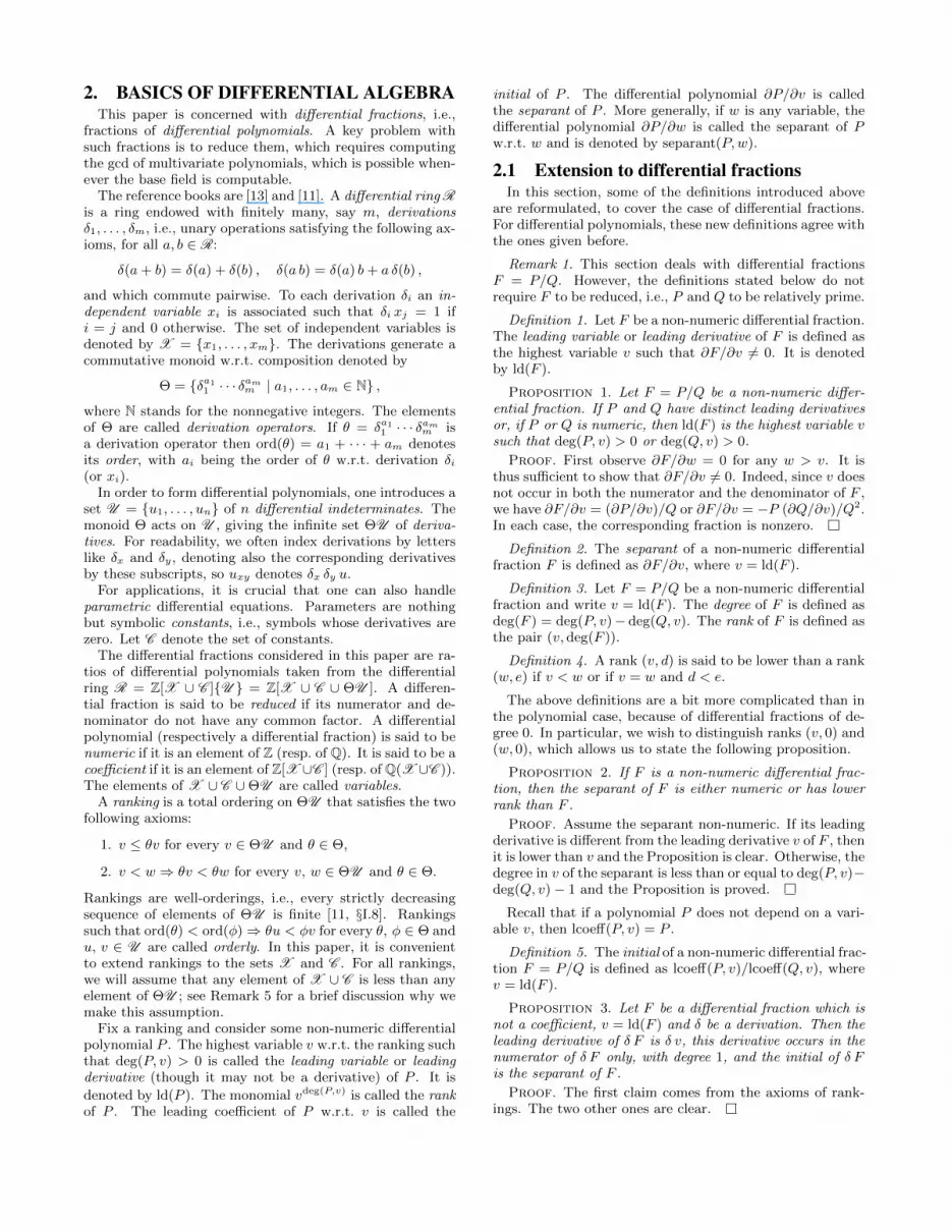
Fix a ranking and consider some non-numeric differentialpolynomial P . The highest variable v w.r.t. the ranking suchthat deg(P, v) > 0 is called the leading variable or leadingderivative (though it may not be a derivative) of P . It is

denoted by ld(P ). The monomial vdeg(P,v) is called the rankof P . The leading coefficient of P w.r.t. v is called the

initial of P . The differential polynomial ∂P/∂v is calledthe separant of P . More generally, if w is any variable, thedifferential polynomial ∂P/∂w is called the separant of Pw.r.t. w and is denoted by separant(P,w).

2.1 Extension to differential fractionsIn this section, some of the definitions introduced above

are reformulated, to cover the case of differential fractions.For differential polynomials, these new definitions agree withthe ones given before.

Remark 1. This section deals with differential fractionsF = P/Q. However, the definitions stated below do notrequire F to be reduced, i.e., P and Q to be relatively prime.

Definition 1. Let F be a non-numeric differential fraction.The leading variable or leading derivative of F is defined asthe highest variable v such that ∂F/∂v 6= 0. It is denotedby ld(F ).

Proposition 1. Let F = P/Q be a non-numeric differ-ential fraction. If P and Q have distinct leading derivativesor, if P or Q is numeric, then ld(F ) is the highest variable vsuch that deg(P, v) > 0 or deg(Q, v) > 0.

Proof. First observe ∂F/∂w = 0 for any w > v. It isthus sufficient to show that ∂F/∂v 6= 0. Indeed, since v doesnot occur in both the numerator and the denominator of F ,we have ∂F/∂v = (∂P/∂v)/Q or ∂F/∂v = −P (∂Q/∂v)/Q2.In each case, the corresponding fraction is nonzero.

Definition 2. The separant of a non-numeric differentialfraction F is defined as ∂F/∂v, where v = ld(F ).

Definition 3. Let F = P/Q be a non-numeric differentialfraction and write v = ld(F ). The degree of F is defined asdeg(F ) = deg(P, v)− deg(Q, v). The rank of F is defined asthe pair (v,deg(F )).

Definition 4. A rank (v, d) is said to be lower than a rank(w, e) if v < w or if v = w and d < e.

The above definitions are a bit more complicated than inthe polynomial case, because of differential fractions of de-gree 0. In particular, we wish to distinguish ranks (v, 0) and(w, 0), which allows us to state the following proposition.

Proposition 2. If F is a non-numeric differential frac-tion, then the separant of F is either numeric or has lowerrank than F .

Proof. Assume the separant non-numeric. If its leadingderivative is different from the leading derivative v of F , thenit is lower than v and the Proposition is clear. Otherwise, thedegree in v of the separant is less than or equal to deg(P, v)−deg(Q, v)− 1 and the Proposition is proved.

Recall that if a polynomial P does not depend on a vari-able v, then lcoeff(P, v) = P .

Definition 5. The initial of a non-numeric differential frac-tion F = P/Q is defined as lcoeff(P, v)/lcoeff(Q, v), wherev = ld(F ).

Proposition 3. Let F be a differential fraction which isnot a coefficient, v = ld(F ) and δ be a derivation. Then theleading derivative of δ F is δ v, this derivative occurs in thenumerator of δ F only, with degree 1, and the initial of δ Fis the separant of F .

Proof. The first claim comes from the axioms of rank-ings. The two other ones are clear.

3. MAIN RESULTIn this section, we write numer(F ) and denom(F ) for the

numerator and denominator of a differential fraction F , bothviewed as differential polynomials of the ring R. Our resultis Algorithm 3. It relies on two sub-algorithms (Algorithms 1and 2), which are purely algebraic (i.e., they do not make useof derivations, in the sense of the differential algebra). Thesetwo sub-algorithms are related to the integration problem ofrational fractions. They are either known or very close toknown methods, such as those described in [7]. We statethem in this paper, because our current implementation isactually based on them, the paper becomes self-contained,and the tools required by Algorithm 3 appear clearly.

Remark 2. In the three presented algorithms, all differen-tial fractions are supposed to be reduced.

Algorithm 1 The prepareForIntegration algorithm

Require: F is a reduced differential fraction, v is a variableEnsure: Three polynomials contF , N , B satisfying Prop. 41: if denom(F ) is numeric then2: contF , N, B := denom(F ), numer(F ), 13: else4: contF := the gcd of all coeffs of denom(F ) w.r.t. v

{ all gcd are of multivariate polynomials }5: P0 := numer(F )6: Q0 := denom(F )/contF { all divisions are exact }7: A0 := gcd(Q0, separant(Q0, v))8: B0 := Q0/A0

9: C0 := gcd(A0, B0)10: D0 := B0/C0

11: A1 := gcd(A0, separant(A0, v))12: N, B := P0 ·D0 ·A1, D0 ·A0

13: end if14: return contF , N, B

Proposition 4 (Specification of Algorithm 1).Let F = P0/(contF Q0) be a differential fraction (P0 and

Q0 being relatively prime, Q0 primitive w.r.t. v, and contFdenoting the content of denom(F ) w.r.t. v). Then the poly-nomials returned by Algorithm 1 satisfy

F =N

contF B2, B = F1 F2 F

23 · · ·Fn−1

n ,

where Q0 = F1 F22 F

33 · · ·Fn

n is the squarefree factorizationof Q0 w.r.t. v.

Proof. The case of F being a polynomial is clear. As-sume F has a non-numeric denominator. We have A0 =F2 F

23 · · ·Fn−1

n at Line 8, B0 = F1 F2 F3 · · ·Fn at Line 9,C0 = F2 F3 · · ·Fn at Line 10, D0 = F1 at Line 11, A1 =F3 F

24 · · ·Fn−2

n at Line 12, N = P0 F1 F3 F24 · · ·Fn−2

n andB = F1 F2 F

23 · · ·Fn−1

n .

The following Lemma, which is easy to see, establishes therelationship between a well-known fact on the integration ofrational fractions and Algorithm 1.

Lemma 1. With the same notations as in Proposition 4,if there exists a reduced differential fraction R such that F =separant(R, v), then F1 = 1 and the denominator of R iscontRB, where contR has degree 0 in v.

Algorithm 2 The integrateWithRemainder algorithm

Require: F0 is a differential fraction, v is a variableEnsure: Two differential fractions R and W such that

1. F0 = separant(R, v) +W

2. W is zero iff there exists R s.t. F0 = separant(R, v)

1: R, W := 0, 02: F := F0

3: while F 6= 0 do4: { invariant: F0 = F + separant(R, v) +W }5: contF , N, B := prepareForIntegration(F, v)6: if deg(B, v) = 0 then7: P := the primitive of F w.r.t. v, with a 0 int. cst.

{ this amounts to integrate a polynomial }8: R := R+ P9: F := 0

10: else11: { look for A such that

separant(A/(contRB), v) = N/(contF B2) }

12: cB , cN := lcoeff(B, v), lcoeff(N, v)13: dB , dN , dA := deg(B, v), deg(N, v), dN − dB + 114: if dN = 2 dB − 1 or dA < 0 then15: H := cN vdN

16: W := W +H/(contF B2)

17: F := F −H/(contF B2)

18: else19: R2 := cN vdA/((dA − dB) contF cB B)20: R := R+R2

21: F := F − separant(R2, v)22: end if23: end if24: end while25: return R, W

Remark 3. Algorithm 2 relies on Algorithm 1 for com-puting contF , N and B. However, it does not need N . Itonly needs its leading coefficient cN and its degree dN . Ourformulation improves the readability of our algorithm.

Proposition 5. Algorithm 2 is correct.

Proof. First suppose Algorithm 2 terminates.The loop invariant stated in the algorithm is clear, since

it is satisfied at the beginning of the first loop and main-tained in each of the three cases considered by the algorithm.Combined with the loop condition, this implies that the firstensured condition is satisfied at the end of the algorithm.

Let us now show that the second ensured condition is sat-isfied. We assume that

∃R s.t. F = separant(R, v) . (2)

We prove that Lines 15–17 are not performed. This is suf-ficient to prove the second ensured condition since, if Lines15–17 are not performed and (2) holds then, after one iter-ation, F is modified either at Line 9 or 21. In both cases,the new value of F satisfies (2) again.

Assume (2) holds. By Lemma 1, the denominator of Ris contRB. Let A = cA v

dA + qA be its numerator andB = cB v

dB +qB (we only need to consider the case dB > 0).One can assume that dA 6= dB . Indeed, if dA = dB , onecan take R = (A − cA/cB B)/B since separant(R, v) =

separant(R, v) = F and deg(A − cA/cB B) < dB . Dif-ferentiating the fraction A/(contRB) w.r.t. v and identi-fying with F = N/(contF B

2) (Proposition 4), we see thatN = (dA−dB) cA cB contF /contR v

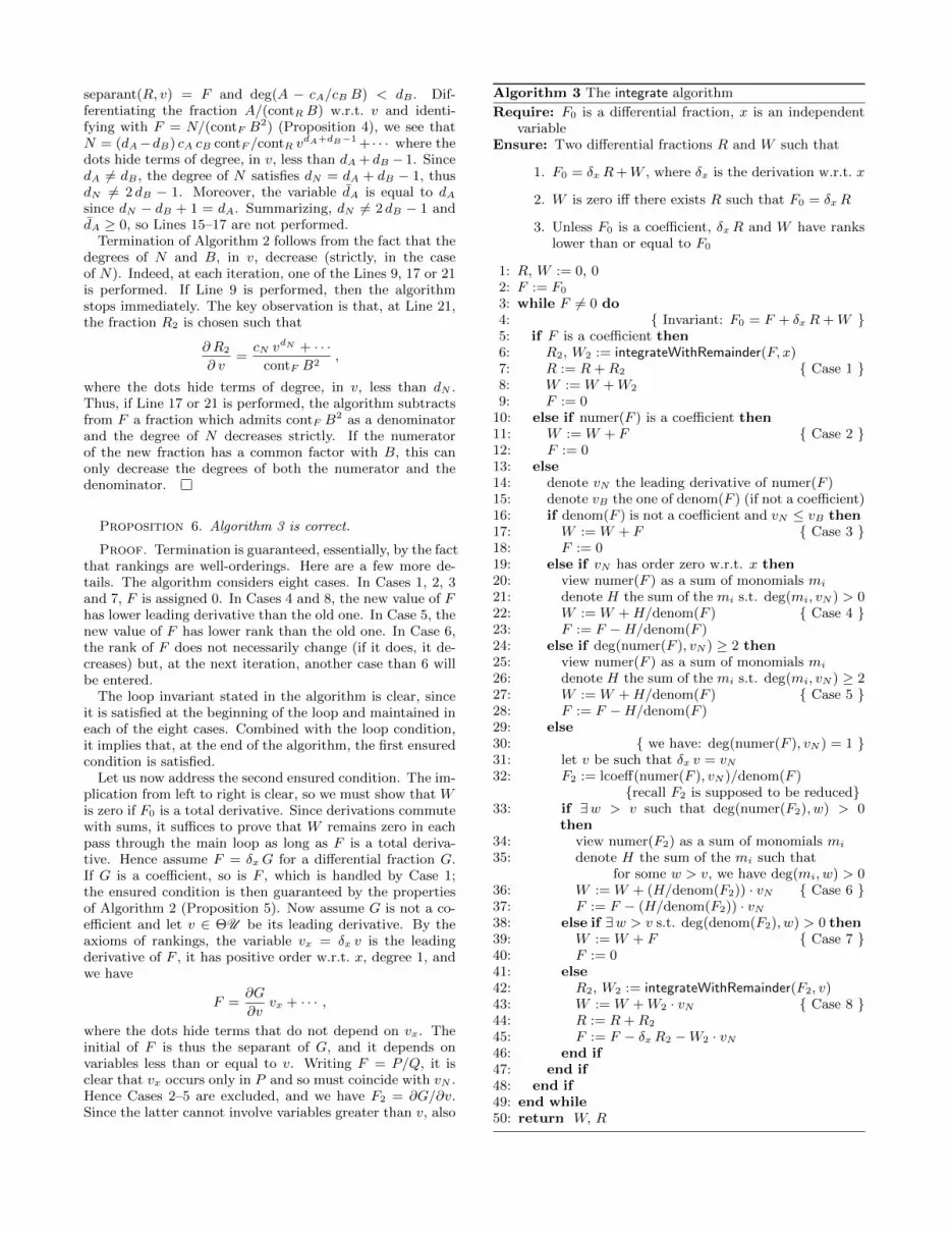
dA+dB−1 + · · · where thedots hide terms of degree, in v, less than dA + dB − 1. SincedA 6= dB , the degree of N satisfies dN = dA + dB − 1, thusdN 6= 2 dB − 1. Moreover, the variable dA is equal to dAsince dN − dB + 1 = dA. Summarizing, dN 6= 2 dB − 1 anddA ≥ 0, so Lines 15–17 are not performed.

Termination of Algorithm 2 follows from the fact that thedegrees of N and B, in v, decrease (strictly, in the caseof N). Indeed, at each iteration, one of the Lines 9, 17 or 21is performed. If Line 9 is performed, then the algorithmstops immediately. The key observation is that, at Line 21,the fraction R2 is chosen such that

∂ R2

∂ v=cN vdN + · · ·

contF B2,

where the dots hide terms of degree, in v, less than dN .Thus, if Line 17 or 21 is performed, the algorithm subtractsfrom F a fraction which admits contF B

2 as a denominatorand the degree of N decreases strictly. If the numeratorof the new fraction has a common factor with B, this canonly decrease the degrees of both the numerator and thedenominator.

Proposition 6. Algorithm 3 is correct.

Proof. Termination is guaranteed, essentially, by the factthat rankings are well-orderings. Here are a few more de-tails. The algorithm considers eight cases. In Cases 1, 2, 3and 7, F is assigned 0. In Cases 4 and 8, the new value of Fhas lower leading derivative than the old one. In Case 5, thenew value of F has lower rank than the old one. In Case 6,the rank of F does not necessarily change (if it does, it de-creases) but, at the next iteration, another case than 6 willbe entered.

The loop invariant stated in the algorithm is clear, sinceit is satisfied at the beginning of the loop and maintained ineach of the eight cases. Combined with the loop condition,it implies that, at the end of the algorithm, the first ensuredcondition is satisfied.

Let us now address the second ensured condition. The im-plication from left to right is clear, so we must show that Wis zero if F0 is a total derivative. Since derivations commutewith sums, it suffices to prove that W remains zero in eachpass through the main loop as long as F is a total deriva-tive. Hence assume F = δxG for a differential fraction G.If G is a coefficient, so is F , which is handled by Case 1;the ensured condition is then guaranteed by the propertiesof Algorithm 2 (Proposition 5). Now assume G is not a co-efficient and let v ∈ ΘU be its leading derivative. By theaxioms of rankings, the variable vx = δx v is the leadingderivative of F , it has positive order w.r.t. x, degree 1, andwe have

F =∂G

∂vvx + · · · ,

where the dots hide terms that do not depend on vx. Theinitial of F is thus the separant of G, and it depends onvariables less than or equal to v. Writing F = P/Q, it isclear that vx occurs only in P and so must coincide with vN .Hence Cases 2–5 are excluded, and we have F2 = ∂G/∂v.Since the latter cannot involve variables greater than v, also

Algorithm 3 The integrate algorithm

Require: F0 is a differential fraction, x is an independentvariable

Ensure: Two differential fractions R and W such that

1. F0 = δxR+W , where δx is the derivation w.r.t. x

2. W is zero iff there exists R such that F0 = δxR

3. Unless F0 is a coefficient, δxR and W have rankslower than or equal to F0

1: R, W := 0, 02: F := F0

3: while F 6= 0 do4: { Invariant: F0 = F + δxR+W }5: if F is a coefficient then6: R2, W2 := integrateWithRemainder(F, x)7: R := R+R2 { Case 1 }8: W := W +W2

9: F := 010: else if numer(F ) is a coefficient then11: W := W + F { Case 2 }12: F := 013: else14: denote vN the leading derivative of numer(F )15: denote vB the one of denom(F ) (if not a coefficient)16: if denom(F ) is not a coefficient and vN ≤ vB then17: W := W + F { Case 3 }18: F := 019: else if vN has order zero w.r.t. x then20: view numer(F ) as a sum of monomials mi

21: denote H the sum of the mi s.t. deg(mi, vN ) > 022: W := W +H/denom(F ) { Case 4 }23: F := F −H/denom(F )24: else if deg(numer(F ), vN ) ≥ 2 then25: view numer(F ) as a sum of monomials mi

26: denote H the sum of the mi s.t. deg(mi, vN ) ≥ 227: W := W +H/denom(F ) { Case 5 }28: F := F −H/denom(F )29: else30: { we have: deg(numer(F ), vN ) = 1 }31: let v be such that δx v = vN32: F2 := lcoeff(numer(F ), vN )/denom(F )

{recall F2 is supposed to be reduced}33: if ∃w > v such that deg(numer(F2), w) > 0

then34: view numer(F2) as a sum of monomials mi

35: denote H the sum of the mi such thatfor some w > v, we have deg(mi, w) > 0

36: W := W + (H/denom(F2)) · vN { Case 6 }37: F := F − (H/denom(F2)) · vN38: else if ∃w > v s.t. deg(denom(F2), w) > 0 then39: W := W + F { Case 7 }40: F := 041: else42: R2, W2 := integrateWithRemainder(F2, v)43: W := W +W2 · vN { Case 8 }44: R := R+R2

45: F := F − δxR2 −W2 · vN46: end if47: end if48: end if49: end while50: return W, R

Cases 6 and 7 are excluded. The remaining Case 8 is againhandled by the properties of Algorithm 2 (Proposition 5).

Let us address the third ensured condition. Assume thiscondition is satisfied by R and W at the beginning of someloop. In Case 1, unless F0 is a coefficient, R2 and W2 areassigned coefficients and have thus lower rank than F0. Thethird condition is thus satisfied again. Cases 2–7 are clear.In Case 8, we show that the contribution δxR2 to the newvalue of F does not increase the rank of F . Recall that vN ,which is the leading derivative of numer(F ), is also the lead-ing derivative of F (by virtue of Case 3). Moreover, thereexists a derivative v such that δx v = vN . An increase of therank of F could only happen if F2 involved derivatives wsuch that δx w > vN and hence w > v by the axioms of rank-ings. This situation is however impossible, due to Cases 6and 7. Thus the third ensured condition is satisfied, and theProposition is proved.

Remark 4. The second ensured condition of Algorithm 3could be made stronger. Indeed, the algorithm does notonly ensure that W is zero whenever it is possible, it alsomakes W as small as possible, storing in this variable ateach iteration, a “small part” of F that cannot be integrated(Cases 5 and 6).

In the next section, we use an “iterated” version of Algo-rithm 3, stated in Algorithm 4.

Algorithm 4 The integrate algorithm (iterated version)

Require: F0 is a differential fraction which is not a coeffi-cient, x is an independent variable

Ensure: A possibly empty list [W0, W1, . . . , Wt] of differ-ential fractions such that

1. Wt is nonzero

2. F0 = W0 + δxW1 + · · ·+ δtxWt

3. W0, W1, . . . , Wi are zero if, and only if there ex-ists R such that F0 = δi+1

x R

4. The differential fractions W0, δxW1, . . . , δtxWt

have ranks lower than or equal to F0

1: L := the empty list2: R := F0

3: while R is not a coefficient do4: W, R := integrate(R, x)5: append W at the end of L6: end while7: if R 6= 0 then8: append R at the end of L9: end if

10: return L

Proposition 7. Algorithm 4 is correct.

Proof. The first ensured condition is clear from the code.The other ones follow the specifications of Algorithm 3.The number of iterations, t, is bounded by the total orderof F0.

4. IMPLEMENTATION AND EXAMPLESA first version of Algorithm 3 was implemented in Maple.

More recently, this algorithm was implemented in C, withinthe BLAD libraries, version 3.10. See [3, bap library, filebap_rat_bilge_mpz.c]. The following computations wereperformed by the C version, through a testing version2 ofthe Maple DifferentialAlgebra package [5].

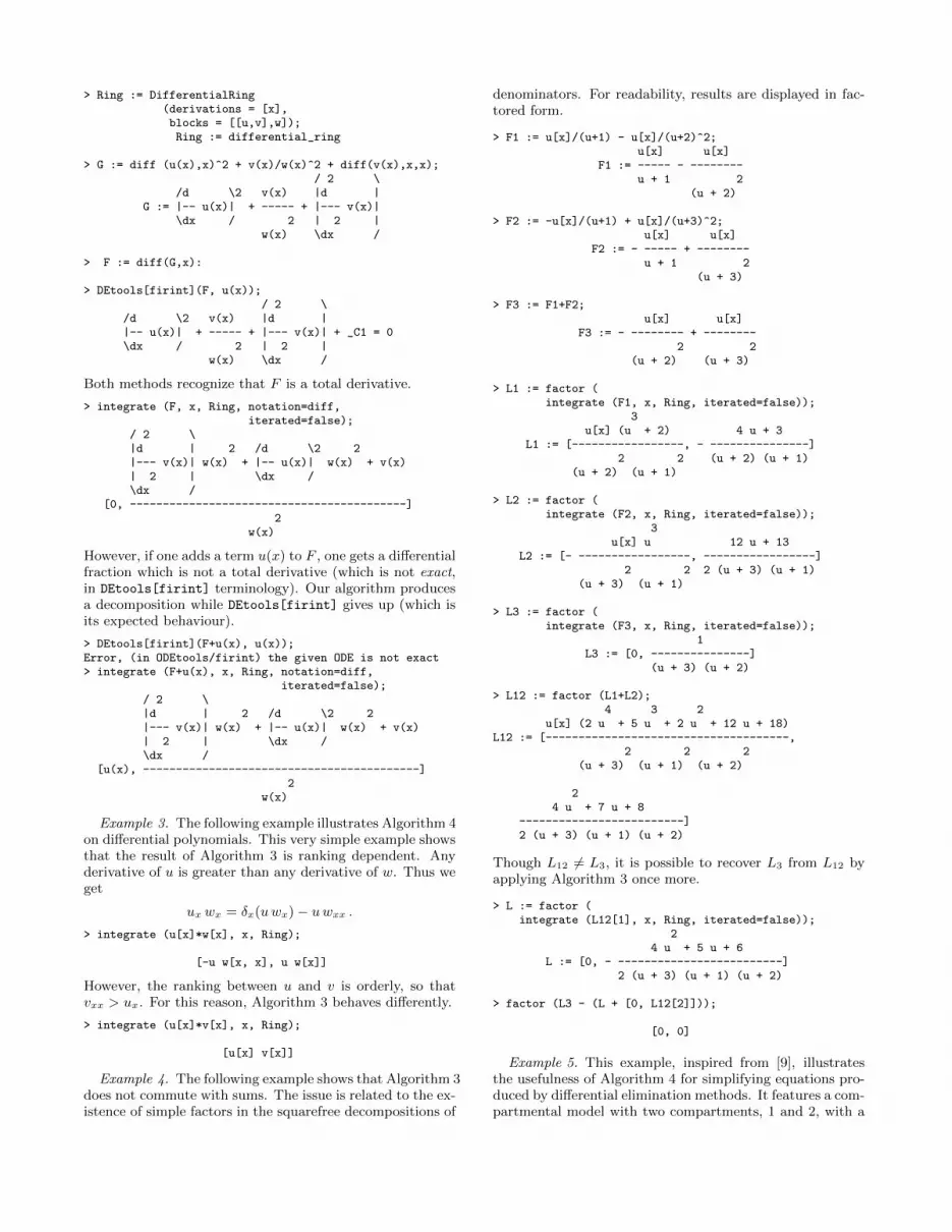
Example 1. The first example shows that Algorithm 3permits to decide if a differential fraction F is the derivativeof some other differential fraction G. Observe that this testwas already implemented in Maple, by the DEtools[firint]function.

The variable Ring receives a description of the differentialranking. The variable G receives a differential fraction, Freceives its derivative w.r.t. x.

> with (DifferentialAlgebra):> with (Tools):> integrate := DifferentialAlgebra0:-Integrate:> Ring := DifferentialRing

(derivations = [x,y],blocks = [[u,v],w]);Ring := differential_ring

> G := u[x]^2 + w[y]/w^2 + w[x,x,y];

2 w[y]G := u[x] + ---- + w[x, x, y]

2w

> F := Differentiate (G, x, Ring);4 4

F := (2 u[x, x] u[x] w + w[x, x, x, y] w

2 / 4+ w[x, y] w - 2 w[x] w[y] w) / w

/

Algorithm 3, implemented here using the name integrate,is applied to F and x. It returns the list [W, R]. We getW = 0, indicating that F = δxR.

> L := integrate (F, x, Ring, iterated=false);2 2 2

u[x] w + w[y] + w[x, x, y] wL := [0, -------------------------------]

2w

> normal (L[2] - G);0

If the optional parameter iterated is left to its default value(true), Algorithm 4 is called.

> L := integrate (F, x, Ring);2 2

u[x] w + w[y]L := [0, ---------------, 0, w[y]]

2w

Example 2. This variant of the previous example showsthe differences between DEtools[firint] and Algorithm 3.Since DEtools[firint] does not handle PDE, we switch toODE and to the standard Maple diff notation.

2This testing version, called DifferentialAlgebra0, isavailable at [4].

> Ring := DifferentialRing(derivations = [x],blocks = [[u,v],w]);Ring := differential_ring

> G := diff (u(x),x)^2 + v(x)/w(x)^2 + diff(v(x),x,x);/ 2 \

/d \2 v(x) |d |G := |-- u(x)| + ----- + |--- v(x)|

\dx / 2 | 2 |w(x) \dx /

> F := diff(G,x):

> DEtools[firint](F, u(x));/ 2 \

/d \2 v(x) |d ||-- u(x)| + ----- + |--- v(x)| + _C1 = 0\dx / 2 | 2 |

w(x) \dx /

Both methods recognize that F is a total derivative.

> integrate (F, x, Ring, notation=diff,iterated=false);

/ 2 \|d | 2 /d \2 2|--- v(x)| w(x) + |-- u(x)| w(x) + v(x)| 2 | \dx /\dx /

[0, ------------------------------------------]2

w(x)

However, if one adds a term u(x) to F , one gets a differentialfraction which is not a total derivative (which is not exact,in DEtools[firint] terminology). Our algorithm producesa decomposition while DEtools[firint] gives up (which isits expected behaviour).

> DEtools[firint](F+u(x), u(x));Error, (in ODEtools/firint) the given ODE is not exact> integrate (F+u(x), x, Ring, notation=diff,

iterated=false);/ 2 \|d | 2 /d \2 2|--- v(x)| w(x) + |-- u(x)| w(x) + v(x)| 2 | \dx /\dx /

[u(x), ------------------------------------------]2

w(x)

Example 3. The following example illustrates Algorithm 4on differential polynomials. This very simple example showsthat the result of Algorithm 3 is ranking dependent. Anyderivative of u is greater than any derivative of w. Thus weget

ux wx = δx(uwx)− uwxx .

> integrate (u[x]*w[x], x, Ring);

[-u w[x, x], u w[x]]

However, the ranking between u and v is orderly, so thatvxx > ux. For this reason, Algorithm 3 behaves differently.

> integrate (u[x]*v[x], x, Ring);

[u[x] v[x]]

Example 4. The following example shows that Algorithm 3does not commute with sums. The issue is related to the ex-istence of simple factors in the squarefree decompositions of

denominators. For readability, results are displayed in fac-tored form.

> F1 := u[x]/(u+1) - u[x]/(u+2)^2;u[x] u[x]

F1 := ----- - --------u + 1 2

(u + 2)

> F2 := -u[x]/(u+1) + u[x]/(u+3)^2;u[x] u[x]

F2 := - ----- + --------u + 1 2

(u + 3)

> F3 := F1+F2;u[x] u[x]

F3 := - -------- + --------2 2

(u + 2) (u + 3)

> L1 := factor (integrate (F1, x, Ring, iterated=false));

3u[x] (u + 2) 4 u + 3

L1 := [-----------------, - ---------------]2 2 (u + 2) (u + 1)

(u + 2) (u + 1)

> L2 := factor (integrate (F2, x, Ring, iterated=false));

3u[x] u 12 u + 13

L2 := [- -----------------, -----------------]2 2 2 (u + 3) (u + 1)

(u + 3) (u + 1)

> L3 := factor (integrate (F3, x, Ring, iterated=false));

1L3 := [0, ---------------]

(u + 3) (u + 2)

> L12 := factor (L1+L2);4 3 2

u[x] (2 u + 5 u + 2 u + 12 u + 18)L12 := [-------------------------------------,

2 2 2(u + 3) (u + 1) (u + 2)

24 u + 7 u + 8

-------------------------]2 (u + 3) (u + 1) (u + 2)

Though L12 6= L3, it is possible to recover L3 from L12 byapplying Algorithm 3 once more.

> L := factor (integrate (L12[1], x, Ring, iterated=false));

24 u + 5 u + 6

L := [0, - -------------------------]2 (u + 3) (u + 1) (u + 2)

> factor (L3 - (L + [0, L12[2]]));

[0, 0]

Example 5. This example, inspired from [9], illustratesthe usefulness of Algorithm 4 for simplifying equations pro-duced by differential elimination methods. It features a com-partmental model with two compartments, 1 and 2, with a

same unit volume. There are two state variables x1 and x2

(one per compartment). State variable xi represents the con-centration of some drug in compartment i. The exchangesbetween the two compartments are supposed to follow lin-ear laws (depending on parameters k1 and k2). The drugis supposed to exit from the model, from compartment 1,following a Michaelis-Menten type law (depending on pa-rameters Ve, ke). The output of the system, denoted y, isthe state variable x1.

> Ring := DifferentialRing (derivations = [t],blocks = [y,[x1,x2],[k1(),k2(),ke(),Ve()]]);

Ring := differential_ring

> S := [ x1[t] = -k1*x1 + k2*x2 - (Ve*x1)/(ke+x1),x2[t] = k1*x1 - k2*x2,

y = x1];

Ve x1S := [x1[t] = -k1 x1 + k2 x2 - -------,

ke + x1

x2[t] = k1 x1 - k2 x2, y = x1]

By means of differential elimination [6], one computes theso-called input-output equation of the system (though thereis no input).

> ideal := RosenfeldGroebner(S, Ring,basefield =

field (generators = [k1,k2,ke,Ve]));

ideal := [regular_differential_chain]

> io_ideal := RosenfeldGroebner(ideal[1],blocks = [[x1,x2],y,[k1(),k2(),ke(),Ve()]]):

> io_eq := Equations(io_ideal, leader = derivative(y))[1];

2 2io_eq := y[t, t] y + 2 y[t, t] y ke + y[t, t] ke

2 2+ y[t] y k1 + y[t] y k2 + 2 y[t] y k1 ke

2 2+ 2 y[t] y k2 ke + y[t] k1 ke + y[t] k2 ke

2+ y[t] ke Ve + y k2 Ve + y k2 ke Ve

Using Algorithm 3, we obtain

> integrate (io_eq / Initial (io_eq, Ring), t, Ring);

2 2 2 2y k2 Ve y k1 + y k2 - k1 ke - k2 ke - ke Ve[-------, ---------------------------------------, y]y + ke y + ke

This list can be translated into the following equation, whosestructure is now much clearer:

y(t) k2 Ve

y(t) + ke+

d

dt

(y(t)2 − k2e) (k1 + k2)− ke Ve

y(t) + ke+

d2

dt2y(t) .

This example also shows that integrating differential frac-tions (as we did above), may yield better formulas than in-tegrating differential polynomials. Indeed:

> integrate (io_eq, t, Ring);

2 2 2[-2 y[t] y - 2 y[t] ke + y k2 Ve + y k2 ke Ve,

3 3y k1 y k2 2 2 2----- + ----- + y k1 ke + y k2 ke + y k1 ke3 3

2 3 2 2+ y k2 ke + y ke Ve, 1/3 y + y ke + y ke ]

While the fractional equation is simpler than that from anintuitive point of view, it would be interesting to investi-gate also their numerical properties from a more systematicviewpoint. In the case of differential-algebraic equations,the usual elimination methods are known to produce typ-ically very lengthy polynomial differential equations whosenumerical treatment may be more costly than that of thecorresponding fractional differential equation.

Remark 5. The four parameters were placed at the bot-tom of the ranking, following the assumptions stated inSection 2. However, the DifferentialAlgebra package,which handles parameters as differential indeterminates con-strained by implicit equations (their derivatives are zero),does not require parameters to lie at the bottom of rank-ings. With such rankings, the second ensured condition ofAlgorithm 3 would not hold anymore.

5. CONCLUSIONThe algorithm presented in this paper may be extended

in many different ways: to handle more complicated differ-ential operators such as δx + δy, possibly with differentialpolynomials for coefficients, for instance. Some prototypesare currently under study.

In this paper, we have not addressed the interest of thethird ensured condition of Algorithm 3. This topic will becovered in a further paper. It is related to the issue of char-acterizing the differential fractions which are returned “asis” by our method.

As mentioned in the Introduction, the decomposition ofa differential polynomial or a differential fraction into a to-tal derivative and a remainder is crucial for constructingthe ring of integro-differential polynomials. Formalizing thisidea in the general category of commutative integro-differen-tial algebras over rings leads to the notion of quasi-antide-rivative [10]. For ordinary differential polynomials in oneindeterminate and for univariate rational functions, a quasi-antiderivative is exhibited in [10] but the case of partial dif-ferential polynomials or differential fractions remains open.While Algorithm 3 comes close to providing such a quasi-antiderivative, it falls short of being linear (Example 4).This question will be addressed in a future paper. It wouldallow us to make progress towards our original goal: definingand computing Grobner bases for ideals of integro-differentialpolynomials of various kinds.

6. ACKNOWLEDGMENTSThe authors thank the referees for their detailed com-

ments, suggestions, and references.

7. REFERENCES[1] A. H. Bilge. A REDUCE program for the integration

of differential polynomials. Computer PhysicsCommunications, 71:263–268, 1992.

[2] G. W. Bluman and S. C. Anco. Symmetry andIntegration Methods for Differential Equations.Springer Verlag, New York, 2002.

[3] F. Boulier. The BLAD libraries.http://www.lifl.fr/~boulier/BLAD, 2004.

[4] F. Boulier. The BMI library.http://www.lifl.fr/~boulier/BMI, 2010.

[5] F. Boulier and E. Cheb-Terrab. Help Pages of theDifferentialAlgebra Package. In MAPLE 14, 2010.

[6] F. Boulier, F. Lemaire, and M. Moreno Maza.Computing differential characteristic sets by change ofordering. Journal of Symbolic Computation,45(1):124–149, 2010.

[7] M. Bronstein. Symbolic Integration I. Springer Verlag,Berlin, Heidelberg, New York, 1997.

[8] G. H. Campbell. Symbolic integration of expressionsinvolving unspecified functions. SIGSAM Bulletin,22(1):25–27, 1988.

[9] L. Denis-Vidal, G. Joly-Blanchard, and C. Noiret.System identifiability (symbolic computation) andparameter estimation (numerical computation). InNumerical Algorithms, volume 34, pages 282–292,2003.

[10] L. Guo, G. Regensburger, and M. Rosenkranz. Onintegro-differential algebras. Preprint available athttp://arxiv.org/abs/1212.0266., 2012.

[11] E. R. Kolchin. Differential Algebra and AlgebraicGroups. Academic Press, New York, 1973.

[12] C. G. Raab. Definite Integration in Differential Fields.PhD thesis, University of Linz, 2012.

[13] J. F. Ritt. Differential Algebra, volume 33 of AmericanMathematical Society Colloquium Publications.American Mathematical Society, New York, 1950.

[14] M. Rosenkranz and G. Regensburger.Integro-differential polynomials and operators. InISSAC’08: Proceedings of the twenty-firstinternational symposium on Symbolic and algebraiccomputation, pages 261–268, New York, NY, USA,2008. ACM.

[15] F. Schwarz. An algorithm for determining polynomialfirst integrals of autonomous systems of ordinarydifferential equations. Journal of SymbolicComputation, 1(2):229–233, 1985.

[16] W. Y. Sit. On Goldman’s algorithm for solvingfirst-order multinomial autonomous systems. InProceedings of the 6th International Conference, onApplied Algebra, Algebraic Algorithms andError-Correcting Codes, AAECC-6, pages 386–395,London, UK, 1989. Springer-Verlag.