arX

iv:1

309.

0314

v2 [

hep-

ph]

1 Ja

n 20

14

Phenomenology of Space-time Imperfection II: LocalDefects

S. Hossenfelder∗

NorditaKTH Royal Institute of Technology and Stockholm University

Roslagstullsbacken 23, SE-106 91 Stockholm, Sweden

Abstract

We propose a phenomenological model for the scattering of particles on space-time defects in a treatment that maintains Lorentz-invariance on the average. Thelocal defects considered here cause a stochastic violationof momentum conser-vation. The scattering probability is parameterized in thedensity of defects andthe distribution of the momentum that a particle can obtain when scattering on thedefect. We identify the most promising observable consequences and derive con-straints from existing data.

1 Introduction

The phenomenology of quantum gravity proceeds by the development of models thatparameterize properties which the, still unknown, theory of quantum gravity might have.These phenomenological models are constructed for the purpose of being testable byexperiment and thereby guide the development of the theory.Among the best studiedphenomenological consequences of quantum gravity are violations or deformations ofLorentz-invariance, additional spatial dimensions, and decoherence induced by quantumfluctuations of space-time. Research in the area of quantum gravity phenomenologytoday encompasses a large variety of models that have been reviewed in [1, 2, 3].

A possible observable consequence of quantum gravity that has so far gotten little at-tention is the existence of space-time defects. If the seemingly smooth space-time that weexperience is not fundamental but merely emergent from an underlying, non-geometrictheory then we expect it to be imperfect – it should have defects. We will here studywhich observational consequences can be expected from suchspace-time imperfectionsof non-geometric origin.

∗hossi@nordita.org

1

S. Hossenfelder Local Defects

Space-time defects are localized both in space and in time and therefore, in contrastto defects in condensed-matter systems, do not have worldlines. There are two differenttypes of defects: Local defects and nonlocal defects. Localdefects respect the emergentlocality of the space-time manifold. A particle that encounters a local defect will scatterand change direction, but continue its world-line continuously. Nonlocal defects on theother hand do not respect the emergent locality of the space-time manifold. A particlethat encounters a nonlocal defect continues its path in space-time elsewhere, but with thesame momentum. The nonlocal defect causes a translation in space-time, while the localdefect causes a translation in momentum-space.

The present paper is the second part of a study of space-time defects and deals withlocal defects. Nonlocal defects have been subject of the first part [4]. In principle aspace-time defect could cause both, a change of position andmomentum. But beforemaking the situation more complicated by combining these two effects, we will firststudy the two cases separately. In this paper, we develop a model for the local type ofdefects. Since Lorentz-invariance violation is the probably most extensively studied areaof Planck-scale physics [5, 6], we will only consider the case where Lorentz-invarianceis maintained on the average. A different model for local space-time defects has recentlybeen put forward in [7]. We will briefly comment on the differences to this model in thediscussion.

We use the unit convention~ = c = 1. The signature of the metric is(+,−,−,−).

2 The distribution of defects

To develop our model for local defects, we will here start with the simplest case in whichthe emergent background space-time is flat Minkowski space,ie background curvatureis not taken into account. This approximation will allow us to describe only systems inwhich gravitational effects are negligible, but it is good enough for Earth-based laborato-ries and interstellar propagation over intergalactic distances where curvature is weak andredshift can still be neglected. These will be the cases we consider in section 5.

The only presently known probability distribution for points in Minkowski space thatpreserves Lorentz-invariance on the average is the result of a Poisson process developedand studied in [8, 9]. With this distribution, the probability of finding N points in aspace-time volumeV is

PN(V ) =(βV )N exp(−βV )

N!, (1)

whereβ is a constant space-time density.The average value of the number of points that one will find in some volumeV is

then the expectation value of the above distribution and given by

〈N(V )〉 =∞∑

N=0

PN(V )N = βV . (2)

2

S. Hossenfelder Local Defects

The variance that quantifies the typical fluctuations aroundthe mean is∆N ∼ √βV , and

the corresponding fluctuations in the density of points are∆(N/V ) ∼√

β/V . In otherwords, the density fluctuations will be small for large volumes.

We will use the distribution (1) to seed the defects with an average densityβ. Inthe following, we will not be concerned with fluctuations in the density as our aim hereis to first get a general understanding for the type and size ofeffects caused by localdefects and using the average will suffice for the present purpose. The probability is adensity over space-timeβ = Ld+1, whereL is a length scale andd is the number ofspatial dimensions. The ratio between the fundamental length scale, that we take to bethe Planck lengthlP, andL is ǫ = lP/L ≪ 1, ie the defects are sparse. Just exactly howsparse is a question of experimental constraints that we will address in section 5.

3 Kinematics of scattering on local defects

The idea which we want to parameterize here is that local defects are deviations fromthe smooth geometry of general relativity that cause a violation of energy-momentumconservation.

The requirement of Lorentz-invariance restricts what the particle can do when it en-counters such a local defect. This restriction is more stringent than for normal scatteringprocesses because we have fewer quantities as input. We onlyhave the ingoing and out-going momenta, whereas one normally has at least three momenta involved in scattering,leading to the three invariant Mandelstam variables.

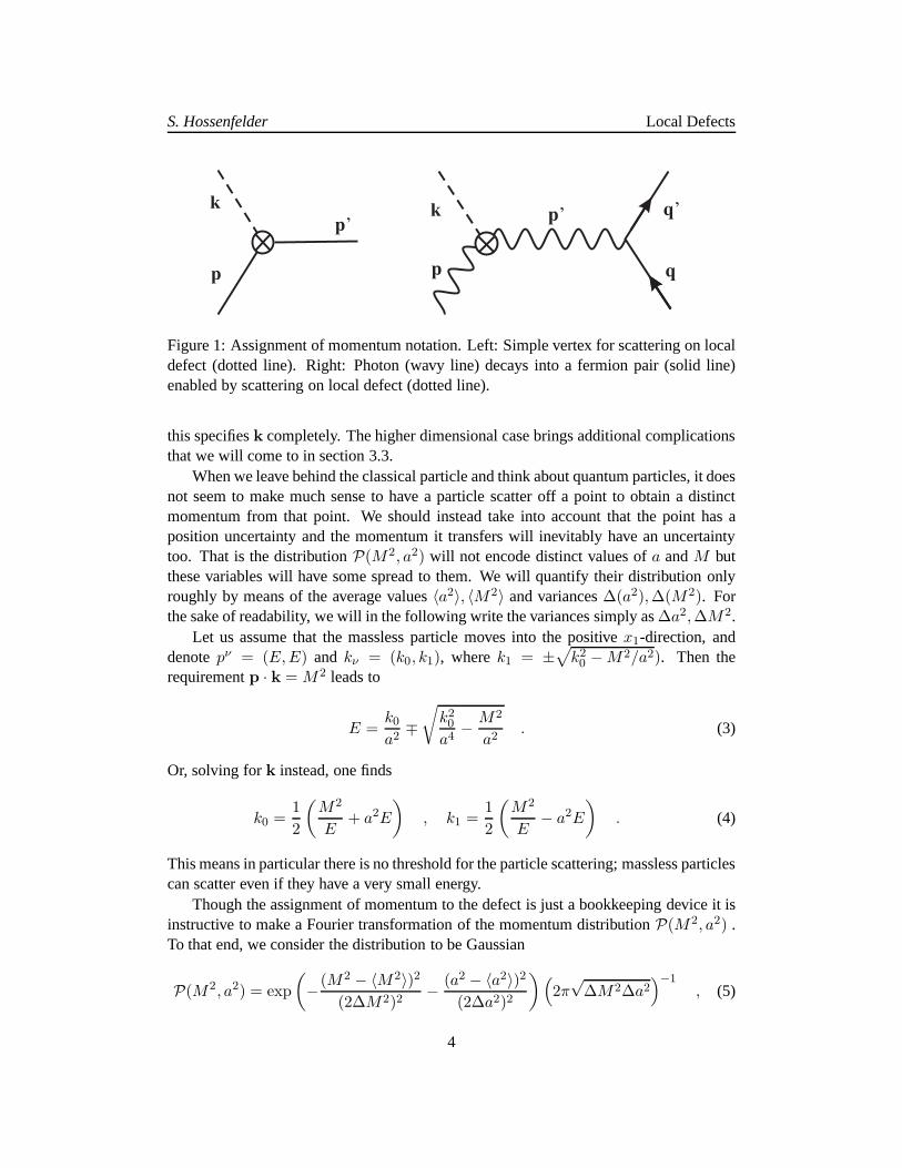
Let us denote the momentum of the particle before it encounters the defect withpand the momentum after it encountered the defect withp′, where boldfaced quantitiesdenote four-vectors. Let us further formally assign the momentumk = p′ − p to thedefect (see Figure 1 left). This assignment of momentum to the defect is a bookkeepingdevice that will allow us to think in terms of normal scattering processes. The space-timedefect itself does however not actually have a momentum; it instead causes a violation ofmomentum conservation.

3.1 Massless particles in 1+1 dimensions

We will first consider the case where the ingoing particle is right moving and massless,m = 0. Sincep2 = 0, we have two Lorentz-invariants left,p · k = M2 andk2 = a2M2

(thusp′2 = (a2+2)M2), wherem andM have dimension mass, anda is a dimensionlessparameter that we expect to be of order one. It is henceforth assumed thata andM arereal-valued to avoid that the mass of the outgoing particle can become tachyonic.

We want to quantify now the probabilityP for what will happen when the particleencounters the defect. Lorentz-invariance requiresP to be a function solely ofa andM , and our expectation is that it is actually a function ofa2 andM2. The conditionp · k = M2 selects a cut in the hyperboloid defined byk2 = a2M2. In 1+1 dimensions,

3

S. Hossenfelder Local Defects

p

p’

k

p

p’

q

q’k

Figure 1: Assignment of momentum notation. Left: Simple vertex for scattering on localdefect (dotted line). Right: Photon (wavy line) decays intoa fermion pair (solid line)enabled by scattering on local defect (dotted line).

this specifiesk completely. The higher dimensional case brings additionalcomplicationsthat we will come to in section 3.3.

When we leave behind the classical particle and think about quantum particles, it doesnot seem to make much sense to have a particle scatter off a point to obtain a distinctmomentum from that point. We should instead take into account that the point has aposition uncertainty and the momentum it transfers will inevitably have an uncertaintytoo. That is the distributionP(M2, a2) will not encode distinct values ofa andM butthese variables will have some spread to them. We will quantify their distribution onlyroughly by means of the average values〈a2〉, 〈M2〉 and variances∆(a2),∆(M2). Forthe sake of readability, we will in the following write the variances simply as∆a2,∆M2.

Let us assume that the massless particle moves into the positive x1-direction, anddenotepν = (E,E) and kν = (k0, k1), wherek1 = ±

√

k20 −M2/a2). Then therequirementp · k = M2 leads to

E =k0a2

∓√

k20a4

− M2

a2. (3)

Or, solving fork instead, one finds

k0 =1

2

(

M2

E+ a2E

)

, k1 =1

2

(

M2

E− a2E

)

. (4)

This means in particular there is no threshold for the particle scattering; massless particlescan scatter even if they have a very small energy.

Though the assignment of momentum to the defect is just a bookkeeping device it isinstructive to make a Fourier transformation of the momentum distributionP(M2, a2) .To that end, we consider the distribution to be Gaussian

P(M2, a2) = exp

(

−(M2 − 〈M2〉)2(2∆M2)2

− (a2 − 〈a2〉)2(2∆a2)2

)

(

2π√∆M2∆a2

)−1, (5)

4

S. Hossenfelder Local Defects

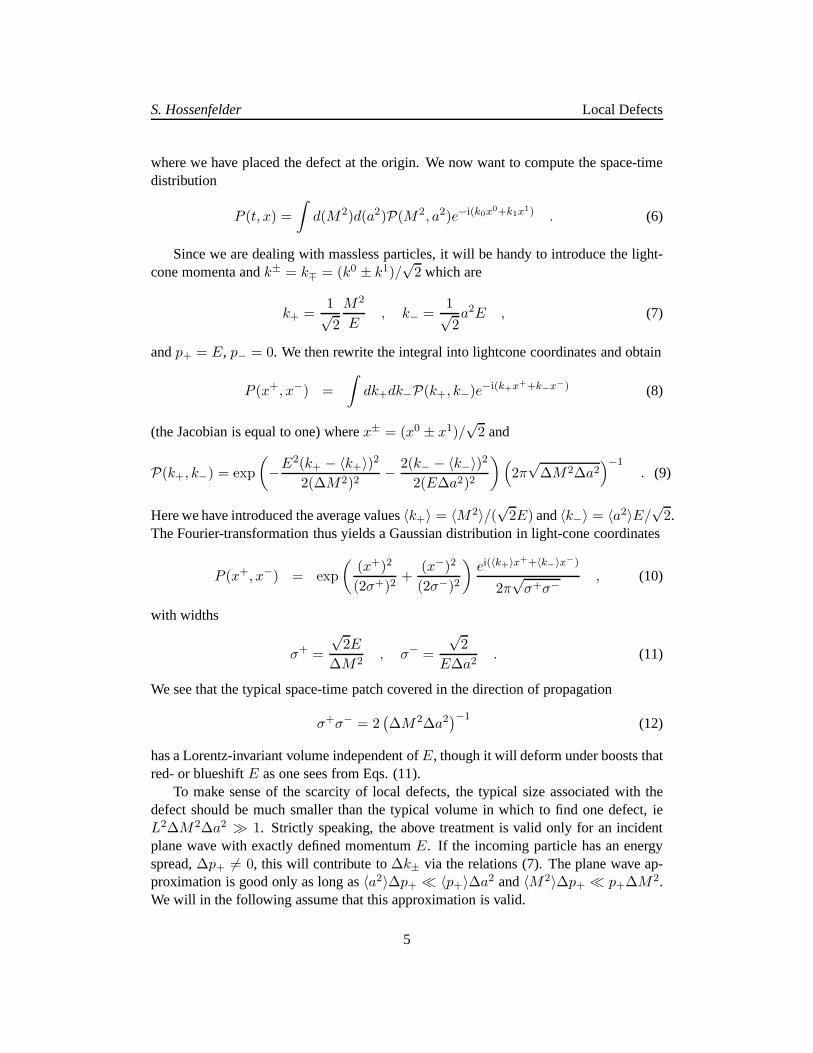
where we have placed the defect at the origin. We now want to compute the space-timedistribution

P (t, x) =

∫

d(M2)d(a2)P(M2, a2)e−i(k0x0+k1x1) . (6)

Since we are dealing with massless particles, it will be handy to introduce the light-cone momenta andk± = k∓ = (k0 ± k1)/

√2 which are

k+ =1√2

M2

E, k− =

1√2a2E , (7)

andp+ = E, p− = 0. We then rewrite the integral into lightcone coordinates and obtain

P (x+, x−) =

∫

dk+dk−P(k+, k−)e−i(k+x++k−x−) (8)

(the Jacobian is equal to one) wherex± = (x0 ± x1)/√2 and

P(k+, k−) = exp

(

−E2(k+ − 〈k+〉)22(∆M2)2

− 2(k− − 〈k−〉)22(E∆a2)2

)

(

2π√∆M2∆a2

)−1. (9)

Here we have introduced the average values〈k+〉 = 〈M2〉/(√2E) and〈k−〉 = 〈a2〉E/

√2.

The Fourier-transformation thus yields a Gaussian distribution in light-cone coordinates

P (x+, x−) = exp

(

(x+)2

(2σ+)2+

(x−)2

(2σ−)2

)

ei(〈k+〉x++〈k−〉x−)

2π√σ+σ−

, (10)

with widths

σ+ =

√2E

∆M2, σ− =

√2

E∆a2. (11)

We see that the typical space-time patch covered in the direction of propagation

σ+σ− = 2(

∆M2∆a2)−1

(12)

has a Lorentz-invariant volume independent ofE, though it will deform under boosts thatred- or blueshiftE as one sees from Eqs. (11).

To make sense of the scarcity of local defects, the typical size associated with thedefect should be much smaller than the typical volume in which to find one defect, ieL2∆M2∆a2 ≫ 1. Strictly speaking, the above treatment is valid only for anincidentplane wave with exactly defined momentumE. If the incoming particle has an energyspread,∆p+ 6= 0, this will contribute to∆k± via the relations (7). The plane wave ap-proximation is good only as long as〈a2〉∆p+ ≪ 〈p+〉∆a2 and〈M2〉∆p+ ≪ p+∆M2.We will in the following assume that this approximation is valid.

5

S. Hossenfelder Local Defects

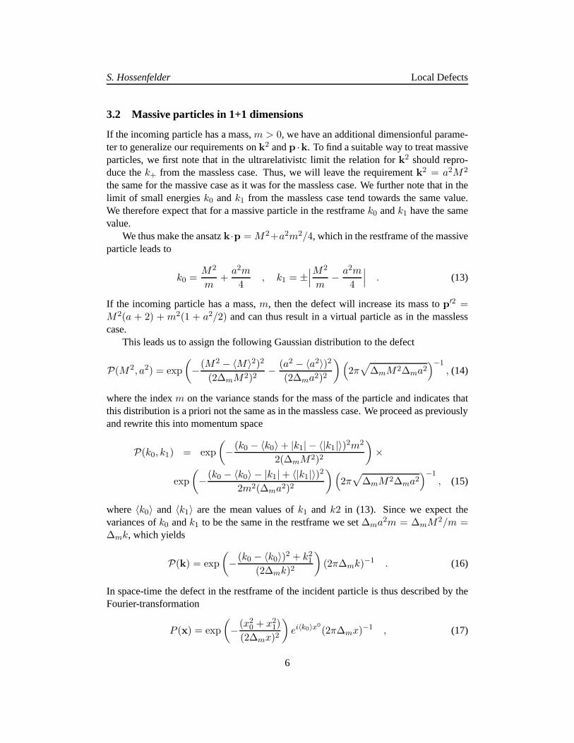
3.2 Massive particles in 1+1 dimensions

If the incoming particle has a mass,m > 0, we have an additional dimensionful parame-ter to generalize our requirements onk2 andp ·k. To find a suitable way to treat massiveparticles, we first note that in the ultrarelativistc limit the relation fork2 should repro-duce thek+ from the massless case. Thus, we will leave the requirementk2 = a2M2

the same for the massive case as it was for the massless case. We further note that in thelimit of small energiesk0 andk1 from the massless case tend towards the same value.We therefore expect that for a massive particle in the restframek0 andk1 have the samevalue.

We thus make the ansatzk·p = M2+a2m2/4, which in the restframe of the massiveparticle leads to

k0 =M2

m+

a2m

4, k1 = ±

∣

∣

∣

M2

m− a2m

4

∣

∣

∣ . (13)

If the incoming particle has a mass,m, then the defect will increase its mass top′2 =M2(a + 2) + m2(1 + a2/2) and can thus result in a virtual particle as in the masslesscase.

This leads us to assign the following Gaussian distributionto the defect

P(M2, a2) = exp

(

−(M2 − 〈M〉2)2(2∆mM2)2

− (a2 − 〈a2〉)2(2∆ma2)2

)

(

2π√

∆mM2∆ma2)−1

, (14)

where the indexm on the variance stands for the mass of the particle and indicates thatthis distribution is a priori not the same as in the massless case. We proceed as previouslyand rewrite this into momentum space

P(k0, k1) = exp

(

−(k0 − 〈k0〉+ |k1| − 〈|k1|〉)2m2

2(∆mM2)2

)

×

exp

(

−(k0 − 〈k0〉 − |k1|+ 〈|k1|〉)22m2(∆ma2)2

)

(

2π√

∆mM2∆ma2)−1

, (15)

where〈k0〉 and 〈k1〉 are the mean values ofk1 and k2 in (13). Since we expect thevariances ofk0 andk1 to be the same in the restframe we set∆ma2m = ∆mM2/m =∆mk, which yields

P(k) = exp

(

−(k0 − 〈k0〉)2 + k21(2∆mk)2

)

(2π∆mk)−1 . (16)

In space-time the defect in the restframe of the incident particle is thus described by theFourier-transformation

P (x) = exp

(

−(x20 + x21)

(2∆mx)2

)

ei〈k0〉x0

(2π∆mx)−1 , (17)

6

S. Hossenfelder Local Defects

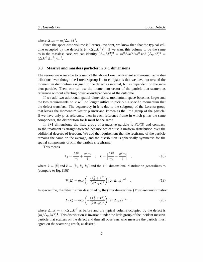
where∆mx = m/∆mM2.Since the space-time volume is Lorentz-invariant, we know then that the typical vol-

ume occupied by the defect is(m/∆mM2)2. If we want this volume to be the sameas in the massless case, we can identify(∆mM2)2 = m2∆M2∆a2 and (∆ma2)2 =(∆M2∆a2)/m2.

3.3 Massive and massless particles in 3+1 dimensions

The reason we were able to construct the above Lorentz-invariant and normalizable dis-tributions even though the Lorentz-group is not compact is that we have not treated themomentum distribution assigned to the defect as internal, but as dependent on the inci-dent particle. Then, one can use the momentum vector of the particle that scatters asreference without affecting observer-independence of theoutcome.

If we add two additional spatial dimensions, momentum spacebecomes larger andthe two requirements onk will no longer suffice to pick out a specific momentum thatthe defect transfers. The degeneracy ink is due to the subgroup of the Lorentz-groupthat leaves the momentum vectorp invariant, known as the little group of the particle.If we have onlyp as reference, then in each reference frame in whichp has the samecomponents, the distribution fork must be the same.

In 3+1 dimensions, the little group of a massive particle isSO(3) and compact,so the treatment is straight-forward because we can use a uniform distribution over theadditional degrees of freedom. We add the requirement that the restframe of the particleremains the same on the average, and the distribution is spherically symmetric for thespatial components ofk in the particle’s restframe.

This means

k0 =M2

m+

a2m

4, k =

∣

∣

∣

M2

m− a2m

4

∣

∣

∣, (18)

wherek = |~k| and~k = (k1, k2, k3) and the 1+1 dimensional distribution generalizes to(compare to Eq. (16))

P(k) = exp

(

−(k20 + k2)

(2∆mk)2

)

(2π∆mk)−2 . (19)

In space-time, the defect is thus described by the (four dimensional) Fourier-transformation

P (x) = exp

(

−(x20 + x2)

(2∆mx)2

)

(2π∆mx)−2 , (20)

where∆mx = m/∆mM2 as before and the typical volume occupied by the defect is(m/∆mM2)4. This distribution is invariant under the little group of the incident massiveparticle that scatters on the defect and thus all observers who measure the particle mustagree on the scattering result, as desired.

7

S. Hossenfelder Local Defects

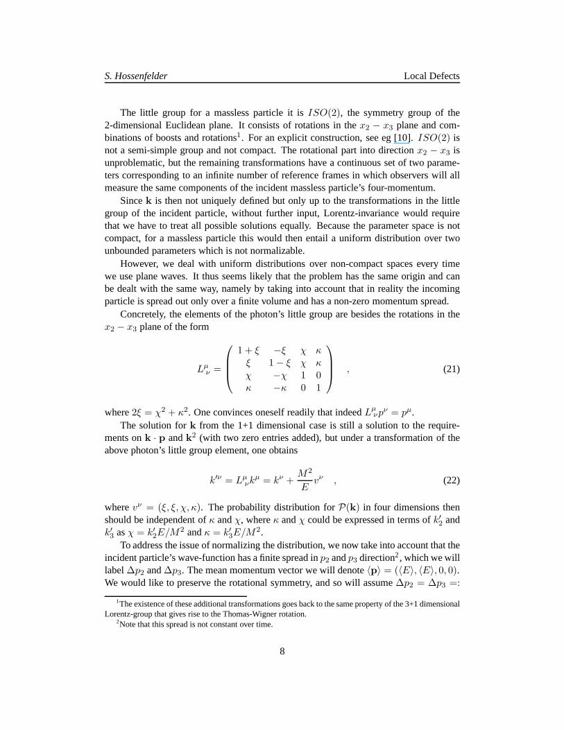
The little group for a massless particle it isISO(2), the symmetry group of the2-dimensional Euclidean plane. It consists of rotations inthex2 − x3 plane and com-binations of boosts and rotations1. For an explicit construction, see eg [10].ISO(2) isnot a semi-simple group and not compact. The rotational partinto directionx2 − x3 isunproblematic, but the remaining transformations have a continuous set of two parame-ters corresponding to an infinite number of reference framesin which observers will allmeasure the same components of the incident massless particle’s four-momentum.

Sincek is then not uniquely defined but only up to the transformations in the littlegroup of the incident particle, without further input, Lorentz-invariance would requirethat we have to treat all possible solutions equally. Because the parameter space is notcompact, for a massless particle this would then entail a uniform distribution over twounbounded parameters which is not normalizable.

However, we deal with uniform distributions over non-compact spaces every timewe use plane waves. It thus seems likely that the problem has the same origin and canbe dealt with the same way, namely by taking into account thatin reality the incomingparticle is spread out only over a finite volume and has a non-zero momentum spread.

Concretely, the elements of the photon’s little group are besides the rotations in thex2 − x3 plane of the form

Lµν =

1 + ξ −ξ χ κξ 1− ξ χ κχ −χ 1 0κ −κ 0 1

, (21)

where2ξ = χ2 + κ2. One convinces oneself readily that indeedLµνpν = pµ.

The solution fork from the 1+1 dimensional case is still a solution to the require-ments onk · p andk2 (with two zero entries added), but under a transformation oftheabove photon’s little group element, one obtains

k′ν = Lµνk

µ = kν +M2

Evν , (22)

wherevν = (ξ, ξ, χ, κ). The probability distribution forP(k) in four dimensions thenshould be independent ofκ andχ, whereκ andχ could be expressed in terms ofk′2 andk′3 asχ = k′2E/M2 andκ = k′3E/M2.

To address the issue of normalizing the distribution, we nowtake into account that theincident particle’s wave-function has a finite spread inp2 andp3 direction2, which we willlabel∆p2 and∆p3. The mean momentum vector we will denote〈p〉 = (〈E〉, 〈E〉, 0, 0).We would like to preserve the rotational symmetry, and so will assume∆p2 = ∆p3 =:

1The existence of these additional transformations goes back to the same property of the 3+1 dimensionalLorentz-group that gives rise to the Thomas-Wigner rotation.

2Note that this spread is not constant over time.

8

S. Hossenfelder Local Defects

∆p⊥. These relevant point is that these extensions in directionx2 andx3 are perpen-dicular to the photon’s wave-vector and not invariant underthe little group. Therefore,they provide us with additional information about the incident particle that we can useto put bounds on the integration overκ andχ, or (dropping the primes) onk2 andk3respectively. We do this by assuming that the width of the defect in momentum space has∆k2 = ∆k3 =: ∆k⊥ = ∆M2/∆p⊥ and so (compare to Eq. (9))

P(k) = exp

(

− 〈E〉2k2+(∆M2)2

− (k− − 〈k−〉)2(〈E〉∆a2)2

− k2⊥2∆k2⊥

)

(

4π2∆k⊥√∆M2∆a2

)−1(23)

wherek2⊥ = k22 + k23 .In (23) we have set〈M2〉 = 0. In this case, the average ofk is parallel to the

average ofp. Any other choice will, in the plane wave limit (when〈E〉 = E), not beinvariant under the little group as one sees from Eq (22). It is thus henceforth assumedthat 〈M2〉 = 0 and thus〈k+〉 = 0. In the plane-wave limit where∆p⊥ → 0, one thenhas∆k⊥ → ∞ and the distribution ofk will go to the uniform distribution over the littlegroup.

This construction for massless particles in 3+1 dimensionsis not invariant under thelittle group of the mean momentum of the incoming photon wavepacket. But this isunnecessary because the incident particle, when it has a finite width, has the rotationalsymmetry inx2 − x3 as the only remaining symmetry. Thus, observer independence ispreserved and the distribution is normalizable. In the plane-wave limit, the components ofk can become arbitrarily large and then the defect can in principle transfer an arbitrarilylarge momentum to the particle. In reality, this momentum transfer will however bebounded because the incident particle has a finite width. We have essentially identifiedthe non-compact part ofISO(2) with the non-compactness of the plane wave.

In summary, we have seen that Lorentz-invariance proves to be surprisingly restric-tive on the possible scattering outcomes. We have dealt withthe non-compactness ofthe Lorentz-group by using measurable properties of the incident particle to reduce thesymmetry of the momentum non-conservation mediated by the defect while preservingobserver-independence.

4 Dynamics of scattering on local defects

This now leads us to ask what we can say about scattering amplitudes. For concreteness,we assume that the defect makes itself noticeable in the covariant derivative since thelocal defect represents a non-geometric inhomogeneity that cannot be accounted for bythe normal covariant derivative.

The local defect thus appears in the Lagrangian together with the derivative terms andgauge fields and can be implemented by replacing the normal gauge-invariant derivativeD = ∂ + eA with D = ∂ + eA + g∂P , whereP is the previously introduced Fourier-transform of the momentum distributionP, and the derivative∂P is proportional top′−

9

S. Hossenfelder Local Defects

p = k. e is some Standard Model coupling constant (not necessarily that of QED thoughthis will be the case we consider later) andg is the coupling constant for the defects. Sincethe mass dimension of[P ] = [E2], the dimension of[g] = [E−2], and since we have onlyone scale of dimension mass at our hands, we useg = 1/∆M2.

The defects are sprinkled over space-time according to the Poisson process describedin section 2, but since we are considering the homogenous case we will not treat thedefects as individual events. We will instead replace the many single defects by a fieldP with which the standard model fields have a small interactionprobability. That is,instead of interacting with defects in rare places, the particle interacts with the defect-field anywhere but with low probability.

In this limit, instead of having a sum over many defects, the probability to interactwith the defect-fieldP is suppressed by the volume of the defect over the typical volumein which to find a defect, ie

g2 =1

(∆M2)2σ+σ−

∆k2⊥L4

. (24)

This is a similar approximation as we have made in [4] in that it is implicitly assumedhere that scattering on defects happens often enough so thatwe can effectively describeit as a homogeneously occuring process. Concretely this means that this approximationis only good if the space-time volume swept out by a particle’s wave-function is largeenough to contain a large number (≫ 1) of defects. In this sense it is an effective de-scription, not unlike in-medium propagation of photons, except that here we maintainLorentz-invariance and thus the effects (have to) scale differently.

We note however that not only is the coupling constant dimensionful, but also goesto zero in the plane wave-limit, when∆p⊥ → 0 and∆k⊥ → ∞. This behavior is anartifact of the normalization and dimension of the fieldP which contains a prefactor of∆k⊥. To avoid having to deal with quantities that diverge in the plane wave limit, wewill thus shift this normalization factor fromP into the coupling constant, so that bothbecome dimensionless. We therefore define

P (x) :=P (x)

∆k⊥√∆M2

, P(k) :=P(k)

∆k⊥√∆M2

, (25)

g := g∆k⊥√∆M2 =

1

∆M2

1√∆a2

1

L2. (26)

With this definition, the coupling to standard model fields isthenD = ∂ + eA + g∂Pandg is dimensionless and remains finite in the plane wave limit.

We will further in the following assume that the defects do not carry any standardmodel charges and do not change the type of the ingoing particle, ie the scattering isentirely elastic. In principle we could have a defect that changes not only the momentumbut also the spin of the particle, but we will not consider this possibility here.

That the assignment ofP (x) to the defect is a bookkeeping device rather than theintroduction of a new field is somewhat hidden in this notation, which looks like we have

10

S. Hossenfelder Local Defects

introduced a new field. ThatP (x) is not actually an independent quantity can be seenmost clearly from Eqs (6) and (4). The momentumk that is assigned to the defect is aderived quantity from the particle’s incoming momentump, andP is thus an operatoracting on the same field that the gauge-covariant derivativeacts on.

From this function ofP (x) it is also clear that the scattering on the local defect, in theform that we have introduced it here, will break gauge invariance. This might not comeas a surprise since the simplest Lorentz-invariant change to the dynamics of a masslessgauge field is adding a mass term. Here, the underlying reasonfor the breaking of gaugeinvariance is that the defect itself is not gauged, ie thek that is derived from the incomingmomentump does not respect the gauge of the incoming particle.

One could fix gauge invariance by appropriately adding the gauge field tok from thebeginning on, but then one would obtain a nasty integral withgauge fields in exponents.Because of this complication together with the breaking of gauge invariance being notunexpected, we will accept that gauge invariance is broken.In the abelian case the addi-tional terms for coupling a fermion field and its gauge-field to the defect are then of theform gΨ†(/∂P )Ψ, e2g∂A(∂P )A, e2g2(∂P )A(∂P )A.

With this prescription one can now calculate the scatteringamplitudes for processesof interest. For each amplitude where one of the incoming particles previously scatteredon the defect, one gets an additional integral overd(a2)d(M2)dk2dk3, ordk+dk−d2k⊥ =d4k respectively. From this one obtains a cross-section or decay rate as usual.

Before we turn towards some examples, let us make a general observation. Since〈M2〉 = 0 andP does not vanish forM2 = 0 if we assume a Gaussian distribution, itseems that a massless on-shell particle could remain on-shell and the momentum of theoutgoing particlep′ would then be a multiple of the momentum of the ingoing particlep. However, unless the incident particle is virtual, the vertex factors all vanish becausethere is then no non-zero contraction of the momentumk and the massless particle’smomentum or its transverse polarization tensor. Thus, if the incoming massless particleis real, the outgoing massless particle will necessarily bevirtual.

For the massive particle, whenM2 = 0 the outgoing momentum must fulfillp′2 =(1 + a2)m2 and thus the particle is virtual unless alsoa2 = 0 in which case the particleonly receives a transverse momentum from the defect that is equally distributed in itsrestframe. Alas, ifM2 = a2 = 0, the particle did not acquire kinetic energy and thus anon-zero transverse momentum would violate the mass-shellcondition. In other words,the massive particle too must be off-shell after changing its momentum by scattering onthe defect.

Since the defects are sparse or the coupling constant is small respectively, we expecteffects to be small and noticeable primarily for long-livedparticles.

11

S. Hossenfelder Local Defects

5 Constraints from observables

We will in the following make the assumption that〈a2〉 ∼ ∆a2 ∼ 1. Then we are leftwith two parameters,∆M2 andL. (For some discussion on this and the other assump-tions, see next section.)

Let us start with some general remarks. Since we are looking for constraints on (nor-mally) stable particles that propagate over long times or distances respectively, we willfocus on the QED sector of the standard model and on particlesthat we observe comingfrom distant astrophysical sources. This makes in particular the photon a sensitive probefor the presence of local defects.

If a photon scatters on the defect and becomes a virtual photon with mass∼√3M , it

can only decay into a fermion pair if√3M is larger than twice the mass of the fermion.

If√3M is smaller than twice the electron mass, this leaves decay into a neutrino and an-

tineutrino as the only option, which would necessitate a higher-order electroweak processand dramatically lower the cross-section. IfM is smaller than even the lightest neutrinos,the only option left for the virtual photon is to scatter on another defect.

The phenomenology thus depends significantly on the value of∆M2 because it de-termines the relevance of possible decay channels through the typical range in the prob-ability distributionP. The is always some possibility forM2 or a2 to take on very smallor very large values, but the probability for this to happen is highly suppressed ifM2

is many orders of magnitude beyond∆M2. For the rest of this section, we will onlyestimate the orders of magnitude for typical values ofM , and will therefore from now onjust writeM2 for ∆M2 and omit factors of order one.

In order to get a grip on the phenomenology, let us thus identify and focus on theparameter range that seems most interesting.

As mentioned previously, to make sense of the defects, we expect their typical volumeto be small in comparison to the typical distance between thedefects which is givenby the densityβ. Or, in other words, we expect the effective coupling constant in thehomogeneous limit,g, to be much smaller than one. Since we have already introducedone small parameterǫ = lP/L that is the (fourth root of) the density of the defects over aPlanck density, the rangeM2L2 ∼ 1/ǫ ≫ 1 is of particular interest. If furthermoreL isin the same range as the length scale associated with the cosmological constant (a tenthof a millimeter or so), thenM is approximately in the TeV range. This is the parameterrange that we will focus on in the following3. In this parameter range, there is then noproblem for the virtual photon to decay into fermions, and there are three processes ofmain interest:

1. Photon decay: The photon can make a vacuum-decay into a pair of electrons via adiagram as shown in Fig 1, right. This results in a finite photon lifetime, and leads

3The energy and the length scales are not necessarily the sameas those parameterizing the effects ofnonlocal defects in [4].

12

S. Hossenfelder Local Defects

to electron-positron pair production. This process is similar to pair production inthe presence of an atomic nucleus in standard QED.

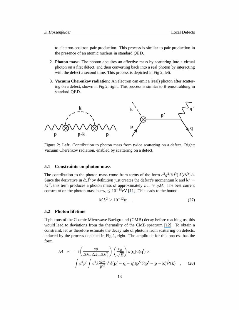
2. Photon mass: The photon acquires an effective mass by scattering into a virtualphoton on a first defect, and then converting back into a real photon by interactingwith the defect a second time. This process is depicted in Fig2, left.

3. Vacuum Cherenkov radiation: An electron can emit a (real) photon after scatter-ing on a defect, shown in Fig 2, right. This process is similarto Bremsstrahlung instandard QED.

p p k- p

k

p

p’

q

q’k

Figure 2: Left: Contribution to photon mass from twice scattering on a defect. Right:Vacuum Cherenkov radiation, enabled by scattering on a defect.

5.1 Constraints on photon mass

The contribution to the photon mass come from terms of the form e2g2(∂P )A(∂P )A.Since the derivative in∂νP by definition just creates the defect’s momentumk andk2 =M2, this term produces a photon mass of approximatelymγ ≈ gM . The best currentconstraint on the photon mass ismγ ≤ 10−18eV [11]. This leads to the bound

ML2 ≥ 10−12m . (27)

5.2 Photon lifetime

If photons of the Cosmic Microwave Background (CMB) decay before reaching us, thiswould lead to deviations from the thermality of the CMB spectrum [12]. To obtain aconstraint, let us therefore estimate the decay rate of photons from scattering on defects,induced by the process depicted in Fig 1, right. The amplitude for this process has theform

M ∼ −i

(

eg

∆k+∆k−∆k2⊥

)(

eµ√E

)

u(q)u(q′)×∫

d4p′∫

d4kηµνp′2

γνδ(p′ − q− q′)p′2δ(p′ − p− k)P(k) , (28)

13

S. Hossenfelder Local Defects

where we have omitted some factors of2π and√2.

In the order displayed, the amplitude (28) is composed of thecoupling constant forthe first and second vertex, the normalization ofP(k), the polarization tensor of the in-coming photoneµ with (dimensionful) normalization, the spinor wave-functions of theoutgoing electron and positronu(q) andu(q′) with normalization omitted, the photonpropagator, the first vertex and the second vertex, multiplied with the probability distri-bution and integrated over the momentum of the virtual photon and that of the defect.

Omitting the polarization and spinor structure, we can perform the integral overqand estimate the integral overP(k) by evaluating the integrant at one standard deviation(times the variances, which cancel with the prefactor). This gives

M ∼ −ieg√Eδ(p′ + k− q− q′) , (29)

wherek is given by Eqs. 4 (recall that we replaced∆M2 with M2). From this we obtainan estimate for the decay rate

Γ(γ → e+e−) ≈ Eαg2 . (30)

The photon half-life timeτγ is thus

τγ ≈ L4M4

αE0z0

∫ z0

0dza(z) , (31)

whereE0 is the photon energy at the present time,z0 ≈ 1100 the redshift at the timeof production of the photon, anda(z) is the redshift-dependent scale factor. WithE0 ∼10−2eV for a typical CMB photon, the requirement that no more thanabout10−4 CMBphotons should have decayed at the present time leads toτγ ≥ 1021s and

LM ≥ 108 . (32)

This constraint however assumes that the density of defectsremains constant in time,the case that was also considered in [13]. If the density of defects dilutes, then it wouldhave been higher in the past, thereby decreasing the averagedecay time and tighteningthe constraint. It would need a more sophisticated model forthe generation of defectsto know how the density evolves in time. However, if one makesthe ad-hoc assumptionthatL(z) ∼ L0a(z), M = M0, then the constraint (onL0M0) is by a factor of about103

stronger.

5.3 Cosmological vacuum opacity

Besides affecting the CMB spectrum, decaying photons will furthermore generally di-minish the luminosity of faraway sources while at the same time not changing the red-shift. Constraints on such a cosmological vacuum opacity have recently been summa-rized in [14]. However, the constraints from the CMB are stronger than the constraints

14

S. Hossenfelder Local Defects

from emission of distant astrophysical light sources, owing to the long travel-time ofCMB photons and the excellent precision by which their spectrum has been measured.

Because the photon sources in this case are localized however, the astrophysical con-straints on vacuum opacity would be interesting to look for effects of inhomogeneitiesthat might be difficult to extract from the CMB data. Since here we do not considerinhomogeneities we will not quantify this constraint, but just mention that it could proveinteresting in the more general case.

5.4 Heating of the CMB

As one expects from our previous discussion, the total decayrate of photons is finitedue to the normalization procedure with a finite width of thek distribution. If we takethe plane wave limit, the total cross-section remains unmodified by construction but thedifferential cross section now includes arbitrarily high momenta. The typical momentumof the outgoing electron is then of the order∆M2∆x, where∆x is the width of theincident particle’s wave-packet. If we assume∆x ∼ 1/E0 (note that this is not anobserver-independent statement), the momentum will be of the order of the Planck massin the restframe where∆x takes on this value (that we identify with the CMB or Earthrestframe, the distinction does not matter for our estimate).

An electron of that high an energy however has a very short lifetime because it willundergo inverse Compton scattering on CMB photons. It has a hugeγ-factor of about1022 and thus an average mean free pathl of about [15]

l ∼ 10−12

γlightyears ∼ 10−4fm , (33)

which means we’ll never see it; it will just deposit its energy into the CMB. At such highenergies, even the outgoing photon will have a short mean free path because it scatterson other CMB photons via box diagrams.

Effectively, the two processes of photon decay and vacuum Cherenkov radiationtherefore just heat up the CMB. Or rather, they prevent it from cooling. Since the uni-verse contains more free photons than electrons, photon decay is the more relevant ofthese processes. This then allows us to make the following rough estimate. The energythat is deposited into the CMB by the photons’ scattering on defects should not signifi-cantly raise the CMB temperature. This means that the typical probability for the photondecay to happen,g2α, should be less than the ratio of the initial photon’s energyover theoutgoing photon’s energy∆M2/E0. This leads to the bound

L2M ≥ 10−2m , (34)

which is considerably stronger than the bound from photon masses.

15

S. Hossenfelder Local Defects

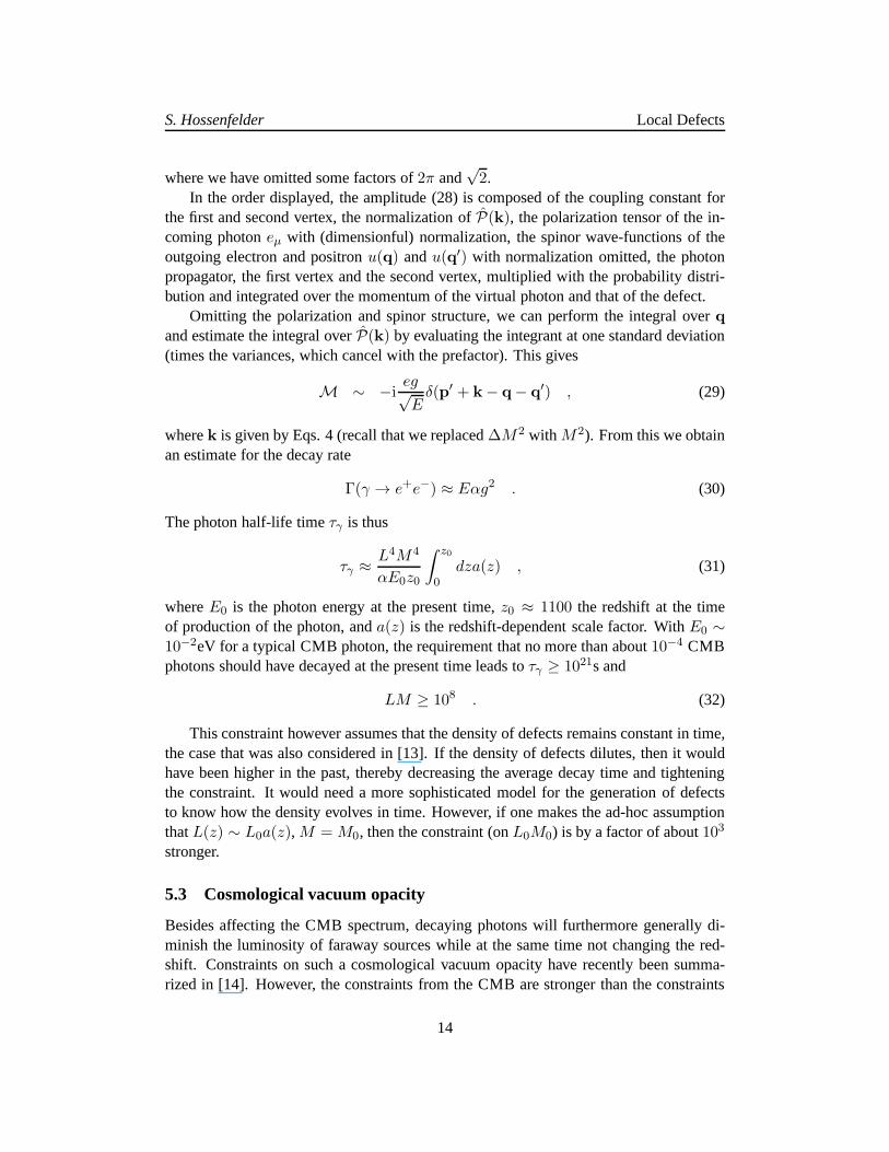
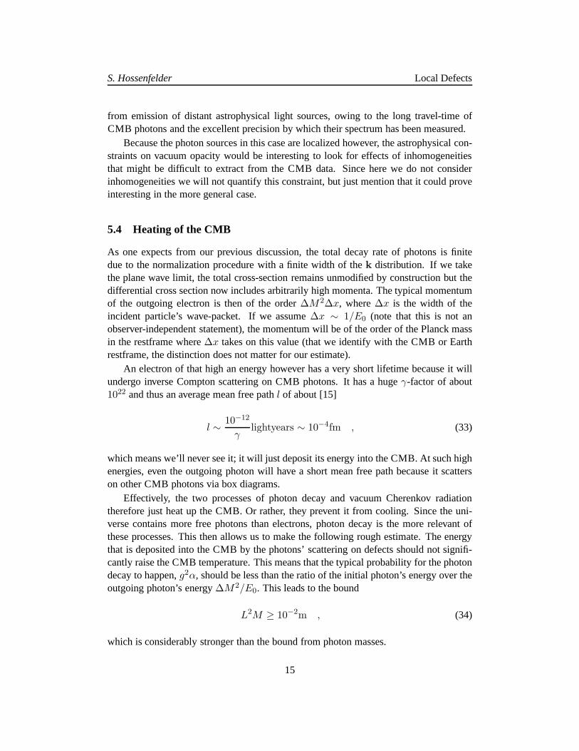
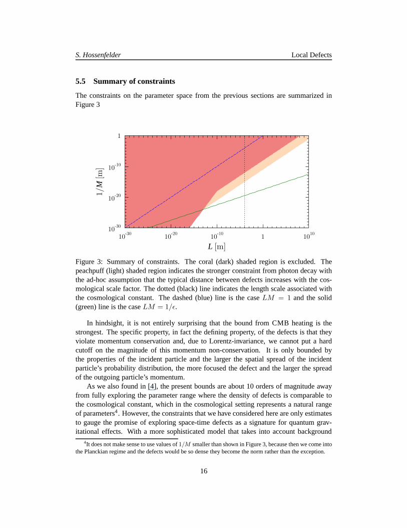
5.5 Summary of constraints

The constraints on the parameter space from the previous sections are summarized inFigure 3

M

L

Figure 3: Summary of constraints. The coral (dark) shaded region is excluded. Thepeachpuff (light) shaded region indicates the stronger constraint from photon decay withthe ad-hoc assumption that the typical distance between defects increases with the cos-mological scale factor. The dotted (black) line indicates the length scale associated withthe cosmological constant. The dashed (blue) line is the case LM = 1 and the solid(green) line is the caseLM = 1/ǫ.

In hindsight, it is not entirely surprising that the bound from CMB heating is thestrongest. The specific property, in fact the defining property, of the defects is that theyviolate momentum conservation and, due to Lorentz-invariance, we cannot put a hardcutoff on the magnitude of this momentum non-conservation.It is only bounded bythe properties of the incident particle and the larger the spatial spread of the incidentparticle’s probability distribution, the more focused thedefect and the larger the spreadof the outgoing particle’s momentum.

As we also found in [4], the present bounds are about 10 ordersof magnitude awayfrom fully exploring the parameter range where the density of defects is comparable tothe cosmological constant, which in the cosmological setting represents a natural rangeof parameters4. However, the constraints that we have considered here are only estimatesto gauge the promise of exploring space-time defects as a signature for quantum grav-itational effects. With a more sophisticated model that takes into account background

4It does not make sense to use values of1/M smaller than shown in Figure 3, because then we come intothe Planckian regime and the defects would be so dense they become the norm rather than the exception.

16

S. Hossenfelder Local Defects

curvature, more of the existing cosmological data could be analyzed. This would openthe possibility of finding evidence for space-time defects or at least deriving better con-straints on their density.

6 Discussion

Let us first summarize the assumptions we have made that can inprinciple be relaxed. Wehave assumed that the defects don’t carry quantum numbers, no spin or gauge charges.We have restricted the study of phenomenological consequences to the case whereM islarger than the electron mass. We looked at the parameter range〈a2〉 ∼ 1. The latter as-sumption in particular could be modified. One could use∆a2 to normalize the extensionof the wave-packet into the third spatial direction in a similar way as the perpendiculardirections. We also remind ourselves that we have worked in the plane-wave approxima-tion, wherep+ ≫ ∆p+. If this approximation is not good, then the width of the defectscan have a different dependence on the momentum of the incident particle and the scalingof effects might change.

As previously mentioned in [4], a certain case of nonlocal defects effectively makesitself noticeable as a local defect. That will be the case when the nonlocal translationcan occur in both directions between the same locations. In this case, a particle thatmakes a nonlocal jump to another location will be replaced atits point of departure witha different particle, making it appear like a non-elastic scattering on a local defect. Theproblem with this kind of scenario is that the probability for a particle to appear at acertain location would depend on the total volume of spacetime, past and future, whereit could have originated from. In this case, it is then impossible to say anything aboutthe interaction rates without first developing a model for the generation of defects in atime-dependent background.

Finally, let us investigate the difference between the approach discussed here and theone in [7]. In the model [7], interaction with the local defects is mediated exclusivelyby a scalar field. The probability distribution of the momentum that is assigned to thedefect is not constrained by a requirement similar to our requirementsp · k = M2 andk2 = a2M2. As a consequence, Lorentz-invariance necessitates that the defect be ableto inject momenta from the full Lorentz-group, which is no longer normalizable. Thusthere arises the need to introduce a cutoff on the momentum integration. While the modelin [7] offers an concrete realization of coupling quantum fields to space-time defects, theneed to eventually introduce a Lorentz-invariance violating cutoff defeats the point ofrequiring a Lorentz-invariant distribution and coupling to begin with. The more relevantdifference between the two models is however that we have here assumed the coupling toappear as a contribution to the covariant derivative and notas an independent interactionvertex.

These approaches are presently the only existing models to describe space-time de-fects and the study of the effects is in its infancy. It is possible, in fact likely, that elements

17

S. Hossenfelder Local Defects

of both approaches will turn out to be necessary for the development of more sophisti-cated models.

7 Summary

We have proposed a model for the scattering of particles on space-time defects that in-duce a violation of energy-momentum conservation. In the plane wave-limit, the energy-momentum non-conservation can become arbitrarily large due to Lorentz-invariance, butit remains bounded if one takes into account the finite widthsof the incident particle’swave-function. We have looked at various phenomenologicalconsequences and esti-mated that the best constraints come from energy deposited by decaying photons into thecosmic microwave background.

Acknowledgements

I thank Julian Heeck and Stefan Scherer for helpful discussions.

References

[1] G. Amelino-Camelia,“Quantum Gravity Phenomenology,”Living Rev. Rel.16, 5 (2013)[arXiv:0806.0339 [gr-qc]].

[2] S. Hossenfelder and L. Smolin,“Phenomenological Quantum Gravity,”Physics in Canada,Vol. 66 No. 2, Apr-June, p 99-102 (2010), arXiv:0911.2761 [physics.pop-ph].

[3] S. Hossenfelder,“Experimental Search for Quantum Gravity,”In “Classical and QuantumGravity: Theory, Analysis and Applications,”Chapter 5, Edited by V. R. Frignanni, NovaPublishers (2011), arXiv:1010.3420 [gr-qc].

[4] S. Hossenfelder,“Phenomenology of Space-time Imperfection I: Nonlocal Defects”

[5] D. Mattingly, “Modern tests of Lorentz invariance,”Living Rev. Rel. 8, 5 (2005) [gr-qc/0502097].

[6] V. A. Kostelecky and N. Russell,“Data Tables for Lorentz and CPT Violation,”Rev. Mod.Phys.83, 11 (2011) [arXiv:0801.0287 [hep-ph]].

[7] M. Schreck, F. Sorba and S. Thambyahpillai,“A simple model of pointlike spacetime defectsand implications for photon propagation,”arXiv:1211.0084 [hep-th].

[8] F. Dowker, J. Henson and R. D. Sorkin,“Quantum gravity phenomenology, Lorentz invari-ance and discreteness,”Mod. Phys. Lett. A19, 1829 (2004) [gr-qc/0311055].

[9] L. Bombelli, J. Henson and R. D. Sorkin,“Discreteness without symmetry breaking: Atheorem,”Mod. Phys. Lett. A24, 2579 (2009) [arXiv:gr-qc/0605006].

18

S. Hossenfelder Local Defects

[10] S. Weinberg,The Quantum Theory of Fields, Volume I, Cambridge University Press, Cam-bridge (1995).

[11] A. S. Goldhaber and M. M. Nieto,“Photon and Graviton Mass Limits,”Rev. Mod. Phys.82, 939 (2010) [arXiv:0809.1003 [hep-ph]].

[12] J. Heeck, “How stable is the photon?,” Phys. Rev. Lett. 111,021801 (2013)[arXiv:1304.2821 [hep-ph]].

[13] C. Prescod-Weinstein and L. Smolin,“Disordered Locality as an Explanation for the DarkEnergy,” Phys. Rev. D80, 063505 (2009) [arXiv:0903.5303 [hep-th]].

[14] R. Jimenez,“Beyond the Standard Model of Physics with Astronomical Observations,”arXiv:1307.2452 [astro-ph.CO].

[15] V. Beckmann, Lecture Notes of the Astrophysical SpringSchool, Cargese/Corsica April 2006, Retrieved July 12, 2013 ateud.gsfc.nasa.gov/Volker.Beckmann/school/download/Longair_Radiation3.pdf,

19