Price Adjustment, Dispersion and Inflation Allen Head * Alok Kumar ** Beverly Lapham * October 22, 2003 preliminary and incomplete Abstract The observation that consumer prices are “sticky” in the sense that the nominal price level typically responds sluggishly or less than fully to short-run changes in economic fundamentals has attracted interest among economists, particularly with regard to its implications for aggregate fluctuations and the effectiveness of monetary policy. In much of the literature, price stickiness is taken as given, with price adjustment impeded by some exogenously imposed nominal rigidity. In this paper we study the responses of both nominal and real prices to random fluctuations in costs, preferences, and money creation using a monetary economy with search frictions and no constraints on sellers’ ability to change prices. In equilibrium, our economy exhibits nominal price stickiness, the degree of which varies with the average rate of inflation. At low levels of inflation, prices are unresponsive to shocks. As the inflation rate rises, prices become more responsive. Our model is consistent with empirical findings suggesting that both the variance of inflation and the degree to which cost shocks are passed-through to prices are increasing in the average rate of inflation. In contrast to models of state-contingent pricing in the presence of menu costs, our model predicts that price dispersion always increases with inflation, rather than vanishing when inflation is sufficiently high; a finding consistent with the evidence on the dispersion of prices during hyperinflations. * Department of Economics, Queen’s University; Kingston, ON; Canada K7L 3N6 ** Department of Economics, University of Victoria; P.O. Box 1700, STN CSC; Victoria, BC; Canada K7L 3N6
Transcript
Price Adjustment, Dispersion and Inflation
Allen Head∗ Alok Kumar∗∗ Beverly Lapham∗
October 22, 2003
preliminary and incomplete
Abstract
The observation that consumer prices are “sticky” in the sense that the nominal price level typicallyresponds sluggishly or less than fully to short-run changes in economic fundamentals has attractedinterest among economists, particularly with regard to its implications for aggregate fluctuationsand the effectiveness of monetary policy. In much of the literature, price stickiness is taken as given,with price adjustment impeded by some exogenously imposed nominal rigidity. In this paper westudy the responses of both nominal and real prices to random fluctuations in costs, preferences,and money creation using a monetary economy with search frictions and no constraints on sellers’ability to change prices. In equilibrium, our economy exhibits nominal price stickiness, the degreeof which varies with the average rate of inflation. At low levels of inflation, prices are unresponsiveto shocks. As the inflation rate rises, prices become more responsive. Our model is consistent withempirical findings suggesting that both the variance of inflation and the degree to which cost shocksare passed-through to prices are increasing in the average rate of inflation. In contrast to modelsof state-contingent pricing in the presence of menu costs, our model predicts that price dispersionalways increases with inflation, rather than vanishing when inflation is sufficiently high; a findingconsistent with the evidence on the dispersion of prices during hyperinflations.
∗ Department of Economics, Queen’s University; Kingston, ON; Canada K7L 3N6∗∗ Department of Economics, University of Victoria; P.O. Box 1700, STN CSC; Victoria, BC; Canada K7L 3N6
1. Introduction
Nominal price “stickiness”, or the tendency of consumer prices to respond sluggishly or incom-
pletely to short-run fluctuations in costs or demand has attracted a great deal of attention from
economists. This observation has generated a large literature focused on the implications of price
stickiness for the ability of monetary authorities to influence the level of economic activity, at least
in the short-run. In much of this literature, nominal price adjustment is impeded by the presence
of exogenously imposed rigidities. These rigidities are modeled in a variety of ways; including as-
suming an explicit cost of changing prices or that the frequency with which prices may be changed
is limited or stochastic.
In this paper, we use a monetary economy with search frictions to examine the responses of
nominal and real prices to random shifts in costs, preferences, and the money growth rate. In our
environment, prices are fully flexible; sellers are neither prevented from changing prices at certain
times nor do they face a cost of changing their price. Our economy nevertheless exhibits incomplete
adjustment of prices (“price stickiness”) in equilibrium. Moreover, the extent to which prices are
sticky depends on both the average level of inflation and on the nature of shocks. When inflation is
low, both nominal and real prices are relatively unresponsive to cost shocks but respond strongly to
preference shocks. In contrast, as inflation rises, prices respond more more strongly to cost shocks
and less so to preference shocks. At very high rates of inflation, prices are effectively fully flexible,
in the sense that cost movements are “passed-through” to prices one for one.
Our work is motivated in part by the observation that the responsiveness of prices to shocks
to fundamentals appears to have changed over time. Several authors have presented evidence
that price stickiness is inversely related to the average rate of inflation in particular instances.
For example, Taylor (2000) argues that the response of nominal prices to increases in costs has
declined with the rate of inflation over time for the U.S. and other developed countries. Devereux
and Yetman (2002) present evidence that the pass-through of nominal exchange rate movements
(which affect costs) to consumer prices is declining in the average rate of inflation for a sample of
107 countries during the post-Bretton Woods era. The predictions of our model for the effects of
cost shocks are consistent with both of these sets of findings. Also, it has long been recognized
that periods of high average inflation tend to be periods of high inflation volatility. Our model
is consistent with this observation when inflation fluctuations are driven by cost and/or monetary
shocks.
1
Our work is also motivated by the desire to model price stickiness endogenously to better
understand the relationships among economic factors which determine the degree of nominal rigidity
in the economy. While the literature examining the effects of exogenously imposed nominal rigidities
is extensive, there have been relatively few attempts to model the sources of incomplete price
adjustment in stochastic monetary economies. A notable paper that does study these issues is
Eden (1994). In our model, as in Eden’s, the extent to which nominal prices adjust to shocks is
endogenous and responds to the state of the economy. In contrast, however, our analysis focuses on
the effects of the average inflation rate for the pricing behavior of firms, whereas in Eden’s model
anticipated money growth has no effect on the distribution of real prices. Our focus also contrasts
with that undertaken in most studies of exogenous price stickiness (see, for example Gali (1999)) as
these typically abstract from the effects of average inflation. Indeed, it is common in these models
to examine the short-run effects of shocks around a zero inflation steady-state.
Our model embeds the price-posting game of Burdett and Judd (1983) into a general equi-
librium environment along the lines of the random matching monetary models of Shi (1999) and
Head and Shi (2003). In an earlier paper, Head and Kumar (2003) study the long-run properties
of a similar environment under certainty. In this paper, we extend their model to a stochastic
environment, and focus on the response of nominal prices to random shocks. In this environment,
the Burdett-Judd pricing framework generates price dispersion in equilibrium, with the extent of
dispersion depending on the average rate of inflation. In our model, the degree of price dispersion,
and its response to shocks are key factors determining price adjustment in equilibrium.
In our economy, shocks to costs, preferences, and the money growth rate are passed-through
differentially to consumer prices by sellers pricing in different regions of the price distribution.
Changes in the distribution affect the fraction of buyers observing more than one price changing
the overall degree of sellers’ market power and the altering adjustment of prices. At low rates of
inflation, a relatively large fraction of buyers observes only a single price. A cost or money growth
shock generates greater dispersion, and causes a large increase in this share. The resulting reduction
in sellers’ market power limits the adjustment of prices in response to these shocks. In contrast,
preference shocks compress the distribution, increasing the share buyers observing a single price.
The resulting increase in sellers’ market power induces them to change prices drastically in response
to preference shocks.
As the rate of trend inflation rises, ceteris paribus, the average share of buyers observing more
than one price falls, and the response of this share (positive or negative) to shocks of any kind
weakens. Pass-through of cost and monetary shocks increases, while the response of prices to
2
preference shocks diminishes. Average prices become more closely tied to marginal cost. As a
result, at sufficiently high trend inflation, inflation moves one-for-one with changes in costs.
A tight relationship between the price level and shocks to fundamentals also emerges in “state-
contingent” pricing models along the lines of Dotsey, King and Wolman (1999) and Devereux and
Yetman (2002). In these models, for a fixed cost of changing prices, a larger share of firms find it
profitable to change their prices in a given period the higher the rate of inflation. At some point,
the rate of inflation is sufficient to induce all firms to change their prices each period, eliminating
price stickiness. These models also, however, predict that price dispersion will vanish at high levels
of inflation. In contrast, in our economy price dispersion increases monotonically with inflation,
a finding consistent with empirical evidence that price dispersion increases with inflation and is
typically very high during hyperinflations (e.g. Cassella and Feinstein (1990), Lach and Tsiddon
(1992), Fershtman, Fishman, and Simhon (2003)).
This version of the paper is preliminary and incomplete. Section 2 describes the environment.
In section 3, we define and Markov monetary equilibrium for this environment and outline our nu-
merical procedure for computing such equilibria. The effects of random shocks to costs, preferences,
and money growth are considered in a series of computational experiments in section 4. Section 5
endogenizes money growth, assuming that the monetary authority chooses it in response to shocks
to costs and preferences either optimally or following an ad hoc sub-optimal policy rule. Section 6
draws conclusions and describes some implications of the results for future work.
2. The Economy
2.1. The environment
The economy is a stochastic version of that studied by Head and Kumar (2003). Time is
discrete. There are large numbers (i.e. unit measures) of H ≥ 3 different types of both households
and non-storable consumption goods. A type h household is able to produce only good h and
derives utility only from consumption of good h + 1, modulo H. Each household is comprised of
large numbers (unit measures) of two different types of members; “buyers” and “sellers”. Individual
buyers and sellers do not have independent preferences and do not undertake independent actions.
Rather, they share equally in household utility and act only on instructions from the household.
Members of a representative type h household who are sellers can produce good h in period
t at marginal cost φt > 0 utils per unit. Production costs are stochastic; φt evolves via a discrete
Markov chain with
Prob φt+1 = φj |φt = φi ≡ πφji ∀t, t + 1; φj , φi ∈ P , (2.1)
3
where P is a finite set of possible production cost parameters. Let xt denote the total quantity
of good h produced by all the sellers from this household in period t. Then the household’s total
disutility from production in this period is equal to φtxt.
Members of this household who are buyers observe random numbers of price quotes and may
purchase good h + 1 at the lowest price that they observe individually. The household chooses
the expected number of price quotes observed by an individual buyer. Or, alternatively, because
each household contains a continuum of symmetric buyers, it chooses the measures of these buyers
that observe different numbers of prices. For each observed price quote, the household pays an
information or search cost of µ utils. We assume that buyers observe either one or two price quotes
only1. In this case the household’s total disutility of information gathering or search in period t
is equal to µ∑2
k=1 kqkt, where qkt is the measure of buyers observing k price quotes at time t.
In period t, a representative type h household receives utility ut(ct) from consumption of ct
units of good h + 1, where ct is equal to the total purchases of its buyers in that period. For
convenience, we assume that for all t, ut(c) takes the constant relative risk aversion (CRRA) form:
ut(c) =c1−αt − 1
1− αt(2.2)
where αt is a random preference parameter which evolves via a discrete Markov chain:
Prob αt+1 = αj |αt = αi ≡ παji ∀t, t + 1; αj , αi ∈ A, (2.3)
with A, like P a finite set. Throughout the paper we require that α > 1 for all α ∈ A. In this case
we have limc→0 utc(c)c = ∞, where utc(c) denotes the derivative of ut with respect to c.
A representative household’s total period t utility is equal to that which it receives from con-
sumption of goods purchased by its buyers minus the production disutility incurred by its sellers
and its information gathering or search costs. The household acts so as to maximize the expected
discounted sum of its period utility over an infinite horizon:
U = E0
[ ∞∑t=0
βt
[u(ct)− φtxt − µ
2∑
k=1
kqkt
]]. (2.4)
1 The assumption that buyers observe only one or two price quotes is not as restrictive as it may seem. Monetary
equilibria of the type on which this paper focuses exist only if strictly positive measures of buyers observe one
and two prices only. Moreover, it can be shown that under certain conditions households will choose to have
buyers observe only one or two prices, thus guaranteeing existence. These claims are proved by Head and
Kumar (2003) and the arguments are summarized in appendix C.
4
Since a type h household produces good h and consumes good h + 1, a double coincidence
of wants between members of any two households is impossible. Moreover, it is assumed that
households of a given type are indistinguishable and that members of individual households cannot
be relocated in the future following an exchange. Since consumption goods are non-storable, direct
exchanges of goods cannot be mutually beneficial. Rather, exchange is facilitated by the existence
of perfectly durable and intrinsically worthless fiat money. A type h household may acquire fiat
money by having its producers sell output to buyers of type h − 1 households. This money may
then be exchanged for consumption good h + 1 by the household’s own buyers in a future period.
In the initial period (t = 0) households of all types are endowed with M0 units of fiat money.
The per household stock of this money is denoted Mt, for each t, At the beginning of each period
t ≥ 1, households receive a lump-sum transfer, (γt − 1)Mt−1, of new units of fiat money from a
monetary authority with no purpose other than to change the stock of money over time. We assume
that the gross growth rate of the money stock,
γt+1 =Mt+1
Mt, (2.5)
evolves stochastically via a discrete Markov chain:
where S ≡ A×P×G. In each period, the state of the economy is given by σt and the per household
stock of money, Mt.
2.2. The current period trading session
In describing the optimization problem of a representative household (of any type), it is useful
to begin with the current period trading session. At the beginning of period t a representative
household observes the state of the economy, (Mt, σt) and has post-transfer household money
2 Where possible, capital letters (e.g. C, Q, M) will be used to distinguish per household quantities from their
counterparts for an individual household (c, q, m) etc..
5
holdings mt.2 The household chooses the probabilities with which an individual buyer observes one
(as opposed to two) price quotes, q1t, and issues trading instructions to both its buyers and sellers
in order to maximize utility. Buyers and sellers then split up for a trading session. We assume that
it is not until this trading session begins that the exact number of quotes observed by individual
buyers is known. As a result, households have no incentive to treat their members asymmetrically;
they distribute money holdings equally to all buyers and issue the same instructions to all buyers
and to all sellers3.
In the trading session, sellers post prices and buyers decide whether or not to purchase at
the posted price, each acting in accordance with household instructions. Exchanges of goods for
fiat money take place in bi-lateral matches between buyers and sellers of different households.
Following trading, buyers and sellers reconvene and the household consumes the goods purchased
by its buyers. The sellers’ revenue (in fiat money) and any remaining money unspent by the buyers
are pooled and carried into the next period, when they are augmented with transfer (γt+1 − 1)Mt
to become mt+1.
With q1t fixed, the mechanism by which buyers and sellers are matched is similar to the “noisy
sequential search” process of Burdett and Judd (1983). Households know the distribution of prices
offered by sellers, but individual buyers may purchase only at a price they are quoted by a specific
prospective seller in a particular period4. Let the distribution of prices posted by sellers of the
appropriate type at time t be described by the cumulative distribution function (c.d.f.) Ft(pt) on
support Ft. Given Ft(pt), the c.d.f. of the distribution of the lowest price quote received by a buyer
at time t is given by
Jt(pt) =2∑
k=1
qk
[1− [1− Ft(pt)]
k]
∀pt ∈ Ft. (2.8)
Individual buyers are constrained to spend no more than the money distributed to them at the
beginning of the session by the household. If buyer i purchases he/she does so at the lowest price
3 In the exposition, we will for now we suppress the economy state vector, (Mt, σt), as it remains fixed throughout
the trading session. Similarly, we postpone analysis of the choice of q1t until later and for now treat qk, k = 1, 2as fixed, as they are once the trading session has begun.
4 We assume that buyers cannot return to sellers from whom they have purchased in the past, and instead draw
new price quotes from the distribution each period. This assumption enables price dispersion to persist in a
stationary equilibrium of our model. Empirical evidence in Lach (2002) suggests that price dispersion is indeed
persistent and that individual sellers change their prices frequently, limiting the ability of buyers to identify
low price sellers for repeat purchases.
6
observed, spending mit(pt) conditional on the price paid. Thus buyers face the exchange constraint
mit(pt) ≤ mt ∀i, pt. (2.9)
Buyers, being identical, act symmetrically if they receive the same lowest price quote. Because
the household contains a continuum of symmetric buyers, it faces no uncertainty with regard to
its overall trading opportunities in the trading session of the current period. Realized household
consumption purchases in this period are then
ct =∫
Ft
mt(pt)pt
dJt(pt). (2.10)
An individual seller produces to meet the demand of the buyers who observe his/her price and
wish to purchase. Expected sales in the current period trading session for a seller who posts pt are
given by
x(pt) =Mt(pt)
pt
2∑
k=1
Qktk [1− Ft(pt)]k−1
. (2.11)
Here Mt(pt) is the spending rule of a type h − 1 buyer, Ft(pt) is the distribution of prices posted
by the seller’s competitors, and Qkt is the average measure of buyers observing k = 1, 2 prices.
In (2.11), Mt(pt)/pt represents the quantity per sale and the summation term is the expected
number of sales. The expected number of sales equals the number of observations of the seller’s
price multiplied by the probability that in each of these instances it is the lowest price observed.
The number of observations is the ratio of the measures of buyers to sellers (in this case one)
times the expected number of price observations for a randomly selected buyer,∑
k Qkk. Given
distribution Ft(pt), the probability that the other k − 1 prices observed by a buyer exceed the
seller’s price is [1− Ft(pt)]k−1, k = 1, 2.
Let Ft(pt) be the distribution of prices posted by a representative household’s sellers and
denote its support Ft. Since this household contains a continuum of sellers, it faces no uncertainty
with regard to its total sales in the current trading session. These are given by
xt =∫
Ft
x(pt)dFt(pt). (2.12)
Using (2.10)—(2.12), we have
mt+1 = mt −∫
Ft
mt(pt)dJt(pt) +∫
Ft
ptx(pt)dFt(pt) + (γt+1 − 1)Mt. (2.13)
A representative household’s money holdings going into next period’s goods trading session are
mt minus the amount spent by its buyers this period; plus its sellers’ receipts of money; plus the
transfer received at the beginning of the next period.
7
We now characterize the households’ choice of instructions, mt(pt) and Ft(pt), to its buyers and
sellers respectively. Consider first the spending rule, mt(pt). The household’s gain to having a buyer
exchange mt(pt) units of currency for consumption at pt is given by the household’s marginal utility
of current consumption, uc(ct), times the quantity of consumption good purchased, mt(pt)/pt. The
household’s cost of this exchange is the number of currency units given up, mt(pt), times the
marginal value of money in the trading session of the next period which we will denote ωt. Note
that ωt is the value of relaxing constraint (2.13) marginally. Since individual buyers are small and
the household may not reallocate money balances across buyers once the goods trading session has
begun, the optimal spending rule instructs buyers to spend their entire money holdings if the lowest
price they observe is below utc(ct)/ωt (the reservation price) and to return with money holdings
unspent otherwise:
Proposition 1:
mt(pt) =
mt pt ≤ utc(ct)ωt
0 pt > utc(ct)ωt
.(2.14)
With regard to the household’s price posting policy, the expected return from having a seller
post a particular price at time t depends on the distribution of prices posted by sellers of other
households of its type, Ft(pt), and the strategies of its prospective buyers, Mt(pt). Let pt denote
the household’s belief regarding the reservation price of its potential customers (all of whom are ex
ante identical). The household will instruct no seller to post pt > pt, as doing so generates no sales
and an expected return to the household of zero.
The expected return to the household from having a seller post a price no greater than pt is
r(pt) =
[ωtMt(pt)− φt
Mt(pt)pt
]2∑
k=1
Qktk [1− Ft(pt)]k−1 ; (2.15)
In (2.15) r(pt) equals the expected return per sale (in brackets) times the expected number of sales
(as in (2.11)). The former term is the value of the currency units obtained minus the disutility of
production. Here it is clear that the return to posting a price lower than p∗t = φt/ωt (the marginal
cost price) is negative, and thus the household will instruct no seller to do so.
The household maximizes returns by instructing its sellers to post only prices such that
pt ∈ argmaxp∗t≤pt≤pt
r(pt) ≡ Ft (2.16)
The household receives the same return from a seller who posts any price in Ft. We thus express
the household’s instructions by a c.d.f. Ft(pt) on support Ft and think of sellers as drawing their
prices randomly from this distribution.
8
2.3: Dynamic optimization
To this point we have focused on the current period trading session holding fixed the prob-
abilities of a representative household’s buyers observing one and two prices and taking as given
the household’s marginal value of a unit of money. We now turn to the household’s dynamic op-
timization problem. To begin with, it is useful to write household consumption as the sum of the
purchases of those of its buyers who observe one and two prices:
ct = q1tc1t + q2tc
2t where ck
t = mt
∫
Ft
1pt
dJkt (pt) (2.17)
and for all pt ∈ Ft(pt)
J1t (pt) = Ft(pt) and J2
t (pt) = 2Ft(pt)− [Ft(pt)]2 (2.18)
are the distributions of the lowest price observed by buyers who observe exactly one and two prices,
respectively. In (2.17) we have made use of the fact that buyers follow the spending rule, (2.14).
Note that the household’s choice of q1t is constrained by the requirement that it be a probability:
qkt ≥ 0, k = 1, 2 and q2t = 1− q1t, ∀t. (2.19)
At time t, for a representative household (of any type), its individual money holdings, mt, are
a relevant state variable in addition to Mt and σt. For σt = σi, we represent dynamic optimization
problem of such a household by the following Bellman equation:
vt(mt,Mt, σi) =
maxqt,mt+1,mt(pt),Ft(pt)
u(ct)− φtxt − (2− qt)µ + β
∑
σj∈SΠjivt+1(mt+1,Mt+1, σj)
(2.20)
subject to:
(2.5) (2.7) (2.9)− (2.13) (2.16) and (2.19),
where q is the probability that a buyer receives one price quote. The household takes as given the
actions of other households, Xt(pt; Mt, σt), Mt(pt; Mt, σt), and Qt(Mt, σt); as well as the distribu-
tion of exchange prices, Jt(pt;Mt, σt). Here Mt and σt are included as arguments to indicate that
these actions and prices depend on the aggregate state.
From the household Bellman equation, we have
ωt(mt,Mt, σi) = β∑
σj∈SΠjivt+1m(mt+1,Mt+1, σj). (2.21)
9
We also have first-order conditions associated with the choice of mt(pt):
Similarly, if the distributions of posted and transactions prices are time-invariant conditional on σ,
then households’ nominal money holdings, mt, spending rule for buyers, mt(pt), and the support
of sellers’ posted prices, Ft may be divided by the per household money stock to obtain time-
invariant conditional real counterparts: m(σ) = mt(σ)/Mt(σ), m(p |σ) = mt(pt |σ)/Mt(σ), and
F(σ) = pt/Mt, pt ∈ Ft.We then have the following definition:
Definition: A symmetric Markov monetary equilibrium (MME) is a collection of time-invariant,
individual household choices, q(σ), m′(σ), m(p |σ), F (p |σ); spending rules M(p |σ) and distribu-
tions of posted prices, F (p |σ); probabilities, Q(σ); and consumption levels, C(σ), conditional on
σ ∈ S, such that
1. In all periods such that σt = σ, taking as given the distribution of posted prices, F (p |σ),
spending rule, M(p |σ), and probability Q(σ), a representative household chooses qt = q(σ),
mt+1 = m′(σ), mt(pt |σ) = m(p |σ), and distribution Ft(pt |σ) = F (p |σ) for all p ∈ F(σ) to
maximize (2.20) subject to (2.5), (2.7), (2.9)—(2.13), (2.16), and (2.19).
2. Individual choices equal per household quantities: q(σ) = Q(σ); and m(p |σ) = M(p |σ) and
F (p |σ) = F (p |σ) for all p ∈ F(σ).
3. Individual household consumption and money holdings equal their per household counterparts:
c(σ) = C(σ) and m′(σ) = 1, respectively.
4. Money has value in equilibrium: Ωt > 0, for all t.
In characterizing an MME for this economy, we begin with the sequence of households’ marginal
valuations of money, Ωt∞t=0. In this economy, Ωt is a key variable as it determines the returns to
sellers and buyers from transacting at a particular price at a particular point in time. Returning
to the household optimization problem and combining (2.21), (2.22), and (2.24), we have
ωt = βEt
[ut+1c(ct+1)
∫
Ft
1pt+1
dJt+1(pt+1)]
∀t. (3.5)
11
In a symmetric equilibrium, substituting (3.1) into (3.5) we have
Ωt = βEt
[ut+1c(Ct+1)
Ct+1
Mt+1
]∀t. (3.6)
Making use of (2.5) and rearranging yields
ΩtMt = βEt
[1
γt+1ut+1c(Ct+1)Ct+1
]. (3.7)
Using (2.7) we define Ω(σ), for all σ ∈ S, using the notation introduced in the definition of an
MME:
Ω(σ) ≡ ΩtMt = β∑
σ′∈SΠ(σ′, σ)
[1γ′
u′c[C(σ′)]C(σ′)]
∀σ ∈ S, ∀t. (3.8)
We thus associate an MME with a collection of N state-contingent values, Ω(σ1), . . . , Ω(σN ), for
households’ marginal value of fiat money.
Under the assumption that an MME exists, it is possible to establish several characteristics
that it must necessarily possess. We will begin in this way and return to the issue of existence later.
To this end, suppose that for all σ ∈ S, Ω(σ), C(σ), Q(σ), F (p |σ), and J(p |σ) are components of
an MME as defined above. In addition, let Q(σ) ∈ (0, 1) for all σ, and γ > β for all γ ∈ G.5 The
following proposition, based on Theorem 4 of Burdett and Judd (1983) and Proposition 1 of Head
and Kumar (2003) imposes some structure on the form of the conditional distributions of posted
prices in an MME:
Proposition 2: Suppose that γ > β for all γ ∈ G and there exists an MME with Q(σ) ∈ (0, 1) for
all σ ∈ S. Then, given Ω(σ) the conditional distribution of real posted prices, F (p |σ) is unique,
dispersed, continuous, and has connected support satisfying: F(σ) = [p¯(σ), p(σ)] where,
p¯(σ) > p∗(σ) =
φ
Ω(σ)and p(σ) =
uc[C(σ)Ω(σ)
. (3.9)
Proposition 2 establishes that there is a unique candidate distribution of real posted prices in
each state for any MME in which a positive measure of buyers observe a single price, conditional on
a representative household’s marginal valuation of money, Ω(σ). For this candidate distribution,
p ∈ F(σ) requires that p ∈ argmaxp
r(p) where writing (2.15) using real quantities we have
r(p) = M(p |σ)[Ω(σ)− φ
p
] [Q(σ) + 2
[1−Q(σ)
][1− F (p)
]]. (3.10)
5 As in Head and Kumar (2003), it is possible to show that there can be no MME in which the probability with
which a buyer observes a single price is equal to either 0 or 1 in any state. Similarly, there can be no MME if
γ ≤ β in any state. See appendix C.
12
Combining (3.9) with (3.10) and noting that F (p(σ) |σ) = 0 and F (p¯(σ) |σ) = 1 for all σ, it is
possible to derive the following expressions:
p¯(σ) =
φ
Ω(σ)
[1−
(1− φ
uc[C(σ)]
)Q(σ)
2−Q(σ)
]−1
(3.11)
and
F (p |σ) =
[Ω(σ)− φ
p
][2−Q(σ)]−
[1− φ
uc[C(σ)]
]Ω(σ)Q(σ)
[Ω(σ)− φ
p
]2[1−Q(σ)]
(3.12)
for all σ ∈ S.
From (3.12), it is convenient to derive the following expressions for the conditional densities of
posted and transactions prices:
f(p |σ) =φ
p2
[Q(σ) + 2[1−Q(σ)][1− F (p |σ)]
[Ω(σ)− φ/p]2[1−Q(σ)]
](3.13)
and
j(p |σ) =[Q(σ) + 2[1−Q(σ)][1− F (p |σ)]
]f(p |σ). (3.14)
Expressions (3.9) and (3.11)—(3.13) describe the conditional distributions of posted and trans-
actions prices in an MME as functions of Q(σ) and C(σ). Taking J(p |σ) (and implicitly, Q and
C) as given, an individual household’s consumption depends on the probability with which its own
buyers observe a single price as indicated by (2.17) and (2.18). Define,
Ck[Q(σ)] ≡∫
F(σ)
1p
dJk(p |σ) k = 1, 2, (3.15)
where Jk(p |σ) is the analog of (2.18) derived from (3.12) and implicitly depends on Q(σ). Using
(3.15) and suppressing the argument Q(σ), the solution for optimal q, (2.23), may be written
q∗ =
0, if µ < µL ≡ uc
(C2
) [C2 − C1
];
1, if µ > µH ≡ uc
(C1
) [C2 − C1
];
1C1−C2
[uc−1
(µ
C2−C1
)− C2
], if µL ≤ µ ≤ µH .
(3.16)
In (3.16), µL may be thought of as a lower bound on the search or information cost such that
if the cost is below µL, then the household will choose to have all of its buyers observe more than
one price (q∗ = 0). Similarly, µH is an upper bound on the search or information cost. If µ > µH ,
the household will choose to have no buyer observe a second quote (q∗ = 1). Note that the critical
levels, µL and µH (and so q∗ itself), depend on C1 and C2 and are functions of Q. The following
proposition establishes the existence of fixed points of (3.16):
13
Proposition 3: For a fixed σ and for any Q ∈ (0, 1), there exists a µ such that q∗(Q) = Q.
An MME requires that q∗ [Q(σ)] = Q(σ) for all σ. Proposition 3, however, establishes the
existence of a fixed point for a particular σ, and in general there may not exist a single µ such that
there is a fixed point of (3.16) for all σ ∈ S. Because we have specified search costs independently
of the state, existence of an MME in our model requires restrictions on S so that for a given µ
there is a fixed point of (3.16) in all N states. We do not derive explicit restrictions that will
suffice. Rather, in the computational/quantitative examples that we consider below, we find that
as a practical matter, if the variation across the three stochastic parameters is not too great, Q(σ)
does indeed exist for all σ ∈ S.
Given the difficulty in specifying conditions under which fixed points of (3.16) exists for all
σ for a single µ, we do not approach the existence of an MME formally.6 Rather, we construct
examples of MME’s for several parameterizations of our economy and use them to consider the
responses of both nominal and real prices to shifts in preferences (α), costs (φ), and the rate of
money creation (γ). We describe the process by which we compute equilibria in general terms here.
For a detailed description of our computational algorithm, see appendix B.
We begin by choosing specific values of the economy’s parameters7. This requires us to set
the discount factor, β, the search cost, µ, and sets of values for the preference parameter, A; cost
parameter, P; money creation rate, G, as well as the transition probabilities, Πji for σi, σj ∈ S.
Having fixed parameters, we then choose initial values for consumption, C0(σ), and the prob-
ability of a buyer observing a single price, Q0(σ), for each σ ∈ S. Using these values, we construct
Ω0(σ), and the distributions of posted and transactions prices using (3.9) and (3.11)—(3.14). We
label these distributions F0(p |σ) and J0(p |σ), respectively. Using these, we construct C10 [Q0(σ)]
and C20 [Q0(σ)]. Next we compute fixed points of (3.16) for each σ and call these Q1(σ). Finally,
using Q1(σ) and F0(p |σ) we construct J1(p |σ) and C1(σ). This procedure is repeated (T times)
until for all σ, CT (σ)− CT−1(σ) and QT (σ)−QT−1(σ) are sufficiently small.
Overall, we find that this algorithm works well in that for a wide range of parameter values it
successfully computes an MME very quickly. While we do not formally rule out non-uniqueness,
experimentation with different starting values in no case produced multiple equilibria for a fixed
set of parameters.
6 For a version of this economy with no aggregate uncertainty (effectively a single σ), Head and Kumar (2003)
formally establish existence of an equilibrium of the type considered here.
7 We report the parameter values chosen in our baseline calibration in the section 4.
14
4. Price Responses to Shocks in Equilibrium
We study random fluctuations in costs, preferences, and money creation, each in isolation, in
numerically computed MME’s. We focus on the effects of these fluctuations on both the level and
dispersion of prices; and on the magnitude and persistence of fluctuations in inflation.
We describe the level of prices by the average transaction price. For real prices, we write:
pavet =
∫
F(σt)
p dJ(p |σt). (4.1)
The average nominal price is given by
P avet = Mtp
avet =
∫
Ft
pt dJt(pt). (4.2)
We consider the dispersion of the distributions of either real or nominal prices with respect to
the range of their supports, by which we mean the ratio of the upper support to the lower support
of the distributions of real prices, p(σt)/p(σt). We define the inflation rate as the net growth rate
of the nominal price level:
It =P ave
t − P avet−1
P avet−1
× 100. (4.3)
In our environment, marginal production cost is expressed in units of utility. It is useful in
the analysis of cost fluctuations to express costs either in units of goods (real marginal cost) or
currency (nominal marginal cost). We define nominal marginal cost at time t:
MCt =φt
Ωt. (4.4)
Real marginal cost is given by
mct =MCt
Mt. (4.5)
Since all producers face the same costs, the distribution of transactions prices induces distributions
of nominal and real markups. The average nominal and real markups are defined by the ratios
P avet /MCt and pave
t /mct, respectively.
4.1: Benchmark Parameterization
We characterize equilibria numerically, and for this reason we begin with a benchmark param-
eterization of the economy. We set the discount factor, β, equal to .96, as this is a value commonly
used in dynamic general equilibrium models calibrated to annual observations. We choose mean
values for the stochastic parameters φ, α, and γ in part to calibrate certain measures for our econ-
omy in a deterministic stationary monetary equilibrium. That is, in a equilibrium in which all of
these parameters (and thus the state vector, σ) are constant.
15
We set α = 1.5 on average, a value consistent with the requirement that limC→0 u′(C)C = ∞,
and within the range typically examined in calibrated macroeconomic models. We set the mean
rate of money creation, γ, in conjunction with the search cost parameter, µ, so that inflation is
at its optimal rate for the deterministic economy, by which we mean the constant inflation rate
that maximizes a representative household’s utility given that there are no shocks to costs or
preferences.8 With µ = .008, the optimal inflation rate in the deterministic economy is roughly
4% per annum (i.e. γ = 1.04 on average). Our chosen combination of µ and γ implies an average
real markup of 1.10, a number within the (fairly wide) range of markups estimated by several
studies of U.S. manufacturing (Morrison (1990), Basu and Fernald (1997), Chirinko and Fazzari
(1994)). Finally, given the values of the other parameters of the economy, µ = .008 lies well in the
interior of the range [µL, µH ] calculated as in (3.16). Thus constant search costs at this level are
consistent with existence of an MME for substantial fluctuations in costs, preferences, and money
creation. Finally, we set the average level of the production disutility parameter, φ = .1, more
or less arbitrarily. Given values for the other parameters, φ controls only the level of output in a
stationary equilibrium.
We specify Markov chains for the stochastic parameters so that in each case the percentage
standard deviation and autocorrelation of aggregate output in an MME with fluctuations induced
by random variation in that parameter alone are equal to 2.56 and .70 respectively, values equal to
their counterparts in annual U.S. GDP, detrended with the Hodrick-Prescott filter for the period
1959-2001. Many Markov chains fit this criterion; we choose the following symmetric processes
simply for illustrative purposes. For all t,
φt ∈ P = .094, .1, .106, αt ∈ A = 1.48, 1.5, 1.52, or γt ∈ G = 1.013, 1.04, 1.067, (4.6)
with
πφ = πα = πγ =
.8 .1 .1
.1 .8 .1
.1 .1 .8
. (4.7)
4.2: The pass-through of cost shocks to prices
We first consider the effects of random fluctuations in costs. For all t, φt ∈ P as specified in
(4.6) with Π = πφ given by (4.7). To begin with we fix the rate of money creation at γ = 1.04 and
8 In our economy, as in that of Head and Kumar (2003), inflation induces search and erodes market power. To
a point, this effect dominates the inflation tax, resulting in an optimal inflation rate exceeding the Friedman
rule (γ = β = .96).
16
throughout this sub-section we fix α = 1.5. Thus we focus on the MME of a three-state economy.
While the state is determined by the realization of φt alone, for notational purposes we continue
to use σt to indicate the current state.
Figure 1 depicts depicts the densities of real transactions prices in each of the three states.
Changes in φt affect Ω(σt), so that increases in φ from .094 to .1 and from .1 to .106 increase real
costs by 5.25% and 4.81% respectively, using (4.5). In Figure 1 it is clear that as real costs increase,
the densities of transactions prices shift from left to right; higher costs are associated with higher
real transactions prices. The average real transaction price, pave(σ), increases from .235 to .242
and to .250, increases of 2.98% and 3.31% as costs rise. From (3.1) it is clear that an increase in
pave is always associated a reduction in equilibrium output and consumption.
Comparison of the percentage increase in the average real price to that of real costs suggests a
sense in which cost “pass-through” is incomplete in our economy. When the disutility of production
increases, ceteris paribus the return to households from posting a given price falls, and they instruct
their sellers to draw from a new distribution of generally higher prices. The price distribution does
not, however, simply shift rightward. In the cases depicted in Figure 1, p(σ)/p(σ) (denoted “pu/pl”
in the figure) increases (slightly) with costs. The intuition for this is important for understanding
the responses of prices to shocks in our economy. Facing an increase in φ, households direct those
sellers pricing near the top of the distribution to pass a relatively large share of the cost increase
through to buyers. These sellers sell predominately to buyers who have no alternative—they observe
only one price quote. A given increase in such a seller’s price thus causes a relatively small loss of
sales to competitors. Those sellers pricing in the lower range of the support of the price distribution,
in contrast, are directed to raise their prices by a smaller amount. A much larger share of these
sellers’ sales are to buyers who have an alternative—they observe two price quotes. The household
limits these sellers’ price increases to avoid a large loss of sales to competitors.
Overall, the household’s reaction to a cost increase extends the upper tail of the distribution
of posted prices, and moves the mean of the distribution closer to its lower support. For a fixed
fraction of buyers observing a single price, these changes in the distribution increase the return to
search. As a result, households choose to increase the share of their buyers observing a second price.
For the cases depicted in Figure 1, Q falls from .624 to .559 and to .500 as real costs increase. This
reduces markups overall and limits the increase in price dispersion associated with differential pass-
through across sellers.. In this example, the coefficient of variation of transaction prices actually falls
while p(σ)/p(σ) rises (although both movements are quantitatively small relative to the increase in
pave(σ)).
17
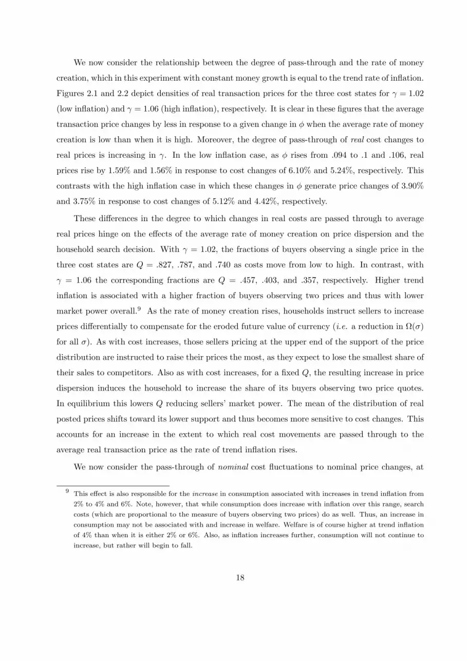
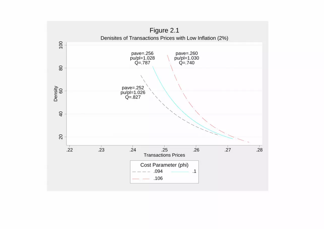
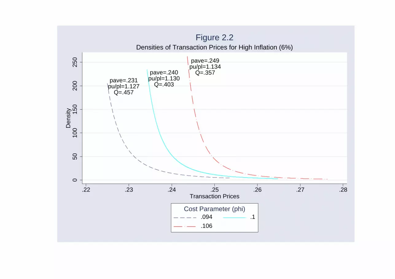
We now consider the relationship between the degree of pass-through and the rate of money
creation, which in this experiment with constant money growth is equal to the trend rate of inflation.
Figures 2.1 and 2.2 depict densities of real transaction prices for the three cost states for γ = 1.02
(low inflation) and γ = 1.06 (high inflation), respectively. It is clear in these figures that the average
transaction price changes by less in response to a given change in φ when the average rate of money
creation is low than when it is high. Moreover, the degree of pass-through of real cost changes to
real prices is increasing in γ. In the low inflation case, as φ rises from .094 to .1 and .106, real
prices rise by 1.59% and 1.56% in response to cost changes of 6.10% and 5.24%, respectively. This
contrasts with the high inflation case in which these changes in φ generate price changes of 3.90%
and 3.75% in response to cost changes of 5.12% and 4.42%, respectively.
These differences in the degree to which changes in real costs are passed through to average
real prices hinge on the effects of the average rate of money creation on price dispersion and the
household search decision. With γ = 1.02, the fractions of buyers observing a single price in the
three cost states are Q = .827, .787, and .740 as costs move from low to high. In contrast, with
γ = 1.06 the corresponding fractions are Q = .457, .403, and .357, respectively. Higher trend
inflation is associated with a higher fraction of buyers observing two prices and thus with lower
market power overall.9 As the rate of money creation rises, households instruct sellers to increase
prices differentially to compensate for the eroded future value of currency (i.e. a reduction in Ω(σ)
for all σ). As with cost increases, those sellers pricing at the upper end of the support of the price
distribution are instructed to raise their prices the most, as they expect to lose the smallest share of
their sales to competitors. Also as with cost increases, for a fixed Q, the resulting increase in price
dispersion induces the household to increase the share of its buyers observing two price quotes.
In equilibrium this lowers Q reducing sellers’ market power. The mean of the distribution of real
posted prices shifts toward its lower support and thus becomes more sensitive to cost changes. This
accounts for an increase in the extent to which real cost movements are passed through to the
average real transaction price as the rate of trend inflation rises.
We now consider the pass-through of nominal cost fluctuations to nominal price changes, at
9 This effect is also responsible for the increase in consumption associated with increases in trend inflation from
2% to 4% and 6%. Note, however, that while consumption does increase with inflation over this range, search
costs (which are proportional to the measure of buyers observing two prices) do as well. Thus, an increase in
consumption may not be associated with and increase in welfare. Welfare is of course higher at trend inflation
of 4% than when it is either 2% or 6%. Also, as inflation increases further, consumption will not continue to
increase, but rather will begin to fall.
18
different levels of trend inflation. In our stochastic economy, the inflation rate as defined in (4.3)
is endogenous because it is determined not only by exogenous money creation (trend inflation at
rate (γ − 1)× 100), but also by the equilibrium response of nominal prices to random fluctuations
in costs. We define the pass-through of nominal cost changes to the nominal price level by the
response of P avet to fluctuations in nominal costs as given by (4.4).
To estimate the degree of pass-through by this measure in our economy we first generate a
realization of the economy’s equilibrium stochastic process 10,000 periods in length. We then adjust
nominal price changes by subtracting the net rate of trend inflation,
It = It − 100(γ − 1), (4.8)
to obtain a time series of inflation generated only by movements in costs. We compute a corre-
sponding series of nominal cost changes as follows:
MCt =[MCt −MCt−1
MCt−1
]100 =
[γmct
mct−1− 1
]100, (4.9)
where MCt and mct are given by (4.4) and (4.5) respectively. We then estimate (by OLS) the
degree of pass-through of nominal cost movements to nominal prices using the following regression
equation:
It = δMCt + εt, (4.10)
where εt is assumed to be an iid, mean zero, normal error.10
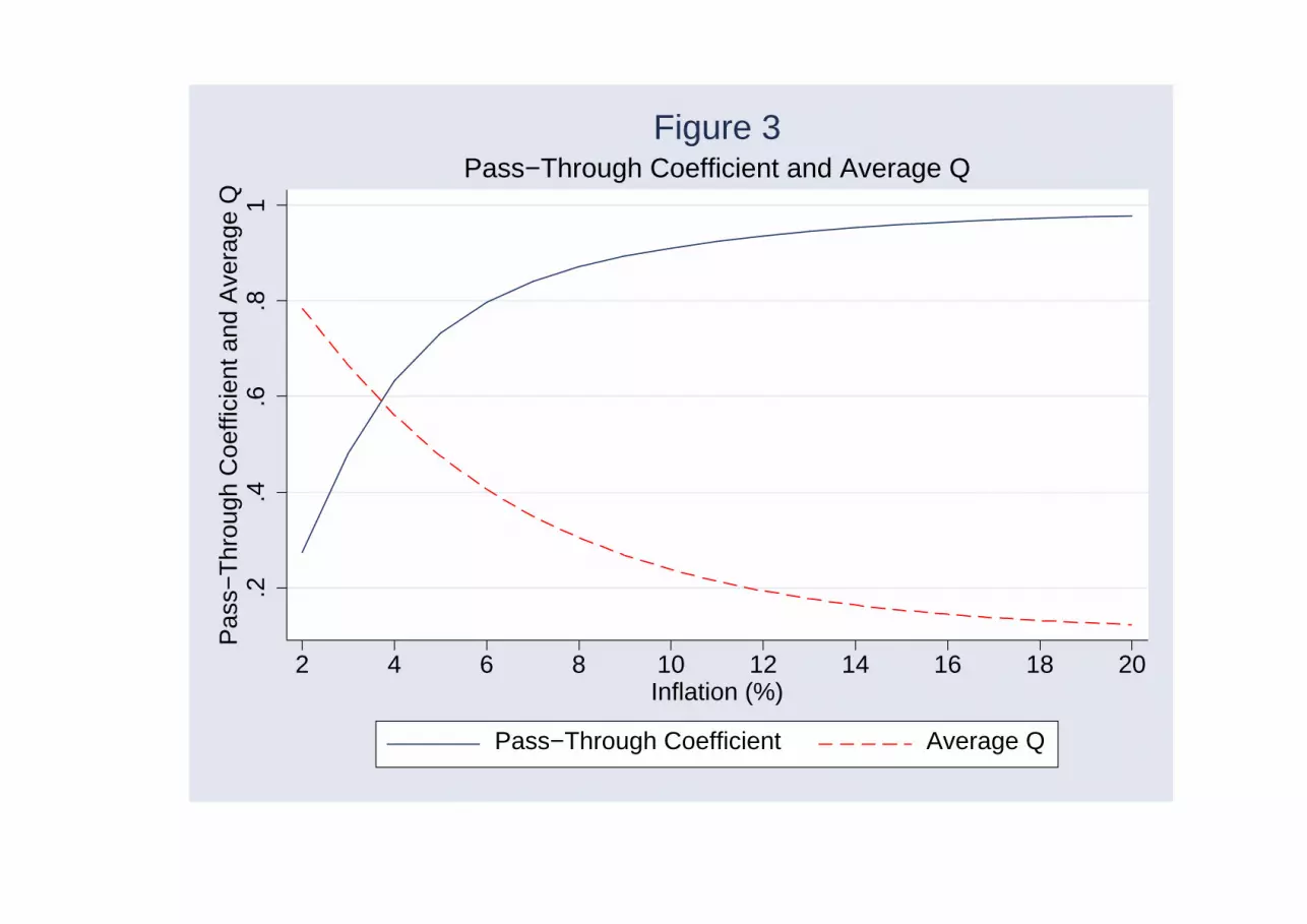
Figure 3 depicts estimated pass-through coefficients, δ, and the average level of Q in equilibrium
for levels of trend inflation ranging from two percent to twelve percent. Over this range our estimates
of pass-through increase monotonically but at a decreasing rate from .27 to .95 as the rate of trend
inflation increases.11
This relationship is in accordance with the empirical findings of Devereux and Yetman (2002) who
found pass-through of nominal exchange rate movements to consumer prices to be increasing in
average inflation at a decreasing rate in a panel of 107 countries over the post-Bretton Woods
period. It is also in accordance with the arguments of Taylor (2000) who cites evidence that the
10 We consider (4.10) to be a reasonable correspondent to the regression equation estimated by Devereux and
Yetman (2002) in their analysis of the pass-through of nominal exchange rate movements to the nominal price
level.
11 These estimates are very precise. All standard errors lie between .0001 and .0004.
19
responsiveness of prices to cost increases has declined with average inflation for several developed
countries during the late 1980’s and 1990’s.
Intuition for the increase in nominal cost pass-through as the trend inflation rate rises may
again be traced to the average share of buyers observing a single price. This fraction decreases
at a decreasing rate as the rate of trend inflation increases. For a fixed Q, an increase in trend
inflation increases price dispersion and raises the return to increasing the share of buyers observing
a single price quote. As a result, an increase in γ lowers Q in all states and reduces sellers’ market
power. With lower Q, the average nominal price shifts toward the lower support of the distribution
of transaction prices and is more sensitive to changes in nominal costs.
Finally, we consider the dynamics of inflation induced by cost fluctuations in our economy.
Figure 4 illustrates that the variance of inflation is increasing in the average rate of money creation.
as the response of nominal prices to changes in nominal costs increases, the variance of inflation
rises relative to that of nominal costs. Inflation induced by cost changes is not, however, persistent
in our economy. The household adjusts to the change in costs within the period in which the cost
shock is realized and inflation either jumps above or falls below its trend level in that period only.
4.3: Prices and inflation dynamics with monetary shocks
We now consider the effect of shocks to the money creation rate, holding fixed the disutility
of production at φ = .1 and the curvature parameter in preferences at α = 1.5. Again we consider
a three-state economy with σ determined by γ alone. To begin with we let γ ∈ G as specified in
(4.6) with Π = πγ given by (4.7). In other experiments we allow the average rate of trend inflation
to differ from the optimum rate of 4% .
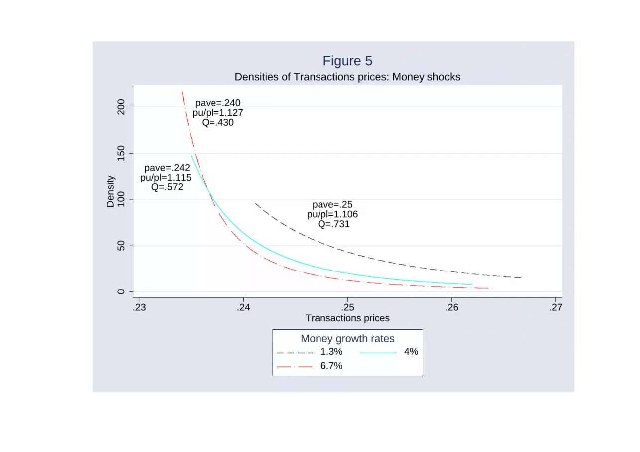
Figure 5 depicts the densities of real transactions prices in the three money growth states, each
identified by the value of γ in that state. In the figure, it can be see that higher money creation
is associated with lower average transactions prices (and thus, higher consumption) for these three
states.12 A higher rate of money creation is also associated with greater price dispersion in the
sense of a higher p/p and a lower fraction of buyers observing a single price.
The overall response of the economy to monetary shocks in equilibrium is a combination of two
effects. Consider an increase in the money growth rate, say from 4% to 6.7%. Because the increase
in money growth is persistent, it raises expected future inflation. This reduces Ω(σ) and increases
price dispersion for a fixed fraction of buyers observing a single price. As with cost increases, high
12 This would not necessarily be true if money creation in the high state were higher than 6.7%. Beyond some
point, higher expected inflation raises the average transaction price and reduces consumption.
20
price sellers raise their price by more than low price sellers because in doing so they lose only a
relatively small proportion of their sales to competitors. Increased price dispersion, however, causes
households to raise the fraction of buyers observing a second price. As in the case of differential
pass-through of cost shocks, this shifts the mass of the distribution of transactions prices towards
its lower support and limits the increase in real prices associated with a depreciation of money. In
the cases depicted, the reduction in market power dominates, and real prices fall in response to a
persistent increase in the money growth rate.
At higher levels of average inflation, the response of prices to a reduction in Ω(σ) dominates.
For example, consider a case in which the average rate of money creation is 15%, and the low
and high money growth states represent the same percentage increase and decrease as in the case
depicted in Figure 5. In this case the average real transaction price rises from .245 to .248 and
.251 as the money creation rate moves from low (12%) to 15% to high (18%). In this case a higher
money growth rate still reduces market power, as Q falls from .180 to .152 to .134 as γ rises. These
reductions are just not sufficient to overcome the inflation tax.
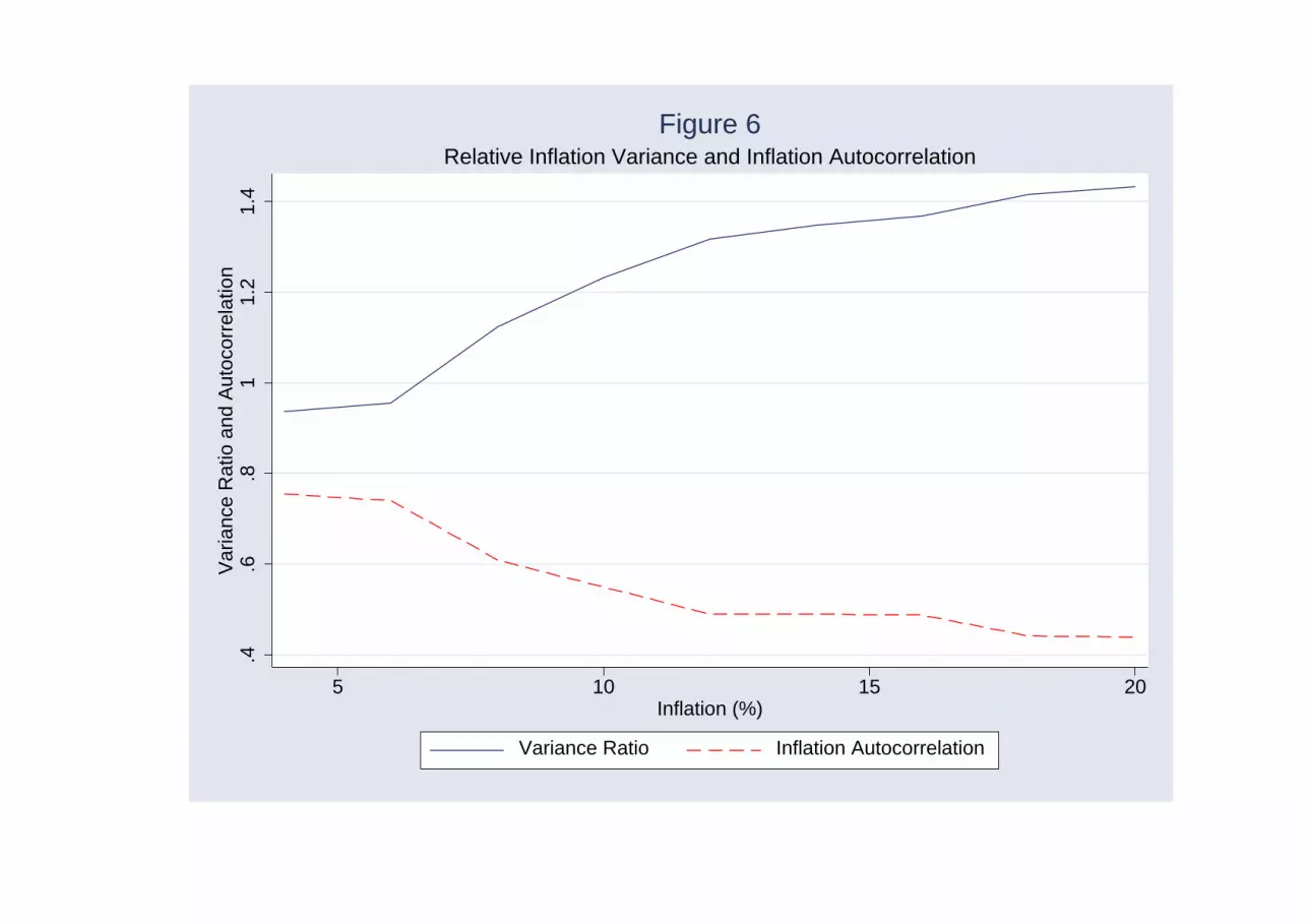
We describe the effect of monetary shocks on nominal prices by considering the dynamics of
the inflation rate as defined by (4.3). Figure 6 plots ratios of the standard deviation and first-order
autocorrelation of inflation to the corresponding statistic for money creation as the average rate
of money creation rises from 4% to 20%. In each case, the low and high money growth states
represent the same percentage decrease and increase. Statistics are computed from simulations of
the equilibrium stochastic process for 10,000 periods. It can be seen that the model can account
for an increase in the variance of inflation as the average rate of inflation (which in our economy is
always equal to the average rate of money creation) rises. At relatively low levels of inflation, the
economy also generates inflation persistence.
Here persistent inflation is associated with the incomplete response of the price level to changes
in the money supply in periods when the money growth rate shifts. At low levels of average inflation,
inflation is less volatile than the money growth rate, and more persistent.
4.4: Preference shocks
We now consider the effects of random shifts in preferences, holding costs and the rate of money
creation constant. In this case the state σ is determined by α ∈ A as specified in (4.6) with Π = πα
again given by (4.7). We initially fix the rate of money creation at γ = 1.04; and throughout we fix
the cost parameter at φ = .1. Figure 7 depicts densities of transactions prices for the three states.
In the figure it can be seen that an increase in α shifts the distribution of transactions prices to
21
the right, increasing the average transaction price. An increase in α also reduces p(σ)/p(σ), and
increases the share of buyers observing a single price.
In our environment, preference shocks are shifts in households’ intertemporal elasticity of
substitution. An increase in α lowers the elasticity and in the presence of inflation lowers Ω(σ),
raising prices overall. Unlike an increase in the cost parameter φ which also lowers Ω, a preference
shift does not directly raise the the marginal cost price. Rather, from (3.11) it can be seen that
an increase in α raises p relative to both p∗ increasing market power overall and compressing the
distribution of posted prices. This in turn reduces households’ return to having a given measure
of buyers observe a second price. For the cases depicted in Figure 7, Q increases from .501 to .561
and .619 as α rises from 1.48 to 1.5 and 1.52, respectively.
The effects of preference shocks contrast significantly with those of cost shocks, even though
increases in α do induce increases in real costs because of their effect on Ω(σ). For the case depicted
in Figures 7, the real disutility of production increases by 1.12% and .97% as α increases from 1.48
to 1.5 and further to 1.52. This increase in costs is more than passed through to real prices,
which increase by 2.66% and 2.85% as α rises. Increases in costs due to direct cost shocks lower
market power, generating incomplete pass-through, whereas increases in costs due to preference
shifts increase market power, resulting in large increases in real prices.
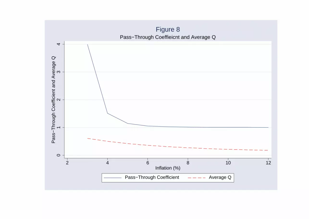
The effects of preference shocks on nominal prices also contrast sharply with those of cost
shocks. Figure 8 (an analog of Figure 3) depicts pass-through coefficients and average Q for rates
of trend inflation between 3% and 12%, estimated again using (4.10). In this case it can be seen that
pass-through is always above one, but declines as inflation increases. The effect of trend inflation
on average Q tends to eliminate the response of Q to increases in α, resulting in a drop in pass-
through. At high rates of inflation, pass-through of cost changes due to either direct cost shocks or
preference shocks to the nominal price level is effectively one-for-one. At low inflation, however, the
two different types of cost movements are passed-through to drastically different degrees. Inflation
dynamics in response to preference shocks also differ markedly from those associated with cost
movements. As trend inflation increases, the variance of inflation induced by preference shocks
falls.
5. Endogenous Money
In this section, we consider versions of our economy in which the monetary authority chooses
the rate of money creation in response to cost and preference shocks.
—TO BE COMPLETED
22
6. Conclusions
This paper has considered a stochastic general equilibrium monetary economy in which both
nominal and real prices respond incompletely to stochastic fluctuations in costs, preferences, and
money creation, in spite of the fact that there are no exogenously imposed constraints on sellers’
ability to adjust prices. As the rate of average inflation increases, the responsiveness of prices to
cost shocks increases. The findings are therefore consistent with the observation that prices and
inflation have become less responsive to cost movements as the average inflation rate has fallen,
and with the observation that the extent to which cost shocks in the form or nominal exchange
rate movements are passed through to consumer prices is declining in the average rate of inflation
across countries. The model is also consistent with the observation that high average inflation is
associated with a high inflation variance.
This version of the paper is preliminary and incomplete. Further work will consider endogenous
money in response to cost and preference shocks. Further work will also focus more closely on
the dynamics of inflation. In our model, sellers’ pricing response to shocks generates a positive
relationship between the variance and mean of inflation. Only in the case of monetary shocks,
however, is endogenous inflation persistent.
23
References:
Basu, S., and J. Fernald. “Returns to Scale in U.S. Production: Estimates and Implications”,Journal of Political Economy 105(2) (April 1997) 249-83.
Benabou, R. “Search, Price Setting and Inflation”, Review of Economic Studies, 55(3) (July 1988)353-376.
———. “Inflation and Efficiency in Search Markets”, Review of Economic Studies, 59(2) (April1992) 299-329.
Burdett, K. and K. Judd. “Equilibrium Price Dispersion”, Econometrica 51(4) (July (1983) 955-70.
Casella, A., and J. Feinstein. “Economic Exchange during Hyperinflation”, Journal of PoliticalEconomy, 96(1) (February 1990) 1-27.
Chirinko, R., and S. Fazzari. “Economic Fluctuations, Market Power, and Returns to Scale: Ev-idence from Firm-Level Data”, Journal of Applied Econometrics 9(1) (January-March 1994)47-69.
Diamond, P. “A Model of Price Adjustment”, Journal of Economic Theory 2 (1971) 156-168.
———. “Search, Sticky Prices, and Inflation”, Review of Economic Studies, 60(1) (January 1993)53-68.
Devereux, M.B. and J. Yetman. “Price Setting and Exchange Rate Pass-through: Theory andEvidence”, manuscript, University of British Columbia and University of Hong Kong, (October2002).
Dotsey, M., R. King, and A. Wolman. “State Dependent Pricing and the General EquilibriumDynamics of Money and Output”, Quarterly Journal of Economics CXIV(2) (April 1999)655-90.
Eden, B.. “The Adjustment of Prices to Monetary Shocks when Trade is Uncertain and Sequential”,Journal of Political Economy 102(3) (June 1994) 493-509.
Fershtman, C., A. Fishman, and A. Simhon. “Inflation and Efficiency in a Search Economy”,International Economic Review, 44(1) (February 2003) 205-22.
Head, A. and A. Kumar. “Price Dispersion, Inflation, and Welfare”, manuscript, Queen’s Univer-sity, April 2003.
Head, A. and S. Shi. “A Fundamental Theory of Exchange Rates and Direct Currency Trade”,manuscript, Queen’s University and University of Toronto, November 2002, Journal of Mone-tary Economics, forthcoming.
Lach, S. and D. Tsiddon. “ The Behavior of Prices and Inflation: An Empirical Analysis ofDisaggregated Price Data”, Journal of Political Economy , 100(2) (April 1992) 349-89.
24
———. “Existence and Persistence of Price Dispersion: An Empirical Analysis”, Review of Eco-nomics and Statistics, 84(3) (August 2002) 433-44.
Morrison, C., “Market Power Economic Profitability, and Productivity Growth Measurement”,NBER Working Paper No. 3355, 1990.
Reinsdorf, M. “New Evidence on the Relation between Inflation and Price Dispersion”, AmericanEconomic Review, 84(3) (1994) 720-731.
Shi, S. “Money and Prices: A Model of Search and Bargaining”, Journal of Economic Theory,67(2) (December 1995) 467-96.
———. “Search, Inflation and Capital Accumulation”, Journal of Monetary Economics, 44(1)(August 1999) 81-103.
Soller-Curtis, E. and R. Wright. “Price Setting and Price Dispersion in a Monetary Economy; orthe Law of Two Prices”, manuscript, (2000).
Taylor, J., “Low Inflation, Pass-through, and the Pricing Power of Firms”, European EconomicReview 44 (2000) 1389-1408.
Tommasi, M., “Inflation and Relative Prices: Evidence from Argentina”, in Optimal Pricing, In-flation, and the Cost of Price Adjustment, E. Sheshinski and Y. Weiss, eds., MIT Press,Cambridge, MA, 1993, 485-511.
———, “The Consequences of Price Instability on Search Markets: Toward Understanding theEffects of Inflation”, American Economic Review, 84(5) (December 1994) 1385-96.
———, “On High Inflation and the Allocation of Resources”, Journal of Monetary Economics,44(3) (December 1999) 401-21.
Van Hoomissen, T., “Price Dispersion and Inflation: Evidence from Israel”, Journal of PoliticalEconomy, 96(6) (December 1988) 1303-13.
25
pave=.235pu/pl=1.114
Q=.624
pave=.242pu/pl=1.116
Q=.560
pave=.25pu/pl=1.118
Q=.5
050
100
150
200
Den
sity
.22 .23 .24 .25 .26 .27 .28Transaction Prices
.094 .1
.106
Cost Parameter (phi)
Densities of Transaction Prices for Optimal Inflation (4%)Figure 1
pave=.252pu/pl=1.026
Q=.827
pave=.256pu/pl=1.028
Q=.787
pave=.260pu/pl=1.030
Q=.74020
4060
8010
0D
ensi
ty
.22 .23 .24 .25 .26 .27 .28Transactions Prices
.094 .1
.106
Cost Parameter (phi)
Denisites of Transactions Prices with Low Inflation (2%)Figure 2.1
pave=.231pu/pl=1.127
Q=.457
pave=.240pu/pl=1.130
Q=.403
pave=.249pu/pl=1.134
Q=.3570
5010
015
020
025
0D
ensi
ty
.22 .23 .24 .25 .26 .27 .28Transaction Prices
.094 .1
.106
Cost Parameter (phi)
Densities of Transaction Prices for High Inflation (6%)Figure 2.2
.2.4
.6.8
1P
ass−
Thr
ough
Coe
ffici
ent a
nd A
vera
ge Q
2 4 6 8 10 12 14 16 18 20Inflation (%)
Pass−Through Coefficient Average Q
Pass−Through Coefficient and Average QFigure 3
0.0
2.0
4.0
6.0
8.1
Var
ianc
e of
Infla
tion
due
to C
ost S
hock
s
0 5 10 15 20Inflation (%)
The Variance and Mean of Inflation with Cost ShocksFigure 4
pave=.25 pu/pl=1.106
Q=.731
pave=.242pu/pl=1.115
Q=.572
pave=.240pu/pl=1.127
Q=.4300
5010
015
020
0D
ensi
ty
.23 .24 .25 .26 .27Transactions prices
1.3% 4%
6.7%
Money growth rates
Densities of Transactions prices: Money shocksFigure 5
.4.6
.81
1.2
1.4
Var
ianc
e R
atio
and
Aut
ocor
rela
tion
5 10 15 20Inflation (%)
Variance Ratio Inflation Autocorrelation
Relative Inflation Variance and Inflation AutocorrelationFigure 6
pave=.236 pu/pl=1.118
Q=.501pave=.242
pu/pl=1.115 Q=.561
pave=.249pu/pl=1.114
Q=.619
050
100
150
200
Den
sity
.23 .24 .25 .26 .27Transactions prices
1.48 1.5
1.52
Curvature parameters (alpha)
Densities of Transactions prices: Preference shocksFigure 7