JOURNAL OF GEOPHYSICAL RESEARCH, VOL. 106, NO. C1, PAGES 1067-1084, JANUARY 15, 2001 Response of a river plume during an upwelling favorable wind event Derek A. Fong • Massachusetts Institute of Technology/Woods Hole Oceanography InstitutionJoint Programin Oceanography Woods Hole, Massachusetts W. Rockwell Geyer Departmentof Applied OceanPhysics and Engineering, WoodsHole Oceanographic Institution Woods Hole, Massachusetts Abstract. The response of a surface-trapped river plume to an upwelling favorable wind is studied using a three-dimensional model in a simple, rectangular domain.Model simulations demonstrate that the plume thins and is advected offshore by the cross-shore Ekman transport. The thinnedplume is susceptible to significant mixing because of the vertically sheared horizontal currents. The Ekman dynamics and shear-induced mixing cause the plume to evolve to a quasi-steady uniform thickness, which can be estimated by a criticalRichardson numbercriterion.Although the mixingrate decreases slowly in time, mixingcontinues under a sustained upwelling wind until the plume is destroyed. Mixing persists at the seaward plume front because of an Ekman straining mechanism in which there is a balancebetween the advection of cross-shore salinitygradients and vertical mixing. The plume mixingrate observed is similarto the mixinglaw obtained by previous studies of one-dimensional mixing,although the river plume mixingis essentially two- dimensional. 1. Introduction It haslongbeen recognized that localwinds play an impor- tant role in the dynamics of river plumes. A theoreticalstudy by Csanady [1978] demonstrates that steady alongshore winds advectthe seaward front associated with a plume either on- shore or offshore in a manner consistent with Ekman dynam- ics. Observations [Masse andMurthy, 1990; Miinchow and Gar- vine,1993] aswell asnumerical simulations [Chao,1987,1988; Kourafalou et al., 1996] of river plumes are consistent with Csanady's [1978]results: upwelling winds tend to spread plume waters offshore. Although the basictendency for the plume to spreadoff- shore duringupwelling windshasbeen observed in the afore- mentioned studies, none of thesestudies quantifies the plume motions in response to upwelling winds nor determines whether or not the Ekman physics are the only importantpart of the dynamical balance. Fonget al. [1997]provideone of the first quantitative testsof the plume response to alongshore winds based on observations of the western Gulf of Maine plume.They find that the motions at the seaward front of the plume are approximately described by an Ekman-dominated alongshore momentum balance. It is likely that the Ekman physics is important for the entire plume behavior,and one might expect the Ekman response to place strong constraints on how the structure of the plume is modifiedduring an up- •Nowat Environmental FluidMechanics Laboratory, Department of Civil and EnvironmentalEngineering, Stanford University, Stan- ford, California. Copyright 2001 by the AmericanGeophysical Union. Paper number2000JC900134. 0148-0227/01/2000JC900134509.00 wellingfavorable wind event.The previous studies suggest that one consequence of upwellingwinds is to thin the plume. However, the details of this thinning process have not been quantified or described in any detail. The wind-induced mixing of a river plumehasreceived little attention in previous studies. Masse andMurthy [1992]observe the spreading of the thermallydriven Niagara River plume to behave qualitatively consistently with the Ekman response. They suggest that the secondary effect of windsis to mix the plume and ambientwaters.They argue that strong upwelling windswill enhance plume mixingby blowingthe plume off- shore and weakeningthe vertical densitygradients. The en- hancedshears inducedby the thinningplume may make the plume more susceptible to shear-induced turbulent mixing. Souza and Simpson [1997] alsonote that winds may be impor- tant in driving mixing in a plume but do not describethe mechanism by whichit wouldbe accomplished. There remains the questions of how the thinning and spreading of the plume waters during upwelling winds induce plume mixing. Xing and Davies[1999]consider the effect of different turbulentenergy models on wind-induced plume mixing. They discuss the ele- vated mixingattributable to wind events but do not elucidate the basic physics behind the mixing. Althoughthe plume is a three-dimensional phenomenon, it is likely that some of the concepts developed in previous stud- iesof one-dimensional mixing maybe helpfulin understanding the wind-induced mixingin the plume. There have been sev- eral investigations that havestudied the one-dimensional mix- ing of a stratified fluid forced by a surface stress [e.g.,Kraus and Turner, 1967; Pollard etal., 1973; Fernando, 1991]. A recent study by Trowbridge [1992] shows that the deepeningof a stratified fluid drivenby a surface stress can be modeledas a gradient transportprocess where turbulent mixing is strong 1067
Transcript
JOURNAL OF GEOPHYSICAL RESEARCH, VOL. 106, NO. C1, PAGES 1067-1084, JANUARY 15, 2001
Response of a river plume during an upwelling favorable wind event
Derek A. Fong • Massachusetts Institute of Technology/Woods Hole Oceanography Institution Joint Program in Oceanography Woods Hole, Massachusetts
W. Rockwell Geyer Department of Applied Ocean Physics and Engineering, Woods Hole Oceanographic Institution Woods Hole, Massachusetts
Abstract. The response of a surface-trapped river plume to an upwelling favorable wind is studied using a three-dimensional model in a simple, rectangular domain. Model simulations demonstrate that the plume thins and is advected offshore by the cross-shore Ekman transport. The thinned plume is susceptible to significant mixing because of the vertically sheared horizontal currents. The Ekman dynamics and shear-induced mixing cause the plume to evolve to a quasi-steady uniform thickness, which can be estimated by a critical Richardson number criterion. Although the mixing rate decreases slowly in time, mixing continues under a sustained upwelling wind until the plume is destroyed. Mixing persists at the seaward plume front because of an Ekman straining mechanism in which there is a balance between the advection of cross-shore salinity gradients and vertical mixing. The plume mixing rate observed is similar to the mixing law obtained by previous studies of one-dimensional mixing, although the river plume mixing is essentially two- dimensional.
1. Introduction
It has long been recognized that local winds play an impor- tant role in the dynamics of river plumes. A theoretical study by Csanady [1978] demonstrates that steady alongshore winds advect the seaward front associated with a plume either on- shore or offshore in a manner consistent with Ekman dynam- ics. Observations [Masse and Murthy, 1990; Miinchow and Gar- vine, 1993] as well as numerical simulations [Chao, 1987, 1988; Kourafalou et al., 1996] of river plumes are consistent with Csanady's [1978] results: upwelling winds tend to spread plume waters offshore.
Although the basic tendency for the plume to spread off- shore during upwelling winds has been observed in the afore- mentioned studies, none of these studies quantifies the plume motions in response to upwelling winds nor determines whether or not the Ekman physics are the only important part of the dynamical balance. Fong et al. [1997] provide one of the first quantitative tests of the plume response to alongshore winds based on observations of the western Gulf of Maine
plume. They find that the motions at the seaward front of the plume are approximately described by an Ekman-dominated alongshore momentum balance. It is likely that the Ekman physics is important for the entire plume behavior, and one might expect the Ekman response to place strong constraints on how the structure of the plume is modified during an up-
•Now at Environmental Fluid Mechanics Laboratory, Department of Civil and Environmental Engineering, Stanford University, Stan- ford, California.
Copyright 2001 by the American Geophysical Union.
Paper number 2000JC900134. 0148-0227/01/2000JC900134509.00
welling favorable wind event. The previous studies suggest that one consequence of upwelling winds is to thin the plume. However, the details of this thinning process have not been quantified or described in any detail.
The wind-induced mixing of a river plume has received little attention in previous studies. Masse and Murthy [1992] observe the spreading of the thermally driven Niagara River plume to behave qualitatively consistently with the Ekman response. They suggest that the secondary effect of winds is to mix the plume and ambient waters. They argue that strong upwelling winds will enhance plume mixing by blowing the plume off- shore and weakening the vertical density gradients. The en- hanced shears induced by the thinning plume may make the plume more susceptible to shear-induced turbulent mixing. Souza and Simpson [1997] also note that winds may be impor- tant in driving mixing in a plume but do not describe the mechanism by which it would be accomplished. There remains the questions of how the thinning and spreading of the plume waters during upwelling winds induce plume mixing. Xing and Davies [1999] consider the effect of different turbulent energy models on wind-induced plume mixing. They discuss the ele- vated mixing attributable to wind events but do not elucidate the basic physics behind the mixing.
Although the plume is a three-dimensional phenomenon, it is likely that some of the concepts developed in previous stud- ies of one-dimensional mixing may be helpful in understanding the wind-induced mixing in the plume. There have been sev- eral investigations that have studied the one-dimensional mix- ing of a stratified fluid forced by a surface stress [e.g., Kraus and Turner, 1967; Pollard et al., 1973; Fernando, 1991]. A recent study by Trowbridge [1992] shows that the deepening of a stratified fluid driven by a surface stress can be modeled as a gradient transport process where turbulent mixing is strong
1067
1068 FONG AND GEYER: RESPONSE OF A RIVER PLUME TO UPWELLING WIND
enough to maintain a gradient Richardson number at a critical value throughout the boundary layer. This conceptual model of mixing is consistent with both laboratory experiments [Kantha et al., 1977; Kato and Phillips, 1969] and oceanic measurements [Price et al., 1978, 1986]. In contrast to slab models, it is ame- nable to regimes such as river plumes in which gradients ex- tend to the water surface.
The mechanism by which mixing is achieved in these studies is stress-induced turbulence: the surface stress induces a
sheared horizontal flow within the pycnocline. If the shears are large enough to overcome the stabilizing influence of stratifi- cation, shear instability may result, followed by turbulent mix- ing. For a plume that thins during an upwelling wind event, horizontal velocity shears, and hence the likelihood of mixing, should be enhanced.
The purpose of this study is to describe the response of a river plume to an upwelling favorable wind event. In particular, this study attempts to accomplish two objectives: (1) to deter- mine how advective processes change the shape of the plume and (2) to investigate the consequences of these advective motions on the mixing of the plume with ambient coastal waters.
In order to accomplish these objectives, two different meth- ods are employed. In section 2 a simple conceptual model is developed, employing simple physics and ideas developed in previous studies of one-dimensional mixing. In section 3 the set of numerical modeling experiments by which the conceptual model is tested is described. While highly idealized, the nu- merical model provides a framework for investigating the im- portant physical processes involved in the advection and mix- ing of a river plume. In section 4 the numerical model is used to study the response of the plume to a moderate-amplitude upwelling favorable wind event. In section 5 these results are generalized for different forcing conditions. In section 6 the mixing during upwelling is compared with mixing during down- welling winds. In section 7 the study is summarized and dis- cussed.
where r w is the wind stress in the along-coast direction, f is the Coriolis parameter, and the stress is assumed to vanish at the base of the plume. If the cross-shore velocity and density anomaly within the plume are approximated by linear profiles with depth that vanish beneath the plume, the bulk Richardson number is estimated by
•7'h 3 (3)
4(3) 2' where #' is the mean reduced gravity ( #Ap/po; Ap is the mean plume density anomaly).
During an upwelling favorable wind event the plume be- comes wider as the seaward front is advected offshore. In order
for the buoyancy of the plume to be conserved the plume must become thinner. The scaling in (3) indicates therefore that an upwelling favorable wind will tend to reduce the bulk Richard- son number in the plume, thus enhancing the likelihood of mixing.
2.2. A Simple Conceptual Model
On the basis of simple Ekman physics and the Richardson number stability criterion discussed in section 2.1 a simple conceptual model is now developed. Although the model will not explicitly include the physics of mixing, it will provide some insight into the advective plume response to an upwelling wind and offer a starting point from which to examine the expected mixing dynamics of a plume.
Since the momentum input by the wind is largely confined within the stratification of the plume and the alongshore mo- mentum is dominated by an Ekman balance [Fong et al., 1997], the mean cross-shore plume velocity is estimated by (2). Fur- thermore, the continuity equation integrated over the plume layer is
Oh 0
O•- + •-• (Sh): 0. (4)
2. Theory 2.1. Parameterizing Vertical Mixing in the Plume
It has been shown in previous studies of one-dimensional mixing that the stability of a stratified fluid, forced by a surface stress, can be characterized by a bulk Richardson number [e.g., Kantha et al., 1977; Karo and Phillips, 1969]
B
Rib = (Au)2, (1) where
p0 (p0- p) dz, h
# is the gravitational acceleration, h is the thickness of the plume, Po is the density of the ambient water, z is the vertical direction, and Au is the magnitude of the velocity difference between the plume and the ambient water beneath it.
If the alongshore momentum is primarily in Ekman balance [Fong et al., 1997], the mean cross-shore plume velocity can be estimated as
• phf' (2)
For a spatially uniform wind stress, (2) requires that gh = const, so Oh/Ot = 0 in the plume. In other words these equa- tions indicate that the plume thickness is locally constant. These assumptions, however, break down at the edges of the plume because the point in the vertical where the stress van- ishes no longer corresponds to the base of the plume. It should be noted that the above constraint does not imply that the shape of the plume does not change in time: only at a fixed location in space does the plume thickness remain constant. The advected plume, in response to the Ekman dynamics, stretches in the moving reference frame owing to cross-shore variations in plume thickness.
To complete the conceptual model, a boundary condition is needed at the seaward front of the plume. The thickness at the seaward front sets the speed at which the plume spreads off- shore. One hypothesis is that this thickness is set by the sta- bility of the front to shear-induced turbulence.
As the simplest means of choosing the boundary condition for the seaward front, (3) can be solved for h with the bulk Richardson number set to some critical value Ri c such that
ß (5) hc• Ap •7 P0
FONG AND GEYER: RESPONSE OF A RIVER PLUME TO UPWELLING WIND 1069
The critical bulk Richardson number Ric is in the range of 0.5-1.0 [Pollard et al., 1973; Price et al., 1986]. Because h c
:1/3 depends on R,c , the uncertainty of Ric only changes h c up to a 14%. It is worth noting that (5) is equivalent to the depth scale found in Pollard et al. [1973] for a linearly stratified fluid with Ric set to unity, and the unsteady solution is neglected.
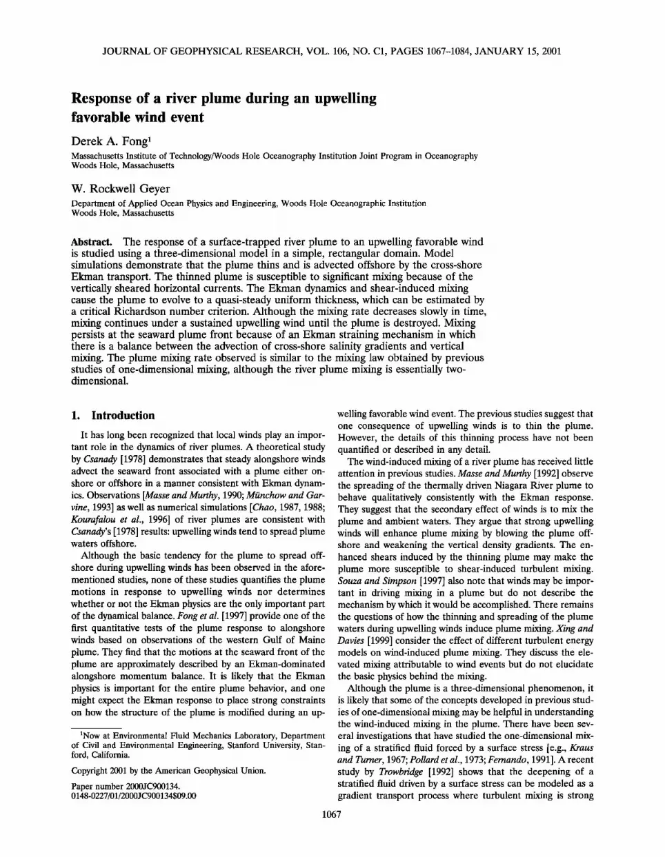
The thickness hc at the seaward edge of the front determines the subsequent evolution of the plume (Figure 1). Substituting b (5) into (2), the rate at which the seaward front moves offshore can be solved for
,r w
•front: ,-,F/, (6) •J"c C
Similarly, the Ekman balance can be used to determine the motion at the shoreward edge of the plume
•.w
• .... [JfhTOw(X) 0 --< X < Lo = (7)
where ho(x) is the initial plume thickness and L o is the initial plume width.
Finally, as mentioned earlier, the conceptual model does not explicitly include any mixing or entrainment physics, nor does it address the details of the physics at the shoreward front. Therefore, if the plume is assumed two-dimensional with no alongshore variations, then the area of the plume must be conserved.
The kinematics implied by the simple model are illustrated by the cartoon shown in Figure 1, where the plume's structure is denoted by the dark shading and its initial structure is shown by the light outline. The seaward edge of the plume moves offshore at a rate inversely proportional to h c. The plume widens as long as the wind forcing persists, and there are cross-shore variations in plume thickness. Eventually, the plume ceases widening once its thickness is uniform. The uni- form thickness plume continues to be advected offshore for as long as the wind forcing continues.
Again, it is important to emphasize that the conceptual model described above does not include any explicit parame- terization of the mixing physics. It only uses a mixing criterion to set the offshore plume boundary condition.
Despite lacking mixing dynamics the conceptual model phys- ics do suggest something about the mixing in the plume. Equa- tion (5) predicts that for portions of the plume thicker than h c the plume should be stable and not susceptible to shear- induced turbulence. However, as any portion of the plume approaches a thickness h c, the Richardson number will ap- proach the critical value, leading to the likelihood of turbulent mixing. If there are no cross-shore gradients in buoyancy within the plume, then mixing will cause a reduction in the salinity anomaly and an increase in thickness, with the total buoyancy remaining constant. The increase in plume thickness implies an increase in the bulk Richardson number because it is dependent on the square of the plume thickness (see (3)). Therefore, without explicit specification of the exchange pro- cesses at the fronts one expects none or very little mixing to take place.
To summarize, the conceptual model suggests that the re- sponse of a plume to a sustained upwelling wind involves the plume's being advected offshore and stretching as long as there are cross-shore variations in plume thickness. If the wind event
ho(x)
h(x)
-- hc
initial plume
plume separates from coast
plume continues
to widen
Lfinal -- hc
thickness and
x = 0 x = L 0 width
Figure 1. Cartoon of conceptual model plume response to a steady upwelling favorable wind.
is sustained long enough, the plume will eventually stop wid- ening and approach a steady state uniform thickness. After the widening process ends, little mixing is expected to take place without any cross-shore buoyancy gradients.
The conditions at the ends of the slab in conceptual model, where there are significant gradients, have not been consid- ered. In section 3 a process-oriented numerical modeling ex- periment is described. The numerical model will be used to test the behavior predicted by the conceptual model and to de- scribe the influence of physics not incorporated in the concep- tual model, particularly those related to the seaward front.
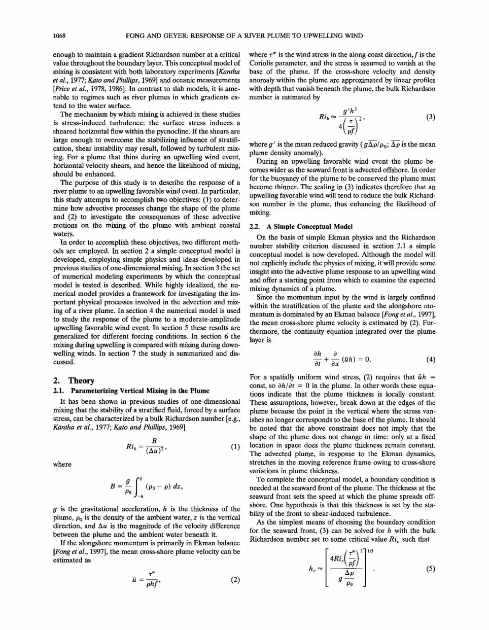
3. Three-Dimensional Model Description A three-dimensional primitive equation hydrodynamic
model [Blumberg and Mellor, 1987] is used to study the wind- induced mixing of a river plume. The model domain, shown in Figure 2, is a rectangular basin, which is an idealized version of the moderately steep nearshore bathymetry found on many narrow continental shelves. Freshwater is discharged via a short river/estuary system at the coast in the upper left hand corner of the 95 km x 450 km model basin (Figure 2). In order to resolve the spatial variability of the plume a spatially vary- ing, high-resolution grid with 50 x 140 x 23 grid cells is employed. The vertical grid varies in proportion to depth, a "sigma coordinate" system. The sigma levels are unevenly spaced, with a higher concentration of levels near the water surface, with the goal of resolving the structure of the surface- trapped plume. Grid cell centers are indicated by dots in Fig-
1070 FONG AND GEYER: RESPONSE OF A RIVER PLUME TO UPWELLING WIND
Plan view
400
35O
3OO Section (x-z) view
,..,250 ,•, '-'
200 -o
1
150 0 20 40 60 80 x (km)
lOO
50
o 20 40 60 80
x (km)
Figure 2. Model configuration. Blumberg and Mellor's Es- tuarine Coastal Ocean Model-3d (ECOM-3D) is run on a 95 km x 450 km x 200 m grid. Grid resolution is indicated by small dots in both plan and section views. Vertical sigma levels are closely spaced at the surface to resolve the near-surface plume behavior. The topography is uniform in the alongshore (y) direction. Freshwater is discharged at the head of the estuary/river system shaded in the northwestern (upper left corner of the plan view) of the model basin. Dashed lines indicate the region over which a composite, alongshore- averaged cross section is constructed to plot different property distributions.
ure 2. For the surface-trapped plume features of interest, res- olution is better than 1 m in the vertical, 1.5-3 km in the cross-shore direction, and 3-6 km in the alongshore direction. For the downwelling case considered in section 6 the cross- shore resolution is 0.75-1.5 km.
The model solves the hydrostatic, Boussinesq equations with sub-grid-scale motions parameterized by eddy coefficients for momentum and scalar diffusion. The coefficients are calcu-
lated using the Mellor-Yamada level 2.5 turbulence closure scheme [Mellor and Yamada, 1982]. This scheme has a gradient Richardson number threshold of 0.24 [Mellor and Yamada, 1982; Nunez Vaz and Simpson, 1994], similar to the criteria used by Trowbridge [1992]. This provides a reasonable param- eterization of the shear-induced turbulent mixing generated by an upwelling favorable wind stress. The background vertical diffusivity is set to 5 x 10 -6 m 2 s -•. The horizontal diffusivities are held constant at 10 m 2 s -•. The influence of rotation is implemented with a constant Coriolis parameter f = 10 -4
--1 S .
Horizontal derivatives are calculated explicitly, while vertical differencing is implicit. The model employs a split time step for internal and external modes. The external mode is two-
dimensional, time-stepped in small increments to satisfy the Courant-Friedrichs-Lewy stability condition associated with
surface gravity waves, while the slower internal mode time step is based on the internal wave speed. For the simulations pre- sented in this paper the external time step is 10 s, and the internal time step is 7 min. The detailed model characteristics are• described by Blumberg and Mellor [1987], and only differ- ences from that model formulation are discussed here.
In advecting the salt and temperature fields a recursive Smo- larkiewicz scheme [Smolarkiewicz and Grabowski, 1990] is used. This scheme has less numerical diffusion than most ad-
vective schemes, which is important when studying fronts.
3.1. Boundary Conditions
At the coastal wall the normal velocity is zero, and a free-slip boundary condition is used for the tangential velocity. The solution does not change appreciably if a semislip or no-slip condition is used instead because of the shallow depth at the wall. At the ocean bottom the fluxes of salt and heat are zero.
There is no flow normal to the topography; the bottom stress is specified using the velocities at the bottom grid cell and a quadratic drag law.
The surface boundary conditions are no flux of salt and heat (no solar radiation, heating, evaporation, nor precipitation), and wind stresses are applied such that
Ou Or] [r wx, r wy] -KM •, • = P0 where r wx and r wy are the applied cross-shore and alongshore wind stress at the surface grid cells, respectively.
A clamped zero elevation is specified at the offshore (x = 95 km; see Figure 2) boundary (no tidal forcing) and a mod- ified Sommerfield radiation condition [Orlanski, 1976] em- ployed at the downstream (y = 0 km) boundary. This imple- mentation is similar to that used by Oey and Mellor [1993], allowing internal waves and bores that propagate along the coast to pass through the model basin. In addition, the model also has enhanced alongshore diffusion at the grid cells near the downstream boundary (y - 0-50 km) in the model do- main. At the upstream (y - 450 km) boundary a steady inflow of 10 cm s -• is applied to represent an ambient coastal flow field in the direction of Kelvin wave propagation (hereinafter referred to as the downstream direction). This value is repre- sentative of the ambient current found on the continental shelf off the east coast of North America [Loder et al., 1998]. The downstream current also serves to avoid the upshelf plume advection observed in numerical models neglecting such an ambient current [Chapman and Lentz, 1994; Fong, 1998; Gar- vine, 1999].
Freshwater discharge is implemented via a small river/ estuary region shaded in Figure 2 at y - 408 km. The river/ estuary system is one grid cell wide and 15 m deep. The fresh water (0 psu) is discharged at the head of the estuary uniformly over the entire 15 m depth.
3.2. Initializing a Freshwater Plume
In order to study the influence of an upwelling wind event on a plume the model plume is "spun up" in the absence of winds for a period of 36 days of buoyancy forcing (0 psu water) at a constant rate of 1500 m 3 s -1 at the head of the estuary. The fresh water is discharged into an initially homogeneous domain of 32 psu water; the fresh water and ambient water are both the same temperature (4øC). The ambient flow field imposed at the northern boundary (see section 3.1) is also 32 psu and 4øC.
FONG AND GEYER: RESPONSE OF A RIVER PLUME TO UPWELLING WIND 1071
t = 0 hrs t = 24 hrs
350 • 3001 ••1]•
(a) .... (b)
200 • i 1
•5o
[I •. I I I I I i i 50-Vi •, .... , ,
I I I I I
0 50 0 50 0 50 0 x (km) x (km) x (km)
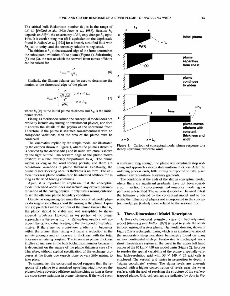
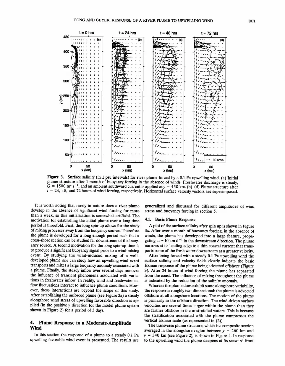
Figure 3. Surface salinity (in 1 psu intervals) for river plume forced by a 0.1 Pa upwelling wind. (a) Initial plume structure after 1 month of buoyancy forcing in the absence of winds. Freshwater discharge is steady, Q = 1500 m 3 s -•, and an ambient southward current is applied aty = 450 km. (b)-(d) Plume structure after t = 24, 48, and 72 hours of wind forcing, respectively. Horizontal surface velocity vectors are superimposed.
It is worth noting that rarely in nature does a river plume develop in the absence of significant wind forcing for more than a week, so this initialization is somewhat artificial. The
motivation for establishing the initial plume over a long time period is threefold. First, the long spin-up allows for the study of mixing processes away from the buoyancy source. Therefore the plume is developed for a long enough period such that a cross-shore section can be studied far downstream of the buoy- ancy source. A second motivation for the long spin-up time is to produce a significant buoyancy signal prior to a wind-mixing event. By studying the wind-induced mixing of a well- developed plume one can study how an upwelling wind event transports and mixes a large buoyancy anomaly associated with a plume. Finally, the steady inflow over several days removes the influence of transient phenomena associated with varia- tions in freshwater inflow. In reality, wind and freshwater in- flow fluctuations interact to influence plume conditions. How- ever, these interactions are beyond the scope of this study. After establishing the unforced plume (see Figure 3a) a steady alongshore wind stress of upwelling favorable direction is ap- plied (in the positive y direction for the model plume system shown in Figure 2) for a period of 3 days.
4. Plume Response to a Moderate-Amplitude Wind
In this section the response of a plume to a steady 0.1 Pa upwelling favorable wind event is presented. The results are
generalized and discussed for different amplitudes of wind stress and buoyancy forcing in section 5.
4.1. Basic Plume Response
A plot of the surface salinity after spin up is shown in Figure 3a. After over a month of buoyancy forcing, in the absence of winds, the plume has developed into a large feature, propa- gating at ---10 km d -• in the downstream direction. The plume narrows at its leading edge to a thin coastal current that trans- ports some of the fresh water downstream at a greater velocity.
After being forced with a steady 0.1 Pa upwelling wind the surface salinity and velocity fields clearly indicate the basic Ekman response of the plume being advected offshore (Figure 3). After 24 hours of wind forcing the plume has separated from the coast. The influence of mixing throughout the plume is indicated by the reduction of the salinity anomaly.
Whereas the plume does exhibit some alongshore variability, the response is roughly two-dimensional: the plume is advected offshore at all alongshore locations. The motion of the plume is primarily in the offshore direction. The wind-driven surface velocities are several times larger within the plume than they are farther offshore in the unstratified waters. This is because
the stratification associated with the plume compresses the vertical Ekman scale (as represented in (2)).
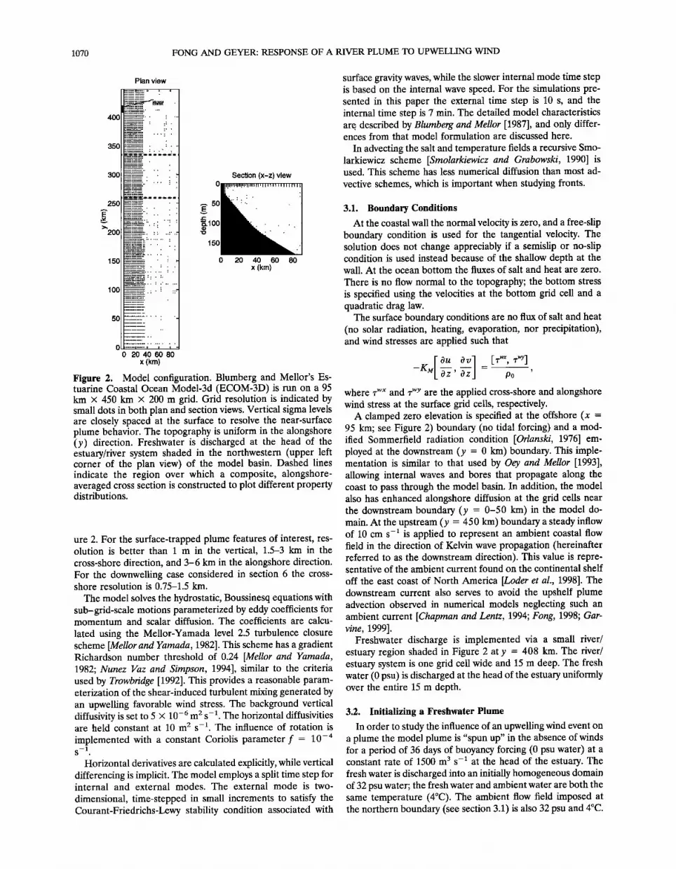
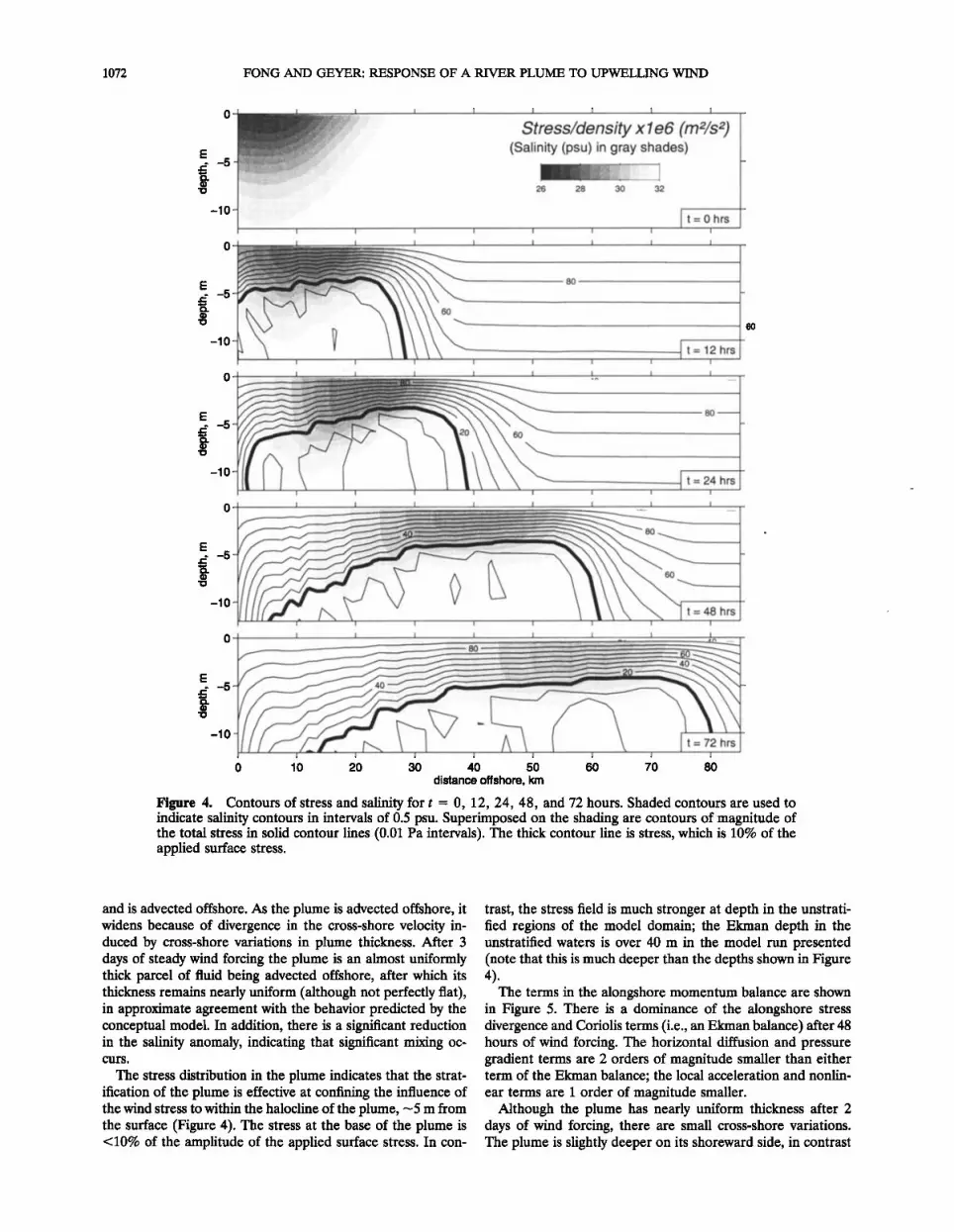
The transverse plume structure, which is a composite section averaged in the alongshore region between y = 260 km and y = 340 km (see Figure 2), is shown in Figure 4. In response to the upwelling wind the plume deepens at its seaward front
1072 FONG AND GEYER: RESPONSE OF A RIVER PLUME TO UPWELLING WIND
Figure 4. Contours of stress and salinity for t = 0, 12, 24, 48, and 72 hours. Shaded contours are used to indicate salinity contours in intervals of 0.5 psu. Superimposed on the shading are contours of magnitude of the total stress in solid contour lines (0.01 Pa intervals). The thick contour line is stress, which is 10% of the applied surface stress.
and is advected offshore. As the plume is advected offshore, it widens because of divergence in the cross-shore velocity in- duced by cross-shore variations in plume thickness. After 3 days of steady wind forcing the plume is an almost uniformly thick parcel of fluid being advected offshore, after which its thickness remains nearly uniform (although not perfectly flat), in approximate agreement with the behavior predicted by the conceptual model. In addition, there is a significant reduction in the salinity anomaly, indicating that significant mixing oc- curs.
The stress distribution in the plume indicates that the strat- ification of the plume is effective at confining the influence of the wind stress to within the halocline of the plume, -5 m from the surface (Figure 4). The stress at the base of the plume is <10% of the amplitude of the applied surface stress. In con-
trast, the stress field is much stronger at depth in the unstrati- fled regions of the model domain; the Ekman depth in the unstratified waters is over 40 m in the model run presented (note that this is much deeper than the depths shown in Figure 4).
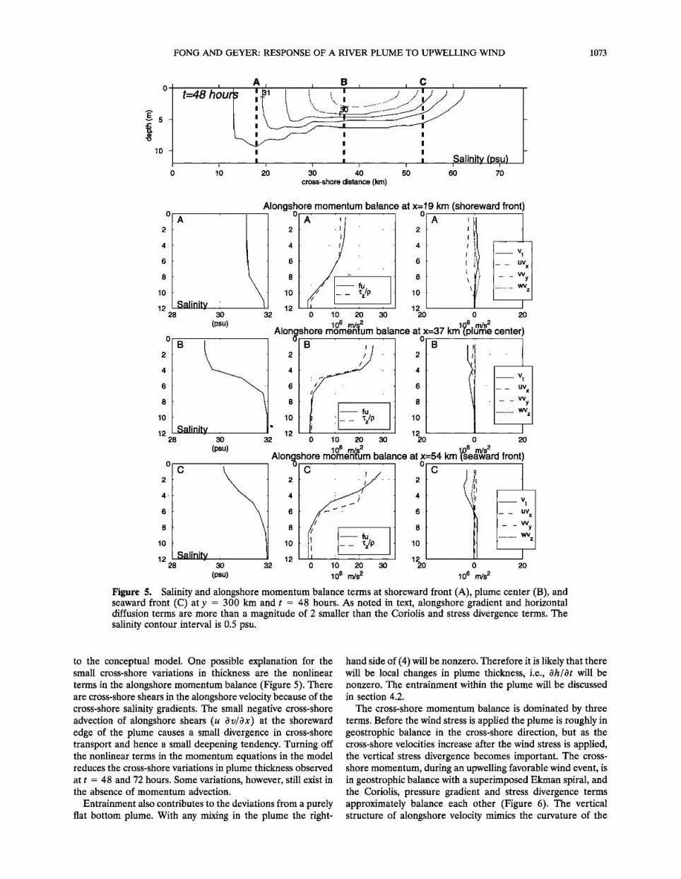
The terms in the alongshore momentum balance are shown in Figure 5. There is a dominance of the alongshore stress divergence and Coriolis terms (i.e., an Ekman balance) after 48 hours of wind forcing. The horizontal diffusion and pressure gradient terms are 2 orders of magnitude smaller than either term of the Ekman balance; the local acceleration and nonlin- ear terms are 1 order of magnitude smaller.
Although the plume has nearly uniform thickness after 2 days of wind forcing, there are small cross-shore variations. The plume is slightly deeper on its shoreward side, in contrast
FONG AND GEYER: RESPONSE OF A RIVER PLUME TO UPWELLING WIND 1073
10 -
I I I ,Salinity (ps, u) 1 20 30 50 60 70
cross-shore distance (km)
o
2
4
6
8
lO
12 28
o
2
4
6
8
lO
12
o
2
4.
6
8
lO
12
Alongshore momentum balance at x=19 km (shoreward front) o o
. .
Salinitv 30 3'0 20 32
A ii
0 10 20 o 20
(psu)
Salinitv 28 3O
(psu)
Salinitv
Alonogsh0re B , • ,
, . .
.
.
ß
• ' -- fu 0 10 20 30
106 m/• 2 Ins m/s 2 momemum balance at x=37 km (plume center'
o
2
4
6
8
lO
12 20 32 o
1ø6 m/s2 (•eaward front' Alonc),shore momenf-um balance at x=54 km 1'ø6 m/s2
6
ß 8
1 / li , 12
_ _ UV x
, • ............ 7 z 2O
I t
28 30
(psu) 32 0 10 20 30 20 0 20
106 m/s 2 106 m/s 2
Figure 5. Salinity and alongshore momentum balance terms at shoreward front (A), plume center (B), and seaward front (C) at y = 300 km and t = 48 hours. As noted in text, alongshore gradient and horizontal diffusion terms are more than a magnitude of 2 smaller than the Coriolis and stress divergence terms. The salinity contour interval is 0.5 psu.
to the conceptual model. One possible explanation for the small cross-shore variations in thickness are the nonlinear
terms in the alongshore momentum balance (Figure 5). There are cross-shore shears in the alongshore velocity because of the cross-shore salinity gradients. The small negative cross-shore advection of alongshore shears (u Ov/Ox) at the shoreward edge of the plume causes a small divergence in cross-shore transport and hence a small deepening tendency. Turning off the nonlinear terms in the momentum equations in the model reduces the cross-shore variations in plume thickness observed at t = 48 and 72 hours. Some variations, however, still exist in the absence of momentum advection.
Entrainment also contributes to the deviations from a purely flat bottom plume. With any mixing in the plume the right-
hand side of (4) will be nonzero. Therefore it is likely that there will be local changes in plume thickness, i.e., Oh/Ot will be nonzero. The entrainment within the plume will be discussed in section 4.2.
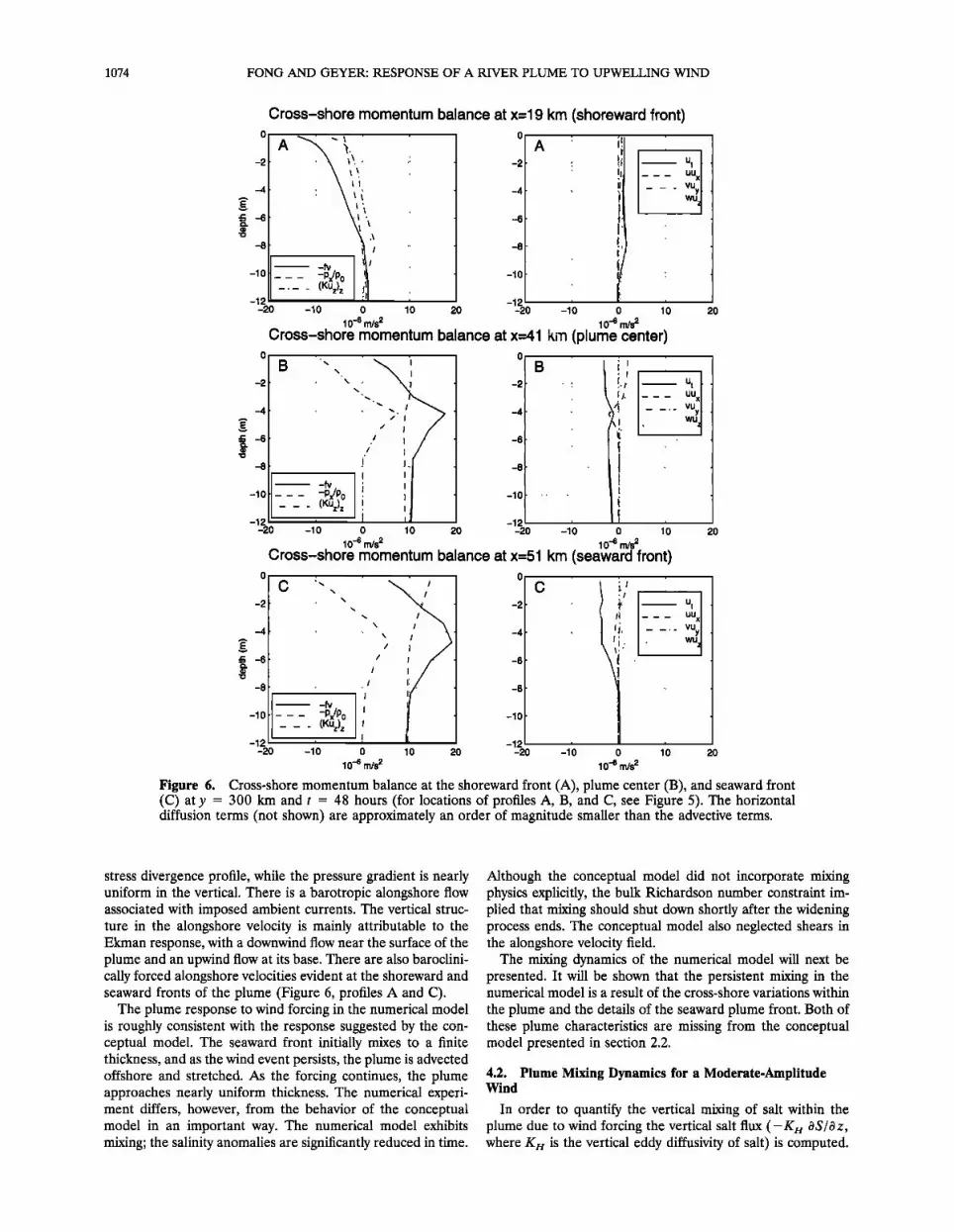
The cross-shore momentum balance is dominated by three terms. Before the wind stress is applied the plume is roughly in geostrophic balance in the cross-shore direction, but as the cross-shore velocities increase after the wind stress is applied, the vertical stress divergence becomes important. The cross- shore momentum, during an upwelling favorable wind event, is in geostrophic balance with a superimposed Ekman spiral, and the Coriolis, pressure gradient and stress divergence terms approximately balance each other (Figure 6). The vertical structure of alongshore velocity mimics the curvature of the
1074 FONG AND GEYER: RESPONSE OF A RIVER PLUME TO UPWELLING WIND
Cross-shore momentum balance at x=l 9 km (shoreward front)
-lO
-12 -20
-. __--ZZ_' :K/p• I,•' -
-10 0 10 20
0
-12 -20 -10 0 10 20
10 -6 m/s 2 10 -6 m/s 2 Cross-shore momentum balance at x=41 km (plume center)
-4
-10
-12 -20
B
_ _ _ -Px/P0 - (KUz) z
-10 20
/
/'
..... /'. ....
j./ I
i .
I o lO
i ii )" ' UUx
I
.
-12 -20 -10 0 10
10 -6 m/s 2 10 -6 m/s 2 Cross-shore momentum balance at x=51 km (seaward front)
20
-2
-10
-12 -20 -1• 20
- - - -P"iPo _ (KUz) z
0
10 -6 m/s 2
\. ' \. 't'' •
j' .
! ....
10 20 -12 •
-20 -10 0 10
10 -6 rn/s 2
Figure 6. Cross-shore momentum balance at the shoreward front (A), plume center (B), and seaward front (C) at y = 300 km and t = 48 hours (for locations of profiles A, B, and C, see Figure 5). The horizontal diffusion terms (not shown) are approximately an order of magnitude smaller than the advective terms.
stress divergence profile, while the pressure gradient is nearly uniform in the vertical. There is a barotropic alongshore flow associated with imposed ambient currents. The vertical struc- ture in the alongshore velocity is mainly attributable to the Ekman response, with a downwind flow near the surface of the plume and an upwind flow at its base. There are also baroclini- cally forced alongshore velocities evident at the shoreward and seaward fronts of the plume (Figure 6, profiles A and C).
The plume response to wind forcing in the numerical model is roughly consistent with the response suggested by the con- ceptual model. The seaward front initially mixes to a finite thickness, and as the wind event persists, the plume is advected offshore and stretched. As the forcing continues, the plume approaches nearly uniform thickness. The numerical experi- ment differs, however, from the behavior of the conceptual model in an important way. The numerical model exhibits mixing; the salinity anomalies are significantly reduced in time.
Although the conceptual model did not incorporate mixing physics explicitly, the bulk Richardson number constraint im- plied that mixing should shut down shortly after the widening process ends. The conceptual model also neglected shears in the alongshore velocity field.
The mixing dynamics of the numerical model will next be presented. It will be shown that the persistent mixing in the numerical model is a result of the cross-shore variations within
the plume and the details of the seaward plume front. Both of these plume characteristics are missing from the conceptual model presented in section 2.2.
4.2. Plume Mixing Dynamics for a Moderate-Amplitude Wind
In order to quantify the vertical mixing of salt within the plume due to wind forcing the vertical salt flux (-Ka• OS/Oz, where Ka• is the vertical eddy diffusivity of salt) is computed.
FONG AND GEYER: RESPONSE OF A RIVER PLUME TO UPWELLING WIND 1075
0 I I I I
-10 integrated mean salt flux = 3.07e-05 psu m2/s I I I I
-10 integrated mean salt flux = 4.80e-04 psu m2/s I I I I
E•_ 5
ß ,• ' "•;i-:!.;:•.i :..-::'•-; • '
-10
0
-10 -
I 1
Vertical Salt Flux (psu m/s) (Salinity (psu) in gray shades)
26 28 30 32
t= 0 hrs i i i
I I I i
-10 -
I t=12hrs i i i
I I I I
integrated mean salt flux = 4.23e-04 psu m2/s I I I I I I
I I I I I I :......:...'.:...' .:.:....-.-:•ii•gi::i•ii:::•::i::i•:•-_'-•i '' . ...... .. .• .-. ........................... •.
t = 24 hrs
integrated mean salt flux = 4.55e-04 psu m2/s i i i I
i I I I
integrated mean salt flux = 4.02e-04 psu m2/s I t = 72 hrs i i I i i i I
10 20 30 40 50 60 70 80 distance offshore (km)
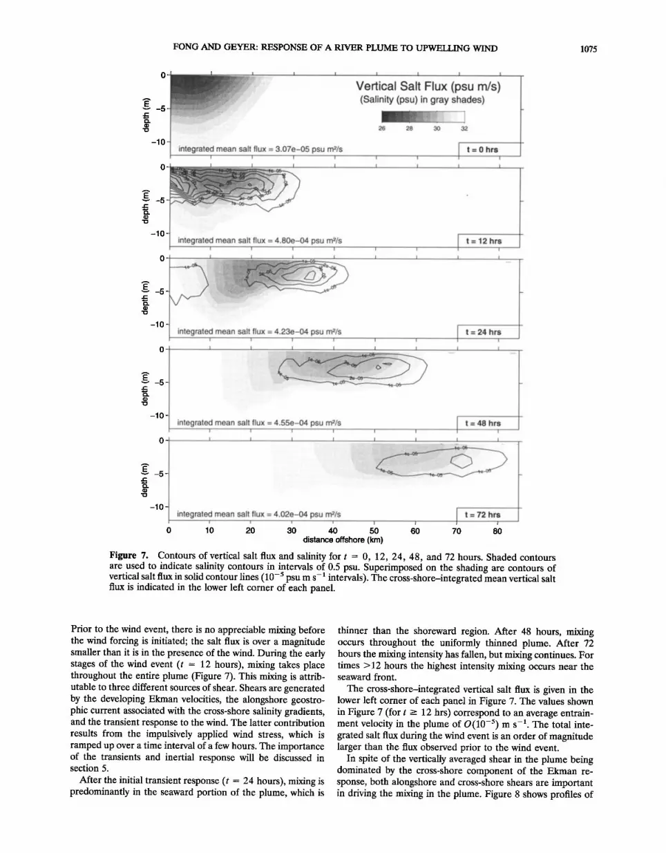
Figure 7. Contours of vertical salt flux and salinity for t = 0, 12, 24, 48, and 72 hours. Shaded contours are used to indicate salinity contours in intervals of 0.5 psu. Superimposed on the shading are contours of vertical salt flux in solid contour lines (10 -s psu m s -• intervals). The cross-shore-integrated mean vertical salt flux is indicated in the lower left corner of each panel.
Prior to the wind event, there is no appreciable mixing before the wind forcing is initiated; the salt flux is over a magnitude smaller than it is in the presence of the wind. During the early stages of the wind event (t = 12 hours), mixing takes place throughout the entire plume (Figure 7). This mixing is attrib- utable to three different sources of shear. Shears are generated by the developing Ekman velocities, the alongshore geostro- phic current associated with the cross-shore salinity gradients, and the transient response to the wind. The latter contribution results from the impulsively applied wind stress, which is ramped up over a time interval of a few hours. The importance of the transients and inertial response will be discussed in section 5.
After the initial transient response (t = 24 hours), mixing is predominantly in the seaward portion of the plume, which is
thinner than the shoreward region. After 48 hours, mixing occurs throughout the uniformly thinned plume. After 72 hours the mixing intensity has fallen, but mixing continues. For times > 12 hours the highest intensity mixing occurs near the seaward front.
The cross-shore-integrated vertical salt flux is given in the lower left corner of each panel in Figure 7. The values shown in Figure 7 (for t --> 12 hrs) correspond to an average entrain- ment velocity in the plume of O(10 -s) m s -•. The total inte- grated salt flux during the wind event is an order of magnitude larger than the flux observed prior to the wind event.
In spite of the vertically averaged shear in the plume being dominated by the cross-shore component of the Ekman re- sponse, both alongshore and cross-shore shears are important in driving the mixing in the plume. Figure 8 shows profiles of
1076 FONG AND GEYER: RESPONSE OF A RIVER PLUME TO UPWELLING WIND
-2
-4
-6
-10
-12
A B C I I I I I I I I
t=48 hrs
i
i i ,
26 28 30
I I Salinity {psu) I I I
I I
i i i i i i
20 30 40 50 60 70
cross-shore distance (km)
Vertical salt
flux (psu ,m/s) i
10 80
-2
-4
-8
-10
-12
-2
-4
-6
-8
-10
-12
o
2
4
6
8
--,0
-12
ß .
Vz / L_J] -0.1 0 O. 1
1/s -0.1 0 0.1 0 0.5 1
1/S (m2/s2) x 10 -4
----A
rYratific•.tion [JVerticai salt flu)• 0 0.5 I 1.5 0 0.005 0.01 0 I 2
(psu/m) (m2/s) (psu m/s) x 10 -5
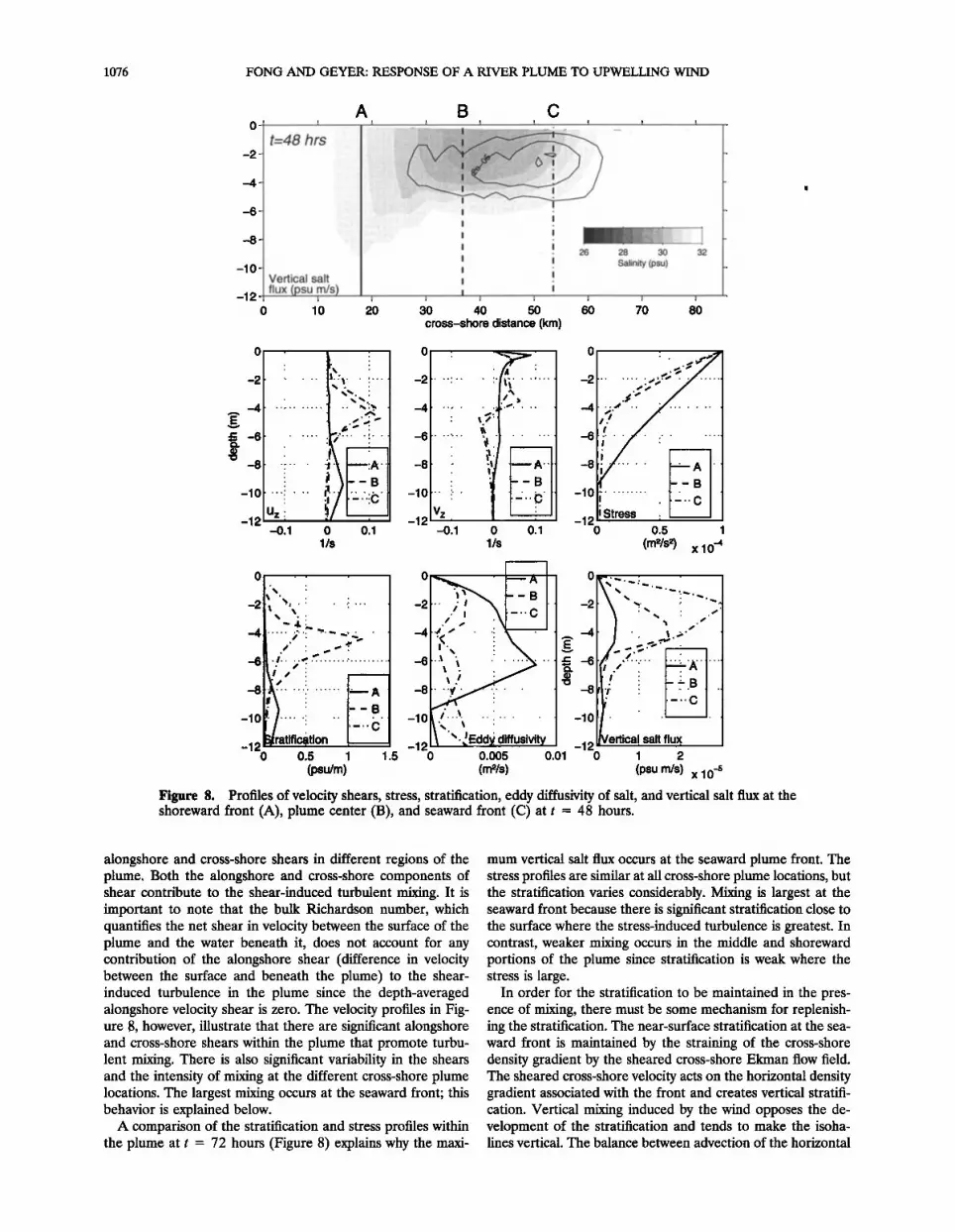
Figure 8. Profiles of velocity shears, stress, stratification, eddy diffusivity of salt, and vertical salt flux at the shoreward front (A), plume center (B), and seaward front (C) at t = 48 hours.
alongshore and cross-shore shears in different regions of the plume. Both the alongshore and cross-shore components of shear contribute to the shear-induced turbulent mixing. It is important to note that the bulk Richardson number, which quantifies the net shear in velocity between the surface of the plume and the water beneath it, does not account for any contribution of the alongshore shear (difference in velocity between the surface and beneath the plume) to the shear- induced turbulence in the plume since the depth-averaged alongshore velocity shear is zero. The velocity profiles in Fig- ure 8, however, illustrate that there are significant alongshore and cross-shore shears within the plume that promote turbu- lent mixing. There is also significant variability in the shears and the intensity of mixing at the different cross-shore plume locations. The largest mixing occurs at the seaward front; this behavior is explained below.
A comparison of the stratification and stress profiles within the plume at t = 72 hours (Figure 8) explains why the maxi-
mum vertical salt flux occurs at the seaward plume front. The stress profiles are similar at all cross-shore plume locations, but the stratification varies considerably. Mixing is largest at the seaward front because there is significant stratification close to the surface where the stress-induced turbulence is greatest. In contrast, weaker mixing occurs in the middle and shoreward portions of the plume since stratification is weak where the stress is large.
In order for the stratification to be maintained in the pres- ence of mixing, there must be some mechanism for replenish- ing the stratification. The near-surface stratification at the sea- ward front is maintained by the straining of the cross-shore density gradient by the sheared cross-shore Ekman flow field. The sheared cross-shore velocity acts on the horizontal density gradient associated with the front and creates vertical stratifi- cation. Vertical mixing induced by the wind opposes the de- velopment of the stratification and tends to make the isoha- lines vertical. The balance between advection of the horizontal
FONG AND GEYER: RESPONSE OF A RIVER PLUME TO UPWELLING WIND 1077
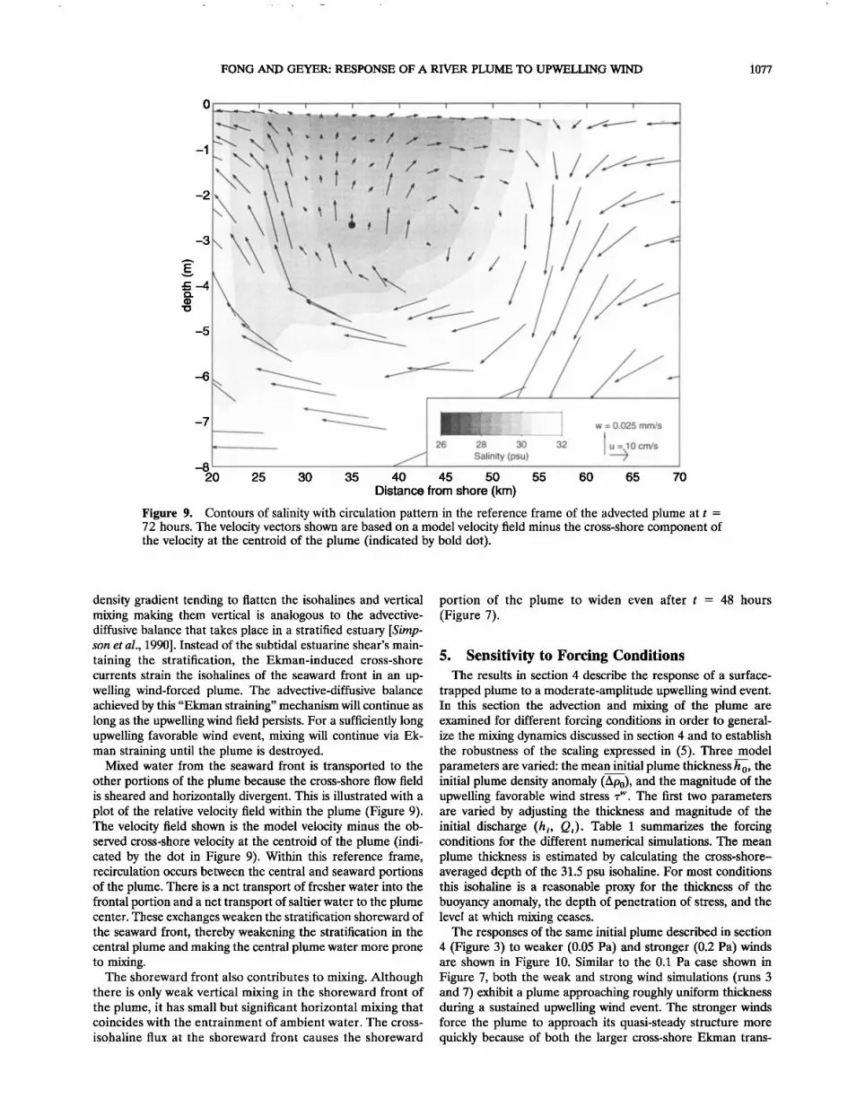
Figure 9. Contours of salinity with circulation pattern in the reference frame of the advected plume at t = 72 hours. The velocity vectors shown are based on a model velocity field minus the cross-shore component of the velocity at the centroid of the plume (indicated by bold dot).
density gradient tending to flatten the isohalines and vertical mixing making them vertical is analogous to the advective- diffusive balance that takes place in a stratified estuary [Simp- son et al., 1990]. Instead of the subtidal estuarine shear's main- taining the stratification, the Ekman-induced cross-shore currents strain the isohalines of the seaward front in an up- welling wind-forced plume. The advective-diffusive balance achieved by this "Ekman straining" mechanism will continue as long as the upwelling wind field persists. For a sufficiently long upwelling favorable wind event, mixing will continue via Ek- man straining until the plume is destroyed.
Mixed water from the seaward front is transported to the other portions of the plume because the cross-shore flow field is sheared and horizontally divergent. This is illustrated with a plot of the relative velocity field within the plume (Figure 9). The velocity field shown is the model velocity minus the ob- served cross-shore velocity at the centroid of the plume (indi- cated by the dot in Figure 9). Within this reference frame, recirculation occurs between the central and seaward portions of the plume. There is a net transport of fresher water into the frontal portion and a net transport of saltier water to the plume center. These exchanges weaken the stratification shoreward of the seaward front, thereby weakening the stratification in the central plume and making the central plume water more prone to mixing.
The shoreward front also contributes to mixing. Although there is only weak vertical mixing in the shoreward front of the plume, it has small but significant horizontal mixing that coincides with the entrainment of ambient water. The cross-
isohaline flux at the shoreward front causes the shoreward
portion of the plume to widen even after t = 48 hours (Figure 7).
5. Sensitivity to Forcing Conditions The results in section 4 describe the response of a surface-
trapped plume to a moderate-amplitude upwelling wind event. In this section the advection and mixing of the plume are examined for different forcing conditions in order to general- ize the mixing dynamics discussed in section 4 and to establish the robustness of the scaling expressed in (5). Three model parameters are varied: the mean initial plume thickness ho, the initial plume density anomaly (Apo), and the magnitude of the upwelling favorable wind stress ,w. The first two parameters are varied by adjusting the thickness and magnitude of the initial discharge (hi, Qi). Table 1 summarizes the forcing conditions for the different numerical simulations. The mean
plume thickness is estimated by calculating the cross-shore- averaged depth of the 31.5 psu isohaline. For most conditions this isohaline is a reasonable proxy for the thickness of the buoyancy anomaly, the depth of penetration of stress, and the level at which mixing ceases.
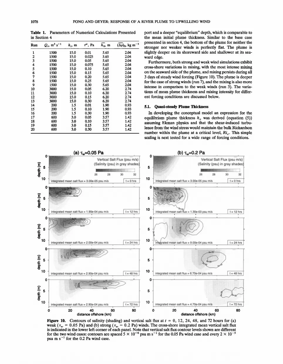
The responses of the same initial plume described in section 4 (Figure 3) to weaker (0.05 Pa) and stronger (0.2 Pa) winds are shown in Figure 10. Similar to the 0.1 Pa case shown in Figure 7, both the weak and strong wind simulations (runs 3 and 7) exhibit a plume approaching roughly uniform thickness during a sustained upwelling wind event. The stronger winds force the plume to approach its quasi-steady structure more quickly because of both the larger cross-shore Ekman trans-
1078 FONG AND GEYER: RESPONSE OF A RIVER PLUME TO UPWELLING WIND
Table 1. Parameters of Numerical Calculations Presented
in Section 4
Run Qi, m3 s-] hi, m 'r w, Pa h0, rn (Ap) 0, kg m -3
port and a deeper "equilibrium" depth, which is comparable to the mean initial plume thickness. Similar to the base case presented in section 4, the bottom of the plume for neither the stronger nor weaker winds is perfectly flat. The plume is slightly deeper on its shoreward side and shallower at its sea- ward edge.
Furthermore, both strong and weak wind simulations exhibit cross-shore variations in mixing, with the most intense mixing on the seaward side of the plume, and mixing persists during all 3 days of steady wind forcing (Figure t0). The plume is deeper for the case of strong winds (run 7), and the mixing is also more intense in comparison to the weak winds (run 3). The varia- tions of mean plume thickness and mixing intensity for differ- ent forcing conditions are discussed below.
5.1. Quasi-steady Plume Thickness
In developing the conceptual model an expression for the equilibrium plume thickness h c was derived (equation (5)) assuming Ekman physics and that the shear-induced turbu- lence from the wind stress would maintain the bulk Richardson
number within the plume at a critical level, Ric. This simple scaling is next tested for a wide range of forcing conditions.
(a) •:w=O.05 Pa i i
•: .................. ;: .... : - Vertical Salt Flux (psu m/s)l (Salinity (psu•}.. in.•....g..•r•..••.:•.•,•.•:..shades t 26 28 30 32
integrated mean salt flux = 3.00e-05 psu m/s I t = 0 hrs ! 0 • i i i
..
. .
E . o
10 integrated mean salt flux = 1.90e-04 psu rn/s I t = 12 hrs ! i i i
5 i" •""'•'•' "•"••••'- ............. ••••i:i•i:•:.:•;•:•'•11'::. ] [ 26 28 30 32 • 0 mean salt flux = 3.•e-05 psu m/s , I t= 0 hTs /
1.30e-03 psu rn/s I i = '1'2 hrs , i i
t = 24 ,hrs
ß
integrated mean salt flux = 6.70e-04 psu m/s I t = 48 hrs _ i i i i
integrated mean salt flux = 4.70e-04 psu' •'i•i; :;!?: ii';':i 20 40 60 80
distance offshore (km)
Figure 10. Contours of salinity (shading) and vertical salt flux at t = 0, 12, 24, 48, and 72 hours for (a) weak (Tw = 0.05 Pa) and (b) strong (T w = 0.2 Pa) winds. The cross-shore integrated mean vertical salt flux is indicated in the lower left corner of each panel. Note that vertical salt flux contour levels shown are different for the two wind cases: contours are spaced 5 x 10 -6 psu m s -1 for the 0.05 Pa wind case and every 2 x t0 -s psu m s-1 for the 0.2 Pa wind case.
FONG AND GEYER: RESPONSE OF A RIVER PLUME TO UPWELLING WIND 1079
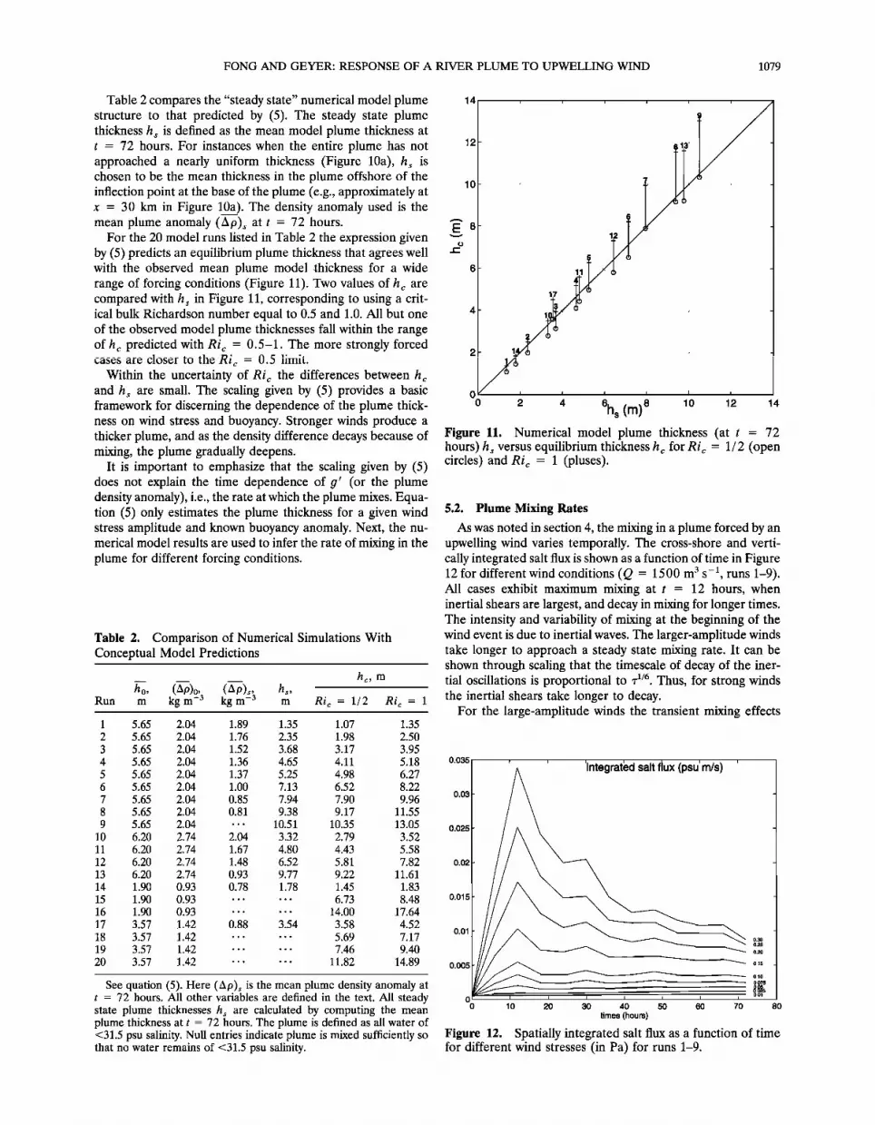
Table 2 compares the "steady state" numerical model plume structure to that predicted by (5). The steady state plume thickness h s is defined as the mean model plume thickness at t - 72 hours. For instances when the entire plume has not approached a nearly uniform thickness (Figure 10a), hs is chosen to be the mean thickness in the plume offshore of the inflection point at the base of the plume (e.g., approximately at x = 30 km in Figure 10a). The density anomaly used is the mean plume anomaly (A p)• at t = 7 2 hours.
For the 20 model runs listed in Table 2 the expression given by (5) predicts an equilibrium plume thickness that agrees well with the observed mean plume model thickness for a wide range of forcing conditions (Figure 11). Two values of h c are compared with h• in Figure 11, corresponding to using a crit- ical bulk Richardson number equal to 0.5 and 1.0. All but one of the observed model plume thicknesses fall within the range of hc predicted with Ric = 0.5-1. The more strongly forced cases are c,o•e• to the lxi c = u.5 limit.
Within the uncertainty of Ric the differences between h c and h• are small. The scaling given by (5) provides a basic framework for discerning the dependence of the plume thick- ness on wind stress and buoyancy. Stronger winds produce a thicker plume, and as the density difference decays because of mixing, the plume gradually deepens.
It is important to emphasize that the scaling given by (5) does not explain the time dependence of #' (or the plume density anomaly), i.e., the rate at which the plume mixes. Equa- tion (5) only estimates the plume thickness for a given wind stress amplitude and known buoyancy anomaly. Next, the nu- merical model results are used to infer the rate of mixing in the plume for different forcing conditions.
Table 2. Comparison of Numerical Simulations With Conceptual Model Predictions
See quation (5). Here (Ap)• is the mean plume density anomaly at t = 72 hours. All other variables are defined in the text. All steady state plume thicknesses h• are calculated by computing the mean plume thickness at t = 72 hours. The plume is defined as all water of <31.5 psu salinity. Null entries indicate plume is mixed sufficiently so that no water remains of <31.5 psu salinity.
14
12
10
2
o o 2
, i , i
i 813' 1
11
17
4 6h (m)8 10 12 s
14
Figure 11. Numerical model plume thickness (at t = 72 hours) h• versus equilibrium thickness hc for Ri c = 1/2 (open circles) and Ric = 1 (pluses).
5.2. Plume Mixing Rates
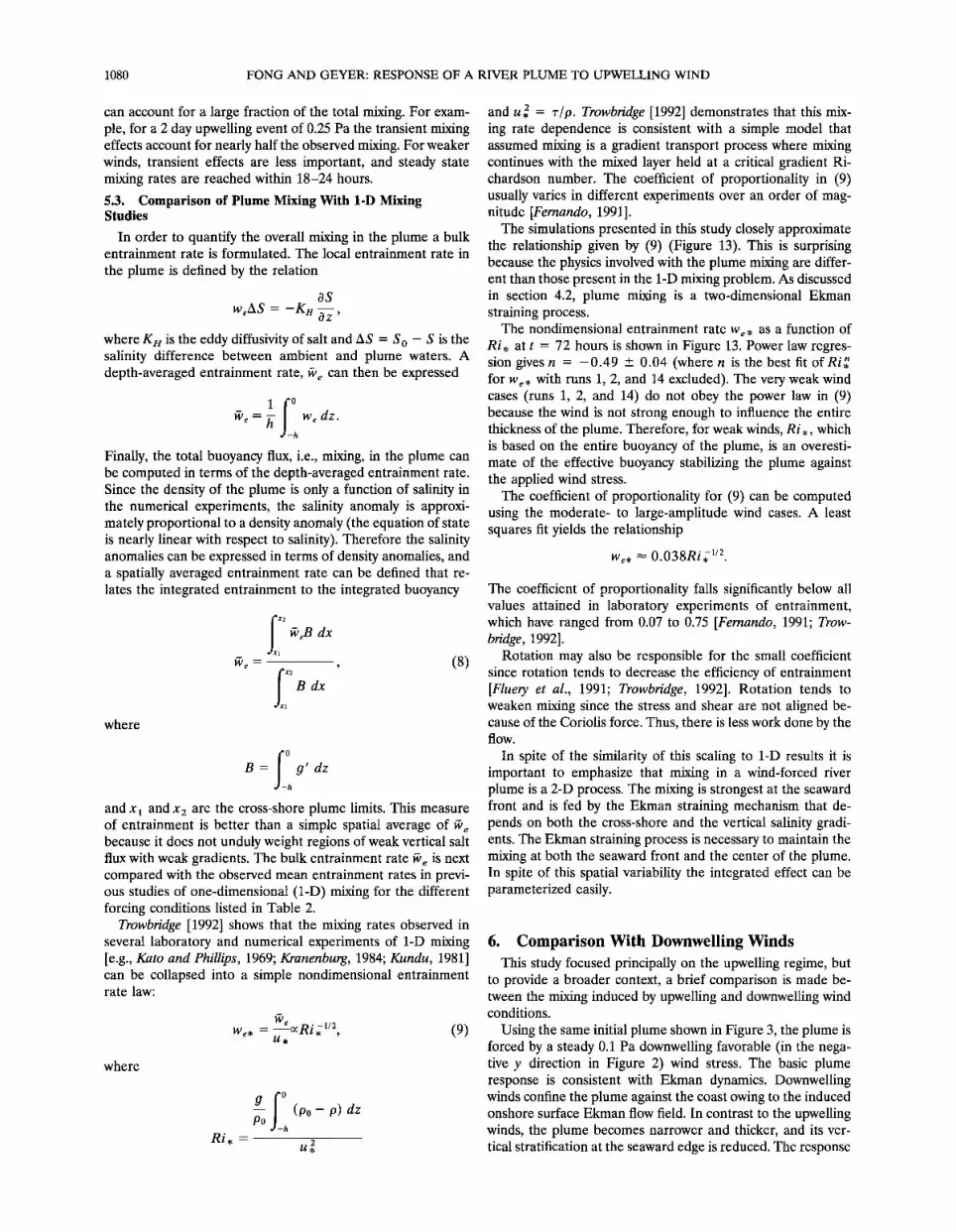
As was noted in section 4, the mixing in a plume forced by an upwelling wind varies temporally. The cross-shore and verti- cally integrated salt flux is shown as a function of time in Figure 12 for different wind conditions (Q = 1500 m 3 s -•, runs 1-9). All cases exhibit maximum mixing at t = 12 hours, when inertial shears are largest, and decay in mixing for longer times. The intensity and variability of mixing at the beginning of the wind event is due to inertial waves. The larger-amplitude winds take longer to approach a steady state mixing rate. It can be shown through scaling that the timescale of decay of the iner- tial oscillations is proportional to r •/6. Thus, for strong winds the inertial shears take longer to decay.
For the large-amplitude winds the transient mixing effects
0.035
0.03
0.025
0.02
0.015
0.01
0.005 015
OlO
o o75
oo•
o o 1 o 20 30 40 50 60 70 80
times (hours)
Figure 12. Spatially integrated salt flux as a function of time for different wind stresses (in Pa) for runs 1-9.
1080 FONG AND GEYER: RESPONSE OF A RIVER PLUME TO UPWELLING WIND
can account for a large fraction of the total mixing. For exam- ple, for a 2 day upwelling event of 0.25 Pa the transient mixing effects account for nearly half the observed mixing. For weaker winds, transient effects are less important, and steady state mixing rates are reached within 18-24 hours.
5.3. Comparison of Plume Mixing With 1-D Mixing Studies
In order to quantify the overall mixing in the plume a bulk entrainment rate is formulated. The local entrainment rate in
the plume is defined by the relation
OS
weAS-- --KH OZ' where K/_/is the eddy diffusivity of salt and AS = So - S is the salinity difference between ambient and plume waters. A depth-averaged entrainment rate, 1• e can then be expressed
]•'e -- •- wed2;. h
Finally, the total buoyancy flux, i.e., mixing, in the plume can be computed in terms of the depth-averaged entrainment rate. Since the density of the plume is only a function of salinity in the numerical experiments, the salinity anomaly is approxi- mately proportional to a density anomaly (the equation of state is nearly linear with respect to salinity). Therefore the salinity anomalies can be expressed in terms of density anomalies, and a spatially averaged entrainment rate can be defined that re- lates the integrated entrainment to the integrated buoyancy
where
x2 •B dx 1
1• e = , (8)
x2 B dx 1
B= g' dz h
and x• and x2 are the cross-shore plume limits. This measure of entrainment is better than a simple spatial average of 1• e because it does not unduly weight regions of weak vertical salt flux with weak gradients. The bulk entrainment rate 1• e is next compared with the observed mean entrainment rates in previ- ous studies of one-dimensional (l-D) mixing for the different forcing conditions listed in Table 2.
Trowbridge [1992] shows that the mixing rates observed in several laboratory and numerical experiments of 1-D mixing [e.g., Kato and Phillips, 1969; Kranenburg, 1984; Kundu, 1981] can be collapsed into a simple nondimensional entrainment rate law:
where
We, -- We•cRi ;1/2, (9)
Ri, =
P0 (P0- P) dz h
and u, 2 = r/p. Trowbridge [1992] demonstrates that this mix- ing rate dependence is consistent with a simple model that assumed mixing is a gradient transport process where mixing continues with the mixed layer held at a critical gradient Ri- chardson number. The coefficient of proportionality in (9) usually varies in different experiments over an order of mag- nitude [Fernando, 1991].
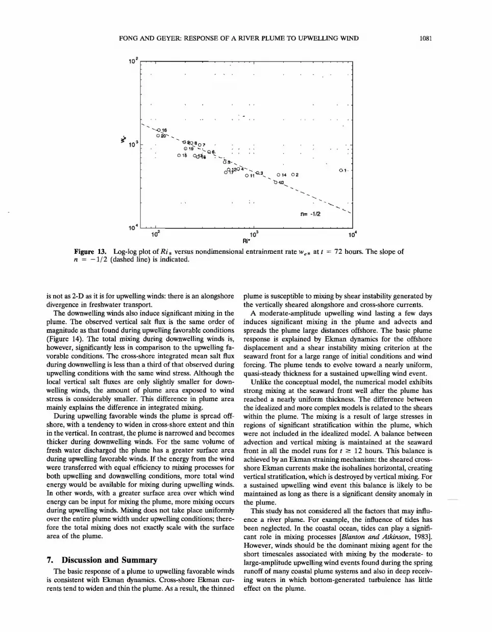
The simulations presented in this study closely approximate the relationship given by (9) (Figure 13). This is surprising because the physics involved with the plume mixing are differ- ent than those present in the 1-D mixing problem. As discussed in section 4.2, plume mixing is a two-dimensional Ekman straining process.
The nondimensional entrainment rate We, as a function of Ri, at t = 72 hours is shown in Figure 13. Power law regres- sion gives n = -0.49 _+ 0.04 (where n is the best fit of Ri•' for We, with runs 1, 2, and 14 excluded). The very weak wind cases (runs 1, 2, and 14) do not obey the power law in (9) because the wind is not strong enough to influence the entire thickness of the plume. Therefore, for weak winds, Ri ,, which is based on the entire buoyancy of the plume, is an overesti- mate of the effective buoyancy stabilizing the plume against the applied wind stress.
The coefficient of proportionality for (9) can be computed using the moderate- to large-amplitude wind cases. A least squares fit yields the relationship
We, • 0.038Ri• •/2.
The coefficient of proportionality falls significantly below all values attained in laboratory experiments of entrainment, which have ranged from 0.07 to 0.75 [Fernando, 1991; Trow- bridge, 1992].
Rotation may also be responsible for the small coefficient since rotation tends to decrease the efficiency of entrainment [Fluery et al., 1991; Trowbridge, 1992]. Rotation tends to weaken mixing since the stress and shear are not aligned be- cause of the Coriolis force. Thus, there is less work done by the flow.
In spite of the similarity of this scaling to 1-D results it is important to emphasize that mixing in a wind-forced river plume is a 2-D process. The mixing is strongest at the seaward front and is fed by the Ekman straining mechanism that de- pends on both the cross-shore and the vertical salinity gradi- ents. The Ekman straining process is necessary to maintain the mixing at both the seaward front and the center of the plume. In spite of this spatial variability the integrated effect can be parameterized easily.
6. Comparison With Downwelling Winds This study focused principally on the upwelling regime, but
to provide a broader context, a brief comparison is made be- tween the mixing induced by upwelling and downwelling wind conditions.
Using the same initial plume shown in Figure 3, the plume is forced by a steady 0.1 Pa downwelling favorable (in the nega- tive y direction in Figure 2) wind stress. The basic plume response is consistent with Ekman dynamics. Downwelling winds confine the plume against the coast owing to the induced onshore surface Ekman flow field. In contrast to the upwelling winds, the plume becomes narrower and thicker, and its ver- tical stratification at the seaward edge is reduced. The response
FONG AND GEYER: RESPONSE OF A RIVER PLUME TO UPWELLING WIND 1081
10 2
10 3
' ' i i
, ,
'O 20'-
ß . •. •o 8 o.7 o1•'
0 15 Od.318 -,-
O
10 4 , • I , , • • • , , , 1 10 2 10 3
Ri*
O t4 02
. .....
n= -1/2 - l lO •
Figure 13. Log-log plot of Ri, versus nondimensional entrainment rate We8 at t = 72 hours. The slope of n = -1/2 (dashed line) is indicated.
is not as 2-D as it is for upwelling winds: there is an alongshore divergence in freshwater transport.
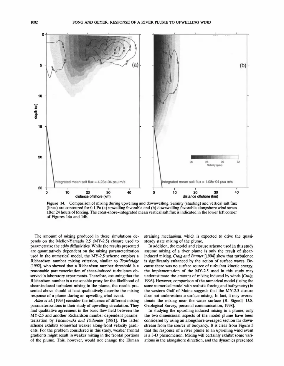
The downwelling winds also induce significant mixing in the plume. The observed vertical salt flux is the same order of magnitude as that found during upwelling favorable conditions (Figure 14). The total mixing during downwelling winds is, however, significantly less in comparison to the upwelling fa- vorable conditions. The cross-shore integrated mean salt flux during downwelling is less than a third of that observed during upwelling conditions with the same wind stress. Although the local vertical salt fluxes are only slightly smaller for down- welling winds, the amount of plume area exposed to wind stress is considerably smaller. This difference in plume area mainly explains the difference in integrated mixing.
During upwelling favorable winds the plume is spread off- shore, with a tendency to widen in cross-shore extent and thin in the vertical. In contrast, the plume is narrowed and becomes thicker during downwelling winds. For the same volume of fresh water discharged the plume has a greater surface area during upwelling favorable winds. If the energy from the wind were transferred with equal efficiency to mixing processes for both upwelling and downwelling conditions, more total wind energy would be available for mixing during upwelling winds. In other words, with a greater surface area over which wind energy can be input for mixing the plume, more mixing occurs during upwelling winds. Mixing does not take place uniformly over the entire plume width under upwelling conditions; there- fore the total mixing does not exactly scale with the surface area of the plume.
7. Discussion and Summary The basic response of a plume to upwelling favorable winds
is consistent with Ekman dynamics. Cross-shore Ekman cur- rents tend to widen and thin the plume. As a result, the thinned
plume is susceptible to mixing by shear instability generated by the vertically sheared alongshore and cross-shore currents.
A moderate-amplitude upwelling wind lasting a few days induces significant mixing in the plume and advects and spreads the plume large distances offshore. The basic plume response is explained by Ekman dynamics for the offshore displacement and a shear instability mixing criterion at the seaward front for a large range of initial conditions and wind forcing. The plume tends to evolve toward a nearly uniform, quasi-steady thickness for a sustained upwelling wind event.
Unlike the conceptual model, the numerical model exhibits strong mixing at the seaward front well after the plume has reached a nearly uniform thickness. The difference between the idealized and more complex models is related to the shears within the plume. The mixing is a result of large stresses in regions of significant stratification within the plume, which were not included in the idealized model. A balance between
advection and vertical mixing is maintained at the seaward front in all the model runs for t > 12 hours. This balance is
achieved by an Ekman straining mechanism: the sheared cross- shore Ekman currents make the isohalines horizontal, creating vertical stratification, which is destroyed by vertical mixing. For a sustained upwelling wind event this balance is likely to be maintained as long as there is a significant density anomaly in the plume.
This study has not considered all the factors that may influ- ence a river plume. For example, the influence of tides has been neglected. In the coastal ocean, tides can play a signifi- cant role in mixing processes [Blanton and Atkinson, 1983]. However, winds should be the dominant mixing agent for the short timescales associated with mixing by the moderate- to large-amplitude upwelling wind events found during the spring runoff of many coastal plume systems and also in deep receiv- ing waters in which bottom-generated turbulence has little effect on the plume.
1082 FONG AND GEYER: RESPONSE OF A RIVER PLUME TO UPWELLING WIND
10 -
15 -
20 -
25
ntegrated
I
lO
mean salt flux = 4.23e-04 psu m/s
I I
(b)
26 28 30 32
Salinity (psu)
integrated mean salt flux = 1.08e-04 psu m/s
I I I I I I
20 30 40 0 10 20 30 40
distance offshore (km) distance offshore (km)
Figure 14. Comparison of mixing during upwelling and downwelling. Salinity (shading) and vertical salt flux (lines) are contoured for 0.1 Pa (a) upwelling favorable and (b) downwelling favorable alongshore wind stress after 24 hours of forcing. The cross-shore-integrated mean vertical salt flux is indicated in the lower left corner of Figures 14a and 14b.
The amount of mixing produced in these simulations de- pends on the Mellor-Yamada 2.5 (MY-2.5) closure used to parameterize the eddy diffusivities. While the results presented are quantitatively dependent on the mixing parameterization used in the numerical model, the MY-2.5 scheme employs a Richardson number mixing criterion, similar to Trowbridge [1992], who showed that a Richardson number threshold is a reasonable parameterization of shear-induced turbulence ob- served in laboratory experiments. Therefore, assuming that the Richardson number is a reasonable proxy for the likelihood of shear-induced turbulent mixing in the plume, the results pre- sented above should at least qualitatively describe the mixing response of a plume during an upwelling wind event.
Allen et al. [1995] consider the influence of different mixing parameterizations in their study of upwelling circulation. They find qualitative agreement in the basic flow field between the MY-2.5 and another Richardson number-dependent parame- terization by Pacanowski and Philander [1981]. The latter scheme exhibits somewhat weaker along-front velocity gradi- ents. For the problem considered in this study, weaker frontal gradients might result in weaker mixing in the frontal portions of the plume. This, however, would not change the Ekman
straining mechanism, which is expected to drive the quasi- steady state mixing of the plume.
In addition, the model and closure scheme used in this study assume mixing of a river plume is only the result of shear- induced mixing. Craig and Banner [1994] show that turbulence is significantly enhanced by the action of surface waves. Be- cause there was no surface source of turbulent kinetic energy, the implementation of the MY-2.5 used in this study may underestimate the amount of mixing induced by winds [Craig, 1996]. However, comparison of the numerical model (using the same numerical model with realistic forcing and bathymetry) in the western Gulf of Maine suggests that the MY-2.5 closure does not underestimate surface mixing. In fact, it may overes- timate the mixing near the water surface (R. Signell, U.S. Geological Survey, personal communication, 1998].
In studying the upwelling-induced mixing in a plume, only the two-dimensional aspects of the model plume have been considered by using an alongshore-averaged section far down- stream from the source of buoyancy. It is clear from Figure 3 that the response of a river plume to an upwelling wind event is a 3-D phenomenon. Mixing will certainly exhibit some vari- ations in the alongshore direction, and the dynamics presented
FONG AND GEYER: RESPONSE OF A RIVER PLUME TO UPWELLING WIND 1083
in this study will most likely fail near the river mouth. However, the 2-D paradigm of mixing under upwelling conditions should be valid over a large part of the plume where the alongshore momentum physics are primarily Ekman-driven.
One interesting feature of the numerical simulations is the vigorous mixing that takes place during the first 12 hours of wind forcing (see Figures 7 and 12). It is during this time period when inertial oscillations are induced by the sudden application of a wind stress. Depending on the timing within the inertial period, total velocity shears will be either enhanced or relaxed [Federiuk and Allen, 1996].
In conclusion, an upwelling wind influences the fate of a freshwater plume in two ways, by advection and by mixing. The advective processes induced by upwelling winds are important in modifying the shape of the plume, and these shape changes are essential to driving mixing processes in the plume. Further- more, downcoast transport of freshwater is also opposed by the barotropic, downwind current established by an upwelling wind. In advecting the plume significant distances offshore during a several day wind event, upwelling winds also affect the plume fate by exposing the buoyancy to large-scale ambient circulation patterns. The ambient coastal currents may be sig- nificantly different in the inshore and offshore regions of a continental shelf.
In nature the forcing of a freshwater plume is significantly more complex than these idealized simulations. In many river plume systems the spring runoff coincides with winds that exhibit large fluctuations in both direction and magnitude. Often, an upwelling wind event is followed by a comparable- amplitude downwelling favorable event that may readvect the plume water onshore. The net influence of an oscillatory wind forcing is to mix the plume, with little net advection.
Acknowledgments. Valuable discussions with D. Chapman and S. Lentz were of immeasurable value during the course of this work. The authors would also like to thank R. Signell for his assistance and expertise with the Blumberg-Mellor model and A. Blumberg for per- mission to use the model code. This work was supported by the Gulf of Maine Regional Marine Research Program grant UM-S227, Office of Naval Research grants N00014-97-10134 and N00014-98-1-0785, and National Science Foundation grant OCE-9808173.
References
Allen, J. S., P. A. Newberger, and J. Federiuk, Upwelling circulation on the Oregon continental shelf, J. Phys. Oceanogr., 25, 1843-1866, 1995.
Blanton, J. O., and L. P. Atkinson, Transport and fate of river dis- charge on the continental shelf of the southeastern United States, J. Geophys. Res., 88, 4730-4738, 1983,
Blumberg, A. F., and G. L. Mellor, A description of a three- dimensional coastal ocean circulation model, in Three-Dimensional Coastal Ocean Models, Coastal Estuarine Sci., vol. 4, edited by N. S. Heaps, pp. 1-16, AGU, Washington, D.C., 1987.
Chao, S.-Y., Wind-driven motion near inner shelf fronts, J. Geophys. Res., 92, 3849-3860, 1987.
Chao, S.-Y., Wind-driven motion of estuarine plumes, J. Phys. Ocean- ogr., 18, 1144-1166, 1988.
Chapman, D.C., and S. J. Lentz, Trapping of a coastal density front by the bottom boundary layer, J. Phys. Oceanogr., 24, 1464-1479, 1994.
Craig, P. D., Velocity profiles and surface roughness under breaking waves, J. Geophys. Res., 101, 1265-1277, 1996.
Craig, P. D., and M. L. Banner, Modeling wave-enhanced turbulence in the ocean surface layer, J. Phys. Oceanogr., 24, 2546-2559, 1994.
Csanady, G. T., Wind effects on surface to bottom fronts, J. Geophys. Res., 83, 4633-4640, 1978.
Federiuk, J., and J. S. Allen, Model studies of near-inertial waves in
flow over the Oregon continental shelf, J. Phys. Oceanogr., 26, 2053- 2075, 1996.
Fernando, H. J. S., Turbulent mixing in stratified fluids, Annu. Rev. Fluid Mech., 23, 455-493, 1991.
Fluery, M., M. Mory, E. J. Hopfinger, and D. Auchere, Effects of rotation on turbulent mixing across a density interface, J. Fluid Mech., 223, 165-191, 1991.
Fong, D. A., Dynamics of freshwater plumes: Observations and nu- merical modeling of the wind-forced response and alongshore fresh- water transport, Program in Oceanogr., Mass. Inst. of Technol./ Woods Hole Oceanogr. Inst. Joint, Ph.d. thesis, Woods Hole, 1998.
Fong, D. A., W. R. Geyer, and R. P. Signell, The wind-forced response of a buoyant coastal current: Observations of the western Gulf of Maine plume, J. Mar. Syst., 12, 69-81, 1997.
Garvine, R. W., Penetration of buoyant coastal discharge onto the continental shelf: A numerical model experiment, J. Phys. Oceanogr., 29, 1892-1909, 1999.
Kantha, L. H., O. M. Phillips, and R. S. Azad, On turbulent entrain- ment at a stable density interface, J. Fluid Mech., 79, 753-768, 1977.
Kato, H., and O. M. Phillips, On the penetration of a turbulent layer into stratified fluid, J. Fluid Mech., 37, 643-655, 1969.
Kourafalou, V. H., T. N. Lee, L.-Y. Oey, and J. D. Wang, The fate of river discharge on the continental shelf, 2, Transport of coastal low-salinity waters under realistic wind and tidal forcing, J. Geophys. Res., 101, 3435-3455, 1996.
Kranenburg, C., Wind-induced entrainment in a stably stratified fluid, J. Fluid Mech., 145, 253-273, 1984.
Kraus, E. B., and J. S. Turner, A one-dimensional model of the sea- sonal thermocline, Tellus, 19, 98-106, 1967.
Kundu, P. K., A numerical investigation of mixed layer dynamics, J. Geophys. Res., 86, 1979-1988, 1981.
Loder, J. W., B. Petrie, and G. Gawarkiewicz, The coastal ocean off northeastern North America: A large-scale view, in The Sea, vol. 11, edited by K. Brink and A. Robinson, John Wiley, New York, in press, 1998.
Masse, A. K., and C. R. Murthy, Observations of the Niagara River thermal plume, J. Geophys. Res., 95, 851-875, 1990.
Masse, A. K., and C. R. Murthy, Analysis of the Niagara River plume dynamics, J. Geophys. Res., 97, 2403-2420, 1992.
Mellor, G. L., and T. Yamada, Development of a turbulence closure model for geophysical fluid problems, Rev. Geophys., 20, 851-875, 1982.
Mtinchow, A., and R. W. Garvine, Dynamical properties of a buoyan- cy-driven coastal current, J. Geophys. Res., 98, 20,063-20,077, 1993.
Nunez Vaz, R. A., and J. H. Simpson, Turbulence closure modeling of estuarine stratification, J. Geophys. Res., 99, 16,143-16,160, 1994.
Oey, L.-Y., and G. L. Mellor, Subtidal variability of estuarine outflow, plume, and coastal current: A model study, J. Phys. Oceanogr., 23, 164-171, 1993.
Orlanski, I., A simple boundary condition for unbounded hyperbolic flows, J. Comput. Phys., 21, 251-269, 1976.
Pacanowski, R. C., and S.C. H. Philander, Parametrization of vertical mixing in numerical models of tropical seas, J. Phys. Oceanogr., 11, 1443-1451, 1981.
Pollard, R. T., P. B. Rhines, and R. O. R. Y. Thompson, The deep- ening of the wind-mixed layer, Geophys. Fluid Dyn., 3, 381-404, 1973.
Price, J. F., C. N. K. Mooers, and J. C. V. Leer, Observation and simulation of storm-induced mixed-layer deepening, J. Phys. Ocean- ogr., 8, 582-599, 1978.
Price, J. F., R. A. Weller, and R. Pinkel, Diurnal cycling: Observations and models of the upper ocean response to diurnal heating, cooling, and wind mixing, J. Geophys. Res., 91, 8411-8427, 1986.
Simpson, J. H., J. Brown, J. Matthews, and G. Allen, Tidal straining, density currents, and stirring in the control of estuarine stratifica- tion, Estuaries, 13, 125-132, 1990.
Smolarkiewicz, P. K., and W. W. Grabowski, The multidimensional positive definite advection transport algorithm, J. Comput. Phys., 86, 355-375, 1990.
Souza, A. J., and J. H. Simpson, Controls on stratification in the Rhine ROFI system, J. Mar. Syst., 12, 311-323, 1997.
Trowbridge, J. H., A simple description of the deepening and structure of a stably stratified flow driven by a surface stress, J. Geophys. Res,, 97, 15,529-15,543, 1992.
Xing, J., and A.M. Davies, The effect of wind direction and mixing
1084 FONG AND GEYER: RESPONSE OF A RIVER PLUME TO UPWELLING WIND
upon the spreading of a buoyant plume in a non-tidal regime, Cont. Shelf Res., 19, 1437-1483, 1999.
D. A. Fong, Environmental Fluid Mechanics Laboratory, Depart- ment of Civil and Environmental Engineering, Stanford University, Stanford, CA 94305-4020. ([email protected])
W. R. Geyer, Department of Applied Ocean Physics and Engineer- ing, MS 12, Woods Hole, MA 02543.
(Received October 5, 1999; revised June 12, 2000; accepted June 23, 2000.)