341
Saline Lakes
| Date post: | 12-Jan-2023 |
| Category: |
Documents |
| Upload: | khangminh22 |
| View: | 0 times |
| Download: | 0 times |

Saline Lakes

Developments in Hydrobiology 162
Series editor H. J. Dumont
Saline Lakes
Publications from the 7th International Conference on Salt Lakes, held in Death Valley National Park, California, U.S.A., September 1999
Edited by
John M. Melack1 , Robert Jellison2 & David B. Herbse 1 Department of Ecology, Evolution and Marine Biology, and
Bren School of Environmental Science and Management, University of California, Santa Barbara, U.S.A.
2 Marine Science Institute, University of California, Santa Barbara, U.S.A. 3 Sierra Nevada Aquatic Research Laboratory, University of California, Mammoth Lakes, U.S.A.
Reprinted from Hydrobiologia, volume 466 (2001)
Springer-Science+Susiness Media, SV.
Library of Congress Cataloging-in-Publication Data
A C.I.P. Catalogue record for this book is available from the Library of Congress.
Printed on acid-free paper
All Rights reserved © 2001 Springer Science+Business Media Dordrecht Originally published by Kluwer Academic Publishers in 2001 Softcover reprint of the hardcover 1 st edition 2001
No part of the material protected by this copyright notice may be reproduced or utilized in any form or by any means, electronic or mechanical, including photocopying, recording or by any information storage and retrieval system, without written permission from the copyright owner.
ISBN 978-90-481-5995-6 (eBook) ISBN 978-94-017-2934-5 DOI 10.1007/978-94-017-2934-5
v
TABLE OF CONTENTS
Preface ix
Nitrogen limitation and particulate elemental ratios of seston in hypersaline Mono Lake, California, U.S.A. Robert Jellison, John M. Melack 1-12
Nutrient fluxes from upwelling and enhanced turbulence at the top of the pycnocline in Mono Lake, California Sally Macintyre, Robert Jellison 13-29
Airborne remote sensing of chlorophyll distributions in Mono Lake, California John M. Melack, Mary Gastil 31-38
Re-appearance of rotifers in hypersaline Mono Lake, California, during a period of rising lake levels and decreasing salinity Robert Jellison, Heather Adams, John M. Melack 39-43
Stratification of microbial assemblages in Mono Lake, California, and response to a mixing event James T. Hollibaugh, Patricia S. Wong, Nasreen Bano, Sunny K. Pak, Ellen M. Prager, Cristian Orrego 45-60
The bioenergetic basis for the decrease in metabolic diversity at increasing salt concentrations: implications for the functioning of salt lake ecosystems Aharon Oren 61-72
Comparative metabolic diversity in two solar salterns Carol D. Litchfield, Amy Irby, Tamar Kis-Papo, Aharon Oren 73-80
Polar lipids and pigments as biomarkers for the study of the microbial community structure of solar salterns Carol D. Litchfield, Aharon Oren 81-89
Limnological effects of anthropogenic desiccation of a large, saline lake, Walker Lake, Nevada Marc W. Beutel, Alex J. Horne, James C. Roth, Nicola J. Barratt 91-105
VI
Oxygen consumption and ammonia accumulation in the hypolimnion of Walker Lake, Nevada Marc W. Beutel 107-117
Limnological control of brine shrimp population dynamics and cyst production in the Great Salt Lake, Utah Wayne A. Wurtsbaugh, Z. Maciej Gliwicz 119-132
International study on Artemia LXIII. Field study of the Artemia urmiana (Gunther, 1890) population in Lake Urmiah, Iran Gilbert Van Stappen, Gholamreza Fayazi, Patrick Sorgeloos 133-143
Dispersal of Artemia franciscana Kellogg (Crustacea; Anostraca) populations in the coastal saltworks of Rio Grande do Norte, northeastern Brazil Marcos R. Camara 145-148
Anostracan cysts found in California salt lakes William D. Shepard, Richard E. Hill 149-158
Thermal, mixing, and oxygen regimes of the Salton Sea, California, 1997-1999 James M. Watts, Brandon K. Swan, Mary Ann Tiffany, Stuart H. Hurlbert 159-176
Pleurochrysis pseudoroscoffensis (Prymnesiophyceae) blooms on the surface of the Salton Sea, California Kristen M. Reifel, Michael P. McCoy, Mary Ann Tiffany, Tonie E. Rocke, Charles C. Trees, Steven B. Barlow, D. John Faulkner, Stuart H. Hurlbert 177-185
Chattonella marina (Raphidophyceae), a potentially toxic alga in the Salton Sea, California Mary A. Tiffany, Steven B. Barlow, Victoria E. Matey, Stuart H. Hurlbert 187-194
Parasites of fish from the Salton Sea, California, U.S.A. Boris I. Kuperman, Victoria E. Matey, Stuart H. Hurlbert 195-208
Gradients of salinity stress, environmental stability and water chemistry as a templet for defining habitat types and physiological strategies in inland salt waters David B. Herbst 209-219
Thermal tolerance and heat shock proteins in encysted embryos of Artemia from widely different thermal habitats James S. Clegg, Nguyen Van Hoa, Patrick Sorgeloos 221-229
Land-use influence on stream water quality and diatom communities in Victoria, Australia: a response to secondary salinization Dean W. Blinn, Paul C.E. Bailey 231-244
A study of the Werewilka Inlet of the saline Lake Wyara, Australia - a harbour of biodiversity for a sea of simplicity Brian V. Timms 245-254
Demography and habitat use of the Badwater snail (Assiminea infima), with observations on its conservation status, Death Valley National Park, California, U.S.A. Donald W. Sada 255-265
Holocene hydrological and climatic changes in the southern Bolivian Altiplano according to diatom assemblages in paleowetlands
Vll
S. Servant-Vildary, M. Servant, O. Jimenez 267-277
Reconnaissance hydrogeochemistry of economic deposits of sodium sulfate (mirabilite) in saline lakes, Saskatchewan, Canada Lynn I. Kelley, Chris Holmden 279-289
Benthos of a seasonally-astatic, saline, soda lake in Mexico Javier Alcocer, Elva G. Escobar, Alfonso Lugo, L. Maritza Lozano, Luis A. Oseguera 291-297
Phytoplankton dynamics in a deep, tropical, hyposaline lake Ma. Guadalupe Oliva, Alfonso Lugo, Javier Alcocer, Laura Peralta, Ma. del Rosario Sanchez 299-306
Food-web structure in two shallow salt lakes in Los Monegros (NE Spain): energetic vs dynamic constraints Paloma Alcorlo, Angel Baltanas, Carlos Montes 307-316
Avian communities in baylands and artificial salt evaporation ponds of the San Fran-cisco Bay estuary John Y. Takekawa, Corinna T. Lu, Ruth T. Pratt 317-328
Anthropogenic salinisation of inland waters William D. Williams 329-337
On salinology Zheng Mianping 339-347
.... Hydrobiologia 466: ix, 2001. ft 1.M. Melack, R. lellison & D.B. Herbst (eds), Saline Lakes.
IX
Preface
The Seventh International Conference on Salt Lakes was held in Death Valley National Park, California, U.S.A. in September 1999. The conference was sponsored by the International Society for Salt Lake Research, Societas Internationalis Limnologiae, and University of California-Santa Barbara. Since 1979 a series of international symposia on inland saline waters have served to strengthen and expand the scope of limnological research on salt lakes. The seventh conference continued this tradition with a set of plenary talks and oral and poster sessions focusing on promising research directions, including the ecology of microbial communities, the influence of habitat geochemistry on biogeography of flora and fauna, physical and geochemical processes, and the conservation of inland saline waters. Sixty participants from eleven countries participated. The venue of the conference in Death Valley encouraged informal interactions in a striking landscape rich in saline environments. A 5-day, post-conference tour visited a wide variety of saline ecosystems located on the western edge of the North American Great Basin, a region noted for its remarkable ecological diversity and striking beauty. Major stops included Owens, Mono, Walker, and Pyramid lakes.
Inland saline waters are threatened worldwide by diversion and pollution of their inflows, introductions of exotic species and economic development of these ecologically valuable habitats. Several sessions at the conference concerned anthropogenic impacts and conservation with special attention paid to Walker Lake, Nevada (U.S.A.), the Salton Sea, Mono and Owens lakes and Death Valley, California (U.S.A.), Siberian salt lakes and salinization in Australia. Continued local, national and international efforts are required to inform the public and decision-makers about the environmental problems faced by saline waters.
All manuscripts were critically refereed by well qualified experts, revised by the authors and edited before acceptance. We gratefully thank Death Valley National Park for hosting the conference, Doug Threloff for his assistance with the local arrangements, and the manuscript reviewers for their care and rigor.
JOHN M. MELACK
ROBERT JELLISON
DAVID B. HERBST
Hydrobiologia 466: 1-12,2001. J.M. Melack, R. Jellison & D.E. Herbst (eds), Saline Lakes. © 200 I Kluwer Academic Publishers.
Nitrogen limitation and particulate elemental ratios of seston in hypersaline Mono Lake, California, U.S.A.
Robert Jellison 1 * & John M. Melack1,2 I Marine Science Institute, University of California, Santa Barbara, CA 93106, U.S.A. 2 Department of Ecology, Evolution and Marine Biology, University of California, Santa Barbara, CA 93106, U.S.A.
Key words: Mono Lake, hypersaline, nutrient limitation, elemental ratios, meromixis
Abstract
Particulate elemental ratios (C:N, N:P and C:Chl a) of seston in hypersaline (70-90 g kg-I) Mono Lake, California, were examined over an II-year period (J 990-2000) which included the onset and persistence of a 5-year period of persistent chemical stratification. Following the onset of meromixis in mid-1995, phytoplankton and dissolved inorganic nitrogen were substantially reduced with the absence of a winter period of holomixis. C:N, N:P and C:Chl a ratios ranged from 5 to 18 mol mol-I, 2 to 19 mol mol- 1 and 25 to 150 g g-I, respectively, and had regular seasonal patterns. Deviations from those expected of nutrient-replete phytoplankton indicated strong nutrient limitation in the summer and roughly balanced growth during the winter prior to the onset of meromixis. Following the onset of meromixis, winter ratios were also indicative of modest nutrient limitation. A 3-year trend in C:N and N:P ratios toward more balanced growth beginning in 1998 suggest the impacts of meromixis weakened due to increased upward fluxes of ammonium associated with weakening stratification and entrainment of ammonium-rich monimolimnetic water. A series of nutrient enrichment experiments with natural assemblages of Mono Lake phytoplankton conducted during the onset of a previous episode of meromixis (1982-1986) confirm the nitrogen will limit phytoplankton before phosphorus or other micronutrients. Particulate ratios of a summer natural assemblage of phytoplankton collected under nitrogen-depleted conditions measured initially, following enrichment, and then after return to a nitrogen-depleted condition followed those expected based on Redfield ratios and laboratory studies.
Introduction
Saline lakes are widely recognized as highly productive aquatic habitats, harboring specialized assemblages of species and often supporting large populations of both migrating and breeding birds. Many saline lake ecosystems throughout the world are threatened by decreasing size and increasing salinity due to diversions of freshwater inflows for irrigation and other human uses (Williams, 1993). Because saline lakes primarily occur in endorheic basins, they may be particularly sensitive to global climate change as their size, salinity and annual mixing regimes vary with alterations in their hydrologic budgets (Romero & Melack, 1996; Jellison et al., \998). Determining
* Corresponding author. E-mail: [email protected]
the temporal variation and degree of nutrient limitation is critical to understanding these ecologically valuable aquatic environments.
Mono Lake lies in a hydrologically closed, highdesert basin just east of the Sierra Nevada. External inputs of nitrogen including nitrogen fixation (Herbst, 1998; Oremland, 1990) are low and dissolved inorganic N:P ratios very low (<<1) (Jellison & Melack, 1993a). Dissolved inorganic phosphorus (DIP) is 350-450 flM throughout the year (Melack & Jellison, 1998), at least two orders of magnitude above saturation for algal uptake. Thus, while limitation by other micronutrients is possible, nitrogen-limited algal growth is expected.
A wide array of methods have been developed and utilized to examine elemental nutrient limitation of primary production in aquatic ecosystems (see Fisher
2
11143
I
I
I
111421 Monomlctlc... ~."""",~ ••• MOflom!ct".. • M......... I 11411171 ..,' '.1 '12',., I'M' '8/1 .. ' '17 '88""''90 't1 "12''13 'S4 .... 'W ' ... ~
Y .. ,
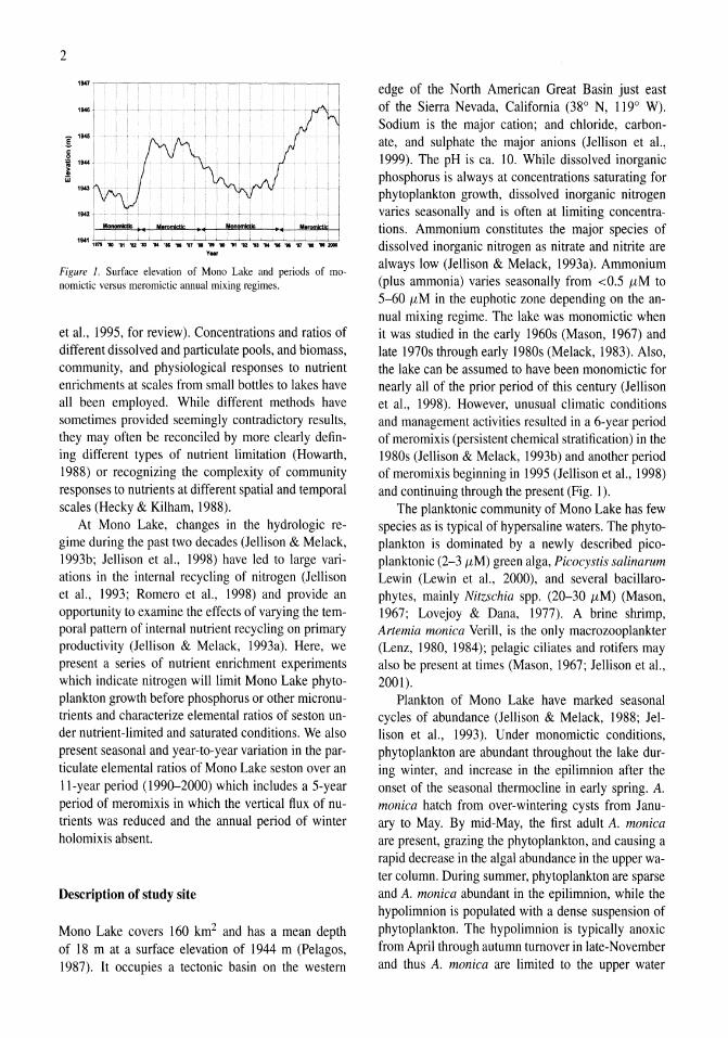
Figure 1. Surface elevation of Mono Lake and periods of monomictic versus meromictic annual mixing regimes.
et aI., 1995, for review). Concentrations and ratios of different dissolved and particulate pools, and biomass, community, and physiological responses to nutrient enrichments at scales from small bottles to lakes have all been employed. While different methods have sometimes provided seemingly contradictory results, they may often be reconciled by more clearly defining different types of nutrient limitation (Howarth, 1988) or recognizing the complexity of community responses to nutrients at different spatial and temporal scales (Hecky & Kilham, 1988).
At Mono Lake, changes in the hydrologic regime during the past two decades (Jellison & Melack, 1993b; Jellison et aI., 1998) have led to large variations in the internal recycling of nitrogen (Jellison et a!., 1993; Romero et a!., 1998) and provide an opportunity to examine the effects of varying the temporal pattern of internal nutrient recycling on primary productivity (Jellison & Melack, 1993a). Here, we present a series of nutrient enrichment experiments which indicate nitrogen will limit Mono Lake phytoplankton growth before phosphorus or other micronutrients and characterize elemental ratios of seston under nutrient-limited and saturated conditions. We also present seasonal and year-to-year variation in the particulate elemental ratios of Mono Lake seston over an II-year period (1990-2000) which includes a 5-year period of meromixis in which the vertical flux of nutrients was reduced and the annual period of winter holomixis absent.
Description of study site
Mono Lake covers 160 km2 and has a mean depth of 18 m at a surface elevation of 1944 m (Pelagos, 1987). It occupies a tectonic basin on the western
edge of the North American Great Basin just east of the Sierra Nevada, California (38 0 N, 1190 W). Sodium is the major cation; and chloride, carbonate, and sulphate the major anions (Jellison et a!., 1999). The pH is ca. 10. While dissolved inorganic phosphorus is always at concentrations saturating for phytoplankton growth, dissolved inorganic nitrogen varies seasonally and is often at limiting concentrations. Ammonium constitutes the major species of dissolved inorganic nitrogen as nitrate and nitrite are always low (Jellison & Melack, 1993a). Ammonium (plus ammonia) varies seasonally from <0.5 11M to 5-60 11M in the euphotic zone depending on the annual mixing regime. The lake was monomictic when it was studied in the early 1960s (Mason, 1967) and late 1970s through early 1980s (Melack, 1983). Also, the lake can be assumed to have been monomictic for nearly all of the prior period of this century (Jellison et a!., 1998). However, unusual climatic conditions and management activities resulted in a 6-year period of meromixis (persistent chemical stratification) in the 1980s (Jellison & Melack, 1993b) and another period of meromixis beginning in 1995 (Jellison et a!., 1998) and continuing through the present (Fig. I).
The planktonic community of Mono Lake has few species as is typical of hypersaline waters. The phytoplankton is dominated by a newly described picoplanktonic (2-3 11M) green alga, Picocystis salinarum Lewin (Lewin et a!., 2000), and several bacillarophytes, mainly Nitzschia spp. (20-30 11M) (Mason, 1967; Lovejoy & Dana, 1977). A brine shrimp, Artemia monica Verill, is the only macrozooplankter (Lenz, 1980, 1984); pelagic ciliates and rotifers may also be present at times (Mason, 1967; Jellison et aI., 2001).
Plankton of Mono Lake have marked seasonal cycles of abundance (Jellison & Melack, 1988; Jellison et aI., 1993). Under monomictic conditions, phytoplankton are abundant throughout the lake during winter, and increase in the epilimnion after the onset of the seasonal thermocline in early spring. A. monica hatch from over-wintering cysts from January to May. By mid-May, the first adult A. monica are present, grazing the phytoplankton, and causing a rapid decrease in the algal abundance in the upper water column. During summer, phytoplankton are sparse and A. monica abundant in the epilimnion, while the hypolimnion is populated with a dense suspension of phytoplankton. The hypolimnion is typically anoxic from April through autumn turnover in late-November and thus A. monica are limited to the upper water
column. In autumn, the phytoplankton increase in the surface waters as thermal stratification weakens and the A. monica population declines becoming virtually absent during winter. During meromictic conditions the vernal and autumn blooms and winter abundance of phytoplankton are much reduced, and the A. monica population develops more slowly (Melack & Jellison, 1998).
Methods
Nutrient enrichment experiments
A series of nutrient enrichment experiments were conducted between August 1982 and March 1986 and in July 1998. Natural assemblages of Mono Lake phytoplankton were collected from just below the surface (ca. 20 cm) at a pelagic station in the western portion of Mono Lake. Water for each nutrient enrichment experiment was thoroughly mixed and subsamples were poured into 4-1 transparent plastic containers. Ammonium chloride was added to duplicate containers resulting in a lO-JLM enrichment; two containers served as controls. During periods of high algal biomass and warm temperatures the ammonium enrichment was increased to 20 JLM to prevent depletion of ammonium in enriched samples. Initial ammonium and chlorophyll a (ChI a) concentrations were determined immediately prior to parceling the water among the containers. Samples were incubated in a water bath near epilimnetic temperatures and illuminated from above by cool-white power groove, fluorescent lamps (GE F48PG 17CW) on a 12: 12 light dark cycle. Light intensity was 250-300 JLEinsteins m-2 s-l (400-700 nm range), which was usually above the intensity for light-saturated photosynthesis (Jellison & Melack, 1988).
Two initial enrichment experiments conducted with samples collected in August 1982 were run for 8 and 20 days. From 1983 through 1986, experiments were run for 72 h. After 48 h, duplicate 50-ml subsamples were removed for ChI a and ammonium determination and an additional lO-JLM enrichment of NH4Cl was added to treatments. Experiments were continued for an additional 24 h after which final ammonium and ChI a concentrations were determined.
A 4-day nutrient enrichment experiment was conducted in July 1998 to determine responses in particulate elemental ratios of seston to addition to of dissolved inorganic phosphorus and ammonium. Duplicate treatments included controls, lO-JLM NH4,
3
20-JLM NH4, lO-JLM P04, and a combination 20-JLM NH4 and 10-JLM P04 enrichment. Responses were determined from subsamples collected after 48 and 96 h.
In situ sampling and analytical measurements
Water samples were collected with a 9-m integrating tube sampler (diameter, 2.5 cm) at one to three centrally located pelagic stations. Samples were immediately passed through a 120-JLM net to remove all stages of the zooplankter, Artemia monica, and a subsample filtered through Gelman AlE glass-fiber filters for analysis of nutrients. Samples were kept chilled and in the dark until returned to the laborat-0ry. Ammonium concentrations were measured with the indophenol blue method (Strickland & Parsons, 1972) using internal standards for each set of determinations. Phytoplankton samples were filtered onto Whatman GFIC (1982-1984) or Gelman AlE (1985-2000) filters and kept frozen at -14°C until pigments were analyzed. A comparison of pigment concentrations obtained by the two filter types with samples from different depths did not detect significant differences (Wilcoxon signed-rank, P<0.14). Except during periods of low biomass, chlorophyll a was determined by spectrophotometric analysis with correction for phaeopigments (Golterman, 1969), after a 40-min extraction of macerated filters in 90% acetone at room temperature in the dark. Low chlorophyll a
concentrations «5 mg ChI a m-3) were measured on a fluorometer that was calibrated against spectrophotometric measurements using large-volume lake samples.
From 1990 through 2000, subsamples were filtered onto precombusted Gelman AlE filters for the determination of particulate C, Nand P. Duplicate carbon and nitrogen filters were acid fumed for 12 hover concentrated HCI, and then dried at 40-50°C before determination by combustion in a Perkin-Elmer 240B elemental analyzer standardized with acetanilide. Additional duplicate particulate phosphorus filters were oxidized with persulfate reagent (Valderrama, 1981) followed by soluble reactive phosphate assay by the molybdenum blue-ascorbic acid method (Strickland & Parsons, 1972).
Filters were not rinsed following collection of particulates due to the potential for lysing algal cells from 1990 through mid-1996. However, while the amount of water retained on Gelman AlE filters is small (ca. 0.1 ml), the high dissolved inorganic phosphorus con-
4
45 18
40 16
fJ5 14
~JO 12~ 3
.. 25 109 c· ~20 6 3 a. ~ 15 6 " ~ ~ Ul0 4
1982 1983 1984 1985 1986
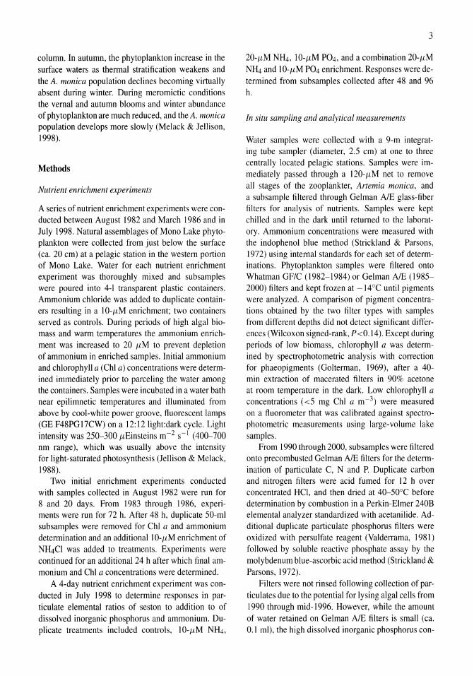
Figure 2. In situ mixolimnetic chlorophyll a (solid) and ammonium (open, dotted) concentrations during the onset and persistence ofthe 1980s episode of meromixis.
centrations in Mono Lake introduced significant error in particulate phosphorus determinations during periods of low biomass, Therefore, beginning in mid-1996 filters were rinsed with synthetic (N and P free) Mono Lake water. To correct earlier data, rinsed and unrinsed filters were collected and compared over the course of a full year. A correction factor for the amount of C, Nand P in the residual water was determined from highly significant regressions between determinations on the rinsed and un-rinsed filters. This correction was small for C and N, but relatively large for P during periods of low algal biomass.
Results
Nutrient enrichments
Twenty-two ammonium enrichment experiments were conducted from 1982 to 1986. This period encompassed a range of in situ conditions with mixed-layer (2 m) ammonium concentrations ranging from <0.1 to 26,5 flM and phytoplankton abundance, as measured by chlorophyll a, ranging from 0.2 to 42.8 flg ChI a I-I (Fig. 2).
Two enrichment experiments were conducted with whole lake samples collected on 5 and 24 August 1982 when ammonium concentrations were fairly high (5 and 10 flM, respectively). In the first enrichment, Chi a response was monitored after 3,5 and 20 days. There were significant increases in chlorophyll in all treatments at each measurement and only on the final day were the responses of the enriched samples significantly more positive than the controls. In the second experiment, ammonium was added to the enriched treatments at days 4 and 8 to maintain concentrations
,. r-------------------------------~ . """'"
~. L-------------------------------~
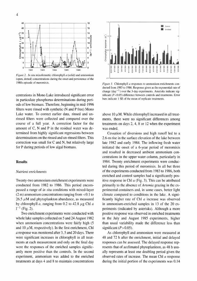
Figure 3. Chlorophyll a responses to ammonium enrichments conducted from 1983 to 1986. Response given as the exponential rate of change (day-I) over the 3-day experiments. Asterisks indicate significant (P<0.05) difference between controls and treatments. Error bars indicate 1 SE of the mean of replicate treatments.
above 10 flM. While chlorophyll increased in all treatments, there were no significant differences among treatments on days 2, 4, 8 or 12 when the experiment was ended.
Cessation of diversions and high runoff led to a 2.6-m rise in the surface elevation of the lake between late 1982 and early 1984. The inflowing fresh water initiated the onset of a 6-year period of meromixis and resulted in decreased ambient ammonium concentrations in the upper water column, particularly in 1984. Twenty enrichment experiments were conducted during this period of meromixis. In all but three of the experiments conducted from 1983 to 1986, both enriched and control samples had a significantly positive response in Chi a (Fig. 3). This can be attributed primarily to the absence of Artemia grazing in the experimental containers and, in some cases, better light climate compared to conditions in the lake. A significantly higher rate of ChI a increase was observed in ammonium-enriched samples in 13 of the 20 experiments (indicated by asterisks). Although a more positive response was observed in enriched treatments in the July and August 1985 experiments, higher than usual variability made the difference less than significant (P>0.05).
As chlorophyll and ammonium were measured at 48 and 72 h after the enrichment, initial and delayed responses can be assessed. The delayed response represents that of acclimated phytoplankton, as 48 h usually represents at least one doubling period given the observed rates of increase. The mean Chi a response during the initial portion of the experiments was 0.14
~r-------------------------------~
~
~ ~ Q) III I: o 0. .• III
~ Ql
~ ..2 .r: 0. e o :c ., ()
A
B
• Con~oI • 81_
. lnitielrete • Ratll IIIIrtfH' tochrnallon
Control
Figure 4. (A) Chlorophyll a response to ammonium enrichment as illustrated by pooling replicate controls and reatments over all experiments shown in Figure 3. Error bars indicate ± I SE. The initial response was measured over the first 48 h and the acclimated response over the following 24 h. (B) Ratio of decrease in ammonium to increase in chlorophyll a for pooled experiments shown in Figure 3. Error bars indicate ± I SE.
and 0.22 day-I in the controls and treatments, respectively. After the 2-day acclimation period, the mean Chi a response was higher in both controls and treatments, 0.29 and 0.44 day-I, respectively (Fig. 4A). In a two-way ANOYA both ammonium enrichment and acclimation had a significantly positive effect on the rate of change of Chi a while the interaction term was not significant.
Decreases in ammonium accompanying increases in ChI a can also provide an indication of nitrogen limitation. At low growth rates (i.e., small changes in Chi a), this ratio was too variable to provide a useful measure; therefore, analysis was only performed on those samples in which the Chi a response was greater than 0.2 day-I. With the replicates pooled from all the experiments, the uptake of ammonium per unit increase in Chi a was significantly higher (P <0.00 I) in the enriched samples compared to controls, while acclimation did not contribute significantly to the overall variance (Fig. 4B). Because the lack of response in controls obscures the effect of acclimation on enriched
70 rA-;----~~~~~--,
" "t-, ------/
D.,
~~E~~--I : '===---------- ~! 1°Ob~:::::;::::;:<~==~
D.,
S
5OC(),....---~----,
"'" ..,-4(XX)
"!3S00 0'= S 2500t-~~~~h"--~ 200J t-~~~----r./~--"--~ 1500 t-~~--ff-----c=" :. lClXl t--~--=~-=-----1
500-
Do, 80 0 r= 70 t-"'-~~~~~~-j
a: eo -------7 Go 50 --~---_____.~_:_i i : ----,~ ~ ~- ,/ i20 ~ IL 10--
o +---_-~_~-J , D.,
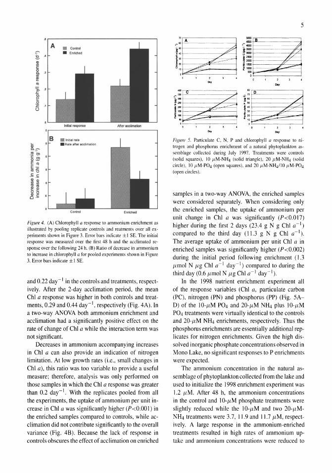
Figure 5. Particulate C, N, P and chlorophyll a response to nitrogen and phosphorus enrichment of a natural phytoplankton assemblage collected during July 1997. Treatments were controls (solid squares), 10 J.LM-NH4 (solid triangle), 20 J.LM-NH4 (solid circle), 10 J.LM-P04 (open squares), and 20 J.LM-NH41l0 J.LM-P04 (open circles).
samples in a two-way ANOYA, the enriched samples were considered separately. When considering only the enriched samples, the uptake of ammonium per unit change in Chi a was significantly (P<O.017) higher during the first 2 days (23.4 g N g Chi a-I)
compared to the third day (11.3 g N g ChI a-I).
The average uptake of ammonium per unit ChI a in enriched samples was significantly higher (P<0.002) during the initial period following enrichment (1.3 I1mol N I1g ChI a-I day-I) compared to during the third day (0.6 I1mol N I1g Chi a-I day-I).
In the 1998 nutrient enrichment experiment all of the response variables (ChI a, particulate carbon (PC), nitrogen (PN) and phosphorus (PP) (Fig. SAD) of the 10-I1M P04 and 20-I1M NH4 plus 10-I1M P04 treatments were virtually identical to the controls and 20-I1M NH4 enrichments, respectively. Thus the phosphorus enrichments are essentially additional replicates for nitrogen enrichments. Given the high dissolved inorganic phosphate concentrations observed in Mono Lake, no significant responses to P enrichments were expected.
The ammonium concentration in the natural assemblage of phytoplankton collected from the lake and used to initialize the 1998 enrichment experiment was 1.2 11M. After 48 h, the ammonium concentrations in the control and iO-I1M phosphate treatments were slightly reduced while the iO-I1M and two 20-I1MNH4 treatments were 3.7, 1l.9 and 1l.7 11M, respectively. A large response in the ammonium-enriched treatments resulted in high rates of ammonium uptake and ammonium concentrations were reduced to
6
0.3-0.5 f1M in all treatments by the end of the experiment (96 h). Thus, enriched treatments were nutrient depleted by the end of the experiment.
All of the response variables (ChI a, PC, PN, PP) increased in all treatments during the first 48 h of the experiment (Fig. SA-D). However, in contrast to the August 1982 experiments, the increases were significantly higher in all of the ammonium-enriched treatments. While the response after 2 days was the same among the low (10 f1M-NH4) and high (20 f1MNH4 and 20 f1M-NH4 plus 10 f1M-P04) ammonium enrichments, all four response variables were significantly greater in the high enrichments by the end of the experiment. Of the four response variables, ChI a responded most strongly, increasing 8-fold from 1.25 to 10.1 f1g ChI a 1-1 in the controls and 17-fold in the ammonium-enriched treatments during the first 48 h. As ammonium was depleted during the next 48 h, ChI a decreased 10% in the controls and increased 50 and 144% in the low-N and high-N treatments, respectively. Particulate C and P increased during both periods of the experiment while particulate nitrogen only increased during the first 2 days. By the end of the experiment particulate C, Nand P were 2-4 times higher in the ammonium-enriched treatments compared to the controls.
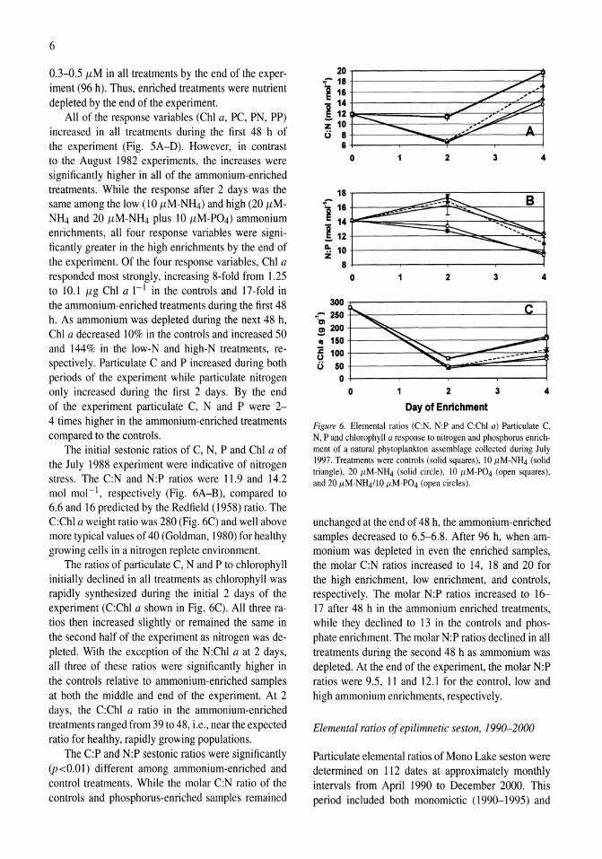
The initial sestonic ratios of C, N, P and ChI a of the July 1988 experiment were indicative of nitrogen stress. The C:N and N:P ratios were 11.9 and 14.2 mol mol-I, respectively (Fig. 6A-B) , compared to 6.6 and 16 predicted by the Redfield (1958) ratio. The C:Chl a weight ratio was 280 (Fig. 6C) and well above more typical values of 40 (Goldman, 1980) for healthy growing cells in a nitrogen replete environment.
The ratios of particulate C, N and P to chlorophyll initially declined in all treatments as chlorophyll was rapidly synthesized during the initial 2 days of the experiment (C:Chl a shown in Fig. 6C). All three ratios then increased slightly or remained the same in the second half of the experiment as nitrogen was depleted. With the exception of the N:Chl a at 2 days, all three of these ratios were significantly higher in the controls relative to ammonium-enriched samples at both the middle and end of the experiment. At 2 days, the C:Chl a ratio in the ammonium-enriched treatments ranged from 39 to 48, i.e., near the expected ratio for healthy, rapidly growing populations.
The C:P and N:P sestonic ratios were significantly (p<0.01) different among ammonium-enriched and control treatments. While the molar C:N ratio of the controls and phosphorus-enriched samples remained
20 ~- 18
1 16 - 14 ~ 12 i" 10 (; 8
6
18 ~- 16
114
! 12 II.. 10 Z
8
300
-- ---.. 0
0
/'-~ -
",.." --,
~ ,-" ~ ~ ,-~
,-:.:-- A ~
2 3 4
2 3 4
~ 250~~~----------------------~~
S 200+---~~----------------------~ • 150+-------~~--------------~~~ ~ 100t---------~~~~~~~~~~~ (; 50+---------~~~~~~~==~
O+------,------~------,-------
o 2 3 4
Day of Enrichment
Figure 6. Elemental ratios (C:N, N:P and C:Chl a) Particulate C, N, P and chlorophyll a response to nitrogen and phosphorus enrichment of a natural phytoplankton assemblage collected during July 1997. Treatments were controls (solid squares), 10 JLM-NH4 (solid triangle), 20 JLM-NH4 (solid circle), 10 JLM-P04 (open squares), and 20 JLM-NH4/1O JLM-P04 (open circles).
unchanged at the end of 48 h, the ammonium-enriched samples decreased to 6.5-6.8. After 96 h, when ammonium was depleted in even the enriched samples, the molar C:N ratios increased to 14, 18 and 20 for the high enrichment, low enrichment, and controls, respectively. The molar N:P ratios increased to 16-17 after 48 h in the ammonium enriched treatments, while they declined to 13 in the controls and phosphate enrichment. The molar N:P ratios declined in all treatments during the second 48 h as ammonium was depleted. At the end of the experiment, the molar N:P ratios were 9.5, 11 and 12.1 for the control, low and high ammonium enrichments, respectively.
Elemental ratios of epilimnetic seston, 1990-2000
Particulate elemental ratios of Mono Lake seston were determined on 112 dates at approximately monthly intervals from April 1990 to December 2000. This period included both monomictic (1990-1995) and
30 A
25 --
i 20 a E " '" 15 0
-- ~-----
E E 0( 10 -
5
0
I~ ~ ~I 1\
IJ :\ ~~ A. .111_
1990 '91 '92 '93 '94 '95 '96 '97 '98 '99 2000
120
B 100
£,80 f---- --
." a .!! 60 .c (J
40
20
I~ t IV
I~ - ~ I
J Ij i.I N\ \AJ~ o 1990 '91 '92 '93 '94 '95 '96 ''i11 '911 '99 2000
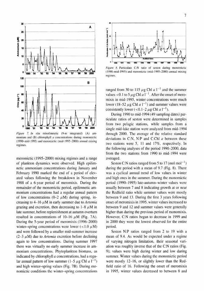
Figure 7. In situ mixolimnetic (9-m integrated) (A) ammonium and (B) chlorophyll a concentrations during monomictic (l990-mid-1995) and meromictic (mid-1995-2000) annual mixing regimes.
meromictic (1995-2000) mixing regimes and a range of plankton dynamics were observed. High epilimnetic ammonium concentrations during January and February 1990 marked the end of a period of elevated values following the breakdown in November 1988 of a 6-year period of meromixis. During the remainder of the monomictic period, epilimnetic ammonium concentrations had a regular annual pattern of low concentrations (0-2 (lM) during spring, increasing to 4-16 {lM in early summer due to Artemia grazing and excretion, then decreasing to 1-8 {lM in late summer, before replenishment at autumn overturn resulted in concentrations of 10-16 {lM (Fig. 7 A). During the 5-year period of meromixis (1996-2000) winter-spring concentrations were lower ( < 1.0 (lM) and were followed by a smaller mid-summer increase (2-3 (lM) due to Artemia excretion before declining again to low concentrations. During summer 1997 there was virtually no early summer increase in ammonium concentrations. Phytoplankton biomass, as indicated by chlorophyll a concentrations, had a regular annual pattern of low summer (1-5 (lg ChI a I-I) and high winter-spring values (Fig. 7B). During monomictic conditions the winter-spring concentrations
~ z (;
7
~,---------------------------------,
i1O~+-~~~#h~~~~~~~~hM~~
I 5 1990 1n1 1992 1993 1994 ,. 1898
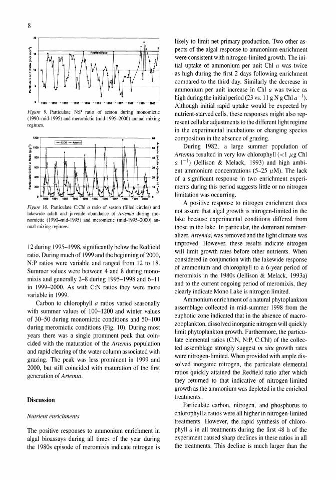
Figure 8. Particulate C:N ratio of seston during monomictic (l990-mid-1995) and meromictic (mid-I 995-2000) annual mixing regimes.
ranged from 30 to 115 {lg ChI a I-I and the summer values <0.1 to 5 {lg ChI a I-I . After the onset of meromixis in mid-1995, winter concentrations were much lower (18-52 (lg ChI a I-I) and summer values were consistently lower ( <0.1-2 (lg ChI a I-I).
During 1990 to mid-1994 (49 sampling dates) particulate ratios of seston were determined in samples from two pelagic stations, while samples from a single mid-lake station were analyzed from mid-1994 through 2000. The average of the relative standard deviations in C:N, N:P and C:Chl a between these two stations were 5, II and 17%, respectively. In the following analyses of the period 1990-2000, data from the two stations from 1990 to mid-1994 were averaged.
Seston C:N ratios ranged from 5 to 17 (mol mol-I) during the period with a mean of 9.7 (Fig. 8). There was a cyclical annual trend of low values in winter and high ones in the summer. During the monomictic period (1990-1995) late-autumn-winter values were usually between 7 and 8 indicating growth at or near the Redfield ratio while summer values were mostly between 9 and 13. During the first 3 years following onset of meromixis in 1995, winter values increased to between 9 and 12 and summer values were generally higher than during the previous period of monomixis. However, C:N ratios began to decrease in 1999 and in 2000 they were the lowest observed for the entire period.
Seston N:P ratios ranged from 2 to 19 with a mean of 9.4. As would be expected under a regime of varying nitrogen limitation, their seasonal variation was roughly inverse that of the C:N ratios (Fig. 9); values were high during winter and low during summer. Winter values during the monomictic period were mostly 12-16, or slightly lower than the Redfield ratio of 16. Following the onset of meromixis in 1995, winter values decreased to between 8 and
8
2D,-------------------------------~
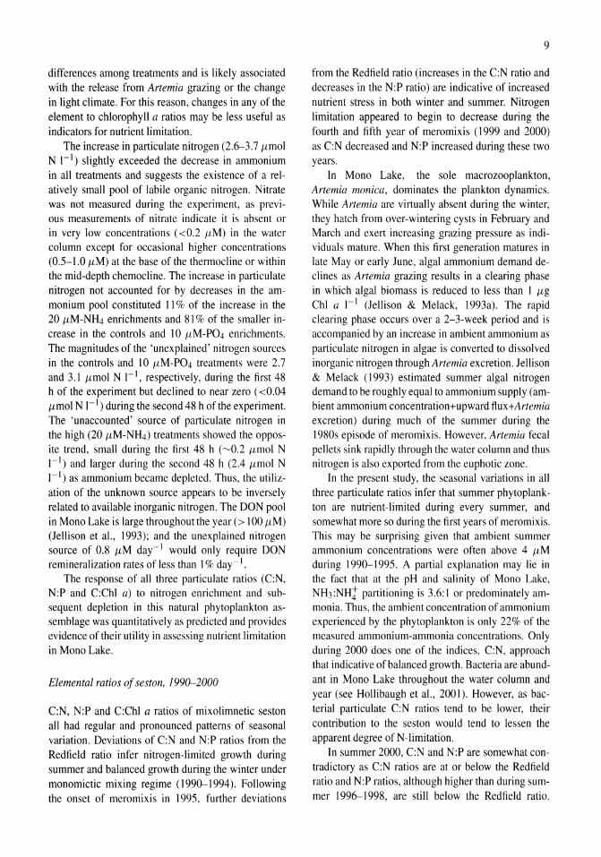
Figure 9. Particulate N:P ratio of seston during monomictic (19~O-mid-1995) and meromictic (mid-1995-2000) annual mixing regimes.
1200
.;; 1_
f ... . 1i ... u I ...
I 200
1 c"'" ""'.1
~
~ "I 1 o
1D~ J ~ ~ ill ~ W tvj ~ II \M~ ~ 1_ 1111 1112 1113 '9M '185 1191 1117 ,.. 1_ 2ODO 0
Figure 10. Particulate C:Chl a ratio of seston (filled circles) and lakewide adult and juvenile abundance of Artemia during monomictic (1990-mid-1995) and meromictic (mid-1995-2000) annual mixing regimes.
12 during 1995-1998, significantly below the Redfield ratio. During much of 1999 and the beginning of 2000, N:P ratios were variable and ranged from 12 to 18. Summer values were between 4 and 8 during monomixis and generally 2-8 during 1995-1998 and 6-11 in 1999-2000. As with C:N ratios they were more variable in 1999.
Carbon to chlorophyll a ratios varied seasonally with summer values of 100-1200 and winter values of 30-50 during monomictic conditions and 50-100 during meromictic conditions (Fig. 10). During most years there was a single prominent peak that coincided with the maturation of the Artemia population and rapid clearing of the water column associated with grazing. The peak was less prominent in 1999 and 2000, but still coincided with maturation of the first generation of Artemia.
Discussion
Nutrient enrichments
The positive responses to ammonium enrichment in algal bioassays during all times of the year during the 1980s episode of meromixis indicate nitrogen is
likely to limit net primary production. Two other aspects of the algal response to ammonium enrichment were consistent with nitrogen-limited growth. The initial uptake of ammonium per unit ChI a was twice as high during the first 2 days following enrichment compared to the third day. Similarly the decrease in ammonium per unit increase in ChI a was twice as high during the initial period (23 vs. 11 g N g ChI a-I). Although initial rapid uptake would be expected by nutrient-starved cells, these responses might also represent cellular adjustments to the different light regime in the experimental incubations or changing species composition in the absence of grazing.
During 1982, a large summer population of Artemia resulted in very low chlorophyll « 1 Jlg ChI a 1-1) (Jellison & Melack, 1993) and high ambient ammonium concentrations (5-25 JlM). The lack of a significant response in two enrichment experiments during this period suggests little or no nitrogen limitation was occurring.
A positive response to nitrogen enrichment does not assure that algal growth is nitrogen-limited in the lake because experimental conditions differed from those in the lake. In particular, the dominant remineralizer, Artemia, was removed and the light climate was improved. However, these results indicate nitrogen will limit growth rates before other nutrients. When considered in conjunction with the lakewide response of ammonium and chlorophyll to a 6-year period of meromixis in the 1980s (Jellison & Me1ack, 1993a) and to the current ongoing period of meromixis, they clearly indicate Mono Lake is nitrogen limited.
Ammonium enrichment of a natural phytoplankton assemblage collected in mid-summer 1998 from the euphotic zone indicated that in the absence of macrozooplankton, dissolved inorganic nitrogen will quickly limit phytoplankton growth. Furthermore, the particulate elemental ratios (C:N, N:P, C:Chl) of the collected assemblage strongly suggest in situ growth rates were nitrogen-limited. When provided with ample dissolved inorganic nitrogen, the particulate elemental ratios quickly attained the Redfield ratio after which they returned to that indicative of nitrogen-limited growth as the ammonium was depleted in the enriched treatments.
Particulate carbon, nitrogen, and phosphorus to chlorophyll a ratios were all higher in nitrogen-limited treatments. However, the rapid synthesis of chlorophyll a in all treatments during the first 48 h of the experiment caused sharp declines in these ratios in all the treatments. This decline is much larger than the
differences among treatments and is likely associated with the release from Artemia grazing or the change in light climate. For this reason, changes in any of the element to chlorophyll a ratios may be less useful as indicators for nutrient limitation.
The increase in particulate nitrogen (2.6-3.7 {lmol N I-I) slightly exceeded the decrease in ammonium in all treatments and suggests the existence of a relatively small pool of labile organic nitrogen. Nitrate was not measured during the experiment, as previous measurements of nitrate indicate it is absent or in very low concentrations «0.2 {lM) in the water column except for occasional higher concentrations (0.5-1.0 {lM) at the base of the thermocline or within the mid-depth chemocline. The increase in particulate nitrogen not accounted for by decreases in the ammonium pool constituted II % of the increase in the 20 {lM-NH4 enrichments and 81 % of the smaller increase in the controls and 10 {lM-P04 enrichments. The magnitudes of the 'unexplained' nitrogen sources in the controls and 10 {lM-P04 treatments were 2.7 and 3.1 {lmol N I-I, respectively, during the first 48 h of the experiment but declined to near zero ( <0.04 {lmol N I-I) during the second 48 h of the experiment. The 'unaccounted' source of particulate nitrogen in the high (20 {lM-NH4) treatments showed the opposite trend, small during the first 48 h (~0.2 {lmol N I-I) and larger during the second 48 h (2.4 {lmol N I-I) as ammonium became depleted. Thus, the utilization of the unknown source appears to be inversely related to available inorganic nitrogen. The DON pool in Mono Lake is large throughout the year (> 100 {lM) (Jellison et aI., 1993); and the unexplained nitrogen source of 0.8 {lM day-I would only require DON remineralization rates of less than 1% day-I.
The response of all three particulate ratios (C:N, N:P and C:Chl a) to nitrogen enrichment and subsequent depletion in this natural phytoplankton assemblage was quantitatively as predicted and provides evidence of their utility in assessing nutrient limitation in Mono Lake.
Elemental ratios of seston, 1990-2000
C:N, N:P and C:Chl a ratios of mixolimnetic seston all had regular and pronounced patterns of seasonal variation. Deviations of C:N and N:P ratios from the Redfield ratio infer nitrogen-limited growth during summer and balanced growth during the winter under monomictic mixing regime (1990-1994). Following the onset of meromixis in 1995, further deviations
9
from the Redfield ratio (increases in the C:N ratio and decreases in the N:P ratio) are indicative of increased nutrient stress in both winter and summer. Nitrogen limitation appeared to begin to decrease during the fourth and fifth year of meromixis (1999 and 2000) as C:N decreased and N:P increased during these two years.
In Mono Lake, the sole macrozooplankton, Artemia monica, dominates the plankton dynamics. While Artemia are virtually absent during the winter, they hatch from over-wintering cysts in February and March and exert increasing grazing pressure as individuals mature. When this first generation matures in late Mayor early June, algal ammonium demand declines as Artemia grazing results in a clearing phase in which algal biomass is reduced to less than I {lg Chi a I-I (Jellison & Melack, 1993a). The rapid clearing phase occurs over a 2-3-week period and is accompanied by an increase in ambient ammonium as particulate nitrogen in algae is converted to dissolved inorganic nitrogen through Artemia excretion. Jellison & Melack (1993) estimated summer algal nitrogen demand to be roughly equal to ammonium supply (ambient ammonium concentration+upward ftux+Artemia excretion) during much of the summer during the 1980s episode of meromixis. However, Artemia fecal pellets sink rapidly through the water column and thus nitrogen is also exported from the euphotic zone.
In the present study, the seasonal variations in all three particulate ratios infer that summer phytoplankton are nutrient-limited during every summer, and somewhat more so during the first years of meromixis. This may be surprising given that ambient summer ammonium concentrations were often above 4 {lM during 1990-1995. A partial explanation may lie in the fact that at the pH and salinity of Mono Lake, NH3 :NHt partitioning is 3.6: I or predominately ammonia. Thus, the ambient concentration of ammonium experienced by the phytoplankton is only 22% of the measured ammonium-ammonia concentrations. Only during 2000 does one of the indices, C:N, approach that indicative of balanced growth. Bacteria are abundant in Mono Lake throughout the water column and year (see Hollibaugh et aI., 2001). However, as bacterial particulate C:N ratios tend to be lower, their contribution to the seston would tend to lessen the apparent degree of N-limitation.
In summer 2000, C:N and N:P are somewhat contradictory as C:N ratios are at or below the Redfield ratio and N:P ratios, although higher than during summer 1996-1998, are still below the Redfield ratio.
10
One potential cause of this discrepancy may be the entrainment of mid-depth bacterial populations. The mixed-layer deepened significantly and chemical stratification weakened during both 1999 and 2000 (see below). While bacterial populations in the mixolimnion are generally small « 1 /LM), many of those at or beneath the chemocline are larger (J. T. Hollibaugh, pers. commun.). Thus, episodic entrainment of these deeper bacterial populations would result in a larger fraction of seston samples (> 1 /LM) being of bacterial origin. As bacterial C:N:P ratios are approximately 45:9: 1 (Goldman et al., 1987), their inclusion would tend to lower N:P more than C:N ratios. N:P ratios were generally more variable than C:N ratios, particularly during 1999 when the mixed layer deepened almost 5 m. Lebo (1994) also found N:P ratios more variable than C:N ratios in Pyramid Lake, but suggested this was due to episodic aeolian inputs of inorganic P associated with dust particles.
All three indicators suggest near balanced growth during much of the winter except during the first 3 years of meromixis (1995-1998). Although winter bacterial populations in Mono Lake contain more large individuals (J. T. Hollibaugh, pers. commun.), it is unlikely that this contribution is responsible for the apparent balanced growth ratios, as it would also lower N:P ratios and raise C:Chl a ratios; neither of which occurred. Thus, low temperatures and light during winter appear to limit phytoplankton growth to within the available nitrogen supply during most years. Deviation from balanced growth ratios in winter 1995-1998 infers N-limited growth following the onset of meromixis.
The C:Chl a ratios of mixolimnetic seston were well above those indicative of healthy growing phytoplankton during all but the mid-winter period. C:Chl a ratios were positively correlated with Artemia abundance (Fig. 10) which increases through spring, reaches a peak during summer, and declines to near zero during the winter. Artemia grazing causes dramatic seasonal changes in the light environment and may also alter the ratio of bacteria to phytoplankton in the > 1 /LM size class of seston. While high C:Chl a ratios likely result from reduced synthesis and repair of chlorophyll pigments during summer nitrogen stress, cellular adaptations to the increased light environment or a larger fraction of non-algal seston may also result in higher C:Chl a ratios. Due to the complex interplay of these factors, C:Chl a ratios of the seston may be less useful as indicators of nutrient limitation by
'945
'940
! 1935
~ 18,. ~ § ,." "5 100 1920
1915
1910
\'997 '99' '99' '994 -- -
~ '99. ~\
'899 ~~\ 2000
\\ \ \ \ \ \ I
nun n ~ ~ M .. M ~ ~
SoI~l1yt.kg·')
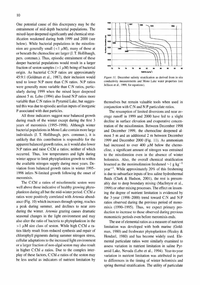
Figure J J. December salinity stratification as derived from in situ conductivity measurements and Mono Lake water properties (see Jellison et aI .• 1999, for equations).
themselves but remain valuable tools when used in conjunction with C:N and N:P particulate ratios.
The resumption of limited diversions and near average runoff in 1999 and 2000 have led to a slight decline in surface elevation and evaporative concentration of the mixolimnion. Between December 1998 and December 1999, the chemocline deepened almost 5 m and an additional 2 m between December 1999 and December 2000 (Fig. 11). As ammonium had increased to over 400 /LM below the chemocline, a significant amount of nitrogen was entrained to the mixolimnion even in the absence of winter holomixis. Also, the overall chemical stratification lessened as the monimolimnion freshened ~ 1 g kg- 1
year-I. While approximately 20% of this freshening is due to subsurface inputs of less saline hydrothermal fluids (Clark & Hudson, 2001), the rest is presumably due to deep boundary mixing (MacIntyre et al., 1999) or other mixing processes. The effect on lessening the degree of nutrient limitation is evidenced by the 3-year (1998-2000) trend toward C:N and N:P ratios observed during the previous period of monomixis (1990-1995). Thus, we expect primary production to increase to those observed during previous monomictic periods even before meromixis ends.
The use of elemental ratios as a measure of nutrient limitation was developed with both marine (Goldman, 1980) and freshwater phytoplankton (Healey & Hendzel, 1980) and has become widely used. Elemental particulate ratios were similarly examined to assess variation in nutrient limitation in saline Pyramid Lake, Nevada (Lebo et al., 1994). Year-to-year variation in nutrient limitation was attributed in part to differences in the timing of winter holomixis and spring thermal stratification. The utility of particulate
elemental ratios to assess nutrient limitation illustrated here contrasts with that of analyzing assimilation
numbers derived from photosynthetic uptake of 14c.
Jellison & Melack (1993a) analyzed the correlation
between assimilation numbers and a suite of environmental co-variates over a 9-year period spanning the extended period of meromixis in the 1980s and found little correlation with any of several measures of nutrient availability. This was despite the fact that there were 4-fold changes in annual primary productivity associated with differences in internal recycling of nitrogen.
Summary
The long-term record of particulate C:N, N:P and
C:Chl a ratios presented here is unique among studies of saline lakes for its frequency and duration. This record illustrates the utility of using elemental ratios of seston for assessing variations in nutrient-limited growth of phytoplankton. Despite large month-tomonth and seasonal variation, the effects of changes in the internal recycling of nitrogen during the onset, persistence and weakening of meromixis were clearly detected. Based on these data, we conclude that Mono Lake phytoplankton (I) achieve early balanced growth during winters under monomictic mixing regimes, (2) experience N-limited growth during winters with no period of holomixis despite deep mixing depth and low light levels, (3) are strongly N-limited during most summers under monomictic regimes and even more so during the first years of meromictic regimes, (4) growth may become less N-limited even before the breakdown of meromixis due to enhanced upward fluxes of ammonium associated with weakening chemical stratification and entrainment of ammoniumrich water during deepening of the mixed layer. Although we do not address the effect of bacteria or detritus directly, it seems unlikely that their influence on particulate elemental ratios would Iter any of these conclusions. From these results and others (Pyramid Lake, Galat et aI., 1981; Great Salt Lake, Wurtsbaugh, 1988) it is clear that many of the large salt lakes in the North American Great Basin are N-limited. Although phosphorus limitation of primary production in lakes
is well known, nitrogen limitation is increasingly documented in a wide array of lakes (see Fisher et a!., 1995 for review).
Diversions of freshwater streams out of the Mono Basin beginning in 1941 have led to an approximate
II
halving of the lake's volume and doubling of the sa
linity. The smaller lake volume relative to variation
in snowmelt runoff, and the larger salinity difference between the lake water and inflowing streams
increase the frequency of multi-year periods of meromixis (Jellison et aI., 1998). The increased frequency of meromixis will increase year-to-year variability in primary production and cause multi-year periods of decreased primary production as observed during the current episode and the 1980s (Jellison & Melack, 1993a) episode of meromixis.
Acknowledgements
Laboratory work was performed at the Sierra Nevada Aquatic Research Laboratory of the University of California. Pete Kirchner, Darla Heil, and Sandra Roll assisted with field and laboratory analyses, and particulate C and N analyses were conducted by the Marine Science Institute Analytical Laboratory, University of Calfiornia, Santa Barbara. This work was supported by grants from the National Science Foundation (NSFDEB95-08733) and the City of Los Angeles awarded to R. Jellison and 1. M. Melack.
References
Clark, 1. F. & G. B. Hudson, 200 I. Quantifying the flux of hydrothermal fluids into Mono Lake by use of helium isotopes. Limnol. Oceanogr. 46: 189-196.
Fisher. T. R .. 1. M. Melack, 1. U. Grobbelaar & R. W. Howarth, 1995. Nutrient limitation of phytoplankton and eutrophication of inland, estuarine, and marine waters. In Tiessen. H. (ed.). Phosphorus in the Global Environment. John Wiley and Sons, New York: 301-322.
Galat, D. L., E. L. Lider, S. Vigg & S. R. Robertson, 1981. limnology of a large, deep, North American terminal lake, Pyramid Lake, Nevada. Hydrobiologia 82: 281-317.
Goldman, 1. c., 1980. Physiological processes, nutrient availability and the concept of relative growth rate in marine phytoplankton ecology. In Falkowski, P. (ed.), Primary Production in the Sea. Plenum, New York: 179-194.
Goldman, 1. C., D. A. Caron & M. R. Dennett, 1987. Regulation of gross growth efficiency and ammonium regeneration in bacteria by substrate C:N ratio. Limnol. Oceanogr. 32: 1239-1252.
Golterman, H. L., 1969. Methods for Chemical Analysis of Fresh Waters. Blackwell, Oxford.
Healey, F. P. & L. L. Hendzel, 1980. Physiological indicators of nutrient deficiency in lake phytoplankton. Can. J. Fish. aquat. Sci. 37: 442-453.
Hecky, R. E. & P. Kilham, 1988. Nutrient limitation of phytoplankton in freshwater and marine environments: a review of recent evidence on the effects of enrichment. Limnol. Oceanogr. 33: 796-822.
12
Herbst, D. B., 1998. Potential salinity limitations on nitrogen fixation in sediments from Mono Lake, California. Int. 1. Salt Lake Res. 7: 261-274.
Howarth, R. w., 1988. Nutrient limitation of net primary production in marine ecosystmes. Annu. Rev. ecol. Syst. 19: 89-110.
Jellison, R. & J. M. Melack, 1988. Photosynthetic activity of phytoplankton and its relation to environmental factors in hypersaline Mono La~e. Hydrobiologia 158: 69-88.
Jellison, R. & J. M. Melack, 1993a. Algal photosynthetic activity and its response to meromixis in hypersaline Mono Lake, California. Limno!. Oceanogr. 38: 818-837.
Jellison, R. & J. M. Melack, 1993b. Meromixis in hypersaline Mono Lake, California. 1. Stratification and vertical mixing during the onset, persistence, and breakdown of meromixis. Limnol. Oceanogr.38: 1008-1019.
Jellison, R., L. G. Miller, 1. M. Melack & G. L. Dana, 1993. Meromixis in hypersaline Mono Lake, California. 2. Nitrogen fluxes. Limno!. Oceanogr. 38: 1020-1039.
Jellison, R., J. Romero & 1. M. Melack, 1998. The onset of meromixis during restoration on Mono Lake, California: unintended consequences of reducing water diversions. Limno!. Oceanogr. 43: 706-711.
Jellison, R., S. MacIntyre & F. Millero, 1999. Density and conductivity properties of Na-C03-CI-S04 brine from Mono Lake, California, USA. Int. J. Salt Lake Res. 8: 41-53.
Jellison, R., H. Adams & J. M. Melack, 2001. Re-appearance of rotifers in hypersaline Mono Lake, California, during a period of rising lake levels and decreasing salinity. Hydrobiologia 466 (Dev. Hydrobio!. 162): 39-43.
Lebo, M. E., J. E. Reuter, C. R. Goldman & C. L. Rhodes, 1994. Interannual variability of nitrogen limitation in a desert lake: Influence of regional climate. Can. J. Fish. aquat. Sci. 51: 862-872.
Lenz, P. H., 1980. Ecology of an alkali-adapted variety of Artemia from Mono Lake, California. USA. In Persone, c., P. Sorgeloos, O. Roels & E. Jaspers (eds), The Brine Shrimp Artemia: Ecology, Culturing, Use in Aquaculture. Universa Press, Wetteren, Belgium: 79-96.
Lenz, P. H., 1984, Life history analysis of an Artemia popUlation in a changing environment. J. Plankton Res. 6: 967-983.
Lewin, R. A., L. Krienitz, R. Goericke, H. Takeda & D. Hepperle, In press. Picocystis salinarum gen. et sp. nov. (Chlorophyta) -a new picoplanktonic green alga. Phycologia.
Lovejoy, C. & G. Dana, 1977. Primary producer level. In Winkler, D. W. (ed.), An Ecological Study of Mono Lake, California. Univ. of Calif., Davis: 42-57.
MacIntyre, S., K. Flynn, R. Jellison & J. Romero, 1999. Boundary mixing and nutrient fluxes in Mono Lake, California. Limno!. Oceanogr. 44: 512-529.
Mason, D. T., 1967. Limnology of Mono Lake, California. Univer. Calif. Pub!. Zool. 83: 1-110,
Melack, J. M., 1983. Large, deep salt lakes: a comparative limnological analysis. Hydrobiologia 105: 223-230.
Melack, 1. M. & R. Jellison, 1998. Limnological conditions in Mono Lake: Contrasting monomixis and meromixis in the 1990s. Hydrobiologia 384: 21-39.
Oremland, R. S., 1990. Nitrogen fixation dynamics of 2 diazotrophic communities in Mono Lake, California. App!. Environ. Microbiol. 56: 614-622 (erratum 56:2590).
Pelagos, c., 1987. A Bathymetric and Geologic Survey of Mono Lake, California. San Diego, CA.
Redfield, A. C., 1958. The biological control of chemical factors in the environment. Am. Sci. 46: 205-222.
Romero, 1. R. & J. M. Melack, 1996, Sensitivity of vertical mixing in a large saline lake to variations in runoff. Limno!. Oceanogr. 41: 955-965.
Romero, J. R., R. Jellison & J. M, Melack, 1998. Stratification, vertical mixing, and upward ammonium flux in hypersaline Mono Lake, California, Arch. Hydrobio!. 142: 283-315.
Strickland, 1. D. H. & T. R. Parsons, 1972. A practical handbook of seawater analysis, 2nd edn. Bull. Fish. Res. Bd Can, 167.
Valderrama, 1. c., 1981. The simultaneous analysis of total nitrogen and total phosphorus in natural waters. Mar. Chern, 10: 109-122.
Williams, W. D., 1993. The worldwide occurrence and limnological significance of falling water-levels in large, permanent saline lakes. Verh. int. Ver. Limno!. 25: 980-983.
Wurtsbaugh, W. A., 1988, Iron, molybdenum, and phosphorus limitation of N2 fixation maintains nitrogen deficiency of plankton in the Great Salt Lake drainage (Utah, USA). Verh. int. Ver. Limnol. 23: 121-130.
Hydrobiologia 466: 13-29,2001. 1.M. Melack, R. 1ellison & D.E. Herbst (eds), Saline Lakes. © 2001 Kluwer Academic Publishers.
13
Nutrient fluxes from upwelling and enhanced turbulence at the top of the pycnocline in Mono Lake, California
Sally MacIntyre & Robert Jellison Marine Science Institute, University of Cal ifomi a, Santa Barbara, CA 93106-6150, U.S.A.
Key words: Turbulence, phytoplankton, nutrients, stratification, nutrient limitation
Abstract
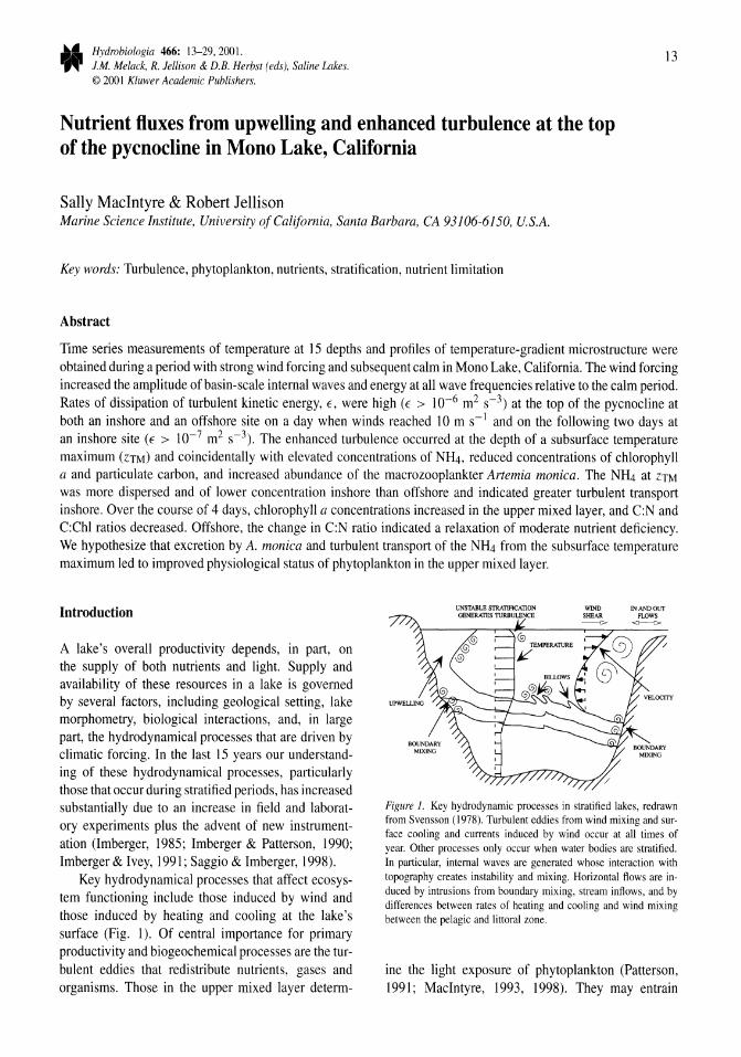
Time series measurements of temperature at 15 depths and profiles of temperature-gradient microstructure were obtained during a period with strong wind forcing and subsequent calm in Mono Lake, California. The wind forcing increased the amplitude of basin-scale internal waves and energy at all wave frequencies relative to the calm period. Rates of dissipation of turbulent kinetic energy, E, were high (E > 10-6 m2 s-3) at the top of the pycnocline at both an inshore and an offshore site on a day when winds reached 10 m s-1 and on the following two days at an inshore site (E > 10-7 m2 s-3). The enhanced turbulence occurred at the depth of a subsurface temperature maximum (ZTM) and coincidentally with elevated concentrations of NIL!, reduced concentrations of chlorophyll a and particulate carbon, and increased abundance of the macrozooplankter Artemia monica. The NH4 at ZTM
was more dispersed and of lower concentration inshore than offshore and indicated greater turbulent transport inshore. Over the course of 4 days, chlorophyll a concentrations increased in the upper mixed layer, and C:N and C:Chl ratios decreased. Offshore, the change in C:N ratio indicated a relaxation of moderate nutrient deficiency. We hypothesize that excretion by A. monica and turbulent transport of the NH4 from the subsurface temperature maximum led to improved physiological status of phytoplankton in the upper mixed layer.
Introduction
A lake's overall productivity depends, in part, on the supply of both nutrients and light. Supply and availability of these resources in a lake is governed by several factors, including geological setting, lake morphometry, biological interactions, and, in large part, the hydrodynamical processes that are driven by climatic forcing. In the last 15 years our understanding of these hydrodynamical processes, particularly those that occur during stratified periods, has increased substantially due to an increase in field and laboratory experiments plus the advent of new instrumentation (Imberger, 1985; Imberger & Patterson, 1990; Imberger & Ivey, 1991; Saggio & Imberger, 1998).
Key hydrodynamical processes that affect ecosystem functioning include those induced by wind and those induced by heating and cooling at the lake's surface (Fig. 1). Of central importance for primary productivity and biogeochemical processes are the turbulent eddies that redistribute nutrients, gases and organisms. Those in the upper mixed layer determ-
Figure 1. Key hydrodynamic processes in stratified lakes, redrawn from Svensson (1978). Thrbulent eddies from wind mixing and surface cooling and currents induced by wind occur at all times of year. Other processes only occur when water bodies are stratified. In particular, internal waves are generated whose interaction with topography creates instability and mixing. Horizontal flows are induced by intrusions from boundary mixing, stream inflows, and by differences between rates of heating and cooling and wind mixing between the pelagic and littoral zone.
ine the light exposure of phytoplankton (Patterson, 1991; MacIntyre, 1993, 1998). They may entrain
14
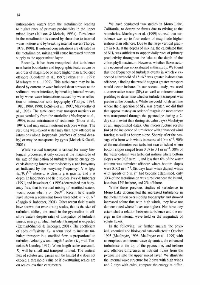
nutrient-rich waters from the metalimnion leading to higher rates of primary productivity in the upper mixed layer (Jellison & Melack, 1993a). Turbulence in the metalimnion is caused by shear due to internal wave motions and by breaking internal waves (Thorpe, 1978, 1998). If nutrient concentrations are elevated in the metalimnion, mixing will cause increased nutrient supply to the upper mixed layer.
Recently, it has been recognized that turbulence near basin boundaries and topographic features can be an order of magnitude or more higher than turbulence offshore (Goudsmit et aI., 1997; Polzin et aI., 1997; Macintyre et aI., 1999). This turbulence may be induced by current or wave induced shear stresses at the sediment-water interface, by breaking internal waves, or by wave-wave interactions caused by wave reflection or interaction with topography (Thorpe, 1984, 1987,1989,1998; DeSilvaet aI., 1997; Maxworthy et aI., 1998). The turbulence may transport nutrients or gases vertically from the nutricline (Macintyre et a!., 1999), cause entrainment of sediments (Gloor et a!., 1994), and may entrain nutrient-rich pore waters. The resulting well-mixed water may then flow offshore as intrusions along isopycnals (surfaces of equal density) or may be transported by gyres (Melack & Gastil, 2001).
While vertical transport is critical for many biological processes, it only occurs if the magnitude of the rate of dissipation of turbulent kinetic energy exceeds damping forces due to viscosity v and buoyancy as indicated by the buoyancy frequency, N = (g/ p
apjad/2 where p is density g is gravity, and z is depth. In laboratory and field studies, Ivey & Imberger (1991) and Itsweire et al. (1993) determined that buoyancy flux, that is vertical mixing of stratified waters, would occur when E > 15vN2. Recent field results have shown a somewhat lower threshold: E > 6vN2
(Saggio & Imberger, 2001). Other recent field results have shown that overturning scales, that is the size of turbulent eddies, are small in the pycnocline in offshore waters despite rates of dissipation of turbulent kinetic energy at which turbulent transport is expected (Etemad-Shahidi & Imberger, 2001). The coefficient of eddy diffusivity K z, a term used to indicate turbulent transport in a stratified flow, is proportional to turbulent velocity u and length I scales (Kz ~ul, Tennekes & Lumley, 1972). When length scales are small, K z will be small and transport limited. The vertical flux of solutes and gasses will be limited if E does not exceed a threshold value or if overturning scales are on scales less than centimeters.
We have conducted two studies in Mono Lake, California, to determine fluxes due to mixing at the boundaries. Macintyre et a!. (1999) showed that turbulence was up to four orders of magnitude higher inshore than offshore. Due to the large vertical gradient in NH4 at the depths of mixing, the calculated flux of NH4 was sufficient to support daily rates of primary productivity throughout the lake at the depth of the chlorophyll maximum. However, whether fluxes actually occurred was not evaluated in this study. We found that the frequency of turbulent events in which E exceeded a threshold of 15v N 2 was greater inshore than offshore, a finding that would suggest greater transport would occur inshore. In our second study, we used a conservative tracer (SF6) as well as microstructure profiling to determine whether turbulent transport was greater at the boundary. While we could not determine where the dispersion of SF6 was greater, we did find that approximately an order of magnitude more tracer was transported through the pycnocline during a 2-day storm event than during six calm days (Macintyre et aI., unpublished data). Our microstructure results linked the incidence of turbulence with enhanced wind forcing as well as bottom slope. Shortly after the passage of a front with winds in excess of 10m s-I, 90% of the metalimnion was turbulent near an island where bottom slopes ranged from 0.07 to 0.1 m m- I, 30% of the water column was turbulent inshore where bottom slopes were 0.02 m m- I, and less than 6% of the water column was turbulent offshore where bottom slopes were 0.002 m m-I. Six days later, when diurnal winds with speeds of 5 m S-1 had become established, only 30% of the metalimnion was turbulent near the island, less than 12% inshore, and 2% offshore.
While these previous studies of turbulence in Mono Lake documented the increased turbulence in the metalimnion over sloping topography and showed increased solute flux with high winds, they have not demonstrated where fluxes are highest. Nor have they established a relation between turbulence and the energy in the internal wave field or the magnitude of solute fluxes.
In the following, we further analyze the physical, chemical and biological data collected in October 1995 (Macintyre, 1998; Macintyre et al., 1999) with an emphasis on internal wave dynamics, the enhanced turbulence at the top of the pycnocline, and inshore and offshore differences in nutrient fluxes from the pycnocline into the upper mixed layer. We illustrate the internal wave structure for 2 days with high winds and 2 days with calm, compare the energy at differ-
----o 1 2 3 kilometers
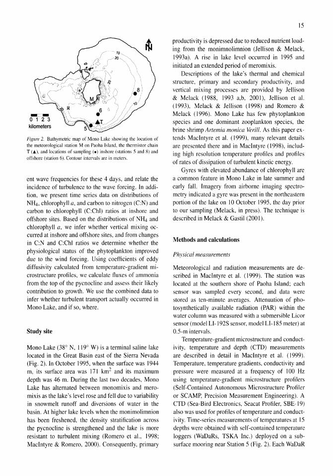
Figure 2. Bathymetric map of Mono Lake showing the location of the meteorological station M on Paoha Island. the thermistor chain T (A), and locations of sampling (e) inshore (stations 5 and 8) and offshore (station 6). Contour intervals are in meters.
ent wave frequencies for these 4 days, and relate the incidence of turbulence to the wave forcing. In addition, we present time series data on distributions of NH4, chlorophyll a, and carbon to nitrogen (C:N) and carbon to chlorophyll (C:Chl) ratios at inshore and offshore sites. Based on the distributions of NH4 and chlorophyll a, we infer whether vertical mixing occurred at inshore and offshore sites, and from changes in C:N and C:Chl ratios we determine whether the physiological status of the phytoplankton improved due to the wind forcing. Using coefficients of eddy diffusivity calculated from temperature-gradient microstructure profiles, we calculate fluxes of ammonia from the top of the pycnocline and assess their likely contribution to growth. We use the combined data to infer whether turbulent transport actually occurred in Mono Lake, and if so, where.
Study site
Mono Lake (380 N, 1190 W) is a terminal saline lake located in the Great Basin east of the Sierra Nevada (Fig. 2). In October 1995, when the surface was 1944 m, its surface area was 171 km2 and its maximum depth was 46 m. During the last two decades, Mono Lake has alternated between monomixis and meromixis as the lake's level rose and fell due to variability in snowmelt runoff and diversions of water in the basin. At higher lake levels when the monimolimnion has been freshened, the density stratification across the pycnocline is strengthened and the lake is more resistant to turbulent mixing (Romero et aI., 1998; MacIntyre & Romero, 2000). Consequently, primary
15
productivity is depressed due to reduced nutrient loading from the monimnolimnion (Jellison & Melack, 1993a). A rise in lake level occurred in 1995 and initiated an extended period of meromixis.
Descriptions of the lake's thermal and chemical structure, primary and secondary productivity, and vertical mixing processes are provided by Jellison & Melack (1988, 1993 a,b, 2001), Jellison et al. (1993), Melack & Jellison (1998) and Romero & Melack (1996). Mono Lake has few phytoplankton species and one dominant zooplankton species, the brine shrimp Artemia monica Veril!. As this paper extends MacIntyre et al. (1999), many relevant details are presented there and in MacIntyre (1998), including high resolution temperature profiles and profiles of rates of dissipation of turbulent kinetic energy.
Gyres with elevated abundance of chlorophyll are a common feature in Mono Lake in late summer and early fall. Imagery from airborne imaging spectrometry indicated a gyre was present in the northeastern portion of the lake on 10 October 1995, the day prior to our sampling (Melack, in press). The technique is described in Melack & Gastil (200 I).
Methods and calculations
Physical measurements
Meteorological and radiation measurements are described in MacIntyre et al. (1999). The station was located at the southern shore of Paoha Island; each sensor was sampled every second, and data were stored as ten-minute averages. Attenuation of photosynthetically available radiation (PAR) within the water column was measured with a submersible Licor sensor (model LI-192S sensor, model LI-185 meter) at 0.5-m intervals.
Temperature-gradient microstructure and conductivity, temperature and depth (CTD) measurements are described in detail in MacIntyre et al. (1999). Temperature, temperature gradients, conductivity and pressure were measured at a frequency of 100 Hz using temperature-gradient microstructure profilers (Self-Contained Autonomous Microstructure Profiler or SCAMP, Precision Measurement Engineering). A CTD (Sea-Bird Electronics, Seacat Profiler, SBE-19) also was used for profiles of temperature and conductivity. Time-series measurements of temperatures at 15 depths were obtained with self-contained temperature loggers (WaDaRs, TSKA Inc.) deployed on a subsurface mooring near Station 5 (Fig. 2). Each WaDaR
16
has an accuracy of 0.001 °C, a resolution of 1.4 mdeg, and a time constant of ~ 3 min.
Chemical analysis
Ammonium (NH4+ + NH3) concentrations were measured by the indophenol-blue method (Strickland & Parsons, 1972). Chlorophyll a was determined by spectrophotometric analysis with correction for phaeopigments (Golterman, 1969). Details for both procedures are given in Jellison et a!. (1993). Particulate organic carbon, phosphorus and nitrogen were measured after samples were filtered through precombusted Gelman AlE filters. Methods are provided in Jellison & Melack (2001).
Calculations
Density was calculated from temperature and conductivity corrected to 25°C using an equation of state developed for Mono Lake (Jellison et a!., 1999). Density profiles from the SCAMP were calculated using data from a fast response (Thermometrics FP07) thermistor and the larger conductivity sensor. The fast response thermistor was filtered to match the time constant of the larger conductivity sensor (180 msec) and offset by 0.4 s so values from both sensors were from the same location. For the CTD profiles, density was computed after averaging the conductivity profiles over I-m intervals centered on every meter; corresponding temperatures at each meter were obtained from interpolated temperature profiles.
Rates of dissipation of turbulent kinetic energy (E) were computed by a least-squares fit of the power spectral densities of the temperature-gradient signal to the Batchelor spectrum (Dillon & Caldwell, 1980; Imberger & Ivey, 1991). Power spectral densities were calculated in segments as described in MacIntyre et a!. (1999). The procedure is an adaptation of that described in Imberger & Ivey (1991) and is used to determine where the turbulence is statistically stationary (Imberger & Ivey, 1991). Vertical eddy diffusivity, Kz, was calculated using Osborn's (1980) model, Kz = r E N-2, where r is the mixing efficiency and N is the buoyancy frequency. We let r = 0.25, the upper limit in Ivey & Imberger's (1991) analysis and similar to the mean mixing efficiency of 0.265 found by Oakey (1985). We calculated the flux of ammonium as F = Kz a[NH4l/3z.
Arithmetic averages of E and Kz were determined for 1 m intervals by determining the percentage of the interval occupied by a segment, multiplying that
percentage by E for that segment, summing the contributions from each segment, and assuming that E
equaled 10-10 m2 s-3 and K z equaled 10-9 m2 s-3 where the water column was not turbulent. The first of these two values reflects instrument threshold for turbulence and the second the rate of molecular diffusion of salts. Depth-averaged values of E and Kz were computed for each site on each day. Estimates of Kz based on the assumption of a log normal distribution of turbulent events (MacIntyre et a!., 1999) were equivalent to arithmetic averages at the depths where we calculated ammonia fluxes.
Isotherm depths were determined using linear interpolation between the depths of the thermistors. Power spectral analyses of the isotherm displacements were computed using a Hanning window and linear detrending. Eighty percent confidence intervals were computed and windows overlapped 75%. To generate smaller confidence intervals at higher frequencies, we decreased the size of our windows as frequencies increased. Power spectral densities were multiplied by the mean buoyancy frequency at the depth of the isotherm so the results would be equal to the potential energy density of the internal wave field. The magnitude of isotherm displacements, 8, at low, moderate and high frequencies were determined using band-pass filtering using an inverse fast Fourier transform. Potential energy per unit mass was calculated for each frequency band as N282 as in Moum et a!. (1992).
Results
Windforcing and thermal, conductivity, and density structure
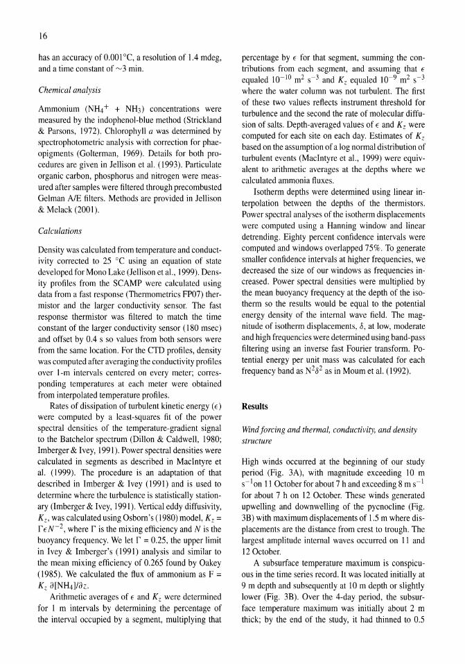
High winds occurred at the beginning of our study period (Fig. 3A), with magnitude exceeding 10 m s- l on II October for about 7 h and exceeding 8 m s-1 for about 7 h on 12 October. These winds generated upwelling and downwelling of the pycnocline (Fig. 3B) with maximum displacements of 1.5 m where displacements are the distance from crest to trough. The largest amplitude internal waves occurred on II and 12 October.
A subsurface temperature maximum is conspicuous in the time series record. It was located initially at 9 m depth and subsequently at 10 m depth or slightly lower (Fig. 3B). Over the 4-day period, the subsurface temperature maximum was initially about 2 m thick; by the end of the study, it had thinned to 0.5
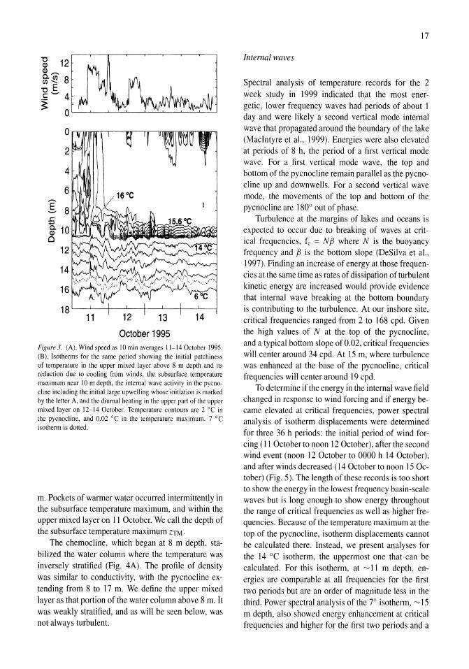
O~~~-'n-"~Emrru~n
2 -
6
E -- 8 .c. g. 10-o
12
14
October 1995 Figure3. (A). Wind speed as 10 min averages 11-14 October 1995. (B). Isotherms for the same period showing the initial patchiness of temperature in the upper mixed layer above 8 m depth and its reduction due to cooling from winds, the subsurface temperature maximum near 10 m depth, the internal wave activity in the pycnocline including the initial large upwelling whose initiation is marked by the letter A, and the diurnal heating in the upper part of the upper mixed layer on 12-14 October. Temperature contours are 2 °C in the pycnocline, and 0.02 °C in the temperature maximum. 7 °C isotherm is dotted.
m. Pockets of warmer water occurred intermittently in the subsurface temperature maximum, and within the upper mixed layer on 11 October. We call the depth of the subsurface temperature maximum ZTM.
The chemocline, which began at 8 m depth, stabilized the water column where the temperature was inversely stratified (Fig. 4A). The profile of density was similar to conductivity, with the pycnocline extending from 8 to 17 m. We define the upper mixed layer as that portion of the water column above 8 m. It was weakly stratified, and as will be seen below, was not always turbulent.
17
Internal waves
Spectral analysis of temperature records for the 2 week study in 1999 indicated that the most energetic, lower frequency waves had periods of about 1 day and were likely a second vertical mode internal wave that propagated around the boundary of the lake (Macintyre et aI., 1999). Energies were also elevated at periods of 8 h, the period of a first vertical mode wave. For a first vertical mode wave, the top and bottom of the pycnocline remain parallel as the pycnocline up and downwells. For a second vertical wave mode, the movements of the top and bottom of the pycnocline are 180° out of phase.
Turbulence at the margins of lakes and oceans is expected to occur due to breaking of waves at critical frequencies, fc = N f3 where N is the buoyancy frequency and f3 is the bottom slope (DeSilva et aI., 1997). Finding an increase of energy at those frequencies at the same time as rates of dissipation of turbulent kinetic energy are increased would provide evidence that internal wave breaking at the bottom boundary is contributing to the turbulence. At our inshore site, critical frequencies ranged from 2 to 168 cpd. Given the high values of N at the top of the pycnocline, and a typical bottom slope of 0.02, critical frequencies will center around 34 cpd. At 15 m, where turbulence was enhanced at the base of the pycnocline, critical frequencies will center around 19 cpd.
To determine if the energy in the internal wave field changed in response to wind forcing and if energy became elevated at critical frequencies, power spectral analysis of isotherm displacements were determined for three 36 h periods: the initial period of wind forcing (11 Octoberto noon 12 October), afterthe second wind event (noon 12 October to 0000 h 14 October), and after winds decreased (14 October to noon 15 October) (Fig. 5). The length ofthese records is too short to show the energy in the lowest frequency basin-scale waves but is long enough to show energy throughout the range of critical frequencies as well as higher frequencies. Because of the temperature maximum at the top of the pycnocline, isotherm displacements cannot be calculated there. Instead, we present analyses for the 14°C isotherm, the uppermost one that can be calculated. For this isotherm, at 'V 11 m depth, energies are comparable at all frequencies for the first two periods but are an order of magnitude less in the third. Power spectral analysis of the 7° isotherm, 'V 15 m depth, also showed energy enhancement at critical frequencies and higher for the first two periods and a
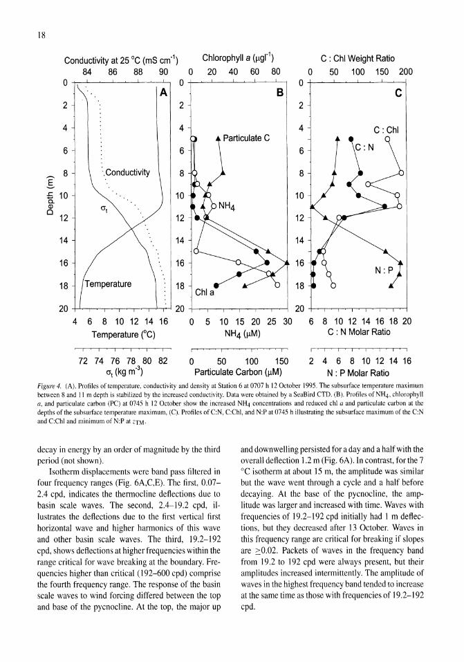
18
Conductivity at 25°C (mS cm-1) Chlorophyll a (llgr1) C : Chi Weight Ratio 84 86 88 90 o 20 40 60 80 o 50 100 150 200
o O+-----.Jc........---'--~-'--~~
A B 2 2
4 4 Particulate C
6 6
g 8 ". Conductivity 8
£; 10 10 c. Ol o
12
14
c 2
4 C:Chl
6
8
4 6 8 10 12 14 16 Temperature (0C)
o 5 10 15 20 25 30 NH4 (IlM)
6 8 10 12 14 16 18 20 C : N Molar Ratio
72 74 76 78 80 82 crt (kg m-3)
o 50 100 150 2 4 6 8 10 12 14 16 N : P Molar Ratio Particulate Carbon (IlM)
Figure 4. (Al. Profiles of temperature, conductivity and density at Station 6 at 0707 h 12 October 1995. The subsurface temperature maximum between 8 and 11 m depth is stabilized by the increased conductivity. Data were obtained by a SeaBird CTD. (B l. Profiles of N14, chlorophyll a, and particulate carbon (PC) at 0745 h 12 October show the increased N14 concentrations and reduced chi a and particulate carbon at the depths ofthe subsurface temperature maximum, (C). Profiles ofC:N, C:Chl, and N:P at 0745 h illustrating the subsurface maximum of the C:N and C:Chl and minimum of N:P at ZIM.
decay in energy by an order of magnitude by the third period (not shown).
Isotherm displacements were band pass filtered in four frequency ranges (Fig. 6A,C,E). The first, 0.07-2.4 cpd, indicates the thermocline deflections due to basin scale waves. The second, 2.4-19.2 cpd, illustrates the deflections due to the first vertical first horizontal wave and higher harmonics of this wave and other basin scale waves. The third, 19.2-192 cpd, shows deflections at higher frequencies within the range critical for wave breaking at the boundary. Frequencies higher than critical (192-600 cpd) comprise the fourth frequency range. The response of the basin scale waves to wind forcing differed between the top and base of the pycnocline. At the top, the major up
and downwelling persisted for a day and a half with the overall deflection 1.2 m (Fig. 6A). In contrast, for the 7 °C isotherm at about 15 m, the amplitude was similar but the wave went through a cycle and a half before decaying. At the base of the pycnocline, the amplitude was larger and increased with time. Waves with frequencies of 19.2-192 cpd initially had 1 m deflections, but they decreased after 13 October. Waves in this frequency range are critical for breaking if slopes are ::::0.02. Packets of waves in the frequency band from 19.2 to 192 cpd were always present, but their amplitUdes increased intermittently. The amplitude of waves in the highest frequency band tended to increase at the same time as those with frequencies of 19.2-192 cpd.
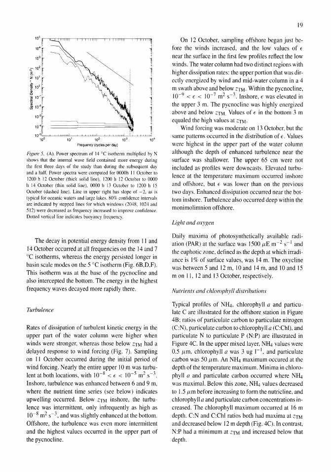
10"
10" '-::---'---'---'--'-.LllL'-;---'---'---'--'-.Lll.L'-;--'---'---'--'-.u.liJ'-;--'---'---'--'-LLW 10° 10' 102 10' 104
Frequency (cycles per day)
Figure 5. (A). Power spectrum of 14 DC isotherm multiplied by N shows that the internal wave field contained more energy during the first three days of the study than during the subsequent day and a half. Power spectra were computed for OOOOh II October to 1200 h 12 October (thick solid line), 1200 h 12 October to 0000 h 14 October (thin solid line), 0000 h 13 October to 1200 h 15 October (dashed line). Line in upper right has slope of -2, as is typical for oceanic waters and large lakes. 80% confidence intervals are indicated by stepped lines for which windows (2048, 1024 and 512) were decreased as frequency increased to improve confidence. Dotted vertical line indicates buoyancy frequency.
The decay in potential energy density from II and 14 October occurred at all frequencies on the 14 and 7 °C isotherms, whereas the energy persisted longer in basin scale modes on the 5 °C isotherm (Fig. 6B,D,F). This isotherm was at the base of the pycnocline and also intercepted the bottom. The energy in the highest frequency waves decayed more rapidly there.
Turbulence
Rates of dissipation of turbulent kinetic energy in the upper part of the water column were higher when winds were stronger, whereas those below ZTM had a delayed response to wind forcing (Fig. 7). Sampling on II October occurred during the initial period of wind forcing. Nearly the entire upper 10m was turbulent at both locations, with 10-8 < f < 10-5 m2 s-3. Inshore, turbulence was enhanced between 6 and 9 m, where the nutrient time series (see below) indicates upwelling occurred. Below ZTM inshore, the turbulence was intermittent, only infrequently as high as 10-8 m2 s-3, and was slightly enhanced at the bottom. Offshore, the turbulence was even more intermittent and the highest values occurred in the upper part of the pycnocline.
19
On 12 October, sampling offshore began just before the winds increased, and the low values of f
near the surface in the first few profiles reflect the low winds. The water column had two distinct regions with higher dissipation rates: the upper portion that was directly energized by wind and mid-water column in a 4 m swath above and below ZTM. Within the pycnocline, 10-9 < f < 10-7 m2 s-3. Inshore, f was elevated in the upper 3 m. The pycnocline was highly energized above and below ZTM. Values of f in the bottom 3 m equaled the high values at ZTM.
Wind forcing was moderate on 13 October, but the same patterns occurred in the distribution of f. Values were highest in the upper part of the water column although the depth of enhanced turbulence near the surface was shallower. The upper 65 cm were not included as profiles were down casts. Elevated turbulence at the temperature maximum occurred inshore and offshore, but f was lower than on the previous two days. Enhanced dissipation occurred near the bottom inshore. Turbulence also occurred deep within the monimolimnion offshore.
Light and oxygen
Daily maxima of photosynthetically available radiation (PAR) at the surface was 1500 {LE m-2 s-I and the euphotic zone, defined as the depth at which irradiance is I % of surface values, was 14 m. The oxycline was between 5 and 12 m, 10 and 14 m, and 10 and 15 m on II, 12 and 13 October, respectively.
Nutrients and chlorophyll distributions
Typical profiles of NH4, chlorophyll a and particulate C are illustrated for the offshore station in Figure 4B; ratios of particulate carbon to particulate nitrogen (C:N), particulate carbon to chlorophyll a (C:Chl), and particulate N to particulate P (N:P) are illustrated in Figure 4C. In the upper mixed layer, NH4 values were 0.5 {Lm, chlorophyll a was 3 ug I-I, and particulate carbon was 50 {Lm. An NH4 maximum occured at the depth of the temperature maximum. Minima in chlorophyll a and particulate carbon occurred where NH4 was maximal. Below this zone, NH4 values decreased to 1.5 {Lm before increasing to form the nutricline, and chlorophyll a and particulate carbon concentrations increased. The chlorophyll maximum occurred at 16 m depth. C:N and C:Chl ratios both had maxima at ZTM
and decreased below 12 m depth (Fig. 4C). In contrast, N:P had a minimum at ZTM and increased below that depth.
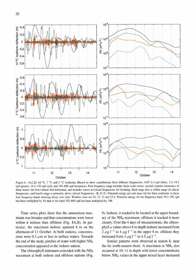
20
§: -0.4
.§ -0.2 g ~ 0 "C
E Q; 0.2 c:. (5 !!! 0.4
~ ;:!: 0.6
~-0 .6
.s
.§ -0.4 U .l!! -0 .2 Qj "C 0 E <D :: 0.2 5l U 0.4 o
,.... 0.6
§: -I c: .2 li -0.5 Qj "C
E 0 CI> .r=
~ 0.5 u o U")
~--~--~--~~--~--~--~~--~--~
11 12 13 14
October
10.7 ~-",----"""",--,--""""-"""",---,-----,-":::,,,,,--,
1~ r-~---r--~--.---r-~---r--.
11 12 13 14 October
Figure 6. (A.C,E) 14 °C, 7 °C and 5 °C isotherms filtered to show contributions from different frequencies: 0.07-2.4 cpd (blue), 2.4-19.2 cpd (green), 19.2-192 cpd (red), and 192-600 cpd (turquoise). First frequency range includes basin scale waves; second contains harmonics of these waves, the first vertical first horizontal, and includes waves at critical frequencies for breaking; third range also is within range of critical frequencies; and fourth range is primarily above critical frequencies. (B, D, F). Potential energy per unit mass for the three isotherms in these four frequency bands showing decay over time. Window sizes are 24, 12, 12 and 12 h. Potential energy for the frequency band 19.2-192 cpd has been multiplied by 10; that in the band 192-600 cpd has been multiplied by 100.
Time series plots show that the ammonium maximum was broader and that concentrations were lower within it inshore than offshore (Fig. 8A,B). In particular, the maximum inshore spanned 4 m on the afternoon of 11 October. At both stations, concentrations were 0.3 p,m or less in surface waters. Towards the end of the study, patches of water with higher NH4
concentration appeared at the inshore station. The chlorophyll minimum coincided with the NH4
maximum at both inshore and offshore stations (Fig.
9). Inshore, it tended to be located at the upper boundary of the NH4 maximum; offshore it tracked it more closely. Over the 4 days of measurements, the chlorophyll a values above 8 m depth inshore increased from 2 p,g 1-1 to 4 p,g I- I in the upper 8 m; offshore they increased from 3 p,g I-I to 4.5 p,g 1-1.
Similar patterns were observed at station 8, near the far north-eastern shore. A maximum in NH4 also occurred at 10-11 m depth with lower concentrations below. N~ values in the upper mixed layer increased
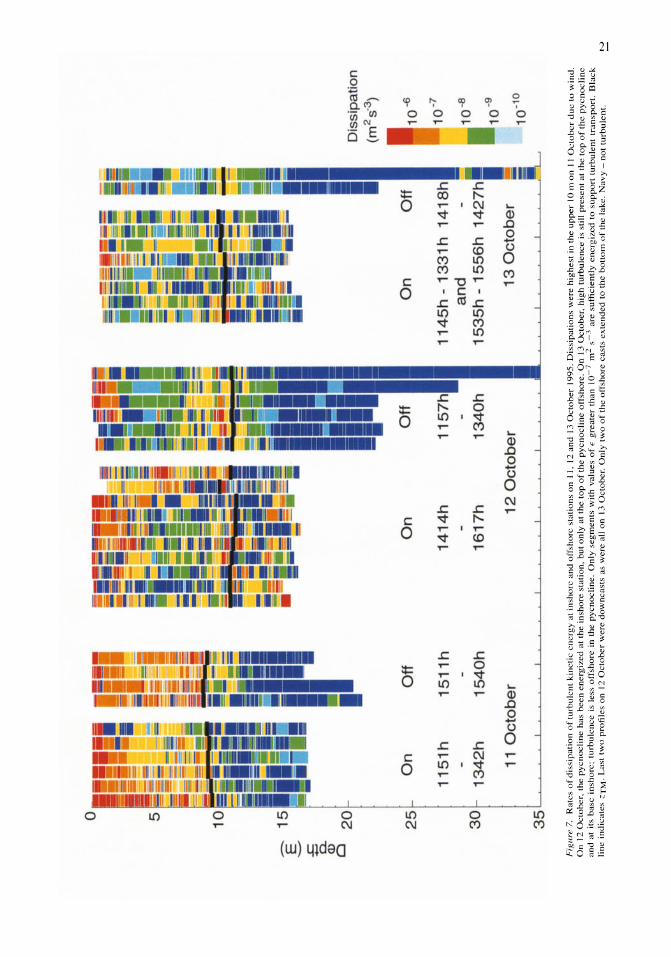
o 5
-E
---- .c: -a. Q)
Dis
sip
ati
on
o
20
(m
2s-
3)
25
O
n O
ff
On
Off
II
O
n O
ff I
11
0-6
1151
h 15
11h
1414
h 11
57h ll
11
45
h -
1331
h 14
18h
-t-
.10
-7
1540
h an
d
-I
10
-8
16
17
h
13
40
h •
1535
h -
1556
h 14
27h I • 10-
9 3
0
1342
h
12 O
cto
ber
•
13 O
cto
ber
;;
iiiiii
10
-10
11
Oct
ob
er
35
IL~~~~L-~~~~~~--~~~~~~~~~~~~--~~~
Fig
ure
7.
Rat
es o
f d
issi
pat
ion
of
turb
ule
nt
kin
etic
en
erg
y a
t in
sho
re a
nd
off
sho
re s
tati
on
s o
n 1
1, 1
2 an
d 1
3 O
cto
ber
]9
95
. D
issi
pat
ion
s w
ere
hig
hes
t in
th
e u
pp
er 1
0 m
011
II
Oct
ob
er d
ue
to w
ind
. O
n 1
2 O
cto
ber
, th
e p
ycn
ocl
ine
has
bee
n e
ner
giz
ed a
t th
e in
sho
re s
tati
on
, b
ut
on
ly a
t th
e to
p o
f th
e p
ycn
ocl
ine
off
sho
re,
On
13
Oct
ob
er,
hig
h t
urb
ule
nce
is
stil
l p
rese
nt
at t
he
top
of
the
py
cno
clin
e an
d a
t it
s b
ase
insh
ore
; tu
rbu
len
ce i
s le
ss o
ffsh
ore
in
the
py
cno
clin
e. O
nly
seg
men
ts w
ith
val
ues
of
E g
reat
er t
han
10
-7 m
2 s-3
are
su
ffic
ien
tly
en
erg
ized
to
su
pp
ort
tu
rbu
len
t tr
ansp
ort
. B
lack
li
ne
ind
icat
es Z
TM
. L
ast
two
pro
file
s o
n 1
2 O
cto
ber
wer
e d
ow
ncasl
s as
wer
e al
1 o
n 1
3 O
cto
ber
. O
nly
tw
o o
f th
e o
ffsh
ore
cas
ts e
xte
nd
ed t
o t
he
bo
tto
m o
f th
e la
ke.
Nav
y -
no
t tu
rbu
len
t.
N
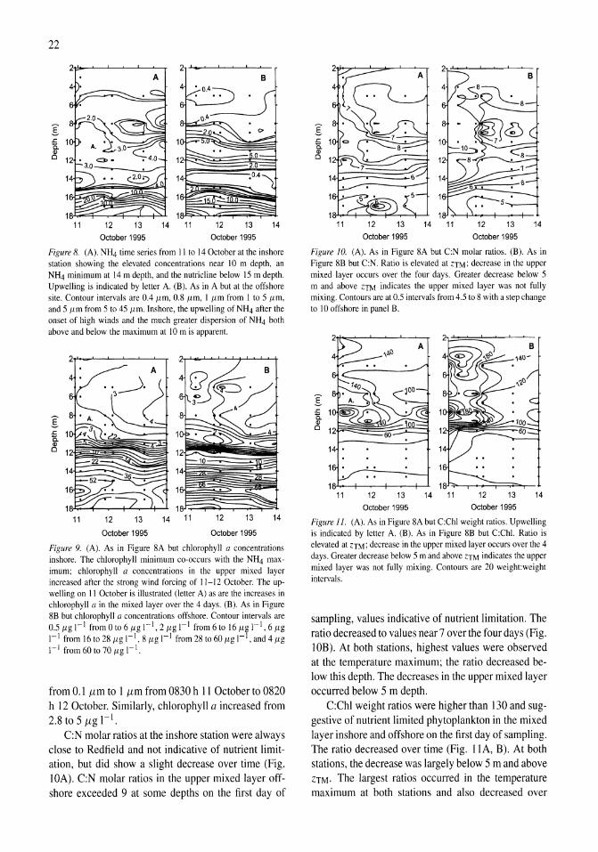
22
A B
11 12 13 14 11 12 13 14
October 1995 October 1995
Figure 8. (A). N14 time series from II to 14 October at the inshore station showing the elevated concentrations near 10 m depth. an NH4 minimum at 14 m depth, and the nutricline below 15 m depth. Upwelling is indicated by letter A. (B). As in A but at the offshore site. Contour intervals are 0.4 /Lm, O.S /Lm, I /Lm from I to 5 /Lm, and 5 /Lm from 5 to 45 /Lm. Inshore, the upwelling of NH4 after the onset of high winds and the much greater dispersion of N14 both above and below the maximum at 10 m is apparent.
:§: ~ Q) 0
11 12 13 14 11 12 13 14
October 1995 October 1995
Figure 9. (A). As in Figure 8A but chlorophyll a concentrations inshore. The chlorophyll minimum co-occurs with the NH4 maximum; chlorophyll a concentrations in the upper mixed layer increased after the strong wind forcing of 11-12 October. The upwelling on 11 October is illustrated (letter A) as are the increases in chlorophyll a in the mixed layer over the 4 days. (B). As in Figure SB but chlorophyll a concentrations offshore. Contour intervals are 0.5 /Lg 1-1 from 0 to 6 /Lg 1-1,2 /Lg 1-1 from 6 to 16 /Lr 1-1,6 /Lg I-I from 16 to 2S /Lg 1-1, S /Lg I-I from 2S to 60 /Lg 1- ,and 4 /Lg 1-1 from 60 to 70 /Lg I-I.
from 0.1 p,m to 1 p,m from 0830 h II October to 0820 h 12 October. Similarly, chlorophyll a increased from 2.8 to 5 p,g I-I.
C:N molar ratios at the inshore station were always close to Redfield and not indicative of nutrient limitation, but did show a slight decrease over time (Fig. lOA). C:N molar ratios in the upper mixed layer offshore exceeded 9 at some depths on the first day of
October 1995 October 1995
Figure 10. (A). As in Figure SA but C:N molar ratios. (B). As in Figure SB but C:N. Ratio is elevated at ZTM; decrease in the upper mixed layer occurs over the four days. Greater decrease below 5 m and above ZTM indicates the upper mixed layer was not fully mixing. Contours are at 0.5 intervals from 4.5 to S with a step change to 10 offshore in panel B.
:§: ~ Q)
0
11 12 13 14 11 12 13 14
October 1995 October 1995
Figure 11. (A). As in Figure SA but C:Chl weight ratios. Upwelling is indicated by letter A. (B). As in Figure SB but C:Chl. Ratio is elevated at ZTM; decrease in the upper mixed layer occurs over the 4 days. Greater decrease below 5 m and above ZTM indicates the upper mixed layer was not fully mixing. Contours are 20 weight weight intervals.
sampling, values indicative of nutrient limitation. The ratio decreased to values near 7 over the four days (Fig. lOB). At both stations, highest values were observed at the temperature maximum; the ratio decreased below this depth. The decreases in the upper mixed layer occurred below 5 m depth.
C:Chl weight ratios were higher than 130 and suggestive of nutrient limited phytoplankton in the mixed layer inshore and offshore on the first day of sampling. The ratio decreased over time (Fig. l1A, B). At both stations, the decrease was largely below 5 m and above ZTM. The largest ratios occurred in the temperature maximum at both stations and also decreased over
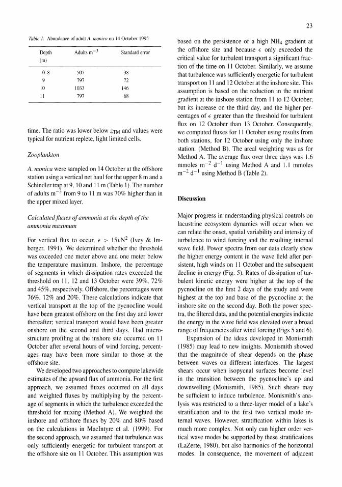
Table I. Abundance of adult A. monica on 14 October 1995
Depth Adults m-3 Standard error
(m)
0-8 507 38
9 797 72
10 1033 146
II 797 68
time. The ratio was lower below ZTM and values were typical for nutrient replete, light limited cells.
Zooplankton
A. monica were sampled on 14 October at the offshore station using a vertical net haul for the upper 8 m and a Schindler trap at 9, 10 and II m (Table 1). The number of adults m-3 from 9 to II m was 70% higher than in the upper mixed layer.
Calculated fluxes of ammonia at the depth of the ammonia maximum
For vertical flux to occur, E > 15vN2 (lvey & lmberger, 1991). We determined whether the threshold was exceeded one meter above and one meter below the temperature maximum. Inshore, the percentage of segments in which dissipation rates exceeded the threshold on II, 12 and 13 October were 39%, 72% and 45%, respectively. Offshore, the percentages were 76%, 12% and 20%. These calculations indicate that vertical transport at the top of the pycnocline would have been greatest offshore on the first day and lower thereafter; vertical transport would have been greater onshore on the second and third days. Had microstructure profiling at the inshore site occurred on II October after several hours of wind forcing, percentages may have been more similar to those at the offshore site.
We developed two approaches to compute lakewide estimates of the upward flux of ammonia. For the first approach, we assumed fluxes occurred on all days and weighted fluxes by multiplying by the percentage of segments in which the turbulence exceeded the threshold for mixing (Method A). We weighted the inshore and offshore fluxes by 20% and 80% based on the calculations in MacIntyre et al. (1999). For the second approach, we assumed that turbulence was only sufficiently energetic for turbulent transport at the offshore site on 11 October. This assumption was
23
based on the persistence of a high NH4 gradient at the offshore site and because E only exceeded the critical value for turbulent transport a significant fraction of the time on II October. Similarly, we assume that turbulence was sufficiently energetic for turbulent transport on II and 12 October at the inshore site. This assumption is based on the reduction in the nutrient gradient at the inshore station from II to 12 October, but its increase on the third day, and the higher percentages of E greater than the threshold for turbulent flux on 12 October than 13 October. Consequently, we computed fluxes for 11 October using results from both stations, for 12 October using only the inshore station. (Method B). The areal weighting was as for Method A. The average flux over three days was 1.6 mmoles m-2 d- 1 using Method A and 1.1 mmoles m-2 d- 1 using Method B (Table 2).
Discussion
Major progress in understanding physical controls on lacustrine ecosystem dynamics will occur when we can relate the onset, spatial variability and intensity of turbulence to wind forcing and the resulting internal wave field. Power spectra from our data clearly show the higher energy content in the wave field after persistent, high winds on 11 October and the subsequent decline in energy (Fig. 5). Rates of dissipation of turbulent kinetic energy were higher at the top of the pycnocline on the first 2 days of the study and were highest at the top and base of the pycnocline at the inshore site on the second day. Both the power spectra, the filtered data, and the potential energies indicate the energy in the wave field was elevated over a broad range of frequencies after wind forcing (Figs 5 and 6).
Expansion of the ideas developed in Monismith (1985) may lead to new insights. Monismith showed that the magnitude of shear depends on the phase between waves on different interfaces. The largest shears occur when isopycnal surfaces become level in the transition between the pycnocline's up and downwelling (Monismith, 1985). Such shears may be sufficient to induce turbulence. Monismith's analysis was restricted to a three-layer model of a lake's stratification and to the first two vertical mode internal waves. However, stratification within lakes is much more complex. Not only can higher order vertical wave modes be supported by these stratifications (LaZerte, 1980), but also harmonics of the horizontal modes. In consequence, the movement of adjacent
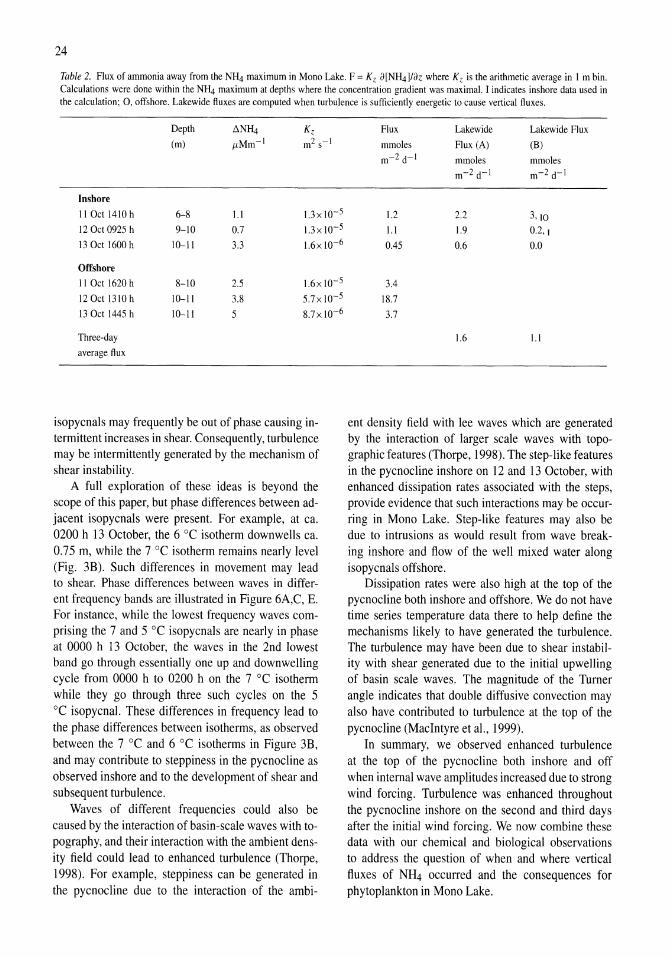
24
Table 2. Flux of ammonia away from the Nl4 maximum in Mono Lake. F = Kz B[NH41/Bz where Kz is the arithmetic average in I m bin. Calculations were done within the N14 maximum at depths where the concentration gradient was maximal. I indicates inshore data used in the calculation; 0, offshore. Lakewide fluxes are computed when turbulence is sufficiently energetic to cause vertical fluxes.
Depth IlNH4 Kz (m) JLMm-1 m2 s-I
Inshore
II Oct 1410 h 6-8 1.1 1.3x 10⁻⁵
12 Oct 0925 h 9-10 0.7 1.3x 10⁻⁵
13 Oct 1600 h 10-11 3.3 1.6x 10⁻⁶
Offshore II Oct 1620 h 8-10 2.5 1.6x 10⁻⁵
12 Oct 1310 h 10-11 3.8 5.7x 10⁻⁵
13 Oct 1445 h 10-11 5 8.7xlO-6
Three-day
average flux
isopycnals may frequently be out of phase causing intermittent increases in shear. Consequently, turbulence may be intermittently generated by the mechanism of shear instability.
A full exploration of these ideas is beyond the scope of this paper, but phase differences between adjacent isopycnals were present. For example, at ca. 0200 h 13 October, the 6 °C isotherm down wells ca. 0.75 m, while the 7°C isotherm remains nearly level (Fig. 3B). Such differences in movement may lead to shear. Phase differences between waves in different frequency bands are illustrated in Figure 6A,C, E. For instance, while the lowest frequency waves comprising the 7 and 5 °C isopycnals are nearly in phase at 0000 h 13 October, the waves in the 2nd lowest band go through essentially one up and downwelling cycle from 0000 h to 0200 h on the 7 °C isotherm while they go through three such cycles on the 5 °C isopycnal. These differences in frequency lead to the phase differences between isotherms, as observed between the 7 °C and 6 °C isotherms in Figure 3B, and may contribute to steppiness in the pycnocline as observed inshore and to the development of shear and subsequent turbulence.
Waves of different frequencies could also be caused by the interaction of basin-scale waves with topography, and their interaction with the ambient density field could lead to enhanced turbulence (Thorpe, 1998). For example, steppiness can be generated in the pycnocline due to the interaction of the ambi-
Flux Lakewide Lakewide Flux
mmoles Flux (A) (B)
m-2 d- I mmoles mmoles m-2 d- I m-2 d- 1
1.2 2.2 3010 1.1 1.9 0.2,)
0.45 0.6 0.0
3.4
18.7
3.7
1.6 1.1
ent density field with lee waves which are generated by the interaction of larger scale waves with topographic features (Thorpe, 1998). The step-like features in the pycnocline inshore on 12 and 13 October, with enhanced dissipation rates associated with the steps, provide evidence that such interactions may be occurring in Mono Lake. Step-like features may also be due to intrusions as would result from wave breaking inshore and flow of the well mixed water along isopycnals offshore.
Dissipation rates were also high at the top of the pycnocline both inshore and offshore. We do not have time series temperature data there to help define the mechanisms likely to have generated the turbulence. The turbulence may have been due to shear instability with shear generated due to the initial upwelling of basin scale waves. The magnitude of the Turner angle indicates that double diffusive convection may also have contributed to turbulence at the top of the pycnocline (Macintyre et aI., 1999).
In summary, we observed enhanced turbulence at the top of the pycnocline both inshore and off when internal wave amplitudes increased due to strong wind forcing. Turbulence was enhanced throughout the pycnocline inshore on the second and third days after the initial wind forcing. We now combine these data with our chemical and biological observations to address the question of when and where vertical fluxes of NH4 occurred and the consequences for phytoplankton in Mono Lake.
The persistent ammonium maximum
Ammonium profiles consistently show that the highest concentration of ammonium occurred within a meter of the temperature maximum and that this feature persisted over a 4-day period despite enhanced turbulence at those depths. Changes in concentration over time depend on sources, sinks and vertical fluxes, and we do not have sufficient data to construct a full budget. For instance, quantifying uptake of N by phytoplankton would have required measurements at the time of the experiment. However, we can evaluate sources and vertical fluxes. If the fluxes due to turbulent mixing were large relative to the sources, we would not expect the NH4 maximum to persist. We can determine whether sufficient ammonium was mixed vertically to affect nutrient limitation by phytoplankton.
Sources
Sources of NH4 include excretion by A. monica, enhanced diffusive fluxes at the sediment water interface, advection or excretion by microzooplankton. Data on microzooplankton are not available. Excretion rates of NH4 by adultA. monica are 0.6 {lmole d-' (Jellison et aI., 1993). With an average abundance of A. monica of 876 adults m-3 at the depths of the temperature maximum, the flux into a 1 m3 parcel of water would be 0.5 mmoles m-3 d-'. JuvenileA. monica were not present in sufficient numbers to contribute to the ammonium pool. Previous lake wide sampling has indicated that the maximum numbers of brine shrimp can range from 500 to 3000 adults m-3 (Lenz, 1980). Were such a wide range present during our sampling, maximum fluxes ofNH4 could be up to l.8 mmoles m-3 d-'.
Jellison et al. (l993b) estimated diffusive fluxes from the sediments at depths below the nutricline to be 6 mmoles m-2 d- 1. Data are not available to calculate fluxes from sediments above the nutricline. Were they comparable, the flux into aim layer spanning the whole lake would be 2 {lmoles m-3 d- 1, a flux three orders of magnitude too low to account for the higher NH4 at those depths. Shear stresses at the sedimentwater interface may enhance the fluxes, but at present, theoretical models indicate at most a three-fold increase due to turbulence at the benthic boundary layer (Dade, 1993). Advection of water with higher NH4 content could contribute to persistence of the feature, but our data do not show large spatial differences in NH4 concentrations.
Based on these comparisons, we infer that the high concentrations of NH4 at the top of the pycnocline
25
resulted from excretion by adult A. monica. The elevated concentrations could only have persisted if the vertical fluxes of NH4 due to turbulence were less than the NH4 excretion rates and if uptake rates by phytoplankton or bacteria were low.
Vertical fluxes
Several lines of evidence suggest that vertical fluxes of NH4 occurred and that turbulent transport may have been greater at inshore sites than offshore sites. The time series measurements of temperature, NH4, chlorophyll a and C:Chl indicate upwelling occurred inshore on II October but not offshore. This upwelling, coupled with the enhanced turbulence at the depths of upwelling, may have contributed to the greater spread of NH4 in the NH4 maximum and of chlorophyll a in the chlorophyll a minimum (Figs 8 and 9). Increased spread of a solute and slightly lower maximum concentrations are to be expected when mixing has occurred. Chlorophyll a is more dispersed inshore below 12 m depth.
For vertical mixing to occur and to cause transport across isopycnals, dissipation rates must be high enough to exceed the damping induced by viscous and buoyancy forcing. Dissipation rates were sufficiently high at the top of the pycnocline 76% of the time offshore but less than 20% of the time on the next 2 days. Inshore, dissipation rates were sufficiently high 72% of the time on the second day and 45% of the time on the third day. Temperature profiles with millimeter scale resolution indicated that temperature inversions with scales of centimeters were present when E was large enough to cause transport. Inversions were on smaller scales or not present when it was less than 15 vN 2 (S. MacIntyre, unpublished data). Consequently, when E exceeded the threshold, turbulent overturns I occurred allowing vertical transport.
Calculated daily vertical fluxes of NH4 at the offshore site are higher than likely excretion rates (Table 2). We assume the flux is into a 1 m3 volume for comparison with the A. monica excretion rates. The calculated fluxes were particularly high on days when E was frequently below the threshold for vertical transport and when the NH4 gradient remained high. These results suggest vertical fluxes, calculated as F = Kz 3[NH4]/3z, were much less than calculated. The discrepancy indicates that calculating K z as rEN-2 (Osborn, 1980) is not always valid. Itsweire et al. (1993) found that the assumptions of Osborn's (1980) model were not met when stratification and viscosity were high relative to the forces
26
that would generate turbulence. In contrast, calculated daily fluxes at the inshore site could be supported by excretion by A. monica. Inshore a greater percentage of the dissipation rates exceeded the threshold for turbulent transport; consequently Osborn's model was applicable for calculating K z.
Vertical fluxes and phytoplankton growth
In comparison to the quantity of ammonia excreted by A. monica, the calculated lake-wide fluxes of NH4 are reasonable although at the upper end of the range possible (Table 2). As these calculated fluxes take into account the percentage of the time that turbulence is sufficiently high to overcome damping forces, we use them to estimate the possible growth of phytoplankton. Using a C:N molar ratio of 7, the lower of the three day averages, 1.1 mmoles m-2 d- I , the fluxes would have supported primary productivities of 0.1 g C m-2 d- I . Daily rates of primary production are between 0.5 and 2 g C m-2d- 1 during the summer in Mono Lake (Jellison & Melack, 1993a). The fluxes would have provided sufficient N~ to support 5-20% of the daily requirements for growth.
Growth will only occur at depths to which the NH4 is mixed. Persistence of thermal stratification in the upper mixed layer and E only consistently exceeding the threshold for vertical mixing in the upper 5 m indicates the upper mixed layer did not fully mix (MacIntyre et aI., 1999, MacIntyre, unpublished data). Consequently, the vertical fluxes of NH4 will be into a limited volume and growth or reduction of nutrient limitation will not occur throughout the entire upper mixed layer. To further determine whether vertical fluxes of NH4 occurred, we detennine whether there was evidence for alleviation of nutrient limitation or for growth.
Vertical fluxes of NH4 and changes in nutrient limitation and abundance of chlorophyll
C:N ratios and C:Chl ratios decreased at depths above the temperature maximum at all sites over the course of the study (Figs 10 and 11). The decrease in the C:N ratio in the upper mixed layer at the offshore station provided the strongest evidence for a reduction in nutrient limitation. C:N molar ratios above 8.3 indicate waters that are moderately N deficient (Guildford & Hecky, 2000), and offshore waters initially had C:N molar ratios in excess of 9. In contrast, the ratios in the upper mixed layer inshore do not indicate nutrient
limitation during this experiment. Decreases occurred below 5 m depth.
Jellison & Melack (2001) illustrate the seasonal variation of C:Chl weight ratios in Mono Lake. Ratios above 200 occur in summer when phytoplankton are most nutrient stressed. Ratios decline in the autumn due to the onset of vertical mixing and have the lowest values in winter. Frenette et al. (1996) attribute a decrease in C:Chl from a range of 100-150 to a range of 50-100 to increased intracellular chlorophyll after a wind event caused resuspension of sediments and nutrient rich pore waters. They reasoned that resuspension of non-algal material would increase the C:Chl ratio, and that the reduction was therefore indicative of increased chlorophyll in phytoplankton cells. An alternate explanation for a decrease in the C:Chl ratio is vertical mixing of dark adapted phytoplankton cells into the upper mixed layer. For instance, for cells grown in cultures at high light the ratio was around 100, at low light, 20 (Cullen & Lewis, 1988).
Depending on the time scale for photoadaptation, a decrease in the ratio in surface waters could indicate upward mixing of dark-adapted cells with higher intracellular chlorophyll. Because a minimum in chlorophyll a occurred at the depths where E was highest, we do not believe the decreased ratio we observed was due to transport of dark-adapted cells from deeper in the pycnocline into the upper mixed layer. The decrease reflected either growth of phytoplankton or growth of chloroplasts within individual cells. Again, the decrease in the ratio occurred below 5 m depth and above ZTM·
Over the 4 days, chlorophyll a abundance doubled in the upper mixed layer at the inshore station and increased by 30-50% offshore. Advection could have led to the observed changes in biomass if the gyre (Melack & Gastil, this volume; Melack, in press) in the northeastern section of the lake on 10 October shifted its position due to wind forcing or was dispersed. On 10 October, chlorophyll concentrations in the gyre ranged from 2.8 to 4.3 ug I-I. Station 8, just on the south-eastern edge of the feature, had a chlorophyll a concentration of 2.9 {Lg I-I, and concentrations at stations 5 and 6 were 2.2 {Lg I-I and 1.9 {Lg I-I, respectively. Movement of the gyre could account for the increased biomass observed at our study sites. Inside the gyre the C:N ratio was ~ 12 and C:Chl ratios exceeded 170. These values indicated the phytoplankton in the gyre were nutrient limited. Consequently, the decreases in these ratios at our study sites indicate
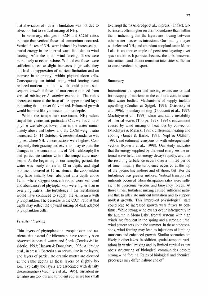
that alleviation of nutrient limitation was not due to advection but to vertical mixing of NH4.
In summary, changes in C:N and C:Chl ratios indicate that vertical fluxes of ammonium occurred. Vertical fluxes of N~ were induced by increased potential energy in the internal wave field due to wind forcing. After the initial wind forcing, fluxes were more likely to occur inshore. While these fluxes were sufficient to cause slight increases in growth, they did lead to suppression of nutrient limitation and an increase in chlorophyll within phytoplankton cells. Consequently, an initial strong wind forcing event reduced nutrient limitation which could permit subsequent growth if fluxes of nutrients continued from vertical mixing or A. monica excretion. The ratios decreased more at the base of the upper mixed layer indicating that it never fully mixed. Enhanced growth would be most likely to occur at those depths.
Within the temperature maximum, NH4 values stayed fairly constant, particulate C as well as chlorophyll a was always lower than in the water immediately above and below, and the C:Chl weight ratio decreased. On 14 October, A. monica abundance was highest where NH4 concentrations were highest. Consequently their grazing and excretion may explain the changes in the concentrations of NH4, chlorophyll a
and particulate carbon within the temperature maximum. At the beginning of our sampling period, the water was nearly anoxic at 12 m depth, and algal biomass increased at 12 m. Hence, the zooplankton may have initially been abundant at a depth above 12 m where oxygen concentrations were sufficient and abundances of phytoplankton were higher than in overlying waters. The turbulence in the metalimnion would have continued to supply the A. monica with phytoplankton. The decrease in the C:Chl ratio at that depth may reflect the upward mixing of dark adapted phytoplankton cells.
Persistent layering
Thin layers of phytoplankton, zooplankton and nutrients that extend for kilometers have recently been observed in coastal waters and fjords (Cowles & Desiderio, 1993; Hanson & Donaghay, 1998; Alldredge et aI., in press.). Bacteria also accumulate in the layers, and layers of particulate organic matter are elevated at the same depths as these layers or slightly below. Typically the layers are associated with density discontinuities (Macintyre et aI., 1995). Turbulent intensities are too low and turbulent eddies are too small
27
to disrupt them (Alldredge et aI., in press.). In fact, turbulence is often higher on their boundaries than within them, indicating that the layers are flowing between other water masses as intrusions. Our finding a layer with elevated N~ and abundant zooplankton in Mono Lake is another example of persistent layering over space and time. It persisted because the turbulence was intermittent, and did not remain at intensities sufficient to cause vertical transport.
Summary
Intermittent transport and mixing events are critical for resupply of nutrients to the euphotic zone in stratified water bodies. Mechanisms of supply include upwelling (Coulter & Spigel, 1991; Ostrovsky et aI., 1996), boundary mixing (Goudsmit et aI., 1997; Macintyre et aI., 1999), shear and static instability of internal waves (Thorpe, 1978, 1994), entrainment caused by wind mixing or heat loss by convection (Macintyre & Melack, 1995), differential heating and cooling (James & Barko, 1991; Nepf & Oldham, 1997), and sediment resuspension with subsequent advection (Robarts et aI., 1998). Our study indicates that the energy supplied by the wind energizes the internal wave field, that energy decays rapidly, and that the resulting turbulence occurs over a limited period of time. Initially the turbulence occurred at the top of the pycnocline inshore and offshore, but later the turbulence was greater inshore. Vertical transport of nutrients occurred when dissipation rates were sufficient to overcome viscous and buoyancy forces. At those times, turbulent mixing caused sufficient nutrient flux to alleviate nutrient limitation and to support modest growth. This improved physiological state could lead to increased growth were fluxes to continue. While strong wind events occur infrequently in the autumn in Mono Lake, frontal systems with high winds are frequent in the spring and a strong diurnal wind pattern sets up in the summer. In these other seasons, wind forcing may lead to injections of limiting nutrients and enhanced growth. Similar scenarios are likely in other lakes. In addition, spatial-temporal variations in vertical mixing and its limited vertical extent abets structuring of biological communities despite strong wind forcing. Rates of biological and chemical processes may differ inshore and off.
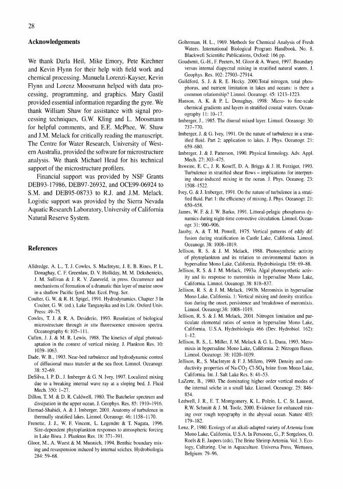
28
Acknowledgements
We thank Darla Heil, Mike Emory, Pete Kirchner and Kevin Flynn for their help with field work and chemical processing. Manuela Lorenzi-Kayser, Kevin Flynn and Lorenz Moosmann helped with data processing, programming, and graphics. Mary Gastil provided essential information regarding the gyre. We thank William Shaw for assistance with signal processing techniques, G.w. Kling and L. Moosmann for helpful comments, and E.E. McPhee, W. Shaw and lM. Melack for critically reading the manuscript. The Centre for Water Research, University of Western Australia, provided the software for microstructure analysis. We thank Michael Head for his technical support of the microstructure profilers.
Financial support was provided by NSF Grants DEB93-17986, DEB97-26932, and OCE99-06924 to S.M. and DEB95-08733 to R.I. and lM. Melack. Logistic support was provided by the Sierra Nevada Aquatic Research Laboratory, University of California Natural Reserve System.
References
Alldredge. A. L., T. J. Cowles, S. MacIntyre, J. E. B. Rines, P. L. Donaghay, C. F. Greenlaw, D. V. Holliday, M. M. Dekshenieks, J. M. Sullivan & J. R. V. Zaneveld, in press. Occurrence and mechanisms of formation of a dramatic thin layer of marine snow in a shallow Pacific fjord. Mar. Eco!. Prog. Ser.
Coulter, G. W. & R. H. Spigel, 1991. Hydrodynamics. Chapter 3 In Coulter, G. W. (ed.), Lake Tanganyika and its Life. Oxford Univ. Press: 49-75.
Cowles, T. J. & R. A. Desiderio, 1993. Resolution of biological microstructure through in situ fluorescence emission spectra. Oceanography 6: lOS-III.
Cullen, J. J. & M. R. Lewis, 1988. The kinetics of algal photoadaptation in the context of vertical mixing. 1. Plankton Res. 10: 1039-1063.
Dade, W. B., 1993. Near-bed turbulence and hydrodynamic control of diffusional mass transfer at the sea floor. Limno!. Oceanogr. 38: 52-69.
DeSilva, I. P. D., J. Imberger & G. N. Ivey, 1997. Localized mixing due to a breaking internal wave ray at a sloping bed. J. Fluid Mech. 350: 1-27.
Dillon, T. M. & D. R. Caldwell, 1980. The Batchelor spectrum and dissipation in the upper ocean. J. Geophys. Res. 85: 1910-1916.
Etemad-Shahidi, A. & J. Imberger, 200 I. Anatomy of turbulence in thermally stratified lakes. Limno!. Oceanogr. 46: 1158-1170.
Frenette, J. J., W. F. Vincent, L. Legendre & T. Nagata, 1996. Size-dependent phytoplankton responses to atmospheric forcing in Lake Biwa. J. Plankton Res. 18: 371-391.
Gloor, M., A. Wuest & M. Munnich, 1994. Benthic boundary mixing and resuspension induced by internal seiches. Hydrobiologia 284: 59-68.
Golterman, H. L., 1969. Methods for Chemical Analysis of Fresh Waters. International Biological Program Handbook. No.8. Blackwell Scientific Publications, Oxford: 166 pp.
Goudsmit, G.-H., F. Peeters, M. Gloor & A. Wuest, 1997. Boundary versus internal diapycnal mixing in stratified natural waters. J. Geophys. Res. 102: 27903-27914.
Guildford, S. J. & R. E. Hecky. 2000.Total nitrogen, total phosphorus, and nutrient limitation in lakes and oceans: is there a common relationship? Limno!. Oceanogr. 45: 1213-1223.
Hanson, A. K. & P. L. Donaghay, 1998: Micro- to fine-scale chemical gradients and layers in stratified coastal waters. Oceanography II: 10--17.
Imberger, J., 1985. The diurnal mixed layer. Limno!. Oceanogr. 30: 737-770.
Imberger, J. & G. Ivey, 1991. On the nature of turbulence in a stratified fluid. Part 2: application to lakes. J. Phys. Oceanogr. 21: 659-680.
Imberger, J. & J. Patterson, 1990. Physical limnology. Adv. App!. Mech. 27: 303-475.
Itsweire, E. C., J. R. Koseff, D. A. Briggs & J. H. Ferziger, 1993. Turbulence in stratified shear flows - implications for interpreting shear-induced mixing in the ocean. J. Phys. Oceanog. 23: 1508-1522.
Ivey, G. & J. Imberger, 1991. On the nature of turbulence in a stratified fluid. Part I: the efficiency of mixing. J. Phys. Oceanogr. 21: 650--658.
James, W. F. & J. W. Barko, 1991. Littoral-pelagic phosphorus dynamics during night-time convective circulation. Limno!. Oceanogr. 31: 900--906.
Jassby, A. & T. M. Powell, 1975. Vertical patterns of eddy diffusion during stratification in Castle Lake, California. Limno!. Oceanogr. 38: 1008-10 19.
Jellison, R. S. & J. M. Melack, 1988. Photosynthetic activity of phytoplankton and its relation to environmental factors in hypersaline Mono Lake, California. Hydrobiologia 158: 69-88.
Jellison, R. S. & J. M. Melack, 1993a. Algal photosynthetic activity and its response to meromixis in hypersaline Mono Lake, California. Limno!. Oceanogr. 38: 818-837.
Jellison, R. S. & J. M. Melack, 1993b. Meromixis in hypersaline Mono Lake, California. I: Vertical mixing and density stratification during the onset, persistence and breakdown of meromixis. Limno!. Oceanogr.38: 1008-1019.
Jellison, R. S. & J. M. Melack, 2001. Nitrogen limitation and particulate elemental ratios of seston in hypersaline Mono Lake, California, U.S.A. Hydrobiologia 466 (Dev. Hydrobio!. 162): 1-12.
Jellison, R. S., L. Miller, J. M. Melack & G. L. Dana, 1993. Meromixis in hypersaline Mono Lake, California. 2: Nitrogen fluxes. Limno!. Oceanogr. 38: 1020-1039.
Jellison, R., S. MacIntyre & F. 1. Millero, 1999. Density and conductivity properties of Na-C03 -CI-S04 brine from Mono Lake, California. Int. J. Salt Lake Res. 8: 41-53.
LaZerte, B., 1980. The dominating higher order vertical modes of the internal seiche in a small lake. Limno!. Oceanogr. 25: 846-854.
Ledwell, J. R., E. T. Montgomery, K. L. Polzin, L. C. St. Laurent, R.W. Schmitt & J. M. Toole, 2000. Evidence for enhanced mixing over rough topography in the abyssal ocean. Nature 403: 179-182.
Lenz, P., 1980. Ecology of an alkali-adapted variety of Artemia from Mono Lake, California, U.S.A. In Persoone, G., P. Sorgeloos, O. Roels & E. Jaspers (eds), The Brine Shrimp Artemia. Vo!. 3. Ecology, Culturing. Use in Aquaculture. Universa Press, Welteren, Belgium: 79-96.
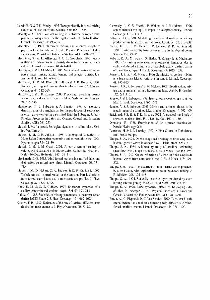
Lueck, R. G. & T. D. Mudge, 1997. Topographically induced mixing around a shallow seamount. Science 276: 1831-1833.
Macintyre, S., 1993. Vertical mixing in a shallow eutrophic lake: possible consequences for the light climate of phytoplankton. Limnol. Oceanogr. 38: 798-817.
Macintyre, S., 1998. Turbulent mixing and resource supply to phytoplankton. In Imberger, J. (ed.), Physical Processes in Lakes and Oceans, Coastal and Estuarine Studies, AGU: 539-567.
Macintyre, S., A. L. Alldredge & C. C. Gotschalk, 1995. Accumulation of marine snow at density discontinuities in the water column. Limnol. Oceanogr. 40: 449-468.
Macintyre, S. & 1. M. Melack, 1995. Vertical and horizontal transport in lakes: linking littoral, benthic and pelagic habitats. J. n. am. Benthol. Soc. 14: 599-615.
Macintyre, S., K. M. Flynn, R. Jellison & 1. R. Romero, 1999. Boundary mixing and nutrient flux in Mono Lake, CA. Limnol. Oceanogr. 44: 512-529.
Macintyre, S. & 1. R. Romero, 2000. Predicting upwelling, boundary mixing, and nutrient fluxes in lakes. Verh. int. Ver. Limnol. 27: 246-250.
Maxwortby, T., J. Imberger & A. Saggio, 1998. A laboratory demonstration of a mechanism for the production of secondary, internal gravity-waves in a stratified fluid. In Imberger, 1. (ed.), Physical Processes in Lakes and Oceans. Coastal and Estuarine Studies, AGU: 261-270.
Melack, J. M., (in press). Ecological dynamics in saline lakes. Verh. int. Ver. Lirnnol.
Melack, J. M. & R. Jellison, 1998. Limnological conditions in Mono Lake: Contrasting monomixis and meromixis in the 1990s. Hydrobiologia 384: 21-39.
Melack, 1. M. & M. Gastil, 2001. Airborne remote sensing of chlorophyll distributions in Mono Lake, California. Hydrobiologia 466 (Dev. Hydrobiol. 162): 31-38.
Monismith, S. G., 1985. Wind-forced motions in stratified lakes and their effect on mixed-layer shear. Limnol. Oceano gr. 30: 771-783.
Mourn, J. N., D. Hebert, C. A. Paulson & D. R. Caldwell, 1992. Turbulence and internal waves at the equator. Part I. Statistics from towed thermistors and a microstructure profiler. J. Phys. Oceanogr. 22: 1330-1345.
Nepf, H. M. & C. E. Oldham, 1997. Exchange dynamics of a shallow contaminated wetland. Aquat. Sci. 59: 193-213.
Oakey, N., 1985. Statistics of mixing parameters in the upper ocean during JASIN Phase 2. J. Phys. Oceanogr. IS: 1662-1675.
Osboru, T. R., 1980. Estimates of the rate of vertical diffusion from dissipation measurements. J. Phys. Oceanogr. 10: 83-89.
29
Ostrovsky, I, Y. Z. Yacobi, P. Walline & I. Kalikhman, 1996. Seiche-induced mixing - its impact on lake productivity. Limnol. Oceanogr. 41: 323-332.
Patterson, 1. c., 1991. Modelling the effects of motion on primary production in the mixed layer oflakes. Aquat. Sci. 53: 218-238.
Polzin, K. L., J. M. Toole, J. R. Ledwell & R. W. Schmidt, 1997. Spatial variability in turbulent mixing in the abyssal ocean. Science 276: 93-96.
Robarts, R. D., M. Waiser, O. Hadas, T. Zohary & S. Macintyre, 1998. Contrasting relaxation of phosphorus limitation due to typhoon-induced mixing in two morphologically distinct basins of Lake Biwa, Japan. Limnol. Oceanogr. 43: 1023-1036.
Romero, J. R. & J. M. Melack, 1996. Sensitivity of vertical mixing in a large saline lake to variations in runoff. Limnol. Oceanogr. 41: 955-965.
Romero, 1. R., R. Jellison & J. M. Me1ack, 1998. Stratification, mixing and ammonia flux in a hypersaline lake. Archiv. Hydrobiol. 142: 283-315.
Saggio, A. & J. Imberger, 1998. Internal wave weather in a stratified lake. Limnol. Oceanogr. 1780-1795.
Saggio, A. & J. Imberger, 2001. Mixing and turbulent fluxes in the metalimnion of a stratified lake. Limnol. Oceanogr. 46: 392-409.
Strickland, 1. S. H. & T. R. Parsons, 1972. A practical handbook of seawater analysis. Bull. Fish. Res. Bd Can. 167: 1-130.
Svensson, U., 1978. Examination of the summer stratification. Nordic Hydrology 9(2).
Tennekes, H. & J. L. Lumley, 1972. A First Course in Turbulence. MIT Press: 300 pp.
Thorpe, S. A., 1978. On the shape and breaking of finite amplitude internal gravity waves in a shear flow. J. Fluid Mech. 85: 7-31.
Thorpe, S. A., 1984. A laboratory study of stratified ace1erating shear flow over a rough boundary. 1. Fluid Mech. 138: 185-196.
Thorpe, S. A, 1987. On the reflection of a train of finite-amplitude internal waves from a uniform slope. J. Fluid Mech. 178: 279-302.
Thorpe, S. A., 1989. The distortion of short internal waves produced by a long wave, with applications to ocean boundary mixing. 1. Fluid Mech. 208: 395-415.
Thorpe, S. A., 1994. Statically unstable layers produced by overturning internal gravity waves. J. Fluid Mech. 260: 333-350.
Thorpe, S. A., 1998. Some dynamical effects of the sloping sides of lakes. In Imberger, J. (ed.), Physical Processes in Lakes and Oceans. Coastal and Estuarine Studies, AGU: 441-460.
Wuest, A., G. Piepke & D. C. Van Senden, 2000. Turbulent kinetic energy balance as a tool for estimating eddy diffusivity in windforced stratified waters. Limnol. Oceanogr. 45: 1388-1400.
Hydrobiologia 466: 31-38,2001. J.M. Melack, R. Jellison & D.B. Herbst (eds), Saline Lakes. © 2001 Kluwer Academic Publishers.
31
Airborne remote sensing of chlorophyll distributions in Mono Lake, California
John M. Melack1,2 & Mary Gastill 1 Institute for Computational Earth System Science, University of California, Santa Barbara, CA 93106, U.S.A. 2 Department of Ecology, Evolution and Marine Biology, University of California, Santa Barbara, CA 93106, U.S.A.
Key words: remote sensing, chlorophyll, Mono Lake, saline lakes
Abstract
As part of a long-term investigation of seasonal and interannual variations of plankton in Mono Lake (California), we developed a methodology using airborne imaging spectrometry to synoptically measure chlorophyll concentrations. Images of Mono Lake were acquired with NASA's Airborne Visible and Infrared Imaging Spectrometer (AVIRIS) and were atmospherically corrected by applying a version of the radiative transfer model MODTRAN. U sing a predictive equation for calculation of chlorophyll based on a band ratio of remote sensing reflectances (Rrs ;
Rrs 490 nml Rrs 550 nm), spatial distributions of chlorophyll throughout the lake were determined; broad east to west gradients in chlorophyll and gyres are evident.
Introduction
Variations in phytoplankton abundance occur over a wide range of temporal and spatial scales as a consequence of interactions among biological, chemical and physical processes (Harris, 1986; Denman, 1994; Neill, 1994). A commonly used measure of the abundance of phytoplankton is the concentration of chlorophyll. Measurement of chlorophyll can be done in the laboratory after collection of discrete samples, in situ by derivation from fluorescence, or by remote sensing, which makes possible synoptic estimates over large areas (e.g., Abbott et aI., 1982; Galat & Verduin, 1989).
Remote sensing of chlorophyll depends on detection of sunlight or laser light (Hoge & Swift, 1983; Kirk, 1983) that has interacted with chlorophyll within aquatic plants and is upwelled toward a sensor located at some altitude above the water. Most sensors are mounted on airborne or spaceborne platforms, although hand-held instruments can be used. Recent advances in remote sensing systems have expanded the capabilities and opportunities for applications to the study of inland waters (Dekker et aI., 1995).
Our purpose here is to describe a methodology for using a remote sensing technique called imaging spec-
trometry for the determination of chlorophyll in lakes. Airborne imaging spectrometry uses high resolution, continuous reflectance spectra to decipher optical conditions in the water and atmosphere. We illustrate the approach with data from hypersaline Mono Lake, California.
Background on remote sensing of lakes
Sunlight incident on a lake is partially reflected from the surface and partially transmitted into the lake where it is scattered and absorbed (Kirk, 1983). The theoretical basis for remote sensing of optical properties of water is well known (Gordon & Morel, 1983; Kirk, 1983; Mobley, 1994). The water-leaving radiance is remotely sensed by inverting the equation describing the radiance measured at high altitude, such as by the Airborne Visible and Infrared Imaging Spectrometer (AVIRIS):
L AVIRISAhB = LpathAhB + LwaterAB TAhe
+ LskYAhOB hhe PAiJ
+LsUnAhoBs hhesPAes (1)
where subscript A is wavelength, h is sensor altitude, ho is lake surface altitude, () is viewing angle (at or
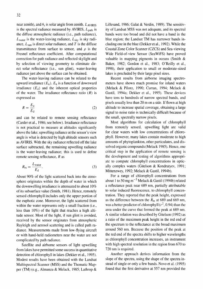
32
near zenith), and es is solar angle from zenith. LAVIRIS
is the spectral radiance measured by AVIRIS, Lpath is the diffuse atmospheric radiance (i.e., path radiance), Lwater is the water-leaving radiance, Lsky is sky radiance, Lsun is direct solar radiance, and T is the diffuse transmittance from surface to sensor, and p is the Fresnel reflectance coefficient. After computational correction for path radiance and reflected skylight and by selection of viewing geometry to eliminate direct solar reflectance (i.e., sun glint), water-leaving radiance just above the surface can be obtained.
The water-leaving radiance can be related to the upward irradiance (Eu). Eu is a function of downward irradiance (Ed) and the inherent optical properties of the water. The irradiance reflectance ratio (R) is expressed as
Eu R=
Ed (2)
and can be related to remote sensing reflectance (Carder et aI., 1986; see below). Irradiance reflectance is not practical to measure at altitudes significantly above the lake; upwelling radiance at the sensor's view angle is what is detected by high altitude sensors such as AVIRIS. With the sky radiance reflected off the lake surface subtracted, the remaining upwelling radiance is the water-leaving radiance; this is used to define remote sensing reflectance, R as
Lwater R rs = --.
Ed (3)
About 90% of the light scattered back into the atmosphere originates within the depth of water in which the downwelling irradiance is attenuated to about 10% of its subsurface value (Smith, 1981). Hence, remotely sensed chlorophyll includes only the upper portion of the euphotic zone. Moreover, the light scattered from within the water represents only a small fraction (i.e., less than 10%) of the light that reaches a high altitude sensor. Most of the light, if sun glint is avoided, received by the sensor originates from atmospheric Rayleigh and aerosol scattering and is called path radiance. Measurements made from low-flying aircraft or with hand-held radiometers near the water are not complicated by path radiance.
Satellite and airborne sensors of light upwelling from lakes have permitted some success in quantitative detection of chlorophyll in lakes (Dekker et aI., 1995). Modest results have been obtained with the Landsat Multispectral Scanner (MSS) and the Thematic Mapper (TM) (e.g., Almanza & Melack, 1985; Lathrop &
Lillesand, 1986; Galat & Verdin, 1989). The sensitivity of Landsat MSS was not adequate, and its spectral bands were too broad and did not have a band in the blue region; the Landsat TM has narrower bands including one in the blue (Dekker et aI., 1992). While the Coastal Zone Color Scanner (CZCS) and Sea-viewing Wide Field-of-view Sensor (SeaWiFS) have proved valuable in mapping pigments in oceans (Smith & Baker, 1982; Gordon et aI., 1983; O'Reilly et aI., 1998), their application to small or moderate-sized lakes is precluded by their large pixel sizes.
Recent results from airborne imaging spectrometers have shown much promise for inland waters (Melack & Pilorz, 1990; Curran, 1994; Melack & Gastil, 1994a; Dekker et aI., 1995). These devices have tens to hundreds of narrow spectral bands, and pixels usually less than 20 m on a side. If flown at high altitude to increase spatial coverage, obtaining a large signal to noise ratio is technically difficult because of the small, spectrally narrow pixels.
Most algorithms for calculation of chlorophyll from remotely sensed, upwelling light are valid for clear waters with low concentrations of chlorophyll. However, many lakes contain moderate to high amounts of phytoplankton, other particulates, and dissolved organic compounds (Melack 1985). Hence, one critical step in the application of remote sensing is the development and testing of algorithms appropriate to compute chlorophyll concentrations in optically complex waters (Gitelson & Kondratyev, 1991; Mittenzwey, 1992; Melack & Gastil, I 994b ).
For a range of chlorophyll concentrations from about I to 50 mg m - 3 Melack & Gastil (1994b) related a reflectance peak near 689 nm, partially attributable to solar induced fluorescence, to chlorophyll concentration. They reported that the peak height, expressed as the difference between the Rrs at 689 and 669 nm, was a better predictor of chlorophyll (r2, 0.94) than the area under the curve that formed the peak at 689 nm. A similar relation was described by Gitelson (1992) as a ratio of the maximum peak height in the red end of the spectrum to the reflectance at the broad maximum around 560 nm. Because the position of the peak at the red end of the spectra shifts to higher wavelengths as chlorophyll concentration increases, an instrument with high spectral resolution in the region from 670 to 720 nm is required.
Another approach derives information from the slope of the spectra, using the shape of the spectra instead of single or only a few bands. Novo et al. (1995) found that the first derivative at 557 nm provided the
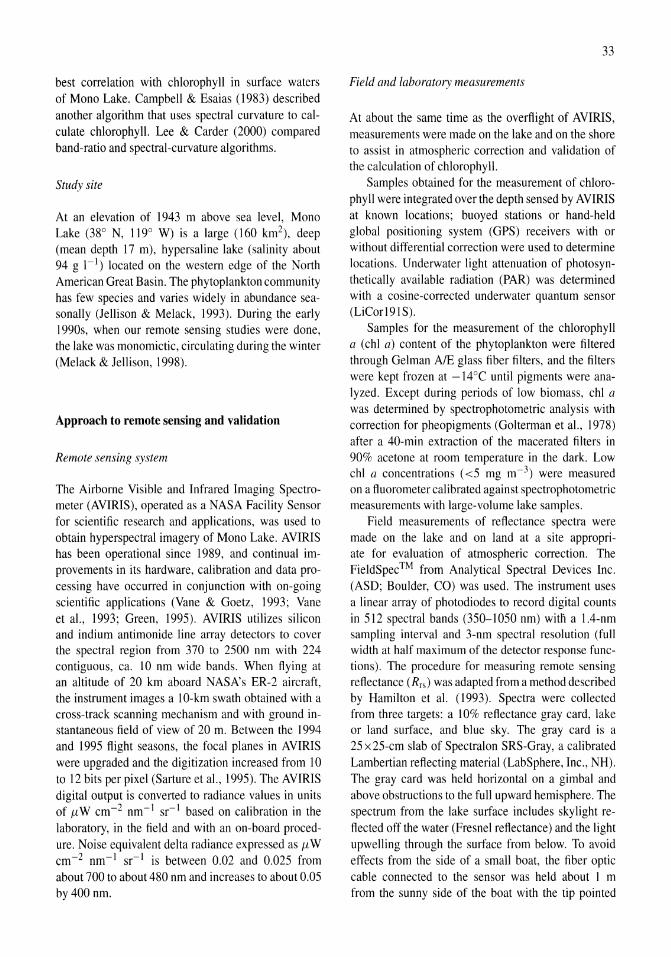
best correlation with chlorophyll in surface waters of Mono Lake. Campbell & Esaias (1983) described another algorithm that uses spectral curvature to calculate chlorophyll. Lee & Carder (2000) compared band-ratio and spectral-curvature algorithms.
Study site
At an elevation of 1943 m above sea level, Mono Lake (38° N, 1190 W) is a large (160 km2), deep (mean depth 17 m), hypersaline lake (salinity about 94 g I-I) located on the western edge of the North American Great Basin. The phytoplankton community has few species and varies widely in abundance seasonally (Jellison & Melack, 1993). During the early 1990s, when our remote sensing studies were done, the lake was monomictic, circulating during the winter (Melack & Jellison, 1998).
Approach to remote sensing and validation
Remote sensing system
The Airborne Visible and Infrared Imaging Spectrometer (AVIRIS), operated as a NASA Facility Sensor for scientific research and applications, was used to obtain hyperspectral imagery of Mono Lake. AVIRIS has been operational since 1989, and continual improvements in its hardware, calibration and data processing have occurred in conjunction with on-going scientific applications (Vane & Goetz, 1993; Vane et aI., 1993; Green, 1995). AVIRIS utilizes silicon and indium antimonide line array detectors to cover the spectral region from 370 to 2500 nm with 224 contiguous, ca. 10 nm wide bands. When flying at an altitude of 20 krn aboard NASA's ER-2 aircraft, the instrument images a 10-km swath obtained with a cross-track scanning mechanism and with ground instantaneous field of view of 20 m. Between the 1994 and 1995 flight seasons, the focal planes in AVIRIS were upgraded and the digitization increased from 10 to 12 bits per pixel (Sarture et aI., 1995). The AVIRIS digital output is converted to radiance values in units of /LW cm-2 nm- I sr- I based on calibration in the laboratory, in the field and with an on-board procedure. Noise equivalent delta radiance expressed as /L W cm-2 nm- I sr- I is between 0.02 and 0.025 from about 700 to about 480 nm and increases to about 0.05 by 400 nm.
33
Field and laboratory measurements
At about the same time as the overflight of AVIRIS, measurements were made on the lake and on the shore to assist in atmospheric correction and validation of the calculation of chlorophyll.
Samples obtained for the measurement of chlorophyll were integrated over the depth sensed by AVIRIS at known locations; buoyed stations or hand-held global positioning system (GPS) receivers with or without differential correction were used to determine locations. Underwater light attenuation of photosynthetically available radiation (PAR) was determined with a cosine-corrected underwater quantum sensor (LiCorI9IS).
Samples for the measurement of the chlorophyll a (chi a) content of the phytoplankton were filtered through Gelman AlE glass fiber filters, and the filters were kept frozen at -14°C until pigments were analyzed. Except during periods of low biomass, chI a was determined by spectrophotometric analysis with correction for pheopigments (Golterman et aI., 1978) after a 40-min extraction of the macerated filters in 90% acetone at room temperature in the dark. Low chI a concentrations «5 mg m-3) were measured on a fluorometer calibrated against spectrophotometric measurements with large-volume lake samples.
Field measurements of reflectance spectra were made on the lake and on land at a site appropriate for evaluation of atmospheric correction. The FieldSpec ™ from Analytical Spectral Devices Inc. (ASD; Boulder, CO) was used. The instrument uses a linear array of photodiodes to record digital counts in 512 spectral bands (350-1050 nm) witn a 1.4-nm sampling interval and 3-nm spectral resolution (full width at half maximum of the detector response functions). The procedure for measuring remote sensing reflectance (Rrs) was adapted from a method described by Hamilton et al. (1993). Spectra were collected from three targets: a 10% reflectance gray card, lake or land surface, and blue sky. The gray card is a 25 x 25-cm slab of Spectralon SRS-Gray, a calibrated Lambertian reflecting material (LabSphere, Inc., NH). The gray card was held horizontal on a gimbal and above obstructions to the full upward hemisphere. The spectrum from the lake surface includes skylight reflected off the water (Fresnel reflectance) and the light upwelling through the surface from below. To avoid effects from the side of a small boat, the fiber optic cable connected to the sensor was held about 1 m from the sunny side of the boat with the tip pointed
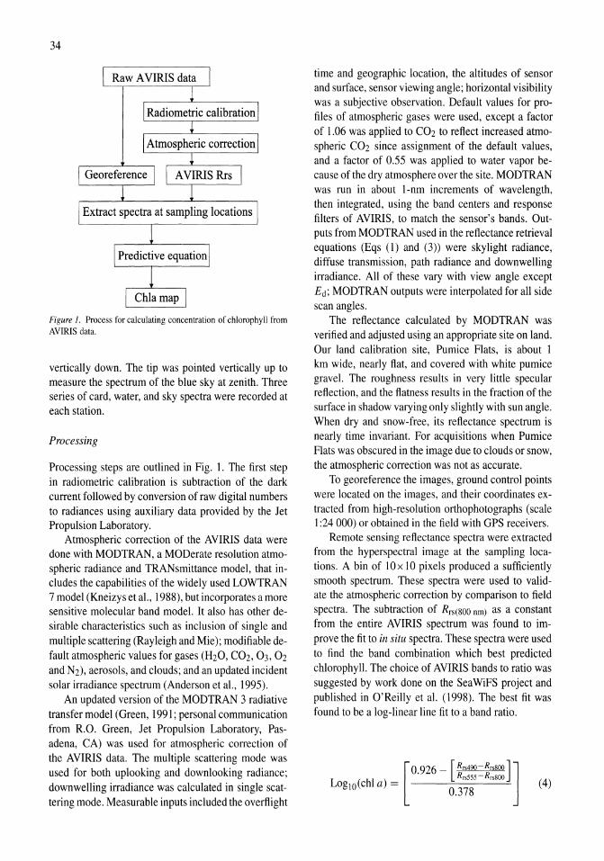
34
Figure I. Process for calculating concentration of chlorophyll from AVIRIS data.
vertically down. The tip was pointed vertically up to measure the spectrum of the blue sky at zenith. Three series of card, water, and sky spectra were recorded at each station.
Processing
Processing steps are outlined in Fig. 1. The first step in radiometric calibration is subtraction of the dark current followed by conversion of raw digital numbers to radiances using auxiliary data provided by the Jet Propulsion Laboratory.
Atmospheric correction of the AVIRIS data were done with MODTRAN, a MODerate resolution atmospheric radiance and TRANsmittance model, that includes the capabilities of the widely used LOWTRAN 7 model (Kneizys et aI., 1988), but incorporates a more sensitive molecular band model. It also has other desirable characteristics such as inclusion of single and multiple scattering (Rayleigh and Mie); modifiable default atmospheric values for gases (H20, C02, 03, 02 and N2), aerosols, and clouds; and an updated incident solar irradiance spectrum (Anderson et aI., 1995).
An updated version of the MODTRAN 3 radiative transfer model (Green, 1991; personal communication from R.O. Green, Jet Propulsion Laboratory, Pasadena, CA) was used for atmospheric correction of the AVIRIS data. The multiple scattering mode was used for both up looking and downlooking radiance; downwelling irradiance was calculated in single scattering mode. Measurable inputs included the overflight
time and geographic location, the altitudes of sensor and surface, sensor viewing angle; horizontal visibility was a subjective observation. Default values for profiles of atmospheric gases were used, except a factor of 1.06 was applied to C02 to reflect increased atmospheric C02 since assignment of the default values, and a factor of 0.55 was applied to water vapor because of the dry atmosphere over the site. MODTRAN was run in about 1-nm increments of wavelength, then integrated, using the band centers and response filters of AVIRIS, to match the sensor's bands. Outputs from MODTRAN used in the reflectance retrieval equations (Eqs (l) and (3)) were skylight radiance, diffuse transmission, path radiance and downwelling irradiance. All of these vary with view angle except Ed; MODTRAN outputs were interpolated for all side scan angles.
The reflectance calculated by MODTRAN was verified and adjusted using an appropriate site on land. Our land calibration site, Pumice Flats, is about 1 km wide, nearly flat, and covered with white pumice gravel. The roughness results in very little specular reflection, and the flatness results in the fraction of the surface in shadow varying only slightly with sun angle. When dry and snow-free, its reflectance spectrum is nearly time invariant. For acquisitions when Pumice Flats was obscured in the image due to clouds or snow, the atmospheric correction was not as accurate.
To georeference the images, ground control points were located on the images, and their coordinates extracted from high-resolution orthophotographs (scale 1:24000) or obtained in the field with GPS receivers.
Remote sensing reflectance spectra were extracted from the hyperspectral image at the sampling locations. A bin of lOx 10 pixels produced a sufficiently smooth spectrum. These spectra were used to validate the atmospheric correction by comparison to field spectra. The subtraction of Rrs(800 nm) as a constant from the entire AVIRIS spectrum was found to improve the fit to in situ spectra. These spectra were used to find the band combination which best predicted chlorophyll. The choice of AVIRIS bands to ratio was suggested by work done on the Sea WiFS project and published in O'Reilly et al. (1998). The best fit was found to be a log-linear line fit to a band ratio.
Log 10 (chI a) = Rrs555 - Rrs800 [0.926 - [Rrs490-RrS800]]
0.378 (4)
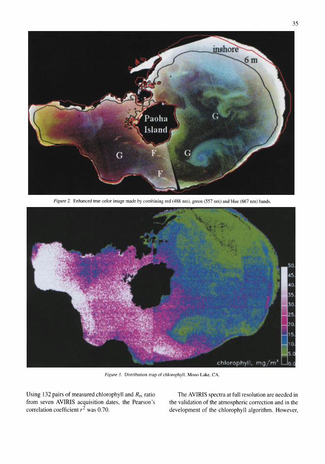
35
Figure 2. Enhanced true color image made by combining red (488 nm), green (557 nm) and blue (667 nm) bands.
Figure 3. Distribution map of chlorophyll, Mono Lake, CA.
Using 132 pairs of measured chlorophyll and Rrs ratio from seven AVIRIS acquisition dates, the Pearson's correlation coefficient r2 was 0.70.
The AVIRIS spectra at full resolution are needed in the validation of the atmospheric correction and in the development of the chlorophyll algorithm. However,
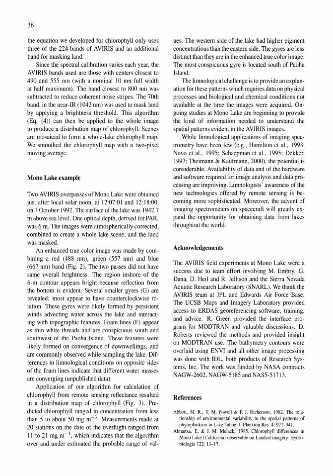
36
the equation we developed for chlorophyll only uses three of the 224 bands of AVIRIS and an additional band for masking land.
Since the spectral calibration varies each year, the AVIRIS bands used are those with centers closest to 490 and 555 nm (with a nominal 10 nm full width at half maximum). The band closest to 800 nm was subtracted to reduce coherent noise stripes. The 70th band, in the near-IR (1042 nm) was used to mask land by applying a brightness threshold. This algorithm (Eq. (4)) can then be applied to the whole image to produce a distribution map of chlorophyll. Scenes are mosaiced to form a whole-lake chlorophyll map. We smoothed the chlorophyll map with a two-pixel moving average.
Mono Lake example
Two AVIRIS overpasses of Mono Lake were obtained just after local solar noon, at 12:07:01 and 12:18:00, on 7 October 1992. The surface of the lake was 1942.7 m above sea level. One optical depth, derived for PAR, was 6 m. The images were atmospherically corrected, combined to create a whole lake scene, and the land was masked.
An enhanced true color image was made by combining a red (488 nm), green (557 nm) and blue (667 nm) band (Fig. 2). The two passes did not have same overall brightness. The region inshore of the 6-m contour appears bright because reflection from the bottom is evident. Several smaller gyres (G) are revealed; most appear to have counterclockwise rotation. These gyres were likely formed by persistent winds advecting water across the lake and interacting with topographic features. Foam lines (F) appear as thin white threads and are conspicuous south and southwest of the Paoha Island. These features were likely formed on convergence of downwellings, and are commonly observed while sampling the lake. Differences in Iimnological conditions on opposite sides of the foam lines indicate that different water masses are converging (unpublished data).
Application of our algorithm for calculation of chlorophyll from remote sensing reflectance resulted in a distribution map of chlorophyll (Fig. 3). Predicted chlorophyll ranged in concentration from less than 5 to about 50 mg m-3. Measurements made at 20 stations on the date of the overflight ranged from II to 21 mg m - 3, which indicates that the algorithm over and under estimated the probable range of val-
ues. The western side of the lake had higher pigment concentrations than the eastern side. The gyres are less distinct than they are in the enhanced true color image. The most conspicuous gyre is located south of Paoha Island.
The limnological challenge is to provide an explanation for these patterns which requires data on physical processes and biological and chemical conditions not available at the time the images were acquired. Ongoing studies at Mono Lake are beginning to provide the kind of information needed to understand the spatial patterns evident in the AVIRIS images.
While Iimnological applications of imaging spectrometry have been few (e.g., Hamilton et aI., 1993; Novo et aI., 1995; Schaepman et aI., 1995; Dekker, 1997; Theimann & Kaufmann, 2000), the potential is considerable. Availability of data and of the hardware and software required for image analysis and data processing are improving. Limnologists' awareness of the new technologies offered by remote sensing is becoming more sophisticated. Moreover, the advent of imaging spectrometers on spacecraft will greatly expand the opportunity for obtaining data from lakes throughout the world.
Acknowledgements
The AVIRIS field experiments at Mono Lake were a success due to team effort involving M. Embry, G. Dana, D. Heil and R. Jellison and the Sierra Nevada Aquatic Research Laboratory (SNARL). We thank the AVIRIS team at JPL and Edwards Air Force Base. The UCSB Maps and Imagery Laboratory provided access to ERDAS georeferencing software, training, and advice. R. Green provided the interface program for MODTRAN and valuable discussions. D. Roberts reviewed the methods and provided insight on MODTRAN use. The bathymetry contours were overlaid using ENVI and all other image processing was done with IDL, both products of Research Systems, Inc. The work was funded by NASA contracts NAGW-2602, NAGW-5185 and NAS5-51713.
References
Abbott. M. R., T. M. Powell & P. 1. Richerson, 1982. The relationship of environmental variability to the spatial patterns of phytoplankton in Lake Tahoe. J. Plankton Res. 4: 927-941.
Almanza. E. & J. M. Melack, 1985. Chlorophyll differences in Mono Lake (California) observable on Landsat imagery. Hydrobiologia 122: 13-17.
Anderson, G. P., 1. Wang & J. H. Chetwynd, 1995. MODTRAN3: An update and recent validations against airborne high resolution interferometer measurements. In Green, R. O. (ed.), Summaries of the Fifth Annual JPL Airborne Earth Science Workshop,
Vol. I. AVIRIS Workshop. JPL Public. 95-1, Jet Propulsion Laboratory, Pasadena, CA: 5-8.
Campbell, J. W. & W. E. Esaias, 1983. Basis for spectral curvature algorithms in remote sensing of chlorophyll. Appl. Optics 22: 1084-1093.
Carder, K. L., R. G. Stewart, J. H. Paul & G. A. Vargo, 1986. Relationships between chlorophyll and ocean color constituents as they affect remote-sensing reflectance models. Limnol. Oceanogr. 31: 403-412.
Carder, K. L, P. Reinersmann, R. F. Chen, F. Muller-Karger, C. O. Davis & M. Hamilton, 1993. AVIRIS calibration and application in coastal oceanic environments. Remote Sens. Environ. 44: 205-216.
Curran, P. J., 1994. Imaging spectrometry. Progr. physical Geogr. 18: 247-266.
Dekker, A. G., T. 1. Malthus, M. M. Wijnen & E. Seyhan, 1992. The effect of spectral bandwidth and positioning on the spectral signature analysis of inland waters. Remote Sens. Environ. 41: 211-225.
Dekker, A. G, T. J. Mallhus & H. J. Hoogenboom, 1995. The remote sensing of inland water quality. In Danson, F. M. & S. E. Plummer (eds), Advances in Environmental Remote Sensing. John Wiley & Sons Ltd., New York: 123-142.
Denman, K. L., 1994. Scale-determining biological-physical interactions in oceanic food webs. In Giller, P. S., A. G. Hildrew & D. G. Raffaelli (eds), Aquatic Ecology: Scale, Pattern and Process. Blackwell Sci. Publ., London: 377-402.
Galat, D. L. & J. P. Verdin, 1989. Patchiness, collapse and succession of a cyanobacterial bloom evaluated by synoptic sampling and remote sensing. 1. Plankt. Res. II: 925-948.
Gastil, M. & 1. M. Melack, Improved atmospheric correction for AVIRIS spectra from inland waters. In Green, R. O. (ed.), Summaries of the Seventh JPL Airborne Earth Science Workshop. JPL Publication 97-21, Vol. 1. Jet Propulsion Laboratory, Pasadena, CA: 141-145.
Gitelson, A. A., 1992. The peak near 700 nm on radiance spectra of algae and water: relationships of its magnitude and position with chlorophyll concentration. Int. 1. Remote Sensing 12: 3367-3373.
Gitelson, A. A. & K. Ya. Kondratyev, 1991. Optical models of mesotrophic and eutrophic water bodies. Int. J. Remote Sensing 12: 373-385.
Gollerman, H. L., R. S. Clymo & M. A. M. Ohnstad, 1978. Methods for Physical and Chemical Analysis of Fresh Waters. IBP Handbook No.8, 2nd edn. Blackwell Sci. Pub!., Oxford.
Gordon, H. R. & A. Morel, 1983. Remote Assessment of Ocean Color for Interpretation of Satellite Visible Imagery: a Review. Springer, New York.
Gordon, H. R., D. K. Clark, J. W. Brown, O. B. Brown, R. H. Evans & w. W. Broenkow, 1983. Phytoplankton pigment concentrations in the Middle Atlantic Bight: Comparison of ship determinations to CZCS estimates. Appl. Optics 22: 20-35.
Green, R. 0.,1991. Retrieval ofreflectance from AVIRIS measured radiance using a radiative transfer code. In Proc. Third AVIRIS Workshop, JPL Publication 91-28. Jet Propulsion Laboratory, Pasadena, CA: 200-210.
Green, R. O. (ed.), 1995. Summaries of the Fifth Annual JPL Airborne Earth Science Workshop, Vol. I. AVIRIS Workshop. JPL Public. 95-1, Jet PropUlsion Laboratory, Pasadena, CA.
37
Hamilton, M. K., C. O. Davis, W. 1. Rhea, S. H. Pilorz & K. L. Carder, 1993. Estimating chlorophyll content and bathymetry of
Lake Tahoe using AVIRIS data. Remote Sens. Environ. 44: 217-230.
Harris, G. P., 1986. Phytoplankton Ecology. Chapman and Hall, London: 384 pp.
Hoge, F. & R. Swift, 1983. Airborne dual laser excitation and mapping phytoplankton photopigments in a Gulf Stream warm core ring. Appl. Opt. 22: 2272-2281.
Jellison, R. & 1. M. Melack, 1993. Algal photosynthetic activity and its response to meromixis in hypersaline Mono Lake, California. Limnol. Oceanogr. 38: 818-837.
Johnson, H. K. & R. O. Green, 1995. AVIRIS user' guide. In Green, R. O. (ed.), Summaries of the Fifth Annual JPL Airborne Earth Science Workshop, Vol. 1. AVIRIS Workshop. JPL Publication 95-1, Jet Propulsion Laboratory, Pasadena, CA: 105-108.
Kirk, 1. T. 0., 1986. Light and Photosynthesis in Aquatic Ecosystems. Cambridge University Press, Cambridge: 40 I pp.
Kneizys, F. X. et aI., 1988. User's guide to LOWTRAN 7, Air Force Geophysics Laboratory.
Lathrop, R. G. & T. M. Lillesand, 1986. Use of thematic mapper data to assess water quality in Green Bay and central Lake Michigan. Photogram. Eng. Remote Sens. 52: 671-680.
Lee, Z. & K. L. Carder, 2000. Band-ratio or spectral-curvature algorithms for satellite remote sensing? Appl. Opt. 39: 4377-4380.
Melack, 1. M., 1985. Interactions of detrital particulates and plankton. Hydrobiologia 125: 209-220.
Melack, 1. M. & S. A. Pilorz, 1990. Reflectance spectra from eutrophic Mono Lake, California, measured with the Airborne Visible and Infrared Imaging Spectrometer (AVIRIS). Int. Soc. Opt. Eng. Imaging Spectroscopy Terrestrial Environment 1298: 202-212.
Melack, 1. M. & M. Gastil, 1994a. Airborne visible imaging spectrometry applied to limnology: chlorophyll variation in Mono Lake. In Proc. of International Symposium on Spectral Sensing Research, San Diego, CA: 691-695.
Melack, 1. M. & M. Gastil, I 994b. Comparison of spectral feature algorithms for remote sensing of chlorophyll in eutrophic lakes. In Proc. Intern. Geosci. Remote Sens. Sympos., Vol. IV: 2363-2365.
Melack, 1. M. & R. Jellison, 1998. Limnological conditions in Mono Lake: contrasting monomixis and meromixis in the 1990s. Hydrobiologia 384: 21-39.
Mittenzwey, K. H., 1992. Determination of chlorophyll of inland waters on the basis of spectral reflectance. Limnol. Oceanogr. 37: 147-149.
Mobley, C. D., 1994. Light and Water: Radiative Transfer in Natural Waters. Academic Press, New York: 592 pp.
Neill, W. E., 1994. Spatial and temporal scaling and the organization of limnetic communities. In Giller, P. S., A. G. Hildrew & D. G. Raffaelli (eds), Aquatic Ecology: Scale, Pattern and Process. Blackwell Sci. PubL London: 189-231.
Novo, E .. M. Gastil & 1. M. Melack, 1995. An algorithm for chi orophy II using first difference transformation of AVIRIS reflectance spectra. In Green, R. O. (ed.), Summaries of the Fifth Annual JPL Airborne Earth Science Workshop, Vol. 1. AVIRIS Workshop. JPL Public. 95-1, Jet Propulsion Laboratory, Pasadena, CA: 121-124.
O'Reilly, 1. E., S. Maritorena, B. G. Mitchell. D. A. Siegel, K. L. Carder, S. A. Garver, M. Kahru, C. McClain, 1998. Ocean color chlorophyll algorithms for SeaWiFS, J.Geophys. Res. (Oceans) 103: 24937-24953.
Sarture, C. M. et aI., 1995. Airborne VisiblelInfrared Imaging Spectrometer (AVIRIS): sensor improvements for 1994 and 1995. In

38
Green, R. 0, (ed.), Summaries of the Fifth Annual JPL Airborne Earth Science Workshop, Vol. 1. AVIRIS Workshop. JPL Public. 95-1, Jet Propulsion Laboratory, Pasadena, CA: 145-148.
Schaepman, M. et aI., 1995. Extraction of ozone and chlorophyll-a distribution from AVIRIS data. In Green, R. 0. (ed.), Summaries of the Fifth Annual JPL Airborne Earth Science Workshop, Vol. I. AVIRIS Workshop. JPL Public. 95-1. Jet Propulsion Laboratory, Pasadena, CA: 149-152.
Smith, R. c., 1981. Remote sensing and depth distribution of ocean chlorophyll. Mar. Ecol. Prog. Ser. 6: 359-361.
Smith, R. C. & K. S. Baker, 1982. Oceanic chlorophyll concentra-
tions as determined by Nimbus 7 Coastal Zone Color Scanner imagery. J. mar. BioI. 66: 269-279.
Thiemann, S. & H. Kaufmann, 2000. Determination of chlorophyll content and trophic state of lakes using field spectrometer and IRS-l C satellite data in the Mecklenberg lake district, Germany. Remote Sens. Environ. 73: 227-235.
Vane, G. & A. F. H. Goetz, 1993. Terrestrial imaging spectrometry: Current status, future trends. Remote Sens. Environ. 44: 117-126.
Vane, G. et aI., 1993. The Airborne Visible/Infrared Imaging Spectrometer (AVIRIS). Remote Sens. Environ. 44: 127-143.
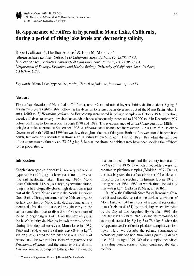
Hydrobiologia 466: 39-43,2001. J.M. Melack, R. Jellison & D.B. Herbst (eds), Saline Lakes. © 2001 Kluwer Academic Publishers.
39
Re-appearance of rotifers in hypersaline Mono Lake, California, during a period of rising lake levels and decreasing salinity
Robert Jellisonl ,*, Heather Adams2 & John M. Melackl ,3
I Marine Science Institute, University of California, Santa Barbara, CA 93106, U.S.A. 2CoUege of Creative Studies, University of California, Santa Barbara, CA 93106, U.S.A. 3 Department of Ecology, Evolution, and Marine Biology, University of California, Santa Barbara, CA 93106, U.S.A.
Key words: Mono Lake, hypersaline, rotifer, Hexarthrajenkinae, Brachionus plicatilis
Abstract
The surface elevation of Mono Lake, California, rose "'2 m and mixed-layer salinities declined about 5 g kg- 1
during the 3 years (1995-1997) following the decision to restrict water diversions out of the Mono Basin. Abundant (18000 m-2) Hexarthrajenkinae de Beauchamp were noted in pelagic samples in October 1997 after three decades of absence or very low abundance. Abundance subsequently increased to 100000 m-2 in December 1997 before declining to low numbers through 1998 and 1999. The re-appearance of Branchionus plicatilis Muller in pelagic samples occurred in September 1998. B. plicatilis areal abundance increased to'" 15000 m-2 in OctoberDecember of both 1998 and 1999 but was low throughout the rest of the year. Both rotifers were noted in nearshore ponds, but were only abundant in those with salinities below 53 g kg-I. During 1998-1999 when the salinities of the upper water column were 73-75 g kg-I, less saline shoreline habitats may have been seeding the offshore rotifer populations.
Introduction
Zooplankton species diversity is severely reduced in hypersaline (>50 g kg-I) lakes compared to less saline and freshwater lakes (Hammer, 1986). Mono Lake, California, U.S.A., is a large, hypersaline saline, lying in a hydrologically closed high-desert basin just east of the Sierra Nevada within the North American Great Basin. Throughout much of the 20th century, the surface elevation of Mono Lake declined and salinity increased, first due to extended drought early in the century and then due to diversion of streams out of the basin beginning in 1941. Over the next 40 years, the lake's salinity doubled as its volume was halved. During limnological surveys of Mono Lake in 1959, 1963 and 1964, when the salinity was 60-70 g kg-I, Mason (1967), noted the presence of several species of protozoans; the two rotifers, Hexarthra jenkinae and Brachionus plicatilis; and the endemic brine shrimp, Artemia monica. Subsequent to these observations, the
* Corresponding author. E-mail: [email protected]
lake continued to shrink and the salinity increased to ",82 g kg- I in 1976, by which time, rotifers were not reported in plankton samples (Winkler, 1977). During the next 16 years, the surface elevation of the lake continued to decline reaching its historic low of 1942 m during winter 1981-1982, at which time, the salinity was "'92 g kg- I (Jellison & Melack, 1993b).
In 1994, the California State Water Resources Control Board decided to raise the surface elevation of Mono Lake to 1948 m as part of a general restoration plan (Decision #1631) by restricting water diversion by the City of Los Angeles. By October 1997, the lake had risen ",2 m to 1945.2 m and the mixolimnetic salinity decreased by 5 g kg- 1 to 76 g kg- 1 when the re-appearance of rotifers in plankton samples was first noted. Here, we describe the pelagic abundance of Hexarthra jenkinae and Brachionus plicatilis during late 1997 through 1999. We also sampled nearshore less saline ponds, some of which contained abundant rotifers.
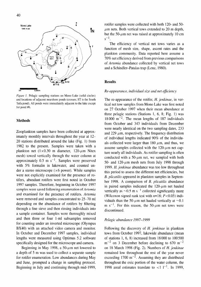
40
Mono Lake 1946 m asl
Om 5,ODom
+ 6
Figure 1. Pelagic sampling stations on Mono Lake (solid circles) and locations of adjacent nearshore ponds (crosses; ST is the South Tufa pond). All ponds were immediately adjacent to the lake except for pond #6.
Methods
Zooplankton samples have been collected at approximately monthly intervals throughout the year at 12-20 stations distributed around the lake (Fig. I) from 1982 to the present. Samples were taken with a plankton net (I xO.30 m diameter, 120-l1m Nitex mesh) towed vertically through the water column at approximately 0.5 m s-I. Samples were preserved with 5% formalin in lakewater, and counted under a stereo microscope (x6 power). While samples were not explicitly examined for the presence of rotifers, abundant rotifers were first noted in October 1997 samples. Therefore, beginning in October 1997 samples were saved following enumeration of Artemia
and examined for thc presence of rotifcrs. Artemia were removed and samples concentrated to 25-70 ml depending on the abundance of rotifers by filtering through a fine sieve and then rinsing individuals into a sample container. Samples were thoroughly mixed and then three or four I-ml subsamples removed for counting under an inverted microscope (Olympus BX40) with an attached video camera and monitor. In October and December 1997 samples, individual lengths were measured using Optimus 5.2 software specifically designed for the microscope and camera.
Beginning in May 1998, a 50-11m net lowered to a depth of 5 m was used to collect a separate sample for rotifer enumeration. Low abundances during May and June, prompted a change in sampling protocol. Beginning in July and continuing through mid-1999,
rotifer samples were collected with both 120- and 50-11m nets. Both vertical tows extended to 20 m depth, but the 50-11m net was raised at approximately 10 cm s-I.
The efficiency of vertical net tows varies as a function of mesh size, shape, ascent rates and the plankton community. Data reported here assume a 70% net efficiency derived from previous comparisons of Artemia abundance collected by vertical net tows and a Schindler-Patalas trap (Lenz, 1980).
Results
Re-appearance, individual size and net efficiency
The re-appearance of the rotifer, H. jenkinae, in vertical net tow samples from Mono Lake was first noted on 27 October 1997 when their mean abundance at three pelagic stations (Stations I, 6, 8; Fig. 1) was 18000 m-2. The mean lengths of 187 individuals from October and 343 individuals from December were nearly identical on the two sampling dates, 233 and 229 11m, respectively. The frequency distribution of individual lengths indicated 90% of the individuals collected were larger than 180 11m, and thus, we assume samples collected with the 120-11m net capture nearly all individuals. As rotifer sampling is often conducted with a 50-11m net, we sampled with both 50- and 120-l1m mesh nets from July 1998 through 1999. H. jenkinae abundance was too low throughout this period to assess the different net efficiencies, but B. plicatilis appeared in plankton samples in September 1998. A comparison of B. plicatilis abundance in paired samples indicated the 120-l1m net hauled vertically as "-'0.5 In S 1 collected significantly more (Wilcoxon signed runk test with n= 18; P<O.05) individuals than the 50-11m net hauled vertically at ~O.l m s-l. For this reason, the 50-11m net tows were discontinued.
Pelagic abundance 1997-1999
Following the discovery of H. jenkinae in plankton tows from October 1997, lakewide abundance (mean of stations 1, 6, 8) increased from 18000 to 100500 m-2 on 3 December before declining to 670 m-2
on 18 March 1998 (Fig. 2). Numbers of H. jenkinae remained low throughout the rest of the year never exceeding 1700 m-2. Assuming they are distributed throughout the oxic portion of the water column, the 1998 areal estimates translate to < I 1-1. In 1999,
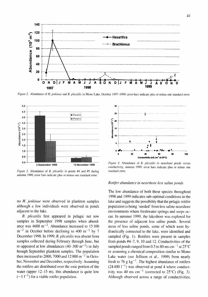
41
140
.-. 120 '1'e ~Hexarthra .., 100 0 ... -- 80 41 C) c 60 lIS "C C 40 :::I .0 c( 20
11\ •• o •• Brachionus
I \ I \ I \
.9. 0
I \~ ~.f , 'l- •• - .... ~.
o N olJ F M A M J J A SON DIJ F M A M J J A S o N D
1997 1998 1999
Figure 2. Abundance of H. jenkinae and B. plica/ilis in Mono Lake, October 1997- 1999; error bars indicate plus or minus one standard error.
5.0 ,------------------
4.5 t---,---------------
4.0
.- 3.5 .... l3.0 .. ~ 2.5 .. -g 2.0 OJ
~ 1.6
1.0
0.6
0.0 2 September 1999 13 November 1999
Figure 3. Abundance of B. plicatilis in ponds #4 and #5 during autumn 1999; error bars indicate plus or minus one standard error.
no H. jenkinae were observed in plankton samples although a few individuals were observed in ponds adjacent to the lake.
B. plicatilis first appeared in pelagic net tow samples in September 1998 samples when abundance was 4600 m- 2. Abundance increased to IS 100 m-2 in October before declining to 400 m-2 by 7 December 1998. In 1999, B. plicatilis was absent from samples collected during February through June, but re-appeared at low abundances (40-300 m- 2) in July hrough September plankton samples. The population then increased to 2000, 7000 and 12000 m- 2 in October, November and December, respectively. Assuming the rotifers are distributed over the oxic portion of the water (upper 12-IS m), this abundance is quite low ('V I I-I) for a viable rotifer population.
30 ,------ - ---.--~ .. ~---------.--~
25 -l--- - - - - - f - ----- - - ----
I ( • o ~. • ••
20 80 80 100
Conductivity (mS em-' at 2S'CI
Figure 4. Abundance of B. plicatilis in nearshore ponds versus conductivity, autumn 1999; error bars indicate plus or minus one standard error.
Rotifer abundance in nearshore less saline ponds
The low abundance of both these species throughout 1998 and 1999 indicates sub-optimal conditions in the lake and suggests the possibility that the pelagic rotifer population is being 'seeded' from less saline nearshore environments where freshwater springs and seeps occur. In summer 1999, the lakeshore was explored for the presence of adjacent less saline ponds. Several areas of less saline ponds, some of which were hydraulically connected to the lake, were identified and sampled (Fig. 1). Rotifers were present in samples from ponds #4-7,9, 10 and 12. Conductivities of the sampled ponds ranged from O.S to 80 ms cm -I at 2SoC or assuming a chemical composition similar to Mono Lake water (see Jellison et aI., 1999) from nearly fresh to 76 g kg- I. The highest abundance of rotifers (24400 I-I) was observed at pond 4 where conductivity was 40 ms cm- I (corrected to 2S°C) (Fig. 3). Although observed across a range of conductivities,
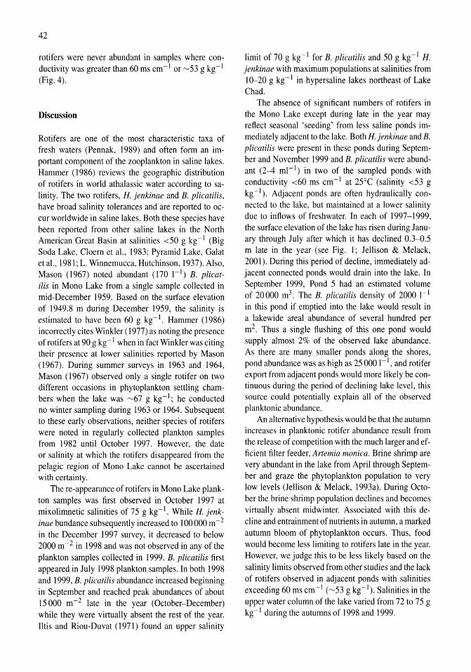
42
rotifers were never abundant in samples where conductivity was greater than 60 ms cm- I or ~53 g kg- I
(Fig. 4).
Discussion
Rotifers are one of the most characteristic taxa of fresh waters (Pennak, 1989) and often form an important component of the zooplankton in saline lakes. Hammer (1986) reviews the geographic distribution of rotifers in world athalassic water according to salinity. The two rotifers, H. jenkinae and B. plicatilis, have broad salinity tolerances and are reported to occur worldwide in saline lakes. Both these species have been reported from other saline lakes in the North American Great Basin at salinities <50 g kg- I (Big Soda Lake, Cloern et al., 1983; Pyramid Lake, Galat et al., 1981; L. Winnemucca, Hutchinson, 1937). Also, Mason (1967) noted abundant (170 I-I) B. plicatilis in Mono Lake from a single sample collected in mid-December 1959. Based on the surface elevation of 1949.8 m during December 1959, the salinity is estimated to have been 60 g kg-I. Hammer (1986) incorrectly cites Winkler (1977) as noting the presence of rotifers at 90 g kg-I when in fact Winkler was citing their presence at lower salinities reported by Mason (1967). During summer surveys in 1963 and 1964, Mason (1967) observed only a single rotifer on two different occasions in phytoplankton settling chambers when the lake was ~67 g kg-I; he conducted no winter sampling during 1963 or 1964. Subsequent to these early observations, neither species of rotifers were noted in regularly collected plankton samples from 1982 until October 1997. However, the date or salinity at which the rotifers disappeared from the pelagic region of Mono Lake cannot be ascertained with certainty.
The re-appearance of rotifers in Mono Lake plankton samples was first observed in October 1997 at mixolimnetic salinities of 75 g kg-I. While H. jenkinae bundance subsequently increased to 100000 m-2
in the December 1997 survey, it decreased to below 2000 m-2 in 1998 and was not observed in any of the plankton samples collected in 1999. B. plicatilis first appeared in July 1998 plankton samples. In both 1998 and 1999, B. plicatilis abundance increased beginning in September and reached peak abundances of about 15000 m-2 late in the year (October-December) while they were virtually absent the rest of the year. litis and Riou-Duvat (1971) found an upper salinity
limit of 70 g kg -I for B. plicatilis and 50 g kg -I H. jenkinae with maximum populations at salinities from 10-20 g kg- I in hypersaline lakes northeast of Lake Chad.
The absence of significant numbers of rotifers in the Mono Lake except during late in the year may reflect seasonal 'seeding' from less saline ponds immediately adjacent to the lake. Both H. jenkinae and B. plicatilis were present in these ponds during September and November 1999 and B. plicatilis were abundant (2-4 ml- I) in two of the sampled ponds with conductivity <60 ms cm- I at 25°C (salinity <53 g kg-I). Adjacent ponds are often hydraulically connected to the lake, but maintained at a lower salinity due to inflows of freshwater. In each of 1997-1999, the surface elevation of the lake has risen during January through July after which it has declined 0.3-0.5 m late in the year (see Fig. 1; Jellison & Melack, 2001). During this period of decline, immediately adjacent connected ponds would drain into the lake. In September 1999, Pond 5 had an estimated volume of 20000 m3. The B. plicatilis density of 2000 I-I in this pond if emptied into the lake would result in a lakewide areal abundance of several hundred per m2. Thus a single flushing of this one pond would supply almost 2% of the observed lake abundance. As there are many smaller ponds along the shores, pond abundance was as high as 25000 I-I , and rotifer export from adjacent ponds would more likely be continuous during the period of declining lake level, this source could potentially explain all of the observed planktonic abundance.
An alternative hypothesis would be that the autumn increases in planktonic rotifer abundance result from the release of competition with the much larger and efficient filter feeder, Artemia monica. Brine shrimp are very abundant in the lake from April through September and graze the phytoplankton population to very low levels (Jellison & Melack, 1993a). During October the brine shrimp population declines and becomes virtually absent midwinter. Associated with this decline and entrainment of nutrients in autumn, a marked autumn bloom of phytoplankton occurs. Thus, food would become less limiting to rotifers late in the year. However, we judge this to be less likely based on the salinity limits observed from other studies and the lack of rotifers observed in adjacent ponds with salinities exceeding 60 ms cm- I (~53 g kg-I). Salinities in the
upper water column of the lake varied from 72 to 75 g kg- I during the autumns of 1998 and 1999.
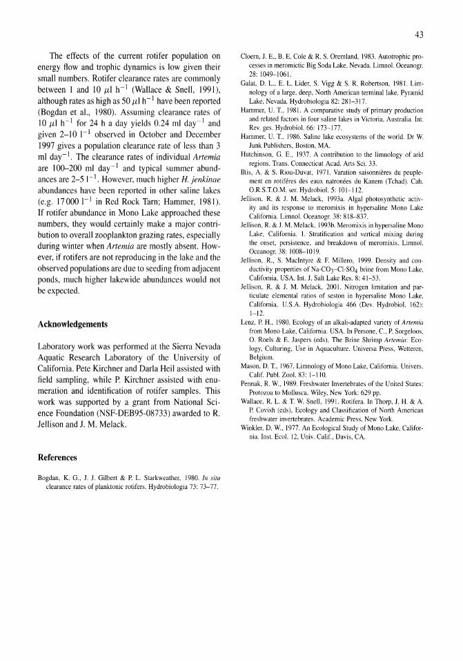
The effects of the current rotifer population on energy flow and trophic dynamics is low given their small numbers. Rotifer clearance rates are commonly between 1 and 10 fLI h -I (Wallace & Snell, 1991), although rates as high as 50 fLI h -1 have been reported (Bogdan et al., 1980). Assuming clearance rates of 10 fLl h- 1 for 24 h a day yields 0.24 ml day-I and given 2-10 I-I observed in October and December 1997 gives a population clearance rate of less than 3 ml day-I. The clearance rates of individual Arremia are 100-200 ml day-l and typical summer abundances are 2-51-1. However, much higher H. jenkinae abundances have been reported in other saline lakes (e.g. 17000 I-I in Red Rock Tam; Hammer, 1981). If rotifer abundance in Mono Lake approached these numbers, they would certainly make a major contribution to overall zooplankton grazing rates, especially during winter when Artemia are mostly absent. However, if rotifers are not reproducing in the lake and the observed populations are due to seeding from adjacent ponds, much higher lakewide abundances would not be expected.
Acknowledgements
Laboratory work was performed at the Sierra Nevada Aquatic Research Laboratory of the University of California. Pete Kirchner and Darla Heil assisted with field sampling, while P. Kirchner assisted with enumeration and identification of rotifer samples. This work was supported by a grant from National Science Foundation (NSF-DEB95-08733) awarded to R. Jellison and J. M. Melack.
References
Bogdan, K. G., 1. 1. Gilbert & P. L. Starkweather. 1980. In situ clearance rates of planktonic rotifers. Hydrobiologia 73: 73-77.
43
Cloem, 1. E., B. E. Cole & R. S. Oremland, 1983. Autotrophic processes in meromictic Big Soda Lake, Nevada. Limno!. Oceanogr. 28: 1049-1061.
Galat, D. L., E. L. Lider, S. Vigg & S. R. Robertson, 1981. Limnology of a large, deep, North American terminal lake, Pyramid Lake, Nevada. Hydrobiologia 82: 281-317.
Hammer, U. T, 1981. A comparative study of primary production and related factors in four saline lakes in Victoria, Australia. Int. Rev. ges. Hydrobio!. 66: 173-177.
Hammer, U. T, 1986. Saline lake ecosystems of the world. Dr W. Junk Publishers, Boston, MA.
Hutchinson, G. E., 1937. A contribution to the limnology of arid regions. Trans. Connecticut Acad. Arts Sci. 33.
Iltis, A. & S. Riou-Duvat, 1971. Varation saisonnieres du peuplement en rotiferes des eaux natronees du Kanem (Tchad). Cah. O.R.S.T.O.M. ser. Hydrobio!. 5: 101-112.
Jellison, R. & 1. M. Melack, I 993a. Algal photosynthetic activity and its response to meromixis in hypersaline Mono Lake California. Limno!. Oceanogr. 38: 818-837.
Jellison, R. & 1. M. Melack, 1993b. Meromixis in hypersaline Mono Lake, California. I. Stratification and vertical mixing during the onset, persistence, and breakdown of meromixis. Limno!. Oceanogr.38: 1008-1019.
Jellison, R., S. MacIntyre & F. Millero, 1999. Density and conductivity properties of Na-C03-CI-S04 brine from Mono Lake, California, USA. Int. 1. Salt Lake Res. 8: 41-53.
Jellison, R. & 1. M. Melack, 2001. Nitrogen limitation and particulate elemental ratios of seston in hypersaline Mono Lake, California, U.S.A. Hydrobiologia 466 (Dev. Hydrobiol. 162): 1-12.
Lenz, P. H., 1980. Ecology of an alkali-adapted variety of A rtemia from Mono Lake, California. USA. In Persone, c., P. Sorgeloos, O. Roels & E. Jaspers (eds), The Brine Shrimp Anemia: Ecology, Culturing, Use in Aquaculture. Universa Press, Welteren, Belgium.
Mason, D. T., 1967. Limnology of Mono Lake, California. Univers. Calif. Pub!. Zoo!. 83: 1-110.
Pennak, R. w., 1989. Freshwater Invertebrates of the United States: Protozoa to Mollusca. Wiley, New York: 629 pp.
Wallace, R. L. & T W. Snell, 1991. Rotifera. In Thorp, 1. H. & A. P. Covish (eds), Ecology and Classification of North American freshwater invertebrates. Academic Press, New York.
Winkler, D. w., 1977. An Ecological Study of Mono Lake, California. Inst. Eco!. 12, Univ. Calif., Davis, CA.
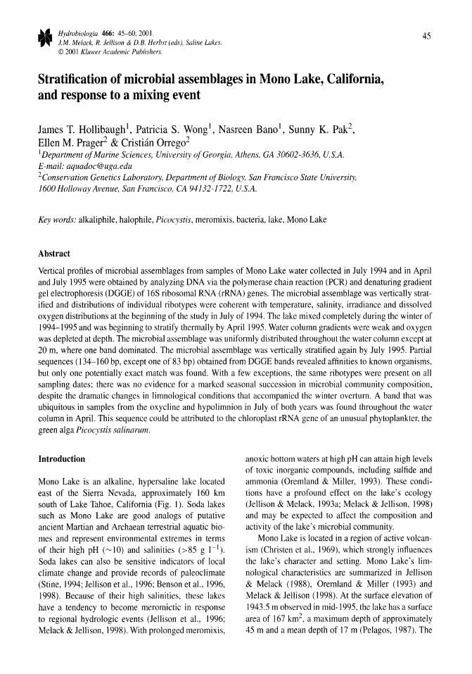
Hydrobiologia 466: 45-60,2001. J.M. Melack, R. Jellison & D.S. Herbst (eds), Saline Lakes. © 2001 Kluwer Academic Publishers.
45
Stratification of microbial assemblages in Mono Lake, California, and response to a mixing event
James T. Hollibaugh!, Patricia S. Wong!, Nasreen Bano!, Sunny K. Pak2,
Ellen M. Prager2 & Cristian Orrego2
1 Department of Marine Sciences, University of Georgia, Athens, GA 30602-3636, U.S.A. E-mail: [email protected] 2Conservation Genetics Laboratory, Department of Biology, San Francisco State University, 1600 Holloway Avenue, San Francisco, CA 94132-1722, u.s.A.
Key words: alkaliphile, halophile, Picocystis, meromixis, bacteria, lake, Mono Lake
Abstract
Vertical profiles of microbial assemblages from samples of Mono Lake water collected in July 1994 and in April and July 1995 were obtained by analyzing DNA via the polymerase chain reaction (PCR) and denaturing gradient gel electrophoresis (DGGE) of 16S ribosomal RNA (rRNA) genes. The microbial assemblage was vertically stratified and distributions of individual ribotypes were coherent with temperature, salinity, irradiance and dissolved oxygen distributions at the beginning of the study in July of 1994. The lake mixed completely during the winter of 1994-1995 and was beginning to stratify thermally by April 1995. Water column gradients were weak and oxygen was depleted at depth. The microbial assemblage was uniformly distributed throughout the water column except at 20 m, where one band dominated. The microbial assemblage was vertically stratified again by July 1995. Partial sequences (134-160 bp, except one of 83 bp) obtained from DGGE bands revealed affinities to known organisms, but only one potentially exact match was found. With a few exceptions, the same ribotypes were present on all sampling dates; there was no evidence for a marked seasonal succession in microbial community composition, despite the dramatic changes in limnological conditions that accompanied the winter overturn. A band that was ubiquitous in samples from the oxycline and hypolimnion in July of both years was found throughout the water column in April. This sequence could be attributed to the chloroplast rRNA gene of an unusual phytoplankter, the green alga Picocystis salinarum.
Introduction
Mono Lake is an alkaline, hypersaline lake located east of the Sierra Nevada, approximately 160 km south of Lake Tahoe, California (Fig. I). Soda lakes such as Mono Lake are good analogs of putative ancient Martian and Archaean terrestrial aquatic biomes and represent environmental extremes in terms of their high pH (~IO) and salinities (>85 g 1-'). Soda lakes can also be sensitive indicators of local climate change and provide records of paleoclimate (Stine, 1994; Jellison et aI., 1996; Benson et aI., 1996, 1998). Because of their high salinities, these lakes have a tendency to become meromictic in response to regional hydrologic events (Jellison et aI., 1996; Melack & Jellison, 1998). With prolonged meromixis,
anoxic bottom waters at high pH can attain high levels of toxic inorganic compounds, including sulfide and ammonia (Oremland & Miller, 1993). These conditions have a profound effect on the lake's ecology (Jellison & Melack, 1993a; Melack & Jellison, 1998) and may be expected to affect the composition and activity of the lake's microbial community.
Mono Lake is located in a region of active volcanism (Christen et aI., 1969), which strongly influences the lake's character and setting. Mono Lake's limnological characteristics are summarized in Jellison & Melack (1988), Oremland & Miller (1993) and Melack & Jellison (1998). At the surface elevation of 1943.5 m observed in mid-1995, the lake has a surface area of 167 km2, a maximum depth of approximately 45 m and a mean depth of 17 m (Pelagos, 1987). The
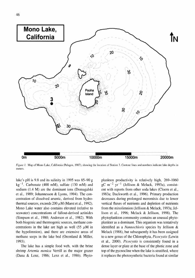
46
Mono Lake,
tN California
,,0 20
i?
I-
C6
"1.0
<6 3 •
0 (')
.... <::>
Om SOOOm 10000m 15000m 20000m
Figure I. Map of Mono Lake, California (Pelagos. 1987). showing the location of Station 3. Contour lines and numbers indicate lake depths in meters.
lake's pH is 9.8 and its salinity in 1995 was 85-90 g kg -I. Carbonate (400 mM), sulfate (130 mM) and sodium (1.4 M) are the dominant ions (Domagalski et al., 1989; Johannesson & Lyons, 1994). The concentration of dissolved arsenic, derived from hydrothermal sources, exceeds 200 f.l.M (Maest et a!., 1992). Mono Lake water also contains elevated (relative to seawater) concentrations of fallout-derived actinides (Simpson et a!., 1980; Anderson et a!., 1982). With both biogenic and thermogenic sources, methane concentrations in the lake are high as well (55 f.l.M in the hypolimnion), and there are extensive areas of methane seeps in the lake bed (Oremland & Miller, 1993).
The lake has a simple food web, with the brine shrimp Artemia monica Verrill as the major grazer (Dana & Lenz, 1986; Lenz et aI., 1986). Phyto-
plankton productivity is relatively high, 269-1060 gC m-2 yC I (Jellison & Melack, 1993a), consistent with reports from other soda lakes (Cloem et al., 1983a; Duckworth et a!., 1996). Primary production decreases during prolonged meromixis due to lower vertical fluxes of nutrients and depletion of nutrients from the mixolimnion (Jellison & Melack, 1993a; Jellison et a!., 1996; Melack & Jellison, 1998). The phytoplankton community contains an unusual phytoplankter as a dominant. This organism was tentatively identified as a Nannochloris species by Jellison & Melack (1988), but subsequently it has been assigned to a new genus of the Chlorophyta, Picocystis (Lewin et al., 2000). Picocystis is consistently found in a dense layer or plate at the base of the photic zone and top of the pycnocline when the lake is stratified, where it replaces the photosynthetic bacteria found at similar
locations in other lakes (for example, Big Soda Lake; Cloern et ai., 1983a,b).
Earlier studies (Domagalski et ai., 1989) and our own unpublished observations have shown that Mono Lake supports elevated dissolved organic carbon (DOC) concentrations (>80 mg 1-1) and bacterioplankton abundance (> 1QlOcells 1-1). Bacterioplankton cells tend to be large (> I /Lm) with many chain-forming organisms, particularly when A. monica is not present. This is also consistent with reports from other soda lakes (Zehr et a1., 1987; Duckworth et ai., 1996). However, relatively little is known about the types of microorganisms dwelling in the lake and their phylogenetic diversity, taxonomy, ecology or ecophysiology.
Bacteria isolated from the lake's surface waters grow best at pH 9.7 and are able to use organic osmolytes as carbon sources (Diaz & Taylor, 1996). Alkaliphilic bacteria are of interest from physiological and industrial perspectives (Horikoshi & Akiba, 1982; Grant el ai., 1990), and recent studies have stressed the phylogenetic diversity of bacteria isolated from soda lakes (Duckworth et ai., 1996). However, little work has been done on the in situ phylogenetic diversity of bacterial populations from soda lakes, or in ascribing aspects of the biogeochemical cycles of these lakes to these bacteria.
Meromixis is a recurring event in Mono Lake's limnology, and several papers have described the consequences of meromixis and its breakdown to Mono Lake's ecology and geochemistry (Jellison et a1., 1993a,b; Miller et ai., 1993; Jellison et aI., 1996; Melack & Jellison, 1998). A long period of meromixis in the 1980's was initiated by runoff from the EI Niiio winter of 1982-1983. This event persisted until 1988, when drought in California contributed to the weakening of salinity stratification, initiating a period of monomixis that persisted through the dry winter of 1993-1994. Meromixis was re-established in 1995 as a result of changes in water management policy and high runoff during the El Niiio winter of 1994-1995. A hydrodynamic mixing model (Jellison et a1., 1998) predicts that the lake will exhibit prolonged meromixis.
The re-establishment of meromixis in Mono Lake in 1995 afforded us an opportunity to investigate the response of the lake's microbial community to this condition. We were able to characterize the microbial community that had developed during 6 years of monomixis and to compare it with the community that developed within months of the re-establishment of
47
meromixis. These ana1yses provide a starting point for future studies of the response of the lake's microbia1 community to prolonged meromixis. We also began characterizing the phylogenetic composition and vertical distribution of Mono Lake's microbia1 community.
Materials and methods
Sample collection
Water samples were collected at Station 3 [Fig. 1; Station 9 in previous papers on Mono Lake such as Jellison & Melack (1993a), Melack & Jellison (1998) and Joye et al. (1999)], located offshore in 30-m deep water. Water column profiles and samples were taken at midday on July 20, 1994; April 9, 1995; and July 20, 1995. Temperature, pressure, photosynthetically active radiation (PAR at 400-700 nm, Licor 41i sensor) and in vivo chlorophyll fluorescence (relative fluorescence, RF, in arbitrary units; SeaTech fluorometer) were obtained with a SeaBird SeaCat profiler on the July expeditions. Conductivity was not measured because this instrument was not equipped with a high-sa1inity conductivity sensor. Oxygen profiles were taken with a polarographic oxygen sensor (YSI) equipped with a Clarke-type electrode. Beam attenuation (%T) was measured with a Martek XMS transmissometer equipped with a 25-cm path length sensor. Conductivity and temperature data for April 1995 were supplied by R. Jellison and were taken with a SeaBird SeaCat conductivity, temperature and pressure logger (CID) equipped with a special highsalinity conductivity sensor. Vertical distributions of chlorophyll, ammonium, methane, ammonia oxidation rate and methane oxidation rate at this station and on these sampling dates are given in Joye et ai. (1999).
Water samples (500-1000 ml) were taken at discrete depths using a Niskin water sampler. The samples were poured into dark plastic bottles and held in a cooler until they were processed (within 4 h of collection). The samples were filtered through either 47 mm diameter Millipore GV filters (0.22 /Lm pore size, 80 kPa vacuum) or Millipore Sterivex filter cartridges (0.22 /Lm pore size, 100 kPa pressure) to collect microbial biomass for subsequent DNA extraction. Flat filters were placed in disposable 15-ml plastic centrifuge tubes (Falcon), bathed with about 3 ml of extraction buffer (40 mM EDTA; 50 mM Tris, pH 8.3; 0.75 M sucrose) and frozen on dry ice. Water
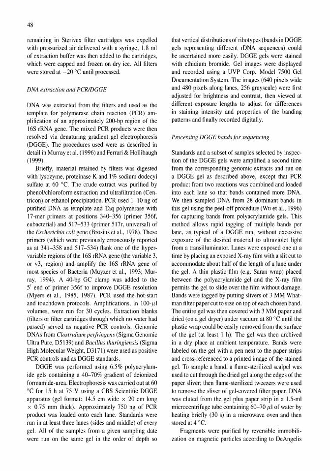
48
remaining in Sterivex filter cartridges was expelled with pressurized air delivered with a syringe; 1.8 ml of extraction buffer was then added to the cartridges, which were capped and frozen on dry ice. All filters were stored at -20°C until processed.
DNA extraction and PCRJDGGE
DNA was extracted from the filters and used as the template for polymerase chain reaction (PCR) amplification of an approx.imately 200-bp region of the 16S rRNA gene. The mixed PCR products were then resolved via denaturing gradient gel electrophoresis (DGGE). The procedures used were as described in detail in Murray et al. (1996) and Ferrari & Hollibaugh (1999).
Briefly, material retained by filters was digested with lysozyme, proteinase K and 1 % sodium dodecyl sulfate at 60°C. The crude extract was purified by phenol/chloroform extraction and ultrafiltration (Centricon) or ethanol precipitation. PCR used I-lOng of purified DNA as template and Taq polymerase with 17-mer primers at positions 340-356 (primer 356f, eubacterial) and 517-533 (primer 517r, universal) of the Escherichia coli gene (Brosius et aI., 1978). These primers (which were previously erroneously reported as at 341-358 and 517-534) flank one of the hypervariable regions of the 16S rRNA gene (the variable 3, or v3, region) and amplify the 16S rRNA gene of most species of Bacteria (Muyzer et aI., 1993; Murray, 1994). A 40-bp GC clamp was added to the 5' end of primer 356f to improve DGGE resolution (Myers et aI., 1985, 1987). PCR used the hot-start and touchdown protocols. Amplifications, in 100-fLl volumes, were run for 30 cycles. Extraction blanks (filters or filter cartridges through which no water had passed) served as negative PCR controls. Genomic DNAs from Clostridium perfringens (Sigma Genomic Ultra Pure, D5l39) and Bacillus thuringiensis (Sigma High Molecular Weight, D3l71) were used as positive PCR controls and as DGGE standards.
DGGE was performed using 6.5% polyacrylamide gels containing a 40-70% gradient of deionized formamide-urea. Electrophoresis was carried out at 60 °C for 15 h at 75 V using a CBS Scientific DGGE apparatus (gel format: 14.5 cm wide x 20 cm long x 0.75 mm thick). Approximately 750 ng of PCR product was loaded onto each lane. Standards were run in at least three lanes (sides and middle) of every gel. All of the samples from a given sampling date were run on the same gel in the order of depth so
that vertical distributions of ribotypes (bands in DGGE gels representing different rDNA sequences) could be ascertained more easily. DGGE gels were stained with ethidium bromide. Gel images were displayed and recorded using a UVP Corp. Model 7500 Gel Documentation System. The images (640 pixels wide and 480 pixels along lanes, 256 grayscale) were first adjusted for brightness and contrast, then viewed at different exposure lengths to adjust for differences in staining intensity and properties of the banding patterns and finally recorded digitally.
Processing DGGE bands for sequencing
Standards and a subset of samples selected by inspection of the DGGE gels were amplified a second time from the corresponding genomic extracts and run on a DGGE gel as described above, except that PCR product from two reactions was combined and loaded into each lane so that bands contained more DNA. We then sampled DNA from 28 dominant bands in this gel using the peel-off procedure (Wu et aI., 1996) for capturing bands from polyacrylamide gels. This method allows rapid tagging of multiple bands per lane, as typical of a DGGE run, without excessive exposure of the desired material to ultraviolet light from a transilluminator. Lanes were exposed one at a time by placing an exposed X-ray film with a slit cut to accommodate about half of the length of a lane under the gel. A thin plastic film (e.g. Saran wrap) placed between the polyacrylamide gel and the X-ray film permits the gel to slide over the film without damage. Bands were tagged by putting slivers of 3 MM Whatman filter paper cut to size on top of each chosen band. The entire gel was then covered with 3 MM paper and dried (on a gel dryer) under vacuum at 80°C until the plastic wrap could be easily removed from the surface of the gel (at least 1 h). The gel was then archived in a dry place at ambient temperature. Bands were labeled on the gel with a pen next to the paper strips and cross-referenced to a printed image of the stained gel. To sample a band, a flame-sterilized scalpel was used to cut through the dried gel along the edges of the paper sliver; then flame-sterilized tweezers were used to remove the sliver of gel-covered filter paper. DNA was eluted from the gel plus paper strip in a 1.5-ml micro centrifuge tube containing 60-70 fLl of water by heating briefly (30 s) in a microwave oven and then stored at 4 0C.
Fragments were purified by reversible immobilization on magnetic particles according to DeAngelis
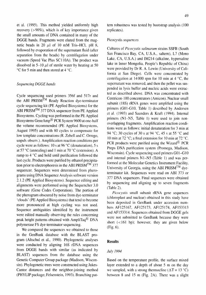
et al. (1995). This method yielded uniformly high recovery (>90%), which is of key importance given the small amounts of DNA contained in many of the DGGE bands. Fragments were eluted from the magnetic beads in 20 ILl of 10 mM Tris-HCl, pH 8, followed by evaporation of the supernatant fluid (after separation from the beads) by centrifugation under vacuum (Speed Vac Plus SCllOA). The product was dissolved in 5-10 ILl of sterile water by heating at 50 °C for 5 min and then stored at 4 0c.
Sequencing DGGE bands
Cycle sequencing used primers 356f and 517r and the ABI PRISM™ Ready Reaction dye-terminator cycle sequencing kit (PE Applied Biosystems) for the ABI PRISM™ 377 DNA sequencer from PE Applied Biosystems. Cycling was performed in the PE Applied Biosystems GeneAmp® PCR System 9600 at one-half the volume recommended (PE Applied Biosystems, August 1995) and with 80 cycles to compensate for low template concentrations (R. Zebell and C. Orrego, unpub. observ.). Amplification reaction conditions per cycle were as follows: 10 s at 96°C (denaturation), 5 s at 57°C (annealing) and I min at 70 °C (extension). A ramp to 4 °C and hold until purification followed the last cycle. Products were purified by ethanol precipitation prior to electrophoresis in the ABI PRISM™ 377 sequencer. Sequences were determined from pherograms using DNA Sequence Analysis software version 2.1.2 (PE Applied Biosystems). Sequence editing and alignments were performed using the Sequencher 3.0 software (Gene Codes Corporation). The portion of the pherogram obscured by noise from dye-terminator 'clouds' (PE Applied Biosystems) that tend to become more pronounced at high cycling was not used. Sequence ambiguities identified by the instrument were edited manually observing the rules concerning peak height patterns obtained with AmpliTaq® DNA polymerase FS dye-terminator sequencing.
We compared the sequences we obtained to those in the GenBank database with the BLAST program (Altschul et a!., 1990). Phylogenetic analyses were conducted by aligning 16S rDNA sequences from DGGE bands with similar (as indicated by BLAST) sequences from the database using the Genetic Computer Group package (Madison, Wisconsin). Phylogenetic trees were constructed using JukesCantor distances and the neighbor-joining method (PHYLIP package; Felsenstein, 1993). Branching pat-
49
tern robustness was tested by bootstrap analysis (100 replicates).
Picocystis sequences
Cultures of Picocystis salinarum strains SSFB (South San Francisco Bay, CA, U.S.A., saltern), L7 (Mono Lake, CA, U.S.A.) and IM214 (alkaline, hypersaline lake in Inner Mongolia, People's Republic of China) were provided by Dr R. A. Lewin (University of California at San Diego). Cells were concentrated by centrifugation at 14000 rpm for 10 min at 4°C, the supernatant was removed, and then the pellet was suspended in lysis buffer and nucleic acids were extracted as described above. DNA was concentrated with Centricon-IOO concentrators (Amicon). Nuclear small subunit (18S) rRNA genes were amplified using the primers (GOl-GlO, Table 1) described by Andersen et al. (1993) and Saunders & Kraft (1994). Internal primers (NI-N5, Table I) were used to join nonoverlapping fragments. Amplification reaction conditions were as follows: initial denaturation for 3 min at 94°C; 30 cycles of 30 s at 94°C, 45 s at 55°C and 10 min at 72 °C; a final extension for 10 min at 72 °C. PCR products were purified using the Wizard® PCR Preps DNA purification system (Promega, Madison, Wisconsin). Cycle sequencing used primers GO I-G 10 and internal primers NI-N5 (Table I) and was performed at the Molecular Genetics Instrument Facility, University of Georgia, using the ABI PRISM™ dyeterminator kit. Sequences were read on ABI 373 or 377 DNA sequencers. Final sequences were obtained by sequencing and aligning up to seven fragments (Table 2).
Picocystis small subunit rRNA gene sequences (chloroplast and nuclear) obtained in this study have been deposited in GenBank under accession numbers AF125167, AFI25173, AFI25174, AF153313 and AF153314. Sequences obtained from DGGE gels were not submitted to GenBank because they were short (<161 bp); however, they are given below (Fig. 6).
Results
July 1994
Based on the temperature profile, the surface mixed layer extended to a depth of about 5 m on the day we sampled, with a strong thermocline (L1T = 13 0c) between 8 and 15 m (Fig. 2A). There was a slight
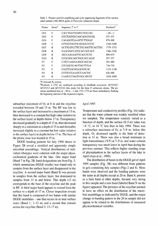
50
Table I. Primers used for amplifying and cycle sequencing fragments of the nuclear small subunit (l8S) rRNA genes of Picocystis salinarum strains
Primer Sensea Sequence, 5' to 3' Positionsb
GOI F CACCTGGTTGATCCTGCCAG -20---1
G03 F GTCTGGTGCCAGCAGCCGCGG 537-557
G04 F CAGAGGTGAAATTCTTGGAT 879-898
G06 F GTTGGTGGTGCATGGCCGTTC 1246-1266
G07 R GCTTGATCCTTCTGCAGGTTCACCTAC 1779-1753
G08 R GAACGGCCATGCACCACCACC 1266-1246
G09 R ATCCAAGAATTTCACCTCTG 898-879
010 R CCGCGGCAGCTGGCACCAGAC 557-537
Nl F CATCCAAGGAAGGCAGCAG 391-409
N2 F GTCGGCGCAGTTACTTTGA 716-734
N3 F GAATTGACGGAACGGCAC 1123-1140
N4 R CCGTCCGAAATCCAACTAC 626-608
N5 R CAATCCCTAGTCGGCATCGT 1028-1009
aF, forward; R, reverse. bpositions 1-1752 are numbered according to GenBank accessions AF125167, AF153313 and AFl533l4 (this study) for the three P. salina rum strains. The po-sitions numbered here as - 20 to -1 and 1753-l779 are those immediately flanking the beginning and end of the sequenced region.
subsurface maximum of 02 at 8 m and the oxycline extended between 10 and 15 m. The RF was low in the surface layer and increased to a maximum at 13 m, then decreased to a constant but high value (relative to the surface layer) at depths below 17 m. Transparency decreased gradually to a depth of 13 m, then decreased sharply to a minimum at a depth of 15 m and thereafter increased slightly to a constant but low value (relative to the surface layer) at depths below 17 m. The base of the photic zone was located at 15 m.
DGGE banding patterns for July 1994 shown in Figure 2B reveal a stratified and apparently simple microbial assemblage. Vertical distributions of individual ribotypes were coherent with the major physicochemical gradients of the lake. One major band (Band 7 in Fig. 2B; band designations are from Fig. 5, which summarizes DGGE results) was found only in samples from the surface layer and disappeared in the oxycline. A second major band (Band 8) was present in samples from the surface layer, but dominated in samples from 13 m and below. This depth (13 m) corresponds to the base of the oxycline and the peak in RF. A third major band appears to extend from the surface to a depth of 17 m. Closer inspection reveals that this band is composed of two bands with similar DGGE mobilities - one that occurs in or near surface water (Band I; 1-12 m) and a second that extends across the oxycline (Band 3; 13-17 m).
April 1995
Temperature and conductivity profiles (Fig. 3A) indicate that the water column was weakly stratified when we sampled. The temperature scarcely varied as a function of depth, and the surface (0-5 m) value was ~6 °C, or 16°C less than in July 1994. There was a subsurface maximum of 02 at 7-9 m; below this depth, 02 decreased rapidly to the limit of detection at 14 m. There was also a broad minimum in light transmittance (%T) at 7-9 m, and water column transparency was much lower in April than during the previous summer. This reflects higher standing crops of phytoplankton in the surface layers of the lake in April (J oye et aI., 1999).
The distribution of bands in the DGGE gel of April 1995 samples (Fig. 3B) was different from patterns in gels containing July samples (Figs 2 and 4). More bands were observed and the banding patterns were the same at all depths except at 20 m. Band 8, present as a faint band at other depths, became very strong in this sample and a new band (labeled Band N on the figure) appeared. The presence of the oxycline seemed to have no effect on the distribution of the microbial assemblage as indicated by DGGE, and the major change in banding pattern in the 20 m sample did not appear to be related to the distributions of measured physicochemical variables.
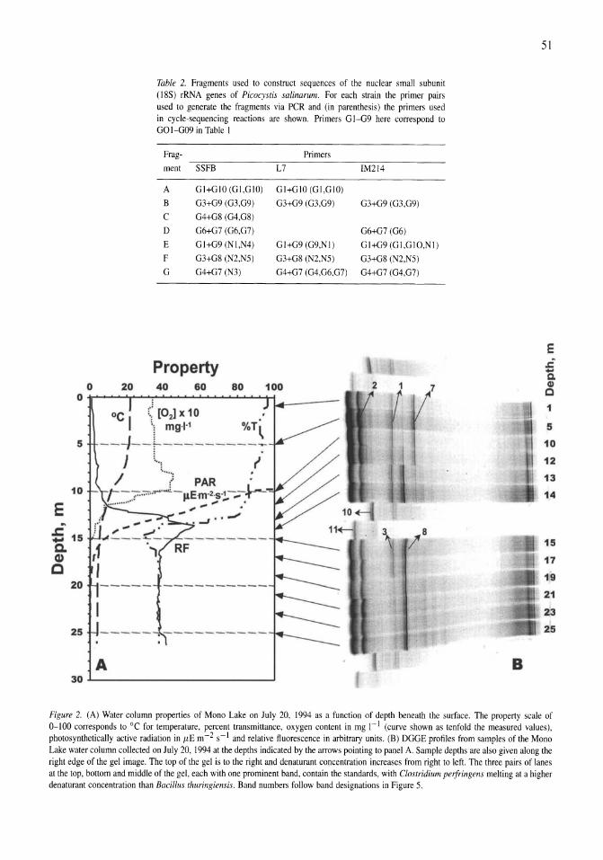
5
10
E ~
;: 15 Co G)
C 20
25
20
A
Table 2. Fragments used to construct sequences of the nuclear small subunit (l8S) rRNA genes of Picocystis salinarum. For each strain the primer pairs used to generate the fragments via PCR and (in parenthesis) the primers used in cycle-sequencing reactions are shown. Primers G I-G9 here correspond to GOI-G09 in Table I
Frag- Primers
ment SSFB L7 IM214
A Gl+GIO (GI ,GIO) Gl+GIO (GI,G 10)
B 03+G9 (G3,G9) G3+G9 (G3,G9) 03+G9 (G3,G9)
C G4+G8 (G4,G8)
D G6+G7 (G6,07) G6+G7 (G6)
E GI+G9 (NI,N4) GI+G9 (G9,NI ) GI+G9 (GI,GIO,NI)
F 03+G8 (N2,NS) G3+G8 (N2,NS) 03+G8 (N2,NS)
G G4+G7 (N3) G4+07 (G4,G6,07) G4+G7 (G4,G7)
Property 40 60 80 2
30~------------------------~
B
51
E ~ .. a. CD C
1
5
10
12
13
14
15
17
19
21
23
25
Figure 2. (A) Water column properties of Mono Lake on July 20, 1994 as a function of depth beneath the surface. The property scale of 0-100 corresponds to °c for temperature, percent transmittance, oxygen content in mg I-I (curve shown as tenfold the measured values), photosynthetically active radiation in JlE m-2 s-1 and relative fluorescence in arbitrary units. (B) DGGE profiles from samples of the Mono Lake water column collected on July 20, 1994 at the depths indicated by the arrows pointing to panel A. Sample depths are also given along the right edge of the gel image. The top of the gel is to the right and denaturant concentration increases from right to left. The three pairs of lanes at the top, bottom and middle of the gel, each with one prominent band, contain the standards, with Clostridium perfringens melting at a higher denaturant concentration than Bacillus thuringiensis. Band numbers follow band designations in Figure S.
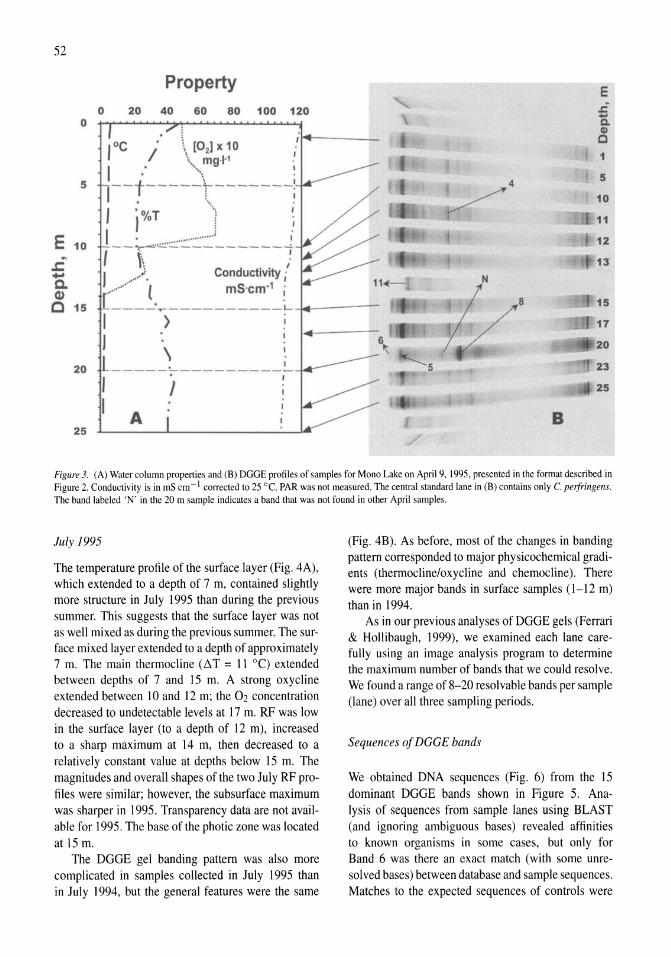
52
o
5
E 10
.c. -c.
Property
o 20 40 60 80 100 120
J °C / \, [02] x 10 ;, mg·,·1 . I . ..... I
I--t-----r-------i J J%T \1 .' I .. , ........ 1 I -- ..... """'~.::::.:::..---------'. It! J ,) Conductivity .1
.,.~ • I
E .r; -Co CII 0
1
4 5
10
11
12
13
N
i 8 15 ,........ l mS'cm-1 i r ____ ' ----------L ...-M----;-
Q)
C 15
20
25
I I
> \
-----'---------_:.. I
A
17
20
5 23
25
B
Figure 3. (A) Water column properties and (B) DGGE profiles of samples for Mono Lake on April 9, 1995, presented in the format described in Figure 2. Conductivity is in mS cm- 1 corrected to 25°C. PAR was not measured. The central standard lane in (B) contains only C. perfringens. The band labeled 'N' in the 20 m sample indicates a band that was not found in other April samples.
July 1995
The temperature profile of the surface layer (Fig. 4A), which extended to a depth of 7 m, contained slightly more structure in July 1995 than during the previous summer. This suggests that the surface layer was not as well mixed as during the previous summer. The surface mixed layer extended to a depth of approximately 7 m. The main thermocline (~T = 11°C) extended between depths of 7 and 15 m. A strong oxycline extended between 10 and 12 m; the 02 concentration decreased to undetectable levels at 17 m. RF was low in the surface layer (to a depth of 12 m), increased to a sharp maximum at 14 m, then decreased to a relatively constant value at depths below 15 m. The magnitudes and overall shapes of the two July RF profiles were similar; however, the subsurface maximum was sharper in 1995. Transparency data are not available for 1995. The base of the photic zone was located at 15 m.
The DGGE gel banding pattern was also more complicated in samples collected in July 1995 than in July 1994, but the general features were the same
(Fig. 4B). As before, most of the changes in banding pattern corresponded to major physicochemical gradients (thermocline/oxycline and chemocline). There were more major bands in surface samples (1-12 m) than in 1994.
As in our previous analyses of DGGE gels (Ferrari & Hollibaugh, 1999), we examined each lane carefully using an image analysis program to determine the maximum number of bands that we could resolve , We found a range of 8-20 resolvable bands per sample (lane) over all three sampling periods.
Sequences of DGGE bands
We obtained DNA sequences (Fig. 6) from the 15 dominant DGGE bands shown in Figure 5. Analysis of sequences from sample lanes using BLAST (and ignoring ambiguous bases) revealed affinities to known organisms in some cases, but only for Band 6 was there an exact match (with some unresolved bases) between database and sample sequences. Matches to the expected sequences of controls were
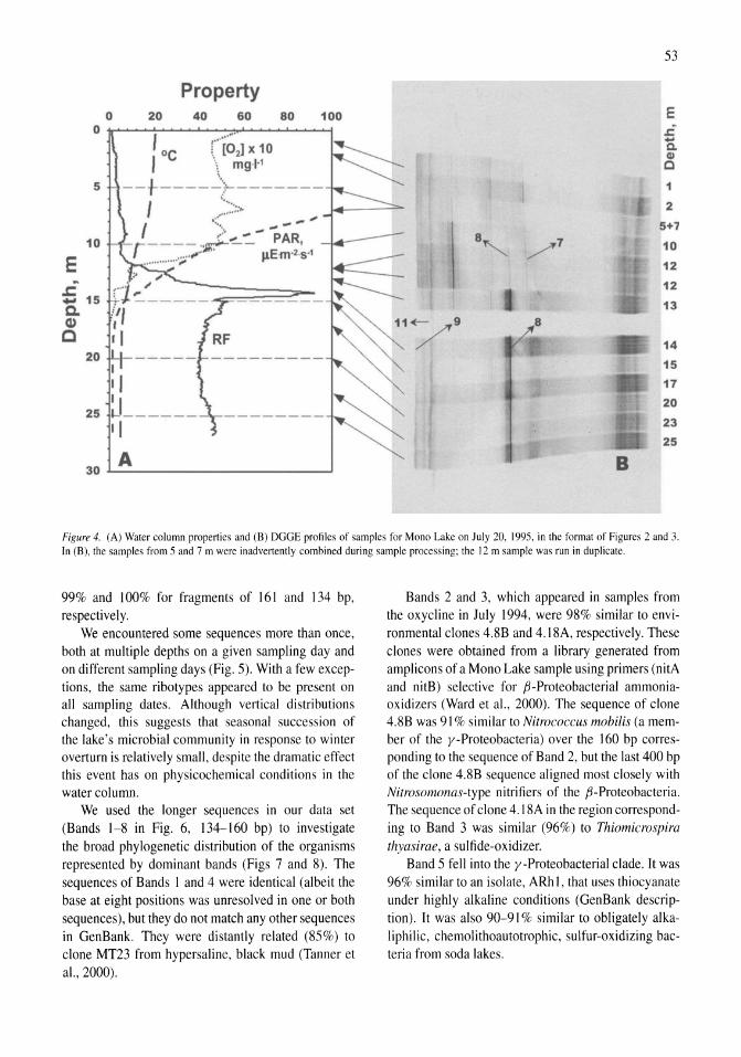
Property 20 40 60 80 100
5
10
E .r::. _ 15
a. Q)
C 20
I
II II 25 W _____ _
II A 30 ______________________ __J
53
E .c ... 0. Q)
C
1
2
5+7 8
/ 7 10
12
12
13
14
15
17
20
23
25
B
Figure 4. (A) Water column properties and (B) DGGE profiles of samples for Mono Lake on July 20. 1995, in the format of Figures 2 and 3. In (B), the samples from 5 and 7 m were inadvertently combined during sample processing; the 12 m sample was run in duplicate.
99% and 100% for fragments of 161 and 134 bp, respectively.
We encountered some sequences more than once, both at multiple depths on a given sampling day and on different sampling days (Fig. 5). With a few exceptions, the same ribotypes appeared to be present on all sampling dates. Although vertical distributions changed, this suggests that seasonal succession of the lake's microbial community in response to winter overturn is relatively small , despite the dramatic effect this event has on physicochemical conditions in the water column,
We used the longer sequences in our data set (Bands 1-8 in Fig. 6, 134-160 bp) to investigate the broad phylogenetic distribution of the organisms represented by dominant bands (Figs 7 and 8). The sequences of Bands I and 4 were identical (albeit the base at eight positions was unresolved in one or both sequences), but they do not match any other sequences in GenBank. They were distantly related (85%) to clone MT23 from hypersaline, black mud (Tanner et aI., 2000).
Bands 2 and 3, which appeared in samples from the oxycline in July 1994, were 98% similar to environmental clones 4.8B and 4.18A, respectively. These clones were obtained from a library generated from amplicons of a Mono Lake sample using primers (nitA and nitB) selective for ,B-Proteobacterial ammoniaoxidizers (Ward et aI., 2000). The sequence of clone 4.8B was 91 % similar to Nitrococcus mobilis (a member of the y-Proteobacteria) over the 160 bp corresponding to the sequence of Band 2, but the last 400 bp of the clone 4.8B sequence aligned most closely with Nitrosomonas-type nitrifiers of the ,B-Proteobacteria. The sequence of clone 4.18A in the region corresponding to Band 3 was similar (96%) to Thiomicrospira thyasirae, a sulfide-oxidizer.
Band 5 fell into the y-Proteobacterial clade. It was 96% similar to an isolate, ARh I, that uses thiocyanate under highly alkaline conditions (GenBank description). It was also 90-91 % similar to obligately alkaliphilic, chemolithoautotrophic, sulfur-oxidizing bacteria from soda lakes.
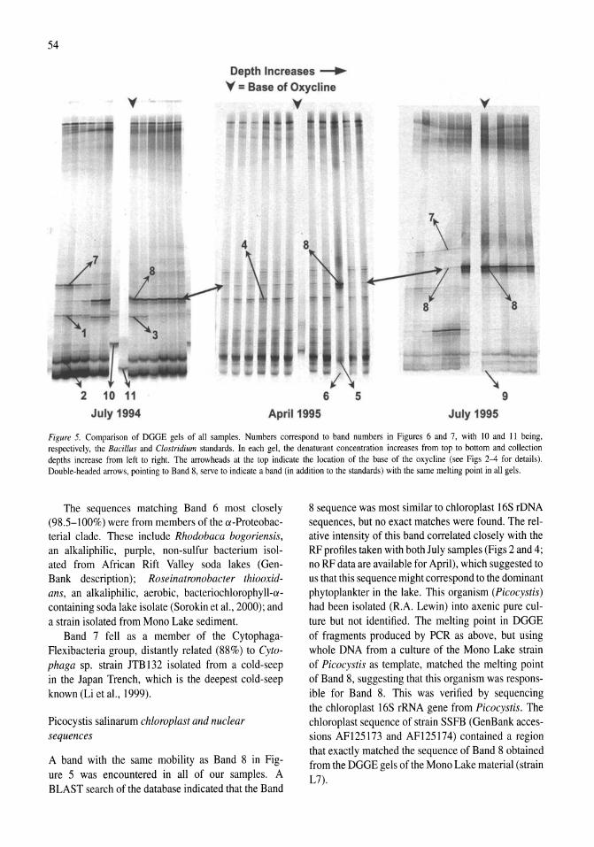
54
Depth Increases --..
V = Base of Oxycline
V
2 10 11 6 5 9
July 1994 April 1995 July 1995
Figure 5. Comparison of DGGE gels of all samples. Numbers correspond to band numbers in Figures 6 and 7, with 10 and 11 being, respectively, the Bacillus and Clostridium standards. In each gel, the denaturant concentration increases from top to bottom and collection depths increase from left to right. The arrowheads at the top indicate the location of the base of the oxycline (see Figs 2-4 for details). Double-headed arrows, pointing to Band 8, serve to indicate a band (in addition to the standards) with the same melting point in all gels.
The sequences matching Band 6 most closely (98.5-100%) were from members of the a-Proteobacterial clade. These include Rhodobaca bogoriensis, an alkaliphilic, purple, non-sulfur bacterium isolated from African Rift Valley soda lakes (GenBank description); Roseinatronobacter thiooxidans, an alkaliphilic, aerobic, bacteriochlorophyll-acontaining soda lake isolate (Sorokin et aI. , 2000); and a strain isolated from Mono Lake sediment.
Band 7 fell as a member of the CytophagaFlexibacteria group, distantly related (88%) to Cytophaga sp. strain JTB 132 isolated from a cold-seep in the Japan Trench, which is the deepest cold-seep known (Li et aI., 1999).
Picocystis salinarum chloroplast and nuclear sequences
A band with the same mobility as Band 8 in Figure 5 was encountered in all of our samples. A BLAST search of the database indicated that the Band
8 sequence was most similar to chloroplast 16S rDNA sequences, but no exact matches were found. The relative intensity of this band correlated closely with the RF profiles taken with both July samples (Figs 2 and 4; no RF data are available for April), which suggested to us that this sequence might correspond to the dominant phytoplankter in the lake. This organism (Picocystis) had been isolated (RA Lewin) into axenic pure culture but not identified. The melting point in DGGE of fragments produced by PCR as above, but using whole DNA from a culture of the Mono Lake strain of Picocystis as template, matched the melting point of Band 8, suggesting that this organism was responsible for Band 8. This was verified by sequencing the chloroplast 16S rRNA gene from Picocystis. The chloroplast sequence of strain SSFB (GenBank accessions AF125173 and AF125174) contained a region that exactly matched the sequence of Band 8 obtained from the DGGE gels of the Mono Lake material (strain L7).
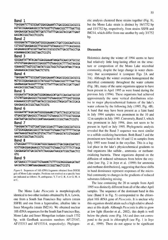
Band 1 TGAGGAATCTTGCGCAATGGAGGAAANTCTGACGCAGCCACGCCG AGTGCCGGAAGAAGGCCCTATGGGTTGTAAACGGCTTTTAATTGG GAAGAAGGATAGGGTNTTGATCTTATTTGACGGTACCGATTGAAT AAGCNCCGGCTACCTCCGTG Band 2 GGGGGAATATTGGACAATGGGGGAAANCCTGATCCAGCAATGCCG CGTGGGTGAAGAAGGCTTGCGGGTTGTAAAGCCCTTTCAGCAGGG AAGAAAAGCNTGCGGTTAATACCCGCGCGTATTGACGTTACCTGA AGAANAAGCNCCGGCTAACTCCGTG Band 3 GGGGAATATTNTACAATGGAGGAAANTANGATGCAACCATGCCGC GTGTGTGAAGAAGGCCCGAGGGTTGTAAAGCACTTTTAGTAAGGA GGAAAGGTTAGTCGCTAATATCGGCTAGCTGTGACNTNACTTACA GAAAAAGCACCGGCTAACTCTGTG Band 4 TGAGGAATNTTGCGCAATGGAGGAAANTCNGACGCAGCCACGCCG NGTGCCGGAAGAAGGCCCTATGGGTTGTAAACGGCTTTTAATTGG GAARAAGGATAGGGTTTTGATCTTATTTGACGGTACCGATTGAAT AAGCACCGGCTANCTCCGTG Band 5 GGGGAATATTAGACAATGGGNGNAAGCNTGATCCAACAATGCCGT GTGTNTGAAGAAGGCCTGCGGGTTGTAAAGCACTTTCAGTGGGGA AGAAAAGCCGTCGGTYAATACCCGGCAGCCTNGACATTACCCACA GAAGAAGCACCGGCTAACTCCGTG Band 6 GGGGAATNTTAGACAATGGGGGAAAMCCTGATCTAGCCATGCCGC GTGAGCGATGAAGGCCTTAGGGTTGTAAAGCTCTTTCGCTGGGGA AGATAATGACGGTACCCANTAAAGAANCCCCGGCTAACTCCGTG Band 7 TGAGGAATATTGGTCAATGGACGCAAGTTTGAACCAGCCATGCCG CGTGCAGGAAGACGGCCTTATGGGTTGTAAACTGCTTTTTTACGA GAATAAAGGTAGGTACGTGTACTTATTTGAAGGTATCGTAGGAAT AAGCACCGGCTAACTCCGTG Band 8 GTGAGGAATTTTCCGCAATGGGCGAAAGCCTGACGGAGCAATGCC GCGTGGAGGAAGAAAGCCTGTGGGTTGTAAACTCCTTTTCTTAGA CAAGAAGATATGACGGTATCTAAGGAATAAGCATCGGCTAACTCC GTG Band 9 GATGAAGCCTTCGGGTTGTAAANCTCTTTCGCNGGGGAAGATAAT GACGGTACCCNNTAAAGNAANCCCCGGCTAACTCCGTG Figure 6. Sequences of 16S rDNA fragments obtained from DGGE gels of Mono Lake samples. Positions not resolved as a specific base are indicated as follows: N. ambiguous; Y. T or C; R. A or G: M. A orC.
The Mono Lake Picocystis is morphologically identical to two other isolates obtained by R.A. Lewin, one from a South San Francisco Bay saltern (strain SSFB) and one from a hypersaline, alkaline lake in Inner Mongolia (strain IM214). We obtained nuclear 18S rDNA sequences for the South San Francisco Bay, Mono Lake and Inner Mongolian isolates (each 1752 bp, with GenBank accession numbers AF125167, AF153313 and AF153314, respectively). Phylogen-
55
etic analysis clustered these strains together (Fig. 8),
but the Mono Lake strain is distinct by 1611752 bp and 15/1752 bp, respectively, from strains SSFB and IM214, which differ from one another by only 311752 bp.
Discussion
Holomixis during the winter of 1994 seems to have had relatively little long-lasting effect on the structure or composition of the Mono Lake microbial community, despite the large change in water chemistry that accompanied it (compare Figs 2A and 3A). Although the winter overturn homogenized the microbial community throughout the water column (Fig. 3B), many of the same organisms appear to have been present in April 1995 as were found during the previous July (1994). These organisms had achieved approximately the same vertical distributions relative to major physicochemical features of the lake's water column by the following July (1995, Fig. 4B). A band that may have been present as a faint band in July 1994 samples was prominent in the 10 and 12 m samples in July 1995. Conversely, Band 3, which was prominent in July 1994, does not seem to be present in April or July 1995. Phylogenetic analysis revealed that the Band 3 sequence was most similar to a sulfide-oxidizing bacterium. Both Band 3 and the prominent new band in the 10 and 12 m samples from July 1995 were found in the oxycline. This is a logical place in the lake's physicochemical gradients to find organisms like sulfide-, ammonia- or methaneoxidizing bacteria. These organisms depend on the diffusion of reduced substances from below the oxycline [see Fig. 2 in Joye et al. (1999) for ammonia and methane distributions], suggesting that these shifts in band dominance represent responses of the microbial community to changes in the gradients of reduced substrates following mixing.
The lane containing the 20 m sample from April 1995 was distinctly different from all of the other April samples. The sequence of the dominant band in this lane (Band 8 in Fig. 5) corresponded to the chloroplast 16S rRNA gene of Picocystis. It is unclear why this organism should attain such a high relative abundance at this depth. Although Picocystis is able to grow at low light (Roesler et a!., 2002), this depth is well below the photic zone (Fig. 3A) and does not correspond to the peak in chlorophyll (see Fig. 1 in Joye et al., 1999). There do not appear to be significant
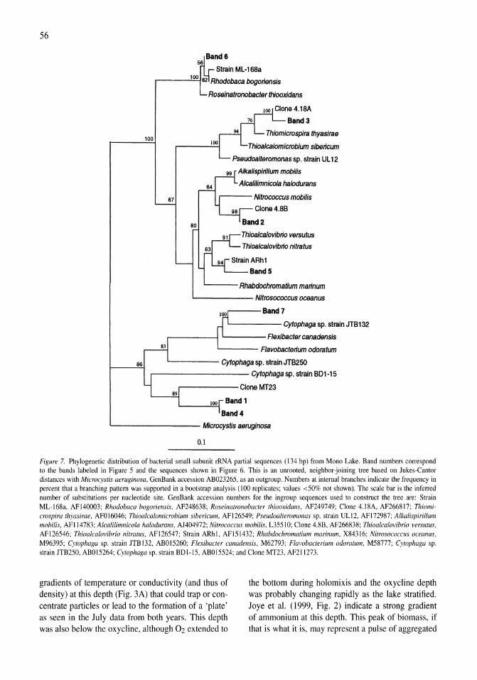
56
86
100
Strain ML-I68a
.-___ 1:,::00"-/82 Rhodobaca bogoriensis
87
80
Roseinatronobacter thiooxidans
100
64
Thiomicrospira thyasirae
Pseudoalteromonas sp. strain UL 12
99 Aikalispirillum mobilis
Aicalilimnicola halodurans
.-----Nitrococcus mobilis
Clone4.8B
Thioaicalovibrio versutus
Thioalcalovibrio nitratus
BandS
'-----Rhabdochromatium marinum
'-------- Nitrosococcus oceanus
,....---Band7
L-. ____ Cytophaga sp. strain JTB132
.-------1 '----- Flexibacter canadensis
'------ Flavobacterium odoratum
'------ Cytophaga sp. strain JTB250
r---------- Cytophaga sp. strain BDI-15
,....------Clone MT23
'---------- Microcystis aeruginosa
0.1
Figure 7. Phylogenetic distribution of bacterial small subunit rRNA partial sequences (134 bp) from Mono Lake. Band numbers correspond to the bands labeled in Figure 5 and the sequences shown in Figure 6. This is an unrooted, neighbor-joining tree based on Jukes-Cantor distances with Microcystis aeruginosa, GenBank accession AB023265, as an outgroup. Numbers at internal branches indicate the frequency in percent that a branching pattern was supported in a bootstrap analysis (100 replicates; values <50% not shown). The scale bar is the inferred number of substitutions per nucleotide site. GenBank accession numbers for the ingroup sequences used to construct the tree are: Strain ML-168a, AF140003; Rhodobaca bogoriensis, AF248638; Roseinatronobacter thiooxidans, AF249749; Clone 4.18A, AF2668l7; Thiomicrospira thyasirae, AF016046; Thioalcalomicrobium sibericum, AF126549; Pseudoalteromonas sp. strain UL12, AFl72987; Alkalispirillum mobilis, AF114783; Alcalilimnicola halodurans, AJ404972; Nitrococcus mobilis, L3551O; Clone 4.8B, AF266838; Thioalcalovibrio versutus, AF126546; Thioalcalovibrio nitratus, AF126547; Strain ARhl, AF15l432; Rhabdochromatium marinum, X84316; Nitrosococcus oceanus, M96395; Cytophaga sp. strain JTB 132, AB015260; Flexibacter canadensis, M62793; Flavobacterium odoratum, M58777; Cyrophaga sp. strain JTB250, ABO 15264; Cyrophaga sp. strain BDl-15, AB015524; and Clone MT23, AF2ll273.
gradients of temperature or conductivity (and thus of density) at this depth (Fig. 3A) that could trap or concentrate particles or lead to the formation of a 'plate' as seen in the July data from both years. This depth was also below the oxycline, although 02 extended to
the bottom during holomixis and the oxycline depth was probably changing rapidly as the lake stratified. Joye et al. (1999, Fig. 2) indicate a strong gradient of ammonium at this depth. This peak of biomass, if that is what it is, may represent a pulse of aggregated
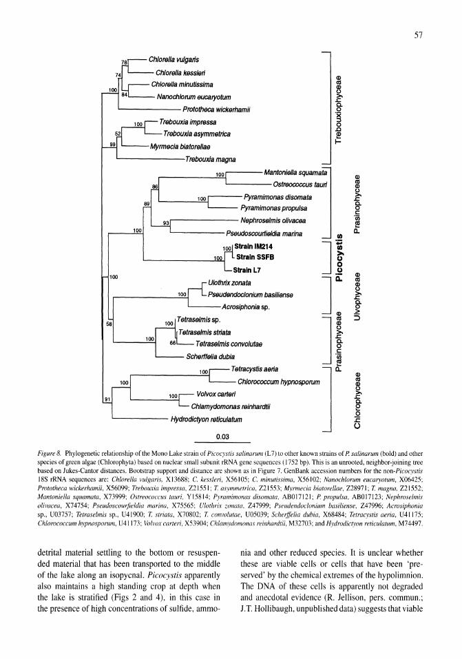
Chlorella vulgaris
Chlorella kessleri
Chlorella minutissima
Nanochlorum eucatyotum
'-------- Prototheca wickerhamii
Trebouxia impressa
Trebouxia asymmetriea
'----Myrmecia biatorellae
L.....-------Trebouxia magna
Q) III
~ .r::. Co o .~ .0 ~ I-
r-_____ ~10~0.-----Mantonie"a squamata
'------Ostreococcus tauri
100
100
58
89 '--___ ...:1..:::00<[---- Pyramimonas disomata
'----- Pyramimonas propulsa
93r-------- Nephroselmis olivacea
'-------Pseudoscourfieldia marina
100 Strain IM214 '--______ ...J1l.l!l00.y Strain SSFB
100
100
U/othrix zonata
Pseudendoclonium basiliense
'-----Acrosiphonia sp.
100 Tetraselmis sp.
Tetraselmis striata
Tetraselmis convolutae
'---- Scherftelia dubia
100 Tetracystis aeria
Chlorococcum hypnosporum
91 Volvox carteri
Chlamydomonas reinhardtii
'------- Hydrodictyon retieulatum
0.03
II)
JI J: Ji
a.
Q)
~ .r::. g. c .~
a.
Q) III
~ .r::. Co e o :c
(,)
57
Figure 8. Phylogenetic relationship of the Mono Lake strain of Picocystis saiinarum (L 7) to other known strains of P. salina rum (bold) and other species of green algae (Chlorophyta) based on nuclear small subunit rRNA gene sequences (1752 bp). This is an unrooted, neighbor-joining tree based on lukes-Cantor distances. Bootstrap support and distance are shown as in Figure 7. GenBank accession numbers for the non-Picocystis 18S rRNA sequences are: Chiorelia vulgaris, X 13688; C. kessleri, X56105; C. minutissima, X56102; Nanochlorum eucaryotum, X06425; Prototheca wickerham ii, X56099; Trebouxia impressa, Z21551; T. asymmetrica, Z21553; Myrmecia biatorellae, Z28971; T. magna, Z21552; Mantoniella squamata, X73999; Ostreococclis tauri, Y15814; Pyramimonas disomata, AB017121; P. propuisa, AB017123; Nephroselmis olivacea, X74754; Pseudoscouljieldia marina, X75565; Ulothrix zonata, Z47999; Pseudendoclonium basiliense, Z47996; Acrosiphonia sp., U03757; Tetraselmis sp., U41900; T. striata, X70802; T. convolutae, U05039; Scherffelia dubia, X68484; Tetracystis aeria, U41175; Chlorococcum hypnosporum, U41173; Volvox carteri, X53904; Chlamydomonas reinhardtii, M32703; and Hydrodictyon reticulatum, M74497.
detrital material settling to the bottom or resuspended material that has been transported to the middle of the lake along an isopycnal. Picocystis apparently also maintains a high standing crop at depth when the lake is stratified (Figs 2 and 4), in this case in the presence of high concentrations of sulfide, ammo-
nia and other reduced species. It is unclear whether these are viable cells or cells that have been 'preserved' by the chemical extremes of the hypolimnion. The DNA of these cells is apparently not degraded and anecdotal evidence (R. Jellison, pers. commun.; J.T. Hollibaugh, unpublished data) suggests that viable
58
Picocystis cells are present because cultures can be started with deep-water inocula.
The type strain of this green alga was isolated from a South San Francisco Bay saltern and is described and named Picocystis salinarum by Lewin et al. (2000). The organism has an unusual composition featuring arabinose as an important component of the cell wall and an unusual suite of pigments (Lewin et aI., 2000; Roesler et aI., 2002). Aspects of the ecophysiology of the Mono Lake strain are described in Roesler et al. (submitted). Phylogenetic analysis of 18S rRNA gene sequences of P. salina rum isolates from Mono Lake, South San Francisco Bay and an alkaline lake in Inner Mongolia (Fig. 8) clustered these three strains together, but the 15-16 of 1752 bp by which the Mono Lake strain is distinct from the other two raise the possibility that it represents a distinct species of Picocystis. Physiological properties of the Mono Lake strain indicate that it is halo- and alkali-tolerant and capable of growth at low light (4 p,E m-2. s-I), and thereby well suited for survival at the base of the lake's photic zone.
Although PCRlDGGE is generally not considered to be quantitative (see discussion in Ferrari & Hollibaugh, 1999), this study provides some indication that it is at least semi-quantitative for some sequences. The intensity of the band corresponding to the Picocystis chloroplast sequence correlates with the distribution of this organism obtained from chlorophyll concentration and direct counts (Joye et al., 1999; Roesler et aI., 2002) or RF. This correlation suggests a semi-quantitative relationship between the relative abundance of the template sequence in the environmental extract and the intensity of the resulting band in the DGGE gel. However, this observation says nothing about organisms that are not represented because they are resistant to DNA extraction or about co-migrating sequences that could yield strong bands containing a mixture of sequences. Co-migration is potentially a serious problem. For example, the fragments in Bands 1 and 3 had very similar melting points, but their aligned sequences differed by about 50 bp and fell into the most distantly related clades in the tree (Fig. 7).
Our modification of the method of Wu et al. (1996) for sampling bands from DGGE gels worked well for these samples. Preparation was simple and the procedure resulted in a durable medium that is stable for long-term storage, which increases flexibility in gel processing and provides an archive gel that can be resampled at a later date. Band excision is also precise, allowing the investigator to obtain clean samples of
bands that are very close to others. DNA suitable for cycle sequencing was easily eluted from the dried gel by a simple and rapid hot water extraction.
The richness of the Mono Lake bacterial assemblage is low compared to other locations we have examined (coastal waters, polar waters, tropical lagoons; Murray et aI., 1996; Ferrari & Hollibaugh, 1999; Hollibaugh et aI., 1999, 2000), where we typically find 20-40 bands per sample. The depressed richness ofthe Mono Lake bacterial assemblage is likely a consequence of the extreme conditions of salinity (Oren, 1999) and pH in the lake. However, halophilic Archaea might be important in this hypersaline environment (Duckworth et aI., 1996; Grant, 1998) and could add to the diversity of the microbial community. We have not yet examined these samples for the presence of Archaea.
Acknowledgements
We thank RS. Oremland and his colleagues at the United States Geological Survey in Menlo Park, California, for their help with field logistics and sample collection. We are grateful to S.B. Joye for helping with sample collection on the July expeditions, collecting samples for us in April and supplying sulfide data; R Jellison for supplying conductivity and temperature data for April; and RA. Lewin for pure cultures of P. salina rum strains. This work was supported by National Science Foundation grants OCE 93-15639 and MCB 99-77886 to IT.H.
References
Altschul, S. E, W. Gish, W. Miller, E. W. Myers & D. 1. Lipman, 1990. Basic local alignment search tool. J. mol. BioI. 215: 403-410.
Andersen, R. A., G. W. Saunders, M. P. Paskind & J. P. Sexton, 1993. Ultrastructure and 18S rRNA gene sequence for Pelagomonas calceolata gen. et sp. nov. and the description of a new algal class, the Pelagophyceae classis nov. J. Phycol. 29: 701-715.
Anderson, R. E, M. P. Bacon & P. G. Brewer, 1982. Elevated concentrations of actinides in Mono Lake. Science 216: 514-516.
Benson, L. Y., J. W. Burdett, M. Kashgarian, S. P. Lund, E M. Phillips & R. O. Rye, 1996. Climatic and hydrologic oscillations in the Owens Lake Basin and adjacent Sierra Nevada, California. Science 274: 746-749.
Benson, L. Y., S. P. Lund, 1. W. Burdett, M. Kashgarian, T. P. Rose, J. P. Smoot & M. Schwartz, 1998. Correlation of late-Pleistocene lake-level oscillations in Mono Lake, California, with North Atlantic climate events. Quat. Res. 49: 1-10.
Brosius, J., M. L. Palmer, J. K. Poindexter & H. E Noller, 1978. Complete nucleotide sequence of a 16S ribosomal RNA gene from Escherichia coli. Proc. natl. Acad. Sci. U.S.A. 75: 4801-4805.
Christen, M. N., C. M. Gilbert. K. R. Lajoie & Y. Alrawi, 1969. Geological-geophysical interpretation of Mono Basin, California-Nevada. 1. geophys. Res. 74: 5221-5337.
Cloern, 1. E., B. E. Cole & R. S. Oremland, 1983a. Autotrophic processes in meromictic Big Soda Lake, Nevada. Limnol. Oceanogr. 28: 1049-1061.
Cloern, 1. E., B. E. Cole & R. S. Oremland, 1983b. Seasonal changes in the chemistry and biology of a meromictic lake (Big Soda Lake, Nevada, U.S.A.). Hydrobiologia 105: 195-206.
Dana, G. L. & P. H. Lenz, 1986. Effects of increasing salinity on an Artemia population from Mono Lake, California. Oecologia 68: 428-436.
DeAngelis, M. M., D. G. Wang & T. L. Hawkins. 1995. Solid-phase reversible immobilization for the isolation of PCR products. Nucleic Acids Res. 23: 4742-4743.
Diaz, M. R & B. F. Taylor, 1996. Metabolism of methylated osmolytes by aerobic bacteria from Mono Lake, a moderately hypersaline, alkaline environment. FEMS Microbio!' Eco!. 19: 239-247.
Domagalski, J. L., W. H. Orem & H. P. Eugster, 1989. Organic geochemistry and brine composition in Great Salt, Mono, and Walker Lakes. Geochim. cosmochim. Acta 53: 2857-2872.
Duckworth, A. W., W. D. Grant, B. E. Jones & R. Van Steenbergen, 1996. Phylogenetic diversity of soda lake alkaliphiles. FEMS Microbial. Ecol. 19: 181-191.
Felsenstein, J., 1993. PHYLIP (Phylogeny Inference Package). Version 3.5c. University of Washington, Seattle.
Ferrari, V. C. & J. T. Hollibaugh, 1999. Distribution of microbial assemblages in the Central Arctic Ocean Basin studied by PCRIDGGE: analysis of a large data set. Hydrobiologia 401: 55-68.
Grant, W. D., 1998. Halophi1es. In Horikoshi, K. & W. D. Grant (eds), Extremophiles: Microbial Life in Extreme Environments. Wiley-Liss, New York: 93-132.
Grant, W. D., W. E. Mwatha & B. E. Jones, 1990. Alkaliphiles -ecology, diversity and applications. FEMS Microbiol. Rev. 75: 255-269.
Hollibaugh, J. T., J. Pages, J.-P. Torreton & P. S. Wong, 1999. Phylogenetic variation in bacterial populations from 10 atoll lagoons in the Tuamotu Islands, French Polynesia. In Brylinsky, M. J. (ed.), Trends in Microbial Ecology. Proceedings of the Eighth International Symposium on Microbial Ecology: Halifax, Nova Scotia, Canada, 9-14 August, 1998: 231-235.
Hollibaugh, 1. T., P. S. Wong & M. C. Murrell, 2000. Similarity of particle-associated and free-living bacterial communities in northern San Francisco Bay, California. Aquatic microb. Ecol. 21: 103-114.
Horikoshi, K. & T. Akiba, 1982. Alkalophilic Microorganisms. Springer-Verlag, Berlin: 213 pp.
Jellison, R & 1. M. Melack, 1988. Photosynthetic activity of phytoplankton and its relation to environmental factors in hypersaline Mono Lake, California. Hydrobiologia 158: 69-8S.
Jellison, R. & J. M. Melack, 1993a. Algal photosynthetic activity and its response to meromixis in hypersaline Mono Lake, California. Limnol. Oceanogr. 3S: SI8-837.
Jellison, R & 1. M. Melack, I 993b. Meromixis in hypersaline Mono Lake, California. I. Stratification and vertical mixing during the onset, persistence, and breakdown of meromixis. Limnol. Oceanogr. 38: 100S-1019.
Jellison, R, R. F. Anderson, J. M. Melack & D. Heil, 1996. Organic matter accumulation in sediments of hypersaline Mono Lake during a period of changing salinity. Limnol. Oceanogr. 41: 1539-1544.
59
Jellison, R., 1. Romero & J. M. Melack, 1998. The onset of meromixis during restoration of Mono Lake, California: unintended consequences of reducing water diversions. Limnol. Oceanogr. 43: 706-711.
Johannesson, K. H. & W. B. Lyons, 1994. The rare earth element geochemistry of Mono Lake water and the importance of carbonate complexing. Limnol. Oceanogr. 39: 1141-1154.
Joye, S. B., T. L. Connell, L. G. Miller, R S. Oremland & R. S. Jellison, 1999. Oxidation of ammonia and methane in an alkaline, saline lake. Limnol. Oceanogr. 44: 178-188.
Lenz, P. H., S. D. Cooper, 1. M. Melack & D. W. Winkler, 1986. Spatial and temporal distribution patterns of three trophic levels in a saline lake. J. Plankton Res. 8: 1051-1064.
Lewin, R. A., L. Krienitz, R. Goericke, H. Takeda & D. Hepperle, 2000. Picoc),stis salina rum gen. et sp. nov. (Chlorophyta) - a new picoplanktonic green alga. Phycologia. 39: 560-565.
Li, L., C. Kato & K. Horikoshi, 1999. Microbial diversity in sediments collected from the deepest cold-seep area, the Japan Trench. Mar. Biotechnol. 1: 391-400.
Maest, A. S., S. P. Pasilis, L. G. Miller & D. K. Nordstrom, 1992. Redox geochemistry of arsenic and iron in Mono Lake, California. In Kharaka, Y. K. & A. S. Maest (eds). WaterRock Interaction. A. A. Balkema, Rotterdam, The Netherlands: 507-511.
Melack. J. M. & R. Jellison, 1998. Limnological conditions in Mono Lake: contrasting monomixis and meromixis in the 1990s. Hydrobiologia 384: 21-39.
Miller, L. G., R. Jellison, R. S. Oremland & C. W. Culbertson, 1993. Meromixis in hypersaline Mono Lake, California. 3. Biogeochemical response to stratification and overturn. Limno!. Oceanogr. 38: 1040-1051.
Murray, A. E., 1994. Community fingerprint analysis: a molecular method for studying marine bacterioplankton diversity. M.A. Thesis, Department of Biology, San Francisco State University, San Francisco, California: 128 pp.
Murray, A. E., J. T. Hollibaugh & c. Orrego, 1996. Phylogenetic compositions of bacterioplankton from two California estuaries compared by denaturing gradient gel electrophoresis of 16S rONA fragments. App!. envir. Microbiol. 62: 2676-2680.
Muyzer, G., E. C. de Waal & A. G. Uitterlinden, 1993. Profiling of complex microhial populations by denaturing gradient gel electrophoresis analysis of polymerase chain reaction-amplified genes coding for 16S rRNA. App!. envir. Microbial. 59: 695-700.
Myers, R. M., S. G. Fischer, L. S. Lerman & T. Maniatis, 1985. Nearly all single base substitutions in DNA fragments joined to a GC-clamp can be detected by denaturing gradient gel electrophoresis. Nucleic Acids Res. 13: 3131-3145.
Myers, R. M., T. Maniatis & L. S. Lerman, 1987. Detection and localization of single base changes by denaturing gradient gel electrophoresis. Meth. Enzymol. 155: 501-527.
Oremland, R. S. & L. G. Miller, 1993. Biochemistry of natural gases in three alkaline, permanently stratified (meromictic) lakes. In Howell, D. G. (ed.). The Future of Energy Gases. U.S. Geological Survey, Menlo Park, California: 439-452 ..
Oren, A., 1999. Bioenergetic aspects of halophilism. Microbial. mo!. BioI. Rev. 63: 334-348.
Pelagos Corporation, 1987. A bathymetric and geologic survey of Mono Lake, California. Report prepared for Los Angeles Department of Water and Power. San Diego, California: 67 pp.
Roesler, C. S., C. W. Culbertson, S. M. Etheridge, R. Goericke, R. P. Kiene, L. G. Miller & R. S. Oremland, 2002. Distribution, production and ecophysiology of Picocystis strain ML in Mono Lake, California. Limnol. Oceanogr. (in press).

60
Saunders, G. W & G. T. Kraft, 1994. Small-subunit rRNA gene sequences from representatives of selected families of the Gigartinales and Rhodymeniales (Rhodophyta). I. Evidence for the Plocamiales ord. nov. Can. 1. Bot. 72: 1250-1263.
Simpson, H. R., R. M. Trier, D. E. Hammond, A. Ege, L. Miller & 1. M. Melack, 1980. Fallout plutonium in an alkaline, saline lake. Science 207: 1071-1073.
Sorokin, D. Iu., T. P. Turova, B. B. Kuznetsov, I. A. Briantseva & V. M. Gorlenko, 2000. Roseinatronobacter thiooxidans gen. nov., sp. nov., a new alkaliphilic aerobic bacteriochlorophyllalpha-containing bacteria from a soda lake. Mikrobiologiia 69: 89-97.
Stine, S., 1994. Extreme and persistent drought in California and Patagonia during mediaeval time. Nature 369: 546-549.
Tanner, M. A., C. L. Everett, W J. Coleman, M. M. Yang & D. C. Youvan, 2000. Complex microbial consortia inhabiting hydrogen sulfide-rich black mud from marine coastal environments. Biotechnology et Alia 8: 1-16.
Ward, B. B., D. P. Martino, M. C. Diaz & S. B. Joye, 2000. Analysis of ammonia-oxidizing bacteria from hypersaline Mono Lake, California, on the basis of 16S rRNA sequences. Appl. envir. Microbiol. 66: 2873-2881.
Wu, S.-M., L. A. Blomberg & W-Y. Chan, 1996. Recovery of unlabeled PCR product from polyacrylamide gel for sequencing. BioTechniques 21: 358-362.
Zehr, J. P., R. W Harvey, R. S. Oremland, J. E. Cloern, L. H. George & 1. L. Lane, 1987. Big Soda Lake (Nevada). I. Pelagic bacterial heterotrophy and biomass. Limnol. Oceanogr. 32: 781-793.
Hydrobiologia 466: 61-72,2001. 1.M. Melack, R. lellison & D.B. Herbst (eds), Saline Lakes. © 2001 Kluwer Academic Publishers.
61
The bioenergetic basis for the decrease in metabolic diversity at increasing salt concentrations: implications for the functioning of salt lake ecosystems
Aharon Oren Division of Microbial and Molecular Ecology, The Institute of Life Sciences, and The Moshe Shilo Minerva Center for Marine Biogeochemistry, The Hebrew University of Jerusalem, Jerusalem 91904, Israel Tel.: +972-2-6584951; Fax: +972-2-6528008; E-mail: [email protected]
Key words: salt lakes, bioenergetics, osmoregulation, methanogenesis, nitrification, sulfate reduction
Abstract
Examination of the microbial diversity in hypersaline lakes of increasing salt concentrations shows that certain types of dissimilatory metabolism do not occur at the highest salinities. Examples are methanogenesis from hydrogen and carbon dioxide or from acetate, dissimilatory sulfate reduction with oxidation of acetate, and autotrophic nitrification. The observations can be explained on the basis of the energetic cost of haloadaptation used by the different metabolic groups and the free-energy change associated with the dissimilatory reactions. All halophilic microorganisms spend large amounts of energy to maintain steep gradients of Na+ and K+ concentrations across their cytoplasmic membrane. Most Bacteria and also the methanogenic Archaea produce high intracellular concentrations of organic osmotic solutes at a high energetic cost. The halophilic aerobic Archaea (order Halobacteriales) and the halophilic fermentative Bacteria (order Halanaerobiales) use KCl as the main intracellular solute. This strategy, while requiring far-reaching adaptations of the intracellular machinery, is energetically more favorable than production of organic compatible solutes. By combining information on the amount of energy available to each physiological group and the strategy used to cope with salt stress, a coherent model emerges that provides explanations for the upper salinity limit at which the different microbial conversions occur in hypersaline lakes.
Introduction
The primary factor that determines the biological properties of salt lakes worldwide is salt concentration. Saline lakes can be found with salt concentrations increasing from below that of sea water (35 g 1-1 dissolved salt) to brines at or approaching saturation, such as, e.g., the Dead Sea and the Great Salt Lake, Utah.
As the presence of high salt concentrations exerts a stress on any living organism that has to cope with life at high ionic strength, salt lakes may be considered extreme environments; the higher the salinity, the more extreme the conditions become. While a wealth of different taxonomic groups of plants and animals inhabit salt lakes at the lower salinity range, life in those lakes with the highest salt concentrations is restricted to a few groups of microorganisms only. Salt lakes thus closely fit the definition of extreme environments as
'such environments that allow life and survival only to a few taxonomic groups of specialists, meaning that whole taxonomic groups are unable to thrive there and are therefore absent' (Schink, 1999: 784).
Microbial life can exist at salt concentrations up to NaCI saturation (approximately 5.2 m). The bright red color of saltern crystallizer ponds and many hypersaline lakes worldwide (including at times even the Dead Sea) shows that such environments may indeed support development of dense microbial communities. However, the number of different microorganisms able to grow at these extremely high salinities is small.
Within the phylogenetic tree of life halophilic behavior is found to be widespread in all three domains: Archaea, Bacteria and Eukarya. The eukaryal green alga Dunaliella is present worldwide as the main or sole primary producer in hypersaline aquatic environments. The aerobic halophilic heterotrophs par excellence are Archaea of the family Halobacteri-
62
aceae which are in most cases responsible for the red color of brines at or near salt saturation. The archaeal family Methanosarcinaceae of anaerobic methanogens also contains a number of halophilic representatives. Within the bacterial domain moderate halophiles are abundant. They can be found in the Proteobacteria (notably in the y-subdivision), the Gram-positive bacteria, the cyanobacterial branch, and elsewhere.
In accordance with the above definition of extreme environments, the number of metabolic types decreases as salinity increases. From a salt concentration of about 100-150 g I-I onwards metabolic diversity becomes limited (Fig. I). Functions that are conspicuously missing already at relatively low salinities are autotrophic nitrification, oxidation of acetate and higher fatty acids with the reduction of sulfate, and methanogenesis based on the reduction of C02 by hydrogen or on the aceticlastic split. On the other hand, methanogenesis using methylated amines or methanol as energy sources can function up to much higher salt concentrations, 270 g I-I being the approximate upper limit (Oren, 1988, 1990; Zhilina & Zavarzin, 1990). Fermentative processes, oxidation of lactate by sulfate reducing bacteria and reduction of C02 by hydrogen with the formation of acetate have their salinity boundary in the same range. Finally, photosynthesis (both oxygenic with water as electron donor and anoxygenic using reduced sulfur species), aerobic respiration and anaerobic respiration with nitrate as electron acceptor can proceed up to the highest salt concentrations. For reviews on microbial diversity in hypersaline environments see, e.g., Oren (1988) and Ollivier et al. (1994).
This paper presents a hypothesis that attempts to explain the different upper salinity limits at which the types of dissimilatory metabolism can occur in salt lakes. The hypothesis is based on the following assumptions:
(1) Life at high salt concentrations is energetically expensive.
(2) The upper salt concentration limit at which a dissimilatory process can occur is determined primarily by bioenergetic constraints.
(3) Therefore the important factors that determine whether a certain type of microorganism can make a living at high salt are:
- The amount of energy generated in its dissimilatory metabolism.
- The mode of osmotic adaptation used.
The ideas described here in brief have been documented in full in a recent review (Oren, 1999). Readers are referred to that paper for a more detailed account.
Osmotic adaptation and its energetic cost
As biological membranes are permeable to water, all halophilic and halotolerant microorganisms have to maintain their cytoplasm at least isoosmotic with the external medium. Buildup of a turgor pressure requires a hyperosmotic cytoplasm. In all cases examined the intracellular milieu differs greatly from that of the medium surrounding the cell. As a result, adaptation to life at high NaCI concentrations is energetically costly.
Two fundamentally different strategies are used by microorganisms to cope with the presence of high salt concentrations in their environment:
I. The accumulation of salts in the cytoplasm at concentrations equal to (or higher than - in case a turgor pressure is to be maintained) those of the outside medium. Generally KCl is used as the main intracellular salt. This strategy is used by two phylogenetically unrelated groups: the aerobic halophilic Archaea (family Halobacteriaceae) and a small group of anaerobic halophilic Bacteria (order Halanaerobiales, families Halanaerobiaceae and Halobacteroidaceae, belonging to the low G+C branch of the Gram-positive Bacteria). This strategy is energetically relatively inexpensive, but requires far-reaching adaptations to the presence of high salt concentrations by the intracellular enzymatic machinery. Adaptability of the cells to changing salt concentrations is limited.
2. The exclusion of salts from the cytoplasm and the accumulation of organic osmotic 'compatible' solutes to provide osmotic balance. This strategy is used by halophilic and halotolerant eukaryal microorganisms, by most salt-requiring and salttolerant Bacteria, and also by halophilic methanogenic Archaea. This strategy is energetically expensive, the energetic cost depending on the type of organic solute synthesized. No major modification of the intracellular machinery is needed in comparison to non-halophiles, and in most cases cells can rapidly adapt to changes in medium salinity.
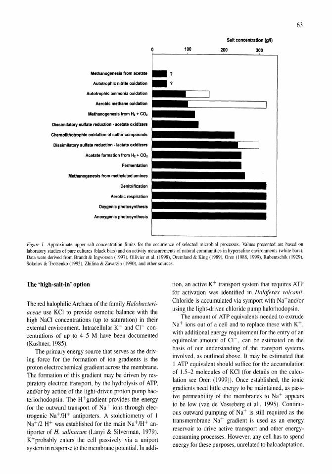
Methanogenesis from acetate
Autotrophic nitrite oxidation
Autotrophic ammonia oxidation
Aerobic methane oxidation
Methanogenesis from H2 + C02
Dissimilatory sulfate reduction - acetate oxidizers
Chemollthotrophic oxidation of sulfur compounds
Dissimilatory sulfate reduction - lactate oxidizers
Acetate formation from H2 + CO2
Fermentation
Methanogenesis from methylated amines
Denitrification
Aerobic respiration
Oxygenic photosynthesis
Anoxygenic photosynthesis
63
Salt concentration (gil)
o 100 200 300
Figure 1. Approximate upper salt concentration limits for the occurrence of selected microbial processes. Values presented are based on laboratory stu~!es of pure cultures (black bars) and on activity measurements of natural communities in hypersaline environments (white bars) Data were denved from Brandt & Ingvorsen (1997), Ollivier et al. (1998), Oremland & Kina (1989) Oren (1988 1999) Rubentschik (1929)' Sokolov & Trotsenko (1995), Zhilina & Zavarzin (1990), and other sources. 10' " ,
The 'high-salt-in' option
The red halophilic Archaea of the family Halobacteriaceae use KCI to provide osmotic balance with the high NaCI concentrations (up to saturation) in their external environment. Intracellular K+ and Cl- concentrations of up to 4-5 M have been documented (Kushner, 1985).
The primary energy source that serves as the driving force for the formation of ion gradients is the proton electrochemical gradient across the membrane. The formation of this gradient may be driven by respiratory electron transport, by the hydrolysis of ATP, and/or by action of the light-driven proton pump bacteriorhodopsin. The H+gradient provides the energy for the outward transport of Na+ ions through electrogenic Na+/H+ antiporters. A stoichiometry of I Na+/2 H+ was established for the main Na+/H+ antiporter of H. salinarum (Lanyi & Silverman, 1979). K+probably enters the cell passively via a uniport system in response to the membrane potential. In addi-
tion, an active K+ transport system that requires ATP for activation was identified in Haloferax volcanii. Chloride is accumulated via symport with Na+and/or using the light-driven chloride pump halorhodopsin.
The amount of ATP equivalents needed to extrude Na+ ions out of a cell and to replace these with K+, with additional energy requirement for the entry of an equimolar amount of Cl-, can be estimated on the basis of our understanding of the transport systems involved, as outlined above. It may be estimated that 1 ATP equivalent should suffice for the accumulation of 1.5-2 molecules of KCI (for details on the calculation see Oren (1999)). Once established, the ionic gradients need little energy to be maintained, as passive permeability of the membranes to Na+ appears to be low (van de Vosseberg et aI., 1995). Continuous outward pumping of Na+ is still required as the transmembrane Na+ gradient is used as an energy reservoir to drive active transport and other energyconsuming processes. However, any cell has to spend energy for these purposes, unrelated to haloadaptation.
64
It thus appears that the amount of energy needed to enable members of the Halobacteriales to thrive at the extremely high salt concentrations is moderate in comparison to the amounts of energy required in the 'high organic solute, low-salt-in' option, discussed below.
The presence of high intracellular concentrations of KCI requires a complete adaptation of all intracellular components to function at high salt. An in-depth survey of the special properties of the salt-adapted enzymes is beyond the framework of this chapter; details can be found in review papers by Lanyi (1974) and Dennis & Shimmin (1997). The unique molecular adaptations of the proteins include the presence of a large excess of acidic amino acids and low amounts of hydrophobic amino acids. The low content of hydrophobic amino acids is offset by a high content of the 'borderline hydrophobic amino acids' serine and threonine (Lanyi, 1974). Most proteins of the halophilic Archaea depend on the presence of relatively high salt concentrations for the maintenance of their proper conformation and activity. These microorganisms thus require the continuous presence of high salt concentrations in their environment.
The anaerobic halophilic Bacteria of the order Halanaerobiales (Oren, 2000) use a mode of osmotic adaptation similar to that of the archaeal group of the Halobacteriales. The order Halanaerobiales consists of obligatory anaerobic fermentative bacteria and also contains homoacetogenic bacteria such as Acetohalobium arabaticum. Representatives of the group investigated (Halanaerobium praevalens,Halanaerobium acetethylicum, Halobacteroides halobius) contain high intracellular KCI concentrations (Oren, 1986; Oren et al., 1997; Rengpipat et aI., 1988), their enzymes require high salt concentrations to function optimally (Rengpipat et aI., 1988), and no organic osmotic solutes have ever been found to accumulate inside the cells.
The 'low-salt-in' option
A fundamentally different strategy of osmotic adaptation is used by all other groups of microorganisms, including halophilic eukaryotic algae, halophilic and halotolerant Bacteria (with the above-mentioned exception of the Halanaerobiales), and also the methanogenic Archaea. Salts are excluded from the cytoplasm to a large extent, and organic solutes are synthesized or accumulated from the outside medium to provide osmotic balance. Presence of high concentrations of such
'compatible' solutes does not require special adaptations of the cellular proteins. However, the energetic price the cells have to pay in this mode of osmotic adaptation is huge, as the biosynthesis of organic osmotic solutes is energetically much more expensive than building up high intracellular KCI concentrations.
The list of compounds known to function as osmotic solutes includes glycerol (found only in Eukarya such as the halophilic alga Dunaliella and certain fungi) (Ben-Amotz & Avron, 1973; Brown, 1990), glycine betaine (in halophilic cyanobacteria, in anoxygenic photosynthetic Bacteria, and also in halophilic methanogenic Archaea), ectoine (in many heterotrophic and phototrophic Proteobacteria), glucosylglycerol (in cyanobacteria with a moderate salt tolerance), and the disaccharides sucrose and trehalose, found, e.g., in many cyanobacteria (Mackay et aI., 1984; Reed et aI., 1984) and others (for reviews see Galinski (1993, 1995)). Glycine betaine may be taken up from the medium by many halophilic and halotolerant heterotrophic Bacteria and used as osmotic solute. However, only a few heterotrophs are capable of synthesizing glycine betaine de novo (Vento sa et aI., 1998).
The amount of ATP molecules needed for the biosynthesis of the organic compatible solutes varies with the size and complexity of the compounds. Based on the known biosynthetic pathways it may be calculated that for an autotroph the production of one molecule of solute costs between 30 ATP for glycerol, the simplest compound, to as high as 109 ATP equivalents for the disaccharides sucrose and trehalose. An aerobic heterotrophic microorganism that has to produce these solutes from glucose has to 'waste' between 23 and 79 potential ATP molecules that could otherwise have been used for energy generation and growth.
Glycerol may be considered the ideal osmotic solute: it is relatively cheap to synthesize, and it is miscible with water in any ratio. Brown (1990: 250) thus could state that glycerol "may be regarded as God's gift to solute-stressed eukaryotes". However, glycerol is not used as an osmotic solute in the prokaryotic world. The reason should probably be sought in the special adaptations of the cell membrane required to prevent leakage of the compound, as most biological membranes are freely permeable to glycerol. Indeed the Dunaliella cell membrane was found to be several orders of magnitude less permeable to glycerol than all other membranes known (Brown et aI., 1982; Gimmler & Hartung, 1988).
Accumulation of osmotic solutes to molar concentrations inside the cytoplasm is energetically expensive. Biosynthesis of organic osmotic solutes can increase the amount of energy required per unit of structural cell biomass material (proteins, cell walls, nucleic acids, etc.) several-fold (Oren, 1999). In addition, cells that produce organic osmotic solutes also have to compensate for loss of these solutes through their semi-permeable membranes. Most halophiles therefore possess transport proteins in the membrane that enable the recovery of at least part of the solute lost to the medium. Transport of solutes from the medium against a concentration gradient is also energetically costly, but enables a significant energy saving as compared to de novo biosynthesis. Finally, the presence of high concentrations of organic solutes does not relieve the need for high activities ofNa+ /H+ antiporters to prevent Na+ions from leaking in, either due to passive permeability of the membrane or as a result of cotransport with, e.g., amino acids. This again adds to the amount of energy required for osmotic adaptation in microorganisms that use organic solutes to provide osmotic balance while maintaining a cytoplasm low in salt.
Salinity limitations to metabolic biodiversity: case studies
As documented above, it may be expected that in order to live and grow in high salt environments cells will have to spend a large percentage of the energy gained in their dissimilatory metabolism for the purpose of osmoregulation: to synthesize organic solutes and/or to activate ion pumps. Energetic constraints may therefore be expected to present severe problems to those groups of microorganisms that obtain small amounts of energy only in the course of their dissimilatory metabolism.
Therefore we may expect the following types of metabolism to function at high salt concentrations:
1. Those processes that use light as energy source (and are generally not energy-limited).
2. Heterotrophs (Bacteria as well as Archaea) that perform aerobic respiration, denitrification, and other dissimilatory processes that yield large amounts of ATP.
3. All types of metabolism performed by organisms that use the 'high-salt-in' strategy, even if the amount of ATP obtained in their dissimilatory metabolism is low.
65
Growth of phototrophic microorganisms is generally limited by the availability of inorganic nutrients and not by lack of light energy. Accordingly, both oxygenic (Dunaliella, cyanobacteria) and anoxygenic phototrophs (Halorhodospira, Thiohalocapsa, Halochromatium), all producing organic solutes for osmotic stabilization, may be found up to very high salt concentrations, in several cases up to salt saturation. However, in the case of chemolithotrophs and anaerobic heterotrophs the amount of energy generated in the course of the dissimilatory metabolism is often insufficient to supply the demands of cell growth, osmotic adaptation, and maintenance. In such cases growth and survival in hypersaline environments may not be possible. The 'high-salt-in' strategy is preferable for strongly energy-limited organisms as it is energetically much less costly than the production of organic osmotic solutes. As the following examples show, there appears to be an excellent correlation between the amount of energy generated in the course of the different dissimilatory processes, the strategy ('high-salt-in' or 'high organic solute, low-salt-in') used for osmoregulation, and the salinity range at which the process occurs (Fig. 1).
Autotrophic nitrification
The aerobic oxidations of ammonia to nitrite and of nitrite to nitrate yield relatively little energy (NH4 + + 1.5 02 --+ N02 - + 2 H+ + H20; !!.Go/ = -274.6 kJ, or-91.5 kJ per 2 electrons; N02- + 0.502 --+ N03-; !!.Go' = -74.1 kJ). The low energy yield is a direct result of the relatively high standard redox potential of the couples N02 - INH4 + and N03 - IN02 -( +0.44 and +0.43 V, respectively). Not only is the energy yield low, but a large fraction of the energy gained has to be used to drive uphill electron transfer for the production of NADPH, the strong reductant (NADP+ INADPH = -0.32 V) required as electron donor for autotrophic C02 reduction. No information is available on the mode the nitrifying bacteria use to adjust their intracellular osmotic value to the external salt concentration. However, being members of the Proteobacteria, they may be expected to use organic osmotic compounds in their osmoregulation.
In view of the above it is not surprising that nitrifying bacteria appear to be absent in high salinity environments. The most halotolerant autotrophic ammonia oxidizer extant in pure culture is Nitrosococcus halophilus, with a growth optimum at 40 g 1-1 NaCl, growing only up to 94 g I-I (Koops et aI., 1990). Mi-
66
crocosm simulations, using a total salt concentration above 300 g 1-1, failed to demonstrate nitrification in the Great Salt Lake, Utah (Post & Stube, 1988). Studies of hypersaline lagoons near Odessa (Ukraine) performed in the 1920s showed autotrophic oxidation of NH4 + to N02 - to occur up to above 150 g 1-1 salt only (Rubentschik, 1929). Lack of substrate is probably not the cause for the absence of nitrifying activity as ammonia is often abundantly found in hypersaline water bodies. Oxygen is also generally available as electron acceptor, albeit at relatively low concentrations due to its reduced solubility in concentrated brines.
Recently I examined the occurrence of nitrification in samples from the solar salterns of Bras del Port, Santa Pola, near Alicante, Spain. Brine samples (40 ml) collected in May 1999 from ponds with 8, II, 15, 22, 31 and 37% salt were incubated in the dark at 30 °C with slow shaking in 50-ml tubes, without addition or amended with 5 mM NH4Cl or 0.2 mM NaN02. Samples were withdrawn periodically and assayed for formation or disappearance of nitrite. Oxidation of ammonia could be shown at salt concentrations of up to II %. At 4% salt, the first appearance of nitrite was noted after 7 days of incubation. At 5.8 and at 8% salt the first nitrite was detected after 3 weeks, and 4 weeks of incubation with ammonia were required to obtain an increase in nitrite concentration at 11 % salt. At 15, 22, 31, and 37% salt no nitrite was detected even after 9 weeks of incubation. No significant disappearance of nitrite was measured at any of the salinities tested for 4 weeks.
The alkaline (pH 9.8) Mono Lake (CA) is probably one ofthe most saline lakes (around 88 g 1-1 salts in the lower water layers) in which active nitrification occurs. Joye et al. (1999) reported rates of autotrophic ammonia oxidation of 580-2830 nmoll- I day-I in the oxic layer (5-7 m depth) and 732-1548 nmoll- I day-I in the oxycline (11-15 m) in the spring and summer of 1995. Ammonia oxidizers were estimated to contribute 70-340 and 89-186 nmoll-1 day-l of dark C02 consumption. It was argued that nitrification significantly reduces loss of available nitrogen from this alkaline lake by converting volatile ammonia to non-volatile nitrite and nitrate. Molecular studies based on the characterization of 16s rDNA sequences recovered from the lake suggest that organisms related to Nitrosomonas europaea are probably responsible for the autotrophic ammonia oxidation (Ward et al., 2000).
There exists one report that suggests that nitrification may occur in the alkaline lakes of the Wadi Natrun, Egypt. Accumulation of nitrite in aerobic enrichment cultures with ammonia as sole nitrogen source was brought forward as evidence for the presence of ammonia oxidizing bacteria in lakes varying in salinity from 92 to 389 g 1-1 at pH values between 10.8 and 11.2 (Imhoff et al., 1979). However, no further documentation was supplied. A renewed examination of this interesting environment for the presence of halophilic or halotolerant nitrifying bacteria is therefore to be recommended.
Methanogenesis
The methanogenic Archaea use organic solutes for osmotic stabilization. Compatible solutes detected in the group include glycine betaine, f3-glutamine, Wacetyl-f3-lysine and others (Lai et al., 1991; Lai & Gunsalus, 1992). Thus, they differ from the aerobic halophilic Archaea of the family Halobacteriaceae, which use the 'high-salt-in' strategy. Nevertheless, methanogens - even the non-halophilic ones - may contain substantial intracellular K+ concentrations. The K+ions probably serve as counterion to cyclic 2,3-diphosphoglycerate, a compound thought to play a role in the thermostability of cytoplasmic enzymes (Laietal.,1991).
In low-salinity environments the most important reactions that lead to the formation of methane are the reduction of C02 with hydrogen and the aceticIastic split. Neither of these reactions has been shown to occur at high salt concentrations. Tests for the occurrence of both these reactions in sediments of Solar Lake (Sinai, Egypt) (70-74 g I-I salt) yielded negative results (Giani et al., 1984). The highest salt concentration at which methanogenesis from H2 + C02 was shown to occur is probably 88 g 1-1 (in the alkaline Mono Lake, CA) (Oremland & King, 1989). The most halotolerant methanogenic isolate that grows on H2 + C02 is Methanocalculus halotolerans recently recovered from an oil well (optimum growth at 50 g I-I NaCl, with growth up to 120 g I-I) (Ollivier et al., 1998). The upper salinity boundary for the aceticIastic split is probably even lower, but data are scarce.
However, methanogenesis does occur in most hypersaline environments up to high salt concentrations (270 g 1-1 at least). The methanogenic precursors are in this case substrates such as trimethylamine and other methylated compounds (Oremland & King, 1989). Halophilic methanogens isolated in pure cul-
tures such as Methanohalophilus mahii, Methanohalophilus halophilus, and Methanosalsum zhilinae grow optimally at 40-120 g 1-1 salt. Even more halotolerant are Methanohalobium evestigatum and Methanohalophilus portucalensis, isolates that grow well up to 240-250 g 1-1 NaCI (Zhilina & Zavarzin, 1987; Lai & Gunsalus, 1992).
It is entirely possible that the apparent lack of halophilic C02-reducing and aceticlastic methanogens may be due to energetic constraints. Methanogenesis from acetate yields very little energy: Acetate- + H20 -+ CH4 + HC03-; !1Go/ = -31.1 kJ. Accordingly, even non-halophilic aceticlastic methanogens are notoriously slow growers. The standard free energy change during growth on hydrogen + C02 is also not very high: 4 H2 + H+ + HC03 - -+ CH4 + 3 H20; !1Go/ = -135.9 kJ, or -34.0 kJ per mol of substrate.
A direct comparison of the energy yield of the above reactions with methanogenic reactions from methylated amines and methanol, substrates that do support methanogenesis at high salt concentrations, is not straightforward. Disproportionation reactions are involved with complex reaction stoichiometries:
4 Methylamine + 3 H+ + 3 H20 -+ 3 CH4 + HC03- + 4 NH4+; !1Go/ = -368.3 kJ, or -92.1 kJ per mol of substrate;
2 Dimethylamine + H+ + 3 H20 -+ 3 CH4 + HC03- + 2 N~+; !1Go/ = -286.5 kJ, or-143.3 kJ per mol of substrate;
4 Trimethylamine + 9 H20 + H+ -+ 9 C~ + 3 HC03- + 4 N~+; !1Go/ = -764.5 kJ, or -191.1 kJ per mol of substrate;
4 Methanol -+ 3 CH4 + HC03- + H20 + H+; !1Go/ = -314.7 kJ, or-78.7 kJ per mol of substrate.
The theoretically available amount of energy per mol of substrate is obviously much higher than that obtained from the split of acetate or from the oxidation of hydrogen. However, little is known on the efficiency of the energy conservation in the form of ATP and/or electrochemical ion gradients during growth on methylated amines as compared to growth on H2+ C02 or on acetate. In any case, the more favorable free energy change of the dissimilatory reactions may provide us with a possible explanation why methanogenesis on methylated amines is feasible up to very high salt concentrations.
67
Sulfate-reducing bacteria
The occurrence of black sediments on the bottom of salt lakes and saltern ponds approaching NaCl saturation provides evidence that dissimilatory sulfate reduction may occur up to very high salinities. In a number of hypersaline lakes the occurrence of sulfate reduction has been proven directly by following the formation of H235S from 35S042- added to the sediments (J~rgensen & Cohen, 1977; see also Oren, 1988).
Halophilic sulfate reducers isolated in culture include Desulfovibrio halophilus (optimum NaCl concentration 60-70 g I-I, maximum 180 g 1-1) (Caumette et ai., 1990), Desulfovibrio oxyclinae (optimum NaCI concentration 50-100 g 1-1, maximum 225 g 1-1) (Krekeler et ai., 1997), and Desulfohalobium retbaense isolated from Lake Retba in Senegal, the most halophilic strain known thus far, with its optimum at 100 g 1-1 NaCl and growing up to 240 g 1-1 NaCl (Ollivier et ai., 1991). With a single exception all halophilic and halotolerant dissimilatory sulfate reducers isolated are incomplete oxidizers, using, e.g., lactate as energy source. A single halotolerant acetate-oxidizing sulfate reducer is known: Desulfobacter halotolerans, recently isolated from the sediments of the Great Salt Lake, Utah (Brandt & Ingvorsen, 1997). Its salt optimum is 10-20 g 1-1 only, and 130 g I-I is the maximum NaCI concentration tolerated.
Bioenergetic constraints may once more explain the upper salinity limits of the different processes. Desulfovibrio halophilus was shown to use organic solutes (trehalose and glycine betaine) to provide osmotic balance (Welsh et ai., 1996), as expected for a member of the Proteobacteria. In view of this energetically expensive way of life it is understandable that dissimilatory sulfate reduction with complete oxidation of acetate does not proceed in the higher range of salt concentrations: acetate oxidation with reduction of sulfate yields little energy (Acetate- + S042- -+ 2 HC03- + HS-; !1Go/ = -47.7 kJ). More energy is generated when sulfate reduction is coupled with the oxidation of hydrogen or lactate (4 H2 + S042- + H+ -+ HS- + 4 H20; !1Go/ = -152.3 kJ; 2 Lactate- + S042- -+ 2 Acetate- + HC03- + HS- + H+; !1Go/ =-160.1 kJ).
Little information is available as yet on the nature of the electron donors used by the communities of sulfate reducing bacteria in sediments of salt lakes of different salinity.
68
Homoacetogens
On the basis of thermodynamic calculations alone one should predict that homoacetogenic bacteria that reduce C02 with hydrogen to form acetate would be even less suitable to life at high salt concentrations than methanogenic bacteria that use the same substrates. Comparison of the reactions
4 H2 + H+ + 2 HC03- -+ Acetate- + 4 H20; ""GO! = -104.6kJ or-26.1 kJ per mol ofH2, and 4 H2 + H+ + HC03 - -+ CH4 + 3 H20; ""Go l = -135.9 kJ or -34.0 kJ per mol of H2
shows that the homoacetogenic reaction provides less energy than the methanogenic reaction.
However, a homoacetogenic bacterium isolated from a hypersaline lagoon of the Arabat spit, Crimea, named Acetohalobium arabaticum, grows optimally at 150-180 g 1-1 NaCl, and tolerates up to 250 g 1-1 (Zhilina & Zavarzin, 1990; Zavarzin et aI., 1994).
The phylogenetic position of the halophilic homoacetogenic bacteria may provide the key to the understanding why the homoacetogenic reaction occurs up to much higher salt concentrations than the methanogenic reaction that uses the same substrates with an even larger free energy change. A. arabaticum belongs to the order Halanaerobiales (low G+C subclass of the Gram-positive Bacteria) (Rainey et aI., 1995). Representatives of this order tested for their mode of osmotic adaptation were found to accumulate inorganic ions (mainly K+ and Cl-, to a smaller extent Na+) to establish osmotic balance (Rengpipat et aI., 1988; Oren, 1986, 2000; Oren et aI., 1997). Organic osmotic solutes were never documented in this group. As explained above, use of inorganic salts to provide osmotic equilibrium is energetically much more favorable than synthesis of organic compatible solutes. The halophilic homoacetogens, have yet to be tested for intracellular ion and organic solute content.
Chemolithotrophic sulfur oxidation
Sulfide and elemental sulfur are much more reduced compounds than ammonia and nitrite. Their aerobic oxidation therefore yields more energy than the reactions of autotrophic nitrification (e.g., H2S + 2 02 -+ S042- + 2 H+; ""GO I = -796.3 kJ, or -199.1 kJ per two electrons). Accordingly, autotrophic sulfur oxidizers are found up to much higher salt concentrations than nitrifying bacteria. Halothiobacillus halophilus, isolated from Lake O'Grady North (Western Australia,
salinity 137 g 1-1), oxidizes thiosulfate, tetrathionate and elemental sulfur, growing optimally at 50-60 g 1-1 NaCI and tolerating up to 240 g 1-1 (Wood & Kelly, 1991). Belonging to the Proteobacteria, this organism may be expected to produce organic osmotic solutes, but to my knowledge no analyses have been performed as yet. Spherical colorless bacteria containing sulfur inclusions, tentatively identified as chemoautotrophic sulfur bacteria, were even found within a gypsum crust found on the bottom of a saltern pond with a salt concentration around 280-290 g 1-1 (Oren et aI., 1995).
Fermentation
When no suitable electron acceptors are available, carbohydrates, amino acids, and other substrates are degraded by fermentative processes. Such fermentations, which result in the formation of products such as ethanol, acetate and other small organic acids, hydrogen and C02, yield small amounts of energy only (generally between two and three ATP per molecule of carbohydrate fermented, even less when amino acids serve as energy source). Fermentations do take place up to very high salt concentrations. Most members of the Halanaerobiales ferment carbohydrates at salt concentrations up to 250 g 1-1 (Oren, 2000; Rainey et aI., 1995). Halobacterium salina rum even thrives anaerobically at salt concentrations approaching saturation by fermenting L-arginine via citrulline to ornithine, C02 and NH3, a process in which 1 ATP only is gained (Hartmann et aI., 1980)
All fermentative halophilic bacteria known belong to the group of anaerobic halophilic Bacteria of the order Halanaerobiales or to the archaeal family Halobacteriaceae. Both these groups use the energetically efficient 'high-salt-in' strategy (Lanyi, 1974; Oren, 1986; Rengpipat et aI., 1988; Oren et aI., 1997; Mermelstein & Zeikus, 1998; Rengpipat et aI., 1988).
Denitrification
Some halophilic Archaea (e.g., Haloarcula marismortui, Haloarcula vallismortis, Haloferax mediterranei) are able to grow anaerobically when nitrate is present as the electron acceptor (Mancinelli & Hochstein, 1986). Also many halophilic and halotolerant Bacteria (e.g., several members of the Halomonadaceae) can grow in the absence of oxygen by denitrification. The ability to grow at high salt concentrations by dissimilatory nitrate reduction is not surprising as the energy yield of oxidation of organic substrates with
nitrate is only little less than with oxygen as electron acceptor (Glucose + 4.8 N03 - + 4.8 H+ ---+ 6
C02 + 2.4 N2 + 8.4 H20; b"Go t = -2716 kJ; com
pare: Glucose + 6 02 ---+ 6 C02 + 6 H20; b"Got = -2872 kJ). Even when the efficiency of the energy conservation may be somewhat reduced when nitrate serves as electron acceptor, sufficient energy may be expected to be available for osmotic adaptation, even when energetically expensive organic solutes are to be synthesized.
Aerobic methanotrophs
There is one case in which energetic constraints alone
cannot explain the apparent lack of a metabolic activity at high salt concentrations, and that is the case of methane oxidation. Methane is produced abundantly in many hypersaline environments; as documented above this methane is generally derived from the degradation of methylated amines. However, hardly any aerobic oxidation of methane appears to occur at high salt concentrations (Giani et aI., 1984; Slobodkin & Zavarzin, 1992). Even in environments with relatively low salinities such as the cyanobacterial mats in the Solar Lake, Sinai (about 85 g I-I salt) and saltern evaporation ponds in Eilat, Israel (132 g I-I salt) no methane oxidation could be measured, although methane and oxygen were both present (Conrad et aI., 1995).
Aerobic oxidation of methane is a highly exergonic process (CH4 + 2 02 ---+ HC03 - + H20; b"Go t = -813.1 kJ). Therefore the apparent lack of methane oxidizing activity in most hypersaline environments is unexpected. Only recently were the first reports published on the occurrence of methane oxidation in hypersaline reservoirs in Ukraine and Tuva (up to 330 g 1-1 salts) and the first halophilic methanotrophs were isolated from these environments (Khmelenina et aI., 1996, 1997; Sokolov & Trotsenko, 1995). The halotolerant methanotrophs Methylobacter alcaliphilus and Methylobacter modestohalophilus contained organic solutes, as expected for representatives of the Proteobacteria: sucrose, ectoine, and 2-oxoproline were detected as compatible solutes (Khmelenina et al., 1999). The apparent lack of methane oxidation in most hypersaline environments deserves a renewed examination in view of the discovery of the existence of such halophilic methanotrophs.
69
The Dead Sea: a case study
The Dead Sea is a harsh environment even for those
microorganisms best adapted to life at high salt concentrations. Not only does the Dead Sea contain the highest salt concentration of all natural lakes inhabited by living organisms, but the peculiar ionic composition of its water, with its high concentrations of the divalent cations magnesium and calcium, is highly inhibitory even to those microorganisms able to live in the lake. In the last decades evaporation from the lake has greatly exceeded the inflow of fresh water, resulting in a drop in water level (nearly a meter annually in recent years).
Different types of fermentative Bacteria have been isolated from Dead Sea sediments. These include Halobacteroides halobius (Oren et aI., 1984), Sporohalobacter marismortui (later renamed Orenia marismortui) (Oren et aI., 1987), and Sporohalobacter lortetii (originally isolated as Clostridium lortetii) (Oren, 1983). These all belong to the order Halanaerobiales, family Halobacteroidaceae. Bacteria resembling Halobacteroides halobius may be quite common in the lake's anaerobic sediments: numbers as high as 103_
105 per g sediment were reported (Oren et aI., 1984). The occurrence of such fermentative bacteria at the highest salt concentrations could be expected in view of their mode of osmotic adaption (KCI as osmotic solute; see above).
A comparison of the stable isotope composition of the sulfate and the sulfide that was present in the lower water layers of the Dead Sea before the 1979 overturn of the water column indicated that dissimilatory sulfate reduction may have provided the source of the sulfide (Nissenbaum & Kaplan, 1976). As argued above, dissimilatory sulfate reduction can hardly be expected to occur at salt concentrations of around 340 g I-I. The nature of the bacteria that may have been responsible for the process remains enigmatic; all attempts to directly demonstrate active sulfate reduction in Dead Sea sediments or to isolate halophilic sulfate reducers from the lake have been unsuccessful. On the other hand, methanogenic activity has recently been identified in Dead Sea sediments. Sediment slurries incubated with 14C-Iabeled methanol formed radioactively labeled CH4. None of the other potential precursors tested (acetate, trimethylamine, dimethylsulfide, methionine) gave rise to the formation of methane (Marvin DiPasquale et aI., 1999). There have also been indications that homoacetogenic bacteria may be active in the anaerobic sediments
70
of the lake, as incubation with hydrogen led to an accumulation of acetate (Oren, 1990). This observation agrees well within the more recent isolations of truly halophilic homoacetogenic bacteria such as Acetohalobium arabaticum.
That the biodiversity of anaerobic bacteria in the Dead Sea sediments may be even greater than assumed thus far became apparent when we recently succeeded isolating an obligatory anaerobic bacterium from the lake that grows by respiration of selenate. The isolate, for which the name Selenihalanaerobacter shriftii has been proposed (Switzer-Blum et aI., 2001), is a Gram-negative, non-motile rod. Analysis of its 16S rRNA gene sequence suggests that the isolate belongs to the order Halanaerobiales.lt grows by oxidation of glycerol to acetate + C02 with the concomitant reduction of selenate to selenite plus elemental selenium. Nitrate and trimethylamine-N-oxide also support anaerobic growth on glycerol. Growth on glycerol in the presence of nitrate occurred over a salinity range from 100-240 g I-I, with an optimum at 210 g I-I.
Conclusions
Salt lakes worldwide are characterized by a wide range of salinities, and they therefore provide us with ideal opportunities to study microbial biodiversity as a function of salt concentration. The qualitative and quantitative assessment of microbial processes in salt lakes, as well as the study of the microorganisms isolated from these salt lakes show that metabolic diversity decreases with increasing salt concentration.
The examples given above provide ample documentation to support the idea that the upper salinity limit at which different types of bacteria can grow and at which the dissimilatory process catalyzed by them may occur is primarily determined by bioenergetic constraints. Adaptation of the intracellular environment to the presence of high osmotic pressures outside is an energetically expensive process. This is true in those rare cases in which KCI is used to achieve osmotic balance (aerobic halophilic Archaea of the family Halobacteriaceae and anaerobic Bacteria of the order Halanaerobiales), and even more so in all other groups of microorganisms that have to produce organic osmotic solutes in large concentrations. The higher the salinity, the higher the energetic cost will be, until all the energy generated would have to be used for osmotic adaptation and maintenance purposes, and growth would no longer be possible.
The search for halophilic and halotolerant microorganisms performing a wide range of dissimilatory metabolic processes should be continued, not only to provide us with model organisms that will allow us to test the hypothesis presented above and to enhance our understanding of osmotic adaptation in microorganisms and its bioenergetic aspects, but also to increase our understanding of the functioning of salt lake ecosystems.
Acknowledgements
I thank Carol D. Litchfield (George Mason University, Fairfax, VA.) for helpful comments. This study was supported by a grant from the Israel Science Foundation founded by the Israel Academy of Sciences and Humanities. The study of the Alicante salterns by the author was supported by a grant from the Israel Ministry of Science and the Spanish Ministry of Foreign Affairs - The General Directorate of Cultural and Scientific Relations.
References
Ben-Amotz, A. & M. Avron, 1973. The role of glycerol in the osmotic regulation of the halophilic alga Dunaliella parva. Plant Physiol. 51: 875-878.
Brandt, K. K. & K. Ingvorsen, 1997. Desulfobacter halotolerans sp. nov., a halotolerant acetate-oxidizing sulfate-reducing bacterium isolated from sediments of Great Salt Lake, Utah. Syst. appl. Microbiol. 20: 366-373.
Brown, A. D., 1990. Microbial water stress physiology. Principles and Perspectives. John Wiley & Sons, Ltd., Chichester, 313 pp.
Brown, E E, 1. Sussman, M. Avron & H. Degani, 1982. NMR studies of glycerol permeability in lipid vesicles, erythrocytes and the alga Dunaliella. Biochim. biophys. Acta 690: 165-173.
Caumette, P., Y. Cohen & R. Matheron, 1990. Isolation and characterization of Desulfovibrio halophilus sp. nov., a halophilic sulfate-reducing bacterium isolated from Solar Lake (Sinai). Syst. appl. Microbiol. 14: 33-38.
Conrad, R., P. Frenzel & Y. Cohen, 1995. Methane emission from hypersaline microbial mats: lack of aerobic methane oxidation activity. FEMS Microbiol. Ecol. 16: 297-305.
Dennis, P. P. & 1. C. Shimmin, 1997. Evolutionary divergence and salinity-mediated selection in halophilic Archaea. Microbiol. mol. BioI. Rev. 61: 90--104.
Galinski, E. A., 1993. Compatible solutes of halophilic eubacteria: molecular principles, water-solute interaction, stress protection. Experientia 49: 487-496.
Galinski, E. A., 1995. Osmoadaptation in bacteria. Adv. microb. Physiol. 37: 273-328.
Giani, D., 1. Giani, Y. Cohen & W. E. Krumbein, 1984. Methanogenesis in the hypersaline Solar Lake (Sinai). FEMS Microbiol. Lett. 25: 219-224.
Gimmler, H. & w. Hartung, 1988. Low permeability of the plasma membrane of Dunaliella parva for solutes. 1. Plant Physiol. 133: 165-172.
Hartmann, R., H.-D. Sickinger & D. Oesterhelt, 1980. Anaerobic growth of halo bacteria. Proc. natn. Acad. Sci. U.S.A. 77: 3821-3825.
Imhoff, 1. F., H. G. Salll, G. S. H. Soliman & H. G. Triiper, 1979. The Wadi Natrun: chemical composition and microbial mass developments in alkaline brines of eutrophic desert lakes. Geomicrobiol. 1. 1: 219-234.
Jl<lrgensen, B. B. & Y. Cohen, 1977. Solar Lake (Sinai). 5. The sulfur cycle of the benthic cyanobacterial mats. Limnol. Oceano gr. 22: 657-666.
Joye, S.B., T.L. Connell, L.G. Miller, RS. Oremland & RS. Jellison, 1999. Oxidation of ammonia and methane in an alkaline, saline lake. Limnol. Oceanogr. 44: 178-188.
Khmelenina, V. N., N. G. Starostina, M. G. Tsvetkova, A. P. Sokolov, N. E. Suzina & Y. A. Trotsenko, 1996. Methanotrophic bacteria in saline reservoirs of Ukraina and Tuva. Mikrobiologiya 65: 696-703 (in Russian).
Khmelenina, V. N., M. G. Kalyuzhneya, N. G. Starostina, N. E. Suzina & Y. A. Trotsenko, 1997. Isolation and characterization of halotolerant alkaliphilic methanotrophic bacteria from Tuva soda lakes. Curro Microbiol. 35: 257-261.
Khmelenina, V. N., M. G. Kalyuzhneya, V. G. Sakharovsky, N. E. Suzina, Y. A. Trotsenko & G. Gottschalk, 1999. Osmoadaptation in halophilic and alka1iphilic methanotrophs. Arch. Microbiol. 172: 321-329.
Koops, H.-P., B. Bottcher, U. Moller, A. Pommerening-Roser & G. Stehr, 1990. Description of a new species of Nitrosococcus. Arch. Microbiol. 154: 244-248.
Krekeler, D. P., P. Sigalevich, A. Teske, H. Cypionka, and Y. Cohen, 1997. A sulfate-reducing bacterium from the oxic layer of a microbial mat from Solar Lake (Sinai), Desulfovibrio oxyclinae sp. nov. Arch. Microbiol. 167: 369-375.
Kushner, D. J., 1985. The Halobacteriaceae. In Woese, C. R & Wolfe, R S. (ed.), The Bacteria. A Treatise on Structure and Function. Vol. VIII. Archaebacteria. Academic Press, Orlando FL.: 171-214.
Lai, M.-C. & R. P. Gunsalus, 1992. Glycine betaine and potassium ion are the major compatible solutes in the extremely halophilic methanogen Methanohalophilus strain Z7302. J. Bact. 174: 7474-7477.
Lai, M.-C., K R Sowers, D. E. Robertson, M. F. Roberts & R. P. Gunsalus, 1991. Distribution of compatible solutes in the halophilic methanogenic archaebacteria. J. Bact. 173: 5352-5358.
Lanyi, 1. K, 1974. Salt-dependent properties of proteins from extremely halophilic bacteria. Bact. Rev. 38: 272-290.
Lanyi, J. K & M. P. Silverman, 1979. Gating effects in Halobacterium halobium membrane transport. J. bioI. Chern. 254: 4750-4755.
Mackay, M. A., R. S. Norton & 1. J. Borowitzka, 1984. Organic osmoregulatory solutes in cyanobacteria. 1. gen. Microbiol. 130: 2177-2191.
Mancinelli, R 1. & 1. I. Hochstein, 1986. The occurrence of denitrification in extremely halophilic bacteria. FEMS Microbiol. Lett. 35: 55-58.
Marvin DiPasquale, M., A. Oren, Y. Cohen & R. S. Oremland, 1999. Radiotracer studies of bacterial methanogenesis in sediments from the Dead Sea and Solar Lake (Sinai). In Oren, A. (ed.), Microbiology and Biogeochemistry of Hypersaline Environments. CRC Press, Boca Raton (FL.): 149-160.
Mermelstein, 1. D. & J. G. Zeikus, 1998. Anaerobic nonmethanogenic extremophiles. In Horikoshi, K & W. D. Grant (eds),
71
Extremophiles. Microbial Life in Extreme Environments. WileyLiss, New York: 255-284.
Nissenbaum, A. & I. R Kaplan, 1976. Sulfur and carbon isotopic evidence for biogeochemical processes in the Dead Sea. In Nriagu, J. O. (ed.), Environmental Biogeochemistry. Vol. I. Ann Arbor Science Publishers, Ann Arbor: 309-325.
Ollivier, B., C. E. Hatchikian, G. Prensier, J. Guezennec & J.-1. Garcia, 1991. Desulfohalobium retbaense gen. nov. sp. nov., a halophilic sulfate-reducing bacterium from sediments of a hypersaline lake in Senegal. Int. J. syst. Bact. 41: 74-81.
Ollivier, B., P. Caumette, J.-L. Garcia & R. A. Mah, 1994. Anaerobic bacteria from hypersaline environments. Microbiol. Rev. 58: 27-38.
Ollivier, B., M.-L. Fardeau, J.-L. Cayol, M. Magot, B. K C. Patel, G. Prensier & J.-L. Garcia, 1998. Methanocalculus halotolerans gen. nov., sp. nov., isolated from an oil-producing well. Int. J. syst. Bact. 48: 821-828.
Oremland, R S. & G. M. King, 1989. Methanogenesis in hypersaline environments. In Cohen, Y. & E. Rosenberg (eds), Microbial Mats. Physiological Ecology of Benthic Microbial Communities. American Society for Microbiology, Washington: 180-190.
Oren, A., 1983. Clostridium lortetii sp. nov., a halophilic obligatory anaerobic bacterium producing endospores with attached gas vacuoles. Arch. Microbiol. 136: 42--48.
Oren, A., 1986. Intracellular salt concentrations of the anaerobic halophilic eubacteria Haloanaerobium praevalens and Halobacteroides halobius. Can. J. Microbiol. 32: 4-9.
Oren, A., 1988. Anaerobic degradation of organic compounds at high salt concentrations. Antonie van Leeuwenhoek 54: 267-277.
Oren, A., 1990. Anaerobic degradation of organic compounds in hypersaline environments: possibilities and limitations. In Wise, D. 1. (ed.), Bioprocessing and Biotreatment of Coal. Marcel Dekker, New York: 155-175.
Oren, A., 1999. Bioenergetic aspects of halophilism. Microbiol. mol. BioI. Rev. 63: 334-348.
Oren, A., 2000. The order Haloanaerobiales. In Dworkin, M., Falkow, S., Rosenberg, E., Schleifer, K-H. & Stackebrandt, E. (eds), The Prokaryotes. A Handbook on the Biology of Bacteria: Ecophysiology, Isolation, Identification, Applications. 3rd edn. Springer-Verlag, New York: in press.
Oren, A., W. G. Weisburg, M. Kessel & c. R. Woese, 1984. Halobacteroides halobius gen. nov., sp. nov., a moderately halophilic anaerobic bacterium from the bottom sediments of the Dead Sea. Syst. appl. Microbiol. 5: 58-70.
Oren, A., H. Pohla & E. Stackebrandt, 1987. Transfer of Clostridium lortetii to a new genus Sporohalobacter gen. nov. as Sporohalobacter lortetii comb. nov., and description of Sporohalobacter marismortui sp. nov. Syst. appl. Microbiol. 9: 239-246.
Oren, A., M. Kiihl & U. Karsten, 1995. An endoevaporitic microbial mat within a gypsum crust: zonation of phototrophs, photopigments, and light penetration. Mar. Ecol. Prog. Ser. 128: 151-159.
Oren, A., M. Heldal & S. Norland, 1997. X-ray microanalysis of intracellular ions in the anaerobic halophilic eubacterium Haloanaerobium praevalens. Can. J. Microbiol. 43: 588-592.
Post, F. 1. & J. C. Stube, 1988. A microcosm study of nitrogen utilization in the Great Salt Lake, Utah. Hydrobiologia 158: 89-100.
Rainey, F. A., T. N. Zhilina, E. S. Boulygina, E. Stackebrandt, T. P. Tourova & G. A. Zavarzin, 1995. The taxonomic status of the fermentative halophilic anaerobic bacteria: description of Haloanaerobiales ord. nov., Halobacteroidaceae fam. nov.,
72
Orenia gen. nov. and further taxonomic rearrangements at the genus and species level. Anaerobe I: 185-199.
Reed, R. H., 1. A. Chudek, R. Foster & W D. P. Stewart, 1984. Osmotic adjustment in cyanobacteria from hypersaline environments. Arch. Microbiol. 138: 333-337.
Rengpipat, S .. S. E. Lowe & 1. G. Zeikus, 1988. Effect of extreme salt concentrations on the physiology and biochemistry of Halobacteroides acetoethylicus. 1. Bact. 170: 3065-3071.
Rubentschik, L., 1929. Zur Nitrifikation bei hohen Salzkonzentrationen. Zentralbl. Bakteriol. II Abt. 77: 1-18.
Schink, B., 1999. Habitats of Prokaryotes. In Lengeler, J. W, G. Drews & H. G. Schlegel (eds), Biology of the Prokarotes. Thieme, Stuttgart: 763-803.
Siobodkin, A. I. & G. A. Zavarzin, 1992. Methane production in halophilic cyanobacterial mats in lagoons of Sivash Lake. Mikrobiologiya 61: 294-298 (in Russian; English translation pp. 198-201).
Sokolov, A. P. & Y. A. Trotsenko, 1995. Methane consumption in (hyper )saline habitats of Crimea (Ukraine). FEMS Microbiol. Ecol. 18: 299-304.
Switzer Blum, 1., 1. F. Stolz, A. Oren, & R. S. Oremland. 2001. Selenihalanaerobacter shriftii gen. nov., sp. nov., a halophilic anaerobe from Dead Sea sediments that respires selenate. Arch. Microbiol. 175: 208-219.
van de Vosseberg, 1. L. C. M., T Ubbink-Kok, M. H. L. Elferink, A. J. M. Driessen & W N. Konings, 1995. Ion permeability of the cytoplasmic membrane limits the maximum growth temperature of bacteria and archaea. Mol. Microbiol. 18: 925-932.
Ventosa, A., J. 1. Nieto & A. Oren, 1998. Biology of moderately aerobic bacteria. Microbiol. mol. BioI. Rev. 62: 504-544.
Ward, B. B., D. P. Martinko, M. C. Diaz & S. B. Joye, 2000. Analysis of ammonia-oxidizing bacteria from hypersaline Mono Lake, California, on the basis of 16S rRNA sequences. Appl. environ. Microbiol. 66: 2873-2881.
Welsh, D. T, Y. E. Lindsay, P. Caumette, R. A. Herbert & 1. Hannan, 1996. Identification of trehalose and glycine betaine as compatible solutes in the moderately halophilic sulfate reducing bacterium Desulfovibrio halophilus. FEMS Microbiol. Lett. 140: 203-207.
Wood, A. P. & D. P. Kelly, 1991. Isolation and characterisation of Thiobacillus halophilus sp. nov., a sulphur-oxidising autotrophic eubacterium from a Western Australian hypersaline lake. Arch. Microbiol. 156: 277-280.
Zavarzin, G. A .. T N. Zhilina & M. A. Pusheva, 1994. Halophilic acetogenic bacteria. In Drake, H. L. (ed.), Acetogenesis. Chapman & Hall, New York: 432-444.
Zhilina, T N. & G. A. Zavarzin, 1987. Methanohalobium evestigatum gen. nov., sp. nov., extremely halophilic methaneproducing archaebacteria. Dok!. Akad. Nauk. S.S.S.R. 293: 464-468 (in Russian).
Zhilina, T N. & G. A. Zavarzin, 1990. Extremely halophilic. methylotrophic, anaerobic bacteria. FEMS Microbiol. Rev. 87: 315-322.
Hydrobiologia 466: 73-80,2001. J.M. Melack, R. Jellison & D.B. Herbst (eds), Saline Lakes. © 2001 Kluwer Academic Publishers.
73
Comparative metabolic diversity in two solar salterns
Carol D. Litchfieldl, Amy Irbyl, Tamar Kis-Papo2,* & Aharon Oren2
1 Department of Biology, George Mason University, Fairfax, VA 22030-4444, U.S.A. 2 Division of Microbial and Molecular Ecology, The Institute of Life Sciences, and The Moshe Shilo Minerva Center for Marine Biogeochemistry, The Hebrew University of Jerusalem, Jerusalem 91904, Israel Tel: +1-703-993-4402;fax: +1-703-993-1046; E-mail: [email protected] * Present address: Institute of Evolution, University of Haifa, Mt. Carmel, Haifa 31905, Israel
Key words: salterns, BIOLOG, metabolic potential, halophiles
Abstract
The purpose of this study was to compare the metabolic diversity of the whole microbial community in an oligotrophic saltern (Eilat, Israel) and in a saltern with a more enriched source water (Newark, California). Between 1993 and 1998 water samples were taken from selected locations within the solar salterns ofthe Cargill Solar Salt Plant, Newark, California, and the Israel Salt Co. in Eilat, Israel. To examine the whole community metabolic diversity, we used the 96-well BIOLOG GN™ plates which contain 95 different carbon sources and a control well. Plates from samples containing greater than 15% salt were excluded from the final analyses because of a lack of reproducibility when multiple plates were inoculated with the same sample. The data were analyzed by simple matching coefficient and principal component analysis. Both methods gave similar results. Two major clusters were formed. These could be subdivided into 1 0 sub-clusters with only three samples from the Newark saltern in December 1997 joining at the 95% similarity level. Most of the inlet and lower salinity samples from the Cargill samples comprised one large subcluster. Several carbon sources were used by 85% of the microbial community from the California samples, while 85% of the Eilat samples had no commonly used carbon sources. These results suggest that ponds in different geographic locations may have communities with different microbial populations despite the similarities in salt content and processing for salt production.
Introduction
Historically, metabolic actlVlty in environmental samples has been measured using the heterotrophic uptake method of Wright & Hobbie (1965). However, this involves the use of radioisotopes, their transport and disposal, and only a few compounds can be assessed at anyone time. More recently, Garland & Mills (1991) introduced the concept of using the BIOLOG plates for an evaluation of the metabolic potential of a whole community. These plates allow one to test 95 different carbon compounds at a time. The disadvantage of this method is that it is less sensitive and requires more time for the organisms to metabolize the substrate and reduce the added tetrazolium dye. Despite this drawback, estimates of whole community metabolism have become wide spread using BIOLOG GN™ (for Gram-negative) plates. If the
GP (for Gram-positive organisms) plates are included in the testing program, 23 additional substrates can be tested, but the cost for this tends to outweigh the benefit unless there is reason to suspect that the community may be primarily composed of Gram-positive microorganisms.
BIOLOG GN™ plates have been used to obtain the metabolic profiles of a number of different environments. Most of the studies to date have dealt with soil communities (Winding, 1994; Zak et aI., 1994; Garland, 1996b; Duineveld et aI., 1998; Smalla et aI., 1998). These studies have generally been used to show differences in the rhizosphere or soil under changes in the environmental conditions or comparisons of the microbial community responses with different soil types. More recently there has been an emphasis on using the time to color development to measure the 'metabolic rate' of the community on the various sub-
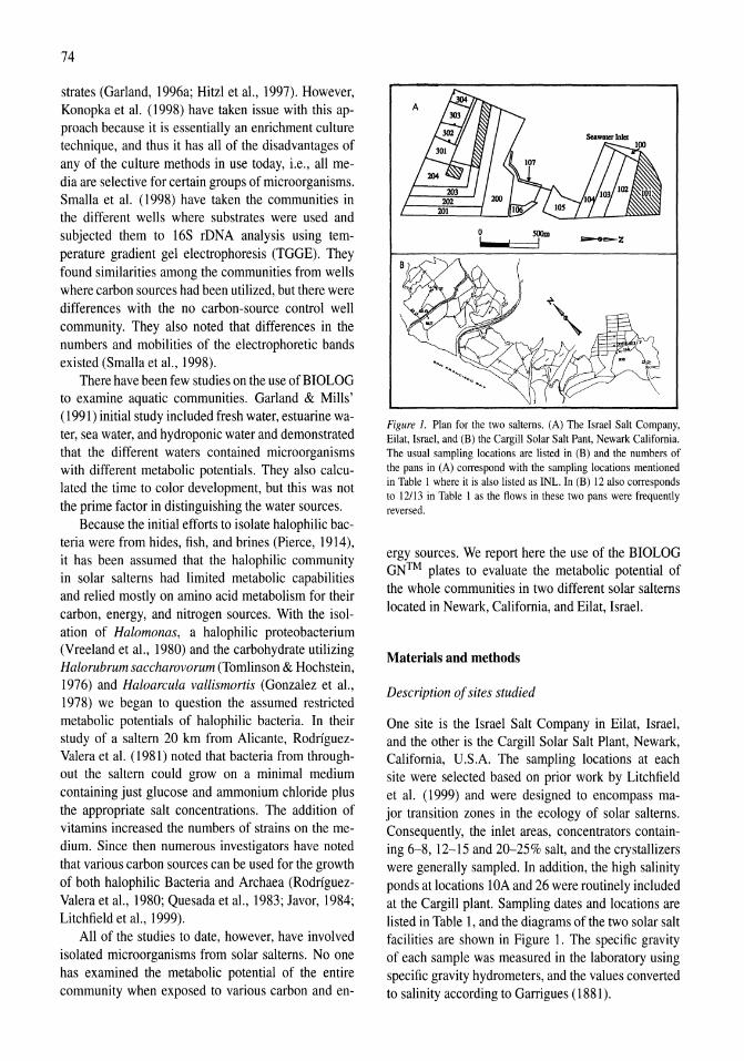
74
strates (Garland, 1996a; Hitzl et aI., 1997). However, Konopka et al. (1998) have taken issue with this approach because it is essentially an enrichment culture technique, and thus it has all of the disadvantages of any of the culture methods in use today, i.e., all media are selective for certain groups of microorganisms. Smalla et al. (1998) have taken the communities in the different wells where substrates were used and subjected them to 16S rDNA analysis using temperature gradient gel electrophoresis (TGGE). They found similarities among the communities from wells where carbon sources had been utilized, but there were differences with the no carbon-source control well community. They also noted that differences in the numbers and mobilities of the electrophoretic bands existed (Smalla et aI., 1998).
There have been few studies on the use of BIOLOG to examine aquatic communities. Garland & Mills' (1991) initial study included fresh water, estuarine water, sea water, and hydroponic water and demonstrated that the different waters contained microorganisms with different metabolic potentials. They also calculated the time to color development, but this was not the prime factor in distinguishing the water sources.
Because the initial efforts to isolate halophilic bacteria were from hides, fish, and brines (Pierce, 1914), it has been assumed that the halophilic community in solar salterns had limited metabolic capabilities and relied mostly on amino acid metabolism for their carbon, energy, and nitrogen sources. With the isolation of Halomonas, a halophilic proteobacterium (Vreeland et aI., 1980) and the carbohydrate utilizing Halorubrum saccharovorum (Tomlinson & Hochstein, 1976) and Haloarcula vallismortis (Gonzalez et aI., 1978) we began to question the assumed restricted metabolic potentials of halophilic bacteria. In their study of a saltern 20 km from Alicante, RodrfguezValera et al. (1981) noted that bacteria from throughout the saltern could grow on a minimal medium containing just glucose and ammonium chloride plus the appropriate salt concentrations. The addition of vitamins increased the numbers of strains on the medium. Since then numerous investigators have noted that various carbon sources can be used for the growth of both halophilic Bacteria and Archaea (RodrfguezValera et aI., 1980; Quesada et aI., 1983; Javor, 1984; Litchfield et aI., 1999).
All of the studies to date, however, have involved isolated microorganisms from solar salterns. No one has examined the metabolic potential of the entire community when exposed to various carbon and en-
-l!!
Figure 1. Plan for the two salterns. (A) The Israel Salt Company, Eilat, Israel, and (B) the Cargill Solar Salt Pant, Newark California. The usual sampling locations are listed in (B) and the numbers of the pans in (A) correspond with the sampling locations mentioned in Table I where it is also listed as INL. In (B) 12 also corresponds to 12/13 in Table I as the flows in these two pans were frequently reversed.
ergy sources. We report here the use of the BIOLOG GN™ plates to evaluate the metabolic potential of the whole communities in two different solar salterns located in Newark, California, and Eilat, Israel.
Materials and methods
Description of sites studied
One site is the Israel Salt Company in Eilat, Israel, and the other is the Cargill Solar Salt Plant, Newark, California, U.S.A. The sampling locations at each site were selected based on prior work by Litchfield et al. (1999) and were designed to encompass major transition zones in the ecology of solar salterns. Consequently, the inlet areas, concentrators containing 6-8, 12-15 and 20-25% salt, and the crystallizers were generally sampled. In addition, the high salinity ponds at locations lOA and 26 were routinely included at the Cargill plant. Sampling dates and locations are listed in Table 1, and the diagrams of the two solar salt facilities are shown in Figure 1. The specific gravity of each sample was measured in the laboratory using specific gravity hydrometers, and the values converted to salinity according to Garrigues (1881).
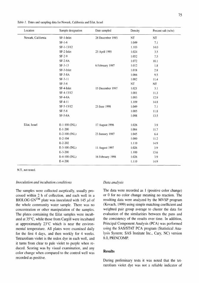
75
Table 1. Dates and sampling data for Newark, California and Eilat, Israel
Location Sample designation
Newark, California SF-I-Inlet
SF-I-6
SF-I-13/12
SF-2-Inlet
SF-2-9
SF-2-SA
SF-3-13
SF-3-Inlet
SF-3-8A SF-3-11
SF-3-8
SF-4-Inlet
SF-4-13/12
SF-4-SA
SF-4-11
SF-5-13/12
SF-5-S
SF-5-SA
Eilat, Israel E-l-l00 (INL)
E-I-200
E-2-100 (INL)
E-2-104
E-2-202
E-3-100 (INL)
E-3-200
E-4-100 (INL)
E-4-200
N.T., not tested.
Inoculation and incubation conditions
The samples were collected aseptically, usually processed within 2 h of collection, and each well in a BIOLOG GN™ plate was inoculated with 145 ILl of the whole community water sample. There was no concentration or other manipulation of the samples. The plates containing the Eilat samples were incubated at 35°C, while those from Cargill were incubated at approximately 23°C which is near the environmental temperature. All plates were examined daily for the first 4 days, and then weekly for 4 weeks. Tetrazolium violet is the redox dye in each well, and it turns from clear to pale violet to purple when reduced. Scoring was by visual examination, and any color change when compared to the control well was recorded as positive.
Date sampled Density Percent salt (w/w)
2S December 1993 NT NT
1.049 7.1
1.103 14.0
25 April 1995 1.024 3.5
1.052 7.5
1.072 10.1
6 February 1997 1.012 I.S
1.0lS 2.S
1.066 9.5 1.082 11.4
NT NT 15 December 1997 1.021 3.1
LOS 1 11.3
1.093 12.9
1.109 14.8
23 June 1995 1.049 7.1
1.0S5 11.8
1.098 13.5
17 August 1996 1.026 3.9 1.084 11.7
23 January 1997 1.045 6.4
1.080 11.2
1.110 14.9
11 August 1997 1.026 3.9
1.100 13.6 16 February 1998 1.026 3.9
1.110 14.9
Data analysis
The data were recorded as 1 (positive color change) or 0 for no color change meaning no reaction. The resulting data were analyzed by the MVSP program (Kovach, 1999) using simple matching coefficient and weighted pair group average to cluster the data for evaluation of the similarities between the pans and the consistency of the results over time. In addition, Principal Component Analysis (PCA) was performed using the SAS/STAT PCA program (Statistical Analysis System; SAS Institute Inc., Cary, NC) version 8.0, PRINCOMP.
Results
During preliminary tests it was noted that the tetrazolium violet dye was not a reliable indicator of
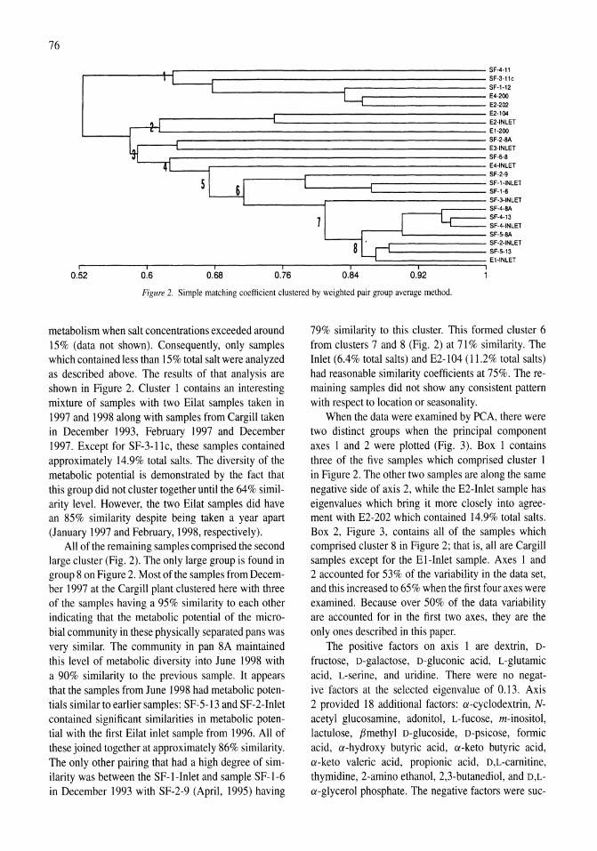
76
.-------+-l------------------------ SF-4-ll L __ r--------------------SF-3-llC
L _________ r----------SF-1-12
r----------- E4-2OQ L..-_________ E2-202
r---------C================ E2-l04 E2-INLET L..-________________________ El-200
r---C======================= SF-2-8A E3-INLET
.------------------------- SF-5-B L--r-------------------- E4-INLET .------f-------------- SF-2-9
L ____ -{========= SF-1-INLEi SF-1-6
L------r------------ SF-3-INLEi .----r--- SF-4-8A ,--__ SF-4-l3
Figure 2. Simple matching coefficient clustered by weighted pair group average method.
metabolism when salt concentrations exceeded around 15% (data not shown). Consequently, only samples which contained less than 15% total salt were analyzed as described above. The results of that analysis are shown in Figure 2. Cluster 1 contains an interesting mixture of samples with two Eilat samples taken in 1997 and 1998 along with samples from Cargill taken in December 1993, February 1997 and December 1997. Except for SF-3-11c, these samples contained approximately 14.9% total salts. The diversity of the metabolic potential is demonstrated by the fact that this group did not cluster together until the 64% similarity level. However, the two Eilat samples did have an 85% similarity despite being taken a year apart (January 1997 and February, 1998, respectively).
All of the remaining samples comprised the second large cluster (Fig. 2). The only large group is found in group 8 on Figure 2. Most of the samples from December 1997 at the Cargill plant clustered here with three of the samples having a 95% similarity to each other indicating that the metabolic potential of the microbial community in these physically separated pans was very similar. The community in pan 8A maintained this level of metabolic diversity into June 1998 with a 90% similarity to the previous sample. It appears that the samples from June 1998 had metabolic potentials similar to earlier samples: SF-5-l3 and SF-2-In1et contained significant similarities in metabolic potential with the first Eilat inlet sample from 1996. All of these joined together at approximately 86% similarity. The only other pairing that had a high degree of similarity was between the SF-I-Inlet and sample SF-1-6 in December 1993 with SF-2-9 (April, 1995) having
79% similarity to this cluster. This formed cluster 6 from clusters 7 and 8 (Fig. 2) at 71 % similarity. The Inlet (6.4% total salts) and E2-104 (11.2% total salts) had reasonable similarity coefficients at 75%. The remaining samples did not show any consistent pattern with respect to location or seasonality.
When the data were examined by PCA, there were two distinct groups when the principal component axes 1 and 2 were plotted (Fig. 3). Box 1 contains three of the five samples which comprised cluster 1 in Figure 2. The other two samples are along the same negative side of axis 2, while the E2-In1et sample has eigenvalues which bring it more closely into agreement with E2-202 which contained 14.9% total salts. Box 2, Figure 3, contains all of the samples which comprised cluster 8 in Figure 2; that is, all are Cargill samples except for the EI-Inlet sample. Axes 1 and 2 accounted for 53% of the variability in the data set, and this increased to 65% when the first four axes were examined. Because over 50% of the data variability are accounted for in the first two axes, they are the only ones described in this paper.
The positive factors on axis 1 are dextrin, Dfructose, D-galactose, D-gluconic acid, L-glutamic acid, L-serine, and uridine. There were no negative factors at the selected eigenvalue of 0.l3. Axis 2 provided 18 additional factors: a-cyclodextrin, Nacetyl glucosamine, adonitol, L-fucose, m-inositol, lactu10se, ,Bmethyl D-glucoside, D-psicose, formic acid, a-hydroxy butyric acid, a-keto butyric acid, a-keto valeric acid, propionic acid, D,L-camitine, thymidine, 2-amino ethanol, 2,3-butanediol, and D,La-glycerol phosphate. The negative factors were suc-
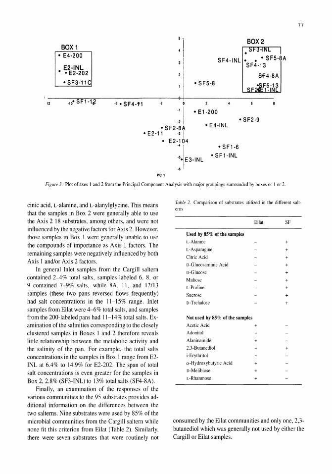
12
BOX 1 • E4·200
E2-INL • • E2·202
·SF3·11C
5 -
-6·SF4·1'1 ·2 0
·1 I ·2 j
77
BOX 2
SF4-INL. •• SF5·8A SF4-13
• SF5·8
·El·200 ·SF2·9
• E4-INL ·SF2-8A ·E2-11 .31
• E2·104 ·4
·5. E 3.INL
PC 1
• SF 1-6 ·SF1-INL
Figure 3. Plot of axes I and 2 from the Principal Component Analysis with major groupings surrounded by boxes or I or 2.
cinic acid, L-alanine, and L-alanylglycine. This means that the samples in Box 2 were generally able to use the Axis 2 18 substrates, among others, and were not influenced by the negative factors for Axis 2. However, those samples in Box 1 were generally unable to use the compounds of importance as Axis I factors. The remaining samples were negatively influenced by both Axis 1 and/or Axis 2 factors.
In general Inlet samples from the Cargill saltern contained 2-4% total salts, samples labeled 6, 8, or 9 contained 7-9% salts, while 8A, II, and 12/13 samples (these two pans reversed flows frequently) had salt concentrations in the 11-15% range. Inlet samples from Eilat were 4-6% total salts, and samples from the 200-labeled pans had 11-14% total salts. Examination of the salinities corresponding to the closely clustered samples in Boxes 1 and 2 therefore reveals little relationship between the metabolic activity and the salinity of the pan. For example, the total salts concentrations in the samples in Box I range from E2-INL at 6.4% to 14.9% for E2-202. The span of total salt concentrations is even greater for the samples in Box 2, 2.8% (SF3-INL) to 13% total salts (SF4-8A).
Finally, an examination of the responses of the various communities to the 95 substrates provides additional information on the differences between the two salterns. Nine substrates were used by 85% of the microbial communities from the Cargill saltern while none fit this criterion from Eilat (Table 2). Similarly, there were seven substrates that were routinely not
Table 2. Comparison of substrates utilized in the different salt-erns
Eilat SF
Used by 85% of the samples
L-Alanine + L-Asparagine + Citric Acid + D-Glucosaminic Acid + D-Glucose + Maltose + L-Proline + Sucrose + D-Trehalose +
Not used by 85 % of the samples
Acetic Acid + Adonitol + Alaninamide + 2.3-Butanediol + + i-Erythritol + a-Hydroxybutyric Acid + D-Melibiose + L-Rhamnose +
consumed by the Eilat communities and only one, 2,3-butanediol which was generally not used by either the Cargill or Eilat samples.
78
Discussion
Because microorganisms are considered the primary decomposers in the environment, it is important to determine the types of organic compounds which can be degraded by the whole community. In the past this was inferred from the various tests performed on pure cultures during their identification. However, it is widely recognized that the metabolism of a community is greater than that of the individuals comprising the community. With this in mind, it seemed reasonable to determine the metabolic potential of the communities in an environment with a salinity gradient to see what metabolic potentials existed throughout the system; whether the communities were influenced by time; or, whether the salt gradient was the predominant factor. To make this determination, we selected two different solar salterns: the Israel Salt Company, in Eilat, Israel, and the Cargill Solar Salt Plant in Newark, California, and used the BIOLOG system to indicate the metabolic potential.
To date, the BIOLOG system for community metabolism has been restricted to non-saline environments. Zak et al. (1994) described six desert soil communities at the 10rnada Long-term Ecological Research site near Las Cruces, New Mexico. They examined the numbers, types, activities, and rates of substrate utilization in BIOLOG plates and related these to the functional diversity of the system. They correlated the rate of color development to the species activity and density. They found that functional diversity was related to two factors: the types of substrates used and the moisture gradient in the soils.
Differences in various plant rhizosphere communities were noted by Garland (1 996b ) who examined the carbon source utilization patterns for hydroponic cultures of wheat, white potato, soybean, and sweet potato. When the experiments were conducted over a 2-year period, only the soybean showed any shift in the microbial community carbon utilization profile. Similar results were shown by Duineveld et al. (1998) for the microbial community at the tip of chrysanthemums, but there were significant changes in the carbon utilization patterns in the rhizosphere during the growth of the plants indicating a change in the microbial community. These latter results were not obtained using BIOLOG, but instead involved a limited substrate set which might have biased the results. Subsequent work by Hitzl et al. (1997) showed that a lower number of substrates could be used to discriminate the microbial communities in soils collected from
Denmark, Germany, and Italy. From the data in Table 2, a subset of substrates could be selected for future testing.
That the community in the Cargill saltern had greater metabolic diversity than expected was shown in Table 2 where the microorganisms consumed nine different carbon sources over 85% of the time and only 2,3-butanediol was not routinely utilized. There was no obvious trend for the other 85 carbon sources indicating that the metabolic potential was highly variable in the Cargill saltern samples. However, the metabolic potential pattern for the Eilat samples was more predictable although there were still 75 carbon sources which were used infrequently. These data imply that the microbial community may be more metabolically versatile than is generally accepted.
Many of the studies including those by Garland (1996a, 1997), Zak et al. (1994), Hitzl et al. (1997) and Winding (1994) have relied on the rate of color formation as the critical feature in the carbon source utilization pattern to discriminate microbial diversity and functionality in different systems. This approach as been questioned by Konopka et al. (1998), Haack et al. (1995) and Winding & Hendriksen (1997). Konopka et al. (1998) particularly noted that the physiological state of the microbes may affect the kinetics and pattern of substrate utilization. Haack et al. (1995) noted that the rates of substrate utilization were not linear with time, and both Haack et al. (1995) and Winding & Hendriksen (1997) commented that results were dependent on inoculum concentration and may be influenced by the organic matter added along with the inoculum. If an additional carbon source is introduced when the wells are inoculated, it will be evident by a change in the color of the control well (A 1) which does not have a carbon source present. If however, the inoculum is interfering with the use of one of the 95 substrates, this would not be noticed and could, therefore, bias the results unknowingly.
In fact, an interference did exist in this study. Initial inoculation of BIOLOG GN™ plates with samples containing greater than 15% total salts sometimes failed to show any consumed substrates while replicates had numerous positive wells. Further investigation showed that the tetrazolium dye did not function properly at these high salt concentrations. Additional redox dyes were tested and replicate plates inoculated. Unlike the results at lower salt concentration, there was no reproducibility in the substrate utilization patterns (Litchfield et aI., unpublished data)
so the data reported here do not include any of these higher salt-containing samples.
Furthermore, in our studies we have avoided the use of kinetic evaluation of carbon utilization because we could not adjust the inoculum concentration. Instead, we read all plates for up to 4 weeks or until there was no further increase in the utilization pattern. Admittedly, this approach included both initial responses and those organisms which could grow over time on the test substrates, but the goal was to evaluate the metabolic potential in the samples and not immediate responses to a carbon source.
This is the first report on metabolic potential in solar salterns. Analysis of the metabolic potential of the samples resulted in two major clusters which contained mainly either Eilat or Cargill samples. This demonstrates that there are significant differences between the two salterns and that the salt gradient is not the driving force in the metabolic diversity of the microbial community. This conclusion was further strengthened by the results shown in Table 2 listing the differences in the types of substrates used or not used by the majority of each saltern's microbial community. Finally, it became very obvious that the community in the salterns is not static, but does vary with time. This had previously been noted by Litchfield & Oren (2001) based on the lipid patterns, and the community metabolic potential confirms the dynamic nature of the saltern environment. Thus, there is greater microbial diversity in solar salterns than has been considered with the exciting possibility for the discovery of novel consortia and new individual Bacteria or Archaea.
Acknowledgments
The authors thank the personnel at the Cargill Solar Salt Plant in Newark, California, U.S.A. and the Israel Salt Company in Eilat, Israel, for their assistance in collecting samples, providing information on the salterns, and allowing access to the sites. We also appreciate the assistance of L. Nichols and G. P. Stojhovic, III for their work on the effects of high salt on BIOLOG plates. Portions of this study were supported by grant No. 95-00027 from the United States-Israel Binational Science Foundation (B.S.F., Jerusalem) and the Halophile Fund of the George Mason University Research Foundation. We also thank R. S. Oremland (U.S. Geological Survey, Menlo Park, California) for the use of his laboratory during the California field trips.
79
References
Duineveld, A. M., A. S. Rosado, 1. D. van Elsas & J. A. van Veen, 1998. Analysis of the dynamics of bacterial communities in the rhizosphere of the chrysanthemum via denaturing gradient gel electrophoresis and substrate utilization patterns. Appl. envir. Microbiol. 64: 4950-4957.
Garland, J. L., 1996a. Analytical approaches to the characterization of samples of microbial communities using patterns of potential C source utilization. Soil BioI. Biochem. 28: 213-221.
Garland, 1. L., 1996b. Patterns of potential C source utilization by rhizosphere communities. Soil BioI. Biochem. 28: 223-230.
Garland, J. L., 1997. Analysis and interpretation of community-level physiological profiles in microbial ecology. FEMS microbiol. Ecol. 24: 289-300.
Garland, J. L. & A. L. Mills, 1991. Classification and characterization of heterotrophic microbial communities on the basis of patterns of community-level sole-carbon source utilization. Appl. envir. Microbiol. 57: 2351-2359.
Garrigues, S. S., 1881. Statistics relating to the saline interests of Michigan. W. S. George & Co., State Printers and Binders, Lansing, pp. 13-15.
Gonzalez, c., C. Gutierrez & c. Ramirez, 1978. Halobacterium vallismortis sp. nov. An amylolytic and carbohydrate-utilizing extremely halophilic bacterium. Can J. Microbiol. 24: 710-715.
Haack, S. K., H. Garchow, M. J. Klug & L. 1. Forney, 1995. Analysis of factors affecting the accuracy, reproducibility, and interpretation of microbial community carbon source utilization patterns. Appl. envir. Microbiol. 61: 1458-1468.
Hitzl, w., A. Rangger, S. Sharma & H. Insam, 1997. Separation power of the 95 substrates of the BIOLOG system determined with various soils. FEMS microbiol. Ecol. 22: 167-174.
Javor, B. 1984. Growth potential of halophilic bacteria isolated form solar salt environments: Carbon sources and salt requirements. Appl. envir. Microbiol. 48: 352-360.
Konopka, A., L. Oliver & R. E Turco, Jr., 1998. The use of carbon substrate utilization patterns in environmental and ecological monitoring. Microbial Ecol. 35: 103-115.
Kovach, W. L. 1999. A MultiVariate Statistical Package for Windows, ver. 3.1. Kovach Computing Services, Pentraeth, Wales, United Kingdom.
Litchfield, C. D. & Oren, A., 2001. Polar lipids and pigments as biomarkers for the study of the microbial community structure of solar salterns. Hydrobiologia 466 (Dev. Hydrobiol. 162): 81-89.
Litchfield, C. D., A. Irby & R. H. Vreeland, 1999. The microbial ecology of solar salt plants. In Oren, A. (ed.), Microbiology and Biogeochemistry of Hypersaline Environments. CRC Press, Boca Raton, FL: 39-54.
Pierce, G. 1., 1914. The behavior of certain micro-organisms in brine. Carnegie Inst. Washington Pub. 193: 49-69.
Quesada, E., A. Ventosa, E Rodriguez-Valera, L. Megias & A. Ramos-Cormenzana, 1983. Numerical taxonomy of moderately halophilic gram-negative bacteria from hypersaline soils. 1. gen. Microbiol. 129: 2649-2657.
Rodriguez-Valera, E, E Ruiz-Berraquero & A. Ramos-Cormenzana, 1980. Isolation of extremely halophilic bacteria able to grow in defined inorganic media with single carbon sources. 1. gen. Microbiol. 119: 535-538.
Rodriguez-Valera, E, E Ruiz-Berraquero & A. RamosCormenzana, 1981. Characteristics of the heterotrophic bacterial populations in hypersaline environments of different salt concentrations. Microb. Ecol. 7: 235-243.

80
Smalla, K., U. Wachtendorf, H. Heuer, W.-T. Liu & 1. J. Forney, 1998. Analysis of BIOLOG GN substrate utilization patterns by microbial communities. App!. envir. Microbio!. 64: 1220-1225.
Tomlinson, G. A. & 1. 1. Hochstein, 1976. Halobacterium saccharovorum sp. nov. a carbohydrate-metabolizing, extremely halophilic bacterium. Can. J. Microbio!. 22: 587-591.
Vreeland, R. H., C. D. Litchfield, E. 1. Martin & E. Elliot, 1980. Halomonas elongata: A new genus and species of extremely salt tolerant bacteria. Int. J. syst. Bacterio!. 30: 485-495.
Winding, A., 1994. Fingerprinting bacterial soil communities using Biolog microtitre plates. In Ritz, K., J. Dighton, & K. E. Giller (eds), Beyond Biomass. John Wiley & Sons, New York: 85-94.
Winding, A. & N. B. Hendriksen, 1997. Biolog substrate utilization assay for metabolic fingerprints of soil bacteria: incubation effects. In Insam, H. & Rangger, A. (eds), Microbial Communities. Functional Versus Structural Approaches. Springer, Berlin: 195-205.
Wright, R. T. & J. E. Hobbie, 1965. The uptake of organic solutes in lake water. Limno!. Oceanogr. 10: 22-28.
Zak, J. C., M. R. Willig, D. 1. Moorhead & H. G. Wildman, 1994. Functional diversity of microbial communities: A quantitative approach. Soil Bio!. Biochem. 26: 1101-1108.
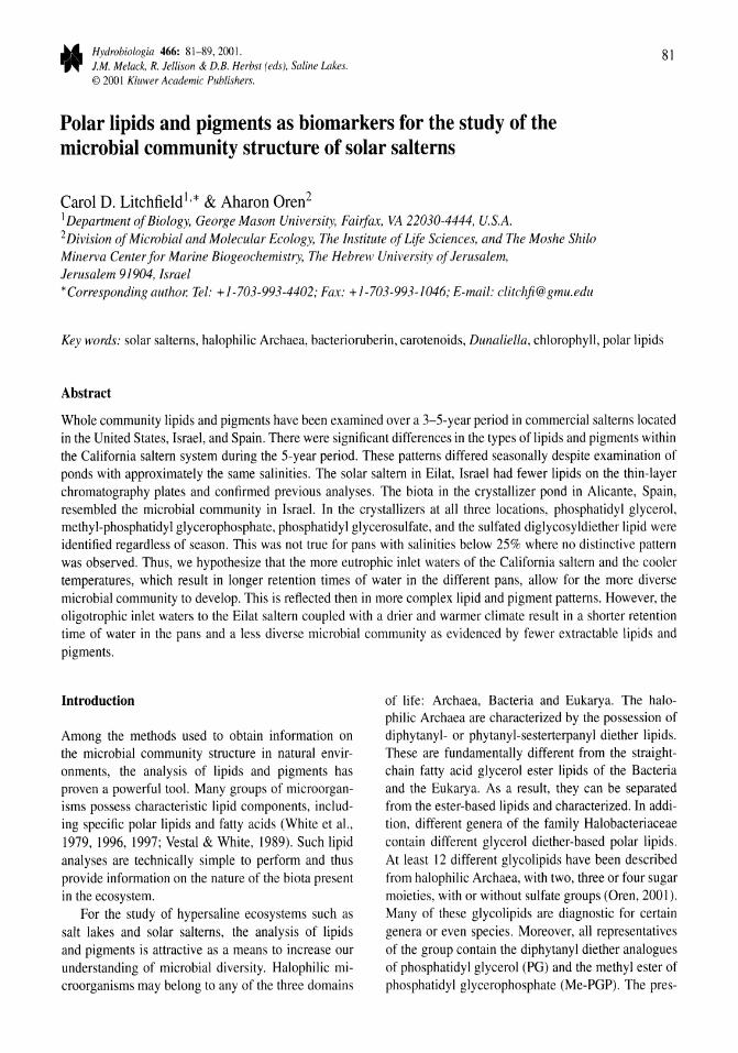
Hydrobiologia 466: 81-89,2001. J.M. Melack, R. Jellison & D.B. Herbst (eds), Saline Lakes. © 2001 Kluwer Academic Publishers.
81
Polar lipids and pigments as biomarkers for the study of the microbial community structure of solar salterns
Carol D. Litchfield\'* & Aharon Oren2
1 Department of Biology, George Mason University, Fairfax, VA 22030-4444, U.S.A. 2 Division of Microbial and Molecular Ecology, The Institute of Life Sciences, and The Moshe Shilo Minerva Center for Marine Biogeochemistry, The Hebrew University of Jerusalem, Jerusalem 91904, Israel * Corresponding author. Tel: +1-703-993-4402; Fax: + 1-703-993-1046; E-mail: [email protected]
Key words: solar salterns, halophilic Archaea, bacterioruberin, carotenoids, Dunaliella, chlorophyll, polar lipids
Abstract
Whole community lipids and pigments have been examined over a 3-5-year period in commercial salterns located in the United States, Israel, and Spain. There were significant differences in the types of lipids and pigments within the California saltern system during the 5-year period. These patterns differed seasonally despite examination of ponds with approximately the same salinities. The solar saltern in Eilat, Israel had fewer lipids on the thin-layer chromatography plates and confirmed previous analyses. The biota in the crystallizer pond in Alicante, Spain, resembled the microbial community in Israel. In the crystallizers at all three locations, phosphatidyl glycerol, methyl-phosphatidyl glycerophosphate, phosphatidyl glycerosulfate, and the sulfated diglycosyldiether lipid were identified regardless of season. This was not true for pans with salinities below 25% where no distinctive pattern was observed. Thus, we hypothesize that the more eutrophic inlet waters of the California saltern and the cooler temperatures, which result in longer retention times of water in the different pans, allow for the more diverse microbial community to develop. This is reflected then in more complex lipid and pigment patterns. However, the oligotrophic inlet waters to the Eilat saltern coupled with a drier and warmer climate result in a shorter retention time of water in the pans and a less diverse microbial community as evidenced by fewer extractable lipids and pigments.
Introduction
Among the methods used to obtain information on the microbial community structure in natural environments, the analysis of lipids and pigments has proven a powerful tool. Many groups of microorganisms possess characteristic lipid components, including specific polar lipids and fatty acids (White et aI., 1979, 1996, 1997; Vestal & White, 1989). Such lipid analyses are technically simple to perform and thus provide information on the nature of the biota present in the ecosystem.
For the study of hypersaline ecosystems such as salt lakes and solar salterns, the analysis of lipids and pigments is attractive as a means to increase our understanding of microbial diversity. Halophilic microorganisms may belong to any of the three domains
of life: Archaea, Bacteria and Eukarya. The halophilic Archaea are characterized by the possession of diphytanyl- or phytanyl-sesterterpanyl diether lipids. These are fundamentally different from the straightchain fatty acid glycerol ester lipids of the Bacteria and the Eukarya. As a result, they can be separated from the ester-based lipids and characterized. In addition, different genera of the family Halobacteriaceae contain different glycerol diether-based polar lipids. At least 12 different glycolipids have been described from halophilic Archaea, with two, three or four sugar moieties, with or without sulfate groups (Oren, 2001). Many of these glycolipids are diagnostic for certain genera or even species. Moreover, all representatives of the group contain the diphytanyl diether analogues of phosphatidyl glycerol (PO) and the methyl ester of phosphatidyl glycerophosphate (Me-POP). The pres-
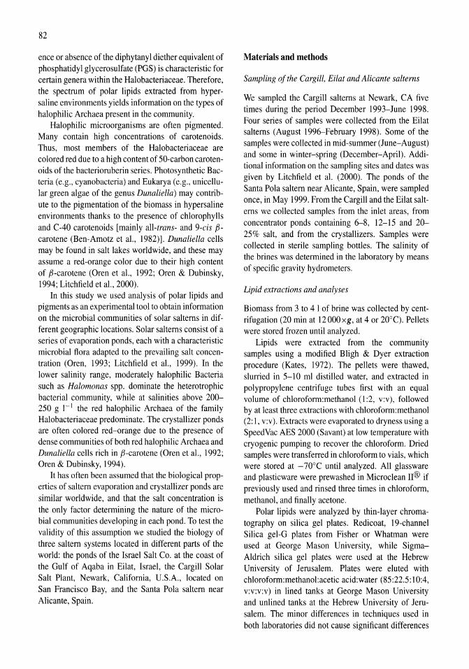
82
ence or absence of the diphytanyl diether equivalent of phosphatidyl glycerosulfate (PGS) is characteristic for certain genera within the Halobacteriaceae. Therefore, the spectrum of polar lipids extracted from hypersaline environments yields information on the types of halophilic Archaea present in the community.
Halophilic microorganisms are often pigmented. Many contain high concentrations of carotenoids. Thus, most members of the Halobacteriaceae are colored red due to a high content of 50-carbon carotenoids of the bacterioruberin series. Photosynthetic Bacteria (e.g., cyanobacteria) and Eukarya (e.g., unicellular green algae of the genus Dunaliella) may contribute to the pigmentation of the biomass in hypersaline environments thanks to the presence of chlorophylls and C-40 carotenoids [mainly all-trans- and 9-cis f3-carotene (Ben-Amotz et aI., 1982)]. Dunaliella cells may be found in salt lakes worldwide, and these may assume a red-orange color due to their high content of f3-carotene (Oren et aI., 1992; Oren & Dubinsky, 1994; Litchfield et al., 2000).
In this study we used analysis of polar lipids and pigments as an experimental tool to obtain information on the microbial communities of solar salterns in different geographic locations. Solar salterns consist of a series of evaporation ponds, each with a characteristic microbial flora adapted to the prevailing salt concentration (Oren, 1993; Litchfield et al., 1999). In the lower salinity range, moderately halophilic Bacteria such as Halomonas spp. dominate the heterotrophic bacterial community, while at salinities above 200-250 g I-I the red halophilic Archaea of the family Halobacteriaceae predominate. The crystallizer ponds are often colored red-orange due to the presence of dense communities of both red halophilic Archaea and Dunaliella cells rich in f3-carotene (Oren et aI., 1992; Oren & Dubinsky, 1994).
It has often been assumed that the biological properties of saltern evaporation and crystallizer ponds are similar worldwide, and that the salt concentration is the only factor determining the nature of the microbial communities developing in each pond. To test the validity of this assumption we studied the biology of three saltern systems located in different parts of the world: the ponds of the Israel Salt Co. at the coast of the Gulf of Aqaba in Eilat, Israel, the Cargill Solar Salt Plant, Newark, California, U.S.A., located on San Francisco Bay, and the Santa Pola saltern near Alicante, Spain.
Materials and methods
Sampling of the Cargill, Eilat and Alicante salterns
We sampled the Cargill salterns at Newark, CA five times during the period December 1993-June 1998. Four series of samples were collected from the Eilat salterns (August 1996-February 1998). Some of the samples were collected in mid-summer (June-August) and some in winter-spring (December-April). Additional information on the sampling sites and dates was given by Litchfield et al. (2000). The ponds of the Santa Pola saltern near Alicante, Spain, were sampled once, in May 1999. From the Cargill and the Eilat salterns we collected samples from the inlet areas, from concentrator ponds containing 6-8, 12-15 and 20-25% salt, and from the crystallizers. Samples were collected in sterile sampling bottles. The salinity of the brines was determined in the laboratory by means of specific gravity hydrometers.
Lipid extractions and analyses
Biomass from 3 to 4 I of brine was collected by centrifugation (20 min at 12 OOOxg, at 4 or 20°C). Pellets were stored frozen until analyzed.
Lipids were extracted from the community samples using a modified Bligh & Dyer extraction procedure (Kates, 1972). The pellets were thawed, slurried in 5-10 ml distilled water, and extracted in polypropylene centrifuge tubes first with an equal volume of chloroform:methanol (I :2, v:v), followed by at least three extractions with chloroform:methanol (2: 1, v:v). Extracts were evaporated to dryness using a SpeedVac AES 2000 (Savant) at low temperature with cryogenic pumping to recover the chloroform. Dried samples were transferred in chloroform to vials, which were stored at -70°C until analyzed. All glassware and plasticware were prewashed in Microclean n® if previously used and rinsed three times in chloroform, methanol, and finally acetone.
Polar lipids were analyzed by thin-layer chromatography on silica gel plates. Redicoat, 19-channel Silica gel-G plates from Fisher or Whatman were used at George Mason University, while SigmaAldrich silica gel plates were used at the Hebrew University of Jerusalem. Plates were eluted with chloroform:methanol:acetic acid:water (85:22.5: 10:4, v:v:v:v) in lined tanks at George Mason University and unlined tanks at the Hebrew University of Jerusalem. The minor differences in techniques used in both laboratories did not cause significant differences
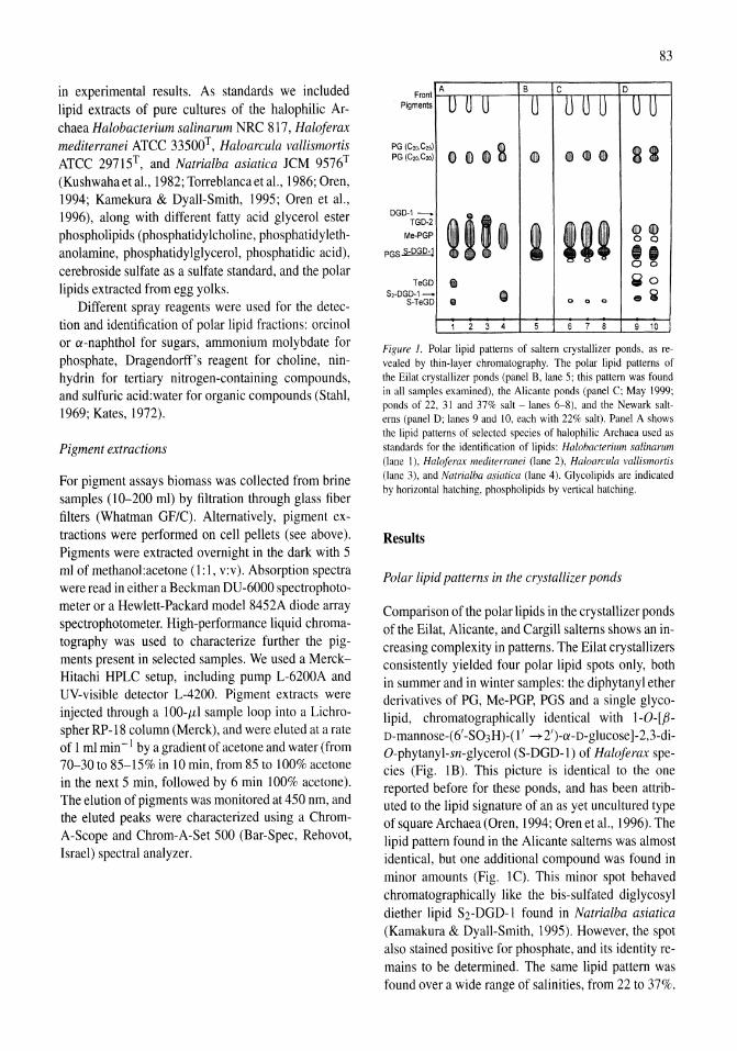
in experimental results. As standards we included lipid extracts of pure cultures of the halophilic Archaea Halobacterium salina rum NRC 817, Haloferax mediterranei ATCC 33500T, Haloarcula vallismortis ATCC 29715T, and Natrialba asiatica JCM 9576T
(Kushwaha et aI., 1982; Torreblanca et aI., 1986; Oren, 1994; Kamekura & Dyall-Smith, 1995; Oren et aI., 1996), along with different fatty acid glycerol ester phospholipids (phosphatidylcholine, phosphatidylethanolamine, phosphatidylglycerol, phosphatidic acid), cerebroside sulfate as a sulfate standard, and the polar lipids extracted from egg yolks.
Different spray reagents were used for the detection and identification of polar lipid fractions: orcinol or a-naphthol for sugars, ammonium molybdate for phosphate, Dragendorff's reagent for choline, ninhydrin for tertiary nitrogen-containing compounds, and sulfuric acid:water for organic compounds (Stahl, 1969; Kates, 1972).
Pigment extractions
For pigment assays biomass was collected from brine samples (10-200 ml) by filtration through glass fiber filters (Whatman OF/C). Alternatively, pigment extractions were performed on cell pellets (see above). Pigments were extracted overnight in the dark with 5 ml of methanol:acetone (1: I, v:v). Absorption spectra were read in either a Beckman DU-6000 spectrophotometer or a Hewlett-Packard model 8452A diode array spectrophotometer. High-performance liquid chromatography was used to characterize further the pigments present in selected samples. We used a MerckHitachi HPLC setup, including pump L-6200A and UV-visible detector L-4200. Pigment extracts were injected through a 100-l--d sample loop into a Lichrospher RP-18 column (Merck), and were eluted at a rate of I ml min - J by a gradient of acetone and water (from 70-30 to 85-15% in 10 min, from 85 to 100% acetone in the next 5 min, followed by 6 min 100% acetone). The elution of pigments was monitored at 450 nm, and the eluted peaks were characterized using a ChromA-Scope and Chrom-A-Set 500 (Bar-Spec, Rehovot, Israel) spectral analyzer.
Front Pigments
PG(C20,C" PG(C20,C20
) )
A
U U U
~m,1
, tUG DGD-1_
TGD-
Me-PGP
PGS S-DGD-l
0
D
TeG S2-DGD-1~
S-TeG
e Ci!I • 1 2 3 4
B
83
C 0
U U U U U U
GIll I I GJ) II
I III @(iJ) o 0
~t ~o
000 e ~
5 6 7 8 9 10
Figure 1. Polar lipid patterns of saltern crystallizer ponds, as revealed by thin-layer chromatography. The polar lipid patterns of the Eilat crystallizer ponds (panel B, lane 5; this pattern was found in all samples examined), the Alicante ponds (panel C; May 1999; ponds of 22, 31 and 37% salt - lanes 6-8), and the Newark salterns (panel 0; lanes 9 and 10, each with 22% salt). Panel A shows the lipid patterns of selected species of halophilic Archaea used as standards for the identification of lipids: Halabacterium salinarul11 (lane I), Halaferax mediterranei (lane 2), Halaarcula val/ismartis (lane 3), and Natrialba asiatica (lane 4). Glycolipids are indicated by horizontal hatching, phospholipids by vertical hatching.
Results
Polar lipid patterns in the crystallizer ponds
Comparison of the polar lipids in the crystallizer ponds of the Eilat, Alicante, and Cargill salterns shows an increasing complexity in patterns. The Eilat crystallizers consistently yielded four polar lipid spots only, both in summer and in winter samples: the diphytanyl ether derivatives of PO, Me-POP, POS and a single glycolipid, chromatographically identical with 1-0-[tJD-mannose-( 6'-S03H)-( I' --+ 2')-a-D-glucose ]-2,3-diO-phytanyl-sn-glycerol (S-DOD-l) of Haloferax species (Fig. IB). This picture is identical to the one reported before for these ponds, and has been attributed to the lipid signature of an as yet uncultured type of square Archaea (Oren, 1994; Oren et aI., 1996). The lipid pattern found in the Alicante salterns was almost identical, but one additional compound was found in minor amounts (Fig. lC). This minor spot behaved chromatographically like the bis-sulfated diglycosyl diether lipid S2-DOD-l found in Natrialba asiatica (Kamakura & Dyall-Smith, 1995). However, the spot also stained positive for phosphate, and its identity remains to be determined. The same lipid pattern was found over a wide range of salinities, from 22 to 37%.
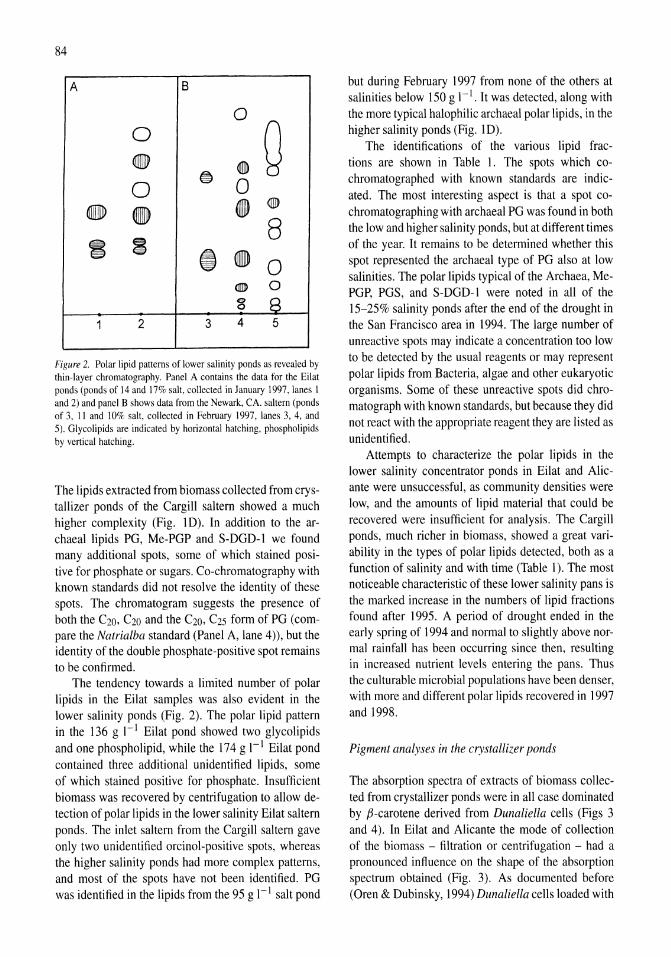
84
A B
0 0
Q ~ G 0
@ 0
• I) • @J)
8 • ~ i I) 0 ({]]I) 0 8 8
1 2 3 4 5
Figure 2. Polar lipid patterns of lower salinity ponds as revealed by thin-layer chromatography. Panel A contains the data for the Eilat ponds (ponds of 14 and 17% salt, collected in January 1997, lanes I and 2) and panel B shows data from the Newark, CA. saltern (ponds of 3, II and 10% salt, collected in February 1997, lanes 3, 4, and 5). Glycolipids are indicated by horizontal hatching, phospholipids by vertical hatching.
The lipids extracted from biomass collected from crystallizer ponds of the Cargill saltern showed a much higher complexity (Fig. lD). In addition to the archaeal lipids PG, Me-PGP and S-DGD-l we found many additional spots, some of which stained positive for phosphate or sugars. Co-chromatography with known standards did not resolve the identity of these spots. The chromatogram suggests the presence of both the C20, C20 and the C20, C25 form of PG (compare the Natrialba standard (Panel A, lane 4)), but the identity of the double phosphate-positive spot remains to be confirmed.
The tendency towards a limited number of polar lipids in the Eilat samples was also evident in the lower salinity ponds (Fig. 2). The polar lipid pattern in the 136 g 1-1 Eilat pond showed two glycolipids and one phospholipid, while the 174 g 1-1 Eilat pond contained three additional unidentified lipids, some of which stained positive for phosphate. Insufficient biomass was recovered by centrifugation to allow detection of polar lipids in the lower salinity Eilat saltern ponds. The inlet saltern from the Cargill saltern gave only two unidentified orcinol-positive spots, whereas the higher salinity ponds had more complex patterns, and most of the spots have not been identified. PG was identified in the lipids from the 95 g 1-1 salt pond
but during February 1997 from none of the others at salinities below 150 g 1-1. It was detected, along with the more typical halophilic archaeal polar lipids, in the higher salinity ponds (Fig. lD).
The identifications of the various lipid fractions are shown in Table 1. The spots which cochromatographed with known standards are indicated. The most interesting aspect is that a spot cochromatographing with archaeal PG was found in both the low and higher salinity ponds, but at different times of the year. It remains to be determined whether this spot represented the archaeal type of PG also at low salinities. The polar lipids typical of the Archaea, MePGP, PGS, and S-DGD-l were noted in all of the 15-25% salinity ponds after the end of the drought in the San Francisco area in 1994. The large number of unreactive spots may indicate a concentration too low to be detected by the usual reagents or may represent polar lipids from Bacteria, algae and other eukaryotic organisms. Some of these unreactive spots did chromatograph with known standards, but because they did not react with the appropriate reagent they are listed as unidentified.
Attempts to characterize the polar lipids in the lower salinity concentrator ponds in Eilat and Alicante were unsuccessful, as community densities were low, and the amounts of lipid material that could be recovered were insufficient for analysis. The Cargill ponds, much richer in biomass, showed a great variability in the types of polar lipids detected, both as a function of salinity and with time (Table 1). The most noticeable characteristic of these lower salinity pans is the marked increase in the numbers of lipid fractions found after 1995. A period of drought ended in the early spring of 1994 and normal to slightly above normal rainfall has been occurring since then, resulting in increased nutrient levels entering the pans. Thus the culturable microbial populations have been denser, with more and different polar lipids recovered in 1997 and 1998.
Pigment analyses in the crystallizer ponds
The absorption spectra of extracts of biomass collected from crystallizer ponds were in all case dominated by .a-carotene derived from Dunaliella cells (Figs 3 and 4). In Eilat and Alicante the mode of collection of the biomass - filtration or centrifugation - had a pronounced influence on the shape of the absorption spectrum obtained (Fig. 3). As documented before (Oren & Dubinsky, 1994) Dunaliella cells loaded with
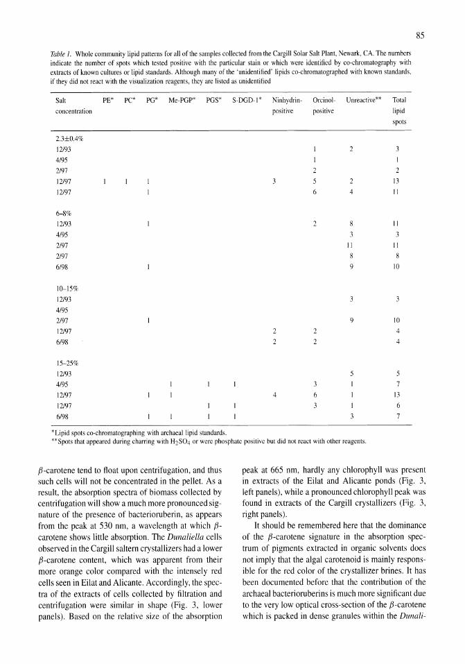
85
Table 1. Whole community lipid patterns for all ofthe samples collected from the Cargill Solar Salt Plant, Newark, CA. The numbers indicate the number of spots which tested positive with the particular stain or which were identified by co-chromatography with extracts of known cultures or lipid standards. Although many of the 'unidentified' lipids co-chromatographed with known standards, if they did not react with the visualization reagents, they are listed as unidentified
Salt PE* PC* PG* Me-PGP* PGS* S-DGD-I* Ninhydrin- Orcinol- U nreactive*' Total
concentration positive positive lipid
spots
2.3±0,4%
12/93 2 3 4195 I
2/97 2 2
12/97 3 5 2 13 12/97 6 4 II
6-8%
12/93 2 8 II
4195 3 3 2/97 II II
2/97 8 8
6/98 9 10
10--15%
12/93 3 3 4195
2/97 9 10 12/97 2 2 4
6198 2 2 4
15-25%
12/93 5 5 4195 3 7
12/97 4 6 13
12/97 3 6
6198 3 7
'Lipid spots co-chromatographing with archaeallipid standards. **Spots that appeared during charring with H2S04 or were phosphate positive but did not react with other reagents.
tl-carotene tend to float upon centrifugation, and thus such cells will not be concentrated in the pellet. As a result, the absorption spectra of biomass collected by centrifugation will show a much more pronounced signature of the presence of bacterioruberin, as appears from the peak at 530 nm, a wavelength at which tlcarotene shows little absorption. The Dunaliella cells observed in the Cargill saltern crystallizers had a lower tl-carotene content, which was apparent from their more orange color compared with the intensely red cells seen in Eilat and Alicante. Accordingly, the spectra of the extracts of cells collected by filtration and centrifugation were similar in shape (Fig. 3, lower panels). Based on the relative size of the absorption
peak at 665 nm, hardly any chlorophyll was present in extracts of the Eilat and Alicante ponds (Fig. 3, left panels), while a pronounced chlorophyll peak was found in extracts of the Cargill crystallizers (Fig. 3, right panels).
It should be remembered here that the dominance of the tl-carotene signature in the absorption spectrum of pigments extracted in organic solvents does not imply that the algal carotenoid is mainly responsible for the red color of the crystallizer brines. It has been documented before that the contribution of the archaeal bacterioruberins is much more significant due to the very low optical cross-section of the tl-carotene which is packed in dense granules within the Dunali-
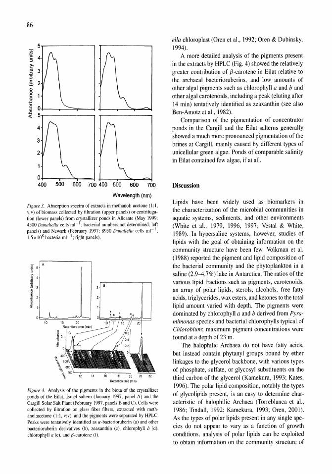
86
5 ~ c: ::J
~ I!! 3 ~
-e 2 ~
8 c: il ... 0 0 1/1 .c 5 c(
4
3
2
500 600 700 400 500 600 700
Wavelength (nm)
Figure 3. Absorption spectra of extracts in methanol: acetone (1: I, v:v) of biomass collected by filtration (upper panels) or centrifugation (lower panels) from crystallizer ponds in Alicante (May 1999; 4500 Dunaliella cells ml- i ; bacterial numbers not determined; left panels) and Newark (February 1997; 8950 Dunaliella cells ml- i ;
1.5 x 10⁸ bacteria ml- i ; right panels).
10
Retention time (min)
Figure 4. Analysis of the pigments in the biota of the crystallizer ponds of the Eilat, Israel saltern (January 1997, panel A) and the Cargill Solar Salt Plant (February 1997, panels B and C). Cells were collected by filtration on glass fiber filters, extracted with methanol:acetone (1:1, v:v), and the pigments were separated by HPLC. Peaks were tentatively identified as a-bacterioruberin (a) and other bacterioruberin derivatives (b), zeaxanthin (c), chlorophyll b (d), chlorophyll a (e), and fJ-carotene (f).
ella chloroplast (Oren et aI., 1992; Oren & Dubinsky, 1994).
A more detailed analysis of the pigments present in the extracts by HPLC (Fig. 4) showed the relatively greater contribution of ,B-carotene in Eilat relative to the archaeal bacterioruberins, and low amounts of other algal pigments such as chlorophyll a and band other algal carotenoids, including a peak (eluting after 14 min) tentatively identified as zeaxanthin (see also Ben-Amotz et aI., 1982) .
Comparison of the pigmentation of concentrator ponds in the Cargill and the Eilat salterns generally showed a much more pronounced pigmentation of the brines at Cargill, mainly caused by different types of unicellular green algae. Ponds of comparable salinity in Eilat contained few algae, if at all.
Discussion
Lipids have been widely used as biomarkers in the characterization of the microbial communities in aquatic systems, sediments, and other environments (White et aI., 1979, 1996, 1997; Vestal & White, 1989). In hypersaline systems, however, studies of lipids with the goal of obtaining information on the community structure have been few. Volkman et aI. (1988) reported the pigment and lipid composition of the bacterial community and the phytoplankton in a saline (2.9--4.7%) lake in Antarctica. The ratios of the various lipid fractions such as pigments, carotenoids, an array of polar lipids, sterols, alcohols, free fatty acids, triglycerides, wax esters, and ketones to the total lipid amount varied with depth. The pigments were dominated by chlorophyll a and b derived from Pyramimonas species and bacterial chlorophylls typical of Chlorobium; maximum pigment concentrations were found at a depth of 23 m.
The halophilic Archaea do not have fatty acids, but instead contain phytanyl groups bound by ether linkages to the glycerol backbone, with various types of phosphate, sulfate, or glycosyl substituents on the third carbon of the glycerol (Kamekura, 1993; Kates, 1996). The polar lipid composition, notably the types of glycolipids present, is an easy to determine characteristic of halophilic Archaea (Torreblanca et aI., 1986; Tindall, 1992; Kamekura, 1993; Oren, 2001). As the types of polar lipids present in any single species do not appear to vary as a function of growth conditions, analysis of polar lipids can be exploited to obtain information on the community structure of
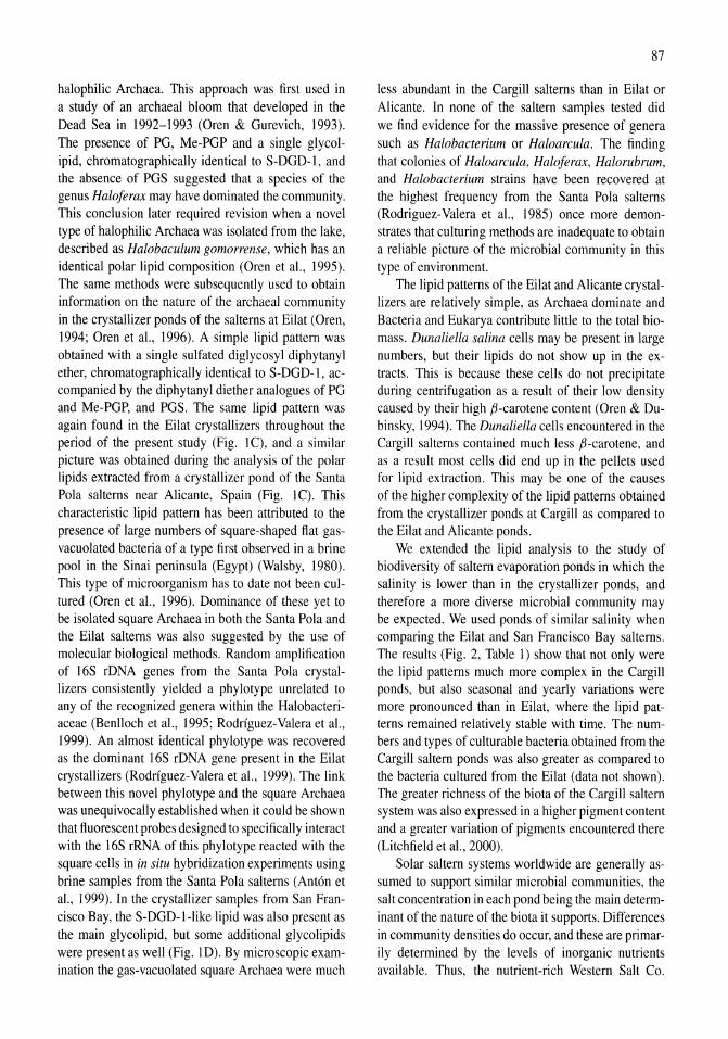
halophilic Archaea. This approach was first used in a study of an archaeal bloom that developed in the Dead Sea in 1992-1993 (Oren & Gurevich, 1993). The presence of PG, Me-PGP and a single glycolipid, chromatographically identical to S-DGD-l, and the absence of PGS suggested that a species of the genus Haloferax may have dominated the community. This conclusion later required revision when a novel type of halophilic Archaea was isolated from the lake, described as Halobaculum gomorrense, which has an identical polar lipid composition (Oren et aI., 1995). The same methods were subsequently used to obtain information on the nature of the archaeal community in the crystallizer ponds of the salterns at Eilat (Oren, 1994; Oren et al., 1996). A simple lipid pattern was obtained with a single sulfated diglycosyl diphytanyl ether, chromatographically identical to S-DGD-l, accompanied by the diphytanyl diether analogues of PG and Me-PGP, and PGS. The same lipid pattern was again found in the Eilat crystallizers throughout the period of the present study (Fig. IC), and a similar picture was obtained during the analysis of the polar lipids extracted from a crystallizer pond of the Santa Pola salterns near Alicante, Spain (Fig. I C). This characteristic lipid pattern has been attributed to the presence of large numbers of square-shaped flat gasvacuolated bacteria of a type first observed in a brine pool in the Sinai peninsula (Egypt) (Walsby, 1980). This type of microorganism has to date not been cultured (Oren et aI., 1996). Dominance of these yet to be isolated square Archaea in both the Santa Pola and the Eilat salterns was also suggested by the use of molecular biological methods. Random amplification of 16S rDNA genes from the Santa Pola crystallizers consistently yielded a phylotype unrelated to any of the recognized genera within the Halobacteriaceae (Benlloch et aI., 1995; Rodriguez-Valera et aI., 1999). An almost identical phylotype was recovered as the dominant 16S rDNA gene present in the Eilat crystallizers (Rodrfguez-Valera et aI., 1999). The link between this novel phylotype and the square Archaea was unequivocally established when it could be shown that fluorescent probes designed to specifically interact with the 16S rRNA of this phylotype reacted with the square cells in in situ hybridization experiments using brine samples from the Santa Pola salterns (Anton et aI., 1999). In the crystallizer samples from San Francisco Bay, the S-DGD-l-like lipid was also present as the main glycolipid, but some additional glycolipids were present as well (Fig. lD). By microscopic examination the gas-vacuolated square Archaea were much
87
less abundant in the Cargill salterns than in Eilat or Alicante. In none of the saltern samples tested did we find evidence for the massive presence of genera such as Halobacterium or Haloarcula. The finding that colonies of Haloarcula, Haloferax, Halorubrum, and Halobacterium strains have been recovered at the highest frequency from the Santa Pola salterns (Rodriguez-Valera et aI., 1985) once more demonstrates that culturing methods are inadequate to obtain a reliable picture of the microbial community in this type of environment.
The lipid patterns of the Eilat and Alicante crystallizers are relatively simple, as Archaea dominate and Bacteria and Eukarya contribute little to the total biomass. Dunaliella salina cells may be present in large numbers, but their lipids do not show up in the extracts. This is because these cells do not precipitate during centrifugation as a result of their low density caused by their high ,B-carotene content (Oren & Dubinsky, 1994). The Dunaliella cells encountered in the Cargill salterns contained much less ,B-carotene, and as a result most cells did end up in the pellets used for lipid extraction. This may be one of the causes of the higher complexity of the lipid patterns obtained from the crystallizer ponds at Cargill as compared to the Eilat and Alicante ponds.
We extended the lipid analysis to the study of biodiversity of saltern evaporation ponds in which the salinity is lower than in the crystallizer ponds, and therefore a more diverse microbial community may be expected. We used ponds of similar salinity when comparing the Eilat and San Francisco Bay salterns. The results (Fig. 2, Table 1) show that not only were the lipid patterns much more complex in the Cargill ponds, but also seasonal and yearly variations were more pronounced than in Eilat, where the lipid patterns remained relatively stable with time. The numbers and types of culturable bacteria obtained from the Cargill saltern ponds was also greater as compared to the bacteria cultured from the Eilat (data not shown). The greater richness of the biota of the Cargill saltern system was also expressed in a higher pigment content and a greater variation of pigments encountered there (Litchfield et aI., 2000).
Solar saltern systems worldwide are generally assumed to support similar microbial communities, the salt concentration in each pond being the main determinant of the nature of the biota it supports. Differences in community densities do occur, and these are primarily determined by the levels of inorganic nutrients available. Thus, the nutrient-rich Western Salt Co.
88
(Chula Vista, California, U.S.A.) and the nutrient-poor Exportadora de Sal (Guerrero Negro, Baja California, Mexico) differed in biomass density (Javor, 1983a, 1983b).
The effect of geographic location, nutrient availability, residence time, and mode of operation of the salterns on the diversity of the microbial community structure has never been documented before. The findings presented here, based on the examination of lipid patterns and pigment analyses, show that the microbial communities in saltern ponds differ not only as a function of the salt concentration. Part of the differences observed are undoubtedly due to the seasonal fluctuations which occur at the California plant, where temperatures are lower and rainfall is significantly greater than in Eilat. Furthermore, the source of the water for the Newark plant is San Francisco Bay. Due to freshwater flow from the Sacramento River and the San Juaquin River along with runoff from the surrounding communities and industries this is a eutrophic environment, and this results in a higher organic loading than that found in Eilat where the main water source for the saltern is the oligotrophic Gulf of Aqaba. Because the California saltern is located in a cooler climate, the retention time of the water in the various pans is much longer, 1-2 years. These conditions thus allow for the development of a relatively dense microbial population. As our results show, these populations are also relatively diverse. In the Eilat salterns, retention times are short (in the order of only a few months), and salt is harvested all the year round. Hence the time for the development of dense and complex microbial communities there is limited.
It may be concluded that saltern ponds provide us with a much more diverse biological systems than previously assumed, and that only a more thorough microbiological comparison of saltern systems worldwide will show the full biodiversity developing in ponds of salt concentrations increasing from seawater salinity up to NaCI saturation and beyond.
Acknowledgements
The authors thank the owners of the Cargill Solar Salt Plant in Newark, California, U.S.A., the Israel Salt Company in Eilat, Israel, and the Santa Pola salterns, Alicante, Spain, for allowing access to the sampling sites. We are also appreciative of the assistance of G. Dimitrov, A Irby, T. Kis-Papo, N. Koval, and S. Vinayak in various aspects of this study. Portions of
this work were supported by grant No. 95-00027 from the United States-Israel Binational Science Foundation (B.S.F., Jerusalem) (to AO. and C.DL) and the Halophile Fund of the George Mason University Research Foundation (to C.D.L.). The study of the Alicante salterns by AO. was supported by a grant from the Israel Ministry of Science and the Spanish Ministry of Foreign Affairs - The General Directorate of Cultural and Scientific Relations. We thank F. Rodrfguez-Valera and S. Benlloch for their hospitality in Alicante and R.S. Oremland (U.S. Geological Survey, Menlo Park, CA) for the use of his laboratory during the California field trips.
References
Ant6n, J., E. Llobet -Brossa, F. Rodriguez-Valera & R. Amann, 1999. Fluorescence in situ analysis of the prokaryotic community inhabiting crystallizer ponds. Environ. Microbiol.l: 517-523.
Ben-Amotz, A., A. Katz & M. Avron, 1982. Accumulation of tJ-carotene in halotolerant algae: purification and characterization of tJ-carotene-rich globules from Dunuliella bardawil (Chlorophyceae). J. Phycol. 18: 529-537.
Benlloch, S., A. Martinez-Murcia & F. Rodriguez-Valera, 1995. Sequencing of bacterial and archaeal 16S rDNA genes directly amplified from a hypersaline environment. Syst. appl. Microbiol. 18: 574-581.
Javor, B. J., 1983a. Planktonic standing crop and nutrients in a saltern ecosystem. Limnol. Oceanogr. 28: 153-159.
Javor, B. J., 1983b. Nutrients and ecology of the Western Salt and Exportadora de Sal saltern brines. In Proceedings of the 6th International Symposium on Salt. Vol. I. Salt Institute, Toronto: 195-205.
Kamekura, M., 1993. Lipids of extreme halophiles. In Vreeland, R. H. & L. I. Hochstein, (eds), The Biology of Halophilic Bacteria. CRC Press. Boca Raton, FL: 135-161.
Kamekura, M. & M. L. Dyall-Smith, 1995. Taxonomy of the family Halobacteriaceae and the description of two new genera Halorubrobacterium and Natrialba. J. gen. app\. Microbiol. 41: 333-350.
Kates, M., 1972. Techniques of Lipidology. North-Holland! American Elsevier Publishing Co., New York.
Kates, M., 1996. Structural analysis of phospholipids and glycolipids in extremely halophilic archaebacteria. J. microbiol. Meth. 25: 113-128.
Kushwaha. S. C., G. Juez-Perez, F. Rodriguez-Valera, M. Kates & D. J. Kushner, 1982. Survey of lipids of a new group of extremely halophilic bacteria from salt ponds in Spain. Can. J. Microbiol. 28: 1365-1372.
Litchfield, C. D., A. Irby & R. H. Vreeland, 1999. The microbial ecology of solar salt plants. In Oren, A. (ed.), Microbiology and Biogeochemistry of Hypersaline Environments. CRC Press, Boca Raton, FL: 39-54.
Litchfield, C. D., A. Irby, T. Kis-Papo & A. Oren, 2000. Comparisons of the polar lipid and pigment profiles of two solar salterns located in Newark, California, U.S.A., and Eilat, Israel. Extremophiles 4: 259-265.
Oren, A., 1994. Characterization of the halophilic archaeal community in saltem crystallizer ponds by means of polar lipid analysis. Int. J. Salt Lake Res. 3: 15-29.
Oren, A., 2001. The order Halobacteriales. In Dworkin, M., S. Falkow, E. Rosenberg, K.-H. Schleifer & E. Stackebrandt, (eds), The Prokaryotes. A Handbook on the Biology of Bacteria: Ecophysiology, Isolation, Identification, Applications. 3rd edn. Springer, New York, on the web.
Oren, A. & Z. Dubinsky, 1994. On the red coloration of saltern crystallizer ponds. II Additional evidence for the contribution of halobacterial pigments. Int. J. Salt Lake Res. 3: 9-l3.
Oren, A. & P. Gurevich, 1993. Characterization of the dominant halophilic Archaea in a bacterial bloom in the Dead Sea. FEMS Microbiol. Ecol. 12: 249-256.
Oren, A., S. Duker & S. Ritter, 1996. The polar lipid composition ofWalsby's square bacterium. FEMS Microbiol. Lett. 138: 135-140.
Oren, A., N. Stambler & Z. Dubinsky, 1992. On the red coloration of saltern crystallizer ponds. Int. J. Salt Lake Res. 1: 77-89.
Oren, A., P. Gurevich, R. T. Gemmell & A. Teske, 1995. Halobaculum gomorrense gen. nov., sp. nov., a novel extremely halophilic Archaeon from the Dead Sea. Int. J. syst. Bacteriol. 45: 747-754.
Rodriguez-Valera, F., S. G. Acinas & J. Anton, 1999. Contribution of molecular techniques to the study of microbial diversity in hypersaline environments. In Oren, A. (ed.), Microbiology and Biogeochemistry of Hypersaline Environments. CRC Press, Boca Raton, FL: 27-38.
Rodriguez-Valera, F., A. Ventosa, G. Juez & J. F. Imhoff, 1985. Variation of environmental features and microbial populations with salt concentration in a multi-pond saltern. Microb. Ecol. II: 107-115.
Stahl, E., 1969. Thin-layer chromatography. Springer, New York.
89
TIndall, B., 1992. The family Halobacteriaceae. In Balows, A., H. G. Triiper, M. Dworkin, W. Harder, & K.-H. Schleifer, (eds), The Prokaryotes. A Handbook on the Biology of Bacteria: Ecophysiology, Isolation, Identification, Applications, Vol. L Springer, New York: 768-808.
Torreblanca, M., F. Rodriguez-Valera, G. Juez, M. Kamekura & M. Kates, 1986. Classification of non-alkaliphilic halobacteria based on numerical taxonomy and polar lipid composition, and description of Haloarcula gen. nov. and Haloferax gen. nov. Syst. appl. Microbiol 8: 89-99.
Vestal, J. R. & D. C. White. 1989. Lipid analysis in microbial ecology - Quantitative approaches to the study of microbial communities. Bioscience 39: 535-541.
Volkman, J. K., H. R. Burton, D. A. Everitt & D. L Allen, 1988. Pigment and lipid composition of algal and bacterial communities in Ace Lake, Vestfold Hills, Antarctica. Hydrobiologia 165: 41-57.
Walsby, A. E., 1980. A square bacterium. Nature 283: 69-71. White, D. C., R. J. Bobbie, K. D. King, J. Nickels & P. Amoe,
1979. Lipid analysis of sediments for microbial biomass and community structure. In Litchfield, C. D. & P. L. Seyfried (eds), Methodology for Biomass Determinations and Microbial Activities in Sediments. ASTM Special Technical Publication 673. Am. Soc. Testing and Materials: 87-103.
White, D. c., J. O. Stair & D. B. Ringelberg, 1996. Quantitative comparisons of in situ biodiversity by signature biomarker analysis. J. indo Microbiol. 17: 185-196.
White, D. C., D. B. Ringelberg, S. J. Macnaughton, S. Alugupalli & D. Schram, 1997. Signature lipid biomarker analysis for quantitative assessment in situ of environmental microbial ecology. Mol. Markers environ. Geochem. 671: 22-34.
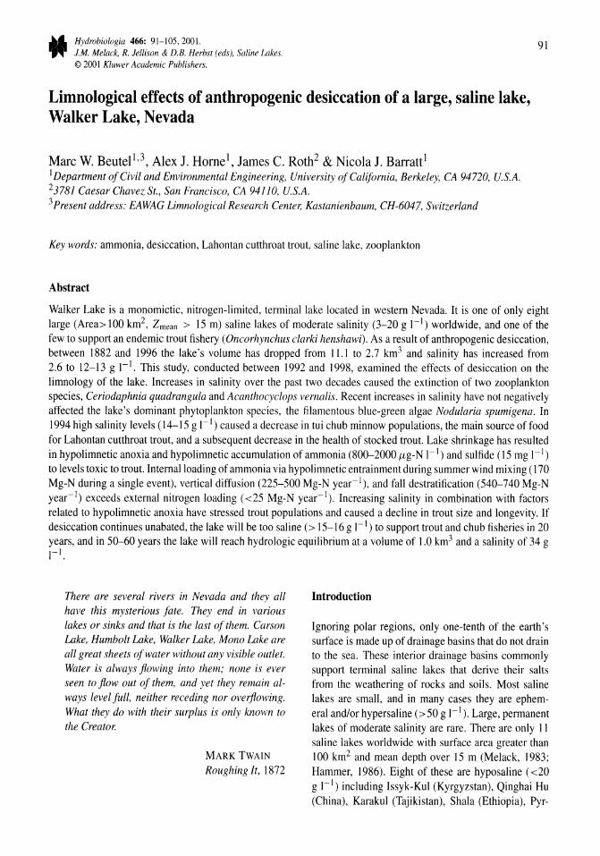
Hydrobiologia 466: 91-105,2001. J.M. Melack, R. Jellison & D.B. Herbst (eds), Saline Lakes. © 2001 Kluwer Academic Publishers.
91
Limnological effects of anthropogenic desiccation of a large, saline lake, Walker Lake, Nevada
Marc W. Beutel l ,3, Alex J. Hornel , James C. Roth2 & Nicola J. Barrattl
1 Department of Civil and Environmental Engineering, University of California, Berkeley, CA 94720, U.S.A. 23781 Caesar Chavez St., San Francisco, CA 941J0, U.S.A. 3 Present address: EAWAG Limnological Research Center, Kastanienbaum, CH-6047, Switzerland
Key words: ammonia, desiccation, Lahontan cutthroat trout, saline lake, zooplankton
Abstract
Walker Lake is a monomictic, nitrogen-limited, terminal lake located in western Nevada. It is one of only eight large (Area> 100 km2, Zmean > 15 m) saline lakes of moderate salinity (3-20 g 1-1) worldwide, and one of the few to support an endemic trout fishery (Oncorhynchus clarki henshawi). As a result of anthropogenic desiccation, between 1882 and 1996 the lake's volume has dropped from ILl to 2.7 km3 and salinity has increased from 2.6 to 12-13 g 1-1. This study, conducted between 1992 and 1998, examined the effects of desiccation on the limnology of the lake. Increases in salinity over the past two decades caused the extinction of two zooplankton species, Ceriodaphnia quadrangula and Acanthocyclops vernalis. Recent increases in salinity have not negatively affected the lake's dominant phytoplankton species, the filamentous blue-green algae Nodularia spumigena. In 1994 high salinity levels (14-15 g I-I) caused a decrease in tui chub minnow populations, the main source of food for Lahontan cutthroat trout, and a subsequent decrease in the health of stocked trout. Lake shrinkage has resulted in hypolimnetic anoxia and hypolimnetic accumulation of ammonia (800-2000 /Lg-N I-I) and sulfide (15 mg I-I) to levels toxic to trout. Internal loading of ammonia via hypolimnetic entrainment during summer wind mixing (170 Mg-N during a single event), vertical diffusion (225-500 Mg-N year-I), and fall destratification (540-740 Mg-N year-I) exceeds external nitrogen loading «25 Mg-N year-I). Increasing salinity in combination with factors related to hypolimnetic anoxia have stressed trout populations and caused a decline in trout size and longevity. If desiccation continues unabated, the lake will be too saline (> 15-16 g I-I) to support trout and chub fisheries in 20 years, and in 50-60 years the lake will reach hydrologic equilibrium at a volume of 1.0 km3 and a salinity of 34 g I-I.
There are several rivers in Nevada and they all have this mysterious fate. They end in various lakes or sinks and that is the last of them. Carson Lake, Humbolt Lake, Walker Lake, Mono Lake are all great sheets of water without any visible outlet. Water is always flowing into them; none is ever seen to flow out of them, and yet they remain always level full, neither receding nor overflowing. What they do with their surplus is only known to the Creator.
MARK TWAIN
Roughing It, 1872
Introduction
Ignoring polar regions, only one-tenth of the earth's surface is made up of drainage basins that do not drain to the sea. These interior drainage basins commonly support terminal saline lakes that derive their salts from the weathering of rocks and soils. Most saline lakes are small, and in many cases they are ephemeral andlor hypersaline (>50 g I-I). Large, permanent lakes of moderate salinity are rare. There are only 11 saline lakes worldwide with surface area greater than 100 km2 and mean depth over 15 m (Melack, 1983; Hammer, 1986). Eight of these are hyposaline (<20 g I-I) including Issyk-Kul (Kyrgyzstan), Qinghai Hu (China), Karakul (Tajikistan), Shala (Ethiopia), Pyr-
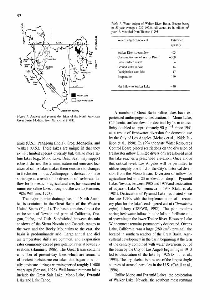
92
Figure 1. Ancient and present day lakes of the North American Great Basin. Modified from Galat et a1. (1981).
amid (U.S.), Panggong (India), Orog (Mongolia) and Walker (U.S.). These lakes are unique in that they exhibit limited species diversity but, unlike more saline lakes (e.g., Mono Lake, Dead Sea), may support robust fisheries. The terminal nature and semi-arid location of saline lakes makes them sensitive to changes in freshwater inflow. Anthropogenic desiccation, lake shrinkage as a result of the diversion of freshwater inflow for domestic or agricultural use, has occurred in numerous saline lakes throughout the world (Hammer, 1986; Williams, 1993).
The major interior drainage basin of North America is contained in the Great Basin of the Western United States (Fig. 1). The basin contains almost the entire state of Nevada and parts of California, Oregon, Idaho, and Utah. Sandwiched between the rain shadows of the Sierra Nevada and Cascade ranges to the west and the Rocky Mountains to the east, the basin is predominantly arid. Large annual and diel air temperature shifts are common, and evaporation rates commonly exceed precipitation rates at lower elevations (Hammer, 1986). The Great Basin contains a number of present-day lakes which are remnants of ancient Pleistocene era lakes that began to naturally desiccate during a warming period roughly 10000 years ago (Benson, 1978). Well-known remnant lakes include the Great Salt Lake, Mono Lake, Pyramid Lake and Lake Tahoe.
Table I. Water budget of Walker River Basin. Budget based on 55-year average (1939-1993). All values are in million m3 year-I. Modified from Thomas (1995)
Water budget component Estimated
quantity
Walker River stream flow 403
Consumptive use of Walker River -309
Local surface runoff 4
Ground water inflow 14
Precipitation onto lake 17
Evaporation -169
Net Inflow to Walker Lake -40
A number of Great Basin saline lakes have experienced anthropogenic desiccation. In Mono Lake, California, surface elevation declined by 14-m and salinity doubled to approximately 90 g I-I since 1941 as a result of freshwater diversion for domestic use by the City of Los Angeles (Melack et aI., 1985; Jellison et aI., 1998). In 1994 the State Water Resources Control Board placed restrictions on the diversion of freshwater inflow. Limited diversions are allowed until the lake reaches a prescribed elevation. Once above this critical level, Los Angeles will be permitted to utilize roughly one-third of the City's historical diversion from the Mono Basin. Diversion of inflow for agriculture led to a 23-m elevation drop in Pyramid Lake, Nevada, between 1905 and 1979 and desiccation of adjacent Lake Winnemucca in 1938 (Galat et aI., 1981). Desiccation of Pyramid Lake has abated since the late 1970s with the implementation of a recovery plan for the lake's endangered cui-ui (Chasmistes cujus) fishery (USFWS, 1992). The plan requires spring freshwater inflow into the lake to facilitate cuiui spawning in the lower Trukee River. However, Lake Winnemucca remains permanently desiccated. Owens Lake, California, was a large (280 km2) terminal lake located in southern reaches of the Great Basin. Agricultural development in the basin beginning at the tum of the century combined with water diversions out of the basin by the City of Los Angels beginning in 1913 led to desiccation of the lake by 1926 (Smith et aI., 1993). The dry lakebed is now one of the largest single sources of aerosol particles in the U.S. (Cahill et aI., 1996).
Unlike Mono and Pyramid Lakes, the desiccation of Walker Lake, Nevada, the southern most remnant
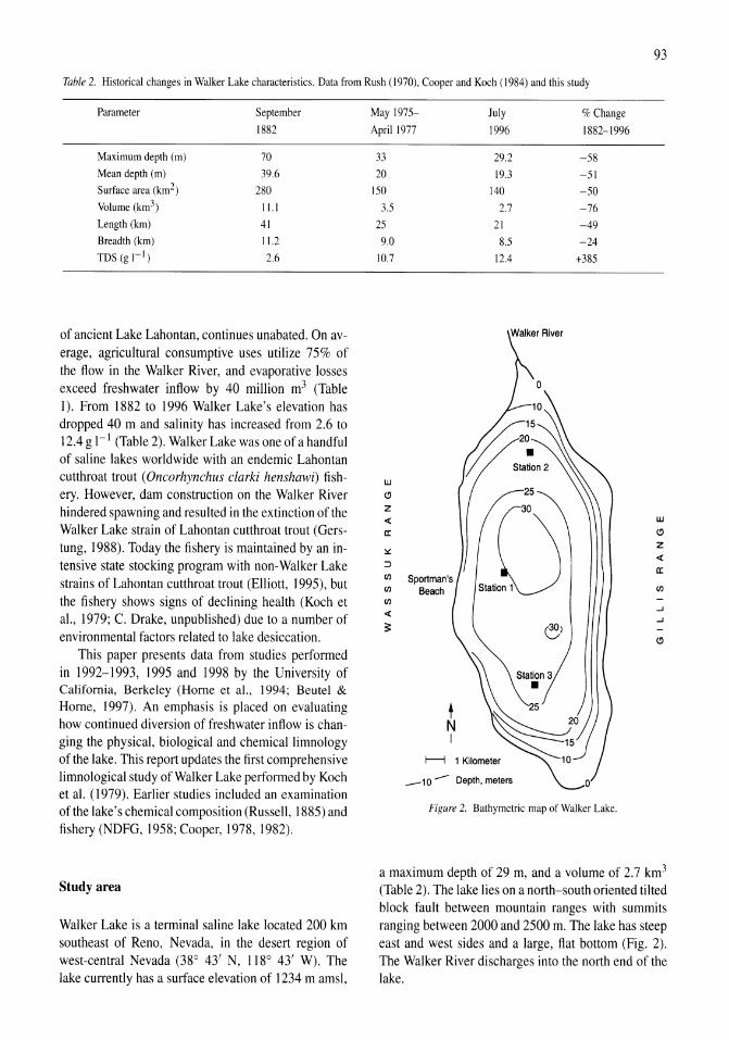
93
Table 2. Historical changes in Walker Lake characteristics. Data from Rush (1970), Cooper and Koch (1984) and this study
Parameter September
1882
Maximum depth (m) 70 Mean depth (m) 39.6 Surface area (km2) 280 Volume (km3) 11.1 Length (km) 41 Breadth (km) 11.2 TDS (g 1-') 2.6
of ancient Lake Lahontan, continues unabated. On average, agricultural consumptive uses utilize 75% of the flow in the Walker River, and evaporative losses exceed freshwater inflow by 40 million m3 (Table I). From 1882 to 1996 Walker Lake's elevation has dropped 40 m and salinity has increased from 2.6 to 12.4g1-1 (Table 2). Walker Lake was one ofa handful of saline lakes worldwide with an endemic Lahontan cutthroat trout (Oncorhynchus clarki henshawi) fishery. However, dam construction on the Walker River hindered spawning and resulted in the extinction of the Walker Lake strain of Lahontan cutthroat trout (Gerstung, 1988). Today the fishery is maintained by an intensive state stocking program with non-Walker Lake strains of Lahontan cutthroat trout (Elliott, 1995), but the fishery shows signs of declining health (Koch et at, 1979; C. Drake, unpublished) due to a number of environmental factors related to lake desiccation.
This paper presents data from studies performed in 1992-1993, 1995 and 1998 by the University of California, Berkeley (Home et aI., 1994; Beutel & Home, 1997). An emphasis is placed on evaluating how continued diversion of freshwater inflow is changing the physical, biological and chemical limnology of the lake. This report updates the first comprehensive limnological study of Walker Lake performed by Koch et at (1979). Earlier studies included an examination of the lake's chemical composition (Russell, 1885) and fishery (NDFG, 1958; Cooper, 1978,1982).
Study area
Walker Lake is a terminal saline lake located 200 km southeast of Reno, Nevada, in the desert region of west-central Nevada (38° 43' N, 118° 43' W). The lake currently has a surface elevation of 1234 m amsl,
May 1975- July
April 1977 1996
33 20
ISO
3.5 25
9.0 10.7
w Cl z « II:
:.:: :J
III
III
III
« ~
Sportman's Beach
+ N I
29.2 19.3
140
2.7
21
8.5 12.4
t---l 1 Kilometer
_10 - Depth, meters
% Change
1882-1996
-S8
-SI
-50 -76
-49 -24
+385
Figure 2. Bathymetric map of Walker Lake.
w Cl Z
« II:
III
..J
..J
Cl
a maximum depth of 29 m, and a volume of 2.7 km3
(Table 2). The lake lies on a north-south oriented tilted block fault between mountain ranges with summits ranging between 2000 and 2500 m. The lake has steep east and west sides and a large, flat bottom (Fig. 2). The Walker River discharges into the north end of the lake.
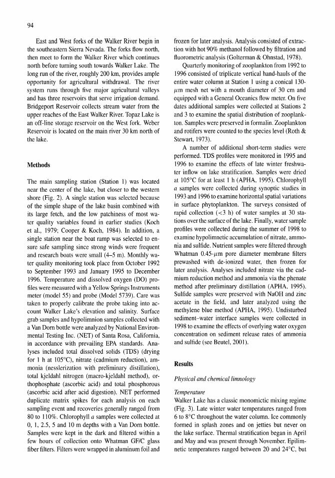
94
East and West forks of the Walker River begin in the southeastern Sierra Nevada. The forks flow north, then meet to form the Walker River which continues north before turning south towards Walker Lake. The long run of the river, roughly 200 km, provides ample opportunity for agricultural withdrawal. The river system runs through five major agricultural valleys and has three reservoirs that serve irrigation demand. Bridgeport Reservoir collects stream water from the upper reaches of the East Walker River. Topaz Lake is an off-line storage reservoir on the West fork. Weber Reservoir is located on the main river 30 km north of the lake.
Methods
The main sampling station (Station 1) was located near the center of the lake, but closer to the western shore (Fig. 2). A single station was selected because of the simple shape of the lake basin combined with its large fetch, and the low patchiness of most water quality variables found in earlier studies (Koch et aI., 1979; Cooper & Koch, 1984). In addition, a single station near the boat ramp was selected to ensure safe sampling since strong winds were frequent and research boats were small (4-5 m). Monthly water quality monitoring took place from October 1992 to September 1993 and January 1995 to December 1996. Temperature and dissolved oxygen (DO) profiles were measured with a Yellow Springs Instruments meter (model 55) and probe (Model 5739). Care was taken to properly calibrate the probe taking into account Walker Lake's elevation and salinity. Surface grab samples and hypolimnion samples collected with a Van Dorn bottle were analyzed by National Environmental Testing Inc. (NET) of Santa Rosa, California, in accordance with prevailing EPA standards. Analyses included total dissolved solids (TDS) (drying for 1 h at 105°C), nitrate (cadmium reduction), ammonia (nesslerization with preliminary distillation), total kjeldahl nitrogen (macro-kjeldahl method), orthophosphate (ascorbic acid) and total phosphorous (ascorbic acid after acid digestion). NET performed duplicate matrix spikes for each analysis on each sampling event and recoveries generally ranged from 80 to 110%. Chlorophyll a samples were collected at 0, 1, 2.5, 5 and 10m depths with a Van Dorn bottle. Samples were kept in the dark and filtered within a few hours of collection onto Whatman GF/C glass fiber filters. Filters were wrapped in aluminum foil and
frozen for later analysis. Analysis consisted of extraction with hot 90% methanol followed by filtration and f1uorometric analysis (Golterman & Ohnstad, 1978).
Quarterly monitoring of zooplankton from 1992 to 1996 consisted of triplicate vertical hand-hauls of the entire water column at Station 1 using a conical 130-/-Lm mesh net with a mouth diameter of 30 cm and equipped with a General Oceanics flow meter. On five dates additional samples were collected at Stations 2 and 3 to examine the spatial distribution of zooplankton. Samples were preserved in formalin. Zooplankton and rotifers were counted to the species level (Roth & Stewart, 1973).
A number of additional short-term studies were performed. TDS profiles were monitored in 1995 and 1996 to examine the effects of late winter freshwater inflow on lake stratification. Samples were dried at 105°C for at least 1 h (APRA, 1995). Chlorophyll a samples were collected during synoptic studies in 1993 and 1996 to examine horizontal spatial variations in surface phytoplankton. The surveys consisted of rapid collection (<3 h) of water samples at 30 stations over the surface of the lake. Finally, water sample profiles were collected during the summer of 1998 to examine hypolimnetic accumulation of nitrate, ammonia and sulfide. Nutrient samples were filtered through Whatman 0.45-/-Lm pore diameter membrane filters prewashed with de-ionized water, then frozen for later analysis. Analyses included nitrate via the cadmium reduction method and ammonia via the phenate method after preliminary distillation (APRA, 1995). Sulfide samples were preserved with NaOR and zinc acetate in the field, and later analyzed using the methylene blue method (APRA, 1995). Undisturbed sediment-water interface samples were collected in 1998 to examine the effects of overlying water oxygen concentration on sediment release rates of ammonia and sulfide (see Beutel, 2001).
Results
Physical and chemical limnology
Temperature Walker Lake has a classic monomictic mixing regime (Fig. 3). Late winter water temperatures ranged from 6 to 8°C throughout the water column. Ice commonly formed in splash zones and on jetties but never on the lake surface. Thermal stratification began in April and May and was present through November. Epilimnetic temperatures ranged between 20 and 24°C, but
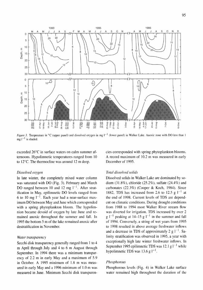
95
1993 1995 1996
0
5
E 10
% 15 .. 0
20
25
30
0
5
E 10 .c ~ 15 0
20
25
30 iiiii ~i § ~ -~ ~ U <> .. :Eli ~ N ~~ .,., ... ~ ~ ~ - " il ~g '!!
Figure 3. Temperature in °C (upper panel) and dissolved oxygen in mg 1-1 (lower panel) in Walker Lake. Anoxic zone with DO less than I mg 1-1 is shaded.
exceeded 26°C in surface waters on calm summer afternoons. Hypolimnetic temperatures ranged from 10 to ]20e. The thermocline was around 12 m deep.
Dissolved oxygen
In late winter, the completely mixed water column was saturated with DO (Fig. 3). February and March DO ranged between 10 and 12 mg I-I. After stratification in May, epilimnetic DO levels ranged from 6 to 10 mg I- I. Each year had a near-surface maximum DO between May and June which corresponded with a spring phytoplankton bloom. The hypolimnion became devoid of oxygen by late June and remained anoxic throughout the summer and fall. In 1995 the bottom 5 m of the lake remained anoxic after destratification in November.
Water transparency
Secchi disk transparency generally ranged from I to 4 m April through July and 4 to 6 m August through September. In 1994 there was a minimum transparency of 2.2 m in early May and a maximum of 5.9 in October. A 1995 minimum of 1.8 m was measured in early May and a 1996 minimum of 1.0 m was measured in June. Minimum Secchi disk transparen-
cies corresponded with spring phytoplankton blooms. A record maximum of 10.2 m was measured in early December of 1995.
Total dissolved solids
Dissolved solids in Walker Lake are dominated by sodium (31.8%), chloride (25.2%), sulfate (24.4%) and carbonates (22.3%) (Cooper & Koch, 1984). Since 1882, TDS has increased from 2.6 to 12.5 g 1-1 at the end of 1998. Current levels of TDS are dependent on climatic conditions. During drought conditions from 1988 to 1994 most Walker River stream flow was diverted for irrigation. TDS increased by over 2 g I- I peaking at 14-15 g I-I in the summer and fall of 1994. Conversely, a string of wet years from 1995 to 1998 resulted in above average freshwater inflows and a decrease in TDS of approximately 2 g I-I. Salinity stratification was observed in 1995, a year with exceptionally high late winter freshwater inflows. In September 1995 epilimnetic TDS was 12.1 g I-I while hypolimnetic TDS was 13.6 g I-I.
Phosphorous
Phosphorous levels (Fig. 4) in Walker Lake surface water remained high throughout the duration of the
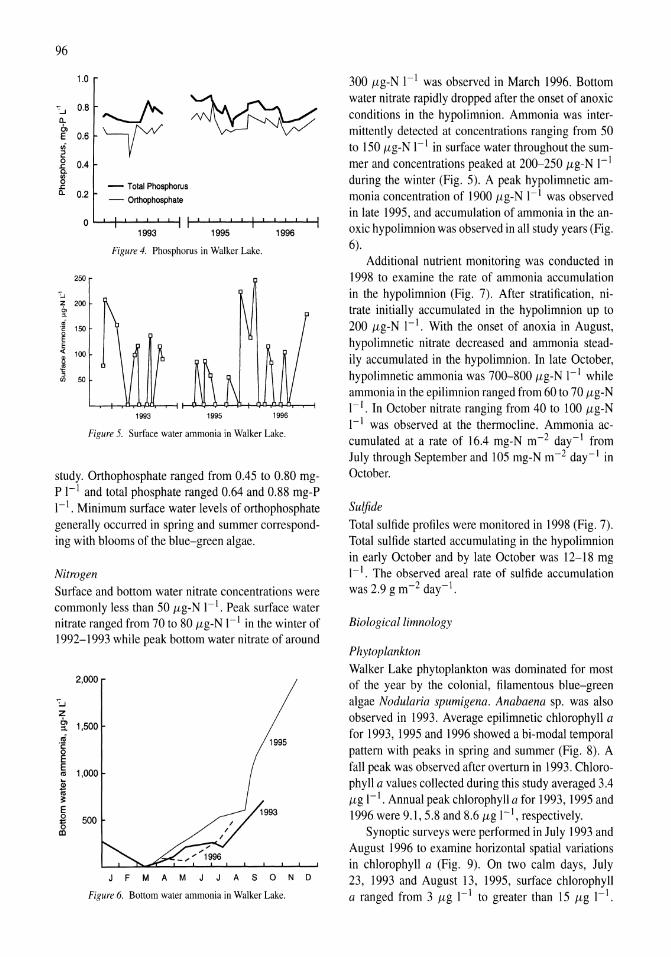
96
1.0
"'...J 0.8 ~ ~ a. m if E 0.6 iii 2 0 0.4 .c 0.
"' 0 - Total Phosphorus .c
a. 0.2 - Orthophosphate
0 I I I I I I I I I I I
1993 1995 1996
Figure 4. Phosphorus in Walker Lake.
250
-CJ
z 200 0, "-.; 'c 150 0 E E < 100 Q)
" ~ "t: , (/J 50
1993 1995 1996
Figure 5. Surface water ammonia in Walker Lake.
study. Orthophosphate ranged from 0.45 to 0.80 mgP 1-1 and total phosphate ranged 0.64 and 0.88 mg-P 1-1. Minimum surface water levels of orthophosphate generally occurred in spring and summer corresponding with blooms of the blue-green algae.
Nitrogen Surface and bottom water nitrate concentrations were commonly less than 50 fLg-N 1-1. Peak surface water nitrate ranged from 70 to 80 fLg-N 1-1 in the winter of 1992-1993 while peak bottom water nitrate of around
2,000
~...J
Z m 1,500 :I. oj 1995 ·c a E E
1,000 <0 ~
* ~
E a 500 :: a [IJ
JFMAMJJASOND
Figure 6. Bottom water ammonia in Walker Lake.
300 fLg-N I-I was observed in March 1996. Bottom water nitrate rapidly dropped after the onset of anoxic conditions in the hypolimnion. Ammonia was intermittently detected at concentrations ranging from 50 to 150 fLg-N 1-1 in surface waterthroughoutthe summer and concentrations peaked at 200-250 fLg-N I-I during the winter (Fig. 5). A peak hypolimnetic ammonia concentration of 1900 fLg-N I-I was observed in late 1995, and accumulation of ammonia in the anoxic hypolimnion was observed in all study years (Fig. 6).
Additional nutrient monitoring was conducted in 1998 to examine the rate of ammonia accumulation in the hypolimnion (Fig. 7). After stratification, nitrate initially accumulated in the hypolimnion up to 200 fLg-N 1-1. With the onset of anoxia in August, hypolimnetic nitrate decreased and ammonia steadily accumulated in the hypolimnion. In late October, hypolimnetic ammonia was 700-800 fLg-N I-I while ammonia in the epilimnion ranged from 60 to 70 fLg-N I-I. In October nitrate ranging from 40 to 100 fLg-N I-I was observed at the thermocline. Ammonia accumulated at a rate of 16.4 mg-N m-2 day-l from July through September and lOS mg-N m-2 day-I in October.
Sulfide
Total sulfide profiles were monitored in 1998 (Fig. 7). Total sulfide started accumulating in the hypolimnion in early October and by late October was 12-18 mg I-I. The observed areal rate of sulfide accumulation was 2.9 g m-2 day-I.
Biological limnology
Phytoplankton
Walker Lake phytoplankton was dominated for most of the year by the colonial, filamentous blue-green algae Nodularia spumigena. Anabaena sp. was also observed in 1993. Average epilimnetic chlorophyll a for 1993, 1995 and 1996 showed a bi-modal temporal pattern with peaks in spring and summer (Fig. 8). A fall peak was observed after overturn in 1993. Chlorophyll a values collected during this study averaged 3.4 fLg 1-1. Annual peak chlorophyll a for 1993, 1995 and 1996 were 9.1, 5.8 and 8.6 fLg 1-1, respectively.
Synoptic surveys were performed in July 1993 and August 1996 to examine horizontal spatial variations in chlorophyll a (Fig. 9). On two calm days, July 23, 1993 and August 13, 1995, surface chlorophyll a ranged from 3 fLg 1-1 to greater than IS fLg 1-1.
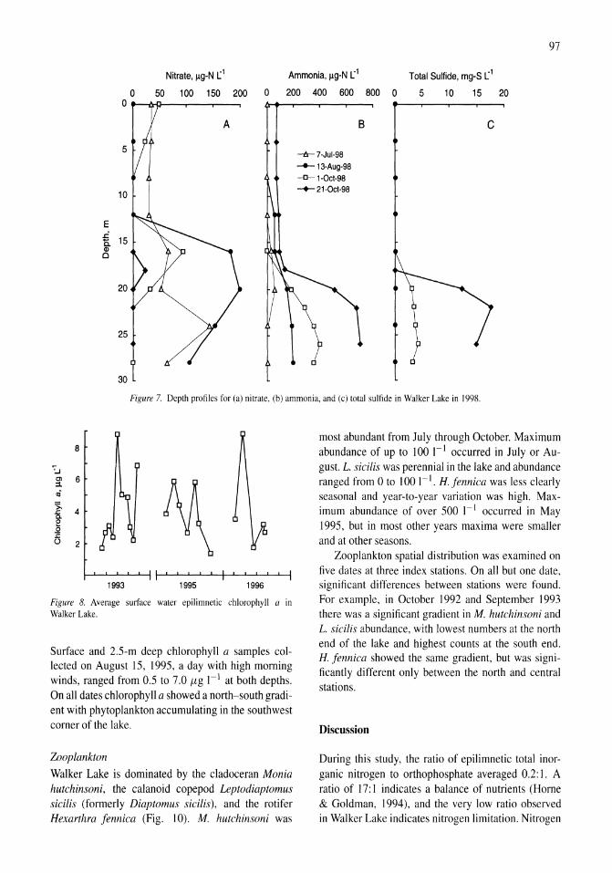
97
Nitrate, Ilg-N L:' Ammonia, Ilg-N L:' Total Sulfide, mg-S l'
50 100 150 200 0 200 400 600 800 0 5 10 15 20
5
10
E ~ C. 15 CD Cl
20
25
30
B c
-1:r- 7-Jul-98
--- 13-Aug-98 -0- 1-Oct-98 -+-21-0ct-98
Figure 7. Depth profiles for (a) nitrate, (b) ammonia, and (e) total sulfide in Walker Lake in 1998.
8
~ Cl 6 ::!. <Ii >.
4 ~ c. ~ .Q ~ 0 2
1--'-...L.......L.-'---1--i I ' I I I I I I I I I I I 1993 1995 1996
Figure 8. Average surface water epilimnelic chlorophyll a In
Walker Lake.
Surface and 2.5-m deep chlorophyll a samples collected on August 15, 1995, a day with high morning winds, ranged from 0.5 to 7.0 f.1g 1-1 at both depths. On all dates chlorophyll a showed a north-south gradient with phytoplankton accumulating in the southwest comer of the lake.
Zooplankton
Walker Lake is dominated by the cladoceran Monia hutchinsoni, the calanoid copepod Leptodiaptomus sidlis (formerly Diaptomus sidlis), and the rotifer Hexarthra fennica (Fig. 10). M. hutchinsoni was
most abundant from July through October. Maximum abundance of up to 1001-1 occurred in July or August. L. sidlis was perennial in the lake and abundance ranged from 0 to 100 I-I. H. fennica was less clearly seasonal and year-to-year variation was high. Maximum abundance of over 500 1-1 occurred in May 1995, but in most other years maxima were smaller and at other seasons.
Zooplankton spatial distribution was examined on five dates at three index stations. On all but one date, significant differences between stations were found. For example, in October 1992 and September 1993 there was a significant gradient in M. hutchinsoni and L. sicilis abundance. with lowest numbers at the north end of the lake and highest counts at the south end. H. fennica showed the same gradient, but was significantly different only between the north and central stations.
Discussion
During this study, the ratio of epilimnetic total inorganic nitrogen to orthophosphate averaged 0.2: I. A ratio of 17: I indicates a balance of nutrients (Home & Goldman, 1994), and the very low ratio observed in Walker Lake indicates nitrogen limitation. Nitrogen
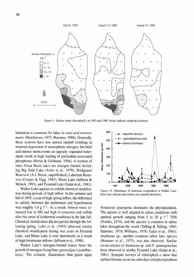
98
Surface Chlorophyll a
119 L"'
D 0·5
05.10
010.15
• ~15
5km
July 23. 1993 August 13. 1996 August 15, 1996
Figure 9. Surface water chlorophyll a in 1993 and 1996. Points indicate sampling locations.
limitation is common for lakes in semi-arid environments (Hutchinson, 1937; Hammer, 1986). Generally, these systems have low annual rainfall resulting in minimal deposition of atmospheric nitrogen, but brief and intense storm events on sparsely vegetated watersheds result in high loading of particulate-associated phosphorus (Home & Goldman, 1994). A number of other Great Basin lakes are nitrogen limited including Big Soda Lake (Axler et aI., 1978), Bridgeport Reservoir (A.J. Home, unpublished), Lahontan Reservoir (Cooper & Vigg, 1983), Mono Lake (Jellison & Melack, 1993), and Pyramid Lake (Galat et aI., 1981).
Walker Lake appears to exhibit chemical stratification during periods of high inflow. In the summer and fall of 1995, a year of high spring inflow, the difference in salinity between the epilimnion and hypolimnion was roughly 1.0 g I-I. As a result, bottom water remained low in DO and high in ammonia and sulfide after the onset of isothermal conditions in the late fall. Chemical stratification did not persist through the following spring. Lebo et al. (1993) observed similar chemical stratification during wet years in Pyramid Lake, and Mono Lake is now meromictic as a result of high freshwater inflows (Jellison et aI., 1998).
Walker Lake's nitrogen-limited waters favor the growth of nitrogen-fixing blue-green algae (cyanobacteria). The colonial, filamentous blue-green algae
600
500
8. 400
'" 'iij ::l
~ 300 'C .!:
~ 200 ::;
100
.. * .. Hexarthra fennica
- -0 - Leptodiaptomus sici/is
_ Moina hutchinsoni
1991 1992 1993
i '. '. " ' . , , · , · . · . , ,
, .
1995 1996
Figure 10. Abundance of dominant zooplankton in Walker Lake. Error bars indicate plus/minus one standard deviation.
Nodularia spumigena dominates the phytoplankton. The species is well adapted to saline conditions with optimal growth ranging from 5 to 20 g 1-1 TDS (Nordin, 1974), and the species is common in saline lakes throughout the world (Tailing & Tailing, 1965; Hammer, 1978; Williams, 1978; Galat et aI., 1981). Anabaena sp., another common saline lake species (Hammer et aI., 1975), was also observed. Similar co-occurrence of Anabaena sp. and N. spumigena has been observed in nearby Pyramid Lake (Galat et aI., 1981). Synoptic surveys of chlorophyll a show that surface blooms occur on calm days and phytoplankton
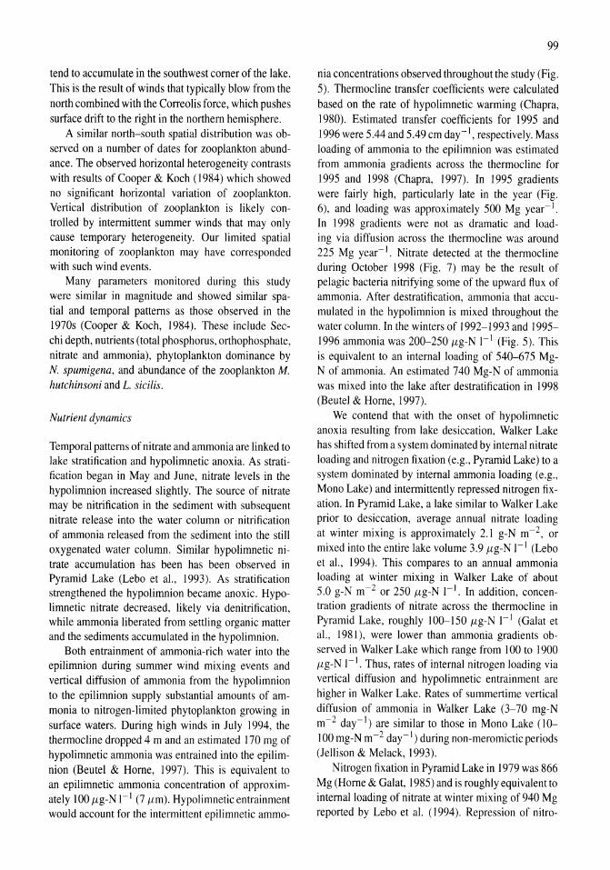
tend to accumulate in the southwest comer of the lake. This is the result of winds that typically blow from the north combined with the Correolis force, which pushes surface drift to the right in the northern hemisphere.
A similar north-south spatial distribution was observed on a number of dates for zooplankton abundance. The observed horizontal heterogeneity contrasts with results of Cooper & Koch (1984) which showed no significant horizontal variation of zooplankton. Vertical distribution of zooplankton is likely controlled by intermittent summer winds that may only cause temporary heterogeneity. Our limited spatial monitoring of zooplankton may have corresponded with such wind events.
Many parameters monitored during this study were similar in magnitude and showed similar spatial and temporal patterns as those observed in the 1970s (Cooper & Koch, 1984). These include Secchi depth, nutrients (total phosphorus, orthophosphate, nitrate and ammonia), phytoplankton dominance by N. spumigena, and abundance of the zooplankton M. hutchinsoni and L. siciUs.
Nutrient dynamics
Temporal patterns of nitrate and ammonia are linked to lake stratification and hypolimnetic anoxia. As stratification began in May and June, nitrate levels in the hypolimnion increased slightly. The source of nitrate may be nitrification in the sediment with subsequent nitrate release into the water column or nitrification of ammonia released from the sediment into the still oxygenated water column. Similar hypolimnetic nitrate accumulation has been has been observed in Pyramid Lake (Lebo et ai., 1993). As stratification strengthened the hypolimnion became anoxic. Hypolimnetic nitrate decreased, likely via denitrification, while ammonia liberated from settling organic matter and the sediments accumulated in the hypolimnion.
Both entrainment of ammonia-rich water into the epilimnion during summer wind mixing events and vertical diffusion of ammonia from the hypolimnion to the epilimnion supply substantial amounts of ammonia to nitrogen-limited phytoplankton growing in surface waters. During high winds in July 1994, the thermocline dropped 4 m and an estimated 170 mg of hypolimnetic ammonia was entrained into the epilimnion (Beutel & Home, 1997). This is equivalent to an epilimnetic ammonia concentration of approximately 100 ttg-N I-I (7 ttm). Hypolimnetic entrainment would account for the intermittent epilimnetic ammo-
99
nia concentrations observed throughout the study (Fig. 5). Thermocline transfer coefficients were calculated based on the rate of hypolimnetic warming (Chapra, 1980). Estimated transfer coefficients for 1995 and 1996 were 5.44 and 5.49 cm day-I, respectively. Mass loading of ammonia to the epilimnion was estimated from ammonia gradients across the thermocline for 1995 and 1998 (Chapra, 1997). In 1995 gradients were fairly high, particularly late in the year (Fig. 6), and loading was approximately 500 Mg year-I. In 1998 gradients were not as dramatic and loading via diffusion across the thermocline was around 225 Mg year-I. Nitrate detected at the thermocline during October 1998 (Fig. 7) may be the result of pelagic bacteria nitrifying some of the upward flux of ammonia. After destratification, ammonia that accumulated in the hypolimnion is mixed throughout the water column. In the winters of 1992-1993 and 1995-1996 ammonia was 200-250 ttg-N I-I (Fig. 5). This is equivalent to an internal loading of 540-675 MgN of ammonia. An estimated 740 Mg-N of ammonia was mixed into the lake after de stratification in 1998 (Beutel & Home, 1997).
We contend that with the onset of hypolimnetic anoxia resulting from lake desiccation, Walker Lake has shifted from a system dominated by internal nitrate loading and nitrogen fixation (e.g., Pyramid Lake) to a system dominated by internal ammonia loading (e.g., Mono Lake) and intermittently repressed nitrogen fixation. In Pyramid Lake, a lake similar to WaIker Lake prior to desiccation, average annual nitrate loading at winter mixing is approximately 2.1 g-N m-2, or mixed into the entire lake volume 3.9 ttg-N I-I (Lebo et ai., 1994). This compares to an annual ammonia loading at winter mixing in Walker Lake of about 5.0 g-N m-2 or 250 ttg-N I-I. In addition, concentration gradients of nitrate across the thermocline in Pyramid Lake, roughly 100-150 ttg-N I-I (Gal at et aI., 1981), were lower than ammonia gradients observed in Walker Lake which range from 100 to 1900 ttg-N I-I. Thus, rates of internal nitrogen loading via vertical diffusion and hypolimnetic entrainment are higher in Walker Lake. Rates of summertime vertical diffusion of ammonia in Walker Lake (3-70 mg-N m-2 day-I) are similar to those in Mono Lake (10-100 mg -N m - 2 day -I ) during non-meromictic periods (Jellison & Melack, 1993).
Nitrogen fixation in Pyramid Lake in 1979 was 866 Mg (Home & GaIat, 1985) and is roughly equivalent to internal loading of nitrate at winter mixing of 940 Mg reported by Lebo et al. (I994). Repression of nitro-
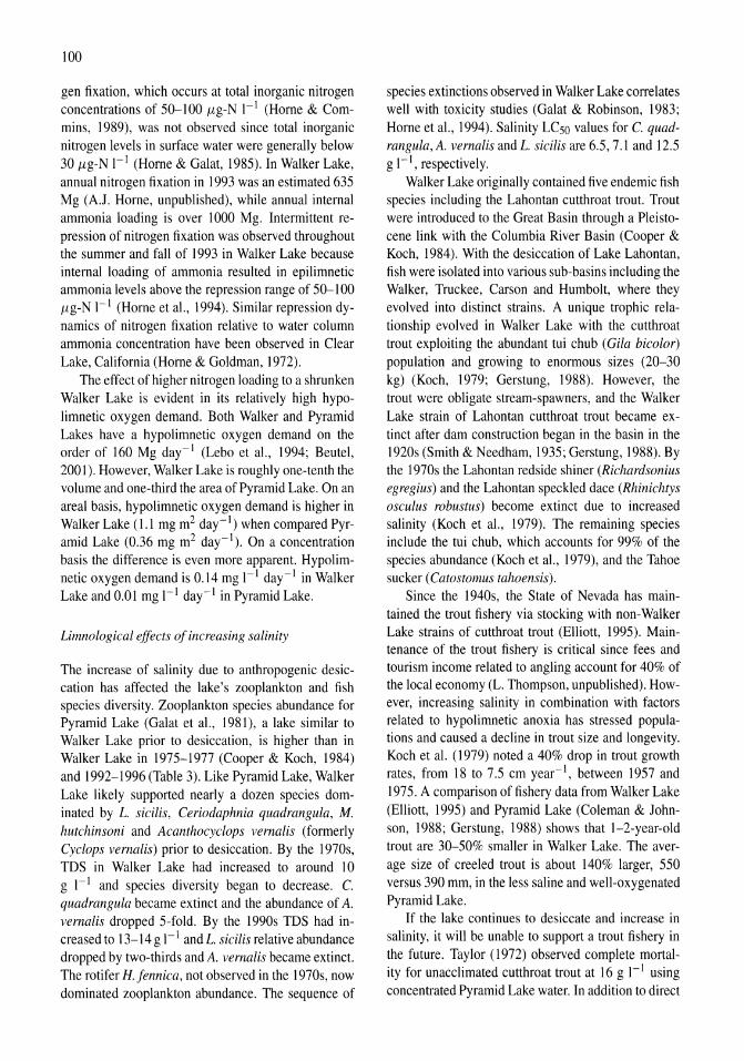
100
gen fixation, which occurs at total inorganic nitrogen concentrations of 50-100 /Lg-N I-I (Home & Commins, 1989), was not observed since total inorganic nitrogen levels in surface water were generally below 30 /Lg-N 1-1 (Home & Galat, 1985). In Walker Lake, annual nitrogen fixation in 1993 was an estimated 635 Mg (AJ. Home, unpublished), while annual internal ammonia loading is over 1000 Mg. Intermittent repression of nitrogen fixation was observed throughout the summer and fall of 1993 in Walker Lake because internal loading of ammonia resulted in epilimnetic ammonia levels above the repression range of 50-100 /Lg-N 1-1 (Home et aI., 1994). Similar repression dynamics of nitrogen fixation relative to water column ammonia concentration have been observed in Clear Lake, California (Home & Goldman, 1972).
The effect of higher nitrogen loading to a shrunken Walker Lake is evident in its relatively high hypoIimnetic oxygen demand. Both Walker and Pyramid Lakes have a hypolimnetic oxygen demand on the order of 160 Mg day-l (Lebo et aI., 1994; Beutel, 2001). However, Walker Lake is roughly one-tenth the volume and one-third the area of Pyramid Lake. On an areal basis, hypolimnetic oxygen demand is higher in Walker Lake (1.1 mg m2 day-I) when compared Pyramid Lake (0.36 mg m2 day-I). On a concentration basis the difference is even more apparent. Hypolimnetic oxygen demand is 0.14 mg 1-1 day-l in Walker Lake and 0.01 mg I-I day-I in Pyramid Lake.
Limnological effects of increasing salinity
The increase of salinity due to anthropogenic desiccation has affected the lake's zooplankton and fish species diversity. Zooplankton species abundance for Pyramid Lake (Galat et aI., 1981), a lake similar to Walker Lake prior to desiccation, is higher than in Walker Lake in 1975-1977 (Cooper & Koch, 1984) and 1992-1996 (Table 3). Like Pyramid Lake, Walker Lake likely supported nearly a dozen species dominated by L. sicilis, Ceriodaphnia quadrangula, M. hutchinsoni and Acanthocyclops vernalis (formerly Cyclops vernalis) prior to desiccation. By the 1970s, TDS in Walker Lake had increased to around 10 g 1-1 and species diversity began to decrease. C. quadrangula became extinct and the abundance of A. vernalis dropped 5-fold. By the 1990s TDS had increased to 13-14 g 1-1 and L. sicilisrelative abundance dropped by two-thirds and A. vernalis became extinct. The rotifer H. fennica, not observed in the 1970s, now dominated zooplankton abundance. The sequence of
species extinctions observed in Walker Lake correlates well with toxicity studies (Galat & Robinson, 1983; Home et aI., 1994). Salinity LCso values for C. quadrangula, A. vernalis and L. sicilis are 6.5, 7.1 and 12.5 g 1-1, respectively.
Walker Lake originally contained five endemic fish species including the Lahontan cutthroat trout. Trout were introduced to the Great Basin through a Pleistocene link with the Columbia River Basin (Cooper & Koch, 1984). With the desiccation of Lake Lahontan, fish were isolated into various sub-basins including the Walker, Truckee, Carson and Humbolt, where they evolved into distinct strains. A unique trophic relationship evolved in Walker Lake with the cutthroat trout exploiting the abundant tui chub (Gila bicolor) population and growing to enormous sizes (20-30 kg) (Koch, 1979; Gerstung, 1988). However, the trout were obligate stream-spawners, and the Walker Lake strain of Lahontan cutthroat trout became extinct after dam construction began in the basin in the 1920s (Smith & Needham, 1935; Gerstung, 1988). By the 1970s the Lahontan redside shiner (Richardsonius egregius) and the Lahontan speckled dace (Rhinichtys osculus robustus) become extinct due to increased salinity (Koch et aI., 1979). The remaining species include the tui chub, which accounts for 99% of the species abundance (Koch et aI., 1979), and the Tahoe sucker (Catostomus tahoensis).
Since the 1940s, the State of Nevada has maintained the trout fishery via stocking with non-Walker Lake strains of cutthroat trout (Elliott, 1995). Maintenance of the trout fishery is critical since fees and tourism income related to angling account for 40% of the local economy (L. Thompson, unpublished). However, increasing salinity in combination with factors related to hypolimnetic anoxia has stressed populations and caused a decline in trout size and longevity. Koch et al. (1979) noted a 40% drop in trout growth rates, from 18 to 7.5 cm year-I, between 1957 and 1975. A comparison of fishery data from Walker Lake (Elliott, 1995) and Pyramid Lake (Coleman & Johnson, 1988; Gerstung, 1988) shows that 1-2-year-old trout are 30-50% smaller in Walker Lake. The average size of creeled trout is about 140% larger, 550 versus 390 mm, in the less saline and well-oxygenated Pyramid Lake.
If the lake continues to desiccate and increase in salinity, it will be unable to support a trout fishery in the future. Taylor (1972) observed complete mortality for unacclimated cutthroat trout at 16 g 1-1 using concentrated Pyramid Lake water. In addition to direct
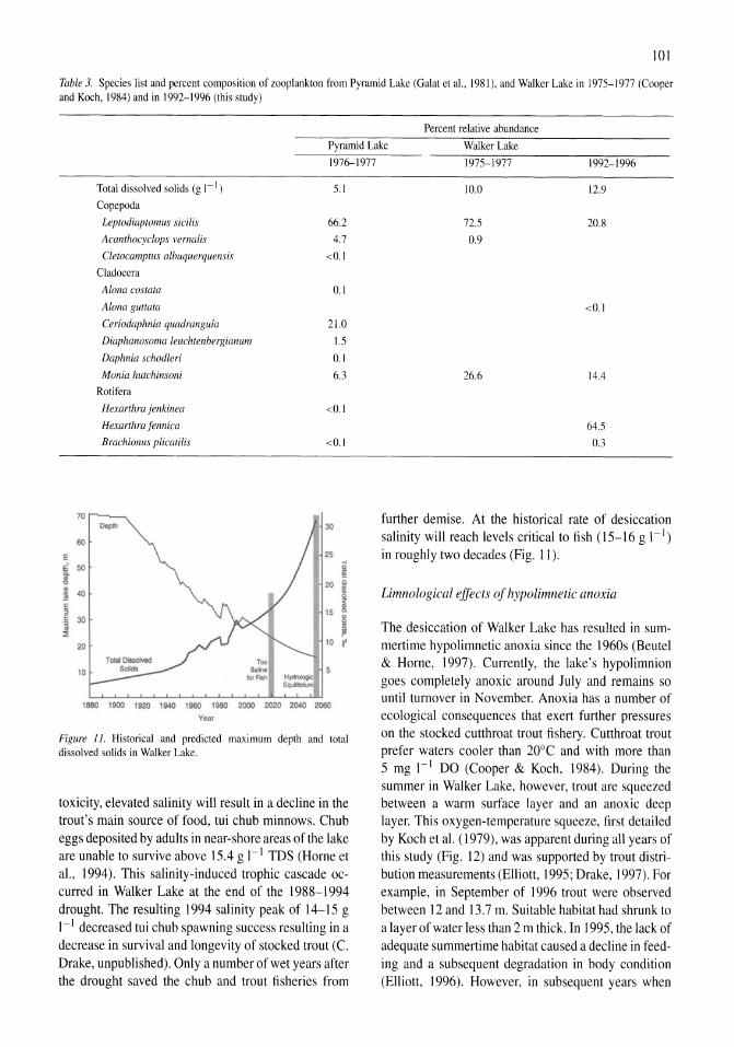
101
Table 3. Species list and percent composition of zooplankton from Pyramid Lake (Galat et aI., 1981), and Walker Lake in 1975-1977 (Cooper and Koch, 1984) and in 1992-1996 (this study)
Percent relative abundance
Pyramid Lake Walker Lake
E t t ~ !11 E
~ .~
::Ii
70
60
50
40
30
20
10
Total dissolved solids (g 1- 1)
Copepoda
Leptodiaptomus sid lis
Acanthocyclops vernalis
Cletocamptus albuquerquensis
Cladocera
Alana castata
Alana guttata
Ceriodaphnia quadrangula
Diaphanosoma leuchtenbergianum
Daphnia schodleri
Monia hutchinsoni
Rotifera
Hexarthra jenkinea
Hexarthra fennica
Brachionus plicatilis
Cop'"
1976-1977
5.1
66,2
4,7
<0,1
0.1
2],0
L5
0,1
6.3
<0.1
<0.1
i I ~ J
10 t
I~ ~ ~ 1~ ~,~ ~ ~~~
Year
Figure ll. Historical and predicted maximum depth and total dissolved solids in Walker Lake.
toxicity, elevated salinity will result in a decline in the trout's main source of food, tui chub minnows. Chub eggs deposited by adults in near-shore areas of the lake are unable to survive above 15.4 g 1-1 TDS (Home et aI., 1994). This salinity-induced trophic cascade occurred in Walker Lake at the end of the 1988-1994 drought. The resulting 1994 salinity peak of 14-15 g I-I decreased tui chub spawning success resulting in a decrease in survival and longevity of stocked trout (c. Drake, unpublished). Only a number of wet years after the drought saved the chub and trout fisheries from
1975- 1977
10.0
72.5
0.9
26.6
1992-1996
12.9
20.8
<0.1
14.4
64.5
0.3
further demise. At the historical rate of desiccation salinity will reach levels critical to fish (15-16 g I- I) in roughly two decades (Fig. 11).
Limnological effects of hypolimnetic anoxia
The desiccation of Walker Lake has resulted in summertime hypolimnetic anoxia since the 1960s (Beutel & Home, 1997). Currently, the lake's hypolimnion goes completely anoxic around July and remains so until turnover in November. Anoxia has a number of ecological consequences that exert further pressures on the stocked cutthroat trout fishery. Cutthroat trout prefer waters cooler than 20DC and with more than 5 mg I-I DO (Cooper & Koch, 1984). During the summer in Walker Lake, however, trout are squeezed between a warm surface layer and an anoxic deep layer. This oxygen-temperature squeeze, first detailed by Koch et a1. (1979), was apparent during all years of this study (Fig. 12) and was supported by trout distribution measurements (Elliott, 1995; Drake, 1997). For example, in September of 1996 trout were observed between 12 and 13.7 m. Suitable habitat had shrunk to a layer of water less than 2 m thick. In 1995, the lack of adequate summertime habitat caused a decline in feeding and a subsequent degradation in body condition (Elliott, 1996). However, in subsequent years when
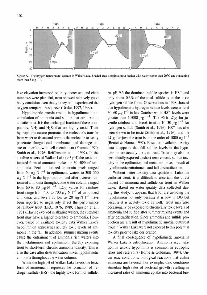
102
1993 1995 1996 M A M o ~~~~~~----~~~~~~-T~~~~~--~~r-~~~~--~~~~~
5
E 10
5 ! 15
20
25
Figure 12. The oxygen-temperature squeeze in Walker Lake. Shaded area is optimal trout habitat with water cooler than 200 e and containing more than 5 mg I-i.
lake elevation increased, salinity decreased, and chub minnows were plentiful, trout showed relatively good body condition even though they still experienced the oxygen-temperature squeeze (Drake, 1997, 1999).
Hypolimnetic anoxia results in hypolimnetic accumulation of ammonia and sulfide that are toxic to aquatic biota. It is the uncharged fraction of these compounds, NH3 and H2S, that are highly toxic. Their hydrophobic nature promotes the molecule's transfer from water to tissue and permits the molecule to easily penetrate charged cell membranes and damage tissue or interfere with cell metabolism (Fromm, 1970; Smith et aI., 1976; Reiffenstien et aI., 1992). In the alkaline waters of Walker Lake (9.3 pH) the toxic unionized form of ammonia makes up 30-40% of total ammonia. Peak un-ionized ammonia levels ranged from 60 /lg-N 1-1 in epilimnetic waters to 300-550 /lg-N 1-1 in the hypolimnion, and after overturn unionized ammonia throughout the water column ranged from 60 to 80 /lg-N I-I. LCso values for rainbow trout range from 400 to 700 /lg-N 1-1 of un-ionized ammonia, and levels as low as 20 /lg-N I-I have been reported to negatively affect the performance of rainbow trout (EPA, 1976, 1989; Thurston et aI., 1981). Having evolved in alkaline waters, the cutthroat trout may have a higher tolerance to ammonia. However, based on available toxicity data Walker Lake's hypolimnion approaches acutely toxic levels of ammonia in the fall. In addition, summer mixing events cause the entrainment of ammonia rich waters into the metalimnion and epilimnion, thereby exposing trout to short-term chronic ammonia toxicity. This is also the case after de stratification mixes hypolimnetic ammonia throughout the water column.
While the high pH of Walker Lake favors the toxic form of ammonia, it represses the formation of hydrogen sulfide (H2S), the highly toxic form of sulfide.
At pH 9.3 the dominant sulfide species is HS- and only about 0.3% of the total sulfide is in the toxic hydrogen sulfide form. Observations in 1998 showed that hypolimnetic hydrogen sulfide levels were around 30-60 /lg 1-1 in late October while HS- levels were greater than 10000 /lg 1-1. The 96-h LCso for juvenile rainbow and brook trout is 10-30 /lg I-I for hydrogen sulfide (Smith et aI., 1976). HS- has also been shown to be toxic (Smith et aI., 1976), and the LCso for juvenile trout is on the order of 1000 /lg I-I (Beutel & Home, 1997). Based on available toxicity data it appears that fall sulfide levels in the hypolimnion are acutely toxic to trout. Trout may also be periodically exposed to short-term chronic sulfide toxicity in the epilimnion and metalimnion as a result of hypolimnetic entrainment and fall destratification.
Without better toxicity data specific to Lahontan cutthroat trout, it is difficult to ascertain the direct impact of ammonia and sulfide on trout in Walker Lake. Based on water quality data collected during this study, it appears that trout are avoiding the hypolimnion not only because it is low in DO but because it is acutely toxic as well. Trout may also occasionally be exposed to chronically toxic levels of ammonia and sulfide after summer mixing events and after destratification. Since ammonia and sulfide production are a result of hypolimnetic anoxia, cutthroat trout in Walker Lake were not exposed to this potential toxicity prior to lake desiccation.
A final consequence of hypolimnetic anoxia in Walker Lake is eutrophication. Ammonia accumulation in anoxic hypolimnia is common in eutrophic lakes and reservoirs (Home & Goldman, 1994). Under oxic conditions, biological reactions that utilize ammonia are favored. For example, oxic conditions stimulate high rates of bacterial growth resulting in increased rates of ammonia uptake into bacterial bio-
mass (Graetz et a!., 1973; Van Duyl et a!., 1993). Oxic conditions also stimulate nitrification and subsequent denitrification, resulting in a net loss of ammonia from the ecosystem (Ahlgren et a!., 1994; Rysgaard et a!., 1994). Ammonia released from anoxic sediment and settling organic matter accumulates in the hypolimnion. This ammonia then enters the epilimnion via turbulent diffusion across the thermocline and entrainment during wind mixing where it can promote algal growth. The increased phytoplankton growth acts as a positive feedback to internal nutrient loading. Increased biomass exerts a larger oxygen demand on the hypolimnion, thereby exacerbating anoxic conditions and increasing the magnitude of internal nutrient loading. In Walker Lake approximately 1000 Mg of ammonia is annually released from anoxic lake sediments and settling organic matter. This loading is larger than nitrogen fixation, estimated at 635 Mg year- I in 1993, and greatly exceeds external nutrient loading which is less than 25 Mg year-I. As Walker Lake has desiccated, the duration and severity of hypolimnetic anoxia has increased, resulting in an increase in the internal loading of ammonia. This has caused a shift in the ecosystem from one dependent on nitrogen fixation and modest internal loading of nitrate to one in which the high internal loading of ammonia drives productivity.
Management options for Walker Lake
In the absence of any management strategies to stabilize elevation, water balance calculations project that in 20 years Walker Lake will be too saline to support tui chub and stocked Lahontan cutthroat trout (Fig. I I). In another 35 years the lake will reach hydrologic steady state with inflow equaling evaporative losses. At equilibrium the lake will have a volume of 1.0 km3,
one-third of its current volume (2.7 km3), and onetenth of its volume prior to anthropogenic desiccation (1 I.l km3). The maximum depth of the lake will have dropped from 70 m in 1882 to 15 m, and its mixing regime will likely shift from monomictic to polymictic. The salinity ofthe lake will increase to 34 g I-I , resulting in a decrease in species diversity of phytoplankton and zooplankton.
Home et al. (1994) examined a wide range of management options for Walker Lake. The most obvious management option is to stabilize the lake at its current elevation and salinity by providing it with a consistent inflow of approximately O. I 3 km3 year-I. The outright purchase of water rights needed to stabilize lake
103
elevation, 40% of the current consumptive uses in the basin, would cost $150-200 million. This option is expensive and would requiring considerable changes in the structure of the basin's economy and population. However, if the lake is recognized as a unique ecosystem worthy of protection, these costs are in line with the cost of establishing, for example, a state or national park. It may be more feasible to institute mechanisms to induce water users to donate water to the lake. A more flexible water rights system could be implemented in which water users could donate unused water to the lake without loss of permanent water rights, and in which water users could gain a tax benefit by donating water to the lake. In addition, a financial subsidy could be provided to water users willing to switch from high to low water use crops.
Alternative water sources could be utilized to supplement freshwater inflow into the lake. The Yerington Mine Pit is located near the Walker River and presently holds 30 million m3 of freshwater. An investigation of the pit's water quality during this study measured low levels of copper (200 f.Lg I-I) relative to typical mine drainage. The source could potentially offset Walker River diversions by using it directly for irrigation, or it could be discharged to the Walker River during times of high flow to ensure sufficient dilution to protect local biota. Water could be diverted from adjacent drainage basins during periods of surplus flow. Massive flood flows occasionally occur in the region and may not be desirable in some basins. However, the adjacent Truckee, Carson and Mono basins are all water short at present and may need any flood flows they receive. Desalination could be used in place of freshwater inflow to control salinity. However, to decrease the lake's salinity from 12.5 to 10 g I-I using reverse osmosis membranes would cost over $ 1.5 billion.
Implementation of additional small-scale management strategies in the basin could result in minor increases of inflow to Walker Lake. For example, the use of a groundwater pump and storage system in place of Weber Reservoir would save approximately 5 million m3 of water currently lost to evaporation each year. Non-native species of phreatophytes (waterloving plants) such as Tamarix could also be removed along stream banks with herbicides (Duncan, 1994). Management practices could be implemented to improve the efficiency of water use such as the lining of irrigation canals and the cessation of flood irrigation. Finally, improved metering of diversions from the Walker River would guarantee fairer distribution of water to both agricultural users and Walker Lake.
104
The management scenarios discussed above would help to stabilize salinity levels and avert the extinction of salinity-sensitive biota. However, they would do little to alleviate the summertime temperature-DO squeeze of trout, the accumulation of ammonia and sulfide in the hypolimnion to levels toxic to biota, or eutrophication resulting from high internal loading of ammonia. Home et al. (1994) proposed the use of hypolimnetic oxygenation to ameliorate the negative ecological consequences of hypolimnetic anoxia. Hypolimnetic oxygenation is a relatively new management strategy in which pure oxygen gas is dissolved into hypolimnetic water via diffusers which oxygenate the water column, or within a submerged contact chamber and distribution system that disburses highly oxygenated water into the hypolimnion (Beutel & Home, 2000). Estimated costs of a hypolimnetic oxygenation system in Walker Lake range from $3-6 million. Results from experimental sediment-water incubations from Walker Lake suggest that maintenance of an oxygenated sediment-water interface would promote a shift from high sediment release rates of ammonia under anoxic conditions to lower release rates of nitrate under oxygenated conditions (Beutel, 2001). In addition, oxygenated conditions inhibited sulfide release from the sediments. A hypolimnetic oxygenation system installed in Walker Lake could supply lake biota with summer time cold-water habitat that is well oxygenated and free of toxins, and reduce hypolimnetic accumulation of ammonia and subsequent internal loading of nitrogen.
Acknowledgments
The authors wish to thank U.S. Senator Harry Reed of Nevada, Dr Jim Cooper of the Nevada Department of Environmental Protection, Mike Sevon and Chris Drake of the Nevada Department of Wildlife, and Randy Pahl of the Nevada Department of Conservation and Natural Resources. We also wish to thank the anonymous reviewers for their constructive criticism of this manuscript. The investigation was funded through the EPA Clean Lakes Program and by the United States Department of Forestry with matching funds from the University of California, Berkeley, Environmental Engineering and Health Sciences Laboratory.
References
Ahlgren, 1., F. Sorensson, T. Waara & K. Vrede, 1994. Nitrogen budgets in relation to microbial transformations in lakes. Ambio. 23: 367-377.
American Public Health Association (APHA), 1995. Standard Methods for the Examination of Water and Wastewater. American Public Health Association. Washington, DC (approx. 1500 pp.).
Axler, R. P., R. M. Gersberg & L. F. Paulson, 1978. Primary productivity in meromictic Big Soda Lake, Nevada. Gt. Basin Nat. 38: 187-192.
Beutel, M. w., 2001. Oxygen consumption and ammonia accumulation in the hypolimnion of Walker Lake, Nevada. Hydrobiologia 466 (Dev. Hydrobio!. 162): 107-117.
Beutel, M. W. & A. J. Horne, 1997. Walker Lake Limnological Report, 1995-1996. University of California, Berkeley, CA, 68 pp.
Beutel, M. W. & A. J. Horne, 1999. A review of the effects of hypolimnetic oxygenation on lake and reservoir water quality. Lake Reserv. Manage. 15: 285-297.
Benson, L. v., 1978. Fluctuations in the level of Pluvial Lake Lahontan for the past 40000 years. Quat. Res. 9: 300-318.
Cahill, T. A., T. E. Gill, 1. S. Reid, E. A. Gearhart & D. A. Gillette, 1996. Saltating particles, playa crusts and dust aerosols at Owens (Dry) Lake, California. Earth Surface Processes Landforms. v. 21, pp. 621-639.
Chapra, S. C., 1980. Application of the phosphorus loading concept to the Great Lakes. In R. C. Loehr et a!. (eds), Phosphorus management strategies for lakes. Ann Arbor Science, Ann Arbor, MI.
Chapra, S. C., 1997. Surface Water-quality Modeling. McGraw Hill, Inc. New York, 844 pp.
Coleman, M. E. & V. K. Johnson, 1988. Summary of Trout Management at Pyramid Lake, Nevada. Am. Fish. Soc. Symp. 4: 107-115.
Cooper, 1. J., 1978. Contribution to the life history of the Lahontan Tui chub (Gila bieolor) in Walker Lake, Nevada. Unpub!' M.Sc. Thesis, Univ. Nevada, Reno. 98 pp.
Cooper, J. 1., 1982. Observations on the reproduction and embryology of the Lahontan Tui chub, Gila bicolor, in Walker Lake, Nevada. Gt. Basin Nat. 42: 60-64.
Cooper, 1. 1. & D. L. Koch, 1984. Limnology of a desert terminal lake, Walker Lake Nevada, USA. Hydrobiologia 118: 275-292.
Cooper, J. 1. & S. Vigg, 1983. Empirical Water Quality Modeling, V. In the Lahontan Reservoir Water Quality Project. Desert Res. Inst. Pub., 111 pp.
Drake, C., 1997. Job Progress Report, Walker Lake, 1996. Nevada Department of Wildlife. Fallon, NV, 32 pp.
Drake, C., 1999. Job Progress Report, Walker Lake, 1998. Nevada Department of Wildlife. Fallon, NV, 38 pp.
Duncan, K. w., 1994. Saltcedar: establishment, effects and management. Wetland 1. 6: 10-12.
Elliott, 1., 1995. Job Progress Report, Walker Lake, 1994. Nevada Department of Wildlife. Fallon, NV, 29 pp.
Elliott, 1., 1996. Job Progress Report, Walker Lake, 1995. Nevada Department of Wildlife. Fallon, NV, 24 pp.
Environmental Protection Agency (EPA), 1976. Quality Criteria for Water, 24 pp.
Environmental Protection Agency (EPA), 1989. Ambient Water Quality Criteria for Ammonia (Saltwater). 22 pp.
Fromm, P. 0 .. 1970. Toxic Action of Water Soluble Pollutants of Freshwater Fish. EPA Water Quality Office, 56 pp.
Galat, D. L. & R. Robinson, 1983. Predicted effects of increasing salinity on the crustacean zooplankton community of Pyramid Lake, Nevada. Hydrobiologia 105: 115-131.
Galat, D. L., E. L. Lider, S. Vigg & S. R. Robertson, 1981. Limnology of a large, deep, North American terminal lake, Lake Pyramid, Nevada. Hydrobiologia 82: 281-317.
Gerstung, E. R., 1988. Status, life history, and management of the Lahontan cutthroat trout. Am. Fish. Soc. Symp. 4: 93-106.
Golterman, H. L. & M. Ohnstad, 1978. Methods for Physical and Chemical Analysis of Fresh Waters. Blackwell Scientific Publishers, Oxford, 213 pp.
Graetz, D. A., D. R. Keeney & R. B. Aspiras, 1973. Eh Status oflake sediment-water systems in relation to nitrogen transformations. Limnol. Oceanogr. 18: 908-917.
Hammer, U. T., 1978. The saline lakes of Saskatchewan. I. Background and rationale for saline lakes research. Int. Rev. ges Hydrobiol. 63: 173-177.
Hammer, U. T., 1986. Saline Lake Ecosystems of the World. Dr W. Junk Publishers, Boston, MA, 616 pp.
Horue, A. 1. & M. L. Commins, 1987. Macronutrient controls on nitrogen fixation in planktonic cyanobacterial populations. New Zealand J. Freshwat. Mar. BioI. 21: 413-423.
Horue, A. 1. & D. L. Galat, 1985. Nitrogen fixation in an oligotrophic, saline desert lake: Pyramid Lake, Nevada. Limnol. Oceanogr. 30: 1229-1239.
Home, A. 1. & C. R. Goldman, 1972. Nitrogen fixation in Clear Lake, California. 1. seasonal variation and the role of heterocysts. Limnol. Oceanogr. 17: 678-692.
Home, A. 1. & C. R. Goldman, 1994. Limnology. McGraw Hill, Inc., New York, 576 pp.
Home, A. J., 1. C. Roth & N. J. Barratt, 1994. Walker Lake Nevada: state of the lake, 1992-1994. U.c. Berkeley Environmental Engineering and Health Sciences Laboratory. Report No. 94-2, 98 pp.
Hutchinson, G. E., 1937. A contribution to the limnology of arid regions. Trans. Connecticut Acad. Arts Sci. 33: 47-132.
Jellison, R. & J. M. Melack, 1993. Algal photosynthetic activity and its response to meromixis in hypersaline Mono Lake, California. Limnol. Oceanogr. 38: 818-837.
Jellison, R., 1. Romero & 1. M. Melack, 1998. The onset of meromixis during restoration of Mono Lake, California: Unintended consequences of reducing water diversions. Limnol. Oceanogr. 43: 706--711.
Koch, D. L., 1. J. Cooper, E. L. Lider, R. L. Jacobson & R. J. Spencer, 1979. Investigations of Walker Lake, Nevada: Dynamic Ecological Relationships. University of Nevada, Reno, Desert Research Laboratory. Publ. No. 50010, 191 pp.
Lebo, M. E., 1. E. Reuter, C. L. Rhodes & c. R. Goldman, 1993. Pyramid Lake, Nevada Water Quality Study, 1989-1993, Volume II. Limnological Description. University of California, Davis, CA, 280pp.
Lebo, M. E., 1. E. Reuter & C. R. Goldman, 1994. Pyramid Lake, Nevada Water Quality Study, 1989-1993, Volume IV. Modeling Studies. University of California, Davis, CA, 243 pp.
105
Melack, J. M., 1983. Large, deep salt lakes: a comparative limnological analysis. Hydrobiologia 105: 223-230.
Melack, J. M., S. D. Cooper & P. H. Lenz, 1985. The ecology of Mono Lake, California, Nat. Geographic. Soc. Res. Rep. 1979 Projects, pp. 461-470.
Nevada Department of Fish & Game (NDFG), 1958. Lakes Pyramid, Walker and Tahoe Investigations. Fish. mgmt. Rep., Dingell-Johnson Proj. FAF-4-r. Reno, NV, 47 pp.
Nordin, R. N., 1974. The biology of Nodularia (Cyanophyceae). Ph.D. Thesis, Univ. Br. Columbia, 98 pp.
Reiffenstien R. 1., W. C. Hulbert & S. H. Roth, 1992. Toxicity of hydrogen sulfide. Annu. Rev. Pharamaol. Toxicol. 109-134.
Roth, J. C. & J. A. Stewart, 1973. Nearshore zooplankton of southeastern Lake Michigan. Proc. 16th Great Lakes Research. Int. Assoc. Great Lakes: 132-142.
Rush, E., 1970. Hydrologic Regimen of Walker Lake, Mineral County, Nevada. U.S. Geol. Surv. Map, Hydrobiological Investigation Atlas HA-415.
Russell, I. c., 1885. Geological history of Lake Lahontan. U.S. Geol. Surv. Monograph. 11, 288 pp.
Rysgaard, S., N. Risgaard-Petersen, N. P. Sloth, K. Jensen & L. P. Nielsen, 1994. Oxygen regulation of nitrification and denitrification in sediments. Limnol. Oceanogr. 39: 1643-1652.
Smith, G. I., 1. L. Bischoff & J. P. Bradbury, 1993. Synthesis of the paleociamatic record from Owens Lake core OL-92. Geo. Soc. Am. Special Paper 317: 143-160.
Smith, L. L., D. M. Oseid, I. R. Adelman & S. 1. Broderius, 1976. Effects of hydrogen sulfide on fish and invertebrates, Parts I and II. US EPA, 250 pp.
Smith, O. R. & P. R. Needham, 1935. A stream survey in the Mono and Inyo national forests, California, 1934. U.S. Bureau of Fisheries, Washington, DC.
Talling, J. F. & I. B. Talling, 1965. The chemical composition of African lake waters. Int. Rev. ges. Hydrobiol. 50: 421-463.
Taylor, R. E., 1972. The effects of increasing salinity of the Pyramid Lake fishery. University of Nevada, Reno, NY, 12 pp.
Thomas, J. M., 1995. Water budget and salinity of Walker Lake, Western Nevada. U.S. Geol. Surv. Fact Sheet 115-94,4 pp.
Thurston, R. v., R. C. Russo & G. A. Vinogradov, 1981. Ammonia toxicity to fishes. Effects of pH on the toxicity of the un-ionized ammonia species. Environ. Sci. Tech. 15: 837-840.
Twain, M., 1872. Roughing It. American Publishing Company. New York,NY.
U.S. Fish and Wildlife Service (USFWS), 1992. Cui-ui (Chasmistes cujus) recovery plan. Second revision. Portland, OR, 47 pp.
Van Duyl, F. C., W. Van Raaphorst & A. 1. Kop, 1993. Benthic bacterial production and nutrient sediment-water exchange in sandy North Sea sediments. Mar. Ecol. Prog. Ser. 100: 85-95.
Williams, W. D., 1978. Limnology of Victorian salt lakes, Australia. Verh. int. Verein. Limnol. 20: 1165-1174.
Williams, W. D., 1993. The worldwide occurrence and limnological significance of falling water-levels in large, permanent saline lakes. Verh. int. Verein. Limnol. 25: 980-983.
Hydrobiologia 466: 107-117,200l. J.M, Melack, R. Jellison & D.B. Herbst (eds), Saline Lakes. © 2001 Kluwer Academic Publishers.
107
Oxygen consumption and ammonia accumulation in the hypolimnion of Walker Lake, Nevada
Marc W. Beutel Department of Civil and Environmental Engineering, University of California, Berkeley, CA 94720, U.S.A. Present Address: EAWAG Limnological Research Center, Kastanienbaum, CH-6047, Switzerland
Key words: ammonia, hypolimnion, oxygen demand, sediment
Abstract
Walker Lake (area = 140 km2, Zmean = 19.3 m) is a large, terminal lake in western Nevada. As a result of anthropogenic desiccation, the lake has decreased in volume by 75% since the 1880s. The hypolimnion of the lake, now too small to meet the oxygen demand exerted by decaying matter, rapidly goes anoxic after thermal stratification. Field and laboratory studies were conducted to examine the feasibility of using oxygenation to avoid hypolimnetic anoxia and subsequent accumulation of ammonia in the hypolimnion, and to estimate the required DO capacity of an oxygenation system for the lake. The accumulation of inorganic nitrogen in water overlaying sediment was measured in laboratory chambers under various DO levels. Rates of ammonia accumulation ranged from 16.8 to 23.5 mg-N m-2 d- I in chambers with 0, 2.5 and 4.8 mg L -I DO, and ammonia release was not significantly different between treatments. Beggiatoa sp. on the sediment surface of the moderately aerated chambers (2.5 and 4.8 mg L -I DO) indicated that oxygen penetration into sediment was minimal. In contrast, ammonia accumulation was reversed in chambers with 10 mg L -I DO, where oxygen penetration into sediment stimulated nitrification and denitrification. Ammonia accumulation in anoxic chambers (18.1 and 20.6 mg-N m-2 d- I) was similar to ammonia accumulation in the hypolimnion from July through September of 1998 (16.5 mg-N m-2 d- I). Areal hypolimnetic oxygen demand averaged 1.2 g 02 m-2 d- I for 1994-1996and 1998. Sediment oxygen demand (SOD) determined in experimental chambers averaged approximately 0.14 g 02 m -2 d- I . Continuous water currents at the sedimentwater interface of 5-6 cm s-I resulted in a substantial increase in SOD (0.38 g 02 m-2 d- I ). The recommended oxygen delivery capacity of an oxygenation system, taking into account increased SOD due to mixing in the hypolimnion after system start-up, is 215 Mg d- I . Experimental results suggest that the system should maintain high levels of DO at the sediment-water interface (~1 0 mg L -I) to insure adequate oxygen penetration into the sediments, and a subsequent inhibition of ammonia accumulation in the hypolimnion of the lake.
Introduction
Depressed dissolved oxygen (DO) concentration in the hypolimnion of lakes is a common symptom of eutrophication (Home & Goldman, 1994). Hypolimnetic DO is consumed by micro-organisms that biodegrade algal biomass sinking from productive surface waters. If eutrophication is severe enough, the hypolimnion may go completely anoxic, resulting in a number of negative ecological consequences. Cold-water fish and zooplankton lose oxygenated, cold-water habitat (Cooper & Koch, 1984; Doke et aI., 1995; Field & Prepas, 1997). The hypolimnion may accumulate reduced compounds such as sulfides or ammonia that,
if discharged to receiving waters or entrained into the epilimnion, may be toxic to aquatic biota (Home, 1989; Beutel & Home, 1997). In municipal water supply reservoirs, iron and manganese released from anoxic sediment into overlaying water can degrade the aesthetic quality of drinking water (AWWA, 1987; Zaw & Chiswell, 1999), and increase potable water treatment costs (Sartoris & Boehmke, 1987; Cooke & Carlson, 1989). Finally, anoxia commonly leads to hypo1imnetic accumulation of ammonia and orthophosphate. In systems where external loading of nutrients is relatively low, these compounds can exacerbate eutrophication by reaching surface waters via diffusion across the thermocline or during hypolimnetic entrain-
108
ment events (Larson et a!., 1981; Marsden, 1989; Auer et a!., 1993; Beutel et aI., 2001).
In Walker Lake, anthropogenic desiccation, lake shrinkage resulting from human diversion of freshwater inflow, rather than eutrophication is the cause of hypolimnetic anoxia (Beutel & Horne, 1997; Beutel et a!., this issue). Since the l880s anthropogenic desiccation of the terminal lake has caused it to shrink from 11.1 to 2.7 km3 (Thomas, 1995; Beutel et aI., this issue). Around the 1960s, lake managers began to report that the health of lake trout was declining as a result of summertime anoxia (M. Sevon, Nevada Department of Wildlife, pers. comm.). Today, the lake's hypolimnion is too small to meet the oxygen demand exerted by decaying matter, and it rapidly goes anoxic after thermal stratification. The primary concerns related to hypolimnetic anoxia in Walker Lake are the loss of oxygenated, cold-water habitat for Lahontan cutthroat trout (Oncorhynchus clarki henshawi) and hypolimnetic accumulation of ammonia (Cooper & Koch, 1984; Beutel et a!., 2001). The high rate of internal loading of ammonia in Walker Lake induces eutrophication that further exacerbates hypolimnetic anoxia. In addition, the lake's alkaline waters (pH of 9.3) favor the formation of the un-ionized fraction of ammonia that is highly toxic to aquatic biota.
Over the past few years, the State of Nevada has shown interest in restoring Walker Lake (R. Pahl, Nevada Department of Conservation & Natural Resources, pers. comm.). A guaranteed annual inflow equaling losses due to evaporation is needed to stabilize lake elevation, and to avoid the extinction of biota sensitive to salinity. However, stabilizing elevation would not remedy ecological problems associated with hypolimnetic anoxia. To avoid these problems, Horne et al. (1994) proposes the use of hypolimnetic oxygenation, a management strategy in which pure oxygen gas is dissolved into hypolimnetic water via diffusers or submerged contact chambers (Beutel & Horne, 1999).
The goal of this study was to evaluate the feasibility of using hypolimnetic oxygenation in Walker Lake. Experimental chambers were used to examine if maintenance of an oxygenated sediment-water interface would inhibit accumulation of ammonia and sulfide in water overlaying sediments. The chambers were also used to examine sediment oxygen demand (SOD) under mixed and unmixed conditions. The magnitude of oxygen demand in the hypolimnion, a primary design parameter for a hypolimnetic oxygenation system, was also estimated based on DO field data
and oxygen demand results of chamber experiments. Finally, ammonia profiles were monitored in 1998 so that accumulation rate of ammonia in the lake could be compared with experimental chamber results.
Study site
Walker Lake is a terminal, saline lake located in southwestern Nevada within the Great Basin of North America (38° 43' N, 118° 43' W). In 1998, the lake had a volume of 2.7 km3, a maximum depth of 29 m, and salinity of 12-13 g L -1 (Beutel et aI., 2001). The lake has a simple basin shape with steep sides and a large, flat bottom. Even at its diminished size, Walker Lake is one of only eight large (Area> 100 km2, Zmean > 15 m), moderately saline (3-20 g L -1)
lakes documented worldwide (Melack, 1983; Hammer, 1986). The nitrogen-limited lake is monomictic, thermally stratifying from June through November (Cooper & Koch, 1984; Beutel et aI., 2001). Walker Lake phytoplankton is dominated for most of the year by the nitrogen-fixing cyanobacteria Nodularia spumigena. The zooplankton is dominated by the cladoceran Monia hutchinsoni, and the calanoid copepod Leptodiaptomus sicilis (Cooper & Koch, 1984; Beutel et aI., 2001).
Prior to desiccation, the lake supported an endemic fishery of Lahontan cutthroat trout that thrived in the lake's moderately saline waters (Gerstung, 1988). The Walker Lake strain of cutthroat trout went extinct when dams isolated trout from spawning grounds up the Walker River. A fishery of non-native Lahontan cutthroat trout is now maintained through a state stocking program, but with limited success (Elliott, 1995, 1996). During the summer, stocked trout have no cold-water habitat since hypolimnetic waters are anoxic and toxic (Cooper & Koch, 1984; Beutel et aI., this issue). In addition, salinity is approaching levels (15-16 g L -1) that are toxic to stocked trout (Taylor, 1972), and that reduce spawning success of the trout's primary food source, the tui chub (Gila bicolor) (Horne et aI., 1994). At historical rates of desiccation, by 2020 the lake will reach salinity levels harmful to the trout and chub fisheries. The lake will attain hydrologic equilibrium around 2055 at a volume of 1 km3, a maximum depth of 15 m, and a salinity of 34 g L -1 (Beutel et aI., 2001).
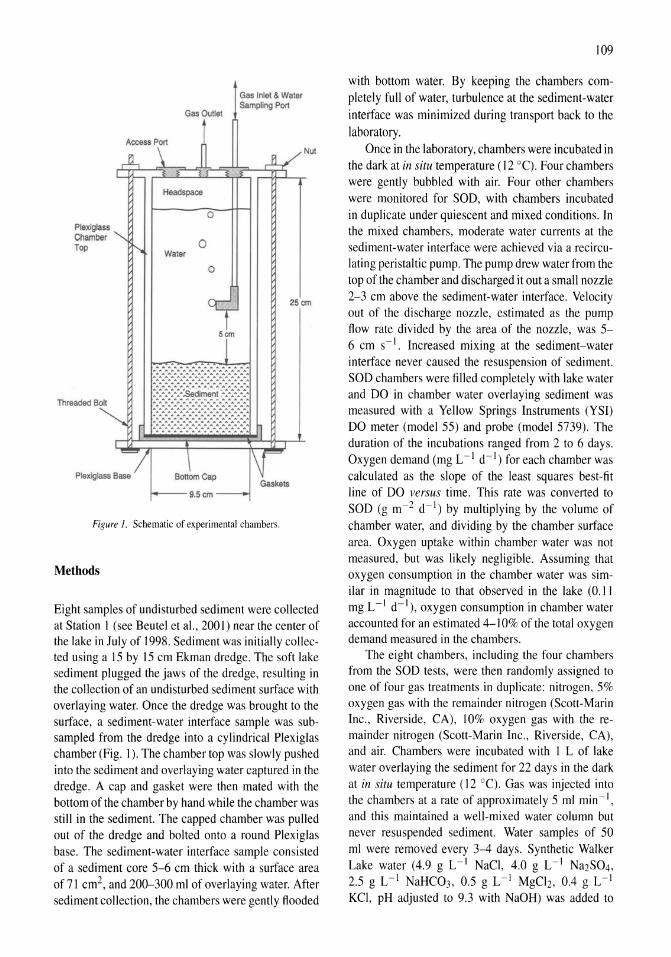
Gas Outlet
Gas Inlel & Waler Sampling Port
Headspace
o Plexig~ss "-Chamber "-Top f'. o
Waler
o
2Scm
5cm
...... : ....... :.:.: ... b ::::::::::::::::::::::::::::::: : :·:·:·:·:·Sediment :.:.:.:.:.
Threaded Boll .. A ....................... _ .. _ .. _ .. .. ........................... ...
~ tft~ttttI n c!~r~~"~
Plexlg~ss B~e=; SouL Cap IV = Gaskets
f..-9.5cm-
Figure 1. Schematic of experimental chambers.
Methods
Eight samples of undisturbed sediment were collected at Station 1 (see Beutel et a!., 2001) near the center of the lake in July of 1998. Sediment was initially collected using a 15 by 15 cm Ekman dredge. The soft lake sediment plugged the jaws of the dredge, resulting in the collection of an undisturbed sediment surface with overlaying water. Once the dredge was brought to the surface, a sediment-water interface sample was subsampled from the dredge into a cylindrical Plexiglas chamber (Fig. 1). The chamber top was slowly pushed into the sediment and overlaying water captured in the dredge. A cap and gasket were then mated with the bottom of the chamber by hand while the chamber was still in the sediment. The capped chamber was pulled out of the dredge and bolted onto a round Plexiglas base. The sediment-water interface sample consisted of a sediment core 5-6 cm thick with a surface area of 71 cm2, and 200-300 ml of overlaying water. After sediment collection, the chambers were gently flooded
109
with bottom water. By keeping the chambers completely full of water, turbulence at the sediment-water interface was minimized during transport back to the laboratory.
Once in the laboratory, chambers were incubated in the dark at in situ temperature (12 0c). Four chambers were gently bubbled with air. Four other chambers were monitored for SOD, with chambers incubated in duplicate under quiescent and mixed conditions. In the mixed chambers, moderate water currents at the sediment-water interface were achieved via a recirculating peristaltic pump. The pump drew water from the top of the chamber and discharged it out a small nozzle 2-3 cm above the sediment-water interface. Velocity out of the discharge nozzle, estimated as the pump flow rate divided by the area of the nozzle, was 5-6 cm s-I. Increased mixing at the sediment-water interface never caused the resuspension of sediment. SOD chambers were filled completely with lake water and DO in chamber water overlaying sediment was measured with a Yellow Springs Instruments (YSI) DO meter (model 55) and probe (model 5739). The duration of the incubations ranged from 2 to 6 days. Oxygen demand (mg L -I d- I) for each chamber was calculated as the slope of the least squares best-fit line of DO versus time. This rate was converted to SOD (g m-2 d- I ) by multiplying by the volume of chamber water, and dividing by the chamber surface area. Oxygen uptake within chamber water was not measured, but was likely negligible. Assuming that oxygen consumption in the chamber water was similar in magnitude to that observed in the lake (0.11 mg L -I d- I ), oxygen consumption in chamber water accounted for an estimated 4-10% of the total oxygen demand measured in the chambers.
The eight chambers, including the four chambers from the SOD tests, were then randomly assigned to one of four gas treatments in duplicate: nitrogen, 5% oxygen gas with the remainder nitrogen (Scott-Marin Inc., Riverside, CA), 10% oxygen gas with the remainder nitrogen (Scott-Marin Inc., Riverside, CA), and air. Chambers were incubated with I L of lake water overlaying the sediment for 22 days in the dark at in situ temperature (12°C). Gas was injected into the chambers at a rate of approximately 5 ml min-I, and this maintained a well-mixed water column but never resuspended sediment. Water samples of 50 ml were removed every 3-4 days. Synthetic Walker Lake water (4.9 g L -I NaCl, 4.0 g L -I Na2S04, 2.5 g L -I NaHC03, 0.5 g L -I MgCb, 0.4 g L- 1
KCI, pH adjusted to 9.3 with NaOH) was added to
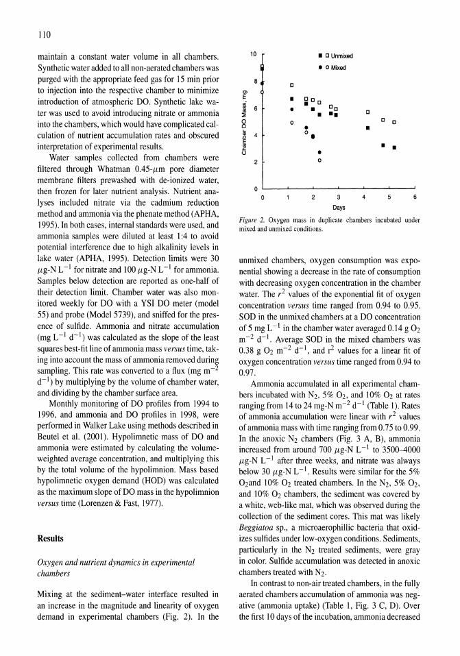
110
maintain a constant water volume in all chambers. Synthetic water added to all non-aerated chambers was purged with the appropriate feed gas for 15 min prior to injection into the respective chamber to minimize introduction of atmospheric DO. Synthetic lake water was used to avoid introducing nitrate or ammonia into the chambers, which would have complicated calculation of nutrient accumulation rates and obscured interpretation of experimental results.
Water samples collected from chambers were filtered through Whatman 0.45-JLm pore diameter membrane filters prewashed with de-ionized water, then frozen for later nutrient analysis. Nutrient analyses included nitrate via the cadmium reduction method and ammonia via the phenate method (APHA, 1995). In both cases, internal standards were used, and ammonia samples were diluted at least 1:4 to avoid potential interference due to high alkalinity levels in lake water (APHA, 1995). Detection limits were 30 JLg-N L -I for nitrate and 100 JLg-N L -I for ammonia. Samples below detection are reported as one-half of their detection limit. Chamber water was also monitored weekly for DO with a YSI DO meter (model 55) and probe (Model 5739), and sniffed for the presence of sulfide. Ammonia and nitrate accumulation (mg L -1 d- l ) was calculated as the slope of the least squares best-fit line of ammonia mass versus time, taking into account the mass of ammonia removed during sampling. This rate was converted to a flux (mg m-2
d- I ) by mUltiplying by the volume of chamber water, and dividing by the chamber surface area.
Monthly monitoring of DO profiles from 1994 to 1996, and ammonia and DO profiles in 1998, were performed in Walker Lake using methods described in Beutel et al. (2001). Hypolimnetic mass of DO and ammonia were estimated by calculating the volumeweighted average concentration, and multiplying this by the total volume of the hypolimnion. Mass based hypolimnetic oxygen demand (HOD) was calculated as the maximum slope of DO mass in the hypolimnion versus time (Lorenzen & Fast, 1977).
Results
Oxygen and nutrient dynamics in experimental chambers
Mixing at the sediment-water interface resulted in an increase in the magnitude and linearity of oxygen demand in experimental chambers (Fig. 2). In the
10
8 0
Cl E • <Ii 'II 6 C1I • ::; 0 0
0
Z 4 E C1I .t: ()
2
0 0
• 0 Unmixed
• 0 Mixed
~oo 00 •
• o.
2
•
• 0
••
3
Days
o IJ 0
• • •
4 5 6
Figure 2. Oxygen mass in duplicate chambers incubated under mixed and unmixed conditions.
unmixed chambers, oxygen consumption was exponential showing a decrease in the rate of consumption with decreasing oxygen concentration in the chamber water. The r2 values of the exponential fit of oxygen concentration versus time ranged from 0.94 to 0.95. SOD in the unmixed chambers at a DO concentration of 5 mg L -I in the chamber water averaged 0.14 g 02 m-2 d- l . Average SOD in the mixed chambers was 0.38 g 02 m-2 d- l , and r2 values for a linear fit of oxygen concentration versus time ranged from 0.94 to 0.97.
Ammonia accumulated in all experimental chambers incubated with N2, 5% 02, and 10% 02 at rates ranging from 14 to 24 mg-N m-2 d- I (Table 1). Rates of ammonia accumulation were linear with r2 values of ammonia mass with time ranging from 0.75 to 0.99. In the anoxic N2 chambers (Fig. 3 A, B), ammonia increased from around 700 JLg-N L -I to 3500-4000 JLg-N L -I after three weeks, and nitrate was always below 30 JLg-N L -I. Results were similar for the 5% 02and 10% 02 treated chambers. In the N2, 5% 02, and 10% 02 chambers, the sediment was covered by a white, web-like mat, which was observed during the collection of the sediment cores. This mat was likely Beggiatoa sp., a microaerophillic bacteria that oxidizes sulfides under low-oxygen conditions. Sediments, particularly in the N2 treated sediments, were gray in color. Sulfide accumulation was detected in anoxic chambers treated with N2.
In contrast to non-air treated chambers, in the fully aerated chambers accumulation of ammonia was negative (ammonia uptake) (Table 1, Fig. 3 C, D). Over the first 10 days of the incubation, ammonia decreased
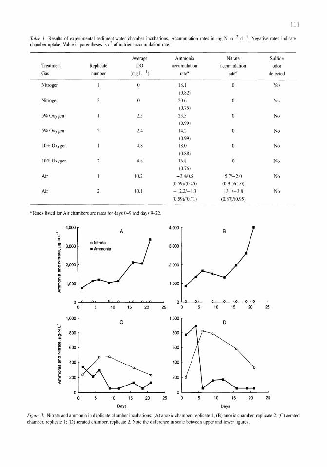
III
Table 1. Results of experimental sediment-water chamber incubations. Accumulation rates in mg-N m-2 d- I. Negative rates indicate chamber uptake. Value in parentheses is r2 of nutrient accumulation rate.
Average
Treatment Replicate DO
Gas number (mgL -I)
Nitrogen 0
Nitrogen 2 0
5% Oxygen 2.5
5% Oxygen 2 2.4
10% Oxygen 4.8
10% Oxygen 2 4.8
Air 10.2
Air 2 10.1
aRates listed for Air chambers are rates for days 0-9 and days 9-22.
-:.J
Z
4,000
~ 3,000
! ; 2,000 ~ <U '2 ~ 1,000
~
A
o~~~--~~--~~~~~
! z "C c: <U <U .~
E E <I:
1,000
600
400
200
a 5 10
5 10
15 20 25
c
15 20 25
Days
Ammonia Nitrate Sulfide
accumulation accumulation odor
rate" ratea detected
18.1 0 Yes
(0.82)
20.6 0 Yes
(0.75)
23.5 0 No
(0.99)
14.2 0 No
(0.99)
18.0 0 No
(088)
16.8 0 No
(0.76)
-3.4/0.5 5.7/-2.0 No
(0.59)/(0.25) (0.91)/(1.0)
-12.2/-1.3 13.1/-3.8 No
(0.59)/(0.71) (0.87)/(0.95)
4,000
3,000
2,000
1,000
o~~~--~~~~--~~~
o 5 10 15 20 25
1,000 o 800
600
400
200
OL---~--~----~--~--~
a 5 10 15 20 25
Days
Figure 3. Nitrate and ammonia in duplicate chamber incubations: (A) anoxic chamber, replicate I; (B) anoxic chamber, replicate 2; (C) aerated chamber, replicate 1; (D) aerated chamber, replicate 2. Note the difference in scale between upper and lower figures.
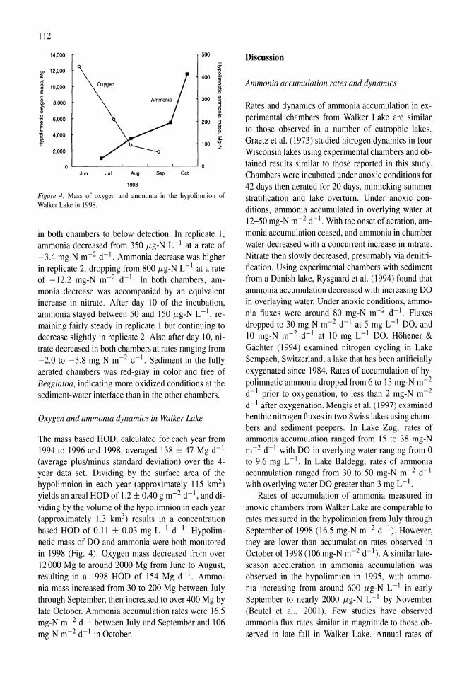
112
14,000
'" 12,000 ::;
'" 0 10,000 ~ E C
" 8,000 ~ 0 u
6,000 ~ c § "0 4,000 Q.
'" I 2,000
Jun Jul Aug
1998
Sep Oct
500
I '< ."
400 Q.
3 " ~ Q
300 ~
3 3 0
" ~.
200 3 ~
.g: ;:::
100 '9 Z
Figure 4. Mass of oxygen and ammonia in the hypolimnion of Walker Lake in 1998.
in both chambers to below detection. In replicate 1, ammonia decreased from 350 p,g-N L -I at a rate of -3.4 mg-N m-2 d- I . Ammonia decrease was higher in replicate 2, dropping from 800 p,g-N L -1 at a rate of -12.2 mg-N m-2 d- 1. In both chambers, ammonia decrease was accompanied by an equivalent increase in nitrate. After day 10 of the incubation, ammonia stayed between 50 and 150 p,g-N L -I, remaining fairly steady in replicate 1 but continuing to decrease slightly in replicate 2. Also after day 10, nitrate decreased in both chambers at rates ranging from -2.0 to -3.8 mg-N m-2 d- I . Sediment in the fully aerated chambers was red-gray in color and free of Beggiatoa, indicating more oxidized conditions at the sediment-water interface than in the other chambers.
Oxygen and ammonia dynamics in Walker Lake
The mass based HOD, calculated for each year from 1994 to 1996 and 1998, averaged 138 ± 47 Mg d- I
(average plus/minus standard deviation) over the 4-year data set. Dividing by the surface area of the hypolimnion in each year (approximately 115 km2)
yields an areal HOD of 1.2 ± 0.40 g m-2 d- 1, and dividing by the volume of the hypolimnion in each year (approximately 1.3 km3) results in a concentration based HOD of 0.11 ± 0.03 mg L-1 d-1. Hypolimnetic mass of DO and ammonia were both monitored in 1998 (Fig. 4). Oxygen mass decreased from over 12000 Mg to around 2000 Mg from June to August, resulting in a 1998 HOD of 154 Mg d- I . Ammonia mass increased from 30 to 200 Mg between July through September, then increased to over 400 Mg by late October. Ammonia accumulation rates were 16.5 mg-N m-2 d- 1 between July and September and 106 mg-N m-2 d- 1 in October.
Discussion
Ammonia accumulation rates and dynamics
Rates and dynamics of ammonia accumulation in experimental chambers from Walker Lake are similar to those observed in a number of eutrophic lakes. Graetz et al. (1973) studied nitrogen dynamics in four Wisconsin lakes using experimental chambers and obtained results similar to those reported in this study. Chambers were incubated under anoxic conditions for 42 days then aerated for 20 days, mimicking summer stratification and lake overturn. Under anoxic conditions, ammonia accumulated in overlying water at 12-50 mg-N m-2 d- 1. With the onset of aeration, ammonia accumulation ceased, and ammonia in chamber water decreased with a concurrent increase in nitrate. Nitrate then slowly decreased, presumably via denitrification. Using experimental chambers with sediment from a Danish lake, Rysgaard et al. (1994) found that ammonia accumulation decreased with increasing DO in overlaying water. Under anoxic conditions, ammonia fluxes were around 80 mg-N m-2 d- I. Fluxes dropped to 30 mg-N m-2 d- 1 at 5 mg L -1 DO, and 10 mg-N m-2 d- 1 at 10 mg L -I DO. Hohener & Gachter (1994) examined nitrogen cycling in Lake Sempach, Switzerland, a lake that has been artificially oxygenated since 1984. Rates of accumulation of hypolimnetic ammonia dropped from 6 to 13 mg-N m-2
d- I prior to oxygenation, to less than 2 mg-N m-2
d- 1 after oxygenation. Mengis et al. (1997) examined benthic nitrogen fluxes in two Swiss lakes using chambers and sediment peepers. In Lake Zug, rates of ammonia accumulation ranged from 15 to 38 mg-N m-2 d- 1 with DO in overlying water ranging from 0 to 9.6 mg L -I. In Lake Baldegg, rates of ammonia accumulation ranged from 30 to 50 mg-N m-2 d- I
with overlying water DO greater than 3 mg L -1.
Rates of accumulation of ammonia measured in anoxic chambers from Walker Lake are comparable to rates measured in the hypolimnion from July through September of 1998 (16.5 mg-N m-2 d- 1). However, they are lower than accumulation rates observed in October of 1998 (106 mg-N m-2 d- 1). A similar lateseason acceleration in ammonia accumulation was observed in the hypolimnion in 1995, with ammonia increasing from around 600 p,g-N L -I in early September to nearly 2000 p,g-N L -1 by November (Beutel et aI., 2001). Few studies have observed ammonia flux rates similar in magnitude to those observed in late fall in Walker Lake. Annual rates of
ammonia accumulation in the hypolimnion of Mono Lake, California during a period of meromixis from 1983 to 1987, based on data from Jellison & Melack (1993), range from 30 to 60 mg-N m-2 d- I . As reported earlier, Rysgaard et a!. (1994) measured an ammonia fluxes of around 80 mg-N m-2 d- I in anoxic lake sediment under anoxic conditions. Ammonia fluxes measured in experimental chambers containing anoxic sediments from eutrophic Lake Elsinore, California, ranged from 80 to 116 mg-N m-2 d- I (M. W. Beutel, unpublished). However, this lake was shallow (Zmax = 8 m) and warm (24-27 0c) compared to Walker Lake. The high fall rates of ammonia accumulation may have resulted from the decay of late summer blooms of blue-green algae, which can produce organic nitrogen via biological fixation of N2 (Horne et a!., 1994). Increased mineralization within the water column of Walker Lake could account for the discrepancy between the high rates of fall ammonia accumulation in the hypolimnion (l06 mg-N m-2
d- I ) and the relatively low rates of sediment ammonia release measured in this study (18-21 mg-Nm-2 d- I)
and generally reported by others (10-50 mg-N m-2
d- I ).
Increases in ammonia content in the water of experimental chambers are reported as an accumulation without reference to the origin of the ammonia. However, the dominant source of ammonia is thought to be biological mineralization processes in the sediment (Jones et aI., 1982). Contributions from biological activity in the small volume of overlaying water were likely minimal, particularly in the chambers with aerated water columns. Thus, ammonia accumulation rates are equivalent to sediment release rates of ammonia.
Enhanced nitrification and denitrification
In the Walker Lake chamber experiments, ammonia accumulation was reversed only in the fully aerated chambers with DO around 10 mg L -I. While experimental results cannot directly identify the mechanisms involved, biological nitrification and denitrification may account for the observed decrease in ammonia accumulation. During the first 10 days of the incubation, aeration appeared to stimulate nitrification of ammonia in the water column, with the decrease in ammonia corresponding with an increase in nitrate (Fig. 3). The rates of ammonia uptake and nitrate accumulation were similar in each chamber. In replicate 1, ammonia accumulation was -3.4 mg-N m-2 d- I
113
while nitrate accumulation was 5.7 mg-N m-2 d- I. In replicate 2, the rates were -12.2 and 13.1 mg-N m-2
d- I , respectively. Denitrification of nitrate diffusing from overlaying water into sediment would account for the subsequent drop in nitrate for the remainder of the incubation. This is supported by the observation that rates of nitrate accumulation were proportional to nitrate concentration. Nitrate accumulation in replicate 1 was -2.0 mg-N m-2 d- I and nitrate levels ranged from 450 to 200 fLg-N L -I. In replicate 2, the rate of nitrate accumulation, -3.8 mg-N m-2 d- 1 ,
and nitrate concentration, 800-300 fLg-N L -I, were roughly twice as high.
Many studies have reported a correlation between water column nitrate and denitrification rates (Seitzinger, 1988; Hbhener & Gachter, 1993; Rysgaard et aI., 1994). It is likely that these biological transformations took place predominately in the sediments rather than in the small water column of the experimental chambers (Vincent & Downes, 1981; Seitzinger, 1988). This premise is supported by the fact that no nitrate was detected in the water of moderately aerated chambers, suggesting that nitrification in the oxygenated water column was minimal. The observed transformations of ammonia and nitrate in the water of full y aerated chambers suggest that nitrification and denitrification were enhanced in the sediments. Nitrification and subsequent denitrification of ammonia produced in the sediment would account for the observed decline in ammonia accumulation under fully aerated conditions.
In a number of sediment-water systems, DO in water overlaying sediment has been shown to stimulate nitrification and denitrification. Rysgaard et al. (1994) found that rates of nitrification and coupled nitrification-denitrification increased with increasing DO in water overlaying sediment from a eutrophic lake. At 10 mg L -1 DO, nitrification was equivalent to 95% of the ammonia flux originally measured from the sediment under anoxic conditions. In addition, increasing DO from 0 to 10 mg L -1 caused coupled nitrification-denitrification to increase from o to 18 mg-N m-2 d- I . Ahlgren et a!. (1994) examined nitrogen cycling in an eutrophic Swedish lake. They found the highest rates of coupled nitrificationdenitrification in profundal sediment just prior to and after thermal stratification, when the water column was oxygenated and contained some nitrate. In addition, denitrification rates were higher in oxygenated, littoral sediments (\.6-2.2 mg-N m-2 d- 1) compared
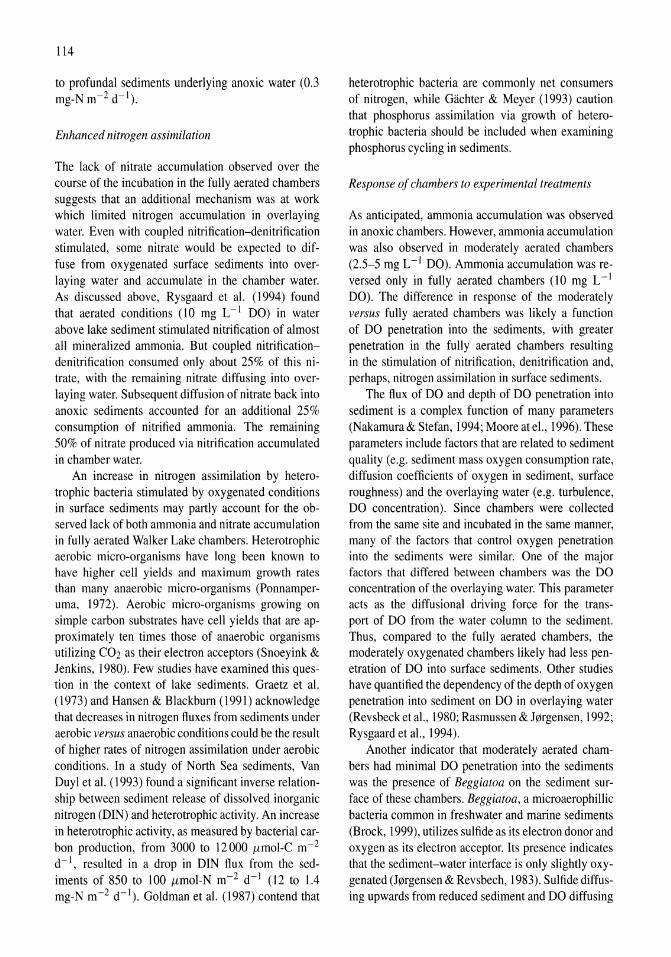
114
to profundal sediments underlying anoxic water (OJ mg-Nm-2 d- I).
Enhanced nitrogen assimilation
The lack of nitrate accumulation observed over the course of the incubation in the fully aerated chambers suggests that an additional mechanism was at work which limited nitrogen accumulation in overlaying water. Even with coupled nitrification-denitrification stimulated, some nitrate would be expected to diffuse from oxygenated surface sediments into overlaying water and accumulate in the chamber water. As discussed above, Rysgaard et a!. (1994) found that aerated conditions (10 mg L -I DO) in water above lake sediment stimulated nitrification of almost all mineralized ammonia. But coupled nitrificationdenitrification consumed only about 25% of this nitrate, with the remaining nitrate diffusing into overlaying water. Subsequent diffusion of nitrate back into anoxic sediments accounted for an additional 25% consumption of nitrified ammonia. The remaining 50% of nitrate produced via nitrification accumulated in chamber water.
An increase in nitrogen assimilation by heterotrophic bacteria stimulated by oxygenated conditions in surface sediments may partly account for the observed lack of both ammonia and nitrate accumulation in fully aerated Walker Lake chambers. Heterotrophic aerobic micro-organisms have long been known to have higher cell yields and maximum growth rates than many anaerobic micro-organisms (Ponnamperuma, 1972). Aerobic micro-organisms growing on simple carbon substrates have cell yields that are approximately ten times those of anaerobic organisms utilizing C02 as their electron acceptors (Snoeyink & Jenkins, 1980). Few studies have examined this question in the context of lake sediments. Graetz et al. (1973) and Hansen & Blackburn (1991) acknowledge that decreases in nitrogen fluxes from sediments under aerobic versus anaerobic conditions could be the result of higher rates of nitrogen assimilation under aerobic conditions. In a study of North Sea sediments, Van Duyl et a!. (1993) found a significant inverse relationship between sediment release of dissolved inorganic nitrogen (DIN) and heterotrophic activity. An increase in heterotrophic activity, as measured by bacterial carbon production, from 3000 to 12000 flmol-C m-2
d- I , resulted in a drop in DIN flux from the sediments of 850 to 100 flmol-N m-2 d- I (12 to 1.4 mg-N m-2 d- I). Goldman et a!. (1987) contend that
heterotrophic bacteria are commonly net consumers of nitrogen, while Gachter & Meyer (1993) caution that phosphorus assimilation via growth of heterotrophic bacteria should be included when examining phosphorus cycling in sediments.
Response of chambers to experimental treatments
As anticipated, ammonia accumulation was observed in anoxic chambers. However, ammonia accumulation was also observed in moderately aerated chambers (2.5-5 mg L -I DO). Ammonia accumulation was reversed only in fully aerated chambers (10 mg L -I DO). The difference in response of the moderately versus fully aerated chambers was likely a function of DO penetration into the sediments, with greater penetration in the fully aerated chambers resulting in the stimulation of nitrification, denitrification and, perhaps, nitrogen assimilation in surface sediments.
The flux of DO and depth of DO penetration into sediment is a complex function of many parameters (Nakamura & Stefan, 1994; Moore at el., 1996). These parameters include factors that are related to sediment quality (e.g. sediment mass oxygen consumption rate, diffusion coefficients of oxygen in sediment, surface roughness) and the overlaying water (e.g. turbulence, DO concentration). Since chambers were collected from the same site and incubated in the same manner, many of the factors that control oxygen penetration into the sediments were similar. One of the major factors that differed between chambers was the DO concentration of the overlaying water. This parameter acts as the diffusional driving force for the transport of DO from the water column to the sediment. Thus, compared to the fully aerated chambers, the moderately oxygenated chambers likely had less penetration of DO into surface sediments. Other studies have quantified the dependency of the depth of oxygen penetration into sediment on DO in overlaying water (Revsbeck et a!., 1980; Rasmussen & Jorgensen, 1992; Rysgaard et aI., 1994).
Another indicator that moderately aerated chambers had minimal DO penetration into the sediments was the presence of Beggiatoa on the sediment surface of these chambers. Beggiatoa, a microaerophillic bacteria common in freshwater and marine sediments (Brock, 1999), utilizes sulfide as its electron donor and oxygen as its electron acceptor. Its presence indicates that the sediment-water interface is only slightly oxygenated (Jorgensen & Revsbech, 1983). Sulfide diffusing upwards from reduced sediment and DO diffusing
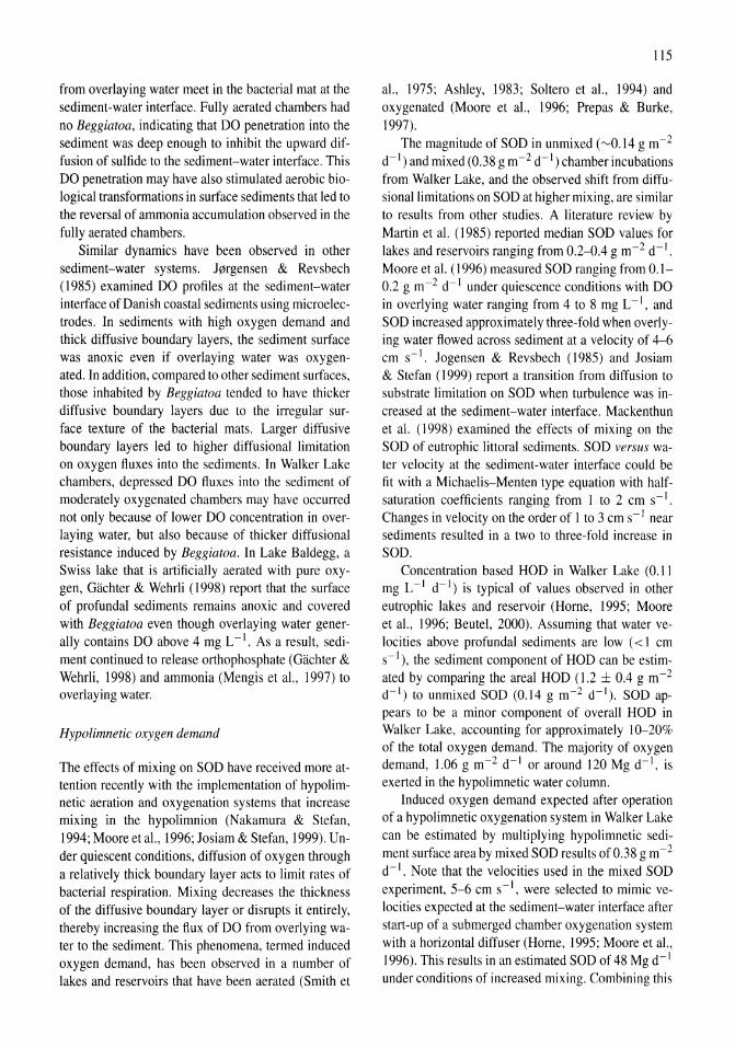
from overlaying water meet in the bacterial mat at the sediment-water interface. Fully aerated chambers had no Beggiatoa, indicating that DO penetration into the sediment was deep enough to inhibit the upward diffusion of sulfide to the sediment-water interface. This DO penetration may have also stimulated aerobic biological transformations in surface sediments that led to the reversal of ammonia accumulation observed in the fully aerated chambers.
Similar dynamics have been observed in other sediment-water systems. J~rgensen & Revsbech (1985) examined DO profiles at the sediment-water interface of Danish coastal sediments using microelectrodes. In sediments with high oxygen demand and thick diffusive boundary layers, the sediment surface was anoxic even if overlaying water was oxygenated. In addition, compared to other sediment surfaces, those inhabited by Beggiatoa tended to have thicker diffusive boundary layers due to the irregular surface texture of the bacterial mats. Larger diffusive boundary layers led to higher diffusional limitation on oxygen fluxes into the sediments. In Walker Lake chambers, depressed DO fluxes into the sediment of moderately oxygenated chambers may have occurred not only because of lower DO concentration in overlaying water, but also because of thicker diffusional resistance induced by Beggiatoa. In Lake Baldegg, a Swiss lake that is artificially aerated with pure oxygen, Gi:ichter & Wehrli (1998) report that the surface of profundal sediments remains anoxic and covered with Beggiatoa even though overlaying water generally contains DO above 4 mg L -I. As a result, sediment continued to release orthophosphate (Gachter & Wehrli, 1998) and ammonia (Mengis et a!., 1997) to overlaying water.
Hypolimnetic oxygen demand
The effects of mixing on SOD have received more attention recently with the implementation of hypo limnetic aeration and oxygenation systems that increase mixing in the hypolimnion (Nakamura & Stefan, 1994; Moore etal., 1996; Josiam & Stefan, 1999). Under quiescent conditions, diffusion of oxygen through a relatively thick boundary layer acts to limit rates of bacterial respiration. Mixing decreases the thickness of the diffusive boundary layer or disrupts it entirely, thereby increasing the flux of DO from overlying water to the sediment. This phenomena, termed induced oxygen demand, has been observed in a number of lakes and reservoirs that have been aerated (Smith et
115
a!., 1975; Ashley, 1983; Soltero et a!., 1994) and oxygenated (Moore et a!., 1996; Prep as & Burke, 1997).
The magnitude of SOD in unmixed ("-'0.14 g m-2
d- I) and mixed (0.38 g m-2 d- I) chamber incubations from Walker Lake, and the observed shift from diffusionallimitations on SOD at higher mixing, are similar to results from other studies. A literature review by Martin et al. (1985) reported median SOD values for lakes and reservoirs ranging from 0.2-0.4 g m-2 d- I. Moore et al. (1996) measured SOD ranging from 0.1-0.2 g m-2 d- I under quiescence conditions with DO in overlying water ranging from 4 to 8 mg L -I, and SOD increased approximately three-fold when overlying water flowed across sediment at a velocity of 4-6 cm s-I. Jogensen & Revsbech (1985) and Josiam & Stefan (1999) report a transition from diffusion to substrate limitation on SOD when turbulence was increased at the sediment-water interface. Mackenthun et al. (1998) examined the effects of mixing on the SOD of eutrophic littoral sediments. SOD versus water velocity at the sediment-water interface could be fit with a Michaelis-Menten type equation with halfsaturation coefficients ranging from 1 to 2 cm s-I. Changes in velocity on the order of 1 to 3 cm s-I near sediments resulted in a two to three-fold increase in SOD.
Concentration based HOD in Walker Lake (0.11 mg L -I d- I) is typical of values observed in other eutrophic lakes and reservoir (Home, 1995; Moore et aI., 1996; Beutel, 2000). Assuming that water velocities above profundal sediments are low « 1 cm s-I), the sediment component of HOD can be estimated by comparing the areal HOD (1.2 ± 0.4 g m-2
d- 1) to unmixed SOD (0.l4 g m-2 d-1). SOD appears to be a minor component of overall HOD in Walker Lake, accounting for approximately 10--20% of the total oxygen demand. The majority of oxygen demand, 1.06 g m-2 d- I or around 120 Mg d- 1, is exerted in the hypolimnetic water column.
Induced oxygen demand expected after operation of a hypolimnetic oxygenation system in Walker Lake can be estimated by multiplying hypolimnetic sediment surface area by mixed SOD results of 0.38 g m-2
d- I. Note that the velocities used in the mixed SOD experiment, 5-6 cm s-l, were selected to mimic velocities expected at the sediment-water interface after start-up of a submerged chamber oxygenation system with a horizontal diffuser (Home, 1995; Moore et a!., 1996). This results in an estimated SOD of 48 Mg d- I under conditions of increased mixing. Combining this
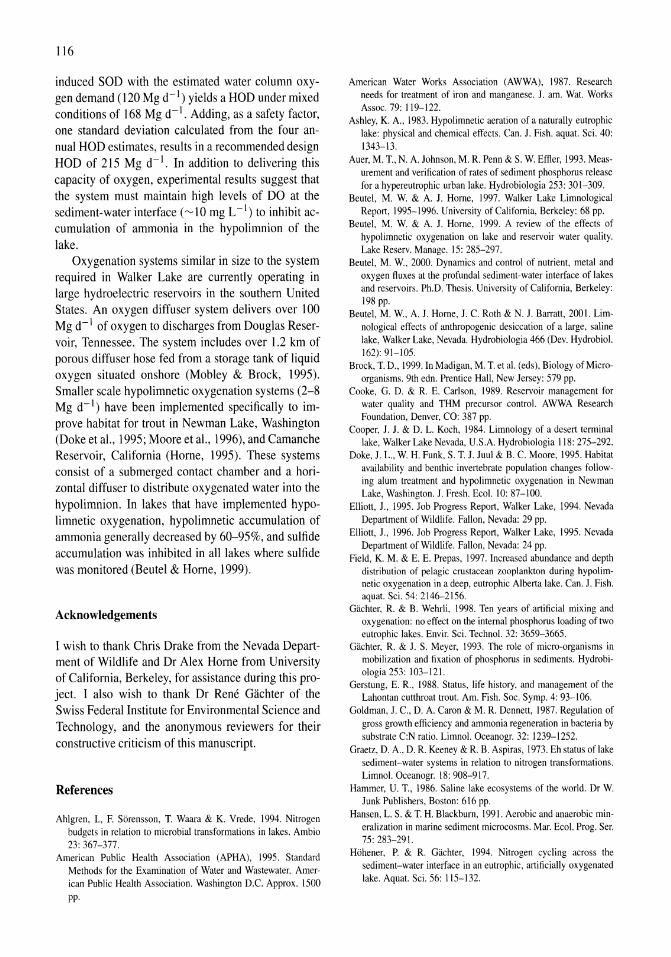
116
induced SOD with the estimated water column oxygen demand (120 Mg d- I ) yields a HOD under mixed conditions of 168 Mg d- I . Adding, as a safety factor, one standard deviation calculated from the four annual HOD estimates, results in a recommended design HOD of 215 Mg d- I . In addition to delivering this capacity of oxygen, experimental results suggest that the system must maintain high levels of DO at the sediment-water interface (~1O mg L -I) to inhibit accumulation of ammonia in the hypolimnion of the lake.
Oxygenation systems similar in size to the system required in Walker Lake are currently operating in large hydroelectric reservoirs in the southern United States. An oxygen diffuser system delivers over 100 Mg d- I of oxygen to discharges from Douglas Reservoir, Tennessee. The system includes over 1.2 km of porous diffuser hose fed from a storage tank of liquid oxygen situated onshore (Mobley & Brock, 1995). Smaller scale hypolimnetic oxygenation systems (2-8 Mg d- I ) have been implemented specifically to improve habitat for trout in Newman Lake, Washington (Doke et al., 1995; Moore et al., 1996), and Camanche Reservoir, California (Home, 1995). These systems consist of a submerged contact chamber and a horizontal diffuser to distribute oxygenated water into the hypolimnion. In lakes that have implemented hypolimnetic oxygenation, hypolimnetic accumulation of ammonia generally decreased by 60-95%, and sulfide accumulation was inhibited in all lakes where sulfide was monitored (Beutel & Home, 1999).
Acknowledgements
I wish to thank Chris Drake from the Nevada Department of Wildlife and Dr Alex Home from University of California, Berkeley, for assistance during this project. I also wish to thank Dr Rene Gachter of the Swiss Federal Institute for Environmental Science and Technology, and the anonymous reviewers for their constructive criticism of this manuscript.
References
Ahlgren, 1., F. Sorensson, T. Waara & K. Vrede, 1994. Nitrogen budgets in relation to microbial transformations in lakes. Ambio 23: 367-377.
American Public Health Association (APHA), 1995. Standard Methods for the Examination of Water and Wastewater. American Public Health Association. Washington D.C. Approx. 1500 pp.
American Water Works Association (AWWA), 1987. Research needs for treatment of iron and manganese. 1. am. Wat. Works Assoc. 79: 119-122.
Ashley, K. A., 1983. Hypolimnetic aeration of a naturally eutrophic lake: physical and chemical effects. Can. J. Fish. aquat. Sci. 40: 1343-13.
Auer, M. T., N. A. Johnson, M. R. Penn & S. W. Effler, 1993. Measurement and verification of rates of sediment phosphorus release for a hypereutrophic urban lake. Hydrobiologia 253: 301-309.
Beutel, M. W. & A. J. Home, 1997. Walker Lake Limnological Report, 1995-1996. University of California, Berkeley: 68 pp.
Beutel, M. W. & A. J. Home, 1999. A review of the effects of hypolimnetic oxygenation on lake and reservoir water quality. Lake Reserv. Manage. 15: 285-297.
Beutel, M. W., 2000. Dynamics and control of nutrient, metal and oxygen fluxes at the profunda! sediment-water interface of lakes and reservoirs. Ph.D. Thesis. University of California, Berkeley: 198 pp.
Beutel, M. w., A. J. Home, J. C. Roth & N. 1. Barratt, 2001. Limnological effects of anthropogenic desiccation of a large, saline lake, Walker Lake, Nevada. Hydrobiologia 466 (Dev. Hydrobiol. 162): 91-105.
Brock, T.D., 1999. In Madigan, M. T. et aI. (eds), Biology of Microorganisms. 9th edn. Prentice Hall, New Jersey: 579 pp.
Cooke, G. D. & R. E. Carlson, 1989. Reservoir management for water quality and THM precursor control. AWWA Research Foundation, Denver, CO: 387 pp.
Cooper, J. J. & D. L. Koch, 1984. Limnology of a desert terminal lake, Walker Lake Nevada, U.S.A. Hydrobiologia 118: 275-292.
Doke, J. L., W. H. Funk, S. T. 1. Juul & B. C. Moore, 1995. Habitat availability and benthic invertebrate population changes following alum treatment and hypolimnetic oxygenation in Newman Lake, Washington. J. Fresh. Ecol. 10: 87-100.
Elliott, 1., 1995. Job Progress Report, Walker Lake, 1994. Nevada Department of Wildlife. Fallon, Nevada: 29 pp.
Elliott, J., 1996. Job Progress Report, Walker Lake, 1995. Nevada Department of Wildlife. Fallon, Nevada: 24 pp.
Field, K. M. & E. E. Prepas, 1997. Increased abundance and depth distribution of pelagic crustacean zooplankton during hypo limnetic oxygenation in a deep, eutrophic Alberta lake. Can. J. Fish. aquat. Sci. 54: 2146-2156.
Giichter, R. & B. Wehrli, 1998. Ten years of artificial mixing and oxygenation: no effect on the internal phosphorus loading of two eutrophic lakes. Envir. Sci. Technol. 32: 3659-3665.
Gachter, R. & J. S. Meyer, 1993. The role of micro-organisms in mobilization and fixation of phosphorus in sediments. Hydrobiologia 253: 103-121.
Gerstung, E. R., 1988. Status, life history, and management of the Lahontan cutthroat trout. Am. Fish. Soc. Symp. 4: 93-106.
Goldman, J. C., D. A. Caron & M. R. Dennett, 1987. Regulation of gross growth efficiency and ammonia regeneration in bacteria by substrate C:N ratio. Limnol. Oceanogr. 32: 1239-1252.
Graetz, D. A., D. R. Keeney &R. B. Aspiras, 1973. Eh status of lake sediment-water systems in relation to nitrogen transformations. Limnol. Oceanogr. 18: 908-917.
Hammer, U. T., 1986. Saline lake ecosystems of the world. Dr W. Junk Publishers, Boston: 616 pp.
Hansen, L. S. & T. H. Blackburn, 1991. Aerobic and anaerobic mineralization in marine sediment microcosms. Mar. Ecol. Prog. Ser. 75: 283-291.
Hohener, P. & R. Gachter, 1994. Nitrogen cycling across the sediment-water interface in an eutrophic, artificially oxygenated lake. Aquat. Sci. 56: 1l5-132.
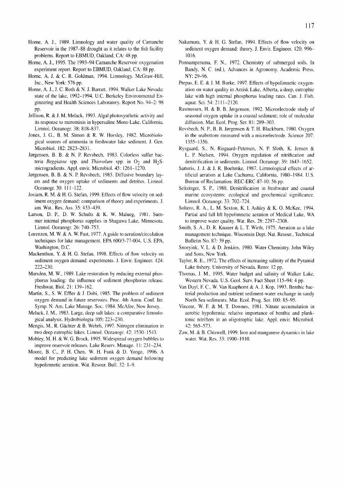
Horne, A. l, 1989. Limnology and water quality of Camanche Reservoir in the 1987-88 drought as it relates to the fish facility problems. Report to EBMUD, Oakland, CA: 48 pp.
Horne, A. l, 1995. The 1993-94 Camanche Reservoir oxygenation experiment report. Report to EBMUD, Oakland, CA: 88 pp.
Horne, A. J. & c. R. Goldman, 1994. Limnology. McGraw-Hill, Inc., New York: 576 pp.
Horne, A. 1., 1. C. Roth & N. J. Barratt, 1994. Walker Lake Nevada: state of the lake, 1992-1994. U.c. Berkeley Environmental Engineering and Health Sciences Laboratory. Report No. 94-2: 98 pp.
Jellison, R. & J. M. Melack, 1993. Algal photosynthetic activity and its response to meromixis in hypersaline Mono Lake, California. Limno!. Oceanogr. 38: 818-837.
Jones, 1. G., B. M. Simon & R. W. Horsley, 1982. Microbiological sources of ammonia in freshwater lake sediment. l Gen. Microbio!. 182: 2823-2831.
J0rgensen, B. B. & N. P. Revsbech, 1983. Colorless sulfur bacteria Beggiatoa spp. and Thiovoiul1l spp. in 02 and H2 Smicrogradients. App!. envir. Microbio!' 45: 1261-1270.
J0rgensen, B. B. & N. P. Revsbech, 1985. Diffusive boundary layers and the oxygen uptake of sediments and detritus. Limno!. Oceanogr. 30: 111-122.
Josiam, R. M. & H. G. Stefan, 1999. Effects of flow velocity on sediment oxygen demand: comparison of theory and experiments. J. am. Wat.. Res. Ass. 35: 433-439.
Larson, D. P., D. W. Schults & K. W. Malueg, 1981. Summer internal phosphorus supplies in Shagawa Lake, Minnesota. Limno!. Oceanogr. 26: 740-753.
Lorenzen, M. W. & A. W. Fast, 1977. A guide to aeration/circulation techniques for lake management. EPA 600/3-77-004, U.S. EPA, Washington, D.C.
Mackenthun, Y. & H. G. Stefan, 1998. Effects of flow velocity on sediment oxygen demand: experiments. 1. Envir. Engineer. 124: 222-230.
Marsden, M. w., 1989. Lake restoration by reducing external phosphorus loading: the influence of sediment phosphorus release. Freshwat. Bio!. 21: 139-162.
Martin, S., S. W. Effler & J. Dobi, 1985. The problem of sediment oxygen demand in future reservoirs. Proc. 4th Annu. Conf. Int. Symp. N. Am. Lake Manage. Soc. 1984. McAfee, New Jersey.
Melack, J. M., 1983. Large, deep salt lakes: a comparative limnological analysis. Hydrobiologia 105: 223-230.
Mengis, M., R. Gachter & B. Wehrli, 1997. Nitrogen elimination in two deep eutrophic lakes. Limno!. Oceanogr. 42: 1530-1543.
Mobley, M. H. & w. G. Brock, 1995. Widespread oxygen bubbles to improve reservoir releases. Lake Reserv. Manage. II: 231-234.
Moore, B. c., P. H. Chen, W. H. Funk & D. Yonge, 1996. A model for predicting lake sediment oxygen demand following hypolimnetic aeration. Wat. Resour. Bul!. 32: 1-9.
117
Nakamura, Y. & H. G. Stefan, 1994. Effects of flow velocity on sediment oxygen demand: theory. l Envir. Engineer. 120: 996-1016,
Ponnamperuma, F. N., 1972. Chemistry of submerged soils. In Bandy, N. C. (ed.), Advances in Agronomy. Academic Press, NY: 29-96,
Prepas, E. E. & l M. Burke, 1997. Effects of hypolimnetic oxygenation on water quality in Amisk Lake, Alberta, a deep, eutrophic lake with high internal phosphorus loading rates. Can. 1. Fish. aquat. Sci. 54: 2111-2120.
Rasmussen, H. & B. B. J0rgensen, 1992. Microelectrode study of seasonal oxygen uptake in a coastal sediment; role of molecular diffusion. Mar. Eco!. Prog. Ser. 81: 289-303.
Revsbech, N. P., B. B. J0rgensen & T. H. Blackburn, 1980. Oxygen in the seabottom measured with a microelectrode. Science 207: 1355-1356.
Rysgaard, S., N. Risgaard-Petersen, N. P. Sloth, K. Jensen & L. P. Nielsen, 1994. Oxygen regulation of nitrification and denitrification in sediments. Limno!. Oceanogr. 39: 1643-1652.
Sartoris, 1. 1. & 1. R. Boehmke, 1987. Limnological effects of artificial aeration at Lake Cachuma, California, 1980-1984. U.S. Bureau of Reclamation. REC-ERC-87 -10: 56 pp.
Seitzinger, S. P .. 1988. Denitrification in freshwater and coastal marine ecosystems: ecological and geochemical significance. Limno!. Oceanogr. 33: 702-724.
Soltero, R. A .. L. M. Sexton, K. 1. Ashley & K. O. McKee, 1994. Partial and full lift hypolimnetic aeration of Medical Lake, WA to improve water quality. Wat. Res. 28: 2297-2308.
Smith, S. A., D. R. Knauer & L. T. Wirth, 1975. Aeration as a lake management technique. Wisconsin Dept. Nat. Resour., Technical Bulletin No. 87: 39 pp.
Snoeyink, V. L. & D. Jenkins, 1980. Water Chemistry. John Wiley and Sons, New York.
Taylor, R. E., 1972. The effects of increasing salinity of the Pyramid Lake fishery. University of Nevada, Reno: 12 pp.
Thomas, 1. M., 1995. Water budget and salinity of Walker Lake, Western Nevada. U.S. Geo!. Surv. Fact Sheet 115-94: 4 pp.
Van Duyl, F. c., W. Van Raaphorst & A. l Kop, 1993. Benthic bacterial production and nutrient sediment-water exchange in sandy North Sea sediments. Mar. Eco!. Prog. Ser. 100: 85-95.
Vincent, W. F. & M. T. Downes, 1981. Nitrate accumulation in aerobic hypolimnia: relative importance of benthic and planktonic nitrifiers in an oligotrophic lake. App!. envir. Microbio!. 42: 565-573.
Zaw, M. & B. Chiswell, 1999. Iron and manganese dynamics in lake water. Wat. Res. 33: 1900-1910.
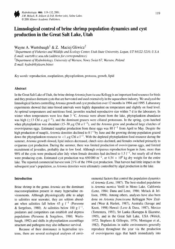
Hydrobiologia 466: 119-132,200l. J.M. Melack. R. Jellison & D.E. Herbst (eds). Saline Lakes. © 2001 Kluwer Academic Publishers.
119
Limnological control of brine shrimp population dynamics and cyst production in the Great Salt Lake, Utah
Wayne A. Wurtsbaugh1 & Z. Maciej Gliwicz2
1 Department of Fisheries and Wildlife and Ecology Center, Utah State University. Logan. UT 84322-5210, U.S.A E-mail: [email protected] (address for correspondence) 2 Department of Hydrobiology, University of Warsaw, Nowy Swiat 67, Warsaw, Poland E-mail: [email protected]
Key words: reproduction, zooplankton, phytoplankton, protozoa, growth, lipid
Abstract
In the Great Salt Lake of Utah, the brine shrimp Artemia franciscana Kellogg is an important food resource for birds and they produce dormant cysts that are harvested and used extensively in the aquaculture industry. We analyzed the limnological factors controlling Artemia growth and cyst production over 12 months in 1994 and 1995. Laboratory experiments showed that inter-brood intervals were highly dependent on temperature and slightly on food level. At optimal temperatures and nutritious food, juveniles reached reproductive size within 7 d in the laboratory. In winter when temperatures were less than 3°C, Artemia were absent from the lake, phytoplankton abundance was high (::: 13 Chi a J.Lg 1-1), and the dominant grazers were ciliated protozoans. In the spring, cysts hatched when phytoplankton was abundant (15-30 J.Lg ChI a 1-1), and the Artemia grew and produced large clutches of ovoviviparous eggs. Estimated naupliar production from these eggs was 801-1 from April to May. Despite the high production of nauplii, Artemia densities declined to 8 1-1 by June and the growing shrimp population grazed down the phytoplankton resource to < 1 J.Lg Chi a 1-1. With the depleted phytoplankton food resource during the summer, Artemia growth slowed, lipid indices decreased, clutch sizes declined, and females switched primarily to oviparous cyst production. During the summer, there was limited production of ovoviviparous eggs, and limited recruitment of juveniles, probably due to low food. Although oviparous reproduction began in June, more than 90% of the cysts were produced after July when female densities had declined to 1.5 1-1, but nearly all of them were producing cysts. Estimated cyst production was 650000 m-2, or 4.54 x 10⁶ kg dry weight for the entire lake. The reported commercial harvest took 21 % of the 1994 cyst production. That harvest had little impact on the subsequent year's population, as Artemia densities were ultimately controlled by algal production in the lake.
Introduction
Brine shrimp in the genus Artemia are the dominant macrozooplankton present in many hypersaline environments. Although physiologically able to adapt to salinities near seawater, they are seldom abundant when salinities fall below 45 g 1-1 (Persoone & Sorgeloos, 1980). At salinities below 100 g 1-1,
predators and competitors can establish and depress populations (Persoone & Sorgeloos, 1980; Wurtsbaugh, 1992) and shifts in phytoplankton assemblage structure and pathogens may also influence survival.
Because of their dominance in hypersaline systems, there are several ecological analyses of envir-
onmental factors that control the population dynamics of Artemia (Lenz, 1987). The best-studied population is Artemia monica Verill in Mono Lake, California (Lenz, 1984; Dana and Lenz, 1986; Melack & Jellison, 1998). Among others, analyses have also been done on Artemia franciscana Kelloggin New Zealand (Wear & Haslett, 1987), Australia (Savage and Knott, 1998) Hawaii (Lenz & Dana, 1987), Mexico (Torrentera, 1993), Sri Lanka (Kuruppu & Ekaratne, 1995), and in the Great Salt Lake, USA (Wirick, 1972; Stephens & Gillespie, 1976; Montague et aI., 1982). Populations in stable environments generally reproduce throughout the year via the production of ovoviviparous eggs that hatch immediately into
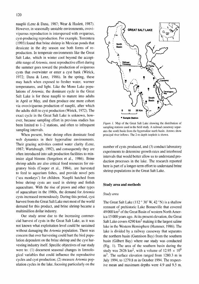
120
nauplii (Lenz & Dana, 1987; Wear & Haslett, 1987). However, in seasonally unstable environments, ovoviviparous reproduction is interspersed with oviparous, cyst-producing reproduction. For example, Torrentera (1993) found that brine shrimp in Mexican ponds that dessicate in the dry season use both forms of reproduction. In temperate environments like the Great Salt Lake, which in winter cool beyond the acceptable range of Artemia, most reproductive effort during the summer goes toward the production of oviparous cysts that overwinter or enter a cyst bank (Wirick, 1972; Dana & Lenz, 1986). In the spring, these may hatch when exposed to fresher water, warmer temperatures, and light. Like the Mono Lake populations of Artemia, the dominant cycle in the Great Salt Lake is for these nauplii to mature into adults in April or May, and then produce one more cohort via ovoviviparous production of nauplii, after which the adults shift to cyst production (Wirick, 1972). The exact cycle in the Great Salt Lake is unknown, however, because sampling effort in previous studies has been limited to 1-2 stations, and often to infrequent sampling intervals.
When present, brine shrimp often dominate food web dynamics in their hypersaline environments. Their grazing activities control water clarity (Lenz, 1987; Wurtsbaugh, 1992), and consequently they are often introduced into salt production facilities to minimize algal blooms (Sorgeloos et a!., 1986). Brine shrimp adults are also critical food resources for migratory birds (Cooper et al., 1984), are harvested to feed to aquarium fishes, and provide novel pets ('sea monkeys') for children. Nauplii hatched from brine shrimp cysts are used in shrimp and finfish aquaculture. With the rise of prawn and other types of aquaculture in the 1980s, the demand for Artemia cysts increased tremendously. During this period, cyst harvest from the Great Salt Lake met most of the world demand for this product, and brine shrimp became a multimillion dollar industry.
Our study arose due to the increasing commercial harvest of cysts in the Great Salt Lake, as it was not known what exploitation level could be sustained without damaging the Artemia population. There was concern that over harvesting could hurt the bird population dependent on the brine shrimp and the cyst harvesting industry itself. Specific objectives of our study were to: (I) document seasonal changes in limnological variables that could influence the reproductive cycles and cyst production; (2) measure Artemia population cycles in the lake, focusing particularly on the
GREAT SALT LAKE
o
• Sample Stalion
Figure 1. Map of the Great Salt Lake showing the distribution of sampling stations used in the field study. A railroad causeway separates the south basin from the hypersaline north basin. Arrows show principal river inflows. The 2-m depth isopleth is shown.
number of cysts produced, and (3) conduct laboratory experiments to determine growth rates and interbrood intervals that would better allow us to understand production processes in the lake. The research reported here is part of a longer-term effort to understand brine shrimp populations in the Great Salt Lake.
Study area and methods
Study area
The Great Salt Lake (112 0 30' W, 42 ON) is a shallow remnant of prehistoric Lake Bonneville that covered 49000 km2 of the Great Basin of western North America 15000 years ago. At its present elevation, the Great Salt Lake covers 4290 km2 making it the largest saline lake in the Western Hemisphere (Hammer, 1986). The lake is divided by a railway causeway that separates the northern basin (Gunnison Bay) from the southern basin (Gilbert Bay) where our study was conducted (Fig. 1). The area of the southern basin during the study was 2626 km2, with a volume of 12.95 x 10⁹
m3. The surface elevation ranged from 1280.3 m in July 1994, to 1279.8 m in October 1994. The respective mean and maximum depths were 4.9 and 9.5 m.
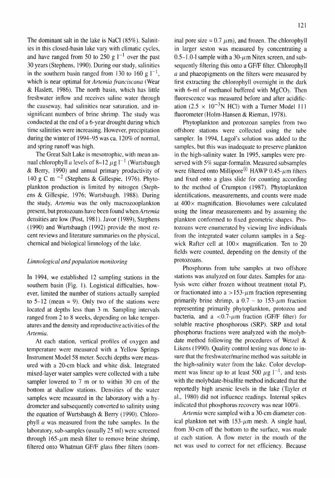
The dominant salt in the lake is NaCI (85%). Salinities in this closed-basin lake vary with climatic cycles, and have ranged from 50 to 250 g I-lover the past 30 years (Stephens, 1990). During our study, salinities in the southern basin ranged from 130 to 160 g 1-1, which is near optimal for Artemia franciscana (Wear & Haslett, 1986). The north basin, which has little freshwater inflow and receives saline water through the causeway, had salinities near saturation, and insignificant numbers of brine shrimp. The study was conducted at the end of a 6-year drought during which time salinities were increasing. However, precipitation during the winter of 1994-95 was ca. 120% of normal, and spring runoff was high.
The Great Salt Lake is mesotrophic, with mean annual chlorophyll a levels of 8-12 /Lg 1-1 (Wurtsbaugh & Berry, 1990) and annual primary productivity of 140 g C m -2 (Stephens & Gillespie, 1976). Phytoplankton production is limited by nitrogen (Stephens & Gillespie, 1976; Wurtsbaugh, 1988). During the study, Artemia was the only macrozooplankton present, but protozoans have been found when Artemia densities are low (Post, 1981). Javor (1989), Stephens (1990) and Wurtsbaugh (1992) provide the most recent reviews and literature summaries on the physical, chemical and biological limnology of the lake.
Limnological and population monitoring
In 1994, we established 12 sampling stations in the southern basin (Fig. 1). Logistical difficulties, however, limited the number of stations actually sampled to 5-12 (mean = 9). Only two of the stations were located at depths less than 3 m. Sampling intervals ranged from 2 to 8 weeks, depending on lake temperatures and the density and reproductive activities of the Artemia.
At each station, vertical profiles of oxygen and temperature were measured with a Yellow Springs Instrument Model 58 meter. Secchi depths were measured with a 20-cm black and white disk. Integrated mixed-layer water samples were collected with a tube sampler lowered to 7 m or to within 30 cm of the bottom at shallow stations. Densities of the water samples were measured in the laboratory with a hydrometer and subsequently converted to salinity using the equation of Wurtsbaugh & Berry (1990). Chlorophyll a was measured from the tube samples. In the laboratory, sub-samples (usually 25 ml) were screened through I 65-/Lm mesh filter to remove brine shrimp, filtered onto Whatman GFIF glass fiber filters (nom-
121
inal pore size = 0.7 /Lm), and frozen. The chlorophyll in larger seston was measured by concentrating a 0.5-1.0-1 sample with a 30-/Lm Nitex screen, and subsequently filtering this onto a GFIF filter. Chlorophyll a and phaeopigments on the filters were measured by first extracting the chlorophyll overnight in the dark with 6-ml of methanol buffered with MgC03. Then fluorescence was measured before and after acidification (2.5 x 1O-3N HCl) with a Turner Model 111 fluorometer (Holm-Hansen & Rieman, 1978).
Phytoplankton and protozoan samples from two offshore stations were collected using the tube sampler. In 1994, Lugol's solution was added to the samples, but this was inadequate to preserve plankton in the high-salinity water. In 1995, samples were preserved with 5% sugar-formalin. Measured subsamples were filtered onto Millipore® HAWP 0.45-/Lm filters and fixed onto a glass slide for counting according to the method of Crumpton (1987). Phytoplankton identifications, measurements, and counts were made at 400x magnification. Biovolumes were calculated using the linear measurements and by assuming the plankton conformed to fixed geometric shapes. Protozoans were enumerated by viewing live individuals from the integrated water column samples in a Segwick Rafter cell at 100 x magnification. Ten to 20 fields were counted, depending on the density of the protozoans.
Phosphorus from tube samples at two offshore stations was analyzed on four dates. Samples for analysis were either frozen without treatment (total P), or fractionated into a > 153-/Lm fraction representing primarily brine shrimp, a 0.7 - to 153-/Lm fraction representing primarily phytoplankton, protozoa and bacteria, and a <0.7-/Lm fraction (GFIF filter) for soluble reactive phosphorous (SRP). SRP and total phosphorus fractions were analyzed with the molybdate method following the procedures of Wetzel & Likens (1990). Quality control testing was done to insure that the freshwater/marine method was suitable in the high-salinity water from the lake. Color development was linear up to at least 500 /Lg 1-1, and tests with the molybdate-bisulfite method indicated that the reportedly high arsenic levels in the lake (Tayler et aI., 1980) did not influence readings. Internal spikes indicated that phosphorus recovery was near 100%.
Artemia were sampled with a 30-cm diameter conical plankton net with 153-/Lm mesh. A single haul, from 30-cm off the bottom to the surface, was made at each station. A flow meter in the mouth of the net was used to correct for net efficiency. Because
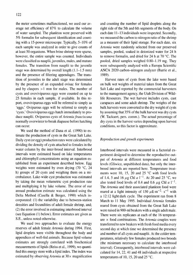
122
the meter sometimes malfunctioned, we used our average net efficiency of 87% to calculate the volume of water sampled. The plankton were preserved with 5% formalin for subsequent identification and counting with a 15-power microscope. Typically, 5-10% of each sample was analyzed in order to give counts of at least 50 organisms. When brine shrimp were sparse, however, the entire sample was counted. Individuals were classified as nauplii, juveniles, males, and mature females. The transition from nauplii to the juvenile stage was determined by overall length (1.1-1.5 mm) and the presence of filtering appendages. The transition of juveniles to the adult stage was determined by the presence of an expanded ovisac for females and by claspers > I mm for males. The number of cysts and ovoviviparous eggs were counted on up to 25 females in each sample, if available. In this report, ovoviviparous eggs will be referred to simply as 'eggs.' Oviparous eggs will be referred to simply as 'cysts.' Ovoviviparous eggs hatch immediately to produce nauplii. Oviparous cysts of Artemia franciscana normally overwinter to break diapause before hatching can occur.
We used the method of Dana et al. (1990) to estimate the production of cysts in the Great Salt Lake. Daily cyst (or egg) production rates were calculated by dividing the density of cysts attached to females in the water column by the inter-brood interval. Interbrood intervals were estimated based on lake temperatures and chlorophyll concentrations using an equation established from an experiment described below. Egg weights were estimated by oven drying (70 °C, 24 h) groups of 20 cysts and weighing them on a microbalance. Lake-wide cyst production was estimated by taking the mean volumetric cyst production rate and multiplying it by lake volume. The error of our annual production estimate was calculated using the Delta Method (Casella & Berger, 1990) which incorporated: (l) the variability due to between-station densities and fecundities of adult female shrimp, and; (2) the error involved in estimating interbrood interval (see Equation (1) below). Error estimates are given as S.E., unless noted otherwise.
We used two approaches to evaluate the energy reserves of adult female Artemia during 1994. First, lipid droplets were visible throughout the body and appendices of well-fed animals. Because lipid volume estimates are strongly correlated with biochemical measurements of lipids (Reiss et aI., 1999), we quantified this energy store with a lipid index. The index was estimated by observing Artemia at 30 x magnification
and counting the number of lipid droplets along the right side of the 5th and 6th segments of the body. On each date 11-13 individuals were inspected. Secondly, we measured the carbon to nitrogen ratio of the shrimp as a measure of their lipid storage. For each date, six Artemia were randomly selected from our preserved samples, pooled, soaked in deionized water for 24 h to remove formalin, and dried for 24 h at 70°C. The pooled, dried samples weighed 0.80-1.l9 mg. They were subsequently analyzed with a Europa Scientific ANCA 2020 carbon-nitrogen analyzer (Barrie et aI., 1989).
Harvest rates of cysts from the lake were based on bulk wet weights of material taken from the Great Salt Lake and reported by the commercial harvesters to the management agency, the Utah Division of Wildlife Resources. The wet harvest includes cysts, cast carapaces and some adult shrimp. The weights of the bulk harvests were converted to the dry weight of cysts by assuming that 35% of the bulk harvest was dry cysts (w. Tackaert, pers. comm.). The actual percentage of dry cysts in the harvest varies depending upon harvest conditions, so this factor is approximate.
Reproduction and growth experiments
Interbrood intervals were measured in a factorial experiment designed to determine the reproductive output of Artemia at different temperatures and food levels (Gliwicz, unpublished data), but only the interbrood intervals are reported here. Temperature treatments were 10, 15, 20 and 25°C with food levels of lA, 5 and 16 fJg ChI a 1-1. At 20 and 25°C, we also tested food levels of 004 and 0.6 fJg ChI a I-I. The Artemia and their associated plankton food were reared at a light intensity of 150 fJE-m- 2. s-I with a 12:12 light dark cycle. The experiment ran from 8 March to 11 May 1995. Individual Artemia females reared from cysts obtained from the Great Salt Lake were raised in 900-ml beakers with a single adult male. There were six replicates at each of the 16 temperature x food combinations. The Artemia couples were transferred to new beakers with fresh food media every second day at which time we determined the presence and number of all cysts and nauplii. At the colder temperatures, relatively few females produced two broods (the minimum necessary to calculate the interbrood interval). Consequently, interbrood intervals were calculated for 14, 22, 41 and 48 individuals at respective temperatures of 10, 15,20 and 25°C.
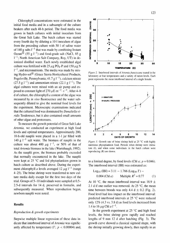
Chlorophyll concentrations were estimated in the initial food media and in a subsample of the culture beakers after each 48-h period. The food media was grown in batch cultures with initial inoculum from the Great Salt Lake. The batch culture was started every fourth day by diluting a 10-1 inoculum of algae from the preceding culture with 50 I of saline water of 140 g salts I-I that was made by combining Instant Ocean® (55 g I-I) and food-grade salt (NaCI, 85 g I-I; North American Salt Company, Roy, UT) in deionized distilled water. Each newly established algal culture was fertilized with 25 JLg P04 -P and 150 JLg N I-I, and micronutrients. The media was made by mixing Hydro-sol® (Grace Sierra Horticultural Products, Fogelsville, Pennsylvania; 41.7 g I-I), calcium nitrate (27.5 g I-I) and ammonium nitrate (22.1 g I-I). The algal cultures were mixed with an air pump and exposed to constant light of 270 JLE.m-2. s-I . After 4-8 d of culture, the chlorophyll a content of the algae was measured by in vivo fluorescence and the water subsequently diluted to give the nominal food levels for the experiment. Microscopic examinations indicated that the cultured food was dominated by Dunaliella viridis Teodoresco, but it also contained small amounts of other algae and protozoans.
To measure the growth potential of Great Salt Lake Artemia, we conducted an experiment at high food levels and optimal temperatures. Approximately 200, lO-h-old nauplii were placed in a I-I jar filled with 140 g I-I salt water. The biomass of nauplii in the culture was about 400 JLg I-I, or 50% of that of total Artemia biomass in the lake (Wurtsbaugh, 1992). As the nauplii grew, the biomass probably exceeded that normally encountered in the lake. The nauplii were kept at 25°C and fed phytoplankton grown in batch culture as described above. During the experiment chlorophyll a levels averaged 12 JLg I-I (range 4-25). The brine shrimp were transferred to new culture media daily except for the first two days of the trial. Groups of 5-1 0 individuals were sampled at 0.5-2.5-d intervals for 14 d, preserved in formalin, and subsequently measured. When reproduction began, newborn nauplii were noted.
Results
Reproduction & growth experiments
Stepwise mUltiple linear regression of these data indicate that interbrood interval of Artemia was significantly affected by temperature (T; p < 0.00004) and,
123
40 iii > c e 30 ....I : .' II: W • . ... 20 ! . .. 0 • . 0 .. 0 .. II: 10 . oJ o· m
m • !
0 5 10 15 20 25 30
TEMPERATURE (C)
Figure 2. Interbrood intervals of Artemia jranciscana reared in the laboratory at four temperatures and a variety of ration levels. Each point represents the mean interbrood interval of a single female.
12r--------------------------------
10 W til N
I = IMMATURE
.j. 8 R=NAUPLI PRODUCED
E §'6 :z: I-(!) 4 Z W oJ
o 2 4 6 8 10 DAYS OF GROWTH
1 R
12 14
Figure 3. Growth rate of brine shrimp held at 25°C with highly nutritious phytoplankton food. Periods when shrimp were immature (IJ. and when some individuals in the batch culture were reproducing (R) are shown.
to a limited degree, by food levels (ChI a; p = 0.046). The interbrood interval (lBI) was estimated as:
LoglO (IBI) = 3.11 - 1.766 (LoglO T) -
0.004 (ChI a) Multiple R2 = 0.77 (1)
At 10°C, the mean interbrood interval was 18.9 ± 2.1 d if one outlier was removed. At 25°C, the mean time between broods was only 4.4 d ± 0.2 (Fig. 2). Food level had less impact on the interbrood interval: predicted interbrood intervals at 25°C were reduced only 12% (4.3 vs. 3.8 d) as food levels increased from 1.4 to 16 JLg ChI a I-I.
In the growth experiment at 25°C and high food levels, the brine shrimp grew rapidly and reached lengths of 9 mm 12 d after hatching (Fig. 3). The growth curve showed a classical sigmoid shape, with the shrimp initially growing slowly, then rapidly in an
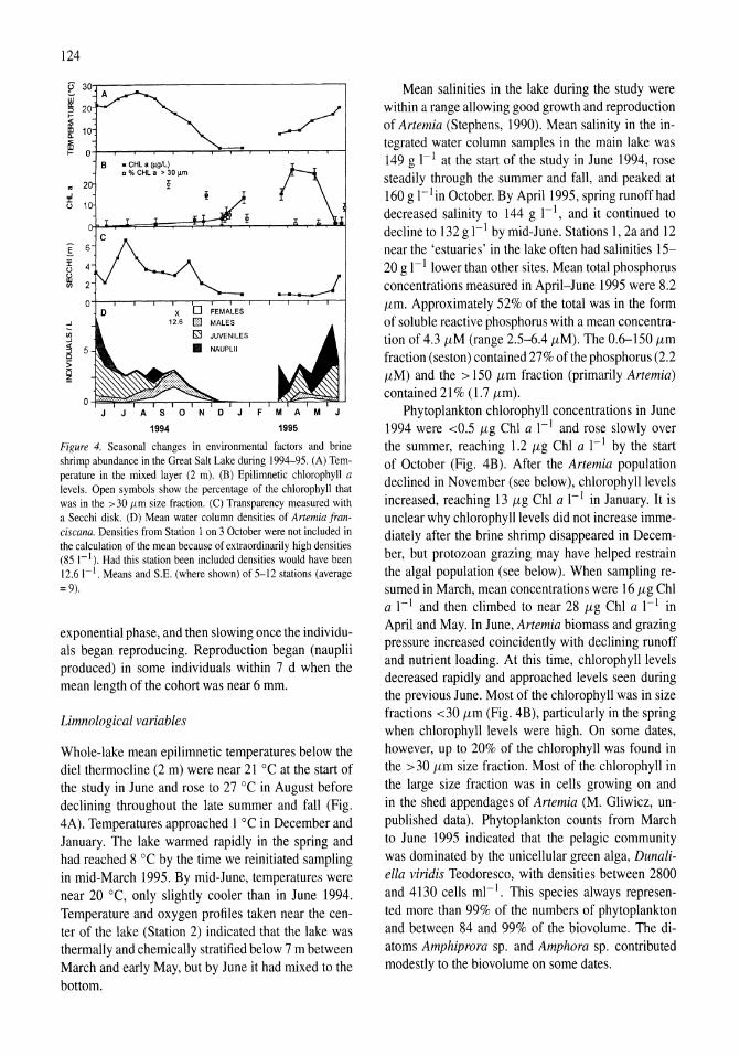
124
~ 30'------------------------------,
f ~
• CHL a ",giL) a%CHLa > 30 lim
~
1995
Figure 4. Seasonal changes in environmental factors and brine shrimp abundance in the Great Salt Lake during 1994-95. (A) Temperature in the mixed layer (2 m). (B) Epilimnetic chlorophyll a levels. Open symbols show the percentage of the chlorophyll that was in the > 30 !Lm size fraction. (C) Transparency measured with a Secchi disk. (D) Mean water colunm densities of Artemia franciscana. Densities from Station 1 on 3 October were not included in the calculation of the mean because of extraordinarily high densities (85 1-1). Had this station been included densities would have been 12.61-1. Means and S.E. (where shown) of 5-12 stations (average = 9).
exponential phase, and then slowing once the individuals began reproducing. Reproduction began (nauplii produced) in some individuals within 7 d when the mean length of the cohort was near 6 mm.
Limnological variables
Whole-lake mean epilimnetic temperatures below the diel thermocline (2 m) were near 21°C at the start of the study in June and rose to 27 °C in August before declining throughout the late summer and fall (Fig. 4A). Temperatures approached 1 °C in December and January. The lake warmed rapidly in the spring and had reached 8 °C by the time we reinitiated sampling in mid-March 1995. By mid-June, temperatures were near 20°C, only slightly cooler than in June 1994. Temperature and oxygen profiles taken near the center of the lake (Station 2) indicated that the lake was thermally and chemically stratified below 7 m between March and early May, but by June it had mixed to the bottom.
Mean salinities in the lake during the study were within a range allowing good growth and reproduction of Artemia (Stephens, 1990). Mean salinity in the integrated water column samples in the main lake was 149 g I-I at the start of the study in June 1994, rose steadily through the summer and fall, and peaked at 160 g I-lin October. By April 1995, spring runoff had decreased salinity to 144 g I-I, and it continued to decline to 132 g I-I by mid-June. Stations 1, 2a and 12 near the 'estuaries' in the lake often had salinities 15-20 g 1-1 lower than other sites. Mean total phosphorus concentrations measured in April-June 1995 were 8.2 {Lm. Approximately 52% of the total was in the form of soluble reactive phosphorus with a mean concentration of 4.3 {LM (range 2.5-6.4 {LM). The 0.6--150 {Lm
fraction (seston) contained 27% of the phosphorus (2.2 {LM) and the> 150 {Lm fraction (primarily Artemia)
contained 21 % (1.7 {Lm).
Phytoplankton chlorophyll concentrations in June 1994 were <0.5 {Lg Chi a I-I and rose slowly over the summer, reaching 1.2 {Lg Chi a I-I by the start of October (Fig. 4B). After the Artemia population declined in November (see below), chlorophyll levels increased, reaching 13 {Lg ChI a I-I in January. It is unclear why chlorophyll levels did not increase immediately after the brine shrimp disappeared in December, but protozoan grazing may have helped restrain the algal population (see below). When sampling resumed in March, mean concentrations were 16 {Lg Chi a I-I and then climbed to near 28 {Lg Chi a I-I in April and May. In June, Artemia biomass and grazing pressure increased coincidently with declining runoff and nutrient loading. At this time, chlorophyll levels decreased rapidly and approached levels seen during the previous June. Most of the chlorophyll was in size fractions <30 {Lm (Fig. 4B), particularly in the spring when chlorophyll levels were high. On some dates, however, up to 20% of the chlorophyll was found in the >30 {Lm size fraction. Most of the chlorophyll in the large size fraction was in cells growing on and in the shed appendages of Artemia (M. Gliwicz, unpublished data). Phytoplankton counts from March to June 1995 indicated that the pelagic community was dominated by the unicellular green alga, Dunali
ella viridis Teodoresco, with densities between 2800 and 4130 cells ml- I. This species always represented more than 99% of the numbers of phytoplankton and between 84 and 99% of the biovolume. The diatoms Amphiprora sp. and Amphora sp. contributed modestly to the biovolume on some dates.
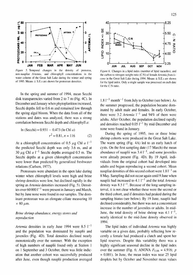
~ 80 4 1:11 ::I.
~ 60 oJ ::E ;;; 40 z c( 0 ~ 20
" /
,... .. / \ ARTEMIA ... / 3 I \ / oJ
! \ / c( I \ i I \ 2
\ w ~
CHLI 1 c(
~ t-O g: 0
JAN FEB MAR APR MAY JUN
Figure 5. Temporal changes in the density of protozoa. non-naupliar Artemia. and chlorophyll concentrations in the water column of the Great Salt Lake during the winter and spring of 1995. Means ± S.E.s are shown for protozoan densities.
In the spring and summer of 1994, mean Secchi disk transparencies varied from 2 to 7 m (Fig. 4C). In December and January when phytoplankton increased, Secchi depths fell to 0.6 m and remained low through the spring algal bloom. When the data from all of the stations and dates was analyzed, there was a strong correlation between Secchi depth and chlorophyll a:
In (Secchi) = 0.931 - 0.473 (In Chi a)
r 2 =0.81,n=116 (2)
At a chlorophyll concentration of 0.5 flg Chi a I-I the predicted Secchi depth was only 3.6 m, and at 30 flg Chi a I-I Secchi depths averaged 0.5 m. The Secchi depths at a given chlorophyll concentration were lower than predicted by generalized freshwater relations (Carlson, 1977).
Protozoans were abundant in the open lake during winter when chlorophyll levels were high and brine shrimp densities were low, but declined rapidly in the spring as Artemia densities increased (Fig. 5). Densities over 60 000 I-I were present in January and March, but by June none were found in our samples. The dominant protozoan was an elongate ciliate measuring 10 x 80 flm.
Brine shrimp abundance. energy stores and reproduction
Artemia densities in early June 1994 were 8.5 I-I and the population was dominated by nauplii and juveniles (Fig. 4D). Total densities declined nearly monotonically over the summer. With the exception of high numbers of nauplii found only at Station I on I September and 3 October, there was little indication that another cohort was successfully produced after June, even though nauplii production averaged
125
40 6.25
UJ en 30 5.50 ...!. (") + X Z UJ 20 4.75 Cl
~ ~ Cl
10 4.00 6 a: :J
o 3.25 JUN JUL AUG SEP OCT NOV
Figure 6. Changes in a lipid index (number of lipid vacuoles), and the carbon to nitrogen weight ratio (C:N) of female Artemia franciscana in the Great Salt Lake during 1994. Means ± S.E.s are shown for the lipid index. Only a single sample was processed on each date for the C:N ratio.
1.81-1 month- I from July to October (see below). As the summer progressed, the population became dominated by adult male and females. In early October, there were 3.2 Artemia I-I and 94% of them were adults. After October, the population declined rapidly and densities reached 0.05 I-I by mid-December and none were found in January.
During the spring of 1995, two or three brine shrimp cohorts were produced in the Great Salt Lake. The warm spring (Fig. 4A) led to an early hatch of cysts. On the first sampling date (17 March) the mean abundance of nauplii was 3.4 I-I, and some juveniles were already present (Fig. 4D). By 19 April, individuals from the original cohort had developed into adults and begun reproducing a second cohort. Mean naupliardensities of this second cohort were 1.81-1 on 8 May. Sampling did not occur again until 9 June when nauplii had increased to 4.1 I-I and the total Artemia density was 8.5 1-1. Because of the long sampling interval, it is not clear whether these were the second or the third cohort. and if densities had peaked during the sampling hiatus (see below). By 19 June, nauplii had declined considerably, but there was not a concomitant increase in the number of juveniles or adults. In midJune, the total density of brine shrimp was 4.1 1-1, nearly identical to the mid-June density observed in 1994.
The lipid index of individual Artemia was highly variable on a given date, probably reflecting how recently a female had produced a clutch and spent her lipid reserves. Despite this variability there was a highly significant seasonal decline in the lipid index over the summer (Fig. 6; ANOYA F5.66 = 4.916; P
= 0.00 I). In June, the mean index was near 25 lipid droplets but by October and November mean values
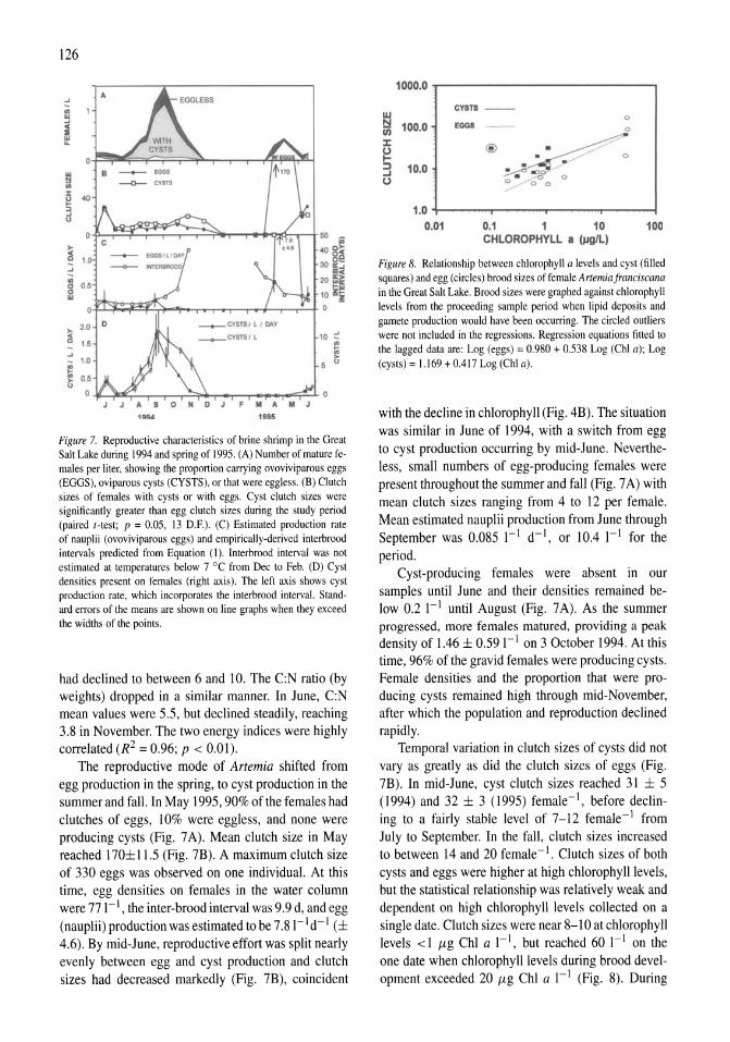
126
~ ., w -' ~ w ...
!':I ., :z: <J
3 <J
50 iii
0() 0>-
JO 8~ ::; "'-' IDc
~ 20 a:~
" 10 ~~ w 0
~ 1Q ::
E 5 ~
~ <J
JJASONDJ FMAMJ
1994 1995
Figure 7. Reproductive characteristics of brine shrimp in the Great Salt Lake during 1994 and spring of 1995. (A) Number of mature females per liter, showing the proportion carrying ovoviviparous eggs (EGGS), oviparous cysts (CYSTS), or that were eggless. (B) Clutch sizes of females with cysts or with eggs. Cyst clutch sizes were significantly greater than egg clutch sizes during the study period (paired I-test; p = 0.05, 13 D.E). (C) Estimated production rate of nauplii (ovoviviparous eggs) and empirically-derived interbrood intervals predicted from Equation (I). Interbrood interval was not estimated at temperatures below 7 0 C from Dec to Feb. (D) Cyst densities present on females (right axis). The left axis shows cyst production rate, which incorporates the interbrood interval. Standard errors of the means are shown on line graphs when they exceed the widths of the points.
had declined to between 6 and 10. The C:N ratio (by weights) dropped in a similar manner. In June, C:N mean values were 5.5, but declined steadily, reaching 3.8 in November. The two energy indices were highly correlated (R2 = 0.96; p < 0.01).
The reproductive mode of Artemia shifted from egg production in the spring, to cyst production in the summer and fall. In May 1995, 90% of the females had clutches of eggs, 10% were eggless, and none were producing cysts (Fig. 7 A). Mean clutch size in May reached 170± 11.5 (Fig. 7B). A maximum clutch size of 330 eggs was observed on one individual. At this time, egg densities on females in the water column were 771- 1, the inter-brood interval was 9.9 d, and egg (nauplii) production was estimated to be 7.81- 1 d- I (± 4.6). By mid-June, reproductive effort was split nearly evenly between egg and cyst production and clutch sizes had decreased markedly (Fig. 7B), coincident
w ~ fIJ I 0 I-;:) ..J 0
1000.0
eYST1l --0
100.0 EGGS 0
@
10.0
1.0 +----r----r----..----1 0.01 O~ 1 10
CHLOROPHYLL a OJg/L) 100
Figure 8. Relationship between chlorophyll a levels and cyst (filled squares) and egg (circles) brood sizes of female A rtemia franciscana in the Great Salt Lake. Brood sizes were graphed against chlorophyll levels from the proceeding sample period when lipid deposits and gamete production would have been occurring. The circled outliers were not included in the regressions. Regression equations fitted to the lagged data are: Log (eggs) = 0.980 + 0.538 Log (Chi a); Log (cysts) = 1.169 + OAI7 Log (Chi a).
with the decline in chlorophyll (Fig. 4B). The situation was similar in June of 1994, with a switch from egg to cyst production occurring by mid-June. Nevertheless, small numbers of egg-producing females were present throughout the summer and fall (Fig. 7 A) with mean clutch sizes ranging from 4 to 12 per female. Mean estimated nauplii production from June through September was 0.085 1-1 d-1, or lOA 1-1 for the period.
Cyst-producing females were absent in our samples until June and their densities remained below 0.2 1-1 until August (Fig. 7A). As the summer progressed, more females matured, providing a peak density of 1.46 ± 0.591- 1 on 3 October 1994. At this time, 96% of the gravid females were producing cysts. Female densities and the proportion that were producing cysts remained high through mid-November, after which the population and reproduction declined rapidly.
Temporal variation in clutch sizes of cysts did not vary as greatly as did the clutch sizes of eggs (Fig. 7B). In mid-June, cyst clutch sizes reached 31 ± 5 (1994) and 32 ± 3 (1995) female- I, before declining to a fairly stable level of 7-12 female-I from July to September. In the fall , clutch sizes increased to between 14 and 20 female -I. Clutch sizes of both cysts and eggs were higher at high chlorophyll levels, but the statistical relationship was relatively weak and dependent on high chlorophyll levels collected on a single date. Clutch sizes were near 8-10 at chlorophyll levels <1 Jlg ChI a I- I, but reached 60 I-Ion the one date when chlorophyll levels during brood development exceeded 20 Jlg Chi a 1- 1 (Fig. 8). During
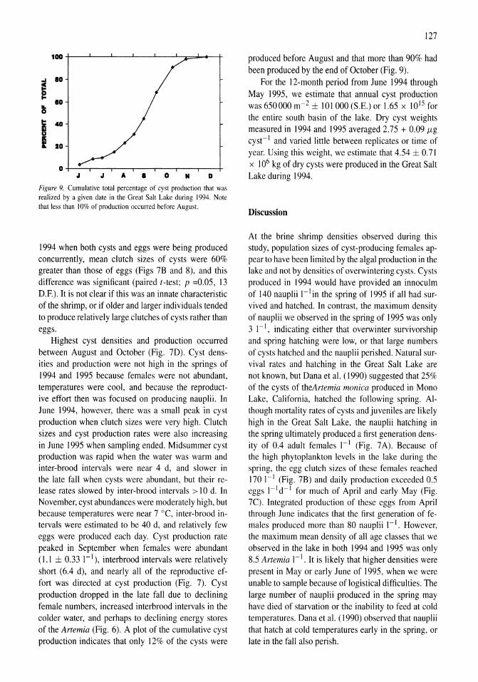
100
.I 10
I 10
!i
i 40
I 20
0 .. .. A I 0 N D
Figure 9. Cumulative total percentage of cyst production that was realized by a given date in the Great Salt Lake during 1994. Note that less than 10% of production occurred before August.
1994 when both cysts and eggs were being produced concurrently, mean clutch sizes of cysts were 60% greater than those of eggs (Figs 7B and 8), and this difference was significant (paired t-test; p =0.05, 13 D.E). It is not clear if this was an innate characteristic of the shrimp, or if older and larger individuals tended to produce relatively large clutches of cysts rather than eggs.
Highest cyst densities and production occurred between August and October (Fig. 7D). Cyst densities and production were not high in the springs of 1994 and 1995 because females were not abundant, temperatures were cool, and because the reproductive effort then was focused on producing nauplii. In June 1994, however, there was a small peak in cyst production when clutch sizes were very high. Clutch sizes and cyst production rates were also increasing in June 1995 when sampling ended. Midsummer cyst production was rapid when the water was warm and inter-brood intervals were near 4 d, and slower in the late fall when cysts were abundant, but their release rates slowed by inter-brood intervals> 10 d. In November, cyst abundances were moderately high, but because temperatures were near 7 DC, inter-brood intervals were estimated to be 40 d, and relatively few eggs were produced each day. Cyst production rate peaked in September when females were abundant (1.1 ± 0.33 I-I), interbrood intervals were relatively short (6.4 d), and nearly all of the reproductive effort was directed at cyst production (Fig. 7). Cyst production dropped in the late fall due to declining female numbers, increased interbrood intervals in the colder water, and perhaps to declining energy stores of the Artemia (Fig. 6). A plot of the cumulative cyst production indicates that only 12% of the cysts were
127
produced before August and that more than 90% had been produced by the end of October (Fig. 9).
For the 12-month period from June 1994 through May 1995, we estimate that annual cyst production was 650000 m-2 ± 101000 (S.E.) or 1.65 x 10¹⁵ for the entire south basin of the lake. Dry cyst weights measured in 1994 and 1995 averaged 2.75 + 0.09 f.Lg cyst- I and varied little between replicates or time of year. Using this weight, we estimate that 4.54 ± 0.71 x 10⁶ kg of dry cysts were produced in the Great Salt Lake during 1994.
Discussion
At the brine shrimp densities observed during this study, population sizes of cyst-producing females appear to have been limited by the algal production in the lake and not by densities of overwintering cysts. Cysts produced in 1994 would have provided an innoculm of 140 nauplii I-I in the spring of 1995 if all had survived and hatched. In contrast, the maximum density of nauplii we observed in the spring of 1995 was only 3 1-1, indicating either that overwinter survivorship and spring hatching were low, or that large numbers of cysts hatched and the nauplii perished. Natural survival rates and hatching in the Great Salt Lake are not known, but Dana et al. (1990) suggested that 25% of the cysts of theArtemia monica produced in Mono Lake, California, hatched the following spring. Although mortality rates of cysts and juveniles are likely high in the Great Salt Lake, the nauplii hatching in the spring ultimately produced a first generation density of 0.4 adult females I-I (Fig. 7A). Because of the high phytoplankton levels in the lake during the spring, the egg clutch sizes of these females reached 170 I-I (Fig. 7B) and daily production exceeded 0.5 eggs l-Id- I for much of April and early May (Fig. 7C). Integrated production of these eggs from April through June indicates that the first generation of females produced more than 80 nauplii I-I. However, the maximum mean density of all age classes that we observed in the lake in both 1994 and 1995 was only 8.5 Artemia I-I. It is likely that higher densities were present in Mayor early June of 1995, when we were unable to sample because of logistical difficulties. The large number of nauplii produced in the spring may have died of starvation or the inability to feed at cold temperatures. Dana et al. (1990) observed that nauplii that hatch at cold temperatures early in the spring, or late in the fall also perish.
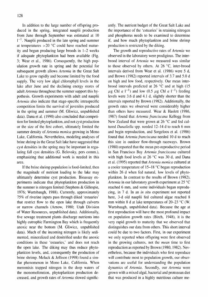
128
In addition to the large number of offspring produced in the spring, integrated nauplii production from June through September was estimated at 10 1-1. Nauplii produced in the late spring and summer at temperatures >20 °C could have reached maturity and begun producing large broods in 1-2 weeks if adequate phytoplankton had been available (Fig. 3; Wear et aI., 1986). Consequently, the high population growth rate in spring and the potential for subsequent growth allows Artemia in the Great Salt Lake to grow rapidly and become limited by the food supply. The very low algal chlorophyll levels in the lake after June and the declining energy stores of adult Artemia throughout the summer support this hypothesis. Growth experiments with adult and nauplii Artemia also indicate that stage-specific intraspecific competition limits the survival of juveniles produced in the spring and summer (M. Gliwicz, unpublished data). Dana et al. (1990) also concluded that competition for limited phytoplankton, and not cyst production or the size of the first cohort, ultimately limited the summer density of Artemia monica growing in Mono Lake, California. Nevertheless, modeling analyses of brine shrimp in the Great Salt lake have suggested that cyst densities in the spring may be important in regulating fall cyst densities (G. Belovsky, pers comm.), emphasizing that additional work is needed in this area.
If the brine shrimp population is food-limited, then the magnitude of nutrient loading to the lake may ultimately determine cyst production. Bioassay experiments indicate that phytoplankton production in the summer is nitrogen limited (Stephens & Gillespie, 1976; Wurtsbaugh, 1988). Currently, approximately 75% of riverine inputs pass through diked 'estuaries' that restrict flow to the open lake through culverts or narrow channels (Arnow, 1980; Utah Division of Water Resources, unpublished data). Additionally, five sewage treatment plants discharge nutrients into highly eutrophic Farmington Bay which is frequently anoxic near the bottom (M. Gliwicz, unpublished data). Much of the incoming nitrogen is likely sedimented, mineralized and denitrified under the anoxic conditions in these 'estuaries,' and does not reach the open lake. The diking may thus reduce phytoplankton levels, and, consequently the production of brine shrimp. Melack & Jellison (1998) found a similar phenomenon in Mono Lake, California. When meromixis trapped nitrogen in the deep waters of the monomolimnion, phytoplankton production decreased, and growth rates of Artemia slowed signific-
antly. The nutrient budget of the Great Salt Lake and the importance of the 'estuaries' in retaining nitrogen and phosphorus needs to be examined to determine if, and how much phytoplankton and brine shrimp production is restricted by the diking.
The growth and reproductive rates of Artemia we observed in the laboratory were prodigious. The interbrood interval of Artemia we measured was similar to those observed by others. At 26°C, inter-brood intervals derived from Wear et al. (1986) were 5 d, and Brown (1982) reported intervals of 3.7 and 5.0 d on high and low food, respectively. Our mean interbrood intervals predicted at 26°C and at high (15 jig Chi a 1-1) and low (0.5 jig Chi a 1-1) feeding levels were 3.6 d and 4.1 d, slightly shorter than the intervals reported by Brown (1982). Additionally, the growth rates we observed were considerably higher than others have measured. Wear & Haslett (1986, 1987) found that Artemia franciscana Kellogg from New Zealand that were grown at 26°C and fed cultured Dunaliella spp. needed 12-14 d to reach 6 mm and begin reproduction, and Sorgeloos et al. (1986) found that Artemia franciscana needed 10 d to reach this size in outdoor flow-through raceways. Brown (1980) reported that the mean pre-reproductive period in San Francisco Bay Artemia franciscana cultured with high food levels at 26°C was 30 d, and Dana et al. (1995) reported that Artemia monica cultured at a cooler temperature of IS-18°C began reproduction within 26 d when fed natural, low levels of phytoplankton. In contrast to the results of Brown (1982), Artemia in our laboratory growth experiment at 25°C reached 6 mm, and some individuals began reproducing, in 7 d. In an in situ experiment not reported here, 3-d old nauplii fed cultured algae reached 8 mm within 8 d at lake temperatures of 20-23 °C (W. Wurtsbaugh, unpublished data). Because the age at first reproduction will have the most profound impact on population growth rates (Birch, 1948), it is the very rapid growth to maturity that we observed that distinguishes our data from others. This short interval could be due to two factors. First, in our experiment we only reported when offspring were first observed in the growing cultures, not the mean time to first reproduction as reported by Brown (1980, 1982). Nevertheless, because the individuals who first reproduce will contribute most to population growth, our observations are useful for understanding the population dynamics of Artemia. Secondly, our Artemia were grown with a mixed algal, bacterial and protozoan diet that was produced in a highly nutritious culture me-
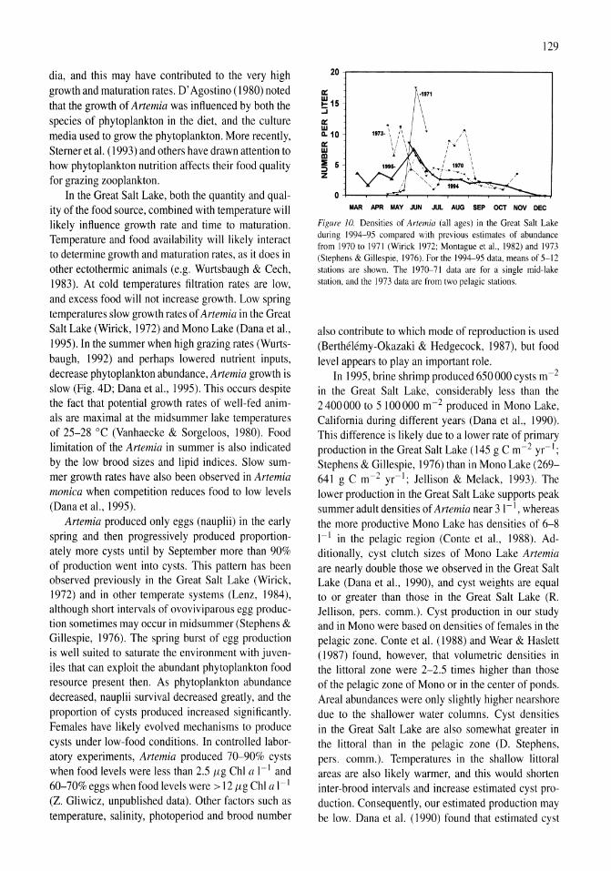
dia, and this may have contributed to the very high growth and maturation rates. D' Agostino (1980) noted that the growth of Artemia was influenced by both the species of phytoplankton in the diet, and the culture media used to grow the phytoplankton. More recently, Sterner et al. (1993) and others have drawn attention to how phytoplankton nutrition affects their food quality for grazing zooplankton.
In the Great Salt Lake, both the quantity and quality of the food source, combined with temperature will likely influence growth rate and time to maturation. Temperature and food availability will likely interact to determine growth and maturation rates, as it does in other ectothermic animals (e.g. Wurtsbaugh & Cech, 1983). At cold temperatures filtration rates are low, and excess food will not increase growth. Low spring temperatures slow growth rates of Artemia in the Great Salt Lake (Wirick, 1972) and Mono Lake (Dana et aI., 1995). In the summer when high grazing rates (Wurtsbaugh, 1992) and perhaps lowered nutrient inputs, decrease phytoplankton abundance, Artemia growth is slow (Fig. 4D; Dana et aI., 1995). This occurs despite the fact that potential growth rates of well-fed animals are maximal at the midsummer lake temperatures of 25-28 °C (Vanhaecke & Sorgeloos, 1980). Food limitation of the Artemia in summer is also indicated by the low brood sizes and lipid indices. Slow summer growth rates have also been observed in Artemia monica when competition reduces food to low levels (Dana et aI., 1995).
Artemia produced only eggs (nauplii) in the early spring and then progressively produced proportionately more cysts until by September more than 90% of production went into cysts. This pattern has been observed previously in the Great Salt Lake (Wirick, 1972) and in other temperate systems (Lenz, 1984), although short intervals of ovoviviparous egg production sometimes may occur in midsummer (Stephens & Gillespie, 1976). The spring burst of egg production is well suited to saturate the environment with juveniles that can exploit the abundant phytoplankton food resource present then. As phytoplankton abundance decreased, nauplii survival decreased greatly, and the proportion of cysts produced increased significantly. Females have likely evolved mechanisms to produce cysts under low-food conditions. In controlled laboratory experiments, Artemia produced 70-90% cysts when food levels were less than 2.5 f.Lg Chi a I-I and 60-70% eggs when food levels were> 12 f.Lg Chi a I-I (Z. Gliwicz, unpublished data). Other factors such as temperature, salinity, photoperiod and brood number
129
20.----------------------------,
0:: I!! 15 ::i 0:: w Q. 10 0:: W ID
~ 5 z
MAR APR MAY JUN JUL AUG SEP OCT NOV DEC
Figure 10. Densities of Artemia (all ages) in the Great Salt Lake during 1994-95 compared with previous estimates of abundance from 1970 to 1971 (Wirick 1972; Montague et a!., 1982) and 1973 (Stephens & Gillespie, 1976). Forthe 1994-95 data, means of 5-12 stations are shown. The 1970-71 data are for a single mid-lake station. and the 1973 data are from two pelagic stations.
also contribute to which mode of reproduction is used (Berthelemy-Okazaki & Hedgecock, 1987), but food level appears to play an important role.
In 1995, brine shrimp produced 650 000 cysts m-2
in the Great Salt Lake, considerably less than the 2400000 to 5 100000 m-2 produced in Mono Lake, California during different years (Dana et aI., 1990). This difference is likely due to a lower rate of primary production in the Great Salt Lake (145 g C m -2 yr- I ;
Stephens & Gillespie, 1976) than in Mono Lake (269-641 g C m-2 yr- I ; Jellison & Melack, 1993). The lower production in the Great Salt Lake supports peak summer adult densities of Artemia near 3 I-I, whereas the more productive Mono Lake has densities of 6-8 I-I in the pelagic region (Conte et aI., 1988). Additionally, cyst clutch sizes of Mono Lake Artemia are nearly double those we observed in the Great Salt Lake (Dana et aI., 1990), and cyst weights are equal to or greater than those in the Great Salt Lake (R. Jellison, pers. comm.). Cyst production in our study and in Mono were based on densities of females in the pelagic zone. Conte et al. (1988) and Wear & Haslett (1987) found, however, that volumetric densities in the littoral zone were 2-2.5 times higher than those of the pelagic zone of Mono or in the center of ponds. Areal abundances were only slightly higher nearshore due to the shallower water columns. Cyst densities in the Great Salt Lake are also somewhat greater in the littoral than in the pelagic zone (D. Stephens, pers. comm.). Temperatures in the shallow littoral areas are also likely warmer, and this would shorten inter-brood intervals and increase estimated cyst production. Consequently, our estimated production may be low. Dana et al. (1990) found that estimated cyst
130
~ a 6000 ,.--------------,.. iii 1i: 5000 ~ Q 4000 z ~ 3000 o ~ 2000 UJ
!1000
Reported Cyst Harvest '"
1994Cyst .......... + y
Production / (
I!? In 0 ~--_.c..,-____._-_y_-_._-,__.___,.----I-
t 82 84 86 88 90 92 94 96
YEAR
120
In 100 ~
80 t= ~ t-
60 In 15 UJ
40 It:
a. 20 1:
In
0
Figure I I. Changes in reported cyst harvest (filled squares) and the number of permits issued for ships (inverted triangles) to collect cysts in the Great Salt Lake from 1982 to 1996. The actual number of ships working is less than the total registered. Also shown is the estimated cyst production in 1994 ± S.E (triangle). Cyst harvest primarily occurs from fall through the winter. Reported dates are for the initiation of cyst harvest in the fall. Note that harvest rates are for dry cysts produced, not bulk wet harvest.
production based on sediment trap catches were 30% higher than those estimated by the same populationbased method used in our study. In addition to those potential errors, other limitations of our cyst production estimate are that the confidence interval was large and that the estimate was based on only 12 months of study, Although brine shrimp abundances during the 1994-95 period we studied were relatively similar to those described in other years when salinity levels were comparable (Fig. 10), natural variation in cyst production would nevertheless be expected. In Mono Lake, cyst production has varied 2.6-fold over a 16-year period (R. Jellison, pers. comm.; Dana et aI., 1990). Nutrient loading and the timing of spring warming would likely influence cyst production. Additionally, changes in salinity in the Great Salt Lake have had pronounced effects on brine shrimp abundance and cyst production. In the mid-1980s and again in 1998, salinities dropped below 100 g I-I, and brine shrimp densities plummeted (Wurtsbaugh, 1992) and then rebounded in 2000 (P. Birdsey, pers. comm.).
Cysts have been commercially harvested in the lake since the early 1950s (Sturm et aI., 1980), but it was not until the mid-1980s that aquaculture demand for them increased the harvest intensity and yield from the lake. Both the harvest intensity and the yield from the lake increased greatly from 1985 to 1989 (Fig. II). The mean reported cyst harvest rate from 1990 to 1996 was 1.8 x 10⁶ kg dry weight. A peak reported harvest of 2.5 x 10⁶ kg occurred in 1996 when harvesting permits reached 79, the maximum allowed by the resource agency in charge of the industry. Prices
of cysts fluctuate greatly depending on supply and demand, but at an expected range of $20-60 US kg-I, the mean harvest would have had a value of $35-110 million. The harvest estimates given here must be used cautiously, as the data result from self-reporting by an industry who are now taxed on the amount they harvest.
It is important to understand the impact of the cyst harvest on brine shrimp production. The annual cyst production of 4.5 x 10⁶ kg we estimated in the Great Salt Lake in 1994 can be compared with the reported commercial harvest of cysts. The mean harvest rate from 1990 to 1996 was 40% of the 1994 cyst production and the maximum harvest in 1995 was 55% of this production. In the fall of 1994 and winter of 1995, the industry reported a harvest that was 21 % of the 1994 production. Despite this harvest, the overwintering cysts were more than adequate to seed the lake and the estimated nauplii production of 80 I-I from April to May 1995 exceeded the lake's carrying capacity. Even if insufficient numbers had been produced by the second generation, a third cohort could have been produced before cyst production began intensively in August, again suggesting that there were excess cysts available in the spring. Although it did not appear that the commercial harvest impacted the 1995 brine shrimp production, the rapidly evolving mechanization and competition of the fleet will greatly increase their efficiency, potentially resulting in over harvest. Consequently, more detailed and prolonged population analyses and models to determine acceptable harvests are needed and are currently being developed (G. Belovsky & D. Stephens, pers. comm.) to protect this valuable resource.
Acknowledgements
We are grateful to David Ross, Mike Slater, Thorsten BIenckner, James Ruzycki and particularly Alan Ward for their assistance in the field and laboratory work. Kirsten Gallo assisted in drafting figures. Fredrik Norsell and Kirsten Gallo analyzed phosphorus concentrations. Richard Cutler and Huey Yan provided statistical advice. Cornelia Sawatzky, David Ross, Donald Archer, Paul Birdsey, Greta Burkart and two anonymous reviewers provided insightful reviews of the manuscript. The late Doyle Stephens, Wim Tackaert and Robert Jellison provided unpublished data and useful comments. Funding was provided by the Utah Division of Wildlife Resources, and the Ecology Cen-
ter and the College of Natural Resources at Utah State University.
References
Arnow, T., 1980. Water budget and water-surface fluctuations of Great Salt Lake. In Gwynn, J. W. (ed.), Great Salt Lake: a Scientific, Historical and Economic Overview. Utab Geological and Mineral Survey, Salt Lake City: 255-264.
Barrie, A, J. E. Davies, A J. Park & c. T. Workman, 1989. Continuous-flow stable isotope analysis for biologists. Spectrophotometry 4: 44-52.
Berthelemy-Okazaki, N. J. & D. Hedgecock, 1987. Effect of environmental factors on cyst formation in the brine shrimp Artemia. In Sorgeloos, P., D. A Bengtson, W. Decleir & E. Jaspers (eds), Artemia Research and its Applications. Vol. 3. Ecology, Culturing, Use in Aquaculture. Universa Press, Wetteren. Belgium: 167-182.
Birch, L. C., 1948. The intrinsic rate of natural increase of an insect population. J. animo Ecol. 17: 15-26.
Brown, R. A, 1980. Reproductive pattern and mode in the brine shrimp. Ecology 61: 466-470.
Brown, R. A., 1982. The costs of reproduction in brine shrimp. Ecology 63: 43-47.
Casella, G. & R. L. Berger, 1990. Statistical Inference. Brooks/Cole. Pacific Grove: 650 pp.
Carlson, R. E., 1977. A trophic state index for lakes. Limnol. Oceanogr. 22: 361-369.
Cooper, S. D., D. W. Winkler & P. H. Lenz, 1984. The effect of grebe predation on a brine shrimp population. J. animo Ecol. 53: 51-64.
Conte, F. P, R. S. Jellison & G. L. Starrett, 1988. Nearshore and pelagic abundances of Artemia monica in Mono Lake, California. Hydrobiologia 158: 173-181.
Crumpton, W. G., 1987. A simple and reliable method for making permanent mounts of phytoplankton for light and fluorescence microscopy. Limnol. Oceanogr. 32: 1154-1159.
Dana, G. L. & P. H. Lenz, 1986. Effects of increasing salinity on an Artemia population from Mono Lake, California. Oecologia 68: 428-436.
Dana, G. L., R. Jellison & J. M. Melack, 1990. Artemia monica cyst production and recruitment in Mono Lake, California, U.S.A. Hydrobiologia 197: 233-243.
Dana, G. L., R. Jellison & J. M. Melack, 1995. Effects of different natural regimes of temperature and food on survival, growth and development of Artemia monica Verrill. J. Plankton Res. 17: 2117-2130.
D' Agostino, A, 1980. The vital requirement of Artemia: physiology and nutrition. In Persoone, G., P. Sorgeloos, O. Roels & E. Jaspers (eds), The Brine Shrimp Artemia, 2. Physiology, Biochemistry, Molecular Biology. U niversa Press, Welteren, Belgium: 55-82.
Hammer, U. T., 1986. Saline lake ecosystems of the world. Dr W. Junk Publishers, Dordrecht: 616 pp.
Holm-Hansen, O. & B. Riemann, 1978. Chlorophyll-a determination: improvements in methodology. Oikos 30: 438-447.
Javor, B., 1989. Hypersaline Environments: Microbiology and Biogeochemistry. Springer-Verlag, Berlin: 328 pp.
Jellison, R. & J. M. Melack, 1993. Algal photosynthetic activity and its response to meromixis in hypersaline Mono Lake, California. Limnol. Oceanogr. 38: 818-837.
131
Kuruppu, M. M. & S. U. K. Ekaratne, 1995. Ecology and population structure of the Artemia parthenogenetica population inhabiting a major saltern in Sri Lanka. Int. J. Salt Lake Res. 4: 117-131.
Lenz, P. H., 1984. Life-history analysis of an Artemia population in a changing environment. J. Plankton Res. 6: 967-983.
Lenz, P. H., 1987. Ecological studies on Artemia: a review. In Sorgeloos, P., D. A Bengtson, W. Decleir & E. Jaspers (eds), Artemia Research and its Applications, 3. Ecology, Culturing, Use in Aquaculture. Universa Press, Wetteren. Belgium: 5-18.
Lenz, P. H. & G. L. Dana, 1987. Life-cycle studies in Artemia: a comparison between a sub-tropical and a temperate population. In Sorgeloos, P., D. A Bengtson, W. Decleir & E. Jaspers (eds), Artemia Research and its Applications, 3. Ecology, Culturing, Use in Aquaculture. Universa Press, Welteren. Belgium: 88-100.
Melack, J. M. & R. Jellison, 1998. Limnological conditions in Mono Lake: Contrasting monomixis and meromixis in the 1990s. Hydrobiologia 384: 21-39.
Montague, C. L., W. R. Fey & D. M. Gillespie, 1982. A causal hypothesis explaining predator-prey dynamics in Great Salt Lake, Utah. Ecol. Mod. 17: 243-270.
Persoone, G. & P. Sorgeloos, 1980. General aspects of the ecology and biogeography of Artemia. In Persoone, G., P. Sorgeloos, O. Roels & E. Jaspers (eds), The Brine Shrimp Artemia, 3. Ecology, Culturing, Use in Aquaculture. Universa Press, Wetteren: 3-23.
Post, F. J., 1981. Microbiology of the Great Salt Lake north arm. Hydrobiologia 81: 59-69.
Reiss, C. S., I. A. McLaren & P. A. Avendano, 1999. Utility of storage lipid volumes in inferring recent trophic history of copepods. Can. J. Fish. aquat. Sci. 56: 2444-2449.
Savage, A & B. Knott, 1998. Artemia parthenogenetica in Lake Hayward, Western Australia. I. Interrupted recruitment into adult stages in response to seasonal limnology. Int. J. Salt Lake Res. 7: 1-12.
Sorgeloos, P., P. Lavens, P. Leger, w. Tackaert & D. Versichele, 1986. Manual for the culture and use of brine shrimp Artemia in aquaculture. State University of Ghent. Faculty of Agriculture: 319 pp.
Stephens, D. W., 1990. Changes in the lake levels, salinity and the biological community of the Great Salt Lake, Utah, U.S.A. (1947-1987). Hydrobiologia 197: 130-146.
Stephens, D. W. & D. M. Gillespie, 1976. Phytoplankton production in the Great Salt lake, Utah, and a laboratory study of algal response to enrichment. Limnol. Oceanogr. 21: 74-87.
Sterner, R. W., D. D. Hagemeier, W. L. Smith & R. F. Smith, 1993. Phytoplankton nutrient limitation and food quality for Daphnia. Limnol. Oceanogr. 38: 857-871.
Sturm, P. A, G. C. Sanders & K. A Allen, 1980. The brine shrimp industry on the Great Salt Lake. In Gwynn, J. W. (ed.), Great Salt Lake: a Scientific, Historical and Economic Overview. Utah Geological and Mineral Survey, Salt Lake City: 243-248.
Tayler, P. L., L. A Hutchinson & M. K. Muir, 1980. Heavy metals in the Great Salt Lake, Utah. In Gwynn, J. W. (ed.), Great Salt Lake: a Scientific, Historical and Economic Overview. Utah Geological and Mineral Survey, Salt Lake City: 195-200.
Torrentera, L., 1993. Ecology and evolution of Yucatan peninsula Artemia. Ph.D. thesis. University of Wisconsin, Madison, Wisconsin, U.S.A.: 104 pp.
Vanhaecke, P. & P. Sorgeloos, 1980. International study on Artemia. XIV. Growth and survival of Artemia larvae of different geographical origin in a standard culture test. Mar. Ecol. Prog. Ser. 3: 303-307.
Wear, R. G. & S. J. Haslett, 1986. Effects of temperature and salinity on the biology of Artemia franciscana Kellogg from Lake

132
Grassmere, New Zealand. I. Growth and mortality. 1. expo mar. BioI. Ecol. 98: 153-166.
Wear, R. G., S. J. Haslett & N. L. Alexander, 1986. Effects of temperature and salinity on the biology of Artemia jranciscana Kellogg from Lake Grassmere, New Zealand. 2. Maturation, fecundity, and generation times. 1. expo mar. BioI. Ecol. 98: 167-183.
Wear, R. G. & S. J. Haslett, 1987. Studies on the biology and ecology of Artemia from Lake Grassmere, New Zealand. In Sorgeloos, P., D. A. Bengtson, W. Decleir & E. Jaspers (eds), Artemia Research and its Applications, 3. Ecology, Culturing, Use in Aquaculture. Universa Press. Welteren, Belgium: 101-133
Wetzel, R. G. & G. E. Likens, 1990. Limnological Analyses, 2nd edn. Springer-Verlag. New York: 391 pp.
Wirick, C. w., 1972. The Dunaliella-Artemia plankton community of the Great Salt Lake, Utah M.S. Thesis, Dept. of Biology, University of Utah: 20 pp.
Wurtsbaugh, W. & J. Cech, 1983. Growth and activity in Gambusia affinis fry: temperature and ration effects. Trans. am. Fish. Soc. 112: 653--660.
Wurtsbaugh, w., 1988. Iron, molybdenum and phosphorus limitation of N2 fixation maintains nitrogen deficiency of plankton in the Great Salt Lake drainage (Utah, U.S.A.). Verh. int. Ver. Limnol. 23: 121-130.
Wurtsbaugh, W. A., 1992. Food-web modification by an invertebrate predator in the Great Salt Lake (U.S.A.). Oecologia 89: 168-175.
Wurtsbaugh, W. A. & T. S. Berry, 1990. Cascading effects of decreased salinity on the plankton, chemistry and physics of the Great Salt Lake (Utah). Can. J. Fish. aquat. Sci. 47: 100-109.
Hydrobiologia 466: 133-143,2001. J.M. Melack, R. Jellison & D.E. Herbst (eds). Saline Lakes. © 2001 Kluwer Academic Publishers.
133
International study on Artemia LXIII. Field study of the Artemia urmiana (Giinther, 1890) population in Lake Urmiah, Iran
Gilbert Van Stappen I , Gholamreza Fayazi2 & Patrick Sorgeloos I 1 Laboratory of Aquaculture & Artemia Reference Center, University of Ghent, Rozier 44, B-9000 Ghent, Belgium 2Iran Fisheries Company (Shilat). Aquaculture Department, Mahan Alley, Vesal Shiraz Ave., 14168 Tehran, Iran
Key words: Artemia, population assessment, Lake Urmiah, Iran
Abstract
Lake Urmiah is a large (total surface 4750-6100 km2 in recent times) thalassohaline hypersaline lake (150-180 g 1-1 in the period 1994-1996), located in northwestern Iran. It is the habitat of the endemic Artemia urmiana. Over the period July 1994-January 1996 a sampling campaign was organized: 36 fixed sampling stations, distributed over the entire lake's area, were sampled weekly to determine water temperature, salinity and transparency. At each occasion a filter net was dragged over a distance of 400 m in the superficial water layer to assess the dcnsity and composition of the Artemia population. A more limited sampling campaign focused on the annual fluctuations in chlorophyll concentration and on the reproductive behaviour of the brine shrimp population. Several stages of brine shrimp survived during winter months (water temperature 3°C) at low densities. Compared to available data for the Great Salt Lake, USA, Lake Unniah shows a low algal biomass and overall low Artemia density. The increasing grazing pressure of the developing brine shrimp population in spring seems to prevent the phytoplankton from reaching high blooming concentrations, and oviparity is the dominant reproductive mode throughout the reproductive season.
Introduction
In 1994 a cooperative project was launched between the Iran Fisheries Company (Shilat), a governmental agency responsible for the exploitation of Artemia urmiana Gunther (1890) from Lake Urmiah, and the Laboratory of Aquaculture & Artemia Reference Center of the University of Ghent, Belgium. The aim of this project was the study of the Artemia resources in the lake, and the application of this Artemia strain in aquaculture. Ecological data on Lake Unniah are scarce, especially in the international scientific literature. An intensive study was therefore required to determine the sustainable level of exploitation for the lake's natural resources.
A sampling campaign was organized, covering the entire lake surface and two consecutive production seasons. The objectives of this sampling campaign were to collect data on the seasonal evolution of the population composition, reproductive behaviour and biomass density of Artemia in Lake Urmiah; and to
relate these data to information collected on abiotic variables and algal biomass.
Site description
Lake Urmiah is a thalassohaline lake (Azari Takami, 1993) located in northwestern Iran (Fig. I) at an altitude of 1250 m above sea level. The total surface area fluctuates between 4750 and 6100 km2 (Laffler, 1961; Azari Takami, 1987). Since the construction of a causeway in 1989, the lake has been divided into northern and southern parts (Fig. 2). A 1400-m gap in this dam allows a limited exchange between both parts. A maximum length and width of 128-149 km and 50 km are reported, respectively (Laffler, 1961; Azari Takami, 1987). The average depth is close to 6 m, maximal depth is 16 m. Annual inputs to the lake are 6.9 x 10⁹ m3; 21 pennanent and seasonal rivers (annual inflow 4.9 x 10⁹ m3) flowing through agricultural, urban and/or industrial areas, drain into
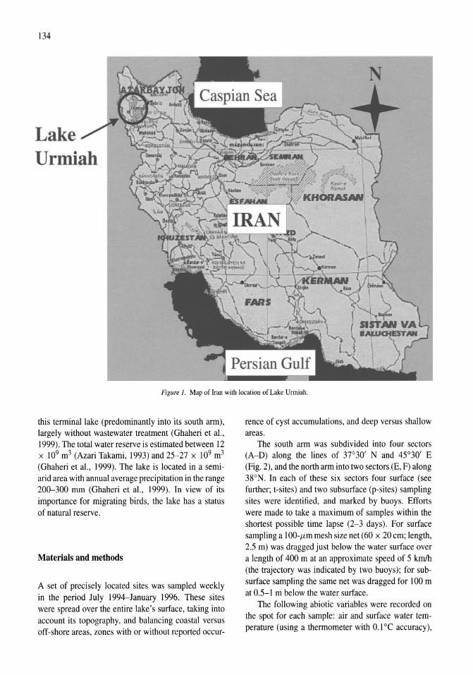
134
Lake Urmiah
Figure 1. Map ofIran with location of Lake Urmiah.
this terminal lake (predominantly into its south arm), largely without wastewater treatment (Ghaheri et aI., 1999). The total water reserve is estimated between 12 x 109 m3 (Azari Takami, 1993) and 25-27 x 109 m3
(Ghaheri et aI., 1999). The lake is located in a semiarid area with annual average precipitation in the range 200-300 mm (Ghaheri et aI., 1999). In view of its importance for migrating birds, the lake has a status of natural reserve.
Materials and methods
A set of precisely located sites was sampled weekly in the period July 1994-January 1996. These sites were spread over the entire lake's surface, taking into account its topography, and balancing coastal versus off-shore areas, zones with or without reported occur-
rence of cyst accumulations, and deep versus shallow areas.
The south arm was subdivided into four sectors (A-D) along the lines of 37°30' Nand 45°30' E (Fig. 2), and the north arm into two sectors (E, F) along 38°N. In each of these six sectors four surface (see further; t-sites) and two subsurface (p-sites) sampling sites were identified, and marked by buoys. Efforts were made to take a maximum of samples within the shortest possible time lapse (2-3 days). For surface sampling a 100-llm mesh size net (60 x 20 cm; length, 2.5 m) was dragged just below the water surface over a length of 400 m at an approximate speed of 5 kmlh (the trajectory was indicated by two buoys); for subsurface sampling the same net was dragged for 100 m at 0.5-1 m below the water surface.
The following abiotic variables were recorded on the spot for each sample: air and surface water temperature (using a thermometer with O.I°C accuracy),
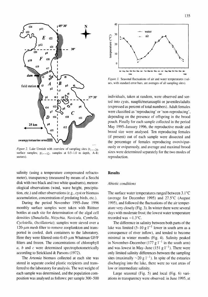
25km
IB 1
p2 1 t7
1 t5 pI 141 p4 \'0\-
N
+
37· 30'
----~~;--114 III 0 p6 p5
p7 C 116: 110
1 1 1 1 1
Figure 2. Lake Urmiah with overview of sampling sites (tl--24' surface samples; PI--12, samples at 0.5-1.0 m depth, A-E: sectors).
salinity (using a temperature compensated refractometer), transparency (measured by means of a Secchi disk with two black and two white quadrants), meteorological observations (wind, wave height, precipitation, etc.) and other observations (e.g., cyst or biomass accumulation, concentration of predating birds, etc.).
During the period November 1995-June 1996 monthly surface samples were taken with Riittner bottles at each site for determination of the algal cell densities (Dunaliella, Nitzschia, Navicula, Cymbella, Cyclotella, Oscillatoria); samples were sieved over a 120-JLm mesh filter to remove zooplankton and transported in cooled, dark containers to the laboratory. Here they were filtered onto 0.45-JLm Whatman GFIF filters and frozen. The concentrations of chlorophyll a, band c were determined spectrophotometric ally according to Strickland & Parsons (1972).
The Artemia biomass collected at each site was stored in separate cooled plastic recipients and transferred to the laboratory for analysis. The wet weight of each sample was determined, and the population composition was analysed as follows: per sample 300-500
135
40
water
G 30 air
0 '-' I>
~ 20
I>
S- 10 .!! .' . .....
0
"94 1995 1996
Figure 3. Seasonal fluctuations of air and water temperatures (values, with standard error bars, are averages of all sampling sites).
individuals, taken at random, were observed and sorted into cysts, nauplii/metanauplii or juveniles/adults (expressed as percent of total numbers). Adult females were classified as 'reproducing' or 'non-reproducing', depending on the presence of offspring in the brood pouch. Finally for each sample collected in the period May 1995-January 1996, the reproductive mode and brood size were analysed. Ten reproducing females (if present) out of each sample were dissected and the percentage of females reproducing ovoviviparously or oviparously, and average and maximal brood sizes were determined separately for the two modes of reproduction.
Results
Abiotic conditions
The surface water temperatures ranged between 3.1 °C (average for December 1995) and 27.5°C (August 1995), and followed the fluctuations of the air temperature very closely (Fig. 3). In winter there were several days with moderate frost; the lowest water temperature recorded was -1.3°C.
The difference in salinity between both parts of the lake was limited (5-10 g 1-1 lower in south arm as a consequence of river inflow), and tended to become minimal in winter months (Fig. 4). Salinity peaked in November-December (177 g 1-1 in the south arm) and was lowest in May-June (151 g 1-1). There were only limited salinity differences between the sampling sites (maximally ~20 g 1-1). In spite of the estuaries discharging into the lake, there were no vast areas of low or intermediate salinity.
Large seasonal (Fig. 5) and local (Fig. 6) variations in transparency were observed: in June 1995, at
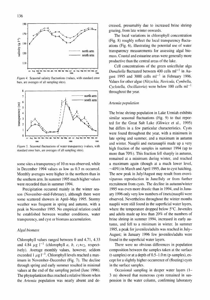
136
190 .,---------------,
170
~ 150
--------- northarm --- south arm
:~ -a 130
110
~-~~~~~~~-~~~--~~~~ 1994 1995 1996
Figure 4. Seasonal salinity fluctuations (values, with standard error bars, are averages of all sampling sites).
--------- north arm ---south arm
,994 , ... , ... Figure 5. Seasonal fluctuations of water transparency (values, with standard error bars, are averages of all sampling sites).
some sites a transparency of 10m was observed, while in December 1994 values as low as 0.3 m occurred. Monthly averages were higher in the northern than in the southern arm. In summer 1995 much higher values were recorded than in summer 1994.
Precipitation occurred mainly in the winter season (November-mid-February), although there were some scattered showers in April-May 1995. Stormy weather was frequent in spring and autumn, with a peak in November 1995. No empirical relation could be established between weather conditions, water transparency, and cyst or biomass accumulation.
Algal biomass
Chlorophyll values ranged between 0 and 4.71, 4.33 and 4.84 jLg I-I (chlorophyll a, b, q+C2, respectively). Average monthly values, however, seldom exceeded 1 jLg 1-1. Chlorophyll levels reached a maximum in November-December (Fig. 7). The decline through spring and early summer resulted in minimal values at the end of the sampling period (June 1996). The phytoplankton thus reached a relative bloom when the Artemia population was nearly absent and de-
creased, presumably due to increased brine shrimp grazing, from late winter onwards.
The local variations in chlorophyll concentration (Fig. 8) roughly reflect the local transparency fluctuations (Fig. 6), illustrating the potential use of water transparency measurements for assessing algal biomass. Coastal and estuarine areas were generally more productive than the central areas of the lake.
Cell concentrations of the green unicellular alga Dunaliella fluctuated between 400 cells ml- I in August 1995 and 3000 cells ml- I in February 1996. Values for other algae (Nitzschia, Navicula, Cymbella, Cyclotella, Oscillatoria) were below 100 cells ml- I
throughout the year.
Artemia population
The brine shrimp population in Lake Urmiah exhibits similar seasonal fluctuations (Fig. 9) to that reported for the Great Salt Lake (Gliwicz et aI., 1995) but differs in a few particular characteristics. Cysts were found throughout the year, with a minimum in late spring and summer, and a maximum in autumn and winter. Nauplii and metanauplii made up a very high fraction of the samples in summer 1994 (up to more than 70%). This fraction fell sharply in autumn, remained at a minimum during winter, and reached a maximum again (though at a much lower level, "'40%) in March and April 1995, due to cyst hatching. The new peak in July/August may result from ovoviviparous reproduction in June/July or from further recruitment from cysts. The decline in autumn/winter 1995 was even more drastic than in 1994, and in January 1996 only very low numbers of (meta)nauplii were observed. Nevertheless throughout the winter months nauplii were still found in the superficial water layers, where the temperature dropped below 5°C. Juveniles and adults made up less than 20% of the numbers of brine shrimp in summer 1994, increased in early autumn, and fell to a minimum in winter. In summer 1995, a peak for juveniles/adults was reached in JulyAugust; in January 1996 few juveniles/adults were found in the superficial water layers.
There were no obvious differences in population composition between the samples taken at the surface (t-samples) or at a depth of 0.5-1.0 m (p-samples), except for a slightly higher occurrence of (floating) cysts in the surface samples.
Occasional sampling in deeper water layers (1-3 m) showed that numerous cysts remained in suspension in the water column, confirming laboratory
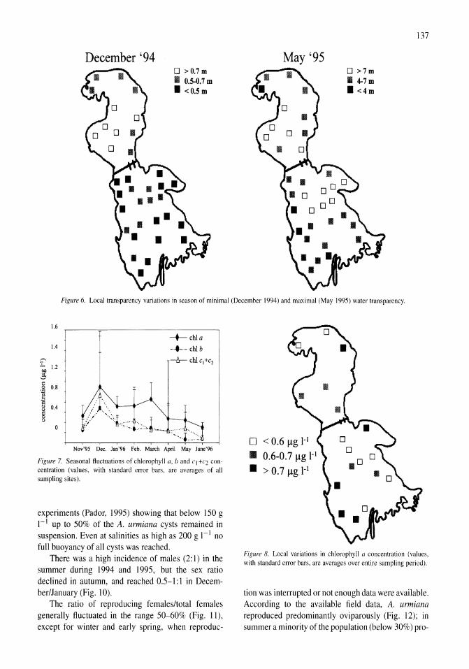
December '94 o >0.7m I 0.5-0.7 m • <0.5 m
May '95 o >7m Ii 4-7m • <4m
137
Figure 6. Local transparency variations in season of minimal (December 1994) and maximal (May 1995) water transparency.
1.6
+-chla 1.4 -t-·- chI b
'""' ---Is- chl c 1 +c2
OIl 1.2
-3 <=i .::: 0.8 .. ... ;:: " 0.4 g 0
"
Nov'95 Dec. Jan'96 Feb. March April May June'96
Figure 7. Seasonal fluctuations of chlorophyll (I, band C] +c2 concentration (values, with standard error bars, are averages of all sampling sites).
experiments (Pador, 1995) showing that below 150 g I-I up to 50% of the A. urmiana cysts remained in suspension. Even at salinities as high as 200 g I-I no full buoyancy of all cysts was reached.
There was a high incidence of males (2: I) in the summer during 1994 and 1995, but the sex ratio declined in autumn, and reached 0.5-1: I in December/January (Fig. 10).
The ratio of reproducing females/total females generally fluctuated in the range 50-60% (Fig. 11), except for winter and early spring, when reproduc-
o < 0.6 Ilg I-I III 0.6-0.7 Ilg 1-1
• > 0.7 Ilg 1-1
Figure 8. Local variations in chlorophyll (I concentration (values, with standard error bars, are averages over entire sampling period).
tion was interrupted or not enough data were available. According to the available field data, A. urmiana reproduced predominantly oviparously (Fig. 12); in summer a minority of the population (below 30%) pro-
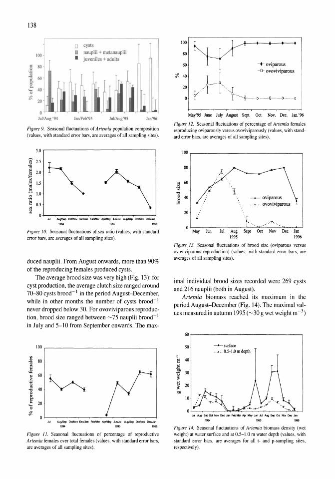
138
0 cysts
100 I nauplii + meianauplii
• juveniles + aduhs
'" 80 0 .~
:; Co
60
8. ..... 40 0
'#. 20
0 I~ I n III ~ U
JuVAug '94 JanfFcb'9S JuVAug'9S 1an'96
Figure 9. Seasonal fluctuations of Artemia population composition (values, with standard error bars, are averages of all sampling sites).
3.0
'Vi' 2.5 OJ
~ til e 2.0 ~ '<Ii OJ 1.5 til g
1.0 0 .~ .... 0.5 ~ OJ
'" Jul AugISep OctlNov DeclJan FebIMar ~rfMay JunlJui AugISep Oct/Nov DedJan
1994 1995 1996
Figure 10. Seasonal fluctuations of sex ratio (values, with standard error bars, are averages of all sampling sites).
duced nauplii. From August onwards, more than 90% of the reproducing females produced cysts.
The average brood size was very high (Fig. 13): for cyst production, the average clutch size ranged around 70-80 cysts brood-I in the period August-December, while in other months the number of cysts brood-I never dropped below 30. For ovoviviparous reproduction, brood size ranged between ~75 nauplii brood-I in July and 5-10 from September onwards. The max-
100,-______________________________ -,
'" OJ 80 til e ~
OJ 60
~ "B .g 40 0 .... Q. OJ .... 20 ..... 0
'#. Jut AuWSep Octmov OecfJan FebIMar AprlMay Ji.J'VJuI Aug/Sep Od/Nov DecJJan
1994 1995 1996
Figure 11. Seasonal fluctuations of percentage of reproductive Artemia females over total females (values, with standard error bars, are averages of all sampling sites).
100
80
60 -+ oviparous
~ 40 --0- ovoviviparous
20
May'95 June July August Sept. Oct. Nov. Dec. Jan.'96
Figure 12. Seasonal fluctuations of percentage of Artemia females reproducing oviparously versus ovoviviparously (values, with standard error bars, are averages of all sampling sites).
100.--________________ -,
80
.~ 60
'" "0 o 40 ]
20
il ____ oviparous ....... ovoviviparous
.... May Jun lui Aug Sept Oct Nov Dec Jan
1995 1996
Figure 13. Seasonal fluctuations of brood size (oviparous versus ovoviviparous reproduction) (values, with standard error bars, are averages of all sampling sites).
imal individual brood sizes recorded were 269 cysts and 216 nauplii (both in August).
Artemia biomass reached its maximum in the period August-December (Fig. 14). The maximal values measured in autumn 1995 (~30 g wet weightm-3)
60
50 ---+- surface ...... 0.5-\.0 m depth
1: 40
11 OIl
30 .~
0) 20 ~ OIl
10
.--~-~~~~--~~--~-~-1~ 1995 1996
Figure 14. Seasonal fluctuations of Artemia biomass density (wet weight) at water surface and at 0.5-\.0 m water depth (values, with standard error bars, are averages for all t- and p-sampling sites, respectively).
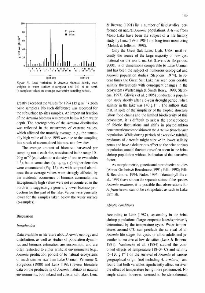
100 ~------------------,
80
1: 60 .§, oil ~ 40
~ OJ) 20
D p-sites • t-sites
1 3 5 7 1 3 5 7 9 11 13 15 9 11 17 19 21 23 2 4 6 8 2 4 6 8 10 12 14 16 10 12 18 20 22 24
south arm north arm
Figure 15. Local variations in Artemia biomass density (wet weight) at water surface (t-samples) and 0.5-1.0 m depth (p-samples) (values are averages over entire sampling period).
greatly exceeded the values for 1994 (15 g m-3) (both t-site samples). No such difference was recorded for the subsurface (p-site) samples. An important fraction of the Artemia biomass was present below 0.5 m water depth. The heterogeneity of the Artemia distribution was reflected in the occurrence of extreme values, which affected the monthly average; e.g., the unusually high value of June 1995 was due to the sampling in a streak of accumulated biomass at a few sites_
The average amount of biomass, harvested per sampling run at each site, was situated in the range 10-20 g m-3 (equivalent to a density of one to two adults I-I), but at some sites (t5, t6, tg, t12) higher densities were encountered (Fig. 15)_ As with temporal abundance these average values were strongly affected by the incidental occurrence of biomass accumulations. Exceptionally high values were not encountered in the north arm, suggesting a generally lower biomass production for this part of the lake. Values were generally lower for the samples taken below the water surface (p-samples).
Discussion
Introduction
Data available in literature about Artemia ecology and distribution, as well as studies of population dynamics and biomass estimation are uncommon, and are often restricted to either artificial environments (e.g., Artemia production ponds) or to natural ecosystems of much smaller size than Lake Urmiah. Persoone & Sorgeloos (1980) and Lenz (1987) review literature data on the productivity of Artemia habitats in natural environments, both inland and coastal salt lakes. Lenz
139
& Browne (1991) list a number of field studies, performed on natural Artemia populations. Artemia from Mono Lake have been the subject of a life history study by Lenz (1980, 1984) and long-term monitoring (Melack & Jellison, 1998).
Only the Great Salt Lake, Utah, USA, until recently the source of the large majority of raw cyst material on the world market (Lavens & Sorgeloos, 2000), is of dimensions comparable to Lake Urmiah and has been the subject of numerous ecological and Artemia population studies (Stephens, 1974). In recent times the Great Salt Lake has seen considerable salinity fluctuations with consequent changes in the ecosystem (Wurtsbaugh & Smith Berry, 1990; Stephens, 1997). Gliwicz et aL (1995) conducted a population study shortly after a 6-year drought period, when salinity in the lake was 140 g I-I. The authors state that, in spite of the simplicity of the trophic structure (short food chain) and the limited biodiversity of this ecosystem, it is difficult to assess the consequences of abiotic fluctuations and shifts in phytoplankton concentration/composition on the Artemiafranciscana population. While during periods of excessive rainfall, predators of Artemia might survive in lower salinity zones and have a deleterious effect on the brine shrimp population, annual fluctuations often occur in the brine shrimp population without indication of the causative factor.
As morphometric, genetic and reproductive studies (Abreu-Grobois & Beardmore, 1991; Pilla, 1992; Pilla & Beardmore, 1994; Pador, 1995; Triantaphyllidis et aI., 1997) have shown the separate status of the species Artemia urmiana, it is possible that observations for A. franciscana cannot be extrapolated as such to Lake Urmiah_
Abiotic conditions
According to Lenz (1987), seasonality in the brine shrimp population oflarge temperate lakes is primarily determined by the temperature cycle. Water temperatures around ODe can preclude the survival of all Artemia life stages but cysts, or allow adults and juveniles to survive at low densities (Lenz & Browne, 1991). Vanhaecke et aL (1984) studied the combined effects of temperature (I8-34°C) and salinity (5-120 g 1-1) on the survival of Artemia of various geographical origin (not including A. urmiana), and found that both variables significantly affect survival, the effect of temperature being more pronounced_ No single strain, however, seemed to be stenothermal,
140
while most strains shared a common area of preference (20-25°C), where mortalities were below lO% after a culture period of 9 days. Substantial strain differences, however, existed with regard to resistance for high temperatures: A. salina and A. parthenogenetica strains did not survive temperatures exceeding 30°C, while 5-10% survival was observed for both Great Salt Lake and San Francisco Bay A. franciscana, cultured at 34°C. Lethal temperatures of 30-34°C were however never attained at the water surface of Lake Urmiah.
Von Hentig (1971) assumes maximal hatching in the range 15-30°C, while Sorgeloos & Persoone (1975) narrow it down to 20-28°C. Nevertheless hatching can occur at lower temperatures (as low as 5-1 O°C, be it at much slower hatching rates) observed in Lake Urmiah from late February or early March onwards. Maximal growth and biomass production takes place in the range 20-27°C (Vanhaecke & Sorgeloos, 1989). Once again, the impact of temperature on growth varies from one strain to another. However, for most strains growth is limited below 15°C. This laboratory finding is also confirmed by field data (Lenz & Browne, 1991). If these data are extrapolated to A. urmiana, the season for optimal biomass production in Lake Urmiah is confined to the period April-October.
Large local salinity differences were not recorded in this sampling campaign. Gliwicz et al. (1995) found that salinity was homogeneous over the entire south arm of Great Salt Lake, and over a total depth of 6 m, indicating that thorough horizontal and vertical mixing of the water column takes place.
As in Lake Urmiah, transparency in Great Salt Lake (Gliwicz et aI., 1995) appeared to be highly variable (0.4-7.0 m) depending on time and sampling site. Seasonal fluctuations in primary productivity and the stirring of bottom sediments by wind and waves affected the transparency of the water column.
Mono Lake (Lenz, 1984) shows seasonal and annual transparency fluctuations, with minimal values in the period October-May and peaks in JUly-August, reflecting the heavy grazing pressure of the brine shrimp population.
Algal biomass
Chlorophyll values in Lake Urmiah, generally situated in the range 0.5-0.8 jLg 1-1, are low compared to the values reported by Gliwicz et al. (1995) for Great Salt Lake « 0.5 jLg 1-1 in June to 13 jLg I-I in January). Even values observed in the more productive estuarine
zones of Lake Urmiah were well below the chlorophyll a levels observed in similar areas in Great Salt Lake (60 jLg I-I). In summer under high grazing pressure, the algal species composition in Great Salt Lake was more diversified (with an important fraction of diatoms like Amphora, Navicula and Nitzschia) than in winter, when the phytoplankton mainly consisted of a Dunaliella monoculture.
The Lake Urmiah study did not assess bacterioplankton and decomposing matter (detritus), potentially important food sources for the Artemia population. Detritus can be up-welled by water currents and storms and bacterioplankton can be abundant. In the zones of river water inflow and in flooded areas decaying matter may contribute significantly to the nutrient balance of the lake. Gliwicz et al. (1995) state that food limitation induces a stage-structured intraspecific competition on growth rate: in an environment with limited primary production the adults compete successfully for food with the earlier stages, resulting in reduced naupliar growth. Culture tests of Great Salt Lake-Artemia in vitro and analysis of stomach content in the field show that nauplii and young juveniles mainly thrive on phytoplankton and other suspended material. Adults and sub adults use this food source only in case its concentration is high, and otherwise consume sedimented detritus and periphyton (in summer the periphyton on exuviae is an important food source).
Artemia population
Comparison of the seasonal fluctuations in population composition (Fig. 9), chlorophyll concentration (Fig. 7) and transparency (Fig. 5), suggests the following population dynamics at Lake Urmiah. A fraction of nauplii and metanauplii may survive the winter months, and start developing from March/April onwards. However, it is difficult to assess the contribution of this overwintering population to the spring generation of adults. Hatching of cysts may occur as early as February. The grazing pressure of this expanding brine shrimp population prevents the phytoplankton from reaching actual blooming concentrations, as observed in other saline habitats in late spring. Consequently, as the number of juveniles and adults increases, the algal concentration steadily declines and reaches absolute minimum levels in late spring, early summer (May/June), after which transparency gradually decreases (late summer, early autumn), even
though the relative proportion of juveniles and adults is reaching a maximum.
Gliwicz et al. (1995) summarize the population dynamics in Great Salt Lake as follows: in AprillMay a first generation hatches from cysts and colonizes the environment rapidly. This generation reproduces ovoviviparously at a high rate, illustrated by large broods of nauplii during late May. These animals produce a second generation of more slowly developing individuals, which do not reach maturity by autumn. Only a small fraction of this second generation seems to survive and reach maturation, producing one or two smaller broods, which do not contribute significantly to the population density. In Mono Lake (Lenz, 1980, 1984; Jellison & Melack, 1998) the number of Artemia is low during winter and the brine shrimp females remain in a non-reproductive state. In spring the Artemia develop slowly from cyst to adult in 10-12 weeks, mainly because of the low prevailing water temperatures, and reach maturity at the end of May, reproducing ovoviviparously. Second generation adults appear in mid-July/August. The first and second generation of females in July produce overwintering cysts. The population reaches a peak in late summer, decreasing afterwards to low numbers in November. However, considerable fluctuations are observed from year to year. For Lake Urmiah, the field data do not allow definitive conclusions with regard to the number of generations produced per season; however, the reproductive data (see further) indicate a predominance of oviparity, suggesting that ovoviviparous colonization of the medium does not take place at a rate comparable to the Great Salt Lake.
The high incidence of males in Lake Urmiah corresponds to the observations in other saline lakes, e.g., Mono Lake (Lenz, 1984) and particularly Great Salt Lake, where similar fluctuations occur, with a sex ratio of 4: 1 in June, decreasing to 1: 1 in NovemberlDecember (Gliwicz et aI., 1995). These fluctuations may be related to the different physiological tolerance of adult males and females to varying conditions of temperature, salinity and/or oxygen, not specific for A. urmiana, but also for other Artemia species.
The data on sex ratio do not permit any decisive conclusions regarding the possible coexistence of a parthenogenetic and a bisexual brine shrimp species in Lake Urmiah. Gunther (1890) described brine shrimp from Lake Urmiah as a unique bisexual species, Artemia urmiana. This characteristic was confirmed when Clark & Bowen (1976) demonstrated the repro-
141
ductive isolation of the species from other bisexual strains. Nevertheless, Barigozzi et al. (1987) reported a popUlation exclusively composed of parthenogenetic individuals after culturing two cyst samples in the laboratory, and proposed to cancel the species designation A. urmiana. Azari Takami (1989) reported the coexistence of bisexual and parthenogenetic populations in the lake. He observed that the parthenogenetic strain was dominant in spring and summer but not common in autumn and winter. The phenomenon of coexistence with varying frequencies throughout the year has already been reported in other Artemia biotopes (Amat, 1983; Perez, 1987). Barigozzi (1989) proposed to reconsider A. urmiana as a species, and Ahmadi et al. (1990) reinforced the idea that the lake sustains a mixed population. Pador (1995), who cultured animals using cysts collected from different sampling stations, found no evidence of a parthenogenetic population. Although the occurrence of a parthenogenetic strain thus remains a possibility, the sex ratio suggests that the Artemia population in Lake Urmiah is at least predominantly bisexual.
The average clutch size (Fig. 13) largely surpasses the average value of 48 eggs female -I reported in laboratory experiments under optimal feeding conditions and a salinity of 140 g I-I (Pador, 1995). Equally low values were found in nature for Great Salt Lake Artemia, where the average brood size in summer and fall fluctuated around 15-30 eggs female-I. In estuarine areas, however, a maximum of 155 eggs female-I was recorded for females larger than 10 mm, and 50 for smaller individuals (7-8 mm). In laboratory experiments with optimal feeding conditions on the contrary, a maximum of 190 eggs female-I was recorded (Gliwicz et aI., 1995), illustrating the effect of food availability on brood size. Lower food availability induced oviparous reproduction, decreased brood size and increased the interval in between broods.
The seasonal decline in percentage of ovoviviparous females in Lake Urmiah (Fig. 12), as well as the decrease in nauplii brood-I (Fig. 13) from July onwards, coincides with the increased transparency (Fig. 5) and thus depletion of phytoplankton. Remarkably, there is no decrease in cysts brood-I before the winter season; Belovsky (1996) notes that cyst production in Great Salt Lake brine shrimp is highest at intermediate food concentrations. Throughout summer and autumn a maximum of reproductive effort is thus invested in cyst production, with nearly all reproductive females producing high numbers of cysts.
142
The difference in parameters, utilized to express the Artemia standing crop, and the divergent values found in literature, confirm that the assessment of the quantity of brine shrimp in a saltwater body is difficult. The distribution of Artemia, which are positively phototactic and subject to water currents by the action of wind, is highly heterogeneous and thus densities may vary widely (Persoone & Sorgeloos, 1980). For instance, Lenz (1980) reports densities ranging from 1 to 400 indo 1-1 in Mono Lake, while Mason (1967) reports only a few adults 1-1 in the top water layer in Mono Lake. In the Lake Urmiah sampling campaign, the hour of sampling was randomized and only occasionally were samples taken in deeper water layers; consequently no information on diurnal migration of the brine shrimp population could be obtained.
If the wet weight of an Artemia adult is estimated at ~ 10 mg individual- I (Reeve, 1963), a density of 30 g m-3corresponds with a density of 3 adults 1-1, a relatively low figure compared to the values presented for Great Salt Lake: 4 adults I-I in July (Wirick, 1972); 20 and 10 indo 1-1 for June and July, respectively (Stephens & Gillespie, 1972); 10--20 indo I-I in late spring (Wurtsbaugh & Smith Berry, 1990). Artemia production in Great Salt Lake is estimated by Gillespie & Stephens (1977) at 100-200 g biomass (dry weight) m-2 year-I.
Although caution is needed when comparing Artemia density values from different lakes, recorded over different seasons with various sampling methods, the Artemia production of Lake Urmiah seems relatively low. These low values correspond well with the low algal biomass values; Belovsky (1996) confirms that in Great Salt Lake the highest Artemia densities coincide with the highest food concentration, illustrating the impact of food availability.
Long-term hydrological records prove that the water level of Lake Urmiah is subject to substantial fluctuations (Fayazi, pers. commun.), caused by climatological factors. In view of the unusual weather conditions that prevailed in the period 1994-1996 (mild winter temperatures, excessive rainfall) the field data cannot be extrapolated as such to production years when more normal weather conditions are to be expected. Since 1996, salinity has steadily increased again, due to reduced precipitation, and presently (fall 1999) it is as high as 240 g 1-1 (Fayazi, pers. commun.). Continued sampling is needed to acquire more insight into the population dynamics of Artemia urmiana.
References
Abreu-Grobois, F. A. & J. A. Beardmore, 1991. Genetic characterization and intrageneric relationships of Artemia monica Verrill andA. urmiana GUnther. Hydrobiologia 212: 151-168.
Ahmadi, M, R. M., H. Leibovitz & K. Simpson, 1990. Characterisation of Uromiah Lake Artemia (Arremia uromiana) by electrofocusing of isozyme patterns. Compo Biochem. Physio!. 95: 115-118.
Amat, D. F., 1983. Zygogenetic and parthenogenetic Artemia in Cadiz sea-side salterns. Mar. Eco!. Prog. Ser. 13: 291-293.
Azari Takami, G., 1987. The use of Artemia from Ormia Lake (Iran) as food for sturgeon. In Sorgeloos, P., D. A. Bengtson, W. Decleir & E. Jaspers (eds), Artemia Research and its Applications, 3. Ecology, Culturing, Use in Aquaculture. Universa Press, Wetteren, Belgium: 467-468.
Azari Takami, G., 1989. Two strains of Artemia in Urmia Lake (Iran). Artemia Newslett. 13: 5.
Azari Takami, G., 1993. Urmiah lake as a valuable source of Artemia for feeding sturgeon fry. J. Vet. Fac. Univ. Tehran 47: 2-14.
Barigozzi, C., 1989. The problem of Artemia umziana. Artemia Newslett. 14: 14.
Barigozzi, C., V. Varotto, L. Baratelli & R. Giarizo, 1987. The Artemia of Urrnia Lake (Iran): mode of reproduction and chromosome numbers. Atti. Acc. Lincei. Rend. Fis. 8 (LXXXI): 87-90.
Belovsky, G. E., 1996. Brine shrimp population dynamics and sustainable harvesting in the Great Salt Lake Utah. Department of Fisheries and Wildlife and Ecology center Utah State University, Logan, Utah. 1996 Progress Report to the Utah Division of Wildlife Resources.
Clark, L. S. & S. T. Bowen, 1976. The genetics of Artemia salina. VII. Reproductive isolation. J. Hered. 67: 385-388.
Ghaheri, M., M. H. Baghal-Vayjooee & J. Naziri, 1999. Lake Urrnia, Iran: a summary review. Int. J. Salt Lake Res. 8: 19-22.
Gillespie, D. M. & D. W. Stephens, 1977. Some aspects of plankton dynamics in the Great Salt Lake, Utah. In Greer, D. C. (ed.), Desertic Terminal Lakes. Proc. Int. Conf. Desertic Terminal Lakes. Utah State University, Logan, UT, USA: 401-409.
Gliwicz, Z. M., W.A.Wurtsbaugh & A. Ward, 1995. Brine shrimp ecology in the Great Salt Lake, Utah. June 1994-May 1995 Performance Report to the Utah Division of Wildlife Resources, Salt Lake City, UT: 83 pp.
GUnther, R. T., 1890. Contributions to the natural history of Lake Urrni, N. W. Persia and its neighbourhood. J. linn. Soc. London 27: 394-398.
Lavens, P. & P. Sorgeloos, 2000. The history, present status and prospects of the availability of Arremia cysts for aquaculture. Aquaculture 181: 397-403.
Lenz, P. H., 1980. Ecology of an alkali-adapted variety of Arremia from Mono Lake, California, USA. In Persoone, G., P. Sorgeloos, O. Roe1s & E. Jaspers (eds), The Brine Shrimp Artemia, 3. Ecology, Culturing, Use in Aquaculture. Universa Press, Wetteren, Belgium: 79-96.
Lenz, P. H., 1984. Life-history analysis of an Artemia population in a changing environment. J. Plankton Res. 6: 967-983.
Lenz, P. H., 1987. Ecological studies on Artemia: a review. In Sorgeloos, P., D. A. Bengtson, W. Decleir & E. Jaspers (eds), Artemia Research and its Applications, 3. Ecology, Culturing, Use in Aquaculture. Universa Press, Wetteren, Belgium: 5-18.
Lenz, P. H. & R. A. Browne, 1991. Ecology of Arremia. In Browne, R. A., P. Sorgeloos & c. N. A. Trotman (eds), Arremia Biology. CRC Press Inc., Boca Raton, FL 33431, USA: 237-253.
LOffier, H., 1961. Beitrage zur Kenntnis der Iranischen Binnengewasser. II. Regiona1-Lirnnologische Studie mit besonderer Beriicksichtigung der Crustaceeenfauna. Int. Rev. ges. Hydrobiol. Hydrogr. 46: 309-406.
Mason, D. T., 1967. Limnology of Mono Lake, California. U. Calif. Public. Zoology 83: 1-110.
Melack, J. M. & R Jellison, 1998. Limnological conditions in Mono Lake: contrasting monomixis and meromixis in the 1990s. Hydrobiologia 384: 21-39.
Pador, E., 1995. Characterisation of the Artemia urmiana Gunther 1900 from Lake Urmia, Iran. M.Sc. Thesis. Vrije Universiteit Brussel and Laboratory of Aquaculture - Artemia Reference Center, University of Ghent, Belgium, 61 pp.
Perez, R., 1987. Cyst production of Artemia in salt ponds in southeastern Spain. In Sorgeloos, P., D. A. Bengston, W. Decleir & E. Jaspers (eds), Artemia Research and its Applications, 3. Universa Press, Welteren, Belgium: 215.
Persoone, G. & P. Sorgeloos, 1980. General aspects of the ecology and biogeography of Artemia. In Persoone, G., P. Sorgeloos, O. Roels & E. Jaspers (eds), The Brine Shrimp Artemia, 3. Ecology, Culturing, Use in Aquaculture. Universa Press, Welteren, Belgium, 3-24.
Pilla, E. J., 1992. Genetic differentiation and speciation in old world Artemia. Ph.D. thesis. Department of Genetics, University College of Swansea, UK, 356 pp.
Pilla, E. J. & J. A. Beardmore, 1994. Genetic and morphometric differentiation in Old World bisexual species of the brine shrimp (Artemia). Heredity 73: 47-56.
Reeve, M. R, 1963. Growth efficiency in Artemia under laboratory conditions. BioI. Bull. 125: 133-145.
Sorgeloos, P. & G. Persoone, 1975. Technological improvements for the cultivation of invertebrates as food for fishes and crustaceans. II. Hatching and culture of the brine shrimp Artemia salina L. Aquaculture 6: 303-317.
143
Stephens, D. w., 1974. A summary of biological investigations concerning the Great Salt Lake, Utah (1861-1973). Great Basin Naturalist 34: 221-229.
Stephens, D. w., 1997. Salinity-induced changes in the aquatic ecosystem of Great Salt Lake, Utah. In Pitman, J. & A. Carroll (eds), Modem and Ancient Lake Systems: New Problems and Perspectives, Utah Geological Association Guidebook 26, 1-7.
Stephens, D. W. & D. M. Gillespie, 1972. Community structure and ecosystem analysis of the Great Salt Lake. In Riley, J. P. (ed.), The Great Lake and Utah's Water Resources. Utah Water Res. Lab., Utah State University, USA: 66-72.
Strickland, 1. D. & T. R Parsons, 1972. A Practical Handbook of Seawater Analysis, 2nd edn. Bull. Fish. Res. Bd Can. 167,310 pp.
Triantaphyllidis, G. v., G. R 1. Criel, T. 1. Abatzopoulos & P. Sorgeloos, 1997. International Study on Artemia. LIII. Morphological study of Artemia with emphasis to Old World strains. I. Bisexual populations. Hydrobiologia, 357: 139-153.
Vanhaecke, P. & P. Sorgeloos, 1989. International Study on Artemia. XLVII. The effect of temperature on cyst hatching, larval survival and biomass production for different geographical strains of brine shrimp Artemia spp. Ann. Soc. r. zool. Belg. 119(1): 7-23.
Vanhaecke, P., S. E. Siddal & P. Sorgeloos, 1984. International Study on Artemia. XXXII. Combined effects of temperature and salinity on the survival of Artemia of various geographical origin. J. expo mar. BioI. Ecol. 80: 259-275.
Von Hentig, R., 1971. Einfluss von Salzgehalt und Temperatur auf Entwicklung, Wachs tum, Fortpflanzung und Energiebilanz von Artemia salina. Mar. BioI. 9: 145-182.
Wirick, C. D., 1972.Dunaliella-Artemia plankton community of the Great Salt Lake, Utah. Thesis. University of Utah. USA, 44 pp.
Wurtsbaugh, W. A. & T. Smith Berry, 1990. Cascading effects of decreased salinity on the plankton, chemistry and physics of the Great Salt Lake (Utah). Can. J. Fish. aquat. Sci., 47: 100-109.
Hydrobiologia 466: 145-148,2001. J.M. Melack, R. Jellison & D.B. Herbst (eds), Saline Lakes. © 2001 Kluwer Academic Publishers.
145
Dispersal of Artemia franciscana Kellogg (Crustacea; Anostraca) populations in the coastal saltworks of Rio Grande do Norte, northeastern Brazil
Marcos R. Camara Department of Oceanography and Limnology, Universidade Federal do Rio Grande do Norte, Natal, RN, 59072-970 Brazil E-mail: [email protected]
Key words: Artemia, reproduction, ecology, dispersal, saltworks, Brazil
Abstract
In spite of the presence of Artemia franciscana Kellogg in several saltworks in the State of Rio Grande do Norte (RN) (northeastern Brazil) that were colonized from inoculations made in Macau (RN) in April 1977 with cysts from a San Francisco Bay (California, U.S.A.) stock, there is no recent data on the degree of regional dispersal of this anostracan. For 12 months (July 1996 - June 1997), 55 saltworks located in the municipalities of Areia Branca, Grossos, Galinhos, Guamare and Macau in RN were visited and sampled for the presence of Artemia franciscana and the occurrence of its cysts. Populations of Artemia franciscana were found in all 55 saltworks, although significant amounts of cysts were only found in six sites. The presence of Artemia franciscana in all visited sites brings further evidence to the ample dispersal of this anostracan throughout the saltwork region of RN. However, the relatively low incidence of cysts suggests that most of these populations are reproducing ovoviviparously.
Introduction
The genus Artemia (Crustacea; Anostraca) is a complex of sibling species and superspecies defined by the criterion of reproductive isolation (Browne & Bowen, 1991). Two bisexual species are represented in the New World: Artemia persimilis Piccinelli & Prosdocimi and Artemia franciscana Kellogg. Artemia persimilis is restricted to some localities in Argentina whereas the bisexual Artemia franciscana superspecies is endemic to the Americas and the Caribbean, with various populations established in South American countries, either by deliberate inoculation or natural dispersal (Lenz & Browne, 1991; Gajardo et aI., 1999). In South America, Artemia franciscana inhabit coastal saltworks in Macau (Rio Grande do Norte, Brazil) and Cabo Frio (Rio de Janeiro, Brazil), coastal salt lakes (Boca Chica Salt Lake, Margarita Island, Venezuela), inland salt lakes (Atacama Lake, Chile), and coastal hypersaline estuaries (Virilla, Peru) (Lenz & Browne, 1991).
Artemia franciscana is found in the State of Rio Grande do Norte (RN) in northeastern Brazil as a result of inoculations made in a very large saltwork in Macau (RN) in April 1977 with cysts from a San Francisco Bay (California, U.S.A.) stock (Persoone & Sorgeloos, 1980; Camara & Castro, 1983). Artemia franciscana cysts have been dispersed to neighboring saltworks by men (for aquacultural purposes and to aid in salt production) and presumably, by wind and by local waterfowl. In view of the favorable climatic conditions, the inoculated strain has become established on a permanent basis (Camara & Castro, 1983; Camara & Rocha, 1987; Rocha & Camara, 1993; Camara, 1996). Recent electrophoretic evidence (similarity of samples of Macau and San Francisco Bay) confirmed the proposed origin, from San Francisco Bay cysts, of the Macau population (Gajardo et aI., 1995).
In this paper, the current degree of dispersal for Artemia franciscana in the saltworks of the State of Rio Grande do Norte (RN) in northeastern Brazil is described.
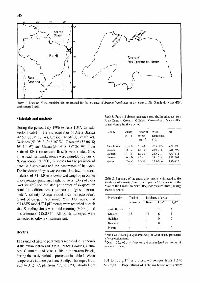
146
500 40° . . i·············:·············;······· . .
State of Rio Grande do Norte
Figure 1. Location of the municipalities prospected for the presence of Artemia franciscana in the State of Rio Grande do Norte (RN), northeastern Brazil.
Materials and methods
During the period July 1996 to June 1997, 55 saltworks located in the municipalities of Areia Branca W 57' S; 37° 08' W), Grossos W 58' S; 37° 09' W), Galinhos (5° OS'S; 36° 16' W), Guamare (5° 06' S; 36° 19' W), and Macau (5° 06' S; 36° 38' W) in the State of RN (northeastern Brazil) were visited (Fig. 1). At each saltwork, ponds were sampled (30 cm x 30 cm scoop net; 500 {Lm mesh) for the presence of ATtemia franciscana and the occurrence of its cysts. The incidence of cysts was estimated as low, i.e. accumulation of 0.1-1.0 kg of cysts (wet weight) per corner of evaporation pond; and high, i.e. over 1.0 kg of cysts (wet weight) accumulated per corner of evaporation pond. In addition, water temperature (glass thermometer), salinity (Atago model S-28 refractometer), dissolved oxygen (YSI model Y55 D.O. meter) and pH (AES model IP4 pH meter) were recorded at each site. Sampling times were mid-morning (9:00 h) and mid-afternoon (15:00 h). All ponds surveyed were subjected to saltwork management.
Results
The range of abiotic parameters recorded in saltponds at the municipalities of Areia Branca, Grossos, Galinhos, Guamare, and Macau (RN, northeastern Brazil) during the study period is presented in Table 1. Water temperature in these permanent saJtponds ranged from 26.5 to 31.5 °C; pH from 7.26 to 8.23; salinity from
Table 1. Range of abiotic parameters recorded in saltponds from Areia Branca, Grossos, Galinhos, Guamare and Macau (RN, Brazil) during the study period
Locality Salinity Dissolved Water pH (gl- l ) oxygen temperature
(mgl- I) ee)
Areia Branca 103-144 3.8-4.6 28.5-30.5 7.30-7.90
Grossos 105-177 2.6-4.0 28.0-31.5 7.26-7.97 Galinhos 101-167 2.9--3.5 26.5-27.1 7.90-8.11 Guarnare 116-130 1.2-4.1 28.1-28.4 7.89--7.93 Macau 107-143 2.6-5.0 27.5-29.6 7.97-8.23
Table 2. Summary of the quantitative results with regard to the incidence of Artemia franciscana cysts in 55 saltworks in the State of Rio Grande do Norte (RN) (northeastern Brazil) during the study period
Municipality Total of Incidence of cysts
saltworks None Lowa Highb
Areia Branca 5 2 2
Grossos 43 33 6 4
Galinhos 0 0
Guamare I 0 0
Macau 5 4 0
aProm 0.1 to 1.0 kg of cysts (wet weight) accumulated per comer of evaporation pond. hOver 1.0 kg of cysts (wet weight) accumulated per comer of evaporation pond.
101 to 177 g I-I and dissolved oxygen from 1.2 to 5.6 mg I-I. Populations of Artemiafranciscana were
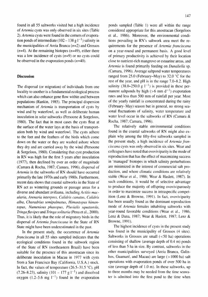
found in all 55 saltworks visited but a high incidence of Artemia cysts was only observed in six sites (Table 2). Artemia cysts were found in the comers of evaporation ponds of intermediate (102 - 138 g I-I) salinity in the municipalities of Areia Branca (n=2) and Grossos (n=4). At the remaining biotopes (n=49), either there was a low incidence of cysts (n=9) or no cysts could be observed in the evaporation ponds (n=40).
Discussion
The dispersal (or migration) of individuals from one locality to another is a fundamental ecological process which can also enhance gene flow within and between populations (Rankin, 1985). The principal dispersion mechanism of Artemia is transportation of cysts by wind and by waterfowl, as well as deliberate human inoculation in solar saltworks (Persoone & Sorgeloos, 1980). The fact that in most cases the cysts float at the surface of the water lays at the basis of transportation both by wind and waterfowl. The cysts adhere to the feet and the feathers of the birds which come down on the water or they are washed ashore where they dry and are carried away by the wind (Persoone & Sorgeloos, 1980). Considering that cyst production in RN was high for the first 5 years after inoculation (1977), then declined by over an order of magnitude (Camara & Rocha, 1987; Camara, 1996), dispersal of Artemia in the saltworks of RN should have occurred primarily the late 1970s and early 1980s. Furthermore, recent data shows that coastal saltworks in the State of RN act as wintering grounds or passage areas for a diverse and abundant avifauna, including Actitis macularia, Arenaria inter pres, Calidris canatus, Calidris alba, Charadrius semipalmatus, Himantopus himantopus, Numenious phaeopus, Pluvialis squatarola, Tringajiavipes and Tringa solita ria (Pena et aI., 2000). Thus, it is likely that the role of migratory birds in the dispersal of Artemia franciscana in the State of RN State might have been underestimated in the past.
In the present study, the occurrence of Artemia franciscana in all 55 sites sampled indicates that the ecological conditions found in the saltwork region of the State of RN (northeastern Brazil) have been suitable for the presence of this anostracan since its deliberate inoculation in Macau in 1977 with cysts from a San Francisco Bay (California, U.S.A.) stock. In fact, the values of temperature (26.5-31.5 DC), pH (7.26-8.23), salinity (101- 177 g I-I) and dissolved oxygen (1.2-5.6 mg I-I) found in the evaporation
147
ponds sampled (Table 1) were all within the range considered appropriate for this anostracan (Sorgeloos et aI., 1986). Moreover, the environmental conditions prevailing in RN's saltwork area meet the requirements for the presence of Artemia franciscana on a year-round and permanent basis. A good level of primary productivity is achieved by their location close to nutrient-rich mangrove or estuarine areas, and Artemia is found primarily feeding on Dunaliella sp. (Camara, 1996). Average saltpond water temperatures ranged from 25.0 (February-May) to 32.0 DC for the rest of the year, and pH is in the range 7.0-8.2. High salinity (38.0-250.0 g I-I) is provided in these permanent saltponds by high (>6 mm d- I ) evaporation rates and less than 500 mm of rainfall per year. Most of the yearly rainfall is concentrated during the rainy (February-May) season but in general, no strong seasonal fluctuations of salinity, water temperature and water level occur in the saltworks of RN (Camara & Rocha, 1987; Camara, 1996).
The relatively stable environmental conditions found in the coastal saltworks of RN might also explain why among the fifty-five saltworks sampled in the present study, a high incidence of Artemia franciscana cysts was only observed in six sites. Wear and colleagues have noted that ovoviviparity is the mode of reproduction that has the effect of maximizing success in 'managed' biotopes in which salinity perturbations are minimized in the interest of commercial salt production, and where climatic conditions are relatively stable (Wear et aI., 1986; Wear & Haslett, 1987). In such conditions, it would be of selective advantage to produce the majority of offspring ovoviviparously in order to maximize success in intraspecific competition (Lenz & Browne, 1991). In fact, ovoviviparity has been usually found as the dominant reproduction mode of Artemia females inhabiting saltworks with year-round favorable conditions (Wear et aI., 1986; Lenz & Dana, 1987; Wear & Haslett, 1987; Lenz & Browne, 1991).
The highest incidence of cysts in the present study was found in the municipality of Grossos (4 sites). Saltworks in Grossos are small «50 ha) operations consisting of shallow (average depth of 0.4 m) ponds of less than 5 ha in size. By contrast, saltworks in the other municipalities surveyed (Areia Branca, Galinhos, Guamare, and Macau) are large (> 1000 ha) salt operations with evaporation ponds of over 500 ha in size (average depth of 1.0 m). In these saltworks, up to three months may be needed from the time seawater is admitted into the first pond to the time when
148
brine reaches the crystallization ponds. Thus, saltworks in Grossos are relatively more susceptible to environmental changes than the large operations found in Areia Branca, Galinhos, Guamare and Macau.
In conclusion, the presence of Artemia franciscana in all saltworks visited during the present study brings further evidence to the ample dispersal of this anostracan throughout the saltwork region of the State of RN. However, the relatively low incidence of cysts suggests that most of these populations are reproducing ovoviviparously.
Acknowledgements
This work has been funded in part by grants from the Brazilian Council for Science and Technology (CNPq) and the International Foundation for Science, IFS (ref.AI1408-2). Appreciation is extended to two anonymous referees for providing valuable review comments. I also thank the owners and managers of the saltworks on which this study was carried out for their co-operation.
References
Browne. R. A. & S. T. Bowen, 1991. Taxonomy and popUlation genetics of Artemia. In Browne, R. A., P. Sorgeloos & C. N. A. Trotman (eds), Artemia Biology. CRC Press, Boca Raton, Florida, U.S.A.: 221-235.
Camara, M. R., 1996. Artemia production in coastal saltworks in Brazil: past, current practices and perspectives. In Gajardo, G. & P. Coutteau (eds), Improvement of the Commercial Production of Marine Aquaculture Species. Proceedings of a Workshop on Fish and Mollusc Larviculture. Impresora Creces, Santiago, Chile: 173-178.
Camara, M. R. & E. V. Castro, 1983, Artemia salina 1. (Anostraca): uma op\,ao para a aqUicultura do nordeste do Brasil. Revta. bras. Zool. I: 145-147.
Camara, M. R. & R, De M. Rocha, 1987. Artemia culture in Brazil: an overview. In Sorgeloos, P., D. A, Bengtson, W. Decleir & E, Jaspers (eds), Artemia Research and its Applications, 3. Universa Press, Wetteren, Belgium: 195-200,
Gajardo. G., M. Da Concei~ao, 1. Weber & 1. A. Beardmore, 1995. Genetic variability and interpopulational differences in Artemia strains from South America. Hydrobiologia 302: 21-29.
Gajardo, G., C. Mercado, J. A. Beardmore & P. Sorgeloos, 1999. International study on Artemia. LX. Allozyme data suggest that a new Artemia population in southern Chile (500 29' S; 73° 45' W) is A. persimilis. Hydrobiologia 405: 117-123.
Lenz, P. H. & G. 1. Dana, 1987. Life-cycle studies in Artemia: a comparison between a sub-tropical and a temperate population. In Sorgeloos, P., D. A. Bengtson, W. Decleir & E. Jaspers (eds), Artemia Research and its Applications. 3. Universa Press, Wetteren, Belgium: 89-100.
Lenz, P. H. & R. A. Browne, 1991. Ecology of Artemia. In Browne, R. A., P. Sorgeloos & c. N. A. Trotman (eds), Artemia Biology. CRC Press, Boca Raton, Florida, U.S.A.: 237-253.
Pena, 0., S. M. Azevedo Jr. & M. Larrazabal, 2000, Monitoramento de aves limicolas na Salina Diamante Branco, Galinhos, RN. In XXIII Congresso Brasileiro de Zoologia, Sociedade Brasileira de Zoologia, Cuiaba, Brasil: 480 pp.
Persoone, G. & P. Sorge1oos, 1980. General aspects of the ecology and biogeography of Artemia. In Persoone, G" P. Sorgeloos, O. Roels & E. Jaspers (eds), The Brine Shrimp Artemia, 3. Universa Press, Wetteren, Belgium: 3-24.
Rankin, M. A" 1985. Migration: mechanisms and adaptive significance. Contributions in Marine Science, 27, The University of Texas, Marine Science Institute, Texas: 868 pp,
Rocha, R. De M. & M. R. Camara, 1993. Prediction, monitoring and management of detrimental algal blooms on solar salt production in NE-Brazil. In 7th Symposium on Salt, 1, Elsevier Science Publishers B. v., Amsterdam: 657-660.
Sorgeloos, P., P. Lavens, Ph. Leger, W. Tackaert & D. Versichele, 1986. Manual for the culture and use of Brine Shrimp Artemia in Aquaculture. State University of Ghent, Belgium: 319 pp.
Wear, R. G., S. J. Haslett & N. 1. Alexander, 1986. Effects of temperature and salinity on the biology of Artemia franciscana Kellogg from Lake Grassmere, New Zealand. 2. Maturation, fecundity and generation times. J. expo mar. BioI. Eco!. 98: 167-183.
Wear, R. G. & S. 1. Haslett, 1987. Studies on the biology and ecology from Lake Grassmere, New Zealand. In Persoone, G., P. Sorgeloos, O. Roels & E. Jaspers (eds), The Brine Shrimp Artemia,3. Universa Press, Wetteren, Belgium: 101-126.
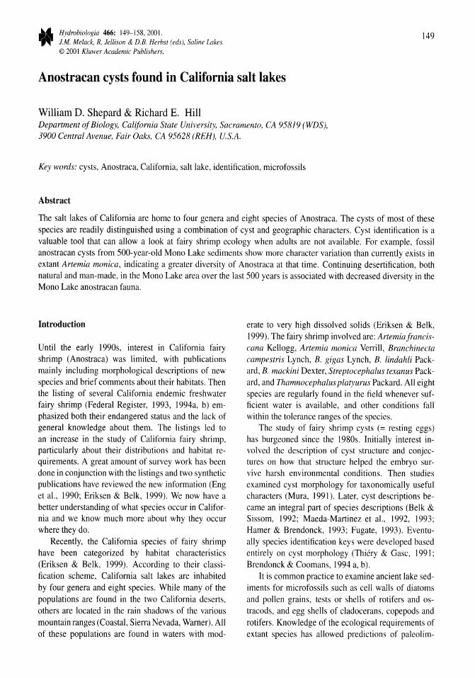
Hydrobiologia 466: 149-158, 200 I. J.M. Melack, R. Jellison & D.B. Herbst (eds), Saline Lakes. © 2001 Kluwer Academic Publishers.
149
Anostracan cysts found in California salt lakes
William D. Shepard & Richard E. Hill Department of Biology, California State University, Sacramento, CA 95819 (WDS), 3900 Central Avenue, Fair Oaks, CA 95628 (REH), U.S.A.
Key words: cysts, Anostraca, California, salt lake, identification, microfossils
Abstract
The salt lakes of California are home to four genera and eight species of Anostraca. The cysts of most of these species are readily distinguished using a combination of cyst and geographic characters. Cyst identification is a valuable tool that can allow a look at fairy shrimp ecology when adults are not available. For example, fossil anostracan cysts from 500-year-old Mono Lake sediments show more character variation than currently exists in extant Artemia monica, indicating a greater diversity of Anostraca at that time. Continuing desertification, both natural and man-made, in the Mono Lake area over the last 500 years is associated with decreased diversity in the Mono Lake anostracan fauna.
Introduction
Until the early 1990s, interest in California fairy shrimp (Anostraca) was limited, with publications mainly including morphological descriptions of new species and brief comments about their habitats. Then the listing of several California endemic freshwater fairy shrimp (Federal Register, 1993, 1994a, b) emphasized both their endangered status and the lack of general knowledge about them. The listings led to an increase in the study of California fairy shrimp, particularly about their distributions and habitat requirements. A great amount of survey work has been done in conjunction with the listings and two synthetic publications have reviewed the new information (Eng et al., 1990; Eriksen & Belk, 1999). We now have a better understanding of what species occur in California and we know much more about why they occur where they do.
Recently, the California species of fairy shrimp have been categorized by habitat characteristics (Eriksen & Belk, 1999). According to their classification scheme, California salt lakes are inhabited by four genera and eight species. While many of the populations are found in the two California deserts, others are located in the rain shadows of the various mountain ranges (Coastal, Sierra Nevada, Warner). All of these populations are found in waters with mod-
erate to very high dissolved solids (Eriksen & Belk, 1999). The fairy shrimp involved are: Artemiafranciscana Kellogg, Artemia monica Verrill, Branchinecta campestris Lynch, B. gigas Lynch, B. lindahli Packard, B. mackini Dexter, Streptocephalus texanus Packard, and Thamnocephalus platyurus Packard. All eight species are regularly found in the field whenever sufficient water is available, and other conditions fall within the tolerance ranges of the species.
The study of fairy shrimp cysts (= resting eggs) has burgeoned since the 1980s. Initially interest involved the description of cyst structure and conjectures on how that structure helped the embryo survive harsh environmental conditions. Then studies examined cyst morphology for taxonomically useful characters (Mura, 1991). Later, cyst descriptions became an integral part of species descriptions (Belk & Sissom, 1992; Maeda-Martinez et al., 1992, 1993; Hamer & Brendonck, 1993; Fugate, 1993). Eventually species identification keys were developed based entirely on cyst morphology (Thiery & Gasc, 1991; Brendonck & Coomans, 1994 a, b).
It is common practice to examine ancient lake sediments for microfossils such as cell walls of diatoms and pollen grains, tests or shells of rotifers and ostracods, and egg shells of cladocerans, copepods and rotifers. Knowledge of the ecological requirements of extant species has allowed predictions of paleolim-
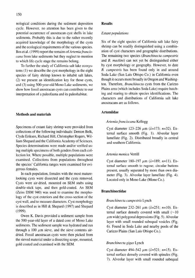
150
nological conditions during the sediment deposition cycle. However, no attention has been given to the potential occurrence of anostracan cyst shells in lake sediments. Probably this is due to the rather recently acquired knowledge of the morphology of the cysts and the ecological requirements of the various species. Bos et al. (1999) report the remains of Artemiafranciscan a from lake sediments but they neglect to mention to which life cycle stage the remains belong.
To further the study of California salt lake ecosystems (1) we describe the cyst morphology in the eight species of fairy shrimp known to inhabit salt lakes, (2) we present an identification key for those cysts, and (3) using 500-year-old Mono Lake sediments, we show how fossil anostracan cysts can contribute to our interpretation of a paleofauna and its paleohabitat.
Methods and materials
Specimens of extant fairy shrimp were provided from collections of the following individuals: Denton Belk, Clyde Eriksen, Richard Hill, Christopher Rogers, William Shepard and the California Academy of Sciences. Species determinations were made and/or verified using multiple specimens of both genders from each collection lot. Where possible, multiple populations were examined. Collections from populations throughout the species' California ranges were examined for ovigerous females.
In each population, females with the most maturelooking cysts were dissected and the cysts removed. Cysts were air-dried, mounted on SEM stubs using double-stick tape, and then gold-coated. An SEM (Zeiss DSM 940) was used to examine the morphology of the cyst exteriors and the cross-section of the cyst wall, and to measure diameters. Cyst morphology is described as in HilI & Shepard (1997) and Shepard (1999).
Owen K. Davis provided a sediment sample from the 500-year-old layer of a dated core of Mono Lake sediments. The sediment sample was hydrated and run through a 100 fLm sieve, and the sieve contents airdried. Fossil anostracan cysts were then picked from the sieved material under a dissecting scope, mounted, gold coated and examined with the SEM.
Results
Extant populations
Six of the eight species of California salt lake fairy shrimp can be readily distinguished using a combination of cyst characters and geographic distributions. The remaining two species (Branchinecta campestris and B. mackini) can not yet be distinguished either by cyst morphology or geography. However, to date B. campestris has been found only in and around Soda Lake (San Luis Obispo Co.) in California even though it occurs more broadly in Oregon and Washington. Therefore, Branchinecta cysts from the Carizzo Plains area (which includes Soda Lake) require hatching and rearing to obtain species identifications. The characters and distributions of California salt lake anostracans are as follows.
Artemiidae
Artemiafranciscana Kellogg
Cyst diameter 123-226 fLm (.x=173; n=32). External surface smooth (Fig. 1). Alveolar layer lamellate (Fig. 2). Distributed broadly in central and southern California.
Artemia monica Verrill
Cyst diameter 180-197 fLm (.x=189; n=II). External surface smooth to rugose; circular buttons present, usually separated by more than own diameter (Fig. 3). Alveolar layer lamellate (Fig. 4). Located only in Mono Lake (Mono Co.).
Branchinectidae
Branchinecta campestris Lynch
Cyst diameter 232-261 fLm (.x=251; n=lO). External surface densely covered with small (~1O fLm wide) polygonal depressions (Fig. 5). Alveolar layer with small rounded subequal vesicles (Fig. 6). Found in Soda Lake and nearby pools of the Carizzo Plains (San Luis Obispo Co.).
Branchinecta gigas Lynch
Cyst diameter 494-542 fLm (.x=521; n= 15). External surface densely covered with spinules (Fig. 7). Alveolar layer with small rounded subequal
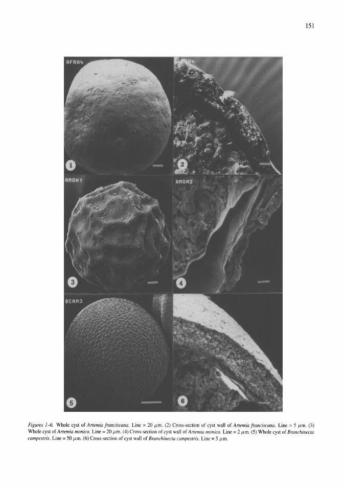
151
Figures 1--6. Whole cyst of Artemia franciscana. Line = 20 Jlm. (2) Cross-section of cyst wall of Artemia franciscana. Line = 5 Jlm. (3) Whole cyst of Artemia monica. Line = 20 Jlm. (4) Cross-section of cyst wall of Artemia monica. Line = 2 Jlm. (5) Whole cyst of Branchinecta campestris. Line = 50 Jlm. (6) Cross-section of cyst wall of Branchinecta campestris. Line = 5 Jlm.
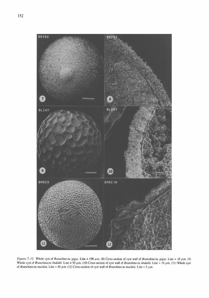
152
Figures 7-12. Whole cyst of Branchinecta gigas. Line = 100 /Im. (8) Cross-section of cyst wall of Branchinecta gigas. Line = 10 /Im. (9) Whole cyst of Branchinecta lindahli. Line = 50 /Im. (10) Cross-section of cyst wall of Branchinecta lindahli. Line = 10 /Im. (II) Whole cyst of Branchinecta mackini. Line = 50 /Im. (12) Cross-section of cyst wall of Branchinecta mackini. Line = 5 /Im.
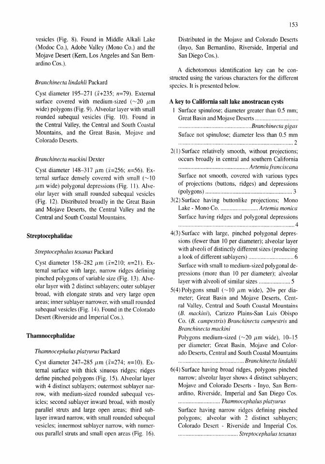
vesicles (Fig. 8). Found in Middle Alkali Lake (Modoc Co.), Adobe Valley (Mono Co.) and the Mojave Desert (Kern, Los Angeles and San Bernardino Cos.).
Branchinecta lindahli Packard
Cyst diameter 195-271 (i+235; n=79). External surface covered with medium-sized (~20 ILm wide) polygons (Fig. 9). Alveolar layer with small rounded subequal vesicles (Fig. 10). Found in the Central Valley, the Central and South Coastal Mountains, and the Great Basin, Mojave and Colorado Deserts.
Branchinecta mackini Dexter
Cyst diameter 148-317 ILm (i=256; n=56). External surface densely covered with small (~lO ILm wide) polygonal depressions (Fig. 11). Alveolar layer with small rounded subequal vesicles (Fig. 12). Distributed broadly in the Great Basin and Mojave Deserts, the Central Valley and the Central and South Coastal Mountains.
Streptocephalidae
Streptocephalus texanus Packard
Cyst diameter 158-282 ILm (i=21O; n=21). External surface with large, narrow ridges defining pinched polygons of variable size (Fig. 13). Alveolar layer with 2 distinct sublayers; outer sublayer broad, with elongate struts and very large open areas; inner sub layer narrower, with small rounded subequal vesicles (Fig. 14). Found in the Colorado Desert (Riverside and Imperial Cos.).
Thamnocephalidae
Thamnocephalus platyurus Packard
Cyst diameter 247-285 ILm (i=274; n=lO). External surface with thick sinuous ridges; ridges define pinched polygons (Fig. 15). Alveolar layer with 4 distinct sublayers; outermost sublayer narrow, with medium-sized rounded subequal vesicles; second sublayer inward broad, with mostly parallel struts and large open areas; third sublayer inward narrow, with small rounded subequal vesicles; innermost sublayer narrow, with numerous parallel struts and small open areas (Fig. 16).
153
Distributed in the Mojave and Colorado Deserts (Inyo, San Bernardino, Riverside, Imperial and San Diego Cos.).
A dichotomous identification key can be constructed using the various characters for the different species. It is presented below.
A key to California salt lake anostracan cysts 1 Surface spinulose; diameter greater than 0.5 mm;
Great Basin and Mojave Deserts ............................ . ............................................ ..... Branchinecta gigas
Suface not spinulose; diameter less than 0.5 mm . ............................................................................ 2
2(1) Surface relatively smooth, without projections; occurs broadly in central and southern California ............................................... Artemia franciscana
Surface not smooth, covered with various types of projections (buttons, ridges) and depressions (polygons) .......................................................... 3
3(2) Surface having buttonlike projections; Mono Lake - Mono Co .......................... Artemia monica Surface having ridges and polygonal depressions . ............................................................................. 4
4(3) Surface with large, pinched polygonal depressions (fewer than 10 per diameter); alveolar layer with alveoli of distinctly different sizes (producing a look of different sublayers) .............................. 6 Surface with small to medium-sized polygonal depressions (more than 10 per diameter); alveolar layer with alveoli of similar sizes ..................... 5
5(4) Polygons small (~1O ILm wide), 20+ per diameter; Great Basin and Mojave Deserts, Central Valley, Central and South Coastal Mountains (B. mackini), Carizzo Plains-San Luis Obispo Co. (B. campestris) Branchinecta campestris and Branchinecta mackini Polygons medium-sized (~20 ILm wide), 10-15 per diameter; Great Basin, Mojave and Colorado Deserts, Central and South Coastal Mountains ............................................ Branchinecta lindahli
6(4) Surface having broad ridges, polygons pinched narrow; alveolar layer shows 4 distinct sublayers; Mojave and Colorado Deserts - Inyo, San Bernardino, Riverside, Imperial and San Diego Cos. ............................ Thamnocephalus platyurus
Surface having narrow ridges defining pinched polygons; alveolar with 2 distinct sublayers; Colorado Desert - Riverside and Imperial Cos. .. ...................................... Streptocephalus texanus
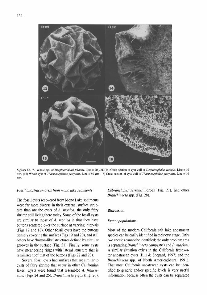
154
Figures 13-/6. Whole cyst of Streptocephalus texanus. Line = 20 {lll. (14) Cross-section of cyst wall of Streptocephalus texanus. Line = 10 fill. (15) Whole cyst of Thamnocephalus platyurus. Line = 50 fill. 16) Cross-section of cyst wall of Thamnocephalus platyurus. Line = 10 {lll.
Fossil anostracan cysts from mono lake sediments
The fossil cysts recovered from Mono Lake sediments were far more diverse in their external surface structure than are the cysts of A. monica, the only fairy shrimp still living there today. Some of the fossil cysts are similar to those of A. monica in that they have buttons scattered over the surface at varying intervals (Figs 17 and 18). Other fossil cysts have the buttons densely covering the surface (Figs 19 and 20), and still others have 'button-like' structures defined by circular grooves in the surface (Fig. 21). Finally, some cysts have meandering ridges with lateral structure that is reminiscent of that of the buttons (Figs 22 and 23).
Several fossil cysts had surfaces that are similar to cysts of fairy shrimp that occur in other Californian lakes. Cysts were found that resembled A. franciscana (Figs 24 and 25), Branchinecta gigas (Fig. 26),
Eubranchipus serratus Forbes (Fig. 27), and other Branchinecta spp. (Fig. 28).
Discussion
Extant populations
Most of the modem California salt lake anostracan species can be easily identified in their cyst stage. Only two species cannot be identified; the only problem area is separating Branchinecta campestris and B. mackini. A similar situation exists in the California freshwater anostracan cysts (Hill & Shepard, 1997) and the Branchinecta spp. of North America(Mura, 1991). That most California anostracan cysts can be identified to generic and/or specific levels is very useful information because often the cysts can be separated
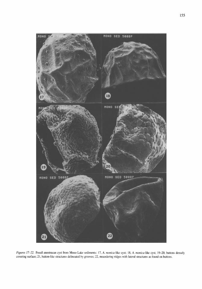
155
Figures 17-22. Fossil anostracan cyst from Mono Lake sediments: 17, A. monica-like cyst; 18, A. monica-like cyst; 19-20, buttons densely covering surface; 21, button-like structures delineated by grooves; 22, meandering ridges with lateral structures as found on buttons.
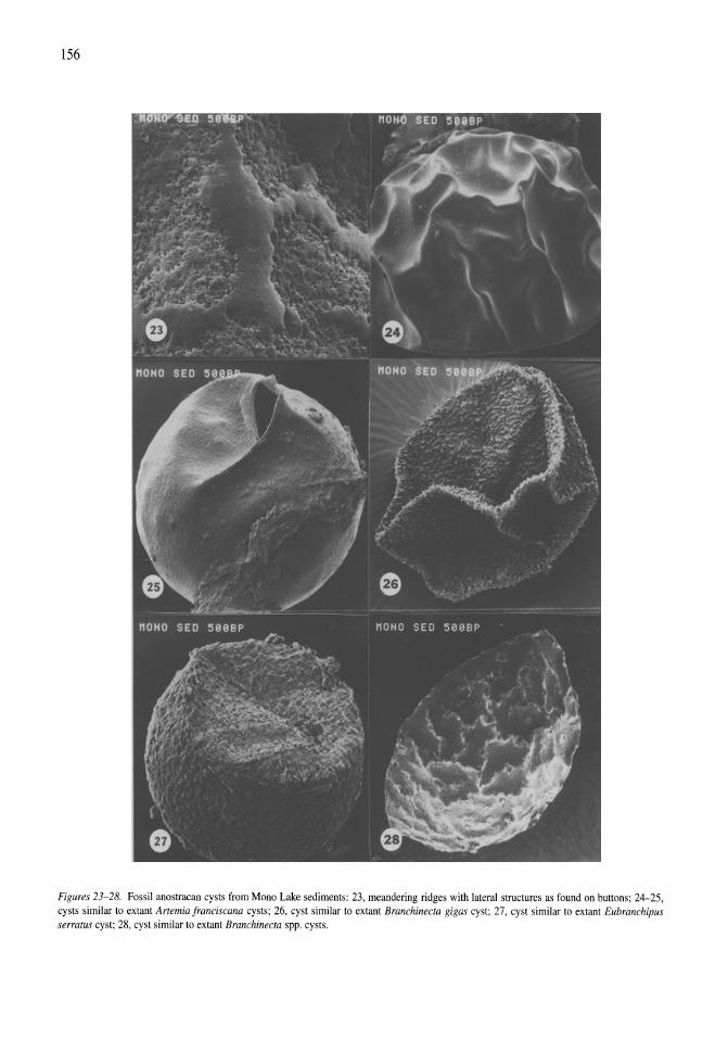
156
Figures 23-28. Fossil anostracan cysts from Mono Lake sediments: 23, meandering ridges with lateral structures as found on buttons; 24-25, cysts similar to extant Artemia franciscana cysts; 26, cyst similar to extant Branchinecta gigas cyst; 27, cyst similar to extant Eubranchipus serratus cyst; 28, cyst similar to extant Branchinecta spp. cysts.
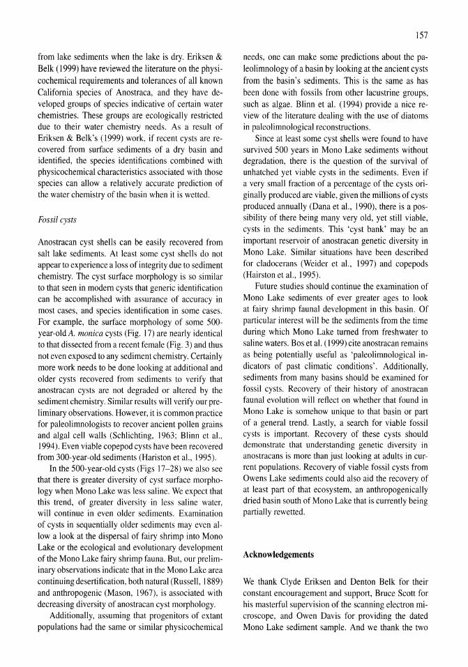
from lake sediments when the lake is dry. Eriksen & Belk (1999) have reviewed the literature on the physicochemical requirements and tolerances of all known California species of Anostraca, and they have developed groups of species indicative of certain water chemistries. These groups are ecologically restricted due to their water chemistry needs. As a result of Eriksen & Belk's (1999) work, if recent cysts are recovered from surface sediments of a dry basin and identified, the species identifications combined with physicochemical characteristics associated with those species can allow a relatively accurate prediction of the water chemistry of the basin when it is wetted.
Fossil cysts
Anostracan cyst shells can be easily recovered from salt lake sediments. At least some cyst shells do not appear to experience a loss of integrity due to sediment chemistry. The cyst surface morphology is so similar to that seen in modem cysts that generic identification can be accomplished with assurance of accuracy in most cases, and species identification in some cases. For example, the surface morphology of some 500-year-old A. monica cysts (Fig. 17) are nearly identical to that dissected from a recent female (Fig. 3) and thus not even exposed to any sediment chemistry. Certainly more work needs to be done looking at additional and older cysts recovered from sediments to verify that anostracan cysts are not degraded or altered by the sediment chemistry. Similar results will verify our preliminary observations. However, it is common practice for paleolirnnologists to recover ancient pollen grains and algal cell walls (Schlichting, 1963; Blinn et aI., 1994). Even viable copepod cysts have been recovered from 300-year-old sediments (Hariston et aI., 1995).
In the 500-year-old cysts (Figs 17-28) we also see that there is greater diversity of cyst surface morphology when Mono Lake was less saline. We expect that this trend, of greater diversity in less saline water, will continue in even older sediments. Examination of cysts in sequentially older sediments may even alIowa look at the dispersal of fairy shrimp into Mono Lake or the ecological and evolutionary development of the Mono Lake fairy shrimp fauna. But, our preliminary observations indicate that in the Mono Lake area continuing desertification, both natural (Russell, 1889) and anthropogenic (Mason, 1967), is associated with decreasing diversity of anostracan cyst morphology.
Additionally, assuming that progenitors of extant populations had the same or similar physicochemical
157
needs, one can make some predictions about the paleolimnology of a basin by looking at the ancient cysts from the basin's sediments. This is the same as has been done with fossils from other lacustrine groups, such as algae. Blinn et al. (1994) provide a nice review of the literature dealing with the use of diatoms in paleolimnological reconstructions.
Since at least some cyst shells were found to have survived 500 years in Mono Lake sediments without degradation, there is the question of the survival of unhatched yet viable cysts in the sediments. Even if a very small fraction of a percentage of the cysts originally produced are viable, given the millions of cysts produced annually (Dana et al., 1990), there is a possibility of there being many very old, yet still viable, cysts in the sediments. This 'cyst bank' may be an important reservoir of anostracan genetic diversity in Mono Lake. Similar situations have been described for cladocerans (Weider et aI., 1997) and copepods (Hairston et aI., 1995).
Future studies should continue the examination of Mono Lake sediments of ever greater ages to look at fairy shrimp faunal development in this basin. Of particular interest will be the sediments from the time during which Mono Lake turned from freshwater to saline waters. Bos et aI. (1999) cite anostracan remains as being potentially useful as 'paleolimnological indicators of past climatic conditions'. Additionally, sediments from many basins should be examined for fossil cysts. Recovery of their history of anostracan faunal evolution will reflect on whether that found in Mono Lake is somehow unique to that basin or part of a general trend. Lastly, a search for viable fossil cysts is important. Recovery of these cysts should demonstrate that understanding genetic diversity in anostracans is more than just looking at adults in current popUlations. Recovery of viable fossil cysts from Owens Lake sediments could also aid the recovery of at least part of that ecosystem, an anthropogenically dried basin south of Mono Lake that is currently being partially rewetted.
Acknowledgements
We thank Clyde Eriksen and Denton Belk for their constant encouragement and support, Bruce Scott for his masterful supervision of the scanning electron microscope, and Owen Davis for providing the dated Mono Lake sediment sample. And we thank the two
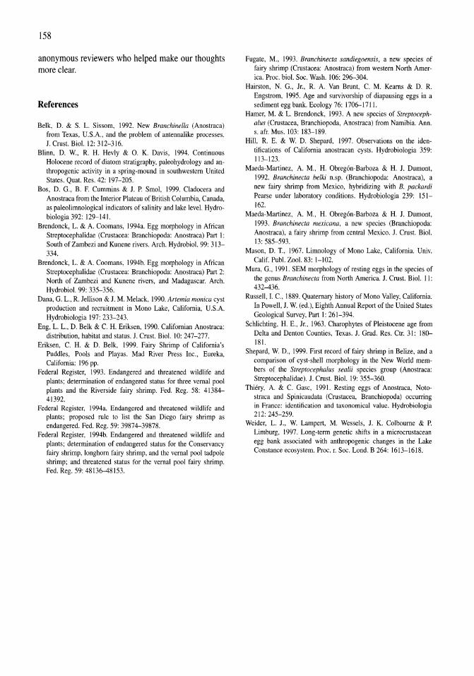
158
anonymous reviewers who helped make our thoughts more clear.
References
Belk. D. & S. L. Sissom. 1992. New Branchinella (Anostraca) from Texas, U.S.A., and the problem of antennalike processes. J. Crust. BioI. 12: 312-316.
Blinn, D. W, R. H. Hev1y & O. K. Davis, 1994. Continuous Holocene record of diatom stratigraphy, paleohydrology and anthropogenic activity in a spring-mound in southwestern United States. Quat. Res. 42: 197-205.
Bos, D. G., B. F. Cummins & 1. P. Smol, 1999. Cladocera and Anostraca from the Interior Plateau of British Columbia, Canada, as paleolimnological indicators of salinity and lake level. Hydrobiologia 392: 129-141.
Brendonck, L. & A. Coomans, 1994a. Egg morphology in African Streptocephalidae (Crustacea: Branchiopoda: Anostraca) Part I: South of Zambezi and Kunene rivers. Arch. Hydrobiol. 99: 313-334.
Brendonck, L. & A. Coomans, 1994b. Egg morphology in African Streptocephalidae (Crustacea: Branchiopoda: Anostraca) Part 2: North of Zambezi and Kunene rivers, and Madagascar. Arch. Hydrobiol. 99: 335-356.
Dana, G. L., R. Jellison & J. M. Melack, 1990. Artemia monica cyst production and recruitment in Mono Lake, California, U.S.A. Hydrobiologia 197: 233-243.
Eng, L. L., D. Belk & c. H. Eriksen, 1990. Californian Anostraca: distribution, habitat and status. J. Crust. BioI. 10: 247-277.
Eriksen, C. H. & D. Belk, 1999. Fairy Shrimp of California's Puddles, Pools and Playas. Mad River Press Inc., Eureka, California: 196 pp.
Federal Register, 1993. Endangered and threatened wildlife and plants; determination of endangered status for three vernal pool plants and the Riverside fairy shrimp. Fed. Reg. 58: 41384-41392.
Federal Register, I 994a. Endangered and threatened wildlife and plants; proposed rule to list the San Diego fairy shrimp as endangered. Fed. Reg. 59: 39874-39878.
Federal Register, 1994b. Endangered and threatened wildlife and plants; determination of endangered status for the Conservancy fairy shrimp, longhorn fairy shrimp, and the vernal pool tadpole shrimp; and threatened status for the vernal pool fairy shrimp. Fed. Reg. 59:48136-48153.
Fugate, M., 1993. Branchinecta sandiegoensis, a new species of fairy shrimp (Crustacea: Anostraca) from western North America. Proc. bioI. Soc. Wash. 106: 296--304.
Hairston, N. G., Jr., R. A. Van Brunt, C. M. Kearns & D. R. Engstrom, 1995. Age and survivorship of diapausing eggs in a sediment egg bank. Ecology 76: 1706--1711.
Hamer, M. & L. Brendonck, 1993. A new species of Streptocephalus (Crustacea, Branchiopoda, Anostraca) from Namibia. Ann. s. afro Mus. 103: 183-189.
Hill, R. E. & W D. Shepard, 1997. Observations on the identifications of California anostracan cysts. Hydrobiologia 359: 113-123.
Maeda-Martinez, A. M., H. Obregon-Barboza & H. 1. Dumont, 1992. Branchinecta belki n.sp. (Branchiopoda: Anostraca), a new fairy shrimp from Mexico, hybridizing with B. packardi Pearse under laboratory conditions. Hydrobiologia 239: 151-162.
Maeda-Martinez, A. M., H. Obregon-Barboza & H. 1. Dumont, 1993. Branchinecta mexicana, a new species (Branchiopoda: Anostraca), a fairy shrimp from central Mexico. 1. Crust. BioI. 13: 585-593.
Mason, D. 1., 1967. Limnology of Mono Lake, California. Univ. Calif. Publ. Zool. 83: 1-102.
Mura, G., 1991. SEM morphology ofresting eggs in the species of the genus Branchinecta from North America. 1. Crust. BioI. 11: 432--436.
Russell, I. C., 1889. Quaternary history of Mono Valley, California. In Powell, J. W (ed.), Eighth Annual Report ofthe United States Geological Survey, Part I: 261-394.
Schlichting. H. E., Jr., 1963. Charophytes of Pleistocene age from Delta and Denton Counties, Texas. J. Grad. Res. Ctr. 31: 180--181.
Shepard, W D., 1999. First record of fairy shrimp in Belize, and a comparison of cyst-shell morphology in the New World members of the Streptocephalus sealii species group (Anostraca: Streptocephalidae). 1. Crust. BioI. 19: 355-360.
Thiery, A. & C. Gasc, 1991. Resting eggs of Anostraca, Notostraca and Spinicaudata (Crustacea, Branchiopoda) occurring in France: identification and taxonomical value. Hydrobiologia 212: 245-259.
Weider, L. J., W Lampert, M. Wessels, 1. K. Colbourne & P. Limburg, 1997. Long-term genetic shifts in a microcrustacean egg bank associated with anthropogenic changes in the Lake Constance ecosystem. Proc. r. Soc. Lond. B 264: 1613-1618.
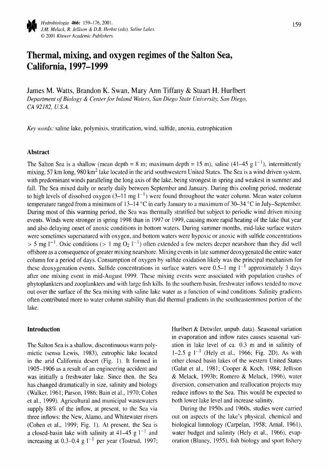
Hydrobiologia 466: 159-176,2001. J.M. Melack, R. Jellison & D.B. Herbst (eds), Saline Lakes. © 2001 Kluwer Academic Publishers.
159
Thermal, mixing, and oxygen regimes of the Salton Sea, California, 1997-1999
James M. Watts, Brandon K. Swan, Mary Ann Tiffany & Stuart H. Hurlbert Department of Biology & Center for Inland Waters, San Diego State University, San Diego, CA 92182, U.S.A.
Key words: saline lake, polymixis, stratification, wind, sulfide, anoxia, eutrophication
Abstract
The Salton Sea is a shallow (mean depth = 8 m; maximum depth = 15 m), saline (41-45 g I-I), intermittently mixing, 57 km long, 980 km2 lake located in the arid southwestern United States. The Sea is a wind driven system, with predominant winds paralleling the long axis of the lake, being strongest in spring and weakest in summer and fall. The Sea mixed daily or nearly daily between September and January. During this cooling period, moderate to high levels of dissolved oxygen (3-11 mg 1-1) were found throughout the water column. Mean water column temperature ranged from a minimum of 13-14 °C in early January to a maximum of 30-34 °C in July-September. During most of this warming period, the Sea was thermally stratified but subject to periodic wind driven mixing events. Winds were stronger in spring 1998 than in 1997 or 1999, causing more rapid heating of the lake that year and also delaying onset of anoxic conditions in bottom waters. During summer months, mid-lake surface waters were sometimes supersatured with oxygen, and bottom waters were hypoxic or anoxic with sulfide concentrations > 5 mg 1-1. Oxic conditions (> I mg 02 1-1) often extended a few meters deeper nearshore than they did well offshore as a consequence of greater mixing nearshore. Mixing events in late summer deoxygenated the entire water column for a period of days. Consumption of oxygen by sulfide oxidation likely was the principal mechanism for these deoxygenation events. Sulfide concentrations in surface waters were 0.5-1 mg I-I approximately 3 days after one mixing event in mid-August ]999. These mixing events were associated with population crashes of phytoplankters and zooplankters and with large fish kills. In the southern basin, freshwater inflows tended to move out over the surface of the Sea mixing with saline lake water as a function of wind conditions. Salinity gradients often contributed more to water column stability than did thermal gradients in the southeasternmost portion of the lake.
Introduction
The Salton Sea is a shallow, discontinuous warm polymictic (sensu Lewis, 1983), eutrophic lake located in the arid California desert (Fig. 1). It formed in ] 905-1906 as a result of an engineering accident and was initially a freshwater lake. Since then, the Sea has changed dramatically in size, salinity and biology (Walker, 196]; Parson, 1986; Bain et aI., 1970; Cohen et aI., ] 999). Agricultural and municipal wastewaters supply 88% of the inflow, at present, to the Sea via three inflows: the New, Alamo, and Whitewater rivers (Cohen et aI., ]999; Fig. I). At present, the Sea is a closed-basin lake with salinity at 4] -45 g I-I and increasing at 0.3-0.4 g 1-1 per year (Tostrud, 1997;
Hurlbert & Detwiler, unpub. data). Seasonal variation in evaporation and inflow rates causes seasonal variation in lake level of ca. 0.3 m and in salinity of ]-2.5 g 1-1 (Hely et aI., ]966; Fig. 2D). As with other closed basin lakes of the western United States (Galat et aI., ] 981; Cooper & Koch, 1984; Jellison & Melack, 1993b; Romero & Melack, ] 996), water diversion, conservation and reallocation projects may reduce inflows to the Sea. This would be expected to both lower lake level and increase salinity.
During the 1950s and 1960s, studies were carried out on aspects of the lake's physical, chemical and biological limnology (Carpelan, 1958; Arnal, 1961), water budget and salinity (Hely et aI., 1966), evaporation (Blaney, 1955), fish biology and sport fishery
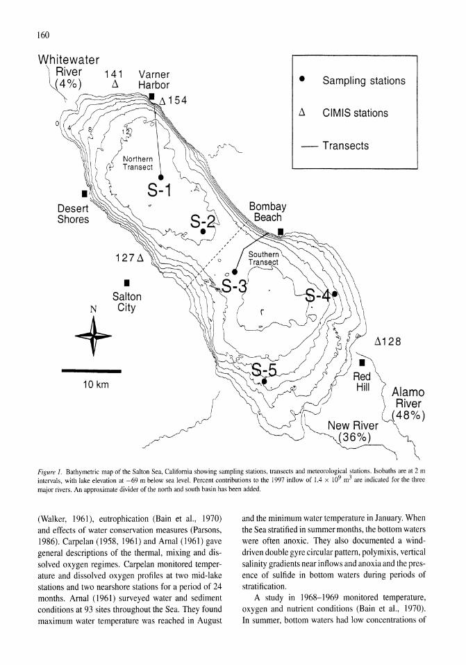
160
Whitewater 141
11 Varner Harbor ~iver
(4%) ---...~--:;=--=
~~~11154
o
Desert Shores
N
+ 10 km
• Salton City
• Sampling stations
11 CIMIS stations
- Transects
11128
Alamo River
(48%)
Figure 1. Bathymetric map of the Salton Sea, California showing sampling stations, transects and meteorological stations. Isobaths are at 2 m intervals, with lake elevation at -69 m below sea level. Percent contributions to the 1997 inflow of 1.4 x 10⁹ m3 are indicated for the three major rivers. An approximate divider of the north and south basin has been added.
(Walker, 1961), eutrophication (Bain et a!., 1970) and effects of water conservation measures (Parsons, 1986). Carpelan (1958, 1961) and Arnal (1961) gave general descriptions of the thermal, mixing and dissolved oxygen regimes. Carpelan monitored temperature and dissolved oxygen profiles at two mid-lake stations and two nearshore stations for a period of 24 months. Arnal (1961) surveyed water and sediment conditions at 93 sites throughout the Sea. They found maximum water temperature was reached in August
and the minimum water temperature in January. When the Sea stratified in summer months, the bottom waters were often anoxic. They also documented a winddriven double gyre circular pattern, polymixis, vertical salinity gradients near inflows and anoxia and the presence of sulfide in bottom waters during periods of stratification.
A study in 1968-1969 monitored temperature, oxygen and nutrient conditions (Bain et a!., 1970). In summer, bottom waters had low concentrations of
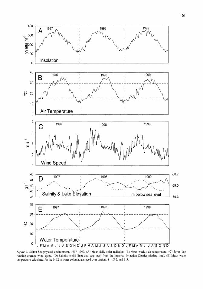
400 1998 1999
N 300 'E ~200 CO
$100
0 Insolation
40 1997 1998 1999
30
~ 20
10
0 Air Temperature
5
C 1997 1998 1999
4
";" I/)
E 3
2
1 . Wind Speed
46 ,-----------------------------------------------------------,
44
- 42 OJ
40
o 1997
.... ' ..
1998 1999 .... - ..... .-.
-.. - -- ..... -
-68.7
-69.0
38 Salinity & Lake 'Ei~~ation m below sea level l---, __ ~:!......._,----__ __'_ _________________ ~___:.c.:..::..::..:.:...:..:....:....::..:::....:..::...:...::..'______1 -69.3
40
E 1997 1998 1999
30 ---------------
~ 20
10
Water Temperature: o JFMAMJ JASOND JFMAMJ JASONDJFMAMJ JASOND
161
Figure 2, Salton Sea physical environment, 1997-1999, (A) Mean daily solar radiation. (E) Mean weekly air temperature, (e) Seven day running average wind speed. (D) Salinity (solid line) and lake level from the Imperial Irrigation District (dashed line). (E) Mean water temperature calculated for the 0-12 m water column, averaged over stations S-I, S-2, and S-3.
162
Table 1. Location and attributes of Salton Sea sampling stations
Station Depth (m) Distance to Geographic coordinates
shore (km) (N latitude; W longitude)
Primary sampling stations S-I 14 6.7 33° 25' 00//; 1150 55' 00//
S-2 12 6.1 33° 21' 00//; 115° SI' 00//
S-3 12 7.6 33° IS' 00//; 115° 4S' 00//
S-4 3.5 33° 16'30//; 115° 38'SO//
S-5 4.5 33° la' 00//; IISo 4S' 30//
Northern transect stations T-I 6 0.1 33° 30'16//; 11So SS' 11//
T-2 0.15 33° 3D' 13//; 115° S5' 13//
T-3 OJ 33° 30' 00//; l1So SS' 18//
T-4 10 2.0 33° 29' 74//; 115° 55' 20//
T-5 12 4.0 33° 29' 17//; 115° 5S' 10//
S-I 14 6.7 33° 25' 00//; 115° 55' 00//
Southern transect stations T-6 2 0.2 33° 21' 13//; 115° 44' 92"
T-7 4 0.4 33° 21' 00//; 115° 45' 03//
T-S 6 0.45 33° 20' 96//; llSo 45' 17//
T-9 0.8 33° 20' 85//; llSo 45' 34//
T-IO 10 3.6 33° 20' 66//; 115° 45' 72//
T-II II 4.4 33° 19'99//; IISo 47' 00//
S-3 12 7.6 33° 18' 00//; 115° 48' 00//
dissolved oxygen and were often hypoxic or anoxic. Surface waters were generally well oxygenated and even supersaturated. Low dissolved oxygen and sulfide were thought possibly responsible for fish kills, but the possibility of ammonia toxicity or toxic algae was not ruled out.
We initiated a long-term study in January 1997 to investigate various aspects of the physics, chemistry and biology of the Salton Sea. In this article, mixing, thermal and dissolved oxygen regimes, along with climatic data are described and analyzed for the 3-year period 1997-1999. The plankton, benthos, fish and aquatic birds of the Sea are affected in numerous direct and indirect ways by the physical and chemical behavior of the system. This study provides a foundation for forthcoming analyses of those populations (Detwiler et a!., 200 I; Riedel et a!., 2002; Tiffany et a!., 2002).
Methods
Monitoring regime
Monitoring of physical and chemical conditions was conducted at three mid-lake stations (S-I, S-2 and
S-3) beginning in January 1997, and at two near shore stations (S-4 and S-5) beginning in January 1999 (Fig. I, Table I). The first three stations were chosen to represent the main water mass of the Sea. The two additional ones were added to better sample the southern basin, monitor nearshore areas, and to document the influence of freshwater inflows. Due to the counter-clockwise current system in the southern part of the Sea, station S-4 was 'upstream' and station S-5 was 'downstream' from the mouths of the two main freshwater inflows.
Monitoring was conducted at 2-5 week intervals, although in 1997-1998 some stations were not visited on all dates due to logistical problems or storms. Sampling dates were, for 1997: 21 January (2,3), 3 February (3), 22 February (2,3), 19 March (2,3), 16 April (3), 20 May (3), 3 June (3), 24 June, 18 July (2,3), 13 August (2), 6 September (2,3), 17 October, 7 November, 25 November; for 1998: 6 January (2,3), 6 February (2,3), 27 February (3), 30 March, 24 April (2,3), 22 May, 4 June, 3 July, 16 July, 30 July, 24 August (2,3), 12 September (2,3), 7 November (2,3), 12 December; and for 1999: 25 January, 28 February, 16 March, 7 April, 25 April, 10 May, 25 May, 8 June, 23 June, 5 July, 19 July, 30 July, 16 August, 28 August, 25 September, 19 October, 2 November, 23 November, 7 December, 6; and for 2000: January 6. Numbers in parentheses in this list indicate the specific stations that were not visited on a given date. Stations were visited, usually in numerical order, between 0800 and 1500 h.
Measurements of temperature, dissolved oxygen and specific conductance were made at each station from surface (actually 15 cm below the surface) to bottom at 1 m intervals using a thermistor (accurate to 0.05±0.01 QC), rapid pulse oxygen probe (accurate to 0.2±0.01 mg I-I), and a 4 electrode specific conductance probe (accurate to 0.01±0.01 mS cm- I )
housed in a YSI 45 or a YSI 6000UPG sonde. At each station phytoplankton, zooplankton, nitrogen, phosphorus and silica concentrations, pH, oxidationreduction potential, light attenuation and Sec chi depth were also sampled or measured. Those variables are reported and analyzed in other reports (Tiffany et a!., 2002). Specific conductance was measured starting 16 July 1998.
As the Salton Sea is located below sea level, measurements of dissolved oxygen must account for the increased atmospheric pressure. Prior to July 1998, dissolved oxygen probes were calibrated daily in air at 100 percent humidity, correcting for probe tem-
perature and for atmospheric pressure using altitude (69 m below sea level). This method did not take into account variations in atmospheric pressure at different sampling dates due to meteorological conditions (source of 2---4% variation). After July 1998, a temperature corrected surveying barometer (Taylor SMT-5-51) was used to calibrate dissolved oxygen concentrations daily in air at 100% humidity, correcting for atmospheric pressure directly. The barometer itself was calibrated using a constant temperature mercury barometer (22 0C) located at San Diego State University. The specific conductance probe was calibrated at 3 month intervals. A two point calibration was performed at temperatures close to 25 °C using standards that covered the expected range of values encountered of ~ I 0 and 65 mS. The temperature thermistor was factory calibrated and did not require calibration during this study.
Observations on a sonar depth sounder suggested that fish vacated the center of the lake in early summer, later confirmed by gill-netting (Riedel et aI., 2002), and led us to examine variation in dissolved oxygen concentrations as a function of distance from shore. Temperature and dissolved oxygen profiles were taken at five stations along each of two onshore-offshore transects on 17 June and 29 August 1999 and 6 January 2000 (Fig. I). A northern transect covered a depth range of 4-14 m and extended from Varner Harbor to mid-lake station S-l. A southern transect covered a depth range of 2-12 m and extended from Bombay Beach to mid-lake station S-3 (Fig. I, Table I). Measurement procedures and depth intervals were the same as for the monitoring of mid-lake stations.
We measured sulfide in the water column on two dates (31 July and 16 August 1999) at all five midlake sampling stations after sulfide was detected in the air during mixing events. Measurements were made at 2 m intervals from surface to bottom using a lead acetate paper (accurate to 0.1±0.5 mg I-I; APHA, 1998). These two dates represented a stratified and a mixed condition, respectively.
Lake elevation data were obtained from the Imperial Irrigation District. These data were taken on the first of every month from January 1997 to December 1999.
Analysis of limnological data
Analysis of data considers that we have data for the whole 1997-1999 period only for the three mid-lake stations. Only for 1999 do we have the additional in-
163
formation on spatial variation provided by stations S-4 and S-5. Mean water temperatures were calculated using data from 0-12 m depths at stations S-l, S-2 and S-3. For this purpose, temperatures at 0 and 1 m were set equal to the temperature at 2 m to reduce noise caused by diel warming and cooling of surface waters.
Mean oxygen profiles for overlying water of stations S-I, S-2 and S-3 and Salton Sea bathymetric data (Ferrari & Weghorst, 1997) were used to calculate the percentage of lake bottom exposed to different dissolved oxygen concentrations: < I mg 1-1, 1-2 mg 1-1, 2---4 mg 1-1, and> 4 mg I-I (Fig. 3C). This calculation assumed a maximum depth of IS m, that oxygen levels below 14 m were the same as those at 14 m, and that dissolved oxygen concentration at a given depth nearshore was the same as the mean oxygen concentration of water at the same depth at the mid-lake stations.
Sulfide oxidation has potential for deoxygenating the water column during mixing events following stratification. We quantified this using oxygen and sulfide profiles for 31 July and 16 August 1999, a mixing and deoxygenation event apparently having occurred between the two dates. pH on these dates was 7.6 - 8.3, and in this range sulfide is found primarily as sulfide ion (HS-) (~80%, pKA 6.88 for 35 g I-I) with hydrogen sulfide (H2S) making up ~ 20% and S2- making up less than 1% (Snoeyink & Jenkins, 1980; Millero, 1986). Proposed reactions of the oxidation of sulfide have three products; thiosulfate, sulfite and sulfate. With time, both thiosulfate and sulfite are converted to sulfate. In addition, experimental data has shown that when oxygen is the limiting reagent in the sulfide oxidation reaction , as in the Sea on the dates sulfide was measured, greater than 50% of the reaction products of sulfide oxidation are sulfate (Cline & Richards, 1969). Therefore, consumption of dissolved oxygen in the lake by oxidation of sulfide was calculated using the reaction:
HS- + 202 -> S042- + H+ (Chen & Morris, 1972)
Three assumptions were made in this calculation. First, that hydrogen sulfide is converted to sulfide ion before oxidization during a mixing event. This assumption makes our estimate of oxygen consumption conservative as more dissolved oxygen is consumed in the oxidation of hydrogen sulfide than in the oxidation of sulfide ion. Second, that all sulfide is oxidized to sulfate. Third, that the dissolved oxygen and sulfide profiles prior to the mixing event were similar to those of 31 JUly.
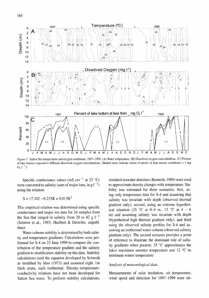
164
.I:
0. Q)
o
100 1997 Percent of lake bottom at less than _ mg02 r1 1999
C 80 -
I r:: 60 Q) u
I .... Q) 40 Q.
20
0 J F M A M J J A D J F M A M J J A S o N D J F M A M J J A SON D
Figure 3. Salton Sea temperature and oxygen conditions, 1997-1999. (A) Water temperature. (B) Dissolved oxygen concentrations. (C) Percent of lake bottom exposed to different dissolved oxygen concentrations. Shaded areas indicate extent of anoxic or near anoxic conditions (> I mg 02 1- 1).
Specific conductance values (mS cm- I at 25 DC) were converted to salinity (sum of major ions, in g 1-1) using the relation:
S = 17.102 -0.233K+ 0.013K2
This empirical relation was determined using specific conductance and major ion data for 24 samples from the Sea that ranged in salinity from 20 to 42 g I-I (Setmire et aI., 1993; Hurlbert & Detwiler, unpubl. data).
Water column stability is determined by both salinity and temperature gradients. Calculations were performed for S-4 on 23 June 1999 to compare the contribution of the temperature gradient and the salinity gradient to stratification stability on this date. Stability calculations used the equation developed by Schmidt as modified by Idso (1973) and assumed eight 1m thick strata, each isothermal. Density-temperatureconductivity relations have not been developed for Salton Sea water. To perform stability calculations,
standard seawater densities (Kennish, 1989) were used to approximate density changes with temperature. Stability was estimated for three scenarios; first, using only temperature data for S-4 and assuming that salinity was invariate with depth (observed thermal gradient only); second, using an extreme hypothetical situation (35 DC at 0-4 m, 12 DC at 4 - 6 m) and assuming salinity was invariate with depth (hypothetical high thermal gradient only); and third using the observed salinity profiles for S-4 and assuming an isothermal water column (observed salinity gradient only). The second scenario provides a point of reference to illustrate the dominant role of salinity gradients when present; 35 DC approximates the lakes maximum summer temperature and 12 DC its minimum winter temperature
Analysis of meteorological data
Measurements of solar insolation, air temperature, wind speed and direction for 1997-1999 were ob-
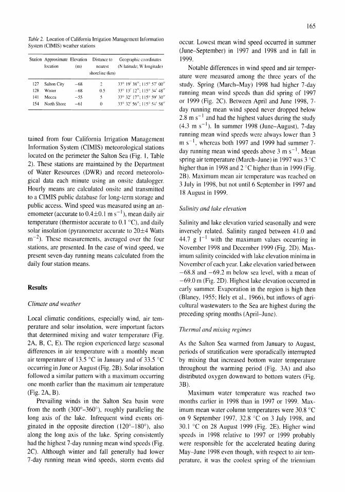
Table 2. Location of California Irrigation Management Infonnation System (CIMIS) weather stations
Station Approximate Elevation Distance to Geographic coordinates
location (m) nearest (N latitude; W longitude)
shoreline (km)
127 Salton City -68 2 33° 19' 38"; 115° 57' 00"
128 Wister -68 0.5 33° I3' 12"; 115° 34' 48"
141 Mecca -55 5 33° 32' 17"; 115° 59' 30"
154 North Shore -61 0 33° 32' 56"; 115° 54' 58"
tained from four California Irrigation Management Information System (CIMIS) meteorological stations located on the perimeter the Salton Sea (Fig. I, Table 2). These stations are maintained by the Department of Water Resources (DWR) and record meteorological data each minute using an onsite datalogger. Hourly means are calculated onsite and transmitted to a CIMIS public database for long-term storage and public access. Wind speed was measured using an anemometer (accurate to 0.4±0.1 m s-I), mean daily air temperature (thermistor accurate to 0.1 °C), and daily solar insolation (pyranometer accurate to 20±4 Watts m-2). These measurements, averaged over the four stations, are presented. In the case of wind speed, we present seven-day running means calculated from the daily four station means.
Results
Climate and weather
Local climatic conditions, especially wind, air temperature and solar insolation, were important factors that determined mixing and water temperature (Fig. 2A, B, C, E). The region experienced large seasonal differences in air temperature with a monthly mean air temperature of 13.5 °C in January and of 33.5 °C occurring in June or August (Fig. 2B). Solar insolation followed a similar pattern with a maximum occurring one month earlier than the maximum air temperature (Fig. 2A, B).
Prevailing winds in the Salton Sea basin were from the north (300°-360°), roughly paralleling the long axis of the lake. Infrequent wind events originated in the opposite direction (120°-180°), also along the long axis of the lake. Spring consistently had the highest 7-day running mean wind speeds (Fig. 2C). Although winter and fall generally had lower 7-day running mean wind speeds, storm events did
165
occur. Lowest mean wind speed occurred in summer (June-September) in 1997 and 1998 and in fall in 1999.
Notable differences in wind speed and air temperature were measured among the three years of the study. Spring (March-May) 1998 had higher 7-day running mean wind speeds than did spring of 1997 or 1999 (Fig. 2C). Between April and June 1998, 7-day running mean wind speed never dropped below 2.8 m s-I and had the highest values during the study (4.3 m s-I). In summer 1998 (June-August), 7-day running mean wind speeds were always lower than 3 m s-I, whereas both 1997 and 1999 had summer 7-day running mean wind speeds above 3 m s-I. Mean spring air temperature (March-June) in 1997 was 3 °C higher than in 1998 and 2 °C higher than in 1999 (Fig. 2B). Maximum mean air temperature was reached on 3 July in 1998, but not until 6 September in 1997 and 18 August in 1999.
Salinity and lake elevation
Salinity and lake elevation varied seasonally and were inversely related. Salinity ranged between 41.0 and 44.7 g I-I with the maximum values occurring in November 1998 and December 1999 (Fig. 2D). Maximum salinity coincided with lake elevation minima in November of each year. Lake elevation varied between -68.8 and -69.2 m below sea level, with a mean of -69.0 m (Fig. 2D). Highest lake elevation occurred in early summer. Evaporation in the region is high then (Blaney, 1955; Hely et aI., 1966), but inflows of agricultural wastewaters to the Sea are highest during the preceding spring months (April-June).
Thermal and mixing regimes
As the Salton Sea warmed from January to August, periods of stratification were sporadically interrupted by mixing that increased bottom water temperature throughout the warming period (Fig. 3A) and also distributed oxygen downward to bottom waters (Fig. 3B).
Maximum water temperature was reached two months earlier in 1998 than in 1997 or 1999. Maximum mean water column temperatures were 30.8 °C on 9 September 1997, 32.8 °C on 3 July 1998, and 30.1 °C on 28 August 1999 (Fig. 2E). Higher wind speeds in 1998 relative to 1997 or 1999 probably were responsible for the accelerated heating during May-June 1998 even though, with respect to air temperature, it was the coolest spring of the triennium
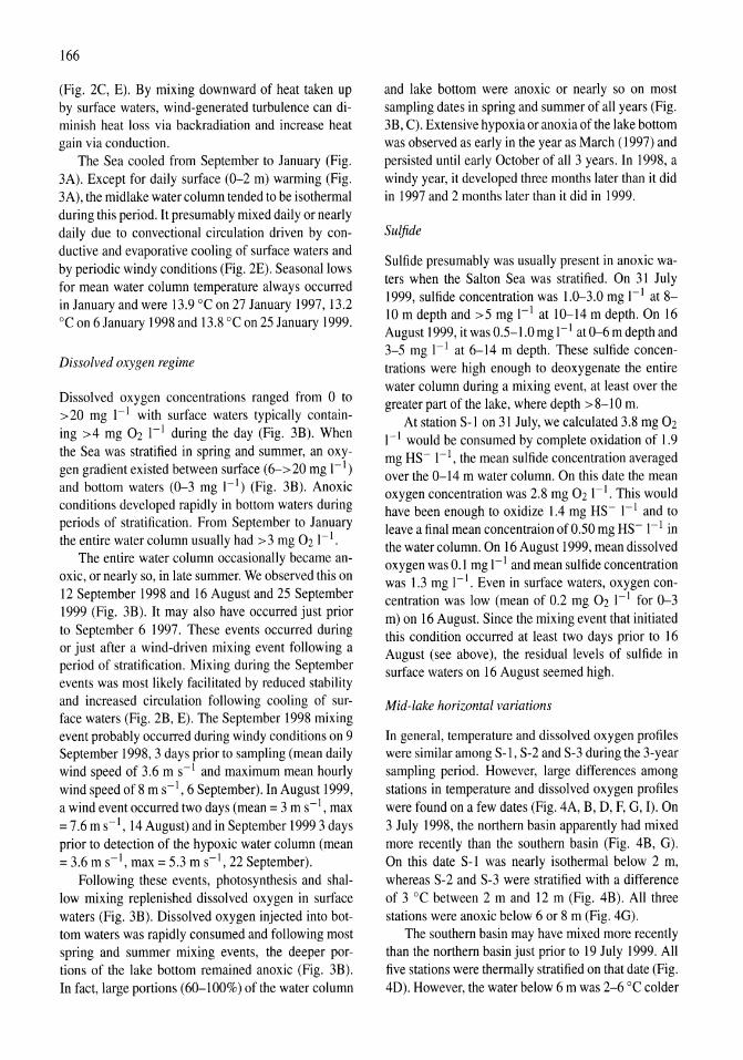
166
(Fig. 2C, E). By mixing downward of heat taken up by surface waters, wind-generated turbulence can diminish heat loss via backradiation and increase heat gain via conduction.
The Sea cooled from September to January (Fig. 3A). Except for daily surface (0-2 m) warming (Fig. 3A), the midlake water column tended to be isothermal during this period. It presumably mixed daily or nearly daily due to convectional circulation driven by conductive and evaporative cooling of surface waters and by periodic windy conditions (Fig. 2E). Seasonal lows for mean water column temperature always occurred in January and were 13.9 °C on 27 January 1997, 13.2 °C on 6 January 1998 and 13.8 °C on 25 January 1999.
Dissolved oxygen regime
Dissolved oxygen concentrations ranged from 0 to >20 mg 1-1 with surface waters typically containing >4 mg 02 1-1 during the day (Fig. 3B). When the Sea was stratified in spring and summer, an oxygen gradient existed between surface (6-> 20 mg 1-1 ) and bottom waters (0-3 mg 1-1) (Fig. 3B). Anoxic conditions developed rapidly in bottom waters during periods of stratification. From September to January the entire water column usually had> 3 mg 02 1-1.
The entire water column occasionally became anoxic, or nearly so, in late summer. We observed this on 12 September 1998 and 16 August and 25 September 1999 (Fig. 3B). It may also have occurred just prior to September 6 1997. These events occurred during or just after a wind-driven mixing event following a period of stratification. Mixing during the September events was most likely facilitated by reduced stability and increased circulation following cooling of surface waters (Fig. 2B, E). The September 1998 mixing event probably occurred during windy conditions on 9 September 1998, 3 days prior to sampling (mean daily wind speed of 3.6 m s-1 and maximum mean hourly wind speed of 8 m s -1 , 6 September). In August 1999, a wind event occurred two days (mean = 3 m s-1 , max = 7.6 m s-l, 14 August) and in September 1999 3 days prior to detection of the hypoxic water column (mean = 3.6 m s-l, max = 5.3 m s-l, 22 September).
Following these events, photosynthesis and shallow mixing replenished dissolved oxygen in surface waters (Fig. 3B). Dissolved oxygen injected into bottom waters was rapidly consumed and following most spring and summer mixing events, the deeper portions of the lake bottom remained anoxic (Fig. 3B). In fact, large portions (60-100%) of the water column
and lake bottom were anoxic or nearly so on most sampling dates in spring and summer of all years (Fig. 3B, C). Extensive hypoxia or anoxia of the lake bottom was observed as early in the year as March (1997) and persisted until early October of all 3 years. In 1998, a windy year, it developed three months later than it did in 1997 and 2 months later than it did in 1999.
Sulfide
Sulfide presumably was usually present in anoxic waters when the Salton Sea was stratified. On 31 July 1999, sulfide concentration was 1.0-3.0 mg 1-1 at 8-10 m depth and >5 mg 1-1 at 10-14 m depth. On 16 August 1999, it wasO.5-1.0mg 1-1 at 0-6 m depth and 3-5 mg 1-1 at 6-14 m depth. These sulfide concentrations were high enough to deoxygenate the entire water column during a mixing event, at least over the greater part of the lake, where depth > 8-1 0 m.
At station S-I on 31 July, we calculated 3.8 mg 02 1-1 would be consumed by complete oxidation of 1.9 mg HS- 1-1, the mean sulfide concentration averaged over the 0-14 m water column. On this date the mean oxygen concentration was 2.8 mg 021-1. This would have been enough to oxidize 1.4 mg HS- 1-1 and to leave a final mean concentraion of 0.50 mg HS - 1-1 in the water column. On 16 August 1999, mean dissolved oxygen was 0.1 mg 1-1 and mean sulfide concentration was 1.3 mg 1-1. Even in surface waters, oxygen concentration was low (mean of 0.2 mg 02 1-1 for 0-3 m) on 16 August. Since the mixing event that initiated this condition occurred at least two days prior to 16 August (see above), the residual levels of sulfide in surface waters on 16 August seemed high.
Mid-lake horizontal variations
In general, temperature and dissolved oxygen profiles were similar among S-l, S-2 and S-3 during the 3-year sampling period. However, large differences among stations in temperature and dissolved oxygen profiles were found on a few dates (Fig. 4A, B, D, F, G, I). On 3 July 1998, the northern basin apparently had mixed more recently than the southern basin (Fig. 4B, G). On this date S-l was nearly isothermal below 2 m, whereas S-2 and S-3 were stratified with a difference of 3 °C between 2 m and 12 m (Fig. 4B). All three stations were anoxic below 6 or 8 m (Fig. 4G).
The southern basin may have mixed more recently than the northern basin just prior to 19 July 1999. All five stations were thermally stratified on that date (Fig. 4D). However, the water below 6 m was 2-6 °C colder
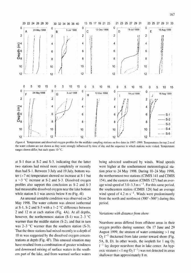
167
20 22 24 26 28 30 30 32 34 36 38 40 13 15 17 19 21 23 21 23 25 27 29 31 23 25 27 29 31 33 o ------J
2
£6 Co Q)
08
A
,
, ,
10· ,
12
o
24-May1998 ,
, , I I
.. 1
5 10 15
o o 3-Ju11998 '
B 2 2
4 - 4
6 6
8 8
10
12 12
o 5 10 15 0
D
-L_~
19-Ju11999, c 12-Dec 1998, o o ~
I 16-Aug 1999' E
2 2
4 4
6 6
8 8
10 10
12 12
5 10 15 o 5 10 15 o 5 10 15
G 3-Ju11998 , 0 +---L-12--D-e-c-19-9-'8
H o
16-Aug 1999: o I---'_~_-l
24-May1998 o
F 2
10
12
I.' 1
I , J
'J !: ;, ., " I, :.: I" '. , ,
2 2 .J'" " ,
/' I 4 4 , 6
8
10 10
12 _ ... -... __ ._._ .. __ .-... 12
2
4
6
'/I , ft: , /I , '. I ~ I }:I
"[i l r
: I 8 ,
, : 10 ;'
;/ ;,
12 ~.-
J
2 I:" , .," '1 f
4 U "
6 " 8
10
--S-1
-- -- S-2 :
·····-·S-3 : _·_·-S-4 :
_ .. -. S-5 12 .. _ ........... ..
Figure 4, Temperature and dissolved oxygen profiles for the midlake sampling stations on five dates in 1997-1999. Temperatures for top 2 m of the water column are not shown as they were strongly influenced by time of day and the sequence in which stations were visited. Temperature ranges shown differ, but each spans 10 °C.
at S-1 than at S-2 and S-3, indicating that the latter two stations had mixed more completely or recently than had S-1. Between 3 July and 19 July, bottom water (> 7 m) temperature showed no increase at S-l but a ~3 °C increase at S-2 and S-3, Dissolved oxygen profiles also support this conclusion as S-2 and S-3 had measurable dissolved oxygen near the lake bottom while station S-1 was anoxic below 8 m (Fig. 41)
An unusual unstable condition was observed on 24 May 1998. The water column was almost isothermal at S-I, S-2 and S-3 with a I-2°C difference between 2 and 12 m at each station (Fig. 4A). At all depths, however, the northernmost station (S-1) was 2-3 °C warmer than the middle station (S-2), and that in tum was 2-3 °C warmer than the southern station (S-3). That the three stations had mixed recently to a depth of 10 m was suggested by the dissolved oxygen concentrations at depth (Fig. 4F). This unusual situation may have resulted from a combination of greater windiness and downward mixing of surface waters in the southern part of the lake, and from warmed surface waters
being advected southward by winds. Wind speeds were higher at the southernmost meteorological station prior to 24 May 1998. During 10-24 May 1998, the northernmost two stations (CIMIS 141 and CIMIS 154), and the eastern station (CIMIS 127) had an average wind speed of 3.0-3.3 m s-I. For this same period, the southeastern station (CIMIS 128) had an average wind speed of 4.2 m s-I. Winds were predominantly from the north and northwest (300°-360°) during this period.
Variations with distance from shore
Nearshore areas differed from offshore areas in their oxygen profiles during summer. On 17 June and 29 August 1999, the stratum of water containing > 1 mg 02 I-I thickened from lake center toward shore (Fig. SA, B, D). In other words, the isopleth for 1 mg 02 I-I lay deeper nearshore than in lake center. An hypoxic stratum ( < 1 mg 02 I-I) was not detected in areas shallower than approximately 8 m.
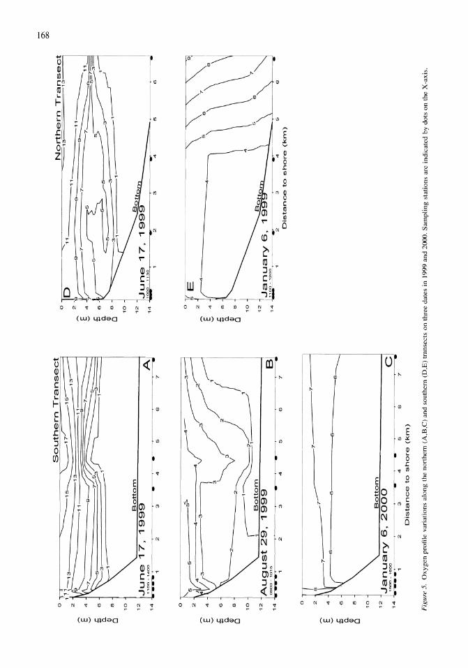
E
~
.c a. Q)
Cl '"' E
~
.c .... c. Q)
Cl S .c .... c. Q)
Cl
" "--
-2j
'\
.~~
0,,,
~
11~
._
11
2.ttg
1
1 ---..r"7~
.'----==-7~~~
5 _
_ ,
3
4 6 a
o N
orth
ern
Tra
nse
ct
ID
'" --=
=1
3
13
2
.
11
_
.-. V
-9
-9
11
=------
---S
4 J,r
-~5
7 -~~=7~
.c ~~ ~~
5.....---
3
~ 6
i"
<=
5 ..
...-
5~_3
----
----
" Cl
a
3 3
_1
---'
r--'
1
0
10
Bo
tto
m
12
Ju
ne 1
7,
19
99
1
'00
-1
40
0
14
•
_w_ i
_ _
_
2 3
4 5
6
A
7
12
6
130
t
Ju
ne 1
7,
19
99
1
4 ~o -
11
30
_
--=---
----
.J
2 3
4 5
0, 5'>
/-~3
., l~/',//
~,L
Bo
tto
m
2 4 6
10
a "-2
_
12
J~~~,~st 2
9,
19
99
S
J
14
.-
__
,
__
OTT
\\'\"
9 5
E
2 .....
.
~l'\
\\ .
S 4
.c ....
6 a. ~
a
10
b_
"
\ 5
, 6
, 7
12
Jan
uary
6,
14
1
10
0 -
12
00
2 3
4 5
6 2
3 4
5 6
7 D
ista
nce
to
sh
ore
(km
)
o
r a , __
____
--7---
-7
7' ____
-' 2 4
,...
.---
---e
6
6 6
6 a
10
Bo
tto
m
12
-!~~6~ary 6
, 2
00
0
C,
14
_
_ •
2 3
4 5
6 7
Dis
tan
ce
to
sh
ore
(krn
)
Fig
ure
5.
Oxy
gen
prof
ile
vari
atio
ns a
long
the
nor
ther
n (A
,B,C
) an
d so
uthe
rn (
D,E
) tr
anse
cts
on t
hree
dat
es i
n 19
99 a
nd 2
000.
Sam
plin
g st
atio
ns a
re i
ndic
ated
by
dots
on
the
X~a
xis.
......
0-
00
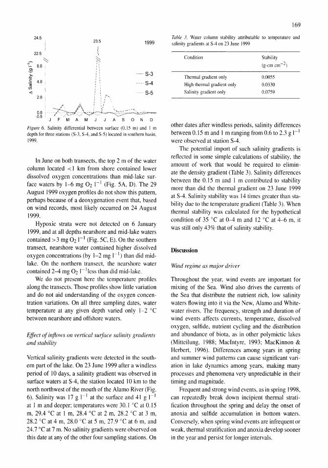
169
24.5 Table 3. Water column stability attributable to temperature and 1999 salinity gradients at S-4 on 23 June 1999 23.5
~ 22.5 "
~ ~ '- 6.0 " I " .9 ' I
I I
~ , I , I
:E 4.0 ' I
I I I
iii I I
II) I ' I
<l : I I
-8-3
---- 8-4
------ 8-5 2.0
j I I ,
i " , , , I
0.0 , I
i ."' '. -0.5 ' -
J F M A M J
\
~.~:.::";::.-:- --'> ..... -.,...,... ." A SON 0
Figure 6. Salinity differential between surface (0.15 m) and I m depth for three stations (S-3, S-4, and S-5) located in southern basin, 1999.
In June on both transects, the top 2 m of the water column located < 1 km from shore contained lower dissolved oxygen concentrations than mid-lake surface waters by 1-6 mg 02 I-I (Fig. SA, D). The 29 August 1999 oxygen profiles do not show this pattern, perhaps because of a deoxygenation event that, based on wind records, most likely occurred on 24 August 1999.
Hypoxic strata were not detected on 6 January 1999, and at all depths nearshore and mid-lake waters contained >3 mg 021-1 (Fig. 5C, E). On the southern transect, nearshore water contained higher dissolved oxygen concentrations (by 1-2 mg I-I) than did midlake. On the northern transect, the nearshore water contained 2-4 mg 02 I-Iless than did mid-lake.
We do not present here the temperature profiles along the transects. Those profiles show little variation and do not aid understanding of the oxygen concentration variations. On all three sampling dates, water temperature at any given depth varied only I-2°C between nearshore and offshore waters.
Effect of inflows on vertical sUrface salinity gradients and stability
Vertical salinity gradients were detected in the southern part of the lake. On 23 June 1999 after a windless period of 10 days, a salinity gradient was observed in surface waters at S-4, the station located 10 km to the north northwest of the mouth of the Alamo River (Fig. 6). Salinity was 17 g I-I at the surface and 41 g I-I at 1 m and deeper; temperatures were 30.1 °C at 0.15 m, 29.4 °C at 1 m, 28.4 °C at 2 m, 28.2 °C at 3 m, 28.2 °C at 4 m, 28.0 °C at 5 m, 27.9 °C at 6 m, and 24.7 °C at 7 m. No salinity gradients were observed on this date at any of the other four sampling stations. On
Condition
Thermal gradient only
High thermal gradient only
Salinity gradient only
Stability
(g-cmcm-2)
0.0055
0.0330
0.0759
other dates after windless periods, salinity differences between 0.15 m and I m ranging from 0.6 to 2.3 g I-I were observed at station S-4.
The potential import of such salinity gradients is reflected in some simple calculations of stability, the amount of work that would be required to eliminate the density gradient (Table 3). Salinity differences between the 0.15 m and 1 m contributed to stability more than did the thermal gradient on 23 June 1999 at S-4. Salinity stability was 14 times greater than stability due to the temperature gradient (Table 3). When thermal stability was calculated for the hypothetical condition of 35°C at 0-4 m and 12°C at 4-6 m, it was still only 43% that of salinity stability.
Discussion
Wind regime as major driver
Throughout the year, wind events are important for mixing of the Sea. Wind also drives the currents of the Sea that distribute the nutrient rich, low salinity waters flowing into it via the New, Alamo and Whitewater rivers. The frequency, strength and duration of wind events affects currents, temperature, dissolved oxygen, sulfide, nutrient cycling and the distribution and abundance of biota, as in other polymictic lakes (Mitteilung, 1988; MacIntyre, 1993; MacKinnon & Herbert, 1996). Differences among years in spring and summer wind patterns can cause significant variation in lake dynamics among years, making many processes and phenomena very unpredictable in their timing and magnitude.
Frequent and strong wind events, as in spring 1998, can repeatedly break down incipient thermal stratification throughout the spring and delay the onset of anoxia and sulfide accumulation in bottom waters. Conversely, when spring wind events are infrequent or weak, thermal stratification and anoxia develop sooner in the year and persist for longer intervals.
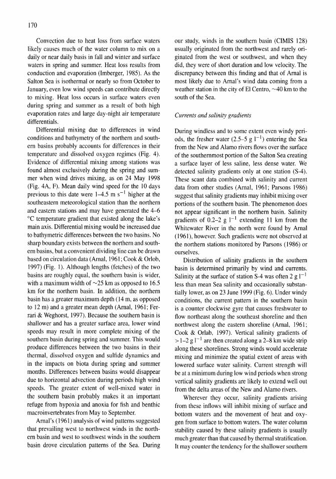
170
Convection due to heat loss from surface waters likely causes much of the water column to mix on a daily or near daily basis in fall and winter and surface waters in spring and summer. Heat loss results from conduction and evaporation (lmberger, 1985). As the Salton Sea is isothermal or nearly so from October to January, even low wind speeds can contribute directly to mixing. Heat loss occurs in surface waters even during spring and summer as a result of both high evaporation rates and large day-night air temperature differentials.
Differential mixing due to differences in wind conditions and bathymetry of the northern and southern basins probably accounts for differences in their temperature and dissolved oxygen regimes (Fig. 4). Evidence of differential mixing among stations was found almost exclusively during the spring and summer when wind drives mixing, as on 24 May 1998 (Fig. 4A, F). Mean daily wind speed for the 10 days previous to this date were 1-4.5 m s-I higher at the southeastern meteorological station than the northern and eastern stations and may have generated the 4-6 DC temperature gradient that existed along the lake's main axis. Differential mixing would be increased due to bathymetric differences between the two basins. No sharp boundary exists between the northern and southern basins, but a convenient dividing line can be drawn based on circulation data (Arnal, 1961; Cook & Orlob, 1997) (Fig. 1). Although lengths (fetches) of the two basins are roughly equal, the southern basin is wider, with a maximum width of ~25 km as opposed to 16.5 km for the northern basin. In addition, the northern basin has a greater maximum depth (14 m, as opposed to 12 m) and a greater mean depth (Arnal, 1961; Ferrari & Weghorst, 1997). Because the southern basin is shallower and has a greater surface area, lower wind speeds may result in more complete mixing of the southern basin during spring and summer. This would produce differences between the two basins in their thermal, dissolved oxygen and sulfide dynamics and in the impacts on biota during spring and summer months. Differences between basins would disappear due to horizontal advection during periods high wind speeds. The greater extent of well-mixed water in the southern basin probably makes it an important refuge from hypoxia and anoxia for fish and benthic macroinvertebrates from May to September.
Arnal's (1961) analysis of wind patterns suggested that prevailing west to northwest winds in the northern basin and west to southwest winds in the southern basin drove circulation patterns of the Sea. During
our study, winds in the southern basin (CIMIS 128) usually originated from the northwest and rarely originated from the west or southwest, and when they did, they were of short duration and low velocity. The discrepancy between this finding and that of Arnal is most likely due to Arnal's wind data coming from a weather station in the city of El Centro, ~40 km to the south of the Sea.
Currents and salinity gradients
During windless and to some extent even windy periods, the fresher water (2.5-5 g 1-1) entering the Sea from the New and Alamo rivers flows over the surface of the southernmost portion of the Salton Sea creating a surface layer of less saline, less dense water. We detected salinity gradients only at one station (SA). These scant data combined with salinity and current data from other studies (Arnal, 1961; Parsons 1986) suggest that salinity gradients may inhibit mixing over portions of the southern basin. The phenomenon does not appear significant in the northern basin. Salinity gradients of 0.2-2 g 1-1 extending 11 km from the Whitewater River in the north were found by Arnal (1961), however. Such gradients were not observed at the northern stations monitored by Parsons (1986) or ourselves.
Distribution of salinity gradients in the southern basin is determined primarily by wind and currents. Salinity at the surface of station S-4 was often 2 g 1-1 less than mean Sea salinity and occasionally substantially lower, as on 23 June 1999 (Fig. 6). Under windy conditions, the current pattern in the southern basin is a counter clockwise gyre that causes freshwater to flow northeast along the southeast shoreline and then northwest along the eastern shoreline (Arnal, 1961; Cook & Orlab, 1997). Vertical salinity gradients of > \-2 g I-I are then created along a 2-8 km wide strip along these shorelines. Strong winds would accelerate mixing and minimize the spatial extent of areas with lowered surface water salinity. Current strength will be at a minimum during low wind periods when strong vertical salinity gradients are likely to extend well out from the delta areas of the New and Alamo rivers.
Wherever they occur, salinity gradients arising from these inflows will inhibit mixing of surface and bottom waters and the movement of heat and oxygen from surface to bottom waters. The water column stability caused by these salinity gradients is usually much greater than that caused by thermal stratification. It may counter the tendency for the shallower southern
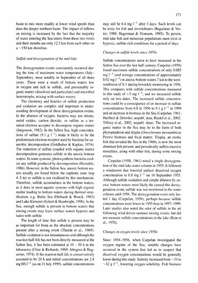
basin to mix more readily at lower wind speeds than does the deeper northern basin. The impact of inflows on mixing is increased by the fact that the majority of water entering the Sea enters from these two rivers and their mouths are only 12.5 km from each other on a ~ 150 km shoreline.
Sulfide and deoxygenation of the mid-lake
The deoxygenation events consistently occurred during the time of maximum water temperatures (JulySeptember), most notably in September of all three years. These were a result of bottom waters low in oxygen and rich in sulfide, and presumably organic matter (dissolved and particulate) and microbial heterotrophs, mixing with surface waters.
The chemistry and kinetics of sulfide production and oxidation are complex and important in understanding development of these deoxygenation events. In the absence of oxygen, bacteria may use nitrate, metal oxides, carbon dioxide, or sulfate as a terminal electron acceptor to decompose organic matter (J0rgenson, 1982). In the Salton Sea, high concentrations of sulfate (9.1 g 1-1) make it likely to be the predominant electron receptor used by bacteria for anaerobic decomposition (Goldhaber & Kaplan, 1974). The reduction of sulfate coupled with organic matter decomposition generates sulfide in the anoxic bottom waters. In some systems, photosynthetic bacteria oxidize any sulfide produced by decomposition (Huxtable, 1986). However, in the Salton Sea, anoxic bottom waters usually are found below the euphotic zone (top 4-5 m) so sulfide is not oxidized by this mechanism. Therefore, sulfide accumulates in the bottom waters, as it does in most aquatic systems with high organic matter loading to bottom waters during thermal stratification, e.g. Baltic Sea (Ehrhardt & Wenck, 1983) and Lake Kinneret (Eckert & Hambright, 1996). In the Sea, enough sulfide is present in bottom waters that mixing events may leave surface waters hypoxic and laden with sulfide.
The length of time that sulfide is present may be as important for biota as the absolute concentrations present after a mixing event (Theede et aI., 1969). Sulfide oxidation is not instantaneous and although the reaction half-life has not been directly measured at the Salton Sea, it has been estimated at 10 - 50 h in the laboratory (Cline & Richards, 1969; Almgren & Hagstrom, 1974). If the reaction half-life is conservatively assumed to be 24 h and initial concentrations are 2.8 mg HS I-I (as on 31 July 1999), sulfide concentrations
171
may still be 0.4 mg I-I after 3 days. Such levels can be toxic for fish and invertebrates (Bagarinao & Vetter, 1989; Hagerman & Vismann, 1995). To persist, mid-lake fish and metazoan populations must exist in hypoxic, sulfide-rich conditions for a period of days.
Changes in sulfide levels since 1950s
Sulfide concentrations seem to have increased in the Salton Sea over the last half century. Carpelan (1958) found maximum sulfide concentrations of only 0.085 mg I-I (and average concentrations of approximately 0.02 mg I-I) in anoxic bottom waters 7 km to the westsouthwest of S-I during biweekly monitoring in 1956. This compares with sulfide concentrations measured in this study of >5 mg I-I, and we measured sulfide only on two dates. The increased sulfide concentrations could be a consequence of an increase in sulfate concentrations from 6.8 in 1956 to 9.1 g I-I in 1999 and an increase in biomass in the Sea (Carpelan, 1961; Hurlbert & Detwiler, unpubi. data; Riedel et aI., 2002; Tiffany et aI., 2002; unpubi. data). The increased organic matter in the Sea may be in the form of both phytoplankton and tilapia (Oreochromis mossambicus Peters) biomass and fecal matter. Tilapia, an exotic fish that invaded the Sea in the 1960s, is now the most abundant fish present, and periodically suffers massive moralities, along with other fish, during some mixing events.
Carpelan (1958, 1961) noted a single deoxygenation of the mid-lake water column in 1955. It followed a windstorm that lowered surface dissolved oxygen concentration to 0.8 mg I-Ion 16 September 1955. Although sulfide oxidation and simple dilution by anoxic bottom waters most likely the caused this deoxygenation event, sulfide was not monitored in the water column until 1956. The deoxygenation event only lasted I day (Carpelan, 1958), perhaps because sulfide concentrations were lower in 1955 than in 1997-1999. Later studies also noted the odor of sulfide in the air following wind driven summer mixing events, but did not measure sulfide concentrations in the lake (Bain et aI., 1970).
Changes in oxygen levels since 1950s
Since 1954-1956, when Carpelan investigated the oxygen regime of the Sea, notable changes have occurred in the system that led us to suspect that dissolved oxygen concentrations would be generally lower during this study. Salinity increased from ~ 33 to ~42 g I-I, lowering oxygen solubility. Fish biomass
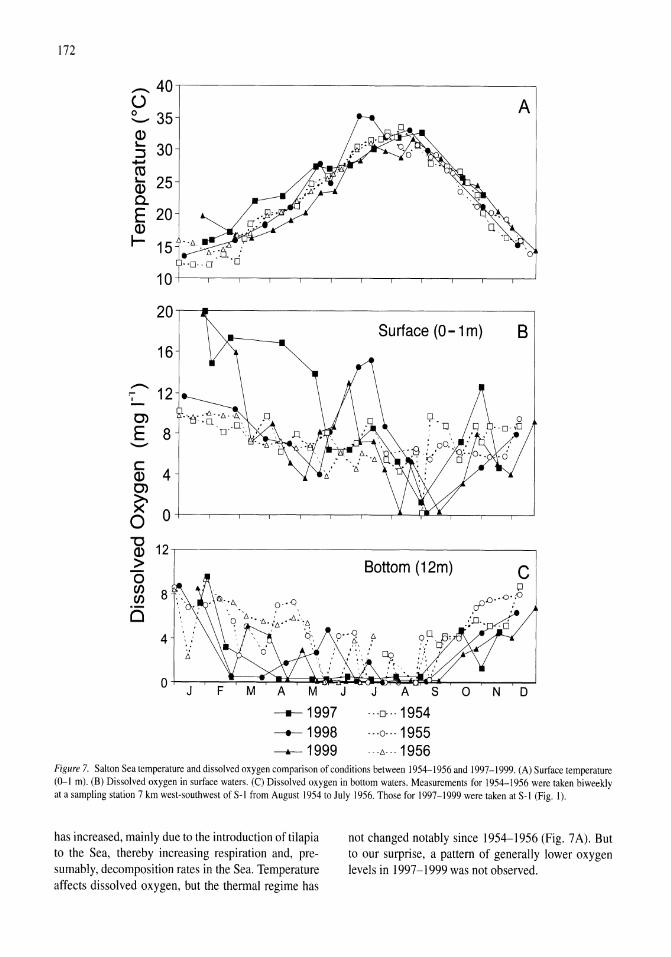
172
.-40 0 A 0 35 --Q) L.. 30 :::J ... CO L.. 25 Q) c. E 20 Q)
I- 15
10
20 Surface (0-1 m) B
16
.-12 ,...
I
0)
E 8 --c 4 Q)
0)
~ 0 0 "'0 12 Q)
> 0
Bottom (12m) C (/) 8 en 0
4 ' . " Ii
0 J F M A M J J A S 0 N 0
----1997 "'0···1954 ---.-1998 "'0 .. ·1955 ~1999 .. ·t:. .. ·1956
Figure 7. Salton Sea temperature and dissolved oxygen comparison of conditions between 1954-1956 and 1997-1999. (A) Surface temperature (0-1 m). (B) Dissolved oxygen in surface waters. (e) Dissolved oxygen in bottom waters. Measurements for 1954-1956 were taken biweekly at a sampling station 7 km west-southwest of S-1 from August 1954 to July 1956. Those for 1997-1999 were taken at S-1 (Fig. 1).
has increased, mainly due to the introduction of til apia to the Sea, thereby increasing respiration and, presumably, decomposition rates in the Sea. Temperature affects dissolved oxygen, but the thermal regime has
not changed notably since 1954-1956 (Fig. 7A). But to our surprise, a pattern of generally lower oxygen levels in 1997-1999 was not observed.
In surface waters, mid-day dissolved oxygen concentrations were, however, more variable during 1997-1999 when compared to 1954-1956 (Fig. 7B). Little inter-annual variation and only small seasonal differences were found in 1954-1956 whereas large variation was found among years and seasons in 1997-1999. In 1954-1956, surface waters were well oxygenated at all seasons (5-11 mg 02 1-1 ) except for one notable date in September 1955 when surface waters were hypoxic (0.8 mg 02 1-1). In contrast, surface waters in 1997-1999 were supersaturated at times during january-july (10-20 mg 02 1-1) and then hypoxic or anoxic at times in August and September. During the cooling period when the Sea was mixing daily or nearly daily, oxygen concentrations of surface waters were similar among all six years.
Bottom waters in 1954-1956 were usually oxic, with periods of hypoxia or anoxia developing during June-August for only a few days at a time (Fig. 7C). During 1997-1999, hypoxic or anoxic conditions began occurring as early as February and persisted for longer periods than in 1954-1956.
These changes in oxygen dynamics are most likely a result of increases since 1954-1956 in rates of primary production, fish production, decomposition, and sulfide production. Higher phytoplankton densities (M.A. Tiffany, unpubl. data) lead to increased photosynthetic rates and, therefore, a greater tendency for surface waters to be supersaturated during spring and summer when the Sea is stratified. Increased primary production supports higher densities of other organisms in the Sea and, therefore, higher rates of decomposition and sulfide production in bottom waters throughout the year. Sulfide production may also have been enhanced by the 34% increase in sulfate concentrations in the Sea since the 1954-1956. These higher sulfide concentrations can now reduce more dissolved oxygen in the water column during a mixing event. During fall and winter, when the Sea is well-mixed, processes favoring supersaturation and deoxygenation are inhibited and dissolved oxygen concentrations in 1997-1999 are comparable to 1954-1956.
Thickening of oxic stratum nearshore
The greater thickness of the oxic stratum in nearshore waters seems likely to be a general phenomenon during the warmer part of the year. Though our own data are limited, we suspect it is attributable to two principal factors: greater turbulence of surface waters nearshore than offshore, and less frequent and intens-
173
ive mixing of oxygen poor bottom waters into surface waters nearshore. The potential biological significance of the thickened oxic stratum nearshore region is great, as the oxic nearshore acts as a refuge from hypoxic or anoxic conditions for fish and benthic macroinvertebrates, even during major deoxygenation events.
Breaking waves at the shoreline, friction at watersediment interface generated by wind driven surface currents, and convection driven by greater nocturnal cooling of shallow waters all probably contribute to the greater oxygenation and mixing of the nearshore waters. These mechanisms were not directly investigated in this study, but would be expected to result in a thicker oxic stratum and less opportunity for build-up of sulfide concentrations close to shore.
Strong wind events that mix the Sea occur sporadically throughout spring and summer at mid-lake. These reduce oxygen concentrations in surface waters by mixing into them, to a greater or lesser degree, oxygen poor, sulfide-rich bottom waters. These midlake surface waters then gradually reoxygenate. In shallower nearshore areas, however, these low quality bottom waters are either absent or occupy a smaller percentage of the water column. Thus a mixing event that reduces oxygen levels in mid-lake surface waters by 50, or 90, or 99% may have negligible effects on oxygen levels in nearshore surface waters. Under the right conditions, however, currents can carry oxygen poor mid-lake surface waters toward shore.
The thickening of the oxic stratum nearshore affects estimates of lake bottom exposed to various dissolved oxygen concentrations (Fig. 3C). Plotted values slightly overestimate the areal extent of low dissolved oxygen conditions. Only oxygen values at the mid-lake stations were used for calculating these percentages. Overestimates only occur during periods of stratification and are on the order of ~5% when conditions mimic those found on 17 June 1999 (Fig. 5A), somewhat greater under conditions such as those found on 29 August 1999 (Fig. 5B).
Consequences for biota
Sulfide and oxygen regimes, themselves driven largely by wind and temperature regimes, have an influence on plankton, benthos and fish populations in the lake. Anoxia and sulfide have well documented adverse effects on aquatic organisms, especially metazoans (Bagarinao, 1992; Hagerman & Vismann, 1995). As the two factors usually coincide in the Salton Sea, their
174
separate effects were not distinguishable in this study, and, for convenience, are sometimes both subsumed under phrases such as 'deoxygenation effects'. Major direct effects of deoxygenation are abandonment of the lake center by fish and benthic macro invertebrates during May-September and abrupt plankton and fish die-offs in August and September.
A recent gillnet survey of fish distribution found that during summer few fish are found in the midlake (Riedel et aI., 2002); and observations with a depth/fish sonar unit mounted on the sampling vessel show that when fish are found mid-lake, they are only found in the top 6 m of the water column. In spring, fish migrate to nearshore waters. This movement may be in response to the first injections of hypoxic and sulfide-bearing bottom waters into surface waters during wind events after early stratification periods in April and May. Reduction of mid-lake fish abundance likely affects mid-lake plankton populations (Tiffany et aI., 2002, unpubi. data). Movement of fish to nearshore occurs when tilapia is reproductively active (Riedel et aI., 2002). Tilapia are mouth brooders that build nests on the lake bottom in the form of depressions a few decimeters in diameter. High densities of their nests have been documented by sonar imaging in offshore areas at depths down to 12 m. It is not known at what time of year these nests were created. Clearly it would have been prior to strong thermal stratification, during which nesting would be restricted to shallow ( <6 m deep) areas. The reduced area habitable by fish may also affect the growth rate of the fish and reduce rates of reproduction (L. Helvenston, pers. comm.).
In April and May, a vacating of the lake bottom below 4 m by benthic macroinvertebrates begins, via either mortality or migration to nearshore areas (Detwiler et aI., 2002). By July, the lake bottom below 4 m depth is devoid of benthic macroinvertebrates. Anoxia and sulfide in bottom waters and sediments are the likely cause. Benthic macroinvertebrates are often tolerant of hypoxic or anoxic bottom waters (Llanso, 1991), but measured concentrations of sulfide in mid-lake areas (1->5 mg HS-I-1) are in the lethal range for many aquatic organisms (Smith et aI., 1976; Bagarinao, 1992). Nearshore areas provide refugia for metazoan benthic macroinvertebrates during summer. Their densities are low even here in summer, however, which represents a further reduction in fish food supplies. The beginning of strong and deep convectional circulation, usually in September, signals when effective recolonization of deep sediments by benthic macroinvertebrates can begin (Detwiler et aI., 2002).
The deoxygenation events in August and September cause mortality of fish and plankton. These events in 1997, 1998 and 1999 were accompanied by crashes in popUlations of the dominant metazoan zooplankters (Apocyclops dengizicus MUller and Brachionus rotundiformis Lepeschkin), reduction in phytoplankton densities (dominated by diatoms, dinoflagellates and a raphidophyte), and increases in anoxia-tolerant ciliates (Tiffany et aI., 2002, unpubi. data). Moribund and freshly dead fish were observed on the lake surface in large numbers following deoxygenation events. Large fish mortalities events are common at the Sea. One fish die-off in August 1999 was estimated to involve 7.6 million tilapia. A deoxygenation event in September 1955 resulted in mortality of bairdiella (Bairdiella icistia Jordan and Gilbert), the most abundant fish in the Sea at the time (Carpelan, 1958). Not all mortality events are associated with deoxygenation events. Mortalities of tilapia that sometimes occur during winter months have been attributed to low water temperatures (<12 0c) (Black, 1988).
In addition to fish kills and zooplankton crashes, the deoxygenation events in spring and summer are associated with bright, milky green-colored water described as 'green tides'. Previously, these 'green tides' were thought to be caused by phytoplankton blooms created by the mixing of nutrient rich water with surface waters after prolonged periods of stratification. In fact, green water has reduced abundance of phytoplankton (K. M. Reifel & M. A. Tiffany, unpubl. data.). Mention of these 'green tides' can be found in daily records kept at the Salton Sea State Recreation Area as early as the 1960s. The green color is an optical effect of gypsum crystals that precipitate as sulfide is oxidized to sulfate, already at saturation with calcium in the water column (Hurlbert et aI., unpubl. data). These 'green tides' only occur in spring or summer and are associated with a strong wind event following a period of stratification, the odor of sulfide in the air and fish kills. The term 'green tides' has also been used' to describe surface blooms of the phytoplankter Pleurochrysis pseudoroscoffensis Gayral et Fresnel that occur at the Sea (Reifel et aI., 2001).
Consequences of future changes
Inflow to the Salton Sea may be reduced in the coming years as a result of water conservation and water transfers to coastal California. The predicted reduction ranges from 25 to 43% depending on legislative and other decisions (Tetratech, 2000). In addition, en-
gineering projects to stop the increase of salinity in the Sea may involve the creation of evaporation ponds using diked-off sections of the existing Sea. Under the various alternatives to 'fix' the Sea over the next 30 years, its level may drop 2-6 m, its area may be reduced from 980 km2 to 675-834 km2, and its salinity may increase and then drop as low as 38 g 1-1 (Tetratech, 2000). The extent and timing of these modifications depend on numerous political and engineering decisions. These should take into account how modifications of the complex mixing, thermal, and dissolved oxygen regimes of the Sea will affect its future value to people and wildlife. Lakes of such large size do not exist in hot endorrheic regions such as the Salton Sink without a large water supply. For the past century, agricultural wastewaters have been the main source of water for the Salton Sea. If this supply cannot be guaranteed for the future, the ecological dynamics of this lake become, of course, irrelevant.
Acknowledgements
We thank the Kristen M. Reifel, James Zimmer, Darrell Bennett and Steve Horvitz for providing logistical support, field and laboratory assistance and Lois Tiffany for funding of field work in 1997 and 1998. We also thank John Melack and reviewers for useful and insightful comments. The research described in this article has been funded in part by the United States Environmental Protection Agency through grant #R826552-0 1-0 to the Salton Sea Authority. The research results have not been subjected, however, to the Agency's required peer review and therefore do not necessarily reflect the views of the Agency. Therefore, no official endorsement should be inferred.
References
Almgren, T. & I. Hagstrom, 1974. The oxidation rate of sulphide in sea water. Wat. Res. 8: 395-400.
American Public Health Association. 1998. Standard methods for the examination of water and wastewater. 20th edn. American Public Health Association. Washington: 1162 pp.
Arnal, R. E., 1961. Limnology. sedimentation. and microorganisms of the Salton Sea. California. Geol. Soc. am. Bull. 72: 427-478.
Bagarinao. T. & R. D. Vette, 1989. Oxidative detoxification of sulfide by mitochondria of the California killifish Fundulus parvipinnis and the speckled sanddab Citharichthys stigmaeus. 1. compo Physiol. 160: 519-527.
Bagarinao, T., 1992. Sulfide as an environmental factor and toxicant: tolerance and adaptations in aquatic organisms. Aquat. Tox. 24: 21-62.
175
Bain, R. C., A. M. Caldwell, R. H. Clawson, H. L. Scotten & R. G. Wills, 1970. Salton Sea California: water quality and ecological management considerations. U.S. Dept. Interior, Federal Water Quality Administration, Pacific Southwest Region: 53 pp.
Black, G. E, 1988. Description of the Salton Sea sport fishery 1982-1983. California Fish and Game Administrative Report 88-9.
Blaney, H. E, 1955. Evaporation from the stabilization of Salton Sea water surface. Am. Geophys. Union. Trans. 36: 3633-640.
Carpelan, L. H., 1958. The Salton Sea: physical and chemical characteristics. Limnol. Oceanogr. 3: 373-386.
Carpelan, L. H., 1961. Physical and chemical characteristics. In Walker, B. W. (ed.), The Ecology of the Salton Sea, California in Relation to the Sportfishery. Calif. Dept. Fish. Game, Fish Bull. 113: 1-204.
Chen, K. Y. & 1. C. Morris, 1972. Kinetics of oxidation of aqueous sulfide by 02. Environ. Sci. Technol. 6: 529-537.
Cline, J. D. & E A. Richards, 1969. Oxygenation of hydrogen sulfide in sea water at constant salinity, temperature and pH. Environ. Sci. Technol. 3: 838-834.
Cohen, M., 1. Morrison & E. P. Glenn, 1999. Haven or hazard: The ecology and future of the Salton Sea. Pacific Institute, Oakland, California: 64 pp.
Cook, C. B. & G. T. Orlob, 1997. Field monitoring and hydrodynamic modeling of the Salton Sea, CA, environmental and coastal hydraulics: protecting the aquatic habitat, Vol. I, 27th Congress of the International Association for Hydraulic Research, Aug 1997: 659-664.
Cooper, 1. 1. & D. L. Koch, 1984. Limnology of a desert terminal lake, Walker Lake, Nevada, U.S.A. Hydrobiologia 118: 275-292.
Detwiler, p" M. E Coe & D. M. Dexter, 2002. Benthic invertebrates of the Salton Sea: distribution and seasonal dynamics. HydrobiologialDevelopments in Hydrobiology (in press).
Eckert W. & D. K. Hambright, 1996. Seasonal and vertical distributions of temperature, pH, oxygen, and sulfide in Lake Kinneret. Limnologica 26: 345-351.
Ehrhardt, M. & A. Wenck, 1984. Wind pattern and hydrogen sulfide in shallow waters of the Western Baltic Sea, a cause and effect relationship? Meeresforsch 30: 10 1-110.
Ferrari, R. L. & P. Weghorst, 1997. Salton Sea 1995 hydrographic GPS survey. U.S. Bureau of Reclamation, Water Resources Services. Denver, Colorado: 23 pp.
Gala!, D. L., E. L. Lider, S. Vigg & S. R. Robertson, 1981. Limnology of a large, deep, North American terminal lake, Pyramid Lake, Nevada, U.S.A. Hydrobiologia 82: 281-317
Goldhaber, M. & I. R. Kaplan, 1974. The sulfur cycle, In Goldberg, E. (ed.), The Sea, Vol. 5, Marine Chemistry. Wiley, New York: 569-665.
Hagerman L. & B. Vis mann, 1995. Anaerobic metabolism in the shrimp Crangon crangon exposed to hypoxia, anoxia and hydrogen sulfide. Mar. BioI. 123: 235-240.
Hely, A. G., G. H. Hughes & B. Irelan, 1966. Hydrologic regimen of Salton Sea, California. U. S. Geol. Surv. Prof. Paper 486-C: 32 pp.
Hutchinson, G. E., 1957. A Treatise on Limnology, volume I. Wiley & Sons: 1015 pp.
Huxtable, R. J., 1986. Biochemistry of Sulfur. Plenum Press: 445 pp.
Idso, S. B., 1973. On the concept of lake stability. Limnol. Oceanogr. 18: 681-683.
Imberger, J., 1985. Thermal characteristics of standing waters: an illustration of dynamic processes. Hydrobiologia 125: 7-29.
176
Llanso, R, J., 1991, Tolerance of low dissolved oxygen and hydrogen sulfide by polychaete Streblospio benedicti, J. expo mar. Bio!. Eco!. 153: 165-178.
MacIntyre, S., 1993. Vertical mixing in a shallow, eutrophic lake: possible consequences for the light climate of phytoplankton. Limno!. Oceanogr. 38: 798-817.
Millero, F. J., 1986. The thermodynamics and kinetics of the hydrogen sulfide system in natural waters. Mar. Chern. 18: 121-147.
Mitteilung, K., 1988. Lake mixis and internal phosphorus dynamics. Arch. Hydrobio!. 113: 629-638.
Parsons, 1986. Proposed water conservation program and initial water transfer, environmental impact report. Draft. Imperial Irrigation District, Imperial California.
Reifel, K. M., M. P. McCoy, M. A. Tiffany, T. E. Rocke, C. C. Trees, S. B. Barlow, D. J. Faulkner & S. H. Hurlbert, 2001, Pleurochrysis pseudoroscoffensis (Prymnesiophyceae) blooms on the surface of the Salton Sea, California. Hydrobiologia 466 (Dev. Hydrobio!. 162): 177-185.
Reifel, K. M., M. P. McCoy, M. A. Tiffany, T. E. Rocke, S. H. Hurlbert & D. 1. Faulkner, 2002. The possible importance of algal toxins in the Salton Sea, California. HydrobiologiaJDevelopments in Hydrobiology (in press).
Riedel, R., L. Caskey & B. Costa-Pierce, 2002. Fish biology and fisheries ecology of the Salton Sea. HydrobiologialDevelopments in Hydrobiology (in press).
Romero, 1. R, & 1. M. Melack, 1996. Sensitivity of vertical mixing in a large saline lake to variation in runoff. Limno!. Oceanogr. 41: 955-965.
Setmire, J. G., R. A. Schroeder, J. N. Densmore, S. L. Goodbred, D. 1. Auden & W. R. Radke, 1993. Detailed study of water quality,
bottom sediment, and biota associated with irrigation drainage in the Salton Sea area, California, 1988-90. U.S. Geo!. Surv. Water-Resources Investigations Report 93-4014: 102 pp.
Smith, L. L., D. M. Oseid, 1. R. Adelman & S. J. Broderius, 1976. Effects of hydrogen sulfide on fish and invertebrates, Parts I and II. U.S. Environmental Protection Agency: 250 pp.
Snoeyink, V. L. & D. Jenkins, 1980. Water Chemistry. John Wiley and Sons, Inc. New York, NY: 430 pp.
Talling, J. E, 1966. The annual cycle of stratification and phytoplankton growth in Lake Victoria (East Africa). Int. Rev. ges. Hydrobio!. 51: 545-621,
Tetra Tech, 2000. Salton Sea restoration project environmental impact statement/environmental impact report. Draft. Tetra Tech Inc., Lafayette, California: 630 pp.
Theede, H., A. Ponat, K. Hiraki & c. Schlieper, 1969. Studies on the resistance of marine bottom invertebrates to oxygen-deficiency and hydrogen sulfide. Mar. Bio!. 2: 325-337.
Tiffany, M. A., B. K. Swan, 1. M. Watts & S. H. Hurlbert, 2002. Metazooplankton dynamics in the Salton Sea, 1997-1999. HydrobiologialDevelopments in Hydrobiology (in press).
Tostrud, M. B., 1997. The Salton Sea 1906-1996: computed and measured salinities and water levels. Colorado River Board of California, Glendale, California.
Vismann, B., 1991. Sulfide tolerance: physiological mechanisms and ecological implications. Ophelia 34: 1-27.
Walker, B. w., R. R. Whitney & G. W. Barlow, 1961, The ecology of the Salton Sea, California in relation to the sportfishery. The Calif. Dept. Fish. Game, Fish Bull. 113: 1-204.
Wetzel, R. G., 1983. Limnology. New York, Saunders College Publishing, Inc.: 767 pp.
Hydrobiologia 466: 177-185,2001. J.M. Melack. R. Jellison & D.B. Herbst (eds), Saline Lakes. © 2001 Kluwer Academic Publishers.
177
Pleurochrysis pseudoroscoffensis (Prymnesiophyceae) blooms on the surface of the Salton Sea, California
Kristen M. Reifel), Michael P. McCoy2, Mary Ann Tiffany), Tonie E. Rocke3,
Charles C. Trees4, Steven B. Barlow), D. John FaulknerZ & Stuart H. Hurlbert) 1 Department of Biology and Center for Inland Waters, San Diego State University, San Diego, CA 92182-4614, U.S.A. 2 Scripps Institution of Oceanography, University of California at San Diego, La Jolla, CA 92093-0212, U.S.A. 3 National Wildlife Health Center, U.S. Geological Survey, Biological Resources Division, 6006 Schroeder Road, Madison, WI 53711, U.S.A. 4Center for Hydro-Optics and Remote Sensing, San Diego State University, 6505 Alvarado Road, Suite 206, San Diego, CA 92120, U.S.A.
Key words: prymnesiophyte, coccolithophore, algal bloom, algal toxins, pigments, saline lakes
Abstract
Dense populations of the coccolithophore Pleurochrysis pseudoroscoffensis were found in surface films at several locations around the Salton Sea in February-August, 1999. An unidentified coccolithophorid was also found in low densities in earlier studies of the lake (1955-1956). To our knowledge, this is the first record of this widespread marine species in any lake. Samples taken from surface films typically contained high densities of one or two other phytoplankton species as well as high densities of the coccolithophore. Presence or absence of specific algal pigments was used to validate direct cell counts. In a preliminary screen using a brine shrimp lethality assay, samples showed moderate activity. Extracts were then submitted to a mouse bioassay, and no toxic activity was observed. These results indicate that blooms of P. pseudoroscoffensis are probably not toxic to vertebrates and do not contribute to the various mortality events of birds and fish that occur in the Salton Sea.
Introduction
Coccolithophorids (Prymnesiophyceae) are common phytoplankters in marine habitats. Species in this group are characterized by an outer covering of small regular plates (coccoliths) consisting of calcium carbonate (Heimdal, 1993). Some species are known to form large and sometimes regularly occurring blooms in the world's oceans (Milliman, 1980; Honjo, 1982; Blackburn & Cresswell, 1993). Several genera consistently occur in near-shore marine waters including Hymenomonas, Cricosphaera, Pleurochrysis, Ochrosphaera and Cruciplacolithus (Johansen et aI., 1988; Heimdal, 1993). Although coccolithophorids are a predominantly marine group, a few species have been found in inland waters (Green et aI., 1990; Heimdal, 1993). Most coccolithophorids are thought to
produce harmless blooms, but some species may be toxic (Moestrup, 1994).
This paper reports on blooms of Pleurochrysis pseudoroscoffensis Gayral et Fresnel observed in the Salton Sea, California, and on assessments of their pigment composition and toxicity. Small numbers of a coccolithophorid were observed during a plankton survey of the lake in 1955-1956 (Carpel an, 1961). The form, however, was not identified or described. Two prymnesiophytes, Prymnesium sp. and a second species, were observed in a microcosm study of salinity effects on Salton Sea phytoplankton (M. Gonzalez, unpublished data). The second species was originally identified as Coccolithus sp., but it is now thought to have been P. pseudoroscoffensis (M. Gonzalez, pers. comm.). The present study is the first to document the occurrence of P. pseudoroscoffensis in the Salton
178
Sea and to describe bloom occurrences there of any coccolithophorid. Of the five species in the genus Pleurochrysis, only one, P carterae Braarud et Fagerland Christensen, has been previously described from an inland body of water, a saline pond in New Mexico (Johansen et aI., 1988).
The Salton Sea is a 980 km2 saline (44 g I-I) lake located in arid southeastern California, U.S.A. It was created in 1905 due to an engineering accident. Although it has a mean depth only of 8 m and a maximum depth of 14 m, it is the largest lake in California (see Cohen et aI., 1999; Watts et aI., 2001 for maps of the Salton Sea). The lake is eutrophic largely because it is in a closed basin and most of its inflows are agricultural and municipal wastewaters (Bain et aI., 1970; Cohen et aI., 1999). Frequent algal blooms occur in the lake, some with chlorophyll a concentrations as high as 500 /Lg I-I (K. M. Reifel, unpublished data).
Materials and methods
Collection and preservation of phytoplankton
Several blooms of P pseudoroscoffensis were observed during the spring and summer of 1999 at the Salton Sea. Samples were taken during three blooms (P2, P3, P4) for analysis of taxonomic and pigment composition. These three blooms and one additional bloom (PI) were also tested for toxic activity using two assays (brine shrimp and mouse). See Table 1 for geographic coordinates of sampling locations.
The first sample (PI) was collected on February 28, 1999. Conditions were calm and a surface film could be seen over much of the lake. The sample was collected 9-10 km offshore from surface water and contained mostly foam. In June 1999, conditions were generally calm and an extensive surface film was observed for several days. It was first seen on June 17 and sampled (P2) on June 20. The sample was collected 2-3 km offshore using a film-concentrating device. This device consisted of thin, 2 m-Iong strips of wood with polystyrene floats attached to either side of each wood strip. It was floated on the surface and acted as a barrier allowing surface film to be concentrated. Several foam accumulations were also seen on July 5. A sample of foam and surface film (P3) was collected mid-lake using the film-concentrating device. Conditions were calm on this date and the surface film appeared oily. On August 17, water supersaturated with oxygen was observed along the shoreline. Wind
was present that caused moderate wave activity. A large (13 L) water sample (P4) was collected from the top 50-100 cm of the water column. All samples were centrifuged using an International Equipment Company HN-SII centrifuge at 2400 rpm to remove as much water as possible. The final concentrates were stored at -80°C until analyzed.
Physical properties (temperature, pH, specific conductance and dissolved oxygen concentration) of each collection site were measured using a YSI model UPG6000 Sonde. A factory-calibrated probe (accuracy: ± 0.15 0C) was used for temperature measurements. Measurements of dissolved oxygen (accuracy: ± 0.2 mg I-I) were made using a probe that was calibrated using barometric pressure measured in the field and internally corrected for salinity using measurements of specific conductance (accuracy: ±5%). The pH electrode (accuracy: ±0.2 pH units) was calibrated in the laboratory using two standards ofknown pH (pH 7 and pH 10), and readings were corrected for temperature internally. The precision of each measured variable was greater than the number of decimal places reported in Table 1.
Sub-samples for enumeration and pigment analysis were taken from each sample collected prior to centrifuging. Samples for enumeration were preserved in 5% Lugol's solution. Because coccolithophorids will dissolve when preserved in Lugol's solution (Throndsen, 1978), a sub-sample was also preserved in 5% buffered formaldehyde solution. Samples for pigment analysis were filtered through Whatman GFIF (0.7 /Lm) filters using a syringe filter apparatus. Filters were stored in liquid nitrogen (-196°C) until analyzed.
Taxonomic and pigment analysis
Preserved samples were enumerated using the Utermohl method (Lund et aI., 1958). Lugol's preserved samples were settled in 25 ml settling chambers for at least 24 h and formalin-preserved samples were settled for at least 48 h before analysis (Hasle, 1978). Two crossed diameters were enumerated using a Leitz inverted microscope at a total magnification of 400 x. All cells larger than 5 /Lm in length were counted and identified to genus or species.
Pigment analysis was done using high performance liquid chromatography (HPLC). Filters were extracted in 90% acetone for 24 h and then sonicated with a microprobe system to enhance extraction efficiencies. An internal pigment standard (canthaxanthin, which is
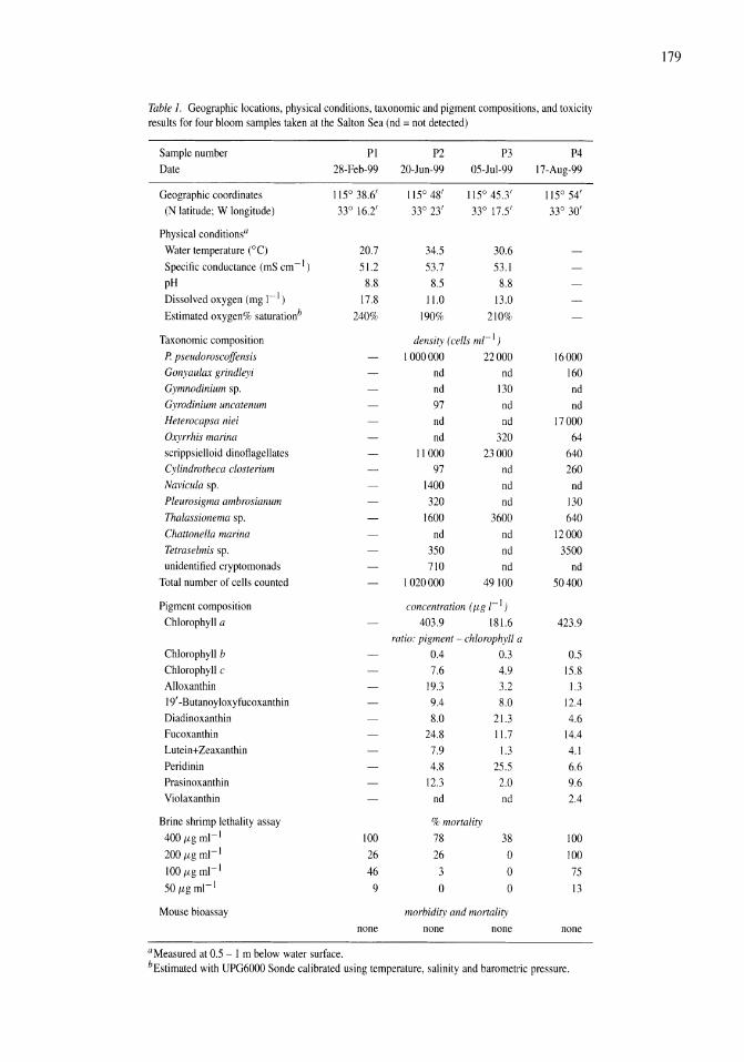
179
Table 1. Geographic locations, physical conditions, taxonomic and pigment compositions, and toxicity results for four bloom samples taken at the Salton Sea (nd = not detected)
Sample number PI P2 P3 P4 Date 28-Feb-99 20-Jun-99 05-Jul-99 17-Aug-99
Geographic coordinates 115° 38.6' 115° 48' 115° 45.3' 115° 54' (N latitude; W longitude) 33° 16.2' 33° 23' 33° 17.5' 33° 30'
Physical conditionsa
Water temperature (0C) 20.7 34.5 30.6 Specific conductance (mS cm- I ) 51.2 53.7 53.1 pH 8.8 8.5 8.8 Dissolved oxygen (mg I-I) 17.8 11.0 13.0 Estimated oxygen% saturationb 240% 190% 210%
Taxonomic composition density (cells ml- I ) P. pseudoroscoffensis 1000000 22000 16000 Gonyaulax grindleyi nd nd 160 Gymnodinium sp. nd 130 nd Gyrodinium uncatenum 97 nd nd Heterocapsa niei nd nd 17000 Oxyrrhis marina nd 320 64 scrippsielloid dinoflagellates 11000 23000 640 Cylindrotheca closterium 97 nd 260 Navicula sp. 1400 nd nd Pleurosigma ambrosianum 320 nd 130 Thalassionema sp. 1600 3600 640 Chattonella marina nd nd 12000 Tetraselmis sp. 350 nd 3500 unidentified cryptomonads 710 nd nd
Total number of cells counted 1020000 49100 50400
Pigment composition concentration (f.Lg I-I)
Chlorophyll a 403.9 181.6 423.9 ratio: pigment - chlorophyll a
Chlorophyll b 0.4 03 0.5 Chlorophyll c 7.6 4.9 15.8 Alloxanthin 19.3 3.2 1.3 19'-Butanoyloxyfucoxanthin 9.4 8.0 12.4 Diadinoxanthin 8.0 21.3 4.6 Fucoxantbin 24.8 11.7 14.4 Lutein+Zeaxanthin 7.9 1.3 4.1 Peridinin 4.8 25.5 6.6 Prasinoxanthin 123 2.0 9.6 Violaxanthin nd nd 2.4
Brine shrimp lethality assay % mortality 400 f.Lg ml- I 100 78 38 100 200 f.Lg ml- I 26 26 0 100 100 f.Lgml- I 46 3 0 75 50 f.Lgml-1 9 0 0 13
Mouse bioassay morbidity and mortality none none none none
aMeasured at 0.5 - I m below water surface. bEstimated with UPG6oo0 Sonde calibrated using temperature, salinity and barometric pressure.
180
not normally found in samples) was used to correct for volume changes during the extraction and injection processes. The method of Wright et al. (1991) was used. Pigment compounds were separated on an ODS-2 column using a three solvent gradient system at a flow rate of 1 ml min-I. Pigment peaks were detected by two absorption detectors; a ThermoQuest UV2000 which measures absorption at 436 and 450 nm and a ThermoQuest UV6000 which measures from 390 to 550 nm every 1 nm. In addition, a fluorescence detector (ThermoQuest FL3000, Ex 404 nm; Em 680 nm) was used to detect and quantify the various chlorophyll degradation products, which usually occur at low concentrations.
Toxicity assessment
The four bloom samples (PI, P2, P3 and P4) collected between February and August were analyzed for toxic activity using two assays. Samples were first screened using a brine shrimp (Artemia salina Leach) lethality assay. Extracts from the four samples were also tested using a mouse bioassay.
Extracts were prepared in the following manner at Scripps Institution of Oceanography (SIO). Frozen centrifuged algal samples were lyophilized and the dry residue subsequently weighed. The dried sample was triturated in methanol (ca. 100 rnl g sample-I) and the resulting suspension was filtered and then washed with methanol (ca. 200 ml g sample-I). The filter plug was dried and washed with water (ca. 300 ml g sample -1) and the filtrate was lyophilized. The methanol extracts were evaporated to dryness. The resulting residue was partitioned between ethyl acetate (ca. 200 ml g sample -1) and water (ca. 200 ml g sample-I). The ethyl acetate partition was dried over sodium sulfate and the solvent evaporated to obtain the crude ethyl acetate extract. After evaporation of the residual ethyl acetate, the aqueous fraction was lyophilized. The combined aqueous extracts were placed on a freshly prepared Amberlite™ XAD-2 column (ca. 10 cm2 packing material g extracC 1) and desalted by washing with water (ca. 80 ml g extracc I). The organic compounds were then washed from the column with methanol. After weighing, each extract was assayed for brine shrimp lethality, and a 1 H NMR spectrum was recorded using a Varian Inova 300 MHz NMR spectrometer.
Brine shrimp lethality assays were performed at SIO using a modification of the methods of Meyer et al. (1982) and Solis et al. (1993). Extracts were dis-
solved in a 15% aqueous dimethyl sulfoxide (DMSO) or methanol solution to obtain a final concentration of 1.33 mg ml- I . Replicates (2) were diluted to 400,200, 100 or 50 {Lg ml- I in the wells of a 96 well micro titer plate. Negative control sample wells (8) were created by duplicating the solvent system. Approximately 15 shrimp nauplii were added to each well. Mortality was monitored over intervals of 2, 4, 6, 12 and 24 h and is reported as percent mortality at 24 h.
Mouse (Mus musculus Linnaeus) bioassays were performed at the National Wildlife Health Center (NWHC). Sample extracts were diluted to 1 mg ml- I in DMSO for inoculation into ICR female mice (15-20 g) purchased from Harlan Sprague Dawley. Using a 1 cc syringe and 25 g needle, 0.1 ml of each of the diluted extracts were inoculated intraperitoneally into each of three mice. Control mice were inoculated with 0.1 ml of DMSO. The mice were observed for signs of morbidity for 30 minutes post-inoculation and daily thereafter for 5 days. Samples were considered toxic if all three mice became sick or died.
Analysis of archived phytoplankton samples
A search was also made for P. pseudoroscoffensis in samples of phytoplankton taken as part of a biological limnology program during 1997-1999. Phytoplankton samples were collected at intervals of 2-5 weeks at 3-5 mid-lake stations at three integrated depths (0-3 m, 3-6 m, 6-9 m) using a 3-m long PVC tube sampler. The samples were preserved in 5% buffered formaldehyde or Lugol's solution. Enumeration of samples was done using the Utermohl method as described above. Reports on the phytoplankton results will be given elsewhere. Here, we report on our search for P. pseudoroscoffensis in samples collected from the northern station, S-1 (see Watts et al., 2001 for a map of stations).
Results
Identification
Coccolithophores are typically identified through detailed observation of their coccoliths using a combination of light microscopy (LM) and electron microscopy (Heimdal, 1993). Individuals from a February 1999 sample were identified by Wuchang Wei (SIO, pers. comm.) as Pleurochrysis pseudoroscoffensis through whole cell observations using LM and through
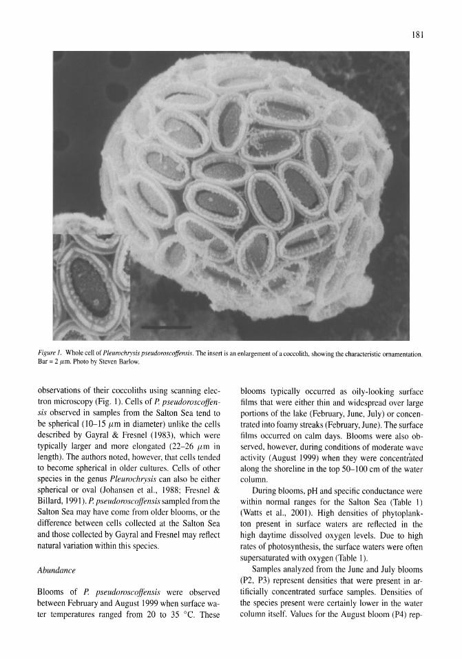
181
Figure 1. Whole cell of Pleurochrysis pseudoroscoffensis. The insert is an enlargement of a coccolith, showing the characteristic ornamentation. Bar = 2 /Lm. Photo by Steven Barlow.
observations of their coccoliths using scanning electron microscopy (Fig. I). Cells of P pseudoroscoffensis observed in samples from the Salton Sea tend to be spherical (10-15 f.im in diameter) unlike the cells described by Gayral & Fresnel (1983), which were typically larger and more elongated (22-26 flm in length). The authors noted, however, that cells tended to become spherical in older cultures. Cells of other species in the genus Pleurochrysis can also be either spherical or oval (Johansen et a!. , 1988; Fresnel & Billard, 1991). P pseudoroscoffensis sampled from the Salton Sea may have come from older blooms, or the difference between cells collected at the Salton Sea and those collected by Gayral and Fresnel may reflect natural variation within this species.
Abundance
Blooms of P pseudoroscoffensis were observed between February and August 1999 when surface water temperatures ranged from 20 to 35 °C. These
blooms typically occurred as oily-looking surface films that were either thin and widespread over large portions of the lake (February, June, July) or concentrated into foamy streaks (February, June). The surface films occurred on calm days. Blooms were also observed, however, during conditions of moderate wave activity (August J 999) when they were concentrated along the shoreline in the top 50-100 cm of the water column.
During blooms, pH and specific conductance were within normal ranges for the Salton Sea (Table 1) (Watts et a!., 2001). High densities of phytoplankton present in surface waters are reflected in the high daytime dissolved oxygen levels. Due to high rates of photosynthesis, the surface waters were often supersaturated with oxygen (Table I).
Samples analyzed from the June and July blooms (P2, P3) represent densities that were present in artificially concentrated surface samples. Densities of the species present were certainly lower in the water column itself. Values for the August bloom (P4) rep-
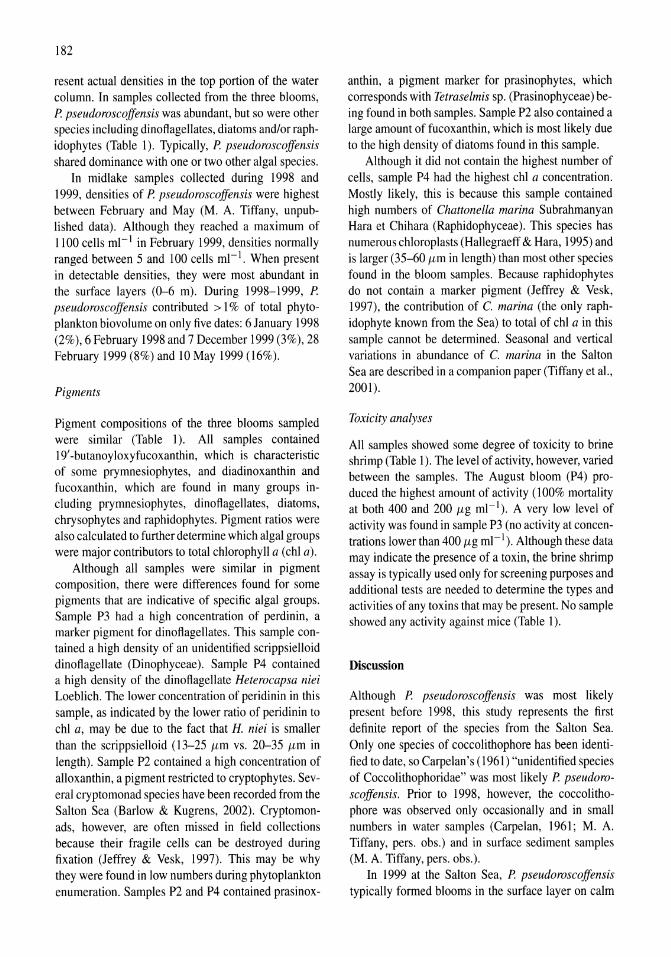
182
resent actual densities in the top portion of the water column. In samples collected from the three blooms, P. pseudoroscoffensis was abundant, but so were other species including dinoflagellates, diatoms and/or raphidophytes (Table 1). Typically, P. pseudoroscoffensis shared dominance with one or two other algal species.
In midlake samples collected during 1998 and 1999, densities of P. pseudoroscoffensis were highest between February and May (M. A. Tiffany, unpublished data). Although they reached a maximum of 1100 cells ml-1 in February 1999, densities nonnally ranged between 5 and 100 cells ml-1. When present in detectable densities, they were most abundant in the surface layers (0-6 m). During 1998-1999, P. pseudoroscoffensis contributed > 1 % of total phytoplankton biovolume on only five dates: 6 January 1998 (2%),6 February 1998 and 7 December 1999 (3%), 28 February 1999 (8%) and 10 May 1999 (16%).
Pigments
Pigment compositions of the three blooms sampled were similar (Table 1). All samples contained 19' -butanoyloxyfucoxanthin, which is characteristic of some prymnesiophytes, and diadinoxanthin and fucoxanthin, which are found in many groups including prymnesiophytes, dinoflagellates, diatoms, chrysophytes and raphidophytes. Pigment ratios were also calculated to further detennine which algal groups were major contributors to total chlorophyll a (chi a).
Although all samples were similar in pigment composition, there were differences found for some pigments that are indicative of specific algal groups. Sample P3 had a high concentration of perdinin, a marker pigment for dinoflagellates. This sample contained a high density of an unidentified scrippsielloid dinoflagellate (Dinophyceae). Sample P4 contained a high density of the dinoflagellate Heterocapsa niei Loeblich. The lower concentration of peridinin in this sample, as indicated by the lower ratio of peridinin to chi a, may be due to the fact that H. niei is smaller than the scrippsielloid (13-25 J-Lm vs. 20-35 J-Lm in length). Sample P2 contained a high concentration of alloxanthin, a pigment restricted to cryptophytes. Several cryptomonad species have been recorded from the Salton Sea (Barlow & Kugrens, 2002). Cryptomonads, however, are often missed in field collections because their fragile cells can be destroyed during fixation (Jeffrey & Vesk, 1997). This may be why they were found in low numbers during phytoplankton enumeration. Samples P2 and P4 contained prasinox-
anthin, a pigment marker for prasinophytes, which corresponds with Tetraselmis sp. (Prasinophyceae) being found in both samples. Sample P2 also contained a large amount of fucoxanthin, which is most likely due to the high density of diatoms found in this sample.
Although it did not contain the highest number of cells, sample P4 had the highest chI a concentration. Mostly likely, this is because this sample contained high numbers of Chattonella marina Subrahmanyan Rara et Chihara (Raphidophyceae). This species has numerous chloroplasts (Rallegraeff & Rara, 1995) and is larger (35--60 J-Lm in length) than most other species found in the bloom samples. Because raphidophytes do not contain a marker pigment (Jeffrey & Vesk, 1997), the contribution of C. marina (the only raphidophyte known from the Sea) to total of chi a in this sample cannot be detennined. Seasonal and vertical variations in abundance of C. marina in the Salton Sea are described in a companion paper (Tiffany et ai., 2001).
Toxicity analyses
All samples showed some degree of toxicity to brine shrimp (Table 1). The level of activity, however, varied between the samples. The August bloom (P4) produced the highest amount of activity (100% mortality at both 400 and 200 J-Lg ml-1). A very low level of activity was found in sample P3 (no activity at concentrations lower than 400 J-Lg ml-1). Although these data may indicate the presence of a toxin, the brine shrimp assay is typically used only for screening purposes and additional tests are needed to determine the types and activities of any toxins that may be present. No sample showed any activity against mice (Table 1).
Discussion
Although P. pseudoroscoffensis was most likely present before 1998, this study represents the first definite report of the species from the Salton Sea. Only one species of coccolithophore has been identified to date, so Carpelan's (1961) ''unidentified species of Coccolithophoridae" was most likely P. pseudoroscoffensis. Prior to 1998, however, the coccolithophore was observed only occasionally and in small numbers in water samples (Carpelan, 1961; M. A. Tiffany, pers. obs.) and in surface sediment samples (M. A. Tiffany, pers. obs.).
In 1999 at the Salton Sea, P. pseudoroscoffensis typically fonned blooms in the surface layer on calm
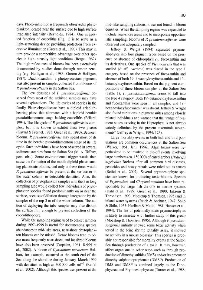
days. Photo-inhibition is frequently observed in phytoplankton located near the surface due to high surface irradiance intensity (Reynolds, 1984). One suggested function of coccoliths (Fig. 1) is to serve as a light-scattering device providing protection from excessive illumination (Green et ai., 1990). This may in tum provide a competitive advantage over other species in high-intensity light conditions (Berge, 1962). The high reflectance of blooms has been extensively documented by studies done through remote sensing (e.g. Holligan et ai., 1983; Groom & Holligan, 1987). Diadinoxanthin, a photoprotectant pigment, was also present in samples collected from blooms of P. pseudoroscoffensis in the Salton Sea.
The low densities of P. pseudoroscoffensis observed from most of the archived samples may have several explanations. The life cycles of species in the family Pleurochrysidaceae have a diploid cricolithbearing phase that alternates with a haploid benthic pseudofilamentous stage lacking coccoliths (Billard, 1994). The life cycle of P. pseudoroscoffensis is complex, but it is known to exhibit these two phases (Gayral & Fresnel, 1983; Green et al., 1990). Between blooms, P. pseudoroscoffensis may spend most of its time in the benthic pseudofilamentous stage of its life cycle. Such individuals have been observed in several sediment samples from the Salton Sea (M. A. Tiffany, pers. obs.). Some environmental trigger would then cause the formation of the motile diploid phase causing planktonic blooms, and only at these times would P. pseudoroscoffensis be present at the surface or in the water column in detectable densities. Also, the collection of phytoplankton samples with the 3 m long sampling tube would collect few individuals of phytoplankton species found predominantly on or near the surface, because of dilution through integration by the sampler of the top 3 m of the water column. The action of deploying the tube sampler may also disrupt the surface film enough to prevent collection of the coccolithophore.
While the sampling regime used to collect samples during 1997-1999 is useful for documenting species abundances in mid-lake areas, near-shore phytoplankton blooms can be missed. Dense blooms tend to occur more frequently near-shore, and localized blooms have also been observed (Carpelan, 1961; Reifel et al., 2002). A bloom of Gyrodinium uncatenum Hulburt, for example, occurred at the south end of the Sea along the shoreline during January-March 1999 with densities as high as 300000 cells ml- 1 (Reifel et ai., 2002). Although this species was present at the
183
mid-lake sampling stations, it was not found in bloom densities. When the sampling regime was expanded to include near-shore areas and to incorporate opportunistic sampling, blooms of P. pseudoroscoffensis were observed and adequately sampled.
Jeffrey & Wright (1994) separated prymnesiophytes into four pigment types based on the presence or absence of chlorophyll C3, fucoxanthin and its derivatives. One species of Pleurochrysis that was studied (P. aff. carterae) was placed in the type 1 category based on the presence of fucoxanthin and absence of both 19' -hexanoyloxyfucoxanthin and 19'butanoyloxyfucoxanthin. Based on the pigment compositions of three bloom samples at the Salton Sea (Table 1), P. pseudoroscoffensis seems to fall into the type 4 category. Both 19'-butanoyloxyfucoxanthin and fucoxanthin were seen in all samples, and 19'hexanoyloxyfucoxanthin was absent. Jeffrey & Wright also found variations in pigment suites among closely related individuals and warned that the "range of pigment suites existing in the Haptophyta is not always strictly delimited by the present taxonomic assignments" (Jeffrey & Wright, 1994: 123).
Large mortality events in both fish and bird populations are common occurrences at the Salton Sea (Walker, 1961; Jehl, 1996). Algal toxins were hypothesized to be involved in die-off events involving large numbers (ca. 150000) of eared grebes (Podiceps nigricollis Brehm) after all common bird diseases, pesticides and heavy metals were ruled out as causes (Reifel et ai., 2002). Several prymnesiophyte species are known for producing toxic blooms. Species of Prymnesium and Chrysochromulina have been responsible for large fish die-offs in marine systems (Dahl et ai., 1989; Green et ai., 1990; Eikrem & Throndsen, 1993; Moestrup & Thomsen, 1995) and in inland water systems (Reich & Aschner, 1947; Shilo & Shilo, 1955; Hurlbert & Mulla, 1981; Hansen et ai., 1994). The list of potentially toxic prymnesiophytes is likely to increase with further study of this group (Moestrup & Thomsen, 1995). Although P. pseudoroscoffensis initially showed some toxic activity when tested in the brine shrimp lethality assay, it showed no activity in a mouse bioassay. This species is probably not responsible for mortality events at the Salton Sea through production of a toxin. It may, however, affect organisms in other ways such as through production of dimethylsulfide (DMS) and/or its precursor dimethylsulphoniopropionate (DMSP). Production of DMS and DMSP is confined largely to the Dinophyceae and Prymnesiophyceae (Turner et ai., 1988;
184
Iverson et aI., 1989), and P. carterae has been shown to produce DMS and DMSP in laboratory cultures (Vairavamurthy et al., 1985). The exclusion of fish from some prymnesiophyte blooms may be due to the production of DMS (Sieburth, 1979). Blooms of coccolithophorids can also affect organisms by altering natural phytoplankton and zooplankton communities. Recent large-scale bird mortality in the Bering Sea was probably due to a shift in dominant zooplankton species caused by a large bloom of the coccolithophore Emiliania huxleyi (Saar, 2000). Further study is needed to document these possible effects of P. pseudoroscoffensis on birds and fish in the Salton Sea.
Acknowledgements
The authors would like to thank Brandon Swan, James Watts and Paul Detwiler for their assistance in the collection of bloom samples. We would also like to thank Dr Wuchang Wei of SIO for his assistance in species identification. This project was made possible in part by a grant from Sigma Xi and supported by the Salton Sea Research Management Committee and the Salton Sea Science Subcommittee. The research described in this article has been funded in part by the United States Environmental Protection Agency through grant #R826552-0 1-0 to the Salton Sea Authority. The research results have not been subjected, however, to the Agency's required peer review and do not necessarily reflect the views of the Agency. Therefore, no official endorsement should be inferred.
References
Bain, R. c., A. M. Caldwell, R. H. Clawson, H. L. Scotten & R. G. Willis, 1970. Salton Sea California: water quality and ecological management considerations. U.S. Dept. Interior, Fed. Wat. Qual. Administration, Pacific Southwest Region: 54 pp.
Barlow, S. B. & P. Kugrens, 2002. Cryptomonads from the Salton Sea, California. HydrobiologiaJDev. Hydrobiol. (in press).
Berge, G., 1962. Discoloration of the sea due to Coccolithus huxleyi 'bloom'. Sarsia 6: 27--40.
Billard, C., 1994. Life cycles. In Green, 1. C. & B. S. C. Leadbeater (eds), The Haptophyte Algae, Systematics Association special volume no. 51. Clarendon Press, Oxford: 167-186.
Blackburn, S.1. & G. Cresswell, 1993. A coccolithophorid bloom in Jervis Bay, Australia. Aust. 1. mar. freshwat. Res. 44: 253-260.
Carpelan, L. H., 1961. Phytoplankton. In Walker, B. W. (ed.), The Ecology of the Salton Sea, California in Relation to the Sportfishery. Calif. Dept. Fish. Game, Fish Bull. 113: 33-42.
Cohen, M. J., J. I. Morrison & E. P. Glenn, 1999. Haven or Hazard: the Ecology and Future of the Salton Sea. Pacific Institute, Oakland, California: 64 pp.
Dahl, E., O. Lindahl, E. Paasche & 1. Throndsen, 1989. The Chrysochromulina polylepis bloom in Scandinavian waters during spring 1988. In Cosper, E. M., V. M. Bricelj & E. J. Carpenter (eds), Coastal and Estuarine Studies, vol 35, Novel Phytoplankton Blooms. Springer-Verlag, Berlin: 383-405.
Eikrem, W. & J. Throndsen, 1993. Toxic prymnesiophytes identified from Norwegian coastal waters. In Smayda, T. 1. & Y. Shimizu (eds), Toxic Phytoplankton Blooms in the Sea. Elsevier, Amsterdam: 687-692.
Fresnel, 1. & C. Billard, 1991. Pleurochrysis placolithoides sp. nov. (Prymnesiophyceae), a new marine coccolithophorid with remarks on the status of cricolith-bearing species. Br. Phycol. 1. 26: 67-80.
Gayral, P. & 1. Fresnel, 1983. Description, sexualite et cycle de developpment d'une nouvelle coccolithophoracee (Prymnesiophyceae): Pleurochrysis pseudoroscoffensis sp. nov. Protistologica 19: 245-261.
Green, 1. c., K. Perch-Nielsen & P. Westbroek, 1990. Phylum Prymnesiophyta. In Margulis, L., J. O. Corliss, M. Melkonian & D. 1. Chapman (eds), Handbook of Protoctista. Jones & Bartlett Publishers, Boston: 293-317.
Groom, S. B. & P. M. Holligan, 1987. Remote sensing of coccolithophore blooms. Adv. Space Res. 7: 73-78.
Hallegraeff, G. M. & Y. Hara, 1995. Taxonomy of harmful marine raphidophytes. In Hallegraeff, G. M., D. M. Anderson & A. D. Cembella (eds), Manual on Harmful Microalgae. IOC Manuals and Guides no. 33. UNESCO Publishing, Paris: 365-371.
Hansen, L. R., 1. Kristiansen & J. V. Rasmussen, 1994. Potential toxicity of the freshwater Chrysochromulina species C. parva (Prymnesiophyceae). Hydrobiologia 287: 157.
Hasle, G. R., 1978. Settling: the inverted-microscope method. In Sournia, A. (ed.), Phytoplankton Manual. UNESCO Publishing, Paris: 88-96.
Heimdal, B. R., 1993. Modern coccolithophorids. In Tomas, C. R. (ed.), Marine Phytoplankton, a Guide to Naked Flagellates and Coccolithophorids. Academic Press, Inc., San Diego, California: 147-247.
Holligan, P. M., M. Viollier, D. S. Harbour, P. Camus & M. Champagne-Philippe, 1983. Satellite and ship studies of coccolithophore production along a continental shelf edge. Nature 304: 339-342.
Honjo, S., 1982. Seasonality and interaction of biogenic and lithogenic particulate flux at the Panama Basin. Science 218: 883-884.
Hurlbert, S. H. & M. S. Mulla, 1981. Impacts of mosquitofish (Gambusia affinis) predation on plankton communities. Hydrobiologia 83: 125-151.
Iverson, R. L., F. L. Nearhoof & M. O. Andreae, 1989. Production of dimethylsulfonium propionate and dimethylsulfide by phytoplankton in estuarine and coastal waters. Limnol. Oceanogr. 34: 53-67.
Jeffrey, s. W. & M. Vesk, 1997. Introduction to marine phytoplankton and their pigment signatures. In Jeffrey, S. w., R. F. C. Mantoura & S. W. Wright (eds), Phytoplankton Pigments in Oceanography: Guidelines to Modern Methods. UNESCO Publishing, Paris: 37-84.
Jeffrey, S. W. & S. W. Wright, 1994. Photosynthetic pigments in the Haptophyta. In Green, 1. C. & B. S. C. Leadbeater (eds), The Haptophyte Algae, Systematics Association special volume no. 51. Clarendon Press, Oxford: 111-132.
Jehl, 1. R. Jr., 1996. Mass mortality events of eared grebes in North America. 1. Field Ornith. 67: 471-476.
Johansen, J. R., G. 1. Doucette, W. R. Barclay & J. D. Bull, 1988. The morphology and ecology of Pleurochrysis carterae var.
dentata var. nov. (Prymnesiophyceae), a new coccolithophorid from an inland saline pond in New Mexico, U.S.A. Phycologia 27: 78-88.
Lund, 1. W. G., C. Kilpling & E. D. LeCren, 1958. The inverted microscope method of estimating algal numbers, and the statistical basis of estimation by counting. Hydrobiologia II: 143-170.
Meyer, B. N., N. R. Ferrigni, J. E. Putman, L. B. Jacobsen. D. E. Nichols & 1. L. MacLaughlin, 1982. Brine shrimp: a convenient general bioassay for active plant constituents. PI. Med. 45: 31-34.
Milliman, J. D., 1980. Coccolithophorid production and sedimentation, Rockall Bank. Deep Sea Res. 27: 959-963.
Moestrup, 0.,1994. Economic aspects: 'blooms', nuisance species. and toxins. In Green, J. C. & B. S. C. Leadbeater (eds), The Haptophyte Algae, Systematics Association special volume no. 51. Clarendon Press, Oxford: 265-285.
Moestrup. 0. & H. A. Thomsen, 1995. Taxonomy of toxic haptophytes (Prymnesiophytes). In Hallegraeff, G. M., D. M. Anderson & A. D. Cembella (eds), Manual on Harmful Microalgae. IOC Manuals & Guides No. 33, UNESCO Publishing: 319-338.
Reich, K. & M. Aschner, 1947. Mass development and control of the phytoflagellate Prymnesium parvum in fish ponds in Palestine. Palestine 1. Bot. Jerusalem 4: 14-23.
Reifel, K. M., M. P. McCoy, T. E. Rocke, M. A. Tiffany, D. 1. Faulkner & S. H. Hurlbert, 2002. Possible importance of algal toxins in the Salton Sea. California. HydrobiologiaiDev. Hydrobiol. (in press).
Reynolds, C. S., 1984. The Ecology of Freshwater Phytoplankton. University Press, Cambridge: 384 pp.
Saar, R. A., 2000. The unbearable capriciousness of Bering. Science 287: 1388-1389.
Shilo, M. & M. Shilo, 1955. Control of the phytoflagellate Prymnesium parvum. Verh. int. Ver. Limnol. 12: 233-240.
185
Sieburth. 1. M., 1979. Sea Microbes. Oxford University Press, New York: 491 pp.
Solis, P. N., C. W. Wright, M. M. Anderson, M. P. Gupta & 1. D. Phillipson, 1993. A microwell cytotoxicity assay using Artemia salina (brine shrimp). PI. Med. 59: 250-252.
Throndsen, 1., 1978. Preservation and storage. In Sournia. A. (ed.), Phytoplankton Manual. UNESCO Publishing, Paris: 69-74.
Tiffany, M. A., S. B. Barlow, V. E. Matey & S. H. Hurlbert, 2001. Chattonella marina (Raphidophyceae), a potentially toxic alga in the Salton Sea, California. Hydrobiologia 466 (Dev. Hydrobiol. 162): 187-194.
Turner, S. M., G. Malin, P. S. Liss, D. S. Harbour & P. M. Holligan. 1988. The seasonal variation of dimethyl sulfide and dimethylsulfoniopropionate concentrations in near-shore waters. Limnol. Oceanogr. 33: 364-375.
Vairavamurthy. A., M. O. Andreae & R. L. Iverson, 1985. Biosynthesis of dimethylsulfide and dimethylpropiothetin by Hymenomanas carterae in relation to sulfur source and salinity variations. Limnol. Oceanogr. 30: 59-70.
Walker, B. w., 1961. The ecology of the Salton Sea, California in relation to the sportfishery. Calif. Dept. Fish. Game, Fish Bull. 113: 1-204.
Watts, 1. M., B. K. Swan, M. A. Tiffany & S. H. Hurlbert, 2001. Thermal, mixing and oxygen regimes of the Salton Sea, California, 1997-1999. Hydrobiologia 466 (Dev. Hydrobiol. 162): 159-176.
Wright, S. w., S. W. Jeffrey, R. F. C. Mantoura, C. A. Llewellyn, T. Bjomland, D. Repeta & N. Welslehmayer, 1991. An improved HPLC method for the analysis of chlorophylls and carotenoids from marine phytoplankton. Mar. Ecol. Prog. Ser. 77: 183-196.
Hydrobiologia 466: 187-194,2001. l.M. Melack, R. Jellison & D.B. Herbst (eds), Saline Lakes. © 2001 Kluwer Academic Publishers.
187
Chattonella marina (Raphidophyceae), a potentially toxic alga in the Salton Sea, California
Mary A. Tiffany, Steven B. Barlow, Victoria E. Matey & Stuart H. Hurlbert Department of Biology, Center for Inland Waters and San Diego State University, San Diego, CA 92182, U.S.A.
Key words: raphidophyte, salt lake, toxic algae, phytoplankton
Abstract
Chattonella marina was found in high abundance in the phytoplankton of the Salton Sea from April to November, 1997. Maximum mean density was over 600 cells ml- 1 mid-lake. It was not detected from January 1997 to March 1997 or in January and February 1998. Transmission electron microscope studies show the typical Chattonella features: a teardrop-shaped nucleus, numerous radially arranged chloroplasts and lack of a cell wall. Gills of fish collected at the height of the Chattonella bloom showed damage to the primary and secondary lamellae and increased numbers of mucus cells. To our knowledge this is the first report of a species of Chattonella in a salt lake.
Introduction
Marine raphidophycean algae such as Chattonella, Fihrocapsa and Heterosigma have been implicated in major fish kills in various parts of the world (e.g. Subrahmanyan, 1954; Imai & Itoh, 1987; Shumalin et aI., 1994; Hallegraeff et aI., 1998; Tomas, 1998). Species in the genus Chattonella have been of special concern because of monetary losses due to mass mortality of finfish raised in aquaCUlture, especially yellowtail (Seriola quinqueradiata Temmick & Schlegel) in Japan (Imai & Hoh, 1987; Onoue et aI., 1989), southern bluefin tuna (Thunnus maccoyi Castelnau) in Australia (Hallegraeff et aI., 1998) and salmon (Salmo salar Linneaus) in Norway (Elbraechter, 1999). The toxic effects of Chattonella marina (Subrahmanyan) y. Hara et Chihara have been ascribed to the production of brevetoxins similar to those of dinoflagellates (Onoue et aI., 1987; Ahmed et aI., 1995; Khan et aI., 1995) and to superoxide radicals (Ishimatsu et aI., 1996; Oda et aI., 1997). Exposure of fish to C. marina causes gill epithelium to become swollen with massive mucous production (Endo et aI., 1985, 1992), and fish appear to smother even in well-oxygenated water.
In laboratory experiments on the strain found in Australian waters (Marshall & Hallegraeff, 1999) C. marina was shown to grow optimally at 25 DC and
at a salinity of 30 p.s.u. (p.s.u=practical salinity units which are essentially equivalent to g kg-I, several percent lower than g 1-1). Cells were capable of good growth from 10 DC to 30 DC and from 15 to 45 p.s.u., however at 50 p.s.u. growth only occurred from 15 to 25 DC. High irradiance (450 {Lmol m-2 s-I) also increased the growth.
The life cycles of C. marina and C. antiqua (Hada) Ono have been studied in the Seto Inland Sea of Japan (Imai & Hoh, 1987; Imai et aI., 1991). This waterbody is a eutrophic marine embayment with only a narrow connection to the ocean and limited circulation. There these species over-winter by forming cysts in late summer and early fall. They excyst into the flagellated form in early summer when the water at the sediment interface warms to ca. 20 DC and then reproduce by asexual division, often forming dense blooms. In laboratory experiments, the cysts required a dormancy period of several months at II DC before excystment occurred.
Whereas excystment of some dinoflagellates appears to be inhibited by conditions of low dissolved oxygen at the sediment interface, Chattonella spp. were found to excyst even at 02 levels of 2 mg 1-1 (Montani et al., 1995). This ability to excyst at low oxygen levels was used to explain the occurrence of
188
red tides of Chattonella spp. in the Seto Inland Sea in the summer, a time of strong stratification.
Another factor strongly controlling the extent of Chattonella spp. red tides is the degree of eutrophication and anthropogenic inputs of nutrients especially to shallow marine ecosystems (Watanabe et aI., 1995).
Description of site
The Salton Sea is below sea level and located in a closed basin in Riverside and Imperial counties in the southeastern comer of California. It formed in 1905-1907 by flooding from the Colorado River. It is the largest lake in California with an area of 980 km2 and a maximum depth of about 15 m (Ferrari & Weghorst, 1997).
The salinity is approximately 43 g 1-1 (as of 1999) and varies somewhat depending on proximity to freshwater inflows and season. It is primarily maintained by agricultural and municipal wastewaters from the Whitewater River in the north and the Alamo River and New River to the south. There is very little precipitation and most of the inflow originates from Colorado River water used for crop irrigation. The resultant high input of nutrients has historically caused dense blooms of algae (Carpelan, 1961; Bain et aI., 1970). Dinoflagellates and diatoms, most of which are of marine origin, are abundant year round. Chattonella has not been previously reported from this or any other lake but two unidentified 'motile green algae' were detected in abundance in 1968-1969 (Bain et aI., 1970) and one or both of these may have been raphidophytes.
Marine organisms from the Gulf of California and Pacific Ocean have been deliberately and accidentally introduced as part of an effort to establish a sport fishery in the lake. These introductions were mostly in the 1940s and 1950s at which time the salinity was similar to that of the ocean (Walker, 1961). This may have been the main source of the marine phytoplankton species presently found in the lake. In addition to deliberate fish introductions, tilapia (Oreochromis mossambicus Peters) has established itself in the lake and has become the dominant fish in the system (Costa-Pierce & Doyle, 1997). The juveniles of this fish are abundant in nearshore areas of the lake in mid-summer.
The presence of toxic algae has been considered as a possible cause of wildlife mortality at the Salton Sea. Therefore, a project to monitor the phytoplankton of the lake was started in January 1997. The purpose
of this project was to determine if any known toxic species were present, and if so, whether present in densities known to be harmful to fish or birds.
Materials and methods
Phytoplankton sampling
Samples for enumeration of phytoplankton species were taken approximately monthly beginning in January of 1997 at the following three mid-lake locations located along the main axis of the lake (see map in Watts et aI., 2001):
S-l 33° 25' 00" N 115° 55' 00" W
S-2 33° 21' 00" N 115° 51' 00" W
S-3 33° 18' 00" N 115° 48' 00" W The present findings are part of a larger study of the plankton dynamics during 1997-1999 (Reifel et aI., 2001,2002; Tiffany et al., 2002).
Integrated samples of whole water from the lake surface to 9 m were taken with a 3 m long tube sampler and fixed in the field with 1 % Lugol's solution. C. marina was enumerated with the standard technique (Utermohl, 1958) using a Leitz Diavert inverted microscope and two crossed diameters at 400 x . On some dates (May 20, and from October 17 forward), the phytoplankton samples from discrete depth intervals of 0-3 m, 3-6 m and 6-9 m were analyzed separately to determine vertical distributions differences in the three strata. On these dates the arithmetic mean densities for the three strata were obtained, so as to have values comparable to those calculated for integrated 0-9 m samples. A constant of 1.5 individuals ml-1,
the lowest non-zero density that could be observed given the volume of water examined, was added to each value. Geometric mean density ofC.marina and its among-station standard error were calculated for those dates where two or three stations were sampled. Not all three stations were sampled on every date due to logistical difficulties, primarily weather conditions that made boat operations unsafe. On dates when only one station was sampled, that value is given without an indication of error.
Temperature and oxygen were measured at each station and date at 1 m depth intervals starting at the surface using a YSI model 57 oxygen meter. Temperature could be accurately read to 0.1 0c. The oxygen probe was calibrated in air at 100% humidity, corrected for a salinity of 40 g 1-1 and an altitude of 69 m below sea level. Oxygen readings were accurate to
0.01 mg 1-1 in the range 0-10 mg 1-1 and 0.1 above 10 mg 1-1. Variation in barometric pressure on different dates was not taken into account, a source of 2-4% error.
Species identification
Live Chattonella cells were collected in summer 1997 and observed with light microscopy using brightfield and Nomarski illumination for confirmation of identification to the genus level. This is necessary because raphidophytes do not generally preserve well due to their fragile nature and tendency to shed flagella upon preservation (Throndsen, 1997). Scanning and transmission electron microscope studies of Chattonella cells were carried out to confirm the identification to species level. One ml water samples from the Salton Sea were fixed for electron microscopy by the sequential addition of 1 ml of 0.1 M cacodylate buffer (pH 7.2) containing 4% glutaraldehyde and 800 mOsm sucrose followed by 0.5 ml of 4% aqueous osmium tetroxide. After 20 min fixation at room temperature, cells were rinsed with fresh buffer. For scanning electron microscopy, cells were collected onto NUcleopore filters, dehydrated in ethanol, critical point dried, then sputter-coated with Au/Pd and viewed in a Hitachi S-2700 SEM. For transmission electron microscopy, cells were collected by centrifugation, then dehydrated in ethanol, and embedded in Spurr's resin. Silver sections were stained with uranyl acetate and lead citrate, then viewed with a Philips 410 TEM.
Examination of fish gills
Seven specimens of til apia (Oreochromis mossambicus) (length 3.7-5.2 cm) were collected from Varner Harbor at northeast comer of the Salton Sea in August 1997, when C.marina was abundant lake-wide, and examined using SEM. Gill arches were fixed in cold Karnovsky fixative for 2 h, postfixed in osmium tetraoxide for 1 h and dehydrated in a graded ethanol series with the final change in absolute ethanol. Then the samples were critical point dried with liquid C02, mounted on stubs, sputter-coated with Au/Pd and examined with a scanning electron microscope (Hitachi S-2700) at an accelerating voltage of 10k V.
189
Results
Species identification
These cells most closely resemble C.marina as described by Hara & Chihara (1982). Cells are yellowbrown, with two subequal, heterodynamic flagella which emerge from a sub-apical depression (Fig. lA, D). The posterior end of the cell exhibits some variation in shape from pointed to blunt-ended, but a groove in the posterior tip of the cell is commonly observed (Fig. IA). Swimming cells divide by binary fission (Fig. lB). A large, tear-shaped nucleus is situated in the center of the cell (Fig. lA, D). There are numerous elliptical chloroplasts arranged radiall y around the cell periphery (Fig. lD). Pyrenoids are located in the internal end of the chloroplasts, and thy lakoids are observed penetrating the pyrenoid matrix (Fig. IE). Electron-dense osmophilic bodies (Fig. lD, E) are widely distributed at the cell surface and appear as small bumps on the cell surface (Fig. IB,C), but no 'oboe-shaped' mucocysts or ejectosomes have been observed in cells examined to date. The cell periphery is highly vacuolated, and cells are fragile, since they are bounded only by a cell membrane.
Fish gill damage
Gills from tilapia collected during the C.marina bloom were distorted due to severe swelling, shortening and fusion of secondary (respiratory) lamellae (Fig. 2A). Similar distortions have been observed in other species of fish exposed to C. marina, C. antiqua and other Chattonella spp. (Tyoshima et al., 1985; Endo et aI., 1992; Ishimatsu et aI., 1995). These alterations were associated with hypertrophy, hyperplasia and edema of the epithelium of the secondary lamellae.
In contrast with Shimada et al. (1991), we found that the epithelium of gill filaments had a much larger than normal number of mucus cells. Numerous pores of these cells were seen mainly along the trailing edge of filaments and between lamellae (Fig. 2B). Hishida et al. (1997) obtained similar results in yellowtail (Seriola quinqueradiata). They suggested that mucus discharged from the filamental epithelium can block lamellar water channels and may be one of the causes of fish asphyxiation when fish are exposed to C. marina.
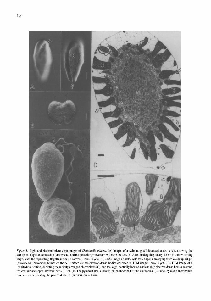
190
Figure 1. Light and electron microscope images of Chattonella marina. (A) Images of a swimming cell focussed at two levels, showing the sub-apical flagellar depression (arrowhead) and the posterior groove (arrow); bar = 10 /Lm. (B) A cell undergoing binary fission in the swimming stage, with the replicating flagella indicated (arrows); bar=lO /Lm. (C) SEM image of cells, with two flagella emerging from a sub-apical pit (arrowhead). Numerous bumps on the cell surface are the electron-dense bodies observed in TEM images; bar=lO /Lm. (0) TEM image of a longitudinal section, depicting the radially arranged chloroplasts (C), and the large, centrally located nucleus (N); electron dense bodies subtend the cell surface (open arrows); bar = l/Lm. (E) The pyrenoid (P) is located in the inner end of the chloroplast (C), and thylakoid membranes can be seen penetrating the pyrenoid matrix (arrows); bar = l/Lm.
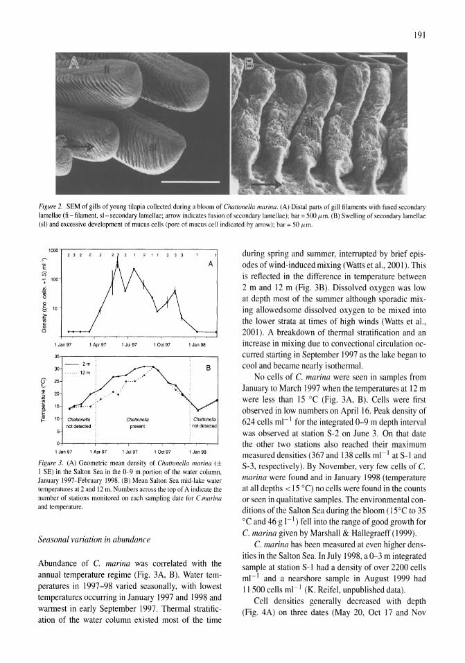
191
Figure 2. SEM of gills of young tilapia collected during a bloom of Chattonella marina. (A) Distal parts of gill filaments with fused secondary lamellae (fi - filament, sl- secondary lamellae; arrow indicates fusion of secondary lamellae); bar = 500 iJ,m. (B) Swelling of secondary lamellae (sl) and excessive development of mucus cells (pore of mucus cell indicated by arrow); bar = 50 iJ,m.
1000,-------------------,
:-E
"' '+ !!i 1ii
" o
100
§ 10
i!' 'in c
~
1 Jan 97 1 Apr 97
A
1 Jul97 1 Oct 97 , Jan 98
35,-------------~--_.
-- 2m 30
---- ·12m
2: 25
l" 20 ~ : ~-' ~ 15 .•. -:
E ~ 10 Chattonella
not detected '
1 Jan 97 1 Apr 97
.. , .'
ChaNonella present
1 Jul97 10ct9? 1 Jan 98
Figure 3. (A) Geometric mean density of Challonella marina (±
I SE) in the Salton Sea in the 0--9 m portion of the water column, January 1997-February 1998. (B) Mean Salton Sea mid-lake water temperatures at 2 and 12 m. Numbers across the top of A indicate the number of stations monitored on each sampling date for C.marina and temperature.
Seasonal variation in abundance
Abundance of C. marina was correlated with the annual temperature regime (Fig. 3A, B). Water temperatures in 1997-98 varied seasonally, with lowest temperatures occurring in January 1997 and 1998 and warmest in early September 1997. Thermal stratification of the water column existed most of the time
during spring and summer, interrupted by brief episodes of wind-induced mixing (Watts et aI., 2001). This is reflected in the difference in temperature between 2 m and 12 m (Fig. 3B). Dissolved oxygen was low at depth most of the summer although sporadic mixing allowed some dissolved oxygen to be mixed into the lower strata at times of high winds (Watts et aI., 200 I). A breakdown of thermal stratification and an increase in mixing due to convectional circulation occurred starting in September 1997 as the lake began to cool and became nearly isothermal.
No cells of C. marina were seen in samples from January to March 1997 when the temperatures at 12 m were less than 15 °C (Fig. 3A, B). Cells were first observed in low numbers on April 16. Peak density of 624 cells ml- I for the integrated 0-9 m depth interval was observed at station S-2 on June 3. On that date the other two stations also reached their maximum measured densities (367 and 138 cells ml- 1 at S-I and S-3, respectively). By November, very few cells of C. marina were found and in January 1998 (temperature at all depths < IS 0c) no cells were found in the counts or seen in qualitative samples. The environmental conditions of the Salton Sea during the bloom (15°C to 35 °C and 46 g I-I) fell into the range of good growth for C. marina given by Marshall & Hallegraeff (1999).
C. marina has been measured at even higher densities in the Salton Sea. In July 1998, a 0- 3 m integrated sample at station S-I had a density of over 2200 cells ml - I and a nearshore sample in August 1999 had II 500 cells ml - 1 (K. Reifel, unpublished data).
Cell densities generally decreased with depth (Fig. 4A) on three dates (May 20, Oct 17 and Nov
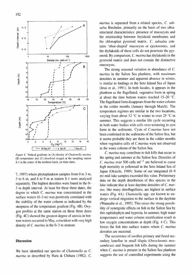
192
0-3 A
g
I 3-6 ~ ... £ ,£; c. Q)
0 6-9
10 100 1000
Density (no. cells mr')
B
g ,£; c. Q)
0
12
1 16 18 20 22 24 26 28 30
Temperature ee)
• c
g .<:: a Q)
0
o 2 4 12 14 16
- 20 May 97 --- 4 Oct 97 " 7 Nov 97
Figure 4. Vertical gradients in (A) density of Chattonella marina, (B) temperature and (C) dissolved oxygen at the sampling station Sol in the center of the northern basin, on three dates.
7, 1997) where phytoplankton samples from 0 to 3 m, 3 to 6 m, and 6 to 9 m at station S-l were analyzed separately_ The highest densities were found in the 0-3 m depth intervaL At least for these three dates, the degree to which C. marina was concentrated in the surface waters (0-3 m) was positively correlated with the stability of the water column as indicated by the steepness of the temperature gradient (Fig. 4B). Oxygen profiles at the same station on these three dates (Fig_ 4C) showed the greatest degree of anoxia in bottom waters occurred in May, coincident with very high density of C marina in the 0-3 m stratum.
Discussion
We have identified our species of Chattonella as C marina as described by Hara & Chihara (1982)_ C.
marina is separated from a related species, C subsalsa Biecheler, primarily on the basis of two ultrastructural characteristics: presence of mucocysts and the relationship between thylakoid membranes and the chloroplast pyrenoid matrix_ C subsalsa contains 'oboe-shaped' mucocysts or ejectosomes, and the thylakoids of these cells do not penetrate the pyrenoid. By comparison, C marina has thylakoids in the pyrenoid matrix and does not contain the distinctive mucocysts.
The strong seasonal variation in abundance of C marina in the Salton Sea plankton, with maximum densities in summer and apparent absence in winter, is similar to findings in the Seto Inland Sea of Japan (lmai et al_, 1991). In both locales, it appears in the plankton as the flagellated, vegetative form in spring at about the time bottom waters reached 15-20 °C. The flagellated form disappears from the water column in the colder months (January through March)_ The temperature regimes are similar in the two locations, varying from about 12°C in winter to over 25 °C in summer_ This suggests a similar life cycle occurring in both water bodies with cells over-wintering in cyst form in the sediments_ Cysts of Cmarina have not been confirmed in the sediments of the Salton Sea, but it seems probable they are there in the colder months when vegetative cells of C.marina were not observed in the water column of the Salton Sea_
C marina may contribute to fish kills that occur in the spring and summer at the Salton Sea_ Densities of C marina over 500 cells ml-1 are believed to cause high mortality in yellowtail in the Seto Inland Sea of Japan (Okaichi, 1989)_ Some of our integrated (0-9 m) mid-lake samples exceeded this value_ Preliminary data on the depth distribution of this species in the lake indicate that at least daytime densities of C marina, like many dinoflagellates, are highest in surface waters (Fig_ 4A). Chattonella spp_ are known to undergo vertical migration to the surface in the daytime (Watanabe et aL, 1995)_ This raises the strong possibility of synergistic effects on fish in the Salton Sea by this raphidophyte and hypoxia. In summer, high water temperatures and water column stratification result in low oxygen concentrations at depth (Fig. 4 C)- This forces the fish into surface waters where C marina densities are maximaL
The occurrence of swollen primary and fused secondary lamellae in small tilapia (Oreochromis mossambicus) and frequent fish kills during the summer when C marina is present in the Salton Sea plankton suggests the use of controlled experiments using the
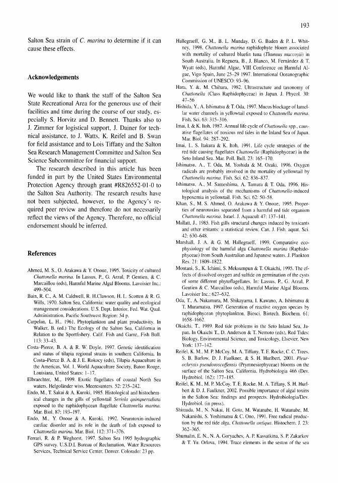
Salton Sea strain of C. marina to determine if it can cause these effects.
Acknowledgements
We would like to thank the staff of the Salton Sea State Recreational Area for the generous use of their facilities and time during the course of our study, especially S. Horvitz and D. Bennett. Thanks also to 1. Zimmer for logistical support, 1. Dainer for technical assistance, to 1. Watts, K. Reifel and B. Swan for field assistance and to Lois Tiffany and the Salton Sea Research Management Committee and Salton Sea Science Subcommittee for financial support.
The research described in this article has been funded in part by the United States Environmental Protection Agency through grant #R826552-0 1-0 to the Salton Sea Authority. The research results have not been subjected, however, to the Agency's required peer review and therefore do not necessarily reflect the views of the Agency. Therefore, no official endorsement should be inferred.
References
Ahmed, M. S., O. Arakawa & Y. Onoue, 1995. Toxicity of cultured Chattonella marina. In Lassus, P., G. Arzul, P. Gentien, & c. Marcaillou (eds), Harmful Marine Algal Blooms. Lavoisier Inc.: 499-504.
Bain, R. C., A. M. Caldwell, R. H.Clawson, H. L. Scotten & R. G. Wills, 1970. Salton Sea, California: water quality and ecological management considerations. U.S. Dept. Interior, Fed. Wat. Qual. Administration, Pacific Southwest Region: 54 p.
Carpelan, L. H., 1961. Phytoplankton and plant productivity. In Walker, B. (ed.) The Ecology of the Salton Sea, California in Relation to the Sportfishery. Calif. Fish and Game, Fish Bull. 113: 33-43.
Costa-Pierce, B. A. & R. W. Doyle, 1997. Genetic identification and status of tilapia regional strains in southern California. In Costa-Pierce B. A. & J. E. Rokocy (eds), Tilapia Aquaculture in the Americas, Vol. I. World Aquaculture Society, Baton Rouge, Louisiana, United States: 1-17.
Elbraechter, M., 1999. Exotic flagellates of coastal North Sea waters. Helgolander wiss. Meeresunters. 52: 235-242.
Endo, M., T. Sakai & A. Kuroki, 1985. Histological and histochemical changes in the gills of yellowtail Seriola quinqueradiata exposed to the raphidophycean flagellate Chattonella marina. Mar. BioI. 87: 193-197.
Endo, M., Y. Onoue & A. Kuroki, 1992. Neurotoxin-induced cardiac disorder and its role in the death of fish exposed to Chattonella marina. Mar. BioI. 112: 371-376.
Ferrari, R. & P. Weghorst, 1997. Salton Sea 1995 hydrographic GPS survey. U.S.D.1. Bureau of Reclamation, Water Resources Services, Technical Service Center, Denver. Colorado: 23 pp.
193
Hallegraeff, G. M., B. L. Munday, D. G. Baden & P. L. Whitney, 1998. Chattonella marina raphidophyte bloom associated with mortality of cultured bluefin tuna (Thunnus maccoyU) in South Australia. In Reguera, B., 1. Blanco, M. Fernandez & T. Wyatt (eds), Harmful Algae, VIII Conference on Harmful Algae, Vigo Spain, June 25-29 1997. International Oceanographic Commission of UNESCO: 93-96.
Hara, Y. &, M. Chihara, 1982. Ultrastructure and taxonomy of Chattonella (Class Raphidophyceae) in Japan. J. Phycol. 30: 47-56
Hishida, Y., A. Ishimatsu & T. Oda, 1997. Mucus blockage of lamellar water channels in yellowtail exposed to Chattonella marina. Fish. Sci. 63: 315-316.
Imai, I. & K. Itoh, 1987. Annual life cycle of Chattonella spp., causative flagellates of noxious red tides in the Inland Sea of Japan. Mar. BioI. 94: 287-292.
Imai, I., S. Ilakura & K. Itoh, 1991. Life cycle strategies of the red tide causing flagellates Chattonella (Raphidophyceae) in the Seto Inland Sea. Mar. Poll. Bull. 23: 165-170.
Ishimatsu, A., T. Oda, M. Yoshida & M. Ozaki, 1996. Oxygen radicals are probably involved in the mortality of yellowtail by Chattonella marina. Fish. Sci. 62: 836-837.
Ishimatsu, A., M. Sameshima, A. Tamura & T. Oda, 1996. Histological analysis of the mechanisms of Chattonella-induced hypoxemia in yellowtail. Fish. Sci. 62: 50-58.
Khan, S., M. S. Ahmed, O. Arakawa & Y. Onoue, 1995. Properties of neurotoxins separated from a harmful red tide organism Chattonella marina. Israel. J. Aquacult 47: 137-141.
Mallatt, J., 1985. Fish gills structural changes induced by toxicants and other irritants: a statistical review. Can. 1. Fish. aquat. Sci. 42: 630-648.
Marshall, J. A. & G. M. Hallegraeff, 1999. Comparative ecophysiology of the harmful alga Chattonella marina (Raphidophyceae) from South Australian and Japanese waters. 1. Plankton Res. 21: 1809-1822.
Montani, S., K. Ichimi, S. Meksumpun & T. Okaichi, 1995. The effects of dissolved oxygen and sulfide on germination of the cysts of some different phytoflagellates. In: Lassus, P., G. Arzul, P. Gentien & C. Marcaillou (eds), Harmful Marine Algal Blooms. Lavoisier Inc.: 627-632.
Oda, T., A. Nakamura, M. Shikayama, I. Kawano, A. Ishimatsu & T. Muramatsu, 1997. Generation of reactive oxygen species by raphidophycean phytoplankton. Biosci. Biotech. Biochem. 61: 1658-1662.
Okaichi, T., 1989. Red tide problems in the Seto Inland Sea, Japan. In Okaichi T., D. Anderson & T. Nemoto (eds), Red Tides: Biology, Environmental Science, and Toxicology, Elsevier, New York: 137-142.
Reifel, K. M., M. P. McCoy, M. A. Tiffany, T. E. Rocke, C. C. Trees, S. B. Barlow, D. 1. Faulkner, & S. H. Hurlbert, 2001. Pleurochrysis pseudoroscoffensis (Prymnesiophyceae) blooms on the surface of the Salton Sea, California. Hydrobiologia 466 (Dev. Hydrobiol. 162): 177-185.
Reifel, K. M., M. P. McCoy, T. E. Rocke, M. A. Tiffany, S. H. Hurlbert & D. 1. Faulkner, 2002. Possible importance of algal toxins in the Salton Sea: findings and prospects. Hydrobiologia/Dev. Hydrobiol. (in press).
Shimada, M., N. Nakai, H. Goto, M. Watanabe, H. Watanabe, M. Nakanishi, S. Yoshimatsu & c. Ono, 1991. Free radical production by the red tide alga, Chattonella antiqua. Histochem. 1. 23: 362-365.
Shumalin, E. N., N. A. Goryachev, A. P. Kassatkina, S. P. Zakarkov & T. Yu. Orlova, 1994. Trace elements in the seston of the sea
194
part of the Razdolnaya River estuary during 'red tide' . Biologiya Morya 20: 286-290 (in Russian).
Subrahmanyan, R., 1954. On the life-history and ecology of Hornellia marina gen. et sp. nov. (Chloromonadineae) causing green discoloration of the sea and mortality among marine organisms off the Malabar coast. Indian 1. Fish. 1: 182-202.
Throndsen, 1., 1997. The planktonic marine flagellates. In Tomas, C. (ed.), Identifying Marine Phytoplankton. Academic Press, Harcourt Brace, San Diego, California: 591-729.
Tiffany, M. A., B. K. Swan, 1. M. Watts & S. H. Hurlbert, 2002. Metazooplankton dynamics in the Salton Sea, California, 1997-1999. Hydrobiologia/Dev. Hydrobiol. (in press).
Tomas, C. R., 1998. Blooms of potentially harmful raphidophycean flagellates in Florida coastal waters. In Reguera, B., J. Blanco, M. Fernandez & T. Wyatt (eds), Harmful Algae, VIII International Conference on Harmful Algae, Vigo Spain, June 25-29 1997. International Oceanographic Commission of UNESCO: 101-103.
Utermohl, H., 1958. Zur Vervollkommnung der quantltatlven Phytoplankton-Methodiks Mitt. int. Ver. theor. angew. Limnol. 9: 1-38.
Walker, B. (ed.), 1961. The Ecology of the Salton Sea, California in Relation to the Sportfishery. Calif. Fish and Game, Fish Bull. 113: 1-204.
Watanabe, M., K. Kohata, T. Kimura & T. Takamatsu, 1995. Generation of a Chattonella antiqua bloom by imposing a shallow nutricline in a mesocosm. Limnol. Oceanogr. 40: 1447-1460.
Watts, 1. M., B. K. Swan, M. A. Tiffany & S. H. Hurlbert, 2001. Thermal, mixing and oxygen regimes of the Salton Sea, California, 1997-1999. Hydrobiologia 466 (Dev. Hydrobiol. 162): 159-176.
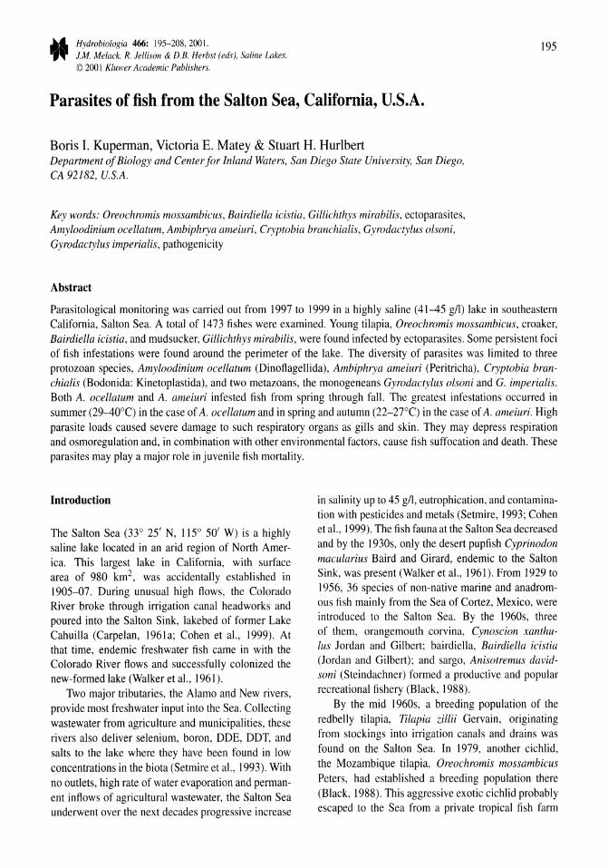
Hydrobiologia 466: 195-208, 200 I. 1.M. Melack, R. Jellison & D.B. Herbst (eds), Saline Lakes. © 2001 Kluwer Academic Publishers.
195
Parasites of fish from the Salton Sea, California, U.S.A.
Boris 1. Kuperman, Victoria E. Matey & Stuart H. Hurlbert Department of Biology and Centerfor Inland Waters, San Diego State University, San Diego, CA 92182, U.S.A.
Key words: Oreochromis mossambicus, Bairdiella icistia, Gillichthys mirabilis, ectoparasites, Amyloodinium ocellatum, Ambiphrya ameiuri, Cryptobia branchialis, Gyrodactylus oisoni, Gyrodactylus imperialis, pathogenicity
Abstract
Parasitological monitoring was carried out from 1997 to 1999 in a highly saline (41-45 gil) lake in southeastern California, Salton Sea. A total of 1473 fishes were examined. Young tilapia, Oreochromis mossambicus, croaker, Bairdiella icistia, and mudsucker, Gillichthys mirabilis, were found infected by ectoparasites. Some persistent foci of fish infestations were found around the perimeter of the lake. The diversity of parasites was limited to three protozoan species, Amyloodinium ocellatum (Dinoflagellida), Ambiphrya ameiuri (Peritricha), Cryptobia branchialis (Bodonida: Kinetoplastida), and two metazoans, the monogeneans Gyrodactylus olsoni and G. imperialis. Both A. ocellatum and A. ameiuri infested fish from spring through fall. The greatest infestations occurred in summer (29-40°C) in the case of A. ocellatum and in spring and autumn (22-27°C) in the case of A. ameiuri. High parasite loads caused severe damage to such respiratory organs as gills and skin. They may depress respiration and osmoregulation and, in combination with other environmental factors, cause fish suffocation and death. These parasites may playa major role in juvenile fish mortality.
Introduction
The Salton Sea (33 0 25' N, 1150 50' W) is a highly saline lake located in an arid region of North America. This largest lake in California, with surface area of 980 km2, was accidentally established in 1905-07. During unusual high flows, the Colorado River broke through irrigation canal headworks and poured into the Salton Sink, lakebed of former Lake Cahuilla (Carpelan, 1961a; Cohen et aI., 1999). At that time, endemic freshwater fish came in with the Colorado River flows and successfully colonized the new-formed lake (Walker et al., 1961).
Two major tributaries, the Alamo and New rivers, provide most freshwater input into the Sea. Collecting wastewater from agriculture and municipalities, these rivers also deliver selenium, boron, DDE, DDT, and salts to the lake where they have been found in low concentrations in the biota (Setmire et aI., 1993). With no outlets, high rate of water evaporation and permanent inflows of agricultural wastewater, the Salton Sea underwent over the next decades progressive increase
in salinity up to 45 gil, eutrophication, and contamination with pesticides and metals (Setmire, 1993; Cohen et al., 1999). The fish fauna at the Salton Sea decreased and by the 1930s, only the desert pupfish Cyprinodon macularius Baird and Girard, endemic to the Salton Sink, was present (Walker et al., 1961). From 1929 to 1956, 36 species of non-native marine and anadromous fish mainly from the Sea of Cortez, Mexico, were introduced to the Salton Sea. By the 1960s, three of them, orangemouth corvina, Cynoscion xanthuIus Jordan and Gilbert; bairdiella, Bairdiella icistia (Jordan and Gilbert); and sargo, Anisotremus davidsoni (Steindachner) formed a productive and popular recreational fishery (Black, 1988).
By the mid 1960s, a breeding population of the redbelly tilapia, Tilapia zillii Gervain, originating from stockings into irrigation canals and drains was found on the Salton Sea. In 1979, another cichlid, the Mozambique tilapia, Oreochromis mossambicus Peters, had established a breeding population there (Black, 1988). This aggressive exotic cichlid probably escaped to the Sea from a private tropical fish farm
196
near Niland, California, or originated from stockings for aquatic plant control in irrigation system (canals and drains) of the Imperial, Palo Verde, and Bard valleys of California and in Yuma Canal, Arizona (Black, 1988; Costa-Pierce & Doyle, 1997). By the early 1980s, O. mossambicus was the dominant fish species in the Sea. Recently, DNA marker studies have shown that tilapia from the Salton Sea are likely hybrids of Oreochromis urolepis hornorum x Oreochromis mossambicus (Costa-Pierce & Doyle, 1997). Both O. mossambicus and its hybrid are among the fish species most tolerant of high water salinity and temperatures (Watanabe, 1997). Tilapia, the most important prey species for the large numbers of piscivorous birds at the Salton Sea, is also a popular recreational fish.
For many decades, the Salton Sea has been the site of large die-offs of fish and water birds (Walker et aI., 1961; Jehl, 1994, 1996; Cohen et a!., 1999; NWHC, \999). Type C avian botulism has been shown to be the cause of some bird mortality events, such as the death of 11 000 pelicans in 1996. Fish, particularly moribund tilapia, are considered the likely vectors to pelicans of this fatal disease. Fish kills have been associated with critical combination of high salinity, temperature extremes, elevated levels of nutrients, low oxygen tension, high sulfate concentrations, and toxic algal blooms (Tiffany et aI., 2001; Watts et aI., 2001).
Until 1997, nothing was known about parasitic infestations of fish in the Salton Sea. Two factors encouraged us to begin parasitological monitoring of this lake. First, by the early 1990s it was generally known that fish from water bodies stressed by anthropogenic pollution or natural environmental factors are predisposed to parasitic infestations (Khan & Thulin, 1991; Overstreet, 1993, MacKenzie et aI., 1995). Second, tilapia, the dominant fish at the Salton Sea, is highly susceptible to parasites and pathogens in poor environmental conditions (Plumb, 1997).
Our first inspections found heavy infestation of young tilapia and croaker by the harmful dinoflagellate Amyloodinium ocellatum [(Brown, 1931) Brown & Hovasse, 1946] (Kuperman & Matey, 1999) and also several other parasites affecting different species of fish in the lake. Here we present results of parasitological monitoring of fish from the Salton Sea during 1997-1999. Our major goals were: (a) to discover and identify the protozoan and metazoan parasites of fish, (b) to document seasonal variations of fish infestation by two of the commonest forms, and (c) to evaluate harmful effects of parasites on the fish tissue with electron and light microscopy.
Table 1. Characteristics of fishes examined at the Salton Sea in 1997-1999
Site of collection Time of collection Number Fish size,
(year, month) of fish (em)
Tilapia, Oreochromis mossambicus
Varner Harbor 1997, VI, VIII, IX 68 1.4-3.9
1998, V-VIII, X, XI 265 1.0-5.5
1999, V-VIII, X 105 1.2-4.1
Bombay Beach 1998, V, Vll-XI 231 1.0-10.8
1999, VI-VIII, X 96 1.1-3.3
Red Hill 1998, VII, X 75 1.0-6.1
1999, VI-VIII, X 115 1.0-4.6
Salton City 1998, X 56 1.0-13.0
1999, VI-VIII, X 200 1.3-5.7
Croaker, Bairdiella icistia
Varner Harbor 1998, VII 25 2.9-3.6
Bombay Beach 1998, V-Vll, X 124 1.2-6.5
Red Hill 1998, VI-VII, X 96 2.5-6.2
Longjaw mudsucker, Gillichthys mirabilis
Bombay Beach 1998, V, VII 30 6.5-12.5
Red Hill 1998, IV, V 26 4.0-11.2
Materials and methods
Sampling and preparation
A total of 1473 juvenile fishes were collected for parasitological examinations in spring, summer and autumn months in 1997-1999 (Table I). In 1997, fish were collected only from Varner Harbor. In 1998-1999, they were collected at four locations along the Salton Sea shoreline: Varner Harbor, Bombay Beach, Red Hill, and Salton City (Fig. I, Table 1). All fish were caught with dip nets and seine in shallow harbors. At each sampling, water temperature was measured to O.I°C at 20-30 cm depth. Along the shoreline, shallow water temperature fluctuations were wide: from < 12SC in winter to >40°C in summer. Oxygen tension varied spatially and temporally from o to > 20 mg/l (Watts et aI., 200 I).
Shortly after capture, the fishes were transported to a field laboratory on the lake shore or were placed into aerated tanks with Salton Sea water and delivered to San Diego State University for further processing. Total length of each fish was measured to the nearest millimeter. The size range for each group of fish examined is presented in Table 1.
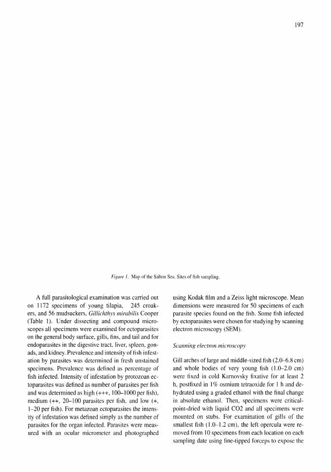
197
Figure 1. Map of the Salton Sea. Sites of fish sampling.
A full parasitological examination was carried out on 1172 specimens of young tilapia, 245 croakers, and 56 mudsuckers, Gillichthys mirabilis Cooper (Table 1). Under dissecting and compound microscopes all specimens were examined for ectoparasites on the general body surface, gills, fins, and tail and for endoparasites in the digestive tract, liver, spleen, gonads, and kidney. Prevalence and intensity offish infestation by parasites was determined in fresh unstained specimens. Prevalence was defined as percentage of fish infected. Intensity of infestation by protozoan ectoparasites was defined as number of parasites per fi sh and was determined as high (+++, 100-1000 per fish), medium (++, 20-100 parasites per fish, and low (+, 1-20 per fish). For metazoan ectoparasites the intensity of infestation was defined simply as the number of parasites for the organ infected. Parasites were measured with an ocular micrometer and photographed
using Kodak film and a Zeiss light microscope. Mean dimensions were measured for 50 specimens of each parasite species found on the fish. Some fish infected by ectoparasites were chosen for studying by scanning electron microscopy (SEM).
Scanning electron microscopy
Gill arches of large and middle-sized fish (2.0-6.8 cm) and whole bodies of very young fish (1.0-2.0 cm) were fixed in cold Karnovsky fixative for at least 2 h, postfixed in 1 % osmium tetraoxide for I h and dehydrated using a graded ethanol with the final change in absolute ethano!' Then, specimens were criticalpoint-dried with liquid C02 and all specimens were mounted on stubs. For examination of gills of the smallest fish (1.0-1.2 cm), the left opercula were removed from 10 specimens from each location on each sampling date using fine-tipped forceps to expose the
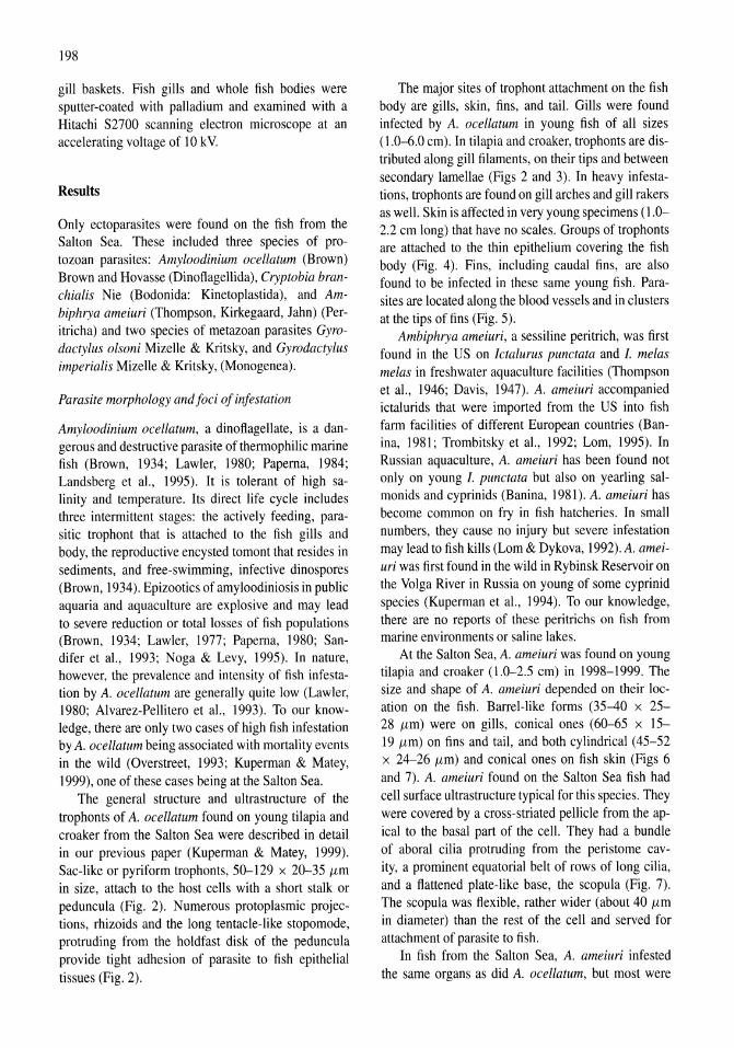
198
gill baskets. Fish gills and whole fish bodies were sputter-coated with palladium and examined with a Hitachi S2700 scanning electron microscope at an accelerating voltage of 10 kV.
Results
Only ectoparasites were found on the fish from the Salton Sea. These included three species of protozoan parasites: Amyloodinium ocellatum (Brown) Brown and Hovasse (Dinoflagellida), Cryptobia branchialis Nie (Bodonida: Kinetoplastida), and Ambiphrya ameiuri (Thompson, Kirkegaard, Jahn) (Peritricha) and two species of metazoan parasites Gyrodactylus olsoni Mizelle & Kritsky, and Gyrodactylus imperialis Mizelle & Kritsky, (Monogenea).
Parasite morphology and foci of infestation
Amyloodinium ocellatum, a dinoflagellate, is a dangerous and destructive parasite of thermophilic marine fish (Brown, 1934; Lawler, 1980; Papema, 1984; Landsberg et aI., 1995). It is tolerant of high salinity and temperature. Its direct life cycle includes three intermittent stages: the actively feeding, parasitic trophont that is attached to the fish gills and body, the reproductive encysted tomont that resides in sediments, and free-swimming, infective dinospores (Brown, 1934). Epizootics of amyloodiniosis in public aquaria and aquaculture are explosive and may lead to severe reduction or total losses of fish populations (Brown, 1934; Lawler, 1977; Papema, 1980; Sandifer et aI., 1993; Noga & Levy, 1995). In nature, however, the prevalence and intensity of fish infestation by A. ocellatum are generally quite low (Lawler, 1980; Alvarez-Pellitero et aI., 1993). To our knowledge, there are only two cases of high fish infestation by A. ocellatum being associated with mortality events in the wild (Overstreet, 1993; Kuperman & Matey, 1999), one of these cases being at the Salton Sea.
The general structure and ultrastructure of the trophonts of A. ocellatum found on young tilapia and croaker from the Salton Sea were described in detail in our previous paper (Kuperman & Matey, 1999). Sac-like or pyriform trophonts, 50-129 x 20-35 /Lm in size, attach to the host cells with a short stalk or peduncula (Fig. 2). Numerous protoplasmic projections, rhizoids and the long tentacle-like stopomode, protruding from the holdfast disk of the peduncula provide tight adhesion of parasite to fish epithelial tissues (Fig. 2).
The major sites of trophont attachment on the fish body are gills, skin, fins, and tail. Gills were found infected by A. ocellatum in young fish of all sizes (1.0-6.0 cm). In til apia and croaker, trophonts are distributed along gill filaments, on their tips and between secondary lamellae (Figs 2 and 3). In heavy infestations, trophonts are found on gill arches and gill rakers as well. Skin is affected in very young specimens (1.0-2.2 cm long) that have no scales. Groups of trophonts are attached to the thin epithelium covering the fish body (Fig. 4). Fins, including caudal fins, are also found to be infected in these same young fish. Parasites are located along the blood vessels and in clusters at the tips of fins (Fig. 5).
Ambiphrya ameiuri, a sessiline peritrich, was first found in the US on Ictalurus punctata and l. melas melas in freshwater aquaculture facilities (Thompson et aI., 1946; Davis, 1947). A. ameiuri accompanied ictalurids that were imported from the US into fish farm facilities of different European countries (Banina, 1981; Trombitsky et aI., 1992; Lorn, 1995). In Russian aquaculture, A. ameiuri has been found not only on young l. punctata but also on yearling salmonids and cyprinids (Banina, 1981). A. ameiuri has become common on fry in fish hatcheries. In small numbers, they cause no injury but severe infestation may lead to fish kills (Lorn & Dykova, 1992). A. ameiuri was first found in the wild in Rybinsk Reservoir on the Volga River in Russia on young of some cyprinid species (Kuperman et aI., 1994). To our knowledge, there are no reports of these peritrichs on fish from marine environments or saline lakes.
At the Salton Sea, A. ameiuri was found on young tilapia and croaker (1.0-2.5 cm) in 1998-1999. The size and shape of A. ameiuri depended on their location on the fish. Barrel-like forms (35-40 x 25-28 /Lm) were on gills, conical ones (60-65 x 15-19 /Lm) on fins and tail, and both cylindrical (45-52 x 24-26 /Lm) and conical ones on fish skin (Figs 6 and 7). A. ameiuri found on the Salton Sea fish had cell surface ultrastructure typical for this species. They were covered by a cross-striated pellicle from the apical to the basal part of the cell. They had a bundle of aboral cilia protruding from the peristome cavity, a prominent equatorial belt of rows of long cilia, and a flattened plate-like base, the scopula (Fig. 7). The scopula was flexible, rather wider (about 40 /Lm in diameter) than the rest of the cell and served for attachment of parasite to fish.
In fish from the Salton Sea, A. ameiuri infested the same organs as did A. ocellatum, but most were
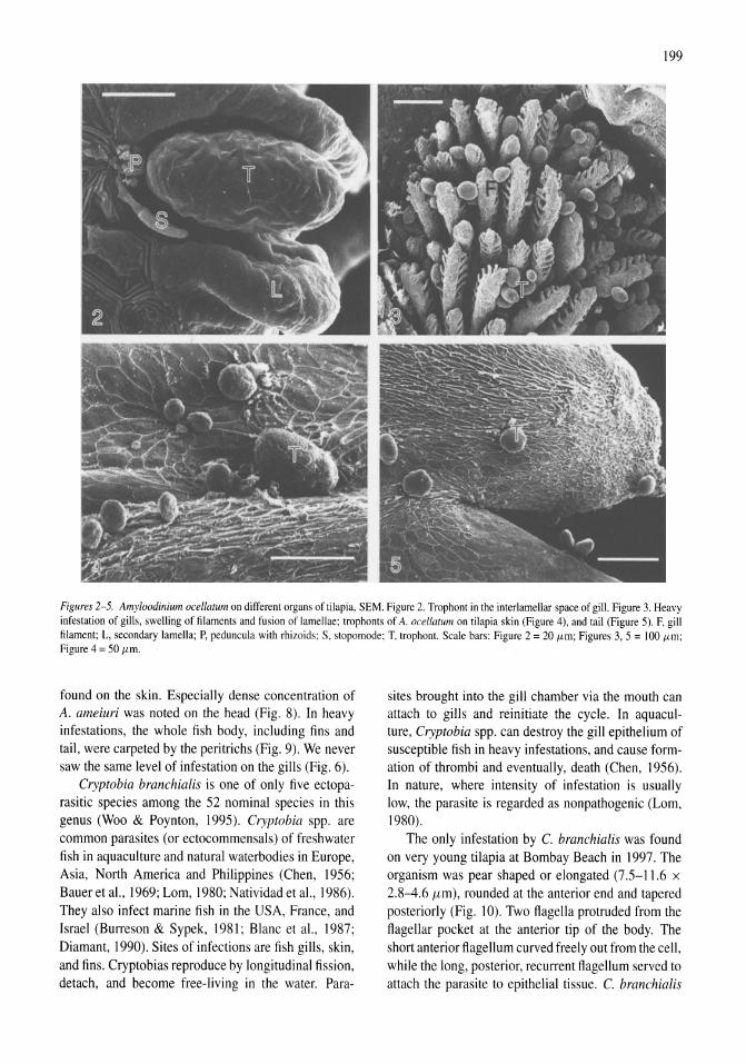
199
Figures 2-5. Amyloodinium ocellarum on different organs of til apia, SEM. Figure 2. Trophont in the interlamellar space of gill. Figure 3. Heavy infestation of gills, swelling of filaments and fusion of lamellae; trophonts of A. ocel/alum on tilapia skin (Figure 4), and tail (Figure 5). F, gill filament; L, secondary lamella; P, peduncula with rhizoids; S, stopomode; T, trophont. Scale bars: Figure 2 = 20 JIm; Figures 3, 5 = 100 JIm; Figure 4 = 50 JIm.
found on the skin. Especially dense concentration of A. ameiuri was noted on the head (Fig. 8). In heavy infestations, the whole fish body, including fins and tail, were carpeted by the peritrichs (Fig. 9). We never saw the same level of infestation on the gills (Fig. 6).
Cryptobia branchialis is one of only five ectoparasitic species among the 52 nominal species in this genus (Woo & Poynton, 1995). Cryptobia spp. are common parasites (or ectocommensals) of freshwater fish in aquaculture and natural waterbodies in Europe, Asia, North America and Philippines (Chen, 1956; Bauer et aI., 1969; Lorn, 1980; Natividad et aI. , 1986). They also infect marine fish in the USA, France, and Israel (Burreson & Sypek, 1981; Blanc et aI., 1987; Diamant, 1990). Sites of infections are fish gills, skin, and fins. Cryptobias reproduce by longitudinal fission, detach, and become free-living in the water. Para-
sites brought into the gill chamber via the mouth can attach to gills and reinitiate the cycle. In aquaculture, Cryptobia spp. can destroy the gill epithelium of susceptible fish in heavy infestations, and cause formation of thrombi and eventually, death (Chen, 1956). In nature, where intensity of infestation is usually low, the parasite is regarded as nonpathogenic (Lorn, 1980).
The only infestation by C. branchialis was found on very young tilapia at Bombay Beach in 1997. The organism was pear shaped or elongated (7.5-11.6 x 2.8-4.6 {tm), rounded at the anterior end and tapered posteriorly (Fig. 10). Two flagella protruded from the flagellar pocket at the anterior tip of the body. The short anterior flagellum curved freely out from the cell , while the long, posterior, recurrent flagellum served to attach the parasite to epithelial tissue. C. branchialis
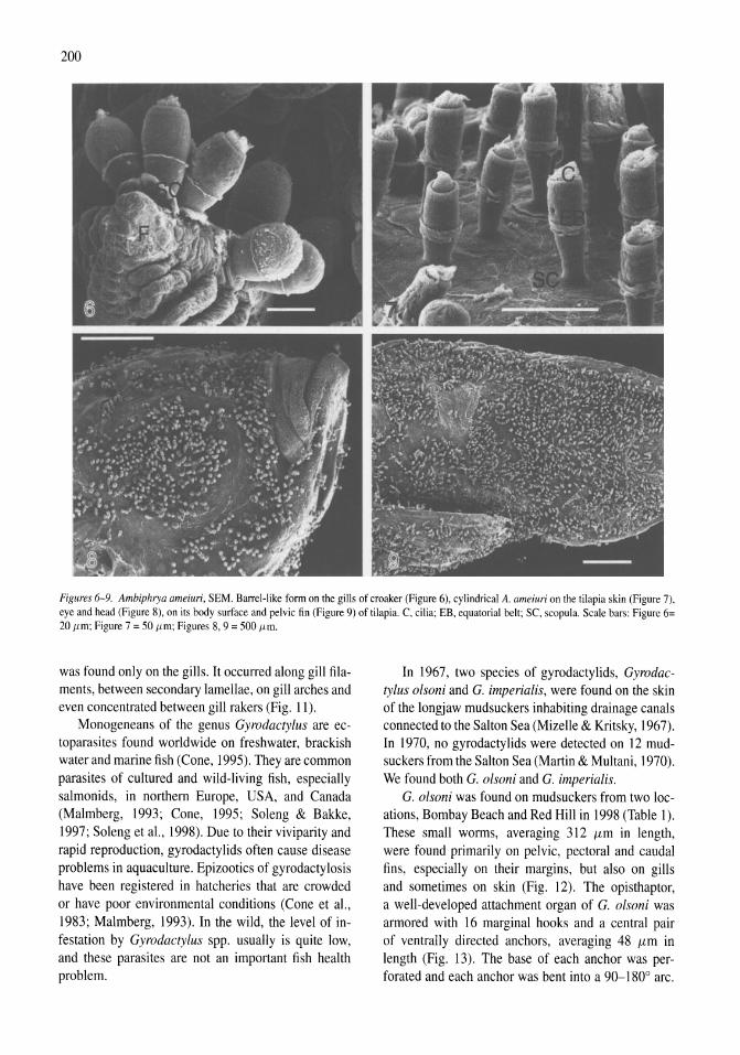
200
Figures 6-9. Ambiphrya ameiuri, SEM. Barrel-like form on the gills of croaker (Figure 6), cylindrical A. ameillri on the tilapia skin (Figure 7), eye and head (Figure 8), on its body surface and pelvic fin (Figure 9) of tilapia. C, cilia; EB, equatorial belt; SC, scopula. Scale bars: Figure 6= 20 /Lm; Figure 7 = 50 /Lm; Figures 8, 9 = 500 /Lm.
was found only on the gills. It occurred along gill filaments, between secondary lamellae, on gill arches and even concentrated between gill rakers (Fig. 1 I).
Monogeneans of the genus Gyrodactylus are ectoparasites found worldwide on freshwater, brackish water and marine fish (Cone, 1995). They are common parasites of cultured and wild-living fish, especially salmonids, in northern Europe, USA, and Canada (Malmberg, 1993; Cone, 1995; Soleng & Bakke, 1997; Soleng et a!., 1998). Due to their viviparity and rapid reproduction, gyrodactylids often cause disease problems in aquaculture. Epizootics of gyrodactylosis have been registered in hatcheries that are crowded or have poor environmental conditions (Cone et a!., 1983; Malmberg, 1993). In the wild, the level of infestation by Gyrodactylus spp. usually is quite low, and these parasites are not an important fish health problem.
In 1967, two species of gyrodactylids, Gyrodactylus olsoni and G. imperialis, were found on the skin of the longjaw mudsuckers inhabiting drainage canals connected to the Salton Sea (Mizelle & Kritsky, 1967). In 1970, no gyrodactylids were detected on 12 mudsuckers from the Salton Sea (Martin & Multani, 1970). We found both G. olsoni and G. imperialis.
G. olsoni was found on mudsuckers from two locations, Bombay Beach and Red Hill in 1998 (Table 1). These small worms, averaging 312 {tm in length, were found primarily on pelvic, pectoral and caudal fins, especially on their margins, but also on gills and sometimes on skin (Fig. 12). The opisthaptor, a well-developed attachment organ of G. olsoni was armored with 16 marginal hooks and a central pair of ventrally directed anchors, averaging 48 {tm in length (Fig. 13). The base of each anchor was perforated and each anchor was bent into a 90-180° arc.
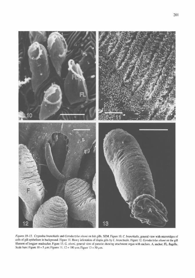
201
Figures 10-13. Cryptobia branchialis and Gvrodactylus olsoni on fish gills. SEM. Figure 10. C. branchialis, general view with microridges of cells of gill epithelium in background. Figure II. Heavy infestation of tilapia gills by C. branchialis. Figure 12. Gyrodactylus olsoni on the gill filament of longjaw mudsucker. Figure 13. G. OISOlli , general view of parasite showing attachment organ with anchors. A, anchor; FL, flagella. Scale bars: Figure 10 = 5 fim; Figures II, 12 = 100 fim; Figure 13 = 50 fim.
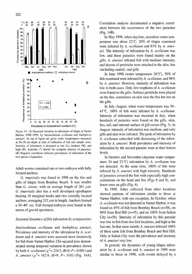
202
T'C 20 20 41 39 24 21 18 32 34 n 50 20 50 50 31 25 20 25 35
100 H M H H H H
~90 M H ~80 1; 70
~ 60 iii 50 Co
~40 g 30
l i 20 I ~. I ~ 10 D-
O May Jun Jul Aug Oct Nov Jun Jul Aug
1998 1999 • Amytoodinium acellatum 0 Ambiph'Ya ameiuri
t 100
." 90
.~ 80
'W 70
~ 60 .c: .9- 50
1l « 40
o 30
g 20
'"
• • • •
1 R= -0.92 1 P = 0.002
• I
• 1 10 D- O'+-'--.-r~-'--r-r-.-'-'
o 10 20 30 40 50 60 70 80 90 100
Prevalence of Amyloodinium ocel/atum (%)
25 25
H A
Oct
8
Figure 14. (A) Seasonal variation in infestation of tilapia in Vamer Harbor, 1998-1999, by Amylaadinium acel/alum and Ambiphrya ameiuri. At top of figure are given water temperatures measured at 20-30 cm depth at time of collection of fish and sample sizes. Intensity of infestation is designed as low (L), medium (M), and high (H). Asterisks (*) denote the complete absence of parasites. (B) Negative correlation between prevalences of infestation of the two species of parasites.
Adult worms contained one or two embryos with fully formed anchors.
G. imperialis was found in 1998 on the fins and gills of tilapia from Bombay Beach. It was smaller than G. olsoni, with an average length of 261 /tm. G. imperialis also has a well developed opisthaptor bearing 16 marginal hooks and two centrally located anchors, averaging 332 /tm in length. Anchors formed a 3~0° arc. Full-formed embryos were found in the uterus of gravid specimens.
Seasonal dynamics of fish infestation by ectoparasites
Amyloodinium ocellatum and Ambiphrya ameiuri. Prevalence and intensity of the infestation by A. ocellatum and A. ameiuri were assessed most intensively for fish from Varner Harbor. Chi-squared tests demonstrated strong temporal variation in prevalence shown bybothA. ocellatum (X 2= 218.5, df=9, P< 0.001) and A. ameiuri (X 2= 162.9, df=9, P< 0.01) (Fig. 14A).
Correlation analysis documented a negative correlation between the occurrences of the two parasites (Fig. 14B).
In May 1998, when daytime, nearshore water temperature was about 22°C, 20% of tilapia examined were infested by A. ocellatum and 83% by A. ameiuri. The intensity of infestation by A. ocellatum was low, and these parasites were found mainly on the gills. A. ameiuri infested fish with medium intensity, and dozens of peritrichs were attached to the skin, fins (including caudal), and gills.
In June 1998 (water temperature 26°C), 50% of fish examined were infested by A. ocellatum, and 96% by A. ameiuri. However, intensity of infestation was low in both cases. Only few trophonts of A. ocellatum were found on the gills. Solitary peritrichs were placed on the fins, sometimes on skin near the fins but not on the gills .
In July-August, when water temperature was 39-41°C, 100% of fish were infested by A. ocellatum . Intensity of infestation was maximal in July, when hundreds of parasites were found on the gills, skin, fins, tail, and internal surface of gill covers (Fig. 3). In August, intensity of infestation was medium, and only gills and skin were infested. The peak of infestation by A. ocellatum coincided with decreasing of the infestation by A. ameiuri. Both prevalence and intensity of infestation by the second parasite were at their lowest levels.
In October and November (daytime water temperature 24 and 21 0c) infestation by A. ocellatum was not detected. At the same time, 100% of fish were infested by A. ameiuri with high intensity. Hundreds of parasites covered the fish with especially high concentrations on the head and fins (Figs 8 and 9), and lower ones on gills (Fig. 6).
In 1998, fishes collected from other locations showed patterns of infestation similar to those at Varner Harbor, with one exception. In October, when A. ocellatum was not detected in Varner Harbor, it was found on 45% of fish from Bombay Beach (n=58), on 80% from Red Hill (n=45), and on 100% from Salton City (n=56). Intensity of infestation by this parasite was low in fish from two first locations, and high at the last one. In that same month, A. ameiuri infested 100% of these same fish from Bombay Beach and Red Hill. Only at Salton City were the prevalence and intensity of A. ameiuri very low.
In general, the dynamics of young tilapia infestation by A. ocellatum and A. ameiuri in 1999 were similar to those in 1998, with events delayed by a
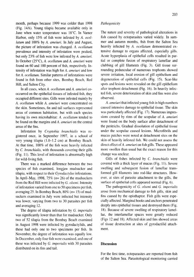
month, perhaps because 1999 was colder than 1998 (Fig. 14A). Young tilapia became available only in June when water temperature was 18°C. In Varner Harbor, only 15% of fish were infested by A. oceltatum and 100% by A. ameiuri. In July and August, the picture of infestation was changed. A. ocellatum prevalence and intensity of infestation were peaked, but only 23% of fish were low infested by A. ameiuri. In October (25°C), A. ocellatum and A. ameiuri were found on 60 and 100 percent of fish, respectively. Intensity of infestation was high for A. ameiuri and low for A. ocellatum. Similar patterns of infestations were found in fish from other sites, Bombay Beach, Red Hill, and Salton City.
In all cases, when A. ocellatum and A. ameiuri cooccurred on the epithelial tissues of infested fish, they occupied different sites. Gills were infested mainly by A. ocellatum while A. ameiuri were concentrated on the skin. Sometimes, fin and tail surfaces represented areas of common habitation, but with each species having its own microhabitat: A. ocellatum tended to be found on the margins and A. ameiuri on the central areas of the fins.
Infestation by Cryptobia branchialis was registered once, in September 1997, in a school of very young tilapia (1.0-1.2 cm) at Bombay Beach. At that time, 100% of the fish were heavily infected by C. branchialis, with thousands covering their gills (Fig. 11). This level of infestation is abnormally high for wild-living fish.
There was a marked difference between the two species of fish examined, longjaw mudsucker and tilapia, with respect to their Gyrodactylus infestations. In April-May, 1998, 75% (n= 26) of the mudsuckers from the Red Hill were infected by G. olsoni. Intensity of infestation varied from one to 50 specimens per fish, averaging 25. In Bombay Beach, 80% (n= 15) of mudsuckers examined in July were infected but intensity was lower, varying from two to 30 parasites per fish and averaging 12.
The degree of tilapia infestation by G. imperialis was significantly lower than that for mudsucker. Only two of 52 tilapia from the Bombay Beach examined in August 1998 were infected by gyrodactylids, and these had only one to two specimens per fish. In November, the degree of infestation was equally low. In December, only four fish were examined, and one of these was infected by G. imperiatis with 30 parasites distributed on its fins and tail.
203
Pathogenicity
The nature and severity of pathological alterations in fish caused by ectoparasites varied widely. In summer and autumn months, fish from the Salton Sea heavily infected by A. ocellatum demonstrated extensive damage to organs affected, especially gills. Acute hyperplasia of epithelial cells resulted in partial or complete fusion of respiratory lamellae and clubbing of gill filaments (Fig. 3). Gill tissue surrounding pedunculae of numerous trophonts showed severe irritation, local erosion of gill epithelium and degeneration of epithelial cells (Fig. 15). Scar-like spots and lesions were revealed on the gill epithelium after trophont detachment (Fig. 16). In heavily infected fish, severe deterioration of skin and fins were also observed.
A. ameiuri that infected young fish in high numbers caused intensive damage to epithelial tissue. The skin was particularly affected (Fig. 17). Numerous impressions created by rims of the scopulae of A. ameiuri were found on the body surface after detachment of the peritrichs. Gradual dissolution of epithelial tissue under the scopulae caused lesions. Microfibrils and mucus patches were noted at detachment sites on the skin of heavily infested fish. We could not assess the direct effect of A. ameiuri on fish gills. These appeared more swollen than usual but the exact reason for this change was unclear.
Gills of fishes infected by C. branchia lis were covered with a thick layer of mucus (Fig. 11). Severe swelling and subsequent fusion of lamellae transformed gill filaments into rod-like structures. However, at sites of parasite attachment to the gills, the surface of epithelial cells appeared normal (Fig. 6).
The pathogenicity of G. olsoni and G. imperialis arose from mechanical damage to fish gills, skin and fins caused by the opisthaptor. Fish gills were especially affected. Marginal hooks and anchors penetrated deeply into epithelial tissues and destroyed them (Fig. 18). Because of severe swelling of respiratory lamellae, the interlamellar spaces were greatly reduced (Figs 12 and 18). Affected skin and fins showed areas of tissue destruction at sites of gyrodactilid attachment.
Discussion
For the first time, ectoparasites are reported from fish of the Salton Sea. Parasitological monitoring carried
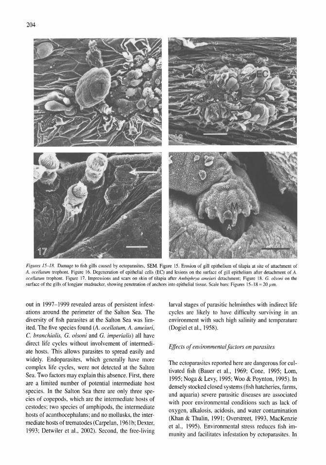
204
Figures 15-18. Damage to fish gills caused by ectoparasites, SEM. Figure 15. Erosion of gill epithelium of tilapia at site of attachment of A. acel/atum trophont. Figure 16. Degeneration of epithelial cells (Eel and lesions on the surface of gill epithelium after detachment of A. acel/alum trophont. Figure 17. Impressions and scars on skin of tilapia after Ambiphrya ame;ur; detachment; Figure 18. C. olson; on the surface of the gills of longjaw mudsucker, showing penetration of anchors into epithelial tissue. Scale bars: Figures 15-18 = 20 j1m.
out in 1997-1999 revealed areas of persistent infestations around the perimeter of the Salton Sea. The diversity of fish parasites at the Salton Sea was limited. The five species found (A. ocellatum, A. ameiuri, C. branchialis, G. olsoni and G. imperialis) all have direct life cycles without involvement of intermediate hosts. This allows parasites to spread easily and widely. Endoparasites, which generally have more complex life cycles, were not detected at the Salton Sea. Two factors may explain this absence. First, there are a limited number of potential intermediate host species. In the Salton Sea there are only three species of copepods, which are the intermediate hosts of cestodes; two species of amphipods, the intermediate hosts of acanthocephalans; and no mollusks, the intermediate hosts of trematodes (Carpelan, 1961b; Dexter, 1993; Detwiler et aI., 2002). Second, the free-living
larval stages of parasitic helminthes with indirect life cycles are likely to have difficulty surviving in an environment with such high salinity and temperature (Dogie! et aI., 1958).
Effects oj environmental Jactors on parasites
The ectoparasites reported here are dangerous for cultivated fish (Bauer et aI., 1969; Cone, 1995; Lorn, 1995; Noga & Levy, 1995; Woo & Poynton, \995). In densely stocked closed systems (fish hatcheries, farms, and aquaria) severe parasitic diseases are associated with poor environmental conditions such as lack of oxygen, alkalosis, acidosis, and water contamination (Khan & Thulin, 1991 ; Overstreet, 1993, MacKenzie et aI., 1995). Environmental stress reduces fish immunity and facilitates infestation by ectoparasites. In
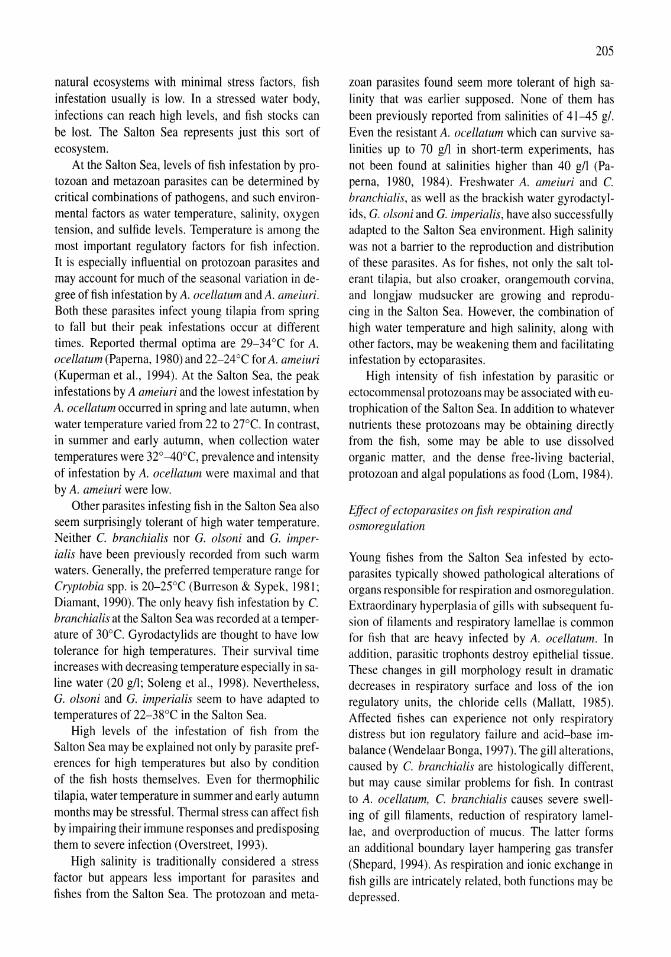
natural ecosystems with minimal stress factors, fish infestation usually is low. In a stressed water body, infections can reach high levels, and fish stocks can be lost. The Salton Sea represents just this sort of ecosystem.
At the Salton Sea, levels of fish infestation by protozoan and metazoan parasites can be determined by critical combinations of pathogens, and such environmental factors as water temperature, salinity, oxygen tension, and sulfide levels. Temperature is among the most important regulatory factors for fish infection. It is especially influential on protozoan parasites and may account for much of the seasonal variation in degree of fish infestation by A. ocellatum and A. ameiuri. Both these parasites infect young tilapia from spring to fall but their peak infestations occur at different times. Reported thermal optima are 29-34°C for A. ocellatum (Paperna, 1980) and 22-24°C for A. ameiuri (Kuperman et aI., 1994). At the Salton Sea, the peak infestations by A ameiuri and the lowest infestation by A. ocellatum occurred in spring and late autumn, when water temperature varied from 22 to 27°C. In contrast, in summer and early autumn, when collection water temperatures were 32° -40°C, prevalence and intensity of infestation by A. ocellatum were maximal and that by A. ameiuri were low.
Other parasites infesting fish in the Salton Sea also seem surprisingly tolerant of high water temperature. Neither C. branchialis nor G. olsoni and G. imperialis have been previously recorded from such warm waters. Generally, the preferred temperature range for Cryptobia spp. is 20-25°C (Burreson & Sypek, 1981; Diamant, 1990). The only heavy fish infestation by C. branchialis at the Salton Sea was recorded at a temperature of 30°C. Gyrodactylids are thought to have low tolerance for high temperatures. Their survival time increases with decreasing temperature especially in saline water (20 gn; Soleng et aI., 1998). Nevertheless, G. olsoni and G. imperialis seem to have adapted to temperatures of 22-38°C in the Salton Sea.
High levels of the infestation of fish from the Salton Sea may be explained not only by parasite preferences for high temperatures but also by condition of the fish hosts themselves. Even for thermophilic tilapia, water temperature in summer and early autumn months may be stressful. Thermal stress can affect fish by impairing their immune responses and predisposing them to severe infection (Overstreet, 1993).
High salinity is traditionally considered a stress factor but appears less important for parasites and fishes from the Salton Sea. The protozoan and meta-
205
zoan parasites found seem more tolerant of high salinity that was earlier supposed. None of them has been previously reported from salinities of 41-45 g/. Even the resistant A. ocellatum which can survive salinities up to 70 gn in short-term experiments, has not been found at salinities higher than 40 gIl (Paperna, 1980, 1984). Freshwater A. ameiuri and C. branchialis, as well as the brackish water gyrodactylids, G. olsoni and G. imperialis, have also successfully adapted to the Salton Sea environment. High salinity was not a barrier to the reproduction and distribution of these parasites. As for fishes, not only the salt tolerant tilapia, but also croaker, orangemouth corvina, and longjaw mudsucker are growing and reproducing in the Salton Sea. However, the combination of high water temperature and high salinity, along with other factors, may be weakening them and facilitating infestation by ectoparasites.
High intensity of fish infestation by parasitic or ectocommensal protozoans may be associated with eutrophication of the Salton Sea. In addition to whatever nutrients these protozoans may be obtaining directly from the fish, some may be able to use dissolved organic matter, and the dense free-living bacterial, protozoan and algal populations as food (Lom, 1984).
Effect of ectoparasites on fish respiration and osmoregulation
Young fishes from the Salton Sea infested by ectoparasites typically showed pathological alterations of organs responsible for respiration and osmoregulation. Extraordinary hyperplasia of gills with subsequent fusion of filaments and respiratory lamellae is common for fish that are heavy infected by A. ocellatum. In addition, parasitic trophonts destroy epithelial tissue. These changes in gill morphology result in dramatic decreases in respiratory surface and loss of the ion regulatory units, the chloride cells (Mallatt, 1985). Affected fishes can experience not only respiratory distress but ion regulatory failure and acid-base imbalance (Wendelaar Bonga, 1997). The gill alterations, caused by C. branchialis are histologically different, but may cause similar problems for fish. In contrast to A. ocellatum, C. branchialis causes severe swelling of gill filaments, reduction of respiratory lamellae, and overproduction of mucus. The latter forms an additional boundary layer hampering gas transfer (Shepard, 1994). As respiration and ionic exchange in fish gills are intricately related, both functions may be depressed.
206
Negative impacts of A. ameiuri are associated with the ability of these peritrichs to colonize the skin of the youngest fishes in the Salton Sea. Larval and postlarval fishes accomplish gas exchange mainly via cutaneous respiration (Rombourg & Ure, 1990). When present in massive numbers, A. ameiuri may be an additional burden to the host, impairing respiration and causing skin irritation or even damage. During heavy infestations of fishes in the Salton Sea, the tightly packed scopulae of A. ameiuri cover large areas of skin depressing its respiratory function. Even fins and tails, with blood vessels separated from the oxygen dissolved in water by a thin epithelium, are covered with peritrichs. After the detachment of parasites, damaged areas of epithelial tissue mark the attachment sites and have reduced capacity for gas exchange. In these conditions asphyxia of fish larvae may take place (Banina, 1981 ).
The major factor contributing to tissue changes is intensity of the infestation. Mild infection provokes minor tissue and cellular reaction. High parasitic load results in extensive histopathological changes. These can be influenced by environmental factors such as temperature extremes.
So, if present at high intensities, ectoparasites may be a substantial burden to their hosts, impairing respiration and causing surface tissue deterioration. Depression of respiratory functions is reinforced by the low oxygen tensions typical in the Salton Sea during summer (Carpel an, 1961b; Watts et aI., 2001).
Ectoparasites and secondary infections
The various types of damage to epithelial tissues caused by ectoparasites create portals of entry for bacterial, viral and fungal infections. Fish with immune responses depressed by environmental stress may be more susceptible to these secondary infections. Sick and dead fish represent a source of disease for piscivorous birds though in the absence of pathogen transmission, they also can constitute an enhanced food supply for these birds.
From ectoparasites to ecosystem
The phenomena reported here may have consequences that go well beyond the physiological interactions between these tiny fish and their tiny parasites. Given the prevalence and intensity of infestations observed, especially during summer and fall months, it seems likely that they may be a major cause of juvenile fish mortality. If that is the case, these ectoparasites could
playa large role in determining fish popUlation dynamics in this lake. They could influence the number of fish that recruit each year into size classes utilized by other fish, e.g., corvina, by fish-eating birds, and by sports fishermen. They could influence total fish biomass in the lake as well as the relative abundance of the fish species. Given the strong influences that fish populations have on lacustrine foodwebs, water chemistry, and other ecosystem properties, the ectoparasites could be influencing these as well. An experiment using Salton Sea microecosystems to assess effects of tilapia (Gonzalez et aI., 1998; Hart et aI., 1998; Simpson et aI., 1998) and an analysis of changes in plankton populations to following introduction of tilapia (Tiffany et aI., 2002) demonstrates the types of influences that tilapia may be having on the Sea. The ultimate driving factor in these dynamics could be the oxygen, temperature and mixing regimes of the lake. These show large variations from one year to another (Watts et aI., 2001), and parasite-fish interactions are likely to be sensitive to them.
Acknowledgements
The authors thank M.A. Tiffany and 1. Watts for their valuable collaboration in field work, 1. Dainer for her technical assistance with computer wrestling and figure preparation, and Steven Barlow for advice and facilitating use of the SDSU College of Sciences Electron Microscope Facility. We are especially grateful to Lois Tiffany and the Salton Sea Research Management Committee and Salton Sea Science Subcommittee for financial support. Our research has been funded in part by the United States Environmental Protection Agency through grant # R826552-0 1-0 to the Salton Sea Authority. The research results have not been subjected to the EPA's peer review and therefore do not necessarily reflect the view of the Agency. Therefore no official endorsement should be inferred.
References
Alvarez-Pellitero, P., A. Sitja-Bobadilla & A. Franco-Sierra, 1993. Protozoan parasites of wild and cultured sea bass, Dicentrarchus labrax (L.), from the Mediterranean area. Aquacult. Fish. Manage 24: 101-108.
Banina, N. N., 1981. Sessiline peritrichs (Ciliophora, Peritricha Sessilina) as parasites and commensals offish. Parasitologiya 15: 58-68 (in Russian).
Bauer, O. N., V. A. Musselius & Y A. Strelkov, 1969. Disease of pond fishes. Izdatelstvo Kolos, Moscow. Israel Program for Scientific Translations, Jerusalem, 1973.
Black, G, F., 1988. Description of the Salton Sea sport fishery, 1982-1983. Inland fisheries Administrative Report N 88-9.
Blanc, E., A. Marques, G. Bouix, G. Brugerolle & G. BreuiL 1989. Cryptobia sp. from the gills of the gilt head sea bream Spagus aurata. Bull. cur. Assoc. Fish Pathol. 9: 81-82.
Brown, E. M., 1934. On Oodiniurn ocellatwn Brown, a parasitic dinoflagellate causing epidemic disease in marine fish. Proc. zooL Soc. Lond.1934: 583-607.
Brown, E. M. & R. Hovasse, 1946. Arnyloodiniurn ocellaturn (Brown), a peridinian parasitic on marine fishes. A complementary study. Proc. zooL Soc. Land. 116: 33-36.
Burreson, E. M. & J. R. Sypek, 1981. Cnptobia sp. (Mastigophora: Kinetoplastida) from the gills of marine fishes in the Chesapeake Bay. 1. Fish Dis. 4: 519-522.
Carpelan, 1. H., 1961a. History of the Salton Sea. In Walker, B. W. (ed.), The Ecology of the Salton Sea, California, in relation to the sportfishery. Calif. Fish and Game, Fish Bull. 113: 9-15.
Carpelan, 1. H., 1961b. Zooplankton. In Walker, B. W. (ed.), The Ecology of the Salton Sea, California, in relation to the sportfishery. Calif. Fish Game, Fish Bull. 113: 49-6\.
Chen, C. 1., 1956. The protozoan parasites from four species of Chinese pond fishes: Ctenopharyngodon idellus, Mylopharyngodon picteus, Aristhichthys nobilis and Hvpophthalrnichthvs molithrix. Acta hydrobiol. Sinica I: 19-42.
Cohen, M. J., 1. I. Morrison & E. P. Glenn, 1999. Haven or Hazard: the ecology and future of the Salton Sea. A report of the Pacific Institute.
Cone, D, K., 1995. Monogenea (Phylum Platyhelminthes). In Woo, P. T. K. (ed.), Fish Diseases and Disorders, Vol. I. Protozoan and Metazoan Infections. CAB International, Oxon, UK: 300--326.
Cone, D. K., M. Beverley-Burton, M. Wiles & T. E. McDonald. 1983. The taxonomy of Gyrodactylus (Monogenea) parasitizing certain salmonid fishes of North America, with a description of Gyrodactylus nekae n.sp. Can. Zoo I. 61: 2587-2597.
Costa-Pierce, B. A. & R. W. Doyle, 1997. Genetic identification and status of tilapia regional strains in Southern California. In CostaPierce, B. A. & 1. E. Rakocy (eds), Tilapia Aquaculture in the Americas, vol. I. World Aquaculture Society, Baton Rouge, LA, USA: 1-17.
Davis, H. S., 1947. Studies on the protozoan parasites of freshwater fishes. Fish Bull. 51: 1-29.
Detwiler, P., M. F. Coe & D. M. Dexter, 2002. Benthic invertebrates of the Salton Sea: distribution and seasonal dynamics. HydrobiologialDev. Hydrobiol. (in press).
Dexter. D. M., 1993. Salinity tolerance of the copepod, Apoc\'clops dengizicus (Lepeshkin, 1900), a key food chain organism in the Salton Sea, California. Hydrobiologia 267: 203-209.
Diamant, A., 1990. Morphology and ultrastructure of Cr\,ptobia eilatica n.sp. (Bodonida: Kinetoplastida), an ectoparasite from the gills of marine fish. 1. Protozool. 37: 482-489.
Dogie!, V. A., G. K. Petrushevsky & Yu. I. Polyansky, 1958. Fundamental problems of the parasitology of fish. In Dogiel, V. A., G. K. Petrushevsky & Yu. I. Polyansky. Oliver and Boyd, Edinburgh and London.
Fitzgerald, M. E. C., B. A. Simco & 1. B. Coons, 1982. Ultrastructure of the peritrich ciliate Ambiphrya ameiuri and its attachment to the gills of the catfish [ctalurus punctatus. 1. Protozool. 29: 213-217.
Gonzalez, M. R., C. M. Hart, 1. Verfaillie & S. Hurlbert, 1998. Salinity and fish effects on the Salton Sea microecosystems: zooplankton and nekton. Hydrobiologia 381: \05-128.
Hart, C. M., M. R. Gonzalez, E. P. Simpson & S. H. Hurlbert, 1998. Salinity and fish effects on the Salton Sea microecosys-
207
terns: water chemistry and nutrient cycling. Hydrobiologia 381: 129-152.
Khan, R. A. & 1. Tulin, 1991. Influence of pollution on parasites of aquatic animals. In Baker, 1. R. & R. Muller (eds), Advances in Parasitology 30: 200-238.
Kuperman, B.1. & V. E. Matey. 1999. Massive infestation by AIIH'Ioodiniulll ocellatum (Dinoflagellida) of fish in a highly saline lake, Salton Sea, California, USA. Dis. aquat. Org. 39: 65-73.
Kuperman, B.I., I. Y. Kolesnikova & A. V. Tyutin, 1994. Ambiphrya ameiuri (Ciliophora: Peritricha): Ultrastructure and distribution on the body of young Cyprinidae. Parasitologiya 28: 214-221 (in Russian).
Landsberg, 1. H., K. A. Steidinger & B. A. Blakesley, 1995. Fishkilling dinoflagellates in a tropical marine aquarium. In Lassus, P., G. Arzul, E. Erard, P. Gentien & C. Marcaillou (eds), Harmful Marine Algal Blooms. Lavoisier Inc.: 65-70.
Lawler, A. R., 1977. The parasitic dinoflagellate AmyloodiniulIl ocellallllll in marine aquaria. Drum Croaker 17: 17-20.
Lawler. A. R., 1980. Studies of Amyloodinium ocellatum (Dinoflagellata) in Mississippi Sound: Natural and experimental hosts. Gulf Res. Rep. 6: 403-413.
Lorn, 1., 1980. Cnptobia branchia lis Nie from fish gills: ultrastructural evidence of ectocommensal function. 1. Fish Dis. 3: 427-436.
Lorn, 1., 1984. Diseases caused by protistans. In Kinne, O. (ed.), Diseases of Marine Animals, vol. IV, part I. Biologishe Anstalt Helgoland, Hamburg, Germany: 114-168.
Lorn, 1.. 1995. Trichodinidae and other ciliates (Phylum Ciliophora). In Woo, P. T. K. (cd.), Fish Diseases and Disorders, vol. I. Protozoan and Metazoan Infections. CAB International, Oxon, UK: 229-252.
Lorn, J. & I. Dykova, 1992. Protozoan Parasites of Fishes. Developments in Aquaculture and Fisheries Sciences, Vol. 26. Elsevier, Amsterdam.
MacKenzie, K., H. H. Williams, B. Williams, A. H. McVicar & R. Siddall. 1995. Parasites as indicators of water quality and the potential use of helminth transmission in marine pollution studies. In Baker, 1. R. & R. Miller (eds), Advances in Parasitology 35: 85-144.
Mallatt, 1., 1985. Fish gill structural changes induced by toxicants and other irritants: a statistical review. Can. J. Fish. aqua!. Sci. 42: 630-648.
Malmberg, G., 1993. Gyrodactylidae and gyrodactylosis of Salmonidae. Bull. Peche Pisces. I: 5-46.
Martin, W. E. & S. Multani, 1970. Some helminth of the mudsucker fish, Gillichthys mirabilis Cooper. Bull. so. calif. Acad. Sci. 69: 161-168.
Mizelle, 1. D. & D. C. Kritsky, 1967. Studied on monogenetic trematodes XXXVI. Gyrodactylid parasites of importance to California fishes. Calif. Fish Game 4: 264-272.
Natividad, 1. M., M. G. Bondad-Reantaso & 1. R. Arthur, 1986. Parasites of Nile Tilapia (Oreochromis nilolicus) in the Philippines. In Maclean, J. 1., 1. B. Dizon & 1. V. Hosilos (eds), The First Asian Fisheries Forum. Asian Fisheries Society, Manila. Philippines: 255-259.
Noga, E. 1. & M. G. Levy, 1995. Dinoflagellida (Phylum Sarcomastigophora). In Woo, P. T. K. (ed.), Fish Diseases and Disorders. Vol. I. Protozoan and Metazoan Parasites. CAB International, Oxon, UK: 3-25.
NWHC, 1999. Quarterly mortality reports. U.S. Geological Survey, National Wildlife health Center, Madison, Wisconsin. http://www.emtc.usgs.gov/http_datalnwhc/gvarterl/gmr.html.
Overstreet, R. M., 1993. Parasitic diseases of fishes and their relationship with toxicants and other environmental factors. In:
208
Couch, I. A. & J. W. Fournie (eds), Pathobiology of Marine and Estuarine Organisms, CRC Press, Boca Raton, FL: 111-156.
Paperna. 1., 1980. Amyloodinium oeellatum (Brown, 1931) (Dinofiagellida) infestation in cultured marine fish at Eilat, Red Sea: epizootiology and pathology. J. Fish Dis. 3: 363-372.
Paperna. 1.. 1984. Reproduction cycle and tolerance to temperature and salinity of Amyloodinium oeellatum (Brown, 1931) (Dinofiagellida). Ann. Parasitol. Hum. Compo 59: 7-30.
Plumb. I. A. 1997. Infection diseases of tilapia. In Costa-Pierce, B. A. & I. E. Rakocy (eds), Tilapia Aquaculture in the Americas, vol. I. World Aquaculture Society. Baton Rouge. LA. USA: 212-228.
Rombough. P. I. & D. Ure. 1990. Partitioning of oxygen uptake between cutaneous and branchial surfaces in larval and juvenile chinook salmon, Oncorhynchus tschawytscha. Physiol. Zool. 64: 717-727.
Saiki. M. K.. 1990. Elemental concentration in fishes from the Salton Sea. Southern California. Wat. Air Soil Pollut. 52: 41-56.
Sandifer P. A.. J. S. Hopkins. A. D. Stokes & R. D. Smiley. 1993. Experimental pond grow-out of red drum, Sciaenops ocellatus, in South Carolina. Aquaculture 118: 217-228.
Setmire I. G .. R. A. Schroeder, J. N. Densmore. S. 1.. Goodbred, D. I. Audet & W. R. Radke, 1993. Detailed study of water quality, bottom sediment, and biota associated with irrigation drainage in the Salton Sea area, California, 1988-90. US Geological Survey Water-Resources Investigations Report 93-4014. Sacramento. CA.
Shepard. K. 1... 1994. Function for fish mucus. Rev. Fish BioI. Fisher. 4: 401-429.
Simpson, E. P., M. R. Gonzalez. C. M. Hart & S. H. Hurlbert. 1998. Salinity effects on Salton Sea microecosystems: benthos. Hydrobiologia 381: 179-190.
Soleng. A. & T. A. Bakke. 1997. Salinity tolerance of Gyrodaetylus salaris (Platyhelminthes, Monogenea): laboratory studies. Can. I. Fish. Aquat. Sci. 54: 1837-1845.
Soleng, A.. T. A. Bakke & P. Hansen, 1998. Potential for dispersal of Gyrodaetylus sa/aris (Platyhelminthes, Monogenea) by sea-
running stages of the Atlantic salmon (Salmo salar): field and laboratory studies. Can 1. aqua!. Sci. 55: 507-514.
Thompson, S., D. Kirkegaard, & T. 1.. Jahn, 1946. Scyphidia ameiuri. n.sp. peritrichous ciliate from the gills of the bullhead Ameiurus me/as me/as. Trans. am. Microsc. Soc. 116: 315-317.
Tiffany, M. A .• S. B. Barlow. V. E. Matey & S. H. Hurlbert. 200 I. Chatonella marina (Raphidophyceae), a potentially toxic alga in the Salton Sea. Hydrobiologia 466 (Dev. Hydrobiol. 162): 187-194.
Tiffany M. A., B. K. Swan, 1. M. Watts. & S. H. Hurlbert, 2002. Metazooplankton dynamics of the Salton Sea 1997-1999. Hydrobiologia/Dev. Hydrobiol. (in press).
Trombitsky. A. D., A. 1. Moshu. & A. V. Bordenjuk. 1992. Ambiphrya ameiuri (Ciliophora, Scyphionidae), its host specificity and ecology in Europe. Eco!. Parasitol. I: 19-30.
Walker, B. w., R. R. Whitney & G. W. Barlow, 1961. The fishes of the Salton Sea. In Walker. B. W. (ed.). The Ecology ofthe Salton Sea. California. in relation to the sportfishery. Calif. Fish Game. Fish Bull. 13: 77-151.
Watanabe W. 0 .• B. 1.. Olla, R. 1. Wicklung & W. D. Head. 1997. Saltwater culture of the Florida red tilapia and other salinetolerant tilapias: a review. In Costa-Pierce, B. A. & 1. E. Rakocy (eds), Tilapia Aquaculture in the Americas. World Aquacult. Soc., Baton Rouge, LA. USA. I: 54-141.
Watts, J. M .• B. K. Swan, M. A. Tiffany & S. H. Hurlbert, 2001. Thermal, mixing and oxygen regimes of the Salton Sea. California, 1997-1999. Hydrobiologia 466 (Dev. Hydrobio!. 162): 159-176.
Wendelaar Bonga, S. E, 1997. The stress response in fish. Physiol. Rev. 77: 591-625.
Woo. P. T. K. & S. 1.. Poynton, 1995. Diplomonadida, Kinetoplastida and Amoebida (Phylum Sarcomastigophora). In Woo. P. T. K. (ed.), Fish Diseases and Disorders, Vol. I. Protozoan and Metazoan Infections. CAB International, Oxon. UK: 27-96.
Hydrobiologia 466: 209-219,2001, J,M, Melack, R. Jellison & D.B. Herbst leds). Saline Lakes. © 2001 Kluwer Academic Publishers.
209
Gradients of salinity stress, environmental stability and water chemistry as a templet for defining habitat types and physiological strategies in inland salt waters
David B. Herbst Sierra Nevada Aquatic Research Laboratory, University of California, Route J, Box 198, Mammoth Lakes, CA 93546, U.S.A. E-mail: herbst@l(fesci.ucsb.edu
Key words: anions, Ephydra, habitat stability, habitat templet, osmoregulation, salinity, salt lakes, stress tolerance
Abstract
The search for pattern in the geographic occurrence of salt lake flora and fauna often reveals strong associations of specific taxa with certain types of water chemistry. Solute composition, along with salinity and habitat stability, may provide a templet shaping the distribution of many organisms inhabiting saline lakes. A review of studies demonstrating habitat associations, specific solute tolerance, and ionic and osmotic adaptations provide evidence of fidelity to particular conditions of environmental chemistry across a wide taxonomic spectrum. Under low salinity conditions, some species show osmoregulatory adaptability to varied solute composition but the capacity for such flexibility is reduced with increased salinity and only certain taxa are found in hypersaline waters dominated by a particular solute. Anionic ratios of chloride, bicarbonate-carbonate, and sulfate appear to be especially important determinants of distribution. Specific solute tolerance presents an alternative explanation to disrupted hydrographic connections in describing how biogeographic distributions may be restricted to certain aquatic habitats in arid regions. Physiological adaptations to chemistry, exemplified in the brine fly genus Ephydra, may be an integral part of the evolution, ecology and diversification of saline water organisms.
Introduction
A substantial body of work in environmental physiology has been dedicated to defining the range of adaptability to extreme conditions. Lethal limits of temperature, pH, oxygen availability and salinity, for example, have been determined for a variety of organisms - but why do such capabilities arise and how do these physiological strategies serve life under sublethal conditions? The thesis of this paper is that physiological tolerance to extreme physico-chemical conditions represents an avenue of escape from the adverse influences of predation and competition found in the more diverse communities of temperate environments. Susceptible organisms would be expected to be those that are most vulnerable as prey or as contenders for resources because they aggregate in local predictable habitat patches and/or have no specialized ability to exploit food resources. Physiological resistance to stress might be viewed as a means of
establishing habitat refugia. Paths to these refugia in saline water environments form along gradients of chemical concentration (salinity), ionic composition and habitat permanence. These variables may form an ecological matrix for the evolution of clades or species complexes in differing saline environments depending on the geographic availability of chemical habitat niches and the physiological constraints inherent in different lineages. The objectives of this paper are to examine schemes for habitat classification, paths of geochemical evolution in salt lakes, some of the evidence for species associations with habitat chemistry, and an outline of integrated research needs for testing hypotheses.
Habitat classification and adaptive strategies
Schemes for organizing habitat types have often used gradients of the physical environment to arrange hab-
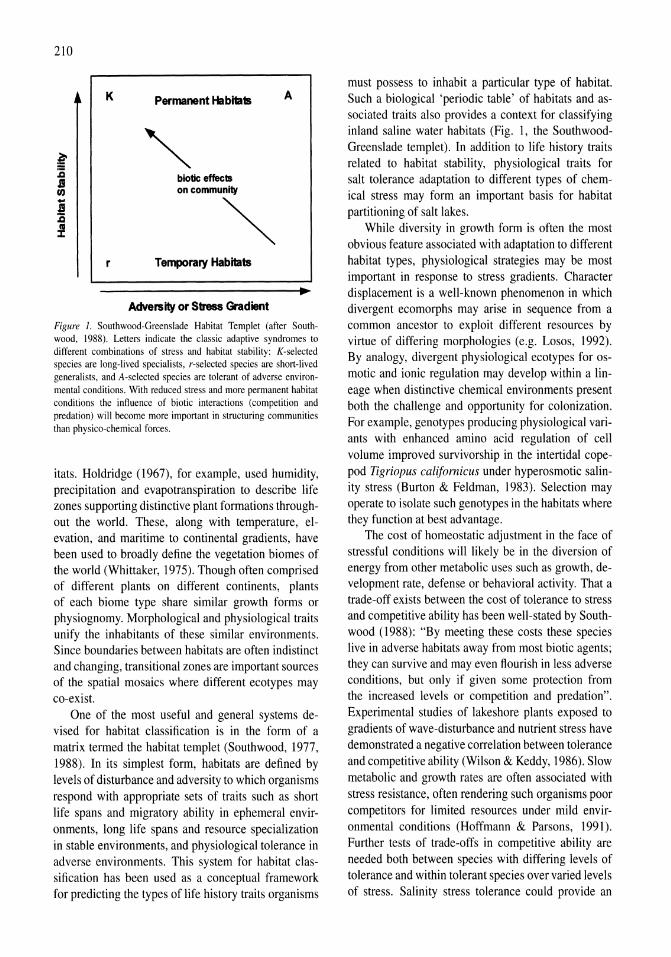
210
K
r
Permanent Habitats
biotic effects on communHy
~ Temporary HabHats
Adversil¥ or Stress Gradient
A
Figure 1. Southwood-Greenslade Habitat Templet (after Southwood, 1988). Letters indicate the classic adaptive syndromes to different combinations of stress and habitat stability: K-selected species are long-lived specialists, r-selected species are short-lived generalists, and A -selected species are tolerant of adverse environmental conditions. With reduced stress and more permanent habitat conditions the influence of biotic interactions (competition and predation) will become more important in structuring communities than physico-chemical forces.
itats. Holdridge (1967), for example, used humidity, precipitation and evapotranspiration to describe life zones supporting distinctive plant formations throughout the world. These, along with temperature, elevation, and maritime to continental gradients, have been used to broadly define the vegetation biomes of the world (Whittaker, 1975). Though often comprised of different plants on different continents, plants of each biome type share similar growth forms or physiognomy. Morphological and physiological traits unify the inhabitants of these similar environments. Since boundaries between habitats are often indistinct and changing, transitional zones are important sources of the spatial mosaics where different ecotypes may co-exist.
One of the most useful and general systems devised for habitat classification is in the form of a matrix termed the habitat templet (Southwood, 1977, 1988). In its simplest form, habitats are defined by levels of disturbance and adversity to which organisms respond with appropriate sets of traits such as short life spans and migratory ability in ephemeral environments, long life spans and resource specialization in stable environments, and physiological tolerance in adverse environments. This system for habitat classification has been used as a conceptual framework for predicting the types of life history traits organisms
must possess to inhabit a particular type of habitat. Such a biological 'periodic table' of habitats and associated traits also provides a context for classifying inland saline water habitats (Fig. I, the SouthwoodGreenslade templet). In addition to life history traits related to habitat stability, physiological traits for salt tolerance adaptation to different types of chemical stress may form an important basis for habitat partitioning of salt lakes.
While diversity in growth form is often the most obvious feature associated with adaptation to different habitat types, physiological strategies may be most important in response to stress gradients. Character displacement is a well-known phenomenon in which divergent ecomorphs may arise in sequence from a common ancestor to exploit different resources by virtue of differing morphologies (e.g. Losos, 1992). By analogy, divergent physiological ecotypes for osmotic and ionic regulation may develop within a lineage when distinctive chemical environments present both the challenge and opportunity for colonization. For example, genotypes producing physiological variants with enhanced amino acid regulation of cell volume improved survivorship in the intertidal copepod Tigriopus califomicus under hyperosmotic salinity stress (Burton & Feldman, 1983). Selection may operate to isolate such genotypes in the habitats where they function at best advantage.
The cost of homeostatic adjustment in the face of stressful conditions will likely be in the diversion of energy from other metabolic uses such as growth, development rate, defense or behavioral activity. That a trade-off exists between the cost of tolerance to stress and competitive ability has been well-stated by Southwood (1988): "By meeting these costs these species live in adverse habitats away from most biotic agents; they can survive and may even flourish in less adverse conditions, but only if given some protection from the increased levels or competition and predation". Experimental studies of lakeshore plants exposed to gradients of wave-disturbance and nutrient stress have demonstrated a negative correlation between tolerance and competitive ability (Wilson & Keddy, 1986). Slow metabolic and growth rates are often associated with stress resistance, often rendering such organisms poor competitors for limited resources under mild environmental conditions (Hoffmann & Parsons, 1991). Further tests of trade-offs in competitive ability are needed both between species with differing levels of tolerance and within tolerant species over varied levels of stress. Salinity stress tolerance could provide an
easily manipulated experimental system for examining such relationships.
Classification of inland saline water habitats
Salt lake environments can be classified in the context of the habitat templet model. Inland saline waters range in stability from shallow temporary ponds to large permanent lakes, and in adversity from dilute salinities to the extreme stress of salt saturation. Before examining how these gradients may produce distinct habitats, I will first review some ideas that have previously been presented as themes for classifying inland saline waters.
Hedgpeth (1959) attempted an early provisional arrangement of inland mineral water habitats as part of a symposium on classification of brackish waters. These included (A) hypersaline lagoons with periodic connection to the sea dominated by a euryhaline marine biota, (B) relict marine waters once connected to the sea, but now isolated and harboring a biota of mixed marine and freshwater origins, (C) salterns and brines comprised of chloride-dominated waters including evaporation ponds, solar salt works and natural brines such as the Great Salt Lake, (D) other inland brines of primarily sulfate and/or carbonate composition, and (E) mineralized waters of thermal springs and groundwater origins. Supporting evidence of a biota with strict affinity to each habitat was presented for some cases but poor records on water chemistry and physical settings for collections were a problem then, as now, in understanding what features unify habitat types. At the same symposium, Beadle (1959) stated on physiological grounds that saline habitats might be defined according to organisms incapable of maintaining dilute body fluids above isotonic conditions, those capable of limited regulation, and those able to maintain hypotonic blood even at high salinities (corresponding to 0-15 ppt, 15-50 ppt and above 50 ppt salinity). Bayly (1967) first introduced the term athalassic to distinguish non-marine saline environments from those of thalassic (marine) origins. Athalassic waters were defined to encompass those that (A) have never been connected to the sea, and (B) those that have been connected in the past but became isolated, evaporated completely and lost all marine life prior to re-filling. Inhabitation by organisms with freshwater ancestry further distinguished truly inland saline habitats from those of marine origin
211
such as the hypersaline lagoons listed by Hedgpeth (1959).
Traditional classifications of the ontogeny of freshwater lakes have used trophic status to distinguish oligotrophic, eutrophic and dystrophic habitat types. Saline lakes may also be regarded as a terminal stage in the aging of endorheic lake basins (Whittaker, 1975). Por (1980) used changes in trophic structure (food chain length) with increased salinity as a means for classifying inland salt water habitats. Por restricted this classification scheme to hypersaline (above seawater) chloride-sulfate waters, claiming the biota of this chemical type to be different from those in carbonate waters. Based on reduced competitive ability and increased omnivory with increasing salinity, Por defined habitat categories corresponding to degrees of food-chain shortening as follows: (A) alpha-hypersaline waters have a reduced diversity of euryhaline taxa and reduced secondary productivity and include habitats of both marine and freshwater ('limnogenic') origin ranging from salinities in excess of seawater to about 100 g 1-1, and have intricate food webs of producers, grazers, and predators; (B) above 100 g 1-1 diversity and primary production become severely restricted and these beta-hypersaline waters are characterized by an almost exclusively limnogenic biota with simple linear food chains and limited predation; (C) in gamma-hypersaline waters salinities in excess of 140 g 1-1 become simple and imbalanced producer-grazer ecosystems (grazers exert limited control); and (D) delta-hypersaline waters in the realm of 200-300 g 1-1 are basically produceronly systems comprised mainly of photosynthetic and chemosynthetic bacteria with little or no animal life and the lowest levels of diversity and productivity.
Based on a habitat templet approach to inland saline water classification (Fig. 2 and Table 1), the emphasis is placed on the traits that unify the biota in adaptation to physical and chemical gradients. As a simplified view, the habitat-adaptive strategy space can be divided into quadrants:
(l) Low to moderate salinity temporary ponds (lower left) represent one broad habitat type comprised of species with rapid development, migratory and/or dormant stages, limited osmoregulatory ability, broad or nonspecific ion regulation capacity, and poor competitive ability. Representative fauna include most branchiopod crustacea exclusive of Artemia, many Dipteran larvae including floodwater mosquitoes of the genus Aedes, some Coleoptera and Hemiptera. Two patterns of osmotic regulation (l) hyperosmotic
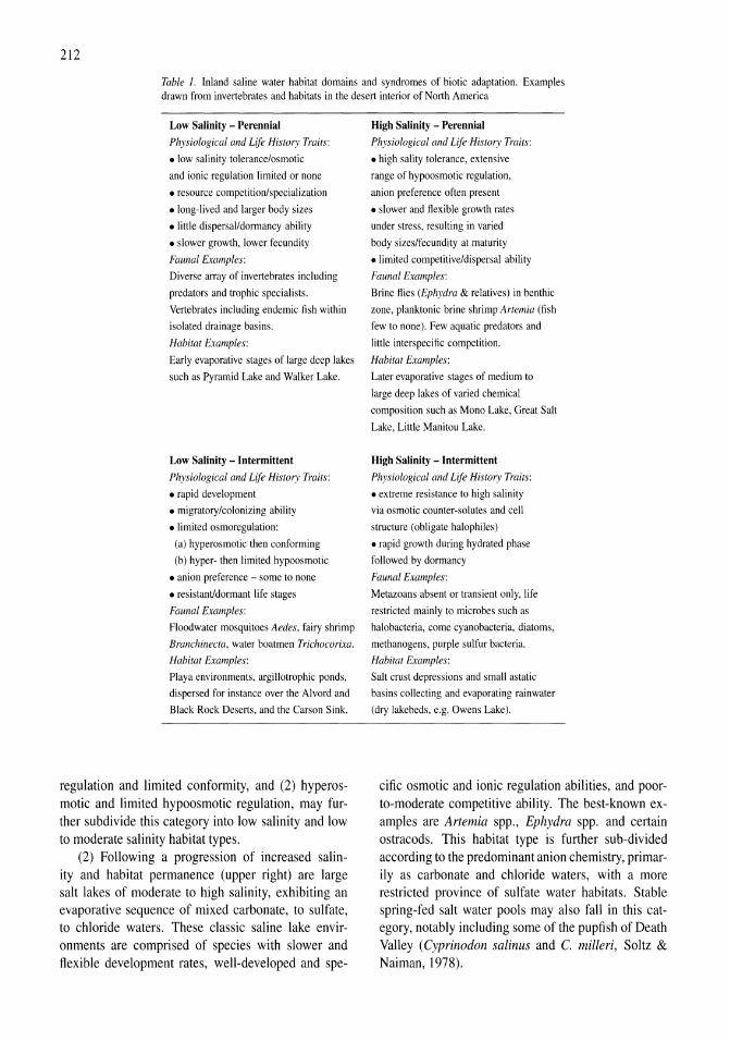
212
Table 1. Inland saline water habitat domains and syndromes of biotic adaptation. Examples drawn from invertebrates and habitats in the desert interior of North America
Low Salinity - Perennial
Physiological and Life History Traits:
• low salinity tolerance/osmotic
and ionic regulation limited or none
• resource competition/specialization
• long-lived and larger body sizes
• little dispersal/dormancy ability
• slower growth, lower fecundity
Faunal Examples:
Diverse array of invertebrates including
predators and trophic specialists.
Vertebrates including endemic fish within
isolated drainage basins.
Habitat Examples:
Early evaporative stages of large deep lakes
such as Pyramid Lake and Walker Lake.
Low Salinity - Intermittent
Physiological and Life History Traits:
• rapid development
• migratory/colonizing ability
• limited osmoregulation:
(a) hyperosmotic then conforming
(b) hyper- then limited hypoosmotic
• anion preference - some to none
• resistant/dormant life stages
Faunal Examples:
Floodwater mosquitoes Aedes, fairy shrimp
Branchinecta, water boatmen Trichocorixa.
Habitat Examples:
Playa environments, argillotrophic ponds,
dispersed for instance over the Alvord and
Black Rock Deserts, and the Carson Sink.
regulation and limited conformity, and (2) hyperosmotic and limited hypoosmotic regulation, may further subdivide this category into low salinity and low to moderate salinity habitat types.
(2) Following a progression of increased salinity and habitat permanence (upper right) are large salt lakes of moderate to high salinity, exhibiting an evaporative sequence of mixed carbonate, to sulfate, to chloride waters. These classic saline lake environments are comprised of species with slower and flexible development rates, well-developed and spe-
High Salinity - Perennial
Physiological and Life History Traits:
• high sality tolerance, extensive
range of hypoosmotic regulation,
anion preference often present
• slower and flexible growth rates
under stress, resulting in varied
body sizes/fecundity at maturity
• limited competitive/dispersal ability
Faunal Examples:
Brine flies (Ephydra & relatives) in benthic
zone, planktonic brine shrimp Artemia (fish
few to none). Few aquatic predators and
little interspecific competition.
Hahitat Examples:
Later evaporative stages of medium to
large deep lakes of varied chemical
composition such as Mono Lake, Great Salt
Lake, Little Manitou Lake.
High Salinity - Intermittent
Physiological and Life History Traits:
• extreme resistance to high salinity
via osmotic counter-solutes and cell
structure (obligate halophiles)
• rapid growth during hydrated phase
followed by dormancy
Faunal Examples:
Metazoans absent or transient only, life
restricted mainly to microbes such as
halobacteria, come cyanobacteria, diatoms,
methanogens, purple sulfur bacteria.
Habitat Examples:
Salt crust depressions and small astatic
basins collecting and evaporating rainwater
(dry lakebeds, e.g. Owens Lake).
cific osmotic and ionic regulation abilities, and poorto-moderate competitive ability. The best-known examples are Artemia spp., Ephydra spp. and certain ostracods. This habitat type is further sub-divided according to the predominant anion chemistry, primarily as carbonate and chloride waters, with a more restricted province of sulfate water habitats. Stable spring-fed salt water pools may also fall in this category, notably including some of the pupfish of Death Valley (Cyprinodon salin us and C. milleri, Soltz & Naiman, 1978).
stable lakes of dilute to low sa Ii nity: diverse communities and biotic interactions
temporary lakes-ponds of low to moderate salinity: mobilel dryingresistant inhabitants wllimiled salt tolerance
extreme unfawrable conditions in ephemeral
hypersaline waters: microbial ha lop hiles
Salin", Stress Gradient
Figure 2. Habitat Templet for Inland Saline Waters. Simplified evaporative sequence of major anions shown for stable lakes of moderate to high salinity. Transition to more saline and stable habitats and geochemical evolution of anionic content (central arrows) selects for development of specialized physiological adaptations for osmotic and anionic tolerance. Low salinity permanent lakes are dominated by diverse biological interactions while highly saline instable environments are lifeless or inhabited only by halophiles.
(3) At the extreme of instable, ephemeral waters of high salinity (lower right) are generally uninhabited (except for microbial life ) severe environments. Some category I organisms may be capable of ranging into such environments but the opportunities and examples are limited. Microbes such as halobacteria, certain methanogens, purple sulfur bacteria and cyanobacteria, and the green alga Dunaliella survive using osmotic counter-solutes to maintain cell integrity, and resistant stages to persist during dryness (including diatom auxospores).
(4) At the opposite extreme are large permanent lakes of dilute salinities in which biotic interactions dominate community organization. These waters are inhabited primarily by long-lived species with specialized abilities for resource utilization, poor tolerance of salinity stress (no hypoosmotic regulation), and reduced ability for migration or dormancy. A great diversity of flora and fauna, including a variety of fish, may live in such waters.
Geographic patterns of salt lake habitat chemistry
Descriptions of the geography and distribution of saline lakes have recognized sequences of chemical change along the evaporative series from sources to terminal lake sinks (Hutchinson, 1957; Cole, 1968).
213
Using triangular plots of relative chloride, carbonate and sulfate anion composition, trends of brine evolution within drainage basins become apparent. Examining closed basins from throughout the world, the general pattern of geochemical change appears to follow a path from carbonate source waters to chloride most commonly, or sulfatochloride composition. If initial carbonate is sufficient the series will pass through mixed chemistry to carbonatochloride type waters. Geochemists have emphasized the importance of initial Ca+MglHC03 ratios in determining the solute branchpoints leading to terminal lakes of differing composition (Eugster & Jones, 1979). With Ca+Mg in excess, chloride or sulfatochloride waters will result. When the ratio is near equal, the level of Mg relative to Ca will affect mineral precipitation of calcite, gypsum or mirabilite and from these branchpoints shift the balance toward differing anion compositions. With bicarbonate in excess of Ca+Mg, alkaline soda lakes are formed. The nature of the geologic source material as the starting point also modifies the potential chemical pathway. A simplified view of this is that volcanic substrata promote carbonate chemistry, while inflows off sedimentary deposits favor chloride or sulfate dominant lake waters.
It is possible that biological evolution tracks geochemical evolution along the series of habitats that become available within a drainage basin. As lakes evaporate or expand, altered chemistry forms a changing mosaic of habitats to which physiological specialists will have selective advantages in colonization and persistence. Branching of a lineage (formation of a clade) may occur as habitats arise over spatial and temporal gradients of chemical differences and provide opportunities for diversification.
Habitat associations of salt lake flora and fauna
The absence and incomplete gathering of physicochemical habitat data to associate with biological collections have impeded progress in the classification of distinct ecological communities in salt lakes. While early authors regarded hypersaline lakes as harboring a cosmopolitan biota because of the widespread occurrence of Artemia and Ephydra, these genera and relatives are now recognized as being comprised of a diversity of species including endemics and physiological specialists (Bowen et al., 1985; Barnby, 1987; Collins, 1977; Herbst, 1999). Data sets such as those collected by Blinn (1993) for benthic diatoms in North
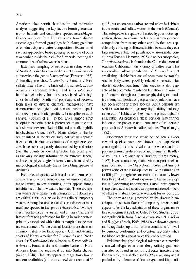
214
American lakes permit classification and ordination analyses suggesting the key factors forming boundaries for habitats and distinctive species assemblages. Cluster analyses from Blinn's study found diatom assemblages formed groupings both along gradients of conductivity and anion composition. Extension of such an approach to broad geographic surveys of other taxa could provide the basis for further delineating the communities of saline water habitats.
Extensive sampling of ostracods in saline waters of North America has revealed distinct anionic associations within the genus Limnocythere (Forester, 1986). Anion diagrams show L. staplini is found in chlorosulfate waters (favoring high salinity sulfate), L. sappaensis in carbonate waters, and L. ceriotuberosa in mixed chemistry but most associated with high chloride salinity. Studies of popUlations of Artemia from lakes of diverse chemical backgrounds have demonstrated ecological isolation and nascent speciation owing to anionic specificity in nauplius to adult survival (Bowen et aI., 1985). Even among strict halophilic bacteria there is preference in anionic content shown between alkalophilic and non-alkalophilic halobacteria (Javor, 1989). Many clades in the biota of inland saline waters may not yet be apparent because the habitat associations of congeneric species have been so poorly documented by collectors (viz. the county or township/sector data often given as the only locality information on museum labels), and because physiological diversity may be masked by morphological similarity (as in the sibling species of Artemia).
Examples of species with broad ionic tolerance (no apparent anionic preferences), and an osmoregulatory range limited to low salinities, often appear among inhabitants of shallow astatic habitats. These are species where development rate, migration and dormancy are critical traits to survival in low salinity temporary waters. Among the smallest of all corixids (water boatmen) are species in the genus Trichocorixa. Two species in particular, T. verticalis and T. reticulata, are of interest for their preference for living in saline waters, primarily associated with habitats marginal to the marine environment. While coastal locations are the most common habitats for these species (Gulf and Atlantic coasts of North America for T. verticalis and Pacific coast for T. reticulata), the subspecies T. verticalis interiores is found in the arid interior basins of North America from the southwest up into Saskatchewan (Sailer, 1948). Habitats appear to range from low to moderate salinities (dilute to somewhat in excess of 50
g I-I) but encompass carbonate and chloride habitats in the south, and sulfate waters in the north (Canada). This subspecies is capable of limited hypoosmotic regulation, shows no anionic preference, and may escape competition from many other corixids that are capable only of living in dilute salinities because they can hyperosmoregulate but perish above isoosmotic conditions (Tones & Hammer, 1975). Another subspecies, T. verticalis saltoni, is found in the Colorado desert of southern California in the vicinity of Salton Sea. This region also harbors populations of T. reticulata that are distinguishable from coastal specimens by notably smaller body sizes, possibly related to selection for shorter development time. This species is also capable of hypo osmotic regulation but shows no anionic preferences, though comparative physiological studies among subspecies or geographic populations have not been done for either species. Adult corixids are well known for their migratory flight ability and may move out of habitats as they become physiologically unsuitable. As predators, these corixids may further influence the presence and abundance of vulnerable prey such as Artemia in saline habitats (Wurtsbaugh, 1992).
Floodwater mosquito larvae of the genus Aedes (several species) have been shown to be capable of osmoregulation and survival in saline waters and display no anionic preferences or requirements (Bradley & Phillips, 1977; Sheplay & Bradley, 1982; Bradley, 1987). Hyperosmotic regulation via transport mechanisms localized in the Malpighian tubules and hindgut permit some of these mosquitoes to live in salinities up to 100 g I-I (though the concentration is usually lower than this and of only short exposure to larvae developing in evaporating floodwaters). Larval development is rapid and adults disperse as opportunistic colonizers of whatever habitats become available for oviposition.
The dormant eggs produced by the diverse branchiopod crustacean fauna of temporary desert ponds appear to be the key adaptation of these organisms to this environment (Belk & Cole, 1975). Studies of osmoregulation in Branchinecta campestris, B. mackini and B. gigas (Broch, 1969, 1988) have shown hyperosmotic regulation up to isoosmotic conditions followed by osmotic conformity and eventual mortality when the blood reaches about twice this concentration.
Evidence that physiological tolerance can provide chemical refugia other than along salinity gradients can also be found in some freshwater invertebrates. For example, thin-shelled snails (Physella) may avoid predation by tolerance of low oxygen and high sulf-
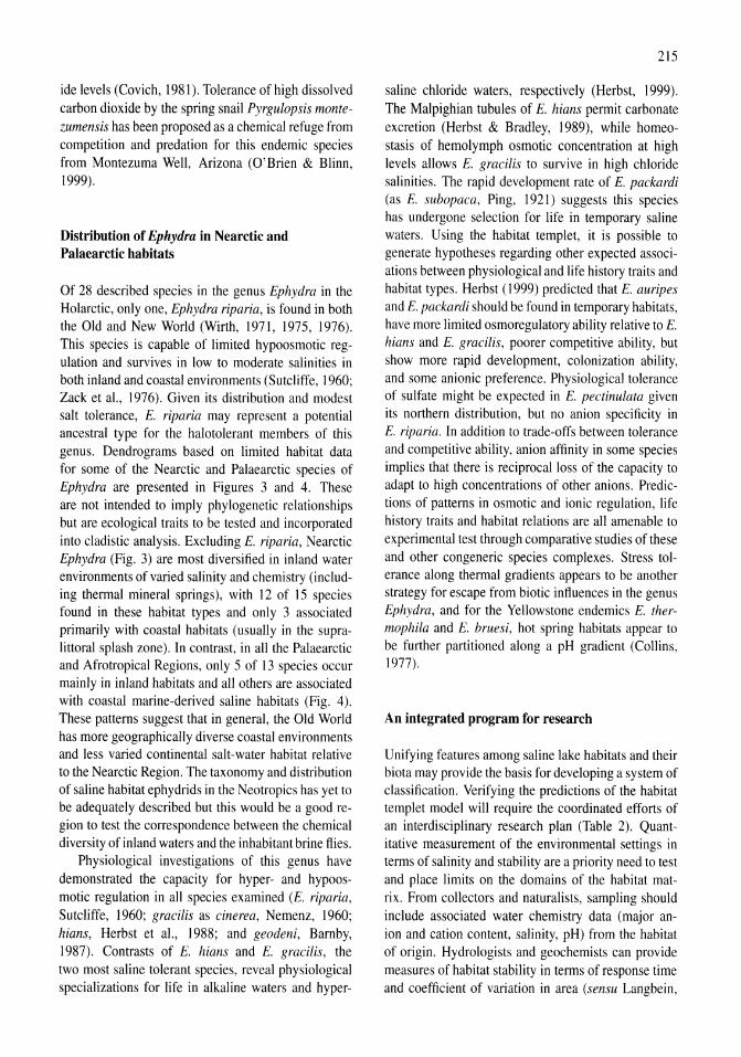
ide levels (Covich, 1981). Tolerance of high dissolved carbon dioxide by the spring snail Pyrgulopsis montezumensis has been proposed as a chemical refuge from competition and predation for this endemic species from Montezuma Well, Arizona (O'Brien & Blinn, 1999).
Distribution of Ephydra in Nearctic and Palaearctic habitats
Of 28 described species in the genus Ephydra in the Holarctic, only one, Ephydra riparia, is found in both the Old and New World (Wirth, 1971, 1975, 1976). This species is capable of limited hypoosmotic regulation and survives in low to moderate salinities in both inland and coastal environments (Sutcliffe, 1960; Zack et al., 1976). Given its distribution and modest salt tolerance, E. riparia may represent a potential ancestral type for the halotolerant members of this genus. Dendrograms based on limited habitat data for some of the Nearctic and Palaearctic species of Ephydra are presented in Figures 3 and 4. These are not intended to imply phylogenetic relationships but are ecological traits to be tested and incorporated into cladistic analysis. Excluding E. riparia, Nearctic Ephydra (Fig. 3) are most diversified in inland water environments of varied salinity and chemistry (including thermal mineral springs), with 12 of 15 species found in these habitat types and only 3 associated primarily with coastal habitats (usually in the supralittoral splash zone). In contrast, in all the Palaearctic and Afrotropical Regions, only 5 of 13 species occur mainly in inland habitats and all others are associated with coastal marine-derived saline habitats (Fig. 4). These patterns suggest that in general, the Old World has more geographically diverse coastal environments and less varied continental salt-water habitat relative to the Nearctic Region. The taxonomy and distribution of saline habitat ephydrids in the Neotropics has yet to be adequately described but this would be a good region to test the correspondence between the chemical diversity of inland waters and the inhabitant brine flies.
Physiological investigations of this genus have demonstrated the capacity for hyper- and hypoosmotic regulation in all species examined (E. riparia, Sutcliffe, 1960; gracilis as cinerea, Nemenz, 1960; hians, Herbst et al., 1988; and geodeni, Barnby, 1987). Contrasts of E. hians and E. gracilis, the two most saline tolerant species, reveal physiological specializations for life in alkaline waters and hyper-
215
saline chloride waters, respectively (Herbst, 1999). The Malpighian tubules of E. hians permit carbonate excretion (Herbst & Bradley, 1989), while homeostasis of hemolymph osmotic concentration at high levels allows E. gracilis to survive in high chloride salinities. The rapid development rate of E. packardi (as E. subopaca, Ping, 1921) suggests this species has undergone selection for life in temporary saline waters. Using the habitat templet, it is possible to generate hypotheses regarding other expected associations between physiological and life history traits and habitat types. Herbst (1999) predicted that E. auripes and E. packardi should be found in temporary habitats, have more limited osmoregulatory ability relative to E. hians and E. gracilis, poorer competitive ability, but show more rapid development, colonization ability, and some anionic preference. Physiological tolerance of sulfate might be expected in E. pectinulata given its northern distribution, but no anion specificity in E. riparia. In addition to trade-offs between tolerance and competitive ability, anion affinity in some species implies that there is reciprocal loss of the capacity to adapt to high concentrations of other anions. Predictions of patterns in osmotic and ionic regulation, life history traits and habitat relations are all amenable to experimental test through comparative studies of these and other congeneric species complexes. Stress tolerance along thermal gradients appears to be another strategy for escape from biotic influences in the genus Ephydra, and for the Yellowstone endemics E. thermophila and E. bruesi, hot spring habitats appear to be further partitioned along a pH gradient (Collins, 1977).
An integrated program for research
Unifying features among saline lake habitats and their biota may provide the basis for developing a system of classification. Verifying the predictions of the habitat temp let model will require the coordinated efforts of an interdisciplinary research plan (Table 2). Quantitative measurement of the environmental settings in terms of salinity and stability are a priority need to test and place limits on the domains of the habitat matrix. From collectors and naturalists, sampling should include associated water chemistry data (major anion and cation content, salinity, pH) from the habitat of origin. Hydrologists and geochemists can provide measures of habitat stability in terms of response time and coefficient of variation in area (sensu Langbein,
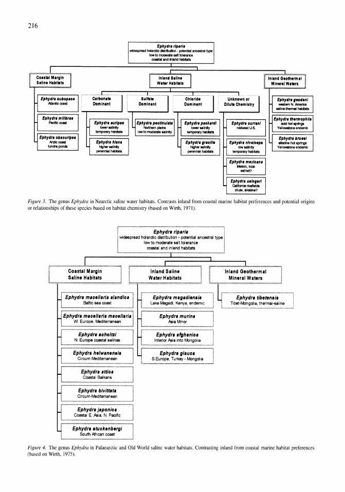
216
Ephyd" mlllb", PocIIIc ....
Ephyd" o""urlp .. _ .... Itrldra ponde
Clrllon.1I Domlnlnt
Ephydr. turlp .. _ .. lIlily
IempoI1Iry -
Ephyd" hl.n. lJIProollnily
poronnIIl-
Ephydre rlp.rI. wIdeopA!lld hoIan:llc _ • poIentlaI anceoInII type
Iowto_ ... n_ coaataIandlnlandhlbllll
Chlorid. Domlnlnt
Ephyd" peolr.trdl _lIIlnly
lernpcnryhlbllll
Ephyd" ,,,o111. hlgherlllinily
_101_ Ephydrt ou","1
_u.s.
Ephydre n/v,lo,p' Iowlllinly
IempoI1Iry -
Ephyd" mexlo.n. _,Iooal
""'1ncI?
Ephyd" u.'n,.rI CIIfam._
dIuIe,elllllllne?
Inland O.oth,rm.1 M'n,r.' W."r.
Ephyd" ,lOd",' _emN._ II1II".--
Ephydrt /hemophll. acid hoi opmga
YeI_endemIc
Ephydrt "ru .. ' ....,Ine hoi opmga YelIOWIIone_
Figure 3. The genus Ephydra in Nearctic saline water habitats. Contrasts inland from coastal marine habitat preferences and potential origins or relationships of these species based on habitat chemistry (based on Wirth, 1971).
Ephydra rip,,;. Voidespread hoi arctic distnbution - potential ancestral type
low to moderate salt tolerance
Ephyd,.. mu.II", •• '.ndIOf Baltic sea coast
Ephydra m.o.lI.ri. m.o.II"I. w. Europe, Mediterranean
Ephyd,.. IOho/tzl N. Europe ccastal salinas
Ephydra h.'w.n.n.'. Circum-Mediterranean
Ephydra .tt/oa Coastal Balkans
Ephydrl blv/ttlt. Circum-Mediterranean
Ephydra japonio. Coastal E. Asia, N. Pacific
Ephydrl ,tuoktnb'rgi South Mrican coast
ccastal and inland habitats
Inland Salin. Water Habitats
Ephydrl m'g.dl.n,i, Lake Magadi, Kenya, endemic
Ephydra murln. Asia Minor
Ephydrl .",h.nloa Intenor Asia into Mongolia
Ephydrl g/.uo. S. Europe, Turkey - Mongolia
Inland G.oth.rmal Mineral Waters
Ephydrl rlb.tln,', libel-Mongolia, thermal-saline
Figure 4. The genus Ephydra in Palaearctic and Old World saline water habitats. Contrasting inland from coastal marine habitat preferences (based on Wirth, 1975).
Table 2. An integrated research plan for defining the habitat templet of saline lakes
Discipline
Collectors and
naturalists
Hydrologists and
geochemists
Physiologists
Systematists
Data contribution needed
Associated habitat salinity, stability,
solute chemistry for collections of
flora and fauna
Measures of the spatial and temporal
components of salinity gradients,
and the stability of habitats (e.g.
response time and coefficient of
variation in lake area)
Comparative ion tolerance within
and between congeneric species
Purpose
Provide data for defining the
relationship of species
distributions to the chemical
and physical setting of
habitat locales
Develop a basis for
quantifying the distribution
of biota along gradients of
habitat salinity and stability
Test hypotheses that suites of
traits enabling adaptation to
complexes of saline water biota; particular environmental
tests of trade-offs between tolerance conditions result in obligate
and competitive ability, and between fidelity to that habitat, and
ion regulating mechanisms even define habitat types
according to the unifying
traits of the biota
Phylogenies and cladograms
developed from habitat associations
and physiological phenotypes to
Examine the question of
biological diversification in
terms of the opportunity for
supplement or contrast with results specialization in the diverse
using traditional morphological data geochemical environments
of saline waters
Stratigraphers, Correlation of sediment core Improve the accuracy of
reconstructions of ancient
environments. lake
ecosystems, and regional
climatic histories
palaeolimnologists communities with data
from experimental calibrations of
biological proxy responses to
salinity and solute variation
217
1961), and historical geographic information on the spatiotemporal distribution of lakes of varied composition. Comparative physiologists should investigate more thoroughly the differences in salinity and ionic tolerance between and within congeneric species, the regulatory mechanisms for coping with chemistry, and develop experiments to test for predicted tradeoffs among physiological and life history traits. Systematists may complement conventional c1adograms based on morphology with data on discrete traits of physiological phenotype and habitat associations. Plesiomorphic traits are expected to be associated with low salinity mixed chemistry adaptations and apo-
morphic derived traits with the terminal branchpoints of solute evolution and anion predominances. This approach to cladistic analysis might be used along with molecular methods to construct phylogenies related to the sequential evolution of species complexes in saline water environments.
An integrated research approach may provide insight not only to current biogeographic patterns of habitat utilization but also to the past. Palaeolimnologists and stratigraphers might be able to improve the accuracy of historical reconstructions through calibration of biological proxy responses to experimental variation of salinity and/or solute composition (e.g.
218
Herbst & Blinn, 1998). Differences in regional geochemical evolution also become a viable alternative explanation to geographic isolation by glacial vicariance events as has been often used to explain the distribution of aquatic fauna (Herbst, 1999). Through coordinated surveys and experimental studies, the variety that characterizes saline lake environments may find unifying themes for the outline of an ecological temp let for organizing these habitats.
Acknowledgements
The ideas presented here build on those of many scientists studying saline lakes over many years. Especially valuable have been discussions with Dean Blinn, Tim Bradley and Rick Forester. I am grateful to Bob Jellison, Wayne Mathis and John Melack for helpful review and editorial comments.
References
Barnby, M. A., 1987. Osmotic and ionic regulation of two brine fly species (Diptera: Ephydridae) from a saline hot spring. Physiol. Zool. 60: 327-338.
Bayly, I. A. E., 1967. The general biological classification of aquatic environments with special reference to those of Australia. In Weatherly, A H. (ed.), Australian Inland Waters and their Fauna: Eleven Studies. Australian National University Press, Canberra.
Beadle, L. C., 1959. Osmotic and ionic regulation in relation to the classification of brackish and inland saline waters. Archo. Oceanogr. Limnol. l1(suppl.): 143-151.
Belk, D. & G. A. Cole, 1975. Adaptational biology of desert temporary-pond inhabitants. In Hadly, N. F. (ed.), Environmental Physiology of Desert Organisms. Dowden, Hutchinson & Ross, Stroudsberg, Pennsylvania.
Blinn, D. W, 1993. Diatom community structure along physicochemical gradients in saline lakes. Ecology 74: 1246-1263.
Bowen, S. T., E. A. Fogarino, K. N. Fitchner, G. L. Dana, V. H. S. Chow, M. R Buoncristiani & J. R Carl, 1985. Ecological isolation in Artemia: population differences in tolerance of anion concentrations. J. Crust. BioI. 5: 106-129.
Bradley, T. J., 1987. Physiology of osmoregulation in mosquitoes. Ann. Rev. Entomol. 32: 439-462.
Bradley, T. J. & J. E. Phillips, 1977. Regulation of rectal secretion in saline-water mosquito larvae living in waters of diverse ionic composition. J. expo BioI. 66: 83-96.
Broch, E. S., 1969. The osmotic adaptation of the fairy shrimp Branchinecta campestris Lynch to saline astatic waters. Limnol. Oceanogr. 14: 485-492.
Broch, E. S., 1988. Osmoregulatory patterns of adaptation to inland astatic waters by two species of fairy shrimps, Branchinecta gigas Lynch and Branchinecta mackini Dexter. J. Crust. BioI. 8: 383-391.
Burton, R S & M. W. Feldman, 1983. Physiological effects of an allozyme polymorphism: glutamate-pyruvate transaminase and response to hyperosmotic stress in the copepod TIgriopus califomicus. Biochem. Genet. 21: 239-251.
Cole, G. A, 1968. Desert linmology. In Brown, J. W Jr. (ed.), Desert Biology. Academic Press, New York.
Collins, N. C., 1977. Mechanisms determining the relative abundance of brine flies (Diptera: Ephydridae) in Yellowstone thermal spring effluents. Can. Entomol. 190: 415-422.
Covich, A. P., 1981. Chemical refugia from predation for thinshelled gastropods in a sulfide-enriched stream. Verh. internat. Ver. Linmol. 21: 1632-1636.
Eugster, H. P. & B. F. Jones, 1979. Behavior of major solutes during closed-basin brine evolution. Am. J. Sci. 279: 609--631.
Forester, R. M., 1986. Determination of the dissolved anion composition of ancient lakes from fossil ostracodes. Geology 14: 796-798.
Hedgpeth, J. W, 1959. Some preliminary considerations of the biology of inland mineral waters. Archo. Oceanogr. Limnol. 11 (suppl.): 111-141.
Herbst, D. B., 1999. Biogeography and physiological adaptations of the brine fly genus Ephydra (Diptera: Ephydridae) in saline waters of the Great Basin. Gr. Basin Nat. 59: 127-135.
Herbst, D. B. & D. W Blinn, 1998. Experimental mesocosm studies of salinity effects on the benthic algal community of a saline lake. J. Phycol. 34: 772-778.
Herbst, D. B. & T. J. Bradley, 1989. A Malpighian tubule lime gland in an insect inhabiting alkaline salt lakes. J. expo BioI. 145: 63-78.
Herbst, D. B., F. P. Conte & V. J. Brookes, 1988. Osmoregulation in an alkaline salt lake insect Ephydra (Hydropyrus) hians Say (Diptera: Ephydridae), in relation to water chemistry. J. Insect Physiol. 34: 903-909.
Hoffmann, A. A. & P. A Parsons, 1991. Evolutionary Genetics and Environmental Stress. Oxford University Press, Oxford.
Holdridge, L. R, 1967. Life Zone Ecology. Rev. edn. Tropical Science Center, San Jose.
Hutchinson, G. E., 1957. A Treatise on Limnology, Volume I, Part 2. Chemistry of Lakes. John Wiley and Sons, New York.
Javor, B., 1989. Hypersaline Environments. Springer-Verlag, Berlin. Langbein, W. B., 1961. Salinity and hydrology of closed lakes. U.S.
Geological Survey Professional Paper #412. Losos, J. B., 1992. The evolution of convergent structure in Carib
bean Anolis communities. Syst. BioI. 41: 403-420. Nemenz, H., 1960. On the osmotic regulation of the larvae of
Ephydra cinerea. J. Insect Physiol. 4: 38-44. O'Brien, C. & D. W Blinn, 1999. The endemic spring snail Pyrgu
lopsis montezumensis in a high C02 environment: importance of extreme chemical habitats as refugia. Freshwat. BioI. 42: 225-234.
Ping, c., 1921. The biology Ephydra subopaca Loew. Cornell University Agriculture Experiment Station Memoirs 49: 561-616.
Por, F. D., 1980. A classification of hypersaline waters, based on trophic criteria. Mar. Ecol. I: 121-131.
Sailer, R. I., 1948. The genus Trichocorixa (Corixidae, Hemiptera). Kans. Univ. Sci. Bull. 32: 289-407.
Sheplay, A. W & T. J. Bradley, 1982. A comparative study of magnesium sulphate tolerance in saline-water mosquito larvae. J. Insect Physiol. 28: 641-646.
Soltz, D. L. & R. J. Naiman, 1978. The Natural History of Native Fishes in the Death Valley System. Natural History Museum of Los Angeles County, Science Series 30.
Southwood, T. R. E., 1977. Habitat, the templet for ecological strategies? J. animo Ecol. 46: 337-365.
Southwood, T. R. E., 1988. Tactics, strategies and templets. Oikos 52: 3-18.
Sutcliffe, D. W, 1960. Osmotic regulation in the larvae of some euryhaline diptera. Nature 187: 331-332.

Tones, P. I. & U. T. Hammer, 1975. Osmoregulation in Trichocorixa verticalis interiores Sailer (Hemiptera, Corixidae) - an inhabitant of Saskatchewan saline lakes, Canada. Can. J. Zoo!. 53: 1207-1212.
Whittaker, R. H., 1975. Communities and Ecosystems, 2nd edn. Macmillan Publishing Co., New York.
Wilson, D. S. & P. A. Keddy, 1986. Species competitive ability and position along a natural stress/disturbance gradient. Ecology 67: 1236-1242.
Wirth, W. w., 1971. The brine flies of the genus Ephydra in North America (Diptera: Ephydridae). Ann. En!. Soc. Am. 64: 357-377.
219
Wirth, W. W., 1975. A revision of the brine flies of the genus Ephydra of the Old World (Diptera: Ephydridae). En!. Scand. 6: 11-44.
Wirth, W. w., 1976. A new species of brine fly from California rice fields. Pan-Pacific Entomo!' 52: 242-243.
Wurtsbaugh, W. A., 1992. Food-web modification by an invertebrate predator in the Great Salt Lake (U.S.A.). Oecologia 89: 168-175.
Zack, R. S., R. W. Their & B. A. Foote, 1976. A possible case of spatial isolation in brine flies of the genus Ephydra (Diptera: Ephydridae). Great Lakes Entomo!' 9: 205.
Hydrobiologia 466: 221-229,200!' J,M, Melack, R, Jellison & D,8, Herbst (eds), Saline Lakes, © 2001 Kluwer Academic Publishers.
221
Thermal tolerance and heat shock proteins in encysted embryos of Artemia from widely different thermal habitats
James S. Clegg l , Nguyen Van Hoa2 & Patrick Sorgeloos3
1 Section of Molecular and Cellular Biology and the Bodega Marine Laboratory, University of California (Davis), Bodega Bay, CA 94923, U.S.A. Tel: +707-875-2010. Fax: +707-875-2009. E-mail: [email protected] 2 Institute of Marine Aquaculture, University of Can Tho, Vietnam 3 Artemia Reference Center, Ghent University, 9000 Ghent, Belgium
Key words: Artemia, thermal adaptation, heat shock, stress proteins, Hsp-70, p26, artemin
Abstract
Encysted embryos (cysts) of the brine shrimp, Artemia provide an excellent model system for the study of biochemical adaptation to environmental extremes. Here, we describe an experiment in which cysts of A. franciscana from the San Francisco Bay (SFB), California, U.S.A., were inoculated into experimental ponds in the Mekong Delta region of Vietnam where water temperatures are much higher than the SFB. Cysts produced in each of three successive growing seasons (1996-1998) were collected and examined in the laboratory for resistance to high temperature and relative contents of three stress proteins (Hsp-70, artemin and p26). Thermal adaptation took place rapidly, during the first growing season. The increase in thermal tolerance was reflected in an overall increase in stress protein content, compared to SFB cysts used for the initial inoculation. Also examined were cysts of A. tibetiana collected from a lake on the high plateau of Tibet, PR China, almost 4.5 km above sea level. These cysts were very sensitive to high temperatures, and contained much lower levels of all stress proteins examined, compared to A. franciscana cysts from SFB and Vietnam. Cysts of A. sinica, collected from a hypersaline lake in Inner Mongolia, PR China, were examined in the same fashion and found to be similar to SFB cysts in terms of thermal resistance and stress protein content. The harsh environments in which Artemia are found, and the great diversity of its habitats, world-wide, provide excellent opportunities to relate the ecological setting of an organism to the underlying physiological and biochemical processes enabling its survival.
Introduction
Species of the brine shrimp, Artemia, are found in a variety of harsh environments world wide (Triantaphyllidis et aI., 1998) in which they encounter severe hypersalinity, high doses of ultraviolet radiation, very low oxygen tensions and extremes of temperature (Clegg & Conte, 1980; Persoone et aI., 1980; Decleir et aI., 1987; Warner et aI., 1989; MacRae et aI., 1989; Browne et aI., 1991; Hand & Hardewig, 1996). These challenging ecological settings suggest that Artemia represents a useful model organism for studies on the stress response at all levels of biological organization. The stress (heat shock) response has been the object of study so intense that the volume of literature is overwhelming (selected reviews and
books are cited as an entry - Nover, 1991; Parsell & Lindquist, 1993; Morimoto et aI., 1994; Fiege et aI., 1996; SchOffi et aI., 1998; Fink & Golo, 1998; Feder & Hofmann, 1999). One feature of the heat shock response is 'induced thermotolerance' (ITT), the ability of a sub-lethal heat shock, well above physiological temperature (but below lethal) to induce resistance to a subsequent, otherwise lethal heat exposure. The basis for ITT is not understood completely, but it has been well-documented that a major contribution comes from an ensemble of heat shock (stress) protein families, many of which act as molecular chaperones to minimize aggregation of unfolded globular proteins and, in some cases, to restore native structures. Once again, the literature is massive (see entry references above, and Beissinger & Buchner, 1998; Lorimer &
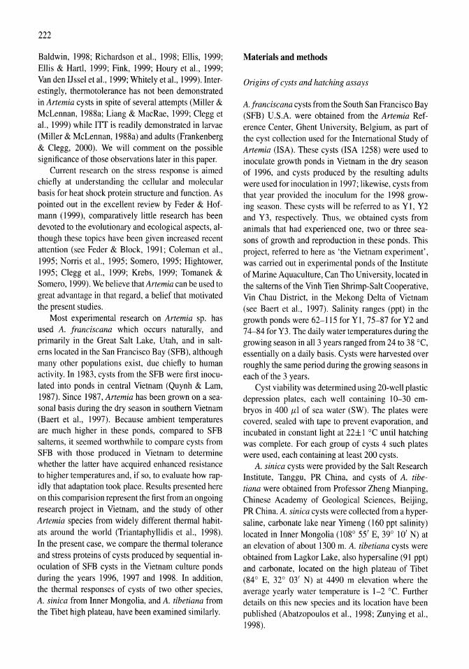
222
Baldwin, 1998; Richardson et al., 1998; Ellis, 1999; Ellis & Hartl, 1999; Fink, 1999; Houry et al., 1999; Van den IJssel et al., 1999; Whitely et al., 1999). Interestingly, thermotolerance has not been demonstrated in Artemia cysts in spite of several attempts (Miller & McLennan, 1988a; Liang & MacRae, 1999; Clegg et al., 1999) while ITT is readily demonstrated in larvae (Miller & McLennan, 1988a) and adults (Frankenberg & Clegg, 2000). We will comment on the possible significance of those observations later in this paper.
Current research on the stress response is aimed chiefly at understanding the cellular and molecular basis for heat shock protein structure and function. As pointed out in the excellent review by Feder & Hofmann (1999), comparatively little research has been devoted to the evolutionary and ecological aspects, although these topics have been given increased recent attention (see Feder & Block, 1991; Coleman et al., 1995; Norris et al., 1995; Somero, 1995; Hightower, 1995; Clegg et al., 1999; Krebs, 1999; Tomanek & Somero, 1999). We believe that Artemia can be used to great advantage in that regard, a belief that motivated the present studies.
Most experimental research on Artemia sp. has used A. franciscana which occurs naturally, and primarily in the Great Salt Lake, Utah, and in salterns located in the San Francisco Bay (SFB), although many other populations exist, due chiefly to human activity. In 1983, cysts from the SFB were first inoculated into ponds in central Vietnam (Quynh & Lam, 1987). Since 1987, Artemia has been grown on a seasonal basis during the dry season in southern Vietnam (Baert et al., 1997). Because ambient temperatures are much higher in these ponds, compared to SFB salterns, it seemed worthwhile to compare cysts from SFB with those produced in Vietnam to determine whether the latter have acquired enhanced resistance to higher temperatures and, if so, to evaluate how rapidly that adaptation took place. Results presented here on this comparision represent the first from an ongoing research project in Vietnam, and the study of other Artemia species from widely different thermal habitats around the world (Triantaphyllidis et al., 1998). In the present case, we compare the thermal tolerance and stress proteins of cysts produced by sequential inoculation of SFB cysts in the Vietnam culture ponds during the years 1996, 1997 and 1998. In addition, the thermal responses of cysts of two other species, A. sinica from Inner Mongolia, and A. tibetiana from the Tibet high plateau, have been examined similarly.
Materials and methods
Origins of cysts and hatching assays
A.franciscana cysts from the South San Francisco Bay (SFB) U.S.A. were obtained from the Artemia Reference Center, Ghent University, Belgium, as part of the cyst collection used for the International Study of Artemia (ISA). These cysts (ISA 1258) were used to inoculate growth ponds in Vietnam in the dry season of 1996, and cysts produced by the resulting adults were used for inoculation in 1997; likewise, cysts from that year provided the inoculum for the 1998 growing season. These cysts will be referred to as Yl, Y2 and Y3, respectively. Thus, we obtained cysts from animals that had experienced one, two or three seasons of growth and reproduction in these ponds. This project, referred to here as 'the Vietnam experiment', was carried out in experimental ponds of the Institute of Marine Aquaculture, Can Tho University, located in the salterns of the Vinh Tien Shrimp-Salt Cooperative, Vin Chau District, in the Mekong Delta of Vietnam (see Baert et al., 1997). Salinity ranges (ppt) in the growth ponds were 62-115 for Yl, 75-87 for Y2 and 74-84 for Y3. The daily water temperatures during the growing season in all 3 years ranged from 24 to 38°C, essentially on a daily basis. Cysts were harvested over roughly the same period during the growing seasons in each of the 3 years.
Cyst viability was determined using 20-well plastic depression plates, each well containing 10-30 embryos in 400 ILl of sea water (SW). The plates were covered, sealed with tape to prevent evaporation, and incubated in constant light at 22± 1 °C until hatching was complete. For each group of cysts 4 such plates were used, each containing at least 200 cysts.
A. sinica cysts were provided by the Salt Research Institute, Tanggu, PR China, and cysts of A. tibetiana were obtained from Professor Zheng Mianping, Chinese Academy of Geological Sciences, Beijing, PR China. A. sinica cysts were collected from a hypersaline, carbonate lake near Yimeng (160 ppt salinity) located in Inner Mongolia (108° 55' E, 39° 10' N) at an elevation of about 1300 m. A. tibetiana cysts were obtained from Lagkor Lake, also hypersaline (91 ppt) and carbonate, located on the high plateau of Tibet (84° E, 32° 03' N) at 4490 m elevation where the average yearly water temperature is I-2°C. Further details on this new species and its location have been published (Abatzopoulos et al., 1998; Zunying et al., 1998).
Heat shock (HS) and protein preparation
Dried cysts were hydrated in SWat 2°C for 16-18 h, collected on cloth filters, and washed briefly with distilled water (10 s) followed by blotting on paper towels for 2 min to remove interstitial water. These cysts were either used as unheated controls or transferred to 50 ml centrifuge tubes containing 35 ml of SW preheated to 22.0 °C in a Lauda RM water bath good to ±0.05 DC. The temperature was then increased to 50.0 °C at a rate of 0.7 degrees min- i with continuous vigorous aeration. This protocol was used to avoid transfer of cysts directly from 2 °C to a much higher temperature. Temperatures were measured in the incubation tubes using a precision thermometer (±0.05 0C). Cysts were held at 50.0 °C for various times, collected as described above, assayed for viability and, in some cases, prepared for stress protein analysis. In the latter case, cysts were homogenized on ice at 100 mg wet weight ml- i of buffer K (150 mM sorbitol, 70 mM potassium gluconate, 5 mM MgC}z, 5 mM NaH2P04, 40 mM Hepes, pH 7.4). Homogenate aliquots were combined separately with equal volumes of 2xSDS sample buffer, vortexed and heated at 100°C for 5 min (Laemmli, 1970). After cooling, the preparations were centrifuged (1630 g, 3 min) to remove insoluble fragments of the chitinous shells that prevent accurate pipetting. Aliquots equivalent to the same wet weight of cysts were applied to the gels to enable direct comparison between samples. That basis seems better than applying the same amounts of protein because of the domination of yolk platelet proteins in these embryos.
SDS-PAGE and Western immunoblotting
SDS-preparations were electrophoresed on 12% polyacrylamide gels. For each experiment, two identical gels were run: one was stained with Coomassie Blue [500 mg Serva Blue 500 ml- i of methanol:acetic acid:H20 (40:50: 10)] and proteins on the other were transferred to a nitrocellulose membrane (Towbin et aI., 1979) for Western immunoblot analysis. Membranes were incubated with monoclonal anti-hsp-70 antibody, clone 7.10 (Affinity BioReagents, Inc., Golden, Colorado). Goat anti-rat IgG conjugated with horseradish peroxidase was used for the secondary antibody (Southern Biotechnology Associates, Inc., Birmingham, Alabama). ECL Western Blotting Reagents (Amersham Corp., Arlington Heights, Illinois) were used for detection of labeled proteins on Kodak BioMax MR single emulsion film (Eastman Kodak Co., Rochester, New York) and developed in an X-Ray
223
C 0 15 30 45 60 75 90 105
Minutes at 50°C (after 22 to 50°C)
Figure 1. Hatching levels of cysts from the Vietnam experiment following return to 22± I °C after exposure to 50.0 °C for the times shown. Unheated cysts are controls (C) and YI, Y2, Y3 refer to cysts produced during the growing seasons of 1996, 1997, 1998, respectively. See text for further details.
film processor. Similar protocols were used to detect artemin, a ferritin-like stress protein present in cysts (De Herdt et aI., 1980; De Graaf et aI., 1990) and p26, a small heat shOCk/a-crystallin protein of known importance to cyst stress resistance (see Clegg et aI., 1999; Liang & MacRae, 1999). Differences from the Western blotting described above for Hsp-70 involved the use of anti-artemin, provided by Herman Slegers, and our anti-p26, both being polyclonal and affinitypurified before use (see Clegg et aI., 1994, 1999 for further details).
Results
The Vietnam experiment
Figure 1 describes the effects of high temperature on viability (% hatching) of the SFB cysts used for the inoculation in 1996, and on cysts produced in Vietnam during the three growth seasons of the study (1996-1998). No differences in hatching performance were noted for cysts produced in Vietnam during 1996 and 1998, compared to the SFB inoculum, during the initial 15 min exposure to 50.0 dc. As exposure time at that temperature increased, the 1996 and 1998 cysts proved to be much more resistant than the SFB inoculum. In contrast, hatching percentages of the cysts
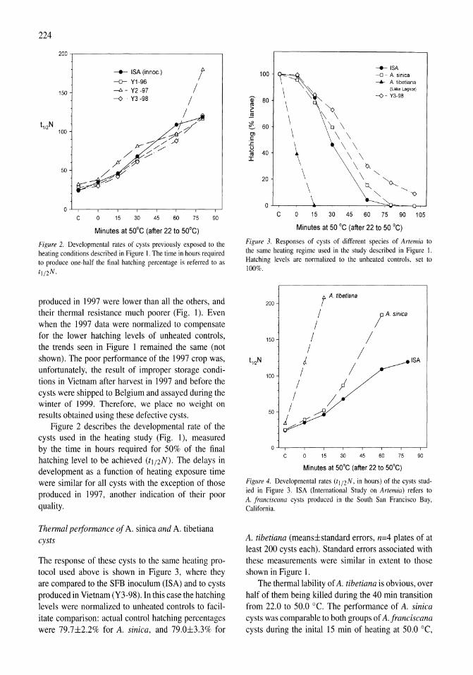
224
200,-------------------------------,
150
---*- ISA (innoc.) ! -D- Y1-96
/ ----6 - Y2 -97 -<>. Y3 -98 /
/ / -;;#"
..--; /fl /Y </
/ ;:;
100
50 /,y
/0'7 <"/
c o 15 30 45 60 75 90
Minutes at 50°C (after 22 to 50°C)
Figure 2. Developmental rates of cysts previously exposed to the heating conditions described in Figure I. The time in hours required to produce one-half the final hatching percentage is referred to as
11/2 N .
produced in 1997 were lower than all the others, and their thermal resistance much poorer (Fig. 1). Even when the 1997 data were normalized to compensate for the lower hatching levels of unheated controls, the trends seen in Figure 1 remained the same (not shown). The poor performance of the 1997 crop was, unfortunately, the result of improper storage conditions in Vietnam after harvest in 1997 and before the cysts were shipped to Belgium and assayed during the winter of 1999. Therefore, we place no weight on results obtained using these defective cysts.
Figure 2 describes the developmental rate of the cysts used in the heating study (Fig. I), measured by the time in hours required for 50% of the final hatching level to be achieved (tl/2N). The delays in development as a function of heating exposure time were similar for all cysts with the exception of those produced in 1997, another indication of their poor quality.
Thermal performance of A. sinica and A. tibetiana cysts
The response of these cysts to the same heating protocol used above is shown in Figure 3, where they are compared to the SFB inoculum (ISA) and to cysts produced in Vietnam (Y3-98). In this case the hatching levels were normalized to unheated controls to facilitate comparison: actual control hatching percentages were 79.7±2.2% for A. sinica, and 79.0±3.3% for
___ ISA
100 --0 - A. sinica -A- A tibetiana
(Lake Lagkor)
Q) ~- Y3-98 80
I1l
","0\ c .!!! :R 0 60 b \ Cl \ \ .~
.r::: \ \ .8 I1l 40 \ \ I
\ ~
\ \ ""-20 ~ \ ~
---" '0
c o 15 30 45 60 75 90 105
Minutes at 50°C (after 22 to 50 °C)
Figure 3. Responses of cysts of different species of Artemia to the same heating regime used in the study described in Figure I. Hatching levels are normalized to the unheated controls. set to 100%.
200 t A tibetiana
/ IA sinica
/ 150 / /
/ / t1l2N d ISA
100 / / / I
/ ! 50 / ~
j
c 15 30 45 60 75 90
Minutes at 50°C (after 22 to 50°C)
Figure 4. Developmental rates (lI/2N, in hours) of the cysts studied in Figure 3. ISA (International Study on Artemia) refers to A. franciscana cysts produced in the South San Francisco Bay. California.
A. tibetiana (means±standard errors, n=4 plates of at least 200 cysts each). Standard errors associated with these measurements were similar in extent to those shown in Figure I.
The thermal lability of A. tibetiana is obvious, over half of them being killed during the 40 min transition from 22.0 to 50.0 0c. The performance of A. sinica cysts was comparable to both groups of A. franciscana cysts during the inital 15 min of heating at 50.0 °c,
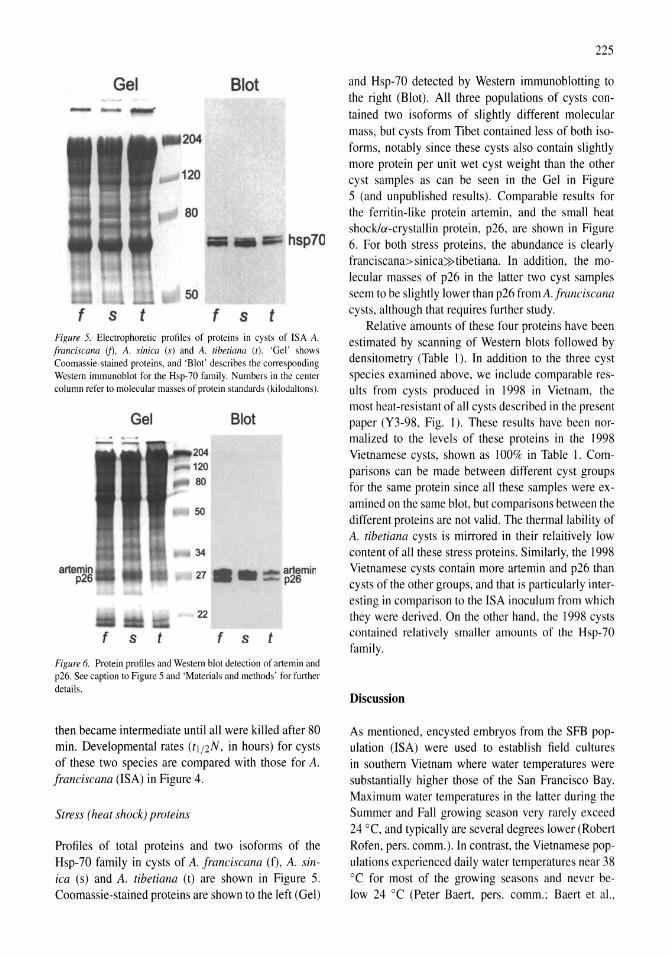
Gel Blot
-204
120
80
hsp70
50
f s t f s t Figure 5. Electrophoretic profiles of proteins in cysts of ISA A. franciscana (j), A. sinica (s) and A. tibetiana (t). 'Gel' shows Coomassie-stained proteins, and 'Blot' describes the corresponding Western immunoblot for the Hsp-70 family. Numbers in the center column refer to molecular masses of protein standards (kilodaltons).
artemin p26
f
Gel
s t
Blot
22
f s t
artemin p26
Figure 6. Protein profiles and Western blot detection of artemin and p26. See caption to Figure 5 and 'Materials and methods' for further details.
then became intermediate until all were killed after 80 min. Developmental rates (tl/2N, in hours) for cysts of these two species are compared with those for A. franciscana (ISA) in Figure 4.
Stress (heat shock) proteins
Profiles of total proteins and two isoforms of the Hsp-70 family in cysts of A. franciscana (f), A. sinica (s) and A. tibetiana (t) are shown in Figure 5. Coomassie-stained proteins are shown to the left (Gel)
225
and Hsp-70 detected by Western immunoblotting to the right (Blot). All three populations of cysts contained two isoforms of slightly different molecular mass, but cysts from Tibet contained less of both isoforms, notably since these cysts also contain slightly more protein per unit wet cyst weight than the other cyst samples as can be seen in the Gel in Figure 5 (and unpublished results). Comparable results for the ferritin-like protein artemin, and the small heat shock/a-crystallin protein, p26, are shown in Figure 6. For both stress proteins, the abundance is clearly franciscana>sinica»tibetiana. In addition, the molecular masses of p26 in the latter two cyst samples seem to be slightly lower than p26 from A. franciscana cysts, although that requires further study.
Relative amounts of these four proteins have been estimated by scanning of Western blots followed by densitometry (Table I). In addition to the three cyst species examined above, we include comparable results from cysts produced in 1998 in Vietnam, the most heat-resistant of all cysts described in the present paper (Y3-98, Fig. I). These results have been normalized to the levels of these proteins in the 1998 Vietnamese cysts, shown as 100% in Table I. Comparisons can be made between different cyst groups for the same protein since all these samples were examined on the same blot, but comparisons between the different proteins are not valid. The thermal lability of A. tibetiana cysts is mirrored in their relaitively low content of all these stress proteins. Similarly, the 1998 Vietnamese cysts contain more artemin and p26 than cysts of the other groups, and that is particularly interesting in comparison to the ISA inoculum from which they were derived. On the other hand, the 1998 cysts contained relatively smaller amounts of the Hsp-70 family.
Discussion
As mentioned, encysted embryos from the SFB population (ISA) were used to establish field cultures in southern Vietnam where water temperatures were substantially higher those of the San Francisco Bay. Maximum water temperatures in the latter during the Summer and Fall growing season very rarely exceed 24°C, and typically are several degrees lower (Robert Rofen, pers. comm.). In contrast, the Vietnamese populations experienced daily water temperatures near 38 DC for most of the growing seasons and never below 24°C (Peter Baert, pers. comm.; Baert et aI.,
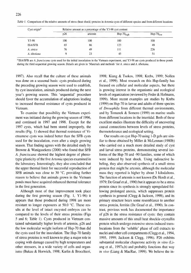
226
Table 1. Comparison of the relative amounts of stress (heat shock) proteins in A rtemia cysts of different species and from different locations
Cyst origina Relative amount as a percentage of the Y3-98 cyst content
p26 artemin HsP-7Ohigh HsP-7Olow
Y3-98 100 100 100 100 ISAlSFB 65 86 123 49
A. sinica 76 49 III 226
A. tibetiana 9 23 45 51
a ISAlSFB are A. franciscana cysts used for the initial inoculation in the Vietnam experiment, and Y3-98 are cysts produced in those ponds during the third sequential growing season. Details are given in 'Materials and methods' for A. sinica and A. tibetiana.
1997). Also recall that the culture of these animals was done on a seasonal basis: cysts produced during the preceding growing season were used to establish, by cyst inoculation, animals produced during the next year's growing season. This 'sequential' procedure should favor the accumulation of adaptations leading to increased thermal resistance of cysts produced in Vietnam.
To examine that possibility the Vietnam experiment was initiated during the growing season of 1996, and continued in 1997 and 1998. Except for the 1997 cysts, which had been stored improperly, the results (Fig. 1) showed that thermal resistance of Vietnamese cysts was indeed better than the SFB cysts used for the inoculation, even after a single growing season. That finding agrees with the detailed study by Browne & Wanigasekera (2000) who found that SFB A. franciscana showed the highest degree of phenotypic plasticity of the five Artemia species examined in the laboratory. Interestingly, they also concluded that the upper thermal limit for successful reproduction of SFB animals was close to 30°C, providing further reason to believe that animals grown in the Vietnam ponds must have acquired enhanced thermal tolerance in the first generation.
Although most of that improvement took place during the first growing season (Fig. I, YI-96) it appears that those produced during 1998 are more resistant to longer exposures at 50.0 °C. These results at the level of intact encysted embryos can be compared to the levels of their stress proteins (Figs 5 and 6; Table 1). Cysts produced in Vietnam contained substantially higher levels of artemin, p26 and the low molecular weight isoform of Hsp-70 than did the cysts used for the inoculation. The Hsp-70 family of stress proteins is well known to playa major role in coping with damage caused by high temperatures and other stressors, in a wide variety of cells and organisms (Bukau & Horwich, 1998; Karlin & Brocchieri,
1998; Kiang & Tsokos, 1998; Krebs, 1999; Nollen et aI., 1999). Most research on this Hsp-family has focused on cellular and molecular aspects, but there is growing interest in the organismic and ecological levels of organization (reviewed by Feder & Hofmann, 1999). More recent examples are studies by Krebs (1999) on Hsp-70 in larvae and adults of three species of Drosophila from different thermal environments, and by Tomanek & Somero (1999) on marine snails from different locations in the intertidal. Both of these excellent studies illustrate the difficulty of uncovering causal connections between levels of stress proteins, thermotolerance and ecological setting.
Our results on cyst Hsp-70 using I-D gels are similar to those obtained by Miller & McLennan (1980b) who carried out a much more detailed study of cyst and larval stress proteins, demonstrating several isoforms of the Hsp-70 and -90 families, some of which were induced by heat shock. Using radioactive labeling, they also observed synthesis of a small stress protein that might be artemin, although the molecular mass they reported is higher by about 3 kilodaltons. The function of artemin is not known (De Herdt et aI., 1979; De Graaf et aI., 1990) but it appears to be a stress protein since its synthesis is strongly upregulated following prolonged anoxia, which suppresses protein synthesis in general (Clegg & Jackson, \998), and its primary structure bears some resemblance to another stress protein, ferritin (De Graaf et aI., 1990). In contrast, previous work has documented the importance of p26 in the stress resistance of cysts: they contain massive amounts of this small heat shockla-crystallin protein which undergo extensive stress-induced translocations from the 'soluble' phase of cell extracts to nuclei and other cell compartments (Clegg et aI., 1994, 1995, 1999; Jackson & Clegg, 1996). P26 exhibits substantial molecular chaperone activity in vitro (liang et aI., 1997a,b) and probably functions that way in vivo (Liang & MacRae, 1999). We believe the in-
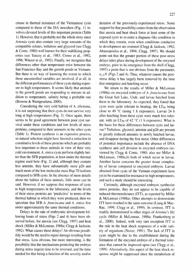
crease in thermal resistance of the Vietnamese cysts compared to those of the ISA inoculum (Fig. I) involves elevated levels of this important protein (Table I). However, that is probably not the whole story since Artemia cysts also contain very large amounts of the compatible solutes, trehalose and glycerol (see Clegg & Conte, 1980) well known for their stabilizing properties (see Yancey et aI., 1983; Crowe et aI., 1992, 1996; Winzor et aI., 1992). Finally, we recognize that differences other than temperature exist between the San Francisco Bay and the growth ponds in Vietnam. But there is no way of knowing the extent to which those uncontrolled variables are involved, if at all, in the different performances of these cysts during exposure to high temperatures. It seems likely that animals in the growth ponds are responding to stresses in addition to temperature, salinity being a probable one (Browne & Wanigesekera, 2000).
Considering the very cold habitat of A. tibetiana, it is not surprising that their cysts do not survive very long at high temperatures (Fig. 3). Once again, there seems to be good agreement between poor cyst survival under these conditions and low levels of stress proteins, compared to their amounts in the other cysts (Table 1). Protein synthesis is an expensive process, so natural selection might have favored a reduction in constitutive levels of these proteins which are probably less important to these animals in view of their very cold environment. A. sinica cysts perform slightly better than the SFB population, at least under the thermal regime used here (Fig. 2) and, although they contain less artemin, they have substantially more p26 and much more of the low molecular mass Hsp-70 isoform compared to SFB cysts. In the absence of more details about the habitat of these animals, little more can be said. However, if we suppose that responses of cysts to high temperatures in the laboratory, and the levels of their stress proteins are 'predictive' in terms of the thermal habitat in which they were produced, then we speculate that SFB A. franciscana and A. sinica live under approximately the same thermal conditions.
Delays in the rate of embryonic development following bouts of stress (Figs 2 and 4) have been observed before, for anoxia (see Clegg, 1997) and heat shock (Miller & McLennan, 1988a; Clegg & Jackson, 1992). What causes these delays? An obvious possibility would be the need to repair damage resulting from that stress. Less obvious, but more interesting, is the possibility that the mechanisms protecting the embryo during stress require time to be reversed, and the time needed for that being a function of the severity and/or
227
duration of the previously-experienced stress. Some support for that possibility comes from the observation that anoxia and heat shock force at least some of the exposed cysts to re-enter a diapause-like condition in which they remain, even when conditions conducive to development are restored (Clegg & Jackson, 1992; Abatzopoulos et aI., 1994; Clegg, 1997). We should point out that the greater portion of these post-stress delays takes place during development of the encysted embryo, prior to its emergence from the shell (Clegg, 1997) a point that is not obvious from the parameter, tl/2N (Figs 2 and 4). Thus, whatever causes the poststress delay it has largely been removed by the time that emergence and hatching occur.
We return to the results of Miller & McLennan (I 988a) on encysted embryos of A. franciscana from the Great Salt Lake, Utah, and larvae hatched from them in the laboratory. As expected, they found that cysts were quite tolerant to heating, the LT50 being close to 49°C (using 1 h exposures). Larvae 24 h after hatching from these cysts were much less tolerant, with an LT50 of 42°C (1 h exposures). What is the basis for these differences between cysts and larvae? Trehalose, glycerol, artemin and p26 are present in greatly reduced amounts in newly hatched larvae, and disappear during the first instar. Other differences of potential importance include the absence of DNA synthesis and cell division in encysted embryos (reviewed by Clegg & Conte, 1980; also see Miller & McLennan, 1988a,b) both of which occur in larvae. Another factor concerns the greater tissue complexity of larvae compared to encysted embryos. Larvae obtained from cysts of the Vietnam experiment have yet to be examined for resistance to high temperatures, and such a study should be interesting.
Curiously, although encysted embryos synthesize stress proteins, they do not appear to be capable of induced thermotolerance (ITT), as reported by Miller & McLennan (1988a). Other attempts to demonstrate ITT have resulted in the same outcome (Liang & MacRae, 1999; Clegg et aI., 1999). In contrast, ITT is readily demonstrated in other stages of Artemia's life cycle (Miller & McLennan, 1988a; Frankenberg et aI., 2000). Indeed, with very rare exception ITT is the rule in the heat shock responses of a wide variety of organisms (Nover, 1991). The lack of ITT in cysts might be due to the establishment during the formation of the encysted embryo of a thermal tolerance that cannot be improved upon (see Clegg et aI., 1999). Alternatively, this aspect of the heat shock response might be suppressed since the metabolism of
228
these embryos is based on endogenous substrates, and strictly limited in terms of amino acid precursors and energy substrates that might be needed for embryonic development (Clegg & Conte, 1980).
Because of the widely different protocols used for heat shock studies (time/temperature) and the often unstated thermal characteristics of the natural setting of the organisms examined, it is difficult to compare our results on Artemia with findings on other invertebrates, at least in the context of adaptation. In this regard, Nover (1991) compiled heat shock response data in 15 pages of tables which illustrate this experimental variation, and emphasize the widely different ecological settings of the organisms under study, both of which make it difficult to extract generalities. Be that as it may, we believe the results described in this paper document further the utility of Artemia as a model for the study of biochemical adaptation.
Acknowledgments
This paper is part LXII of the "International Study on Artemia". Cysts from the PR China were provided by Dr Xin Naihong of the Salt Research Institute at Tanggu-Tianjin, and by Dr Zheng Mianping, Chinese Academy of Geological Sciences, Beijing. Financial support for part of this work was provided through project BILl96/43 of the Bilateral Scientific and Technological Cooperation Flanders-China, and the Science and Technology Commission of China, by project G.0260.97 of the Fund for Scientific Research, Flanders, and by the project "Eigen InitiatievenArtemia, Can Tho University" of the Flemish InterUniversity Council (VLIR). Peter Baert (Can Tho University, Vietnam) and Robert Rofen (Novalek, Inc., Hayward, California) are gratefully acknowledged for providing information on water temperatures and other conditions in Vietnam and the San Francisco Bay, respectively. Herman Slegers (University of Antwerp, Belgium) is thanked for the gift of anti-arternin, and Reinout Amons (Leiden University, The Netherlands) for providing purified artemin. Financial support to JSC from United States NSF grant MCB-98 07762 is gratefully acknowledged, as is the award of a Senior Fulbright Research Fellowship (JanuaryJune 1999) while at Ghent University, Belgium, where some of this work was done. The technical support of Susan Jackson and professional clerical contribution of Diane Cosgrove, both at the Bodega Marine Laboratory, are recognized as important to this study.
References
Abatzopoulos, T., T. Triantaphyllidis, P. Sorgeloos & J. S. Clegg, 1994. Evidence for the induction of cyst diapause by heat shock in Artemia. J. Crust. BioI. 14: 226-230.
Abatzopoulos, T., B. Zheng & P. Sorgeloos, 1998. Artemia tibe· tiana: preliminary characterization of a new Artemia species found in Tibet (People's Republic of China). International Study on Artemia LIX. Int. J. Salt Lake Res. 7: 41-44.
Baert, P., N. T. Anh, V. D. Quynh, N. V. Hoa & P. Sorgeloos, 1997. Increasing cyst yields in Artemia culture ponds in Vietnam: the multi-cycle system. Aquacult. Res. 28: 809-814.
Beissinger, M. & J. Buchner, 1998. How chaperones fold proteins. BioI. Chern. 379: 245-259.
Browne, R. A. & G. Wanigasekera, 2000. Combined effects of salinity and temperature on survival and reproduction of five species of Artemia. J. expo mar. BioI. Ecol. 244: 29-44.
Browne, R. A., P. Sorgeloos & c. N. A. Trotman, 1991. Artemia Biology. CRC Press, Boca Raton, Florida: 374 pp.
Bukau, B. & A. L. Horwich, 1998. The Hsp 70 and Hsp 60 chaperone machines. Cell 92: 351-366.
Clegg, J. S., 1997. Embryos ofArtemia franciscana survive 4 years of continuous anoxia: the case for complete metabolic rate depression. J. Exp. BioI. 200: 467-475.
Clegg, J. S. & F. P. Conte, 1980. A review of the cellular and developmental biology of Artemia. In Persoone, G., P. Sorgeloos, O. Roels & E. Jaspers (eds), The Brine Shrimp Artemia, Vol. 2. Universa Press, Wetteren, Belgium: II-54.
Clegg, J. S. & S. A. Jackson, 1992. Aerobic heat shock activates trehalose synthesis in embryos of Artemia franciscana. FEBS Lett. 303: 45-47.
Clegg, J. S. & S. A. Jackson, 1998. The metabolic status of quiescent and diapause embryos of Artemia franciscana. Arch. Hydrobiol. 52: 425-439.
Clegg, J. S., S. A. Jackson & A. H. Warner, 1994. Extensive intracellular translocations of a major protein accompany anoxia in embryos of Artemiafranciscana. Exp. Cell Res. 212: 77-83.
Clegg, J. S., S. A. Jackson, P. Liang & T. H. MacRae, 1995. Nuclearcytoplasmic translocations of protein p26 during aerobic-anoxic transitions in embryos of Artemia franciscana. Exp. Cell Res. 219: 1-7.
Clegg, J. S., J. K. Willsie & S. A. Jackson, 1999. Adaptive significance of a small heat shOCk/a-crystallin protein in encysted embryos of the brine shrimp, Artemia franciscana. Am. Zool. 39: 836-847.
Coleman, J. S., S. A. Heckathorn & R. L. Hallberg, 1995. Heat shock proteins and thermotolerance: linking molecular and ecological perspectives. Trends Ecol. Evol. \0: 305-306.
Crowe, J. H., F. A. Hoekstra & L. M. Crowe, 1992. Anhydrobiosis. Ann. Rev. Physiol. 54: 579-599.
Crowe, L. M., D. S. Reid & J. H. Crowe, 1996. Is trehalose special for preserving dry biomaterials? Biophys. J. 71: 2087-2093.
Decleir, W., L. Moens, H. Slegers, P. Sorgeloos & E. Jaspers, 1987. Artemia Research and its Applications, Vol. 2. Universa Press, Wetteren, Belgium, 541 pp.
De Graaf, J., R. Amons & w. Moiler, 1990. The primary structure of artemin from Artemia cysts. Eur. J. Biochem. 193: 737-750.
De Herdt, E., H. Slegers & M. Kondo, 1979. Identification and characterization of a 19-5 complex containing a 27 OOO-Mr protein in Artemia salina. Eur. J. Biochem. 96: 423-430.
Ellis, R. J., 1999. Molecular chaperones: pathways and networks. Curro BioI. 9: R137-RI39.
Ellis, R. J. & F. U. Hartl, 1999. Principles of protein folding in the cellular environment. Curro Opin. Struct. BioI. 9: \02-110.
Feder, M. E. & B. A. Block, 1991. On the future of animal physiological ecology. Funct. Ecol. 5: 136-144.
Feder, M. E. & G. E. Hofmann, 1999. Heat-shock proteins, molecular chaperones and the stress response: evolutionary and ecological physiology. Ann. Rev. Physiol. 61: 243-282.
Fiege, U., R. I. Morimoto, I. Yahara & B. S. Polla, 1996. StressInducible Cellular Responses. Birkhliuser-Verlag, Berlin: 492 pp.
Fink, A L., 1999. Chaperone-mediated protein folding. Physiol. Rev. 79: 425-449.
Fink, A L. & Y. Golo, 1998. Molecular Chaperones in the Life Cycle of Proteins. Marcel Dekker, New York: 626 pp.
Frankenberg, M. M., S. A Jackson & J. S. Clegg, 2000. The heat shock response of adult Artemiajranciscana. J. thermal BioI. 25: 481-490.
Hand, S. C. & I. Hardewig, 1996. Downregulation of cellular metabolism during environmental stress: mechanisms and implications. Ann. Rev. Physiol. 58: 539-563.
Hightower, L. E., 1998. The promise of molecular biomarkers for environmental monitoring. BioI. Chern. 379: 1213-1215.
Houry, W. A., D. Frishman, C. Eckerskorn, E Lottspe1ch & E U. Hartl, 1999. Identification of in vivo substrates of the chaperon in GroEL. Nature 402: 147-154.
Jackson, S. A. & J. S. Clegg, 1996. The ontogney of low molecular weight stress protein p26 during early development of the brine shrimp, Anemia jranciscana. Dev. Growth Differen. 38: 153-160.
Karlin, S. & L. Brocchieri, 1998. Heat shock protein 70 family: multiple sequence comparisons, function and evolution. J. Mol. Evol. 47: 565-577.
Kiang, J. G. & G. C. Tsokos, 1998. Heat shock protein 70 kD: molecular biology, biochemistry and physiology. Pharmacol. Therapeut. 80: 183-201.
Krebs, R. A, 1999. A comparison of Hsp 70 expression and thermotolerance in adults and larvae of three Drosophila species. Cell Stress & Chaperones 4: 243-249.
Laemmli, U. K., 1970. Cleavage of structural proteins during the assembly ofthe head of bacteriophage T4. Nature 227: 680-685.
Liang, P. & T. H. MacRae, 1999. The synthesis of a small heat shock/a-crystallin protein in Artemia and its relationship to stress tolerance during development. Dev. BioI. 207: 445-456.
Liang, P., R. Amons, T. H. MacRae & J. S. Clegg, 1997a. Purification, structure and molecular chaperone activity in vitro of Artemia p26, a small heat shock/a-crystallin protein. Eur. J. Biochem. 243: 225-232.
Liang, P., R. Amons, J. S. Clegg & T. H. MacRae, 1997b. Molecular characterization of a small heat-shock/a-crystallin protein from encysted Artemia embryos. J. BioI. Chern. 272: 19051-19058.
Lorimer, G. H. & T. O. Baldwin, 1998. Molecular chaperones. Meth. Enzymol. 290: 1-500.
MacRae, T. H., J. C. Bagshaw & A H. Warner, 1989. Biochemistry and Cell Biology of Artemia. CRC Press, Boca Raton, Florida: 264 pp.
Miller, D. & A G. McLennan, 1988a. The heat shock response of the cryptobiotic brine shrimp, Artemia. I. Thermotolerance. J. thermo BioI. 13: 119-123.
Miller, D. & A. G. Mclennan, 1988b. The heat shock response of the cryptobiotic brine shrimp, Anemia. II. Heat shock proteins. J. thermo BioI. 13: 125-134.
Morimoto, R. I., A. Tissieres & C. Georgopoulos, 1994. The Biology of Heat Shock Proteins and Molecular Chaperones. Cold Spring Harbor Laboratory Press, New York: 610 pp.
229
Nollen, E. A. A., J. E Brunsting, H. Roelofsen, L. A. Weber & H. H. Kampinga, 1999. In vivo chaperone activity of heat shock protein 70 and thermotolerance. Molec. Cell. BioI. 19: 2069-2079.
Norris, C. E., P. J. Dilorio, R. J. Schultz & L. E. Hightower, 1995. Variation in heat shock proteins within tropical and desert species of Poeciliid fishes. Mol. BioI. Evol. 12: 1048-1062.
Nover, L., 1991. Heat Shock Response, CRC Press, Boca Raton, Florida: 509 pp.
Parsell, D. A. & S. Lindquist, 1993. The function of heat-shock proteins in stress tolerance: degradation and reactivation of damaged proteins. Ann. Rev. Genet. 27: 437-496.
Persoone, G., P. Sorgeloos, O. Roels & E. Jaspers, 1980. The Brine Shrimp, Artemia, Vol. 2. Universa Press, Wetteren, Belgium: 636 pp.
Quynh, v. D. & N. N. Lam, 1987. Inoculation of Artemia in experimental ponds in central Vietnam: an ecological approach and a comparison of three geographical strains. In Sorgeloos, P., D. A. Bengston, W. Decleir & E. Jaspers (eds), Anemia Research and its Applications, Vol. 3. Universa Press, Wetteren, Belgium: 253-269.
Richardson, A., S. J. Landry & C. Georgopoulos, 1998. The ins and outs of a molecular chaperone machine. Trends Biochem. Sci. 23: 138-143.
Schiiffl, E, R. Prlindel & A Reindl, 1998. Regulation of the heat shock response. Plant Physiol. 117: 1135-1341.
Somero, G. N., 1995. Proteins and temperature. Ann. Rev. Physiol. 57: 43-68.
Tomanek, L. & G. N. Somero, 1999. Evolutionary and acclimationinduced variation in the heat-shock responses of congeneric marine snails (Genus Tegula) from different thermal habitats: implications for limits of thermotolerance and biogeography. J. expo BioI. 202: 2925-2936.
Towbin, H., T. Staehelin & J. Gordon, 1979. Electrophoretic transfer of proteins from polyacrylamide gels to nitrocellulose sheets: procedure and some applications. Proc. natl. Acad. Sci. U.S.A. 76: 4350-4354.
Triantaphyllidis, G. V., T. J. Abatzopoulos & P. Sorgeloos, 1998. Review of the biogeography of the genus Anemia (Crustacea, Anostraca). J. Biogeogr. 25: 213-226.
Van den IJssel, P., D. G. Norman & R. A Quinlan, 1999. Molecular chaperones: small heat shock proteins in the limelight. Cur. BioI. 9: RI03-RI05.
Warner, A. H., T. H. MacRae & J. C. Bagshaw, 1989. Cell and Molecular Biology of Artemia Development. Plenum Press, New York: 453 pp.
Whitley, D., S. P. Goldberg & W. D. Jordan, 1999. Heat shock proteins: a review of the molecular chaperones. J. Vasco Surg. 29: 748-751.
Winzor, C. L., D. J. Winzor, L. G. Paleg, L. G. Jones & B. P. Naidu, 1992. Rationalization of the effects of compatible solutes on protein stability in terms of thermodynamic nonideality. Arch. Biochem. Biophys. 296: 102-107.
Yancey, P. H., M. E. Clark, S. C. Hand, R. D. Bowlus & G. N. Somero, 1983. Living with water stress: evolution of osmolyte systems. Science 217: 1214-1222.
Zunying, L., Z. Mianping & L. Jian, 1998. A study of Anemia in Lagkor Co, Tibet: Biological features. J. Lake Res. 10: 92-96 (in Chinese).
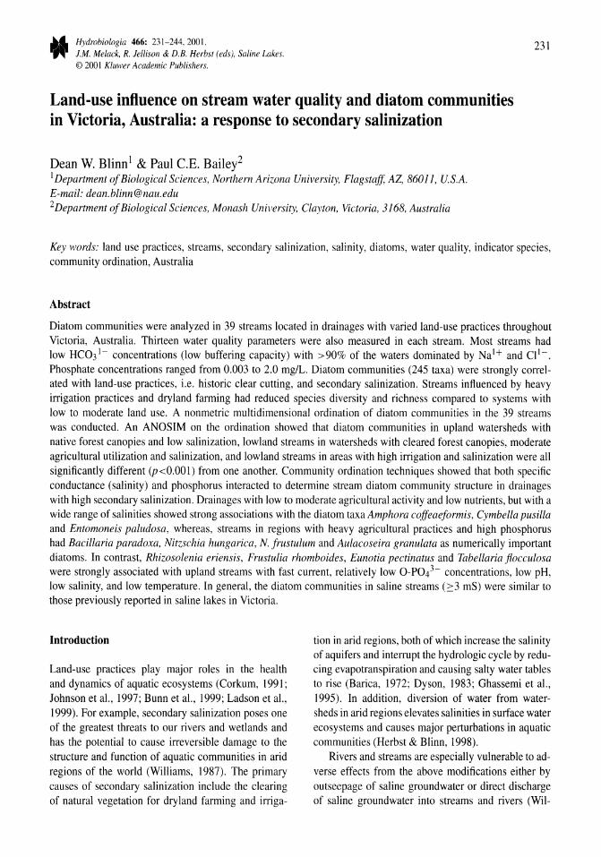
Hydrobiologia 466: 231-244,2001, J,M, Melack, R, Jellison & D,S, Herbst (eds), Saline Lakes, © 2001 Kluwer Academic Publishers.
231
Land-use influence on stream water quality and diatom communities in Victoria, Australia: a response to secondary salinization
Dean W. Blinn 1 & Paul C.E. Bailey2 1 Department of Biological Sciences, Northern Arizona University, Flagstaff, AZ, 86011, U.S,A. E-mail: dean.blinn@nau,edu 2 Department of Biological Sciences, Monash University, Clayton, Victoria, 3168, Australia
Key words: land use practices, streams, secondary salinization, salinity, diatoms, water quality, indicator species, community ordination, Australia
Abstract
Diatom communities were analyzed in 39 streams located in drainages with varied land-use practices throughout Victoria, Australia, Thirteen water quality parameters were also measured in each stream, Most streams had low HC031- concentrations (low buffering capacity) with > 90% of the waters dominated by N a 1 + and C1 1-,
Phosphate concentrations ranged from 0,003 to 2,0 mg/L. Diatom communities (245 taxa) were strongly correlated with land-use practices, i,e. historic clear cutting, and secondary salinization. Streams influenced by heavy irrigation practices and dryland farming had reduced species diversity and richness compared to systems with low to moderate land use, A nonmetric multidimensional ordination of diatom communities in the 39 streams was conducted. An ANOSIM on the ordination showed that diatom communities in upland watersheds with native forest canopies and low salinization, lowland streams in watersheds with cleared forest canopies, moderate agricultural utilization and salinization, and lowland streams in areas with high irrigation and salinization were all significantly different (p<0.001) from one another. Community ordination techniques showed that both specific conductance (salinity) and phosphorus interacted to determine stream diatom community structure in drainages with high secondary salinization. Drainages with low to moderate agricultural activity and low nutrients, but with a wide range of salinities showed strong associations with the diatom taxa Amphora coffeaeformis, Cymbella pusilla and Entomoneis paludosa, whereas, streams in regions with heavy agricultural practices and high phosphorus had Bacillaria paradoxa, Nitzschia hungarica, N. frustulum and Aulacoseira granulata as numerically important diatoms. In contrast, Rhizosolenia eriensis, Frustulia rhomboides, Eunotia pectinatus and Tabellaria flocculosa were strongly associated with upland streams with fast current, relatively low O-P043- concentrations, low pH, low salinity, and low temperature. In general, the diatom communities in saline streams (2:3 mS) were similar to those previously reported in saline lakes in Victoria.
Introduction
Land-use practices play major roles in the health and dynamics of aquatic ecosystems (Corkum, 1991; Johnson et aI., 1997; Bunn et aI., 1999; Ladson et aI., 1999). For example, secondary salinization poses one of the greatest threats to our rivers and wetlands and has the potential to cause irreversible damage to the structure and function of aquatic communities in arid regions of the world (Williams, 1987). The primary causes of secondary salinization include the clearing of natural vegetation for dryland farming and irriga-
tion in arid regions, both of which increase the salinity of aquifers and interrupt the hydrologic cycle by reducing evapotranspiration and causing salty water tables to rise (Barica, 1972; Dyson, 1983; Ghassemi et aI., 1995). In addition, diversion of water from watersheds in arid regions elevates salinities in surface water ecosystems and causes major perturbations in aquatic communities (Herbst & Blinn, 1998).
Rivers and streams are especially vulnerable to adverse effects from the above modifications either by outseepage of saline groundwater or direct discharge of saline groundwater into streams and rivers (Wil-
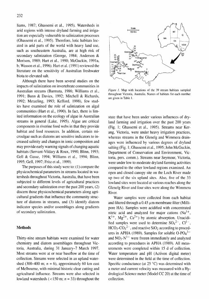
232
Iiams, 1987; Ghassemi et ai., 1995). Watersheds in arid regions with intense dry1and farming and irrigation are especially vulnerable to salinization processes (Ghassemi et ai., 1995). Therefore, 10tic habitats located in arid parts of the world with heavy land use, such as southeastern Australia, are at high risk of secondary salinization (George, 1984; Anderson & Morison, 1989; Hart et aI., 1990; McGuckin, 1991 a, b; Wasson et aI., 1996). Hart et al. (1991) reviewed the literature on the sensitivity of Australian freshwater biota to elevated salt.
Although there have been several studies on the impacts of salinization on invertebrate communities in Australian streams (Barmuta, 1986; Williams et aI., 1991; Bunn & Davies, 1992; Mitchell & Richards, 1992; Metzeling, 1993; Kefford, 1998), few studies have examined the role of salinization on algal communities (Hart et aI., 1990). In fact, there is limited information on the ecology of algae in Australian streams in general (Lake, 1995). Algae are critical components in riverine food webs in that they provide habitat and food resources. In addition, certain microalgae such as diatoms are sensitive indicators to increased salinity and changes in ionic composition and may provide early warning signals of changing aquatic habitats (Servant-Vildary & Roux, 1990; Blinn, 1993; Gell & Gasse, 1994; Williams et al., 1994; Blinn, 1995; Gell, 1997; Fritz et aI., 1999).
The purposes of this study were to: (1) compare the physicochemical parameters in streams located in watersheds throughout Victoria, Australia, that have been subjected to different levels of agricultural practices and secondary salinization over the past 200 years, (2) discern those physicochemical parameters along agricultural gradients that influence the community structure of diatoms in streams, and (3) identify diatom indicator species and/or assemblages along gradients of secondary salinization.
Methods
Thirty-nine stream habitats were examined for water chemistry and diatom assemblages throughout Victoria, Australia, during 31 January-7 March 1997. Most streams were at or near baseflow at the time of collection. Streams were selected in an upland watershed (300-400 m; n = 6), approximately 60 km east of Melbourne, with minimal historic clear cutting and agricultural influence. Streams were also selected in lowland watersheds « 150 m; n = 33) throughout the
Scale f-------<
150Km
Figure 1. Map with locations of the 39 stream habitats sampled throughout Victoria, Australia. Names of habitats for each number are given in Table I.
state that have been under various influences of dryland farming and irrigation over the past 200 years (Fig. 1; Ghassemi et aI., 1995). Streams near Kerang, Victoria, were under heavy irrigation practices, whereas streams in the Glenelg and Wimmera drainages were influenced by various degrees of dryland salting (Fig. 1; Ghassemi et ai., 1995; John McGuckin, Department of Conservation and Environment, Victoria, pers. comm.). Streams near Seymour, Victoria, were under low to moderate dry land farming activities compared to the other lowland regions examined. An open and closed canopy site on the Loch River made up two of the six upland sites. Also, five of the 33 lowland sites were located at various reaches along the Glenelg River and four sites were along the Wimmera River.
Water samples were collected from each habitat and filtered through a 0.45 {tm membrane filter (Millipore HA). Samples were acidified with concentrated nitric acid and analyzed for major cations (Na I +, K1+, Mg2+, Ca2+) by atomic absorption. Unacidified samples were used to determine S04 2-, Cl1-,
HC03 -C03 2-, and reactive Si02 according to procedures in APHA (1989). Samples for soluble 0-P043-
and N03-N1- were frozen immediately and analyzed according to procedures in APHA (1989). All measurements were completed within 15 d of collection. Water temperature and pH (Activon digital meter) were determined in the field at the time of collection. Specific conductance (at 25°C) was determined with a meter and current velocity was measured with a Hydrological Science meter (Model CC 20) at the time of collection.
Diatom samples were collected from natural substrata including epipelon (associated with submerged sediments), epilithon (associated with submerged rocks) and epiphyton (associated with submerged vegetation) at each stream. Samples were digested following the procedures of Van der Werff (1955) and permanent Hyrax® slide mounts were prepared for each sample. A minimum of 500 diatom valves were counted for each slide. Relative abundance values for each site were averaged in the final analyses. A diversity index (H') was calculated for diatom assemblages for each saline stream (Shannon & Weaver, 1949).
The following index for specific conductance (SCI) was used to examine the distribution of diatom taxa along a specific conductance (salinity) gradient from the equation used by Blinn (1993, 1995):
Nx
L [loglO(RAj . 100)] (Specific Conductance), SCIx =_i=_I ______________ _
Nx
Additional indices were developed for O-P043-(PI) from similar equations:
PIx =
Nx L [loglO(RAj . 100)] i=1
(Ortho-Phosphorus Concentration), Nx
where RAj = relative abundance (percent) of species x in the stream habitat, and N = number of stream habitats in which species x occurred. These univariate indices (SCI, PI) provided a relative numeric scale to evaluate various diatom taxa with selected variables and were employed in cluster analyses with numerically important diatom taxa.
We also used global non-metric multi-dimensional scaling ordination (GNMDS) techniques to determine differences in diatom community composition and to relate changes in diatom composition to water quality characteristics in different streams. An ordination of relative frequency of diatom taxa at each site was made using Bray-Curtis distance measures (Minchin, 1999). Thirteen physicochemical variables were fitted into the ordination space as vectors to show relationships between abiotic factors and diatom community composition along agricultural gradients for each stream. Environmental variables tested were: cations (Na1+· K1+, Ca2+, Mg2+), anions (CI1-, S042-, HC031-/C032-), O-P043-, N03-N1-, specific conductance, water temperature, pH and current
233
velocity. Elevation was not examined due to the limited differences in this factor between streams in canopied upland regions and those in lowland regions that had been clear-cutted for agricultural purposes over the past two centuries (Ghassemi et a!., 1995). The fit of abiotic vectors to diatom community composition was tested against 1000 random iterations of fit (Kantvilas & Minchin, 1989). Significance levels for vector correlations were Bonferroni adjusted. Similarity of community composition between streams was tested using the Analysis of Similarity (AN OS 1M) routine (Clark, 1993), which tests a priori grouping designations against 1000 random group designations in ordination space. Analysis was made with the assistance of DECODA software (Minchin, 1999).
Weighted species averages from the multidimensional ordination scored along vectors for specific conductance and O-P043- were compared to values generated for the SCI and PI values with a Spearman rank correlation (rs) to evaluate the power of the univariate SCI and PI analyses.
We also used principal components analysis (PCA) to determine relationships between dependent (diatom taxa) and independent (physicochemical) variables with SYSTAT software (Version 5.1, Wilkinson, 1989). Correlations between various paired combinations of diatom taxa and physicochemical variables were also calculated using Pearson's product-moment correlation coefficient with SYSTAT software (Version 5.1, Wilkinson, 1989). Significant differences between paired measurements were obtained from Bonferroni values.
Results
Chemical characteristics of streams along salinity and agricultural gradients
The specific conductance of the stream habitats examined throughout Victoria, Australia, ranged from 0.043 to 14.1 mS (Table I). Waters in upland streams ranged from 0.043 to 0.D75 mS compared to 0.24 to 14.1 mS in lowland streams (Table I). Specific conductance for those lowland streams examined in the heavy irrigation district of Kerang averaged 5.1 mS (SE ±0.8), 4.2 mS (±1.2) for streams in regions of high dryland salting, and 2.3 mS (±0.9) for regions with low to moderate dryland salting.
All streams examined had Na1+ as the dominant cation, while Cl1- was typically the dominant anion
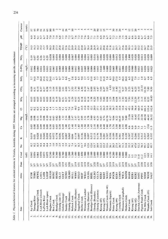
Tab
le 1
. P
hy
sico
chem
ical
fea
ture
s fo
r se
lect
ed s
trea
ms
in V
icto
ria.
Aus
tral
ia d
urin
g 19
97.
Str
eam
s ar
e ar
ran
ged
acc
ordi
ng t
o i
ncre
asin
g sp
ecif
ic c
on
du
ctan
ce
I.
2.
3.
4.
5.
6.
7.
8.
9.
10.
11.
12.
13.
14.
15.
16.
17.
18.
19.
20.
21.
22.
23.
24.
Sit
e
Icy
Cre
ek
To
ron
ga
Riv
er
Pen
ny
wei
gh
t C
reek
L
och
Riv
er (
clos
ed)
LaT
rob
e R
iver
L
och
Riv
er (
open
) H
ug
hes
Cre
ek
Bo
x C
reek
B
end
igo
Cre
ek
Gle
nel
g (
site
13
)
Gol
ton
Dra
inag
e S
un
day
Cre
ek
Gle
nelg
(M
oo
ree)
B
ull
ock
Cre
ek
Wim
mer
a (H
osh
am)
Su
gar
loaf
Cre
ek
Hei
ffer
Cre
ek
Wim
mer
a at
Lo
chie
l G
len
elg
(H
arro
w)
Ben
dig
o C
reek
(E
lmo
re)
Gle
nel
g (
Bo
urk
es)
Gle
nelg
(C
aste
rto
n)
Ker
ang
(#3)
K
eran
g (#
5)
25.
Wan
alta
Cre
ek (
Sit
e #
2)
26.
Wim
mer
a (J
apar
it)
27.
Po
tter
Cre
ek
28.
Ker
ang
(#4
)
29.
Co
mel
la C
reek
30
. W
imm
era
(Cam
pb
ell)
31
. 32
. 33
. 34
. 35
. 36
. 37
. 38
. 39
.
Mat
her
s C
reek
B
arr
Cre
ek
Ker
ang
(#1
) K
eran
g (#
2)
Dat
chak
Cre
ek (
An
twer
p)
Pig
eon
Po
nd
s C
rcek
S
ix M
ile
Cre
ek
Wan
alta
Cre
ek (
#1
) S
alt
Cre
ek
Ahh
r.
Dat
e C
on
d
Na
K
Ca
Mg
C
I S
04
C
03
S
i02
O
-P0
4
N0
3
TE
MP
p
H
Cur
rent
(mS
) -----------meq~-----------
lCO
R
317
0.04
3 0
.2
0.0
18
0.
03
0.08
T
OR
O
317
0.0
54
0
.2
0.05
0.
08
0.08
P
EW
E
317
0.06
1 0.
3 0
.02
8
0.0
4
0.11
L
OC
L
317
0.0
70
0
.4
0.04
1 0
.09
0
.10
L
AT
R
317
0.07
3 0
.4
0.0
49
0.
08
0.08
L
OO
P
317
0.07
5 0
.4
0.0
38
0
.09
0
.10
H
UG
H
1131
0
.24
0
1.4
0.0
74
0
.30
0.
41
BO
XC
21
7 0
.30
0
1.6
0.0
72
0.
03
0.63
B
EN
D
217
0.3
60
1.
8 0
.17
4
0.45
0
.82
G
LI3
21
20
0.6
80
2.
5 0
.03
6
0.28
0
.99
G
OL
T
2/19
0
.76
0
4.4
0.0
79
0.
49
1.32
S
UN
D
1/31
0
.80
0
3.9
0.0
82
1.
00
2.14
G
LM
O
2/2
0
1.20
0 6.
1 0
.04
3
0.75
2.
00
BU
LL
21
7 1.
260
7.4
0
19
4
1.40
2.
47
WIH
O
2/1
9
1.48
0 8.
7 0
.11
8
1.10
2.
47
SU
LO
1/
31
1.60
0 8.
3 0
.09
7
1.85
4
.77
H
EIF
2/
19
1.85
0 11
.7
0.1
36
1.
20
3.95
W
ILO
2/
19
1.90
0 9
.6
0.0
69
1.
50
3.21
G
LH
A
2/2
0
2.10
0 12
.6
0.0
97
1.
50
3.78
B
EE
L
217
2.10
0 12
.6
0.5
12
1.
45
5.6
0
GL
BO
2
/20
2.
600
15.7
0
.11
5
2.1
0
4.93
G
LC
A
2120
3.
400
20.9
0
.17
6
3.0
0
6.25
K
ER
3
217
3.5
00
22
.2
0.2
48
2
.50
6.
83
KE
R5
21
7 4
.00
0
22.2
0.
281
4.4
0
6.7
4
WA
N2
1/
31
4.10
0 2
2.6
0
.30
7
2.8
0
10.7
0 W
IJA
2/
19
4.15
0 26
.1
0.3
58
1.
70
6.17
P
OC
R
2/19
4
.20
0
26.5
0
.18
9
3.7
4
9.04
K
ER
4
217
4.4
00
27
.4
0.3
58
3
.50
8.
22
CO
RN
11
31
5.0
00
28
.7
0.46
1 4
.00
16
.45
WIC
A
2/19
4
.80
0
31.3
0
.16
4
2.55
9.
05
2/2
0
217
217
217
5.0
00
3
1.8
5
.4
35
.2
5.5
39
.2
7.2
47
.8
0.1
20
0
.30
7
0.3
32
0
.24
6
4.9
0
4.6
6
.0
6.0
5.6
0
13.1
6 15
.63
16.4
5
0.2
0.
2 0.
3 0.
3 0
.4
0.3
1.4
1.7
1.7
2.8
5.1
4.5
7.6
7
.9
10.2
9
.9
13.5
13
.8
15.8
12
.1
20.9
27
.1
24.5
24
.3
0.03
0
.03
0
.03
0
.03
0
.03
0
.03
0
.04
0.
25
0.1
9
0.0
7
0.21
0
.27
0.
15
1.29
0
.52
0.
25
0.1
4
0.2
3
0.1
4
1.38
0
.20
1.
04
5.0
0
5.0
0
0.0
9
0.31
0
.19
0
.37
0
.27
0
.38
1.
15
1.04
1.
93
0.6
0
1.01
4
.00
1.
17
3.5
3
2.7
0
7.4
0
4.3
0
0.1
9
2.47
8.
00
2.83
4
.47
5
.00
6.
27
5.7
14
.0
7.4
16
.0
15.0
15
.5
24
.0
2.1
6.7
0.7
1.
2 6.
6 1.
5 5.8
6.0
8.
5 9
.0
2.7
4.5
13.0
6.
6 7
.7
13.0
11
.0
33
.8
0.0
8
2.83
5
.8
28.2
1.
25
4.9
3
8.3
36.7
2
.04
2
.62
19
.0
33.8
6
.04
5
.40
17
.0
33.8
1.
33
23.1
3 5.
5 33
.8
2.3
0
9.2
7
18.0
45
.1
0.25
45
.1
7.5
0
50.8
7
.50
56
.4
12.2
9
5.07
5.
23
6.43
6.
23
18.0
6.
5 M
AT
H
BA
RR
K
ER
I K
ER
2
DA
TC
P
IPO
S
IXM
W
AN
I S
AL
T
2/19
11
.0
52
.2
0.3
32
7.
5 19
.74
64.9
1.
79
4.1
0
19.0
7
.9
7.1
1.9
0.7
4
.4
8.5
2/20
11
.2
78.3
0
.51
2
3.1
22.2
0 87
.4
3.1
3
22.3
3 2/
19
12.5
9
5.7
0
.53
7
1.7
40
.30
10
1.5
2.5
0
32
.20
1/
31
14.0
82
.6
0.5
63
13
.0
44.4
1 13
5.4
0.3
3
7.8
0
2120
14
.1
95.7
0
.33
2
11.5
26
.32
112.
8 10
.83
9.5
0
--mg~-
-e
C)
0.0
12
0
.00
6
0.00
3 0.
011
0.0
19
0.
013
0.01
1 0
.06
7
0.04
1 0
.00
5
0.0
04
0.
005
0.0
04
0.
003
0.0
12
0.
005
0.01
5 0.
005
0.00
5 0
.00
4
0.0
04
0.
015
0.8
40
1.
600
0.0
09
0
.02
0
0.00
5 2.
000
0.0
13
0
.00
6
0.0
26
0
.03
0
0.9
00
0
.88
0
0.01
3 0.
015
0.0
20
0.
035
0.02
5
0.1
9
0.07
0
.54
0
.26
0
.32
0
.29
0
.03
8
0.0
03
0
.03
4
0.0
04
0
.00
4
0.0
09
0
.00
4
0.0
67
0
.00
4
0.0
04
0
.00
4
0.0
04
0
.01
2
0.00
5 0
.01
6
0.0
47
0
.00
4
0.0
20
14.5
16
.3
16.2
15
.2
15.7
14
.9
30
.3
29
.0
27.3
25
.8
29.3
2
2.6
27
.5
29.9
29
.5
23.5
2
3.0
3
0.7
2
6.4
2
6.0
2
6.9
2
6.7
2
9.2
29
.8
0.0
20
2
5.6
0
.00
4
31
.8
0.0
09
33
.1
0.0
12
29
.7
0.0
20
2
4.7
0
.01
0
25
.6
0.0
04
2
.80
0
0.0
20
0
.02
0
0.0
20
0
.01
3
0.0
18
0
.02
0
0.0
09
22
.0
30
.3
31
.5
30
.5
33
.2
23.5
24
.7
27
.0
23.5
(cm
fs)
6.0
5
7
6.4
45
6.
1 7
0
5.7
51
6
.7
54
6
.4
65
7.0
8
0
7.4
10
7
.0
2 6.
8 2
7.7
4
4
7.0
2
6
7.2
3
8.7
10
7.6
2
7.2
3
7.9
5
7.6
5
6.9
5
7.1
5 7.
1 2
0
7.5
50
6
.9
12
7.0
15
6.
7 2
8.3
5 7
.2
30
7.
1 14
7
.6
20
7.
5 5
6.8
8.1
8.6
8.
5 8
.0
6.7
8.
3 6
.6
7.3
5 12
13
20
5 3 2 5 5
N
W ~
except for waters in the Torongo and Loch Rivers in the upland region, and Bendigo Creek in the lowlands, where HC031-/C032- exceeded Cl1- concentrations (Table 1). In general, the relative proportions of HC031-/C032-were low compared to other anions in lowland streams except for Hughes, Sugarloaf, Sunday, Bendigo and Comella Creeks where concentrations made up >40% of the anions (Table 1). All of these streams were located near the community of Seymour (Fig. 1).
Waters in upland streams had average N03-N1- concentrations of 0.28 mg/L (±0.06) and low O-P043- (0.01 mg/L, ±0.0004) concentrations (Table 1). In contrast, the average concentration for N03-N1- in lowland streams, excluding Barr Creek, was 0.015 (±0.003) mg/L, while the average O-P043-concentration was 0.2 mg/L (±0.2). Barr Creek had an average N03-N 1- concentration of 2.8 mg/L. Streams examined in the heavy agricultural region of Kerang had the highest average O-P043- concentration (x=1.24 mg/L ±0.24), while other lowland streams averaged 0.07 mgIL (±0.05).
Concentrations of Si02 in stream waters were relatively high and variable (x = 7.4 mg/L; ± 1.1). The average silica concentration in upland streams was higher (12.2 mg/L; ± 1.5) than that for lowland streams (8.4 mg/L ± 1.1). Average silica concentration along the five sites in the Glenelg River was 4.2 (± 1.2) mg/L compared to 8.8 (±2.6) mg/L at four sites along the Wimmera River. The highest Si02 concentration was found in Hughes Creek (24 mg/L), while lowest concentrations were found in Glenelg River (site 13) and Six Mile Creek (0.7 mg/L).
Hydrogen-ion concentration averaged 6.2 (±0.2) in upland streams compared to 7.4 (±O.l) in the lowland streams examined. The relatively undisturbed closed canopy site (Eucalyptus regans and E. viminarlis) on the Loch River had the lowest pH (5.7), while an open pasture site, a few kilometers downstream, had a pH of 6.4. Bullock Creek near Kerang had the highest pH (8.7) recorded in the study. Streams in the heavy agricultural region of Kerang had the highest average pH (x = 7.7, ±0.3) values. Current velocities at the site of collection were typically higher in upland sites (x = 57 cm s-I, ±3.7) compared to lowland streams (x = 13.6 cm s-I, ±2.9), and average water temperatures were considerably lower in the upland sites (x = 15.5 DC, ±0.3) compared to those measured in lowland sites (x = 27.6 DC, ±0.5).
Based on Pearson product-moment correlation coefficients, all major ions except S042- showed sig-
235
nificant (p<0.0l) positive correlations with specific conductance for stream waters examined in this study (Table 2). There were significant (p<0.0l) positive correlations between Mg2+ and Nal+, K1+, Cl1-and HC031-/ C032-, and for Cl1- and all cations, but no significant correlations with other ions and S04 2-. No ions showed a significant correlation with pH (Table 2).
Diatom distribution and ecology along salinity and agricultural gradients
Two hundred and forty-five diatom taxa were identified from 39 stream habitats in regions subjected to different levels of land use throughout Victoria, Australia. The overall relative frequencies and ecological ranges (conductance, pH and O-P04-3) for the dominant taxa are presented in Table 3. These taxa represented 87% of the mean relative frequencies of diatom taxa collected in the stream habitats. Taxa that were present in 75% of the stream habitats included, Achnanthes delicatula, A. minutissima, Bacillaria paradoxa, Cyclotella meneghiniana, C. stelligera, Fragilaria ulna, Gomphonema parvulum, Navicula cryptocephala, Nitzschia frustulum, N. filiformis, N. palea, Pleurosigma delicatulum and Rhopalodia gibberula (Table 3). Fragilaria ulna and Gomphonema parvulum were collected in all stream habitats investigated.
Upland streams showed a very limited diatom flora with only 20% of the 245 taxa collected in the study represented. Diatom assemblages in upland streams had mean H' diversities of 2.94 compared to 4.69 and 3.67 for low and high nutrient habitats, respectively, in lowland streams. The average number of taxa associated with upland streams was 40 compared to 71 and 53 taxa for lowland streams in regions of low and high agricultural activity, respectively. Although there were reduced numbers of taxa in both high conductance and high nutrient habitats, there were no significant correlations between these chemical parameters and biotic indices when both upland and lowland habitats were combined (Table 2). However, when only the 33 lowland stream habitats were examined there was a highly significant negative correlation (r = -0.738; p<O.OOI) between number of taxa and O-P04 -3 concentration and a pattern showing a negative relationship between number of taxa and specific conductance (r = -0.370). An average of 46 (±4.5) taxa were collected in habitats with high O-P04 -3 concentrations compared to 70 (± 1.6) taxa in habitats with relatively low O-P04-3
236
Table 2. Matrix of Pearson correlation coefficients for physicochemical characteristics and biotic indices [Shannon-Weaver (H') and species richness (No. Taxa)] for 39 saline streams in Victoria. Australia
Specific pH Na K Ca Mg C1 S04 C03 0-P04 N03 Temp
condo
pH 0.302 Na **0.986 0.310
K '*0.781 0.330 **0.776
Ca **0.841 0.236 **0.780 **0.608
Mg **0.944 0.285 **0.943 *'0.810 **0.773
C1 *'0.984 0.256 *'0.980 **0.766 **0.856 "0.961
S04 0.528 0.431 0.556 0.414 0.575 0.418 0.503
C03 '0.610 0.330 "0.665 **0.665 0.254 '*0.665 *0.583 0.222
0-P04 0.100 0.124 0.099 0.228 0.209
N03 -0.012 0.070 -0.004 0.014 0.032
Temp 0.278 **0.698 0.233 0.343 0.329 Current -0.443 -0.447 -0.424 -0.465 -0.363 H' 0.364 0.252 0.334 0.376 0.293
No. taxa -0.003 0.324 -0.019 0.008 -0.074
• P < 0.05, •• P < 0.01.
concentrations. Stream habitats with specific conductance values> 10 mS had 64 (±0.6) species compared to 70.1 (± 1.8) taxa in habitats with conductance values < 10 mS. There were no significant correlations between N03-N1- and either of the two biotic indices.
Members of the Achnanthaceae (39.2% ±2.3), Eunotiaceae (16.3% ±1.4), Naviculaceae (11.3% ±1.7) and Fragilariaceae (10.7% ±1.1) were the dominant diatom groups in upland streams. Numerically dominant taxa in the upland systems included Achnanthes minutissima (31.5% ±5.7), Eunotia pectinatus (16.1 % ±2.9), Fragilaria pinnata (15.9% ±5.4), Navicula radiosa (14.7% ±0.5) and Tabellariaflocculosa (4.9% ±2). Rhizosolenia eriensis was collected only in the upland streams at low densities where pH was <7.0 and current velocity was ~45 cm s-I.
Diatom taxa within the families of Bacillariaceae (32.2% ±2.6), Naviculaceae (25.1% ±3.l), and Achnanthaceae (14.3% 1.7) were the numerically dominant groups in lowland streams. However, the composition of diatoms in lowland streams with high nutrients (O-P043- and N03-N1-) shifted dramatically to Bacillariaceae (54.7% ±6.9) and Centrales (16.8% ±2). Diatom taxa associated with habitats with high O-P043- concentrations included Nitzschia Jrustulum (18.6% ±6.3), Nitzschia palea (13.7% ± 5.8), Aulacoseira granulata (12.1 %± 5.8), Cyclotella meneghiniana (9.5% ±1.7), Thalassiosira weissflogii (6.4 ±2.l) and Bacillaria paradoxa (5.6% ±2.l).
0.059 0.085 0.563 0.005
0.005 0.005 0.236 -0.085 -0.084
0.222 0.239 0.337 0.130 0.300 -0.033
-0.391 -0.413 -0.221 -0.389 -0.096 0.114 -0.505
0.317 0.311 0.162 0.450 0.161 0.022 0.426
0.009 -0.025 -0.264 0.161 -0.411 -0.034 0.481
Aulacoseira granulata, Bacillaria paradoxa, Cyclotella meneghiniana, Fragilaria construens f. venter, Nitzschia Jrustulum and N. reversa made up nearly 70% of the relative diatom abundance in Barr Creek, the single lowland stream habitat with high N03-N 1-concentrations (Table 1). The stream habitats with relatively high nutrients had waters with specific conductance values between 3.5 and 7.2 mS.
In contrast, lowland streams with relatively low nutrient concentrations (:::::0.01 mg/L) and salinities (::::3.5 mS) were dominated by assemblages of Achnanthes minutissima, Cocconeis placentula var. euglypta, C. placentula var. lineata, Fragilaria construens var. venter, Gomphonema parvulum, Hantzschia amphioxys, Navicula cryptocephala, Nitzschia lorenziana, Pleurosigma delicatulum and Rhopalodia gibberula (Table 3). Diatom taxa in lowland streams typically associated with relatively high salinities (~5 mS), but low nutrients, included Achnanthes minutissima, Amphora coffeaeJormis, Cymbella pusilla, Entomoneis paludosa, Fragilaria Jasciculata, F. pulchella, F. tenera, Navicula schroeterii. Diploneis oblongella, Mastogloia pumila and Nitzschia epithemoides were only collected in habitats with ionic strengths ~11.0 mS.
The specific conductance (SCI) and phosphorus (PI) indices numerically ranked various diatom taxa according to their association with each variable. Therefore, the taxa examined with high SCI values
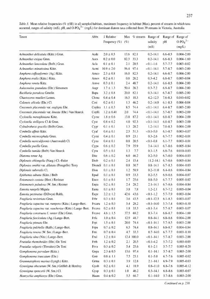
237
Table 3. Mean relative frequencies (% ±SE) in all sampled habitats. maximum frequency in habitat (Max). percent of streams in which taxa occurred, ranges of salinity (mS), pH, and O-P043- (mg/L) for dominant diatom taxa collected from 39 streams in Victoria. Australia
Taxon Abbr. x Relative Max % streams Range of Range of Range of
Frequency (%) (%) salinity pH O-P043-
Achnanthes delicatula (Klitz.) Grun.
Achnanthes exigua Grun.
Achnanthes lanceolata (Breb.) Grun.
Achnanthes minutissima Klitz.
Amphora coffeaeformis (Ag.) Klitz.
Amphora ovalis (Klitz.) Klitz.
Amphora veneta Klitz.
Aulacoseira granulata (Ehr.) Simonsen
Bacil/aria paradoxa Gmelin
Chaetoceros muelleri Lemm.
Caloneis silicula (Ehr.) Cl.
Cocconeis placentula var. eugi)pta Ehr.
Cocconeis placentula var. lineata (Ehr.) Van Heurck
Cyclotella meneghiniana Klitz.
Cyclotella stelligera CI & Grun.
Cylindrotheca gracilis (Breb) Grun.
Cymbella affinis Klitz.
Cymbella microcephala Grun.
Cymbella naviculijormis (Auerswald) Cl.
Cymbeila pusilla Grun.
Cymbeila tumida (Breb) Van Heurck
Diatoma tenue Ag.
Diploneis oblongeila (Naeg.) Cl.-Euler
Diplonies smithii var. dila/ata (Peragello) Terry
Acde 2.0 ± 0.5
Acex 0.2 ± 0.0
Acla 0.1 ± 0.1
Acmi 10.9 ± 2.0
Amco 2.3 ± 0.8
Amov 0.2 ± 0.1
Amve 0.3 ± 0.1
Augr 1.7 ± 1.3
Bapa 3.2 ± 0.8
Chmu 0.4 ± 0.4
Casi 0.2 ± 0.1
Copleu 1.l ± 0.3
Coplli 1.2 ± 0.41
Cyme 1.8 ± 0.6
Cyst 0.8 ± 0.2
Cygr 0.1 ± 0.1
Cyaf
Cymi
Cyna
Cypu
0.4 ± 0.1
0.4 ± 0.1
0.4 ± 0.1
0.6 ± 0.2
Cytu 0.5 ± 0.1
Dite 0.6 ± 0.2
Diob 0.2 ± 0.1
Dismdi 0.1 ± 0.1
Dipioneis subovalis Cl. Disu 0.1 ±O.I
0.1 ±O.I
0.1 ±O.I
0.2 ± 0.1
0.1 ± 0.1
2.2 ± 1.2
0.3 ± 0.1
1.2 ± 0.3
0.2 ± 0.1
4.6 ± 1.5
1.0 ± 0.4
1.5 ± 0.1
0.7 ± 0.2
0.7 ± 0.4
1.2 ± 0.4
1.2 ± 0.2
0.3 ± 0.2
2.3 ± 0.5
0.8 ± l.l 0.3 ± 0.1
0.2±0.1
0.3 ±O.I
0.4 ± 0.2
Epithemia adnata (Klitz.) Breb Epad
Entomoneis costata (Hust.) Rerimer Enco
Entomoneis paludosa (W. Sm.) Reimer Enpa
Eunotia naegelii Migula Euna
Eunotia pectinatus (Dillwyn) Rabh. Eupe
Fragilaria revistriata Grun. Frbr
Fragilaria capucina var. rumpens (Klitz.) Lange-Bert. Frcaru
Fragilaria capucina var. vaucheriae (Kiitz.) Lange-Bert. Frcava
Fragilaria construens f. venter (Ehr.) Grun.
Fragilariafasciculata (Ag.) Lange-Bert.
Fragilaria pinnata Ehr.
Fragilaria pulchella (Ralfs.) Lange-Bert.
Fragilaria tenera (w. Sm.) Lange-Bert.
Fragilaria ulna (Nitz.) Lange-Bert.
Frustulia rhomoboides (Ehr.) De Toni
Frustulia vulgaris (Thwaites) De Toni
Gomphonema parvulum (Klitz.)
Gomphonema truncatum (Ehr.)
Grammatophora marina (Lyngb.) Klitz.
Gyrosigma obscurum (w. Sm.) Griffith & Henfrey
Gyrosigma spencerii (w. Sm.) Cl.
Hantzschia amphioxys (Ehr.) Grun.
Frcave
Frfa
Frpi
Frpu
Frte
Frul
Frrh
Frvu
Gopa
Gotr
Grma
Gyob
Gysp
Haam
13.6 82.1
82.3 33.3
2.1 20.5
56.4 97.4
16.0 82.5
0.8 28.2
2.4 48.7
50.4 28.2
20.0 82.1
16.5 10.3
1.3 46.2
8.5 74.4
2.0 74.4
13.8 87.2
4.0 92.3
1.3 28.2
2.5 51.3
0.9 23.1
0.8 20.5
7.9 35.9
1.3 7.7
6.0 46.2
2.4 15.4
0.8 30.7
1.2 58.9
0.9 33.3
1.7 25.6
2.4 28.2
3.8 7.8
42.6 43.6
3.6 43.5
5.4 28.2
1.8 33.3
37.5 69.2
12.9 48.7
20.0 74.4
6.5 74.4
4.7 33.3
12.4 100.0
2.1 20.5
5.4 25.6
13.6 97.4
7.5 23.1
3.9 12.8
4.1 18.9
1.0 46.2
5.5 66.7
(mS) (mg/L)
0.2-14.1 6.6-8.5
0.2-14.1 6.6-8.3
<0.1-1.6 5.7-7.7
<0.1-14.1 5.7-8.7
0.2-14.1 6.6-8.7
0.3-4.2 6.8-8.7
0.2-14.1 6.6-8.5
0.3-7.2 6.9-8.7
0.3-14.1 6.7-8.7
4.2-12.5 7.6-8.3
0.2-14.0 6.1-8.3
0.004-2.00
0.004-1.60
0.003-0.02
0.003-2.00
0.004-2.00
0.003-0.04
0.004-2.00
0.004-2.00
0.005-2.00
0.010-0.02
0.004-0.04
<0.1-14.1 6.4-8.7 0.003-2.00
<0.1-14.1 5.7-8.7 0.003-2.00
<0.1-14.1 6.0-8.7 0.004-2.00
<0.1-14.1 6.0-8.7 0.003-2.00
1.2-14.1 7.0-8.3 0.004-2.00
<0.1-5.0
0.3-2.6
<0.1-0.8
3.4-14.1
6.1-8.7
6.7-7.7
6.1-7.7
6.7-8.6
0.3-1.5 6.8-7.6
0.2-5.0 6.7-8.0
11.2-14.1 6.7-8.6
0.8-14.1 6.7-8.3
0.2-11.0
0.2-5.5
0.8-5.0
2.1-14.1
1.2-2.1
<0.1-1.2
<0.1-12.5
<0.1-14.0
<0.1-3.4
0.3-7.4
0.8-14.1
<0.1-14.1
0.8-14.1
0.7-14.0
<0.1-14.1
<0.1-4.2
0.1-2.1
0.1-14.1
0.1-5.0
2.1-14.1
0.8-11.0
0.3-14.1
0.1-14.0
6.4-8.6
6.9-8.6
6.7-7.7
6.7-8.6
6.7-7.2
5.7-7.9
6.1-8.3
5.7-7.4
5.7-8.7
6.8-8.7
6.8-8.6
5.7-8.5
6.8-8.7
6.7-7.7
5.7-8.7
5.7-7.2
5.7-7.7
5.7-8.7
6.7-7.6
6.9-7.9
6.8-7.6
6.8-8.6
5.7-8.6
0.003-0.07
0.002-0.01
0.003-0.01
0.005-0.84
0.010-0.03
0.004-0.03
0.005-0.84
0.004-0.03
0.004-0.84
0.004-0.07
0.005-0.02
0.004-0.84
0.005-0.04
0.003-0.04
0.003-0.07
0.003-0.10
0.003-0.07
0.004-1.60
0.004-2.00
0.003-2.00
0.004-0.84
0.003-0.10
0.003-2.00
0.003-0.05
0.003-0.20
0.003-2.00
0.005-0.02
0.005-0.03
0.005-0.12
0.003-0.07
0.003-2.00
Continued on p. 238
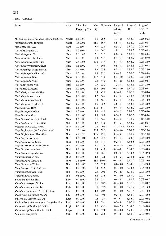
238
Table 3. Continued
Taxon
Mastogloia elliptica var. dansei (Thwaites) Grun.
Mastogloia smithii Thwaites
Melosira varian.l· Ag.
Navicula brasiliana Cl.
Navicula capitata Ehr.
Navicula cincta (Ehr.) Ralfs.
Navicula cryptocephala Klitz.
Navicula duerrenbergiana Hust.
Navicula erifuga Lange-Bertatlot
Navicula halophila (Grun.) Cl.
Navicula mutica Klitz.
Navicula pupula Klitz.
Navicula pygmaea Klitz.
Navicula radiosa Klitz.
Navicula rhyncocephala Klitz.
Navicula salinarum Grun.
Navicula schroeterii Meister
Navicula spicula (Hickie) Cl.
Navicula tenera Hust.
Nitzschia amphibia Grun.
Nitzschia calida Grun.
Nitzschia constricta (Klitz.) Ralfs
Nitzschia dissipata (Klitz) Grun.
Nitzschia epithemoides Grun.
Nitzschiafiliformis (w. Sm.) Van Heurck
Nitzschia Irustulum (Klitz.) Grun.
Nitzschia gracilis Hantz.
Nitzschia hungarica Grun.
Nitzschia levidensis (w. Sm.) Grun.
Nitzschia lorenziana Grun.
Nitzschia microcephala Grun.
Nitzschia obtusa W. Sm.
Nitzschia palea (Klitz.) Sm.
Nitzschia reversa W. Sm.
Nitzschia sigma (Klitz.) w. Sm.
Nitzschia tryblionella Hantz.
Nitzschia tubicola Grun.
Pinnularia borealis Ehr.
Pinnularia divergens W. Sm.
Pinnularia obscura Krasske
Pinnularia subrostrata (A. Cl.) Cl.-Euler
PleurosigllUl delicatulum W. Sm.
Rhizosolenia eriensis H.L. Sm.
Rhoicosphenia abbreviata (Ag.) Lange-Bertalot
Rhopalodia gibba (Ehr.) O. Mliller
Rhopalodia gibberula (Ehr.) O. Mliller
Stauroneis anceps Ehr.
Abbr.
Maelda
Masm
Meva
Nabr
Naca
Naci
Nacr
Nadu
Naer
Naha
Namu
Napu
Napy
Nara
Narh
Nasa
Nasc
Nasp
Nate
Naam
Nica
Nico
Nidi
Niep
Nifi
Nifr
Nigr
Nihu
Nile
Nilo
Nimi
Niob
Nipa
Nire
Nisi
Nitr
Nitu
Pibo
Pidi
Piob
Pisu
Plde
Rher
Rhab
Rhgi
Rhgib
Stan
X Relative
Frequency (%)
0.1 ±O.I
1.6 ± 0.5
1.0 ± 0.7
0.5 ± 0.4
0.6 ± 0.2
0.3 ±O.I
2.8 ± 0.5
0.5 ± OJ
0.4 ± 0.1
0.3 ± 0.1
0.3 ± 0.3
0.2± 0.1
0.1 ± 0.1
0.9 ± 0.5
0.1 ± 0.1
0.5 ± 0.2
0.3 ± 0.2
0.2 ± 0.1
0.6 ± OJ
0.2 ± 0.1
0.8 ± 0.2
0.5 ± 0.1
0.4 ± 0.1
0.1 ±O.I
1.0 ± 0.6
6.2 ± 2.1
0.8 ± 0.8
0.6 ± 0.1
0.2 ± 0.1
0.2±0.1
0.4 ± 0.1
0.1 ±0.1
3.8 ± 0.6
0.6± 0.3
0.4 ± 0.2
OJ ± 0.1
0.8 ± 0.2
0.7 ± OJ
0.2 ± 0.1
0.1 ±O.I
0.1 ±0.1
0.5 ± 0.1
0.1 ± 0.1
0.5 ± 0.2
0.3 ± 0.1
1.1 ± 0.1
0.1 ± 0.1
Max
(%)
2.3
14.8
5.7
1.2
2.1
1.8
10.8
9J
2.3
1.0
10.7
2.4
0.9
11.3
0.9
4.2
5.9
4.5
10.0
1.4
1.5
2.1
1.7
0.6
20.5
46.5
12.2
3.3
2.1
% streams Range of
salinity
(mS)
20.5 1.9-12.5
56.4 0.8-14.1
25.6 0.3-3.5
20.5 1.9-12.5
35.9 0.2-11.0
53.9 0.1-14.1
97.4 0.1-14.1
30.8 0.8-14.1
53.9 0.3-14.1
23.1 0.4-4.2
41.0 0.1-14.0
41.0 0.1-12.5
33.3 1.2-14.1
30.8 <0.1-14.0
43.6 0.1-4.8
56.4 0.2-14.1
56.4 0.2-14.1
38.5 2.6-14.1
64.1 0.4-14.1
41.0 0.1-5.5
18.0 0.2-5.0
56.4 0.4-14.1
41.0 0.1-4.2
10.4 11.2-12.5
79.5 0.1-14.0
87.2 0.1-14.1
35.9 0.3-14.1
74.4 0.2-14.1
53.9 0.2-12.5
2.9 41.0
2.9 48.7
1.8 12.8
<0.1-4.8
0.8-14.1
5.5-7.2
18.0 100.0
6.2 59.0
5.4 53.5
2.3 39.5
3.2 35.9
2.4 23.1
2.6 20.5
3.0 12.5
1.3 20.5
3.0 79.5
0.5 15.4
1.8 23.1
2.0 43.5
13.7 77.0
1.0 25.6
<0.1-14.1
0.8-14.0
0.3-14.0
0.2-12.5
0.1-14.0
0.6-14.1
<0.1-14.0
0.1-14.0
0.1-14.0
0.2-14.1
<0.1-0.1
0.2-5.0
0.4-12.5
0.1-14.0
0.1-14.1
Range of
pH
6.9-8.3
6.8-8.7
6.4-7.6
6.7-8.3
6.8-8.0
6.4-8.7
5.7-8.7
6.9-8.3
6.7-8.5
6.7-8.3
6.0-8.0
6.1-8.6
6.9-8.6
5.7-7.6
6.1-7.7
7.0--8.6
6.8-8.7
6.7-8.6
6.9-8.7
5.7-8.7
6.9-7.6
6.6-8.7
5.7-8.7
6.7-8.3
5.7-8.7
5.7-8.7
6.9-8.3
6.8-8.5
6.8-8.7
6.8-8.7
6.8-8.6
7.0--8.6
5.7-8.7
6.8-8.7
6.7-8.6
6.9-8.7
6.4-8.5
6.1-8.3
6.0-7.7
6.7-7.2
5.7-7.4
6.8-8.7
5.7-6.7
6.8-7.6
6.8-8.7
6.7-8.7
6.4-8.7
Range of
O-P043-
(mg/L)
0.005-0.02
0.004-0.04
0.004-0.08
0.005-0.03
0.004-0.04
0.003-0.90
0.003-2.00
0.004-0.03
0.005-2.00
0.004-0.04
0.003-2.00
0.003-0.84
0.004-2.00
0.003-0.07
0.003-0.84
0.004-2.00
0.004-1.60
0.004-2.00
0.004-2.00
0.005-0.90
0.005-0.84
0.003-2.00
0.003-0.07
0.010-0.02
0.003-2.00
0.003-2.00
0.004-2.00
0.003-2.00
0.003-2.00
0.003-0.04
0.005-0.90
0.020-1.60
0.003-2.00
0.003-2.00
0.004-2.00
0.003-2.00
0.004-1.60
0.003-0.07
0.005-0.07
0.005-1.60
0.020-1.60
0.003-2.00
0.003-0.02
0.004-0.03
0.003-0.04
0.003-2.00
0.003-0.04
Continued on p. 239
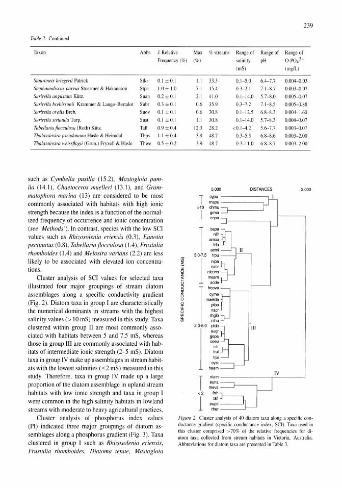
239
Table 3. Continued
Taxon Abbr. x Relative Max % streams Range of Range of Range of
Frequency (%) (%) salinity pH O-P043-
Stauroneis kriegerii Patrick Stkr 0.1 ±O.I Stephanodiscus parvus Stoermer & Hakansson Stpa 1.0 ± 1.0
Surirella angustata Klitz. Suan 0.2 ± 0.1
Surirella brebissonii Krammer & Lange-Bertalot Subr 0.3 ±O.I Surirella ovalis Breb. Suov 0.1 ±O.I Surirella striatula Turp. Sust 0.1 ±O.I Tabellaria flocculosa (Roth) Klitz. Tall 0.9 ± 0.4
Thalassiosira pseudonana Hasle & Heimdal Thps 1.1 ± 0.4
Thalassiosira weissflogii (Grun.) Fryxell & Hasle Thwe 0.5 ± 0.2
such as Cymbella pusilla (15.2), Mastogloia pumita (14.1), Chaetoceros muelleri (13.1), and Grammatophora marina (13) are considered to be most commonly associated with habitats with high ionic strength because the index is a function of the normalized frequency of occurrence and ionic concentration (see 'Methods'). In contrast, species with the low SCI values such as Rhizosolenia eriensis (0.3), Eunotia pectinatus (0.8), Tabellaria jiocculosa (1.4), Frustulia rhomboides (1.4) and Melosira varians (2.2) are less likely to be associated with elevated ion concentrations.
Cluster analysis of SCI values for selected taxa illustrated four major groupings of stream diatom assemblages along a specific conductivity gradient (Fig. 2). Diatom taxa in group I are characteristically the numerical dominants in streams with the highest salinity values (> 10 mS) measured in this study. Taxa clustered within group II are most commonly associated with habitats between 5 and 7.5 mS, whereas those in group III are commonly associated with habitats of intermediate ionic strength (2-5 mS). Diatom taxa in group IV make up assemblages in stream habitats with the lowest salinities (::;2 mS) measured in this study. Therefore, taxa in group IV made up a large proportion of the diatom assemblage in upland stream habitats with low ionic strength and taxa in group I were common in the high salinity habitats in lowland streams with moderate to heavy agricultural practices.
Cluster analysis of phosphorus index values (PI) indicated three major groupings of diatom assemblages along a phosphorus gradient (Fig. 3). Taxa clustered in group I such as Rhizosolenia eriensis, Frustulia rhomboides, Diatoma tenue, Mastogloia
rn e w C.l z ;:!: C.l :::;) CI
8 C.l u:: U W 0.. C/l
(mS)
l.l 33.3 0.1-5.0 6.4-7.7
7.1 15.4 0.3-2.1 7.1-8.7
2.1 41.0 0.1-14.0 5.7-8.0
0.6 35.9 0.3-7.2 7.1-8.5
0.6 30.8 0.1-12.5 6.8-8.3
1.1 30.8 0.1-14.0 5.7-8.3
12.3 28.2 <0.1-4.2 5.6-7.7
3.9 48.7 0.3-5.5 6.8-8.6
3.9 48.7 0.3-11.0 6.8-8.7
0.000 DISTANCES
I T cypu ______ ~ mapu
>10 chmu
1 gnna enpa
I bapa nifr
~ acmi
5.01-7.5 nif~~ masm acde I ;~~~: pibo nacr rhgib nihu
2.0
j_5.0 ~~~~
gopa coeu
nitr frul frpi
cyst haam
niam
I euna meva
<2 frrh
1 tafl eupe rhar
II
III
IV
(mgIL)
0.004--0.03
0.003--0.07
0.005--0.07
0.005--0.88
0.004-1.60
0.004-0.07
0.003--0.07
0.003-2.00
0.003-2.00
2.000
Figure 2. Cluster analysis of 40 diatom taxa along a specific conductance gradient (specific conductance index, SCI). Taxa used in this cluster comprised > 70% of the relative frequencies for diatom taxa collected from stream habitats in Victoria, Australia. Abbreviations for diatom taxa are presented in Table 3.
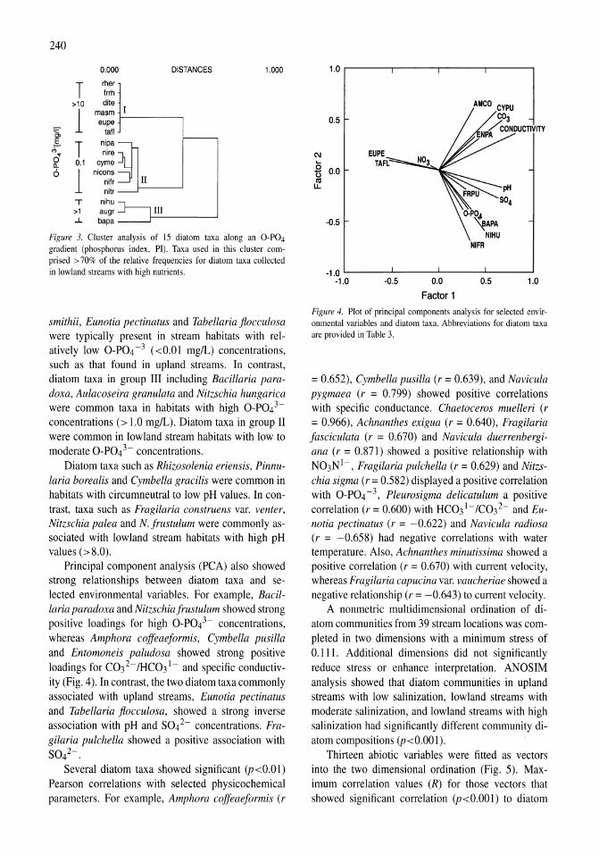
240
0.000 DISTANCES 1.000 1.0 r-------r----,----,--------,
T rher Irrh
>10 dite
1 masm eupe
~ tall
oS T nipa cI, nire " 0 o.t cyme D-
O 1 nicons nifr II nitr
T nihu >1 augr III ..l.. bapa
Figure 3. Cluster analysis of 15 diatom taxa along an O-P04 gradient (phosphorus index, PI). Taxa used in this cluster comprised > 70% of the relative frequencies for diatom taxa collected in lowland streams with high nutrients.
smithii, Eunotia pectinatus and Tabellaria flocculosa were typically present in stream habitats with relatively low O-P04 -3 «0.01 mg/L) concentrations, such as that found in upland streams. In contrast, diatom taxa in group III including Bacillaria paradoxa, Aulacoseira granulata and Nitzschia hungarica were common taxa in habitats with high O-P043-concentrations (>1.0 mg/L). Diatom taxa in group II were common in lowland stream habitats with low to moderate O-P043- concentrations.
Diatom taxa such as Rhizosolenia eriensis, Pinnularia borealis and Cymbella gracilis were common in habitats with circumneutral to low pH values. In contrast, taxa such as Fragilaria construens var. venter, Nitzschia palea and N. frustulum were commonly associated with lowland stream habitats with high pH values (>8.0).
Principal component analysis (PCA) also showed strong relationships between diatom taxa and selected environmental variables. For example, Bacillaria paradoxa and Nitzschia frustulum showed strong positive loadings for high O-P043- concentrations, whereas Amphora coffeaeformis, Cymbella pusilla and Entomoneis paludosa showed strong positive loadings for C032-/HC031- and specific conductiv
ity (Fig. 4). In contrast, the two diatom taxa commonly associated with upland streams, Eunotia pectinatus and Tabellaria flocculosa, showed a strong inverse association with pH and S042- concentrations. Fragilaria pulchella showed a positive association with S042-.
Several diatom taxa showed significant (p<0.01) Pearson correlations with selected physicochemical parameters. For example, Amphora coffeaeformis (r
(\J
a u co u.
0.5
0.0
-0.5
-1.0 L-__ --'-___ -'-___ -'-__ ---'
-1.0 -0.5 0.0
Factor 1
0.5 1.0
Figure 4. Plot of principal components analysis for selected envir-0nmental variables and diatom taxa. Abbreviations for diatom taxa are provided in Table 3.
= 0.652), Cymbella pusilla (r = 0.639), and Navicula pygmaea (r = 0.799) showed positive correlations with specific conductance. Chaetoceros muelleri (r = 0.966), Achnanthes exigua (r = 0.640), Fragilaria fasciculata (r = 0.670) and Navicula duerrenbergiana (r = 0.871) showed a positive relationship with N03N 1-, Fragilaria pulchella (r = 0.629) and Nitzschia sigma (r = 0.582) displayed a positive correlation with O-P04 -3, Pleurosigma delicatulum a positive correlation (r = 0.600) with HC031- IC03 2- and Eunotia pectinatus (r = -0.622) and Navicula radiosa (r = -0.658) had negative correlations with water temperature. Also, Achnanthes minutissima showed a positive correlation (r = 0.670) with current velocity, whereas Fragilaria capucina var. vaucheriae showed a negative relationship (r = -0.643) to current velocity.
A nonmetric multidimensional ordination of diatom communities from 39 stream locations was completed in two dimensions with a minimum stress of 0.111. Additional dimensions did not significantly reduce stress or enhance interpretation. ANOSIM analysis showed that diatom communities in upland streams with low salinization, lowland streams with moderate salinization, and lowland streams with high salinization had significantly different community diatom compositions (p<0.001).
Thirteen abiotic variables were fitted as vectors into the two dimensional ordination (Fig. 5). Maximum correlation values (R) for those vectors that showed significant correlation (p<0.001) to diatom
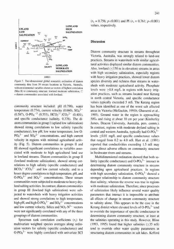
UPLAND LOW SALINZATION
MATH o
GOLT o
CURRENT SULOCO GLHA W1bo '!rxc KERI A
LOWLAND HIGH SALINIZATION
()-P04
BARR pH N PEeR LOOP SUND WIH0.6,
III cD [J G1130 B GLMO WlJA KER4
~ ICOR LOCl J'TR HU:~ PI~ 0 well. b. Il ~R~ :::A5 504
C TORO
~T 0 BEND BULL TEMP GLCAO 0 HEIF
o SIX"C) CORN
POeR 0 WAN2 BEEL
DAlC
o WAN1
C03
SALINITY
AXISl
LOWLAND MODERATE SALINIZATION
Figure 5. Two-dimensional global nonmetric ordination of diatom community data from 39 stream locations in Victoria, Australia, with environmental variables shown as vectors of highest correlation (Max R) to community structure. lowland moderate salinization, D = diatom communities associated with lowland.
community structure included: pH (0.798), water temperature (0.774), current velocity (0.660), S042-(0.587), 0-P04-3 (0.553), HC031-IC032- (00401), and specific conductance (salinity, 0.376). The diatom communities in group I (upland low salinization) showed strong correlations to low salinity (specific conductance), low pH, low water temperature, low 0-P043- and S042- concentrations, and high current velocity in regions with minimal agricultural activity (Fig. 5). Diatom communities in groups II and III showed significant correlations to variables associated with moderate to high agricultural land use in lowland streams. Diatom communities in group II (lowland moderate salinization), showed strong correlations to high salinity (specific conductance) and HC03'- IC03 2- and low current velocity, and to a lesser degree correlations to high temperature, pH, and 0-P043- and S042- concentrations. These stream communities were subjected to moderate to heavy dryland salting activities. In contrast, diatom communities in group III (lowland high salinization) were subjected to watersheds with heavy irrigation activities and showed strong correlations to high temperature, high pH, and high 0-P043- and S042- concentrations and low current velocity. Silica and N03-N1- vectors were not significantly correlated with any of the three groupings of diatom communities.
Spearman rank correlation coefficients (rs) for multivariate weighted species averages along ordination vectors for salinity (specific conductance) and 0-P043- were highly correlated with univariate SCI
241
(rs = 0.756; p<O.OOl) and PI (rs = 0.761; p<O.OOl) values, respectively.
Discussion
Diatom community structure in streams throughout Victoria, Australia, was strongly related to land-use practices. Streams in watersheds with similar agricultural activities displayed similar diatom communities. Also, lowland (:'S150 m in elevation) streams in areas with high secondary salinization, especially regions with heavy irrigation practices, showed lower diatom species diversity and richness than streams in watersheds with moderate agricultural activity. Phosphate levels were :::0.8 mg/L in regions with heavy irrigation practices, such as streams located near Kerang in north central Victoria, and specific conductance values typically exceeded 5 mS. The Kerang region has been identified as one of the worst salt affected areas in Victoria (McGuckin, 1991b; Ghassemi et aI., 1995). Ground water in the region is approaching 50%0 and rising at about 10 cm per year (Kimberley James, Deacon University, Australia, pers. comm.). In contrast, regions with moderate dryland salting in central and western Australia, typically had 0-P043-levels :'Som mg/L and specific conductance values that ranged from 0.2 to 4.0 mS. Hart et aI. (1991) reported that conductivities exceeding 1.5 mS may cause direct adverse effects on community structure in freshwater rivers and streams.
Multidimensional ordination showed that both salinity (specific conductance) and 0-P043- interact in determining diatom community structure in streams depending upon agricultural practices. In regions with high secondary salinization, 0-P043-showed a stronger relationship to diatom community structure than salinity; whereas the reverse was true in regions with moderate salinization. Therefore, since processes of salinization likely influence several water quality parameters that interact it is impossible to attribute all effects of change in stream community structure to salinity alone. This appears to be the case in the Kerang district where elevated levels of 0-P043-tend to override the importance of specific conductance in determining diatom community structure, at least at the salinities operating in this study. However, Blinn (1993, 1995) found that higher salinities (:::35 mS) tend to override other water quality parameters in structuring diatom communities in salt lakes. Kefford
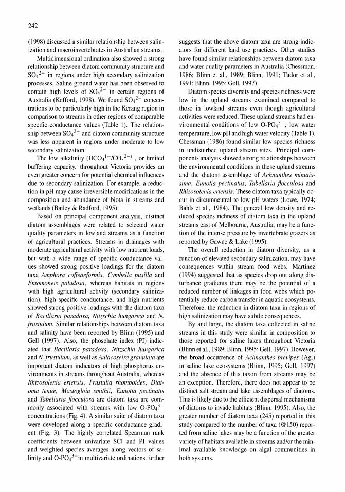
242
(1998) discussed a similar relationship between salinization and macroinvertebrates in Australian streams.
Multidimensional ordination also showed a strong relationship between diatom community structure and S042- in regions under high secondary salinization processes. Saline ground water has been observed to contain high levels of S042- in certain regions of Australia (Kefford, 1998). We found S042- concentrations to be particularly high in the Kerang region in comparison to streams in other regions of comparable specific conductance values (Table 1). The relationship between S042- and diatom community structure was less apparent in regions under moderate to low secondary salinization.
The low alkalinity (HC031-/C032-) , or limited buffering capacity, throughout Victoria provides an even greater concern for potential chemical influences due to secondary salinization. For example, a reduction in pH may cause irreversible modifications in the composition and abundance of biota in streams and wetlands (Bailey & Radford, 1995).
Based on principal component analysis, distinct diatom assemblages were related to selected water quality parameters in lowland streams as a function of agricultural practices. Streams in drainages with moderate agricultural activity with low nutrient loads, but with a wide range of specific conductance values showed strong positive loadings for the diatom taxa Amphora coffeaeformis, Cymbella pusilla and Entomoneis paludosa, whereas habitats in regions with high agricultural activity (secondary salinization), high specific conductance, and high nutrients showed strong positive loadings with the diatom taxa of Bacillaria paradoxa, Nitzschia hungarica and N. frustulum. Similar relationships between diatom taxa and salinity have been reported by Blinn (1995) and Gell (1997). Also, the phosphate index (PI) indicated that Bacillaria paradoxa, Nitzschia hungarica and N. frustulum, as well as Aulacoseira granulata are important diatom indicators of high phosphorus environments in streams throughout Australia, whereas Rhizosolenia eriensis, Frustulia rhomboides, Diatoma tenue, Mastogloia smithii, Eunotia pectinatis and Tabellaria fiocculosa are diatom taxa are commonly associated with streams with low O-P043-concentrations (Fig. 4). A similar suite of diatom taxa were developed along a specific conductance gradient (Fig. 3). The highly correlated Spearman rank coefficients between univariate SCI and PI values and weighted species averages along vectors of salinity and O-P043-in multivariate ordinations further
suggests that the above diatom taxa are strong indicators for different land use practices. Other studies have found similar relationships between diatom taxa and water quality parameters in Australia (Chessman, 1986; Blinn et a!., 1989; Blinn, 1991; Tudor et a!., 1991; Blinn, 1995; Gell, 1997).
Diatom species diversity and species richness were low in the upland streams examined compared to those in lowland streams even though agricultural activities were reduced. These upland streams had environmental conditions of low O-P043-, low water temperature, low pH and high water velocity (Table I). Chessman (1986) found similar low species richness in undisturbed upland stream sites. Principal components analysis showed strong relationships between the environmental conditions in these upland streams and the diatom assemblage of Achnanthes minutissima, Eunotia pectinatus, Tabellaria fiocculosa and Rhizosolenia eriensis. These diatom taxa typically occur in circumneutral to low pH waters (Lowe, 1974; Bahls et a!., 1984). The general low density and reduced species richness of diatom taxa in the upland streams east of Melbourne, Australia, may be a function of the intense pressure by invertebrate grazers as reported by Gawne & Lake (1995).
The overall reduction in diatom diversity, as a function of elevated secondary salinization, may have consequences within stream food webs. Martinez (1994) suggested that as species drop out along disturbance gradients there may be the potential of a reduced number of linkages in food webs which potentially reduce carbon transfer in aquatic ecosystems. Therefore, the reduction in diatom taxa in regions of high salinization may have subtle consequences.
By and large, the diatom taxa collected in saline streams in this study were similar in composition to those reported for saline lakes throughout Victoria (Blinn et a!., 1989; Blinn, 1995; Gell, 1997). However, the broad occurrence of Achnanthes brevipes (Ag.) in saline lake ecosystems (Blinn, 1995; Gell, 1997) and the absence of this taxon from streams may be an exception. Therefore, there does not appear to be distinct salt stream and lake assemblages of diatoms. This is likely due to the efficient dispersal mechanisms of diatoms to invade habitats (Blinn, 1995). Also, the greater number of diatom taxa (245) reported in this study compared to the number of taxa (@150) reported from saline lakes may be a function of the greater variety of habitats available in streams and/or the minimal available knowledge on algal communities in both systems.
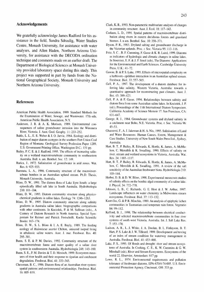
Acknowledgements
We gratefully acknowledge James Radford for his assistance in the field, Sandra Sdraulig, Water Studies Centre, Monash University, for assistance with water analyses, and Allen Haden, Northern Arizona University, for assistance with the DECODA ordination technique and comments made on an earlier draft. The Department of Biological Sciences at Monash University provided laboratory space during this study. This project was supported in part by funds from the National Geographical Society, Monash University and Northern Arizona University.
References
American Public Health Association, 1989. Standard Methods for the Examination of Water, Sewage, and Wastewater. 17th edn. American Public Health Association, N.Y.
Anderson, J. R. & A. K. Morison, 1989. Environmental consequences of saline groundwater intrusion into the Wimmera River, Victoria. 1. Aust. Geol. Geophy. II: 233-252.
Bahls, 1. 1., E. E. Weber & J. O. Jarvie, 1984. Ecology and distribution of major diatom ecotypes in the southern Fort Union Coal Region of Montana. Geological Survey Profession Paper 1289. U.S. Government Printing Office, Washington D.C.: 151 pp.
Bailey, P. C. E. & J. Radford, 1995. The effects of increasing salinity on a wetland macroinvertebrate community in southeastern Australia. Bull. n. am. Benthol. Soc. 12: 149.
Barica, J., 1972. Salinization of groundwater in arid zones. Wat. Res. 6: 925-933.
Barmuta, 1. A., 1986. Community structure of the macroinvertebrate benthos in an Australian upland stream. Ph.D. Thesis, Monash University, Australia.
Blinn, D. W., 1991. The diatom flora of Lake Eyre South: a large episodically filled salt lake in South Australia. Hydrobiologia 210: 101-104.
Blinn, D. W., 1993. Diatom community structure along physicochemical gradients in saline lakes. Ecology 74: 1246--1263.
Blinn, D. w., 1995. Diatom community structure along salinity gradients in Australia saline lakes: biogeographic comparisons with other continents. In Kociolek, P. & M. Sullivan (eds)., A Century of Diatom Research in North America. Special Symposium for Reimer and Patrick Festschrift. Koeltz Scientific Books: 163-174.
Blinn, D. W., S. 1. Blinn & I. A. E. Bayly, 1989. The feeding ecology of Haloniscus searlei Chilton, oniscoid isopod living in athalassic saline waters. Aust. J. mar. Freshwat. Res. 40: 295-301.
Bunn, S. E. & P. M. Davies, 1992. Community structure of the macroinvertebrate fauna and water quality of a saline river system in southwestern Australia. Hydrobiologia 248: 143-160.
Bunn, S. E., P. M. Davies & T. D. Mosisch, 1999. Ecosystem measures of river health and their response to riparian and catchment degradation. Freshwat. BioI. 41: 333-345.
Chessman, B. C., 1986. Diatom flora of an Australian river system: spatial patterns and environmental relationships. Freshwat. BioI. 16: 805-819.
243
Clark, K. R., 1993. Non-parametric multivariate analyses of changes in community structure. Aust. J. Ecol. 18: 117-143.
Corkum, 1. D., 1991. Spatial patterns of macroinvertebrate distribution along rivers in eastern deciduous forests and grassland biomes. 1. n am. Benthol. Soc. 10: 358-371.
Dyson, P. R., 1983. Dryland salting and groundwater discharge in the Victorian uplands. Proc. r. Soc. Victoria 95: 113-116.
Fritz, S. C. , B. E Cumming, E Gasse & K. R. Laird, 1999. Diatoms as indicators of hydrologic and climatic changes in saline lakes. In Stoermer, E. E & 1. P. Smol (eds), The Diatoms: Applications for the Environmental and Earth Sciences. Cambridge University Press, U.K.: 41-72.
Gawne, B. &P. S. Lake, 1995. Effects of micro spatial complexity on a herbivore- epilithon interaction in an Australian upland stream. Freshwat. BioI. 33: 557-565.
Gell, P. A., 1997. The development of a diatom database for inferring lake salinity, Western Victoria, Australia: towards a quantitative approach for reconstructing past climates. Aust. 1. Bot. 45: 389-423.
Gell, P. A. & E Gasse, 1994. Relationships between salinity and diatom flora from some Australian saline lakes. In Kociolek, 1. P. (ed.), Proceedings of the 11th International Diatom Symposium. California Academy of Science Memoir 17. San Francisco, CA: 631-647.
George, R. J., 1984. Groundwater systems and dryland salinity in a catchment near Boho, N.E. Victoria. Proc. r. Soc. Victoria 96: 45-53.
Ghassemi, E, A. 1. Jakeman & H. A. Nix, 1995. Salinisation of Land and Water Resources: Human Causes, Extent, Management & Case Studies. University of New South Wales Press Ltd., Sydney, Australia.
Hart, B. T., P. Bailey, R. Edwards, K. Hortle, K. James, A. McMahon, C. Meredith & K. Swadling, 1990. Effects of salinity on river, stream and wetland ecosystems in Victoria, Australia. Wat. Res. 24: 1103-1117.
Hart, B. T., P. Bailey, R. Edwards, K. Hortle, K. James, A. McMahon, C. Meredith & K. Swadling, 1991. A review of the salt sensitivity of the Australian freshwater biota. Hydrobiologia 210: 105-144.
Herbst, D. B. & D. W. Blinn, 1998. Experimental mesocosm studies of salinity effects on the benthic algal community of a saline lake. 1. Phycol. 34: 772-778.
Johnson, 1. B., C. Richards, G. E. Host & J. W. Arthur, 1997. Landscape influences on water chemistry in Midwestern stream ecosystems. Freshwat. BioI. 37: 113-132.
Kantvilas, G. & P. R. Minchin, 1989. An analysis of epiphytic lichen communities in Tasmanian cool temperate rain forest. Vegetatio 84: 99-112.
Kefford, B. J., 1998. The relationship between electrical conductivity and selected macroinvertebrate communities in four river systems of south-west Victoria, Australia. Int. J. Salt Lake Res. 7: 153-170.
Ladson, A. R., 1. J. White, J. A. Doolan, B. 1. Finlayson, B. T. Hart, P. S. Lake & J. W. Tilleard, 1999. Development and testing of an index of stream condition for waterway management in Australia. Freshwat. BioI. 41: 453-468.
Lake, P. S., 1995. Of floods and drought: river and stream ecosystems of Australia. In Cushing, C. E., K. W. Cummins & G. W. Minshall (eds), River and Stream Ecosystems. Ecosystems of the world 22. Elservier, Amsterdam: 817 pp.
Lowe, R. 1., 1974. Environmental requirements and pollution tolerance of freshwater diatoms. EPA-670/4-74-005. U.S. Environmental Protection Agency, Cincinnati, OH: 333 pp.
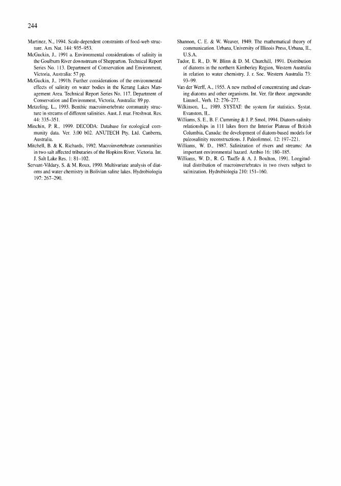
244
Martinez, N., 1994. Scale-dependent constraints of food-web structure. Am. Nat. 144: 935-953.
McGuckin, 1., 1991 a. Environmental considerations of salinity in the Goulburn River downstream of Shepparton. Technical Report Series No. III Department of Conservation and Environment, Victoria, Australia: 57 pp.
McGuckin, 1., 1991 b. Further considerations of the environmental effects of salinity on water bodies in the Kerang Lakes Management Area. Technical Report Series No. 117. Department of Conservation and Environment, Victoria, Australia: 89 pp.
Metzeling, L., 1993. Benthic macroinvertebrate community structure in streams of different salinities. Aust. 1. mar. Freshwat. Res. 44: 335-351.
Minchin, P. R., 1999. DECODA: Database for ecological community data. Ver. 3.00 b02. ANUTECH Pty. Ltd. Canberra, Australia.
Mitchell, B. & K. Richards, 1992. Macroinvertebrate communities in two salt affected tributaries of the Hopkins River, Victoria. Int. 1. Salt Lake Res. I: 81-102.
Servant-Vildary, S. & M. Roux, 1990. Multivariate analysis of diatoms and water chemistry in Bolivian saline lakes. Hydrobiologia 197: 267-290.
Shannon, C. E. & W. Weaver, 1949. The mathematical theory of communication. Urbana, University of Illinois Press, Urbana, IL, U.S.A.
Tudor, E. R., D. W. Blinn & D. M. Churchill, 1991. Distribution of diatoms in the northern Kimberley Region, Western Australia in relation to water chemistry. 1. r. Soc. Western Australia 73: 93-99.
Van der Werff, A., 1955. A new method of concentrating and cleaning diatoms and other organisms. Int. Ver. fUr theor. angewandte Limnol., Verh. 12: 276--277.
Wilkinson, L., 1989. SYSTAT: the system for statistics. Systat. Evanston, IL.
Williams. S. E., B. F. Cumming & 1. P. Smol, 1994. Diatom-salinity relationships in III lakes from the Interior Plateau of British Columbia, Canada: the development of diatom-based models for paleosalinity reconstructions. J. Paleolimnol. 12: 197-221.
Williams, W. D., 1987. Salinization of rivers and streams: An important environmental hazard. Ambio 16: 180--185.
Williams, W. D., R. G. Taaffe & A. 1. Boulton, 1991. Longitudinal distribution of macroinvertebrates in two rivers subject to salinization. Hydrobiologia 210: 151-160.
Hydrobiologia 466: 245-254, 200 I. 1,M, Melack, R, Jellison & D,S, Herbst (eds), Saline Lakes. © 2001 Kluwer Academic Publishers.
245
A study of the Werewilka Inlet of the saline Lake Wyara, Australia -a harbour of biodiversity for a sea of simplicity
Brian V, Timms School of Geosciences, University of Newcastle, Callaghan, NSW, 2308, Australia E-mail: [email protected]
Key words: saline lakes, macroinvertebrates, biodiversity, habitat heterogeneity
Abstract
Lake Wyara receives most of its water from Werewilka Creek, with the area between the two forming Werewilka Inlet which is highly variable in area, and salinity and has high habitat heterogeneity. Over 12 years, 84 species of macroinvertebrate were found in the inlet, but only 34 in the lake. Halobiont and halophilic species were the same in each, but there were many fewer salt-tolerant species in the lake and no freshwater species. The latter were excluded by salinity, but habitat homogeneity due to strong wave action in the lake seems to limit many salt-tolerant species to the inlet. Species richness in large saline lakes in inland Australia is limited by salinity, poor speciation opportunities engendered by their episodic nature, and habitat homogeneity.
Introduction
Large episodically-filled temporary saline lakes support fewer species than equivalent lakes which are filled regularly (Williams, 1984; Timms, 1998a; Williams et aI., 1998). Because of habitat unreliability, they are thought to be poor evolutionary loci, a hypothesis supported by presence of widely dispersed species and few endemics in large lakes in inland South Australia (Williams & Kokkinn, 1988). However, habitat homogeneity is also believed to contribute to their relatively depauperate fauna, as shown for Lake Wyara in southwest Queensland (Timms, 1998a). This lake is less speciose than nearby smaller lakes, which are otherwise reasonably similar in their salinity fluctuations and intensity of study (see Table 5 in Timms, 1998a).
Shallow saline lakes are usually well mixed and generally of the same salinity throughout the lake basin (Hammer, 1986), but it is possible in semiisolated bays and in inlets receiving river inflows, for salinities to be different from those in the main lake. Given the inverse relationship between species richness and salinity (e.g. Timms, 1998b; Williams, 1998), lake inlets receiving fresh waters may support more species than the lake itself. Furthermore in large lakes, shores are generally wave washed and in
those confined to old soft sediments, shorelines are often homogeneous as they are in Lake Wyara (Timms, 1998a). By contrast, in inlets the habitat is likely to be heterogenous due to uneven and unsorted sediments and chance accumulation of organic detritus, large and small. Therefore, if the fauna is restricted by habitat homogeneity, the inlets would be expected to be much more speciose than the main lake. On the other hand, if the depauperate fauna observed in large inland lakes is due solely to their being poor evolutionary loci, then biodiversity in the inlet would be no greater than that associated with its lower salinity.
Wyara and its associated inlets at 144° 14' E, 28° 42' S in south-western Queensland provides a site for exploring these relationships. The lake body is 34 km2
in area and is subject to irregular wind action, particularly from the south-west and north-west, while there are four main inlets receiving freshwater inflows (Timms, 1998a). Werewilka Inlet at the northern end (Fig. 1) provides about 76% of the inflows received by the lake, and is 7.5 km long and 6.4 km2 in area when flooded (Timms, 1997). Although previously referred to as an 'estuary', it has few similarities with marine estuaries (e.g. no tidal flushing, no regular changes in salinity or water-levels) so the use of this term is discouraged and the neutral term 'inlet' is preferred.
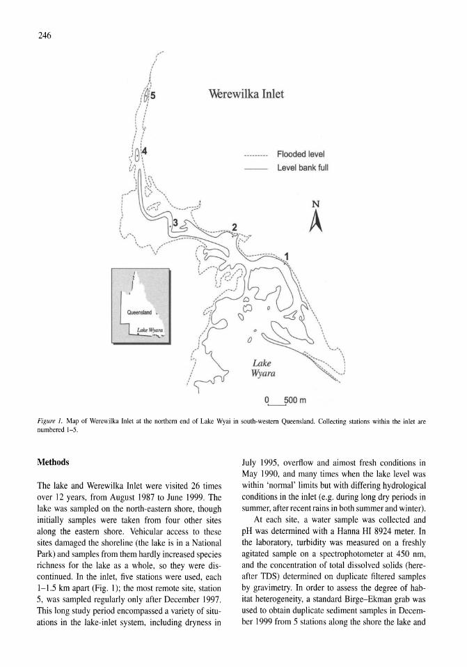
246
\\erewilka Inlet
-- -. (:;:-
Flooded level
level bank full
N
A ',,------------,_ 1
--,
"yara
O-----?OO m
Figure 1. Map of Werewilka Inlet at the northern end of Lake Wyai in south-western Queensland. Collecting stations within the inlet are numbered 1-5.
Methods
The lake and Werewilka Inlet were visited 26 times over 12 years, from August 1987 to June 1999. The lake was sampled on the north-eastern shore, though initially samples were taken from four other sites along the eastern shore. Vehicular access to these sites damaged the shoreline (the lake is in a National Park) and samples from them hardly increased species richness for the lake as a whole, so they were discontinued. In the inlet, five stations were used, each 1-1.5 km apart (Fig. 1); the most remote site, station 5, was sampled regularly only after December 1997. This long study period encompassed a variety of situations in the lake-inlet system, including dryness in
July 1995, overflow and aimost fresh conditions in May 1990, and many times when the lake level was within 'normal' limits but with differing hydrological conditions in the inlet (e.g. during long dry periods in summer, after recent rains in both summer and winter).
At each site, a water sample was collected and pH was determined with a Hanna HI 8924 meter. In the laboratory, turbidity was measured on a freshly agitated sample on a spectrophotometer at 450 nm, and the concentration of total dissolved solids (hereafter TDS) determined on duplicate filtered samples by gravimetry. In order to assess the degree of habitat heterogeneity, a standard Birge-Ekman grab was used to obtain duplicate sediment samples in December 1999 from 5 stations along the shore the lake and
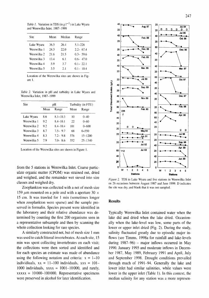
Table 1. Variation in TDS (in g 1-1) in Lake Wyara and Werewilka Inlet, 1987-1999
Site Mean Median Range
Lake Wyara 36.5 2604 5.1-226
Werewilka I 24.3 22.0 2.2- 6704
Werewilka 2 21.6 21.5 0.3- 59.6
Werewilka 3 1304 6.1 0.6- 47.0 Werewilka4 5.9 3.7 0.1- 22.1
Werewilka 5 3.5 2.1 0.1- lOA
Location of the Werewilka sites are shown in Figure 1.
Table 2. Variation in pH and turbidity in Lake Wyara and Werewilka Inlet, 1987-1999
Site pH Turbidity (in FfU)
Mean Range Mean Range
LakeWyara 8.6 8.1-10.3 10 0-40 Werewilka 1 9.2 8.4--10.1 22 0-60 Werewilka2 9.2 804-1004 101 0-600 Werewilka3 8.7 7.5- 9.7 68 0-550
Werewilka4 8.3 7.2- 9.8 376 15-1200
Werewilka5 7.9 7.0- 8.6 352 25-1340
Location of the Werewilka sites are shown in Figure 1.
from the 5 stations in Werewilka Inlet. Coarse particulate organic matter (CPOM) was strained out, dried and weighed, and the remainder wet sieved into size classes and weighed dry.
Zooplankton was collected with a net of mesh size 159 /Lm mounted on a pole and with a aperture 30 x 15 cm. It was trawled for 1 min (sometimes longer when zooplankton were sparse) and the sample preserved in formalin. Species present were identified in the laboratory and their relative abundance was determined by counting the first 200 organisms seen in a representative subsample and then by scanning the whole collection looking for rare species.
A similarly constructed net, but of mesh size 1 mm was used to catch littoral invertebrates. At each site, 15 min was spent collecting invertebrates on each visit; the collections were then sorted and identified and for each species an estimate was made of abundance using the following notation and criteria: x = 1-10 individiuals, xx = 11-100 individuals, xxx = 101-1000 individuals, xxxx = 1001-10000, and rarely, xxxxx = 10000-100000. Representative specimens were preserved in alcohol for later identification.
40
20
40
20
20
40
20
40
20
20
~ 40 .. ~ 20 ., ... 40
~ .. 20 .11 C
~ 80
60
40
20
20
20
20
60
40
au 0
r ----. Al4I. 87
r
~ Feb.88
~C.88
~b.89
.. ~ _ Mar.89
~.89
~P.88
\ Nov. 89
Feb. 90 226
t
0 0 .... May 90
• • • • ~91
....... • • • JIl.92
112 JIl.93
.... W12345
Station.
20
20
40
20
60
40
20
40
20
60
40
20
40
20
20
60
60
40
20
20
20
40
20
40
20
o
247
JIl.94 0 0 0 0 0 0
JIl.95
Od.96
~ ~-.
Mar. 97
~ ........ \:" ~
Dec. 97
"----Feb. 98
/"--. Apr. 98
0 0
~ .. Sap. 98
Apr. 99
• • • • ". JU\99
~ W12345
Stallon.
Figure 2. TDS in Lake Wyara and five stations in Werewilka Inlet on 26 occasions between August 1987 and June 1999. D indicates the site was dry, and blank that it was not sampled.
Results
Typically Werewilka Inlet contained water when the lake did and dried when the lake dried. Occasionally when the lake-level was low, some parts of the lower or upper inlet dried (Fig. 2). During the study, salinity fluctuated greatly due to episodic major inflows (see Timms, 1998a for rainfall and lake-levels during 1987-96) - major inflows occurred in May 1990. January 1995 and moderate inflows in December 1987, May 1989, February 1991 and April, July and September 1998. Drought conditions prevailed through much of 1991-94. Generally the lake and lower inlet had similar salinities, while values were lower in the upper inlet (Table 1). In this context, the median salinity for any station was a more represen-
248
tative of the 'average' condition than the mean salinity. Four major patterns in instantaneous salinity profiles along the inlet were apparent (Fig. 2): (a) a decrease steadily away from the lake - most common in cooler seasons and after recent rain (within the previous two weeks), (b) little change throughout the inlet except perhaps at the most remote station - most common in cooler seasons with little preceding rainfall, (c) sharp declines at any point along the inlet - associated with significant rainfall (>20 mm) within the previous 2 weeks and occurring in any season, and (d) salinity markedly higher in most of the inlet than in the lake - associated with dry conditions in summer when evaporation is highest.
On some occasions a drift of lake water into the inlet was noticed at Stations 1 and 2 when strong south-easterly or south-westerly winds were blowing, and on other occasions there was a drift outwards associated with strong north-westerly winds. No seiches or macrotides were observed nor river currents except at the two upper stations. However, significant river currents occur at times of major inflows as evidenced by points and bars in the sediments of the channel from station 5 down to station 2.
The shoreline of the lake generally consists of a uniform muddy clay (Fig. 3) with little variation horizontally along the shore. At higher water levels, there are beaches of well sorted sand. Unlike the main lake, inlet stations had variable sediments of larger particle size and higher amounts of CPOM (Fig. 3). On a mesoscale, the bottom and shoreline of the inlet are uneven, with deeper pools, shallow bars, minor inlets and braided channels. Deposits of coarse organic detritus (leaves, sticks, small logs) and beds of pebbles are increasingly common upstream. Aquatic plants are rare in the inlet, though occasionally some grow at the lower stations. Overall, station I has similar topography and sediments to the shores of the main lake, station 2 is otherwise similar but with sandy deposits, stations 3 and 4 have very uneven topography and mainly sediments of pebble, while station 5 is also uneven topographically but with sediments of various grades of sand.
There were also trends in pH and turbidity along the length of the inlet (Table 2). Mostly at lower stations, pH was similar or higher than the lake, but upstream values were lower, particularly after inflows. Turbidity increased up the inlet, particularly at stations 4 and 5 associated with turbid fresh inflows. Occasionally these inflows were observed further down the inlet and caused mean values there to be much higher and
unrepresentative of normal conditions. Almost certainly during major inflows, this turbid water flowed into the lake, but this was not observed due difficulty of access during major rainfall events.
Eighty-four species of invertebrates were found in the Werewilka Inlet over the 12 years (Table 3). Momentary species richness ranged from 8 to 34 and averaged 18.9; it was not correlated with mean salinity of the estuary (r = 0.328, P = 0.1, n = 25) or with season for the whole estuary (r = 0.102, P>O.I, n = 25). The most common species were Moina baylyi, Apocyclops dengizicus and Mytilocypris splendida in the plankton, and Anisops gratus, Micronecta spp., Paratanytarsus sp. and Antiporus gilberti in the littoral. Forty species occurred three or fewer times and 17 were encountered only once; most of these were freshwater species with low salinity tolerance (e.g. the conchostracan Eulimnadia sp., the crab Hoithuisiana transversa), or freshwater species with limited tolerance to salinity (e.g. cladoceran Dunhevedia crassa, mayfly Tasmanocoenis tillyardi). Also, many of these 40 species are more common in other habitats such as freshwater riverine waterholes (e.g. the shrimp Macrobrachium australiae, copepod Calamoecia lucasi or in claypans (e.g. fairy shrimp Branchinella australiensis, clam shrimp Caenestheria lutraria) (Timms, 1997). The most abundant group in the inlet are salttolerant freshwater species (Table 4), though many of the dominant species are halophilic or halobiont (Tables 3 and 4). Most species occurred within known salinity ranges (see Tables 6, 7 and 8 in Timms, 1993), but for many, particularly beetles, salinity limits were extended upwards (see Table 3).
The number of species in Lake Wyara is less than half that in the inlet (Table 5 and Timms, 1998a) but dominant species are similar. The number of species of plankton for the two is almost identical, though there are some differences in abundance with the cladoceran Daphniopsis queenslandensis and the ostracod Diacypris spp. more important in the lake than the inlet. It is among littoral species that there are large differences between the lake and inlet: all groups, particularly beetles and odonates, are more speciose in the inlet than in the lake, and where species are shared (e.g. Aniosops gratus and Antiporus gilberti) they are typically more common in the inlet.
Notwithstanding the greater number of species in the inlet, the number of species there is less than half that known to be living in wetlands of the area (Timms, 1997; Timms and Bouton, unpublished data). Notably, phyllopods (which live mainly in claypans and
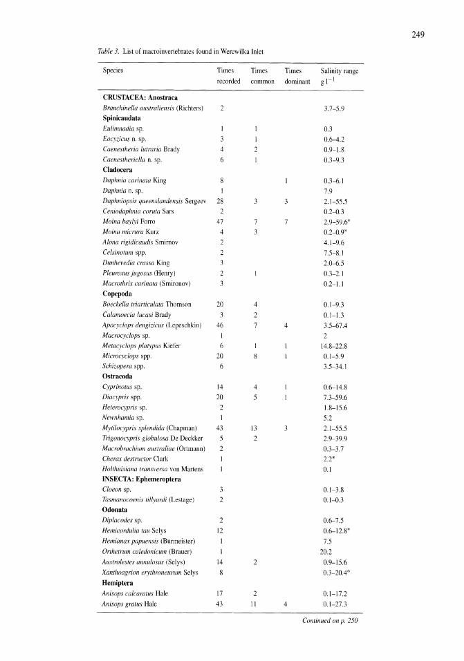
249
Table 3. List of macroinvertebrates found in Werewilka Inlet
Species Times Times Times Salinity range
recorded common dominant gl-l
CRUSTACEA: Anostraca Branchinella australiensis (Richters) 2 3.7-5.9 Spinicaudata Eulimnadia sp. I 0.3 Eocyzicus n. sp. 3 0.6-4.2 Caenestheria lutraria Brady 4 2 0.9-1.8
Caenestheriella n. sp. 6 I 0.3-9.3
Cladocera Daphnia carinata King 8 0.3-6.1
Daphnia n. sp. 7.9 Daphniopsis queenslandensis Sergeev 28 3 3 2.1-55.5 Ceniodaphnia coruta Sars 2 0.2--0.3 Moina baylyi Forro 47 7 7 2.9-59.6* Moina micrura Kurz 4 3 0.2--0.9*
Alona rigidicaudis Smimov 2 4.1-9.6 Celsinotum spp. 2 7.5-8.1
Dunhevedia crassa King 3 2.0-6.5 Pleuroxus jugosus (Henry) 2 0.3-2.1 Macrothrix carinata (Smironov) 3 0.2-1.1
Copepoda Boeekella triarticulata Thomson 20 4 0.1-9.3
Calamoecia lucasi Brady 3 2 0.1-1.3 Apocyclops dengizieus (Lepeschkin) 46 7 4 3.5-67.4 Macroeyclops sp. I 2 Metacyclops platypus Kiefer 6 14.8-22.8 Mieroeyclops spp. 20 8 0.1-5.9
Schizopera spp. 6 3.5-34.1
Ostracoda Cyprinotus sp. 14 4 0.6-14.8
Diacypris spp. 20 5 7.3-59.6 Heterocypris sp. 2 1.8-15.6
Newnhamia sp. 1 5.2 Mytiloeypris splendida (Chapman) 43 13 3 2.1-55.5 Trigonocypris globulosa De Deckker 5 2 2.9-39.9
Macrobrachium australiae (Ortmann) 2 0.3-3.7
Cherax destructor Clark 2.2*
Holthuisiana transversa von Martens 0.1 INSECTA: Ephemeroptera Cloeon sp. 3 0.1-3.8 Tasmanoeoenis tillyardi (Lestage) 2 0.1--0.3
Odonata Diplaeodes sp. 2 0.6-7.5
Hemieordulia tau Selys 12 0.6-12.8'
Hemianax papuensis (Burmeister) I 7.5
Orthetrum ealedonieum (Brauer) I 20.2
Austrolestes annulosus (Selys) 14 2 0.9-15.6
Xanthoagrion erythroneurum Selys 8 0.3-20.4*
Hemiptera Anisops ealcaratus Hale 17 2 0.1-17.2
Anisops gratus Hale 43 II 4 0.1-27.3
Continued on p. 250
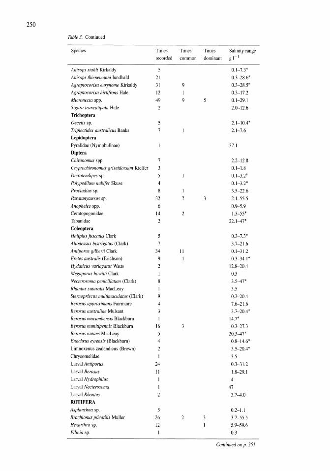
250
Table 3. Continued
Species Times Times Times Salinity range
recorded common dominant gl-l
Anisops stahli Kirkaldy 5 0.1-7.3'
Anisops thienemanni lundbald 21 0.3-28.6'
Agraptocorixa eurynome Kirkaldy 31 9 0.3-28.5'
Agraptocorixa hirtifrons Hale 12 0.3-17.2
Micronecta spp. 49 9 5 0.1-29.1
Sigara truncatipala Hale 2 2.0-12.6
Trlchoptera Oecetis sp. 5 2.1-10.4'
Triplectides australicus Banks 7 2.1-7.6
Lepidoptera Pyralidae (N ymphulinae) 37.1
Diptera Chironomus spp. 7 2.2-12.8
Cryptochironomus griseidorsum Kieffer 3 0.1-1.8
Dicrotendipes sp. 5 0.1-3.2'
Polypedilum nubifer Skuse 4 0.1-3.2'
Procladius sp. 8 3.5-22.6
Paratanytarsus sp. 32 7 3 2.1-55.5
Anopheles spp. 6 0.9-5.9
Ceratopogonidae 14 2 1.3-55'
Tabanidae 2 22.1-47'
Coleoptera Haliplus fuscatus Clark 5 0.3-7.3'
Allodessus bistrigatus (Clark) 7 3.7-21.6
Antiporus gilberti Clark 34 11 0.1-31.2
Eretes australis (Erichson) 9 0.3-34.1"
Hydaticus variagatus Watts 2 12.8-20.4
Megaporus howitti Clark 0.3
Necterosoma penicillatum (Clark) 8 3.5-47"
Rhantus suturalis MacLeay 3.5
Stemopriscus multimaculatus (Clark) 9 0.3-20.4
Berosus approximans Fairmaire 4 7.6-21.6
Berosus australiae Mulsant 3 3.7-20.4"
Berosus macumbensis Blackburn 14.7"
Berosus munitipennis Blackburn 16 3 0.3-27.3
Berosus nutans MacLeay 5 20.3-47"
Enochrus eyrensis (Blackburn) 4 0.8-14.6"
Limnoxenus zealandicus (Brown) 2 3.5-20.4"
Chrysomelidae 3.5
Larval Antiporus 24 0.3-31.2
Larval Berosus 11 1.8-29.1
Larval Hydrophilus 4
Larval Necterosoma I 47
Larval Rhantus 2 3.7-4.0
ROTIFERA Asplanchna sp. 5 0.2-1.1
Brachionus plicatilis Muller 26 2 3 3.7-55.5
Hexarthra sp. 12 5.9-59.6
Filinia sp. 1 0.3
Continued on p. 251
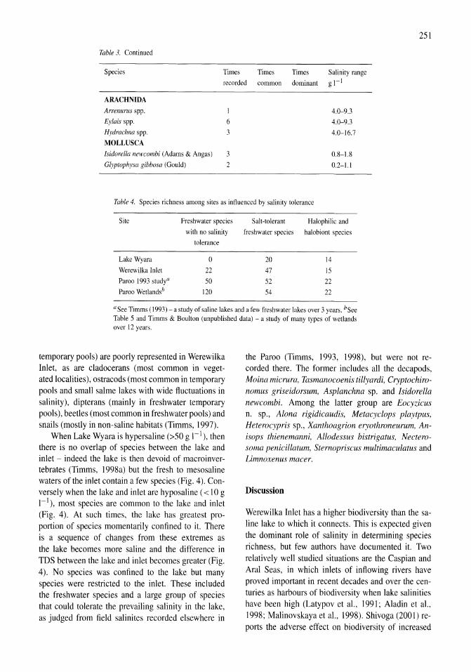
251
Table 3. Continued
Species Times Times Times Salinity range
recorded common dominant g I-I
ARACHNIDA
Arrenurus spp. 4.0-9.3
Eylais spp. 6 4.0-9.3
Hydrachna spp. 3 4.0-16.7
MOLLUSCA
Isidorella newcombi (Adams & Angas) 3 0.8-\.8
Glyptophysa gibbosa (Gould) 2 0.2-1.1
Table 4. Species richness among sites as influenced by salinity tolerance
Site Freshwater species Salt-tolerant Halophilic and
with no salinity freshwater species halobiont species
tolerance
LakeWyara 0 20 14
Werewilka Inlet 22 47 15
Paroo 1993 study" 50 52 22
Paroo Wetlandsb 120 54 22
aSee Timms (1993) - a study of saline lakes and a few freshwater lakes over 3 years. bSee Table 5 and Timms & Boulton (unpublished data) - a study of many types of wetlands over 12 years.
temporary pools) are poorly represented in Werewilka Inlet, as are cladocerans (most common in vegetated localities), ostracods (most common in temporary pools and small salme lakes with wide fluctuations in salinity), dipterans (mainly in freshwater temporary pools), beetles (most common in freshwater pools) and snails (mostly in non-saline habitats (Timms, 1997).
When Lake Wyara is hypersaline (>50 g 1-1), then there is no overlap of species between the lake and inlet - indeed the lake is then devoid of macroinvertebrates (Timms, 1998a) but the fresh to mesosaline waters of the inlet contain a few species (Fig. 4). Conversely when the lake and inlet are hyposaline ( < 10 g I-I), most species are common to the lake and inlet (Fig. 4). At such times, the lake has greatest proportion of species momentarily confined to it. There is a sequence of changes from these extremes as the lake becomes more saline and the difference in IDS between the lake and inlet becomes greater (Fig. 4). No species was confined to the lake but many species were restricted to the inlet. These included the freshwater species and a large group of species that could tolerate the prevailing salinity in the lake, as judged from field salinites recorded elsewhere in
the Paroo (Timms, 1993, 1998), but were not recorded there. The former includes all the decapods, Moina micrura, Tasmanocoenis tillyardi, Cryptochironomus griseidorsum, Asplanchna sp. and Isidorella newcombi. Among the latter group are Eocyzicus n. sp., Alona rigidicaudis, Metacyclops playtpus, Heterocypris sp., Xanthoagrion eryothroneurum, Anisops thienemanni, Allodessus bistrigatus, Necterosoma penicillatum, Stemopriscus multimaculatus and Limnoxenus macer.
Discussion
Werewilka Inlet has a higher biodiversity than the saline lake to which it connects. This is expected given the dominant role of salinity in determining species richness, but few authors have documented it. Two relatively well studied situations are the Caspian and Aral Seas, in which inlets of inflowing rivers have proved important in recent decades and over the centuries as harbours of biodiversity when lake salinities have been high (Latypov et al., 1991; Aladin et al., 1998; Malinovskaya et al., 1998). Shivoga (2001) reports the adverse effect on biodiversity of increased
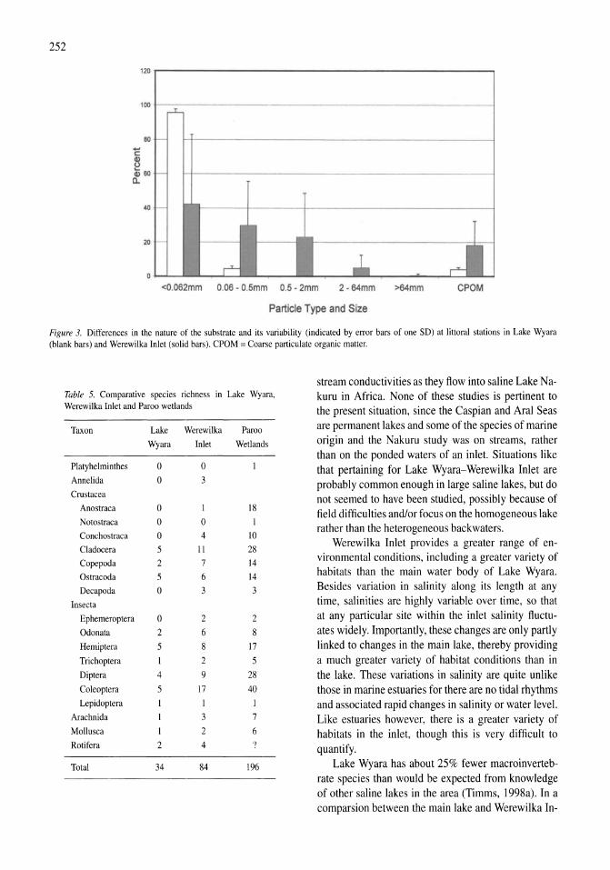
252
1~r-----------------------------------------------------~
l00t-----------------------------------------------------~
40
o <0.062mm 0.06 - 0.5mm 0.5 - 2mm 2-64mm >64mm CPOM
Particle Type and Size
Figure 3. Differences in the nature of the substrate and its variability (indicated by error bars of one SD) at littoral stations in Lake Wyara (blank bars) and Werewilka Inlet (solid bars). CPOM = Coarse particulate organic matter.
stream conductivities as they flow into saline Lake Na-Table 5. Comparative species richness in Lake Wyara, kuru in Africa. None of these studies is pertinent to Werewilka Inlet and Paroo wetlands the present situation, since the Caspian and Aral Seas
Taxon Lake Werewilka Parao are permanent lakes and some of the species of marine
Wyara Inlet Wetlands origin and the Nakuru study was on streams, rather than on the ponded waters of an inlet. Situations like
Platyhelminthes 0 0 that pertaining for Lake Wyara-Werewilka Inlet are Annelida 0 3 probably common enough in large saline lakes, but do Crustacea not seemed to have been studied, possibly because of
Anostraca 0 18 field difficulties and/or focus on the homogeneous lake Notostraca 0 0
Conchostraca 0 4 10 rather than the heterogeneous backwaters.
Cladocera 5 11 28 Werewilka Inlet provides a greater range of en-
Copepoda 2 7 14 vironmental conditions, including a greater variety of
Ostracoda 5 6 14 habitats than the main water body of Lake Wyara.
Decapoda 0 3 3 Besides variation in salinity along its length at any
Insecta time, salinities are highly variable over time, so that
Ephemeroptera 0 2 2 at any particular site within the inlet salinity fluctu-Odonata 2 6 8 ates widely. Importantly, these changes are only partly Hemiptera 5 8 17 linked to changes in the main lake, thereby providing Trichoptera 1 2 5 a much greater variety of habitat conditions than in Diptera 4 9 28 the lake. These variations in salinity are quite unlike Coleoptera 5 17 40 those in marine estuaries for there are no tidal rhythms Lepidoptera 1 1 and associated rapid changes in salinity or water level.
Arachnida 3 7 Like estuaries however, there is a greater variety of Mollusca 1 2 6 habitats in the inlet, though this is very difficult to Rotifera 2 4 quantify.
Total 34 84 196 Lake Wyara has about 25% fewer macroinverteb-rate species than would be expected from knowledge of other saline lakes in the area (Timms, 1998a). In a comparsion between the main lake and Werewilka In-
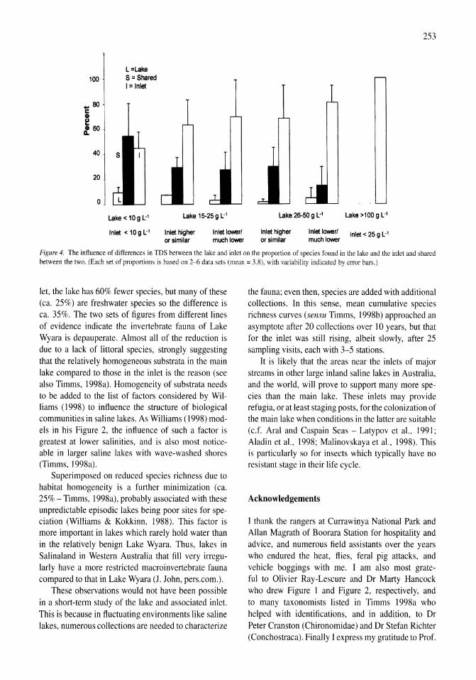
L=Lake 100 S = Shared
I = Inlet
.. 80 c
~ 60
40
20
o
Lake < 10 9 L"
Inlet < 10 9 L"
Lake 15-25 9 L"
Inlet higher or similar
Inlet lowerl much lower
Lake 26-50 9 L"
Inlet higher or similar
Inlet lowerl much lower
253
Lake >100 9 L"
Inlet < 25 9 L"
Figure 4. The influence of differences in TDS between the lake and inlet on the proportion of species found in the lake and the inlet and shared between the two. (Each set of proportions is based on 2-6 data sets (mean = 3.8), with variability indicated by error bars.)
let, the lake has 60% fewer species, but many of these (ca. 25%) are freshwater species so the difference is ca. 35%. The two sets of figures from different lines of evidence indicate the invertebrate fauna of Lake Wyara is depauperate. Almost all of the reduction is due to a lack of littoral species, strongly suggesting that the relatively homogeneous substrata in the main lake compared to those in the inlet is the reason (see also Timms, 1998a). Homogeneity of substrata needs to be added to the list of factors considered by Williams (1998) to influence the structure of biological communities in saline lakes. As Williams (1998) models in his Figure 2, the influence of such a factor is greatest at lower salinities, and is also most noticeable in larger saline lakes with wave-washed shores (Timms, 1998a).
Superimposed on reduced species richness due to habitat homogeneity is a further minimization (ca. 25% - Timms, 1998a), probably associated with these unpredictable episodic lakes being poor sites for speciation (Williams & Kokkinn, 1988). This factor is more important in lakes which rarely hold water than in the relatively benign Lake Wyara. Thus, lakes in Salinaland in Western Australia that fill very irregularly have a more restricted macroinvertebrate fauna compared to that in Lake Wyara (J. John, pers.com.).
These observations would not have been possible in a short-term study of the lake and associated inlet. This is because in fluctuating environments like saline lakes, numerous collections are needed to characterize
the fauna; even then, species are added with additional collections. In this sense, mean cumulative species richness curves (sensu Timms, 1998b) approached an asymptote after 20 collections over 10 years, but that for the inlet was still rising, albeit slowly, after 25 sampling visits, each with 3-5 stations.
It is likely that the areas near the inlets of major streams in other large inland saline lakes in Australia, and the world, will prove to support many more species than the main lake. These inlets may provide refugia, or at least staging posts, for the colonization of the main lake when conditions in the latter are suitable (c.f. Aral and Caspain Seas - Latypov et al., 1991; Aladin et aI., 1998; Malinovskaya et aI., 1998). This is particularly so for insects which typically have no resistant stage in their life cycle.
Acknowledgements
I thank the rangers at Currawinya National Park and Allan Magrath of Boorara Station for hospitality and advice, and numerous field assistants over the years who endured the heat, flies, feral pig attacks, and vehicle boggings with me. I am also most grateful to Olivier Ray-Lescure and Dr Marty Hancock who drew Figure 1 and Figure 2, respectively, and to many taxonomists listed in Timms 1998a who helped with identifications, and in addition, to Dr Peter Cranston (Chironomidae) and Dr Stefan Richter (Conchostraca). Finally I express my gratitude to Prof.
254
W.D. Williams for his constructive criticism of the manuscript.
References
Aladin, N. V., A. A. Filipov, I. S. Plotnikov, M.1. Orlova & W. D. Williams, 1998. Changes in the structure and function of biological communities in the Aral Sea, with particular reference to the northern part (Small Aral Sea), 1985-1994: a review. Int. J. Salt Lake Res. 7: 301-343.
Hammer, U. T., 1986. Saline Lake Ecosystems of the World. Dr W. Junk Publishers, Dordrecht: 616 pp.
Latypov, Yu, Ya., V. V. Gublin & Yu, M. Yakovlev, 1991. The Change of Caspian Sea level and its influence on nearshore ecosystems. Bioljgiya morya 21: 281-285 (in Russian).
Malinovskaja, L. V., A. A. Filipov, V. F. Osadchikh & N. V. Adadin, 1998. Benthic macroinvertebrates of the northern Caspian Sea during recent rises in water-level. Int. J. Salt lake Res. 7: 211-233.
Shivoga, W. A., 2001. Stream fauna distribution along a steep gradient. Verh. int. Ver. Lirnnol. 27: 1285-1289.
Timms, B. V., 1993. Saline lakes of the Paroo, inland New South Wales, Australia, Hydrobiologia 267: 269-289.
Timms, B. V., 1997. A Study of the wetlands of Currawinya National Park. A report to the Queensland Department of Environment, Toowoomba, Qld: 135 pp.
Timms, B. V., 1998a. A study of Lake Wyara, an episodically filled saline lake in southwest Queensland, Australia. Int. 1. Salt Lake Res. 7: 113-132.
Timms, B. V., 1998b. Further studies on the saline lakes of the Paroo, inland New South Wales, Australia. Hydrobiologia 381: 31-42.
Williams, W. D., 1984. Chemical and biological features of salt lakes on Eyre Penisula, South Australia, and an explanation of regional differences in the fauna of Australian salt lakes. Verh. int. Ver. Lirnnol. 22: 1208-1215.
Williams, W. D., 1998. Salinity as a determinant of the structure of biological communities in salt lakes. Hydrobiologia 381: 191-201.
Williams, W. D., & M. J. Kokkinn, 1988. The biological affinities of the fauna in episodically filled salt lakes: a study of Lake Eyre, South Australia. Hydrobiologia 158: 227-236.
Williams, W. D., P. De Deckker & R. J. Shiel, 1998. The limnology of Lake Torrens, an episodic salt lake of central Australia, with particular reference to unique events in 1989. Hydrobiologia 384: 101-110.
Hydrobiologia 466: 255-265,2001. J.M. Melack, R. Jellison & D.B. Herbst (eds), Saline Lakes. © 2001 Kluwer Academic Publishers.
255
Demography and habitat use of the Badwater snail (Assiminea infima), with observations on its conservation status, Death Valley National Park, California, U.S.A.
Donald W. Sada Desert Research Institute and University of Nevada, Reno, Biological Resources and Research Center, U.S.A. Mailing address: 2215 Raggio Parkway, Reno, NV 89512-1095, U.S.A.
Key words: Assiminea ecology, Death Valley National Park, Mollusca, spring ecology, riparian management, playa, habitat use, disturbance
Abstract
Cultural use of spring-fed wetlands in Death Valley National Park, California has reduced populations of endemic macroinvertebrates. Studies were conducted during the spring and late autumn of 1994 to assess demography and habitat use by the Badwater snail (Assiminea infima), which is endemic to low-elevation, spring-fed habitats in Death Valley where its abundance is believed to be adversely affected by municipal diversions and habitat trampling by Park visitors. Effects on demography and habitat were examined at sites highly, lightly, and unaffected by these activities. Field experiments examined the response of its habitat and abundance to trampling.
Snail density ranged from 0 to 19000 m-2 along the banks of seven springs sampled at Badwater and Cotton ball Marsh. Spring brooks with high, steep, and overhanging banks were preferred A. infima habitat. Mean distance of snails from water ranged from 1 mm at Badwater to 39 mm at Cottonball Marsh, and distance from water was greater in autumn than spring. Frequency distributions of shell height showed each population was comprised of several cohorts during spring and autumn, suggesting that reproduction occurs several times a year.
Field experiments demonstrated that trampling reduces bank heights, angles and overhangs, and A. infima population density. Actions are required to manage public use at Badwater to arrest declines in abundance and distribution of A. infima, and to allow for recovery. Historical diversion of springs for irrigation and municipal uses have reduced and dried many aquatic and riparian habitats in the Funeral Mountains, causing current distribution in these springs to be approximately 15% of historical levels.
Introduction
Desert springs in North America support many endemic fishes and macroinvertebrates, with some relictual populations surviving since the Pleistocene (Smith, 1978; Taylor, 1985). Recent taxonomic studies revealed a surprising diversity of endemic aquatic invertebrates, particularly mollusks (e.g. Hershler & Sada, 1987; Hershler, 1989, 1998, 1999), but there is little knowledge of their ecology. Historical and recent extinctions and population extirpations indicate that additional ecological information is needed to protect this unique fauna by facilitating implementation of conservation programs (Williams et aI., 1985; Shepard, 1993; Sada & Vinyard, 2002).
Like many aquatic habitats in the Great Basin, many permanent wetlands in Death Valley National Park are spring-fed and occupied by endemic fishes and macroinvertebrates (Sada et aI., 1995). The Badwater snail (Assiminea infima) is endemic to some of these habitats. The genus Assiminea includes several North American species. With the exception of Fowler's (1980) study of A. californica reproductive biology, there is little known about Assiminea life history and ecology. A. californica inhabits mud substrate in salt marshes along the Pacific coast from Vancouver Island to Baja California (Fowler, 1980). Knowledge of A. infima ecology is limited to qualitative information accumulated during taxonomic studies by Berry (1947) and Hersh1er (1987) who described it as a semi-
256
aquatic species that inhabits emergent vegetation and moist soils lying beneath salt crust that borders valleyfloor springs at Badwater and Cottonball Marsh, and the moist basal stratum of riparian sedges, grasses, and debris along Texas, Travertine and Nevares Springs in the Funeral Mountains (Hershler, 1987). Its habitats ranges in elevation from 100 m above sea level in the Funeral Mountains to 86 m below sea level at Badwater.
Even though Death Valley is a National Park, a variety of cultural activities have modified its springs over the past 100 years. Habitats at Badwater have been affected by visitors who inadvertently trample vegetation and salt crust. Badwater is the lowest point in North America, and it is a popular attraction that is visited by at least 700000 people annually (Death Valley National Park files). Visitation to Death Valley has increased by approximately 15% annually over the past decade, suggesting that increased public use of Badwater will continue. A. infima habitat at Badwater is highly localized along several small springs that cover less than 0.5 hectare, where visitor use is most concentrated. Diversions, which provide the only water to Death Valley visitors and residents, have decreased discharge from many Funeral Mountains springs occupied by A. infima.
In contrast to Badwater, Cotton ball Marsh is a large (approximately 260 hectares), remote wetland that is visited infrequently (probably <5 people/year) and undisturbed. It lies at least 10 km from the nearest road in Death Valley National Park Wilderness where the climate is severe and there is no potable water. Borax mining during the 1920s disturbed dry portions of Cotton ball Marsh but avoided wetlands occupied by A. infima. It is one of the few aquatic habitats in western North America minimally affected by cultural disturbance.
This study assessed A. infima demography by examining spatial and temporal variation in habitat use, distribution, abundance, and age structure at Cotton ball Marsh and Badwater. Preferred habitat was quantified at the two wetlands by assessing relationships between snail abundance and salient features of springbrook bank morphology. Potential impacts of public use were examined during field experiments that tested the response of A. infima abundance and salt crust habitat to minimal trampling. Distribution and relative abundance of A. infima at springs in the Funeral Mountains were also assessed.
Description of sites studies
Habitats occupied by aquatic animals endemic to Death Valley are relictual wetlands that have persisted since the Pleistocene Epoch. Many of these habitats have been isolated since the most recent Holocene lake in Death Valley retreated approximately 2000 years ago (Miller, 1981). Assiminea infima occurs at low elevations where mean annual precipitation is less than 3 cm and temperatures range from a maximum of 55°C during summer to a winter minimum of -5 °C (Hunt, 1975). When field studies were conducted, air temperatures recorded at Furnace Creek (which is on the Death Valley floor and approximately 30 km north of Badwater and 15 km southeast of Cottonball Marsh) ranged from 10 °C to 36°C in March and 8 °C to 24°C, in December 1994.
Cottonball Marsh
A. infima habitat lies along the west side of Cottonball Basin, which is a barren salt flat comprised mostly of sodium-calcium borate (Hunt, 1975). Observations during 12 visits between February 1993 and February 1996 indicated that A. infima occurs under salt crust that borders at least 60 springs where aquatic habitat is persistent. Most of these springs are inhabited by Cottonball Marsh pupfish (Cyprinodon salinus milleri) and Cottonball Marsh springsnails (Tryonia salinus); both are endemic to this wetland (La Bounty & Deacon, 1972; Hershler, 1989). These springs range from 5 cm to I m in depth, have an estimated mean wetted area of 40 m2, and occur only within an area approximately 300 m wide and 1.5 km long. Many springs are connected during winter, but most are isolated during summer when evaporation decreases surface water coverage over the marsh by at least 90% (Hunt et aI., 1966). Salt crust borders all springs, and pickleweed (Allenfolfea occidentalis) is the only vegetation present, which covers less than I % of springbrook banks.
Maximum and minimum temperatures, recorded in snail habitat using a thermal probe (HOBO@ thermograph, measurements every 72 min) placed beneath the salt crust along a south-facing springbrook bank, were 40°C in July and 5 °C in January, respectively. Daily variation in habitat temperatures appeared to closely follow variation in ambient temperatures at Furnace Creek.
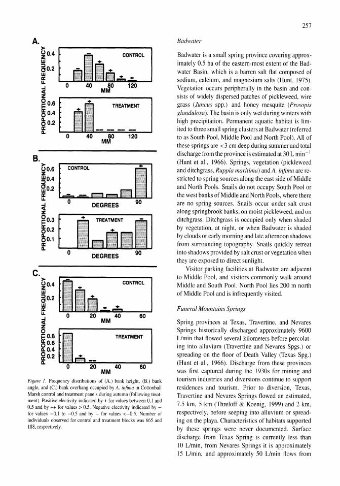
A.
B.
c.
>-~0.4 U.I ::) 0 0.2 U.I
IE ~ o ~0.6 0°·4 a. 00.2 II: a.
>-00.6 z ~0.4
SO.2 II: u.
~ o ~0.3 0°·2 a. 00.1 II: a.
>-~0.4 U.I
8°·2 U.I II: u.
~ o ~0.8 0°·6 a. 0.4 ~0.2 a.
TREATMENT
80 120 MM
° DEGREES
° DEGREES 90
CONTROL.
60
TREATMENT
° 20 40 60 MM
Figure 1. Frequency distributions of (A.) bank height, (B.) bank angle, and (C.) bank overhang occupied by A. infima in Cottonball Marsh control and treatment panels during autumn (following treatment). Positive electivity indicated by + for values between 0.1 and 0.5 and by ++ for values> 0.5. Negative electivity indicated by -for values -0.1 to -0.5 and by - for values <-0.5. Number of individuals observed for control and treatment blocks was 665 and 188, respectively.
257
Badwater
Badwater is a small spring province covering approximately 0.5 ha of the eastern-most extent of the Badwater Basin, which is a barren salt flat composed of sodium, calcium, and magnesium salts (Hunt, 1975). Vegetation occurs peripherally in the basin and consists of widely dispersed patches of pickleweed, wire grass (Juncus spp.) and honey mesquite (Prosopis glandulosa). The basin is only wet during winters with high precipitation. Permanent aquatic habitat is limited to three small spring clusters at Badwater (referred to as South Pool, Middle Pool and North Pool). All of these springs are <3 cm deep during summer and total discharge from the province is estimated at 30 L min- I
(Hunt et aI., 1966). Springs, vegetation (pickleweed and ditchgrass, Ruppia maritima) and A. infima are restricted to spring sources along the east side of Middle and North Pools. Snails do not occupy South Pool or the west banks of Middle and North Pools, where there are no spring sources. Snails occur under salt crust along springbrook banks, on moist pickleweed, and on ditchgrass. Ditchgrass is occupied only when shaded by vegetation, at night, or when Badwater is shaded by clouds or early morning and late afternoon shadows from surrounding topography. Snails quickly retreat into shadows provided by salt crust or vegetation when they are exposed to direct sunlight.
Visitor parking facilities at Badwater are adjacent to Middle Pool, and visitors commonly walk around Middle and South Pool. North Pool lies 200 m north of Middle Pool and is infrequently visited.
Funeral Mountains Springs
Spring provinces at Texas, Travertine, and Nevares Springs historically discharged approximately 9600 Umin that flowed several kilometers before percolating into alluvium (Travertine and Nevares Spgs.) or spreading on the floor of Death Valley (Texas Spg.) (Hunt et aI., 1966). Discharge from these provinces was first captured during the 1930s for mining and tourism industries and diversions continue to support residences and tourism. Prior to diversion, Texas, Travertine and Nevares Springs flowed an estimated, 7.5 km, 5 km (Threloff & Koenig, 1999) and 2 km, respectively, before seeping into alluvium or spreading on the playa. Characteristics of habitats supported by these springs were never documented. Surface discharge from Texas Spring is currently less than 10 Umin, from Nevares Springs it is approximately 15 Umin, and approximately 50 Umin flows from
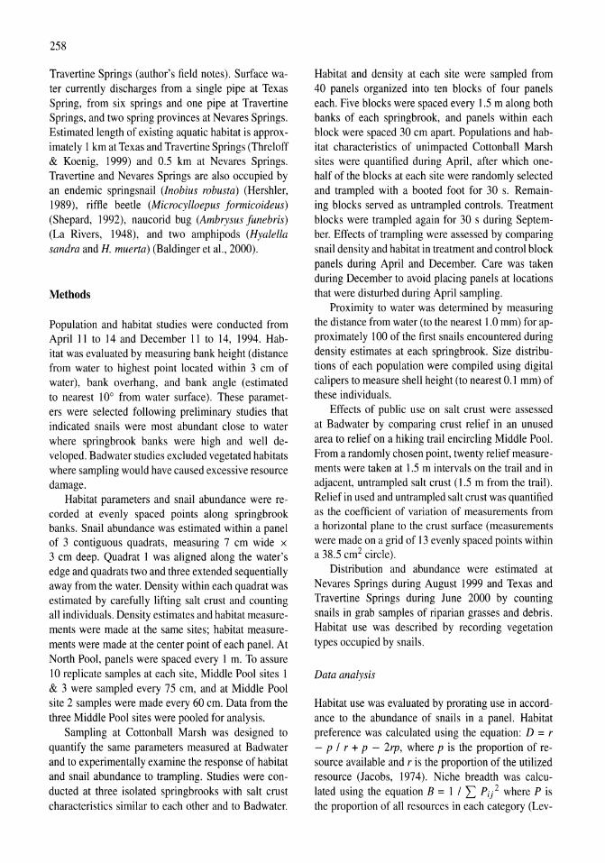
258
Travertine Springs (author's field notes). Surface water currently discharges from a single pipe at Texas Spring, from six springs and one pipe at Travertine Springs, and two spring provinces at Nevares Springs. Estimated length of existing aquatic habitat is approximately I km at Texas and Travertine Springs (Threloff & Koenig, 1999) and 0.5 km at Nevares Springs. Travertine and Nevares Springs are also occupied by an endemic springsnail (Inobius robusta) (Hershler, 1989), riffle beetle (Microcylloepus formicoideus) (Shepard, 1992), naucorid bug (Ambrysus funebris) (La Rivers, 1948), and two amphipods (Hyalella sandra and H. muerta) (Baldinger et aI., 2000).
Methods
Population and habitat studies were conducted from April II to 14 and December II to 14, 1994. Habitat was evaluated by measuring bank height (distance from water to highest point located within 3 cm of water), bank overhang, and bank angle (estimated to nearest 10° from water surface). These parameters were selected following preliminary studies that indicated snails were most abundant close to water where springbrook banks were high and well developed. Badwater studies excluded vegetated habitats where sampling would have caused excessive resource damage.
Habitat parameters and snail abundance were recorded at evenly spaced points along springbrook banks. Snail abundance was estimated within a panel of 3 contiguous quadrats, measuring 7 cm wide x 3 cm deep. Quadrat I was aligned along the water's edge and quadrats two and three extended sequentiany away from the water. Density within each quadrat was estimated by carefully lifting salt crust and counting all individuals. Density estimates and habitat measurements were made at the same sites; habitat measurements were made at the center point of each panel. At North Pool, panels were spaced every I m. To assure 10 replicate samples at each site, Middle Pool sites I & 3 were sampled every 75 cm, and at Middle Pool site 2 samples were made every 60 cm. Data from the three Middle Pool sites were pooled for analysis.
Sampling at Cotton ball Marsh was designed to quantify the same parameters measured at Badwater and to experimentally examine the response of habitat and snail abundance to trampling. Studies were conducted at three isolated springbrooks with salt crust characteristics similar to each other and to Badwater.
Habitat and density at each site were sampled from 40 panels organized into ten blocks of four panels each. Five blocks were spaced every 1.5 m along both banks of each springbrook, and panels within each block were spaced 30 cm apart. Populations and habitat characteristics of unimpacted Cottonball Marsh sites were quantified during April, after which onehalf of the blocks at each site were randomly selected and trampled with a booted foot for 30 s. Remaining blocks served as untrampled controls. Treatment blocks were trampled again for 30 s during September. Effects of trampling were assessed by comparing snail density and habitat in treatment and control block panels during April and December. Care was taken during December to avoid placing panels at locations that were disturbed during April sampling.
Proximity to water was determined by measuring the distance from water (to the nearest 1.0 mm) for approximately 100 of the first snails encountered during density estimates at each springbrook. Size distributions of each population were compiled using digital calipers to measure shell height (to nearest 0.1 mm) of these individuals.
Effects of public use on salt crust were assessed at Badwater by comparing crust relief in an unused area to relief on a hiking trail encircling Middle Pool. From a randomly chosen point, twenty relief measurements were taken at 1.5 m intervals on the trail and in adjacent, untrampled salt crust (1.5 m from the trail). Relief in used and untrampled salt crust was quantified as the coefficient of variation of measurements from a horizontal plane to the crust surface (measurements were made on a grid of 13 evenly spaced points within a 38.5 cm2 circle).
Distribution and abundance were estimated at Nevares Springs during August 1999 and Texas and Travertine Springs during June 2000 by counting snails in grab samples of riparian grasses and debris. Habitat use was described by recording vegetation types occupied by snails.
Data analysis
Habitat use was evaluated by prorating use in accordance to the abundance of snails in a panel. Habitat preference was calculated using the equation: D = r - p / r + p - 2rp, where p is the proportion of resource available and r is the proportion of the utilized resource (Jacobs, 1974). Niche breadth was calculated using the equation B = I / L Pij2 where P is the proportion of all resources in each category (Lev-
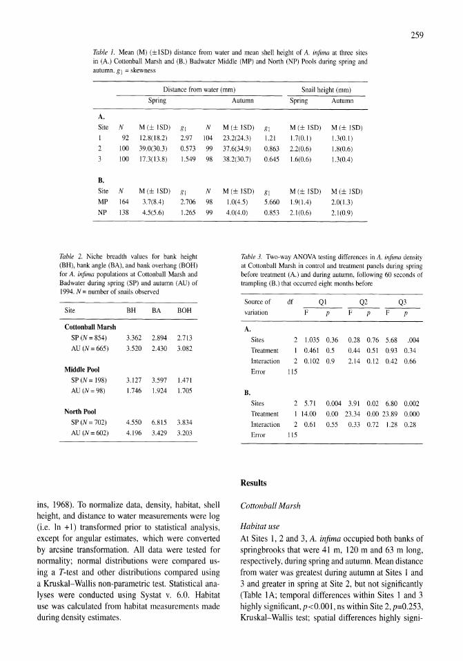
259
Table 1. Mean (M) (±lSD) distance from water and mean shell height of A. infima at three sites in (A.) Cottonball Marsh and (B.) Badwater Middle (MP) and North (NP) Pools during spring and autumn. g1 = skewness
Distance from water (mm) Snail height (mm)
Spring
A. Site N M(±ISD) gl N
I 92 12.8(18.2) 2.97 104
2 100 39.0(30.3) 0.573 99
3 100 17.3(13.8) 1.549 98
B. Site N M (± ISD) gl N
MP 164 3.7(8.4) 2.706 98
NP 138 4.5(5.6) 1.265 99
Table 2. Niche breadth values for bank height (BH), bank angle (BA), and bank overhang (BOH) for A. infima popUlations at Cottonball Marsh and Badwater during spring (SP) and autumn (AU) of 1994. N = number of snails observed
Site BH BA BOH
Cottonball Marsh
SP (N = 854) 3.362 2.894 2.713
AU (N=665) 3.520 2.430 3.082
Middle Pool
SP(N= 198) 3.127 3.597 1.471
AU (N=98) 1.746 1.924 1.705
North Pool
SP(N=702) 4.550 6.815 3.834
AU (N=602) 4.196 3.429 3.203
ins, 1968). To normalize data, density, habitat, shell height, and distance to water measurements were log (i.e. In + 1) transformed prior to statistical analysis, except for angular estimates, which were converted by arcsine transformation. All data were tested for normality; normal distributions were compared using a T-test and other distributions compared using a Kruskal-Wallis non-parametric test. Statistical analyses were conducted using Systat v. 6.0. Habitat use was calculated from habitat measurements made during density estimates.
Autumn Spring Autumn
M(± ISD) gl M(± ISD) M(± ISD) 23.2(24.3) 1.21 1.7(0.1) 1.3(0.1)
37.6(34.9) 0.863 2.2(0.6) 1.8(0.6)
38.2(30.7) 0.645 1.6(0.6) 1.3(0.4)
M(±ISD) gl M(± ISD) M(±ISD)
1.0(4.5) 5.660 1.9(1.4) 2.0(1.3)
4.0(4.0) 0.853 2.1(0.6) 2.1(0.9)
Table 3. Two-way ANOVA testing differences in A. infima density at Cottonball Marsh in control and treatment panels during spring before treatment (A.) and during autumn, following 60 seconds of trampling (B.) that occurred eight months before
Source of df QI Q2 Q3 variation F p F p F P
A.
Sites 2 1.035 0.36 0.28 0.76 5.68 .004
Treatment 1 0.461 0.5 0.44 0.51 0.93 0.34
Interaction 2 0.102 0.9 2.14 0.12 0.42 0.66
Error 115
B.
Sites 2 5.71 0.004 3.91 0.02 6.80 0.002 Treatment I 14.00 0.00 23.34 0.00 23.89 0.000 Interaction 2 0.61 0.55 0.33 0.72 1.28 0.28
Error 115
Results
Cottonball Marsh
Habitat use At Sites 1,2 and 3, A. infima occupied both banks of springbrooks that were 41 m, 120 m and 63 m long, respectively, during spring and autumn. Mean distance from water was greatest during autumn at Sites 1 and 3 and greater in spring at Site 2, but not significantly (Table 1A; temporal differences within Sites 1 and 3 highly significant, p<0.001, ns within Site 2, p=0.253, Kruskal-Wallis test; spatial differences highly signi-
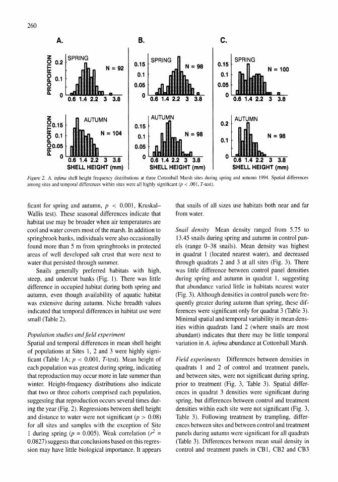
260
A. B. C.
z SPRING SPRING Q 0.2 0.15 0.15 Ii: 0 0.1 0.1 Q, 0.1 0 0.05 0.05 II: Q, 0 0 0
3.8 0.6 1.4 2.2 3 3.8
z 0 0.2 ~0.15 0.15
o 0.1 N = 104 0.1 Q, 0.1 ~0.05 0.05 Q, 0 0 0 .4
SHELL HEIGHT (mm) SHELL HEIGHT (mm)
Figure 2. A. infima shell height frequency distributions at three Cottonball Marsh sites during spring and autumn 1994. Spatial differences among sites and temporal differences within sites were all highly significant (p < .001, T-test).
ficant for spring and autumn, p < 0.001, KruskalWallis test). These seasonal differences indicate that habitat use may be broader when air temperatures are cool and water covers most of the marsh. In addition to springbrook banks, individuals were also occasionally found more than 5 m from springbrooks in protected areas of well developed salt crust that were next to water that persisted through summer.
Snails generally preferred habitats with high, steep, and undercut banks (Fig. 1). There was little difference in occupied habitat during both spring and autumn, even though availability of aquatic habitat was extensive during autumn. Niche breadth values indicated that temporal differences in habitat use were small (Table 2).
Population studies and field experiment Spatial and temporal differences in mean shell height of populations at Sites 1, 2 and 3 were highly significant (Table 1A; p < 0.001, T-test). Mean height of each popUlation was greatest during spring, indicating that reproduction may occur more in late summer than winter. Height-frequency distributions also indicate that two or three cohorts comprised each population, suggesting that reproduction occurs several times during the year (Fig. 2). Regressions between shell height and distance to water were not significant (p > 0.08) for all sites and samples with the exception of Site 1 during spring (p = 0.005). Weak correlation (,1 = 0.0827) suggests that conclusions based on this regression may have little biological importance. It appears
that snails of all sizes use habitats both near and far from water.
Snail density Mean density ranged from 5.75 to 13.45 snails during spring and autumn in control panels (range 0-38 snails). Mean density was highest in quadrat 1 (located nearest water), and decreased through quadrats 2 and 3 at all sites (Fig. 3). There was little difference between control panel densities during spring and autumn in quadrat 1, suggesting that abundance varied little in habitats nearest water (Fig. 3). Although densities in control panels were frequently greater during autumn than spring, these differences were significant only for quadrat 3 (Table 3). Minimal spatial and temporal variability in mean densities within quadrats land 2 (where snails are most abundant) indicates that there may be little temporal variation in A. infima abundance at Cottonball Marsh.
Field experiments Differences between densities in quadrats 1 and 2 of control and treatment panels, and between sites, were not significant during spring, prior to treatment (Fig. 3, Table 3). Spatial differences in quadrat 3 densities were significant during spring, but differences between control and treatment densities within each site were not significant (Fig. 3, Table 3). Following treatment by trampling, differences between sites and between control and treatment panels during autumn were significant for all quadrats (Table 3). Differences between mean snail density in control and treatment panels in CB 1, CB2 and CB3
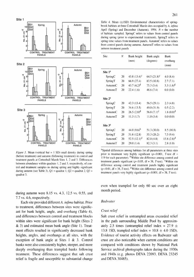
Site t
DOl Spring Autumn 10 ~~ DOl
N <:' 6 IJQ2 'E 8 E C03 " " " 8 "4
~4 0 z
l ~ 2
~ 2
0 0 CONTIIOL TREATMENT CONTIIOL TREATMeNT
PANELS PANELS
Site 2
10 ~~ Spring Autumn ca1
<:' ca3 <:' 4 IJQ2
e 8 E COO " " ,,8 " .,:
~ ~2 Z4
m 2 1 _h. 0 0
CONTROL TREATMENT CONTIIOL TREATMENT PANELS PANELS
Site 3
a ~r1 Spring Autumn
N C~ <:'e 6 oal 'E 6 002 " " oa3 ... " ~4 0 4 0 Z Z
0 ~ R
0 "Ii CONTROL TREATMENT CONTIIOL TREATMENT
PANELS PANELS
Figure 3. Mean (vertical bar = 1 SO) snail density during spring (before treatment) and autumn (following treatment) in control and treatment panels at Cottonball Marsh Sites 1, 2 and 3. Differences between abundance within quadrats 1, 2 and 3, respectively, of control and treatment samples ns during spring and highly significant during autumn (see Table 3). Ql = quadrat 1, Q2 = quadrat 2, Q3 = quadrat 3.
during autumn were 8.15 vs. 4.3, 12.5 vs. 0.55, and 7.7 vs. 4.6, respectively.
Each site provided differentA. infima habitat. Prior to treatment, differences between sites were significant for bank height, angle, and overhang (Table 4), and differences between control and treatment blocks within sites were significant for bank height (Sites 2 & 3) and estimated mean bank angle (Site I). Treatment effects resulted in significantly decreased bank heights, angles, and overhangs at all sites, with the exception of bank angle at Sites I & 3. Control banks were also consistently higher, steeper, and more deeply overhanging than trampled banks following treatment. These differences suggest that salt crust relief is fragile and susceptible to substantial change
261
Table 4. Mean (±ISD) Environmental characteristics of springbrook habitats at three Cottonball Marsh sites occupied by A. illfima April (Spring) and December (Autumn), 1994. N = the number of habitats sampled. SpringC refers to values from control panels during spring (prior to experimental treatment), SpringT refers to spring time values from treatment panels. AutumnC refers to values from control panels during autumn, AutumnT refers to values from autumn treatment panels
Site N Bank height Bank angle Bank
(mm) (degrees) overhang
(mm)
Site 13
SpringC 20 43.8 (13.4)C 64.5 (21.8)" 4.0 (8.4)
SpringT 20 66.9 (27.4) 83.5 (108) 2.7 (7.1)
AutumnC 20 43.7 (4.2)d 75.3 (5.4) 5.3 (1.6)d
AutumnT 20 22.4 (1.6) 48.6 (7.4) 0.0 (0.0)
Site 23
SpringC 20 42.3 (13.4) 56.5 (29.1) 2.3 (4.8)
SpringT 20 34.6 (13.5) 49.0 (31.9) 0.5 (2.2)
AutumnC 20 26.5 (2.8)d 56.8 (7.l)d 1.8 (O.O)d
AutumnT 20 11.3 (1.7) 11.0 (3.4) 0.0 (0.0)
Site 3a
SpringC 20 44.0 (9.6)b 51.3 (30.0) 8.5 (l08)
SpringT 20 51.6 (12.8) 55.3 (26.2) 7.5 (9.4)
AutumnC 20 52.5 (12.l)d 82.0 (4.8) 13.8 (2.8)d
AutumnT 20 290 (1.4) 82.3 (3.1) 2.8 (1.0)
aSpatial differences among habitats for all parameters at three sites prior to treatment very highly significant (p<0.001, T-test df = 119 for each parameter). hWithin site difference among control and treatment panels significant (p<0.05, df = 38, T-test). "Within site ditrerence among control and treatment panels highly significant (p<0.0 1, df = 38, T-test). dWithin site difference among control and treatment panels very highly significant (p<O.OOI, df = 38, T-test).
even when trampled for only 60 sec over an eight month period.
Badwater
Crust relief
Salt crust relief in un trampled areas exceeded relief in the path surrounding Middle Pool by approximately 2.5 times (untrampled relief index = 27.9 ± 13.8 I SO, trampled relief index = 10.8 ± 4.0 I SO). Evidence of tourist activity effects on Badwater salt crust are also noticeable when current conditions are compared with conditions shown by National Park Service archival photographs taken during the 1930s and 1940s (e.g. photos OEVA 22093, OEVA 23245 and OEVA 30485).
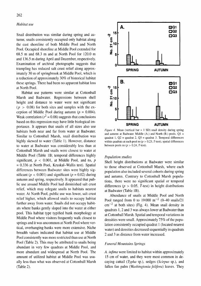
262
Habitat use
Snail distribution was similar during spring and autumn; snails consistently occupied only habitat along the east shoreline of both Middle Pool and North Pool. Occupied shoreline at Middle Pool extended for 68.5 m and 68.3 m and at North Pool for 120.0 m and 136.5 m during April and December, respectively. Examination of archival photographs suggests that trampling has reduced salt crust relief along approximately 30 m of springbrook at Middle Pool, which is a reduction of approximately 30% of historical habitat these springs. There had been no apparent habitat loss at North Pool.
Habitat use patterns were similar at Cottonball Marsh and Badwater. Regressions between shell height and distance to water were not significant (p > 0.08) for both sites and samples with the exception of Middle Pool during autumn (p = 0.004). Weak correlation (,1 = 0.08) suggests that conclusions based on this regression may have little biological importance. It appears that snails of all sizes also use habitats both near and far from water at Badwater. Similar to Cotton ball Marsh, snail distribution was highly skewed to water (Table I). However, distance to water at Badwater was considerably less than at Cottonball Marsh and snails were closest to water at Middle Pool (Table IB; temporal differences highly significant, p < 0.001, at Middle Pool, and ns, p = 0.336 at North Pool, Kruskal-Wallis test). Spatial differences between Badwater sites were highly significant (p < 0.001) and significant (p = 0.02) during autumn and spring, respectively. It appeared that public use around Middle Pool had diminished salt crust relief, which may relegate snails to habitats nearest water. At North Pool, public use was lower, salt crust relief higher, which allowed snails to occupy habitat further away from water. Snails did not occupy habitats where banks gently sloped into the water at either pool. This habitat type typified bank morphology at Middle Pool where visitors frequently walk closest to springs and it was uncommon at North Pool where vertical, overhanging banks were more extensive. Niche breadth values indicated that habitat use at Middle Pool consistently was more restricted than use at North Pool (Table 2). This may be attributed to snails being abundant in very few quadrats at Middle Pool, and more abundant and widespread at North Pool. The amount of utilized habitat at Middle Pool was usually less than what was observed at Cottonball Marsh (Table 2).
C'I 15 Ie ~10 C'I
ci Z 5
~ 15 e u
c::i10 ci Z
5
0
A.
SPRING
B.
SPRING
AUTUMN
AUTUMN
SQ1 CQ2 CQ3
E3Q1 CQ2 CQ3
Figure 4. Mean (vertical bar = I SD) snail density during spring and autumn at Badwater Middle (A.) and North (B.) pools. QI = quadrat I, Q2 = quadrat 2, Q3 = quadrat 3. Temporal differences within quadrats at each pool ns (p > 0.23, T-test), spatial differences between pools ns (p > 0.24, T-test).
Population studies Shell height distributions at Badwater were similar to those observed at Cottonball Marsh, where each population also included several cohorts during spring and autumn. Contrary to Cottonball Marsh populations, there were no significant spatial or temporal differences (p > 0.05, T-test) in height distributions at Badwater (Table IB).
Abundance of snails at Middle Pool and North Pool ranged from 0 to 19000 m-2 (0-40 snails/21 cm-2 at both sites) (Fig. 4). Mean snail density in quadrats I, 2 and 3 was always lower at Badwater than at Cottonball Marsh. Spatial and temporal variations in densities were small. Approximately 75% of the population consistently occupied quadrat 1 (located nearest water) and densities decreased sequentially in quadrats 2 and 3 as distance from water increased.
Funeral Mountains Springs
A. infima were limited to habitat within approximately IS cm of water, and they were most common in decaying cattail (Typha sp.), sedges (Scirpus sp.), and fallen fan palm (Washingtonia felifera) leaves. They
were rare in decaying salt grass (Distich lis spictata) and wire grass (funcus spp.). At Nevares Springs, 11 were found in 83 grab samples taken along a total of 370 m of the largest spring in the province. It was absent in 37 grabs taken from all other springs and seeps in the area. Absence from seeps can be attributed zeric conditions caused by small discharge and periodic drying. Reasons they did not occur at flowing springs are not clear, however, evidence of dredging at these springs suggests that existing habitat conditions have naturalized from past disturbance that may have extirpated populations.
At Travertine Springs, 28 were observed in 162 grabs along approximately 1 km of springbrook. It was absent from 56 grabs taken from springbrooks without vegetation or debris, from Texas Spring, and all seeps in the area. Absence from Texas Spring can be attributed to dry conditions caused by total diversion of its outflow for many years. Threloff & Koenig (1999) estimated that diversion has eliminated approximately 85 % of historical springbrooks at Travertine and Texas springs, which suggests that A. infima habitat has been reduced by a similar amount at these springs.
Discussion
Even though desert wetlands are comparatively small they provide the only persistent water over expansive landscapes of most continents. In the Death Valley region of North America, persistent water is additionally distinguished by providing habitat for at least 60 endemic plants and animals (Sada et al., 1995). A number of studies have examined fish ecology and fish and invertebrate taxonomy in these systems, but invertebrate ecology has received little attention.
Characteristics of the semi-aquatic habitat occupied by A. infima suggests that its demography may be highly influenced by seasonal conditions affecting soil temperature and water availability. Its demography and habitat use indicate, however, that seasonal variation in abundance, size class structure, and habitat use is small. Size class structure of all Badwater and Cottonball Marsh populations were similar during spring and autumn, and there was little spatial and temporal variation in population size. Snail abundance at Badwater was consistently less than at Cottonball Marsh. It is difficult to determine if this is attributable to impacts of human disturbance, the small size of Badwater springs, or differences in chemical composition of salts at the two areas. Results of trampling exper-
263
iments indicate, however, that snail abundance and habitat may be detrimentally impacted by visitors.
Preferred habitat for A. infima at Badwater and Cottonball Marsh consisted of high banks, high bank angles and bank overhangs. There was little seasonal variation in habitat use, but the amount of available habitat during autumn at Cottonball Marsh appeared to be greater than during spring. This was indicated by densities in quadrats 2 and 3 that were highest in all three sites during autumn and lowest in spring. Increased abundance in habitats more distant from water may result from seasonal changes in water availability and temperature that expand habitat availability during periods when air temperatures are low and the amount of water greatest. Snails may be excluded from these habitats during spring and summer when air temperatures are highest and soil moisture is lowest.
On the Death Valley floor, A. infima relies on persistent water and high-relief salt crust that forms when evaporation draws moisture and salts from soils deposited during pluvial periods. Its preferred habitat occurs along springbrooks where salt crust banks are high, steeply angled and deeply undercut. Experimental manipulations indicated that trampling decreased bank heights, angles, undercuts, and snail abundance. The comparatively large declines that were caused by only 60 s of trampling suggest that populations can be easily extirpated with similar, but more extended, activities. The specificity of A. infima habitat use also suggests that it is poorly suited to occupy other habitat types, and that populations can be eliminated when habitats are altered. Reliance on persistent water and their absence from habitats without undercuts, and with low bank angles and height also indicates that populations may be extirpated when spring brooks are physically modified. These impacts are similar to effects to riparian and aquatic habitats that are caused intensive livestock grazing (Fleischner, 1994). Sada & Vinyard (2002) concluded that these types of impacts have resulted in extinctions and population extirpations of many aquatic taxa endemic to the Great Basin region of North America.
Impacts of human trampling on salt crust relief, examination of recent and historical photographs, and the influence of trampling on A. infima habitat and abundance all indicate that public use has altered physical and biological characteristics of Badwater. Death Valley National Park archival photographs indicate that Badwater remained in comparatively natural condition until the first road was constructed into the area during 1933 (Lingenfelter, 1986). Photographs
264
taken over the past 50 years show the extent of highrelief salt crust dwindling over much of Badwater. It is difficult to compare extant and historical A. infima populations at Badwater without knowledge of its abundance and distribution prior to human disturbance. However, historical changes in the extent of flattened salt crust indicates that little habitat has been lost at North Pool and that approximately 30 m has been lost at Middle Pool. This represents a reduction of approximately 30% of historical habitat at Middle Pool.
Abundance and distribution of A. infima has also been affected by diversions that dried aquatic and riparian habitats supported by Texas, Travertine and Nevares Springs. Influence of these diversions on A. infima is also difficult to determine because there were no studies documenting its historical abundance and distribution. Its present occurrence in all springfed riparian areas with persistent water unaffected by frequent flood events suggests, however, that diversions eliminated several kilometers of habitat that may have been occupied by millions of individuals. Other aquatic macroinvertebrates endemic to Funeral Mountain springs have also been affected by these diversions. It is likely that continuation of historical use patterns at Badwater and future springbrook diversions will cause additional declines in abundance and distribution of many aquatic macro invertebrates endemic to Death Valley. Fortunately, A. infima populations at Cotton ball Marsh appear to occupy its historical habitat and to be comparatively unaffected by cultural uses.
Although information is needed to design recovery programs for Badwater populations of A. infima, observations at Cottonball Marsh indicated that trampled salt crust can regain its relief when protected from trampling. Growth rates were comparatively slow, approximately 2 cm yr- I in trampled areas, and considerable time may be required to allow the crust to mature and provide A. infima habitat. Water rights granting diversions from Funeral Mountain Springs may preclude restoration of these systems, but diversions should be curtailed as much as possible to prevent additional losses and restore as much A. infima habitat as possible. Public use of aquatic and riparian resources in Death Valley National Park should consider biological integrity of these spring resources. These uses should be allowed only when management programs result in functional conditions at these springs that are more similar to those at Cottonball
Marsh than to those currently existing at Badwater and in the Funeral Mountains.
Acknowledgements
Funding and assistance with this work was provided by the U.S. National Park Service, Death Valley National Park. D. Threloff, B. Davenport and B. Thornburg assisted with field work. S. Smith, D. Herbst and J. Wehausen, D. Blinn and an anonymous reviewer provided helpful comments to early manuscripts.
References
Baldinger. A. 1., W. D. Shepard & D. L. Threloff. 2000. Two new species of Hyalella (Crustacea: Amphipoda: Hyalellidae) from Death Valley National Park, California, U.S.A. Proc. BioI. Soc. Wash. 1l3: 443-457.
Berry, S. S., 1947. A surprising molluscan discovery in Death Valley. Leaflets in Malacology I: 5-8.
Fleischner. T. L., 1994. Ecological costs of livestock grazing in western North America. Cons. Bio. 8: 629-644.
Fowler, B. H., 1980. Reproductive biology of Assiminea californica (Tyron, 1865) (MesogaSlropoda: Rissoacea). Veliger 23: 163-166.
Hershler, R., 1987. Redescription of Ass imine a infima Berry, 1947, from Death Valley, California. Veliger 29: 274-288.
Hershler, R., 1989. Springsnails (Gastropoda: Hydrobiidae) of Owens and Amargosa River (exclusive of Ash Meadows) drainages, Death Valley system, California-Nevada. Proc. BioI. Soc. Wash. 102: 176-248.
Hershler, R., 1998. A systematic review of the hydrobiid snails (Gastropoda: Rissooidea) of the Great Basin, western United States. Part I. Genus Pyrgulopsis. Veliger 41: 1-132.
Hershler. R., 1999. A systematic review of the hydrobiid snails (Gastropoda: Rissooidea) of the Great Basin, western United States. Part II. Genera Colligyrus, Eremopygrus, Fluminicola, Pristinicola and Tryonia. Veliger 42: 306-337.
Hershler, R. & D. W. Sada, 1987. Springs nails (Gastropoda: Hydrobiidae) of Ash Meadows, California-Nevada. Proc. BioI. Soc. Wash. 100: 776-843.
Hunt, C. B., 1975. Death Valley Geology, Ecology, and Archaeology. U. California Press, Berkeley, CA: U.S.A., 234 pp.
Hunt, C. B., T. W. Robinson, W. A. Bowles & A. L. Washburn, 1966. Hydrologic basin, Death Valley, California. U.S.G.S. Prof. Pap., 494-B: BI-B138.
Jacobs, 1., 1974. Quantitative measurement of food selection: a modification of the forage ratio and Ivlev's electivity index. Oecologia (Berlin) 14: 413-417.
La Bounty, 1. F. & J. E. Deacon, 1972. Cyprinodon miller;, a new species of pup fish (Family Cyprinodontidae) from Death Valley, California. Copeia 1972: 769-780.
La Rivers, I., 1948. A new species of Ambrysus from Death Valley with notes on the genus in the United States (Hemiptera: Naucoridae). Bull. S. Calif. Acad. Sci. 47: 103-110.
Levins, R., 1968. Evolution in Changing Environments. Princeton U. Press, Princeton, NJ, U.S.A.: 120 pp.
Lingenfelter, R. E., 1986. Death Valley and the Amargosa. A Land of Illusion. U. California Press, Berkeley, CA, U.S.A.: 664 pp.
Miller, R. R., 1981. Coevolution of deserts and pupfishes (genus Cyprinodon) in the American southwest. In Naiman, R. 1. & D. L. Soltz (eds), Fishes in North American Deserts. John Wiley & Sons, NY, U.S.A.: 39-94.
Sada, D. W. & G. L. Vinyard, 2002. Anthropogenic changes in biogeography of Great Basin aquatic biota. Smiths. Contr. Earth Sci.: in press.
Sada, D. w., H. B. Britten & P. F. Brussard, 1995. Desert aquatic ecosystems and the genetic and morphological diversity of Death Valley system speckled dace (Rhil1ichthys osculus).ln Nielsen, J. L. (ed.), Evolution and the Aquatic Ecosystem. Defining unique units in population conservation. Am. Fish. Soc. Sym. 17: 350-359.
Shepard, W. D., 1993. Desert springs - both rare and endangered. Aq. Conser.: Mar. and Freshwat. Eco!. 3: 351-359.
Shepard, W. D., 1992. Riffle beetles (Coleoptera: Elmidae) of Death Valley National Monument, California. Great Basin Natur. 52: 378-381.
265
Smith, G. R., 1978. Biogeography of intermountain fishes. Great Basin Natur. Mem. 2: 17-42.
Taylor, D. w., 1985. Evolution offreshwater drainages and molluscs in western North America. In Smiley, C. J. (ed.), Late Cenozoic History of the Pacific Northwest. Amer. Ass. Adv. Sci. San Francisco, CA, U.S.A.: 265-321.
Threloff. D. L. & S. Koenig, 1999. Effects of water diversion activities on stream lengths in the Travertine-Texas Spring complex, Death Valley National Park, summer 1999. Unpublished U.S. National Park Service report, Death Valley National Park, CA, U.S.A.: 7 pp.
Williams, 1. E., D. B. Bowman, 1. E. Brooks, A. A. Echelle, R. J. Edwards, D. A. Hendrickson & 1. 1. Landye, 1985. Endangered aquatic ecosystems of North American deserts, with a list of vanishing fishes of the region. J. Arizona-Nevada Acad. Sci. 20: 1-62.
Hydrobiologia 466: 267-277, 2001. J.M. Melack. R. Jellison & D.E. Herbst (eds), Saline Lakes. © 200 I Kluwer Academic Publishers.
267
Holocene hydrological and climatic changes in the southern Bolivian Altiplano according to diatom assemblages in paleo wetlands
S, Servant-Vildaryl, M, Servant2 & O. Jimenez l I Antenne [RD, ESA 7073, Laboratoire de Geologie, MNHN, 43 Rue Buffon, 75005 Paris, France 2[RD, Centre de Recherche Ile de France, 32 Rue Henri Varagnat, 93143 Bondy, France
Key words: Bolivia, Altiplano, river deposits, diatoms, paleoclimate, Holocene
Abstract
This paper presents the first Holocene continuous record from the southern Bolivian Altiplano. In this area, the climate is now characterized by weak summer monsoon rains. The record is located north of Salar de Uyuni in a non-glacial valley (Rio Baja). Between ~ 11600 and ~221 0 cal year BP, the rivers accumulated fine deposits, while under the present climatic conditions, the fine particles are carried downstream by strong water floods. These deposits contain a rich diatom flora showing that the valley floor was occupied by paleowetlands. Water input needed to be more or less continuous to explain that the paleowetlands survived over a long period of time. We show that diatoms can be used to reconstruct the relative variations in the water level and the salinity throughout time, despite of the spatial complexity of this type of environment. During the Holocene, the water level was low except during some periods, dated ~ II 600-9800, ~6330-5300, and ~ 3110-2210 cal year BP. Saline and freshwater microhabitats were simultaneously present in the valley floor as indicated by a mixed diatom flora evidenced throughout the record. We propose a paleoclimatic scenario based on the assumption that the NE wet atmospheric flow of the monsoon was replaced by the westerlies of the southern hemisphere at the latitude of the study site.
Introduction
The tropical southern Andes are characterized between 19° and 24°S by the largest salt flats and salt lakes of the world. Lake Poop6 is a 3000-km2 salt lake which episodically dries up, Uyuni and Coipasa salt flats cover 10 000 km2, and numerous shallow saline lakes and salt pans are observed in the southern subtropical Andes in Bolivia and Chile (Fig. I). These salt environments reflect dry climatic conditions that arose at the beginning of the Holocene. This dry period, marked by a 10-m deep salt bed in the Salar de Uyuni (Risacher & Fritz, 1992), followed a relatively wet phase (the Coipasa event) marked by the presence of a shallow saline lake (Servant et al., 1995; Sylvestre et aL, 1999). At the same latitudes in the northern Chilean Altiplano, dryness set in at ~ 1 a 900 cal year BP, water level decreased between ~ 10900 and 8000 cal year BP and the lakes were desiccated between ~8000 and 4000 cal year BP (Geyh et aL, 1999).
Despite of these dry conditions, Holocene paleowetlands were well-developed and widespread in the valley floors, both in northern Chile (Betancourt et aL, 2000) and in Bolivia, particularly in the nonglacial valleys (Servant & Fontes, 1984). The paleowetland sediments which deposited in a continuous fashion through time in the southern Bolivian Andes, provide excellent material for detailed paleoclimatic reconstruction. They contain a rich diatom flora (Frohlich & Servant-Vildary, 1989, Betancourt et al., 2000) which can be used, as currently done in lake deposits, to reconstruct changes in water level and salinity in a reliable river record (e.g., see reviews by Smol & Cumming, 2000).
In this paper, we present a diatom study from a paleowetland located north of the Salar de Uyuni. Our objectives were (I) to reconstruct changes in water level and salinity in a river system, (2) to construct a paleoclimatic scenario in order to explain the presence of evaporites in the Salar de Uyuni while wetlands
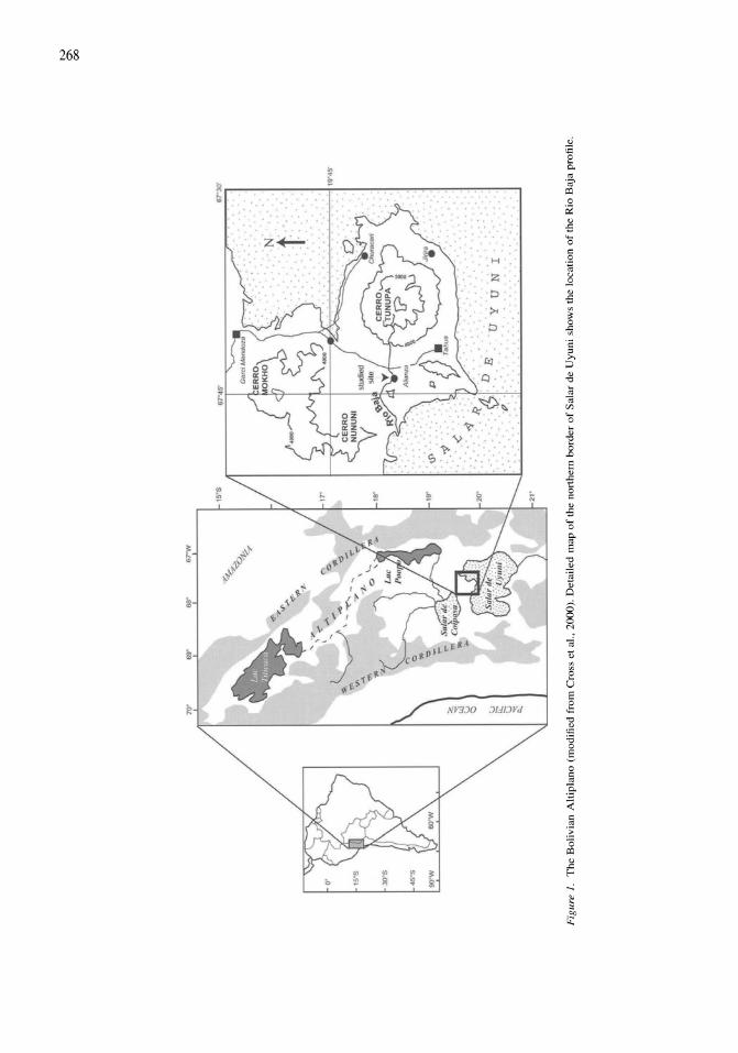
Fig
ure
1.
Th
e B
oliv
ian
Alt
ipla
no
(m
odif
ied
from
Cro
ss e
t at
.. 20
00).
Det
aile
d m
ap o
f th
e no
rthe
rn b
ord
er o
f S
alar
de
Uy
un
i sh
ows
the
loca
tion
of
the
Rio
Baj
a pr
ofil
e.
N
0\
00
were developed in the catchment and finally (3) to discuss this scenario according to the data available from the different areas of the Southern tropical Andes, both in the northern Altiplano (Lake Titicaca area) and the southern Altiplano (the Uyuni-Coipasa and northern Chile areas),
Climatic and paleoclimatic setting
At the present time, the climate is characterized by low precipitation and by two contrasted seasons: a short rainy season between December and March (austral summer) and a long dry season between April and November. The seasonal distribution of precipitation reflects changes in the atmospheric circulation throughout the year at the latitudes where Bolivia is located. During the austral winter, the southern westerlies spread toward the equator and reach the Lake Titicaca area at the mid and upper level of the troposphere (Vuille, 1999) and the Bolivian Andes are submitted to dry and subsident air from the Pacific region. During the austral summer, the westerlies shift southwards, the NE humid air flow (hereafter referred to as 'South American monsoon') from the Atlantic reaches the southern tropical Andes. Summer precipitation consistently decreases from the NE to the SW, 800 mm year-1 in the Lake Titicaca area, 300 mm year-1 in the Uyuni area, and -100 mm year-1 in the northern Chile. These seasonal changes are modulated on the synoptical time scale by atmospheric processes related to interactions between high and low latitudes. West of the Andes, along the Pacific coast of northern Chile and southern Peru, cold air masses from the southern polar region episodically reach the sub-tropical latitudes at the mid levels of the troposphere (Vuille & Caspar, 1997). East of the Andes the low troposphere is characterized all year round by south-north cold air incursions, that can reach the central Amazon Basin (Garreaud, 1999). Occasional non-stormy rainfall and snowfall occur in the southern tropical Andes when the tropical atmosphere is destabilized by cold air incursions, particularly during the winter dry season.
Under these climatic conditions, the rivers in the non-glacial valleys are submitted to strong floods during the wet season (December to March), the valley floors are intensively eroded, and fine particles are carried downstream. During the rest of the year (April to November) the non-glacial valley floors are desiccated, except in some areas where water input from
269
extended groundwater reservoirs buffers the effect of the seasonal dryness.
Most data concerning the Holocene climatic changes in the Bolivian Andes were obtained from the northern Altiplano. Lake Titicaca water-level variations indicate that the precipitation minus evaporation (P-E) balance in the watershed changed fundamentally throughout the Holocene. The water level was lower and the climate drier than at present between ~ 11 500 and ~4500 cal year BP (Ybert, 1992; Mourguiart et aI., 1998; Cross et aI., 2000). However, increased lake level phases occurred during this general dry trend, they are dated ~ 1 0 000-8500 and 7000-6000 cal year BP (Baker et aI., 2001). Between ~4500 and 3500 cal year BP, the Lake Titicaca water level increased substantially and reached the present level after 1000 cal year BP (Mourguiart et aI., 1998) showing a wet climatic trend. This wet trend has been interrupted by short dry phases, recorded by strong drops in the water level, at ~3000, 2800, 1800, and 700 cal year BP (Abbott et aI., 1997a). These climatic changes have been interpreted to be the result of modifications in the intensity of the South American monsoon.
Material and Methods
The outcrop is exposed on the bank of the Rio Baja, located near the village of Alianza (67°45'W, 19°50'S) at about 3700 m above sea level, ~56 m above the Salar de Uyuni (Fig. 1). The 8-m deep profile has been continuously sampled using 30-cm deep boxes. Twenty-six boxes, representing the totality of the outcrop, were collected (courtesy of D. Wirrmann). Between 850 and 725 cm, sands and gravels are predominant, diatoms are lacking, except in a silt clay layer intercalated at 806 cm. Between 725 and 529 cm, silts and clays are dominant. From 529 to 280 cm, the fine deposits are calcareous (a calcareous crust is interbedded at 500 cm). From 280 to 180 cm, fine sands are abundant in silts, and from 180 cm to the top, silt and clays are followed by a calcareous fine deposit. Dark organic layers are intercalated in the sequence, particularly in the lower and the upper parts.
Time control was based on six total organic matter samples that were 14C dated. Ages were calibrated according to the method outlined for CALIB 3.0. by Stuiver & Reimer (1993). Uncalibrated radiocarbon ages and calibrated ages (cal year BP) versus depth are reported in Figure 2. The sedimentation rate was low: 0.04 cm year-1 before 6610 yr BP, with an increase
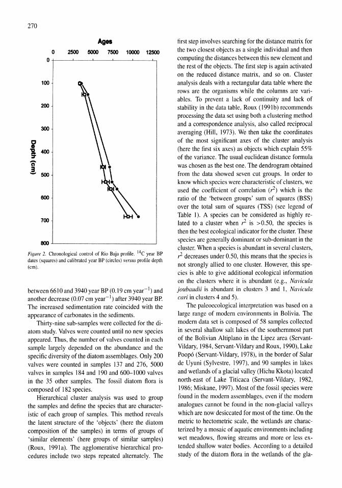
270
Ages 0 2500 5000 7500 10000 12500
0
100
200
300
i ~ 400 :r -n 3 - 500
600
700
6OOL---------------------~
Figure 2. Chronological control of Rio Baja profile. 14C year BP dates (squares) and calibrated year BP (circles) versus profile depth (cm).
between 6610 and 3940 year BP (0.19 cm year-I) and another decrease (0.07 cm year-I) after 3940 year BP. The increased sedimentation rate coincided with the appearance of carbonates in the sediments.
Thirty-nine sub-samples were collected for the diatom study. Valves were counted until no new species appeared. Thus, the number of valves counted in each sample largely depended on the abundance and the specific diversity of the diatom assemblages. Only 200 valves were counted in samples 137 and 276, 5000 valves in samples 184 and 190 and 600-1000 valves in the 35 other samples. The fossil diatom flora is composed of 182 species.
Hierarchical cluster analysis was used to group the samples and define the species that are characteristic of each group of samples. This method reveals the latent structure of the 'objects' (here the diatom composition of the samples) in terms of groups of 'similar elements' (here groups of similar samples) (Roux, 1991 a). The agglomerative hierarchical procedures include two steps repeated alternately. The
first step involves searching for the distance matrix for the two closest objects as a single individual and then computing the distances between this new element and the rest of the objects. The first step is again activated on the reduced distance matrix, and so on. Cluster analysis deals with a rectangular data table where the rows are the organisms while the columns are variables. To prevent a lack of continuity and lack of stability in the data table, Roux ( 1991 b) recommends processing the data set using both a clustering method and a correspondence analysis, also called reciprocal averaging (Hill, 1973). We then take the coordinates of the most significant axes of the cluster analysis (here the first six axes) as objects which explain 55% of the variance. The usual euclidean distance formula was chosen as the best one. The dendrogram obtained from the data showed seven cut groups. In order to know which species were characteristic of clusters, we used the coefficient of correlation (,1) which is the ratio of the 'between groups' sum of squares (BSS) over the total sum of squares (TSS) (see legend of Table I). A species can be considered as highly related to a cluster when ,1 is >0.50, the species is then the best ecological indicator for the cluster. These species are generally dominant or sub-dominant in the cluster. When a species is abundant in several clusters, ,1 decreases under 0.50, this means that the species is not strongly allied to one cluster. However, this species is able to give additional ecological information on the clusters where it is abundant (e.g., Navicula joubaudii is abundant in clusters 3 and 1, Navicula cari in clusters 4 and 5).
The paleoecological interpretation was based on a large range of modern environments in Bolivia. The modern data set is composed of 58 samples collected in several shallow salt lakes of the southernmost part of the Bolivian Altiplano in the Lipez area (ServantVildary, 1984, Servant-Vildary and Roux, 1990), Lake Poop6 (Servant-Vildary, 1978), in the border of Salar de Uyuni (Sylvestre, 1997), and 90 samples in lakes and wetlands of a glacial valley (Hichu Kkota) located north-east of Lake Titicaca (Servant-Vildary, 1982, 1986; Miskane, 1997). Most of the fossil species were found in the modern assemblages, even if the modern analogues cannot be found in the non-glacial valleys which are now desiccated for most of the time. On the metric to hectometric scale, the wetlands are characterized by a mosaic of aquatic environments including wet meadows, flowing streams and more or less extended shallow water bodies. According to a detailed study of the diatom flora in the wetlands of the gla-
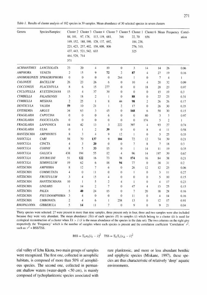
271
Table 1. Results of cluster analysis of 182 species in 39 samples. Mean abundance of 30 selected species in seven clusters
Genera Species/Samples: Cluster 2 Cluster 3 Cluster 4 Cluster 7 Cluster 5 Cluster 1 Cluster 6 Mean Frequency Correl-
84,101, 97,178, 113,119, 681, 346 22,70 656 ation
149, 152, 188,190, 128, 137, 692, 184,238,
221,423, 257,402, 158,608, 806
437,443, 521,542, 633
276,310,
325
464,529, 714
571
ACHNANTHES LANCEOLATA 23
AMPHORA VENETA 2
ANOMOEONEIS SPHAEROPHORA 0
CALONEIS BACILLUM 26 COCCONE~ PLACENTULA 8 CYCLOTELLA KUElZINGIANA 15
CYMBELLA FALAISENSIS 5
CYMBELLA MESIANA 2 DENTICULA VALIDA S9 EPITHEMIA ARGUS 34
FRAGILARIA CAPUCINA 0
FRAGILARIA FASCICULATA 0
FRAGILARIA
FRAGILARIA
HANTZSCHIA
NAVICULA
NAVICULA
NAVICULA
NAVICULA
NAVICULA
NAVICULA
NITZSCHIA
NITZSCHIA
NITZSCHIA
NITZSCHIA
NITZSCHIA
NITZSCHIA
NITZSCHIA
NITZSCHIA
RHOPALODIA
LAPPONICA 14
ULNA 0
AMPHIOXYS 8
CARl 58
ClNCTA 4
COHNII 8
GALLICA 438
JOUBAUDII 51
SEMINULUM 19
AMPHIBIA 8
COMMUTATA 4
FRUSTULUM 3
HANTZSCHIANA 10
LlNEARIS 1
PALEA 5
PSEUDOAMPHIBIA 3
UMBONATA 2
GIBBERULA 5
20
15
o 23
6
4
18
25
10
63
o o
42
1
3
70
3
5
194
122 62
12
o 4
14
40 4
4
14
4
9
o 26
15
37
2
21
3
o o
13
2
4
137 20 33 55
16
6
7
11
15
5
2
24
o 6
11
19
72
o 6
277
39
8
45
6
o 3
39
9
9
o 15
12
73 18
6
o 4
2
7
15
o I
7
o 2
264
o o o o
44
2
o o o
222
o 12
104 o o 4
38
94
o o o 4
o o o
258
o
3
87
10
o o
88
98
17
168 o o
397
o 1
72
7
1
96
174 77
26
1
o
47 7
11
13
9
14
4
o 4
18
o o 2 o 6
80
174
4
8
o 12
8
14
14
16
o 12
o o o 4
20
o o o
14 26
27 19
7 4 20 32
28 23
15 19
22 23
26 26
26 30
58 30
3 3
5 2 93
4
5
74
7
II
197
84
38
12
3
5 4
13
18
4
12
9
27
11
25
39
18
19
39
38
31
25
11
10
17
25
28
14
17
21
0.06
0.16
1
0.09
0.97
OJ
OJ1
0.17
OJ5
0.15
0.97
0.74
0.58
OJ5
0.21
OJ
OJ5
0.67
0.21
0.2
0.06
0.27
0.15
0.23
0.15
0.16
0.16
0.91
0.04
Thirty species were selected: 27 were present in more than nine samples, three present only in four, three and two samples were also included because they were very abundant. The mean abundance (Xk) of each species (X) in samples (i) which belong to a cluster (k) is used for ecological reconstruction of a cluster when Xk > i (i is the mean abundance of the species in the data set). The two columns on the right give respectively the 'Frequency' which is the number of samples where each species is present and the correlation coefficient 'Correlation' ,2, such as: ,2 = BSSITSS.
cial valley of Ichu Kkota, two main groups of samples were recognized. The first one, collected in aerophilic habitats, is composed of more than 50% of aerophilous species. The second one, collected in permanent shallow waters (water-depth <50 cm), is mainly composed of tychoplanktonic species associated with
rare planktonic, and more or less abundant benthic and epiphytic species (Miskane, 1997), these species are thus characteristic of relatively 'deep' aquatic environments.
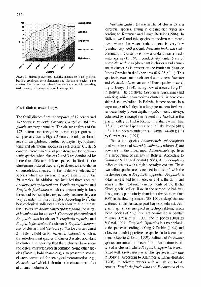
272
100 o aerophllous
80
ao Elbenthlc
70
ao % 50
o epiphytic
.. •• III Iychoplanktonlc
20
10 • planktonic
/'~ /'~ /" /" /''' /" /'~ Cluste ..
Figure 3. Habitat preferences. Relative abundance of aerophilous, benthic, epiphytic, tychoplanktonic and planktonic species in the clusters. The clusters are ordered from the left to the right according to decreasing percentages of aerophilous species.
Fossil diatom assemblages
The fossil diatom flora is composed of 19 genera and 182 species: Navicula,Cocconeis, Nitzchia, and Fragilaria are very abundant. The cluster analysis of the 182 diatom taxa recognized seven major groups of samples or clusters. Figure 3 shows the relative abundance of aerophilous, benthic, epiphytic, tychoplanktonic and planktonic species in each cluster. Cluster 6 contains more than 60% of planktonic and tychoplanktonic species when clusters 2 and 3 are dominated by more than 50% aerophilous species. In Table I, the clusters are ordered according to decreased abundance of aerophilous species. In this table, we selected 27 species which are present in more than nine of the 39 samples. In addition, we included three species: Anomoeoneis sphaerophora, Fragilaria capucina and Fragilaria fasciculata which are present only in four, three, and two samples, respectively, because they are very abundant in these samples. According to ?, the best ecological indicators which allow to discriminate the clusters are Anomoeoneis sphaerophora and Nitzschia umbonata for cluster 5, Cocconeis placentula and Fragilaria ulna for cluster 7, Fragilaria capucina and Fragilariafasciculata for cluster 6, Fragilaria lapponica for cluster 1 and Navicula gallica for clusters 2 and 3 (Table 1, bold cells). Navicula joubaudii which is the sub-dominant species of cluster 3 is also abundant in cluster I, suggesting that these clusters have some ecological characteristics in common. Some other species (Table I, bold characters), also present in several clusters, were used for ecological reconstruction, e.g., Navicula cari which is dominant in cluster 4 but also abundant in cluster 5.
Navicula gallica (characteristic of cluster 2) is a terrestrial species, living in organic-rich water according to Krammer and Lange-Bertalot (1986). In Bolivia, we found this species in modern wet meadows, where the water ionic content is very low (conductivity <60 I1S/cm). Navicula joubaudii (subdominant in cluster 3) is now abundant near a freshwater spring (45 I1S/cm conductivity) under 5 cm of water. Navicula cari (dominant in cluster 4 and abundant in cluster 5) is present on the border of Salar de Pastos Grandes in the Lipez area (0.6-35 g I-I). This species is associated in cluster 4 with several Nitzchia and Navicula cincta, an aerophilous species according to Denys (1994), living now at around 109 I-I in Bolivia. The epiphytic Cocconeis placentula (and varieties) which characterizes cluster 7, is here considered as euryhaline. In Bolivia, it now occurs in a large range of salinity: in a large permanent freshwater water body (30 cm depth, 40 I1Slcm conductivity), colonized by macrophytes (essentially lsoetes) in the glacial valley of Hichu Kkota, in a shallow salt lake (15 g 1-1) of the Lipez area, and in Lake Poop6 (40 g I-I). It has been recorded in salt works (44-80 g I-I) by Clavero et al. (1994).
The saline species Anomoeoneis sphaerophora (and varieties) and Nitzschia umbonata (cluster 5) are now rare in the Lipez area. Anomoeoneis sp. lives in a large range of salinity in Bolivia. According to Krammer & Lange-Bertalot (1988), A. sphaerophora indicates waters with a high electrolyte content. These two saline species are associated in cluster 5 with the freshwater species Fragilaria lapponica. Fragilaria is today represented by 17 species and is the dominant genus in the freshwater environments of the Hichu Kkota glacial valley. Rare in the aerophilic habitats, this genus is particularly abundant (always more than 50%) in the flowing streams (50--100 cm deep) that are scattered in the Juncacae peat bogs (bofedales). Fragila ria sp is here assigned as tychoplanktonic when some species of Fragilaria are considered as benthic in lakes (Cross et aI., 2000) and in ponds (Douglas & Smol, 1994). Fragilaria /apponica is a tychoplanktonic species according to Yang & Duthie, (1994) and a low conductivity preference species in lotic environments (Reavie & Smol, 1999). Saline and freshwater species are mixed in cluster 5, similar feature is observed in cluster I where Fragilaria lapponica is associated with Epithemia argus. This species is now rare in Bolivia. According to Krammer & Lange-Bertalot (1988), it indicates waters with a high electrolyte content. Fragilaria fasciculata and F capucina char-
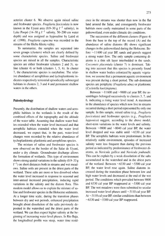
acterize cluster 6. We observe again mixed saline and freshwater species. Fragilaria Jasciculata is now known in the Uyuni area (0.9-30 g 1-1 salinity), in Lake Poop6 (14-30 g 1-1 salinity, 50-200 cm water depth) and was assigned as hyposaline by Laird et al. (1998). Fragilaria capucina was recorded in the streams of the Hichu Kkota valley.
To summarize, the samples are separated into seven groups (clusters) which are clearly defined by some characteristic species. Saline and freshwater species are mixed in all the samples. Characteristic species are either freshwater (clusters 2 and 3), saline (cluster 4) or both (clusters 1, 5, 6). In cluster 7, the characteristic species is euryhaline. The relative abundance of aerophilous and tychoplanktonic indicates respectively terrestrial episodically submerged habitats in clusters 2, 3 and 4 and permanent shallow waters in the others.
Paleohydrology
Presently, the distribution of shallow waters and aerophilic habitats in the wetlands is the result of the combined effects of the topography and the altitude of the water table. Assuming that shallow water bodies extended when the water level increased and that aerophilic habitats extended when the water level decreased, we expect that, in the past, water-level changes were recorded by the relative abundance of tychoplanktonic-planktonic and aerophilous species.
The mixture of saline and freshwater species is now observed on the border of the Salar de Uyuni, under a dry climate. Groundwater discharge allows the formation of wetlands. This type of environment shows strong spatial variations in the salinity (0.9-33 g 1-1 ) on short distances both in streams and wet meadows. Saline soils are present in the driest parts of the wetland. These salts are more or less dissolved when the water level increased in response to seasonal and inter-annual increased precipitation, inducing rapid variations in the salinity and the diatom flora. This modem model allows us to explain the mixture of saline and freshwater species in the Holocene sediments. At a longer time scale, during the transition phases between dry and wet periods, enhanced precipitation brought about dissolution of the salts previously deposited in the watershed and the driest parts of the wetland. We can thus expect higher salinity at the beginning of increasing water level phases. In Rio Baja, the longitudinal profile was steep, water time resid-
273
ence in the streams was shorter than now in the flat land around the Salar, and consequently freshwater habitats more easily maintained in some parts of the paleowetland, even under climatic dry conditions.
The succession of the different clusters (Figure 4) from the base to the top of the record (A) and the abundance of saline diatoms (B) shows significant changes in the paleowetland during the Holocene. Before ~ II 600 cal year BP, sands and gravels suggest a strong water flow. The only sample containing diatoms is a thin silt layer interbedded in the sands. Cocconeis placentula (cluster 7) is dominant. Taking into account that this species is presently found in shallow water bodies colonized by aquatic vegetation, we assume that a permanent aquatic environment was present during a short period. The sub-dominant species are periphytic (Fragilaria ulna) or planktonic (Cyclotella kuetzingiana).
Between ~ II 600 and ~9800 cal year BP, the assemblages belonged successively to clusters 3, 7, and 6, indicating a rising water level trend. A maximum in the abundance of species which now live in streams occurred during a short period represented by only one sample. In this sample, mixed saline (e.g., Fragilaria Jasciculata) and freshwater species (e.g., Fragilaria lapponica) suggest, according to the above model, short-term variations in the water levels and salinity. Between ~9800 and ~8040 cal year BP, the water level dropped and was stable until ~6330 cal year BP. The aerophilic habitats were predominant. In this relatively stable environment, episodes of increased salinity were less frequent than during the previous period as indicated by predominance of freshwater diatoms, as Navicula gallica and Navicula joubaudii. This can be explain by a weak dissolution of the salts accumulated in the watershed and in the driest parts of the wetland. Between ~6330 and ~5300 cal year BP, the water level rose again. Saline diatoms increased during the transition phase between low and high water levels and decreased at the end of the wet period. The conditions which prevailed between 9800 and 6330 cal year BP reappeared at ~5300 cal year BP. The wet meadows were then submitted to secular increased water level phases until ~ 3110 cal year BP. At ~ 3110 cal year BP, similar conditions than between ~6330 and ~5300 cal year BP reappeared.
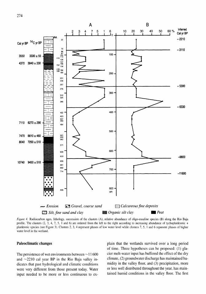
274
A B 2 3 4 7 5 6 10 20 30 40 50 60% Inferred
Calyr BP
Cal yr BP 14C yr BP 22 ~2210
10 ~3110
84 91
3550 3330±55 'v' 119 ~2!
4370 3940±330 131
152 ~:: 118 ,84 ,88 ,90
221 238
251 ~5300
216
310 325
346
~6330
402
423
431
7110 6270±290 443
464
7470 6610 ± 460 521 529 542
8040 7250±510 511
608
633 ~800
10740 9450±510 656
681 692
114 ~11600
806 em
,.,.,. Erosion ~ Gravel, coarse sand El Calcareous fine deposits
~ Silt, fine sand and clay • Organic silt clay • Peat
Figure 4. Radiocarbon ages, lithology, succession of the clusters (A), relative abundance of oligo-eusaline species (B) along the Rio Baja profile. The clusters (2, 3, 4, 7, 5, I and 6) are ordered from the left to the right according to increasing abundance of tychoplanktonic + planktonic species (see Figure 3). Clusters 2, 3, 4 represent phases of low water level while clusters 7, 5, I and 6 represent phases of higher water level in the wetland.
Paleoclimatic changes
The persistence of wet environments between'" 11 600 and "'2210 cal year BP in the Rio Baja valley indicates that past hydrological and climatic conditions were very different from those present today. Water input needed to be more or less continuous to ex-
plain that the wetlands survived over a long period of time. Three hypotheses can be proposed: (1) glacier melt-water input has buffered the effect of the dry climate, (2) groundwater discharge has maintained humidity in the valley floor, and (3) precipitation, more or less well distributed throughout the year, has maintained humid conditions in the valley floor. The first
hypothesis can be rejected because the non-glacial valleys were always ice-free, particularly during the Holocene. The second hypothesis is considered unlikely because in this area groundwater reservoirs are very small. The third hypothesis being the most likely, we concluded that precipitation was relatively well-distributed throughout the year. Moreover, fine particles, silts, fine sands, and clays accumulated in the valley floor while now they are carried downstream by seasonal strong water floods. This indicates that precipitation on the catchment area was of the non-stormy type.
This type of precipitation is similar to today's precipitation which occurs when the westerlies expand northwards, in winter. In the past, westerlies were located at the latitude of Uyuni, not only in winter but also in summer, and replaced the NE tropical atmospheric flow of the monsoon. Cold air incursions brought about non-stormy precipitation and snowfall that more or less attenuated the dryness due to the lack of monsoon rains. These cold air incursions occurred episodically throughout the year. They were more intense and more frequent during the relatively wet periods recorded by increased water level phases at 11600-9800, 6330-5300 and 3110-2210 cal year BP.
Such climatic conditions also took place in the Lake Titicaca watershed. Paleowetlands were also present in the non-glacial valleys. But contrary to the Uyuni area, frequent hiatuses of sedimentation were observed in the records (Servant & Fontes, 1984). These gaps of sedimentation were interpreted as erosion phases related to stormy rains, similar to today's convective rains that occur in summer. During these erosion phases, westerlies retreated to the south in summer, and were replaced by the NE wet atmospheric flow of the monsoon: precipitation increased and water levels in Lake Titicaca rose, these wet phases occurred at 10000-8500, 7000-6000 and 4500-3500 cal year BP (Baker et al., 2001). The last one was marked by the strongest water-level rise of the Holocene. It coincides with a major climatic change at the southern tropics of South America: rainforest developed in the Carajas area in south-eastern Amazonia (Absy et al., 1991), outflow increased in the Amazon river (Maslin & Bums, 2000), and arboreal vegetation developed in Central Brazil (Ledru et al., 1998; Salgado-Labouriau et al., 1997). This climatic change confirms that the monsoon was reinforced at the southern tropical latitudes. However, in Bolivia, the monsoon did not reach the southern Altiplano as
275
indicated by predominance of non-stormy precipitation. In Rio Baja, short-term hydrological changes superimposed on a general dry trend suggest secular modifications in the intensity of cold air incursions, between "-'5300 and "-'3110 cal year BP. In the northern Bolivian Altiplano, short dry phases occurred after the previous wet period. They were recorded at "-'2800 and 1800 cal year BP in Lake Titicaca (Abbott et al., 1997a), and in the glacial valleys, between 2700 and 1850 cal year BP (Servant-Vildary et al., 2001), and prior to 2290 cal year BP (Abbott et al., 1997b). These dry phases indicate a weakening of the monsoon. In the southern Altiplano, intensification of cold air incursions, between 3110 and 2210 cal year BP, is suggested by relatively high water level in the Rio Baja wetland.
Conclusion
This paper concerns the first study on the diatom flora from Holocene paleowetlands in the southern tropical Andes. We demonstrated that diatoms are good indicators for paleohydrological reconstruction, despite of the great spatial complexity of these aquatic environments. Using a modem ecological reference, we inferred relative changes in water level, salinity and precipitation. We proposed a paleoclimatic scenario based on the assumption that the southern westerlies extended northwards and replaced the NE humid atmospheric flow of the monsoon. The dry climatic conditions due to the absence of monsoon rains explain salt deposits in the Salar de Uyuni. However, cold air incursions in the mid troposphere (west of the Andes) and in the low troposphere (east of the Andes) brought about precipitation that more or less attenuated the effects of the dryness and explain formation of wetlands in the valley floors. We thus think that the atmospheric circulation of the southern hemisphere played a prominent role on the climate of Bolivia during the Holocene at the latitude of the Salar de Uyuni and that the climate was driven by interactions between the low and high latitudes of the southern hemisphere.
Acknowledgments
This work is a part of a scientific cooperation between the Universidad Mayor de San Andres, UMSA, La Paz
276
Bolivia and the Institut de Recherche pour le Developpement, IRD, Paris, France. The studied samples were donated by D. Wirrmann.
References
Absy, M. L., A. L. M. Cleef, M. Fournier, L. Martin, M. Servant, A Sideddine, M. F. Da Silva, F. Soubies, K. Suguio, R Turcq & T. Van Der Hammen, 1991. Mise en evidence de quatre phases d'ouverture de la foret dense dans Ie sud-est de I' Arnazonie au cours des 60000 dernieres annees. Premieres comparaisons avec d'autres regions tropicales. C.R. Acad. Sci. Paris II. 312: 673-678.
Abbott, M. R, M. W. Binford, M. Brenner & K. R Kelts, 1997a. "A 3500 14C yr High-Resolution Record of Water-Level Changes in Lake Titicaca, BolivialPeru." Quaternary Research, 47: 169-180.
Abbott, M. R, G. R Seltzer & K. R Kelts, 1997b. Holocene paleohydrology of the tropical Andes from lake records. Quaternary Res, 47: 70-80.
Baker, P. A, G. O. Seltzer, S. C. Fritz, R. B. Dunbar, M. 1. Grove, P. M. Tapia, S. L. Cross, H. D. Rowe & 1. P. Broda, 2001. The history of South American tropical precipitation for the past 25000 years. Science, 291: 640-644
Betancourt, 1. L., C. Latore, J. A Rech, J. Qyade & K. A. Rylander, 2000. A 22 OOO-year record of monsoonal precipitations from northern Chile's Atacama desert. Science, 289: 1542-1546.
Clavero, E., Y. Merino, J. Grimalt & M. Hernandez-Marine, 1994. Diatoms from hypersaline coastal environments in La Trinitat salt works (Spain). In Marino, D. & M. Montresor (eds), 13th International Diatom Symposium: 173-182.
Cross, S. L., P. A Baker, G. O. Seltzer, S. C. Fritz & R B. Dunbar, 2000. A new estimate of the Holocene lowstand level of Lake Titicaca, central Andes, and implications for tropical palaeohydrology. The Holocene 10: 21-32.
Denys, L. 1994. The diatom record of a core from the seaward part of the coastal plain of Belgium. In Marino, D. & M. Montresor (eds), 13th International Diatom Symposium: 471-487.
Douglas, M. S.Y. & J. P. Smol, 1994. Limnology of arctic ponds (Cape Herschel, Ellesmere Island. N.W.T.). Arch. Hydrobiol., 131: 401-434
Frohlich, F. & S. Servant-Vildary, 1989. Evaluation of diatom content by counting and infrared analysis in Quaternary fluviolacustrine deposits from Bolivia. Diatom Res. 4 (2): 241-248.
Garreaud, R. D., 1999. Cold air incursions over Subtropical and Tropical South America: a numerical case study. Am. Meteorol. Soc. 127:2823-2853
Geyh, M. A, M. Grosjean, L. Nunes U. & Schotterer, 1999. Radiocarbon reservoir effect and the timing of the LateGlaciallEarly Holocene humid phase in the Atacama desert (Northern Chile).Quaternary Res. 52: 143-153.
Hill, M. O. 1973. Reciprocal averaging: an eigenvector method of ordination. J. Ecol. 61: 340-354.
Krammer, K. & H. Lange-Bertalot, 1986. 'Bacillariophyceae: Teil I: Naviculaceae. VEB Gustav Fisher, Jena, 875 pp.
Krammer, K. & H. Lange-Bertalot, 1988. 'Bacillariophyceae: Teil 2: Bacillariaceae, Epithemiaceae, Surirellaceae. VEB Gustav Fisher, Jena, 596 pp.
Laird, K. R, S. C. Fritz, R F. Cumming & E. Grimm, 1998. Early Holocene limnological and climatic variability in the Northern Great Plains, USA. The Holocene 8: 275-286
Ledru, M. P., M. L. Salgado-Labouriau & M. L. Lorscheitter, 1998. Vegetation dynamics in southern and central Brazil during the last 10000 year BP. Rev. Palaeobot. Palynol. 99: 131-142.
Maslin, M. A. & S. J. Burns, 2000. Reconstruction of the Amazon Basin effective moisture availability over the past 14000 years. Science 290: 2285-2287
Miskane, N. 1997. 'Les paleoenvironnements de haute montagne pendant I'Holocene recent d'apres I'etude des diatomees actuelles et fossiles de deux vallees glaciaires de Bolivie. Implications paleoclimatiques: Unpublished PhD thesis, Museum National Histoire Naturelle, Paris: 350 pp.
Mourguiart, P., T. Correge, D. Wirrmann, 1. Argollo, M. Pourchet & P. Carbonnel, 1998. Holocene paleohydrology of lake Titicaca estimated from an ostracod-based transfer function. Palaeogeogr. Palaeoclimatol. Palaeoecol. 143: 51-72.
Reavie, E. D. & J. Smol, 1999. Diatom epiphyton in the St Lawrence river (Canada): characterization and relationship to environmental conditions. In Mayama, S., M. Idei & I. Koizumi (eds), Proceedings of the 14th International Diatom Symposium, 1996: 489-500.
Risacher, F. & R Fritz, 1992. Mise en evidence d'une phase climatique holocene extremement aride dans l' Altiplano central, par la presence de la polyhalite dans Ie salar de Uyuni (Bolivie). C.R. Acad. Sci. Paris 314: 1371-1377.
Roux, M., 1991a. Basic procedures in Hierarchical Cluster Analysis. In Devillers, J. & W. Karcher (eds), Applied Multivariate Analysis in SAR and Environmental Studies. KJuwer Academic Publishers, Dordrecht, The Netherlands: 115-135.
Roux, M., 1991b. Interpretation of Hierarchical Clustering. In Devillers, J. & W. Karcher (eds), Applied Multivariate Analysis in SAR and Environmental Studies. Kluwer Academic Publishers, Dordrecht, The Netherlands: 137-152.
Salgado-Labouriau, M. L., M. Barberi, K. R Ferraz-Vicentini & M. G. Parizzi, 1997. A dry climatic event during the late Quaternary of tropical Brazil. Rev. Palaeobot. and Palynol. 99: 115-129.
Servant, M. & J. C. Fontes, 1984. Les basses terrasses fluviatiles du Quaternaire recent des Andes boliviennes. Cahiers ORSTOM Ser. Geol. 14: 15-28. '
Servant, M., M. Fournier, J. Argollo, S. Servant-Vildary, F. Sylvestre, D. Wirrrnann & J. P. Ybert., 1995. La derniere transition glaciaire/interglaciaire des Andes tropicales sud (Bolivie) d'apres I'etude des variations des niveaux lacustres et des fluctuations glaciaires. C.R Acad. Sci. Paris 320: 729-736.
Servant-Vildary, S., 1978. Les diatomees des sediments superficiels d'un lac sale, chlorure, sulfate sodique de l' Altiplano bolivien, Ie lac Poop6. Cab. ORSTOM Ser. Geol. 10: 79-90.
Servant-Vildary, S., 1982. Altitudinal zonation of mountainous diatom flora in Bolivia. Application to the study of the Quaternary. Acta Geol. Acad. Sci. Hungaricae 25: 179-210.
Servant-Vildary, S., 1984. Les diatomees des lacs sursales boliviens. Sous-classe des Pennatophycidees. 1- Famille des Nitzschiacees. Cab. ORSTOM 14: 35-53.
Servant-Vildary, S., 1986. Les diatomees actuelles des Andes de Bolivie (taxonomie, ecologie). Cahiers Micropaleontol. CNRS I (3-4): 99-124.
Servant-Vildary, S. & M. Roux, 1990. Multivariate analysis of diatoms and water chemistry in Bolivian saline lakes. Hydrobiologia 197: 267-290.
Servant-Vildary, S., N. Miskane & M. Servant, 2001. Holocene hydrological changes in the Bolivian Andes from wetland deposits in a glacial valley. Central Andean Paleoclimate Workshop, Tucson: 5 pp.

Smol, 1. P. & B. E Cumming, 2000. Tracking long-term changes in climate using algal indicators in lake sediments. 1. Phycol. 36: 986-1011.
Stuiver, M. & P. J. Reimer, 1993. Extended 14C data base and revised CALm 3.0. 14C calibration program. Radiocarbon 35: 215-230.
Sylvestre, E, 1997. La derniere transition glaciaire-interglaciaire (18000--8000 14C BP) des Andes tropicales sud (Bolivie) d' apres l' etude des diatomees. Unpublished PhD dissertation. Museum National d'Histoire Naturelle, Paris: 230 pp.
Sylvestre, E, S. Servant-Vildary, M. Servant, C. Causse, M. Fournier & J. P. Ybert, 1999. Lake-level chronology on the Southern Bolivian Altiplano (18-23°S) during Late-Glacial Time and the Early Holocene. Quaternary Res. 51: 54-66.
277
Yuille, M. 1999. Atmospheric circulation over the Bolivian Altiplano during dry and wet periods and extreme phases of the Southern Oscillation. Int. J. Climatol. 19: 1579-1600.
Yuille, M. & A. Caspar, 1997. Regional snowfall patterns in the High, arid Andes. Climatic Changes 35: 413-423.
Yang, 1.R. & H.A. Duthie, 1994. Diatom paleoecology of East Lake, Ontario: a 5400 yr record of 1imnological change. In Marino, D. & M. Montresor (eds), 13th International Diatom Symposium: 555-571.
Ybert, J. P., 1992. Ancient lake environments as deduced from pollen analysis. In Dejoux, C. & A. Iltis (eds), Lake Titicaca, a Synthesis of Limno1ogical Knowledge. Kluwer Academic Publishers, Dordrecht, The Netherlands: 49-62.
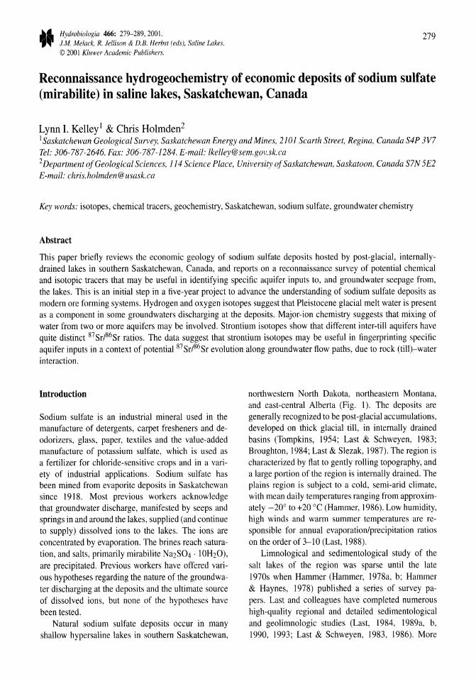
Hydrobiologia 466: 279-289, 2001. J.M. Melack, R. Jellison & D.E. Herbst (eds), Saline Lakes. © 2001 Kluwer Academic Publishers.
279
Reconnaissance hydrogeochemistry of economic deposits of sodium sulfate (mirabilite) in saline lakes, Saskatchewan, Canada
Lynn 1. Kelley! & Chris Holmden2
I Saskatchewan Geological Survey, Saskatchewan Energy and Mines, 2101 Scarth Street, Regina, Canada S4P 3V7 Tel: 306-787-2646. Fax: 306-787-1284. E-mail: [email protected] 2 Department of Geological Sciences, 114 Science Place, University of Saskatchewan, Saskatoon, Canada S7N 5E2 E-mail: [email protected]
Key words: isotopes, chemical tracers, geochemistry, Saskatchewan, sodium sulfate, groundwater chemistry
Abstract
This paper briefly reviews the economic geology of sodium sulfate deposits hosted by post-glacial, internallydrained lakes in southern Saskatchewan, Canada, and reports on a reconnaissance survey of potential chemical and isotopic tracers that may be useful in identifying specific aquifer inputs to, and groundwater seepage from, the lakes. This is an initial step in a five-year project to advance the understanding of sodium sulfate deposits as modem ore forming systems. Hydrogen and oxygen isotopes suggest that Pleistocene glacial melt water is present as a component in some groundwaters discharging at the deposits. Major-ion chemistry suggests that mixing of water from two or more aquifers may be involved. Strontium isotopes show that different inter-till aquifers have quite distinct 87 Sr/86Sr ratios. The data suggest that strontium isotopes may be useful in fingerprinting specific aquifer inputs in a context of potential 87Sr/86Sr evolution along groundwater flow paths, due to rock (till)-water interaction.
Introduction
Sodium sulfate is an industrial mineral used in the manufacture of detergents, carpet fresheners and deodorizers, glass, paper, textiles and the value-added manufacture of potassium sulfate, which is used as a fertilizer for chloride-sensitive crops and in a variety of industrial applications. Sodium sulfate has been mined from evaporite deposits in Saskatchewan since 1918. Most previous workers acknowledge that groundwater discharge, manifested by seeps and springs in and around the lakes, supplied (and continue to supply) dissolved ions to the lakes. The ions are concentrated by evaporation. The brines reach saturation, and salts, primarily mirabilite Na2S04 . lOH20), are precipitated. Previous workers have offered various hypotheses regarding the nature of the groundwater discharging at the deposits and the ultimate source of dissolved ions, but none of the hypotheses have been tested.
Natural sodium sulfate deposits occur in many shallow hypersaline lakes in southern Saskatchewan,
northwestern North Dakota, northeastern Montana, and east-central Alberta (Fig. 1). The deposits are generally recognized to be post-glacial accumulations, developed on thick glacial till, in internally drained basins (Tompkins, 1954; Last & Schweyen, 1983; Broughton, 1984; Last & Slezak, 1987). The region is characterized by flat to gently rolling topography, and a large portion of the region is internally drained. The plains region is subject to a cold, semi-arid climate, with mean daily temperatures ranging from approximately - 20° to +20 °C (Hammer, 1986). Low humidity, high winds and warm summer temperatures are responsible for annual evaporation/precipitation ratios on the order of 3-10 (Last, 1988).
Limnological and sedimentological study of the salt lakes of the region was sparse until the late 1970s when Hammer (Hammer, 1978a, b; Hammer & Haynes, 1978) published a series of survey papers. Last and colleagues have completed numerous high-quality regional and detailed sedimentological and geolimnologic studies (Last, 1984, 1989a, b, 1990, 1993; Last & Schweyen, 1983, 1986). More
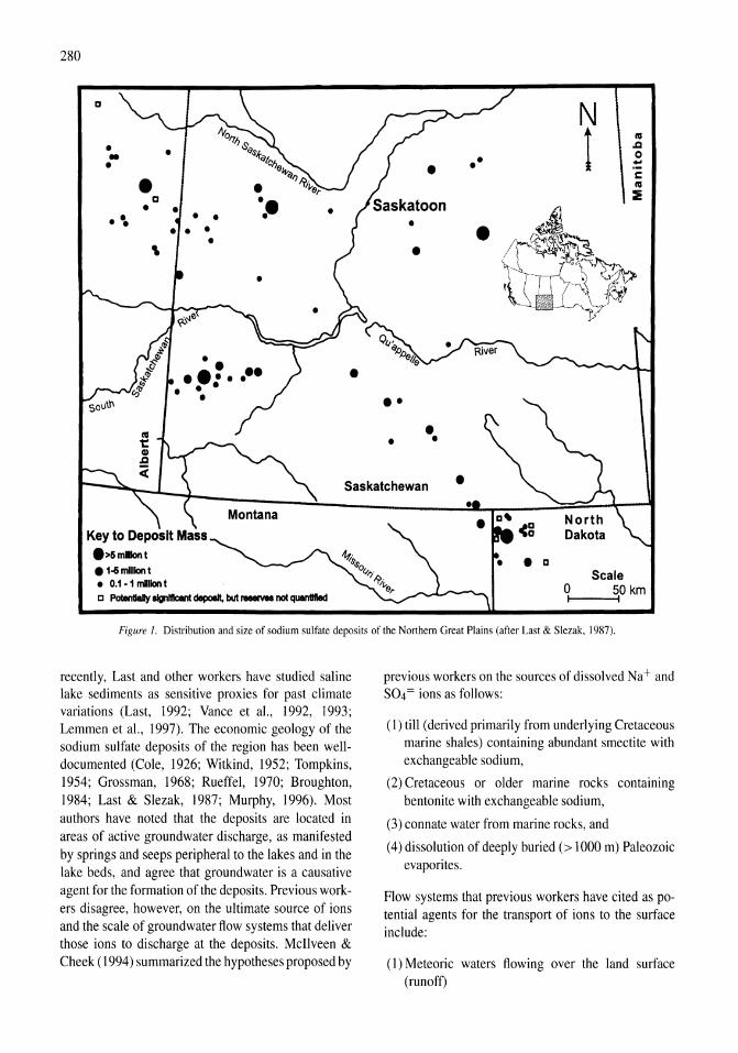
280
a
• -• . \ • a
•
\
•
• •• • •
•
• •
•
•• • • •
••
•
N t
CIS ..c o ...
Saskatchewan • Key to Deposit Mass
.>5mllont • 1-6 million t • 0.1-1 mliiont C PotentIally IIgnIftcant depoeIt, but ___ not quantltled
•
• a Scale
o 50 km I I
Figure 1. Distribution and size of sodium sulfate deposits of the Northern Great Plains (after Last & Slezak. 1987).
recently, Last and other workers have studied saline lake sediments as sensitive proxies for past climate variations (Last, 1992; Vance et aI., 1992, 1993; Lemmen et aI., 1997). The economic geology of the sodium sulfate deposits of the region has been welldocumented (Cole, 1926; Witkind, 1952; Tompkins, 1954; Grossman, 1968; Rueffel, 1970; Broughton, 1984; Last & Slezak, 1987; Murphy, 1996). Most authors have noted that the deposits are located in areas of active groundwater discharge, as manifested by springs and seeps peripheral to the lakes and in the lake beds, and agree that groundwater is a causative agent for the formation of the deposits. Previous workers disagree, however, on the ultimate source of ions and the scale of groundwater flow systems that deliver those ions to discharge at the deposits. McIlveen & Cheek (1994) summarized the hypotheses proposed by
previous workers on the sources of dissolved Na+ and S04= ions as follows:
(1) till (derived primarily from underlying Cretaceous marine shales) containing abundant smectite with exchangeable sodium,
(2) Cretaceous or older marine rocks containing bentonite with exchangeable sodium,
(3) connate water from marine rocks, and
(4) dissolution of deeply buried (> 1 000 m) Paleozoic evaporites.
Flow systems that previous workers have cited as potential agents for the transport of ions to the surface include:
(I) Meteoric waters flowing over the land surface (runoff)
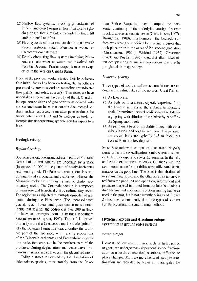
(2) Shallow flow systems, involving groundwater of Recent (meteoric) origin andlor Pleistocene (glacial) origin that circulates through fractured till andlor intertill aquifers
(3) Flow systems of intermediate depth that involve Recent meteoric water, Pleistocene water, or Cretaceous connate water
(4) Deeply-circulating flow systems involving Paleozoic connate water or water that dissolved salt from the Devonian Prairie Evaporite or other evaporites in the Western Canada Basin.
None of the previous workers tested their hypotheses. Our initial focus has been on testing the hypotheses presented by previous workers regarding groundwater flow path(s) and solute source(s). Therefore, we have undertaken a reconnaissance study of the H, 0 and Sr isotope compositions of groundwater associated with six Saskatchewan lakes that contain documented sodium sulfate resources, in an attempt to evaluate the tracer potential of H, 0 and Sr isotopes as tools for isotopically fingerprinting specific aquifer inputs to a lake.
Geologic setting
Regional geology
Southern Saskatchewan and adjacent parts of Montana, North Dakota and Alberta are underlain by a thick (in excess of 1000 m) sequence of nearly-horizontal sedimentary rock. The Paleozoic section consists predominantly of carbonates and evaporites, whereas the Mesozoic rocks are dominantly marine clastic sedimentary rocks. The Cenozoic section is composed of nearshore and terrestrial clastic sedimentary rocks. The region was subjected to multiple episodes of glaciation during the Pleistocene. The unconsolidated glacial, glaciofluvial and glaciolacustrine sediment (drift) that mantles the bedrock is over 300 m thick in places, and averages about 100 m thick in southern Saskatchewan (Simpson, 1997). The drift is derived primarily from the Cretaceous marine shale (principally the Bearpaw Formation) that underlies the southern part of the province, with varying proportions of the Paleozoic carbonates and Precambrian crystalline rocks that crop out in the northern part of the province. During deglaciation, meltwater carved numerous channels and spillways in the glacial sediment.
Collapse structures caused by the dissolution of Paleozoic evaporites, most notably from the Devo-
281
nian Prairie Evaporite, have disrupted the horizontal continuity of the underlying stratigraphy over much of southern Saskatchewan (Christiansen, 1967a; Broughton, 1988). Furthermore, the bedrock surface was strongly modified by riverine erosion that took place prior to the onset of Pleistocene glaciation (Christiansen, 1967b). Witkind (1952), Grossman (1968) and Rueffel (1970) noted that alkali lakes often occupy elongate surface depressions that overlie pre-glacial drainage Valleys.
Economic geology
Three types of sodium sulfate accumulations are recognized in saline lakes of the northern Great Plains.
(1) As lake brine. (2) As beds of intermittent crystal, deposited from
the brine in autumn as the ambient temperature cools. Intermittent crystal re-dissolves the following spring with dilution of the brine by runoff by the Spring snow-melt.
(3) As permanent beds of mirabilite mixed with other salts, clastics, and organic sediment. The permanent crystal beds are typically 1-5 m thick, but exceed 30 m in a few deposits.
Most Saskatchewan companies that mine Na2S04 pump brine into crystallization ponds, where it is concentrated by evaporation over the summer. In the fall, as the ambient temperature cools, Glauber's salt (the commercial name for mirabilite) crystallizes and accumulates on the pond liner. The pond is then drained of any remaining liquid, and the Glauber's salt is harvested from the pond. At one operation, intermittent and permanent crystal is mined from the lake bed using a dredge-mounted excavator. Solution mining has been tried in the past, but is not currently being used. Figure 2 illustrates schematically the three types of sodium sulfate accumulations and mining methods.
Hydrogen, oxygen and strontium isotope systematics in groundwater systems
Water isotopes
Elements of low atomic mass, such as hydrogen or oxygen, can undergo mass-dependent isotope fractionation as a result of chemical reactions, diffusion or phase changes. Multiple increments of isotopic fractionation are recorded by water as it navigates the
282
Brine Lake + ~ Intermittent
~"-+"---;,~~ Crystal Bed
+----Permanent Drying Crystal Bed
NOT TO SCALE
AnhYdrols sodium sulfate
Figure 2. Schematic cross-section of idealized Saskatchewan sodium sulfate deposit. Mining methods illustrated are: (I) Evaporative concentration of lake brine in crystallization pond, followed by precipitation of crystals of Glauber's salt (mirabilite) as the brine cools in autumn; (2) Solution mining of thick crystal beds. The brine return is treated as in I; and (3) Dredging of lake bottom crystal beds.
Earth's meteoric water cycle. Therefore, continental surface waters and groundwaters exhibit isotope compositions indicative of water source and history of movements in the global water cycle. The isotopic composition of water changes with evaporation, condensation, freezing, thawing, sublimation, reaction with hydrous minerals and mixing with other waters.
Oxygen and hydrogen isotopes are measured as isotope abundance ratios (80/160, DIH), and reported as 8180 and 8D, defined as:
8 I 80sample= { [(80/160)sample/
cI80/160)SMow]-I}.1000%0
The 8180 value represents the permil (%0) enrichment or depletion of 180 in the sample relative to Standard Mean Ocean Water (SMOW). For example, a sample with 8180 = -25%0 contains 25 parts-per-thousand (or 2.5%) less 180 than standard mean ocean water. The convention for hydrogen is identical, with D eH) taking the place of 180 and H (I H) taking the place of 160 (for reviews, see Kendall & Caldwell, 1998 and Clark & Fritz, 1997).
Strontium isotopes
Although the relative mass differences between the four isotopes of Sr are too small to exhibit natural mass dependent isotope variation, one isotope, 87 Sr, varies in abundance relative to the other isotopes of Sr because it is the natural radioactive decay product of 87Rb. By convention, differences in 87 Sr abundance are reported as the ratio 87 Sr/86Sr. Old crustal rocks have typically high 87Srl86Sr ratios, whereas younger crustal rocks, and marine carbonates, have lower 87Sr/86Sr ratios. Strontium readily dissolves in aqueous solutions, following calcium in geochemical behavior. Strontium isotopes (87Sr/86Sr) are generally conservative in mixing of waters in lakes or estuaries. In surface waters, strontium concentration may be changed by precipitation or dissolution of calcite, gypsum or other Sr-containing minerals, but the 87 Sr/86Sr ratio is not affected by these reactions. This is in contrast to Hand 0 isotopes, which are often non-conservative in mixing of surface waters due to evaporation effects causing enrichment of the residual water in D and 180.
In groundwater systems dissolved Sr is less conservative than Hand 0 isotopes, due to Sr-exchange between rocks and water along the flow path. The degree of non-conservative behavior is a function of the groundwater velocity and rock type. In general, faster moving groundwater is more conservative for Sr isotopes than slower moving groundwater, the latter undergoing more exchange of strontium with minerals in the rocks. Therefore, the isotopic composition of dissolved Sr in a slow moving groundwater will evolve towards a 87Sr/86Sr ratio that is similar to the rock (Bullen & Kendall, 1998; Bullen et aI., 1996; Johnson & DePaolo, 1997a, b).
Methods
Field methods
During 1998, we sampled groundwater from seeps, discrete spring orifices, and shallow wells in the immediate vicinity of four saline lakes (Vincent, Corral, Boot and Chain) that host documented sodium sulfate resources. In 1999, we sampled groundwater and lake brine at three ofthe lakes sampled during 1998 (Vincent, Corral, Chain) and two additional lakes (Grandora N., Whiteshore). The lakes that were sampled are shown in Figure 3.
Water samples were filtered in the field using 0.45 11m filters and stored in acid-cleaned 250 ml highdensity polyethylene (HDPE) bottles. The samples were split, and one aliquot was acidified to pH=2. Alkalinity, major anions, 8D and 8180 were determined on the non-acidified sample, whereas 87Sr/86Sr and major cations were determined on the acidified sample. Specific gravity, temperature, and pH were measured at each sampling event.
The well samples are generally from depths of 5-30 m in domestic or stock (mostly flowing) wells within a few hundred meters of the respective lake. Exceptions include a municipal well that is "-'50 m deep at Chain Lake, which samples an intertill aquifer; and two wells that are approximately 150 m deep at Whiteshore Lake. Both White shore wells sample the Judith River Formation, an upper Cretaceous aquifer with good water quality. The spring samples are from springs or seeps that discharge near the lakeshore, generally at or above lake level. The discharge water immediately mixes with the lake brine.
Lake brines were sampled in locations remote from springs and seeps. Where more than one sample
283
was collected from a lake (Vincent, Grandora, and Whiteshore), the sampling locations are up to several kilometers apart, in order to capture any compositional heterogeneity.
Laboratory methods
The 0 isotope composition of water was analyzed using the C02-H20 equilibration method of Epstein & Mayeda (1953) using an equilibrium isotope fractionation factor of 1.0412. Hydrogen isotope analyses were performed by the V-reduction methods of Bigeleisen et al. (1952). Hand 0 isotope analyses were performed on a Finnigan MAT Delta E, gas isotope-ratio mass spectrometer. External precision is based on the reproducibility of our internal water standard over the course of this work, and is better than ±2%0 (10-) for 80, and 0.2%0 (10-) for 8180.
Strontium was purified from the solution using standard cation exchange chromatograpy in a clean lab environment. Purified Sr was loaded onto a single Re filament with Ta-gel and measured using a multidynamic peak-hopping routine on a Finnigan MAT 261 thermal ionization mass spectrometer. The 87 Sr/86Sr ratios were normalized to 88Sr/86Sr = 8.375209. External precision is ±0.00002 (20-), based on multiple analysis of the SRM 987 SrC03 standard which yielded 0.71026 during the course of this study.
Major element concentrations were performed by ICP-AES at the Saskatchewan Research Council with external precision typically ± 10% (20-).
Evaluation of tracer potential
Water isotopes
Field and analytical results for all samples collected in this study are summarized in Table 1. Hydrogen and oxygen isotope results for groundwater sampled from springs, seeps and shallow wells near sodium sulfate deposits ranged from approximately -145%0 to -170%0 for 80 and from -15%0 to -20%0 for 8180 (Fig. 4). These data are similar to the range reported for shallow Saskatchewan groundwater by McMonagle (1987) and very depleted of D and 180 compared to the data from deeper saline Paleozoic aquifers reported by Rostron et al. (1998). The data fall between the averages for Saskatchewan meteoric water (8D ~ -138%0 and 8180 ~ -17%0 (McMonagle, 1987)) and a component of porewater in the glacial till that was last recharged during the
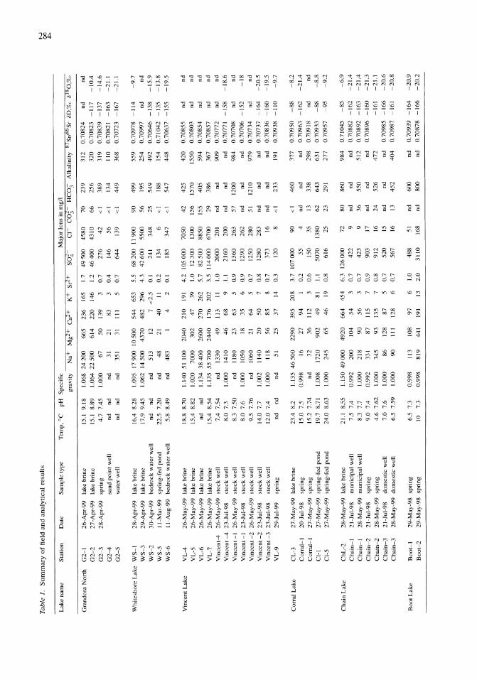
Tab
le 1
. S
um
mar
y o
f fi
eld
and
anal
ytic
al r
esul
ts
Lak
e n
ame
Sta
tion
D
ate
Sam
ple
type
Gra
ndor
a N
ort
h
G2
-I
G2
-2
G2
-3
G2
-4
G2
-5
26-A
pr-9
9 la
ke b
rine
27
-Apr
-99
lake
bri
ne
28-A
pr-9
9 sp
ring
sa
nd
poi
nt w
ell
wat
er w
ell
Whi
tesh
ore
Lak
e W
S-I
W
S-3
W
S-2
W
S-5
W
S-6
28-A
pr-9
9 la
ke b
rine
29
-Apr
-99
lake
bri
ne
30-A
pr-9
9 be
droc
k w
ater
wel
l ll
-Mar
-99
sp
ring
-fed
po
nd
ll
-Au
g-9
9
bedr
ock
wat
er w
ell
Vin
cent
Lak
e
Cor
ral
Lak
e
Ch
ain
Lak
e
Boo
t Lak
e
VL
-4
26-M
ay-9
9 la
ke b
rine
V
L-5
26
-May
-99
lake
bri
ne
VL
-6
26-M
ay-9
9 la
ke b
rine
V
L-7
26
-May
-99
lake
bri
ne
Vin
cent
-4
26-M
ay-9
9 st
ock
wen
V
ince
nt -
4
23-J
ul-9
8 st
ock
wel
l
Vin
cent
-I
26-M
ay-9
9 st
ock
wel
l V
ince
nt -
I 23
-Jul
-98
stoc
k w
ell
Vin
cen
t-2
26
-May
-99
stoc
k w
ell
Vin
cent
-2
23
-Jul
-98
stoc
k w
ell
Vin
cent
-3
23
-Jul
-98
stoc
k w
ell
VL
-9
29-J
ul-9
9 sp
ring
CL
-3
Co
rral
-I
Co
rral
-I
CI-
I C
I-5
Ch
L-2
C
hai
n-I
C
hai
n-I
C
hai
n-2
C
hai
n-2
C
hai
n-3
C
hai
n-3
Bo
ot-
I B
oo
t-2
27-M
ay-9
9 la
ke b
rine
20
-JuI
-98
spri
ng
27-M
ay-9
9 sp
ring
27
-May
-99
spri
ng-f
ed p
on
d
27-M
ay-9
9 sp
ring
-fed
po
nd
28-M
ay-9
9 la
ke b
rine
21
-Jul
-98
mun
icip
al w
ell
28-M
ay-9
9 m
unic
ipal
wel
l 21
-JuI
-98
spri
ng
28-M
ay-9
9 sp
ring
21
-JuI
-98
dom
esti
c w
ell
28-M
ay-9
9 do
mes
tic
wel
l
29-M
ay-9
8 sp
ring
29
-May
-98
spri
ng
Tem
p, °
C
pH
S
peci
fic
Maj
or
Ions
in
mg/
l
grav
ity
Na+
M
g2
+
Ca2
+
K+
s1
2+
SO
i C
I CO~
HC
03
Alk
alin
ity
87S
r/86
Sr
80,%
0 8
180,
%0
15.1
9.
18
15.1
8.
89
4.7
7.45
n
d
nd
nd
nd
16.4
8.
28
17.9
9.
45
nd
nd
22
.5
7.2
0
5.8
8.49
18.8
8.
70
15.4
8.
82
nd
n
d
15.4
8.
54
7.4
7.
54
8.0
7.3
8.3
7.50
8.
0 7.
6 9.
5 7.
76
14.0
7.
7 12
.0
7.4
nd
nd
23.4
8.
2 15
.0
7.5
15.2
7.
74
19.7
8.
71
24.0
8.
63
21.1
8.
55
7.5
7.4
8.3
7.7
9.0
7.
4 4.
6 7.
62
7.0
7.
6 6.
5 7.
59
6.5
7.3
10
7.3
1.06
8 2
4 2
00
1.
064
22 5
00
1.
000
67
n
d
31
nd
351
665
61
4
50
21
31
1.09
5 17
90
0
10 5
00
1.
062
14
50
0
43
70
nd
n
d
513
48
nd
4
83
1.14
0 51
100
1.
020
70
00
1.
134
38
40
0
1.13
5 5
57
00
n
d
1330
1.
000
1410
nd
11
80
1.00
0 10
50
nd
1060
1.
002
1140
1.
000
118
nd
51
1.13
5 4
65
00
0.
998
16
nd
32
1.
008
1720
1.
000
245
1.15
0 4
90
00
0.
992
20
0
1.00
0 2
18
0.
992
331
1.00
0 34
5 1.
000
86
1.00
0 9
0
12
21
20
40
3
02
2
60
0
24
40
49
4
6
23
18
21
20
56
25
22
90
27
3
6
90
2
65
49
20
10
4 9
0
87
93
12
8 II
I
23
6
165
22
0
146
139
3 83
3
111
5
54
4
653
48
2
29
6
7 <
2.5
4
0
11
4 2
21
0
191
47
39
27
0
262
176
20
2
113
11
68
9
63
5 35
6
64
5
50
7
85
8 37
14
395
20
8
94
1
112
3 4
9
81
46
19
66
4
45
4
54
3
56
3
115
7 13
5 7
87
5 12
8 6
1.7
49
50
0
1.2
46
40
0
0.7
27
6
0.4
146
0.7
64
4
45
80
4
31
0
42
56
13
9
5.5
68
20
0
11 9
00
4.
3 4
26
00
55
00
0.1
0.2
0.1
241
134
185
4.2
10
50
00
1.
0 1
23
00
5.
7 8
25
00
3.
5 1
14
00
0
1.0
20
00
1.
1 2
16
0
0.9
13
60
0.9
1290
0.
7 12
50
0.8
1280
0.
7 37
3 0.
3 12
0
3.7
10
70
00
0.2
55
0
.6
150
1.1
50
70
0.
8 6
16
6.3
12
60
00
0.
7 4
22
0.
7 42
3 0.
9 9
03
0.
8 9
12
0.
7 5
20
0.
7 56
7
348 6
347
7050
1300
88
50
6700
20
1 2
00
26
3 26
2 28
0 28
3 16 8
90
4 35
13
80
25
72
9 9 17
16
15
16
0.99
8 0.
998
113
819
108
97
6
1.0
48
8
3110
51
16
8 44
1 19
1 13
2.
0
70
6
6
<1
<1
<
1
90
5
6
25
<1
<
1 42
156
155
29
n
d
nd
57
n
d
51
nd
n
d
<I
<1 nd
13
6
2
23
80
nd
36
nd
24
n
d
13
nd
n
d
23
9
25
6
38
9
134
44
9
49
9
195
54
9
188
54
7
42
5
1570
4
05
3
86
n
d
nd
12
00
nd
12
10
nd
n
d
233
46
0
nd
338
643
291
86
0
nd
55
0
nd
52
6
nd
4
52
60
0
80
0
312
0.70
824
nd
32
0
0.70
823
-11
7
31
9
0.70
839
-13
7
110
0.70
821
-16
3
368
0.70
723
-16
7
559
25
4
49
2
154
44
8
42
0
1550
5
94
36
7 9
09
nd
9
84
n
d
97
9
nd
n
d
191
0.70
978
-11
4
0.70
997
nd
0.70
646
-13
8
0.71
042
-13
5
0.70
637
-15
5
0.70
855
nd
0.70
803
nd
0.7
08
54
nd
0.70
857
nd
0.70
772
nd
0.70
771
-15
8
0.70
708
nd
0.70
706
-15
2
0.70
734
nd
0.70
737
-16
4
0.70
836
-16
0
0.70
938
-11
0
377
0.70
950
-88
n
d
0.70
963
-16
2
29
8
0.70
918
nd
631
0.70
933
-88
27
7 0.
7095
7 -9
5
98
4
0.71
045
-85
nd
0.
7088
2 -1
62
5
12
0.
7089
2 -1
63
nd
0.
7089
6 -1
60
4
72
-1
61
n
d
0.70
985
-16
6
40
4
0.70
987
-16
1
nd
-1
0.4
-14
.6
-21
.1
-21
.1
-9.7
nd
-1
5.9
-1
3.8
-1
9.5
nd
nd
nd
nd
nd
-1
8.6
nd
-1
8
nd
-2
0.5
-1
9.5
-9
.7
-8.2
-2
1.4
n
d
-8.8
-9
.2
-6.9
-2
1.4
-2
1.4
-2
1.3
-2
1.1
-2
0.6
-2
0.8
nd
0.
7093
9 -1
64
-2
0.9
nd
0.
7087
8 -1
66
-2
0.2
N
00
.j:
:>.
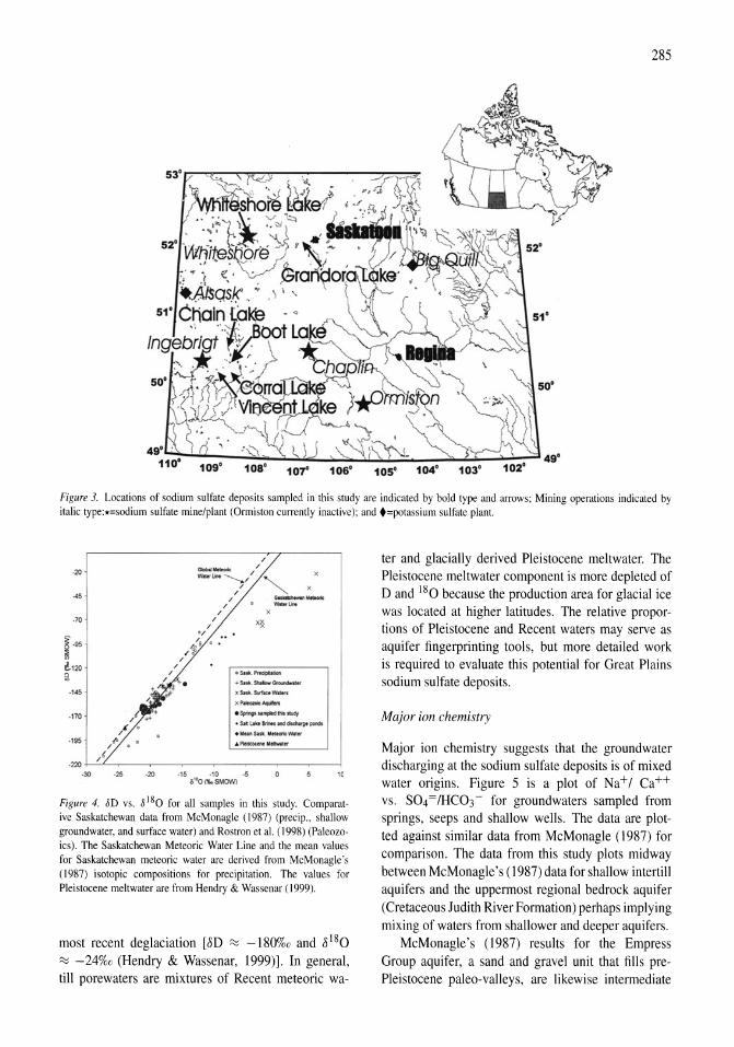
285
107" 106· 105·
Figure 3. Locations of sodium sulfate deposits sampled in this study are indicated by bold type and arrows; Mining operations indicated by italic type:*=sodium sulfate mine/plant (Ormiston currently inactive); and +=potassium sulfate plant.
--_ .... ·20
.. ~ / /
/
·10 I /
1.95
e120 It
·14,$
.170
·195
·220 -30 ·20
/ /
/ X /
/ / --,..""
X
x*
19$Hk.~
"' 5HII.5JIBoow~1"
x SIIILSVfac.w.w. x __
. Spo"nr ... "JfIItd~~
. SlIUb""'a8d~pcrdI
. .... SltIt. WttNtcWllw
. PW«6ctMMMwM.
10
Figure 4. 8D vs. 8180 for all samples in this study. Comparative Saskatchewan data from McMonagle (1987) (precip., shallow groundwater, and surface water) and Rostron et a1. (1998) (Paleozoics). The Saskatchewan Meteoric Water Line and the mean values for Saskatchewan meteoric water are derived from McMonagle's (1987) isotopic compositions for precipitation. The values for Pleistocene meltwater are from Hendry & Wassenar (1999).
most recent deglaciation [8D ~ -180%0 and 8180 ~ -24%0 (Hendry & Wassenar, 1999)]. In general, till porewaters are mixtures of Recent meteoric wa-
ter and glacially derived Pleistocene meltwater. The Pleistocene meltwater component is more depleted of D and 180 because the production area for glacial ice was located at higher latitudes. The relative proportions of Pleistocene and Recent waters may serve as aquifer fingerprinting tools, but more detailed work is required to evaluate this potential for Great Plains sodium sulfate deposits.
Major ion chemistry
Major ion chemistry suggests that the groundwater discharging at the sodium sulfate deposits is of mixed water origins. Figure 5 is a plot of Na+j Ca++ vs. S04 = !HC03 - for groundwaters sampled from springs, seeps and shallow wells. The data are plotted against similar data from McMonagle (1987) for comparison. The data from this study plots midway between McMonagle's (1987) data for shallow intertill aquifers and the uppermost regional bedrock aquifer (Cretaceous Judith River Formation) perhaps implying mixing of waters from shallower and deeper aquifers.
McMonagle's (1987) results for the Empress Group aquifer, a sand and gravel unit that fills prePleistocene paleo-valleys, are likewise intermediate
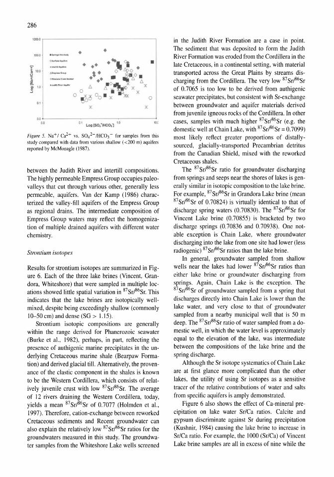
286
10000
1000 .~I II'tI __ • • 0 __
• I '00 ._-¥ o. ... _c~ ......... ;>;.
........ fIIww ......
8' 10
-' 0 o
01
00 00 0 1 Log[SO:IHCO,l .0
10,
Figure 5. Na+; Ca2+ vs. S042-IHC03- for samples from this study compared with data from various shallow «200 m) aquifers reported by McMonagle (1987).
between the Judith River and intertill compositions. The highly permeable Empress Group occupies paleovalleys that cut through various other, generally less permeable, aquifers. Van der Kamp (1986) characterized the valley-fill aquifers of the Empress Group as regional drains. The intermediate composition of Empress Group waters may reflect the homogenization of multiple drained aquifers with different water chemistry.
Strontium isotopes
Results for strontium isotopes are summarized in Figure 6. Each of the three lake brines (Vincent, Grandora, Whiteshore) that were sampled in multiple locations showed little spatial variation in 87 Sr/86Sr. This indicates that the lake brines are isotopically wellmixed, despite being exceedingly shallow (commonly 10-50 cm) and dense (SG > 1.15).
Strontium isotopic compositions are generally within the range derived for Phanerozoic seawater (Burke et al., 1982), perhaps, in part, reflecting the presence of authigenic marine precipitates in the underlying Cretaceous marine shale (Bearpaw Formation) and derived glacial till. Alternatively, the provenance of the clastic component in the shales is known to be the Western Cordillera, which consists of relatively juvenile crust with low 87 Sr/86Sr. The average of 12 rivers draining the Western Cordillera, today, yields a mean 87Sr/86Sr of 0.7077 (Holmden et aI., 1997). Therefore, cation-exchange between reworked Cretaceous sediments and Recent groundwater can also explain the relatively low 87 Sr/86 Sr ratios for the ground waters measured in this study. The groundwater samples from the White shore Lake wells screened
in the Judith River Formation are a case in point. The sediment that was deposited to form the Judith River Formation was eroded from the Cordillera in the late Cretaceous, in a continental setting, with material transported across the Great Plains by streams discharging from the Cordillera. The very low 87 Sr/86Sr of 0.7065 is too low to be derived from authigenic seawater precipitates, but consistent with Sr-exchange between groundwater and aquifer materials derived from juvenile igneous rocks of the Cordillera. In other cases, samples with much higher 87Sr/86Sr (e.g. the domestic well at Chain Lake, with 87Sr/86Sr = 0.7099) most likely reflect greater proportions of distallysourced, glacially-transported Precambrian detritus from the Canadian Shield, mixed with the reworked Cretaceous shales.
The 87 Sr/86Sr ratio for groundwater discharging from springs and seeps near the shores of lakes is generally similar in isotopic composition to the lake brine. For example, 87Sr/86Sr in Grandora Lake brine (mean 87Sr/86Sr of 0.70824) is virtually identical to that of discharge spring waters (0.70830). The 87Sr/86Sr for Vincent Lake brine (0.70855) is bracketed by two discharge springs (0.70836 and 0.70938). One notable exception is Chain Lake, where groundwater discharging into the lake from one site had lower (less radiogenic) 87Sr/86Sr ratios than the lake brine.
In general, groundwater sampled from shallow wells near the lakes had lower 87Sr/86Sr ratios than either lake brine or groundwater discharging from springs. Again, Chain Lake is the exception. The 87Sr/86Sr of groundwater sampled from a spring that discharges directly into Chain Lake is lower than the lake water, and very close to that of groundwater sampled from a nearby municipal well that is 50 m deep. The 87Sr/86Sr ratio of water sampled from a domestic well, in which the water level is approximately equal to the elevation of the lake, was intermediate between the compositions of the lake brine and the spring discharge.
Although the Sr isotope systematics of Chain Lake are at first glance more complicated than the other lakes, the utility of using Sr isotopes as a sensitive tracer of the relative contributions of water and salts from specific aquifers is amply demonstrated.
Figure 6 also shows the effect of Ca-mineral precipitation on lake water Sr/Ca ratios. Calcite and gypsum discriminate against Sr during precipitation (Kushnir, 1984) causing the lake brine to increase in Sr/Ca ratio. For example, the 1000 (Sr/Ca) of Vincent Lake brine samples are all in excess of nine while the
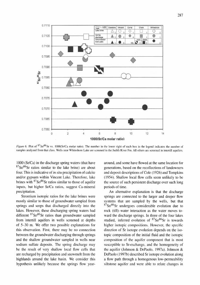
287
07110
0.7105
0.7100
07095
07090 .. (/)
~ 07085 (/) .... eo
0.7080
• • 0.7075
0.7070
0.7065
07060
0 2 4 6 8 10 12 14
1000{Sr/Ca molar ratio)
Figure 6. Plot of 87Sr/86Sr vs. lOOO(Sr/Ca molar ratio). The number in the lower right of each box in the legend indicates the number of samples analyzed from that class. Wells near Whiteshore Lake are screened in the Judith River Fm. All others are screened in intertill aquifers.
1000 (Sr/Ca) in the discharge spring waters (that have 87 Sr/86Sr ratios similar to the lake brine) are about four. This is indicative of in situ precipitation of calcite and/or gypsum within Vincent Lake. Therefore, lake brines with 87Sr/86Sr ratios similar to those of aquifer inputs, but higher Sr/Ca ratios, suggest Ca-mineral precipitation.
Strontium isotopic ratios for the lake brines were mostly similar to those of groundwater sampled from springs and seeps that discharged directly into the lakes. However, these discharging spring waters had different 87Sr/86Sr ratios than groundwater sampled from intertill aquifers in wells screened at depths of 5-30 m. We offer two possible explanations for this observation. First, there may be no connection between the groundwater discharging through springs and the shallow groundwater sampled in wells near sodium sulfate deposits. The spring discharge may be the result of very shallow local flow cells that are recharged by precipitation and snowmelt from the highlands around the lake basin. We consider this hypothesis unlikely because the springs flow year-
around, and some have flowed at the same location for generations, based on the recollections of landowners and deposit descriptions of Cole (1926) and Tompkins (1954). Shallow local flow cells seem unlikely to be the source of such persistent discharge over such long periods of time.
An alternative explanation is that the discharge springs are connected to the larger and deeper flow systems that are sampled by the wells, but that 87 Sr/86Sr undergoes considerable evolution due to rock (till)-water interaction as the water moves toward the discharge springs. In three of the four lakes studied, inferred evolution of 87Sr/86Sr is towards
higher isotopic compositions. However, the specific direction of Sr isotope evolution depends on the isotopic composition of the initial fluid and the isotopic composition of the aquifer component that is most susceptible to Sr-exchange, and the homogeneity of the aquifer (Johnson & DePaolo, 1997a). Johnson & DePaolo (1997b) described Sr isotope evolution along a flow path through a homogenous low-permeability siltstone aquifer and were able to relate changes in

288
87 Sr/86Sr to fluid flow rates, and identify preferential fluid flow paths.
The large variations seen thus far in Sr isotope compositions of saline lakes, and associated springs and groundwater indicates that there is sufficient isotopic sensitivity to be of use in constructing water balances in these lakes. For example, we know that the Sr isotope balance of Chain Lake is incomplete in that the lake has a higher Sr isotope composition (0.7104) than any of the groundwaters (0.7088-0.7099) or discharge springs (0.7090) that we have measured, thus far. Clearly, there is another aquifer input of Sr to this lake that we have not identified. Furthermore, Sr isotopes appear to be a powerful tool for elucidation of the mechanisms controlling till-water Sr isotope interactions, which in tum may improve our understanding of how groundwaters evolve towards the Na-S04 compositions needed to form a Na2S04-dominated evaporite deposit in a c1osed-basinlake.
Conclusions
Sodium sulfate deposits of the northern Great Plains continue to be supplied with dissolved ions via groundwater discharge. The net rate of salt accumulation in these modem ore-forming systems is related to fluid and solute mass balances. The geochemical tracers investigated in this reconnaissance study will be tested in more detailed hydrogeological investigations of individual deposits.
The water isotope data suggests that there are subtle isotopic differences in H and 0 isotopes that could be useful for discriminating aquifers with a substantial component of seasonally recharged water from aquifers that carry older, more evolved waters, or those that have a component of Pleistocene glacial melt water.
Comparison of ion ratios for data from this study with data of McMonagle (1987) suggests that groundwater sampled from springs and seeps near sodium sulfate deposits may be at least partly from a bedrock source, perhaps mixed with shallower groundwater during ascent.
Strontium isotopes hold the greatest promise for fingerprinting aquifer inputs to the saline lake basins that host sodium sulfate deposits. 87 Sr/86Sr ratios must be examined in the context of flow-path evolution, constrained by physical hydrogeology, to be ultimately useful in identifying solute source(s), elucidating till-water evolution of the major cations (Na,
Ca), and quantifying aquifer input(s) to the lake basins that host sodium sulfate deposits.
References
Bigeleisen, J., M. L. Perlman & H. C. Prosser, 1952. Conversion of hydrogenic materials to hydrogen for isotopic analysis. Anal. Chern. 24: 1356-1357.
Broughton, P. L., 1984. Sodium sulphate deposits of western Canada. In Guillet, G. R. & W. Martin (eds), The Geology ofIndustrial Minerals in Canada. Can. Inst. Min. Met. Special Volume 29: 195-200.
Broughton, P. L., 1988. Formation of Tertiary coal basins in southern Saskatchewan. Sask. Energy Mines, Open File Rep. 88-1: 53 pp.
Bullen, 1. D. & C. Kendall, 1998. Tracing of weathering reactions and water flowpaths: a mUlti-isotope approach. In Kendall, C. & J. J. McDonnell (eds), Isotope Tracers in Catchment Hydrology. Elsevier Science B.V, Amsterdam: 611-646.
Bullen, 1. D., D. P. Krabbenhoft & C. Kendall, 1996. Kinetic and mineralogic controls on the evolution of groundwater chemistry and 87Sr/86Sr in a sandy silicate aquifer, northern Wisconsin, U.S.A. Geochim. Cosmochim. Acta. 10: 1807-1821.
Burke, W. H., E. A. Denison, R. B. Hetherington, R. B. Koepnick, H. F. Nelson & J. B. Otto. 1982. Variation of seawater 87 Sr/86Sr ratio throughout Phanerozoic time. Geology 10: 516-519.
Christiansen, E. A., 1967a. Collapse structures near Saskatoon, Saskatchewan, Canada. Can. J. Earth Sci. 4: 757-766.
Christiansen, E. A., 1967b. Preglacial valleys in southern Saskatchewan;. Sask. Resear. Counc., Map 3, Scale I: 1500000.
Clark, I. & P. Fritz, 1997. Environmental Isotopes in Hydrogeology. Lewis Publishers, Boca Raton: 328 pp.
Cole, L. H., 1926. Sodium sulphate of western Canada: Occurrence, uses, and technology. Canada Department of Mines, Report 646, Ottawa: 160 pp.
Epstein, S. & 1. K. Mayeda, 1953. Variations of the 18 0/160 ratio in natural waters. Geochim. Cosmochim. Acta. 4: 213.
Grossman, l. G., 1968. Origin of the sodium sulfate deposits of the northern Great Plains of Canada and the United States. Prof. Pap. 600-B: B 104-B 109.
Hammer, U. 1., 1978a. The saline lakes of Saskatchewan. I. Background and rationale for saline lakes research. Int. Rev. ges. Hydrobiol. 63(2): 173-177.
Hammer, U. 1., I 978b. The saline lakes ofSasktachewan III. Chemical characterization. Int. Rev. ges. Hydrobiol. 63: 311-335.
Hammer, U.T., 1986. Saline Ecosystems of the World. Monographiae Biologicae, 59. Dr W. Junk Publishers, Dordrecht: 616 pp.
Hammer, U. 1. & R. C. Haynes, 1978. The saline lakes of Saskatchewan II. Locale, hydrography and other physical aspects. Int. Rev. ges. Hydrobiol. 63: 179-203.
Hendry, M. J. & L. I. Wassenar, 1999. Implications for transport of 8D in porewaters for groundwater flow and the timing of geologic events in a thick aquitard system. Wat. Resour. Res. 35: 1751-1760.
Holmden, C., K. Muehlenbachs & R. A. Creaser, 1997. Depositional environment of the early Cretaceous Ostracode Zone: Paleohydrologic constraints from 0, C and Sr isotopes. In Pemberton, S. G. & D. P. James (eds), Petroleum Geology of the Cretaceous Mannville Group, Western Canada. Memoir. Canadian Society of Petroleum Geologists, Calgary: 77-92.
Johnson, T M. & D. 1. DePaolo. 1997a. Rapid exchange effects on isotope ratios in groundwater systems I. Development of a transport-dissolution-exchange model. Wat. Resour. Res. 33(1): 187-195.
Johnson, T M. & D. J. DePaolo, I 997b. Rapid exchange effects on isotope ratios in groundwater systems 2. flow investigation using Sr isotope ratios. Wat. Resour. Res. 33(1): 197-209.
Kendall, C & E. A. Caldwell, 1998. Fundamentals of isotope geochemistry. In Kendall, C & J. 1. McDonnell (eds), Isotope Tracers in Catchment Hydrology. Elsevier Science, Amsterdam: 51-86.
Kushnir, K., 1984. The co-precipitation of strontium, magnesium, sodium, potassium and chloride ions with gypsum: an experimental study. Geochim. Cosmochim. Acta. 44: 1471-1482.
Last, W. M., 1984. Sedimentology of playa lakes of the northern Great Plains. Can. J. Earth Sci. 21: 107-125.
Last, W. M., 1988. Salt lakes of western Canada: a spatial and temporal geochemical perspective. In Nicholaichuk, W. & H. Steppuhn (eds), Proceeding of the Symposium on Water Management Affecting the Wet-to-Dry Transition: Planning at the Margins. Water Studies Institute. University of Regina, Regina: 99-113.
Last, W. M., 1989a. Continental brines and evaporites of the northern Great Plains of Canada. Sedimentary Geology 64: 207-221.
Last, W. M., 1989b. Sedimentology of a saline playa in the northern Great Plains, Canada. Sedimentology 36: 109-123.
Last, W. M., 1990. Paleochemistry and paleohydrology of Ceylon Lake, a salt-dominated playa basin in the northern Great Plains, Canada. 1. Paleolimnol. 4: 219-238.
Last, W. M., 1992. Salt lake paleolimnology in the northern Great Plains: the facts, the fears, the future. In Robarts, R. D. & M. L. Bothwell (eds), Aquatic Ecosystems in Semi-arid Regions: Implications for Resource Management. National Hydrology Research Institute Symposium. Environment Canada. Saskatoon: 51-62.
Last, W. M., 1993. Geolimnology of Freefight Lake: an unusual hypersaline lake in the northern Great Plains of western Canada. Sedimentology 40: 431-448.
Last, W. M. & T H. Schweyen, 1983. Sedimentology and geochemistry of saline lakes of the Great Plains. Hydrobiologia 105: 245-263.
Last. W. M. & L. A. Slezak, 1986. Paleohydrology, sedimentology and geochemistry of two meromictic lakes in southern Saskatchewan. Geographie physique et Quaternaire. 40(1): 5-15.
289
Last. W. M. & L. A. Slezak, 1987. Sodium sulphate deposits of western Canada: Geology, mineralogy and origin. In Gilboy, C. F. & L. W. Vigrass (eds), Economic Minerals of Saskatchewan. Saskatchewan Geological Society, Special Publication 8. Regina: 197-205.
Lemmen, D. S., R. E. Vance, S. A. Wolfe & W. M. Last, 1997. Impacts offuture climate change on the southern Canadian prairies: a paleoenvironmental perspective. Geoscience Canada 24(3): 121-133.
McIlveen, S. & R. L. Cheek, 1994. Sodium sulfate resources. In Carr, D. D. (ed.), Industrial Minerals and Rocks, 6th edn. Soc. Mining. Metal. Explor: 1129-1158.
McMonagle, A. L.. 1987. Stable isotope and chemical compositions of surface and subsurface waters in Saskatchewan. M. Sc. Thesis. University of Saskatchewan, Saskatoon: 108 pp.
Murphy, E. C, 1996. The sodium sulfate deposits of northwestern North Dakota. North Dakota Geological Survey. Report 99: 73 pp.
Rostron, B. 1., C Holmden & L. K. Kreis. 1998. Hydrogen and oxygen isotope compositions of Cambrian to Devonian formation waters, Midale area, Saskatchewan, Proceedings, 8th International Williston Basin Symposium. Sask. Saskatchewan Geo!. Soc., Spec. Pub!. 13: 267-273.
Rueffel, P. G .. 1970. Natural sodium sulfate in North America, 3rd Symposium on Salt. Northern Ohio Geological Society. Columbus: 429-451.
Simpson. M. A .. 1997. Surficial Geology Map of Saskatchewan. Sask. Energy Mines/Sask. Resear. Coune., scale 1:1 000000.
Tompkins, R. V, 1954. Natural sodium sulphate in Saskatchewan. Sask. Dep. Miner. Resour .. Report 6: 71 pp.
Van der Kamp. G.. 1986. The groundwater resources of Saskatchewan's deep buried-valley aquifers, Canadian Hydrology Symposium No 16, Regina: 529-543.
Vance, R. E., 1. J. Clague & R. W. Matthewes. 1993. Holocene paleohydrology of a hypersaline lake in southeastern Alberta. 1. Paleolimnol. 8: 103-120.
Vance, R. E .. R. W. Matthewes & 1. 1. Clague. 1992. 7000 year record oflake-Ievel change on the northern Great Plains: A highresolution proxy of past climate. Geology 20: 879-882.
Witkind, I., 1952. The localization of sodium sulfate deposits in northeastern Montana and northwestern North Dakota. Am. 1. Sci. 250: 667-676.
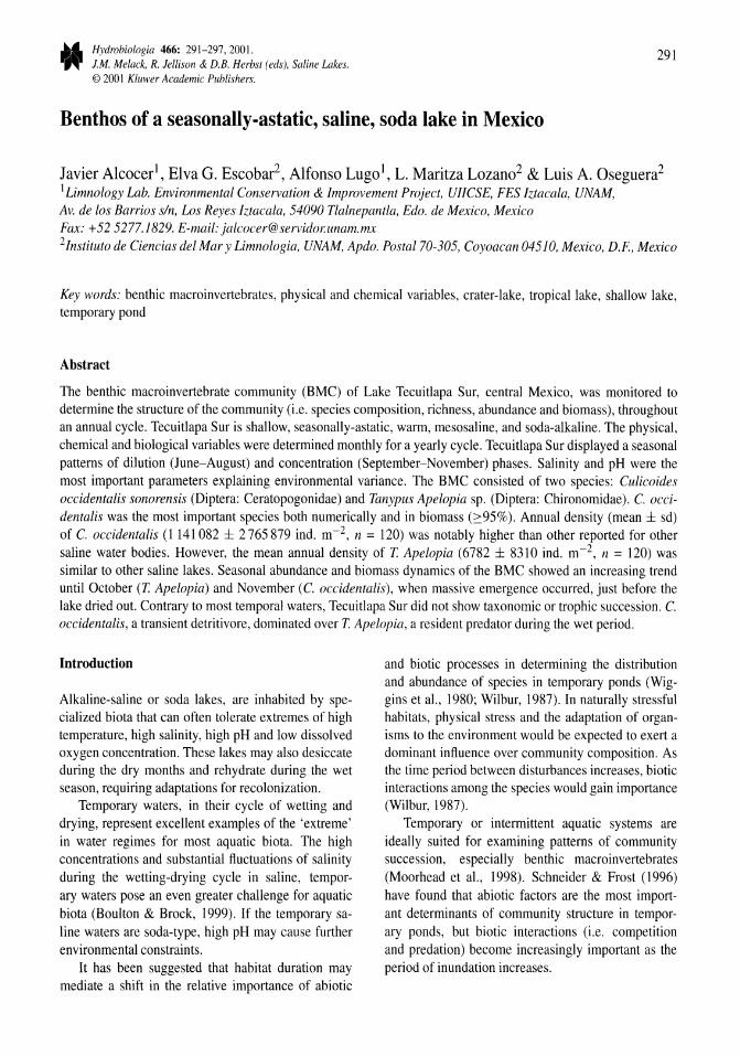
Hydrobiologia 466: 291-297,2001. J.M. Melack, R. Jellison & D,E, Herbst (eds), Saline Lakes, © 2001 KhlWer Academic Publishers,
291
Benthos of a seasonally-astatic, saline, soda lake in Mexico
Javier Alcocer!, Elva G, Escobar2, Alfonso Lugo1, L Maritza Lozano2 & Luis A, Oseguera2 1 Limnology Lab, Environmental Conservation & Improvement Project, UIICSE, FES Iztacala, UNAM, Av. de los Barrios sin, Los Reyes /ztacala, 54090 Tlalnepantla, Edo. de Mexico, Mexico Fax: +52 5277.1829. E-mail: [email protected] 2Instituto de Ciencias del Mar y Limnologia, UNAM, Apdo. Postal 70-305, Coyoacan 04510, Mexico, D.F., Mexico
Key words: benthic macroinvertebrates, physical and chemical variables, crater-lake, tropical lake, shallow lake, temporary pond
Abstract
The benthic macroinvertebrate community (BMC) of Lake Tecuitlapa Sur, central Mexico, was monitored to determine the structure of the community (i.e. species composition, richness, abundance and biomass), throughout an annual cycle. Tecuitlapa Sur is shallow, seasonally-astatic, warm, meso saline, and soda-alkaline. The physical, chemical and biological variables were determined monthly for a yearly cycle. Tecuitlapa Sur displayed a seasonal patterns of dilution (June-August) and concentration (September-November) phases. Salinity and pH were the most important parameters explaining environmental variance. The BMC consisted of two species: Culicoides occidentalis sonorensis (Diptera: Ceratopogonidae) and Tanypus Apelopia sp. (Diptera: Chironomidae). C. occidentalis was the most important species both numerically and in biomass (2':95%). Annual density (mean ± sd) of C. occidentalis (1141 082 ± 2765879 indo m-2, n = 120) was notably higher than other reported for other saline water bodies. However, the mean annual density of T. Apelopia (6782 ± 8310 indo m -2, n = 120) was similar to other saline lakes. Seasonal abundance and biomass dynamics of the BMC showed an increasing trend until October (T. Apelopia) and November (c. occidentalis), when massive emergence occurred, just before the lake dried out. Contrary to most temporal waters, Tecuitlapa Sur did not show taxonomic or trophic succession. C. occidentalis, a transient detritivore, dominated over T. Apelopia, a resident predator during the wet period.
Introduction
Alkaline-saline or soda lakes, are inhabited by specialized biota that can often tolerate extremes of high temperature, high salinity, high pH and low dissolved oxygen concentration. These lakes may also desiccate during the dry months and rehydrate during the wet season, requiring adaptations for recolonization.
Temporary waters, in their cycle of wetting and drying, represent excellent examples of the 'extreme' in water regimes for most aquatic biota. The high concentrations and substantial fluctuations of salinity during the wetting-drying cycle in saline, temporary waters pose an even greater challenge for aquatic biota (Boulton & Brock, 1999). If the temporary saline waters are soda-type, high pH may cause further environmental constraints.
It has been suggested that habitat duration may mediate a shift in the relative importance of abiotic
and biotic processes in determining the distribution and abundance of species in temporary ponds (Wiggins et aI., 1980; Wilbur, 1987). In naturally stressful habitats, physical stress and the adaptation of organisms to the environment would be expected to exert a dominant influence over community composition. As the time period between disturbances increases, biotic interactions among the species would gain importance (Wilbur, 1987).
Temporary or intermittent aquatic systems are ideally suited for examining patterns of community succession, especially benthic macroinvertebrates (Moorhead et aI., 1998). Schneider & Frost (1996) have found that abiotic factors are the most important determinants of community structure in temporary ponds, but biotic interactions (i.e. competition and predation) become increasingly important as the period of inundation increases.
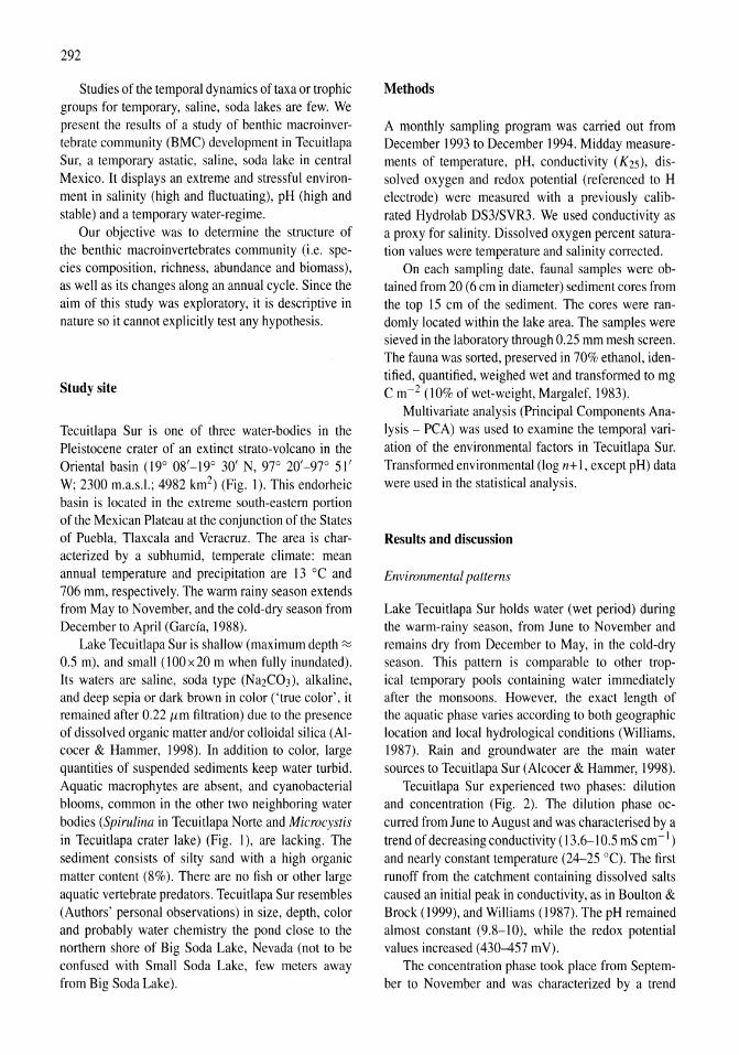
292
Studies of the temporal dynamics of taxa or trophic groups for temporary, saline, soda lakes are few. We present the results of a study of benthic macroinvertebrate community (BMC) development in Tecuitlapa Sur, a temporary astatic, saline, soda lake in central Mexico. It displays an extreme and stressful environment in salinity (high and fluctuating), pH (high and stable) and a temporary water-regime.
Our objective was to determine the structure of the benthic macroinvertebrates community (i.e. species composition, richness, abundance and biomass), as well as its changes along an annual cycle. Since the aim of this study was exploratory, it is descriptive in nature so it cannot explicitly test any hypothesis.
Study site
Tecuitlapa Sur is one of three water-bodies in the Pleistocene crater of an extinct strato-volcano in the Oriental basin (19° 08'-19° 30' N, 97° 20'-97° 51' W; 2300 m.a.s.\.; 4982 km2) (Fig. I). This endorheic basin is located in the extreme south-eastern portion of the Mexican Plateau at the conjunction of the States of Puebla, Tlaxcala and Veracruz. The area is characterized by a subhumid, temperate climate: mean annual temperature and precipitation are 13°C and 706 mm, respectively. The warm rainy season extends from May to November, and the cold-dry season from December to April (Garda, 1988).
Lake Tecuitlapa Sur is shallow (maximum depth ~ 0.5 m), and small (100 x 20 m when fully inundated). Its waters are saline, soda type (Na2C03), alkaline, and deep sepia or dark brown in color ('true color', it remained after 0.22 (tm filtration) due to the presence of dissolved organic matter and/or colloidal silica (Alcocer & Hammer, 1998). In addition to color, large quantities of suspended sediments keep water turbid. Aquatic macrophytes are absent, and cyanobacterial blooms, common in the other two neighboring water bodies (Spiruiina in Tecuitlapa Norte and Microcystis in Tecuitlapa crater lake) (Fig. I), are lacking. The sediment consists of silty sand with a high organic matter content (8%). There are no fish or other large aquatic vertebrate predators. Tecuitlapa Sur resembles (Authors' personal observations) in size, depth, color and probably water chemistry the pond close to the northern shore of Big Soda Lake, Nevada (not to be confused with Small Soda Lake, few meters away from Big Soda Lake).
Methods
A monthly sampling program was carried out from December 1993 to December 1994. Midday measurements of temperature, pH, conductivity (K2S), dissolved oxygen and redox potential (referenced to H electrode) were measured with a previously calibrated Hydrolab DS3/SVR3. We used conductivity as a proxy for salinity. Dissolved oxygen percent saturation values were temperature and salinity corrected.
On each sampling date, faunal samples were obtained from 20 (6 cm in diameter) sediment cores from the top 15 cm of the sediment. The cores were randomly located within the lake area. The samples were sieved in the laboratory through 0.25 mm mesh screen. The fauna was sorted, preserved in 70% ethanol, identified, quantified, weighed wet and transformed to mg C m-2 (10% of wet-weight, Margalef, 1983).
Multivariate analysis (Principal Components Analysis - PCA) was used to examine the temporal variation of the environmental factors in Tecuitlapa Sur. Transformed environmental (log n+ 1, except pH) data were used in the statistical analysis.
Results and discussion
Environmental patterns
Lake Tecuitlapa Sur holds water (wet period) during the warm-rainy season, from June to November and remains dry from December to May, in the cold-dry season. This pattern is comparable to other tropical temporary pools containing water immediately after the monsoons. However, the exact length of the aquatic phase varies according to both geographic location and local hydrological conditions (Williams, 1987). Rain and groundwater are the main water sources to Tecuitlapa Sur (Alcocer & Hammer, 1998).
Tecuitlapa Sur experienced two phases: dilution and concentration (Fig. 2). The dilution phase occurred from June to August and was characterised by a trend of decreasing conductivity (13.6-10.5 mS cm-1)
and nearly constant temperature (24-25 0C). The first runoff from the catchment containing dissolved salts caused an initial peak in conductivity, as in Boulton & Brock (1999), and Williams (1987). The pH remained almost constant (9.8-10), while the redox potential values increased (430-457 mV).
The concentration phase took place from September to November and was characterized by a trend
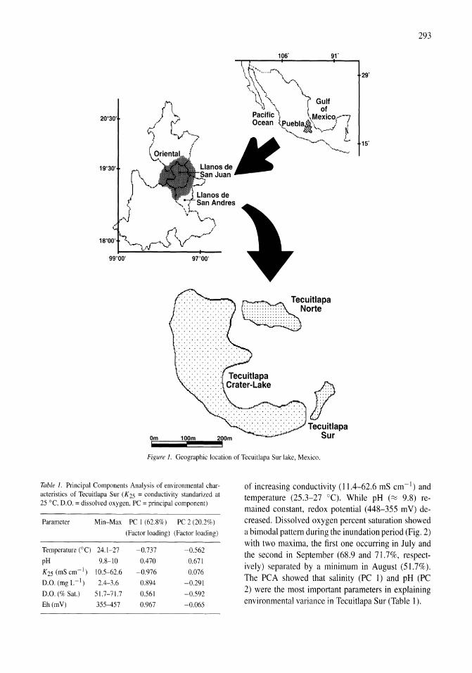
99"00' 97"00'
0~m~ ... 1~0~om!!!!~2~00m
106'
" . ........ ~-
Gulf of
91'
Ocean puebl~
... Tecuitlapa _:::::::::::::::: Norte ................. .................. ................. ................ . . .....
..... .. fl··
Tecuitlapa Sur
293
29'
15'
Figure 1. Geographic location of Tecuitlapa Sur lake, Mexico.
Table 1. Principal Components Analysis of environmental characteristics of Tecuitlapa Sur (K 25 = conductivity standarized at 25°C, D.O. = dissolved oxygen, PC = principal component)
Parameter Min-Max PC I (62.8%) PC 2 (20.2%)
(Factor loading) (Factor loading)
Temperature (0C) 24.1-27 -0.737 -0.562
pH 9.8-10 0.470 0.671
K25 (mScm- l ) 10.5-62.6 -0.976 0.076
D.O. (mgL -I) 2.4-3.6 0.894 -0.291
D.O. (% Sat.) 5\.7-71.7 0.561 -0.592
Eh(mV) 355-457 0.967 -0.065
of increasing conductivity (11.4-62.6 mS cm -I) and temperature (25.3-27 0c). While pH (~ 9.8) remained constant, redox potential (448-355 mY) decreased. Dissolved oxygen percent saturation showed a bimodal pattern during the inundation period (Fig. 2) with two maxima, the first one occurring in July and the second in September (68.9 and 71.7%, respectively) separated by a minimum in August (51.7%). The PCA showed that salinity (PC 1) and pH (PC 2) were the most important parameters in explaining environmental variance in Tecuitlapa Sur (Table 1).
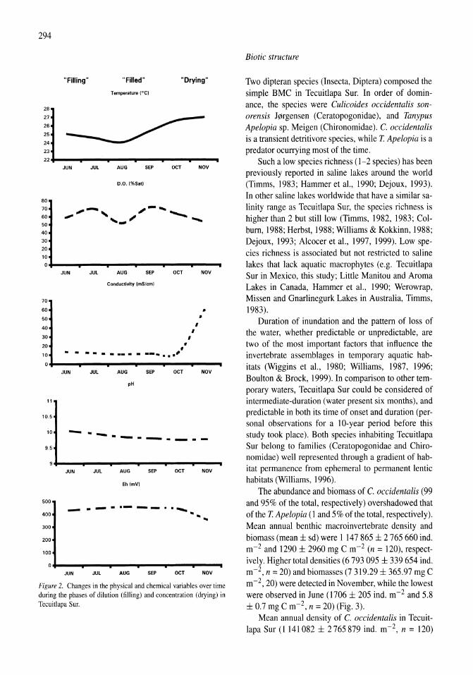
294
~I 80
70
60
50
40
30
20
10
0
70
60
50
40
30
20
10
"Filling" "Filled" "Drying"
Temperature (OC)
:::::= - : JUN JUL AUG SEP OCT
D.O.I%S.,)
,,-, ~-"'- ........ ,. .... _"
JUN
- -
JUL AUG SEP
Conductivity emS/em)
OCT
• • -. -- -- - - -- ..... " ,
-
NOV
.....
, I
NOV
• •
o+---~----~----P----.----.---~ JUN JUL AUG SEP OCT NOV
pH
11
10.5
-- --------10 -9.5
JUN JUL AUG SEP OCT NOV
EhlmV)
500 - -- _.- -_ .......... 400 .. .. 300
200
100
0
JUN JUL AUG SEP OCT NOV
Figure 2. Changes in the physical and chemical variables over time during the phases of dilution (filling) and concentration (drying) in Tecuitlapa Sur.
Biotic structure
Two dipteran species (Insecta, Diptera) composed the simple BMC in Tecuitlapa Sur. In order of dominance, the species were Culicoides occidentalis sonorensis J0rgensen (Ceratopogonidae), and Tanypus Apelopia sp. Meigen (Chironomidae). C. occidentalis is a transient detritivore species, while T. Apelopia is a predator ocurrying most of the time.
Such a low species richness (1-2 species) has been previously reported in saline lakes around the world (Timms, 1983; Hammer et aI., 1990; Dejoux, 1993). In other saline lakes worldwide that have a similar salinity range as Tecuitlapa Sur, the species richness is higher than 2 but still low (Timms, 1982, 1983; Colburn, 1988; Herbst, 1988; Williams & Kokkinn, 1988; Dejoux, 1993; Alcocer et al., 1997, 1999). Low species richness is associated but not restricted to saline lakes that lack aquatic macrophytes (e.g. Tecuitlapa Sur in Mexico, this study; Little Manitou and Aroma Lakes in Canada, Hammer et aI., 1990; Werowrap, Missen and Gnarlinegurk Lakes in Australia, Timms, 1983).
Duration of inundation and the pattern of loss of the water, whether predictable or unpredictable, are two of the most important factors that influence the invertebrate assemblages in temporary aquatic habitats (Wiggins et aI., 1980; Williams, 1987, 1996; Boulton & Brock, 1999). In comparison to other temporary waters, Tecuitlapa Sur could be considered of intermediate-duration (water present six months), and predictable in both its time of onset and duration (personal observations for a lO-year period before this study took place). Both species inhabiting Tecuitlapa Sur belong to families (Ceratopogonidae and Chironomidae) well represented through a gradient of habitat permanence from ephemeral to permanent lentic habitats (Williams, 1996).
The abundance and biomass of C. occidentalis (99 and 95% of the total, respectively) overshadowed that of the T. Apelopia (1 and 5% ofthe total, respectively). Mean annual benthic macroinvertebrate density and biomass (mean ± sd) were 1147865 ± 2 765 660 indo m-2 and 1290 ± 2960 mg C m-2 (n = 120), respectively. Higher total densities (6 793 095 ± 339 654 indo m-2, n = 20) and biomasses (7 319.29 ± 365.97 mg C m-2, 20) were detected in November, while the lowest were observed in June (1706 ± 205 indo m-2 and 5.8 ± 0.7 mg C m-2, n = 20) (Fig. 3).
Mean annual density of C. occidentalis in Tecuitlapa Sur (1141082 ± 2765879 indo m-2, n = 120)
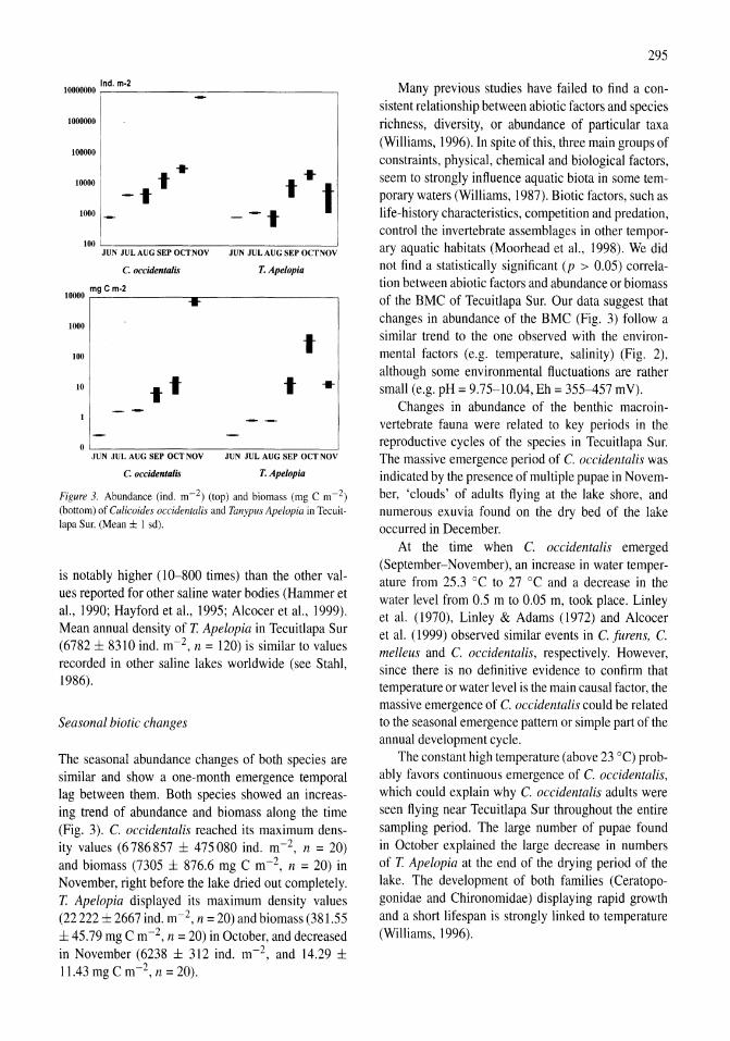
Ind. m-2 10000000 ~ _____________ --,
1000000
100000
10000
1000
•• -I t"l-_-I f
100 ,"=c:-=-..,.=-=-==-=~-,----___ --=,-------' JUN JUL AUG SEP OCT NOV JUN JUL AUG SEP OCT NOV
C. occidentaJis T. Apelopia
10000 mg C m-2
1000
t 100
10 It • JUN JUL AUG SEP OCTNOV JUN JUL AUG SEP OCT NOV
C. occidentalis T. Apelopia
Figure 3. Abundance (ind. m-2) (top) and biomass (mg C m-2) (bottom) of Culicaides occidentalis and Tanypus Apelapia in Tecuitlapa Sur. (Mean ± I sd).
is notably higher (10-800 times) than the other values reported for other saline water bodies (Hammer et aI., 1990; Hayford et aI., 1995; Alcocer et aI., 1999). Mean annual density of T. Apelopia in Tecuitlapa Sur (6782 ± 8310 indo m-2, n = 120) is similar to values recorded in other saline lakes worldwide (see Stahl, 1986).
Seasonal biotic changes
The seasonal abundance changes of both species are similar and show a one-month emergence temporal lag between them. Both species showed an increasing trend of abundance and biomass along the time (Fig. 3). C. occidentalis reached its maximum density values (6786857 ± 475080 indo m-2, n = 20) and biomass (7305 ± 876.6 mg C m-2, n = 20) in November, right before the lake dried out completely. T. Apelopia displayed its maximum density values (22222 ± 2667 indo m-2, n = 20) and biomass (381.55 ± 45.79 mg C m-2, n = 20) in October, and decreased in November (6238 ± 312 indo m-2, and 14.29 ± 11.43 mg C m-2, n = 20).
295
Many previous studies have failed to find a consistent relationship between abiotic factors and species richness, diversity, or abundance of particular taxa (Williams, 1996). In spite of this, three main groups of constraints, physical, chemical and biological factors, seem to strongly influence aquatic biota in some temporary waters (Williams, 1987). Biotic factors, such as life-history characteristics, competition and predation, control the invertebrate assemblages in other temporary aquatic habitats (Moorhead et aI., 1998). We did not find a statistically significant (p > 0.05) correlation between abiotic factors and abundance or biomass of the BMC of Tecuitlapa Sur. Our data suggest that changes in abundance of the BMC (Fig. 3) follow a similar trend to the one observed with the environmental factors (e.g. temperature, salinity) (Fig. 2), although some environmental fluctuations are rather small (e.g. pH = 9.75-10.04, Eh = 355-457 mY).
Changes in abundance of the benthic macroinvertebrate fauna were related to key periods in the reproductive cycles of the species in Tecuitlapa Sur. The massive emergence period of C. occidentalis was indicated by the presence of multiple pupae in November, 'clouds' of adults flying at the lake shore, and numerous exuvia found on the dry bed of the lake occurred in December.
At the time when C. occidentalis emerged (September-November), an increase in water temperature from 25.3 °C to 27°C and a decrease in the water level from 0.5 m to 0.05 m, took place. Linley et aI. (1970), Linley & Adams (1972) and Alcocer et aI. (1999) observed similar events in C. jurens, C. melleus and C. occidentalis, respectively. However, since there is no definitive evidence to confirm that temperature or water level is the main causal factor, the massive emergence of C. occidentalis could be related to the seasonal emergence pattern or simple part of the annual development cycle.
The constant high temperature (above 23°C) probably favors continuous emergence of C. occidentalis, which could explain why C. occidentalis adults were seen flying near Tecuitlapa Sur throughout the entire sampling period. The large number of pupae found in October explained the large decrease in numbers of T. Apelopia at the end of the drying period of the lake. The development of both families (Ceratopogonidae and Chironomidae) displaying rapid growth and a short lifespan is strongly linked to temperature (Williams, 1996).
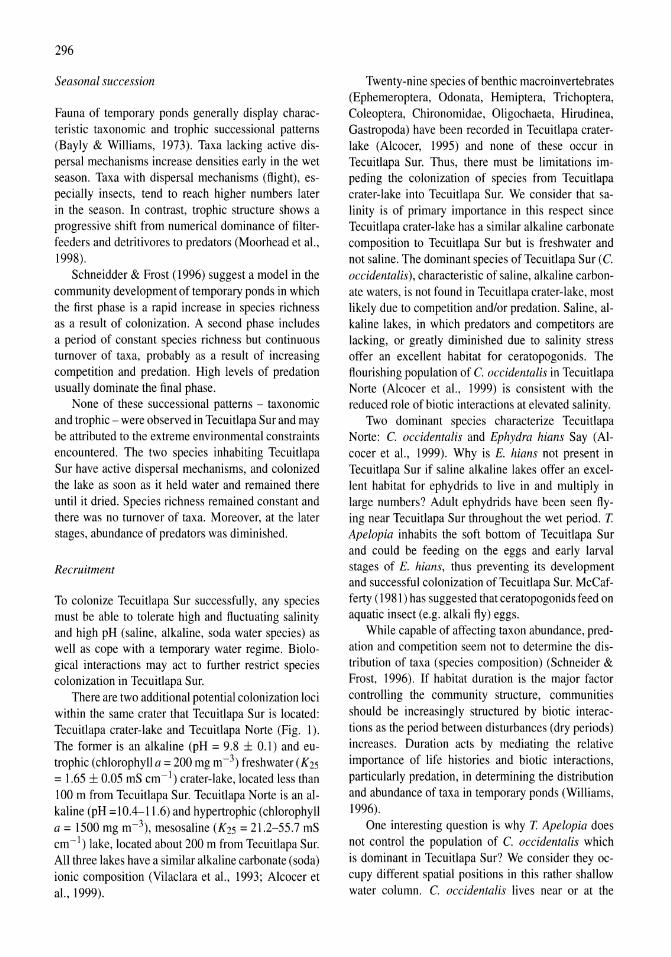
296
Seasonal succession
Fauna of temporary ponds generally display characteristic taxonomic and trophic successional patterns (Bayly & Williams, 1973). Taxa lacking active dispersal mechanisms increase densities early in the wet season. Taxa with dispersal mechanisms (flight), especially insects, tend to reach higher numbers later in the season. In contrast, trophic structure shows a progressive shift from numerical dominance of filterfeeders and detritivores to predators (Moorhead et aI., 1998).
Schneidder & Frost (1996) suggest a model in the community development of temporary ponds in which the first phase is a rapid increase in species richness as a result of colonization. A second phase includes a period of constant species richness but continuous turnover of taxa, probably as a result of increasing competition and predation. High levels of predation usually dominate the final phase.
None of these successional patterns - taxonomic and trophic - were observed in Tecuitlapa Sur and may be attributed to the extreme environmental constraints encountered. The two species inhabiting Tecuitlapa Sur have active dispersal mechanisms, and colonized the lake as soon as it held water and remained there until it dried. Species richness remained constant and there was no turnover of taxa. Moreover, at the later stages, abundance of predators was diminished.
Recruitment
To colonize Tecuitlapa Sur successfully, any species must be able to tolerate high and fluctuating salinity and high pH (saline, alkaline, soda water species) as well as cope with a temporary water regime. Biological interactions may act to further restrict species colonization in Tecuitlapa Sur.
There are two additional potential colonization loci within the same crater that Tecuitlapa Sur is located: Tecuitlapa crater-lake and Tecuitlapa Norte (Fig. 1). The former is an alkaline (pH = 9.8 ± 0.1) and eutrophic (chlorophyll a = 200 mg m-3) freshwater (K25 = 1.65 ± 0.05 mS cm- I ) crater-lake, located less than 100 m from Tecuitlapa Sur. Tecuitlapa Norte is an alkaline (pH =10.4-11.6) and hypertrophic (chlorophyll a = 1500 mg m-3), mesosaline (K25 = 21.2-55.7 mS cm -I) lake, located about 200 m from Tecuitlapa Sur. All three lakes have a similar alkaline carbonate (soda) ionic composition (Vilaclara et al., 1993; Alcocer et aI., 1999).
Twenty-nine species of benthic macroinvertebrates (Ephemeroptera, Odonata, Hemiptera, Trichoptera, Coleoptera, Chironomidae, Oligochaeta, Hirudinea, Gastropoda) have been recorded in Tecuitlapa craterlake (Alcocer, 1995) and none of these occur in Tecuitlapa Sur. Thus, there must be limitations impeding the colonization of species from Tecuitlapa crater-lake into Tecuitlapa Sur. We consider that salinity is of primary importance in this respect since Tecuitlapa crater-lake has a similar alkaline carbonate composition to Tecuitlapa Sur but is freshwater and not saline. The dominant species of Tecuitlapa Sur (c. occidentalis), characteristic of saline, alkaline carbonate waters, is not found in Tecuitlapa crater-lake, most likely due to competition and/or predation. Saline, alkaline lakes, in which predators and competitors are lacking, or greatly diminished due to salinity stress offer an excellent habitat for ceratopogonids. The flourishing population of C. occidentalis in Tecuitlapa Norte (Alcocer et aI., 1999) is consistent with the reduced role of biotic interactions at elevated salinity.
Two dominant species characterize Tecuitlapa Norte: C. occidentalis and Ephydra hians Say (Alcocer et aI., 1999). Why is E. hians not present in Tecuitlapa Sur if saline alkaline lakes offer an excellent habitat for ephydrids to live in and multiply in large numbers? Adult ephydrids have been seen flying near Tecuitlapa Sur throughout the wet period. T. Apelopia inhabits the soft bottom of Tecuitlapa Sur and could be feeding on the eggs and early larval stages of E. hians, thus preventing its development and successful colonization of Tecuitlapa Sur. McCafferty (1981) has suggested that ceratopogonids feed on aquatic insect (e.g. alkali fly) eggs.
While capable of affecting taxon abundance, predation and competition seem not to determine the distribution of taxa (species composition) (Schneider & Frost, 1996). If habitat duration is the major factor controlling the community structure, communities should be increasingly structured by biotic interactions as the period between disturbances (dry periods) increases. Duration acts by mediating the relative importance of life histories and biotic interactions, particularly predation, in determining the distribution and abundance of taxa in temporary ponds (Williams, 1996).
One interesting question is why T. Apelopia does not control the popUlation of C. occidentalis which is dominant in Tecuitlapa Sur? We consider they occupy different spatial positions in this rather shallow water column. C. occidentalis lives near or at the
water surface; especially pupae that maintain contact with air at the water surface by means of thoracic respiratory horns. T. Apelopia is a bottom dweller (bottom browser). In addition, ceratopogonids are highly mobile swimmers and may elude T. Apelopia.
Summarizing, salinity and pH were the most important parameters explaining environmental variance of Tecuitlapa Sur. Two species of BMC occurred in Tecuitlapa Sur: C. occidentalis and T. Apelopia. Both species coexisted throughout the year. C. occidentalis was most important both numerically and in biomass (2:95%). While mean annual density of C. occidentalis was notably higher than the values reported for other saline water bodies, T. Apelopia density was in the same range of other studies. Seasonal dynamics of the BMC showed an increasing trend until October (T. Apelopia) and November (c. occidentalis), when massive emergence occurred, just before the lake dried out completely. Tecuitlapa Sur did not show taxonomic or trophic succession. C. occidentalis, a transient detritivore species, dominated over T. Ape/opia, a resident predator during the wet period.
Acknowledgements
We gratefully acknowledge the help of M. R. Sanchez, M. M. Chavez, L. Peralta and M. 1. Montoya in the field and the laboratory work. Financial support was partially given by CONACYT project T-25430, and DGAPA project IN204597. The authors thank Dr D. W. Webb and Dr A. Borkent (Ceratopogonidae) and Dr A. Contreras (Chironomidae) for taxonomic identification.
References
Alcocer, J., 1995. Amilisis hoHstico de la comunidad de macroinvertebrados bent6nicos litorales de seis lagos-crater con un gradiente de salinidad. Ph.D. Thesis. Universidad Nacional Aut6noma de Mexico. Facultad de Ciencias. Mexico: 106 pp.
Alcocer, J. & U. T. Hammer, 1998. Saline lake ecosystems of Mexico. Aquat. Ecosystems Health and Management I: 291-315.
Alcocer. J., A. Lugo, E. Escobar & M. Sanchez, 1997. The macrobenthic fauna of a former perennial and now episodically filled Mexican saline lake. Int. J. Salt Lake Res. 5: 1-14.
Alcocer, J., E. Escobar, A. Lugo & L. A. Oseguera, 1999. Benthos of a perennially-astatic, saline, soda lake in Mexico. Int. J. Salt Lake Res. 8: 113-126.
Bayly, 1. A. E. & W. D. Williams, 1973. Inland Waters and their Ecology. Longman, Melbourne: 314 pp.
297
Boulton, A. J. & M. A. Brock, 1999. Australian Freshwater Ecology. Processes and Management. Cooperative Research Center for Freshwater Ecology, Australia: 300 pp.
Colburn, E. A., 1988. Factors influencing species diversity in saline waters of Death Valley, U.S.A. Hydrobiologia 158: 215-226.
Dejoux, C., 1993. Benthic macroinvertebrates of some saline lakes of the Sud Lipez region, Bolivia. Hydrobiologia 267: 257-267.
Garda. E., 1988. Modificaciones al Sistema de Clasificaci6n CIimatica de Koppen. E. Garcia, Mexico: 217 pp.
Hammer, U. T.. J. S. Sheard & J. Kranabetter, 1990. Distribution and abundance oflittoral benthic fauna in Canadian prairie saline lakes. Hydrobiologia 197: 173-192.
Hayford, B. L., J. E. Sublette & S. 1. Hermann, 1995. Distribution of chironomids (Diptera: Chironomidae) and ceratopogonids (Diptera: Ceratopogonidae) along a Colorado thermal spring etfluent. J. Kansas Entomo!' Soc. 68: 77-92.
Herbst, D. B., 1988. Comparative population ecology of Ephydra hians Say (Diptera: Ephydridae) at Mono Lake (California) and Abert Lake (Oregon). Hydrobiologia 158: 145-166.
Linley, J. R. & G. M. Adams, 1972. Ecology and behavior of immature Culicoides melleus (Coq.) (Dipt., Ceratopogonidae). Bull. Entomo!. Res. 62: 113-127.
Linley. J. R., F. D. S. Evans & H. T. Evans, 1970. Seasonal emergence of Culicoides furens (Diptera: Ceratopogonidae) at Vero Beach, Florida. Ann. Entomo!. Soc. Am. 5: 1332-1339.
Margalef, R., 1983. Limnologfa. Omega, Barcelona: 1010 pp. McCafferty, W. P., 1981. Aquatic Entomology. Science Books
International, Boston: 448 pp. Moorhead, D. 1.. D. 1. Hall & M. R. Willig, 1998. Succession of
macroinvertebrates in playas ofthe Southern High Plains, U.S.A. 1. n. am. Benthol. Soc. 17: 430-442.
Schneider, D. W. & T. M. Frost, 1996. Habitat duration and community structure in temporary ponds. 1. n. am. Benthol. Soc. 15: 64-86.
Stahl, 1. B., 1986. A six-year study of abundance and voltinism of Chironomidae (Diptera) in an Illinois cooling reservoir. Hydrobiologia 134: 67-79.
Timms, B. v., 1982. A study of the benthic communities of twenty lakes in South Island. New Zealand. Freshwat. BioI. 12: 123-138.
Timms, B. v., 1983. A study of benthic communities in some shallow saline lakes of western Victoria, Australia. Hydrobiologia 105: 165-177.
Vilaclara, G., M. Chavez, A. Lugo, H. Gonzalez & M. Gaytan, 1993. Comparative description of crater-lakes basic chemistry in Puebla state, Mexico. Verh. int. Ver. Limno!. 25: 435-440.
Wiggins, G. B., R. 1. Mackay & I. M. Smith, 1980. Evolutionary and ecological strategies of animals in annual temporary pools. Arch. Hydrobio!., Supple. 58: 97-206.
Wilbur, H. M., 1987. Regulation of structure in complex systems: experimental temporary pond communities. Ecology 68: 1437-1452.
Williams, D. D., 1987. The Ecology of Temporary Waters. Croom Helm, London: 205 pp.
Williams, D. D., 1996. Environmental constraints in temporary fresh waters and their consequences for the insect fauna. J. n. am. Benthol. Soc. 15: 634-650.
Williams, W. D. & M. 1. Kokkinn, 1988. The biogeographical at1inities of the fauna in episodically filled salt lakes: a study of Lake Eyre South, Australia. Hydrobiologia 158: 227-236.
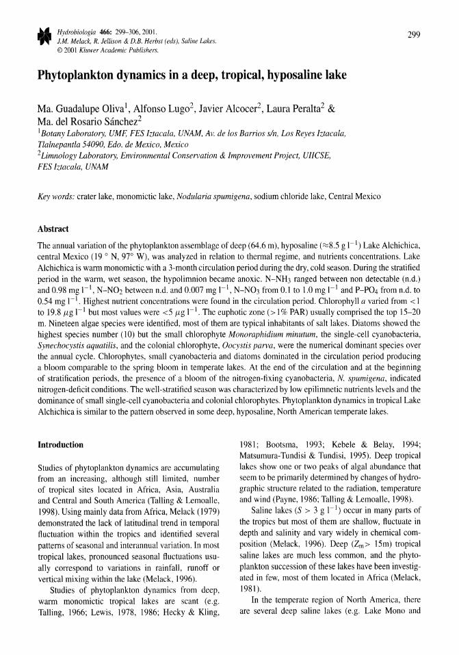
Hydrobiologia 466: 299-306,2001. J.M. Me/ack, R. Jellison & D.E. Herbst (eds), Saline Lakes. © 2001 Kluwer Academic Publishers.
299
Phytoplankton dynamics in a deep, tropical, hyposaline lake
Ma. Guadalupe Oliva), Alfonso Lugo2, Javier Alcocer2, Laura Peralta2 & Ma. del Rosario Sanchez2
1 Botany Laboratory, UMF, FES Iztacala, UNAM, Av. de los Barrios sin, Los Reyes [ztacala, Tlalnepantla 54090, Edo. de Mexico, Mexico 2Limnology Laboratory, Environmental Conservation & Improvement Project, UIICSE, FES Iztacala, UNAM
Key words: crater lake, monomictic lake, Nodularia spumigena, sodium chloride lake, Central Mexico
Abstract
The annual variation of the phytoplankton assemblage of deep (64.6 m), hyposaline (~8.5 g 1-1) Lake Alchichica, central Mexico (19 0 N, 970 W), was analyzed in relation to thermal regime, and nutrients concentrations. Lake Alchichica is warm monomictic with a 3-month circulation period during the dry, cold season. During the stratified period in the warm, wet season, the hypolimnion became anoxic. N-NH3 ranged between non detectable (n.d.) and 0.98 mg 1-1, N-N02 between n.d. and 0.007 mg 1-1, N-N03 from 0.1 to 1.0 mg I-I and P-P04 from n.d. to 0.54 mg I-I. Highest nutrient concentrations were found in the circulation period. Chlorophyll a varied from < I to 19.8 J.Lg 1-1 but most values were <5 J.Lg 1-1. The euphotic zone (> I % PAR) usually comprised the top 15-20 m. Nineteen algae species were identified, most of them are typical inhabitants of salt lakes. Diatoms showed the highest species number (l0) but the small chlorophyte Monoraphidium minutum, the single-cell cyanobacteria, Synechocystis aquatilis, and the colonial chlorophyte, Oocystis parva, were the numerical dominant species over the annual cycle. Chlorophytes, small cyanobacteria and diatoms dominated in the circulation period producing a bloom comparable to the spring bloom in temperate lakes. At the end of the circulation and at the beginning of stratification periods, the presence of a bloom of the nitrogen-fixing cyanobacteria, N. spumigena, indicated nitrogen-deficit conditions. The well-stratified season was characterized by low epilimnetic nutrients levels and the dominance of small single-cell cyanobacteria and colonial chlorophytes. Phytoplankton dynamics in tropical Lake Alchichica is similar to the pattern observed in some deep, hyposaline, North American temperate lakes.
Introduction
Studies of phytoplankton dynamics are accumulating from an increasing, although still limited, number of tropical sites located in Africa, Asia, Australia and Central and South America (Talling & Lemoalle, 1998). Using mainly data from Africa, Melack (1979) demonstrated the lack of latitudinal trend in temporal fluctuation within the tropics and identified several patterns of seasonal and interannual variation. In most tropical lakes, pronounced seasonal fluctuations usually correspond to variations in rainfall, runoff or vertical mixing within the lake (Melack, 1996).
Studies of phytoplankton dynamics from deep, warm monomictic tropical lakes are scant (e.g. Tailing, 1966; Lewis, 1978, 1986; Hecky & Kling,
1981; Bootsma, 1993; Kebele & Belay, 1994; Matsumura-Tundisi & Tundisi, 1995). Deep tropical lakes show one or two peaks of algal abundance that seem to be primarily determined by changes of hydrographic structure related to the radiation, temperature and wind (Payne, 1986; TaIling & Lemoalle, 1998).
Saline lakes (S > 3 g 1-1) occur in many parts of the tropics but most of them are shallow, fluctuate in depth and salinity and vary widely in chemical composition (Melack, 1996). Deep (lm> 15m) tropical saline lakes are much less common, and the phytoplankton succession of these lakes have been investigated in few, most of them located in Africa (Melack, 1981).
In the temperate region of North America, there are several deep saline lakes (e.g. Lake Mono and
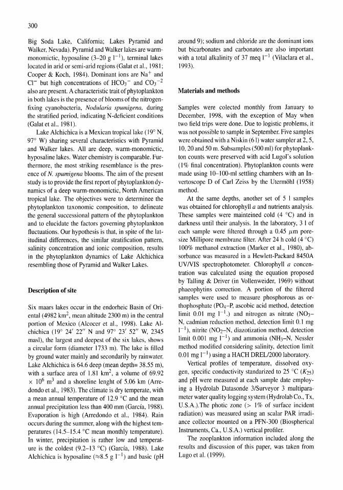
300
Big Soda Lake, California; Lakes Pyramid and Walker, Nevada). Pyramid and Walker lakes are warmmonomictic, hypos aline (3-20 g 1-1), terminal lakes located in arid or semi-arid regions (Galat et aI., 1981; Cooper & Koch, 1984). Dominant ions are Na+ and Cl- but high concentrations of HC03 - and C03-2 also are present. A characteristic trait of phytoplankton in both lakes is the presence of blooms of the nitrogenfixing cyanobacteria, Nodularia spumigena, during the stratified period, indicating N-deficient conditions (Galatetal.,1981).
Lake Alchichica is a Mexican tropical lake (19° N, 97° W) sharing several characteristics with Pyramid and Walker lakes. All are deep, warm-monomictic, hyposaline lakes. Water chemistry is comparable. Furthermore, the most striking resemblance is the presence of N. spumigena blooms. The aim of the present study is to provide the first report of phytoplankton dynamics of a deep warm-monomictic, North American tropical lake. The objectives were to determinee the phytoplankton taxonomic composition, to delineate the general successional pattern of the phytoplankton and to elucidate the factors governing phytoplankton fluctuations. Our hypothesis is that, in spite of the latitudinal differences, the similar stratification pattern, salinity concentration and ionic composition, results in the phytoplankton dynamics of Lake Alchichica resembling those of Pyramid and Walker Lakes.
Description of site
Six maars lakes occur in the endorheic Basin of Oriental (4982 km2, mean altitude 2300 m) in the central portion of Mexico (Alcocer et al., 1998). Lake Alchichica (19° 24' 22" Nand 97° 23' 52" W, 2345 masl), the largest and deepest of the six lakes, shows a circular form (diameter 1733 m). The lake is filled by ground water mainly and secondarily by rainwater. Lake Alchichica is 64.6 deep (mean depth= 38.55 m), with a surface area of 1.81 km2, a volume of 69.92 x 10⁶ m3 and a shoreline lenght of 5.06 km (Arredondo et aI., 1983). The climate is dry temperate, with a mean annual temperature of 12.9 °C and the mean annual precipitation less than 400 mm (Garda, 1988). Evaporation is high (Arredondo et aI., 1984). Rain occurs during the summer, along with the highest temperatures (14.5-15.4 °C mean monthly temperature). In winter, precipitation is rather low and temperature is the coldest (9.2-13 0c) (Garda, 1988). Lake Alchichica is hyposaline (~8.5 g I-I) and basic (pH
around 9); sodium and chloride are the dominant ions but bicarbonates and carbonates are also important with a total alkalinity of 37 meq I-I (Vilaclara et ai., 1993).
Materials and methods
Samples were colected monthly from January to December, 1998, with the exception of May when two field trips were done. Due to logistic problems, it was not possible to sample in September. Five samples were obtained with a Niskin (61) water sampler at 2,5, 10,20 and 50 m. Subsamples (500 ml) for phytoplankton counts were preserved with acid Lugol's solution (1 % final concentration). Phytoplankton counts were made using 1O-100-ml settling chambers with an Invertoscope D of Carl Zeiss by the Utermohl (1958) method.
At the same depths, another set of 5 I samples was obtained for chlorophyll a and nutrients analysis. These samples were mainteined cold (4°C) and in darkness until their analysis. In the laboratory, 3 I of each sample were filtered through a 0.45 f.,Lm poresize Millipore membrane filter. After 24 h cold (4°C) 100% methanol extraction (Marker et aI., 1980), absorbance was measured in a Hewlett-Packard 8450A UVNIS spectrophotometer. Chlorophyll a concentration was calculated using the equation proposed by Talling & Driver (in Vollenweider, 1969) without phaeophytins correction. A portion of the filtered samples were used to measure phosphorous as orthophosphate (P04-P, ascobic acid method, detection limit 0.01 mg I-I.) and nitrogen as nitrate (N03-N, cadmiun reduction method, detection limit 0.1 mg I-I), nitrite (N02-N, diazotization method, detection limit 0.001 mg 1-1) and ammonia (NH3-N, Nessler method modified considering salinity, detection limit 0.01 mg 1-1) using a HACH DRELl2000 laboratory.
Vertical profiles of temperature, dissolved oxygen, specific conductivity standarized to 25°C (K2S) and pH were measured at each sample date employing a Hydrolab Datasonde 3/Surveyor 3 multiparameter water quality logging system (Hydrolab Co., Tx, U.S.A.).The photic zone (> 1 % of surface incident radiation) was measured using an scalar PAR irradiance collector mounted on a PFN-300 (Biospherical Instruments, Ca., U.S.A.) vertical profiler.
The zooplankton information included along the results and discussion of this paper, was taken from Lugo et al. (1999).
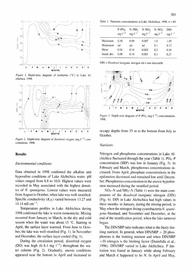
?rJ(O~~(J il ~Airf~~3t
:. ~I .. , , Jr MONTHS
Figure 2. Depth-time diagram of dissolved oxygen (mg I-I) concentrations. 1998.
Results
Environmental conditions
Data obtained in 1998 confirmed the alkaline and hyposaline conditions of Lake Alchichica water. pH values ranged from 8.8 to 10.0. Highest values were recorded in May associated with the highest densities of N. spumigena. Lowest values were measured from August to October, when lake was well-stratified. Specific conductivity (K2S) varied between 13.27 and 14.14 mS cm- I .
Temperature profiles in Lake Alchichica during 1998 confirmed the lake is warm monomictic. Mixing occurred from January to March, in the dry and cold season when the water was about 15 cC. Starting in April, the surface layer warmed. From June to October, the lake was well-stratified (Fig. 1). In November and December, the surface layer cooled (Fig. 1).
During the circulation period, dissolved oxygen (DO) was high (6-8.1 mg I-I) throughout the water column (Fig. 2). Gradually, anoxic conditions appeared near the bottom in April and increased to
301
Table 1. Nutrients concentrations in Lake Alchichica. 1998. n = 60
P-P04 N-NH3 N-N02 N-N03 DIN mgl- I mgl- I mgl- I mgl- 1 mgl- 1
Maximum 0.56 0.98 0.007 1.0 1.85 Mimimum nd nd nd 0.1 0.12
Mean 0.04 0.16 0.002 0.2 0.38 Stand. dev. 0.08 0.19 0.001 0.1 0.27
DIN = Dissolved inorganic nitrogen nd = non detectable
J( ~~~_ (.<_1' Lot!. / /·\S=:::'~'''.'05::? ~21
4C ". j:!'i~~fL15~~. J __ Ll i ' n (\ '\, /0.20 - P'(~
50:'~I'~r;I' .. ;r;T7l~! AI' 51 0 I To MONTHS
Figure 3. Depth time diagram of P-P04 (mg I-I) concentrations. 1998.
occupy depths from 35 m to the bottom from July to October.
Nutrients
Nitrogen and phosphorus concentrations in Lake Alchichica fluctuated through the year (Table 1). P04-P concentration (SRP) was low in January (Fig. 3). In February and March, phosphorous concentrations increased. From April, phosphate concentrations in the epilimnion decreased and remained low until December. Phosphorous concentration in the anoxic hypolimnion increased during the stratified period.
N03-N and NH3-N (Table I) were the main components of the dissolved inorganic nitrogen (DIN) (Fig. 4). DIN in Lake Alchichica had high values in three months: in January, during the mixing period, in May when the nitrogen-fixing cyanobacteriaN. spumigena bloomed, and November and December, at the end of the stratification period, when the lake turnover began.
The DIN/SRP ratio indicates what is the likely limiting nutrient. In general, when DIN/SRP > 20 phosphorous is the limiting nutrient and when DIN/SRP < 1 0 nitrogen is the limiting factor (Danielidis et aI., 1996). DIN/SRP varied in Lake Alchichica. P limitation was found in January while along February and March it happened to be N. In April and May,
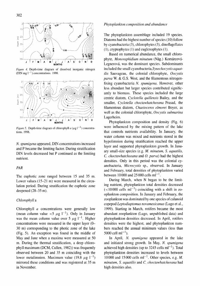
302
Figure 4. Depth-time diagram of dissolved inorganic nitrogen (DIN mg 1-1) concentrations. 1998.
N. spumigena appeared, DIN concentrations increased and P became the limiting factor. During stratification DIN levels decreased but P continued as the limiting nutrient.
PAR
The euphotic zone ranged between 15 and 35 m. Lower values (15-21 m) were measured in the circulation period. During stratification the euphotic zone deepened (28-35 m).
Chlorophyll a
Chlorophyll a concentrations were generally low (mean column value <5 jJ.g I-I). Only in January was the mean column value over 5 jJ.g 1-1. Higher concentrations were measured in the upper layer (0-30 m) corresponding to the photic zone of the lake (Fig. 5). An exception was found in the middle of May and June when a maxima were measured at 50 m. During the thermal stratification, a deep chlorophyll maximum (DCM, Cullen, 1982)) was frequently observed between 20 and 35 m coinciding with the lower metalimnion. Maximum value (19.8 jJ.g I-I) mirrored these conditions and was registered at 35 m in November.
Phytoplankton composition and abundance
The phytoplankton assemblage included 19 species. Diatoms had the highest number of species (10) follow by cyanobacteria (3), chlorophytes (3), dinoflagellates (1), cryptophytes (1) and euglenophytes (1).
Based on numerical abundance, the small chi orophyte, Monoraphidium minutum (Nag.) KomarcovaLegnerova, was the dominant species. Subdominants included the small cyanobacteria,Synechocystis aquatilis Sauvageau, the colonial chlorophyte, Oocystis parva W. & G.S. West, and the filamentous nitrogenfixing cyanobacteria N. spumigena. However, other less abundant but larger species contributed significantly to biomass. These species included the large centric diatom, Cyclotella quillensis Bailey, and the smaller, Cyclotella choctawhatcheeana Prasad, the filamentous diatom, Chaetoceros elmo rei Boyer, as well as the colonial chlorophyte, Oocystis submarina Lagerheim.
Phytoplankton composition and density (Fig. 6) were influenced by the mixing pattern of the lake that controls nutrients availability. In January, the water column was mixed and nutrients stored in the hypolimnion during stratification reached the upper layer and supported phytoplankton growth. In January small-size species (e.g. M. minutum, S. aquatilis, C. choctawhatcheeana and O. parva) had the highest densities. Only in this period was the colonial cyanobacteria, Microcystis sp., observed. In January and February, total densities of phytoplankton varied between 10 000 and 25000 cells ml- I .
During March, when N began to be the limiting nutrient, phytoplankton total densities decreased (<10000 cells ml- I ) coinciding with a shift in zooplankton composition. In January and February, the zooplankton was dominated by one species of calanoid copepod Leptodiaptomus novamexicanus (Lugo et aI., 1999). Starting in March, rotifers became the most abundant zooplankton (Lugo, unpublished data) and phytoplankton densities decreased. In April, rotifers densities were the highest, and phytoplankton numbers reached the annual minimum values (less than 5000 cell ml- 1).
In April, N. spumigena appeared in the lake and initiated strong growth. In May, N. spumigena achieved high densities (up to 3245 cells ml- I ). Total
phytoplankton densities increased to levels between 10 000 and 15000 cells ml- I . Other species, e.g. M. minutum, S. aquatiUs and C. choctawhatcheeana had high densities also.
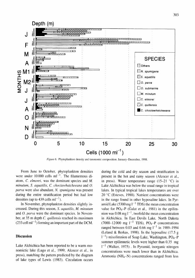
Depth (m)
II J ~I F ~~ M ~~ A ~I
en M1 ~~ ~ M2~~ ~ J a~
J ~~ A d o ~~ N ~~ D ~~
~
g:w
f-"<'I
P-""
Pl
~
p=
~
o 5
303
SPECIES BlOthers
BN. spumigena
IQ;ls. aquatilis
[]o. parva
Do. submarina
OM. minutum
Dc. elmorei
[J C. quillensis
.C. choctawhatcheeana
10 15 20 25 30
Cells (1000 ml-1 )
Figure 6. Phytoplankton density and taxonomic composition. January-December, 1998.
From June to October, phytoplankton densities were under 10 000 cells ml- I . The filamentous diatom, C. eimorei, was the dominant species and M. minutum, S. aquatilis, C. choctawhatcheeana and O. parva were also abundant. N. spumigena was present during the entire stratification period but had low densities (up to 439 cells ml- I ).
In November, phytoplankton densities slightly increased. During this season, S. aquatiUs, M. minutum and O. parva were the dominant species. In November, at 35 m depth C. quillensis reached its maximum (233 cell ml- I ) forming an important part ofthe DCM.
Discussion
Lake Alchichica has been reported to be a warm monomictic lake (Lugo et aI., 1999; Alcocer et al., in press), matching the pattern predicted by the diagram of lake types of Lewis (1983). Circulation occurs
during the cold and dry season and stratification is present in the hot and rainy season (Alcocer et aI., in press). Water temperature range (15-21 DC) in Lake Alchichica was below the usual range in tropical lakes. In typical tropical lakes temperatures are over 20°C (Esteves, 1988). Nutrient concentrations were in the range found in other hyposaline lakes. In Pyramid Lake (5300 mg 1- I TDS) the mean concentration value for P04-P (Galat et aI., 1981) in the epilimnion was 0.08 mg 1-1 , twofold the mean concentration in Alchichica. In East Devils Lake, North Dakota (7000-12000 mg 1-1 TDS), P04-P concentrations ranged between 0.03 and 0.66 mg 1-1 in 1989-1994 (Leland & Berkas, 1998). In the hypos aline (17.5 g 1-1) mixolimnion of Soap Lake, Washington, P04-P summer epilimnetic levels were higher than 0.35 mg I-I (Walker, 1975) . In Pyramid, inorganic nitrogen concentrations were much lower than in Alchichica. Ammonia (NH4-N) concentrations ranged from less
304
than 0.01 mg 1-1 to 0.07 mg 1-1. Nitrate (N03-N) concentration varied between 0.01 and 0.17 mg I-I and a mean epilimnetic value of 0.03 mg 1-1. Inorganic nitrogen levels (0.02-2.5 mg I-I) in East Devils Lake were closer to the range found in Alchichica. In Soap Lake, N03-N summer concentrations were much higher (> 4 mg I-I).
Chlorophyll a concentrations in Alchichica were generally low in 1998. Margalef (1983) established 5 {Lg 1-1 as the limit between oligotrophic and eutrophic conditions. According to these criteria Lake Alchichica is oligotrophic.
The phytoplantkon assemblage in Lake Alchichica is a mixture of fresh and saline water species. Most abundant species, M. minutum and S. aquatiUs, are freshwater cosmopolitan species that can inhabit moderately saline and alkaline environments (Comas, 1996). On the other hand, N. spumigena, C. elmorei, C. quillensis, C.choctawhatcheeana and O. submarina are typical inhabitants of saline and alkaline waters and most of them were found also inhabiting Pyramid and Walker lakes (Galat et aI., 1981; Hammer et aI., 1983; Battarbee et aI., 1984; Leland & Berkas, 1998). Williams (1998) asserts that in hypos aline lakes the biota usually is comprised of halotolerant freshwater forms. In Alchichica, most phytoplankton species are truly saline, restricted to inland saline waters of moderate to high salinity.
The low phytoplankton species richness in Lake Alchichica seems to confirm Williams et al. (1990) opinion about the effect of salinity above 3 g I-Ion species richness. In the hyposaline (7000-12000 mg 1-1 TDS) East Devils Lake, the mean ± standard deviation for species richness were 10.3 ± 4.6 species (Leland & Berkas, 1998). In Pyramid Lake, with only 5350 mg I-I TDS, around 42 phytoplankton taxa have been recorded (Galat et aI., 1981).
Seasonal dynamics of phytoplankton in Lake AIchichica is influenced by circulation and stratification. In Alchichica, circulation produces a phytoplankton bloom at the beginning of the dry and cold season, similar to the 'spring bloom' observed in many temperate lakes (Wetzel, 1975). Cold-water diatoms are the main component of the spring bloom in temperate lakes (Esteves, 1988) while in Alchichica diatoms are also important but, at least numerically, chlorophytes and cyanobacteria are the most important. Circulation is the season when phytoplankton biomass (measured as chlorophyll a concentration) in Alchichica achieved its maximum mean column values.
Coupled to the circulation phytoplankton bloom, a zooplankton bloom appeared. First copepods, and later rotifers, consumed the available food. When rotifers became abundant, phytoplankton densities diminished, with the greatest decreased in the number of the small sized ( < 10 {Lm) species. As a result, a clear water phase appeared in Alchichica., similar to these observed in temperate lakes after the spring bloom (Wetzel, 1975).
Several years observations in Lake Alchichica have shown the presence of N. spumigena blooms on a regular basis generally between April and May (Lugo et aI., 1999), at the beginning of the thermal stratification. Nodularia bloom conditions seem to last less than I month and the bloom intensity varies considerably year among years. In 1998, maximum densities of N. spumigena were observed in May, but the comparison of chlorophyll values in this season with those measured in other years (e.g. Lugo et aI., 1999) indicated that bloom was weak. With respect to this, 1998 could be considered as an unusual year in Lake Alchichica.
At the end of the mixing period, PIN ratio indicates nitrogen to be the limiting nutrient in Alchichica. Under N-limited conditions, a rise in surface water temperature from 15 to 17-18 DC favored Nodularia growth. Home et al. (1979) found that nitrogenfixing cyanobacteria blooms are promoted by warm water temperatures, low concentrations of inorganic nitrogen in surface waters and high phosphorous concentrations, conditions found in Alchichica in May, 1998.
Blooms of N. spumigena have also been observed in Pyramid and Walker lakes (Gal at et aI., 1981; Cooper & Koch, 1984). In Pyramid, Nodularia blooms appeared when summer stratification was well-developed and they lasted until the autumm. In Walker Lake, N. spumigena regularly dominated the summer phytoplankton. Such midsummer cyanobacterial blooms have been commonly observed in saline lakes (Haynes & Hammer, 1978). Nodularia blooms in Alchichica differ from those mentioned above, in that they start at the early stages of the stratification and last less than one month. A 3- months Nodularia bloom was observed in 1992 in Lake Atexcac, also a deep (Zm= 39 m) hyposaline crater-lake close to Alchichica (Macek et aI., 1994).
The stratified period in Alchichica are similar to those found in many temperate and tropical lakes: growth of phytoplankton in the epilimnion was limited by low levels of nutrients, mainly phosphorous. Conditions of high light intensity and low nutrients
availability favored the growth of chlorophytes and cyanobacteria (Lewis, 1978). These groups dominated in the stratified period in Alchichica. Higher temperatures also favored species such as the diatom C. elmorei, frequently observed in North American saline lakes during the warm-water season (Galat et al., 1981; Leland & Berkas, 1998).
In spite of the latitudinal difference, similar stratification patterns as well as salinity (concentration and ionic composition), results in Lake Alchichica sharing the following traits with other hyposaline, monomictic lakes in North America with regard to their phytoplankton assemblage: taxonomic composition, the development of a phytoplankton bloom during the circulation period, and a season of nitrogen limiting conditions favoring the presence of N. spumigena blooms. In contrast, there are also differences including an earlier rise of N. spumigena bloom in Lake Alchichica and a shorter period of occurrence.
Acknowledgements
This research was financially supported by Direcci6n General de Asuntos del Personal Academico, UNAM project IN204597 and by CONACyT grant 25430-T. M. Sc. Jaqueline Cafietas, (Electron Microscopy Department, Institute of Physics, UNAM) is ackowledge for logistic support. Luis A. Oseguera provide valuable assistance in field work. The authors thank Dr John Melack for helpful comments that greatly improved this paper.
References
Alcocer, 1., A. Lugo, M. A. Sanchez, M. Chavez & E. Escobar, 1998. Threats to the saline lakes of the Oriental basin, Mexico, by human activities. Verh. int. Ver. Limno!. 26: l383-l386.
Alcocer, 1., A. Lugo, G. Vilaclara, Ma. del R Sanchez & E. Escobar, in press. Water column stratification and its implications in the tropical warm monomictic Lake Alchichica, Puebla, Mexico. Verh. int. Ver. Limno!. 27.
Arredondo, J. L., L. E. Borrego, R. M. Castillo & M. A. Valladolid, 1983. Batimetrfa y morfometria de los lagos "maars" de la cuenca de Oriental, Puebla, Mexico. Biotica 8: 37-47.
Arredondo, J. L., O. Vera & A. O. Ortiz, 1984. Analisis de Componentes Principales y Ctimulos de datos Iimnol6gicos, en ellago de Alchichica, Puebla. Biotica 9: 23-39.
Battarvee, R w., C. M. Keister & J. P. Bradbury, 1984. Difrustular morphology and taxonomic relationships of Cyclotella quillensis Bailey. In Mann, D. G. (ed.), Proceedings of the 7th. International Diatom Symposium, Koenigstein: 173-184.
Bootsma, H. A., 1993. Spatio-temporal variation of phytoplankton biomass in Lake Malawi, Central Africa. Verh. int. Ver. Limno!. 25: 882-886.
305
Comas, A., 1996. Las chlorococcales dulceacuicolas de Cuba. Bibliotheca Phicologica. Band 99. J. Cramer, Berlin-Stutgart: 192 p.
Cooper, J. J. & D. L. Kosh., 1984. Limnology of a desertic terminal lake, Walker Lake, Nevada, U.S.A. Hydrobiologia 118: 275-292.
Cullen, J. J., 1982. The deep chlorophyll maximum: comparing vertical profiles of chlorophyll 'a'. Can. J. Fish. aquat. Sci. 39: 791-803.
Danielidis, D. B., M. Spartinou & A. Economou-Amilli, 1996. Limnological survey of Lake Amavrakia, western Greece. Hydrobiologia 318: 207-218.
Esteves, F. de A., 1988. Fundamentos de Limnologia. IntercienciaIFINEP, Rio de Janeiro: 575 p.
Galat, D. L., E. L. Lider, S. Vigg & S. R. Robertson, 1981. Limnology of a large, deep, North American terminal lake, Pyramid Lake, Nevada, U.S.A. Hydrobiologia 82: 281-317.
Garcia, E., 1988. Modificaciones al sistema de clasificaci6n climatica de Koppen. E. Garcia, Mexico: 217 pp.
Hammer, U. T., 1. Shamess & R. C. Haynes, 1983. The distribution and abundance of algae in saline lakes of Saskatchewan, Canada. Hydrobiologia 105: 1-26.
Haynes, R C. & U. T. Hammer, 1978. The saline lakes of Saskatchewan. IV. Primary production by phytoplankton in selected saline ecosystems. Int. Rev. ges. Hydrobio!. 63: 337-351.
Hecky, R E. & J. J. Kling, 1981. The phytoplankton and protozooplankton of the euphotic zone of Lake Tanganyika: species composition, biomass, chlorophyl content and spatio-temporal distribution. Limno!. Oceanogr. 26: 548-564.
Horne, A. J, J. C. Sandusky & C. J. W. Carmiggelt, 1979. Nitrogen fixation in Clear Lake, California. 3. Repetitive synoptic sampling of the spring Aphanizomenon blooms. Limno!. Oceanogr. 24: 316-328.
Hutchinson, G. E., 1957. A Treatise on Limnology, I. Wiley & Sons, New York: 540 pp.
Kebele, E. & A. Belay, 1994. Species composition and phytoplankton biomass in a tropical African Lake (Lake Awasa, Ethiopia). Hydrobiologia 288: 13-32.
Leland, H. V. & W. R Berkas, 1998. Temporal variation in plankton assemblages and physicochemistry of Devils Lake, North Dakota. Hydrobiologia 377: 57-71.
Lewis, W. M. Jr., 1978. Dynamics and succession of the phytoplankton in a tropical lake: Lake Lanao, Philippines. J. Eco!. 66: 849-880.
Lewis, W. M. Jr., 1983. A revised classification of lakes based on mixing. Can. J. Fish. aquat. Sci. 40: 1779-1787.
Lewis, W. M. Jr., 1986. Phytoplankton succession in Lake Valencia, Venezuela. Hydrobiologia 138: 189-203.
Lugo, A., Ma. E. Gonzalez, Ma. del R. Sanchez & 1. Alcocer, 1999. Distribution of Leptodiaptomus novamexicanus (Copepoda: Calanoida) in a Mexican hyposaline lake. Rev. Bio!. trop. 47: 145-152.
Macek, M., G. Vilaclara & A. Lugo, 1994. Changes in protozoan assemblage structure and activity in a stratified tropical lake. Mar. microb. Food Webs 8: 235-249.
Margalef, R, 1983. Limnologia. Ed. Omega, Barcelona: 1010 pp. Marker, A. F. H., C. A. Crowther & R. J. M. Gunn, 1980. Meth
anol and acetone as solvents for estimating chlorophyll a and phaeopigments by spectrophotometry. Archiv. Hydrobio!. 14: 52-69.
Matsumura-Tundisi, T. & J. G. Tundisi, 1995. Limnology ofa warm monomictic lake at Rio Doce Forest Park (Lake Dom Helvecio, MG, Eastern Brazil). In Tundisi, J. G., C. E. M. Bicudo & T.

306
Matsumura-Tundisi (eds), Limnology in Brazi!. ABC/SBL, Rio de Janeiro: 245-256.
Melack, J., 1979. Temporal variability of phytoplankton in tropical lakes. Oecologia 44: 1-7.
Melack, 1. M., 1996. Recent developments in tropical limnology. Verh. int. Ver. Limno!. 26: 211-217.
Tailing, 1. F., 1966. The annual cycle of stratification and phytoplankton growth in Lake Victoria (East Africa). lnt. Rev. ges. Hydrobio!. 51: 545-621.
Tailing, 1. F. & J. Lemoalle, 1998. Ecological dynamics of tropical inland waters. Cambridge University Press: 441 pp.
Utermohl, H., 1958. Zur Vervollkomung der quantitativen Phytoplankton-Methodik. Mitt. int. Ver. Limno!. 9: 1-38.
Vilaclara, G., M. Chavez, A. Lugo, H. Gonzalez & M. L. Gaytan,
1993. Comparative description of crater-lakes basic chemistry in Puebla state, Mexico. Verh. int. Ver. Limno!. 25: 435-440.
Vollenweider, R. (ed.), 1969. A Manual on Methods for Measuring Primary Production in Aquatic Environments. Blackwell: 213 pp.
Walker, K. F., 1975. The seasonal phytoplankton cycles of two saline lakes in central Washington. Limno!. Oceanogr. 20: 40-73.
Wetzel, R. G., 1975. Limnology. Saunders, Philadelphia: 743 pp. Williams, W. D, 1998. Salinity as determinant of the structure of
biological communities in salt lakes. Hydrobiologia 381: 191-201.
Williams, W. D., A. 1. Boulton & R. G. Tafee, 1990. Salinity as determinant of salt lake fauna: a question of scale. Hydrobiologia 197: 257-266.
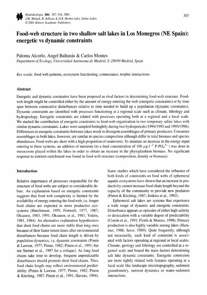
Hydrobiologia 466: 307-316,2001. J.M. Melack, R. Jellison & D.H. Herbst (eds), Saline Lakes. © 2001 Kluwer Academic Publishers.
307
Food-web structure in two shallow salt lakes in Los Monegros (NE Spain): energetic vs dynamic constraints
Paloma A1corlo, Angel Baltamis & Carlos Montes Department of Ecology, Universidad Autonoma de Madrid, E-28049 Madrid, Spain
Key words: food web patterns, ecosystem functioning, connectance, trophic interactions
Abstract
Energetic and dynamic constraints have been proposed as rival factors in determining food-web structure. Foodweb length might be controlled either by the amount of energy entering the web (energetic constraints) or by time span between consecutive disturbances relative to time needed to build up a popUlation (dynamic constraints). Dynamic constraints are identified with processes functioning at a regional scale such as climate, lithology and hydrogeology. Energetic constraints are related with processes operating both at a regional and a local scale. We studied the contribution of energetic constraints to food-web organization in two temporary saline lakes with similar dynamic constraints. Lakes were sampled fortnightly during two hydroperiods (199411995 and 1995/1996). Differences in energetic constraints between lakes result in divergent assemblages of primary producers. Consumer assemblages in both lakes, however, are similar in species composition although differ in total biomass and species abundances. Food-webs are short with a high proportion of omnivores. To simulate an increase in the energy input entering to these systems, an addition of nutrients (to a final concentration of 100 JLg.l-1 P-P043-) was done in mesocosms placed within the lakes in order to obtain an increase in the phytoplankton biomass. No significant response to nutrient enrichment was found in food-web structure (composition, density or biomass).
Introduction
Relative importance of processes responsible for the structure of food webs are subject to considerable debate. An explanation based on energetic constraints suggests that food web complexity is limited by the availability of energy entering the food web, i.e. longer food chains are expected in more productive ecosystems (Hutchinson, 1959; Fretwell, 1977, 1987; Oksanen, 1983, 1991; Oksanen, et aI., 1981; Yodzis, 1981, 1984). An alternative explanation hypothesizes that short food chains are more stable than long ones because of their faster return times after environmental disturbances because food chain length is driven by population dynamics, i.e, dynamic constraints (Pimm & Lawton, 1977; Pimm, 1982; Pimm et aI., 1991; but see Sterner et aI., 1997 for a critique). As long food chains take time to develop, frequent unpredictable disturbances should promote short food chains. Thus, food chain length may reflect environmental predictability (Pimm & Lawton, 1977; Pimm, 1982; Pimm & Kitching, 1987; Pimm et aI., 1991; Havens, 1994).
Some studies which have considered the influence of both kinds of constraints on food webs of ephemeral aquatic ecosystems have shown that an increase in productivity cannot increase food chain length beyond the capacity of the community to provide new predators (Pimm & Kitching, 1987; Jenkins et aI., 1992).
Ephemeral salt lakes are systems that experience a wide range of dynamic and energetic constraints. Disturbance appears as episodes of either high salinity or desiccation with a variable degree of predictability (Comin et aI., 1991; Florin & Montes, 1998). Primary production is also highly variable among lakes (Hammer, 1986; Javor, 1989). Quite frequently, although not necessarily, each kind of constraint is associated with factors operating at regional or local scales. Climate, geology and lithology are controlled at a regional scale and bound the main factors determining salt lake dynamic constraints. Energetic constraints are more tightly related with features operating at a local scale like landscape microtopography, sediment granulometry, nutrient dynamics or water-sediment interactions.
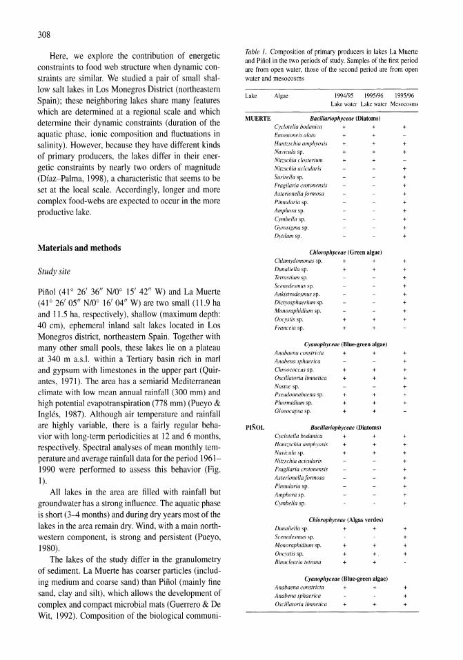
308
Here, we explore the contribution of energetic constraints to food web structure when dynamic constraints are similar. We studied a pair of small shallow salt lakes in Los Monegros District (northeastern Spain); these neighboring lakes share many features which are determined at a regional scale and which determine their dynamic constraints (duration of the aquatic phase, ionic composition and fluctuations in salinity). However, because they have different kinds of primary producers, the lakes differ in their energetic constraints by nearly two orders of magnitude (Diaz-Palma, 1998), a characteristic that seems to be set at the local scale. Accordingly, longer and more complex food-webs are expected to occur in the more productive lake.
Materials and methods
Study site
Piliol (41 0 26' 36" N/O° 15' 42" W) and La Muerte (41 0 26' 05" NlO° 16' 04" W) are two small (11.9 ha and 11.5 ha, respectively), shallow (maximum depth: 40 cm), ephemeral inland salt lakes located in Los Monegros district, northeastern Spain. Together with many other small pools, these lakes lie on a plateau at 340 m a.s.l. within a Tertiary basin rich in marl and gypsum with limestones in the upper part (Quirantes, 1971). The area has a semiarid Mediterranean climate with low mean annual rainfall (300 mm) and high potential evapotranspiration (778 mm) (Pueyo & Ingles, 1987). Although air temperature and rainfall are highly variable, there is a fairly regular behavior with long-term periodicities at 12 and 6 months, respectively. Spectral analyses of mean monthly temperature and average rainfall data for the period 1961-1990 were performed to assess this behavior (Fig. 1).
All lakes in the area are filled with rainfall but groundwater has a strong influence. The aquatic phase is short (3-4 months) and during dry years most of the lakes in the area remain dry. Wind, with a main northwestern component, is strong and persistent (Pueyo, 1980).
The lakes of the study differ in the granulometry of sediment. La Muerte has coarser particles (including medium and coarse sand) than Pinol (mainly fine sand, clay and silt), which allows the development of complex and compact microbial mats (Guerrero & De Wit, 1992). Composition of the biological communi-
Table 1. Composition of primary producers in lakes La Muerte and Piiiol in the two periods of study. Samples of the first period are from open water, those of the second period are from open water and mesocosms
Lake
MUERTE
PINOL
Algae 1994/95 1995/96 1995196 Lake water Lake water Mesocosms
Bacil/ariophyceae (Diatoms)
Cyclotella bodanica + + Entomoneis alata + + Hantzschia amphyoxis + + Navicula sp. + + Nitzschia closterium + + Nitzschia acicularis Surirella sp. Fragilaria crotonensis Asterionelfa formosa Pinnularia sp. Amphora sp. Cymbella sp. Gyrosigma sp. Dytilumsp.
Chlorophyceae (Green algae) Chlamydomonas sp. Dunalielfa sp. Tetrastium 'p. Scenedesmus sp. Ankistrodesmus sp. Dictyosphaerium sp. Monoraphidium sp. Oocystis sp. F ranceia sp.
+ +
+ +
+ +
+ +
Cyanophyceae (Blue-green algae) Anabaena constricta + + Anabena sphaerica Chroococcus sp. + + Oscillatoria limnetica + + Nostoc sp. Pseudoanabaena sp. + + Phormidium sp. + + Gloeocapsa sp. + +
Bacil/ariophyceae (Diatoms)
Cyclotella bodanica + + Hantzschia amphyoxis + + Navicula sp. + + Nitzschia acicularis Fragilaria crotonensis Asterionella formosa Pinnularia sp. Amphora sp. Cymbella sp.
Chlorophyceae (Algas verdes) Dunaliella sp. + + Scenedesmus sp. Monoraphidium 'p. + + Oocystis sp. + + Binuclearia tetrana + +
Cyanophyceae (Blue-green algae) Anabaena constricta + + Anabena sphaerica Oscillatoria limnetica + +
+
+ +
+ + + + + + + + +
+ + + + + + + +
+ + + + + + +
+ + + + + + + + +
+ + + +
+ + +
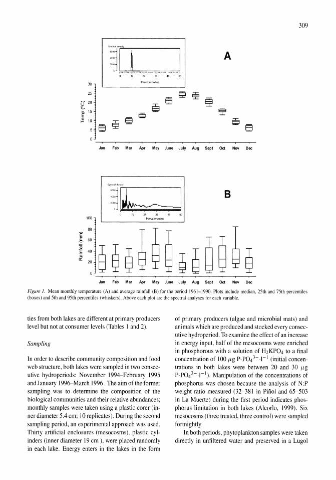
309
I A ~T I
iii o 12 24
ii' 36 48 60
30 Period irroothsj
25
Jan Feb Mar Apr May June July Aug Sept Oct Nov Dec
SJl$Cltaldol'lj~
~11L-J B , , i i i , 0 12 24 36 48 60
100 Penod (!1'IOfIths)
80
8~~~ I 60
~gQ8 ~ 40
~ c
'Qi cr:
20
0
Jan Feb Mar Apr May June July Aug Sept Oct Nov Dec
Figure 1. Mean monthly temperature (A) and average rainfall (B) for the period 1961-1990. Plots include median, 25th and 75th percentiles (boxes) and 5th and 95th percentiles (whiskers). Above each plot are the spectral analyses for each variable.
ties from both lakes are different at primary producers level but not at consumer levels (Tables 1 and 2).
Sampling
In order to describe community composition and food web structure, both lakes were sampled in two consecutive hydroperiods: November 1994-February 1995 and January 1996-March 1996. The aim of the former sampling was to determine the composition of the biological communities and their relative abundances; monthly samples were taken using a plastic corer (inner diameter 5.4 cm; 10 replicates). During the second sampling period, an experimental approach was used. Thirty artificial enclosures (mesocosms), plastic cylinders (inner diameter 19 cm ), were placed randomly in each lake. Energy enters in the lakes in the form
of primary producers (algae and microbial mats) and animals which are produced and stocked every consecutive hydroperiod. To examine the effect of an increase in energy input, half of the mesocosms were enriched in phosphorous with a solution of H2KP04 to a final concentration of 100 {.lg P-P043- .1-1 (initial concentrations in both lakes were between 20 and 30 {.lg P-P043- .1-1). Manipulation of the concentrations of phosphorus was chosen because the analysis of N:P weight ratio measured (32-381 in Pinol and 65-503 in La Muerte) during the first period indicates phosphorus limitation in both lakes (A1corlo, 1999). Six mesocosms (three treated, three control) were sampled fortnightly.
In both periods, phytoplankton samples were taken directly in unfiltered water and preserved in a Lugol
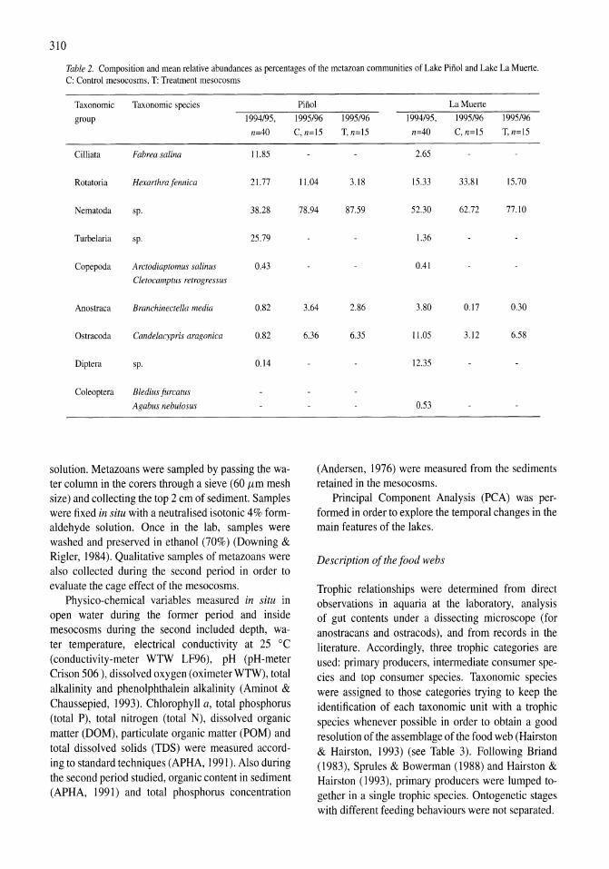
310
Table 2. Composition and mean relative abundances as percentages of the metazoan communities of Lake Pinol and Lake La Muerte. C: Control mesocosms, T: Treatment mesocosms
Taxonomic Taxonomic species group 1994/95,
n=40
Cilliata Fabrea salina 11.85
Rotatoria Hexarthra fennica 21.77
Nematoda sp. 38.28
Turbelaria sp. 25.79
Copepoda Arctodiaptomus salinus 0.43
Cletocamptus retrogressus
Anostraca Branchinectella media 0.82
Ostracoda Candelacypris aragonica 0.82
Diptera sp. 0.14
Coleoptera Bledius furcatus
Agabus nebulosus
solution. Metazoans were sampled by passing the water column in the corers through a sieve (60 /Lm mesh size) and collecting the top 2 cm of sediment. Samples were fixed in situ with a neutralised isotonic 4% formaldehyde solution. Once in the lab, samples were washed and preserved in ethanol (70%) (Downing & Rigler, 1984). Qualitative samples of metazoans were also collected during the second period in order to evaluate the cage effect of the mesocosms.
Physico-chemical variables measured in situ in open water during the former period and inside mesocosms during the second included depth, water temperature, electrical conductivity at 25°C (conductivity-meter WTW LF96), pH (pH-meter Crison 506 ), dissolved oxygen (oximeter WTW), total alkalinity and phenolphthalein alkalinity (Aminot & Chaussepied, 1993). Chlorophyll a, total phosphorus (total P), total nitrogen (total N), dissolved organic matter (DOM), particulate organic matter (POM) and total dissolved solids (IDS) were measured according to standard techniques (APHA, 1991). Also during the second period studied, organic content in sediment (APHA, 1991) and total phosphorus concentration
Pinol La Muerte 1995/96 1995196 1994/95, 1995196 1995196
C, n=15 T, n=15 n=40 C, n=15 T, n=15
2.65
11.04 3.18 15.33 33.81 15.70
78.94 87.59 52.30 62.72 77.10
1.36
0.41
3.64 2.86 3.80 0.17 0.30
6.36 6.35 11.05 3.12 6.58
12.35
0.53
(Andersen, 1976) were measured from the sediments retained in the mesocosms.
Principal Component Analysis (PCA) was performed in order to explore the temporal changes in the main features of the lakes.
Description of the food webs
Trophic relationships were determined from direct observations in aquaria at the laboratory, analysis of gut contents under a dissecting microscope (for anostracans and ostracods), and from records in the literature. Accordingly, three trophic categories are used: primary producers, intermediate consumer species and top consumer species. Taxonomic species were assigned to those categories trying to keep the identification of each taxonomic unit with a trophic species whenever possible in order to obtain a good resolution of the assemblage of the food web (Hairston & Hairston, 1993) (see Table 3). Following Briand (1983), Sprules & Bowerman (1988) and Hairston & Hairston (1993), primary producers were lumped together in a single trophic species. Ontogenetic stages with different feeding behaviours were not separated.
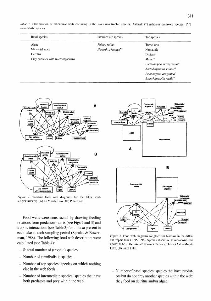
311
Table 3. Classification of taxonomic units occurring in the lakes into trophic species. Asterisk (*) indicates omnivore species, (* *) cannibalistic species
Basal species Intermediate species Top species
Algae Microbial mats
Detritus
Fabrea salina Hexarthra fennica**
Turbellaria
Nematoda
Diptera
Moina" Clay particles with microorganisms
Figure 2. Standard food web diagrams for the lakes studied.(l9941l995). (A) La Muerte Lake, (B) Pinol Lake.
Food webs were constructed by drawing feeding relations from predation matrix (see Figs 2 and 3) and trophic interactions (see Table 3) for all taxa present in each lake at each sampling period (Sprules & Bowerman, 1988). The following food web descriptors were calculated (see Table 4):
- S: total number of (trophic) species.
- Number of cannibalistic species.
- Number of top species: species on which nothing else in the web feeds.
- Number of intermediate species: species that have both predators and prey within the web.
A
-......
Cletocamptus retrogressus'
Arctodiaptomus salinus'
Prionocypris aragonica*
Branchinectella media*
B
Figure 3. Food web diagrams weighted for biomass in the different trophic taxa (1995/1996). Species absent in the mesocosms but known to be in the lake are drawn with dashed lines. (A) La Muerte Lake, (B) Pinol Lake.
- Number of basal species: species that have predators but do not prey another species within the web; they feed on detritus and/or algae.
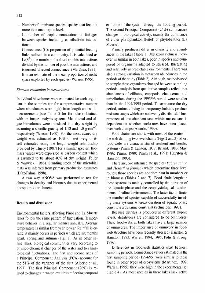
312
- Number of omnivore species: species that feed on more than one trophic level.
- L: number of trophic connections or linkages between species including cannibalistic interactions.
- Connectance (C): proportion of potential feeding links realised in a community. It is calculated as L/(S2), the number of realised trophic interactions divided by the number of possible interactions, and is termed 'directedconnectance' (Martinez, 1991). It is an estimate of the mean proportion of niche space exploited by each species (Warren, 1995).
Biomass estimation in mesoscosms
Individual biovolumes were estimated for each organism in the samples (or for a representative number when abundances were high) from length and width measurements (see Table 5 for formulas) obtained with an image analysis system. Meiofaunal and algae biovolumes were translated into dry weight by assuming a specific gravity of 1.13 and 1.0 g.cm-3,
respectively (Wieser, 1960). For the anostracans, dry weight was estimated as 10% of wet weight, itself estimated using the length-weight relationship provided by Thiery (1987) for a similar species. Biomass values were expressed as carbon content which is assumed to be about 40% of dry weight (Feller & Warwick, 1988). Standing stock of the microbial mats was inferred from primary production estimates (Diaz-Palma, 1998).
A two way ANOYA was performed to test for changes in density and biomass due to experimental phosphorus enrichment.
Results and discussion
Environmental factors affecting Pinol and La Muerte lakes follow the same pattern of fluctuation. Temperature behaves in a regular manner annually. Average temperature is similar from year to year. Rainfall is erratic; it mainly occurs in periods which are six months apart, spring and autumn (Fig. 1). As in other saline lakes, biological communities vary according to physico-chemical changes of the water and to climatological fluctuations. The first and second axes of a Principal Component Analysis (PCA) account for the 51 % of the variance of the data (Alcorlo et aI., 1997). The first Principal Component (26%) is related to changes in water level thus reflecting temporal
evolution of the system through the flooding period. The second Principal Component (24%) summarizes changes in biological activity, mainly the dominance of either phytoplankton (Pinol) or phytobenthos (La Muerte).
Primary producers differ in diversity and abundances in the lakes (Table I). Metazoan richness, however, is similar in both lakes, poor in species and composed of organisms adapted to stressed, fluctuating and relatively unpredictable environments. There was also a strong variation in metazoan abundances in the periods of the study (Table 2). Although, methods used to sample these organisms changed between sampling periods, analysis from qualitative samples reflect that abundances of cilliates, copepods, cladocerans and turbellarians during the 1995/96 period were smaller than in the 199411995 period. To overcome the dry period, animals living in temporary habitats produce resistant stages which are not evenly distributed. Thus, presence of low-abundant taxa within mesocosms is dependent on whether enclosures have been placed over such clumps (Alcorlo, 1999).
Food chains are short, with most of the routes in the web defining two level chains (Figs 2 and 3). Short food-webs are characteristic of resilient and benthic systems (Pimm & Lawton, 1977; Briand, 1983; May, 1986; Pimm, 1988; Pimm et aI., 1991; Hairston & Hairston, 1993).
There are, two intermediate species (Fabrea salina and Hexarthra fennica) which determine three level routes; those species are not dominant in numbers or in biomass (Tables 2 and 7). Food chain length in these systems is mainly controlled by the duration of the aquatic phase and the ecophysiological requirements of saline environments. The latter factor limits the number of species capable of successfully invading these systems whereas duration of aquatic phase constitute a dynamic constraint (Schneider, 1997).
Because detritus is produced at different trophic levels, detritivores are considered to be omnivores. Thus, food-webs at both lakes have a large number of omnivores. The importance of omnivory in foodweb structure have been recently stressed (Hairston & Hairston, 1993; Warren, 1994, 1995; Polis & Strong, 1996).
Differences in food-web statistics exist between sampling periods. Connectance values estimated in the first sampling period (1994/95) were similar to those found in other types of ecosystems (Martinez, 1992; Warren, 1995); they were high in the experimental set (Table 4). As most species in these lakes lack active
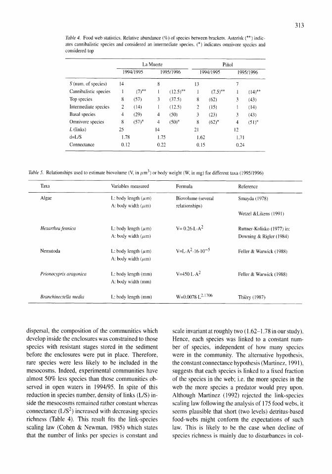
313
Table 4. Food web statistics. Relative abundance (%) of species between brackets. Asterisk (**) indicates cannibalistic species and considered an intermediate species. (*) indicates omnivore species and considered top
La Muerte Piiiol
199411995 1995/1996 1994/1995 199511996
S (num. of species) 14 8 13 7
Cannibalistic species I (7)** I (12.5)** I (7.5)*' I (14)**
Top species 8 (57) 3 (37.5) 8 (62) 3 (43)
Intermediate species 2 (14) (12.5) 2 (15) (14)
Basal species 4 (29) 4 (50) 3 (23) 3 (43)
Omnivore species 8 (57)* 4 (50)* 8 (62)* 4 (51)'
L (links) 25 14 21 12
d=LlS 1.78 1.75 1.62 1.71
Connectance 0.12 0.22 0.15 0.24
Table 5. Relationships used to estimate biovolume (V, in /Lm3) or body weight (W, in mg) for different taxa (1995/1996)
Taxa Variables measured
Algae L: body length (/Lm)
A: body width (/Lm)
Hexarthra fennica L: body length (/Lm)
A: body width (/Lm)
Nematoda L: body length (/Lm)
A: body width (/Lm)
Prionocypris aragonica L: body length (mm)
A: body width (mm)
Branchinectella media L: body length (mm)
dispersal, the composition of the communities which develop inside the enclosures was constrained to those species with resistant stages stored in the sediment before the enclosures were put in place. Therefore, rare species were less likely to be included in the mesocosms. Indeed, experimental communities have almost 50% less species than those communities observed in open waters in 1994/95. In spite of this reduction in species number, density of links (LIS) inside the mesocosms remained rather constant whereas connectance (LlS2) increased with decreasing species richness (Table 4). This result fits the link-species scaling law (Cohen & Newman, 1985) which states that the number of links per species is constant and
Formula Reference
Biovolume (several Smayda (1978)
relationships)
Wetzel &Likens (1991)
V= 0.26.L.A2 Ruttner-Kolisko (1977) in:
Downing & Rigler (1984)
V=L·A2.16·1O-5 Feller & Warwick (1988)
V=450L·A2 Feller & Warwick (1988)
W=O.0078.L2.1706 Thiery (1987)
scale invariant at roughly two (1.62-1.78 in our study). Hence, each species was linked to a constant number of species, independent of how many species were in the community. The alternative hypothesis, the constant connectance hypothesis (Martinez, 1991), suggests that each species is linked to a fixed fraction of the species in the web; i.e. the more species in the web the more species a predator would prey upon. Although Martinez (1992) rejected the link-species scaling law following the analysis of 175 food webs, it seems plausible that short (two levels) detritus-based food-webs might conform the expectations of such law. This is likely to be the case when decline of species richness is mainly due to disturbances in col-
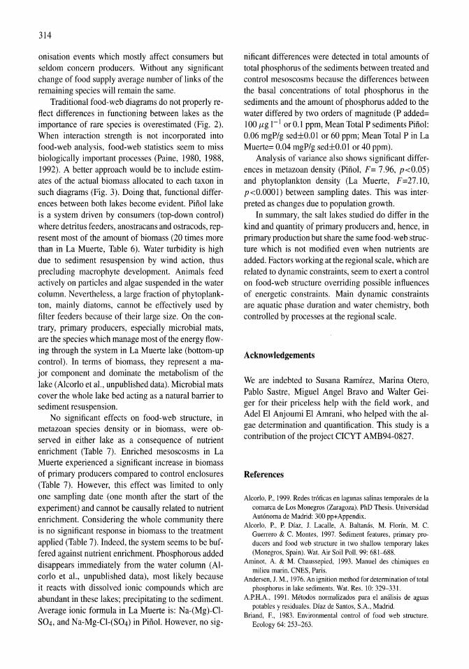
314
onisation events which mostly affect consumers but seldom concern producers. Without any significant change of food supply average number of links of the remaining species will remain the same.
Traditional food-web diagrams do not properly reflect differences in functioning between lakes as the importance of rare species is overestimated (Fig. 2). When interaction strength is not incorporated into food-web analysis, food-web statistics seem to miss biologically important processes (Paine, 1980, 1988, 1992). A better approach would be to include estimates of the actual biomass allocated to each taxon in such diagrams (Fig. 3). Doing that, functional differences between both lakes become evident. Pinol lake is a system driven by consumers (top-down control) where detritus feeders, anostracans and ostracods, represent most of the amount of biomass (20 times more than in La Muerte, Table 6). Water turbidity is high due to sediment resuspension by wind action, thus precluding macrophyte development. Animals feed actively on particles and algae suspended in the water column. Nevertheless, a large fraction of phytoplankton, mainly diatoms, cannot be effectively used by filter feeders because of their large size. On the contrary, primary producers, especially microbial mats, are the species which manage most of the energy flowing through the system in La Muerte lake (bottom-up control). In terms of biomass, they represent a major component and dominate the metabolism of the lake (Alcorlo et aI., unpublished data). Microbial mats cover the whole lake bed acting as a natural barrier to sediment resuspension.
No significant effects on food-web structure, in metazoan species density or in biomass, were observed in either lake as a consequence of nutrient enrichment (Table 7). Enriched mesoscosms in La Muerte experienced a significant increase in biomass of primary producers compared to control enclosures (Table 7). However, this effect was limited to only one sampling date (one month after the start of the experiment) and cannot be causally related to nutrient enrichment. Considering the whole community there is no significant response in biomass to the treatment applied (Table 7). Indeed, the system seems to be buffered against nutrient enrichment. Phosphorous added disappears immediately from the water column (AIcorio et aI., unpublished data), most likely because it reacts with dissolved ionic compounds which are abundant in these lakes; precipitating to the sediment. Average ionic formula in La Muerte is: Na-(Mg)-CIS04, and Na-Mg-CI-(S04) in Pinol. However, no sig-
nificant differences were detected in total amounts of total phosphorus of the sediments between treated and control mesoscosms because the differences between the basal concentrations of total phosphorus in the sediments and the amount of phosphorus added to the water differed by two orders of magnitude (P added= 100 fLg I-lor 0.1 ppm, Mean Total P sediments Pinol: 0.06 mgP/g sed±O.OI or 60 ppm; Mean Total P in La Muerte= 0.04 mgP/g sed±O.O 1 or 40 ppm).
Analysis of variance also shows significant differences in metazoan density (Pinol, F= 7.96, p<0.05) and phytoplankton density (La Muerte, F =27 .lO, p<O.OOOl) between sampling dates. This was interpreted as changes due to population growth.
In summary, the salt lakes studied do differ in the kind and quantity of primary producers and, hence, in primary production but share the same food-web structure which is not modified even when nutrients are added. Factors working at the regional scale, which are related to dynamic constraints, seem to exert a control on food-web structure overriding possible influences of energetic constraints. Main dynamic constraints are aquatic phase duration and water chemistry, both controlled by processes at the regional scale.
Acknowledgements
We are indebted to Susana RamIrez, Marina Otero, Pablo Sastre, Miguel Angel Bravo and Walter Geiger for their priceless help with the field work, and Adel EI Anjoumi EI Amrani, who helped with the algae determination and quantification. This study is a contribution of the project CICYT AMB94-0827.
References
Alcorlo, P., 1999. Redes troficas en lagunas salinas temporales de la comarca de Los Monegros (Zaragoza). PhD Thesis. Universidad Autonoma de Madrid: 300 pp+Appendix.
Alcorlo, P., P. Diaz, J. Lacalle, A. Baltamis, M. Florin, M. C. Guerrero & C. Montes, 1997. Sediment features, primary producers and food web structure in two shallow temporary lakes (Monegros, Spain). Wat. Air Soil Poll. 99: 681--688.
Aminot, A. & M. Chaussepied, 1993. Manuel des chimiques en milieu marin. CNES, Paris.
Andersen, J. M., 1976. An ignition method fordeterrnination of total phosphorus in lake sediments. Wat. Res. 10: 329-331.
A.P.H.A., 1991. Metodos normalizados para el analisis de aguas potables y residuales. Diaz de Santos, S.A., Madrid.
Briand, F., 1983. Environmental control of food web structure. Ecology 64: 253-263.
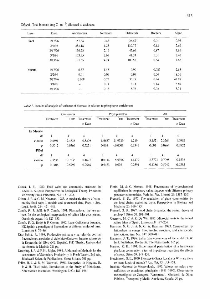
315
Table 6. Total biomass (mg C . m-2) allocated to each taxa
Lake Date Anostracans Nematods Ostracods Rotifers Algae
Pinol 1/17/96 157.34 0.48 26.52 om 0.98
212/96 282.18 1.25 139.77 0.13 2.69 2/17/96 130.73 2.19 45.66 0.87 3.86
3/1/96 103.35 2.67 41.24 1.01 2.40 3/13/96 71.55 4.24 100.55 0.64 1.62
Muerte 1/17/96 0.87 1.58 0.90 0.027 2.63
2/2/96 0.01 0.09 0.99 0.04 18.26 2/17/96 0.008 0.23 33.19 0.24 41.89
3/1/96 0.14 8.11 0.14 6.69
3/13/96 0.18 5.76 0.02 3.71
Table 7. Results of analysis of variance of biomass in relation to phosphorus enrichment
Consumers Phytoplankton All Treatment Date Treatment Treatment
x Date
La Muerte
df 1 4 4
F-ratio 0.4691 2.4836 0.8209 p 0.5012 0.0766 0.5271
Piiiol
df 1 4 4
F-ratio 2.3538 0.7338 0.1627
p 0.1406 0.5797 0.9548
Cohen, J. E., 1989. Food webs and community structure. In Levin, S. A. (eds), Perspectives in Ecological Theory. Princeton University Press, Princeton, N.J.: 181-202.
Cohen, 1. E. & c. M. Newman, 1985. A stochastic theory of community food webs I. models and aggregated data. Proc. r. Soc. Lond. Ser.B. 224: 421-448.
Comin, E, R. Julia & P. Comin, 1991. Fluctuations, the key aspect for the ecological interpretation of saline lake ecosystems. Oecologia Aquat. 10: 127-135.
Comin, E, X. Rodo & P. Comin, 1992. Lake Gallocanta (Aragon, NE.Spain), a paradigm of fluctuations at different scales of time. Lirnnetica 8: 79-86.
Dfaz Palma, P., 1998. Produccion primaria y su relacion con las fluctuaciones asociadas al ciclo hidrologico en lagunas salinas de la Depresion del Ebro (NE, Espana). PhD Thesis., Universidad Autonoma de Madrid: 221 pp.
Downing, J. A. & E H., Rigler, 1984. A Manual on Methods for the Assessment of Secondary Productivity in Fresh Waters. 2nd edn. Blackwell Scientific Publications, Great Britain: 501 pp.
Feller, R.1. & R. M. Warwick, 1988. Energetics. In Higgins, R. P. & H. Thiel (eds), Introduction to the Study of Meiofauna. Smithsonian Institution, Washington, D.C.: 181-196.
I
8.6637
0.008
0.0114
0.9163
Date Treatment Treatment Date Treatment
x Date x Date
4 4 4 4
21.9529 1.219 3.1521 2.3764 1.0968
<0.0001 0.3341 0.091 0.0864 0.3852
4 4 1 4 4
5.9936 1.4479 2.3793 0.7095 0.1592
0.003 0.2591 0.1386 0.5949 0.9565
Florin, M. & C. Montes, 1998. Fluctuations of hydrochemical equilibrium in temporary saline lagWlas with different primary producer communities. Verh. int. VeT. Limnol. 26: 1387-1391.
Fretwell, S. D., 1977. The regulation of plant communities by the food chains exploiting them. Perspectives in Biology and Medicine 20: 169-185.
Fretwell, S. D., 1987. Food chain dynamics: the central theory of ecology? Oikos 50: 291-301.
Guerrero, M. C. & R. De Wit, 1992. Microbial mats in the inland saline lakes of Spain. Limnetica 8: 197-204.
Hairston, N. G. Jr. & N. G. Sr. Hairston, 1993. Cause-effect relationships in energy flow, trophic structure, and interspecific interactions. Am. Nat. 142: 379-411.
Hammer, U. T., 1986. Saline lake ecosystems of the world. Dr W. Junk Publishers, Dordrecht, The Netherlands: 615 pp.
Havens, K. E., 1994. Experimental perturbation of a freshwater plankton community: a test of hypotheses regarding the effects of stress. Oikos 69: 147-153.
Hutchinson, G. E., 1959. Homage to Santa Rosalia or Why are there so many kinds of animals? Am. Nat. 93: 145-158.
Instituto Nacional de Meteorologia, 1995. Val ores norrnales y estadisticos de estaciones principales (\ 961-1990). Observatorio metereologico de Zaragoza 'Aeropuerto'. Ministerio de Obras Publicas, Transporte y Medio Ambiente, Espana: 56 pp.
316
Javor, B., 1989. Hypersaline environments. Microbiology and biogeochemistry. Springer-Verlag, New York, U.S.A.: 328 pp.
Jenkins, B., R. L. Kitching & S. L. Pimm, 1992. Productivity, disturbance and food web structure at a local spatial scale in experimental container habitats. Oikos 65: 249-255.
Lawton, J. H. & P. H. Warren, 1988. Static and dynamic explanations for patterns in food webs. Trends Ecol. Evol. 3: 242-245.
Martinez, N. D., 1991. Artifacts or attributes? Effects of resolution of the Little Rock Lake food web. Ecol. Monogr. 61: 367-392.
Martinez, N. D., 1992. Constant connectance in community food webs. Am. Nat. 139: 1208-1218.
Martinez, N. D. &J. H. Lawton, 1995. Scale and food-web structure - from local to global. Oikos 73: 148-154.
May, R. M., 1986. The search for patterns in the balance of nature: advances and retreats. Ecology 67: 1115-1126.
Oksanen, L., 1983. Trophic exploitation and arctic phytomass patterns. Am. Nat. 122: 45-52.
Oksanen, L., 1991. Trophic levels and trophic dynamics: a consensus emerging? Trends Ecol. Evol. 6: 58-90.
Oksanen, L., S. Fretwell, J. Aruda & P. Niemela, 1981. Exploitation ecosystems in gradients of primary productivity. Am. Nat. 118: 240--261.
Paine, R. T., 1980. Food webs: linkage, interaction strenght and community infrastructure. J. animo Eco1.49: 667-686.
Paine, R. T., 1988. Food webs: road maps of interactions or grist for theoretical deveplopment? Ecology 69: 1648-1654.
Paine, R. T., 1992. Food-web analysis through field measurement of per capita interaction strength. Nature 355: 73-75.
Pimm, S. L., 1982. Food Webs. Chapman & Hall, London: 218 pp. Pimm, S. L., 1988. Energy flow and trophic structure. In Pomeroy,
L. R. & 1. J. Alberts (eds), Concepts of Ecosystem Ecology. Springer-Verlag, New York: 263-278.
Pimm, S. L. & R. L. Kitching, 1987. The determinants offood chain lenghts. Oikos 50: 302-307.
Pimm, S. L. & 1. H. Lawton, 1977. The number of trophic levels in ecological communities. Nature 268: 329-331.
Pimm, S. L., J. H. Lawton & J. E. Cohen, 1991. Food web patterns and their consequences. Nature 350: 669-674.
Polis, G. A & D. R. Strong, 1996. Food web complexity and community dynamics. Am. Nat. 147: 813-846.
Pueyo, 1. J., 1980. Procesos diageneticos observados en las lagunas tipo playa de la zona de Bujaraloz-Alcaniz (provincias de Zaragoza y Teruel). Revista Investigaciones Geologicas 34: 195-207.
Pueyo, J. 1. & M. Ingles, 1987. Magnesite formation in recent playa lakes, Los Monegros, Spain. In Marshall, J. D. (eds), Diagenesis of Sedimentary Sequences. Geological Society Special Publication: 119-122.
Quirantes, J., 1971. Las calizas en el Terciario continental de Los Monegros. Estudios Geologicos 27: 355-362.
Schneider, D. w., 1997. Predation and food web structure along a habitat duration gradient. Oecologia 110: 567-575.
Smayda, T. J., 1978. From phytoplankters to biomass. In Sournia, A. (ed.), Phytoplankton Manual. UNESCO, Paris: 273-279.
Sprules, W. G. & J. E. Bowerman, 1988. Omnivory and food chain length in zooplankton food webs. Ecology 69: 418-426.
Sterner, R. w., A. Bajpai & T. Adams, 1997. The enigma of food chain length: absence of theoretical evidence for dynamic constraints. Ecology 78: 2258-2262.
Thiery, A., 1987. Les crustaces branchiopodes anostraca, notostraca et conchostraca des milieux limniques temporaires (dayas) au maroc. Taxonomie, biogeographie, ecologie. Tesis Doctoral, Faculte des Sciences et techniques de St Jerome, Universite de Droit d'Economie et des Sciences d' Aix-Marseille: 406 pp.
Warren, P. H., 1994. Making connections in food webs. Trends Ecol. Evol. 9: 136-141.
Warren, P. H., 1995. Estimating morphologically determined connectance and structure for food webs of freshwater invertebrates. Freshwat. BioI. 33: 213-221.
Wetzel, R. G. & G. E., Likens, 1991. Limnological Analyses. Springer-Verlag, New York: 391 pp.
Wieser, W., 1960. Benthic studies in Buzzards Bay. II. The meiofauna. Limnol. Oceanogr. 5: 121-137.
Yodzis, P., 1981. The structure of assembled communities. J. Theor. BioI. 289: 674-676.
Yodzis, P., 1984. The structure of assembled communities. II. J. Theor. BioI. 92: 115-126.
Hydrobiologia 466: 317-328,2001. J.M. Melack, R. Jellison & D.B. Herbst (eds), Saline Lakes. © 2001 Kluwer Academic Publishers.
317
Avian communities in baylands and artificial salt evaporation ponds of the San Francisco Bay estuary
John Y. Takekawa1, Corinna T. Lu1,2 & Ruth T. Pratt3,4
1 U.S. Geological Survey, Western Ecological Research Center, San Francisco Bay Estuary Field Station, P.O. Box 2012, Vallejo, CA 94592, U.S.A. Tel: 707/562-2000. Fax:707/562-3001. E-mail: [email protected] 2U.S. Geological Survey, California Cooperative Research Unit, Humboldt State University, Arcata, CA 95521, U.S.A. 3u.S. Fish and Wildlife Service, Ecological Services, Endangered Species Branch, P.O. Box 2012, Vallejo, CA 94592, U.S.A. 4Present address: 307 North Street, Sausalito, CA 94965, U.S.A.
Key words: salt evaporation ponds, waterbirds, San Francisco Bay, migratory birds, baylands, salt ponds
Abstract
San Francisco Bay wetlands, seasonal and tidal marshes between the historic low and high tide lines, are now highly fragmented because of development during the past 150 years. Artificial salt pond systems in the Bay are hypersaline and typically support simple assemblages of algae and invertebrates. In order to establish the value of salt ponds for migratory waterbirds, we used datasets to conduct a meta-analysis of avian communities in the baylands and salt ponds of San Pablo Bay. Fifty-three species of waterbirds in the salt ponds represented six foraging guilds: surface feeders, shallow probers, deep probers, dabblers, diving benthivores and piscivores. The total number of species and the Shannon-Weiner diversity index was higher in baylands than in salt ponds during all four seasons. However, overall bird density (numberlha) was higher in salt ponds compared with baylands in the winter and spring, primarily because of large concentrations of benthivores. Cessation of salt production in 1993 and subsequent reduction in water depth resulted in a decline of some diving duck populations that used the salt ponds.
Introduction
The San Francisco Bay estuary is one of the most important staging and wintering areas for migratory waterfowl and shorebirds in the Pacific Flyway (Harvey et al., 1992). San Francisco Bay is recognized as a site of hemispheric importance because it supports at least 30% of some individual shorebird populations in the flyway (Harrington & Perry, 1995) and up to half of many diving duck populations (Accurso, 1992). Many migratory waterbirds use the baylands, which consists of the area between the historic high and low tide lines and comprises 85 830 ha in the estuary (Goals Project, 1999). More than 90% of the historic wetlands in the bay lands have been lost to urban development, agriculture, and salt production (Josselyn,
1983; Nichols et al., 1986), and many tidal marsh species are now threatened or endangered. The remaining bayland wetlands are isolated from tidal action by the construction of levees or water control structures and comprise a fragmented landscape of non-tidal salt, brackish and fresh water wetlands, agricultural lands, seasonal ponds, vernal pools, riparian scrub and artificial salt evaporation ponds (Goals Project, 1999).
Historically, salt pans were a common wetland type in the baylands (Goals Project, 1999). Salt pans and seasonal wetlands likely provided foraging habitat and invertebrate prey for migratory waterbirds, as well as protected roosting areas during high tides or winter storms. All of the salt pans and most seasonal wetlands were lost to development during the past century, but salt evaporation pond systems developed for commer-
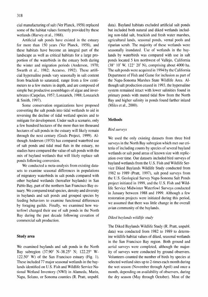
318
cial manufacturing of salt (Ver Planck, 1958) replaced some of the habitat values formerly provided by these wetlands (Harvey et aI., 1988).
Artificial salt ponds have existed in the estuary for more than 150 years (Ver Planck, 1958), and these habitats have become an integral part of the landscape as well as critical habitats for a large proportion of the waterbirds in the estuary both during the winter and migration periods (Anderson, 1970; Swarth et aI., 1982; Accurso, 1992). These artificial hypersaline ponds vary seasonally in salt content from brackish to saturated, range from a few centimeters to a few meters in depth, and are composed of simple but productive assemblages of algae and invertebrates (Carpelan, 1957; Lonzarich, 1988; Lonzarich & Smith, 1997).
Some conservation organizations have proposed converting the salt ponds into tidal wetlands to aid in reversing the decline of tidal wetland species and to mitigate for development. Under such a scenario, only a few hundred hectares of the more than ten thousand hectares of salt ponds in the estuary will likely remain through the next century (Goals Project, 1999). Although Anderson (1970) has compared waterbird use of salt ponds and tidal mud flats in the estuary, no studies have compared the value of salt ponds with the mix of bayland wetlands that will likely replace salt ponds following conversion.
We conducted a meta-analysis from existing datasets to examine seasonal differences in populations of migratory waterbirds in salt ponds compared with other bayland wetlands (hereafter baylands) in San Pablo Bay, part of the northern San Francisco Bay estuary. We compared total species, density and diversity in baylands and salt ponds and grouped species by feeding behaviors to examine functional differences by foraging guilds. Finally, we examined how waterfowl changed their use of salt ponds in the North Bay during the past decade following cessation of commercial salt production.
Study area
We examined bay lands and salt ponds in the North Bay subregion (37.90° N-38.25° N; 122.25° W-122.50° W) of the San Francisco estuary (Fig. 1). These included 77 major seasonal wetlands in the baylands identified on U.S. Fish and Wildlife Service National Wetland Inventory (NWI) in Alameda, Marin, Napa, Solano, or Sonoma counties (R. Pratt, unpub\.
data). Bayland habitats excluded artificial salt ponds but included both natural and diked wetlands including non-tidal salt, brackish and fresh water marshes, agricultural lands, seasonal ponds, vernal pools and riparian scrub. The majority of these wetlands were seasonally inundated. Use of wetlands in the baylands by waterbirds was compared with use in salt ponds located 5 km northwest of Vallejo, California (38° 10' W, 122° 20' N), comprising about 4000 ha. The salt ponds were acquired in 1994 by the California Department of Fish and Game for inclusion as part of the Napa-Sonoma Marshes State Wildlife Area. Although salt production ceased in 1993, the hypersaline system remained intact with lower salinities found in primary ponds with muted tidal flow from the North Bay and higher salinity in ponds found farther inland (Miles et aI., 2000).
Methods
Bird surveys
We used the only existing data sets from three bird surveys in the North Bay subregion which met our criteria of including counts by species of several bayland wetlands or salt pond areas of known size with replication over time. Our datasets included bird surveys of bayland wetlands from the U.S. Fish and Wildlife Service Diked Baylands Wildlife Study conducted from 1982 to 1989 (Pratt, 1997), salt pond surveys from the U.S. Geological Survey Napa-Sonoma Salt Ponds project initiated in 1999, and the U.S. Fish and Wildlife Service Midwinter Waterfowl Surveys conducted in January between 1988 and 1999. Although a few restoration projects were initiated during this period, we assumed that there was little change in the overall avian community of the bay lands.
Diked baylands wildlife study
The Diked Baylands Wildlife Study (R. Pratt, unpub\. data) was conducted from 1982 to 1989 to determine wildlife habitat values of diked, seasonal wetlands in the San Francisco Bay region. Both ground and aerial surveys were completed, although the majority of surveys were conducted by ground observers. Volunteers counted the number of birds by species at selected wetland sites up to 2-times each month during the wet season (November through April) and once a month, depending on availability of observers, during the dry season (May through October). Most of the
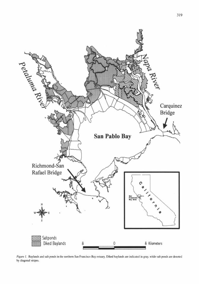
Rafael Bridge
s
~ Saltponds c=J Diked 8aylands
San Pablo Bay
8 o
• ", ", ,
o
8 Kilaneters
319
Figure 1. Baylands and salt ponds in the northern San Francisco Bay estuary. Diked baylands are indicated in gray, while salt ponds are denoted by diagonal stripes.
320
volunteers were experienced in bird identification and were members of local chapters of the National Audubon Society. On larger wetlands, the proportion of a wetland that was counted varied from 5% to 100% of the total area depending on visibility and landowner access. We limited our analyses to waterbird species, primarily shorebirds and waterfowl, which were readily counted in surveys of the North Bay subregion in 74 of the 77 wetlands surveyed where the size of the survey area was known.
Napa-Sonoma salt ponds
We initiated monthly complete counts of 5 of the 11 salt ponds (Ponds 1, 2, 3, 4, 7) within the NapaSonoma Marshes selected from a range of salinities in January 1999 (Miles et aI., 2000). The ponds ranged in size from 127 to 534 ha, and salinities varied from 22 g .1-1 to 225 g .1-1, similar to the range found in low and mid salinity ponds in commercial salt production systems. Observers conducted counts of species with binoculars and spotting scopes from vantage points at the edge of ponds during the first week of each month from January through December, and locations of waterbirds were placed in a geographic information system coverage into 250 m x 250 m grid squares (Miles et aI., 2000). Surveys were conducted during the day within 3 h of the highest high tide when the largest number of waterbirds were roosting in the salt ponds.
Foraging guilds
We separated the waterbirds into 6 guilds to examine differences among foraging groups rather than differences among individual species. These foraging guilds included: (1) surface feeders - obtained prey from the surface such as American avocet (Recurvirostra americana), black-necked stilt (Himantopus mexican us) and red-necked phalarope (Phalaropus lobatus); (2) shallow probers - foraged in the top layer «3 cm) of sediments such as western sandpiper (Calidris mauri) and dunlin (Calidris alpina); (3) deep probers - reached several centimeters into the substratum including marbled godwit (Limosa fedoa) and long-billed dowitcher (Limnodromus scolopaceus), (4) dabblers - fed in the upper water column such as northern pintail (Anas acuta) and northern shoveler (Anas clypeata); (5) diving benthivores -fed in deeper water on benthic invertebrates including lesser and greater scaup (Aythya marila, Aythya affinis), ruddy duck (Oxyura jamaicensis) and eared
grebe (Podiceps nigricollis); and (6) piscivores - fish consumers such as American white pelican (Pelecanus erythrorhynchos), Caspian and Forster's terns (Sterna caspia, Sterna forsteri), and double-crested cormorant (Phalacrocorax auritus), and (7) other - incidental species including Canada geese (Branta canadensis) and ring-billed gulls (Larus delawarensis). Most of the major waterbird species that use salt ponds are not endangered, but some species seen infrequently in the North Bay such as western snowy plover (Charadrius alexandrinus nivosa) and least terns (Sterna antillarun browni) are federal or state listed.
Analyses
The total number of waterbirds counted at a particular site varied widely depending on the number of surveys and water levels, especially in bayland wetlands where few or no birds were counted if the wetlands were dry. Thus, we used maximum daily counts and peak densities (birds.ha-1) of species found at each site to examine their greatest importance for waterbirds during each season. We examined differences by wetland type (bayland or salt pond) among foraging guilds during the winter (Nov-Jan), spring (Feb-Mar), summer (Apr-Aug) and autumn (Sep-Oct) seasons. Months were assigned to seasons to encompass the major migration chronology in spring and autumn. Monthly or semi-monthly surveys across years were treated as repeated measures, species were combined into guilds, and means were derived for each site. We examined differences in densities of the foraging guilds by wetland type, season, and the type-by-season interaction with two-way multivariate analysis of variance (MANOVA) techniques (Johnson & Wichern, 1988; SAS Institute, 1990). We conducted univariate analysis of variance tests for unequal sample sizes for each guild when significant multivariate results were detected, followed by pairwise comparison to locate differences among wetland types or seasons with Fisher's protected Least Squares Difference Test (Milliken & Johnson, 1984). Overall species diversity for bay lands and salt ponds was assessed with the Shannon-Weiner index (Krebs, 1989). Results were deemed significant when P S 0.05.
Midwinter waterfowl survey
The U.S. Fish and Wildlife Service midwinter aerial waterfowl survey indices were used to examine changes in waterfowl popUlations during the last 10 years as salt production ended in the North Bay ponds.
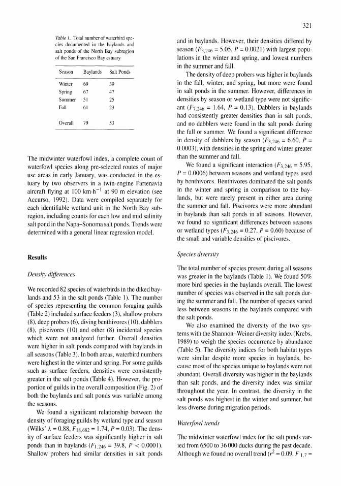
Table 1. Total number of waterbird species documented in the bay lands and salt ponds of the North Bay subregion of the San Francisco Bay estuary
Season Baylands Salt Ponds
Winter 69 39
Spring 67 47
Summer 51 25
Fall 61 23
Overall 79 53
The midwinter waterfowl index, a complete count of waterfowl species along pre-selected routes of major use areas in early January, was conducted in the estuary by two observers in a twin-engine Partenavia aircraft fiying at 100 km·h- 1 at 90 m elevation (see Accurso, 1992). Data were compiled separately for each identifiable wetland unit in the North Bay subregion, including counts for each low and mid salinity salt pond in the Napa-Sonoma salt ponds. Trends were determined with a general linear regression model.
Results
Density differences
We recorded 82 species of waterbirds in the diked baylands and 53 in the salt ponds (Table 1). The number of species representing the common foraging guilds (Table 2) included surface feeders (3), shallow probers (8), deep probers (6), diving benthivores (10), dabblers (8), piscivores (10) and other (8) incidental species which were not analyzed further. Overall densities were higher in salt ponds compared with bay lands in all seasons (Table 3). In both areas, waterbird numbers were highest in the winter and spring. For some guilds such as surface feeders, densities were consistently greater in the salt ponds (Table 4). However, the proportion of guilds in the overall composition (Fig. 2) of both the bay lands and salt ponds was variable among the seasons.
We found a significant relationship between the density of foraging guilds by wetland type and season (Wilks' A = 0.88, F18.682 = 1.74, P = 0.03). The density of surface feeders was significantly higher in salt ponds than in baylands (F\,246 = 39.8, P < 0.0001). Shallow probers had similar densities in salt ponds
321
and in baylands. However, their densities differed by season (F3,246 = 5.05, P = 0.0021) with largest populations in the winter and spring, and lowest numbers in the summer and fall.
The density of deep probers was higher in baylands in the fall, winter, and spring, but more were found in salt ponds in the summer. However, differences in densities by season or wetland type were not significant (F7.246 = 1.64, P = 0.13). Dabblers in baylands had consistently greater densities than in salt ponds, and no dabblers were found in the salt ponds during the fall or summer. We found a significant difference in density of dabblers by season (F3,246 = 6.60, P = 0.0003), with densities in the spring and winter greater than the summer and fall.
We found a significant interaction (F3,246 = 5.95, P = 0.0006) between seasons and wetland types used by benthivores. Benthivores dominated the salt ponds in the winter and spring in comparison to the baylands, but were rarely present in either area during the summer and fall. Piscivores were more abundant in baylands than salt ponds in all seasons. However, we found no significant differences between seasons or wetland types (F3,246 = 0.27, P = 0.60) because of the small and variable densities of piscivores.
Species diversity
The total number of species present during all seasons was greater in the baylands (Table I). We found 50% more bird species in the bay lands overall. The lowest number of species was observed in the salt ponds during the summer and fall. The number of species varied less between seasons in the baylands compared with the salt ponds.
We also examined the diversity of the two systems with the Shannon-Weiner diversity index (Krebs, 1989) to weigh the species occurrence by abundance (Table 5). The diversity indices for both habitat types were similar despite more species in baylands, because most of the species unique to baylands were not abundant. Overall diversity was higher in the baylands than salt ponds, and the diversity index was similar throughout the year. In contrast, the diversity in the salt ponds was highest in the winter and summer, but less diverse during migration periods.
Waterfowl trends
The midwinter waterfowl index for the salt ponds varied from 6500 to 36000 ducks during the past decade. Although we found no overall trend (,1 = 0.09, F 1,7 =
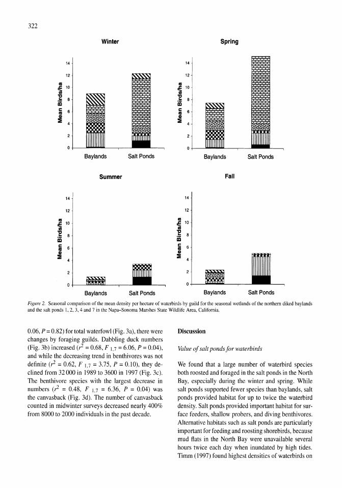
322
Winter Spring
14 14
12 12
III III
~ 10 .c 10
Ui 'E ~
8 .. 8 iii iii c 6 C 6 III III GI GI
::::E 4 ::::E 4
2 2
0 0
Baylands Salt Ponds Baylands Salt Ponds
Summer Fall
14 14
12 12
III III
~ 10 ~
10
~ ~ .. 8 .. 8 iii iii c 6
C 6 III III GI GI
::::E ::::E 4 4
2 2
0 0
Baylands Salt Ponds Baylands Salt Ponds
Figure 2. Seasonal comparison of the mean density per hectare of waterbirds by guild for the seasonal wetlands of the northern diked bay lands and the salt ponds I, 2, 3,4 and 7 in the Napa-Sonoma Marshes State Wildlife Area, California.
0.06, P = 0.82) for total waterfowl (Fig. 3a), there were changes by foraging guilds. Dabbling duck numbers (Fig. 3b) increased (,1 = 0.68, F 1,7 = 6.06, P = 0.04), and while the decreasing trend in benthivores was not definite (,1 = 0.62, F 1,7 = 3.75, P = 0.1 0), they declined from 32000 in 1989 to 3600 in 1997 (Fig. 3c). The benthivore species with the largest decrease in numbers (,1 = 0.48, F 1,7 = 6.36, P = 0.04) was the canvasback (Fig. 3d). The number of canvasback counted in midwinter surveys decreased nearly 400% from 8000 to 2000 individuals in the past decade.
Discussion
Value of salt ponds for waterbirds
We found that a large number of waterbird species both roosted and foraged in the salt ponds in the North Bay, especially during the winter and spring. While salt ponds supported fewer species than bay lands, salt ponds provided habitat for up to twice the waterbird density. Salt ponds provided important habitat for surface feeders, shallow probers, and diving benthivores. Alternative habitats such as salt ponds are particularly important for feeding and roosting shorebirds, because mud fiats in the North Bay were unavailable several hours twice each day when inundated by high tides. Timm (1997) found highest densities of waterbirds on
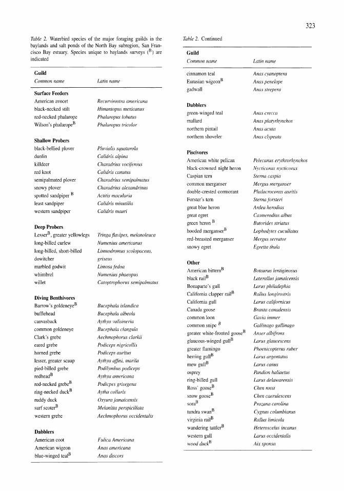
323
Table 2. Waterbird species of the major foraging guilds in the Table 2. Continued baylands and salt ponds of the North Bay subregion, San Fran-cisco Bay estuary. Species unique to baylands surveys (B) are Guild indicated Common name Latin name
Guild cinnamon teal Anas cyanoptera
Common name Latin name Eurasian wigeonB Anas penelope
Surface Feeders gadwall Anas strepera
American avocet Recurvirostra americana Dabblers
black-necked stilt Himantopus mexicanus green-winged teal Anas crecca
red-necked phalarope Phalaropus lobatus mallard Anas platyrhynchos
Wilson's phalaropeB Phalaropus tricolor northern pintail Anas acuta
northern shoveler Anas clypeata Shallow Probers black-bellied plover Pluvialis squatarola
Piscivores dunlin Calidris alpina
killdeer Charadrius vociferous American white pelican Pelecanus erythrorhynchos
red knot Calidris canutus black-crowned night heron Nycticorax nycticorax
semipalmated plover Charadrius semipalmatus Caspian tern Sterna caspia
snowy plover Charadrius alexandrinus common merganser Mergus merganser
spotted sandpiper B double-crested cormorant Phalacrocorax auritis
Actitis macularia Forster's tern Sterna .torsteri
least sandpiper Calidris minutil/a great blue heron Ardea herodias
western sandpiper Calidris mauri great egret Casmerodius albus
green heron B Butorides striatus Deep Probers
hooded merganserB Lophodytes cucullatus LesserB, greater yellowlegs Tringa jiavipes, melanoleuca
long-billed curlew Numenius americanus red-breasted merganser Mergus serrator
long-billed, short -billed Limnodromus scolopaceus, snowy egret Egretta thula
dowitcher griseus Other
marbled godwit Limosafedoa American bitternB Botaurus lentiginosus
whimbrel Numenius phaeopus black railB
willet Catoptrophorus semipalmatus Laterallus jamaicensis
Bonaparte's gull Larus philadephia
Diving Benthivores California clapper railB Rallus longirostris
Barrow's goldeneyeB Bucephala islandica Cal ifornia gull Larus californicus
Canada goose Branta canadensis bufflehead Bucephala albeola
common loon Cavia immer canvasback Aythya valisineria
common snipe B common goldeneye Bucephala clangula
Callinago gal/inago
greater white-fronted gooseB Anser albifrons Clark's grebe Aechmophorus clarkii
glaucous-winged gullB Larus glaucescens eared grebe Podiceps nig rieollis
greater flamingo Phoenicopterus ruber horned grebe Podiceps auritus
herring gullB Larus argentatus lesser, greater scaup Aythya affini, marila
mew gullB Larus canus pied-billed grebe Podilymbus podiceps
Pandion haliaetus redheadB Aythya americana
osprey
red-necked grebeB ring-billed gull Larus delawarensis
Podicpes grisegena Ross' gooseB Chen rossi
ring-necked duckB Aytha collaris snow gooseB Chen caerulescens
ruddy duck Oxyura jamaicensis soraB ProZ(lIla carolina
surf scoterB Melanilta perspicillata tundra swanB Cygnus columbianus
western grebe Aechmophorus occidentalis virginia railB Rallus limicola
wandering tattlerB Heteroscelus incanus Dabblers
western gull Larus occidentalis American coot Fulica Americana
wood duckB American wigeon Anas americana
Aix spollsa
blue-winged tealB Anas discors
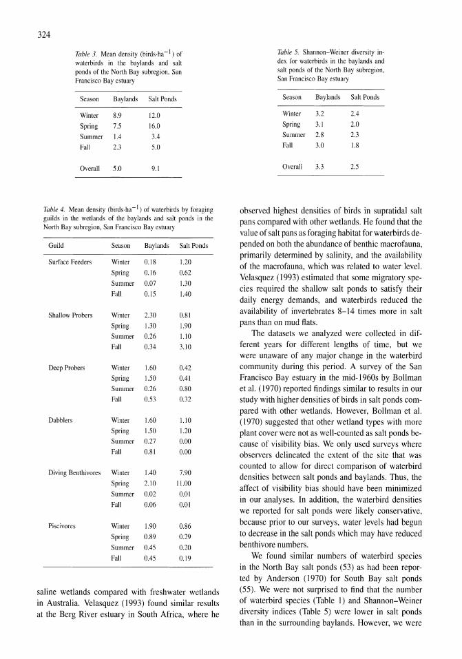
324
Table 3. Mean density (birds.ha- I) of waterbirds in the baylands and salt ponds of the North Bay subregion. San Francisco Bay estuary
Season Baylands Salt Ponds
Winter 8.9 12.0
Spring 7.5 16.0
Summer 1.4 3.4
Fall 2.3 5.0
Overall 5.0 9.1
Table 4. Mean density (birds·ha -I) of waterbirds by foraging guilds in the wetlands of the baylands and salt ponds in the North Bay subregion, San Francisco Bay estuary
Guild Season Baylands Salt Ponds
Surface Feeders Winter 0.18 1.20
Spring 0.16 0.62
Summer 0.07 1.30
Fall 0.15 1.40
Shallow Probers Winter 2.30 0.81
Spring 1.30 1.90
Summer 0.26 1.10
Fall 0.34 3.10
Deep Probers Winter 1.60 0.42
Spring 1.50 0.41
Summer 0.26 0.80
Fall 0.53 0.32
Dabblers Winter 1.60 1.10
Spring 1.50 1.20
Summer 0.27 0.00
Fall 0.81 0.00
Diving Benthivores Winter 1.40 7.90
Spring 2.10 11.00
Summer 0.02 0.01
Fall 0.06 0.01
Piscivorcs Winter 1.90 0.86
Spring 0.89 0.29
Summer 0.45 0.20
Fall 0.45 0.19
saline wetlands compared with freshwater wetlands in Australia. Velasquez (1993) found similar results at the Berg River estuary in South Africa, where he
Table 5. Shannon-Weiner diversity in-dex for waterbirds in the bay lands and salt ponds of the North Bay subregion. San Francisco Bay estuary
Season Baylands Salt Ponds
Winter 3.2 2.4
Spring 3.1 2.0
Summer 2.8 2.3
Fall 3.0 1.8
Overall 3.3 2.5
observed highest densities of birds in supratidal salt pans compared with other wetlands. He found that the value of salt pans as foraging habitat for waterbirds depended on both the abundance of benthic macrofauna, primarily determined by salinity, and the availability of the macrofauna, which was related to water level. Velasquez (1993) estimated that some migratory species required the shallow salt ponds to satisfy their daily energy demands, and waterbirds reduced the availability of invertebrates 8-14 times more in salt pans than on mud fiats.
The datasets we analyzed were collected in different years for different lengths of time, but we were unaware of any major change in the waterbird community during this period. A survey of the San Francisco Bay estuary in the mid-1960s by Bollman et al. (1970) reported findings similar to results in our study with higher densities of birds in salt ponds compared with other wetlands. However, Bollman et al. (1970) suggested that other wetland types with more plant cover were not as well-counted as salt ponds because of visibility bias. We only used surveys where observers delineated the extent of the site that was counted to allow for direct comparison of waterbird densities between salt ponds and baylands. Thus, the affect of visibility bias should have been minimized in our analyses. In addition, the waterbird densities we reported for salt ponds were likely conservative, because prior to our surveys, water levels had begun to decrease in the salt ponds which may have reduced benthivore numbers.
We found similar numbers of waterbird species in the North Bay salt ponds (53) as had been reported by Anderson (1970) for South Bay salt ponds (55). We were not surprised to find that the number of waterbird species (Table I) and Shannon-Weiner diversity indices (Table 5) were lower in salt ponds than in the surrounding baylands. However, we were
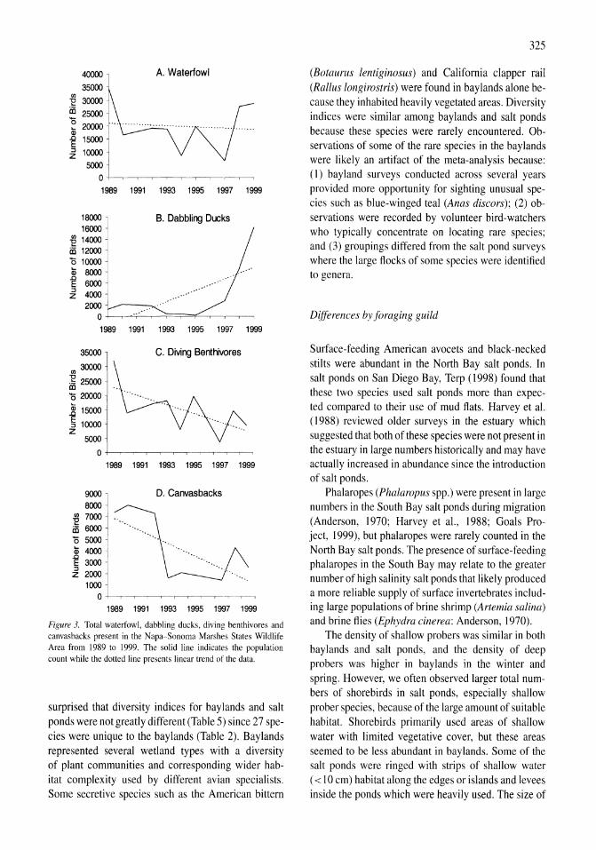
40000 A. Waterfowl 35000
-e 30000 ~ 25000 ~ 20000 CD
~ 15000 ::::I 10000 z
5000 0
1989 1991 1993 1995 1997 1999
18000 B. Dabbling Ducks 16000
-e 14000 ai12000 '0 10000 ~ 8000 .c
6000 E ::::I
4000 z 2000
0
1989 1991 1993 1995 1997 1999
35000 C. Diving Benthivores
II) 30000
~25000 .. '020000 ~ 15000
~10000 z 5000
0 1989 1991 1993 1995 1997 1999
9000 D. Canvasbacks 8000
~= '0 5000 ~ 4000 .c E 3000 ~2000
1000 0
1989 1991 1993 1995 1997 1999
Figure 3. Total waterfowl, dabbling ducks, diving benthivores and canvasbacks present in the Napa-Sonoma Marshes States Wildlife Area from 1989 to 1999. The solid line indicates the population count while the dotted line presents linear trend of the data.
surprised that diversity indices for baylands and salt ponds were not greatly different (Table 5) since 27 species were unique to the baylands (Table 2). Baylands represented several wetland types with a diversity of plant communities and corresponding wider habitat complexity used by different avian specialists. Some secretive species such as the American bittern
325
(Botaurus lentiginosus) and California clapper rail (Rallus longirostris) were found in baylands alone because they inhabited heavily vegetated areas. Diversity indices were similar among baylands and salt ponds because these species were rarely encountered. Observations of some of the rare species in the baylands were likely an artifact of the meta-analysis because: (1) bayland surveys conducted across several years provided more opportunity for sighting unusual species such as blue-winged teal (Anas discors); (2) observations were recorded by volunteer bird-watchers who typically concentrate on locating rare species; and (3) groupings differed from the salt pond surveys where the large flocks of some species were identified to genera .
Differences by foraging guild
Surface-feeding American avocets and black-necked stilts were abundant in the North Bay salt ponds. In salt ponds on San Diego Bay, Terp (1998) found that these two species used salt ponds more than expected compared to their use of mud flats. Harvey et al. (1988) reviewed older surveys in the estuary which suggested that both of these species were not present in the estuary in large numbers historically and may have actually increased in abundance since the introduction of salt ponds.
Phalaropes (Phalaropus spp.) were present in large numbers in the South Bay salt ponds during migration (Anderson, 1970; Harvey et aI., 1988; Goals Project, 1999), but phalaropes were rarely counted in the North Bay salt ponds. The presence of surface-feeding phalaropes in the South Bay may relate to the greater number of high salinity salt ponds that likely produced a more reliable supply of surface invertebrates including large populations of brine shrimp (Artemia salina) and brine flies (Ephydra cinerea: Anderson, 1970).
The density of shallow probers was similar in both bay lands and salt ponds, and the density of deep probers was higher in baylands in the winter and spring. However, we often observed larger total numbers of shorebirds in salt ponds, especially shallow prober species, because of the large amount of suitable habitat. Shorebirds primarily used areas of shallow water with limited vegetative cover, but these areas seemed to be less abundant in baylands. Some of the salt ponds were ringed with strips of shallow water ( < 10 cm) habitat along the edges or islands and levees inside the ponds which were heavily used. The size of
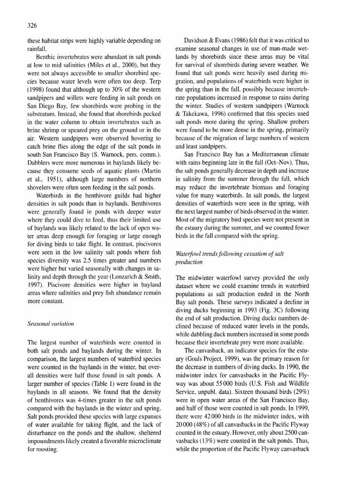
326
these habitat strips were highly variable depending on rainfall.
Benthic invertebrates were abundant in salt ponds at low to mid salinities (Miles et al., 2000), but they were not always accessible to smaller shorebird species because water levels were often too deep. Terp (1998) found that although up to 30% of the western sandpipers and willets were feeding in salt ponds on San Diego Bay, few shorebirds were probing in the substratum. Instead, she found that shorebirds pecked in the water column to obtain invertebrates such as brine shrimp or speared prey on the ground or in the air. Western sandpipers were observed hovering to catch brine flies along the edge of the salt ponds in south San Francisco Bay (S. Warnock, pers. comm.). Dabblers were more numerous in baylands likely because they consume seeds of aquatic plants (Martin et al., 1951), although large numbers of northern shovelers were often seen feeding in the salt ponds.
Waterbirds in the benthivore guilds had higher densities in salt ponds than in baylands. Benthivores were generally found in ponds with deeper water where they could dive to feed, thus their limited use of bay lands was likely related to the lack of open water areas deep enough for foraging or large enough for diving birds to take flight. In contrast, piscivores were seen in the low salinity salt ponds where fish species diversity was 2.5 times greater and numbers were higher but varied seasonally with changes in salinity and depth through the year (Lonzarich & Smith, 1997). Piscivore densities were higher in bayland areas where salinities and prey fish abundance remain more constant.
Seasonal variation
The largest number of waterbirds were counted in both salt ponds and baylands during the winter. In comparison, the largest numbers of waterbird species were counted in the baylands in the winter, but overall densities were half those found in salt ponds. A larger number of species (Table 1) were found in the bay lands in all seasons. We found that the density of benthivores was 4-times greater in the salt ponds compared with the baylands in the winter and spring. Salt ponds provided these species with large expanses of water available for taking flight, and the lack of disturbance on the ponds and the shallow, sheltered impoundments likely created a favorable microclimate for roosting.
Davidson & Evans (1986) felt that it was critical to examine seasonal changes in use of man-made wetlands by shorebirds since these areas may be vital for survival of shorebirds during severe weather. We found that salt ponds were heavily used during migration, and populations of waterbirds were higher in the spring than in the fall, possibly because invertebrate populations increased in response to rains during the winter. Studies of western sandpipers (Warnock & Takekawa, 1996) confirmed that this species used salt ponds more during the spring. Shallow probers were found to be more dense in the spring, primarily because of the migration of large numbers of western and least sandpipers.
San Francisco Bay has a Mediterranean climate with rains beginning late in the fall (Oct-Nov). Thus, the salt ponds generally decrease in depth and increase in salinity from the summer through the fall, which may reduce the invertebrate biomass and foraging value for many waterbirds. In salt ponds, the largest densities of waterbirds were seen in the spring, with the next largest number of birds observed in the winter. Most of the migratory bird species were not present in the estuary during the summer, and we counted fewer birds in the fall compared with the spring.
Waterfowl trends following cessation of salt production
The midwinter waterfowl survey provided the only dataset where we could examine trends in waterbird populations as salt production ended in the North Bay salt ponds. These surveys indicated a decline in diving ducks beginning in 1993 (Fig. 3C) following the end of salt production. Diving ducks numbers declined because of reduced water levels in the ponds, while dabbling duck numbers increased in some ponds because their invertebrate prey were more available.
The canvasback, an indicator species for the estuary (Goals Project, 1999), was the primary reason for the decrease in numbers of diving ducks. In 1990, the midwinter index for canvasbacks in the Pacific Flyway was about 55000 birds (U.S. Fish and Wildlife Service, unpubl. data). Sixteen thousand birds (29%) were in open water areas of the San Francisco Bay, and half of those were counted in salt ponds. In 1999, there were 42000 birds in the midwinter index, with 20000 (48%) of all canvasbacks in the Pacific Flyway counted in the estuary. However, only about 2500 canvasbacks (13%) were counted in the salt ponds. Thus, while the proportion of the Pacific Flyway canvasback
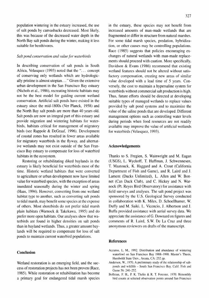
population wintering in the estuary increased, the use of salt ponds by canvasbacks decreased. Most likely, this was because of the decreased water depth in the North Bay salt ponds during the winter, making it less suitable for benthivores.
Salt pond conservation and value for waterbirds
In describing conservation of salt ponds in South Africa, Velasquez (1993) noted that the " ... concept of conserving only wetlands which are hydrologically pristine is almost utopian ... " Given the extensive urban development in the San Francisco Bay estuary (Nichols et aI., 1986), recreating historic habitats may not be the best model for guiding current wetland conservation. Artificial salt ponds have existed in the estuary since the mid-1800s (Ver Planck, 1958) and the North Bay salt ponds are more than 40 years old. Salt ponds are now an integral part of this estuary and provide migration and wintering habitats for waterbirds, habitats critical for management of migratory birds (see Rappole & DeGraaf, 1996). Development of coastal zones has resulted in fewer areas available for migratory waterbirds in the flyway, and alternative wetlands may not exist outside of the San Francisco Bay estuary to compensate for loss of waterbird habitats in the ecosystem.
Restoring or rehabilitating diked baylands in the estuary is likely beneficial for waterbirds most of the time. Historic wetland habitats that were converted to agriCUlture or urban development now have limited value for waterbird species, with the exception of areas inundated seasonally during the winter and spring (Haas, 1994). However, converting from one wetland habitat type to another, such as converting salt ponds to tidal marsh, may benefit some species at the expense of others. Most shorebirds do not prefer tidal marsh plain habitats (Warnock & Takekawa, 1995) and do prefer more open habitats. Our analyses show that waterbirds are found in higher densities on salt ponds than in bayland wetlands. Thus, a greater amount baylands will be required to compensate for loss of salt ponds to maintain current waterbird populations.
Conclusion
Wetland restoration is an emerging field, and the success of restoration projects has not been proven (Race, 1985). While restoration or rehabilitation has become a primary goal for endangered tidal marsh species
327
in the estuary, these species may not benefit from increased amounts of man-made wetlands that are fragmented or differ in structure from natural marshes. For some tidal marsh species, predation, hybridization, or other causes may be controlling populations. Race (1985) suggests that policies encouraging exchanges of natural wetlands with man-made replacements should proceed with caution. More specifically, Davidson & Evans (1986) recommend that existing wetland features should not be altered without satisfactory compensation, creating new areas of similar value developed with a lead time of 5 years. Conversely, the cost to maintain a hypersaline system for waterbirds without commercial salt production is high. Thus, future efforts should be directed at developing suitable types of managed wetlands to replace values provided by salt pond systems and to maximize the value of the saline ponds that are developed. Different management options such as controlling water levels during periods when food resources are not readily available may improve the value of artificial wetlands for waterbirds (Velasquez, 1993).
Acknowledgements
Thanks to S. Fregien, S. Wainwright and M. Eagan (USGS), L. Wyckoff, T. Huffman, 1. Schwennesen, T. Maatouck, K. Haggard and A. Crout (California Department of Fish and Game), and R. Laird and J. Lament (Ducks Unlimited), L. Allen and W. Bonnet (Can Duck Club), and C. Hickey and N. Warnock (Pt. Reyes Bird Observatory) for assistance with field surveys and analyses. The salt pond project was sponsored by the U.S. Geological Survey conducted in collaboration with K. Miles, D. Schoellhamer, W. Duffy and M. Saiki. L. Vicencio, J. Albertson and J. Buffa provided assistance with aerial survey data. We appreciate the assistance of G. Downard on figures and comments of R. Laird, S.w. De La Cruz and three anonymous reviewers on drafts of the manuscript.
References
Accurso, L. M .. 1992. Distribution and abundance of wintering waterfowl on San Francisco Bay 1988-1990. Master's Thesis. Humboldt State Univ., Arcata, CA: 252 pp.
Anderson, w., 1970. A preliminary study of the relationship of saltponds and wildlife - South San Francisco Bay. Calif. Fish and Game 56: 240-252.
Bollman, F. H., P. K. Thelin & R. T. Forester, 1970. Bimonthly bird counts at selected observation points around San Francisco
328
Bay, Febuary 1964 to January 1966. Calif. Fish and Game 56: 224--239.
Carpelan, L. H., 1957. Hydrobiology of the Alviso salt ponds. Ecology 38: 382-385.
Davidson, N. C. & P. R. Evans, 1986. The role and potential of manmade and man-modified wetlands in enhancement of the survival of overwintering shorebirds. Colon. Waterbirds 9: 176-188.
Goals Project, 1999. Baylands ecosystem habitat goals. A report of habitat recommendations prepared by the San Francisco Bay Area Wetlands Ecosystem Goals Project. U.S. Environmental Protection Agency, San Francisco, CA and S. F. Bay Regional Water Quality Control Board, Oakland, CA: 209 pp.
Haas, J. E., 1994. Waterfowl use of grazed and ungrazed wetlands, Napa and Sonoma counties, California. Master's Thesis. Calif. State Univ. Sonoma. Rohnert Park, CA: 116 pp.
Harrington, B. & E. Perry, 1995. Important shorebird stating sites meeting Western Hemisphere Shorebird Reserve Network criteria in the United States. Unpub!. Rep. to the U.S. Fish and Wildlife Serv., Portland, OR: 121 pp.
Harvey, T. E., P. R. Kelly, R. W. Lowe & D. Fearn, 1988. The value of saltponds for waterbirds in San Francisco Bay and considerations for future management. Unpub!. Rep. at Wetlands '88: Urban Wetlands and Riparian Habitat. Oakland, CA.
Harvey, T. E., K. J. Miller, R. L. Hothem, M. J. Rauzon, G. W. Page & R. A. Keck, 1992. Status and trends report on the wildlife of the San Francisco Bay estuary. EPA Coop. Agreement CE-009519-01-0 Final Report, U.S. Fish and Wildlife Service, Sacramento, CA: 283 pp.
Johnson, R. A. & D. W. Wichern, 1988. Applied multivariate statistical analysis, 2nd edn. Prentice Hall, Englewood Cliffs, N1.
Josselyn, M., 1983. The ecology of San Francisco Bay tidal marshes: a community profile. FWS/OBS-83/23, U. S. Fish and Wildlife Service, Washington, DC.
Krebs, C. J., 1989. Ecological Methodology. Harper & Row, New York: 654 pp.
Lonzarich, D. G., 1988. Temporal and spatial variations in salt pond environments and implications for fish and invertebrates. Master's Thesis, San Jose State Univ., San Jose, CA: 81 pp.
Lonzarich, D. G. & J. J. Smith, 1997. Water chemistry and community structure of saline and hypersaline salt evaporation ponds in San Francisco Bay, California. Calif. Fish and Game 83: 89-104.
Martin, A. c., H. S. Zim & A. L. Nelson, 1951. American Wildlife and Plants: a Guide to Wildlife Food Habits. McGraw-Hill Book Co., New York, NY: 500 pp.
Miles, A. K., 1. Y. Takekawa, D. H. Schoellhamer, C. T. Lu, W. G. Duffy & M. K. Saiki, 2000. Science support for wetland restoration in the Napa-Sonoma salt ponds, San Francisco Bay estuary, 1999 progress report. Unpubl. Prog. Rep., U.S. Geological Survey, Davis and Vallejo, CA: 57 pp.
Milliken, G. A. & D. E. Johnson, 1984. Analysis of Messy Data, Vo!. 1: Designed Experiments. Van Nostrand Reinhold, New York.
Nichols, F. H., J. E. Cloern, S. N. Luoma & D. H. Peterson, 1986. The modification of an estuary. Science 231: 569-573.
Race, M. S., 1985. Critique of present wetlands mitigation policies in the United States based on an analysis of past restoration projects in San Francisco Bay. Environ. Manage. 9: 71-82.
Rappole, J. H. & R. M. DeGraaf. 1996. Research and effective management of neotropical migrant birds. Trans. n. am. Wild!. Natur. Resour. Conf. 61: 450-462.
SAS Institute, 1990. SAS Procedure Guide, Release 6.04 Edition. SAS Institute, Cary, NC.
Swarth, C. w., C. Akagi & P. Metropoulus, 1982. The distribution patterns and ecology of waterbirds using Coyote Hills salt ponds. U.S. Fish and Wildlife Service, San Francisco Bay National Wildlife Refuge, Newark, CA.
Terp, J. M., 1998. Habitat use patterns of wintering shorebirds: the role of salt evaporation ponds in south San Diego Bay. Master's Thesis, San Diego State Univ., San Diego: 79 pp.
Velasquez, C. R., 1993. The ecology and management of waterbirds at commercial saltpans in South Africa. Ph.D. Dissertation, Percy FitzPatrick Institute of African Ornithology, Univ. of Cape Town, South Africa: 248 pp.
Ver Planck, W. E., 1958. Salt in California. Calif. Div. Of Mines Bull. No. 175.
Warnock, S. E. &1. Y. Takekawa, 1995. Habitat preferences of wintering shorebirds in a temporally changing environment: western sandpipers in the San Francisco Bay estuary. Auk 112: 920-930.
Warnock, S. E. & 1. Y. Takekawa, 1996. Wintering site fidelity and movement patterns of western sandpipers Calidris mauri in the San Francisco Bay estuary. Ibis 138: 160-167.
Hydrobiologia 466: 329-337,2001. J.M. Melack, R. Jellison & D.B. Herbst (eds), Saline Lakes. © 200! Kluwer Academic Publishers.
329
Anthropogenic salinisation of inland waters
W.D. Williams Department of Environmental Biology, University of Adelaide, Adelaide, 5005, Australia
Key words: salinisation, salinity increases, salinity, salt lakes, anthropogenic impacts, drylands, water resources
Abstract
Many inland waters are becoming more saline from human activities, particularly in semi-arid and arid regions. The causes and distribution of anthropogenic salinisation, the salinisation of freshwater lakes, rivers and streams, and increases in the salinity of large, permanent saline lakes are discussed. The impacts of anthropogenic salinisation are far-reaching, increasing, deleterious and largely irreparable. Environmental, social and environmental costs are high. Attention is drawn to the importance of anthropogenic salinisation and its impacts. The need for better recognition of the costs of salinisation and for more effective management is stressed.
Introduction
Salt lakes are perceived by many limnologists as unimportant inland bodies of water of less interest, utility and abundance than fresh waters. This perception is erroneous in many respects and can be easily refuted (e.g. Williams, 1986, 1998), but there is no satisfaction from the additional knowledge that the relative importance of salt lakes is now rapidly and significantly increasing. This change is being brought about by secondary or anthropogenic salinisation. In this process, catchment changes and other anthropogenic disturbances to hydrological cycles increase salt loads to water-bodies: fresh waters become saline and saline waters become even more saline.
Anthropogenic salinisation is distinct from natural or primary salinisation which is responsible for the development of natural salt lakes. Primary salinisation involves the accumulation in closed basins of salts from rainwater and leached from terrestrial sources at rates unaffected by human activities. Natural salt lakes have been the focus of most limnological studies of saline waters.
A major aim of this paper is to draw attention to the importance of anthropogenic salinisation and its impacts on natural inland aquatic ecosystems, both fresh and saline. These impacts are often ignored by limnologists outside the semi-arid and arid regions (or underestimated, cf. Groombridge & Jenkins, 1998) despite their significant, deleterious and often irre-
parable economic, social and environmental costs. Decreased biodiversity, changes in the natural character of aquatic ecosystems, and lower productivity are some obvious ecological costs. In some countries, anthropogenic salinisation represents the most important threat to water resources.
A second aim is to stress the need to recognize more fully the costs of salinisation and the need for more effective management. Many agencies responsible for the management of water resources in dryland countries already do recognize the importance of salinisation, yet its full environmental, social and other 'non-market' costs are often not fully taken into account and the management of salt is often ineffective or of a short term nature. Studies of natural salt lakes are likely to prove and indeed have already proven to be of considerable interest in this matter. This suggests a new strategic direction for studies of saline water-bodies, particularly those of recent anthropogenic origin. Large scale ecosystem changes are being made which offer opportunities for the study of salt lakes not otherwise available.
The aims are addressed by considering:
• the causes and distribution of anthropogenic salin-isation
• the salinisation of freshwater lakes
• the salinisation of rivers and streams, and
• increases in the salinity of large, permanent salt lakes.
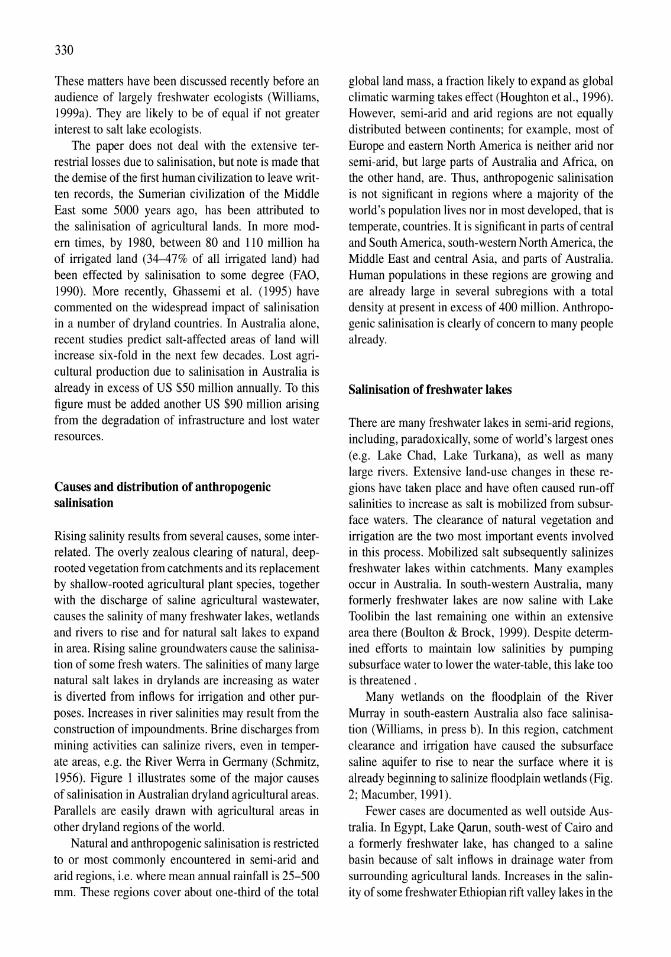
330
These matters have been discussed recently before an audience of largely freshwater ecologists (Williams, 1999a). They are likely to be of equal if not greater interest to salt lake ecologists.
The paper does not deal with the extensive terrestrial losses due to salinisation, but note is made that the demise ofthe first human civilization to leave written records, the Sumerian civilization of the Middle East some 5000 years ago, has been attributed to the salinisation of agricultural lands. In more modem times, by 1980, between 80 and 110 million ha of irrigated land (34-47% of all irrigated land) had been effected by salinisation to some degree (FAO, 1990). More recently, Ghassemi et al. (1995) have commented on the widespread impact of salinisation in a number of dryland countries. In Australia alone, recent studies predict salt -affected areas of land will increase six-fold in the next few decades. Lost agricultural production due to salinisation in Australia is already in excess of US $50 million annually. To this figure must be added another US $90 million arising from the degradation of infrastructure and lost water resources.
Causes and distribution of anthropogenic salinisation
Rising salinity results from several causes, some interrelated. The overly zealous clearing of natural, deeprooted vegetation from catchments and its replacement by shallow-rooted agricultural plant species, together with the discharge of saline agricultural wastewater, causes the salinity of many freshwater lakes, wetlands and rivers to rise and for natural salt lakes to expand in area. Rising saline groundwaters cause the salinisation of some fresh waters. The salinities of many large natural salt lakes in drylands are increasing as water is diverted from inflows for irrigation and other purposes. Increases in river salinities may result from the construction of impoundments. Brine discharges from mining activities can salinize rivers, even in temperate areas, e.g. the River Werra in Germany (Schmitz, 1956). Figure 1 illustrates some of the major causes of salinisation in Australian dry land agricultural areas. Parallels are easily drawn with agricultural areas in other dry land regions of the world.
Natural and anthropogenic salinisation is restricted to or most commonly encountered in semi-arid and arid regions, i.e. where mean annual rainfall is 25-500 mm. These regions cover about one-third of the total
global land mass, a fraction likely to expand as global climatic warming takes effect (Houghton et aI., 1996). However, semi-arid and arid regions are not equally distributed between continents; for example, most of Europe and eastern North America is neither arid nor semi-arid, but large parts of Australia and Africa, on the other hand, are. Thus, anthropogenic salinisation is not significant in regions where a majority of the world's population lives nor in most developed, that is temperate, countries. It is significant in parts of central and South America, south-western North America, the Middle East and central Asia, and parts of Australia. Human populations in these regions are growing and are already large in several subregions with a total density at present in excess of 400 million. Anthropogenic salinisation is clearly of concern to many people already.
Salinisation of freshwater lakes
There are many freshwater lakes in semi-arid regions, including, paradoxically, some of world's largest ones (e.g. Lake Chad, Lake Turkana), as well as many large rivers. Extensive land-use changes in these regions have taken place and have often caused run-off salinities to increase as salt is mobilized from subsurface waters. The clearance of natural vegetation and irrigation are the two most important events involved in this process. Mobilized salt subsequently salinizes freshwater lakes within catchments. Many examples occur in Australia. In south-western Australia, many formerly freshwater lakes are now saline with Lake Toolibin the last remaining one within an extensive area there (Boulton & Brock, 1999). Despite determined efforts to maintain low salinities by pumping subsurface water to lower the water-table, this lake too is threatened.
Many wetlands on the floodplain of the River Murray in south-eastern Australia also face salinisation (Williams, in press b). In this region, catchment clearance and irrigation have caused the subsurface saline aquifer to rise to near the surface where it is already beginning to salinize floodplain wetlands (Fig. 2; Macumber, 1991).
Fewer cases are documented as well outside Australia. In Egypt, Lake Qarun, south-west of Cairo and a formerly freshwater lake, has changed to a saline basin because of salt inflows in drainage water from surrounding agricultural lands. Increases in the salinity of some freshwater Ethiopian rift valley lakes in the
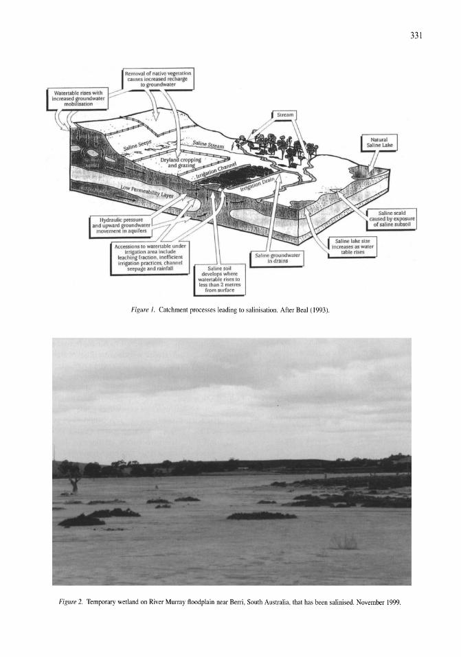
Accessions to wa(er'able under Irrigation area include
le3chins rraclion. inemcienl irrigarion practices. channel
•• c"age .IId r.Iinr.1I
Figure 1. Catchment processes leading to salinisation. After Beal (1993).
Figure 2. Temporary wetland on River Murray floodplain near Berri , South Australia, that has been salinised. November 1999.
331
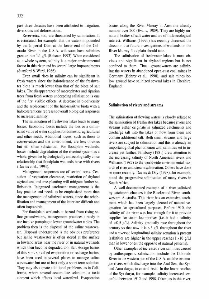
332
past three decades have been attributed to inigation, diversions and deforestation ..
Reservoirs, too, are threatened by salinisation. It is estimated, for example, that the waters impounded by the Imperial Dam at the lower end of the Colorado River in the U.S.A. will soon have salinities greater than 1.1 gIL (Reisner, 1993). When considered as a whole system, salinity is a major environmental factor in this river and its several large impoundments (Stanford & Ward, 1986).
Even small rises in salinity can be significant in fresh waters since the halo tolerance of the freshwater biota is much lower than that of the biota of salt lakes. The disappearance of macrophytes and riparian trees from fresh waters undergoing salinisation is one of the first visible effects. A decrease in biodiversity and the replacement of the halosensitive biota with a halotolerant one represent overall biological responses to increased salinity.
The salinisation of freshwater lakes leads to many losses. Economic losses include the loss or a diminished value of water supplies for domestic, agricultural and other needs. Additional losses, such as those to conservation and the environment, are less obvious but still often substantial. For floodplain wetlands, losses include degradation of the riverine system as a whole, given the hydrologically and ecologically close relationship that floodplain wetlands have with rivers (Davies et aI., 1994).
Management responses are of several sorts. Cessation of vegetation clearance, restriction of dry land agriculture, and tree-planting will mitigate further salinisation. Integrated catchment management is the key practice and needs to be emphasized more than the management of salinized waters, since the rehabilitation and management of the latter are difficult and often impossible.
For floodplain wetlands at hazard from rising saline ground waters, management practices already in use involve pumping to lower groundwater tables. The problem then is the disposal of the saline wastewater. Disposal underground is the obvious preference but saline wastewater is often stored at the surface in lowland areas near the river or in natural wetlands which then become degraded too. Salt storage basins of this sort, so-called evaporation or recharge basins, have been used in several places to manage saline wastewater but are at best only a short-term solution. They may also create additional problems, as in California, where several accumulate selenium, a toxic element which affects local waterfowl. Evaporation
basins along the River Murray in Australia already number over 200 (Evans, 1989). They are highly unnatural bodies of salt water and are of little ecological interest. Williams (1999b) has recently discussed the direction that future investigations of wetlands on the River Murray floodplain should take.
The salinisation of freshwater lakes is most obvious and significant in dryland regions but is not confined to them. Thus, groundwaters are salinizing the waters in abandoned open-cast coal mines in Germany (Bohrer et aI., 1998), and salt mines below ground have salinized several lakes in Cheshire, England.
Salinisation of rivers and streams
The salinisation of flowing waters is closely related to the salinisation of freshwater lakes because rivers and streams either originate in salinized catchments and discharge salt into the lakes or flow from them and contain additional salt. Both small streams and large rivers are subject to salinisation and this is already an important global phenomenon with salinities set to increase yet further. Pillsbury (1981) drew attention to the increasing salinity of North American rivers and Williams (1987) to the worldwide environmental hazards of river and stream salinisation. Others have done so more recently. Davies & Day (1998), for example, noted the progressive salinisation of many rivers in South Africa.
A well-documented example of a river salinized by catchment changes is the Blackwood River, southwestern Australia. This river has an extensive catchment which has been largely cleared of natural vegetation for agricultural purposes. Before 1910, the salinity of the river was low enough for it to provide supplies for steam locomotives (i.e. it had a salinity of <0.5 gIL). Salinity gradually rose throughout the century so that now it is >3 gIL throughout the river and a reversed longitudinal salinity zonation is present (salinities are higher in the upper reaches [> 10 giLl than in lower ones, the opposite of natural patterns).
Other examples of increased river salinities caused by anthropogenic salinisation include the Colorado River in the western part ofthe U.S.A. and the two major rivers which discharge into the Aral Sea, the Syrand Amu-darya, in central Asia. In the lower reaches of the Syr-darya, for example, salinity increased sevenfold between 1912 and 1998. Often, as in this river,
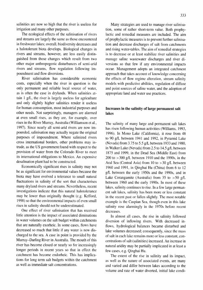
salinities are now so high that the river is useless for irrigation and many other purposes.
The ecological effects of the salinisation of rivers and streams are largely the same as those encountered in freshwater lakes; overall, biodiversity decreases and a halotolerant biota develops. Biological changes in rivers and streams, however, are less easily distinguished from those changes which result from two other major anthropogenic disturbances of semi-arid rivers and streams, flow regulation following impoundment and flow diversions.
River salinisation has considerable economic costs, especially when the river in question is the only permanent and reliable local source of water, as is often the case in drylands. When salinities attain 1 gIL, the river is largely useless for agriculture and only slightly higher salinities render it useless for human consumption, most industrial purposes and other needs. Not surprizingly, managers are alarmed at even small rises, as they are, for example, over rises in the River Murray, Australia (Williamson et aI., 1997). Since nearly all semi-arid rivers are now impounded, salinisation may actually negate the original purposes of impoundment. Where salinized rivers cross international borders, other problems may intrude, as the US government found with respect to the provision of water from the Colorado River to meet its international obligations to Mexico. An expensive desalination plant had to be constructed.
Economically significant rises in salinity may not be as significant for environmental values because the biota may have evolved a tolerance to small natural fluctuations in salinity of the sort that characterises many dryland rivers and streams. Nevertheless, recent investigations indicate that this natural halotolerance may be lower than originally thought (e.g. Kefford, 1998) so that the environmental impacts of even small rises in salinity should not be underestimated.
One effect of river salinisation that has received little attention is the impact of associated diminutions in water volumes on the salt budget within catchments that are naturally exorheic. In some cases, flows have decreased so much that little if any water is now discharged to the sea. A case in point is provided by the Murray-Darling River in Australia. The mouth of this river has become closed or nearly so for increasingly longer periods in recent years so that in effect the catchment has become endorheic. This has implications for long term salt budgets within the catchment as well as immediate salt concentrations.
333
Many strategies are used to manage river salinisation, some of rather short-term value. Both prophylactic and remedial measures are included. The aim of prophylactic measures is to prevent further salinisation and decrease discharges of salt from catchments and rising water-tables. The aim of remedial strategies is to decrease or at least stabilize river salinities and manage saline wastewater discharges and river diversions so that few if any environmental impacts occur. Management adopts an integrated catchment approach that takes account of knowledge concerning the effects of flow regime alteration, stream salinity models with predictive abilities, regulation of diffuse and point sources of saline water, and the adoption of appropriate land and water use practices.
Increases in the salinity of large permanent salt lakes
The salinity of many large and permanent salt lakes has risen following human activities (Williams, 1993, 1996). In Mono Lake (California), it rose from 48 to 90 gIL between 1941 and 1992, in Pyramid Lake (Nevada) from 3.75 to 5.5 gIL between 1933 and 1980, in Walker Lake (Nevada) from 2.5 to 14.5 gIL between 1875 and 1999, in the Dead Sea (Middle East) from 200 to > 300 gIL between 1910 and the 1990s, in the Aral Sea (Central Asia) from 10 to >30 gIL between 1960 and 1991, in Qinghai Hu (China) from 6 to 12 gIL between the early 1950s and the 1990s, and in Lake Corangamite (Australia) from 35 to >50 gIL between 1960 and the early 1990s. In most of these lakes, salinity continues to rise. In a few large permanent salt lakes, salinity has been more or less constant in the recent past or fallen slightly. The most notable example is the Caspian Sea, though even in this lake salinity rose alarmingly in the 1970s before recent decreases.
In almost all cases, the rise in salinity followed diversion of inflowing rivers. With decreased inflows, hydrological balances became disturbed and lake volumes decreased; consequently, since the mass of salt in each lake remains more or less constant, concentrations of salt (salinities) increased. An increase in natural aridity may be partially implicated in at least a few cases, e.g. Qinghai Hu.
The extent of the rise in salinity and its impact, as well as the nature of associated events, are many and varied and differ between lakes according to the volume and rate of water diverted, initial lake condi-
334
tions, and lake morphometry. In the Aral Sea (Williams & Aladin, 1991; Letolle & Mainguet, 1993; Glazovsky, 1995), perhaps the lake where salinisation has attracted most attention, salinities rose threefold in as many decades and the increase was accompanied by falling water-levels (>15 m since 1960). These, in tum, led to a large decrease in the surface area of water, the exposure of large areas of the former lake bed, and the disappearance of the south-eastern archipelago. Significant alterations to the biota of the lake also occurred. Additionally, the frequency of dust storms increased, and agricultural production around the lake decreased (because of salt emissions from the dry bed of the lake).
The cost of changes to the Aral Sea has been very high. The disappearance of the south-eastern archipelago involved the loss of extensive habitat for both local wildlife and migrating waterfowl. The economically and socially important fishery collapsed. Shipping became impossible and the frequency of respiratory and other human illnesses increased. As well, the Arallost much of its aesthetic and cultural value to local communities.
Not all of such impacts have followed the anthropogenic salinisation of large salt lakes elsewhere, but falling water-levels and altered ecological conditions have inevitably done so. Even so, globally, the salinisation of many large salt lakes has undoubtedly resulted in serious economic, social, conservation and environmental losses. Any comparison of these with the benefits derived from diverted waters depends upon the perspective taken. Economic benefits probably always exceed economic losses, but from the conservation and environmental perspective this is certainly not so; conservation and environmental losses far exceed gains.
The end result of water diversions from salt lakes, of course, is the complete desiccation of the lakes involved. Several examples already exist (all poorly documented). Two are discussed: Winnemucca Lake in Nevada and Owens Lake in California. During the late nineteenth and early twentieth centuries, Winnemucca Lake was about 40 km long and 5 km wide (Murray, 1910) and had a salinity of 3.6 gIL in 1884 (Clarke, 1924). The lake had been temporarily dry for part of the nineteenth century, but permanently dried following diversions from the Truckee River (these diversions also led to falls in the water-levels of nearby Pyramid Lake). The lake is now merely a fiat expanse of permanently dry lake bed (Fig. 3) adjacent to Pyramid Lake. Owens Lake was about 24 km long, 16 km
wide and 10 m deep (Sharp & Glazner, 1997). Recorded salinities between 1890 and 1914 ranged from 16 to 214 gIL (Clarke, 1924; the lower value is doubted by Clarke). From 1913, diversions of water from the lake to Los Angeles led to its complete and permanent desiccation by 1924 (Fig. 4).
The extent and nature of the losses from the desiccation of Winnemucca and Owens lakes remain largely speculative. What is not speCUlative, however, is at least one contemporary impact resulting from the desiccation of Owens Lake; the emission of significant emissions of small dust particles to the atmosphere from its dry bed. The bed is also characterized by the presence of high levels of phytoxic elements including arsenic and boron. Attempts to control dust emissions include planting Distichlis spicata var. stricta (salt grass) (Fig. 5). The plantings need irrigation.
With regard to the management of salt lakes still extant, the most obvious action is that river diversions need to be restricted. Implementing restrictions, however, is not easy. It requires clear recognition of the decreased values of lakes from which water is diverted as well as management actions to compensate for lower volumes of available water. These actions are not easily achieved, but in at least one case, Mono Lake, California (Fig. 6), have been achieved. Salinities in this lake rose over most of the twentieth century as water was diverted from it for consumption by Los Angeles. Cultural, scenic and conservation values suffered as a result, but after a long community and legal campaign diversions were limited. Present lake levels and salinity have now more or less stabilized. Limitations will stay in place until water-levels and salinities reach pre-1940 values.
Notwithstanding the events which followed diversions from the Aral Sea and other salt lakes, diversions from more salt lakes are planned and being implemented. Of particular concern is the scheme to divert water from Mar Chiquita, a large saline lake in northern Argentina (Reati et aI., 1997). This will result in large conservation losses for the lake provides food and refuge to considerable numbers of migrant waterfowl ("'500000 each year) and is an important locus on the Western Hemisphere Shorebird Reserve Network. If the scheme were implemented, other losses will also occur.
335
Figure 3. Winnemucca Lake. Nevada, September 1999. Now permanently dry.
Figure 4. Owens Lake, California, September 1999. Now permanently dry.

336
Figure 5. Owens Lake. California, September 1999. Photograph shows irrigated lines of Distichlis spicata var. stricta planted to control dust emissions.
Figure 6. Mono Lake, California, September 1999. Note tufa formations exposed by former falls in lake level.
Acknowledgements
I am grateful to David Herbst, Robert Jellison, and Darla Heil (University of California) and Carla Scheidlinger (Agrarian Systems, California) for interpretive discussions of Californian and Nevadan salt lakes during a visit to several of them.
References
Beal, A., 1993. Dryland salinity management in the MurrayDarling Basin. Murray-Darling Basin Commission, Canberra.
Bohrer, B., H. Heidenreich, M. Schimmele, & M. Schultze, 1998. Numerical prognosis for salinity profiles of future lakes in the opencast mine of Merseburg-Ost. Int. J. Salt Lake Res. 7: 235-260.
Boulton, A. J. & M. Brock, 1999. Australian Freshwater Ecology: Processes and Management. GIeneagles Publishing, Adelaide.
Clarke, F. W, 1924. The composition of the river and lake waters of the United States. U.S. Geol. Surv. Prof. Pap. 135: 1-199.
Davies, B. R & J. Day, 1998. Vanishing Waters. University of Cape Town Press, Cape Town.
Davies, B. R, M. C. Thoms, K. F. Walker, J. H. O'Keefe & J. A. Gore, 1994. Dryland rivers: their ecology, conservation and management. In Calow, P. & G. E. Petts (eds), The Rivers Handbook, vol. 2. Blackwell Science, Oxford.
Evans, R S., 1989. Saline water disposal options in the Murray Basin. BMR J. Aust. Geophys. 11: 167-185.
FAO, 1990. Water and sustainable agricultural development: an international action plan. A strategy for the implementation of the Mar del Plata Action Plan for the 1990s. Food and Agricultural Organization of the United Nations, Rome.
Ghassemi, F., A. J. Jakeman & H. A. Nix, 1995. Salinisation of Land and Water Resources. Human Causes, Extent, Management and Case Studies. University of New South Wales Press, Sydney.
Glazovsky, N. F., 1995. Aral Sea. In Mandych, A. F. (ed.), Enclosed Seas and Large Lakes of Eastern Europe and Middle Asia. SPB Academic Publishing, Amsterdam.
Groombridge, B. & M. Jenkins, 1998. Freshwater Biodiversity: a preliminary global assessment. WCMC Biodiversity Series no. 8. World Conservation Monitoring Centre, World Conservation Press, Cambridge, U.K.
Houghton, J. T., L. G. Meiro FiIho, N. Callander et al. (eds), 1996. Climate Change 1995, the Science of Climate Change. Cambridge University Press, Cambridge, U.K.
Kefford, B. J., 1998. The relationship between electrical conductivity and selected macro invertebrate communities in four river systems of south-west Victoria, Australia. Int. J. Salt Lake Res. 7: 153-170.
337
Letolle, R. & M. Mainguet, 1993. Aral. Springer-Verlag, Paris. Macumber, P. J., 1991. Interaction between Groundwater and Sur
face Systems in Northern Victoria. Department of Conservation and Environrnent, Melbourne.
Murray, J., 1910. The characteristics of lakes in general, and their distribution over the surface of the globe. In Murray, J. & L. Pullar (eds), Bathymetrical Survey of the Scottish Freshwater Lochs. Vol. I. Challenger Office, Edinburgh: 514--658.
Pillsbury, A. F., 1981. The salinity of rivers. Scientific American 245: 32-43.
Reati, G. J., M. Florin, G. J. Fernandez & c. Montes, 1997. The Laguna de Mar Chiquita (Cordoba, Argentina): a little known, secularly fluctuating saline lake. Int. J. Salt Lake Res. 5: 187-219.
Reisner, M., 1993. Cadillac Desert. The American West and its Disappearing Water. Penguin Books, New York.
Schmitz, W., 1956. Salzgehaltschwankungen in der Werra und ihre fischereilichen Auswirkungen. Vom Wasser 23: 113-136.
Sharp, R. P. & A. F. Glazner, 1997. Geology Underfoot in Death Valley and Owens Valley. Mountain Press, Missoula, Montana.
Stanford, J. A. & J. V. Ward, 1986. Reservoirs of the Colorado system. In Davies, B. R & K. F. Walker (eds), The Ecology of River Systems. Dr W Junk Publishers, Dordrecht: 375-383.
Williams, W D., 1986. Limnology, the study of inland waters: a comment on perceptions of salt lake studies, past and present. In De Deckker, P. & W D. Williams (eds), Limnology in Australia. CSIRO and Dr W. Junk Publishers, Melbourne and Dordrecht: 471-484.
Williams, W D., 1987. Salinization of rivers and streams: an important environmental hazard. Ambio 16: 180-185.
Williams, W D., 1993. The worldwide occurrence and limnological significance of falling water-levels in large, permanent saline lakes. Verh. int. Ver. Limnol. 25: 980-983.
Williams, W D., 1996. What future saline lakes? Environment 38: 12-20,38-39.
Williams, W D., 1998. The Management of Inland Saline Waters. Guidelines of Lake Management. Vol. 6. ILECIUNEP, Kusatsu.
Williams, W D., 1999a. Salinisation: a major threat to water resources in the arid and semi-arid regions of the world. Lakes and Reservoirs: Research and Management 4: 85-91.
Williams, W D., 1999b. Wetlands, salinity and the River Murray: three elements of a changing environmental scenario. What can be done? Rivers for the Future 10: 30-33.
Williams, W D. & N. V. AIadin, 1991. The Aral Sea: recent limnological changes and their conservation significance. Aquat. Conserv. Mar. Freshwat. Ecosyst. I: 3-23.
Williamson, D. R, G. W B. Gates, G. Robinson, G. K. Linke, M. P. Seker & W R. Evans, Salt trends. Historic trend in salt concentration and salt load of stream flow in the Murray-Darling Drainage Basin. Dryland Salinity Report no. I. Murray-Darling Basin Commission, Canberra.
Hydrobiologia 466: 339-347,2001. l.M. Melack, R. Jellison & D.B. Herbst (eds), Saline Lakes. © 2001 Kluwer Academic Publishers.
On salinology
Zheng Mianping
339
Research and Development Center of Saline Lake and Epithermal Deposits, Chinese Academy of Geological Sciences; Open Laboratory of Saline Lake Resources and Environment, CAGS, Beijing 100037
Key words: saline lakes, salinology
Abstract
A new field for the study of saline lakes called 'salinology' is proposed. Salinology is a branch of applied science focused on the study of the chemistry, physics and biology of saline lake systems. The basic task of salinology is to study and explore the features of saline lakes, to provide a scientific and technological basis for the coordination between mankind and saline lakes, to promote the scientific management and rational utilization of saline lake, and to contribute to the sustainable development of saline lake agriculture, mining and tourism.
Introduction
Saline lakes are an important type of lake, viz. one where water-bodies contain a relatively high concentration of dissolved salts. According to recent advances in the study of saline lake geology, biology and other fields, I suggest that the lower limit of salinity for saline lakes sensu stricto be defined as >3.5%, while that for saline lakes sensu lato 2:0.30%1 or in excess of 3 gil (Willians, 1996). Saline lakes can contain important raw materials for industry, agriculture, and medicine, e.g. halite, mirabilite, lithium, magnesium, boron, gypsum calcium chloride, tungsten, cesium, rubidium, strontium, hydromagnesite and zeolite. Considerable amounts of biological resources, such as halophilic algae, Artemia, Spirulina, of economic and scientific value, occur in saline lakes. Moreover, saline lakes are important for tourism. The heat-storing features of lake brine solar evaporation ponds have also been used in electricity. Finally, saline lakes are sensitive indicators of the past and important for reconstructing paleoclimatic, paleoenvironmental and tectonic events.
1 Saline lakes sensu stricto refer to those lakes which use the limit of saline lake salinity used commonly in geological communities and this limit of salinity is higher than the average salinity of the world ocean water; saline lakes sensu lato refer to those lakes in which some organic groups show significant change at the limit of saline lake salinity used commonly in biological communities.
Trends of scientific and technological development
If we consider that research on saline lakes started from an analysis of the brines of the Karabugaz Lagoon in the mid-nineteenth century, saline lake research has experienced three stages. The first stage lasted from the middle of the nineteenth to the beginning of the twentieth century (the Van't-Hoff school and N.S. Kumakov school). Research during this period was dominated by physical-chemical analysis. The second stage, from the early-twentieth century to the 1960s, can be referred to as the stage of traditional geological, biological and chemical disciplinary research. Since the 1970s, research on saline lakes has developed into a stage with multidisciplinary research (Matter and Tucker, 1978; Kushner, 1978; Eugster and Hardie, 1978; Smith, J 979; Brock, 1979; Dietor, 1979; Gwynn, 1980; Nissenbaum, 1980; Borowitzka et aI., 1981; Hammer, 1981; Williams, 1981; Yuan, 1982; Javor, 1989; Hurlbert, 1993; Zheng, 1995, 1996; Oren, 1999).
Development and expansion of the scope of research on saline lakes
Saline lakes are valuable natural resources. With continued reconnaissance, exploration and development of their resources, research on them has deepened and its scope expanded, with progress in experimental studies of their values and uses. The concept of sa-
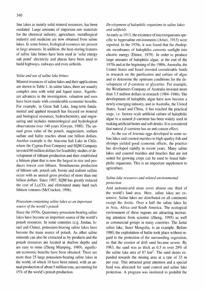
340
line lakes as mainly solid mineral resources, has been outdated. Large amounts of important raw materials for the chemical industry, agriculture, metallurgical industry and medicine are now obtained from saline lakes. In some brines, biological resources are present in large amounts. In addition, the heat-storing features of saline lake brines have been used in 'solar energy salt pond' electricity and playas have been used to build highways, railways and even airfields.
Value and use of saline lake brines
Mineral resources of saline lakes and their applications are shown in Table 1. In saline lakes, there are usually complex ores with solid and liquid states. Significant advances in the investigation, valuation and uses have been made with considerable economic benefits. For example, in Great Salt Lake, long-term fundamental and applied research has focused on mineral and biological resources, hydrochemistry, and engineering and includes meteorological and hydrological observations over 140 years (Gwynn, 1980). The annual gross value of the potash, magnesium, sodium sulfate and halite reaches about one billion dollars. Another example is the Atacama Salt Lake in Chile, where the Cyprus-Foot Company and SQM Company invested 60 million dollars for feasibility studies of development of lithium production and then established a lithium plant that is now the largest in size and produces lowest cost lithium. Simultaneous production of lithium salt, potash salt, borate and sodium sulfate occur with an annual gross product of more than one billion dollars. Since 1997, SQM has greatly reduced the cost of Li2C03 and eliminated many hard rock lithium ventures (McCracken, 1998).
Potassium-containing saline lakes as an important source of the world's potash
Since the 1970s, Quaternary potassium-bearing saline lakes have become an important source of the world's potash resources. In some countries (e.g. Jordan, Israel and China), potassium-bearing saline lakes have become the main source of potash. As other saline minerals can also be extracted as by-products and the potash resources are located at shallow depths and are easy to mine (Zheng Mianping, 1989), significant economic benefits have been obtained. There are more than 25 large potassium-bearing saline lakes in the world, of which 10 have been mined, with an annual production of about 5 million tons, accounting for 15% of the world's potash production.
Development of halophilic organisms in saline lakes and saltfields As early as 1913, the existence of microorganisms specific to hypersaline environments (Artari, 1913) were reported. In the 1970s, it was found that the rhodopsin membranes of halophiles convertz sunlight into electric energy (Dietor, 1979). In order to produce large amounts of halophilic algae, at the end of the 1970s and at the beginning of the 1980s, Australia, the United States and Israel invested considerable funds in research on the purification and culture of algae and to determine the optimum conditions for the development of ,B-carotene or glycerine. For example, the Westfarmers Company of Australia invested more than 3.5 million dollars in research (1984-1986). The development of halophilic algae have now become a newly-emerging industry, and in Australia, the United States, Israel and China, it has reached the practical stage, i.e. factory-scale artificial culture of halophilic algae to a natural ,B-carotene has been widely used in making artificial butter and soft drinks. It is considered that natural ,B-carotene has an anti-cancer effect.
As the use of Artemia eggs developed in some saline lakes and coasted marshes to high-quality fish and shrimps yielded good economic effects, the practice has developed rapidly in recent years. Many saline lakes and coasted marshes and beaches that are not suited for growing crops can be used to breed halophilic organisms. This is an important supplement to agriculture.
Saline lake resources and related environmental protection Arid and semi-arid areas cover almost one third of the world's land area. Here, saline lakes are extensive. Saline lakes are distributed on all continents except the Arctic. Over a half the saline lakes lie in Asia, Africa and South America. The ecological environment of these regions are attracting increasing attention from scientist (Zheng, 1995) as well as commercial groups in many countries. The Jartai saline lake, Inner Mongolia, is an example. Before 1980, the exploitation of halite took place without regard to the protection of the surrounding vegetation, so that the erosion of drift sand became severe. By 1983, the sand was as thick as 0.5 mover 29% of the saline lake area of 87 km2. The sand dunes expanded towards the mining area at a rate of 33 m per year. This attracted great attention and a special fund was allocated for sand control and saline lake protection. A program was instituted to prohibit the
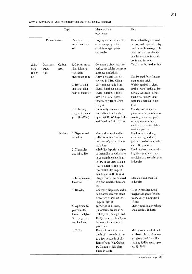
341
Table 1. Summary of types, magnitudes and uses of saline lake resources
Type Magnitude and Uses occurrence
Classic material Clay, sand, Large quantities available; Used in building and road gravel, volcanic economic-geographic paving, and especially clay ash conditions appropriate; used in brick-making; vol-
exploitable canic ash used as absorb-ents for automobiles, ship docks and factories
Solid- Dominant Carbon- I. Calcite, arago- Commonly dispersed; low Calcite can be used as lime
state evapo- ates nite, dolomite, purity; but calcite occurs as miner- rites magnesite large accumulations als Hydromagnesite A few thousand tons dis- Can be used for refractory
covered in Tibet, China magnesium bricks 2. Trona, soda Vary in magnitude from Widely applied in glass, and other alkali- several hundreds tons and textile, paper-making, dye,
bearing materials several hundred million rubber, synthetic rubber, tons (in U.S.A., Russia, medicine, battery, deter-Inner Mongolia of China, gent and chemical indus-Kenya) tries
3. Li-bearing Commonly contain a few Mainly used in special magnesite, Zabu- per mil to a few hundred glass, ceramic, aluminium yaite (Li2C03) ppm Li2C03 (Zubuye Lake smelting, chemical prod-
and Bangkog Lake, Tibet) ucts, synthetic rubber, medicine, batteries, lubri-cant, air purifier
Sulfates I. Gypsum and Mostly dispersed and lo- Used in light building anhydrite cally occur as a few mil- materials, agriculture,
lion tons of gypsum accu- gypsum products and other mulations daily life products
2. Thenardite Mirabilite deposits and part Used in glass, paper-mak-and mirabilite of thenardite deposits have ing, detergent, dynamite,
large magnitude and high medicine and metallurgical purity, larger ones attain a industries few hundred million to a few billion tons (e.g. in Karabujiaz Gulf, Russia)
3. Epsomite and Range from a few hundred Medicine and chemical kieserite to a few hundred thousand industries
tons 4. Bloedite Generally dispersed, and in U sed in manufacturing
some areas reserves attain magnesium glass for labo-a few tens of million tons ratory use yielding good (e.g. in Russia) effects
5. Aphthitalite, Dispersed and locally Mainly used in agriculture picromerite, picromerite occurs as pa- and chemical industry
kainite, polyha- tash layers (Dalang P. and lite, syngenite, Da Qaidam L., China); can and hanksite be mined for mUlti-pur-
pose uses I. Halite Ranges from a few hun- Mainly used in edible salt
dreds of thousands of tons and basic chemical indus-
to a few hundreds of bil- try; those used for edible lions oftons (e.g. Qarhan salt and fodder make up to P., China); widely distri- ca. 65-70% buted in world
Continued on p. 342
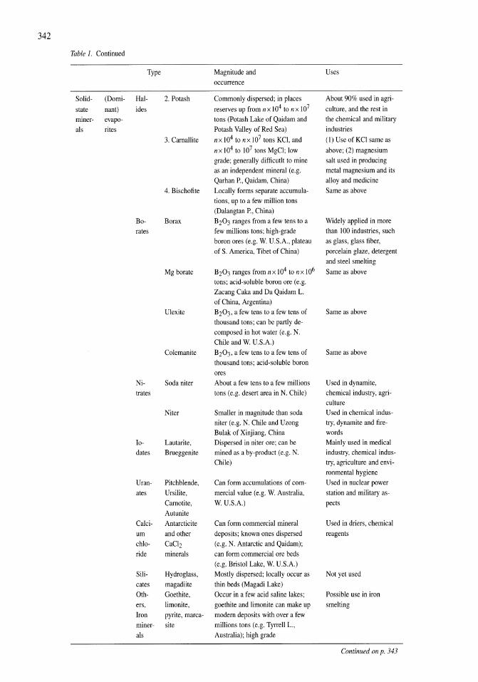
342
Table 1. Continued
Type Magnitude and Uses occurrence
Solid- (Domi- Hal- 2. Potash Commonly dispersed; in places About 90% used in agri-state nant) ides reserves up from nx 104 to nx 107 culture, and the rest in miner- evapo- tons (Potash Lake of Qaidam and the chemical and military als rites Potash Valley of Red Sea) industries
3. Carnallite nx 104 to nx 107 tons KCl, and (1) Use of KCl same as nx 104 to 107 tons MgCl; low above; (2) magnesium grade; generally difficutlt to mine salt used in producing as an independent mineral (e.g. metal magnesium and its Qarhan P., Qaidam, China) alloy and medicine
4. Bischofite Locally forms separate accumula- Same as above tions, up to a few million tons (Dalangtan P., China)
Bo- Borax B203 ranges from a few tens to a Widely applied in more rates few millions tons; high-grade than 100 industries, such
boron ores (e.g. W. U.S.A., plateau as glass, glass fiber, of S. America, Tibet of China) porcelain glaze, detergent
and steel smelting Mgborate B203 ranges from n x 104 to n x 106 Same as above
tons; acid-soluble boron ore (e.g. Zacang Caka and Da Qaidam L. of China, Argentina)
Ulexite B203, a few tens to a few tens of Same as above thousand tons; can be partly de-composed in hot water (e.g. N. Chile and W. U.S.A.)
Colemanite B203, a few tens to a few tens of Same as above thousand tons; acid-soluble boron ores
Ni- Soda niter About a few tens to a few millions Used in dynamite, trates tons (e.g. desert area in N. Chile) chemical industry, agri-
culture Niter Smaller in magnitude than soda Used in chemical indus-
niter (e.g. N. Chile and Uzong try, dynamite and fire-Bulak of Xinjiang, China words
10- Lautarite, Dispersed in niter ore; can be Mainly used in medical dates Brueggenite mined as a by-product (e.g. N. industry, chemical indus-
Chile) try, agriculture and envi-ronmental hygiene
Uran- Pitchblende, Can form accumulations of corn- U sed in nuclear power ates Ursilite, mercial value (e.g. W. Australia, station and military as-
Carnotite, W. U.S.A.) peets Autunite
Calci- Antarcticite Can form commercial mineral Used in driers, chemical urn and other deposits; known ones dispersed reagents chlo- CaCl2 (e.g. N. Antarctic and Qaidam); ride minerals can form commercial ore beds
(e.g. Bristol Lake, W. U.S.A.) Sili- Hydroglass, Mostly dispersed; locally occur as Not yet used cates magadiite thin beds (Magadi Lake) Oth- Goethite, Occur in a few acid saline lakes; Possible use in iron ers, limonite, goethite and limonite can make up smelting Iron pyrite, marca- modem deposits with over a few miner- site millions tons (e.g. Tyrrell L., als Australia); high grade
Continued on p. 343
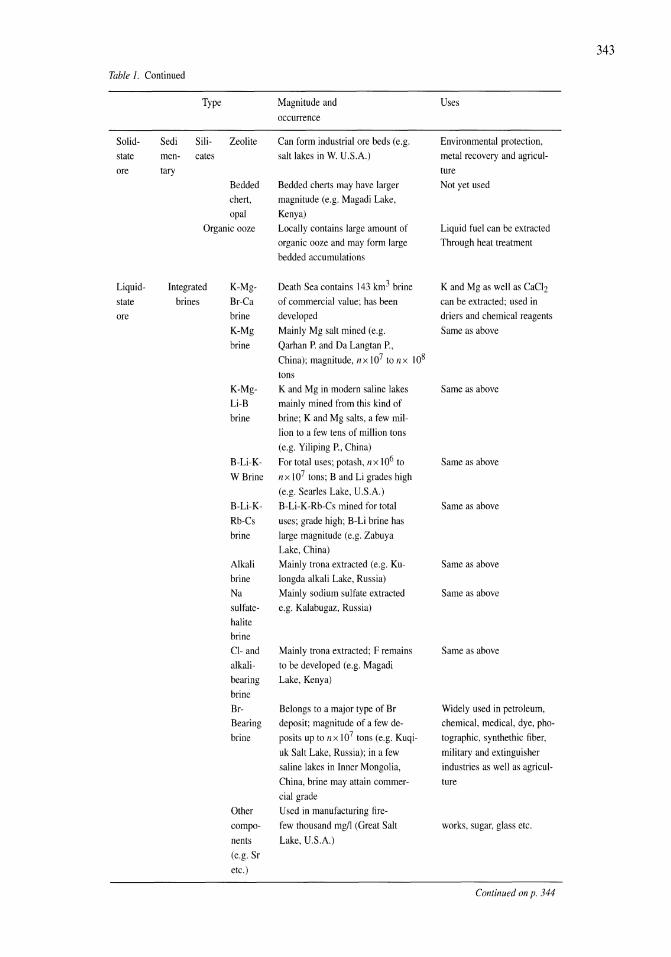
Table J. Continued
Solid
state
ore
Liquid-
state ore
Type Magnitude and
occurrence
Uses
Sedi Sili- Zeolite Can form industrial ore beds (e.g. salt lakes in W. U.S.A.)
Environmental protection, metal recovery and agricul
ture
men- cates
tary Bedded Bedded cherts may have larger Not yet used chert. magnitude (e.g. Magadi Lake, opal Kenya)
Organic ooze Locally contains large amount of Liquid fuel can be extracted
Integrated
brines
organic ooze and may form large Through heat treatment
bedded accumulations
K-Mg- Death Sea contains 143 km3 brine K and Mg as well as CaCl2
Br-Ca of commercial value; has been can be extracted; used in
brine developed driers and chemical reagents
K-Mg Mainly Mg salt mined (e.g. Same as above
brine
K-MgLi-B
Qarhan P. and Da Langtan P.,
China); magnitude, nx 107 to nx 108
tons K and Mg in modern saline lakes mainly mined from this kind of
brine brine; K and Mg salts, a few million to a few tens of million tons
(e.g. Yiliping P., China)
B-Li-K- For total uses; potash, nx 106 to
W Brine nx 107 tons; Band Li grades high
(e.g. Searles Lake, U.S.A.) B-Li-K- B-Li-K-Rb-Cs mined for total
Rb-Cs
brine
Alkali
brine Na sulfatehalite brine Cl- and alkali
bearing
brine BrBearing
brine
Other
compo
nents
(e.g. Sr
etc.)
uses; grade high; B-Li brine has large magnitude (e.g. Zabuya Lake, China)
Mainly trona extracted (e.g. Kulongda alkali Lake, Russia)
Mainly sodium sulfate extracted e.g. Kalabugaz, Russia)
Mainly trona extracted; F remains
to be developed (e.g. Magadi Lake, Kenya)
Belongs to a major type of Br deposit; magnitude of a few de
posits up to IlX 107 tons (e.g. Kuqi
uk Salt Lake, Russia); in a few
saline lakes in Inner Mongolia,
China, brine may attain commer
cial grade Used in manufacturing fire
few thousand mg/l (Great Salt
Lake, U.S.A.)
Same as above
Same as above
Same as above
Same as above
Same as above
Same as above
Widely used in petroleum, chemical, medical, dye, pho
tographic, synthethic fiber,
military and extinguisher industries as well as agricul
ture
works, sugar, glass etc.
Continued on p. 344
343
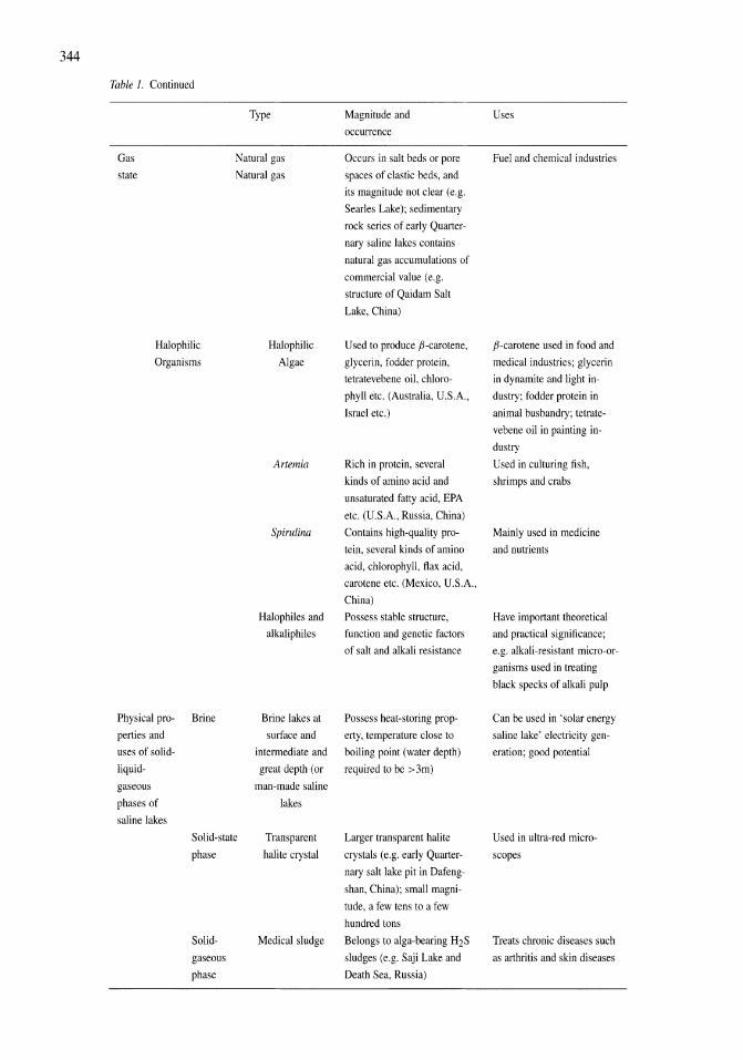
344
Table 1. Continued
Type Magnitude and
occurrence
Gas
state
Natural gas
Natural gas
Occurs in salt beds or pore
spaces of clastic beds, and
its magnitude not clear (e.g.
Searles Lake); sedimentary
rock series of early Quarter
nary saline lakes contains
natural gas accumulations of
commercial value (e.g.
structure of Qaidam Salt
Lake, China)
Halophilic
Organisms
Physical pro- Brine
perties and
uses of solid-
liquid-
gaseous
phases of
saline lakes
Solid-state
phase
Solid-
gaseous
phase
Halophilic
Algae
Artemia
Spirulina
Halophiles and
alkaliphiles
Brine lakes at
Used to produce ,6-carotene,
glycerin, fodder protein,
tetratevebene oil, chloro
phyll etc. (Australia, U.S.A.,
Israel etc.)
Rich in protein, several
kinds of amino acid and
unsaturated fatty acid, EPA
etc. (U.S.A., Russia, China)
Contains high-quality pro
tein, several kinds of amino
acid, chlorophyll, flax acid,
carotene etc. (Mexico, U.S.A.,
China)
Possess stable structure,
function and genetic factors
of salt and alkali resistance
Possess heat -storing prop-
surface and erty, temperature close to
intermediate and boiling point (water depth)
great depth (or
man-made saline
lakes
Transparent
halite crystal
Medical sludge
required to be > 3m)
Larger transparent halite
crystals (e.g. early Quarter
nary salt lake pit in Dafeng
shan, China); small magni
tude, a few tens to a few
hundred tons
Belongs to alga-bearing H2S
sludges (e.g. Saji Lake and
Death Sea, Russia)
Uses
Fuel and chemical industries
/i-carotene used in food and
medical industries; glycerin
in dynamite and light in
dustry; fodder protein in
animal busbandry; tetrate
vebene oil in painting in
dustry
Used in culturing fish,
shrimps and crabs
Mainly used in medicine
and nutrients
Have important theoretical
and practical significance;
e,g, alkali-resistant micro-or
ganisms used in treating
black specks of alkali pulp
Can be used in 'solar energy
saline lake' electricity gen
eration; good potential
Used in ultra-red micro
scopes
Treats chronic diseases such
as arthritis and skin diseases
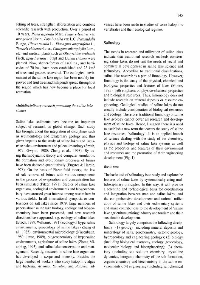
felling of trees, strengthen afforestation and combine scientific research with production. Over a period of 10 years, Picea asperata Mast, Pinus sylvestris var. mongolica Litvin., Populus alba var. L.c. Pyramidalis Bunge, Ulmus pumila L., Elaeagnus angustifolia L., Tamarix chinensis Lour., Caragana microphylla Lam., etc. and medical plants such as Glycyrrhiza uralensis Fisch, Ephedra sinica Stapf and Licium chinese were planted. Now, shelter-forests of 1400 ha., and barricades of 70 ha., have been established and 23 km2
of trees and grasses recovered. The ecological environment of the saline lake region has been notably improved and fruit trees and fish ponds spread throughout the region which has now become a place for local recreation.
Multidisciplinary research promoting the saline lake studies
Saline lake sediments have become an important subject of research on global change. Such study has brought about the integration of disciplines such as sedimentology and Quaternary geology and thus given impetus to the study of saline lakes and lacustrine paleo-environment and paleoclimatology (Smith, 1979; Gwynn, 1980; Zheng et aI., 1998). By using thermodynamic theory and computer simulation, the formation and evolutionary processes of brines have been deduced quantitatively (Eugster & Hardie, 1978). On the basis of Pitzer fluid theory, the law of salt removal of brines with various components in the process of evaporation and concentration has been simulated (Pitzer, 1991). Studies of saline lake organisms, ecological environments and biogeochemistry have aroused great interest among researchers in various fields. In all international symposia or conferences on salt lakes since 1979, large numbers of papers about saline lake biology, ecology and biogeochemistry have been presented, and new research directions have appeared, e.g. ecology of saline lakes (Brock, 1979; Williams, 1981), ecology of hypersaline environments, geoecology of saline lakes (Zheng et aI., 1985), environmental microbiology (Nissenbaun, 1980; Javor, 1989), biogeochemistry of hypersaline environments, agriculture of saline lakes (Zheng Mianping, 1995), and saline lake conservation and management. Recently, research on saline lake organisms has developed in scope and intensity. Besides the large number of workers who study halophilic algae and bacteria, Artemia, Spirulina and Rotifera, ad-
345
vances have been made in studies of some halophilic vertebrates and their ecological regimes.
SaJinology
The trends in research and utilization of saline lakes indicate that traditional research methods concerning saline lakes do not suit the needs of social and commercial development in saline lake science and technology. According to traditional classifications, saline lake research is a part of limnology. However, limnology is the study of the physical, chemical and biological properties and features of lakes (Moore, 1975), with emphasis on physico-chemical properties and biological resources. Thus, limonology does not include research on mineral deposits or resource engineering. Geological studies of saline lakes do not usually include consideration of biological resources and ecology. Therefore, traditional limnology or saline lake geology cannot cover all research and development of saline lakes. Hence, I suggest there is a need to establish a new term that covers the study of saline lake resources, 'salinology'. It is an applied branch of science dealing with the study of the chemistry, physics and biology of saline lake systems as well as the properties and features of their environment and resources and the promotion of their engineering development (Fig. 1).
Basic task
The basic task of salinology is to study and explore the features of saline lakes by systematically using multidisciplinary principles. In this way, it will provide a scientific and technological basis for coordination and integration between man and saline lakes, and the comprehensive development and rational utilization of saline lakes and their sedimentary systems and make contributions to the development of 'saline lake agriculture, mining industry and tourism and their sustainable development.
Salinology largely comprises the following disciplinary: (1) geology (including mineral deposits and mineralogy of salts, geochemistry, tectonic geology, hydrogeology and engineering geology); (2) biology (including biological taxonomy, ecology, geoecology, molecular biology and bioengineering); (3) chemistry (including salt solution chemistry, crystalline dynamics, inorganic chemistry of the salt-formation, organic chemistry and biochemistry in the saline environments); (4) engineering (including salt chemical
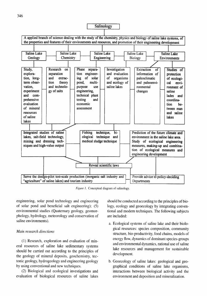
346
I Salinology
A applied branch of science dealing with the study of the chemistry, physics and biology of saline lake systems, of the properties and features of their environments and resources, and promotion of their engineering development
I I I I Saline Lake Saline Lake Saline Lake Saline Lake Saline Lake
Geology Chemistry Engineering Biology Environments
I I I I / I Study, Research on Phase separa- Investigation Extraction of Studies of explora- separation tion engineer- and evaluation information of protection tion, long- and extrac- ing of solar of organisms paleoclimatic of ecologi-term obser- tion theory pond, multi- and ecology of and paleoenvi- cal envi-vation, and technolo- purpose use saline lakes ronmental ronment of experiment - gy of salts t- engineering, - - changes """-
saline and com- technical plant lades and prehensive testing and coordina-evaluation economic tion be-of mineral assessment tween man resources and saline of saline lakes lakes
I I / I Integrated studies of saline Fishing technique, bi- Prediction of the future climate and lakes. salt-field technology, ological technique and environment in the saline lake area mining and dressing tech- medical sludge technique
r---Study of ecological engineering
niques and high-value output measures, making-up and combina-tion of ecological measures and engineering development
I L I Reveal scientific laws I
I Serve the desisn-pilot test-scale production (inorganic salt industry and ~ Provide advice t policy-deciding "agriculture" of saline lakes) and tourism industry Departments
Figure 1. Conceptual diagram of salinology.
engineering, solar pond technology and engineering of solar pond and beneficial saIt engineering); (5) environmental studies (Quaternary geology, geomorphology, hydrology, meteorology and conservation of saline environments).
Main research directions
(1) Research, exploration and evaluation of mineral resources of saline lake sedimentary systems should be carried out according to the principles of the geology of mineral deposits, geochemistry, tectonic geology, hydrogeology and engineering geology by using conventional and new techniques.
(2) Biological and ecological investigations and evaluation of biological resources of saline lakes
should be conducted according to the principles of biology, ecology and geoecology by integrating conventional and modem techniques. The following subjects are included:
a. Ecological systems of saline lake and their biological resources: species composition, community structure, bio-productivity, food chains, models of energy flow, dynamics of dominant species-groups and environmental dynamics, rational use of saline lake resources and management for sustainable development.
b. Geoecology of saline lakes: geological and geographical conditions of saline lake organisms, interactions between biological activity and the environment and deposition and mineralization.
c. Biological engineering of saline lakes: principles, means and feasibility of engineering development of biological resources of saline lakes.
(3) Saline lake chemical study focuses on the processes of salt dissolution in solvent or crystallization from solution, relations among composition, structure and characters of solution, thermal chemistry, thermodynamics, phase balance thermodynamics of solution and crystallization kinetic mechanism of the water-salt system, principle and application of heat storage and electrochemical energy of 18 salt-forming elements.
(4) On the basis ofthe knowledge obtained by studies of (I), (2) and (3) above, we should carry out investigation of well-integrated engineering techniques with high-value output and comprehensive development as the target, including division of saline lake areas, saltfield technology, mining and dressing techniques, fisheries and biological techniques, medical sludges and other uses.
(5) In light of principles of sedimentology and Quaternary geology, and through a study of such indicators as the high resolution of sediments and geomorphological features of saline lakes, we should extract information on past global changes and elucidate paleoclimatic changes and the response of lakes to the interaction of man and nature. In key saline lakes, we should establish long-term meteorologicalhydrological and biological observation stations to obtain systematic values of changes of ecological environments and integrate the observations with geographic information system (GIS) techniques to monitor the dynamic change in saline lake areas. On that basis, we will study the engineering development of protective measures for the ecological environments of saline lakes.
Acknowledgements
This research was supported by the National Natural Science Foundation of China Grant 49833010.
References
Bogoslovskii, B. B. & C. D. Muraveiskii, 1955. Introduction to Limnology. Moscow University Press, Moscow (in Russian).
Borowitzka, L. J. et aI., 1981. The microflora-adaptations to life in extremely saline lakes. Hydrobiologia 81: 33-40.
Brock, 1. D., 1979. Ecology of Saline Lakes. Strategies of Microbial Life in Extreme Environments, M. Shilo: 29-47.
347
Dietor, w.. 1979. Reviews on bioenergetics. Biochem. Biophys. Acta 505: 279-353.
Dzens-Litovskii, 1957. Comprehensive Research and Exploration Methods of Saline Lake Mineral Deposits. Leningrad Publishing House (in Russian).
Eugster, P. & A. Hardie, 1978. Saline Lakes - Lakes Chemistry Geology Physics (Chapter 8), Springer Verlag, New York INC: 237-283.
Guillcrino, C. D., 1988. The Cenozoic saline deposits of the Chilean Andes between 18° 00 and 27° 00' south latitude. Lecuture Notes in Earth Sciences, Vol. 17. Springer-Verlag. Berlin Heiidelbeg.
Gwynn, J. w., 1980. Great Salt Lake - a Scientific, Historical and Econonmic Overview. In Utah Geological and Mineral Survey: 1-400.
Hammer. U. T., 1981. Primary production in saline lakes: a review. Hydrobiologia 81: 47-57.
Hurlbert, S. H. (ed.), 1993. Salt Lakes V-Developments in Hydrobiology. Kluwer Academic Publishers, Dordrecht: 87 pp.
Javor, B .. 1989. Hypersaline Environments. In: Microbiology and Biogeochemistry, Springer-Verlag, Berlin.
Kudhner, D. J., 1978. Microbial Life in Extreme Environments, Academic Press INC. London: 319-352.
Matter, A. & M. E. Tucker, 1978. Modern and Ancient Lake Sediments. Blackwell Schentilic Publications, Oxford, London.
McCracken, D. & Mike, H., 1998. Lithium, Minerals, Supplement to Mining Journal, Aug. 7, II.
Nisserbaum, A. (ed.), 1980. Hypersaline brines evaporite environments. Dev. Sedimentol. 28: 23-29.
Oren, A., 1999. Bioenergetic aspects of Halophilism. Microbial. Molec. BioI. Rev., 63: 334-348.
Pitzer, K. S., 1991. Activity Coefficients in Electrolytes Solutions, 2nd edn. CRC, Florida: 75-153.
Smith, G. I .. 1979. Supsurface Stratigraphy and Geochemistry of Lake Quaternary Evaporite, Scarles Lake California, U.S. Geol. Survey Prof. 1043: 98-100.
Usiglio, I., 1849. L.' Analyse de Ipeau de la Mediterannee sur les coles de France. Etutes sur la composition leau dela Mediterannee et sur Ipexploitation des sels quele contient. Ann. de Chim. et de phys. XXVII.
Williams, W. D., 1981. Inland salt lakes: Introduction. Hydrobiologia 81: 1-13.
Williams, W. D., 1996. How important is salinity in structuring biological communitities in salt lakes" Resources environment and global change of saline lakes. In Selected papers of the 6th International Conference on Salt Lakes. Beijing: Geological Publishing House: 103-114.
Yuan Jianqi, 1982, New development of the genetic theory of saline mineral deposits and its position in the geology of mineral deposits. Geology of Mineral Deposits, 1(1): 16-33 (in Chinese with English abstract).
Zheng Mianping & Liu Wengao, 1985. The discovery of halophilic algae and halobacteria at Zabuye Salt Lake Tibet and preliminary study on the geoecology. Acta Geologica Sinica, 2: 162-171.
Zheng Mianping, 1995. On 'agriculture of saline lakes'. J. Geosci. 4: 404 (in Chinese with English abstract).
Zheng Mianping (ed.), 1996. Resources Environment and Global Change of Saline Lakes. In Selected Papers of the 6th International Conference on Salt Lakes. Geological Publish House, Beijing: 1-20: 145-157 (in Chinese).
Zheng Mianping, Zhao Yuanyi & Liu Junying, 1998. Sedimnetation and paleoclimate of Quarternary saline lakes. Quaternary Research 4: 297-307 (in Chinese).


