SIMULATION OF THE TRANSFORMATION OF INTERNAL

SOLITARY WAVES ON OCEANIC SHELVES

Roger Grimshaw1), Efim Pelinovsky2,3), Tatiana Talipova2), and Andrey Kurkin3)

1) Department of Mathematical Sciences, Loughborough University, Loughborough, UK 2) Laboratory of Hydrophysics, Institute of Applied Physics, Nizhny Novgorod, Russia 3) Applied Mathematics Department, State Technical University, Nizhny Novgorod, Russia

Version 1 October 6, 2003

Abstract

Due to the horizontal variability of oceanic hydrology (density and current stratification) and the variable depth over the continental shelf, internal solitary waves transform as they propagate shorewards into the coastal zone. If the background variability is smooth enough, a solitary wave possesses a soliton-like form with varying amplitude and phase. This stage is studied in detail in the framework of the variable-coefficient extended Korteweg–de Vries equation where the variation of the solitary wave parameters can be described analytically through an asymptotic description a slowly-varying solitary wave. Direct numerical simulation of the variable-coefficient extended Korteweg–de Vries equation is performed for several oceanic shelves (North-west Shelf of Australia, Malin Shelf Edge, Arctic Shelf) to demonstrate the applicability of the asymptotic theory. It is shown that the solitary wave may maintain its soliton-like form for large distances (up to 100 km), and this confirms why internal solitons are observed widely in the world’s oceans. In some cases the background stratification contains critical points (when the coefficients of the nonlinear terms in the extended Korteweg–de Vries equation change sign), or does not vary sufficiently smoothly; in such cases the solitary wave deforms a group of secondary waves. This stage is studied numerically.

Submitted for “Journal Physical Oceanography”

Correspondence: Professor Roger Grimshaw, Department of Mathematical Sciences, Loughborough

University, Loughborough, Leicestershire LE11 3TU UK; email: R.H.J.Grimshaw@lboro.ac.uk

1. INTRODUCTION

Nonlinear internal waves observed in the ocean frequently occur as solitary waves often

described as solitons. Examples have been reported from many regions of the world oceans

including the Sulu Sea, the North-West Shelf of Australia, the Bay of Biscay, the Sea of

Okhotsk, East and West China Seas and the east coast of the Canadian Shelf. Ostrovsky and

Stepanyants (1989) and Jeans (1995) have provided recent reviews of observations of internal

solitary waves in the ocean. Some observations made from space demonstrate the influence of a

variable background (e.g. variable bottom topography, an inhomogeneous thermocline) on the

evolution of internal solitons (Liu and Chang, 1998; Zheng et al, 2001).

The theoretical description of weakly nonlinear long internal solitary waves in the fluid with

continuous stratification on density and current is based on the Korteweg–de Vries (KdV) and

the extended Korteweg–de Vries (eKdV) equations (see, for instance, Benney, 1966; Lee and

Beardsley, 1974; Lamb and Yan, 1996; Pelinovsky et al, 2000; Grimshaw, 2001; Holloway et al,

2001; Grimshaw et al, 2002). The oceanic stratification as well as the total water depth usually

varies smoothly (on the scale of the internal solitary waves) in space and time. This variability

can be included in the theoretical models leading to the variable-coefficient nonlinear evolution

equations (see, for instance, Grimshaw, 2001). The variability of the coefficients of the

Korteweg–de Vries equations has been studied for some areas of the world’s oceans (Pelinovsky

et al, 1995; Poloukhin et al, 2003). The extended Korteweg–de Vries, as well as the Korteweg–

de Vries equation, is often used in oceanographic practice to investigate the nonlinear wave

transformation in the coastal zone, taking into account both the variable depth and horizontal

variability of the hydrology (Holloway et al, 1997, 1999; Liu and Chang, 1998; Small, 2001a,b;

Cai et al, 2002). The results of these calculations demonstrate the evolution of internal tides (or

long-scale disturbances) into large-amplitude short-scale pulses of solitary-like form. In many

cases the number of such pulses is large and they interact between themselves and with the

background flow. Consequently, it is difficult to determine when an individual solitary wave

2

may propagate for a long distance preserving its form. The investigation of the possible

“lifetime” of an internal soliton propagating in the ocean with real variability of hydrology and

depth is the main goal of this paper.

The paper is organized as follows. The theoretical model based on the extended Korteweg-de

Vries equation is briefly presented in section 2. The influence of the smoothly horizontal

variability of the ocean hydrology and basin depth on the solitary wave dynamics is studied in

section 3, using the asymptotic theory of a slowly-varying solitary wave. Direct numerical

simulation of the variable-coefficient extended Korteweg–de Vries equation is given for several

oceanic shelves: the North-West Shelf of Australia, the Malin Shelf Edge (west of Scotland), and

the Arctic Shelf (Laptev Sea). These are described in detail in section 4. The results of these

calculations are used to estimate the “lifetime” of a solitary wave in relation to the variability of

the oceanic environment, and to the applicability of the asymptotic approach for internal solitary

waves.

2. THEORETICAL BACKGROUND

The Korteweg–de Vries equation for long weakly nonlinear internal waves was derived first by

Benney (1966) taking into account the continuous stratification of the fluid for both background

density and shear flow. Subsequently, this equation has been widely used for an explanation of

the properties of the solitary-like disturbances observed in the pycnocline, and for the

interpretation of SAR images of internal waves. For many coastal areas the coefficient of the

nonlinear term in the Korteweg–de Vries equation is small (for instance when the pycnocline lies

near the middle depth of the fluid), and high-order correction terms should be taken into account.

The extended Korteweg–de Vries equation was first derived for a two-layer fluid (Kakutani and

Yamasaki, 1978), and then for the more general case of a continuous stratification in density and

shear flow (Lamb and Yan, 1996; Talipova et al, 1999; Grimshaw et al, 2002). It can be written

as

3

0)( 3

32

1 =++++xx

ct ∂

η∂β∂∂ηηααη

∂∂η , (1)

where η(x,t) is the vertical displacement of the pycnocline (see below), x is a horizontal

coordinate and t is time, and the coefficients c, α, α1, and β are the wave speed, quadratic and

cubic nonlinear coefficients and dispersion parameter respectively. The wave speed c is

determined from the eigenvalue problem for the modal structure function Φ(z) of the vertical

displacement in the linear long-wave limit (the Boussinesq approximation and the rigid-lid

approximation are used here for simplicity)

( )

,0)0()(

,0)()( 22

=Φ=−Φ

=Φ+

Φ

−

H

zNdzdzUc

dzd

(2)

where N(z) is the Brunt-Väisäilä frequency, U(z) is the background shear flow, and H is water

depth. We assume that modal function, Φ(z) is normalized, and its maximum, Φmax = 1. The

dispersion parameter β is represented by the integral

β =

−

−

−

−

∫

∫

12

2 20

20

( )

( )( / )

c U dz

c U d dz dz

H

H

Φ

Φ, (3)

and the nonlinear coefficients α and α1 are

α =

−

−

−

−

∫

∫

32

2 30

20

( ) ( / )

( )( / )

c U d dz dz

c U d dz dz

H

H

Φ

Φ, (4)

4

{ [ ] }

∫∫

Φ−

Π+Φ−ΦΦ−−=

dzdzdUc

dzddzddzddzdTUcdz2

22222

1)/)((

)/()/()/(2/(3)(3 αα ,

(5)

[ ] dzddzdTdzdUc //4)/(5)( 2 Φ−Φ−=Π α .

Here T(z) is the nonlinear correction to the modal structure, and it is found from the

inhomogeneous eigenvalue problem

( )

Φ

−+

Φ

−−=+

−

2222 )(

23)(

dzdUc

dzd

dzdUc

dzdTN

dzdTUc

dzd α (6)

with zero boundary conditions on the sea bottom and free surface. Also we normalize the

function T(z) that T(zmax) = 0, where zmax is found from Φ (zmax) = 1. The vertical displacement

of the isopycnal surface, ξ(x,z,t) is represented with the same accuracy by

)(),()(),(),,( 2 zTtxztxtxz ηηξ +Φ= . (7)

Taking into account the normalization of the functions, Φ and T, the wave function, η(x,t)

represents the vertical isopycnal displacement at the depth zmax.

The extended Korteweg–de Vries equation has been well studied from the mathematical point of

view, and it is a fully integrable model with the availability of an inverse scattering method to

find solutions. The Cauchy problem and multi-soliton solutions are discussed in Slyunyaev and

Pelinovsky, 1998, Slyunyaev, 2001, and in Grimshaw et al, 2002.

When the water depth and the oceanic stratification vary smoothly in the horizontal direction, the

modal structure of the internal wave also varies smoothly and to the first approximation can be

calculated from equation (2), as for constant conditions. Also similarly, all the coefficients of the

extended Korteweg–de Vries equation can be calculated as for a constant background, but they

will now be functions of the horizontal coordinate. Using the asymptotic method, the variable-

5

coefficient extended Korteweg – de Vries equation can be derived (Zhou and Grimshaw, 1989;

Holloway et al, 1999; Grimshaw, 2001)

023

32

1 =++∂∂

+++ η∂

η∂βηηα∂∂ηαη

∂∂η

∂∂η

dxdQ

Qc

xxxxc

t, (8)

where

Qc c U d dz dz

c c U d dz dz

H

H

=−

−

−

−

∫

∫

02

0 0 02

0

2 20

( )( / )

( )( / )

Φ

Φ. (9)

The term Q represents the amplification factor in the linear long-wave theory due to variable

depth and a horizontally variable stratification. The index “0” corresponds to a fixed horizontal

location, x0, which may be taken to be the initial position of a solitary wave. After the change of

variables

∫ −= txc

dxs)(

, )(),(),(

xQsxsx ηζ = , (10)

equation (8) can be reduced in the same approximation to

0)( 3

3

42

2

21

2 =+++scsc

Qc

Qx ∂

ς∂β∂∂ςςαςα

∂∂ς

. (11)

This is the spatial version of the extended Korteweg-de Vries equation, and the “initial

condition” for it corresponds to a time series of the wave displacement at the fixed point x0.

Equation (11) in various modifications (with/without cubic nonlinear term, with additional

dissipative terms, with/without taking into account the Earth’s rotation) has been applied to the

study of internal wave transformation in the coastal zone (Djordjevic and Redekopp, 1978; Zhou

6

and Grimshaw, 1989; Holloway et al, 1997, 1999, 2001; Grimshaw et al, 1998, 1999; Liu and

Chang, 1998; Small, 2001a,b; Pelinovsky et al, 2002; Cai et al, 2002).

3. ADIABATIC TRANSFORMATION OF A SOLITARY WAVE

The main goal of this paper is to investigate the dynamics of internal solitary waves in a

horizontally inhomogeneous ocean taking into account real variability of the ocean parameters.

Before considering our numerical simulations of equation (11) we will discuss the possible

scenarios of the wave transformation, using the asymptotic theory of a slowly-varying solitary

wave, in which the solitary wave locally maintains its soliton-like form.

First of all, let us briefly reproduce the well-known formula for the steady-state solitary wave

solutions of (11) for “frozen” coefficients (see for instance, Grimshaw, 2001). In its most general

form, the soliton is described by

([ )]xsBA

κγς

−+=

cosh1, (12)

.

where the parameters A, B, κ and γ are given by

QcA 2

26α

βγ= , )1(

62

1

22

−= Bcβα

αγ , 4

2

cβγκ = . (13)

The amplitude of the solitary wave is

)1(1 1

−=+

= BQB

Aaαα . (14)

Only one of parameters in (12) is arbitrary, and the other parameters then depend on this one and

the values of the coefficients of equation (11).

There are branches of solitary wave described by equation (12). They depend on the sign of the

coefficient cubic α1 of the cubic nonlinear term in equation (11).

7

Negative α1:

For this case there is only one branch of solitary waves (0 < B < 1). The polarity of such solitons

is determined by the sign of quadratic nonlinear coefficient, α. In particular, in the case α > 0

solitary waves have positive polarity, where we note that the dispersion parameter β is always

positive (3). The amplitude a of the solitary wave is bounded (in modulus) by the value

1lim α

αQ

a −= . (15)

When the solitary wave amplitude approaches this value, the length of the solitary wave tends to

infinity and such solitary waves are known as “table” or “thick” soliton. Possible solitary wave

shapes for α1 < 0 are shown on Fig. 1a in dimensionless form (c = α = |α1| = β = 1).

Positive α1:

For α1 > 0 there are two branches of solitary waves of opposite polarity (B2 > 1). In the case α >

0 (1 < B < ∞) a solitary wave of positive polarity may take any amplitude and it tends to the

KdV soliton in the weak amplitude limit. A solitary wave of negative polarity (-1 > B > -∞) may

take an amplitude only greater in absolute value than the amplitude of an algebraic soliton which

is

1

2αα

Qaal −= . (16)

Both branches of solitary waves in dimensionless form (c = α = α1 = β = 1) are presented on

Fig. 1b. The algebraic soliton is marked by a dashed line.

For a variable oceanic background, the wave shape changes, and the wave parameters

(amplitude, width, speed) vary. If the oceanic parameters vary sufficiently smoothly (the actual

8

condition will be discussed later), the wave is locally close to the solitary wave (12) but with a

variable amplitude, width and speed. The variation of the solitary wave parameters can be found

from the conservation of wave action flux, often referred to simply as energy conservation. This

energetic approach may be justified by the use of an asymptotic expansion (see, for instance,

Grimshaw and Mitsudera, 1993). The relevant conservation law can be easily derived from (11),

const2 =∫∞

∞−

dsζ . (17)

Using (12) it becomes

∫∞

∞−

=+

const)cosh1( 2

2

ττ

γ BdA , (18)

or in terms of just one independent parameter, B,

const)1()(1 2/3231

2

2 =−BBFcQ α

βα , (19)

where F(B) is the value of the integral in (18) and depends on the choice of the family of the

soliton solutions.

For α1 < 0, the value of B lies between 0 and 1, and (19) reduces to

const111tanh21 21-

31

2

2 =

−−

+− B

BB

cQ αβα . (20)

For α1 > 0 there are two branches of solitary waves. If the solitary wave polarity has the same

sign as the coefficient of the quadratic nonlinear term, α , the value of B > 1, and (19) takes the

form

9

const11tan211 1-2

31

2

2 =

+−

−−BBB

cQ αβα . (21)

If the solitary wave has the opposite polarity to the sign of α, the value of B < -1, and (19)

reduces to

const11

tan211 1-231

2

2 =

−+

+−BB

BcQ α

βα . (22)

Using (20) - (22) and (14) the solitary wave amplitude, a can be determined as a function of the

oceanic parameters through the variation of c, α, α1, β, Q calculated from the local hydrology at

each point of the wave path. In fact, the solitary waves change adiabatically (retaining their

soliton-like shape) only at the leading order of the asymptotic theory. At the next order the

solitary wave radiates, generating a tail behind the solitary wave. A detailed investigation of the

solitary wave tail structure in the framework of the variable-coefficient Korteweg–de Vries

equation can be found in Grimshaw & Mitsudera (1993), El & Grimshaw (2002) and Grimshaw

& Pudjaprasetya (2003). The nature of the shelves appearing behind solitary wave (in particular,

its polarity) can be found from the mass conservation law, derived from (11)

const=∫∞

∞−

dsζ . (23)

It is easy to show that the calculation of the mass integral with the use of only the soliton

solution (12) leads to a variable solitary wave mass, and, therefore, the corresponding mass

deficit is associated with formation of a tail behind variable solitary wave.

The smoothness of the variable oceanic parameters (depth, shear flow, density

stratification) is usually understood as smoothness on the scale of the internal solitary waves (cf.

geometrical optics). It is used to neglect wave reflection and to derive a variable- coefficient

10

nonlinear evolution equation for unidirectional waves. For an adiabatic transformation of a

solitary wave this condition by itself is not enough, and the smallness of the last term in (8) is

also required here to provide a weak perturbation to the solitary wave. Physically, this condition

requires that the characteristic scale for the horizontal variability of the oceanic parameters

should be large compared with the characteristic scales of both nonlinearity and dispersion. Due

to the present case of weak nonlinearity and dispersion, this condition is harder to fulfill than the

usual conditions for the calculations of geometrical optics and similar systems. For the

determination of the applicability of adiabatic formulas to the processes of internal soliton

transformation on real oceanic shelves, it is important to select all possible “non-adiabatic”

factors even when the horizontal variability of the oceanic parameters may seem smooth enough.

First, this approximation fails for the “table” solitons which exist for negative values of the

coefficient of the cubic nonlinear term. As one approaches to the limiting amplitude the soliton

width is indefinitely increased, and will be comparable with the characteristic scale of the

oceanic horizontal variability. Thus the adiabatic approximation is not valid if the solitary wave

amplitude tends to the limiting value (15). The same situation is realized for the opposite case of

a very weak in amplitude solitary wave (for either sign of the coefficient of the cubic nonlinear

term); its width is large and comparable with the characteristic scale of the oceanic horizontal

variability. The third situation appears for solitary waves with an amplitude close to that of the

algebraic soliton (16); such a situation may be realized for positive values of the coefficient of

the cubic nonlinear term. The algebraic soliton in the framework of the extended Korteweg–de

Vries equation is unstable (Pelinovsky and Grimshaw, 1997), and the soliton breaks down if its

amplitude passes through the algebraic value (16). Further, there will be possible failures in the

adiabatic theory if the coefficients of nonlinearity or dispersion in the extended Korteweg–de

Vries equation pass through a zero value. The dispersion parameter β is always positive for

stable flows, see (3), but the coefficients of the quadratic and cubic nonlinear terms can be zero

(independently) for certain conditions of the oceanic stratification. When the both nonlinear

11

coefficients become zero simultaneously, the soliton cannot exist and any disturbance evolves

into a dispersive wave packet; in this case the soliton-like structure is destroyed. If the

coefficient of the quadratic nonlinear term passes through zero, but not that of the cubic

nonlinear term, the solitary wave is destroyed at the critical point if the cubic nonlinear term is

negative (Grimshaw et al, 1998, 1999). Formally, the soliton amplitude tends to zero at the

critical point according to the adiabatic formula (20). Secondary solitary waves of the opposite

polarity can appear from the tail of the primary soliton, but the primary soliton itself disappears.

The impossibility of an adiabatic transformation of a solitary wave in this case is illustrated in

Fig. 2, where there are no connecting arrows between solitary waves in the lower half-plane

(between quadrants III and IV). If the cubic nonlinear term is positive, an adiabatic transfer of

the solitary wave is possible between quadrants I and II (upper-plane in Fig. 2), and formally the

soliton amplitude is determined at the critical point according to the adiabatic formulas (21) and

(22). But if the soliton amplitude is close to the algebraic value, the adiabatic transformation is

impossible, and soliton-like structure destroys. If the coefficient of cubic nonlinear term changes

its sign, but not the coefficient of the quadratic nonlinear term (Nakoulima et al, 2003), the

transformation of the solitary wave of the same polarity (negative for α < 0 and positive for α >

0) can be adiabatic (between quadrants I and III on left half-plane or II and IV on right-half),

except for the case when the solitary wave amplitude is close to the amplitude of the “table”

soliton. If the soliton in the upper-half plane (Fig. 2) has opposite polarity (positive for α < 0 and

negative for α > 0), it is destroyed at the critical point, when the cubic nonlinear term becomes

zero. This simple classification will be used to analyze the data from our numerical simulations

of internal solitary wave transformation on oceanic shelves.

4. SOLITARY WAVE TRANSFORMATION ACROSS OCEAN SHELVES

The formulas given above describe the adiabatic solitary wave transformation when the wave

maintains its soliton-like shape. However, oceanic shelves may contain wave paths along which

12

the parameters do not vary sufficiently smoothly, and they may also include several critical

points. In this case n internal solitary wave transforms with loss of its individuality as a soliton,

and so we may say the soliton-like wave has a finite “life-time”. To consider the non-adiabatic

effects of the wave transformation and estimate of the soliton “life-time”, direct numerical

simulations are performed in the framework of the variable-coefficient extended Korteweg–de

Vries equation (11) for several oceanic shelves: the North-West Shelf of Australia, the Malin

Shelf Edge (west of Scotland) and the Arctic Shelf (in the Laptev Sea). Equation (11) is solved

numerically using a finite difference scheme with periodic boundary conditions (see, Holloway

et al, 1999) with the initial condition being a typical solitary wave for each shelf. In all

simulations we use only the density stratification of the coastal zone and ignore any effect to

background currents.

4.1. North-West Shelf of Australia

Nonlinear internal waves on the North-West Shelf of Australia (NWS) have been investigated by

Holloway over many years (Holloway, 1987, Holloway et al, 1997, 1999). He conducted several

measurements of the background stratification for this area. Here the observations obtained from

a CTD survey carried out on the NWS in January of 1995 (summer) are used. There were 11

CTD station data from the point (19.2oS, 115.7oE) to the point (19.8oS, 116.5oE). At each of

these 11 locations, ranging in depth from 416 to 66 m a sequence of repeated profiles were

measured every 30, 60 or 90 min, depending on the water depth, over a 13 h cycle. These

profiles have been averaged at each location to remove the variability induced from the internal

waves themselves, and the resulting CTD across-section is used to define the coefficients. The

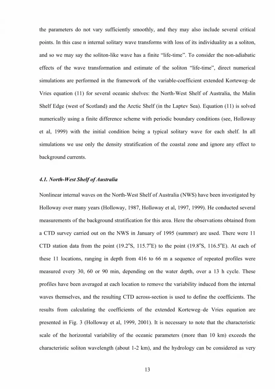
results from calculating the coefficients of the extended Korteweg–de Vries equation are

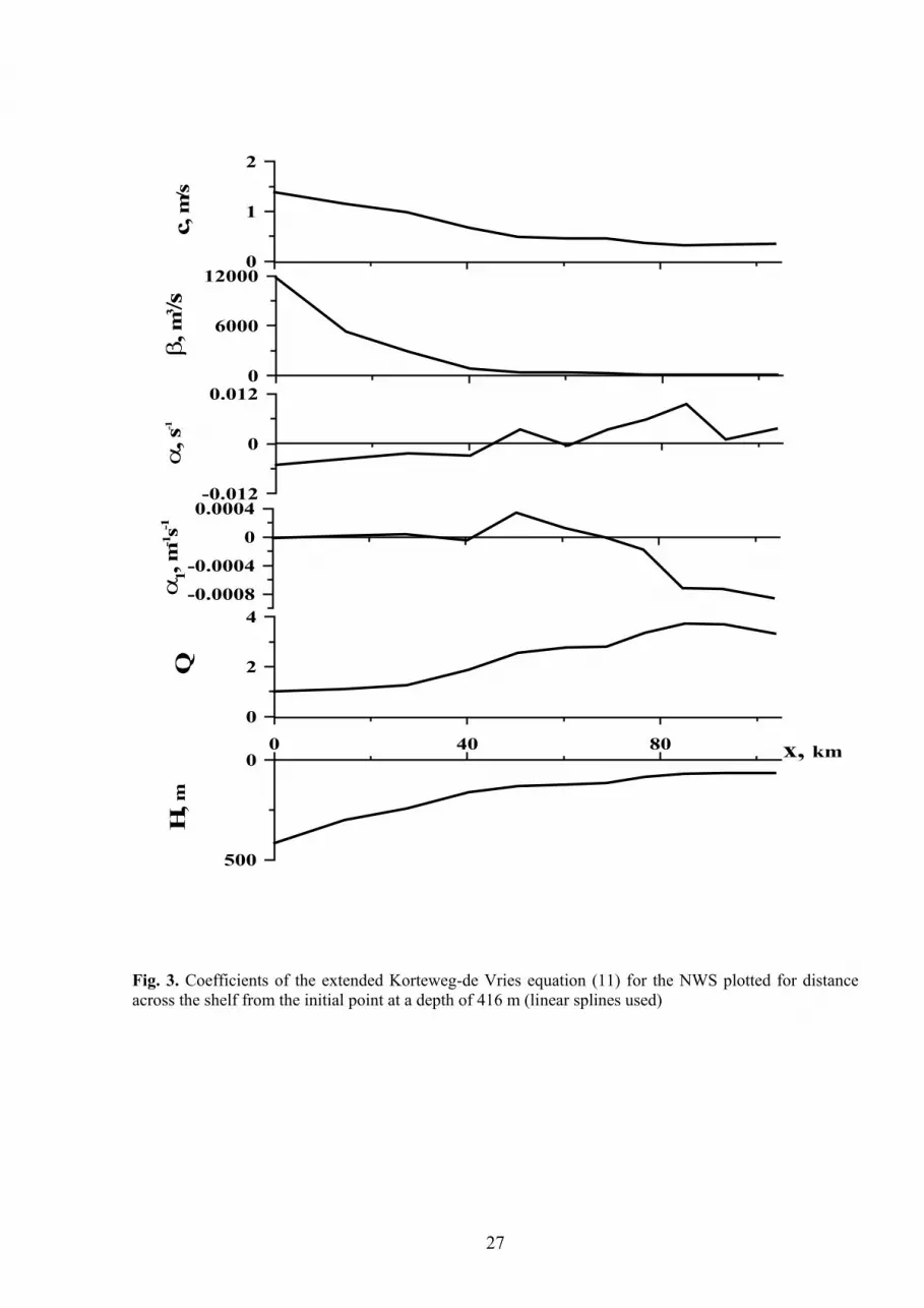
presented in Fig. 3 (Holloway et al, 1999, 2001). It is necessary to note that the characteristic

scale of the horizontal variability of the oceanic parameters (more than 10 km) exceeds the

characteristic soliton wavelength (about 1-2 km), and the hydrology can be considered as very

13

smooth. It is also clearly seen from Fig. 3 that both nonlinear coefficients change sign several

times along the wave path.

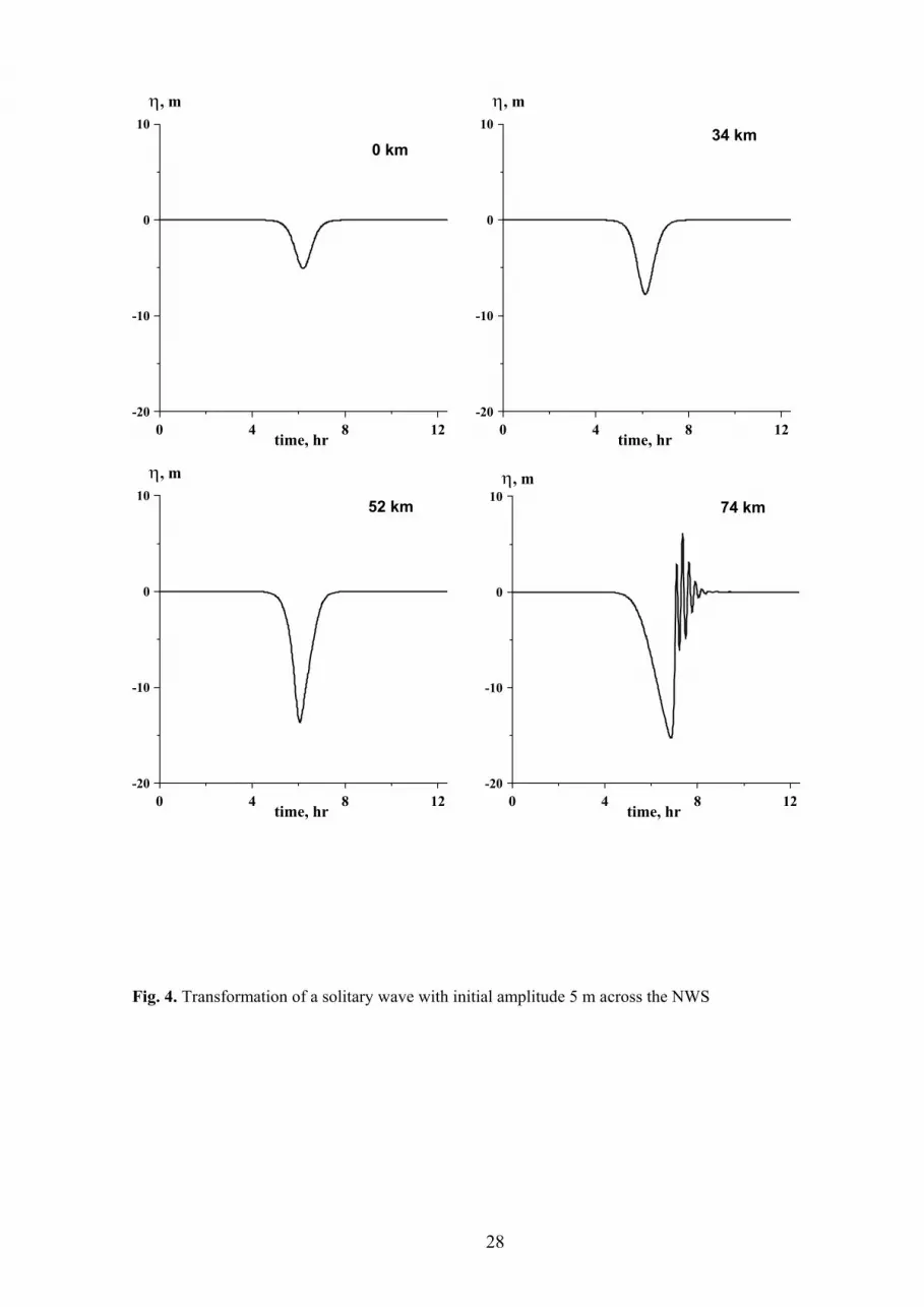
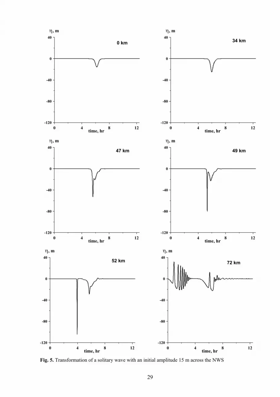
Two simulations have been done for NWS conditions. The first run was done for a solitary wave

of initial amplitude 5 m, and the second run for an initial wave amplitude of 15 m. The initial

solitary wave has negative polarity (as the coefficients of quadratic and cubic nonlinear terms are

negative), and its amplitude is significantly less than the limiting value (250 m); hence the

coefficient of cubic nonlinearity is negligible in the initial stage. The wave evolution at several

distances from the initial point is presented in Figs. 4–5 (the time in all figures is the time in a

shifted system of coordinates). The solitary wave maintains a soliton-like shape for a distance of

about 40 km while the influence of the cubic nonlinear term is weak. Consequently the two

critical points where the coefficient of the cubic nonlinear term passes through zero do not lead

to any change in the wave dynamics. For large distances both nonlinear coefficients change sign

and have non-monotonic behavior. At the distance 45 km the coefficient of the quadratic

nonlinear term changes its sign and becomes positive. According to Fig. 2 the negative soliton

from quadrant I in the vicinity of this distance transfers to a negative soliton in quadrant II, and

this process can be described by the adiabatic formulas (no change in the wave dynamics).

However, the solitary wave which initially has a weak amplitude is close to the algebraic soliton

wave in this quadrant, and their amplitudes are equal at a distance 46 km. After this point the

wave amplitude is less than the value for the algebraic soliton, and so such a wave cannot be a

soliton and has to transform into a breather. This process is slow because the difference in

amplitudes is weak; in particular, at a distance 55 km they are equal again. Then the coefficient

of the quadratic nonlinear term tends to zero (at about 60 km) and becomes negative for a short

distance. In this case, the wave amplitude again exceeds the value for an algebraic soliton, thus

supporting a soliton-like structure. As a result, there is no visible deformation in the soliton-like

shape. At a distance 68 km the coefficient of the cubic nonlinear term changes its sign and

becomes negative. A soliton of negative polarity cannot transform from quadrant II to quadrant

14

IV in Fig. 2, and so the soliton now disappears transforming into a dispersive wave packet. This

process is clearly seen in Fig. 4.

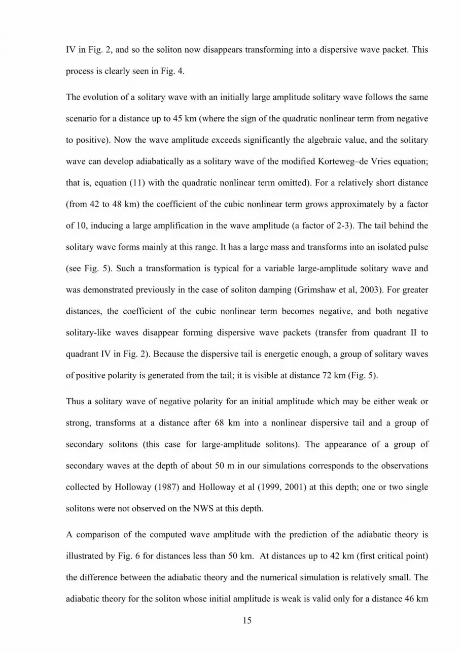
The evolution of a solitary wave with an initially large amplitude solitary wave follows the same

scenario for a distance up to 45 km (where the sign of the quadratic nonlinear term from negative

to positive). Now the wave amplitude exceeds significantly the algebraic value, and the solitary

wave can develop adiabatically as a solitary wave of the modified Korteweg–de Vries equation;

that is, equation (11) with the quadratic nonlinear term omitted). For a relatively short distance

(from 42 to 48 km) the coefficient of the cubic nonlinear term grows approximately by a factor

of 10, inducing a large amplification in the wave amplitude (a factor of 2-3). The tail behind the

solitary wave forms mainly at this range. It has a large mass and transforms into an isolated pulse

(see Fig. 5). Such a transformation is typical for a variable large-amplitude solitary wave and

was demonstrated previously in the case of soliton damping (Grimshaw et al, 2003). For greater

distances, the coefficient of the cubic nonlinear term becomes negative, and both negative

solitary-like waves disappear forming dispersive wave packets (transfer from quadrant II to

quadrant IV in Fig. 2). Because the dispersive tail is energetic enough, a group of solitary waves

of positive polarity is generated from the tail; it is visible at distance 72 km (Fig. 5).

Thus a solitary wave of negative polarity for an initial amplitude which may be either weak or

strong, transforms at a distance after 68 km into a nonlinear dispersive tail and a group of

secondary solitons (this case for large-amplitude solitons). The appearance of a group of

secondary waves at the depth of about 50 m in our simulations corresponds to the observations

collected by Holloway (1987) and Holloway et al (1999, 2001) at this depth; one or two single

solitons were not observed on the NWS at this depth.

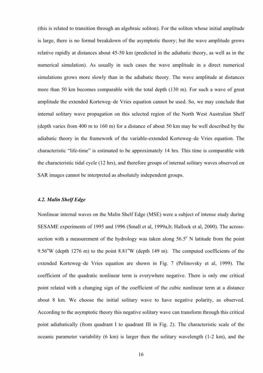
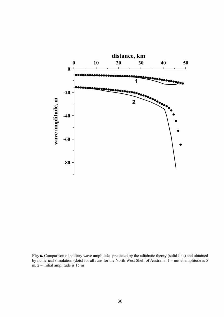
A comparison of the computed wave amplitude with the prediction of the adiabatic theory is

illustrated by Fig. 6 for distances less than 50 km. At distances up to 42 km (first critical point)

the difference between the adiabatic theory and the numerical simulation is relatively small. The

adiabatic theory for the soliton whose initial amplitude is weak is valid only for a distance 46 km

15

(this is related to transition through an algebraic soliton). For the soliton whose initial amplitude

is large, there is no formal breakdown of the asymptotic theory; but the wave amplitude grows

relative rapidly at distances about 45-50 km (predicted in the adiabatic theory, as well as in the

numerical simulation). As usually in such cases the wave amplitude in a direct numerical

simulations grows more slowly than in the adiabatic theory. The wave amplitude at distances

more than 50 km becomes comparable with the total depth (130 m). For such a wave of great

amplitude the extended Korteweg–de Vries equation cannot be used. So, we may conclude that

internal solitary wave propagation on this selected region of the North West Australian Shelf

(depth varies from 400 m to 160 m) for a distance of about 50 km may be well described by the

adiabatic theory in the framework of the variable-extended Korteweg–de Vries equation. The

characteristic “life-time” is estimated to be approximately 14 hrs. This time is comparable with

the characteristic tidal cycle (12 hrs), and therefore groups of internal solitary waves observed on

SAR images cannot be interpreted as absolutely independent groups.

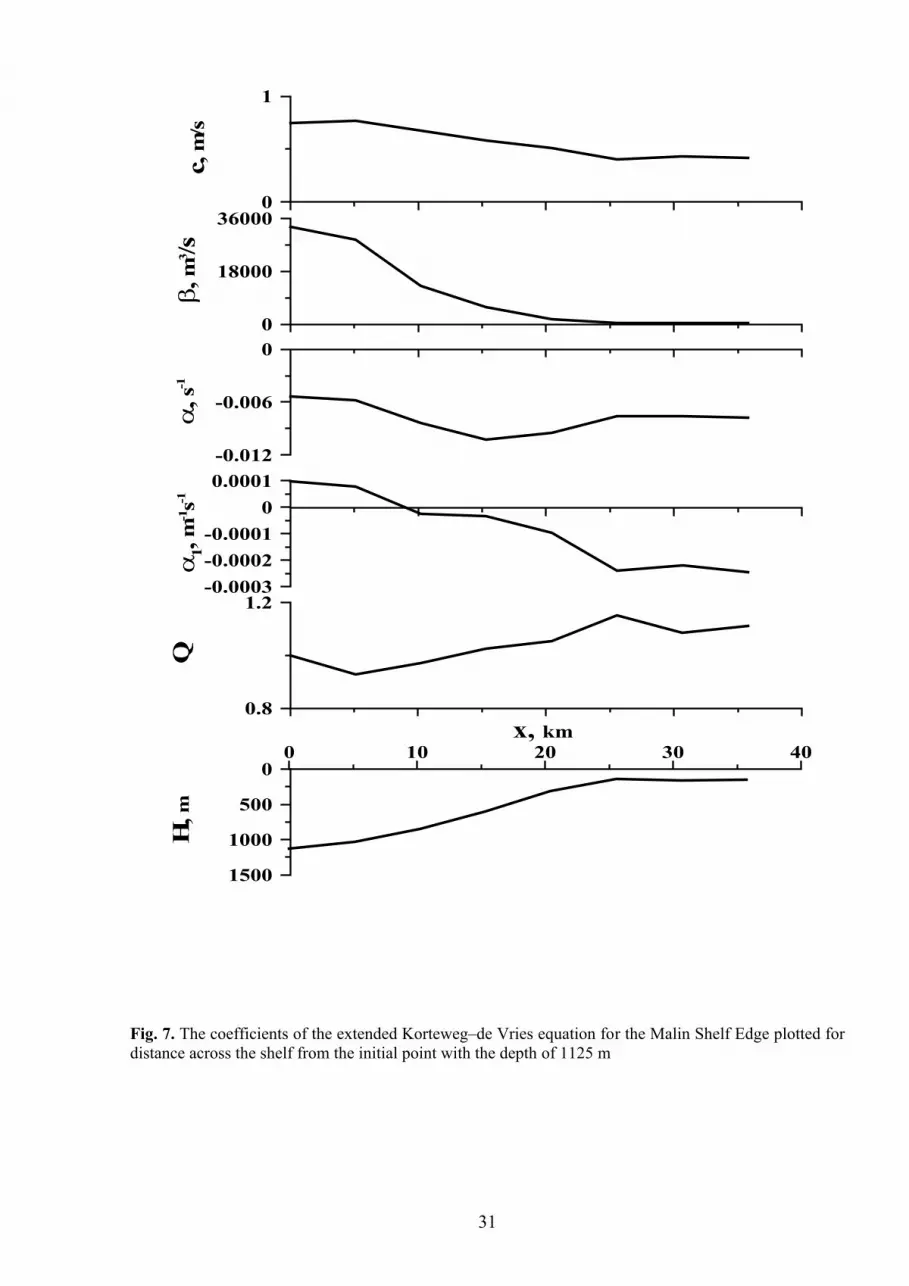
4.2. Malin Shelf Edge

Nonlinear internal waves on the Malin Shelf Edge (MSE) were a subject of intense study during

SESAME experiments of 1995 and 1996 (Small et al, 1999a,b; Hallock et al, 2000). The across-

section with a measurement of the hydrology was taken along 56.5o N latitude from the point

9.56oW (depth 1276 m) to the point 8.81oW (depth 149 m). The computed coefficients of the

extended Korteweg–de Vries equation are shown in Fig. 7 (Pelinovsky et al, 1999). The

coefficient of the quadratic nonlinear term is everywhere negative. There is only one critical

point related with a changing sign of the coefficient of the cubic nonlinear term at a distance

about 8 km. We choose the initial solitary wave to have negative polarity, as observed.

According to the asymptotic theory this negative solitary wave can transform through this critical

point adiabatically (from quadrant I to quadrant III in Fig. 2). The characteristic scale of the

oceanic parameter variability (6 km) is larger then the solitary wavelength (1-2 km), and the

16

horizontal variability can be considered smooth. Nevertheless, the ratio between the wavelength

and the characteristic scale of background variability for the Malin Shelf Edge is not as small as

for the North-West Shelf of Australia, and the relatively steep slopes of the parameter variability

after the first 6 km may lead to non-adiabatic wave deformation across the shelf.

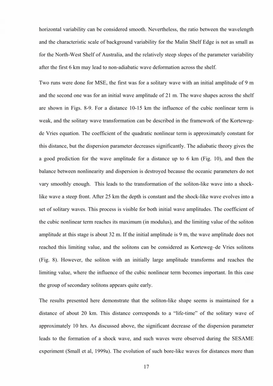
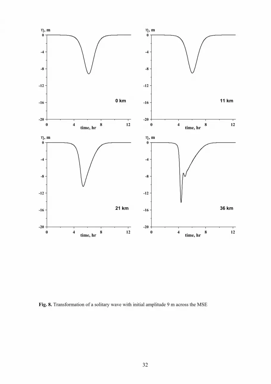
Two runs were done for MSE, the first was for a solitary wave with an initial amplitude of 9 m

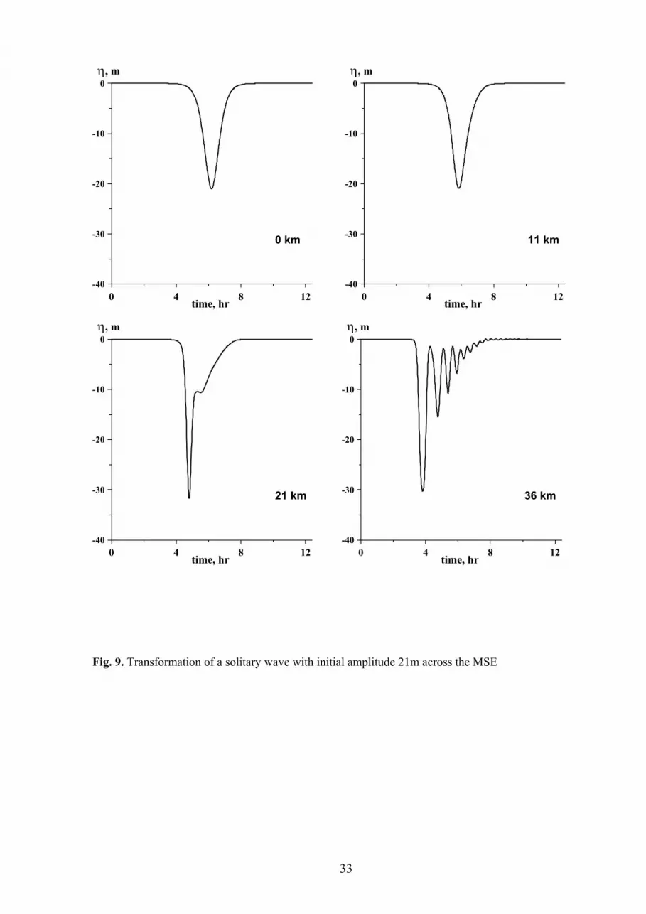
and the second one was for an initial wave amplitude of 21 m. The wave shapes across the shelf

are shown in Figs. 8-9. For a distance 10-15 km the influence of the cubic nonlinear term is

weak, and the solitary wave transformation can be described in the framework of the Korteweg-

de Vries equation. The coefficient of the quadratic nonlinear term is approximately constant for

this distance, but the dispersion parameter decreases significantly. The adiabatic theory gives the

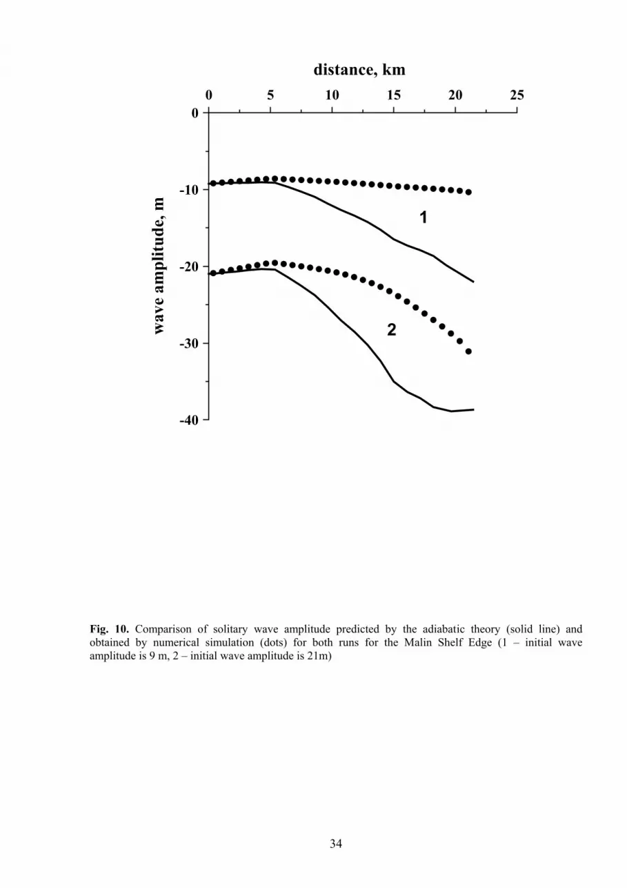
a good prediction for the wave amplitude for a distance up to 6 km (Fig. 10), and then the

balance between nonlinearity and dispersion is destroyed because the oceanic parameters do not

vary smoothly enough. This leads to the transformation of the soliton-like wave into a shock-

like wave a steep front. After 25 km the depth is constant and the shock-like wave evolves into a

set of solitary waves. This process is visible for both initial wave amplitudes. The coefficient of

the cubic nonlinear term reaches its maximum (in modulus), and the limiting value of the soliton

amplitude at this stage is about 32 m. If the initial amplitude is 9 m, the wave amplitude does not

reached this limiting value, and the solitons can be considered as Korteweg–de Vries solitons

(Fig. 8). However, the soliton with an initially large amplitude transforms and reaches the

limiting value, where the influence of the cubic nonlinear term becomes important. In this case

the group of secondary solitons appears quite early.

The results presented here demonstrate that the soliton-like shape seems is maintained for a

distance of about 20 km. This distance corresponds to a “life-time” of the solitary wave of

approximately 10 hrs. As discussed above, the significant decrease of the dispersion parameter

leads to the formation of a shock wave, and such waves were observed during the SESAME

experiment (Small et al, 1999a). The evolution of such bore-like waves for distances more than

17

25 km can be described in the framework of the extended Korteweg–de Vries equation with

constant coefficients. This equation was used to explain the observed transformation of the bore-

like disturbance into solitary waves, and results of simulations and observations are in reasonable

agreement (Small et al, 1999a; Pelinovsky et al, 1999).

4.3. Arctic Shelf

Internal waves in the Arctic shelves are now studied intensively (Sandven and Johannessen,

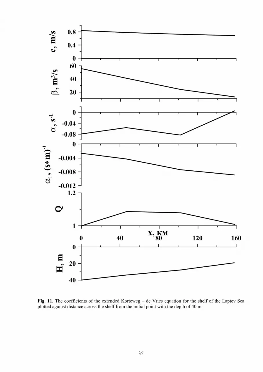
1987; Konyaev et al., 1996; Dokken et al, 2001; Pelinovsky al, 2002). Fig. 11 demonstrates the

variability of the coefficients of the extended Korteweg–de Vries equation for the shelf of the

Laptev Sea (Talipova et al, 2003). They are calculated using hydrological data obtained into

cruise of R/V “Ivan Kireev” (the meridian 127.5o E from latitude 75.4o N to 74o N) in the

summer of 1993. The depth decreases of almost a factor of 2 for a distance 160 km is quite

smooth. The linear speed of wave propagation decreases only slightly from 0.84 m/s to 0.7 m/s,

and this leads to a small variation of the linear amplification ratio, Q (10%). Meanwhile, the

nonlinear coefficients, as well as dispersion parameter, vary significantly, but also quite

smoothly. The coefficient of the cubic nonlinear coefficient is negative everywhere, and

increases by a factor of 3, but quite smoothly. The characteristic wavelength is about 20–30 m

only, and this shelf is thus excellent for the application of the adiabatic theory, so we expect that

the wave should maintain its soliton-like shape. Taking into account that quadratic nonlinear

coefficient is negative everywhere (except in the last 5 km) only a solitary wave of negative

polarity may exist. The critical point (zero value of the coefficient of the quadratic nonlinear

term) appears at the end of the wave path at a distance 155 km. Adiabatic transformation of the

wave at this critical point (from quadrant III to quadrant IV in Fig. 2) is impossible, and the

solitary wave should thus be destroyed. Hence we may expect that the adiabatic approximation

will be good for the solitary wave transformation for a large distance, excepting only the last 20

km.

18

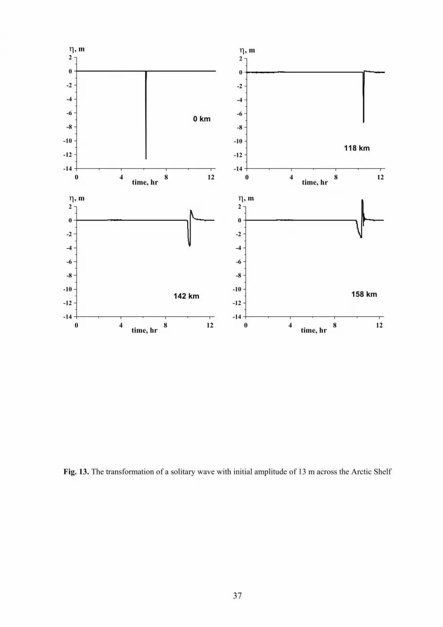
Two solitary waves with initial amplitudes of 4 and 13 m are chosen for study. The results of our

numerical simulation are shown in Figs. 12-13. It is evident that solitary waves of both

amplitudes hold the soliton-like shape practically for all distances up to the critical point. The

adiabatic formulas for the solitary wave amplitude agree well with the computed results (Fig.

14). These examples demonstrate that the solitary wave may maintain its soliton-like shape for

very long distances (140 km) if the background varies very sufficiently smoothly and does not

include any critical points. The characteristic “life-time” of the solitary wave predicted for the

Arctic Shelf is about 50 hrs. However, in this case the “life-time” may be bounded by other

factors, for instance by energy dissipation (see for instance, Grimshaw et al (2003)).

It is interesting to note that that the character of the wave amplitude curve is different for

different amplitudes. For instance, a solitary wave of small amplitude grows slightly for a

distance of 79 km, but the solitary wave of the large amplitude falls in this range to an amplitude

10 m. This may be explained by the significant contribution of the cubic nonlinear term. Thus

the limiting value for the soliton amplitude (15 m) varies with distance; it is 30 m at the

beginning of the wave path and only 11.8 m at the point 79 km. The large-amplitude solitary

wave must vary between these limits. In the vicinity of the critical point the solitary wave

amplitude decreases as is predicted by the asymptotic theory.

5. TRANSFORMATION AND INTERACTION OF TWO SOLITARY WAVES

The results described so far demonstrate the complicated dynamics of a single solitary wave in a

horizontally inhomogeneous ocean containing critical points. An important feature of the

adiabatic deformation of an internal solitary wave is the inevitable generation of a trailing tail. If

this tail is long enough and large enough, it may influence the propagation of any solitary waves

behind the main wave. A full treatment of this issue would require us to consider the propagation

of a modulated nonlinear periodic wave packet through a horizontally inhomogeneous ocean.

This is beyond the scope of the present study. Instead, we briefly describe here the

19

transformation of two solitary waves across two typical oceanic shelves, taken here to be the

North-West Shelf of Australia and the Arctic Shelf. Thus we replace the previous initial

condition of a single solitary wave, by an initial condition which consists of two widely-

separated solitary waves. In the case when the background is homogeneous so that all the

coefficients in equation (11) are constants, the separation distance is sufficient to ensure that

each solitary wave propagate essentially independently of the other wave. Of course, since in this

case the governing equation is integrable there would be an elastic collision between the waves,

albeit very small, in which there would be a slight adjustment in amplitudes and positions.

The first example for the North-West Shelf demonstrates the transformation of two solitary

waves of the same amplitude of 15 m generated with an initial shift of almost 2 hr (Fig. 15). Up

to the first critical point, there is no observable effect of the first soliton on the second soliton.

But, after the first critical point (at a distance 45 km), when the coefficient of the quadratic

nonlinear term becomes positive, large tails form behind both solitary waves. Between the

distances 50 and 55 km the second solitary wave interacts with the tail behind the first solitary

wave. Due to the positive polarity of the tail, the amplitude of the second wave decreases, and

the time series at a distance 52 km can be interpreted as a group of three solitons typical for the

evolution of a bore-like disturbance. But here it is due to the unsteady process of a solitary wave

interaction with the tail of the preceding solitary wave, and this ambiguity of wave images may

lead to difficulties in interpretation of observed wave data. After this interaction, the solitary

waves again have the almost the same amplitudes, and the result of any inelastic interaction is

rather weak.

The second example is for the Arctic Shelf (Fig. 16). The solitary waves now propagate for a

long distance up to 100 km with no interaction due to very smooth variation of the oceanic

parameters in this case. But, the wave evolution is not described by the adiabatic scenarios

because as the waves pass the critical point (155 km) the solitary wave structure is destroyed.

The tail formed just before the critical point has opposite polarity to the wave, as predicted by

20

theory (see, for instance, Grimshaw et al, 1998, 1999). The second solitary wave, interacting

with the positive tail of the first wave, now increases in amplitude.

6. CONCLUSION

Internal solitary wave dynamics on oceanic shelves is studied in the framework of the variable-

coefficient extended Korteweg–de Vries equation. For smoothly-varying background (water

depth, horizontal variability of the density and current stratification) theoretical formulas for the

wave amplitude are derived in explicit form. The possible breakdown of the asymptotic approach

related to critical points (zero values of the coefficients of quadratic and cubic nonlinear terms) is

discussed. Detail simulations have been described for the North-West Shelf of Australia, Malin

Shelf Edge and Arctic Shelf (Laptev Sea). They demonstrate the wave process at the critical

points, and also the situation when the oceanic parameters do not vary sufficiently smoothly..

The results of our numerical simulations show that an internal solitary wave maintains a soliton-

like shape for various distances, ranging from 20 km for Malin Shelf Edge to 140 km for the

Laptev Sea in the Arctic Ocean. The corresponding characteristic “life-time” of the solitary

waves due the effect of the horizontally inhomogeneous background may vary from 10 to 50 hrs

comparable with the internal tide cycle (12 hrs).

Acknowledgement

This paper is dedicated to the memory of Peter Holloway, whose influential work on internal

solitary waves through theory, numerical simulations and observations have stimulated our own

work in this area. This work is supported particularly by the London Mathematical Society

through Loughborough University for EP and TT, INTAS (01-0025) and RFBR (03-05-64978)

for TT, RFBR (03-05-64426) for AK, and an ONR grant for RG.

21

References

Benney, D.J. Long nonlinear waves in fluid flows. J. Math. Phys., 1966, 45, 52 - 63.

Cai, S., Long, X., and Gan, Z. A numerical study of the generation and propagation of internal solitary

waves in the Luzon Strait. Oceanologica Acta, 2002, vol. 25, 51-60.

Djordjevic, V., and Redekopp, L. The fission and desintegration of internal solitary waves moving over

two- dimensional topography. J. Phys. Oceanography, 1978, 8, 1016 - 1024.

Dokken, S.T., Olsen, R., Wahl, T., and Tantillo, M.V. Identification and characterization of internal

waves in SAR images along the coast of Norway. Geophysical Research Letters, 2001, vol. 28, 2803-

2806.

El, G.A., and Grimshaw, R.H.J. Generation of undular bores in the shelves of slowly-varying solitary

waves. Chaos, 2002, vol. 12, No. 4, 985-1076.

Grimshaw, R. Internal solitary waves. Chapter 1 in the book: Environmental Stratified Flows (Ed. R.

Grimshaw). Kluwer Acad. Publ. 2001, 1-28.

Grimshaw, R. and Mitsudera, H. Slowly-varying solitary wave solutions of the perturbed Korteweg-de

Vries equation revisited. Stud. Appl. Math., 1993, vol. 90, 75-86.

Grimshaw, R.H.J., and Pudjaprasetya, S.R. Generation of secondary solitary waves in the variable-

coefficient Korteweg-de Vries equation. Stud. Appl. Math, 2003 (accepted).

Grimshaw, R., Pelinovsky, E., and Talipova, T. Solitary wave transformation due to a change in

polarity. Stud. Appl. Math., 1998, vol. 101, 357 – 388.

Grimshaw, R., Pelinovsky, E., and Talipova, T. Solitary wave transformation in a medium with sign-

variable quadratic nonlinearity and cubic nonlinearity. Physica D, 1999, vol. 132, 40 - 62.

Grimshaw, R., Pelinovsky, E., Poloukhina, O. Higher-order Korteweg-de Vries models for internal

solitary waves in a stratified shear flow with a free surface. Nonlinear Processes in Geophysics, 2002,

vol. 9, N. 3, 221-235.

Grimshaw, R., Pelinovsky, D., Pelinovsky, E., and Slunyaev, A. Generation of large-amplitude

solitons in the extended Korteweg–de Vries equation. Chaos, 2002, vol. 12, N. 4, 1070-1076.

Grimshaw, R, Pelinovsky, E., and Talipova, T. Damping of large-amplitude solitary waves. Wave

Motion, 2003, v. 37, N. 4, 351 – 364.

Hallock, Z., Small, J., George, J., Field, R.L., and Scott, J.C. Shoreward propagation of internal waves

at the Malin Shelf Edge. Cont. Shelf Research, 2000, vol. 20, 2035-2045.

Holloway, P.E. Internal hydraulic jumps and solitons at a shelf break region on the Australian North

West Shelf. J. Geophys. Research, 1987, C95, 5405 - 5416.

22

Holloway, P., Pelinovsky, E., Talipova, T, and Barnes, B. A nonlinear model of the internal tide

transformation on the Australian North West Shelf. J. Phys. Oceanography, 1997, vol. 27, No. 6, 871 -

896.

Holloway, P., Pelinovsky, E., and Talipova, T. A Generalized Korteweg-de Vries Model of Internal

Tide Transformation in the Coastal Zone. J. Geophys. Research, 1999, vol. 104, N. C8, 18,333 – 18,350.

Holloway, P., Pelinovsky, E., and Talipova, T. Internal tide transformation and oceanic internal solitary

waves. Chapter 2 in the book: Environmental Stratified Flows (Ed. R. Grimshaw). Kluwer Acad. Publ.

2001, 29 - 60.

Jeans, D.R.G. Solitary internal waves in the ocean: A literature review completed as part of the internal

waves contribution to Morena. UCES, Marine Science Laboratories, Gwynedd, UK. 1995, Rep. U95-1,

64pp

Kakutani, T., and Yamasaki, N. Solitary waves on a two- layer fluid. J. Phys. Soc. Japan, 1978, 45,

674 - 679.

Konyaev, K.V., Plyudeman, A., and Sabinin, K.D. Internal tide on the Ermak Plateau in the Arctic

Ocean. Oceanology, 1996, vol. 36, 542-552.

Lamb, K.G., and Yan, L. The evolution of internal wave undular bores: comparisons of a fully

nonlinear numerical model with weakly nonlinear theory. J. Phys. Oceanography, 1996, 26,

2712 - 2734.

Lee, C., and Beardsley, R.C. The generation of long nonlinear internal waves in a weakly stratified

shear flow. J. Geophys. Research, 1974, 79, 453 - 462.

Liu, A.K., and Chang, Y.S. Evolution of nonlinear internal waves in the East and South China Seas. J.

Geophys. Research, 1998, vol. 103, 7995 – 8008.

Nakoulima, O., Zahibo, N., Pelinovsky, E., Talipova, T., Slunyaev, A., and Kurkin, A. Analytical and

numerical studies of the variable-coefficient Gardner equation. Applied Mathematics and Computation,

2003 (accepted).

Ostrovsky, L.A., and Stepanyants, Yu.A. Do internal solitons exist in the ocean? Reviews

Geophysics, 1989, v. 27, 293 - 310.

Pelinovsky, D., and Grimshaw, R. Structural transformation of eigenvalues for a perturbed algebraic

soliton potential. Phys. Letters, A, 1997, vol. 229, 165 - 172.

Pelinovsky, E., Talipova, T., and Ivanov, V. Estimations of nonlinear properties of internal wave field

off the Israel Coast. Nonlinear Processes in Geophysics, 1995, vol. 2, N. 2, 80 - 88.

Pelinovsky, E., Talipova, T., Small, J. Numerical modelling of the evolution of internal bores and

generation of internal solitons at the Malin Shelf. The 1998 WHOI/IOS/ONR Internal Solitary Wave

Workshop: Contributed Papers. Eds: T.Duda and D.Farmer. Technical Report WHOI-99-07, 229 – 236.

23

Pelinovsky, E., Polukhina, O., and Lamb K. Nonlinear internal waves in the ocean stratified in density

and current. Oceanology, 2000, vol. 40, N. 6, 757 - 765.

Pelinovsky, E., Poloukhin, N., and Talipova, T. Modeling of the internal wave characteristics in the

Arctic. Chapter in Book: Surface and Internal Waves in the Arctic Seas. (Eds: Lavrenov I & Morozov E.).

St Petersburg: Gidrometeoizdat, 2002, 235-279.

Poloukhin, N.V., Talipova, T.G., Pelinovsky, E.N., and Lavrenov I.V. Kinematic Characteristics of

the High-Frequency Internal Wave Field in the Arctic Ocean. Oceanology, 2003, vol. 43, N. 3, 356-367.

Sandven, S., and Johannessen, O.M. High-frequency internal wave observations in the marginal ice

zone. J. Geophys. Research, 1987, vol. 92, 6911-6920.

Slyunyaev, A.V., Dynamics of localized waves with large amplitude in a weakly dispersive medium with

a quadratic and positive cubic nonlinearity. JETP, 2001, vol. 92, 529-534.

Slyunyaev, A., and Pelinovsky, E. Dynamics of large-amplitude solitons. JETP, 1999, vol. 89, N. 1, 173

- 181.

Small, J. A Nonlinear Model of the Shoaling and Refraction of Interfacial Solitary Waves in the Ocean.

Part I: Development of the Model and Investigations of the Shoaling Effect. J. Phys. Oceanography,

2001a, vol. 31, No. 11, 3163-3183.

Small, J. A Nonlinear Model of the Shoaling and Refraction of Interfacial Solitary Waves in the Ocean.

Part II: Oblique Refraction across a Continental Slope and Propagation over a Seamount. J. Phys.

Oceanography, 2001b, vol. 31, No. 11, 3184-3199.

Small, J., Sawyer, T.C., and Scott, J.C. The evolution of an internal bore at the Malin shelf break.

Annales Geophysicae, 1999a, vol. 17, 547-565.

Small, J., Hallock, Z., Pavey, G., and Scott J. Observations of large amplitude internal waves at the

Malin Shelf edge during SESAME 1995. Cont. Shelf Research, 1999b, vol. 19, 1389-1436.

Talipova, T., Pelinovsky, E., Lamb, K., Grimshaw, R., and Holloway, P. Cubic nonlinearity effects in

the propagation of intense internal waves. Doklady Earth Sciences, 1999, vol. 365, N. 2, 241 - 244.

Talipova, T., Poloukhin, N., Kurkin, A., and Lavrenov, I. Modeling of the internal soliton

transformation on the Laptev Sea Shelf. Izvestiya, Russian Academy Eng. Sciences, 2003, vol. 4, 3–16.

Zheng, Q., Klemas, V., Yan, X-H., and Pan, J. Nonlinear evolution of ocean internal solitons

propagating along an inhomogeneous thermocline. J. Geophys. Research, 2001, vol. 106, 14,083-14,094.

Zhou, X., and Grimshaw, R. The effect of variable currents on internal solitary waves. Dyn. Atm.

Oceans, 1989, vol. 14, 17 - 39.

24

FIGURE CAPTIONS

Fig. 1. Possible solitary wave shapes: a) for α1 < 0; b) for α1 > 0

Fig. 2. The possible adiabatic transformation of solitary wave on plane (α, α1)

Fig. 3. Coefficients of the extended Korteweg-de Vries equation (11) for the NWS plotted for

distance across the shelf from the initial point at a depth of 416 m (linear splines used)

Fig. 4. Transformation of a solitary wave with initial amplitude 5 m across the NWS

Fig. 5. Transformation of a solitary wave with initial amplitude 15 m across the NWS

Fig. 6. Comparison of solitary wave amplitudes predicted by the adiabatic theory (solid line) and

obtained by numerical simulation (dots) for all runs for the North West Shelf of Australia: 1 –

initial amplitude is 5 m, 2 – initial amplitude is 15 m

Fig. 7. The coefficients of the extended Korteweg–de Vries equation for the Malin Shelf Edge

plotted for distance across the shelf from the initial point with the depth of 1125 m

Fig. 8. Transformation of a solitary wave with initial amplitude 9 m across the MSE

Fig. 9. Transformation of a solitary wave with initial amplitude 21m across the MSE

Fig. 10. Comparison of solitary wave amplitude predicted by the adiabatic theory (solid line) and

obtained by numerical simulation (dots) for both runs for the Malin Shelf Edge (1 – initial wave

amplitude is 9 m, 2 – initial wave amplitude is 21m)

Fig. 11. The coefficients of the extended Korteweg – de Vries equation for the shelf of the

Laptev Sea plotted against distance across the shelf from the initial point with the depth of 40 m

Fig. 12. The transformation of a solitary wave with initial amplitude of 4 m across the Arctic

Shelf

Fig. 13. The transformation of a solitary wave with initial amplitude of 13 m across the Arctic

Shelf

Fig. 14. Comparison of solitary wave amplitudes predicted by the adiabatic theory (solid line)

and obtained by numerical simulation (dots) for both runs for the Arctic Shelf (1 – initial wave

amplitude is 4 m, 2 – initial wave amplitude is 13 m)

Fig. 15. Transformation and interaction of the two solitary waves on the North-West Shelf of

Australia

Fig. 16. Transformation and interaction of two solitary waves on the Arctic Shelf

25

-60 -30 0 30 60

S

0

0.5

1 η

α1 < 0

-25 0 25

s

-5

-2.5

0

2.5

5 η

α1 > 0

a) b)

Fig. 1. Possible solitary wave shapes: a) for α1 < 0; b) for α1 > 0

α1

α

I II

III IV

Fig. 2. The possible adiabatic transformation of solitary wave on plane (α, α1)

26

0 40 80 x, km

500

0

H, m

0

2

4

Q

0

1

2c,

m/s

0

6000

12000

β, m

3 /s

-0.012

0

0.012

α, s

-1

-0.0008

-0.0004

0

0.0004

α1,

m-1s-1

Fig. 3. Coefficients of the extended Korteweg-de Vries equation (11) for the NWS plotted for distance across the shelf from the initial point at a depth of 416 m (linear splines used)

27

0 4 8time, hr

12-20

-10

0

10

η, m

0 km

0 4 8

time, hr12

-20

-10

0

10

η, m

34 km

0 4 8time, hr

12-20

-10

0

10

η, m

52 km

0 4 8

time, hr12

-20

-10

0

10η, m

74 km

Fig. 4. Transformation of a solitary wave with initial amplitude 5 m across the NWS

28

0 4 8time, hr

12-120

-80

-40

0

40

η, m

0 km

0 4 8

time, hr12

-120

-80

-40

0

40

η, m

34 km

0 4 8time, hr

12-120

-80

-40

0

40

η, m

47 km

0 4 8

time, hr12

-120

-80

-40

0

40

η, m

49 km

0 4 8time, hr

12-120

-80

-40

0

40

η, m

52 km

0 4 8

time, hr12

-120

-80

-40

0

40

η, m

72 km

Fig. 5. Transformation of a solitary wave with an initial amplitude 15 m across the NWS

29

0 10 20 30 40 5distance, km

0

-80

-60

-40

-20

0

wav

e am

plitu

de, m

1

2

Fig. 6. Comparison of solitary wave amplitudes predicted by the adiabatic theory (solid line) and obtained by numerical simulation (dots) for all runs for the North West Shelf of Australia: 1 – initial amplitude is 5 m, 2 – initial amplitude is 15 m

30

0 10 20 30 4x, km

0

1500

1000

500

0

H, m

0.8

1.2

Q0

1

c, m

/s

0

18000

36000

β, m

3 /s

-0.012

-0.006

0

α, s

-1

-0.0003-0.0002-0.0001

00.0001

α1,

m-1s-1

Fig. 7. The coefficients of the extended Korteweg–de Vries equation for the Malin Shelf Edge plotted for distance across the shelf from the initial point with the depth of 1125 m

31

0 4 8time, hr

12-20

-16

-12

-8

-4

0η, m

0 km

0 4 8

time, hr12

-20

-16

-12

-8

-4

0η, m

11 km

0 4 8time, hr

12-20

-16

-12

-8

-4

0η, m

21 km

0 4 8

time, hr12

-20

-16

-12

-8

-4

0η, m

36 km

Fig. 8. Transformation of a solitary wave with initial amplitude 9 m across the MSE

32

0 4 8time, hr

12-40

-30

-20

-10

0η, m

0 km

0 4 8

time, hr12

-40

-30

-20

-10

0η, m

11 km

0 4 8time, hr

12-40

-30

-20

-10

0η, m

21 km

0 4 8

time, hr12

-40

-30

-20

-10

0η, m

36 km

Fig. 9. Transformation of a solitary wave with initial amplitude 21m across the MSE

33

0 5 10 15 20 25

distance, km

-40

-30

-20

-10

0

wav

e am

plitu

de, m 1

2

Fig. 10. Comparison of solitary wave amplitude predicted by the adiabatic theory (solid line) and obtained by numerical simulation (dots) for both runs for the Malin Shelf Edge (1 – initial wave amplitude is 9 m, 2 – initial wave amplitude is 21m)

34

0

0.4

0.8

c, m

/s

-0.08-0.04

0

α, s

-1

20

40

60β,

m3 /s

-0.012

-0.008

-0.004

0

α1,

(s∗m

)-1

1

1.2

Q

0 40 80 120x, км

160

40

20

0

H, m

Fig. 11. The coefficients of the extended Korteweg – de Vries equation for the shelf of the Laptev Sea plotted against distance across the shelf from the initial point with the depth of 40 m.

35

0 4 8time, hr

12-6

-4

-2

0

2η, m

0 km

0 4 8

time, hr12

-6

-4

-2

0

2η, m

118 km

0 4 8time, hr

12-6

-4

-2

0

2η, m

142 km

0 4 8

time, hr12

-6

-4

-2

0

2η, m

158 km

Fig. 12. The transformation of a solitary wave with initial amplitude of 4 m across the Arctic Shelf

36

0 4 8time, hr

12-14

-12

-10

-8

-6

-4

-2

0

2η, m

0 km

0 4 8

time, hr12

-14

-12

-10

-8

-6

-4

-2

0

2η, m

118 km

0 4 8time, hr

12-14

-12

-10

-8

-6

-4

-2

0

2η, m

142 km

0 4 8

time, hr12

-14

-12

-10

-8

-6

-4

-2

0

2η, m

158 km

Fig. 13. The transformation of a solitary wave with initial amplitude of 13 m across the Arctic Shelf

37

0 40 80 120distance, km

160

-16

-12

-8

-4

0

wav

e am

plitu

de, m

1

2

Fig. 14. Comparison of solitary wave amplitudes predicted by the adiabatic theory (solid line) and obtained by numerical simulation (dots) for both runs for the Arctic Shelf (1 – initial wave amplitude is 4 m, 2 – initial wave amplitude is 13 m)

38

0 4 8time, hr

12-20

-10

0

10

η, m

0 km

0 4 8time, hr

12-120

-80

-40

0

η, m

50 km

0 4 8time, hr

12-120

-80

-40

0

η, m

52 km

0 4 8time, hr

12-120

-80

-40

0

η, m

56 km

Fig. 15. Transformation and interaction of the two solitary waves on the North-West Shelf of Australia

39

4 5 6 7 8time, hr

-12

-8

-4

0

η, m

0 km

8 9 10 11 12time, hr

-8

-6

-4

-2

0

2

η, m

126 km

Fig. 16. Transformation and interaction of two solitary waves on the Arctic Shelf

40