864
PUBLIC SQL Anywhere Server Document Version: 17 – 2020-12-11 SQL Anywhere SQL Usage © 2020 SAP SE or an SAP affiliate company. All rights reserved. THE BEST RUN
| Date post: | 09-Feb-2023 |
| Category: |
Documents |
| Upload: | khangminh22 |
| View: | 1 times |
| Download: | 0 times |

PUBLICSQL Anywhere ServerDocument Version: 17 – 2020-12-11
SQL Anywhere SQL Usage
© 2
020
SAP
SE o
r an
SAP affi
liate
com
pany
. All r
ight
s re
serv
ed.
THE BEST RUN
Content
1 SQL Anywhere Server - SQL Usage. . . . . . . . . . . . . . . . . . . . . . . . . . . . . . . . . . . . . . . . . . . . . . . 61.1 Tables, Views, and Indexes. . . . . . . . . . . . . . . . . . . . . . . . . . . . . . . . . . . . . . . . . . . . . . . . . . . . . . . 7
Database Object Names and Prefixes. . . . . . . . . . . . . . . . . . . . . . . . . . . . . . . . . . . . . . . . . . . . 8Viewing a List of System Objects (SQL Central). . . . . . . . . . . . . . . . . . . . . . . . . . . . . . . . . . . . . 9Viewing a List of System Objects (SQL). . . . . . . . . . . . . . . . . . . . . . . . . . . . . . . . . . . . . . . . . . 10Tables. . . . . . . . . . . . . . . . . . . . . . . . . . . . . . . . . . . . . . . . . . . . . . . . . . . . . . . . . . . . . . . . . . 11Temporary Tables. . . . . . . . . . . . . . . . . . . . . . . . . . . . . . . . . . . . . . . . . . . . . . . . . . . . . . . . . .18Computed Columns. . . . . . . . . . . . . . . . . . . . . . . . . . . . . . . . . . . . . . . . . . . . . . . . . . . . . . . . 21Primary Keys. . . . . . . . . . . . . . . . . . . . . . . . . . . . . . . . . . . . . . . . . . . . . . . . . . . . . . . . . . . . .25Foreign Keys. . . . . . . . . . . . . . . . . . . . . . . . . . . . . . . . . . . . . . . . . . . . . . . . . . . . . . . . . . . . . 29Indexes. . . . . . . . . . . . . . . . . . . . . . . . . . . . . . . . . . . . . . . . . . . . . . . . . . . . . . . . . . . . . . . . .35Views. . . . . . . . . . . . . . . . . . . . . . . . . . . . . . . . . . . . . . . . . . . . . . . . . . . . . . . . . . . . . . . . . . 48Materialized Views. . . . . . . . . . . . . . . . . . . . . . . . . . . . . . . . . . . . . . . . . . . . . . . . . . . . . . . . . 64
1.2 Stored Procedures, Triggers, Batches, and User-defined Functions . . . . . . . . . . . . . . . . . . . . . . . . . 87Benefits of Procedures, Triggers, and User-defined Functions . . . . . . . . . . . . . . . . . . . . . . . . . . 88Procedures. . . . . . . . . . . . . . . . . . . . . . . . . . . . . . . . . . . . . . . . . . . . . . . . . . . . . . . . . . . . . . 89User-defined Functions. . . . . . . . . . . . . . . . . . . . . . . . . . . . . . . . . . . . . . . . . . . . . . . . . . . . . 101Triggers. . . . . . . . . . . . . . . . . . . . . . . . . . . . . . . . . . . . . . . . . . . . . . . . . . . . . . . . . . . . . . . . 107Batches. . . . . . . . . . . . . . . . . . . . . . . . . . . . . . . . . . . . . . . . . . . . . . . . . . . . . . . . . . . . . . . 120The Structure of Procedures, Triggers, and User-defined Functions. . . . . . . . . . . . . . . . . . . . . . 123Control Statements. . . . . . . . . . . . . . . . . . . . . . . . . . . . . . . . . . . . . . . . . . . . . . . . . . . . . . . 127Result Sets. . . . . . . . . . . . . . . . . . . . . . . . . . . . . . . . . . . . . . . . . . . . . . . . . . . . . . . . . . . . . 129Cursors in Procedures, Triggers, User-defined Functions, and Batches. . . . . . . . . . . . . . . . . . . 139Error and Warning Handling. . . . . . . . . . . . . . . . . . . . . . . . . . . . . . . . . . . . . . . . . . . . . . . . . .142EXECUTE IMMEDIATE Used in Procedures, Triggers, User-defined Functions, and Batches. . . . . . . . . . . . . . . . . . . . . . . . . . . . . . . . . . . . . . . . . . . . . . . . . . . . . . . . . . . . . . . . . . . . . .154Transactions and Savepoints in Procedures, Triggers, and User-defined Functions . . . . . . . . . . . 156Tips for Writing Procedures, Triggers, User-defined Functions, and Batches. . . . . . . . . . . . . . . . 157Statements Allowed in Procedures, Triggers, Events, and Batches. . . . . . . . . . . . . . . . . . . . . . .158Hiding the Contents of a Procedure, Function, Trigger, Event, or View. . . . . . . . . . . . . . . . . . . . 160
1.3 Queries and Data Modification. . . . . . . . . . . . . . . . . . . . . . . . . . . . . . . . . . . . . . . . . . . . . . . . . . 161Queries. . . . . . . . . . . . . . . . . . . . . . . . . . . . . . . . . . . . . . . . . . . . . . . . . . . . . . . . . . . . . . . . 162Full Text Search. . . . . . . . . . . . . . . . . . . . . . . . . . . . . . . . . . . . . . . . . . . . . . . . . . . . . . . . . . 254Tutorial: Pivoting Table Data. . . . . . . . . . . . . . . . . . . . . . . . . . . . . . . . . . . . . . . . . . . . . . . . . 359Summarizing, Grouping, and Sorting Query Results. . . . . . . . . . . . . . . . . . . . . . . . . . . . . . . . 362Joins: Retrieving Data from Several Tables. . . . . . . . . . . . . . . . . . . . . . . . . . . . . . . . . . . . . . . 384
2 PUBLICSQL Anywhere SQL Usage
Content
Common Table Expressions. . . . . . . . . . . . . . . . . . . . . . . . . . . . . . . . . . . . . . . . . . . . . . . . . 429OLAP Support. . . . . . . . . . . . . . . . . . . . . . . . . . . . . . . . . . . . . . . . . . . . . . . . . . . . . . . . . . . 444Use of Subqueries. . . . . . . . . . . . . . . . . . . . . . . . . . . . . . . . . . . . . . . . . . . . . . . . . . . . . . . . 485Data Manipulation Statements. . . . . . . . . . . . . . . . . . . . . . . . . . . . . . . . . . . . . . . . . . . . . . . 510
1.4 SQL Dialects and Compatibility. . . . . . . . . . . . . . . . . . . . . . . . . . . . . . . . . . . . . . . . . . . . . . . . . 527SQL Compliance Testing Using the SQL Flagger. . . . . . . . . . . . . . . . . . . . . . . . . . . . . . . . . . . 528Features That Differ from Other SQL Implementations. . . . . . . . . . . . . . . . . . . . . . . . . . . . . . 530Watcom SQL. . . . . . . . . . . . . . . . . . . . . . . . . . . . . . . . . . . . . . . . . . . . . . . . . . . . . . . . . . . . 535Transact-SQL Compatibility. . . . . . . . . . . . . . . . . . . . . . . . . . . . . . . . . . . . . . . . . . . . . . . . . 535Comparison of SQL Anywhere with Adaptive Server Enterprise. . . . . . . . . . . . . . . . . . . . . . . . 538Transact-SQL-compatible Databases. . . . . . . . . . . . . . . . . . . . . . . . . . . . . . . . . . . . . . . . . . . 542Transact-SQL Compatible SQL Statements. . . . . . . . . . . . . . . . . . . . . . . . . . . . . . . . . . . . . . 550Transact-SQL Procedure Language. . . . . . . . . . . . . . . . . . . . . . . . . . . . . . . . . . . . . . . . . . . . 556Automatic Translation of Stored Procedures. . . . . . . . . . . . . . . . . . . . . . . . . . . . . . . . . . . . . .558Result Sets Returned from Transact-SQL Procedures. . . . . . . . . . . . . . . . . . . . . . . . . . . . . . . 559Variables in Transact-SQL Procedures. . . . . . . . . . . . . . . . . . . . . . . . . . . . . . . . . . . . . . . . . . 560Error Handling in Transact-SQL Procedures. . . . . . . . . . . . . . . . . . . . . . . . . . . . . . . . . . . . . . 561
1.5 XML in the Database. . . . . . . . . . . . . . . . . . . . . . . . . . . . . . . . . . . . . . . . . . . . . . . . . . . . . . . . . 563Storage of XML Documents in Relational Databases. . . . . . . . . . . . . . . . . . . . . . . . . . . . . . . . 564Relational Data Exported as XML. . . . . . . . . . . . . . . . . . . . . . . . . . . . . . . . . . . . . . . . . . . . . .565Ways to Import XML Documents as Relational Data. . . . . . . . . . . . . . . . . . . . . . . . . . . . . . . . 566Query Results as XML. . . . . . . . . . . . . . . . . . . . . . . . . . . . . . . . . . . . . . . . . . . . . . . . . . . . . .574Use of Interactive SQL to View Results. . . . . . . . . . . . . . . . . . . . . . . . . . . . . . . . . . . . . . . . . . 592Use of SQL/XML to Obtain Query Results as XML. . . . . . . . . . . . . . . . . . . . . . . . . . . . . . . . . . 593
1.6 JSON in the Database. . . . . . . . . . . . . . . . . . . . . . . . . . . . . . . . . . . . . . . . . . . . . . . . . . . . . . . . 601Use of the FOR JSON Clause to Retrieve Query Results as JSON. . . . . . . . . . . . . . . . . . . . . . . .601FOR JSON RAW. . . . . . . . . . . . . . . . . . . . . . . . . . . . . . . . . . . . . . . . . . . . . . . . . . . . . . . . . . 602FOR JSON AUTO. . . . . . . . . . . . . . . . . . . . . . . . . . . . . . . . . . . . . . . . . . . . . . . . . . . . . . . . . 603FOR JSON EXPLICIT. . . . . . . . . . . . . . . . . . . . . . . . . . . . . . . . . . . . . . . . . . . . . . . . . . . . . . 604
1.7 Data Import and Export. . . . . . . . . . . . . . . . . . . . . . . . . . . . . . . . . . . . . . . . . . . . . . . . . . . . . . . 607Performance Aspects of Bulk Operations. . . . . . . . . . . . . . . . . . . . . . . . . . . . . . . . . . . . . . . . 608Data Recovery Issues for Bulk Operations. . . . . . . . . . . . . . . . . . . . . . . . . . . . . . . . . . . . . . . 609Data Import. . . . . . . . . . . . . . . . . . . . . . . . . . . . . . . . . . . . . . . . . . . . . . . . . . . . . . . . . . . . 609Data Export. . . . . . . . . . . . . . . . . . . . . . . . . . . . . . . . . . . . . . . . . . . . . . . . . . . . . . . . . . . . . 627Access to Data on Client Computers. . . . . . . . . . . . . . . . . . . . . . . . . . . . . . . . . . . . . . . . . . . 643Database Rebuilds. . . . . . . . . . . . . . . . . . . . . . . . . . . . . . . . . . . . . . . . . . . . . . . . . . . . . . . . 646Database Extraction. . . . . . . . . . . . . . . . . . . . . . . . . . . . . . . . . . . . . . . . . . . . . . . . . . . . . . .663Database Migration to SQL Anywhere . . . . . . . . . . . . . . . . . . . . . . . . . . . . . . . . . . . . . . . . . . 664SQL Script Files. . . . . . . . . . . . . . . . . . . . . . . . . . . . . . . . . . . . . . . . . . . . . . . . . . . . . . . . . . 669Adaptive Server Enterprise Compatibility. . . . . . . . . . . . . . . . . . . . . . . . . . . . . . . . . . . . . . . . 674
1.8 Remote Data Access. . . . . . . . . . . . . . . . . . . . . . . . . . . . . . . . . . . . . . . . . . . . . . . . . . . . . . . . . 674
SQL Anywhere SQL UsageContent PUBLIC 3
Remote Servers and Remote Table Mappings. . . . . . . . . . . . . . . . . . . . . . . . . . . . . . . . . . . . . 677Stored Procedures as an Alternative to Directory Access Servers. . . . . . . . . . . . . . . . . . . . . . . 686Directory Access Servers. . . . . . . . . . . . . . . . . . . . . . . . . . . . . . . . . . . . . . . . . . . . . . . . . . . 686External Logins. . . . . . . . . . . . . . . . . . . . . . . . . . . . . . . . . . . . . . . . . . . . . . . . . . . . . . . . . . 695Proxy Tables. . . . . . . . . . . . . . . . . . . . . . . . . . . . . . . . . . . . . . . . . . . . . . . . . . . . . . . . . . . . 698Native Statements and Remote Servers. . . . . . . . . . . . . . . . . . . . . . . . . . . . . . . . . . . . . . . . . 706Remote Procedure Calls (RPCs). . . . . . . . . . . . . . . . . . . . . . . . . . . . . . . . . . . . . . . . . . . . . . 707Transaction Management and Remote Data. . . . . . . . . . . . . . . . . . . . . . . . . . . . . . . . . . . . . . .711Internal Operations Performed on Queries. . . . . . . . . . . . . . . . . . . . . . . . . . . . . . . . . . . . . . . 712Other Internal Operations. . . . . . . . . . . . . . . . . . . . . . . . . . . . . . . . . . . . . . . . . . . . . . . . . . . 713Troubleshooting: Features Not Supported for Remote Data. . . . . . . . . . . . . . . . . . . . . . . . . . . 716Troubleshooting: Case Sensitivity and Remote Data Access. . . . . . . . . . . . . . . . . . . . . . . . . . . 716Troubleshooting: Connectivity Tests for Remote Data Access. . . . . . . . . . . . . . . . . . . . . . . . . . 716Troubleshooting: Queries Blocked on Themselves. . . . . . . . . . . . . . . . . . . . . . . . . . . . . . . . . . 717Troubleshooting: Remote Data Access Connections via ODBC. . . . . . . . . . . . . . . . . . . . . . . . . 717Server Classes for Remote Data Access. . . . . . . . . . . . . . . . . . . . . . . . . . . . . . . . . . . . . . . . . 717
1.9 Data Integrity. . . . . . . . . . . . . . . . . . . . . . . . . . . . . . . . . . . . . . . . . . . . . . . . . . . . . . . . . . . . . . 740How Your Data Can Become Invalid. . . . . . . . . . . . . . . . . . . . . . . . . . . . . . . . . . . . . . . . . . . . 741Integrity Constraints. . . . . . . . . . . . . . . . . . . . . . . . . . . . . . . . . . . . . . . . . . . . . . . . . . . . . . .742Tools for Maintaining Data Integrity. . . . . . . . . . . . . . . . . . . . . . . . . . . . . . . . . . . . . . . . . . . . 742SQL Statements for Implementing Integrity Constraints. . . . . . . . . . . . . . . . . . . . . . . . . . . . . 743Column Defaults. . . . . . . . . . . . . . . . . . . . . . . . . . . . . . . . . . . . . . . . . . . . . . . . . . . . . . . . . 744Table and Column Constraints. . . . . . . . . . . . . . . . . . . . . . . . . . . . . . . . . . . . . . . . . . . . . . . . 751How to Use Domains to Improve Data Integrity. . . . . . . . . . . . . . . . . . . . . . . . . . . . . . . . . . . . 757Entity and Referential Integrity. . . . . . . . . . . . . . . . . . . . . . . . . . . . . . . . . . . . . . . . . . . . . . . 759Integrity Rules in the System Tables. . . . . . . . . . . . . . . . . . . . . . . . . . . . . . . . . . . . . . . . . . . . 770
1.10 Transactions and Isolation Levels. . . . . . . . . . . . . . . . . . . . . . . . . . . . . . . . . . . . . . . . . . . . . . . . 771Transactions. . . . . . . . . . . . . . . . . . . . . . . . . . . . . . . . . . . . . . . . . . . . . . . . . . . . . . . . . . . . 772Concurrency. . . . . . . . . . . . . . . . . . . . . . . . . . . . . . . . . . . . . . . . . . . . . . . . . . . . . . . . . . . . 774Savepoints Within Transactions. . . . . . . . . . . . . . . . . . . . . . . . . . . . . . . . . . . . . . . . . . . . . . . 776Isolation Levels and Consistency. . . . . . . . . . . . . . . . . . . . . . . . . . . . . . . . . . . . . . . . . . . . . . 777Transaction Blocking and Deadlock. . . . . . . . . . . . . . . . . . . . . . . . . . . . . . . . . . . . . . . . . . . . 793How Locking Works. . . . . . . . . . . . . . . . . . . . . . . . . . . . . . . . . . . . . . . . . . . . . . . . . . . . . . . 796Guidelines for Choosing Isolation Levels. . . . . . . . . . . . . . . . . . . . . . . . . . . . . . . . . . . . . . . . . 817Isolation Level Tutorials. . . . . . . . . . . . . . . . . . . . . . . . . . . . . . . . . . . . . . . . . . . . . . . . . . . . .821Use of a Sequence to Generate Unique Values. . . . . . . . . . . . . . . . . . . . . . . . . . . . . . . . . . . . 845
1.11 The SQL Anywhere Debugger. . . . . . . . . . . . . . . . . . . . . . . . . . . . . . . . . . . . . . . . . . . . . . . . . . 849Requirements for Using the Debugger. . . . . . . . . . . . . . . . . . . . . . . . . . . . . . . . . . . . . . . . . . 850Tutorial: Getting Started with the Debugger. . . . . . . . . . . . . . . . . . . . . . . . . . . . . . . . . . . . . . 850Breakpoints. . . . . . . . . . . . . . . . . . . . . . . . . . . . . . . . . . . . . . . . . . . . . . . . . . . . . . . . . . . . 856Variable Modification with the Debugger. . . . . . . . . . . . . . . . . . . . . . . . . . . . . . . . . . . . . . . . 859
4 PUBLICSQL Anywhere SQL Usage
Content

Connections and Breakpoints. . . . . . . . . . . . . . . . . . . . . . . . . . . . . . . . . . . . . . . . . . . . . . . . 862
SQL Anywhere SQL UsageContent PUBLIC 5
1 SQL Anywhere Server - SQL Usage
This book describes how to add objects to a database; how to import, export, and modify data; how to retrieve data; and how to build stored procedures and triggers.
In this section:
Tables, Views, and Indexes [page 7]Tables, views, and indexes hold data within the database.
Stored Procedures, Triggers, Batches, and User-defined Functions [page 87]Procedures and triggers store procedural SQL statements in a database.
Queries and Data Modification [page 161]Many features are provided to help you query and modify data in your database.
SQL Dialects and Compatibility [page 527]Information about compliance is provided in the reference documentation for each feature in the software.
XML in the Database [page 563]Extensible Markup Language (XML) represents structured data in text format. XML was designed specifically to meet the challenges of large-scale electronic publishing.
JSON in the Database [page 601]JavaScript Object Notation (JSON) is a language-independent, text-based data interchange format developed for the serialization of JavaScript data.
Data Import and Export [page 607]The term bulk operations is used to describe the process of importing and exporting data.
Remote Data Access [page 674]Remote data access gives you access to data in other data sources as well as access to the files on the computer that is running the database server.
Data Integrity [page 740]Data integrity means that the data is valid (correct and accurate) and the relational structure of the database is intact.
Transactions and Isolation Levels [page 771]Transactions and isolation levels help to ensure data integrity through consistency.
The SQL Anywhere Debugger [page 849]You can use the SQL Anywhere debugger to debug SQL stored procedures, triggers, event handlers, and user-defined functions you create.
6 PUBLICSQL Anywhere SQL Usage
SQL Anywhere Server - SQL Usage

1.1 Tables, Views, and Indexes
Tables, views, and indexes hold data within the database.
The SQL statements for creating, changing, and dropping database tables, views, and indexes are called the Data Definition Language (DDL). The definitions of the database objects form the database schema. A schema is the logical framework of the database.
In this section:
Database Object Names and Prefixes [page 8]The name of an every database object, including its prefix, is an identifier.
Viewing a List of System Objects (SQL Central) [page 9]Use SQL Central to display information about system objects including system tables, system views, stored procedures, and domains.
Viewing a List of System Objects (SQL) [page 10]Query the SYSOBJECT system view to display information about system objects including system tables, system views, stored procedures, and domains.
Tables [page 11]When a database is first created, the only tables in the database are the system tables. System tables hold the database schema.
Temporary Tables [page 18]Temporary tables are stored in the temporary file.
Computed Columns [page 21]A computed column is an expression that can refer to the values of other columns, called dependent columns, in the same row.
Primary Keys [page 25]Each table in a relational database should have a primary key. A primary key is a column, or set of columns, that uniquely identifies each row.
Foreign Keys [page 29]A foreign key consists of a column or set of columns, and represents a reference to a row in the primary table with the matching key value.
Indexes [page 35]An index provides an ordering on the rows in a column or the columns of a table.
Views [page 48]A view is a computed table that is defined by the result set of its view definition, which is expressed as a SQL query.
Materialized Views [page 64]A materialized view is a view whose result set has been precomputed from the base tables that it refers to and stored on disk, similar to a base table.
SQL Anywhere SQL UsageSQL Anywhere Server - SQL Usage PUBLIC 7
Related Information
Stored Procedures, Triggers, Batches, and User-defined Functions [page 87]Data Integrity [page 740]
1.1.1 Database Object Names and Prefixes
The name of an every database object, including its prefix, is an identifier.
In the sample queries used in this documentation, database objects from the sample database are generally referred to using only their identifier. For example:
SELECT * FROM Employees;
Tables, procedures, and views all have an owner. The GROUPO user owns the sample tables in the sample database. In some circumstances, you must prefix the object name with the owner user ID, as in the following statement.
SELECT * FROM GROUPO.Employees;
The Employees table reference is qualified. In other circumstances it is enough to give the object name.
When referring to a database object, you require a prefix unless:
● You are the owner of the database object.● The database object is owned by a role that you have been granted.
Example
Consider the following example of a corporate database for the Acme company. A user ID Admin is created with full administrative privileges on the database. Two other user IDs, Joe and Sally, are created for employees who work in the sales department.
CREATE USER Admin IDENTIFIED BY secret; GRANT ROLE SYS_AUTH_SSO_ROLE TO Admin;GRANT ROLE SYS_AUTH_SA_ROLE TO Admin;CREATE USER Sally IDENTIFIED BY xxxxx; CREATE USER Joe IDENTIFIED BY xxxxx;
The Admin user creates the tables in the database and assigns ownership to the Acme role.
CREATE ROLE Acme; CREATE TABLE Acme.Customers ( ... );CREATE TABLE Acme.Products ( ... );CREATE TABLE Acme.Orders ( ... );CREATE TABLE Acme.Invoices ( ... );CREATE TABLE Acme.Employees ( ... ); CREATE TABLE Acme.Salaries ( ... );
Not everybody in the company should have access to all information. Joe and Sally, who work in the sales department, should have access to the Customers, Products, and Orders tables but not other tables. To do
8 PUBLICSQL Anywhere SQL Usage
SQL Anywhere Server - SQL Usage
this, you create a SalesForce role, assign this role the privileges required to access a restricted set of the tables, and assign the role to these two employees.
CREATE ROLE SalesForce; GRANT ALL ON Acme.Customers TO SalesForce;GRANT ALL ON Acme.Orders TO SalesForce;GRANT SELECT ON Acme.Products TO SalesForce;GRANT ROLE SalesForce TO Sally; GRANT ROLE SalesForce TO Joe;
Joe and Sally have the privileges required to use these tables, but they still have to qualify their table references because the table owner is Acme.
SELECT * FROM Acme.Customers;
To rectify the situation, you grant the Acme role to the Sales role.
GRANT ROLE Acme TO SalesForce;
Joe and Sally, having been granted the Sales role, are now indirectly granted the Acme role, and can reference their tables without qualifiers. The SELECT statement can be simplified as follows:
SELECT * FROM Customers;
NoteThe Acme user-defined role does not confer any object-level privileges. This role simply permits a user to reference the objects owned by the role without owner qualification. Joe and Sally do not have any extra privileges because of the Acme role. The Acme role has not been explicitly granted any special privileges. The Admin user has implicit privilege to look at tables like Salaries because it created the tables and has the appropriate privileges. So, Joe and Sally still get an error executing either of the following statements:
SELECT * FROM Acme.Salaries; SELECT * FROM Salaries;
In either case, Joe and Sally do not have the privileges required to look at the Salaries table.
1.1.2 Viewing a List of System Objects (SQL Central)
Use SQL Central to display information about system objects including system tables, system views, stored procedures, and domains.
Context
You perform this task when you want see the list of system objects in the database, and their definitions, or when you want to use their definition to create other similar objects.
SQL Anywhere SQL UsageSQL Anywhere Server - SQL Usage PUBLIC 9
Procedure
1. In SQL Central, use the SQL Anywhere 17 plug-in to connect to the database.
2. Select the database and click File Configure Owner Filter .3. Select SYS and dbo.4. Click OK.
Results
The list of system objects displays in SQL Central.
1.1.3 Viewing a List of System Objects (SQL)
Query the SYSOBJECT system view to display information about system objects including system tables, system views, stored procedures, and domains.
Context
You perform this task when you want see the list of system objects in the database, and their definitions, or when you want to use their definition to create other similar objects.
Procedure
1. In Interactive SQL, connect to a database.2. Execute a SELECT statement, querying the SYSOBJECT system view for a list of objects.
Results
The list of system objects displays in Interactive SQL.
10 PUBLICSQL Anywhere SQL Usage
SQL Anywhere Server - SQL Usage
Example
The following SELECT statement queries the SYSOBJECT system view, and returns the list of all tables and views owned by SYS and dbo. A join is made to the SYSTAB system view to return the object name, and SYSUSER system view to return the owner name.
SELECT b.table_name "Object Name", c.user_name "Owner", b.object_id "ID", a.object_type "Type", a.status "Status" FROM ( SYSOBJECT a JOIN SYSTAB b ON a.object_id = b.object_id ) JOIN SYSUSER cWHERE c.user_name = 'SYS' OR c.user_name = 'dbo' ORDER BY c.user_name, b.table_name;
1.1.4 Tables
When a database is first created, the only tables in the database are the system tables. System tables hold the database schema.
To make it easier for you to re-create the database schema when necessary, create SQL script files to define the tables in your database. The SQL script files should contain the CREATE TABLE and ALTER TABLE statements.
In this section:
Creating a Table [page 12]Use SQL Central to create a table in your database.
Table Alteration [page 13]Alter the structure or column definitions of a table by adding columns, changing various column attributes, or deleting columns.
Viewing Data in Tables (SQL Central) [page 17]Use SQL Central to browse the data in tables.
Viewing Data in Tables (SQL) [page 18]Use Interactive SQL to view the data in tables.
Related Information
Database Object Names and Prefixes [page 8]
SQL Anywhere SQL UsageSQL Anywhere Server - SQL Usage PUBLIC 11
1.1.4.1 Creating a Table
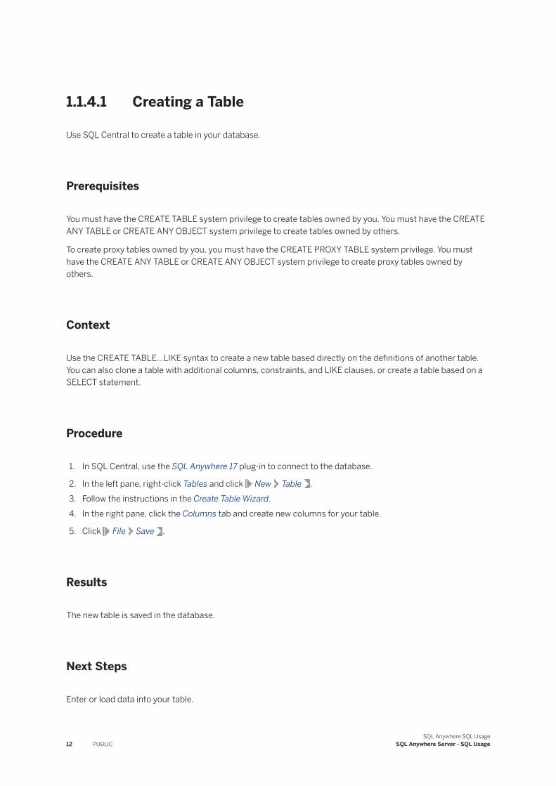
Use SQL Central to create a table in your database.
Prerequisites
You must have the CREATE TABLE system privilege to create tables owned by you. You must have the CREATE ANY TABLE or CREATE ANY OBJECT system privilege to create tables owned by others.
To create proxy tables owned by you, you must have the CREATE PROXY TABLE system privilege. You must have the CREATE ANY TABLE or CREATE ANY OBJECT system privilege to create proxy tables owned by others.
Context
Use the CREATE TABLE...LIKE syntax to create a new table based directly on the definitions of another table. You can also clone a table with additional columns, constraints, and LIKE clauses, or create a table based on a SELECT statement.
Procedure
1. In SQL Central, use the SQL Anywhere 17 plug-in to connect to the database.
2. In the left pane, right-click Tables and click New Table .3. Follow the instructions in the Create Table Wizard.4. In the right pane, click the Columns tab and create new columns for your table.
5. Click File Save .
Results
The new table is saved in the database.
Next Steps
Enter or load data into your table.
12 PUBLICSQL Anywhere SQL Usage
SQL Anywhere Server - SQL Usage
Related Information
Addition of Data Using INSERT [page 513]Data Import with the INSERT Statement [page 617]
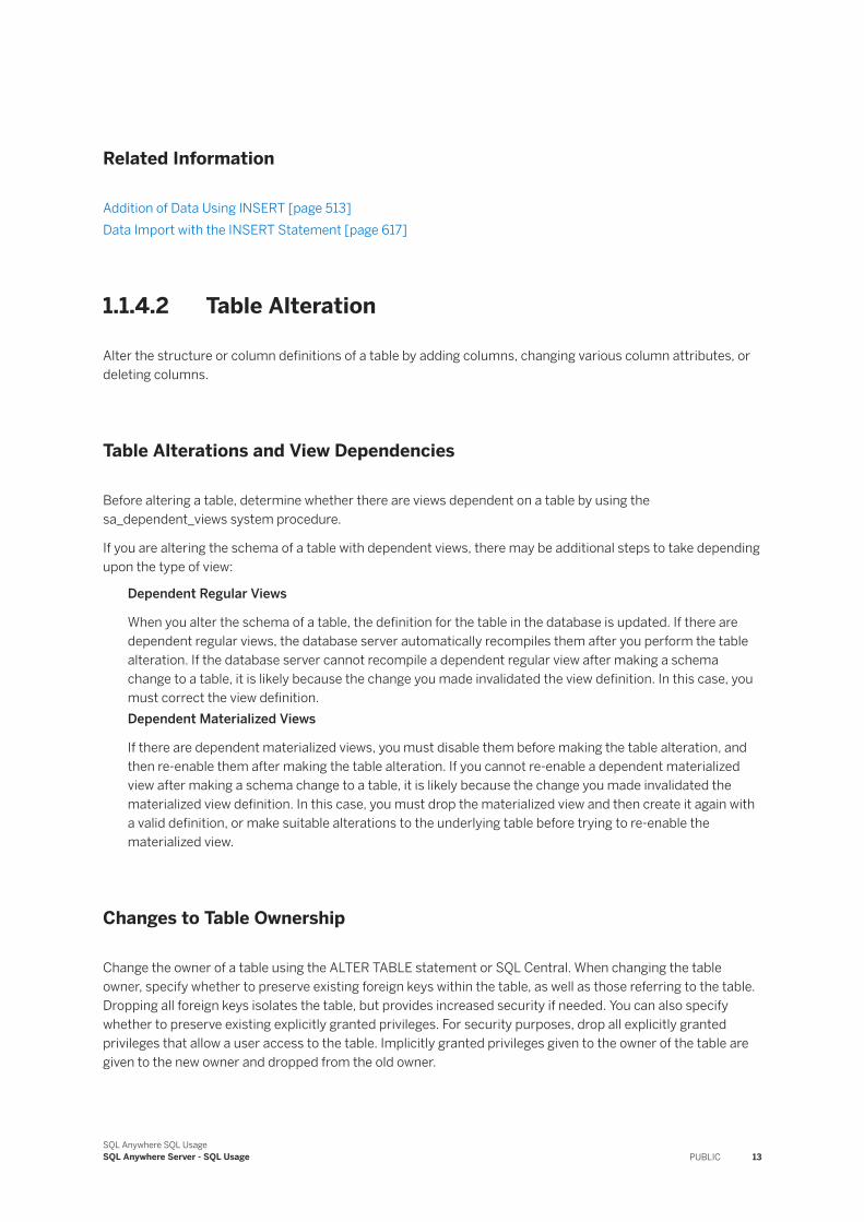
1.1.4.2 Table Alteration
Alter the structure or column definitions of a table by adding columns, changing various column attributes, or deleting columns.
Table Alterations and View Dependencies
Before altering a table, determine whether there are views dependent on a table by using the sa_dependent_views system procedure.
If you are altering the schema of a table with dependent views, there may be additional steps to take depending upon the type of view:
Dependent Regular Views
When you alter the schema of a table, the definition for the table in the database is updated. If there are dependent regular views, the database server automatically recompiles them after you perform the table alteration. If the database server cannot recompile a dependent regular view after making a schema change to a table, it is likely because the change you made invalidated the view definition. In this case, you must correct the view definition.Dependent Materialized Views
If there are dependent materialized views, you must disable them before making the table alteration, and then re-enable them after making the table alteration. If you cannot re-enable a dependent materialized view after making a schema change to a table, it is likely because the change you made invalidated the materialized view definition. In this case, you must drop the materialized view and then create it again with a valid definition, or make suitable alterations to the underlying table before trying to re-enable the materialized view.
Changes to Table Ownership
Change the owner of a table using the ALTER TABLE statement or SQL Central. When changing the table owner, specify whether to preserve existing foreign keys within the table, as well as those referring to the table. Dropping all foreign keys isolates the table, but provides increased security if needed. You can also specify whether to preserve existing explicitly granted privileges. For security purposes, drop all explicitly granted privileges that allow a user access to the table. Implicitly granted privileges given to the owner of the table are given to the new owner and dropped from the old owner.
SQL Anywhere SQL UsageSQL Anywhere Server - SQL Usage PUBLIC 13
In this section:
Altering a Table [page 14]Use SQL Central to alter tables in your database, for example to add or remove columns, or change the table owner.
Dropping a Table [page 15]Use SQL Central to drop a table from your database, for example, when you no longer need it.
Related Information
View Dependencies [page 50]Altering a Regular View [page 58]Creating a Materialized View [page 72]
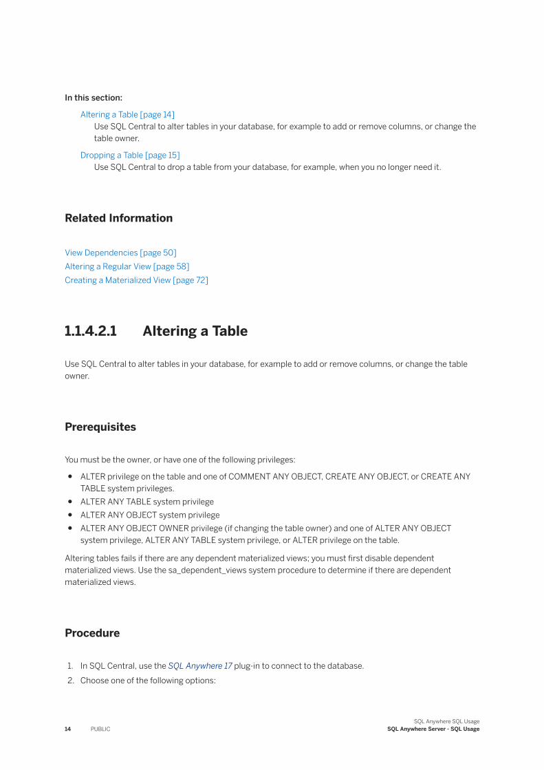
1.1.4.2.1 Altering a Table
Use SQL Central to alter tables in your database, for example to add or remove columns, or change the table owner.
Prerequisites
You must be the owner, or have one of the following privileges:
● ALTER privilege on the table and one of COMMENT ANY OBJECT, CREATE ANY OBJECT, or CREATE ANY TABLE system privileges.
● ALTER ANY TABLE system privilege● ALTER ANY OBJECT system privilege● ALTER ANY OBJECT OWNER privilege (if changing the table owner) and one of ALTER ANY OBJECT
system privilege, ALTER ANY TABLE system privilege, or ALTER privilege on the table.
Altering tables fails if there are any dependent materialized views; you must first disable dependent materialized views. Use the sa_dependent_views system procedure to determine if there are dependent materialized views.
Procedure
1. In SQL Central, use the SQL Anywhere 17 plug-in to connect to the database.2. Choose one of the following options:
14 PUBLICSQL Anywhere SQL Usage
SQL Anywhere Server - SQL Usage
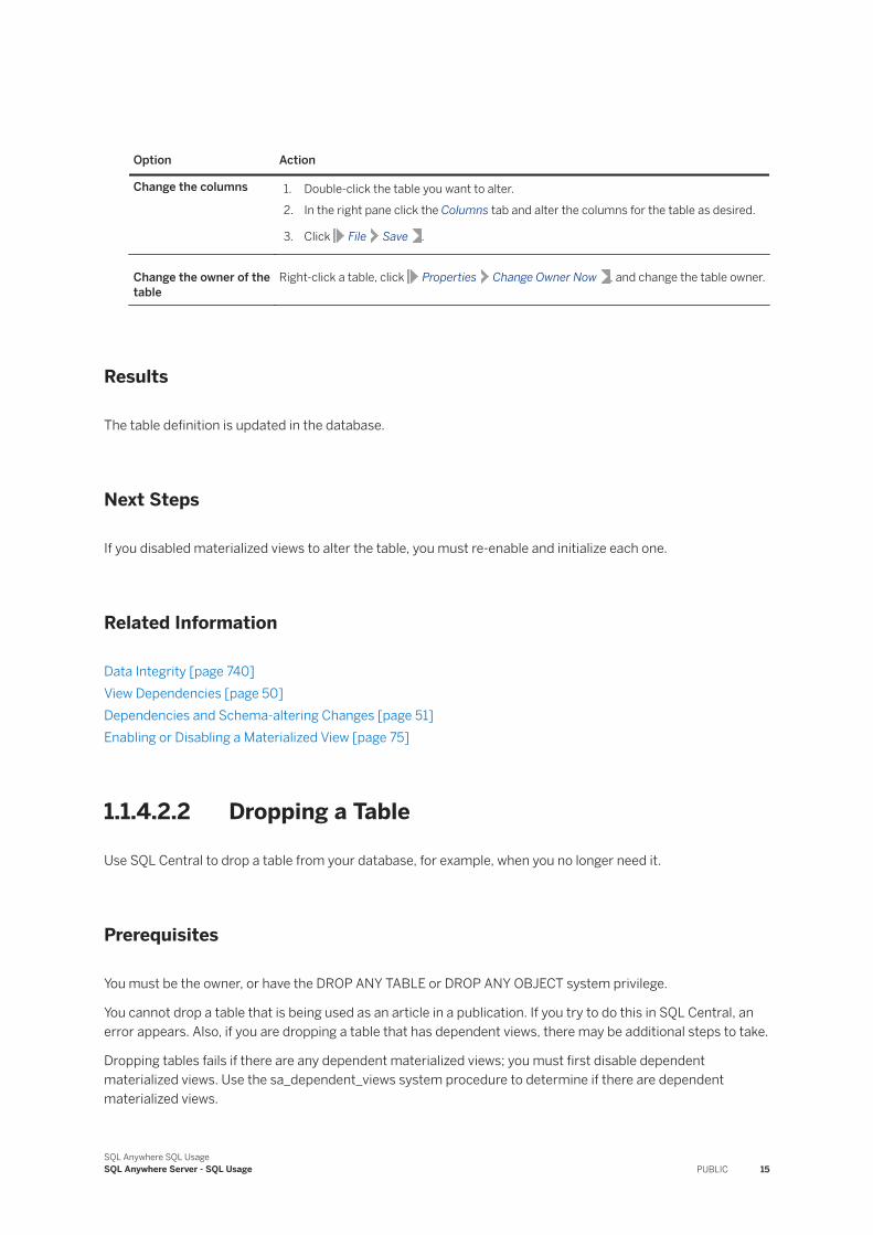
Option Action
Change the columns 1. Double-click the table you want to alter.2. In the right pane click the Columns tab and alter the columns for the table as desired.
3. Click File Save .
Change the owner of the table
Right-click a table, click Properties Change Owner Now , and change the table owner.
Results
The table definition is updated in the database.
Next Steps
If you disabled materialized views to alter the table, you must re-enable and initialize each one.
Related Information
Data Integrity [page 740]View Dependencies [page 50]Dependencies and Schema-altering Changes [page 51]Enabling or Disabling a Materialized View [page 75]
1.1.4.2.2 Dropping a Table
Use SQL Central to drop a table from your database, for example, when you no longer need it.
Prerequisites
You must be the owner, or have the DROP ANY TABLE or DROP ANY OBJECT system privilege.
You cannot drop a table that is being used as an article in a publication. If you try to do this in SQL Central, an error appears. Also, if you are dropping a table that has dependent views, there may be additional steps to take.
Dropping tables fails if there are any dependent materialized views; you must first disable dependent materialized views. Use the sa_dependent_views system procedure to determine if there are dependent materialized views.
SQL Anywhere SQL UsageSQL Anywhere Server - SQL Usage PUBLIC 15
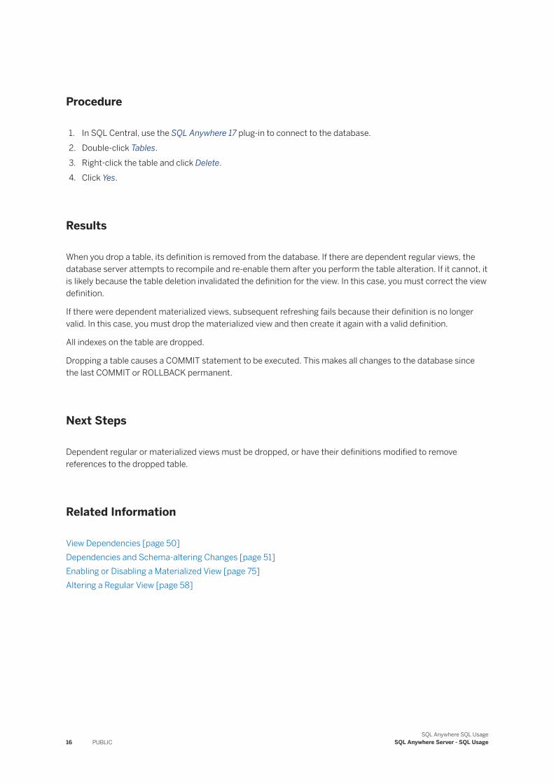
Procedure
1. In SQL Central, use the SQL Anywhere 17 plug-in to connect to the database.2. Double-click Tables.3. Right-click the table and click Delete.4. Click Yes.
Results
When you drop a table, its definition is removed from the database. If there are dependent regular views, the database server attempts to recompile and re-enable them after you perform the table alteration. If it cannot, it is likely because the table deletion invalidated the definition for the view. In this case, you must correct the view definition.
If there were dependent materialized views, subsequent refreshing fails because their definition is no longer valid. In this case, you must drop the materialized view and then create it again with a valid definition.
All indexes on the table are dropped.
Dropping a table causes a COMMIT statement to be executed. This makes all changes to the database since the last COMMIT or ROLLBACK permanent.
Next Steps
Dependent regular or materialized views must be dropped, or have their definitions modified to remove references to the dropped table.
Related Information
View Dependencies [page 50]Dependencies and Schema-altering Changes [page 51]Enabling or Disabling a Materialized View [page 75]Altering a Regular View [page 58]
16 PUBLICSQL Anywhere SQL Usage
SQL Anywhere Server - SQL Usage
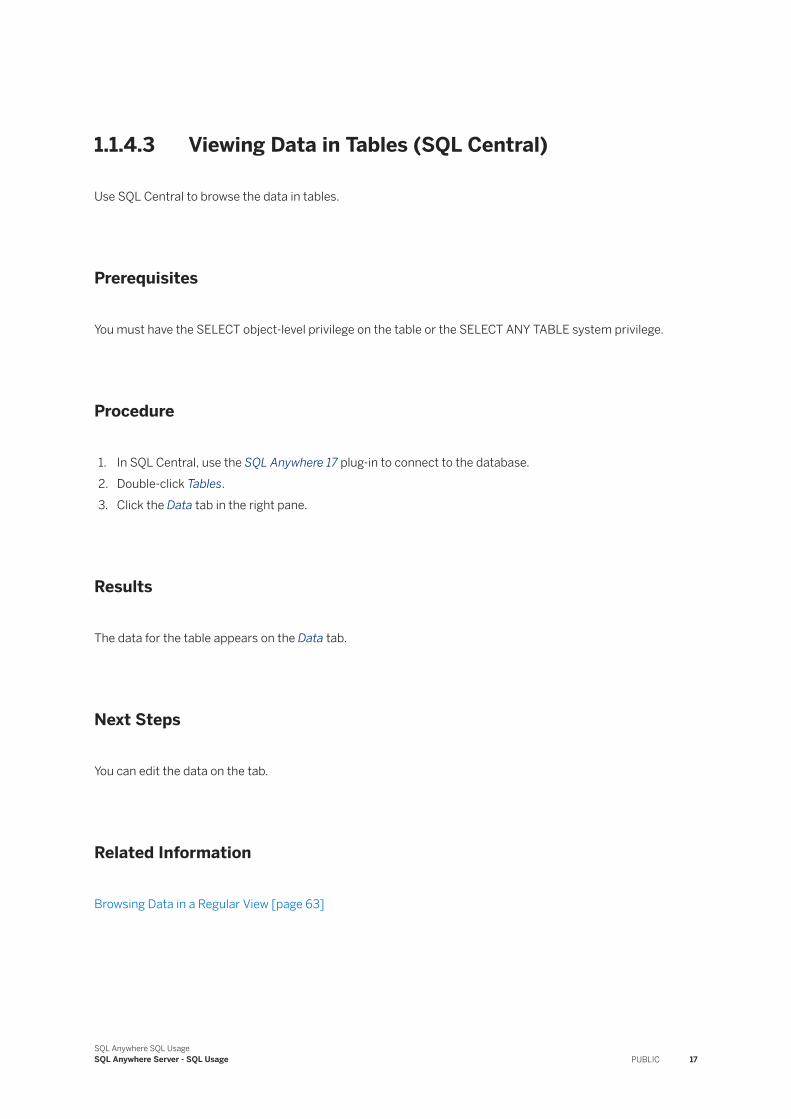
1.1.4.3 Viewing Data in Tables (SQL Central)
Use SQL Central to browse the data in tables.
Prerequisites
You must have the SELECT object-level privilege on the table or the SELECT ANY TABLE system privilege.
Procedure
1. In SQL Central, use the SQL Anywhere 17 plug-in to connect to the database.2. Double-click Tables.3. Click the Data tab in the right pane.
Results
The data for the table appears on the Data tab.
Next Steps
You can edit the data on the tab.
Related Information
Browsing Data in a Regular View [page 63]
SQL Anywhere SQL UsageSQL Anywhere Server - SQL Usage PUBLIC 17
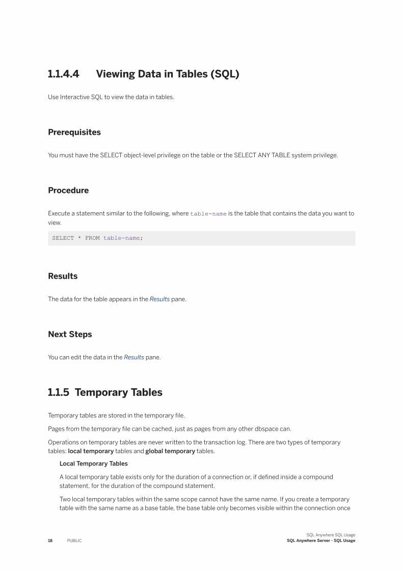
1.1.4.4 Viewing Data in Tables (SQL)
Use Interactive SQL to view the data in tables.
Prerequisites
You must have the SELECT object-level privilege on the table or the SELECT ANY TABLE system privilege.
Procedure
Execute a statement similar to the following, where table-name is the table that contains the data you want to view.
SELECT * FROM table-name;
Results
The data for the table appears in the Results pane.
Next Steps
You can edit the data in the Results pane.
1.1.5 Temporary Tables
Temporary tables are stored in the temporary file.
Pages from the temporary file can be cached, just as pages from any other dbspace can.
Operations on temporary tables are never written to the transaction log. There are two types of temporary tables: local temporary tables and global temporary tables.
Local Temporary Tables
A local temporary table exists only for the duration of a connection or, if defined inside a compound statement, for the duration of the compound statement.
Two local temporary tables within the same scope cannot have the same name. If you create a temporary table with the same name as a base table, the base table only becomes visible within the connection once
18 PUBLICSQL Anywhere SQL Usage
SQL Anywhere Server - SQL Usage
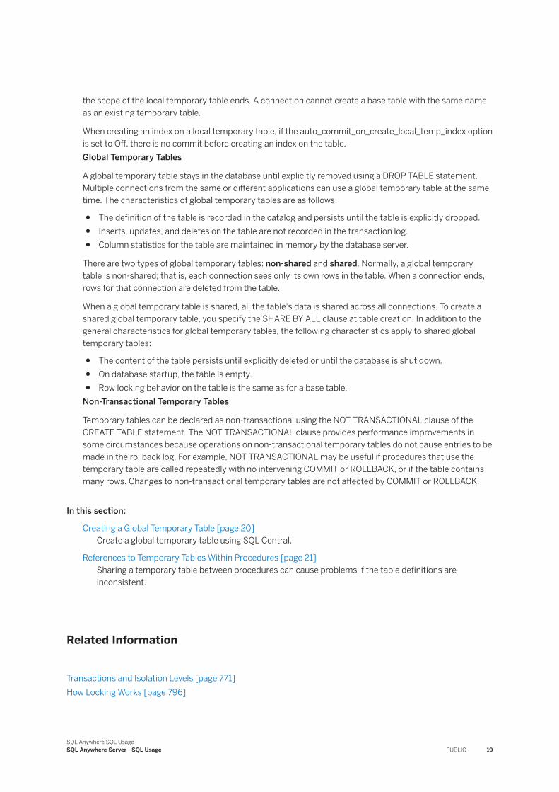
the scope of the local temporary table ends. A connection cannot create a base table with the same name as an existing temporary table.
When creating an index on a local temporary table, if the auto_commit_on_create_local_temp_index option is set to Off, there is no commit before creating an index on the table.Global Temporary Tables
A global temporary table stays in the database until explicitly removed using a DROP TABLE statement. Multiple connections from the same or different applications can use a global temporary table at the same time. The characteristics of global temporary tables are as follows:
● The definition of the table is recorded in the catalog and persists until the table is explicitly dropped.● Inserts, updates, and deletes on the table are not recorded in the transaction log.● Column statistics for the table are maintained in memory by the database server.
There are two types of global temporary tables: non-shared and shared. Normally, a global temporary table is non-shared; that is, each connection sees only its own rows in the table. When a connection ends, rows for that connection are deleted from the table.
When a global temporary table is shared, all the table's data is shared across all connections. To create a shared global temporary table, you specify the SHARE BY ALL clause at table creation. In addition to the general characteristics for global temporary tables, the following characteristics apply to shared global temporary tables:
● The content of the table persists until explicitly deleted or until the database is shut down.● On database startup, the table is empty.● Row locking behavior on the table is the same as for a base table.
Non-Transactional Temporary Tables
Temporary tables can be declared as non-transactional using the NOT TRANSACTIONAL clause of the CREATE TABLE statement. The NOT TRANSACTIONAL clause provides performance improvements in some circumstances because operations on non-transactional temporary tables do not cause entries to be made in the rollback log. For example, NOT TRANSACTIONAL may be useful if procedures that use the temporary table are called repeatedly with no intervening COMMIT or ROLLBACK, or if the table contains many rows. Changes to non-transactional temporary tables are not affected by COMMIT or ROLLBACK.
In this section:
Creating a Global Temporary Table [page 20]Create a global temporary table using SQL Central.
References to Temporary Tables Within Procedures [page 21]Sharing a temporary table between procedures can cause problems if the table definitions are inconsistent.
Related Information
Transactions and Isolation Levels [page 771]How Locking Works [page 796]
SQL Anywhere SQL UsageSQL Anywhere Server - SQL Usage PUBLIC 19
1.1.5.1 Creating a Global Temporary Table
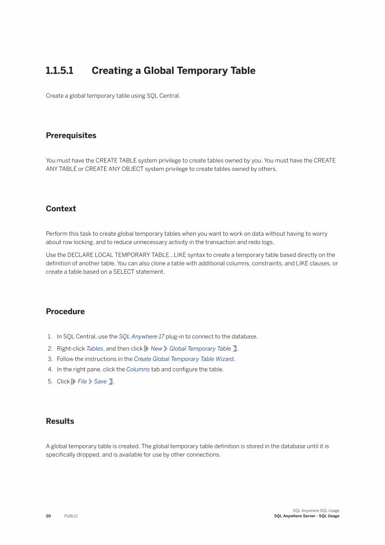
Create a global temporary table using SQL Central.
Prerequisites
You must have the CREATE TABLE system privilege to create tables owned by you. You must have the CREATE ANY TABLE or CREATE ANY OBJECT system privilege to create tables owned by others.
Context
Perform this task to create global temporary tables when you want to work on data without having to worry about row locking, and to reduce unnecessary activity in the transaction and redo logs.
Use the DECLARE LOCAL TEMPORARY TABLE...LIKE syntax to create a temporary table based directly on the definition of another table. You can also clone a table with additional columns, constraints, and LIKE clauses, or create a table based on a SELECT statement.
Procedure
1. In SQL Central, use the SQL Anywhere 17 plug-in to connect to the database.
2. Right-click Tables, and then click New Global Temporary Table .3. Follow the instructions in the Create Global Temporary Table Wizard.4. In the right pane, click the Columns tab and configure the table.
5. Click File Save .
Results
A global temporary table is created. The global temporary table definition is stored in the database until it is specifically dropped, and is available for use by other connections.
20 PUBLICSQL Anywhere SQL Usage
SQL Anywhere Server - SQL Usage
1.1.5.2 References to Temporary Tables Within Procedures
Sharing a temporary table between procedures can cause problems if the table definitions are inconsistent.
For example, suppose you have two procedures, procA and procB, both of which define a temporary table, temp_table, and call another procedure called sharedProc. Neither procA nor procB has been called yet, so the temporary table does not yet exist.
Now, suppose that the procA definition for temp_table is slightly different than the definition in procB. While both used the same column names and types, the column order is different.
When you call procA, it returns the expected result. However, when you call procB, it returns a different result.
This is because when procA was called, it created temp_table, and then called sharedProc. When sharedProc was called, the SELECT statement inside of it was parsed and validated, and then a parsed representation of the statement was cached so that it can be used again when another SELECT statement is executed. The cached version reflects the column ordering from the table definition in procA.
Calling procB causes the temp_table to be recreated, but with different column ordering. When procB calls sharedProc, the database server uses the cached representation of the SELECT statement. So, the results are different.
You can avoid this situation from happening by doing one of the following:
● ensure that temporary tables used in this way are defined consistently● use a global temporary table instead
1.1.6 Computed Columns
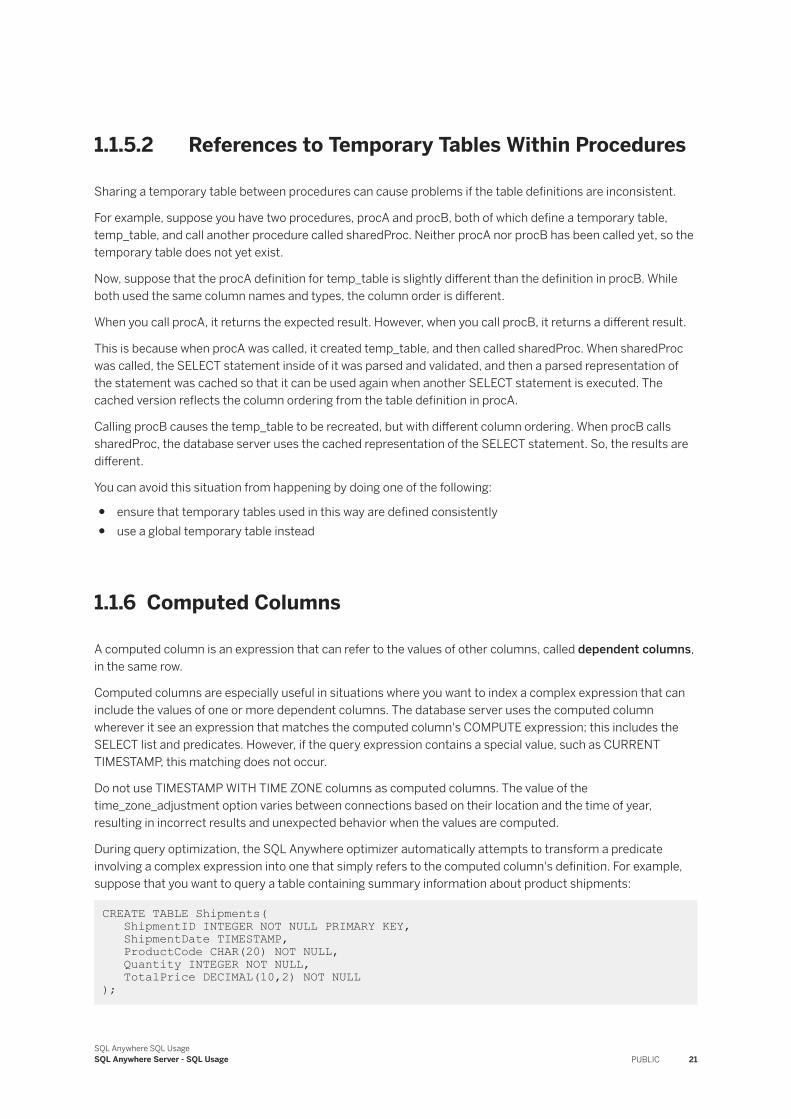
A computed column is an expression that can refer to the values of other columns, called dependent columns, in the same row.
Computed columns are especially useful in situations where you want to index a complex expression that can include the values of one or more dependent columns. The database server uses the computed column wherever it see an expression that matches the computed column's COMPUTE expression; this includes the SELECT list and predicates. However, if the query expression contains a special value, such as CURRENT TIMESTAMP, this matching does not occur.
Do not use TIMESTAMP WITH TIME ZONE columns as computed columns. The value of the time_zone_adjustment option varies between connections based on their location and the time of year, resulting in incorrect results and unexpected behavior when the values are computed.
During query optimization, the SQL Anywhere optimizer automatically attempts to transform a predicate involving a complex expression into one that simply refers to the computed column's definition. For example, suppose that you want to query a table containing summary information about product shipments:
CREATE TABLE Shipments( ShipmentID INTEGER NOT NULL PRIMARY KEY, ShipmentDate TIMESTAMP, ProductCode CHAR(20) NOT NULL, Quantity INTEGER NOT NULL, TotalPrice DECIMAL(10,2) NOT NULL );
SQL Anywhere SQL UsageSQL Anywhere Server - SQL Usage PUBLIC 21
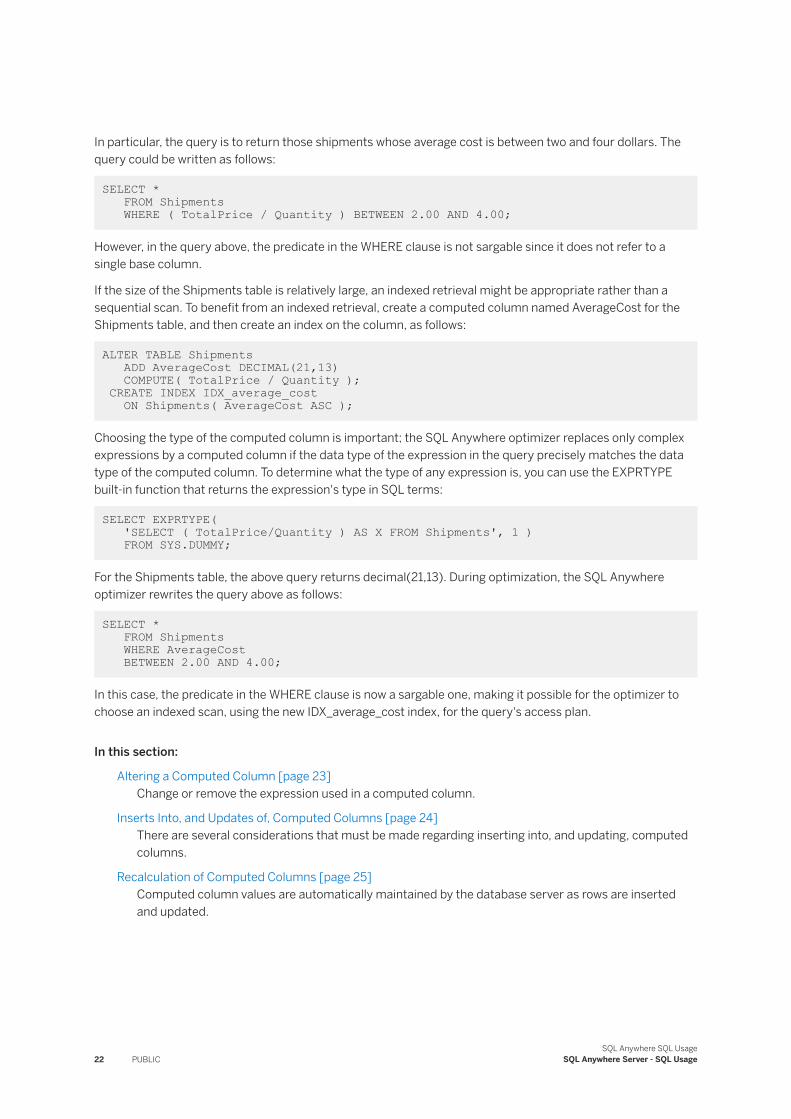
In particular, the query is to return those shipments whose average cost is between two and four dollars. The query could be written as follows:
SELECT * FROM Shipments WHERE ( TotalPrice / Quantity ) BETWEEN 2.00 AND 4.00;
However, in the query above, the predicate in the WHERE clause is not sargable since it does not refer to a single base column.
If the size of the Shipments table is relatively large, an indexed retrieval might be appropriate rather than a sequential scan. To benefit from an indexed retrieval, create a computed column named AverageCost for the Shipments table, and then create an index on the column, as follows:
ALTER TABLE Shipments ADD AverageCost DECIMAL(21,13) COMPUTE( TotalPrice / Quantity ); CREATE INDEX IDX_average_cost ON Shipments( AverageCost ASC );
Choosing the type of the computed column is important; the SQL Anywhere optimizer replaces only complex expressions by a computed column if the data type of the expression in the query precisely matches the data type of the computed column. To determine what the type of any expression is, you can use the EXPRTYPE built-in function that returns the expression's type in SQL terms:
SELECT EXPRTYPE( 'SELECT ( TotalPrice/Quantity ) AS X FROM Shipments', 1 ) FROM SYS.DUMMY;
For the Shipments table, the above query returns decimal(21,13). During optimization, the SQL Anywhere optimizer rewrites the query above as follows:
SELECT * FROM Shipments WHERE AverageCost BETWEEN 2.00 AND 4.00;
In this case, the predicate in the WHERE clause is now a sargable one, making it possible for the optimizer to choose an indexed scan, using the new IDX_average_cost index, for the query's access plan.
In this section:
Altering a Computed Column [page 23]Change or remove the expression used in a computed column.
Inserts Into, and Updates of, Computed Columns [page 24]There are several considerations that must be made regarding inserting into, and updating, computed columns.
Recalculation of Computed Columns [page 25]Computed column values are automatically maintained by the database server as rows are inserted and updated.
22 PUBLICSQL Anywhere SQL Usage
SQL Anywhere Server - SQL Usage
Related Information
Query Predicates [page 164]
1.1.6.1 Altering a Computed Column
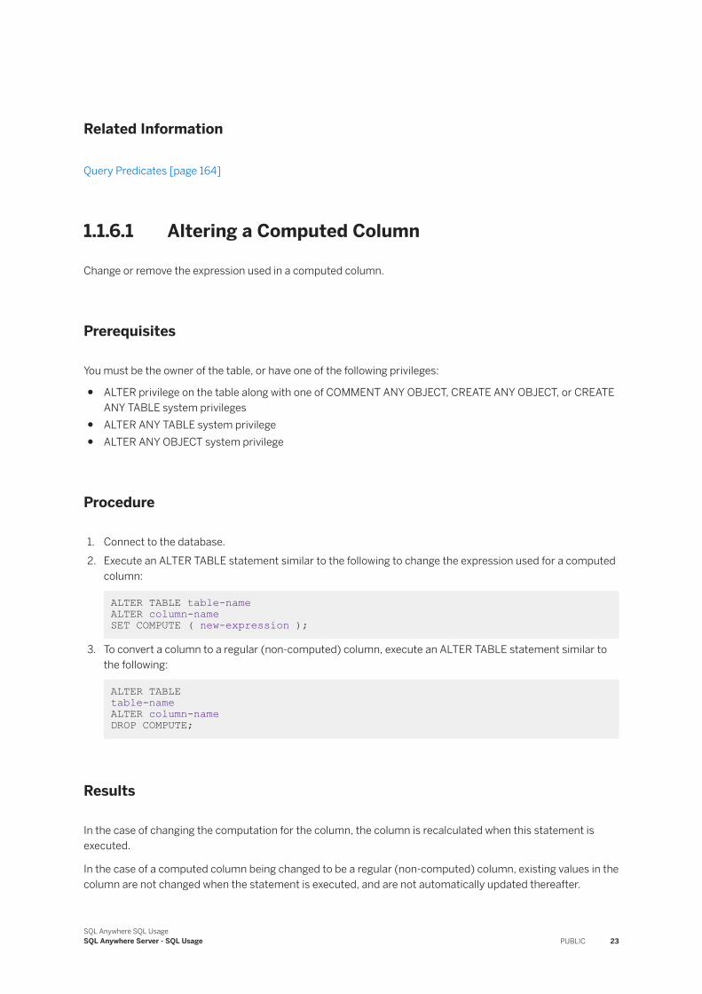
Change or remove the expression used in a computed column.
Prerequisites
You must be the owner of the table, or have one of the following privileges:
● ALTER privilege on the table along with one of COMMENT ANY OBJECT, CREATE ANY OBJECT, or CREATE ANY TABLE system privileges
● ALTER ANY TABLE system privilege● ALTER ANY OBJECT system privilege
Procedure
1. Connect to the database.2. Execute an ALTER TABLE statement similar to the following to change the expression used for a computed
column:
ALTER TABLE table-name ALTER column-name SET COMPUTE ( new-expression );
3. To convert a column to a regular (non-computed) column, execute an ALTER TABLE statement similar to the following:
ALTER TABLE table-name ALTER column-name DROP COMPUTE;
Results
In the case of changing the computation for the column, the column is recalculated when this statement is executed.
In the case of a computed column being changed to be a regular (non-computed) column, existing values in the column are not changed when the statement is executed, and are not automatically updated thereafter.
SQL Anywhere SQL UsageSQL Anywhere Server - SQL Usage PUBLIC 23
Example
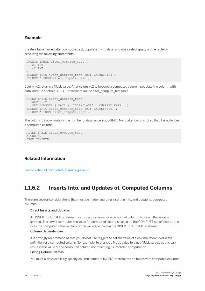
Create a table named alter_compute_test, populate it with data, and run a select query on the table by executing the following statements:
CREATE TABLE alter_compute_test ( c1 INT, c2 INT) ;INSERT INTO alter_compute_test (c1) VALUES(100); SELECT * FROM alter_compute_test ;
Column c2 returns a NULL value. Alter column c2 to become a computed column, populate the column with data, and run another SELECT statement on the alter_compute_test table.
ALTER TABLE alter_compute_test ALTER c2 SET COMPUTE ( DAYS ( '2001-01-01' , CURRENT DATE ) )INSERT INTO alter_compute_test (c1) VALUES(200) ; SELECT * FROM alter_compute_test ;
The column c2 now contains the number of days since 2001-01-01. Next, alter column c2 so that it is no longer a computed column:
ALTER TABLE alter_compute_test ALTER c2 DROP COMPUTE ;
Related Information
Recalculation of Computed Columns [page 25]
1.1.6.2 Inserts Into, and Updates of, Computed Columns
There are several considerations that must be made regarding inserting into, and updating, computed columns.
Direct Inserts and Updates
An INSERT or UPDATE statement can specify a value for a computed column; however, the value is ignored. The server computes the value for computed columns based on the COMPUTE specification, and uses the computed value in place of the value specified in the INSERT or UPDATE statement.Column Dependencies
It is strongly recommended that you do not use triggers to set the value of a column referenced in the definition of a computed column (for example, to change a NULL value to a not-NULL value), as this can result in the value of the computed column not reflecting its intended computation.Listing Column Names
You must always explicitly specify column names in INSERT statements on tables with computed columns.
24 PUBLICSQL Anywhere SQL Usage
SQL Anywhere Server - SQL Usage
Triggers
If you define triggers on a computed column, any INSERT or UPDATE statement that affects the column fires the triggers.
The LOAD TABLE statement permits the optional computation of computed columns. Suppressing computation during a load operation may make performing complex unload/reload sequences faster. It can also be useful when the value of a computed column must stay constant, even though the COMPUTE expression refers a non-deterministic value, such as CURRENT TIMESTAMP.
Avoid changing the values of dependent columns in triggers as changing the values may cause the value of the computed column to be inconsistent with the column definition.
If a computed column x depends on a column y that is declared not-NULL, then an attempt to set y to NULL is rejected with an error before triggers fire.
1.1.6.3 Recalculation of Computed Columns
Computed column values are automatically maintained by the database server as rows are inserted and updated.
Most applications should never have to update or insert computed column values directly.
Computed columns are recalculated under the following circumstances:
● Any column is deleted, added, or renamed.● The table is changed by an ALTER TABLE statement that modifies any column's data type or COMPUTE
clause.● A row is inserted.● A row is updated.
Computed columns are not recalculated under the following circumstances:
● The table is renamed.● The computed column is queried.● The computed column depends on the values of other rows (using a subquery or user-defined function),
and these rows are changed.
1.1.7 Primary Keys
Each table in a relational database should have a primary key. A primary key is a column, or set of columns, that uniquely identifies each row.
No two rows in a table can have the same primary key value, and no column in a primary key can contain the NULL value.
Only base tables and global temporary tables can have primary keys. With declared temporary tables, you can create a unique index over a set of NOT NULL columns to mimic the semantics of a primary key.
Do not use approximate data types such as FLOAT and DOUBLE for primary keys or for columns with unique constraints. Approximate numeric data types are subject to rounding errors after arithmetic operations.
SQL Anywhere SQL UsageSQL Anywhere Server - SQL Usage PUBLIC 25
You can also specify whether to cluster the primary key index, using the CLUSTERED clause.
NotePrimary key column order is determined by the order of the columns as specified in the primary key declaration of the CREATE TABLE (or ALTER TABLE) statement. You can also specify the sort order (ascending or descending) for each individual column. These sort order specifications are used by the database server when creating the primary key index.
The order of the columns in a primary key does not dictate the order of the columns in any referential constraints. You can specify a different column order, and different sort orders, with any foreign key declaration.
Example
In the SQL Anywhere sample database, the Employees table stores personal information about employees. It has a primary key column named EmployeeID, which holds a unique ID number assigned to each employee. A single column holding an ID number is a common way to assign primary keys and has advantages over names and other identifiers that may not always be unique.
A more complex primary key can be seen in the SalesOrderItems table of the SQL Anywhere sample database. The table holds information about individual items on orders from the company, and has the following columns:
ID
An order number, identifying the order the item is part of.LineID
A line number, identifying each item on any order.ProductID
A product ID, identifying the product being ordered.Quantity
A quantity, displaying how many items were ordered.ShipDate
A ship date, displaying when the order was shipped.
In this section:
Managing Primary Keys (SQL Central) [page 27]Manage primary keys by using SQL Central to help improve query performance on a table.
Managing Primary Keys (SQL) [page 28]Manage primary keys by using SQL to help improve query performance on a table.
26 PUBLICSQL Anywhere SQL Usage
SQL Anywhere Server - SQL Usage
Related Information
Clustered Indexes [page 39]Primary Keys Enforce Entity Integrity [page 761]
1.1.7.1 Managing Primary Keys (SQL Central)
Manage primary keys by using SQL Central to help improve query performance on a table.
Prerequisites
You must be the owner of the table, or have one of the following privileges:
● ALTER ANY OBJECT system privilege● ALTER ANY INDEX and ALTER ANY TABLE system privileges● ALTER and REFERENCES privileges for the table along with one of COMMENT ANY OBJECT, CREATE ANY
OBJECT, or CREATE ANY TABLE system privileges
Procedure
1. In SQL Central, use the SQL Anywhere 17 plug-in to connect to the database.2. In the left pane, double-click Tables.3. Right-click the table, and choose one of the following options:
Option Action
Create or alter a primary key Click Set Primary Key and follow the instructions in the Set Primary Key Wizard.
Delete a primary key In the Columns pane of the table, clear the checkmark from the PKey column and then click Save.
Results
A primary key is added, altered, or deleted.
Related Information
Primary Keys Enforce Entity Integrity [page 761]
SQL Anywhere SQL UsageSQL Anywhere Server - SQL Usage PUBLIC 27
Managing Primary Keys (SQL) [page 28]
1.1.7.2 Managing Primary Keys (SQL)
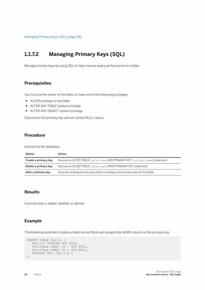
Manage primary keys by using SQL to help improve query performance on a table.
Prerequisites
You must be the owner of the table, or have one of the following privileges:
● ALTER privilege on the table● ALTER ANY TABLE system privilege● ALTER ANY OBJECT system privilege
Columns in the primary key cannot contain NULL values.
Procedure
Connect to the database.
Option Action
Create a primary key Execute an ALTER TABLE table-name ADD PRIMARY KEY (column-name) statement.
Delete a primary key Execute an ALTER TABLE table-name DROP PRIMARY KEY statement.
Alter a primary key Drop the existing primary key before creating a new primary key for the table.
Results
A primary key is added, deleted, or altered.
Example
The following statement creates a table named Skills and assigns the SkillID column as the primary key:
CREATE TABLE Skills ( SkillID INTEGER NOT NULL, SkillName CHAR( 20 ) NOT NULL, SkillType CHAR( 20 ) NOT NULL, PRIMARY KEY( SkillID ) );
28 PUBLICSQL Anywhere SQL Usage
SQL Anywhere Server - SQL Usage
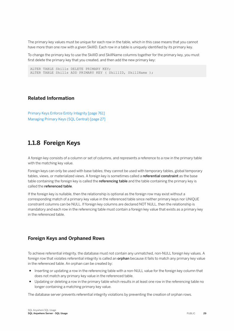
The primary key values must be unique for each row in the table, which in this case means that you cannot have more than one row with a given SkillID. Each row in a table is uniquely identified by its primary key.
To change the primary key to use the SkillID and SkillName columns together for the primary key, you must first delete the primary key that you created, and then add the new primary key:
ALTER TABLE Skills DELETE PRIMARY KEY; ALTER TABLE Skills ADD PRIMARY KEY ( SkillID, SkillName );
Related Information
Primary Keys Enforce Entity Integrity [page 761]Managing Primary Keys (SQL Central) [page 27]
1.1.8 Foreign Keys
A foreign key consists of a column or set of columns, and represents a reference to a row in the primary table with the matching key value.
Foreign keys can only be used with base tables; they cannot be used with temporary tables, global temporary tables, views, or materialized views. A foreign key is sometimes called a referential constraint as the base table containing the foreign key is called the referencing table and the table containing the primary key is called the referenced table.
If the foreign key is nullable, then the relationship is optional as the foreign row may exist without a corresponding match of a primary key value in the referenced table since neither primary keys nor UNIQUE constraint columns can be NULL. If foreign key columns are declared NOT NULL, then the relationship is mandatory and each row in the referencing table must contain a foreign key value that exists as a primary key in the referenced table.
Foreign Keys and Orphaned Rows
To achieve referential integrity, the database must not contain any unmatched, non-NULL foreign key values. A foreign row that violates referential integrity is called an orphan because it fails to match any primary key value in the referenced table. An orphan can be created by:
● Inserting or updating a row in the referencing table with a non-NULL value for the foreign key column that does not match any primary key value in the referenced table.
● Updating or deleting a row in the primary table which results in at least one row in the referencing table no longer containing a matching primary key value.
The database server prevents referential integrity violations by preventing the creation of orphan rows.
SQL Anywhere SQL UsageSQL Anywhere Server - SQL Usage PUBLIC 29
Composite Foreign Keys
Multi-column primary and foreign keys, called composite keys, are also supported. With a composite foreign key, NULL values still signify the absence of a match, but how an orphan is identified depends on how referential constraints are defined in the MATCH clause.
Foreign Key Indexes and Sorting Order
When you create a foreign key, an index for the key is automatically created. The foreign key column order does not need to reflect the order of columns in the primary key, nor does the sorting order of the primary key index have to match the sorting order of the foreign key index. The sorting (ascending or descending) of each indexed column in the foreign key index can be customized to ensure that the sorting order of the foreign key index matches the sorting order required by specific SQL queries in your application, as specified in those statements' ORDER BY clauses. You can specify the sorting for each column when setting the foreign key constraint.
Example
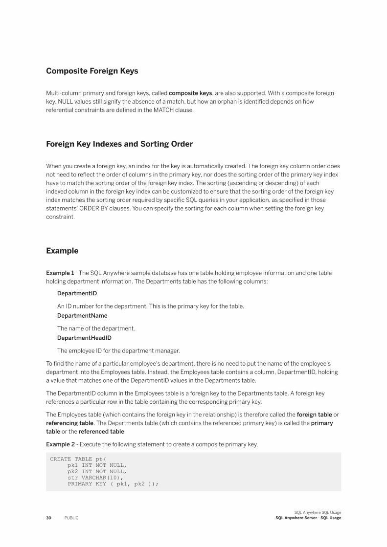
Example 1 - The SQL Anywhere sample database has one table holding employee information and one table holding department information. The Departments table has the following columns:
DepartmentID
An ID number for the department. This is the primary key for the table.DepartmentName
The name of the department.DepartmentHeadID
The employee ID for the department manager.
To find the name of a particular employee's department, there is no need to put the name of the employee's department into the Employees table. Instead, the Employees table contains a column, DepartmentID, holding a value that matches one of the DepartmentID values in the Departments table.
The DepartmentID column in the Employees table is a foreign key to the Departments table. A foreign key references a particular row in the table containing the corresponding primary key.
The Employees table (which contains the foreign key in the relationship) is therefore called the foreign table or referencing table. The Departments table (which contains the referenced primary key) is called the primary table or the referenced table.
Example 2 - Execute the following statement to create a composite primary key.
CREATE TABLE pt( pk1 INT NOT NULL, pk2 INT NOT NULL, str VARCHAR(10), PRIMARY KEY ( pk1, pk2 ));
30 PUBLICSQL Anywhere SQL Usage
SQL Anywhere Server - SQL Usage
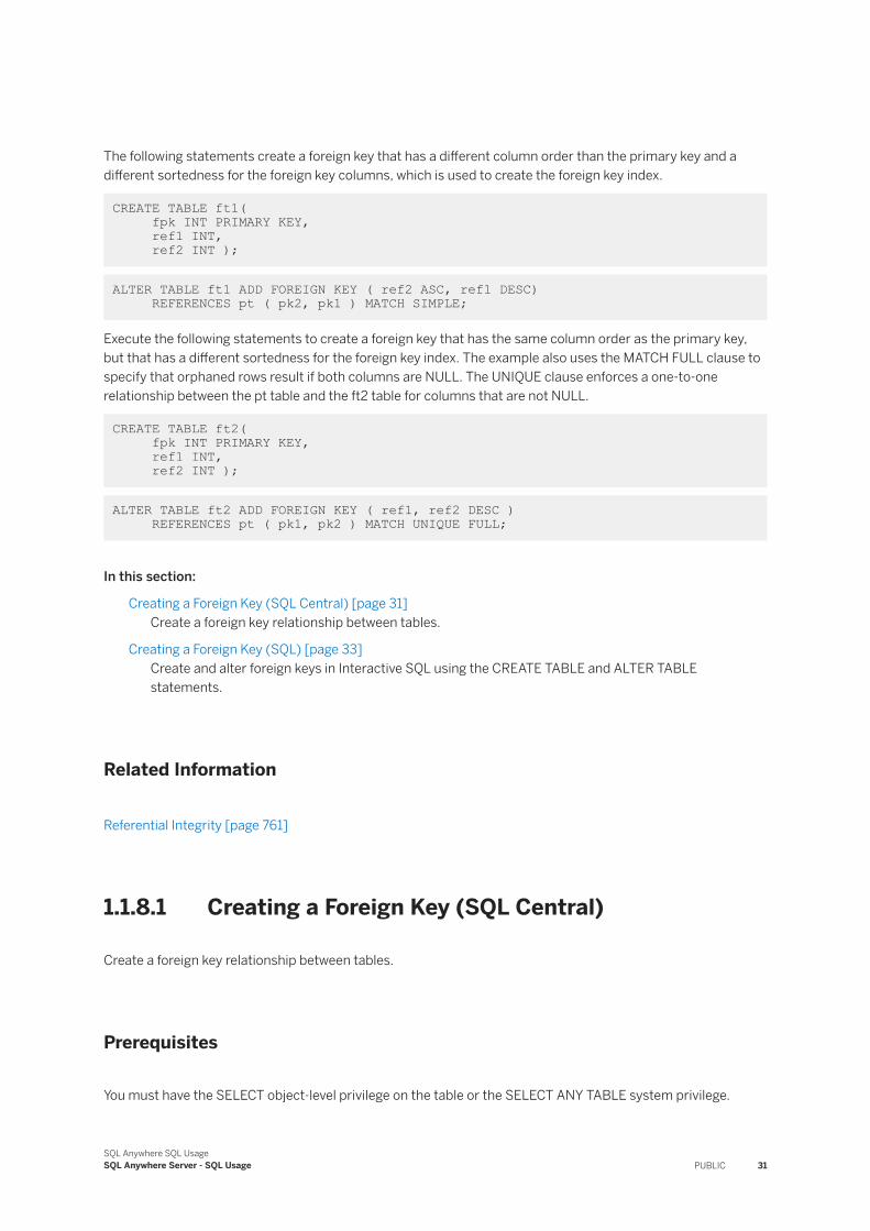
The following statements create a foreign key that has a different column order than the primary key and a different sortedness for the foreign key columns, which is used to create the foreign key index.
CREATE TABLE ft1( fpk INT PRIMARY KEY, ref1 INT, ref2 INT );
ALTER TABLE ft1 ADD FOREIGN KEY ( ref2 ASC, ref1 DESC) REFERENCES pt ( pk2, pk1 ) MATCH SIMPLE;
Execute the following statements to create a foreign key that has the same column order as the primary key, but that has a different sortedness for the foreign key index. The example also uses the MATCH FULL clause to specify that orphaned rows result if both columns are NULL. The UNIQUE clause enforces a one-to-one relationship between the pt table and the ft2 table for columns that are not NULL.
CREATE TABLE ft2( fpk INT PRIMARY KEY, ref1 INT, ref2 INT );
ALTER TABLE ft2 ADD FOREIGN KEY ( ref1, ref2 DESC ) REFERENCES pt ( pk1, pk2 ) MATCH UNIQUE FULL;
In this section:
Creating a Foreign Key (SQL Central) [page 31]Create a foreign key relationship between tables.
Creating a Foreign Key (SQL) [page 33]Create and alter foreign keys in Interactive SQL using the CREATE TABLE and ALTER TABLE statements.
Related Information
Referential Integrity [page 761]
1.1.8.1 Creating a Foreign Key (SQL Central)
Create a foreign key relationship between tables.
Prerequisites
You must have the SELECT object-level privilege on the table or the SELECT ANY TABLE system privilege.
SQL Anywhere SQL UsageSQL Anywhere Server - SQL Usage PUBLIC 31
You must also be the owner of the table, or have one of the following privileges:
● ALTER privilege on the table along with one of COMMENT ANY OBJECT, CREATE ANY OBJECT, or CREATE ANY TABLE system privileges
● ALTER ANY TABLE system privilege● ALTER ANY OBJECT system privilege
Context
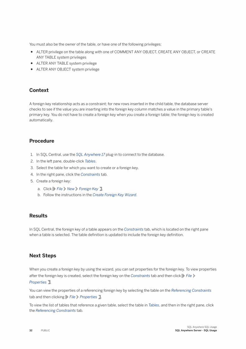
A foreign key relationship acts as a constraint; for new rows inserted in the child table, the database server checks to see if the value you are inserting into the foreign key column matches a value in the primary table's primary key. You do not have to create a foreign key when you create a foreign table; the foreign key is created automatically.
Procedure
1. In SQL Central, use the SQL Anywhere 17 plug-in to connect to the database.2. In the left pane, double-click Tables.3. Select the table for which you want to create or a foreign key.4. In the right pane, click the Constraints tab.5. Create a foreign key:
a. Click File New Foreign Key .b. Follow the instructions in the Create Foreign Key Wizard.
Results
In SQL Central, the foreign key of a table appears on the Constraints tab, which is located on the right pane when a table is selected. The table definition is updated to include the foreign key definition.
Next Steps
When you create a foreign key by using the wizard, you can set properties for the foreign key. To view properties after the foreign key is created, select the foreign key on the Constraints tab and then click FileProperties .
You can view the properties of a referencing foreign key by selecting the table on the Referencing Constraints tab and then clicking File Properties .
To view the list of tables that reference a given table, select the table in Tables, and then in the right pane, click the Referencing Constraints tab.
32 PUBLICSQL Anywhere SQL Usage
SQL Anywhere Server - SQL Usage
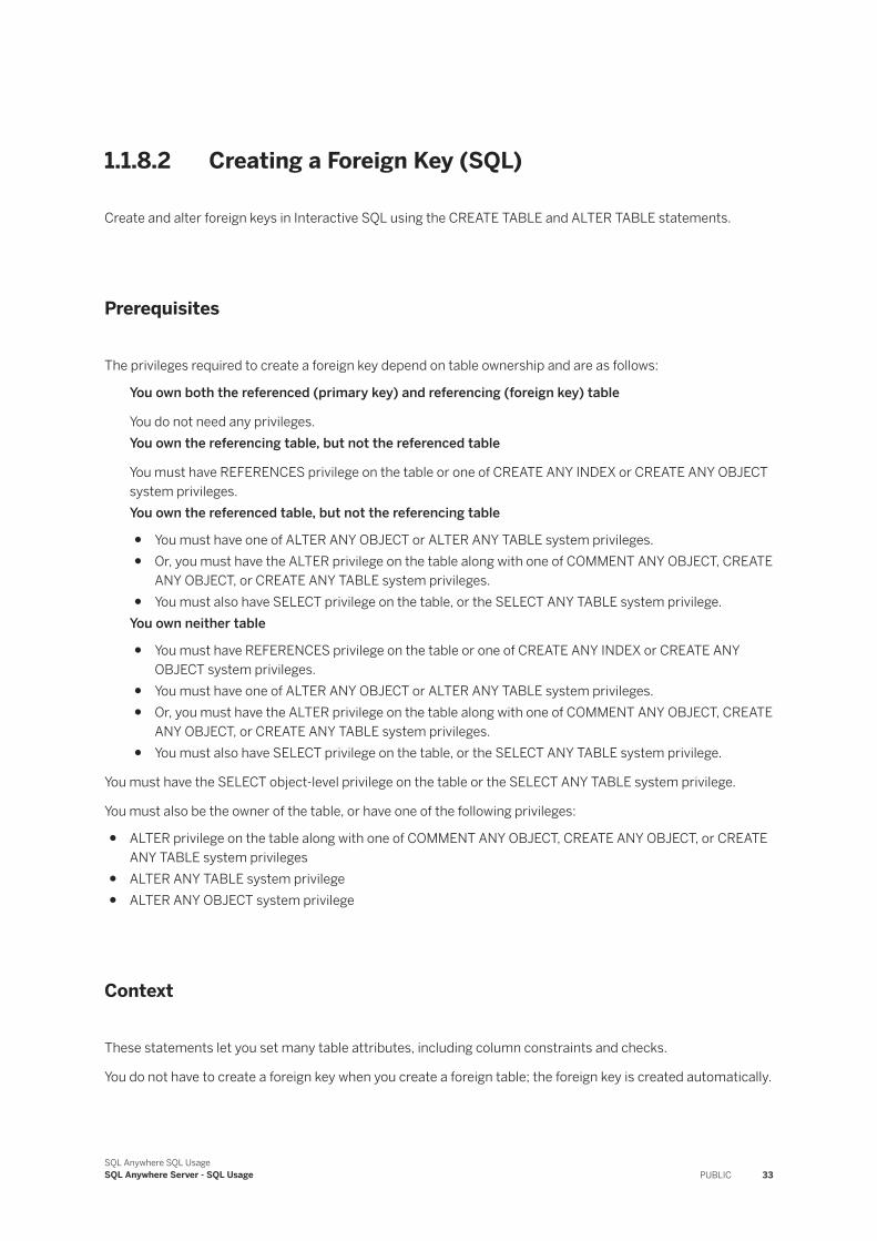
1.1.8.2 Creating a Foreign Key (SQL)
Create and alter foreign keys in Interactive SQL using the CREATE TABLE and ALTER TABLE statements.
Prerequisites
The privileges required to create a foreign key depend on table ownership and are as follows:
You own both the referenced (primary key) and referencing (foreign key) table
You do not need any privileges.You own the referencing table, but not the referenced table
You must have REFERENCES privilege on the table or one of CREATE ANY INDEX or CREATE ANY OBJECT system privileges.You own the referenced table, but not the referencing table
● You must have one of ALTER ANY OBJECT or ALTER ANY TABLE system privileges.● Or, you must have the ALTER privilege on the table along with one of COMMENT ANY OBJECT, CREATE
ANY OBJECT, or CREATE ANY TABLE system privileges.● You must also have SELECT privilege on the table, or the SELECT ANY TABLE system privilege.
You own neither table
● You must have REFERENCES privilege on the table or one of CREATE ANY INDEX or CREATE ANY OBJECT system privileges.
● You must have one of ALTER ANY OBJECT or ALTER ANY TABLE system privileges.● Or, you must have the ALTER privilege on the table along with one of COMMENT ANY OBJECT, CREATE
ANY OBJECT, or CREATE ANY TABLE system privileges.● You must also have SELECT privilege on the table, or the SELECT ANY TABLE system privilege.
You must have the SELECT object-level privilege on the table or the SELECT ANY TABLE system privilege.
You must also be the owner of the table, or have one of the following privileges:
● ALTER privilege on the table along with one of COMMENT ANY OBJECT, CREATE ANY OBJECT, or CREATE ANY TABLE system privileges
● ALTER ANY TABLE system privilege● ALTER ANY OBJECT system privilege
Context
These statements let you set many table attributes, including column constraints and checks.
You do not have to create a foreign key when you create a foreign table; the foreign key is created automatically.
SQL Anywhere SQL UsageSQL Anywhere Server - SQL Usage PUBLIC 33
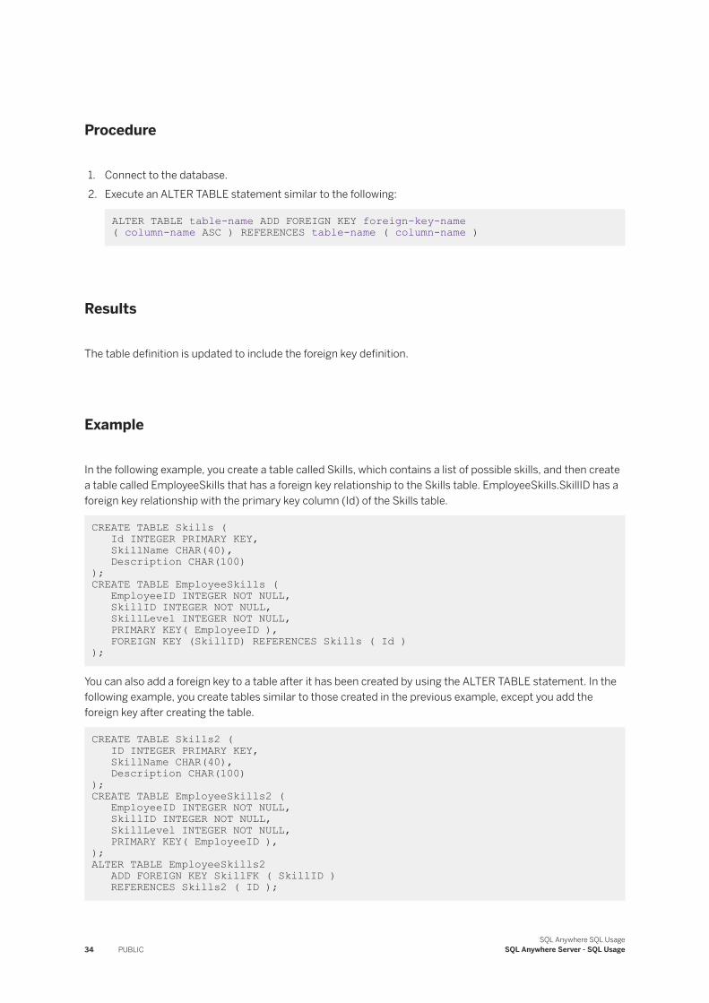
Procedure
1. Connect to the database.2. Execute an ALTER TABLE statement similar to the following:
ALTER TABLE table-name ADD FOREIGN KEY foreign-key-name ( column-name ASC ) REFERENCES table-name ( column-name )
Results
The table definition is updated to include the foreign key definition.
Example
In the following example, you create a table called Skills, which contains a list of possible skills, and then create a table called EmployeeSkills that has a foreign key relationship to the Skills table. EmployeeSkills.SkillID has a foreign key relationship with the primary key column (Id) of the Skills table.
CREATE TABLE Skills ( Id INTEGER PRIMARY KEY, SkillName CHAR(40), Description CHAR(100) );CREATE TABLE EmployeeSkills ( EmployeeID INTEGER NOT NULL, SkillID INTEGER NOT NULL, SkillLevel INTEGER NOT NULL, PRIMARY KEY( EmployeeID ), FOREIGN KEY (SkillID) REFERENCES Skills ( Id ) );
You can also add a foreign key to a table after it has been created by using the ALTER TABLE statement. In the following example, you create tables similar to those created in the previous example, except you add the foreign key after creating the table.
CREATE TABLE Skills2 ( ID INTEGER PRIMARY KEY, SkillName CHAR(40), Description CHAR(100) );CREATE TABLE EmployeeSkills2 ( EmployeeID INTEGER NOT NULL, SkillID INTEGER NOT NULL, SkillLevel INTEGER NOT NULL, PRIMARY KEY( EmployeeID ),);ALTER TABLE EmployeeSkills2 ADD FOREIGN KEY SkillFK ( SkillID ) REFERENCES Skills2 ( ID );
34 PUBLICSQL Anywhere SQL Usage
SQL Anywhere Server - SQL Usage
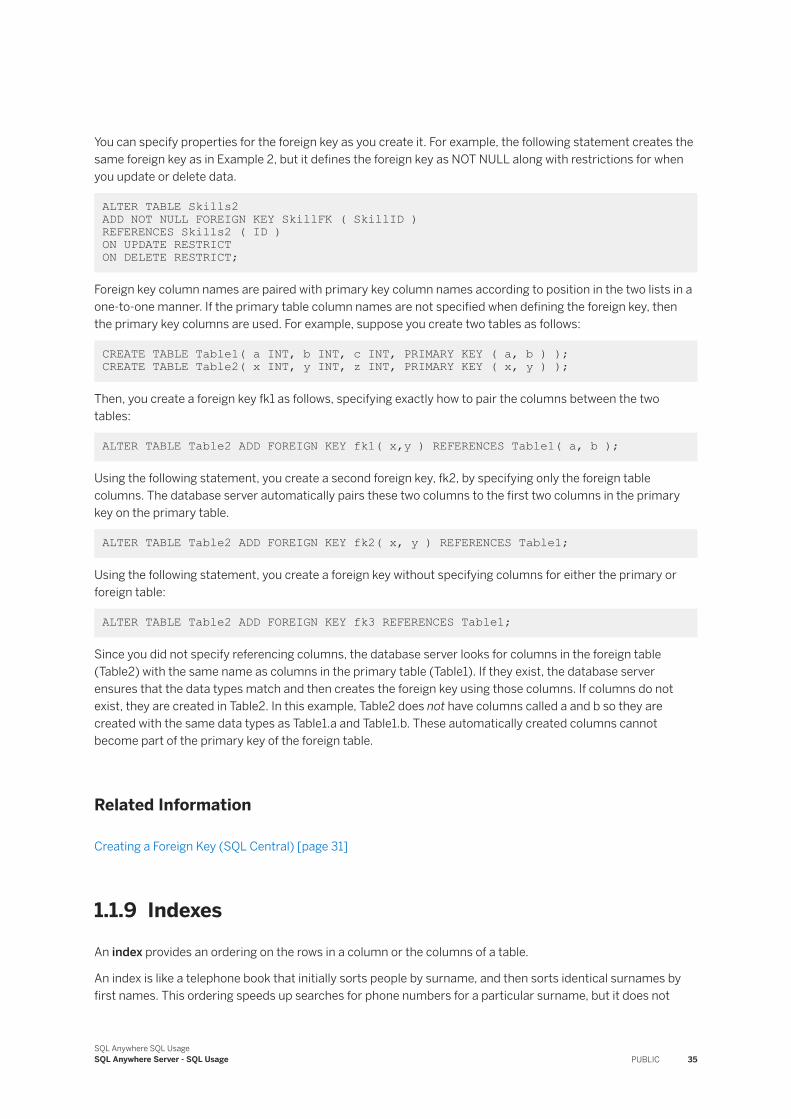
You can specify properties for the foreign key as you create it. For example, the following statement creates the same foreign key as in Example 2, but it defines the foreign key as NOT NULL along with restrictions for when you update or delete data.
ALTER TABLE Skills2 ADD NOT NULL FOREIGN KEY SkillFK ( SkillID )REFERENCES Skills2 ( ID )ON UPDATE RESTRICT ON DELETE RESTRICT;
Foreign key column names are paired with primary key column names according to position in the two lists in a one-to-one manner. If the primary table column names are not specified when defining the foreign key, then the primary key columns are used. For example, suppose you create two tables as follows:
CREATE TABLE Table1( a INT, b INT, c INT, PRIMARY KEY ( a, b ) ); CREATE TABLE Table2( x INT, y INT, z INT, PRIMARY KEY ( x, y ) );
Then, you create a foreign key fk1 as follows, specifying exactly how to pair the columns between the two tables:
ALTER TABLE Table2 ADD FOREIGN KEY fk1( x,y ) REFERENCES Table1( a, b );
Using the following statement, you create a second foreign key, fk2, by specifying only the foreign table columns. The database server automatically pairs these two columns to the first two columns in the primary key on the primary table.
ALTER TABLE Table2 ADD FOREIGN KEY fk2( x, y ) REFERENCES Table1;
Using the following statement, you create a foreign key without specifying columns for either the primary or foreign table:
ALTER TABLE Table2 ADD FOREIGN KEY fk3 REFERENCES Table1;
Since you did not specify referencing columns, the database server looks for columns in the foreign table (Table2) with the same name as columns in the primary table (Table1). If they exist, the database server ensures that the data types match and then creates the foreign key using those columns. If columns do not exist, they are created in Table2. In this example, Table2 does not have columns called a and b so they are created with the same data types as Table1.a and Table1.b. These automatically created columns cannot become part of the primary key of the foreign table.
Related Information
Creating a Foreign Key (SQL Central) [page 31]
1.1.9 Indexes
An index provides an ordering on the rows in a column or the columns of a table.
An index is like a telephone book that initially sorts people by surname, and then sorts identical surnames by first names. This ordering speeds up searches for phone numbers for a particular surname, but it does not
SQL Anywhere SQL UsageSQL Anywhere Server - SQL Usage PUBLIC 35
provide help in finding the phone number at a particular address. In the same way, a database index is useful only for searches on a specific column or columns.
Indexes get more useful as the size of the table increases. The average time to find a phone number at a given address increases with the size of the phone book, while it does not take much longer to find the phone number of K. Kaminski in a large phone book than in a small phone book.
The optimizer automatically uses indexes to improve the performance of any database statement whenever it is possible to do so. Also, the index is updated automatically when rows are deleted, updated, or inserted. While you can explicitly refer to indexes using index hints when forming your query, there is no need to.
There are some down sides to creating indexes. In particular, any indexes must be maintained along with the table itself when the data in a column is modified, so that the performance of inserts, updates, and deletes can be affected by indexes. For this reason, unnecessary indexes should be dropped. Use the Index Consultant to identify unnecessary indexes.
Deciding What Indexes to Create
Choosing an appropriate set of indexes for a database is an important part of optimizing performance. Identifying an appropriate set can also be a demanding problem.
There is no simple formula to determine whether an index should be created. Consider the trade-off of the benefits of indexed retrieval versus the maintenance overhead of that index. The following factors may help to determine whether to create an index:
Keys and unique columns
The database server automatically creates indexes on primary keys, foreign keys, and unique columns. Do not create additional indexes on these columns. The exception is composite keys, which can sometimes be enhanced with additional indexes.Frequency of search
If a particular column is searched frequently, you can achieve performance benefits by creating an index on that column. Creating an index on a column that is rarely searched may not be worthwhile.Size of table
Indexes on relatively large tables with many rows provide greater benefits than indexes on relatively small tables. For example, a table with only 20 rows is unlikely to benefit from an index, since a sequential scan would not take any longer than an index lookup.Number of updates
An index is updated every time a row is inserted or deleted from the table and every time an indexed column is updated. An index on a column slows the performance of inserts, updates, and deletes. A database that is frequently updated should have fewer indexes than one that is read-only.Space considerations
Indexes take up space within the database. If database size is a primary concern, create indexes sparingly.Data distribution
If an index lookup returns too many values, it is more costly than a sequential scan. The database server does not make use of the index when it recognizes this condition. For example, the database server would not make use of an index on a column with only two values, such as Employees.Sex in the SQL Anywhere sample database. For this reason, do not create an index on a column that has only a few distinct values.
36 PUBLICSQL Anywhere SQL Usage
SQL Anywhere Server - SQL Usage
When creating indexes, the order in which you specify the columns becomes the order in which the columns appear in the index. Duplicate references to column names in the index definition is not allowed.
NoteThe Index Consultant is a tool that assists you in proper selection of indexes. It analyzes either a single query or a set of operations and recommends which indexes to add to your database. It also notifies you of indexes that are unused.
Indexes on Temporary Tables
You can create indexes on both local and global temporary tables. Consider indexing a temporary table if you expect it to be large and accessed several times in sorted order or in a join. Otherwise, any improvement in performance for queries is likely to be outweighed by the cost of creating and dropping the index.
In this section:
Composite Indexes [page 38]An index on more than one column is called a composite index.
Clustered Indexes [page 39]You can improve the performance of a large index scan by declaring that the index is clustered.
Creating an Index [page 41]Create indexes on base tables, temporary tables, and materialized views.
Validating an Index [page 42]Validate an index to ensure that every row referenced in the index actually exists in the table.
Rebuilding an Index [page 43]Rebuild an index that is fragmented due to extensive insertion and deletion operations on the table or materialized view.
Dropping an Index [page 44]Drop an index when it is no longer needed, or when you must modify the definition of a column that is part of a primary or foreign key.
Advanced: Index Information in the Catalog [page 45]There are several system tables in the catalog that provide information about indexes in the database.
Advanced: Logical and Physical Indexes [page 45]The software supports logical and physical indexes.
Advanced: Index Selectivity and Fan-out [page 47]Index selectivity is the ability of an index to locate a desired index entry without having to read additional data.
Advanced: Other Ways the Database Server Uses Indexes [page 48]The database server uses indexes to achieve performance benefits.
SQL Anywhere SQL UsageSQL Anywhere Server - SQL Usage PUBLIC 37
1.1.9.1 Composite Indexes
An index on more than one column is called a composite index.
For example, the following statement creates a two-column composite index:
CREATE INDEX name ON Employees ( Surname, GivenName );
A composite index is useful if the first column alone does not provide high selectivity. For example, a composite index on Surname and GivenName is useful when many employees have the same surname. A composite index on EmployeeID and Surname would not be useful because each employee has a unique ID, so the column Surname does not provide any additional selectivity.
Additional columns in an index can allow you to narrow down your search, but having a two-column index is not the same as having two separate indexes. A composite index is structured like a telephone book, which first sorts people by their surnames, and then all the people with the same surname by their given names. A telephone book is useful if you know the surname, even more useful if you know both the given name and the surname, but worthless if you only know the given name and not the surname.
Column Order
When you create composite indexes, think carefully about the order of the columns. Composite indexes are useful for doing searches on all the columns in the index or on the first columns only; they are not useful for doing searches on any of the later columns alone.
If you are likely to do many searches on one column only, that column should be the first column in the composite index. If you are likely to do individual searches on both columns of a two-column index, consider creating a second index that contains the second column only.
For example, suppose you create a composite index on two columns. One column contains employee's given names, the other their surnames. You could create an index that contains their given name, then their surname. Alternatively, you could index the surname, then the given name. Although these two indexes organize the information in both columns, they have different functions.
CREATE INDEX IX_GivenName_Surname ON Employees ( GivenName, Surname );CREATE INDEX IX_Surname_GivenName ON Employees ( Surname, GivenName );
Suppose you then want to search for the given name John. The only useful index is the one containing the given name in the first column of the index. The index organized by surname then given name is of no use because someone with the given name John could appear anywhere in the index.
If you are more likely to look up people by given name only or surname only, consider creating both of these indexes.
Alternatively, you could make two indexes, each containing only one of the columns. However, remember that the database server only uses one index to access any one table while processing a single query. Even if you know both names, it is likely that the database server needs to read extra rows, looking for those with the correct second name.
38 PUBLICSQL Anywhere SQL Usage
SQL Anywhere Server - SQL Usage
When you create an index using the CREATE INDEX statement, as in the example above, the columns appear in the order shown in your statement.
Composite Indexes and ORDER BY
By default, the columns of an index are sorted in ascending order, but they can optionally be sorted in descending order by specifying DESC in the CREATE INDEX statement.
The database server can choose to use an index to optimize an ORDER BY query as long as the ORDER BY clause contains only columns included in that index. In addition, the columns in the index must be ordered in exactly the same way, or in exactly the opposite way, as the ORDER BY clause. For single-column indexes, the ordering is always such that it can be optimized, but composite indexes require slightly more thought. The table below shows the possibilities for a two-column index.
Index columns Optimizable ORDER BY queries Not optimizable ORDER BY queries
ASC, ASC ASC, ASC or DESC, DESC ASC, DESC or DESC, ASC
ASC, DESC ASC, DESC or DESC, ASC ASC, ASC or DESC, DESC
DESC, ASC DESC, ASC or ASC, DESC ASC, ASC or DESC, DESC
DESC, DESC DESC, DESC or ASC, ASC ASC, DESC or DESC, ASC
An index with more than two columns follows the same general rule as above. For example, suppose you have the following index:
CREATE INDEX idx_example ON table1 ( col1 ASC, col2 DESC, col3 ASC );
In this case, the following queries can be optimized:
SELECT col1, col2, col3 FROM table1 ORDER BY col1 ASC, col2 DESC, col3 ASC;
SELECT col1, col2, col3 FROM example ORDER BY col1 DESC, col2 ASC, col3 DESC;
The index is not used to optimize a query with any other pattern of ASC and DESC in the ORDER BY clause. For example, the following statement is not optimized:
SELECT col1, col2, col3 FROM table1 ORDER BY col1 ASC, col2 ASC, col3 ASC;
1.1.9.2 Clustered Indexes
You can improve the performance of a large index scan by declaring that the index is clustered.
Using a clustered index increases the chance that two rows from adjacent index entries will appear on the same page in the database. This strategy can lead to performance benefits by reducing the number of times a table page needs to be read into the buffer pool.
SQL Anywhere SQL UsageSQL Anywhere Server - SQL Usage PUBLIC 39
The existence of an index with a clustering property causes the database server to attempt to store table rows in approximately the same order as they appear in the clustered index. However, while the database server attempts to preserve the key order, clustering is approximate and total clustering is not guaranteed. So, the database server cannot sequentially scan the table and retrieve all the rows in a clustered index key sequence. Ensuring that the rows of the table are returned in sorted order requires an access plan that either accesses the rows through the index, or performs a physical sort.
The optimizer exploits an index with a clustering property by modifying the expected cost of indexed retrieval to take into account the expected physical adjacency of table rows with matching or adjacent index key values.
The amount of clustering for a given table may degrade over time, as more and more rows are inserted or updated. The database server automatically keeps track of the amount of clustering for each clustered index in the ISYSPHYSIDX system table. If the database server detects that the rows in a table have become significantly unclustered, the optimizer adjusts its expected index retrieval costs.
If you decide to make one of the indexes on a table clustered, consider the expected query workload. Some experimentation is usually required. Generally, the database server can use a clustered index to improve performance when the following conditions hold for a specified query:
● Many of the table pages required for answering the query are not already in memory. When the table pages are already in memory, the server does not need to read these pages and such clustering is irrelevant.
● The query can be answered by performing an index retrieval that is expected to return a non-trivial number of rows. As an example, clustering is usually irrelevant for simple primary key searches.
● The database server actually needs to read table pages, as opposed to performing an index-only retrieval.
Declaring Clustered Indexes
The clustering property of an index can be added or removed at any time using SQL statements. Any primary key index, foreign key index, UNIQUE constraint index, or secondary index can be declared with the CLUSTERED property. However, you may declare at most one clustered index per table. You can do this using any of the following statements:
● CREATE TABLE statement● ALTER DATABASE statement● CREATE INDEX statement● DECLARE LOCAL TEMPORARY TABLE statement
Several statements work together to allow you to maintain and restore the clustering effect:
● The UNLOAD TABLE statement allows you to unload a table in the order of the clustered index key.● The LOAD TABLE statement inserts rows into the table in the order of the clustered index key.● The INSERT statement attempts to put new rows on the same table page as the one containing adjacent
rows, as per the clustered index key.● The REORGANIZE TABLE statement restores the clustering of a table by rearranging the rows according to
the clustered index. If REORGANIZE TABLE is used with tables where clustering is not specified, the tables are reordered using the primary key.
You can also create clustered indexes in SQL Central using the Create Index Wizard, and clicking Create A Clustered Index when prompted.
40 PUBLICSQL Anywhere SQL Usage
SQL Anywhere Server - SQL Usage
Related Information
Creating an Index [page 41]
1.1.9.3 Creating an Index
Create indexes on base tables, temporary tables, and materialized views.
Prerequisites
To create an index on a table, you must be the owner of the table or have one of the following privileges:
● CREATE ANY INDEX system privilege● CREATE ANY OBJECT system privilege● REFERENCES privilege on the table and either the COMMENT ANY OBJECT system privilege, the ALTER
ANY INDEX system privilege, or the ALTER ANY OBJECT system privilege
To create an index on a materialized view, you must be the owner of the materialized view or have one of the following privileges:
● CREATE ANY INDEX system privilege● CREATE ANY OBJECT system privilege
You cannot create an index on a regular view. You cannot create an index on a materialized view that is disabled.
Context
You can also create indexes on a built-in function using a computed column.
When creating indexes, the order in which you specify the columns becomes the order in which the columns appear in the index. Duplicate references to column names in the index definition is not allowed. You can use the Index Consultant to guide you in a proper selection of indexes for your database.
There is an automatic commit when creating an index on a local temporary table if the auto_commit_on_create_local_temp_index option is set to On. This option is set to Off by default.
Creating an index on a function (an implicit computed column) causes a checkpoint.
Column statistics are updated (or created if they do not exist).
Procedure
1. In SQL Central, use the SQL Anywhere 17 plug-in to connect to the database.
SQL Anywhere SQL UsageSQL Anywhere Server - SQL Usage PUBLIC 41
2. In the left pane, right-click Indexes and click New Index .3. Follow the instructions in the Create Index Wizard.
Results
The new index appears on the Index tab for the table and in Indexes. The new index is available to be used by queries.
1.1.9.4 Validating an Index
Validate an index to ensure that every row referenced in the index actually exists in the table.
Prerequisites
You must be the owner of the index, or have the VALIDATE ANY OBJECT system privilege.
Perform validation only when no connections are making changes to the database.
Context
For foreign key indexes, a validation check also ensures that the corresponding row exists in the primary table.
Procedure
1. In SQL Central, use the SQL Anywhere 17 plug-in to connect to the database.2. In the left pane, double-click Indexes.3. Right-click an index and click Validate.4. Click OK.
Results
A check is done to ensure that every row referenced in the index actually exists in the table. For foreign key indexes, the check ensures that the corresponding row exists in the primary table.
42 PUBLICSQL Anywhere SQL Usage
SQL Anywhere Server - SQL Usage
1.1.9.5 Rebuilding an Index
Rebuild an index that is fragmented due to extensive insertion and deletion operations on the table or materialized view.
Prerequisites
To rebuild an index on a table, you must be the owner of the table or have one of the following privileges:
● REFERENCES privilege on the table● ALTER ANY INDEX system privilege● ALTER ANY OBJECT system privilege
To rebuild an index on a materialized view, you must be the owner of the materialized view or have one of the following privileges:
● ALTER ANY INDEX system privilege● ALTER ANY OBJECT system privilege
Context
When you rebuild an index, you rebuild the physical index. All logical indexes that use the physical index benefit from the rebuild operation. You do not need to perform a rebuild on logical indexes.
Procedure
1. In SQL Central, use the SQL Anywhere 17 plug-in to connect to the database.2. In the left pane, double-click Indexes.3. Right-click the index and click Rebuild.4. Click OK.
Results
The index is rebuilt with fragmentation removed.
Related Information
Advanced: Logical and Physical Indexes [page 45]
SQL Anywhere SQL UsageSQL Anywhere Server - SQL Usage PUBLIC 43
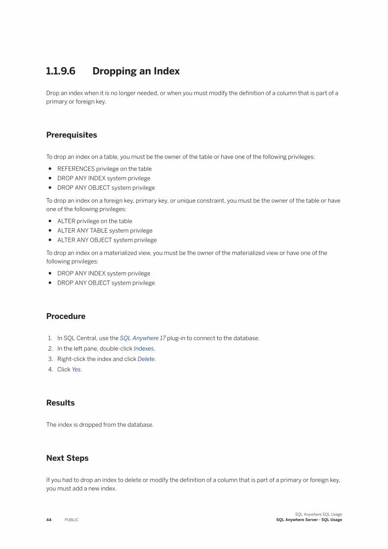
1.1.9.6 Dropping an Index
Drop an index when it is no longer needed, or when you must modify the definition of a column that is part of a primary or foreign key.
Prerequisites
To drop an index on a table, you must be the owner of the table or have one of the following privileges:
● REFERENCES privilege on the table● DROP ANY INDEX system privilege● DROP ANY OBJECT system privilege
To drop an index on a foreign key, primary key, or unique constraint, you must be the owner of the table or have one of the following privileges:
● ALTER privilege on the table● ALTER ANY TABLE system privilege● ALTER ANY OBJECT system privilege
To drop an index on a materialized view, you must be the owner of the materialized view or have one of the following privileges:
● DROP ANY INDEX system privilege● DROP ANY OBJECT system privilege
Procedure
1. In SQL Central, use the SQL Anywhere 17 plug-in to connect to the database.2. In the left pane, double-click Indexes.3. Right-click the index and click Delete.4. Click Yes.
Results
The index is dropped from the database.
Next Steps
If you had to drop an index to delete or modify the definition of a column that is part of a primary or foreign key, you must add a new index.
44 PUBLICSQL Anywhere SQL Usage
SQL Anywhere Server - SQL Usage
Related Information
Creating an Index [page 41]
1.1.9.7 Advanced: Index Information in the Catalog
There are several system tables in the catalog that provide information about indexes in the database.
The ISYSIDX system table provides a list of all indexes in the database, including primary and foreign key indexes. Additional information about the indexes is found in the ISYSPHYSIDX, ISYSIDXCOL, and ISYSFKEY system tables. You can use SQL Central or Interactive SQL to browse the system views for these tables to see the data they contain.
Following is a brief overview of how index information is stored in the system tables:
ISYSIDX system table
The central table for tracking indexes, each row in the ISYSIDX system table defines a logical index (PKEY, FKEY, UNIQUE constraint, Secondary index) in the database.ISYSPHYSIDX system table
Each row in the ISYSPHYSIDX system table defines a physical index in the database.ISYSIDXCOL system table
Just as each row in the SYSIDX system view describes one index in the database, each row in the SYSIDXCOL system view describes one column of an index described in the SYSIDX system view.ISYSFKEY system table
Every foreign key in the database is defined by one row in the ISYSFKEY system table and one row in the ISYSIDX system table.
Related Information
Advanced: Logical and Physical Indexes [page 45]
1.1.9.8 Advanced: Logical and Physical Indexes
The software supports logical and physical indexes.
A physical index is the actual indexing structure as it is stored on disk. A logical index is a reference to a physical index. When you create a primary key, secondary key, foreign key, or unique constraint, the database server ensures referential integrity by creating a logical index for the constraint. Then, the database server looks to see if a physical index already exists that satisfies the constraint. If a qualifying physical index already exists, the database server points the logical index to it. If one does not exist, the database server creates a new physical index and then points the logical index to it.
SQL Anywhere SQL UsageSQL Anywhere Server - SQL Usage PUBLIC 45
For a physical index to satisfy the requirements of a logical index, the columns, column order, and the ordering (ascending, descending) of data for each column must be identical.
Information about all logical and physical indexes in the database is recorded in the ISYSIDX and ISYSPHYSIDX system tables, respectively. When you create a logical index, an entry is made in the ISYSIDX system table to hold the index definition. A reference to the physical index used to satisfy the logical index is recorded in the ISYSIDX.phys_id column. The physical index is defined in the ISYSPHYSIDX system table.
Using logical indexes means that the database server does not need to create and maintain duplicate physical indexes since more than one logical index can point to a single physical index.
When you delete a logical index, its definition is removed from the ISYSIDX system table. If it was the only logical index referencing a particular physical index, the physical index is also deleted, along with its corresponding entry in the ISYSPHYSIDX system table.
Physical indexes are not created for remote tables. For temporary tables, physical indexes are created, but they are not recorded in ISYSPHYSIDX, and are discarded after use. Also, physical indexes for temporary tables are not shared.
In this section:
Determination of Which Logical Indexes Share a Physical Index [page 46]More than one logical index can share a physical index.
1.1.9.8.1 Determination of Which Logical Indexes Share a Physical Index
More than one logical index can share a physical index.
When you drop a in index, you are dropping a logical index that makes use of a physical index. If the logical index is the only index that uses the physical index, the physical index is dropped as well. If another logical index shares the same physical index, the physical index is not dropped. This is important to consider, especially if you expect disk space to be freed by dropping an index, or if you are dropping an index with the intent to physically recreate it.
To determine whether an index for a table is sharing a physical index with any other indexes, select the table in SQL Central, and then click the Indexes tab. Note whether the Phys. ID value for the index is also present for other indexes in the list. Matching Phys. ID values mean that those indexes share the same physical index. To recreate a physical index, you can use the ALTER INDEX...REBUILD statement. Alternatively, you can drop all the indexes, and then recreate them.
Determining Tables in Which Physical Indexes Are Being Shared
At any time, you can obtain a list of all tables in which physical indexes are being shared, by executing a query similar to the following:
SELECT tab.table_name, idx.table_id, phys.phys_index_id, COUNT(*) FROM SYSIDX idx JOIN SYSTAB tab ON (idx.table_id = tab.table_id) JOIN SYSPHYSIDX phys ON ( idx.phys_index_id = phys.phys_index_id
46 PUBLICSQL Anywhere SQL Usage
SQL Anywhere Server - SQL Usage
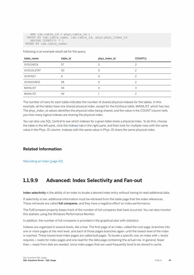
AND idx.table_id = phys.table_id ) GROUP BY tab.table_name, idx.table_id, phys.phys_index_id HAVING COUNT(*) > 1 ORDER BY tab.table_name;
Following is an example result set for the query:
table_name table_id phys_index_id COUNT()
ISYSCHECK 57 0 2
ISYSCOLSTAT 50 0 2
ISYSFKEY 6 0 2
ISYSSOURCE 58 0 2
MAINLIST 94 0 3
MAINLIST 94 1 2
The number of rows for each table indicates the number of shared physical indexes for the tables. In this example, all the tables have one shared physical index, except for the fictitious table, MAINLIST, which has two. The phys_index_id values identifies the physical index being shared, and the value in the COUNT column tells you how many logical indexes are sharing the physical index.
You can also use SQL Central to see which indexes for a given table share a physical index. To do this, choose the table in the left pane, click the Indexes tab in the right pane, and then look for multiple rows with the same value in the Phys. ID column. Indexes with the same value in Phys. ID share the same physical index.
Related Information
Rebuilding an Index [page 43]
1.1.9.9 Advanced: Index Selectivity and Fan-out
Index selectivity is the ability of an index to locate a desired index entry without having to read additional data.
If selectivity is low, additional information must be retrieved from the table page that the index references. These retrievals are called full compares, and they have a negative effect on index performance.
The FullCompare property keeps track of the number of full compares that have occurred. You can also monitor this statistic using the Windows Performance Monitor.
In addition, the number of full compares is provided in the graphical plan with statistics.
Indexes are organized in several levels, like a tree. The first page of an index, called the root page, branches into one or more pages at the next level, and each of those pages branches again, until the lowest level of the index is reached. These lowest level index pages are called leaf pages. To locate a specific row, an index with n levels requires n reads for index pages and one read for the data page containing the actual row. In general, fewer than n reads from disk are needed, since index pages that are used frequently tend to be stored in cache.
SQL Anywhere SQL UsageSQL Anywhere Server - SQL Usage PUBLIC 47
The index fan-out is the number of index entries stored on a page. An index with a higher fan-out may have fewer levels than an index with a lower fan-out. Therefore, higher index fan-out generally means better index performance. Choosing the correct page size for your database can improve index fan-out.
You can see the number of levels in an index by using the sa_index_levels system procedure.
Related Information
Execution Plan Components [page 235]
1.1.9.10 Advanced: Other Ways the Database Server Uses Indexes
The database server uses indexes to achieve performance benefits.
Having an index allows the database server to enforce column uniqueness, to reduce the number of rows and pages that must be locked, and to better estimate the selectivity of a predicate.
Enforce Column Uniqueness
Without an index, the database server has to scan the entire table every time that a value is inserted to ensure that it is unique. For this reason, the database server automatically builds an index on every column with a uniqueness constraint.Reduce Locks
Indexes reduce the number of rows and pages that must be locked during inserts, updates, and deletes. This reduction is a result of the ordering that indexes impose on a table.Estimate Selectivity
Because an index is ordered, the optimizer can estimate the percentage of values that satisfy a given query by scanning the upper levels of the index. This action is called a partial index scan.
Related Information
How Locking Works [page 796]
1.1.10 Views
A view is a computed table that is defined by the result set of its view definition, which is expressed as a SQL query.
You can use views to show database users exactly the information you want to present, in a format that you can control. Two types of views are supported: regular views and materialized views.
48 PUBLICSQL Anywhere SQL Usage
SQL Anywhere Server - SQL Usage
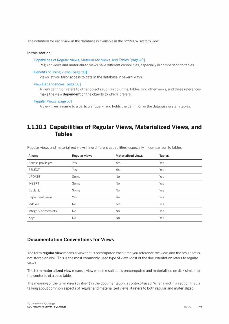
The definition for each view in the database is available in the SYSVIEW system view.
In this section:
Capabilities of Regular Views, Materialized Views, and Tables [page 49]Regular views and materialized views have different capabilities, especially in comparison to tables.
Benefits of Using Views [page 50]Views let you tailor access to data in the database in several ways.
View Dependencies [page 50]A view definition refers to other objects such as columns, tables, and other views, and these references make the view dependent on the objects to which it refers.
Regular Views [page 53]A view gives a name to a particular query, and holds the definition in the database system tables.
1.1.10.1 Capabilities of Regular Views, Materialized Views, and Tables
Regular views and materialized views have different capabilities, especially in comparison to tables.
Allows Regular views Materialized views Tables
Access privileges Yes Yes Yes
SELECT Yes Yes Yes
UPDATE Some No Yes
INSERT Some No Yes
DELETE Some No Yes
Dependent views Yes Yes Yes
Indexes No Yes Yes
Integrity constraints No No Yes
Keys No No Yes
Documentation Conventions for Views
The term regular view means a view that is recomputed each time you reference the view, and the result set is not stored on disk. This is the most commonly used type of view. Most of the documentation refers to regular views.
The term materialized view means a view whose result set is precomputed and materialized on disk similar to the contents of a base table.
The meaning of the term view (by itself) in the documentation is context-based. When used in a section that is talking about common aspects of regular and materialized views, it refers to both regular and materialized
SQL Anywhere SQL UsageSQL Anywhere Server - SQL Usage PUBLIC 49
views. If the term is used in documentation for materialized views, it refers to materialized views, and likewise for regular views.
1.1.10.2 Benefits of Using Views
Views let you tailor access to data in the database in several ways.
Efficient resource use
Regular views do not require additional storage space for data; they are recomputed each time you invoke them. Materialized views require disk space, but do not need to be recomputed each time they are invoked. Materialized views can improve response time in environments where the database is large, and the database server processes frequent, repetitive requests to join the same tables.Improved security
It allows access to only the information that is relevant.Improved usability
It presents users and application developers with data in a more easily understood form than in the base tables.Improved consistency
It centralizes the definition of common queries in the database.
1.1.10.3 View Dependencies
A view definition refers to other objects such as columns, tables, and other views, and these references make the view dependent on the objects to which it refers.
The set of referenced objects for a given view includes all the objects to which it refers either directly or indirectly. For example, a view can indirectly refer to a table, by referring to another view that references that table.
Consider the following set of tables and views:
CREATE TABLE t1 ( c1 INT, c2 INT ); CREATE TABLE t2( c3 INT, c4 INT );CREATE VIEW v1 AS SELECT * FROM t1;CREATE VIEW v2 AS SELECT c3 FROM t2; CREATE VIEW v3 AS SELECT c1, c3 FROM v1, v2;
The following view dependencies can be determined from the definitions above:
● View v1 is dependent on each individual column of t1, and on t1 itself.● View v2 is dependent on t2.c3, and on t2 itself.● View v3 is dependent on columns t1.c1 and t2.c3, tables t1 and t2, and views v1 and v2.
The database server keeps track of columns, tables, and views referenced by a given view. The database server uses this dependency information to ensure that schema changes to referenced objects do not leave a referencing view in an unusable state.
50 PUBLICSQL Anywhere SQL Usage
SQL Anywhere Server - SQL Usage
In this section:
Dependencies and Schema-altering Changes [page 51]An attempt to alter the schema defined for a table or view requires that the database server consider if there are dependent views impacted by the change.
Retrieving Dependency Information (SQL) [page 52]Retrieve a list of objects that are dependent on any table or view in the database.
1.1.10.3.1 Dependencies and Schema-altering Changes
An attempt to alter the schema defined for a table or view requires that the database server consider if there are dependent views impacted by the change.
Examples of schema-altering operations include:
● Dropping a table, view, materialized view, or column● Renaming a table, view, materialized view, or column● Adding, dropping, or altering columns● Altering a column's data type, size, or nullability● Disabling views or table view dependencies
Events that Take Place During Schema-Altering Operations
1. The database server generates a list of views that depend directly or indirectly upon the table or view being altered. Views with a DISABLED status are ignored.If any of the dependent views are materialized views, the request fails, an error is returned, and the remaining events do not occur. You must explicitly disable dependent materialized views before you can proceed with the schema-altering operation.
2. The database server obtains exclusive schema locks on the object being altered, and on all dependent regular views.
3. The database server sets the status of all dependent regular views to INVALID.4. The database server performs the schema-altering operation. If the operation fails, the locks are released,
the status of dependent regular views is reset to VALID, an error is returned, and the following step does not occur.
5. The database server recompiles the dependent regular views, setting each view status to VALID when successful. If compilation fails for any regular view, the status of that view continues to be INVALID. Subsequent requests for an INVALID regular view causes the database server to attempt to recompile the view. If subsequent attempts fail, it is likely that an alteration is required on the INVALID view, or on an object it depends on.
Regular Views: Dependencies and Schema Alterations
● A regular view can reference tables or views, including materialized views.
SQL Anywhere SQL UsageSQL Anywhere Server - SQL Usage PUBLIC 51
● When you change the schema of a table or view, the database automatically attempts to recompile all referencing regular views.
● When you disable or drop a view or table, all dependent regular views are automatically disabled.● You can use the DISABLE VIEW DEPENDENCIES clause of the ALTER TABLE statement to disable
dependent regular views.
Materialized Views: Dependencies and Schema Alterations
● A materialized view can only reference base tables.● Schema changes to a base table are not permitted if it is referenced by any enabled materialized views. You
can add foreign keys to the table (for example, ALTER TABLE ADD FOREIGN KEY).● Before you drop a table, you must disable or drop all dependent materialized views.● The DISABLE VIEW DEPENDENCIES clause of the ALTER TABLE statement does not impact materialized
views. To disable a materialized view, you must use the ALTER MATERIALIZED VIEW...DISABLE statement.● Once you disable a materialized view, you must explicitly re-enable it, for example using the ALTER
MATERIALIZED VIEW...ENABLE statement.
Related Information
Enabling or Disabling a Materialized View [page 75]
1.1.10.3.2 Retrieving Dependency Information (SQL)
Retrieve a list of objects that are dependent on any table or view in the database.
Prerequisites
Execution of the task does not require any privileges and assumes that PUBLIC has access to the catalog.
Context
The SYSDEPENDENCY system view stores dependency information. Each row in the SYSDEPENDENCY system view describes a dependency between two database objects. A direct dependency is when one object directly references another object in its definition. The database server uses direct dependency information to determine indirect dependencies as well. For example, suppose View A references View B, which in turn references Table C. In this case, View A is directly dependent on View B, and indirectly dependent on Table C.
52 PUBLICSQL Anywhere SQL Usage
SQL Anywhere Server - SQL Usage
This task is useful when you want to alter a table or view and must know the other objects that could be impacted.
Procedure
1. Connect to the database.2. Execute a statement that calls the sa_dependent_views system procedure.
Results
A list of IDs for the dependent views is returned.
Example
In this example, the sa_dependent_views system procedure is used in a SELECT statement to obtain the list of names of views dependent on the SalesOrders table. The procedure returns the ViewSalesOrders view.
SELECT t.table_name FROM SYSTAB t, sa_dependent_views( 'SalesOrders' ) v WHERE t.table_id = v.dep_view_id;
1.1.10.4 Regular Views
A view gives a name to a particular query, and holds the definition in the database system tables.
When you create a regular view, the database server stores the view definition in the database; no data is stored for the view. Instead, the view definition is executed only when it is referenced, and only for the duration of time that the view is in use. Creating a view does not require storing duplicate data in the database.
Suppose you must list the number of employees in each department frequently. You can get this list with the following statement:
SELECT DepartmentID, COUNT(*) FROM Employees GROUP BY DepartmentID;
Restrictions on SELECT Statements for Regular Views
There are some restrictions on the SELECT statements you can use as regular views. In particular, you cannot use an ORDER BY clause in the SELECT query. A characteristic of relational tables is that there is no
SQL Anywhere SQL UsageSQL Anywhere Server - SQL Usage PUBLIC 53
significance to the ordering of the rows or columns, and using an ORDER BY clause would impose an order on the rows of the view. You can use the GROUP BY clause, subqueries, and joins in view definitions.
To develop a view, tune the SELECT query by itself until it provides exactly the results you need in the format you want. Once you have the SELECT statement just right, you can add a phrase in front of the query to create the view:
CREATE VIEW view-name AS query;
Statements that Update Regular Views
Updates can be performed on a view using the UPDATE, INSERT, or DELETE statements if the query specification defining the view is updatable. Views are considered inherently non-updatable if their definition includes any one of the following in their query specification:
● UNION, EXCEPT, or INTERSECT.● DISTINCT clause.● GROUP BY clause.● WINDOW clause.● FIRST, TOP, or LIMIT clause.● aggregate functions.● more than one table in the FROM clause, when ansi_update_constraints option is set to 'Strict' or Cursor'.● ORDER BY clause, when ansi_update_constraints option is set to 'Strict' or Cursor'.● all SELECT list items are not base table columns.
The WITH CHECK OPTION Clause
When creating a view, the WITH CHECK OPTION clause is useful for controlling what data is changed when inserting into, or updating, a base table through a view. The following example illustrates this.
Execute the following statement to create the SalesEmployees view with a WITH CHECK OPTION clause.
CREATE VIEW SalesEmployees AS SELECT EmployeeID, GivenName, Surname, DepartmentID FROM Employees WHERE DepartmentID = 200 WITH CHECK OPTION;
Select to view the contents of this view, as follows:
SELECT * FROM SalesEmployees;
EmployeeID GivenName Surname DepartmentID
129 Philip Chin 200
195 Marc Dill 200
54 PUBLICSQL Anywhere SQL Usage
SQL Anywhere Server - SQL Usage
EmployeeID GivenName Surname DepartmentID
299 Rollin Overbey 200
467 James Klobucher 200
... ... ... ...
Next, attempt to update DepartmentID to 400 for Philip Chin:
UPDATE SalesEmployees SET DepartmentID = 400 WHERE EmployeeID = 129;
Since the WITH CHECK OPTION was specified, the database server evaluates whether the update violates anything in the view definition (in this case, the expression in the WHERE clause). The statement fails (DepartmentID must be 200), and the database server returns the error, "WITH CHECK OPTION violated for insert/update on base table 'Employees'".
If you had not specified the WITH CHECK OPTION in the view definition, the update operation would proceed, causing the Employees table to be modified with the new value, and subsequently causing Philip Chin to disappear from the view.
If a view (for example, View2) is created that references the SalesEmployees view, any updates or inserts on View2 are rejected that would cause the WITH CHECK OPTION criteria on SalesEmployees to fail, even if View2 is defined without a WITH CHECK OPTION clause.
In this section:
Statuses for Regular Views [page 56]Regular views have a status associated with them.
Creating a Regular View [page 57]Create a view that combines data from one or more sources.
Altering a Regular View [page 58]Alter a regular view by editing its definition in the database.
Dropping a Regular View [page 59]Drop a view when it is no longer required.
Disabling or Enabling a Regular View (SQL Central) [page 60]Control whether a regular view is available for use by the database server by enabling or disabling it.
Disabling or Enabling a Regular View (SQL) [page 61]Control whether a regular view is available for use by the database server by enabling or disabling it.
Browsing Data in a Regular View [page 63]Browse data in a regular view.
Related Information
Summarizing, Grouping, and Sorting Query Results [page 362]Materialized Views [page 64]
SQL Anywhere SQL UsageSQL Anywhere Server - SQL Usage PUBLIC 55
1.1.10.4.1 Statuses for Regular Views
Regular views have a status associated with them.
The status reflects the availability of the view for use by the database server.
You can view the status of all views by clicking Views in the left pane of SQL Central, and examining the values in the Status column in the right pane. Or, to see the status of a single view, right-click the view in SQL Central and click Properties to examine the Status value.
Following are descriptions of the possible statuses for regular views:
VALID
The view is valid and is guaranteed to be consistent with its definition. The database server can make use of this view without any additional work. An enabled view has the status VALID.
In the SYSOBJECT system view, the value 1 indicates a status of VALID.INVALID
An INVALID status occurs after a schema change to a referenced object where the change results in an unsuccessful attempt to enable the view. For example, suppose a view, v1, references a column, c1, in table t. If you alter t to remove c1, the status of v1 is set to INVALID when the database server tries to recompile the view as part of the ALTER operation that drops the column. In this case, v1 can recompile only after c1 is added back to t, or v1 is changed to no longer refer to c1. Views can also become INVALID if a table or view that they reference is dropped.
An INVALID view is different from a DISABLED view in that each time an INVALID view is referenced, for example by a query, the database server tries to recompile the view. If the compilation succeeds, the query proceeds. The view's status continues to be INVALID until it is explicitly enabled. If the compilation fails, an error is returned.
When the database server internally enables an INVALID view, it issues a performance warning.
In the SYSOBJECT system view, the value 2 indicates a status of INVALID.DISABLED
Disabled views are not available for use by the database server for answering queries. Any query that attempts to use a disabled view returns an error.
A regular view has this state if:
● you explicitly disable the view, for example by executing an ALTER VIEW...DISABLE statement.● you disable a view (materialized or not) that the view depends on.● you disable view dependencies for a table, for example by executing an ALTER TABLE...DISABLE VIEW
DEPENDENCIES statement.
In the SYSOBJECT system view, the value 4 indicates a status of DISABLED.
Related Information
Disabling or Enabling a Regular View (SQL) [page 61]
56 PUBLICSQL Anywhere SQL Usage
SQL Anywhere Server - SQL Usage
1.1.10.4.2 Creating a Regular View
Create a view that combines data from one or more sources.
Prerequisites
Views can improve performance and allow you to control the data that users can query.
You must have the CREATE VIEW system privilege to create views owned by you. You must have the CREATE ANY VIEW or CREATE ANY OBJECT system privilege to create views owned by others.
Procedure
1. In SQL Central, use the SQL Anywhere 17 plug-in to connect to the database.
2. In the left pane, right-click Views and click New View .3. Follow the instructions in the Create View Wizard.
4. In the right pane, click the SQL tab to edit the view definition. To save your changes, click File Save .
Results
The definition for the view you created is added to the database. Each time a query references the view, the definition is used to populate the view with data and return results.
Next Steps
Query the view to examine the results and ensure the correct data is returned.
SQL Anywhere SQL UsageSQL Anywhere Server - SQL Usage PUBLIC 57
1.1.10.4.3 Altering a Regular View
Alter a regular view by editing its definition in the database.
Prerequisites
You must be the owner of the view, or have one of the following privileges:
● ALTER ANY VIEW system privilege● ALTER ANY OBJECT system privilege
Context
If you want the view to contain data from an additional table, update the view definition to join the table data with the existing data sources in the view definition.
You must alter a view if the view definition is out of date (won't compile because of a schema change in the underlying data), needs columns added or removed, or requires changes related to its settings.
You cannot rename an existing view. Instead, you must create a new view with the new name, copy the previous definition to it, and then drop the old view.
Procedure
1. In SQL Central, use the SQL Anywhere 17 plug-in to connect to the database.2. In the left pane, double-click Views.3. Select the view.4. In the right pane, click the SQL tab and edit the view's definition.
TipTo edit multiple views, you can open separate windows for each view rather than editing each view on the SQL tab in the right pane. You can open a separate window by selecting a view and then clicking
File Edit In New Window .
5. Click File Save .
Results
The definition of the view is updated in the database.
58 PUBLICSQL Anywhere SQL Usage
SQL Anywhere Server - SQL Usage
Next Steps
Query the view to examine the results and ensure the correct data is returned.
If you alter a regular view and there are other views that are dependent on the view, there may be additional steps to take after the alteration is complete. For example, after you alter a view, the database server automatically recompiles it, enabling it for use by the database server. If there are dependent regular views, the database server disables and re-enables them as well. If they cannot be enabled, they are given the status INVALID and you must either make the definition of the regular view consistent with the definitions of the dependent regular views, or vice versa. To determine whether a regular view has dependent views, use the sa_dependent_views system procedure.
Related Information
View Dependencies [page 50]Dropping a Regular View [page 59]
1.1.10.4.4 Dropping a Regular View
Drop a view when it is no longer required.
Prerequisites
You must be the owner, or have the DROP ANY VIEW or DROP ANY OBJECT system privilege.
You must drop any INSTEAD OF triggers that reference the view before the view can be dropped.
Context
You must also drop a view (and recreate it) when you want to change the name of a view.
Procedure
1. In SQL Central, use the SQL Anywhere 17 plug-in to connect to the database.2. In the left pane, double-click Views.3. Right-click the view and click Delete.4. Click Yes.
SQL Anywhere SQL UsageSQL Anywhere Server - SQL Usage PUBLIC 59
Results
The definition for the regular view is deleted from the database.
Next Steps
If you drop a regular view that has dependent views, then the dependent views are made INVALID as part of the drop operation. The dependent views are not usable until they are changed or the original dropped view is recreated.
To determine whether a regular view has dependent views, use the sa_dependent_views system procedure.
Related Information
View Dependencies [page 50]INSTEAD OF Triggers [page 119]Altering a Regular View [page 58]Dropping a Trigger [page 115]
1.1.10.4.5 Disabling or Enabling a Regular View (SQL Central)
Control whether a regular view is available for use by the database server by enabling or disabling it.
Prerequisites
You must be the owner, or have one of the following privileges:
● ALTER ANY VIEW system privilege● ALTER ANY OBJECT system privilege
To enable a regular view, you must also have the following privileges SELECT privilege on the underlying table(s), or the SELECT ANY TABLE system privilege.
Before you enable a regular view, you must re-enable any disabled views that it references.
Procedure
1. In SQL Central, use the SQL Anywhere 17 plug-in to connect to the database.
60 PUBLICSQL Anywhere SQL Usage
SQL Anywhere Server - SQL Usage
2. In the left pane, double-click Views.3. To disable a regular view, right-click the view and click Disable.4. To enable a regular view, right-click the view and click Recompile And Enable.
Results
When you disable a regular view, the database server keeps the definition of the view in the database; however, the view is not available for use in satisfying a query.
If a query explicitly references a disabled view, the query fails and an error is returned.
Next Steps
Once you re-enable a view, you must re-enable all other views that were dependent on the view before it was disabled. You can determine the list of dependent views before disabling a view by using the sa_dependent_views system procedure.
When you enable a regular view, the database server recompiles it using the definition stored for the view in the database. If the compilation is successful, the view status changes to VALID. An unsuccessful recompile could indicate that the schema has changed in one or more of the referenced objects. If so, you must change either the view definition or the referenced objects until they are consistent with each other, and then enable the view.
Once a view is disabled, it must be explicitly re-enabled so that the database server can use it.
1.1.10.4.6 Disabling or Enabling a Regular View (SQL)
Control whether a regular view is available for use by the database server by enabling or disabling it.
Prerequisites
You must be the owner, or have one of the following privileges:
● ALTER ANY VIEW system privilege● ALTER ANY OBJECT system privilege
To enable a regular view, you must also have the following privileges SELECT privilege on the underlying table(s), or the SELECT ANY TABLE system privilege.
Before you enable a regular view, you must re-enable any disabled views that it references.
SQL Anywhere SQL UsageSQL Anywhere Server - SQL Usage PUBLIC 61
Context
If you disable a view, other views that reference it, directly or indirectly, are automatically disabled. So, once you re-enable a view, you must re-enable all other views that were dependent on the view when it was disabled. You can determine the list of dependent views before disabling a view using the sa_dependent_views system procedure.
Procedure
1. Connect to the database.2. To disable a regular view, execute an ALTER VIEW...DISABLE statement.3. To enable a regular view, execute an ALTER VIEW...ENABLE statement.
Results
When you disable a regular view, the database server keeps the definition of the view in the database; however, the view is not available for use in satisfying a query.
If a query explicitly references a disabled view, the query fails and an error is returned.
Example
The following example disables a regular view called ViewSalesOrders owned by GROUPO.
ALTER VIEW GROUPO.ViewSalesOrders DISABLE;
The following example re-enables the regular view called ViewSalesOrders owned by GROUPO.
ALTER VIEW GROUPO.ViewSalesOrders ENABLE;
Next Steps
Once you re-enable a view, you must re-enable all other views that were dependent on the view before it was disabled. You can determine the list of dependent views before disabling a view by using the sa_dependent_views system procedure.
When you enable a regular view, the database server recompiles it using the definition stored for the view in the database. If the compilation is successful, the view status changes to VALID. An unsuccessful recompile could indicate that the schema has changed in one or more of the referenced objects. If so, you must change either the view definition or the referenced objects until they are consistent with each other, and then enable the view.
62 PUBLICSQL Anywhere SQL Usage
SQL Anywhere Server - SQL Usage
Once a view is disabled, it must be explicitly re-enabled so that the database server can use it.
1.1.10.4.7 Browsing Data in a Regular View
Browse data in a regular view.
Prerequisites
The regular view must already be defined and be a valid view that is enabled.
You must be the owner, or have one of the following privileges:
● SELECT privilege on the view● SELECT ANY TABLE system privilege
Context
Regular views are stored in the database as definitions for the view. The view is populated with data when it is queried so that the data in the view is current.
This task starts in SQL Central, where you request the regular view that you want to view, and completes in Interactive SQL, where the data for the regular view is displayed.
Procedure
1. In SQL Central, use the SQL Anywhere 17 plug-in to connect to the database.2. In the left pane, click Views.
3. Select a view and then click File View Data In Interactive SQL .
Results
Interactive SQL opens with the view contents displayed on the Results tab of the Results pane.
Related Information
Queries [page 162]
SQL Anywhere SQL UsageSQL Anywhere Server - SQL Usage PUBLIC 63
Disabling or Enabling a Regular View (SQL Central) [page 60]
1.1.11 Materialized Views
A materialized view is a view whose result set has been precomputed from the base tables that it refers to and stored on disk, similar to a base table.
Conceptually, a materialized view is both a view (it has a query specification stored in the catalog) and a table (it has persistent materialized rows). So, many operations that you perform on tables can be performed on materialized views as well. For example, you can build indexes on materialized views.
When you create a materialized view the database server validates the definition to make sure it compiles properly. All column and table references are fully qualified by the database server to ensure that all users with access to the view see an identical definition. After successfully creating a materialized view, you populate it with data, also known as initializing the view.
Materialized views are listed in the Views folder in SQL Central.
In this section:
Performance Improvements Using Materialized Views [page 65]Materialized views can significantly improve performance by precomputing expensive operations such as joins and storing the results in the form of a view that is stored on disk.
Creating a Materialized View [page 72]Create a materialized view to store data from a query.
Initializing a Materialized View [page 73]Initialize a materialized view to populate it with data and make it available for use by the database server.
Refreshing a Materialized View Manually [page 74]Manually refresh materialized views that are not configured to refresh automatically.
Enabling or Disabling a Materialized View [page 75]Control whether a materialized view is available for querying by enabling and disabling it.
Hiding a Materialized View Definition [page 76]Hide a materialized view definition from users. This obfuscates the view definition stored in the database.
Dropping a Materialized View [page 78]Drop a materialized view from the database.
Encrypting or Decrypting a Materialized View [page 79]Encrypt materialized views for additional security on data.
Enabling or Disabling Optimizer Use of a Materialized View [page 80]Enable or disable optimizer use of a materialized view for satisfying queries.
Viewing Materialized View Information in the Catalog [page 81]View a list of all materialized views and their statuses, and also review the database options that were in force when each materialized view was created.
Changing the Refresh Type for a Materialized View [page 82]
64 PUBLICSQL Anywhere SQL Usage
SQL Anywhere Server - SQL Usage
Change the refresh type of a materialized view from manual to immediate and back again.
Advanced: Status and Properties for Materialized Views [page 83]Materialized view availability and state can be determined from their status and properties.
Advanced: Settings Controlling Data Staleness for Materialized Views [page 86]Data in a materialized view becomes stale when the data changes in the tables referenced by the materialized view.
1.1.11.1 Performance Improvements Using Materialized Views
Materialized views can significantly improve performance by precomputing expensive operations such as joins and storing the results in the form of a view that is stored on disk.
The optimizer considers materialized views when deciding on the most efficient way to satisfy a query, even when the materialized view is not referenced in the query.
In designing your application, consider defining materialized views for frequently executed expensive queries or expensive parts of your queries, such as those involving intensive aggregation and join operations. Materialized views are designed to improve performance in environments where:
● the database is large● frequent queries result in repetitive aggregation and join operations on large amounts of data● changes to underlying data are relatively infrequent● access to up-to-the-moment data is not a critical requirement
Consider the following requirements, settings, and restrictions before using a materialized view:
Disk space requirements
Since materialized views contain a duplicate of data from base tables, you may need to allocate additional space on disk for the database to accommodate the materialized views you create. Careful consideration needs to be given to the additional space requirements so that the benefit derived is balanced against the cost of using materialized views.Maintenance costs and data freshness requirements
The data in materialized views needs to be refreshed when data in the underlying tables changes. The frequency at which a materialized view needs to be refreshed needs to be determined by taking into account potentially conflicting factors, such as:
Rate at which underlying data changes
Frequent or large changes to data render manual views stale. Consider using an immediate view if data freshness is important.Cost of refreshing
Depending on the complexity of the underlying query for each materialized view, and the amount of data involved, the computation required for refreshing may be very expensive, and frequent refreshing of materialized views may impose an unacceptable workload on the database server. Additionally, materialized views are unavailable for use during the refresh operation.Data freshness requirements of applications
If the database server uses a stale materialized view, it presents stale data to applications. Stale data no longer represents the current state of data in the underlying tables. The degree of staleness is
SQL Anywhere SQL UsageSQL Anywhere Server - SQL Usage PUBLIC 65
governed by the frequency at which the materialized view is refreshed. An application must be designed to determine the degree of staleness it can tolerate to achieve improved performance.Data consistency requirements
When refreshing materialized views, you must determine the consistency with which the materialized views should be refreshed.
Use in optimization
Verify that the optimizer considers the materialized views when executing a query. You can see the list of materialized views used for a particular query by looking at the Advanced Details window of the query's graphical plan in Interactive SQL.Data-altering operations
Materialized views are read-only; no data-altering operations such as INSERT, LOAD, DELETE, and UPDATE, can be used on them.Keys, constraints, triggers, and articles
While you can create indexes on materialized views, you cannot create keys, constraints, triggers, or articles on them.
In this section:
Materialized Views and View Dependencies [page 66]You can control whether a materialized view is available for use by the database server by enabling or disabling it.
Whether to Set Refresh Type to Manual or Immediate [page 67]There are two refresh types for materialized views: manual and immediate.
Materialized Views Restrictions [page 69]There are many restrictions when creating, initializing, refreshing, and using materialized views.
Related Information
Advanced: Settings Controlling Data Staleness for Materialized Views [page 86]Advanced: Query Execution Plans [page 215]Enabling or Disabling Optimizer Use of a Materialized View [page 80]
1.1.11.1.1 Materialized Views and View Dependencies
You can control whether a materialized view is available for use by the database server by enabling or disabling it.
A disabled materialized view is not considered by the optimizer during optimization. If a query explicitly references a disabled materialized view, the query fails and an error is returned. When you disable a materialized view, the database server drops the data for the view, but keeps the definition in the database. When you re-enable a materialized view, it is in an uninitialized state and you must refresh it to populate it with data.
66 PUBLICSQL Anywhere SQL Usage
SQL Anywhere Server - SQL Usage
Regular views that are dependent on a materialized view are automatically disabled by the database server if the materialized view is disabled. As a result, once you re-enable a materialized view, you must re-enable all dependent views. For this reason, determine the list of views dependent on the materialized view before disabling it. You can do this using the sa_dependent_views system procedure. This procedure examines the ISYSDEPENDENCY system table and returns the list of dependent views, if any.
You can grant privileges on disabled objects. Privileges on disabled objects are stored in the database and become effective when the object is enabled.
Related Information
Dependencies and Schema-altering Changes [page 51]Enabling or Disabling a Materialized View [page 75]Retrieving Dependency Information (SQL) [page 52]
1.1.11.1.2 Whether to Set Refresh Type to Manual or Immediate
There are two refresh types for materialized views: manual and immediate.
Manual views
A manual materialized view, or manual view, is a materialized view with a refresh type defined as MANUAL REFRESH. Data in manual views can become stale because manual views are not refreshed until a refresh is explicitly requested, for example by using the REFRESH MATERIALIZED VIEW statement or the sa_refresh_materialized_views system procedure. By default, when you create a materialized view, it is a manual view.
A manual view is considered stale when any of the underlying tables change, even if the change does not impact data in the materialized view. You can determine whether a manual view is considered stale by examining the DataStatus value returned by the sa_materialized_view_info system procedure. If S is returned, the manual view is stale.Immediate views
An immediate materialized view, or immediate view, is a materialized view with a refresh type defined as IMMEDIATE REFRESH. Data in an immediate view is automatically refreshed when changes to the underlying tables affect data in the view. If changes to the underlying tables do not impact data in the view, the view is not refreshed.
Also, when an immediate view is refreshed, only stale rows must be changed. This is different from refreshing a manual view, where all data is dropped and recreated for a refresh.
You can change a manual view to an immediate view, and vice versa. However, the process for changing from a manual view to an immediate view has more steps.
Changing the refresh type for a materialized view can impact the status and properties of the view, especially when you change a manual view to an immediate view.
SQL Anywhere SQL UsageSQL Anywhere Server - SQL Usage PUBLIC 67
In this section:
Staleness and Manual Materialized Views [page 68]Materialized views that are manually refreshed become stale when changes occur to their underlying base tables.
Related Information
Advanced: Status and Properties for Materialized Views [page 83]Changing the Refresh Type for a Materialized View [page 82]
1.1.11.1.2.1 Staleness and Manual Materialized Views
Materialized views that are manually refreshed become stale when changes occur to their underlying base tables.
The optimizer does not consider a materialized view as a candidate for satisfying a query if the data has exceeded the staleness threshold configured for the view. Refreshing a manual view means that the database server re-executes the query definition for the view and replaces the view data with the new result set of the query. Refreshing makes the view data consistent with the underlying data. Consider the acceptable degree of data staleness for the manual view and devise a refresh strategy. Your strategy should allow for the time it takes to complete a refresh, since the view is not available for querying during the refresh operation.
You can also set up a strategy in which the view is refreshed using events. For example, you can create an event to refresh at some regular interval.
Immediate materialized views do not need to be refreshed unless they are uninitialized (contain no data), for example after being truncated.
You can configure a staleness threshold beyond which the optimizer should not use a materialized view when processing queries, by using the materialized_view_optimization database option.
NoteRefresh materialized views after upgrading your database server, or after rebuilding or upgrading your database to work with an upgraded database server.
Related Information
Advanced: Settings Controlling Data Staleness for Materialized Views [page 86]Refreshing a Materialized View Manually [page 74]
68 PUBLICSQL Anywhere SQL Usage
SQL Anywhere Server - SQL Usage
1.1.11.1.3 Materialized Views Restrictions
There are many restrictions when creating, initializing, refreshing, and using materialized views.
Creation Restrictions
● When you create a materialized view, the definition for the materialized view must define column names explicitly; you cannot include a SELECT * construct as part of the column definition.
● Do not include columns defined as TIMESTAMP WITH TIME ZONE in the materialized view. The value of the time_zone_adjustment option varies between connections based on their location and the time of year, resulting in incorrect results and unexpected behavior.
● When creating a materialized view, the definition for the materialized view cannot contain:○ references to other views, materialized or not○ references to remote or temporary tables○ variables such as CURRENT USER; all expressions must be deterministic○ calls to stored procedures, user-defined functions, or external functions○ Transact-SQL outer joins○ FOR XML clauses
The grouped-select-project-join query block must contain COUNT(*) n the select list, and is only allowed the SUM and COUNT aggregate functions.
● The following database options must have the specified settings when a materialized view is created; otherwise, an error is returned. These database option values are also required for the view to be used by the optimizer:○ ansinull=On○ conversion_error=On○ divide_by_zero_error=On○ sort_collation=Internal○ string_rtruncation=On
● The following database option settings are stored for each materialized view when it is created. The current option values for the connection must match the stored values for a materialized view for the view to be used in optimization:○ date_format○ date_order○ default_timestamp_increment○ first_day_of_week○ nearest_century○ precision○ scale○ time_format○ timestamp_format○ timestamp_with_time_zone_format○ default_timestamp_increment○ uuid_has_hyphens
SQL Anywhere SQL UsageSQL Anywhere Server - SQL Usage PUBLIC 69
● When a view is refreshed, the connection settings for all the options listed in the bullets above are ignored. Instead, the database option settings (which must match the stored settings for the view) are used.
ORDER BY Clause in a Materialized View Definition Has No Effect
Materialized views are similar to base tables in that the rows are not stored in any particular order; the database server orders the rows in the most efficient manner when computing the data. Therefore, specifying an ORDER BY clause in a materialized view definition has no impact on the ordering of rows when the view is materialized. Also, the ORDER BY clause in the view's definition is ignored by the optimizer when performing view matching.
Restrictions when Changing a Materialized View from Manual to Immediate
The following restrictions are checked when changing a manual view to an immediate view. An error is returned if the view violates any of the restrictions:
NoteYou can use the sa_materialized_view_can_be_immediate system procedure to find out if a manual view is eligible to become an immediate view.
● The view must be uninitialized.● If the view does not contain outer joins, then the view must have a unique index on non nullable columns. If
the view contains outer joins, the view must have a unique index on non nullable columns, or a unique index declared as WITH NULLS NOT DISTINCT on nullable columns.
● If the view definition is a grouped query, the unique index columns must correspond to SELECT list items that are not aggregate functions.
● The view definition cannot contain:○ GROUPING SETS clauses○ CUBE clauses○ ROLLUP clauses○ DISTINCT clauses○ row limit clauses○ non-deterministic expressions○ self and recursive joins○ LATERAL, CROSS APPLY, or APPLY clauses
● The view definition must be a single select-project-join or grouped-select-project-join query block, and the grouped-select-project-join query block cannot contain a HAVING clause.
● The grouped-select-project-join query block must contain COUNT ( * ) in the SELECT list, and is allowed only with the SUM and COUNT aggregate functions.
● An aggregate function in the SELECT list cannot be referenced in a complex expression. For example, SUM( expression ) + 1 is not allowed in the SELECT list.
● If the SELECT list contains the SUM( expression ) aggregate function and expression is a nullable expression, then the SELECT list must include a COUNT( expression ) aggregate function.
70 PUBLICSQL Anywhere SQL Usage
SQL Anywhere Server - SQL Usage
● If the view definition contains outer joins (LEFT OUTER JOIN, RIGHT OUTER JOIN, FULL OUTER JOIN) then the view definition must satisfy the following extra conditions:1. If a table, T, is referenced in an ON condition of an OUTER JOIN as a preserved side, then T must have a
primary key and the primary key columns must be present in the SELECT list of the view. For example, the immediate materialized view V defined as SELECT T1.pk, R1.X FROM T1, T2 LEFT OUTER JOIN ( R1 KEY JOIN R2 ) ON T1.Y = R.Y has the preserved table, T1, referenced in the ON clause and its primary key column, T1.pk, is in the SELECT list of the immediate materialized view, V.
2. For each NULL-supplying side of an outer join, there must be at least one base table such that one of its non-nullable columns is present in the SELECT list of the immediate materialized view. For example, for the immediate materialized view, V, defined as SELECT T1.pk, R1.X FROM T1, T2 LEFT OUTER JOIN ( R1 KEY JOIN R2 ) ON T1.Y = R1.Y, the NULL-supplying side of the left outer join is the table expression ( R1 KEY JOIN R2 ). The column R1.X is in the SELECT list of the V and R1.X is a non nullable column of the table R1.
3. If the view is a grouped view and the previous condition does not hold, then for each NULL-supplying side of an outer join, there must be at least one base table, T, such that one of its non-nullable columns, T.C, is used in the aggregate function COUNT( T.C ) in the SELECT list of the immediate materialized view. For example, for the immediate materialized view, V, defined as SELECT T1.pk, COUNT( R1.X ) FROM T1, T2 LEFT OUTER JOIN ( R1 KEY JOIN R2 ) ON T1.Y = R1.Y GROUP BY T1.pk, the NULL-supplying side of the left outer join is the table expression ( R1 KEY JOIN R2 ). The aggregate function COUNT( R1.X ) is in the SELECT list of the V and R1.X is a non-nullable column of the table R1.
4. The following conditions must be satisfied by the predicates of the views with outer joins:○ The ON clause predicates for LEFT, RIGHT, and FULL OUTER JOINs must refer to both preserved
and NULL-supplying table expression. For example, T LEFT OUTER JOIN R ON R.X = 1 does not satisfy this condition as the predicate R.X=1 references only the NULL-supplying side R.
○ Any predicate must reject NULL-supplied rows produced by a nested outer join. In other words, if a predicate refers to a table expression which is NULL-supplied by a nested outer join, then it must reject all rows which have nulls generated by that outer join.For example, the view V1 SELECT T1.pk, R1.X FROM T1, T2 LEFT OUTER JOIN ( R1 KEY JOIN R2 ) ON ( T1.Y = R1.Y ) WHERE R1.Z = 10 has the predicate R1.Z=10 referencing the table R1 which can be NULL-supplied by the T2 LEFT OUTER JOIN ( R1 KEY JOIN R2 ), hence it must reject any NULL-supplied rows. This is true because the predicate evaluates to UNKNOWN when the column R1.Z is NULL.However, the view V2 SELECT T1.pk, R1.X FROM T1, T2 LEFT OUTER JOIN ( R1 KEY JOIN R2 ) ON ( T1.Y = R1.Y ) WHERE R1.Z IS NULL does not have this property. The predicate R1.Z IS NULL references the NULL-supplying side R1 but it evaluates to TRUE when the table R1 is NULL-supplied (that is, the R1.Z column is null). The method of rejecting NULL-supplied rows is not as restrictive as a NULL-intolerant property. For example, the predicate R.X IS NOT DISTINCT FROM T.X and rowid( T ) IS NOT NULL is not NULL-intolerant on the table T as it evaluates to TRUE when T.X is NULL. However, the predicate rejects all the rows which are NULL-supplied on the base table T.
Related Information
Advanced: Status and Properties for Materialized Views [page 83]Outer Joins [page 396]
SQL Anywhere SQL UsageSQL Anywhere Server - SQL Usage PUBLIC 71
Creating an Index [page 41]Creating a Materialized View [page 72]
1.1.11.2 Creating a Materialized View
Create a materialized view to store data from a query.
Prerequisites
To create a materialized view owned by you, you must have the CREATE MATERIALIZED VIEW system privilege along with SELECT privilege on all underlying tables.
To create materialized views owned by others, you must have the CREATE ANY MATERIALIZED VIEW or CREATE ANY OBJECT system privileges along with SELECT privilege on all underlying tables.
Context
Create materialized views to satisfy queries that are frequently executed and that result in repetitive aggregation and join operations on large amounts of data. Materialized views can improve performance by pre-computing expensive operations in the form of a view that is stored on disk.
Procedure
1. In SQL Central, use the SQL Anywhere 17 plug-in to connect to the database.
2. In the left pane, right-click Views and click New Materialized View .3. Follow the instructions in the Create Materialized View Wizard.
Results
A non-initialized materialized view is created in the database. It does not have any data in it yet.
Next Steps
You must initialize the materialized view to populate it with data before you can use it.
72 PUBLICSQL Anywhere SQL Usage
SQL Anywhere Server - SQL Usage
Related Information
Materialized Views Restrictions [page 69]Dropping a Materialized View [page 78]Initializing a Materialized View [page 73]
1.1.11.3 Initializing a Materialized View
Initialize a materialized view to populate it with data and make it available for use by the database server.
Prerequisites
You must be the owner of the materialized view, have INSERT privilege on the materialized view, or have the INSERT ANY TABLE privilege.
Before creating, initializing, or refreshing materialized views, ensure that all materialized view restrictions have been met.
Context
To initialize a materialized view, you follow the same steps as refreshing a materialized view.
You can initialize all uninitialized materialized views in the database at once using the sa_refresh_materialized_views system procedure.
Procedure
1. In SQL Central, use the SQL Anywhere 17 plug-in to connect to the database.2. In the left pane, double-click Views.3. Right-click a materialized view and click Refresh Data.4. Select an isolation level and click OK.
Results
The materialized view is populated with data and becomes available for use by the database server. You can now query the materialized view.
SQL Anywhere SQL UsageSQL Anywhere Server - SQL Usage PUBLIC 73
Next Steps
Query the materialized view to ensure that it returns the expected data.
A failed initialization (refresh) attempt returns the materialized view to an uninitialized state. If initialization fails, review the definition for the materialized view to confirm that the underlying tables and columns specified are valid and available objects in your database.
Related Information
Materialized Views Restrictions [page 69]Dropping a Materialized View [page 78]Enabling or Disabling a Materialized View [page 75]
1.1.11.4 Refreshing a Materialized View Manually
Manually refresh materialized views that are not configured to refresh automatically.
Prerequisites
You must be the owner of the materialized view, have INSERT privilege on the materialized view, or have the INSERT ANY TABLE system privilege.
Procedure
1. In SQL Central, use the SQL Anywhere 17 plug-in to connect to the database.2. In the left pane, double-click Views.3. Right-click a materialized view and click Refresh Data.4. Select an isolation level and click OK.
Results
The data in the materialized view is refreshed to show the most recent data in the underlying objects.
74 PUBLICSQL Anywhere SQL Usage
SQL Anywhere Server - SQL Usage
Next Steps
Query the materialized view to ensure that it returns the expected data.
A failed refresh attempt converts the materialized view to an uninitialized state. If this occurs, review the definition for the materialized view to confirm that the underlying tables and columns specified are valid and available objects in your database.
Related Information
Dropping a Materialized View [page 78]Changing the Refresh Type for a Materialized View [page 82]
1.1.11.5 Enabling or Disabling a Materialized View
Control whether a materialized view is available for querying by enabling and disabling it.
Prerequisites
You must be the owner of the materialized view or have one of the following system privileges:
● ALTER ANY MATERIALIZED VIEW● ALTER ANY OBJECT
To enable a materialized view, you must also have the SELECT privilege on the underlying table(s) or the SELECT ANY TABLE system privilege.
Procedure
1. In SQL Central, use the SQL Anywhere 17 plug-in to connect to the database.2. In the left pane, double-click Views.
Option Action
Enable a materialized view
1. Right-click the view and click Recompile And Enable.2. (optional) Right-click the view and click Refresh Data to populate the view with data. This
step is optional because the first query that is run against the views after enabling it would also cause the view to be populated with data.
Disable a materialized view
Right-click the view and click Disable.
SQL Anywhere SQL UsageSQL Anywhere Server - SQL Usage PUBLIC 75
Results
When you enable a materialized view, it becomes available for use by the database server and you can query it.
When you disable a materialized view, the data and indexes are dropped. If the view was an immediate view, it is changed to a manual view. Querying a disabled materialized view fails and returns and error.
Next Steps
After you re-enable a view, you must rebuild any indexes for it, and change it back to an immediate view if it was an immediate view when it was disabled.
Related Information
View Dependencies [page 50]Changing the Refresh Type for a Materialized View [page 82]
1.1.11.6 Hiding a Materialized View Definition
Hide a materialized view definition from users. This obfuscates the view definition stored in the database.
Prerequisites
You must be the owner of the materialized view or have one of the following system privileges:
● ALTER ANY MATERIALIZED VIEW● ALTER ANY OBJECT
Context
When hiding a materialized view, this setting is irreversible.
When a materialized view is hidden, debugging using the debugger does not show the view definition, nor is the definition available through procedure profiling. The view can still be unloaded and reloaded into other databases.
Hiding a materialized view is irreversible and only possible using SQL.
76 PUBLICSQL Anywhere SQL Usage
SQL Anywhere Server - SQL Usage
Procedure
1. Connect to the database.2. Execute an ALTER MATERIALIZED VIEW...SET HIDDEN statement.
Results
An automatic commit is executed.
The view is no longer visible when browsing the catalog. The view can still be directly referenced, and is still eligible for use during query processing.
Example
The following statements create a materialized view, EmployeeConfid3, refresh it, and then obfuscate its view definition.
CautionWhen you are done running the following example, drop the materialized view you created. Otherwise, you will not be able to make schema changes to its underlying tables, Employees and Departments, when trying out other examples.
CREATE MATERIALIZED VIEW EmployeeConfid3 AS SELECT EmployeeID, Employees.DepartmentID, SocialSecurityNumber, Salary, ManagerID, Departments.DepartmentName, Departments.DepartmentHeadID FROM Employees, Departments WHERE Employees.DepartmentID=Departments.DepartmentID;REFRESH MATERIALIZED VIEW EmployeeConfid3; ALTER MATERIALIZED VIEW EmployeeConfid3 SET HIDDEN;
Related Information
Dropping a Materialized View [page 78]
SQL Anywhere SQL UsageSQL Anywhere Server - SQL Usage PUBLIC 77
1.1.11.7 Dropping a Materialized View
Drop a materialized view from the database.
Prerequisites
You must be the owner, or have the DROP ANY MATERIALIZED VIEW or DROP ANY OBJECT system privilege.
Before you can drop a materialized view, you must drop or disable all dependent views. To determine whether there are views dependent on a materialized view, use the sa_dependent_views system procedure.
Context
Perform this task when you no longer need the materialized view, or when you have made a schema change to an underlying referenced object such that the materialized view definition is no longer valid.
Procedure
1. In SQL Central, use the SQL Anywhere 17 plug-in to connect to the database.2. In the left pane, double-click Views.3. Right-click the materialized view and click Delete.4. Click Yes.
Results
The materialized view is dropped from the database.
Next Steps
If you had regular views that were dependent on the materialized view, you will not be able to enable them. You must change their definition or drop them.
Related Information
View Dependencies [page 50]
78 PUBLICSQL Anywhere SQL Usage
SQL Anywhere Server - SQL Usage
1.1.11.8 Encrypting or Decrypting a Materialized View
Encrypt materialized views for additional security on data.
Prerequisites
You must be the owner, or have both the CREATE ANY MATERIALIZED VIEW and DROP ANY MATERIALIZED VIEW system privileges, or both the CREATE ANY OBJECT and DROP ANY OBJECT system privileges.
Table encryption must already be enabled in the database to encrypt a materialized view.
Context
An example of when you might perform this task is when a materialized view contains data that was encrypted in the underlying table, and you want the data to be encrypted in the materialized view as well.
The encryption algorithm and key specified at database creation are used to encrypt the materialized view. To see the encryption settings in effect for your database, including whether table encryption is enabled, query the Encryption database property using the DB_PROPERTY function, as follows:
SELECT DB_PROPERTY( 'Encryption' );
As with table encryption, encrypting a materialized view can impact performance since the database server must decrypt data it retrieves from the view.
Procedure
1. In SQL Central, use the SQL Anywhere 17 plug-in to connect to the database.2. In the left pane, double-click Views.3. Right-click the materialized view and click Properties.4. Click the Miscellaneous tab.5. Select or clear the Materialized View Data Is Encrypted checkbox as appropriate.6. Click OK.
Results
The materialized view data is encrypted.
SQL Anywhere SQL UsageSQL Anywhere Server - SQL Usage PUBLIC 79

1.1.11.9 Enabling or Disabling Optimizer Use of a Materialized View
Enable or disable optimizer use of a materialized view for satisfying queries.
Prerequisites
You must be the owner, or have the ALTER ANY MATERIALIZED VIEW or ALTER ANY OBJECT system privilege.
Context
Even if a query does not reference a materialized view, the optimizer can decide to use the view to satisfy a query if doing so improves performance.
Procedure
1. In SQL Central, use the SQL Anywhere 17 plug-in to connect to the database.2. In the left pane, double-click Views.3. Right-click the materialized view and click Properties.4. Click the General tab and select or clear Used In Optimization, as appropriate.5. Click OK.
Results
When a materialized view is enabled for use by the optimizer, the optimizer will consider it when calculating the best plan for satisfying a query, even though the view is not explicitly referenced in the query. If a materialized view is disabled for use by the optimizer, the optimizer does not consider the view.
Next Steps
Query the underlying objects of the view to see if the optimizer makes use of the view by looking at the query execution plan. However, the availability of the view does not guarantee the optimizer uses it. The optimizer's choice is based on performance.
80 PUBLICSQL Anywhere SQL Usage
SQL Anywhere Server - SQL Usage
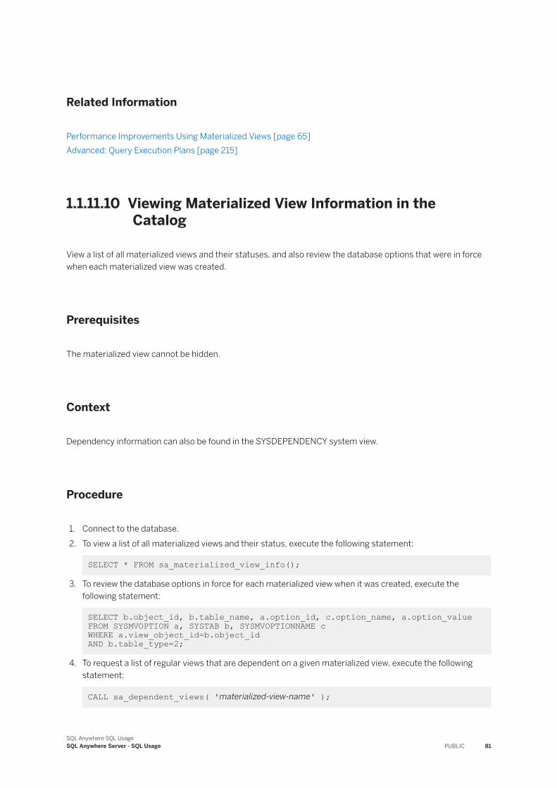
Related Information
Performance Improvements Using Materialized Views [page 65]Advanced: Query Execution Plans [page 215]
1.1.11.10 Viewing Materialized View Information in the Catalog
View a list of all materialized views and their statuses, and also review the database options that were in force when each materialized view was created.
Prerequisites
The materialized view cannot be hidden.
Context
Dependency information can also be found in the SYSDEPENDENCY system view.
Procedure
1. Connect to the database.2. To view a list of all materialized views and their status, execute the following statement:
SELECT * FROM sa_materialized_view_info();
3. To review the database options in force for each materialized view when it was created, execute the following statement:
SELECT b.object_id, b.table_name, a.option_id, c.option_name, a.option_value FROM SYSMVOPTION a, SYSTAB b, SYSMVOPTIONNAME cWHERE a.view_object_id=b.object_id AND b.table_type=2;
4. To request a list of regular views that are dependent on a given materialized view, execute the following statement:
CALL sa_dependent_views( 'materialized-view-name' );
SQL Anywhere SQL UsageSQL Anywhere Server - SQL Usage PUBLIC 81
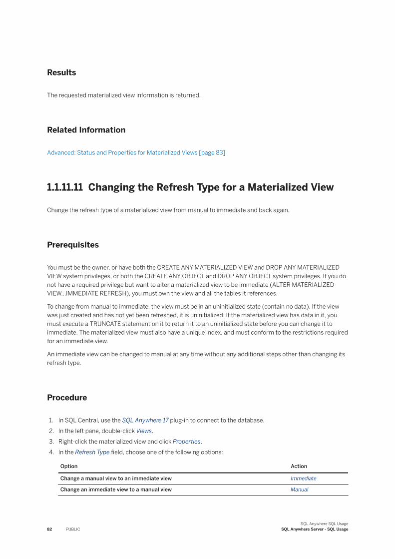
Results
The requested materialized view information is returned.
Related Information
Advanced: Status and Properties for Materialized Views [page 83]
1.1.11.11 Changing the Refresh Type for a Materialized View
Change the refresh type of a materialized view from manual to immediate and back again.
Prerequisites
You must be the owner, or have both the CREATE ANY MATERIALIZED VIEW and DROP ANY MATERIALIZED VIEW system privileges, or both the CREATE ANY OBJECT and DROP ANY OBJECT system privileges. If you do not have a required privilege but want to alter a materialized view to be immediate (ALTER MATERIALIZED VIEW...IMMEDIATE REFRESH), you must own the view and all the tables it references.
To change from manual to immediate, the view must be in an uninitialized state (contain no data). If the view was just created and has not yet been refreshed, it is uninitialized. If the materialized view has data in it, you must execute a TRUNCATE statement on it to return it to an uninitialized state before you can change it to immediate. The materialized view must also have a unique index, and must conform to the restrictions required for an immediate view.
An immediate view can be changed to manual at any time without any additional steps other than changing its refresh type.
Procedure
1. In SQL Central, use the SQL Anywhere 17 plug-in to connect to the database.2. In the left pane, double-click Views.3. Right-click the materialized view and click Properties.4. In the Refresh Type field, choose one of the following options:
Option Action
Change a manual view to an immediate view Immediate
Change an immediate view to a manual view Manual
82 PUBLICSQL Anywhere SQL Usage
SQL Anywhere Server - SQL Usage
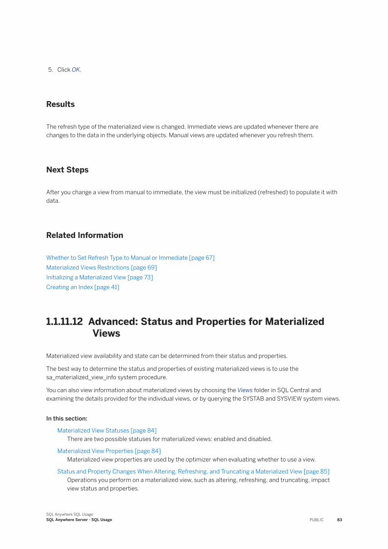
5. Click OK.
Results
The refresh type of the materialized view is changed. Immediate views are updated whenever there are changes to the data in the underlying objects. Manual views are updated whenever you refresh them.
Next Steps
After you change a view from manual to immediate, the view must be initialized (refreshed) to populate it with data.
Related Information
Whether to Set Refresh Type to Manual or Immediate [page 67]Materialized Views Restrictions [page 69]Initializing a Materialized View [page 73]Creating an Index [page 41]
1.1.11.12 Advanced: Status and Properties for Materialized Views
Materialized view availability and state can be determined from their status and properties.
The best way to determine the status and properties of existing materialized views is to use the sa_materialized_view_info system procedure.
You can also view information about materialized views by choosing the Views folder in SQL Central and examining the details provided for the individual views, or by querying the SYSTAB and SYSVIEW system views.
In this section:
Materialized View Statuses [page 84]There are two possible statuses for materialized views: enabled and disabled.
Materialized View Properties [page 84]Materialized view properties are used by the optimizer when evaluating whether to use a view.
Status and Property Changes When Altering, Refreshing, and Truncating a Materialized View [page 85]Operations you perform on a materialized view, such as altering, refreshing, and truncating, impact view status and properties.
SQL Anywhere SQL UsageSQL Anywhere Server - SQL Usage PUBLIC 83
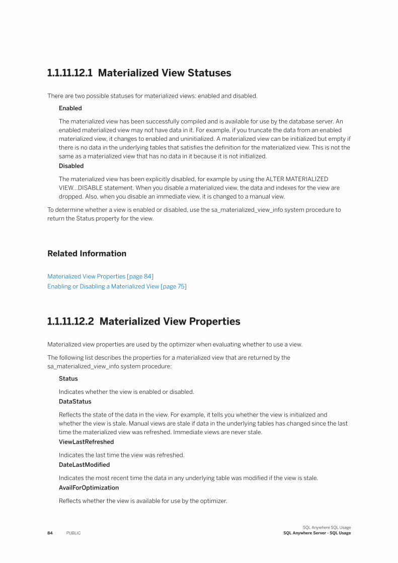
1.1.11.12.1 Materialized View Statuses
There are two possible statuses for materialized views: enabled and disabled.
Enabled
The materialized view has been successfully compiled and is available for use by the database server. An enabled materialized view may not have data in it. For example, if you truncate the data from an enabled materialized view, it changes to enabled and uninitialized. A materialized view can be initialized but empty if there is no data in the underlying tables that satisfies the definition for the materialized view. This is not the same as a materialized view that has no data in it because it is not initialized.Disabled
The materialized view has been explicitly disabled, for example by using the ALTER MATERIALIZED VIEW...DISABLE statement. When you disable a materialized view, the data and indexes for the view are dropped. Also, when you disable an immediate view, it is changed to a manual view.
To determine whether a view is enabled or disabled, use the sa_materialized_view_info system procedure to return the Status property for the view.
Related Information
Materialized View Properties [page 84]Enabling or Disabling a Materialized View [page 75]
1.1.11.12.2 Materialized View Properties
Materialized view properties are used by the optimizer when evaluating whether to use a view.
The following list describes the properties for a materialized view that are returned by the sa_materialized_view_info system procedure:
Status
Indicates whether the view is enabled or disabled.DataStatus
Reflects the state of the data in the view. For example, it tells you whether the view is initialized and whether the view is stale. Manual views are stale if data in the underlying tables has changed since the last time the materialized view was refreshed. Immediate views are never stale.ViewLastRefreshed
Indicates the last time the view was refreshed.DateLastModified
Indicates the most recent time the data in any underlying table was modified if the view is stale.AvailForOptimization
Reflects whether the view is available for use by the optimizer.
84 PUBLICSQL Anywhere SQL Usage
SQL Anywhere Server - SQL Usage
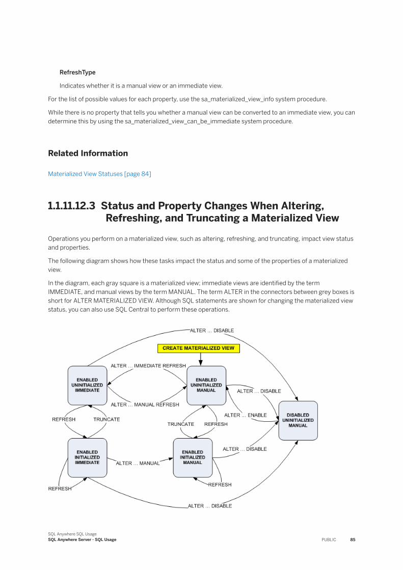
RefreshType
Indicates whether it is a manual view or an immediate view.
For the list of possible values for each property, use the sa_materialized_view_info system procedure.
While there is no property that tells you whether a manual view can be converted to an immediate view, you can determine this by using the sa_materialized_view_can_be_immediate system procedure.
Related Information
Materialized View Statuses [page 84]
1.1.11.12.3 Status and Property Changes When Altering, Refreshing, and Truncating a Materialized View
Operations you perform on a materialized view, such as altering, refreshing, and truncating, impact view status and properties.
The following diagram shows how these tasks impact the status and some of the properties of a materialized view.
In the diagram, each gray square is a materialized view; immediate views are identified by the term IMMEDIATE, and manual views by the term MANUAL. The term ALTER in the connectors between grey boxes is short for ALTER MATERIALIZED VIEW. Although SQL statements are shown for changing the materialized view status, you can also use SQL Central to perform these operations.
SQL Anywhere SQL UsageSQL Anywhere Server - SQL Usage PUBLIC 85
● When you create a materialized view, it is an enabled manual view and it is uninitialized (contains no data).● When you refresh an uninitialized view, it becomes initialized (populated with data).● Changing from a manual view to an immediate view requires several steps, and there are additional
restrictions for immediate views.● When you disable a materialized view:
○ the data is dropped○ the view reverts to uninitialized○ the indexes are dropped○ an immediate view reverts to manual
Related Information
Whether to Set Refresh Type to Manual or Immediate [page 67]Materialized Views Restrictions [page 69]Materialized View Properties [page 84]Materialized View Statuses [page 84]Changing the Refresh Type for a Materialized View [page 82]
1.1.11.13 Advanced: Settings Controlling Data Staleness for Materialized Views
Data in a materialized view becomes stale when the data changes in the tables referenced by the materialized view.
If the materialized view is not considered by the optimizer, then it may be due to staleness. Adjust the staleness threshold for materialized views using the materialized_view_optimization database option.
You can also adjust the interval specified for the event or trigger that is responsible for refreshing the view.
If a query explicitly references a materialized view, then the view is used to process the query regardless of freshness of the data in the view. As well, the OPTION clause of statements such as SELECT, UPDATE, and INSERT can be used to override the setting of the materialized_view_optimization database option, forcing the use of a materialized view.
When snapshot isolation is in use, the optimizer avoids using a materialized view if it was refreshed after the start of the snapshot for a transaction.
86 PUBLICSQL Anywhere SQL Usage
SQL Anywhere Server - SQL Usage
1.2 Stored Procedures, Triggers, Batches, and User-defined Functions
Procedures and triggers store procedural SQL statements in a database.
They can include control statements that allow repetition (LOOP statement) and conditional execution (IF statement and CASE statement) of SQL statements. Batches are sets of SQL statements submitted to the database server as a group. Many features available in procedures and triggers, such as control statements, are also available in batches.
CautionUse source control software to track changes to source code, and changes to objects created from source (including stored procedures), that you deploy to the database.
Procedures are invoked with a CALL statement, and use parameters to accept values and return values to the calling environment. SELECT statements can also operate on procedure result sets by including the procedure name in the FROM clause.
Procedures can return result sets to the caller, call other procedures, or fire triggers. For example, a user-defined function is a type of stored procedure that returns a single value to the calling environment. User-defined functions do not modify parameters passed to them, but rather, they broaden the scope of functions available to queries and other SQL statements.
Triggers are associated with specific database tables. They fire automatically whenever someone inserts, updates or deletes rows of the associated table. Triggers can call procedures and fire other triggers, but they have no parameters and cannot be invoked by a CALL statement.
Troubleshooting and Profiling Stored SQL
You can profile stored procedures to analyze performance characteristics in SQL Anywhere Profiler.
In this section:
Benefits of Procedures, Triggers, and User-defined Functions [page 88]Procedures and triggers enhance the security, efficiency, and standardization of databases.
Procedures [page 89]Procedures perform one or more specific tasks in the database.
User-defined Functions [page 101]User-defined functions return a single value to the calling environment.
Triggers [page 107]A trigger is a special form of stored procedure that is executed automatically when a statement that modifies data is executed.
Batches [page 120]A batch is a set of SQL statements submitted together and executed as a group, one after the other.
The Structure of Procedures, Triggers, and User-defined Functions [page 123]
SQL Anywhere SQL UsageSQL Anywhere Server - SQL Usage PUBLIC 87
The body of a procedure, trigger, and user-defined function consist of a compound statement.
Control Statements [page 127]There are several control statements for logical flow and decision making in the body of a procedure, trigger, or user-defined function, or in a batch.
Result Sets [page 129]Procedures can return results in the form of a single row of data, or multiple rows.
Cursors in Procedures, Triggers, User-defined Functions, and Batches [page 139]Cursors retrieve rows one at a time from a query or stored procedure with multiple rows in its result set.
Error and Warning Handling [page 142]After an application program executes a SQL statement, it can examine a status code (or return code) which indicates whether the statement executed successfully or failed and gives the reason for the failure.
EXECUTE IMMEDIATE Used in Procedures, Triggers, User-defined Functions, and Batches [page 154]The EXECUTE IMMEDIATE statement allows statements to be constructed using a combination of literal strings (in quotes) and variables.
Transactions and Savepoints in Procedures, Triggers, and User-defined Functions [page 156]SQL statements in a procedure or trigger are part of the current transaction.
Tips for Writing Procedures, Triggers, User-defined Functions, and Batches [page 157]There are several pointers that are helpful for writing procedures, triggers, user-defined functions, and batches.
Statements Allowed in Procedures, Triggers, Events, and Batches [page 158]Most SQL statements are acceptable in batches, but there are several exceptions.
Hiding the Contents of a Procedure, Function, Trigger, Event, or View [page 160]Use the SET HIDDEN clause to obscure the contents of a procedure, function, trigger, event, or view.
Related Information
The SQL Anywhere Debugger [page 849]
1.2.1 Benefits of Procedures, Triggers, and User-defined Functions
Procedures and triggers enhance the security, efficiency, and standardization of databases.
Definitions for procedures and triggers appear in the database, separately from any one database application. This separation provides several advantages.
88 PUBLICSQL Anywhere SQL Usage
SQL Anywhere Server - SQL Usage
Standardization
Procedures and triggers standardize actions performed by more than one application program. By coding the action once and storing it in the database for future use, applications need only call the procedure or fire the trigger to achieve the desired result repeatedly. And since changes occur in only one place, all applications using the action automatically acquire the new functionality if the implementation of the action changes.
Efficiency
Procedures and triggers used in a network database server environment can access data in the database without requiring network communication. This means they execute faster and with less impact on network performance than if they had been implemented in an application on one of the client machines.
When you create a procedure or trigger, it is automatically checked for correct syntax, and then stored in the system tables. The first time any application calls or fires a procedure or trigger, it is compiled from the system tables into the server's virtual memory and executed from there. Since one copy of the procedure or trigger remains in memory after the first execution, repeated executions of the same procedure or trigger happen instantly. As well, several applications can use a procedure or trigger concurrently, or one application can use it recursively.
1.2.2 Procedures
Procedures perform one or more specific tasks in the database.
In this section:
Procedures and Functions Running with Owner or Invoker Privileges [page 90]When you create a procedure or function you can specify whether you want the procedure or function to run with the privileges of its owner, or with the privileges of the person or procedure that calls it (the invoker).
Creating a Procedure (SQL Central) [page 96]Use the Create Procedure Wizard to create a procedure using a procedure template.
Altering a Procedure (SQL Central) [page 97]Alter an existing procedure in SQL Central.
Calling a Procedure (SQL) [page 98]Call a procedure and insert values.
Copying a Procedure (SQL Central) [page 99]Copy procedures between databases or within the same database by using SQL Central.
Dropping a Procedure (SQL Central) [page 100]Drop a procedure from your database, for example, when you no longer need it.
SQL Anywhere SQL UsageSQL Anywhere Server - SQL Usage PUBLIC 89
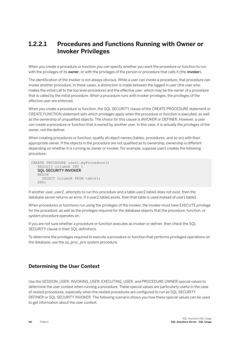
1.2.2.1 Procedures and Functions Running with Owner or Invoker Privileges
When you create a procedure or function you can specify whether you want the procedure or function to run with the privileges of its owner, or with the privileges of the person or procedure that calls it (the invoker).
The identification of the invoker is not always obvious. While a user can invoke a procedure, that procedure can invoke another procedure. In these cases, a distinction is made between the logged in user (the user who makes the initial call to the top level procedure) and the effective user, which may be the owner of a procedure that is called by the initial procedure. When a procedure runs with invoker privileges, the privileges of the effective user are enforced.
When you create a procedure or function, the SQL SECURITY clause of the CREATE PROCEDURE statement or CREATE FUNCTION statement sets which privileges apply when the procedure or function is executed, as well as the ownership of unqualified objects. The choice for this clause is INVOKER or DEFINER. However, a user can create a procedure or function that is owned by another user. In this case, it is actually the privileges of the owner, not the definer.
When creating procedures or function, qualify all object names (tables, procedures, and so on) with their appropriate owner. If the objects in the procedure are not qualified as to ownership, ownership is different depending on whether it is running as owner or invoker. For example, suppose user1 creates the following procedure:
CREATE PROCEDURE user1.myProcedure() RESULT( columnA INT ) SQL SECURITY INVOKER BEGIN SELECT columnA FROM table1; END;
If another user, user2, attempts to run this procedure and a table user2.table1 does not exist, then the database server returns an error. If a user2.table1 exists, then that table is used instead of user1.table1.
When procedures or functions run using the privileges of the invoker, the invoker must have EXECUTE privilege for the procedure, as well as the privileges required for the database objects that the procedure, function, or system procedure operates on.
If you are not sure whether a procedure or function executes as invoker or definer, then check the SQL SECURITY clause in their SQL definitions.
To determine the privileges required to execute a procedure or function that performs privileged operations on the database, use the sp_proc_priv system procedure.
Determining the User Context
Use the SESSION_USER, INVOKING_USER, EXECUTING_USER, and PROCEDURE OWNER special values to determine the user context when running a procedure. These special values are particularly useful in the case of nested procedures, especially when the nested procedures are configured to run as SQL SECURITY DEFINER or SQL SECURITY INVOKER. The following scenario shows you how these special values can be used to get information about the user context.
90 PUBLICSQL Anywhere SQL Usage
SQL Anywhere Server - SQL Usage
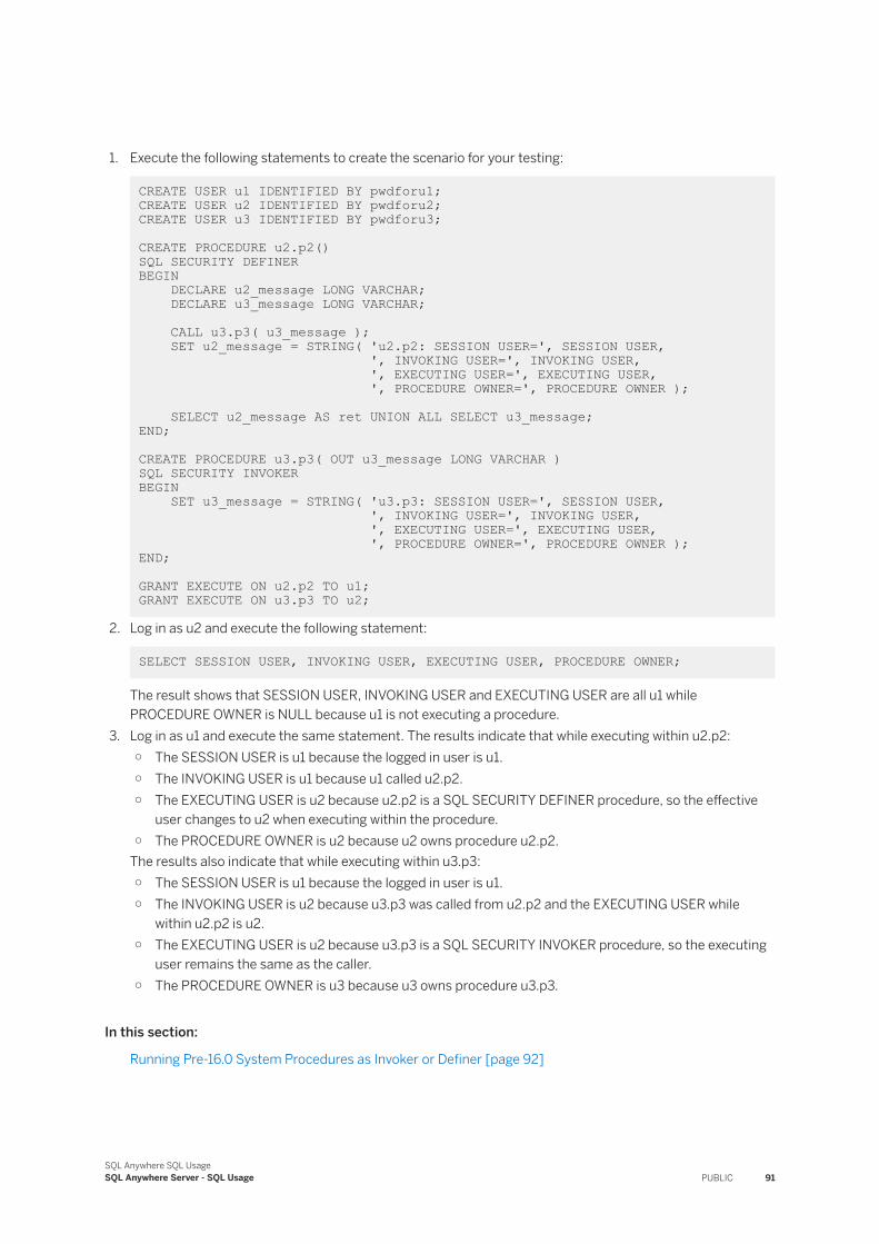
1. Execute the following statements to create the scenario for your testing:
CREATE USER u1 IDENTIFIED BY pwdforu1; CREATE USER u2 IDENTIFIED BY pwdforu2;CREATE USER u3 IDENTIFIED BY pwdforu3; CREATE PROCEDURE u2.p2()SQL SECURITY DEFINERBEGIN DECLARE u2_message LONG VARCHAR; DECLARE u3_message LONG VARCHAR; CALL u3.p3( u3_message ); SET u2_message = STRING( 'u2.p2: SESSION USER=', SESSION USER, ', INVOKING USER=', INVOKING USER, ', EXECUTING USER=', EXECUTING USER, ', PROCEDURE OWNER=', PROCEDURE OWNER ); SELECT u2_message AS ret UNION ALL SELECT u3_message;END; CREATE PROCEDURE u3.p3( OUT u3_message LONG VARCHAR )SQL SECURITY INVOKERBEGIN SET u3_message = STRING( 'u3.p3: SESSION USER=', SESSION USER, ', INVOKING USER=', INVOKING USER, ', EXECUTING USER=', EXECUTING USER, ', PROCEDURE OWNER=', PROCEDURE OWNER );END; GRANT EXECUTE ON u2.p2 TO u1;GRANT EXECUTE ON u3.p3 TO u2;
2. Log in as u2 and execute the following statement:
SELECT SESSION USER, INVOKING USER, EXECUTING USER, PROCEDURE OWNER;
The result shows that SESSION USER, INVOKING USER and EXECUTING USER are all u1 while PROCEDURE OWNER is NULL because u1 is not executing a procedure.
3. Log in as u1 and execute the same statement. The results indicate that while executing within u2.p2:○ The SESSION USER is u1 because the logged in user is u1.○ The INVOKING USER is u1 because u1 called u2.p2.○ The EXECUTING USER is u2 because u2.p2 is a SQL SECURITY DEFINER procedure, so the effective
user changes to u2 when executing within the procedure.○ The PROCEDURE OWNER is u2 because u2 owns procedure u2.p2.
The results also indicate that while executing within u3.p3:○ The SESSION USER is u1 because the logged in user is u1.○ The INVOKING USER is u2 because u3.p3 was called from u2.p2 and the EXECUTING USER while
within u2.p2 is u2.○ The EXECUTING USER is u2 because u3.p3 is a SQL SECURITY INVOKER procedure, so the executing
user remains the same as the caller.○ The PROCEDURE OWNER is u3 because u3 owns procedure u3.p3.
In this section:
Running Pre-16.0 System Procedures as Invoker or Definer [page 92]
SQL Anywhere SQL UsageSQL Anywhere Server - SQL Usage PUBLIC 91
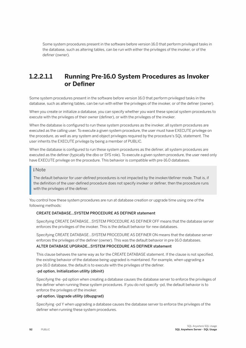
Some system procedures present in the software before version 16.0 that perform privileged tasks in the database, such as altering tables, can be run with either the privileges of the invoker, or of the definer (owner).
1.2.2.1.1 Running Pre-16.0 System Procedures as Invoker or Definer
Some system procedures present in the software before version 16.0 that perform privileged tasks in the database, such as altering tables, can be run with either the privileges of the invoker, or of the definer (owner).
When you create or initialize a database, you can specify whether you want these special system procedures to execute with the privileges of their owner (definer), or with the privileges of the invoker.
When the database is configured to run these system procedures as the invoker, all system procedures are executed as the calling user. To execute a given system procedure, the user must have EXECUTE privilege on the procedure, as well as any system and object privileges required by the procedure's SQL statement. The user inherits the EXECUTE privilege by being a member of PUBLIC.
When the database is configured to run these system procedures as the definer, all system procedures are executed as the definer (typically the dbo or SYS role). To execute a given system procedure, the user need only have EXECUTE privilege on the procedure. This behavior is compatible with pre-16.0 databases.
NoteThe default behavior for user-defined procedures is not impacted by the invoker/definer mode. That is, if the definition of the user-defined procedure does not specify invoker or definer, then the procedure runs with the privileges of the definer.
You control how these system procedures are run at database creation or upgrade time using one of the following methods:
CREATE DATABASE...SYSTEM PROCEDURE AS DEFINER statement
Specifying CREATE DATABASE...SYSTEM PROCEDURE AS DEFINER OFF means that the database server enforces the privileges of the invoker. This is the default behavior for new databases.
Specifying CREATE DATABASE...SYSTEM PROCEDURE AS DEFINER ON means that the database server enforces the privileges of the definer (owner). This was the default behavior in pre-16.0 databases.ALTER DATABASE UPGRADE...SYSTEM PROCEDURE AS DEFINER statement
This clause behaves the same way as for the CREATE DATABASE statement. If the clause is not specified, the existing behavior of the database being upgraded is maintained. For example, when upgrading a pre-16.0 database, the default is to execute with the privileges of the definer.-pd option, Initialization utility (dbinit)
Specifying the -pd option when creating a database causes the database server to enforce the privileges of the definer when running these system procedures. If you do not specify -pd, the default behavior is to enforce the privileges of the invoker.-pd option, Upgrade utility (dbupgrad)
Specifying -pd Y when upgrading a database causes the database server to enforce the privileges of the definer when running these system procedures.
92 PUBLICSQL Anywhere SQL Usage
SQL Anywhere Server - SQL Usage
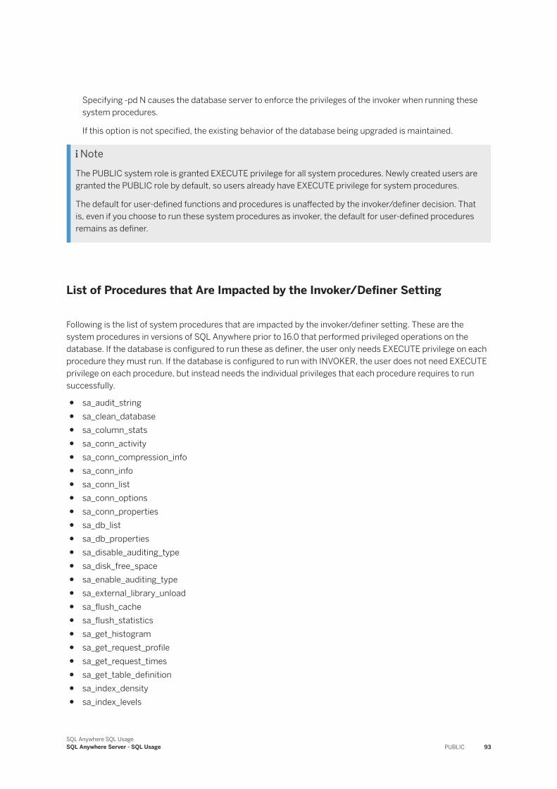
Specifying -pd N causes the database server to enforce the privileges of the invoker when running these system procedures.
If this option is not specified, the existing behavior of the database being upgraded is maintained.
NoteThe PUBLIC system role is granted EXECUTE privilege for all system procedures. Newly created users are granted the PUBLIC role by default, so users already have EXECUTE privilege for system procedures.
The default for user-defined functions and procedures is unaffected by the invoker/definer decision. That is, even if you choose to run these system procedures as invoker, the default for user-defined procedures remains as definer.
List of Procedures that Are Impacted by the Invoker/Definer Setting
Following is the list of system procedures that are impacted by the invoker/definer setting. These are the system procedures in versions of SQL Anywhere prior to 16.0 that performed privileged operations on the database. If the database is configured to run these as definer, the user only needs EXECUTE privilege on each procedure they must run. If the database is configured to run with INVOKER, the user does not need EXECUTE privilege on each procedure, but instead needs the individual privileges that each procedure requires to run successfully.
● sa_audit_string● sa_clean_database● sa_column_stats● sa_conn_activity● sa_conn_compression_info● sa_conn_info● sa_conn_list● sa_conn_options● sa_conn_properties● sa_db_list● sa_db_properties● sa_disable_auditing_type● sa_disk_free_space● sa_enable_auditing_type● sa_external_library_unload● sa_flush_cache● sa_flush_statistics● sa_get_histogram● sa_get_request_profile● sa_get_request_times● sa_get_table_definition● sa_index_density● sa_index_levels
SQL Anywhere SQL UsageSQL Anywhere Server - SQL Usage PUBLIC 93
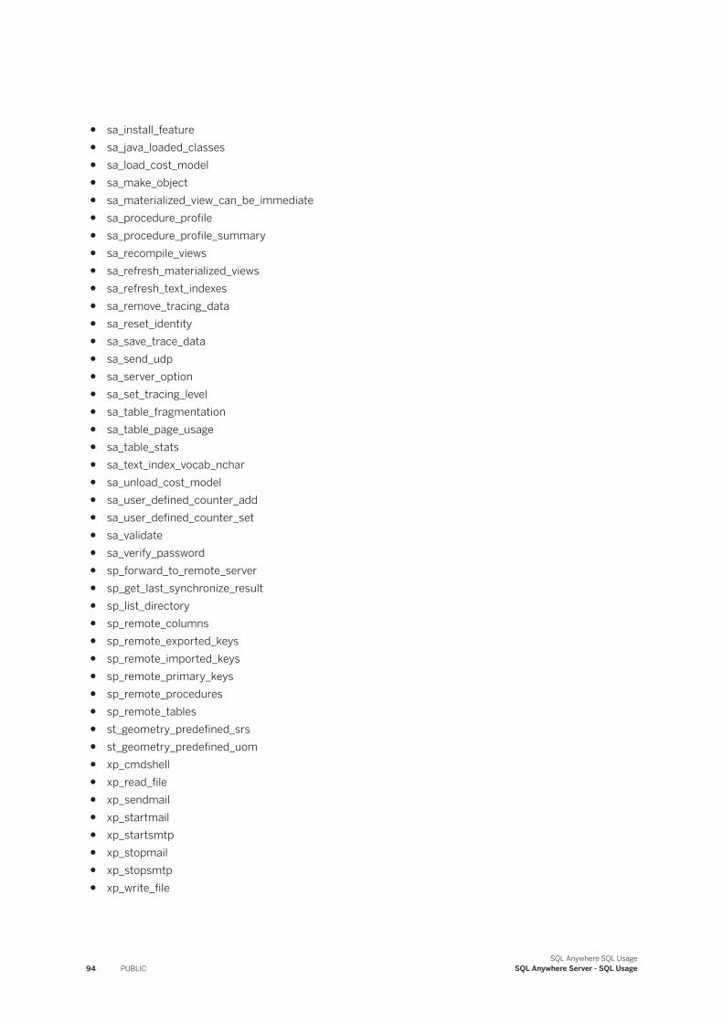
● sa_install_feature● sa_java_loaded_classes● sa_load_cost_model● sa_make_object● sa_materialized_view_can_be_immediate● sa_procedure_profile● sa_procedure_profile_summary● sa_recompile_views● sa_refresh_materialized_views● sa_refresh_text_indexes● sa_remove_tracing_data● sa_reset_identity● sa_save_trace_data● sa_send_udp● sa_server_option● sa_set_tracing_level● sa_table_fragmentation● sa_table_page_usage● sa_table_stats● sa_text_index_vocab_nchar● sa_unload_cost_model● sa_user_defined_counter_add● sa_user_defined_counter_set● sa_validate● sa_verify_password● sp_forward_to_remote_server● sp_get_last_synchronize_result● sp_list_directory● sp_remote_columns● sp_remote_exported_keys● sp_remote_imported_keys● sp_remote_primary_keys● sp_remote_procedures● sp_remote_tables● st_geometry_predefined_srs● st_geometry_predefined_uom● xp_cmdshell● xp_read_file● xp_sendmail● xp_startmail● xp_startsmtp● xp_stopmail● xp_stopsmtp● xp_write_file
94 PUBLICSQL Anywhere SQL Usage
SQL Anywhere Server - SQL Usage
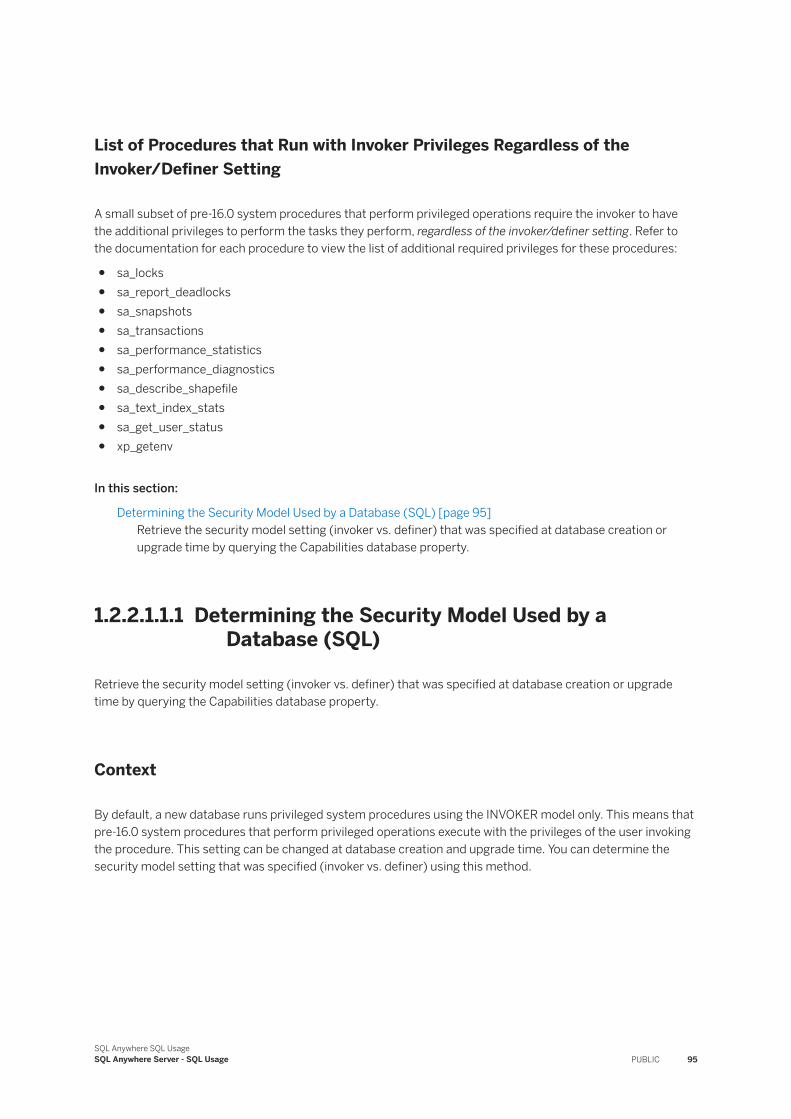
List of Procedures that Run with Invoker Privileges Regardless of the Invoker/Definer Setting
A small subset of pre-16.0 system procedures that perform privileged operations require the invoker to have the additional privileges to perform the tasks they perform, regardless of the invoker/definer setting. Refer to the documentation for each procedure to view the list of additional required privileges for these procedures:
● sa_locks● sa_report_deadlocks● sa_snapshots● sa_transactions● sa_performance_statistics● sa_performance_diagnostics● sa_describe_shapefile● sa_text_index_stats● sa_get_user_status● xp_getenv
In this section:
Determining the Security Model Used by a Database (SQL) [page 95]Retrieve the security model setting (invoker vs. definer) that was specified at database creation or upgrade time by querying the Capabilities database property.
1.2.2.1.1.1 Determining the Security Model Used by a Database (SQL)
Retrieve the security model setting (invoker vs. definer) that was specified at database creation or upgrade time by querying the Capabilities database property.
Context
By default, a new database runs privileged system procedures using the INVOKER model only. This means that pre-16.0 system procedures that perform privileged operations execute with the privileges of the user invoking the procedure. This setting can be changed at database creation and upgrade time. You can determine the security model setting that was specified (invoker vs. definer) using this method.
SQL Anywhere SQL UsageSQL Anywhere Server - SQL Usage PUBLIC 95
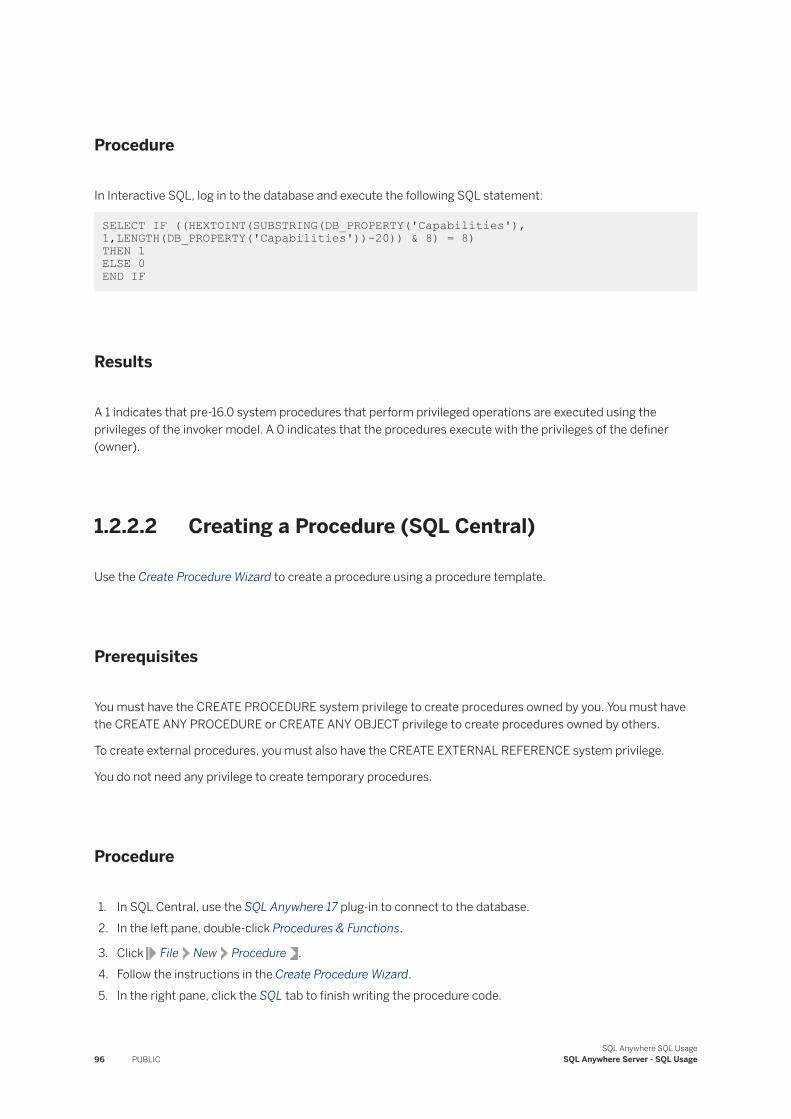
Procedure
In Interactive SQL, log in to the database and execute the following SQL statement:
SELECT IF ((HEXTOINT(SUBSTRING(DB_PROPERTY('Capabilities'),1,LENGTH(DB_PROPERTY('Capabilities'))-20)) & 8) = 8) THEN 1ELSE 0 END IF
Results
A 1 indicates that pre-16.0 system procedures that perform privileged operations are executed using the privileges of the invoker model. A 0 indicates that the procedures execute with the privileges of the definer (owner).
1.2.2.2 Creating a Procedure (SQL Central)
Use the Create Procedure Wizard to create a procedure using a procedure template.
Prerequisites
You must have the CREATE PROCEDURE system privilege to create procedures owned by you. You must have the CREATE ANY PROCEDURE or CREATE ANY OBJECT privilege to create procedures owned by others.
To create external procedures, you must also have the CREATE EXTERNAL REFERENCE system privilege.
You do not need any privilege to create temporary procedures.
Procedure
1. In SQL Central, use the SQL Anywhere 17 plug-in to connect to the database.2. In the left pane, double-click Procedures & Functions.
3. Click File New Procedure .4. Follow the instructions in the Create Procedure Wizard.5. In the right pane, click the SQL tab to finish writing the procedure code.
96 PUBLICSQL Anywhere SQL Usage
SQL Anywhere Server - SQL Usage
Results
The new procedure appears in Procedures & Functions. You can use this procedure in your application.
Related Information
Compound Statements [page 128]Remote Servers and Remote Table Mappings [page 677]Creating Remote Procedures (SQL Central) [page 709]
1.2.2.3 Altering a Procedure (SQL Central)
Alter an existing procedure in SQL Central.
Prerequisites
You must be the owner of the procedure or have one of the following privileges:
● ALTER ANY PROCEDURE system privilege● ALTER ANY OBJECT system privilege
Context
In SQL Central, you cannot rename an existing procedure directly. Instead, you must create a new procedure with the new name, copy the previous code to it, and then delete the old procedure.
Procedure
1. In SQL Central, use the SQL Anywhere 17 plug-in to connect to the database.2. In the left pane, double-click Procedures & Functions.3. Select the procedure.4. Use one of the following methods to edit the procedure:
○ In the right pane, click the SQL tab.○ Right-click the procedure and click Edit in New Window.
SQL Anywhere SQL UsageSQL Anywhere Server - SQL Usage PUBLIC 97
TipYou can open a separate window for each procedure and copy code between procedures.
○ To add or edit a procedure comment, right-click the procedure and click Properties.If you use the Database Documentation Wizard to document your SQL Anywhere database, you have the option to include these comments in the output.
Results
The code of the procedure is altered.
Related Information
Creating a Procedure (SQL Central) [page 96]Translating a Stored Procedure [page 559]
1.2.2.4 Calling a Procedure (SQL)
Call a procedure and insert values.
Prerequisites
You must be the owner of the procedure, have the EXECUTE privilege on the procedure, or have the EXECUTE ANY PROCEDURE system privilege.
All users who have been granted EXECUTE privilege for the procedure can call the procedure, even if they have no privilege on the table.
Context
CALL statements invoke procedures.
98 PUBLICSQL Anywhere SQL Usage
SQL Anywhere Server - SQL Usage
Procedure
Execute the following statement to call a procedure and insert values:
CALL procedure-name( values );
After this call, you may want to ensure that the values have been added.
NoteYou can call a procedure that returns a result set by calling it in a query. You can execute queries on the result sets of procedures and apply WHERE clauses and other SELECT features to limit the result set.
Results
The procedure is called and executed.
Example
The following statement calls the NewDepartment procedure to insert an Eastern Sales department:
CALL NewDepartment( 210, 'Eastern Sales', 902 );
After this call completes, you can to check the Departments table to verify that the new department has been added.
All users who have been granted EXECUTE privilege for the procedure can call the NewDepartment procedure, even if they have no privilege on the Departments table.
1.2.2.5 Copying a Procedure (SQL Central)
Copy procedures between databases or within the same database by using SQL Central.
Prerequisites
To copy a procedure and assign yourself as the owner, you must have the CREATE PROCEDURE system privilege in the database you are copying the procedure to. To copy a procedure and assign a different user as the owner, you must have the CREATE ANY PROCEDURE or CREATE ANY OBJECT system privilege in the database you are copying the procedure to.
SQL Anywhere SQL UsageSQL Anywhere Server - SQL Usage PUBLIC 99
Context
If you copy a procedure within the same database, you must rename the procedure or choose a different owner for the copied procedure.
Procedure
1. In SQL Central, use the SQL Anywhere 17 plug-in to connect to the database that contains the procedure you want to copy.
2. Connect to the database that you want to copy the procedure to.3. Select the procedure you want to copy in the left pane of the first database, and drag it to Procedures &
Functions of the second database.
Results
A new procedure is created, and the original procedure's code is copied to it. Only the procedure code is copied to the new procedure. Other procedure properties, such as privileges, are not copied.
1.2.2.6 Dropping a Procedure (SQL Central)
Drop a procedure from your database, for example, when you no longer need it.
Prerequisites
You must be the owner of the procedure or have one of the following system privileges:
● DROP ANY PROCEDURE● DROP ANY OBJECT
Procedure
1. In SQL Central, use the SQL Anywhere 17 plug-in to connect to the database.2. In the left pane, double-click Procedures & Functions.3. Right-click the procedure and click Delete.4. Click Yes.
100 PUBLICSQL Anywhere SQL Usage
SQL Anywhere Server - SQL Usage
Results
The procedure is removed from the database.
Next Steps
Dependent database objects must have their definitions modified to remove reference to the dropped procedure.
1.2.3 User-defined Functions
User-defined functions return a single value to the calling environment.
NoteThe database server does not make any assumptions about whether user-defined functions are thread-safe. This is the responsibility of the application developer.
The CREATE FUNCTION syntax differs slightly from that of the CREATE PROCEDURE statement.
● No IN, OUT, or INOUT keywords are required, as all parameters are IN parameters.● The RETURNS clause is required to specify the data type being returned.● The RETURN statement is required to specify the value being returned.● Named parameters are not supported.
In this section:
Creating a User-defined Function [page 102]Create a user-defined function using SQL Central.
Calling a User-defined Function [page 102]Create a user-defined function using Interactive SQL.
Dropping a User-defined Function (SQL) [page 105]Drop a user-defined function.
Granting the Ability to Execute a User-defined Function (SQL) [page 106]Grant the ability to execute a user-defined function by granting the EXECUTE object-level privilege.
Advanced Information About User-defined Functions [page 107]The database server treats all user-defined functions as idempotent unless they are declared NOT DETERMINISTIC.
SQL Anywhere SQL UsageSQL Anywhere Server - SQL Usage PUBLIC 101
1.2.3.1 Creating a User-defined Function
Create a user-defined function using SQL Central.
Prerequisites
You must have the CREATE PROCEDURE system privilege to create functions owned by you. You must have the CREATE ANY PROCEDURE or CREATE ANY OBJECT system privilege to create functions owned by others.
You must have the CREATE EXTERNAL REFERENCE system privilege to create an external function.
No privilege is required to create temporary functions.
Context
User-defined functions are a class of procedures that return a single value to the calling environment.
Procedure
1. In SQL Central, use the SQL Anywhere 17 plug-in to connect to the database.
2. In the left pane, right-click Procedures & Functions and click New Function .3. Follow the instructions in the Create Function Wizard.4. In the right pane, click the SQL tab to finish writing the function code.
Results
The new function appears in Procedures & Functions.
1.2.3.2 Calling a User-defined Function
Create a user-defined function using Interactive SQL.
Prerequisites
You must have EXECUTE privilege on the function.
102 PUBLICSQL Anywhere SQL Usage
SQL Anywhere Server - SQL Usage
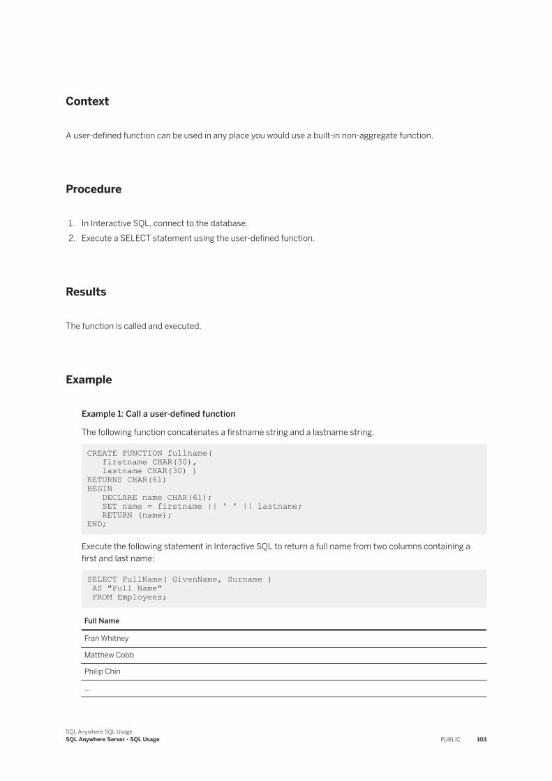
Context
A user-defined function can be used in any place you would use a built-in non-aggregate function.
Procedure
1. In Interactive SQL, connect to the database.2. Execute a SELECT statement using the user-defined function.
Results
The function is called and executed.
Example
Example 1: Call a user-defined function
The following function concatenates a firstname string and a lastname string.
CREATE FUNCTION fullname( firstname CHAR(30), lastname CHAR(30) )RETURNS CHAR(61)BEGIN DECLARE name CHAR(61); SET name = firstname || ' ' || lastname; RETURN (name); END;
Execute the following statement in Interactive SQL to return a full name from two columns containing a first and last name:
SELECT FullName( GivenName, Surname ) AS "Full Name" FROM Employees;
Full Name
Fran Whitney
Matthew Cobb
Philip Chin
...
SQL Anywhere SQL UsageSQL Anywhere Server - SQL Usage PUBLIC 103
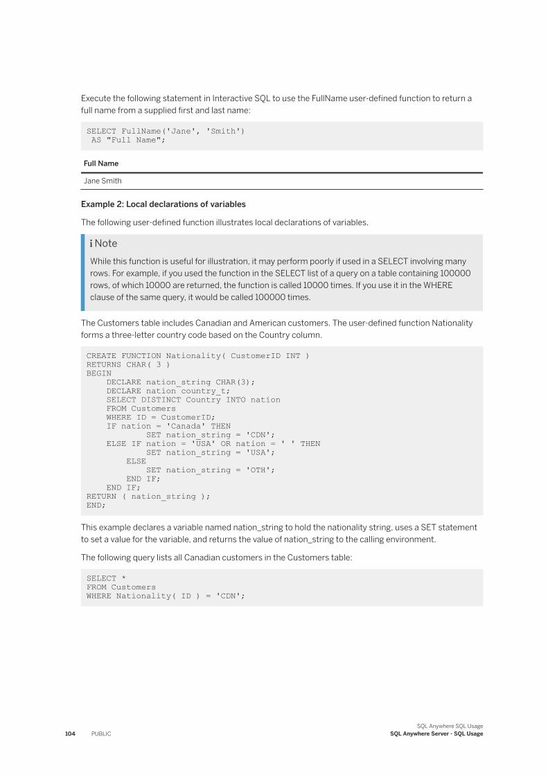
Execute the following statement in Interactive SQL to use the FullName user-defined function to return a full name from a supplied first and last name:
SELECT FullName('Jane', 'Smith') AS "Full Name";
Full Name
Jane Smith
Example 2: Local declarations of variables
The following user-defined function illustrates local declarations of variables.
NoteWhile this function is useful for illustration, it may perform poorly if used in a SELECT involving many rows. For example, if you used the function in the SELECT list of a query on a table containing 100000 rows, of which 10000 are returned, the function is called 10000 times. If you use it in the WHERE clause of the same query, it would be called 100000 times.
The Customers table includes Canadian and American customers. The user-defined function Nationality forms a three-letter country code based on the Country column.
CREATE FUNCTION Nationality( CustomerID INT ) RETURNS CHAR( 3 )BEGIN DECLARE nation_string CHAR(3); DECLARE nation country_t; SELECT DISTINCT Country INTO nation FROM Customers WHERE ID = CustomerID; IF nation = 'Canada' THEN SET nation_string = 'CDN'; ELSE IF nation = 'USA' OR nation = ' ' THEN SET nation_string = 'USA'; ELSE SET nation_string = 'OTH'; END IF; END IF;RETURN ( nation_string ); END;
This example declares a variable named nation_string to hold the nationality string, uses a SET statement to set a value for the variable, and returns the value of nation_string to the calling environment.
The following query lists all Canadian customers in the Customers table:
SELECT * FROM Customers WHERE Nationality( ID ) = 'CDN';
104 PUBLICSQL Anywhere SQL Usage
SQL Anywhere Server - SQL Usage
1.2.3.3 Dropping a User-defined Function (SQL)
Drop a user-defined function.
Prerequisites
You must be the owner of the user-defined function or have one of the following system privileges:
● DROP ANY PROCEDURE● DROP ANY OBJECT
Procedure
1. Connect to the database.2. Execute a DROP FUNCTION statement similar to the following:
DROP FUNCTION function-name;
Results
The user-defined function is dropped.
Example
The following statement removes the function FullName from the database:
DROP FUNCTION FullName;
SQL Anywhere SQL UsageSQL Anywhere Server - SQL Usage PUBLIC 105
1.2.3.4 Granting the Ability to Execute a User-defined Function (SQL)
Grant the ability to execute a user-defined function by granting the EXECUTE object-level privilege.
Prerequisites
You must be the owner of the user-defined function, or have EXECUTE privilege with administrative rights on the function.
Ownership of a user-defined function belongs to the user who created it, and no privilege is required for that user to execute it.
Context
You have created a function and you want other user to be able to use it.
Procedure
1. Connect to the database.2. Execute a GRANT EXECUTE statement similar to the following:
GRANT EXECUTE ON function-name TO user-id;
Results
The grantee can now execute the procedure.
Example
For example, the creator of the Nationality function could allow another user to use Nationality with the statement:
GRANT EXECUTE ON Nationality TO BobS;
106 PUBLICSQL Anywhere SQL Usage
SQL Anywhere Server - SQL Usage
1.2.3.5 Advanced Information About User-defined Functions
The database server treats all user-defined functions as idempotent unless they are declared NOT DETERMINISTIC.
Idempotent functions return a consistent result for the same parameters and are free of side effects. Two successive calls to an idempotent function with the same parameters return the same result, and have no unwanted side effects on the query's semantics.
Related Information
Function Caching [page 214]
1.2.4 Triggers
A trigger is a special form of stored procedure that is executed automatically when a statement that modifies data is executed.
You use triggers whenever referential integrity and other declarative constraints are insufficient.
You may want to enforce a more complex form of referential integrity involving more detailed checking, or you may want to enforce checking on new data, but allow legacy data to violate constraints. Another use for triggers is in logging the activity on database tables, independent of the applications using the database.
NoteThere are three special statements that triggers do not fire after: LOAD TABLE, TRUNCATE, and WRITETEXT.
Privileges to Execute Triggers
Triggers execute with the privileges of the owner of the associated table or view, not the user ID whose actions cause the trigger to fire. A trigger can modify rows in a table that a user could not modify directly.
You can prevent triggers from being fired by specifying the -gf server option, or by setting the fire_triggers option.
SQL Anywhere SQL UsageSQL Anywhere Server - SQL Usage PUBLIC 107
Trigger types
The following trigger types are supported:
BEFORE trigger
A BEFORE trigger fires before a triggering action is performed. BEFORE triggers can be defined for tables, but not views.AFTER trigger
An AFTER trigger fires after the triggering action is complete. AFTER triggers can be defined for tables, but not views.INSTEAD OF trigger
An INSTEAD OF trigger is a conditional trigger that fires instead of the triggering action. INSTEAD OF triggers can be defined for tables and views (except materialized views).
Trigger Events
Triggers can be defined on one or more of the following triggering events:
Action Description
INSERT Invokes the trigger whenever a new row is inserted into the table associated with the trigger.
DELETE Invokes the trigger whenever a row of the associated table is deleted.
UPDATE Invokes the trigger whenever a row of the associated table is updated.
UPDATE OF column-list Invokes the trigger whenever a row of the associated table is updated such that a column in the column-list is modified.
You can write separate triggers for each event that you must handle or, if you have some shared actions and some actions that depend on the event, you can create a trigger for all events and use an IF statement to distinguish the action taking place.
Trigger Times
Triggers can be either row-level or statement-level:
● A row-level trigger executes once for each row that is changed. Row-level triggers execute BEFORE or AFTER the row is changed.Column values for the new and old images of the affected row are made available to the trigger via variables.
● A statement-level trigger executes after the entire triggering statement is completed. Rows affected by the triggering statement are made available to the trigger via temporary tables representing the new and old images of the rows. SQL Anywhere does not support statement-level BEFORE triggers.
108 PUBLICSQL Anywhere SQL Usage
SQL Anywhere Server - SQL Usage

Flexibility in trigger execution time is useful for triggers that rely on referential integrity actions such as cascaded updates or deletes being performed (or not) as they execute.
If an error occurs while a trigger is executing, the operation that fired the trigger fails. INSERT, UPDATE, and DELETE are atomic operations. When they fail, all effects of the statement (including the effects of triggers and any procedures called by triggers) revert to their preoperative state.
In this section:
Creating a Trigger on a Table (SQL Central) [page 110]Create a trigger on a table using the Create Trigger Wizard.
Creating a Trigger on a Table (SQL) [page 111]Create a trigger on a table using the CREATE TRIGGER statement.
Trigger Execution [page 113]Triggers execute automatically whenever an INSERT, UPDATE, or DELETE operation is performed on the table named in the trigger.
Altering a Trigger [page 114]Use SQL Central to edit the definition of a trigger.
Dropping a Trigger [page 115]Use SQL Central to drop a trigger from your database.
Example: Temporarily Disabling Trigger Operations [page 116]You can set triggers so that their operations are disabled when users perform actions (that fire the trigger) on column data.
Privileges to Execute Triggers [page 118]Users cannot execute triggers: the database server fires them in response to actions on the database.
Advanced Information on Triggers [page 118]Whether competing triggers are fired, and the order in which they are fired, depends on two things: trigger type (BEFORE, INSTEAD OF, or AFTER), and trigger scope (row-level or statement-level).
Related Information
Data Integrity [page 740]INSTEAD OF Triggers [page 119]Atomic Compound Statements [page 128]
SQL Anywhere SQL UsageSQL Anywhere Server - SQL Usage PUBLIC 109
1.2.4.1 Creating a Trigger on a Table (SQL Central)
Create a trigger on a table using the Create Trigger Wizard.
Prerequisites
You must have the CREATE ANY TRIGGER or CREATE ANY OBJECT system privilege. Additionally, you must be the owner of the table the trigger is built on or have one of the following privileges:
● ALTER privilege on the table● ALTER ANY TABLE system privilege● ALTER ANY OBJECT system privilege
Procedure
1. Use the SQL Anywhere 17 plug-in to connect to the database.
2. In the left pane, right-click Triggers and click New Trigger .3. Follow the instructions in the Create Trigger Wizard.4. To complete the code, in the right pane click the SQL tab.
Results
The new trigger is created.
Related Information
Compound Statements [page 128]
110 PUBLICSQL Anywhere SQL Usage
SQL Anywhere Server - SQL Usage
1.2.4.2 Creating a Trigger on a Table (SQL)
Create a trigger on a table using the CREATE TRIGGER statement.
Prerequisites
You must have the CREATE ANY TRIGGER or CREATE ANY OBJECT system privilege. Additionally, you must be the owner of the table the trigger is built on or have one of the following privileges:
● ALTER privilege on the table● ALTER ANY TABLE system privilege● ALTER ANY OBJECT system privilege
Context
You cannot use COMMIT and ROLLBACK and some ROLLBACK TO SAVEPOINT statements within a trigger.
Procedure
1. Connect to the database.2. Execute a CREATE TRIGGER statement.
The body of a trigger consists of a compound statement: a set of semicolon-delimited SQL statements bracketed by a BEGIN and an END statement.
Results
The new trigger is created.
Example
Example 1: A row-level INSERT trigger
The following trigger is an example of a row-level INSERT trigger. It checks that the birth date entered for a new employee is reasonable:
CREATE TRIGGER check_birth_date AFTER INSERT ON EmployeesREFERENCING NEW AS new_employee
SQL Anywhere SQL UsageSQL Anywhere Server - SQL Usage PUBLIC 111
FOR EACH ROWBEGIN DECLARE err_user_error EXCEPTION FOR SQLSTATE '99999'; IF new_employee.BirthDate > 'June 6, 2001' THEN SIGNAL err_user_error; END IF; END;
NoteYou may already have a trigger with the name check_birth_date in your SQL Anywhere sample database. If so, and you attempt to run the above SQL statement, an error is returned indicating that the trigger definition conflicts with existing triggers.
This trigger fires after any row is inserted into the Employees table. It detects and disallows any new rows that correspond to birth dates later than June 6, 2001.
The phrase REFERENCING NEW AS new_employee allows statements in the trigger code to refer to the data in the new row using the alias new_employee.
Signaling an error causes the triggering statement, and any previous trigger effects, to be undone.
For an INSERT statement that adds many rows to the Employees table, the check_birth_date trigger fires once for each new row. If the trigger fails for any of the rows, all effects of the INSERT statement roll back.
You can specify that the trigger fires before the row is inserted, rather than after, by changing the second line of the example to say
BEFORE INSERT ON Employees
The REFERENCING NEW clause refers to the inserted values of the row; it is independent of the timing (BEFORE or AFTER) of the trigger.
Sometimes it is easier to enforce constraints using declarative referential integrity or CHECK constraints, rather than triggers. For example, implementing the above example with a column check constraint proves more efficient and concise:
CHECK (@col <= 'June 6, 2001')
Example 2: A row-level DELETE trigger example
The following CREATE TRIGGER statement defines a row-level DELETE trigger:
CREATE TRIGGER mytrigger BEFORE DELETE ON EmployeesREFERENCING OLD AS oldtableFOR EACH ROWBEGIN ... END;
The REFERENCING OLD clause is independent of the timing (BEFORE or AFTER) of the trigger, and enables the delete trigger code to refer to the values in the row being deleted using the alias oldtable.Example 3: A statement-level UPDATE trigger example
The following CREATE TRIGGER statement is appropriate for statement-level UPDATE triggers:
CREATE TRIGGER mytrigger AFTER UPDATE ON Employees
112 PUBLICSQL Anywhere SQL Usage
SQL Anywhere Server - SQL Usage
REFERENCING NEW AS table_after_update OLD AS table_before_updateFOR EACH STATEMENTBEGIN ... END;
The REFERENCING NEW and REFERENCING OLD clause allows the UPDATE trigger code to refer to both the old and new values of the rows being updated. The table alias table_after_update refers to columns in the new row and the table alias table_before_update refers to columns in the old row.
The REFERENCING NEW and REFERENCING OLD clause has a slightly different meaning for statement-level and row-level triggers. For statement-level triggers the REFERENCING OLD or NEW aliases are table aliases, while in row-level triggers they refer to the row being altered.
Related Information
Compound Statements [page 128]
1.2.4.3 Trigger Execution
Triggers execute automatically whenever an INSERT, UPDATE, or DELETE operation is performed on the table named in the trigger.
A row-level trigger fires once for each row affected, while a statement-level trigger fires once for the entire statement.
When an INSERT, UPDATE, or DELETE fires a trigger, the order of operation is as follows, depending on the trigger type (BEFORE or AFTER):
1. BEFORE triggers fire.2. The operation itself is performed.3. Referential actions are performed.4. AFTER triggers fire.
NoteWhen creating a trigger using the CREATE TRIGGER statement, if a trigger-type is not specified, the default is AFTER.
If any of the steps encounter an error not handled within a procedure or trigger, the preceding steps are undone, the subsequent steps are not performed, and the operation that fired the trigger fails.
SQL Anywhere SQL UsageSQL Anywhere Server - SQL Usage PUBLIC 113

1.2.4.4 Altering a Trigger
Use SQL Central to edit the definition of a trigger.
Prerequisites
To add or edit a comment, you must have one of the following system privileges:
● COMMENT ANY OBJECT● ALTER ANY TRIGGER● ALTER ANY OBJECT● CREATE ANY TRIGGER● CREATE ANY OBJECT
To edit the code, you must have the ALTER ANY OBJECT system privilege or the ALTER ANY TRIGGER system privilege and one of the following:
● You must be owner of the underlying table● ALTER ANY TABLE system privilege● ALTER privilege on the underlying table
Context
In SQL Central, you cannot rename an existing trigger directly. Instead, you must create a new trigger with the new name, copy the previous code to it, and then delete the old trigger.
Procedure
1. In SQL Central, use the SQL Anywhere 17 plug-in to connect to the database.2. In the left pane, double-click Triggers.3. Select a trigger.4. Use one of the following methods to alter the trigger:
Option Action
Edit the code
You can either right-click the trigger and click Edit in New Window, or you can edit the code in the SQL tab in the right pane.
TipYou can open a separate window for each procedure and copy code between triggers.
114 PUBLICSQL Anywhere SQL Usage
SQL Anywhere Server - SQL Usage
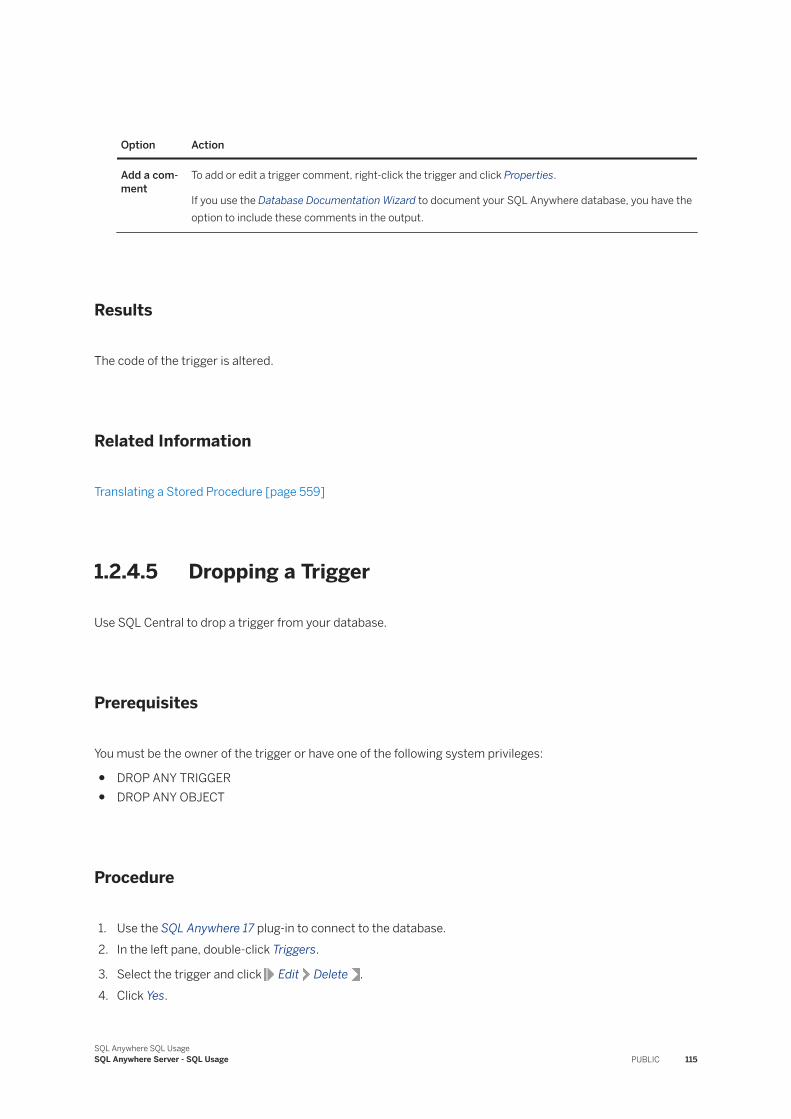
Option Action
Add a comment
To add or edit a trigger comment, right-click the trigger and click Properties.
If you use the Database Documentation Wizard to document your SQL Anywhere database, you have the option to include these comments in the output.
Results
The code of the trigger is altered.
Related Information
Translating a Stored Procedure [page 559]
1.2.4.5 Dropping a Trigger
Use SQL Central to drop a trigger from your database.
Prerequisites
You must be the owner of the trigger or have one of the following system privileges:
● DROP ANY TRIGGER● DROP ANY OBJECT
Procedure
1. Use the SQL Anywhere 17 plug-in to connect to the database.2. In the left pane, double-click Triggers.
3. Select the trigger and click Edit Delete .4. Click Yes.
SQL Anywhere SQL UsageSQL Anywhere Server - SQL Usage PUBLIC 115
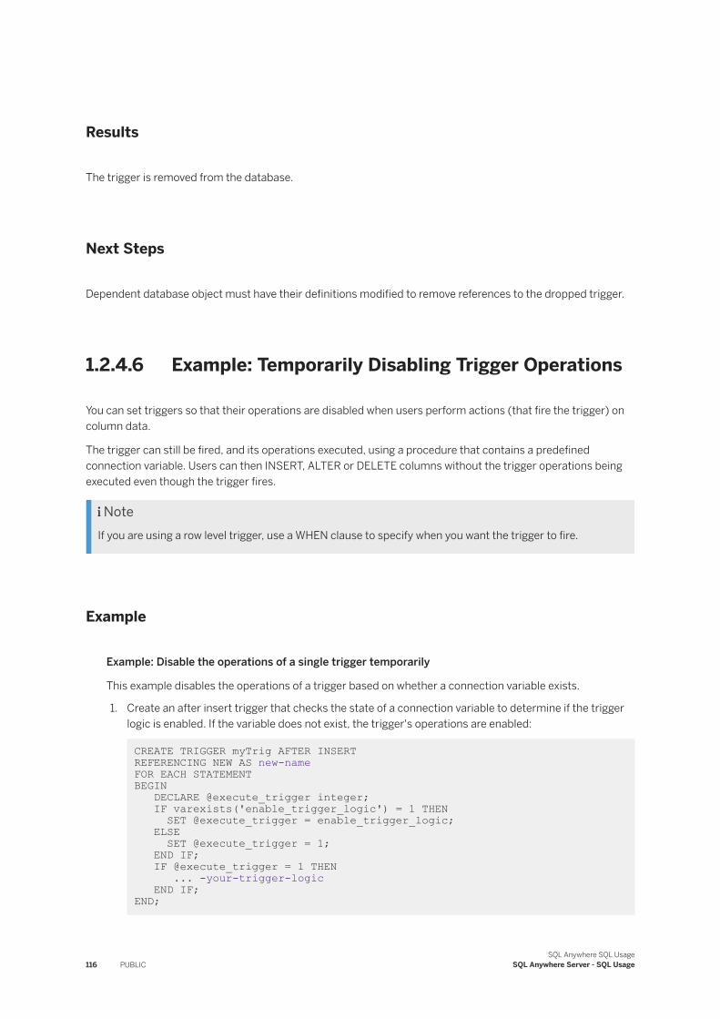
Results
The trigger is removed from the database.
Next Steps
Dependent database object must have their definitions modified to remove references to the dropped trigger.
1.2.4.6 Example: Temporarily Disabling Trigger Operations
You can set triggers so that their operations are disabled when users perform actions (that fire the trigger) on column data.
The trigger can still be fired, and its operations executed, using a procedure that contains a predefined connection variable. Users can then INSERT, ALTER or DELETE columns without the trigger operations being executed even though the trigger fires.
NoteIf you are using a row level trigger, use a WHEN clause to specify when you want the trigger to fire.
Example
Example: Disable the operations of a single trigger temporarily
This example disables the operations of a trigger based on whether a connection variable exists.
1. Create an after insert trigger that checks the state of a connection variable to determine if the trigger logic is enabled. If the variable does not exist, the trigger's operations are enabled:
CREATE TRIGGER myTrig AFTER INSERT REFERENCING NEW AS new-name FOR EACH STATEMENTBEGIN DECLARE @execute_trigger integer; IF varexists('enable_trigger_logic') = 1 THEN SET @execute_trigger = enable_trigger_logic; ELSE SET @execute_trigger = 1; END IF; IF @execute_trigger = 1 THEN ... -your-trigger-logic END IF; END;
116 PUBLICSQL Anywhere SQL Usage
SQL Anywhere Server - SQL Usage
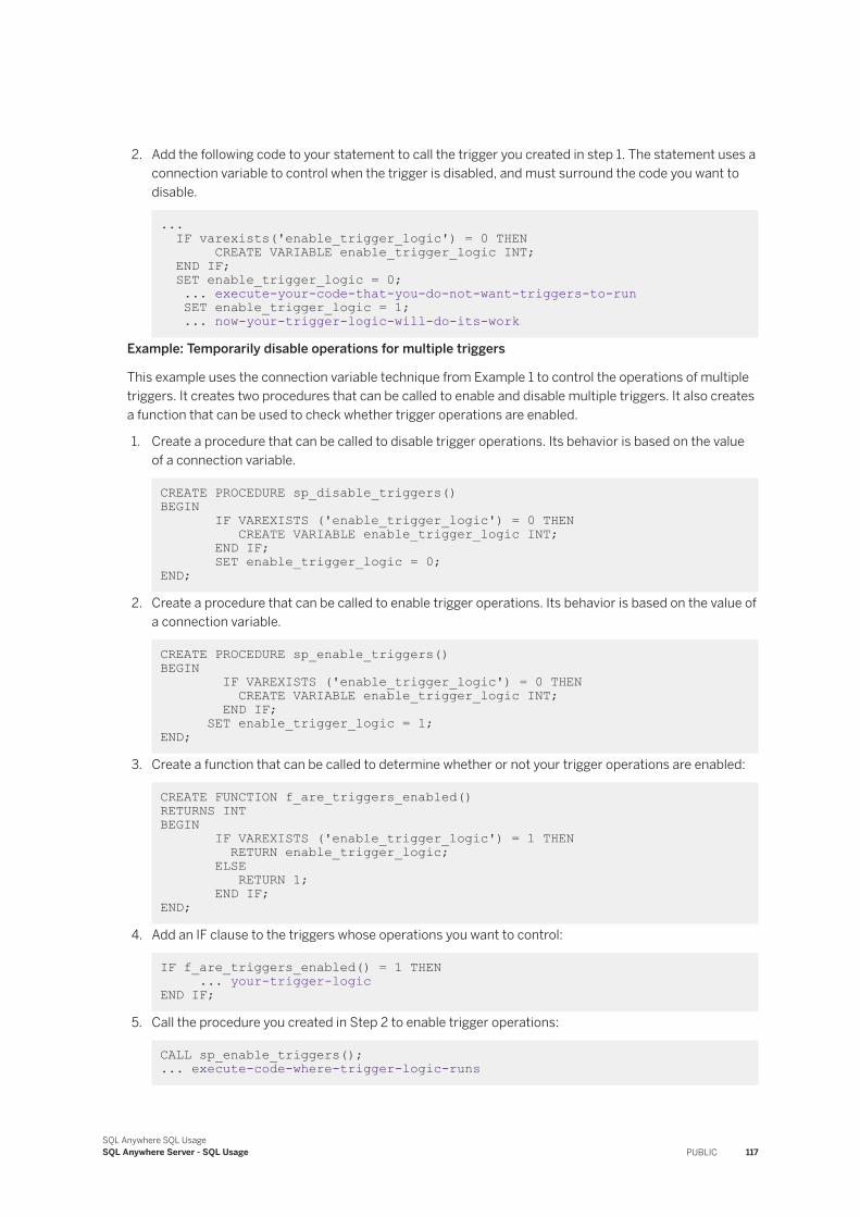
2. Add the following code to your statement to call the trigger you created in step 1. The statement uses a connection variable to control when the trigger is disabled, and must surround the code you want to disable.
... IF varexists('enable_trigger_logic') = 0 THEN CREATE VARIABLE enable_trigger_logic INT; END IF; SET enable_trigger_logic = 0; ... execute-your-code-that-you-do-not-want-triggers-to-run SET enable_trigger_logic = 1; ... now-your-trigger-logic-will-do-its-work
Example: Temporarily disable operations for multiple triggers
This example uses the connection variable technique from Example 1 to control the operations of multiple triggers. It creates two procedures that can be called to enable and disable multiple triggers. It also creates a function that can be used to check whether trigger operations are enabled.
1. Create a procedure that can be called to disable trigger operations. Its behavior is based on the value of a connection variable.
CREATE PROCEDURE sp_disable_triggers() BEGIN IF VAREXISTS ('enable_trigger_logic') = 0 THEN CREATE VARIABLE enable_trigger_logic INT; END IF; SET enable_trigger_logic = 0; END;
2. Create a procedure that can be called to enable trigger operations. Its behavior is based on the value of a connection variable.
CREATE PROCEDURE sp_enable_triggers() BEGIN IF VAREXISTS ('enable_trigger_logic') = 0 THEN CREATE VARIABLE enable_trigger_logic INT; END IF; SET enable_trigger_logic = 1; END;
3. Create a function that can be called to determine whether or not your trigger operations are enabled:
CREATE FUNCTION f_are_triggers_enabled() RETURNS INTBEGIN IF VAREXISTS ('enable_trigger_logic') = 1 THEN RETURN enable_trigger_logic; ELSE RETURN 1; END IF; END;
4. Add an IF clause to the triggers whose operations you want to control:
IF f_are_triggers_enabled() = 1 THEN ... your-trigger-logic END IF;
5. Call the procedure you created in Step 2 to enable trigger operations:
CALL sp_enable_triggers(); ... execute-code-where-trigger-logic-runs
SQL Anywhere SQL UsageSQL Anywhere Server - SQL Usage PUBLIC 117

6. Call the procedure you created in Step 1 to disable trigger operations:
CALL sp_disable_triggers(); ... execute-your-code-where-trigger-logic-is-disabled
1.2.4.7 Privileges to Execute Triggers
Users cannot execute triggers: the database server fires them in response to actions on the database.
Nevertheless, a trigger does have privileges associated with it as it executes, defining its right to perform certain actions.
Triggers execute using the privileges of the owner of the table on which they are defined, not the privileges of the user who caused the trigger to fire, and not the privileges of the user who created the trigger.
When a trigger refers to a table, it uses the role memberships of the table creator to locate tables with no explicit owner name specified. For example, if a trigger on user_1.Table_A references Table_B and does not specify the owner of Table_B, then either Table_B must have been created by user_1 or user_1 must be a member of a role (directly or indirectly) that is the owner of Table_B. If neither condition is met, the database server returns a message when the trigger fires, indicating that the table cannot be found.
Also, user_1 must have privileges to perform the operations specified in the trigger.
1.2.4.8 Advanced Information on Triggers
Whether competing triggers are fired, and the order in which they are fired, depends on two things: trigger type (BEFORE, INSTEAD OF, or AFTER), and trigger scope (row-level or statement-level).
UPDATE statements can modify column values in more than one table. The sequence of trigger firing is the same for each table, but the order that the tables are updated is not guaranteed.
For row-level triggers, BEFORE triggers fire before INSTEAD OF triggers, which fire before AFTER triggers. All row-level triggers for a given row fire before any triggers fire for a subsequent row.
For statement-level triggers, INSTEAD OF triggers fire before AFTER triggers. Statement-level BEFORE triggers are not supported.
If there are competing statement-level and row-level AFTER triggers, the statement-level AFTER triggers fire after all row-level triggers have completed.
If there are competing statement-level and row-level INSTEAD OF triggers, the row-level triggers do not fire.
The OLD and NEW temporary tables created for AFTER STATEMENT triggers have the same schema as the underlying base table, with the same column names and data types. However these tables do not have primary keys, foreign keys, or indexes. The order of the rows in the OLD and NEW temporary tables is not guaranteed and may not match the order in which the base table rows were updated originally.
In this section:
INSTEAD OF Triggers [page 119]
118 PUBLICSQL Anywhere SQL Usage
SQL Anywhere Server - SQL Usage
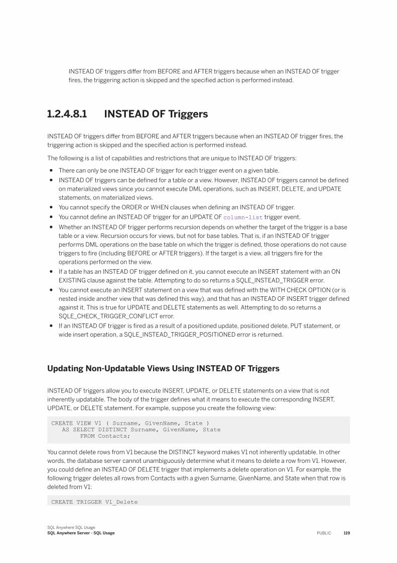
INSTEAD OF triggers differ from BEFORE and AFTER triggers because when an INSTEAD OF trigger fires, the triggering action is skipped and the specified action is performed instead.
1.2.4.8.1 INSTEAD OF Triggers
INSTEAD OF triggers differ from BEFORE and AFTER triggers because when an INSTEAD OF trigger fires, the triggering action is skipped and the specified action is performed instead.
The following is a list of capabilities and restrictions that are unique to INSTEAD OF triggers:
● There can only be one INSTEAD OF trigger for each trigger event on a given table.● INSTEAD OF triggers can be defined for a table or a view. However, INSTEAD OF triggers cannot be defined
on materialized views since you cannot execute DML operations, such as INSERT, DELETE, and UPDATE statements, on materialized views.
● You cannot specify the ORDER or WHEN clauses when defining an INSTEAD OF trigger.● You cannot define an INSTEAD OF trigger for an UPDATE OF column-list trigger event.● Whether an INSTEAD OF trigger performs recursion depends on whether the target of the trigger is a base
table or a view. Recursion occurs for views, but not for base tables. That is, if an INSTEAD OF trigger performs DML operations on the base table on which the trigger is defined, those operations do not cause triggers to fire (including BEFORE or AFTER triggers). If the target is a view, all triggers fire for the operations performed on the view.
● If a table has an INSTEAD OF trigger defined on it, you cannot execute an INSERT statement with an ON EXISTING clause against the table. Attempting to do so returns a SQLE_INSTEAD_TRIGGER error.
● You cannot execute an INSERT statement on a view that was defined with the WITH CHECK OPTION (or is nested inside another view that was defined this way), and that has an INSTEAD OF INSERT trigger defined against it. This is true for UPDATE and DELETE statements as well. Attempting to do so returns a SQLE_CHECK_TRIGGER_CONFLICT error.
● If an INSTEAD OF trigger is fired as a result of a positioned update, positioned delete, PUT statement, or wide insert operation, a SQLE_INSTEAD_TRIGGER_POSITIONED error is returned.
Updating Non-Updatable Views Using INSTEAD OF Triggers
INSTEAD OF triggers allow you to execute INSERT, UPDATE, or DELETE statements on a view that is not inherently updatable. The body of the trigger defines what it means to execute the corresponding INSERT, UPDATE, or DELETE statement. For example, suppose you create the following view:
CREATE VIEW V1 ( Surname, GivenName, State ) AS SELECT DISTINCT Surname, GivenName, State FROM Contacts;
You cannot delete rows from V1 because the DISTINCT keyword makes V1 not inherently updatable. In other words, the database server cannot unambiguously determine what it means to delete a row from V1. However, you could define an INSTEAD OF DELETE trigger that implements a delete operation on V1. For example, the following trigger deletes all rows from Contacts with a given Surname, GivenName, and State when that row is deleted from V1:
CREATE TRIGGER V1_Delete
SQL Anywhere SQL UsageSQL Anywhere Server - SQL Usage PUBLIC 119
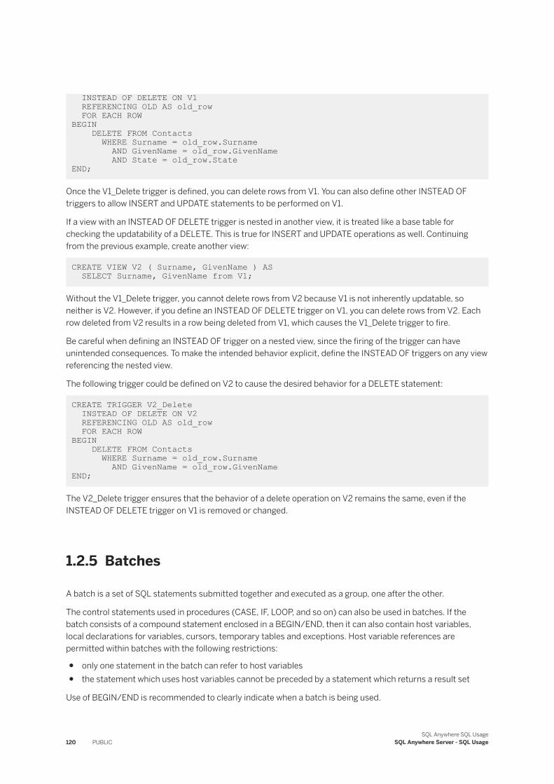
INSTEAD OF DELETE ON V1 REFERENCING OLD AS old_row FOR EACH ROWBEGIN DELETE FROM Contacts WHERE Surname = old_row.Surname AND GivenName = old_row.GivenName AND State = old_row.State END;
Once the V1_Delete trigger is defined, you can delete rows from V1. You can also define other INSTEAD OF triggers to allow INSERT and UPDATE statements to be performed on V1.
If a view with an INSTEAD OF DELETE trigger is nested in another view, it is treated like a base table for checking the updatability of a DELETE. This is true for INSERT and UPDATE operations as well. Continuing from the previous example, create another view:
CREATE VIEW V2 ( Surname, GivenName ) AS SELECT Surname, GivenName from V1;
Without the V1_Delete trigger, you cannot delete rows from V2 because V1 is not inherently updatable, so neither is V2. However, if you define an INSTEAD OF DELETE trigger on V1, you can delete rows from V2. Each row deleted from V2 results in a row being deleted from V1, which causes the V1_Delete trigger to fire.
Be careful when defining an INSTEAD OF trigger on a nested view, since the firing of the trigger can have unintended consequences. To make the intended behavior explicit, define the INSTEAD OF triggers on any view referencing the nested view.
The following trigger could be defined on V2 to cause the desired behavior for a DELETE statement:
CREATE TRIGGER V2_Delete INSTEAD OF DELETE ON V2 REFERENCING OLD AS old_row FOR EACH ROWBEGIN DELETE FROM Contacts WHERE Surname = old_row.Surname AND GivenName = old_row.GivenName END;
The V2_Delete trigger ensures that the behavior of a delete operation on V2 remains the same, even if the INSTEAD OF DELETE trigger on V1 is removed or changed.
1.2.5 Batches
A batch is a set of SQL statements submitted together and executed as a group, one after the other.
The control statements used in procedures (CASE, IF, LOOP, and so on) can also be used in batches. If the batch consists of a compound statement enclosed in a BEGIN/END, then it can also contain host variables, local declarations for variables, cursors, temporary tables and exceptions. Host variable references are permitted within batches with the following restrictions:
● only one statement in the batch can refer to host variables● the statement which uses host variables cannot be preceded by a statement which returns a result set
Use of BEGIN/END is recommended to clearly indicate when a batch is being used.
120 PUBLICSQL Anywhere SQL Usage
SQL Anywhere Server - SQL Usage
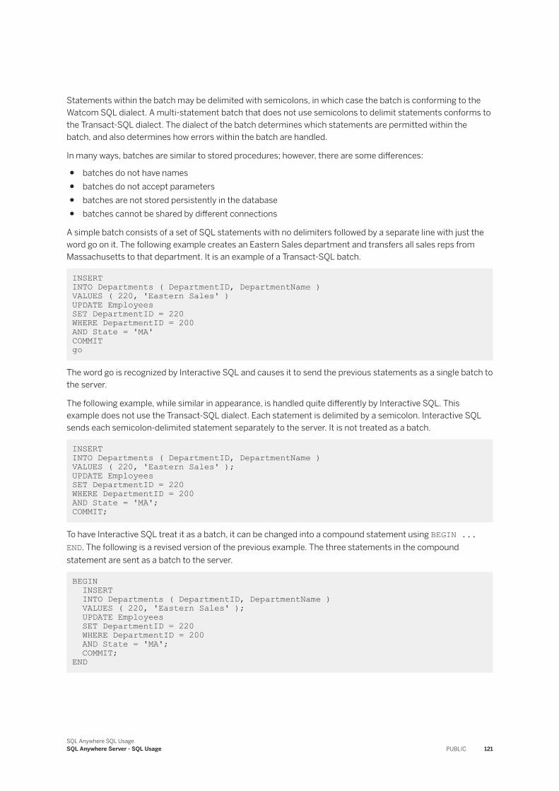
Statements within the batch may be delimited with semicolons, in which case the batch is conforming to the Watcom SQL dialect. A multi-statement batch that does not use semicolons to delimit statements conforms to the Transact-SQL dialect. The dialect of the batch determines which statements are permitted within the batch, and also determines how errors within the batch are handled.
In many ways, batches are similar to stored procedures; however, there are some differences:
● batches do not have names● batches do not accept parameters● batches are not stored persistently in the database● batches cannot be shared by different connections
A simple batch consists of a set of SQL statements with no delimiters followed by a separate line with just the word go on it. The following example creates an Eastern Sales department and transfers all sales reps from Massachusetts to that department. It is an example of a Transact-SQL batch.
INSERT INTO Departments ( DepartmentID, DepartmentName )VALUES ( 220, 'Eastern Sales' )UPDATE EmployeesSET DepartmentID = 220WHERE DepartmentID = 200AND State = 'MA'COMMIT go
The word go is recognized by Interactive SQL and causes it to send the previous statements as a single batch to the server.
The following example, while similar in appearance, is handled quite differently by Interactive SQL. This example does not use the Transact-SQL dialect. Each statement is delimited by a semicolon. Interactive SQL sends each semicolon-delimited statement separately to the server. It is not treated as a batch.
INSERT INTO Departments ( DepartmentID, DepartmentName )VALUES ( 220, 'Eastern Sales' );UPDATE EmployeesSET DepartmentID = 220WHERE DepartmentID = 200AND State = 'MA'; COMMIT;
To have Interactive SQL treat it as a batch, it can be changed into a compound statement using BEGIN ... END. The following is a revised version of the previous example. The three statements in the compound statement are sent as a batch to the server.
BEGIN INSERT INTO Departments ( DepartmentID, DepartmentName ) VALUES ( 220, 'Eastern Sales' ); UPDATE Employees SET DepartmentID = 220 WHERE DepartmentID = 200 AND State = 'MA'; COMMIT; END
SQL Anywhere SQL UsageSQL Anywhere Server - SQL Usage PUBLIC 121
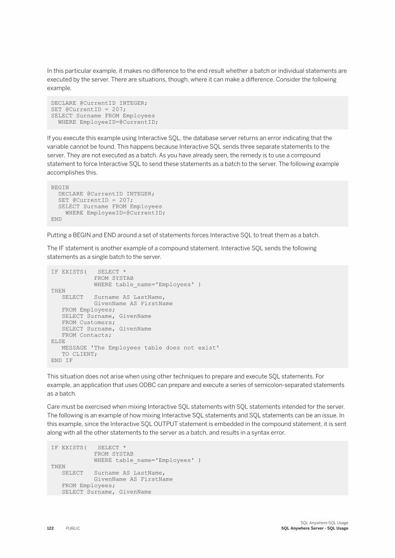
In this particular example, it makes no difference to the end result whether a batch or individual statements are executed by the server. There are situations, though, where it can make a difference. Consider the following example.
DECLARE @CurrentID INTEGER; SET @CurrentID = 207;SELECT Surname FROM Employees WHERE EmployeeID=@CurrentID;
If you execute this example using Interactive SQL, the database server returns an error indicating that the variable cannot be found. This happens because Interactive SQL sends three separate statements to the server. They are not executed as a batch. As you have already seen, the remedy is to use a compound statement to force Interactive SQL to send these statements as a batch to the server. The following example accomplishes this.
BEGIN DECLARE @CurrentID INTEGER; SET @CurrentID = 207; SELECT Surname FROM Employees WHERE EmployeeID=@CurrentID; END
Putting a BEGIN and END around a set of statements forces Interactive SQL to treat them as a batch.
The IF statement is another example of a compound statement. Interactive SQL sends the following statements as a single batch to the server.
IF EXISTS( SELECT * FROM SYSTAB WHERE table_name='Employees' )THEN SELECT Surname AS LastName, GivenName AS FirstName FROM Employees; SELECT Surname, GivenName FROM Customers; SELECT Surname, GivenName FROM Contacts;ELSE MESSAGE 'The Employees table does not exist' TO CLIENT; END IF
This situation does not arise when using other techniques to prepare and execute SQL statements. For example, an application that uses ODBC can prepare and execute a series of semicolon-separated statements as a batch.
Care must be exercised when mixing Interactive SQL statements with SQL statements intended for the server. The following is an example of how mixing Interactive SQL statements and SQL statements can be an issue. In this example, since the Interactive SQL OUTPUT statement is embedded in the compound statement, it is sent along with all the other statements to the server as a batch, and results in a syntax error.
IF EXISTS( SELECT * FROM SYSTAB WHERE table_name='Employees' )THEN SELECT Surname AS LastName, GivenName AS FirstName FROM Employees; SELECT Surname, GivenName
122 PUBLICSQL Anywhere SQL Usage
SQL Anywhere Server - SQL Usage
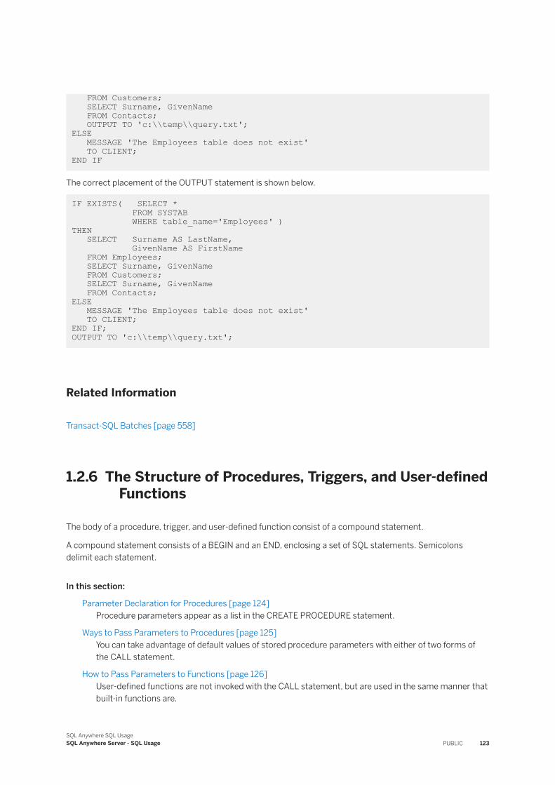
FROM Customers; SELECT Surname, GivenName FROM Contacts; OUTPUT TO 'c:\\temp\\query.txt';ELSE MESSAGE 'The Employees table does not exist' TO CLIENT; END IF
The correct placement of the OUTPUT statement is shown below.
IF EXISTS( SELECT * FROM SYSTAB WHERE table_name='Employees' )THEN SELECT Surname AS LastName, GivenName AS FirstName FROM Employees; SELECT Surname, GivenName FROM Customers; SELECT Surname, GivenName FROM Contacts; ELSE MESSAGE 'The Employees table does not exist' TO CLIENT;END IF; OUTPUT TO 'c:\\temp\\query.txt';
Related Information
Transact-SQL Batches [page 558]
1.2.6 The Structure of Procedures, Triggers, and User-defined Functions
The body of a procedure, trigger, and user-defined function consist of a compound statement.
A compound statement consists of a BEGIN and an END, enclosing a set of SQL statements. Semicolons delimit each statement.
In this section:
Parameter Declaration for Procedures [page 124]Procedure parameters appear as a list in the CREATE PROCEDURE statement.
Ways to Pass Parameters to Procedures [page 125]You can take advantage of default values of stored procedure parameters with either of two forms of the CALL statement.
How to Pass Parameters to Functions [page 126]User-defined functions are not invoked with the CALL statement, but are used in the same manner that built-in functions are.
SQL Anywhere SQL UsageSQL Anywhere Server - SQL Usage PUBLIC 123
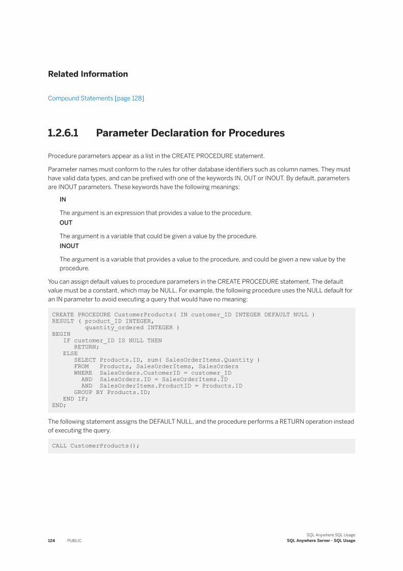
Related Information
Compound Statements [page 128]
1.2.6.1 Parameter Declaration for Procedures
Procedure parameters appear as a list in the CREATE PROCEDURE statement.
Parameter names must conform to the rules for other database identifiers such as column names. They must have valid data types, and can be prefixed with one of the keywords IN, OUT or INOUT. By default, parameters are INOUT parameters. These keywords have the following meanings:
IN
The argument is an expression that provides a value to the procedure.OUT
The argument is a variable that could be given a value by the procedure.INOUT
The argument is a variable that provides a value to the procedure, and could be given a new value by the procedure.
You can assign default values to procedure parameters in the CREATE PROCEDURE statement. The default value must be a constant, which may be NULL. For example, the following procedure uses the NULL default for an IN parameter to avoid executing a query that would have no meaning:
CREATE PROCEDURE CustomerProducts( IN customer_ID INTEGER DEFAULT NULL ) RESULT ( product_ID INTEGER, quantity_ordered INTEGER )BEGIN IF customer_ID IS NULL THEN RETURN; ELSE SELECT Products.ID, sum( SalesOrderItems.Quantity ) FROM Products, SalesOrderItems, SalesOrders WHERE SalesOrders.CustomerID = customer_ID AND SalesOrders.ID = SalesOrderItems.ID AND SalesOrderItems.ProductID = Products.ID GROUP BY Products.ID; END IF; END;
The following statement assigns the DEFAULT NULL, and the procedure performs a RETURN operation instead of executing the query.
CALL CustomerProducts();
124 PUBLICSQL Anywhere SQL Usage
SQL Anywhere Server - SQL Usage
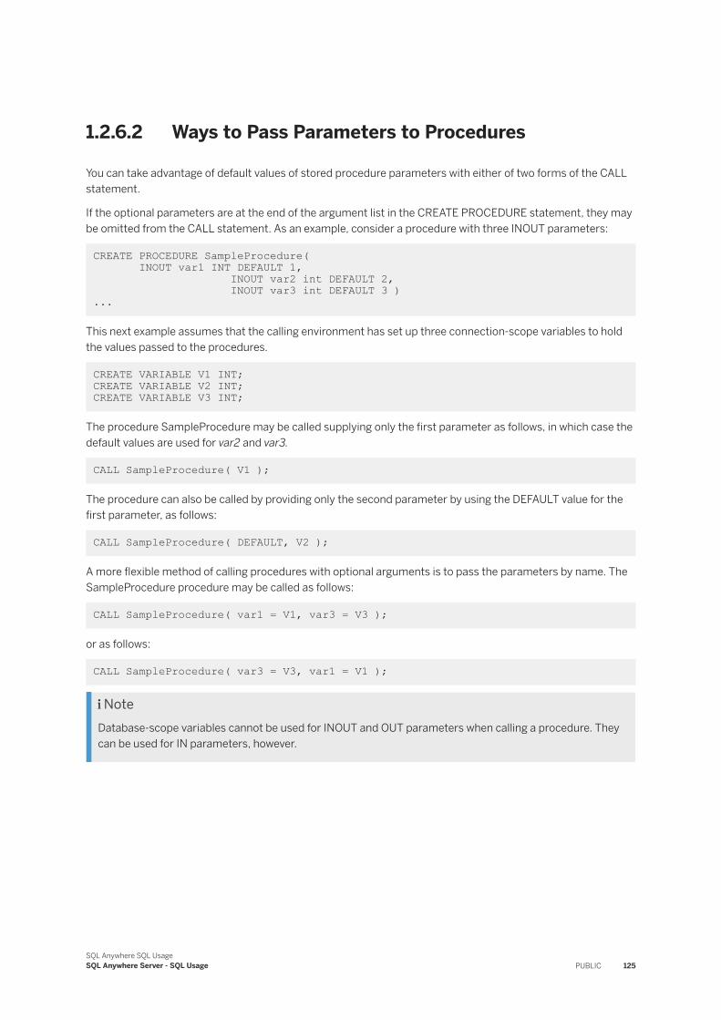
1.2.6.2 Ways to Pass Parameters to Procedures
You can take advantage of default values of stored procedure parameters with either of two forms of the CALL statement.
If the optional parameters are at the end of the argument list in the CREATE PROCEDURE statement, they may be omitted from the CALL statement. As an example, consider a procedure with three INOUT parameters:
CREATE PROCEDURE SampleProcedure( INOUT var1 INT DEFAULT 1, INOUT var2 int DEFAULT 2, INOUT var3 int DEFAULT 3 ) ...
This next example assumes that the calling environment has set up three connection-scope variables to hold the values passed to the procedures.
CREATE VARIABLE V1 INT; CREATE VARIABLE V2 INT; CREATE VARIABLE V3 INT;
The procedure SampleProcedure may be called supplying only the first parameter as follows, in which case the default values are used for var2 and var3.
CALL SampleProcedure( V1 );
The procedure can also be called by providing only the second parameter by using the DEFAULT value for the first parameter, as follows:
CALL SampleProcedure( DEFAULT, V2 );
A more flexible method of calling procedures with optional arguments is to pass the parameters by name. The SampleProcedure procedure may be called as follows:
CALL SampleProcedure( var1 = V1, var3 = V3 );
or as follows:
CALL SampleProcedure( var3 = V3, var1 = V1 );
NoteDatabase-scope variables cannot be used for INOUT and OUT parameters when calling a procedure. They can be used for IN parameters, however.
SQL Anywhere SQL UsageSQL Anywhere Server - SQL Usage PUBLIC 125
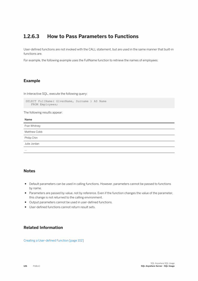
1.2.6.3 How to Pass Parameters to Functions
User-defined functions are not invoked with the CALL statement, but are used in the same manner that built-in functions are.
For example, the following example uses the FullName function to retrieve the names of employees:
Example
In Interactive SQL, execute the following query:
SELECT FullName( GivenName, Surname ) AS Name FROM Employees;
The following results appear:
Name
Fran Whitney
Matthew Cobb
Philip Chin
Julie Jordan
...
Notes
● Default parameters can be used in calling functions. However, parameters cannot be passed to functions by name.
● Parameters are passed by value, not by reference. Even if the function changes the value of the parameter, this change is not returned to the calling environment.
● Output parameters cannot be used in user-defined functions.● User-defined functions cannot return result sets.
Related Information
Creating a User-defined Function [page 102]
126 PUBLICSQL Anywhere SQL Usage
SQL Anywhere Server - SQL Usage
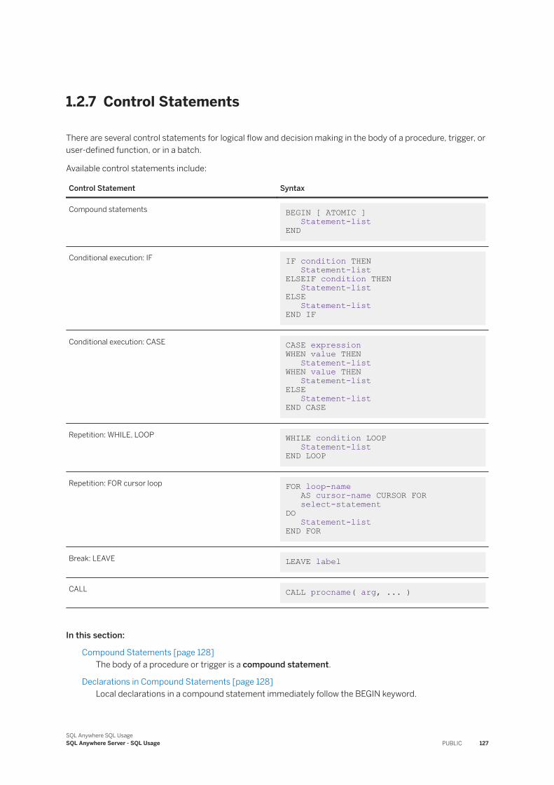
1.2.7 Control Statements
There are several control statements for logical flow and decision making in the body of a procedure, trigger, or user-defined function, or in a batch.
Available control statements include:
Control Statement Syntax
Compound statements BEGIN [ ATOMIC ] Statement-list END
Conditional execution: IF IF condition THEN Statement-list ELSEIF condition THEN Statement-list ELSE Statement-list END IF
Conditional execution: CASE CASE expression WHEN value THEN Statement-list WHEN value THEN Statement-list ELSE Statement-list END CASE
Repetition: WHILE, LOOP WHILE condition LOOP Statement-list END LOOP
Repetition: FOR cursor loop FOR loop-name AS cursor-name CURSOR FOR select-statement DO Statement-list END FOR
Break: LEAVE LEAVE label
CALL CALL procname( arg, ... )
In this section:
Compound Statements [page 128]The body of a procedure or trigger is a compound statement.
Declarations in Compound Statements [page 128]Local declarations in a compound statement immediately follow the BEGIN keyword.
SQL Anywhere SQL UsageSQL Anywhere Server - SQL Usage PUBLIC 127
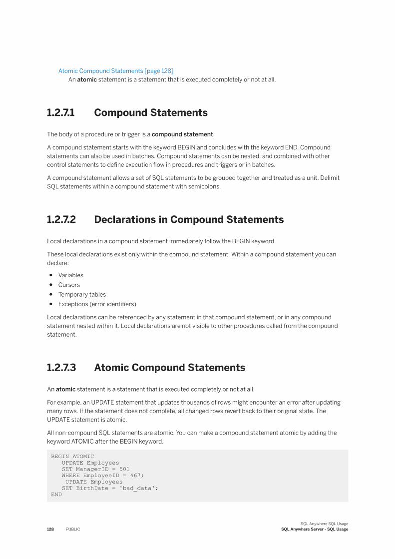
Atomic Compound Statements [page 128]An atomic statement is a statement that is executed completely or not at all.
1.2.7.1 Compound Statements
The body of a procedure or trigger is a compound statement.
A compound statement starts with the keyword BEGIN and concludes with the keyword END. Compound statements can also be used in batches. Compound statements can be nested, and combined with other control statements to define execution flow in procedures and triggers or in batches.
A compound statement allows a set of SQL statements to be grouped together and treated as a unit. Delimit SQL statements within a compound statement with semicolons.
1.2.7.2 Declarations in Compound Statements
Local declarations in a compound statement immediately follow the BEGIN keyword.
These local declarations exist only within the compound statement. Within a compound statement you can declare:
● Variables● Cursors● Temporary tables● Exceptions (error identifiers)
Local declarations can be referenced by any statement in that compound statement, or in any compound statement nested within it. Local declarations are not visible to other procedures called from the compound statement.
1.2.7.3 Atomic Compound Statements
An atomic statement is a statement that is executed completely or not at all.
For example, an UPDATE statement that updates thousands of rows might encounter an error after updating many rows. If the statement does not complete, all changed rows revert back to their original state. The UPDATE statement is atomic.
All non-compound SQL statements are atomic. You can make a compound statement atomic by adding the keyword ATOMIC after the BEGIN keyword.
BEGIN ATOMIC UPDATE Employees SET ManagerID = 501 WHERE EmployeeID = 467; UPDATE Employees SET BirthDate = 'bad_data'; END
128 PUBLICSQL Anywhere SQL Usage
SQL Anywhere Server - SQL Usage
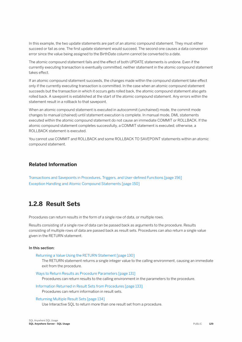
In this example, the two update statements are part of an atomic compound statement. They must either succeed or fail as one. The first update statement would succeed. The second one causes a data conversion error since the value being assigned to the BirthDate column cannot be converted to a date.
The atomic compound statement fails and the effect of both UPDATE statements is undone. Even if the currently executing transaction is eventually committed, neither statement in the atomic compound statement takes effect.
If an atomic compound statement succeeds, the changes made within the compound statement take effect only if the currently executing transaction is committed. In the case when an atomic compound statement succeeds but the transaction in which it occurs gets rolled back, the atomic compound statement also gets rolled back. A savepoint is established at the start of the atomic compound statement. Any errors within the statement result in a rollback to that savepoint.
When an atomic compound statement is executed in autocommit (unchained) mode, the commit mode changes to manual (chained) until statement execution is complete. In manual mode, DML statements executed within the atomic compound statement do not cause an immediate COMMIT or ROLLBACK. If the atomic compound statement completes successfully, a COMMIT statement is executed; otherwise, a ROLLBACK statement is executed.
You cannot use COMMIT and ROLLBACK and some ROLLBACK TO SAVEPOINT statements within an atomic compound statement.
Related Information
Transactions and Savepoints in Procedures, Triggers, and User-defined Functions [page 156]Exception Handling and Atomic Compound Statements [page 150]
1.2.8 Result Sets
Procedures can return results in the form of a single row of data, or multiple rows.
Results consisting of a single row of data can be passed back as arguments to the procedure. Results consisting of multiple rows of data are passed back as result sets. Procedures can also return a single value given in the RETURN statement.
In this section:
Returning a Value Using the RETURN Statement [page 130]The RETURN statement returns a single integer value to the calling environment, causing an immediate exit from the procedure.
Ways to Return Results as Procedure Parameters [page 131]Procedures can return results to the calling environment in the parameters to the procedure.
Information Returned in Result Sets from Procedures [page 133]Procedures can return information in result sets.
Returning Multiple Result Sets [page 134]Use Interactive SQL to return more than one result set from a procedure.
SQL Anywhere SQL UsageSQL Anywhere Server - SQL Usage PUBLIC 129
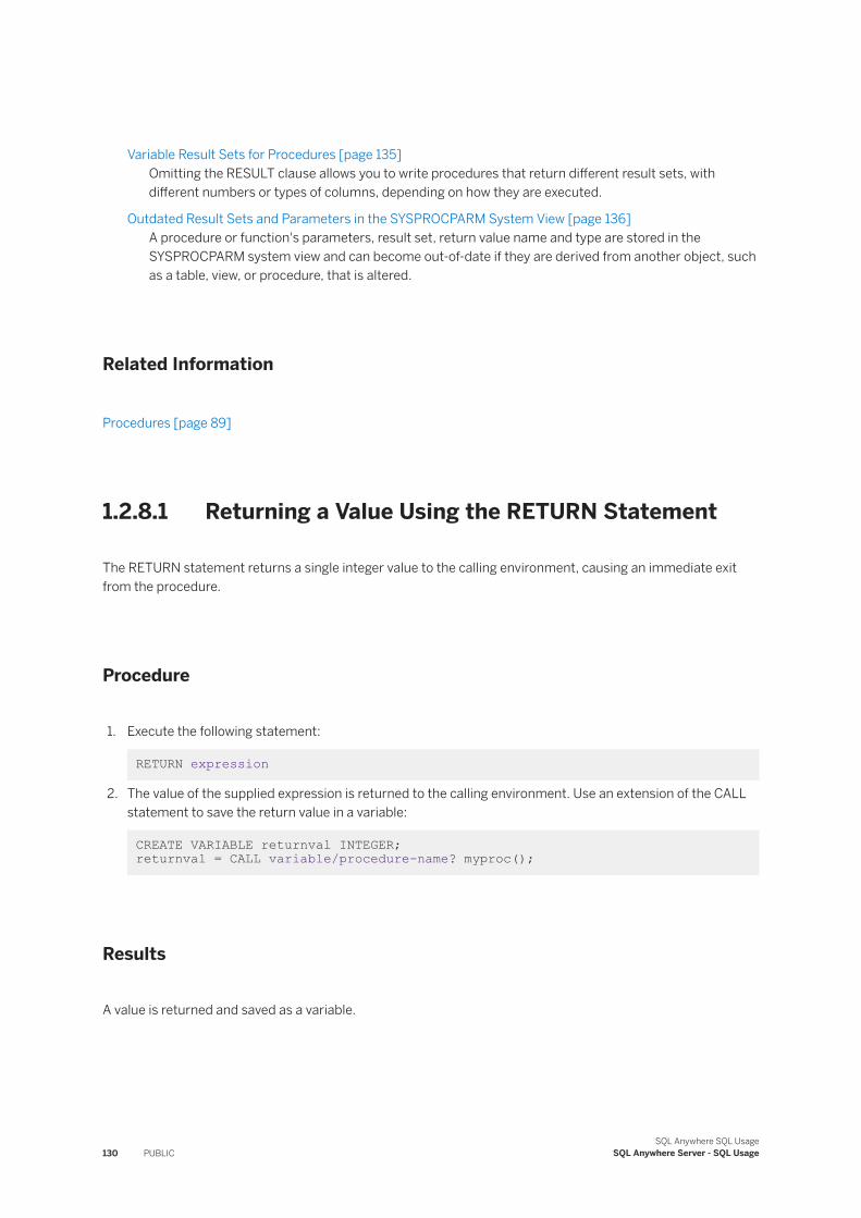
Variable Result Sets for Procedures [page 135]Omitting the RESULT clause allows you to write procedures that return different result sets, with different numbers or types of columns, depending on how they are executed.
Outdated Result Sets and Parameters in the SYSPROCPARM System View [page 136]A procedure or function's parameters, result set, return value name and type are stored in the SYSPROCPARM system view and can become out-of-date if they are derived from another object, such as a table, view, or procedure, that is altered.
Related Information
Procedures [page 89]
1.2.8.1 Returning a Value Using the RETURN Statement
The RETURN statement returns a single integer value to the calling environment, causing an immediate exit from the procedure.
Procedure
1. Execute the following statement:
RETURN expression
2. The value of the supplied expression is returned to the calling environment. Use an extension of the CALL statement to save the return value in a variable:
CREATE VARIABLE returnval INTEGER; returnval = CALL variable/procedure-name? myproc();
Results
A value is returned and saved as a variable.
130 PUBLICSQL Anywhere SQL Usage
SQL Anywhere Server - SQL Usage
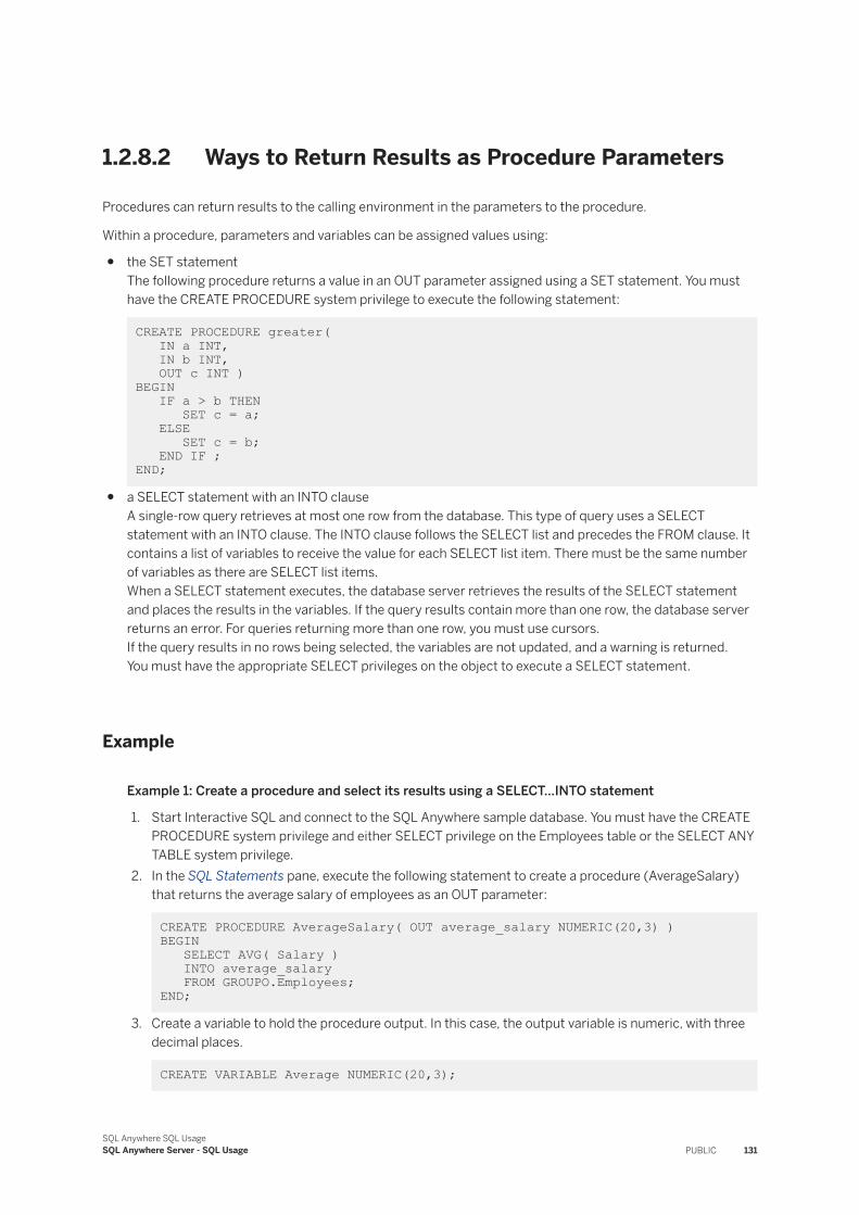
1.2.8.2 Ways to Return Results as Procedure Parameters
Procedures can return results to the calling environment in the parameters to the procedure.
Within a procedure, parameters and variables can be assigned values using:
● the SET statementThe following procedure returns a value in an OUT parameter assigned using a SET statement. You must have the CREATE PROCEDURE system privilege to execute the following statement:
CREATE PROCEDURE greater( IN a INT, IN b INT, OUT c INT )BEGIN IF a > b THEN SET c = a; ELSE SET c = b; END IF ; END;
● a SELECT statement with an INTO clauseA single-row query retrieves at most one row from the database. This type of query uses a SELECT statement with an INTO clause. The INTO clause follows the SELECT list and precedes the FROM clause. It contains a list of variables to receive the value for each SELECT list item. There must be the same number of variables as there are SELECT list items.When a SELECT statement executes, the database server retrieves the results of the SELECT statement and places the results in the variables. If the query results contain more than one row, the database server returns an error. For queries returning more than one row, you must use cursors.If the query results in no rows being selected, the variables are not updated, and a warning is returned.You must have the appropriate SELECT privileges on the object to execute a SELECT statement.
Example
Example 1: Create a procedure and select its results using a SELECT...INTO statement
1. Start Interactive SQL and connect to the SQL Anywhere sample database. You must have the CREATE PROCEDURE system privilege and either SELECT privilege on the Employees table or the SELECT ANY TABLE system privilege.
2. In the SQL Statements pane, execute the following statement to create a procedure (AverageSalary) that returns the average salary of employees as an OUT parameter:
CREATE PROCEDURE AverageSalary( OUT average_salary NUMERIC(20,3) ) BEGIN SELECT AVG( Salary ) INTO average_salary FROM GROUPO.Employees; END;
3. Create a variable to hold the procedure output. In this case, the output variable is numeric, with three decimal places.
CREATE VARIABLE Average NUMERIC(20,3);
SQL Anywhere SQL UsageSQL Anywhere Server - SQL Usage PUBLIC 131
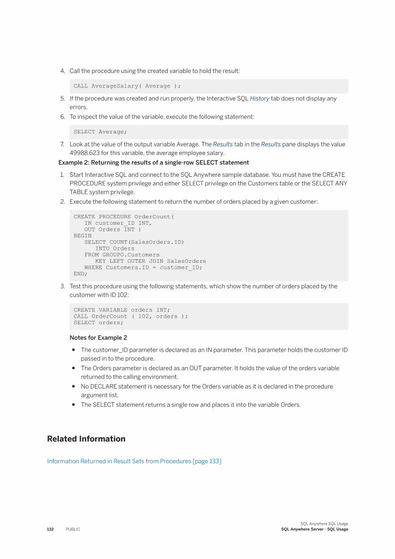
4. Call the procedure using the created variable to hold the result:
CALL AverageSalary( Average );
5. If the procedure was created and run properly, the Interactive SQL History tab does not display any errors.
6. To inspect the value of the variable, execute the following statement:
SELECT Average;
7. Look at the value of the output variable Average. The Results tab in the Results pane displays the value 49988.623 for this variable, the average employee salary.
Example 2: Returning the results of a single-row SELECT statement
1. Start Interactive SQL and connect to the SQL Anywhere sample database. You must have the CREATE PROCEDURE system privilege and either SELECT privilege on the Customers table or the SELECT ANY TABLE system privilege.
2. Execute the following statement to return the number of orders placed by a given customer:
CREATE PROCEDURE OrderCount( IN customer_ID INT, OUT Orders INT )BEGIN SELECT COUNT(SalesOrders.ID) INTO Orders FROM GROUPO.Customers KEY LEFT OUTER JOIN SalesOrders WHERE Customers.ID = customer_ID; END;
3. Test this procedure using the following statements, which show the number of orders placed by the customer with ID 102:
CREATE VARIABLE orders INT; CALL OrderCount ( 102, orders ); SELECT orders;
Notes for Example 2
● The customer_ID parameter is declared as an IN parameter. This parameter holds the customer ID passed in to the procedure.
● The Orders parameter is declared as an OUT parameter. It holds the value of the orders variable returned to the calling environment.
● No DECLARE statement is necessary for the Orders variable as it is declared in the procedure argument list.
● The SELECT statement returns a single row and places it into the variable Orders.
Related Information
Information Returned in Result Sets from Procedures [page 133]
132 PUBLICSQL Anywhere SQL Usage
SQL Anywhere Server - SQL Usage
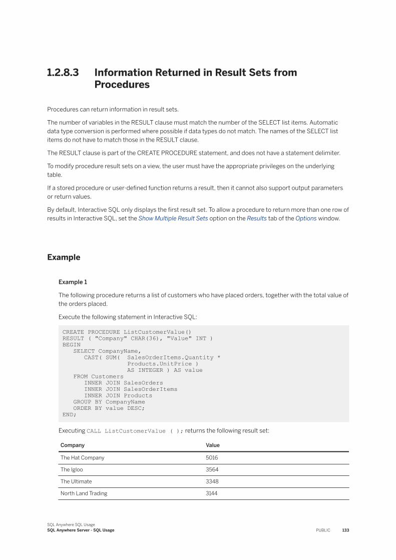
1.2.8.3 Information Returned in Result Sets from Procedures
Procedures can return information in result sets.
The number of variables in the RESULT clause must match the number of the SELECT list items. Automatic data type conversion is performed where possible if data types do not match. The names of the SELECT list items do not have to match those in the RESULT clause.
The RESULT clause is part of the CREATE PROCEDURE statement, and does not have a statement delimiter.
To modify procedure result sets on a view, the user must have the appropriate privileges on the underlying table.
If a stored procedure or user-defined function returns a result, then it cannot also support output parameters or return values.
By default, Interactive SQL only displays the first result set. To allow a procedure to return more than one row of results in Interactive SQL, set the Show Multiple Result Sets option on the Results tab of the Options window.
Example
Example 1
The following procedure returns a list of customers who have placed orders, together with the total value of the orders placed.
Execute the following statement in Interactive SQL:
CREATE PROCEDURE ListCustomerValue() RESULT ( "Company" CHAR(36), "Value" INT )BEGIN SELECT CompanyName, CAST( SUM( SalesOrderItems.Quantity * Products.UnitPrice ) AS INTEGER ) AS value FROM Customers INNER JOIN SalesOrders INNER JOIN SalesOrderItems INNER JOIN Products GROUP BY CompanyName ORDER BY value DESC; END;
Executing CALL ListCustomerValue ( ); returns the following result set:
Company Value
The Hat Company 5016
The Igloo 3564
The Ultimate 3348
North Land Trading 3144
SQL Anywhere SQL UsageSQL Anywhere Server - SQL Usage PUBLIC 133
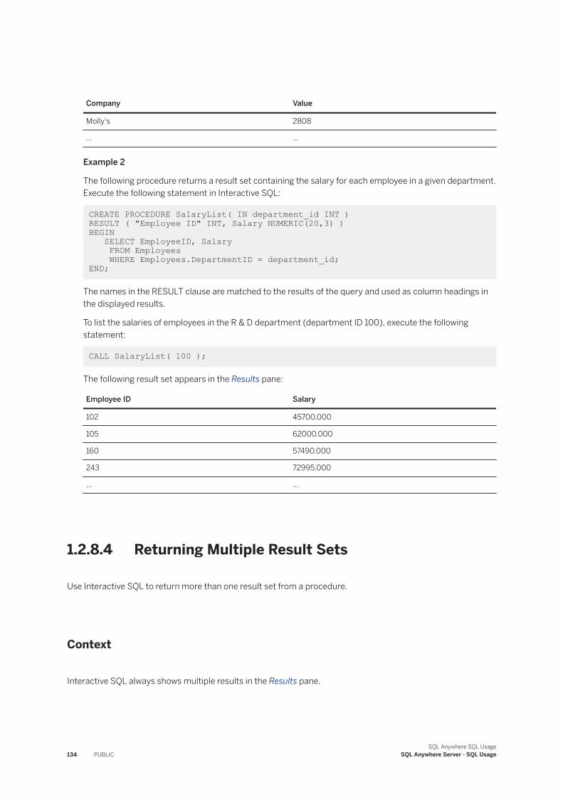
Company Value
Molly's 2808
... ...
Example 2
The following procedure returns a result set containing the salary for each employee in a given department. Execute the following statement in Interactive SQL:
CREATE PROCEDURE SalaryList( IN department_id INT ) RESULT ( "Employee ID" INT, Salary NUMERIC(20,3) )BEGIN SELECT EmployeeID, Salary FROM Employees WHERE Employees.DepartmentID = department_id; END;
The names in the RESULT clause are matched to the results of the query and used as column headings in the displayed results.
To list the salaries of employees in the R & D department (department ID 100), execute the following statement:
CALL SalaryList( 100 );
The following result set appears in the Results pane:
Employee ID Salary
102 45700.000
105 62000.000
160 57490.000
243 72995.000
... ...
1.2.8.4 Returning Multiple Result Sets
Use Interactive SQL to return more than one result set from a procedure.
Context
Interactive SQL always shows multiple results in the Results pane.
134 PUBLICSQL Anywhere SQL Usage
SQL Anywhere Server - SQL Usage
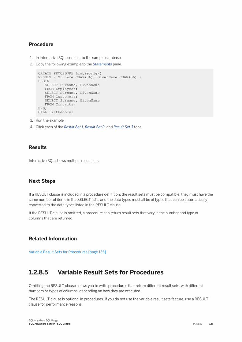
Procedure
1. In Interactive SQL, connect to the sample database.2. Copy the following example to the Statements pane.
CREATE PROCEDURE ListPeople() RESULT ( Surname CHAR(36), GivenName CHAR(36) )BEGIN SELECT Surname, GivenName FROM Employees; SELECT Surname, GivenName FROM Customers; SELECT Surname, GivenName FROM Contacts;END; CALL ListPeople;
3. Run the example.4. Click each of the Result Set 1, Result Set 2, and Result Set 3 tabs.
Results
Interactive SQL shows multiple result sets.
Next Steps
If a RESULT clause is included in a procedure definition, the result sets must be compatible: they must have the same number of items in the SELECT lists, and the data types must all be of types that can be automatically converted to the data types listed in the RESULT clause.
If the RESULT clause is omitted, a procedure can return result sets that vary in the number and type of columns that are returned.
Related Information
Variable Result Sets for Procedures [page 135]
1.2.8.5 Variable Result Sets for Procedures
Omitting the RESULT clause allows you to write procedures that return different result sets, with different numbers or types of columns, depending on how they are executed.
The RESULT clause is optional in procedures. If you do not use the variable result sets feature, use a RESULT clause for performance reasons.
SQL Anywhere SQL UsageSQL Anywhere Server - SQL Usage PUBLIC 135
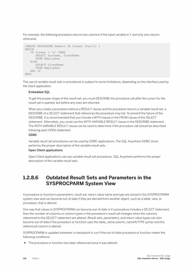
For example, the following procedure returns two columns if the input variable is Y, but only one column otherwise:
CREATE PROCEDURE Names( IN formal char(1) ) BEGIN IF formal = 'y' THEN SELECT Surname, GivenName FROM Employees ELSE SELECT GivenName FROM Employees END IF END;
The use of variable result sets in procedures is subject to some limitations, depending on the interface used by the client application.
Embedded SQL
To get the proper shape of the result set, you must DESCRIBE the procedure call after the cursor for the result set is opened, but before any rows are returned.
When you create a procedure without a RESULT clause and the procedure returns a variable result set, a DESCRIBE of a SELECT statement that references the procedure may fail. To prevent the failure of the DESCRIBE, it is recommended that you include a WITH clause in the FROM clause of the SELECT statement. Alternately, you could use the WITH VARIABLE RESULT clause in the DESCRIBE statement. The WITH VARIABLE RESULT clause can be used to determine if the procedure call should be described following each OPEN statement.ODBC
Variable result set procedures can be used by ODBC applications. The SQL Anywhere ODBC driver performs the proper description of the variable result sets.Open Client applications
Open Client applications can use variable result set procedures. SQL Anywhere performs the proper description of the variable result sets.
1.2.8.6 Outdated Result Sets and Parameters in the SYSPROCPARM System View
A procedure or function's parameters, result set, return value name and type are stored in the SYSPROCPARM system view and can become out-of-date if they are derived from another object, such as a table, view, or procedure, that is altered.
One way that values in SYSPROCPARM can become out-of-date is if a procedure includes a SELECT statement, then the number of columns or column types in the procedure's result set changes when the columns referenced in the SELECT statement are altered. Result sets, parameters, and return value types can also become out-of-date if the procedure or function uses the table_name.column_name%TYPE syntax and the referenced column is altered.
SYSPROCPARM is updated whenever a checkpoint is run if the out-of-date procedure or function meets the following conditions:
● The procedure or function has been referenced since it was altered.
136 PUBLICSQL Anywhere SQL Usage
SQL Anywhere Server - SQL Usage
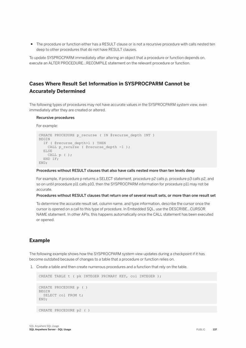
● The procedure or function either has a RESULT clause or is not a recursive procedure with calls nested ten deep to other procedures that do not have RESULT clauses.
To update SYSPROCPARM immediately after altering an object that a procedure or function depends on, execute an ALTER PROCEDURE...RECOMPILE statement on the relevant procedure or function.
Cases Where Result Set Information in SYSPROCPARM Cannot be Accurately Determined
The following types of procedures may not have accurate values in the SYSPROCPARM system view, even immediately after they are created or altered.
Recursive procedures
For example:
CREATE PROCEDURE p_recurse ( IN @recurse_depth INT ) BEGIN IF ( @recurse_depth>1 ) THEN CALL p_recurse ( @recurse_depth -1 ); ELSE CALL p ( ); END IF; END;
Procedures without RESULT clauses that also have calls nested more than ten levels deep
For example, if procedure p returns a SELECT statement, procedure p2 calls p, procedure p3 calls p2, and so on until procedure p11 calls p10, then the SYSPROCPARM information for procedure p11 may not be accurate.Procedures without RESULT clauses that return one of several result sets, or more than one result set
To determine the accurate result set, column name, and type information, describe the cursor once the cursor is opened on a call to this type of procedure. In Embedded SQL, use the DESCRIBE...CURSOR NAME statement. In other APIs, this happens automatically once the CALL statement has been executed or opened.
Example
The following example shows how the SYSPROCPARM system view updates during a checkpoint if it has become outdated because of changes to a table that a procedure or function relies on.
1. Create a table and then create numerous procedures and a function that rely on the table.
CREATE TABLE t ( pk INTEGER PRIMARY KEY, col INTEGER );
CREATE PROCEDURE p ( ) BEGIN SELECT col FROM t; END;
CREATE PROCEDURE p2 ( )
SQL Anywhere SQL UsageSQL Anywhere Server - SQL Usage PUBLIC 137
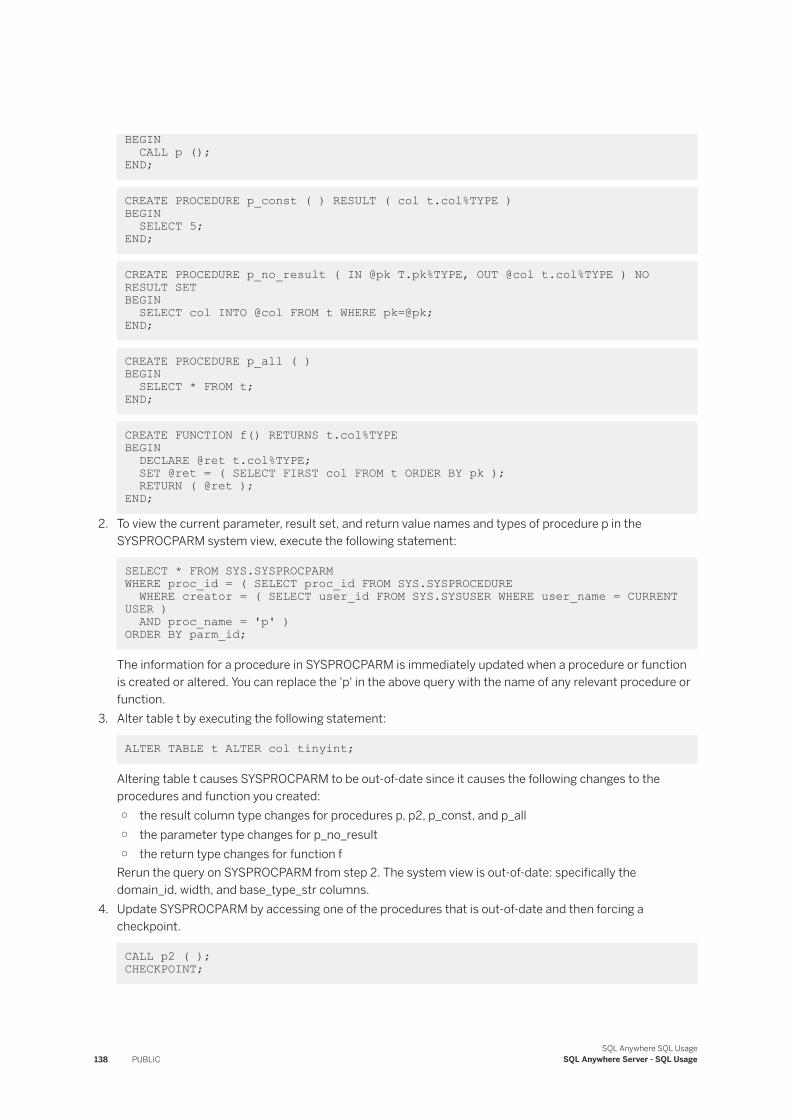
BEGIN CALL p (); END;
CREATE PROCEDURE p_const ( ) RESULT ( col t.col%TYPE ) BEGIN SELECT 5; END;
CREATE PROCEDURE p_no_result ( IN @pk T.pk%TYPE, OUT @col t.col%TYPE ) NO RESULT SET BEGIN SELECT col INTO @col FROM t WHERE pk=@pk; END;
CREATE PROCEDURE p_all ( ) BEGIN SELECT * FROM t; END;
CREATE FUNCTION f() RETURNS t.col%TYPE BEGIN DECLARE @ret t.col%TYPE; SET @ret = ( SELECT FIRST col FROM t ORDER BY pk ); RETURN ( @ret ); END;
2. To view the current parameter, result set, and return value names and types of procedure p in the SYSPROCPARM system view, execute the following statement:
SELECT * FROM SYS.SYSPROCPARM WHERE proc_id = ( SELECT proc_id FROM SYS.SYSPROCEDURE WHERE creator = ( SELECT user_id FROM SYS.SYSUSER WHERE user_name = CURRENT USER ) AND proc_name = 'p' ) ORDER BY parm_id;
The information for a procedure in SYSPROCPARM is immediately updated when a procedure or function is created or altered. You can replace the 'p' in the above query with the name of any relevant procedure or function.
3. Alter table t by executing the following statement:
ALTER TABLE t ALTER col tinyint;
Altering table t causes SYSPROCPARM to be out-of-date since it causes the following changes to the procedures and function you created:○ the result column type changes for procedures p, p2, p_const, and p_all○ the parameter type changes for p_no_result○ the return type changes for function f
Rerun the query on SYSPROCPARM from step 2. The system view is out-of-date: specifically the domain_id, width, and base_type_str columns.
4. Update SYSPROCPARM by accessing one of the procedures that is out-of-date and then forcing a checkpoint.
CALL p2 ( ); CHECKPOINT;
138 PUBLICSQL Anywhere SQL Usage
SQL Anywhere Server - SQL Usage
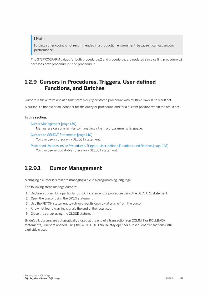
NoteForcing a checkpoint is not recommended in a production environment, because it can cause poor performance.
The SYSPROCPARM values for both procedure p2 and procedure p are updated since calling procedure p2 accesses both procedure p2 and procedure p.
1.2.9 Cursors in Procedures, Triggers, User-defined Functions, and Batches
Cursors retrieve rows one at a time from a query or stored procedure with multiple rows in its result set.
A cursor is a handle or an identifier for the query or procedure, and for a current position within the result set.
In this section:
Cursor Management [page 139]Managing a cursor is similar to managing a file in a programming language.
Cursors on SELECT Statements [page 140]You can use a cursor on a SELECT statement.
Positioned Updates Inside Procedures, Triggers, User-defined Functions, and Batches [page 142]You can use an updatable cursor on a SELECT statement.
1.2.9.1 Cursor Management
Managing a cursor is similar to managing a file in a programming language.
The following steps manage cursors:
1. Declare a cursor for a particular SELECT statement or procedure using the DECLARE statement.2. Open the cursor using the OPEN statement.3. Use the FETCH statement to retrieve results one row at a time from the cursor.4. A row not found warning signals the end of the result set.5. Close the cursor using the CLOSE statement.
By default, cursors are automatically closed at the end of a transaction (on COMMIT or ROLLBACK statements). Cursors opened using the WITH HOLD clause stay open for subsequent transactions until explicitly closed.
SQL Anywhere SQL UsageSQL Anywhere Server - SQL Usage PUBLIC 139
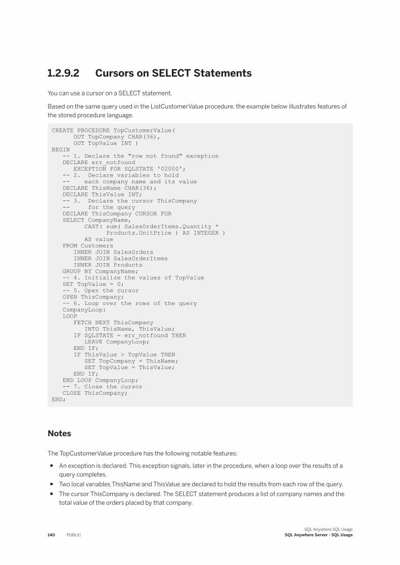
1.2.9.2 Cursors on SELECT StatementsYou can use a cursor on a SELECT statement.
Based on the same query used in the ListCustomerValue procedure, the example below illustrates features of the stored procedure language.
CREATE PROCEDURE TopCustomerValue( OUT TopCompany CHAR(36), OUT TopValue INT )BEGIN -- 1. Declare the "row not found" exception DECLARE err_notfound EXCEPTION FOR SQLSTATE '02000'; -- 2. Declare variables to hold -- each company name and its value DECLARE ThisName CHAR(36); DECLARE ThisValue INT; -- 3. Declare the cursor ThisCompany -- for the query DECLARE ThisCompany CURSOR FOR SELECT CompanyName, CAST( sum( SalesOrderItems.Quantity * Products.UnitPrice ) AS INTEGER ) AS value FROM Customers INNER JOIN SalesOrders INNER JOIN SalesOrderItems INNER JOIN Products GROUP BY CompanyName; -- 4. Initialize the values of TopValue SET TopValue = 0; -- 5. Open the cursor OPEN ThisCompany; -- 6. Loop over the rows of the query CompanyLoop: LOOP FETCH NEXT ThisCompany INTO ThisName, ThisValue; IF SQLSTATE = err_notfound THEN LEAVE CompanyLoop; END IF; IF ThisValue > TopValue THEN SET TopCompany = ThisName; SET TopValue = ThisValue; END IF; END LOOP CompanyLoop; -- 7. Close the cursor CLOSE ThisCompany; END;
Notes
The TopCustomerValue procedure has the following notable features:
● An exception is declared. This exception signals, later in the procedure, when a loop over the results of a query completes.
● Two local variables ThisName and ThisValue are declared to hold the results from each row of the query.● The cursor ThisCompany is declared. The SELECT statement produces a list of company names and the
total value of the orders placed by that company.
140 PUBLICSQL Anywhere SQL Usage
SQL Anywhere Server - SQL Usage
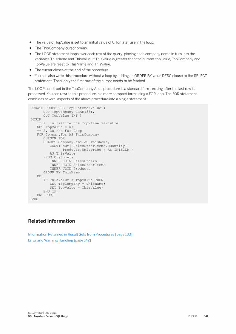
● The value of TopValue is set to an initial value of 0, for later use in the loop.● The ThisCompany cursor opens.● The LOOP statement loops over each row of the query, placing each company name in turn into the
variables ThisName and ThisValue. If ThisValue is greater than the current top value, TopCompany and TopValue are reset to ThisName and ThisValue.
● The cursor closes at the end of the procedure.● You can also write this procedure without a loop by adding an ORDER BY value DESC clause to the SELECT
statement. Then, only the first row of the cursor needs to be fetched.
The LOOP construct in the TopCompanyValue procedure is a standard form, exiting after the last row is processed. You can rewrite this procedure in a more compact form using a FOR loop. The FOR statement combines several aspects of the above procedure into a single statement.
CREATE PROCEDURE TopCustomerValue2( OUT TopCompany CHAR(36), OUT TopValue INT )BEGIN -- 1. Initialize the TopValue variable SET TopValue = 0; -- 2. Do the For Loop FOR CompanyFor AS ThisCompany CURSOR FOR SELECT CompanyName AS ThisName, CAST( sum( SalesOrderItems.Quantity * Products.UnitPrice ) AS INTEGER ) AS ThisValue FROM Customers INNER JOIN SalesOrders INNER JOIN SalesOrderItems INNER JOIN Products GROUP BY ThisName DO IF ThisValue > TopValue THEN SET TopCompany = ThisName; SET TopValue = ThisValue; END IF; END FOR; END;
Related Information
Information Returned in Result Sets from Procedures [page 133]Error and Warning Handling [page 142]
SQL Anywhere SQL UsageSQL Anywhere Server - SQL Usage PUBLIC 141
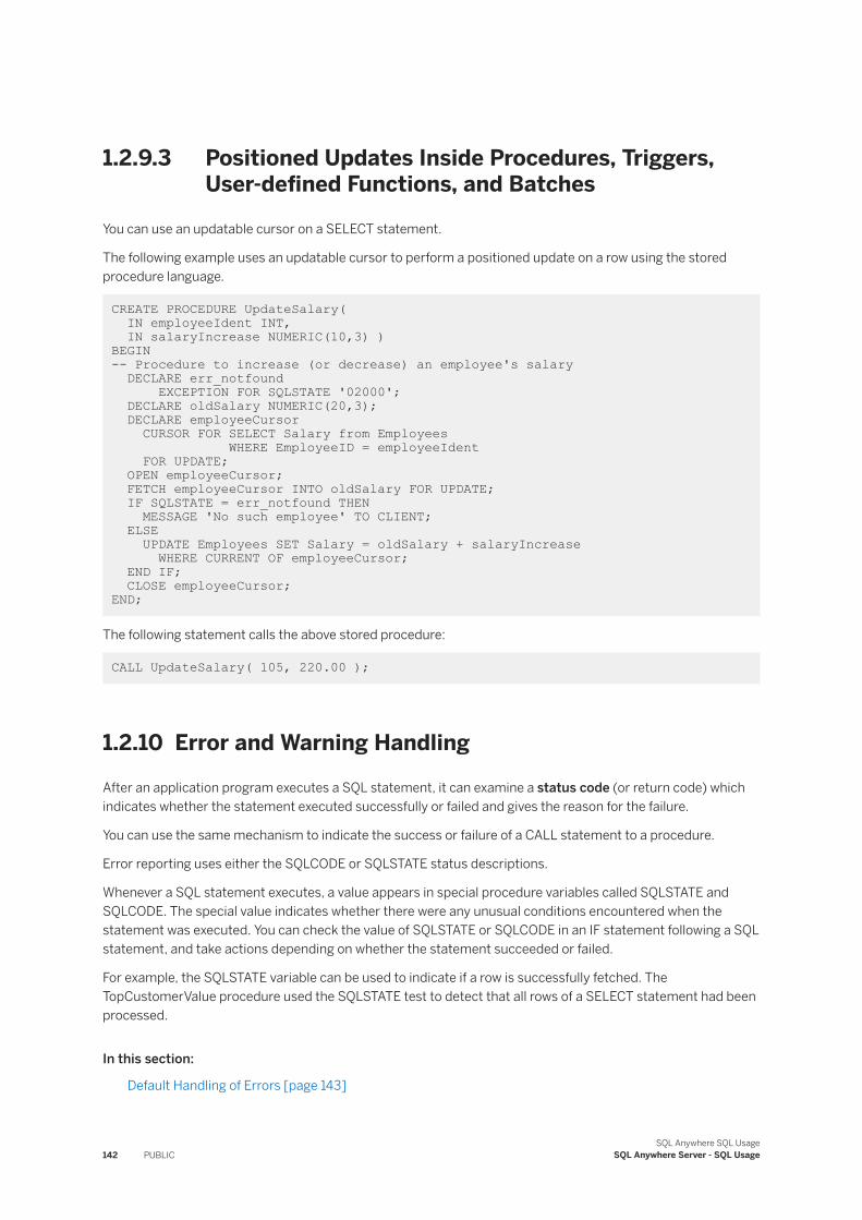
1.2.9.3 Positioned Updates Inside Procedures, Triggers, User-defined Functions, and Batches
You can use an updatable cursor on a SELECT statement.
The following example uses an updatable cursor to perform a positioned update on a row using the stored procedure language.
CREATE PROCEDURE UpdateSalary( IN employeeIdent INT, IN salaryIncrease NUMERIC(10,3) )BEGIN -- Procedure to increase (or decrease) an employee's salary DECLARE err_notfound EXCEPTION FOR SQLSTATE '02000'; DECLARE oldSalary NUMERIC(20,3); DECLARE employeeCursor CURSOR FOR SELECT Salary from Employees WHERE EmployeeID = employeeIdent FOR UPDATE; OPEN employeeCursor; FETCH employeeCursor INTO oldSalary FOR UPDATE; IF SQLSTATE = err_notfound THEN MESSAGE 'No such employee' TO CLIENT; ELSE UPDATE Employees SET Salary = oldSalary + salaryIncrease WHERE CURRENT OF employeeCursor; END IF; CLOSE employeeCursor; END;
The following statement calls the above stored procedure:
CALL UpdateSalary( 105, 220.00 );
1.2.10 Error and Warning Handling
After an application program executes a SQL statement, it can examine a status code (or return code) which indicates whether the statement executed successfully or failed and gives the reason for the failure.
You can use the same mechanism to indicate the success or failure of a CALL statement to a procedure.
Error reporting uses either the SQLCODE or SQLSTATE status descriptions.
Whenever a SQL statement executes, a value appears in special procedure variables called SQLSTATE and SQLCODE. The special value indicates whether there were any unusual conditions encountered when the statement was executed. You can check the value of SQLSTATE or SQLCODE in an IF statement following a SQL statement, and take actions depending on whether the statement succeeded or failed.
For example, the SQLSTATE variable can be used to indicate if a row is successfully fetched. The TopCustomerValue procedure used the SQLSTATE test to detect that all rows of a SELECT statement had been processed.
In this section:
Default Handling of Errors [page 143]
142 PUBLICSQL Anywhere SQL Usage
SQL Anywhere Server - SQL Usage
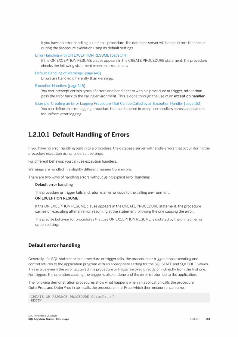
If you have no error handling built in to a procedure, the database server will handle errors that occur during the procedure execution using its default settings.
Error Handling with ON EXCEPTION RESUME [page 144]If the ON EXCEPTION RESUME clause appears in the CREATE PROCEDURE statement, the procedure checks the following statement when an error occurs.
Default Handling of Warnings [page 146]Errors are handled differently than warnings.
Exception Handlers [page 146]You can intercept certain types of errors and handle them within a procedure or trigger, rather than pass the error back to the calling environment. This is done through the use of an exception handler.
Example: Creating an Error Logging Procedure That Can be Called by an Exception Handler [page 153]You can define an error logging procedure that can be used in exception handlers across applications for uniform error logging.
1.2.10.1 Default Handling of Errors
If you have no error handling built in to a procedure, the database server will handle errors that occur during the procedure execution using its default settings.
For different behavior, you can use exception handlers.
Warnings are handled in a slightly different manner from errors.
There are two ways of handling errors without using explicit error handling:
Default error handling
The procedure or trigger fails and returns an error code to the calling environment.ON EXCEPTION RESUME
If the ON EXCEPTION RESUME clause appears in the CREATE PROCEDURE statement, the procedure carries on executing after an error, resuming at the statement following the one causing the error.
The precise behavior for procedures that use ON EXCEPTION RESUME is dictated by the on_tsql_error option setting.
Default error handling
Generally, if a SQL statement in a procedure or trigger fails, the procedure or trigger stops executing and control returns to the application program with an appropriate setting for the SQLSTATE and SQLCODE values. This is true even if the error occurred in a procedure or trigger invoked directly or indirectly from the first one. For triggers the operation causing the trigger is also undone and the error is returned to the application.
The following demonstration procedures show what happens when an application calls the procedure OuterProc, and OuterProc in turn calls the procedure InnerProc, which then encounters an error.
CREATE OR REPLACE PROCEDURE OuterProc() BEGIN
SQL Anywhere SQL UsageSQL Anywhere Server - SQL Usage PUBLIC 143
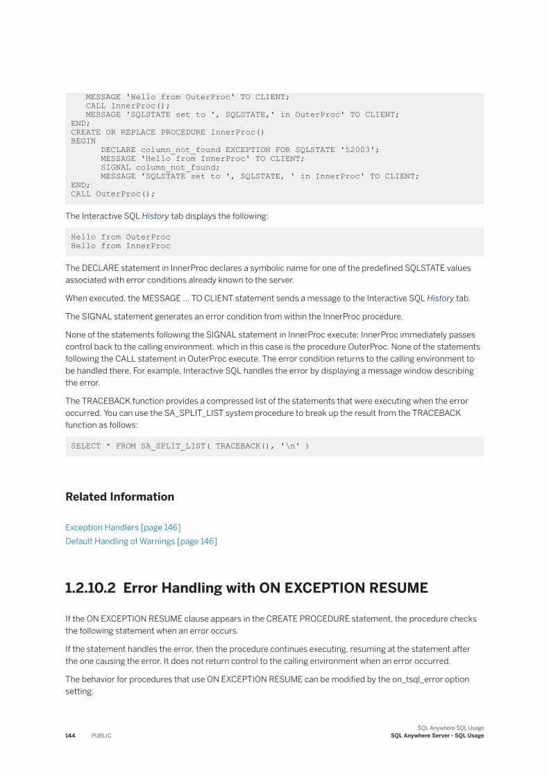
MESSAGE 'Hello from OuterProc' TO CLIENT; CALL InnerProc(); MESSAGE 'SQLSTATE set to ', SQLSTATE,' in OuterProc' TO CLIENT;END;CREATE OR REPLACE PROCEDURE InnerProc()BEGIN DECLARE column_not_found EXCEPTION FOR SQLSTATE '52003'; MESSAGE 'Hello from InnerProc' TO CLIENT; SIGNAL column_not_found; MESSAGE 'SQLSTATE set to ', SQLSTATE, ' in InnerProc' TO CLIENT;END; CALL OuterProc();
The Interactive SQL History tab displays the following:
Hello from OuterProc Hello from InnerProc
The DECLARE statement in InnerProc declares a symbolic name for one of the predefined SQLSTATE values associated with error conditions already known to the server.
When executed, the MESSAGE ... TO CLIENT statement sends a message to the Interactive SQL History tab.
The SIGNAL statement generates an error condition from within the InnerProc procedure.
None of the statements following the SIGNAL statement in InnerProc execute: InnerProc immediately passes control back to the calling environment, which in this case is the procedure OuterProc. None of the statements following the CALL statement in OuterProc execute. The error condition returns to the calling environment to be handled there. For example, Interactive SQL handles the error by displaying a message window describing the error.
The TRACEBACK function provides a compressed list of the statements that were executing when the error occurred. You can use the SA_SPLIT_LIST system procedure to break up the result from the TRACEBACK function as follows:
SELECT * FROM SA_SPLIT_LIST( TRACEBACK(), '\n' )
Related Information
Exception Handlers [page 146]Default Handling of Warnings [page 146]
1.2.10.2 Error Handling with ON EXCEPTION RESUME
If the ON EXCEPTION RESUME clause appears in the CREATE PROCEDURE statement, the procedure checks the following statement when an error occurs.
If the statement handles the error, then the procedure continues executing, resuming at the statement after the one causing the error. It does not return control to the calling environment when an error occurred.
The behavior for procedures that use ON EXCEPTION RESUME can be modified by the on_tsql_error option setting.
144 PUBLICSQL Anywhere SQL Usage
SQL Anywhere Server - SQL Usage
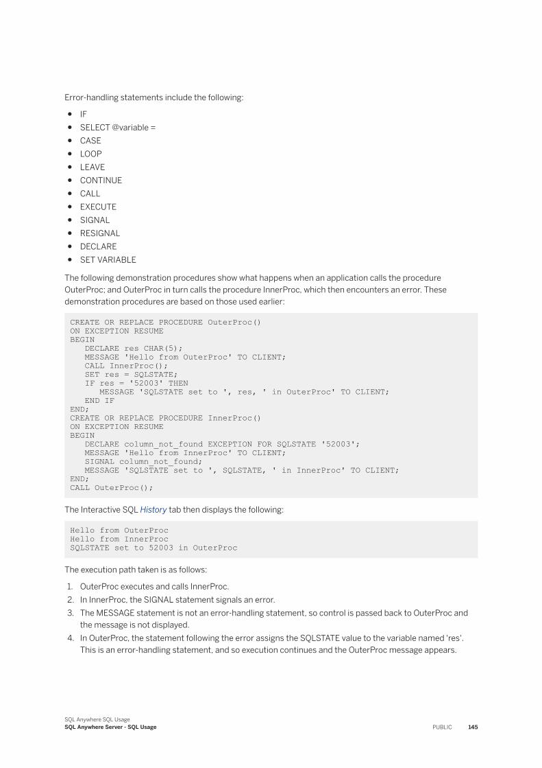
Error-handling statements include the following:
● IF● SELECT @variable =● CASE● LOOP● LEAVE● CONTINUE● CALL● EXECUTE● SIGNAL● RESIGNAL● DECLARE● SET VARIABLE
The following demonstration procedures show what happens when an application calls the procedure OuterProc; and OuterProc in turn calls the procedure InnerProc, which then encounters an error. These demonstration procedures are based on those used earlier:
CREATE OR REPLACE PROCEDURE OuterProc() ON EXCEPTION RESUMEBEGIN DECLARE res CHAR(5); MESSAGE 'Hello from OuterProc' TO CLIENT; CALL InnerProc(); SET res = SQLSTATE; IF res = '52003' THEN MESSAGE 'SQLSTATE set to ', res, ' in OuterProc' TO CLIENT; END IFEND;CREATE OR REPLACE PROCEDURE InnerProc()ON EXCEPTION RESUMEBEGIN DECLARE column_not_found EXCEPTION FOR SQLSTATE '52003'; MESSAGE 'Hello from InnerProc' TO CLIENT; SIGNAL column_not_found; MESSAGE 'SQLSTATE set to ', SQLSTATE, ' in InnerProc' TO CLIENT;END; CALL OuterProc();
The Interactive SQL History tab then displays the following:
Hello from OuterProc Hello from InnerProc SQLSTATE set to 52003 in OuterProc
The execution path taken is as follows:
1. OuterProc executes and calls InnerProc.2. In InnerProc, the SIGNAL statement signals an error.3. The MESSAGE statement is not an error-handling statement, so control is passed back to OuterProc and
the message is not displayed.4. In OuterProc, the statement following the error assigns the SQLSTATE value to the variable named 'res'.
This is an error-handling statement, and so execution continues and the OuterProc message appears.
SQL Anywhere SQL UsageSQL Anywhere Server - SQL Usage PUBLIC 145
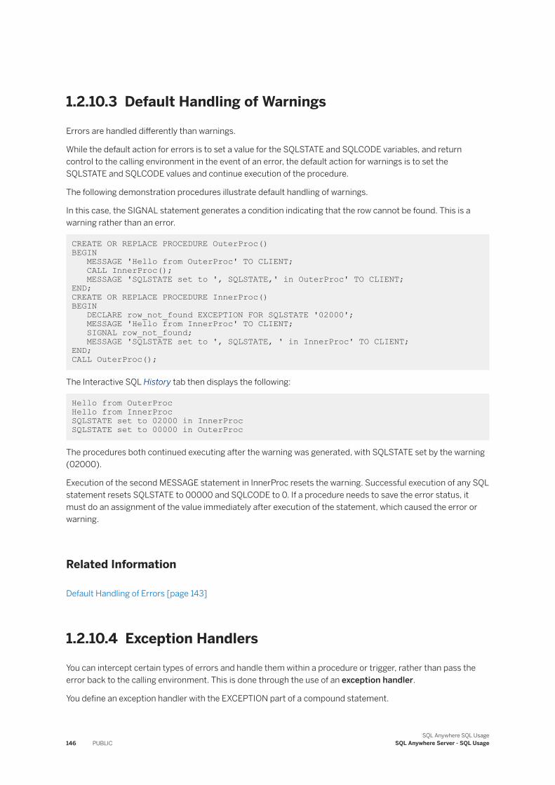
1.2.10.3 Default Handling of Warnings
Errors are handled differently than warnings.
While the default action for errors is to set a value for the SQLSTATE and SQLCODE variables, and return control to the calling environment in the event of an error, the default action for warnings is to set the SQLSTATE and SQLCODE values and continue execution of the procedure.
The following demonstration procedures illustrate default handling of warnings.
In this case, the SIGNAL statement generates a condition indicating that the row cannot be found. This is a warning rather than an error.
CREATE OR REPLACE PROCEDURE OuterProc() BEGIN MESSAGE 'Hello from OuterProc' TO CLIENT; CALL InnerProc(); MESSAGE 'SQLSTATE set to ', SQLSTATE,' in OuterProc' TO CLIENT;END;CREATE OR REPLACE PROCEDURE InnerProc()BEGIN DECLARE row_not_found EXCEPTION FOR SQLSTATE '02000'; MESSAGE 'Hello from InnerProc' TO CLIENT; SIGNAL row_not_found; MESSAGE 'SQLSTATE set to ', SQLSTATE, ' in InnerProc' TO CLIENT;END; CALL OuterProc();
The Interactive SQL History tab then displays the following:
Hello from OuterProcHello from InnerProcSQLSTATE set to 02000 in InnerProc SQLSTATE set to 00000 in OuterProc
The procedures both continued executing after the warning was generated, with SQLSTATE set by the warning (02000).
Execution of the second MESSAGE statement in InnerProc resets the warning. Successful execution of any SQL statement resets SQLSTATE to 00000 and SQLCODE to 0. If a procedure needs to save the error status, it must do an assignment of the value immediately after execution of the statement, which caused the error or warning.
Related Information
Default Handling of Errors [page 143]
1.2.10.4 Exception Handlers
You can intercept certain types of errors and handle them within a procedure or trigger, rather than pass the error back to the calling environment. This is done through the use of an exception handler.
You define an exception handler with the EXCEPTION part of a compound statement.
146 PUBLICSQL Anywhere SQL Usage
SQL Anywhere Server - SQL Usage
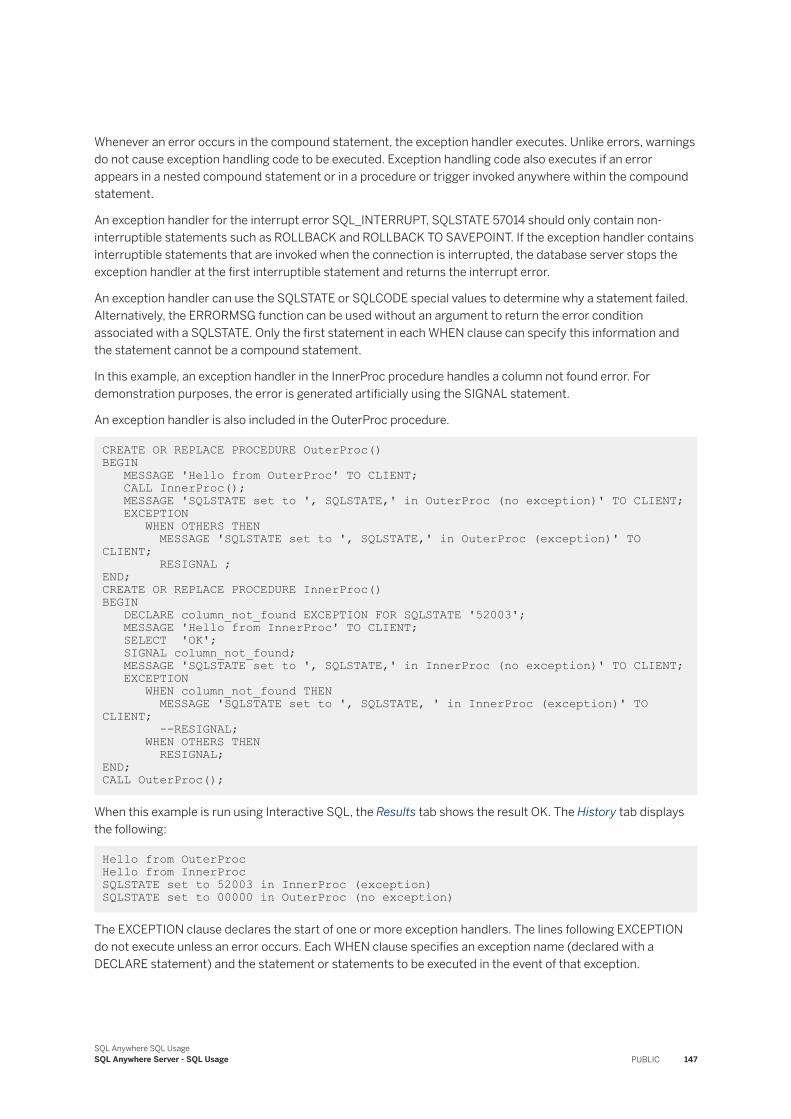
Whenever an error occurs in the compound statement, the exception handler executes. Unlike errors, warnings do not cause exception handling code to be executed. Exception handling code also executes if an error appears in a nested compound statement or in a procedure or trigger invoked anywhere within the compound statement.
An exception handler for the interrupt error SQL_INTERRUPT, SQLSTATE 57014 should only contain non-interruptible statements such as ROLLBACK and ROLLBACK TO SAVEPOINT. If the exception handler contains interruptible statements that are invoked when the connection is interrupted, the database server stops the exception handler at the first interruptible statement and returns the interrupt error.
An exception handler can use the SQLSTATE or SQLCODE special values to determine why a statement failed. Alternatively, the ERRORMSG function can be used without an argument to return the error condition associated with a SQLSTATE. Only the first statement in each WHEN clause can specify this information and the statement cannot be a compound statement.
In this example, an exception handler in the InnerProc procedure handles a column not found error. For demonstration purposes, the error is generated artificially using the SIGNAL statement.
An exception handler is also included in the OuterProc procedure.
CREATE OR REPLACE PROCEDURE OuterProc() BEGIN MESSAGE 'Hello from OuterProc' TO CLIENT; CALL InnerProc(); MESSAGE 'SQLSTATE set to ', SQLSTATE,' in OuterProc (no exception)' TO CLIENT; EXCEPTION WHEN OTHERS THEN MESSAGE 'SQLSTATE set to ', SQLSTATE,' in OuterProc (exception)' TO CLIENT; RESIGNAL ;END;CREATE OR REPLACE PROCEDURE InnerProc()BEGIN DECLARE column_not_found EXCEPTION FOR SQLSTATE '52003'; MESSAGE 'Hello from InnerProc' TO CLIENT; SELECT 'OK'; SIGNAL column_not_found; MESSAGE 'SQLSTATE set to ', SQLSTATE,' in InnerProc (no exception)' TO CLIENT; EXCEPTION WHEN column_not_found THEN MESSAGE 'SQLSTATE set to ', SQLSTATE, ' in InnerProc (exception)' TO CLIENT; --RESIGNAL; WHEN OTHERS THEN RESIGNAL;END; CALL OuterProc();
When this example is run using Interactive SQL, the Results tab shows the result OK. The History tab displays the following:
Hello from OuterProc Hello from InnerProcSQLSTATE set to 52003 in InnerProc (exception) SQLSTATE set to 00000 in OuterProc (no exception)
The EXCEPTION clause declares the start of one or more exception handlers. The lines following EXCEPTION do not execute unless an error occurs. Each WHEN clause specifies an exception name (declared with a DECLARE statement) and the statement or statements to be executed in the event of that exception.
SQL Anywhere SQL UsageSQL Anywhere Server - SQL Usage PUBLIC 147
The WHEN OTHERS THEN clause specifies the statement(s) to be executed when the exception that occurred does not appear in the preceding WHEN clauses.
In the above example, the statement RESIGNAL passes the exception on to a higher-level exception handler. If WHEN OTHERS THEN is not specified in an exception handler, the default action for any unhandled exception is RESIGNAL.
To pass the column_not_found exception to OuterProc, remove the comment indicator from the RESIGNAL statement. This will cause the exception handler in the OuterProc procedure to be invoked.
Additional Notes
● The EXCEPTION handler executes, rather than the lines following the SIGNAL statement in InnerProc.● As the error encountered was an error about a column that cannot be found, the MESSAGE statement
included to handle the error executes, and SQLSTATE resets to zero (indicating no errors).● After the exception handling code executes, control passes back to OuterProc, which proceeds as if no
error was encountered.● Do not use ON EXCEPTION RESUME together with explicit exception handling. The exception handling
code is not executed if ON EXCEPTION RESUME is included.● If the error handling code for the error is a RESIGNAL statement, control returns to the OuterProc
procedure with SQLSTATE still set at the value 52003. This is just as if there were no error handling code in InnerProc. Since there is no error handling code in OuterProc, the procedure fails.
In this section:
Exception Handling with RESIGNAL [page 149]When a user-defined stored procedure includes an EXCEPTION handler that uses RESIGNAL to pass the exception to caller, the calling procedure may not be able to obtain a result set. It depends on how the user-defined stored procedure was invoked.
Exception Handling and Atomic Compound Statements [page 150]If an error occurs within an atomic compound statement and that statement has an exception handler that handles the error, then the compound statement completes without an active exception and the changes before the exception are not reversed.
Exception Handling and Nested Compound Statements [page 150]The code following a statement that causes an error executes only if an ON EXCEPTION RESUME clause appears in a procedure definition.
Related Information
Default Handling of Errors [page 143]Compound Statements [page 128]
148 PUBLICSQL Anywhere SQL Usage
SQL Anywhere Server - SQL Usage
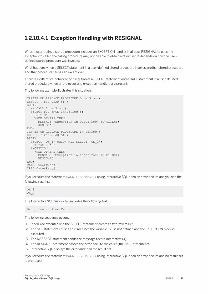
1.2.10.4.1 Exception Handling with RESIGNAL
When a user-defined stored procedure includes an EXCEPTION handler that uses RESIGNAL to pass the exception to caller, the calling procedure may not be able to obtain a result set. It depends on how the user-defined stored procedure was invoked.
What happens when a SELECT statement in a user-defined stored procedure invokes another stored procedure and that procedure causes an exception?
There is a difference between the execution of a SELECT statement and a CALL statement in a user-defined stored procedure when errors occur and exception handlers are present.
The following example illustrates this situation.
CREATE OR REPLACE PROCEDURE OuterProc() RESULT ( res CHAR(5) )BEGIN -- CALL InnerProc(); SELECT res FROM InnerProc(); EXCEPTION WHEN OTHERS THEN MESSAGE 'Exception in OuterProc' TO CLIENT; RESIGNAL;END;CREATE OR REPLACE PROCEDURE InnerProc()RESULT ( res CHAR(5) )BEGIN SELECT 'OK_1' UNION ALL SELECT 'OK_2'; SET tst = '3'; EXCEPTION WHEN OTHERS THEN MESSAGE 'Exception in InnerProc' TO CLIENT; RESIGNAL;END;CALL InnerProc(); CALL OuterProc();
If you execute the statement CALL InnerProc() using Interactive SQL, then an error occurs and you see the following result set:
OK_1 OK_2
The Interactive SQL History tab includes the following text:
Exception in InnerProc
The following sequence occurs.
1. InnerProc executes and the SELECT statement creates a two-row result.2. The SET statement causes an error since the variable tst is not defined and the EXCEPTION block is
executed.3. The MESSAGE statement sends the message text to Interactive SQL.4. The RESIGNAL statement passes the error back to the caller (the CALL statement).5. Interactive SQL displays the error and then the result set.
If you execute the statement CALL OuterProc() using Interactive SQL, then an error occurs and no result set is produced.
SQL Anywhere SQL UsageSQL Anywhere Server - SQL Usage PUBLIC 149
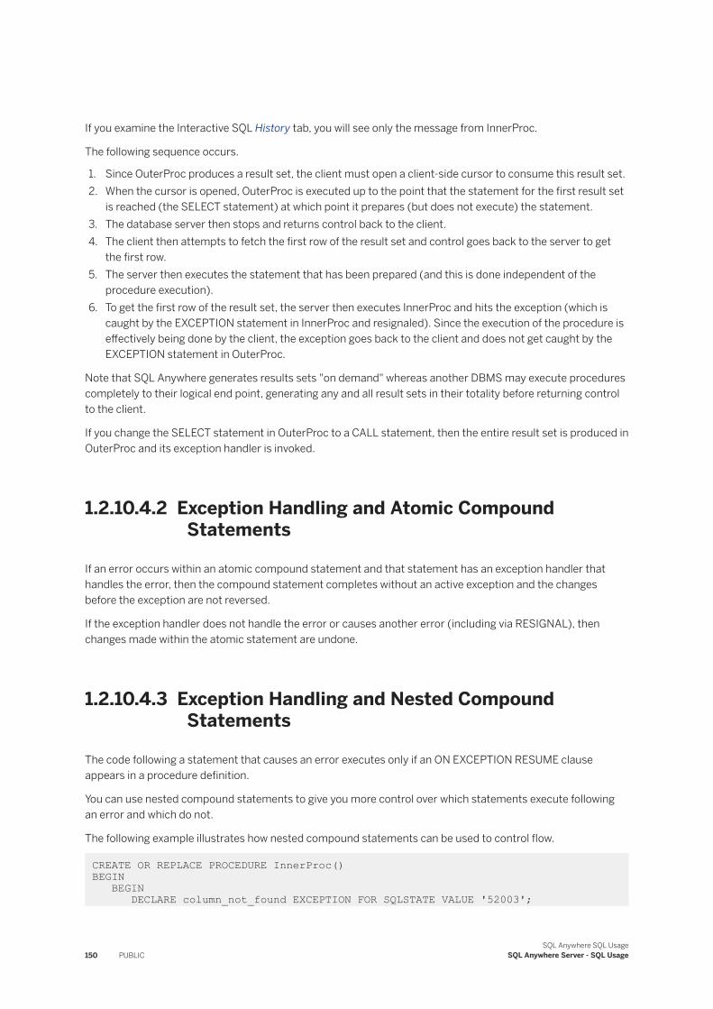
If you examine the Interactive SQL History tab, you will see only the message from InnerProc.
The following sequence occurs.
1. Since OuterProc produces a result set, the client must open a client-side cursor to consume this result set.2. When the cursor is opened, OuterProc is executed up to the point that the statement for the first result set
is reached (the SELECT statement) at which point it prepares (but does not execute) the statement.3. The database server then stops and returns control back to the client.4. The client then attempts to fetch the first row of the result set and control goes back to the server to get
the first row.5. The server then executes the statement that has been prepared (and this is done independent of the
procedure execution).6. To get the first row of the result set, the server then executes InnerProc and hits the exception (which is
caught by the EXCEPTION statement in InnerProc and resignaled). Since the execution of the procedure is effectively being done by the client, the exception goes back to the client and does not get caught by the EXCEPTION statement in OuterProc.
Note that SQL Anywhere generates results sets "on demand" whereas another DBMS may execute procedures completely to their logical end point, generating any and all result sets in their totality before returning control to the client.
If you change the SELECT statement in OuterProc to a CALL statement, then the entire result set is produced in OuterProc and its exception handler is invoked.
1.2.10.4.2 Exception Handling and Atomic Compound Statements
If an error occurs within an atomic compound statement and that statement has an exception handler that handles the error, then the compound statement completes without an active exception and the changes before the exception are not reversed.
If the exception handler does not handle the error or causes another error (including via RESIGNAL), then changes made within the atomic statement are undone.
1.2.10.4.3 Exception Handling and Nested Compound Statements
The code following a statement that causes an error executes only if an ON EXCEPTION RESUME clause appears in a procedure definition.
You can use nested compound statements to give you more control over which statements execute following an error and which do not.
The following example illustrates how nested compound statements can be used to control flow.
CREATE OR REPLACE PROCEDURE InnerProc() BEGIN BEGIN DECLARE column_not_found EXCEPTION FOR SQLSTATE VALUE '52003';
150 PUBLICSQL Anywhere SQL Usage
SQL Anywhere Server - SQL Usage
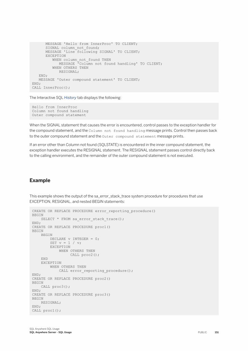
MESSAGE 'Hello from InnerProc' TO CLIENT; SIGNAL column_not_found; MESSAGE 'Line following SIGNAL' TO CLIENT; EXCEPTION WHEN column_not_found THEN MESSAGE 'Column not found handling' TO CLIENT; WHEN OTHERS THEN RESIGNAL; END; MESSAGE 'Outer compound statement' TO CLIENT;END; CALL InnerProc();
The Interactive SQL History tab displays the following:
Hello from InnerProc Column not found handling Outer compound statement
When the SIGNAL statement that causes the error is encountered, control passes to the exception handler for the compound statement, and the Column not found handling message prints. Control then passes back to the outer compound statement and the Outer compound statement message prints.
If an error other than Column not found (SQLSTATE) is encountered in the inner compound statement, the exception handler executes the RESIGNAL statement. The RESIGNAL statement passes control directly back to the calling environment, and the remainder of the outer compound statement is not executed.
Example
This example shows the output of the sa_error_stack_trace system procedure for procedures that use EXCEPTION, RESIGNAL, and nested BEGIN statements:
CREATE OR REPLACE PROCEDURE error_reporting_procedure() BEGIN SELECT * FROM sa_error_stack_trace();END;CREATE OR REPLACE PROCEDURE proc1()BEGIN BEGIN DECLARE v INTEGER = 0; SET v = 1 / v; EXCEPTION WHEN OTHERS THEN CALL proc2(); END EXCEPTION WHEN OTHERS THEN CALL error_reporting_procedure();END;CREATE OR REPLACE PROCEDURE proc2()BEGIN CALL proc3();END;CREATE OR REPLACE PROCEDURE proc3()BEGIN RESIGNAL;END; CALL proc1();
SQL Anywhere SQL UsageSQL Anywhere Server - SQL Usage PUBLIC 151
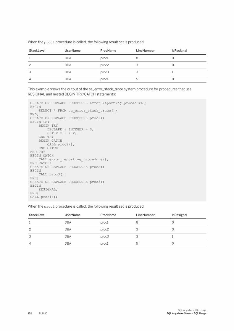
When the proc1 procedure is called, the following result set is produced:
StackLevel UserName ProcName LineNumber IsResignal
1 DBA proc1 8 0
2 DBA proc2 3 0
3 DBA proc3 3 1
4 DBA proc1 5 0
This example shows the output of the sa_error_stack_trace system procedure for procedures that use RESIGNAL and nested BEGIN TRY/CATCH statements:
CREATE OR REPLACE PROCEDURE error_reporting_procedure() BEGIN SELECT * FROM sa_error_stack_trace();END;CREATE OR REPLACE PROCEDURE proc1()BEGIN TRY BEGIN TRY DECLARE v INTEGER = 0; SET v = 1 / v; END TRY BEGIN CATCH CALL proc2(); END CATCHEND TRYBEGIN CATCH CALL error_reporting_procedure();END CATCH;CREATE OR REPLACE PROCEDURE proc2()BEGIN CALL proc3();END;CREATE OR REPLACE PROCEDURE proc3()BEGIN RESIGNAL;END; CALL proc1();
When the proc1 procedure is called, the following result set is produced:
StackLevel UserName ProcName LineNumber IsResignal
1 DBA proc1 8 0
2 DBA proc2 3 0
3 DBA proc3 3 1
4 DBA proc1 5 0
152 PUBLICSQL Anywhere SQL Usage
SQL Anywhere Server - SQL Usage
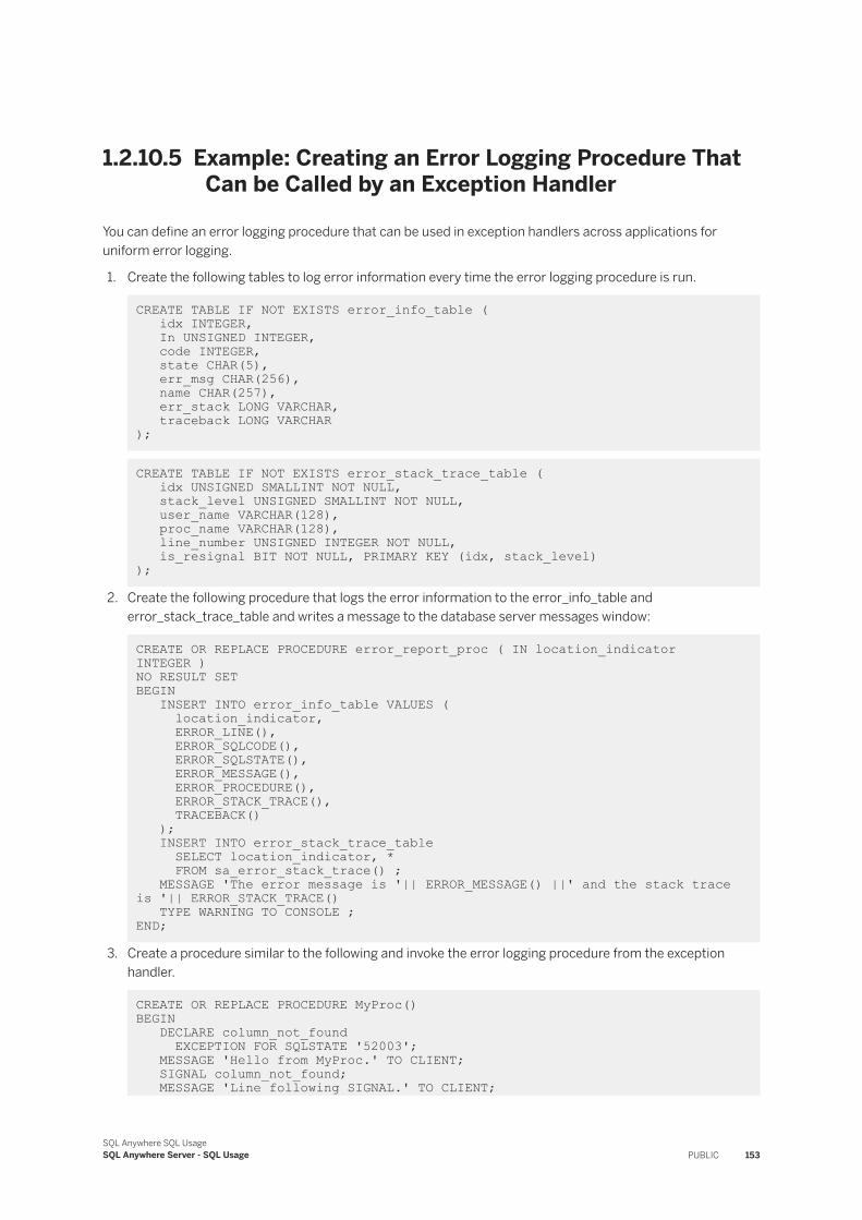
1.2.10.5 Example: Creating an Error Logging Procedure That Can be Called by an Exception Handler
You can define an error logging procedure that can be used in exception handlers across applications for uniform error logging.
1. Create the following tables to log error information every time the error logging procedure is run.
CREATE TABLE IF NOT EXISTS error_info_table ( idx INTEGER, In UNSIGNED INTEGER, code INTEGER, state CHAR(5), err_msg CHAR(256), name CHAR(257), err_stack LONG VARCHAR, traceback LONG VARCHAR );
CREATE TABLE IF NOT EXISTS error_stack_trace_table ( idx UNSIGNED SMALLINT NOT NULL, stack_level UNSIGNED SMALLINT NOT NULL, user_name VARCHAR(128), proc_name VARCHAR(128), line_number UNSIGNED INTEGER NOT NULL, is_resignal BIT NOT NULL, PRIMARY KEY (idx, stack_level) );
2. Create the following procedure that logs the error information to the error_info_table and error_stack_trace_table and writes a message to the database server messages window:
CREATE OR REPLACE PROCEDURE error_report_proc ( IN location_indicator INTEGER ) NO RESULT SETBEGIN INSERT INTO error_info_table VALUES ( location_indicator, ERROR_LINE(), ERROR_SQLCODE(), ERROR_SQLSTATE(), ERROR_MESSAGE(), ERROR_PROCEDURE(), ERROR_STACK_TRACE(), TRACEBACK() ); INSERT INTO error_stack_trace_table SELECT location_indicator, * FROM sa_error_stack_trace() ; MESSAGE 'The error message is '|| ERROR_MESSAGE() ||' and the stack trace is '|| ERROR_STACK_TRACE() TYPE WARNING TO CONSOLE ; END;
3. Create a procedure similar to the following and invoke the error logging procedure from the exception handler.
CREATE OR REPLACE PROCEDURE MyProc() BEGIN DECLARE column_not_found EXCEPTION FOR SQLSTATE '52003'; MESSAGE 'Hello from MyProc.' TO CLIENT; SIGNAL column_not_found; MESSAGE 'Line following SIGNAL.' TO CLIENT;
SQL Anywhere SQL UsageSQL Anywhere Server - SQL Usage PUBLIC 153
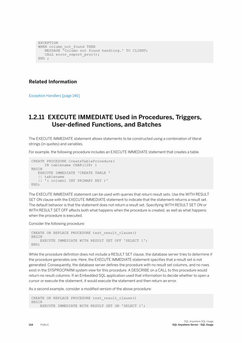
EXCEPTIONWHEN column_not_found THEN MESSAGE 'Column not found handling.' TO CLIENT; CALL error_report_proc(); END ;
Related Information
Exception Handlers [page 146]
1.2.11 EXECUTE IMMEDIATE Used in Procedures, Triggers, User-defined Functions, and Batches
The EXECUTE IMMEDIATE statement allows statements to be constructed using a combination of literal strings (in quotes) and variables.
For example, the following procedure includes an EXECUTE IMMEDIATE statement that creates a table.
CREATE PROCEDURE CreateTableProcedure( IN tablename CHAR(128) )BEGIN EXECUTE IMMEDIATE 'CREATE TABLE ' || tablename || '( column1 INT PRIMARY KEY )' END;
The EXECUTE IMMEDIATE statement can be used with queries that return result sets. Use the WITH RESULT SET ON clause with the EXECUTE IMMEDIATE statement to indicate that the statement returns a result set. The default behavior is that the statement does not return a result set. Specifying WITH RESULT SET ON or WITH RESULT SET OFF affects both what happens when the procedure is created, as well as what happens when the procedure is executed.
Consider the following procedure:
CREATE OR REPLACE PROCEDURE test_result_clause() BEGIN EXECUTE IMMEDIATE WITH RESULT SET OFF 'SELECT 1'; END;
While the procedure definition does not include a RESULT SET clause, the database server tries to determine if the procedure generates one. Here, the EXECUTE IMMEDIATE statement specifies that a result set is not generated. Consequently, the database server defines the procedure with no result set columns, and no rows exist in the SYSPROCPARM system view for this procedure. A DESCRIBE on a CALL to this procedure would return no result columns. If an Embedded SQL application used that information to decide whether to open a cursor or execute the statement, it would execute the statement and then return an error.
As a second example, consider a modified version of the above procedure:
CREATE OR REPLACE PROCEDURE test_result_clause() BEGIN EXECUTE IMMEDIATE WITH RESULT SET ON 'SELECT 1';
154 PUBLICSQL Anywhere SQL Usage
SQL Anywhere Server - SQL Usage
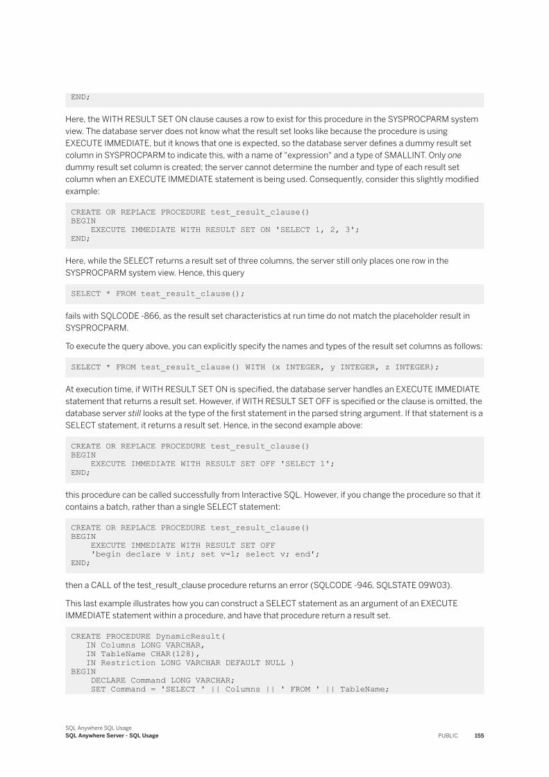
END;
Here, the WITH RESULT SET ON clause causes a row to exist for this procedure in the SYSPROCPARM system view. The database server does not know what the result set looks like because the procedure is using EXECUTE IMMEDIATE, but it knows that one is expected, so the database server defines a dummy result set column in SYSPROCPARM to indicate this, with a name of "expression" and a type of SMALLINT. Only one dummy result set column is created; the server cannot determine the number and type of each result set column when an EXECUTE IMMEDIATE statement is being used. Consequently, consider this slightly modified example:
CREATE OR REPLACE PROCEDURE test_result_clause() BEGIN EXECUTE IMMEDIATE WITH RESULT SET ON 'SELECT 1, 2, 3'; END;
Here, while the SELECT returns a result set of three columns, the server still only places one row in the SYSPROCPARM system view. Hence, this query
SELECT * FROM test_result_clause();
fails with SQLCODE -866, as the result set characteristics at run time do not match the placeholder result in SYSPROCPARM.
To execute the query above, you can explicitly specify the names and types of the result set columns as follows:
SELECT * FROM test_result_clause() WITH (x INTEGER, y INTEGER, z INTEGER);
At execution time, if WITH RESULT SET ON is specified, the database server handles an EXECUTE IMMEDIATE statement that returns a result set. However, if WITH RESULT SET OFF is specified or the clause is omitted, the database server still looks at the type of the first statement in the parsed string argument. If that statement is a SELECT statement, it returns a result set. Hence, in the second example above:
CREATE OR REPLACE PROCEDURE test_result_clause() BEGIN EXECUTE IMMEDIATE WITH RESULT SET OFF 'SELECT 1'; END;
this procedure can be called successfully from Interactive SQL. However, if you change the procedure so that it contains a batch, rather than a single SELECT statement:
CREATE OR REPLACE PROCEDURE test_result_clause() BEGIN EXECUTE IMMEDIATE WITH RESULT SET OFF 'begin declare v int; set v=1; select v; end'; END;
then a CALL of the test_result_clause procedure returns an error (SQLCODE -946, SQLSTATE 09W03).
This last example illustrates how you can construct a SELECT statement as an argument of an EXECUTE IMMEDIATE statement within a procedure, and have that procedure return a result set.
CREATE PROCEDURE DynamicResult( IN Columns LONG VARCHAR, IN TableName CHAR(128), IN Restriction LONG VARCHAR DEFAULT NULL )BEGIN DECLARE Command LONG VARCHAR; SET Command = 'SELECT ' || Columns || ' FROM ' || TableName;
SQL Anywhere SQL UsageSQL Anywhere Server - SQL Usage PUBLIC 155
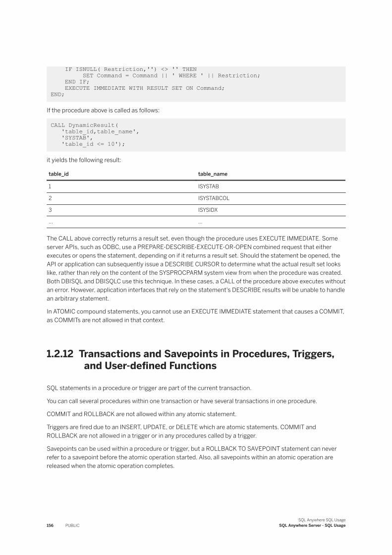
IF ISNULL( Restriction,'') <> '' THEN SET Command = Command || ' WHERE ' || Restriction; END IF; EXECUTE IMMEDIATE WITH RESULT SET ON Command; END;
If the procedure above is called as follows:
CALL DynamicResult( 'table_id,table_name', 'SYSTAB', 'table_id <= 10');
it yields the following result:
table_id table_name
1 ISYSTAB
2 ISYSTABCOL
3 ISYSIDX
... ...
The CALL above correctly returns a result set, even though the procedure uses EXECUTE IMMEDIATE. Some server APIs, such as ODBC, use a PREPARE-DESCRIBE-EXECUTE-OR-OPEN combined request that either executes or opens the statement, depending on if it returns a result set. Should the statement be opened, the API or application can subsequently issue a DESCRIBE CURSOR to determine what the actual result set looks like, rather than rely on the content of the SYSPROCPARM system view from when the procedure was created. Both DBISQL and DBISQLC use this technique. In these cases, a CALL of the procedure above executes without an error. However, application interfaces that rely on the statement's DESCRIBE results will be unable to handle an arbitrary statement.
In ATOMIC compound statements, you cannot use an EXECUTE IMMEDIATE statement that causes a COMMIT, as COMMITs are not allowed in that context.
1.2.12 Transactions and Savepoints in Procedures, Triggers, and User-defined Functions
SQL statements in a procedure or trigger are part of the current transaction.
You can call several procedures within one transaction or have several transactions in one procedure.
COMMIT and ROLLBACK are not allowed within any atomic statement.
Triggers are fired due to an INSERT, UPDATE, or DELETE which are atomic statements. COMMIT and ROLLBACK are not allowed in a trigger or in any procedures called by a trigger.
Savepoints can be used within a procedure or trigger, but a ROLLBACK TO SAVEPOINT statement can never refer to a savepoint before the atomic operation started. Also, all savepoints within an atomic operation are released when the atomic operation completes.
156 PUBLICSQL Anywhere SQL Usage
SQL Anywhere Server - SQL Usage
Related Information
Transactions and Isolation Levels [page 771]Atomic Compound Statements [page 128]Savepoints Within Transactions [page 776]
1.2.13 Tips for Writing Procedures, Triggers, User-defined Functions, and Batches
There are several pointers that are helpful for writing procedures, triggers, user-defined functions, and batches.
Check If You Must Change the SQL Statement Delimiter
You do not have to change the statement delimiter when you write procedures. However, if you create and test procedures and triggers from some other browsing tool, you must change the statement delimiter from the semicolon to another character.
Each statement within the procedure ends with a semicolon. For some browsing applications to parse the CREATE PROCEDURE statement itself, you need the statement delimiter to be something other than a semicolon.
If you are using an application that requires changing the statement delimiter, a good choice is to use two semicolons as the statement delimiter (;;) or a question mark (?) if the system does not permit a multi-character delimiter.
Remember to Delimit Statements Within Your Procedure
End each statement within the procedure with a semicolon. Although you can leave off semicolons for the last statement in a statement list, it is good practice to use semicolons after each statement.
The CREATE PROCEDURE statement itself contains both the RESULT specification and the compound statement that forms its body. No semicolon is needed after the BEGIN or END keywords, or after the RESULT clause.
Use Fully Qualified Names for Tables in Procedures
If a procedure has references to tables in it, preface the table name with the name of the owner (creator) of the table.
When a procedure refers to a table, it uses the role memberships of the procedure creator to locate tables with no explicit owner name specified. For example, if a procedure created by user_1 references Table_B and does
SQL Anywhere SQL UsageSQL Anywhere Server - SQL Usage PUBLIC 157
not specify the owner of Table_B, then either Table_B must have been created by user_1 or user_1 must be a member of a role (directly or indirectly) that is the owner of Table_B. If neither condition is met, a table not found message results when the procedure is called.
You can minimize the inconvenience of long fully qualified names by using a correlation name for the table in the FROM clause.
Specifying Dates and Times in Procedures
When dates and times are sent to the database from procedures, they are sent as strings. The date part of the string is interpreted according to the current setting of the date_order database option. As different connections may set this option to different values, some strings may be converted incorrectly to dates, or the database may not be able to convert the string to a date.
Use the unambiguous date format yyyy-mm-dd or yyyy/mm/dd when using date strings within procedures. The server interprets these strings unambiguously as dates, regardless of the date_order database option setting.
Verifying that Procedure Input Arguments Are Passed Correctly
One way to verify input arguments is to display the value of the parameter on the Interactive SQL History tab using the MESSAGE statement. For example, the following procedure simply displays the value of the input parameter var:
CREATE PROCEDURE message_test( IN var char(40) ) BEGIN MESSAGE var TO CLIENT; END;
You can also use the debugger to verify that procedure input arguments were passed correctly.
Related Information
Lesson 2: Diagnosing the Bug [page 853]
1.2.14 Statements Allowed in Procedures, Triggers, Events, and Batches
Most SQL statements are acceptable in batches, but there are several exceptions.
● ALTER DATABASE (depending on the syntax)● CONNECT
158 PUBLICSQL Anywhere SQL Usage
SQL Anywhere Server - SQL Usage
● CREATE DATABASE● CREATE DECRYPTED FILE● CREATE ENCRYPTED FILE● DISCONNECT● DROP CONNECTION● DROP DATABASE● FORWARD TO● Interactive SQL statements such as INPUT or OUTPUT● PREPARE TO COMMIT● STOP SERVER
You can use COMMIT, ROLLBACK, and SAVEPOINT statements within procedures, triggers, events, and batches with certain restrictions.
In this section:
SELECT Statements Used in Batches [page 159]You can include one or more SELECT statements in a batch.
Related Information
Transactions and Savepoints in Procedures, Triggers, and User-defined Functions [page 156]
1.2.14.1 SELECT Statements Used in Batches
You can include one or more SELECT statements in a batch.
For example:
IF EXISTS( SELECT * FROM SYSTAB WHERE table_name='Employees' )THEN SELECT Surname AS LastName, GivenName AS FirstName FROM Employees; SELECT Surname, GivenName FROM Customers; SELECT Surname, GivenName FROM Contacts; END IF;
The alias for the result set is necessary only in the first SELECT statement, as the server uses the first SELECT statement in the batch to describe the result set.
A RESUME statement is necessary following each query to retrieve the next result set.
SQL Anywhere SQL UsageSQL Anywhere Server - SQL Usage PUBLIC 159
1.2.15 Hiding the Contents of a Procedure, Function, Trigger, Event, or View
Use the SET HIDDEN clause to obscure the contents of a procedure, function, trigger, event, or view.
Prerequisites
You must be the owner of the object, have the ALTER ANY OBJECT system privilege, or have one of the following privileges:
Procedures and functions
ALTER ANY PROCEDURE system privilegeViews
ALTER ANY VIEW system privilegeEvents
MANAGE ANY EVENT system privilegeTriggers
● ALTER ANY TRIGGER system privilege● ALTER privilege on the underlying table and the CREATE ANY OBJECT system privilege● For triggers on views, you must have the ALTER ANY TRIGGER and ALTER ANY VIEW system privileges
Context
To distribute an application and a database without disclosing the logic contained within procedures, functions, triggers, events, and views, you can obscure the contents of these objects using the SET HIDDEN clause of the ALTER PROCEDURE, ALTER FUNCTION, ALTER TRIGGER, ALTER EVENT and ALTER VIEW statements.
The SET HIDDEN clause obfuscates the contents of the associated objects and makes them unreadable, while still allowing the objects to be used. You can also unload and reload the objects into another database.
The modification is irreversible, and deletes the original text of the object. Preserving the original source for the object outside the database is required.
Debugging using the debugger does not show the procedure definition, nor does the SQL Anywhere Profiler display the source.
NoteSetting the preserve_source_format database option to On causes the database server to save the formatted source from CREATE and ALTER statements on procedures, views, triggers, and events, and put it in the appropriate system view's source column. In this case both the object definition and the source definition are hidden.
However, setting the preserve_source_format database option to On does not prevent the SET HIDDEN clause from deleting the original source definition of the object.
160 PUBLICSQL Anywhere SQL Usage
SQL Anywhere Server - SQL Usage
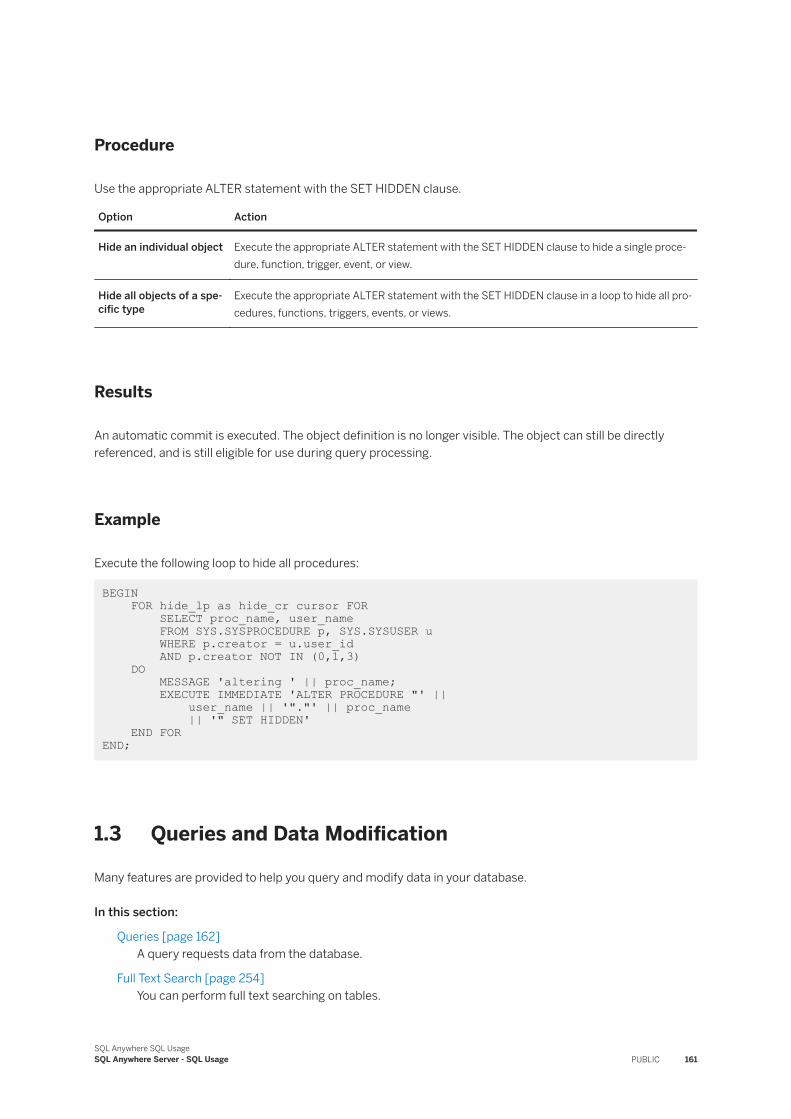
Procedure
Use the appropriate ALTER statement with the SET HIDDEN clause.
Option Action
Hide an individual object Execute the appropriate ALTER statement with the SET HIDDEN clause to hide a single procedure, function, trigger, event, or view.
Hide all objects of a specific type
Execute the appropriate ALTER statement with the SET HIDDEN clause in a loop to hide all procedures, functions, triggers, events, or views.
Results
An automatic commit is executed. The object definition is no longer visible. The object can still be directly referenced, and is still eligible for use during query processing.
Example
Execute the following loop to hide all procedures:
BEGIN FOR hide_lp as hide_cr cursor FOR SELECT proc_name, user_name FROM SYS.SYSPROCEDURE p, SYS.SYSUSER u WHERE p.creator = u.user_id AND p.creator NOT IN (0,1,3) DO MESSAGE 'altering ' || proc_name; EXECUTE IMMEDIATE 'ALTER PROCEDURE "' || user_name || '"."' || proc_name || '" SET HIDDEN' END FOR END;
1.3 Queries and Data Modification
Many features are provided to help you query and modify data in your database.
In this section:
Queries [page 162]A query requests data from the database.
Full Text Search [page 254]You can perform full text searching on tables.
SQL Anywhere SQL UsageSQL Anywhere Server - SQL Usage PUBLIC 161
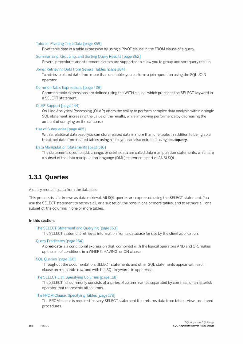
Tutorial: Pivoting Table Data [page 359]Pivot table data in a table expression by using a PIVOT clause in the FROM clause of a query.
Summarizing, Grouping, and Sorting Query Results [page 362]Several procedures and statement clauses are supported to allow you to group and sort query results.
Joins: Retrieving Data from Several Tables [page 384]To retrieve related data from more than one table, you perform a join operation using the SQL JOIN operator.
Common Table Expressions [page 429]Common table expressions are defined using the WITH clause, which precedes the SELECT keyword in a SELECT statement.
OLAP Support [page 444]On-Line Analytical Processing (OLAP) offers the ability to perform complex data analysis within a single SQL statement, increasing the value of the results, while improving performance by decreasing the amount of querying on the database.
Use of Subqueries [page 485]With a relational database, you can store related data in more than one table. In addition to being able to extract data from related tables using a join, you can also extract it using a subquery.
Data Manipulation Statements [page 510]The statements used to add, change, or delete data are called data manipulation statements, which are a subset of the data manipulation language (DML) statements part of ANSI SQL.
1.3.1 QueriesA query requests data from the database.
This process is also known as data retrieval. All SQL queries are expressed using the SELECT statement. You use the SELECT statement to retrieve all, or a subset of, the rows in one or more tables, and to retrieve all, or a subset of, the columns in one or more tables.
In this section:
The SELECT Statement and Querying [page 163]The SELECT statement retrieves information from a database for use by the client application.
Query Predicates [page 164]A predicate is a conditional expression that, combined with the logical operators AND and OR, makes up the set of conditions in a WHERE, HAVING, or ON clause.
SQL Queries [page 166]Throughout the documentation, SELECT statements and other SQL statements appear with each clause on a separate row, and with the SQL keywords in uppercase.
The SELECT List: Specifying Columns [page 168]The SELECT list commonly consists of a series of column names separated by commas, or an asterisk operator that represents all columns.
The FROM Clause: Specifying Tables [page 178]The FROM clause is required in every SELECT statement that returns data from tables, views, or stored procedures.
162 PUBLICSQL Anywhere SQL Usage
SQL Anywhere Server - SQL Usage
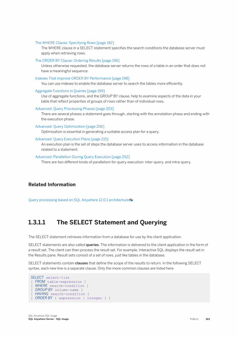
The WHERE Clause: Specifying Rows [page 182]The WHERE clause in a SELECT statement specifies the search conditions the database server must apply when retrieving rows.
The ORDER BY Clause: Ordering Results [page 196]Unless otherwise requested, the database server returns the rows of a table in an order that does not have a meaningful sequence.
Indexes That Improve ORDER BY Performance [page 198]You can use indexes to enable the database server to search the tables more efficiently.
Aggregate Functions in Queries [page 199]Use of aggregate functions, and the GROUP BY clause, help to examine aspects of the data in your table that reflect properties of groups of rows rather than of individual rows.
Advanced: Query Processing Phases [page 203]There are several phases a statement goes through, starting with the annotation phase and ending with the execution phase.
Advanced: Query Optimization [page 206]Optimization is essential in generating a suitable access plan for a query.
Advanced: Query Execution Plans [page 215]An execution plan is the set of steps the database server uses to access information in the database related to a statement.
Advanced: Parallelism During Query Execution [page 252]There are two different kinds of parallelism for query execution: inter-query, and intra-query.
Related Information
Query processing based on SQL Anywhere 12.0.1 architecture
1.3.1.1 The SELECT Statement and Querying
The SELECT statement retrieves information from a database for use by the client application.
SELECT statements are also called queries. The information is delivered to the client application in the form of a result set. The client can then process the result set. For example, Interactive SQL displays the result set in the Results pane. Result sets consist of a set of rows, just like tables in the database.
SELECT statements contain clauses that define the scope of the results to return. In the following SELECT syntax, each new line is a separate clause. Only the more common clauses are listed here.
SELECT select-list [ FROM table-expression ] [ WHERE search-condition ] [ GROUP BY column-name ] [ HAVING search-condition ] [ ORDER BY { expression | integer } ]
SQL Anywhere SQL UsageSQL Anywhere Server - SQL Usage PUBLIC 163
The clauses in the SELECT statement are as follows:
● The SELECT clause specifies the columns you want to retrieve. It is the only required clause in the SELECT statement.
● The FROM clause specifies the tables from which columns are pulled. It is required in all queries that retrieve data from tables. SELECT statements without FROM clauses have a different meaning.Although most queries operate on tables, queries may also retrieve data from other objects that have columns and rows, including views, other queries (derived tables) and stored procedure result sets.
● The WHERE clause specifies the rows in the tables you want to see.● The GROUP BY clause allows you to aggregate data.● The HAVING clause specifies rows on which aggregate data is to be collected.● The ORDER BY clause sorts the rows in the result set. (By default, rows are returned from relational
databases in an order that has no meaning.)
Most of the clauses are optional, but if they are included then they must appear in the correct order.
Related Information
Summarizing, Grouping, and Sorting Query Results [page 362]
1.3.1.2 Query Predicates
A predicate is a conditional expression that, combined with the logical operators AND and OR, makes up the set of conditions in a WHERE, HAVING, or ON clause.
In SQL, a predicate that evaluates to UNKNOWN is interpreted as FALSE.
A predicate that can exploit an index to retrieve rows from a table is called sargable. This name comes from the phrase search argument-able. Predicates that involve comparisons of a column with constants, other columns, or expressions may be sargable.
The predicate in the following statement is sargable. The database server can evaluate it efficiently using the primary index of the Employees table.
SELECT * FROM Employees WHERE Employees.EmployeeID = 102;
In the best access plan, this appears as: Employees<Employees>.
In contrast, the following predicate is not sargable. Although the EmployeeID column is indexed in the primary index, using this index does not expedite the computation because the result contains all, or all except one, row.
SELECT * FROM Employees where Employees.EmployeeID <> 102;
In the best access plan, this appears as: Employees<seq>.
164 PUBLICSQL Anywhere SQL Usage
SQL Anywhere Server - SQL Usage
Similarly, no index can assist in a search for all employees whose given name ends in the letter k. Again, the only means of computing this result is to examine each of the rows individually.
Functions
In general, a predicate that has a function on the column name is not sargable. For example, an index would not be used on the following query:
SELECT * FROM SalesOrders WHERE YEAR ( OrderDate ) ='2000';
To avoid using a function, you can rewrite a query to make it sargable. For example, you can rephrase the above query:
SELECT * FROM SalesOrdersWHERE OrderDate > '1999-12-31' AND OrderDate < '2001-01-01';
A query that uses a function becomes sargable if you store the function values in a computed column and build an index on this column. A computed column is a column whose values are obtained from other columns in the table. For example, if you have a column called OrderDate that holds the date of an order, you can create a computed column called OrderYear that holds the values for the year extracted from the OrderDate column.
ALTER TABLE SalesOrders ADD OrderYear INTEGER COMPUTE ( YEAR( OrderDate ) );
You can then add an index on the column OrderYear in the ordinary way:
CREATE INDEX IDX_year ON SalesOrders ( OrderYear );
If you then execute the following statement, the database server recognizes that there is an indexed column that holds that information and uses that index to answer the query.
SELECT * FROM SalesOrders WHERE YEAR( OrderDate ) = '2000';
The domain of the computed column must be equivalent to the domain of the COMPUTE expression in order for the column substitution to be made. In the above example, if YEAR( OrderDate ) had returned a string instead of an integer, the optimizer would not have substituted the computed column for the expression, and the index IDX_year could not have been used to retrieve the required rows.
Example
In each of these examples, attributes x and y are each columns of a single table. Attribute z is contained in a separate table. Assume that an index exists for each of these attributes.
SQL Anywhere SQL UsageSQL Anywhere Server - SQL Usage PUBLIC 165
Sargable Non-sargable
x = 10 x < > 10
x IS NULL
x IS NOT NULL
x > 25 x = 4 OR y = 5
x = z x = y
x IN (4, 5, 6) x NOT IN (4, 5, 6)
x LIKE 'pat%' x LIKE '%tern'
x = 20 - 2 x + 2 = 20
X IS NOT DISTINCT FROM Y+1
X IS DISTINCT FROM Y+1
Sometimes it may not be obvious whether a predicate is sargable. In these cases, you may be able to rewrite the predicate so it is sargable. For each example, you could rewrite the predicate x LIKE 'pat%' using the fact that u is the next letter in the alphabet after t: x >= 'pat' and x < 'pau'. In this form, an index on attribute x is helpful in locating values in the restricted range. Fortunately, the database server makes this particular transformation for you automatically.
A sargable predicate used for indexed retrieval on a table is a matching predicate. A WHERE clause can have many matching predicates. The most suitable predicate depends on the access plan. The optimizer re-evaluates its choice of matching predicates when considering alternate access plans.
Related Information
Computed Columns [page 21]
1.3.1.3 SQL Queries
Throughout the documentation, SELECT statements and other SQL statements appear with each clause on a separate row, and with the SQL keywords in uppercase.
This is done to make the statements easier to read but is not a requirement. You can enter SQL keywords in any case, and you can have line breaks anywhere in the statement.
Keywords and Line Breaks
For example, the following SELECT statement finds the first and last names of contacts living in California from the Contacts table.
SELECT GivenName, Surname
166 PUBLICSQL Anywhere SQL Usage
SQL Anywhere Server - SQL Usage
FROM Contacts WHERE State = 'CA';
It is equally valid, though not as readable, to enter the statement as follows:
SELECT GivenName, Surname from ContactsWHERE State = 'CA';
Case Sensitivity of Strings and Identifiers
Identifiers such as table names, column names, and so on, are case insensitive in SQL Anywhere databases.
Strings are case insensitive by default, so that 'CA', 'ca', 'cA', and 'Ca' are equivalent, but if you create a database as case sensitive then the case of strings is significant. The SQL Anywhere sample database is case insensitive.
Qualifying Identifiers
You can qualify the names of database identifiers if there is ambiguity about which object is being referred to. For example, the SQL Anywhere sample database contains several tables with a column called City, so you may have to qualify references to City with the name of the table. In a larger database you may also have to use the name of the owner of the table to identify the table.
SELECT Contacts.City FROM Contacts WHERE State = 'CA';
Since these examples involve single-table queries, column names in syntax models and examples are usually not qualified with the names of the tables or owners to which they belong.
These elements are left out for readability; it is never wrong to include qualifiers.
Row Order in the Result Set
Row order in the result set is insignificant. There is no guarantee of the order in which rows are returned from the database, and no meaning to the order. To retrieve rows in a particular order, you must specify the order in the query.
Related Information
Case Sensitivity [page 546]
SQL Anywhere SQL UsageSQL Anywhere Server - SQL Usage PUBLIC 167
1.3.1.4 The SELECT List: Specifying Columns
The SELECT list commonly consists of a series of column names separated by commas, or an asterisk operator that represents all columns.
More generally, the SELECT list can include one or more expressions, separated by commas. There is no comma after the last column in the list, or if there is only one column in the list.
The general syntax for the SELECT list looks like this:
SELECT expression [, expression ]..
If any table or column name in the list does not conform to the rules for valid identifiers, you must enclose the identifier in double quotes.
The SELECT list expressions can include * (all columns), a list of column names, character strings, column headings, and expressions including arithmetic operators. You can also include aggregate functions.
In this section:
Selection of All Columns from a Table [page 169]The asterisk (*) has a special meaning in SELECT statements, representing all the column names in all the tables specified in the FROM clause.
Selection of Specific Columns from a Table [page 171]You can limit the columns that a SELECT statement retrieves by listing the column(s) immediately after the SELECT keyword.
Renamed Columns in Query Results [page 172]Columns in query results can be renamed in several different ways.
Character Strings in Query Results [page 174]Strings of characters can be displayed in query results by enclosing them in single quotation marks and separating them from other elements in the SELECT list with commas.
Computed Values in the SELECT List [page 174]The expressions in a SELECT list can be more complicated than just column names or strings because you can perform computations with data from numeric columns.
Elimination of Duplicate Query Results [page 177]The DISTINCT keyword eliminates duplicate rows from the results of a SELECT statement.
Related Information
Summarizing, Grouping, and Sorting Query Results [page 362]
168 PUBLICSQL Anywhere SQL Usage
SQL Anywhere Server - SQL Usage
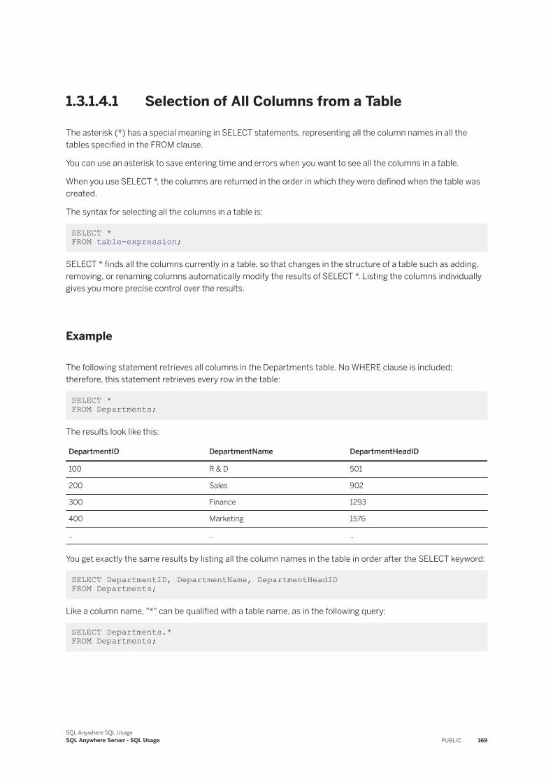
1.3.1.4.1 Selection of All Columns from a Table
The asterisk (*) has a special meaning in SELECT statements, representing all the column names in all the tables specified in the FROM clause.
You can use an asterisk to save entering time and errors when you want to see all the columns in a table.
When you use SELECT *, the columns are returned in the order in which they were defined when the table was created.
The syntax for selecting all the columns in a table is:
SELECT * FROM table-expression;
SELECT * finds all the columns currently in a table, so that changes in the structure of a table such as adding, removing, or renaming columns automatically modify the results of SELECT *. Listing the columns individually gives you more precise control over the results.
Example
The following statement retrieves all columns in the Departments table. No WHERE clause is included; therefore, this statement retrieves every row in the table:
SELECT * FROM Departments;
The results look like this:
DepartmentID DepartmentName DepartmentHeadID
100 R & D 501
200 Sales 902
300 Finance 1293
400 Marketing 1576
.. .. ..
You get exactly the same results by listing all the column names in the table in order after the SELECT keyword:
SELECT DepartmentID, DepartmentName, DepartmentHeadID FROM Departments;
Like a column name, "*" can be qualified with a table name, as in the following query:
SELECT Departments.* FROM Departments;
SQL Anywhere SQL UsageSQL Anywhere Server - SQL Usage PUBLIC 169
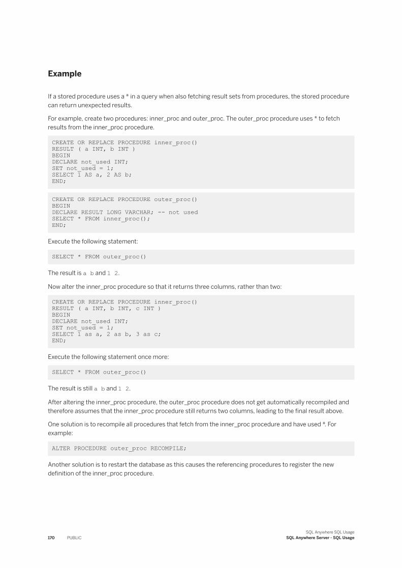
Example
If a stored procedure uses a * in a query when also fetching result sets from procedures, the stored procedure can return unexpected results.
For example, create two procedures: inner_proc and outer_proc. The outer_proc procedure uses * to fetch results from the inner_proc procedure.
CREATE OR REPLACE PROCEDURE inner_proc() RESULT ( a INT, b INT )BEGINDECLARE not_used INT;SET not_used = 1;SELECT 1 AS a, 2 AS b; END;
CREATE OR REPLACE PROCEDURE outer_proc() BEGINDECLARE RESULT LONG VARCHAR; -- not usedSELECT * FROM inner_proc(); END;
Execute the following statement:
SELECT * FROM outer_proc()
The result is a b and 1 2.
Now alter the inner_proc procedure so that it returns three columns, rather than two:
CREATE OR REPLACE PROCEDURE inner_proc() RESULT ( a INT, b INT, c INT )BEGINDECLARE not_used INT;SET not_used = 1;SELECT 1 as a, 2 as b, 3 as c; END;
Execute the following statement once more:
SELECT * FROM outer_proc()
The result is still a b and 1 2.
After altering the inner_proc procedure, the outer_proc procedure does not get automatically recompiled and therefore assumes that the inner_proc procedure still returns two columns, leading to the final result above.
One solution is to recompile all procedures that fetch from the inner_proc procedure and have used *. For example:
ALTER PROCEDURE outer_proc RECOMPILE;
Another solution is to restart the database as this causes the referencing procedures to register the new definition of the inner_proc procedure.
170 PUBLICSQL Anywhere SQL Usage
SQL Anywhere Server - SQL Usage
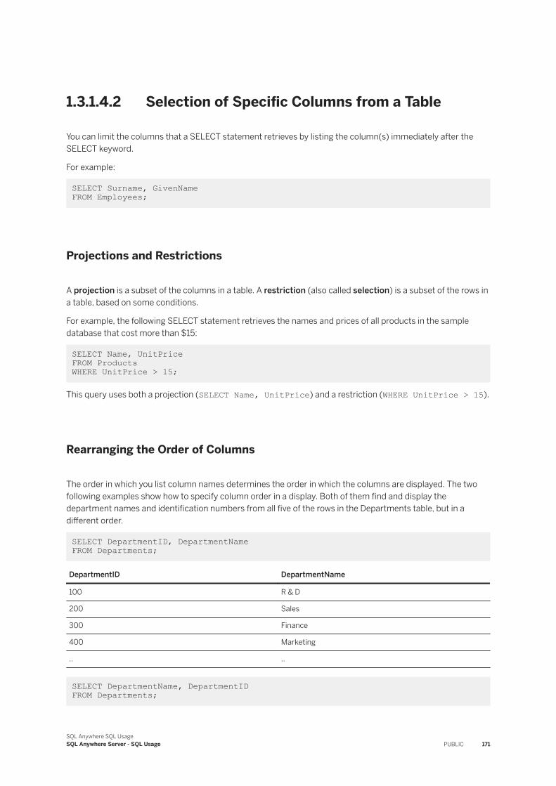
1.3.1.4.2 Selection of Specific Columns from a Table
You can limit the columns that a SELECT statement retrieves by listing the column(s) immediately after the SELECT keyword.
For example:
SELECT Surname, GivenName FROM Employees;
Projections and Restrictions
A projection is a subset of the columns in a table. A restriction (also called selection) is a subset of the rows in a table, based on some conditions.
For example, the following SELECT statement retrieves the names and prices of all products in the sample database that cost more than $15:
SELECT Name, UnitPrice FROM Products WHERE UnitPrice > 15;
This query uses both a projection (SELECT Name, UnitPrice) and a restriction (WHERE UnitPrice > 15).
Rearranging the Order of Columns
The order in which you list column names determines the order in which the columns are displayed. The two following examples show how to specify column order in a display. Both of them find and display the department names and identification numbers from all five of the rows in the Departments table, but in a different order.
SELECT DepartmentID, DepartmentName FROM Departments;
DepartmentID DepartmentName
100 R & D
200 Sales
300 Finance
400 Marketing
.. ..
SELECT DepartmentName, DepartmentID FROM Departments;
SQL Anywhere SQL UsageSQL Anywhere Server - SQL Usage PUBLIC 171
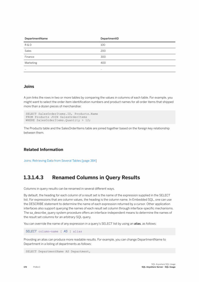
DepartmentName DepartmentID
R & D 100
Sales 200
Finance 300
Marketing 400
.. ..
Joins
A join links the rows in two or more tables by comparing the values in columns of each table. For example, you might want to select the order item identification numbers and product names for all order items that shipped more than a dozen pieces of merchandise:
SELECT SalesOrderItems.ID, Products.Name FROM Products JOIN SalesOrderItems WHERE SalesOrderItems.Quantity > 12;
The Products table and the SalesOrderItems table are joined together based on the foreign key relationship between them.
Related Information
Joins: Retrieving Data from Several Tables [page 384]
1.3.1.4.3 Renamed Columns in Query Results
Columns in query results can be renamed in several different ways.
By default, the heading for each column of a result set is the name of the expression supplied in the SELECT list. For expressions that are column values, the heading is the column name. In Embedded SQL, one can use the DESCRIBE statement to determine the name of each expression returned by a cursor. Other application interfaces also support querying the names of each result set column through interface-specific mechanisms. The sa_describe_query system procedure offers an interface-independent means to determine the names of the result set columns for an arbitrary SQL query.
You can override the name of any expression in a query's SELECT list by using an alias, as follows:
SELECT column-name [ AS ] alias
Providing an alias can produce more readable results. For example, you can change DepartmentName to Department in a listing of departments as follows:
SELECT DepartmentName AS Department,
172 PUBLICSQL Anywhere SQL Usage
SQL Anywhere Server - SQL Usage
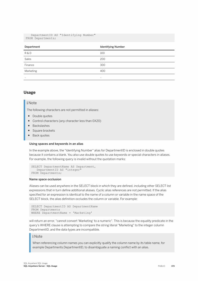
DepartmentID AS "Identifying Number" FROM Departments;
Department Identifying Number
R & D 100
Sales 200
Finance 300
Marketing 400
.. ..
Usage
NoteThe following characters are not permitted in aliases:
● Double quotes● Control characters (any character less than 0X20)● Backslashes● Square brackets● Back quotes
Using spaces and keywords in an alias
In the example above, the "Identifying Number" alias for DepartmentID is enclosed in double quotes because it contains a blank. You also use double quotes to use keywords or special characters in aliases. For example, the following query is invalid without the quotation marks:
SELECT DepartmentName AS Department, DepartmentID AS "integer" FROM Departments;
Name space occlusion
Aliases can be used anywhere in the SELECT block in which they are defined, including other SELECT list expressions that in turn define additional aliases. Cyclic alias references are not permitted. If the alias specified for an expression is identical to the name of a column or variable in the name space of the SELECT block, the alias definition occludes the column or variable. For example:
SELECT DepartmentID AS DepartmentName FROM Departments WHERE DepartmentName = 'Marketing'
will return an error, "cannot convert 'Marketing' to a numeric". This is because the equality predicate in the query's WHERE clause is attempting to compare the string literal "Marketing" to the integer column DepartmentID, and the data types are incompatible.
NoteWhen referencing column names you can explicitly qualify the column name by its table name, for example Departments.DepartmentID, to disambiguate a naming conflict with an alias.
SQL Anywhere SQL UsageSQL Anywhere Server - SQL Usage PUBLIC 173
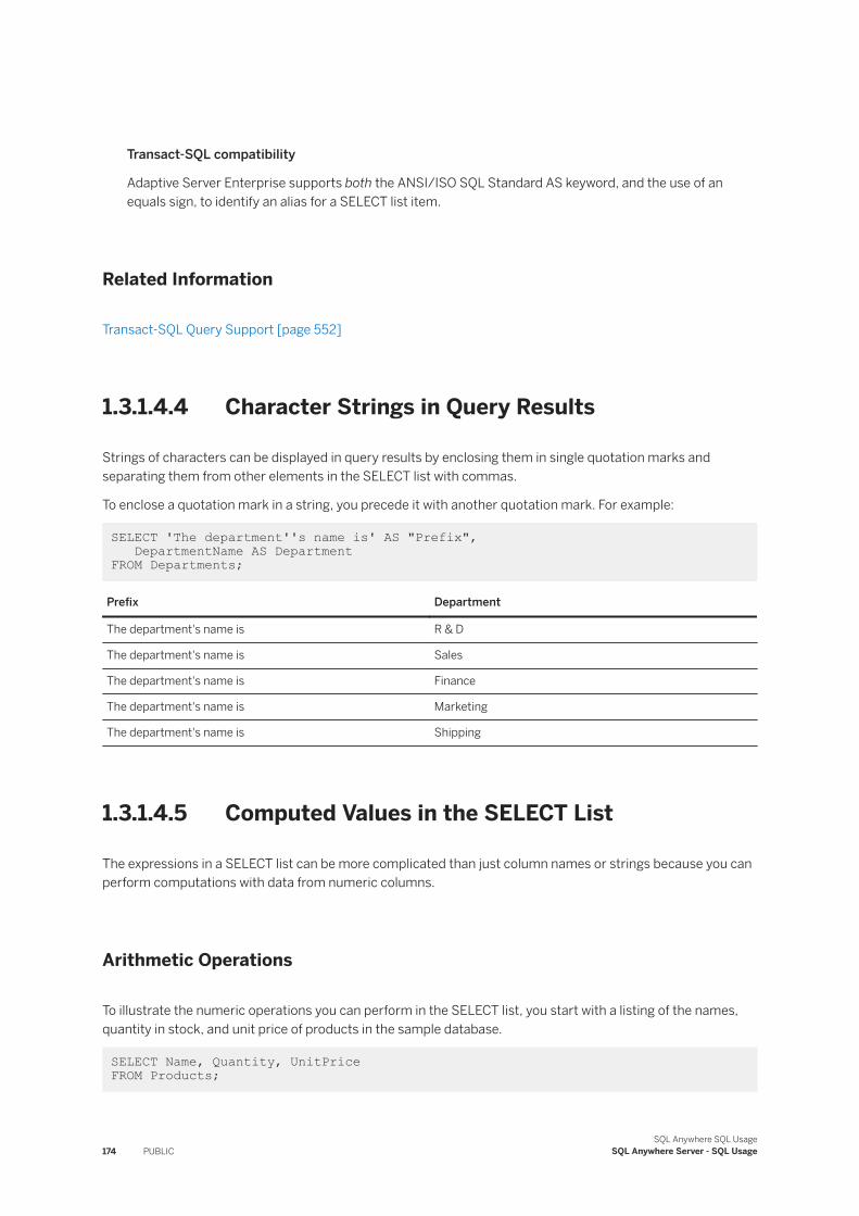
Transact-SQL compatibility
Adaptive Server Enterprise supports both the ANSI/ISO SQL Standard AS keyword, and the use of an equals sign, to identify an alias for a SELECT list item.
Related Information
Transact-SQL Query Support [page 552]
1.3.1.4.4 Character Strings in Query Results
Strings of characters can be displayed in query results by enclosing them in single quotation marks and separating them from other elements in the SELECT list with commas.
To enclose a quotation mark in a string, you precede it with another quotation mark. For example:
SELECT 'The department''s name is' AS "Prefix", DepartmentName AS Department FROM Departments;
Prefix Department
The department's name is R & D
The department's name is Sales
The department's name is Finance
The department's name is Marketing
The department's name is Shipping
1.3.1.4.5 Computed Values in the SELECT List
The expressions in a SELECT list can be more complicated than just column names or strings because you can perform computations with data from numeric columns.
Arithmetic Operations
To illustrate the numeric operations you can perform in the SELECT list, you start with a listing of the names, quantity in stock, and unit price of products in the sample database.
SELECT Name, Quantity, UnitPrice FROM Products;
174 PUBLICSQL Anywhere SQL Usage
SQL Anywhere Server - SQL Usage
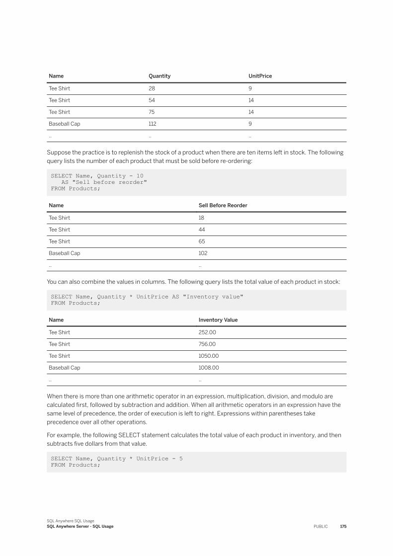
Name Quantity UnitPrice
Tee Shirt 28 9
Tee Shirt 54 14
Tee Shirt 75 14
Baseball Cap 112 9
.. .. ..
Suppose the practice is to replenish the stock of a product when there are ten items left in stock. The following query lists the number of each product that must be sold before re-ordering:
SELECT Name, Quantity - 10 AS "Sell before reorder" FROM Products;
Name Sell Before Reorder
Tee Shirt 18
Tee Shirt 44
Tee Shirt 65
Baseball Cap 102
.. ..
You can also combine the values in columns. The following query lists the total value of each product in stock:
SELECT Name, Quantity * UnitPrice AS "Inventory value" FROM Products;
Name Inventory Value
Tee Shirt 252.00
Tee Shirt 756.00
Tee Shirt 1050.00
Baseball Cap 1008.00
.. ..
When there is more than one arithmetic operator in an expression, multiplication, division, and modulo are calculated first, followed by subtraction and addition. When all arithmetic operators in an expression have the same level of precedence, the order of execution is left to right. Expressions within parentheses take precedence over all other operations.
For example, the following SELECT statement calculates the total value of each product in inventory, and then subtracts five dollars from that value.
SELECT Name, Quantity * UnitPrice - 5 FROM Products;
SQL Anywhere SQL UsageSQL Anywhere Server - SQL Usage PUBLIC 175
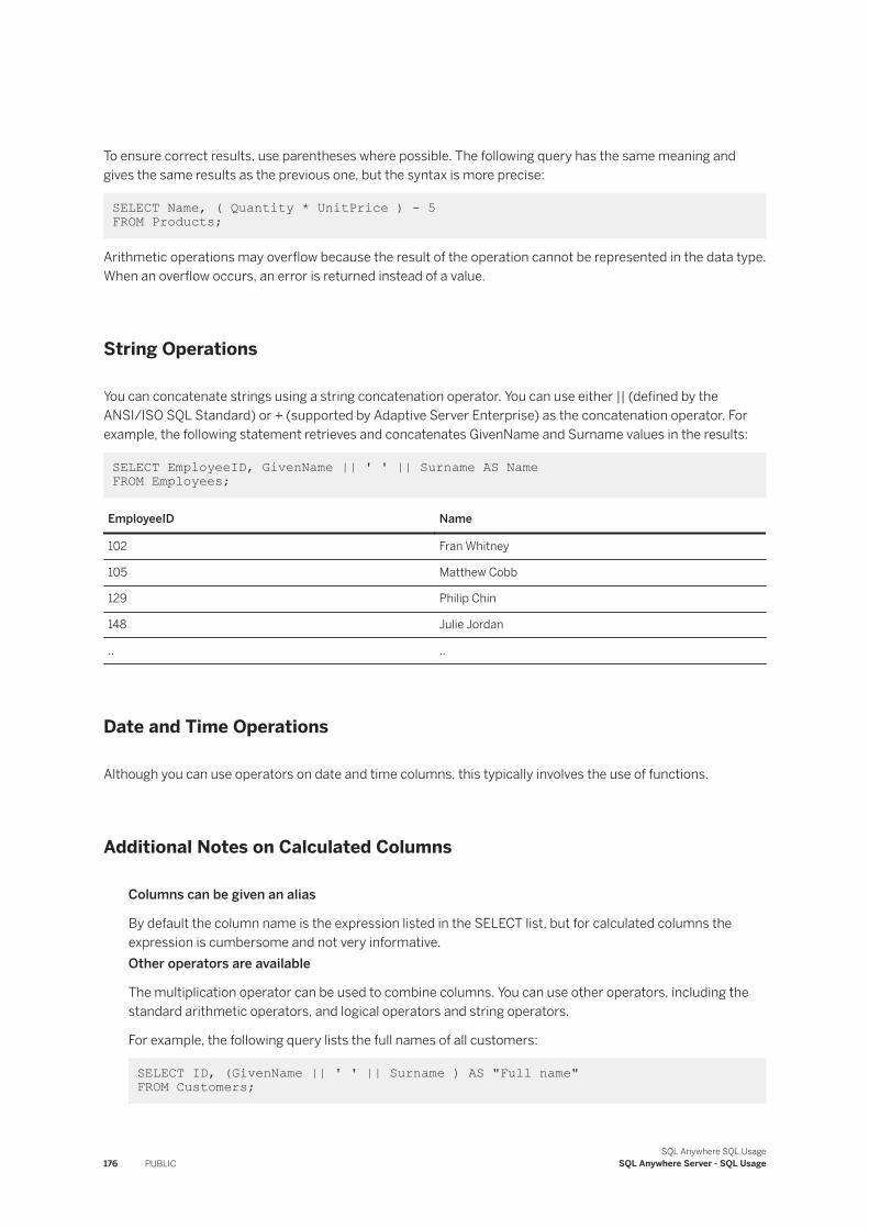
To ensure correct results, use parentheses where possible. The following query has the same meaning and gives the same results as the previous one, but the syntax is more precise:
SELECT Name, ( Quantity * UnitPrice ) - 5 FROM Products;
Arithmetic operations may overflow because the result of the operation cannot be represented in the data type. When an overflow occurs, an error is returned instead of a value.
String Operations
You can concatenate strings using a string concatenation operator. You can use either || (defined by the ANSI/ISO SQL Standard) or + (supported by Adaptive Server Enterprise) as the concatenation operator. For example, the following statement retrieves and concatenates GivenName and Surname values in the results:
SELECT EmployeeID, GivenName || ' ' || Surname AS Name FROM Employees;
EmployeeID Name
102 Fran Whitney
105 Matthew Cobb
129 Philip Chin
148 Julie Jordan
.. ..
Date and Time Operations
Although you can use operators on date and time columns, this typically involves the use of functions.
Additional Notes on Calculated Columns
Columns can be given an alias
By default the column name is the expression listed in the SELECT list, but for calculated columns the expression is cumbersome and not very informative.Other operators are available
The multiplication operator can be used to combine columns. You can use other operators, including the standard arithmetic operators, and logical operators and string operators.
For example, the following query lists the full names of all customers:
SELECT ID, (GivenName || ' ' || Surname ) AS "Full name" FROM Customers;
176 PUBLICSQL Anywhere SQL Usage
SQL Anywhere Server - SQL Usage
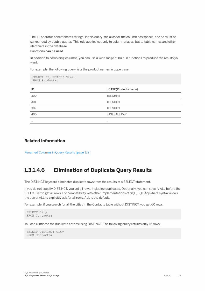
The || operator concatenates strings. In this query, the alias for the column has spaces, and so must be surrounded by double quotes. This rule applies not only to column aliases, but to table names and other identifiers in the database.Functions can be used
In addition to combining columns, you can use a wide range of built-in functions to produce the results you want.
For example, the following query lists the product names in uppercase:
SELECT ID, UCASE( Name ) FROM Products;
ID UCASE(Products.name)
300 TEE SHIRT
301 TEE SHIRT
302 TEE SHIRT
400 BASEBALL CAP
.. ..
Related Information
Renamed Columns in Query Results [page 172]
1.3.1.4.6 Elimination of Duplicate Query Results
The DISTINCT keyword eliminates duplicate rows from the results of a SELECT statement.
If you do not specify DISTINCT, you get all rows, including duplicates. Optionally, you can specify ALL before the SELECT list to get all rows. For compatibility with other implementations of SQL, SQL Anywhere syntax allows the use of ALL to explicitly ask for all rows. ALL is the default.
For example, if you search for all the cities in the Contacts table without DISTINCT, you get 60 rows:
SELECT City FROM Contacts;
You can eliminate the duplicate entries using DISTINCT. The following query returns only 16 rows:
SELECT DISTINCT City FROM Contacts;
SQL Anywhere SQL UsageSQL Anywhere Server - SQL Usage PUBLIC 177
NULL Values Are Not Distinct
The DISTINCT keyword treats NULL values as duplicates of each other. In other words, when DISTINCT is included in a SELECT statement, only one NULL is returned in the results, no matter how many NULL values are encountered.
1.3.1.5 The FROM Clause: Specifying Tables
The FROM clause is required in every SELECT statement that returns data from tables, views, or stored procedures.
The FROM clause can include JOIN conditions linking two or more tables, and can include joins to other queries (derived tables).
Qualifying Table Names
In the FROM clause, the full naming syntax for tables and views is always permitted, such as:
SELECT select-list FROM owner.table-name;
Qualifying table, view, and procedure names is necessary only when the object is owned by a user ID that is different from the user ID of the current connection, or if the user ID of the owner is not the name of a role to which the user ID of the current connection belongs.
Using Correlation Names
You can give a table name a correlation name to improve readability, and to save entering the full table name each place it is referenced. You assign the correlation name in the FROM clause by entering it after the table name, like this:
SELECT d.DepartmentID, d.DepartmentName FROM Departments d;
When a correlation name is used, all other references to the table, for example in a WHERE clause, must use the correlation name, rather than the table name. Correlation names must conform to the rules for valid identifiers.
Querying Derived Tables
A derived table is a table derived directly, or indirectly, from one or more tables by the evaluation of a query expression. Derived tables are defined in the FROM clause of a SELECT statement.
178 PUBLICSQL Anywhere SQL Usage
SQL Anywhere Server - SQL Usage
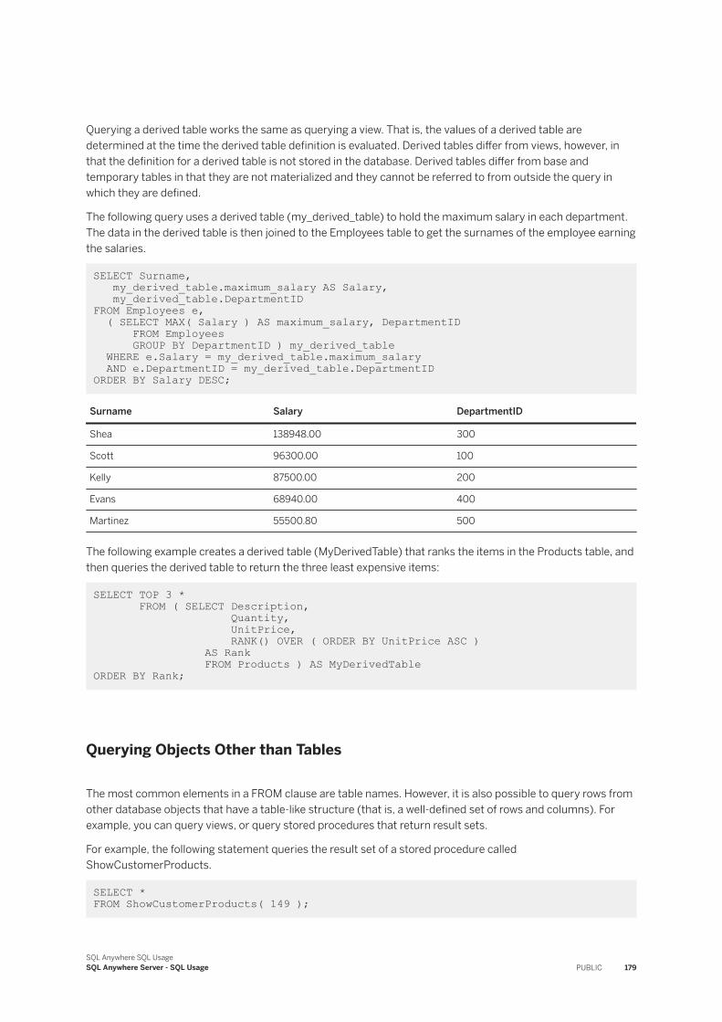
Querying a derived table works the same as querying a view. That is, the values of a derived table are determined at the time the derived table definition is evaluated. Derived tables differ from views, however, in that the definition for a derived table is not stored in the database. Derived tables differ from base and temporary tables in that they are not materialized and they cannot be referred to from outside the query in which they are defined.
The following query uses a derived table (my_derived_table) to hold the maximum salary in each department. The data in the derived table is then joined to the Employees table to get the surnames of the employee earning the salaries.
SELECT Surname, my_derived_table.maximum_salary AS Salary, my_derived_table.DepartmentID FROM Employees e, ( SELECT MAX( Salary ) AS maximum_salary, DepartmentID FROM Employees GROUP BY DepartmentID ) my_derived_table WHERE e.Salary = my_derived_table.maximum_salary AND e.DepartmentID = my_derived_table.DepartmentID ORDER BY Salary DESC;
Surname Salary DepartmentID
Shea 138948.00 300
Scott 96300.00 100
Kelly 87500.00 200
Evans 68940.00 400
Martinez 55500.80 500
The following example creates a derived table (MyDerivedTable) that ranks the items in the Products table, and then queries the derived table to return the three least expensive items:
SELECT TOP 3 * FROM ( SELECT Description, Quantity, UnitPrice, RANK() OVER ( ORDER BY UnitPrice ASC ) AS Rank FROM Products ) AS MyDerivedTable ORDER BY Rank;
Querying Objects Other than Tables
The most common elements in a FROM clause are table names. However, it is also possible to query rows from other database objects that have a table-like structure (that is, a well-defined set of rows and columns). For example, you can query views, or query stored procedures that return result sets.
For example, the following statement queries the result set of a stored procedure called ShowCustomerProducts.
SELECT * FROM ShowCustomerProducts( 149 );
SQL Anywhere SQL UsageSQL Anywhere Server - SQL Usage PUBLIC 179
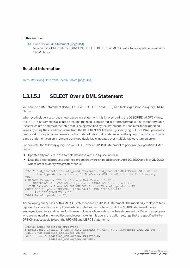
In this section:
SELECT Over a DML Statement [page 180]You can use a DML statement (INSERT, UPDATE, DELETE, or MERGE) as a table expression in a query FROM clause.
Related Information
Joins: Retrieving Data from Several Tables [page 384]
1.3.1.5.1 SELECT Over a DML Statement
You can use a DML statement (INSERT, UPDATE, DELETE, or MERGE) as a table expression in a query FROM clause.
When you include a dml-derived-table in a statement, it is ignored during the DESCRIBE. At OPEN time, the UPDATE statement is executed first, and the results are stored in a temporary table. The temporary table uses the column names of the table that is being modified by the statement. You can refer to the modified values by using the correlation name from the REFERENCING clause. By specifying OLD or FINAL, you do not need a set of unique column names for the updated table that is referenced in the query. The dml-derived-table statement can only reference one updatable table; updates over multiple tables return an error.
For example, the following query uses a SELECT over an UPDATE statement to perform the operations listed below:
● Updates all products in the sample database with a 7% price increase● Lists the affected products and their orders that were shipped between April 10, 2000 and May 21, 2000
whose order quantity was greater than 36
SELECT old_products.ID, old_products.name, old_products.UnitPrice AS OldPrice, final_products.UnitPrice AS NewPrice, SOI.ID AS OrderID, SOI.QuantityFROM( UPDATE Products SET UnitPrice = UnitPrice * 1.07 ) REFERENCING ( OLD AS old_products FINAL AS final_products ) JOIN SalesOrderItems AS SOI ON SOI.ProductID = old_products.IDWHERE SOI.ShipDate BETWEEN '2000-04-10' AND '2000-05-21' AND SOI.QUANTITY > 36 ORDER BY old_products.ID;
The following query uses both a MERGE statement and an UPDATE statement. The modified_employees table represents a collection of employees whose state has been altered, while the MERGE statement merges employee identifiers and names for those employees whose salary has been increased by 3% with employees who are included in the modified_employees table. In this query, the option settings that are specified in the OPTION clause apply to both the UPDATE and MERGE statements.
CREATE TABLE modified_employees ( EmployeeID INTEGER PRIMARY KEY, Surname VARCHAR(40), GivenName VARCHAR(40) );MERGE INTO modified_employees AS meUSING (SELECT modified_employees.EmployeeID, modified_employees.Surname,
180 PUBLICSQL Anywhere SQL Usage
SQL Anywhere Server - SQL Usage
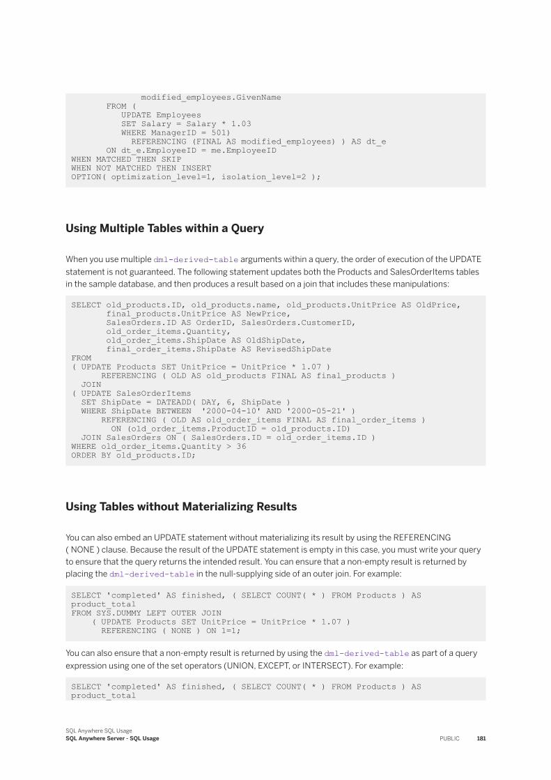
modified_employees.GivenName FROM ( UPDATE Employees SET Salary = Salary * 1.03 WHERE ManagerID = 501) REFERENCING (FINAL AS modified_employees) ) AS dt_e ON dt_e.EmployeeID = me.EmployeeID WHEN MATCHED THEN SKIPWHEN NOT MATCHED THEN INSERT OPTION( optimization_level=1, isolation_level=2 );
Using Multiple Tables within a Query
When you use multiple dml-derived-table arguments within a query, the order of execution of the UPDATE statement is not guaranteed. The following statement updates both the Products and SalesOrderItems tables in the sample database, and then produces a result based on a join that includes these manipulations:
SELECT old_products.ID, old_products.name, old_products.UnitPrice AS OldPrice, final_products.UnitPrice AS NewPrice, SalesOrders.ID AS OrderID, SalesOrders.CustomerID, old_order_items.Quantity, old_order_items.ShipDate AS OldShipDate, final_order_items.ShipDate AS RevisedShipDateFROM ( UPDATE Products SET UnitPrice = UnitPrice * 1.07 ) REFERENCING ( OLD AS old_products FINAL AS final_products ) JOIN ( UPDATE SalesOrderItems SET ShipDate = DATEADD( DAY, 6, ShipDate ) WHERE ShipDate BETWEEN '2000-04-10' AND '2000-05-21' ) REFERENCING ( OLD AS old_order_items FINAL AS final_order_items ) ON (old_order_items.ProductID = old_products.ID) JOIN SalesOrders ON ( SalesOrders.ID = old_order_items.ID )WHERE old_order_items.Quantity > 36 ORDER BY old_products.ID;
Using Tables without Materializing Results
You can also embed an UPDATE statement without materializing its result by using the REFERENCING ( NONE ) clause. Because the result of the UPDATE statement is empty in this case, you must write your query to ensure that the query returns the intended result. You can ensure that a non-empty result is returned by placing the dml-derived-table in the null-supplying side of an outer join. For example:
SELECT 'completed' AS finished, ( SELECT COUNT( * ) FROM Products ) AS product_total FROM SYS.DUMMY LEFT OUTER JOIN ( UPDATE Products SET UnitPrice = UnitPrice * 1.07 ) REFERENCING ( NONE ) ON 1=1;
You can also ensure that a non-empty result is returned by using the dml-derived-table as part of a query expression using one of the set operators (UNION, EXCEPT, or INTERSECT). For example:
SELECT 'completed' AS finished, ( SELECT COUNT( * ) FROM Products ) AS product_total
SQL Anywhere SQL UsageSQL Anywhere Server - SQL Usage PUBLIC 181
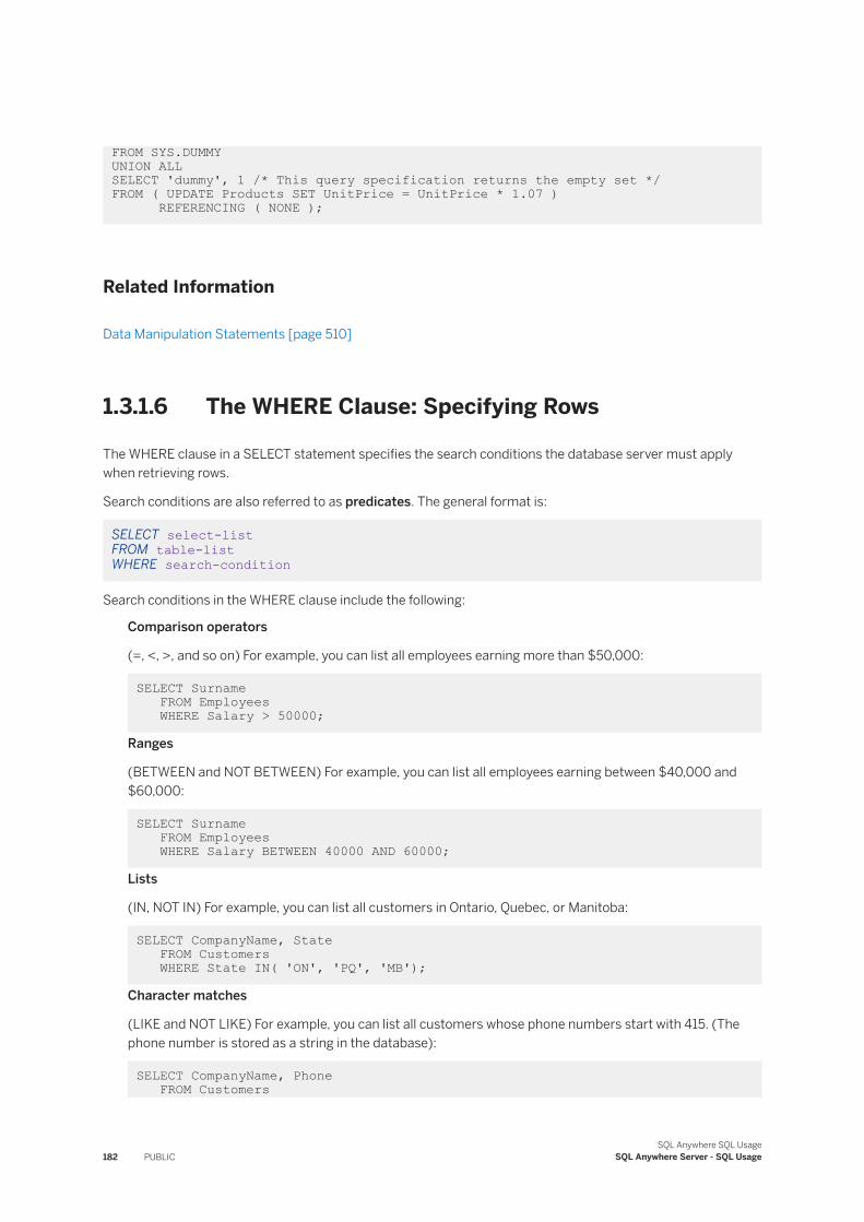
FROM SYS.DUMMYUNION ALLSELECT 'dummy', 1 /* This query specification returns the empty set */FROM ( UPDATE Products SET UnitPrice = UnitPrice * 1.07 ) REFERENCING ( NONE );
Related Information
Data Manipulation Statements [page 510]
1.3.1.6 The WHERE Clause: Specifying Rows
The WHERE clause in a SELECT statement specifies the search conditions the database server must apply when retrieving rows.
Search conditions are also referred to as predicates. The general format is:
SELECT select-list FROM table-list WHERE search-condition
Search conditions in the WHERE clause include the following:
Comparison operators
(=, <, >, and so on) For example, you can list all employees earning more than $50,000:
SELECT Surname FROM Employees WHERE Salary > 50000;
Ranges
(BETWEEN and NOT BETWEEN) For example, you can list all employees earning between $40,000 and $60,000:
SELECT Surname FROM Employees WHERE Salary BETWEEN 40000 AND 60000;
Lists
(IN, NOT IN) For example, you can list all customers in Ontario, Quebec, or Manitoba:
SELECT CompanyName, State FROM Customers WHERE State IN( 'ON', 'PQ', 'MB');
Character matches
(LIKE and NOT LIKE) For example, you can list all customers whose phone numbers start with 415. (The phone number is stored as a string in the database):
SELECT CompanyName, Phone FROM Customers
182 PUBLICSQL Anywhere SQL Usage
SQL Anywhere Server - SQL Usage
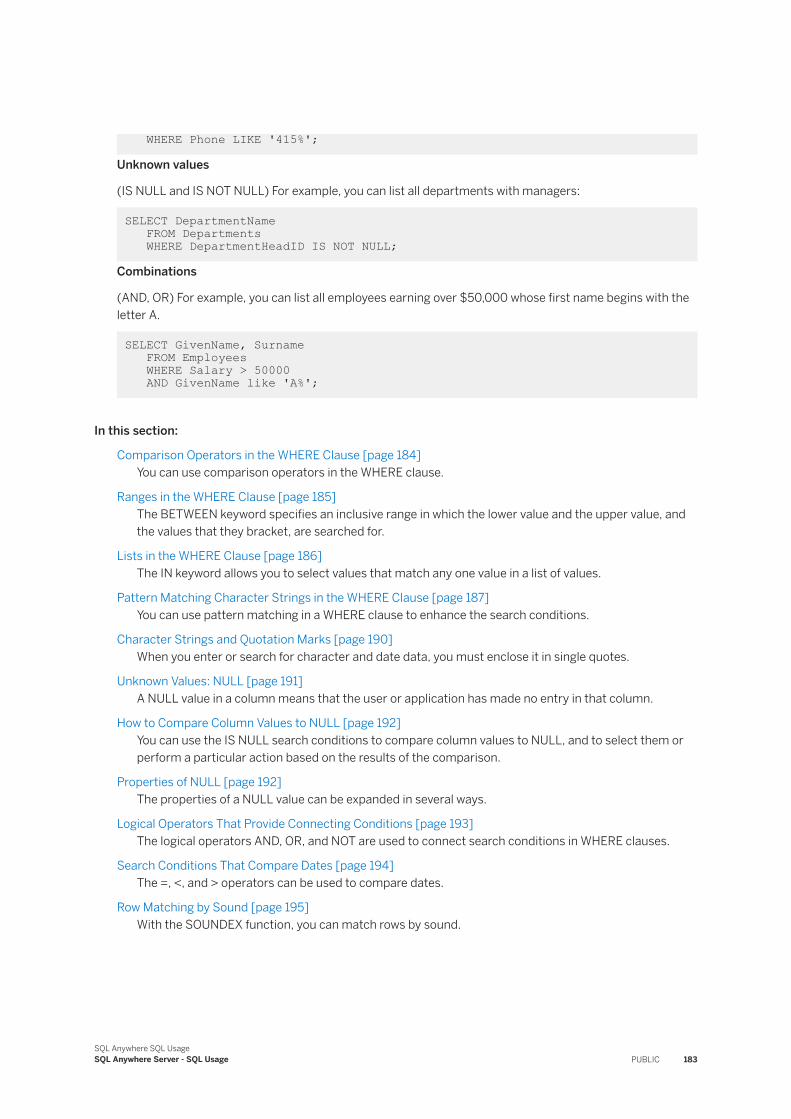
WHERE Phone LIKE '415%';
Unknown values
(IS NULL and IS NOT NULL) For example, you can list all departments with managers:
SELECT DepartmentName FROM Departments WHERE DepartmentHeadID IS NOT NULL;
Combinations
(AND, OR) For example, you can list all employees earning over $50,000 whose first name begins with the letter A.
SELECT GivenName, Surname FROM Employees WHERE Salary > 50000 AND GivenName like 'A%';
In this section:
Comparison Operators in the WHERE Clause [page 184]You can use comparison operators in the WHERE clause.
Ranges in the WHERE Clause [page 185]The BETWEEN keyword specifies an inclusive range in which the lower value and the upper value, and the values that they bracket, are searched for.
Lists in the WHERE Clause [page 186]The IN keyword allows you to select values that match any one value in a list of values.
Pattern Matching Character Strings in the WHERE Clause [page 187]You can use pattern matching in a WHERE clause to enhance the search conditions.
Character Strings and Quotation Marks [page 190]When you enter or search for character and date data, you must enclose it in single quotes.
Unknown Values: NULL [page 191]A NULL value in a column means that the user or application has made no entry in that column.
How to Compare Column Values to NULL [page 192]You can use the IS NULL search conditions to compare column values to NULL, and to select them or perform a particular action based on the results of the comparison.
Properties of NULL [page 192]The properties of a NULL value can be expanded in several ways.
Logical Operators That Provide Connecting Conditions [page 193]The logical operators AND, OR, and NOT are used to connect search conditions in WHERE clauses.
Search Conditions That Compare Dates [page 194]The =, <, and > operators can be used to compare dates.
Row Matching by Sound [page 195]With the SOUNDEX function, you can match rows by sound.
SQL Anywhere SQL UsageSQL Anywhere Server - SQL Usage PUBLIC 183
1.3.1.6.1 Comparison Operators in the WHERE Clause
You can use comparison operators in the WHERE clause.
The operators follow the syntax:
WHERE expression comparison-operator expression
Notes on Comparisons
Case sensitivity
When you create a database, you indicate whether string comparisons are case sensitive or not.
By default, databases are created case insensitive. For example, 'Dirk' is the same as 'DIRK'.
You can find out the database case sensitivity using the Information utility (dbinfo):
dbinfo -c "uid=DBA;pwd=sql"
Look for the collation CaseSensitivity information.
You can also ascertain the database case sensitivity from SQL Central using the Settings tab of the Database Properties window.
Comparing dates
When comparing dates, < means earlier and > means later.
Sort order
When you create a database, you chose the database collations for CHAR and NCHAR data types.
When comparing character data, < means earlier in the sort order and > means later in the sort order. The sort order is determined by the database collation.
You can find out the database collation using the Information utility (dbinfo):
dbinfo -c "uid=DBA;pwd=sql"
You can also ascertain the collation from SQL Central using the Settings tab of the Database Properties window.Trailing blanks
When you create a database, you indicate whether trailing blanks are ignored for comparison purposes.
By default, databases are created with trailing blanks not ignored. For example, 'Dirk' is not the same as 'Dirk '. You can create databases with blank padding, so that trailing blanks are ignored.
You can find out the database blank padding property using the Information utility (dbinfo):
dbinfo -c "uid=DBA;pwd=sql"
You can also ascertain the database blank padding property from SQL Central by inspecting the Ignore trailing blanks property in the Settings tab of the Database Properties window.
184 PUBLICSQL Anywhere SQL Usage
SQL Anywhere Server - SQL Usage
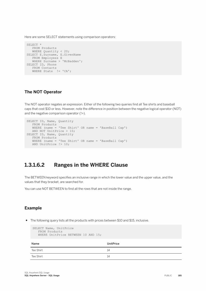
Here are some SELECT statements using comparison operators:
SELECT * FROM Products WHERE Quantity < 20;SELECT E.Surname, E.GivenName FROM Employees E WHERE Surname > 'McBadden';SELECT ID, Phone FROM Contacts WHERE State != 'CA';
The NOT Operator
The NOT operator negates an expression. Either of the following two queries find all Tee shirts and baseball caps that cost $10 or less. However, note the difference in position between the negative logical operator (NOT) and the negative comparison operator (!>).
SELECT ID, Name, Quantity FROM Products WHERE (name = 'Tee Shirt' OR name = 'BaseBall Cap') AND NOT UnitPrice > 10;SELECT ID, Name, Quantity FROM Products WHERE (name = 'Tee Shirt' OR name = 'BaseBall Cap') AND UnitPrice !> 10;
1.3.1.6.2 Ranges in the WHERE Clause
The BETWEEN keyword specifies an inclusive range in which the lower value and the upper value, and the values that they bracket, are searched for.
You can use NOT BETWEEN to find all the rows that are not inside the range.
Example
● The following query lists all the products with prices between $10 and $15, inclusive.
SELECT Name, UnitPrice FROM Products WHERE UnitPrice BETWEEN 10 AND 15;
Name UnitPrice
Tee Shirt 14
Tee Shirt 14
SQL Anywhere SQL UsageSQL Anywhere Server - SQL Usage PUBLIC 185
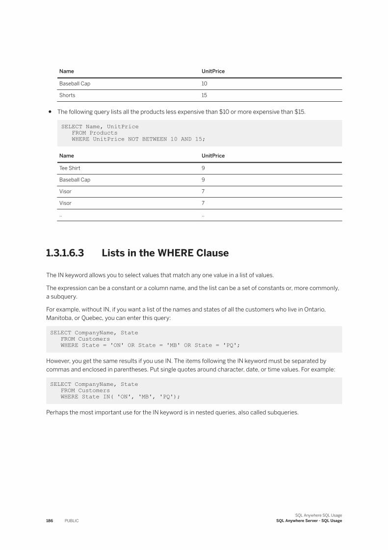
Name UnitPrice
Baseball Cap 10
Shorts 15
● The following query lists all the products less expensive than $10 or more expensive than $15.
SELECT Name, UnitPrice FROM Products WHERE UnitPrice NOT BETWEEN 10 AND 15;
Name UnitPrice
Tee Shirt 9
Baseball Cap 9
Visor 7
Visor 7
.. ..
1.3.1.6.3 Lists in the WHERE Clause
The IN keyword allows you to select values that match any one value in a list of values.
The expression can be a constant or a column name, and the list can be a set of constants or, more commonly, a subquery.
For example, without IN, if you want a list of the names and states of all the customers who live in Ontario, Manitoba, or Quebec, you can enter this query:
SELECT CompanyName, State FROM Customers WHERE State = 'ON' OR State = 'MB' OR State = 'PQ';
However, you get the same results if you use IN. The items following the IN keyword must be separated by commas and enclosed in parentheses. Put single quotes around character, date, or time values. For example:
SELECT CompanyName, State FROM Customers WHERE State IN( 'ON', 'MB', 'PQ');
Perhaps the most important use for the IN keyword is in nested queries, also called subqueries.
186 PUBLICSQL Anywhere SQL Usage
SQL Anywhere Server - SQL Usage
1.3.1.6.4 Pattern Matching Character Strings in the WHERE Clause
You can use pattern matching in a WHERE clause to enhance the search conditions.
In SQL, the LIKE keyword is used to search for patterns. Pattern matching employs wildcard characters to match different combinations of characters.
The LIKE keyword indicates that the following character string is a matching pattern. LIKE is used with character data.
The syntax for LIKE is:
expression [ NOT ] LIKE match-expression
The expression to be matched is compared to a match-expression that can include these special symbols:
Symbols Meaning
% Matches any string of 0 or more characters
_ Matches any one character
[specifier] The specifier in the brackets may take the following forms:
Range
A range is of the form rangespec1-rangespec2, where rangespec1 indicates the start of a range of characters, the hyphen indicates a range, and rangespec2 indicates the end of a range of characters.Set
A set can include any discrete set of values, in any order. For example, [a2bR].
The range [a-f], and the sets [abcdef] and [fcbdae] return the same set of values.
[^specifier] The caret symbol (^) preceding a specifier indicates non-inclusion. [^a-f] means not in the range a-f; [^a2bR] means not a, 2, b, or R.
You can match the column data to constants, variables, or other columns that contain the wildcard characters displayed in the table. When using constants, enclose the match strings and character strings in single quotes.
Example
All the following examples use LIKE with the Surname column in the Contacts table. Queries are of the form:
SELECT Surname FROM Contacts WHERE Surname LIKE match-expression;
SQL Anywhere SQL UsageSQL Anywhere Server - SQL Usage PUBLIC 187
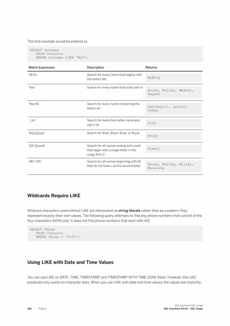
The first example would be entered as
SELECT Surname FROM Contacts WHERE Surname LIKE 'Mc%';
Match Expression Description Returns
'Mc%' Search for every name that begins with the letters Mc McEvoy
'%er' Search for every name that ends with er Brier, Miller, Weaver, Rayner
'%en%' Search for every name containing the letters en. Pettengill, Lencki,
Cohen
'_ish' Search for every four-letter name ending in ish. Fish
'Br[iy][ae]r' Search for Brier, Bryer, Briar, or Bryar. Brier
'[M-Z]owell' Search for all names ending with owell that begin with a single letter in the range M to Z.
Powell
'M[^c]%' Search for all names beginning with M' that do not have c as the second letter Moore, Mulley, Miller,
Masalsky
Wildcards Require LIKE
Wildcard characters used without LIKE are interpreted as string literals rather than as a pattern: they represent exactly their own values. The following query attempts to find any phone numbers that consist of the four characters 415% only. It does not find phone numbers that start with 415.
SELECT Phone FROM Contacts WHERE Phone = '415%';
Using LIKE with Date and Time Values
You can use LIKE on DATE, TIME, TIMESTAMP, and TIMESTAMP WITH TIME ZONE fields. However, the LIKE predicate only works on character data. When you use LIKE with date and time values, the values are implicitly
188 PUBLICSQL Anywhere SQL Usage
SQL Anywhere Server - SQL Usage
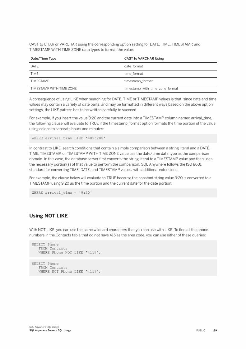
CAST to CHAR or VARCHAR using the corresponding option setting for DATE, TIME, TIMESTAMP, and TIMESTAMP WITH TIME ZONE data types to format the value:
Date/Time Type CAST to VARCHAR Using
DATE date_format
TIME time_format
TIMESTAMP timestamp_format
TIMESTAMP WITH TIME ZONE timestamp_with_time_zone_format
A consequence of using LIKE when searching for DATE, TIME or TIMESTAMP values is that, since date and time values may contain a variety of date parts, and may be formatted in different ways based on the above option settings, the LIKE pattern has to be written carefully to succeed.
For example, if you insert the value 9:20 and the current date into a TIMESTAMP column named arrival_time, the following clause will evaluate to TRUE if the timestamp_format option formats the time portion of the value using colons to separate hours and minutes:
WHERE arrival_time LIKE '%09:20%'
In contrast to LIKE, search conditions that contain a simple comparison between a string literal and a DATE, TIME, TIMESTAMP, or TIMESTAMP WITH TIME ZONE value use the date/time data type as the comparison domain. In this case, the database server first converts the string literal to a TIMESTAMP value and then uses the necessary portion(s) of that value to perform the comparison. SQL Anywhere follows the ISO 8601 standard for converting TIME, DATE, and TIMESTAMP values, with additional extensions.
For example, the clause below will evaluate to TRUE because the constant string value 9:20 is converted to a TIMESTAMP using 9:20 as the time portion and the current date for the date portion:
WHERE arrival_time = '9:20'
Using NOT LIKE
With NOT LIKE, you can use the same wildcard characters that you can use with LIKE. To find all the phone numbers in the Contacts table that do not have 415 as the area code, you can use either of these queries:
SELECT Phone FROM Contacts WHERE Phone NOT LIKE '415%';
SELECT Phone FROM Contacts WHERE NOT Phone LIKE '415%';
SQL Anywhere SQL UsageSQL Anywhere Server - SQL Usage PUBLIC 189
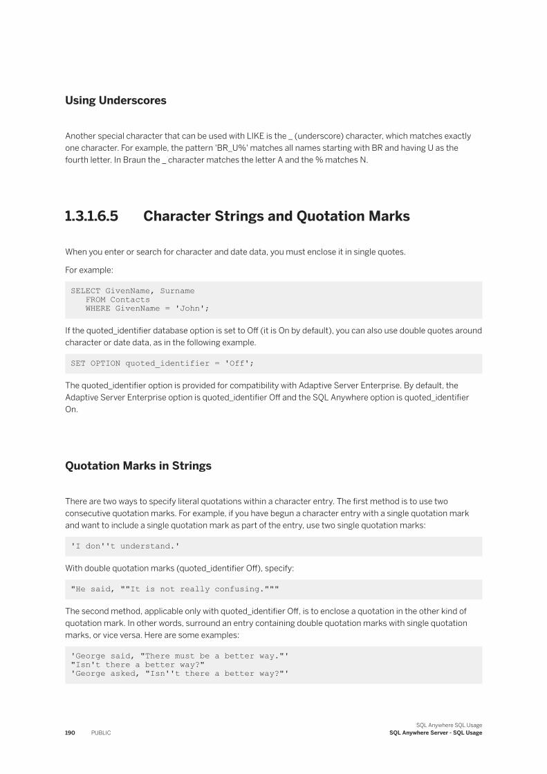
Using Underscores
Another special character that can be used with LIKE is the _ (underscore) character, which matches exactly one character. For example, the pattern 'BR_U%' matches all names starting with BR and having U as the fourth letter. In Braun the _ character matches the letter A and the % matches N.
1.3.1.6.5 Character Strings and Quotation Marks
When you enter or search for character and date data, you must enclose it in single quotes.
For example:
SELECT GivenName, Surname FROM Contacts WHERE GivenName = 'John';
If the quoted_identifier database option is set to Off (it is On by default), you can also use double quotes around character or date data, as in the following example.
SET OPTION quoted_identifier = 'Off';
The quoted_identifier option is provided for compatibility with Adaptive Server Enterprise. By default, the Adaptive Server Enterprise option is quoted_identifier Off and the SQL Anywhere option is quoted_identifier On.
Quotation Marks in Strings
There are two ways to specify literal quotations within a character entry. The first method is to use two consecutive quotation marks. For example, if you have begun a character entry with a single quotation mark and want to include a single quotation mark as part of the entry, use two single quotation marks:
'I don''t understand.'
With double quotation marks (quoted_identifier Off), specify:
"He said, ""It is not really confusing."""
The second method, applicable only with quoted_identifier Off, is to enclose a quotation in the other kind of quotation mark. In other words, surround an entry containing double quotation marks with single quotation marks, or vice versa. Here are some examples:
'George said, "There must be a better way."' "Isn't there a better way?" 'George asked, "Isn''t there a better way?"'
190 PUBLICSQL Anywhere SQL Usage
SQL Anywhere Server - SQL Usage
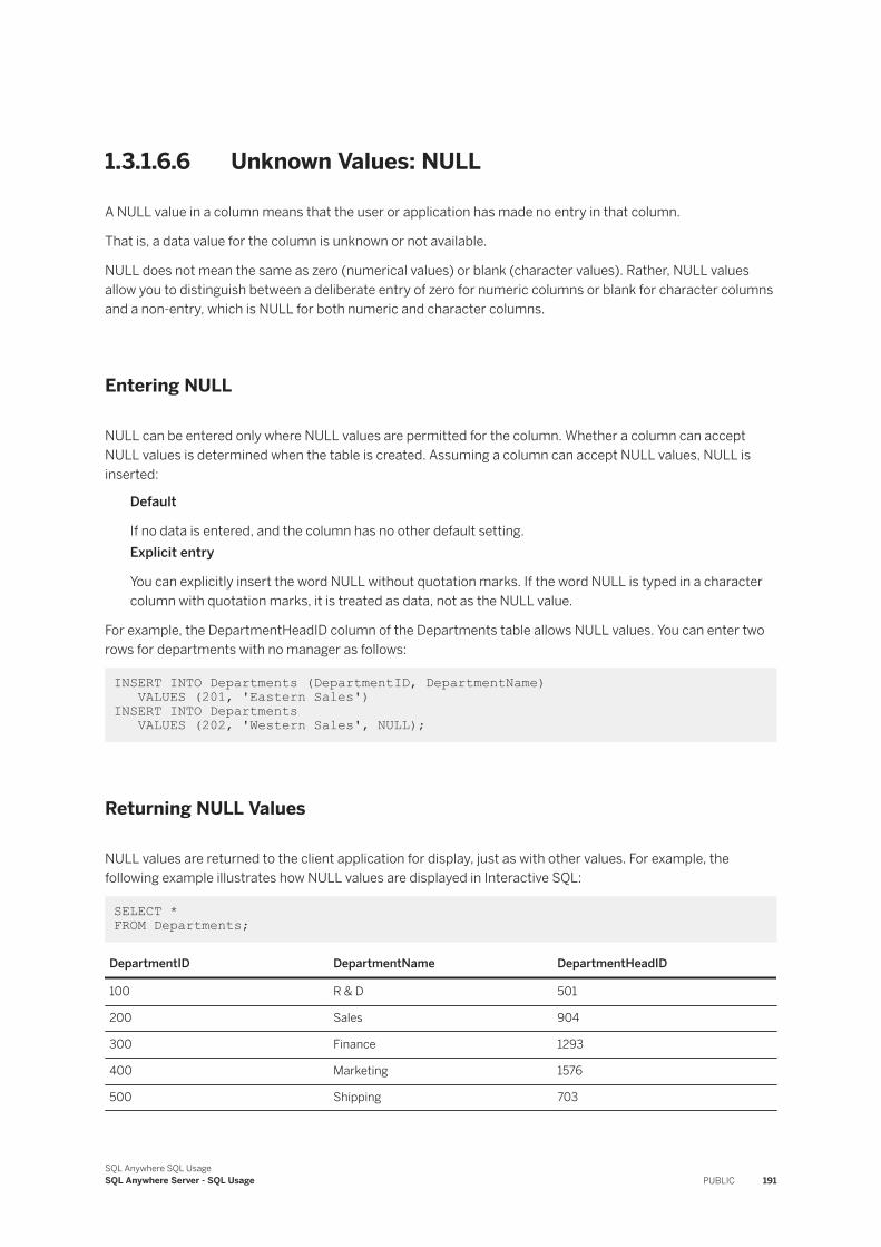
1.3.1.6.6 Unknown Values: NULL
A NULL value in a column means that the user or application has made no entry in that column.
That is, a data value for the column is unknown or not available.
NULL does not mean the same as zero (numerical values) or blank (character values). Rather, NULL values allow you to distinguish between a deliberate entry of zero for numeric columns or blank for character columns and a non-entry, which is NULL for both numeric and character columns.
Entering NULL
NULL can be entered only where NULL values are permitted for the column. Whether a column can accept NULL values is determined when the table is created. Assuming a column can accept NULL values, NULL is inserted:
Default
If no data is entered, and the column has no other default setting.Explicit entry
You can explicitly insert the word NULL without quotation marks. If the word NULL is typed in a character column with quotation marks, it is treated as data, not as the NULL value.
For example, the DepartmentHeadID column of the Departments table allows NULL values. You can enter two rows for departments with no manager as follows:
INSERT INTO Departments (DepartmentID, DepartmentName) VALUES (201, 'Eastern Sales')INSERT INTO Departments VALUES (202, 'Western Sales', NULL);
Returning NULL Values
NULL values are returned to the client application for display, just as with other values. For example, the following example illustrates how NULL values are displayed in Interactive SQL:
SELECT * FROM Departments;
DepartmentID DepartmentName DepartmentHeadID
100 R & D 501
200 Sales 904
300 Finance 1293
400 Marketing 1576
500 Shipping 703
SQL Anywhere SQL UsageSQL Anywhere Server - SQL Usage PUBLIC 191
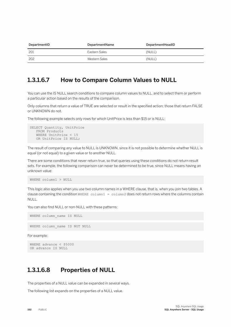
DepartmentID DepartmentName DepartmentHeadID
201 Eastern Sales (NULL)
202 Western Sales (NULL)
1.3.1.6.7 How to Compare Column Values to NULL
You can use the IS NULL search conditions to compare column values to NULL, and to select them or perform a particular action based on the results of the comparison.
Only columns that return a value of TRUE are selected or result in the specified action; those that return FALSE or UNKNOWN do not.
The following example selects only rows for which UnitPrice is less than $15 or is NULL:
SELECT Quantity, UnitPrice FROM Products WHERE UnitPrice < 15 OR UnitPrice IS NULL;
The result of comparing any value to NULL is UNKNOWN, since it is not possible to determine whether NULL is equal (or not equal) to a given value or to another NULL.
There are some conditions that never return true, so that queries using these conditions do not return result sets. For example, the following comparison can never be determined to be true, since NULL means having an unknown value:
WHERE column1 > NULL
This logic also applies when you use two column names in a WHERE clause, that is, when you join two tables. A clause containing the condition WHERE column1 = column2 does not return rows where the columns contain NULL.
You can also find NULL or non-NULL with these patterns:
WHERE column_name IS NULL
WHERE column_name IS NOT NULL
For example:
WHERE advance < $5000 OR advance IS NULL
1.3.1.6.8 Properties of NULL
The properties of a NULL value can be expanded in several ways.
The following list expands on the properties of a NULL value.
192 PUBLICSQL Anywhere SQL Usage
SQL Anywhere Server - SQL Usage
The difference between FALSE and UNKNOWN
Although neither FALSE nor UNKNOWN returns values, there is an important logical difference between FALSE and UNKNOWN; the opposite of false ("not false") is true, whereas the opposite of UNKNOWN does not mean something is known. For example, 1 = 2 evaluates to false, and 1 != 2 (1 does not equal 2) evaluates to true.
But if a NULL is included in a comparison, you cannot negate the expression to get the opposite set of rows or the opposite truth value. An UNKNOWN value remains UNKNOWN.Substituting a value for NULL values
You can use the ISNULL built-in function to substitute a particular value for NULL values. The substitution is made only for display purposes; actual column values are not affected. The syntax is:
ISNULL( expression, value )
For example, use the following statement to select all the rows from Departments, and display all the NULL values in column DepartmentHeadID with the value -1.
SELECT DepartmentID, DepartmentName, ISNULL( DepartmentHeadID, -1 ) AS DepartmentHead FROM Departments;
Expressions that evaluate to NULL
An expression with an arithmetic or bitwise operator evaluates to NULL if any of the operands are the NULL value. For example, 1 + column1 evaluates to NULL if column1 is NULL.Concatenating strings and NULL
If you concatenate a string and NULL, the expression evaluates to the string. For example, the following statement returns the string abcdef:
SELECT 'abc' || NULL || 'def';
1.3.1.6.9 Logical Operators That Provide Connecting Conditions
The logical operators AND, OR, and NOT are used to connect search conditions in WHERE clauses.
When more than one logical operator is used in a statement, AND operators are normally evaluated before OR operators. You can change the order of execution with parentheses.
Using AND
The AND operator joins two or more conditions and returns results only when all the conditions are true. For example, the following query finds only the rows in which the contact's last name is Purcell and the contact's first name is Beth.
SELECT *
SQL Anywhere SQL UsageSQL Anywhere Server - SQL Usage PUBLIC 193
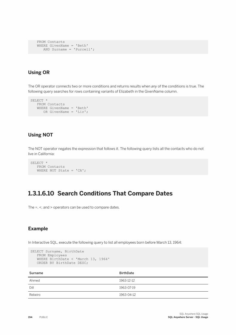
FROM Contacts WHERE GivenName = 'Beth' AND Surname = 'Purcell';
Using OR
The OR operator connects two or more conditions and returns results when any of the conditions is true. The following query searches for rows containing variants of Elizabeth in the GivenName column.
SELECT * FROM Contacts WHERE GivenName = 'Beth' OR GivenName = 'Liz';
Using NOT
The NOT operator negates the expression that follows it. The following query lists all the contacts who do not live in California:
SELECT * FROM Contacts WHERE NOT State = 'CA';
1.3.1.6.10 Search Conditions That Compare Dates
The =, <, and > operators can be used to compare dates.
Example
In Interactive SQL, execute the following query to list all employees born before March 13, 1964:
SELECT Surname, BirthDate FROM Employees WHERE BirthDate < 'March 13, 1964' ORDER BY BirthDate DESC;
Surname BirthDate
Ahmed 1963-12-12
Dill 1963-07-19
Rebeiro 1963-04-12
194 PUBLICSQL Anywhere SQL Usage
SQL Anywhere Server - SQL Usage
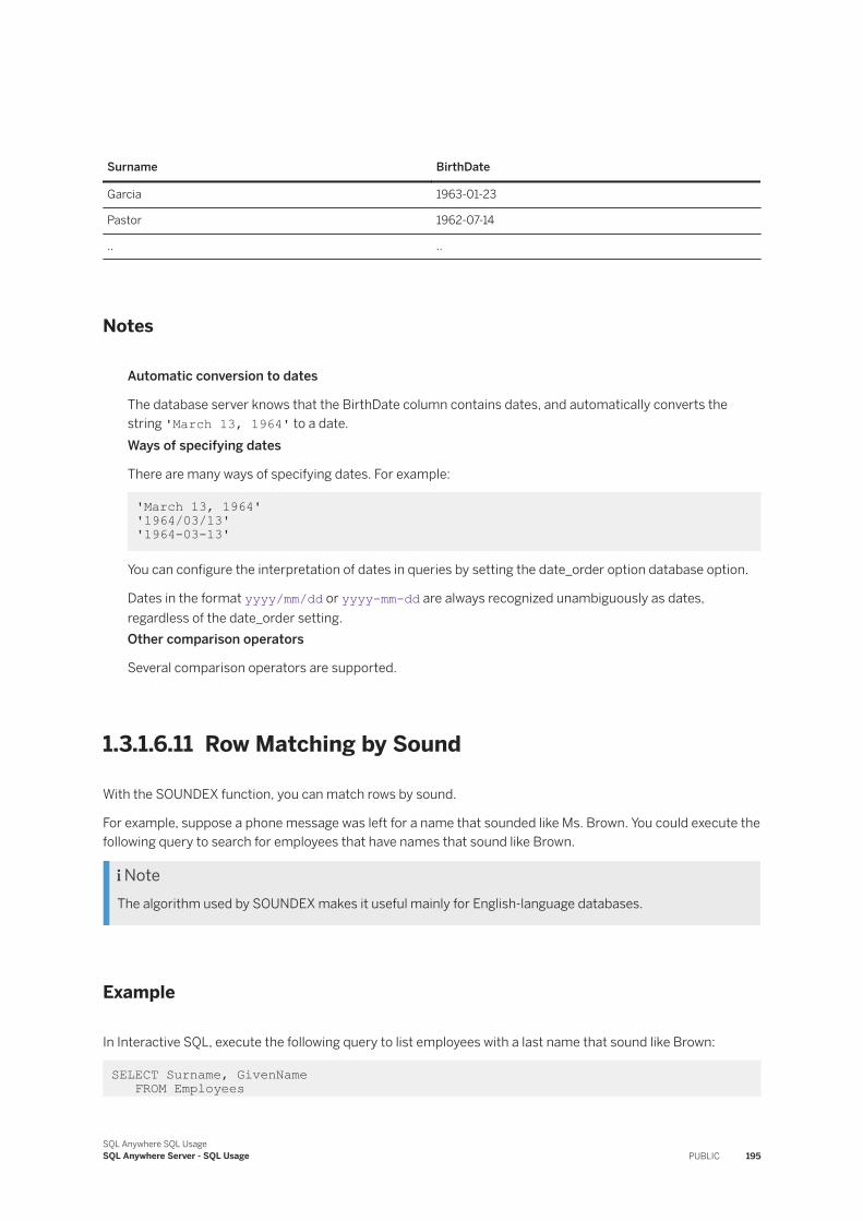
Surname BirthDate
Garcia 1963-01-23
Pastor 1962-07-14
.. ..
Notes
Automatic conversion to dates
The database server knows that the BirthDate column contains dates, and automatically converts the string 'March 13, 1964' to a date.Ways of specifying dates
There are many ways of specifying dates. For example:
'March 13, 1964' '1964/03/13' '1964-03-13'
You can configure the interpretation of dates in queries by setting the date_order option database option.
Dates in the format yyyy/mm/dd or yyyy-mm-dd are always recognized unambiguously as dates, regardless of the date_order setting.Other comparison operators
Several comparison operators are supported.
1.3.1.6.11 Row Matching by Sound
With the SOUNDEX function, you can match rows by sound.
For example, suppose a phone message was left for a name that sounded like Ms. Brown. You could execute the following query to search for employees that have names that sound like Brown.
NoteThe algorithm used by SOUNDEX makes it useful mainly for English-language databases.
Example
In Interactive SQL, execute the following query to list employees with a last name that sound like Brown:
SELECT Surname, GivenName FROM Employees
SQL Anywhere SQL UsageSQL Anywhere Server - SQL Usage PUBLIC 195
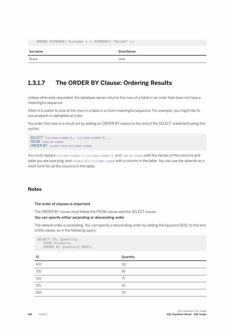
WHERE SOUNDEX( Surname ) = SOUNDEX( 'Brown' );
Surname GivenName
Braun Jane
1.3.1.7 The ORDER BY Clause: Ordering Results
Unless otherwise requested, the database server returns the rows of a table in an order that does not have a meaningful sequence.
Often it is useful to look at the rows in a table in a more meaningful sequence. For example, you might like to see products in alphabetical order.
You order the rows in a result set by adding an ORDER BY clause to the end of the SELECT statement using this syntax:
SELECT column-name-1, column-name-2,.. FROM table-name ORDER BY order-by-column-name
You must replace column-name-1, column-name-2, and table-name with the names of the columns and table you are querying, and order-by-column-name with a column in the table. You can use the asterisk as a short form for all the columns in the table.
Notes
The order of clauses is important
The ORDER BY clause must follow the FROM clause and the SELECT clause.You can specify either ascending or descending order
The default order is ascending. You can specify a descending order by adding the keyword DESC to the end of the clause, as in the following query:
SELECT ID, Quantity FROM Products ORDER BY Quantity DESC;
ID Quantity
400 112
700 80
302 75
301 54
600 39
196 PUBLICSQL Anywhere SQL Usage
SQL Anywhere Server - SQL Usage
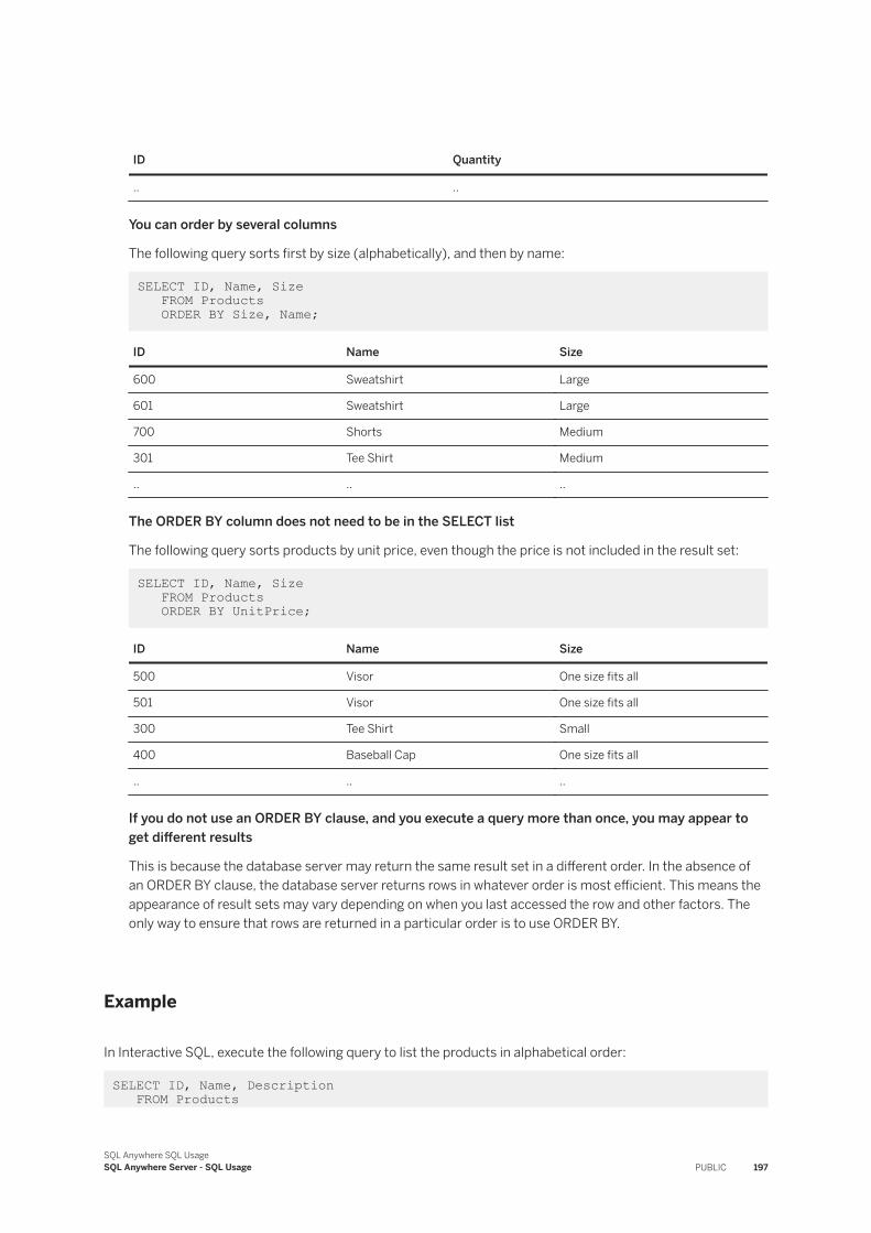
ID Quantity
.. ..
You can order by several columns
The following query sorts first by size (alphabetically), and then by name:
SELECT ID, Name, Size FROM Products ORDER BY Size, Name;
ID Name Size
600 Sweatshirt Large
601 Sweatshirt Large
700 Shorts Medium
301 Tee Shirt Medium
.. .. ..
The ORDER BY column does not need to be in the SELECT list
The following query sorts products by unit price, even though the price is not included in the result set:
SELECT ID, Name, Size FROM Products ORDER BY UnitPrice;
ID Name Size
500 Visor One size fits all
501 Visor One size fits all
300 Tee Shirt Small
400 Baseball Cap One size fits all
.. .. ..
If you do not use an ORDER BY clause, and you execute a query more than once, you may appear to get different results
This is because the database server may return the same result set in a different order. In the absence of an ORDER BY clause, the database server returns rows in whatever order is most efficient. This means the appearance of result sets may vary depending on when you last accessed the row and other factors. The only way to ensure that rows are returned in a particular order is to use ORDER BY.
Example
In Interactive SQL, execute the following query to list the products in alphabetical order:
SELECT ID, Name, Description FROM Products
SQL Anywhere SQL UsageSQL Anywhere Server - SQL Usage PUBLIC 197
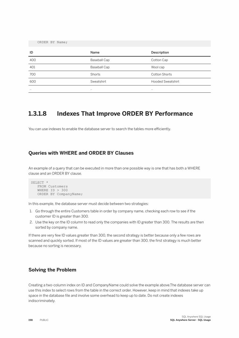
ORDER BY Name;
ID Name Description
400 Baseball Cap Cotton Cap
401 Baseball Cap Wool cap
700 Shorts Cotton Shorts
600 Sweatshirt Hooded Sweatshirt
.. .. ..
1.3.1.8 Indexes That Improve ORDER BY Performance
You can use indexes to enable the database server to search the tables more efficiently.
Queries with WHERE and ORDER BY Clauses
An example of a query that can be executed in more than one possible way is one that has both a WHERE clause and an ORDER BY clause.
SELECT * FROM Customers WHERE ID > 300 ORDER BY CompanyName;
In this example, the database server must decide between two strategies:
1. Go through the entire Customers table in order by company name, checking each row to see if the customer ID is greater than 300.
2. Use the key on the ID column to read only the companies with ID greater than 300. The results are then sorted by company name.
If there are very few ID values greater than 300, the second strategy is better because only a few rows are scanned and quickly sorted. If most of the ID values are greater than 300, the first strategy is much better because no sorting is necessary.
Solving the Problem
Creating a two-column index on ID and CompanyName could solve the example above.The database server can use this index to select rows from the table in the correct order. However, keep in mind that indexes take up space in the database file and involve some overhead to keep up to date. Do not create indexes indiscriminately.
198 PUBLICSQL Anywhere SQL Usage
SQL Anywhere Server - SQL Usage
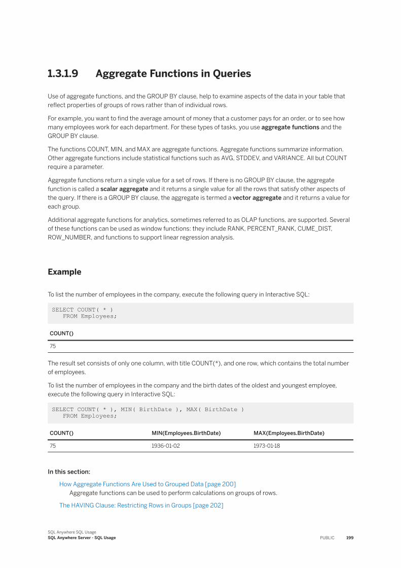
1.3.1.9 Aggregate Functions in Queries
Use of aggregate functions, and the GROUP BY clause, help to examine aspects of the data in your table that reflect properties of groups of rows rather than of individual rows.
For example, you want to find the average amount of money that a customer pays for an order, or to see how many employees work for each department. For these types of tasks, you use aggregate functions and the GROUP BY clause.
The functions COUNT, MIN, and MAX are aggregate functions. Aggregate functions summarize information. Other aggregate functions include statistical functions such as AVG, STDDEV, and VARIANCE. All but COUNT require a parameter.
Aggregate functions return a single value for a set of rows. If there is no GROUP BY clause, the aggregate function is called a scalar aggregate and it returns a single value for all the rows that satisfy other aspects of the query. If there is a GROUP BY clause, the aggregate is termed a vector aggregate and it returns a value for each group.
Additional aggregate functions for analytics, sometimes referred to as OLAP functions, are supported. Several of these functions can be used as window functions: they include RANK, PERCENT_RANK, CUME_DIST, ROW_NUMBER, and functions to support linear regression analysis.
Example
To list the number of employees in the company, execute the following query in Interactive SQL:
SELECT COUNT( * ) FROM Employees;
COUNT()
75
The result set consists of only one column, with title COUNT(*), and one row, which contains the total number of employees.
To list the number of employees in the company and the birth dates of the oldest and youngest employee, execute the following query in Interactive SQL:
SELECT COUNT( * ), MIN( BirthDate ), MAX( BirthDate ) FROM Employees;
COUNT() MIN(Employees.BirthDate) MAX(Employees.BirthDate)
75 1936-01-02 1973-01-18
In this section:
How Aggregate Functions Are Used to Grouped Data [page 200]Aggregate functions can be used to perform calculations on groups of rows.
The HAVING Clause: Restricting Rows in Groups [page 202]
SQL Anywhere SQL UsageSQL Anywhere Server - SQL Usage PUBLIC 199
You can restrict the rows in groups by using the HAVING clause.
Combination of WHERE and HAVING Clauses [page 202]You can specify the same set of rows using either a WHERE clause or a HAVING clause.
Related Information
OLAP Support [page 444]
1.3.1.9.1 How Aggregate Functions Are Used to Grouped Data
Aggregate functions can be used to perform calculations on groups of rows.
The GROUP BY clause arranges rows into groups, and aggregate functions return a single value for each group of rows.
Semantic Differences with the Empty Set
The SQL language treats the empty set differently when using aggregate functions. Without a GROUP BY clause, a query containing an aggregate function over zero input rows returns a single row as the result. In the case of COUNT, its result is the value zero, and with all other aggregate functions the result will be NULL. However, if the query contains a GROUP BY clause, and the input to the query is empty, then the query result is empty and no rows are returned.
For example, the following query returns a single row with the value 0; there are no employees in department 103.
SELECT COUNT() FROM Employees WHERE DepartmentID = 103;
However, this modified query returns no rows, due to the presence of the GROUP BY clause.
SELECT COUNT() FROM Employees WHERE DepartmentID = 103 GROUP BY State;
A Common Error with GROUP BY
A common error with GROUP BY is to try to get information that cannot properly be put in a group. For example, the following query gives an error:
SELECT SalesRepresentative, Surname, COUNT( * ) FROM SalesOrders KEY JOIN Employees GROUP BY SalesRepresentative;
200 PUBLICSQL Anywhere SQL Usage
SQL Anywhere Server - SQL Usage
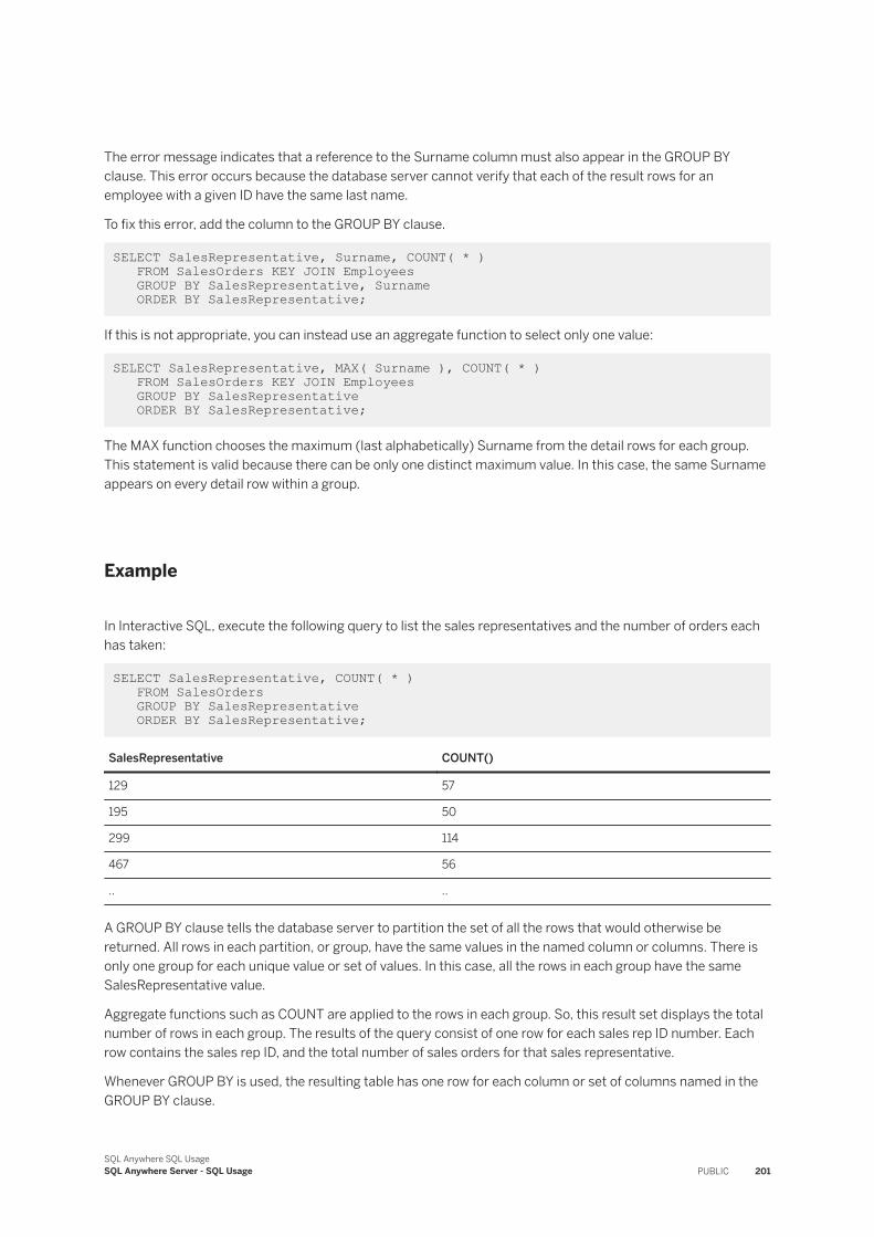
The error message indicates that a reference to the Surname column must also appear in the GROUP BY clause. This error occurs because the database server cannot verify that each of the result rows for an employee with a given ID have the same last name.
To fix this error, add the column to the GROUP BY clause.
SELECT SalesRepresentative, Surname, COUNT( * ) FROM SalesOrders KEY JOIN Employees GROUP BY SalesRepresentative, Surname ORDER BY SalesRepresentative;
If this is not appropriate, you can instead use an aggregate function to select only one value:
SELECT SalesRepresentative, MAX( Surname ), COUNT( * ) FROM SalesOrders KEY JOIN Employees GROUP BY SalesRepresentative ORDER BY SalesRepresentative;
The MAX function chooses the maximum (last alphabetically) Surname from the detail rows for each group. This statement is valid because there can be only one distinct maximum value. In this case, the same Surname appears on every detail row within a group.
Example
In Interactive SQL, execute the following query to list the sales representatives and the number of orders each has taken:
SELECT SalesRepresentative, COUNT( * ) FROM SalesOrders GROUP BY SalesRepresentative ORDER BY SalesRepresentative;
SalesRepresentative COUNT()
129 57
195 50
299 114
467 56
.. ..
A GROUP BY clause tells the database server to partition the set of all the rows that would otherwise be returned. All rows in each partition, or group, have the same values in the named column or columns. There is only one group for each unique value or set of values. In this case, all the rows in each group have the same SalesRepresentative value.
Aggregate functions such as COUNT are applied to the rows in each group. So, this result set displays the total number of rows in each group. The results of the query consist of one row for each sales rep ID number. Each row contains the sales rep ID, and the total number of sales orders for that sales representative.
Whenever GROUP BY is used, the resulting table has one row for each column or set of columns named in the GROUP BY clause.
SQL Anywhere SQL UsageSQL Anywhere Server - SQL Usage PUBLIC 201
Related Information
The GROUP BY Clause: Organizing Query Results into Groups [page 367]GROUP BY with Aggregate Functions [page 370]
1.3.1.9.2 The HAVING Clause: Restricting Rows in Groups
You can restrict the rows in groups by using the HAVING clause.
Example
In Interactive SQL, execute the following query to list all sales representatives with more than 55 orders:
SELECT SalesRepresentative, COUNT( * ) AS orders FROM SalesOrders KEY JOIN EmployeesGROUP BY SalesRepresentativeHAVING count( * ) > 55 ORDER BY orders DESC;
SalesRepresentative Orders
299 114
129 57
1142 57
467 56
Related Information
The HAVING Clause: Selecting Groups of Data [page 372]Subqueries in the HAVING Clause [page 493]
1.3.1.9.3 Combination of WHERE and HAVING Clauses
You can specify the same set of rows using either a WHERE clause or a HAVING clause.
In such cases, one method is not more or less efficient than the other. The optimizer always automatically analyzes each statement you enter and selects an efficient means of executing it. It is best to use the syntax that most clearly describes the intended result. In general, that means eliminating undesired rows in earlier clauses.
202 PUBLICSQL Anywhere SQL Usage
SQL Anywhere Server - SQL Usage
Example
To list all sales reps with more than 55 orders and an ID of more than 1000, enter the following query:
SELECT SalesRepresentative, COUNT( * ) FROM SalesOrdersWHERE SalesRepresentative > 1000GROUP BY SalesRepresentativeHAVING count( * ) > 55 ORDER BY SalesRepresentative;
The following query produces the same results:
SELECT SalesRepresentative, COUNT( * ) FROM SalesOrdersGROUP BY SalesRepresentativeHAVING count( * ) > 55 AND SalesRepresentative > 1000 ORDER BY SalesRepresentative;
The database server detects that both statements describe the same result set, and so executes each efficiently.
1.3.1.10 Advanced: Query Processing PhasesThere are several phases a statement goes through, starting with the annotation phase and ending with the execution phase.
Statements that have no result sets, such as UPDATE or DELETE statements, go through the query processing phases.
Annotation phase
When the database server receives a query, it uses a parser to parse the statement and transform it into an algebraic representation of the query, also known as a parse tree. At this stage the parse tree is used for semantic and syntactic checking (for example, validating that objects referenced in the query exist in the catalog), privilege checking, KEY JOINs and NATURAL JOINs transformation using defined referential constraints, and non-materialized view expansion. The output of this phase is a rewritten query, in the form of a parse tree, which contains annotation to all the objects referenced in the original query.Semantic transformation phase
During this phase, the query undergoes iterative semantic transformations. While the query is still represented as an annotated parse tree, rewrite optimizations, such as join elimination, DISTINCT elimination, and predicate normalization, are applied in this phase. The semantic transformations in this phase are performed based on semantic transformation rules that are applied heuristically to the parse tree representation.
Queries with plans already cached by the database server skip this phase of query processing. Simple statements may also skip this phase of query processing. For example, many statements that use heuristic plan selection in the optimizer bypass are not processed by the semantic transformation phase. The complexity of the SQL statement determines if this phase is applied to a statement.Optimization phase
The optimization phase uses a different internal representation of the query, the query optimization structure, which is built from the parse tree.
SQL Anywhere SQL UsageSQL Anywhere Server - SQL Usage PUBLIC 203
Queries with plans already cached by the database server skip this phase of query processing. As well, simple statements may also skip this phase of query processing.
This phase is broken into two sub-phases:
Pre-optimization phase
The pre-optimization phase completes the optimization structure with the information needed later in the enumeration phase. During this phase the query is analyzed to find all relevant indexes and materialized views that can be used in the query access plan. For example, in this phase, the View Matching algorithm determines all the materialized views that can be used to satisfy all, or part of the query. In addition, based on query predicate analysis, the optimizer builds alternative join methods that can be used in the enumeration phase to join the query's tables. During this phase, no decision is made regarding the best access plan for the query; the goal of this phase is to prepare for the enumeration phase.Enumeration phase
During this phase, the optimizer enumerates possible access plans for the query using the building blocks generated in the pre-optimization phase. The search space is very large and the optimizer uses a proprietary enumeration algorithm to generate and prune the generated access plans. For each plan, cost estimation is computed, which is used to compare the current plan with the best plan found so far. Expensive plans are discarded during these comparisons. Cost estimation takes into account resource utilization such as disk and CPU operations, the estimated number of rows of the intermediate results, optimization goal, cache size, and so on. The output of the enumeration phase is the best access plan for the query.
Plan building phase
The plan building phase takes the best access plan and builds the corresponding final representation of the query execution plan used to execute the query. You can see a graphical version of the plan in the Plan Viewer in Interactive SQL. The graphical plan has a tree structure where each node is a physical operator implementing a specific relational algebraic operation, for example, Hash Join and Ordered Group By are physical operators implementing a join and a group by operation, respectively.
Queries with plans already cached by the database server skip this phase of query processing.Execution phase
The result of the query is computed using the query execution plan built in the plan building phase.
In this section:
Eligibility to Skip Query Processing Phases [page 205]Almost all statements pass through all query processing phases.
Related Information
Optimizations Performed During Query Processing [page 214]Plan Caching [page 211]Graphical Plans [page 221]How the Optimizer Works [page 207]Query Processing Based on SQL Anywhere 12.0.1 Architecture
204 PUBLICSQL Anywhere SQL Usage
SQL Anywhere Server - SQL Usage
1.3.1.10.1 Eligibility to Skip Query Processing Phases
Almost all statements pass through all query processing phases.
However, there are two main exceptions: queries that benefit from plan caching (queries whose plans are already cached by the database server), and bypass queries.
Plan caching
For queries contained inside stored procedures and user-defined functions, the database server may cache the execution plans so that they can be reused. For this class of queries, the query execution plan is cached after execution. The next time the query is executed, the plan is retrieved and all the phases up to the execution phase are skipped.Bypass queries
Bypass queries are a subclass of simple queries that have certain characteristics that the database server recognizes as making them eligible for bypassing the optimizer. Bypassing optimization can reduce the time needed to build an execution plan.
If a query is recognized as a bypass query, then a heuristic rather than cost-based optimization is used. That is, the semantic transformation and optimization phases may be skipped and the query execution plan is built directly from the parse tree representation of the query.
Simple Queries
A simple query is a SELECT, INSERT, DELETE, or UPDATE statement with a single query block and the following characteristics:
● The query block does not contain subqueries or additional query blocks such as those for UNION, INTERSECT, EXCEPT, and common table expressions.
● The query block references a single base table or materialized view.● The query block may include the TOP N, FIRST, ORDER BY, or DISTINCT clauses.● The query block may include aggregate functions without GROUP BY or HAVING clauses.● The query block does not include window functions.● The query block expressions do not include NUMBER, IDENTITY, or subqueries.● The constraints defined on the base table are simple expressions.
A complex statement may be transformed into a simple statement after the semantic transformation phase. When this occurs, the query can be processed by the optimizer bypass or have its plan cached by the SQL Anywhere Server.
Forcing Optimization, and Forcing No Optimization
You can force queries that qualify for plan caching, or for bypassing the optimizer, to be processed by the SQL Anywhere optimizer. To do so, use the FORCE OPTIMIZATION clause with any SQL statement.
SQL Anywhere SQL UsageSQL Anywhere Server - SQL Usage PUBLIC 205
You can also try to force a statement to bypass the optimizer. To do so, use the FORCE NO OPTIMIZATION clause of the statement. If the statement is too complex to bypass the optimizer - possibly due to database option settings or characteristics of the schema or query - the query fails and an error is returned.
The FORCE OPTIMIZATION and FORCE NO OPTIMIZATION clauses are permitted in the OPTION clause of the following statements:
● SELECT statement● UPDATE statement● INSERT statement● DELETE statement
Related Information
Plan Caching [page 211]
1.3.1.11 Advanced: Query Optimization
Optimization is essential in generating a suitable access plan for a query.
Once a query is parsed, the query optimizer (or simply, the optimizer) analyzes it and decides on an access plan that computes the result using as few resources as possible. Optimization begins just before execution. If you are using cursors in your application, optimization commences when the cursor is opened.
Unlike many other commercial database systems, SQL Anywhere usually optimizes each statement just before executing it. Because the database server performs just-in-time optimization of each statement, the optimizer has access to the values of host and stored procedure variables, which allows for better selectivity estimation analysis. In addition, just-in-time optimization allows the optimizer to adjust its choices based on the statistics saved after previous query executions.
To operate efficiently, the database server rewrites your queries into semantically equivalent, but syntactically different, forms. The database server performs many different rewrite operations. If you read the access plans, you frequently find that they do not correspond to a literal interpretation of your original statement. For example, to make your SQL statements more efficient, the optimizer tries as much as possible to rewrite subqueries with joins.
In this section:
How the Optimizer Works [page 207]The role of the optimizer is to devise an efficient way to execute SQL statements.
Optimizations Performed During Query Processing [page 214]In the query rewrite phase, the database server performs semantic transformations in search of more efficient representations of the query.
206 PUBLICSQL Anywhere SQL Usage
SQL Anywhere Server - SQL Usage
Related Information
Query optimization based on SQL Anywhere 12.0.1 architecture
1.3.1.11.1 How the Optimizer Works
The role of the optimizer is to devise an efficient way to execute SQL statements.
To do this, the optimizer must determine an execution plan for a query. This includes decisions about the access order for tables referenced in the query, the join operators and access methods used for each table, and whether materialized views that are not referenced in the query can be used to compute parts of the query. The optimizer attempts to pick the best plan for executing the query during the join enumeration phase, when possible access plans for a query are generated and costed. The best access plan is the one that the optimizer estimates will return the desired result set in the shortest period of time, with the least cost. The optimizer determines the cost of each enumerated strategy by estimating the number of disk reads and writes required.
In Interactive SQL, you can view the best access plan used to execute a query by clicking Tools Plan Viewer .
Minimizing the Cost of Returning the First Row
The optimizer uses a generic disk access cost model to differentiate the relative performance differences between random and sequential retrieval on the database file. It is possible to calibrate a database for a particular hardware configuration using an ALTER DATABASE statement.
By default, query processing is optimized towards returning the complete result set. You can change the default behavior using the optimization_goal option, to minimize the cost of returning the first row quickly. When the option is set to First-row, the optimizer favors an access plan that is intended to reduce the time to fetch the first row of the query result, likely at the expense of total retrieval time.
Using Semantically Equivalent Syntax
Most statements can be expressed in many different ways using the SQL language. These expressions are semantically equivalent in that they do the same task, but may differ substantially in syntax. With few exceptions, the optimizer devises a suitable access plan based only on the semantics of each statement.
Syntactic differences, although they may appear to be substantial, usually have no effect. For example, differences in the order of predicates, tables, and attributes in the query syntax have no effect on the choice of access plan. Neither is the optimizer affected by whether a query contains a non-materialized view.
SQL Anywhere SQL UsageSQL Anywhere Server - SQL Usage PUBLIC 207
Reducing the Cost of Optimizing Queries
The optimizer attempts to identify the most efficient access plan possible, but this goal is often impractical. Given a complicated query, a great number of possibilities exist.
However efficient the optimizer, analyzing each option takes time and resources. The optimizer compares the cost of further optimization with the cost of executing the best plan it has found so far. If a plan has been devised that has a relatively low cost, the optimizer stops and allows execution of that plan to proceed. Further optimization might consume more resources than would execution of an access plan already found. You can control the amount of effort made by the optimizer by setting a high value for the optimization_level option.
The optimizer works longer for expensive and complex queries, or when the optimization level is set high. For very expensive queries, it may run long enough to cause a discernible delay.
In this section:
Optimizer Estimates and Statistics [page 208]The optimizer chooses a strategy for processing a statement based on column statistics stored in the database and on heuristics.
Selectivity Estimate Sources [page 210]For any predicate, the optimizer can use several sources for selectivity estimates. The chosen source is indicated in the graphical and long plan for the query.
Plan Caching [page 211]The optimizer can use cached plans when executing a query.
Subquery and Function Caching [page 213]When the database server processes a subquery, it caches the result.
Related Information
Graphical Plans [page 221]Advanced: Query Execution Plans [page 215]
1.3.1.11.1.1 Optimizer Estimates and Statistics
The optimizer chooses a strategy for processing a statement based on column statistics stored in the database and on heuristics.
For each access plan considered by the optimizer, an estimated result size (number of rows) must be computed. For example, for each join method or index access based on the selectivity estimations of the predicates used in the query, an estimated result size is calculated. The estimated result sizes are used to compute the estimated disk access and CPU cost for each operator such as a join method, a group by method, or a sequential scan, used in the plan. Column statistics are the primary data used by the optimizer to compute selectivity estimation of predicates. Therefore, they are vital to estimating correctly the cost of an access plan.
208 PUBLICSQL Anywhere SQL Usage
SQL Anywhere Server - SQL Usage
If column statistics become stale, or are missing, performance can degrade since inaccurate statistics may result in an inefficient execution plan. If you suspect that poor performance is due to inaccurate column statistics, recreate them.
How the Optimizer Uses Statistics
The most important component of the column statistics used by the optimizer are histograms. Histograms store information about the distribution of values in a column. A histogram represents the data distribution for a column by dividing the domain of the column into a set of consecutive value ranges (also called buckets) and by remembering, for each value range (or bucket), the number of rows in the table for which the column value falls in the bucket.
The database server pays particular attention to single column values that are present in a large number of rows in the table. Significant single value selectivities are maintained in singleton histogram buckets (for example, buckets that encompass a single value in the column domain). The database server tries to maintain a minimum number of singleton buckets in each histogram, usually between 10 and 100 depending upon the size of the table. Additionally, all single values with selectivities greater than 1% are kept as singleton buckets. As a result, a histogram for a given column remembers the top N single value selectivities for the column where the value of N is dependent upon the size of the table and the number of single value selectivities that are greater than 1%.
Once the minimum number of value ranges has been met, low-selectivity frequencies are replaced by large-selectivity frequencies as they come along. The histogram will only have more than the minimum number of singleton value ranges after it has seen enough values with a selectivity of greater than 1%.
Unlike base tables, procedure calls executed in the FROM clause do not have column statistics. Therefore, the optimizer uses defaults or guesses for all selectivity estimates on data coming from a procedure call. The execution time of a procedure call, and the total number of rows in its result set, are estimated using statistics collected from previous calls. These statistics are maintained in the stats column of the ISYSPROCEDURE system table.
How the Optimizer Uses Heuristics
For each table in a potential execution plan, the optimizer estimates the number of rows that will form part of the results. The number of rows depends on the size of the table and the restrictions in the WHERE clause or the ON clause of the query.
Given the histogram on a column, the database server estimates the number of rows satisfying a given query predicate on the column by adding up the number of rows in all value ranges that overlap the values satisfying the specified predicate. For value ranges in the histograms that are partially contained in the query result set, the database server uses interpolation within the value range.
Often, the optimizer uses more sophisticated heuristics. For example, the optimizer only uses default estimates when better statistics are unavailable. As well, the optimizer makes use of indexes and keys to improve its guess of the number of rows. The following are a few single-column examples:
● Equating a column to a value: estimate one row when the column has a unique index or is the primary key.● A comparison of an indexed column to a constant: probe the index to estimate the percentage of rows that
satisfy the comparison.
SQL Anywhere SQL UsageSQL Anywhere Server - SQL Usage PUBLIC 209
● Equating a foreign key to a primary key (key join): use relative table sizes in determining an estimate. For example, if a 5000 row table has a foreign key to a 1000 row table, the optimizer guesses that there are five foreign key rows for each primary key row.
Related Information
Selectivity Estimate Sources [page 210]
1.3.1.11.1.2 Selectivity Estimate Sources
For any predicate, the optimizer can use several sources for selectivity estimates. The chosen source is indicated in the graphical and long plan for the query.
These are the possible sources for selectivity estimates:
Statistics
The optimizer can use stored column statistics to calculate selectivity estimates. If constants are used in the predicate, the stored statistics are available only when the selectivity of a constant is a significant enough number that it is stored in the statistics.
For example, the predicate EmployeeID > 100 can use column statistics as the selectivity estimate source if the statistics for the EmployeeID column exists.Join
The optimizer can use referential integrity constraints, unique constraints, or join histograms to compute selectivity estimates. Join histograms are computed for a predicate of the form T.X=R.X from the available statistics of the T.X and R.X columns.Column-column
In the case of a join where there are no referential integrity constraints, unique constraints, or join histograms available to use as selectivity sources, the optimizer can use, as a selectivity source, the estimated number of rows in the joined result set divided by the number of rows in the Cartesian product of the two tables.Column
The optimizer can use the average of all values that have been stored in the column statistics.
For example, the selectivity of the predicate DepartmentName = expression can be computed using the average if expression is not a constant.Index
The optimizer can probe indexes to compute selectivity estimates. In general, an index is used for selectivity estimates if no other sources of selectivity estimates, for example column statistics, can be used.
For example, for the predicate DepartmentName = 'Sales', the optimizer can use an index defined on the column DepartmentName to estimate the number of rows having the value Sales.User
210 PUBLICSQL Anywhere SQL Usage
SQL Anywhere Server - SQL Usage
The optimizer can use user-supplied selectivity estimates, provided the user_estimates database option is not set to Disabled.Guess
The optimizer can resort to best guessing to calculate selectivity estimates when there is no relevant index to use, no statistics have been collected for the referenced columns, or the predicate is a complex predicate. In this case, built-in guesses are defined for each type of predicate.Computed
For example, a very complex predicate may have the selectivity estimate set to 100% and the selectivity source set to Computed if the selectivity estimate was computed, for example, by multiplying or adding the selectivities.Always
If a predicate is always true, the selectivity source is 'Always'. For example, the predicate 1=1 is always true.Combined
If the selectivity estimate is computed by combining more than one of the sources above, the selectivity source is 'Combined'.Bounded
When the database server has placed an upper and/or lower bound on the selectivity estimate, the selectivity source is 'Bounded'. For example, bounds are sets to ensure that an estimate is not greater than 100%, or that the selectivity is not less than 0%.
Related Information
Selectivity Information in the Graphical Plan [page 226]
1.3.1.11.1.3 Plan Caching
The optimizer can use cached plans when executing a query.
The plan cache is a per-connection cache of the data structures used to execute an access plan, with the goal to reuse a plan when it is efficient to do so. Reusing a cached plan involves looking up the plan in the cache, but typically, this is substantially faster than reprocessing a statement through all of the query processing phases.
Optimization at query execution time allows the optimizer to choose a plan based on the current system state, on the values of current selectivity estimates, and on estimates that are based on the values of host variables. For queries that are executed frequently, the cost of query optimization can outweigh the benefits of optimizing at execution time. To reduce the cost of optimizing these statements repeatedly, the database server considers caching the execution plans for reuse later.
For client statements, the lifetimes of cached execution plans are limited to the lifetimes of the corresponding statements and are dropped from the plan cache when the client statements are dropped. The lifetimes of client statements (and any corresponding execution plans) can be extended by a separate cache of prepared client statements, which is controlled by the max_client_statements_cached option. Depending on how your system is configured, client statements may be cached in a parameterized form to increase the chances that corresponding execution plans will be reused.
SQL Anywhere SQL UsageSQL Anywhere Server - SQL Usage PUBLIC 211
The maximum number of plans to cache is specified with the max_plans_cached option.
Use the sp_plancache_contents system procedure to examine the current contents of your plan cache.
You can use the QueryCachedPlans statistic to show how many query execution plans are currently cached. This property can be retrieved using the CONNECTION_PROPERTY function to show how many query execution plans are cached for a given connection, or the DB_PROPERTY function can be used to count the number of cached execution plans across all connections. This property can be used in combination with QueryCachePages, QueryOptimized, QueryBypassed, and QueryReused to help determine the best setting for the max_plans_cached option.
You can use the database or QueryCachePages connection property to determine the number of pages used to cache execution plans. These pages occupy space in the temporary file, but are not necessarily resident in memory.
When Is a Plan Cached?
The database server decides which plans to cache and which plans to avoid caching. Plan caching policies define criteria to meet and actions to take when evaluating statements and their plans. The policies are at work behind the scenes, governing plan caching behavior. For example, a policy might determine the number of executions (training period) a statement must go through, and the results to look for in the resulting plans, to qualify a plan for caching and reuse.
After a qualifying statement has been executed several times by a connection, the database server may decide to build a reusable plan. If the reusable plan has the same structure as the plans built in previous executions of the statement, the database server adds the reusable plan to the plan cache. The execution plan is not cached when the risks inherent in not optimizing on each execution outweighs the savings from avoiding optimization.
Query execution plans are not cached for queries that have long running times because the benefits of avoiding query optimization are small compared to the total cost of the query. Additionally, the database server may not cache plans for queries that are very sensitive to the values of their host variables.
If an execution plan uses a materialized view that was not referenced by the statement, and the materialized_view_optimization option is set to something other than Stale, then the execution plan is not cached and the statement is optimized again the next time it is executed.
To minimize cache usage, cached plans may be stored to disk if they are used infrequently. Also, the optimizer periodically re-optimizes queries to verify that the cached plan is still efficient.
Plan Caching and Statement Parameterization
The database server can parameterize qualifying client statements to enhance plan caching opportunities. Parameterized statements use placeholders that act like variables that are evaluated at execution time. Although parameterization may introduce a very small amount of performance overhead for some statements, the parameterized statement text is more general and can be matched to more SQL queries. As a result, statement parameterization can improve the efficiency of plan caching because all SQL queries that match the parameterized statement can share the same cached plan.
The parameterization of statements is controlled by the parameterization_level option. This option can be set to allow the database server to make decisions about when to parameterize (Simple), to parameterize all
212 PUBLICSQL Anywhere SQL Usage
SQL Anywhere Server - SQL Usage
statements as soon as possible (Forced), or not to parameterize any statement (Off). The default is to allow the database server to decide when to parameterize statements (Simple).
Obtain the parameterization behavior that is in place by querying the parameterization_level connection property. If parameterization is enabled, obtain the number of prepare requests for parameterized statements that the current connection has issued to the database server by querying the ParameterizationPrepareCount connection property.
Related Information
Eligibility to Skip Query Processing Phases [page 205]Materialized Views [page 64]Advanced: Query Processing Phases [page 203]
1.3.1.11.1.4 Subquery and Function Caching
When the database server processes a subquery, it caches the result.
This caching is done on a request-by-request basis; cached results are never shared by concurrent requests or connections. Should the database server need to re-evaluate the subquery for the same set of correlation values, it can simply retrieve the result from the cache. In this way, the database server avoids many repetitious and redundant computations. When the request is completed (the query's cursor is closed), the database server releases the cached values.
As the processing of a query progresses, the database server monitors the frequency with which cached subquery values are reused. If the values of the correlated variable rarely repeat, then the database server needs to compute most values only once. In this situation, the database server recognizes that it is more efficient to recompute occasional duplicate values, than to cache numerous entries that occur only once. So, the database server suspends the caching of this subquery for the remainder of the statement and proceeds to re-evaluate the subquery for each and every row in the outer query block.
The database server also does not cache if the size of the dependent column is more than 255 bytes. In such cases, consider rewriting your query or add another column to your table to make such operations more efficient.
In this section:
Function Caching [page 214]Some built-in and user-defined functions are cached in the same way that subquery results are cached.
SQL Anywhere SQL UsageSQL Anywhere Server - SQL Usage PUBLIC 213
1.3.1.11.1.4.1 Function Caching
Some built-in and user-defined functions are cached in the same way that subquery results are cached.
This can result in a substantial improvement for expensive functions that are called during query processing with the same parameters. However, it may mean that a function is called fewer times than would otherwise be expected.
For a function to be cached, it must satisfy two conditions:
● It must always return the same result for a given set of parameters.● It must have no side effects on the underlying data.
Functions that satisfy these conditions are called deterministic or idempotent functions. The database server treats all user-defined functions as deterministic (unless they specifically declared NOT DETERMINISTIC at creation time). That is, the database server assumes that two successive calls to the same function with the same parameters returns the same result, and does not have any unwanted side effects on the query semantics.
Built-in functions are treated as deterministic with a few exceptions. The RAND, NEWID, and GET_IDENTITY functions are treated as non-deterministic, and their results are not cached.
1.3.1.11.2 Optimizations Performed During Query Processing
In the query rewrite phase, the database server performs semantic transformations in search of more efficient representations of the query.
Because the query may be rewritten into a semantically equivalent query, the plan may look quite different from your original query. Common manipulations include:
● Eliminating unnecessary DISTINCT conditions● Un-nesting subqueries● Performing a predicate push-down in UNION or GROUPed views and derived tables● Optimizing of OR and IN-list predicates● Optimizing of LIKE predicates● Converting outer joins to inner joins● Eliminating outer joins and inner joins● Discovering exploitable conditions through predicate inference● Eliminating unnecessary case translation● Rewriting subqueries as EXISTS predicates● Inferring sargable IN predicates, which can be used for partial index scans from OR predicates that cannot
be transformed into AND predicates
NoteSome query rewrite optimizations cannot be performed on the main query block if the cursor is updatable. Declare the cursor as read-only to take advantage of the optimizations.
Some of the rewrite optimizations performed during the Query Rewrite phase can be observed in the results returned by the REWRITE function.
214 PUBLICSQL Anywhere SQL Usage
SQL Anywhere Server - SQL Usage
1.3.1.12 Advanced: Query Execution Plans
An execution plan is the set of steps the database server uses to access information in the database related to a statement.
The execution plan for a statement can be saved and reviewed, regardless of whether it was just optimized, whether it bypassed the optimizer, or whether its plan was cached from previous executions. A query execution plan may not correspond exactly to the syntax used in the original statement, and may use materialized views instead of the base tables explicitly specified in the query. However, the operations described in the execution plan are semantically equivalent to the original query.
You can view the execution plan in Interactive SQL or by using SQL functions. You can choose to retrieve the execution plan in several different formats:
● Short text plan● Long text plan● Graphical plan● Graphical plan with root statistics● Graphical plan with full statistics● UltraLite (short, long, or graphical)
There are two types of text representations of a query execution plan: short and long. Use the SQL functions to access the text plan. There is also a graphical version of the plan. You can also obtain plans for SQL queries with a particular cursor type by using the GRAPHICAL_PLAN and EXPLANATION functions.
In this section:
Short Text Plan [page 216]The short text plan is useful when you want to compare plans quickly.
Long Text Plan [page 217]The long text plan provides more information than the short text plan, and is easy to print and view without scrolling.
Viewing a Short Text Plan [page 218]View a short text plan using SQL.
Viewing a Long Text Plan [page 220]View a long text plan using SQL.
Graphical Plans [page 221]The graphical plan feature in Interactive SQL and the Profiler displays the execution plan for a query.
Tutorial: Comparing Plans in Interactive SQL [page 229]You can compare query execution plans using the Compare Plans tool in Interactive SQL.
Execution Plan Components [page 235]There are many abbreviations used in execution plans. This topic has been updated for 17.0 PL 41 Build 5745.
Related Information
SQL Anywhere SQL UsageSQL Anywhere Server - SQL Usage PUBLIC 215
Advanced: Query Processing Phases [page 203]Advanced: Query Optimization [page 206]Query processing based on SQL Anywhere 12.0.1 architectureViewing a Graphical Plan [page 228]
1.3.1.12.1 Short Text Plan
The short text plan is useful when you want to compare plans quickly.
It provides the least amount of information of all the plan formats, but it provides it on a single line.
In the following example, the plan starts with Work[Sort because the ORDER BY clause causes the entire result set to be sorted. The Customers table is accessed by its primary key index, CustomersKey. An index scan is used to satisfy the search condition because the column Customers.ID is a primary key. The abbreviation JNL indicates that the optimizer chose a merge join to process the join between Customers and SalesOrders. Finally, the SalesOrders table is accessed using the foreign key index FK_CustomerID_ID to find rows where CustomerID is less than 100 in the Customers table.
SELECT EXPLANATION ('SELECT GivenName, Surname, OrderDate FROM Customers JOIN SalesOrdersWHERE CustomerID < 100 ORDER BY OrderDate');
Work[ Sort[ Customers<CustomersKey> JNL SalesOrders<FK_CustomerID_ID> ] ]
Colons Separate Join Strategies
The following statement contains two query blocks: the outer select block referencing the SalesOrders and SalesOrderItems tables, and the subquery that selects from the Products table.
SELECT EXPLANATION ('SELECT * FROM SalesOrders AS o KEY JOIN SalesOrderItems AS IWHERE EXISTS ( SELECT * FROM Products p WHERE p.ID = 300 )');
o<seq> JNL i<FK_ID_ID> : p<ProductsKey>
Colons separate join strategies of the different query blocks. Short plans always list the join strategy for the main block first. Join strategies for other query blocks follow. The order of join strategies for these other query blocks may not correspond to the order of the query blocks in your statement, or to the order in which they execute.
216 PUBLICSQL Anywhere SQL Usage
SQL Anywhere Server - SQL Usage
Related Information
Execution Plan Components [page 235]Tutorial: Comparing Plans in Interactive SQL [page 229]
1.3.1.12.2 Long Text Plan
The long text plan provides more information than the short text plan, and is easy to print and view without scrolling.
Long plans include information such as the cached plan for a statement.
Example
Example 1
In this example, the long text plan is based on the following statement:
SELECT PLAN ('SELECT GivenName, Surname, OrderDate, Region, Country FROM Customers JOIN SalesOrders ON ( SalesOrders.CustomerID = Customers.ID )WHERE CustomerID < 120 AND ( Region LIKE ''Eastern'' OR Country LIKE ''Canada'' )ORDER BY OrderDate', 'keyset-driven', 'read-only');
The long text plan reads as follows:
( Plan [ Total Cost Estimate: 6.46e-005, Costed Best Plans: 1, Costed Plans: 10, Optimization Time: 0.0011462, Estimated Cache Pages: 348 ] ( WorkTable ( Sort ( NestedLoopsJoin ( IndexScan Customers CustomersKey[ Customers.ID < 100 : 0.0001% Index | Bounded ] ) ( IndexScan SalesOrders FK_CustomerID_ID[ Customers.ID = SalesOrders.CustomerID : 0.79365% Statistics ] [ ( SalesOrders.CustomerID < 100 : 0.0001% Index | Bounded ) AND ( ( ((Customers.Country LIKE 'Canada' : 100% Computed) AND (Customers.Country = 'Canada' : 5% Guess)) OR ((SalesOrders.Region LIKE 'Eastern' : 100% Computed) AND (SalesOrders.Region = 'Eastern' : 5% Guess)) ) : 100% Guess ) ] ) ) ) ) )
The word Plan indicates the start of a query block. The Total Cost Estimate is the optimizer estimated time, in milliseconds, for the execution of the plan. The Costed Best Plans, Costed Plans, and Optimization Time are statistics of the optimization process while the Estimated Cache Pages is the estimated current cache size available for processing the statement.
The plan indicates that the results are sorted, and that a Nested Loops Join is used. On the same line as the join operator, there is the join condition and its selectivity estimate (which is evaluated for all the rows
SQL Anywhere SQL UsageSQL Anywhere Server - SQL Usage PUBLIC 217
produced by the join operator). The IndexScan lines indicate that the Customers and SalesOrders tables are accessed via indexes CustomersKey and FK_CustomerID_ID respectively.Example 2
If the following statement is used inside a procedure, trigger, or function, and the plan for the statement was cached and reused five times, the long text plan contains the string [R: 5] to indicate that the statement is reusable and was used five times after it was cached. The parameter parm1 used in the statement has an unknown value in this plan.
UPDATE Account SET Account.A = 10 WHERE Account.B =parm1
( Update [ Total Cost Estimate: 1e-006, Costed Best Plans: 1, Costed Plans: 2, Carver pages: 0, Estimated Cache Pages: 46768 ] [ R: 5 ] ( Keyset ( TableScan ( Account ) ) [ Account.B = parm1 : 0.39216% Column ] ) ) )
If the same statement does not yet have its plan cached, the long text plan contains the value for the parameter parm1 (for example, 10), indicating that the plan was optimized using this parameter's value.
( Update [ Total Cost Estimate: 1e-006, Costed Best Plans: 1, Costed Plans: 2, Carver pages: 0, Estimated Cache Pages: 46768 ] ( Keyset ( TableScan ( Account ) ) [ Account.B = parm1 [ 10 ] : 0.001% Statistics ] ) ) )
Related Information
Execution Plan Components [page 235]
1.3.1.12.3 Viewing a Short Text Plan
View a short text plan using SQL.
Prerequisites
You must be the owner of the object(s) upon which the function is executed, or have the appropriate SELECT, UPDATE, DELETE, or INSERT privileges on the object(s).
218 PUBLICSQL Anywhere SQL Usage
SQL Anywhere Server - SQL Usage
Procedure
1. Connect to a database.2. Execute the EXPLANATION function.
Results
The short text plan appears in the Results pane in Interactive SQL.
Example
In this example, the short text plan is based on the following statement:
SELECT EXPLANATION ('SELECT GivenName, Surname, OrderDate FROM GROUPO.Customers JOIN GROUPO.SalesOrdersWHERE CustomerID < 100 ORDER BY OrderDate');
The short text plan reads as follows:
Work[ Sort[ Customers<CustomersKey> JNL SalesOrders<FK_CustomerID_ID> ] ]
The short text plan starts with Work[Sort because the ORDER BY clause causes the entire result set to be sorted. The Customers table is accessed by its primary key index, CustomersKey. An index scan is used to satisfy the search condition because the column Customers.ID is a primary key. The abbreviation JNL indicates that the optimizer chose a merge join to process the join between Customers and SalesOrders. Finally, the SalesOrders table is accessed using the foreign key index FK_CustomerID_ID to find rows where CustomerID is less than 100 in the Customers table.
Related Information
Execution Plan Components [page 235]Short Text Plan [page 216]Viewing a Long Text Plan [page 220]
SQL Anywhere SQL UsageSQL Anywhere Server - SQL Usage PUBLIC 219

1.3.1.12.4 Viewing a Long Text Plan
View a long text plan using SQL.
Prerequisites
You must be the owner of the object(s) upon which the function is executed, or have the appropriate SELECT, UPDATE, DELETE, or INSERT privileges on the object(s).
Procedure
1. Connect to a database.2. Execute the PLAN function.
Results
The long text plan appears in the Results pane in Interactive SQL.
Example
In this example, the long text plan is based on the following statement:
SELECT PLAN ('SELECT GivenName, Surname, OrderDate, Region, Country FROM GROUPO.Customers JOIN GROUPO.SalesOrders ON ( SalesOrders.CustomerID = Customers.ID )WHERE CustomerID < 100 AND ( Region LIKE ''Eastern'' OR Country LIKE ''Canada'' ) ORDER BY OrderDate');
The long text plan reads as follows:
( Plan [ Total Cost Estimate: 6.46e-005, Costed Best Plans: 1, Costed Plans: 10, Optimization Time: 0.0011462, Estimated Cache Pages: 348 ] ( WorkTable ( Sort ( NestedLoopsJoin ( IndexScan Customers CustomersKey[ Customers.ID < 100 : 0.0001% Index | Bounded ] ) ( IndexScan SalesOrders FK_CustomerID_ID[ Customers.ID = SalesOrders.CustomerID : 0.79365% Statistics ] [ ( SalesOrders.CustomerID < 100 : 0.0001% Index | Bounded ) AND ( ( ((Customers.Country LIKE 'Canada' : 100% Computed) AND (Customers.Country = 'Canada' : 5% Guess)) OR ((SalesOrders.Region LIKE 'Eastern' : 100% Computed)
220 PUBLICSQL Anywhere SQL Usage
SQL Anywhere Server - SQL Usage

AND (SalesOrders.Region = 'Eastern' : 5% Guess)) ) : 100% Guess ) ] ) ) ) ) )
The word Plan indicates the start of a query block. The Total Cost Estimate is the optimizer estimated time, in milliseconds, for the execution of the plan. The Costed Best Plans, Costed Plans, and Optimization Time are statistics of the optimization process while the Estimated Cache Pages is the estimated current cache size available for processing the statement.
The plan indicates that the results are sorted, and that a Nested Loops Join is used. On the same line as the join operator, there is the join condition and its selectivity estimate (which is evaluated for all the rows produced by the join operator). The IndexScan lines indicate that the Customers and SalesOrders tables are accessed via indexes CustomersKey and FK_CustomerID_ID respectively.
Related Information
Execution Plan Components [page 235]Long Text Plan [page 217]Viewing a Short Text Plan [page 218]
1.3.1.12.5 Graphical Plans
The graphical plan feature in Interactive SQL and the Profiler displays the execution plan for a query.
The execution plan consists of a tree of relational algebra operators that, starting at the leaves of the tree, consume the base inputs of the query (usually rows from a table) and process the rows from bottom to top, so that the root of the tree yields the final result. Nodes in this tree correspond to specific algebraic operators, though not all query evaluation performed by the server is represented by nodes. For example, the effects of subquery and function caching are not directly displayed in a graphical plan.
Nodes displayed in the graphical plan are different shapes that indicate the type of operation performed:
● Hexagons represent operations that materialize data.● Trapezoids represent index scans.● Rectangles with square corners represent table scans.● Rectangles with round corners represent operations not listed above.
You can use a graphical plan to diagnose performance issues with specific queries. For example, the information in the plan can help you decide if a table requires an index to improve the performance of this specific query.
In Interactive SQL, you can save the graphical plan for a query for future reference by clicking Save As... in the Plan Viewer window. In the Profiler, you can obtain and save the graphical plan for an execution statement by navigating to the Plan tab in the Execution Statement Properties window, and clicking Graphical Plan, Get Plan, and Save As.... To save the graphical plan for an expensive statement, navigate to the Plan tab in the Expensive Statement Properties window and then click Save As.... SQL Anywhere graphical plans are saved with the extension .saplan.
SQL Anywhere SQL UsageSQL Anywhere Server - SQL Usage PUBLIC 221
Possible performance issues are identified by thick lines and red borders in the graphical plan. For example:
● Thicker lines between nodes in a plan indicate a corresponding increase in the number of rows processed. The presence of a thick line over a table scan may indicate that the creation of an index might be required.
● Red borders around a node indicate that the operation was expensive in comparison with the other operations in the execution plan.
Node shapes and other graphical components of the plan can be customized within Interactive SQL and Profiler.
You can view either a graphical plan, a graphical plan with a summary, or a graphical plan with detailed statistics. All three plans allow you to view the parts of the plan that are estimated to be the most expensive. Generating a graphical plan with statistics is more expensive because it provides the actual query execution statistics as monitored by the database server when the query is executed. Graphical plans with statistics permits direct comparison between the estimates used by the query optimizer in constructing the access plan with the actual statistics monitored during execution. Note, however, that the optimizer is often unable to estimate precisely a query's cost, so expect differences between the estimated and actual values.
In this section:
Graphical Plan with Statistics [page 222]The graphical plan provides more information than the short or long text plans.
Performance Analysis Using the Graphical Plan with Statistics [page 223]You can use the graphical plan with statistics to identify database performance issues.
Detailed Graphical Plan Node Information [page 225]You can view detailed information about nodes in the graphical plan.
Selectivity Information in the Graphical Plan [page 226]You can view selectivity information in the graphical plan.
Viewing a Graphical Plan [page 228]View a graphical plan in Interactive SQL.
Related Information
Execution Plan Components [page 235]
1.3.1.12.5.1 Graphical Plan with Statistics
The graphical plan provides more information than the short or long text plans.
The graphical plan with statistics, though more expensive to generate, provides the query execution statistics the database server monitors when the query is executed, and permits direct comparison between the estimates used by the optimizer in constructing the access plan with the actual statistics monitored during execution. Significant differences between actual and estimated statistics might indicate that the optimizer does not have enough information to correctly estimate the query's cost, which may result an inefficient execution plan.
222 PUBLICSQL Anywhere SQL Usage
SQL Anywhere Server - SQL Usage
To generate a graphical plan with statistics, the database server must execute the statement. The generation of a graphical plan for long-running statements might take a significant amount of time. If the statement is an UPDATE, INSERT, or DELETE, only the read-only portion of the statement is executed; table manipulations are not performed. However, if a statement contains user-defined functions, they are executed as part of the query. If the user-defined functions have side effects (for example, modifying rows, creating tables, sending messages to the console, and so on), these changes are made when getting the graphical plan with statistics. Sometimes you can undo these side effects by issuing a ROLLBACK statement after getting the graphical plan with statistics.
1.3.1.12.5.2 Performance Analysis Using the Graphical Plan with Statistics
You can use the graphical plan with statistics to identify database performance issues.
Identifying Query Execution Issues
You can display database options and other global settings that affect query execution for the root operator node.
Reviewing Selectivity Performance
The selectivity of a predicate (conditional expression) is the percentage of rows that satisfy the condition. The estimated selectivity of predicates provides the information that the optimizer bases its cost estimates on. Accurate selectivity estimates are critical for the proper operation of the optimizer. For example, if the optimizer mistakenly estimates a predicate to be highly selective (for example, a selectivity of 5%), but in reality, the predicate is much less selective (for example, 50%), then performance might suffer. Although selectivity estimates might not be precise, a significantly large error might indicate a problem.
If you determine that the selectivity information for a key part of your query is inaccurate, you can use CREATE STATISTICS to generate a new set of statistics for the column(s). In rare cases, consider supplying explicit selectivity estimates, although this approach can introduce problems when you later update the statistics.
Selectivity statistics are not displayed if the query is determined to be a bypass query.
Indicators of poor selectivity occur in the following places:
RowsReturned, actual and estimated
RowsReturned is the number of rows in the result set. The RowsReturned statistic appears in the table for the root node at the top of the tree. If the estimated row count is significantly different from the actual row count, the selectivity of predicates attached to this node or to the subtree may be incorrect.Predicate selectivity, actual and estimated
Look for the Predicate subheading to see predicate selectivities.
SQL Anywhere SQL UsageSQL Anywhere Server - SQL Usage PUBLIC 223
If the predicate is over a base column for which there is no histogram, executing a CREATE STATISTICS statement to create a histogram may correct the problem.
If selectivity error continues to be a problem, consider specifying a user estimate of selectivity along with the predicate in the query text.Estimate source
The source of selectivity estimates is also listed under the Predicate subheading in the Statistics pane.
When the source of a predicate selectivity estimate is Guess, the optimizer has no information to use to determine the filtering characteristics of that predicate, which may indicate a problem (such as a missing histogram). If the estimate source is Index and the selectivity estimate is incorrect, your problem may be that the index is unbalanced; you may benefit from defragmenting the index with the REORGANIZE TABLE statement.
Reviewing Cache Performance
If the number of cache reads (CacheRead field) and cache hits (CacheHits field) are the same, then all the objects processed for this SQL statement are resident in cache. When cache reads are greater than cache hits, it indicates that the database server is reading table or index pages from disk as they are not already resident in the server's cache. In some circumstances, such as hash joins, this is expected. In other circumstances, such as nested loops joins, a poor cache-hit ratio might indicate there is insufficient cache (buffer pool) to permit the query to execute efficiently. In this situation, you might benefit from increasing the server's cache size.
Identifying Ineffective Indexes
It is often not obvious from query execution plans whether indexes help improve performance. Some of the scan-based query operations provide excellent performance for many queries without using indexes.
Identifying Data Fragmentation Problems
The Runtime and FirstRowRunTime actual and estimated values are provided in the root node statistics. Only RunTime appears in the Subtree Statistics section if it exists for that node.
The interpretation of RunTime depends on the statistics section in which it appears. In Node Statistics, RunTime is the cumulative time the corresponding operator spent during execution for this node alone. In Subtree Statistics, RunTime represents the total execution time spent for the entire operator subtree immediately beneath this node. So, for most operators RunTime and FirstRowRunTime are independent measures that should be separately analyzed.
FirstRowRunTime is the time required to produce the first row of the intermediate result of this node.
If a node's RunTime is greater than expected for a table scan or index scan, you may improve performance by executing the REORGANIZE TABLE statement. You can use the sa_table_fragmentation() and the sa_index_density() system procedures to determine whether the table or index are fragmented.
224 PUBLICSQL Anywhere SQL Usage
SQL Anywhere Server - SQL Usage
Related Information
Execution Plan Components [page 235]How the Optimizer Works [page 207]Execution Plan Components [page 235]Selectivity Information in the Graphical Plan [page 226]
1.3.1.12.5.3 Detailed Graphical Plan Node InformationYou can view detailed information about nodes in the graphical plan.
Details about each node appear on the right in the Details and Advanced Details panes. In the Details pane, statistics for the node may appear in three main sections:
● Node Statistics● Subtree Statistics● Optimizer Statistics
Node statistics are statistics related to the execution of the specific node. Plan nodes have a Details pane that displays estimated, actual, and average statistics for the operator. Any node can be executed multiple times. For example when a leaf node appears on the right side of a nested loops join node, you can fetch rows from the leaf node operator multiple times. In this case, the Details pane of the leaf node (a sequential, index, or RowID scan node) contains both per-invocation (average) and cumulative actual run-time statistics.
When a node is not a leaf node it consumes intermediate results from other nodes and the Details pane displays the estimated and actual cumulative statistics for this node's entire subtree in the Subtree Statistics section. Optimizer statistic information representing the entire SQL request is present only for root nodes. Optimizer statistic values are related specifically to the optimization of the statement, and include values such as the optimization goal setting, the optimization level setting, the number of plans considered, and so on.
Consider the following query, which orders the customers by their order date:
SELECT GROUPO.Customers.GivenName, GROUPO.Customers.Surname, GROUPO.SalesOrders.OrderDate FROM Customers KEY JOIN SalesOrdersWHERE CustomerID > 100 ORDER BY OrderDate
In the graphical plan for this query, the Hash Join (JH) node is selected and the information displayed in the Details pane pertains only to that node. The Predicates description indicates that Customers.ID = SalesOrders.CustomerID : 0.79365% Statistics | Join is the predicate applied at the Hash Join node. If you click the Customers node, the Scan Predicates indicates that Customers.ID > 100 : 100% Index; is the predicate applied at the Customers node.
NoteIf you run the query in the example above, you may get a different plan in the Plan Viewer than the one shown. Many factors such as database settings and recent queries can impact the optimizer's choice of plan.
The information displayed in the Advanced Details pane is dependent on the specific operator. For root nodes, the Advanced Details pane contains the settings that were in effect for the connection options when the query
SQL Anywhere SQL UsageSQL Anywhere Server - SQL Usage PUBLIC 225
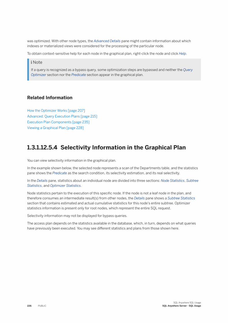
was optimized. With other node types, the Advanced Details pane might contain information about which indexes or materialized views were considered for the processing of the particular node.
To obtain context-sensitive help for each node in the graphical plan, right-click the node and click Help.
NoteIf a query is recognized as a bypass query, some optimization steps are bypassed and neither the Query Optimizer section nor the Predicate section appear in the graphical plan.
Related Information
How the Optimizer Works [page 207]Advanced: Query Execution Plans [page 215]Execution Plan Components [page 235]Viewing a Graphical Plan [page 228]
1.3.1.12.5.4 Selectivity Information in the Graphical Plan
You can view selectivity information in the graphical plan.
In the example shown below, the selected node represents a scan of the Departments table, and the statistics pane shows the Predicate as the search condition, its selectivity estimation, and its real selectivity.
In the Details pane, statistics about an individual node are divided into three sections: Node Statistics, Subtree Statistics, and Optimizer Statistics.
Node statistics pertain to the execution of this specific node. If the node is not a leaf node in the plan, and therefore consumes an intermediate result(s) from other nodes, the Details pane shows a Subtree Statistics section that contains estimated and actual cumulative statistics for this node's entire subtree. Optimizer statistics information is present only for root nodes, which represent the entire SQL request.
Selectivity information may not be displayed for bypass queries.
The access plan depends on the statistics available in the database, which, in turn, depends on what queries have previously been executed. You may see different statistics and plans from those shown here.
226 PUBLICSQL Anywhere SQL Usage
SQL Anywhere Server - SQL Usage
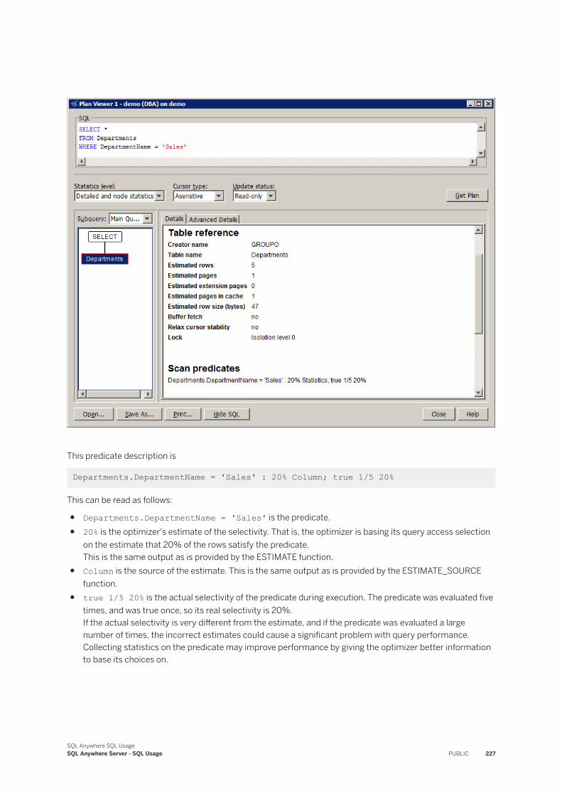
This predicate description is
Departments.DepartmentName = 'Sales' : 20% Column; true 1/5 20%
This can be read as follows:
● Departments.DepartmentName = 'Sales' is the predicate.● 20% is the optimizer's estimate of the selectivity. That is, the optimizer is basing its query access selection
on the estimate that 20% of the rows satisfy the predicate.This is the same output as is provided by the ESTIMATE function.
● Column is the source of the estimate. This is the same output as is provided by the ESTIMATE_SOURCE function.
● true 1/5 20% is the actual selectivity of the predicate during execution. The predicate was evaluated five times, and was true once, so its real selectivity is 20%.If the actual selectivity is very different from the estimate, and if the predicate was evaluated a large number of times, the incorrect estimates could cause a significant problem with query performance. Collecting statistics on the predicate may improve performance by giving the optimizer better information to base its choices on.
SQL Anywhere SQL UsageSQL Anywhere Server - SQL Usage PUBLIC 227

NoteIf you select the graphical plan, but not the graphical plan with statistics, the final two statistics are not displayed.
Related Information
Selectivity Estimate Sources [page 210]How the Optimizer Works [page 207]
1.3.1.12.5.5 Viewing a Graphical Plan
View a graphical plan in Interactive SQL.
Procedure
1. Start Interactive SQL and connect to the database.
2. Click Tools Plan Viewer (or press Shift+F5).3. Type a statement in the SQL pane.4. Select a Statistics level, a Cursor type, and an Update status.5. Click Get Plan.
Results
The graphical plan appears.
Related Information
Execution Plan Components [page 235]Advanced: Query Execution Plans [page 215]
228 PUBLICSQL Anywhere SQL Usage
SQL Anywhere Server - SQL Usage
1.3.1.12.6 Tutorial: Comparing Plans in Interactive SQL
You can compare query execution plans using the Compare Plans tool in Interactive SQL.
Prerequisites
No additional privileges are required to use the Compare Plans tool in Interactive SQL.
For this tutorial, you must have the SERVER OPERATOR system privilege because you execute the sa_flush_cache system procedure. You must also have SELECT privilege on the following tables and materialized view in the sample database because these are the objects you query when generating the plans:
● SalesOrders table● Employees table● SalesOrderItems table● Products table● MarketingInformation materialized view
Context
Many variables such as the state of tables, optimizer settings, and the contents of the database cache, can impact the execution of two otherwise identical SQL queries. Likewise, running a query on two database servers, or on two versions of the software, can result in noticeably different result times.
In these circumstances, you can save, compare, and analyze the execution plans to understand where differences occurred. The Compare Plans tool in Interactive SQL allows you to compare two saved execution plans to determine differences between them.
In this tutorial, you use the Plan Viewer and the Compare Plans tools to create two different execution plans for a query and compare them. During normal operations, you would not typically save two plans for the same query within minutes of each other. Normally, you'd have a plan for a query that you saved a while ago, and you now want to save a new plan so you can compare the plans and understand how they are different.
In this section:
Lesson 1: Creating Two Execution Plans and Saving Them to File [page 230]Use Interactive SQL to create two plans for the same query.
Lesson 2: Analyzing a Plan Comparison [page 231]Analyze the results of two plans that have been compared by the Compare Plan tool in Interactive SQL.
Lesson 3: Manually Match and Unmatch Operators and Queries [page 233]The Compare Plan tool attempts to find all matching operators and queries when comparing two plans.
SQL Anywhere SQL UsageSQL Anywhere Server - SQL Usage PUBLIC 229
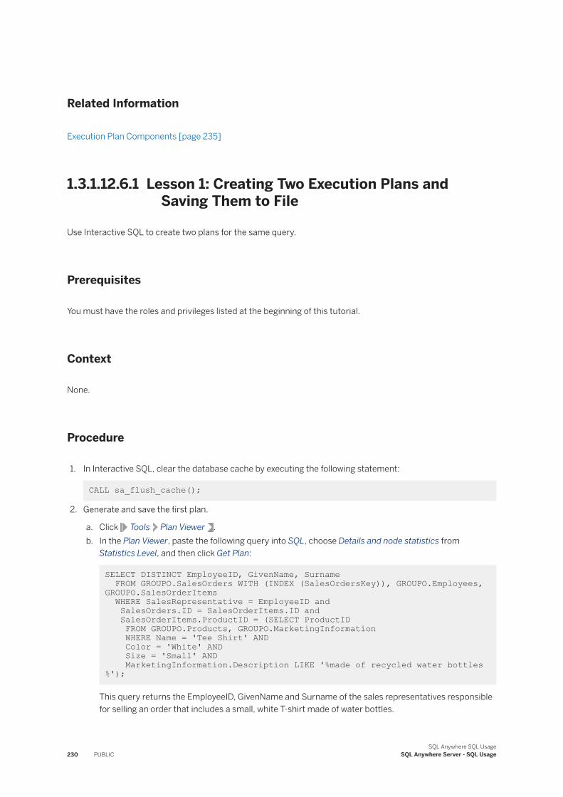
Related Information
Execution Plan Components [page 235]
1.3.1.12.6.1 Lesson 1: Creating Two Execution Plans and Saving Them to File
Use Interactive SQL to create two plans for the same query.
Prerequisites
You must have the roles and privileges listed at the beginning of this tutorial.
Context
None.
Procedure
1. In Interactive SQL, clear the database cache by executing the following statement:
CALL sa_flush_cache();
2. Generate and save the first plan.
a. Click Tools Plan Viewer .b. In the Plan Viewer, paste the following query into SQL, choose Details and node statistics from
Statistics Level, and then click Get Plan:
SELECT DISTINCT EmployeeID, GivenName, Surname FROM GROUPO.SalesOrders WITH (INDEX (SalesOrdersKey)), GROUPO.Employees, GROUPO.SalesOrderItems WHERE SalesRepresentative = EmployeeID and SalesOrders.ID = SalesOrderItems.ID and SalesOrderItems.ProductID = (SELECT ProductID FROM GROUPO.Products, GROUPO.MarketingInformation WHERE Name = 'Tee Shirt' AND Color = 'White' AND Size = 'Small' AND MarketingInformation.Description LIKE '%made of recycled water bottles%');
This query returns the EmployeeID, GivenName and Surname of the sales representatives responsible for selling an order that includes a small, white T-shirt made of water bottles.
230 PUBLICSQL Anywhere SQL Usage
SQL Anywhere Server - SQL Usage
c. Click Save As and save the plan in a file called FirstPlan.
3. Do not close the Plan Viewer.4. Generate and save the second plan.
a. In Interactive SQL, paste the same query into SQL Statements and execute it.b. Change to the Plan Viewer, and click Get Plan to get the plan again, and save it in a file called
SecondPlan.
Results
You created two plans for the same query, and saved them to separate files.
Next Steps
Proceed to the next lesson.
1.3.1.12.6.2 Lesson 2: Analyzing a Plan Comparison
Analyze the results of two plans that have been compared by the Compare Plan tool in Interactive SQL.
Prerequisites
You must have completed the previous lessons in this tutorial.
You must have the roles and privileges listed at the beginning of this tutorial.
Context
You do not have to be connected to a database server to compare two plans that are saved to file.
Procedure
1. Generate a comparison of the two plans you created in the previous lesson.
a. In Interactive SQL, click Tools Compare Plans to open the Compare Plans tool.b. For Plan 1:, browse to and select the file FirstPlan.saplan you created.
SQL Anywhere SQL UsageSQL Anywhere Server - SQL Usage PUBLIC 231
c. For Plan 2:, browse to and select the file SecondPlan.saplan you created.d. Click Compare Plans.
The Compare Plans tool attempts to match subqueries and operators between the two plans. These matches are listed in the Comparison Overview area.
The numbers to the left of items in Comparison Overview are match identifiers that identify operator or query matches found by the Compare Plans tool. If an item has no match identifier, then the item was not matched by the Compare Plans tool.
2. Use the numbered lists in Comparison Overview to analyze the differences in operators and subqueries between the two plans. Matching operators and queries are placed on the same line. However, the match identifier is the best indicator of what the Compare Plan tool considered a match. For example, the Compare Plan tool matched the SELECT operators in both plans, and gave the match the identifier 7.
An icon between the entries gives more details about each match:
○ The not equals sign (≠) indicates that the operator exists in both plans, but that the values in the Estimates column (found in the Details pane below the plan diagrams) were different. In almost all cases where an operator exists in both plans, the not equal sign will be displayed. This is because the likelihood of two query executions having identical estimates--measured to a precision ranging from tens to thousandths of a second, and sometimes beyond--is very small.
○ The equals sign (=) indicates that the operator exists in both plans, and that the values in the Estimates column are identical.
○ The greater than sign (>) indicates that the operator exists only in the first plan.○ The less than sign (<) indicates that the operator exists only in the second plan.○ The dash sign (-) indicates a matching sub-query node.
Selecting a row in the Comparison Overview pane, or in either graphical plan diagrams (1. FirstPlan and 2. SecondPlan) causes property values of those operators to display in the Details and Advanced Details tabs at the bottom.
3. Click the operators in the Comparison Overview pane, or in either graphical plan diagrams to analyze the differences between the two plans.
For example, in Comparison Overview, click the 3: NestedLoopsJoin listed under FirstPlan. This causes 3: HashJoin for SecondPlan to be selected, as these nodes are identified as a match.
4. Use the Details and Advanced Details tabs to analyze statistical differences found between the two plans.○ If a statistic is available in both plans and the values are the same, there is no special formatting.○ Yellow highlighting indicates that the statistic is only available in one plan. Missing statistics offer clues
to how the query was processed differently between the two plans.○ Dark red highlighting signals a major difference in statistics.○ Light red highlighting signals a minor difference in statistics.
In the two plans for this tutorial, almost all of the significant differences between the two plans are caused by the fact that the second time the query was executed, the database server was able to use the data in the cache and did not need to read data from the disk. This is why SecondPlan has statistics for memory use, while FirstPlan does not. Also, there are significantly different values for DiskReadTime and DiskRead for all of the matched nodes; values for these operators in SecondPlan are noticeably lower, because data was read from memory, not disk.
232 PUBLICSQL Anywhere SQL Usage
SQL Anywhere Server - SQL Usage
Results
You have compared two saved execution plans for a query using the Compare Plan tool in Interactive SQL, and have analyzed the results.
Next Steps
Proceed to the next lesson.
Related Information
Graphical Plans [page 221]Execution Plan Components [page 235]
1.3.1.12.6.3 Lesson 3: Manually Match and Unmatch Operators and Queries
The Compare Plan tool attempts to find all matching operators and queries when comparing two plans.
Prerequisites
You must have completed the previous lessons in this tutorial.
You must have the roles and privileges listed at the beginning of this tutorial.
Context
The Compare Plan tool determines a match not just by operator or subquery name, but also by looking at the results that operators produce, and how the results are used later in the plan. For example, in this tutorial, the NestedLoopJoin operator in FirstPlan is matched with the HashJoin operator in SecondPlan because they produce the same result, although using a different algorithm to do so.
Sometimes, the Compare Plan tool does not identify a match that it should. You can create the match manually to compare the statistics, and you can do this for operators or subqueries. You can also remove matches that the Compare Plan tool made.
SQL Anywhere SQL UsageSQL Anywhere Server - SQL Usage PUBLIC 233
Procedure
1. In the Comparison Overview pane, scroll to the bottom of the list of operators. The last two items item in the list for FirstPlan, HashFilter, are not matched with any operator in SecondPlan. Similarly, there are two HashFilter operators at the bottom of the list for SecondPlan that do not match up with operators in FirstPlan.
2. Click the first HashFilter operator for FirstPlan to find the value of Hash list in the Details pane: the value is Employees.EmployeeID integer.
3. Click the first HashFilter operator for SecondPlan to find the value of Hash list in the Details pane: the value is Employees.EmployeeID integer.
This means that the HashFilter operator in FirstPlan can be matched with the first instance of the HashFilter operator in the SecondPlan.
4. Match the operators as follows:a. In the graphical plan for FirstPlan, click to select the HF node. This is the HashFilter operator for
FirstPlan.b. In the graphical plan for SecondPlan, click to select the HF node that is a child node to the JH (join
hash) node. This is the HashFilter operator that can be matched to the HashFilter operator in FirstPlan.
c. Click Match Operators.
The Compare Plan tool creates the manual match and assigns a match identifier (for example, SubQ 1). The Comparison Overview pane is updated to reflect the new match, aligning the operators on the same line.
d. Repeat the same steps to match the remaining HashFilter operators at the bottom of FirstPlan and SecondPlan in the Comparison Overview pane.
5. To remove a match, select an operator involved in a match and click Unmatch Operators. You can remove the match from manually matched operators, as well as operators that the Compare Plan tool matched.
6. Create or remove a manual match of subqueries by following the same steps as for operators, except using the Match Queries and Unmatch Queries buttons instead.
Results
You have learned how to match and unmatch operators and subqueries in the Compare Plan tool.
Related Information
Graphical Plans [page 221]Execution Plan Components [page 235]
234 PUBLICSQL Anywhere SQL Usage
SQL Anywhere Server - SQL Usage
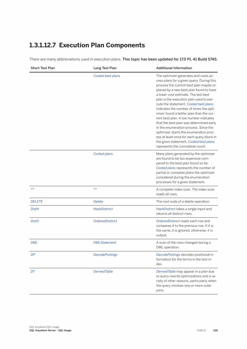
1.3.1.12.7 Execution Plan Components
There are many abbreviations used in execution plans. This topic has been updated for 17.0 PL 41 Build 5745.
Short Text Plan Long Text Plan Additional Information
Costed best plans The optimizer generates and costs access plans for a given query. During this process the current best plan maybe replaced by a new best plan found to have a lower cost estimate. The last best plan is the execution plan used to execute the statement. Costed best plans indicates the number of times the optimizer found a better plan than the current best plan. A low number indicates that the best plan was determined early in the enumeration process. Since the optimizer starts the enumeration process at least once for each query block in the given statement, Costed best plans represents the cumulative count.
Costed plans Many plans generated by the optimizer are found to be too expensive compared to the best plan found so far. Costed plans represents the number of partial or complete plans the optimizer considered during the enumeration processes for a given statement.
** ** A complete index scan. The index scan reads all rows.
DELETE Delete The root node of a delete operation.
DistH HashDistinct HashDistinct takes a single input and returns all distinct rows.
DistO OrderedDistinct OrderedDistinct reads each row and compares it to the previous row. If it is the same, it is ignored; otherwise, it is output.
DML DMLStatement A scan of the rows changed during a DML operation.
DP DecodePostings DecodePostings decodes positional information for the terms in the text index.
DT DerivedTable DerivedTable may appear in a plan due to query rewrite optimizations and a variety of other reasons, particularly when the query involves one or more outer joins.
SQL Anywhere SQL UsageSQL Anywhere Server - SQL Usage PUBLIC 235
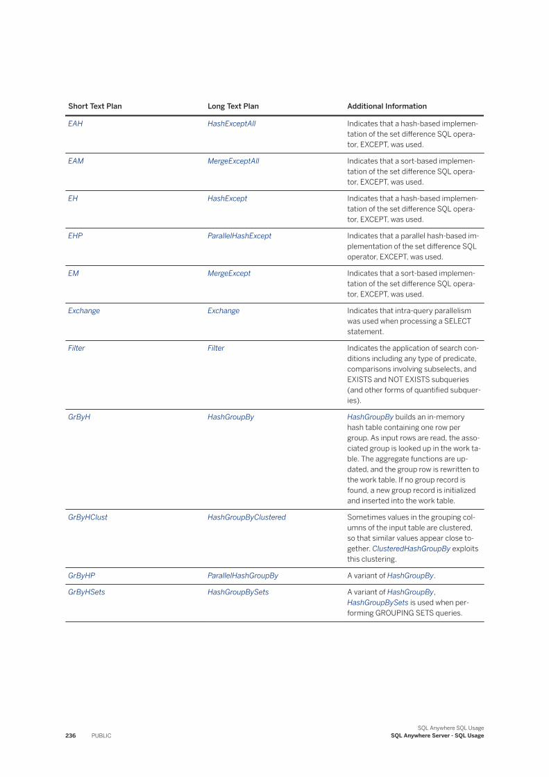
Short Text Plan Long Text Plan Additional Information
EAH HashExceptAll Indicates that a hash-based implementation of the set difference SQL operator, EXCEPT, was used.
EAM MergeExceptAll Indicates that a sort-based implementation of the set difference SQL operator, EXCEPT, was used.
EH HashExcept Indicates that a hash-based implementation of the set difference SQL operator, EXCEPT, was used.
EHP ParallelHashExcept Indicates that a parallel hash-based implementation of the set difference SQL operator, EXCEPT, was used.
EM MergeExcept Indicates that a sort-based implementation of the set difference SQL operator, EXCEPT, was used.
Exchange Exchange Indicates that intra-query parallelism was used when processing a SELECT statement.
Filter Filter Indicates the application of search conditions including any type of predicate, comparisons involving subselects, and EXISTS and NOT EXISTS subqueries (and other forms of quantified subqueries).
GrByH HashGroupBy HashGroupBy builds an in-memory hash table containing one row per group. As input rows are read, the associated group is looked up in the work table. The aggregate functions are updated, and the group row is rewritten to the work table. If no group record is found, a new group record is initialized and inserted into the work table.
GrByHClust HashGroupByClustered Sometimes values in the grouping columns of the input table are clustered, so that similar values appear close together. ClusteredHashGroupBy exploits this clustering.
GrByHP ParallelHashGroupBy A variant of HashGroupBy.
GrByHSets HashGroupBySets A variant of HashGroupBy, HashGroupBySets is used when performing GROUPING SETS queries.
236 PUBLICSQL Anywhere SQL Usage
SQL Anywhere Server - SQL Usage
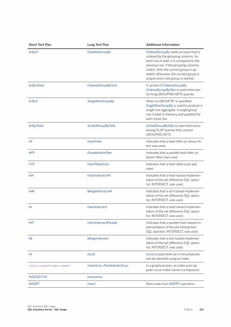
Short Text Plan Long Text Plan Additional Information
GrByO OrderedGroupBy OrderedGroupBy reads an input that is ordered by the grouping columns. As each row is read, it is compared to the previous row. If the grouping columns match, then the current group is updated; otherwise, the current group is output and a new group is started.
GrByOSets OrderedGroupBySets A variant of OrderedGroupBy, OrderedGroupBySets is used when performing GROUPING SETS queries.
GrByS SingleRowGroupBy When no GROUP BY is specified, SingleRowGroupBy is used to produce a single row aggregate. A single group row is kept in memory and updated for each input row.
GrBySSets SortedGroupBySets SortedGroupBySets is used when processing OLAP queries that contain GROUPING SETS.
HF HashFilter Indicates that a hash filter (or bloom fil-ter) was used.
HFP ParallelHashFilter Indicates that a parallel hash filter (or bloom filter) was used.
HTS HashTableScan Indicates that a hash table scan was used.
IAH HashIntersectAll Indicates that a hash-based implementation of the set difference SQL operator, INTERSECT, was used.
IAM MergeIntersectAll Indicates that a sort-based implementation of the set difference SQL operator, INTERSECT, was used.
IH HashIntersect Indicates that a hash-based implementation of the set difference SQL operator, INTERSECT, was used.
IHP HashIntersectParallel Indicates that a parallel hash-based implementation of the set intersection SQL operator, INTERSECT, was used.
IM MergeIntersect Indicates that a sort-based implementation of the set difference SQL operator, INTERSECT, was used.
IN InList InList is used when an in-list predicate can be satisfied using an index.
table-name<index-name> IndexScan, ParallelIndexScan In a graphical plan, an index scan appears as an index name in a trapezoid.
INSENSITIVE Insensitive
INSERT Insert Root node of an INSERT operation.
SQL Anywhere SQL UsageSQL Anywhere Server - SQL Usage PUBLIC 237
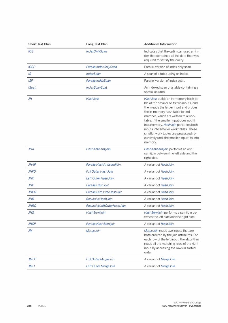
Short Text Plan Long Text Plan Additional Information
IOS IndexOnlyScan Indicates that the optimizer used an index that contained all the data that was required to satisfy the query.
IOSP ParallelIndexOnlyScan Parallel version of index only scan.
IS IndexScan A scan of a table using an index.
ISP ParallelIndexScan Parallel version of index scan.
ISpat IndexScanSpat An indexed scan of a table containing a spatial column.
JH HashJoin HashJoin builds an in-memory hash table of the smaller of its two inputs, and then reads the larger input and probes the in-memory hash table to find matches, which are written to a work table. If the smaller input does not fit into memory, HashJoin partitions both inputs into smaller work tables. These smaller work tables are processed recursively until the smaller input fits into memory.
JHA HashAntisemijoin HashAntisemijoin performs an anti-semijoin between the left side and the right side.
JHAP ParallelHashAntisemijoin A variant of HashJoin.
JHFO Full Outer HashJoin A variant of HashJoin.
JHO Left Outer HashJoin A variant of HashJoin.
JHP ParallelHashJoin A variant of HashJoin.
JHPO ParallelLeftOuterHashJoin A variant of HashJoin.
JHR RecursiveHashJoin A variant of HashJoin.
JHRO RecursiveLeftOuterHashJoin A variant of HashJoin.
JHS HashSemijoin HashSemijoin performs a semijoin between the left side and the right side.
JHSP ParallelHashSemijoin A variant of HashJoin.
JM MergeJoin MergeJoin reads two inputs that are both ordered by the join attributes. For each row of the left input, the algorithm reads all the matching rows of the right input by accessing the rows in sorted order.
JMFO Full Outer MergeJoin A variant of MergeJoin.
JMO Left Outer MergeJoin A variant of MergeJoin.
238 PUBLICSQL Anywhere SQL Usage
SQL Anywhere Server - SQL Usage
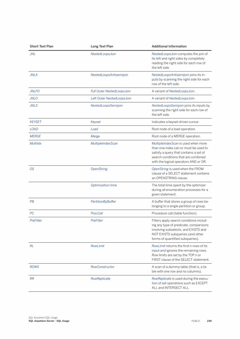
Short Text Plan Long Text Plan Additional Information
JNL NestedLoopsJoin NestedLoopsJoin computes the join of its left and right sides by completely reading the right side for each row of the left side.
JNLA NestedLoopsAntisemijoin NestedLoopsAntisemijoin joins its inputs by scanning the right side for each row of the left side.
JNLFO Full Outer NestedLoopsJoin A variant of NestedLoopsJoin.
JNLO Left Outer NestedLoopsJoin A variant of NestedLoopsJoin.
JNLS NestedLoopsSemijoin NestedLoopsSemijoin joins its inputs by scanning the right side for each row of the left side.
KEYSET Keyset Indicates a keyset-driven cursor.
LOAD Load Root node of a load operation.
MERGE Merge Root node of a MERGE operation.
MultiIdx MultipleIndexScan MultipleIndexScan is used when more than one index can or must be used to satisfy a query that contains a set of search conditions that are combined with the logical operators AND or OR.
OS OpenString OpenString is used when the FROM clause of a SELECT statement contains an OPENSTRING clause.
Optimization time The total time spent by the optimizer during all enumeration processes for a given statement.
PB PartitionByBuffer A buffer that stores a group of rows belonging to a single partition or group.
PC ProcCall Procedure call (table function).
PreFilter PreFilter Filters apply search conditions including any type of predicate, comparisons involving subselects, and EXISTS and NOT EXISTS subqueries (and other forms of quantified subqueries).
RL RowLimit RowLimit returns the first n rows of its input and ignores the remaining rows. Row limits are set by the TOP n or FIRST clause of the SELECT statement.
ROWS RowConstructor A scan of a dummy table (that is, a table with one row and no columns).
RR RowReplicate RowReplicate is used during the execution of set operations such as EXCEPT ALL and INTERSECT ALL.
SQL Anywhere SQL UsageSQL Anywhere Server - SQL Usage PUBLIC 239
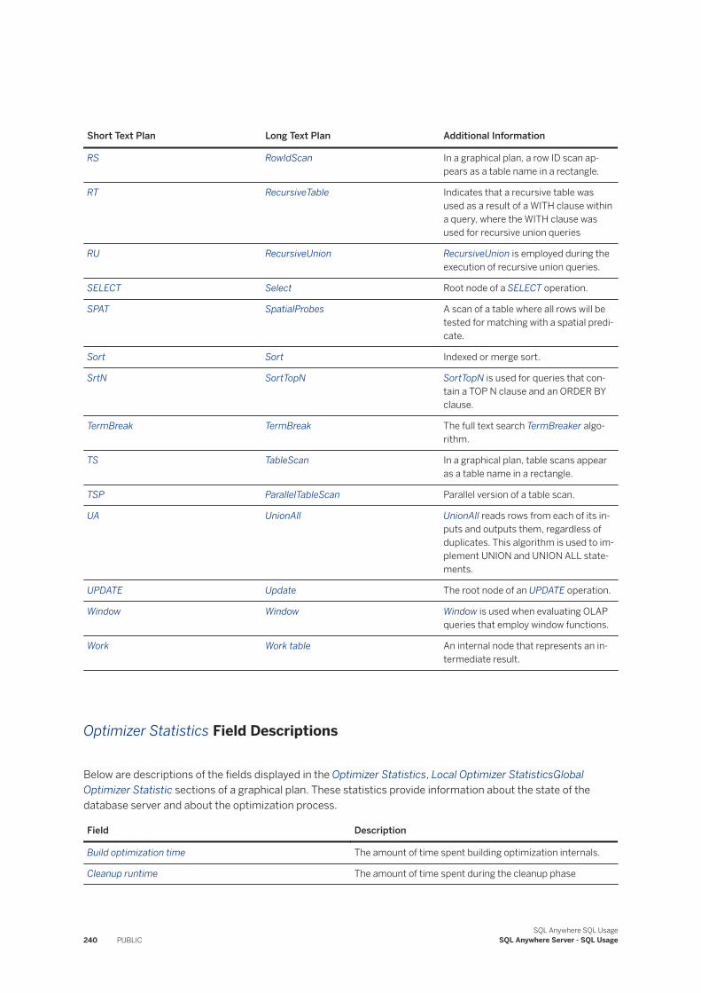
Short Text Plan Long Text Plan Additional Information
RS RowIdScan In a graphical plan, a row ID scan appears as a table name in a rectangle.
RT RecursiveTable Indicates that a recursive table was used as a result of a WITH clause within a query, where the WITH clause was used for recursive union queries
RU RecursiveUnion RecursiveUnion is employed during the execution of recursive union queries.
SELECT Select Root node of a SELECT operation.
SPAT SpatialProbes A scan of a table where all rows will be tested for matching with a spatial predicate.
Sort Sort Indexed or merge sort.
SrtN SortTopN SortTopN is used for queries that contain a TOP N clause and an ORDER BY clause.
TermBreak TermBreak The full text search TermBreaker algorithm.
TS TableScan In a graphical plan, table scans appear as a table name in a rectangle.
TSP ParallelTableScan Parallel version of a table scan.
UA UnionAll UnionAll reads rows from each of its inputs and outputs them, regardless of duplicates. This algorithm is used to implement UNION and UNION ALL statements.
UPDATE Update The root node of an UPDATE operation.
Window Window Window is used when evaluating OLAP queries that employ window functions.
Work Work table An internal node that represents an intermediate result.
Optimizer Statistics Field Descriptions
Below are descriptions of the fields displayed in the Optimizer Statistics, Local Optimizer StatisticsGlobal Optimizer Statistic sections of a graphical plan. These statistics provide information about the state of the database server and about the optimization process.
Field Description
Build optimization time The amount of time spent building optimization internals.
Cleanup runtime The amount of time spent during the cleanup phase
240 PUBLICSQL Anywhere SQL Usage
SQL Anywhere Server - SQL Usage
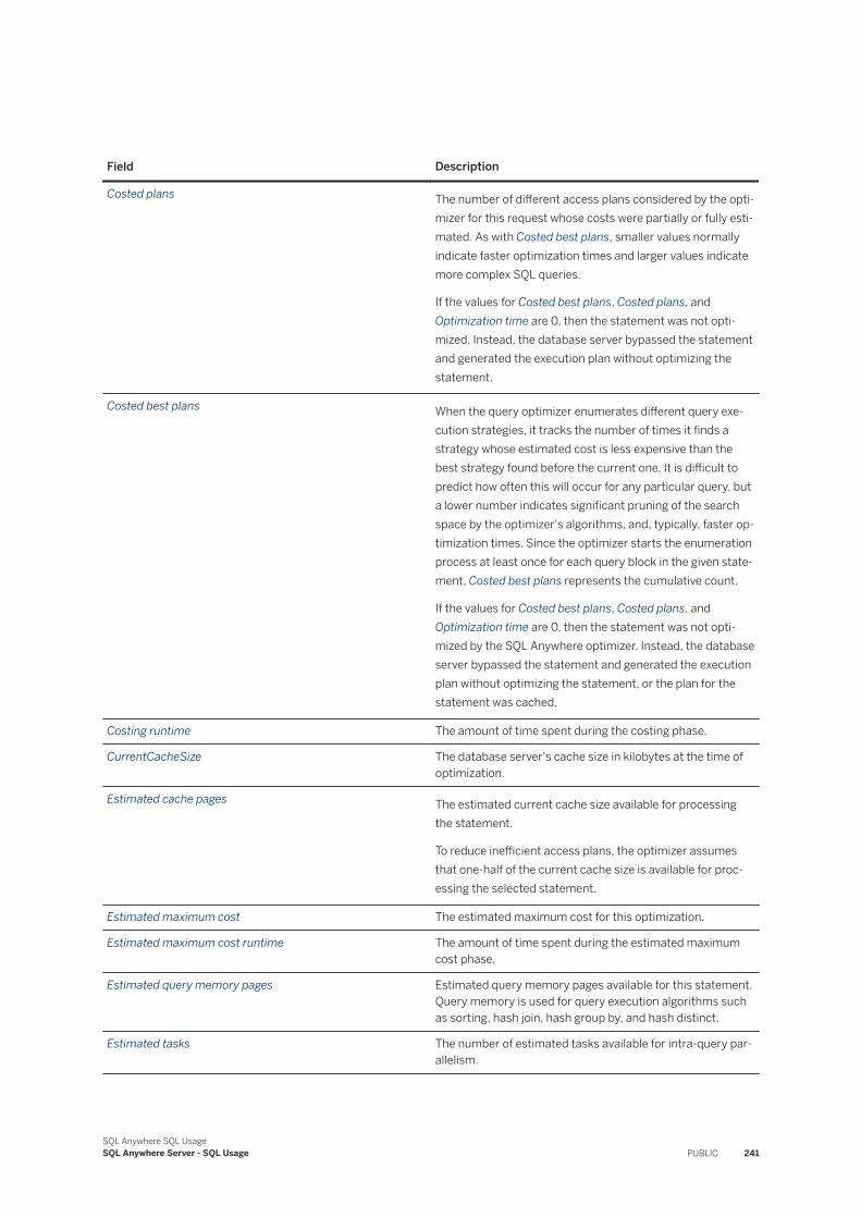
Field Description
Costed plans The number of different access plans considered by the optimizer for this request whose costs were partially or fully estimated. As with Costed best plans, smaller values normally indicate faster optimization times and larger values indicate more complex SQL queries.
If the values for Costed best plans, Costed plans, and Optimization time are 0, then the statement was not optimized. Instead, the database server bypassed the statement and generated the execution plan without optimizing the statement.
Costed best plans When the query optimizer enumerates different query execution strategies, it tracks the number of times it finds a strategy whose estimated cost is less expensive than the best strategy found before the current one. It is difficult to predict how often this will occur for any particular query, but a lower number indicates significant pruning of the search space by the optimizer's algorithms, and, typically, faster optimization times. Since the optimizer starts the enumeration process at least once for each query block in the given statement, Costed best plans represents the cumulative count.
If the values for Costed best plans, Costed plans, and Optimization time are 0, then the statement was not optimized by the SQL Anywhere optimizer. Instead, the database server bypassed the statement and generated the execution plan without optimizing the statement, or the plan for the statement was cached.
Costing runtime The amount of time spent during the costing phase.
CurrentCacheSize The database server's cache size in kilobytes at the time of optimization.
Estimated cache pages The estimated current cache size available for processing the statement.
To reduce inefficient access plans, the optimizer assumes that one-half of the current cache size is available for processing the selected statement.
Estimated maximum cost The estimated maximum cost for this optimization.
Estimated maximum cost runtime The amount of time spent during the estimated maximum cost phase.
Estimated query memory pages Estimated query memory pages available for this statement. Query memory is used for query execution algorithms such as sorting, hash join, hash group by, and hash distinct.
Estimated tasks The number of estimated tasks available for intra-query parallelism.
SQL Anywhere SQL UsageSQL Anywhere Server - SQL Usage PUBLIC 241
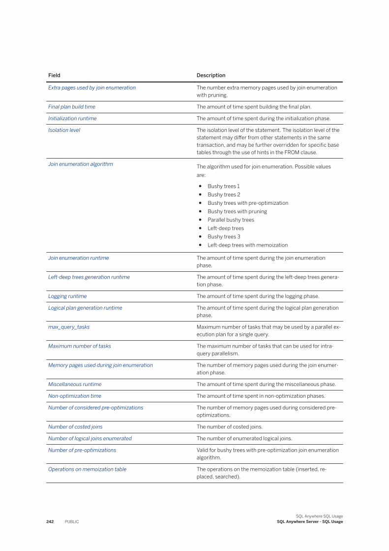
Field Description
Extra pages used by join enumeration The number extra memory pages used by join enumeration with pruning.
Final plan build time The amount of time spent building the final plan.
Initialization runtime The amount of time spent during the initialization phase.
Isolation level The isolation level of the statement. The isolation level of the statement may differ from other statements in the same transaction, and may be further overridden for specific base tables through the use of hints in the FROM clause.
Join enumeration algorithm The algorithm used for join enumeration. Possible values are:
● Bushy trees 1● Bushy trees 2● Bushy trees with pre-optimization● Bushy trees with pruning● Parallel bushy trees● Left-deep trees● Bushy trees 3● Left-deep trees with memoization
Join enumeration runtime The amount of time spent during the join enumeration phase.
Left-deep trees generation runtime The amount of time spent during the left-deep trees generation phase.
Logging runtime The amount of time spent during the logging phase.
Logical plan generation runtime The amount of time spent during the logical plan generation phase.
max_query_tasks Maximum number of tasks that may be used by a parallel execution plan for a single query.
Maximum number of tasks The maximum number of tasks that can be used for intra-query parallelism.
Memory pages used during join enumeration The number of memory pages used during the join enumeration phase.
Miscellaneous runtime The amount of time spent during the miscellaneous phase.
Non-optimization time The amount of time spent in non-optimization phases.
Number of considered pre-optimizations The number of memory pages used during considered pre-optimizations.
Number of costed joins The number of costed joins.
Number of logical joins enumerated The number of enumerated logical joins.
Number of pre-optimizations Valid for bushy trees with pre-optimization join enumeration algorithm.
Operations on memoization table The operations on the memoization table (inserted, replaced, searched).
242 PUBLICSQL Anywhere SQL Usage
SQL Anywhere Server - SQL Usage
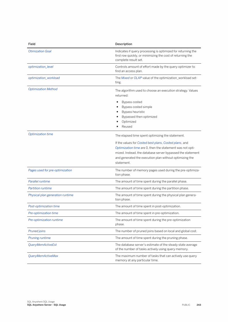
Field Description
Otimization Goal Indicates if query processing is optimized for returning the first row quickly, or minimizing the cost of returning the complete result set.
optimization_level Controls amount of effort made by the query optimizer to find an access plan.
optimization_workload The Mixed or OLAP value of the optimization_workload setting.
Optimization Method The algorithm used to choose an execution strategy. Values returned:
● Bypass costed● Bypass costed simple● Bypass heuristic● Bypassed then optimized● Optimized● Reused
Optimization time The elapsed time spent optimizing the statement.
If the values for Costed best plans, Costed plans, and Optimization time are 0, then the statement was not optimized. Instead, the database server bypassed the statement and generated the execution plan without optimizing the statement.
Pages used for pre-optimization The number of memory pages used during the pre-optimization phase.
Parallel runtime The amount of time spent during the parallel phase.
Partition runtime The amount of time spent during the partition phase.
Physical plan generation runtime The amount of time spent during the physical plan generation phase.
Post-optimization time The amount of time spent in post-optimization.
Pre-optimization time The amount of time spent in pre-optimization.
Pre-optimization runtime The amount of time spent during the pre-optimization phase.
Pruned joins The number of pruned joins based on local and global cost.
Pruning runtime The amount of time spent during the pruning phase.
QueryMemActiveEst The database server's estimate of the steady state average of the number of tasks actively using query memory.
QueryMemActiveMax The maximum number of tasks that can actively use query memory at any particular time.
SQL Anywhere SQL UsageSQL Anywhere Server - SQL Usage PUBLIC 243
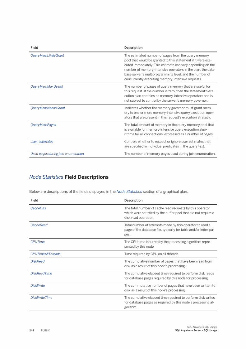
Field Description
QueryMemLikelyGrant The estimated number of pages from the query memory pool that would be granted to this statement if it were executed immediately. This estimate can vary depending on the number of memory-intensive operators in the plan, the database server's multiprogramming level, and the number of concurrently executing memory-intensive requests.
QueryMemMaxUseful The number of pages of query memory that are useful for this request. If the number is zero, then the statement's execution plan contains no memory-intensive operators and is not subject to control by the server's memory governor.
QueryMemNeedsGrant Indicates whether the memory governor must grant memory to one or more memory-intensive query execution operators that are present in this request's execution strategy.
QueryMemPages The total amount of memory in the query memory pool that is available for memory-intensive query execution algorithms for all connections, expressed as a number of pages.
user_estimates Controls whether to respect or ignore user estimates that are specified in individual predicates in the query text.
Used pages during join enumeration The number of memory pages used during join enumeration.
Node Statistics Field Descriptions
Below are descriptions of the fields displayed in the Node Statistics section of a graphical plan.
Field Description
CacheHits The total number of cache read requests by this operator which were satisfied by the buffer pool that did not require a disk read operation.
CacheRead Total number of attempts made by this operator to read a page of the database file, typically for table and/or index pages.
CPUTime The CPU time incurred by the processing algorithm represented by this node.
CPUTimeAllThreads Time required by CPU on all threads.
DiskRead The cumulative number of pages that have been read from disk as a result of this node's processing.
DiskReadTime The cumulative elapsed time required to perform disk reads for database pages required by this node for processing.
DiskWrite The commutative number of pages that have been written to disk as a result of this node's processing.
DiskWriteTime The cumulative elapsed time required to perform disk writes for database pages as required by this node's processing algorithm.
244 PUBLICSQL Anywhere SQL Usage
SQL Anywhere Server - SQL Usage
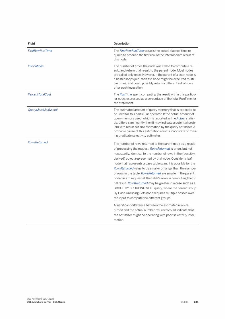
Field Description
FirstRowRunTime The FirstRowRunTime value is the actual elapsed time required to produce the first row of the intermediate result of this node.
Invocations The number of times the node was called to compute a result, and return that result to the parent node. Most nodes are called only once. However, if the parent of a scan node is a nested loops join, then the node might be executed multiple times, and could possibly return a different set of rows after each invocation.
PercentTotalCost The RunTime spent computing the result within this particular node, expressed as a percentage of the total RunTime for the statement.
QueryMemMaxUseful The estimated amount of query memory that is expected to be used for this particular operator. If the actual amount of query memory used, which is reported as the Actual statistic, differs significantly then it may indicate a potential problem with result set size estimation by the query optimizer. A probable cause of this estimation error is inaccurate or missing predicate selectivity estimates.
RowsReturned The number of rows returned to the parent node as a result of processing the request. RowsReturned is often, but not necessarily, identical to the number of rows in the (possibly derived) object represented by that node. Consider a leaf node that represents a base table scan. It is possible for the RowsReturned value to be smaller or larger than the number of rows in the table. RowsReturned are smaller if the parent node fails to request all the table's rows in computing the fi-nal result. RowsReturned may be greater in a case such as a GROUP BY GROUPING SETS query, where the parent Group By Hash Grouping Sets node requires multiple passes over the input to compute the different groups.
A significant difference between the estimated rows returned and the actual number returned could indicate that the optimizer might be operating with poor selectivity information.
SQL Anywhere SQL UsageSQL Anywhere Server - SQL Usage PUBLIC 245
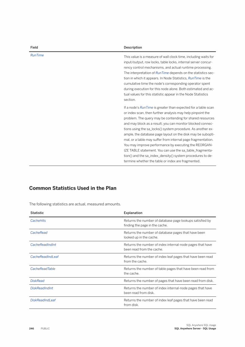
Field Description
RunTime This value is a measure of wall clock time, including waits for input/output, row locks, table locks, internal server concurrency control mechanisms, and actual runtime processing. The interpretation of RunTime depends on the statistics section in which it appears. In Node Statistics, RunTime is the cumulative time the node's corresponding operator spent during execution for this node alone. Both estimated and actual values for this statistic appear in the Node Statistics section.
If a node's RunTime is greater than expected for a table scan or index scan, then further analysis may help pinpoint the problem. The query may be contending for shared resources and may block as a result; you can monitor blocked connections using the sa_locks() system procedure. As another example, the database page layout on the disk may be suboptimal, or a table may suffer from internal page fragmentation. You may improve performance by executing the REORGANIZE TABLE statement. You can use the sa_table_fragmentation() and the sa_index_density() system procedures to determine whether the table or index are fragmented.
Common Statistics Used in the Plan
The following statistics are actual, measured amounts.
Statistic Explanation
CacheHits Returns the number of database page lookups satisfied by finding the page in the cache.
CacheRead Returns the number of database pages that have been looked up in the cache.
CacheReadIndInt Returns the number of index internal-node pages that have been read from the cache.
CacheReadIndLeaf Returns the number of index leaf pages that have been read from the cache.
CacheReadTable Returns the number of table pages that have been read from the cache.
DiskRead Returns the number of pages that have been read from disk.
DiskReadIndInt Returns the number of index internal-node pages that have been read from disk.
DiskReadIndLeaf Returns the number of index leaf pages that have been read from disk.
246 PUBLICSQL Anywhere SQL Usage
SQL Anywhere Server - SQL Usage
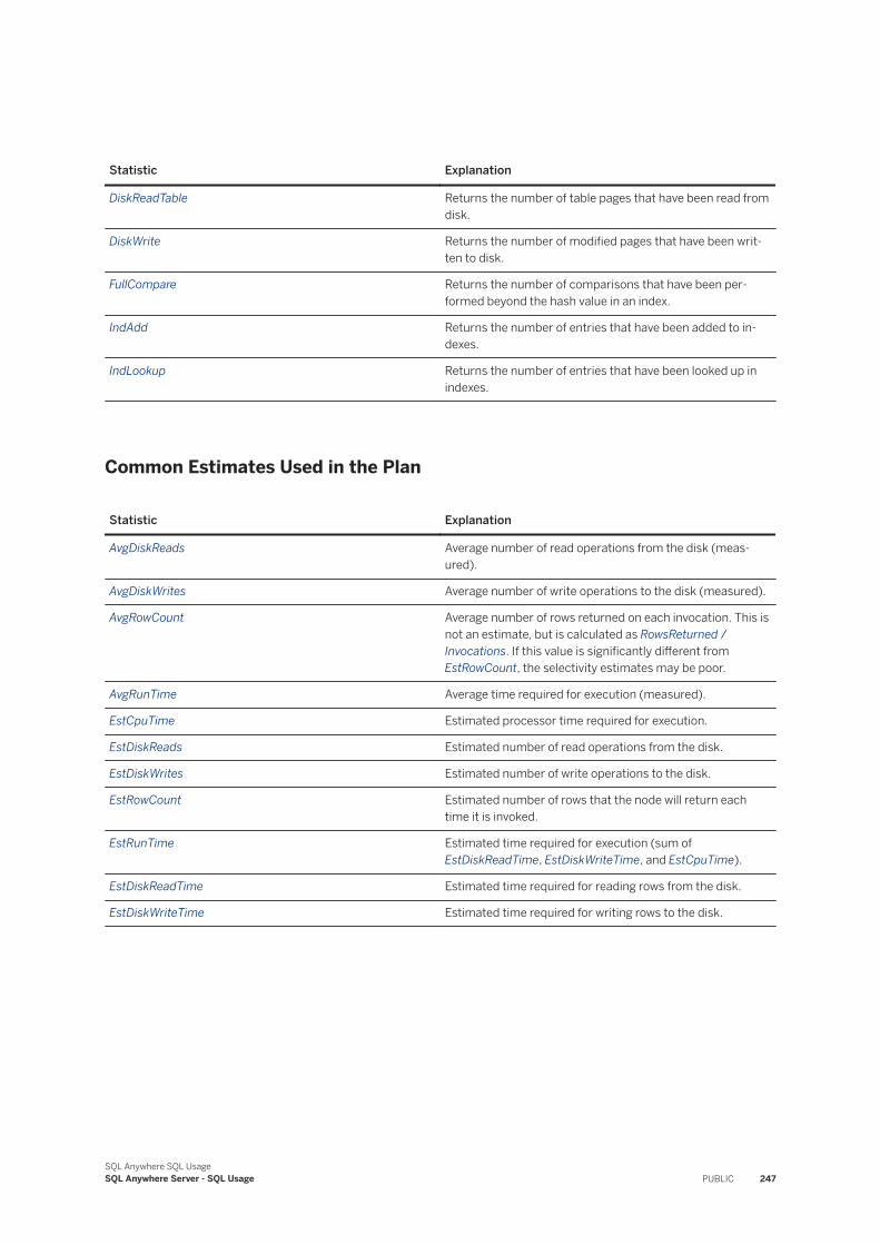
Statistic Explanation
DiskReadTable Returns the number of table pages that have been read from disk.
DiskWrite Returns the number of modified pages that have been written to disk.
FullCompare Returns the number of comparisons that have been performed beyond the hash value in an index.
IndAdd Returns the number of entries that have been added to indexes.
IndLookup Returns the number of entries that have been looked up in indexes.
Common Estimates Used in the Plan
Statistic Explanation
AvgDiskReads Average number of read operations from the disk (measured).
AvgDiskWrites Average number of write operations to the disk (measured).
AvgRowCount Average number of rows returned on each invocation. This is not an estimate, but is calculated as RowsReturned / Invocations. If this value is significantly different from EstRowCount, the selectivity estimates may be poor.
AvgRunTime Average time required for execution (measured).
EstCpuTime Estimated processor time required for execution.
EstDiskReads Estimated number of read operations from the disk.
EstDiskWrites Estimated number of write operations to the disk.
EstRowCount Estimated number of rows that the node will return each time it is invoked.
EstRunTime Estimated time required for execution (sum of EstDiskReadTime, EstDiskWriteTime, and EstCpuTime).
EstDiskReadTime Estimated time required for reading rows from the disk.
EstDiskWriteTime Estimated time required for writing rows to the disk.
SQL Anywhere SQL UsageSQL Anywhere Server - SQL Usage PUBLIC 247
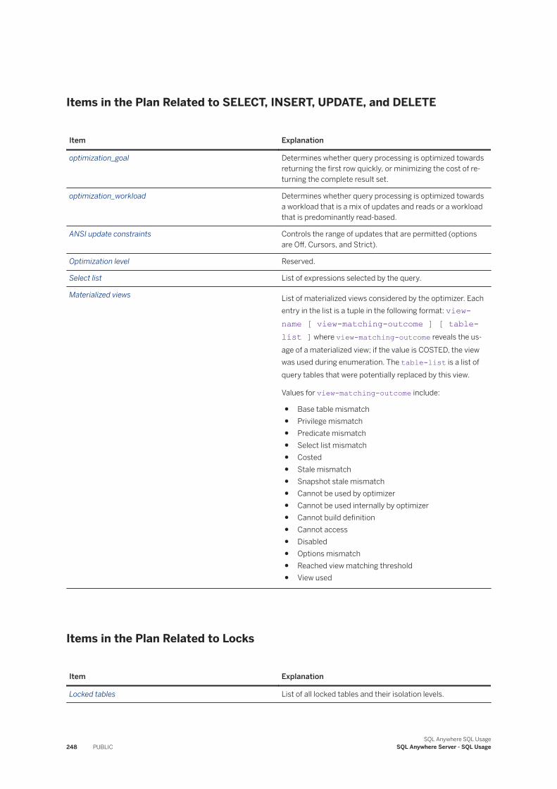
Items in the Plan Related to SELECT, INSERT, UPDATE, and DELETE
Item Explanation
optimization_goal Determines whether query processing is optimized towards returning the first row quickly, or minimizing the cost of returning the complete result set.
optimization_workload Determines whether query processing is optimized towards a workload that is a mix of updates and reads or a workload that is predominantly read-based.
ANSI update constraints Controls the range of updates that are permitted (options are Off, Cursors, and Strict).
Optimization level Reserved.
Select list List of expressions selected by the query.
Materialized views List of materialized views considered by the optimizer. Each entry in the list is a tuple in the following format: view-name [ view-matching-outcome ] [ table-list ] where view-matching-outcome reveals the usage of a materialized view; if the value is COSTED, the view was used during enumeration. The table-list is a list of query tables that were potentially replaced by this view.
Values for view-matching-outcome include:
● Base table mismatch● Privilege mismatch● Predicate mismatch● Select list mismatch● Costed● Stale mismatch● Snapshot stale mismatch● Cannot be used by optimizer● Cannot be used internally by optimizer● Cannot build definition● Cannot access● Disabled● Options mismatch● Reached view matching threshold● View used
Items in the Plan Related to Locks
Item Explanation
Locked tables List of all locked tables and their isolation levels.
248 PUBLICSQL Anywhere SQL Usage
SQL Anywhere Server - SQL Usage
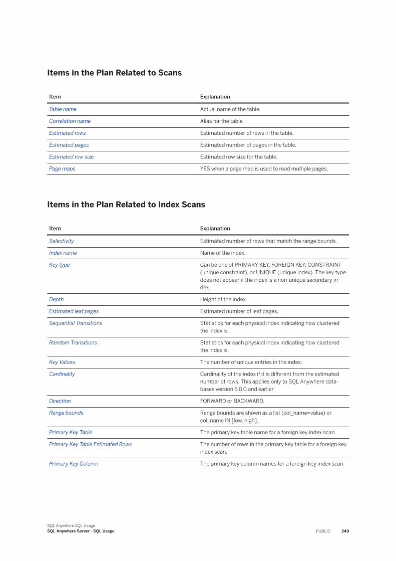
Items in the Plan Related to Scans
Item Explanation
Table name Actual name of the table.
Correlation name Alias for the table.
Estimated rows Estimated number of rows in the table.
Estimated pages Estimated number of pages in the table.
Estimated row size Estimated row size for the table.
Page maps YES when a page map is used to read multiple pages.
Items in the Plan Related to Index Scans
Item Explanation
Selectivity Estimated number of rows that match the range bounds.
Index name Name of the index.
Key type Can be one of PRIMARY KEY, FOREIGN KEY, CONSTRAINT (unique constraint), or UNIQUE (unique index). The key type does not appear if the index is a non-unique secondary index.
Depth Height of the index.
Estimated leaf pages Estimated number of leaf pages.
Sequential Transitions Statistics for each physical index indicating how clustered the index is.
Random Transitions Statistics for each physical index indicating how clustered the index is.
Key Values The number of unique entries in the index.
Cardinality Cardinality of the index if it is different from the estimated number of rows. This applies only to SQL Anywhere databases version 6.0.0 and earlier.
Direction FORWARD or BACKWARD.
Range bounds Range bounds are shown as a list (col_name=value) or col_name IN [low, high].
Primary Key Table The primary key table name for a foreign key index scan.
Primary Key Table Estimated Rows The number of rows in the primary key table for a foreign key index scan.
Primary Key Column The primary key column names for a foreign key index scan.
SQL Anywhere SQL UsageSQL Anywhere Server - SQL Usage PUBLIC 249
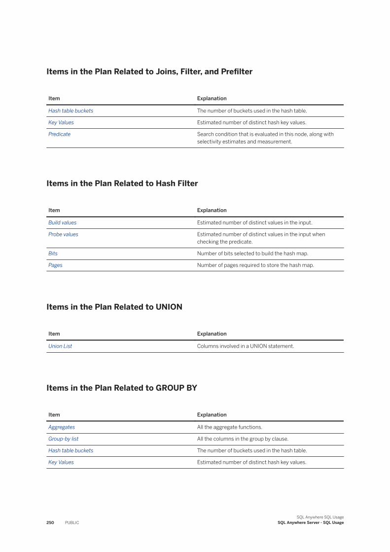
Items in the Plan Related to Joins, Filter, and Prefilter
Item Explanation
Hash table buckets The number of buckets used in the hash table.
Key Values Estimated number of distinct hash key values.
Predicate Search condition that is evaluated in this node, along with selectivity estimates and measurement.
Items in the Plan Related to Hash Filter
Item Explanation
Build values Estimated number of distinct values in the input.
Probe values Estimated number of distinct values in the input when checking the predicate.
Bits Number of bits selected to build the hash map.
Pages Number of pages required to store the hash map.
Items in the Plan Related to UNION
Item Explanation
Union List Columns involved in a UNION statement.
Items in the Plan Related to GROUP BY
Item Explanation
Aggregates All the aggregate functions.
Group-by list All the columns in the group by clause.
Hash table buckets The number of buckets used in the hash table.
Key Values Estimated number of distinct hash key values.
250 PUBLICSQL Anywhere SQL Usage
SQL Anywhere Server - SQL Usage
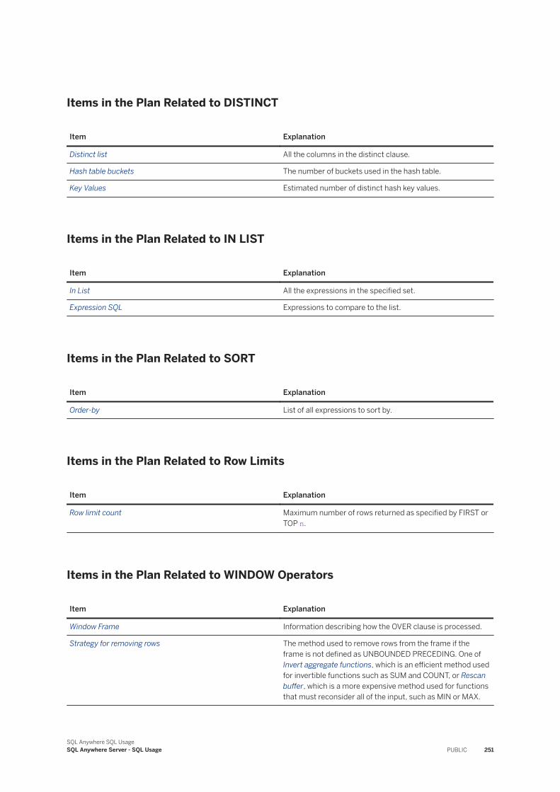
Items in the Plan Related to DISTINCT
Item Explanation
Distinct list All the columns in the distinct clause.
Hash table buckets The number of buckets used in the hash table.
Key Values Estimated number of distinct hash key values.
Items in the Plan Related to IN LIST
Item Explanation
In List All the expressions in the specified set.
Expression SQL Expressions to compare to the list.
Items in the Plan Related to SORT
Item Explanation
Order-by List of all expressions to sort by.
Items in the Plan Related to Row Limits
Item Explanation
Row limit count Maximum number of rows returned as specified by FIRST or TOP n.
Items in the Plan Related to WINDOW Operators
Item Explanation
Window Frame Information describing how the OVER clause is processed.
Strategy for removing rows The method used to remove rows from the frame if the frame is not defined as UNBOUNDED PRECEDING. One of Invert aggregate functions, which is an efficient method used for invertible functions such as SUM and COUNT, or Rescan buffer, which is a more expensive method used for functions that must reconsider all of the input, such as MIN or MAX.
SQL Anywhere SQL UsageSQL Anywhere Server - SQL Usage PUBLIC 251
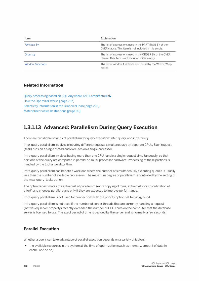
Item Explanation
Partition By The list of expressions used in the PARTITION BY of the OVER clause. This item is not included if it is empty.
Order-by The list of expressions used in the ORDER BY of the OVER clause. This item is not included if it is empty.
Window Functions The list of window functions computed by the WINDOW operator.
Related Information
Query processing based on SQL Anywhere 12.0.1 architectureHow the Optimizer Works [page 207]Selectivity Information in the Graphical Plan [page 226]Materialized Views Restrictions [page 69]
1.3.1.13 Advanced: Parallelism During Query Execution
There are two different kinds of parallelism for query execution: inter-query, and intra-query.
Inter-query parallelism involves executing different requests simultaneously on separate CPUs. Each request (task) runs on a single thread and executes on a single processor.
Intra-query parallelism involves having more than one CPU handle a single request simultaneously, so that portions of the query are computed in parallel on multi-processor hardware. Processing of these portions is handled by the Exchange algorithm.
Intra-query parallelism can benefit a workload where the number of simultaneously executing queries is usually less than the number of available processors. The maximum degree of parallelism is controlled by the setting of the max_query_tasks option.
The optimizer estimates the extra cost of parallelism (extra copying of rows, extra costs for co-ordination of effort) and chooses parallel plans only if they are expected to improve performance.
Intra-query parallelism is not used for connections with the priority option set to background.
Intra-query parallelism is not used if the number of server threads that are currently handling a request (ActiveReq server property) recently exceeded the number of CPU cores on the computer that the database server is licensed to use. The exact period of time is decided by the server and is normally a few seconds.
Parallel Execution
Whether a query can take advantage of parallel execution depends on a variety of factors:
● the available resources in the system at the time of optimization (such as memory, amount of data in cache, and so on)
252 PUBLICSQL Anywhere SQL Usage
SQL Anywhere Server - SQL Usage
● the number of logical processors on the computer● the number of disk devices used for the storage of the database, and their speed relative to that of the
processor and the computer's I/O architecture.● the specific algebraic operators required by the request. SQL Anywhere supports five algebraic operators
that can execute in parallel:○ parallel sequential scan (table scan)○ parallel index scan○ parallel hash join, and parallel versions of hash semijoin and anti-semijoin○ parallel nested loops joins, and parallel versions of nested loops semijoin and anti-semijoin○ parallel hash filter○ parallel hash group by
A query that uses unsupported operators can still execute in parallel, but the supported operators must appear below the unsupported ones in the plan (as viewed in Interactive SQL). A query where most of the unsupported operators can appear near the top is more likely to use parallelism. For example, a sort operator cannot be parallelized but a query that uses an ORDER BY on the outermost block may be parallelized by positioning the sort at the top of the plan and all the parallel operators below it. In contrast, a query that uses a TOP n and ORDER BY in a derived table is less likely to use parallelism since the sort must appear somewhere other than the top of the plan.
By default, the database server assumes that any dbspace resides on a disk subsystem with a single platter. While there can be advantages to parallel query execution in such an environment, the optimizer I/O cost model for a single device makes it difficult for the optimizer to choose a parallel table or index scan unless the table data is fully resident in the cache. However, if you calibrate disk subsystem using the ALTER DATABASE CALIBRATE PARALLEL READ statement, the optimizer can cost the benefits of parallel execution with greater accuracy. The optimizer is likely to choose execution plans with parallelism when the disk subsystem has multiple platters.
When intra-query parallelism is used for an access plan, the plan contains an Exchange operator whose effect is to merge (union) the results of the parallel computation of each subtree. The number of subtrees underneath the Exchange operator is the degree of parallelism. Each subtree, or access plan component, is a database server task. The database server kernel schedules these tasks for execution in the same manner as if they were individual SQL requests, based on the availability of execution threads (or fibers). This architecture means that parallel computation of any access plan is largely self-tuning, in that work for a parallel execution task is scheduled on a thread (fiber) as the server kernel allows, and execution of the plan components is performed evenly.
In this section:
Parallelism in Queries [page 254]A query is more likely to use parallelism if the query processes a lot more rows than are returned.
Related Information
Advanced: Query Execution Plans [page 215]Query processing based on SQL Anywhere 12.0.1 architecture
SQL Anywhere SQL UsageSQL Anywhere Server - SQL Usage PUBLIC 253
1.3.1.13.1 Parallelism in Queries
A query is more likely to use parallelism if the query processes a lot more rows than are returned.
In this case, the number of rows processed includes the size of all rows scanned plus the size of all intermediate results. It does not include rows that are never scanned because an index is used to skip most of the table. An ideal case is a single-row GROUP BY over a large table, which scans many rows and returns only one. Multi-group queries are also candidates if the size of the groups is large. Any predicate or join condition that drops a lot of rows is also a good candidate for parallel processing.
Following is a list of circumstances in which a query cannot take advantage of parallelism, either at optimization or execution time:
● the server computer does not have multiple processors● the server computer is not licensed to use multiple processors. You can check this by looking at the
NumLogicalProcessorsUsed server property. However, hyperthreaded processors are not counted for intra-query parallelism so you must divide the value of NumLogicalProcessorsUsed by two if the computer is hyperthreaded.
● the max_query_tasks option is set to 1● the priority option is set to background● the statement containing the query is not a SELECT statement● the value of ActiveReq has been greater than, or equal to, the value of NumLogicalProcessorsUsed at any
time in the recent past (divide the number of processors by two if the computer is hyperthreaded)● there are not enough available tasks.
1.3.2 Full Text Search
You can perform full text searching on tables.
In this section:
What Is Full Text Search? [page 255]Full text search is a more advanced way to search a database.
Types of Full Text Searches [page 266]Using full text search, you can search for terms, phrases (sequences of terms), or prefixes.
Scores for Full Text Search Results [page 283]When you include a CONTAINS clause in the FROM clause of a query, each match has a score associated with it.
Text Configuration Object Concepts and Reference [page 286]A text configuration object controls what terms go into a text index when it is built or refreshed, and how a full text query is interpreted.
Text Index Concepts and Reference [page 300]A text index stores positional information for terms in the indexed columns.
Tutorial: Performing a Full Text Search on a GENERIC TeIt index [page 302]Perform a full text search on a text index that uses a GENERIC term breaker.
Tutorial: Performing a Fuzzy Full Text Search [page 313]
254 PUBLICSQL Anywhere SQL Usage
SQL Anywhere Server - SQL Usage
Perform a fuzzy full text search on a text index that uses an NGRAM term breaker.
Tutorial: Performing a Non-fuzzy Full Text Search on an NGRAM Text Index [page 318]Perform a non-fuzzy full text search on a text index that uses an NGRAM term breaker. This procedure can also be used to create a full text search of Chinese, Japanese, or Korean data.
Advanced: Term Dropping in Full Text Search [page 332]Text indexes are built according to the settings defined for the text configuration object used to create the text index.
Advanced: External Term Breaker and Prefilter Libraries [page 333]You can create and use custom external term breakers and prefilter libraries.
Advanced: API for External Full Text Libraries [page 341]Follow these steps to create and use a prefilter or term breaker external library with text indexes.
1.3.2.1 What Is Full Text Search?
Full text search is a more advanced way to search a database.
Full text search quickly finds all instances of a term (word) in a table without having to scan rows and without having to know which column a term is stored in. Full text search works by using text indexes. A text index stores positional information for all terms found in the columns you create the text index on. Using a text index can be faster than using a regular index to find rows containing a given value.
Full text search capability in SQL Anywhere differs from searching using predicates such as LIKE, REGEXP, and SIMILAR TO, because the matching is term-based, not pattern-based.
String comparisons in full text search use all the normal collation settings for the database. For example, if the database is configured to be case insensitive, then full text searches are case insensitive.
Except where noted, full text search leverages all the international features supported by SQL Anywhere.
Two Ways to Perform a Full Text Search
You can perform a full text query either by using a CONTAINS clause in the FROM clause of a SELECT statement, or by using a CONTAINS search condition (predicate) in a WHERE clause. Both return the same rows; however, use a CONTAINS clause in a FROM clause also returns scores for the matching rows.
The following examples show how the CONTAINS clause and search condition are used in a query. These examples use the example MarketingInformation.Description text index that is provided in the sample database:
SELECT * FROM MarketingInformation CONTAINS ( Description, 'cotton' );
SELECT * FROM MarketingInformation WHERE CONTAINS ( Description, 'cotton' );
SQL Anywhere SQL UsageSQL Anywhere Server - SQL Usage PUBLIC 255
Considerations Before Using Full Text Search
Here are some considerations to make when deciding whether to use full text indexes over regular indexes:
● You cannot use aliases in a CONTAINS clause or a CONTAINS search condition.● When using duplicate correlation names in a query, a CONTAINS (FROM CONTAINS()) is only supported
on the first instance of the correlation name. For example, the following syntax returns an error because of the second CONTAINS predicate involving A:
SELECT * FROM CONTAINS(A contains-query-string) JOIN B ON A.x = B.x, CONTAINS(A contains-query-string) JOIN C ON A.y = C.y;
When using external term breaker and prefilter libraries, there are several additional considerations:
Querying and updating
The external library must remain available for any operations that require updating, querying, or altering the text indexes built using the libraries.Unloading and reloading
The external library must be available during unloading and reloading of data of data associated with the full text index.Database recovery
The external library must be available to recover the database. This is because the database cannot recover if there are operations in the transaction log that involved the external library since the last checkpoint.
In this section:
Creating a Text Configuration Object (SQL Central) [page 257]Create a text configuration object in SQL Central by using the Create Text Configuration Object Wizard.
Altering a Text Configuration Object [page 258]Alter text configuration object properties such as the term breaker type, the stoplist, and option settings.
Viewing a Text Configuration Object in the Database [page 259]View the settings and other properties of a text configuration object in SQL Central.
Creating a Text Index [page 260]Create text indexes on columns.
Refreshing a Text Index [page 261]Refresh text indexes to update the data in the text index. Refreshing a text index causes it to reflect any data changes that have occurred in the underlying table.
Text Index Alterations [page 262]Alter the refresh type, name, and content characteristics of a text index.
Viewing Text Index Terms and Settings (SQL Central) [page 264]View text index terms and settings in SQL Central.
Viewing Text Index Terms and Settings (SQL) [page 265]View text index terms and settings in Interactive SQL.
256 PUBLICSQL Anywhere SQL Usage
SQL Anywhere Server - SQL Usage
Related Information
Advanced: External Term Breaker and Prefilter Libraries [page 333]Text Index Concepts and Reference [page 300]
1.3.2.1.1 Creating a Text Configuration Object (SQL Central)
Create a text configuration object in SQL Central by using the Create Text Configuration Object Wizard.
Prerequisites
To create text configurations on objects that you own, you must have the CREATE TEXT CONFIGURATION system privilege.
To create text configurations for objects owned by other users, you must have the CREATE ANY TEXT CONFIGURATION or CREATE ANY OBJECT system privilege.
Context
Text configuration objects are used when you build and update text indexes.
Procedure
1. In SQL Central, use the SQL Anywhere 17 plug-in to connect to the database.
2. Right-click Text Configuration Objects and click New Text Configuration Object .3. Follow the instructions in the Create Text Configuration Object Wizard.4. Click the Text Configuration Objects pane.
Results
The new text configuration object appears on the Text Configuration Objects pane.
SQL Anywhere SQL UsageSQL Anywhere Server - SQL Usage PUBLIC 257

Related Information
What to Specify When Creating or Altering Text Configuration Objects [page 287]Example Text Configuration Objects [page 293]Viewing a Text Configuration Object in the Database [page 259]
1.3.2.1.2 Altering a Text Configuration Object
Alter text configuration object properties such as the term breaker type, the stoplist, and option settings.
Prerequisites
You must have the CREATE EXTERNAL REFERENCE system privilege.
Context
A text index is dependent on the text configuration object used to create it so you must be sure to truncate or drop dependent text indexes. Also, if you intend to change the date or time format options that are saved for the text configuration object, you must connect to the database with the options set to the desired settings.
Procedure
1. In SQL Central, use the SQL Anywhere 17 plug-in to connect to the database.2. In the left pane, click Text Configuration Objects.3. Right-click the text configuration object and click Properties.4. Edit the text configuration object properties and click OK.
Results
The text configuration object is altered.
Related Information
What to Specify When Creating or Altering Text Configuration Objects [page 287]
258 PUBLICSQL Anywhere SQL Usage
SQL Anywhere Server - SQL Usage
Example Text Configuration Objects [page 293]Viewing a Text Configuration Object in the Database [page 259]
1.3.2.1.3 Viewing a Text Configuration Object in the Database
View the settings and other properties of a text configuration object in SQL Central.
Prerequisites
You must be the owner of the text configuration object or have ALTER ANY TEXT CONFIGURATION or ALTER ANY OBJECT system privileges.
● ALTER ANY TEXT CONFIGURATION● ALTER ANY OBJECT
Procedure
1. In SQL Central, use the SQL Anywhere 17 plug-in to connect to the database.2. In the left pane, click Text Configuration Objects.3. Right-click the text configuration object and click Properties.
Results
The settings for the text configuration object are displayed.
Related Information
What to Specify When Creating or Altering Text Configuration Objects [page 287]
SQL Anywhere SQL UsageSQL Anywhere Server - SQL Usage PUBLIC 259
1.3.2.1.4 Creating a Text Index
Create text indexes on columns.
Prerequisites
To create a text index on a table, you must be the owner of the table or have one of the following privileges:
● CREATE ANY INDEX system privilege● CREATE ANY OBJECT system privilege● REFERENCES privilege on the table and either the COMMENT ANY OBJECT system privilege, the ALTER
ANY INDEX system privilege, or the ALTER ANY OBJECT system privilege
To create a text index on a materialized view, you must be the owner of the materialized view or have one of the following privileges:
● CREATE ANY INDEX system privilege● CREATE ANY OBJECT system privilege
You cannot create a text index when there are cursors opened with the WITH HOLD clause that use either statement or transaction snapshots.
You cannot create a text index on a regular view or a temporary table. You cannot create a text index on a materialized view that is disabled.
Context
Text indexes consume disk space and need to be refreshed. Create them only on the columns that are required to support your queries.
Columns that are not of type VARCHAR or NVARCHAR are converted to strings during indexing.
Creating more than one text index referencing a column can return unexpected results.
Procedure
1. In SQL Central, use the SQL Anywhere 17 plug-in to connect to the database.2. Click the Text Indexes tab.
3. Click File New Text Index .4. Follow the instructions in the Create Index Wizard.
The new text index appears on the Text Indexes tab. It also appears in the Text Indexes folder.
260 PUBLICSQL Anywhere SQL Usage
SQL Anywhere Server - SQL Usage
Results
The text index is created. If you created an immediate refresh text index, it is automatically populated with data. For other refresh types, you must manually refresh the text index.
Related Information
Text Index Refresh Types [page 300]Refreshing a Text Index [page 261]
1.3.2.1.5 Refreshing a Text Index
Refresh text indexes to update the data in the text index. Refreshing a text index causes it to reflect any data changes that have occurred in the underlying table.
Prerequisites
To refresh a text index, you must be the owner of the underlying table or have one of the following privileges:
● CREATE ANY INDEX system privilege● CREATE ANY OBJECT system privilege● ALTER ANY INDEX system privilege● ALTER ANY OBJECT system privilege● REFERENCES privilege on the table
You can only refresh text indexes that are defined as AUTO REFRESH and MANUAL REFRESH. You cannot refresh text indexes that are defined as IMMEDIATE.
Context
Text indexes for materialized views are refreshed whenever the materialized view is updated or refreshed.
Procedure
1. In SQL Central, use the SQL Anywhere 17 plug-in to connect to the database.2. In the left pane, click Text Indexes.
SQL Anywhere SQL UsageSQL Anywhere Server - SQL Usage PUBLIC 261
3. Right-click the text index and click Refresh Data.4. Select an isolation level for the refresh and click OK.
Results
The text index is refreshed.
Related Information
Text Index Refresh Types [page 300]
1.3.2.1.6 Text Index Alterations
Alter the refresh type, name, and content characteristics of a text index.
Refresh type
You can change the refresh type from AUTO REFRESH to MANUAL REFRESH, and vice versa. Use the REFRESH clause of the ALTER TEXT INDEX statement to change the refresh type.
You cannot change a text index to, or from, IMMEDIATE REFRESH; to make this change, you must drop the text index and recreate it.Name
You can rename the text index using the RENAME clause of the ALTER TEXT INDEX statement.Content
With the exception of the column list, settings that control what is indexed are stored in a text configuration object. To change what is indexed, you alter the text configuration object that a text index refers to. You must truncate dependent text indexes before you can alter the text configuration object, and refresh the text index after altering the text configuration object. For immediate refresh text indexes, you must drop the text index and recreate it after you alter the text configuration object.
You cannot alter a text index to refer to a different text configuration object. If you want a text index to refer to another text configuration object, drop the text index and recreate it specifying the new text configuration object.
In this section:
Altering a Text Index [page 263]Change the name of a text index, or change its refresh type.
262 PUBLICSQL Anywhere SQL Usage
SQL Anywhere Server - SQL Usage
Related Information
Text Index Refresh Types [page 300]Text Configuration Object Concepts and Reference [page 286]Text Index Concepts and Reference [page 300]
1.3.2.1.6.1 Altering a Text Index
Change the name of a text index, or change its refresh type.
Prerequisites
To alter a text index on a table, you must be the owner of the table or have one of the following privileges:
● ALTER ANY INDEX system privilege● ALTER ANY OBJECT system privilege● REFERENCES privilege on the table and either the COMMENT ANY OBJECT system privilege, the CREATE
ANY INDEX system privilege, or the CREATE ANY OBJECT system privilege
To alter a text index on a materialized view, you must be the owner of the materialized view or have one of the following privileges:
● ALTER ANY INDEX system privilege● ALTER ANY OBJECT system privilege
You cannot alter a text index to refer to a different text configuration object. If you want a text index to refer to another text configuration object, drop the text index and recreate it specifying the new text configuration object.
You cannot change a text index to, or from, IMMEDIATE REFRESH; to make this change, you must drop the text index and recreate it.
Procedure
1. In SQL Central, use the SQL Anywhere 17 plug-in to connect to the database.2. In the left pane, click Text Indexes.3. Right-click the text index and click Properties.4. Edit the text index properties.
You can rename the text index on the General tab.5. Click OK.
SQL Anywhere SQL UsageSQL Anywhere Server - SQL Usage PUBLIC 263
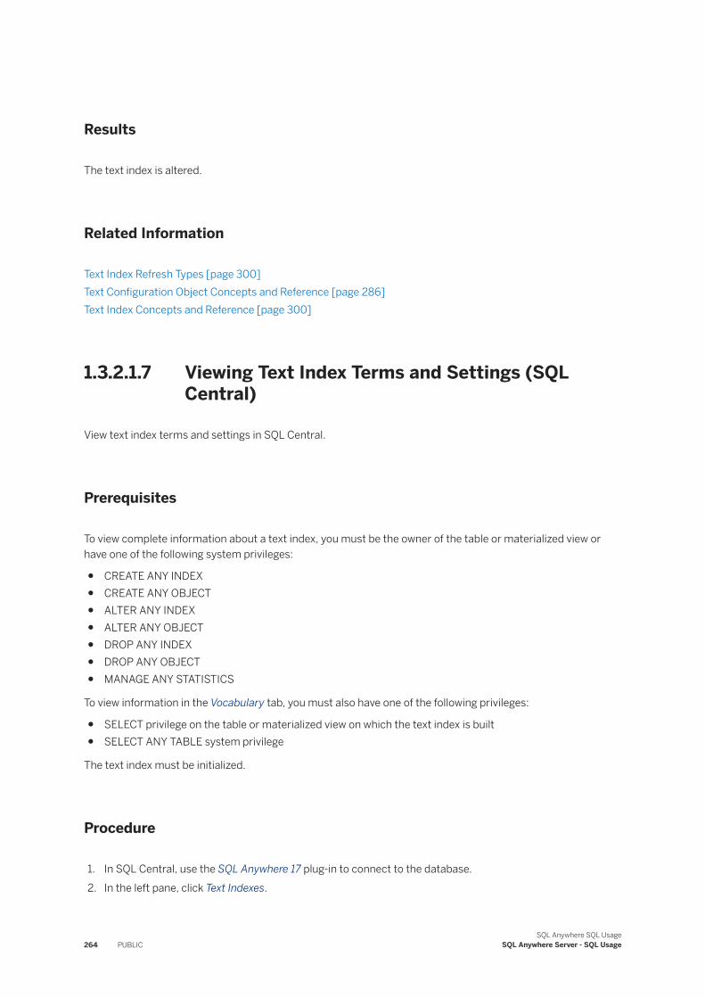
Results
The text index is altered.
Related Information
Text Index Refresh Types [page 300]Text Configuration Object Concepts and Reference [page 286]Text Index Concepts and Reference [page 300]
1.3.2.1.7 Viewing Text Index Terms and Settings (SQL Central)
View text index terms and settings in SQL Central.
Prerequisites
To view complete information about a text index, you must be the owner of the table or materialized view or have one of the following system privileges:
● CREATE ANY INDEX● CREATE ANY OBJECT● ALTER ANY INDEX● ALTER ANY OBJECT● DROP ANY INDEX● DROP ANY OBJECT● MANAGE ANY STATISTICS
To view information in the Vocabulary tab, you must also have one of the following privileges:
● SELECT privilege on the table or materialized view on which the text index is built● SELECT ANY TABLE system privilege
The text index must be initialized.
Procedure
1. In SQL Central, use the SQL Anywhere 17 plug-in to connect to the database.2. In the left pane, click Text Indexes.
264 PUBLICSQL Anywhere SQL Usage
SQL Anywhere Server - SQL Usage
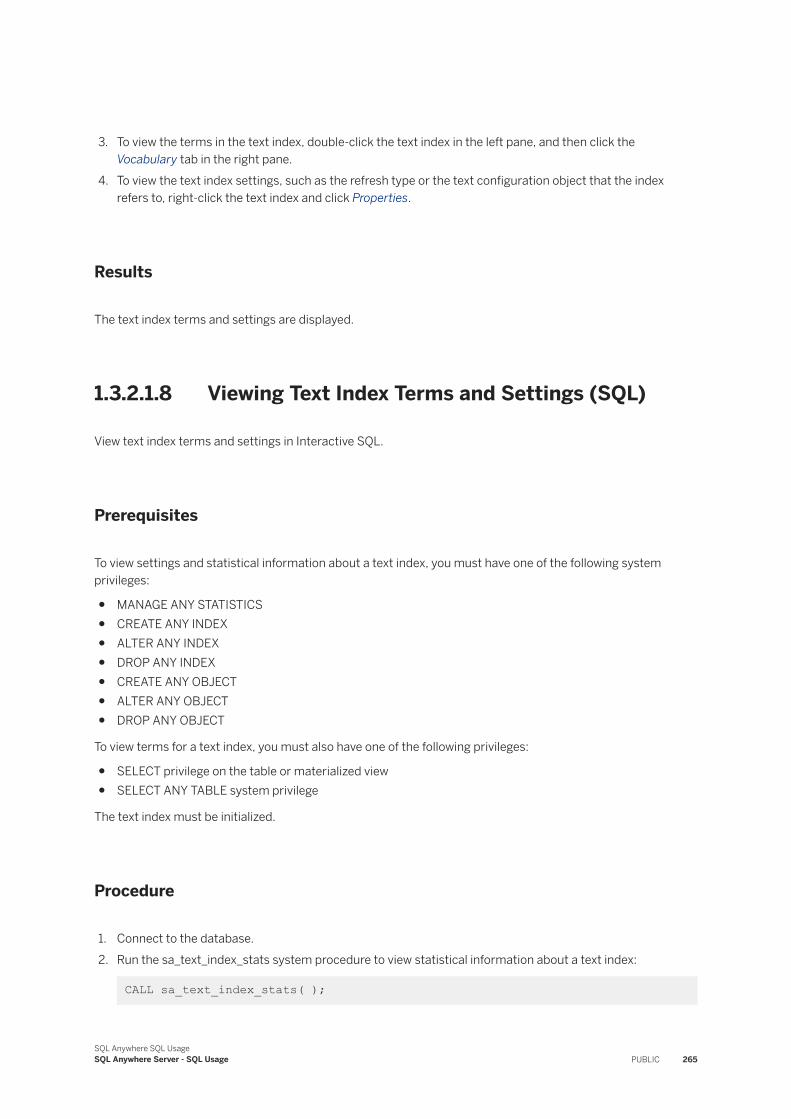
3. To view the terms in the text index, double-click the text index in the left pane, and then click the Vocabulary tab in the right pane.
4. To view the text index settings, such as the refresh type or the text configuration object that the index refers to, right-click the text index and click Properties.
Results
The text index terms and settings are displayed.
1.3.2.1.8 Viewing Text Index Terms and Settings (SQL)
View text index terms and settings in Interactive SQL.
Prerequisites
To view settings and statistical information about a text index, you must have one of the following system privileges:
● MANAGE ANY STATISTICS● CREATE ANY INDEX● ALTER ANY INDEX● DROP ANY INDEX● CREATE ANY OBJECT● ALTER ANY OBJECT● DROP ANY OBJECT
To view terms for a text index, you must also have one of the following privileges:
● SELECT privilege on the table or materialized view● SELECT ANY TABLE system privilege
The text index must be initialized.
Procedure
1. Connect to the database.2. Run the sa_text_index_stats system procedure to view statistical information about a text index:
CALL sa_text_index_stats( );
SQL Anywhere SQL UsageSQL Anywhere Server - SQL Usage PUBLIC 265
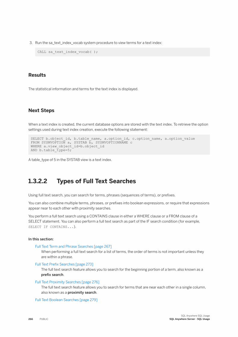
3. Run the sa_text_index_vocab system procedure to view terms for a text index:
CALL sa_text_index_vocab( );
Results
The statistical information and terms for the text index is displayed.
Next Steps
When a text index is created, the current database options are stored with the text index. To retrieve the option settings used during text index creation, execute the following statement:
SELECT b.object_id, b.table_name, a.option_id, c.option_name, a.option_value FROM SYSMVOPTION a, SYSTAB b, SYSMVOPTIONNAME cWHERE a.view_object_id=b.object_id AND b.table_type=5;
A table_type of 5 in the SYSTAB view is a text index.
1.3.2.2 Types of Full Text Searches
Using full text search, you can search for terms, phrases (sequences of terms), or prefixes.
You can also combine multiple terms, phrases, or prefixes into boolean expressions, or require that expressions appear near to each other with proximity searches.
You perform a full text search using a CONTAINS clause in either a WHERE clause or a FROM clause of a SELECT statement. You can also perform a full text search as part of the IF search condition (for example, SELECT IF CONTAINS...).
In this section:
Full Text Term and Phrase Searches [page 267]When performing a full text search for a list of terms, the order of terms is not important unless they are within a phrase.
Full Text Prefix Searches [page 273]The full text search feature allows you to search for the beginning portion of a term, also known as a prefix search.
Full Text Proximity Searches [page 276]The full text search feature allows you to search for terms that are near each other in a single column, also known as a proximity search.
Full Text Boolean Searches [page 279]
266 PUBLICSQL Anywhere SQL Usage
SQL Anywhere Server - SQL Usage
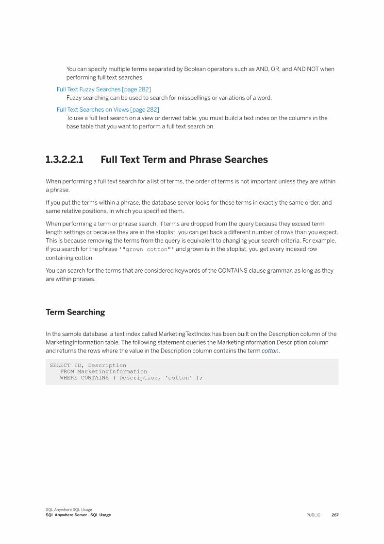
You can specify multiple terms separated by Boolean operators such as AND, OR, and AND NOT when performing full text searches.
Full Text Fuzzy Searches [page 282]Fuzzy searching can be used to search for misspellings or variations of a word.
Full Text Searches on Views [page 282]To use a full text search on a view or derived table, you must build a text index on the columns in the base table that you want to perform a full text search on.
1.3.2.2.1 Full Text Term and Phrase Searches
When performing a full text search for a list of terms, the order of terms is not important unless they are within a phrase.
If you put the terms within a phrase, the database server looks for those terms in exactly the same order, and same relative positions, in which you specified them.
When performing a term or phrase search, if terms are dropped from the query because they exceed term length settings or because they are in the stoplist, you can get back a different number of rows than you expect. This is because removing the terms from the query is equivalent to changing your search criteria. For example, if you search for the phrase '"grown cotton"' and grown is in the stoplist, you get every indexed row containing cotton.
You can search for the terms that are considered keywords of the CONTAINS clause grammar, as long as they are within phrases.
Term Searching
In the sample database, a text index called MarketingTextIndex has been built on the Description column of the MarketingInformation table. The following statement queries the MarketingInformation.Description column and returns the rows where the value in the Description column contains the term cotton.
SELECT ID, Description FROM MarketingInformation WHERE CONTAINS ( Description, 'cotton' );
SQL Anywhere SQL UsageSQL Anywhere Server - SQL Usage PUBLIC 267
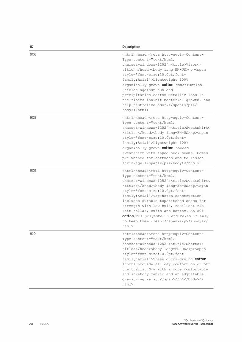
ID Description
906 <html><head><meta http-equiv=Content-Type content="text/html; charset=windows-1252"><title>Visor</title></head><body lang=EN-US><p><span style='font-size:10.0pt;font-family:Arial'>Lightweight 100% organically grown cotton construction. Shields against sun and precipitation.cotton Metallic ions in the fibers inhibit bacterial growth, and help neutralize odor.</span></p></body></html>
908 <html><head><meta http-equiv=Content-Type content="text/html; charset=windows-1252"><title>Sweatshirt</title></head><body lang=EN-US><p><span style='font-size:10.0pt;font-family:Arial'>Lightweight 100% organically grown cotton hooded sweatshirt with taped neck seams. Comes pre-washed for softness and to lessen shrinkage.</span></p></body></html>
909 <html><head><meta http-equiv=Content-Type content="text/html; charset=windows-1252"><title>Sweatshirt</title></head><body lang=EN-US><p><span style='font-size:10.0pt;font-family:Arial'>Top-notch construction includes durable topstitched seams for strength with low-bulk, resilient rib-knit collar, cuffs and bottom. An 80% cotton/20% polyester blend makes it easy to keep them clean.</span></p></body></html>
910 <html><head><meta http-equiv=Content-Type content="text/html; charset=windows-1252"><title>Shorts</title></head><body lang=EN-US><p><span style='font-size:10.0pt;font-family:Arial'>These quick-drying cotton shorts provide all day comfort on or off the trails. Now with a more comfortable and stretchy fabric and an adjustable drawstring waist.</span></p></body></html>
268 PUBLICSQL Anywhere SQL Usage
SQL Anywhere Server - SQL Usage
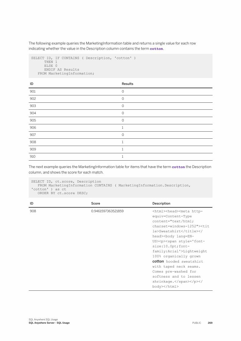
The following example queries the MarketingInformation table and returns a single value for each row indicating whether the value in the Description column contains the term cotton.
SELECT ID, IF CONTAINS ( Description, 'cotton' ) THEN 1 ELSE 0 ENDIF AS Results FROM MarketingInformation;
ID Results
901 0
902 0
903 0
904 0
905 0
906 1
907 0
908 1
909 1
910 1
The next example queries the MarketingInformation table for items that have the term cotton the Description column, and shows the score for each match.
SELECT ID, ct.score, Description FROM MarketingInformation CONTAINS ( MarketingInformation.Description, 'cotton' ) as ct ORDER BY ct.score DESC;
ID Score Description
908 0.9461597363521859 <html><head><meta http-equiv=Content-Type content="text/html; charset=windows-1252"><title>Sweatshirt</title></head><body lang=EN-US><p><span style='font-size:10.0pt;font-family:Arial'>Lightweight 100% organically grown cotton hooded sweatshirt with taped neck seams. Comes pre-washed for softness and to lessen shrinkage.</span></p></body></html>
SQL Anywhere SQL UsageSQL Anywhere Server - SQL Usage PUBLIC 269
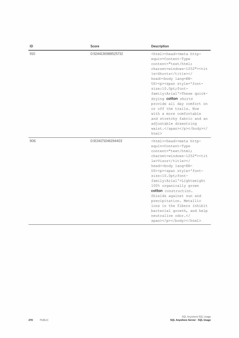
ID Score Description
910 0.9244136988525732 <html><head><meta http-equiv=Content-Type content="text/html; charset=windows-1252"><title>Shorts</title></head><body lang=EN-US><p><span style='font-size:10.0pt;font-family:Arial'>These quick-drying cotton shorts provide all day comfort on or off the trails. Now with a more comfortable and stretchy fabric and an adjustable drawstring waist.</span></p></body></html>
906 0.9134171046194403 <html><head><meta http-equiv=Content-Type content="text/html; charset=windows-1252"><title>Visor</title></head><body lang=EN-US><p><span style='font-size:10.0pt;font-family:Arial'>Lightweight 100% organically grown cotton construction. Shields against sun and precipitation. Metallic ions in the fibers inhibit bacterial growth, and help neutralize odor.</span></p></body></html>
270 PUBLICSQL Anywhere SQL Usage
SQL Anywhere Server - SQL Usage
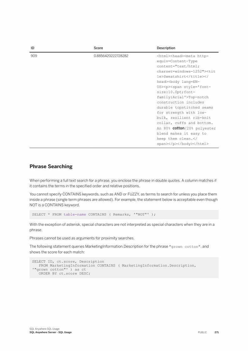
ID Score Description
909 0.8856420222728282 <html><head><meta http-equiv=Content-Type content="text/html; charset=windows-1252"><title>Sweatshirt</title></head><body lang=EN-US><p><span style='font-size:10.0pt;font-family:Arial'>Top-notch construction includes durable topstitched seams for strength with low-bulk, resilient rib-knit collar, cuffs and bottom. An 80% cotton/20% polyester blend makes it easy to keep them clean.</span></p></body></html>
Phrase Searching
When performing a full text search for a phrase, you enclose the phrase in double quotes. A column matches if it contains the terms in the specified order and relative positions.
You cannot specify CONTAINS keywords, such as AND or FUZZY, as terms to search for unless you place them inside a phrase (single term phrases are allowed). For example, the statement below is acceptable even though NOT is a CONTAINS keyword.
SELECT * FROM table-name CONTAINS ( Remarks, '"NOT"' );
With the exception of asterisk, special characters are not interpreted as special characters when they are in a phrase.
Phrases cannot be used as arguments for proximity searches.
The following statement queries MarketingInformation.Description for the phrase "grown cotton", and shows the score for each match:
SELECT ID, ct.score, Description FROM MarketingInformation CONTAINS ( MarketingInformation.Description, '"grown cotton"' ) as ct ORDER BY ct.score DESC;
SQL Anywhere SQL UsageSQL Anywhere Server - SQL Usage PUBLIC 271
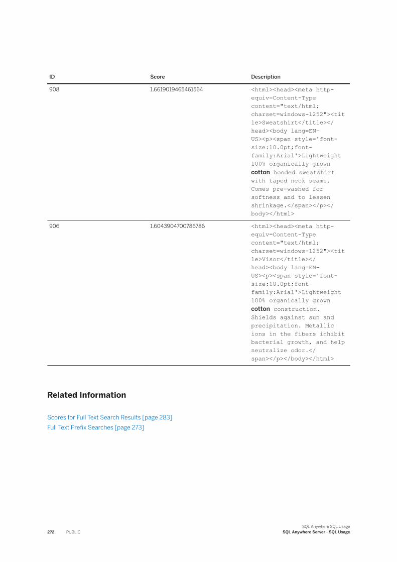
ID Score Description
908 1.6619019465461564 <html><head><meta http-equiv=Content-Type content="text/html; charset=windows-1252"><title>Sweatshirt</title></head><body lang=EN-US><p><span style='font-size:10.0pt;font-family:Arial'>Lightweight 100% organically grown cotton hooded sweatshirt with taped neck seams. Comes pre-washed for softness and to lessen shrinkage.</span></p></body></html>
906 1.6043904700786786 <html><head><meta http-equiv=Content-Type content="text/html; charset=windows-1252"><title>Visor</title></head><body lang=EN-US><p><span style='font-size:10.0pt;font-family:Arial'>Lightweight 100% organically grown cotton construction. Shields against sun and precipitation. Metallic ions in the fibers inhibit bacterial growth, and help neutralize odor.</span></p></body></html>
Related Information
Scores for Full Text Search Results [page 283]Full Text Prefix Searches [page 273]
272 PUBLICSQL Anywhere SQL Usage
SQL Anywhere Server - SQL Usage
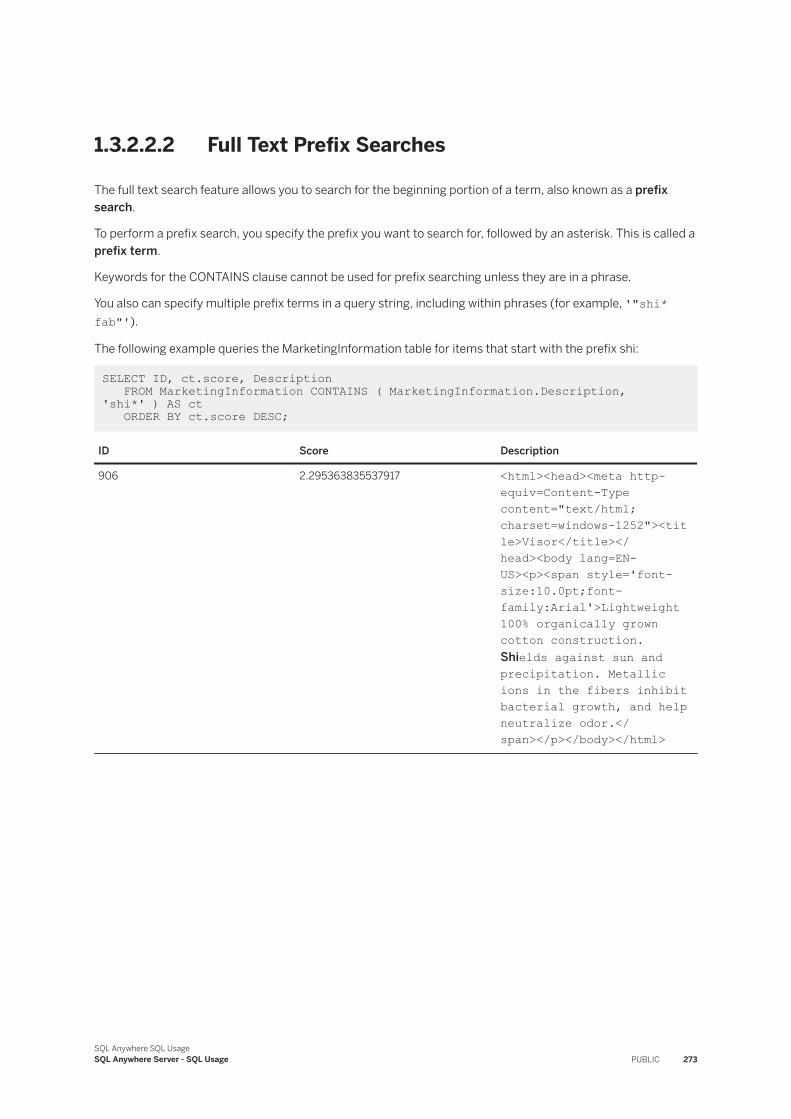
1.3.2.2.2 Full Text Prefix Searches
The full text search feature allows you to search for the beginning portion of a term, also known as a prefix search.
To perform a prefix search, you specify the prefix you want to search for, followed by an asterisk. This is called a prefix term.
Keywords for the CONTAINS clause cannot be used for prefix searching unless they are in a phrase.
You also can specify multiple prefix terms in a query string, including within phrases (for example, '"shi* fab"').
The following example queries the MarketingInformation table for items that start with the prefix shi:
SELECT ID, ct.score, Description FROM MarketingInformation CONTAINS ( MarketingInformation.Description, 'shi*' ) AS ct ORDER BY ct.score DESC;
ID Score Description
906 2.295363835537917 <html><head><meta http-equiv=Content-Type content="text/html; charset=windows-1252"><title>Visor</title></head><body lang=EN-US><p><span style='font-size:10.0pt;font-family:Arial'>Lightweight 100% organically grown cotton construction. Shields against sun and precipitation. Metallic ions in the fibers inhibit bacterial growth, and help neutralize odor.</span></p></body></html>
SQL Anywhere SQL UsageSQL Anywhere Server - SQL Usage PUBLIC 273
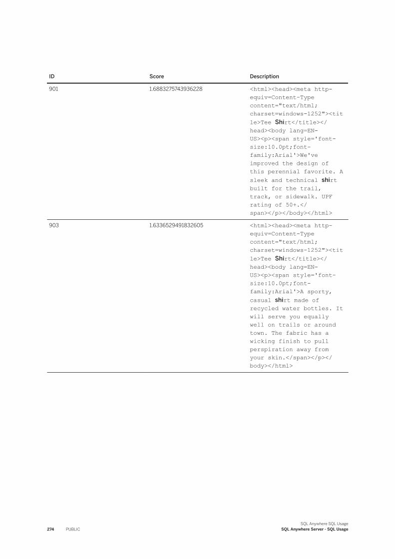
ID Score Description
901 1.6883275743936228 <html><head><meta http-equiv=Content-Type content="text/html; charset=windows-1252"><title>Tee Shirt</title></head><body lang=EN-US><p><span style='font-size:10.0pt;font-family:Arial'>We've improved the design of this perennial favorite. A sleek and technical shirt built for the trail, track, or sidewalk. UPF rating of 50+.</span></p></body></html>
903 1.6336529491832605 <html><head><meta http-equiv=Content-Type content="text/html; charset=windows-1252"><title>Tee Shirt</title></head><body lang=EN-US><p><span style='font-size:10.0pt;font-family:Arial'>A sporty, casual shirt made of recycled water bottles. It will serve you equally well on trails or around town. The fabric has a wicking finish to pull perspiration away from your skin.</span></p></body></html>
274 PUBLICSQL Anywhere SQL Usage
SQL Anywhere Server - SQL Usage
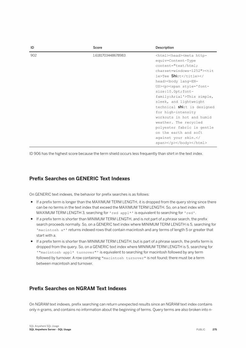
ID Score Description
902 1.6181703448678983 <html><head><meta http-equiv=Content-Type content="text/html; charset=windows-1252"><title>Tee Shirt</title></head><body lang=EN-US><p><span style='font-size:10.0pt;font-family:Arial'>This simple, sleek, and lightweight technical shirt is designed for high-intensity workouts in hot and humid weather. The recycled polyester fabric is gentle on the earth and soft against your skin.</span></p></body></html>
ID 906 has the highest score because the term shield occurs less frequently than shirt in the text index.
Prefix Searches on GENERIC Text Indexes
On GENERIC text indexes, the behavior for prefix searches is as follows:
● If a prefix term is longer than the MAXIMUM TERM LENGTH, it is dropped from the query string since there can be no terms in the text index that exceed the MAXIMUM TERM LENGTH. So, on a text index with MAXIMUM TERM LENGTH 3, searching for 'red appl*' is equivalent to searching for 'red'.
● If a prefix term is shorter than MINIMUM TERM LENGTH, and is not part of a phrase search, the prefix search proceeds normally. So, on a GENERIC text index where MINIMUM TERM LENGTH is 5, searching for 'macintosh a*' returns indexed rows that contain macintosh and any terms of length 5 or greater that start with a.
● If a prefix term is shorter than MINIMUM TERM LENGTH, but is part of a phrase search, the prefix term is dropped from the query. So, on a GENERIC text index where MINIMUM TERM LENGTH is 5, searching for '"macintosh appl* turnover"' is equivalent to searching for macintosh followed by any term followed by turnover. A row containing "macintosh turnover" is not found; there must be a term between macintosh and turnover.
Prefix Searches on NGRAM Text Indexes
On NGRAM text indexes, prefix searching can return unexpected results since an NGRAM text index contains only n-grams, and contains no information about the beginning of terms. Query terms are also broken into n-
SQL Anywhere SQL UsageSQL Anywhere Server - SQL Usage PUBLIC 275
grams, and searching is performed using the n-grams not the query terms. Because of this, the following behaviors should be noted:
● If a prefix term is shorter than the n-gram length (MAXIMUM TERM LENGTH), the query returns all indexed rows that contain n-grams starting with the prefix term. For example, on a 3-gram text index, searching for 'ea*' returns all indexed rows containing n-grams starting with ea. So, if the terms weather and fear were indexed, the rows would be considered matches since their n-grams include eat and ear, respectively.
● If a prefix term is longer than n-gram length, and is not part of a phrase, and not an argument in a proximity search, the prefix term is converted to an n-grammed phrase and the asterisk is dropped. For example, on a 3-gram text index, searching for 'purple blac*' is equivalent to searching for '"pur urp rpl ple" AND "bla lac"'.
● For phrases, the following behavior also takes place:○ If the prefix term is the only term in the phrase, it is converted to an n-grammed phrase and the
asterisk is dropped. For example, on a 3-gram text index, searching for '"purpl*"' is equivalent to searching for '"pur urp rpl"'.
○ If the prefix term is in the last position of the phrase, the asterisk is dropped and the terms are converted to a phrase of n-grams. For example, on a 3-gram text index, searching for '"purple blac*"' is equivalent to searching for '"pur urp rpl ple bla lac"'.
○ If the prefix term is not in the last position of the phrase, the phrase is broken up into phrases that are ANDed together. For example, on a 3-gram text index, searching for '"purp* blac*"' is equivalent to searching for '"pur urp" AND "bla lac"'.
● If a prefix term is an argument in a proximity search, the proximity search is converted to an AND. For example, on a 3-gram text index, searching for 'red NEAR[1] appl*' is equivalent to searching for 'red AND "app ppl"'.
Related Information
Text Index Concepts and Reference [page 300]
1.3.2.2.3 Full Text Proximity Searches
The full text search feature allows you to search for terms that are near each other in a single column, also known as a proximity search.
To perform a proximity search, you specify two terms with either the keyword NEAR between them, or the tilde (~).
You can use an integer argument with the NEAR keyword to specify the maximum distance. For example, term1 NEAR[5] term2 finds instances of term1 that are within five terms of term2. The order of terms is not significant; 'term1 NEAR term2' is equivalent to 'term2 NEAR term1'.
If you do not specify a distance, the database server uses 10 as the default distance.
You can also specify a tilde (~) instead of the NEAR keyword. For example, 'term1 ~ term2'. However, you cannot specify a distance when using the tilde form; the default of ten terms is applied.
You cannot specify a phrase as an argument in proximity searches.
276 PUBLICSQL Anywhere SQL Usage
SQL Anywhere Server - SQL Usage
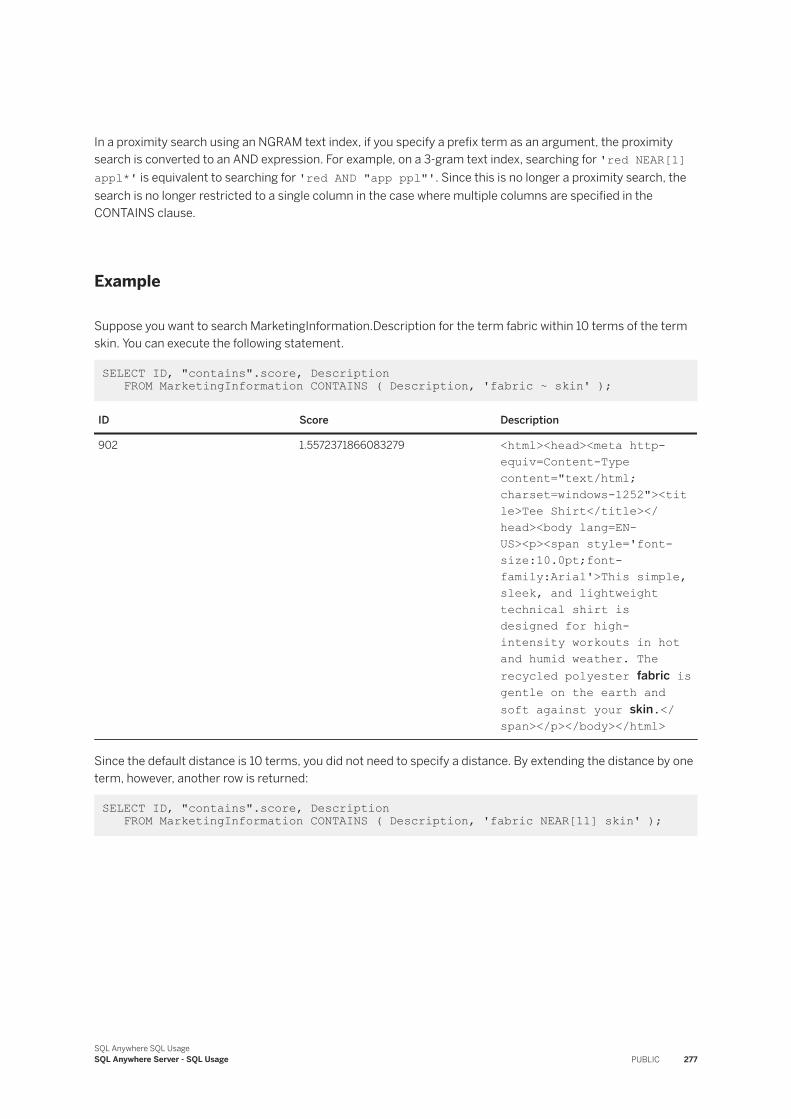
In a proximity search using an NGRAM text index, if you specify a prefix term as an argument, the proximity search is converted to an AND expression. For example, on a 3-gram text index, searching for 'red NEAR[1] appl*' is equivalent to searching for 'red AND "app ppl"'. Since this is no longer a proximity search, the search is no longer restricted to a single column in the case where multiple columns are specified in the CONTAINS clause.
Example
Suppose you want to search MarketingInformation.Description for the term fabric within 10 terms of the term skin. You can execute the following statement.
SELECT ID, "contains".score, Description FROM MarketingInformation CONTAINS ( Description, 'fabric ~ skin' );
ID Score Description
902 1.5572371866083279 <html><head><meta http-equiv=Content-Type content="text/html; charset=windows-1252"><title>Tee Shirt</title></head><body lang=EN-US><p><span style='font-size:10.0pt;font-family:Arial'>This simple, sleek, and lightweight technical shirt is designed for high-intensity workouts in hot and humid weather. The recycled polyester fabric is gentle on the earth and soft against your skin.</span></p></body></html>
Since the default distance is 10 terms, you did not need to specify a distance. By extending the distance by one term, however, another row is returned:
SELECT ID, "contains".score, Description FROM MarketingInformation CONTAINS ( Description, 'fabric NEAR[11] skin' );
SQL Anywhere SQL UsageSQL Anywhere Server - SQL Usage PUBLIC 277
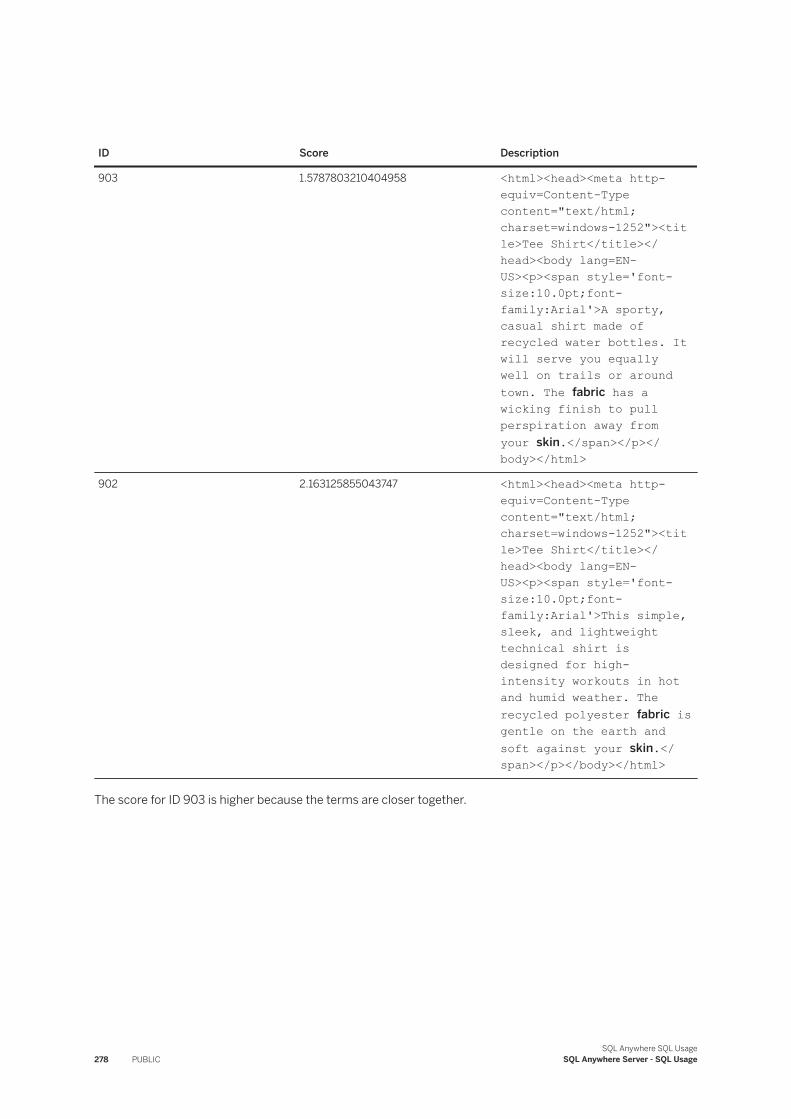
ID Score Description
903 1.5787803210404958 <html><head><meta http-equiv=Content-Type content="text/html; charset=windows-1252"><title>Tee Shirt</title></head><body lang=EN-US><p><span style='font-size:10.0pt;font-family:Arial'>A sporty, casual shirt made of recycled water bottles. It will serve you equally well on trails or around town. The fabric has a wicking finish to pull perspiration away from your skin.</span></p></body></html>
902 2.163125855043747 <html><head><meta http-equiv=Content-Type content="text/html; charset=windows-1252"><title>Tee Shirt</title></head><body lang=EN-US><p><span style='font-size:10.0pt;font-family:Arial'>This simple, sleek, and lightweight technical shirt is designed for high-intensity workouts in hot and humid weather. The recycled polyester fabric is gentle on the earth and soft against your skin.</span></p></body></html>
The score for ID 903 is higher because the terms are closer together.
278 PUBLICSQL Anywhere SQL Usage
SQL Anywhere Server - SQL Usage
1.3.2.2.4 Full Text Boolean Searches
You can specify multiple terms separated by Boolean operators such as AND, OR, and AND NOT when performing full text searches.
Using the AND Operator in Full Text Searches
The AND operator matches a row if it contains both of the terms specified on either side of the AND. You can also use an ampersand (&) for the AND operator. If terms are specified without an operator between them, AND is implied.
The order in which the terms are listed is not important.
For example, each of the following statements finds rows in MarketingInformation.Description that contain the term fabric and a term that begins with ski:
SELECT * FROM MarketingInformation WHERE CONTAINS ( MarketingInformation.Description, 'ski* AND fabric' );SELECT * FROM MarketingInformation WHERE CONTAINS ( MarketingInformation.Description, 'fabric & ski*' );SELECT * FROM MarketingInformation WHERE CONTAINS ( MarketingInformation.Description, 'ski* fabric' );
Using the OR Operator in Full Text Searches
The OR operator matches a row if it contains at least one of the specified search terms on either side of the OR. You can also use a vertical bar (|) for the OR operator; the two are equivalent.
The order in which the terms are listed is not important.
For example, either statement below returns rows in the MarketingInformation.Description that contain either the term fabric or a term that starts with ski:
SELECT * FROM MarketingInformation WHERE CONTAINS ( MarketingInformation.Description, 'ski* OR fabric' );SELECT * FROM MarketingInformation WHERE CONTAINS ( MarketingInformation.Description, 'fabric | ski*' );
Using the AND NOT Operator in Full Text Searches
The AND NOT operator finds results that match the left argument and do not match the right argument. You can also use a hyphen (-) for the AND NOT operator; the two are equivalent.
SQL Anywhere SQL UsageSQL Anywhere Server - SQL Usage PUBLIC 279
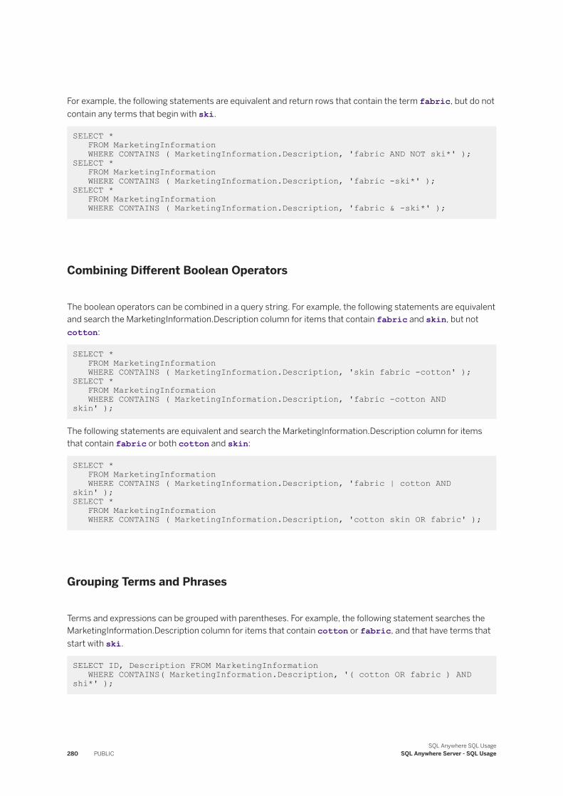
For example, the following statements are equivalent and return rows that contain the term fabric, but do not contain any terms that begin with ski.
SELECT * FROM MarketingInformation WHERE CONTAINS ( MarketingInformation.Description, 'fabric AND NOT ski*' );SELECT * FROM MarketingInformation WHERE CONTAINS ( MarketingInformation.Description, 'fabric -ski*' );SELECT * FROM MarketingInformation WHERE CONTAINS ( MarketingInformation.Description, 'fabric & -ski*' );
Combining Different Boolean Operators
The boolean operators can be combined in a query string. For example, the following statements are equivalent and search the MarketingInformation.Description column for items that contain fabric and skin, but not cotton:
SELECT * FROM MarketingInformation WHERE CONTAINS ( MarketingInformation.Description, 'skin fabric -cotton' );SELECT * FROM MarketingInformation WHERE CONTAINS ( MarketingInformation.Description, 'fabric -cotton AND skin' );
The following statements are equivalent and search the MarketingInformation.Description column for items that contain fabric or both cotton and skin:
SELECT * FROM MarketingInformation WHERE CONTAINS ( MarketingInformation.Description, 'fabric | cotton AND skin' );SELECT * FROM MarketingInformation WHERE CONTAINS ( MarketingInformation.Description, 'cotton skin OR fabric' );
Grouping Terms and Phrases
Terms and expressions can be grouped with parentheses. For example, the following statement searches the MarketingInformation.Description column for items that contain cotton or fabric, and that have terms that start with ski.
SELECT ID, Description FROM MarketingInformation WHERE CONTAINS( MarketingInformation.Description, '( cotton OR fabric ) AND shi*' );
280 PUBLICSQL Anywhere SQL Usage
SQL Anywhere Server - SQL Usage
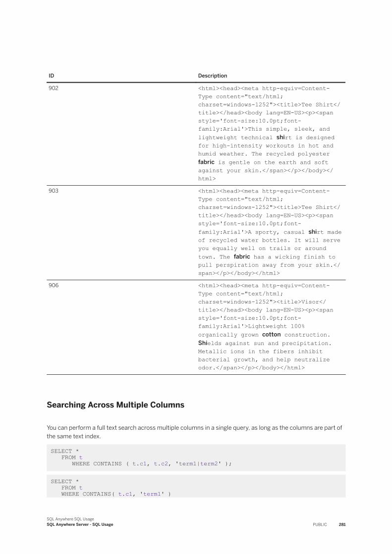
ID Description
902 <html><head><meta http-equiv=Content-Type content="text/html; charset=windows-1252"><title>Tee Shirt</title></head><body lang=EN-US><p><span style='font-size:10.0pt;font-family:Arial'>This simple, sleek, and lightweight technical shirt is designed for high-intensity workouts in hot and humid weather. The recycled polyester fabric is gentle on the earth and soft against your skin.</span></p></body></html>
903 <html><head><meta http-equiv=Content-Type content="text/html; charset=windows-1252"><title>Tee Shirt</title></head><body lang=EN-US><p><span style='font-size:10.0pt;font-family:Arial'>A sporty, casual shirt made of recycled water bottles. It will serve you equally well on trails or around town. The fabric has a wicking finish to pull perspiration away from your skin.</span></p></body></html>
906 <html><head><meta http-equiv=Content-Type content="text/html; charset=windows-1252"><title>Visor</title></head><body lang=EN-US><p><span style='font-size:10.0pt;font-family:Arial'>Lightweight 100% organically grown cotton construction. Shields against sun and precipitation. Metallic ions in the fibers inhibit bacterial growth, and help neutralize odor.</span></p></body></html>
Searching Across Multiple Columns
You can perform a full text search across multiple columns in a single query, as long as the columns are part of the same text index.
SELECT * FROM t WHERE CONTAINS ( t.c1, t.c2, 'term1|term2' );
SELECT * FROM t WHERE CONTAINS( t.c1, 'term1' )
SQL Anywhere SQL UsageSQL Anywhere Server - SQL Usage PUBLIC 281
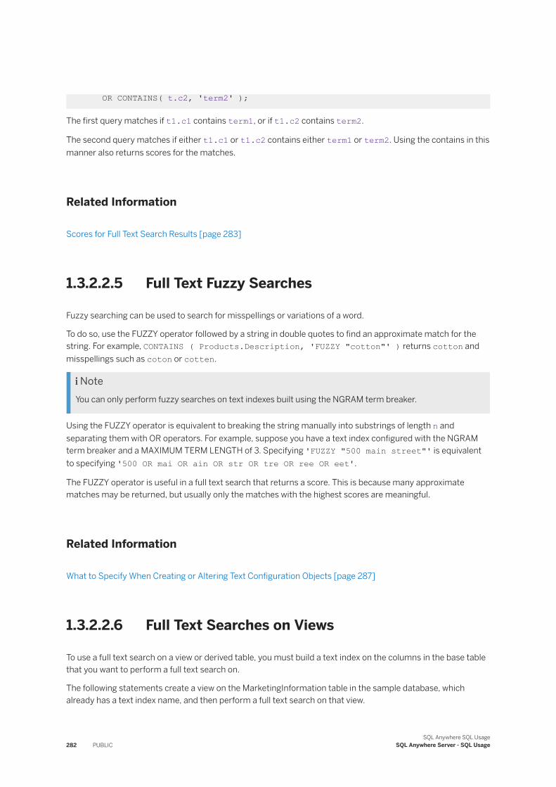
OR CONTAINS( t.c2, 'term2' );
The first query matches if t1.c1 contains term1, or if t1.c2 contains term2.
The second query matches if either t1.c1 or t1.c2 contains either term1 or term2. Using the contains in this manner also returns scores for the matches.
Related Information
Scores for Full Text Search Results [page 283]
1.3.2.2.5 Full Text Fuzzy Searches
Fuzzy searching can be used to search for misspellings or variations of a word.
To do so, use the FUZZY operator followed by a string in double quotes to find an approximate match for the string. For example, CONTAINS ( Products.Description, 'FUZZY "cotton"' ) returns cotton and misspellings such as coton or cotten.
NoteYou can only perform fuzzy searches on text indexes built using the NGRAM term breaker.
Using the FUZZY operator is equivalent to breaking the string manually into substrings of length n and separating them with OR operators. For example, suppose you have a text index configured with the NGRAM term breaker and a MAXIMUM TERM LENGTH of 3. Specifying 'FUZZY "500 main street"' is equivalent to specifying '500 OR mai OR ain OR str OR tre OR ree OR eet'.
The FUZZY operator is useful in a full text search that returns a score. This is because many approximate matches may be returned, but usually only the matches with the highest scores are meaningful.
Related Information
What to Specify When Creating or Altering Text Configuration Objects [page 287]
1.3.2.2.6 Full Text Searches on Views
To use a full text search on a view or derived table, you must build a text index on the columns in the base table that you want to perform a full text search on.
The following statements create a view on the MarketingInformation table in the sample database, which already has a text index name, and then perform a full text search on that view.
282 PUBLICSQL Anywhere SQL Usage
SQL Anywhere Server - SQL Usage
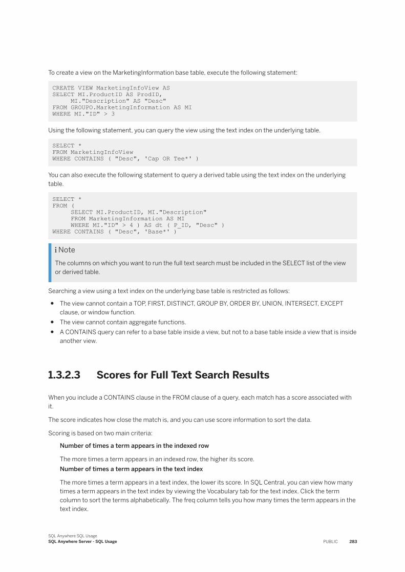
To create a view on the MarketingInformation base table, execute the following statement:
CREATE VIEW MarketingInfoView AS SELECT MI.ProductID AS ProdID, MI."Description" AS "Desc"FROM GROUPO.MarketingInformation AS MI WHERE MI."ID" > 3
Using the following statement, you can query the view using the text index on the underlying table.
SELECT * FROM MarketingInfoView WHERE CONTAINS ( "Desc", 'Cap OR Tee*' )
You can also execute the following statement to query a derived table using the text index on the underlying table.
SELECT * FROM ( SELECT MI.ProductID, MI."Description" FROM MarketingInformation AS MI WHERE MI."ID" > 4 ) AS dt ( P_ID, "Desc" ) WHERE CONTAINS ( "Desc", 'Base*' )
NoteThe columns on which you want to run the full text search must be included in the SELECT list of the view or derived table.
Searching a view using a text index on the underlying base table is restricted as follows:
● The view cannot contain a TOP, FIRST, DISTINCT, GROUP BY, ORDER BY, UNION, INTERSECT, EXCEPT clause, or window function.
● The view cannot contain aggregate functions.● A CONTAINS query can refer to a base table inside a view, but not to a base table inside a view that is inside
another view.
1.3.2.3 Scores for Full Text Search Results
When you include a CONTAINS clause in the FROM clause of a query, each match has a score associated with it.
The score indicates how close the match is, and you can use score information to sort the data.
Scoring is based on two main criteria:
Number of times a term appears in the indexed row
The more times a term appears in an indexed row, the higher its score.Number of times a term appears in the text index
The more times a term appears in a text index, the lower its score. In SQL Central, you can view how many times a term appears in the text index by viewing the Vocabulary tab for the text index. Click the term column to sort the terms alphabetically. The freq column tells you how many times the term appears in the text index.
SQL Anywhere SQL UsageSQL Anywhere Server - SQL Usage PUBLIC 283
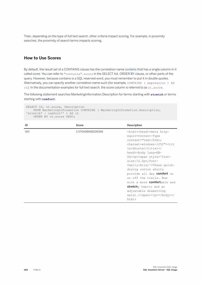
Then, depending on the type of full text search, other criteria impact scoring. For example, in proximity searches, the proximity of search terms impacts scoring.
How to Use Scores
By default, the result set of a CONTAINS clause has the correlation name contains that has a single column in it called score. You can refer to "contains".score in the SELECT list, ORDER BY clause, or other parts of the query. However, because contains is a SQL reserved word, you must remember to put it in double quotes. Alternatively, you can specify another correlation name such (for example, CONTAINS ( expression ) AS ct). In the documentation examples for full text search, the score column is referred to as ct.score.
The following statement searches MarketingInformation.Description for terms starting with stretch or terms starting with comfort:
SELECT ID, ct.score, Description FROM MarketingInformation CONTAINS ( MarketingInformation.Description, 'stretch* | comfort*' ) AS ct ORDER BY ct.score DESC;
ID Score Description
910 5.570408968026068 <html><head><meta http-equiv=Content-Type content="text/html; charset=windows-1252"><title>Shorts</title></head><body lang=EN-US><p><span style='font-size:10.0pt;font-family:Arial'>These quick-drying cotton shorts provide all day comfort on or off the trails. Now with a more comfortable and stretchy fabric and an adjustable drawstring waist.</span></p></body></html>
284 PUBLICSQL Anywhere SQL Usage
SQL Anywhere Server - SQL Usage
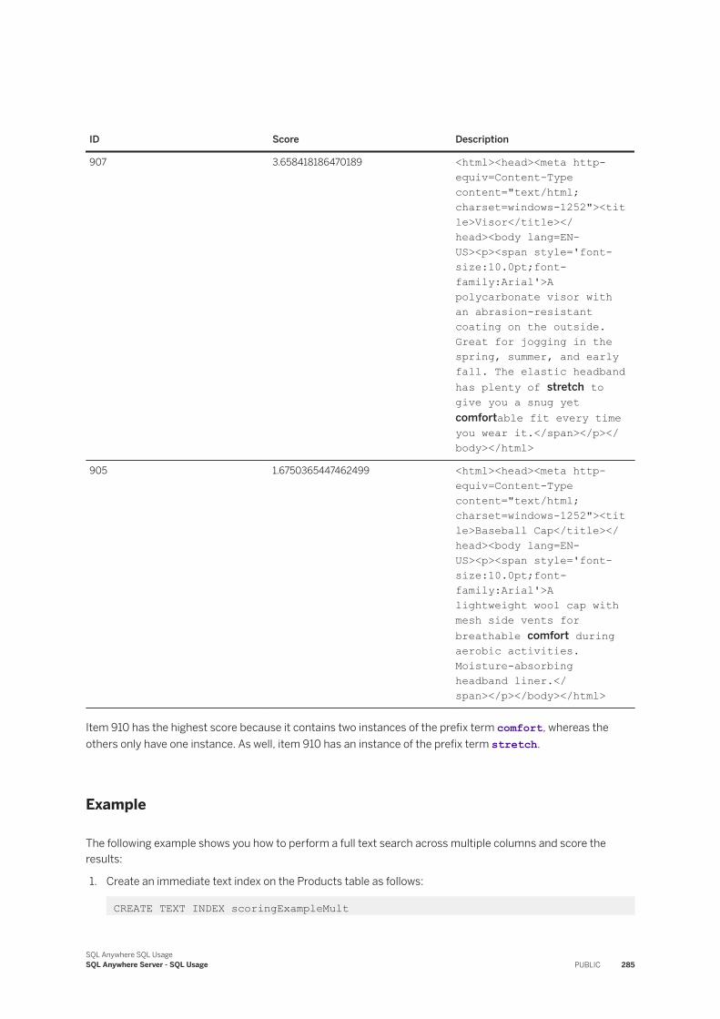
ID Score Description
907 3.658418186470189 <html><head><meta http-equiv=Content-Type content="text/html; charset=windows-1252"><title>Visor</title></head><body lang=EN-US><p><span style='font-size:10.0pt;font-family:Arial'>A polycarbonate visor with an abrasion-resistant coating on the outside. Great for jogging in the spring, summer, and early fall. The elastic headband has plenty of stretch to give you a snug yet comfortable fit every time you wear it.</span></p></body></html>
905 1.6750365447462499 <html><head><meta http-equiv=Content-Type content="text/html; charset=windows-1252"><title>Baseball Cap</title></head><body lang=EN-US><p><span style='font-size:10.0pt;font-family:Arial'>A lightweight wool cap with mesh side vents for breathable comfort during aerobic activities. Moisture-absorbing headband liner.</span></p></body></html>
Item 910 has the highest score because it contains two instances of the prefix term comfort, whereas the others only have one instance. As well, item 910 has an instance of the prefix term stretch.
Example
The following example shows you how to perform a full text search across multiple columns and score the results:
1. Create an immediate text index on the Products table as follows:
CREATE TEXT INDEX scoringExampleMult
SQL Anywhere SQL UsageSQL Anywhere Server - SQL Usage PUBLIC 285
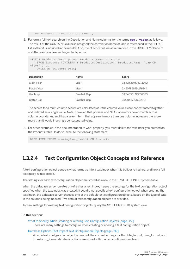
ON Products ( Description, Name );
2. Perform a full text search on the Description and Name columns for the terms cap or visor, as follows. The result of the CONTAINS clause is assigned the correlation name ct, and is referenced in the SELECT list so that it is included in the results. Also, the ct.score column is referenced in the ORDER BY clause to sort the results in descending order by score.
SELECT Products.Description, Products.Name, ct.score FROM Products CONTAINS ( Products.Description, Products.Name, 'cap OR visor' ) ct ORDER BY ct.score DESC;
Description Name Score
Cloth Visor Visor 3.5635154905713042
Plastic Visor Visor 3.4507856451176244
Wool cap Baseball Cap 3.2340501745357333
Cotton Cap Baseball Cap 3.090467108972918
The scores for a multi-column search are calculated as if the column values were concatenated together and indexed as a single value. Note, however, that phrases and NEAR operators never match across column boundaries, and that a search term that appears in more than one column increases the score more than it would in a single concatenated value.
3. For other examples in the documentation to work properly, you must delete the text index you created on the Products table. To do so, execute the following statement:
DROP TEXT INDEX scoringExampleMult ON Products;
1.3.2.4 Text Configuration Object Concepts and Reference
A text configuration object controls what terms go into a text index when it is built or refreshed, and how a full text query is interpreted.
The settings for each text configuration object are stored as a row in the ISYSTEXTCONFIG system table.
When the database server creates or refreshes a text index, it uses the settings for the text configuration object specified when the text index was created. If you did not specify a text configuration object when creating the text index, the database server chooses one of the default text configuration objects, based on the type of data in the columns being indexed. Two default text configuration objects are provided.
To view settings for existing text configuration objects, query the SYSTEXTCONFIG system view.
In this section:
What to Specify When Creating or Altering Text Configuration Objects [page 287]There are many settings to configure when creating or altering a text configuration object.
Database Options That Impact Text Configuration Objects [page 292]When a text configuration object is created, the current settings for the date_format, time_format, and timestamp_format database options are stored with the text configuration object.
286 PUBLICSQL Anywhere SQL Usage
SQL Anywhere Server - SQL Usage
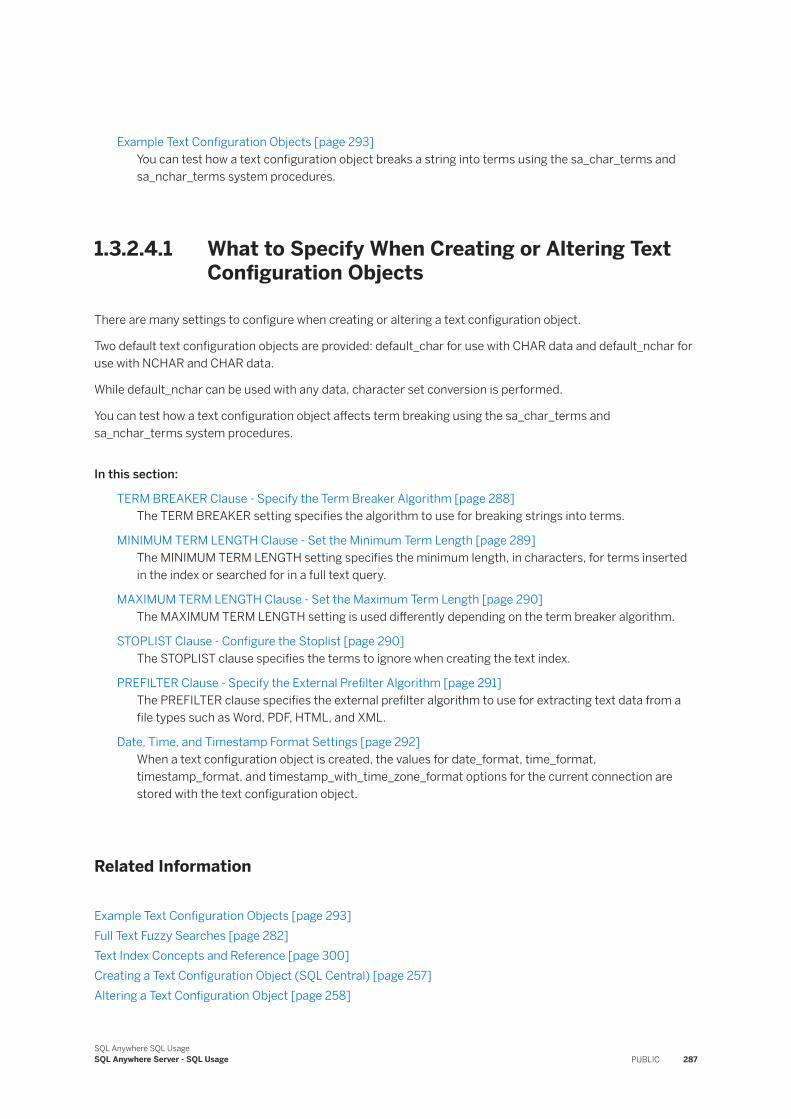
Example Text Configuration Objects [page 293]You can test how a text configuration object breaks a string into terms using the sa_char_terms and sa_nchar_terms system procedures.
1.3.2.4.1 What to Specify When Creating or Altering Text Configuration Objects
There are many settings to configure when creating or altering a text configuration object.
Two default text configuration objects are provided: default_char for use with CHAR data and default_nchar for use with NCHAR and CHAR data.
While default_nchar can be used with any data, character set conversion is performed.
You can test how a text configuration object affects term breaking using the sa_char_terms and sa_nchar_terms system procedures.
In this section:
TERM BREAKER Clause - Specify the Term Breaker Algorithm [page 288]The TERM BREAKER setting specifies the algorithm to use for breaking strings into terms.
MINIMUM TERM LENGTH Clause - Set the Minimum Term Length [page 289]The MINIMUM TERM LENGTH setting specifies the minimum length, in characters, for terms inserted in the index or searched for in a full text query.
MAXIMUM TERM LENGTH Clause - Set the Maximum Term Length [page 290]The MAXIMUM TERM LENGTH setting is used differently depending on the term breaker algorithm.
STOPLIST Clause - Configure the Stoplist [page 290]The STOPLIST clause specifies the terms to ignore when creating the text index.
PREFILTER Clause - Specify the External Prefilter Algorithm [page 291]The PREFILTER clause specifies the external prefilter algorithm to use for extracting text data from a file types such as Word, PDF, HTML, and XML.
Date, Time, and Timestamp Format Settings [page 292]When a text configuration object is created, the values for date_format, time_format, timestamp_format, and timestamp_with_time_zone_format options for the current connection are stored with the text configuration object.
Related Information
Example Text Configuration Objects [page 293]Full Text Fuzzy Searches [page 282]Text Index Concepts and Reference [page 300]Creating a Text Configuration Object (SQL Central) [page 257]Altering a Text Configuration Object [page 258]
SQL Anywhere SQL UsageSQL Anywhere Server - SQL Usage PUBLIC 287
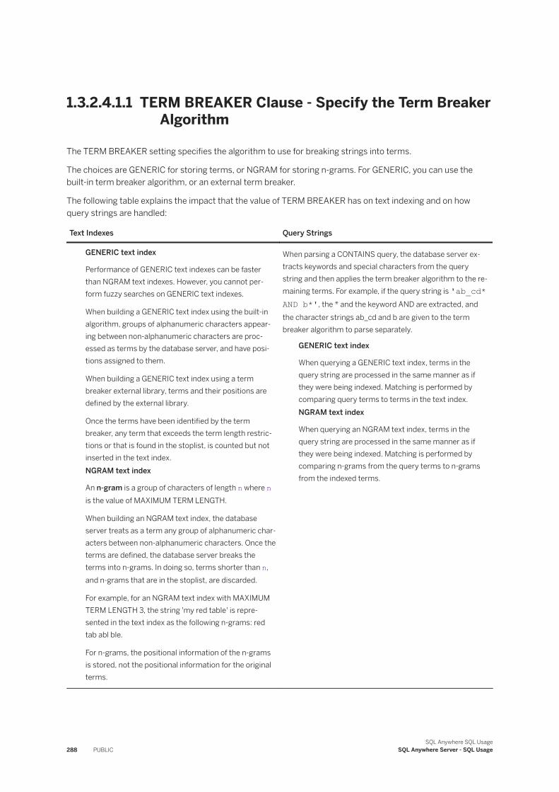
1.3.2.4.1.1 TERM BREAKER Clause - Specify the Term Breaker Algorithm
The TERM BREAKER setting specifies the algorithm to use for breaking strings into terms.
The choices are GENERIC for storing terms, or NGRAM for storing n-grams. For GENERIC, you can use the built-in term breaker algorithm, or an external term breaker.
The following table explains the impact that the value of TERM BREAKER has on text indexing and on how query strings are handled:
Text Indexes Query Strings
GENERIC text index
Performance of GENERIC text indexes can be faster than NGRAM text indexes. However, you cannot perform fuzzy searches on GENERIC text indexes.
When building a GENERIC text index using the built-in algorithm, groups of alphanumeric characters appearing between non-alphanumeric characters are processed as terms by the database server, and have positions assigned to them.
When building a GENERIC text index using a term breaker external library, terms and their positions are defined by the external library.
Once the terms have been identified by the term breaker, any term that exceeds the term length restrictions or that is found in the stoplist, is counted but not inserted in the text index.NGRAM text index
An n-gram is a group of characters of length n where n is the value of MAXIMUM TERM LENGTH.
When building an NGRAM text index, the database server treats as a term any group of alphanumeric characters between non-alphanumeric characters. Once the terms are defined, the database server breaks the terms into n-grams. In doing so, terms shorter than n, and n-grams that are in the stoplist, are discarded.
For example, for an NGRAM text index with MAXIMUM TERM LENGTH 3, the string 'my red table' is represented in the text index as the following n-grams: red tab abl ble.
For n-grams, the positional information of the n-grams is stored, not the positional information for the original terms.
When parsing a CONTAINS query, the database server extracts keywords and special characters from the query string and then applies the term breaker algorithm to the remaining terms. For example, if the query string is 'ab_cd* AND b*', the * and the keyword AND are extracted, and the character strings ab_cd and b are given to the term breaker algorithm to parse separately.
GENERIC text index
When querying a GENERIC text index, terms in the query string are processed in the same manner as if they were being indexed. Matching is performed by comparing query terms to terms in the text index.NGRAM text index
When querying an NGRAM text index, terms in the query string are processed in the same manner as if they were being indexed. Matching is performed by comparing n-grams from the query terms to n-grams from the indexed terms.
288 PUBLICSQL Anywhere SQL Usage
SQL Anywhere Server - SQL Usage
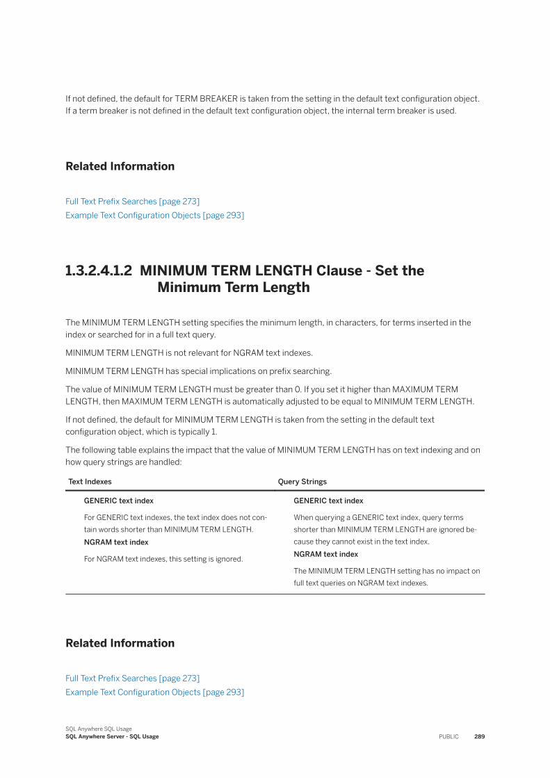
If not defined, the default for TERM BREAKER is taken from the setting in the default text configuration object. If a term breaker is not defined in the default text configuration object, the internal term breaker is used.
Related Information
Full Text Prefix Searches [page 273]Example Text Configuration Objects [page 293]
1.3.2.4.1.2 MINIMUM TERM LENGTH Clause - Set the Minimum Term Length
The MINIMUM TERM LENGTH setting specifies the minimum length, in characters, for terms inserted in the index or searched for in a full text query.
MINIMUM TERM LENGTH is not relevant for NGRAM text indexes.
MINIMUM TERM LENGTH has special implications on prefix searching.
The value of MINIMUM TERM LENGTH must be greater than 0. If you set it higher than MAXIMUM TERM LENGTH, then MAXIMUM TERM LENGTH is automatically adjusted to be equal to MINIMUM TERM LENGTH.
If not defined, the default for MINIMUM TERM LENGTH is taken from the setting in the default text configuration object, which is typically 1.
The following table explains the impact that the value of MINIMUM TERM LENGTH has on text indexing and on how query strings are handled:
Text Indexes Query Strings
GENERIC text index
For GENERIC text indexes, the text index does not contain words shorter than MINIMUM TERM LENGTH.NGRAM text index
For NGRAM text indexes, this setting is ignored.
GENERIC text index
When querying a GENERIC text index, query terms shorter than MINIMUM TERM LENGTH are ignored because they cannot exist in the text index.NGRAM text index
The MINIMUM TERM LENGTH setting has no impact on full text queries on NGRAM text indexes.
Related Information
Full Text Prefix Searches [page 273]Example Text Configuration Objects [page 293]
SQL Anywhere SQL UsageSQL Anywhere Server - SQL Usage PUBLIC 289
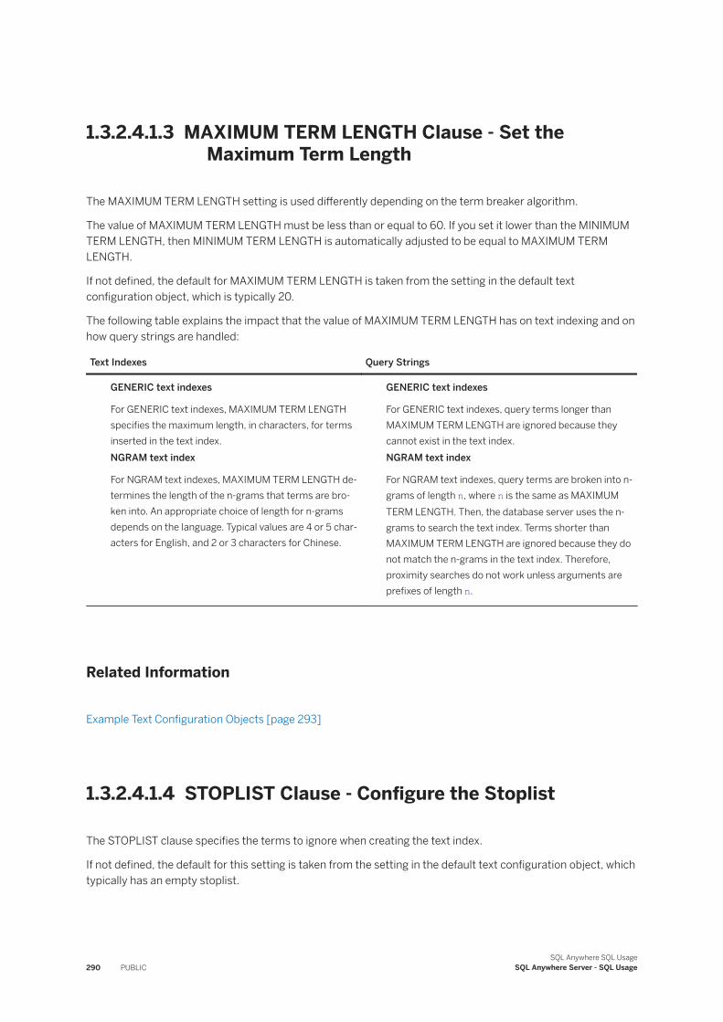
1.3.2.4.1.3 MAXIMUM TERM LENGTH Clause - Set the Maximum Term Length
The MAXIMUM TERM LENGTH setting is used differently depending on the term breaker algorithm.
The value of MAXIMUM TERM LENGTH must be less than or equal to 60. If you set it lower than the MINIMUM TERM LENGTH, then MINIMUM TERM LENGTH is automatically adjusted to be equal to MAXIMUM TERM LENGTH.
If not defined, the default for MAXIMUM TERM LENGTH is taken from the setting in the default text configuration object, which is typically 20.
The following table explains the impact that the value of MAXIMUM TERM LENGTH has on text indexing and on how query strings are handled:
Text Indexes Query Strings
GENERIC text indexes
For GENERIC text indexes, MAXIMUM TERM LENGTH specifies the maximum length, in characters, for terms inserted in the text index.NGRAM text index
For NGRAM text indexes, MAXIMUM TERM LENGTH determines the length of the n-grams that terms are broken into. An appropriate choice of length for n-grams depends on the language. Typical values are 4 or 5 characters for English, and 2 or 3 characters for Chinese.
GENERIC text indexes
For GENERIC text indexes, query terms longer than MAXIMUM TERM LENGTH are ignored because they cannot exist in the text index.NGRAM text index
For NGRAM text indexes, query terms are broken into n-grams of length n, where n is the same as MAXIMUM TERM LENGTH. Then, the database server uses the n-grams to search the text index. Terms shorter than MAXIMUM TERM LENGTH are ignored because they do not match the n-grams in the text index. Therefore, proximity searches do not work unless arguments are prefixes of length n.
Related Information
Example Text Configuration Objects [page 293]
1.3.2.4.1.4 STOPLIST Clause - Configure the Stoplist
The STOPLIST clause specifies the terms to ignore when creating the text index.
If not defined, the default for this setting is taken from the setting in the default text configuration object, which typically has an empty stoplist.
290 PUBLICSQL Anywhere SQL Usage
SQL Anywhere Server - SQL Usage
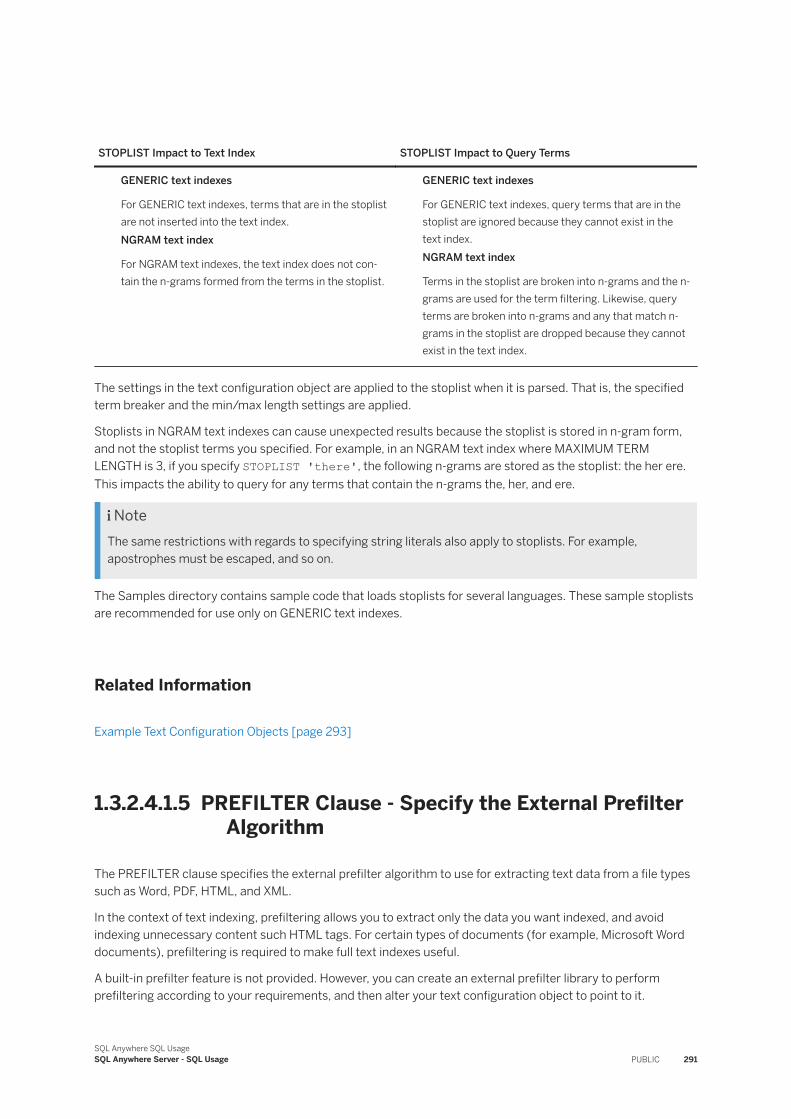
STOPLIST Impact to Text Index STOPLIST Impact to Query Terms
GENERIC text indexes
For GENERIC text indexes, terms that are in the stoplist are not inserted into the text index.NGRAM text index
For NGRAM text indexes, the text index does not contain the n-grams formed from the terms in the stoplist.
GENERIC text indexes
For GENERIC text indexes, query terms that are in the stoplist are ignored because they cannot exist in the text index.NGRAM text index
Terms in the stoplist are broken into n-grams and the n-grams are used for the term filtering. Likewise, query terms are broken into n-grams and any that match n-grams in the stoplist are dropped because they cannot exist in the text index.
The settings in the text configuration object are applied to the stoplist when it is parsed. That is, the specified term breaker and the min/max length settings are applied.
Stoplists in NGRAM text indexes can cause unexpected results because the stoplist is stored in n-gram form, and not the stoplist terms you specified. For example, in an NGRAM text index where MAXIMUM TERM LENGTH is 3, if you specify STOPLIST 'there', the following n-grams are stored as the stoplist: the her ere. This impacts the ability to query for any terms that contain the n-grams the, her, and ere.
NoteThe same restrictions with regards to specifying string literals also apply to stoplists. For example, apostrophes must be escaped, and so on.
The Samples directory contains sample code that loads stoplists for several languages. These sample stoplists are recommended for use only on GENERIC text indexes.
Related Information
Example Text Configuration Objects [page 293]
1.3.2.4.1.5 PREFILTER Clause - Specify the External Prefilter Algorithm
The PREFILTER clause specifies the external prefilter algorithm to use for extracting text data from a file types such as Word, PDF, HTML, and XML.
In the context of text indexing, prefiltering allows you to extract only the data you want indexed, and avoid indexing unnecessary content such HTML tags. For certain types of documents (for example, Microsoft Word documents), prefiltering is required to make full text indexes useful.
A built-in prefilter feature is not provided. However, you can create an external prefilter library to perform prefiltering according to your requirements, and then alter your text configuration object to point to it.
SQL Anywhere SQL UsageSQL Anywhere Server - SQL Usage PUBLIC 291
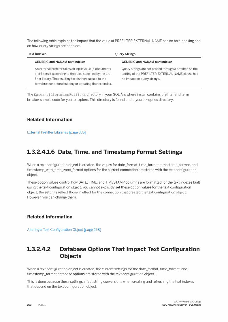
The following table explains the impact that the value of PREFILTER EXTERNAL NAME has on text indexing and on how query strings are handled:
Text Indexes Query Strings
GENERIC and NGRAM text indexes
An external prefilter takes an input value (a document) and filters it according to the rules specified by the prefilter library. The resulting text is then passed to the term breaker before building or updating the text index.
GENERIC and NGRAM text indexes
Query strings are not passed through a prefilter, so the setting of the PREFILTER EXTERNAL NAME clause has no impact on query strings.
The ExternalLibrariesFullText directory in your SQL Anywhere install contains prefilter and term breaker sample code for you to explore. This directory is found under your Samples directory.
Related Information
External Prefilter Libraries [page 335]
1.3.2.4.1.6 Date, Time, and Timestamp Format Settings
When a text configuration object is created, the values for date_format, time_format, timestamp_format, and timestamp_with_time_zone_format options for the current connection are stored with the text configuration object.
These option values control how DATE, TIME, and TIMESTAMP columns are formatted for the text indexes built using the text configuration object. You cannot explicitly set these option values for the text configuration object; the settings reflect those in effect for the connection that created the text configuration object. However, you can change them.
Related Information
Altering a Text Configuration Object [page 258]
1.3.2.4.2 Database Options That Impact Text Configuration Objects
When a text configuration object is created, the current settings for the date_format, time_format, and timestamp_format database options are stored with the text configuration object.
This is done because these settings affect string conversions when creating and refreshing the text indexes that depend on the text configuration object.
292 PUBLICSQL Anywhere SQL Usage
SQL Anywhere Server - SQL Usage
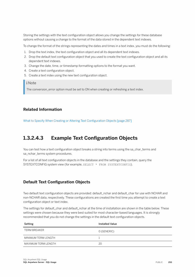
Storing the settings with the text configuration object allows you change the settings for these database options without causing a change to the format of the data stored in the dependent text indexes.
To change the format of the strings representing the dates and times in a text index, you must do the following:
1. Drop the text index, the text configuration object and all its dependent text indexes.2. Drop the default text configuration object that you used to create the text configuration object and all its
dependent text indexes.3. Change the date, time, or timestamp formatting options to the format you want.4. Create a text configuration object.5. Create a text index using the new text configuration object.
NoteThe conversion_error option must be set to ON when creating or refreshing a text index.
Related Information
What to Specify When Creating or Altering Text Configuration Objects [page 287]
1.3.2.4.3 Example Text Configuration Objects
You can test how a text configuration object breaks a string into terms using the sa_char_terms and sa_nchar_terms system procedures.
For a list of all text configuration objects in the database and the settings they contain, query the SYSTEXTCONFIG system view (for example, SELECT * FROM SYSTEXTCONFIG).
Default Text Configuration Objects
Two default text configuration objects are provided: default_nchar and default_char for use with NCHAR and non-NCHAR data, respectively. These configurations are created the first time you attempt to create a text configuration object or text index.
The settings for default_char and default_nchar at the time of installation are shown in the table below. These settings were chosen because they were best suited for most character-based languages. It is strongly recommended that you do not change the settings in the default text configuration objects.
Setting Installed Value
TERM BREAKER 0 (GENERIC)
MINIMUM TERM LENGTH 1
MAXIMUM TERM LENGTH 20
SQL Anywhere SQL UsageSQL Anywhere Server - SQL Usage PUBLIC 293
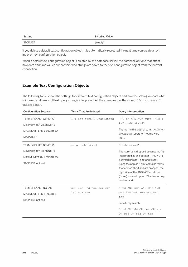
Setting Installed Value
STOPLIST (empty)
If you delete a default text configuration object, it is automatically recreated the next time you create a text index or text configuration object.
When a default text configuration object is created by the database server, the database options that affect how date and time values are converted to strings are saved to the text configuration object from the current connection.
Example Text Configuration Objects
The following table shows the settings for different text configuration objects and how the settings impact what is indexed and how a full text query string is interpreted. All the examples use the string 'I'm not sure I understand'.
Configuration Settings Terms That Are Indexed Query Interpretation
TERM BREAKER GENERIC
MINIMUM TERM LENGTH 1
MAXIMUM TERM LENGTH 20
STOPLIST ''
I m not sure I understand ("I m" AND NOT sure) AND I AND understand'
The 'not' in the original string gets interpreted as an operator, not the word 'not'.
TERM BREAKER GENERIC
MINIMUM TERM LENGTH 2
MAXIMUM TERM LENGTH 20
STOPLIST 'not and'
sure understand 'understand'.
The 'sure' gets dropped because 'not' is interpreted as an operator (AND NOT) between phrase "i am" and "sure". Since the phrase "i am" contains terms that are too short and are dropped, the right side of the AND NOT condition ('sure') is also dropped. This leaves only 'understand'.
TERM BREAKER NGRAM
MAXIMUM TERM LENGTH 3
STOPLIST 'not and'
sur ure und nde der ers rst sta tan
'und AND nde AND der AND ers AND rst AND sta AND tan'.
For a fuzzy search:
'und OR nde OR der OR ers OR rst OR sta OR tan'
294 PUBLICSQL Anywhere SQL Usage
SQL Anywhere Server - SQL Usage
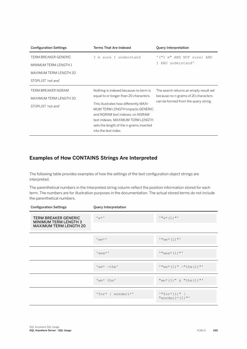
Configuration Settings Terms That Are Indexed Query Interpretation
TERM BREAKER GENERIC
MINIMUM TERM LENGTH 1
MAXIMUM TERM LENGTH 20
STOPLIST 'not and'
I m sure I understand '("I m" AND NOT sure) AND I AND understand'.
TERM BREAKER NGRAM
MAXIMUM TERM LENGTH 20
STOPLIST 'not and'
Nothing is indexed because no term is equal to or longer than 20 characters.
This illustrates how differently MAXIMUM TERM LENGTH impacts GENERIC and NGRAM text indexes; on NGRAM text indexes, MAXIMUM TERM LENGTH sets the length of the n-grams inserted into the text index.
The search returns an empty result set because no n-grams of 20 characters can be formed from the query string.
Examples of How CONTAINS Strings Are Interpreted
The following table provides examples of how the settings of the text configuration object strings are interpreted.
The parenthetical numbers in the Interpreted string column reflect the position information stored for each term. The numbers are for illustration purposes in the documentation. The actual stored terms do not include the parenthetical numbers.
Configuration Settings Query Interpretation
TERM BREAKER GENERICMINIMUM TERM LENGTH 3MAXIMUM TERM LENGTH 20
'w*' '"w*(1)"'
'we*' '"we*(1)"'
'wea*' '"wea*(1)"'
'we* -the' '"we*(1)" -"the(1)"'
'we* the' "we*(1)" & "the(1)"'
'for* | wonderl*' '"for*(1)" | "wonderl*(1)"'
SQL Anywhere SQL UsageSQL Anywhere Server - SQL Usage PUBLIC 295
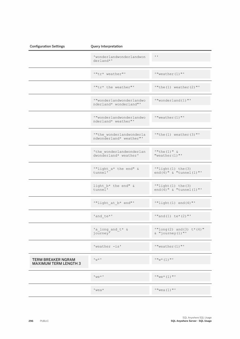
Configuration Settings Query Interpretation
'wonderlandwonderlandwonderland*'
''
'"tr* weather"' '"weather(1)"'
'"tr* the weather"' '"the(1) weather(2)"'
'"wonderlandwonderlandwonderland* wonderland"'
'"wonderland(1)"'
'"wonderlandwonderlandwonderland* weather"'
'"weather(1)"'
'"the_wonderlandwonderlandwonderland* weather"'
'"the(1) weather(3)"'
'the_wonderlandwonderlandwonderland* weather'
'"the(1)" & "weather(1)"'
'"light_a* the end" & tunnel'
'"light(1) the(3) end(4)" & "tunnel(1)"'
light_b* the end" & tunnel'
'"light(1) the(3) end(4)" & "tunnel(1)"'
'"light_at_b* end"' '"light(1) end(4)"'
'and_te*' '"and(1) te*(2)"'
'a_long_and_t* & journey'
'"long(2) and(3) t*(4)" & "journey(1)"'
'weather -is' '"weather(1)"'
TERM BREAKER NGRAMMAXIMUM TERM LENGTH 3
'w*' '"w*(1)"'
'we*' '"we*(1)"'
'wea* '"wea(1)"'
296 PUBLICSQL Anywhere SQL Usage
SQL Anywhere Server - SQL Usage
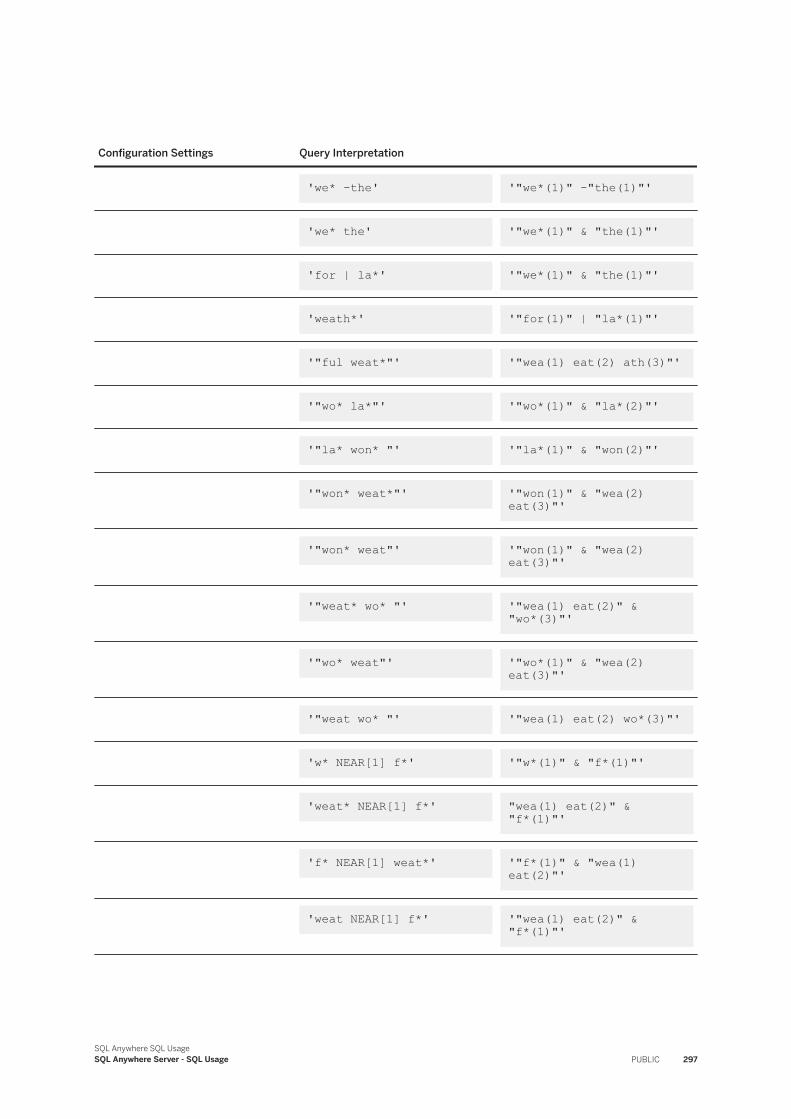
Configuration Settings Query Interpretation
'we* -the' '"we*(1)" -"the(1)"'
'we* the' '"we*(1)" & "the(1)"'
'for | la*' '"we*(1)" & "the(1)"'
'weath*' '"for(1)" | "la*(1)"'
'"ful weat*"' '"wea(1) eat(2) ath(3)"'
'"wo* la*"' '"wo*(1)" & "la*(2)"'
'"la* won* "' '"la*(1)" & "won(2)"'
'"won* weat*"' '"won(1)" & "wea(2) eat(3)"'
'"won* weat"' '"won(1)" & "wea(2) eat(3)"'
'"weat* wo* "' '"wea(1) eat(2)" & "wo*(3)"'
'"wo* weat"' '"wo*(1)" & "wea(2) eat(3)"'
'"weat wo* "' '"wea(1) eat(2) wo*(3)"'
'w* NEAR[1] f*' '"w*(1)" & "f*(1)"'
'weat* NEAR[1] f*' "wea(1) eat(2)" & "f*(1)"'
'f* NEAR[1] weat*' '"f*(1)" & "wea(1) eat(2)"'
'weat NEAR[1] f*' '"wea(1) eat(2)" & "f*(1)"'
SQL Anywhere SQL UsageSQL Anywhere Server - SQL Usage PUBLIC 297
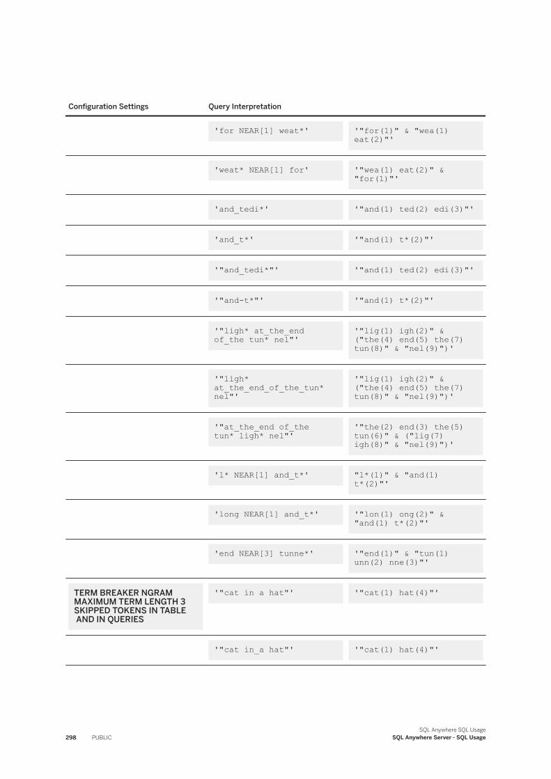
Configuration Settings Query Interpretation
'for NEAR[1] weat*' '"for(1)" & "wea(1) eat(2)"'
'weat* NEAR[1] for' '"wea(1) eat(2)" & "for(1)"'
'and_tedi*' '"and(1) ted(2) edi(3)"'
'and_t*' '"and(1) t*(2)"'
'"and_tedi*"' '"and(1) ted(2) edi(3)"'
'"and-t*"' '"and(1) t*(2)"'
'"ligh* at_the_end of_the tun* nel"'
'"lig(1) igh(2)" & ("the(4) end(5) the(7) tun(8)" & "nel(9)")'
'"ligh* at_the_end_of_the_tun* nel"'
'"lig(1) igh(2)" & ("the(4) end(5) the(7) tun(8)" & "nel(9)")'
'"at_the_end of_the tun* ligh* nel"'
'"the(2) end(3) the(5) tun(6)" & ("lig(7) igh(8)" & "nel(9)")'
'l* NEAR[1] and_t*' "l*(1)" & "and(1) t*(2)"'
'long NEAR[1] and_t*' '"lon(1) ong(2)" & "and(1) t*(2)"'
'end NEAR[3] tunne*' '"end(1)" & "tun(1) unn(2) nne(3)"'
TERM BREAKER NGRAMMAXIMUM TERM LENGTH 3SKIPPED TOKENS IN TABLE AND IN QUERIES
'"cat in a hat"' '"cat(1) hat(4)"'
'"cat in_a hat"' '"cat(1) hat(4)"'
298 PUBLICSQL Anywhere SQL Usage
SQL Anywhere Server - SQL Usage
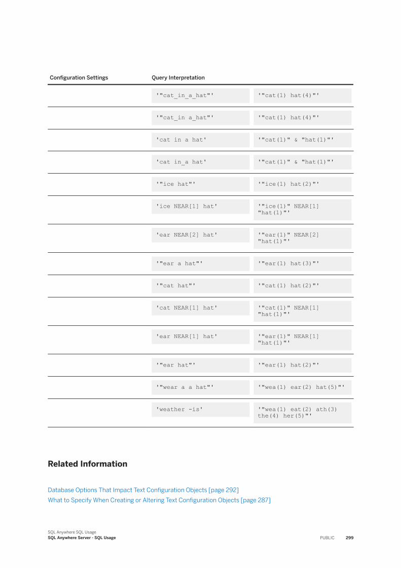
Configuration Settings Query Interpretation
'"cat_in_a_hat"' '"cat(1) hat(4)"'
'"cat_in a_hat"' '"cat(1) hat(4)"'
'cat in a hat' '"cat(1)" & "hat(1)"'
'cat in_a hat' '"cat(1)" & "hat(1)"'
'"ice hat"' '"ice(1) hat(2)"'
'ice NEAR[1] hat' '"ice(1)" NEAR[1] "hat(1)"'
'ear NEAR[2] hat' '"ear(1)" NEAR[2] "hat(1)"'
'"ear a hat"' '"ear(1) hat(3)"'
'"cat hat"' '"cat(1) hat(2)"'
'cat NEAR[1] hat' '"cat(1)" NEAR[1] "hat(1)"'
'ear NEAR[1] hat' '"ear(1)" NEAR[1] "hat(1)"'
'"ear hat"' '"ear(1) hat(2)"'
'"wear a a hat"' '"wea(1) ear(2) hat(5)"'
'weather -is' '"wea(1) eat(2) ath(3) the(4) her(5)"'
Related Information
Database Options That Impact Text Configuration Objects [page 292]What to Specify When Creating or Altering Text Configuration Objects [page 287]
SQL Anywhere SQL UsageSQL Anywhere Server - SQL Usage PUBLIC 299
1.3.2.5 Text Index Concepts and Reference
A text index stores positional information for terms in the indexed columns.
When you perform a full text search, you are searching a text index (not table rows). So, before you can perform a full text search, you must create a text index on the columns you want to search. Queries that use text indexes can be faster than those that must scan all the values in the table.
When you create a text index, you can specify which text configuration object to use when creating and refreshing the text index. A text configuration object contains settings that affect how an index is built. If you do not specify a text configuration object, the database server uses a default configuration object.
You can also specify a refresh type for the text index. The refresh type defines how often the text index is refreshed. A more recently refreshed text index returns more accurate results. However, refreshing takes time and can impede performance. For example, frequent updates to an indexed table can impact performance if the text index is configured to refresh each time the underlying data changes.
You can use the VALIDATE TEXT INDEX statement to verify that the positional information for the terms in the text index is intact. If the positional information is not intact, an error is generated.
To view settings for existing text indexes, use the sa_text_index_stats system procedure.
In this section:
Text Index Refresh Types [page 300]When you create a text index, you must also choose a refresh type that is either immediate, automatic, or manual.
Related Information
Text Configuration Object Concepts and Reference [page 286]
1.3.2.5.1 Text Index Refresh Types
When you create a text index, you must also choose a refresh type that is either immediate, automatic, or manual.
When you create a text index, you must also choose a refresh type. There are three refresh types supported for text indexes: immediate, automatic, and manual. You define the refresh type for a text index at creation time. With the exception of immediate text indexes, you can change the refresh type after creating the text index.
IMMEDIATE REFRESH
IMMEDIATE REFRESH text indexes are refreshed when data in the underlying table or materialized view changes, and are recommended for base tables only when the data must always be up-to-date, when the indexed columns are relatively short, or when the data changes are infrequent.
The default refresh type for text indexes is IMMEDIATE REFRESH. Materialized view text indexes only support IMMEDIATE REFRESH.
300 PUBLICSQL Anywhere SQL Usage
SQL Anywhere Server - SQL Usage
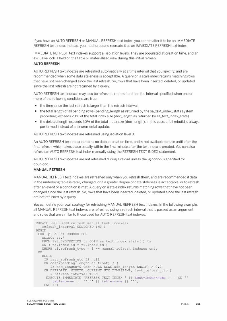
If you have an AUTO REFRESH or MANUAL REFRESH text index, you cannot alter it to be an IMMEDIATE REFRESH text index. Instead, you must drop and recreate it as an IMMEDIATE REFRESH text index.
IMMEDIATE REFRESH text indexes support all isolation levels. They are populated at creation time, and an exclusive lock is held on the table or materialized view during this initial refresh.AUTO REFRESH
AUTO REFRESH text indexes are refreshed automatically at a time interval that you specify, and are recommended when some data staleness is acceptable. A query on a stale index returns matching rows that have not been changed since the last refresh. So, rows that have been inserted, deleted, or updated since the last refresh are not returned by a query.
AUTO REFRESH text indexes may also be refreshed more often than the interval specified when one or more of the following conditions are true:
● the time since the last refresh is larger than the refresh interval.● the total length of all pending rows (pending_length as returned by the sa_text_index_stats system
procedure) exceeds 20% of the total index size (doc_length as returned by sa_text_index_stats).● the deleted length exceeds 50% of the total index size (doc_length). In this case, a full rebuild is always
performed instead of an incremental update.
AUTO REFRESH text indexes are refreshed using isolation level 0.
An AUTO REFRESH text index contains no data at creation time, and is not available for use until after the first refresh, which takes place usually within the first minute after the text index is created. You can also refresh an AUTO REFRESH text index manually using the REFRESH TEXT INDEX statement.
AUTO REFRESH text indexes are not refreshed during a reload unless the -g option is specified for dbunload.MANUAL REFRESH
MANUAL REFRESH text indexes are refreshed only when you refresh them, and are recommended if data in the underlying table is rarely changed, or if a greater degree of data staleness is acceptable, or to refresh after an event or a condition is met. A query on a stale index returns matching rows that have not been changed since the last refresh. So, rows that have been inserted, deleted, or updated since the last refresh are not returned by a query.
You can define your own strategy for refreshing MANUAL REFRESH text indexes. In the following example, all MANUAL REFRESH text indexes are refreshed using a refresh interval that is passed as an argument, and rules that are similar to those used for AUTO REFRESH text indexes.
CREATE PROCEDURE refresh_manual_text_indexes( refresh_interval UNSIGNED INT )BEGIN FOR lp1 AS c1 CURSOR FOR SELECT ts.* FROM SYS.SYSTEXTIDX ti JOIN sa_text_index_stats( ) ts ON ( ts.index_id = ti.index_id ) WHERE ti.refresh_type = 1 -- manual refresh indexes only DO BEGIN IF last_refresh_utc IS null OR cast(pending_length as float) / ( IF doc_length=0 THEN NULL ELSE doc_length ENDIF) > 0.2 OR DATEDIFF( MINUTE, CURRENT UTC TIMESTAMP, last_refresh_utc ) > refresh_interval THEN EXECUTE IMMEDIATE 'REFRESH TEXT INDEX ' || text-index-name || ' ON "' || table-owner || '"."' || table-name || '"'; END IF;
SQL Anywhere SQL UsageSQL Anywhere Server - SQL Usage PUBLIC 301
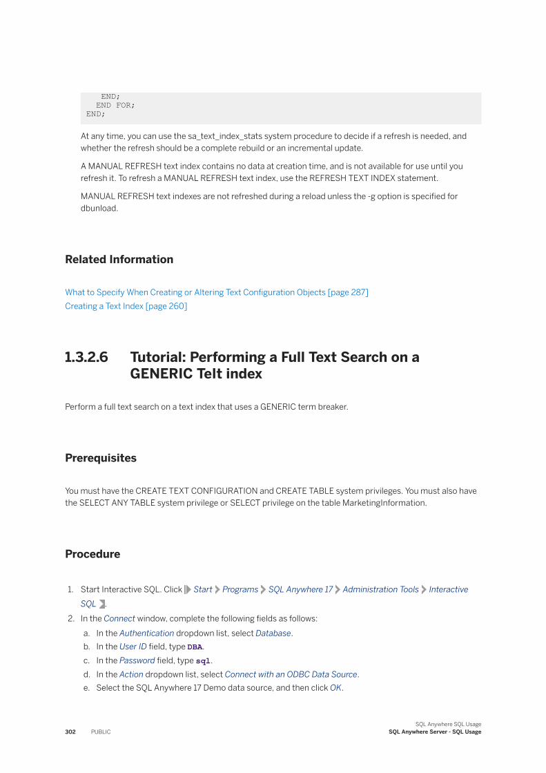
END; END FOR; END;
At any time, you can use the sa_text_index_stats system procedure to decide if a refresh is needed, and whether the refresh should be a complete rebuild or an incremental update.
A MANUAL REFRESH text index contains no data at creation time, and is not available for use until you refresh it. To refresh a MANUAL REFRESH text index, use the REFRESH TEXT INDEX statement.
MANUAL REFRESH text indexes are not refreshed during a reload unless the -g option is specified for dbunload.
Related Information
What to Specify When Creating or Altering Text Configuration Objects [page 287]Creating a Text Index [page 260]
1.3.2.6 Tutorial: Performing a Full Text Search on a GENERIC TeIt index
Perform a full text search on a text index that uses a GENERIC term breaker.
Prerequisites
You must have the CREATE TEXT CONFIGURATION and CREATE TABLE system privileges. You must also have the SELECT ANY TABLE system privilege or SELECT privilege on the table MarketingInformation.
Procedure
1. Start Interactive SQL. Click Start Programs SQL Anywhere 17 Administration Tools Interactive SQL .
2. In the Connect window, complete the following fields as follows:a. In the Authentication dropdown list, select Database.b. In the User ID field, type DBA.c. In the Password field, type sql.d. In the Action dropdown list, select Connect with an ODBC Data Source.e. Select the SQL Anywhere 17 Demo data source, and then click OK.
302 PUBLICSQL Anywhere SQL Usage
SQL Anywhere Server - SQL Usage
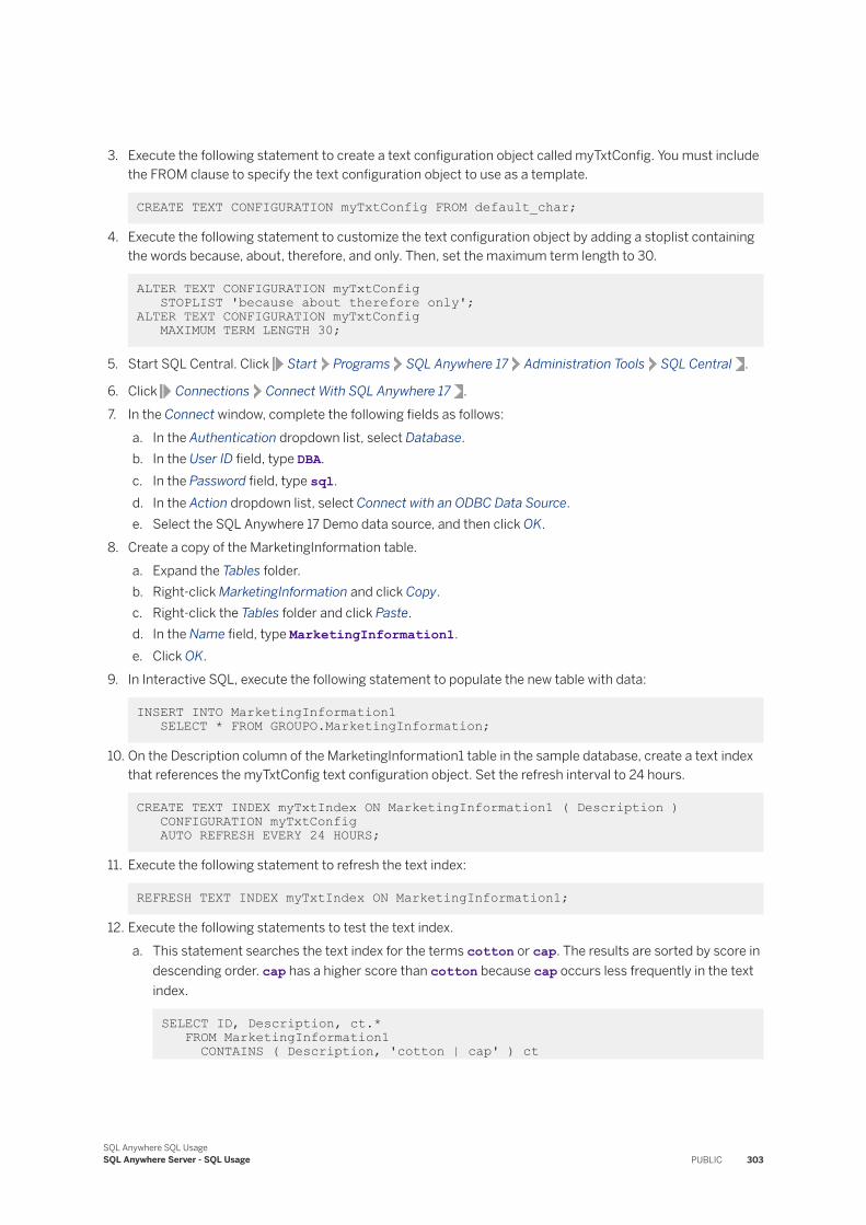
3. Execute the following statement to create a text configuration object called myTxtConfig. You must include the FROM clause to specify the text configuration object to use as a template.
CREATE TEXT CONFIGURATION myTxtConfig FROM default_char;
4. Execute the following statement to customize the text configuration object by adding a stoplist containing the words because, about, therefore, and only. Then, set the maximum term length to 30.
ALTER TEXT CONFIGURATION myTxtConfig STOPLIST 'because about therefore only';ALTER TEXT CONFIGURATION myTxtConfig MAXIMUM TERM LENGTH 30;
5. Start SQL Central. Click Start Programs SQL Anywhere 17 Administration Tools SQL Central .
6. Click Connections Connect With SQL Anywhere 17 .7. In the Connect window, complete the following fields as follows:
a. In the Authentication dropdown list, select Database.b. In the User ID field, type DBA.c. In the Password field, type sql.d. In the Action dropdown list, select Connect with an ODBC Data Source.e. Select the SQL Anywhere 17 Demo data source, and then click OK.
8. Create a copy of the MarketingInformation table.a. Expand the Tables folder.b. Right-click MarketingInformation and click Copy.c. Right-click the Tables folder and click Paste.d. In the Name field, type MarketingInformation1.e. Click OK.
9. In Interactive SQL, execute the following statement to populate the new table with data:
INSERT INTO MarketingInformation1 SELECT * FROM GROUPO.MarketingInformation;
10. On the Description column of the MarketingInformation1 table in the sample database, create a text index that references the myTxtConfig text configuration object. Set the refresh interval to 24 hours.
CREATE TEXT INDEX myTxtIndex ON MarketingInformation1 ( Description ) CONFIGURATION myTxtConfig AUTO REFRESH EVERY 24 HOURS;
11. Execute the following statement to refresh the text index:
REFRESH TEXT INDEX myTxtIndex ON MarketingInformation1;
12. Execute the following statements to test the text index.a. This statement searches the text index for the terms cotton or cap. The results are sorted by score in
descending order. cap has a higher score than cotton because cap occurs less frequently in the text index.
SELECT ID, Description, ct.* FROM MarketingInformation1 CONTAINS ( Description, 'cotton | cap' ) ct
SQL Anywhere SQL UsageSQL Anywhere Server - SQL Usage PUBLIC 303
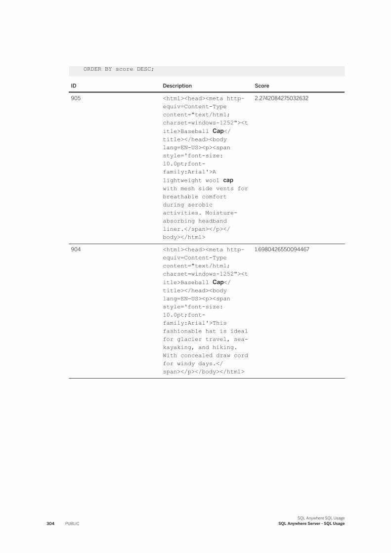
ORDER BY score DESC;
ID Description Score
905 <html><head><meta http-equiv=Content-Type content="text/html; charset=windows-1252"><title>Baseball Cap</title></head><body lang=EN-US><p><span style='font-size:10.0pt;font-family:Arial'>A lightweight wool cap with mesh side vents for breathable comfort during aerobic activities. Moisture-absorbing headband liner.</span></p></body></html>
2.2742084275032632
904 <html><head><meta http-equiv=Content-Type content="text/html; charset=windows-1252"><title>Baseball Cap</title></head><body lang=EN-US><p><span style='font-size:10.0pt;font-family:Arial'>This fashionable hat is ideal for glacier travel, sea-kayaking, and hiking. With concealed draw cord for windy days.</span></p></body></html>
1.6980426550094467
304 PUBLICSQL Anywhere SQL Usage
SQL Anywhere Server - SQL Usage
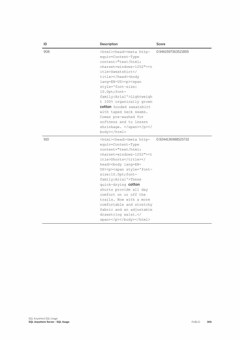
ID Description Score
908 <html><head><meta http-equiv=Content-Type content="text/html; charset=windows-1252"><title>Sweatshirt</title></head><body lang=EN-US><p><span style='font-size:10.0pt;font-family:Arial'>Lightweight 100% organically grown cotton hooded sweatshirt with taped neck seams. Comes pre-washed for softness and to lessen shrinkage. </span></p></body></html>
0.9461597363521859
910 <html><head><meta http-equiv=Content-Type content="text/html; charset=windows-1252"><title>Shorts</title></head><body lang=EN-US><p><span style='font-size:10.0pt;font-family:Arial'>These quick-drying cotton shorts provide all day comfort on or off the trails. Now with a more comfortable and stretchy fabric and an adjustable drawstring waist.</span></p></body></html>
0.9244136988525732
SQL Anywhere SQL UsageSQL Anywhere Server - SQL Usage PUBLIC 305
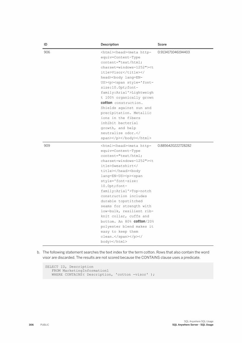
ID Description Score
906 <html><head><meta http-equiv=Content-Type content="text/html; charset=windows-1252"><title>Visor</title></head><body lang=EN-US><p><span style='font-size:10.0pt;font-family:Arial'>Lightweight 100% organically grown cotton construction. Shields against sun and precipitation. Metallic ions in the fibers inhibit bacterial growth, and help neutralize odor.</span></p></body></html>
0.9134171046194403
909 <html><head><meta http-equiv=Content-Type content="text/html; charset=windows-1252"><title>Sweatshirt</title></head><body lang=EN-US><p><span style='font-size:10.0pt;font-family:Arial'>Top-notch construction includes durable topstitched seams for strength with low-bulk, resilient rib-knit collar, cuffs and bottom. An 80% cotton/20% polyester blend makes it easy to keep them clean.</span></p></body></html>
0.8856420222728282
b. The following statement searches the text index for the term cotton. Rows that also contain the word visor are discarded. The results are not scored because the CONTAINS clause uses a predicate.
SELECT ID, Description FROM MarketingInformation1 WHERE CONTAINS( Description, 'cotton -visor' );
306 PUBLICSQL Anywhere SQL Usage
SQL Anywhere Server - SQL Usage
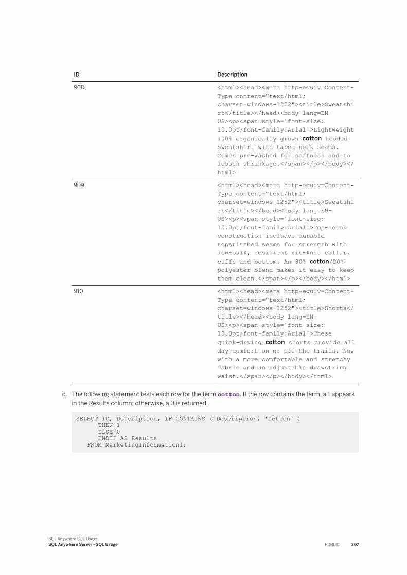
ID Description
908 <html><head><meta http-equiv=Content-Type content="text/html; charset=windows-1252"><title>Sweatshirt</title></head><body lang=EN-US><p><span style='font-size:10.0pt;font-family:Arial'>Lightweight 100% organically grown cotton hooded sweatshirt with taped neck seams. Comes pre-washed for softness and to lessen shrinkage.</span></p></body></html>
909 <html><head><meta http-equiv=Content-Type content="text/html; charset=windows-1252"><title>Sweatshirt</title></head><body lang=EN-US><p><span style='font-size:10.0pt;font-family:Arial'>Top-notch construction includes durable topstitched seams for strength with low-bulk, resilient rib-knit collar, cuffs and bottom. An 80% cotton/20% polyester blend makes it easy to keep them clean.</span></p></body></html>
910 <html><head><meta http-equiv=Content-Type content="text/html; charset=windows-1252"><title>Shorts</title></head><body lang=EN-US><p><span style='font-size:10.0pt;font-family:Arial'>These quick-drying cotton shorts provide all day comfort on or off the trails. Now with a more comfortable and stretchy fabric and an adjustable drawstring waist.</span></p></body></html>
c. The following statement tests each row for the term cotton. If the row contains the term, a 1 appears in the Results column; otherwise, a 0 is returned.
SELECT ID, Description, IF CONTAINS ( Description, 'cotton' ) THEN 1 ELSE 0 ENDIF AS Results FROM MarketingInformation1;
SQL Anywhere SQL UsageSQL Anywhere Server - SQL Usage PUBLIC 307
ID Description Results
901 <html><head><meta http-equiv=Content-Type content="text/html; charset=windows-1252"><title>Tee Shirt</title></head><body lang=EN-US><p><span style='font-size:10.0pt;font-family:Arial'>We've improved the design of this perennial favorite. A sleek and technical shirt built for the trail, track, or sidewalk. UPF rating of 50+.</span></p></body></html>
0
902 <html><head><meta http-equiv=Content-Type content="text/html; charset=windows-1252"><title>Tee Shirt</title></head><body lang=EN-US><p><span style='font-size:10.0pt;font-family:Arial'>This simple, sleek, and lightweight technical shirt is designed for high-intensity workouts in hot and humid weather. The recycled polyester fabric is gentle on the earth and soft against your skin.</span></p></body></html>
0
308 PUBLICSQL Anywhere SQL Usage
SQL Anywhere Server - SQL Usage
ID Description Results
903 <html><head><meta http-equiv=Content-Type content="text/html; charset=windows-1252"><title>Tee Shirt</title></head><body lang=EN-US><p><span style='font-size:10.0pt;font-family:Arial'>A sporty, casual shirt made of recycled water bottles. It will serve you equally well on trails or around town. The fabric has a wicking finish to pull perspiration away from your skin.</span></p></body></html>
0
904 <html><head><meta http-equiv=Content-Type content="text/html; charset=windows-1252"><title>Baseball Cap</title></head><body lang=EN-US><p><span style='font-size:10.0pt;font-family:Arial'>This fashionable hat is ideal for glacier travel, sea-kayaking, and hiking. With concealed draw cord for windy days.</span></p></body></html>
0
SQL Anywhere SQL UsageSQL Anywhere Server - SQL Usage PUBLIC 309
ID Description Results
905 <html><head><meta http-equiv=Content-Type content="text/html; charset=windows-1252"><title>Baseball Cap</title></head><body lang=EN-US><p><span style='font-size:10.0pt;font-family:Arial'>A lightweight wool cap with mesh side vents for breathable comfort during aerobic activities. Moisture-absorbing headband liner.</span></p></body></html>
0
906 <html><head><meta http-equiv=Content-Type content="text/html; charset=windows-1252"><title>Visor</title></head><body lang=EN-US><p><span style='font-size:10.0pt;font-family:Arial'>Lightweight 100% organically grown cotton construction. Shields against sun and precipitation. Metallic ions in the fibers inhibit bacterial growth, and help neutralize odor.</span></p></body></html>
1
310 PUBLICSQL Anywhere SQL Usage
SQL Anywhere Server - SQL Usage
ID Description Results
907 <html><head><meta http-equiv=Content-Type content="text/html; charset=windows-1252"><title>Visor</title></head><body lang=EN-US><p><span style='font-size:10.0pt;font-family:Arial'>A polycarbonate visor with an abrasion-resistant coating on the outside. Great for jogging in the spring, summer, and early fall. The elastic headband has plenty of stretch to give you a snug yet comfortable fit every time you wear it.</span></p></body></html>
0
908 <html><head><meta http-equiv=Content-Type content="text/html; charset=windows-1252"><title>Sweatshirt</title></head><body lang=EN-US><p><span style='font-size:10.0pt;font-family:Arial'>Lightweight 100% organically grown cotton hooded sweatshirt with taped neck seams. Comes pre-washed for softness and to lessen shrinkage.</span></p></body></html>
1
SQL Anywhere SQL UsageSQL Anywhere Server - SQL Usage PUBLIC 311
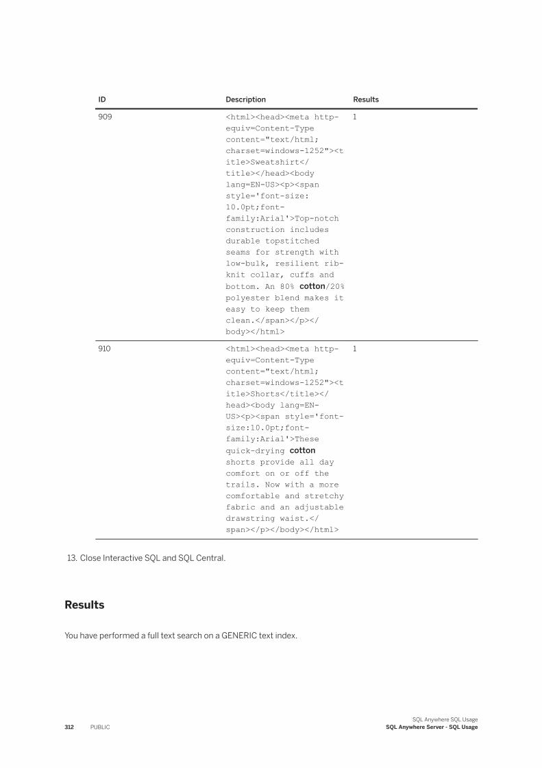
ID Description Results
909 <html><head><meta http-equiv=Content-Type content="text/html; charset=windows-1252"><title>Sweatshirt</title></head><body lang=EN-US><p><span style='font-size:10.0pt;font-family:Arial'>Top-notch construction includes durable topstitched seams for strength with low-bulk, resilient rib-knit collar, cuffs and bottom. An 80% cotton/20% polyester blend makes it easy to keep them clean.</span></p></body></html>
1
910 <html><head><meta http-equiv=Content-Type content="text/html; charset=windows-1252"><title>Shorts</title></head><body lang=EN-US><p><span style='font-size:10.0pt;font-family:Arial'>These quick-drying cotton shorts provide all day comfort on or off the trails. Now with a more comfortable and stretchy fabric and an adjustable drawstring waist.</span></p></body></html>
1
13. Close Interactive SQL and SQL Central.
Results
You have performed a full text search on a GENERIC text index.
312 PUBLICSQL Anywhere SQL Usage
SQL Anywhere Server - SQL Usage
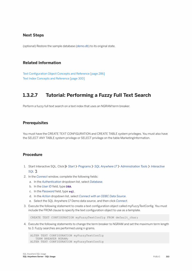
Next Steps
(optional) Restore the sample database (demo.db) to its original state.
Related Information
Text Configuration Object Concepts and Reference [page 286]Text Index Concepts and Reference [page 300]
1.3.2.7 Tutorial: Performing a Fuzzy Full Text Search
Perform a fuzzy full text search on a text index that uses an NGRAM term breaker.
Prerequisites
You must have the CREATE TEXT CONFIGURATION and CREATE TABLE system privileges. You must also have the SELECT ANY TABLE system privilege or SELECT privilege on the table MarketingInformation.
Procedure
1. Start Interactive SQL. Click Start Programs SQL Anywhere 17 Administration Tools Interactive SQL .
2. In the Connect window, complete the following fields:a. In the Authentication dropdown list, select Database.b. In the User ID field, type DBA.c. In the Password field, type sql.d. In the Action dropdown list, select Connect with an ODBC Data Source.e. Select the SQL Anywhere 17 Demo data source, and then click Connect.
3. Execute the following statement to create a text configuration object called myFuzzyTextConfig. You must include the FROM clause to specify the text configuration object to use as a template.
CREATE TEXT CONFIGURATION myFuzzyTextConfig FROM default_char;
4. Execute the following statements to change the term breaker to NGRAM and set the maximum term length to 3. Fuzzy searches are performed using n-grams.
ALTER TEXT CONFIGURATION myFuzzyTextConfig TERM BREAKER NGRAM;ALTER TEXT CONFIGURATION myFuzzyTextConfig
SQL Anywhere SQL UsageSQL Anywhere Server - SQL Usage PUBLIC 313
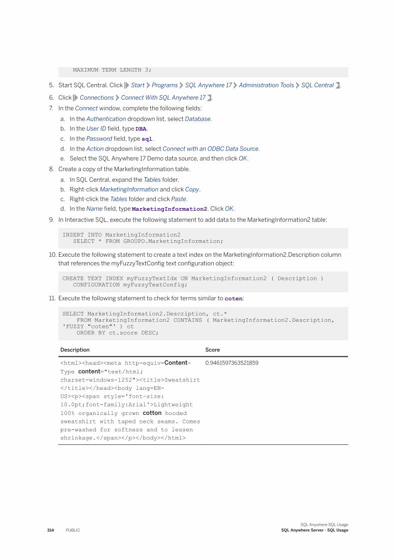
MAXIMUM TERM LENGTH 3;
5. Start SQL Central. Click Start Programs SQL Anywhere 17 Administration Tools SQL Central .
6. Click Connections Connect With SQL Anywhere 17 .7. In the Connect window, complete the following fields:
a. In the Authentication dropdown list, select Database.b. In the User ID field, type DBA.c. In the Password field, type sql.d. In the Action dropdown list, select Connect with an ODBC Data Source.e. Select the SQL Anywhere 17 Demo data source, and then click OK.
8. Create a copy of the MarketingInformation table.a. In SQL Central, expand the Tables folder.b. Right-click MarketingInformation and click Copy.c. Right-click the Tables folder and click Paste.d. In the Name field, type MarketingInformation2. Click OK.
9. In Interactive SQL, execute the following statement to add data to the MarketingInformation2 table:
INSERT INTO MarketingInformation2 SELECT * FROM GROUPO.MarketingInformation;
10. Execute the following statement to create a text index on the MarketingInformation2.Description column that references the myFuzzyTextConfig text configuration object:
CREATE TEXT INDEX myFuzzyTextIdx ON MarketingInformation2 ( Description ) CONFIGURATION myFuzzyTextConfig;
11. Execute the following statement to check for terms similar to coten:
SELECT MarketingInformation2.Description, ct.* FROM MarketingInformation2 CONTAINS ( MarketingInformation2.Description, 'FUZZY "coten"' ) ct ORDER BY ct.score DESC;
Description Score
<html><head><meta http-equiv=Content-Type content="text/html; charset=windows-1252"><title>Sweatshirt</title></head><body lang=EN-US><p><span style='font-size:10.0pt;font-family:Arial'>Lightweight 100% organically grown cotton hooded sweatshirt with taped neck seams. Comes pre-washed for softness and to lessen shrinkage.</span></p></body></html>
0.9461597363521859
314 PUBLICSQL Anywhere SQL Usage
SQL Anywhere Server - SQL Usage
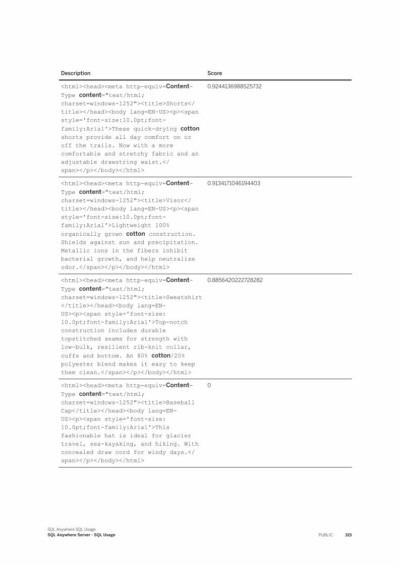
Description Score
<html><head><meta http-equiv=Content-Type content="text/html; charset=windows-1252"><title>Shorts</title></head><body lang=EN-US><p><span style='font-size:10.0pt;font-family:Arial'>These quick-drying cotton shorts provide all day comfort on or off the trails. Now with a more comfortable and stretchy fabric and an adjustable drawstring waist.</span></p></body></html>
0.9244136988525732
<html><head><meta http-equiv=Content-Type content="text/html; charset=windows-1252"><title>Visor</title></head><body lang=EN-US><p><span style='font-size:10.0pt;font-family:Arial'>Lightweight 100% organically grown cotton construction. Shields against sun and precipitation. Metallic ions in the fibers inhibit bacterial growth, and help neutralize odor.</span></p></body></html>
0.9134171046194403
<html><head><meta http-equiv=Content-Type content="text/html; charset=windows-1252"><title>Sweatshirt</title></head><body lang=EN-US><p><span style='font-size:10.0pt;font-family:Arial'>Top-notch construction includes durable topstitched seams for strength with low-bulk, resilient rib-knit collar, cuffs and bottom. An 80% cotton/20% polyester blend makes it easy to keep them clean.</span></p></body></html>
0.8856420222728282
<html><head><meta http-equiv=Content-Type content="text/html; charset=windows-1252"><title>Baseball Cap</title></head><body lang=EN-US><p><span style='font-size:10.0pt;font-family:Arial'>This fashionable hat is ideal for glacier travel, sea-kayaking, and hiking. With concealed draw cord for windy days.</span></p></body></html>
0
SQL Anywhere SQL UsageSQL Anywhere Server - SQL Usage PUBLIC 315
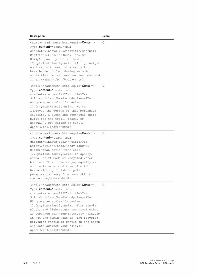
Description Score
<html><head><meta http-equiv=Content-Type content="text/html; charset=windows-1252"><title>Baseball Cap</title></head><body lang=EN-US><p><span style='font-size:10.0pt;font-family:Arial'>A lightweight wool cap with mesh side vents for breathable comfort during aerobic activities. Moisture-absorbing headband liner.</span></p></body></html>
0
<html><head><meta http-equiv=Content-Type content="text/html; charset=windows-1252"><title>Tee Shirt</title></head><body lang=EN-US><p><span style='font-size:10.0pt;font-family:Arial'>We've improved the design of this perennial favorite. A sleek and technical shirt built for the trail, track, or sidewalk. UPF rating of 50+.</span></p></body></html>
0
<html><head><meta http-equiv=Content-Type content="text/html; charset=windows-1252"><title>Tee Shirt</title></head><body lang=EN-US><p><span style='font-size:10.0pt;font-family:Arial'>A sporty, casual shirt made of recycled water bottles. It will serve you equally well on trails or around town. The fabric has a wicking finish to pull perspiration away from your skin.</span></p></body></html>
0
<html><head><meta http-equiv=Content-Type content="text/html; charset=windows-1252"><title>Tee Shirt</title></head><body lang=EN-US><p><span style='font-size:10.0pt;font-family:Arial'>This simple, sleek, and lightweight technical shirt is designed for high-intensity workouts in hot and humid weather. The recycled polyester fabric is gentle on the earth and soft against your skin.</span></p></body></html>
0
316 PUBLICSQL Anywhere SQL Usage
SQL Anywhere Server - SQL Usage
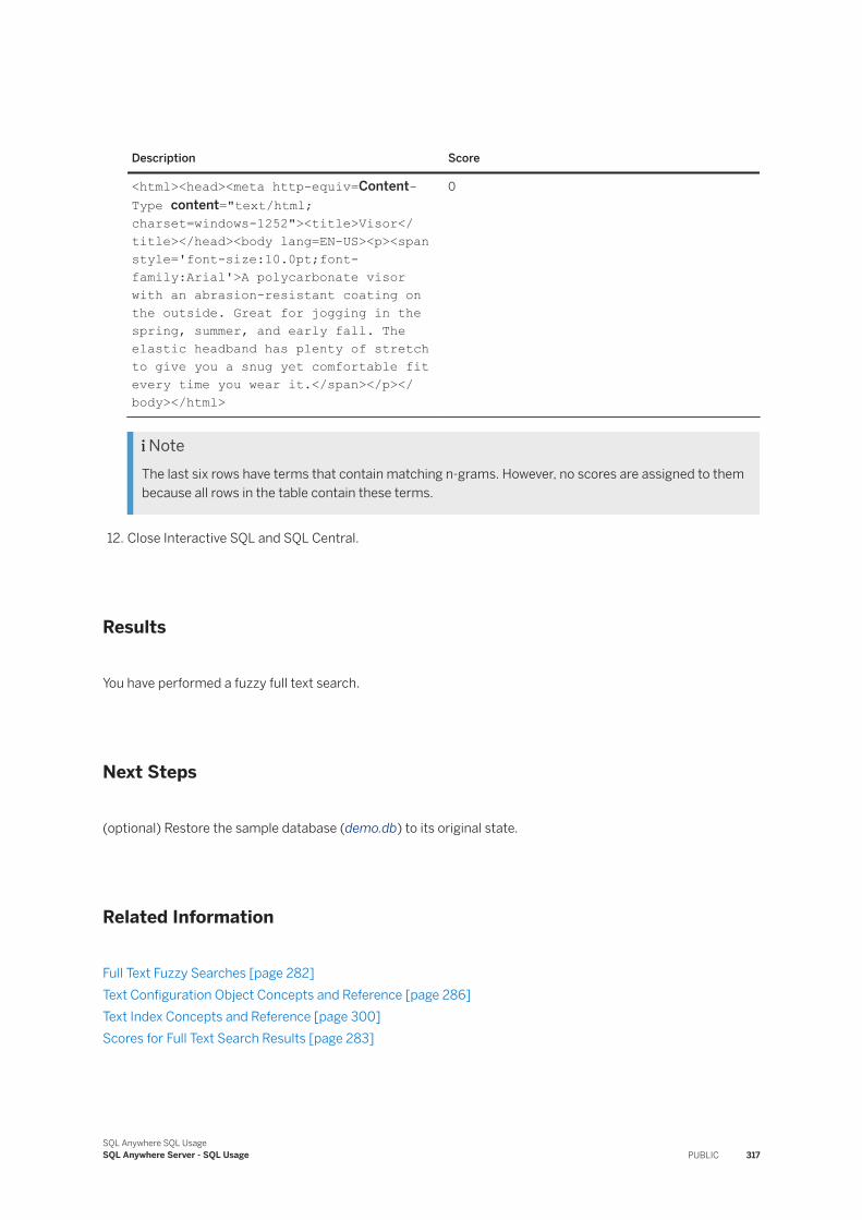
Description Score
<html><head><meta http-equiv=Content-Type content="text/html; charset=windows-1252"><title>Visor</title></head><body lang=EN-US><p><span style='font-size:10.0pt;font-family:Arial'>A polycarbonate visor with an abrasion-resistant coating on the outside. Great for jogging in the spring, summer, and early fall. The elastic headband has plenty of stretch to give you a snug yet comfortable fit every time you wear it.</span></p></body></html>
0
NoteThe last six rows have terms that contain matching n-grams. However, no scores are assigned to them because all rows in the table contain these terms.
12. Close Interactive SQL and SQL Central.
Results
You have performed a fuzzy full text search.
Next Steps
(optional) Restore the sample database (demo.db) to its original state.
Related Information
Full Text Fuzzy Searches [page 282]Text Configuration Object Concepts and Reference [page 286]Text Index Concepts and Reference [page 300]Scores for Full Text Search Results [page 283]
SQL Anywhere SQL UsageSQL Anywhere Server - SQL Usage PUBLIC 317
1.3.2.8 Tutorial: Performing a Non-fuzzy Full Text Search on an NGRAM Text Index
Perform a non-fuzzy full text search on a text index that uses an NGRAM term breaker. This procedure can also be used to create a full text search of Chinese, Japanese, or Korean data.
Prerequisites
You must have the CREATE TEXT CONFIGURATION and CREATE TABLE system privileges. You must also have the SELECT ANY TABLE system privilege or SELECT privilege on the table MarketingInformation.
Context
In databases with multibyte character sets, some punctuation and space characters such as full width commas and full width spaces may be treated as alphanumeric characters.
Procedure
1. Start Interactive SQL. Click Start Programs SQL Anywhere 17 Administration Tools Interactive SQL .
2. In the Connect window, complete the following fields:a. In the Authentication dropdown list, select Database.b. In the User ID field, type DBA.c. In the Password field, type sql.d. In the Action dropdown list, select Connect with an ODBC Data Source.e. Select the SQL Anywhere 17 Demo data source, and then click OK.f. Click Connect.
3. Execute the following statement to create an NCHAR text configuration object named myNcharNGRAMTextConfig:
CREATE TEXT CONFIGURATION myNcharNGRAMTextConfig FROM default_nchar;
4. Execute the following statements to change the TERM BREAKER algorithm to NGRAM and to set the MAXIMUM TERM LENGTH to 2:
ALTER TEXT CONFIGURATION myNcharNGRAMTextConfig TERM BREAKER NGRAM;ALTER TEXT CONFIGURATION myNcharNGRAMTextConfig MAXIMUM TERM LENGTH 2;
318 PUBLICSQL Anywhere SQL Usage
SQL Anywhere Server - SQL Usage
For Chinese, Japanese, and Korean data, the recommended value for N is 2 or 3. For searches limited to one or two characters, set the N value to 1. Setting the N value to 1 can cause slower execution of long queries.
5. Start SQL Central. Click Start Programs SQL Anywhere 17 Administration Tools SQL Central .
6. Click Connections Connect With SQL Anywhere 17 .7. In the Connect window, complete the following fields:
a. In the Authentication dropdown list, select Database.b. In the User ID field, type DBA.c. In the Password field, type sql.d. In the Action dropdown list, select Connect with an ODBC Data Source.e. Select the SQL Anywhere 17 Demo data source, and then click OK.f. Click Connect.
8. Create a copy of the MarketingInformation table.a. Expand the Tables folder.b. Right-click MarketingInformation and click Copy.c. Right-click the Tables folder and click Paste.d. In the Name field, type MarketingInformationNgram.e. Click OK.
9. In Interactive SQL, execute the following statement to add data to the MarketingInformationNgram table:
INSERT INTO MarketingInformationNgram SELECT * FROM GROUPO.MarketingInformation; COMMIT;
10. Execute the following statement to create an IMMEDIATE REFRESH text index on the MarketingInformationNgram.Description column using the myNcharNGRAMTextConfig text configuration object:
CREATE TEXT INDEX ncharNGRAMTextIndex ON MarketingInformationNgram( Description ) CONFIGURATION myNcharNGRAMTextConfig;
11. Test the text index.a. The following statement searches the 2-GRAM text index for terms containing sw. The results are
sorted by score in descending order.
SELECT M.Description, ct.* FROM MarketingInformationNgram AS M CONTAINS( M.Description, 'sw' ) ct ORDER BY ct.score DESC;
SQL Anywhere SQL UsageSQL Anywhere Server - SQL Usage PUBLIC 319
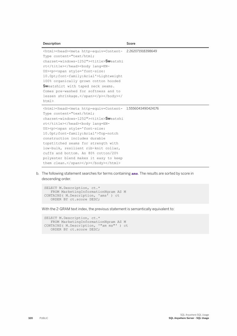
Description Score
<html><head><meta http-equiv=Content-Type content="text/html; charset=windows-1252"><title>Sweatshirt</title></head><body lang=EN-US><p><span style='font-size:10.0pt;font-family:Arial'>Lightweight 100% organically grown cotton hooded Sweatshirt with taped neck seams. Comes pre-washed for softness and to lessen shrinkage.</span></p></body></html>
2.262071918398649
<html><head><meta http-equiv=Content-Type content="text/html; charset=windows-1252"><title>Sweatshirt</title></head><body lang=EN-US><p><span style='font-size:10.0pt;font-family:Arial'>Top-notch construction includes durable topstitched seams for strength with low-bulk, resilient rib-knit collar, cuffs and bottom. An 80% cotton/20% polyester blend makes it easy to keep them clean.</span></p></body></html>
1.5556043490424176
b. The following statement searches for terms containing ams. The results are sorted by score in descending order.
SELECT M.Description, ct.* FROM MarketingInformationNgram AS M CONTAINS( M.Description, 'ams' ) ct ORDER BY ct.score DESC;
With the 2-GRAM text index, the previous statement is semantically equivalent to:
SELECT M.Description, ct.* FROM MarketingInformationNgram AS M CONTAINS( M.Description, '"am ms"' ) ct ORDER BY ct.score DESC;
320 PUBLICSQL Anywhere SQL Usage
SQL Anywhere Server - SQL Usage
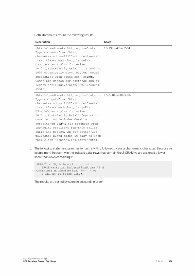
Both statements return the following results:
Description Score
<html><head><meta http-equiv=Content-Type content="text/html; charset=windows-1252"><title>Sweatshirt</title></head><body lang=EN-US><p><span style='font-size:10.0pt;font-family:Arial'>Lightweight 100% organically grown cotton hooded sweatshirt with taped neck seams. Comes pre-washed for softness and to lessen shrinkage.</span></p></body></html>
1.6619019465461564
<html><head><meta http-equiv=Content-Type content="text/html; charset=windows-1252"><title>Sweatshirt</title></head><body lang=EN-US><p><span style='font-size:10.0pt;font-family:Arial'>Top-notch construction includes durable topstitched seams for strength with low-bulk, resilient rib-knit collar, cuffs and bottom. An 80% cotton/20% polyester blend makes it easy to keep them clean.</span></p></body></html>
1.5556043490424176
c. The following statement searches for terms with v followed by any alphanumeric character. Because ve occurs more frequently in the indexed data, rows that contain the 2-GRAM ve are assigned a lower score than rows containing vi.
SELECT M.ID, M.Description, ct.* FROM MarketingInformationNgram AS M CONTAINS( M.Description, 'v*' ) ct ORDER BY ct.score DESC;
The results are sorted by score in descending order.
SQL Anywhere SQL UsageSQL Anywhere Server - SQL Usage PUBLIC 321
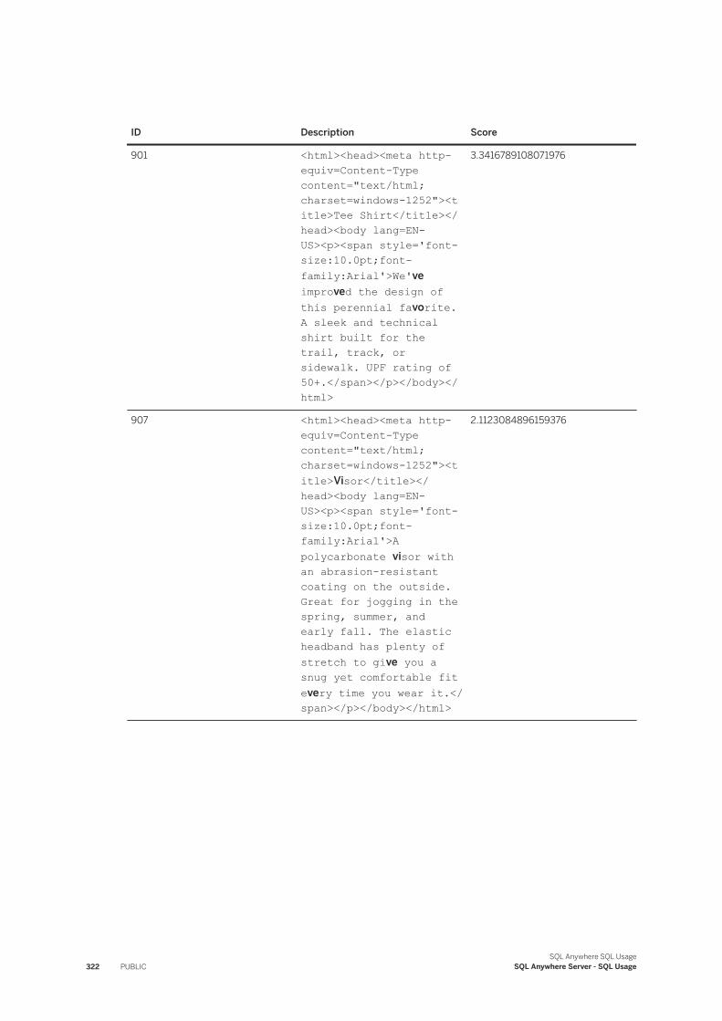
ID Description Score
901 <html><head><meta http-equiv=Content-Type content="text/html; charset=windows-1252"><title>Tee Shirt</title></head><body lang=EN-US><p><span style='font-size:10.0pt;font-family:Arial'>We've improved the design of this perennial favorite. A sleek and technical shirt built for the trail, track, or sidewalk. UPF rating of 50+.</span></p></body></html>
3.3416789108071976
907 <html><head><meta http-equiv=Content-Type content="text/html; charset=windows-1252"><title>Visor</title></head><body lang=EN-US><p><span style='font-size:10.0pt;font-family:Arial'>A polycarbonate visor with an abrasion-resistant coating on the outside. Great for jogging in the spring, summer, and early fall. The elastic headband has plenty of stretch to give you a snug yet comfortable fit every time you wear it.</span></p></body></html>
2.1123084896159376
322 PUBLICSQL Anywhere SQL Usage
SQL Anywhere Server - SQL Usage
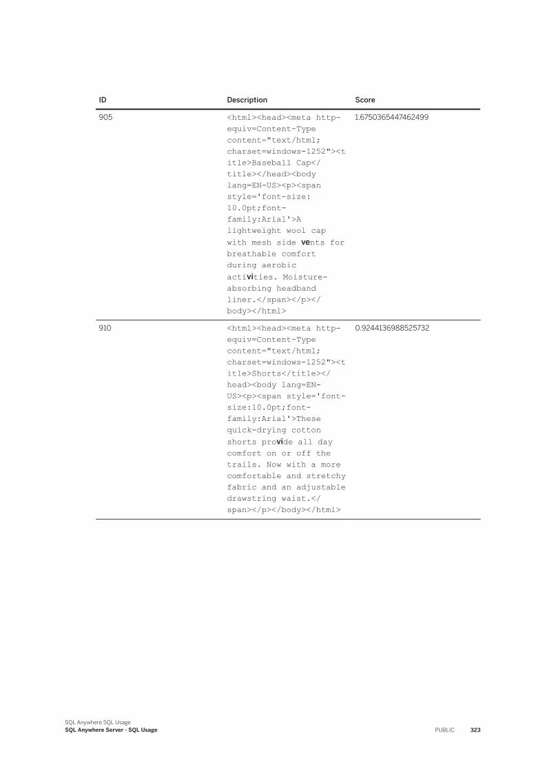
ID Description Score
905 <html><head><meta http-equiv=Content-Type content="text/html; charset=windows-1252"><title>Baseball Cap</title></head><body lang=EN-US><p><span style='font-size:10.0pt;font-family:Arial'>A lightweight wool cap with mesh side vents for breathable comfort during aerobic activities. Moisture-absorbing headband liner.</span></p></body></html>
1.6750365447462499
910 <html><head><meta http-equiv=Content-Type content="text/html; charset=windows-1252"><title>Shorts</title></head><body lang=EN-US><p><span style='font-size:10.0pt;font-family:Arial'>These quick-drying cotton shorts provide all day comfort on or off the trails. Now with a more comfortable and stretchy fabric and an adjustable drawstring waist.</span></p></body></html>
0.9244136988525732
SQL Anywhere SQL UsageSQL Anywhere Server - SQL Usage PUBLIC 323
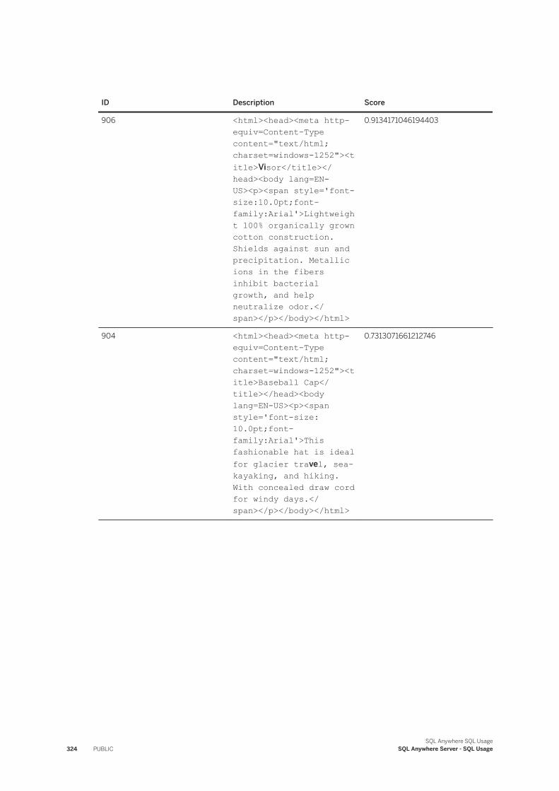
ID Description Score
906 <html><head><meta http-equiv=Content-Type content="text/html; charset=windows-1252"><title>Visor</title></head><body lang=EN-US><p><span style='font-size:10.0pt;font-family:Arial'>Lightweight 100% organically grown cotton construction. Shields against sun and precipitation. Metallic ions in the fibers inhibit bacterial growth, and help neutralize odor.</span></p></body></html>
0.9134171046194403
904 <html><head><meta http-equiv=Content-Type content="text/html; charset=windows-1252"><title>Baseball Cap</title></head><body lang=EN-US><p><span style='font-size:10.0pt;font-family:Arial'>This fashionable hat is ideal for glacier travel, sea-kayaking, and hiking. With concealed draw cord for windy days.</span></p></body></html>
0.7313071661212746
324 PUBLICSQL Anywhere SQL Usage
SQL Anywhere Server - SQL Usage
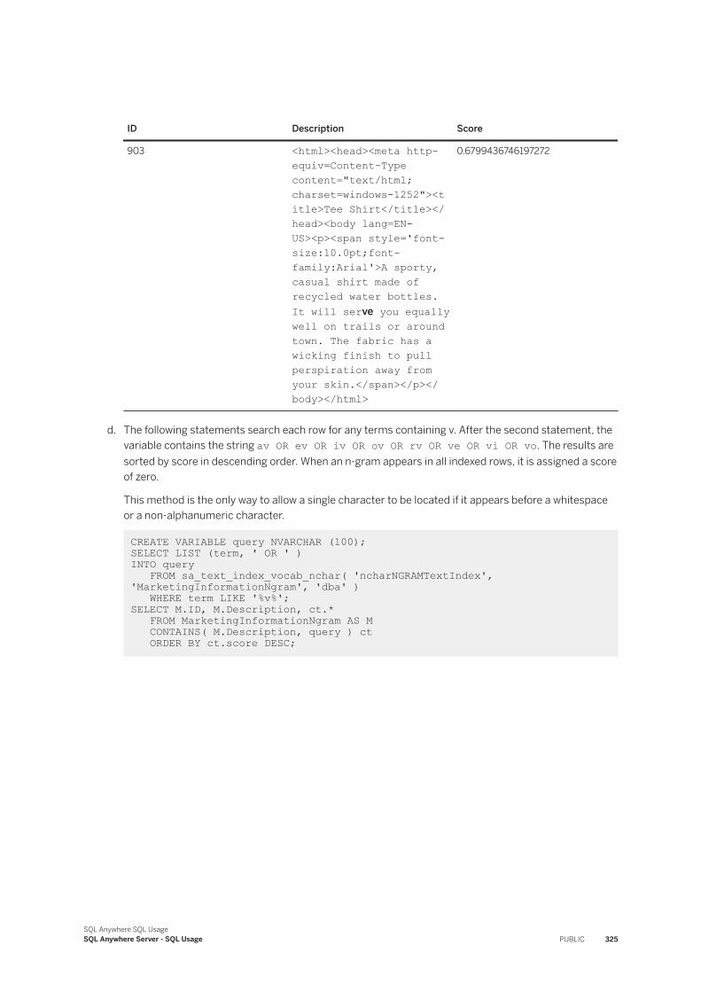
ID Description Score
903 <html><head><meta http-equiv=Content-Type content="text/html; charset=windows-1252"><title>Tee Shirt</title></head><body lang=EN-US><p><span style='font-size:10.0pt;font-family:Arial'>A sporty, casual shirt made of recycled water bottles. It will serve you equally well on trails or around town. The fabric has a wicking finish to pull perspiration away from your skin.</span></p></body></html>
0.6799436746197272
d. The following statements search each row for any terms containing v. After the second statement, the variable contains the string av OR ev OR iv OR ov OR rv OR ve OR vi OR vo. The results are sorted by score in descending order. When an n-gram appears in all indexed rows, it is assigned a score of zero.
This method is the only way to allow a single character to be located if it appears before a whitespace or a non-alphanumeric character.
CREATE VARIABLE query NVARCHAR (100); SELECT LIST (term, ' OR ' )INTO query FROM sa_text_index_vocab_nchar( 'ncharNGRAMTextIndex', 'MarketingInformationNgram', 'dba' ) WHERE term LIKE '%v%';SELECT M.ID, M.Description, ct.* FROM MarketingInformationNgram AS M CONTAINS( M.Description, query ) ct ORDER BY ct.score DESC;
SQL Anywhere SQL UsageSQL Anywhere Server - SQL Usage PUBLIC 325
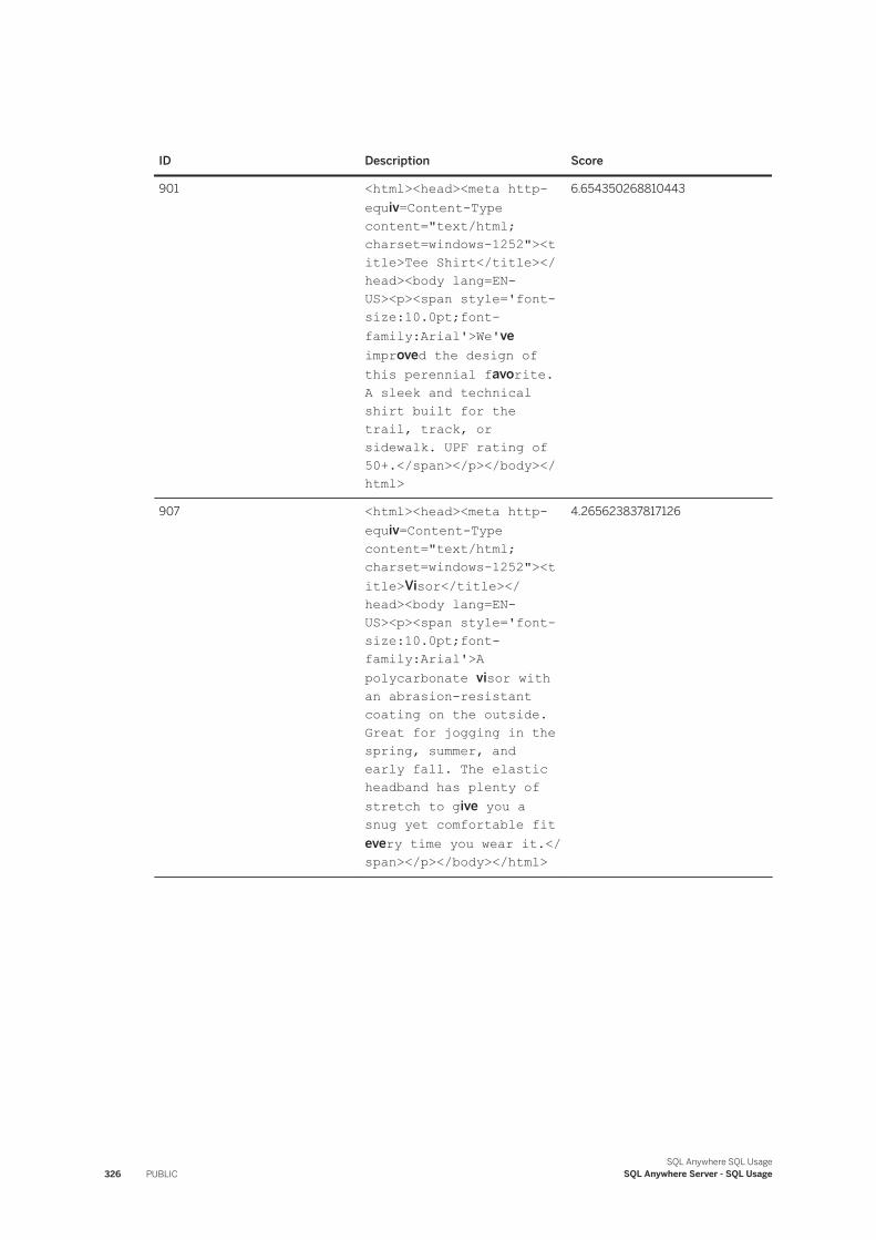
ID Description Score
901 <html><head><meta http-equiv=Content-Type content="text/html; charset=windows-1252"><title>Tee Shirt</title></head><body lang=EN-US><p><span style='font-size:10.0pt;font-family:Arial'>We've improved the design of this perennial favorite. A sleek and technical shirt built for the trail, track, or sidewalk. UPF rating of 50+.</span></p></body></html>
6.654350268810443
907 <html><head><meta http-equiv=Content-Type content="text/html; charset=windows-1252"><title>Visor</title></head><body lang=EN-US><p><span style='font-size:10.0pt;font-family:Arial'>A polycarbonate visor with an abrasion-resistant coating on the outside. Great for jogging in the spring, summer, and early fall. The elastic headband has plenty of stretch to give you a snug yet comfortable fit every time you wear it.</span></p></body></html>
4.265623837817126
326 PUBLICSQL Anywhere SQL Usage
SQL Anywhere Server - SQL Usage
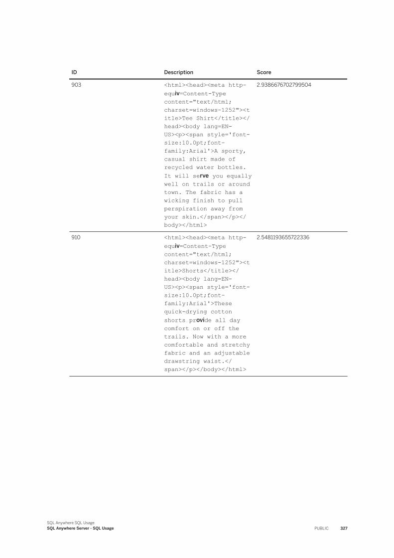
ID Description Score
903 <html><head><meta http-equiv=Content-Type content="text/html; charset=windows-1252"><title>Tee Shirt</title></head><body lang=EN-US><p><span style='font-size:10.0pt;font-family:Arial'>A sporty, casual shirt made of recycled water bottles. It will serve you equally well on trails or around town. The fabric has a wicking finish to pull perspiration away from your skin.</span></p></body></html>
2.9386676702799504
910 <html><head><meta http-equiv=Content-Type content="text/html; charset=windows-1252"><title>Shorts</title></head><body lang=EN-US><p><span style='font-size:10.0pt;font-family:Arial'>These quick-drying cotton shorts provide all day comfort on or off the trails. Now with a more comfortable and stretchy fabric and an adjustable drawstring waist.</span></p></body></html>
2.5481193655722336
SQL Anywhere SQL UsageSQL Anywhere Server - SQL Usage PUBLIC 327
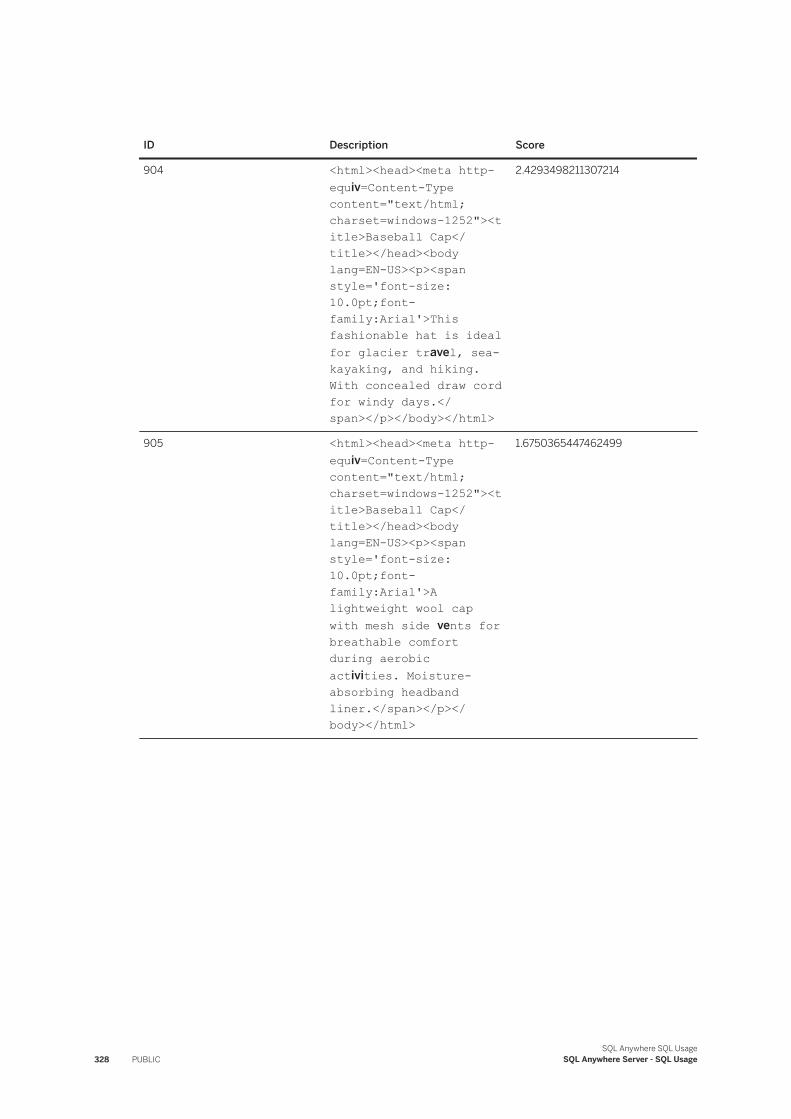
ID Description Score
904 <html><head><meta http-equiv=Content-Type content="text/html; charset=windows-1252"><title>Baseball Cap</title></head><body lang=EN-US><p><span style='font-size:10.0pt;font-family:Arial'>This fashionable hat is ideal for glacier travel, sea-kayaking, and hiking. With concealed draw cord for windy days.</span></p></body></html>
2.4293498211307214
905 <html><head><meta http-equiv=Content-Type content="text/html; charset=windows-1252"><title>Baseball Cap</title></head><body lang=EN-US><p><span style='font-size:10.0pt;font-family:Arial'>A lightweight wool cap with mesh side vents for breathable comfort during aerobic activities. Moisture-absorbing headband liner.</span></p></body></html>
1.6750365447462499
328 PUBLICSQL Anywhere SQL Usage
SQL Anywhere Server - SQL Usage
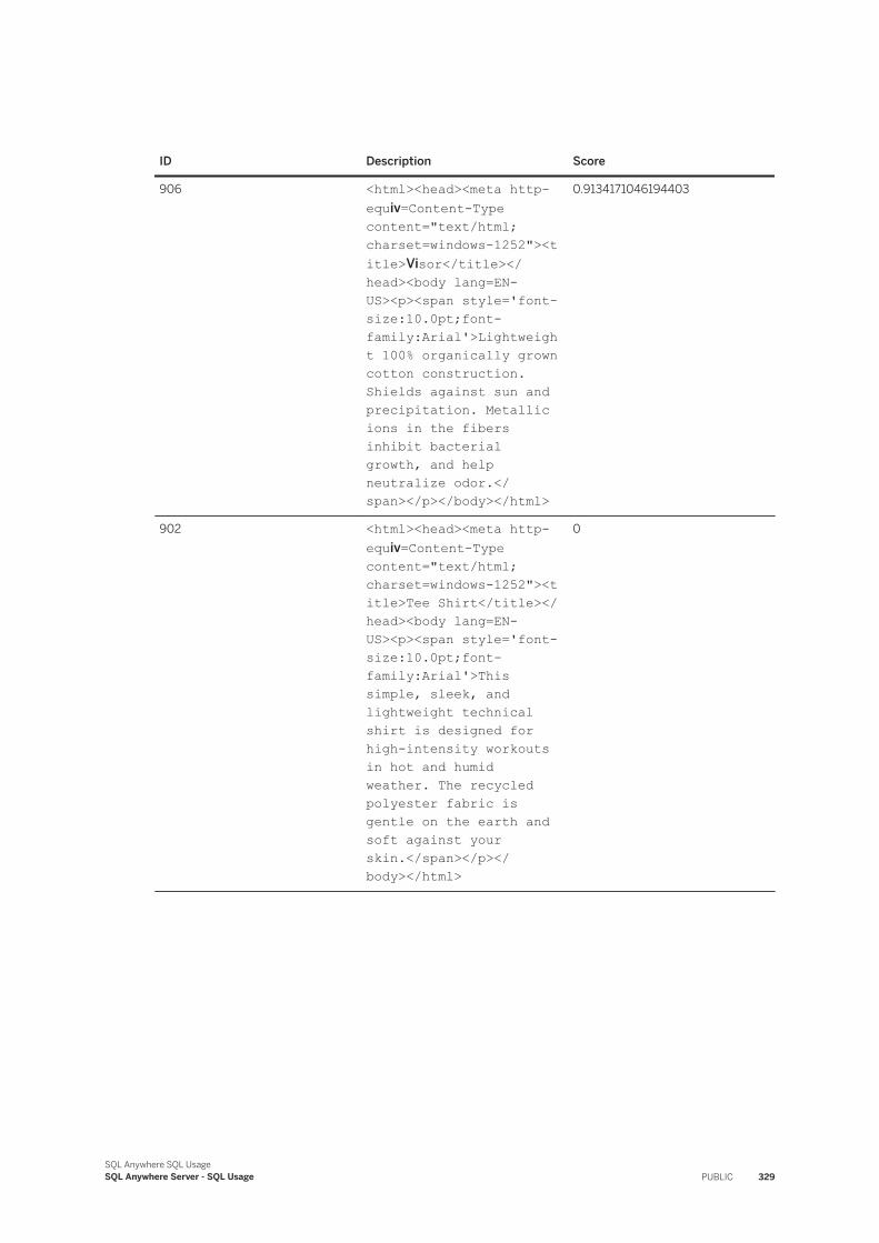
ID Description Score
906 <html><head><meta http-equiv=Content-Type content="text/html; charset=windows-1252"><title>Visor</title></head><body lang=EN-US><p><span style='font-size:10.0pt;font-family:Arial'>Lightweight 100% organically grown cotton construction. Shields against sun and precipitation. Metallic ions in the fibers inhibit bacterial growth, and help neutralize odor.</span></p></body></html>
0.9134171046194403
902 <html><head><meta http-equiv=Content-Type content="text/html; charset=windows-1252"><title>Tee Shirt</title></head><body lang=EN-US><p><span style='font-size:10.0pt;font-family:Arial'>This simple, sleek, and lightweight technical shirt is designed for high-intensity workouts in hot and humid weather. The recycled polyester fabric is gentle on the earth and soft against your skin.</span></p></body></html>
0
SQL Anywhere SQL UsageSQL Anywhere Server - SQL Usage PUBLIC 329
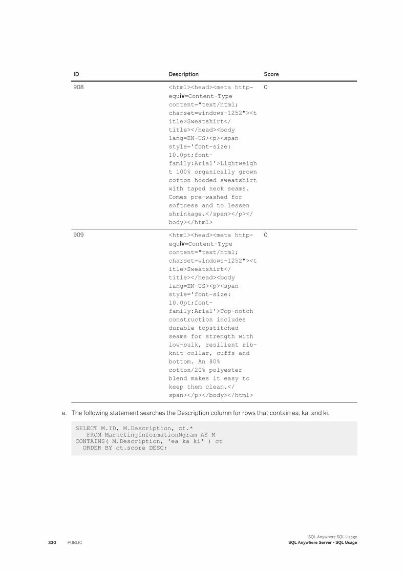
ID Description Score
908 <html><head><meta http-equiv=Content-Type content="text/html; charset=windows-1252"><title>Sweatshirt</title></head><body lang=EN-US><p><span style='font-size:10.0pt;font-family:Arial'>Lightweight 100% organically grown cotton hooded sweatshirt with taped neck seams. Comes pre-washed for softness and to lessen shrinkage.</span></p></body></html>
0
909 <html><head><meta http-equiv=Content-Type content="text/html; charset=windows-1252"><title>Sweatshirt</title></head><body lang=EN-US><p><span style='font-size:10.0pt;font-family:Arial'>Top-notch construction includes durable topstitched seams for strength with low-bulk, resilient rib-knit collar, cuffs and bottom. An 80% cotton/20% polyester blend makes it easy to keep them clean.</span></p></body></html>
0
e. The following statement searches the Description column for rows that contain ea, ka, and ki.
SELECT M.ID, M.Description, ct.* FROM MarketingInformationNgram AS M CONTAINS( M.Description, 'ea ka ki' ) ct ORDER BY ct.score DESC;
330 PUBLICSQL Anywhere SQL Usage
SQL Anywhere Server - SQL Usage
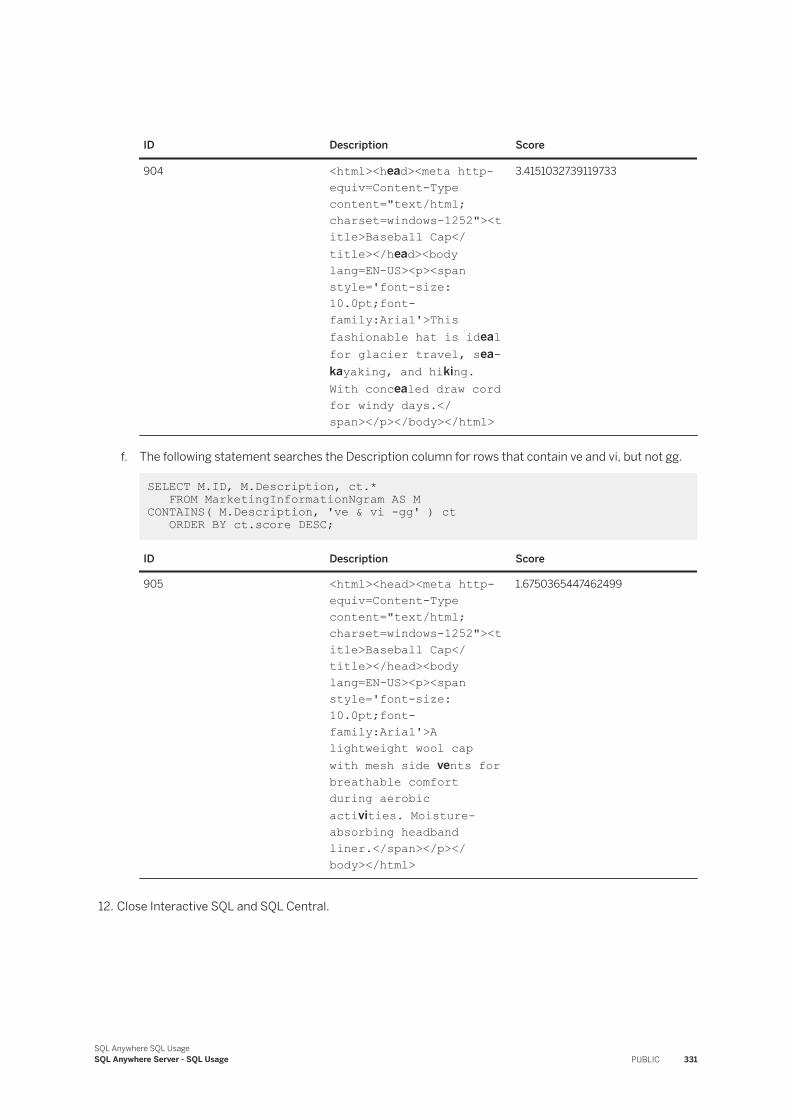
ID Description Score
904 <html><head><meta http-equiv=Content-Type content="text/html; charset=windows-1252"><title>Baseball Cap</title></head><body lang=EN-US><p><span style='font-size:10.0pt;font-family:Arial'>This fashionable hat is ideal for glacier travel, sea-kayaking, and hiking. With concealed draw cord for windy days.</span></p></body></html>
3.4151032739119733
f. The following statement searches the Description column for rows that contain ve and vi, but not gg.
SELECT M.ID, M.Description, ct.* FROM MarketingInformationNgram AS M CONTAINS( M.Description, 've & vi -gg' ) ct ORDER BY ct.score DESC;
ID Description Score
905 <html><head><meta http-equiv=Content-Type content="text/html; charset=windows-1252"><title>Baseball Cap</title></head><body lang=EN-US><p><span style='font-size:10.0pt;font-family:Arial'>A lightweight wool cap with mesh side vents for breathable comfort during aerobic activities. Moisture-absorbing headband liner.</span></p></body></html>
1.6750365447462499
12. Close Interactive SQL and SQL Central.
SQL Anywhere SQL UsageSQL Anywhere Server - SQL Usage PUBLIC 331
Results
You have performed a full text search on an NGRAM text index.
Next Steps
(optional) Restore the sample database (demo.db) to its original state.
Related Information
Text Configuration Object Concepts and Reference [page 286]Text Index Concepts and Reference [page 300]
1.3.2.9 Advanced: Term Dropping in Full Text Search
Text indexes are built according to the settings defined for the text configuration object used to create the text index.
A term does not appear in a text index if one or more of the following conditions are true:
● the term is included in the stoplist● the term is shorter than the minimum term length (GENERIC only)● the term is longer than the maximum term length
The same rules apply to query strings. The dropped term can match zero or more terms at the end or beginning of the phrase. For example, suppose the term 'the' is in the stoplist:
● If the term appears on either side of an AND, OR, or NEAR, then both the operator and the term are removed. For example, searching for 'the AND apple', 'the OR apple', or 'the NEAR apple' are equivalent to searching for 'apple'.
● If the term appears on the right side of an AND NOT, both the AND NOT and the term are dropped. For example, searching for 'apple AND NOT the' is equivalent to searching for 'apple'.If the term appears on the left side of an AND NOT, the entire expression is dropped and no rows are returned. For example, 'orange and the AND NOT apple' = 'orange'
● If the term appears in a phrase, the phrase is allowed to match with any term at the dropped term's position. For example, searching for 'feed the dog' matches 'feed the dog', 'feed my dog', 'feed any dog', and so on.
If none of the terms you are searching for are in the text index, no rows are returned. For example, suppose both 'the' and 'a' are in the stoplist. Searching for 'a OR the' returns no rows.
332 PUBLICSQL Anywhere SQL Usage
SQL Anywhere Server - SQL Usage
Related Information
Text Configuration Object Concepts and Reference [page 286]
1.3.2.10 Advanced: External Term Breaker and Prefilter Libraries
You can create and use custom external term breakers and prefilter libraries.
In this section:
Why Use an External Term Breaker or Prefilter Library [page 333]External term breaker and prefilter libraries can be used to perform custom term breaking and prefiltering on data before it is indexed.
Full Text Pipeline Workflow [page 334]The workflow for creating a text index, updating it, and querying it, is referred to as the pipeline.
External Prefilter Libraries [page 335]You can create and use external prefilter libraries.
External Term Breaker Libraries [page 338]You can create and use external term breaker libraries.
1.3.2.10.1 Why Use an External Term Breaker or Prefilter Library
External term breaker and prefilter libraries can be used to perform custom term breaking and prefiltering on data before it is indexed.
For example, suppose you want to create a text index on a column containing XML values. A prefilter allows you to filter out the XML tags so that they are not indexed with the content.
When a text index is created, each document is processed by a built-in term breaker specified in the text configuration of the text index to determine the terms contained in the document, and the positions of the terms in the document.
Full text search in SQL Anywhere is performed using a text index. Each value in a column on which a text index has been built is referred to as a document. When a text index is created, each document is processed by a built-in term breaker specified in the text configuration of the text index to determine the terms (also referred to as tokens) contained in the document, and the positions of the terms in the document. The built-in term breaker is also used to perform term breaking on the documents (text components) of a query string. For example, the query string 'rain or shine' consists of two documents, 'rain' and 'shine', connected by the OR operator. The built-in term breaker algorithm specified in the text configuration is also used to break the stoplist into terms, and to break the input of the sa_char_terms system procedure into terms.
Depending on the needs of your application, you may find some behaviors of the built-in GENERIC term breaker to be undesirable or limiting and NGRAM term breaker not suitable for the needs of the application. For
SQL Anywhere SQL UsageSQL Anywhere Server - SQL Usage PUBLIC 333
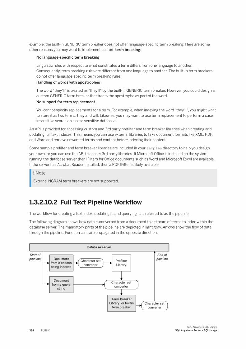
example, the built-in GENERIC term breaker does not offer language-specific term breaking. Here are some other reasons you may want to implement custom term breaking:
No language-specific term breaking
Linguistic rules with respect to what constitutes a term differs from one language to another. Consequently, term breaking rules are different from one language to another. The built-in term breakers do not offer language-specific term breaking rules.Handling of words with apostrophes
The word "they'll" is treated as "they ll" by the built-in GENERIC term breaker. However, you could design a custom GENERIC term breaker that treats the apostrophe as part of the word.No support for term replacement
You cannot specify replacements for a term. For example, when indexing the word "they'll", you might want to store it as two terms: they and will. Likewise, you may want to use term replacement to perform a case insensitive search on a case sensitive database.
An API is provided for accessing custom and 3rd party prefilter and term breaker libraries when creating and updating full text indexes. This means you can use external libraries to take document formats like XML, PDF, and Word and remove unwanted terms and content before indexing their content.
Some sample prefilter and term breaker libraries are included in your Samples directory to help you design your own, or you can use the API to access 3rd party libraries. If Microsoft Office is installed on the system running the database server then IFilters for Office documents such as Word and Microsoft Excel are available. If the server has Acrobat Reader installed, then a PDF IFilter is likely available.
NoteExternal NGRAM term breakers are not supported.
1.3.2.10.2 Full Text Pipeline WorkflowThe workflow for creating a text index, updating it, and querying it, is referred to as the pipeline.
The following diagram shows how data is converted from a document to a stream of terms to index within the database server. The mandatory parts of the pipeline are depicted in light gray. Arrows show the flow of data through the pipeline. Function calls are propagated in the opposite direction.
334 PUBLICSQL Anywhere SQL Usage
SQL Anywhere Server - SQL Usage
High Level View of How the Pipeline Works
1. The processing of each document is initiated by the database server calling the begin_document method on the end of the pipeline, which is either the term breaker or the character set converter. Each component in the pipeline calls begin_document on its own producer before returning from its begin_document method invocation.
2. The database server calls get_words on the end of the pipeline after the begin_document completes successfully.○ While executing get_words, the term breaker calls get_next_piece on its producer to get data to
process. If a prefilter exists in the pipeline, the data is filtered by it during the get_next_piece call.○ The term breaker breaks the data it receives from its producer into terms according to its term
breaking rules.3. The database server applies the minimum and maximum term length settings, as well as the stoplist
restrictions to the terms returned from get_words call.4. The database server continues to call get_words until no more terms are returned. At that point, the
database server calls end_document. This call is propagated through the pipeline in the same manner as the begin_document call.
NoteCharacter set converters are transparently added to the pipeline by the database server where necessary.
Prefilter and Term Breaker Code Samples
The ExternalLibrariesFullText directory in your SQL Anywhere install contains prefilter and term breaker sample code for you to explore. This directory is found under your Samples directory.
Related Information
External Prefilter Library Workflow [page 337]How to Design an External Term Breaker Library [page 339]
1.3.2.10.3 External Prefilter Libraries
You can create and use external prefilter libraries.
In this section:
SQL Anywhere SQL UsageSQL Anywhere Server - SQL Usage PUBLIC 335
How to Configure SQL Anywhere to Use an External Prefilter [page 336]To have data pass through an external prefilter library, you specify the library and its entry point function using the ALTER TEXT CONFIGURATION statement. A built-in prefilter algorithm is not provided.
How to Design an External Prefilter Library [page 336]The prefilter library must be implemented in C/C++.
1.3.2.10.3.1 How to Configure SQL Anywhere to Use an External Prefilter
To have data pass through an external prefilter library, you specify the library and its entry point function using the ALTER TEXT CONFIGURATION statement. A built-in prefilter algorithm is not provided.
ALTER TEXT CONFIGURATION my_text_config PREFILTER EXTERNAL NAME '[email protected]'
This example tells the database server to use the my_prefilter entry point function in the myprefilterLibrary.dll library to obtain a prefilter instance to use when building or updating a text index using the my_text_config text configuration object.
Related Information
a_text_source Interface [page 345]
1.3.2.10.3.2 How to Design an External Prefilter Library
The prefilter library must be implemented in C/C++.
Also, the prefilter library must:
● include the prefilter interface definition header file, extpfapiv1.h.● implement the a_text_source interface.● provide an entry point function that initializes and returns an instance of a_text_source (prefilter) and the
label of the character set supported by the prefilter.
Calling Sequence for the Prefilter
The following calling sequence is executed by the consumer of the prefilter for each document being processed:
begin_document(a_text_source*)
336 PUBLICSQL Anywhere SQL Usage
SQL Anywhere Server - SQL Usage
get_next_piece(a_text_source*, buffer**, len*)get_next_piece(a_text_source*, buffer**, len*)... end_document(a_text_source*)
Noteend_document can be called multiple times without an intervening begin_document call. For example, if one of the documents to be indexed is empty, the database server may call end_document for that document without calling begin_document.
The get_next_piece function should filter out the unnecessary data such as formatting information and images from the incoming byte stream and return the next chunk of filtered data in a self-allocated buffer.
In this section:
External Prefilter Library Workflow [page 337]The following flow chart shows the logic flow when the get_next_piece function is called:
Related Information
Full Text Pipeline Workflow [page 334]a_text_source Interface [page 345]
1.3.2.10.3.2.1 External Prefilter Library Workflow
The following flow chart shows the logic flow when the get_next_piece function is called:
SQL Anywhere SQL UsageSQL Anywhere Server - SQL Usage PUBLIC 337

Related Information
Full Text Pipeline Workflow [page 334]a_text_source Interface [page 345]
1.3.2.10.4 External Term Breaker Libraries
You can create and use external term breaker libraries.
In this section:
How to Configure SQL Anywhere to Use an External Term Breaker [page 339]By default, when you create a text configuration object, a built-in term breaker is used for data associated with that text configuration object.
How to Design an External Term Breaker Library [page 339]An external term breaker library must be implemented in C/C++.
338 PUBLICSQL Anywhere SQL Usage
SQL Anywhere Server - SQL Usage
1.3.2.10.4.1 How to Configure SQL Anywhere to Use an External Term Breaker
By default, when you create a text configuration object, a built-in term breaker is used for data associated with that text configuration object.
To have data instead pass through an external term breaker library, you specify the library and its entry point function using the ALTER TEXT CONFIGURATION statement, similar to the following:
ALTER TEXT CONFIGURATION my_text_config TERM BREAKER GENERIC EXTERNAL NAME 'my_termbreaker@termbreaker'
This example tells the database server to use the my_termbreaker entry point function in the termbreaker library to obtain a term breaker instance to use when building, updating, or querying a text index associated with the my_text_config text configuration object, when parsing the text configuration object's stoplist, and when processing input to the sa_char_terms system procedure.
Related Information
a_word_source Interface [page 350]
1.3.2.10.4.2 How to Design an External Term Breaker Library
An external term breaker library must be implemented in C/C++.
Also, the external term breaker library must:
● include of the term breaker interface definition header file, exttbapiv1.h.● implement the a_word_source interface.● provide an entry point function that initializes and returns an instance of a_word_source (term breaker)
and the label of the character set supported by the term breaker.
Calling Sequence for the Term Breaker
The following calling sequence is executed by the consumer of the term breaker for each document being processed:
begin_document(a_word_source*, asql_uint32); get_words(a_word_source*, a_term**, uint32 *num_words)get_words(a_word_source*, a_term**, uint32 *num_words)... end_document(a_word_source*)
The get_words function must call get_next_piece on its producer to get data to break into terms until the array of a_term structures is filled, or there is no more data to process.
SQL Anywhere SQL UsageSQL Anywhere Server - SQL Usage PUBLIC 339
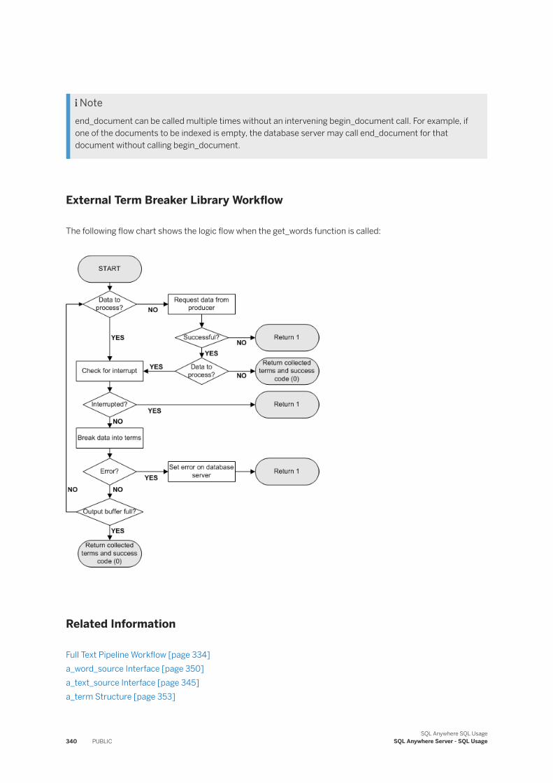
Noteend_document can be called multiple times without an intervening begin_document call. For example, if one of the documents to be indexed is empty, the database server may call end_document for that document without calling begin_document.
External Term Breaker Library Workflow
The following flow chart shows the logic flow when the get_words function is called:
Related Information
Full Text Pipeline Workflow [page 334]a_word_source Interface [page 350]a_text_source Interface [page 345]a_term Structure [page 353]
340 PUBLICSQL Anywhere SQL Usage
SQL Anywhere Server - SQL Usage

1.3.2.11 Advanced: API for External Full Text Libraries
Follow these steps to create and use a prefilter or term breaker external library with text indexes.
● Implement the SQL Anywhere C/C++ interfaces.● Create a dynamically loadable library by compiling and linking the code written in the above step.● Create the text configuration object in the database and then modify it to specify the entry point function
in the external library for prefilter and/or term breaker.The entry point functions are used to obtain the prefilter and term breaker objects to be used while inserting/deleting text index entries when underlying documents (column values) are modified. In the case of an external term breaker library, the entry point function is also used to parse queries over the text indexes that use the term breaker.
In this section:
a_server_context Structure [page 342]Several callbacks are supported by the database server and are exposed to the full text external libraries through the a_server_context structure to perform: error reporting, interrupt processing and message logging.
a_init_pre_filter Structure [page 344]The a_init_pre_filter structure is used for negotiating the input and output requirements for instances of an external prefilter entry point function.
a_text_source Interface [page 345]The external prefilter library must implement the a_text_source interface to perform document prefiltering for full text index population or updating.
a_init_term_breaker Structure [page 348]The a_init_term_breaker structure is used for negotiating the input and output requirements for instances of an external term breaker.
a_term_breaker_for Enumeration [page 350]Use the a_term_breaker_for enumeration to specify whether the pipeline is built for use during update or querying of the text index.
a_word_source Interface [page 350]The external term breaker library must implement the a_word_source interface to perform term breaking for text index operations.
a_term Structure [page 353]The a_term structure stores a term, its length, and its position.
extpf_use_new_api Entry Point Function (Prefilters) [page 354]The extpf_use_new_api entry point function notifies the database server about the interface version implemented in the external prefilter library.
exttb_use_new_api Entry Point Function (Term Breakers) [page 355]The exttb_use_new_api entry point function provides information about the interface version implemented in the external term breaker library.
extfn_post_load_library Global Entry Point Function [page 356]The extfn_post_load_library global entry point function is required when there is a library-specific requirement to do library-wide setup before any function within the library is called.
extfn_pre_unload_library Global Entry Point Function [page 356]
SQL Anywhere SQL UsageSQL Anywhere Server - SQL Usage PUBLIC 341
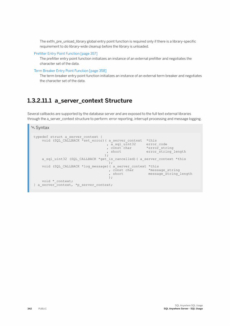
The extfn_pre_unload_library global entry point function is required only if there is a library-specific requirement to do library-wide cleanup before the library is unloaded.
Prefilter Entry Point Function [page 357]The prefilter entry point function initializes an instance of an external prefilter and negotiates the character set of the data.
Term Breaker Entry Point Function [page 358]The term breaker entry point function initializes an instance of an external term breaker and negotiates the character set of the data.
1.3.2.11.1 a_server_context Structure
Several callbacks are supported by the database server and are exposed to the full text external libraries through the a_server_context structure to perform: error reporting, interrupt processing and message logging.
Syntax
typedef struct a_server_context { void (SQL_CALLBACK *set_error)( a_server_context *this , a_sql_uint32 error_code , const char *error_string , short error_string_length ); a_sql_uint32 (SQL_CALLBACK *get_is_cancelled)( a_server_context *this ); void (SQL_CALLBACK *log_message)( a_server_context *this , const char *message_string , short message_string_length ); void *_context; } a_server_context, *p_server_context;
342 PUBLICSQL Anywhere SQL Usage
SQL Anywhere Server - SQL Usage
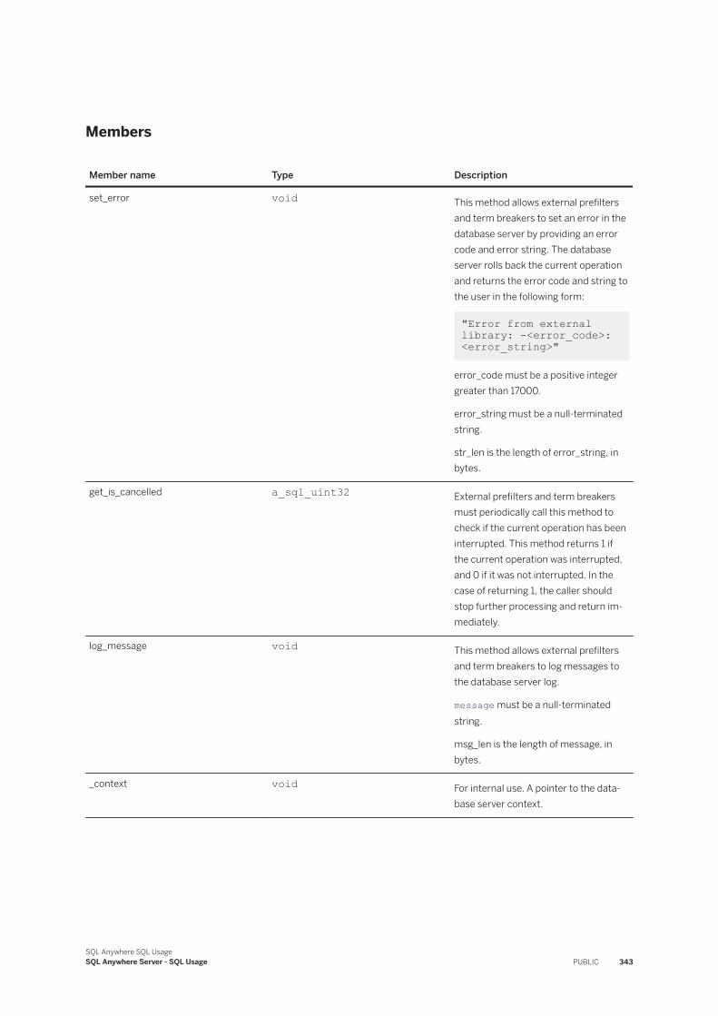
Members
Member name Type Description
set_error void This method allows external prefilters and term breakers to set an error in the database server by providing an error code and error string. The database server rolls back the current operation and returns the error code and string to the user in the following form:
"Error from external library: -<error_code>: <error_string>"
error_code must be a positive integer greater than 17000.
error_string must be a null-terminated string.
str_len is the length of error_string, in bytes.
get_is_cancelled a_sql_uint32 External prefilters and term breakers must periodically call this method to check if the current operation has been interrupted. This method returns 1 if the current operation was interrupted, and 0 if it was not interrupted. In the case of returning 1, the caller should stop further processing and return immediately.
log_message void This method allows external prefilters and term breakers to log messages to the database server log.
message must be a null-terminated string.
msg_len is the length of message, in bytes.
_context void For internal use. A pointer to the database server context.
SQL Anywhere SQL UsageSQL Anywhere Server - SQL Usage PUBLIC 343
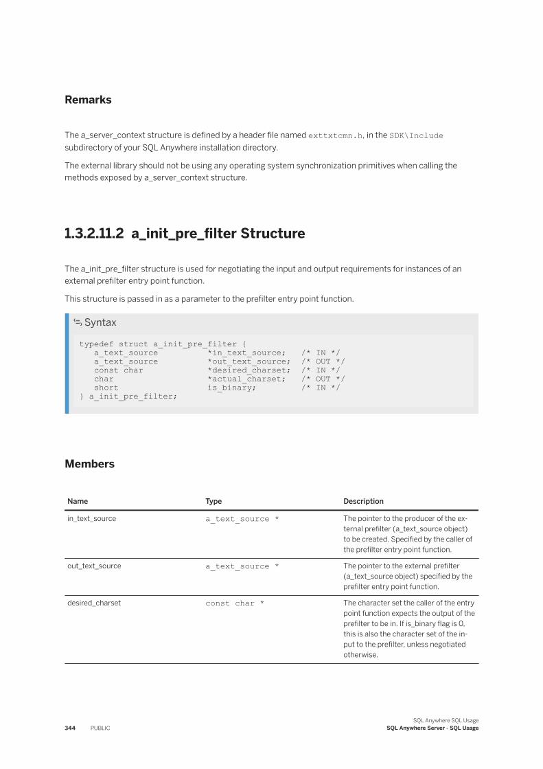
Remarks
The a_server_context structure is defined by a header file named exttxtcmn.h, in the SDK\Include subdirectory of your SQL Anywhere installation directory.
The external library should not be using any operating system synchronization primitives when calling the methods exposed by a_server_context structure.
1.3.2.11.2 a_init_pre_filter Structure
The a_init_pre_filter structure is used for negotiating the input and output requirements for instances of an external prefilter entry point function.
This structure is passed in as a parameter to the prefilter entry point function.
Syntax
typedef struct a_init_pre_filter { a_text_source *in_text_source; /* IN */ a_text_source *out_text_source; /* OUT */ const char *desired_charset; /* IN */ char *actual_charset; /* OUT */ short is_binary; /* IN */ } a_init_pre_filter;
Members
Name Type Description
in_text_source a_text_source * The pointer to the producer of the external prefilter (a_text_source object) to be created. Specified by the caller of the prefilter entry point function.
out_text_source a_text_source * The pointer to the external prefilter (a_text_source object) specified by the prefilter entry point function.
desired_charset const char * The character set the caller of the entry point function expects the output of the prefilter to be in. If is_binary flag is 0, this is also the character set of the input to the prefilter, unless negotiated otherwise.
344 PUBLICSQL Anywhere SQL Usage
SQL Anywhere Server - SQL Usage
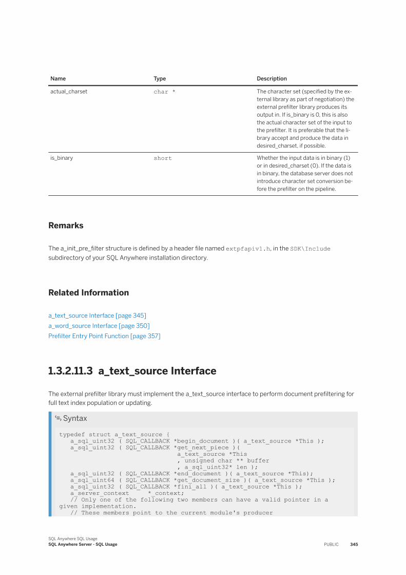
Name Type Description
actual_charset char * The character set (specified by the external library as part of negotiation) the external prefilter library produces its output in. If is_binary is 0, this is also the actual character set of the input to the prefilter. It is preferable that the library accept and produce the data in desired_charset, if possible.
is_binary short Whether the input data is in binary (1) or in desired_charset (0). If the data is in binary, the database server does not introduce character set conversion before the prefilter on the pipeline.
Remarks
The a_init_pre_filter structure is defined by a header file named extpfapiv1.h, in the SDK\Include subdirectory of your SQL Anywhere installation directory.
Related Information
a_text_source Interface [page 345]a_word_source Interface [page 350]Prefilter Entry Point Function [page 357]
1.3.2.11.3 a_text_source Interface
The external prefilter library must implement the a_text_source interface to perform document prefiltering for full text index population or updating.
Syntax
typedef struct a_text_source { a_sql_uint32 ( SQL_CALLBACK *begin_document )( a_text_source *This ); a_sql_uint32 ( SQL_CALLBACK *get_next_piece )( a_text_source *This , unsigned char ** buffer , a_sql_uint32* len ); a_sql_uint32 ( SQL_CALLBACK *end_document )( a_text_source *This); a_sql_uint64 ( SQL_CALLBACK *get_document_size )( a_text_source *This ); a_sql_uint32 ( SQL_CALLBACK *fini_all )( a_text_source *This ); a_server_context *_context; // Only one of the following two members can have a valid pointer in a given implementation. // These members point to the current module's producer
SQL Anywhere SQL UsageSQL Anywhere Server - SQL Usage PUBLIC 345
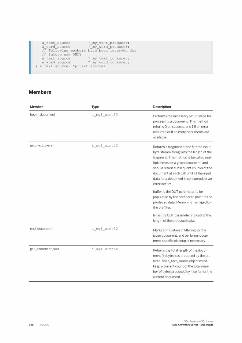
a_text_source *_my_text_producer; a_word_source *_my_word_producer; // Following members have been reserved for // future use ONLY a_text_source *_my_text_consumer; a_word_source *_my_word_consumer; } a_text_source, *p_text_source;
Members
Member Type Description
begin_document a_sql_uint32 Performs the necessary setup steps for processing a document. This method returns 0 on success, and 1 if an error occurred or if no more documents are available.
get_next_piece a_sql_uint32 Returns a fragment of the filtered input byte stream along with the length of the fragment. This method is be called multiple times for a given document, and should return subsequent chunks of the document at each call until all the input data for a document is consumed, or an error occurs.
buffer is the OUT parameter to be populated by the prefilter to point to the produced data. Memory is managed by the prefilter.
len is the OUT parameter indicating the length of the produced data.
end_document a_sql_uint32 Marks completion of filtering for the given document, and performs document-specific cleanup, if necessary.
get_document_size a_sql_uint64 Returns the total length of the document (in bytes) as produced by the prefilter. The a_text_source object must keep a current count of the total number of bytes produced by it so far for the current document.
346 PUBLICSQL Anywhere SQL Usage
SQL Anywhere Server - SQL Usage
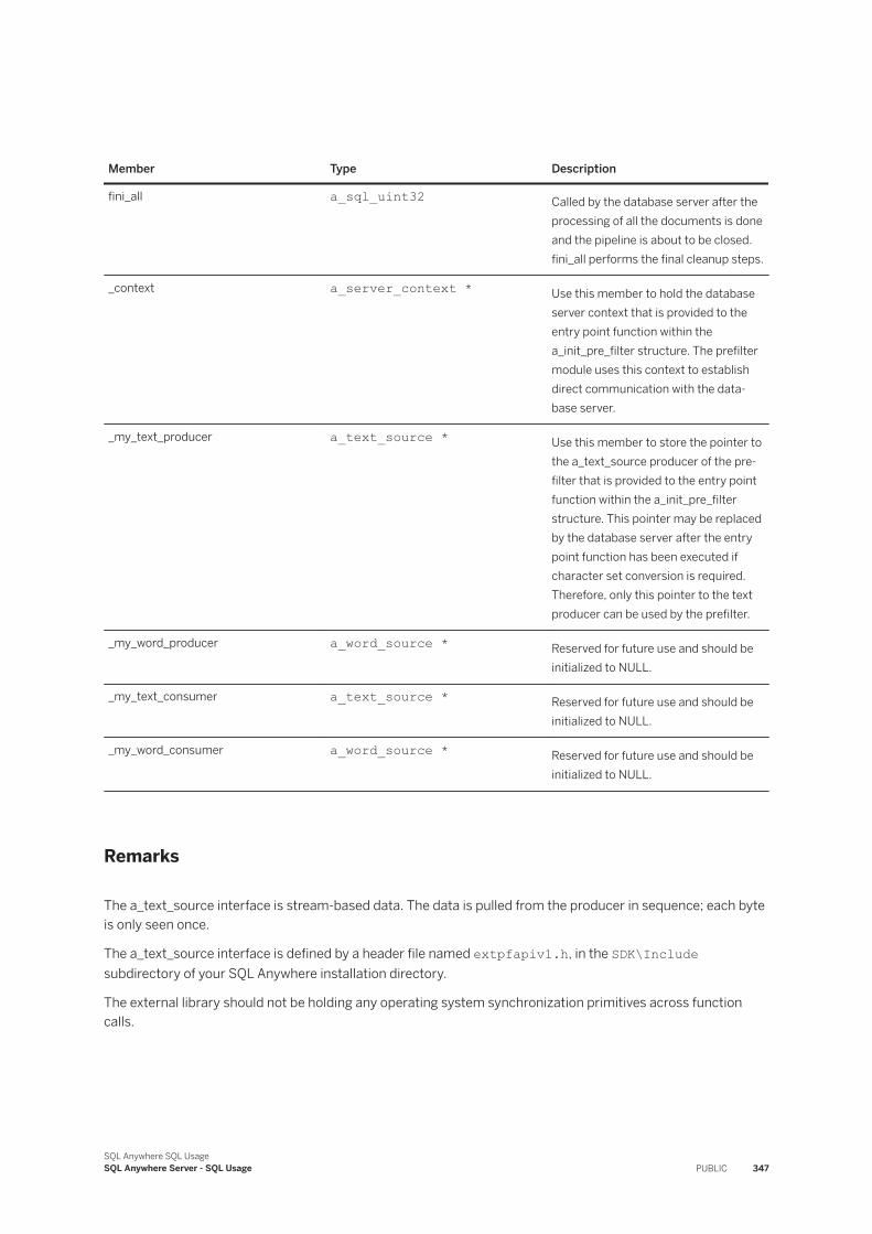
Member Type Description
fini_all a_sql_uint32 Called by the database server after the processing of all the documents is done and the pipeline is about to be closed. fini_all performs the final cleanup steps.
_context a_server_context * Use this member to hold the database server context that is provided to the entry point function within the a_init_pre_filter structure. The prefilter module uses this context to establish direct communication with the database server.
_my_text_producer a_text_source * Use this member to store the pointer to the a_text_source producer of the prefilter that is provided to the entry point function within the a_init_pre_filter structure. This pointer may be replaced by the database server after the entry point function has been executed if character set conversion is required. Therefore, only this pointer to the text producer can be used by the prefilter.
_my_word_producer a_word_source * Reserved for future use and should be initialized to NULL.
_my_text_consumer a_text_source * Reserved for future use and should be initialized to NULL.
_my_word_consumer a_word_source * Reserved for future use and should be initialized to NULL.
Remarks
The a_text_source interface is stream-based data. The data is pulled from the producer in sequence; each byte is only seen once.
The a_text_source interface is defined by a header file named extpfapiv1.h, in the SDK\Include subdirectory of your SQL Anywhere installation directory.
The external library should not be holding any operating system synchronization primitives across function calls.
SQL Anywhere SQL UsageSQL Anywhere Server - SQL Usage PUBLIC 347
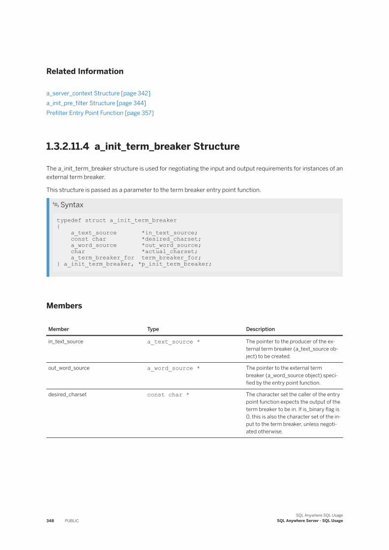
Related Information
a_server_context Structure [page 342]a_init_pre_filter Structure [page 344]Prefilter Entry Point Function [page 357]
1.3.2.11.4 a_init_term_breaker Structure
The a_init_term_breaker structure is used for negotiating the input and output requirements for instances of an external term breaker.
This structure is passed as a parameter to the term breaker entry point function.
Syntax
typedef struct a_init_term_breaker { a_text_source *in_text_source; const char *desired_charset; a_word_source *out_word_source; char *actual_charset; a_term_breaker_for term_breaker_for; } a_init_term_breaker, *p_init_term_breaker;
Members
Member Type Description
in_text_source a_text_source * The pointer to the producer of the external term breaker (a_text_source object) to be created.
out_word_source a_word_source * The pointer to the external term breaker (a_word_source object) specified by the entry point function.
desired_charset const char * The character set the caller of the entry point function expects the output of the term breaker to be in. If is_binary flag is 0, this is also the character set of the input to the term breaker, unless negotiated otherwise.
348 PUBLICSQL Anywhere SQL Usage
SQL Anywhere Server - SQL Usage
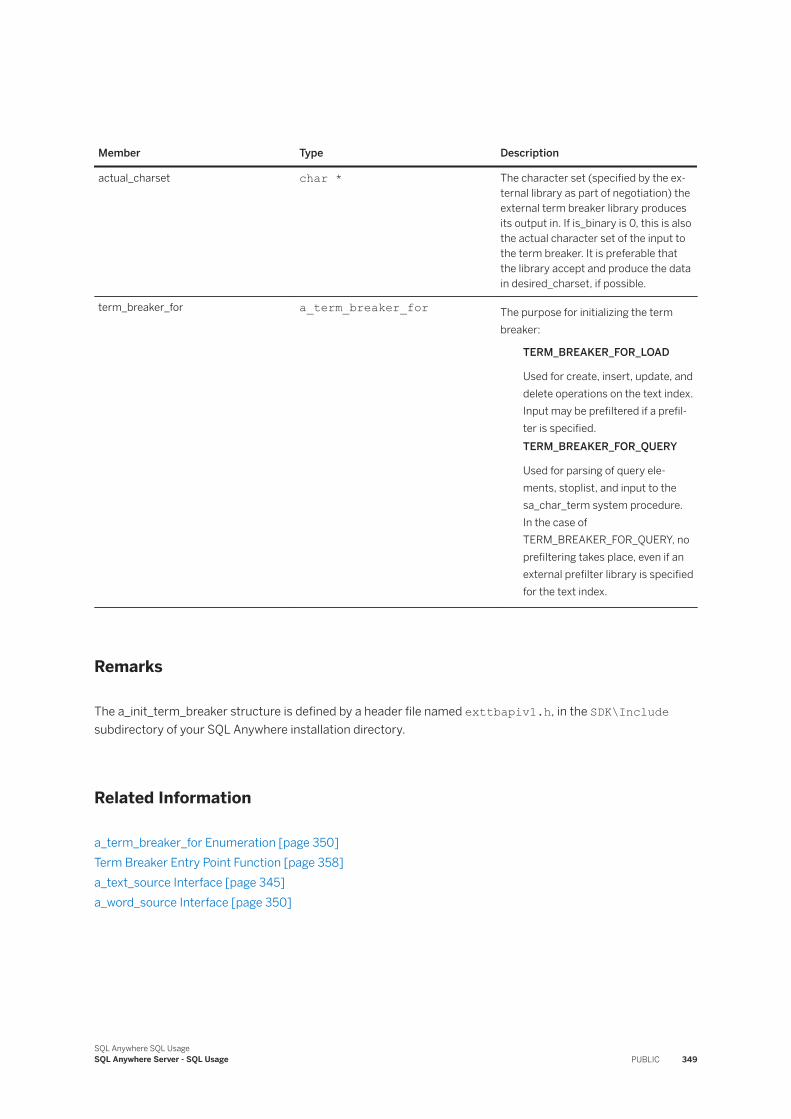
Member Type Description
actual_charset char * The character set (specified by the external library as part of negotiation) the external term breaker library produces its output in. If is_binary is 0, this is also the actual character set of the input to the term breaker. It is preferable that the library accept and produce the data in desired_charset, if possible.
term_breaker_for a_term_breaker_for The purpose for initializing the term breaker:
TERM_BREAKER_FOR_LOAD
Used for create, insert, update, and delete operations on the text index. Input may be prefiltered if a prefil-ter is specified.TERM_BREAKER_FOR_QUERY
Used for parsing of query elements, stoplist, and input to the sa_char_term system procedure. In the case of TERM_BREAKER_FOR_QUERY, no prefiltering takes place, even if an external prefilter library is specified for the text index.
Remarks
The a_init_term_breaker structure is defined by a header file named exttbapiv1.h, in the SDK\Include subdirectory of your SQL Anywhere installation directory.
Related Information
a_term_breaker_for Enumeration [page 350]Term Breaker Entry Point Function [page 358]a_text_source Interface [page 345]a_word_source Interface [page 350]
SQL Anywhere SQL UsageSQL Anywhere Server - SQL Usage PUBLIC 349
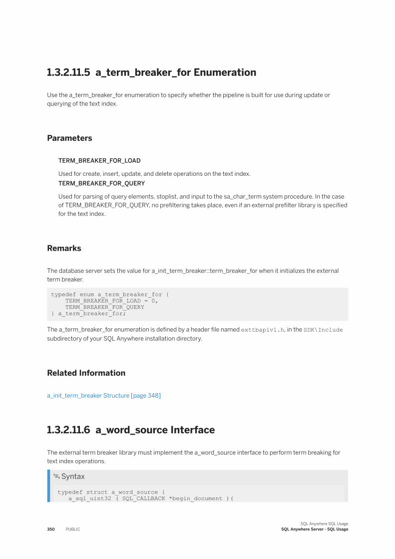
1.3.2.11.5 a_term_breaker_for Enumeration
Use the a_term_breaker_for enumeration to specify whether the pipeline is built for use during update or querying of the text index.
Parameters
TERM_BREAKER_FOR_LOAD
Used for create, insert, update, and delete operations on the text index.TERM_BREAKER_FOR_QUERY
Used for parsing of query elements, stoplist, and input to the sa_char_term system procedure. In the case of TERM_BREAKER_FOR_QUERY, no prefiltering takes place, even if an external prefilter library is specified for the text index.
Remarks
The database server sets the value for a_init_term_breaker::term_breaker_for when it initializes the external term breaker.
typedef enum a_term_breaker_for { TERM_BREAKER_FOR_LOAD = 0, TERM_BREAKER_FOR_QUERY } a_term_breaker_for;
The a_term_breaker_for enumeration is defined by a header file named exttbapiv1.h, in the SDK\Include subdirectory of your SQL Anywhere installation directory.
Related Information
a_init_term_breaker Structure [page 348]
1.3.2.11.6 a_word_source Interface
The external term breaker library must implement the a_word_source interface to perform term breaking for text index operations.
Syntax
typedef struct a_word_source { a_sql_uint32 ( SQL_CALLBACK *begin_document )(
350 PUBLICSQL Anywhere SQL Usage
SQL Anywhere Server - SQL Usage
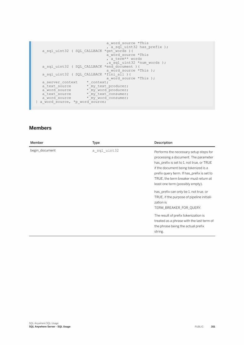
a_word_source *This , a_sql_uint32 has_prefix ); a_sql_uint32 ( SQL_CALLBACK *get_words )( a_word_source *This , a_term** words ,a_sql_uint32 *num_words ); a_sql_uint32 ( SQL_CALLBACK *end_document )( a_word_source *This ); a_sql_uint32 ( SQL_CALLBACK *fini_all )( a_word_source *This ); a_server_context *_context; a_text_source *_my_text_producer; a_word_source *_my_word_producer; a_text_source *_my_text_consumer; a_word_source *_my_word_consumer; } a_word_source, *p_word_source;
Members
Member Type Description
begin_document a_sql_uint32 Performs the necessary setup steps for processing a document. The parameter has_prefix is set to 1, not true, or TRUE if the document being tokenized is a prefix query term. If has_prefix is set to TRUE, the term breaker must return at least one term (possibly empty).
has_prefix can only be 1, not true, or TRUE, if the purpose of pipeline initialization is TERM_BREAKER_FOR_QUERY.
The result of prefix tokenization is treated as a phrase with the last term of the phrase being the actual prefix string.
SQL Anywhere SQL UsageSQL Anywhere Server - SQL Usage PUBLIC 351
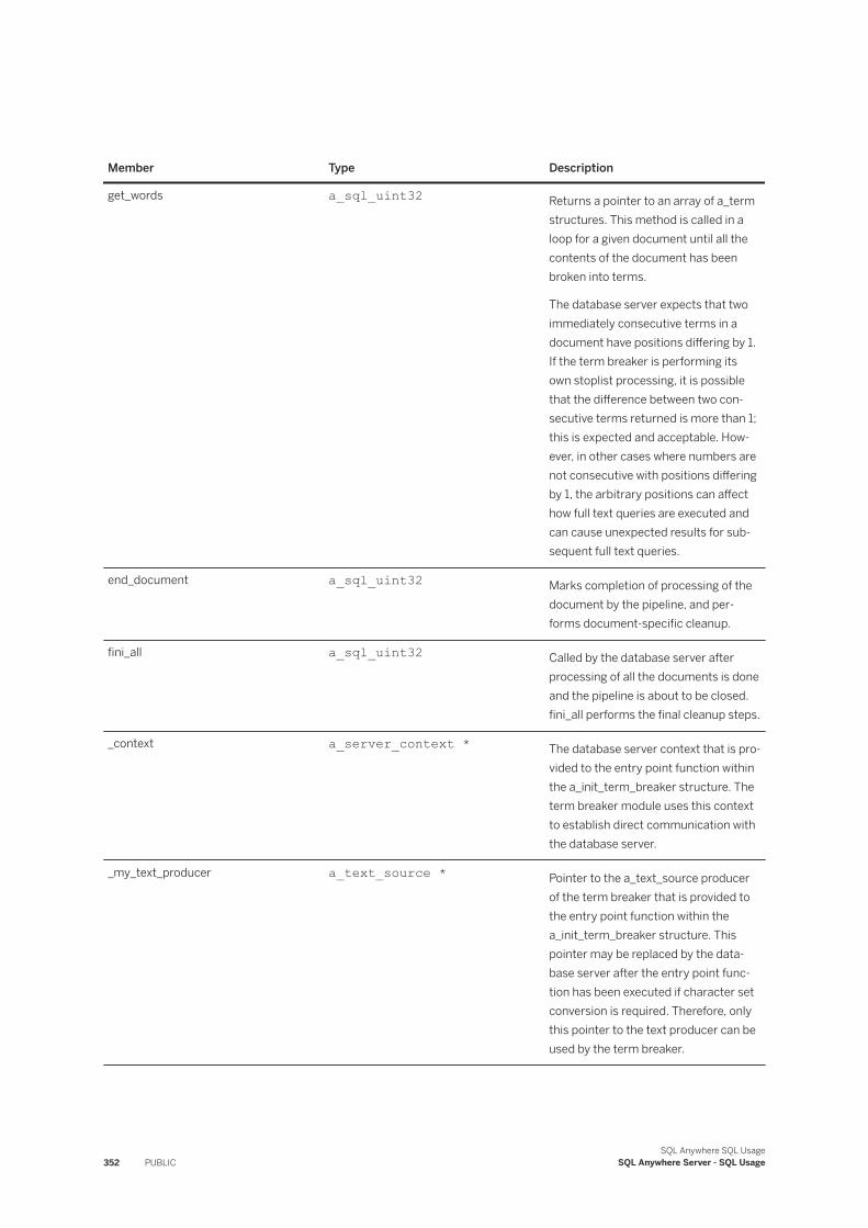
Member Type Description
get_words a_sql_uint32 Returns a pointer to an array of a_term structures. This method is called in a loop for a given document until all the contents of the document has been broken into terms.
The database server expects that two immediately consecutive terms in a document have positions differing by 1. If the term breaker is performing its own stoplist processing, it is possible that the difference between two consecutive terms returned is more than 1; this is expected and acceptable. However, in other cases where numbers are not consecutive with positions differing by 1, the arbitrary positions can affect how full text queries are executed and can cause unexpected results for subsequent full text queries.
end_document a_sql_uint32 Marks completion of processing of the document by the pipeline, and performs document-specific cleanup.
fini_all a_sql_uint32 Called by the database server after processing of all the documents is done and the pipeline is about to be closed. fini_all performs the final cleanup steps.
_context a_server_context * The database server context that is provided to the entry point function within the a_init_term_breaker structure. The term breaker module uses this context to establish direct communication with the database server.
_my_text_producer a_text_source * Pointer to the a_text_source producer of the term breaker that is provided to the entry point function within the a_init_term_breaker structure. This pointer may be replaced by the database server after the entry point function has been executed if character set conversion is required. Therefore, only this pointer to the text producer can be used by the term breaker.
352 PUBLICSQL Anywhere SQL Usage
SQL Anywhere Server - SQL Usage
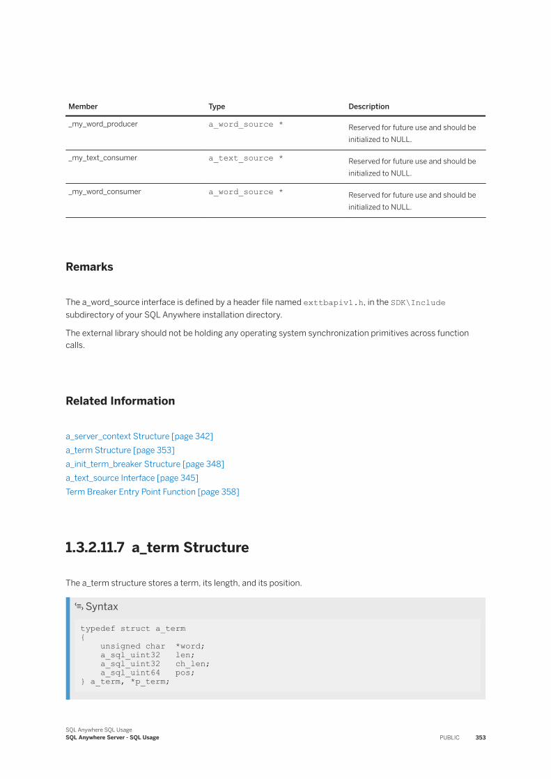
Member Type Description
_my_word_producer a_word_source * Reserved for future use and should be initialized to NULL.
_my_text_consumer a_text_source * Reserved for future use and should be initialized to NULL.
_my_word_consumer a_word_source * Reserved for future use and should be initialized to NULL.
Remarks
The a_word_source interface is defined by a header file named exttbapiv1.h, in the SDK\Include subdirectory of your SQL Anywhere installation directory.
The external library should not be holding any operating system synchronization primitives across function calls.
Related Information
a_server_context Structure [page 342]a_term Structure [page 353]a_init_term_breaker Structure [page 348]a_text_source Interface [page 345]Term Breaker Entry Point Function [page 358]
1.3.2.11.7 a_term Structure
The a_term structure stores a term, its length, and its position.
Syntax
typedef struct a_term { unsigned char *word; a_sql_uint32 len; a_sql_uint32 ch_len; a_sql_uint64 pos; } a_term, *p_term;
SQL Anywhere SQL UsageSQL Anywhere Server - SQL Usage PUBLIC 353
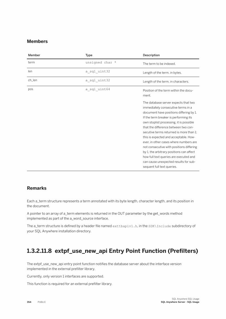
Members
Member Type Description
term unsigned char * The term to be indexed.
len a_sql_uint32 Length of the term, in bytes.
ch_len a_sql_uint32 Length of the term, in characters.
pos a_sql_uint64 Position of the term within the document.
The database server expects that two immediately consecutive terms in a document have positions differing by 1. If the term breaker is performing its own stoplist processing, it is possible that the difference between two consecutive terms returned is more than 1; this is expected and acceptable. However, in other cases where numbers are not consecutive with positions differing by 1, the arbitrary positions can affect how full text queries are executed and can cause unexpected results for subsequent full text queries.
Remarks
Each a_term structure represents a term annotated with its byte length, character length, and its position in the document.
A pointer to an array of a_term elements is returned in the OUT parameter by the get_words method implemented as part of the a_word_source interface.
The a_term structure is defined by a header file named exttbapiv1.h, in the SDK\Include subdirectory of your SQL Anywhere installation directory.
1.3.2.11.8 extpf_use_new_api Entry Point Function (Prefilters)
The extpf_use_new_api entry point function notifies the database server about the interface version implemented in the external prefilter library.
Currently, only version 1 interfaces are supported.
This function is required for an external prefilter library.
354 PUBLICSQL Anywhere SQL Usage
SQL Anywhere Server - SQL Usage
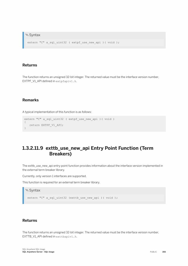
Syntax
extern "C" a_sql_uint32 ( extpf_use_new_api )( void );
Returns
The function returns an unsigned 32-bit integer. The returned value must be the interface version number, EXTPF_V1_API defined in extpfapiv1.h.
Remarks
A typical implementation of this function is as follows:
extern "C" a_sql_uint32 ( extpf_use_new_api )( void ) { return EXTPF_V1_API; }
1.3.2.11.9 exttb_use_new_api Entry Point Function (Term Breakers)
The exttb_use_new_api entry point function provides information about the interface version implemented in the external term breaker library.
Currently, only version 1 interfaces are supported.
This function is required for an external term breaker library.
Syntax
extern "C" a_sql_uint32 (exttb_use_new_api )( void );
Returns
The function returns an unsigned 32-bit integer. The returned value must be the interface version number, EXTTB_V1_API defined in exttbapiv1.h.
SQL Anywhere SQL UsageSQL Anywhere Server - SQL Usage PUBLIC 355
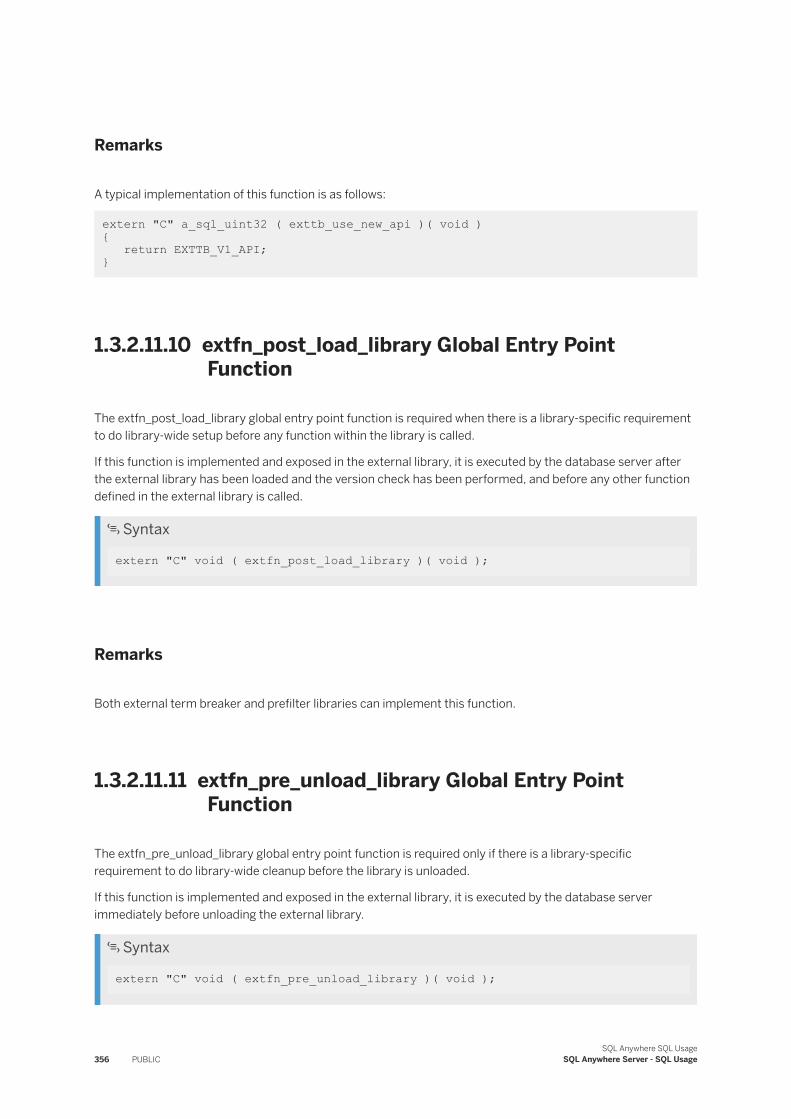
Remarks
A typical implementation of this function is as follows:
extern "C" a_sql_uint32 ( exttb_use_new_api )( void ) { return EXTTB_V1_API; }
1.3.2.11.10 extfn_post_load_library Global Entry Point Function
The extfn_post_load_library global entry point function is required when there is a library-specific requirement to do library-wide setup before any function within the library is called.
If this function is implemented and exposed in the external library, it is executed by the database server after the external library has been loaded and the version check has been performed, and before any other function defined in the external library is called.
Syntax
extern "C" void ( extfn_post_load_library )( void );
Remarks
Both external term breaker and prefilter libraries can implement this function.
1.3.2.11.11 extfn_pre_unload_library Global Entry Point Function
The extfn_pre_unload_library global entry point function is required only if there is a library-specific requirement to do library-wide cleanup before the library is unloaded.
If this function is implemented and exposed in the external library, it is executed by the database server immediately before unloading the external library.
Syntax
extern "C" void ( extfn_pre_unload_library )( void );
356 PUBLICSQL Anywhere SQL Usage
SQL Anywhere Server - SQL Usage
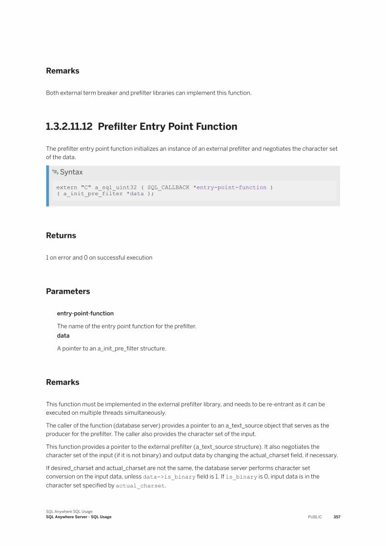
Remarks
Both external term breaker and prefilter libraries can implement this function.
1.3.2.11.12 Prefilter Entry Point Function
The prefilter entry point function initializes an instance of an external prefilter and negotiates the character set of the data.
Syntax
extern "C" a_sql_uint32 ( SQL_CALLBACK *entry-point-function )( a_init_pre_filter *data );
Returns
1 on error and 0 on successful execution
Parameters
entry-point-function
The name of the entry point function for the prefilter.data
A pointer to an a_init_pre_filter structure.
Remarks
This function must be implemented in the external prefilter library, and needs to be re-entrant as it can be executed on multiple threads simultaneously.
The caller of the function (database server) provides a pointer to an a_text_source object that serves as the producer for the prefilter. The caller also provides the character set of the input.
This function provides a pointer to the external prefilter (a_text_source structure). It also negotiates the character set of the input (if it is not binary) and output data by changing the actual_charset field, if necessary.
If desired_charset and actual_charset are not the same, the database server performs character set conversion on the input data, unless data->is_binary field is 1. If is_binary is 0, input data is in the character set specified by actual_charset.
SQL Anywhere SQL UsageSQL Anywhere Server - SQL Usage PUBLIC 357
Requiring character set conversion can cause a degradation in performance.
This entry point function is specified by the user by calling ALTER TEXT CONFIGURATION...PREFILTER EXTERNAL NAME.
Related Information
a_init_pre_filter Structure [page 344]a_init_pre_filter Structure [page 344]a_text_source Interface [page 345]
1.3.2.11.13 Term Breaker Entry Point Function
The term breaker entry point function initializes an instance of an external term breaker and negotiates the character set of the data.
Syntax
extern "C" a_sql_uint32 ( SQL_CALLBACK *entry-point-function )( a_init_term_breaker *data );
Returns
1 on error and 0 on successful execution
Parameters
entry-point-function
The name of the entry point function for the term breaker.data
A pointer to an a_init_term_breaker structure.
Remarks
This function must be implemented in the external term breaker library, and needs to be re-entrant as it can be executed on multiple threads simultaneously.
358 PUBLICSQL Anywhere SQL Usage
SQL Anywhere Server - SQL Usage
The caller of the function provides a pointer to an a_text_source object that serves as the producer for the term breaker. The caller should also provide the character set of the input.
This function provides to the caller a pointer to an external term breaker (a_word_source structure) and the supported character set.
If desired_charset and actual_charset are not the same, the database server converts the term breaker input to the character set specified by actual_charset.
Character set conversion can cause a degradation in performance.
Related Information
a_word_source Interface [page 350]a_text_source Interface [page 345]a_init_term_breaker Structure [page 348]
1.3.3 Tutorial: Pivoting Table Data
Pivot table data in a table expression by using a PIVOT clause in the FROM clause of a query.
Prerequisites
You must have SELECT privileges on the table you are pivoting.
Context
You have data in a table and you want to rotate and group the data in a way that is easier to read and analyze.
Procedure
1. Connect to the sample database (demo.db) using Interactive SQL.
2. Suppose you have a table, Employees, that stores information for employees of your company such as salary, department, and the state the employee lives in. You want to see which state has the highest salary cost for each department, and you are only interested in four states that are close to the west coast
SQL Anywhere SQL UsageSQL Anywhere Server - SQL Usage PUBLIC 359
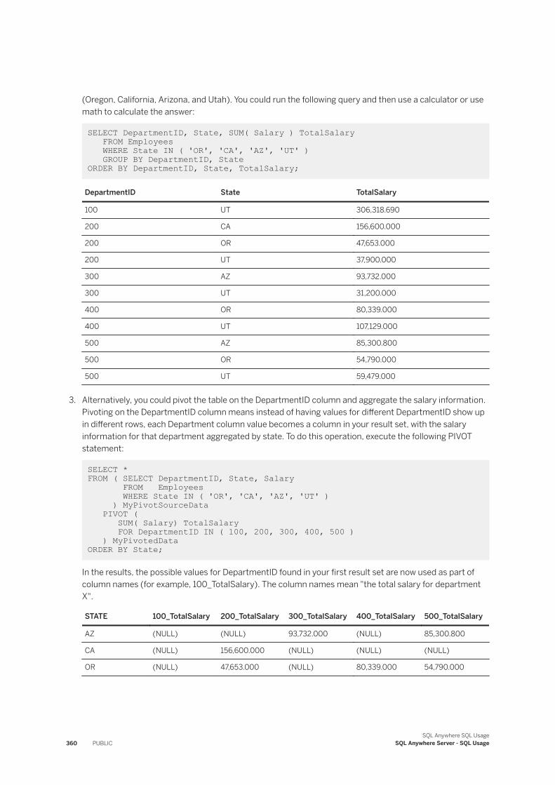
(Oregon, California, Arizona, and Utah). You could run the following query and then use a calculator or use math to calculate the answer:
SELECT DepartmentID, State, SUM( Salary ) TotalSalary FROM Employees WHERE State IN ( 'OR', 'CA', 'AZ', 'UT' ) GROUP BY DepartmentID, StateORDER BY DepartmentID, State, TotalSalary;
DepartmentID State TotalSalary
100 UT 306,318.690
200 CA 156,600.000
200 OR 47,653.000
200 UT 37,900.000
300 AZ 93,732.000
300 UT 31,200.000
400 OR 80,339.000
400 UT 107,129.000
500 AZ 85,300.800
500 OR 54,790.000
500 UT 59,479.000
3. Alternatively, you could pivot the table on the DepartmentID column and aggregate the salary information. Pivoting on the DepartmentID column means instead of having values for different DepartmentID show up in different rows, each Department column value becomes a column in your result set, with the salary information for that department aggregated by state. To do this operation, execute the following PIVOT statement:
SELECT * FROM ( SELECT DepartmentID, State, Salary FROM Employees WHERE State IN ( 'OR', 'CA', 'AZ', 'UT' ) ) MyPivotSourceData PIVOT ( SUM( Salary) TotalSalary FOR DepartmentID IN ( 100, 200, 300, 400, 500 ) ) MyPivotedData ORDER BY State;
In the results, the possible values for DepartmentID found in your first result set are now used as part of column names (for example, 100_TotalSalary). The column names mean "the total salary for department X".
STATE 100_TotalSalary 200_TotalSalary 300_TotalSalary 400_TotalSalary 500_TotalSalary
AZ (NULL) (NULL) 93,732.000 (NULL) 85,300.800
CA (NULL) 156,600.000 (NULL) (NULL) (NULL)
OR (NULL) 47,653.000 (NULL) 80,339.000 54,790.000
360 PUBLICSQL Anywhere SQL Usage
SQL Anywhere Server - SQL Usage
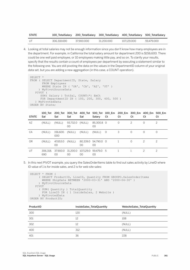
STATE 100_TotalSalary 200_TotalSalary 300_TotalSalary 400_TotalSalary 500_TotalSalary
UT 306,318.690 37,900.000 31,200.000 107,129.000 59,479.000
4. Looking at total salaries may not be enough information since you don't know how many employees are in the department. For example, in California the total salary amount for department 200 is $156,600. There could be one well paid employee, or 10 employees making little pay, and so on. To clarify your results, specify that the results contain a count of employees per department by executing a statement similar to the following one. You are still pivoting the data on the values in the DepartmentID column of your original data set, but you are adding a new aggregation (in this case, a COUNT operation).
SELECT * FROM ( SELECT DepartmentID, State, Salary FROM Employees WHERE State IN ( 'OR', 'CA', 'AZ', 'UT' ) ) MyPivotSourceData PIVOT ( SUM( Salary ) TotSal, COUNT(*) EmCt FOR DepartmentID IN ( 100, 200, 300, 400, 500 ) ) MyPivotedData ORDER BY State;
STATE100_TotSal
200_TotSal
300_TotSal
400_TotSal
500_TotSalary
100_EmCt
200_EmCt
300_EmCt
400_EmCt
500_EmCt
AZ (NULL) (NULL) 93,732.000
(NULL) 85,300.800
0 0 2 0 2
CA (NULL) 156,600.000
(NULL) (NULL) (NULL) 0 3 0 0 0
OR (NULL) 47,653.000
(NULL) 80,339.000
54,790.000
0 1 0 2 2
UT 306,318.690
37,900.000
31,200.000
107,129.000
59,479.000
5 1 1 2 2
5. In this next PIVOT example, you query the SalesOrderItems table to find out sales activity by LineID where ID value of 1 is for inside sales, and 2 is for web site sales:
SELECT * FROM ( ( SELECT ProductID, LineID, Quantity FROM GROUPO.SalesOrderItems WHERE ShipDate BETWEEN '2000-03-31' AND '2000-04-30' ) ) MyPivotSourceData PIVOT ( SUM( Quantity ) TotalQuantity FOR LineID IN ( 1 InsideSales, 2 Website ) ) MyPivotedData ORDER BY ProductID;
ProductID InsideSales_TotalQuantity WebsiteSales_TotalQuantity
300 120 (NULL)
301 12 108
302 12 (NULL)
400 312 (NULL)
401 36 228
SQL Anywhere SQL UsageSQL Anywhere Server - SQL Usage PUBLIC 361
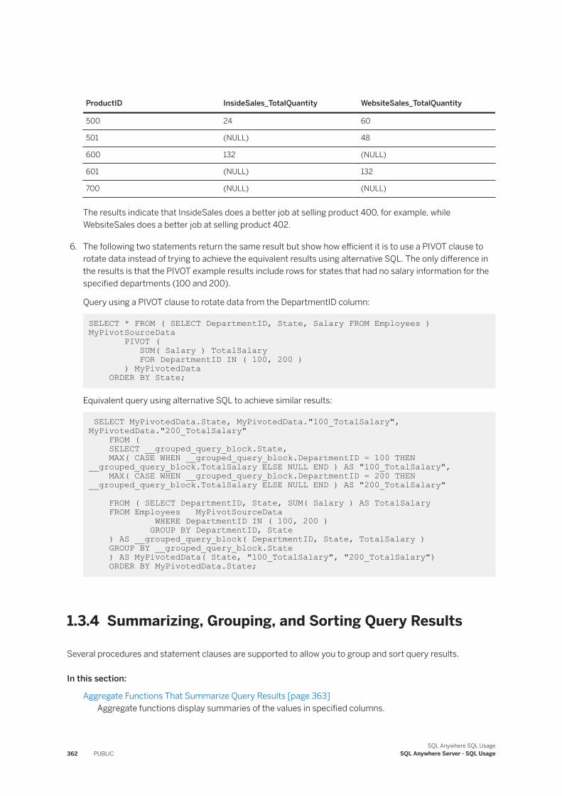
ProductID InsideSales_TotalQuantity WebsiteSales_TotalQuantity
500 24 60
501 (NULL) 48
600 132 (NULL)
601 (NULL) 132
700 (NULL) (NULL)
The results indicate that InsideSales does a better job at selling product 400, for example, while WebsiteSales does a better job at selling product 402.
6. The following two statements return the same result but show how efficient it is to use a PIVOT clause to rotate data instead of trying to achieve the equivalent results using alternative SQL. The only difference in the results is that the PIVOT example results include rows for states that had no salary information for the specified departments (100 and 200).
Query using a PIVOT clause to rotate data from the DepartmentID column:
SELECT * FROM ( SELECT DepartmentID, State, Salary FROM Employees ) MyPivotSourceData PIVOT ( SUM( Salary ) TotalSalary FOR DepartmentID IN ( 100, 200 ) ) MyPivotedData ORDER BY State;
Equivalent query using alternative SQL to achieve similar results:
SELECT MyPivotedData.State, MyPivotedData."100_TotalSalary", MyPivotedData."200_TotalSalary" FROM ( SELECT __grouped_query_block.State, MAX( CASE WHEN __grouped_query_block.DepartmentID = 100 THEN __grouped_query_block.TotalSalary ELSE NULL END ) AS "100_TotalSalary", MAX( CASE WHEN __grouped_query_block.DepartmentID = 200 THEN __grouped_query_block.TotalSalary ELSE NULL END ) AS "200_TotalSalary" FROM ( SELECT DepartmentID, State, SUM( Salary ) AS TotalSalary FROM Employees MyPivotSourceData WHERE DepartmentID IN ( 100, 200 ) GROUP BY DepartmentID, State ) AS __grouped_query_block( DepartmentID, State, TotalSalary ) GROUP BY __grouped_query_block.State ) AS MyPivotedData( State, "100_TotalSalary", "200_TotalSalary") ORDER BY MyPivotedData.State;
1.3.4 Summarizing, Grouping, and Sorting Query Results
Several procedures and statement clauses are supported to allow you to group and sort query results.
In this section:
Aggregate Functions That Summarize Query Results [page 363]Aggregate functions display summaries of the values in specified columns.
362 PUBLICSQL Anywhere SQL Usage
SQL Anywhere Server - SQL Usage
The GROUP BY Clause: Organizing Query Results into Groups [page 367]The GROUP BY clause divides the output of a table into groups.
The HAVING Clause: Selecting Groups of Data [page 372]The HAVING clause restricts the rows returned by a query.
The ORDER BY Clause: Sorting Query Results [page 374]The ORDER BY clause allows sorting of query results by one or more columns.
Set Operations on Query Results using UNION, INTERSECT, and EXCEPT [page 378]UNION, INTERSECT, and EXCEPT perform set operations on the results of two or more queries.
1.3.4.1 Aggregate Functions That Summarize Query Results
Aggregate functions display summaries of the values in specified columns.
You can also use the GROUP BY clause, HAVING clause, and ORDER BY clause to group and sort the results of queries using aggregate functions, and the UNION operator to combine the results of queries.
When an ORDER BY clause contains constants, they are interpreted by the optimizer and then replaced by an equivalent ORDER BY clause. For example, the optimizer interprets ORDER BY 'a' as ORDER BY expression.
A query block containing more than one aggregate function with valid ORDER BY clauses can be executed if the ORDER BY clauses can be logically combined into a single ORDER BY clause. For example, the following clauses:
ORDER BY expression1, 'a', expression2
ORDER BY expression1, 'b', expression2, 'c', expression3
are subsumed by the clause:
ORDER BY expression1, expression2, expression3
You can apply aggregate functions to all the rows in a table, to a subset of the table specified by a WHERE clause, or to one or more groups of rows in the table. From each set of rows to which an aggregate function is applied, the database server generates a single value.
The following are some of the supported aggregate functions:
AVG( expression )
The mean of the supplied expression over the returned rows.COUNT( expression )
The number of rows in the supplied group where the expression is not NULL.COUNT( * )
The number of rows in each group.LIST( string-expr )
A string containing a comma-separated list composed of all the values for string-expr in each group of rows.
SQL Anywhere SQL UsageSQL Anywhere Server - SQL Usage PUBLIC 363
MAX( expression )
The maximum value of the expression, over the returned rows.MIN( expression )
The minimum value of the expression, over the returned rows.STDDEV( expression )
The standard deviation of the expression, over the returned rows.SUM( expression )
The sum of the expression, over the returned rows.VARIANCE( expression )
The variance of the expression, over the returned rows.
You can use the optional keyword DISTINCT with AVG, SUM, LIST, and COUNT to eliminate duplicate values before the aggregate function is applied.
The expression to which the syntax statement refers is usually a column name. It can also be a more general expression.
For example, with this statement you can find what the average price of all products would be if one dollar were added to each price:
SELECT AVG ( UnitPrice + 1 ) FROM Products;
Example
The following query calculates the total payroll from the annual salaries in the Employees table:
SELECT SUM( Salary ) FROM Employees;
To use aggregate functions, you must give the function name followed by an expression on whose values it will operate. The expression, which is the Salary column in this example, is the function's argument and must be specified inside parentheses.
In this section:
Where You Can Use Aggregate Functions [page 365]Aggregate functions can be used in a SELECT list or in the HAVING clause of a grouped query block.
Aggregate Functions and Data types [page 365]Some aggregate functions have meaning only for certain kinds of data.
COUNT( * ) [page 365]COUNT( * ) returns the number of rows in the specified table without eliminating duplicates.
Aggregate Functions with DISTINCT [page 366]When you specify the DISTINCT keyword in a query, duplicate values are eliminated before calculating the SUM, AVG, or COUNT.
Aggregate Functions and NULL [page 366]
364 PUBLICSQL Anywhere SQL Usage
SQL Anywhere Server - SQL Usage
NULLS in the column on which the aggregate function is operating are ignored for the function except COUNT(*), which includes them.
1.3.4.1.1 Where You Can Use Aggregate Functions
Aggregate functions can be used in a SELECT list or in the HAVING clause of a grouped query block.
You cannot use aggregate functions in a WHERE clause or in a JOIN condition. However, a SELECT query block with aggregate functions in its SELECT list often includes a WHERE clause that restricts the rows to which the aggregate is applied.
Whenever an aggregate function is used in a SELECT query block that does not include a GROUP BY clause, it produces a single value, whether it is operating on all the rows in a table or on a subset of rows defined by a WHERE clause.
You can use more than one aggregate function in the same SELECT list, and produce more than one aggregate in a single SELECT query block.
Related Information
The HAVING Clause: Selecting Groups of Data [page 372]
1.3.4.1.2 Aggregate Functions and Data types
Some aggregate functions have meaning only for certain kinds of data.
For example, you can use SUM and AVG with numeric columns only.
However, you can use MIN to find the lowest value (the one closest to the beginning of the alphabet) in a character column:
SELECT MIN( Surname ) FROM Contacts;
1.3.4.1.3 COUNT( * )
COUNT( * ) returns the number of rows in the specified table without eliminating duplicates.
It counts each row separately, including rows that contain NULL. This function does not require an expression as an argument because, by definition, it does not use information about any particular column.
The following statement finds the total number of employees in the Employees table:
SELECT COUNT( * )
SQL Anywhere SQL UsageSQL Anywhere Server - SQL Usage PUBLIC 365
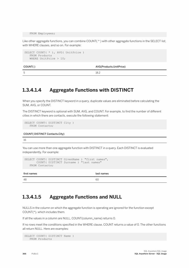
FROM Employees;
Like other aggregate functions, you can combine COUNT( * ) with other aggregate functions in the SELECT list, with WHERE clauses, and so on. For example:
SELECT COUNT( * ), AVG( UnitPrice ) FROM Products WHERE UnitPrice > 10;
COUNT( ) AVG(Products.UnitPrice)
5 18.2
1.3.4.1.4 Aggregate Functions with DISTINCT
When you specify the DISTINCT keyword in a query, duplicate values are eliminated before calculating the SUM, AVG, or COUNT.
The DISTINCT keyword is optional with SUM, AVG, and COUNT. For example, to find the number of different cities in which there are contacts, execute the following statement:
SELECT COUNT( DISTINCT City ) FROM Contacts;
COUNT( DISTINCT Contacts.City)
16
You can use more than one aggregate function with DISTINCT in a query. Each DISTINCT is evaluated independently. For example:
SELECT COUNT( DISTINCT GivenName ) "first names", COUNT( DISTINCT Surname ) "last names" FROM Contacts;
first names last names
48 60
1.3.4.1.5 Aggregate Functions and NULL
NULLS in the column on which the aggregate function is operating are ignored for the function except COUNT(*), which includes them.
If all the values in a column are NULL, COUNT(column_name) returns 0.
If no rows meet the conditions specified in the WHERE clause, COUNT returns a value of 0. The other functions all return NULL. Here are examples:
SELECT COUNT( DISTINCT Name ) FROM Products
366 PUBLICSQL Anywhere SQL Usage
SQL Anywhere Server - SQL Usage
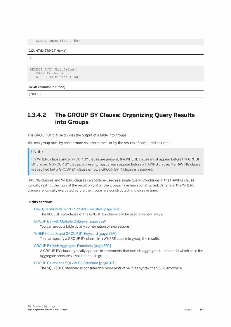
WHERE UnitPrice > 50;
COUNT(DISTINCT Name)
0
SELECT AVG( UnitPrice ) FROM Products WHERE UnitPrice > 50;
AVG(Products.UnitPrice)
( NULL )
1.3.4.2 The GROUP BY Clause: Organizing Query Results into Groups
The GROUP BY clause divides the output of a table into groups.
You can group rows by one or more column names, or by the results of computed columns.
NoteIf a WHERE clause and a GROUP BY clause are present, the WHERE clause must appear before the GROUP BY clause. A GROUP BY clause, if present, must always appear before a HAVING clause. If a HAVING clause is specified but a GROUP BY clause is not, a GROUP BY () clause is assumed.
HAVING clauses and WHERE clauses can both be used in a single query. Conditions in the HAVING clause logically restrict the rows of the result only after the groups have been constructed. Criteria in the WHERE clause are logically evaluated before the groups are constructed, and so save time.
In this section:
How Queries with GROUP BY Are Executed [page 368]The ROLLUP sub-clause of the GROUP BY clause can be used in several ways.
GROUP BY with Multiple Columns [page 369]You can group a table by any combination of expressions.
WHERE Clause and GROUP BY Keyword [page 369]You can specify a GROUP BY clause in a WHERE clause to group the results.
GROUP BY with Aggregate Functions [page 370]A GROUP BY clause typically appears in statements that include aggregate functions, in which case the aggregate produces a value for each group.
GROUP BY and the SQL/2008 Standard [page 371]The SQL/2008 standard is considerably more restrictive in its syntax than SQL Anywhere.
SQL Anywhere SQL UsageSQL Anywhere Server - SQL Usage PUBLIC 367
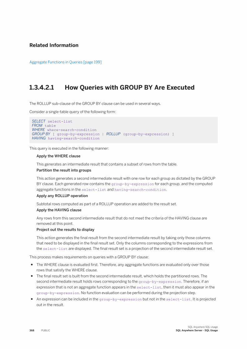
Related Information
Aggregate Functions in Queries [page 199]
1.3.4.2.1 How Queries with GROUP BY Are Executed
The ROLLUP sub-clause of the GROUP BY clause can be used in several ways.
Consider a single-table query of the following form:
SELECT select-list FROM table WHERE where-search-condition GROUP BY [ group-by-expression | ROLLUP (group-by-expression) ] HAVING having-search-condition
This query is executed in the following manner:
Apply the WHERE clause
This generates an intermediate result that contains a subset of rows from the table.Partition the result into groups
This action generates a second intermediate result with one row for each group as dictated by the GROUP BY clause. Each generated row contains the group-by-expression for each group, and the computed aggregate functions in the select-list and having-search-condition.Apply any ROLLUP operation
Subtotal rows computed as part of a ROLLUP operation are added to the result set.Apply the HAVING clause
Any rows from this second intermediate result that do not meet the criteria of the HAVING clause are removed at this point.Project out the results to display
This action generates the final result from the second intermediate result by taking only those columns that need to be displayed in the final result set. Only the columns corresponding to the expressions from the select-list are displayed. The final result set is a projection of the second intermediate result set.
This process makes requirements on queries with a GROUP BY clause:
● The WHERE clause is evaluated first. Therefore, any aggregate functions are evaluated only over those rows that satisfy the WHERE clause.
● The final result set is built from the second intermediate result, which holds the partitioned rows. The second intermediate result holds rows corresponding to the group-by-expression. Therefore, if an expression that is not an aggregate function appears in the select-list, then it must also appear in the group-by-expression. No function evaluation can be performed during the projection step.
● An expression can be included in the group-by-expression but not in the select-list. It is projected out in the result.
368 PUBLICSQL Anywhere SQL Usage
SQL Anywhere Server - SQL Usage
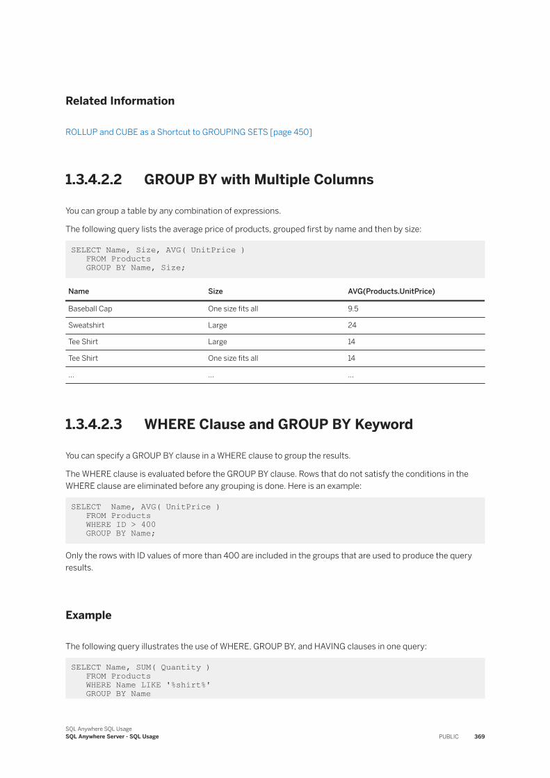
Related Information
ROLLUP and CUBE as a Shortcut to GROUPING SETS [page 450]
1.3.4.2.2 GROUP BY with Multiple Columns
You can group a table by any combination of expressions.
The following query lists the average price of products, grouped first by name and then by size:
SELECT Name, Size, AVG( UnitPrice ) FROM Products GROUP BY Name, Size;
Name Size AVG(Products.UnitPrice)
Baseball Cap One size fits all 9.5
Sweatshirt Large 24
Tee Shirt Large 14
Tee Shirt One size fits all 14
... ... ...
1.3.4.2.3 WHERE Clause and GROUP BY Keyword
You can specify a GROUP BY clause in a WHERE clause to group the results.
The WHERE clause is evaluated before the GROUP BY clause. Rows that do not satisfy the conditions in the WHERE clause are eliminated before any grouping is done. Here is an example:
SELECT Name, AVG( UnitPrice ) FROM Products WHERE ID > 400 GROUP BY Name;
Only the rows with ID values of more than 400 are included in the groups that are used to produce the query results.
Example
The following query illustrates the use of WHERE, GROUP BY, and HAVING clauses in one query:
SELECT Name, SUM( Quantity ) FROM Products WHERE Name LIKE '%shirt%' GROUP BY Name
SQL Anywhere SQL UsageSQL Anywhere Server - SQL Usage PUBLIC 369
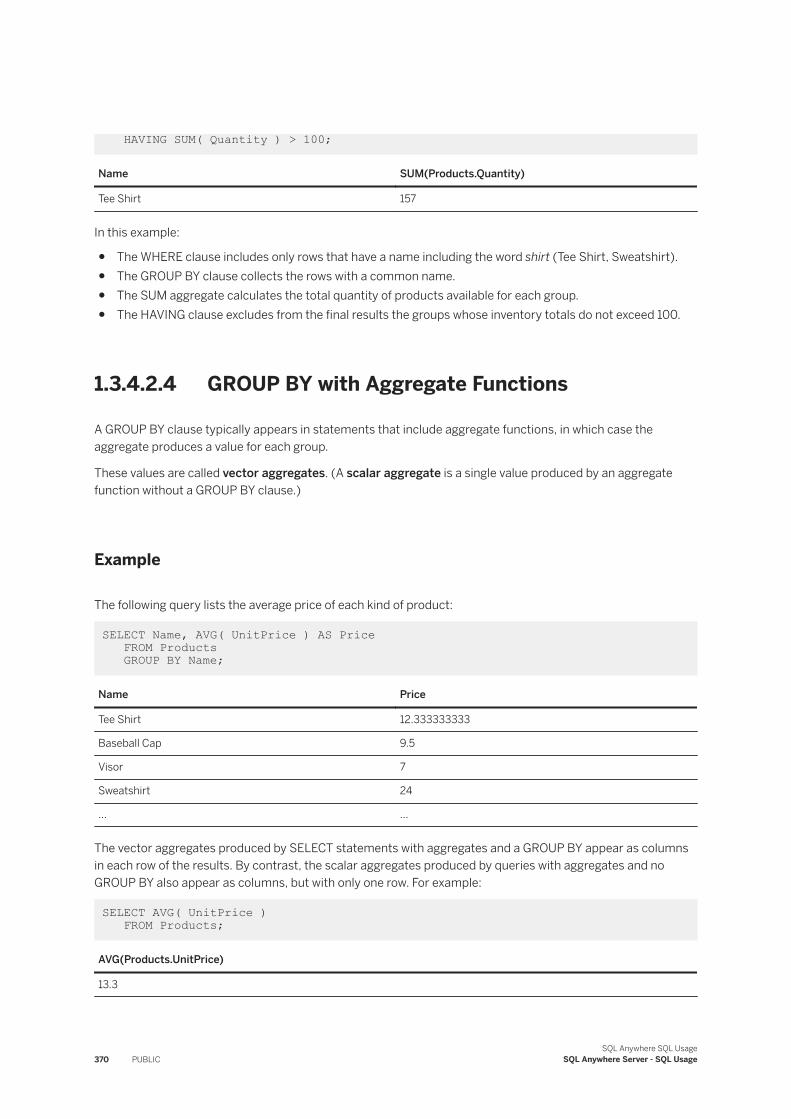
HAVING SUM( Quantity ) > 100;
Name SUM(Products.Quantity)
Tee Shirt 157
In this example:
● The WHERE clause includes only rows that have a name including the word shirt (Tee Shirt, Sweatshirt).● The GROUP BY clause collects the rows with a common name.● The SUM aggregate calculates the total quantity of products available for each group.● The HAVING clause excludes from the final results the groups whose inventory totals do not exceed 100.
1.3.4.2.4 GROUP BY with Aggregate Functions
A GROUP BY clause typically appears in statements that include aggregate functions, in which case the aggregate produces a value for each group.
These values are called vector aggregates. (A scalar aggregate is a single value produced by an aggregate function without a GROUP BY clause.)
Example
The following query lists the average price of each kind of product:
SELECT Name, AVG( UnitPrice ) AS Price FROM Products GROUP BY Name;
Name Price
Tee Shirt 12.333333333
Baseball Cap 9.5
Visor 7
Sweatshirt 24
... ...
The vector aggregates produced by SELECT statements with aggregates and a GROUP BY appear as columns in each row of the results. By contrast, the scalar aggregates produced by queries with aggregates and no GROUP BY also appear as columns, but with only one row. For example:
SELECT AVG( UnitPrice ) FROM Products;
AVG(Products.UnitPrice)
13.3
370 PUBLICSQL Anywhere SQL Usage
SQL Anywhere Server - SQL Usage
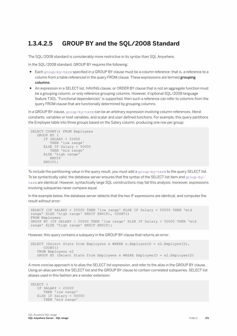
1.3.4.2.5 GROUP BY and the SQL/2008 Standard
The SQL/2008 standard is considerably more restrictive in its syntax than SQL Anywhere.
In the SQL/2008 standard, GROUP BY requires the following:
● Each group-by-term specified in a GROUP BY clause must be a column reference: that is, a reference to a column from a table referenced in the query FROM clause. These expressions are termed grouping columns.
● An expression in a SELECT list, HAVING clause, or ORDER BY clause that is not an aggregate function must be a grouping column, or only reference grouping columns. However, if optional SQL/2008 language feature T301, "Functional dependencies" is supported, then such a reference can refer to columns from the query FROM clause that are functionally determined by grouping columns.
In a GROUP BY clause, group-by-term can be an arbitrary expression involving column references, literal constants, variables or host variables, and scalar and user-defined functions. For example, this query partitions the Employee table into three groups based on the Salary column, producing one row per group:
SELECT COUNT() FROM Employees GROUP BY ( IF SALARY < 25000 THEN 'low range' ELSE IF Salary < 50000 THEN 'mid range' ELSE 'high range' ENDIF ENDIF);
To include the partitioning value in the query result, you must add a group-by-term to the query SELECT list. To be syntactically valid, the database server ensures that the syntax of the SELECT list item and group-by-term are identical. However, syntactically large SQL constructions may fail this analysis; moreover, expressions involving subqueries never compare equal.
In the example below, the database server detects that the two IF expressions are identical, and computes the result without error:
SELECT (IF SALARY < 25000 THEN 'low range' ELSE IF Salary < 50000 THEN 'mid range' ELSE 'high range' ENDIF ENDIF), COUNT() FROM Employees GROUP BY (IF SALARY < 25000 THEN 'low range' ELSE IF Salary < 50000 THEN 'mid range' ELSE 'high range' ENDIF ENDIF);
However, this query contains a subquery in the GROUP BY clause that returns an error:
SELECT (Select State from Employees e WHERE e.EmployeeID = e2.EmployeeID), COUNT() FROM Employees e2 GROUP BY (Select State from Employees e WHERE EmployeeID = e2.EmployeeID)
A more concise approach is to alias the SELECT list expression, and refer to the alias in the GROUP BY clause. Using an alias permits the SELECT list and the GROUP BY clause to contain correlated subqueries. SELECT list aliases used in this fashion are a vendor extension:
SELECT ( IF SALARY < 25000 THEN 'low range' ELSE IF Salary < 50000 THEN 'mid range'
SQL Anywhere SQL UsageSQL Anywhere Server - SQL Usage PUBLIC 371
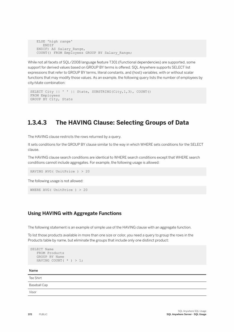
ELSE 'high range' ENDIF ENDIF) AS Salary_Range, COUNT() FROM Employees GROUP BY Salary_Range;
While not all facets of SQL/2008 language feature T301 (Functional dependencies) are supported, some support for derived values based on GROUP BY terms is offered. SQL Anywhere supports SELECT list expressions that refer to GROUP BY terms, literal constants, and (host) variables, with or without scalar functions that may modify those values. As an example, the following query lists the number of employees by city/state combination:
SELECT City || ' ' || State, SUBSTRING(City,1,3), COUNT() FROM Employees GROUP BY City, State
1.3.4.3 The HAVING Clause: Selecting Groups of Data
The HAVING clause restricts the rows returned by a query.
It sets conditions for the GROUP BY clause similar to the way in which WHERE sets conditions for the SELECT clause.
The HAVING clause search conditions are identical to WHERE search conditions except that WHERE search conditions cannot include aggregates. For example, the following usage is allowed:
HAVING AVG( UnitPrice ) > 20
The following usage is not allowed:
WHERE AVG( UnitPrice ) > 20
Using HAVING with Aggregate Functions
The following statement is an example of simple use of the HAVING clause with an aggregate function.
To list those products available in more than one size or color, you need a query to group the rows in the Products table by name, but eliminate the groups that include only one distinct product:
SELECT Name FROM Products GROUP BY Name HAVING COUNT( * ) > 1;
Name
Tee Shirt
Baseball Cap
Visor
372 PUBLICSQL Anywhere SQL Usage
SQL Anywhere Server - SQL Usage
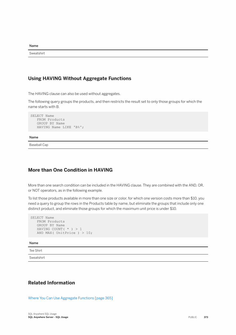
Name
Sweatshirt
Using HAVING Without Aggregate Functions
The HAVING clause can also be used without aggregates.
The following query groups the products, and then restricts the result set to only those groups for which the name starts with B.
SELECT Name FROM Products GROUP BY Name HAVING Name LIKE 'B%';
Name
Baseball Cap
More than One Condition in HAVING
More than one search condition can be included in the HAVING clause. They are combined with the AND, OR, or NOT operators, as in the following example.
To list those products available in more than one size or color, for which one version costs more than $10, you need a query to group the rows in the Products table by name, but eliminate the groups that include only one distinct product, and eliminate those groups for which the maximum unit price is under $10.
SELECT Name FROM Products GROUP BY Name HAVING COUNT( * ) > 1 AND MAX( UnitPrice ) > 10;
Name
Tee Shirt
Sweatshirt
Related Information
Where You Can Use Aggregate Functions [page 365]
SQL Anywhere SQL UsageSQL Anywhere Server - SQL Usage PUBLIC 373
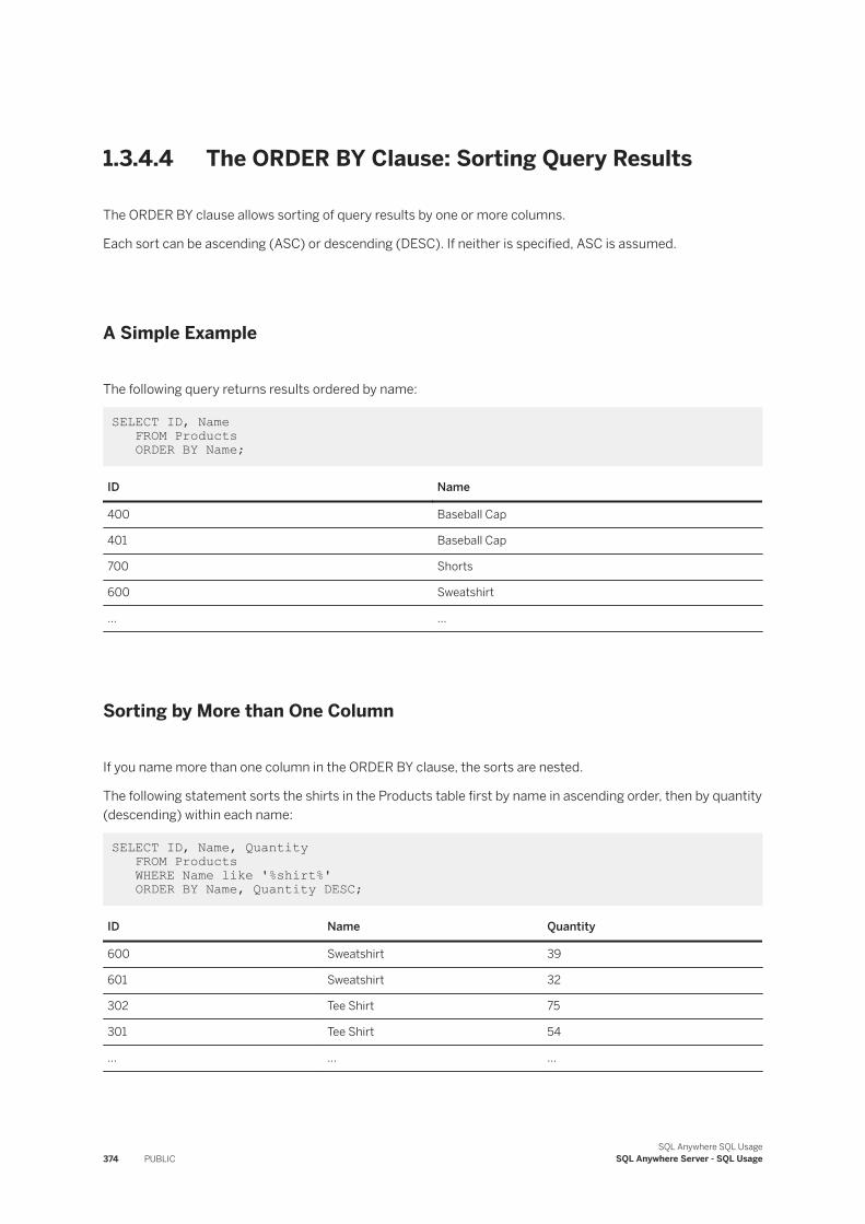
1.3.4.4 The ORDER BY Clause: Sorting Query Results
The ORDER BY clause allows sorting of query results by one or more columns.
Each sort can be ascending (ASC) or descending (DESC). If neither is specified, ASC is assumed.
A Simple Example
The following query returns results ordered by name:
SELECT ID, Name FROM Products ORDER BY Name;
ID Name
400 Baseball Cap
401 Baseball Cap
700 Shorts
600 Sweatshirt
... ...
Sorting by More than One Column
If you name more than one column in the ORDER BY clause, the sorts are nested.
The following statement sorts the shirts in the Products table first by name in ascending order, then by quantity (descending) within each name:
SELECT ID, Name, Quantity FROM Products WHERE Name like '%shirt%' ORDER BY Name, Quantity DESC;
ID Name Quantity
600 Sweatshirt 39
601 Sweatshirt 32
302 Tee Shirt 75
301 Tee Shirt 54
... ... ...
374 PUBLICSQL Anywhere SQL Usage
SQL Anywhere Server - SQL Usage
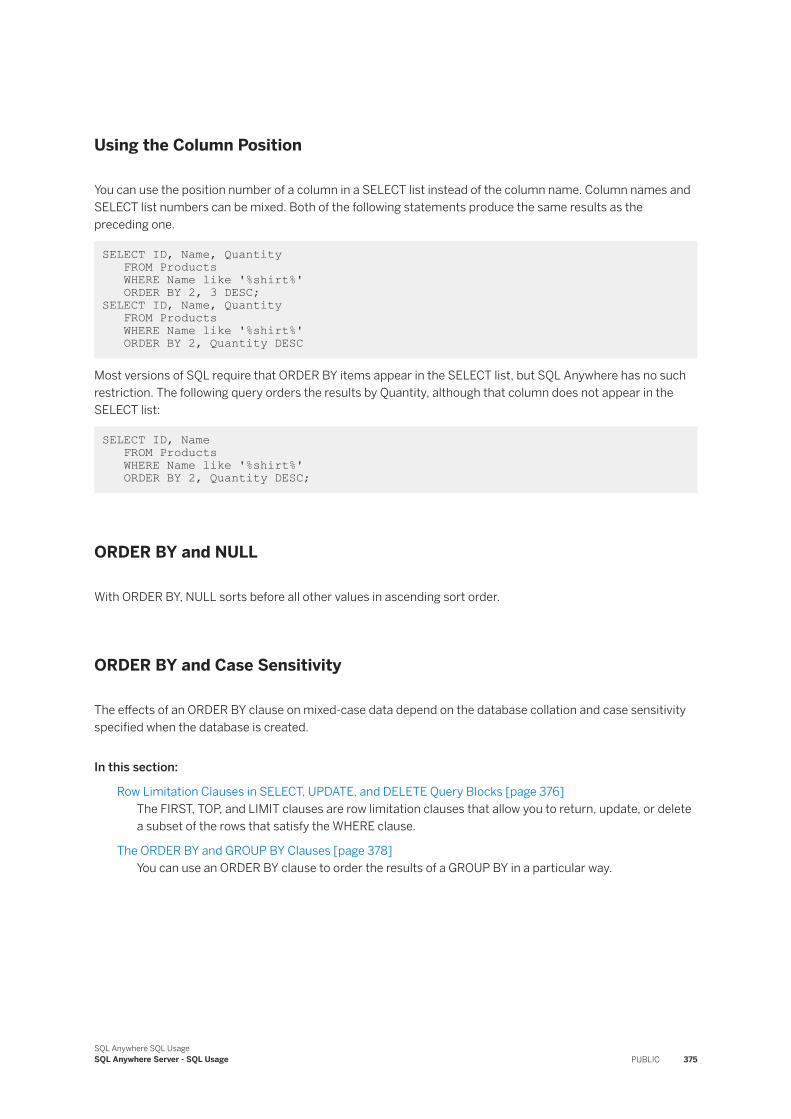
Using the Column Position
You can use the position number of a column in a SELECT list instead of the column name. Column names and SELECT list numbers can be mixed. Both of the following statements produce the same results as the preceding one.
SELECT ID, Name, Quantity FROM Products WHERE Name like '%shirt%' ORDER BY 2, 3 DESC;SELECT ID, Name, Quantity FROM Products WHERE Name like '%shirt%' ORDER BY 2, Quantity DESC
Most versions of SQL require that ORDER BY items appear in the SELECT list, but SQL Anywhere has no such restriction. The following query orders the results by Quantity, although that column does not appear in the SELECT list:
SELECT ID, Name FROM Products WHERE Name like '%shirt%' ORDER BY 2, Quantity DESC;
ORDER BY and NULL
With ORDER BY, NULL sorts before all other values in ascending sort order.
ORDER BY and Case Sensitivity
The effects of an ORDER BY clause on mixed-case data depend on the database collation and case sensitivity specified when the database is created.
In this section:
Row Limitation Clauses in SELECT, UPDATE, and DELETE Query Blocks [page 376]The FIRST, TOP, and LIMIT clauses are row limitation clauses that allow you to return, update, or delete a subset of the rows that satisfy the WHERE clause.
The ORDER BY and GROUP BY Clauses [page 378]You can use an ORDER BY clause to order the results of a GROUP BY in a particular way.
SQL Anywhere SQL UsageSQL Anywhere Server - SQL Usage PUBLIC 375
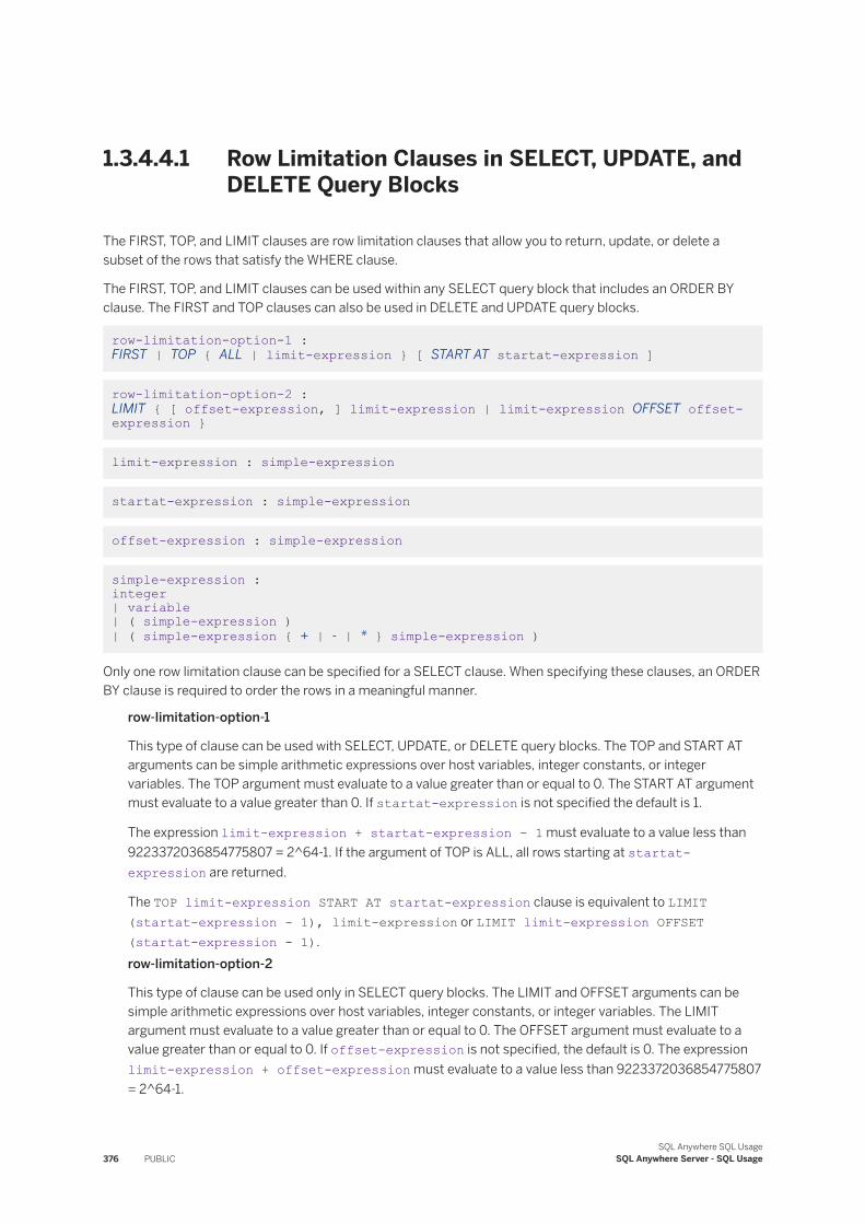
1.3.4.4.1 Row Limitation Clauses in SELECT, UPDATE, and DELETE Query Blocks
The FIRST, TOP, and LIMIT clauses are row limitation clauses that allow you to return, update, or delete a subset of the rows that satisfy the WHERE clause.
The FIRST, TOP, and LIMIT clauses can be used within any SELECT query block that includes an ORDER BY clause. The FIRST and TOP clauses can also be used in DELETE and UPDATE query blocks.
row-limitation-option-1 : FIRST | TOP { ALL | limit-expression } [ START AT startat-expression ]
row-limitation-option-2 : LIMIT { [ offset-expression, ] limit-expression | limit-expression OFFSET offset-expression }
limit-expression : simple-expression
startat-expression : simple-expression
offset-expression : simple-expression
simple-expression : integer | variable | ( simple-expression ) | ( simple-expression { + | - | * } simple-expression )
Only one row limitation clause can be specified for a SELECT clause. When specifying these clauses, an ORDER BY clause is required to order the rows in a meaningful manner.
row-limitation-option-1
This type of clause can be used with SELECT, UPDATE, or DELETE query blocks. The TOP and START AT arguments can be simple arithmetic expressions over host variables, integer constants, or integer variables. The TOP argument must evaluate to a value greater than or equal to 0. The START AT argument must evaluate to a value greater than 0. If startat-expression is not specified the default is 1.
The expression limit-expression + startat-expression - 1 must evaluate to a value less than 9223372036854775807 = 2^64-1. If the argument of TOP is ALL, all rows starting at startat-expression are returned.
The TOP limit-expression START AT startat-expression clause is equivalent to LIMIT (startat-expression - 1), limit-expression or LIMIT limit-expression OFFSET (startat-expression - 1).row-limitation-option-2
This type of clause can be used only in SELECT query blocks. The LIMIT and OFFSET arguments can be simple arithmetic expressions over host variables, integer constants, or integer variables. The LIMIT argument must evaluate to a value greater than or equal to 0. The OFFSET argument must evaluate to a value greater than or equal to 0. If offset-expression is not specified, the default is 0. The expression limit-expression + offset-expression must evaluate to a value less than 9223372036854775807 = 2^64-1.
376 PUBLICSQL Anywhere SQL Usage
SQL Anywhere Server - SQL Usage
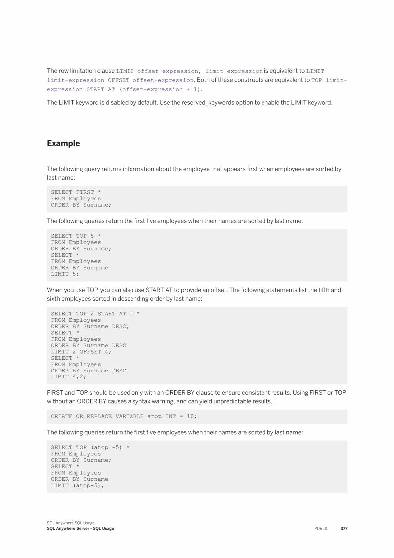
The row limitation clause LIMIT offset-expression, limit-expression is equivalent to LIMIT limit-expression OFFSET offset-expression. Both of these constructs are equivalent to TOP limit-expression START AT (offset-expression + 1).
The LIMIT keyword is disabled by default. Use the reserved_keywords option to enable the LIMIT keyword.
Example
The following query returns information about the employee that appears first when employees are sorted by last name:
SELECT FIRST * FROM Employees ORDER BY Surname;
The following queries return the first five employees when their names are sorted by last name:
SELECT TOP 5 * FROM EmployeesORDER BY Surname;SELECT *FROM EmployeesORDER BY Surname LIMIT 5;
When you use TOP, you can also use START AT to provide an offset. The following statements list the fifth and sixth employees sorted in descending order by last name:
SELECT TOP 2 START AT 5 * FROM EmployeesORDER BY Surname DESC;SELECT *FROM EmployeesORDER BY Surname DESCLIMIT 2 OFFSET 4;SELECT *FROM EmployeesORDER BY Surname DESC LIMIT 4,2;
FIRST and TOP should be used only with an ORDER BY clause to ensure consistent results. Using FIRST or TOP without an ORDER BY causes a syntax warning, and can yield unpredictable results.
CREATE OR REPLACE VARIABLE atop INT = 10;
The following queries return the first five employees when their names are sorted by last name:
SELECT TOP (atop -5) * FROM EmployeesORDER BY Surname;SELECT *FROM EmployeesORDER BY Surname LIMIT (atop-5);
SQL Anywhere SQL UsageSQL Anywhere Server - SQL Usage PUBLIC 377
The following statements list the fifth and sixth employees sorted in descending order by last name:
SELECT TOP (atop - 8) START AT (atop -2 -3) * FROM EmployeesORDER BY Surname DESC;SELECT *FROM EmployeesORDER BY Surname DESC LIMIT (atop - 8) OFFSET (atop -2 -3 -1);
1.3.4.4.2 The ORDER BY and GROUP BY Clauses
You can use an ORDER BY clause to order the results of a GROUP BY in a particular way.
Example
The following query finds the average price of each product and orders the results by average price:
SELECT Name, AVG( UnitPrice ) FROM Products GROUP BY Name ORDER BY AVG( UnitPrice );
Name AVG(Products.UnitPrice)
Visor 7
Baseball Cap 9.5
Tee Shirt 12.333333333
Shorts 15
... ...
1.3.4.5 Set Operations on Query Results using UNION, INTERSECT, and EXCEPT
UNION, INTERSECT, and EXCEPT perform set operations on the results of two or more queries.
While many of the operations can also be performed using operations in the WHERE clause or HAVING clause, there are some operations that are very difficult to perform in any way other than using these set-based operators. For example:
● When data is not normalized, you may want to assemble seemingly disparate information into a single result set, even though the tables are unrelated.
● NULL is treated differently by set operators than in the WHERE clause or HAVING clause. In the WHERE clause or HAVING clause, two null-containing rows with identical non-null entries are not seen as identical, as the two NULL values are not defined to be identical. The set operators see two such rows as the same.
378 PUBLICSQL Anywhere SQL Usage
SQL Anywhere Server - SQL Usage
In this section:
The UNION Clause: Combining Result Sets [page 379]The UNION operator combines the results of two or more queries into a single result set.
The EXCEPT and INTERSECT Clauses [page 379]The EXCEPT clause returns the differences between two result sets, and the INTERSECT clause returns the rows that appear in each of two result sets.
Rules for Set Operations [page 380]There are several rules that apply to UNION, EXCEPT, and INTERSECT statements.
Set Operators and the NULL Value [page 381]NULLs are treated differently by set operators UNION, EXCEPT, and INTERSECT than it is in search conditions.
1.3.4.5.1 The UNION Clause: Combining Result Sets
The UNION operator combines the results of two or more queries into a single result set.
By default, the UNION operator removes duplicate rows from the result set. If you use the ALL option, duplicates are not removed. The columns in the final result set have the same names as the columns in the first result set. Any number of union operators can be used.
By default, a statement containing multiple UNION operators is evaluated from left to right. Parentheses can be used to specify the order of evaluation.
For example, the following two expressions are not equivalent, due to the way that duplicate rows are removed from result sets:
x UNION ALL ( y UNION z )
(x UNION ALL y) UNION z
In the first expression, duplicates are eliminated in the UNION between y and z. In the UNION between that set and x, duplicates are not eliminated. In the second expression, duplicates are included in the union between x and y, but are then eliminated in the subsequent union with z.
1.3.4.5.2 The EXCEPT and INTERSECT Clauses
The EXCEPT clause returns the differences between two result sets, and the INTERSECT clause returns the rows that appear in each of two result sets.
Like the UNION clause, both EXCEPT and INTERSECT take the ALL modifier, which prevents the elimination of duplicate rows from the result set.
SQL Anywhere SQL UsageSQL Anywhere Server - SQL Usage PUBLIC 379
1.3.4.5.3 Rules for Set Operations
There are several rules that apply to UNION, EXCEPT, and INTERSECT statements.
Precedence
The UNION and EXCEPT operators have equal precedence and are both evaluated from left to right. The INTERSECT operator has a higher precedence than the UNION and EXCEPT operators and is also evaluated from left to right when more than one INTERSECT operator is used.Same number of items in the SELECT lists
All SELECT lists in the queries must have the same number of expressions (such as column names, arithmetic expressions, and aggregate functions). The following statement is invalid because the first SELECT list is longer than the second:
SELECT store_id, city, state FROM storesUNION SELECT store_id, city FROM stores_east;
Data types must match
Corresponding expressions in the SELECT lists must be of the same data type, or an implicit data conversion must be possible between the two data types, or an explicit conversion should be supplied.
For example, a UNION, INTERSECT, or EXCEPT is not possible between a column of the CHAR data type and one of the INT data type, unless an explicit conversion is supplied. However, a set operation is possible between a column of the MONEY data type and one of the INT data type.Column ordering
You must place corresponding expressions in the individual queries of a set operation in the same order, because the set operators compare the expressions one-to-one in the order given in the individual queries in the SELECT clauses.Multiple set operations
You can string several set operations together, as in the following example:
SELECT City AS Cities FROM Contacts UNION SELECT City FROM Customers UNION SELECT City FROM Employees;
For UNION statements, the order of queries is not important. For INTERSECT, the order is important when there are two or more queries. For EXCEPT, the order is always important.Column headings
The column names in the table resulting from a UNION are taken from the first individual query in the statement. Define a new column heading for the result set in the SELECT list of the first query, as in the following example:
SELECT City AS Cities FROM Contacts UNION
380 PUBLICSQL Anywhere SQL Usage
SQL Anywhere Server - SQL Usage
SELECT City FROM Customers;
In the following query, the column heading remains as City, as it is defined in the first query of the UNION clause.
SELECT City FROM Contacts UNION SELECT City AS Cities FROM Customers;
Alternatively, you can use the WITH clause to define the column names. For example:
WITH V( Cities ) AS ( SELECT City FROM Contacts UNION SELECT City FROM Customers ) SELECT * FROM V;
Ordering the results
You can use the WITH clause of the SELECT statement to order the column names in the SELECT list. For example:
WITH V( CityName ) AS ( SELECT City AS Cities FROM Contacts UNION SELECT City FROM Customers )SELECT * FROM V ORDER BY CityName;
Alternatively, you can use a single ORDER BY clause at the end of the list of queries, but you must use integers rather than column names, as in the following example:
SELECT City AS Cities FROM Contacts UNION SELECT City FROM Customers ORDER BY 1;
1.3.4.5.4 Set Operators and the NULL Value
NULLs are treated differently by set operators UNION, EXCEPT, and INTERSECT than it is in search conditions.
This difference is one of the main reasons to use set operators.
When comparing rows, set operators treat NULL values as equal to each other. In contrast, when NULL is compared to NULL in a search condition the result is unknown (not true).
One result of this difference is that the number of rows in the result set for query-1 EXCEPT ALL query-2 is always the difference in the number of rows in the result sets of the individual queries.
SQL Anywhere SQL UsageSQL Anywhere Server - SQL Usage PUBLIC 381
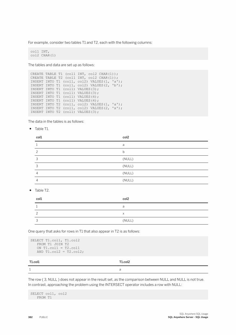
For example, consider two tables T1 and T2, each with the following columns:
col1 INT, col2 CHAR(1)
The tables and data are set up as follows:
CREATE TABLE T1 (col1 INT, col2 CHAR(1)); CREATE TABLE T2 (col1 INT, col2 CHAR(1));INSERT INTO T1 (col1, col2) VALUES(1, 'a');INSERT INTO T1 (col1, col2) VALUES(2, 'b');INSERT INTO T1 (col1) VALUES(3);INSERT INTO T1 (col1) VALUES(3);INSERT INTO T1 (col1) VALUES(4);INSERT INTO T1 (col1) VALUES(4);INSERT INTO T2 (col1, col2) VALUES(1, 'a');INSERT INTO T2 (col1, col2) VALUES(2, 'x');INSERT INTO T2 (col1) VALUES(3);
The data in the tables is as follows:
● Table T1.
col1 col2
1 a
2 b
3 (NULL)
3 (NULL)
4 (NULL)
4 (NULL)
● Table T2.
col1 col2
1 a
2 x
3 (NULL)
One query that asks for rows in T1 that also appear in T2 is as follows:
SELECT T1.col1, T1.col2 FROM T1 JOIN T2 ON T1.col1 = T2.col1 AND T1.col2 = T2.col2;
T1.col1 T1.col2
1 a
The row ( 3, NULL ) does not appear in the result set, as the comparison between NULL and NULL is not true. In contrast, approaching the problem using the INTERSECT operator includes a row with NULL:
SELECT col1, col2 FROM T1
382 PUBLICSQL Anywhere SQL Usage
SQL Anywhere Server - SQL Usage
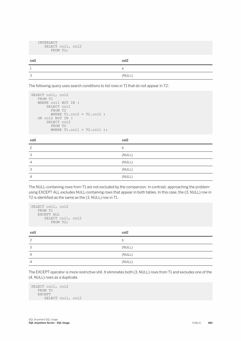
INTERSECT SELECT col1, col2 FROM T2;
col1 col2
1 a
3 (NULL)
The following query uses search conditions to list rows in T1 that do not appear in T2:
SELECT col1, col2 FROM T1 WHERE col1 NOT IN ( SELECT col1 FROM T2 WHERE T1.col2 = T2.col2 ) OR col2 NOT IN ( SELECT col2 FROM T2 WHERE T1.col1 = T2.col1 );
col1 col2
2 b
3 (NULL)
4 (NULL)
3 (NULL)
4 (NULL)
The NULL-containing rows from T1 are not excluded by the comparison. In contrast, approaching the problem using EXCEPT ALL excludes NULL-containing rows that appear in both tables. In this case, the (3, NULL) row in T2 is identified as the same as the (3, NULL) row in T1.
SELECT col1, col2 FROM T1 EXCEPT ALL SELECT col1, col2 FROM T2;
col1 col2
2 b
3 (NULL)
4 (NULL)
4 (NULL)
The EXCEPT operator is more restrictive still. It eliminates both (3, NULL) rows from T1 and excludes one of the (4, NULL) rows as a duplicate.
SELECT col1, col2 FROM T1 EXCEPT SELECT col1, col2
SQL Anywhere SQL UsageSQL Anywhere Server - SQL Usage PUBLIC 383
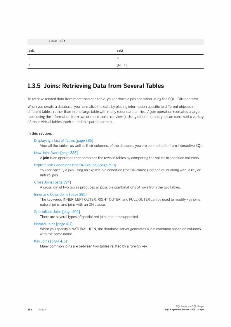
FROM T2;
col1 col2
2 b
4 (NULL)
1.3.5 Joins: Retrieving Data from Several Tables
To retrieve related data from more than one table, you perform a join operation using the SQL JOIN operator.
When you create a database, you normalize the data by placing information specific to different objects in different tables, rather than in one large table with many redundant entries. A join operation recreates a larger table using the information from two or more tables (or views). Using different joins, you can construct a variety of these virtual tables, each suited to a particular task.
In this section:
Displaying a List of Tables [page 385]View all the tables, as well as their columns, of the database you are connected to from Interactive SQL.
How Joins Work [page 385]A join is an operation that combines the rows in tables by comparing the values in specified columns.
Explicit Join Conditions (the ON Clause) [page 390]You can specify a join using an explicit join condition (the ON clause) instead of, or along with, a key or natural join.
Cross Joins [page 394]A cross join of two tables produces all possible combinations of rows from the two tables.
Inner and Outer Joins [page 395]The keywords INNER, LEFT OUTER, RIGHT OUTER, and FULL OUTER can be used to modify key joins, natural joins, and joins with an ON clause.
Specialized Joins [page 402]There are several types of specialized joins that are supported.
Natural Joins [page 411]When you specify a NATURAL JOIN, the database server generates a join condition based on columns with the same name.
Key Joins [page 415]Many common joins are between two tables related by a foreign key.
384 PUBLICSQL Anywhere SQL Usage
SQL Anywhere Server - SQL Usage
1.3.5.1 Displaying a List of Tables
View all the tables, as well as their columns, of the database you are connected to from Interactive SQL.
Prerequisites
You must be connected to the database.
Procedure
1. In Interactive SQL, press F7 to display a list of tables in the database you are connected to.2. Select a table and click Show Columns to see the columns for that table.3. Press Esc to return to the table list; press Esc again to return to the SQL Statements pane. Press Enter to
copy the selected table or column name into the SQL Statements pane at the current cursor position.4. Press Esc to leave the list.
Results
A list of all the tables of the database you are connected to is displayed. You have the option of viewing the columns for each table.
1.3.5.2 How Joins Work
A join is an operation that combines the rows in tables by comparing the values in specified columns.
A relational database stores information about different types of objects in different tables. For example, information particular to employees appears in one table, and information that pertains to departments in another. The Employees table contains information such as employee names and addresses. The Departments table contains information about one department, such as the name of the department and who the department head is.
Most questions can only be answered using a combination of information from different tables. For example, to answer the question "Who manages the Sales department?", you use the Departments table to identify the correct employee, and then look up the employee name in the Employees table.
Joins are a means of answering such questions by forming a new virtual table that includes information from multiple tables. For example, you could create a list of the department heads by combining the information contained in the Employees table and the Departments table. You specify which tables contain the information you need using the FROM clause.
To make the join useful, you must combine the correct columns of each table. To list department heads, each row of the combined table should contain the name of a department and the name of the employee who
SQL Anywhere SQL UsageSQL Anywhere Server - SQL Usage PUBLIC 385
manages it. You control how columns are matched in the composite table by either specifying a particular type of join operation or using the ON clause.
In this section:
Join Conditions [page 386]Tables can be joined using join conditions. A join condition is a search condition that returns a subset of rows from the joined tables based on the relationship between values in the columns.
Joined Tables [page 387]There are several classes of table joins that are supported.
Joins Between Two Tables [page 388]You can use a simple inner join to join two tables.
Joins Between More than Two Tables [page 388]There is no fixed limit on the number of tables you can join.
Joins in Delete, Update, and Insert Statements [page 389]You can use joins in DELETE, UPDATE, INSERT, and SELECT statements.
Non-ANSI Joins [page 389]The ISO/ANSI standards for joins are supported, as well as a few non-standard joins.
1.3.5.2.1 Join Conditions
Tables can be joined using join conditions. A join condition is a search condition that returns a subset of rows from the joined tables based on the relationship between values in the columns.
For example, the following query retrieves data from the Products and SalesOrderItems tables.
SELECT * FROM Products JOIN SalesOrderItems ON Products.ID = SalesOrderItems.ProductID;
The join condition in this query is:
Products.ID = SalesOrderItems.ProductID
This join condition means that rows can be combined in the result set only if they have the same product ID in both tables.
Join conditions can be explicit or generated. An explicit join condition is a join condition that is put in an ON clause or a WHERE clause. The following query uses an ON clause. It produces a cross product of the two tables (all combinations of rows), but with rows excluded if the ID numbers do not match. The result is a list of customers with details of their orders.
SELECT * FROM Customers JOIN SalesOrders ON SalesOrders.CustomerID = Customers.ID;
A generated join condition is a join condition that is automatically created when you specify KEY JOIN or NATURAL JOIN. For key joins, the generated join condition is based on the foreign key relationships between the tables. For natural joins, the generated join condition is based on columns that have the same name.
386 PUBLICSQL Anywhere SQL Usage
SQL Anywhere Server - SQL Usage
TipBoth key join syntax and natural join syntax are shortcuts: you get identical results from using the keyword JOIN without KEY or NATURAL, and then explicitly stating the same join condition in an ON clause.
When you use an ON clause with a key join or natural join, the join condition that is used is the conjunction of the explicitly specified join condition with the generated join condition. The join conditions are combined with the keyword AND.
1.3.5.2.2 Joined Tables
There are several classes of table joins that are supported.
CROSS JOIN
This type of join of two tables produces all possible combinations of rows from the two tables. The size of the result set is the number of rows in the first table multiplied by the number of rows in the second table. A cross join is also called a cross product or Cartesian product. You cannot use an ON clause with a cross join.KEY JOIN
This type of join condition uses the foreign key relationships between the tables. Key join is the default when the JOIN keyword is used without specifying a join type (such as INNER, OUTER, and so on) and there is no ON clause.NATURAL JOIN
This join is automatically generated based on columns having the same name.Join using an ON clause
This type of join results from explicit specification of the join condition in an ON clause. When used with a key join or natural join, the join condition contains both the generated join condition and the explicit join condition. When used with the keyword JOIN without the keywords KEY or NATURAL, there is no generated join condition.
Inner and Outer Joins
Key joins, natural joins and joins with an ON clause may be qualified by specifying INNER, LEFT OUTER, RIGHT OUTER, or FULL OUTER. The default is INNER. When using the keywords LEFT, RIGHT or FULL, the keyword OUTER is optional.
In an inner join, each row in the result satisfies the join condition.
In a left or right outer join, all rows are preserved for one of the tables, and for the other table nulls are returned for rows that do not satisfy the join condition. For example, in a right outer join the right side is preserved and the left side is null-supplying.
In a full outer join, all rows are preserved for both of the tables, and nulls are supplied for rows that do not satisfy the join condition.
SQL Anywhere SQL UsageSQL Anywhere Server - SQL Usage PUBLIC 387
Related Information
Explicit Join Conditions (the ON Clause) [page 390]
1.3.5.2.3 Joins Between Two Tables
You can use a simple inner join to join two tables.
To understand how a simple inner join is computed, consider the following query. It answers the question: which product sizes have been ordered in the same quantity as the quantity in stock?
SELECT DISTINCT Name, Size, SalesOrderItems.QuantityFROM Products JOIN SalesOrderItemsON Products.ID = SalesOrderItems.ProductID AND Products.Quantity = SalesOrderItems.Quantity;
Name Size Quantity
Baseball Cap One size fits all 12
Visor One size fits all 36
You can interpret the query as follows. This is a conceptual explanation of the processing of this query, used to illustrate the semantics of a query involving a join. It does not represent how the database server actually computes the result set.
● Create a cross product of the Products table and SalesOrderItems table. A cross product contains every combination of rows from the two tables.
● Exclude all rows where the product IDs are not identical (because of the join condition Products.ID = SalesOrderItems.ProductID).
● Exclude all rows where the quantity is not identical (because of the join condition Products.Quantity = SalesOrderItems.Quantity).
● Create a result table with three columns: Products.Name, Products.Size, and SalesOrderItems.Quantity.● Exclude all duplicate rows (because of the DISTINCT keyword).
Related Information
Outer Joins [page 396]
1.3.5.2.4 Joins Between More than Two Tables
There is no fixed limit on the number of tables you can join.
When you join two tables, the columns you compare must have the same or compatible data types.
388 PUBLICSQL Anywhere SQL Usage
SQL Anywhere Server - SQL Usage
Also, when joining more than two tables, parentheses are optional. If you do not use parentheses, the database server evaluates the statement from left to right. Therefore, A JOIN B JOIN C is equivalent to ( A JOIN B ) JOIN C. Also, the following two SELECT statements are equivalent:
SELECT * FROM A JOIN B JOIN C JOIN D;
SELECT * FROM ( ( A JOIN B ) JOIN C ) JOIN D;
Whenever more than two tables are joined, the join involves table expressions. In the example A JOIN B JOIN C, the table expression A JOIN B is joined to C. This means, conceptually, that A and B are joined, and then the result is joined to C.
The order of joins is important if the table expression contains outer joins. For example, A JOIN B LEFT OUTER JOIN C is interpreted as (A JOIN B) LEFT OUTER JOIN C. The table expression A JOIN B is joined to C. The table expression A JOIN B is preserved and table C is null-supplying.
Related Information
Outer Joins [page 396]Key Joins of Table Expressions [page 420]Natural Joins of Table Expressions [page 414]
1.3.5.2.5 Joins in Delete, Update, and Insert Statements
You can use joins in DELETE, UPDATE, INSERT, and SELECT statements.
You can update some cursors that contain joins if the ansi_update_constraints option is set to Off. This is the default for databases created before SQL Anywhere 7. For databases created with version 7 or later, the default is Cursors.
1.3.5.2.6 Non-ANSI Joins
The ISO/ANSI standards for joins are supported, as well as a few non-standard joins.
● Transact-SQL outer joins (*= or =*)● Duplicate correlation names in joins (star joins)● Key joins
You can use the REWRITE function to see the ANSI equivalent of a non-ANSI join.
SQL Anywhere SQL UsageSQL Anywhere Server - SQL Usage PUBLIC 389
Related Information
Transact-SQL Outer Joins (*= or =*) [page 400]Duplicate Correlation Names in Joins (Star Joins) [page 405]Key Joins [page 415]
1.3.5.3 Explicit Join Conditions (the ON Clause)
You can specify a join using an explicit join condition (the ON clause) instead of, or along with, a key or natural join.
You specify a join condition by inserting an ON clause immediately after the join. The join condition always refers to the join immediately preceding it. The ON clause applies a restriction to the rows in a join, in much the same way that the WHERE clause applies restrictions to the rows of a query.
The ON clause allows you to construct more useful joins than the CROSS JOIN. For example, you can apply the ON clause to a join of the SalesOrders and Employees table to retrieve only those rows for which the SalesRepresentative in the SalesOrders table is the same as the one in the Employees table in every row of the result. Then each row contains information about an order and the sales representative responsible for it.
For example, in the following query, the first ON clause is used to join SalesOrders to Customers. The second ON clause is used to join the table expression (SalesOrders JOIN Customers) to the base table SalesOrderItems.
SELECT * FROM SalesOrders JOIN Customers ON SalesOrders.CustomerID = Customers.ID JOIN SalesOrderItems ON SalesOrderItems.ID = SalesOrders.ID;
In this section:
Table References in ON Clauses [page 391]The tables that are referenced in an ON clause must be part of the join that the ON clause modifies.
Generated Joins and the ON Clause [page 392]Key joins are the default when the keyword JOIN is used and no join type is specified, unless you use an ON clause. If you use an ON clause with an unspecified JOIN, key join is not the default and no generated join condition is applied.
Types of Explicit Join Conditions [page 393]Most join conditions are based on equality, and so are called equijoins.
WHERE Clauses in Join Conditions [page 393]You can specify join conditions in the WHERE clause instead of the ON clause, except when using outer joins.
390 PUBLICSQL Anywhere SQL Usage
SQL Anywhere Server - SQL Usage
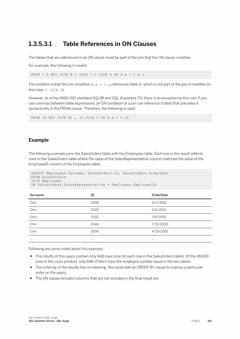
1.3.5.3.1 Table References in ON Clauses
The tables that are referenced in an ON clause must be part of the join that the ON clause modifies.
For example, the following is invalid:
FROM ( A KEY JOIN B ) JOIN ( C JOIN D ON A.x = C.x )
The problem is that the join condition A.x = C.x references table A, which is not part of the join it modifies (in this case, C JOIN D).
However, as of the ANSI/ISO standard SQL99 and SQL Anywhere 7.0, there is an exception to this rule: if you use commas between table expressions, an ON condition of a join can reference a table that precedes it syntactically in the FROM clause. Therefore, the following is valid:
FROM (A KEY JOIN B) , (C JOIN D ON A.x = C.x)
Example
The following example joins the SalesOrders table with the Employees table. Each row in the result reflects rows in the SalesOrders table where the value of the SalesRepresentative column matched the value of the EmployeeID column of the Employees table.
SELECT Employees.Surname, SalesOrders.ID, SalesOrders.OrderDate FROM SalesOrders JOIN Employees ON SalesOrders.SalesRepresentative = Employees.EmployeeID;
Surname ID OrderDate
Chin 2008 4/2/2001
Chin 2020 3/4/2001
Chin 2032 7/5/2001
Chin 2044 7/15/2000
Chin 2056 4/15/2001
... ... ...
Following are some notes about this example:
● The results of this query contain only 648 rows (one for each row in the SalesOrders table). Of the 48,600 rows in the cross product, only 648 of them have the employee number equal in the two tables.
● The ordering of the results has no meaning. You could add an ORDER BY clause to impose a particular order on the query.
● The ON clause includes columns that are not included in the final result set.
SQL Anywhere SQL UsageSQL Anywhere Server - SQL Usage PUBLIC 391
Related Information
Key Joins [page 415]Commas [page 394]
1.3.5.3.2 Generated Joins and the ON Clause
Key joins are the default when the keyword JOIN is used and no join type is specified, unless you use an ON clause. If you use an ON clause with an unspecified JOIN, key join is not the default and no generated join condition is applied.
For example, the following is a key join, because key join is the default when the keyword JOIN is used and there is no ON clause:
SELECT * FROM A JOIN B;
The following is a join between table A and table B with the join condition A.x = B.y. It is not a key join.
SELECT * FROM A JOIN B ON A.x = B.y;
If you specify a KEY JOIN or NATURAL JOIN and use an ON clause, the final join condition is the conjunction of the generated join condition and the explicit join condition(s). For example, the following statement has two join conditions: one generated because of the key join, and one explicitly stated in the ON clause.
SELECT * FROM A KEY JOIN B ON A.x = B.y;
If the join condition generated by the key join is A.w = B.z, then the following statement is equivalent:
SELECT * FROM A JOIN B ON A.x = B.y AND A.w = B.z;
Related Information
Key Joins [page 415]
392 PUBLICSQL Anywhere SQL Usage
SQL Anywhere Server - SQL Usage
1.3.5.3.3 Types of Explicit Join Conditions
Most join conditions are based on equality, and so are called equijoins.
For example:
SELECT * FROM Departments JOIN Employees ON Departments.DepartmentID = Employees.DepartmentID;
However, you do not have to use equality (=) in a join condition. You can use any search condition, such as conditions containing LIKE, SOUNDEX, BETWEEN, > (greater than), and != (not equal to).
Example
The following example answers the question: For which products has someone ordered more than the quantity in stock?
SELECT DISTINCT Products.Name FROM Products JOIN SalesOrderItemsON Products.ID = SalesOrderItems.ProductID AND SalesOrderItems.Quantity > Products.Quantity;
1.3.5.3.4 WHERE Clauses in Join Conditions
You can specify join conditions in the WHERE clause instead of the ON clause, except when using outer joins.
However, you should be aware that there may be semantic differences between the two if the query contains outer joins.
The ON clause is part of the FROM clause, and so is processed before the WHERE clause. This does not make a difference to results except for outer joins, where using the WHERE clause can convert the join to an inner join.
When deciding whether to put join conditions in an ON clause or WHERE clause, keep the following rules in mind:
● When you specify an outer join, putting a join condition in the WHERE clause may convert the outer join to an inner join.
● Conditions in an ON clause can only refer to tables that are in the table expressions joined by the associated JOIN. However, conditions in a WHERE clause can refer to any tables, even if they are not part of the join.
● You cannot use an ON clause with the keywords CROSS JOIN, but you can always use a WHERE clause.● When join conditions are in an ON clause, key join is not the default. However, key join can be the default if
join conditions are put in a WHERE clause.
In the examples in this documentation, join conditions are put in an ON clause. In examples using outer joins, this is necessary. In other cases it is done to make it obvious that they are join conditions and not general search conditions.
SQL Anywhere SQL UsageSQL Anywhere Server - SQL Usage PUBLIC 393
Related Information
Outer Joins and Join Conditions [page 398]Key Joins [page 415]
1.3.5.4 Cross Joins
A cross join of two tables produces all possible combinations of rows from the two tables.
A cross join is also called a cross product or Cartesian product.
Each row of the first table appears once with each row of the second table. So, the number of rows in the result set is the product of the number of rows in the first table and the number of rows in the second table, minus any rows that are omitted because of restrictions in a WHERE clause.
You cannot use an ON clause with cross joins. However, you can put restrictions in a WHERE clause.
Inner and outer modifiers do not apply to cross joins
Except in the presence of additional restrictions in the WHERE clause, all rows of both tables always appear in the result set of cross joins. So, the keywords INNER, LEFT OUTER and RIGHT OUTER are not applicable to cross joins.
For example, the following statement joins two tables.
SELECT * FROM A CROSS JOIN B;
The result set from this query includes all columns in A and all columns in B. There is one row in the result set for each combination of a row in A and a row in B. If A has n rows and B has m rows, the query returns n x m rows.
In this section:
Commas [page 394]A comma can work like a join operator.
1.3.5.4.1 Commas
A comma can work like a join operator.
A comma creates a cross product exactly as the keyword CROSS JOIN does. However, join keywords create table expressions, and commas create lists of table expressions.
394 PUBLICSQL Anywhere SQL Usage
SQL Anywhere Server - SQL Usage
In the following simple inner join of two tables, a comma and the keywords CROSS JOIN are equivalent:
SELECT * FROM A, B, C WHERE A.x = B.y;
SELECT * FROM A CROSS JOIN B CROSS JOIN C WHERE A.x = B.y;
Generally, you can use a comma instead of the keywords CROSS JOIN. The comma syntax is equivalent to cross join syntax, except for generated join conditions in table expressions using commas.
In the syntax of star joins, commas have a special use.
Related Information
Key Joins of Table Expressions [page 420]Duplicate Correlation Names in Joins (Star Joins) [page 405]
1.3.5.5 Inner and Outer Joins
The keywords INNER, LEFT OUTER, RIGHT OUTER, and FULL OUTER can be used to modify key joins, natural joins, and joins with an ON clause.
The default is INNER. These modifiers do not apply to cross joins.
In this section:
Inner Joins [page 396]By default, joins are inner joins. Rows are included in the result set only if they satisfy the join condition.
Outer Joins [page 396]To preserve all the rows of one table in a join, you use an outer join.
Transact-SQL Outer Joins (*= or =*) [page 400]In the Transact-SQL dialect, you create outer joins by supplying a comma-separated list of tables in the FROM clause, and using the special operators *= or =* in the WHERE clause.
SQL Anywhere SQL UsageSQL Anywhere Server - SQL Usage PUBLIC 395
1.3.5.5.1 Inner Joins
By default, joins are inner joins. Rows are included in the result set only if they satisfy the join condition.
Example
For example, each row of the result set of the following query contains the information from one Customers row and one SalesOrders row, satisfying the key join condition. If a particular customer has placed no orders, the condition is not satisfied and the result set does not contain the row corresponding to that customer.
SELECT GivenName, Surname, OrderDate FROM Customers KEY INNER JOIN SalesOrders ORDER BY OrderDate;
GivenName Surname OrderDate
Hardy Mums 2000-01-02
Aram Najarian 2000-01-03
Tommie Wooten 2000-01-03
Alfredo Margolis 2000-01-06
... ... ...
Because inner joins and key joins are the defaults, you obtain the same results as above using the FROM clause as follows:
SELECT GivenName, Surname, OrderDate FROM Customers JOIN SalesOrders ORDER BY OrderDate;
1.3.5.5.2 Outer Joins
To preserve all the rows of one table in a join, you use an outer join.
Otherwise, you create joins that return rows only if they satisfy join conditions; these are called inner joins, and are the default join used when querying.
A left or right outer join of two tables preserves all the rows in one table, and supplies nulls for the other table when it does not meet the join condition. A left outer join preserves every row in the left table, and a right outer join preserves every row in the right table. In a full outer join, all rows from both tables are preserved and both tables are null-supplying.
The table expressions on either side of a left or right outer join are referred to as preserved and null-supplying. In a left outer join, the left table expression is preserved and the right table expression is null-supplying. In a full outer join both left and right table expressions are preserved and both are null-supplying.
396 PUBLICSQL Anywhere SQL Usage
SQL Anywhere Server - SQL Usage
Example
The following statement includes all customers. If a particular customer has not placed an order, each column in the result that corresponds to order information contains the NULL value.
SELECT Surname, OrderDate, City FROM Customers LEFT OUTER JOIN SalesOrders ON Customers.ID = SalesOrders.CustomerIDWHERE Customers.State = 'NY' ORDER BY OrderDate;
Surname OrderDate City
Thompson (NULL) Bancroft
Reiser 2000-01-22 Rockwood
Clarke 2000-01-27 Rockwood
Mentary 2000-01-30 Rockland
... ... ...
You can interpret the outer join in this statement as follows. This is a conceptual explanation, and does not represent how the database server actually computes the result set.
● Return one row for every sales order placed by a customer. More than one row is returned when the customer placed two or more sales orders, because a row is returned for each sales order. This is the same result as an inner join. The ON condition is used to match customer and sales order rows. The WHERE clause is not used for this step.
● Include one row for every customer who has not placed any sales orders. This ensures that every row in the Customers table is included. For all these rows, the columns from SalesOrders are filled with nulls. These rows are added because the keyword OUTER is used, and would not have appeared in an inner join. Neither the ON condition nor the WHERE clause is used for this step.
● Exclude every row where the customer does not live in New York, using the WHERE clause.
In this section:
Outer Joins and Join Conditions [page 398]If you place restrictions on the null-supplying table in a WHERE clause, the join is usually equivalent to an inner join.
Complex Outer Joins [page 398]The order of joins is important when a query includes table expressions using outer joins.
Outer Joins of Views and Derived Tables [page 399]Outer joins can be specified for views and derived tables.
Related Information
Transact-SQL Outer Joins (*= or =*) [page 400]Key Joins [page 415]
SQL Anywhere SQL UsageSQL Anywhere Server - SQL Usage PUBLIC 397
1.3.5.5.2.1 Outer Joins and Join Conditions
If you place restrictions on the null-supplying table in a WHERE clause, the join is usually equivalent to an inner join.
The reason for this is that most search conditions cannot evaluate to TRUE when any of their inputs are NULL. The WHERE clause restriction on the null-supplying table compares values to NULL, resulting in the elimination of the row from the result set. The rows in the preserved table are not preserved and so the join is an inner join.
The exception to this is comparisons that can evaluate to true when any of their inputs are NULL. These include IS NULL, IS UNKNOWN, IS FALSE, IS NOT TRUE, and expressions involving ISNULL or COALESCE.
Example
For example, the following statement computes a left outer join.
SELECT * FROM Customers KEY LEFT OUTER JOIN SalesOrders ON SalesOrders.OrderDate < '2000-01-03';
In contrast, the following statement creates an inner join.
SELECT Surname, OrderDate FROM Customers KEY LEFT OUTER JOIN SalesOrders WHERE SalesOrders.OrderDate < '2000-01-03';
The first of these two statements can be thought of as follows: First, left-outer join the Customers table to the SalesOrders table. The result set includes every row in the Customers table. For those customers who have no orders before January 3 2000, fill the sales order fields with nulls.
In the second statement, first left-outer join Customers and SalesOrders. The result set includes every row in the Customers table. For those customers who have no orders, fill the sales order fields with nulls. Next, apply the WHERE condition by selecting only those rows in which the customer has placed an order since January 3 2000. For those customers who have not placed orders, these values are NULL. Comparing any value to NULL evaluates to UNKNOWN. So, these rows are eliminated and the statement reduces to an inner join.
1.3.5.5.2.2 Complex Outer Joins
The order of joins is important when a query includes table expressions using outer joins.
For example, A JOIN B LEFT OUTER JOIN C is interpreted as (A JOIN B) LEFT OUTER JOIN C. The table expression (A JOIN B) is joined to C. The table expression (A JOIN B) is preserved and table C is null-supplying.
Consider the following statement, in which A, B and C are tables:
SELECT * FROM A LEFT OUTER JOIN B RIGHT OUTER JOIN C;
398 PUBLICSQL Anywhere SQL Usage
SQL Anywhere Server - SQL Usage

To understand this statement, first remember that the database server evaluates statements from left to right, adding parentheses. This results in:
SELECT * FROM (A LEFT OUTER JOIN B) RIGHT OUTER JOIN C;
Next, you may want to convert the right outer join to a left outer join so that both joins are the same type. To do this, simply reverse the position of the tables in the right outer join, resulting in:
SELECT * FROM C LEFT OUTER JOIN (A LEFT OUTER JOIN B);
A is the preserved table and B is the null-supplying table for the nested outer join. C is the preserved table for the first outer join.
You can interpret this join as follows:
● Join A to B, preserving all rows in A.● Next, join C to the results of the join of A and B, preserving all rows in C.
The join does not have an ON clause, and so is by default a key join.
In addition, the join condition for an outer join must only include tables that have previously been referenced in the FROM clause. This restriction is according to the ANSI/ISO standard, and is enforced to avoid ambiguity. For example, the following two statements are syntactically incorrect, because C is referenced in the join condition before the table itself is referenced.
SELECT * FROM (A LEFT OUTER JOIN B ON B.x = C.x) JOIN C;
SELECT * FROM A LEFT OUTER JOIN B ON A.x = C.x, C;
Related Information
Key Joins of Table Expressions That Do Not Contain Commas [page 421]
1.3.5.5.2.3 Outer Joins of Views and Derived Tables
Outer joins can be specified for views and derived tables.
The statement:
SELECT * FROM V LEFT OUTER JOIN A ON (V.x = A.x);
can be interpreted as follows:
● Compute the view V.● Join all the rows from the computed view V with A by preserving all the rows from V, using the join
condition V.x = A.x.
SQL Anywhere SQL UsageSQL Anywhere Server - SQL Usage PUBLIC 399
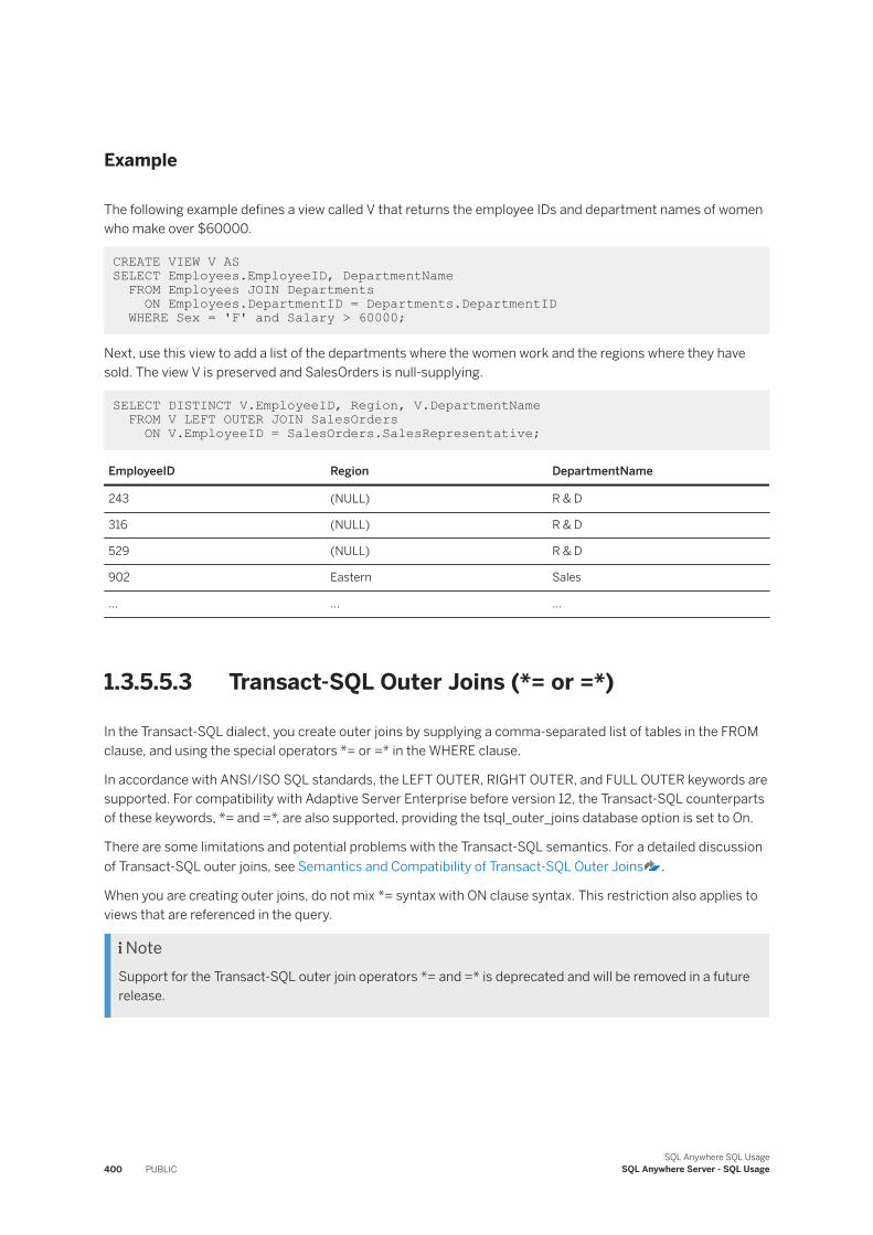
Example
The following example defines a view called V that returns the employee IDs and department names of women who make over $60000.
CREATE VIEW V AS SELECT Employees.EmployeeID, DepartmentName FROM Employees JOIN Departments ON Employees.DepartmentID = Departments.DepartmentID WHERE Sex = 'F' and Salary > 60000;
Next, use this view to add a list of the departments where the women work and the regions where they have sold. The view V is preserved and SalesOrders is null-supplying.
SELECT DISTINCT V.EmployeeID, Region, V.DepartmentName FROM V LEFT OUTER JOIN SalesOrders ON V.EmployeeID = SalesOrders.SalesRepresentative;
EmployeeID Region DepartmentName
243 (NULL) R & D
316 (NULL) R & D
529 (NULL) R & D
902 Eastern Sales
... ... ...
1.3.5.5.3 Transact-SQL Outer Joins (*= or =*)
In the Transact-SQL dialect, you create outer joins by supplying a comma-separated list of tables in the FROM clause, and using the special operators *= or =* in the WHERE clause.
In accordance with ANSI/ISO SQL standards, the LEFT OUTER, RIGHT OUTER, and FULL OUTER keywords are supported. For compatibility with Adaptive Server Enterprise before version 12, the Transact-SQL counterparts of these keywords, *= and =*, are also supported, providing the tsql_outer_joins database option is set to On.
There are some limitations and potential problems with the Transact-SQL semantics. For a detailed discussion of Transact-SQL outer joins, see Semantics and Compatibility of Transact-SQL Outer Joins .
When you are creating outer joins, do not mix *= syntax with ON clause syntax. This restriction also applies to views that are referenced in the query.
NoteSupport for the Transact-SQL outer join operators *= and =* is deprecated and will be removed in a future release.
400 PUBLICSQL Anywhere SQL Usage
SQL Anywhere Server - SQL Usage
Example
The following left outer join lists all customers and finds their order dates (if any):
SELECT GivenName, Surname, OrderDate FROM Customers, SalesOrdersWHERE Customers.ID *= SalesOrders.CustomerID ORDER BY OrderDate;
This statement is equivalent to the following statement, in which ANSI/ISO syntax is used:
SELECT GivenName, Surname, OrderDate FROM Customers LEFT OUTER JOIN SalesOrdersON Customers.ID = SalesOrders.CustomerID ORDER BY OrderDate;
In this section:
Transact-SQL Outer Join Limitations [page 401]There are several Transact-SQL outer join restrictions.
Views and Transact-SQL Outer Joins [page 402]If you define a view with an outer join, and then query the view with a qualification on a column from the null-supplying table of the outer join, the results may not be what you expect.
How NULL Affects Transact-SQL Joins [page 402]NULL values in tables or views being joined never match each other in a Transact-SQL outer join.
1.3.5.5.3.1 Transact-SQL Outer Join Limitations
There are several Transact-SQL outer join restrictions.
● If you specify an outer join and a qualification on a column from the null-supplying table of the outer join, the results may not be what you expect. The qualification in the query does not exclude rows from the result set, but rather affects the values that appear in the rows of the result set. For rows that do not meet the qualification, a NULL value appears in the null-supplying table.
● You cannot mix ANSI/ISO SQL syntax and Transact-SQL outer join syntax in a single query. If a view is defined using one dialect for an outer join, you must use the same dialect for any outer-join queries on that view.
● A null-supplying table cannot participate in both a Transact-SQL outer join and a regular join or two outer joins. For example, the following WHERE clause is not allowed, because table S violates this limitation.
WHERE R.x *= S.x AND S.y = T.y
When you cannot rewrite your query to avoid using a table in both an outer join and a regular join clause, you must divide your statement into two separate queries, or use only ANSI/ISO SQL syntax.
● You cannot use a subquery that contains a join condition involving the null-supplying table of an outer join. For example, the following WHERE clause is not allowed:
WHERE R.x *= S.y AND EXISTS ( SELECT *
SQL Anywhere SQL UsageSQL Anywhere Server - SQL Usage PUBLIC 401
FROM T WHERE T.x = S.x )
NoteSupport for Transact-SQL outer join operators *= and =* is deprecated and will be removed in a future release.
1.3.5.5.3.2 Views and Transact-SQL Outer Joins
If you define a view with an outer join, and then query the view with a qualification on a column from the null-supplying table of the outer join, the results may not be what you expect.
The query returns all rows from the null-supplying table. Rows that do not meet the qualification show a NULL value in the appropriate columns of those rows.
The following rules determine what types of updates you can make to columns through views that contain outer joins:
● INSERT and DELETE statements are not allowed on outer join views.● UPDATE statements are allowed on outer join views. If the view is defined WITH CHECK option, the update
fails if any of the affected columns appears in the WHERE clause in an expression that includes columns from more than one table.
1.3.5.5.3.3 How NULL Affects Transact-SQL Joins
NULL values in tables or views being joined never match each other in a Transact-SQL outer join.
The result of comparing a NULL value with any other NULL value is FALSE.
1.3.5.6 Specialized Joins
There are several types of specialized joins that are supported.
In this section:
Self-joins [page 403]In a self-join, a table is joined to itself by referring to the same table using a different correlation name.
Duplicate Correlation Names in Joins (Star Joins) [page 405]A star join joins one table or view to several others. To create a star join, you use the same table name, view name, or correlation name more than once in the FROM clause.
Joins That Use Derived Tables [page 408]Derived tables allow you to nest queries within a FROM clause. Derived tables allow you to perform grouping of groups, or construct a join with a group, without having to create a separate view or table and join to it.
402 PUBLICSQL Anywhere SQL Usage
SQL Anywhere Server - SQL Usage
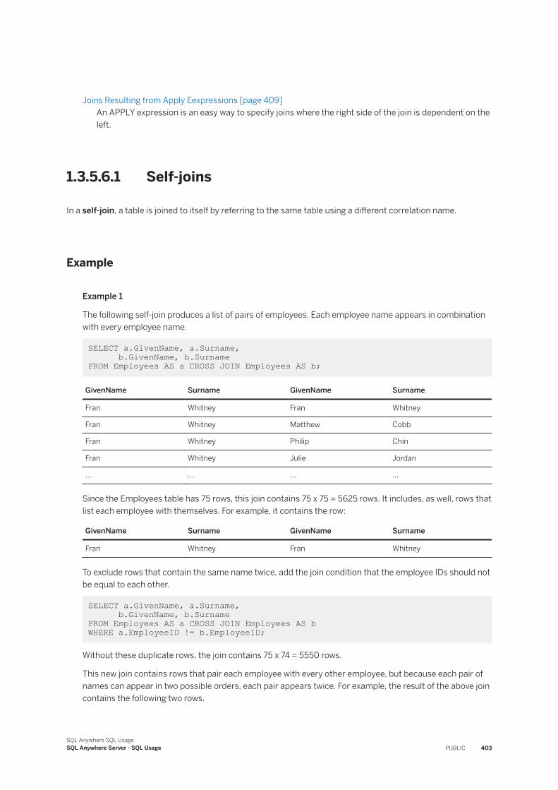
Joins Resulting from Apply Eexpressions [page 409]An APPLY expression is an easy way to specify joins where the right side of the join is dependent on the left.
1.3.5.6.1 Self-joins
In a self-join, a table is joined to itself by referring to the same table using a different correlation name.
Example
Example 1
The following self-join produces a list of pairs of employees. Each employee name appears in combination with every employee name.
SELECT a.GivenName, a.Surname, b.GivenName, b.Surname FROM Employees AS a CROSS JOIN Employees AS b;
GivenName Surname GivenName Surname
Fran Whitney Fran Whitney
Fran Whitney Matthew Cobb
Fran Whitney Philip Chin
Fran Whitney Julie Jordan
... ... ... ...
Since the Employees table has 75 rows, this join contains 75 x 75 = 5625 rows. It includes, as well, rows that list each employee with themselves. For example, it contains the row:
GivenName Surname GivenName Surname
Fran Whitney Fran Whitney
To exclude rows that contain the same name twice, add the join condition that the employee IDs should not be equal to each other.
SELECT a.GivenName, a.Surname, b.GivenName, b.SurnameFROM Employees AS a CROSS JOIN Employees AS b WHERE a.EmployeeID != b.EmployeeID;
Without these duplicate rows, the join contains 75 x 74 = 5550 rows.
This new join contains rows that pair each employee with every other employee, but because each pair of names can appear in two possible orders, each pair appears twice. For example, the result of the above join contains the following two rows.
SQL Anywhere SQL UsageSQL Anywhere Server - SQL Usage PUBLIC 403
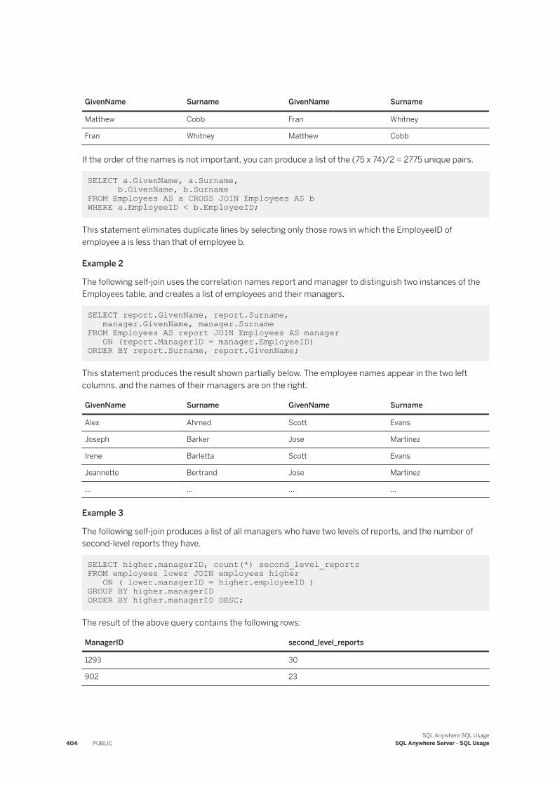
GivenName Surname GivenName Surname
Matthew Cobb Fran Whitney
Fran Whitney Matthew Cobb
If the order of the names is not important, you can produce a list of the (75 x 74)/2 = 2775 unique pairs.
SELECT a.GivenName, a.Surname, b.GivenName, b.SurnameFROM Employees AS a CROSS JOIN Employees AS b WHERE a.EmployeeID < b.EmployeeID;
This statement eliminates duplicate lines by selecting only those rows in which the EmployeeID of employee a is less than that of employee b.
Example 2
The following self-join uses the correlation names report and manager to distinguish two instances of the Employees table, and creates a list of employees and their managers.
SELECT report.GivenName, report.Surname, manager.GivenName, manager.SurnameFROM Employees AS report JOIN Employees AS manager ON (report.ManagerID = manager.EmployeeID) ORDER BY report.Surname, report.GivenName;
This statement produces the result shown partially below. The employee names appear in the two left columns, and the names of their managers are on the right.
GivenName Surname GivenName Surname
Alex Ahmed Scott Evans
Joseph Barker Jose Martinez
Irene Barletta Scott Evans
Jeannette Bertrand Jose Martinez
... ... ... ...
Example 3
The following self-join produces a list of all managers who have two levels of reports, and the number of second-level reports they have.
SELECT higher.managerID, count(*) second_level_reports FROM employees lower JOIN employees higher ON ( lower.managerID = higher.employeeID )GROUP BY higher.managerID ORDER BY higher.managerID DESC;
The result of the above query contains the following rows:
ManagerID second_level_reports
1293 30
902 23
404 PUBLICSQL Anywhere SQL Usage
SQL Anywhere Server - SQL Usage
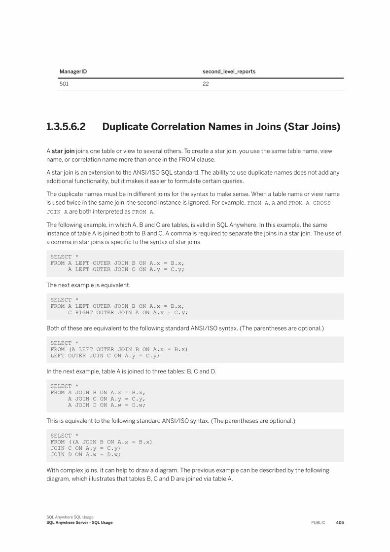
ManagerID second_level_reports
501 22
1.3.5.6.2 Duplicate Correlation Names in Joins (Star Joins)
A star join joins one table or view to several others. To create a star join, you use the same table name, view name, or correlation name more than once in the FROM clause.
A star join is an extension to the ANSI/ISO SQL standard. The ability to use duplicate names does not add any additional functionality, but it makes it easier to formulate certain queries.
The duplicate names must be in different joins for the syntax to make sense. When a table name or view name is used twice in the same join, the second instance is ignored. For example, FROM A,A and FROM A CROSS JOIN A are both interpreted as FROM A.
The following example, in which A, B and C are tables, is valid in SQL Anywhere. In this example, the same instance of table A is joined both to B and C. A comma is required to separate the joins in a star join. The use of a comma in star joins is specific to the syntax of star joins.
SELECT * FROM A LEFT OUTER JOIN B ON A.x = B.x, A LEFT OUTER JOIN C ON A.y = C.y;
The next example is equivalent.
SELECT * FROM A LEFT OUTER JOIN B ON A.x = B.x, C RIGHT OUTER JOIN A ON A.y = C.y;
Both of these are equivalent to the following standard ANSI/ISO syntax. (The parentheses are optional.)
SELECT * FROM (A LEFT OUTER JOIN B ON A.x = B.x) LEFT OUTER JOIN C ON A.y = C.y;
In the next example, table A is joined to three tables: B, C and D.
SELECT * FROM A JOIN B ON A.x = B.x, A JOIN C ON A.y = C.y, A JOIN D ON A.w = D.w;
This is equivalent to the following standard ANSI/ISO syntax. (The parentheses are optional.)
SELECT * FROM ((A JOIN B ON A.x = B.x)JOIN C ON A.y = C.y) JOIN D ON A.w = D.w;
With complex joins, it can help to draw a diagram. The previous example can be described by the following diagram, which illustrates that tables B, C and D are joined via table A.
SQL Anywhere SQL UsageSQL Anywhere Server - SQL Usage PUBLIC 405
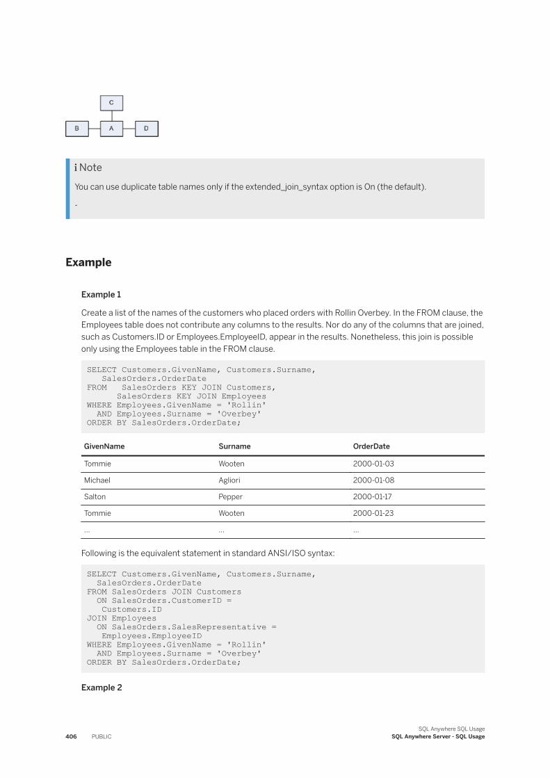
NoteYou can use duplicate table names only if the extended_join_syntax option is On (the default).
-
Example
Example 1
Create a list of the names of the customers who placed orders with Rollin Overbey. In the FROM clause, the Employees table does not contribute any columns to the results. Nor do any of the columns that are joined, such as Customers.ID or Employees.EmployeeID, appear in the results. Nonetheless, this join is possible only using the Employees table in the FROM clause.
SELECT Customers.GivenName, Customers.Surname, SalesOrders.OrderDateFROM SalesOrders KEY JOIN Customers, SalesOrders KEY JOIN EmployeesWHERE Employees.GivenName = 'Rollin' AND Employees.Surname = 'Overbey' ORDER BY SalesOrders.OrderDate;
GivenName Surname OrderDate
Tommie Wooten 2000-01-03
Michael Agliori 2000-01-08
Salton Pepper 2000-01-17
Tommie Wooten 2000-01-23
... ... ...
Following is the equivalent statement in standard ANSI/ISO syntax:
SELECT Customers.GivenName, Customers.Surname, SalesOrders.OrderDateFROM SalesOrders JOIN Customers ON SalesOrders.CustomerID = Customers.IDJOIN Employees ON SalesOrders.SalesRepresentative = Employees.EmployeeIDWHERE Employees.GivenName = 'Rollin' AND Employees.Surname = 'Overbey' ORDER BY SalesOrders.OrderDate;
Example 2
406 PUBLICSQL Anywhere SQL Usage
SQL Anywhere Server - SQL Usage
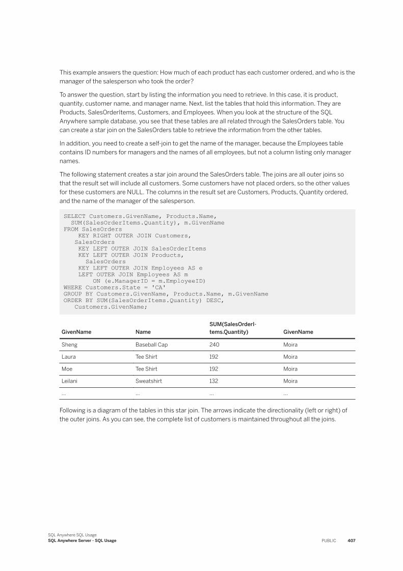
This example answers the question: How much of each product has each customer ordered, and who is the manager of the salesperson who took the order?
To answer the question, start by listing the information you need to retrieve. In this case, it is product, quantity, customer name, and manager name. Next, list the tables that hold this information. They are Products, SalesOrderItems, Customers, and Employees. When you look at the structure of the SQL Anywhere sample database, you see that these tables are all related through the SalesOrders table. You can create a star join on the SalesOrders table to retrieve the information from the other tables.
In addition, you need to create a self-join to get the name of the manager, because the Employees table contains ID numbers for managers and the names of all employees, but not a column listing only manager names.
The following statement creates a star join around the SalesOrders table. The joins are all outer joins so that the result set will include all customers. Some customers have not placed orders, so the other values for these customers are NULL. The columns in the result set are Customers, Products, Quantity ordered, and the name of the manager of the salesperson.
SELECT Customers.GivenName, Products.Name, SUM(SalesOrderItems.Quantity), m.GivenNameFROM SalesOrders KEY RIGHT OUTER JOIN Customers, SalesOrders KEY LEFT OUTER JOIN SalesOrderItems KEY LEFT OUTER JOIN Products, SalesOrders KEY LEFT OUTER JOIN Employees AS e LEFT OUTER JOIN Employees AS m ON (e.ManagerID = m.EmployeeID)WHERE Customers.State = 'CA'GROUP BY Customers.GivenName, Products.Name, m.GivenNameORDER BY SUM(SalesOrderItems.Quantity) DESC, Customers.GivenName;
GivenName NameSUM(SalesOrderItems.Quantity) GivenName
Sheng Baseball Cap 240 Moira
Laura Tee Shirt 192 Moira
Moe Tee Shirt 192 Moira
Leilani Sweatshirt 132 Moira
... ... ... ...
Following is a diagram of the tables in this star join. The arrows indicate the directionality (left or right) of the outer joins. As you can see, the complete list of customers is maintained throughout all the joins.
SQL Anywhere SQL UsageSQL Anywhere Server - SQL Usage PUBLIC 407
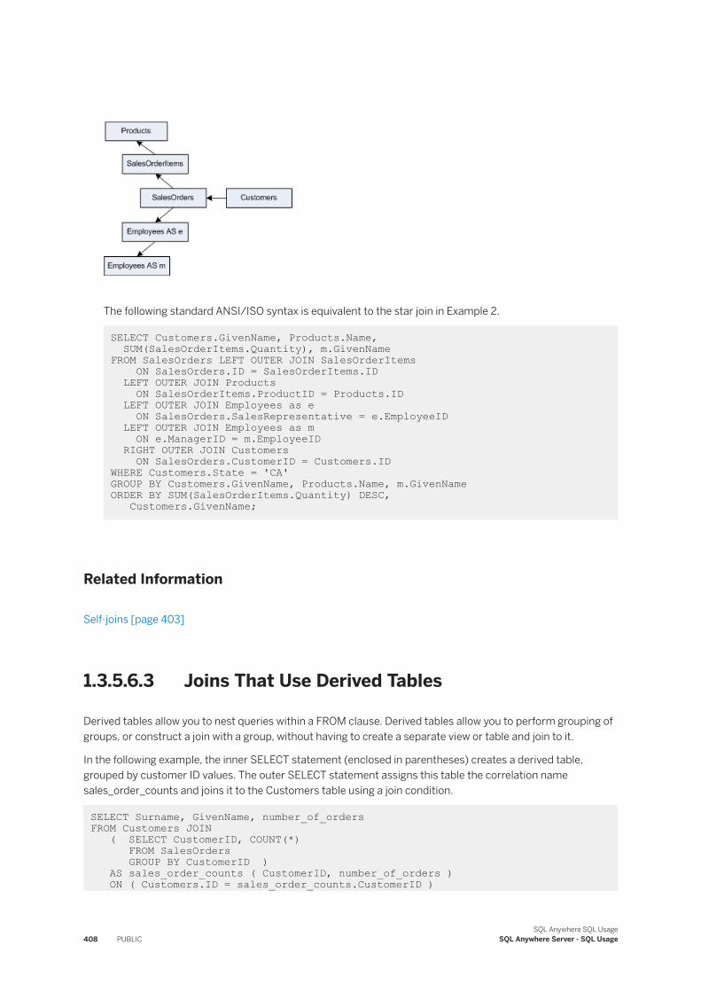
The following standard ANSI/ISO syntax is equivalent to the star join in Example 2.
SELECT Customers.GivenName, Products.Name, SUM(SalesOrderItems.Quantity), m.GivenNameFROM SalesOrders LEFT OUTER JOIN SalesOrderItems ON SalesOrders.ID = SalesOrderItems.ID LEFT OUTER JOIN Products ON SalesOrderItems.ProductID = Products.ID LEFT OUTER JOIN Employees as e ON SalesOrders.SalesRepresentative = e.EmployeeID LEFT OUTER JOIN Employees as m ON e.ManagerID = m.EmployeeID RIGHT OUTER JOIN Customers ON SalesOrders.CustomerID = Customers.IDWHERE Customers.State = 'CA'GROUP BY Customers.GivenName, Products.Name, m.GivenNameORDER BY SUM(SalesOrderItems.Quantity) DESC, Customers.GivenName;
Related Information
Self-joins [page 403]
1.3.5.6.3 Joins That Use Derived Tables
Derived tables allow you to nest queries within a FROM clause. Derived tables allow you to perform grouping of groups, or construct a join with a group, without having to create a separate view or table and join to it.
In the following example, the inner SELECT statement (enclosed in parentheses) creates a derived table, grouped by customer ID values. The outer SELECT statement assigns this table the correlation name sales_order_counts and joins it to the Customers table using a join condition.
SELECT Surname, GivenName, number_of_orders FROM Customers JOIN ( SELECT CustomerID, COUNT(*) FROM SalesOrders GROUP BY CustomerID ) AS sales_order_counts ( CustomerID, number_of_orders ) ON ( Customers.ID = sales_order_counts.CustomerID )
408 PUBLICSQL Anywhere SQL Usage
SQL Anywhere Server - SQL Usage
WHERE number_of_orders > 3;
The result is a table of the names of those customers who have placed more than three orders, including the number of orders each has placed.
Related Information
Key Joins of Views and Derived Tables [page 425]Natural Joins of Views and Derived Tables [page 415]Outer Joins of Views and Derived Tables [page 399]
1.3.5.6.4 Joins Resulting from Apply Eexpressions
An APPLY expression is an easy way to specify joins where the right side of the join is dependent on the left.
For example, use an apply expression to evaluate a procedure or derived table once for each row in a table expression. Apply expressions are placed in the FROM clause of a SELECT statement, and do not permit the use of an ON clause.
An APPLY combines rows from multiple sources, similar to a JOIN except that you cannot specify an ON condition for APPLY. The main difference between an APPLY and a JOIN is that the right side of an APPLY can change depending on the current row from the left side. For each row on the left side, the right side is recalculated and the resulting rows are joined with the row on the left. In the case where a row on the left side returns more than one row on the right, the left side is duplicated in the results as many times as there are rows returned from the right.
There are two types of APPLY you can specify: CROSS APPLY and OUTER APPLY. CROSS APPLY returns only rows on the left side that produce results on the right side. OUTER APPLY returns all rows that a CROSS APPLY returns, plus all rows on the left side for which the right side does not return rows (by supplying NULLs for the right side).
The syntax of an apply expression is as follows:
table-expression { CROSS | OUTER } APPLY table-expression
Example
The following example creates a procedure, EmployeesWithHighSalary, which takes as input a department ID, and returns the names of all employees in that department with salaries greater than $80,000.
CREATE PROCEDURE EmployeesWithHighSalary( IN dept INTEGER ) RESULT ( Name LONG VARCHAR ) BEGIN SELECT E.GivenName || ' ' || E.Surname FROM Employees E WHERE E.DepartmentID = dept AND E.Salary > 80000;
SQL Anywhere SQL UsageSQL Anywhere Server - SQL Usage PUBLIC 409
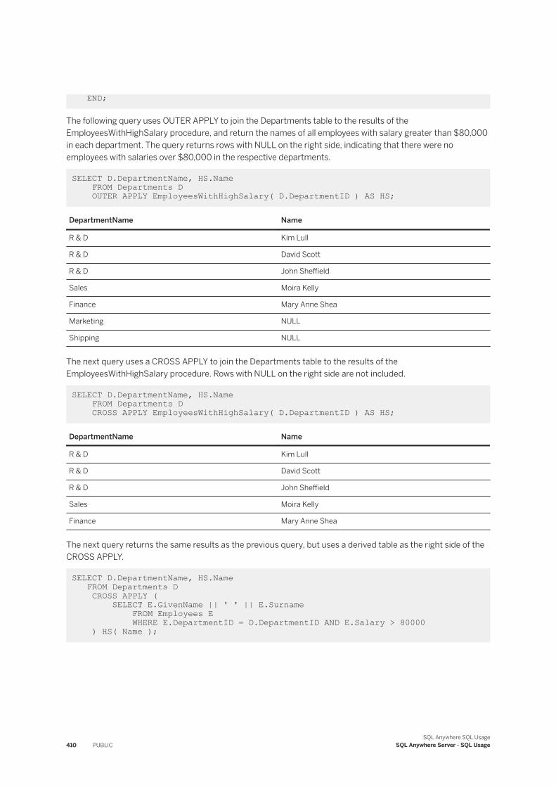
END;
The following query uses OUTER APPLY to join the Departments table to the results of the EmployeesWithHighSalary procedure, and return the names of all employees with salary greater than $80,000 in each department. The query returns rows with NULL on the right side, indicating that there were no employees with salaries over $80,000 in the respective departments.
SELECT D.DepartmentName, HS.Name FROM Departments D OUTER APPLY EmployeesWithHighSalary( D.DepartmentID ) AS HS;
DepartmentName Name
R & D Kim Lull
R & D David Scott
R & D John Sheffield
Sales Moira Kelly
Finance Mary Anne Shea
Marketing NULL
Shipping NULL
The next query uses a CROSS APPLY to join the Departments table to the results of the EmployeesWithHighSalary procedure. Rows with NULL on the right side are not included.
SELECT D.DepartmentName, HS.Name FROM Departments D CROSS APPLY EmployeesWithHighSalary( D.DepartmentID ) AS HS;
DepartmentName Name
R & D Kim Lull
R & D David Scott
R & D John Sheffield
Sales Moira Kelly
Finance Mary Anne Shea
The next query returns the same results as the previous query, but uses a derived table as the right side of the CROSS APPLY.
SELECT D.DepartmentName, HS.Name FROM Departments D CROSS APPLY ( SELECT E.GivenName || ' ' || E.Surname FROM Employees E WHERE E.DepartmentID = D.DepartmentID AND E.Salary > 80000 ) HS( Name );
410 PUBLICSQL Anywhere SQL Usage
SQL Anywhere Server - SQL Usage
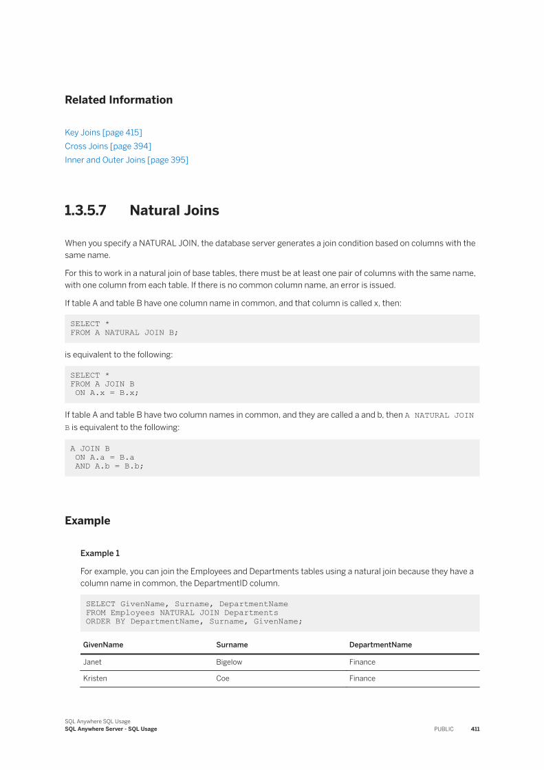
Related Information
Key Joins [page 415]Cross Joins [page 394]Inner and Outer Joins [page 395]
1.3.5.7 Natural Joins
When you specify a NATURAL JOIN, the database server generates a join condition based on columns with the same name.
For this to work in a natural join of base tables, there must be at least one pair of columns with the same name, with one column from each table. If there is no common column name, an error is issued.
If table A and table B have one column name in common, and that column is called x, then:
SELECT * FROM A NATURAL JOIN B;
is equivalent to the following:
SELECT * FROM A JOIN B ON A.x = B.x;
If table A and table B have two column names in common, and they are called a and b, then A NATURAL JOIN B is equivalent to the following:
A JOIN B ON A.a = B.a AND A.b = B.b;
Example
Example 1
For example, you can join the Employees and Departments tables using a natural join because they have a column name in common, the DepartmentID column.
SELECT GivenName, Surname, DepartmentName FROM Employees NATURAL JOIN Departments ORDER BY DepartmentName, Surname, GivenName;
GivenName Surname DepartmentName
Janet Bigelow Finance
Kristen Coe Finance
SQL Anywhere SQL UsageSQL Anywhere Server - SQL Usage PUBLIC 411
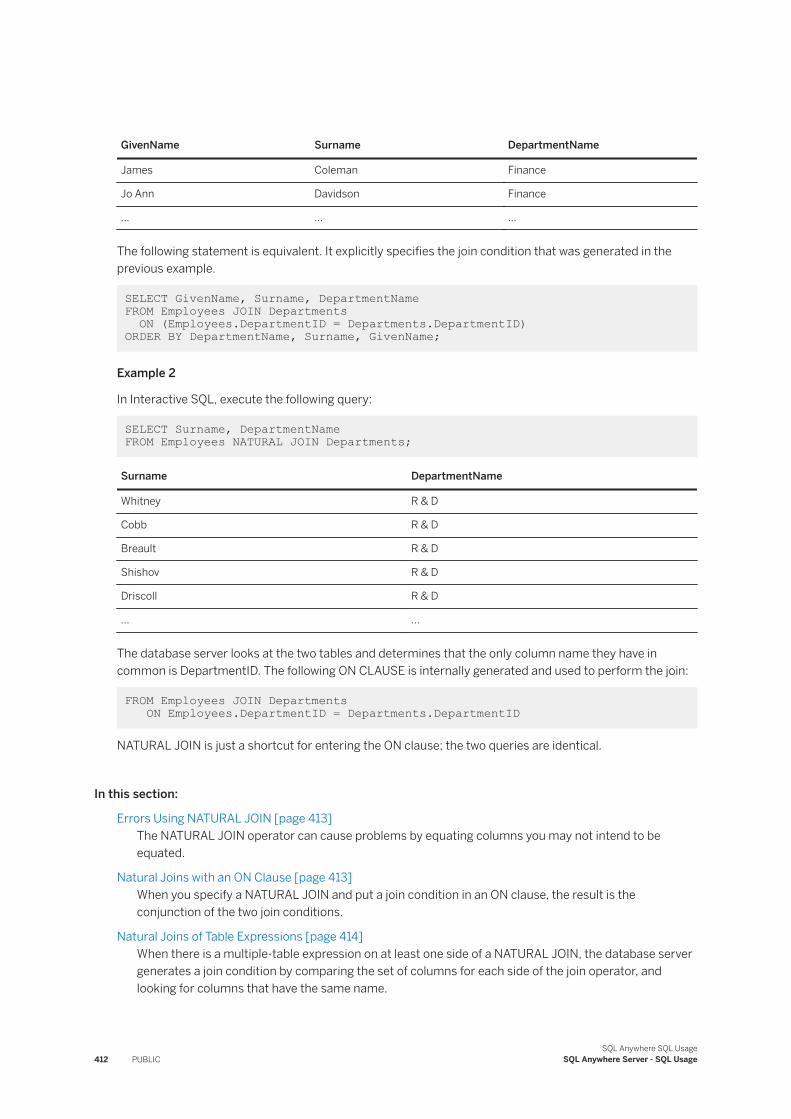
GivenName Surname DepartmentName
James Coleman Finance
Jo Ann Davidson Finance
... ... ...
The following statement is equivalent. It explicitly specifies the join condition that was generated in the previous example.
SELECT GivenName, Surname, DepartmentName FROM Employees JOIN Departments ON (Employees.DepartmentID = Departments.DepartmentID) ORDER BY DepartmentName, Surname, GivenName;
Example 2
In Interactive SQL, execute the following query:
SELECT Surname, DepartmentName FROM Employees NATURAL JOIN Departments;
Surname DepartmentName
Whitney R & D
Cobb R & D
Breault R & D
Shishov R & D
Driscoll R & D
... ...
The database server looks at the two tables and determines that the only column name they have in common is DepartmentID. The following ON CLAUSE is internally generated and used to perform the join:
FROM Employees JOIN Departments ON Employees.DepartmentID = Departments.DepartmentID
NATURAL JOIN is just a shortcut for entering the ON clause; the two queries are identical.
In this section:
Errors Using NATURAL JOIN [page 413]The NATURAL JOIN operator can cause problems by equating columns you may not intend to be equated.
Natural Joins with an ON Clause [page 413]When you specify a NATURAL JOIN and put a join condition in an ON clause, the result is the conjunction of the two join conditions.
Natural Joins of Table Expressions [page 414]When there is a multiple-table expression on at least one side of a NATURAL JOIN, the database server generates a join condition by comparing the set of columns for each side of the join operator, and looking for columns that have the same name.
412 PUBLICSQL Anywhere SQL Usage
SQL Anywhere Server - SQL Usage
Natural Joins of Views and Derived Tables [page 415]You can specify views or derived tables on either side of a NATURAL JOIN. This is an extension to the ANSI/ISO SQL standard.
1.3.5.7.1 Errors Using NATURAL JOIN
The NATURAL JOIN operator can cause problems by equating columns you may not intend to be equated.
For example, the following query generates unwanted results:
SELECT * FROM SalesOrders NATURAL JOIN Customers;
The result of this query has no rows. The database server internally generates the following ON clause:
FROM SalesOrders JOIN Customers ON SalesOrders.ID = Customers.ID
The ID column in the SalesOrders table is an ID number for the order. The ID column in the Customers table is an ID number for the customer. None of them match. Of course, even if a match were found, it would be a meaningless one.
1.3.5.7.2 Natural Joins with an ON Clause
When you specify a NATURAL JOIN and put a join condition in an ON clause, the result is the conjunction of the two join conditions.
For example, the following two queries are equivalent. In the first query, the database server generates the join condition Employees.DepartmentID = Departments.DepartmentID. The query also contains an explicit join condition.
SELECT GivenName, Surname, DepartmentName FROM Employees NATURAL JOIN Departments ON Employees.ManagerID = Departments.DepartmentHeadID;
The next query is equivalent. In it, the natural join condition that was generated in the previous query is specified in the ON clause.
SELECT GivenName, Surname, DepartmentName FROM Employees JOIN Departments ON Employees.ManagerID = Departments.DepartmentHeadID AND Employees.DepartmentID = Departments.DepartmentID;
SQL Anywhere SQL UsageSQL Anywhere Server - SQL Usage PUBLIC 413
1.3.5.7.3 Natural Joins of Table Expressions
When there is a multiple-table expression on at least one side of a NATURAL JOIN, the database server generates a join condition by comparing the set of columns for each side of the join operator, and looking for columns that have the same name.
For example, in the statement:
SELECT * FROM (A JOIN B) NATURAL JOIN (C JOIN D);
there are two table expressions. The column names in the table expression A JOIN B are compared to the column names in the table expression C JOIN D, and a join condition is generated for each unambiguous pair of matching column names. An unambiguous pair of matching columns means that the column name occurs in both table expressions, but does not occur twice in the same table expression.
If there is a pair of ambiguous column names, an error is issued. However, a column name may occur twice in the same table expression, as long as it doesn't also match the name of a column in the other table expression.
Natural Joins of Lists
When a list of table expressions is on at least one side of a natural join, a separate join condition is generated for each table expression in the list.
Consider the following tables:
● table A consists of columns called a, b and c● table B consists of columns called a and d● table C consists of columns called d and c
In this case, the join (A,B) NATURAL JOIN C causes the database server to generate two join conditions:
ON A.c = C.c AND B.d = C.d
If there is no common column name for A-C or B-C, an error is issued.
If table C consists of columns a, d, and c, then the join (A,B) NATURAL JOIN C is invalid. The reason is that column a appears in all three tables, and so the join is ambiguous.
Example
The following example answers the question: for each sale, provide information about what was sold and who sold it.
SELECT * FROM ( Employees KEY JOIN SalesOrders ) NATURAL JOIN ( SalesOrderItems KEY JOIN Products );
414 PUBLICSQL Anywhere SQL Usage
SQL Anywhere Server - SQL Usage
This is equivalent to:
SELECT * FROM ( Employees KEY JOIN SalesOrders ) JOIN ( SalesOrderItems KEY JOIN Products ) ON SalesOrders.ID = SalesOrderItems.ID;
1.3.5.7.4 Natural Joins of Views and Derived Tables
You can specify views or derived tables on either side of a NATURAL JOIN. This is an extension to the ANSI/ISO SQL standard.
In the following statement:
SELECT * FROM View1 NATURAL JOIN View2;
the columns in View1 are compared to the columns in View2. If, for example, a column called EmployeeID is found to occur in both views, and there are no other columns that have identical names, then the generated join condition is (View1.EmployeeID = View2.EmployeeID).
Example
The following example illustrates that a view used in a natural join can include expressions, and not just columns, and they are treated the same way in the natural join. First, create the view V with a column called x, as follows:
CREATE VIEW V(x) AS SELECT R.y + 1 FROM R;
Next, create a natural join of the view to a derived table. The derived table has a correlation name T with a column called x.
SELECT * FROM V NATURAL JOIN (SELECT P.y FROM P) as T(x);
This join is equivalent to the following:
SELECT * FROM V JOIN (SELECT P.y FROM P) as T(x) ON (V.x = T.x);
1.3.5.8 Key Joins
Many common joins are between two tables related by a foreign key.
The most common join restricts foreign key values to be equal to primary key values. The KEY JOIN operator joins two tables based on a foreign key relationship. In other words, the database server generates an ON
SQL Anywhere SQL UsageSQL Anywhere Server - SQL Usage PUBLIC 415
clause that equates the primary key column from one table with the foreign key column of the other. To use a key join, there must be a foreign key relationship between the tables, or an error is issued.
A key join can be considered a shortcut for the ON clause; the two queries are identical. However, you can also use the ON clause with a KEY JOIN. Key join is the default when you specify JOIN but do not specify CROSS, NATURAL, KEY, or use an ON clause. If you look at the diagram of the SQL Anywhere sample database, lines between tables represent foreign keys. You can use the KEY JOIN operator anywhere two tables are joined by a line in the diagram.
When Key Join Is the Default
Key join is the default when all the following apply:
● The keyword JOIN is used.● The keywords CROSS, NATURAL or KEY are not specified.● There is no ON clause.
Example
For example, the following query joins the tables Products and SalesOrderItems based on the foreign key relationship in the database:
SELECT * FROM Products KEY JOIN SalesOrderItems;
The next query is equivalent. It leaves out the word KEY, but by default a JOIN without an ON clause is a KEY JOIN:
SELECT * FROM Products JOIN SalesOrderItems;
The next query is also equivalent because the join condition specified in the ON clause is the same as the join condition that the database server generates for these tables based on their foreign key relationship in the SQL Anywhere sample database:
SELECT * FROM Products JOIN SalesOrderItems ON SalesOrderItems.ProductID = Products.ID;
In this section:
Key Joins with an ON Clause [page 417]When you specify a KEY JOIN and put a join condition in an ON clause, the result is the conjunction of the two join conditions.
Key Joins When There Are Multiple Foreign Key Relationships [page 417]When the database server attempts to generate a join condition based on a foreign key relationship, it sometimes finds more than one relationship.
Key Joins of Table Expressions [page 420]
416 PUBLICSQL Anywhere SQL Usage
SQL Anywhere Server - SQL Usage
The database server generates join conditions for the key join of table expressions by examining the foreign key relationship of each pair of tables in the statement.
Key Joins of Views and Derived Tables [page 425]When you include a view or derived table in a key join, the database server follows the same basic procedure as with tables, but there are a few differences.
Rules Describing the Operation of Key Joins [page 427]There are several rules that describe the operation of key joins.
1.3.5.8.1 Key Joins with an ON Clause
When you specify a KEY JOIN and put a join condition in an ON clause, the result is the conjunction of the two join conditions.
For example:
SELECT * FROM A KEY JOIN B ON A.x = B.y;
If the join condition generated by the key join of A and B is A.w = B.z, then this query is equivalent to:
SELECT * FROM A JOIN B ON A.x = B.y AND A.w = B.z;
1.3.5.8.2 Key Joins When There Are Multiple Foreign Key Relationships
When the database server attempts to generate a join condition based on a foreign key relationship, it sometimes finds more than one relationship.
In these cases, the database server determines which foreign key relationship to use by matching the role name of the foreign key to the correlation name of the primary key table that the foreign key references.
Correlation Name and Role Name
A correlation name is the name of a table or view that is used in the FROM clause of the query: either its original name, or an alias that is defined in the FROM clause.
A role name is the name of the foreign key. It must be unique for a given foreign (child) table.
If you do not specify a role name for a foreign key, the name is assigned as follows:
● If there is no foreign key with the same name as the primary table name, the primary table name is assigned as the role name.
SQL Anywhere SQL UsageSQL Anywhere Server - SQL Usage PUBLIC 417
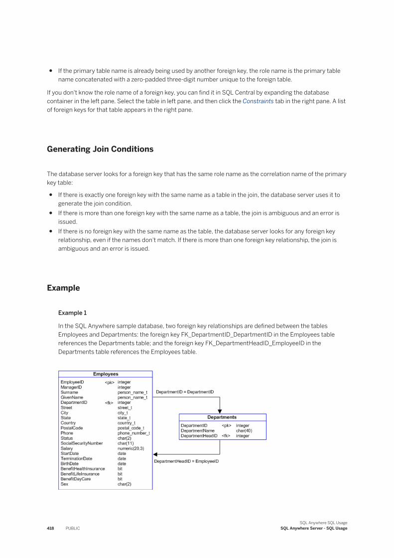
● If the primary table name is already being used by another foreign key, the role name is the primary table name concatenated with a zero-padded three-digit number unique to the foreign table.
If you don't know the role name of a foreign key, you can find it in SQL Central by expanding the database container in the left pane. Select the table in left pane, and then click the Constraints tab in the right pane. A list of foreign keys for that table appears in the right pane.
Generating Join Conditions
The database server looks for a foreign key that has the same role name as the correlation name of the primary key table:
● If there is exactly one foreign key with the same name as a table in the join, the database server uses it to generate the join condition.
● If there is more than one foreign key with the same name as a table, the join is ambiguous and an error is issued.
● If there is no foreign key with the same name as the table, the database server looks for any foreign key relationship, even if the names don't match. If there is more than one foreign key relationship, the join is ambiguous and an error is issued.
Example
Example 1
In the SQL Anywhere sample database, two foreign key relationships are defined between the tables Employees and Departments: the foreign key FK_DepartmentID_DepartmentID in the Employees table references the Departments table; and the foreign key FK_DepartmentHeadID_EmployeeID in the Departments table references the Employees table.
418 PUBLICSQL Anywhere SQL Usage
SQL Anywhere Server - SQL Usage
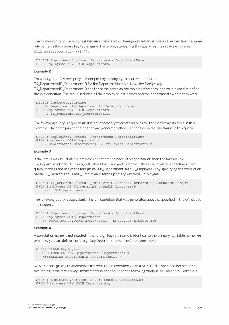
The following query is ambiguous because there are two foreign key relationships and neither has the same role name as the primary key table name. Therefore, attempting this query results in the syntax error SQLE_AMBIGUOUS_JOIN (-147).
SELECT Employees.Surname, Departments.DepartmentName FROM Employees KEY JOIN Departments;
Example 2
This query modifies the query in Example 1 by specifying the correlation name FK_DepartmentID_DepartmentID for the Departments table. Now, the foreign key FK_DepartmentID_DepartmentID has the same name as the table it references, and so it is used to define the join condition. The result includes all the employee last names and the departments where they work.
SELECT Employees.Surname, FK_DepartmentID_DepartmentID.DepartmentNameFROM Employees KEY JOIN Departments AS FK_DepartmentID_DepartmentID;
The following query is equivalent. It is not necessary to create an alias for the Departments table in this example. The same join condition that was generated above is specified in the ON clause in this query:
SELECT Employees.Surname, Departments.DepartmentName FROM Employees JOIN Departments ON Departments.DepartmentID = Employees.DepartmentID;
Example 3
If the intent was to list all the employees that are the head of a department, then the foreign key FK_DepartmentHeadID_EmployeeID should be used and Example 1 should be rewritten as follows. This query imposes the use of the foreign key FK_DepartmentHeadID_EmployeeID by specifying the correlation name FK_DepartmentHeadID_EmployeeID for the primary key table Employees.
SELECT FK_DepartmentHeadID_EmployeeID.Surname, Departments.DepartmentName FROM Employees AS FK_DepartmentHeadID_EmployeeID KEY JOIN Departments;
The following query is equivalent. The join condition that was generated above is specified in the ON clause in this query:
SELECT Employees.Surname, Departments.DepartmentName FROM Employees JOIN Departments ON Departments.DepartmentHeadID = Employees.EmployeeID;
Example 4
A correlation name is not needed if the foreign key role name is identical to the primary key table name. For example, you can define the foreign key Departments for the Employees table:
ALTER TABLE Employees ADD FOREIGN KEY Departments (DepartmentID) REFERENCES Departments (DepartmentID);
Now, this foreign key relationship is the default join condition when a KEY JOIN is specified between the two tables. If the foreign key Departments is defined, then the following query is equivalent to Example 3.
SELECT Employees.Surname, Departments.DepartmentName FROM Employees KEY JOIN Departments;
SQL Anywhere SQL UsageSQL Anywhere Server - SQL Usage PUBLIC 419
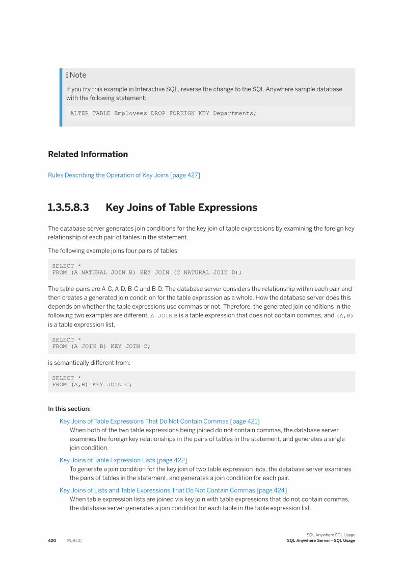
NoteIf you try this example in Interactive SQL, reverse the change to the SQL Anywhere sample database with the following statement:
ALTER TABLE Employees DROP FOREIGN KEY Departments;
Related Information
Rules Describing the Operation of Key Joins [page 427]
1.3.5.8.3 Key Joins of Table Expressions
The database server generates join conditions for the key join of table expressions by examining the foreign key relationship of each pair of tables in the statement.
The following example joins four pairs of tables.
SELECT * FROM (A NATURAL JOIN B) KEY JOIN (C NATURAL JOIN D);
The table-pairs are A-C, A-D, B-C and B-D. The database server considers the relationship within each pair and then creates a generated join condition for the table expression as a whole. How the database server does this depends on whether the table expressions use commas or not. Therefore, the generated join conditions in the following two examples are different. A JOIN B is a table expression that does not contain commas, and (A,B) is a table expression list.
SELECT * FROM (A JOIN B) KEY JOIN C;
is semantically different from:
SELECT * FROM (A,B) KEY JOIN C;
In this section:
Key Joins of Table Expressions That Do Not Contain Commas [page 421]When both of the two table expressions being joined do not contain commas, the database server examines the foreign key relationships in the pairs of tables in the statement, and generates a single join condition.
Key Joins of Table Expression Lists [page 422]To generate a join condition for the key join of two table expression lists, the database server examines the pairs of tables in the statement, and generates a join condition for each pair.
Key Joins of Lists and Table Expressions That Do Not Contain Commas [page 424]When table expression lists are joined via key join with table expressions that do not contain commas, the database server generates a join condition for each table in the table expression list.
420 PUBLICSQL Anywhere SQL Usage
SQL Anywhere Server - SQL Usage
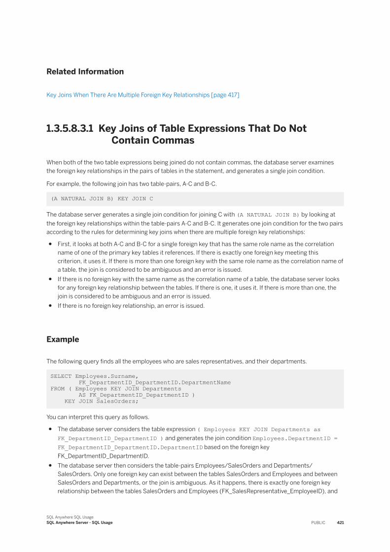
Related Information
Key Joins When There Are Multiple Foreign Key Relationships [page 417]
1.3.5.8.3.1 Key Joins of Table Expressions That Do Not Contain Commas
When both of the two table expressions being joined do not contain commas, the database server examines the foreign key relationships in the pairs of tables in the statement, and generates a single join condition.
For example, the following join has two table-pairs, A-C and B-C.
(A NATURAL JOIN B) KEY JOIN C
The database server generates a single join condition for joining C with (A NATURAL JOIN B) by looking at the foreign key relationships within the table-pairs A-C and B-C. It generates one join condition for the two pairs according to the rules for determining key joins when there are multiple foreign key relationships:
● First, it looks at both A-C and B-C for a single foreign key that has the same role name as the correlation name of one of the primary key tables it references. If there is exactly one foreign key meeting this criterion, it uses it. If there is more than one foreign key with the same role name as the correlation name of a table, the join is considered to be ambiguous and an error is issued.
● If there is no foreign key with the same name as the correlation name of a table, the database server looks for any foreign key relationship between the tables. If there is one, it uses it. If there is more than one, the join is considered to be ambiguous and an error is issued.
● If there is no foreign key relationship, an error is issued.
Example
The following query finds all the employees who are sales representatives, and their departments.
SELECT Employees.Surname, FK_DepartmentID_DepartmentID.DepartmentNameFROM ( Employees KEY JOIN Departments AS FK_DepartmentID_DepartmentID ) KEY JOIN SalesOrders;
You can interpret this query as follows.
● The database server considers the table expression ( Employees KEY JOIN Departments as FK_DepartmentID_DepartmentID ) and generates the join condition Employees.DepartmentID = FK_DepartmentID_DepartmentID.DepartmentID based on the foreign key FK_DepartmentID_DepartmentID.
● The database server then considers the table-pairs Employees/SalesOrders and Departments/SalesOrders. Only one foreign key can exist between the tables SalesOrders and Employees and between SalesOrders and Departments, or the join is ambiguous. As it happens, there is exactly one foreign key relationship between the tables SalesOrders and Employees (FK_SalesRepresentative_EmployeeID), and
SQL Anywhere SQL UsageSQL Anywhere Server - SQL Usage PUBLIC 421
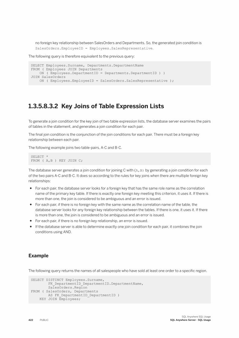
no foreign key relationship between SalesOrders and Departments. So, the generated join condition is SalesOrders.EmployeeID = Employees.SalesRepresentative.
The following query is therefore equivalent to the previous query:
SELECT Employees.Surname, Departments.DepartmentName FROM ( Employees JOIN Departments ON ( Employees.DepartmentID = Departments.DepartmentID ) )JOIN SalesOrders ON ( Employees.EmployeeID = SalesOrders.SalesRepresentative );
1.3.5.8.3.2 Key Joins of Table Expression Lists
To generate a join condition for the key join of two table expression lists, the database server examines the pairs of tables in the statement, and generates a join condition for each pair.
The final join condition is the conjunction of the join conditions for each pair. There must be a foreign key relationship between each pair.
The following example joins two table-pairs, A-C and B-C.
SELECT * FROM ( A,B ) KEY JOIN C;
The database server generates a join condition for joining C with (A,B) by generating a join condition for each of the two pairs A-C and B-C. It does so according to the rules for key joins when there are multiple foreign key relationships:
● For each pair, the database server looks for a foreign key that has the same role name as the correlation name of the primary key table. If there is exactly one foreign key meeting this criterion, it uses it. If there is more than one, the join is considered to be ambiguous and an error is issued.
● For each pair, if there is no foreign key with the same name as the correlation name of the table, the database server looks for any foreign key relationship between the tables. If there is one, it uses it. If there is more than one, the join is considered to be ambiguous and an error is issued.
● For each pair, if there is no foreign key relationship, an error is issued.● If the database server is able to determine exactly one join condition for each pair, it combines the join
conditions using AND.
Example
The following query returns the names of all salespeople who have sold at least one order to a specific region.
SELECT DISTINCT Employees.Surname, FK_DepartmentID_DepartmentID.DepartmentName, SalesOrders.RegionFROM ( SalesOrders, Departments AS FK_DepartmentID_DepartmentID ) KEY JOIN Employees;
422 PUBLICSQL Anywhere SQL Usage
SQL Anywhere Server - SQL Usage
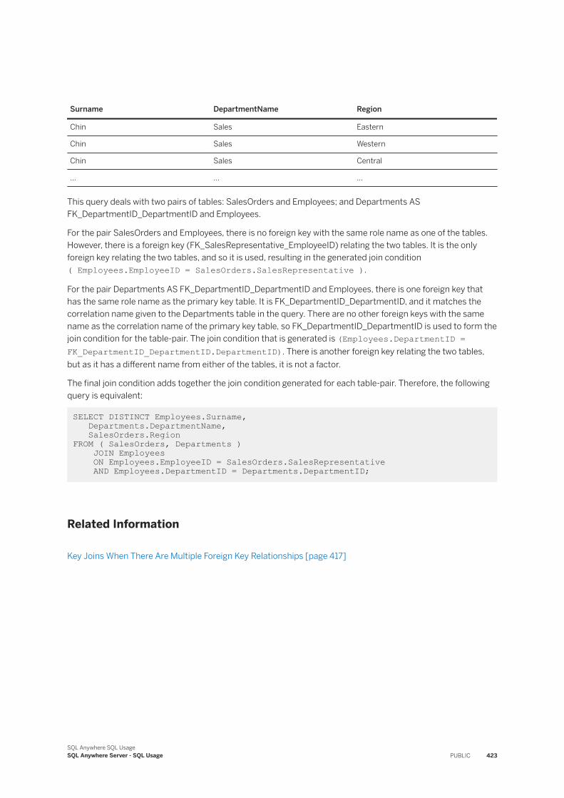
Surname DepartmentName Region
Chin Sales Eastern
Chin Sales Western
Chin Sales Central
... ... ...
This query deals with two pairs of tables: SalesOrders and Employees; and Departments AS FK_DepartmentID_DepartmentID and Employees.
For the pair SalesOrders and Employees, there is no foreign key with the same role name as one of the tables. However, there is a foreign key (FK_SalesRepresentative_EmployeeID) relating the two tables. It is the only foreign key relating the two tables, and so it is used, resulting in the generated join condition ( Employees.EmployeeID = SalesOrders.SalesRepresentative ).
For the pair Departments AS FK_DepartmentID_DepartmentID and Employees, there is one foreign key that has the same role name as the primary key table. It is FK_DepartmentID_DepartmentID, and it matches the correlation name given to the Departments table in the query. There are no other foreign keys with the same name as the correlation name of the primary key table, so FK_DepartmentID_DepartmentID is used to form the join condition for the table-pair. The join condition that is generated is (Employees.DepartmentID = FK_DepartmentID_DepartmentID.DepartmentID). There is another foreign key relating the two tables, but as it has a different name from either of the tables, it is not a factor.
The final join condition adds together the join condition generated for each table-pair. Therefore, the following query is equivalent:
SELECT DISTINCT Employees.Surname, Departments.DepartmentName, SalesOrders.RegionFROM ( SalesOrders, Departments ) JOIN Employees ON Employees.EmployeeID = SalesOrders.SalesRepresentative AND Employees.DepartmentID = Departments.DepartmentID;
Related Information
Key Joins When There Are Multiple Foreign Key Relationships [page 417]
SQL Anywhere SQL UsageSQL Anywhere Server - SQL Usage PUBLIC 423
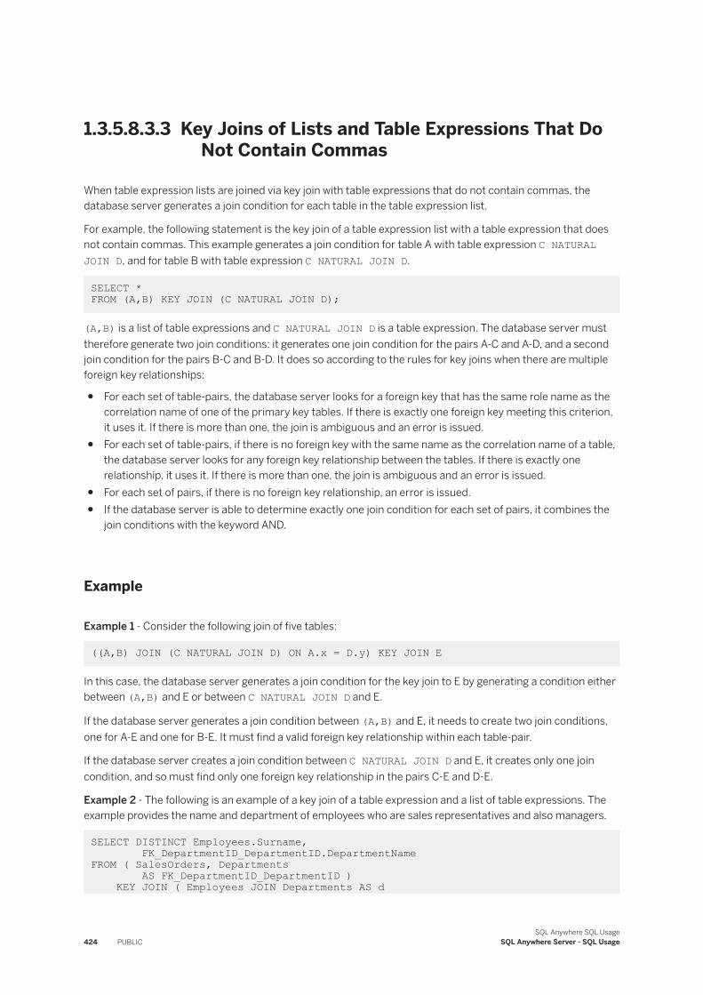
1.3.5.8.3.3 Key Joins of Lists and Table Expressions That Do Not Contain Commas
When table expression lists are joined via key join with table expressions that do not contain commas, the database server generates a join condition for each table in the table expression list.
For example, the following statement is the key join of a table expression list with a table expression that does not contain commas. This example generates a join condition for table A with table expression C NATURAL JOIN D, and for table B with table expression C NATURAL JOIN D.
SELECT * FROM (A,B) KEY JOIN (C NATURAL JOIN D);
(A,B) is a list of table expressions and C NATURAL JOIN D is a table expression. The database server must therefore generate two join conditions: it generates one join condition for the pairs A-C and A-D, and a second join condition for the pairs B-C and B-D. It does so according to the rules for key joins when there are multiple foreign key relationships:
● For each set of table-pairs, the database server looks for a foreign key that has the same role name as the correlation name of one of the primary key tables. If there is exactly one foreign key meeting this criterion, it uses it. If there is more than one, the join is ambiguous and an error is issued.
● For each set of table-pairs, if there is no foreign key with the same name as the correlation name of a table, the database server looks for any foreign key relationship between the tables. If there is exactly one relationship, it uses it. If there is more than one, the join is ambiguous and an error is issued.
● For each set of pairs, if there is no foreign key relationship, an error is issued.● If the database server is able to determine exactly one join condition for each set of pairs, it combines the
join conditions with the keyword AND.
Example
Example 1 - Consider the following join of five tables:
((A,B) JOIN (C NATURAL JOIN D) ON A.x = D.y) KEY JOIN E
In this case, the database server generates a join condition for the key join to E by generating a condition either between (A,B) and E or between C NATURAL JOIN D and E.
If the database server generates a join condition between (A,B) and E, it needs to create two join conditions, one for A-E and one for B-E. It must find a valid foreign key relationship within each table-pair.
If the database server creates a join condition between C NATURAL JOIN D and E, it creates only one join condition, and so must find only one foreign key relationship in the pairs C-E and D-E.
Example 2 - The following is an example of a key join of a table expression and a list of table expressions. The example provides the name and department of employees who are sales representatives and also managers.
SELECT DISTINCT Employees.Surname, FK_DepartmentID_DepartmentID.DepartmentNameFROM ( SalesOrders, Departments AS FK_DepartmentID_DepartmentID ) KEY JOIN ( Employees JOIN Departments AS d
424 PUBLICSQL Anywhere SQL Usage
SQL Anywhere Server - SQL Usage
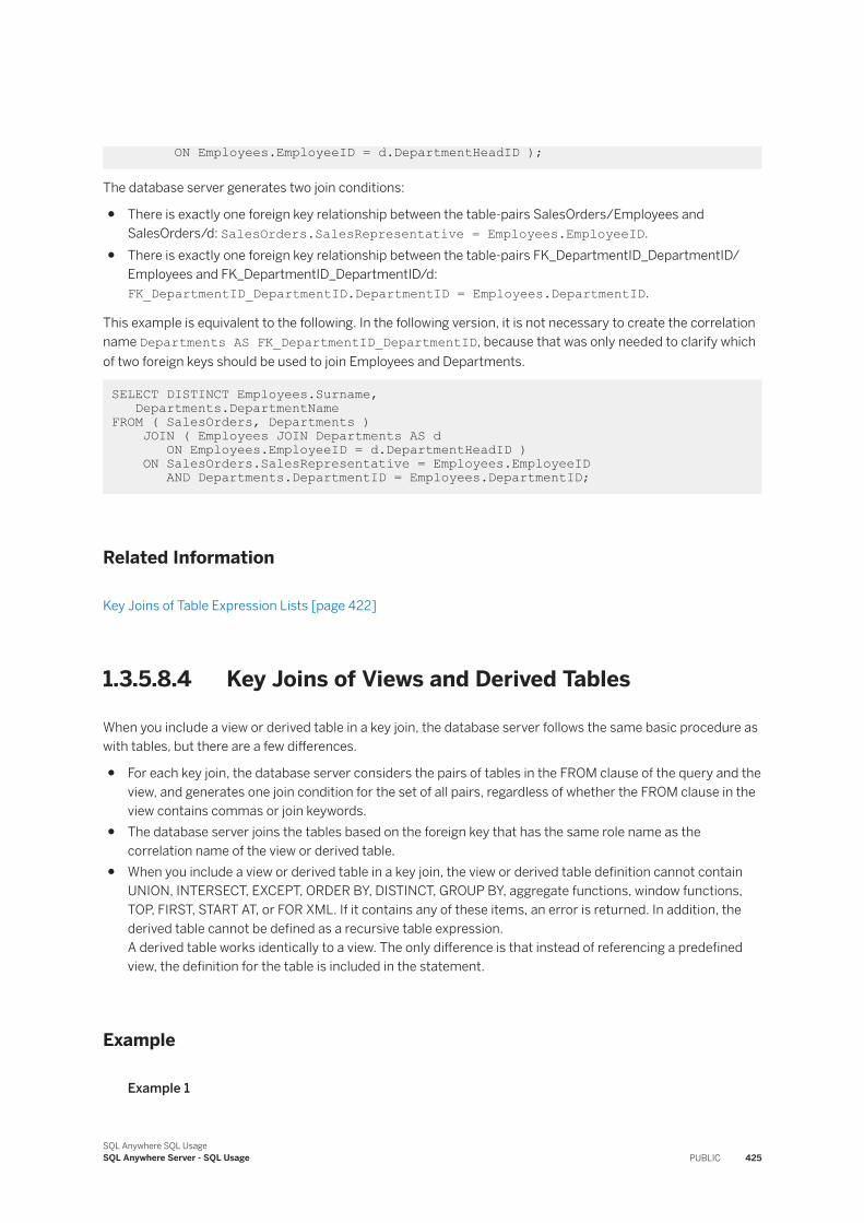
ON Employees.EmployeeID = d.DepartmentHeadID );
The database server generates two join conditions:
● There is exactly one foreign key relationship between the table-pairs SalesOrders/Employees and SalesOrders/d: SalesOrders.SalesRepresentative = Employees.EmployeeID.
● There is exactly one foreign key relationship between the table-pairs FK_DepartmentID_DepartmentID/Employees and FK_DepartmentID_DepartmentID/d: FK_DepartmentID_DepartmentID.DepartmentID = Employees.DepartmentID.
This example is equivalent to the following. In the following version, it is not necessary to create the correlation name Departments AS FK_DepartmentID_DepartmentID, because that was only needed to clarify which of two foreign keys should be used to join Employees and Departments.
SELECT DISTINCT Employees.Surname, Departments.DepartmentNameFROM ( SalesOrders, Departments ) JOIN ( Employees JOIN Departments AS d ON Employees.EmployeeID = d.DepartmentHeadID ) ON SalesOrders.SalesRepresentative = Employees.EmployeeID AND Departments.DepartmentID = Employees.DepartmentID;
Related Information
Key Joins of Table Expression Lists [page 422]
1.3.5.8.4 Key Joins of Views and Derived Tables
When you include a view or derived table in a key join, the database server follows the same basic procedure as with tables, but there are a few differences.
● For each key join, the database server considers the pairs of tables in the FROM clause of the query and the view, and generates one join condition for the set of all pairs, regardless of whether the FROM clause in the view contains commas or join keywords.
● The database server joins the tables based on the foreign key that has the same role name as the correlation name of the view or derived table.
● When you include a view or derived table in a key join, the view or derived table definition cannot contain UNION, INTERSECT, EXCEPT, ORDER BY, DISTINCT, GROUP BY, aggregate functions, window functions, TOP, FIRST, START AT, or FOR XML. If it contains any of these items, an error is returned. In addition, the derived table cannot be defined as a recursive table expression.A derived table works identically to a view. The only difference is that instead of referencing a predefined view, the definition for the table is included in the statement.
Example
Example 1
SQL Anywhere SQL UsageSQL Anywhere Server - SQL Usage PUBLIC 425
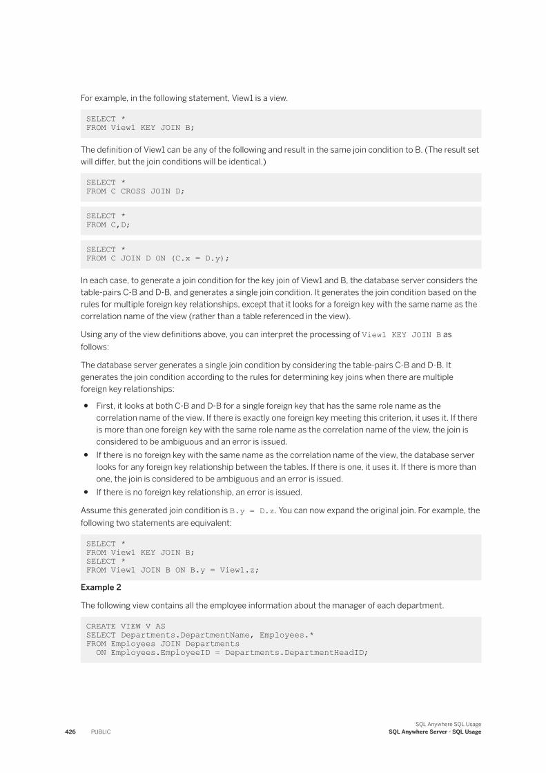
For example, in the following statement, View1 is a view.
SELECT * FROM View1 KEY JOIN B;
The definition of View1 can be any of the following and result in the same join condition to B. (The result set will differ, but the join conditions will be identical.)
SELECT * FROM C CROSS JOIN D;
SELECT * FROM C,D;
SELECT * FROM C JOIN D ON (C.x = D.y);
In each case, to generate a join condition for the key join of View1 and B, the database server considers the table-pairs C-B and D-B, and generates a single join condition. It generates the join condition based on the rules for multiple foreign key relationships, except that it looks for a foreign key with the same name as the correlation name of the view (rather than a table referenced in the view).
Using any of the view definitions above, you can interpret the processing of View1 KEY JOIN B as follows:
The database server generates a single join condition by considering the table-pairs C-B and D-B. It generates the join condition according to the rules for determining key joins when there are multiple foreign key relationships:
● First, it looks at both C-B and D-B for a single foreign key that has the same role name as the correlation name of the view. If there is exactly one foreign key meeting this criterion, it uses it. If there is more than one foreign key with the same role name as the correlation name of the view, the join is considered to be ambiguous and an error is issued.
● If there is no foreign key with the same name as the correlation name of the view, the database server looks for any foreign key relationship between the tables. If there is one, it uses it. If there is more than one, the join is considered to be ambiguous and an error is issued.
● If there is no foreign key relationship, an error is issued.
Assume this generated join condition is B.y = D.z. You can now expand the original join. For example, the following two statements are equivalent:
SELECT * FROM View1 KEY JOIN B;SELECT * FROM View1 JOIN B ON B.y = View1.z;
Example 2
The following view contains all the employee information about the manager of each department.
CREATE VIEW V AS SELECT Departments.DepartmentName, Employees.*FROM Employees JOIN Departments ON Employees.EmployeeID = Departments.DepartmentHeadID;
426 PUBLICSQL Anywhere SQL Usage
SQL Anywhere Server - SQL Usage
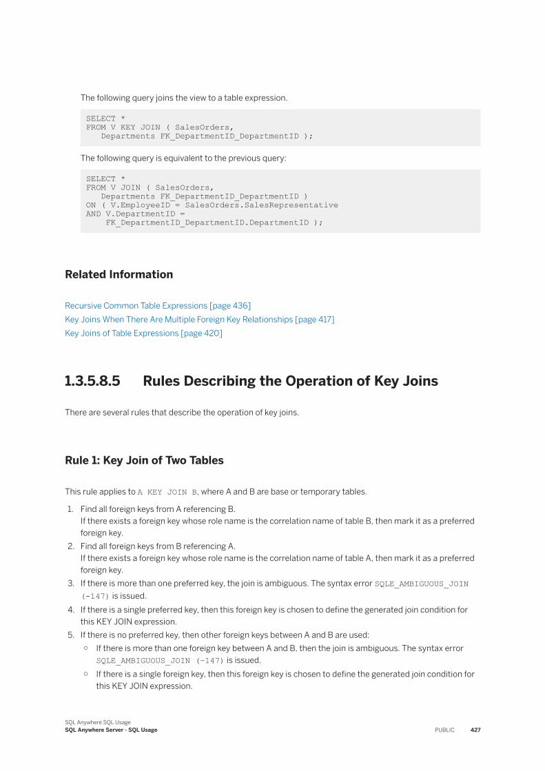
The following query joins the view to a table expression.
SELECT * FROM V KEY JOIN ( SalesOrders, Departments FK_DepartmentID_DepartmentID );
The following query is equivalent to the previous query:
SELECT * FROM V JOIN ( SalesOrders, Departments FK_DepartmentID_DepartmentID )ON ( V.EmployeeID = SalesOrders.SalesRepresentativeAND V.DepartmentID = FK_DepartmentID_DepartmentID.DepartmentID );
Related Information
Recursive Common Table Expressions [page 436]Key Joins When There Are Multiple Foreign Key Relationships [page 417]Key Joins of Table Expressions [page 420]
1.3.5.8.5 Rules Describing the Operation of Key Joins
There are several rules that describe the operation of key joins.
Rule 1: Key Join of Two Tables
This rule applies to A KEY JOIN B, where A and B are base or temporary tables.
1. Find all foreign keys from A referencing B.If there exists a foreign key whose role name is the correlation name of table B, then mark it as a preferred foreign key.
2. Find all foreign keys from B referencing A.If there exists a foreign key whose role name is the correlation name of table A, then mark it as a preferred foreign key.
3. If there is more than one preferred key, the join is ambiguous. The syntax error SQLE_AMBIGUOUS_JOIN (-147) is issued.
4. If there is a single preferred key, then this foreign key is chosen to define the generated join condition for this KEY JOIN expression.
5. If there is no preferred key, then other foreign keys between A and B are used:○ If there is more than one foreign key between A and B, then the join is ambiguous. The syntax error
SQLE_AMBIGUOUS_JOIN (-147) is issued.○ If there is a single foreign key, then this foreign key is chosen to define the generated join condition for
this KEY JOIN expression.
SQL Anywhere SQL UsageSQL Anywhere Server - SQL Usage PUBLIC 427
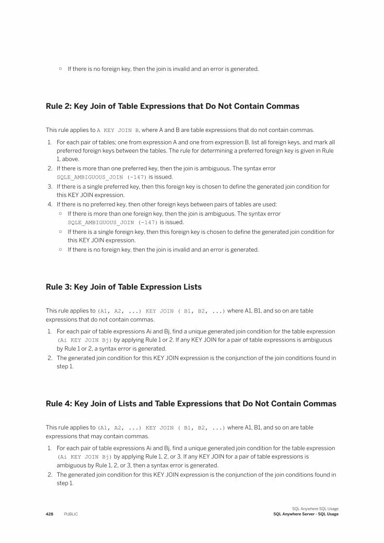
○ If there is no foreign key, then the join is invalid and an error is generated.
Rule 2: Key Join of Table Expressions that Do Not Contain Commas
This rule applies to A KEY JOIN B, where A and B are table expressions that do not contain commas.
1. For each pair of tables; one from expression A and one from expression B, list all foreign keys, and mark all preferred foreign keys between the tables. The rule for determining a preferred foreign key is given in Rule 1, above.
2. If there is more than one preferred key, then the join is ambiguous. The syntax error SQLE_AMBIGUOUS_JOIN (-147) is issued.
3. If there is a single preferred key, then this foreign key is chosen to define the generated join condition for this KEY JOIN expression.
4. If there is no preferred key, then other foreign keys between pairs of tables are used:○ If there is more than one foreign key, then the join is ambiguous. The syntax error
SQLE_AMBIGUOUS_JOIN (-147) is issued.○ If there is a single foreign key, then this foreign key is chosen to define the generated join condition for
this KEY JOIN expression.○ If there is no foreign key, then the join is invalid and an error is generated.
Rule 3: Key Join of Table Expression Lists
This rule applies to (A1, A2, ...) KEY JOIN ( B1, B2, ...) where A1, B1, and so on are table expressions that do not contain commas.
1. For each pair of table expressions Ai and Bj, find a unique generated join condition for the table expression (Ai KEY JOIN Bj) by applying Rule 1 or 2. If any KEY JOIN for a pair of table expressions is ambiguous by Rule 1 or 2, a syntax error is generated.
2. The generated join condition for this KEY JOIN expression is the conjunction of the join conditions found in step 1.
Rule 4: Key Join of Lists and Table Expressions that Do Not Contain Commas
This rule applies to (A1, A2, ...) KEY JOIN ( B1, B2, ...) where A1, B1, and so on are table expressions that may contain commas.
1. For each pair of table expressions Ai and Bj, find a unique generated join condition for the table expression (Ai KEY JOIN Bj) by applying Rule 1, 2, or 3. If any KEY JOIN for a pair of table expressions is ambiguous by Rule 1, 2, or 3, then a syntax error is generated.
2. The generated join condition for this KEY JOIN expression is the conjunction of the join conditions found in step 1.
428 PUBLICSQL Anywhere SQL Usage
SQL Anywhere Server - SQL Usage
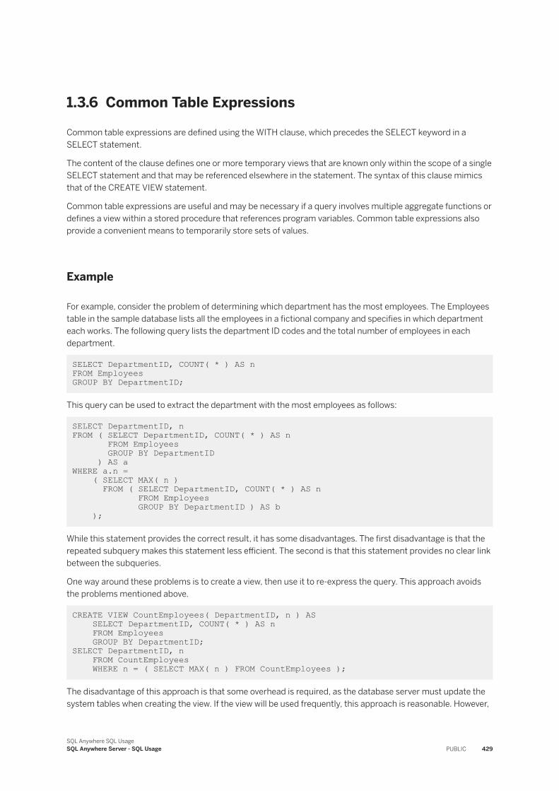
1.3.6 Common Table Expressions
Common table expressions are defined using the WITH clause, which precedes the SELECT keyword in a SELECT statement.
The content of the clause defines one or more temporary views that are known only within the scope of a single SELECT statement and that may be referenced elsewhere in the statement. The syntax of this clause mimics that of the CREATE VIEW statement.
Common table expressions are useful and may be necessary if a query involves multiple aggregate functions or defines a view within a stored procedure that references program variables. Common table expressions also provide a convenient means to temporarily store sets of values.
Example
For example, consider the problem of determining which department has the most employees. The Employees table in the sample database lists all the employees in a fictional company and specifies in which department each works. The following query lists the department ID codes and the total number of employees in each department.
SELECT DepartmentID, COUNT( * ) AS n FROM Employees GROUP BY DepartmentID;
This query can be used to extract the department with the most employees as follows:
SELECT DepartmentID, n FROM ( SELECT DepartmentID, COUNT( * ) AS n FROM Employees GROUP BY DepartmentID ) AS aWHERE a.n = ( SELECT MAX( n ) FROM ( SELECT DepartmentID, COUNT( * ) AS n FROM Employees GROUP BY DepartmentID ) AS b );
While this statement provides the correct result, it has some disadvantages. The first disadvantage is that the repeated subquery makes this statement less efficient. The second is that this statement provides no clear link between the subqueries.
One way around these problems is to create a view, then use it to re-express the query. This approach avoids the problems mentioned above.
CREATE VIEW CountEmployees( DepartmentID, n ) AS SELECT DepartmentID, COUNT( * ) AS n FROM Employees GROUP BY DepartmentID; SELECT DepartmentID, n FROM CountEmployees WHERE n = ( SELECT MAX( n ) FROM CountEmployees );
The disadvantage of this approach is that some overhead is required, as the database server must update the system tables when creating the view. If the view will be used frequently, this approach is reasonable. However,
SQL Anywhere SQL UsageSQL Anywhere Server - SQL Usage PUBLIC 429
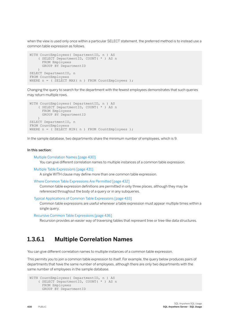
when the view is used only once within a particular SELECT statement, the preferred method is to instead use a common table expression as follows.
WITH CountEmployees( DepartmentID, n ) AS ( SELECT DepartmentID, COUNT( * ) AS n FROM Employees GROUP BY DepartmentID )SELECT DepartmentID, nFROM CountEmployees WHERE n = ( SELECT MAX( n ) FROM CountEmployees );
Changing the query to search for the department with the fewest employees demonstrates that such queries may return multiple rows.
WITH CountEmployees( DepartmentID, n ) AS ( SELECT DepartmentID, COUNT( * ) AS n FROM Employees GROUP BY DepartmentID )SELECT DepartmentID, nFROM CountEmployees WHERE n = ( SELECT MIN( n ) FROM CountEmployees );
In the sample database, two departments share the minimum number of employees, which is 9.
In this section:
Multiple Correlation Names [page 430]You can give different correlation names to multiple instances of a common table expression.
Multiple Table Expressions [page 431]A single WITH clause may define more than one common table expression.
Where Common Table Expressions Are Permitted [page 432]Common table expression definitions are permitted in only three places, although they may be referenced throughout the body of a query or in any subqueries.
Typical Applications of Common Table Expressions [page 433]Common table expressions are useful whenever a table expression must appear multiple times within a single query.
Recursive Common Table Expressions [page 436]Recursion provides an easier way of traversing tables that represent tree or tree-like data structures.
1.3.6.1 Multiple Correlation Names
You can give different correlation names to multiple instances of a common table expression.
This permits you to join a common table expression to itself. For example, the query below produces pairs of departments that have the same number of employees, although there are only two departments with the same number of employees in the sample database.
WITH CountEmployees( DepartmentID, n ) AS ( SELECT DepartmentID, COUNT( * ) AS n FROM Employees GROUP BY DepartmentID
430 PUBLICSQL Anywhere SQL Usage
SQL Anywhere Server - SQL Usage
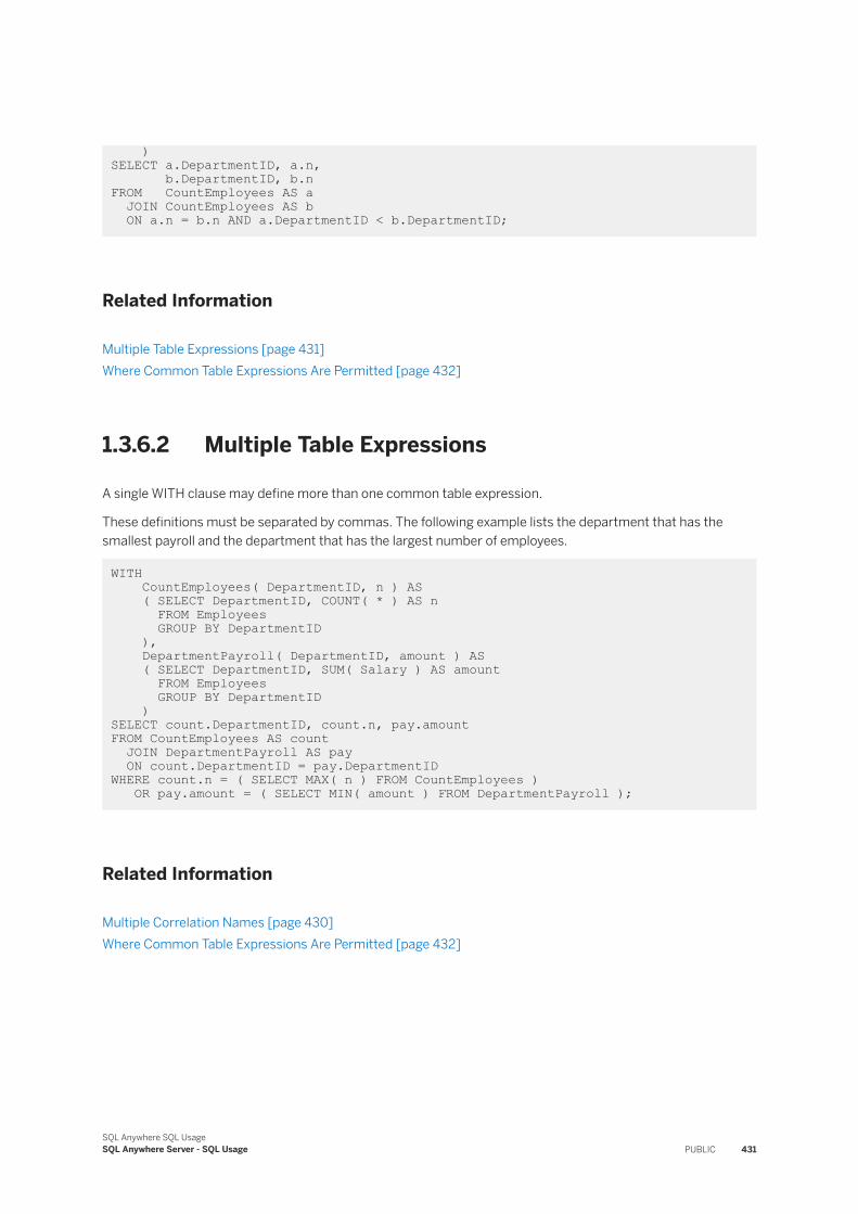
)SELECT a.DepartmentID, a.n, b.DepartmentID, b.nFROM CountEmployees AS a JOIN CountEmployees AS b ON a.n = b.n AND a.DepartmentID < b.DepartmentID;
Related Information
Multiple Table Expressions [page 431]Where Common Table Expressions Are Permitted [page 432]
1.3.6.2 Multiple Table Expressions
A single WITH clause may define more than one common table expression.
These definitions must be separated by commas. The following example lists the department that has the smallest payroll and the department that has the largest number of employees.
WITH CountEmployees( DepartmentID, n ) AS ( SELECT DepartmentID, COUNT( * ) AS n FROM Employees GROUP BY DepartmentID ), DepartmentPayroll( DepartmentID, amount ) AS ( SELECT DepartmentID, SUM( Salary ) AS amount FROM Employees GROUP BY DepartmentID )SELECT count.DepartmentID, count.n, pay.amountFROM CountEmployees AS count JOIN DepartmentPayroll AS pay ON count.DepartmentID = pay.DepartmentIDWHERE count.n = ( SELECT MAX( n ) FROM CountEmployees ) OR pay.amount = ( SELECT MIN( amount ) FROM DepartmentPayroll );
Related Information
Multiple Correlation Names [page 430]Where Common Table Expressions Are Permitted [page 432]
SQL Anywhere SQL UsageSQL Anywhere Server - SQL Usage PUBLIC 431
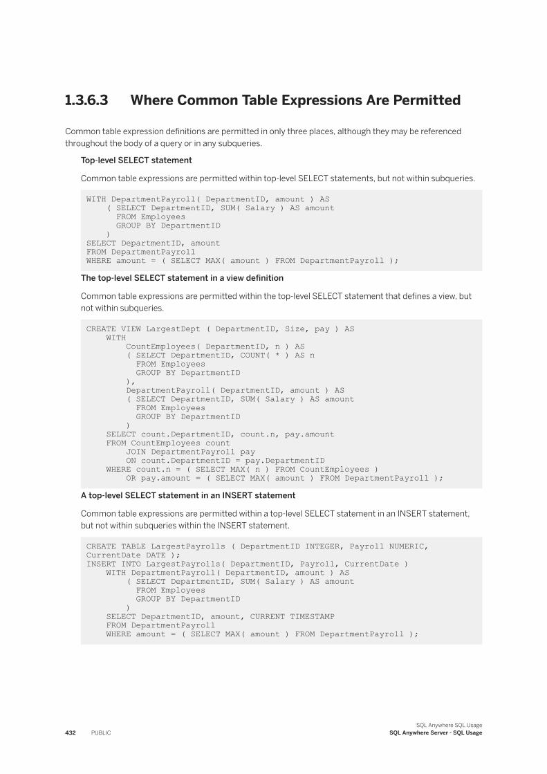
1.3.6.3 Where Common Table Expressions Are Permitted
Common table expression definitions are permitted in only three places, although they may be referenced throughout the body of a query or in any subqueries.
Top-level SELECT statement
Common table expressions are permitted within top-level SELECT statements, but not within subqueries.
WITH DepartmentPayroll( DepartmentID, amount ) AS ( SELECT DepartmentID, SUM( Salary ) AS amount FROM Employees GROUP BY DepartmentID )SELECT DepartmentID, amountFROM DepartmentPayroll WHERE amount = ( SELECT MAX( amount ) FROM DepartmentPayroll );
The top-level SELECT statement in a view definition
Common table expressions are permitted within the top-level SELECT statement that defines a view, but not within subqueries.
CREATE VIEW LargestDept ( DepartmentID, Size, pay ) AS WITH CountEmployees( DepartmentID, n ) AS ( SELECT DepartmentID, COUNT( * ) AS n FROM Employees GROUP BY DepartmentID ), DepartmentPayroll( DepartmentID, amount ) AS ( SELECT DepartmentID, SUM( Salary ) AS amount FROM Employees GROUP BY DepartmentID ) SELECT count.DepartmentID, count.n, pay.amount FROM CountEmployees count JOIN DepartmentPayroll pay ON count.DepartmentID = pay.DepartmentID WHERE count.n = ( SELECT MAX( n ) FROM CountEmployees ) OR pay.amount = ( SELECT MAX( amount ) FROM DepartmentPayroll );
A top-level SELECT statement in an INSERT statement
Common table expressions are permitted within a top-level SELECT statement in an INSERT statement, but not within subqueries within the INSERT statement.
CREATE TABLE LargestPayrolls ( DepartmentID INTEGER, Payroll NUMERIC, CurrentDate DATE ); INSERT INTO LargestPayrolls( DepartmentID, Payroll, CurrentDate ) WITH DepartmentPayroll( DepartmentID, amount ) AS ( SELECT DepartmentID, SUM( Salary ) AS amount FROM Employees GROUP BY DepartmentID ) SELECT DepartmentID, amount, CURRENT TIMESTAMP FROM DepartmentPayroll WHERE amount = ( SELECT MAX( amount ) FROM DepartmentPayroll );
432 PUBLICSQL Anywhere SQL Usage
SQL Anywhere Server - SQL Usage
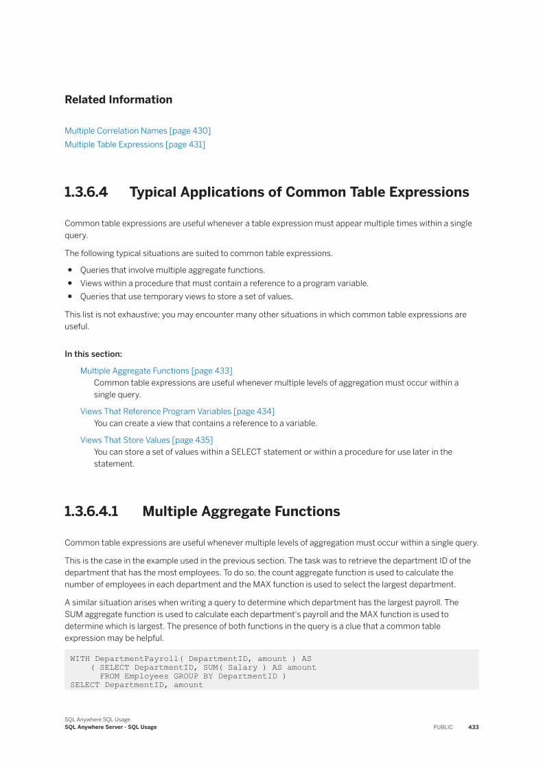
Related Information
Multiple Correlation Names [page 430]Multiple Table Expressions [page 431]
1.3.6.4 Typical Applications of Common Table Expressions
Common table expressions are useful whenever a table expression must appear multiple times within a single query.
The following typical situations are suited to common table expressions.
● Queries that involve multiple aggregate functions.● Views within a procedure that must contain a reference to a program variable.● Queries that use temporary views to store a set of values.
This list is not exhaustive; you may encounter many other situations in which common table expressions are useful.
In this section:
Multiple Aggregate Functions [page 433]Common table expressions are useful whenever multiple levels of aggregation must occur within a single query.
Views That Reference Program Variables [page 434]You can create a view that contains a reference to a variable.
Views That Store Values [page 435]You can store a set of values within a SELECT statement or within a procedure for use later in the statement.
1.3.6.4.1 Multiple Aggregate Functions
Common table expressions are useful whenever multiple levels of aggregation must occur within a single query.
This is the case in the example used in the previous section. The task was to retrieve the department ID of the department that has the most employees. To do so, the count aggregate function is used to calculate the number of employees in each department and the MAX function is used to select the largest department.
A similar situation arises when writing a query to determine which department has the largest payroll. The SUM aggregate function is used to calculate each department's payroll and the MAX function is used to determine which is largest. The presence of both functions in the query is a clue that a common table expression may be helpful.
WITH DepartmentPayroll( DepartmentID, amount ) AS ( SELECT DepartmentID, SUM( Salary ) AS amount FROM Employees GROUP BY DepartmentID )SELECT DepartmentID, amount
SQL Anywhere SQL UsageSQL Anywhere Server - SQL Usage PUBLIC 433
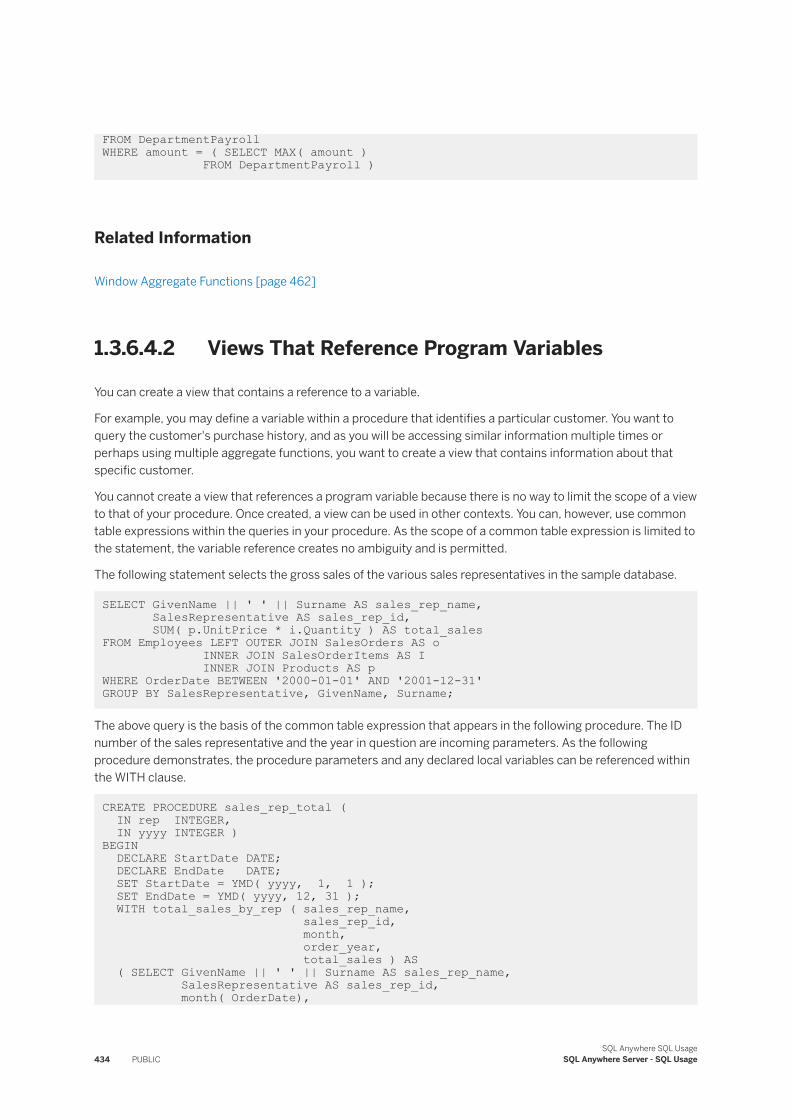
FROM DepartmentPayrollWHERE amount = ( SELECT MAX( amount ) FROM DepartmentPayroll )
Related Information
Window Aggregate Functions [page 462]
1.3.6.4.2 Views That Reference Program Variables
You can create a view that contains a reference to a variable.
For example, you may define a variable within a procedure that identifies a particular customer. You want to query the customer's purchase history, and as you will be accessing similar information multiple times or perhaps using multiple aggregate functions, you want to create a view that contains information about that specific customer.
You cannot create a view that references a program variable because there is no way to limit the scope of a view to that of your procedure. Once created, a view can be used in other contexts. You can, however, use common table expressions within the queries in your procedure. As the scope of a common table expression is limited to the statement, the variable reference creates no ambiguity and is permitted.
The following statement selects the gross sales of the various sales representatives in the sample database.
SELECT GivenName || ' ' || Surname AS sales_rep_name, SalesRepresentative AS sales_rep_id, SUM( p.UnitPrice * i.Quantity ) AS total_salesFROM Employees LEFT OUTER JOIN SalesOrders AS o INNER JOIN SalesOrderItems AS I INNER JOIN Products AS pWHERE OrderDate BETWEEN '2000-01-01' AND '2001-12-31' GROUP BY SalesRepresentative, GivenName, Surname;
The above query is the basis of the common table expression that appears in the following procedure. The ID number of the sales representative and the year in question are incoming parameters. As the following procedure demonstrates, the procedure parameters and any declared local variables can be referenced within the WITH clause.
CREATE PROCEDURE sales_rep_total ( IN rep INTEGER, IN yyyy INTEGER )BEGIN DECLARE StartDate DATE; DECLARE EndDate DATE; SET StartDate = YMD( yyyy, 1, 1 ); SET EndDate = YMD( yyyy, 12, 31 ); WITH total_sales_by_rep ( sales_rep_name, sales_rep_id, month, order_year, total_sales ) AS ( SELECT GivenName || ' ' || Surname AS sales_rep_name, SalesRepresentative AS sales_rep_id, month( OrderDate),
434 PUBLICSQL Anywhere SQL Usage
SQL Anywhere Server - SQL Usage
year( OrderDate ), SUM( p.UnitPrice * i.Quantity ) AS total_sales FROM Employees LEFT OUTER JOIN SalesOrders o INNER JOIN SalesOrderItems I INNER JOIN Products p WHERE OrderDate BETWEEN StartDate AND EndDate AND SalesRepresentative = rep GROUP BY year( OrderDate ), month( OrderDate ), GivenName, Surname, SalesRepresentative ) SELECT sales_rep_name, monthname( YMD(yyyy, month, 1) ) AS month_name, order_year, total_sales FROM total_sales_by_rep WHERE total_sales = ( SELECT MAX( total_sales) FROM total_sales_by_rep ) ORDER BY order_year ASC, month ASC; END;
The following statement calls the previous procedure.
CALL sales_rep_total( 129, 2000 );
1.3.6.4.3 Views That Store Values
You can store a set of values within a SELECT statement or within a procedure for use later in the statement.
For example, suppose a company prefers to analyze the results of its sales staff by thirds of a year, instead of by quarter. Since there is no built-in date part for thirds, as there is for quarters, it is necessary to store the dates within the procedure.
WITH thirds ( q_name, q_start, q_end ) AS ( SELECT 'T1', '2000-01-01', '2000-04-30' UNION SELECT 'T2', '2000-05-01', '2000-08-31' UNION SELECT 'T3', '2000-09-01', '2000-12-31' )SELECT q_name, SalesRepresentative, count(*) AS num_orders, SUM( p.UnitPrice * i.Quantity ) AS total_salesFROM thirds LEFT OUTER JOIN SalesOrders AS o ON OrderDate BETWEEN q_start and q_end KEY JOIN SalesOrderItems AS I KEY JOIN Products AS p GROUP BY q_name, SalesRepresentative ORDER BY q_name, SalesRepresentative;
This method should be used with care, as the values may need periodic maintenance. For example, the above statement must be modified if it is to be used for any other year.
You can also apply this method within procedures. The following example declares a procedure that takes the year in question as an argument.
CREATE PROCEDURE sales_by_third ( IN y INTEGER ) BEGIN WITH thirds ( q_name, q_start, q_end ) AS ( SELECT 'T1', YMD( y, 01, 01), YMD( y, 04, 30 ) UNION SELECT 'T2', YMD( y, 05, 01), YMD( y, 08, 31 ) UNION SELECT 'T3', YMD( y, 09, 01), YMD( y, 12, 31 ) ) SELECT q_name, SalesRepresentative,
SQL Anywhere SQL UsageSQL Anywhere Server - SQL Usage PUBLIC 435
count(*) AS num_orders, SUM( p.UnitPrice * i.Quantity ) AS total_sales FROM thirds LEFT OUTER JOIN SalesOrders AS o ON OrderDate BETWEEN q_start and q_end KEY JOIN SalesOrderItems AS I KEY JOIN Products AS p GROUP BY q_name, SalesRepresentative ORDER BY q_name, SalesRepresentative; END;
The following statement calls the previous procedure.
CALL sales_by_third (2000);
1.3.6.5 Recursive Common Table Expressions
Recursion provides an easier way of traversing tables that represent tree or tree-like data structures.
Common table expressions are recursive when they are executed repeatedly, with each execution returning additional rows until the complete result set is retrieved.
You can make a common table expression recursive by inserting the RECURSIVE keyword immediately following WITH in the WITH clause. A single WITH clause may contain multiple recursive expressions that can be both recursive and non-recursive.
Without using recursive expressions, the only way to traverse such a structure in a single statement is to join the table to itself once for each possible level.
Restrictions on Recursive Common Table Expressions
● References to other recursive common table expressions cannot appear within the definition of recursive common table expressions as recursive common table expressions cannot be mutually recursive. However, non-recursive common table expressions can contain references to recursive table expressions, and recursive common table expressions can contain references to non-recursive common table expressions.
● The only set operator supported between the initial subquery and the recursive subquery is UNION ALL.● Within the definition of a recursive subquery, a self-reference to the recursive common table expression
can appear only within the FROM clause of the recursive subquery and cannot appear on the null-supplying side of an outer join.
● The recursive subquery cannot contain a DISTINCT, GROUP BY, or ORDER BY clause.● The recursive subquery cannot use an aggregate function.● To prevent runaway recursive queries, an error is generated if the number of levels of recursion exceeds the
current setting of the max_recursive_iterations option. The default value of this option is 100.
436 PUBLICSQL Anywhere SQL Usage
SQL Anywhere Server - SQL Usage
Example
Given a table that represents the reporting relationships within a company, you can write a query that returns all the employees that report to one particular person.
Depending on how you write the query, you may want to limit the number of levels of recursion. For example, limiting the number of levels allows you to return only the top levels of management, but may exclude some employees if the chains of command are longer than you anticipated. Providing no restriction on the number of levels ensures no employees are excluded, but can introduce infinite recursion should the execution require any cycles, such as an employee directly or indirectly reporting to her or himself. This situation could arise within a company's management hierarchy if an employee within the company also sits on the board of directors.
The following query demonstrates how to list the employees by management level. Level 0 represents employees with no managers. Level 1 represents employees who report directly to one of the level 0 managers, level 2 represents employees who report directly to a level 1 manager, and so on.
WITH RECURSIVE manager ( EmployeeID, ManagerID, GivenName, Surname, mgmt_level ) AS( ( SELECT EmployeeID, ManagerID, -- initial subquery GivenName, Surname, 0 FROM Employees AS e WHERE ManagerID = EmployeeID ) UNION ALL ( SELECT e.EmployeeID, e.ManagerID, -- recursive subquery e.GivenName, e.Surname, m.mgmt_level + 1 FROM Employees AS e JOIN manager AS m ON e.ManagerID = m.EmployeeID AND e.ManagerID <> e.EmployeeID AND m.mgmt_level < 20 ) )SELECT * FROM manager ORDER BY mgmt_level, Surname, GivenName;
The condition within the recursive query that restricts the management level to less than 20 (m.mgmt leve < 20) is called a stop condition, and is an important precaution. It prevents infinite recursion if the table data contains a cycle.
The max_recursive_iterations option can also be used to catch runaway recursive queries. The default value of this option is 100 and recursive queries that exceed this number of iterations end, but cause an error. Although this option may seem to diminish the importance of a stop condition, this is not usually the case. The number of rows selected during each iteration may grow exponentially, seriously impacting performance before the maximum is reached. Stop conditions within recursive queries provide a means of setting appropriate limits in each situation.
Recursive common table expressions contain an initial subquery, or seed, and a recursive subquery that, during each iteration, appends additional rows to the result set. The two parts can be connected only with the operator UNION ALL. The initial subquery is an ordinary non-recursive query and is processed first. The recursive portion contains a reference to the rows added during the previous iteration. Recursion stops automatically whenever an iteration generates no new rows. There is no way to reference rows selected before the previous iteration.
The SELECT list of the recursive subquery must match that of the initial subquery in number and data type. If automatic translation of data types cannot be performed, explicitly cast the results of one subquery so that they match those in the other subquery.
In this section:
SQL Anywhere SQL UsageSQL Anywhere Server - SQL Usage PUBLIC 437
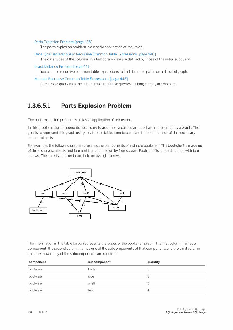
Parts Explosion Problem [page 438]The parts explosion problem is a classic application of recursion.
Data Type Declarations in Recursive Common Table Expressions [page 440]The data types of the columns in a temporary view are defined by those of the initial subquery.
Least Distance Problem [page 441]You can use recursive common table expressions to find desirable paths on a directed graph.
Multiple Recursive Common Table Expressions [page 443]A recursive query may include multiple recursive queries, as long as they are disjoint.
1.3.6.5.1 Parts Explosion Problem
The parts explosion problem is a classic application of recursion.
In this problem, the components necessary to assemble a particular object are represented by a graph. The goal is to represent this graph using a database table, then to calculate the total number of the necessary elemental parts.
For example, the following graph represents the components of a simple bookshelf. The bookshelf is made up of three shelves, a back, and four feet that are held on by four screws. Each shelf is a board held on with four screws. The back is another board held on by eight screws.
The information in the table below represents the edges of the bookshelf graph. The first column names a component, the second column names one of the subcomponents of that component, and the third column specifies how many of the subcomponents are required.
component subcomponent quantity
bookcase back 1
bookcase side 2
bookcase shelf 3
bookcase foot 4
438 PUBLICSQL Anywhere SQL Usage
SQL Anywhere Server - SQL Usage
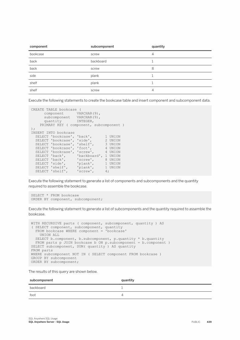
component subcomponent quantity
bookcase screw 4
back backboard 1
back screw 8
side plank 1
shelf plank 1
shelf screw 4
Execute the following statements to create the bookcase table and insert component and subcomponent data.
CREATE TABLE bookcase ( component VARCHAR(9), subcomponent VARCHAR(9), quantity INTEGER, PRIMARY KEY ( component, subcomponent )); INSERT INTO bookcase SELECT 'bookcase', 'back', 1 UNION SELECT 'bookcase', 'side', 2 UNION SELECT 'bookcase', 'shelf', 3 UNION SELECT 'bookcase', 'foot', 4 UNION SELECT 'bookcase', 'screw', 4 UNION SELECT 'back', 'backboard', 1 UNION SELECT 'back', 'screw', 8 UNION SELECT 'side', 'plank', 1 UNION SELECT 'shelf', 'plank', 1 UNION SELECT 'shelf', 'screw', 4;
Execute the following statement to generate a list of components and subcomponents and the quantity required to assemble the bookcase.
SELECT * FROM bookcase ORDER BY component, subcomponent;
Execute the following statement to generate a list of subcomponents and the quantity required to assemble the bookcase.
WITH RECURSIVE parts ( component, subcomponent, quantity ) AS ( SELECT component, subcomponent, quantity FROM bookcase WHERE component = 'bookcase' UNION ALL SELECT b.component, b.subcomponent, p.quantity * b.quantity FROM parts p JOIN bookcase b ON p.subcomponent = b.component )SELECT subcomponent, SUM( quantity ) AS quantityFROM partsWHERE subcomponent NOT IN ( SELECT component FROM bookcase )GROUP BY subcomponent ORDER BY subcomponent;
The results of this query are shown below.
subcomponent quantity
backboard 1
foot 4
SQL Anywhere SQL UsageSQL Anywhere Server - SQL Usage PUBLIC 439
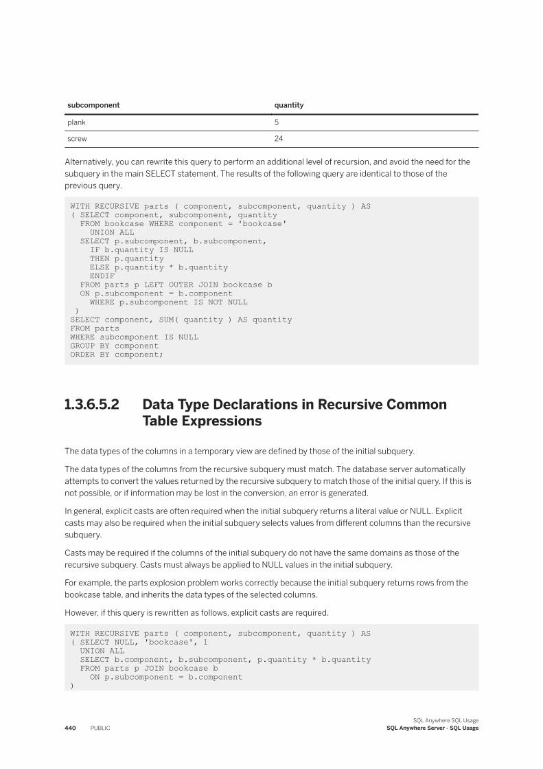
subcomponent quantity
plank 5
screw 24
Alternatively, you can rewrite this query to perform an additional level of recursion, and avoid the need for the subquery in the main SELECT statement. The results of the following query are identical to those of the previous query.
WITH RECURSIVE parts ( component, subcomponent, quantity ) AS ( SELECT component, subcomponent, quantity FROM bookcase WHERE component = 'bookcase' UNION ALL SELECT p.subcomponent, b.subcomponent, IF b.quantity IS NULL THEN p.quantity ELSE p.quantity * b.quantity ENDIF FROM parts p LEFT OUTER JOIN bookcase b ON p.subcomponent = b.component WHERE p.subcomponent IS NOT NULL )SELECT component, SUM( quantity ) AS quantityFROM partsWHERE subcomponent IS NULLGROUP BY component ORDER BY component;
1.3.6.5.2 Data Type Declarations in Recursive Common Table Expressions
The data types of the columns in a temporary view are defined by those of the initial subquery.
The data types of the columns from the recursive subquery must match. The database server automatically attempts to convert the values returned by the recursive subquery to match those of the initial query. If this is not possible, or if information may be lost in the conversion, an error is generated.
In general, explicit casts are often required when the initial subquery returns a literal value or NULL. Explicit casts may also be required when the initial subquery selects values from different columns than the recursive subquery.
Casts may be required if the columns of the initial subquery do not have the same domains as those of the recursive subquery. Casts must always be applied to NULL values in the initial subquery.
For example, the parts explosion problem works correctly because the initial subquery returns rows from the bookcase table, and inherits the data types of the selected columns.
However, if this query is rewritten as follows, explicit casts are required.
WITH RECURSIVE parts ( component, subcomponent, quantity ) AS ( SELECT NULL, 'bookcase', 1 UNION ALL SELECT b.component, b.subcomponent, p.quantity * b.quantity FROM parts p JOIN bookcase b ON p.subcomponent = b.component)
440 PUBLICSQL Anywhere SQL Usage
SQL Anywhere Server - SQL Usage
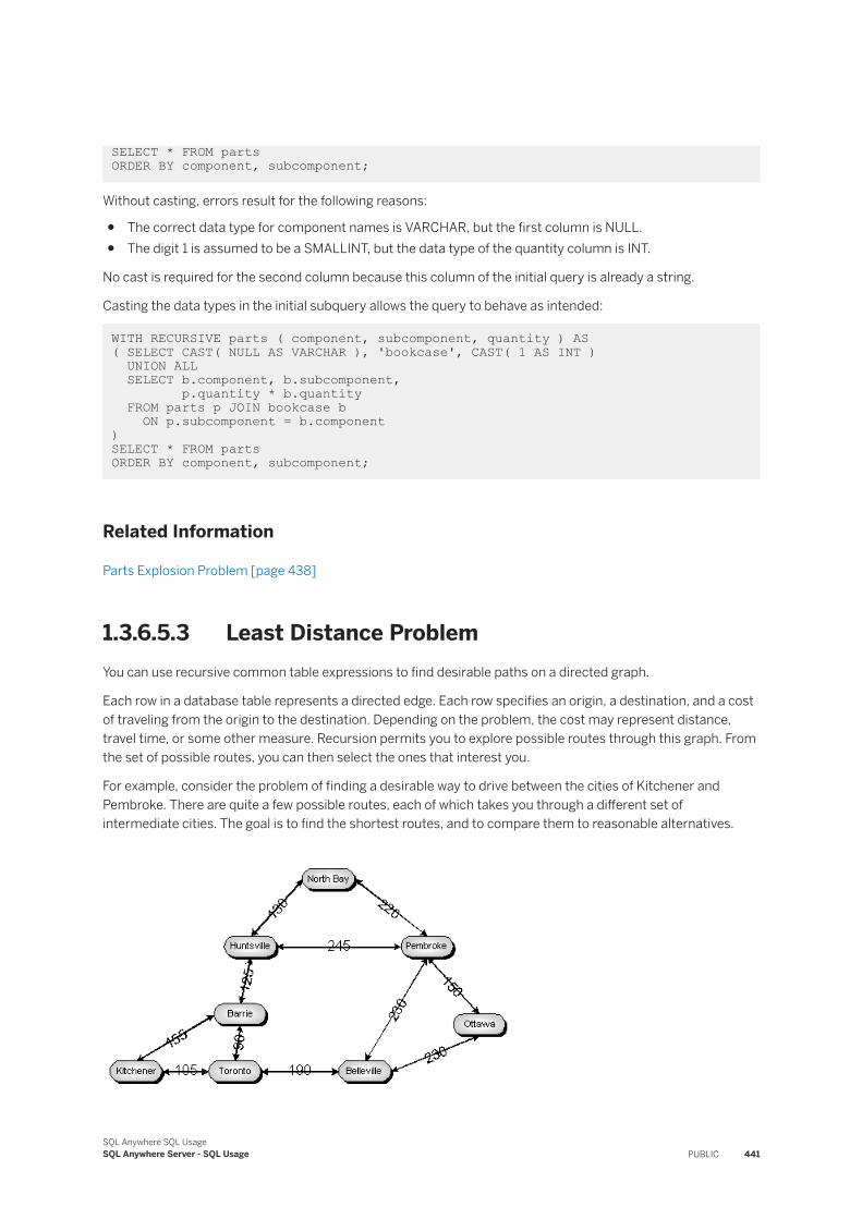
SELECT * FROM parts ORDER BY component, subcomponent;
Without casting, errors result for the following reasons:
● The correct data type for component names is VARCHAR, but the first column is NULL.● The digit 1 is assumed to be a SMALLINT, but the data type of the quantity column is INT.
No cast is required for the second column because this column of the initial query is already a string.
Casting the data types in the initial subquery allows the query to behave as intended:
WITH RECURSIVE parts ( component, subcomponent, quantity ) AS ( SELECT CAST( NULL AS VARCHAR ), 'bookcase', CAST( 1 AS INT ) UNION ALL SELECT b.component, b.subcomponent, p.quantity * b.quantity FROM parts p JOIN bookcase b ON p.subcomponent = b.component)SELECT * FROM parts ORDER BY component, subcomponent;
Related Information
Parts Explosion Problem [page 438]
1.3.6.5.3 Least Distance ProblemYou can use recursive common table expressions to find desirable paths on a directed graph.
Each row in a database table represents a directed edge. Each row specifies an origin, a destination, and a cost of traveling from the origin to the destination. Depending on the problem, the cost may represent distance, travel time, or some other measure. Recursion permits you to explore possible routes through this graph. From the set of possible routes, you can then select the ones that interest you.
For example, consider the problem of finding a desirable way to drive between the cities of Kitchener and Pembroke. There are quite a few possible routes, each of which takes you through a different set of intermediate cities. The goal is to find the shortest routes, and to compare them to reasonable alternatives.
SQL Anywhere SQL UsageSQL Anywhere Server - SQL Usage PUBLIC 441
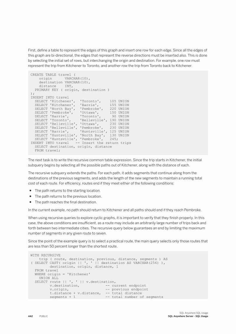
First, define a table to represent the edges of this graph and insert one row for each edge. Since all the edges of this graph are bi-directional, the edges that represent the reverse directions must be inserted also. This is done by selecting the initial set of rows, but interchanging the origin and destination. For example, one row must represent the trip from Kitchener to Toronto, and another row the trip from Toronto back to Kitchener.
CREATE TABLE travel ( origin VARCHAR(10), destination VARCHAR(10), distance INT, PRIMARY KEY ( origin, destination )); INSERT INTO travel SELECT 'Kitchener', 'Toronto', 105 UNION SELECT 'Kitchener', 'Barrie', 155 UNION SELECT 'North Bay', 'Pembroke', 220 UNION SELECT 'Pembroke', 'Ottawa', 150 UNION SELECT 'Barrie', 'Toronto', 90 UNION SELECT 'Toronto', 'Belleville', 190 UNION SELECT 'Belleville', 'Ottawa', 230 UNION SELECT 'Belleville', 'Pembroke', 230 UNION SELECT 'Barrie', 'Huntsville', 125 UNION SELECT 'Huntsville', 'North Bay', 130 UNION SELECT 'Huntsville', 'Pembroke', 245; INSERT INTO travel -- Insert the return trips SELECT destination, origin, distance FROM travel;
The next task is to write the recursive common table expression. Since the trip starts in Kitchener, the initial subquery begins by selecting all the possible paths out of Kitchener, along with the distance of each.
The recursive subquery extends the paths. For each path, it adds segments that continue along from the destinations of the previous segments, and adds the length of the new segments to maintain a running total cost of each route. For efficiency, routes end if they meet either of the following conditions:
● The path returns to the starting location.● The path returns to the previous location.● The path reaches the final destination.
In the current example, no path should return to Kitchener and all paths should end if they reach Pembroke.
When using recursive queries to explore cyclic graphs, it is important to verify that they finish properly. In this case, the above conditions are insufficient, as a route may include an arbitrarily large number of trips back and forth between two intermediate cities. The recursive query below guarantees an end by limiting the maximum number of segments in any given route to seven.
Since the point of the example query is to select a practical route, the main query selects only those routes that are less than 50 percent longer than the shortest route.
WITH RECURSIVE trip ( route, destination, previous, distance, segments ) AS( SELECT CAST( origin || ', ' || destination AS VARCHAR(256) ), destination, origin, distance, 1 FROM travel WHERE origin = 'Kitchener' UNION ALL SELECT route || ', ' || v.destination, v.destination, -- current endpoint v.origin, -- previous endpoint t.distance + v.distance, -- total distance segments + 1 -- total number of segments
442 PUBLICSQL Anywhere SQL Usage
SQL Anywhere Server - SQL Usage
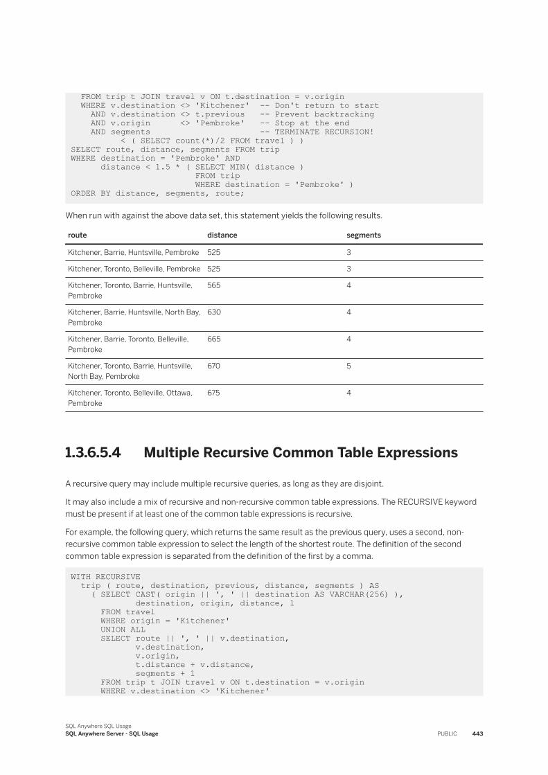
FROM trip t JOIN travel v ON t.destination = v.origin WHERE v.destination <> 'Kitchener' -- Don't return to start AND v.destination <> t.previous -- Prevent backtracking AND v.origin <> 'Pembroke' -- Stop at the end AND segments -- TERMINATE RECURSION! < ( SELECT count(*)/2 FROM travel ) )SELECT route, distance, segments FROM tripWHERE destination = 'Pembroke' AND distance < 1.5 * ( SELECT MIN( distance ) FROM trip WHERE destination = 'Pembroke' ) ORDER BY distance, segments, route;
When run with against the above data set, this statement yields the following results.
route distance segments
Kitchener, Barrie, Huntsville, Pembroke 525 3
Kitchener, Toronto, Belleville, Pembroke 525 3
Kitchener, Toronto, Barrie, Huntsville, Pembroke
565 4
Kitchener, Barrie, Huntsville, North Bay, Pembroke
630 4
Kitchener, Barrie, Toronto, Belleville, Pembroke
665 4
Kitchener, Toronto, Barrie, Huntsville, North Bay, Pembroke
670 5
Kitchener, Toronto, Belleville, Ottawa, Pembroke
675 4
1.3.6.5.4 Multiple Recursive Common Table Expressions
A recursive query may include multiple recursive queries, as long as they are disjoint.
It may also include a mix of recursive and non-recursive common table expressions. The RECURSIVE keyword must be present if at least one of the common table expressions is recursive.
For example, the following query, which returns the same result as the previous query, uses a second, non-recursive common table expression to select the length of the shortest route. The definition of the second common table expression is separated from the definition of the first by a comma.
WITH RECURSIVE trip ( route, destination, previous, distance, segments ) AS ( SELECT CAST( origin || ', ' || destination AS VARCHAR(256) ), destination, origin, distance, 1 FROM travel WHERE origin = 'Kitchener' UNION ALL SELECT route || ', ' || v.destination, v.destination, v.origin, t.distance + v.distance, segments + 1 FROM trip t JOIN travel v ON t.destination = v.origin WHERE v.destination <> 'Kitchener'
SQL Anywhere SQL UsageSQL Anywhere Server - SQL Usage PUBLIC 443
AND v.destination <> t.previous AND v.origin <> 'Pembroke' AND segments < ( SELECT count(*)/2 FROM travel ) ), shortest ( distance ) AS -- Additional, ( SELECT MIN(distance) -- non-recursive FROM trip -- common table WHERE destination = 'Pembroke' ) -- expressionSELECT route, distance, segments FROM tripWHERE destination = 'Pembroke' AND distance < 1.5 * ( SELECT distance FROM shortest ) ORDER BY distance, segments, route;
Like non-recursive common table expressions, recursive expressions, when used within stored procedures, may contain references to local variables or procedure parameters. For example, the best_routes procedure, defined below, identifies the shortest routes between the two named cities.
CREATE PROCEDURE best_routes ( IN initial VARCHAR(10), IN final VARCHAR(10))BEGIN WITH RECURSIVE trip ( route, destination, previous, distance, segments ) AS ( SELECT CAST( origin || ', ' || destination AS VARCHAR(256) ), destination, origin, distance, 1 FROM travel WHERE origin = initial UNION ALL SELECT route || ', ' || v.destination, v.destination, -- current endpoint v.origin, -- previous endpoint t.distance + v.distance, -- total distance segments + 1 -- total number of segments FROM trip t JOIN travel v ON t.destination = v.origin WHERE v.destination <> initial -- Don't return to start AND v.destination <> t.previous -- Prevent backtracking AND v.origin <> final -- Stop at the end AND segments -- TERMINATE RECURSION! < ( SELECT count(*)/2 FROM travel ) ) SELECT route, distance, segments FROM trip WHERE destination = final AND distance < 1.4 * ( SELECT MIN( distance ) FROM trip WHERE destination = final ) ORDER BY distance, segments, route; END;
The following statement calls the previous procedure.
CALL best_routes ( 'Pembroke', 'Kitchener' );
1.3.7 OLAP Support
On-Line Analytical Processing (OLAP) offers the ability to perform complex data analysis within a single SQL statement, increasing the value of the results, while improving performance by decreasing the amount of querying on the database.
OLAP functionality is made possible through the use of extensions to SQL statements and window functions. These SQL extensions and functions provide the ability, in a concise way, to perform multidimensional data
444 PUBLICSQL Anywhere SQL Usage
SQL Anywhere Server - SQL Usage
analysis, data mining, time series analysis, trend analysis, cost allocations, goal seeking, and exception alerting, often with a single SQL statement.
Extensions to the SELECT statement
Extensions to the SELECT statement allow you to group input rows, analyze the groups, and include the findings in the final result set. These extensions include extensions to the GROUP BY clause (GROUPING SETS, CUBE, and ROLLUP subclauses), and the WINDOW clause.
The extensions to the GROUP BY clause allow you to partition the input rows in multiple ways, yielding a result set that concatenates the different groups together. You can also create a sparse, multi-dimensional result set for data mining analysis (also known as a data cube). Finally, the extensions provide sub-total and grand-total rows to make analysis more convenient.
The WINDOW clause is used with window functions to provide additional analysis opportunities on groups of input rows.Window aggregate functions
Most of the aggregate functions support the concept of a configurable sliding window that moves down through the input rows as they are processed. Additional calculations can be performed on data in the window as it moves, allowing further analysis in a manner that is more efficient than using semantically equivalent self-join queries, or correlated subqueries.
For example, window aggregate functions, coupled with the CUBE, ROLLUP, and GROUPING SETS extensions to the GROUP BY clause, provide an efficient mechanism to compute percentiles, moving averages, and cumulative sums in a single SQL statement that would otherwise require self-joins, correlated subqueries, temporary tables, or some combination of all three.
You can use window aggregate functions to obtain such information as the quarterly moving average of the Dow Jones Industrial Average, or all employees and their cumulative salaries for each department. You can also use them to compute variance, standard deviation, correlation, and regression measures.Window ranking functions
Window ranking functions allow you to form single-statement SQL queries to obtain information such as the top 10 products shipped this year by total sales, or the top 5% of salespersons who sold orders to at least 15 different companies.
In this section:
OLAP Performance Improvements [page 446]To improve OLAP performance, set the optimization_workload database option to OLAP to instruct the optimizer to consider using the Clustered Group By Hash operator in the possibilities it investigates.
GROUP BY Clause Extensions [page 446]The standard GROUP BY clause of a SELECT statement allows you to group rows in the result set according the grouping expressions you supply.
ROLLUP and CUBE as a Shortcut to GROUPING SETS [page 450]Use ROLLUP and CUBE when you want to concatenate several different data partitions into a single result set.
Window Functions [page 455]Functions that allow you to perform analytic operations over a set of input rows are referred to as window functions. OLAP functionality includes the concept of a sliding window that moves down through the input rows as they are processed.
SQL Anywhere SQL UsageSQL Anywhere Server - SQL Usage PUBLIC 445
Window Aggregate Functions [page 462]Window aggregate functions return a value for a specified set of rows in the input.
Basic Aggregate Functions [page 463]There are several supported basic aggregate functions you can use to return values for groups of rows.
Standard Deviation and Variance Functions [page 471]Two versions of variance and standard deviation functions are supported: a sampling version, and a population version.
Correlation and Linear Regression Functions [page 475]A variety of statistical functions is supported, the results of which can be used to assist in analyzing the quality of a linear regression.
Window Ranking Functions [page 476]Window ranking functions return the rank of a row relative to the other rows in a partition.
Row Numbering Functions [page 483]Row numbering functions uniquely number the rows in a partition.
Related Information
Window Ranking Functions [page 476]Window Aggregate Functions [page 462]
1.3.7.1 OLAP Performance Improvements
To improve OLAP performance, set the optimization_workload database option to OLAP to instruct the optimizer to consider using the Clustered Group By Hash operator in the possibilities it investigates.
You can also tune indexes for OLAP workloads using the FOR OLAP WORKLOAD option when defining the index. Using this option causes the database server to perform certain optimizations which include maintaining a statistic used by the Clustered Group By Hash operator regarding the maximum page distance between two rows within the same key.
1.3.7.2 GROUP BY Clause Extensions
The standard GROUP BY clause of a SELECT statement allows you to group rows in the result set according the grouping expressions you supply.
For example, if you specify GROUP BY columnA, columnB, the rows are grouped by combinations of unique values from columnA and columnB. In the standard GROUP BY clause, the groups reflect the evaluation of the combination of all specified GROUP BY expressions.
However, you may want to specify different groupings or subgroupings of the result set. For example, you may want to your results to show your data grouped by unique values of columnA and columnB, and then regrouped
446 PUBLICSQL Anywhere SQL Usage
SQL Anywhere Server - SQL Usage
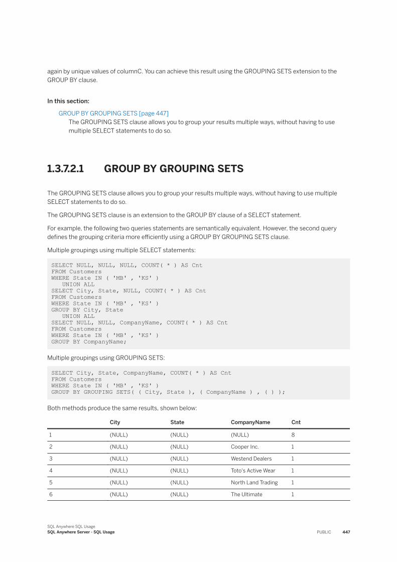
again by unique values of columnC. You can achieve this result using the GROUPING SETS extension to the GROUP BY clause.
In this section:
GROUP BY GROUPING SETS [page 447]The GROUPING SETS clause allows you to group your results multiple ways, without having to use multiple SELECT statements to do so.
1.3.7.2.1 GROUP BY GROUPING SETS
The GROUPING SETS clause allows you to group your results multiple ways, without having to use multiple SELECT statements to do so.
The GROUPING SETS clause is an extension to the GROUP BY clause of a SELECT statement.
For example, the following two queries statements are semantically equivalent. However, the second query defines the grouping criteria more efficiently using a GROUP BY GROUPING SETS clause.
Multiple groupings using multiple SELECT statements:
SELECT NULL, NULL, NULL, COUNT( * ) AS Cnt FROM CustomersWHERE State IN ( 'MB' , 'KS' ) UNION ALLSELECT City, State, NULL, COUNT( * ) AS CntFROM CustomersWHERE State IN ( 'MB' , 'KS' )GROUP BY City, State UNION ALLSELECT NULL, NULL, CompanyName, COUNT( * ) AS CntFROM CustomersWHERE State IN ( 'MB' , 'KS' ) GROUP BY CompanyName;
Multiple groupings using GROUPING SETS:
SELECT City, State, CompanyName, COUNT( * ) AS Cnt FROM CustomersWHERE State IN ( 'MB' , 'KS' ) GROUP BY GROUPING SETS( ( City, State ), ( CompanyName ) , ( ) );
Both methods produce the same results, shown below:
City State CompanyName Cnt
1 (NULL) (NULL) (NULL) 8
2 (NULL) (NULL) Cooper Inc. 1
3 (NULL) (NULL) Westend Dealers 1
4 (NULL) (NULL) Toto's Active Wear 1
5 (NULL) (NULL) North Land Trading 1
6 (NULL) (NULL) The Ultimate 1
SQL Anywhere SQL UsageSQL Anywhere Server - SQL Usage PUBLIC 447
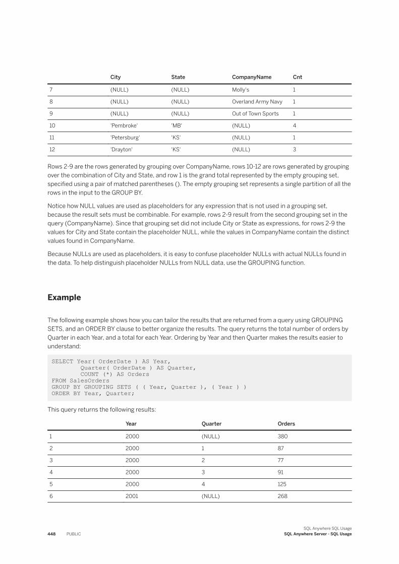
City State CompanyName Cnt
7 (NULL) (NULL) Molly's 1
8 (NULL) (NULL) Overland Army Navy 1
9 (NULL) (NULL) Out of Town Sports 1
10 'Pembroke' 'MB' (NULL) 4
11 'Petersburg' 'KS' (NULL) 1
12 'Drayton' 'KS' (NULL) 3
Rows 2-9 are the rows generated by grouping over CompanyName, rows 10-12 are rows generated by grouping over the combination of City and State, and row 1 is the grand total represented by the empty grouping set, specified using a pair of matched parentheses (). The empty grouping set represents a single partition of all the rows in the input to the GROUP BY.
Notice how NULL values are used as placeholders for any expression that is not used in a grouping set, because the result sets must be combinable. For example, rows 2-9 result from the second grouping set in the query (CompanyName). Since that grouping set did not include City or State as expressions, for rows 2-9 the values for City and State contain the placeholder NULL, while the values in CompanyName contain the distinct values found in CompanyName.
Because NULLs are used as placeholders, it is easy to confuse placeholder NULLs with actual NULLs found in the data. To help distinguish placeholder NULLs from NULL data, use the GROUPING function.
Example
The following example shows how you can tailor the results that are returned from a query using GROUPING SETS, and an ORDER BY clause to better organize the results. The query returns the total number of orders by Quarter in each Year, and a total for each Year. Ordering by Year and then Quarter makes the results easier to understand:
SELECT Year( OrderDate ) AS Year, Quarter( OrderDate ) AS Quarter, COUNT (*) AS Orders FROM SalesOrdersGROUP BY GROUPING SETS ( ( Year, Quarter ), ( Year ) ) ORDER BY Year, Quarter;
This query returns the following results:
Year Quarter Orders
1 2000 (NULL) 380
2 2000 1 87
3 2000 2 77
4 2000 3 91
5 2000 4 125
6 2001 (NULL) 268
448 PUBLICSQL Anywhere SQL Usage
SQL Anywhere Server - SQL Usage
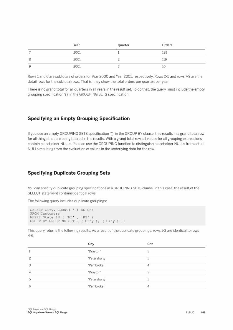
Year Quarter Orders
7 2001 1 139
8 2001 2 119
9 2001 3 10
Rows 1 and 6 are subtotals of orders for Year 2000 and Year 2001, respectively. Rows 2-5 and rows 7-9 are the detail rows for the subtotal rows. That is, they show the total orders per quarter, per year.
There is no grand total for all quarters in all years in the result set. To do that, the query must include the empty grouping specification '()' in the GROUPING SETS specification.
Specifying an Empty Grouping Specification
If you use an empty GROUPING SETS specification '()' in the GROUP BY clause, this results in a grand total row for all things that are being totaled in the results. With a grand total row, all values for all grouping expressions contain placeholder NULLs. You can use the GROUPING function to distinguish placeholder NULLs from actual NULLs resulting from the evaluation of values in the underlying data for the row.
Specifying Duplicate Grouping Sets
You can specify duplicate grouping specifications in a GROUPING SETS clause. In this case, the result of the SELECT statement contains identical rows.
The following query includes duplicate groupings:
SELECT City, COUNT( * ) AS Cnt FROM CustomersWHERE State IN ( 'MB' , 'KS' ) GROUP BY GROUPING SETS( ( City ), ( City ) );
This query returns the following results. As a result of the duplicate groupings, rows 1-3 are identical to rows 4-6:
City Cnt
1 'Drayton' 3
2 'Petersburg' 1
3 'Pembroke' 4
4 'Drayton' 3
5 'Petersburg' 1
6 'Pembroke' 4
SQL Anywhere SQL UsageSQL Anywhere Server - SQL Usage PUBLIC 449
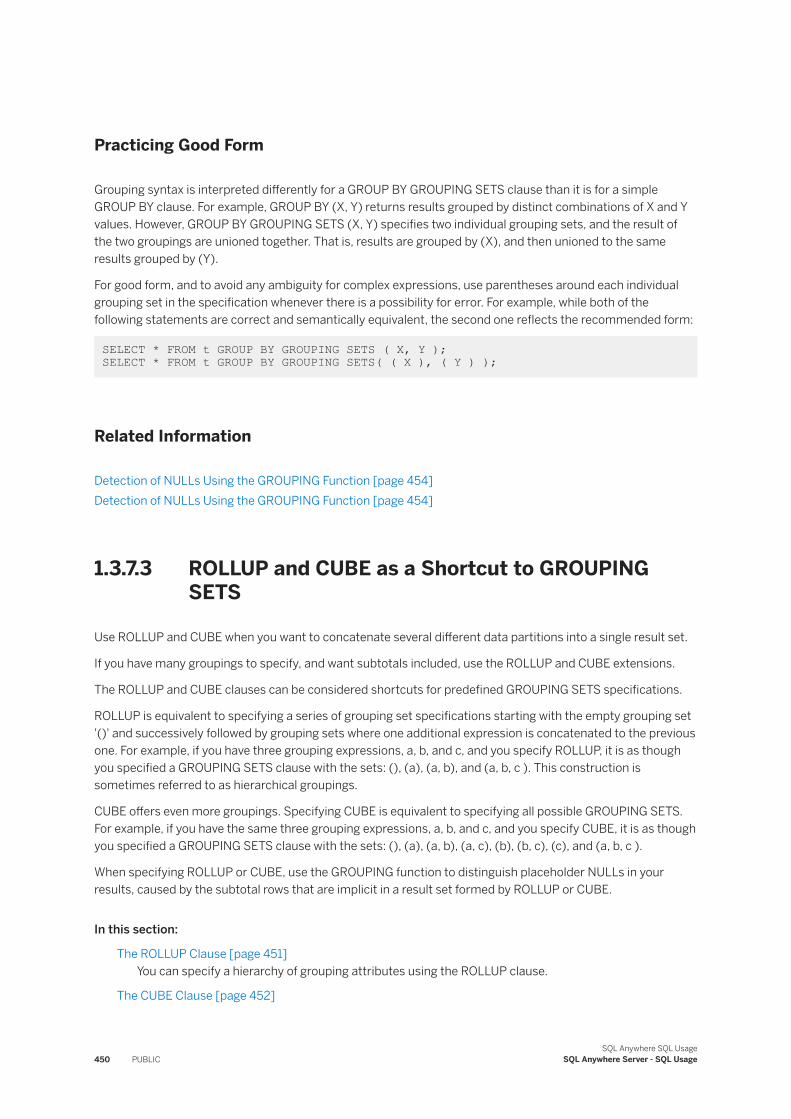
Practicing Good Form
Grouping syntax is interpreted differently for a GROUP BY GROUPING SETS clause than it is for a simple GROUP BY clause. For example, GROUP BY (X, Y) returns results grouped by distinct combinations of X and Y values. However, GROUP BY GROUPING SETS (X, Y) specifies two individual grouping sets, and the result of the two groupings are unioned together. That is, results are grouped by (X), and then unioned to the same results grouped by (Y).
For good form, and to avoid any ambiguity for complex expressions, use parentheses around each individual grouping set in the specification whenever there is a possibility for error. For example, while both of the following statements are correct and semantically equivalent, the second one reflects the recommended form:
SELECT * FROM t GROUP BY GROUPING SETS ( X, Y ); SELECT * FROM t GROUP BY GROUPING SETS( ( X ), ( Y ) );
Related Information
Detection of NULLs Using the GROUPING Function [page 454]Detection of NULLs Using the GROUPING Function [page 454]
1.3.7.3 ROLLUP and CUBE as a Shortcut to GROUPING SETS
Use ROLLUP and CUBE when you want to concatenate several different data partitions into a single result set.
If you have many groupings to specify, and want subtotals included, use the ROLLUP and CUBE extensions.
The ROLLUP and CUBE clauses can be considered shortcuts for predefined GROUPING SETS specifications.
ROLLUP is equivalent to specifying a series of grouping set specifications starting with the empty grouping set '()' and successively followed by grouping sets where one additional expression is concatenated to the previous one. For example, if you have three grouping expressions, a, b, and c, and you specify ROLLUP, it is as though you specified a GROUPING SETS clause with the sets: (), (a), (a, b), and (a, b, c ). This construction is sometimes referred to as hierarchical groupings.
CUBE offers even more groupings. Specifying CUBE is equivalent to specifying all possible GROUPING SETS. For example, if you have the same three grouping expressions, a, b, and c, and you specify CUBE, it is as though you specified a GROUPING SETS clause with the sets: (), (a), (a, b), (a, c), (b), (b, c), (c), and (a, b, c ).
When specifying ROLLUP or CUBE, use the GROUPING function to distinguish placeholder NULLs in your results, caused by the subtotal rows that are implicit in a result set formed by ROLLUP or CUBE.
In this section:
The ROLLUP Clause [page 451]You can specify a hierarchy of grouping attributes using the ROLLUP clause.
The CUBE Clause [page 452]
450 PUBLICSQL Anywhere SQL Usage
SQL Anywhere Server - SQL Usage
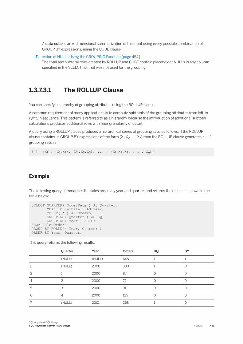
A data cube is an n-dimensional summarization of the input using every possible combination of GROUP BY expressions, using the CUBE clause.
Detection of NULLs Using the GROUPING Function [page 454]The total and subtotal rows created by ROLLUP and CUBE contain placeholder NULLs in any column specified in the SELECT list that was not used for the grouping.
1.3.7.3.1 The ROLLUP Clause
You can specify a hierarchy of grouping attributes using the ROLLUP clause.
A common requirement of many applications is to compute subtotals of the grouping attributes from left-to-right, in sequence. This pattern is referred to as a hierarchy because the introduction of additional subtotal calculations produces additional rows with finer granularity of detail.
A query using a ROLLUP clause produces a hierarchical series of grouping sets, as follows. If the ROLLUP clause contains n GROUP BY expressions of the form (X1,X2, ... , Xn) then the ROLLUP clause generates n + 1 grouping sets as:
{(), (X1), (X1,X2), (X1,X2,X3), ... , (X1,X2,X3, ... , Xn)}
Example
The following query summarizes the sales orders by year and quarter, and returns the result set shown in the table below:
SELECT QUARTER( OrderDate ) AS Quarter, YEAR( OrderDate ) AS Year, COUNT( * ) AS Orders, GROUPING( Quarter ) AS GQ, GROUPING( Year ) AS GYFROM SalesOrdersGROUP BY ROLLUP( Year, Quarter ) ORDER BY Year, Quarter;
This query returns the following results:
Quarter Year Orders GQ GY
1 (NULL) (NULL) 648 1 1
2 (NULL) 2000 380 1 0
3 1 2000 87 0 0
4 2 2000 77 0 0
5 3 2000 91 0 0
6 4 2000 125 0 0
7 (NULL) 2001 268 1 0
SQL Anywhere SQL UsageSQL Anywhere Server - SQL Usage PUBLIC 451
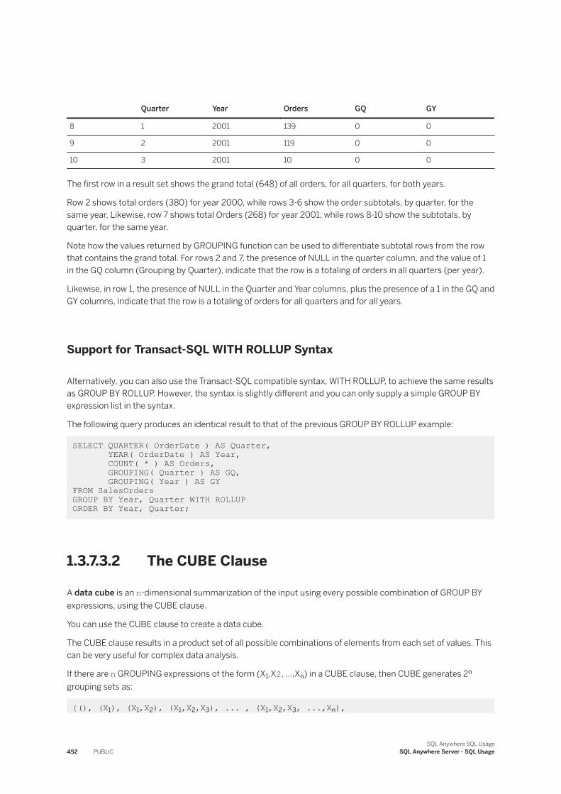
Quarter Year Orders GQ GY
8 1 2001 139 0 0
9 2 2001 119 0 0
10 3 2001 10 0 0
The first row in a result set shows the grand total (648) of all orders, for all quarters, for both years.
Row 2 shows total orders (380) for year 2000, while rows 3-6 show the order subtotals, by quarter, for the same year. Likewise, row 7 shows total Orders (268) for year 2001, while rows 8-10 show the subtotals, by quarter, for the same year.
Note how the values returned by GROUPING function can be used to differentiate subtotal rows from the row that contains the grand total. For rows 2 and 7, the presence of NULL in the quarter column, and the value of 1 in the GQ column (Grouping by Quarter), indicate that the row is a totaling of orders in all quarters (per year).
Likewise, in row 1, the presence of NULL in the Quarter and Year columns, plus the presence of a 1 in the GQ and GY columns, indicate that the row is a totaling of orders for all quarters and for all years.
Support for Transact-SQL WITH ROLLUP Syntax
Alternatively, you can also use the Transact-SQL compatible syntax, WITH ROLLUP, to achieve the same results as GROUP BY ROLLUP. However, the syntax is slightly different and you can only supply a simple GROUP BY expression list in the syntax.
The following query produces an identical result to that of the previous GROUP BY ROLLUP example:
SELECT QUARTER( OrderDate ) AS Quarter, YEAR( OrderDate ) AS Year, COUNT( * ) AS Orders, GROUPING( Quarter ) AS GQ, GROUPING( Year ) AS GYFROM SalesOrdersGROUP BY Year, Quarter WITH ROLLUP ORDER BY Year, Quarter;
1.3.7.3.2 The CUBE Clause
A data cube is an n-dimensional summarization of the input using every possible combination of GROUP BY expressions, using the CUBE clause.
You can use the CUBE clause to create a data cube.
The CUBE clause results in a product set of all possible combinations of elements from each set of values. This can be very useful for complex data analysis.
If there are n GROUPING expressions of the form (X1,X2, ...,Xn) in a CUBE clause, then CUBE generates 2n
grouping sets as:
{(), (X1), (X1,X2), (X1,X2,X3), ... , (X1,X2,X3, ...,Xn),
452 PUBLICSQL Anywhere SQL Usage
SQL Anywhere Server - SQL Usage
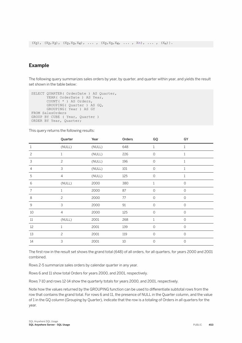
(X2), (X2,X3), (X2,X3,X4), ... , (X2,X3,X4, ... , Xn), ... , (Xn)}.
Example
The following query summarizes sales orders by year, by quarter, and quarter within year, and yields the result set shown in the table below:
SELECT QUARTER( OrderDate ) AS Quarter, YEAR( OrderDate ) AS Year, COUNT( * ) AS Orders, GROUPING( Quarter ) AS GQ, GROUPING( Year ) AS GYFROM SalesOrdersGROUP BY CUBE ( Year, Quarter ) ORDER BY Year, Quarter;
This query returns the following results:
Quarter Year Orders GQ GY
1 (NULL) (NULL) 648 1 1
2 1 (NULL) 226 0 1
3 2 (NULL) 196 0 1
4 3 (NULL) 101 0 1
5 4 (NULL) 125 0 1
6 (NULL) 2000 380 1 0
7 1 2000 87 0 0
8 2 2000 77 0 0
9 3 2000 91 0 0
10 4 2000 125 0 0
11 (NULL) 2001 268 1 0
12 1 2001 139 0 0
13 2 2001 119 0 0
14 3 2001 10 0 0
The first row in the result set shows the grand total (648) of all orders, for all quarters, for years 2000 and 2001 combined.
Rows 2-5 summarize sales orders by calendar quarter in any year.
Rows 6 and 11 show total Orders for years 2000, and 2001, respectively.
Rows 7-10 and rows 12-14 show the quarterly totals for years 2000, and 2001, respectively.
Note how the values returned by the GROUPING function can be used to differentiate subtotal rows from the row that contains the grand total. For rows 6 and 11, the presence of NULL in the Quarter column, and the value of 1 in the GQ column (Grouping by Quarter), indicate that the row is a totaling of Orders in all quarters for the year.
SQL Anywhere SQL UsageSQL Anywhere Server - SQL Usage PUBLIC 453
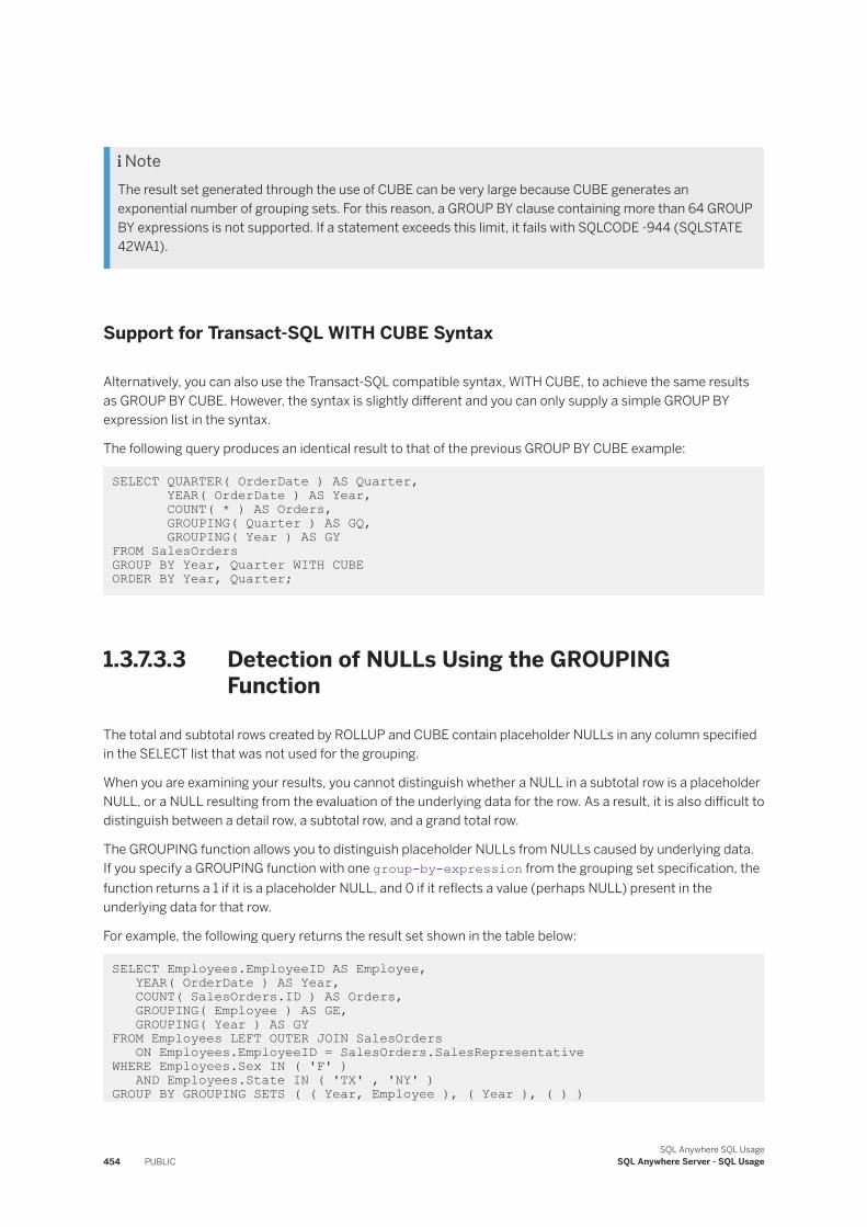
NoteThe result set generated through the use of CUBE can be very large because CUBE generates an exponential number of grouping sets. For this reason, a GROUP BY clause containing more than 64 GROUP BY expressions is not supported. If a statement exceeds this limit, it fails with SQLCODE -944 (SQLSTATE 42WA1).
Support for Transact-SQL WITH CUBE Syntax
Alternatively, you can also use the Transact-SQL compatible syntax, WITH CUBE, to achieve the same results as GROUP BY CUBE. However, the syntax is slightly different and you can only supply a simple GROUP BY expression list in the syntax.
The following query produces an identical result to that of the previous GROUP BY CUBE example:
SELECT QUARTER( OrderDate ) AS Quarter, YEAR( OrderDate ) AS Year, COUNT( * ) AS Orders, GROUPING( Quarter ) AS GQ, GROUPING( Year ) AS GYFROM SalesOrdersGROUP BY Year, Quarter WITH CUBE ORDER BY Year, Quarter;
1.3.7.3.3 Detection of NULLs Using the GROUPING Function
The total and subtotal rows created by ROLLUP and CUBE contain placeholder NULLs in any column specified in the SELECT list that was not used for the grouping.
When you are examining your results, you cannot distinguish whether a NULL in a subtotal row is a placeholder NULL, or a NULL resulting from the evaluation of the underlying data for the row. As a result, it is also difficult to distinguish between a detail row, a subtotal row, and a grand total row.
The GROUPING function allows you to distinguish placeholder NULLs from NULLs caused by underlying data. If you specify a GROUPING function with one group-by-expression from the grouping set specification, the function returns a 1 if it is a placeholder NULL, and 0 if it reflects a value (perhaps NULL) present in the underlying data for that row.
For example, the following query returns the result set shown in the table below:
SELECT Employees.EmployeeID AS Employee, YEAR( OrderDate ) AS Year, COUNT( SalesOrders.ID ) AS Orders, GROUPING( Employee ) AS GE, GROUPING( Year ) AS GYFROM Employees LEFT OUTER JOIN SalesOrders ON Employees.EmployeeID = SalesOrders.SalesRepresentativeWHERE Employees.Sex IN ( 'F' ) AND Employees.State IN ( 'TX' , 'NY' )GROUP BY GROUPING SETS ( ( Year, Employee ), ( Year ), ( ) )
454 PUBLICSQL Anywhere SQL Usage
SQL Anywhere Server - SQL Usage
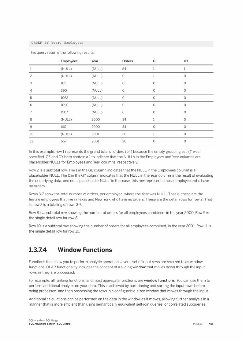
ORDER BY Year, Employee;
This query returns the following results:
Employees Year Orders GE GY
1 (NULL) (NULL) 54 1 1
2 (NULL) (NULL) 0 1 0
3 102 (NULL) 0 0 0
4 390 (NULL) 0 0 0
5 1062 (NULL) 0 0 0
6 1090 (NULL) 0 0 0
7 1507 (NULL) 0 0 0
8 (NULL) 2000 34 1 0
9 667 2000 34 0 0
10 (NULL) 2001 20 1 0
11 667 2001 20 0 0
In this example, row 1 represents the grand total of orders (54) because the empty grouping set '()' was specified. GE and GY both contain a 1 to indicate that the NULLs in the Employees and Year columns are placeholder NULLs for Employees and Year columns, respectively.
Row 2 is a subtotal row. The 1 in the GE column indicates that the NULL in the Employees column is a placeholder NULL. The 0 in the GY column indicates that the NULL in the Year column is the result of evaluating the underlying data, and not a placeholder NULL; in this case, this row represents those employees who have no orders.
Rows 3-7 show the total number of orders, per employee, where the Year was NULL. That is, these are the female employees that live in Texas and New York who have no orders. These are the detail rows for row 2. That is, row 2 is a totaling of rows 3-7.
Row 8 is a subtotal row showing the number of orders for all employees combined, in the year 2000. Row 9 is the single detail row for row 8.
Row 10 is a subtotal row showing the number of orders for all employees combined, in the year 2001. Row 11 is the single detail row for row 10.
1.3.7.4 Window FunctionsFunctions that allow you to perform analytic operations over a set of input rows are referred to as window functions. OLAP functionality includes the concept of a sliding window that moves down through the input rows as they are processed.
For example, all ranking functions, and most aggregate functions, are window functions. You can use them to perform additional analysis on your data. This is achieved by partitioning and sorting the input rows before being processed, and then processing the rows in a configurable-sized window that moves through the input.
Additional calculations can be performed on the data in the window as it moves, allowing further analysis in a manner that is more efficient than using semantically equivalent self-join queries, or correlated subqueries.
SQL Anywhere SQL UsageSQL Anywhere Server - SQL Usage PUBLIC 455
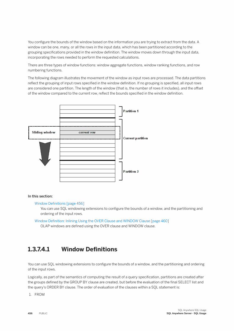
You configure the bounds of the window based on the information you are trying to extract from the data. A window can be one, many, or all the rows in the input data, which has been partitioned according to the grouping specifications provided in the window definition. The window moves down through the input data, incorporating the rows needed to perform the requested calculations.
There are three types of window functions: window aggregate functions, window ranking functions, and row numbering functions.
The following diagram illustrates the movement of the window as input rows are processed. The data partitions reflect the grouping of input rows specified in the window definition. If no grouping is specified, all input rows are considered one partition. The length of the window (that is, the number of rows it includes), and the offset of the window compared to the current row, reflect the bounds specified in the window definition.
In this section:
Window Definitions [page 456]You can use SQL windowing extensions to configure the bounds of a window, and the partitioning and ordering of the input rows.
Window Definition: Inlining Using the OVER Clause and WINDOW Clause [page 460]OLAP windows are defined using the OVER clause and WINDOW clause.
1.3.7.4.1 Window Definitions
You can use SQL windowing extensions to configure the bounds of a window, and the partitioning and ordering of the input rows.
Logically, as part of the semantics of computing the result of a query specification, partitions are created after the groups defined by the GROUP BY clause are created, but before the evaluation of the final SELECT list and the query's ORDER BY clause. The order of evaluation of the clauses within a SQL statement is:
1. FROM
456 PUBLICSQL Anywhere SQL Usage
SQL Anywhere Server - SQL Usage
2. WHERE3. GROUP BY4. HAVING5. WINDOW6. DISTINCT7. ORDER BY
When forming your query, the impact of the order of evaluation should be considered. For example, you cannot have a predicate on an expression referencing a window function in the same SELECT query block. However, by putting the query block in a derived table, you can specify a predicate on the derived table. The following query fails with a message indicating that the failure was the result of a predicate being specified on a window function:
SELECT DepartmentID, Surname, StartDate, Salary, SUM( Salary ) OVER ( PARTITION BY DepartmentID ORDER BY StartDate RANGE BETWEEN UNBOUNDED PRECEDING AND CURRENT ROW ) AS "Sum_Salary" FROM Employees WHERE State IN ( 'CA', 'UT', 'NY', 'AZ' ) AND DepartmentID IN ( '100', '200' ) GROUP BY DepartmentID, Surname, StartDate, Salary HAVING Salary > 0 AND "Sum_Salary" > 200 ORDER BY DepartmentID, StartDate;
Use a derived table (DT) and specify a predicate on it to achieve the results you want:
SELECT * FROM ( SELECT DepartmentID, Surname, StartDate, Salary, SUM( Salary ) OVER ( PARTITION BY DepartmentID ORDER BY StartDate RANGE BETWEEN UNBOUNDED PRECEDING AND CURRENT ROW ) AS "Sum_Salary" FROM Employees WHERE State IN ( 'CA', 'UT', 'NY', 'AZ' ) AND DepartmentID IN ( '100', '200' ) GROUP BY DepartmentID, Surname, StartDate, Salary HAVING Salary > 0 ORDER BY DepartmentID, StartDate ) AS DT WHERE DT.Sum_Salary > 200;
Because window partitioning follows a GROUP BY operator, the result of any aggregate function, such as SUM, AVG, or VARIANCE, is available to the computation done for a partition. So, windows provide another opportunity to perform grouping and ordering operations in addition to a query's GROUP BY and ORDER BY clauses.
Defining a Window Specification
When you define the window over which a window function operates, you specify one or more of the following:
Partitioning (PARTITION BY clause)
The PARTITION BY clause defines how the input rows are grouped. If omitted, the entire input is treated as a single partition. A partition can be one, several, or all input rows, depending on what you specify. Data from two partitions is never mixed. That is, when a window reaches the boundary between two partitions, it completes processing the data in one partition, before beginning on the data in the next partition. The
SQL Anywhere SQL UsageSQL Anywhere Server - SQL Usage PUBLIC 457
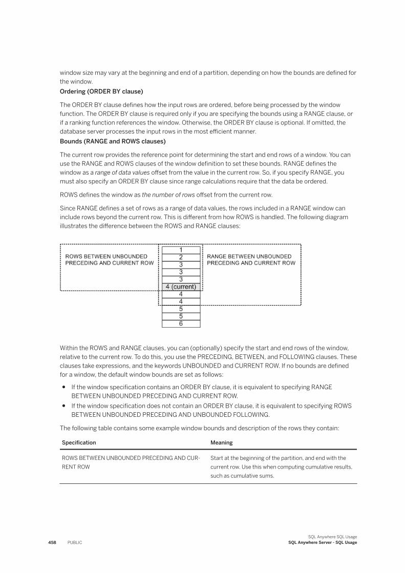
window size may vary at the beginning and end of a partition, depending on how the bounds are defined for the window.Ordering (ORDER BY clause)
The ORDER BY clause defines how the input rows are ordered, before being processed by the window function. The ORDER BY clause is required only if you are specifying the bounds using a RANGE clause, or if a ranking function references the window. Otherwise, the ORDER BY clause is optional. If omitted, the database server processes the input rows in the most efficient manner.Bounds (RANGE and ROWS clauses)
The current row provides the reference point for determining the start and end rows of a window. You can use the RANGE and ROWS clauses of the window definition to set these bounds. RANGE defines the window as a range of data values offset from the value in the current row. So, if you specify RANGE, you must also specify an ORDER BY clause since range calculations require that the data be ordered.
ROWS defines the window as the number of rows offset from the current row.
Since RANGE defines a set of rows as a range of data values, the rows included in a RANGE window can include rows beyond the current row. This is different from how ROWS is handled. The following diagram illustrates the difference between the ROWS and RANGE clauses:
Within the ROWS and RANGE clauses, you can (optionally) specify the start and end rows of the window, relative to the current row. To do this, you use the PRECEDING, BETWEEN, and FOLLOWING clauses. These clauses take expressions, and the keywords UNBOUNDED and CURRENT ROW. If no bounds are defined for a window, the default window bounds are set as follows:
● If the window specification contains an ORDER BY clause, it is equivalent to specifying RANGE BETWEEN UNBOUNDED PRECEDING AND CURRENT ROW.
● If the window specification does not contain an ORDER BY clause, it is equivalent to specifying ROWS BETWEEN UNBOUNDED PRECEDING AND UNBOUNDED FOLLOWING.
The following table contains some example window bounds and description of the rows they contain:
Specification Meaning
ROWS BETWEEN UNBOUNDED PRECEDING AND CURRENT ROW
Start at the beginning of the partition, and end with the current row. Use this when computing cumulative results, such as cumulative sums.
458 PUBLICSQL Anywhere SQL Usage
SQL Anywhere Server - SQL Usage
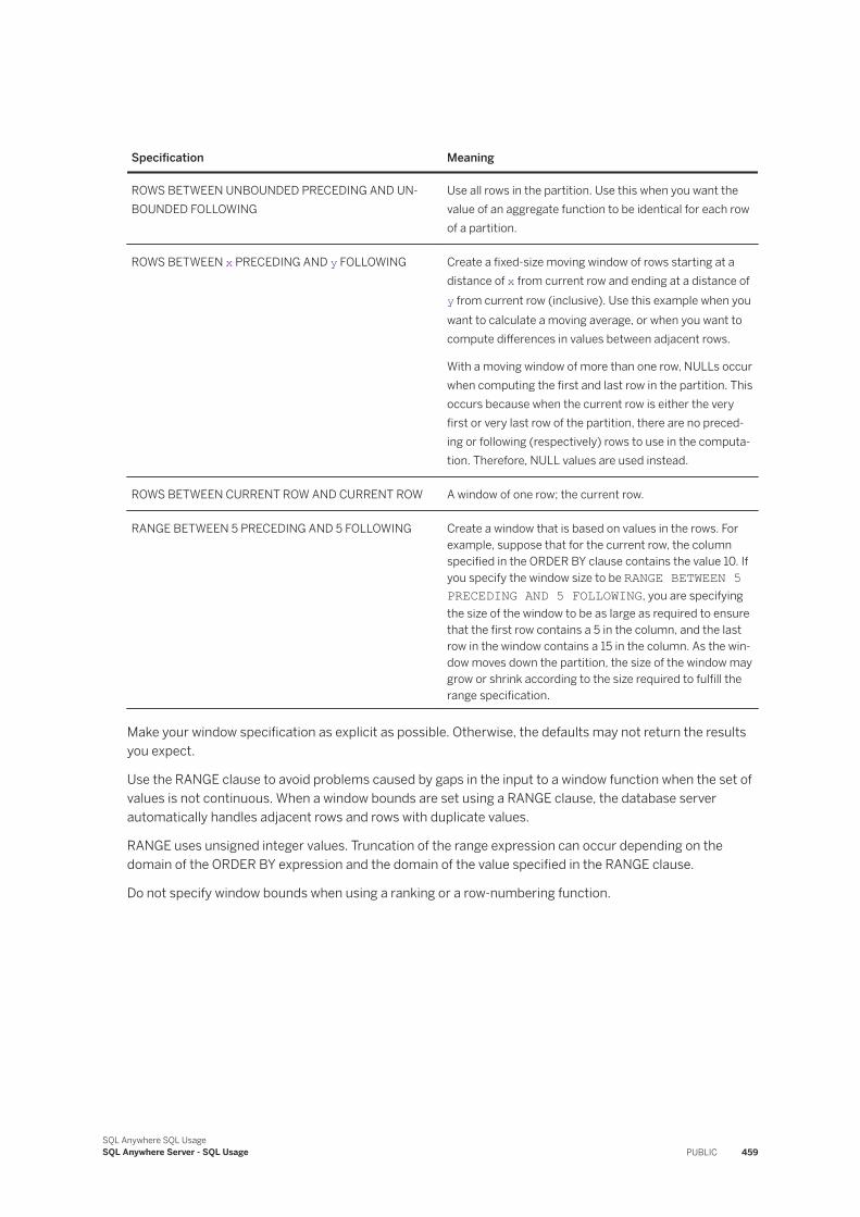
Specification Meaning
ROWS BETWEEN UNBOUNDED PRECEDING AND UNBOUNDED FOLLOWING
Use all rows in the partition. Use this when you want the value of an aggregate function to be identical for each row of a partition.
ROWS BETWEEN x PRECEDING AND y FOLLOWING Create a fixed-size moving window of rows starting at a distance of x from current row and ending at a distance of y from current row (inclusive). Use this example when you want to calculate a moving average, or when you want to compute differences in values between adjacent rows.
With a moving window of more than one row, NULLs occur when computing the first and last row in the partition. This occurs because when the current row is either the very first or very last row of the partition, there are no preceding or following (respectively) rows to use in the computation. Therefore, NULL values are used instead.
ROWS BETWEEN CURRENT ROW AND CURRENT ROW A window of one row; the current row.
RANGE BETWEEN 5 PRECEDING AND 5 FOLLOWING Create a window that is based on values in the rows. For example, suppose that for the current row, the column specified in the ORDER BY clause contains the value 10. If you specify the window size to be RANGE BETWEEN 5 PRECEDING AND 5 FOLLOWING, you are specifying the size of the window to be as large as required to ensure that the first row contains a 5 in the column, and the last row in the window contains a 15 in the column. As the window moves down the partition, the size of the window may grow or shrink according to the size required to fulfill the range specification.
Make your window specification as explicit as possible. Otherwise, the defaults may not return the results you expect.
Use the RANGE clause to avoid problems caused by gaps in the input to a window function when the set of values is not continuous. When a window bounds are set using a RANGE clause, the database server automatically handles adjacent rows and rows with duplicate values.
RANGE uses unsigned integer values. Truncation of the range expression can occur depending on the domain of the ORDER BY expression and the domain of the value specified in the RANGE clause.
Do not specify window bounds when using a ranking or a row-numbering function.
SQL Anywhere SQL UsageSQL Anywhere Server - SQL Usage PUBLIC 459
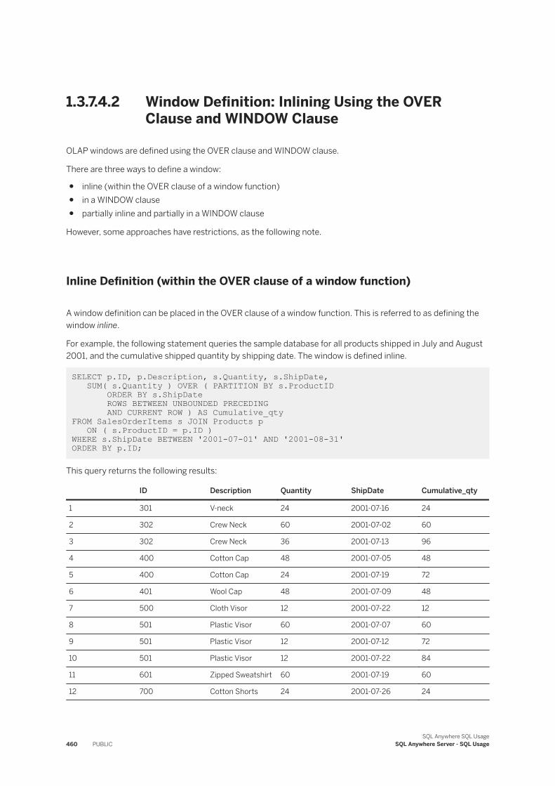
1.3.7.4.2 Window Definition: Inlining Using the OVER Clause and WINDOW Clause
OLAP windows are defined using the OVER clause and WINDOW clause.
There are three ways to define a window:
● inline (within the OVER clause of a window function)● in a WINDOW clause● partially inline and partially in a WINDOW clause
However, some approaches have restrictions, as the following note.
Inline Definition (within the OVER clause of a window function)
A window definition can be placed in the OVER clause of a window function. This is referred to as defining the window inline.
For example, the following statement queries the sample database for all products shipped in July and August 2001, and the cumulative shipped quantity by shipping date. The window is defined inline.
SELECT p.ID, p.Description, s.Quantity, s.ShipDate, SUM( s.Quantity ) OVER ( PARTITION BY s.ProductID ORDER BY s.ShipDate ROWS BETWEEN UNBOUNDED PRECEDING AND CURRENT ROW ) AS Cumulative_qtyFROM SalesOrderItems s JOIN Products p ON ( s.ProductID = p.ID )WHERE s.ShipDate BETWEEN '2001-07-01' AND '2001-08-31' ORDER BY p.ID;
This query returns the following results:
ID Description Quantity ShipDate Cumulative_qty
1 301 V-neck 24 2001-07-16 24
2 302 Crew Neck 60 2001-07-02 60
3 302 Crew Neck 36 2001-07-13 96
4 400 Cotton Cap 48 2001-07-05 48
5 400 Cotton Cap 24 2001-07-19 72
6 401 Wool Cap 48 2001-07-09 48
7 500 Cloth Visor 12 2001-07-22 12
8 501 Plastic Visor 60 2001-07-07 60
9 501 Plastic Visor 12 2001-07-12 72
10 501 Plastic Visor 12 2001-07-22 84
11 601 Zipped Sweatshirt 60 2001-07-19 60
12 700 Cotton Shorts 24 2001-07-26 24
460 PUBLICSQL Anywhere SQL Usage
SQL Anywhere Server - SQL Usage
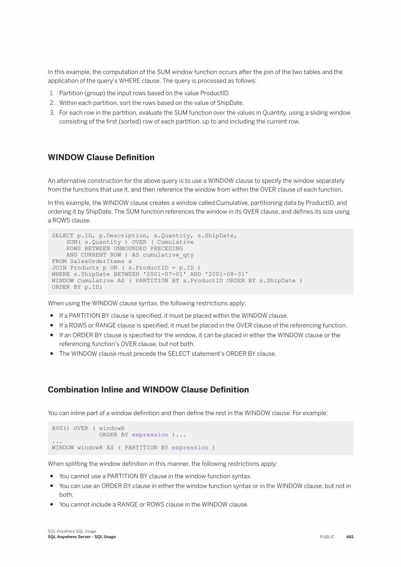
In this example, the computation of the SUM window function occurs after the join of the two tables and the application of the query's WHERE clause. The query is processed as follows:
1. Partition (group) the input rows based on the value ProductID.2. Within each partition, sort the rows based on the value of ShipDate.3. For each row in the partition, evaluate the SUM function over the values in Quantity, using a sliding window
consisting of the first (sorted) row of each partition, up to and including the current row.
WINDOW Clause Definition
An alternative construction for the above query is to use a WINDOW clause to specify the window separately from the functions that use it, and then reference the window from within the OVER clause of each function.
In this example, the WINDOW clause creates a window called Cumulative, partitioning data by ProductID, and ordering it by ShipDate. The SUM function references the window in its OVER clause, and defines its size using a ROWS clause.
SELECT p.ID, p.Description, s.Quantity, s.ShipDate, SUM( s.Quantity ) OVER ( Cumulative ROWS BETWEEN UNBOUNDED PRECEDING AND CURRENT ROW ) AS cumulative_qtyFROM SalesOrderItems s JOIN Products p ON ( s.ProductID = p.ID )WHERE s.ShipDate BETWEEN '2001-07-01' AND '2001-08-31'WINDOW Cumulative AS ( PARTITION BY s.ProductID ORDER BY s.ShipDate ) ORDER BY p.ID;
When using the WINDOW clause syntax, the following restrictions apply:
● If a PARTITION BY clause is specified, it must be placed within the WINDOW clause.● If a ROWS or RANGE clause is specified, it must be placed in the OVER clause of the referencing function.● If an ORDER BY clause is specified for the window, it can be placed in either the WINDOW clause or the
referencing function's OVER clause, but not both.● The WINDOW clause must precede the SELECT statement's ORDER BY clause.
Combination Inline and WINDOW Clause Definition
You can inline part of a window definition and then define the rest in the WINDOW clause. For example:
AVG() OVER ( windowA ORDER BY expression )... ... WINDOW windowA AS ( PARTITION BY expression )
When splitting the window definition in this manner, the following restrictions apply:
● You cannot use a PARTITION BY clause in the window function syntax.● You can use an ORDER BY clause in either the window function syntax or in the WINDOW clause, but not in
both.● You cannot include a RANGE or ROWS clause in the WINDOW clause.
SQL Anywhere SQL UsageSQL Anywhere Server - SQL Usage PUBLIC 461
Related Information
Window Aggregate Functions [page 462]Window Ranking Functions [page 476]Window Definitions [page 456]
1.3.7.5 Window Aggregate Functions
Window aggregate functions return a value for a specified set of rows in the input.
For example, you can use window functions to calculate a moving average of the sales figures for a company over a specified time period.
Window aggregate functions are organized into the following three categories:
Basic Aggregate Functions
Following is the list of supported basic aggregate functions:
● SUM function [Aggregate]● AVG function [Aggregate]● MAX function [Aggregate]● MIN function [Aggregate]● MEDIAN function [Aggregate]● FIRST_VALUE function [Aggregate]● LAST_VALUE function [Aggregate]● COUNT function [Aggregate]
Standard Deviation and Variance Functions
Following is the list of supported standard deviation and variance functions:
● STDDEV function [Aggregate]● STDDEV_POP function [Aggregate]● STDDEV_SAMP function [Aggregate]● VAR_POP function [Aggregate]● VAR_SAMP function [Aggregate]● VARIANCE function [Aggregate]
Correlation and Linear Regression Functions
Following is the list of supported correlation and linear regression functions:
● COVAR_POP function [Aggregate]● COVAR_SAMP function [Aggregate]● REGR_AVGX function [Aggregate]● REGR_AVGY function [Aggregate]● REGR_COUNT function [Aggregate]● REGR_INTERCEPT function [Aggregate]● REGR_R2 function [Aggregate]● REGR_SLOPE function [Aggregate]
462 PUBLICSQL Anywhere SQL Usage
SQL Anywhere Server - SQL Usage
● REGR_SXX function [Aggregate]● REGR_SXY function [Aggregate]● REGR_SYY function [Aggregate]
Related Information
Basic Aggregate Functions [page 463]Correlation and Linear Regression Functions [page 475]Standard Deviation and Variance Functions [page 471]
1.3.7.6 Basic Aggregate Functions
There are several supported basic aggregate functions you can use to return values for groups of rows.
Complex data analysis often requires multiple levels of aggregation. Window partitioning and ordering, in addition to, or instead of, a GROUP BY clause, offers you considerable flexibility in the composition of complex SQL queries. For example, by combining a window construct with a simple aggregate function, you can compute values such as moving average, moving sum, moving minimum or maximum, and cumulative sum.
Following are the supported basic aggregate functions:
SUM function
Returns the total of the specified expression for each group of rows.AVG function
Returns the average of a numeric expression or of a set unique values for a set of rows.MAX function
Returns the maximum expression value found in each group of rows.MIN function
Returns the minimum expression value found in each group of rows.MEDIAN function
Returns the median of a numeric expression for a set of rows.FIRST_VALUE function
Returns values from the first row of a window. This function requires a window specification.LAST_VALUE function
Returns values from the last row of a window. This function requires a window specification.COUNT function
Returns the number of rows that qualify for the specified expression.
In this section:
SUM Function Example [page 464]You can use the SUM function to return the sum of values in a set of rows.
SQL Anywhere SQL UsageSQL Anywhere Server - SQL Usage PUBLIC 463
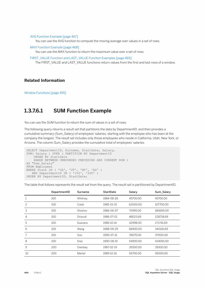
AVG Function Example [page 467]You can use the AVG function to compute the moving average over values in a set of rows.
MAX Function Example [page 468]You can use the MAX function to return the maximum value over a set of rows.
FIRST_VALUE Function and LAST_VALUE Function Examples [page 469]The FIRST_VALUE and LAST_VALUE functions return values from the first and last rows of a window.
Related Information
Window Functions [page 455]
1.3.7.6.1 SUM Function Example
You can use the SUM function to return the sum of values in a set of rows.
The following query returns a result set that partitions the data by DepartmentID, and then provides a cumulative summary (Sum_Salary) of employees' salaries, starting with the employee who has been at the company the longest. The result set includes only those employees who reside in California, Utah, New York, or Arizona. The column Sum_Salary provides the cumulative total of employees' salaries.
SELECT DepartmentID, Surname, StartDate, Salary, SUM( Salary ) OVER ( PARTITION BY DepartmentID ORDER BY StartDate RANGE BETWEEN UNBOUNDED PRECEDING AND CURRENT ROW ) AS "Sum_Salary"FROM EmployeesWHERE State IN ( 'CA', 'UT', 'NY', 'AZ' ) AND DepartmentID IN ( '100', '200' ) ORDER BY DepartmentID, StartDate;
The table that follows represents the result set from the query. The result set is partitioned by DepartmentID.
DepartmentID Surname StartDate Salary Sum_Salary
1 100 Whitney 1984-08-28 45700.00 45700.00
2 100 Cobb 1985-01-01 62000.00 107700.00
3 100 Shishov 1986-06-07 72995.00 180695.00
4 100 Driscoll 1986-07-01 48023.69 228718.69
5 100 Guevara 1986-10-14 42998.00 271716.69
6 100 Wang 1988-09-29 68400.00 340116.69
7 100 Soo 1990-07-31 39075.00 379191.69
8 100 Diaz 1990-08-19 54900.00 434091.69
9 200 Overbey 1987-02-19 39300.00 39300.00
10 200 Martel 1989-10-16 55700.00 95000.00
464 PUBLICSQL Anywhere SQL Usage
SQL Anywhere Server - SQL Usage
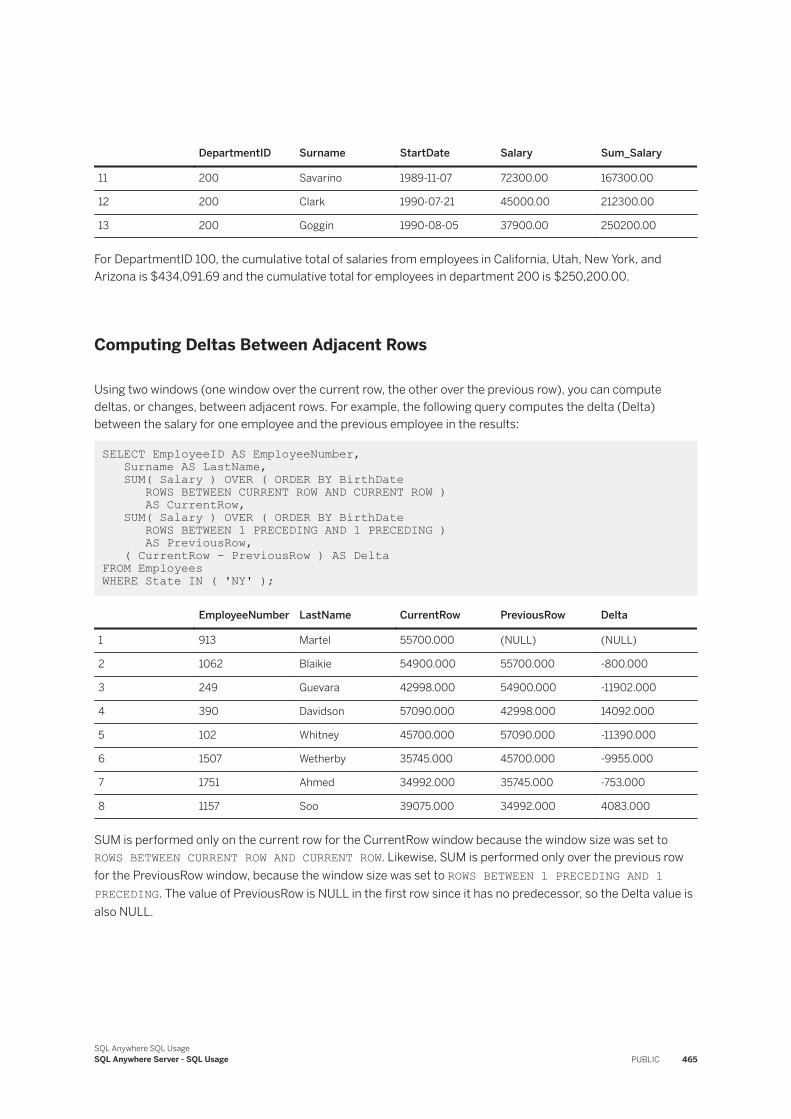
DepartmentID Surname StartDate Salary Sum_Salary
11 200 Savarino 1989-11-07 72300.00 167300.00
12 200 Clark 1990-07-21 45000.00 212300.00
13 200 Goggin 1990-08-05 37900.00 250200.00
For DepartmentID 100, the cumulative total of salaries from employees in California, Utah, New York, and Arizona is $434,091.69 and the cumulative total for employees in department 200 is $250,200.00.
Computing Deltas Between Adjacent Rows
Using two windows (one window over the current row, the other over the previous row), you can compute deltas, or changes, between adjacent rows. For example, the following query computes the delta (Delta) between the salary for one employee and the previous employee in the results:
SELECT EmployeeID AS EmployeeNumber, Surname AS LastName, SUM( Salary ) OVER ( ORDER BY BirthDate ROWS BETWEEN CURRENT ROW AND CURRENT ROW ) AS CurrentRow, SUM( Salary ) OVER ( ORDER BY BirthDate ROWS BETWEEN 1 PRECEDING AND 1 PRECEDING ) AS PreviousRow, ( CurrentRow - PreviousRow ) AS DeltaFROM Employees WHERE State IN ( 'NY' );
EmployeeNumber LastName CurrentRow PreviousRow Delta
1 913 Martel 55700.000 (NULL) (NULL)
2 1062 Blaikie 54900.000 55700.000 -800.000
3 249 Guevara 42998.000 54900.000 -11902.000
4 390 Davidson 57090.000 42998.000 14092.000
5 102 Whitney 45700.000 57090.000 -11390.000
6 1507 Wetherby 35745.000 45700.000 -9955.000
7 1751 Ahmed 34992.000 35745.000 -753.000
8 1157 Soo 39075.000 34992.000 4083.000
SUM is performed only on the current row for the CurrentRow window because the window size was set to ROWS BETWEEN CURRENT ROW AND CURRENT ROW. Likewise, SUM is performed only over the previous row for the PreviousRow window, because the window size was set to ROWS BETWEEN 1 PRECEDING AND 1 PRECEDING. The value of PreviousRow is NULL in the first row since it has no predecessor, so the Delta value is also NULL.
SQL Anywhere SQL UsageSQL Anywhere Server - SQL Usage PUBLIC 465
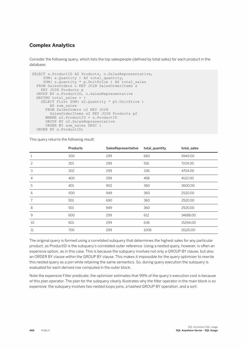
Complex Analytics
Consider the following query, which lists the top salespeople (defined by total sales) for each product in the database:
SELECT s.ProductID AS Products, o.SalesRepresentative, SUM( s.Quantity ) AS total_quantity, SUM( s.Quantity * p.UnitPrice ) AS total_sales FROM SalesOrders o KEY JOIN SalesOrderItems s KEY JOIN Products p GROUP BY s.ProductID, o.SalesRepresentative HAVING total_sales = ( SELECT First SUM( s2.Quantity * p2.UnitPrice ) AS sum_sales FROM SalesOrders o2 KEY JOIN SalesOrderItems s2 KEY JOIN Products p2 WHERE s2.ProductID = s.ProductID GROUP BY o2.SalesRepresentative ORDER BY sum_sales DESC ) ORDER BY s.ProductID;
This query returns the following result:
Products SalesRepresentative total_quantity total_sales
1 300 299 660 5940.00
2 301 299 516 7224.00
3 302 299 336 4704.00
4 400 299 458 4122.00
5 401 902 360 3600.00
6 500 949 360 2520.00
7 501 690 360 2520.00
8 501 949 360 2520.00
9 600 299 612 14688.00
10 601 299 636 15264.00
11 700 299 1008 15120.00
The original query is formed using a correlated subquery that determines the highest sales for any particular product, as ProductID is the subquery's correlated outer reference. Using a nested query, however, is often an expensive option, as in this case. This is because the subquery involves not only a GROUP BY clause, but also an ORDER BY clause within the GROUP BY clause. This makes it impossible for the query optimizer to rewrite this nested query as a join while retaining the same semantics. So, during query execution the subquery is evaluated for each derived row computed in the outer block.
Note the expensive Filter predicate; the optimizer estimates that 99% of the query's execution cost is because of this plan operator. The plan for the subquery clearly illustrates why the filter operator in the main block is so expensive: the subquery involves two nested loops joins, a hashed GROUP BY operation, and a sort.
466 PUBLICSQL Anywhere SQL Usage
SQL Anywhere Server - SQL Usage
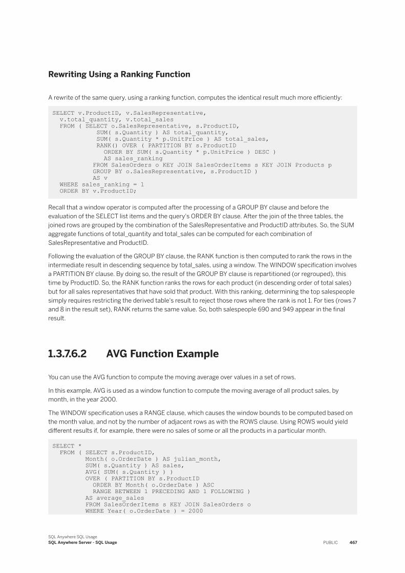
Rewriting Using a Ranking Function
A rewrite of the same query, using a ranking function, computes the identical result much more efficiently:
SELECT v.ProductID, v.SalesRepresentative, v.total_quantity, v.total_sales FROM ( SELECT o.SalesRepresentative, s.ProductID, SUM( s.Quantity ) AS total_quantity, SUM( s.Quantity * p.UnitPrice ) AS total_sales, RANK() OVER ( PARTITION BY s.ProductID ORDER BY SUM( s.Quantity * p.UnitPrice ) DESC ) AS sales_ranking FROM SalesOrders o KEY JOIN SalesOrderItems s KEY JOIN Products p GROUP BY o.SalesRepresentative, s.ProductID ) AS v WHERE sales_ranking = 1 ORDER BY v.ProductID;
Recall that a window operator is computed after the processing of a GROUP BY clause and before the evaluation of the SELECT list items and the query's ORDER BY clause. After the join of the three tables, the joined rows are grouped by the combination of the SalesRepresentative and ProductID attributes. So, the SUM aggregate functions of total_quantity and total_sales can be computed for each combination of SalesRepresentative and ProductID.
Following the evaluation of the GROUP BY clause, the RANK function is then computed to rank the rows in the intermediate result in descending sequence by total_sales, using a window. The WINDOW specification involves a PARTITION BY clause. By doing so, the result of the GROUP BY clause is repartitioned (or regrouped), this time by ProductID. So, the RANK function ranks the rows for each product (in descending order of total sales) but for all sales representatives that have sold that product. With this ranking, determining the top salespeople simply requires restricting the derived table's result to reject those rows where the rank is not 1. For ties (rows 7 and 8 in the result set), RANK returns the same value. So, both salespeople 690 and 949 appear in the final result.
1.3.7.6.2 AVG Function Example
You can use the AVG function to compute the moving average over values in a set of rows.
In this example, AVG is used as a window function to compute the moving average of all product sales, by month, in the year 2000.
The WINDOW specification uses a RANGE clause, which causes the window bounds to be computed based on the month value, and not by the number of adjacent rows as with the ROWS clause. Using ROWS would yield different results if, for example, there were no sales of some or all the products in a particular month.
SELECT * FROM ( SELECT s.ProductID, Month( o.OrderDate ) AS julian_month, SUM( s.Quantity ) AS sales, AVG( SUM( s.Quantity ) ) OVER ( PARTITION BY s.ProductID ORDER BY Month( o.OrderDate ) ASC RANGE BETWEEN 1 PRECEDING AND 1 FOLLOWING ) AS average_sales FROM SalesOrderItems s KEY JOIN SalesOrders o WHERE Year( o.OrderDate ) = 2000
SQL Anywhere SQL UsageSQL Anywhere Server - SQL Usage PUBLIC 467
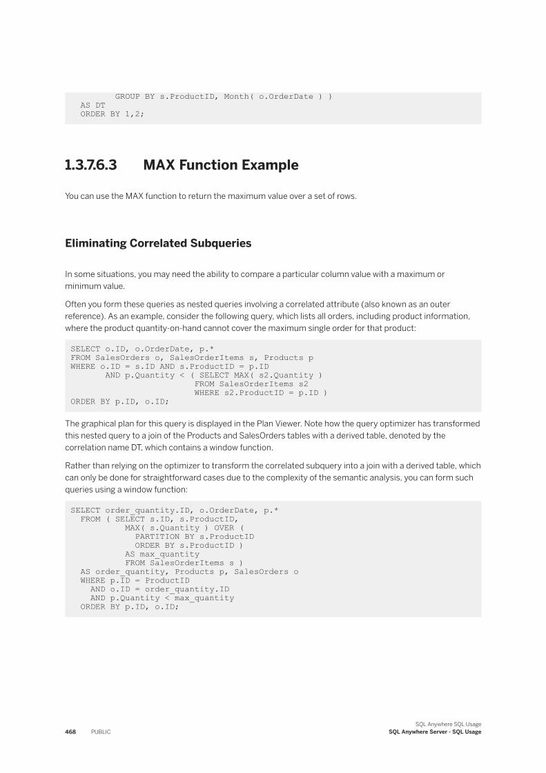
GROUP BY s.ProductID, Month( o.OrderDate ) ) AS DT ORDER BY 1,2;
1.3.7.6.3 MAX Function Example
You can use the MAX function to return the maximum value over a set of rows.
Eliminating Correlated Subqueries
In some situations, you may need the ability to compare a particular column value with a maximum or minimum value.
Often you form these queries as nested queries involving a correlated attribute (also known as an outer reference). As an example, consider the following query, which lists all orders, including product information, where the product quantity-on-hand cannot cover the maximum single order for that product:
SELECT o.ID, o.OrderDate, p.* FROM SalesOrders o, SalesOrderItems s, Products pWHERE o.ID = s.ID AND s.ProductID = p.ID AND p.Quantity < ( SELECT MAX( s2.Quantity ) FROM SalesOrderItems s2 WHERE s2.ProductID = p.ID ) ORDER BY p.ID, o.ID;
The graphical plan for this query is displayed in the Plan Viewer. Note how the query optimizer has transformed this nested query to a join of the Products and SalesOrders tables with a derived table, denoted by the correlation name DT, which contains a window function.
Rather than relying on the optimizer to transform the correlated subquery into a join with a derived table, which can only be done for straightforward cases due to the complexity of the semantic analysis, you can form such queries using a window function:
SELECT order_quantity.ID, o.OrderDate, p.* FROM ( SELECT s.ID, s.ProductID, MAX( s.Quantity ) OVER ( PARTITION BY s.ProductID ORDER BY s.ProductID ) AS max_quantity FROM SalesOrderItems s ) AS order_quantity, Products p, SalesOrders o WHERE p.ID = ProductID AND o.ID = order_quantity.ID AND p.Quantity < max_quantity ORDER BY p.ID, o.ID;
468 PUBLICSQL Anywhere SQL Usage
SQL Anywhere Server - SQL Usage
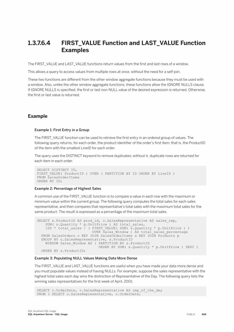
1.3.7.6.4 FIRST_VALUE Function and LAST_VALUE Function Examples
The FIRST_VALUE and LAST_VALUE functions return values from the first and last rows of a window.
This allows a query to access values from multiple rows at once, without the need for a self-join.
These two functions are different from the other window aggregate functions because they must be used with a window. Also, unlike the other window aggregate functions, these functions allow the IGNORE NULLS clause. If IGNORE NULLS is specified, the first or last non-NULL value of the desired expression is returned. Otherwise, the first or last value is returned.
Example
Example 1: First Entry in a Group
The FIRST_VALUE function can be used to retrieve the first entry in an ordered group of values. The following query returns, for each order, the product identifier of the order's first item; that is, the ProductID of the item with the smallest LineID for each order.
The query uses the DISTINCT keyword to remove duplicates; without it, duplicate rows are returned for each item in each order.
SELECT DISTINCT ID, FIRST_VALUE( ProductID ) OVER ( PARTITION BY ID ORDER BY LineID )FROM SalesOrderItems ORDER BY ID;
Example 2: Percentage of Highest Sales
A common use of the FIRST_VALUE function is to compare a value in each row with the maximum or minimum value within the current group. The following query computes the total sales for each sales representative, and then compares that representative's total sales with the maximum total sales for the same product. The result is expressed as a percentage of the maximum total sales.
SELECT s.ProductID AS prod_id, o.SalesRepresentative AS sales_rep, SUM( s.Quantity * p.UnitPrice ) AS total_sales, 100 * total_sales / ( FIRST_VALUE( SUM( s.Quantity * p.UnitPrice ) ) OVER Sales_Window ) AS total_sales_percentage FROM SalesOrders o KEY JOIN SalesOrderItems s KEY JOIN Products p GROUP BY o.SalesRepresentative, s.ProductID WINDOW Sales_Window AS ( PARTITION BY s.ProductID ORDER BY SUM( s.Quantity * p.UnitPrice ) DESC ) ORDER BY s.ProductID;
Example 3: Populating NULL Values Making Data More Dense
The FIRST_VALUE and LAST_VALUE functions are useful when you have made your data more dense and you must populate values instead of having NULLs. For example, suppose the sales representative with the highest total sales each day wins the distinction of Representative of the Day. The following query lists the winning sales representatives for the first week of April, 2001:
SELECT v.OrderDate, v.SalesRepresentative AS rep_of_the_day FROM ( SELECT o.SalesRepresentative, o.OrderDate,
SQL Anywhere SQL UsageSQL Anywhere Server - SQL Usage PUBLIC 469
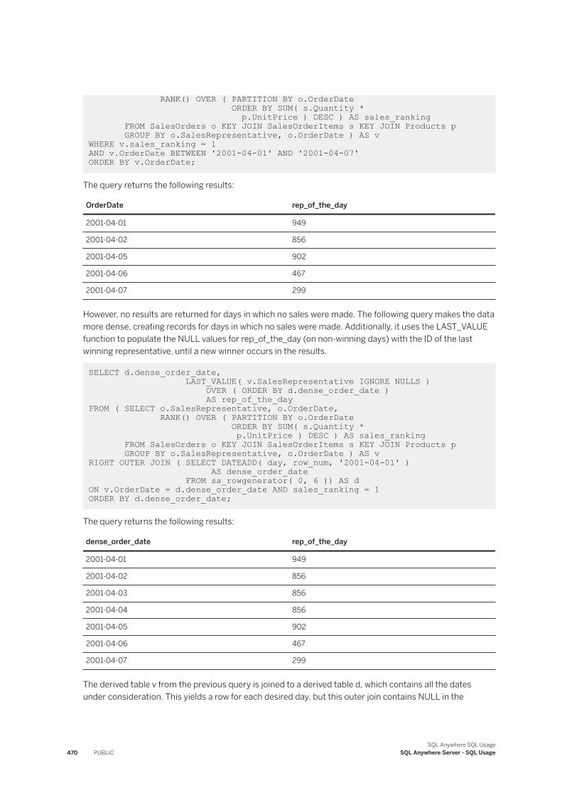
RANK() OVER ( PARTITION BY o.OrderDate ORDER BY SUM( s.Quantity * p.UnitPrice ) DESC ) AS sales_ranking FROM SalesOrders o KEY JOIN SalesOrderItems s KEY JOIN Products p GROUP BY o.SalesRepresentative, o.OrderDate ) AS vWHERE v.sales_ranking = 1AND v.OrderDate BETWEEN '2001-04-01' AND '2001-04-07' ORDER BY v.OrderDate;
The query returns the following results:
OrderDate rep_of_the_day
2001-04-01 949
2001-04-02 856
2001-04-05 902
2001-04-06 467
2001-04-07 299
However, no results are returned for days in which no sales were made. The following query makes the data more dense, creating records for days in which no sales were made. Additionally, it uses the LAST_VALUE function to populate the NULL values for rep_of_the_day (on non-winning days) with the ID of the last winning representative, until a new winner occurs in the results.
SELECT d.dense_order_date, LAST_VALUE( v.SalesRepresentative IGNORE NULLS ) OVER ( ORDER BY d.dense_order_date ) AS rep_of_the_dayFROM ( SELECT o.SalesRepresentative, o.OrderDate, RANK() OVER ( PARTITION BY o.OrderDate ORDER BY SUM( s.Quantity * p.UnitPrice ) DESC ) AS sales_ranking FROM SalesOrders o KEY JOIN SalesOrderItems s KEY JOIN Products p GROUP BY o.SalesRepresentative, o.OrderDate ) AS vRIGHT OUTER JOIN ( SELECT DATEADD( day, row_num, '2001-04-01' ) AS dense_order_date FROM sa_rowgenerator( 0, 6 )) AS d ON v.OrderDate = d.dense_order_date AND sales_ranking = 1 ORDER BY d.dense_order_date;
The query returns the following results:
dense_order_date rep_of_the_day
2001-04-01 949
2001-04-02 856
2001-04-03 856
2001-04-04 856
2001-04-05 902
2001-04-06 467
2001-04-07 299
The derived table v from the previous query is joined to a derived table d, which contains all the dates under consideration. This yields a row for each desired day, but this outer join contains NULL in the
470 PUBLICSQL Anywhere SQL Usage
SQL Anywhere Server - SQL Usage
SalesRepresentative column for dates on which no sales were made. Using the LAST_VALUE function solves this problem by defining rep_of_the_day for a given row to be the last non-NULL value of SalesRepresentative leading up to the corresponding day.
Related Information
Window Functions [page 455]
1.3.7.7 Standard Deviation and Variance Functions
Two versions of variance and standard deviation functions are supported: a sampling version, and a population version.
Choosing between the two versions depends on the statistical context in which the function is to be used.
All the variance and standard deviation functions are true aggregate functions in that they can compute values for a partition of rows as determined by the query's GROUP BY clause. As with other basic aggregate functions such as MAX or MIN, their computation also ignores NULL values in the input.
For improved performance, the database server calculates the mean and the deviation from the mean in one step, so only one pass over the data is required.
Also, regardless of the domain of the expression being analyzed, all variance and standard deviation computation is done using IEEE double-precision floating-point arithmetic. If the input to any variance or standard deviation function is the empty set, then each function returns NULL as its result. If VAR_SAMP is computed for a single row, then it returns NULL, while VAR_POP returns the value 0.
Following are the supported standard deviation and variance functions:
● STDDEV function● STDDEV_POP function● STDDEV_SAMP function● VARIANCE function● VAR_POP function● VAR_SAMP function
STDDEV function
This function is an alias for the STDDEV_SAMP function.
SQL Anywhere SQL UsageSQL Anywhere Server - SQL Usage PUBLIC 471
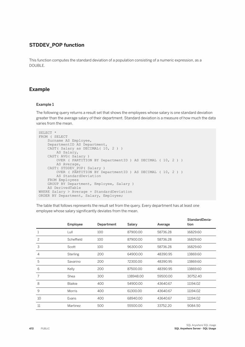
STDDEV_POP function
This function computes the standard deviation of a population consisting of a numeric expression, as a DOUBLE.
Example
Example 1
The following query returns a result set that shows the employees whose salary is one standard deviation greater than the average salary of their department. Standard deviation is a measure of how much the data varies from the mean.
SELECT * FROM ( SELECT Surname AS Employee, DepartmentID AS Department, CAST( Salary as DECIMAL( 10, 2 ) ) AS Salary, CAST( AVG( Salary ) OVER ( PARTITION BY DepartmentID ) AS DECIMAL ( 10, 2 ) ) AS Average, CAST( STDDEV_POP( Salary ) OVER ( PARTITION BY DepartmentID ) AS DECIMAL ( 10, 2 ) ) AS StandardDeviation FROM Employees GROUP BY Department, Employee, Salary ) AS DerivedTableWHERE Salary > Average + StandardDeviation ORDER BY Department, Salary, Employee;
The table that follows represents the result set from the query. Every department has at least one employee whose salary significantly deviates from the mean.
Employee Department Salary AverageStandardDeviation
1 Lull 100 87900.00 58736.28 16829.60
2 Scheffield 100 87900.00 58736.28 16829.60
3 Scott 100 96300.00 58736.28 16829.60
4 Sterling 200 64900.00 48390.95 13869.60
5 Savarino 200 72300.00 48390.95 13869.60
6 Kelly 200 87500.00 48390.95 13869.60
7 Shea 300 138948.00 59500.00 30752.40
8 Blaikie 400 54900.00 43640.67 11194.02
9 Morris 400 61300.00 43640.67 11194.02
10 Evans 400 68940.00 43640.67 11194.02
11 Martinez 500 55500.00 33752.20 9084.50
472 PUBLICSQL Anywhere SQL Usage
SQL Anywhere Server - SQL Usage
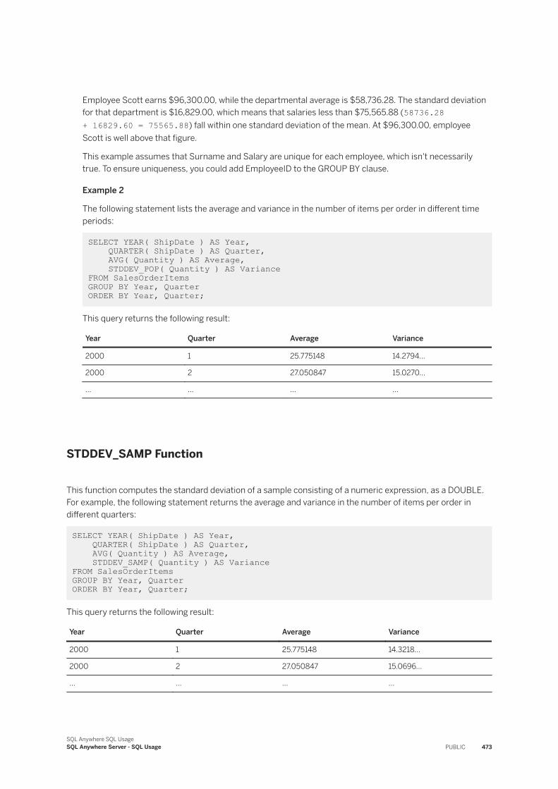
Employee Scott earns $96,300.00, while the departmental average is $58,736.28. The standard deviation for that department is $16,829.00, which means that salaries less than $75,565.88 (58736.28 + 16829.60 = 75565.88) fall within one standard deviation of the mean. At $96,300.00, employee Scott is well above that figure.
This example assumes that Surname and Salary are unique for each employee, which isn't necessarily true. To ensure uniqueness, you could add EmployeeID to the GROUP BY clause.
Example 2
The following statement lists the average and variance in the number of items per order in different time periods:
SELECT YEAR( ShipDate ) AS Year, QUARTER( ShipDate ) AS Quarter, AVG( Quantity ) AS Average, STDDEV_POP( Quantity ) AS VarianceFROM SalesOrderItemsGROUP BY Year, Quarter ORDER BY Year, Quarter;
This query returns the following result:
Year Quarter Average Variance
2000 1 25.775148 14.2794...
2000 2 27.050847 15.0270...
... ... ... ...
STDDEV_SAMP Function
This function computes the standard deviation of a sample consisting of a numeric expression, as a DOUBLE. For example, the following statement returns the average and variance in the number of items per order in different quarters:
SELECT YEAR( ShipDate ) AS Year, QUARTER( ShipDate ) AS Quarter, AVG( Quantity ) AS Average, STDDEV_SAMP( Quantity ) AS VarianceFROM SalesOrderItemsGROUP BY Year, Quarter ORDER BY Year, Quarter;
This query returns the following result:
Year Quarter Average Variance
2000 1 25.775148 14.3218...
2000 2 27.050847 15.0696...
... ... ... ...
SQL Anywhere SQL UsageSQL Anywhere Server - SQL Usage PUBLIC 473
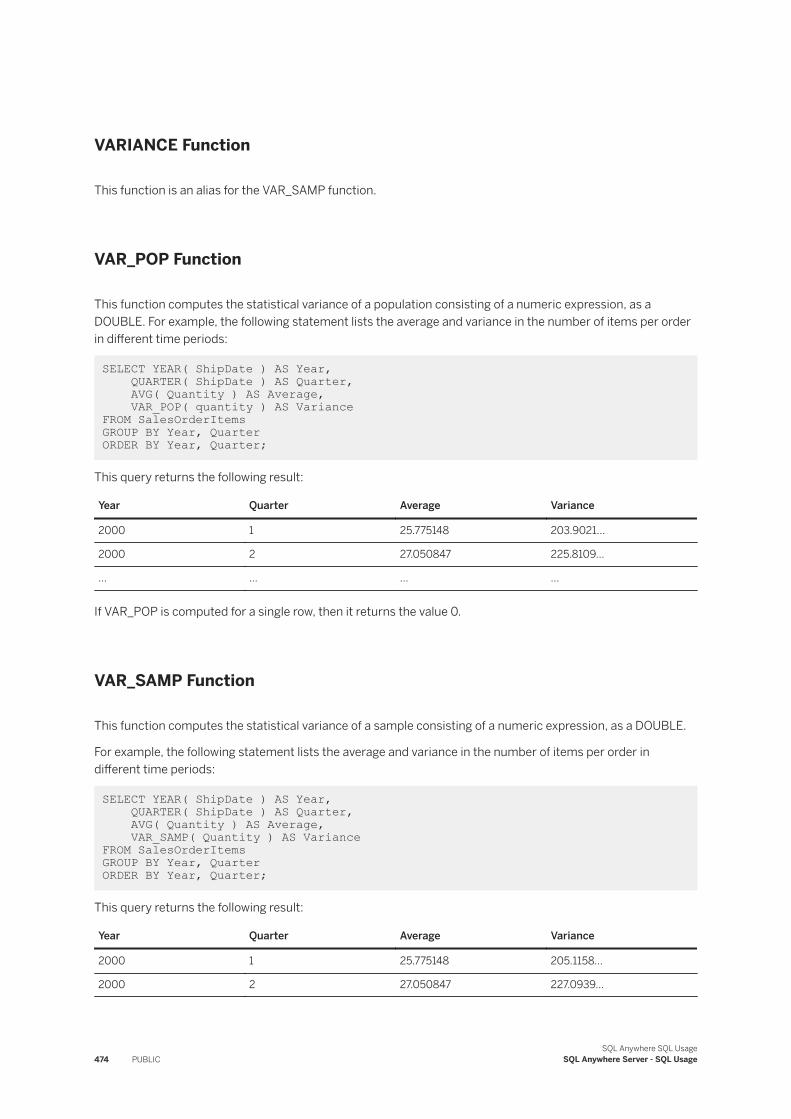
VARIANCE Function
This function is an alias for the VAR_SAMP function.
VAR_POP Function
This function computes the statistical variance of a population consisting of a numeric expression, as a DOUBLE. For example, the following statement lists the average and variance in the number of items per order in different time periods:
SELECT YEAR( ShipDate ) AS Year, QUARTER( ShipDate ) AS Quarter, AVG( Quantity ) AS Average, VAR_POP( quantity ) AS VarianceFROM SalesOrderItemsGROUP BY Year, Quarter ORDER BY Year, Quarter;
This query returns the following result:
Year Quarter Average Variance
2000 1 25.775148 203.9021...
2000 2 27.050847 225.8109...
... ... ... ...
If VAR_POP is computed for a single row, then it returns the value 0.
VAR_SAMP Function
This function computes the statistical variance of a sample consisting of a numeric expression, as a DOUBLE.
For example, the following statement lists the average and variance in the number of items per order in different time periods:
SELECT YEAR( ShipDate ) AS Year, QUARTER( ShipDate ) AS Quarter, AVG( Quantity ) AS Average, VAR_SAMP( Quantity ) AS VarianceFROM SalesOrderItemsGROUP BY Year, Quarter ORDER BY Year, Quarter;
This query returns the following result:
Year Quarter Average Variance
2000 1 25.775148 205.1158...
2000 2 27.050847 227.0939...
474 PUBLICSQL Anywhere SQL Usage
SQL Anywhere Server - SQL Usage
Year Quarter Average Variance
... ... ... ...
If VAR_SAMP is computed for a single row, then it returns NULL.
Related Information
Mathematical Formulas for the Aggregate Functions [page 484]
1.3.7.8 Correlation and Linear Regression Functions
A variety of statistical functions is supported, the results of which can be used to assist in analyzing the quality of a linear regression.
The first argument of each function is the dependent expression (designated by Y), and the second argument is the independent expression (designated by X).
COVAR_SAMP function
The COVAR_SAMP function returns the sample covariance of a set of (Y, X) pairs.COVAR_POP function
The COVAR_POP function returns the population covariance of a set of (Y, X) pairs.CORR function
The CORR function returns the correlation coefficient of a set of (Y, X) pairs.REGR_AVGX function
The REGR_AVGX function returns the mean of the x-values from all the non-NULL pairs of (Y, X) values.REGR_AVGY function
The REGR_AVGY function returns the mean of the y-values from all the non-NULL pairs of (Y, X) values.REGR_SLOPE function
The REGR_SLOPE function computes the slope of the linear regression line fitted to non-NULL pairs.REGR_INTERCEPT function
The REGR_INTERCEPT function computes the y-intercept of the linear regression line that best fits the dependent and independent variables.REGR_R2 function
The REGR_R2 function computes the coefficient of determination (also referred to as R-squared or the goodness of fit statistic) for the regression line.REGR_COUNT function
The REGR_COUNT function returns the number of non-NULL pairs of (Y, X) values in the input. Only if both X and Y in a given pair are non-NULL is that observation be used in any linear regression computation.REGR_SXX function
SQL Anywhere SQL UsageSQL Anywhere Server - SQL Usage PUBLIC 475
The function returns the sum of squares of x-values of the (Y, X) pairs.
The equation for this function is equivalent to the numerator of the sample or population variance formulas. Note, as with the other linear regression functions, that REGR_SXX ignores any pair of (Y, X) values in the input where either X or Y is NULL.REGR_SYY function
The function returns the sum of squares of y-values of the (Y, X) pairs.REGR_SXY function
The function returns the difference of two sum of products over the set of (Y, X) pairs.
1.3.7.9 Window Ranking Functions
Window ranking functions return the rank of a row relative to the other rows in a partition.
The supported ranking functions are:
● CUME_DIST● DENSE_RANK● PERCENT_RANK● RANK
Ranking functions are not considered aggregate functions because they do not compute a result from multiple input rows in the same manner as, for example, the SUM aggregate function. Rather, each of these functions computes the rank, or relative ordering, of a row within a partition based on the value of a particular expression. Each set of rows within a partition is ranked independently; if the OVER clause does not contain a PARTITION BY clause, the entire input is treated as a single partition. So, you cannot specify a ROWS or RANGE clause for a window used by a ranking function. It is possible to form a query containing multiple ranking functions, each of which partition or sort the input rows differently.
All ranking functions require an ORDER BY clause to specify the sort order of the input rows upon which the ranking functions depend. If the ORDER BY clause includes multiple expressions, the second and subsequent expressions are used to break ties if the first expression has the same value in adjacent rows. NULL values are sorted before any other value (in ascending sequence).
In this section:
Window Ranking Functions: RANK Function [page 477]You use the RANK function to return the rank of the value in the current row as compared to the value in other rows.
Window Ranking Functions: DENSE_RANK Function [page 479]You use the DENSE_RANK function to return the rank of the value in the current row as compared to the value in other rows.
Window Ranking Functions: CUME_DIST Function [page 481]The cumulative distribution function, CUME_DIST, is sometimes defined as the inverse of percentile.
Window Ranking Functions: PERCENT_RANK Function [page 482]The PERCENT_RANK function returns the rank for the value in the column specified in the window's ORDER BY clause, but expressed as a fraction between 0 an 1, calculated as (RANK - 1)/(- 1).
476 PUBLICSQL Anywhere SQL Usage
SQL Anywhere Server - SQL Usage
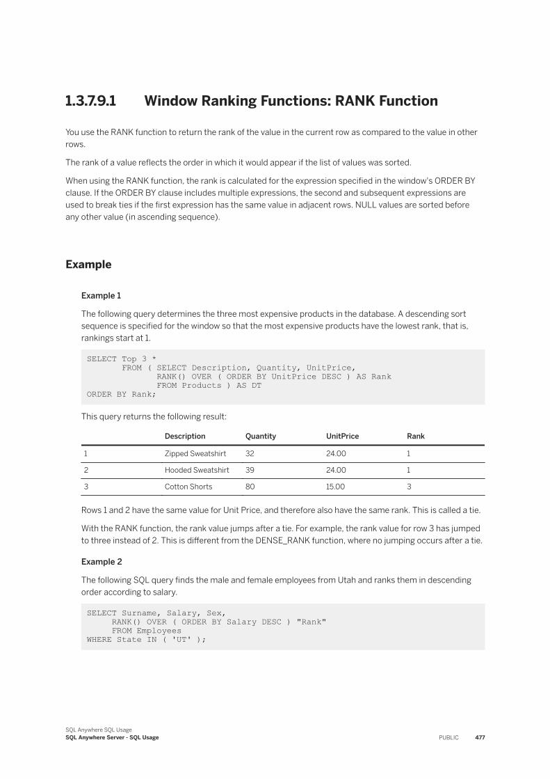
1.3.7.9.1 Window Ranking Functions: RANK Function
You use the RANK function to return the rank of the value in the current row as compared to the value in other rows.
The rank of a value reflects the order in which it would appear if the list of values was sorted.
When using the RANK function, the rank is calculated for the expression specified in the window's ORDER BY clause. If the ORDER BY clause includes multiple expressions, the second and subsequent expressions are used to break ties if the first expression has the same value in adjacent rows. NULL values are sorted before any other value (in ascending sequence).
Example
Example 1
The following query determines the three most expensive products in the database. A descending sort sequence is specified for the window so that the most expensive products have the lowest rank, that is, rankings start at 1.
SELECT Top 3 * FROM ( SELECT Description, Quantity, UnitPrice, RANK() OVER ( ORDER BY UnitPrice DESC ) AS Rank FROM Products ) AS DT ORDER BY Rank;
This query returns the following result:
Description Quantity UnitPrice Rank
1 Zipped Sweatshirt 32 24.00 1
2 Hooded Sweatshirt 39 24.00 1
3 Cotton Shorts 80 15.00 3
Rows 1 and 2 have the same value for Unit Price, and therefore also have the same rank. This is called a tie.
With the RANK function, the rank value jumps after a tie. For example, the rank value for row 3 has jumped to three instead of 2. This is different from the DENSE_RANK function, where no jumping occurs after a tie.
Example 2
The following SQL query finds the male and female employees from Utah and ranks them in descending order according to salary.
SELECT Surname, Salary, Sex, RANK() OVER ( ORDER BY Salary DESC ) "Rank" FROM Employees WHERE State IN ( 'UT' );
SQL Anywhere SQL UsageSQL Anywhere Server - SQL Usage PUBLIC 477
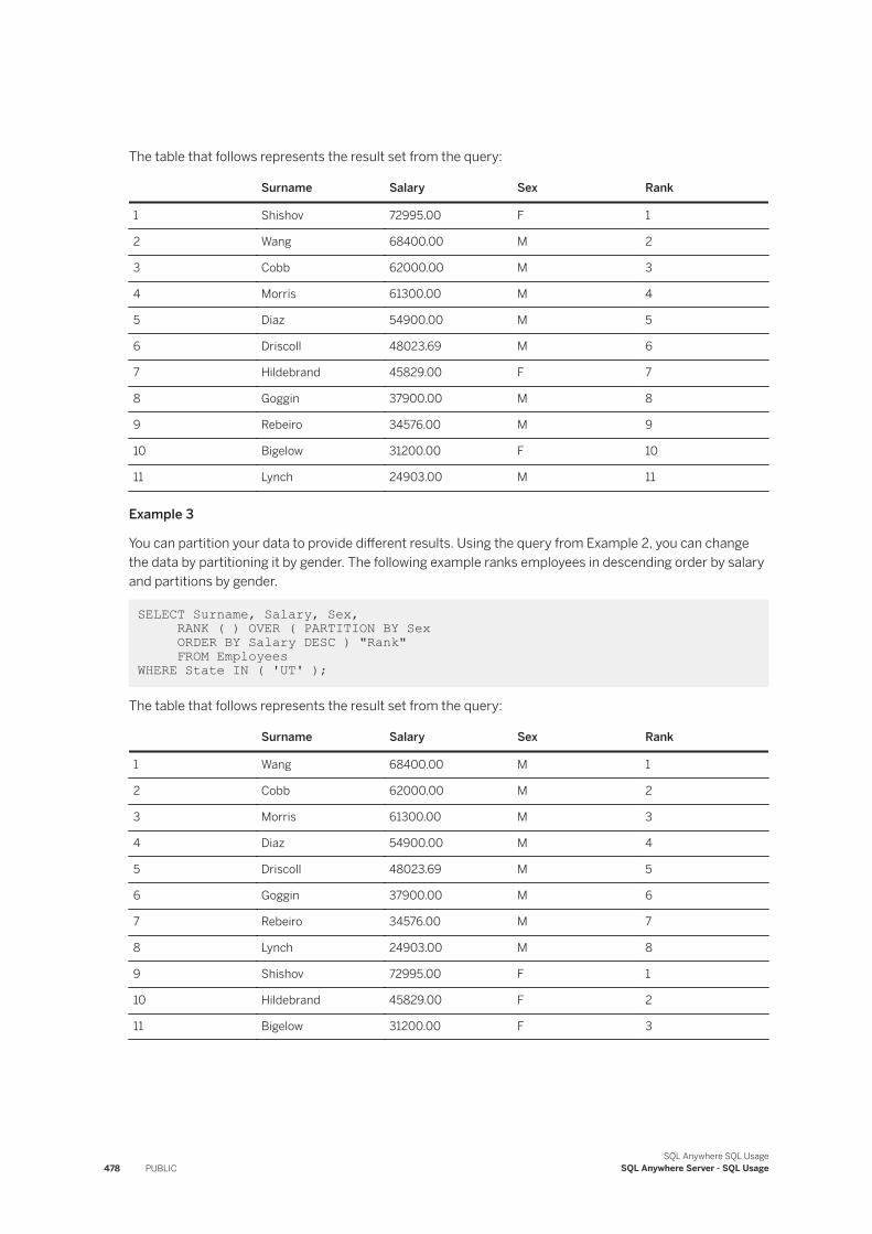
The table that follows represents the result set from the query:
Surname Salary Sex Rank
1 Shishov 72995.00 F 1
2 Wang 68400.00 M 2
3 Cobb 62000.00 M 3
4 Morris 61300.00 M 4
5 Diaz 54900.00 M 5
6 Driscoll 48023.69 M 6
7 Hildebrand 45829.00 F 7
8 Goggin 37900.00 M 8
9 Rebeiro 34576.00 M 9
10 Bigelow 31200.00 F 10
11 Lynch 24903.00 M 11
Example 3
You can partition your data to provide different results. Using the query from Example 2, you can change the data by partitioning it by gender. The following example ranks employees in descending order by salary and partitions by gender.
SELECT Surname, Salary, Sex, RANK ( ) OVER ( PARTITION BY Sex ORDER BY Salary DESC ) "Rank" FROM Employees WHERE State IN ( 'UT' );
The table that follows represents the result set from the query:
Surname Salary Sex Rank
1 Wang 68400.00 M 1
2 Cobb 62000.00 M 2
3 Morris 61300.00 M 3
4 Diaz 54900.00 M 4
5 Driscoll 48023.69 M 5
6 Goggin 37900.00 M 6
7 Rebeiro 34576.00 M 7
8 Lynch 24903.00 M 8
9 Shishov 72995.00 F 1
10 Hildebrand 45829.00 F 2
11 Bigelow 31200.00 F 3
478 PUBLICSQL Anywhere SQL Usage
SQL Anywhere Server - SQL Usage
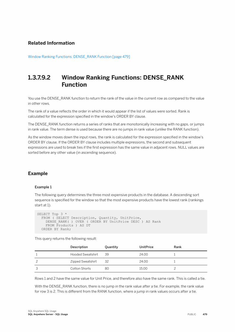
Related Information
Window Ranking Functions: DENSE_RANK Function [page 479]
1.3.7.9.2 Window Ranking Functions: DENSE_RANK Function
You use the DENSE_RANK function to return the rank of the value in the current row as compared to the value in other rows.
The rank of a value reflects the order in which it would appear if the list of values were sorted. Rank is calculated for the expression specified in the window's ORDER BY clause.
The DENSE_RANK function returns a series of ranks that are monotonically increasing with no gaps, or jumps in rank value. The term dense is used because there are no jumps in rank value (unlike the RANK function).
As the window moves down the input rows, the rank is calculated for the expression specified in the window's ORDER BY clause. If the ORDER BY clause includes multiple expressions, the second and subsequent expressions are used to break ties if the first expression has the same value in adjacent rows. NULL values are sorted before any other value (in ascending sequence).
Example
Example 1
The following query determines the three most expensive products in the database. A descending sort sequence is specified for the window so that the most expensive products have the lowest rank (rankings start at 1).
SELECT Top 3 * FROM ( SELECT Description, Quantity, UnitPrice, DENSE_RANK( ) OVER ( ORDER BY UnitPrice DESC ) AS Rank FROM Products ) AS DT ORDER BY Rank;
This query returns the following result:
Description Quantity UnitPrice Rank
1 Hooded Sweatshirt 39 24.00 1
2 Zipped Sweatshirt 32 24.00 1
3 Cotton Shorts 80 15.00 2
Rows 1 and 2 have the same value for Unit Price, and therefore also have the same rank. This is called a tie.
With the DENSE_RANK function, there is no jump in the rank value after a tie. For example, the rank value for row 3 is 2. This is different from the RANK function, where a jump in rank values occurs after a tie.
SQL Anywhere SQL UsageSQL Anywhere Server - SQL Usage PUBLIC 479
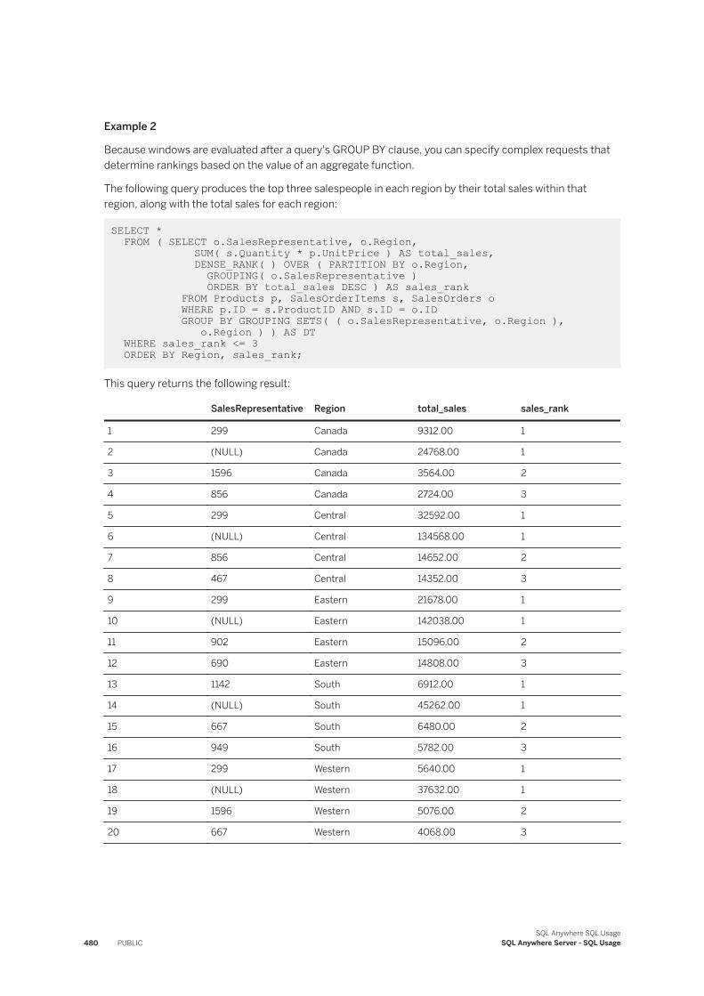
Example 2
Because windows are evaluated after a query's GROUP BY clause, you can specify complex requests that determine rankings based on the value of an aggregate function.
The following query produces the top three salespeople in each region by their total sales within that region, along with the total sales for each region:
SELECT * FROM ( SELECT o.SalesRepresentative, o.Region, SUM( s.Quantity * p.UnitPrice ) AS total_sales, DENSE_RANK( ) OVER ( PARTITION BY o.Region, GROUPING( o.SalesRepresentative ) ORDER BY total_sales DESC ) AS sales_rank FROM Products p, SalesOrderItems s, SalesOrders o WHERE p.ID = s.ProductID AND s.ID = o.ID GROUP BY GROUPING SETS( ( o.SalesRepresentative, o.Region ), o.Region ) ) AS DT WHERE sales_rank <= 3 ORDER BY Region, sales_rank;
This query returns the following result:
SalesRepresentative Region total_sales sales_rank
1 299 Canada 9312.00 1
2 (NULL) Canada 24768.00 1
3 1596 Canada 3564.00 2
4 856 Canada 2724.00 3
5 299 Central 32592.00 1
6 (NULL) Central 134568.00 1
7 856 Central 14652.00 2
8 467 Central 14352.00 3
9 299 Eastern 21678.00 1
10 (NULL) Eastern 142038.00 1
11 902 Eastern 15096.00 2
12 690 Eastern 14808.00 3
13 1142 South 6912.00 1
14 (NULL) South 45262.00 1
15 667 South 6480.00 2
16 949 South 5782.00 3
17 299 Western 5640.00 1
18 (NULL) Western 37632.00 1
19 1596 Western 5076.00 2
20 667 Western 4068.00 3
480 PUBLICSQL Anywhere SQL Usage
SQL Anywhere Server - SQL Usage
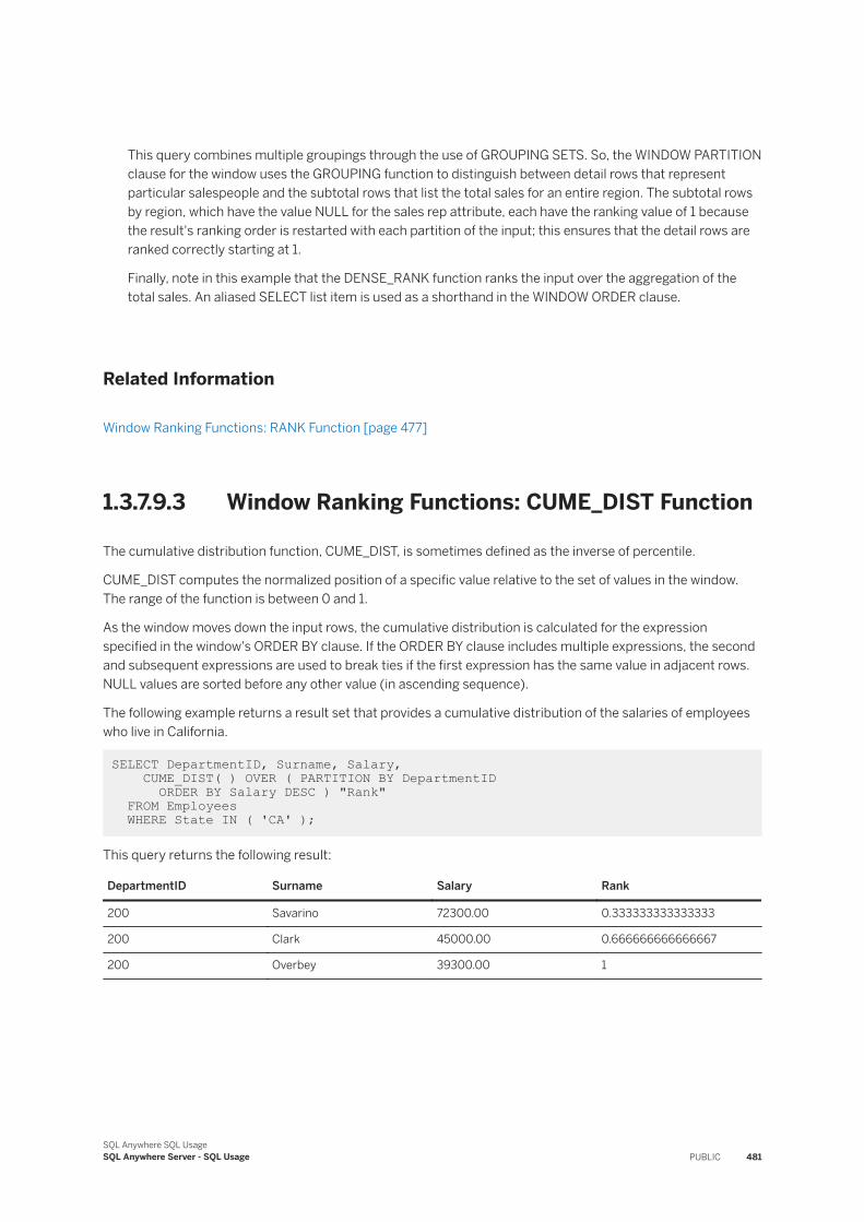
This query combines multiple groupings through the use of GROUPING SETS. So, the WINDOW PARTITION clause for the window uses the GROUPING function to distinguish between detail rows that represent particular salespeople and the subtotal rows that list the total sales for an entire region. The subtotal rows by region, which have the value NULL for the sales rep attribute, each have the ranking value of 1 because the result's ranking order is restarted with each partition of the input; this ensures that the detail rows are ranked correctly starting at 1.
Finally, note in this example that the DENSE_RANK function ranks the input over the aggregation of the total sales. An aliased SELECT list item is used as a shorthand in the WINDOW ORDER clause.
Related Information
Window Ranking Functions: RANK Function [page 477]
1.3.7.9.3 Window Ranking Functions: CUME_DIST Function
The cumulative distribution function, CUME_DIST, is sometimes defined as the inverse of percentile.
CUME_DIST computes the normalized position of a specific value relative to the set of values in the window. The range of the function is between 0 and 1.
As the window moves down the input rows, the cumulative distribution is calculated for the expression specified in the window's ORDER BY clause. If the ORDER BY clause includes multiple expressions, the second and subsequent expressions are used to break ties if the first expression has the same value in adjacent rows. NULL values are sorted before any other value (in ascending sequence).
The following example returns a result set that provides a cumulative distribution of the salaries of employees who live in California.
SELECT DepartmentID, Surname, Salary, CUME_DIST( ) OVER ( PARTITION BY DepartmentID ORDER BY Salary DESC ) "Rank" FROM Employees WHERE State IN ( 'CA' );
This query returns the following result:
DepartmentID Surname Salary Rank
200 Savarino 72300.00 0.333333333333333
200 Clark 45000.00 0.666666666666667
200 Overbey 39300.00 1
SQL Anywhere SQL UsageSQL Anywhere Server - SQL Usage PUBLIC 481
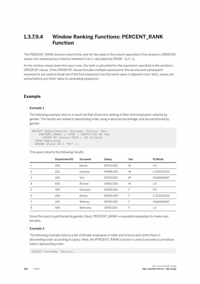
1.3.7.9.4 Window Ranking Functions: PERCENT_RANK Function
The PERCENT_RANK function returns the rank for the value in the column specified in the window's ORDER BY clause, but expressed as a fraction between 0 an 1, calculated as (RANK - 1)/(- 1).
As the window moves down the input rows, the rank is calculated for the expression specified in the window's ORDER BY clause. If the ORDER BY clause includes multiple expressions, the second and subsequent expressions are used to break ties if the first expression has the same value in adjacent rows. NULL values are sorted before any other value (in ascending sequence).
Example
Example 1
The following example returns a result set that shows the ranking of New York employees' salaries by gender. The results are ranked in descending order using a decimal percentage, and are partitioned by gender.
SELECT DepartmentID, Surname, Salary, Sex, PERCENT_RANK( ) OVER ( PARTITION BY Sex ORDER BY Salary DESC ) AS PctRank FROM Employees WHERE State IN ( 'NY' );
This query returns the following results:
DepartmentID Surname Salary Sex PctRank
1 200 Martel 55700.000 M 0.0
2 100 Guevara 42998.000 M 0.333333333
3 100 Soo 39075.000 M 0.666666667
4 400 Ahmed 34992.000 M 1.0
5 300 Davidson 57090.000 F 0.0
6 400 Blaikie 54900.000 F 0.333333333
7 100 Whitney 45700.000 F 0.666666667
8 400 Wetherby 35745.000 F 1.0
Since the input is partitioned by gender (Sex), PERCENT_RANK is evaluated separately for males and females.
Example 2
The following example returns a list of female employees in Utah and Arizona and ranks them in descending order according to salary. Here, the PERCENT_RANK function is used to provide a cumulative total in descending order.
SELECT Surname, Salary,
482 PUBLICSQL Anywhere SQL Usage
SQL Anywhere Server - SQL Usage
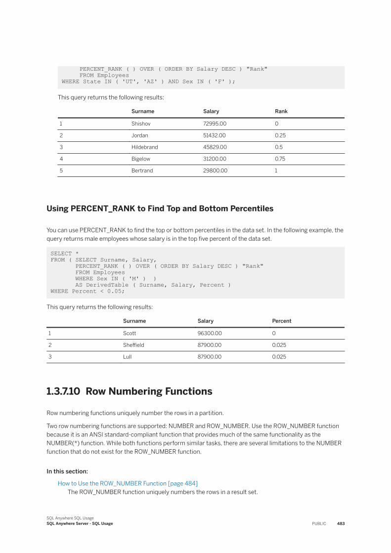
PERCENT_RANK ( ) OVER ( ORDER BY Salary DESC ) "Rank" FROM Employees WHERE State IN ( 'UT', 'AZ' ) AND Sex IN ( 'F' );
This query returns the following results:
Surname Salary Rank
1 Shishov 72995.00 0
2 Jordan 51432.00 0.25
3 Hildebrand 45829.00 0.5
4 Bigelow 31200.00 0.75
5 Bertrand 29800.00 1
Using PERCENT_RANK to Find Top and Bottom Percentiles
You can use PERCENT_RANK to find the top or bottom percentiles in the data set. In the following example, the query returns male employees whose salary is in the top five percent of the data set.
SELECT * FROM ( SELECT Surname, Salary, PERCENT_RANK ( ) OVER ( ORDER BY Salary DESC ) "Rank" FROM Employees WHERE Sex IN ( 'M' ) ) AS DerivedTable ( Surname, Salary, Percent ) WHERE Percent < 0.05;
This query returns the following results:
Surname Salary Percent
1 Scott 96300.00 0
2 Sheffield 87900.00 0.025
3 Lull 87900.00 0.025
1.3.7.10 Row Numbering Functions
Row numbering functions uniquely number the rows in a partition.
Two row numbering functions are supported: NUMBER and ROW_NUMBER. Use the ROW_NUMBER function because it is an ANSI standard-compliant function that provides much of the same functionality as the NUMBER(*) function. While both functions perform similar tasks, there are several limitations to the NUMBER function that do not exist for the ROW_NUMBER function.
In this section:
How to Use the ROW_NUMBER Function [page 484]The ROW_NUMBER function uniquely numbers the rows in a result set.
SQL Anywhere SQL UsageSQL Anywhere Server - SQL Usage PUBLIC 483
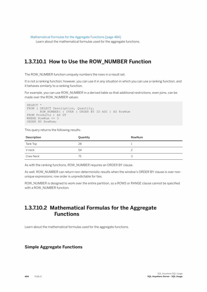
Mathematical Formulas for the Aggregate Functions [page 484]Learn about the mathematical formulas used for the aggregate functions.
1.3.7.10.1 How to Use the ROW_NUMBER Function
The ROW_NUMBER function uniquely numbers the rows in a result set.
It is not a ranking function; however, you can use it in any situation in which you can use a ranking function, and it behaves similarly to a ranking function.
For example, you can use ROW_NUMBER in a derived table so that additional restrictions, even joins, can be made over the ROW_NUMBER values:
SELECT * FROM ( SELECT Description, Quantity, ROW_NUMBER( ) OVER ( ORDER BY ID ASC ) AS RowNumFROM Products ) AS DTWHERE RowNum <= 3 ORDER BY RowNum;
This query returns the following results:
Description Quantity RowNum
Tank Top 28 1
V-neck 54 2
Crew Neck 75 3
As with the ranking functions, ROW_NUMBER requires an ORDER BY clause.
As well, ROW_NUMBER can return non-deterministic results when the window's ORDER BY clause is over non-unique expressions; row order is unpredictable for ties.
ROW_NUMBER is designed to work over the entire partition, so a ROWS or RANGE clause cannot be specified with a ROW_NUMBER function.
1.3.7.10.2 Mathematical Formulas for the Aggregate Functions
Learn about the mathematical formulas used for the aggregate functions.
Simple Aggregate Functions
484 PUBLICSQL Anywhere SQL Usage
SQL Anywhere Server - SQL Usage
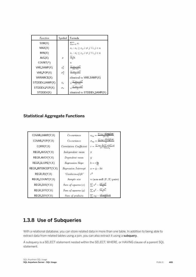
Statistical Aggregate Functions
1.3.8 Use of Subqueries
With a relational database, you can store related data in more than one table. In addition to being able to extract data from related tables using a join, you can also extract it using a subquery.
A subquery is a SELECT statement nested within the SELECT, WHERE, or HAVING clause of a parent SQL statement.
SQL Anywhere SQL UsageSQL Anywhere Server - SQL Usage PUBLIC 485
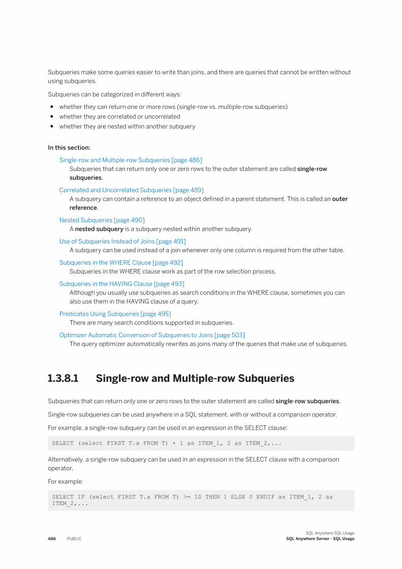
Subqueries make some queries easier to write than joins, and there are queries that cannot be written without using subqueries.
Subqueries can be categorized in different ways:
● whether they can return one or more rows (single-row vs. multiple-row subqueries)● whether they are correlated or uncorrelated● whether they are nested within another subquery
In this section:
Single-row and Multiple-row Subqueries [page 486]Subqueries that can return only one or zero rows to the outer statement are called single-row subqueries.
Correlated and Uncorrelated Subqueries [page 489]A subquery can contain a reference to an object defined in a parent statement. This is called an outer reference.
Nested Subqueries [page 490]A nested subquery is a subquery nested within another subquery.
Use of Subqueries Instead of Joins [page 491]A subquery can be used instead of a join whenever only one column is required from the other table.
Subqueries in the WHERE Clause [page 492]Subqueries in the WHERE clause work as part of the row selection process.
Subqueries in the HAVING Clause [page 493]Although you usually use subqueries as search conditions in the WHERE clause, sometimes you can also use them in the HAVING clause of a query.
Predicates Using Subqueries [page 495]There are many search conditions supported in subqueries.
Optimizer Automatic Conversion of Subqueries to Joins [page 503]The query optimizer automatically rewrites as joins many of the queries that make use of subqueries.
1.3.8.1 Single-row and Multiple-row Subqueries
Subqueries that can return only one or zero rows to the outer statement are called single-row subqueries.
Single-row subqueries can be used anywhere in a SQL statement, with or without a comparison operator.
For example, a single-row subquery can be used in an expression in the SELECT clause:
SELECT (select FIRST T.x FROM T) + 1 as ITEM_1, 2 as ITEM_2,...
Alternatively, a single-row subquery can be used in an expression in the SELECT clause with a comparison operator.
For example:
SELECT IF (select FIRST T.x FROM T) >= 10 THEN 1 ELSE 0 ENDIF as ITEM_1, 2 as ITEM_2,...
486 PUBLICSQL Anywhere SQL Usage
SQL Anywhere Server - SQL Usage
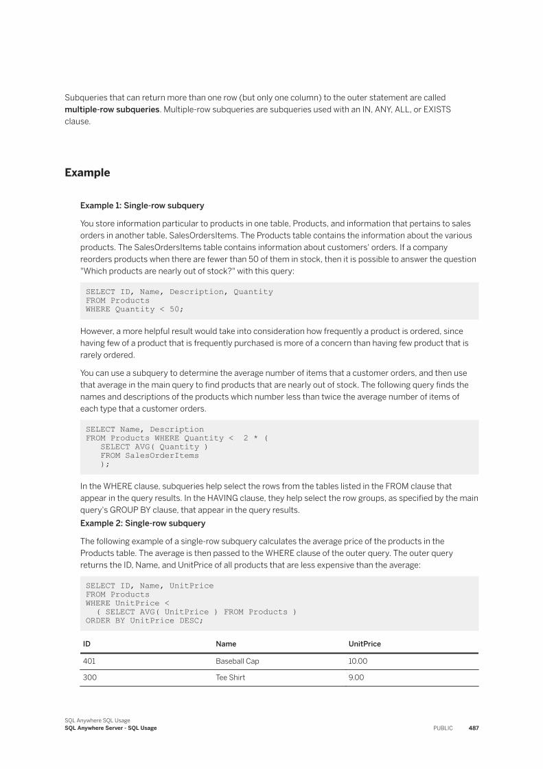
Subqueries that can return more than one row (but only one column) to the outer statement are called multiple-row subqueries. Multiple-row subqueries are subqueries used with an IN, ANY, ALL, or EXISTS clause.
Example
Example 1: Single-row subquery
You store information particular to products in one table, Products, and information that pertains to sales orders in another table, SalesOrdersItems. The Products table contains the information about the various products. The SalesOrdersItems table contains information about customers' orders. If a company reorders products when there are fewer than 50 of them in stock, then it is possible to answer the question "Which products are nearly out of stock?" with this query:
SELECT ID, Name, Description, Quantity FROM Products WHERE Quantity < 50;
However, a more helpful result would take into consideration how frequently a product is ordered, since having few of a product that is frequently purchased is more of a concern than having few product that is rarely ordered.
You can use a subquery to determine the average number of items that a customer orders, and then use that average in the main query to find products that are nearly out of stock. The following query finds the names and descriptions of the products which number less than twice the average number of items of each type that a customer orders.
SELECT Name, Description FROM Products WHERE Quantity < 2 * ( SELECT AVG( Quantity ) FROM SalesOrderItems );
In the WHERE clause, subqueries help select the rows from the tables listed in the FROM clause that appear in the query results. In the HAVING clause, they help select the row groups, as specified by the main query's GROUP BY clause, that appear in the query results.Example 2: Single-row subquery
The following example of a single-row subquery calculates the average price of the products in the Products table. The average is then passed to the WHERE clause of the outer query. The outer query returns the ID, Name, and UnitPrice of all products that are less expensive than the average:
SELECT ID, Name, UnitPrice FROM ProductsWHERE UnitPrice < ( SELECT AVG( UnitPrice ) FROM Products ) ORDER BY UnitPrice DESC;
ID Name UnitPrice
401 Baseball Cap 10.00
300 Tee Shirt 9.00
SQL Anywhere SQL UsageSQL Anywhere Server - SQL Usage PUBLIC 487
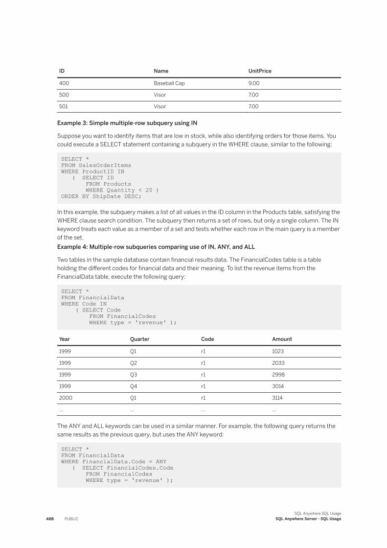
ID Name UnitPrice
400 Baseball Cap 9.00
500 Visor 7.00
501 Visor 7.00
Example 3: Simple multiple-row subquery using IN
Suppose you want to identify items that are low in stock, while also identifying orders for those items. You could execute a SELECT statement containing a subquery in the WHERE clause, similar to the following:
SELECT * FROM SalesOrderItemsWHERE ProductID IN ( SELECT ID FROM Products WHERE Quantity < 20 ) ORDER BY ShipDate DESC;
In this example, the subquery makes a list of all values in the ID column in the Products table, satisfying the WHERE clause search condition. The subquery then returns a set of rows, but only a single column. The IN keyword treats each value as a member of a set and tests whether each row in the main query is a member of the set.Example 4: Multiple-row subqueries comparing use of IN, ANY, and ALL
Two tables in the sample database contain financial results data. The FinancialCodes table is a table holding the different codes for financial data and their meaning. To list the revenue items from the FinancialData table, execute the following query:
SELECT * FROM FinancialDataWHERE Code IN ( SELECT Code FROM FinancialCodes WHERE type = 'revenue' );
Year Quarter Code Amount
1999 Q1 r1 1023
1999 Q2 r1 2033
1999 Q3 r1 2998
1999 Q4 r1 3014
2000 Q1 r1 3114
... ... ... ...
The ANY and ALL keywords can be used in a similar manner. For example, the following query returns the same results as the previous query, but uses the ANY keyword:
SELECT * FROM FinancialDataWHERE FinancialData.Code = ANY ( SELECT FinancialCodes.Code FROM FinancialCodes WHERE type = 'revenue' );
488 PUBLICSQL Anywhere SQL Usage
SQL Anywhere Server - SQL Usage
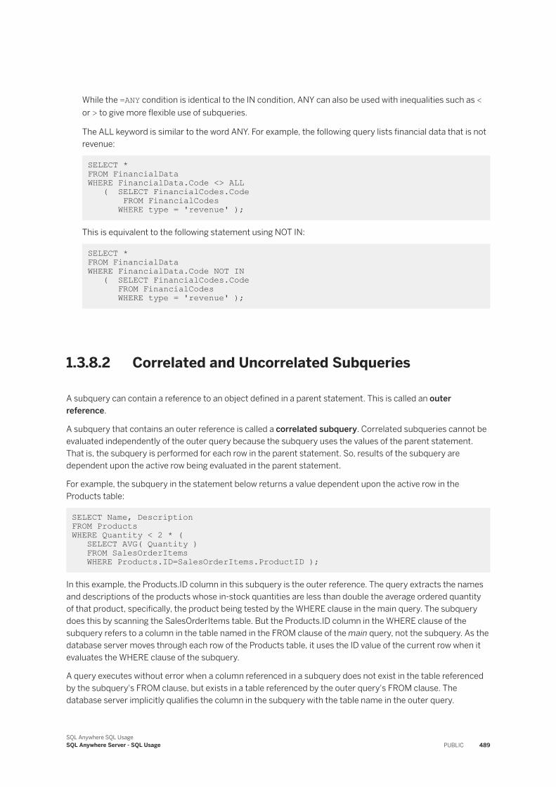
While the =ANY condition is identical to the IN condition, ANY can also be used with inequalities such as < or > to give more flexible use of subqueries.
The ALL keyword is similar to the word ANY. For example, the following query lists financial data that is not revenue:
SELECT * FROM FinancialDataWHERE FinancialData.Code <> ALL ( SELECT FinancialCodes.Code FROM FinancialCodes WHERE type = 'revenue' );
This is equivalent to the following statement using NOT IN:
SELECT * FROM FinancialDataWHERE FinancialData.Code NOT IN ( SELECT FinancialCodes.Code FROM FinancialCodes WHERE type = 'revenue' );
1.3.8.2 Correlated and Uncorrelated Subqueries
A subquery can contain a reference to an object defined in a parent statement. This is called an outer reference.
A subquery that contains an outer reference is called a correlated subquery. Correlated subqueries cannot be evaluated independently of the outer query because the subquery uses the values of the parent statement. That is, the subquery is performed for each row in the parent statement. So, results of the subquery are dependent upon the active row being evaluated in the parent statement.
For example, the subquery in the statement below returns a value dependent upon the active row in the Products table:
SELECT Name, Description FROM ProductsWHERE Quantity < 2 * ( SELECT AVG( Quantity ) FROM SalesOrderItems WHERE Products.ID=SalesOrderItems.ProductID );
In this example, the Products.ID column in this subquery is the outer reference. The query extracts the names and descriptions of the products whose in-stock quantities are less than double the average ordered quantity of that product, specifically, the product being tested by the WHERE clause in the main query. The subquery does this by scanning the SalesOrderItems table. But the Products.ID column in the WHERE clause of the subquery refers to a column in the table named in the FROM clause of the main query, not the subquery. As the database server moves through each row of the Products table, it uses the ID value of the current row when it evaluates the WHERE clause of the subquery.
A query executes without error when a column referenced in a subquery does not exist in the table referenced by the subquery's FROM clause, but exists in a table referenced by the outer query's FROM clause. The database server implicitly qualifies the column in the subquery with the table name in the outer query.
SQL Anywhere SQL UsageSQL Anywhere Server - SQL Usage PUBLIC 489
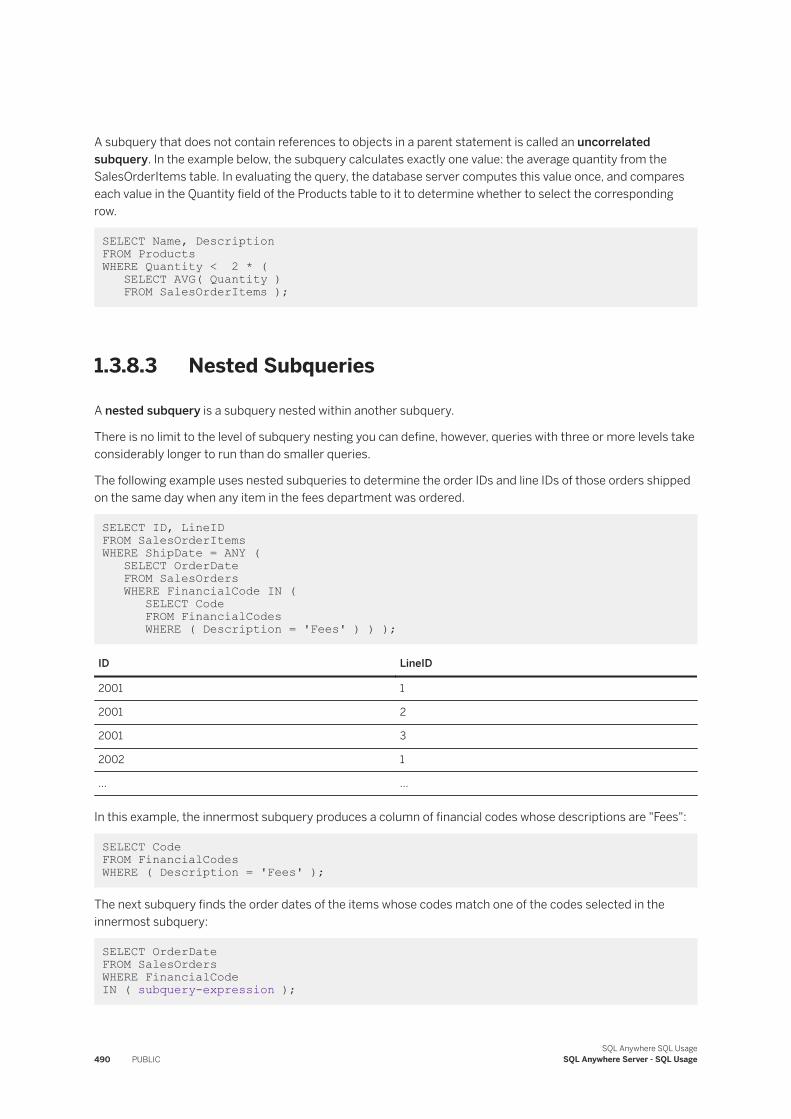
A subquery that does not contain references to objects in a parent statement is called an uncorrelated subquery. In the example below, the subquery calculates exactly one value: the average quantity from the SalesOrderItems table. In evaluating the query, the database server computes this value once, and compares each value in the Quantity field of the Products table to it to determine whether to select the corresponding row.
SELECT Name, Description FROM ProductsWHERE Quantity < 2 * ( SELECT AVG( Quantity ) FROM SalesOrderItems );
1.3.8.3 Nested Subqueries
A nested subquery is a subquery nested within another subquery.
There is no limit to the level of subquery nesting you can define, however, queries with three or more levels take considerably longer to run than do smaller queries.
The following example uses nested subqueries to determine the order IDs and line IDs of those orders shipped on the same day when any item in the fees department was ordered.
SELECT ID, LineID FROM SalesOrderItemsWHERE ShipDate = ANY ( SELECT OrderDate FROM SalesOrders WHERE FinancialCode IN ( SELECT Code FROM FinancialCodes WHERE ( Description = 'Fees' ) ) );
ID LineID
2001 1
2001 2
2001 3
2002 1
... ...
In this example, the innermost subquery produces a column of financial codes whose descriptions are "Fees":
SELECT Code FROM FinancialCodes WHERE ( Description = 'Fees' );
The next subquery finds the order dates of the items whose codes match one of the codes selected in the innermost subquery:
SELECT OrderDate FROM SalesOrdersWHERE FinancialCode IN ( subquery-expression );
490 PUBLICSQL Anywhere SQL Usage
SQL Anywhere Server - SQL Usage
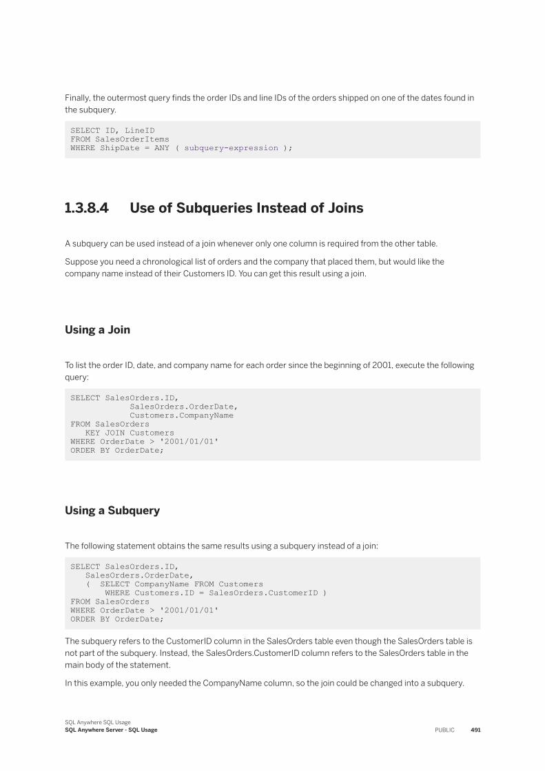
Finally, the outermost query finds the order IDs and line IDs of the orders shipped on one of the dates found in the subquery.
SELECT ID, LineID FROM SalesOrderItems WHERE ShipDate = ANY ( subquery-expression );
1.3.8.4 Use of Subqueries Instead of Joins
A subquery can be used instead of a join whenever only one column is required from the other table.
Suppose you need a chronological list of orders and the company that placed them, but would like the company name instead of their Customers ID. You can get this result using a join.
Using a Join
To list the order ID, date, and company name for each order since the beginning of 2001, execute the following query:
SELECT SalesOrders.ID, SalesOrders.OrderDate, Customers.CompanyNameFROM SalesOrders KEY JOIN CustomersWHERE OrderDate > '2001/01/01' ORDER BY OrderDate;
Using a Subquery
The following statement obtains the same results using a subquery instead of a join:
SELECT SalesOrders.ID, SalesOrders.OrderDate, ( SELECT CompanyName FROM Customers WHERE Customers.ID = SalesOrders.CustomerID )FROM SalesOrdersWHERE OrderDate > '2001/01/01' ORDER BY OrderDate;
The subquery refers to the CustomerID column in the SalesOrders table even though the SalesOrders table is not part of the subquery. Instead, the SalesOrders.CustomerID column refers to the SalesOrders table in the main body of the statement.
In this example, you only needed the CompanyName column, so the join could be changed into a subquery.
SQL Anywhere SQL UsageSQL Anywhere Server - SQL Usage PUBLIC 491
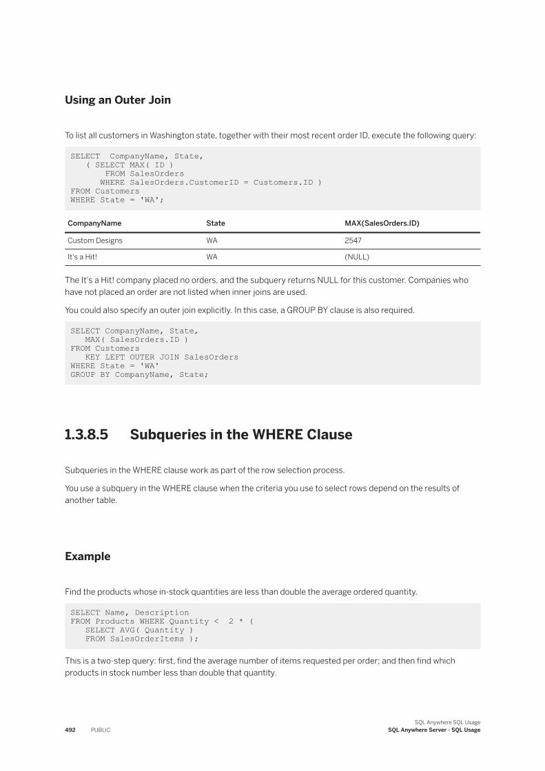
Using an Outer Join
To list all customers in Washington state, together with their most recent order ID, execute the following query:
SELECT CompanyName, State, ( SELECT MAX( ID ) FROM SalesOrders WHERE SalesOrders.CustomerID = Customers.ID )FROM Customers WHERE State = 'WA';
CompanyName State MAX(SalesOrders.ID)
Custom Designs WA 2547
It's a Hit! WA (NULL)
The It's a Hit! company placed no orders, and the subquery returns NULL for this customer. Companies who have not placed an order are not listed when inner joins are used.
You could also specify an outer join explicitly. In this case, a GROUP BY clause is also required.
SELECT CompanyName, State, MAX( SalesOrders.ID )FROM Customers KEY LEFT OUTER JOIN SalesOrdersWHERE State = 'WA' GROUP BY CompanyName, State;
1.3.8.5 Subqueries in the WHERE Clause
Subqueries in the WHERE clause work as part of the row selection process.
You use a subquery in the WHERE clause when the criteria you use to select rows depend on the results of another table.
Example
Find the products whose in-stock quantities are less than double the average ordered quantity.
SELECT Name, Description FROM Products WHERE Quantity < 2 * ( SELECT AVG( Quantity ) FROM SalesOrderItems );
This is a two-step query: first, find the average number of items requested per order; and then find which products in stock number less than double that quantity.
492 PUBLICSQL Anywhere SQL Usage
SQL Anywhere Server - SQL Usage
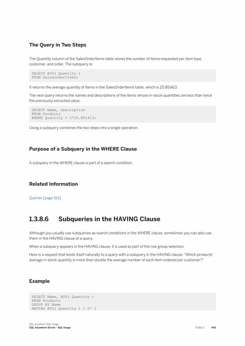
The Query in Two Steps
The Quantity column of the SalesOrderItems table stores the number of items requested per item type, customer, and order. The subquery is:
SELECT AVG( Quantity ) FROM SalesOrderItems;
It returns the average quantity of items in the SalesOrderItems table, which is 25.851413.
The next query returns the names and descriptions of the items whose in-stock quantities are less than twice the previously extracted value.
SELECT Name, Description FROM Products WHERE Quantity < 2*25.851413;
Using a subquery combines the two steps into a single operation.
Purpose of a Subquery in the WHERE Clause
A subquery in the WHERE clause is part of a search condition.
Related Information
Queries [page 162]
1.3.8.6 Subqueries in the HAVING Clause
Although you usually use subqueries as search conditions in the WHERE clause, sometimes you can also use them in the HAVING clause of a query.
When a subquery appears in the HAVING clause, it is used as part of the row group selection.
Here is a request that lends itself naturally to a query with a subquery in the HAVING clause: "Which products' average in-stock quantity is more than double the average number of each item ordered per customer?"
Example
SELECT Name, AVG( Quantity ) FROM ProductsGROUP BY NameHAVING AVG( Quantity ) > 2* (
SQL Anywhere SQL UsageSQL Anywhere Server - SQL Usage PUBLIC 493
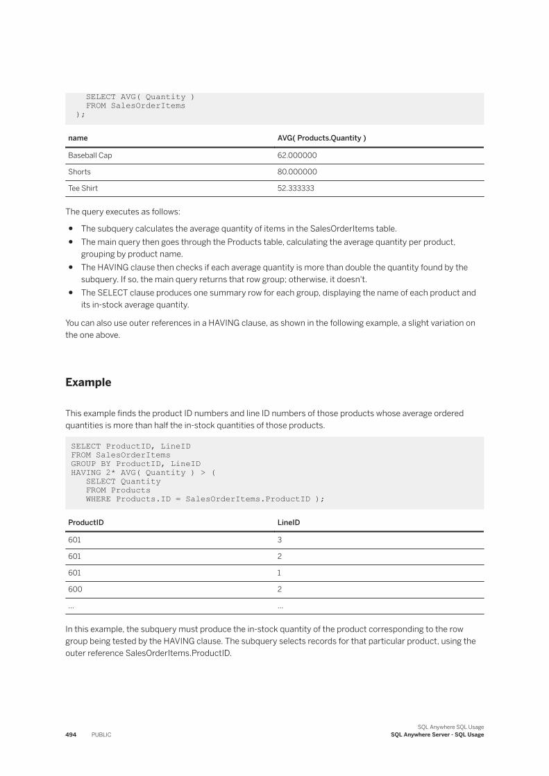
SELECT AVG( Quantity ) FROM SalesOrderItems );
name AVG( Products.Quantity )
Baseball Cap 62.000000
Shorts 80.000000
Tee Shirt 52.333333
The query executes as follows:
● The subquery calculates the average quantity of items in the SalesOrderItems table.● The main query then goes through the Products table, calculating the average quantity per product,
grouping by product name.● The HAVING clause then checks if each average quantity is more than double the quantity found by the
subquery. If so, the main query returns that row group; otherwise, it doesn't.● The SELECT clause produces one summary row for each group, displaying the name of each product and
its in-stock average quantity.
You can also use outer references in a HAVING clause, as shown in the following example, a slight variation on the one above.
Example
This example finds the product ID numbers and line ID numbers of those products whose average ordered quantities is more than half the in-stock quantities of those products.
SELECT ProductID, LineID FROM SalesOrderItemsGROUP BY ProductID, LineIDHAVING 2* AVG( Quantity ) > ( SELECT Quantity FROM Products WHERE Products.ID = SalesOrderItems.ProductID );
ProductID LineID
601 3
601 2
601 1
600 2
... ...
In this example, the subquery must produce the in-stock quantity of the product corresponding to the row group being tested by the HAVING clause. The subquery selects records for that particular product, using the outer reference SalesOrderItems.ProductID.
494 PUBLICSQL Anywhere SQL Usage
SQL Anywhere Server - SQL Usage
A Subquery with a Comparison Returns a Single Value
This query uses the comparison >, suggesting that the subquery must return exactly one value. In this case, it does. Since the ID field of the Products table is a primary key, there is only one record in the Products table corresponding to any particular product ID.
1.3.8.7 Predicates Using Subqueries
There are many search conditions supported in subqueries.
Comparison predicates using subqueries
Compares the value of an expression to a single value produced by the subquery for each record in the table(s) in the main query. Comparison tests use the operators (=, <>, <. <=, >, >=) provided with the subquery.Quantified comparison test
Compares the value of an expression to each of the set of values produced by a subquery.Subquery set membership test
Checks if the value of an expression matches one of the set of values produced by a subquery.Existence test
Checks if the subquery produces any rows.
In this section:
Subquery Comparison Ttest [page 496]The subquery comparison test (=, <>, <. <=, >, >=) is a modified version of the simple comparison test.
Subqueries and the IN Test [page 497]You can use the subquery set membership test to compare a value from the main query to more than one value in the subquery.
Subqueries and the ANY Test [page 498]The ANY test, used with one of the SQL comparison operators (=, >, <, >=, <=, !=, <>, !>, !<), compares a single value to the column of data values produced by the subquery.
Subqueries and the ALL Test [page 500]The ALL test is used with one of the SQL comparison operators (=, >, <, >=, <=, !=, <>, !>, !<) to compare a single value to the data values produced by the subquery.
Subqueries and the EXISTS Test [page 501]Subqueries used in the subquery comparison test and set membership test both return data values from the subquery table.
Related Information
Queries [page 162]
SQL Anywhere SQL UsageSQL Anywhere Server - SQL Usage PUBLIC 495
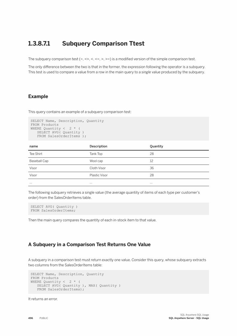
1.3.8.7.1 Subquery Comparison Ttest
The subquery comparison test (=, <>, <. <=, >, >=) is a modified version of the simple comparison test.
The only difference between the two is that in the former, the expression following the operator is a subquery. This test is used to compare a value from a row in the main query to a single value produced by the subquery.
Example
This query contains an example of a subquery comparison test:
SELECT Name, Description, Quantity FROM ProductsWHERE Quantity < 2 * ( SELECT AVG( Quantity ) FROM SalesOrderItems );
name Description Quantity
Tee Shirt Tank Top 28
Baseball Cap Wool cap 12
Visor Cloth Visor 36
Visor Plastic Visor 28
... ... ...
The following subquery retrieves a single value (the average quantity of items of each type per customer's order) from the SalesOrderItems table.
SELECT AVG( Quantity ) FROM SalesOrderItems;
Then the main query compares the quantity of each in-stock item to that value.
A Subquery in a Comparison Test Returns One Value
A subquery in a comparison test must return exactly one value. Consider this query, whose subquery extracts two columns from the SalesOrderItems table:
SELECT Name, Description, Quantity FROM ProductsWHERE Quantity < 2 * ( SELECT AVG( Quantity ), MAX( Quantity ) FROM SalesOrderItems);
It returns an error.
496 PUBLICSQL Anywhere SQL Usage
SQL Anywhere Server - SQL Usage
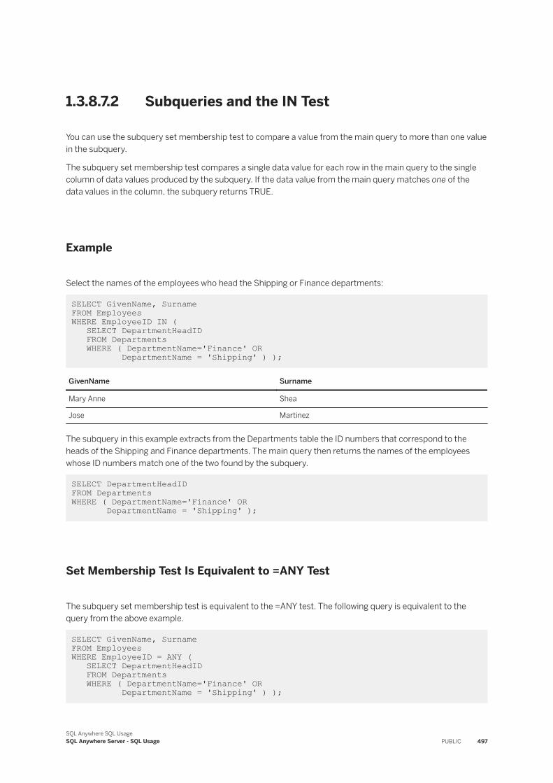
1.3.8.7.2 Subqueries and the IN Test
You can use the subquery set membership test to compare a value from the main query to more than one value in the subquery.
The subquery set membership test compares a single data value for each row in the main query to the single column of data values produced by the subquery. If the data value from the main query matches one of the data values in the column, the subquery returns TRUE.
Example
Select the names of the employees who head the Shipping or Finance departments:
SELECT GivenName, Surname FROM EmployeesWHERE EmployeeID IN ( SELECT DepartmentHeadID FROM Departments WHERE ( DepartmentName='Finance' OR DepartmentName = 'Shipping' ) );
GivenName Surname
Mary Anne Shea
Jose Martinez
The subquery in this example extracts from the Departments table the ID numbers that correspond to the heads of the Shipping and Finance departments. The main query then returns the names of the employees whose ID numbers match one of the two found by the subquery.
SELECT DepartmentHeadID FROM DepartmentsWHERE ( DepartmentName='Finance' OR DepartmentName = 'Shipping' );
Set Membership Test Is Equivalent to =ANY Test
The subquery set membership test is equivalent to the =ANY test. The following query is equivalent to the query from the above example.
SELECT GivenName, Surname FROM EmployeesWHERE EmployeeID = ANY ( SELECT DepartmentHeadID FROM Departments WHERE ( DepartmentName='Finance' OR DepartmentName = 'Shipping' ) );
SQL Anywhere SQL UsageSQL Anywhere Server - SQL Usage PUBLIC 497
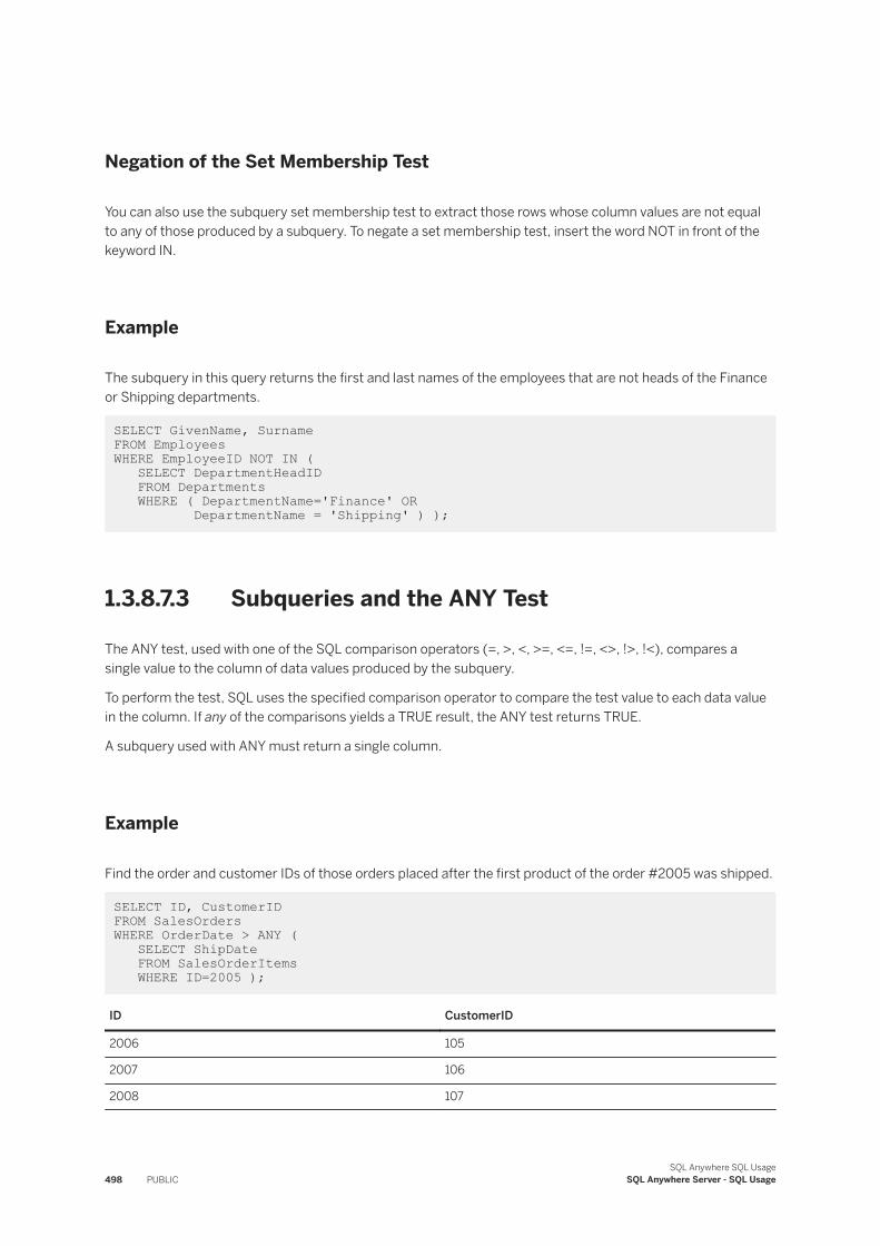
Negation of the Set Membership Test
You can also use the subquery set membership test to extract those rows whose column values are not equal to any of those produced by a subquery. To negate a set membership test, insert the word NOT in front of the keyword IN.
Example
The subquery in this query returns the first and last names of the employees that are not heads of the Finance or Shipping departments.
SELECT GivenName, Surname FROM EmployeesWHERE EmployeeID NOT IN ( SELECT DepartmentHeadID FROM Departments WHERE ( DepartmentName='Finance' OR DepartmentName = 'Shipping' ) );
1.3.8.7.3 Subqueries and the ANY Test
The ANY test, used with one of the SQL comparison operators (=, >, <, >=, <=, !=, <>, !>, !<), compares a single value to the column of data values produced by the subquery.
To perform the test, SQL uses the specified comparison operator to compare the test value to each data value in the column. If any of the comparisons yields a TRUE result, the ANY test returns TRUE.
A subquery used with ANY must return a single column.
Example
Find the order and customer IDs of those orders placed after the first product of the order #2005 was shipped.
SELECT ID, CustomerID FROM SalesOrdersWHERE OrderDate > ANY ( SELECT ShipDate FROM SalesOrderItems WHERE ID=2005 );
ID CustomerID
2006 105
2007 106
2008 107
498 PUBLICSQL Anywhere SQL Usage
SQL Anywhere Server - SQL Usage
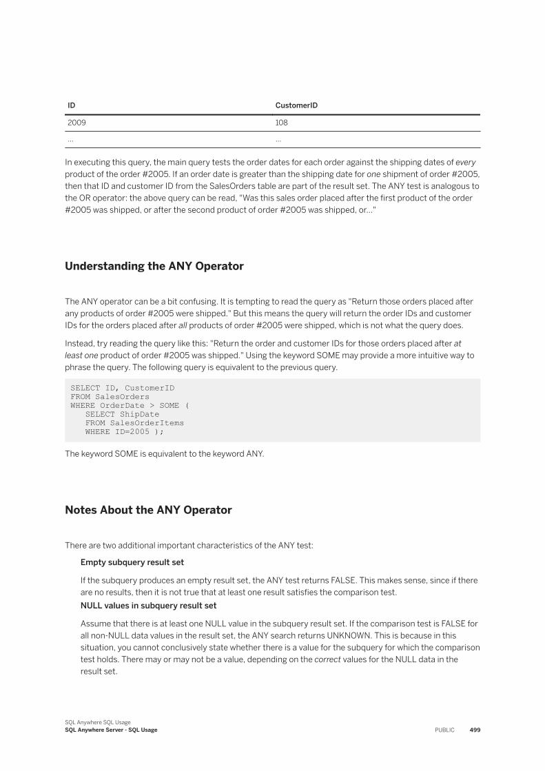
ID CustomerID
2009 108
... ...
In executing this query, the main query tests the order dates for each order against the shipping dates of every product of the order #2005. If an order date is greater than the shipping date for one shipment of order #2005, then that ID and customer ID from the SalesOrders table are part of the result set. The ANY test is analogous to the OR operator: the above query can be read, "Was this sales order placed after the first product of the order #2005 was shipped, or after the second product of order #2005 was shipped, or..."
Understanding the ANY Operator
The ANY operator can be a bit confusing. It is tempting to read the query as "Return those orders placed after any products of order #2005 were shipped." But this means the query will return the order IDs and customer IDs for the orders placed after all products of order #2005 were shipped, which is not what the query does.
Instead, try reading the query like this: "Return the order and customer IDs for those orders placed after at least one product of order #2005 was shipped." Using the keyword SOME may provide a more intuitive way to phrase the query. The following query is equivalent to the previous query.
SELECT ID, CustomerID FROM SalesOrdersWHERE OrderDate > SOME ( SELECT ShipDate FROM SalesOrderItems WHERE ID=2005 );
The keyword SOME is equivalent to the keyword ANY.
Notes About the ANY Operator
There are two additional important characteristics of the ANY test:
Empty subquery result set
If the subquery produces an empty result set, the ANY test returns FALSE. This makes sense, since if there are no results, then it is not true that at least one result satisfies the comparison test.NULL values in subquery result set
Assume that there is at least one NULL value in the subquery result set. If the comparison test is FALSE for all non-NULL data values in the result set, the ANY search returns UNKNOWN. This is because in this situation, you cannot conclusively state whether there is a value for the subquery for which the comparison test holds. There may or may not be a value, depending on the correct values for the NULL data in the result set.
SQL Anywhere SQL UsageSQL Anywhere Server - SQL Usage PUBLIC 499
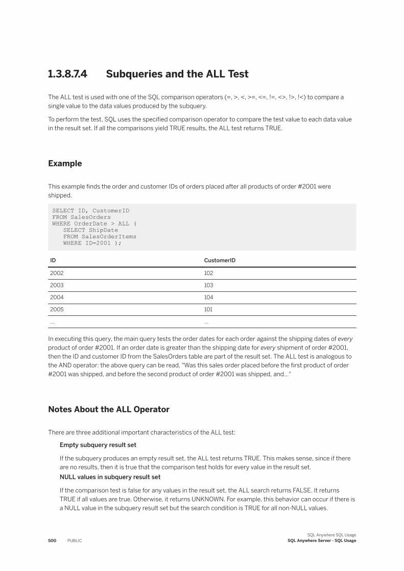
1.3.8.7.4 Subqueries and the ALL Test
The ALL test is used with one of the SQL comparison operators (=, >, <, >=, <=, !=, <>, !>, !<) to compare a single value to the data values produced by the subquery.
To perform the test, SQL uses the specified comparison operator to compare the test value to each data value in the result set. If all the comparisons yield TRUE results, the ALL test returns TRUE.
Example
This example finds the order and customer IDs of orders placed after all products of order #2001 were shipped.
SELECT ID, CustomerID FROM SalesOrdersWHERE OrderDate > ALL ( SELECT ShipDate FROM SalesOrderItems WHERE ID=2001 );
ID CustomerID
2002 102
2003 103
2004 104
2005 101
... ...
In executing this query, the main query tests the order dates for each order against the shipping dates of every product of order #2001. If an order date is greater than the shipping date for every shipment of order #2001, then the ID and customer ID from the SalesOrders table are part of the result set. The ALL test is analogous to the AND operator: the above query can be read, "Was this sales order placed before the first product of order #2001 was shipped, and before the second product of order #2001 was shipped, and..."
Notes About the ALL Operator
There are three additional important characteristics of the ALL test:
Empty subquery result set
If the subquery produces an empty result set, the ALL test returns TRUE. This makes sense, since if there are no results, then it is true that the comparison test holds for every value in the result set.NULL values in subquery result set
If the comparison test is false for any values in the result set, the ALL search returns FALSE. It returns TRUE if all values are true. Otherwise, it returns UNKNOWN. For example, this behavior can occur if there is a NULL value in the subquery result set but the search condition is TRUE for all non-NULL values.
500 PUBLICSQL Anywhere SQL Usage
SQL Anywhere Server - SQL Usage
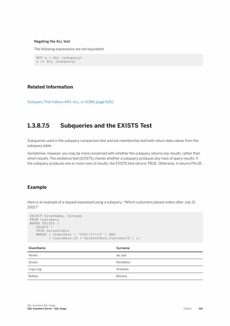
Negating the ALL test
The following expressions are not equivalent.
NOT a = ALL (subquery) a <> ALL (subquery)
Related Information
Subquery That Follows ANY, ALL, or SOME [page 505]
1.3.8.7.5 Subqueries and the EXISTS Test
Subqueries used in the subquery comparison test and set membership test both return data values from the subquery table.
Sometimes, however, you may be more concerned with whether the subquery returns any results, rather than which results. The existence test (EXISTS) checks whether a subquery produces any rows of query results. If the subquery produces one or more rows of results, the EXISTS test returns TRUE. Otherwise, it returns FALSE.
Example
Here is an example of a request expressed using a subquery: "Which customers placed orders after July 13, 2001?"
SELECT GivenName, Surname FROM CustomersWHERE EXISTS ( SELECT * FROM SalesOrders WHERE ( OrderDate > '2001-07-13' ) AND ( Customers.ID = SalesOrders.CustomerID ) );
GivenName Surname
Almen de Joie
Grover Pendelton
Ling Ling Andrews
Bubba Murphy
SQL Anywhere SQL UsageSQL Anywhere Server - SQL Usage PUBLIC 501
Explanation of the Existence Test
Here, for each row in the Customers table, the subquery checks if that customer ID corresponds to one that has placed an order after July 13, 2001. If it does, the query extracts the first and last names of that customer from the main table.
The EXISTS test does not use the results of the subquery; it just checks if the subquery produces any rows. So the existence test applied to the following two subqueries return the same results. These are subqueries and cannot be processed on their own, because they refer to the Customers table which is part of the main query, but not part of the subquery.
SELECT * FROM Customers, SalesOrdersWHERE ( OrderDate > '2001-07-13' ) AND ( Customers.ID = SalesOrders.CustomerID )SELECT OrderDateFROM Customers, SalesOrdersWHERE ( OrderDate > '2001-07-13' ) AND ( Customers.ID = SalesOrders.CustomerID );
It does not matter which columns from the SalesOrders table appear in the SELECT statement, though by convention, the "SELECT *" notation is used.
Negating the Existence Test
You can reverse the logic of the EXISTS test using the NOT EXISTS form. In this case, the test returns TRUE if the subquery produces no rows, and FALSE otherwise.
Correlated Subqueries
You may have noticed that the subquery contains a reference to the ID column from the Customers table. A reference to columns or expressions in the main table(s) is called an outer reference and the subquery is correlated. Conceptually, SQL processes the above query by going through the Customers table, and performing the subquery for each customer. If the order date in the SalesOrders table is after July 13, 2001, and the customer ID in the Customers and SalesOrders tables match, then the first and last names from the Customers table appear. Since the subquery references the main query, the subquery above, unlike those from previous sections, returns an error if you attempt to run it by itself.
Related Information
Correlated and Uncorrelated Subqueries [page 489]
502 PUBLICSQL Anywhere SQL Usage
SQL Anywhere Server - SQL Usage
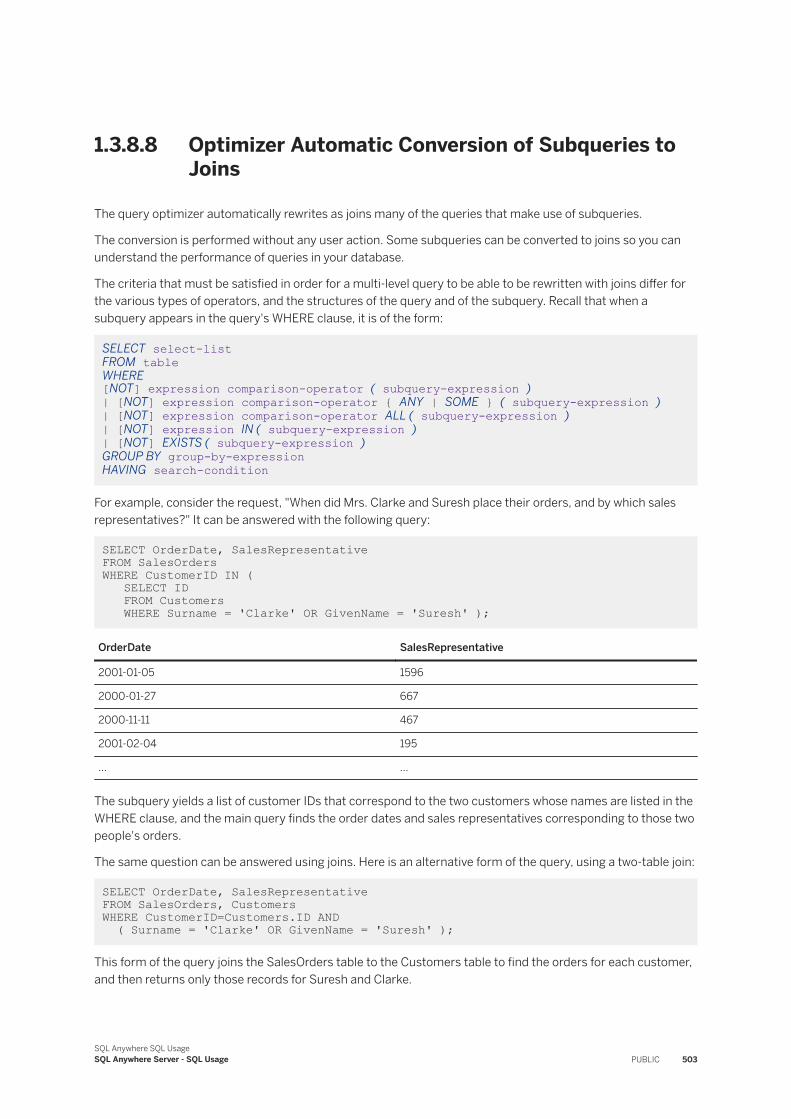
1.3.8.8 Optimizer Automatic Conversion of Subqueries to Joins
The query optimizer automatically rewrites as joins many of the queries that make use of subqueries.
The conversion is performed without any user action. Some subqueries can be converted to joins so you can understand the performance of queries in your database.
The criteria that must be satisfied in order for a multi-level query to be able to be rewritten with joins differ for the various types of operators, and the structures of the query and of the subquery. Recall that when a subquery appears in the query's WHERE clause, it is of the form:
SELECT select-list FROM table WHERE [NOT] expression comparison-operator ( subquery-expression ) | [NOT] expression comparison-operator { ANY | SOME } ( subquery-expression ) | [NOT] expression comparison-operator ALL ( subquery-expression ) | [NOT] expression IN ( subquery-expression ) | [NOT] EXISTS ( subquery-expression ) GROUP BY group-by-expression HAVING search-condition
For example, consider the request, "When did Mrs. Clarke and Suresh place their orders, and by which sales representatives?" It can be answered with the following query:
SELECT OrderDate, SalesRepresentative FROM SalesOrdersWHERE CustomerID IN ( SELECT ID FROM Customers WHERE Surname = 'Clarke' OR GivenName = 'Suresh' );
OrderDate SalesRepresentative
2001-01-05 1596
2000-01-27 667
2000-11-11 467
2001-02-04 195
... ...
The subquery yields a list of customer IDs that correspond to the two customers whose names are listed in the WHERE clause, and the main query finds the order dates and sales representatives corresponding to those two people's orders.
The same question can be answered using joins. Here is an alternative form of the query, using a two-table join:
SELECT OrderDate, SalesRepresentative FROM SalesOrders, CustomersWHERE CustomerID=Customers.ID AND ( Surname = 'Clarke' OR GivenName = 'Suresh' );
This form of the query joins the SalesOrders table to the Customers table to find the orders for each customer, and then returns only those records for Suresh and Clarke.
SQL Anywhere SQL UsageSQL Anywhere Server - SQL Usage PUBLIC 503
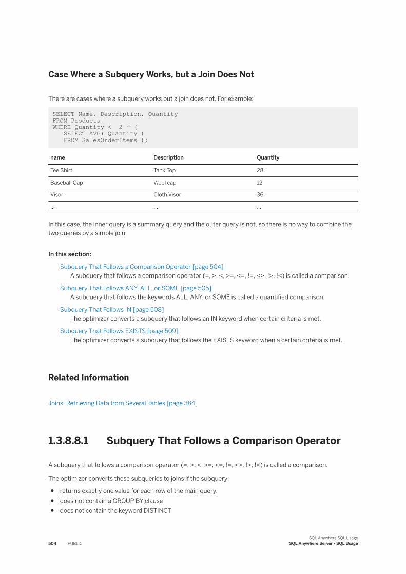
Case Where a Subquery Works, but a Join Does Not
There are cases where a subquery works but a join does not. For example:
SELECT Name, Description, Quantity FROM ProductsWHERE Quantity < 2 * ( SELECT AVG( Quantity ) FROM SalesOrderItems );
name Description Quantity
Tee Shirt Tank Top 28
Baseball Cap Wool cap 12
Visor Cloth Visor 36
... ... ...
In this case, the inner query is a summary query and the outer query is not, so there is no way to combine the two queries by a simple join.
In this section:
Subquery That Follows a Comparison Operator [page 504]A subquery that follows a comparison operator (=, >, <, >=, <=, !=, <>, !>, !<) is called a comparison.
Subquery That Follows ANY, ALL, or SOME [page 505]A subquery that follows the keywords ALL, ANY, or SOME is called a quantified comparison.
Subquery That Follows IN [page 508]The optimizer converts a subquery that follows an IN keyword when certain criteria is met.
Subquery That Follows EXISTS [page 509]The optimizer converts a subquery that follows the EXISTS keyword when a certain criteria is met.
Related Information
Joins: Retrieving Data from Several Tables [page 384]
1.3.8.8.1 Subquery That Follows a Comparison Operator
A subquery that follows a comparison operator (=, >, <, >=, <=, !=, <>, !>, !<) is called a comparison.
The optimizer converts these subqueries to joins if the subquery:
● returns exactly one value for each row of the main query.● does not contain a GROUP BY clause● does not contain the keyword DISTINCT
504 PUBLICSQL Anywhere SQL Usage
SQL Anywhere Server - SQL Usage
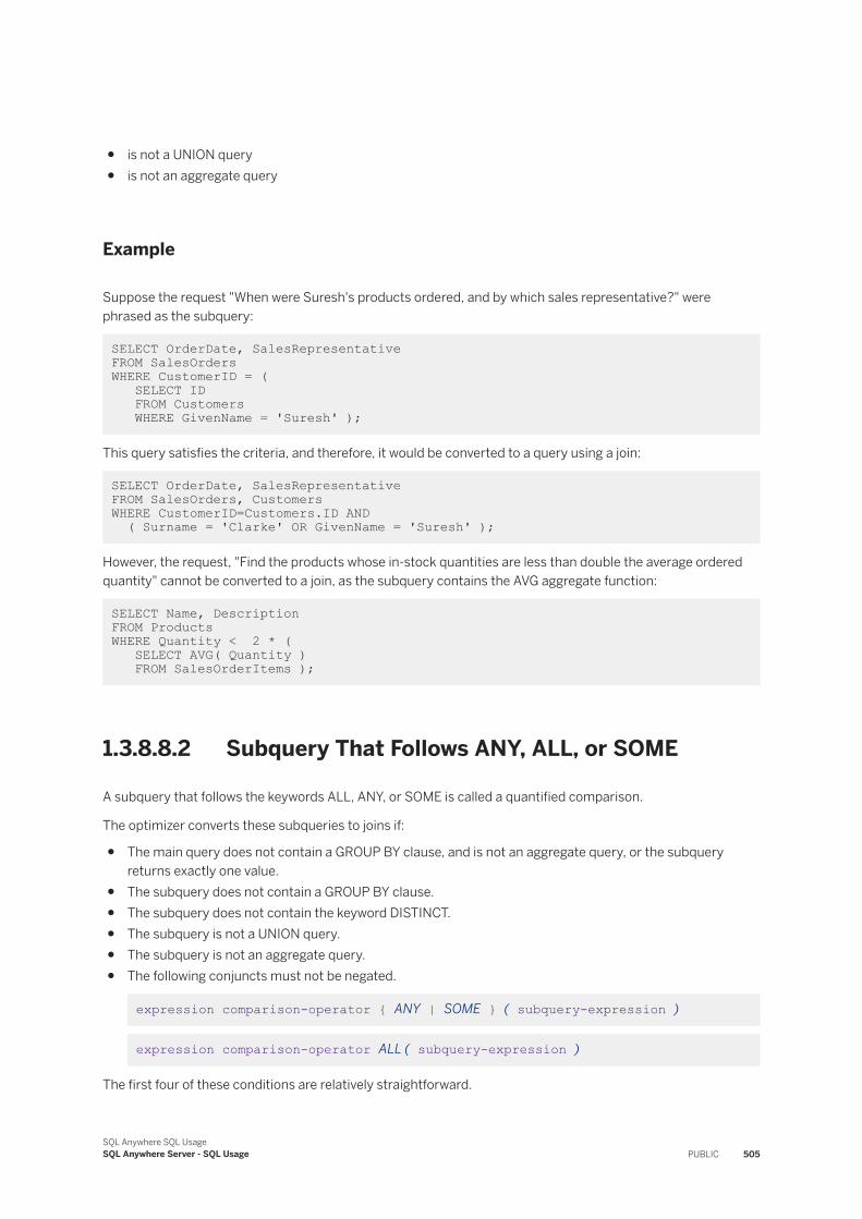
● is not a UNION query● is not an aggregate query
Example
Suppose the request "When were Suresh's products ordered, and by which sales representative?" were phrased as the subquery:
SELECT OrderDate, SalesRepresentative FROM SalesOrdersWHERE CustomerID = ( SELECT ID FROM Customers WHERE GivenName = 'Suresh' );
This query satisfies the criteria, and therefore, it would be converted to a query using a join:
SELECT OrderDate, SalesRepresentative FROM SalesOrders, CustomersWHERE CustomerID=Customers.ID AND ( Surname = 'Clarke' OR GivenName = 'Suresh' );
However, the request, "Find the products whose in-stock quantities are less than double the average ordered quantity" cannot be converted to a join, as the subquery contains the AVG aggregate function:
SELECT Name, Description FROM ProductsWHERE Quantity < 2 * ( SELECT AVG( Quantity ) FROM SalesOrderItems );
1.3.8.8.2 Subquery That Follows ANY, ALL, or SOME
A subquery that follows the keywords ALL, ANY, or SOME is called a quantified comparison.
The optimizer converts these subqueries to joins if:
● The main query does not contain a GROUP BY clause, and is not an aggregate query, or the subquery returns exactly one value.
● The subquery does not contain a GROUP BY clause.● The subquery does not contain the keyword DISTINCT.● The subquery is not a UNION query.● The subquery is not an aggregate query.● The following conjuncts must not be negated.
expression comparison-operator { ANY | SOME } ( subquery-expression )
expression comparison-operator ALL ( subquery-expression )
The first four of these conditions are relatively straightforward.
SQL Anywhere SQL UsageSQL Anywhere Server - SQL Usage PUBLIC 505
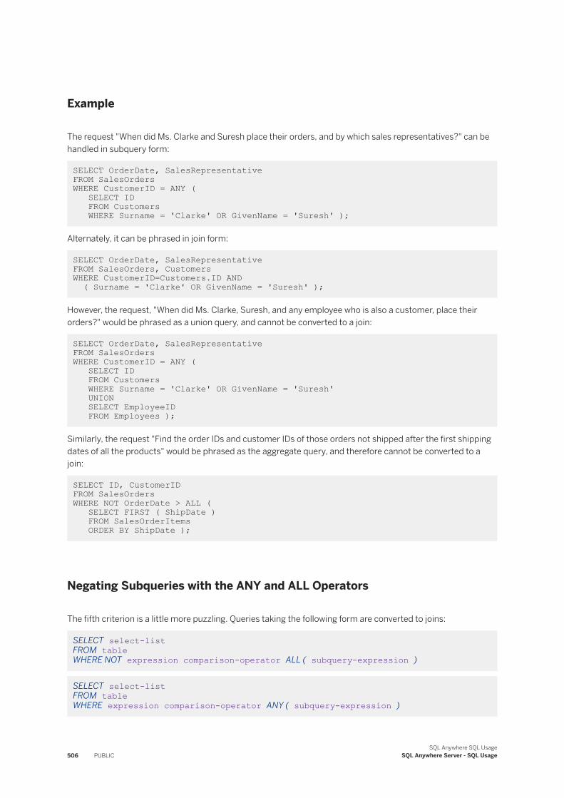
Example
The request "When did Ms. Clarke and Suresh place their orders, and by which sales representatives?" can be handled in subquery form:
SELECT OrderDate, SalesRepresentative FROM SalesOrdersWHERE CustomerID = ANY ( SELECT ID FROM Customers WHERE Surname = 'Clarke' OR GivenName = 'Suresh' );
Alternately, it can be phrased in join form:
SELECT OrderDate, SalesRepresentative FROM SalesOrders, CustomersWHERE CustomerID=Customers.ID AND ( Surname = 'Clarke' OR GivenName = 'Suresh' );
However, the request, "When did Ms. Clarke, Suresh, and any employee who is also a customer, place their orders?" would be phrased as a union query, and cannot be converted to a join:
SELECT OrderDate, SalesRepresentative FROM SalesOrdersWHERE CustomerID = ANY ( SELECT ID FROM Customers WHERE Surname = 'Clarke' OR GivenName = 'Suresh' UNION SELECT EmployeeID FROM Employees );
Similarly, the request "Find the order IDs and customer IDs of those orders not shipped after the first shipping dates of all the products" would be phrased as the aggregate query, and therefore cannot be converted to a join:
SELECT ID, CustomerID FROM SalesOrdersWHERE NOT OrderDate > ALL ( SELECT FIRST ( ShipDate ) FROM SalesOrderItems ORDER BY ShipDate );
Negating Subqueries with the ANY and ALL Operators
The fifth criterion is a little more puzzling. Queries taking the following form are converted to joins:
SELECT select-list FROM table WHERE NOT expression comparison-operator ALL ( subquery-expression )
SELECT select-list FROM table WHERE expression comparison-operator ANY ( subquery-expression )
506 PUBLICSQL Anywhere SQL Usage
SQL Anywhere Server - SQL Usage
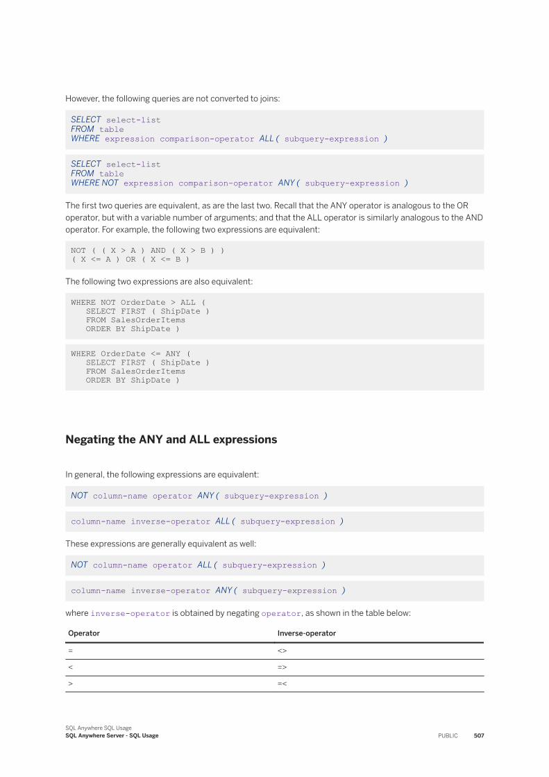
However, the following queries are not converted to joins:
SELECT select-list FROM table WHERE expression comparison-operator ALL ( subquery-expression )
SELECT select-list FROM table WHERE NOT expression comparison-operator ANY ( subquery-expression )
The first two queries are equivalent, as are the last two. Recall that the ANY operator is analogous to the OR operator, but with a variable number of arguments; and that the ALL operator is similarly analogous to the AND operator. For example, the following two expressions are equivalent:
NOT ( ( X > A ) AND ( X > B ) ) ( X <= A ) OR ( X <= B )
The following two expressions are also equivalent:
WHERE NOT OrderDate > ALL ( SELECT FIRST ( ShipDate ) FROM SalesOrderItems ORDER BY ShipDate )
WHERE OrderDate <= ANY ( SELECT FIRST ( ShipDate ) FROM SalesOrderItems ORDER BY ShipDate )
Negating the ANY and ALL expressions
In general, the following expressions are equivalent:
NOT column-name operator ANY ( subquery-expression )
column-name inverse-operator ALL ( subquery-expression )
These expressions are generally equivalent as well:
NOT column-name operator ALL ( subquery-expression )
column-name inverse-operator ANY ( subquery-expression )
where inverse-operator is obtained by negating operator, as shown in the table below:
Operator Inverse-operator
= <>
< =>
> =<
SQL Anywhere SQL UsageSQL Anywhere Server - SQL Usage PUBLIC 507
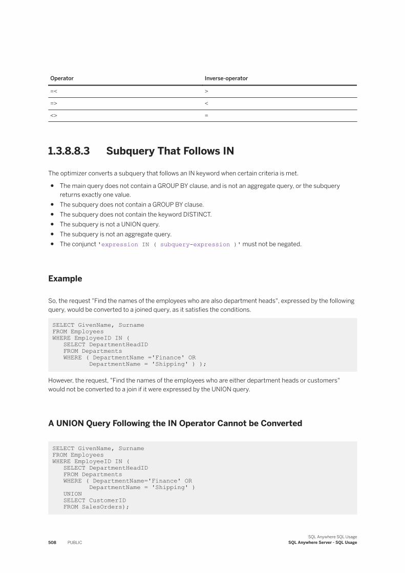
Operator Inverse-operator
=< >
=> <
<> =
1.3.8.8.3 Subquery That Follows IN
The optimizer converts a subquery that follows an IN keyword when certain criteria is met.
● The main query does not contain a GROUP BY clause, and is not an aggregate query, or the subquery returns exactly one value.
● The subquery does not contain a GROUP BY clause.● The subquery does not contain the keyword DISTINCT.● The subquery is not a UNION query.● The subquery is not an aggregate query.● The conjunct 'expression IN ( subquery-expression )' must not be negated.
Example
So, the request "Find the names of the employees who are also department heads", expressed by the following query, would be converted to a joined query, as it satisfies the conditions.
SELECT GivenName, Surname FROM EmployeesWHERE EmployeeID IN ( SELECT DepartmentHeadID FROM Departments WHERE ( DepartmentName ='Finance' OR DepartmentName = 'Shipping' ) );
However, the request, "Find the names of the employees who are either department heads or customers" would not be converted to a join if it were expressed by the UNION query.
A UNION Query Following the IN Operator Cannot be Converted
SELECT GivenName, Surname FROM EmployeesWHERE EmployeeID IN ( SELECT DepartmentHeadID FROM Departments WHERE ( DepartmentName='Finance' OR DepartmentName = 'Shipping' ) UNION SELECT CustomerID FROM SalesOrders);
508 PUBLICSQL Anywhere SQL Usage
SQL Anywhere Server - SQL Usage
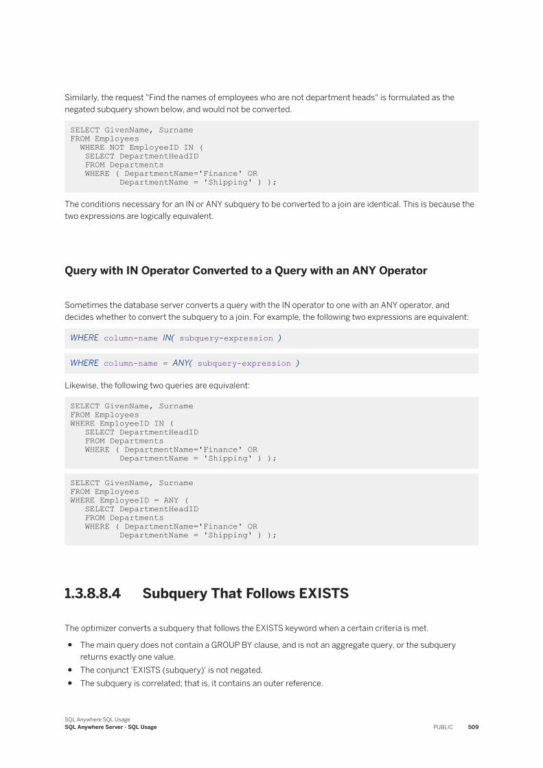
Similarly, the request "Find the names of employees who are not department heads" is formulated as the negated subquery shown below, and would not be converted.
SELECT GivenName, Surname FROM Employees WHERE NOT EmployeeID IN ( SELECT DepartmentHeadID FROM Departments WHERE ( DepartmentName='Finance' OR DepartmentName = 'Shipping' ) );
The conditions necessary for an IN or ANY subquery to be converted to a join are identical. This is because the two expressions are logically equivalent.
Query with IN Operator Converted to a Query with an ANY Operator
Sometimes the database server converts a query with the IN operator to one with an ANY operator, and decides whether to convert the subquery to a join. For example, the following two expressions are equivalent:
WHERE column-name IN( subquery-expression )
WHERE column-name = ANY( subquery-expression )
Likewise, the following two queries are equivalent:
SELECT GivenName, Surname FROM EmployeesWHERE EmployeeID IN ( SELECT DepartmentHeadID FROM Departments WHERE ( DepartmentName='Finance' OR DepartmentName = 'Shipping' ) );
SELECT GivenName, Surname FROM EmployeesWHERE EmployeeID = ANY ( SELECT DepartmentHeadID FROM Departments WHERE ( DepartmentName='Finance' OR DepartmentName = 'Shipping' ) );
1.3.8.8.4 Subquery That Follows EXISTS
The optimizer converts a subquery that follows the EXISTS keyword when a certain criteria is met.
● The main query does not contain a GROUP BY clause, and is not an aggregate query, or the subquery returns exactly one value.
● The conjunct 'EXISTS (subquery)' is not negated.● The subquery is correlated; that is, it contains an outer reference.
SQL Anywhere SQL UsageSQL Anywhere Server - SQL Usage PUBLIC 509
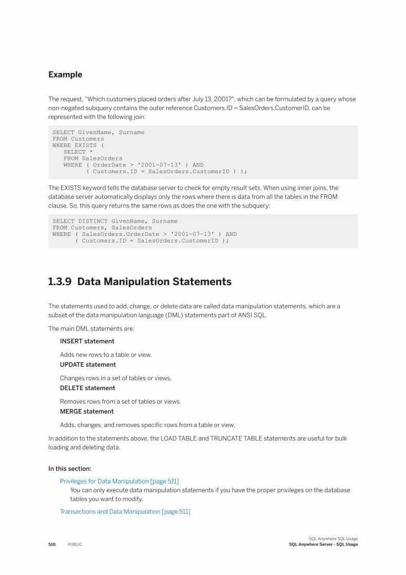
Example
The request, "Which customers placed orders after July 13, 2001?", which can be formulated by a query whose non-negated subquery contains the outer reference Customers.ID = SalesOrders.CustomerID, can be represented with the following join:
SELECT GivenName, Surname FROM CustomersWHERE EXISTS ( SELECT * FROM SalesOrders WHERE ( OrderDate > '2001-07-13' ) AND ( Customers.ID = SalesOrders.CustomerID ) );
The EXISTS keyword tells the database server to check for empty result sets. When using inner joins, the database server automatically displays only the rows where there is data from all the tables in the FROM clause. So, this query returns the same rows as does the one with the subquery:
SELECT DISTINCT GivenName, Surname FROM Customers, SalesOrdersWHERE ( SalesOrders.OrderDate > '2001-07-13' ) AND ( Customers.ID = SalesOrders.CustomerID );
1.3.9 Data Manipulation Statements
The statements used to add, change, or delete data are called data manipulation statements, which are a subset of the data manipulation language (DML) statements part of ANSI SQL.
The main DML statements are:
INSERT statement
Adds new rows to a table or view.UPDATE statement
Changes rows in a set of tables or views.DELETE statement
Removes rows from a set of tables or views.MERGE statement
Adds, changes, and removes specific rows from a table or view.
In addition to the statements above, the LOAD TABLE and TRUNCATE TABLE statements are useful for bulk loading and deleting data.
In this section:
Privileges for Data Manipulation [page 511]You can only execute data manipulation statements if you have the proper privileges on the database tables you want to modify.
Transactions and Data Manipulation [page 511]
510 PUBLICSQL Anywhere SQL Usage
SQL Anywhere Server - SQL Usage
When you modify data, the rollback log stores a copy of the old and new state of each row affected by each data manipulation statement.
Permanent Data Changes [page 512]Use the COMMIT statement after groups of statements that make sense together. The COMMIT statement makes database changes permanent.
Cancellation of Changes [page 512]Any uncommitted change you make can be canceled.
Transactions and Data Recovery [page 512]The integrity of your database is protected in the event of a system failure or power outage.
Addition of Data Using INSERT [page 513]Rows can be added to the database using the INSERT statement.
Data Changes Using UPDATE [page 520]The UPDATE statement specifies the row or rows you want changed, and the expressions to be used as the new values for specific columns in those rows.
Data Changes Using INSERT [page 525]You can use the ON EXISTING clause of the INSERT statement to update existing rows in a table (based on primary key lookup) with new values.
Deletion of Data Using DELETE [page 525]You can use the DELETE statements to remove data permanently from the database.
1.3.9.1 Privileges for Data Manipulation
You can only execute data manipulation statements if you have the proper privileges on the database tables you want to modify.
The database administrator and the owners of database objects use the GRANT and REVOKE statements to decide who has access to which data manipulation functions.
Privileges can be granted to individual users, roles, and user-extended roles.
1.3.9.2 Transactions and Data Manipulation
When you modify data, the rollback log stores a copy of the old and new state of each row affected by each data manipulation statement.
If you begin a transaction, realize you have made a mistake, and roll the transaction back, you restore the database to its previous condition.
Related Information
Transactions and Isolation Levels [page 771]
SQL Anywhere SQL UsageSQL Anywhere Server - SQL Usage PUBLIC 511
1.3.9.3 Permanent Data Changes
Use the COMMIT statement after groups of statements that make sense together. The COMMIT statement makes database changes permanent.
For example, to transfer money from one customer's account to another, you should add money to one customer's account, then delete it from the other's, and then commit, since in this case it does not make sense to leave your database with less or more money than it started with.
You can instruct Interactive SQL to commit your changes automatically by setting the auto_commit option to On. This is an Interactive SQL option. When auto_commit is set to On, Interactive SQL issues a COMMIT statement after every insert, update, and delete statement you make. This can slow down performance considerably. Therefore, it is a good idea to leave the auto_commit option set to Off.
NoteWhen trying the examples in this tutorial, be careful not to commit changes until you are sure that you want to change the database permanently.
1.3.9.4 Cancellation of Changes
Any uncommitted change you make can be canceled.
SQL allows you to undo all the changes you made since your last commit with the ROLLBACK statement. This statement undoes all changes you have made to the database since the last time you made changes permanent.
1.3.9.5 Transactions and Data Recovery
The integrity of your database is protected in the event of a system failure or power outage.
You have several different options for restoring your database server. For example, the transaction log file that the database server stores on a separate drive can be used to restore your data. When using a transaction log file for recovery, the database server does not need to update your database as frequently, and the performance of your database server is improved.
Transaction processing allows the database server to identify situations in which your data is in a consistent state. Transaction processing ensures that if, for any reason, a transaction is not successfully completed, then the entire transaction is undone, or rolled back. The database is left entirely unaffected by failed transactions.
The transaction processing in SQL Anywhere ensures that the contents of a transaction are processed securely, even in the event of a system failure in the middle of a transaction.
512 PUBLICSQL Anywhere SQL Usage
SQL Anywhere Server - SQL Usage
1.3.9.6 Addition of Data Using INSERT
Rows can be added to the database using the INSERT statement.
The INSERT statement has two forms: you can use the VALUES keyword or a SELECT statement:
INSERT Using Values
The VALUES keyword specifies values for some or all the columns in a new row. A simplified version of the syntax for the INSERT statement using the VALUES keyword is:
INSERT [ INTO ] table-name [ ( column-name, ... ) ] VALUES ( expression, ... )
You can omit the list of column names if you provide a value for each column in the table, in the order in which they appear when you execute a query using SELECT *.
INSERT from SELECT
You can use SELECT within an INSERT statement to pull values from one or more tables. If the table you are inserting data into has a large number of columns, you can also use WITH AUTO NAME to simplify the syntax. Using WITH AUTO NAME, you only need to specify the column names in the SELECT statement, rather than in both the INSERT and the SELECT statements. The names in the SELECT statement must be column references or aliased expressions.
A simplified version of the syntax for the INSERT statement using a select statement is:
INSERT [ INTO ] table-name [ WITH AUTO NAME ] select-statement
In this section:
Inserting Values into All Columns of a Row [page 514]Insert values into all the columns of a row using an INSERT statement.
Value Insertion into Specific Columns [page 515]Values are inserted into columns according to what is specified in the INSERT statement.
Addition of New Rows with SELECT [page 517]To pull values into a table from one or more other tables, you can use a SELECT clause in the INSERT statement.
Insertion of Documents and Images [page 518]To store documents or images in your database, you can write an application that reads the contents of the file into a variable, and supplies that variable as a value for an INSERT statement.
Advanced: Disk Allocation for Inserted Rows [page 519]You can control whether the disk allocation for inserted rows is contiguous or whether rows can be inserted in any order.
SQL Anywhere SQL UsageSQL Anywhere Server - SQL Usage PUBLIC 513
1.3.9.6.1 Inserting Values into All Columns of a Row
Insert values into all the columns of a row using an INSERT statement.
Prerequisites
You must have the INSERT object-level privilege on the table. If the ON EXISTING UPDATE clause is specified, UPDATE privilege on the table is also required.
Type the values in the same order as the column names in the original CREATE TABLE statement.
Surround the values with parentheses.
Enclose all character data in single quotes.
Use a separate INSERT statement for each row you add.
Procedure
Execute an INSERT statement that includes values for each column.
Results
The specified values are inserted into each column of a new row.
Example
The following INSERT statement adds a new row to the Departments table, giving a value for every column in the row:
INSERT INTO GROUPO.Departments VALUES ( 702, 'Eastern Sales', 902 );
514 PUBLICSQL Anywhere SQL Usage
SQL Anywhere Server - SQL Usage
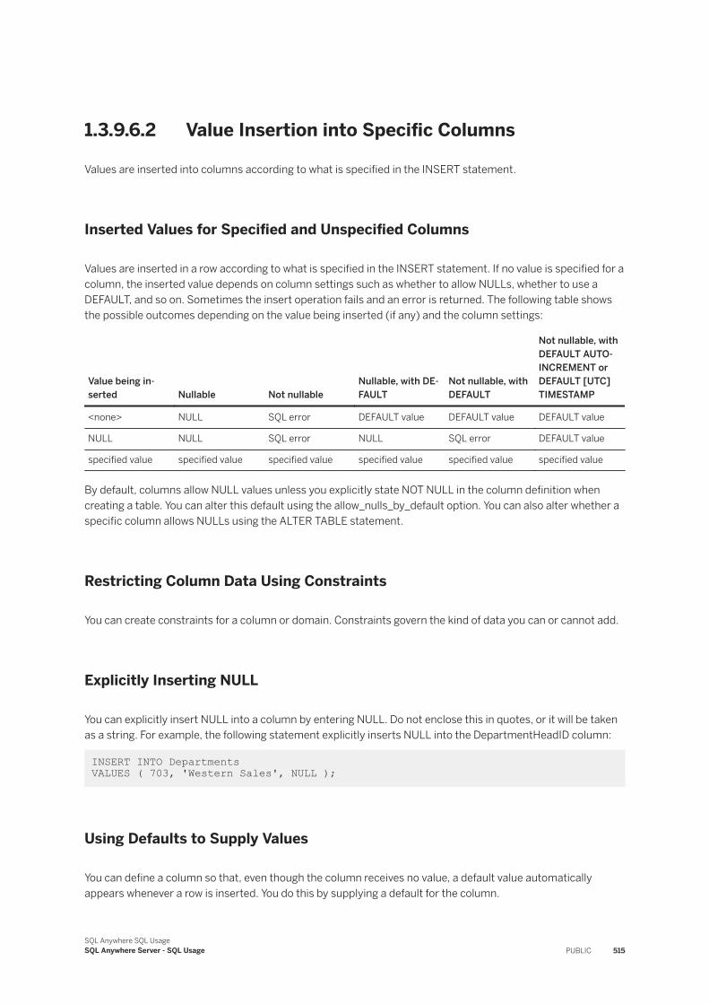
1.3.9.6.2 Value Insertion into Specific Columns
Values are inserted into columns according to what is specified in the INSERT statement.
Inserted Values for Specified and Unspecified Columns
Values are inserted in a row according to what is specified in the INSERT statement. If no value is specified for a column, the inserted value depends on column settings such as whether to allow NULLs, whether to use a DEFAULT, and so on. Sometimes the insert operation fails and an error is returned. The following table shows the possible outcomes depending on the value being inserted (if any) and the column settings:
Value being inserted Nullable Not nullable
Nullable, with DEFAULT
Not nullable, with DEFAULT
Not nullable, with DEFAULT AUTOINCREMENT or DEFAULT [UTC] TIMESTAMP
<none> NULL SQL error DEFAULT value DEFAULT value DEFAULT value
NULL NULL SQL error NULL SQL error DEFAULT value
specified value specified value specified value specified value specified value specified value
By default, columns allow NULL values unless you explicitly state NOT NULL in the column definition when creating a table. You can alter this default using the allow_nulls_by_default option. You can also alter whether a specific column allows NULLs using the ALTER TABLE statement.
Restricting Column Data Using Constraints
You can create constraints for a column or domain. Constraints govern the kind of data you can or cannot add.
Explicitly Inserting NULL
You can explicitly insert NULL into a column by entering NULL. Do not enclose this in quotes, or it will be taken as a string. For example, the following statement explicitly inserts NULL into the DepartmentHeadID column:
INSERT INTO Departments VALUES ( 703, 'Western Sales', NULL );
Using Defaults to Supply Values
You can define a column so that, even though the column receives no value, a default value automatically appears whenever a row is inserted. You do this by supplying a default for the column.
SQL Anywhere SQL UsageSQL Anywhere Server - SQL Usage PUBLIC 515
In this section:
Inserting Values into Specific Columns [page 516]Add data to specific columns in a row by specifying only those columns and their values.
Related Information
Table and Column Constraints [page 751]Column Defaults [page 744]
1.3.9.6.2.1 Inserting Values into Specific Columns
Add data to specific columns in a row by specifying only those columns and their values.
Prerequisites
You must have the INSERT object-level privilege on the table. If the ON EXISTING UPDATE clause is specified, UPDATE privilege on the table is also required.
Context
The column order you specify does not need to match the order of columns in the table, it must match the order in which you specify the values you are inserting.
Define all other columns not included in the column list to allow NULL or have defaults. If you skip a column that has a default value, the default appears in that column.
Procedure
Execute an INSERT INTO statement to add data to specific columns.
For example, the following statement adds data in only two columns, DepartmentID and DepartmentName:
INSERT INTO GROUPO.Departments ( DepartmentID, DepartmentName ) VALUES ( 703, 'Western Sales' );
DepartmentHeadID does not have a default value but accepts NULL. therefore a NULL is automatically assigned to that column.
516 PUBLICSQL Anywhere SQL Usage
SQL Anywhere Server - SQL Usage
Results
The data is inserted into the specified columns.
1.3.9.6.3 Addition of New Rows with SELECT
To pull values into a table from one or more other tables, you can use a SELECT clause in the INSERT statement.
The select clause can insert values into some or all of the columns in a row.
Inserting values for only some columns can be useful when you want to take some values from an existing table. Then, you can use the UPDATE statement to add the values for the other columns.
Before inserting values for only some of the columns in a table, make sure that either a default exists, or that you specify NULL for the columns into which you are not inserting values. Otherwise, an error appears.
When you insert rows from one table into another, the two tables must have compatible structures. That is, the matching columns must be either the same data types or data types between which the database server automatically converts.
Inserting Data into Some Columns
You can use the SELECT statement to add data to only some columns in a row just as you do with the VALUES clause. Simply specify the columns to which you want to add data in the INSERT clause.
Inserting Data from the Same Table
You can insert data into a table based on other data in the same table. Essentially, this means copying all or part of a row.
For example, you can insert new products, based on existing products, into the Products table. The following statement adds new Extra Large Tee Shirts (of Tank Top, V-neck, and Crew Neck varieties) into the Products table. The identification number is 30 greater than the existing sized shirt:
INSERT INTO Products SELECT ID + 30, Name, Description, 'Extra large', Color, 50, UnitPrice, NULLFROM Products WHERE Name = 'Tee Shirt';
SQL Anywhere SQL UsageSQL Anywhere Server - SQL Usage PUBLIC 517
Example
If the columns are in the same order in both tables, you do not need to specify column names in either table. For example, suppose you have a table named NewProducts that has the same schema as the Products table and contains some rows of product information that you want to add to the Products table. You could execute the following statement:
INSERT Products SELECT * FROM NewProducts;
1.3.9.6.4 Insertion of Documents and Images
To store documents or images in your database, you can write an application that reads the contents of the file into a variable, and supplies that variable as a value for an INSERT statement.
You can also use the xp_read_file system procedure to insert file contents into a table. This procedure is useful to insert file contents from Interactive SQL, or some other environment that does not provide a full programming language.
Example
In this example, you create a table, and insert an image into a column of the table. You can perform these steps from Interactive SQL.
1. Create a table to hold images.
CREATE TABLE Pictures ( C1 INT DEFAULT AUTOINCREMENT PRIMARY KEY, Filename VARCHAR(254), Picture LONG BINARY );
2. Insert the contents of portrait.gif, in the current working directory of the database server, into the table.
INSERT INTO Pictures ( Filename, Picture ) VALUES ( 'portrait.gif', xp_read_file( 'portrait.gif' ) );
Related Information
XML Import Using the OPENXML Operator [page 566]
518 PUBLICSQL Anywhere SQL Usage
SQL Anywhere Server - SQL Usage
1.3.9.6.5 Advanced: Disk Allocation for Inserted Rows
You can control whether the disk allocation for inserted rows is contiguous or whether rows can be inserted in any order.
SQL Anywhere Stores Rows Contiguously, If Possible
Every new row that is smaller than the page size of the database file is always stored on a single page. If no present page has enough free space for the new row, the database server writes the row to a new page. For example, if the new row requires 600 bytes of space but only 500 bytes are available on a partially filled page, then the database server places the row on a new page.
To make table pages more contiguous on the disk, the database server allocates table pages in blocks of eight pages. For example, when it needs to allocate a page it allocates eight pages, inserts the page in the block, and then fills up with the block with the next seven pages. In addition, it uses a free page bitmap to find contiguous blocks of pages within the dbspace, and performs sequential scans by reading groups of 64 KB, using the bitmap to find relevant pages. This leads to more efficient sequential scans.
SQL Anywhere May Store Rows in Any Order
The database server locates space on pages and inserts rows in the order it receives them in. It assigns each row to a page, but the locations it chooses in the table may not correspond to the order they were inserted in. For example, the database server may have to start a new page to store a long row contiguously. Should the next row be shorter, it may fit in an empty location on a previous page.
The rows of all tables are unordered. If the order that you receive or process the rows is important, use an ORDER BY clause in your SELECT statement to apply an ordering to the result. Applications that rely on the order of rows in a table can fail without warning.
If you frequently require the rows of a table to be in a particular order, consider creating an index on those columns specified in the query's ORDER BY clause.
Space Is Not Reserved for NULL Columns
By default, whenever the database server inserts a row, it reserves only the space necessary to store the row with the values it contains at the time of creation. It reserves no space to store values that are NULL or to accommodate fields, such as text strings, which may enlarge.
You can force the database server to reserve space by using the PCTFREE option when creating the table.
SQL Anywhere SQL UsageSQL Anywhere Server - SQL Usage PUBLIC 519
Once Inserted, Rows Identifiers Are Immutable
Once assigned a home position on a page, a row never moves from that page. If an update changes any of the values in the row so that it no longer fits in its assigned page, then the row splits and the extra information is inserted on another page.
This characteristic deserves special attention, especially since the database server allows no extra space when you insert the row. For example, suppose you insert a large number of empty rows into a table, then fill in the values, one column at a time, using UPDATE statements. The result would be that almost every value in a single row is stored on a separate page. To retrieve all the values from one row, the database server may need to read several disk pages. This simple operation would become extremely and unnecessarily slow.
You should consider filling new rows with data at the time of insertion. Once inserted, they then have enough room for the data you expect them to hold.
A Database File Never Shrinks
As you insert and delete rows from the database, the database server automatically reuses the space they occupy. So, the database server may insert a row into space formerly occupied by another row.
The database server keeps a record of the amount of empty space on each page. When you ask it to insert a new row, it first searches its record of space on existing pages. If it finds enough space on an existing page, it places the new row on that page, reorganizing the contents of the page if necessary. If not, it starts a new page.
Over time, if you delete several rows and do not insert new rows small enough to use the empty space, the information in the database may become sparse. You can reload the table, or use the REORGANIZE TABLE statement to defragment the table.
1.3.9.7 Data Changes Using UPDATE
The UPDATE statement specifies the row or rows you want changed, and the expressions to be used as the new values for specific columns in those rows.
You can use the UPDATE statement to change single rows, groups of rows, or all the rows in a table. Unlike the other data manipulation statements (INSERT, MERGE, and DELETE), the UPDATE statement can also modify rows in more than one table at the same time. In all cases, the execution of the UPDATE statement is atomic; either all of the rows are modified without error, or none of them are. For example, if one of the values being modified is the wrong data type, or if the new value causes a CHECK constraint violation, the UPDATE fails and the entire operation is rolled back.
UPDATE Syntax
A simplified version of the UPDATE statement syntax is:
UPDATE table-name
520 PUBLICSQL Anywhere SQL Usage
SQL Anywhere Server - SQL Usage
SET column_name = expression WHERE search-condition
If the company Newton Ent. (in the Customers table of the SQL Anywhere sample database) is taken over by Einstein, Inc., you can update the name of the company using a statement such as the following:
UPDATE Customers SET CompanyName = 'Einstein, Inc.' WHERE CompanyName = 'Newton Ent.';
You can use any expression in the WHERE clause. If you are not sure how the company name was spelled, you could try updating any company called Newton, with a statement such as the following:
UPDATE Customers SET CompanyName = 'Einstein, Inc.' WHERE CompanyName LIKE 'Newton%';
The search condition need not refer to the column being updated. The company ID for Newton Entertainments is 109. As the ID value is the primary key for the table, you could be sure of updating the correct row using the following statement:
UPDATE Customers SET CompanyName = 'Einstein, Inc.' WHERE ID = 109;
TipYou can also modify rows from the result set in Interactive SQL.
SET Clause
The SET clause specifies which columns are to be updated, and what their new values are. The WHERE clause determines the row or rows to be updated. If you do not have a WHERE clause, the specified columns of all rows are updated with the values given in the SET clause.
The expressions specified in a SET clause can be a constant literal, a host or SQL variable, a subquery, a special value such as CURRENT TIMESTAMP, an expression value pulled from another table, or any combination of these. You can also specify DEFAULT in a SET clause to denote the default value for that base table column. If the data type of the expression differs from the data type of the column to be modified, the database server automatically converts the expression to the column's type, if possible. If the conversion is not possible, a data exception results and the UPDATE statement fails.
You can use the SET clause to set the value of a variable, in addition to modifying column values. This example assigns a value to the variable @var in addition to updating table T:
UPDATE T SET @var = expression1, col1 = expression2 WHERE...;
This is roughly equivalent to the serial execution of a SELECT statement, followed by an UPDATE:
SELECT @var = expression1 FROM T
SQL Anywhere SQL UsageSQL Anywhere Server - SQL Usage PUBLIC 521
WHERE... ;UPDATE T SET col1 = expression2 WHERE...;
The advantage of variable assignment within an UPDATE statement is that the variable's value can be set within the execution of the statement while write locks are held, which prevents the assignment of unexpected values due to concurrent update activity from other connections.
WHERE Clause
The WHERE clause specifies which rows are to be updated by applying search-condition to the table or Cartesian product of table expressions specified in the UPDATE statement. For example, the following statement replaces the One Size Fits All Tee Shirt with an Extra Large Tee Shirt:
UPDATE Products SET Size = 'Extra Large'WHERE Name = 'Tee Shirt' AND Size = 'One Size Fits All';
Complex UPDATE Statements
More complex forms of the UPDATE statement permit updates over joins and other types of table expressions.
Consider the following syntax for the UPDATE statement:
UPDATE [ row-limitation ] table-name SET set-item[, ...] FROM table-expression [, ...] ] [ WHERE search-condition ] [ ORDER BY expression [ ASC | DESC ] , ...] [ OPTION( query-hint, ... ) ]
The semantics of this form of the UPDATE statement are to first compute a result set consisting of all combinations of rows from each table-expression, subsequently apply the search-condition in the WHERE clause, and then order the resulting rows using the ORDER BY clause. This computation results in the set of rows that will be modified. Each table-expression can consist of joins of base tables, views, and derived tables. The syntax permits the update of one or more tables with values from columns in other tables. The query optimizer may reorder the operations to create a more efficient execution strategy for the UPDATE statement.
If a base table row appears in a set of rows to be modified more than once, then the row is updated multiple times if the row's new values differ with each manipulation attempt. If a BEFORE ROW UPDATE trigger exists, the BEFORE ROW UPDATE trigger is fired for each individual row manipulation, subject to the trigger's UPDATE OF column-list clause. AFTER ROW UPDATE triggers are also fired with each row manipulation, but only if the row's values are actually changed, subject to the trigger's UPDATE OF column-list clause.
Triggers are fired for each updated table based on the type of the trigger and the value of the ORDER clause with each trigger definition. If an UPDATE statement modifies more than one table, however, the order in which the tables are updated is not guaranteed.
522 PUBLICSQL Anywhere SQL Usage
SQL Anywhere Server - SQL Usage
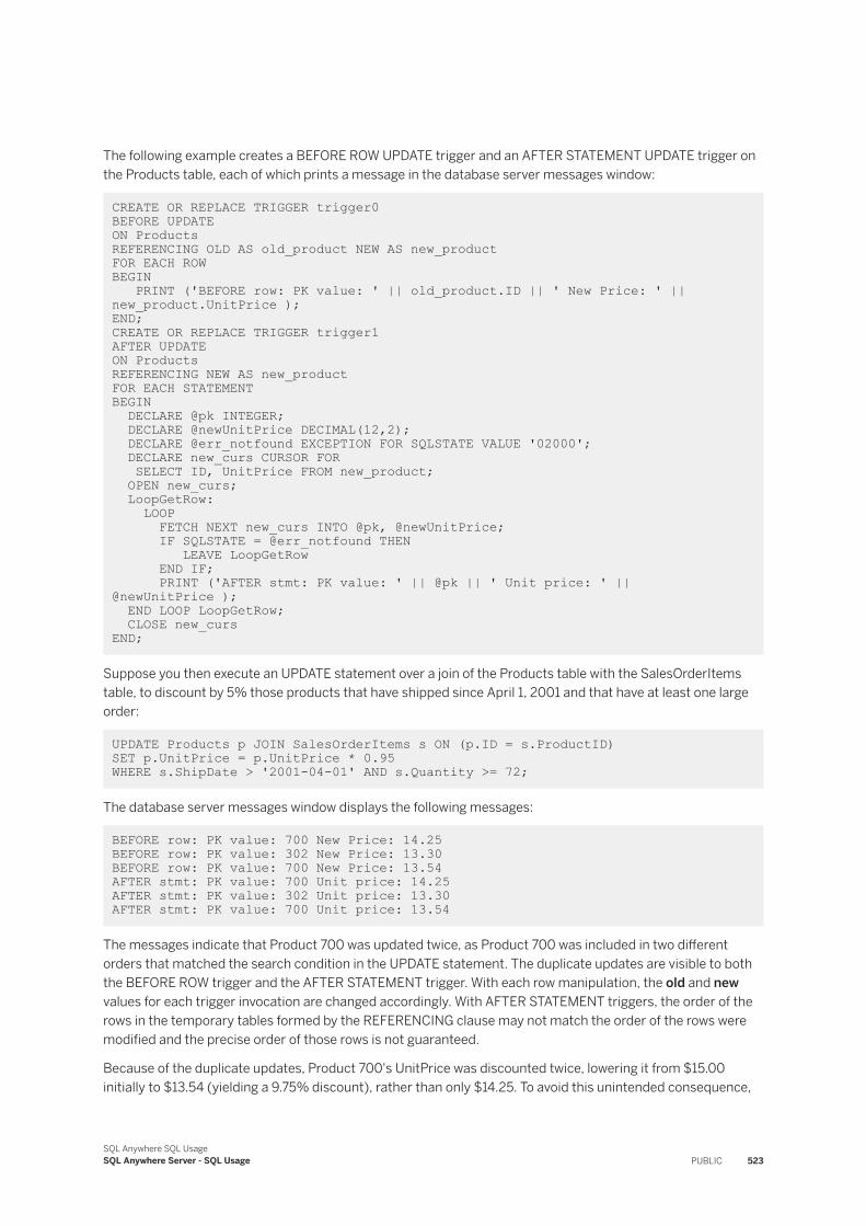
The following example creates a BEFORE ROW UPDATE trigger and an AFTER STATEMENT UPDATE trigger on the Products table, each of which prints a message in the database server messages window:
CREATE OR REPLACE TRIGGER trigger0 BEFORE UPDATE ON ProductsREFERENCING OLD AS old_product NEW AS new_product FOR EACH ROWBEGIN PRINT ('BEFORE row: PK value: ' || old_product.ID || ' New Price: ' || new_product.UnitPrice );END;CREATE OR REPLACE TRIGGER trigger1AFTER UPDATE ON ProductsREFERENCING NEW AS new_product FOR EACH STATEMENTBEGIN DECLARE @pk INTEGER; DECLARE @newUnitPrice DECIMAL(12,2); DECLARE @err_notfound EXCEPTION FOR SQLSTATE VALUE '02000'; DECLARE new_curs CURSOR FOR SELECT ID, UnitPrice FROM new_product; OPEN new_curs; LoopGetRow: LOOP FETCH NEXT new_curs INTO @pk, @newUnitPrice; IF SQLSTATE = @err_notfound THEN LEAVE LoopGetRow END IF; PRINT ('AFTER stmt: PK value: ' || @pk || ' Unit price: ' || @newUnitPrice ); END LOOP LoopGetRow; CLOSE new_curs END;
Suppose you then execute an UPDATE statement over a join of the Products table with the SalesOrderItems table, to discount by 5% those products that have shipped since April 1, 2001 and that have at least one large order:
UPDATE Products p JOIN SalesOrderItems s ON (p.ID = s.ProductID) SET p.UnitPrice = p.UnitPrice * 0.95 WHERE s.ShipDate > '2001-04-01' AND s.Quantity >= 72;
The database server messages window displays the following messages:
BEFORE row: PK value: 700 New Price: 14.25 BEFORE row: PK value: 302 New Price: 13.30BEFORE row: PK value: 700 New Price: 13.54AFTER stmt: PK value: 700 Unit price: 14.25AFTER stmt: PK value: 302 Unit price: 13.30 AFTER stmt: PK value: 700 Unit price: 13.54
The messages indicate that Product 700 was updated twice, as Product 700 was included in two different orders that matched the search condition in the UPDATE statement. The duplicate updates are visible to both the BEFORE ROW trigger and the AFTER STATEMENT trigger. With each row manipulation, the old and new values for each trigger invocation are changed accordingly. With AFTER STATEMENT triggers, the order of the rows in the temporary tables formed by the REFERENCING clause may not match the order of the rows were modified and the precise order of those rows is not guaranteed.
Because of the duplicate updates, Product 700's UnitPrice was discounted twice, lowering it from $15.00 initially to $13.54 (yielding a 9.75% discount), rather than only $14.25. To avoid this unintended consequence,
SQL Anywhere SQL UsageSQL Anywhere Server - SQL Usage PUBLIC 523
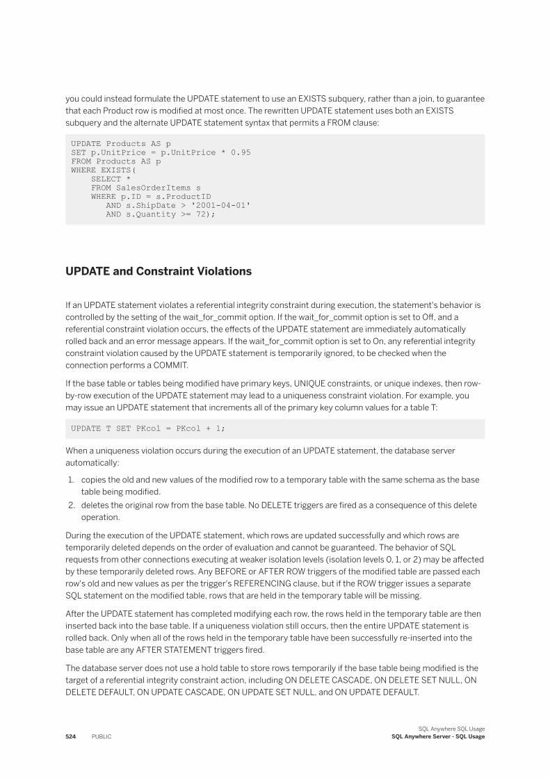
you could instead formulate the UPDATE statement to use an EXISTS subquery, rather than a join, to guarantee that each Product row is modified at most once. The rewritten UPDATE statement uses both an EXISTS subquery and the alternate UPDATE statement syntax that permits a FROM clause:
UPDATE Products AS p SET p.UnitPrice = p.UnitPrice * 0.95FROM Products AS pWHERE EXISTS( SELECT * FROM SalesOrderItems s WHERE p.ID = s.ProductID AND s.ShipDate > '2001-04-01' AND s.Quantity >= 72);
UPDATE and Constraint Violations
If an UPDATE statement violates a referential integrity constraint during execution, the statement's behavior is controlled by the setting of the wait_for_commit option. If the wait_for_commit option is set to Off, and a referential constraint violation occurs, the effects of the UPDATE statement are immediately automatically rolled back and an error message appears. If the wait_for_commit option is set to On, any referential integrity constraint violation caused by the UPDATE statement is temporarily ignored, to be checked when the connection performs a COMMIT.
If the base table or tables being modified have primary keys, UNIQUE constraints, or unique indexes, then row-by-row execution of the UPDATE statement may lead to a uniqueness constraint violation. For example, you may issue an UPDATE statement that increments all of the primary key column values for a table T:
UPDATE T SET PKcol = PKcol + 1;
When a uniqueness violation occurs during the execution of an UPDATE statement, the database server automatically:
1. copies the old and new values of the modified row to a temporary table with the same schema as the base table being modified.
2. deletes the original row from the base table. No DELETE triggers are fired as a consequence of this delete operation.
During the execution of the UPDATE statement, which rows are updated successfully and which rows are temporarily deleted depends on the order of evaluation and cannot be guaranteed. The behavior of SQL requests from other connections executing at weaker isolation levels (isolation levels 0, 1, or 2) may be affected by these temporarily deleted rows. Any BEFORE or AFTER ROW triggers of the modified table are passed each row's old and new values as per the trigger's REFERENCING clause, but if the ROW trigger issues a separate SQL statement on the modified table, rows that are held in the temporary table will be missing.
After the UPDATE statement has completed modifying each row, the rows held in the temporary table are then inserted back into the base table. If a uniqueness violation still occurs, then the entire UPDATE statement is rolled back. Only when all of the rows held in the temporary table have been successfully re-inserted into the base table are any AFTER STATEMENT triggers fired.
The database server does not use a hold table to store rows temporarily if the base table being modified is the target of a referential integrity constraint action, including ON DELETE CASCADE, ON DELETE SET NULL, ON DELETE DEFAULT, ON UPDATE CASCADE, ON UPDATE SET NULL, and ON UPDATE DEFAULT.
524 PUBLICSQL Anywhere SQL Usage
SQL Anywhere Server - SQL Usage
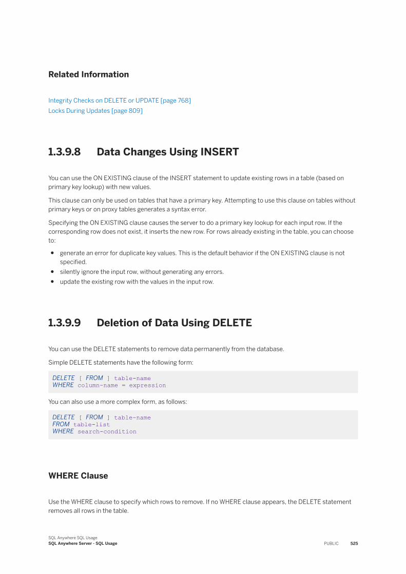
Related Information
Integrity Checks on DELETE or UPDATE [page 768]Locks During Updates [page 809]
1.3.9.8 Data Changes Using INSERT
You can use the ON EXISTING clause of the INSERT statement to update existing rows in a table (based on primary key lookup) with new values.
This clause can only be used on tables that have a primary key. Attempting to use this clause on tables without primary keys or on proxy tables generates a syntax error.
Specifying the ON EXISTING clause causes the server to do a primary key lookup for each input row. If the corresponding row does not exist, it inserts the new row. For rows already existing in the table, you can choose to:
● generate an error for duplicate key values. This is the default behavior if the ON EXISTING clause is not specified.
● silently ignore the input row, without generating any errors.● update the existing row with the values in the input row.
1.3.9.9 Deletion of Data Using DELETE
You can use the DELETE statements to remove data permanently from the database.
Simple DELETE statements have the following form:
DELETE [ FROM ] table-name WHERE column-name = expression
You can also use a more complex form, as follows:
DELETE [ FROM ] table-name FROM table-list WHERE search-condition
WHERE Clause
Use the WHERE clause to specify which rows to remove. If no WHERE clause appears, the DELETE statement removes all rows in the table.
SQL Anywhere SQL UsageSQL Anywhere Server - SQL Usage PUBLIC 525
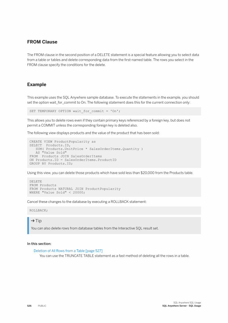
FROM Clause
The FROM clause in the second position of a DELETE statement is a special feature allowing you to select data from a table or tables and delete corresponding data from the first-named table. The rows you select in the FROM clause specify the conditions for the delete.
Example
This example uses the SQL Anywhere sample database. To execute the statements in the example, you should set the option wait_for_commit to On. The following statement does this for the current connection only:
SET TEMPORARY OPTION wait_for_commit = 'On';
This allows you to delete rows even if they contain primary keys referenced by a foreign key, but does not permit a COMMIT unless the corresponding foreign key is deleted also.
The following view displays products and the value of the product that has been sold:
CREATE VIEW ProductPopularity as SELECT Products.ID, SUM( Products.UnitPrice * SalesOrderItems.Quantity ) AS "Value Sold"FROM Products JOIN SalesOrderItemsON Products.ID = SalesOrderItems.ProductID GROUP BY Products.ID;
Using this view, you can delete those products which have sold less than $20,000 from the Products table.
DELETE FROM ProductsFROM Products NATURAL JOIN ProductPopularity WHERE "Value Sold" < 20000;
Cancel these changes to the database by executing a ROLLBACK statement:
ROLLBACK;
TipYou can also delete rows from database tables from the Interactive SQL result set.
In this section:
Deletion of All Rows from a Table [page 527]You can use the TRUNCATE TABLE statement as a fast method of deleting all the rows in a table.
526 PUBLICSQL Anywhere SQL Usage
SQL Anywhere Server - SQL Usage
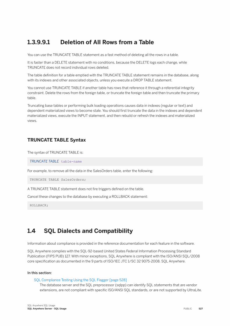
1.3.9.9.1 Deletion of All Rows from a Table
You can use the TRUNCATE TABLE statement as a fast method of deleting all the rows in a table.
It is faster than a DELETE statement with no conditions, because the DELETE logs each change, while TRUNCATE does not record individual rows deleted.
The table definition for a table emptied with the TRUNCATE TABLE statement remains in the database, along with its indexes and other associated objects, unless you execute a DROP TABLE statement.
You cannot use TRUNCATE TABLE if another table has rows that reference it through a referential integrity constraint. Delete the rows from the foreign table, or truncate the foreign table and then truncate the primary table.
Truncating base tables or performing bulk loading operations causes data in indexes (regular or text) and dependent materialized views to become stale. You should first truncate the data in the indexes and dependent materialized views, execute the INPUT statement, and then rebuild or refresh the indexes and materialized views.
TRUNCATE TABLE Syntax
The syntax of TRUNCATE TABLE is:
TRUNCATE TABLE table-name
For example, to remove all the data in the SalesOrders table, enter the following:
TRUNCATE TABLE SalesOrders;
A TRUNCATE TABLE statement does not fire triggers defined on the table.
Cancel these changes to the database by executing a ROLLBACK statement:
ROLLBACK;
1.4 SQL Dialects and Compatibility
Information about compliance is provided in the reference documentation for each feature in the software.
SQL Anywhere complies with the SQL-92-based United States Federal Information Processing Standard Publication (FIPS PUB) 127. With minor exceptions, SQL Anywhere is compliant with the ISO/ANSI SQL/2008 core specification as documented in the 9 parts of ISO/IEC JTC 1/SC 32 9075-2008. SQL Anywhere.
In this section:
SQL Compliance Testing Using the SQL Flagger [page 528]The database server and the SQL preprocessor (sqlpp) can identify SQL statements that are vendor extensions, are not compliant with specific ISO/ANSI SQL standards, or are not supported by UltraLite.
SQL Anywhere SQL UsageSQL Anywhere Server - SQL Usage PUBLIC 527

Features That Differ from Other SQL Implementations [page 530]There are several SQL features that differ from other SQL implementations.
Watcom SQL [page 535]The dialect of SQL supported by SQL Anywhere is referred to as Watcom SQL.
Transact-SQL Compatibility [page 535]SQL Anywhere supports a large subset of Transact-SQL, the dialect of SQL supported by SAP Adaptive Server Enterprise.
Comparison of SQL Anywhere with Adaptive Server Enterprise [page 538]Adaptive Server Enterprise and SQL Anywhere are complementary products, with architectures designed to suit their distinct purposes.
Transact-SQL-compatible Databases [page 542]You can eliminate some differences in behavior between SQL Anywhere and Adaptive Server Enterprise by selecting appropriate options when creating a database or when rebuilding an existing database.
Transact-SQL Compatible SQL Statements [page 550]Several considerations apply when writing SQL statements that work in Transact-SQL.
Transact-SQL Procedure Language [page 556]SQL Anywhere supports a large part of the Transact-SQL stored procedure language in addition to the Watcom SQL dialect based on the ISO/ANSI SQL standard.
Automatic Translation of Stored Procedures [page 558]SQL Anywhere provides aids for translating statements between the Watcom SQL and Transact-SQL dialects.
Result Sets Returned from Transact-SQL Procedures [page 559]SQL Anywhere uses a RESULT clause to specify returned result sets.
Variables in Transact-SQL Procedures [page 560]SQL Anywhere uses the SET statement to assign values to variables in a procedure.
Error Handling in Transact-SQL Procedures [page 561]Default procedure error handling is different in the Watcom SQL and Transact-SQL dialects.
1.4.1 SQL Compliance Testing Using the SQL FlaggerThe database server and the SQL preprocessor (sqlpp) can identify SQL statements that are vendor extensions, are not compliant with specific ISO/ANSI SQL standards, or are not supported by UltraLite.
This functionality is called the SQL Flagger, first introduced as optional ANSI/ISO SQL Language Feature F812 of the ISO/ANSI 9075-1999 SQL standard. The SQL Flagger helps an application developer to identify SQL language constructs that violate a specified subset of the SQL language. The SQL Flagger can also be used to ensure compliance with core features of a SQL standard, or compliance with a combination of core and optional features. The SQL Flagger can also be used when prototyping an UltraLite application with SQL Anywhere, to ensure that the SQL being used is supported by UltraLite.
As spatial data support is standardized as Part 3 of the SQL/MM standard (ISO/IEC 13249-3), spatial functions, operations, and syntax are not supported by the SQL Flagger and are flagged if they are not in the standard.
The SQL Flagger is intended to provide static, compile-time checking of compliance, although both syntactic and semantic elements of a SQL statement are candidates for analysis by the SQL Flagger. An example test of
528 PUBLICSQL Anywhere SQL Usage
SQL Anywhere Server - SQL Usage
syntactic compliance is the lack of the optional INTO keyword in an INSERT statement (for example, INSERT Products VALUES( ... )), which is a grammar extension to the SQL language. The use of an INSERT statement without the INTO keyword is flagged because the ANSI ANSI/ISO SQL Standard mandates the use of the INTO keyword. Note, however, that the INTO keyword is optional for UltraLite applications.
Key joins are also flagged as a vendor extension. A key join is used by default when the JOIN keyword is used without an ON clause. A key join uses existing foreign key relationships to join the tables. Key joins are not supported by UltraLite. For example, the following query specifies an implicit join condition between the Products and SalesOrderItems tables. This query is flagged by the SQL Flagger as a vendor extension.
SELECT * FROM Products JOIN SalesOrderItems;
SQL Flagger functionality is not dependent on the execution of a SQL statement; all flagging logic is done only as a static, compile-time process.
In this section:
Invocation of the SQL Flagger [page 529]Use the SQL Flagger to check a SQL statement, or a batch of SQL statements for compliance to a SQL standard.
Standards and Compatibility [page 530]The flagging functionality used in the database server and in the SQL preprocessor follows the SQL Flagger functionality defined in Part 1 (Framework) of the ANSI/ISO SQL Standard.
Related Information
Key Joins [page 415]
1.4.1.1 Invocation of the SQL Flagger
Use the SQL Flagger to check a SQL statement, or a batch of SQL statements for compliance to a SQL standard.
SQLFLAGGER function
The SQLFLAGGER function analyzes a single SQL statement, or batch, passed as a string argument, for compliance with a given SQL standard. The statement or batch is parsed, but not executed.sa_ansi_standard_packages system procedure
The sa_ansi_standard_packages system procedure analyzes a statement, or batch, for the use of optional SQL language features, or packages, from the ANSI SQL/2008, SQL/2003 or SQL/1999 international standards. The statement or batch is parsed, but not executed.sql_flagger_error_level and sql_flagger_warning_level options
The sql_flagger_error_level and sql_flagger_warning_level options invoke the SQL Flagger for any statement prepared or executed for the connection. If the statement does not comply with the option setting, which is a specific ANSI standard or UltraLite, the statement either terminates with an error
SQL Anywhere SQL UsageSQL Anywhere Server - SQL Usage PUBLIC 529
(SQLSTATE 0AW03), or returns a warning (SQLSTATE 01W07), depending upon the option setting. If the statement complies, statement execution proceeds normally.SQL preprocessor (sqlpp)
The SQL preprocessor (sqlpp) has the ability to flag static SQL statements in an Embedded SQL application at compile time. This feature can be especially useful when developing an UltraLite application, to verify SQL statements for UltraLite compatibility.
Related Information
Batches [page 120]
1.4.1.2 Standards and Compatibility
The flagging functionality used in the database server and in the SQL preprocessor follows the SQL Flagger functionality defined in Part 1 (Framework) of the ANSI/ISO SQL Standard.
The SQL Flagger supports the following ANSI SQL standards when determining the compliance of SQL language constructions:
● SQL/1992 Entry level, Intermediate level, and Full level● SQL/1999 Core, and SQL/1999 optional packages● SQL/2003 Core, and SQL/2003 optional packages● SQL/2008 Core, and SQL/2008 optional packages
NoteSQL Flagger support for SQL/1992 (all levels) is deprecated.
In addition, the SQL Flagger can identify statements that are not compliant with UltraLite SQL. For example, UltraLite has only limited abilities to CREATE and ALTER schema objects.
All SQL statements can be analyzed by the SQL Flagger. However, most statements that create or alter schema objects, including statements that create tables, indexes, materialized views, publications, subscriptions, and proxy tables, are vendor extensions to the ANSI SQL standards, and are flagged as non-conforming.
The SET OPTION statement, including its optional components, is never flagged for non-compliance with any SQL standard, or for compatibility with UltraLite.
1.4.2 Features That Differ from Other SQL Implementations
There are several SQL features that differ from other SQL implementations.
A rich SQL functionality is provided, including: per-row, per-statement, and INSTEAD OF triggers; SQL stored procedures and user-defined functions; RECURSIVE UNION queries; common table expressions; table
530 PUBLICSQL Anywhere SQL Usage
SQL Anywhere Server - SQL Usage
functions; LATERAL derived tables; integrated full-text search; window aggregate functions; regular-expression searching; XML support; materialized views; snapshot isolation; and referential integrity.
Dates
Date, time and timestamp types are provided that include a year, month and day, hour, minutes, seconds, and fraction of a second. For insertions or updates to date fields, or comparisons with date fields, a free format date is supported.
In addition, the following operations are allowed on dates:
date + integer
Add the specified number of days to a date.date - integer
Subtract the specified number of days from a date.date - date
Compute the number of days between two dates.date + time
Make a timestamp out of a date and time.
The INTERVAL data type, which is SQL Language Feature F052 of the ANSI/ISO SQL Standard, is not supported. However, many functions, such as DATEADD, are provided for manipulating dates and times.
Entity and Referential Integrity
Entity and referential integrity are supported via the PRIMARY KEY and FOREIGN KEY clauses of the CREATE TABLE and ALTER TABLE statements.
PRIMARY KEY [ CLUSTERED ] ( column-name [ ASC | DESC ], ... ) [NOT NULL] FOREIGN KEY [role-name] [(column-name [ ASC | DESC ], ...) ] REFERENCES table-name [(column-name, ...) ] [ MATCH [ UNIQUE | SIMPLE | FULL ] ] [ ON UPDATE [ CASCADE | RESTRICT | SET DEFAULT | SET NULL ] ] [ ON DELETE [ CASCADE | RESTRICT | SET DEFAULT | SET NULL ] ] [ CHECK ON COMMIT ] [ CLUSTERED ]
The PRIMARY KEY clause declares the primary key for the table. The database server then enforces the uniqueness of the primary key by creating a unique index over the primary key column(s). Two grammar extensions permit the customization of this index:
CLUSTERED
The CLUSTERED keyword signifies that the primary key index is a clustered index, and therefore adjacent index entries in the index point to physically adjacent rows in the table.ASC | DESC
The sortedness (ascending or descending) of each indexed column in the primary key index can be customized. This customization can be used to ensure that the sortedness of the primary key index
SQL Anywhere SQL UsageSQL Anywhere Server - SQL Usage PUBLIC 531
matches the sortedness required by specific SQL queries, as specified in those statements' ORDER BY clauses.
The FOREIGN KEY clause defines a relationship between two tables. This relationship is represented by a column (or columns) in this table that must contain values in the primary key of another table. The database server automatically constructs an index for each FOREIGN KEY defined to enforce the referential constraint. The semantics of the constraint, and physical characteristics of this index, can be customized as follows:
CLUSTERED
The CLUSTERED keyword signifies that the foreign key index is a clustered index, and therefore adjacent index entries in the index point to physically adjacent rows in the foreign table.ASC | DESC
The sortedness (ascending or descending) of each indexed column in the foreign key index can be customized. The sortedness of the foreign key index may differ from that of the primary key index. Sortedness customization can be used to ensure that the sortedness of the foreign key index matches the sortedness required by specific SQL queries in your application, as specified in those statements' ORDER BY clauses.MATCH clause
The MATCH clause, which is SQL language feature F741 of the ANSI/ISO SQL Standard, is supported, as well as MATCH UNIQUE, which enforces a one-to-one relationship between the primary and foreign tables without the need for an additional UNIQUE index.
Unique Indexes
Support is provided for the creation of unique indexes, sometimes called unique secondary indexes, over nullable columns. By default, each index key must be unique or contain a NULL in at least one column. For example, two index entries ('a', NULL) and ('a', NULL) are each considered unique index values. You can also have unique secondary indexes where NULL values are treated as special values in each domain. This is accomplished using the WITH NULLS NOT DISTINCT clause. With such an index, the two pairs of values ('a', NULL) and ('a', NULL) are considered duplicates.
Joins
You can use INNER, LEFT OUTER, RIGHT OUTER, and FULL OUTER joins. In addition to explicit join predicates, you can also use NATURAL joins and a vendor extension known as KEY joins, which specifies an implicit join predicate based on the tables' foreign key relationships.
CHAR, NCHAR, and BINARY Data Types
The database server does not distinguish between fixed- and varying-length string types (CHAR, NCHAR, or BINARY). It also does not truncate trailing blanks from string types when such values are inserted to the database. The database server distinguishes between the NULL value and the empty string. By default, the
532 PUBLICSQL Anywhere SQL Usage
SQL Anywhere Server - SQL Usage
database uses a case-insensitive collation to support case-insensitive string comparisons. Fixed-length string types are never blank-padded; rather, blank-padding semantics are simulated during the execution of each string comparison. These semantics may differ subtly from string comparisons with other SQL implementations.
UPDATE Statements
SQL Anywhere partially supports optional ANSI/ISO SQL Language Feature T111 that permits an UPDATE statement to refer to a view that contains a join. In addition, the UPDATE and UPDATE WHERE CURRENT OF statements permit more than one table to be referenced in the statement's SET clause, and the FROM clause of an UPDATE statement can be comprised of an arbitrary table expression containing joins and derived tables.
SQL Anywhere also allows the UPDATE, INSERT, MERGE, and DELETE statements to be embedded within another SQL statement as a derived table. One of the benefits of this support is that you can construct a query that returns the set of rows that has been modified by an UPDATE statement in a straightforward way.
Table Functions
SQL Anywhere lets you refer to the result set of a stored procedure as a table in a statement's FROM clause, a feature commonly referred to as table functions. Table functions are SQL language feature T326 of the ANSI/ISO SQL Standard. In the standard, table functions are specified using the TABLE keyword. In SQL Anywhere, use of the TABLE keyword is unnecessary; a stored procedure can be referenced directly in the FROM clause, optionally with a correlation name and a specification of schema of the result set returned by the procedure.
The following example joins the result of the stored procedure ShowCustomerProducts with the base table Products. Accompanying the stored procedure reference is an explicit declaration of the schema of the procedure's result, using the WITH clause:
SELECT sp.ident, sp.quantity, Products.name FROM ShowCustomerProducts( 149 ) WITH ( ident INT, description CHAR(20), quantity INT ) sp JOIN Products ON sp.ident = Products.ID
Materialized Views
SQL Anywhere supports materialized views, which are precomputed result sets that can be referenced directly or indirectly from within a SQL query. In SQL Anywhere, both immediately maintained and manually maintained views can be created using the CREATE MATERIALIZED VIEW statement. Other database products may use different terms to describe this functionality.
SQL Anywhere SQL UsageSQL Anywhere Server - SQL Usage PUBLIC 533
Cursors
SQL Anywhere supports optional ANSI/ISO SQL Language Feature F431 of the ANSI/ISO SQL Standard. In SQL Anywhere, all cursors are bi-directionally scrollable unless they are explicitly declared FORWARD ONLY, and applications can scroll through a cursor using either relative or absolute positioning with the FETCH statement or its equivalent with other application programming interfaces, such as ODBC.
SQL Anywhere supports value-sensitive and row-membership sensitive cursors. Commonly supported cursor types, including INSENSITIVE, KEYSET-DRIVEN, and SENSITIVE cursors, are supported. When using Embedded SQL, cursor positions can be moved arbitrarily on the FETCH statement. Cursors can be moved forward or backward relative to the current position or a given number of records from the beginning or end of the cursor.
By default, cursors in Embedded SQL and SQL procedures, user-defined functions, and triggers are updatable. They can be made explicitly updatable by using the FOR UPDATE clause. However, specifying the FOR UPDATE clause alone does not acquire any locks on the rows in the cursor's result set. To ensure that rows in the result set cannot be modified by other transactions, you can specify either:
FOR UPDATE BY LOCK
This clause causes the database server to acquire intent row locks on fetched rows of the result set. These are long-term locks that are held until the transaction is committed or rolled back.FOR UPDATE BY { VALUES | TIMESTAMP }
The SQL Anywhere database server uses a keyset-driven cursor to enable the application to be informed when rows have been modified or deleted as the result set is scrolled.
Alias References
SQL Anywhere permits aliased expressions in the SELECT list of a query to be referenced in other parts of the query. Most other SQL implementations and the ANSI/ISO SQL Standard do not allow this behavior. For example, you can specify the SQL query:
SELECT column-or-expression AS alias-name FROM table-reference WHERE alias-name = expression
Aliases can be used anywhere in the SELECT block, including other SELECT list expressions that in turn define additional aliases. Cyclic alias references are not permitted. If the alias specified for an expression is identical to the name of a column or variable in the name space of the SELECT block, the alias definition occludes the column or variable. Column names, however, can be explicitly qualified by table name in such cases.
Snapshot Isolation
SQL Anywhere supports snapshot isolation, which is also known as Multi-Version Concurrency Control, or MVCC. In other SQL implementations that support snapshot isolation, writer-writer conflicts - that is, concurrent updates by two or more transactions to the same row - are made apparent only at the time of
534 PUBLICSQL Anywhere SQL Usage
SQL Anywhere Server - SQL Usage
COMMIT. In such cases, usually the first COMMIT wins, and the other transactions involved in the conflict must abort.
In SQL Anywhere, write operations to rows cause write row locks to be acquired so that snapshot transactions can co-exist with transactions executing at ANSI isolation levels. Consequently, a writer-writer conflict in SQL Anywhere will result in blocking, though the precise behavior can be controlled through the BLOCKING and BLOCKING_TIMEOUT connection options.
Related Information
Key Joins [page 415]Materialized Views [page 64]Snapshot Isolation [page 779]
1.4.3 Watcom SQL
The dialect of SQL supported by SQL Anywhere is referred to as Watcom SQL.
The original version of SQL Anywhere was called Watcom SQL when it was introduced in 1992. The term Watcom SQL is still used to identify the dialect of SQL supported by SQL Anywhere.
SQL Anywhere also supports a large subset of Transact-SQL, the dialect of SQL supported by SAP Adaptive Server Enterprise.
Related Information
Transact-SQL Compatibility [page 535]
1.4.4 Transact-SQL Compatibility
SQL Anywhere supports a large subset of Transact-SQL, the dialect of SQL supported by SAP Adaptive Server Enterprise.
Goals
The goals of Transact-SQL support in SQL Anywhere are as follows:
Application portability
SQL Anywhere SQL UsageSQL Anywhere Server - SQL Usage PUBLIC 535
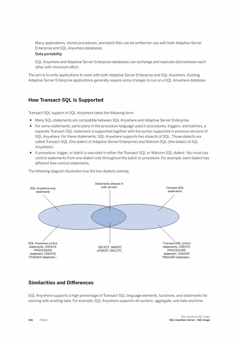
Many applications, stored procedures, and batch files can be written for use with both Adaptive Server Enterprise and SQL Anywhere databases.Data portability
SQL Anywhere and Adaptive Server Enterprise databases can exchange and replicate data between each other with minimum effort.
The aim is to write applications to work with both Adaptive Server Enterprise and SQL Anywhere. Existing Adaptive Server Enterprise applications generally require some changes to run on a SQL Anywhere database.
How Transact-SQL Is Supported
Transact-SQL support in SQL Anywhere takes the following form:
● Many SQL statements are compatible between SQL Anywhere and Adaptive Server Enterprise.● For some statements, particularly in the procedure language used in procedures, triggers, and batches, a
separate Transact-SQL statement is supported together with the syntax supported in previous versions of SQL Anywhere. For these statements, SQL Anywhere supports two dialects of SQL. Those dialects are called Transact-SQL (the dialect of Adaptive Server Enterprise) and Watcom SQL (the dialect of SQL Anywhere).
● A procedure, trigger, or batch is executed in either the Transact-SQL or Watcom SQL dialect. You must use control statements from one dialect only throughout the batch or procedure. For example, each dialect has different flow control statements.
The following diagram illustrates how the two dialects overlap.
Similarities and Differences
SQL Anywhere supports a high percentage of Transact-SQL language elements, functions, and statements for working with existing data. For example, SQL Anywhere supports all numeric, aggregate, and date and time
536 PUBLICSQL Anywhere SQL Usage
SQL Anywhere Server - SQL Usage
functions, and all but one string function. As another example, SQL Anywhere supports extended DELETE and UPDATE statements using joins.
Further, SQL Anywhere supports a high percentage of the Transact-SQL stored procedure language (CREATE PROCEDURE and CREATE TRIGGER syntax, control statements, and so on) and many aspects of Transact-SQL data definition language statements.
There are design differences in the architectural and configuration facilities supported by each product. Device management, user management, and maintenance tasks such as backups tend to be system-specific. Even here, SQL Anywhere provides Transact-SQL system tables as views, where the tables that are not meaningful in SQL Anywhere have no rows. Also, SQL Anywhere provides a set of system procedures for some common administrative tasks.
Transact-SQL Only
Some SQL statements supported by SQL Anywhere are part of one dialect, but not the other. You cannot mix the two dialects within a procedure, trigger, or batch. For example, SQL Anywhere supports the following statements, but as part of the Transact-SQL dialect only:
● Transact-SQL control statements IF and WHILE● Transact-SQL EXECUTE statement● Transact-SQL CREATE PROCEDURE and CREATE TRIGGER statements● Transact-SQL BEGIN TRANSACTION statement● SQL statements not separated by semicolons are part of a Transact-SQL procedure or batch
SQL Anywhere Only
Adaptive Server Enterprise does not support the following statements:
● LOOP and FOR control statements● SQL Anywhere versions of IF and WHILE● CALL statement● SIGNAL statement● SQL Anywhere versions of the CREATE PROCEDURE, CREATE FUNCTION, and CREATE TRIGGER
statements
Notes
The two dialects cannot be mixed within a procedure, trigger, or batch.
● You can include Transact-SQL-only statements together with statements that are part of both dialects in a batch, procedure, or trigger.
● You can include statements not supported by Adaptive Server Enterprise together with statements that are supported by both servers in a batch, procedure, or trigger.
SQL Anywhere SQL UsageSQL Anywhere Server - SQL Usage PUBLIC 537
● You cannot include Transact-SQL-only statements together with SQL Anywhere-only statements in a batch, procedure, or trigger.
1.4.5 Comparison of SQL Anywhere with Adaptive Server Enterprise
Adaptive Server Enterprise and SQL Anywhere are complementary products, with architectures designed to suit their distinct purposes.
SQL Anywhere includes Adaptive Server Enterprise-like tools for compatible database management.
In this section:
Servers and Databases in Adaptive Server Enterprise [page 538]The relationship between servers and databases is different in Adaptive Server Enterprise and SQL Anywhere.
Device Management in Adaptive Server Enterprise [page 539]SQL Anywhere and Adaptive Server Enterprise use different models for managing devices and disk space, reflecting the different uses for the two products.
Defaults and Rules in Adaptive Server Enterprise [page 539]SQL Anywhere does not support the Transact-SQL CREATE DEFAULT statement or CREATE RULE statement.
System Tables in Adaptive Server Enterprise [page 540]In addition to its own system tables, SQL Anywhere provides a set of system views that mimic relevant parts of the Adaptive Server Enterprise system tables.
Administrative Roles in Adaptive Server Enterprise [page 540]Adaptive Server Enterprise has a more elaborate set of administrative roles than SQL Anywhere.
Users and Groups in Adaptive Server Enterprise [page 541]SQL Anywhere supports several Adaptive Server Enterprise system procedures that manage users and groups.
1.4.5.1 Servers and Databases in Adaptive Server Enterprise
The relationship between servers and databases is different in Adaptive Server Enterprise and SQL Anywhere.
In Adaptive Server Enterprise, each database exists inside a server, and each server can contain several databases. Users can have login rights to the server, and can connect to the server. They can then use each database on that server for which they have permissions. System-wide system tables, held in a master database, contain information common to all databases on the server.
538 PUBLICSQL Anywhere SQL Usage
SQL Anywhere Server - SQL Usage
No master database in SQL Anywhere
In SQL Anywhere, there is no level corresponding to the Adaptive Server Enterprise master database. Instead, each database is an independent entity, containing all of its system tables. Users can have connection rights to a database, not to the server. When a user connects, they connect to an individual database. There is no system-wide set of system tables maintained at a master database level. Each SQL Anywhere database server can dynamically load and unload multiple databases, and users can maintain independent connections on each.
SQL Anywhere provides tools in its Transact-SQL support and in its Open Server support to allow some tasks to be performed in a manner similar to Adaptive Server Enterprise. For example, SQL Anywhere provides an implementation of the Adaptive Server Enterprise sp_addlogin system procedure that performs the nearest equivalent action: adding a user to a database.
File manipulation statements
SQL Anywhere does not support the Transact-SQL statements DUMP DATABASE and LOAD DATABASE for backing up and restoring. Instead, SQL Anywhere has its own BACKUP DATABASE and RESTORE DATABASE statements with different syntax.
1.4.5.2 Device Management in Adaptive Server Enterprise
SQL Anywhere and Adaptive Server Enterprise use different models for managing devices and disk space, reflecting the different uses for the two products.
While Adaptive Server Enterprise sets out a comprehensive resource management scheme using a variety of Transact-SQL statements, SQL Anywhere manages its own resources automatically, and its databases are regular operating system files.
SQL Anywhere does not support Transact-SQL DISK statements, such as DISK INIT, DISK MIRROR, DISK REFIT, DISK REINIT, DISK REMIRROR, and DISK UNMIRROR.
1.4.5.3 Defaults and Rules in Adaptive Server Enterprise
SQL Anywhere does not support the Transact-SQL CREATE DEFAULT statement or CREATE RULE statement.
The CREATE DOMAIN statement allows you to incorporate a default and a rule (called a CHECK condition) into the definition of a domain, and so provides similar functionality to the Transact-SQL CREATE DEFAULT and CREATE RULE statements.
In SQL Anywhere, a domain can have a default value and a CHECK condition associated with it, which are applied to all columns defined on that data type. You create the domain using the CREATE DOMAIN statement.
You can define default values and rules, or CHECK conditions, for individual columns using the CREATE TABLE statement or the ALTER TABLE statement.
SQL Anywhere SQL UsageSQL Anywhere Server - SQL Usage PUBLIC 539
In Adaptive Server Enterprise, the CREATE DEFAULT statement creates a named default. This default can be used as a default value for columns by binding the default to a particular column or as a default value for all columns of a domain by binding the default to the data type using the sp_bindefault system procedure. The CREATE RULE statement creates a named rule that can be used to define the domain for columns by binding the rule to a particular column or as a rule for all columns of a domain by binding the rule to the data type. A rule is bound to a data type or column using the sp_bindrule system procedure.
1.4.5.4 System Tables in Adaptive Server Enterprise
In addition to its own system tables, SQL Anywhere provides a set of system views that mimic relevant parts of the Adaptive Server Enterprise system tables.
The SQL Anywhere system tables rest entirely within each database, while the Adaptive Server Enterprise system tables rest partly inside each database and partly in the master database. The SQL Anywhere architecture does not include a master database.
In Adaptive Server Enterprise, the database owner (user dbo) owns the system tables. In SQL Anywhere, the system owner (user SYS) owns the system tables. The user dbo owns the Adaptive Server Enterprise-compatible system views provided by SQL Anywhere.
1.4.5.5 Administrative Roles in Adaptive Server Enterprise
Adaptive Server Enterprise has a more elaborate set of administrative roles than SQL Anywhere.
In Adaptive Server Enterprise there is a set of distinct roles, although more than one login account on an Adaptive Server Enterprise can be granted any role, and one account can possess more than one role.
Adaptive Server Enterprise Roles
In Adaptive Server Enterprise distinct roles include:
System Administrator
Responsible for general administrative tasks unrelated to specific applications; can access any database object.System Security Officer
Responsible for security-sensitive tasks in Adaptive Server Enterprise, but has no special permissions on database objects.Database Owner
Has full privileges on objects inside the database he or she owns, can add users to a database and grant other users the required privileges to create objects and execute statements within the database.Data definition statements
Privileges can be granted to users for specific data definition statements, such as CREATE TABLE or CREATE VIEW, enabling the user to create database objects.
540 PUBLICSQL Anywhere SQL Usage
SQL Anywhere Server - SQL Usage
Object owner
Each database object has an owner who may grant privileges to other users to access the object. The owner of an object automatically has all privileges on the object.
● The Database Administrator role has, like the Adaptive Server Enterprise database owner, full privileges on all objects inside the database (other than objects owned by SYS) and can grant other users the privileges required to create objects and execute statements within the database. The default database administrator is user DBA.
● The Resource role allows a user to create any kind of object within a database. This is instead of the Adaptive Server Enterprise scheme of granting permissions on individual CREATE statements.
● SQL Anywhere has object owners in the same way that Adaptive Server Enterprise does. The owner of an object automatically has all privileges on the object, including the right to grant privileges.
For seamless access to data held in both Adaptive Server Enterprise and SQL Anywhere, you should create user IDs with appropriate privileges in the database and create objects from that user ID. If you use the same user ID in each environment, object names and qualifiers can be identical in the two databases, ensuring compatible access.
1.4.5.6 Users and Groups in Adaptive Server Enterprise
SQL Anywhere supports several Adaptive Server Enterprise system procedures that manage users and groups.
System Procedure Description
sp_addlogin In Adaptive Server Enterprise, this adds a user to the server. In SQL Anywhere, this adds a user to a database.
sp_adduser In Adaptive Server Enterprise and SQL Anywhere, this adds a user to a database. While this is a distinct task from sp_addlogin in Adaptive Server Enterprise, in SQL Anywhere, they are the same.
sp_addgroup Adds a group to a database.
sp_changegroup Adds a user to a group, or moves a user from one group to another.
sp_droplogin In Adaptive Server Enterprise, removes a user from the server. In SQL Anywhere, removes a user from the database.
sp_dropuser Removes a user from the database.
sp_dropgroup Removes a group from the database.
In Adaptive Server Enterprise, login IDs are server-wide. In SQL Anywhere, users belong to individual databases.
Database Object Privileges
The Adaptive Server Enterprise and SQL Anywhere GRANT and REVOKE statements for granting privileges on individual database objects are very similar. Both allow SELECT, INSERT, DELETE, UPDATE, and REFERENCES
SQL Anywhere SQL UsageSQL Anywhere Server - SQL Usage PUBLIC 541
privileges on database tables and views, and UPDATE privilege on selected columns of database tables. Both allow EXECUTE privilege to be granted on stored procedures.
For example, the following statement is valid in both Adaptive Server Enterprise and SQL Anywhere:
GRANT INSERT, DELETE ON Employees TO MARY, SALES;
This statement grants the privileges required to use the INSERT and DELETE statements on the Employees table to user MARY and to the SALES group.
Both SQL Anywhere and Adaptive Server Enterprise support the WITH GRANT OPTION clause, allowing the recipient of privileges to grant them in turn, although SQL Anywhere does not permit WITH GRANT OPTION to be used on a GRANT EXECUTE statement. In SQL Anywhere, you can only specify WITH GRANT OPTION for users. Members of groups do not inherit the WITH GRANT OPTION if it is granted to a group.
Database-Wide Privileges
Adaptive Server Enterprise and SQL Anywhere use different models for database-wide privileges. SQL Anywhere employs a DBA role to allow a user full authority within a database. The System Administrator in Adaptive Server Enterprise enjoys this privilege for all databases on a server. However, the DBA role on a SQL Anywhere database is different from the permissions of an Adaptive Server Enterprise Database Owner, who must use the Adaptive Server Enterprise SETUSER statement to gain permissions on objects owned by other users.
1.4.6 Transact-SQL-compatible Databases
You can eliminate some differences in behavior between SQL Anywhere and Adaptive Server Enterprise by selecting appropriate options when creating a database or when rebuilding an existing database.
You can control other differences by setting connection level options using the SET TEMPORARY OPTION statement in SQL Anywhere or the SET statement in Adaptive Server Enterprise.
Make the Database Case Sensitive
By default, string comparisons in Adaptive Server Enterprise databases are case sensitive, while those in SQL Anywhere are case insensitive.
When building an Adaptive Server Enterprise-compatible database using SQL Anywhere, choose the case sensitive option.
● If you are using SQL Central, this option is in the Create Database Wizard.● If you are using the dbinit utility, specify the -c option.● If you are using the CREATE DATABASE statement, specify the CASE RESPECT clause.
542 PUBLICSQL Anywhere SQL Usage
SQL Anywhere Server - SQL Usage
Ignore Trailing Blanks in Comparisons
When building an Adaptive Server Enterprise-compatible database using SQL Anywhere, choose the option to ignore trailing blanks in comparisons.
● If you are using SQL Central, this option is in the Create Database Wizard.● If you are using the dbinit utility, specify the -b option.● If you are using the CREATE DATABASE statement, specify the BLANK PADDING ON clause.
When you choose this option, Adaptive Server Enterprise and SQL Anywhere considers the following two strings equal:
'ignore the trailing blanks ' 'ignore the trailing blanks'
If you do not choose this option, SQL Anywhere considers the two strings above different.
A side effect of choosing this option is that strings are padded with blanks when fetched by a client application.
Remove Historical System Views
Older versions of SQL Anywhere employed two system views whose names conflict with the Adaptive Server Enterprise system views provided for compatibility. These views are SYSCOLUMNS and SYSINDEXES. If you are using Open Client or JDBC interfaces, create your database excluding these views. You can do this with the dbinit -k option.
If you do not use this option when creating your database, executing the statement SELECT * FROM SYSCOLUMNS; results in the error SQLE_AMBIGUOUS_TABLE_NAME.
In this section:
Creating a Transact-SQL-compatible Database (SQL Central) [page 544]Use SQL Central to create a Transact-SQL-compatible database.
Creating a Transact-SQL-compatible Database (Command Line) [page 544]Use the Initialization Utility (dbinit) to create a Transact-SQL-compatible database.
Creating a Transact-SQL-compatible Database (SQL) [page 545]Use the CREATE DATABASE statement to create a Transact-SQL-compatible database.
Options for Transact-SQL Compatibility [page 545]Several database option settings are relevant to Transact-SQL behavior.
Case Sensitivity [page 546]Case sensitivity in databases impacts data, identifiers, and passwords.
Compatible Object Names [page 547]Each database object must have a unique name within a name space.
The Special Transact-SQL TIMESTAMP Column and Data Type [page 548]The Transact-SQL special TIMESTAMP column is supported.
The Special IDENTITY Column [page 549]The value of the IDENTITY column uniquely identifies each row in a table.
SQL Anywhere SQL UsageSQL Anywhere Server - SQL Usage PUBLIC 543
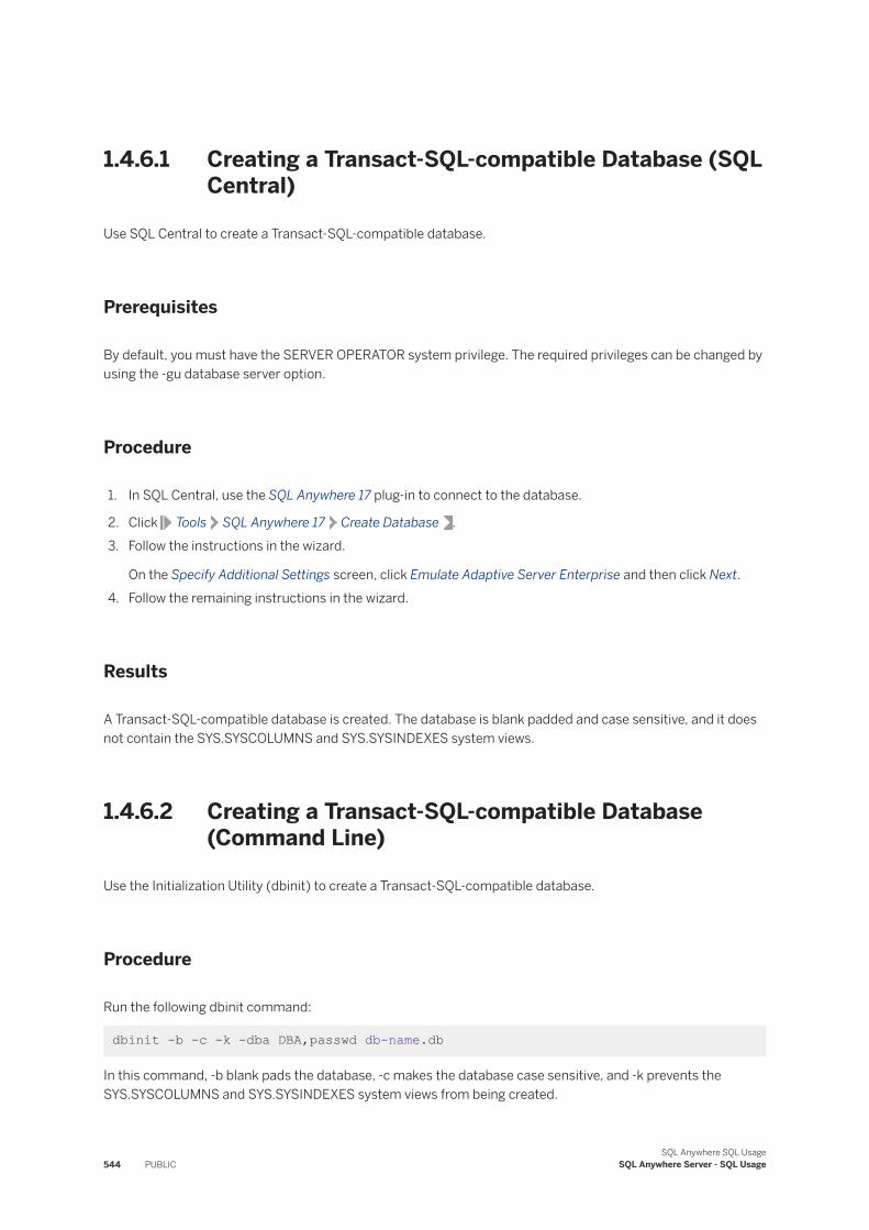
1.4.6.1 Creating a Transact-SQL-compatible Database (SQL Central)
Use SQL Central to create a Transact-SQL-compatible database.
Prerequisites
By default, you must have the SERVER OPERATOR system privilege. The required privileges can be changed by using the -gu database server option.
Procedure
1. In SQL Central, use the SQL Anywhere 17 plug-in to connect to the database.
2. Click Tools SQL Anywhere 17 Create Database .3. Follow the instructions in the wizard.
On the Specify Additional Settings screen, click Emulate Adaptive Server Enterprise and then click Next.4. Follow the remaining instructions in the wizard.
Results
A Transact-SQL-compatible database is created. The database is blank padded and case sensitive, and it does not contain the SYS.SYSCOLUMNS and SYS.SYSINDEXES system views.
1.4.6.2 Creating a Transact-SQL-compatible Database (Command Line)
Use the Initialization Utility (dbinit) to create a Transact-SQL-compatible database.
Procedure
Run the following dbinit command:
dbinit -b -c -k -dba DBA,passwd db-name.db
In this command, -b blank pads the database, -c makes the database case sensitive, and -k prevents the SYS.SYSCOLUMNS and SYS.SYSINDEXES system views from being created.
544 PUBLICSQL Anywhere SQL Usage
SQL Anywhere Server - SQL Usage
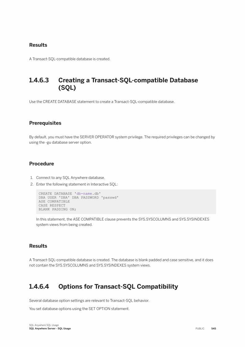
Results
A Transact-SQL-compatible database is created.
1.4.6.3 Creating a Transact-SQL-compatible Database (SQL)
Use the CREATE DATABASE statement to create a Transact-SQL-compatible database.
Prerequisites
By default, you must have the SERVER OPERATOR system privilege. The required privileges can be changed by using the -gu database server option.
Procedure
1. Connect to any SQL Anywhere database.2. Enter the following statement in Interactive SQL:
CREATE DATABASE 'db-name.db' DBA USER 'DBA' DBA PASSWORD 'passwd'ASE COMPATIBLECASE RESPECT BLANK PADDING ON;
In this statement, the ASE COMPATIBLE clause prevents the SYS.SYSCOLUMNS and SYS.SYSINDEXES system views from being created.
Results
A Transact-SQL-compatible database is created. The database is blank padded and case sensitive, and it does not contain the SYS.SYSCOLUMNS and SYS.SYSINDEXES system views.
1.4.6.4 Options for Transact-SQL Compatibility
Several database option settings are relevant to Transact-SQL behavior.
You set database options using the SET OPTION statement.
SQL Anywhere SQL UsageSQL Anywhere Server - SQL Usage PUBLIC 545
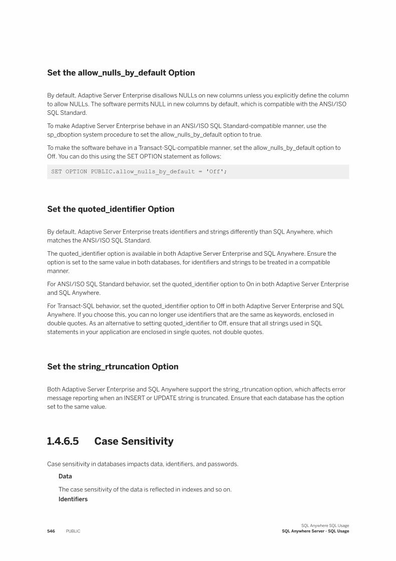
Set the allow_nulls_by_default Option
By default, Adaptive Server Enterprise disallows NULLs on new columns unless you explicitly define the column to allow NULLs. The software permits NULL in new columns by default, which is compatible with the ANSI/ISO SQL Standard.
To make Adaptive Server Enterprise behave in an ANSI/ISO SQL Standard-compatible manner, use the sp_dboption system procedure to set the allow_nulls_by_default option to true.
To make the software behave in a Transact-SQL-compatible manner, set the allow_nulls_by_default option to Off. You can do this using the SET OPTION statement as follows:
SET OPTION PUBLIC.allow_nulls_by_default = 'Off';
Set the quoted_identifier Option
By default, Adaptive Server Enterprise treats identifiers and strings differently than SQL Anywhere, which matches the ANSI/ISO SQL Standard.
The quoted_identifier option is available in both Adaptive Server Enterprise and SQL Anywhere. Ensure the option is set to the same value in both databases, for identifiers and strings to be treated in a compatible manner.
For ANSI/ISO SQL Standard behavior, set the quoted_identifier option to On in both Adaptive Server Enterprise and SQL Anywhere.
For Transact-SQL behavior, set the quoted_identifier option to Off in both Adaptive Server Enterprise and SQL Anywhere. If you choose this, you can no longer use identifiers that are the same as keywords, enclosed in double quotes. As an alternative to setting quoted_identifier to Off, ensure that all strings used in SQL statements in your application are enclosed in single quotes, not double quotes.
Set the string_rtruncation Option
Both Adaptive Server Enterprise and SQL Anywhere support the string_rtruncation option, which affects error message reporting when an INSERT or UPDATE string is truncated. Ensure that each database has the option set to the same value.
1.4.6.5 Case Sensitivity
Case sensitivity in databases impacts data, identifiers, and passwords.
Data
The case sensitivity of the data is reflected in indexes and so on.Identifiers
546 PUBLICSQL Anywhere SQL Usage
SQL Anywhere Server - SQL Usage
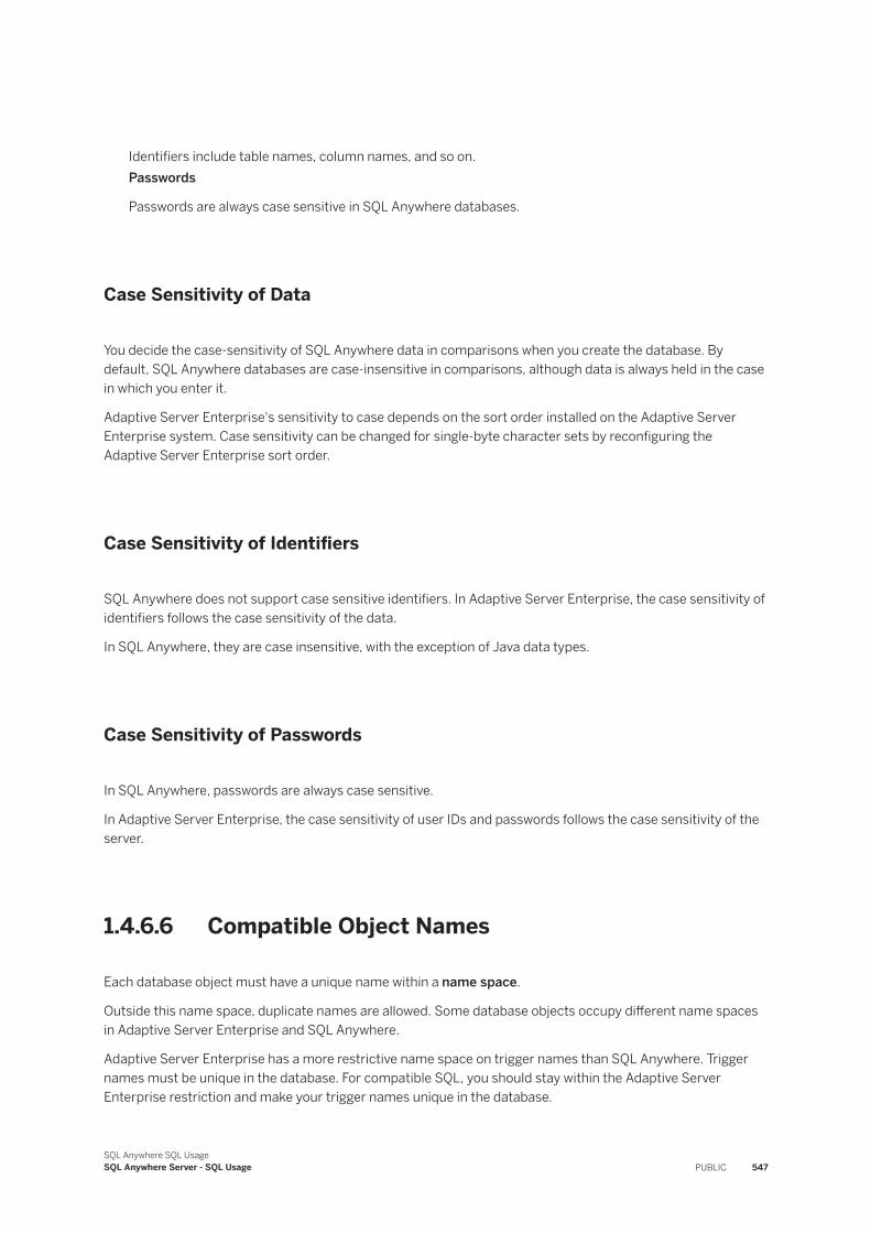
Identifiers include table names, column names, and so on.Passwords
Passwords are always case sensitive in SQL Anywhere databases.
Case Sensitivity of Data
You decide the case-sensitivity of SQL Anywhere data in comparisons when you create the database. By default, SQL Anywhere databases are case-insensitive in comparisons, although data is always held in the case in which you enter it.
Adaptive Server Enterprise's sensitivity to case depends on the sort order installed on the Adaptive Server Enterprise system. Case sensitivity can be changed for single-byte character sets by reconfiguring the Adaptive Server Enterprise sort order.
Case Sensitivity of Identifiers
SQL Anywhere does not support case sensitive identifiers. In Adaptive Server Enterprise, the case sensitivity of identifiers follows the case sensitivity of the data.
In SQL Anywhere, they are case insensitive, with the exception of Java data types.
Case Sensitivity of Passwords
In SQL Anywhere, passwords are always case sensitive.
In Adaptive Server Enterprise, the case sensitivity of user IDs and passwords follows the case sensitivity of the server.
1.4.6.6 Compatible Object Names
Each database object must have a unique name within a name space.
Outside this name space, duplicate names are allowed. Some database objects occupy different name spaces in Adaptive Server Enterprise and SQL Anywhere.
Adaptive Server Enterprise has a more restrictive name space on trigger names than SQL Anywhere. Trigger names must be unique in the database. For compatible SQL, you should stay within the Adaptive Server Enterprise restriction and make your trigger names unique in the database.
SQL Anywhere SQL UsageSQL Anywhere Server - SQL Usage PUBLIC 547
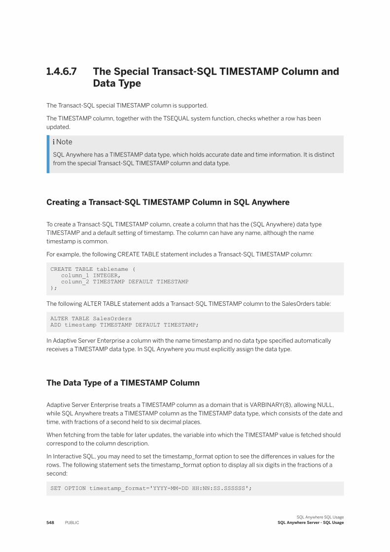
1.4.6.7 The Special Transact-SQL TIMESTAMP Column and Data Type
The Transact-SQL special TIMESTAMP column is supported.
The TIMESTAMP column, together with the TSEQUAL system function, checks whether a row has been updated.
NoteSQL Anywhere has a TIMESTAMP data type, which holds accurate date and time information. It is distinct from the special Transact-SQL TIMESTAMP column and data type.
Creating a Transact-SQL TIMESTAMP Column in SQL Anywhere
To create a Transact-SQL TIMESTAMP column, create a column that has the (SQL Anywhere) data type TIMESTAMP and a default setting of timestamp. The column can have any name, although the name timestamp is common.
For example, the following CREATE TABLE statement includes a Transact-SQL TIMESTAMP column:
CREATE TABLE tablename ( column_1 INTEGER, column_2 TIMESTAMP DEFAULT TIMESTAMP );
The following ALTER TABLE statement adds a Transact-SQL TIMESTAMP column to the SalesOrders table:
ALTER TABLE SalesOrders ADD timestamp TIMESTAMP DEFAULT TIMESTAMP;
In Adaptive Server Enterprise a column with the name timestamp and no data type specified automatically receives a TIMESTAMP data type. In SQL Anywhere you must explicitly assign the data type.
The Data Type of a TIMESTAMP Column
Adaptive Server Enterprise treats a TIMESTAMP column as a domain that is VARBINARY(8), allowing NULL, while SQL Anywhere treats a TIMESTAMP column as the TIMESTAMP data type, which consists of the date and time, with fractions of a second held to six decimal places.
When fetching from the table for later updates, the variable into which the TIMESTAMP value is fetched should correspond to the column description.
In Interactive SQL, you may need to set the timestamp_format option to see the differences in values for the rows. The following statement sets the timestamp_format option to display all six digits in the fractions of a second:
SET OPTION timestamp_format='YYYY-MM-DD HH:NN:SS.SSSSSS';
548 PUBLICSQL Anywhere SQL Usage
SQL Anywhere Server - SQL Usage
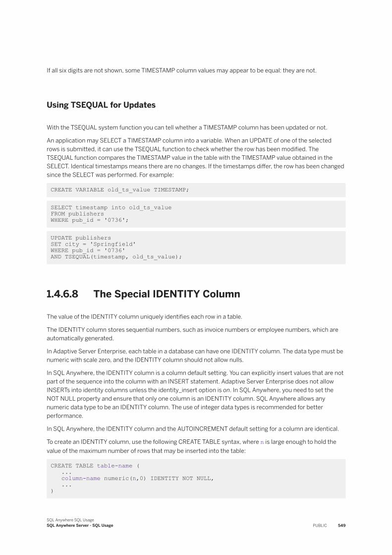
If all six digits are not shown, some TIMESTAMP column values may appear to be equal: they are not.
Using TSEQUAL for Updates
With the TSEQUAL system function you can tell whether a TIMESTAMP column has been updated or not.
An application may SELECT a TIMESTAMP column into a variable. When an UPDATE of one of the selected rows is submitted, it can use the TSEQUAL function to check whether the row has been modified. The TSEQUAL function compares the TIMESTAMP value in the table with the TIMESTAMP value obtained in the SELECT. Identical timestamps means there are no changes. If the timestamps differ, the row has been changed since the SELECT was performed. For example:
CREATE VARIABLE old_ts_value TIMESTAMP;
SELECT timestamp into old_ts_value FROM publishers WHERE pub_id = '0736';
UPDATE publishers SET city = 'Springfield'WHERE pub_id = '0736' AND TSEQUAL(timestamp, old_ts_value);
1.4.6.8 The Special IDENTITY Column
The value of the IDENTITY column uniquely identifies each row in a table.
The IDENTITY column stores sequential numbers, such as invoice numbers or employee numbers, which are automatically generated.
In Adaptive Server Enterprise, each table in a database can have one IDENTITY column. The data type must be numeric with scale zero, and the IDENTITY column should not allow nulls.
In SQL Anywhere, the IDENTITY column is a column default setting. You can explicitly insert values that are not part of the sequence into the column with an INSERT statement. Adaptive Server Enterprise does not allow INSERTs into identity columns unless the identity_insert option is on. In SQL Anywhere, you need to set the NOT NULL property and ensure that only one column is an IDENTITY column. SQL Anywhere allows any numeric data type to be an IDENTITY column. The use of integer data types is recommended for better performance.
In SQL Anywhere, the IDENTITY column and the AUTOINCREMENT default setting for a column are identical.
To create an IDENTITY column, use the following CREATE TABLE syntax, where n is large enough to hold the value of the maximum number of rows that may be inserted into the table:
CREATE TABLE table-name ( ... column-name numeric(n,0) IDENTITY NOT NULL, ... )
SQL Anywhere SQL UsageSQL Anywhere Server - SQL Usage PUBLIC 549
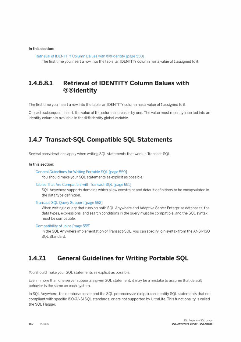
In this section:
Retrieval of IDENTITY Column Balues with @@identity [page 550]The first time you insert a row into the table, an IDENTITY column has a value of 1 assigned to it.
1.4.6.8.1 Retrieval of IDENTITY Column Balues with @@identity
The first time you insert a row into the table, an IDENTITY column has a value of 1 assigned to it.
On each subsequent insert, the value of the column increases by one. The value most recently inserted into an identity column is available in the @@identity global variable.
1.4.7 Transact-SQL Compatible SQL Statements
Several considerations apply when writing SQL statements that work in Transact-SQL.
In this section:
General Guidelines for Writing Portable SQL [page 550]You should make your SQL statements as explicit as possible.
Tables That Are Compatible with Transact-SQL [page 551]SQL Anywhere supports domains which allow constraint and default definitions to be encapsulated in the data type definition.
Transact-SQL Query Support [page 552]When writing a query that runs on both SQL Anywhere and Adaptive Server Enterprise databases, the data types, expressions, and search conditions in the query must be compatible, and the SQL syntax must be compatible.
Compatibility of Joins [page 555]In the SQL Anywhere implementation of Transact-SQL, you can specify join syntax from the ANSI/ISO SQL Standard.
1.4.7.1 General Guidelines for Writing Portable SQL
You should make your SQL statements as explicit as possible.
Even if more than one server supports a given SQL statement, it may be a mistake to assume that default behavior is the same on each system.
In SQL Anywhere, the database server and the SQL preprocessor (sqlpp) can identify SQL statements that not compliant with specific ISO/ANSI SQL standards, or are not supported by UltraLite. This functionality is called the SQL Flagger.
550 PUBLICSQL Anywhere SQL Usage
SQL Anywhere Server - SQL Usage
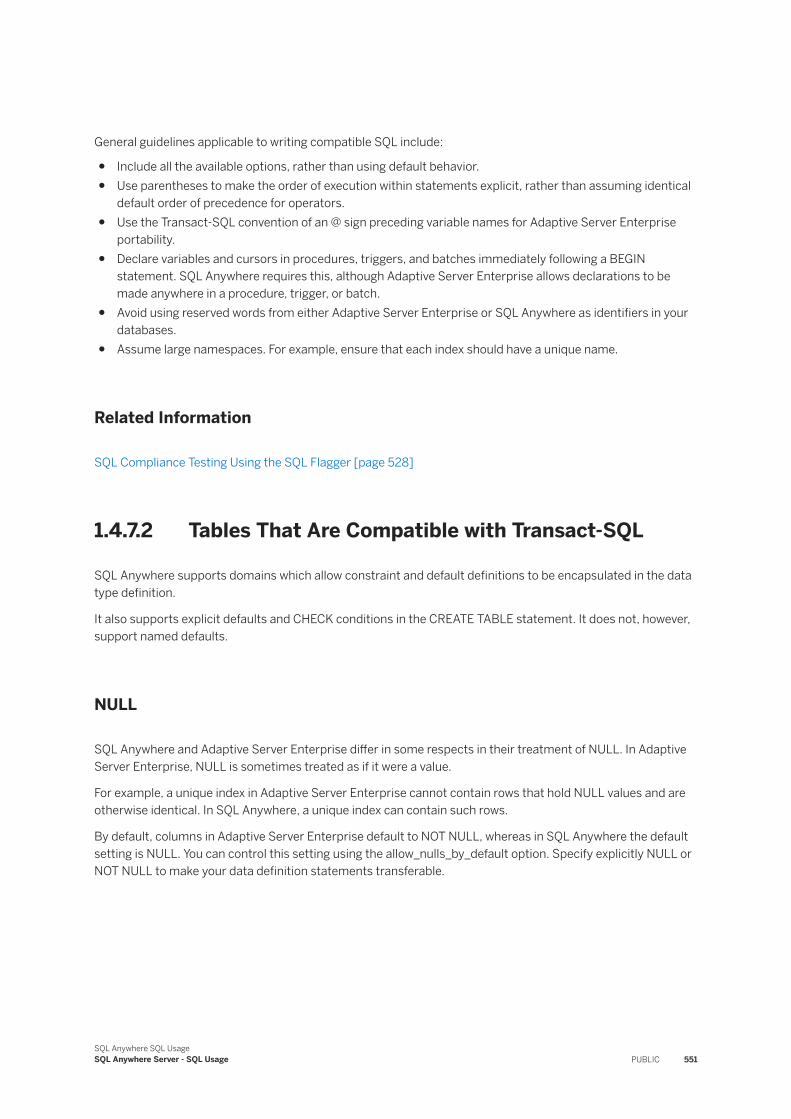
General guidelines applicable to writing compatible SQL include:
● Include all the available options, rather than using default behavior.● Use parentheses to make the order of execution within statements explicit, rather than assuming identical
default order of precedence for operators.● Use the Transact-SQL convention of an @ sign preceding variable names for Adaptive Server Enterprise
portability.● Declare variables and cursors in procedures, triggers, and batches immediately following a BEGIN
statement. SQL Anywhere requires this, although Adaptive Server Enterprise allows declarations to be made anywhere in a procedure, trigger, or batch.
● Avoid using reserved words from either Adaptive Server Enterprise or SQL Anywhere as identifiers in your databases.
● Assume large namespaces. For example, ensure that each index should have a unique name.
Related Information
SQL Compliance Testing Using the SQL Flagger [page 528]
1.4.7.2 Tables That Are Compatible with Transact-SQL
SQL Anywhere supports domains which allow constraint and default definitions to be encapsulated in the data type definition.
It also supports explicit defaults and CHECK conditions in the CREATE TABLE statement. It does not, however, support named defaults.
NULL
SQL Anywhere and Adaptive Server Enterprise differ in some respects in their treatment of NULL. In Adaptive Server Enterprise, NULL is sometimes treated as if it were a value.
For example, a unique index in Adaptive Server Enterprise cannot contain rows that hold NULL values and are otherwise identical. In SQL Anywhere, a unique index can contain such rows.
By default, columns in Adaptive Server Enterprise default to NOT NULL, whereas in SQL Anywhere the default setting is NULL. You can control this setting using the allow_nulls_by_default option. Specify explicitly NULL or NOT NULL to make your data definition statements transferable.
SQL Anywhere SQL UsageSQL Anywhere Server - SQL Usage PUBLIC 551
Temporary Tables
You can create a temporary table by placing a number sign (#) in front of the table name in a CREATE TABLE statement. These temporary tables are SQL Anywhere declared temporary tables, and are available only in the current connection.
Physical placement of a table is performed differently in Adaptive Server Enterprise and in SQL Anywhere. SQL Anywhere supports the ON segment-name clause, but segment-name refers to a SQL Anywhere dbspace.
Related Information
SQL Compliance Testing Using the SQL Flagger [page 528]Options for Transact-SQL Compatibility [page 545]
1.4.7.3 Transact-SQL Query Support
When writing a query that runs on both SQL Anywhere and Adaptive Server Enterprise databases, the data types, expressions, and search conditions in the query must be compatible, and the SQL syntax must be compatible.
Data types, expressions, and search conditions must also be compatible. The examples assume the quoted_identifier option is set to OFF, which is the default Adaptive Server Enterprise setting, but not the default SQL Anywhere setting.
The SQL Anywhere implementation of the Transact-SQL dialect supports much of the query expression syntax from the Watcom SQL dialect, even though some of these SQL constructions are not supported by Adaptive Server Enterprise. In a Transact-SQL query, SQL Anywhere supports the following SQL constructions:
● the back quote character `, the double quote character ", and square parentheses [] to denote identifiers● UNION, EXCEPT, and INTERSECT query expressions● derived tables● table functions● CONTAINS table expressions for full text search● REGEXP, SIMILAR, IS DISTINCT FROM, and CONTAINS predicates● user-defined SQL or external functions● LEFT, RIGHT and FULL outer joins● GROUP BY ROLLUP, CUBE, and GROUPING SETS● TOP N START AT M● window aggregate functions and other analytic functions including statistical analysis and linear regression
functions
In this section:
Supported Transact-SQL Query Syntax [page 553]The SQL Anywhere supports the Transact-SQL dialect for queries.
552 PUBLICSQL Anywhere SQL Usage
SQL Anywhere Server - SQL Usage
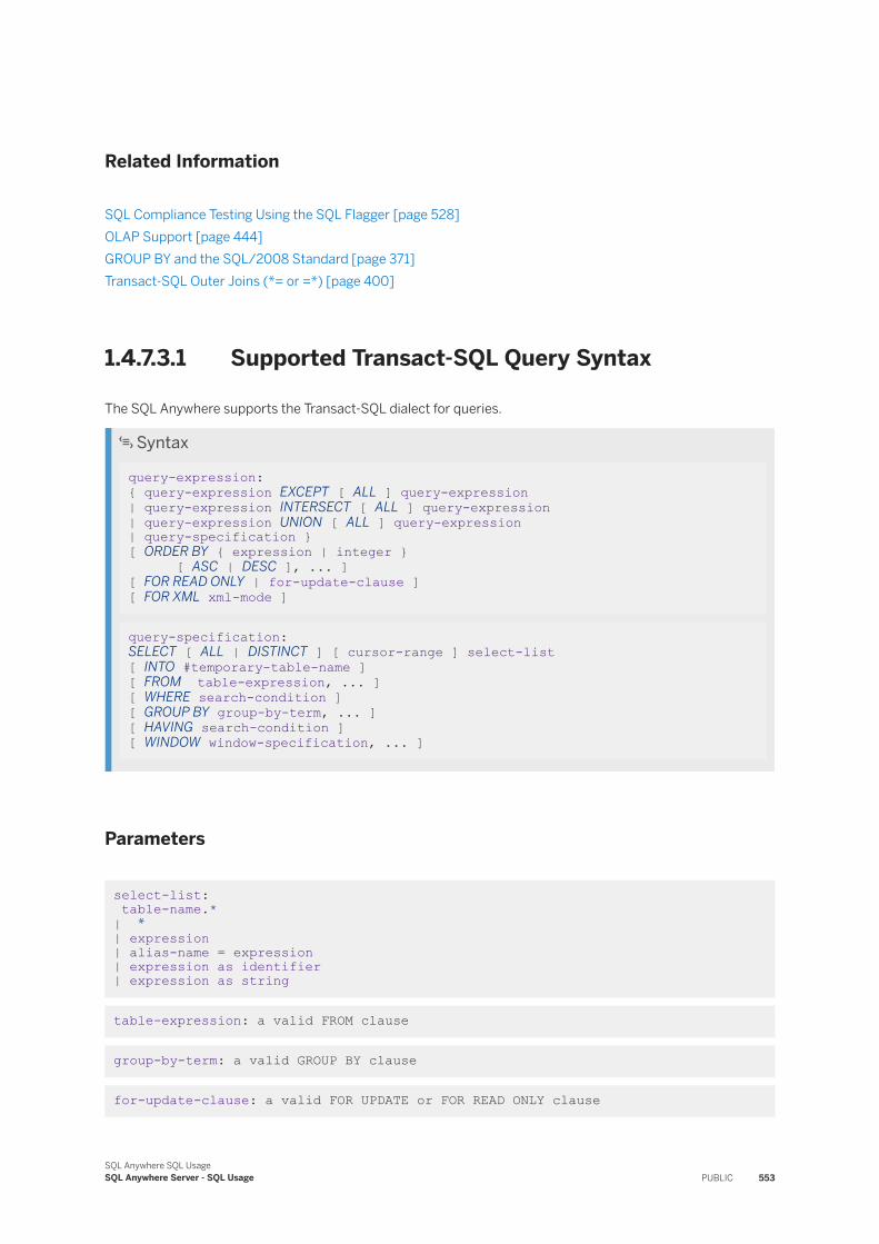
Related Information
SQL Compliance Testing Using the SQL Flagger [page 528]OLAP Support [page 444]GROUP BY and the SQL/2008 Standard [page 371]Transact-SQL Outer Joins (*= or =*) [page 400]
1.4.7.3.1 Supported Transact-SQL Query Syntax
The SQL Anywhere supports the Transact-SQL dialect for queries.
Syntax
query-expression: { query-expression EXCEPT [ ALL ] query-expression | query-expression INTERSECT [ ALL ] query-expression | query-expression UNION [ ALL ] query-expression | query-specification } [ ORDER BY { expression | integer } [ ASC | DESC ], ... ] [ FOR READ ONLY | for-update-clause ] [ FOR XML xml-mode ]
query-specification: SELECT [ ALL | DISTINCT ] [ cursor-range ] select-list [ INTO #temporary-table-name ] [ FROM table-expression, ... ] [ WHERE search-condition ] [ GROUP BY group-by-term, ... ] [ HAVING search-condition ] [ WINDOW window-specification, ... ]
Parameters
select-list: table-name.* | * | expression | alias-name = expression | expression as identifier | expression as string
table-expression: a valid FROM clause
group-by-term: a valid GROUP BY clause
for-update-clause: a valid FOR UPDATE or FOR READ ONLY clause
SQL Anywhere SQL UsageSQL Anywhere Server - SQL Usage PUBLIC 553
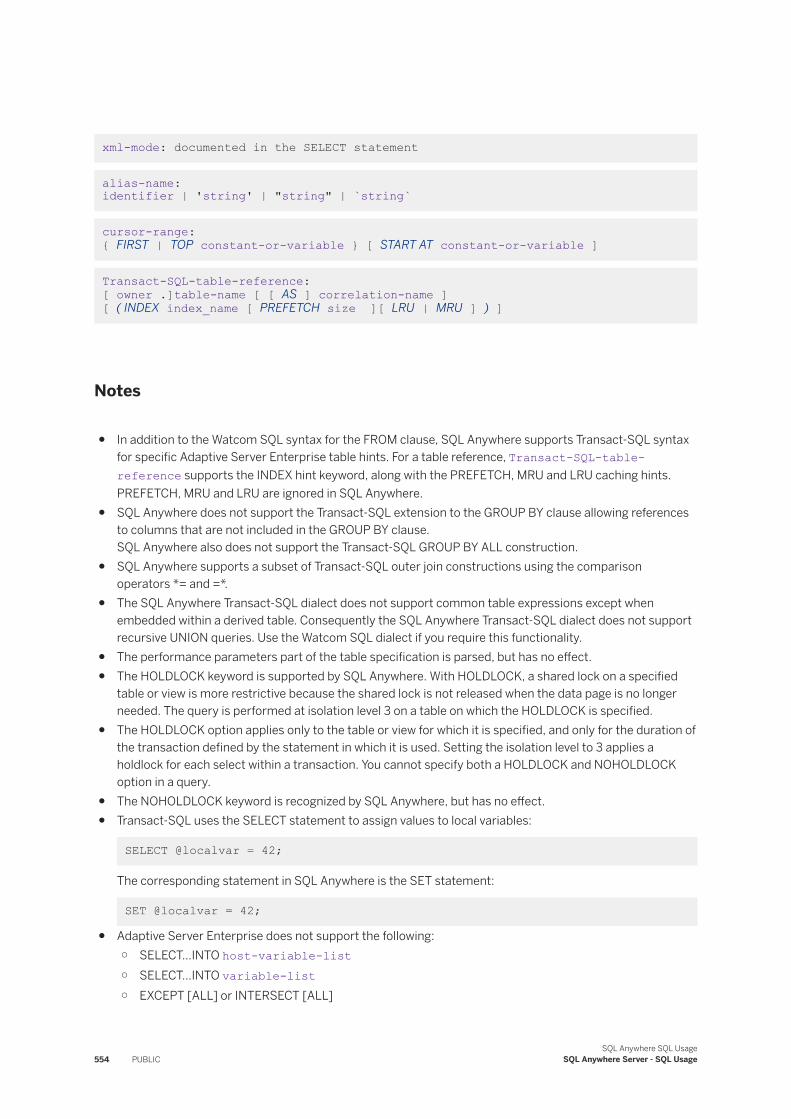
xml-mode: documented in the SELECT statement
alias-name: identifier | 'string' | "string" | `string`
cursor-range: { FIRST | TOP constant-or-variable } [ START AT constant-or-variable ]
Transact-SQL-table-reference: [ owner .]table-name [ [ AS ] correlation-name ] [ ( INDEX index_name [ PREFETCH size ][ LRU | MRU ] ) ]
Notes
● In addition to the Watcom SQL syntax for the FROM clause, SQL Anywhere supports Transact-SQL syntax for specific Adaptive Server Enterprise table hints. For a table reference, Transact-SQL-table-reference supports the INDEX hint keyword, along with the PREFETCH, MRU and LRU caching hints. PREFETCH, MRU and LRU are ignored in SQL Anywhere.
● SQL Anywhere does not support the Transact-SQL extension to the GROUP BY clause allowing references to columns that are not included in the GROUP BY clause.SQL Anywhere also does not support the Transact-SQL GROUP BY ALL construction.
● SQL Anywhere supports a subset of Transact-SQL outer join constructions using the comparison operators *= and =*.
● The SQL Anywhere Transact-SQL dialect does not support common table expressions except when embedded within a derived table. Consequently the SQL Anywhere Transact-SQL dialect does not support recursive UNION queries. Use the Watcom SQL dialect if you require this functionality.
● The performance parameters part of the table specification is parsed, but has no effect.● The HOLDLOCK keyword is supported by SQL Anywhere. With HOLDLOCK, a shared lock on a specified
table or view is more restrictive because the shared lock is not released when the data page is no longer needed. The query is performed at isolation level 3 on a table on which the HOLDLOCK is specified.
● The HOLDLOCK option applies only to the table or view for which it is specified, and only for the duration of the transaction defined by the statement in which it is used. Setting the isolation level to 3 applies a holdlock for each select within a transaction. You cannot specify both a HOLDLOCK and NOHOLDLOCK option in a query.
● The NOHOLDLOCK keyword is recognized by SQL Anywhere, but has no effect.● Transact-SQL uses the SELECT statement to assign values to local variables:
SELECT @localvar = 42;
The corresponding statement in SQL Anywhere is the SET statement:
SET @localvar = 42;
● Adaptive Server Enterprise does not support the following:○ SELECT...INTO host-variable-list○ SELECT...INTO variable-list○ EXCEPT [ALL] or INTERSECT [ALL]
554 PUBLICSQL Anywhere SQL Usage
SQL Anywhere Server - SQL Usage
○ START AT clause○ SQL Anywhere-defined table hints○ table functions○ FULL OUTER JOIN○ FOR UPDATE BY { LOCK | TIMESTAMP }○ window aggregate functions and linear regression functions
● SQL Anywhere does not support the following keywords and clauses of the Adaptive Server Enterprise Transact-SQL SELECT statement syntax:○ SHARED keyword○ PARTITION keyword○ COMPUTE clause○ FOR BROWSE clause○ GROUP BY ALL clause○ PLAN clause○ ISOLATION clause
● SQL Anywhere does not support the following characters in identifiers or aliases:○ Double quotes○ Control characters (any character less than 0X20)○ Backslashes○ Square brackets○ Back quotes
1.4.7.4 Compatibility of Joins
In the SQL Anywhere implementation of Transact-SQL, you can specify join syntax from the ANSI/ISO SQL Standard.
This includes using the keywords JOIN, LEFT OUTER JOIN, and RIGHT OUTER JOIN, and FULL OUTER JOIN, along with legacy Transact-SQL outer join syntax that uses the specialty comparison operators *= and =* in the statement's WHERE clause.
NoteSupport for Transact-SQL outer join operators *= and =* is deprecated and will be removed in a future release.
Related Information
Joins: Retrieving Data from Several Tables [page 384]Transact-SQL Outer Joins (*= or =*) [page 400]SQL Compliance Testing Using the SQL Flagger [page 528]
SQL Anywhere SQL UsageSQL Anywhere Server - SQL Usage PUBLIC 555
1.4.8 Transact-SQL Procedure Language
SQL Anywhere supports a large part of the Transact-SQL stored procedure language in addition to the Watcom SQL dialect based on the ISO/ANSI SQL standard.
In this section:
Transact-SQL Stored Procedures [page 556]The Watcom-SQL stored procedure dialect differs from the Transact-SQL dialect in many ways.
Transact-SQL Triggers [page 556]Trigger compatibility requires compatibility of trigger features and syntax.
Transact-SQL Batches [page 558]In Transact-SQL, a batch is a set of SQL statements submitted together and executed as a group.
1.4.8.1 Transact-SQL Stored Procedures
The Watcom-SQL stored procedure dialect differs from the Transact-SQL dialect in many ways.
The native SQL Anywhere dialect, Watcom-SQL, is based on the ISO/ANSI SQL standard. Many of the concepts and features are similar, but the syntax is different. SQL Anywhere support for Transact-SQL takes advantage of the similar concepts by providing automatic translation between dialects. However, a procedure must be written exclusively in one of the two dialects, not in a mixture of the two.
Support for Transact-SQL Stored Procedures
There are a variety of aspects to the support of Transact-SQL stored procedures, including:
● Use of semicolons to delimit SQL statements in procedures● Passing parameters● Returning result sets● Returning status information● Providing default values for parameters● Control statements● Error handling● User-defined functions
1.4.8.2 Transact-SQL Triggers
Trigger compatibility requires compatibility of trigger features and syntax.
Adaptive Server Enterprise supports statement-level AFTER triggers; that is, triggers that execute after the triggering statement has completed. The Watcom-SQL dialect supported by SQL Anywhere supports row-level BEFORE, AFTER, and INSTEAD OF triggers, and statement-level AFTER and INSTEAD OF triggers.
556 PUBLICSQL Anywhere SQL Usage
SQL Anywhere Server - SQL Usage
Row-level triggers are not part of the Transact-SQL compatibility features.
Description of Unsupported or Different Transact-SQL Triggers
Features of Transact-SQL triggers that are either unsupported or different in SQL Anywhere include:
Triggers firing other triggers
Suppose a trigger performs an action that would, if performed directly by a user, fire another trigger. SQL Anywhere and Adaptive Server Enterprise respond slightly differently to this situation. By default in Adaptive Server Enterprise, triggers fire other triggers up to a configurable nesting level, which has the default value of 16. You can control the nesting level with the Adaptive Server Enterprise nested triggers option. In SQL Anywhere, triggers fire other triggers without limit unless there is insufficient memory.Triggers firing themselves
Suppose a trigger performs an action that would, if performed directly by a user, fire the same trigger. SQL Anywhere and Adaptive Server Enterprise respond slightly differently to this situation. By default, in SQL Anywhere, non-Transact-SQL triggers fire themselves recursively, whereas Transact-SQL dialect triggers do not fire themselves recursively. However, for Transact-SQL dialect triggers, you can use the self_recursion option of the SET statement [T-SQL] to allow a trigger to call itself recursively.
By default in Adaptive Server Enterprise, a trigger does not call itself recursively, but you can use the self_recursion option to allow recursion to occur.ROLLBACK statement in triggers not supported
Adaptive Server Enterprise permits the ROLLBACK TRANSACTION statement within triggers, to roll back the entire transaction of which the trigger is a part. SQL Anywhere does not permit ROLLBACK (or ROLLBACK TRANSACTION) statements in triggers because a triggering action and its trigger together form an atomic statement.
SQL Anywhere does provide the Adaptive Server Enterprise-compatible ROLLBACK TRIGGER statement to undo actions within triggers.ORDER clause not supported
Transact-SQL triggers do not permit an ORDER nn clause; the value of trigger_order is automatically set to 1. This can cause an error to be returned creating a T-SQL trigger if there is already a statement level trigger. This is because the SYSTRIGGER system table has a unique index on table_id, event, trigger_time, trigger_order. For a particular event (insert, update, delete) statement-level triggers are always AFTER and trigger_order cannot be set, so there can be only one per table, assuming any other triggers do not set an order other than 1.
Related Information
Triggers [page 107]Stored Procedures, Triggers, Batches, and User-defined Functions [page 87]
SQL Anywhere SQL UsageSQL Anywhere Server - SQL Usage PUBLIC 557
1.4.8.3 Transact-SQL Batches
In Transact-SQL, a batch is a set of SQL statements submitted together and executed as a group.
Batches can be stored in SQL script files. Interactive SQL can be used to execute batches interactively.
The control statements used in procedures can also be used in batches. SQL Anywhere supports the use of control statements in batches and the Transact-SQL-like use of non-delimited groups of statements terminated with a GO statement to signify the end of a batch.
The use of semicolons to delimit statements in a Transact-SQL batch is also supported.
For batches stored in SQL script files, Interactive SQL supports the use of parameters in these files.
1.4.9 Automatic Translation of Stored Procedures
SQL Anywhere provides aids for translating statements between the Watcom SQL and Transact-SQL dialects.
SQL language built-in functions returning information about SQL statements and enabling automatic translation of SQL statements include:
SQLDIALECT( statement )
Returns Watcom-SQL or Transact-SQL.WATCOMSQL( statement )
Returns the Watcom-SQL syntax for the statement.TRANSACTSQL( statement )
Returns the Transact-SQL syntax for the statement.
These are functions, and so can be accessed using a select statement from Interactive SQL. For example, the following statement returns the value Watcom-SQL:
SELECT SQLDIALECT( 'SELECT * FROM Employees' );
In this section:
Translating a Stored Procedure [page 559]Translate stored procedures between SQL dialects, for example between Watcom-SQL and Transact-SQL.
558 PUBLICSQL Anywhere SQL Usage
SQL Anywhere Server - SQL Usage
1.4.9.1 Translating a Stored Procedure
Translate stored procedures between SQL dialects, for example between Watcom-SQL and Transact-SQL.
Prerequisites
You must be the owner of the procedure or have one of the following privileges:
● ALTER ANY PROCEDURE system privilege● ALTER ANY OBJECT system privilege
Procedure
1. In SQL Central, use the SQL Anywhere 17 plug-in to connect to the database.2. Click the Procedures & Functions folder and select one of the stored procedures in the list.3. In the right pane, click the SQL tab and then click the text window.4. Click File and click one of the Translate To options.
The procedure appears in the right pane in the selected dialect. If the selected dialect is not the one in which the procedure is stored, the database server translates it to that dialect. Any untranslated lines appear as comments.
5. Rewrite any untranslated lines.
6. Click File Save .
Results
The stored procedure is translated and saved in the database.
1.4.10 Result Sets Returned from Transact-SQL Procedures
SQL Anywhere uses a RESULT clause to specify returned result sets.
In Transact-SQL procedures, the column names or alias names of the first query are returned to the calling environment.
SQL Anywhere SQL UsageSQL Anywhere Server - SQL Usage PUBLIC 559
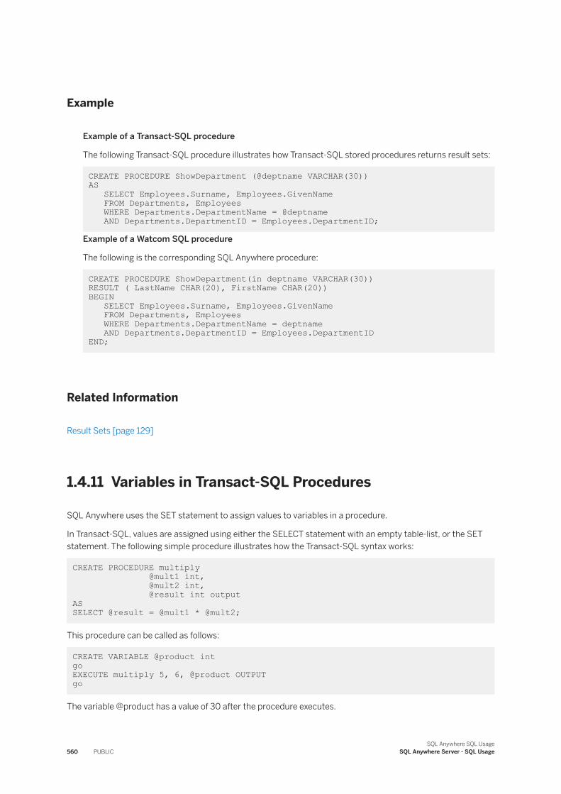
Example
Example of a Transact-SQL procedure
The following Transact-SQL procedure illustrates how Transact-SQL stored procedures returns result sets:
CREATE PROCEDURE ShowDepartment (@deptname VARCHAR(30)) AS SELECT Employees.Surname, Employees.GivenName FROM Departments, Employees WHERE Departments.DepartmentName = @deptname AND Departments.DepartmentID = Employees.DepartmentID;
Example of a Watcom SQL procedure
The following is the corresponding SQL Anywhere procedure:
CREATE PROCEDURE ShowDepartment(in deptname VARCHAR(30)) RESULT ( LastName CHAR(20), FirstName CHAR(20))BEGIN SELECT Employees.Surname, Employees.GivenName FROM Departments, Employees WHERE Departments.DepartmentName = deptname AND Departments.DepartmentID = Employees.DepartmentID END;
Related Information
Result Sets [page 129]
1.4.11 Variables in Transact-SQL Procedures
SQL Anywhere uses the SET statement to assign values to variables in a procedure.
In Transact-SQL, values are assigned using either the SELECT statement with an empty table-list, or the SET statement. The following simple procedure illustrates how the Transact-SQL syntax works:
CREATE PROCEDURE multiply @mult1 int, @mult2 int, @result int outputAS SELECT @result = @mult1 * @mult2;
This procedure can be called as follows:
CREATE VARIABLE @product int goEXECUTE multiply 5, 6, @product OUTPUT go
The variable @product has a value of 30 after the procedure executes.
560 PUBLICSQL Anywhere SQL Usage
SQL Anywhere Server - SQL Usage
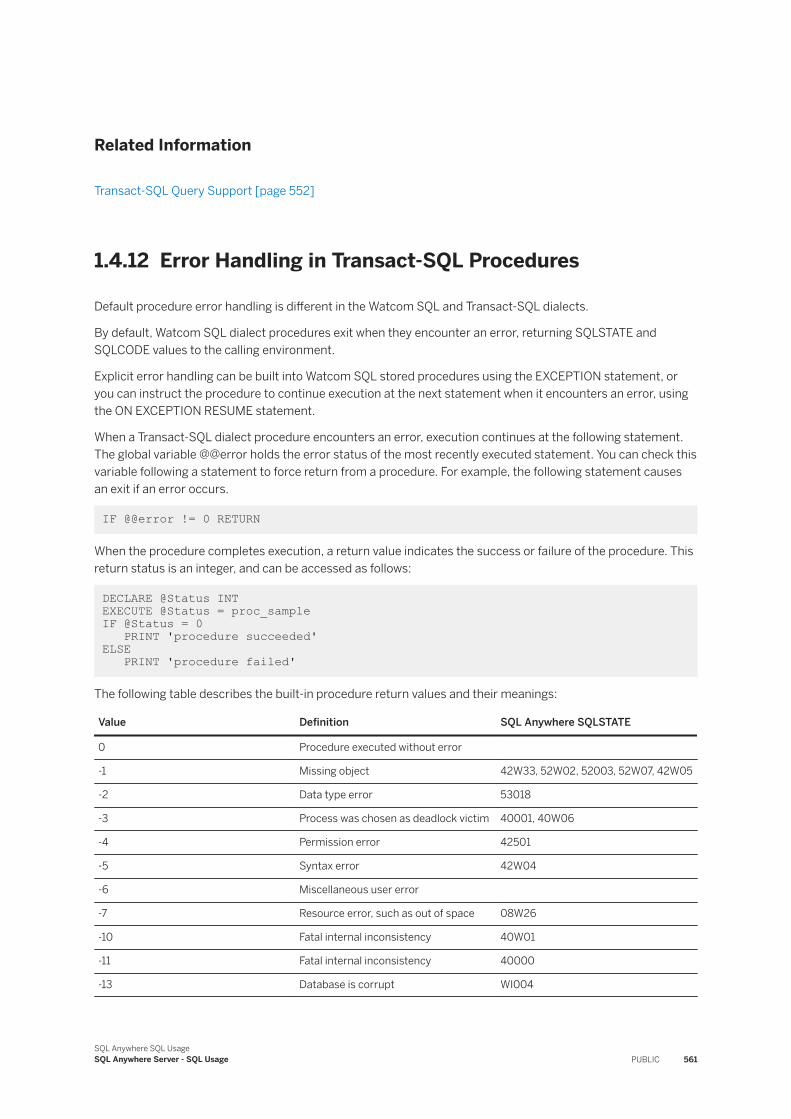
Related Information
Transact-SQL Query Support [page 552]
1.4.12 Error Handling in Transact-SQL Procedures
Default procedure error handling is different in the Watcom SQL and Transact-SQL dialects.
By default, Watcom SQL dialect procedures exit when they encounter an error, returning SQLSTATE and SQLCODE values to the calling environment.
Explicit error handling can be built into Watcom SQL stored procedures using the EXCEPTION statement, or you can instruct the procedure to continue execution at the next statement when it encounters an error, using the ON EXCEPTION RESUME statement.
When a Transact-SQL dialect procedure encounters an error, execution continues at the following statement. The global variable @@error holds the error status of the most recently executed statement. You can check this variable following a statement to force return from a procedure. For example, the following statement causes an exit if an error occurs.
IF @@error != 0 RETURN
When the procedure completes execution, a return value indicates the success or failure of the procedure. This return status is an integer, and can be accessed as follows:
DECLARE @Status INT EXECUTE @Status = proc_sampleIF @Status = 0 PRINT 'procedure succeeded'ELSE PRINT 'procedure failed'
The following table describes the built-in procedure return values and their meanings:
Value Definition SQL Anywhere SQLSTATE
0 Procedure executed without error
-1 Missing object 42W33, 52W02, 52003, 52W07, 42W05
-2 Data type error 53018
-3 Process was chosen as deadlock victim 40001, 40W06
-4 Permission error 42501
-5 Syntax error 42W04
-6 Miscellaneous user error
-7 Resource error, such as out of space 08W26
-10 Fatal internal inconsistency 40W01
-11 Fatal internal inconsistency 40000
-13 Database is corrupt WI004
SQL Anywhere SQL UsageSQL Anywhere Server - SQL Usage PUBLIC 561
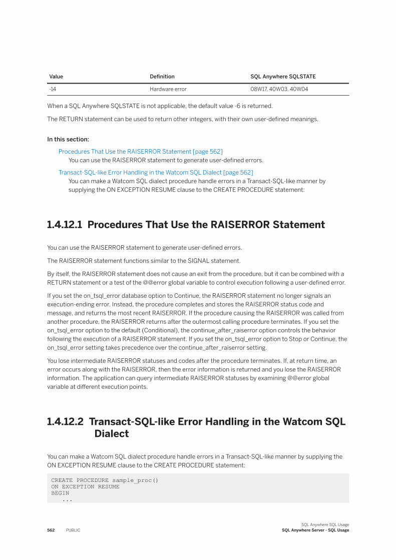
Value Definition SQL Anywhere SQLSTATE
-14 Hardware error 08W17, 40W03, 40W04
When a SQL Anywhere SQLSTATE is not applicable, the default value -6 is returned.
The RETURN statement can be used to return other integers, with their own user-defined meanings.
In this section:
Procedures That Use the RAISERROR Statement [page 562]You can use the RAISERROR statement to generate user-defined errors.
Transact-SQL-like Error Handling in the Watcom SQL Dialect [page 562]You can make a Watcom SQL dialect procedure handle errors in a Transact-SQL-like manner by supplying the ON EXCEPTION RESUME clause to the CREATE PROCEDURE statement:
1.4.12.1 Procedures That Use the RAISERROR Statement
You can use the RAISERROR statement to generate user-defined errors.
The RAISERROR statement functions similar to the SIGNAL statement.
By itself, the RAISERROR statement does not cause an exit from the procedure, but it can be combined with a RETURN statement or a test of the @@error global variable to control execution following a user-defined error.
If you set the on_tsql_error database option to Continue, the RAISERROR statement no longer signals an execution-ending error. Instead, the procedure completes and stores the RAISERROR status code and message, and returns the most recent RAISERROR. If the procedure causing the RAISERROR was called from another procedure, the RAISERROR returns after the outermost calling procedure terminates. If you set the on_tsql_error option to the default (Conditional), the continue_after_raiserror option controls the behavior following the execution of a RAISERROR statement. If you set the on_tsql_error option to Stop or Continue, the on_tsql_error setting takes precedence over the continue_after_raiserror setting.
You lose intermediate RAISERROR statuses and codes after the procedure terminates. If, at return time, an error occurs along with the RAISERROR, then the error information is returned and you lose the RAISERROR information. The application can query intermediate RAISERROR statuses by examining @@error global variable at different execution points.
1.4.12.2 Transact-SQL-like Error Handling in the Watcom SQL Dialect
You can make a Watcom SQL dialect procedure handle errors in a Transact-SQL-like manner by supplying the ON EXCEPTION RESUME clause to the CREATE PROCEDURE statement:
CREATE PROCEDURE sample_proc() ON EXCEPTION RESUMEBEGIN ...
562 PUBLICSQL Anywhere SQL Usage
SQL Anywhere Server - SQL Usage
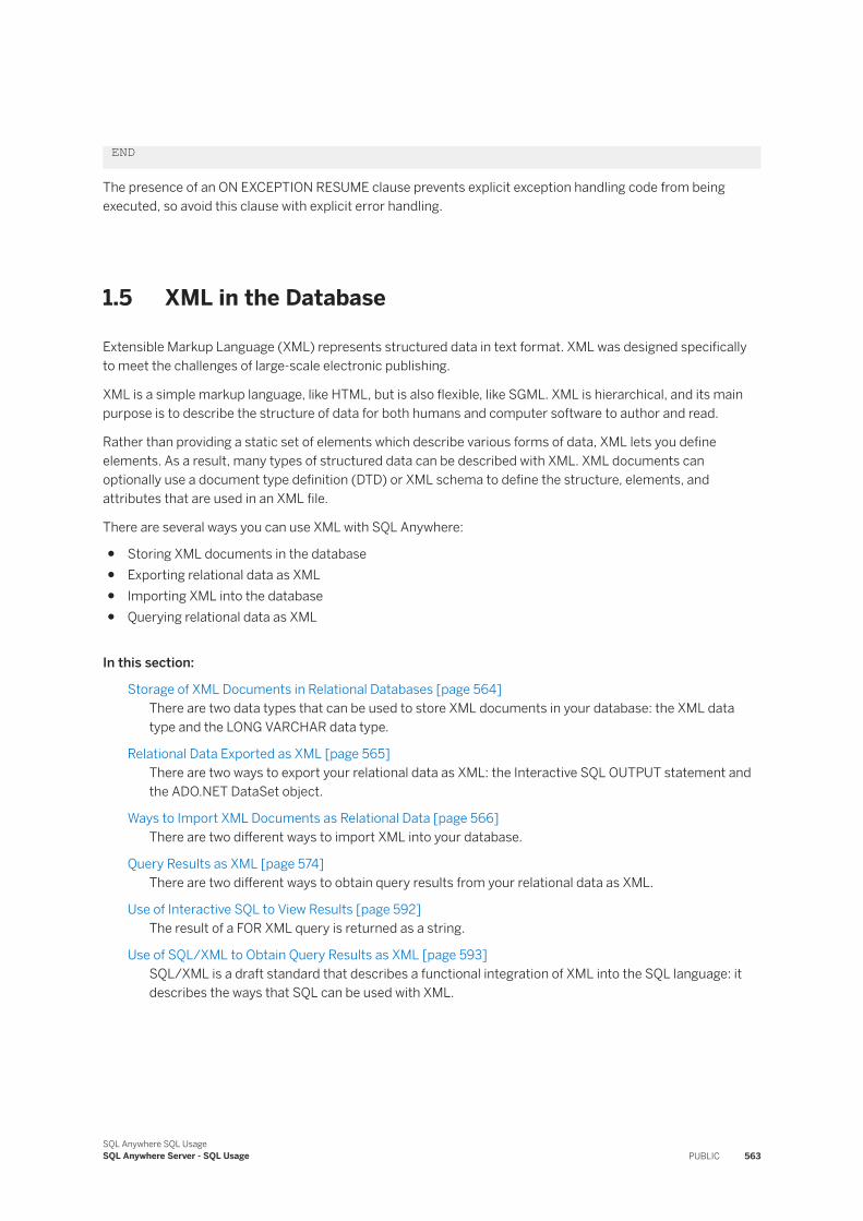
END
The presence of an ON EXCEPTION RESUME clause prevents explicit exception handling code from being executed, so avoid this clause with explicit error handling.
1.5 XML in the Database
Extensible Markup Language (XML) represents structured data in text format. XML was designed specifically to meet the challenges of large-scale electronic publishing.
XML is a simple markup language, like HTML, but is also flexible, like SGML. XML is hierarchical, and its main purpose is to describe the structure of data for both humans and computer software to author and read.
Rather than providing a static set of elements which describe various forms of data, XML lets you define elements. As a result, many types of structured data can be described with XML. XML documents can optionally use a document type definition (DTD) or XML schema to define the structure, elements, and attributes that are used in an XML file.
There are several ways you can use XML with SQL Anywhere:
● Storing XML documents in the database● Exporting relational data as XML● Importing XML into the database● Querying relational data as XML
In this section:
Storage of XML Documents in Relational Databases [page 564]There are two data types that can be used to store XML documents in your database: the XML data type and the LONG VARCHAR data type.
Relational Data Exported as XML [page 565]There are two ways to export your relational data as XML: the Interactive SQL OUTPUT statement and the ADO.NET DataSet object.
Ways to Import XML Documents as Relational Data [page 566]There are two different ways to import XML into your database.
Query Results as XML [page 574]There are two different ways to obtain query results from your relational data as XML.
Use of Interactive SQL to View Results [page 592]The result of a FOR XML query is returned as a string.
Use of SQL/XML to Obtain Query Results as XML [page 593]SQL/XML is a draft standard that describes a functional integration of XML into the SQL language: it describes the ways that SQL can be used with XML.
SQL Anywhere SQL UsageSQL Anywhere Server - SQL Usage PUBLIC 563
Related Information
Extensible Markup Language (XML)
1.5.1 Storage of XML Documents in Relational Databases
There are two data types that can be used to store XML documents in your database: the XML data type and the LONG VARCHAR data type.
Both of these data types store the XML document as a string in the database.
The XML data type uses the character set encoding of the database server. The XML encoding attribute should match the encoding used by the database server. The XML encoding attribute does not specify how the automatic character set conversion is completed.
You can cast between the XML data type and any other data type that can be cast to or from a string. There is no checking that the string is well formed when it is cast to XML.
When you generate elements from relational data, any characters that are invalid in XML are escaped unless the data is of type XML. For example, suppose you want to generate a <product> element with the following content so that the element content contains less than and greater than signs:
<hat>bowler</hat>
If you write a query that specifies that the element content is of type XML, then the greater than and less than signs are not quoted, as follows:
SELECT XMLFOREST( CAST( '<hat>bowler</hat>' AS XML ) AS product );
You get the following result:
<product><hat>bowler</hat></product>
However, if the query does not specify that the element content is of type XML, for example:
SELECT XMLFOREST( '<hat>bowler</hat>' AS product );
In this case, the less than and greater than signs are replaced with entity references as follows:
<product><hat>bowler</hat></product>
Attributes are always quoted, regardless of the data type.
Related Information
Rules for Encoding Illegal XML Names [page 577]
564 PUBLICSQL Anywhere SQL Usage
SQL Anywhere Server - SQL Usage
1.5.2 Relational Data Exported as XML
There are two ways to export your relational data as XML: the Interactive SQL OUTPUT statement and the ADO.NET DataSet object.
The FOR XML clause and SQL/XML functions allow you to generate a result set as XML from the relational data in your database. You can then export the generated XML to a file using the UNLOAD statement or the xp_write_file system procedure.
In this section:
Relational Data Exported as XML from Interactive SQL [page 565]The Interactive SQL OUTPUT statement supports an XML format that outputs query results to a generated XML file.
Relational Data Exported as XML Using the DataSet Object [page 565]The ADO.NET DataSet object allows you to save the contents of the DataSet in an XML document.
1.5.2.1 Relational Data Exported as XML from Interactive SQL
The Interactive SQL OUTPUT statement supports an XML format that outputs query results to a generated XML file.
This generated XML file is encoded in UTF-8 and contains an embedded DTD. In the XML file, binary values are encoded in character data (CDATA) blocks with the binary data rendered as 2-hex-digit strings.
The INPUT statement does not accept XML as a file format. However, you can import XML using the OPENXML operator or the ADO.NET DataSet object.
Related Information
Ways to Import XML Documents as Relational Data [page 566]
1.5.2.2 Relational Data Exported as XML Using the DataSet Object
The ADO.NET DataSet object allows you to save the contents of the DataSet in an XML document.
Once you have filled the DataSet (for example, with the results of a query on your database) you can save either the schema or both the schema and data from the DataSet in an XML file. The WriteXml method saves both the schema and data in an XML file, while the WriteXmlSchema method saves only the schema in an XML file. You can fill a DataSet object using the SQL Anywhere .NET Data Provider.
SQL Anywhere SQL UsageSQL Anywhere Server - SQL Usage PUBLIC 565
1.5.3 Ways to Import XML Documents as Relational Data
There are two different ways to import XML into your database.
● using the OPENXML operator to generate a result set from an XML document● using the ADO.NET DataSet object to read the data and/or schema from an XML document into a DataSet
In this section:
XML Import Using the OPENXML Operator [page 566]The OPENXML operator is used in the FROM clause of a query to generate a result set from an XML document.
Import XML Using the DataSet Object [page 572]The ADO.NET DataSet object allows you to read the data and/or schema from an XML document into a DataSet.
Definition of Default XML Namespaces [page 573]You define a default namespace in an element of an XML document with an attribute of the form xmlns="URI".
1.5.3.1 XML Import Using the OPENXML Operator
The OPENXML operator is used in the FROM clause of a query to generate a result set from an XML document.
OPENXML uses a subset of the XPath query language to select nodes from an XML document.
Using XPath Expressions
When you use OPENXML, the XML document is parsed and the result is modeled as a tree. The tree is made up of nodes. XPath expressions are used to select nodes in the tree. The following list describes some commonly used XPath expressions:
/
indicates the root node of the XML document//
indicates all descendants of the root, including the root node. (single period)
indicates the current node of the XML document.//
indicates all descendants of the current node, including the current node..
indicates the parent node of the current node./@attributename
566 PUBLICSQL Anywhere SQL Usage
SQL Anywhere Server - SQL Usage
indicates the attribute of the current node having the name attributename./childname
indicates the children of the current node that are elements having the name childname
Consider the following XML document:
<inventory> <product ID="301" size="Medium">Tee Shirt <quantity>54</quantity> </product> <product ID="302" size="One Size fits all">Tee Shirt <quantity>75</quantity> </product> <product ID="400" size="One Size fits all">Baseball Cap <quantity>112</quantity> </product> </inventory>
The <inventory> element is the root node. You can refer to it using the following XPath expression:
/inventory
Suppose that the current node is a <quantity> element. You can refer to this node using the following XPath expression:
.
To find all the <product> elements that are children of the <inventory> element, use the following XPath expression:
/inventory/product
If the current node is a <product> element and you want to refer to the size attribute, use the following XPath expression:
./@size
Generating a Result Set Using OPENXML
Each match for the first xpath-query argument to OPENXML generates one row in the result set. The WITH clause specifies the schema of the result set and how the value is found for each column in the result set. For example, consider the following query:
SELECT * FROM OPENXML( '<inventory> <product>Tee Shirt <quantity>54</quantity> <color>Orange</color> </product> <product>Baseball Cap <quantity>112</quantity> <color>Black</color> </product></inventory>','/inventory/product' )
SQL Anywhere SQL UsageSQL Anywhere Server - SQL Usage PUBLIC 567
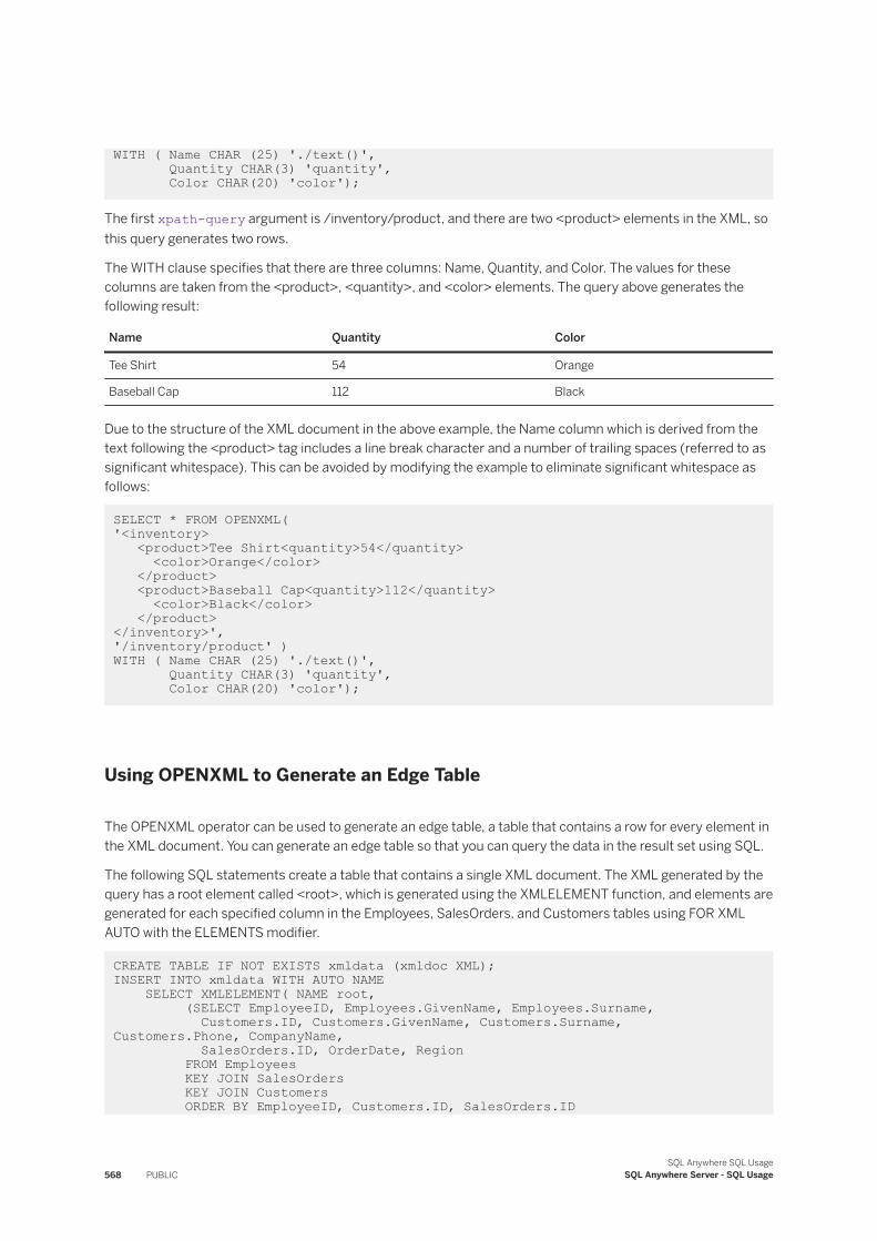
WITH ( Name CHAR (25) './text()', Quantity CHAR(3) 'quantity', Color CHAR(20) 'color');
The first xpath-query argument is /inventory/product, and there are two <product> elements in the XML, so this query generates two rows.
The WITH clause specifies that there are three columns: Name, Quantity, and Color. The values for these columns are taken from the <product>, <quantity>, and <color> elements. The query above generates the following result:
Name Quantity Color
Tee Shirt 54 Orange
Baseball Cap 112 Black
Due to the structure of the XML document in the above example, the Name column which is derived from the text following the <product> tag includes a line break character and a number of trailing spaces (referred to as significant whitespace). This can be avoided by modifying the example to eliminate significant whitespace as follows:
SELECT * FROM OPENXML( '<inventory> <product>Tee Shirt<quantity>54</quantity> <color>Orange</color> </product> <product>Baseball Cap<quantity>112</quantity> <color>Black</color> </product></inventory>','/inventory/product' )WITH ( Name CHAR (25) './text()', Quantity CHAR(3) 'quantity', Color CHAR(20) 'color');
Using OPENXML to Generate an Edge Table
The OPENXML operator can be used to generate an edge table, a table that contains a row for every element in the XML document. You can generate an edge table so that you can query the data in the result set using SQL.
The following SQL statements create a table that contains a single XML document. The XML generated by the query has a root element called <root>, which is generated using the XMLELEMENT function, and elements are generated for each specified column in the Employees, SalesOrders, and Customers tables using FOR XML AUTO with the ELEMENTS modifier.
CREATE TABLE IF NOT EXISTS xmldata (xmldoc XML); INSERT INTO xmldata WITH AUTO NAME SELECT XMLELEMENT( NAME root, (SELECT EmployeeID, Employees.GivenName, Employees.Surname, Customers.ID, Customers.GivenName, Customers.Surname, Customers.Phone, CompanyName, SalesOrders.ID, OrderDate, Region FROM Employees KEY JOIN SalesOrders KEY JOIN Customers ORDER BY EmployeeID, Customers.ID, SalesOrders.ID
568 PUBLICSQL Anywhere SQL Usage
SQL Anywhere Server - SQL Usage
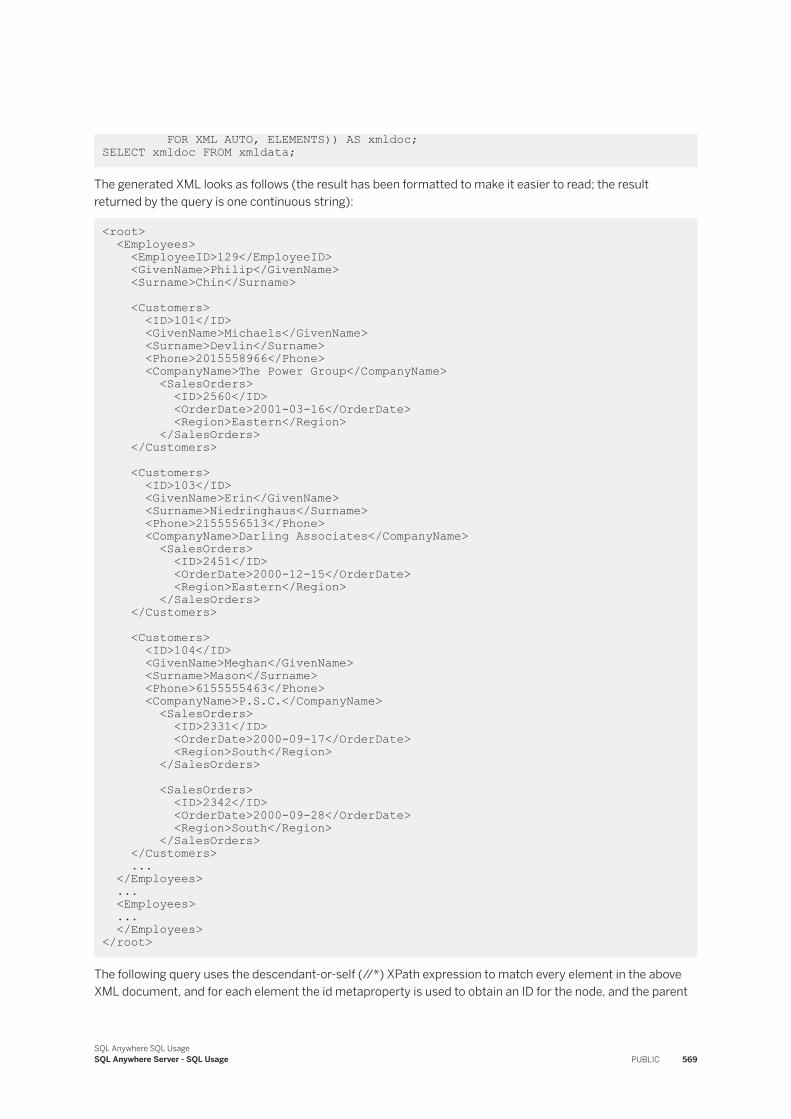
FOR XML AUTO, ELEMENTS)) AS xmldoc; SELECT xmldoc FROM xmldata;
The generated XML looks as follows (the result has been formatted to make it easier to read; the result returned by the query is one continuous string):
<root> <Employees> <EmployeeID>129</EmployeeID> <GivenName>Philip</GivenName> <Surname>Chin</Surname> <Customers> <ID>101</ID> <GivenName>Michaels</GivenName> <Surname>Devlin</Surname> <Phone>2015558966</Phone> <CompanyName>The Power Group</CompanyName> <SalesOrders> <ID>2560</ID> <OrderDate>2001-03-16</OrderDate> <Region>Eastern</Region> </SalesOrders> </Customers> <Customers> <ID>103</ID> <GivenName>Erin</GivenName> <Surname>Niedringhaus</Surname> <Phone>2155556513</Phone> <CompanyName>Darling Associates</CompanyName> <SalesOrders> <ID>2451</ID> <OrderDate>2000-12-15</OrderDate> <Region>Eastern</Region> </SalesOrders> </Customers> <Customers> <ID>104</ID> <GivenName>Meghan</GivenName> <Surname>Mason</Surname> <Phone>6155555463</Phone> <CompanyName>P.S.C.</CompanyName> <SalesOrders> <ID>2331</ID> <OrderDate>2000-09-17</OrderDate> <Region>South</Region> </SalesOrders> <SalesOrders> <ID>2342</ID> <OrderDate>2000-09-28</OrderDate> <Region>South</Region> </SalesOrders> </Customers> ... </Employees> ... <Employees> ... </Employees> </root>
The following query uses the descendant-or-self (//*) XPath expression to match every element in the above XML document, and for each element the id metaproperty is used to obtain an ID for the node, and the parent
SQL Anywhere SQL UsageSQL Anywhere Server - SQL Usage PUBLIC 569
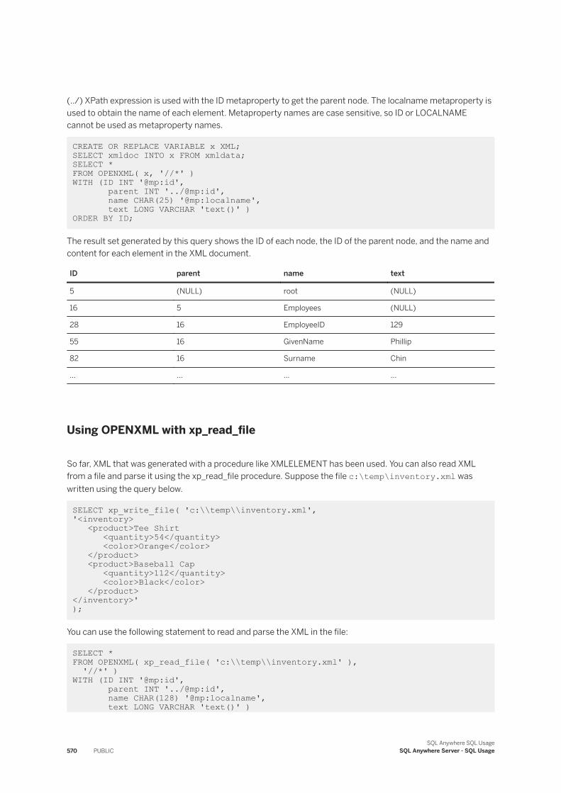
(../) XPath expression is used with the ID metaproperty to get the parent node. The localname metaproperty is used to obtain the name of each element. Metaproperty names are case sensitive, so ID or LOCALNAME cannot be used as metaproperty names.
CREATE OR REPLACE VARIABLE x XML; SELECT xmldoc INTO x FROM xmldata;SELECT * FROM OPENXML( x, '//*' )WITH (ID INT '@mp:id', parent INT '../@mp:id', name CHAR(25) '@mp:localname', text LONG VARCHAR 'text()' ) ORDER BY ID;
The result set generated by this query shows the ID of each node, the ID of the parent node, and the name and content for each element in the XML document.
ID parent name text
5 (NULL) root (NULL)
16 5 Employees (NULL)
28 16 EmployeeID 129
55 16 GivenName Phillip
82 16 Surname Chin
... ... ... ...
Using OPENXML with xp_read_file
So far, XML that was generated with a procedure like XMLELEMENT has been used. You can also read XML from a file and parse it using the xp_read_file procedure. Suppose the file c:\temp\inventory.xml was written using the query below.
SELECT xp_write_file( 'c:\\temp\\inventory.xml', '<inventory> <product>Tee Shirt <quantity>54</quantity> <color>Orange</color> </product> <product>Baseball Cap <quantity>112</quantity> <color>Black</color> </product></inventory>' );
You can use the following statement to read and parse the XML in the file:
SELECT * FROM OPENXML( xp_read_file( 'c:\\temp\\inventory.xml' ), '//*' )WITH (ID INT '@mp:id', parent INT '../@mp:id', name CHAR(128) '@mp:localname', text LONG VARCHAR 'text()' )
570 PUBLICSQL Anywhere SQL Usage
SQL Anywhere Server - SQL Usage
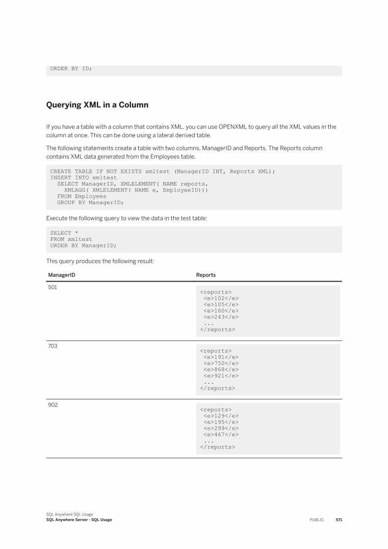
ORDER BY ID;
Querying XML in a Column
If you have a table with a column that contains XML, you can use OPENXML to query all the XML values in the column at once. This can be done using a lateral derived table.
The following statements create a table with two columns, ManagerID and Reports. The Reports column contains XML data generated from the Employees table.
CREATE TABLE IF NOT EXISTS xmltest (ManagerID INT, Reports XML); INSERT INTO xmltest SELECT ManagerID, XMLELEMENT( NAME reports, XMLAGG( XMLELEMENT( NAME e, EmployeeID))) FROM Employees GROUP BY ManagerID;
Execute the following query to view the data in the test table:
SELECT * FROM xmltest ORDER BY ManagerID;
This query produces the following result:
ManagerID Reports
501 <reports> <e>102</e> <e>105</e> <e>160</e> <e>243</e> ... </reports>
703 <reports> <e>191</e> <e>750</e> <e>868</e> <e>921</e> ... </reports>
902 <reports> <e>129</e> <e>195</e> <e>299</e> <e>467</e> ... </reports>
SQL Anywhere SQL UsageSQL Anywhere Server - SQL Usage PUBLIC 571
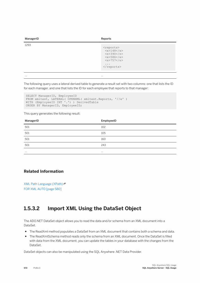
ManagerID Reports
1293 <reports> <e>148</e> <e>390</e> <e>586</e> <e>757</e> ... </reports>
... ...
The following query uses a lateral derived table to generate a result set with two columns: one that lists the ID for each manager, and one that lists the ID for each employee that reports to that manager:
SELECT ManagerID, EmployeeID FROM xmltest, LATERAL( OPENXML( xmltest.Reports, '//e' )WITH (EmployeeID INT '.') ) DerivedTable ORDER BY ManagerID, EmployeeID;
This query generates the following result:
ManagerID EmployeeID
501 102
501 105
501 160
501 243
... ...
Related Information
XML Path Language (XPath)FOR XML AUTO [page 580]
1.5.3.2 Import XML Using the DataSet Object
The ADO.NET DataSet object allows you to read the data and/or schema from an XML document into a DataSet.
● The ReadXml method populates a DataSet from an XML document that contains both a schema and data.● The ReadXmlSchema method reads only the schema from an XML document. Once the DataSet is filled
with data from the XML document, you can update the tables in your database with the changes from the DataSet.
DataSet objects can also be manipulated using the SQL Anywhere .NET Data Provider.
572 PUBLICSQL Anywhere SQL Usage
SQL Anywhere Server - SQL Usage
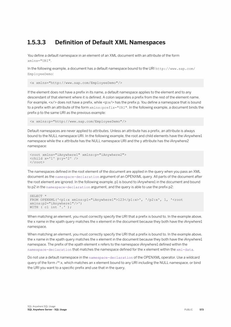
1.5.3.3 Definition of Default XML Namespaces
You define a default namespace in an element of an XML document with an attribute of the form xmlns="URI".
In the following example, a document has a default namespace bound to the URI http://www.sap.com/EmployeeDemo:
<x xmlns="http://www.sap.com/EmployeeDemo"/>
If the element does not have a prefix in its name, a default namespace applies to the element and to any descendant of that element where it is defined. A colon separates a prefix from the rest of the element name. For example, <x/> does not have a prefix, while <p:x/> has the prefix p. You define a namespace that is bound to a prefix with an attribute of the form xmlns:prefix="URI". In the following example, a document binds the prefix p to the same URI as the previous example:
<x xmlns:p="http://www.sap.com/EmployeeDemo"/>
Default namespaces are never applied to attributes. Unless an attribute has a prefix, an attribute is always bound to the NULL namespace URI. In the following example, the root and child elements have the iAnywhere1 namespace while the x attribute has the NULL namespace URI and the y attribute has the iAnywhere2 namespace:
<root xmlns="iAnywhere1" xmlns:p="iAnywhere2"> <child x='1' p:y='2' /> </root>
The namespaces defined in the root element of the document are applied in the query when you pass an XML document as the namespace-declaration argument of an OPENXML query. All parts of the document after the root element are ignored. In the following example, p1 is bound to iAnywhere1 in the document and bound to p2 in the namespace-declaration argument, and the query is able to use the prefix p2:
SELECT * FROM OPENXML('<p1:x xmlns:p1="iAnywhere1">123</p1:x>', '/p2:x', 1, '<root xmlns:p2="iAnywhere1"/>') WITH ( c1 int '.' );
When matching an element, you must correctly specify the URI that a prefix is bound to. In the example above, the x name in the xpath query matches the x element in the document because they both have the iAnywhere1 namespace.
When matching an element, you must correctly specify the URI that a prefix is bound to. In the example above, the x name in the xpath query matches the x element in the document because they both have the iAnywhere1 namespace. The prefix of the xpath element x refers to the namespace iAnywhere1 defined within the namespace-declaration that matches the namespace defined for the x element within the xml-data.
Do not use a default namespace in the namespace-declaration of the OPENXML operator. Use a wildcard query of the form /*:x, which matches an x element bound to any URI including the NULL namespace, or bind the URI you want to a specific prefix and use that in the query,
SQL Anywhere SQL UsageSQL Anywhere Server - SQL Usage PUBLIC 573
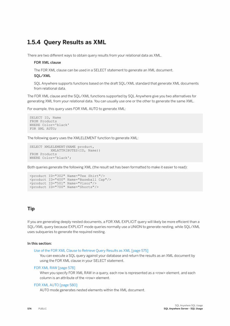
1.5.4 Query Results as XML
There are two different ways to obtain query results from your relational data as XML.
FOR XML clause
The FOR XML clause can be used in a SELECT statement to generate an XML document.SQL/XML
SQL Anywhere supports functions based on the draft SQL/XML standard that generate XML documents from relational data.
The FOR XML clause and the SQL/XML functions supported by SQL Anywhere give you two alternatives for generating XML from your relational data. You can usually use one or the other to generate the same XML.
For example, this query uses FOR XML AUTO to generate XML:
SELECT ID, Name FROM ProductsWHERE Color='black' FOR XML AUTO;
The following query uses the XMLELEMENT function to generate XML:
SELECT XMLELEMENT(NAME product, XMLATTRIBUTES(ID, Name))FROM Products WHERE Color='black';
Both queries generate the following XML (the result set has been formatted to make it easier to read):
<product ID="302" Name="Tee Shirt"/> <product ID="400" Name="Baseball Cap"/><product ID="501" Name="Visor"/> <product ID="700" Name="Shorts"/>
Tip
If you are generating deeply nested documents, a FOR XML EXPLICIT query will likely be more efficient than a SQL/XML query because EXPLICIT mode queries normally use a UNION to generate nesting, while SQL/XML uses subqueries to generate the required nesting.
In this section:
Use of the FOR XML Clause to Retrieve Query Results as XML [page 575]You can execute a SQL query against your database and return the results as an XML document by using the FOR XML clause in your SELECT statement.
FOR XML RAW [page 578]When you specify FOR XML RAW in a query, each row is represented as a <row> element, and each column is an attribute of the <row> element.
FOR XML AUTO [page 580]AUTO mode generates nested elements within the XML document.
574 PUBLICSQL Anywhere SQL Usage
SQL Anywhere Server - SQL Usage
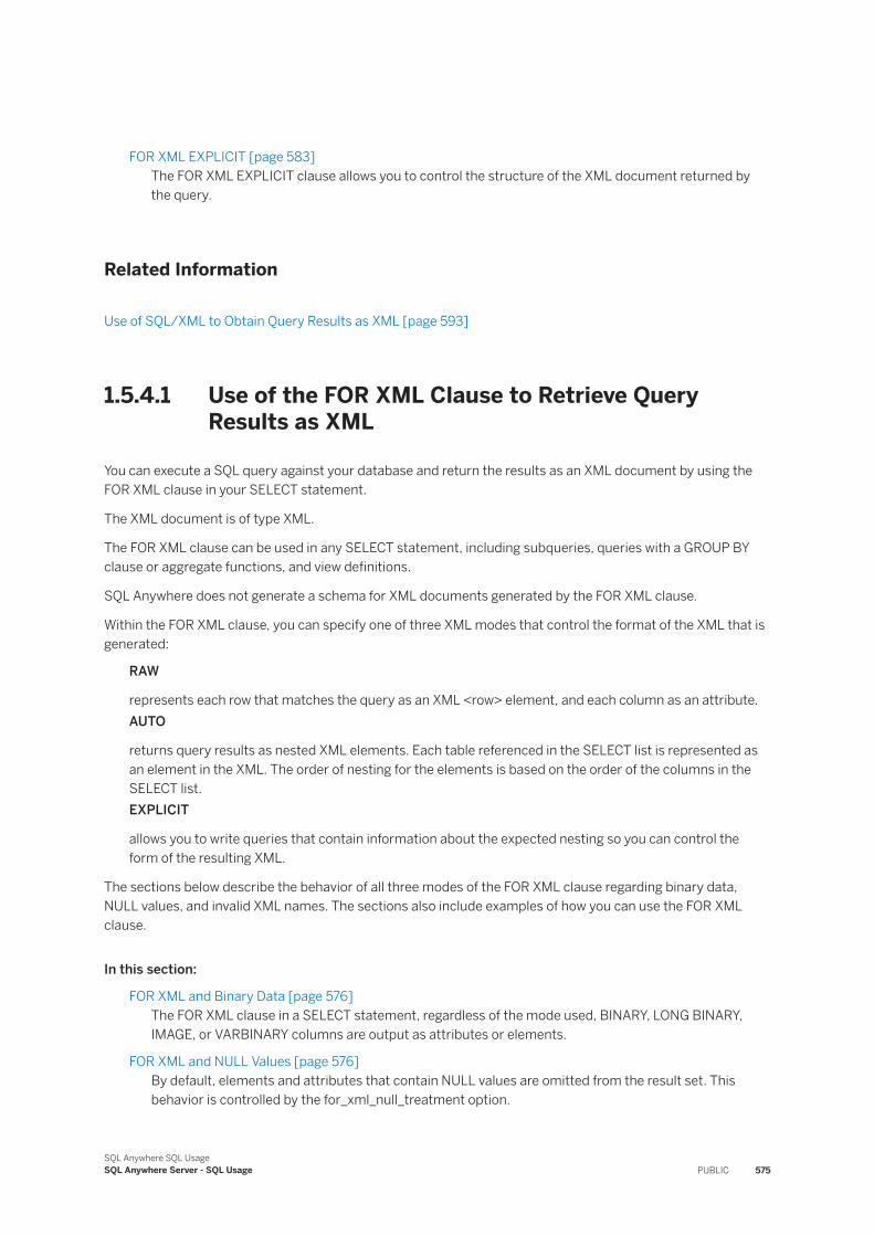
FOR XML EXPLICIT [page 583]The FOR XML EXPLICIT clause allows you to control the structure of the XML document returned by the query.
Related Information
Use of SQL/XML to Obtain Query Results as XML [page 593]
1.5.4.1 Use of the FOR XML Clause to Retrieve Query Results as XML
You can execute a SQL query against your database and return the results as an XML document by using the FOR XML clause in your SELECT statement.
The XML document is of type XML.
The FOR XML clause can be used in any SELECT statement, including subqueries, queries with a GROUP BY clause or aggregate functions, and view definitions.
SQL Anywhere does not generate a schema for XML documents generated by the FOR XML clause.
Within the FOR XML clause, you can specify one of three XML modes that control the format of the XML that is generated:
RAW
represents each row that matches the query as an XML <row> element, and each column as an attribute.AUTO
returns query results as nested XML elements. Each table referenced in the SELECT list is represented as an element in the XML. The order of nesting for the elements is based on the order of the columns in the SELECT list.EXPLICIT
allows you to write queries that contain information about the expected nesting so you can control the form of the resulting XML.
The sections below describe the behavior of all three modes of the FOR XML clause regarding binary data, NULL values, and invalid XML names. The sections also include examples of how you can use the FOR XML clause.
In this section:
FOR XML and Binary Data [page 576]The FOR XML clause in a SELECT statement, regardless of the mode used, BINARY, LONG BINARY, IMAGE, or VARBINARY columns are output as attributes or elements.
FOR XML and NULL Values [page 576]By default, elements and attributes that contain NULL values are omitted from the result set. This behavior is controlled by the for_xml_null_treatment option.
SQL Anywhere SQL UsageSQL Anywhere Server - SQL Usage PUBLIC 575
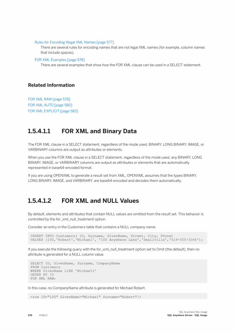
Rules for Encoding Illegal XML Names [page 577]There are several rules for encoding names that are not legal XML names (for example, column names that include spaces).
FOR XML Examples [page 578]There are several examples that show how the FOR XML clause can be used in a SELECT statement.
Related Information
FOR XML RAW [page 578]FOR XML AUTO [page 580]FOR XML EXPLICIT [page 583]
1.5.4.1.1 FOR XML and Binary Data
The FOR XML clause in a SELECT statement, regardless of the mode used, BINARY, LONG BINARY, IMAGE, or VARBINARY columns are output as attributes or elements.
When you use the FOR XML clause in a SELECT statement, regardless of the mode used, any BINARY, LONG BINARY, IMAGE, or VARBINARY columns are output as attributes or elements that are automatically represented in base64-encoded format.
If you are using OPENXML to generate a result set from XML, OPENXML assumes that the types BINARY, LONG BINARY, IMAGE, and VARBINARY, are base64-encoded and decodes them automatically.
1.5.4.1.2 FOR XML and NULL Values
By default, elements and attributes that contain NULL values are omitted from the result set. This behavior is controlled by the for_xml_null_treatment option.
Consider an entry in the Customers table that contains a NULL company name.
INSERT INTO Customers( ID, Surname, GivenName, Street, City, Phone) VALUES (100,'Robert','Michael', '100 Anywhere Lane','Smallville','519-555-3344');
If you execute the following query with the for_xml_null_treatment option set to Omit (the default), then no attribute is generated for a NULL column value.
SELECT ID, GivenName, Surname, CompanyName FROM CustomersWHERE GivenName LIKE 'Michael%'ORDER BY ID FOR XML RAW;
In this case, no CompanyName attribute is generated for Michael Robert.
<row ID="100" GivenName="Michael" Surname="Robert"/>
576 PUBLICSQL Anywhere SQL Usage
SQL Anywhere Server - SQL Usage
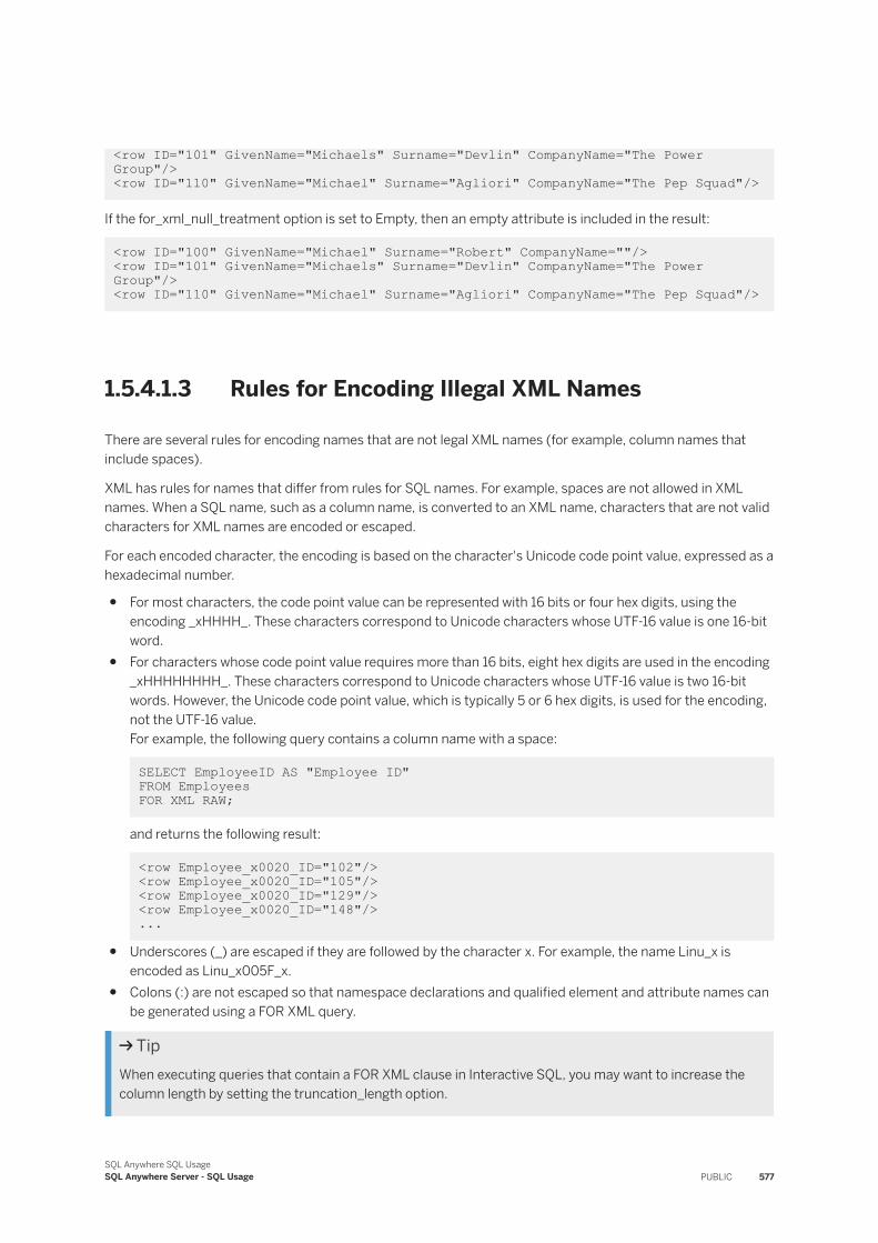
<row ID="101" GivenName="Michaels" Surname="Devlin" CompanyName="The Power Group"/> <row ID="110" GivenName="Michael" Surname="Agliori" CompanyName="The Pep Squad"/>
If the for_xml_null_treatment option is set to Empty, then an empty attribute is included in the result:
<row ID="100" GivenName="Michael" Surname="Robert" CompanyName=""/> <row ID="101" GivenName="Michaels" Surname="Devlin" CompanyName="The Power Group"/> <row ID="110" GivenName="Michael" Surname="Agliori" CompanyName="The Pep Squad"/>
1.5.4.1.3 Rules for Encoding Illegal XML Names
There are several rules for encoding names that are not legal XML names (for example, column names that include spaces).
XML has rules for names that differ from rules for SQL names. For example, spaces are not allowed in XML names. When a SQL name, such as a column name, is converted to an XML name, characters that are not valid characters for XML names are encoded or escaped.
For each encoded character, the encoding is based on the character's Unicode code point value, expressed as a hexadecimal number.
● For most characters, the code point value can be represented with 16 bits or four hex digits, using the encoding _xHHHH_. These characters correspond to Unicode characters whose UTF-16 value is one 16-bit word.
● For characters whose code point value requires more than 16 bits, eight hex digits are used in the encoding _xHHHHHHHH_. These characters correspond to Unicode characters whose UTF-16 value is two 16-bit words. However, the Unicode code point value, which is typically 5 or 6 hex digits, is used for the encoding, not the UTF-16 value.For example, the following query contains a column name with a space:
SELECT EmployeeID AS "Employee ID" FROM Employees FOR XML RAW;
and returns the following result:
<row Employee_x0020_ID="102"/> <row Employee_x0020_ID="105"/><row Employee_x0020_ID="129"/><row Employee_x0020_ID="148"/> ...
● Underscores (_) are escaped if they are followed by the character x. For example, the name Linu_x is encoded as Linu_x005F_x.
● Colons (:) are not escaped so that namespace declarations and qualified element and attribute names can be generated using a FOR XML query.
TipWhen executing queries that contain a FOR XML clause in Interactive SQL, you may want to increase the column length by setting the truncation_length option.
SQL Anywhere SQL UsageSQL Anywhere Server - SQL Usage PUBLIC 577
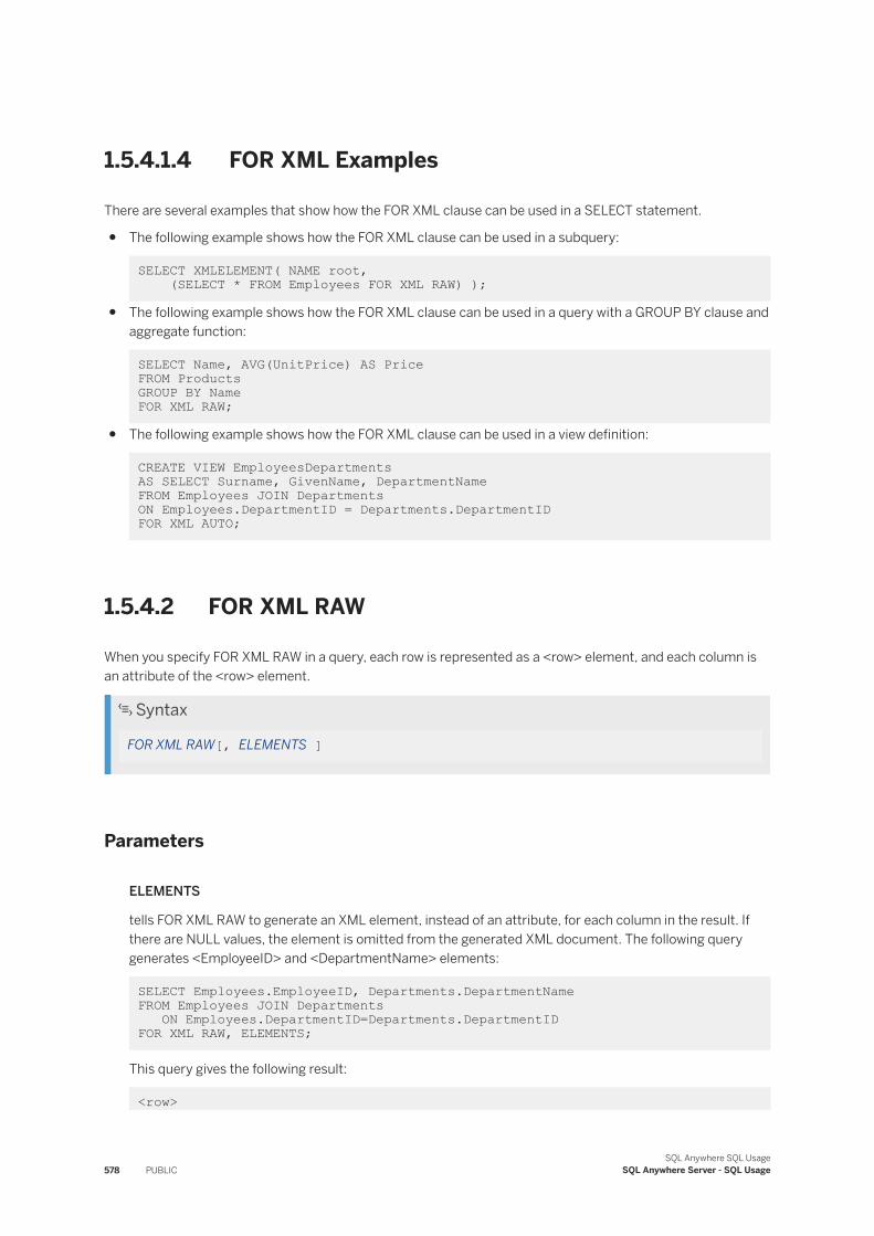
1.5.4.1.4 FOR XML Examples
There are several examples that show how the FOR XML clause can be used in a SELECT statement.
● The following example shows how the FOR XML clause can be used in a subquery:
SELECT XMLELEMENT( NAME root, (SELECT * FROM Employees FOR XML RAW) );
● The following example shows how the FOR XML clause can be used in a query with a GROUP BY clause and aggregate function:
SELECT Name, AVG(UnitPrice) AS Price FROM ProductsGROUP BY Name FOR XML RAW;
● The following example shows how the FOR XML clause can be used in a view definition:
CREATE VIEW EmployeesDepartments AS SELECT Surname, GivenName, DepartmentNameFROM Employees JOIN DepartmentsON Employees.DepartmentID = Departments.DepartmentID FOR XML AUTO;
1.5.4.2 FOR XML RAW
When you specify FOR XML RAW in a query, each row is represented as a <row> element, and each column is an attribute of the <row> element.
Syntax
FOR XML RAW[, ELEMENTS ]
Parameters
ELEMENTS
tells FOR XML RAW to generate an XML element, instead of an attribute, for each column in the result. If there are NULL values, the element is omitted from the generated XML document. The following query generates <EmployeeID> and <DepartmentName> elements:
SELECT Employees.EmployeeID, Departments.DepartmentName FROM Employees JOIN Departments ON Employees.DepartmentID=Departments.DepartmentID FOR XML RAW, ELEMENTS;
This query gives the following result:
<row>
578 PUBLICSQL Anywhere SQL Usage
SQL Anywhere Server - SQL Usage
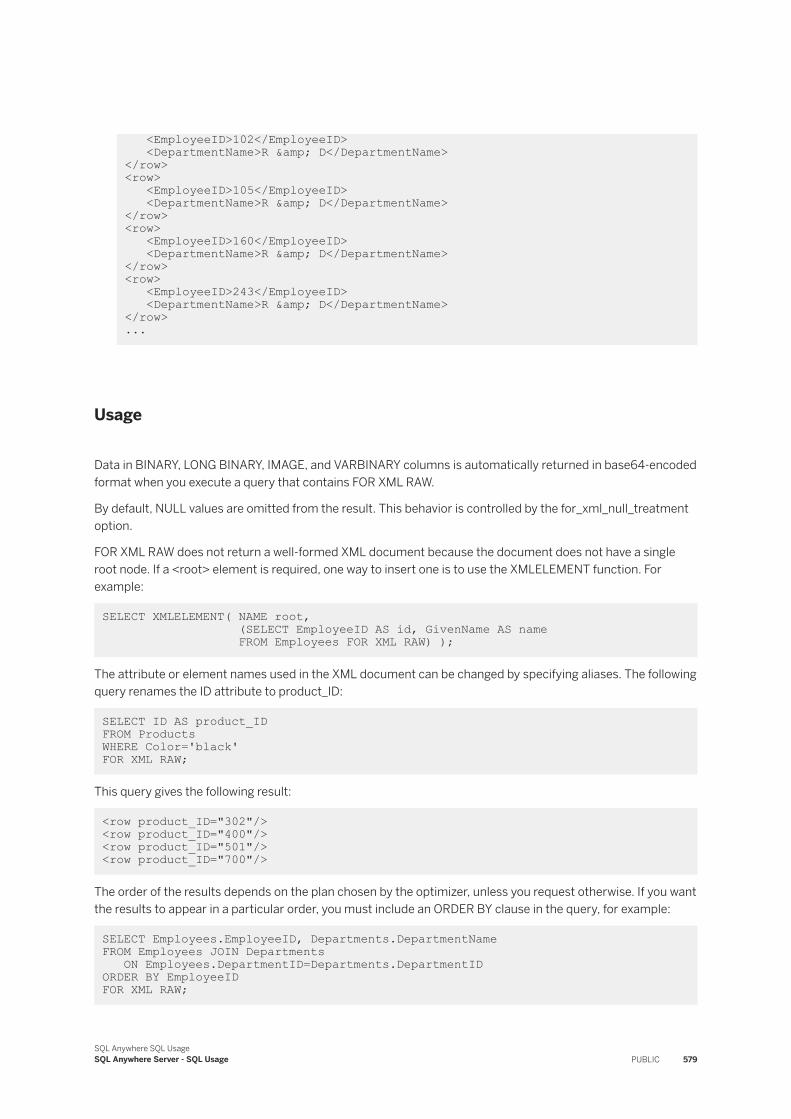
<EmployeeID>102</EmployeeID> <DepartmentName>R & D</DepartmentName></row><row> <EmployeeID>105</EmployeeID> <DepartmentName>R & D</DepartmentName></row> <row> <EmployeeID>160</EmployeeID> <DepartmentName>R & D</DepartmentName></row><row> <EmployeeID>243</EmployeeID> <DepartmentName>R & D</DepartmentName></row> ...
Usage
Data in BINARY, LONG BINARY, IMAGE, and VARBINARY columns is automatically returned in base64-encoded format when you execute a query that contains FOR XML RAW.
By default, NULL values are omitted from the result. This behavior is controlled by the for_xml_null_treatment option.
FOR XML RAW does not return a well-formed XML document because the document does not have a single root node. If a <root> element is required, one way to insert one is to use the XMLELEMENT function. For example:
SELECT XMLELEMENT( NAME root, (SELECT EmployeeID AS id, GivenName AS name FROM Employees FOR XML RAW) );
The attribute or element names used in the XML document can be changed by specifying aliases. The following query renames the ID attribute to product_ID:
SELECT ID AS product_ID FROM ProductsWHERE Color='black' FOR XML RAW;
This query gives the following result:
<row product_ID="302"/> <row product_ID="400"/><row product_ID="501"/> <row product_ID="700"/>
The order of the results depends on the plan chosen by the optimizer, unless you request otherwise. If you want the results to appear in a particular order, you must include an ORDER BY clause in the query, for example:
SELECT Employees.EmployeeID, Departments.DepartmentName FROM Employees JOIN Departments ON Employees.DepartmentID=Departments.DepartmentIDORDER BY EmployeeID FOR XML RAW;
SQL Anywhere SQL UsageSQL Anywhere Server - SQL Usage PUBLIC 579
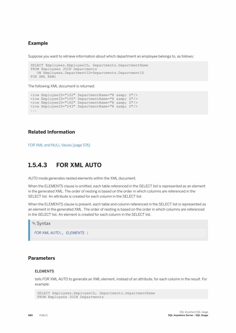
Example
Suppose you want to retrieve information about which department an employee belongs to, as follows:
SELECT Employees.EmployeeID, Departments.DepartmentName FROM Employees JOIN Departments ON Employees.DepartmentID=Departments.DepartmentID FOR XML RAW;
The following XML document is returned:
<row EmployeeID="102" DepartmentName="R & D"/> <row EmployeeID="105" DepartmentName="R & D"/><row EmployeeID="160" DepartmentName="R & D"/><row EmployeeID="243" DepartmentName="R & D"/> ...
Related Information
FOR XML and NULL Values [page 576]
1.5.4.3 FOR XML AUTO
AUTO mode generates nested elements within the XML document.
When the ELEMENTS clause is omitted, each table referenced in the SELECT list is represented as an element in the generated XML. The order of nesting is based on the order in which columns are referenced in the SELECT list. An attribute is created for each column in the SELECT list.
When the ELEMENTS clause is present, each table and column referenced in the SELECT list is represented as an element in the generated XML. The order of nesting is based on the order in which columns are referenced in the SELECT list. An element is created for each column in the SELECT list.
Syntax
FOR XML AUTO[, ELEMENTS ]
Parameters
ELEMENTS
tells FOR XML AUTO to generate an XML element, instead of an attribute, for each column in the result. For example:
SELECT Employees.EmployeeID, Departments.DepartmentName FROM Employees JOIN Departments
580 PUBLICSQL Anywhere SQL Usage
SQL Anywhere Server - SQL Usage
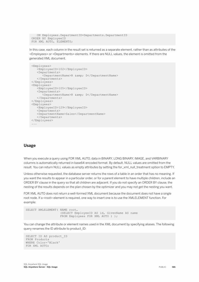
ON Employees.DepartmentID=Departments.DepartmentIDORDER BY EmployeeID FOR XML AUTO, ELEMENTS;
In this case, each column in the result set is returned as a separate element, rather than as attributes of the <Employees> or <Departments> elements. If there are NULL values, the element is omitted from the generated XML document.
<Employees> <EmployeeID>102</EmployeeID> <Departments> <DepartmentName>R & D</DepartmentName> </Departments></Employees> <Employees> <EmployeeID>105</EmployeeID> <Departments> <DepartmentName>R & D</DepartmentName> </Departments></Employees> <Employees> <EmployeeID>129</EmployeeID> <Departments> <DepartmentName>Sales</DepartmentName> </Departments></Employees> ...
Usage
When you execute a query using FOR XML AUTO, data in BINARY, LONG BINARY, IMAGE, and VARBINARY columns is automatically returned in base64-encoded format. By default, NULL values are omitted from the result. You can return NULL values as empty attributes by setting the for_xml_null_treatment option to EMPTY.
Unless otherwise requested, the database server returns the rows of a table in an order that has no meaning. If you want the results to appear in a particular order, or for a parent element to have multiple children, include an ORDER BY clause in the query so that all children are adjacent. If you do not specify an ORDER BY clause, the nesting of the results depends on the plan chosen by the optimizer and you may not get the nesting you want.
FOR XML AUTO does not return a well-formed XML document because the document does not have a single root node. If a <root> element is required, one way to insert one is to use the XMLELEMENT function. For example:
SELECT XMLELEMENT( NAME root, (SELECT EmployeeID AS id, GivenName AS name FROM Employees FOR XML AUTO ) );
You can change the attribute or element names used in the XML document by specifying aliases. The following query renames the ID attribute to product_ID:
SELECT ID AS product_ID FROM ProductsWHERE Color='Black' FOR XML AUTO;
SQL Anywhere SQL UsageSQL Anywhere Server - SQL Usage PUBLIC 581
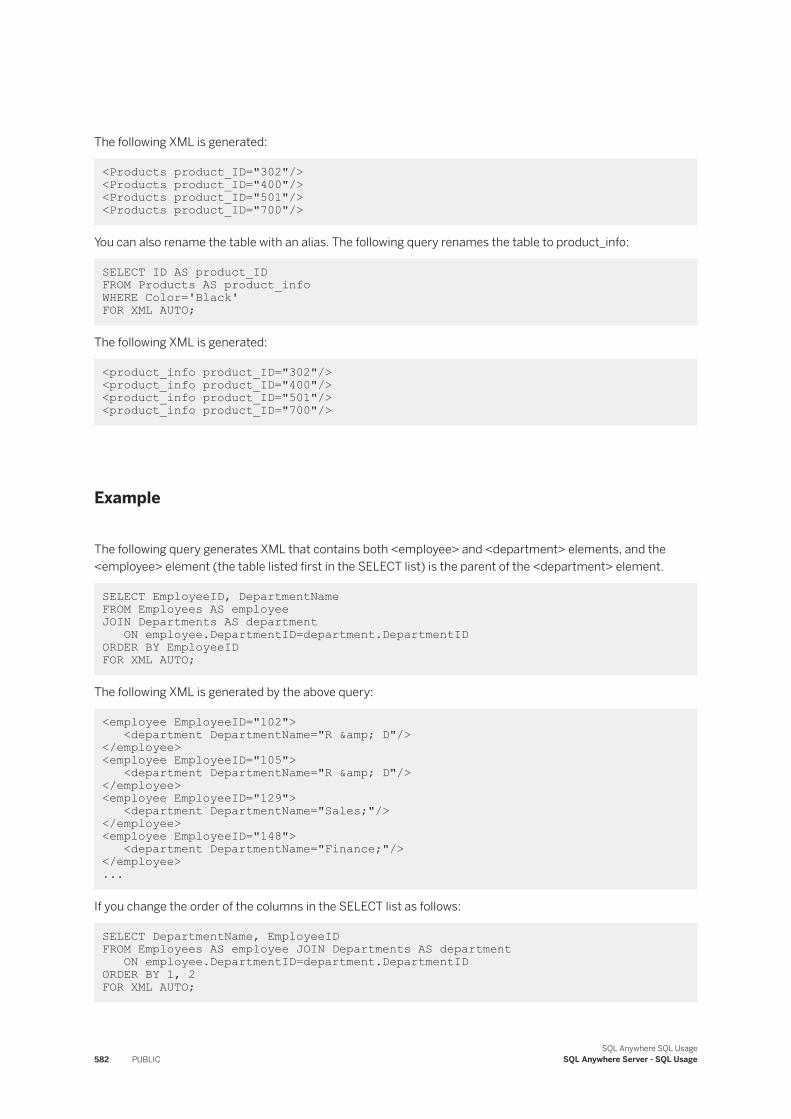
The following XML is generated:
<Products product_ID="302"/> <Products product_ID="400"/><Products product_ID="501"/> <Products product_ID="700"/>
You can also rename the table with an alias. The following query renames the table to product_info:
SELECT ID AS product_ID FROM Products AS product_infoWHERE Color='Black' FOR XML AUTO;
The following XML is generated:
<product_info product_ID="302"/> <product_info product_ID="400"/><product_info product_ID="501"/> <product_info product_ID="700"/>
Example
The following query generates XML that contains both <employee> and <department> elements, and the <employee> element (the table listed first in the SELECT list) is the parent of the <department> element.
SELECT EmployeeID, DepartmentName FROM Employees AS employee JOIN Departments AS department ON employee.DepartmentID=department.DepartmentIDORDER BY EmployeeID FOR XML AUTO;
The following XML is generated by the above query:
<employee EmployeeID="102"> <department DepartmentName="R & D"/></employee><employee EmployeeID="105"> <department DepartmentName="R & D"/></employee><employee EmployeeID="129"> <department DepartmentName="Sales;"/></employee><employee EmployeeID="148"> <department DepartmentName="Finance;"/></employee> ...
If you change the order of the columns in the SELECT list as follows:
SELECT DepartmentName, EmployeeID FROM Employees AS employee JOIN Departments AS department ON employee.DepartmentID=department.DepartmentIDORDER BY 1, 2 FOR XML AUTO;
582 PUBLICSQL Anywhere SQL Usage
SQL Anywhere Server - SQL Usage
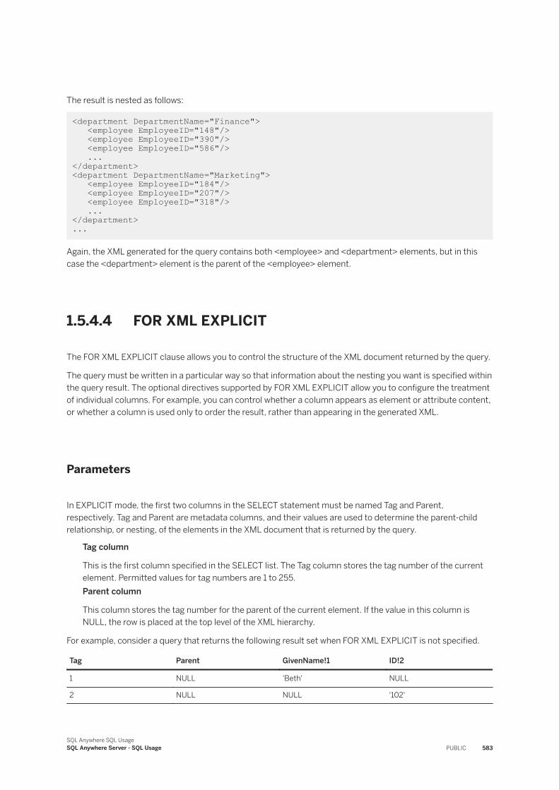
The result is nested as follows:
<department DepartmentName="Finance"> <employee EmployeeID="148"/> <employee EmployeeID="390"/> <employee EmployeeID="586"/> ...</department> <department DepartmentName="Marketing"> <employee EmployeeID="184"/> <employee EmployeeID="207"/> <employee EmployeeID="318"/> ...</department> ...
Again, the XML generated for the query contains both <employee> and <department> elements, but in this case the <department> element is the parent of the <employee> element.
1.5.4.4 FOR XML EXPLICIT
The FOR XML EXPLICIT clause allows you to control the structure of the XML document returned by the query.
The query must be written in a particular way so that information about the nesting you want is specified within the query result. The optional directives supported by FOR XML EXPLICIT allow you to configure the treatment of individual columns. For example, you can control whether a column appears as element or attribute content, or whether a column is used only to order the result, rather than appearing in the generated XML.
Parameters
In EXPLICIT mode, the first two columns in the SELECT statement must be named Tag and Parent, respectively. Tag and Parent are metadata columns, and their values are used to determine the parent-child relationship, or nesting, of the elements in the XML document that is returned by the query.
Tag column
This is the first column specified in the SELECT list. The Tag column stores the tag number of the current element. Permitted values for tag numbers are 1 to 255.Parent column
This column stores the tag number for the parent of the current element. If the value in this column is NULL, the row is placed at the top level of the XML hierarchy.
For example, consider a query that returns the following result set when FOR XML EXPLICIT is not specified.
Tag Parent GivenName!1 ID!2
1 NULL 'Beth' NULL
2 NULL NULL '102'
SQL Anywhere SQL UsageSQL Anywhere Server - SQL Usage PUBLIC 583
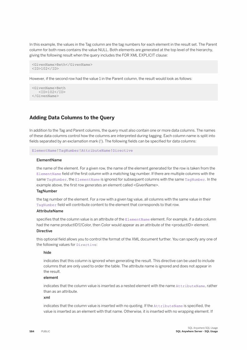
In this example, the values in the Tag column are the tag numbers for each element in the result set. The Parent column for both rows contains the value NULL. Both elements are generated at the top level of the hierarchy, giving the following result when the query includes the FOR XML EXPLICIT clause:
<GivenName>Beth</GivenName> <ID>102</ID>
However, if the second row had the value 1 in the Parent column, the result would look as follows:
<GivenName>Beth <ID>102</ID> </GivenName>
Adding Data Columns to the Query
In addition to the Tag and Parent columns, the query must also contain one or more data columns. The names of these data columns control how the columns are interpreted during tagging. Each column name is split into fields separated by an exclamation mark (!). The following fields can be specified for data columns:
ElementName!TagNumber!AttributeName!Directive
ElementName
the name of the element. For a given row, the name of the element generated for the row is taken from the ElementName field of the first column with a matching tag number. If there are multiple columns with the same TagNumber, the ElementName is ignored for subsequent columns with the same TagNumber. In the example above, the first row generates an element called <GivenName>.TagNumber
the tag number of the element. For a row with a given tag value, all columns with the same value in their TagNumber field will contribute content to the element that corresponds to that row.AttributeName
specifies that the column value is an attribute of the ElementName element. For example, if a data column had the name productID!1!Color, then Color would appear as an attribute of the <productID> element.Directive
this optional field allows you to control the format of the XML document further. You can specify any one of the following values for Directive:
hide
indicates that this column is ignored when generating the result. This directive can be used to include columns that are only used to order the table. The attribute name is ignored and does not appear in the result.element
indicates that the column value is inserted as a nested element with the name AttributeName, rather than as an attribute.xml
indicates that the column value is inserted with no quoting. If the AttributeName is specified, the value is inserted as an element with that name. Otherwise, it is inserted with no wrapping element. If
584 PUBLICSQL Anywhere SQL Usage
SQL Anywhere Server - SQL Usage
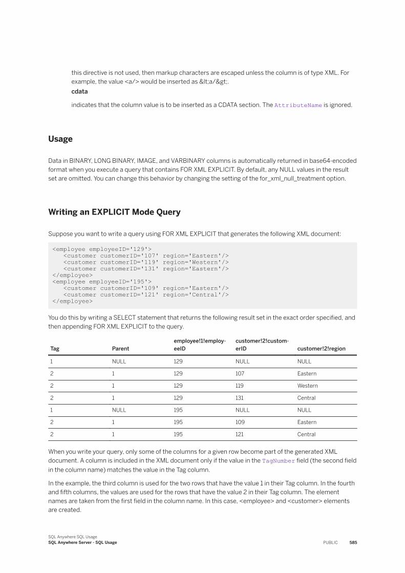
this directive is not used, then markup characters are escaped unless the column is of type XML. For example, the value <a/> would be inserted as <a/>.cdata
indicates that the column value is to be inserted as a CDATA section. The AttributeName is ignored.
Usage
Data in BINARY, LONG BINARY, IMAGE, and VARBINARY columns is automatically returned in base64-encoded format when you execute a query that contains FOR XML EXPLICIT. By default, any NULL values in the result set are omitted. You can change this behavior by changing the setting of the for_xml_null_treatment option.
Writing an EXPLICIT Mode Query
Suppose you want to write a query using FOR XML EXPLICIT that generates the following XML document:
<employee employeeID='129'> <customer customerID='107' region='Eastern'/> <customer customerID='119' region='Western'/> <customer customerID='131' region='Eastern'/></employee><employee employeeID='195'> <customer customerID='109' region='Eastern'/> <customer customerID='121' region='Central'/> </employee>
You do this by writing a SELECT statement that returns the following result set in the exact order specified, and then appending FOR XML EXPLICIT to the query.
Tag Parentemployee!1!employeeID
customer!2!customerID customer!2!region
1 NULL 129 NULL NULL
2 1 129 107 Eastern
2 1 129 119 Western
2 1 129 131 Central
1 NULL 195 NULL NULL
2 1 195 109 Eastern
2 1 195 121 Central
When you write your query, only some of the columns for a given row become part of the generated XML document. A column is included in the XML document only if the value in the TagNumber field (the second field in the column name) matches the value in the Tag column.
In the example, the third column is used for the two rows that have the value 1 in their Tag column. In the fourth and fifth columns, the values are used for the rows that have the value 2 in their Tag column. The element names are taken from the first field in the column name. In this case, <employee> and <customer> elements are created.
SQL Anywhere SQL UsageSQL Anywhere Server - SQL Usage PUBLIC 585
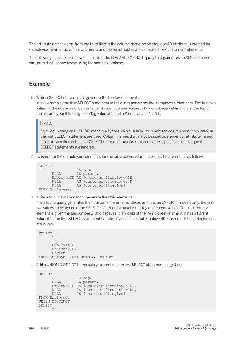
The attribute names come from the third field in the column name, so an employeeID attribute is created for <employee> elements, while customerID and region attributes are generated for <customer> elements.
The following steps explain how to construct the FOR XML EXPLICIT query that generates an XML document similar to the first one above using the sample database.
Example
1. Write a SELECT statement to generate the top-level elements.In this example, the first SELECT statement in the query generates the <employee> elements. The first two values in the query must be the Tag and Parent column values. The <employee> element is at the top of the hierarchy, so it is assigned a Tag value of 1, and a Parent value of NULL.
NoteIf you are writing an EXPLICIT mode query that uses a UNION, then only the column names specified in the first SELECT statement are used. Column names that are to be used as element or attribute names must be specified in the first SELECT statement because column names specified in subsequent SELECT statements are ignored.
2. To generate the <employee> elements for the table above, your first SELECT statement is as follows:
SELECT 1 AS tag, NULL AS parent, EmployeeID AS [employee!1!employeeID], NULL AS [customer!2!customerID], NULL AS [customer!2!region] FROM Employees;
3. Write a SELECT statement to generate the child elements.The second query generates the <customer> elements. Because this is an EXPLICIT mode query, the first two values specified in all the SELECT statements must be the Tag and Parent values. The <customer> element is given the tag number 2, and because it is a child of the <employee> element, it has a Parent value of 1. The first SELECT statement has already specified that EmployeeID, CustomerID, and Region are attributes.
SELECT 2, 1, EmployeeID, CustomerID, Region FROM Employees KEY JOIN SalesOrders
4. Add a UNION DISTINCT to the query to combine the two SELECT statements together:
SELECT 1 AS tag, NULL AS parent, EmployeeID AS [employee!1!employeeID], NULL AS [customer!2!customerID], NULL AS [customer!2!region]FROM EmployeesUNION DISTINCT SELECT 2,
586 PUBLICSQL Anywhere SQL Usage
SQL Anywhere Server - SQL Usage
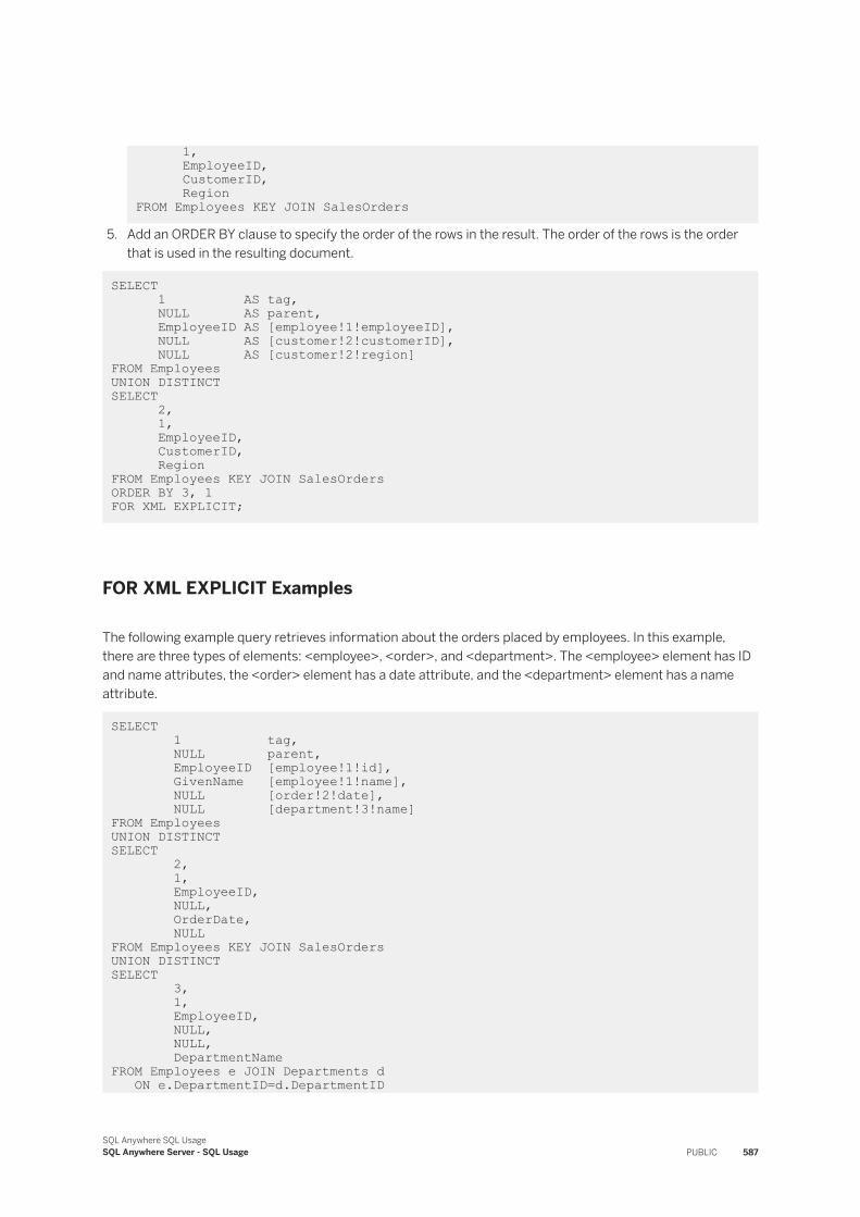
1, EmployeeID, CustomerID, Region FROM Employees KEY JOIN SalesOrders
5. Add an ORDER BY clause to specify the order of the rows in the result. The order of the rows is the order that is used in the resulting document.
SELECT 1 AS tag, NULL AS parent, EmployeeID AS [employee!1!employeeID], NULL AS [customer!2!customerID], NULL AS [customer!2!region]FROM EmployeesUNION DISTINCT SELECT 2, 1, EmployeeID, CustomerID, RegionFROM Employees KEY JOIN SalesOrdersORDER BY 3, 1 FOR XML EXPLICIT;
FOR XML EXPLICIT Examples
The following example query retrieves information about the orders placed by employees. In this example, there are three types of elements: <employee>, <order>, and <department>. The <employee> element has ID and name attributes, the <order> element has a date attribute, and the <department> element has a name attribute.
SELECT 1 tag, NULL parent, EmployeeID [employee!1!id], GivenName [employee!1!name], NULL [order!2!date], NULL [department!3!name]FROM EmployeesUNION DISTINCT SELECT 2, 1, EmployeeID, NULL, OrderDate, NULLFROM Employees KEY JOIN SalesOrdersUNION DISTINCT SELECT 3, 1, EmployeeID, NULL, NULL, DepartmentNameFROM Employees e JOIN Departments d ON e.DepartmentID=d.DepartmentID
SQL Anywhere SQL UsageSQL Anywhere Server - SQL Usage PUBLIC 587
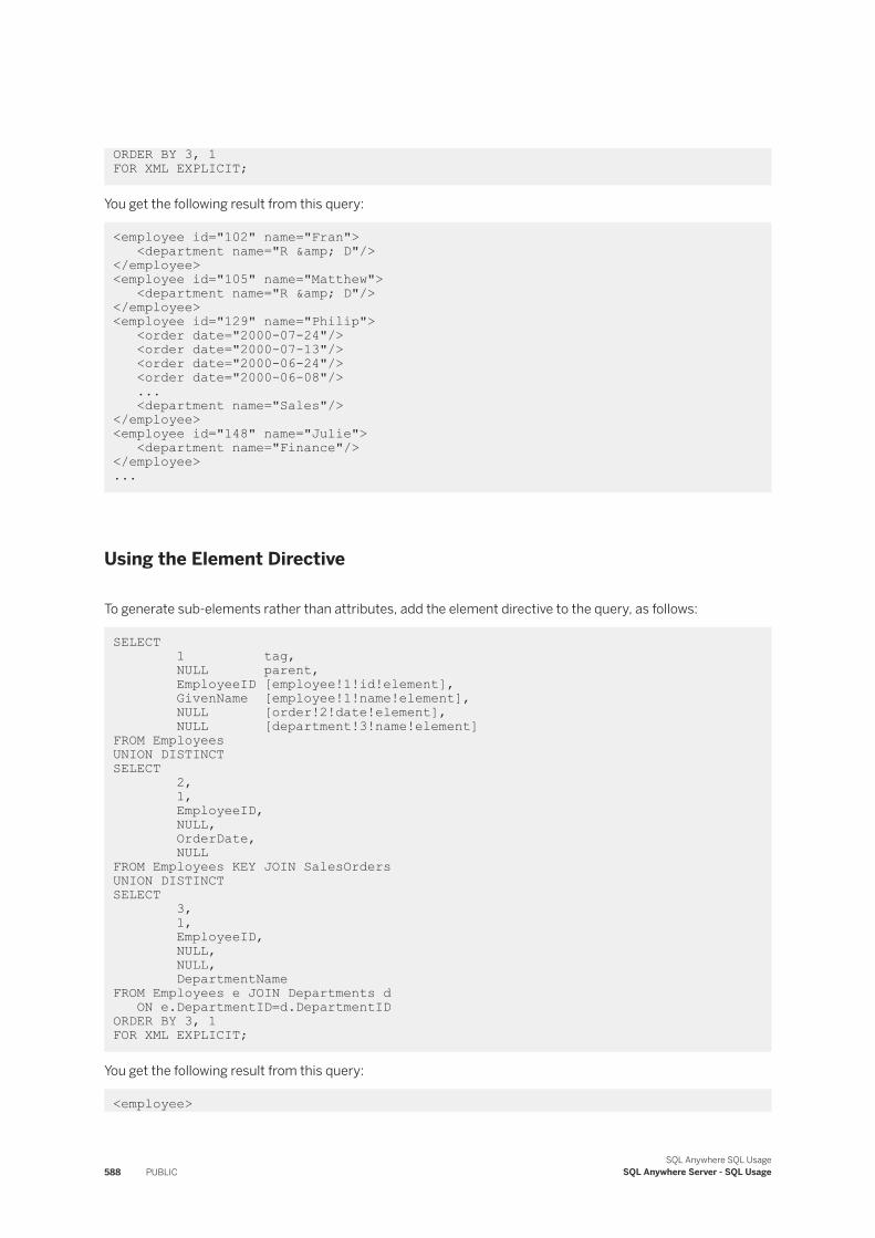
ORDER BY 3, 1 FOR XML EXPLICIT;
You get the following result from this query:
<employee id="102" name="Fran"> <department name="R & D"/></employee><employee id="105" name="Matthew"> <department name="R & D"/></employee> <employee id="129" name="Philip"> <order date="2000-07-24"/> <order date="2000-07-13"/> <order date="2000-06-24"/> <order date="2000-06-08"/> ... <department name="Sales"/></employee> <employee id="148" name="Julie"> <department name="Finance"/></employee> ...
Using the Element Directive
To generate sub-elements rather than attributes, add the element directive to the query, as follows:
SELECT 1 tag, NULL parent, EmployeeID [employee!1!id!element], GivenName [employee!1!name!element], NULL [order!2!date!element], NULL [department!3!name!element]FROM Employees UNION DISTINCTSELECT 2, 1, EmployeeID, NULL, OrderDate, NULLFROM Employees KEY JOIN SalesOrdersUNION DISTINCTSELECT 3, 1, EmployeeID, NULL, NULL, DepartmentNameFROM Employees e JOIN Departments d ON e.DepartmentID=d.DepartmentIDORDER BY 3, 1 FOR XML EXPLICIT;
You get the following result from this query:
<employee>
588 PUBLICSQL Anywhere SQL Usage
SQL Anywhere Server - SQL Usage
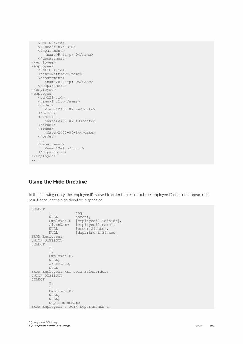
<id>102</id> <name>Fran</name> <department> <name>R & D</name> </department></employee> <employee> <id>105</id> <name>Matthew</name> <department> <name>R & D</name> </department></employee> <employee> <id>129</id> <name>Philip</name> <order> <date>2000-07-24</date> </order> <order> <date>2000-07-13</date> </order> <order> <date>2000-06-24</date> </order> ... <department> <name>Sales</name> </department></employee> ...
Using the Hide Directive
In the following query, the employee ID is used to order the result, but the employee ID does not appear in the result because the hide directive is specified:
SELECT 1 tag, NULL parent, EmployeeID [employee!1!id!hide], GivenName [employee!1!name], NULL [order!2!date], NULL [department!3!name]FROM EmployeesUNION DISTINCT SELECT 2, 1, EmployeeID, NULL, OrderDate, NULLFROM Employees KEY JOIN SalesOrdersUNION DISTINCT SELECT 3, 1, EmployeeID, NULL, NULL, DepartmentNameFROM Employees e JOIN Departments d
SQL Anywhere SQL UsageSQL Anywhere Server - SQL Usage PUBLIC 589
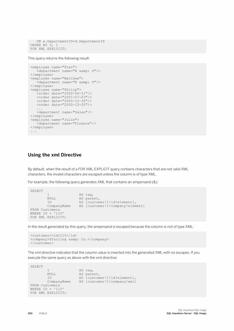
ON e.DepartmentID=d.DepartmentIDORDER BY 3, 1 FOR XML EXPLICIT;
This query returns the following result:
<employee name="Fran"> <department name="R & D"/></employee><employee name="Matthew"> <department name="R & D"/></employee> <employee name="Philip"> <order date="2000-04-21"/> <order date="2001-07-23"/> <order date="2000-12-30"/> <order date="2000-12-20"/> ... <department name="Sales"/></employee> <employee name="Julie"> <department name="Finance"/></employee> ...
Using the xml Directive
By default, when the result of a FOR XML EXPLICIT query contains characters that are not valid XML characters, the invalid characters are escaped unless the column is of type XML.
For example, the following query generates XML that contains an ampersand (&):
SELECT 1 AS tag, NULL AS parent, ID AS [customer!1!id!element], CompanyName AS [customer!1!company!element]FROM CustomersWHERE ID = '115' FOR XML EXPLICIT;
In the result generated by this query, the ampersand is escaped because the column is not of type XML:
<customer><id>115</id> <company>Sterling & Co.</company> </customer>
The xml directive indicates that the column value is inserted into the generated XML with no escapes. If you execute the same query as above with the xml directive:
SELECT 1 AS tag, NULL AS parent, ID AS [customer!1!id!element], CompanyName AS [customer!1!company!xml]FROM CustomersWHERE ID = '115' FOR XML EXPLICIT;
590 PUBLICSQL Anywhere SQL Usage
SQL Anywhere Server - SQL Usage
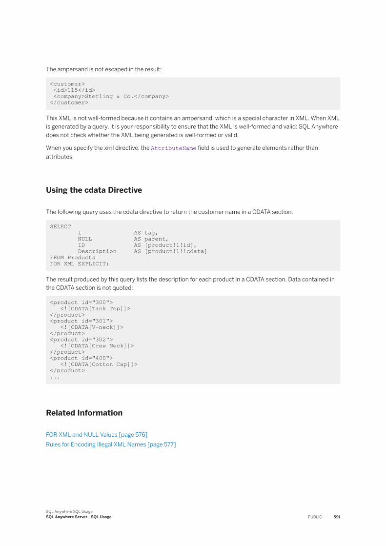
The ampersand is not escaped in the result:
<customer> <id>115</id> <company>Sterling & Co.</company> </customer>
This XML is not well-formed because it contains an ampersand, which is a special character in XML. When XML is generated by a query, it is your responsibility to ensure that the XML is well-formed and valid: SQL Anywhere does not check whether the XML being generated is well-formed or valid.
When you specify the xml directive, the AttributeName field is used to generate elements rather than attributes.
Using the cdata Directive
The following query uses the cdata directive to return the customer name in a CDATA section:
SELECT 1 AS tag, NULL AS parent, ID AS [product!1!id], Description AS [product!1!!cdata]FROM Products FOR XML EXPLICIT;
The result produced by this query lists the description for each product in a CDATA section. Data contained in the CDATA section is not quoted:
<product id="300"> <![CDATA[Tank Top]]></product><product id="301"> <![CDATA[V-neck]]></product> <product id="302"> <![CDATA[Crew Neck]]></product><product id="400"> <![CDATA[Cotton Cap]]></product> ...
Related Information
FOR XML and NULL Values [page 576]Rules for Encoding Illegal XML Names [page 577]
SQL Anywhere SQL UsageSQL Anywhere Server - SQL Usage PUBLIC 591
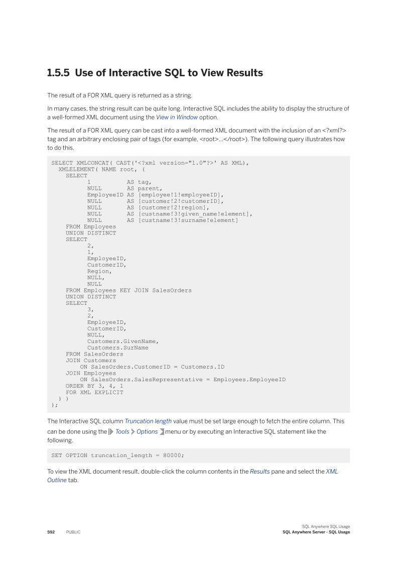
1.5.5 Use of Interactive SQL to View Results
The result of a FOR XML query is returned as a string.
In many cases, the string result can be quite long. Interactive SQL includes the ability to display the structure of a well-formed XML document using the View in Window option.
The result of a FOR XML query can be cast into a well-formed XML document with the inclusion of an <?xml?> tag and an arbitrary enclosing pair of tags (for example, <root>...</root>). The following query illustrates how to do this.
SELECT XMLCONCAT( CAST('<?xml version="1.0"?>' AS XML), XMLELEMENT( NAME root, ( SELECT 1 AS tag, NULL AS parent, EmployeeID AS [employee!1!employeeID], NULL AS [customer!2!customerID], NULL AS [customer!2!region], NULL AS [custname!3!given_name!element], NULL AS [custname!3!surname!element] FROM Employees UNION DISTINCT SELECT 2, 1, EmployeeID, CustomerID, Region, NULL, NULL FROM Employees KEY JOIN SalesOrders UNION DISTINCT SELECT 3, 2, EmployeeID, CustomerID, NULL, Customers.GivenName, Customers.SurName FROM SalesOrders JOIN Customers ON SalesOrders.CustomerID = Customers.ID JOIN Employees ON SalesOrders.SalesRepresentative = Employees.EmployeeID ORDER BY 3, 4, 1 FOR XML EXPLICIT ) ) );
The Interactive SQL column Truncation length value must be set large enough to fetch the entire column. This can be done using the Tools Options menu or by executing an Interactive SQL statement like the following.
SET OPTION truncation_length = 80000;
To view the XML document result, double-click the column contents in the Results pane and select the XML Outline tab.
592 PUBLICSQL Anywhere SQL Usage
SQL Anywhere Server - SQL Usage
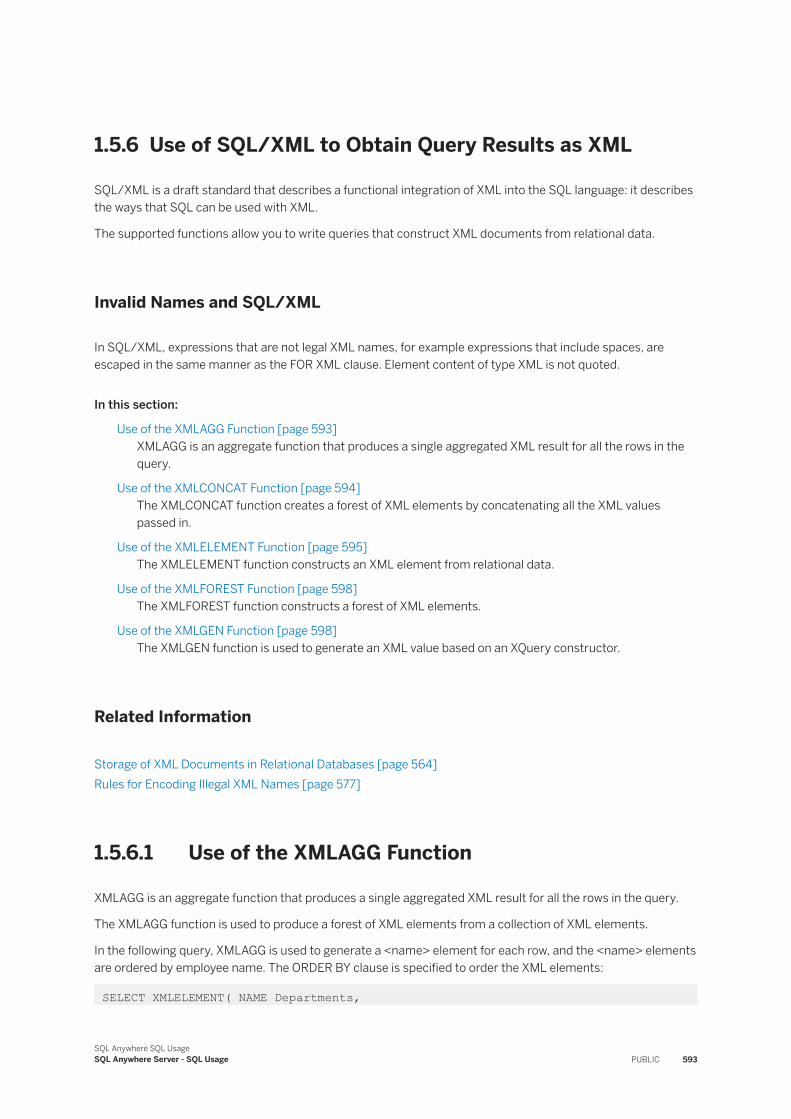
1.5.6 Use of SQL/XML to Obtain Query Results as XML
SQL/XML is a draft standard that describes a functional integration of XML into the SQL language: it describes the ways that SQL can be used with XML.
The supported functions allow you to write queries that construct XML documents from relational data.
Invalid Names and SQL/XML
In SQL/XML, expressions that are not legal XML names, for example expressions that include spaces, are escaped in the same manner as the FOR XML clause. Element content of type XML is not quoted.
In this section:
Use of the XMLAGG Function [page 593]XMLAGG is an aggregate function that produces a single aggregated XML result for all the rows in the query.
Use of the XMLCONCAT Function [page 594]The XMLCONCAT function creates a forest of XML elements by concatenating all the XML values passed in.
Use of the XMLELEMENT Function [page 595]The XMLELEMENT function constructs an XML element from relational data.
Use of the XMLFOREST Function [page 598]The XMLFOREST function constructs a forest of XML elements.
Use of the XMLGEN Function [page 598]The XMLGEN function is used to generate an XML value based on an XQuery constructor.
Related Information
Storage of XML Documents in Relational Databases [page 564]Rules for Encoding Illegal XML Names [page 577]
1.5.6.1 Use of the XMLAGG Function
XMLAGG is an aggregate function that produces a single aggregated XML result for all the rows in the query.
The XMLAGG function is used to produce a forest of XML elements from a collection of XML elements.
In the following query, XMLAGG is used to generate a <name> element for each row, and the <name> elements are ordered by employee name. The ORDER BY clause is specified to order the XML elements:
SELECT XMLELEMENT( NAME Departments,
SQL Anywhere SQL UsageSQL Anywhere Server - SQL Usage PUBLIC 593
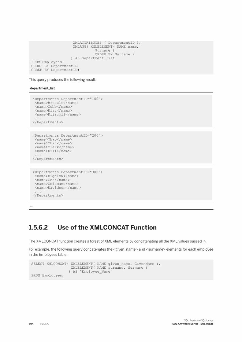
XMLATTRIBUTES ( DepartmentID ), XMLAGG( XMLELEMENT( NAME name, Surname ) ORDER BY Surname ) ) AS department_listFROM EmployeesGROUP BY DepartmentID ORDER BY DepartmentID;
This query produces the following result:
department_list
<Departments DepartmentID="100"> <name>Breault</name> <name>Cobb</name> <name>Diaz</name> <name>Driscoll</name> ... </Departments>
<Departments DepartmentID="200"> <name>Chao</name> <name>Chin</name> <name>Clark</name> <name>Dill</name> ... </Departments>
<Departments DepartmentID="300"> <name>Bigelow</name> <name>Coe</name> <name>Coleman</name> <name>Davidson</name> ... </Departments>
...
1.5.6.2 Use of the XMLCONCAT Function
The XMLCONCAT function creates a forest of XML elements by concatenating all the XML values passed in.
For example, the following query concatenates the <given_name> and <surname> elements for each employee in the Employees table:
SELECT XMLCONCAT( XMLELEMENT( NAME given_name, GivenName ), XMLELEMENT( NAME surname, Surname ) ) AS "Employee_Name" FROM Employees;
594 PUBLICSQL Anywhere SQL Usage
SQL Anywhere Server - SQL Usage
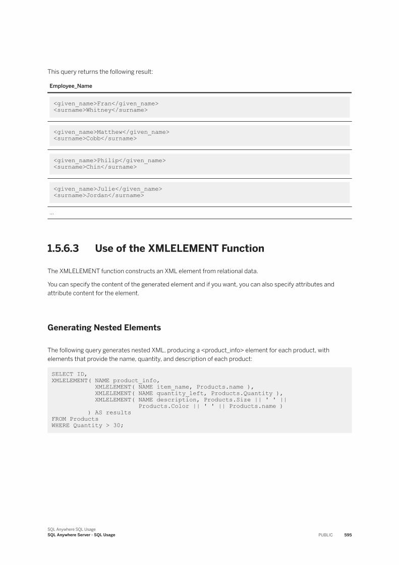
This query returns the following result:
Employee_Name
<given_name>Fran</given_name> <surname>Whitney</surname>
<given_name>Matthew</given_name> <surname>Cobb</surname>
<given_name>Philip</given_name> <surname>Chin</surname>
<given_name>Julie</given_name> <surname>Jordan</surname>
...
1.5.6.3 Use of the XMLELEMENT Function
The XMLELEMENT function constructs an XML element from relational data.
You can specify the content of the generated element and if you want, you can also specify attributes and attribute content for the element.
Generating Nested Elements
The following query generates nested XML, producing a <product_info> element for each product, with elements that provide the name, quantity, and description of each product:
SELECT ID, XMLELEMENT( NAME product_info, XMLELEMENT( NAME item_name, Products.name ), XMLELEMENT( NAME quantity_left, Products.Quantity ), XMLELEMENT( NAME description, Products.Size || ' ' || Products.Color || ' ' || Products.name ) ) AS resultsFROM Products WHERE Quantity > 30;
SQL Anywhere SQL UsageSQL Anywhere Server - SQL Usage PUBLIC 595
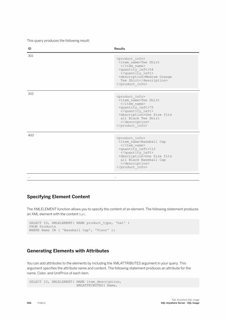
This query produces the following result:
ID Results
301 <product_info> <item_name>Tee Shirt </item_name> <quantity_left>54 </quantity_left> <description>Medium Orange Tee Shirt</description> </product_info>
302 <product_info> <item_name>Tee Shirt </item_name> <quantity_left>75 </quantity_left> <description>One Size fits all Black Tee Shirt </description> </product_info>
400 <product_info> <item_name>Baseball Cap </item_name> <quantity_left>112 </quantity_left> <description>One Size fits all Black Baseball Cap </description> </product_info>
... ...
Specifying Element Content
The XMLELEMENT function allows you to specify the content of an element. The following statement produces an XML element with the content hat.
SELECT ID, XMLELEMENT( NAME product_type, 'hat' ) FROM Products WHERE Name IN ( 'Baseball Cap', 'Visor' );
Generating Elements with Attributes
You can add attributes to the elements by including the XMLATTRIBUTES argument in your query. This argument specifies the attribute name and content. The following statement produces an attribute for the name, Color, and UnitPrice of each item.
SELECT ID, XMLELEMENT( NAME item_description, XMLATTRIBUTES( Name,
596 PUBLICSQL Anywhere SQL Usage
SQL Anywhere Server - SQL Usage
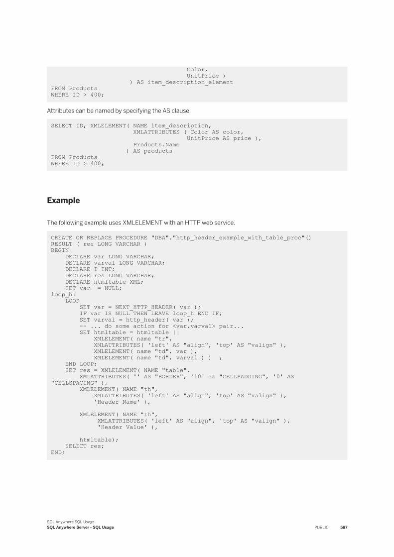
Color, UnitPrice ) ) AS item_description_elementFROM Products WHERE ID > 400;
Attributes can be named by specifying the AS clause:
SELECT ID, XMLELEMENT( NAME item_description, XMLATTRIBUTES ( Color AS color, UnitPrice AS price ), Products.Name ) AS productsFROM Products WHERE ID > 400;
Example
The following example uses XMLELEMENT with an HTTP web service.
CREATE OR REPLACE PROCEDURE "DBA"."http_header_example_with_table_proc"() RESULT ( res LONG VARCHAR )BEGIN DECLARE var LONG VARCHAR; DECLARE varval LONG VARCHAR; DECLARE I INT; DECLARE res LONG VARCHAR; DECLARE htmltable XML; SET var = NULL;loop_h: LOOP SET var = NEXT_HTTP_HEADER( var ); IF var IS NULL THEN LEAVE loop_h END IF; SET varval = http_header( var ); -- ... do some action for <var,varval> pair... SET htmltable = htmltable || XMLELEMENT( name "tr", XMLATTRIBUTES( 'left' AS "align", 'top' AS "valign" ), XMLELEMENT( name "td", var ), XMLELEMENT( name "td", varval ) ) ; END LOOP; SET res = XMLELEMENT( NAME "table", XMLATTRIBUTES( '' AS "BORDER", '10' as "CELLPADDING", '0' AS "CELLSPACING" ), XMLELEMENT( NAME "th", XMLATTRIBUTES( 'left' AS "align", 'top' AS "valign" ), 'Header Name' ), XMLELEMENT( NAME "th", XMLATTRIBUTES( 'left' AS "align", 'top' AS "valign" ), 'Header Value' ), htmltable); SELECT res; END;
SQL Anywhere SQL UsageSQL Anywhere Server - SQL Usage PUBLIC 597
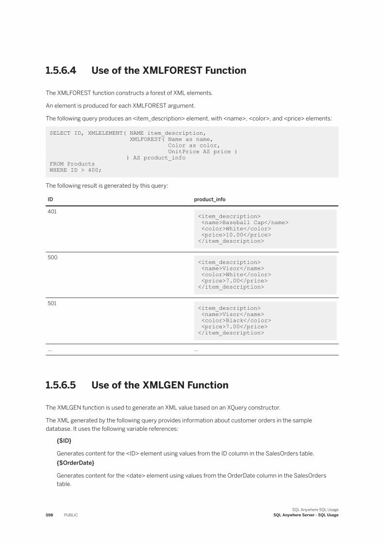
1.5.6.4 Use of the XMLFOREST Function
The XMLFOREST function constructs a forest of XML elements.
An element is produced for each XMLFOREST argument.
The following query produces an <item_description> element, with <name>, <color>, and <price> elements:
SELECT ID, XMLELEMENT( NAME item_description, XMLFOREST( Name as name, Color as color, UnitPrice AS price ) ) AS product_infoFROM Products WHERE ID > 400;
The following result is generated by this query:
ID product_info
401 <item_description> <name>Baseball Cap</name> <color>White</color> <price>10.00</price> </item_description>
500 <item_description> <name>Visor</name> <color>White</color> <price>7.00</price> </item_description>
501 <item_description> <name>Visor</name> <color>Black</color> <price>7.00</price> </item_description>
... ...
1.5.6.5 Use of the XMLGEN Function
The XMLGEN function is used to generate an XML value based on an XQuery constructor.
The XML generated by the following query provides information about customer orders in the sample database. It uses the following variable references:
{$ID}
Generates content for the <ID> element using values from the ID column in the SalesOrders table.{$OrderDate}
Generates content for the <date> element using values from the OrderDate column in the SalesOrders table.
598 PUBLICSQL Anywhere SQL Usage
SQL Anywhere Server - SQL Usage
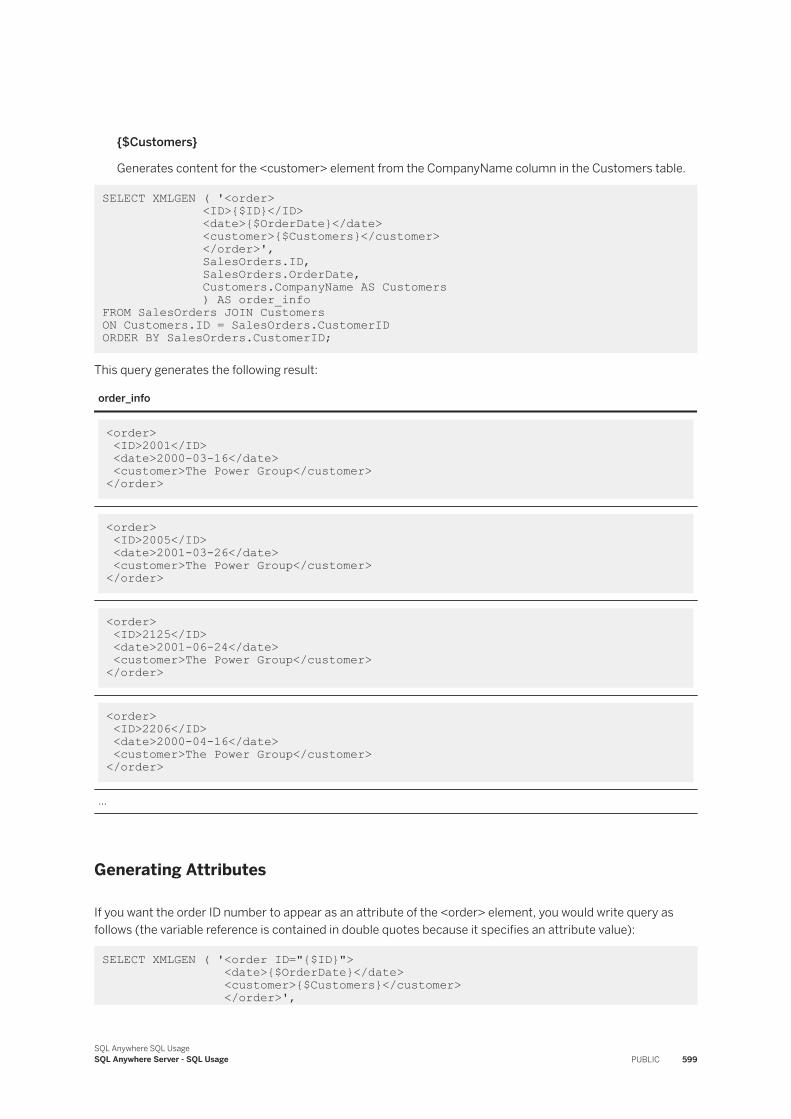
{$Customers}
Generates content for the <customer> element from the CompanyName column in the Customers table.
SELECT XMLGEN ( '<order> <ID>{$ID}</ID> <date>{$OrderDate}</date> <customer>{$Customers}</customer> </order>', SalesOrders.ID, SalesOrders.OrderDate, Customers.CompanyName AS Customers ) AS order_info FROM SalesOrders JOIN CustomersON Customers.ID = SalesOrders.CustomerID ORDER BY SalesOrders.CustomerID;
This query generates the following result:
order_info
<order> <ID>2001</ID> <date>2000-03-16</date> <customer>The Power Group</customer> </order>
<order> <ID>2005</ID> <date>2001-03-26</date> <customer>The Power Group</customer> </order>
<order> <ID>2125</ID> <date>2001-06-24</date> <customer>The Power Group</customer> </order>
<order> <ID>2206</ID> <date>2000-04-16</date> <customer>The Power Group</customer> </order>
...
Generating Attributes
If you want the order ID number to appear as an attribute of the <order> element, you would write query as follows (the variable reference is contained in double quotes because it specifies an attribute value):
SELECT XMLGEN ( '<order ID="{$ID}"> <date>{$OrderDate}</date> <customer>{$Customers}</customer> </order>',
SQL Anywhere SQL UsageSQL Anywhere Server - SQL Usage PUBLIC 599
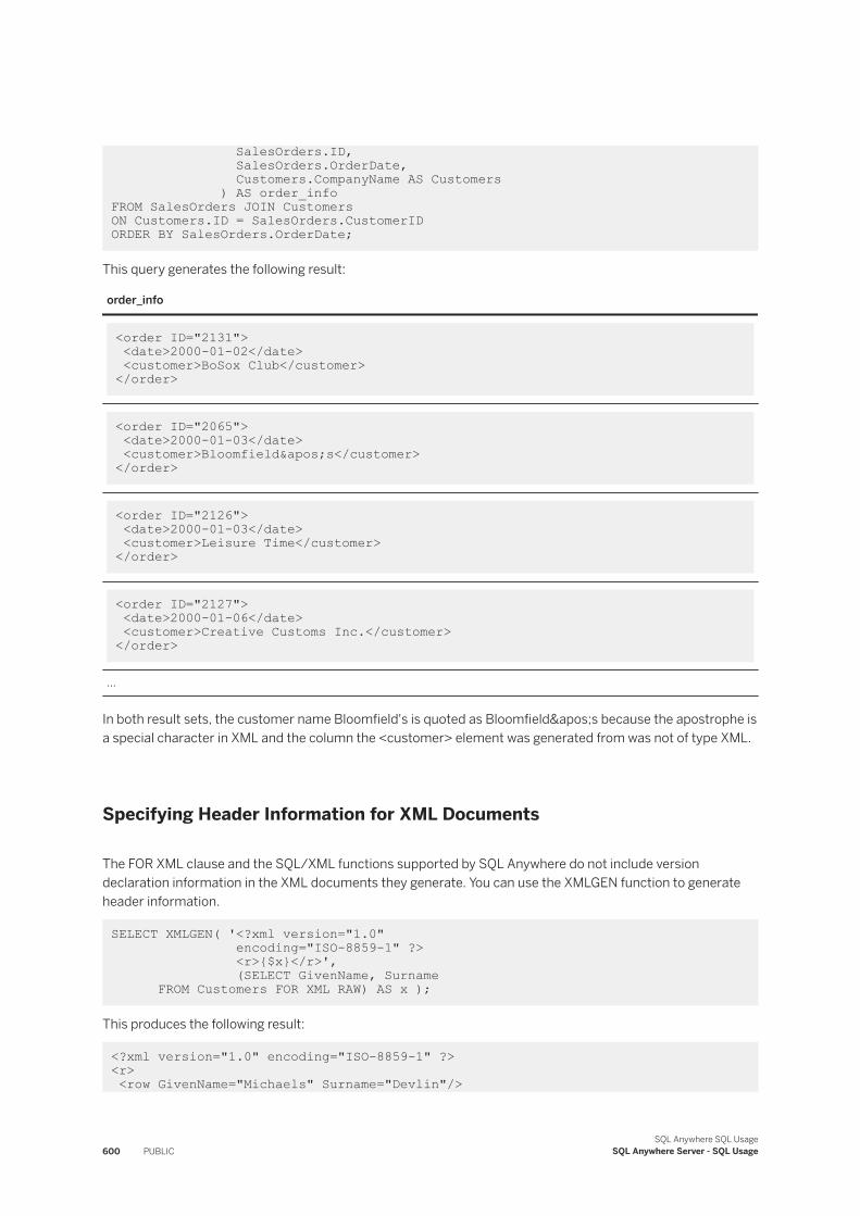
SalesOrders.ID, SalesOrders.OrderDate, Customers.CompanyName AS Customers ) AS order_info FROM SalesOrders JOIN CustomersON Customers.ID = SalesOrders.CustomerID ORDER BY SalesOrders.OrderDate;
This query generates the following result:
order_info
<order ID="2131"> <date>2000-01-02</date> <customer>BoSox Club</customer> </order>
<order ID="2065"> <date>2000-01-03</date> <customer>Bloomfield's</customer> </order>
<order ID="2126"> <date>2000-01-03</date> <customer>Leisure Time</customer> </order>
<order ID="2127"> <date>2000-01-06</date> <customer>Creative Customs Inc.</customer> </order>
...
In both result sets, the customer name Bloomfield's is quoted as Bloomfield's because the apostrophe is a special character in XML and the column the <customer> element was generated from was not of type XML.
Specifying Header Information for XML Documents
The FOR XML clause and the SQL/XML functions supported by SQL Anywhere do not include version declaration information in the XML documents they generate. You can use the XMLGEN function to generate header information.
SELECT XMLGEN( '<?xml version="1.0" encoding="ISO-8859-1" ?> <r>{$x}</r>', (SELECT GivenName, Surname FROM Customers FOR XML RAW) AS x );
This produces the following result:
<?xml version="1.0" encoding="ISO-8859-1" ?> <r> <row GivenName="Michaels" Surname="Devlin"/>
600 PUBLICSQL Anywhere SQL Usage
SQL Anywhere Server - SQL Usage
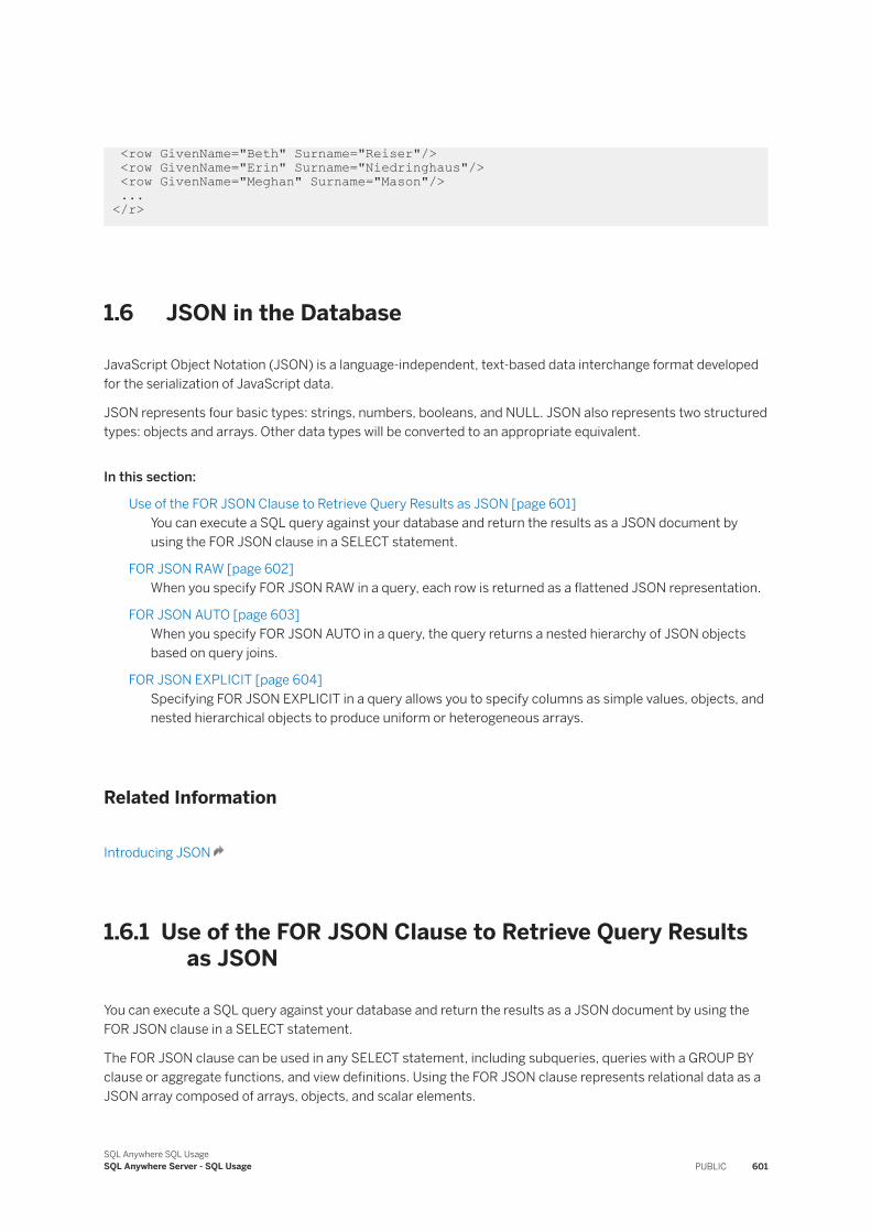
<row GivenName="Beth" Surname="Reiser"/> <row GivenName="Erin" Surname="Niedringhaus"/> <row GivenName="Meghan" Surname="Mason"/> ... </r>
1.6 JSON in the Database
JavaScript Object Notation (JSON) is a language-independent, text-based data interchange format developed for the serialization of JavaScript data.
JSON represents four basic types: strings, numbers, booleans, and NULL. JSON also represents two structured types: objects and arrays. Other data types will be converted to an appropriate equivalent.
In this section:
Use of the FOR JSON Clause to Retrieve Query Results as JSON [page 601]You can execute a SQL query against your database and return the results as a JSON document by using the FOR JSON clause in a SELECT statement.
FOR JSON RAW [page 602]When you specify FOR JSON RAW in a query, each row is returned as a flattened JSON representation.
FOR JSON AUTO [page 603]When you specify FOR JSON AUTO in a query, the query returns a nested hierarchy of JSON objects based on query joins.
FOR JSON EXPLICIT [page 604]Specifying FOR JSON EXPLICIT in a query allows you to specify columns as simple values, objects, and nested hierarchical objects to produce uniform or heterogeneous arrays.
Related Information
Introducing JSON
1.6.1 Use of the FOR JSON Clause to Retrieve Query Results as JSON
You can execute a SQL query against your database and return the results as a JSON document by using the FOR JSON clause in a SELECT statement.
The FOR JSON clause can be used in any SELECT statement, including subqueries, queries with a GROUP BY clause or aggregate functions, and view definitions. Using the FOR JSON clause represents relational data as a JSON array composed of arrays, objects, and scalar elements.
SQL Anywhere SQL UsageSQL Anywhere Server - SQL Usage PUBLIC 601
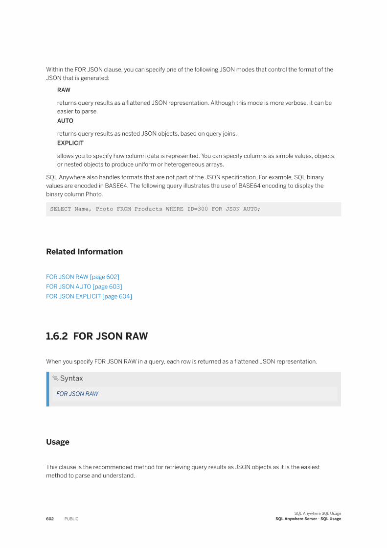
Within the FOR JSON clause, you can specify one of the following JSON modes that control the format of the JSON that is generated:
RAW
returns query results as a flattened JSON representation. Although this mode is more verbose, it can be easier to parse.AUTO
returns query results as nested JSON objects, based on query joins.EXPLICIT
allows you to specify how column data is represented. You can specify columns as simple values, objects, or nested objects to produce uniform or heterogeneous arrays.
SQL Anywhere also handles formats that are not part of the JSON specification. For example, SQL binary values are encoded in BASE64. The following query illustrates the use of BASE64 encoding to display the binary column Photo.
SELECT Name, Photo FROM Products WHERE ID=300 FOR JSON AUTO;
Related Information
FOR JSON RAW [page 602]FOR JSON AUTO [page 603]FOR JSON EXPLICIT [page 604]
1.6.2 FOR JSON RAW
When you specify FOR JSON RAW in a query, each row is returned as a flattened JSON representation.
Syntax
FOR JSON RAW
Usage
This clause is the recommended method for retrieving query results as JSON objects as it is the easiest method to parse and understand.
602 PUBLICSQL Anywhere SQL Usage
SQL Anywhere Server - SQL Usage
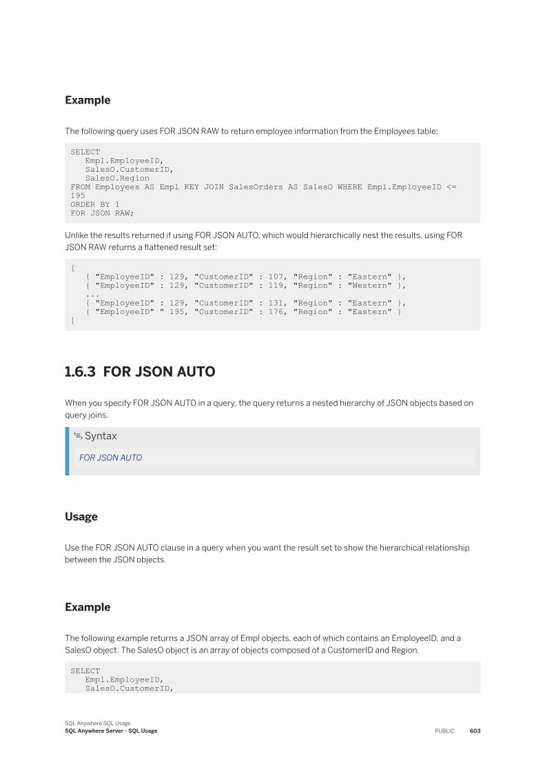
Example
The following query uses FOR JSON RAW to return employee information from the Employees table:
SELECT Empl.EmployeeID, SalesO.CustomerID, SalesO.RegionFROM Employees AS Empl KEY JOIN SalesOrders AS SalesO WHERE Empl.EmployeeID <= 195ORDER BY 1 FOR JSON RAW;
Unlike the results returned if using FOR JSON AUTO, which would hierarchically nest the results, using FOR JSON RAW returns a flattened result set:
[ { "EmployeeID" : 129, "CustomerID" : 107, "Region" : "Eastern" }, { "EmployeeID" : 129, "CustomerID" : 119, "Region" : "Western" }, ... { "EmployeeID" : 129, "CustomerID" : 131, "Region" : "Eastern" }, { "EmployeeID" " 195, "CustomerID" : 176, "Region" : "Eastern" } ]
1.6.3 FOR JSON AUTO
When you specify FOR JSON AUTO in a query, the query returns a nested hierarchy of JSON objects based on query joins.
Syntax
FOR JSON AUTO
Usage
Use the FOR JSON AUTO clause in a query when you want the result set to show the hierarchical relationship between the JSON objects.
Example
The following example returns a JSON array of Empl objects, each of which contains an EmployeeID, and a SalesO object. The SalesO object is an array of objects composed of a CustomerID and Region.
SELECT Empl.EmployeeID, SalesO.CustomerID,
SQL Anywhere SQL UsageSQL Anywhere Server - SQL Usage PUBLIC 603
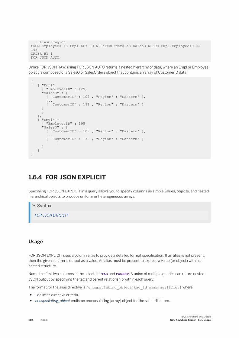
SalesO.RegionFROM Employees AS Empl KEY JOIN SalesOrders AS SalesO WHERE Empl.EmployeeID <= 195ORDER BY 1 FOR JSON AUTO;
Unlike FOR JSON RAW, using FOR JSON AUTO returns a nested hierarchy of data, where an Empl or Employee object is composed of a SalesO or SalesOrders object that contains an array of CustomerID data:
[ { "Empl": { "EmployeeID" : 129, "SalesO" : [ { "CustomerID" : 107 , "Region" : "Eastern" }, ... { "CustomerID" : 131 , "Region" : "Eastern" } ] } }, { "Empl" : { "EmployeeID" : 195, "SalesO" : [ { "CustomerID" : 109 , "Region" : "Eastern" }, ... { "CustomerID" : 176 , "Region" : "Eastern" } ] } } ]
1.6.4 FOR JSON EXPLICIT
Specifying FOR JSON EXPLICIT in a query allows you to specify columns as simple values, objects, and nested hierarchical objects to produce uniform or heterogeneous arrays.
Syntax
FOR JSON EXPLICIT
Usage
FOR JSON EXPLICIT uses a column alias to provide a detailed format specification. If an alias is not present, then the given column is output as a value. An alias must be present to express a value (or object) within a nested structure.
Name the first two columns in the select-list TAG and PARENT. A union of multiple queries can return nested JSON output by specifying the tag and parent relationship within each query.
The format for the alias directive is [encapsulating_object!tag_id!name!qualifier] where:
● ! delimits directive criteria.● encapsulating_object emits an encapsulating (array) object for the select-list item.
604 PUBLICSQL Anywhere SQL Usage
SQL Anywhere Server - SQL Usage
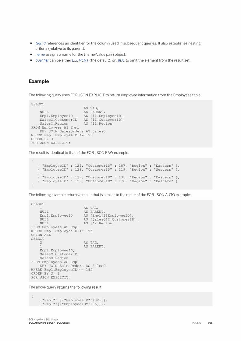
● tag_id references an identifier for the column used in subsequent queries. It also establishes nesting criteria (relative to its parent).
● name assigns a name for the (name/value pair) object.● qualifier can be either ELEMENT (the default), or HIDE to omit the element from the result set.
Example
The following query uses FOR JSON EXPLICIT to return employee information from the Employees table:
SELECT 1 AS TAG, NULL AS PARENT, Empl.EmployeeID AS [!1!EmployeeID], SalesO.CustomerID AS [!1!CustomerID], SalesO.Region AS [!1!Region]FROM Employees AS Empl KEY JOIN SalesOrders AS SalesO WHERE Empl.EmployeeID <= 195ORDER BY 3 FOR JSON EXPLICIT;
The result is identical to that of the FOR JSON RAW example:
[ { "EmployeeID" : 129, "CustomerID" : 107, "Region" : "Eastern" }, { "EmployeeID" : 129, "CustomerID" : 119, "Region" : "Western" }, ... { "EmployeeID" : 129, "CustomerID" : 131, "Region" : "Eastern" }, { "EmployeeID" " 195, "CustomerID" : 176, "Region" : "Eastern" } ]
The following example returns a result that is similar to the result of the FOR JSON AUTO example:
SELECT 1 AS TAG, NULL AS PARENT, Empl.EmployeeID AS [Empl!1!EmployeeID], NULL AS [SalesO!2!CustomerID], NULL AS [!2!Region]FROM Employees AS Empl WHERE Empl.EmployeeID <= 195UNION ALLSELECT 2 AS TAG, 1 AS PARENT, Empl.EmployeeID, SalesO.CustomerID, SalesO.Region FROM Employees AS Empl KEY JOIN SalesOrders AS SalesO WHERE Empl.EmployeeID <= 195ORDER BY 3, 1 FOR JSON EXPLICIT;
The above query returns the following result:
[ {"Empl": [{"EmployeeID":102}]}, {"Empl":[{"EmployeeID":105}]},
SQL Anywhere SQL UsageSQL Anywhere Server - SQL Usage PUBLIC 605
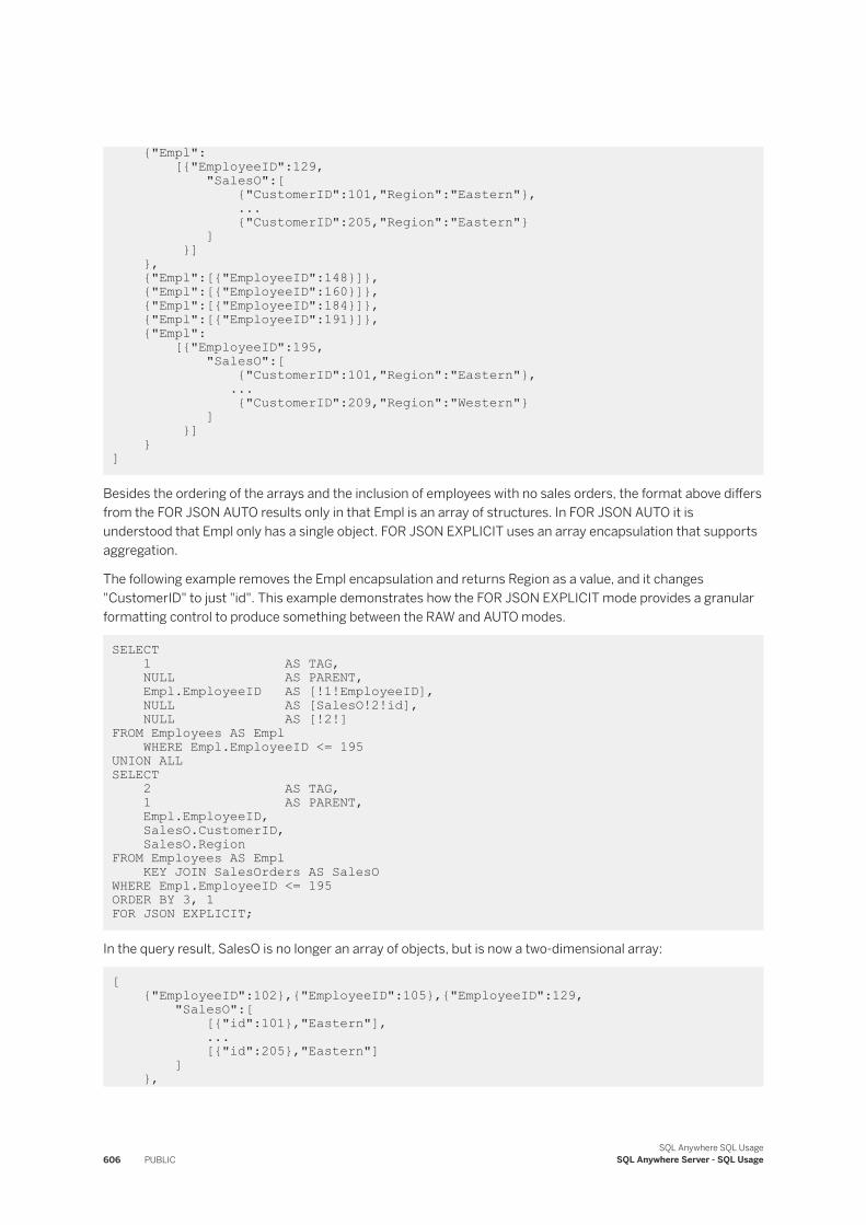
{"Empl": [{"EmployeeID":129, "SalesO":[ {"CustomerID":101,"Region":"Eastern"}, ... {"CustomerID":205,"Region":"Eastern"} ] }] }, {"Empl":[{"EmployeeID":148}]}, {"Empl":[{"EmployeeID":160}]}, {"Empl":[{"EmployeeID":184}]}, {"Empl":[{"EmployeeID":191}]}, {"Empl": [{"EmployeeID":195, "SalesO":[ {"CustomerID":101,"Region":"Eastern"}, ... {"CustomerID":209,"Region":"Western"} ] }] } ]
Besides the ordering of the arrays and the inclusion of employees with no sales orders, the format above differs from the FOR JSON AUTO results only in that Empl is an array of structures. In FOR JSON AUTO it is understood that Empl only has a single object. FOR JSON EXPLICIT uses an array encapsulation that supports aggregation.
The following example removes the Empl encapsulation and returns Region as a value, and it changes "CustomerID" to just "id". This example demonstrates how the FOR JSON EXPLICIT mode provides a granular formatting control to produce something between the RAW and AUTO modes.
SELECT 1 AS TAG, NULL AS PARENT, Empl.EmployeeID AS [!1!EmployeeID], NULL AS [SalesO!2!id], NULL AS [!2!] FROM Employees AS Empl WHERE Empl.EmployeeID <= 195UNION ALLSELECT 2 AS TAG, 1 AS PARENT, Empl.EmployeeID, SalesO.CustomerID, SalesO.Region FROM Employees AS Empl KEY JOIN SalesOrders AS SalesO WHERE Empl.EmployeeID <= 195ORDER BY 3, 1 FOR JSON EXPLICIT;
In the query result, SalesO is no longer an array of objects, but is now a two-dimensional array:
[ {"EmployeeID":102},{"EmployeeID":105},{"EmployeeID":129, "SalesO":[ [{"id":101},"Eastern"], ... [{"id":205},"Eastern"] ] },
606 PUBLICSQL Anywhere SQL Usage
SQL Anywhere Server - SQL Usage
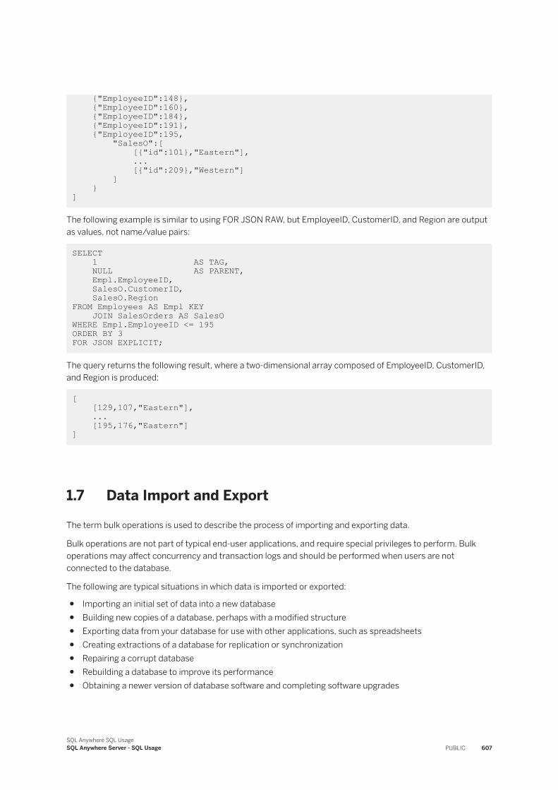
{"EmployeeID":148}, {"EmployeeID":160}, {"EmployeeID":184}, {"EmployeeID":191}, {"EmployeeID":195, "SalesO":[ [{"id":101},"Eastern"], ... [{"id":209},"Western"] ] } ]
The following example is similar to using FOR JSON RAW, but EmployeeID, CustomerID, and Region are output as values, not name/value pairs:
SELECT 1 AS TAG, NULL AS PARENT, Empl.EmployeeID, SalesO.CustomerID, SalesO.RegionFROM Employees AS Empl KEY JOIN SalesOrders AS SalesO WHERE Empl.EmployeeID <= 195ORDER BY 3 FOR JSON EXPLICIT;
The query returns the following result, where a two-dimensional array composed of EmployeeID, CustomerID, and Region is produced:
[ [129,107,"Eastern"], ... [195,176,"Eastern"] ]
1.7 Data Import and Export
The term bulk operations is used to describe the process of importing and exporting data.
Bulk operations are not part of typical end-user applications, and require special privileges to perform. Bulk operations may affect concurrency and transaction logs and should be performed when users are not connected to the database.
The following are typical situations in which data is imported or exported:
● Importing an initial set of data into a new database● Building new copies of a database, perhaps with a modified structure● Exporting data from your database for use with other applications, such as spreadsheets● Creating extractions of a database for replication or synchronization● Repairing a corrupt database● Rebuilding a database to improve its performance● Obtaining a newer version of database software and completing software upgrades
SQL Anywhere SQL UsageSQL Anywhere Server - SQL Usage PUBLIC 607
In this section:
Performance Aspects of Bulk Operations [page 608]The performance of bulk operations depends on several factors, including whether the operation is internal or external to the database server.
Data Recovery Issues for Bulk Operations [page 609]You can run the database server in bulk operations mode using the -b server option.
Data Import [page 609]Importing data involves reading data into your database as a bulk operation.
Data Export [page 627]Exporting data involves writing data out of your database.
Access to Data on Client Computers [page 643]You can load data from, and unload data to, a file on a client computer using SQL statements and functions, without having to copy files to or from the database server computer.
Database Rebuilds [page 646]Rebuilding a database is a specific type of import and export involving unloading and reloading your database.
Database Extraction [page 663]Database extraction creates a remote SQL Anywhere database from a consolidated SQL Anywhere database.
Database Migration to SQL Anywhere [page 664]You can use the sa_migrate system procedures or the Migrate Database Wizard, to import tables from several sources.
SQL Script Files [page 669]SQL script files are text files that contain SQL statements, and are useful to execute the same SQL statements repeatedly.
Adaptive Server Enterprise Compatibility [page 674]You can import and export files between SQL Anywhere and Adaptive Server Enterprise using the BCP FORMAT clause.
1.7.1 Performance Aspects of Bulk Operations
The performance of bulk operations depends on several factors, including whether the operation is internal or external to the database server.
Internal Bulk Operations
Internal bulk operations, also referred to as server-side bulk operations, are import and export operations performed by the database server using the LOAD TABLE, and UNLOAD statements.
When performing internal bulk operations, you can load from, and unload to, ASCII text files, or Adaptive Server Enterprise BCP files. These files can exist on the same computer as the database server, or on a client
608 PUBLICSQL Anywhere SQL Usage
SQL Anywhere Server - SQL Usage
computer. The specified path to the file being written or read is relative to the database server. Internal bulk operations are the fastest method of importing and exporting data into the database.
External Bulk Operations
External bulk operations, also referred to as client-side bulk operations, are import and export operations performed by a client such as Interactive SQL, using INPUT and OUTPUT statements. When the client issues an INPUT statement, an INSERT statement is recorded in the transaction log for each row that is read when processing the file specified in the INPUT statement. As a result, client-side loading is considerably slower than server-side loading. As well, INSERT triggers fire during an INPUT.
The OUTPUT statement allows you to write the result set of a SELECT statement to many different file formats.
For external bulk operations, the specified path to the file being read or written is relative to the computer on which the client application is running.
1.7.2 Data Recovery Issues for Bulk Operations
You can run the database server in bulk operations mode using the -b server option.
When you use this option, the database server does not perform certain important functions. Specifically:
Function Implication
Maintain a transaction log There is no record of the changes. Each COMMIT causes a checkpoint.
Lock any records There are no serious implications.
Alternatively, ensure that data from bulk loading is still available in the event of recovery. You can do so by keeping the original data sources intact, and in their original location. You can also use some of the logging options available for the LOAD TABLE statement that allow bulk-loaded data to be recorded in the transaction log.
CautionBack up the database before and after using bulk operations mode because your database is not protected against media failure in this mode.
1.7.3 Data Import
Importing data involves reading data into your database as a bulk operation.
You can:
● import entire tables or portions of tables from text files
SQL Anywhere SQL UsageSQL Anywhere Server - SQL Usage PUBLIC 609
● import data from a variable● import several tables consecutively by automating the import procedure with a script● insert or add data into tables● replace data in tables● create a table before the import or during the import● load data from a file on a client computer● transfer files between SQL Anywhere and Adaptive Server Enterprise using the BCP format clause
If you are trying to create an entirely new database, consider loading the data using LOAD TABLE for the best performance.
In this section:
Performance Tips for Importing Data [page 611]Importing large volumes of data can be time consuming, but there are options that are available to conserve time.
Data Import with the INPUT Statement [page 611]Use the INPUT statement to import data in different file formats into existing or new tables.
Importing Data from Files [Interactive SQL] [page 612]Import data into a database from a text file, Microsoft Excel file, or a comma-separated values (CSV) file using Interactive SQL.
Importing Data with the Import Wizard (Interactive SQL) [page 614]Use the Interactive SQL Import Wizard to select a source, format, and destination table for the data.
Data Import with the LOAD TABLE Statement [page 615]Use the LOAD TABLE statement to import data residing on a database server or a client computer into an existing table in text/ASCII format.
Data Import with the INSERT Statement [page 617]Use the INSERT statement to add rows to the database.
Data Import with the MERGE Statement [page 618]Use the MERGE statement to perform an update operation and update large amounts of table data.
Tips on Importing Data with Proxy Tables [page 623]Use proxy tables to import remote data such as data from another database.
Conversion Errors During Import [page 624]When you load data from external sources, there may be errors in the data.
Importing Tables (LOAD TABLE Statement) [page 624]Import data from a text file, another table in any database, or a shape file, into a table in your database.
Table Structures for Import [page 625]The structure of the source data does not need to match the structure of the destination table itself.
Merging Different Table Structures [page 626]Use the INSERT statement and a global temporary table to rearrange the import data to fit the table.
Related Information
610 PUBLICSQL Anywhere SQL Usage
SQL Anywhere Server - SQL Usage
Performance Aspects of Bulk Operations [page 608]Access to Data on Client Computers [page 643]Database Rebuilds [page 646]
1.7.3.1 Performance Tips for Importing Data
Importing large volumes of data can be time consuming, but there are options that are available to conserve time.
● Place data files on a separate physical disk drive from the database. This could avoid excessive disk head movement during the load.
● Extend the size of the database. The ALTER DBSPACE statement allows a database to be extended in large amounts before the space is required, rather than in smaller amounts when the space is needed. It also improves performance when loading large amounts of data, and keeps the database more contiguous within the file system.
● Use temporary tables to load data. Local or global temporary tables are useful when you must load a set of data repeatedly, or when you must merge tables with different structures.
● Start the database server without the -b option (bulk operations mode) when using the LOAD TABLE statement.
● Run Interactive SQL or the client application on the same computer as the database server if you are using the INPUT or OUTPUT statement. Loading data over the network adds extra communication overhead. Load new data at a time when the database server is not busy.
1.7.3.2 Data Import with the INPUT Statement
Use the INPUT statement to import data in different file formats into existing or new tables.
If you have the ODBC drivers for the databases, then use the USING clause to import data from different types of databases.
Use the default input format, or you can specify the file format for each INPUT statement. Because the INPUT statement is an Interactive SQL statement, you cannot use it in any compound statement (such as an IF statement), in a stored procedure, or in any statement executed by the database server.
Considerations for Materialized Views
For immediate views, an error is returned when you attempt to bulk load data into an underlying table. Truncate the data in the view first, and then perform the bulk load operation.
For manual views, you can bulk load data into an underlying table. However, the data in the view remains stale until the next refresh.
Consider truncating data in dependent materialized views before attempting a bulk load operation such as INPUT on a table. After you have loaded the data, refresh the view.
SQL Anywhere SQL UsageSQL Anywhere Server - SQL Usage PUBLIC 611
Considerations for Text Indexes
For immediate text indexes, updating the text index after performing a bulk load operation such as INPUT on the underlying table can take a while even though the update is automatic. For manual text indexes, even a refresh can take a while.
Consider dropping dependent text indexes before performing a bulk load operation such as INPUT on a table. After you have loaded the data, recreate the text index.
Impact on the Database
Changes are recorded in the transaction log when you use the INPUT statement. In the event of a media failure, there is a detailed record of the changes. However, there are performance impacts associated with importing large amounts of data with this method since all rows are written to the transaction log.
In comparison, the LOAD TABLE statement does not save each row to the transaction log and so it can be faster than the INPUT statement. However, the INPUT statement supports more databases and file formats.
1.7.3.3 Importing Data from Files [Interactive SQL]
Import data into a database from a text file, Microsoft Excel file, or a comma-separated values (CSV) file using Interactive SQL.
Prerequisites
You must be the owner of the table, or have the following privileges:
● INSERT privilege on the table, or the INSERT ANY TABLE system privilege● SELECT privilege on the table, or the SELECT ANY TABLE system privilege
If you are importing data from a Microsoft Excel workbook file, then you must have a compatible ODBC driver installed.
Context
Because the INPUT statement is an Interactive SQL statement, you cannot use it in any compound statement (such as an IF statement), in a stored procedure, or in any statement executed by the database server.
When files with a .txt or .csv extension are imported with the FORMAT EXCEL clause, they follow the default formatting for Microsoft Excel workbook files.
612 PUBLICSQL Anywhere SQL Usage
SQL Anywhere Server - SQL Usage
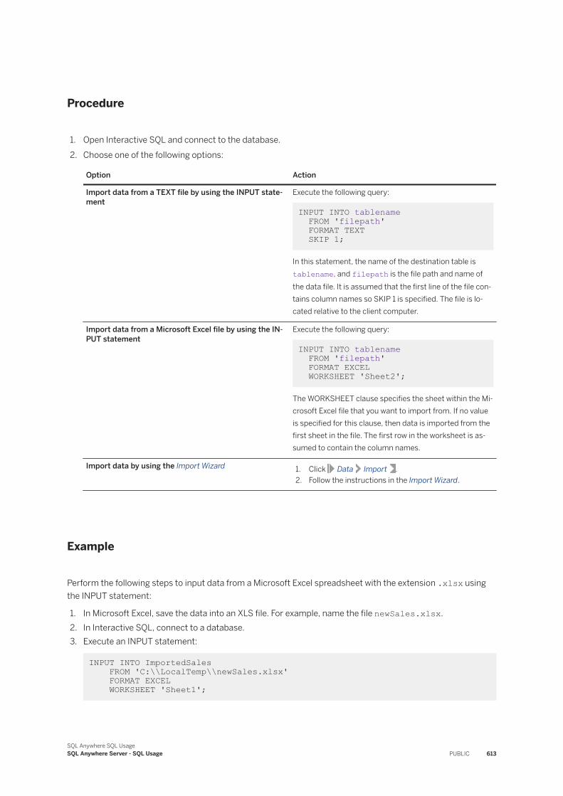
Procedure
1. Open Interactive SQL and connect to the database.2. Choose one of the following options:
Option Action
Import data from a TEXT file by using the INPUT statement
Execute the following query:
INPUT INTO tablename FROM 'filepath' FORMAT TEXT SKIP 1;
In this statement, the name of the destination table is tablename, and filepath is the file path and name of the data file. It is assumed that the first line of the file contains column names so SKIP 1 is specified. The file is located relative to the client computer.
Import data from a Microsoft Excel file by using the INPUT statement
Execute the following query:
INPUT INTO tablename FROM 'filepath' FORMAT EXCEL WORKSHEET 'Sheet2';
The WORKSHEET clause specifies the sheet within the Microsoft Excel file that you want to import from. If no value is specified for this clause, then data is imported from the first sheet in the file. The first row in the worksheet is assumed to contain the column names.
Import data by using the Import Wizard 1. Click Data Import .2. Follow the instructions in the Import Wizard.
Example
Perform the following steps to input data from a Microsoft Excel spreadsheet with the extension .xlsx using the INPUT statement:
1. In Microsoft Excel, save the data into an XLS file. For example, name the file newSales.xlsx.2. In Interactive SQL, connect to a database.3. Execute an INPUT statement:
INPUT INTO ImportedSales FROM 'C:\\LocalTemp\\newSales.xlsx' FORMAT EXCEL WORKSHEET 'Sheet1';
SQL Anywhere SQL UsageSQL Anywhere Server - SQL Usage PUBLIC 613
If the table does not exist, it is created for you using appropriate column names and data types. The schema of the table is displayed using the Interactive SQL DESCRIBE statement.
DESCRIBE ImportedSales;
Related Information
Data Export [page 627]Data Export [page 627]
1.7.3.4 Importing Data with the Import Wizard (Interactive SQL)
Use the Interactive SQL Import Wizard to select a source, format, and destination table for the data.
Prerequisites
If you import data into an existing table, you must be the owner of the table, have SELECT and INSERT privileges on the table, or have the SELECT ANY TABLE and INSERT ANY TABLE system privileges.
If you import data into a new table, you must have the CREATE TABLE, CREATE ANY TABLE, or CREATE ANY OBJECT system privilege.
Context
You can import data from text files, Microsoft Excel files, fix format files, and shapefiles, into an existing table or a new table.
Use the Import Wizard to import data between databases of different types or different versions.
Use the Interactive SQL Import Wizard when you:
● want to create a table at the same time you import the data● prefer using a point-and click interface to import data in a format other than text
Procedure
1. In Interactive SQL, click Data Import .
614 PUBLICSQL Anywhere SQL Usage
SQL Anywhere Server - SQL Usage
2. Specify the file type, then click Next.3. In the File name field, click Browse to add the file.4. Specify the table that you want to import the data into. For new tables, fill in the Table name.5. Click Next.6. For text files, specify the way the file is read and then click Next.7. Make any changes to the column names and data types and then click Import.8. Click Close.
Example
Perform the following steps to import data from the SQL Anywhere sample database into an UltraLite database:
1. Connect to an UltraLite database, such as, C:\Users\Public\Documents\SQL Anywhere 17\Samples\UltraLite\CustDB\custdb.udb.
2. In Interactive SQL, click Data Import .3. Click In a database. Click Next.4. In the Database type list, click SQL Anywhere.5. In the Action dropdown list, click Connect with an ODBC Data Source.6. Click ODBC Data Source name, and then in the box below type SQL Anywhere 17 Demo, and specify the
password sql.7. Click Next.8. In the Table name list, click Customers. Click Next.9. Click In a new table.10. In the Table name field, type SQLAnyCustomers.11. Click Import.12. Click Close.
13. To view the generated SQL statement, click SQL Previous SQL .The INPUT statement generated by the Import Wizard appears in the SQL Statements pane:
-- Generated by the Import Wizard input using 'dsn=SQL Anywhere 17 Demo;PWD=sql;CON=''''' from "GROUPO.Customers" into "SQLAnyCustomers" create table on
1.7.3.5 Data Import with the LOAD TABLE Statement
Use the LOAD TABLE statement to import data residing on a database server or a client computer into an existing table in text/ASCII format.
You can also use the LOAD TABLE statement to import data from a column from another table, or from a value expression (for example, from the results of a function or system procedure). It is also possible to import data into some views.
The LOAD TABLE statement adds rows into a table; it doesn't replace them.
SQL Anywhere SQL UsageSQL Anywhere Server - SQL Usage PUBLIC 615
Loading data using the LOAD TABLE statement (without the WITH ROW LOGGING and WITH CONTENT LOGGING options) is considerably faster than using the INPUT statement.
Triggers do not fire for data loaded using the LOAD TABLE statement.
Considerations for Materialized Views
For immediate views, an error is returned when you attempt to bulk load data into an underlying table. You must truncate the data in the view first, and then perform the bulk load operation.
For manual views, you can bulk load data into an underlying table; however, the data in the view becomes stale until the next refresh.
Consider truncating data in dependent materialized views before attempting a bulk load operation such as LOAD TABLE on a table. After you have loaded the data, refresh the view.
Considerations for Text Indexes
For immediate text indexes, updating the text index after performing a bulk load operation such as LOAD TABLE on the underlying table can take a while even though the update is automatic. For manual text indexes, even a refresh can take a while.
Consider dropping dependent text indexes before performing a bulk load operation such as LOAD TABLE on a table. After you have loaded the data, recreate the text index.
Considerations for Database Recovery and Synchronization
By default, when data is loaded from a file (for example, LOAD TABLE table-name FROM filename;), only the LOAD TABLE statement is recorded in the transaction log, not the actual rows of data that are being loaded. This presents a problem when trying to recover the database using the transaction log if the original load file has been changed, moved, or deleted. It also means that databases involved in synchronization or replication do not get the new data.
To address the recovery and synchronization considerations, two logging options are available for the LOAD TABLE statement: WITH ROW LOGGING, which creates INSERT statements in the transaction log for every row that is loaded, and WITH CONTENT LOGGING, which groups the loaded rows into chunks and records the chunks in the transaction log. These options allow a load operation to be repeated, even when the source of the loaded data is no longer available.
Considerations for Database Mirroring
If your database is involved in mirroring, use the LOAD TABLE statement carefully. For example, if you are loading data from a file, consider whether the file is available for loading on the mirror server, or whether data in
616 PUBLICSQL Anywhere SQL Usage
SQL Anywhere Server - SQL Usage
the source you are loading from will change by the time the mirror database processes the load. If either of these risks exists, consider specifying either WITH ROW LOGGING or WITH CONTENT LOGGING as the logging level in the LOAD TABLE statement. That way, the data loaded into the mirror database is identical to what was loaded in the mirrored database.
Related Information
Access to Data on Client Computers [page 643]
1.7.3.6 Data Import with the INSERT Statement
Use the INSERT statement to add rows to the database.
Because the import data for your destination table is included in the INSERT statement, it is considered interactive input. You can also use the INSERT statement with remote data access to import data from another database rather than a file.
Use the INSERT statement to import data when you:
● want to import small amounts of data into a single table● are flexible with your file formats● want to import remote data from an external database rather than from a file
The INSERT statement provides an ON EXISTING clause to specify the action to take if a row you are inserting is already found in the destination table. However, if you anticipate many rows qualifying for the ON EXISTING condition, consider using the MERGE statement instead. The MERGE statement provides more control over the actions you can take for matching rows. It also provides a more sophisticated syntax for defining what constitutes a match.
Considerations for Materialized Views
For immediate views, an error is returned when you attempt to bulk load data into an underlying table. You must truncate the data in the view first, and then perform the bulk load operation.
For manual views, you can bulk load data into an underlying table; however, the data in the view becomes stale until the next refresh.
Consider truncating data in dependent materialized views before attempting a bulk load operation such as INSERT on a table. After you have loaded the data, refresh the view.
SQL Anywhere SQL UsageSQL Anywhere Server - SQL Usage PUBLIC 617
Considerations for Text Indexes
For immediate text indexes, updating the text index after performing a bulk load operation such as INSERT on the underlying table can take a while even though the update is automatic. For manual text indexes, even a refresh can take a while.
Consider dropping dependent text indexes before performing a bulk load operation such as INSERT on a table. After you have loaded the data, recreate the text index.
Impact on the Database
Changes are recorded in the transaction log when you use the INSERT statement. If there is a media failure involving the database file, you can recover information about the changes you made from the transaction log.
1.7.3.7 Data Import with the MERGE Statement
Use the MERGE statement to perform an update operation and update large amounts of table data.
When you merge data, you can specify what actions to take when rows from the source data match or do not match the rows in the target data.
Defining the Merge Behavior
The following is an abbreviated version of the MERGE statement syntax.
MERGE INTO target-object USING source-object ON merge-search-condition { WHEN MATCHED | WHEN NOT MATCHED } [...]
When the database performs a merge operation, it compares rows in source-object to rows in target-object to find rows that either match or do not match according to the definition contained in the ON clause. Rows in source-object are considered a match if there exists at least one row in target-table such that merge-search-condition evaluates to true.
source-object can be a base table, view, materialized view, derived table, or the results of a procedure. target-object can be any of these objects except for materialized views and procedures.
The ANSI/ISO SQL Standard does not allow rows in target-object to be updated by more than one row in source-object during a merge operation.
Once a row in source-object is considered matching or non-matching, it is evaluated against the respective matching or non-matching WHEN clauses (WHEN MATCHED or WHEN NOT MATCHED). A WHEN MATCHED clause defines an action to perform on the row in target-object (for example, WHEN MATCHED ... UPDATE
618 PUBLICSQL Anywhere SQL Usage
SQL Anywhere Server - SQL Usage
specifies to update the row in target-object). A WHEN NOT MATCHED clause defines an action to perform on the target-object using non-matching rows of the source-object.
You can specify unlimited WHEN clauses; they are processed in the order in which you specify them. You can also use the AND clause within a WHEN clause to specify actions against a subset of rows. For example, the following WHEN clauses define different actions to perform depending on the value of the Quantity column for matching rows:
WHEN MATCHED AND myTargetTable.Quantity<=500 THEN SKIP WHEN MATCHED AND myTargetTable.Quantity>500 THEN UPDATE SET myTargetTable.Quantity=500
Branches in a Merge Operation
The grouping of matched and non-matched rows by action is referred to as branching, and each group is referred to as a branch. A branch is equivalent to a single WHEN MATCHED or WHEN NOT MATCHED clause. For example, one branch might contain the set of non-matching rows from source-object that must be inserted. Execution of the branch actions begins only after all branching activities are complete (all rows in source-object have been evaluated). The database server begins executing the branch actions according to the order in which the WHEN clauses were specified.
Once a non-matching row from source-object or a pair of matching rows from source-object and target-object is placed in a branch, it is not evaluated against the succeeding branches. This makes the order in which you specify WHEN clauses significant.
A row in source-object that is considered a match or non-match, but does not belong to any branch (that is, it does not satisfy any WHEN clause) is ignored. This can occur when the WHEN clauses contain AND clauses, and the row does not satisfy any of the AND clause conditions. In this case, the row is ignored since no action is defined for it.
In the transaction log, actions that modify data are recorded as individual INSERT, UPDATE, and DELETE statements.
Triggers Defined on the Target Table
Triggers fire normally as each INSERT, UPDATE, and DELETE statement is executed during the merge operation. For example, when processing a branch that has an UPDATE action defined for it, the database server:
1. fires all BEFORE UPDATE triggers.2. executes the UPDATE statement on the candidate set of rows while firing any row-level UPDATE triggers.3. fires the AFTER UPDATE triggers.
Triggers on target-table can cause conflicts during a merge operation if it impacts rows that might be updated in another branch. For example, suppose an action is performed on row A, causing a trigger to fire that deletes row B. However, row B has an action defined for it that has not yet been performed. When an action cannot be performed on a row, the merge operation fails, all changes are rolled back, and an error is returned.
SQL Anywhere SQL UsageSQL Anywhere Server - SQL Usage PUBLIC 619
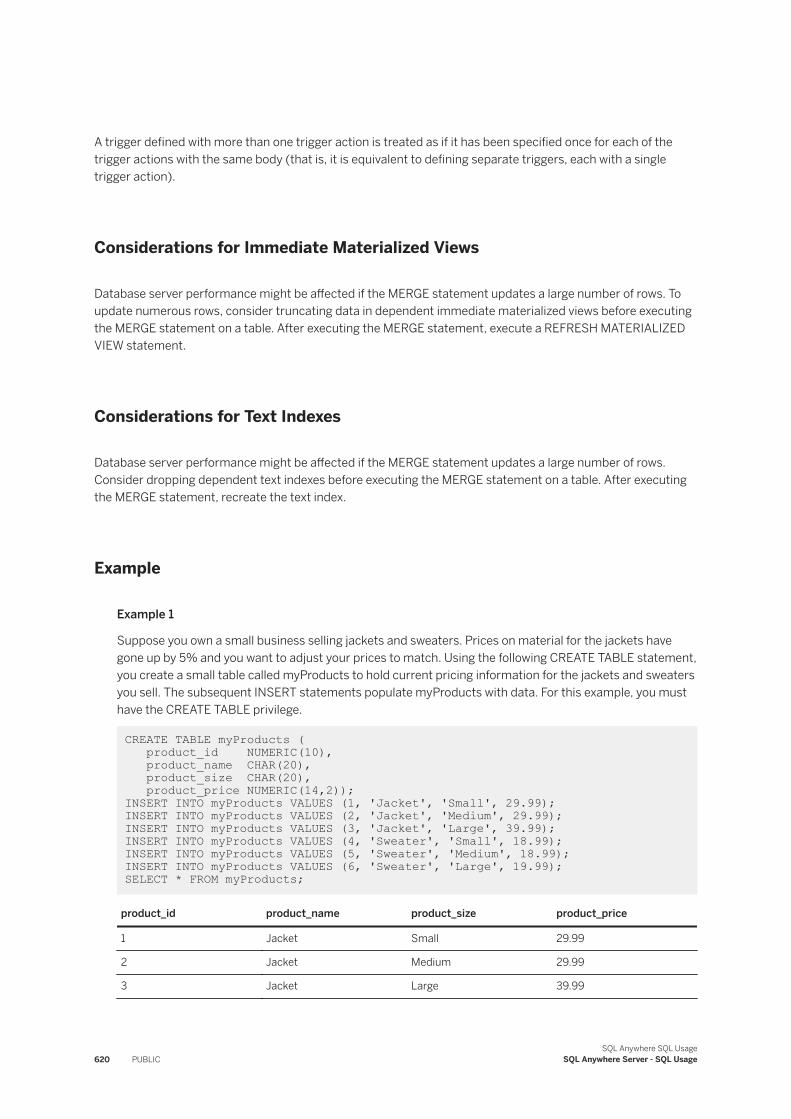
A trigger defined with more than one trigger action is treated as if it has been specified once for each of the trigger actions with the same body (that is, it is equivalent to defining separate triggers, each with a single trigger action).
Considerations for Immediate Materialized Views
Database server performance might be affected if the MERGE statement updates a large number of rows. To update numerous rows, consider truncating data in dependent immediate materialized views before executing the MERGE statement on a table. After executing the MERGE statement, execute a REFRESH MATERIALIZED VIEW statement.
Considerations for Text Indexes
Database server performance might be affected if the MERGE statement updates a large number of rows. Consider dropping dependent text indexes before executing the MERGE statement on a table. After executing the MERGE statement, recreate the text index.
Example
Example 1
Suppose you own a small business selling jackets and sweaters. Prices on material for the jackets have gone up by 5% and you want to adjust your prices to match. Using the following CREATE TABLE statement, you create a small table called myProducts to hold current pricing information for the jackets and sweaters you sell. The subsequent INSERT statements populate myProducts with data. For this example, you must have the CREATE TABLE privilege.
CREATE TABLE myProducts ( product_id NUMERIC(10), product_name CHAR(20), product_size CHAR(20), product_price NUMERIC(14,2));INSERT INTO myProducts VALUES (1, 'Jacket', 'Small', 29.99);INSERT INTO myProducts VALUES (2, 'Jacket', 'Medium', 29.99);INSERT INTO myProducts VALUES (3, 'Jacket', 'Large', 39.99);INSERT INTO myProducts VALUES (4, 'Sweater', 'Small', 18.99);INSERT INTO myProducts VALUES (5, 'Sweater', 'Medium', 18.99);INSERT INTO myProducts VALUES (6, 'Sweater', 'Large', 19.99); SELECT * FROM myProducts;
product_id product_name product_size product_price
1 Jacket Small 29.99
2 Jacket Medium 29.99
3 Jacket Large 39.99
620 PUBLICSQL Anywhere SQL Usage
SQL Anywhere Server - SQL Usage
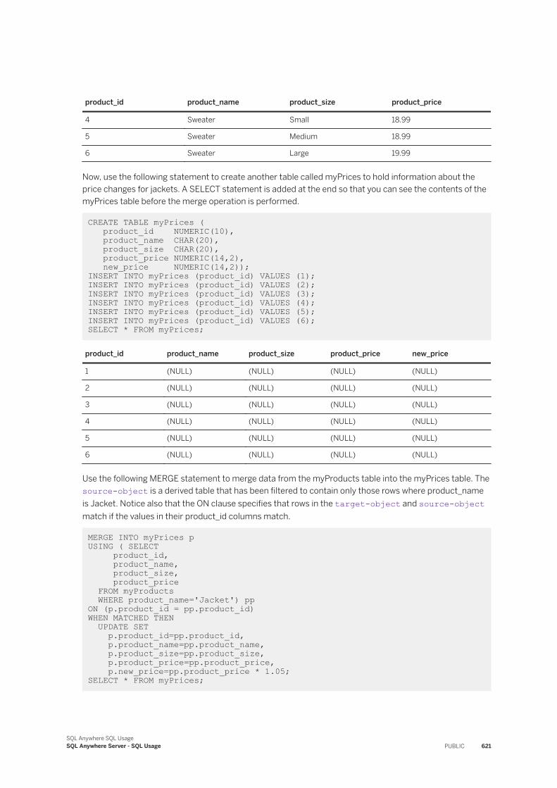
product_id product_name product_size product_price
4 Sweater Small 18.99
5 Sweater Medium 18.99
6 Sweater Large 19.99
Now, use the following statement to create another table called myPrices to hold information about the price changes for jackets. A SELECT statement is added at the end so that you can see the contents of the myPrices table before the merge operation is performed.
CREATE TABLE myPrices ( product_id NUMERIC(10), product_name CHAR(20), product_size CHAR(20), product_price NUMERIC(14,2), new_price NUMERIC(14,2));INSERT INTO myPrices (product_id) VALUES (1);INSERT INTO myPrices (product_id) VALUES (2);INSERT INTO myPrices (product_id) VALUES (3);INSERT INTO myPrices (product_id) VALUES (4);INSERT INTO myPrices (product_id) VALUES (5);INSERT INTO myPrices (product_id) VALUES (6); SELECT * FROM myPrices;
product_id product_name product_size product_price new_price
1 (NULL) (NULL) (NULL) (NULL)
2 (NULL) (NULL) (NULL) (NULL)
3 (NULL) (NULL) (NULL) (NULL)
4 (NULL) (NULL) (NULL) (NULL)
5 (NULL) (NULL) (NULL) (NULL)
6 (NULL) (NULL) (NULL) (NULL)
Use the following MERGE statement to merge data from the myProducts table into the myPrices table. The source-object is a derived table that has been filtered to contain only those rows where product_name is Jacket. Notice also that the ON clause specifies that rows in the target-object and source-object match if the values in their product_id columns match.
MERGE INTO myPrices p USING ( SELECT product_id, product_name, product_size, product_price FROM myProducts WHERE product_name='Jacket') ppON (p.product_id = pp.product_id)WHEN MATCHED THEN UPDATE SET p.product_id=pp.product_id, p.product_name=pp.product_name, p.product_size=pp.product_size, p.product_price=pp.product_price, p.new_price=pp.product_price * 1.05; SELECT * FROM myPrices;
SQL Anywhere SQL UsageSQL Anywhere Server - SQL Usage PUBLIC 621
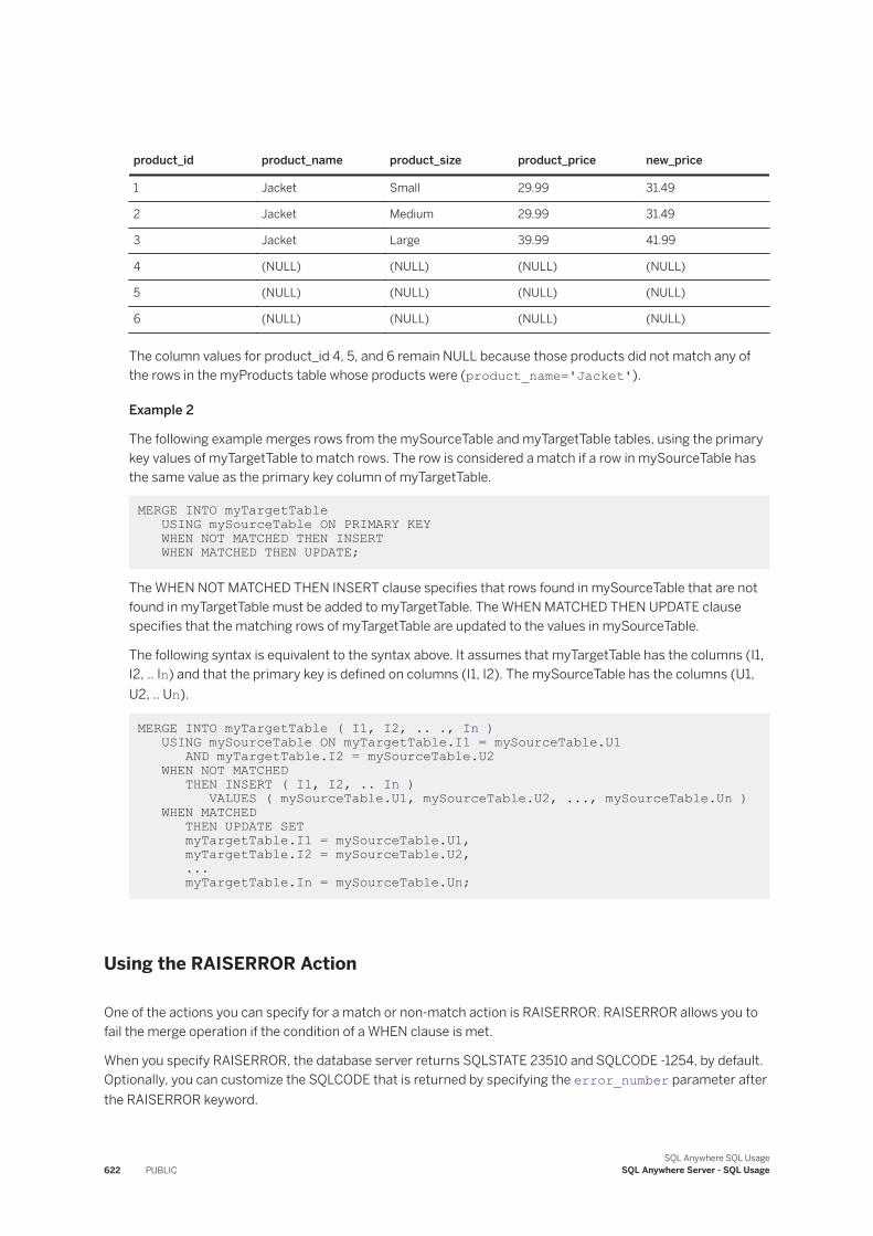
product_id product_name product_size product_price new_price
1 Jacket Small 29.99 31.49
2 Jacket Medium 29.99 31.49
3 Jacket Large 39.99 41.99
4 (NULL) (NULL) (NULL) (NULL)
5 (NULL) (NULL) (NULL) (NULL)
6 (NULL) (NULL) (NULL) (NULL)
The column values for product_id 4, 5, and 6 remain NULL because those products did not match any of the rows in the myProducts table whose products were (product_name='Jacket').
Example 2
The following example merges rows from the mySourceTable and myTargetTable tables, using the primary key values of myTargetTable to match rows. The row is considered a match if a row in mySourceTable has the same value as the primary key column of myTargetTable.
MERGE INTO myTargetTable USING mySourceTable ON PRIMARY KEY WHEN NOT MATCHED THEN INSERT WHEN MATCHED THEN UPDATE;
The WHEN NOT MATCHED THEN INSERT clause specifies that rows found in mySourceTable that are not found in myTargetTable must be added to myTargetTable. The WHEN MATCHED THEN UPDATE clause specifies that the matching rows of myTargetTable are updated to the values in mySourceTable.
The following syntax is equivalent to the syntax above. It assumes that myTargetTable has the columns (I1, I2, .. In) and that the primary key is defined on columns (I1, I2). The mySourceTable has the columns (U1, U2, .. Un).
MERGE INTO myTargetTable ( I1, I2, .. ., In ) USING mySourceTable ON myTargetTable.I1 = mySourceTable.U1 AND myTargetTable.I2 = mySourceTable.U2 WHEN NOT MATCHED THEN INSERT ( I1, I2, .. In ) VALUES ( mySourceTable.U1, mySourceTable.U2, ..., mySourceTable.Un ) WHEN MATCHED THEN UPDATE SET myTargetTable.I1 = mySourceTable.U1, myTargetTable.I2 = mySourceTable.U2, ... myTargetTable.In = mySourceTable.Un;
Using the RAISERROR Action
One of the actions you can specify for a match or non-match action is RAISERROR. RAISERROR allows you to fail the merge operation if the condition of a WHEN clause is met.
When you specify RAISERROR, the database server returns SQLSTATE 23510 and SQLCODE -1254, by default. Optionally, you can customize the SQLCODE that is returned by specifying the error_number parameter after the RAISERROR keyword.
622 PUBLICSQL Anywhere SQL Usage
SQL Anywhere Server - SQL Usage
Specifying a custom SQLCODE can be beneficial when, later, you are trying to determine the specific circumstances that caused the error to be raised.
The custom SQLCODE must be a positive integer greater than 17000, and can be specified either as a number or a variable.
The following statements provide a simple demonstration of how customizing a custom SQLCODE affects what is returned. For this example, you must have the CREATE TABLE privilege.
Create the table targetTable as follows:
CREATE TABLE targetTable( c1 int ); INSERT INTO targetTable VALUES( 1 );
The following statement returns an error with SQLSTATE = '23510' and SQLCODE = -1254:
MERGE INTO targetTable USING (SELECT 1 c1 ) AS sourceData ON targetTable.c1 = sourceData.c1 WHEN MATCHED THEN RAISERROR; SELECT sqlstate, sqlcode;
The following statement returns an error with SQLSTATE = '23510' and SQLCODE = -17001:
MERGE INTO targetTable USING (SELECT 1 c1 ) AS sourceData ON targetTable.c1 = sourceData.c1 WHEN MATCHED THEN RAISERROR 17001 WHEN NOT MATCHED THEN RAISERROR 17002; SELECT sqlstate, sqlcode;
The following statement returns an error with SQLSTATE = '23510' and SQLCODE = -17002:
MERGE INTO targetTable USING (SELECT 2 c1 ) AS sourceData ON targetTable.c1 = sourceData.c1 WHEN MATCHED THEN RAISERROR 17001 WHEN NOT MATCHED THEN RAISERROR 17002; SELECT sqlstate, sqlcode;
1.7.3.8 Tips on Importing Data with Proxy Tables
Use proxy tables to import remote data such as data from another database.
A proxy table is a local table containing metadata used to access a table on a remote database server as if it were a local table.
Impact on the Database
Changes are recorded in the transaction log when you import using proxy tables. If there is a media failure involving the database file, you can recover information about the changes you made from the transaction log.
SQL Anywhere SQL UsageSQL Anywhere Server - SQL Usage PUBLIC 623
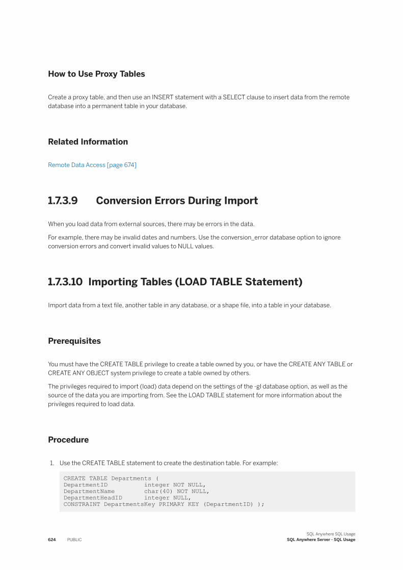
How to Use Proxy Tables
Create a proxy table, and then use an INSERT statement with a SELECT clause to insert data from the remote database into a permanent table in your database.
Related Information
Remote Data Access [page 674]
1.7.3.9 Conversion Errors During Import
When you load data from external sources, there may be errors in the data.
For example, there may be invalid dates and numbers. Use the conversion_error database option to ignore conversion errors and convert invalid values to NULL values.
1.7.3.10 Importing Tables (LOAD TABLE Statement)
Import data from a text file, another table in any database, or a shape file, into a table in your database.
Prerequisites
You must have the CREATE TABLE privilege to create a table owned by you, or have the CREATE ANY TABLE or CREATE ANY OBJECT system privilege to create a table owned by others.
The privileges required to import (load) data depend on the settings of the -gl database option, as well as the source of the data you are importing from. See the LOAD TABLE statement for more information about the privileges required to load data.
Procedure
1. Use the CREATE TABLE statement to create the destination table. For example:
CREATE TABLE Departments ( DepartmentID integer NOT NULL,DepartmentName char(40) NOT NULL,DepartmentHeadID integer NULL, CONSTRAINT DepartmentsKey PRIMARY KEY (DepartmentID) );
624 PUBLICSQL Anywhere SQL Usage
SQL Anywhere Server - SQL Usage
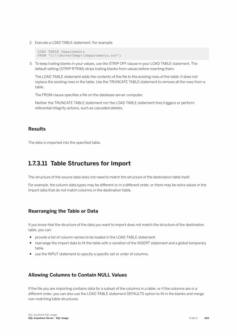
2. Execute a LOAD TABLE statement. For example:
LOAD TABLE Departments FROM 'C:\\ServerTemp\\Departments.csv';
3. To keep trailing blanks in your values, use the STRIP OFF clause in your LOAD TABLE statement. The default setting (STRIP RTRIM) strips trailing blanks from values before inserting them.
The LOAD TABLE statement adds the contents of the file to the existing rows of the table; it does not replace the existing rows in the table. Use the TRUNCATE TABLE statement to remove all the rows from a table.
The FROM clause specifies a file on the database server computer.
Neither the TRUNCATE TABLE statement nor the LOAD TABLE statement fires triggers or perform referential integrity actions, such as cascaded deletes.
Results
The data is imported into the specified table.
1.7.3.11 Table Structures for Import
The structure of the source data does not need to match the structure of the destination table itself.
For example, the column data types may be different or in a different order, or there may be extra values in the import data that do not match columns in the destination table.
Rearranging the Table or Data
If you know that the structure of the data you want to import does not match the structure of the destination table, you can:
● provide a list of column names to be loaded in the LOAD TABLE statement.● rearrange the import data to fit the table with a variation of the INSERT statement and a global temporary
table.● use the INPUT statement to specify a specific set or order of columns.
Allowing Columns to Contain NULL Values
If the file you are importing contains data for a subset of the columns in a table, or if the columns are in a different order, you can also use the LOAD TABLE statement DEFAULTS option to fill in the blanks and merge non-matching table structures.
SQL Anywhere SQL UsageSQL Anywhere Server - SQL Usage PUBLIC 625
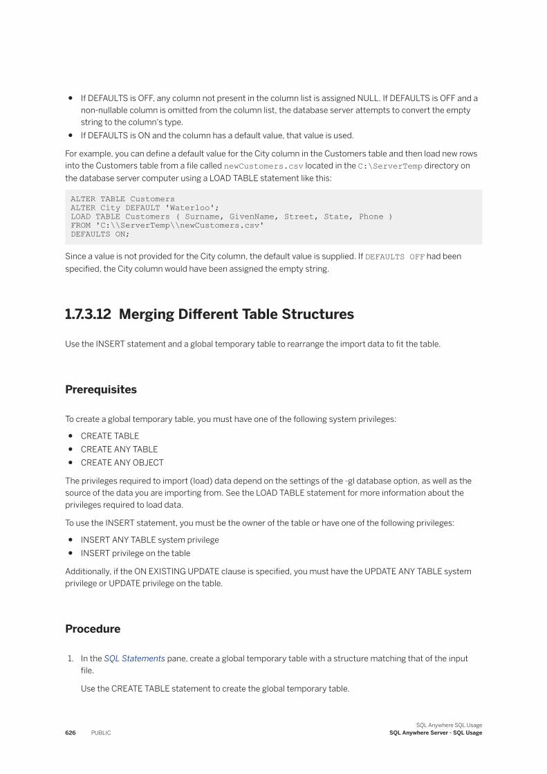
● If DEFAULTS is OFF, any column not present in the column list is assigned NULL. If DEFAULTS is OFF and a non-nullable column is omitted from the column list, the database server attempts to convert the empty string to the column's type.
● If DEFAULTS is ON and the column has a default value, that value is used.
For example, you can define a default value for the City column in the Customers table and then load new rows into the Customers table from a file called newCustomers.csv located in the C:\ServerTemp directory on the database server computer using a LOAD TABLE statement like this:
ALTER TABLE Customers ALTER City DEFAULT 'Waterloo';LOAD TABLE Customers ( Surname, GivenName, Street, State, Phone )FROM 'C:\\ServerTemp\\newCustomers.csv' DEFAULTS ON;
Since a value is not provided for the City column, the default value is supplied. If DEFAULTS OFF had been specified, the City column would have been assigned the empty string.
1.7.3.12 Merging Different Table Structures
Use the INSERT statement and a global temporary table to rearrange the import data to fit the table.
Prerequisites
To create a global temporary table, you must have one of the following system privileges:
● CREATE TABLE● CREATE ANY TABLE● CREATE ANY OBJECT
The privileges required to import (load) data depend on the settings of the -gl database option, as well as the source of the data you are importing from. See the LOAD TABLE statement for more information about the privileges required to load data.
To use the INSERT statement, you must be the owner of the table or have one of the following privileges:
● INSERT ANY TABLE system privilege● INSERT privilege on the table
Additionally, if the ON EXISTING UPDATE clause is specified, you must have the UPDATE ANY TABLE system privilege or UPDATE privilege on the table.
Procedure
1. In the SQL Statements pane, create a global temporary table with a structure matching that of the input file.
Use the CREATE TABLE statement to create the global temporary table.
626 PUBLICSQL Anywhere SQL Usage
SQL Anywhere Server - SQL Usage
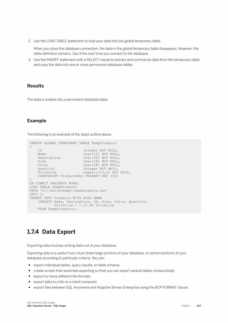
2. Use the LOAD TABLE statement to load your data into the global temporary table.
When you close the database connection, the data in the global temporary table disappears. However, the table definition remains. Use it the next time you connect to the database.
3. Use the INSERT statement with a SELECT clause to extract and summarize data from the temporary table and copy the data into one or more permanent database tables.
Results
The data is loaded into a permanent database table.
Example
The following is an example of the steps outline above.
CREATE GLOBAL TEMPORARY TABLE TempProducts ( ID integer NOT NULL, Name char(15) NOT NULL, Description char(30) NOT NULL, Size char(18) NOT NULL, Color char(18) NOT NULL, Quantity integer NOT NULL, UnitPrice numeric(15,2) NOT NULL, CONSTRAINT ProductsKey PRIMARY KEY (ID))ON COMMIT PRESERVE ROWS;LOAD TABLE TempProductsFROM 'C:\\ServerTemp\\newProducts.csv'SKIP 1;INSERT INTO Products WITH AUTO NAME (SELECT Name, Description, ID, Size, Color, Quantity, UnitPrice * 1.25 AS UnitPrice FROM TempProducts);
1.7.4 Data Export
Exporting data involves writing data out of your database.
Exporting data is a useful if you must share large portions of your database, or extract portions of your database according to particular criteria. You can:
● export individual tables, query results, or table schema.● create scripts that automate exporting so that you can export several tables consecutively.● export to many different file formats.● export data to a file on a client computer.● export files between SQL Anywhere and Adaptive Server Enterprise using the BCP FORMAT clause.
SQL Anywhere SQL UsageSQL Anywhere Server - SQL Usage PUBLIC 627
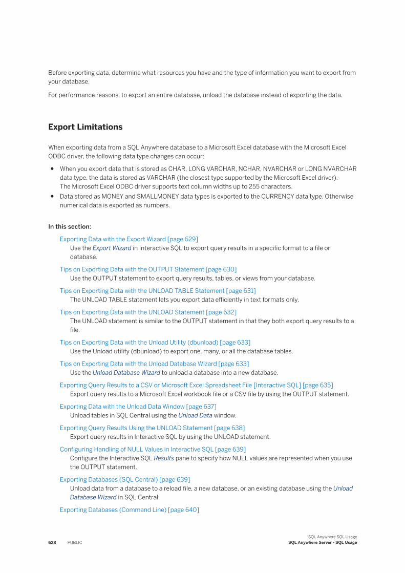
Before exporting data, determine what resources you have and the type of information you want to export from your database.
For performance reasons, to export an entire database, unload the database instead of exporting the data.
Export Limitations
When exporting data from a SQL Anywhere database to a Microsoft Excel database with the Microsoft Excel ODBC driver, the following data type changes can occur:
● When you export data that is stored as CHAR, LONG VARCHAR, NCHAR, NVARCHAR or LONG NVARCHAR data type, the data is stored as VARCHAR (the closest type supported by the Microsoft Excel driver).The Microsoft Excel ODBC driver supports text column widths up to 255 characters.
● Data stored as MONEY and SMALLMONEY data types is exported to the CURRENCY data type. Otherwise numerical data is exported as numbers.
In this section:
Exporting Data with the Export Wizard [page 629]Use the Export Wizard in Interactive SQL to export query results in a specific format to a file or database.
Tips on Exporting Data with the OUTPUT Statement [page 630]Use the OUTPUT statement to export query results, tables, or views from your database.
Tips on Exporting Data with the UNLOAD TABLE Statement [page 631]The UNLOAD TABLE statement lets you export data efficiently in text formats only.
Tips on Exporting Data with the UNLOAD Statement [page 632]The UNLOAD statement is similar to the OUTPUT statement in that they both export query results to a file.
Tips on Exporting Data with the Unload Utility (dbunload) [page 633]Use the Unload utility (dbunload) to export one, many, or all the database tables.
Tips on Exporting Data with the Unload Database Wizard [page 633]Use the Unload Database Wizard to unload a database into a new database.
Exporting Query Results to a CSV or Microsoft Excel Spreadsheet File [Interactive SQL] [page 635]Export query results to a Microsoft Excel workbook file or a CSV file by using the OUTPUT statement.
Exporting Data with the Unload Data Window [page 637]Unload tables in SQL Central using the Unload Data window.
Exporting Query Results Using the UNLOAD Statement [page 638]Export query results in Interactive SQL by using the UNLOAD statement.
Configuring Handling of NULL Values in Interactive SQL [page 639]Configure the Interactive SQL Results pane to specify how NULL values are represented when you use the OUTPUT statement.
Exporting Databases (SQL Central) [page 639]Unload data from a database to a reload file, a new database, or an existing database using the Unload Database Wizard in SQL Central.
Exporting Databases (Command Line) [page 640]
628 PUBLICSQL Anywhere SQL Usage
SQL Anywhere Server - SQL Usage
Unload data from a database to a reload file, a new database, or an existing database using the Unload utility (dbunload) on the command line.
Exporting Tables (SQL) [page 641]Export a table by executing an UNLOAD TABLE statement from Interactive SQL.
Exporting Tables (Command Line) [page 643]Export a table by running the Unload utility (dbunload) on the command line.
Related Information
Performance Aspects of Bulk Operations [page 608]Access to Data on Client Computers [page 643]Database Rebuilds [page 646]
1.7.4.1 Exporting Data with the Export Wizard
Use the Export Wizard in Interactive SQL to export query results in a specific format to a file or database.
Prerequisites
You must be the owner of the table you are querying, have SELECT privilege on the table, or have the SELECT ANY TABLE system privilege.
Procedure
1. Execute a query.
2. In Interactive SQL, click Data Export .3. Follow the instructions in the Export Wizard.
Results
The query results are exported to the specified file or database.
SQL Anywhere SQL UsageSQL Anywhere Server - SQL Usage PUBLIC 629
Example
1. Execute the following query while connected to the sample database. You must have SELECT privilege on the table Employees or the SELECT ANY TABLE system privilege.
SELECT * FROM Employees WHERE State = 'GA';
2. The result set includes a list of all the employees who live in Georgia.
3. Click Data Export .4. Click In a database and then click Next.5. In the Database type list, click UltraLite.6. In the User Id field, type DBA.7. In the Password field, type sql.8. In the Database file field, type C:\Users\Public\Documents\SQL Anywhere 17\Samples\UltraLite
\CustDB\custdb.udb.9. Click Next.10. Click Create a new table.11. In the Table name field, type GAEmployees.12. Click Export.13. Click Close.
14. Click SQL Previous SQL .The OUTPUT USING statement created and used by the Export Wizard appears in the SQL Statements pane:
-- Generated by the Export Wizard output using 'driver=UltraLite 17;UID=DBA;PWD=***; DBF=C:\\Users\\Public\\Documents\\SQL Anywhere 17\\Samples\\UltraLite\\CustDB\\custdb.udb' into "GAEmployees" create table on
1.7.4.2 Tips on Exporting Data with the OUTPUT Statement
Use the OUTPUT statement to export query results, tables, or views from your database.
The OUTPUT statement is useful when compatibility is an issue because it can write out the result set of a SELECT statement in several different file formats. You can use the default output format, or you can specify the file format on each OUTPUT statement. Interactive SQL can execute a SQL script file containing multiple OUTPUT statements.
The default Interactive SQL output format is specified on the Import/Export tab of the Interactive SQL Options window (accessed by clicking Tools Options in Interactive SQL).
Use the Interactive SQL OUTPUT statement when you want to:
● export all or part of a table or view in a format other than text● automate the export process using a SQL script file
630 PUBLICSQL Anywhere SQL Usage
SQL Anywhere Server - SQL Usage
Impact on the Database
If you have a choice between using the OUTPUT statement, UNLOAD statement, or UNLOAD TABLE statement, choose the UNLOAD TABLE statement for performance reasons.
There are performance impacts associated with exporting large amounts of data with the OUTPUT statement. Use the OUTPUT statement on the same computer as the server if possible to avoid sending large amounts of data across the network.
1.7.4.3 Tips on Exporting Data with the UNLOAD TABLE Statement
The UNLOAD TABLE statement lets you export data efficiently in text formats only.
The UNLOAD TABLE statement exports one row per line, with values separated by a comma delimiter. To make reloading faster, the data is exported in order by primary key values.
Use the UNLOAD TABLE statement when you:
● want to export entire tables in text format● are concerned about database performance● export data to a file on a client computer
To use the UNLOAD TABLE statement, you must have the appropriate privileges. For example, the SELECT ANY TABLE system privilege is usually sufficient, unless the -gl database server option is set to NONE.
The -gl database server option controls who can use the UNLOAD TABLE statement.
Impact on the Database
If you have a choice between using the OUTPUT statement, UNLOAD statement, or UNLOAD TABLE statement, choose the UNLOAD TABLE statement for performance reasons.
The UNLOAD TABLE statement places an exclusive lock on the whole table while you are unloading it.
Example
Using the SQL Anywhere sample database, you can unload the Employees table to a text file named Employees.csv by executing the following statement:
UNLOAD TABLE Employees TO 'C:\\ServerTemp\\Employees.csv';
Using this form of the UNLOAD TABLE statement, the file path is relative to the database server computer.
SQL Anywhere SQL UsageSQL Anywhere Server - SQL Usage PUBLIC 631
Related Information
Access to Data on Client Computers [page 643]
1.7.4.4 Tips on Exporting Data with the UNLOAD Statement
The UNLOAD statement is similar to the OUTPUT statement in that they both export query results to a file.
However, the UNLOAD statement exports data more efficiently in a text format. The UNLOAD statement exports with one row per line, with values separated by a comma delimiter.
Use the UNLOAD statement to unload data when you want to:
● export query results if performance is an issue● store output in text format● embed an export statement in an application● export data to a file on a client computer
To use the UNLOAD statement with a SELECT, you must have the appropriate privileges. For example, the SELECT ANY TABLE system privilege is usually sufficient, unless the -gl database server option is set to NONE. At minimum, you must have the permissions required to execute the SELECT on the table that is specified within the UNLOAD statement
The -gl database server option controls who can use the UNLOAD statement.
Impact on the Database
If you have a choice between using the OUTPUT statement, UNLOAD statement, or UNLOAD TABLE statement, choose the UNLOAD TABLE statement for performance reasons.
The UNLOAD statement with a SELECT is executed at the current isolation level.
Example
Using the SQL Anywhere sample database, you can unload a subset of the Employees table to a text file named GAEmployees.csv by executing the following statement:
UNLOAD SELECT * FROM Employees WHERE State = 'GA'TO 'C:\\ServerTemp\\GAEmployees.csv' QUOTE '"';
Using this form of the UNLOAD TABLE statement, the file path is relative to the database server computer.
632 PUBLICSQL Anywhere SQL Usage
SQL Anywhere Server - SQL Usage
Related Information
Access to Data on Client Computers [page 643]
1.7.4.5 Tips on Exporting Data with the Unload Utility (dbunload)
Use the Unload utility (dbunload) to export one, many, or all the database tables.
You can export table data, and table schemas. To rearrange your database tables, you can also use dbunload to create the necessary SQL script files and modify them as needed. These files can be used to create identical tables in different databases. You can unload tables with structure only, data only, or with both structure and data. You can also unload directly into an existing database using the -ac option.
Use dbunload to:
● rebuild or extract your database● export data in different file formats● process large amounts of data quickly
NoteThe Unload utility (dbunload) is functionally equivalent to the SQL Central Unload Database Wizard. You can use either one interchangeably to produce the same results.
1.7.4.6 Tips on Exporting Data with the Unload Database Wizard
Use the Unload Database Wizard to unload a database into a new database.
When using the Unload Database Wizard to unload your database, you can choose to unload all the objects in a database, or a subset of tables from the database. Only tables for users selected in the Configure Owner Filter window appear in the Unload Database Wizard. To view tables belonging to a particular database user, right-click the database you are unloading, click Configure Owner Filter, and then select the user in the resulting window.
You can also use the Unload Database Wizard to unload an entire database in text comma-delimited format and to create the necessary SQL script files to completely recreate your database. This is useful for creating SQL Remote extractions or building new copies of your database with the same or a slightly modified structure. The Unload Database Wizard is useful for exporting SQL Anywhere files intended for reuse within SQL Anywhere.
The Unload Database Wizard also gives you the option to reload into an existing database or a new database, rather than into a reload file.
NoteThe Unload utility (dbunload) is functionally equivalent to the Unload Database Wizard. You can use either one interchangeably to produce the same results.
SQL Anywhere SQL UsageSQL Anywhere Server - SQL Usage PUBLIC 633
In this section:
Unloading a Database File or Running Database [page 634]Unload a stopped or running database in SQL Central using the Unload Database Wizard.
1.7.4.6.1 Unloading a Database File or Running Database
Unload a stopped or running database in SQL Central using the Unload Database Wizard.
Prerequisites
When unloading into a variable, no privileges are required. Otherwise, the required privileges depend on the database server -gl option, as follows:
● If the -gl option is set to ALL, you must be the owner of the tables, or have SELECT privilege on the tables, or have the SELECT ANY TABLE system privilege.
● If the -gl option is set to DBA, you must have the SELECT ANY TABLE system privilege.● If the -gl option is set to NONE, UNLOAD is not permitted.
When unloading to a file on a client computer:
● You must have the WRITE CLIENT FILE privilege.● You must have write permissions on the directory where the file is located.● The allow_write_client_file database option must be enabled.● The WRITE_CLIENT_FILE feature must be enabled.
Context
NoteWhen you unload only tables, the user IDs that own the tables are not unloaded. You must create the user IDs that own the tables in the new database before reloading the tables.
Procedure
1. Click Tools SQL Anywhere 17 Unload Database .2. Follow the instructions in the Unload Database Wizard.
634 PUBLICSQL Anywhere SQL Usage
SQL Anywhere Server - SQL Usage
Results
The specified database is unloaded.
1.7.4.7 Exporting Query Results to a CSV or Microsoft Excel Spreadsheet File [Interactive SQL]
Export query results to a Microsoft Excel workbook file or a CSV file by using the OUTPUT statement.
Prerequisites
You must be the owner of the table you are querying, have SELECT privilege on the table, or have the SELECT ANY TABLE system privilege.
If you are exporting data to a Microsoft Excel workbook file, then you must have a compatible Microsoft Excel ODBC driver installed.
Context
When files with a .csv or .txt extension are exported with the FORMAT EXCEL clause, they follow the default formatting for Microsoft Excel files. For Microsoft Excel workbook files, the WORKSHEET clause specifies the name of the worksheet to export the data to. If the clause is omitted, then the data is exported to the first sheet in the file. If the file does not exist, then a new file is created and the data is exported to a default worksheet.
Procedure
1. Type your query in the SQL Statements pane of Interactive SQL.2. At the end of the query, choose one of the following options:
Option Specify the OUTPUT Statement
Export an entire table For example:
SELECT * FROM TableName; OUTPUT TO 'filepath';
Export query results and append the results to another file
Specify the APPEND clause:
SELECT * FROM TableName; OUTPUT TO 'filepath'
SQL Anywhere SQL UsageSQL Anywhere Server - SQL Usage PUBLIC 635
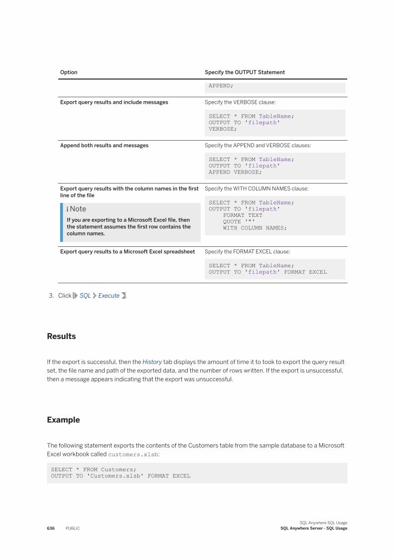
Option Specify the OUTPUT Statement
APPEND;
Export query results and include messages Specify the VERBOSE clause:
SELECT * FROM TableName; OUTPUT TO 'filepath' VERBOSE;
Append both results and messages Specify the APPEND and VERBOSE clauses:
SELECT * FROM TableName; OUTPUT TO 'filepath' APPEND VERBOSE;
Export query results with the column names in the first line of the file
NoteIf you are exporting to a Microsoft Excel file, then the statement assumes the first row contains the column names.
Specify the WITH COLUMN NAMES clause:
SELECT * FROM TableName; OUTPUT TO 'filepath' FORMAT TEXT QUOTE '"' WITH COLUMN NAMES;
Export query results to a Microsoft Excel spreadsheet Specify the FORMAT EXCEL clause:
SELECT * FROM TableName; OUTPUT TO 'filepath' FORMAT EXCEL
3. Click SQL Execute .
Results
If the export is successful, then the History tab displays the amount of time it to took to export the query result set, the file name and path of the exported data, and the number of rows written. If the export is unsuccessful, then a message appears indicating that the export was unsuccessful.
Example
The following statement exports the contents of the Customers table from the sample database to a Microsoft Excel workbook called customers.xlsb:
SELECT * FROM Customers; OUTPUT TO 'Customers.xlsb' FORMAT EXCEL
636 PUBLICSQL Anywhere SQL Usage
SQL Anywhere Server - SQL Usage
Related Information
Adaptive Server Enterprise Compatibility [page 674]Data Import [page 609]
1.7.4.8 Exporting Data with the Unload Data Window
Unload tables in SQL Central using the Unload Data window.
Prerequisites
You must be the owner of the table, have SELECT privilege on the table, or have the SELECT ANY TABLE system privilege.
Context
Use the Unload Data window in SQL Central to unload one or more tables in a database. This functionality is also available with either the Unload Database Wizard or the Unload utility (dbunload), but this window allows you to unload tables in one step, instead of completing the entire Unload Database Wizard.
Procedure
1. In SQL Central, use the SQL Anywhere 17 plug-in to connect to the database.2. Double-click Tables.3. Right-click the table you want to export data from, and click Unload Data.4. Complete the Unload Data window. Click OK.
Results
The data is saved to the specified file.
SQL Anywhere SQL UsageSQL Anywhere Server - SQL Usage PUBLIC 637
1.7.4.9 Exporting Query Results Using the UNLOAD Statement
Export query results in Interactive SQL by using the UNLOAD statement.
Prerequisites
When unloading into a variable, no privileges are required. Otherwise, the required privileges depend on the database server -gl option, as follows:
● If the -gl option is set to ALL, you must be the owner of the tables, or have SELECT privilege on the tables, or have the SELECT ANY TABLE system privilege.
● If the -gl option is set to DBA, you must have the SELECT ANY TABLE system privilege.● If the -gl option is set to NONE, UNLOAD is not permitted.
When unloading to a file on a client computer:
● You must have the WRITE CLIENT FILE privilege.● You must have write permissions on the directory where the file is located.● The allow_write_client_file database option must be enabled.● The WRITE_CLIENT_FILE feature must be enabled.
Procedure
In the SQL Statements pane, execute an UNLOAD statement. For example:
UNLOAD SELECT * FROM Employees TO 'C:\\ServerTemp\\Employees.csv';
If the export is successful, the History tab in Interactive SQL displays the amount of time it to took to export the query result set, the file name and path of the exported data, and the number of rows written. If the export is unsuccessful, a message appears indicating that the export was unsuccessful.
Using this form of the UNLOAD TABLE statement, the file path is relative to the database server computer.
Include the FORMAT BCP clause to import and export files between SQL Anywhere and Adaptive Server Enterprise.
Results
The query results are exported to the specified location.
638 PUBLICSQL Anywhere SQL Usage
SQL Anywhere Server - SQL Usage
Related Information
Adaptive Server Enterprise Compatibility [page 674]
1.7.4.10 Configuring Handling of NULL Values in Interactive SQL
Configure the Interactive SQL Results pane to specify how NULL values are represented when you use the OUTPUT statement.
Procedure
1. In Interactive SQL, click Tools Options .2. Click SQL Anywhere.3. Click the Results tab.4. In the Display null values as field, type the value you want to use for NULLs.5. Click OK.
Results
The value that appears in the place of the NULL value is changed.
1.7.4.11 Exporting Databases (SQL Central)
Unload data from a database to a reload file, a new database, or an existing database using the Unload Database Wizard in SQL Central.
Prerequisites
When unloading into a variable, no privileges are required. Otherwise, the required privileges depend on the database server -gl option, as follows:
● If the -gl option is set to ALL, you must be the owner of the tables, or have SELECT privilege on the tables, or have the SELECT ANY TABLE system privilege.
● If the -gl option is set to DBA, you must have the SELECT ANY TABLE system privilege.
SQL Anywhere SQL UsageSQL Anywhere Server - SQL Usage PUBLIC 639
● If the -gl option is set to NONE, UNLOAD is not permitted.
When unloading to a file on a client computer:
● You must have the WRITE CLIENT FILE privilege.● You must have write permissions on the directory where the file is located.● The allow_write_client_file database option must be enabled.● The WRITE_CLIENT_FILE feature must be enabled.
Procedure
1. Click Tools SQL Anywhere 17 Unload Database .2. Follow the instructions in the Unload Database Wizard.
Results
The data is unloaded to the specified location.
Related Information
Exporting Databases (Command Line) [page 640]
1.7.4.12 Exporting Databases (Command Line)
Unload data from a database to a reload file, a new database, or an existing database using the Unload utility (dbunload) on the command line.
Prerequisites
For an unload without a reload, you must have the SELECT ANY TABLE system privilege. For an unload with reload, you must have the SELECT ANY TABLE and SERVER OPERATOR system privileges.
Procedure
Run the Unload utility (dbunload), and use the -c option to specify the connection parameters.
640 PUBLICSQL Anywhere SQL Usage
SQL Anywhere Server - SQL Usage
Option Action
Unload the entire database
To unload the entire database to the directory C:\ServerTemp\DataFiles on the server computer:
dbunload -c "DBN=demo;UID=DBA;PWD=sql" C:\ServerTemp\DataFiles
Export data only Use the -d and -ss options. For example:
dbunload -c "DBN=demo;UID=DBA;PWD=sql" -d -ss C:\ServerTemp\DataFiles
Export schema only Use the -n option. For example:
dbunload -c "DBN=demo;UID=DBA;PWD=sql" -n
The statements required to recreate the schema and/or reload the tables are written to reload.sql in the client's current directory.
Results
The data is unloaded to the specified location.
Related Information
Exporting Databases (SQL Central) [page 639]
1.7.4.13 Exporting Tables (SQL)
Export a table by executing an UNLOAD TABLE statement from Interactive SQL.
Prerequisites
When unloading into a variable, no privileges are required. Otherwise, the required privileges depend on the database server -gl option, as follows:
● If the -gl option is set to ALL, you must be the owner of the tables, or have SELECT privilege on the tables, or have the SELECT ANY TABLE system privilege.
● If the -gl option is set to DBA, you must have the SELECT ANY TABLE system privilege.● If the -gl option is set to NONE, UNLOAD is not permitted.
SQL Anywhere SQL UsageSQL Anywhere Server - SQL Usage PUBLIC 641
When unloading to a file on a client computer:
● You must have the WRITE CLIENT FILE privilege.● You must have write permissions on the directory where the file is located.● The allow_write_client_file database option must be enabled.● The WRITE_CLIENT_FILE feature must be enabled.
Context
Export a table by selecting all the data in a table and exporting the query results.
Procedure
Execute an UNLOAD TABLE statement. For example:
UNLOAD TABLE Departments TO 'C:\\ServerTemp\\Departments.csv';
This statement unloads the Departments table from the SQL Anywhere sample database into the file Departments.csv in a directory on the database server computer, not the client computer. Since the file path is specified in a SQL literal, the backslash characters are escaped by doubling them to prevent translation of escape sequences such as '\n' or '\x'.
Each row of the table is output on a single line of the output file, and no column names are exported. The columns are delimited by a comma. The delimiter character can be changed using the DELIMITED BY clause. The fields are not fixed-width fields. Only the characters in each entry are exported, not the full width of the column.
Results
The data is exported into the specified file.
Related Information
Exporting Data with the Export Wizard [page 629]
642 PUBLICSQL Anywhere SQL Usage
SQL Anywhere Server - SQL Usage
1.7.4.14 Exporting Tables (Command Line)
Export a table by running the Unload utility (dbunload) on the command line.
Prerequisites
For an unload without reload, you must have the SELECT ANY TABLE system privilege. For an unload with reload, you must have the SELECT ANY TABLE and SERVER OPERATOR system privileges.
Context
Unload more than one table by separating the table names with a comma (,) delimiter.
Procedure
Run the following command:
dbunload -c "DBN=demo;UID=DBA;PWD=sql" -t Employees C:\ServerTemp\DataFiles
In this command, -c specifies the database connection parameters and -t specifies the name of the table or tables you want to export. This dbunload command unloads the data from the SQL Anywhere sample database (assumed to be running on the default database server) into a set of files in the C:\ServerTemp\DataFiles directory on the server computer. A SQL script file to rebuild the tables from the data files is created with the default name reload.sql in the client's current directory.
Results
The data is exported to the specified location.
1.7.5 Access to Data on Client Computers
You can load data from, and unload data to, a file on a client computer using SQL statements and functions, without having to copy files to or from the database server computer.
To do this, the database server initiates the transfer using a Command Sequence communication protocol (CmdSeq) file handler. The CmdSeq file handler is invoked after the database server receives a request from the client application requiring a transfer of data to or from the client computer, and before sending the response. The file handler supports simultaneous and interleaved transfer of multiple files from the client at
SQL Anywhere SQL UsageSQL Anywhere Server - SQL Usage PUBLIC 643
any given time. For example, the database server can initiate the transfer of multiple files simultaneously if the statement executed by the client application requires it.
Using a CmdSeq file handler to achieve transfer of client data means that applications do not require any new specialized code and can start benefiting immediately from the feature using the SQL components listed below:
READ_CLIENT_FILE function
The READ_CLIENT_FILE function reads data from the specified file on the client computer, and returns a LONG BINARY value representing the contents of the file. This function can be used anywhere in SQL code that a BLOB can be used. The data returned by the READ_CLIENT_FILE function is not materialized in memory when possible, unless the statement explicitly causes materialization to take place. For example, the LOAD TABLE statement streams the data from the client file without materializing it. Assigning the value returned by the READ_CLIENT_FILE function to a connection variable causes the database server to retrieve and materialize the client file contents.WRITE_CLIENT_FILE function
The WRITE_CLIENT_FILE function writes data to the specified file on the client computer.READ CLIENT FILE system privilege
READ CLIENT FILE system privilege allows you to read from a file on a client computer.WRITE CLIENT FILE system privilege
WRITE CLIENT FILE system privilege allows you to write to a file on a client computer.LOAD TABLE ... USING CLIENT FILE clause
The USING CLIENT FILE clause allows you to load a table using data in a file located on the client computer. For example, LOAD TABLE ... USING CLIENT FILE 'my-file.txt'; loads a file called my-file.txt from the client computer.LOAD TABLE ... USING VALUE clause
The USING VALUE clause allows you to specify a BLOB expression as a value. The BLOB expression can make use of the READ_CLIENT_FILE function to load a BLOB from a file on a client computer. For example, LOAD TABLE ... USING VALUE READ_CLIENT_FILE( 'my-file' ), where my-file is a file on the client computer.UNLOAD TABLE ... INTO CLIENT FILE clause
The INTO CLIENT FILE clause allows you to specify a file on the client computer to unload data into.UNLOAD TABLE ... INTO VARIABLE clause
The INTO VARIABLE clause allows you to specify a variable to unload data into.read_client_file and write_client_file secure features
The read_client_file and write_client_file secure features control the use of statements that can cause a client file to be read from, or written to.
To allow reading from or writing to a client file from a procedure, function or other indirect statements, a callback function must be registered. The callback function is called to confirm that the application allows the client transfer that it did not directly request.
In this section:
Client-side Data Security [page 645]
644 PUBLICSQL Anywhere SQL Usage
SQL Anywhere Server - SQL Usage
There are several mechanisms that ensure that the transfer of client files does not permit the unauthorized transfer of data residing on the client computer, which is often in a different location than the database server computer.
Recovery When Loading Client-side Data [page 645]If you must recover a LOAD TABLE statement from your transaction log, files on the client computer that you used to load data are likely no longer available, or have changed, so the original data is no longer available.
1.7.5.1 Client-side Data Security
There are several mechanisms that ensure that the transfer of client files does not permit the unauthorized transfer of data residing on the client computer, which is often in a different location than the database server computer.
To do this, the database server tracks the origin of each executed statement, and determines if the statement was received directly from the client application. When initiating the transfer of a new file from the client, the database server includes information about the origin of the statement. The CmdSeq file handler then allows the transfer of files for statements sent directly by the client application. If the statement was not sent directly by the client application, the application must register a verification callback. If no callback is registered, the transfer is denied and the statement fails with an error.
Also, the transfer of client data is not allowed until after the connection has been successfully established. This restriction prevents unauthorized access using connection strings or login procedures.
To protect against attempts to gain access to a system by users posing as an authorized user, consider encrypting the data that is being transferred.
SQL Anywhere also provides the following security mechanisms to control access at various levels:
Server level security
The read_client_file and write_client_file secure features allow you to disable all client-side transfers on a server-wide basis.Application and DBA level security
The allow_read_client_file and allow_write_client_file database options provide access control at the database, user, or connection level. For example, an application could set this database option to OFF after connecting to prevent itself from being used for any client-side transfers.User level security
The READ CLIENT FILE and WRITE CLIENT FILE system privileges provide user-level access control for reading data from, and writing data to, a client computer, respectively.
1.7.5.2 Recovery When Loading Client-side Data
If you must recover a LOAD TABLE statement from your transaction log, files on the client computer that you used to load data are likely no longer available, or have changed, so the original data is no longer available.
To prevent this situation from occurring, make sure that logging is not turned off. Then, specify either the WITH ROW LOGGING or WITH CONTENT LOGGING clauses when loading the data. These clauses cause the data you
SQL Anywhere SQL UsageSQL Anywhere Server - SQL Usage PUBLIC 645
are loading to be recorded in the transaction log, so that the transaction log can be replayed later in the event of a recovery.
The WITH ROW LOGGING causes each inserted row to be recorded as an INSERT statement in the transaction log. The WITH CONTENT LOGGING causes the inserted data to be recorded in the transaction log in chunks for the database server to process during recovery. Both methods are suitable for ensuring that the client-side data is available for loading during recovery. However, you cannot use WITH CONTENT LOGGING when loading data into a database that is involved in synchronization.
When you specify any of the following LOAD TABLE statements, but do not specify a logging level, WITH CONTENT LOGGING is the default behavior:
● LOAD TABLE...USING CLIENT FILE client-filename-expression● LOAD TABLE...USING VALUE value-expression● LOAD TABLE...USING COLUMN column-expression
1.7.6 Database Rebuilds
Rebuilding a database is a specific type of import and export involving unloading and reloading your database.
The rebuild (unload/load) and extract tools are used to rebuild databases, to create new databases from part of an existing one, and to eliminate unused free pages.
You can rebuild your database from SQL Central or by using dbunload.
NoteIt is good practice to make backups of your database before rebuilding, especially if you choose to replace the original database with the rebuilt database.
With importing and exporting, the destination of the data is either into your database or out of your database. Importing reads data into your database. Exporting writes data out of your database. Often the information is either coming from or going to another non-SQL Anywhere database.
If you specify the encryption options -ek, -ep, or -et, the LOAD TABLE statements in the reload.sql file must include the encryption key. Hard-coding the key compromises security, so a parameter in the reload.sql file specifies the encryption key. When you execute the reload.sql file with Interactive SQL, you must specify the encryption key as a parameter. If you do not specify the key in the READ statement, Interactive SQL prompts for the key.
Loading and unloading takes data and schema out of a SQL Anywhere database and then places the data and schema back into a SQL Anywhere database. The unloading procedure produces data files and a reload.sql file which contains table definitions required to recreate the tables exactly. Running the reload.sql script recreates the tables and loads the data back into them.
Rebuilding a database can be a time-consuming operation, and can require a large amount of disk space. As well, the database is unavailable for use while being unloaded and reloaded. For these reasons, rebuilding a database is not advised in a production environment unless you have a definite goal in mind.
646 PUBLICSQL Anywhere SQL Usage
SQL Anywhere Server - SQL Usage
From One SQL Anywhere Database to Another
Rebuilding generally copies data out of a SQL Anywhere database and then reloads that data back into a SQL Anywhere database. Unloading and reloading are related since you usually perform both tasks, rather than just one or the other.
Rebuilding Versus Exporting
Rebuilding is different from exporting in that rebuilding exports and imports table definitions and schema in addition to the data. The unload portion of the rebuild process produces text format data files and a reload.sql file that contains table and other definitions. You can run the reload.sql script to recreate the tables and load the data into them.
Consider extracting a database (creating a new database from an old database) if you are using SQL Remote or MobiLink.
Rebuilding Replicating Databases
The procedure for rebuilding a database depends on whether the database is involved in replication or not. If the database is involved in replication, you must preserve the transaction log offsets across the operation, as the Message Agent requires this information. If the database is not involved in replication, the process is simpler.
In this section:
Reasons to Rebuild Databases [page 648]There are several reasons to consider rebuilding your database.
Tips on Rebuilding Databases Using the Unload Utility [page 649]You can use the Unload utility (dbunload) to unload an entire database into a text comma-delimited format and create the necessary SQL script files to completely recreate your database.
Performing a Database Rebuild with Minimum Downtime Using dbunload -ao [page 650]Rebuild a production database with minimum downtime using dbunload -ao.
Performing a Database Rebuild with Minimum Downtime Using dbunload -aob [page 652]Rebuild a production database with minimum downtime by using dbunload -aob.
Performing a Minimum Downtime Database Rebuild Using High Availability [page 654]Use a running high availability system to switch to a rebuilt database.
Rebuilding Databases Not Involved in Synchronization or Replication [page 656]Use the Unload utility (dbunload) to unload a database and rebuild it to a new database, reload it to an existing database, or replace an existing database.
Rebuilding Databases Involved in Synchronization or Replication (dbunload) [page 657]Rebuild a database involved in synchronization or replication using the dbunload -ar option, which unloads and reloads the database in a way that does not interfere with synchronization or replication.
SQL Anywhere SQL UsageSQL Anywhere Server - SQL Usage PUBLIC 647
Rebuilding Databases Involved in Synchronization or Replication (Manual) [page 658]Rebuild a database involved in synchronization or replication.
Tips on Rebuilding Databases Using the UNLOAD TABLE Statement [page 659]The UNLOAD TABLE statement lets you export data efficiently in a specific character encoding.
Exporting Table Data [page 659]Unload table data using the Unload utility (dbunload).
Exporting a Table Schema [page 660]Unload the table schema using the Unload utility (dbunload).
Reloading a Database [page 661]Reload databases from the command line.
Minimizing Downtime When Rebuilding a Database [page 662]Minimize downtime when rebuilding a database by using the Backup utility (dbbackup) and Log Translation utility (dbtran).
Related Information
Database Extraction [page 663]Rebuilding Databases Not Involved in Synchronization or Replication [page 656]Refreshing a Materialized View Manually [page 74]
1.7.6.1 Reasons to Rebuild Databases
There are several reasons to consider rebuilding your database.
You might rebuild your database to do any of the following:
Upgrade your database file format
Some new features are made available by applying the Upgrade utility, but others require a database file format upgrade, which is performed by unloading and reloading the database.
New versions of the SQL Anywhere database server can be used without upgrading your database. To use features of the new version that require access to new system tables or database options, you must use the Upgrade utility to upgrade your database. The Upgrade utility does not unload or reload any data.
To use the new version of SQL Anywhere that relies on changes in the database file format, you must unload and reload your database. Back up your database before rebuilding the database.
NoteIf you are upgrading from version 9 or earlier, you must rebuild the database file. If you are upgrading from version 10.0.0 or later, you can use the Upgrade utility or rebuild your database.
Reclaim disk space
Databases do not shrink if you delete data. Instead, any empty pages are simply marked as free so they can be used again. They are not removed from the database unless you rebuild it. Rebuilding a database
648 PUBLICSQL Anywhere SQL Usage
SQL Anywhere Server - SQL Usage
can reclaim disk space if you have deleted a large amount of data from your database and do not anticipate adding more.Improve database performance
Rebuilding databases can improve performance. Since the database can be unloaded and reloaded in order by primary keys, access to related information can be faster as related rows may appear on the same or adjacent pages.
NoteIf you detect that performance is poor because a table is highly fragmented, you can reorganize the table.
1.7.6.2 Tips on Rebuilding Databases Using the Unload Utility
You can use the Unload utility (dbunload) to unload an entire database into a text comma-delimited format and create the necessary SQL script files to completely recreate your database.
For example, you can use these files to create SQL Remote extractions or build new copies of your database with the same or a slightly modified structure.
Use the Unload utility (dbunload) to:
● rebuild your database or extract data from your database● export in multiple file formats● process large amounts of data quickly
NoteThe Unload utility (dbunload) and the Unload Database Wizard are functionally equivalent. You can use them interchangeably to produce the same results. You can also unload a database using the Interactive SQL OUTPUT statement or the SQL UNLOAD statement.
Related Information
Rebuilding Databases Involved in Synchronization or Replication (dbunload) [page 657]
SQL Anywhere SQL UsageSQL Anywhere Server - SQL Usage PUBLIC 649
1.7.6.3 Performing a Database Rebuild with Minimum Downtime Using dbunload -ao
Rebuild a production database with minimum downtime using dbunload -ao.
Prerequisites
The following conditions must be met:
● The original database must be created with SQL Anywhere version 17.● The computer where the rebuild is run must have enough space to hold twice the total of the database,
dbspaces, and the log file of the original database as intermediate files are required.● If any dbspaces are in use by the current database, the dbspace files must be in the same directory as the
database file and must not use an absolute path.● The database must not be using high availability.
Context
There must be quiet periods when there are no outstanding transactions by any user on the production server so that a backup may be created, and transaction log renames can occur. Otherwise, consider rebuilding the database using dbunload -aob.
Procedure
1. Run a command like the following to create a rebuilt database named rebuild.db:
dbunload -c connection-string-to-production-database -ao rebuild.db
It is a good practice to ensure that the name of the rebuilt database matches that of the production database to avoid any application incompatibilities.
First, the unload utility will create a temporary local backup of the production database. You can specify the -dt option to control where this backup is located.
Then it will initialize a new database called rebuild.db and create database objects in this database file that match those in the production database.
Then it will apply the most recent version of the production database transaction log to the newly rebuilt database.
For very large databases, this process may take some time. For example, if it requires 30 minutes to complete the process then the production database will have 30 minutes of new transactions that have not been applied to the rebuilt database. The -aot option can be used to cause the unload utility to continuously apply the most recent version of the production database transaction log to the newly rebuilt
650 PUBLICSQL Anywhere SQL Usage
SQL Anywhere Server - SQL Usage
database repeatedly until the elapsed time to do so is shorter than the number of seconds specified by the -aot option. The -aot option helps to ensure that the rebuilt database is relatively up-to-date with the production database. The following example ensures that when the unload utility completes, the rebuilt database will have required less than 20 seconds to apply the most recent transactions.
dbunload -c connection-string-to-production-database -aot 20 -ao rebuild.db
When you use the -aot option, several transaction log renames can occur on the production database.2. If the rebuild was performed on a computer other than the production computer, then copy the rebuilt
database file to the production computer, but to a different directory from the current production database.
3. If the database is involved in transaction log-based synchronization (MobiLink, SQL Remote, or database mirroring), copy all renamed transaction log files from the production database to the same directory as the rebuilt database on the production computer.
4. Stop the production database.5. Copy the current production database transaction log to the same directory as the rebuilt database on the
production computer. If the transaction log filename does not match the rebuilt database filename then the transaction log must be renamed to match (for example, rebuild.log).
6. Restart the rebuilt database file as the new production database. If you used the -aot option and you shut down the production database very shortly after the unload utility completed, the rebuilt database should undergo a short recovery as the last few transactions on the original production database are applied to the rebuilt database. If you did not use the -aot option or there was a delay in shutting down the production database, then the rebuilt database may undergo a longer recovery as the remaining transactions on the original production database are applied to the rebuilt database.
7. Ensure that the rebuilt database is used when the production server is restarted in the future. If necessary, modify any scripts or services used to start the production server to refer to the rebuilt database file in place of the original production database file.
Results
The production database is rebuilt with minimum downtime. The page size, encryption algorithm, and encryption key of the rebuilt database are identical to the original database.
SQL Anywhere SQL UsageSQL Anywhere Server - SQL Usage PUBLIC 651
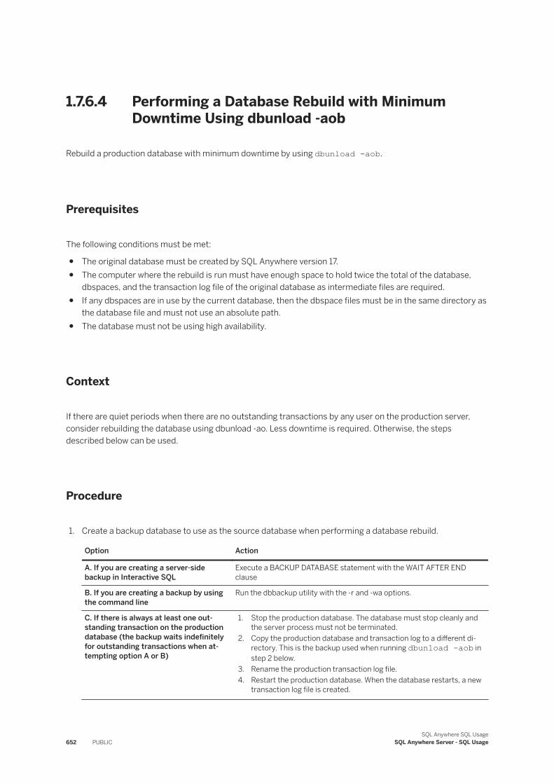
1.7.6.4 Performing a Database Rebuild with Minimum Downtime Using dbunload -aob
Rebuild a production database with minimum downtime by using dbunload -aob.
Prerequisites
The following conditions must be met:
● The original database must be created by SQL Anywhere version 17.● The computer where the rebuild is run must have enough space to hold twice the total of the database,
dbspaces, and the transaction log file of the original database as intermediate files are required.● If any dbspaces are in use by the current database, then the dbspace files must be in the same directory as
the database file and must not use an absolute path.● The database must not be using high availability.
Context
If there are quiet periods when there are no outstanding transactions by any user on the production server, consider rebuilding the database using dbunload -ao. Less downtime is required. Otherwise, the steps described below can be used.
Procedure
1. Create a backup database to use as the source database when performing a database rebuild.
Option Action
A. If you are creating a server-side backup in Interactive SQL
Execute a BACKUP DATABASE statement with the WAIT AFTER END clause
B. If you are creating a backup by using the command line
Run the dbbackup utility with the -r and -wa options.
C. If there is always at least one outstanding transaction on the production database (the backup waits indefinitely for outstanding transactions when attempting option A or B)
1. Stop the production database. The database must stop cleanly and the server process must not be terminated.
2. Copy the production database and transaction log to a different directory. This is the backup used when running dbunload -aob in step 2 below.
3. Rename the production transaction log file.4. Restart the production database. When the database restarts, a new
transaction log file is created.
652 PUBLICSQL Anywhere SQL Usage
SQL Anywhere Server - SQL Usage
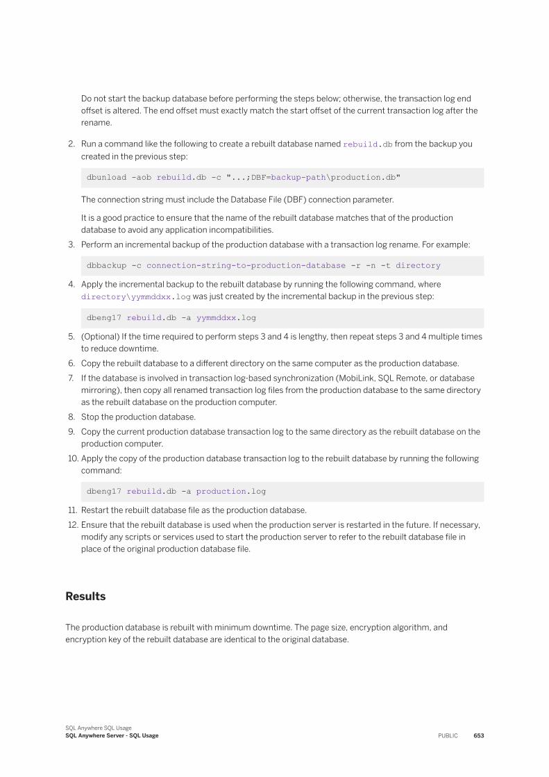
Do not start the backup database before performing the steps below; otherwise, the transaction log end offset is altered. The end offset must exactly match the start offset of the current transaction log after the rename.
2. Run a command like the following to create a rebuilt database named rebuild.db from the backup you created in the previous step:
dbunload -aob rebuild.db -c "...;DBF=backup-path\production.db"
The connection string must include the Database File (DBF) connection parameter.
It is a good practice to ensure that the name of the rebuilt database matches that of the production database to avoid any application incompatibilities.
3. Perform an incremental backup of the production database with a transaction log rename. For example:
dbbackup -c connection-string-to-production-database -r -n -t directory
4. Apply the incremental backup to the rebuilt database by running the following command, where directory\yymmddxx.log was just created by the incremental backup in the previous step:
dbeng17 rebuild.db -a yymmddxx.log
5. (Optional) If the time required to perform steps 3 and 4 is lengthy, then repeat steps 3 and 4 multiple times to reduce downtime.
6. Copy the rebuilt database to a different directory on the same computer as the production database.7. If the database is involved in transaction log-based synchronization (MobiLink, SQL Remote, or database
mirroring), then copy all renamed transaction log files from the production database to the same directory as the rebuilt database on the production computer.
8. Stop the production database.9. Copy the current production database transaction log to the same directory as the rebuilt database on the
production computer.10. Apply the copy of the production database transaction log to the rebuilt database by running the following
command:
dbeng17 rebuild.db -a production.log
11. Restart the rebuilt database file as the production database.12. Ensure that the rebuilt database is used when the production server is restarted in the future. If necessary,
modify any scripts or services used to start the production server to refer to the rebuilt database file in place of the original production database file.
Results
The production database is rebuilt with minimum downtime. The page size, encryption algorithm, and encryption key of the rebuilt database are identical to the original database.
SQL Anywhere SQL UsageSQL Anywhere Server - SQL Usage PUBLIC 653
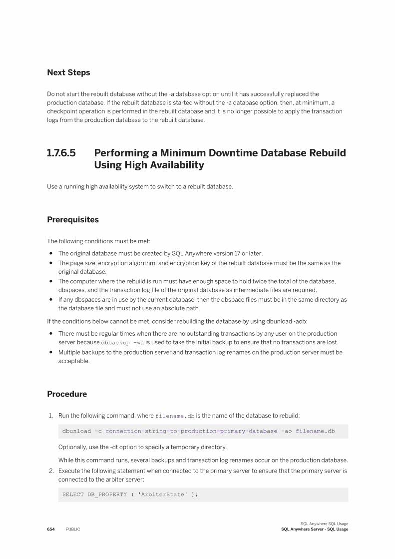
Next Steps
Do not start the rebuilt database without the -a database option until it has successfully replaced the production database. If the rebuilt database is started without the -a database option, then, at minimum, a checkpoint operation is performed in the rebuilt database and it is no longer possible to apply the transaction logs from the production database to the rebuilt database.
1.7.6.5 Performing a Minimum Downtime Database Rebuild Using High Availability
Use a running high availability system to switch to a rebuilt database.
Prerequisites
The following conditions must be met:
● The original database must be created by SQL Anywhere version 17 or later.● The page size, encryption algorithm, and encryption key of the rebuilt database must be the same as the
original database.● The computer where the rebuild is run must have enough space to hold twice the total of the database,
dbspaces, and the transaction log file of the original database as intermediate files are required.● If any dbspaces are in use by the current database, then the dbspace files must be in the same directory as
the database file and must not use an absolute path.
If the conditions below cannot be met, consider rebuilding the database by using dbunload -aob:
● There must be regular times when there are no outstanding transactions by any user on the production server because dbbackup -wa is used to take the initial backup to ensure that no transactions are lost.
● Multiple backups to the production server and transaction log renames on the production server must be acceptable.
Procedure
1. Run the following command, where filename.db is the name of the database to rebuild:
dbunload -c connection-string-to-production-primary-database -ao filename.db
Optionally, use the -dt option to specify a temporary directory.
While this command runs, several backups and transaction log renames occur on the production database.2. Execute the following statement when connected to the primary server to ensure that the primary server is
connected to the arbiter server:
SELECT DB_PROPERTY ( 'ArbiterState' );
654 PUBLICSQL Anywhere SQL Usage
SQL Anywhere Server - SQL Usage
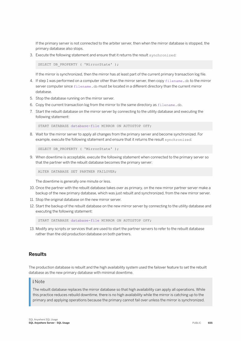
If the primary server is not connected to the arbiter server, then when the mirror database is stopped, the primary database also stops.
3. Execute the following statement and ensure that it returns the result synchronized:
SELECT DB_PROPERTY ( 'MirrorState' );
If the mirror is synchronized, then the mirror has at least part of the current primary transaction log file.4. If step 1 was performed on a computer other than the mirror server, then copy filename.db to the mirror
server computer since filename.db must be located in a different directory than the current mirror database.
5. Stop the database running on the mirror server.6. Copy the current transaction log from the mirror to the same directory as filename.db.
7. Start the rebuilt database on the mirror server by connecting to the utility database and executing the following statement:
START DATABASE database-file MIRROR ON AUTOSTOP OFF;
8. Wait for the mirror server to apply all changes from the primary server and become synchronized. For example, execute the following statement and ensure that it returns the result synchronized:
SELECT DB_PROPERTY ( 'MirrorState' );
9. When downtime is acceptable, execute the following statement when connected to the primary server so that the partner with the rebuilt database becomes the primary server:
ALTER DATABASE SET PARTNER FAILOVER;
The downtime is generally one minute or less.10. Once the partner with the rebuilt database takes over as primary, on the new mirror partner server make a
backup of the new primary database, which was just rebuilt and synchronized, from the new mirror server.11. Stop the original database on the new mirror server.12. Start the backup of the rebuilt database on the new mirror server by connecting to the utility database and
executing the following statement:
START DATABASE database-file MIRROR ON AUTOSTOP OFF;
13. Modify any scripts or services that are used to start the partner servers to refer to the rebuilt database rather than the old production database on both partners.
Results
The production database is rebuilt and the high availability system used the failover feature to set the rebuilt database as the new primary database with minimal downtime.
NoteThe rebuilt database replaces the mirror database so that high availability can apply all operations. While this practice reduces rebuild downtime, there is no high availability while the mirror is catching up to the primary and applying operations because the primary cannot fail over unless the mirror is synchronized.
SQL Anywhere SQL UsageSQL Anywhere Server - SQL Usage PUBLIC 655
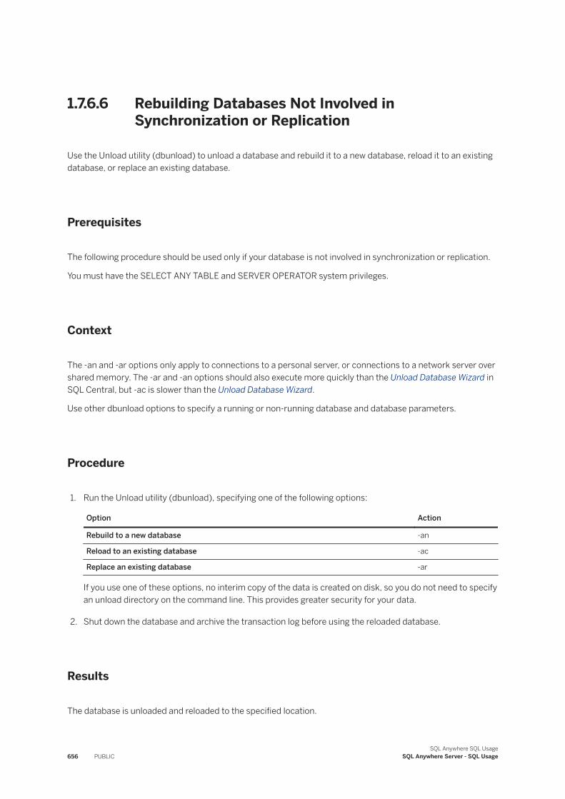
1.7.6.6 Rebuilding Databases Not Involved in Synchronization or Replication
Use the Unload utility (dbunload) to unload a database and rebuild it to a new database, reload it to an existing database, or replace an existing database.
Prerequisites
The following procedure should be used only if your database is not involved in synchronization or replication.
You must have the SELECT ANY TABLE and SERVER OPERATOR system privileges.
Context
The -an and -ar options only apply to connections to a personal server, or connections to a network server over shared memory. The -ar and -an options should also execute more quickly than the Unload Database Wizard in SQL Central, but -ac is slower than the Unload Database Wizard.
Use other dbunload options to specify a running or non-running database and database parameters.
Procedure
1. Run the Unload utility (dbunload), specifying one of the following options:
Option Action
Rebuild to a new database -an
Reload to an existing database -ac
Replace an existing database -ar
If you use one of these options, no interim copy of the data is created on disk, so you do not need to specify an unload directory on the command line. This provides greater security for your data.
2. Shut down the database and archive the transaction log before using the reloaded database.
Results
The database is unloaded and reloaded to the specified location.
656 PUBLICSQL Anywhere SQL Usage
SQL Anywhere Server - SQL Usage

1.7.6.7 Rebuilding Databases Involved in Synchronization or Replication (dbunload)
Rebuild a database involved in synchronization or replication using the dbunload -ar option, which unloads and reloads the database in a way that does not interfere with synchronization or replication.
Prerequisites
You must have the SELECT ANY TABLE and SERVER OPERATOR system privileges.
All subscriptions must be synchronized before rebuilding a database participating in MobiLink synchronization.
Context
This task applies to SQL Anywhere MobiLink clients (clients using dbmlsync) and SQL Remote.
Synchronization and replication are based on the offsets in the transaction log. When you rebuild a database, the offsets in the old transaction log are different than the offsets in the new log, making the old log unavailable. For this reason, good backup practices are especially important for databases participating in synchronization or replication.
NoteUse other dbunload options to specify a running or non-running database and database parameters.
Procedure
1. Shut down the database.2. Perform a full off-line backup by copying the database and transaction log files to a secure location.3. Run the following dbunload command to rebuild the database:
dbunload -c connection-string -ar directory
The connection-string is a connection with appropriate privileges, and directory is the directory used in your replication environment for old transaction logs. There can be no other connections to the database.
The -ar option only applies to connections to a personal server, or connections to a network server over shared memory.
4. Shut down the new database and then perform the validity checks that you would usually perform after restoring a database.
5. Start the database using any production options you need. You can now allow user access to the reloaded database.
SQL Anywhere SQL UsageSQL Anywhere Server - SQL Usage PUBLIC 657
Results
The database is reloaded and started.
1.7.6.8 Rebuilding Databases Involved in Synchronization or Replication (Manual)
Rebuild a database involved in synchronization or replication.
Prerequisites
You must have the SELECT ANY TABLE and SERVER OPERATOR system privileges to rebuild the database.
All subscriptions must be synchronized before rebuilding a database participating in MobiLink synchronization.
Context
This task applies to SQL Anywhere MobiLink clients (clients using dbmlsync) and SQL Remote.
Synchronization and replication are based on the offsets in the transaction log. When you rebuild a database, the offsets in the old transaction log are different than the offsets in the new log, making the old log unavailable. For this reason, good backup practices are especially important for databases participating in synchronization or replication.
Procedure
1. Shut down the database.2. Perform a full offline backup by copying the database and transaction log files to a secure location.3. Run the dbtran utility to display the starting offset, ending offset, and current timeline, of the database's
current transaction log file.
Note the ending offset and timeline for use in Step 8.4. Rename the current transaction log file so that it is not modified during the unload process, and place this
file in the dbremote offline logs directory.5. Rebuild the database.6. Shut down the new database.7. Erase the current transaction log file for the new database.
658 PUBLICSQL Anywhere SQL Usage
SQL Anywhere Server - SQL Usage
8. Use dblog on the new database with the ending offset and timeline noted in Step 3 as the -z option, and also set the relative offset to zero.
dblog -x 0 -z 0000698242 -ft timeline -ir -is database-name.db
9. When you run the Message Agent, provide it with the location of the original offline directory on its command line.
10. Start the database. You can now allow user access to the reloaded database.
Results
The database is reloaded and started.
1.7.6.9 Tips on Rebuilding Databases Using the UNLOAD TABLE Statement
The UNLOAD TABLE statement lets you export data efficiently in a specific character encoding.
Consider using the UNLOAD TABLE statement to rebuild databases when you want to export data in text format.
The UNLOAD TABLE statement places an exclusive lock on the entire table.
1.7.6.10 Exporting Table Data
Unload table data using the Unload utility (dbunload).
Prerequisites
You must be the owner of the table being queried, or have SELECT privilege on the table, or have the SELECT ANY TABLE system privilege.
Context
The statements required to recreate the schema and reload the specified tables are written to reload.sql in the current local directory.
Unload more than one table by separating the table names with a comma.
SQL Anywhere SQL UsageSQL Anywhere Server - SQL Usage PUBLIC 659
Procedure
Run the dbunload command, specifying connection parameters using the -c option, table(s) you want to export data for using the -t option, whether you want to suppress column statistics by specifying the -ss option, and whether you want to unload only data by specifying the -d option.
For example, to export the data from the Employees table, run the following command:
dbunload -c "DBN=demo;UID=DBA;PWD=sql" -ss -d -t Employees C:\ServerTemp\DataFiles
The reload.sql file is written to the client's current directory and will contain the LOAD TABLE statement required to reload the data for the Employees table. The data files are written to the server directory C:\ServerTemp\DataFiles.
Results
The table data is exported to the specified directory.
1.7.6.11 Exporting a Table Schema
Unload the table schema using the Unload utility (dbunload).
Prerequisites
You must be the owner of the table, have SELECT privilege on the table, or have the SELECT ANY TABLE system privilege.
Context
The statements required to recreate the schema and reload the specified tables are written to reload.sql in the client's current directory.
Unload more than one table by separating the table names with a comma delimiter.
660 PUBLICSQL Anywhere SQL Usage
SQL Anywhere Server - SQL Usage
Procedure
Run the dbunload command, specifying connection parameters using the -c option, the table(s) you want to export data for using the -t option, and whether you want to unload only the schema by specifying the -n option.
For example, to export only the schema for the Employees table, run the following command:
dbunload -c "DBN=demo;UID=DBA;PWD=sql" -n -t Employees
Results
The table schema is exported.
1.7.6.12 Reloading a Database
Reload databases from the command line.
Prerequisites
You must have an existing reload.sql file.
Context
Reloading involves creating an empty database file and using an existing reload.sql file to create the schema and insert all the data unloaded from another SQL Anywhere database into the newly created tables.
Procedure
1. Run the dbinit utility to create a new empty database file.2. Connect to the new database.3. Execute the reload.sql script.
SQL Anywhere SQL UsageSQL Anywhere Server - SQL Usage PUBLIC 661
Results
The database is reloaded.
Example
The following command creates a file named mynewdb.db.
dbinit -dba DBA,passwd mynewdb.db
The following command loads and runs the reload.sql script in the current directory.
dbisql -c "DBF=mynewdb;UID=DBA;PWD=passwd" reload.sql
1.7.6.13 Minimizing Downtime When Rebuilding a Database
Minimize downtime when rebuilding a database by using the Backup utility (dbbackup) and Log Translation utility (dbtran).
Prerequisites
Make backup copies of your database files before rebuilding a database.
Verify that no other scheduled backups can rename the transaction log. If the transaction log is renamed, then the transactions from the renamed transaction logs must be applied to the rebuilt database in the correct order.
You must have the BACKUP DATABASE system privilege.
Context
NoteIf your database was created with SQL Anywhere 17, use dbunload -ao or dbunload -aob rather than the steps below.
662 PUBLICSQL Anywhere SQL Usage
SQL Anywhere Server - SQL Usage
Procedure
1. Using dbbackup -r -wa, create a backup of the database and transaction log, and rename the transaction log once there are no active transactions. This backup does not complete until there are no outstanding transactions.
NoteUse the -wa parameter to avoid losing transactions that were active during the transaction log rename. For client-side backups, the connection string provided for dbbackup must be to a version 17 database server .
2. Rebuild the backed up database on another computer.3. Perform another dbbackup -r on the production server to rename the transaction log.4. Run the dbtran utility on the renamed transaction log and apply the transactions to the rebuilt database.5. Shut down the production server and copy the database and transaction log.6. Copy the rebuilt database onto the production server.7. Run dbtran on the transaction log from step 5.8. Start the rebuilt database on a personal server (dbeng17), to ensure that users cannot connect.9. Apply the transactions from step 7.10. Shut down the database server and start the database on a network server (dbsrv17), to allow users to
connect.
Results
Downtime is minimized during the rebuild of a database.
1.7.7 Database Extraction
Database extraction creates a remote SQL Anywhere database from a consolidated SQL Anywhere database.
Database extraction is used by SQL Remote.
You can use the SQL Central Extract Database Wizard or the Extraction utility to extract databases. The Extraction utility (dbxtract) is the recommended way of creating remote databases from a consolidated database for use in SQL Remote replication.
SQL Anywhere SQL UsageSQL Anywhere Server - SQL Usage PUBLIC 663
1.7.8 Database Migration to SQL Anywhere
You can use the sa_migrate system procedures or the Migrate Database Wizard, to import tables from several sources.
● SAP SQL Anywhere● SAP UltraLite● SAP Adaptive Server Enterprise● SAP IQ● SAP HANA● SAP Advantage Database Server● IBM DB2● Microsoft SQL Server● Microsoft Access● Oracle Database● Oracle MySQL● generic ODBC driver that connects to a remote server
Before you can migrate data using the Migrate Database Wizard, or the sa_migrate set of system procedures, you must first create a target database. The target database is the database into which data is migrated.
NoteWhen SAP HANA tables are migrated to SQL Anywhere, indexes are not migrated along with them and must be created manually after the migration.
In this section:
Using the Migrate Database Wizard [page 664]Use SQL Central to create a remote server to connect to the remote database, and an external login (if required) to connect the current user to the remote database using the Migrate Database Wizard.
The sa_migrate System Procedures [page 666]Use the sa_migrate system procedures to migrate remote data.
1.7.8.1 Using the Migrate Database Wizard
Use SQL Central to create a remote server to connect to the remote database, and an external login (if required) to connect the current user to the remote database using the Migrate Database Wizard.
Prerequisites
You must already have a remote server created. You must already have a user to own the tables in the target database.
664 PUBLICSQL Anywhere SQL Usage
SQL Anywhere Server - SQL Usage
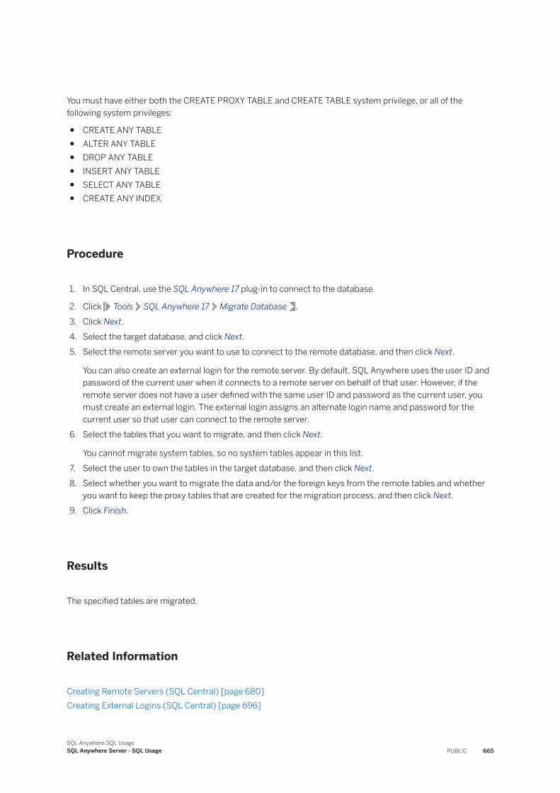
You must have either both the CREATE PROXY TABLE and CREATE TABLE system privilege, or all of the following system privileges:
● CREATE ANY TABLE● ALTER ANY TABLE● DROP ANY TABLE● INSERT ANY TABLE● SELECT ANY TABLE● CREATE ANY INDEX
Procedure
1. In SQL Central, use the SQL Anywhere 17 plug-in to connect to the database.
2. Click Tools SQL Anywhere 17 Migrate Database .3. Click Next.4. Select the target database, and click Next.5. Select the remote server you want to use to connect to the remote database, and then click Next.
You can also create an external login for the remote server. By default, SQL Anywhere uses the user ID and password of the current user when it connects to a remote server on behalf of that user. However, if the remote server does not have a user defined with the same user ID and password as the current user, you must create an external login. The external login assigns an alternate login name and password for the current user so that user can connect to the remote server.
6. Select the tables that you want to migrate, and then click Next.
You cannot migrate system tables, so no system tables appear in this list.7. Select the user to own the tables in the target database, and then click Next.8. Select whether you want to migrate the data and/or the foreign keys from the remote tables and whether
you want to keep the proxy tables that are created for the migration process, and then click Next.9. Click Finish.
Results
The specified tables are migrated.
Related Information
Creating Remote Servers (SQL Central) [page 680]Creating External Logins (SQL Central) [page 696]
SQL Anywhere SQL UsageSQL Anywhere Server - SQL Usage PUBLIC 665
1.7.8.2 The sa_migrate System Procedures
Use the sa_migrate system procedures to migrate remote data.
Use the extended method to remove tables or foreign key mappings.
In this section:
Migrating All Tables Using the sa_migrate System Procedure [page 666]Migrate all tables using the sa_migrate system procedure.
Migrating Individual Tables Using the Database Migration System Procedures [page 667]Migrate an individual table using the database migration system procedures.
1.7.8.2.1 Migrating All Tables Using the sa_migrate System Procedure
Migrate all tables using the sa_migrate system procedure.
Prerequisites
You must have the following system privileges:
● CREATE TABLE or CREATE ANY TABLE (if you are not the base table owner)● SELECT ANY TABLE (if you are not the base table owner)● INSERT ANY TABLE (if you are not the base table owner)● ALTER ANY TABLE (if you are not the base table owner)● CREATE ANY INDEX (if you are not the base table owner)● DROP ANY TABLE (if you are not the base table owner)
You must already have a user to own the migrated tables in the target database.
To create an external login, you must have the MANAGE ANY USER system privilege.
Context
Tables that have the same name, but different owners, in the remote database all belong to one owner in the target database. For these reasons, migrate tables associated with one owner at a time.
If you do not want all the migrated tables to be owned by the same user on the target database, you must run the sa_migrate procedure for each owner on the target database, specifying the local-table-owner and owner-name arguments.
666 PUBLICSQL Anywhere SQL Usage
SQL Anywhere Server - SQL Usage
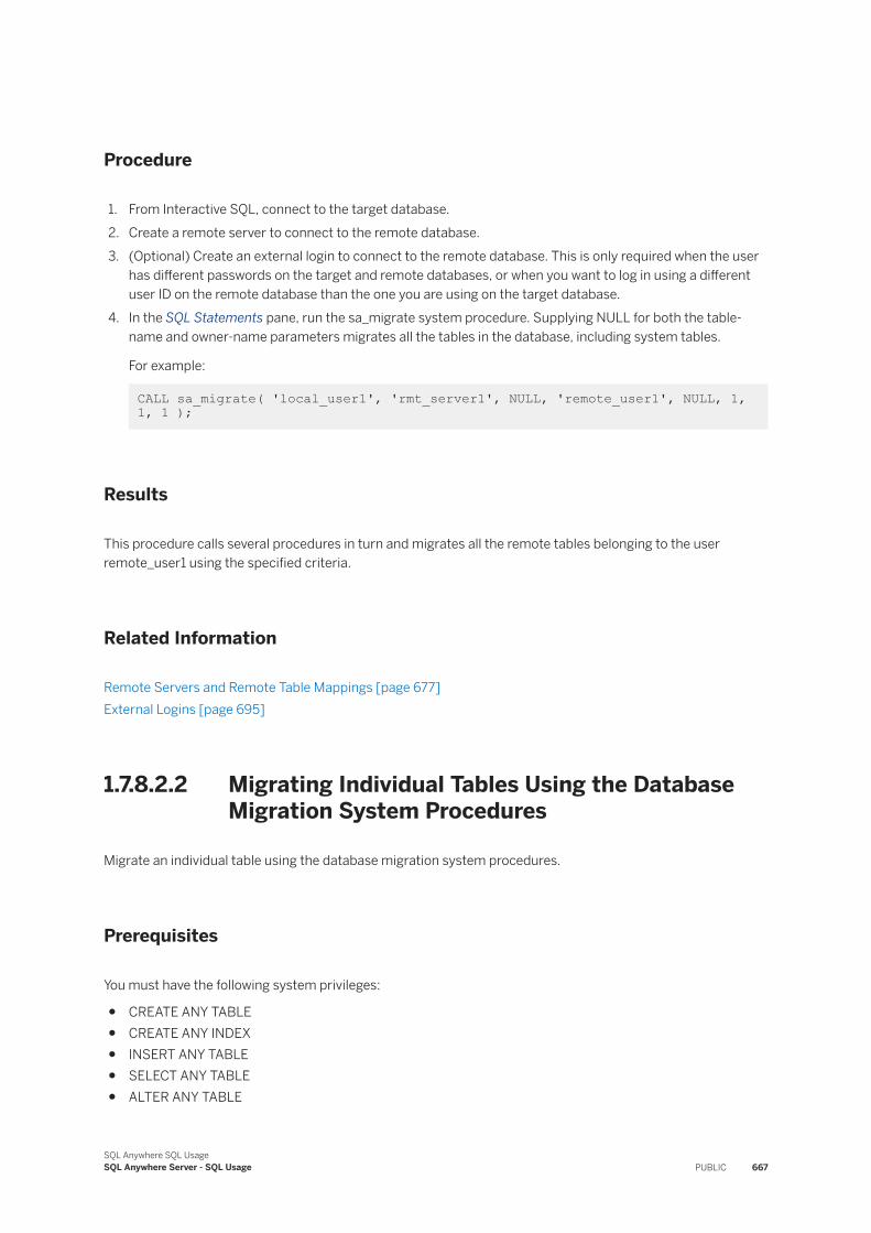
Procedure
1. From Interactive SQL, connect to the target database.2. Create a remote server to connect to the remote database.3. (Optional) Create an external login to connect to the remote database. This is only required when the user
has different passwords on the target and remote databases, or when you want to log in using a different user ID on the remote database than the one you are using on the target database.
4. In the SQL Statements pane, run the sa_migrate system procedure. Supplying NULL for both the table-name and owner-name parameters migrates all the tables in the database, including system tables.
For example:
CALL sa_migrate( 'local_user1', 'rmt_server1', NULL, 'remote_user1', NULL, 1, 1, 1 );
Results
This procedure calls several procedures in turn and migrates all the remote tables belonging to the user remote_user1 using the specified criteria.
Related Information
Remote Servers and Remote Table Mappings [page 677]External Logins [page 695]
1.7.8.2.2 Migrating Individual Tables Using the Database Migration System Procedures
Migrate an individual table using the database migration system procedures.
Prerequisites
You must have the following system privileges:
● CREATE ANY TABLE● CREATE ANY INDEX● INSERT ANY TABLE● SELECT ANY TABLE● ALTER ANY TABLE
SQL Anywhere SQL UsageSQL Anywhere Server - SQL Usage PUBLIC 667
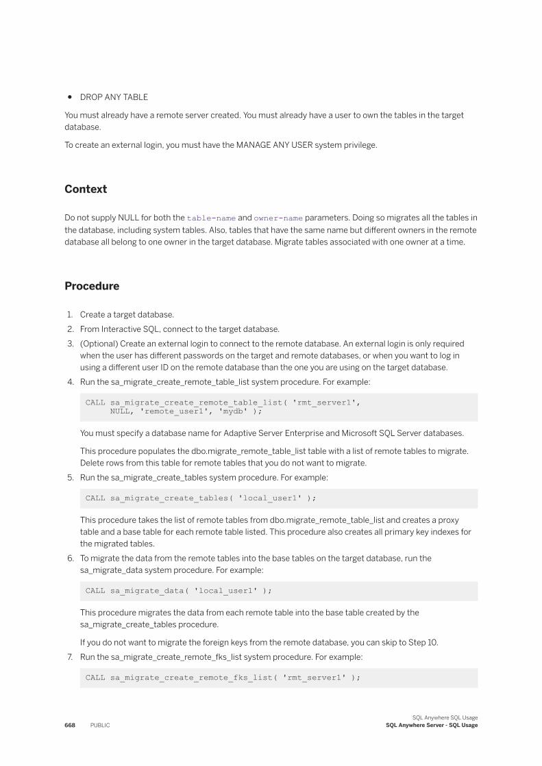
● DROP ANY TABLE
You must already have a remote server created. You must already have a user to own the tables in the target database.
To create an external login, you must have the MANAGE ANY USER system privilege.
Context
Do not supply NULL for both the table-name and owner-name parameters. Doing so migrates all the tables in the database, including system tables. Also, tables that have the same name but different owners in the remote database all belong to one owner in the target database. Migrate tables associated with one owner at a time.
Procedure
1. Create a target database.2. From Interactive SQL, connect to the target database.3. (Optional) Create an external login to connect to the remote database. An external login is only required
when the user has different passwords on the target and remote databases, or when you want to log in using a different user ID on the remote database than the one you are using on the target database.
4. Run the sa_migrate_create_remote_table_list system procedure. For example:
CALL sa_migrate_create_remote_table_list( 'rmt_server1', NULL, 'remote_user1', 'mydb' );
You must specify a database name for Adaptive Server Enterprise and Microsoft SQL Server databases.
This procedure populates the dbo.migrate_remote_table_list table with a list of remote tables to migrate. Delete rows from this table for remote tables that you do not want to migrate.
5. Run the sa_migrate_create_tables system procedure. For example:
CALL sa_migrate_create_tables( 'local_user1' );
This procedure takes the list of remote tables from dbo.migrate_remote_table_list and creates a proxy table and a base table for each remote table listed. This procedure also creates all primary key indexes for the migrated tables.
6. To migrate the data from the remote tables into the base tables on the target database, run the sa_migrate_data system procedure. For example:
CALL sa_migrate_data( 'local_user1' );
This procedure migrates the data from each remote table into the base table created by the sa_migrate_create_tables procedure.
If you do not want to migrate the foreign keys from the remote database, you can skip to Step 10.7. Run the sa_migrate_create_remote_fks_list system procedure. For example:
CALL sa_migrate_create_remote_fks_list( 'rmt_server1' );
668 PUBLICSQL Anywhere SQL Usage
SQL Anywhere Server - SQL Usage
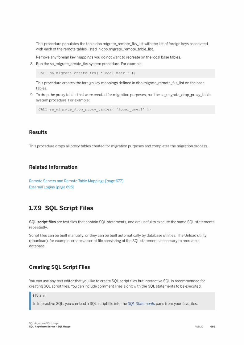
This procedure populates the table dbo.migrate_remote_fks_list with the list of foreign keys associated with each of the remote tables listed in dbo.migrate_remote_table_list.
Remove any foreign key mappings you do not want to recreate on the local base tables.8. Run the sa_migrate_create_fks system procedure. For example:
CALL sa_migrate_create_fks( 'local_user1' );
This procedure creates the foreign key mappings defined in dbo.migrate_remote_fks_list on the base tables.
9. To drop the proxy tables that were created for migration purposes, run the sa_migrate_drop_proxy_tables system procedure. For example:
CALL sa_migrate_drop_proxy_tables( 'local_user1' );
Results
This procedure drops all proxy tables created for migration purposes and completes the migration process.
Related Information
Remote Servers and Remote Table Mappings [page 677]External Logins [page 695]
1.7.9 SQL Script Files
SQL script files are text files that contain SQL statements, and are useful to execute the same SQL statements repeatedly.
Script files can be built manually, or they can be built automatically by database utilities. The Unload utility (dbunload), for example, creates a script file consisting of the SQL statements necessary to recreate a database.
Creating SQL Script Files
You can use any text editor that you like to create SQL script files but Interactive SQL is recommended for creating SQL script files. You can include comment lines along with the SQL statements to be executed.
NoteIn Interactive SQL, you can load a SQL script file into the SQL Statements pane from your favorites.
SQL Anywhere SQL UsageSQL Anywhere Server - SQL Usage PUBLIC 669
In this section:
Running a SQL Script File Without Loading [page 670]Use Interactive SQL to run a SQL script file without loading it into the SQL Statements pane.
Running a SQL Script File Using the Interactive SQL READ Statement [page 671]Run a SQL script file without loading it into the SQL Statements pane with the Interactive SQL READ statement.
Running a SQL Script File in Batch Mode (Command Line) [page 672]Supply a SQL script file as a command line argument for Interactive SQL.
Loading a SQL Script from a File into the SQL Statements Pane [page 672]Use Interactive SQL to load a SQL script file into the SQL Statements pane and execute it directly from there.
Writing Database Output to a File [page 673]Save the output of a SQL statement to file.
1.7.9.1 Running a SQL Script File Without Loading
Use Interactive SQL to run a SQL script file without loading it into the SQL Statements pane.
Prerequisites
Ensure that Interactive SQL is set up as the default editor for .sql files.
In Interactive SQL, click Tools Options General and then click Make Interactive SQL the default editor for .SQL files and plan files.
The privileges required depend on the statements being executed.
Context
The Run Script menu item is the equivalent of a READ statement.
Procedure
1. In Interactive SQL, click File Run Script .2. Locate the file, and click Open.
670 PUBLICSQL Anywhere SQL Usage
SQL Anywhere Server - SQL Usage
Results
The contents of the specified file are run immediately. A Status window appears to show the execution progress.
1.7.9.2 Running a SQL Script File Using the Interactive SQL READ Statement
Run a SQL script file without loading it into the SQL Statements pane with the Interactive SQL READ statement.
Prerequisites
The privileges required depend on the statements being executed.
Procedure
In the SQL Statements pane, execute a statement like the following example:
READ 'C:\\LocalTemp\\filename.sql';
In this statement, C:\LocalTemp\filename.sql is the path, name, and extension of the file. Single quotation marks (as shown) are required only if the path contains spaces. If you use single quotation marks then the backslash characters are escaped by doubling them to prevent translation of escape sequences such as '\n' or '\x'.
Results
The SQL script file is run.
SQL Anywhere SQL UsageSQL Anywhere Server - SQL Usage PUBLIC 671
1.7.9.3 Running a SQL Script File in Batch Mode (Command Line)
Supply a SQL script file as a command line argument for Interactive SQL.
Prerequisites
The privileges required depend on the statements being executed.
Procedure
Run the dbisql utility and supply a SQL script file as a command line argument.
Results
The SQL script file is run.
Example
The following command runs the SQL script file myscript.sql against the SQL Anywhere sample database.
dbisql -c "DSN=SQL Anywhere 17 Demo;PWD=sql" myscript.sql
1.7.9.4 Loading a SQL Script from a File into the SQL Statements Pane
Use Interactive SQL to load a SQL script file into the SQL Statements pane and execute it directly from there.
Prerequisites
Interactive SQL is set up as the default editor for .sql files.
In Interactive SQL, click Tools Options General and then click Make Interactive SQL the default editor for .SQL files and plan files.
672 PUBLICSQL Anywhere SQL Usage
SQL Anywhere Server - SQL Usage
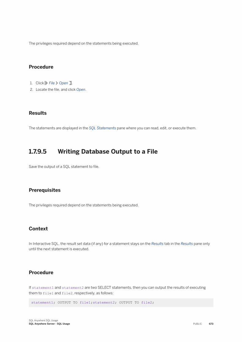
The privileges required depend on the statements being executed.
Procedure
1. Click File Open .2. Locate the file, and click Open.
Results
The statements are displayed in the SQL Statements pane where you can read, edit, or execute them.
1.7.9.5 Writing Database Output to a File
Save the output of a SQL statement to file.
Prerequisites
The privileges required depend on the statements being executed.
Context
In Interactive SQL, the result set data (if any) for a statement stays on the Results tab in the Results pane only until the next statement is executed.
Procedure
If statement1 and statement2 are two SELECT statements, then you can output the results of executing them to file1 and file2, respectively, as follows:
statement1; OUTPUT TO file1;statement2; OUTPUT TO file2;
SQL Anywhere SQL UsageSQL Anywhere Server - SQL Usage PUBLIC 673
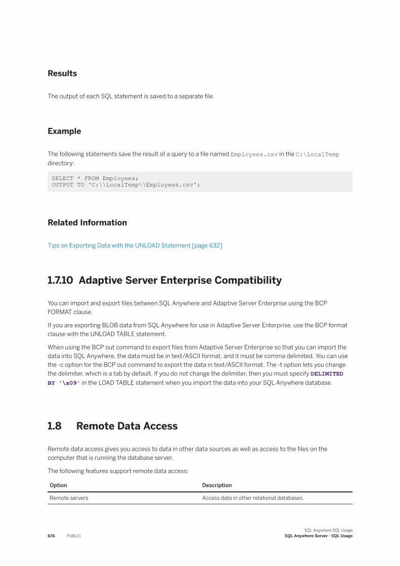
Results
The output of each SQL statement is saved to a separate file.
Example
The following statements save the result of a query to a file named Employees.csv in the C:\LocalTemp directory:
SELECT * FROM Employees; OUTPUT TO 'C:\\LocalTemp\\Employees.csv';
Related Information
Tips on Exporting Data with the UNLOAD Statement [page 632]
1.7.10 Adaptive Server Enterprise Compatibility
You can import and export files between SQL Anywhere and Adaptive Server Enterprise using the BCP FORMAT clause.
If you are exporting BLOB data from SQL Anywhere for use in Adaptive Server Enterprise, use the BCP format clause with the UNLOAD TABLE statement.
When using the BCP out command to export files from Adaptive Server Enterprise so that you can import the data into SQL Anywhere, the data must be in text/ASCII format, and it must be comma delimited. You can use the -c option for the BCP out command to export the data in text/ASCII format. The -t option lets you change the delimiter, which is a tab by default. If you do not change the delimiter, then you must specify DELIMITED BY '\x09' in the LOAD TABLE statement when you import the data into your SQL Anywhere database.
1.8 Remote Data Access
Remote data access gives you access to data in other data sources as well as access to the files on the computer that is running the database server.
The following features support remote data access:
Option Description
Remote servers Access data in other relational databases.
674 PUBLICSQL Anywhere SQL Usage
SQL Anywhere Server - SQL Usage
Option Description
Directory access servers Access the local file structure on the computer running a database server.
Directory and file system procedures Access the local file structure of the computer running a database server by using file and directory system procedures, such as the sp_create_directory system procedure.
With remote data access you can do the following:
● Use SQL Anywhere to move data from one location to another using INSERT and SELECT statements.● Access data in relational databases such as, SAP Adaptive Server Enterprise, SAP HANA, Oracle Database,
and IBM DB2.● Access data in Microsoft Excel spreadsheets, Microsoft Access databases, Microsoft Visual FoxPro, and
text files.● Access any data source that supports an ODBC interface.● Perform joins between local and remote data, although performance is much slower than if all the data is in
a single SQL Anywhere database.● Perform joins between tables in separate SQL Anywhere databases. Performance limitations here are the
same as with other remote data sources.● Use SQL Anywhere features on data sources that would normally not have that ability. For instance, you
could use a Java function against data stored in an Oracle database, or perform a subquery on spreadsheets. SQL Anywhere compensates for features not supported by a remote data source by operating on the data after it is retrieved.
● Access remote servers directly using the FORWARD TO statement.● Execute remote procedure calls to other servers.
You can also have access to the following external data sources:
● SQL Anywhere ● SAP Adaptive Server Enterprise● SAP HANA● SAP IQ● SAP UltraLite● SAP Advantage Database Server● IBM DB2● Microsoft Access● Microsoft SQL Server● Oracle MySQL● Oracle Database● Other ODBC data sources
In this section:
Remote Servers and Remote Table Mappings [page 677]SQL Anywhere presents tables to a client application as if all the data in the tables were stored in the database to which the application is connected. Before you can map remote objects to a local proxy table, you must define the remote server where the remote object is located.
Stored Procedures as an Alternative to Directory Access Servers [page 686]
SQL Anywhere SQL UsageSQL Anywhere Server - SQL Usage PUBLIC 675
This full set of stored procedures, combined with the xp_read_file system procedure and xp_write_file system procedure, provides the same functionality as directory access servers without you creating remote servers with external logins.
Directory Access Servers [page 686]A directory access server is a remote server that gives you access to the local file structure of the computer running the database server.
External Logins [page 695]External logins are used to communicate with a remote server or to permit access to a directory access server.
Proxy Tables [page 698]Use a proxy table to access any object (including tables, views, and materialized views) that the remote database exports as a candidate for a proxy table.
Native Statements and Remote Servers [page 706]Use the FORWARD TO statement to send one or more statements to the remote server in its native syntax.
Remote Procedure Calls (RPCs) [page 707]You can issue procedure calls to remote servers that support user-defined functions and procedures.
Transaction Management and Remote Data [page 711]Transactions provide a way to group SQL statements so that they are treated as a unit (either all work performed by the statements is committed to the database, or none of it is).
Internal Operations Performed on Queries [page 712]The are several steps that are performed on all queries, both local and remote.
Other Internal Operations [page 713]In addition to internal operations performed on queries, the several internal operations performed by the database server.
Troubleshooting: Features Not Supported for Remote Data [page 716]Several features are not supported for remote data.
Troubleshooting: Case Sensitivity and Remote Data Access [page 716]The case sensitivity setting of your SQL Anywhere database should match the settings used by any remote servers accessed.
Troubleshooting: Connectivity Tests for Remote Data Access [page 716]There are a few steps you can take to ensure that you can connect to a remote server.
Troubleshooting: Queries Blocked on Themselves [page 717]You must have enough threads available to support the individual tasks that are being run by a query.
Troubleshooting: Remote Data Access Connections via ODBC [page 717]If you access remote databases via ODBC, the connection to the remote server is given a name.
Server Classes for Remote Data Access [page 717]The server class you specify in the CREATE SERVER statement determines the behavior of a remote connection.
676 PUBLICSQL Anywhere SQL Usage
SQL Anywhere Server - SQL Usage
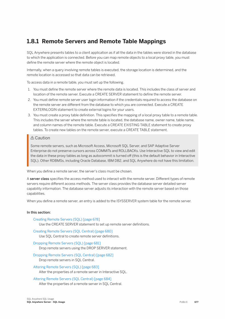
1.8.1 Remote Servers and Remote Table MappingsSQL Anywhere presents tables to a client application as if all the data in the tables were stored in the database to which the application is connected. Before you can map remote objects to a local proxy table, you must define the remote server where the remote object is located.
Internally, when a query involving remote tables is executed, the storage location is determined, and the remote location is accessed so that data can be retrieved.
To access data in a remote table, you must set up the following.
1. You must define the remote server where the remote data is located. This includes the class of server and location of the remote server. Execute a CREATE SERVER statement to define the remote server.
2. You must define remote server user login information if the credentials required to access the database on the remote server are different from the database to which you are connected. Execute a CREATE EXTERNLOGIN statement to create external logins for your users.
3. You must create a proxy table definition. This specifies the mapping of a local proxy table to a remote table. This includes the server where the remote table is located, the database name, owner name, table name, and column names of the remote table. Execute a CREATE EXISTING TABLE statement to create proxy tables. To create new tables on the remote server, execute a CREATE TABLE statement.
CautionSome remote servers, such as Microsoft Access, Microsoft SQL Server, and SAP Adaptive Server Enterprise do not preserve cursors across COMMITs and ROLLBACKs. Use Interactive SQL to view and edit the data in these proxy tables as long as autocommit is turned off (this is the default behavior in Interactive SQL). Other RDBMSs, including Oracle Database, IBM DB2, and SQL Anywhere do not have this limitation.
When you define a remote server, the server's class must be chosen.
A server class specifies the access method used to interact with the remote server. Different types of remote servers require different access methods. The server class provides the database server detailed server capability information. The database server adjusts its interaction with the remote server based on those capabilities.
When you define a remote server, an entry is added to the ISYSSERVER system table for the remote server.
In this section:
Creating Remote Servers (SQL) [page 678]Use the CREATE SERVER statement to set up remote server definitions.
Creating Remote Servers (SQL Central) [page 680]Use SQL Central to create remote server definitions.
Dropping Remote Servers (SQL) [page 681]Drop remote servers using the DROP SERVER statement.
Dropping Remote Servers (SQL Central) [page 682]Drop remote servers in SQL Central.
Altering Remote Servers (SQL) [page 683]Alter the properties of a remote server in Interactive SQL.
Altering Remote Servers (SQL Central) [page 684]Alter the properties of a remote server in SQL Central.
SQL Anywhere SQL UsageSQL Anywhere Server - SQL Usage PUBLIC 677
Listing the Tables on a Remote Server (SQL) [page 685]View a limited or comprehensive list of all the tables on a remote server using a system procedure.
Remote Server Capabilities [page 685]The database server uses remote server capability information to determine how much of a SQL statement can be passed to a remote server.
Related Information
Server Classes for Remote Data Access [page 717]
1.8.1.1 Creating Remote Servers (SQL)
Use the CREATE SERVER statement to set up remote server definitions.
Prerequisites
You must have the SERVER OPERATOR system privilege.
Context
Each remote server is accessed using an ODBC driver. A remote server definition is required for each database.
A connection string is used to identify a data source. On UNIX and Linux platforms, the ODBC driver must be referenced in the connection string as well.
Procedure
Use the CREATE SERVER statement to define a remote data access server that links to a remote server.
For example, the following statement defines the remote server RemoteASE. The SQL Anywhere database server connects to an Adaptive Server Enterprise 16 database server using the ODBC connection string specified in the USING clause.
CREATE SERVER RemoteASE CLASS 'ASEODBC' USING 'DRIVER=SAP ASE ODBC Driver;Server=TestASE;Port=5000;Database=testdb;UID=username;PWD=password';
The following is an analysis of the components of the CREATE SERVER statement.
678 PUBLICSQL Anywhere SQL Usage
SQL Anywhere Server - SQL Usage
SERVER
This clause is used to name the remote server. In the example, RemoteASE is the remote server name.CLASS
This clause is used to indicate how the SQL Anywhere database server should communicate with the remote server. In the example, ASEODBC indicates that the remote server is Adaptive Server Enterprise (ASE) and that the connection is made using the ASE ODBC driver.USING
This clause specifies the ODBC connection string for the remote server. In the example, the Adaptive Server Enterprise 16 ODBC driver name is specified.
Results
The CREATE SERVER statement creates an entry in the ISYSSERVER system table.
Example
The following statement defines the remote server RemoteSA. The SQL Anywhere database server connects to a SQL Anywhere database server using the ODBC Data Source Name (DSN) specified in the USING clause.
CREATE SERVER RemoteSA CLASS 'SAODBC' USING 'SQL Anywhere 17 CustDB';
Next Steps
Create external login information if required.
Related Information
Creating External Logins (SQL Central) [page 696]Creating Proxy Tables (SQL) [page 701]
SQL Anywhere SQL UsageSQL Anywhere Server - SQL Usage PUBLIC 679
1.8.1.2 Creating Remote Servers (SQL Central)
Use SQL Central to create remote server definitions.
Prerequisites
You must have the MANAGE ANY USER and SERVER OPERATOR system privileges.
Procedure
1. Use the SQL Anywhere 17 plug-in to connect to the host database.2. In the left pane, double-click Remote Servers.
3. Click File New Remote Server .4. In the What Do You Want To Name The New Remote Server field, type a name for the remote server, and
then click Next.5. Select a remote server type, and then click Next.6. Select a connection type, and in the What Is The Connection Information field type the connection
information:○ For an ODBC-based connection, supply a data source name or specify the ODBC Driver parameter and
other connection parameters.○ For a JDBC-based connection, supply a URL in the form computer-name:port-number.
The data access method (JDBC or ODBC) is the method used by the database server to access the remote database. This is not related to the method used by SQL Central to connect to your database.
JDBC-based remote server access is not supported in the current release.7. Click Next.8. Specify whether you want the remote server to be read-only and then click Next.9. Click Create An External Login For The Current User and complete the required fields.
By default, the database server uses the user ID and password of the current user when it connects to a remote server on behalf of that user. However, if the remote server does not have a user defined with the same user ID and password as the current user, you must create an external login. The external login assigns an alternate login name and password for the current user so that user can connect to the remote server.
10. Click Test Connection to test the remote server connection.11. Click Finish.
Results
A remote server is created with the specified definitions.
680 PUBLICSQL Anywhere SQL Usage
SQL Anywhere Server - SQL Usage
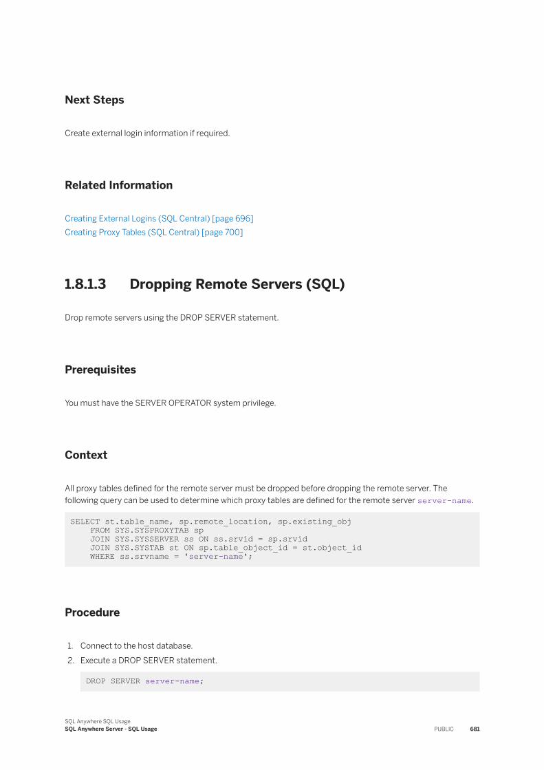
Next Steps
Create external login information if required.
Related Information
Creating External Logins (SQL Central) [page 696]Creating Proxy Tables (SQL Central) [page 700]
1.8.1.3 Dropping Remote Servers (SQL)
Drop remote servers using the DROP SERVER statement.
Prerequisites
You must have the SERVER OPERATOR system privilege.
Context
All proxy tables defined for the remote server must be dropped before dropping the remote server. The following query can be used to determine which proxy tables are defined for the remote server server-name.
SELECT st.table_name, sp.remote_location, sp.existing_obj FROM SYS.SYSPROXYTAB sp JOIN SYS.SYSSERVER ss ON ss.srvid = sp.srvid JOIN SYS.SYSTAB st ON sp.table_object_id = st.object_id WHERE ss.srvname = 'server-name';
Procedure
1. Connect to the host database.2. Execute a DROP SERVER statement.
DROP SERVER server-name;
SQL Anywhere SQL UsageSQL Anywhere Server - SQL Usage PUBLIC 681
Results
The remote server is dropped.
Example
The following statement drops the remote server named RemoteASE.
DROP SERVER RemoteASE;
Related Information
Dropping Remote Servers (SQL Central) [page 682]
1.8.1.4 Dropping Remote Servers (SQL Central)
Drop remote servers in SQL Central.
Prerequisites
You must have the SERVER OPERATOR system privilege.
Context
All proxy tables defined for the remote server must be dropped before dropping the remote server. SQL Central automatically determines which proxy tables are defined for a remote server and drops them first.
Procedure
1. Use the SQL Anywhere 17 plug-in to connect to the host database.2. In the left pane, double-click Remote Servers.
3. Select the remote server, and then click Edit Delete .
682 PUBLICSQL Anywhere SQL Usage
SQL Anywhere Server - SQL Usage
Results
The remote server is dropped.
Related Information
Dropping Remote Servers (SQL) [page 681]
1.8.1.5 Altering Remote Servers (SQL)
Alter the properties of a remote server in Interactive SQL.
Prerequisites
You must have the SERVER OPERATOR system privilege.
Context
The ALTER SERVER statement can also be used to enable or disable a server's known capabilities.
Procedure
1. Connect to the host database.2. Execute an ALTER SERVER statement.
Results
The remote server properties are altered.
However, changes to the remote server do not take effect until the next connection to the remote server.
SQL Anywhere SQL UsageSQL Anywhere Server - SQL Usage PUBLIC 683
Example
The following statement changes the server class of the server named RemoteASE to ASEODBC.
ALTER SERVER RemoteASE CLASS 'ASEODBC';
1.8.1.6 Altering Remote Servers (SQL Central)
Alter the properties of a remote server in SQL Central.
Prerequisites
You must have the SERVER OPERATOR system privilege.
Context
Changes to the remote server do not take effect until the next connection to the remote server.
Procedure
1. Use the SQL Anywhere 17 plug-in to connect to the host database.2. In the left pane, double-click Remote Servers.
3. Select the remote server, and then click File Properties .4. Alter the remote server settings, and then click OK.
Results
The remote server properties are altered.
684 PUBLICSQL Anywhere SQL Usage
SQL Anywhere Server - SQL Usage
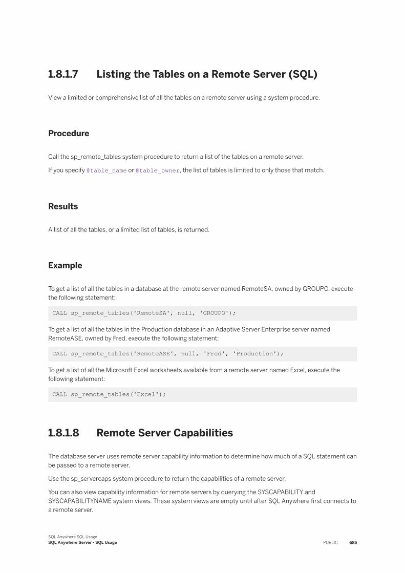
1.8.1.7 Listing the Tables on a Remote Server (SQL)
View a limited or comprehensive list of all the tables on a remote server using a system procedure.
Procedure
Call the sp_remote_tables system procedure to return a list of the tables on a remote server.
If you specify @table_name or @table_owner, the list of tables is limited to only those that match.
Results
A list of all the tables, or a limited list of tables, is returned.
Example
To get a list of all the tables in a database at the remote server named RemoteSA, owned by GROUPO, execute the following statement:
CALL sp_remote_tables('RemoteSA', null, 'GROUPO');
To get a list of all the tables in the Production database in an Adaptive Server Enterprise server named RemoteASE, owned by Fred, execute the following statement:
CALL sp_remote_tables('RemoteASE', null, 'Fred', 'Production');
To get a list of all the Microsoft Excel worksheets available from a remote server named Excel, execute the following statement:
CALL sp_remote_tables('Excel');
1.8.1.8 Remote Server Capabilities
The database server uses remote server capability information to determine how much of a SQL statement can be passed to a remote server.
Use the sp_servercaps system procedure to return the capabilities of a remote server.
You can also view capability information for remote servers by querying the SYSCAPABILITY and SYSCAPABILITYNAME system views. These system views are empty until after SQL Anywhere first connects to a remote server.
SQL Anywhere SQL UsageSQL Anywhere Server - SQL Usage PUBLIC 685
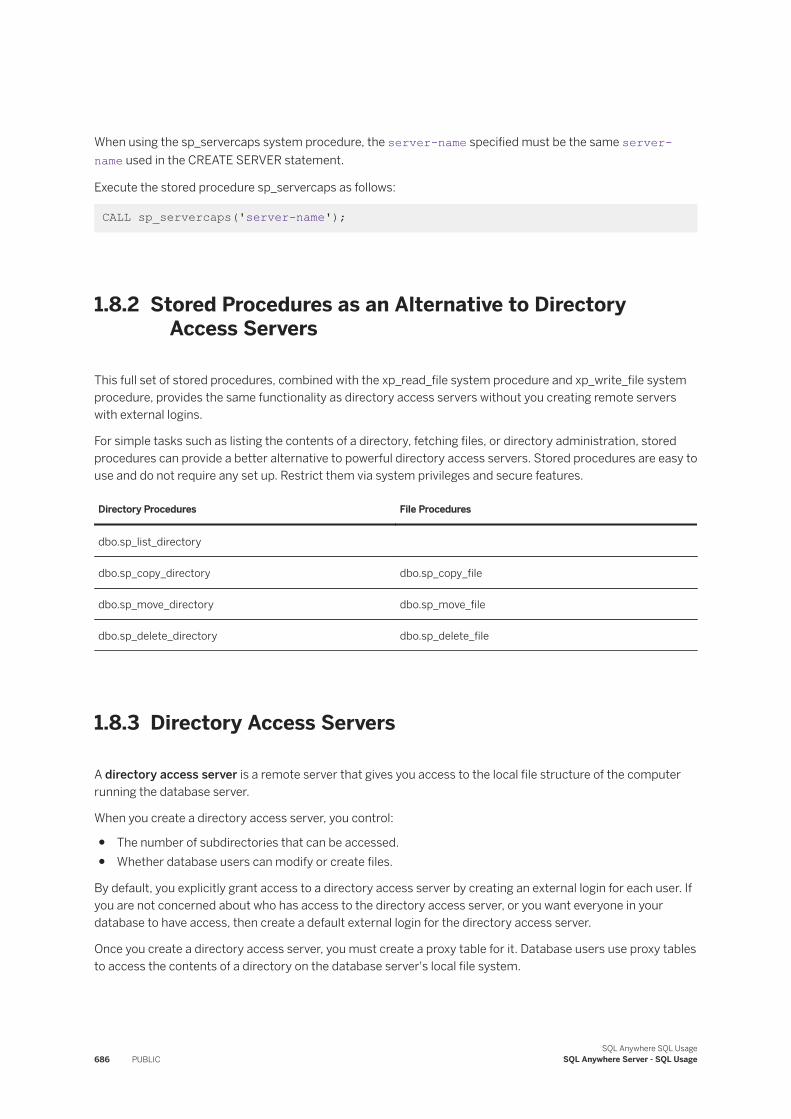
When using the sp_servercaps system procedure, the server-name specified must be the same server-name used in the CREATE SERVER statement.
Execute the stored procedure sp_servercaps as follows:
CALL sp_servercaps('server-name');
1.8.2 Stored Procedures as an Alternative to Directory Access Servers
This full set of stored procedures, combined with the xp_read_file system procedure and xp_write_file system procedure, provides the same functionality as directory access servers without you creating remote servers with external logins.
For simple tasks such as listing the contents of a directory, fetching files, or directory administration, stored procedures can provide a better alternative to powerful directory access servers. Stored procedures are easy to use and do not require any set up. Restrict them via system privileges and secure features.
Directory Procedures File Procedures
dbo.sp_list_directory
dbo.sp_copy_directory dbo.sp_copy_file
dbo.sp_move_directory dbo.sp_move_file
dbo.sp_delete_directory dbo.sp_delete_file
1.8.3 Directory Access Servers
A directory access server is a remote server that gives you access to the local file structure of the computer running the database server.
When you create a directory access server, you control:
● The number of subdirectories that can be accessed.● Whether database users can modify or create files.
By default, you explicitly grant access to a directory access server by creating an external login for each user. If you are not concerned about who has access to the directory access server, or you want everyone in your database to have access, then create a default external login for the directory access server.
Once you create a directory access server, you must create a proxy table for it. Database users use proxy tables to access the contents of a directory on the database server's local file system.
686 PUBLICSQL Anywhere SQL Usage
SQL Anywhere Server - SQL Usage
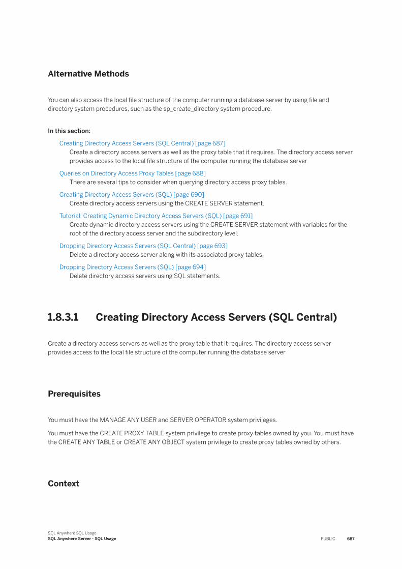
Alternative Methods
You can also access the local file structure of the computer running a database server by using file and directory system procedures, such as the sp_create_directory system procedure.
In this section:
Creating Directory Access Servers (SQL Central) [page 687]Create a directory access servers as well as the proxy table that it requires. The directory access server provides access to the local file structure of the computer running the database server
Queries on Directory Access Proxy Tables [page 688]There are several tips to consider when querying directory access proxy tables.
Creating Directory Access Servers (SQL) [page 690]Create directory access servers using the CREATE SERVER statement.
Tutorial: Creating Dynamic Directory Access Servers (SQL) [page 691]Create dynamic directory access servers using the CREATE SERVER statement with variables for the root of the directory access server and the subdirectory level.
Dropping Directory Access Servers (SQL Central) [page 693]Delete a directory access server along with its associated proxy tables.
Dropping Directory Access Servers (SQL) [page 694]Delete directory access servers using SQL statements.
1.8.3.1 Creating Directory Access Servers (SQL Central)
Create a directory access servers as well as the proxy table that it requires. The directory access server provides access to the local file structure of the computer running the database server
Prerequisites
You must have the MANAGE ANY USER and SERVER OPERATOR system privileges.
You must have the CREATE PROXY TABLE system privilege to create proxy tables owned by you. You must have the CREATE ANY TABLE or CREATE ANY OBJECT system privilege to create proxy tables owned by others.
Context
SQL Anywhere SQL UsageSQL Anywhere Server - SQL Usage PUBLIC 687
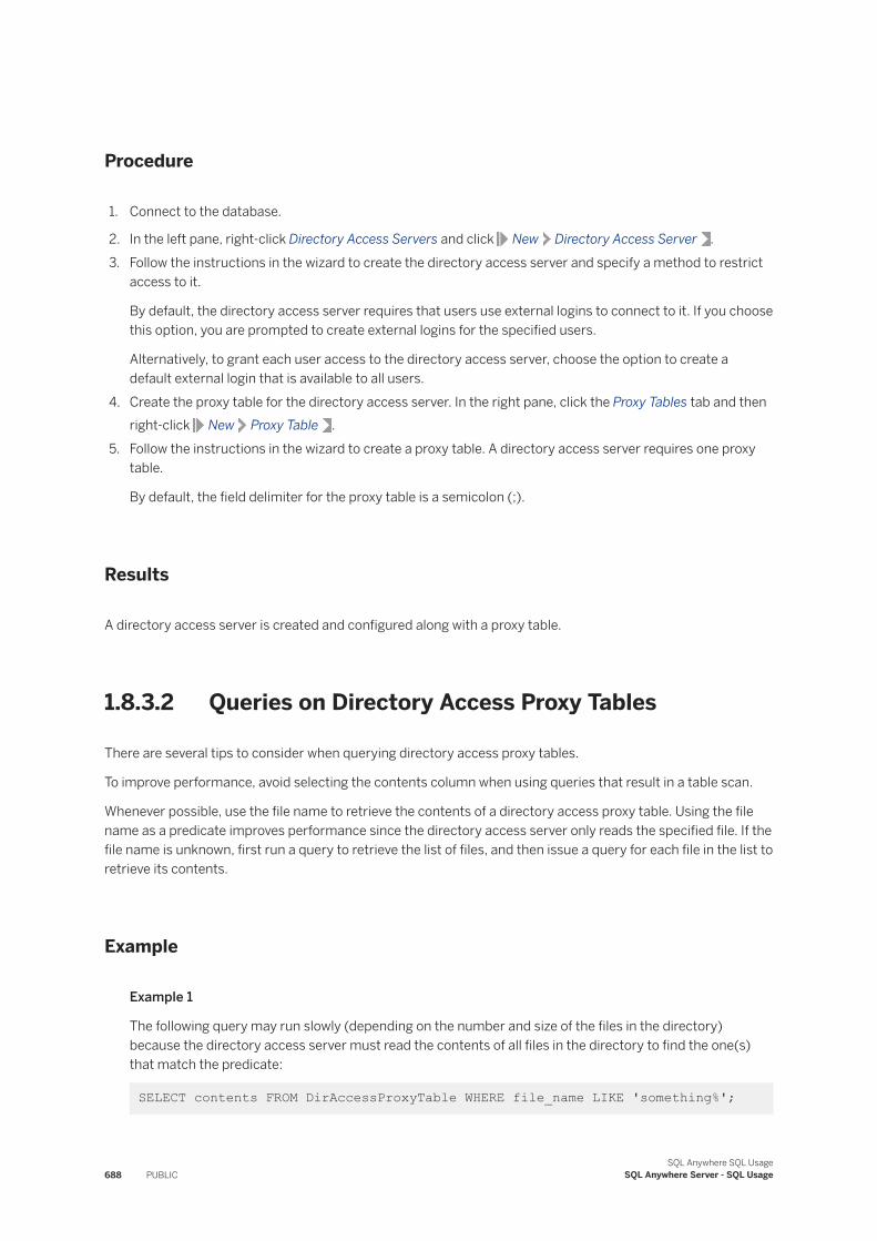
Procedure
1. Connect to the database.
2. In the left pane, right-click Directory Access Servers and click New Directory Access Server .3. Follow the instructions in the wizard to create the directory access server and specify a method to restrict
access to it.
By default, the directory access server requires that users use external logins to connect to it. If you choose this option, you are prompted to create external logins for the specified users.
Alternatively, to grant each user access to the directory access server, choose the option to create a default external login that is available to all users.
4. Create the proxy table for the directory access server. In the right pane, click the Proxy Tables tab and then right-click New Proxy Table .
5. Follow the instructions in the wizard to create a proxy table. A directory access server requires one proxy table.
By default, the field delimiter for the proxy table is a semicolon (;).
Results
A directory access server is created and configured along with a proxy table.
1.8.3.2 Queries on Directory Access Proxy Tables
There are several tips to consider when querying directory access proxy tables.
To improve performance, avoid selecting the contents column when using queries that result in a table scan.
Whenever possible, use the file name to retrieve the contents of a directory access proxy table. Using the file name as a predicate improves performance since the directory access server only reads the specified file. If the file name is unknown, first run a query to retrieve the list of files, and then issue a query for each file in the list to retrieve its contents.
Example
Example 1
The following query may run slowly (depending on the number and size of the files in the directory) because the directory access server must read the contents of all files in the directory to find the one(s) that match the predicate:
SELECT contents FROM DirAccessProxyTable WHERE file_name LIKE 'something%';
688 PUBLICSQL Anywhere SQL Usage
SQL Anywhere Server - SQL Usage
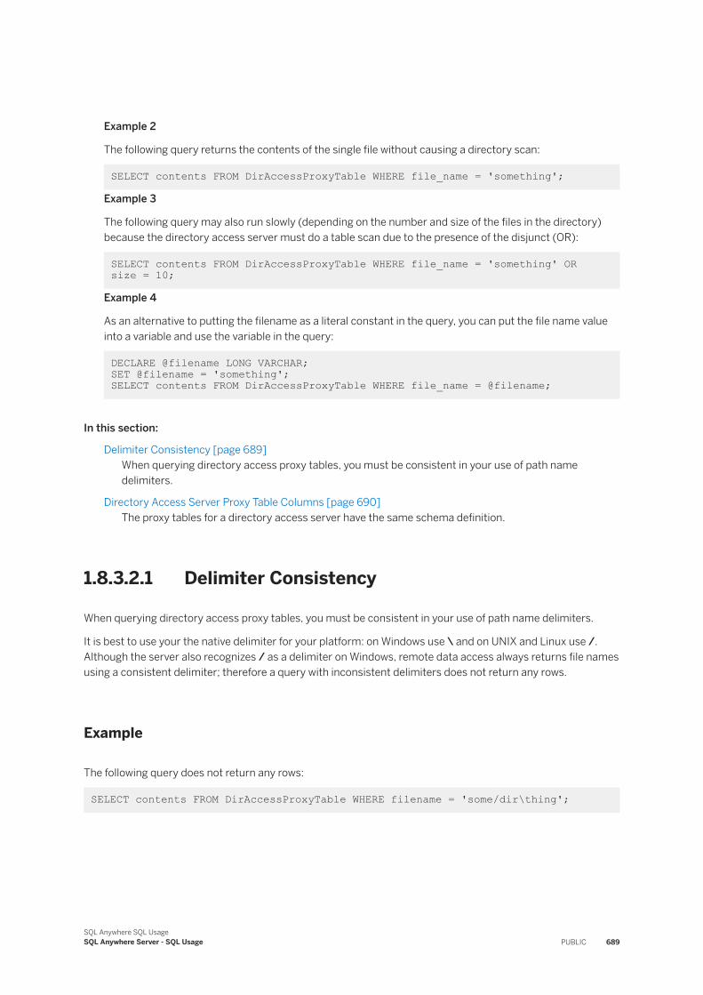
Example 2
The following query returns the contents of the single file without causing a directory scan:
SELECT contents FROM DirAccessProxyTable WHERE file_name = 'something';
Example 3
The following query may also run slowly (depending on the number and size of the files in the directory) because the directory access server must do a table scan due to the presence of the disjunct (OR):
SELECT contents FROM DirAccessProxyTable WHERE file_name = 'something' OR size = 10;
Example 4
As an alternative to putting the filename as a literal constant in the query, you can put the file name value into a variable and use the variable in the query:
DECLARE @filename LONG VARCHAR; SET @filename = 'something'; SELECT contents FROM DirAccessProxyTable WHERE file_name = @filename;
In this section:
Delimiter Consistency [page 689]When querying directory access proxy tables, you must be consistent in your use of path name delimiters.
Directory Access Server Proxy Table Columns [page 690]The proxy tables for a directory access server have the same schema definition.
1.8.3.2.1 Delimiter Consistency
When querying directory access proxy tables, you must be consistent in your use of path name delimiters.
It is best to use your the native delimiter for your platform: on Windows use \ and on UNIX and Linux use /. Although the server also recognizes / as a delimiter on Windows, remote data access always returns file names using a consistent delimiter; therefore a query with inconsistent delimiters does not return any rows.
Example
The following query does not return any rows:
SELECT contents FROM DirAccessProxyTable WHERE filename = 'some/dir\thing';
SQL Anywhere SQL UsageSQL Anywhere Server - SQL Usage PUBLIC 689
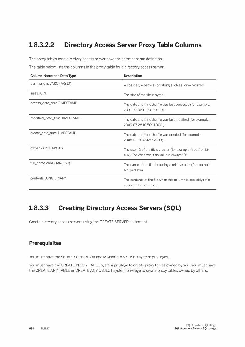
1.8.3.2.2 Directory Access Server Proxy Table Columns
The proxy tables for a directory access server have the same schema definition.
The table below lists the columns in the proxy table for a directory access server.
Column Name and Data Type Description
permissions VARCHAR(10) A Posix-style permission string such as "drwxrwxrwx".
size BIGINT The size of the file in bytes.
access_date_time TIMESTAMP The date and time the file was last accessed (for example, 2010-02-08 11:00:24.000).
modified_date_time TIMESTAMP The date and time the file was last modified (for example, 2009-07-28 10:50:11.000 ).
create_date_time TIMESTAMP The date and time the file was created (for example, 2008-12-18 10:32:26.000).
owner VARCHAR(20) The user ID of the file's creator (for example, "root" on Linux). For Windows, this value is always "0".
file_name VARCHAR(260) The name of the file, including a relative path (for example, bin\perl.exe).
contents LONG BINARY The contents of the file when this column is explicitly referenced in the result set.
1.8.3.3 Creating Directory Access Servers (SQL)
Create directory access servers using the CREATE SERVER statement.
Prerequisites
You must have the SERVER OPERATOR and MANAGE ANY USER system privileges.
You must have the CREATE PROXY TABLE system privilege to create proxy tables owned by you. You must have the CREATE ANY TABLE or CREATE ANY OBJECT system privilege to create proxy tables owned by others.
690 PUBLICSQL Anywhere SQL Usage
SQL Anywhere Server - SQL Usage
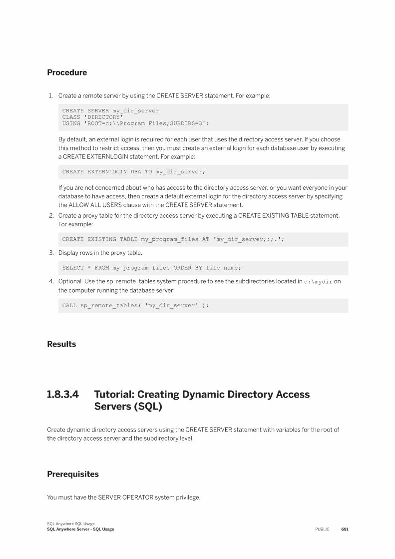
Procedure
1. Create a remote server by using the CREATE SERVER statement. For example:
CREATE SERVER my_dir_server CLASS 'DIRECTORY' USING 'ROOT=c:\\Program Files;SUBDIRS=3';
By default, an external login is required for each user that uses the directory access server. If you choose this method to restrict access, then you must create an external login for each database user by executing a CREATE EXTERNLOGIN statement. For example:
CREATE EXTERNLOGIN DBA TO my_dir_server;
If you are not concerned about who has access to the directory access server, or you want everyone in your database to have access, then create a default external login for the directory access server by specifying the ALLOW ALL USERS clause with the CREATE SERVER statement.
2. Create a proxy table for the directory access server by executing a CREATE EXISTING TABLE statement. For example:
CREATE EXISTING TABLE my_program_files AT 'my_dir_server;;;.';
3. Display rows in the proxy table.
SELECT * FROM my_program_files ORDER BY file_name;
4. Optional. Use the sp_remote_tables system procedure to see the subdirectories located in c:\mydir on the computer running the database server:
CALL sp_remote_tables( 'my_dir_server' );
Results
1.8.3.4 Tutorial: Creating Dynamic Directory Access Servers (SQL)
Create dynamic directory access servers using the CREATE SERVER statement with variables for the root of the directory access server and the subdirectory level.
Prerequisites
You must have the SERVER OPERATOR system privilege.
SQL Anywhere SQL UsageSQL Anywhere Server - SQL Usage PUBLIC 691
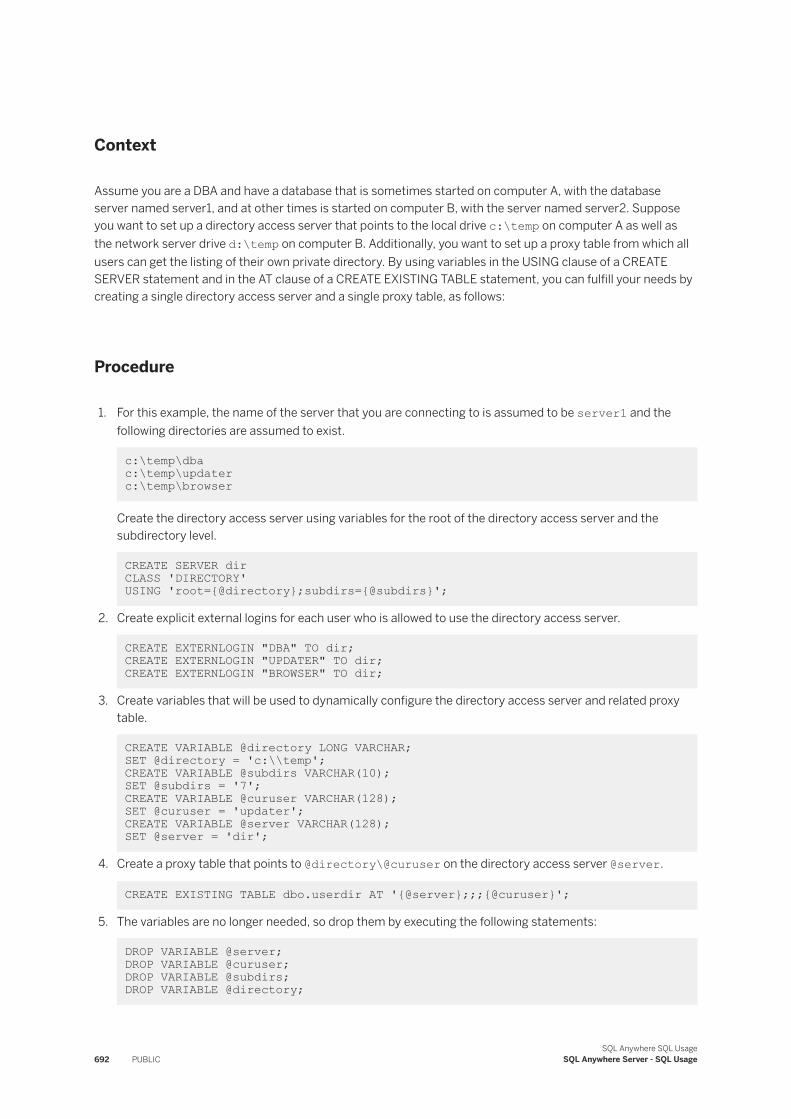
Context
Assume you are a DBA and have a database that is sometimes started on computer A, with the database server named server1, and at other times is started on computer B, with the server named server2. Suppose you want to set up a directory access server that points to the local drive c:\temp on computer A as well as the network server drive d:\temp on computer B. Additionally, you want to set up a proxy table from which all users can get the listing of their own private directory. By using variables in the USING clause of a CREATE SERVER statement and in the AT clause of a CREATE EXISTING TABLE statement, you can fulfill your needs by creating a single directory access server and a single proxy table, as follows:
Procedure
1. For this example, the name of the server that you are connecting to is assumed to be server1 and the following directories are assumed to exist.
c:\temp\dba c:\temp\updater c:\temp\browser
Create the directory access server using variables for the root of the directory access server and the subdirectory level.
CREATE SERVER dir CLASS 'DIRECTORY' USING 'root={@directory};subdirs={@subdirs}';
2. Create explicit external logins for each user who is allowed to use the directory access server.
CREATE EXTERNLOGIN "DBA" TO dir; CREATE EXTERNLOGIN "UPDATER" TO dir; CREATE EXTERNLOGIN "BROWSER" TO dir;
3. Create variables that will be used to dynamically configure the directory access server and related proxy table.
CREATE VARIABLE @directory LONG VARCHAR; SET @directory = 'c:\\temp';CREATE VARIABLE @subdirs VARCHAR(10);SET @subdirs = '7';CREATE VARIABLE @curuser VARCHAR(128);SET @curuser = 'updater';CREATE VARIABLE @server VARCHAR(128); SET @server = 'dir';
4. Create a proxy table that points to @directory\@curuser on the directory access server @server.
CREATE EXISTING TABLE dbo.userdir AT '{@server};;;{@curuser}';
5. The variables are no longer needed, so drop them by executing the following statements:
DROP VARIABLE @server; DROP VARIABLE @curuser;DROP VARIABLE @subdirs; DROP VARIABLE @directory;
692 PUBLICSQL Anywhere SQL Usage
SQL Anywhere Server - SQL Usage
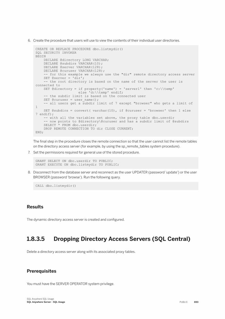
6. Create the procedure that users will use to view the contents of their individual user directories.
CREATE OR REPLACE PROCEDURE dbo.listmydir() SQL SECURITY INVOKERBEGIN DECLARE @directory LONG VARCHAR; DECLARE @subdirs VARCHAR(10); DECLARE @server VARCHAR(128); DECLARE @curuser VARCHAR(128); -- for this example we always use the "dir" remote directory access server SET @server = 'dir'; -- the root directory is based on the name of the server the user is connected to SET @directory = if property('name') = 'server1' then 'c:\\temp' else 'd:\\temp' endif; -- the subdir limit is based on the connected user SET @curuser = user_name(); -- all users get a subdir limit of 7 except "browser" who gets a limit of 1 SET @subdirs = convert( varchar(10), if @curuser = 'browser' then 1 else 7 endif); -- with all the variables set above, the proxy table dbo.userdir -- now points to @directory\@curuser and has a subdir limit of @subdirs SELECT * FROM dbo.userdir; DROP REMOTE CONNECTION TO dir CLOSE CURRENT; END;
The final step in the procedure closes the remote connection so that the user cannot list the remote tables on the directory access server (for example, by using the sp_remote_tables system procedure).
7. Set the permissions required for general use of the stored procedure.
GRANT SELECT ON dbo.userdir TO PUBLIC; GRANT EXECUTE ON dbo.listmydir TO PUBLIC;
8. Disconnect from the database server and reconnect as the user UPDATER (password 'update') or the user BROWSER (password 'browse'). Run the following query.
CALL dbo.listmydir()
Results
The dynamic directory access server is created and configured.
1.8.3.5 Dropping Directory Access Servers (SQL Central)
Delete a directory access server along with its associated proxy tables.
Prerequisites
You must have the SERVER OPERATOR system privilege.
SQL Anywhere SQL UsageSQL Anywhere Server - SQL Usage PUBLIC 693
Procedure
1. Connect to the database.2. In the left pane, click Directory Access Servers.
3. Select the directory access server, and then click Edit Delete .
Results
The directory access server and its associated proxy tables are deleted.
Related Information
Dropping Proxy Tables (SQL Central) [page 703]
1.8.3.6 Dropping Directory Access Servers (SQL)
Delete directory access servers using SQL statements.
Prerequisites
You must have the SERVER OPERATOR system privilege.
All proxy tables defined for the directory access server must be dropped before dropping the directory access server. The following query can be used to determine which proxy tables are defined for the directory access server server-name.
SELECT st.table_name, sp.remote_location, sp.existing_obj FROM SYS.SYSPROXYTAB sp JOIN SYS.SYSSERVER ss ON ss.srvid = sp.srvid JOIN SYS.SYSTAB st ON sp.table_object_id = st.object_id WHERE ss.srvname = 'server-name';
Procedure
1. Connect to the host database.2. Execute a DROP TABLE statement for each proxy table associated with the directory access server.
DROP TABLE my_program_files;
694 PUBLICSQL Anywhere SQL Usage
SQL Anywhere Server - SQL Usage
3. Execute a DROP SERVER statement for the directory access server.
DROP SERVER my_dir_server;
Results
The directory access server is deleted.
Related Information
Dropping Proxy Tables (SQL Central) [page 703]
1.8.4 External Logins
External logins are used to communicate with a remote server or to permit access to a directory access server.
Remote Server Connections
With remote servers an external login maps a database user to the login credentials of the remote server.
By default, a remote server requires that each database user be explicitly assigned their own external login to access the remote server. However, you can create a remote server with a default login using the CREATE REMOTE SERVER statement that can be used by all database users.
Even if a default login is specified for the remote server, you can create an external login for individual database users. For example, the remote server could have a default login that permits all database users read access, and the DBA database user could have an external login that permits read-write access to the remote server.
Connections to a remote server are first attempted using the database user's external login. If the user does not have an external login, then the connection is attempted using the default login credentials of the remote server. If the remote server does not have a default login, and no external login has been defined for the user, then the connection is attempted with the current user ID and password.
Directory Access Server Connections
With directory access servers an external login restricts access to the directory access server.
By default, a directory access server requires that each database user be explicitly assigned their own external login to access the directory access server. However, you can create a directory access server that has a default external login that is available to all database users. Specify a default external login for a directory access
SQL Anywhere SQL UsageSQL Anywhere Server - SQL Usage PUBLIC 695
server when you are not concerned about who has access to the directory access server, or you want everyone in your database to have access.
In this section:
Creating External Logins (SQL Central) [page 696]Create an external login for a user to use to communicate with a remote server or a directory access server.
Dropping External Logins (SQL Central) [page 697]Delete external logins from users to remote servers and directory access servers that are no longer required.
Related Information
Directory Access Servers [page 686]Remote Servers and Remote Table Mappings [page 677]
1.8.4.1 Creating External Logins (SQL Central)
Create an external login for a user to use to communicate with a remote server or a directory access server.
Prerequisites
The remote server or the directory access server must exist in the database.
You must have the MANAGE ANY USER system privilege.
Procedure
1. Use the SQL Anywhere 17 plug-in to connect to the database.2. In the left pane, click Remote Servers.3. Select the remote server, and in the right pane click the External Logins tab.
4. From the File menu, click New External Login .5. Follow the instructions in the wizard.
696 PUBLICSQL Anywhere SQL Usage
SQL Anywhere Server - SQL Usage
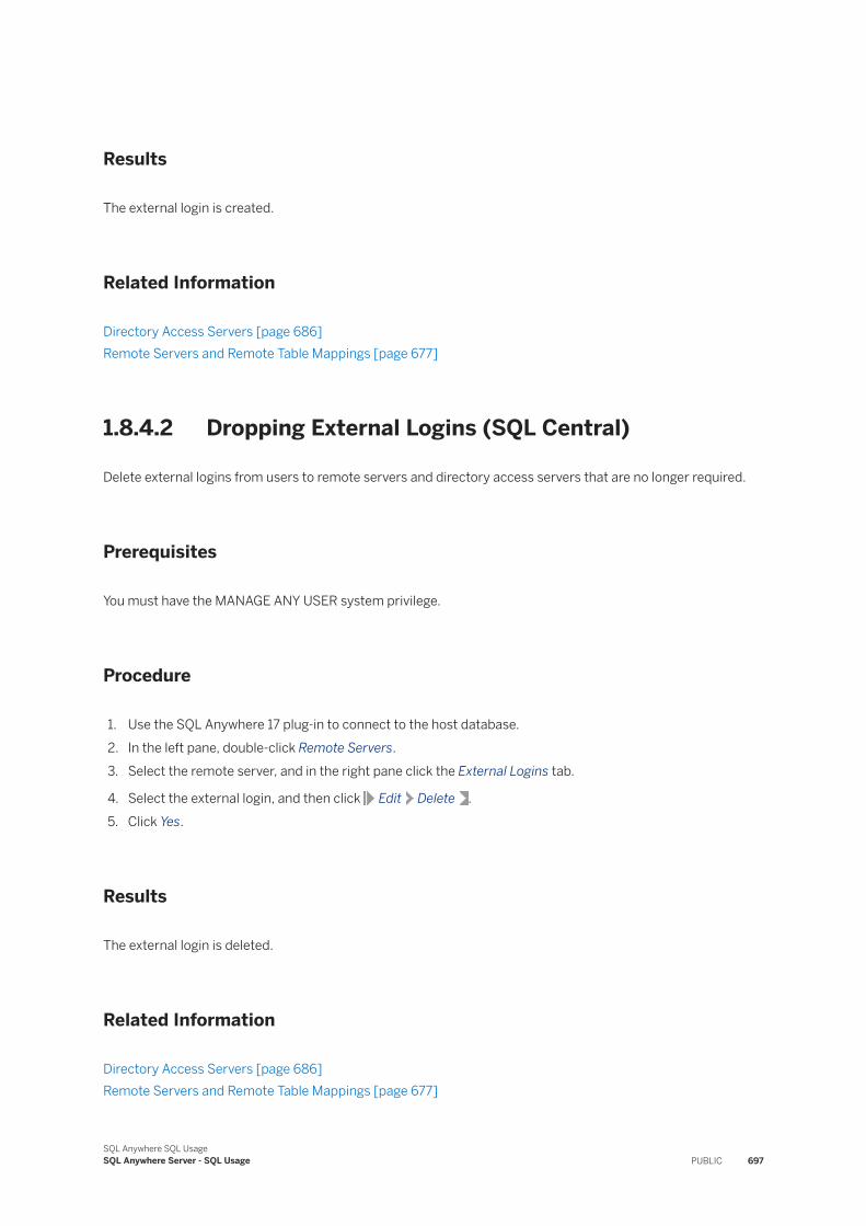
Results
The external login is created.
Related Information
Directory Access Servers [page 686]Remote Servers and Remote Table Mappings [page 677]
1.8.4.2 Dropping External Logins (SQL Central)
Delete external logins from users to remote servers and directory access servers that are no longer required.
Prerequisites
You must have the MANAGE ANY USER system privilege.
Procedure
1. Use the SQL Anywhere 17 plug-in to connect to the host database.2. In the left pane, double-click Remote Servers.3. Select the remote server, and in the right pane click the External Logins tab.
4. Select the external login, and then click Edit Delete .5. Click Yes.
Results
The external login is deleted.
Related Information
Directory Access Servers [page 686]Remote Servers and Remote Table Mappings [page 677]
SQL Anywhere SQL UsageSQL Anywhere Server - SQL Usage PUBLIC 697
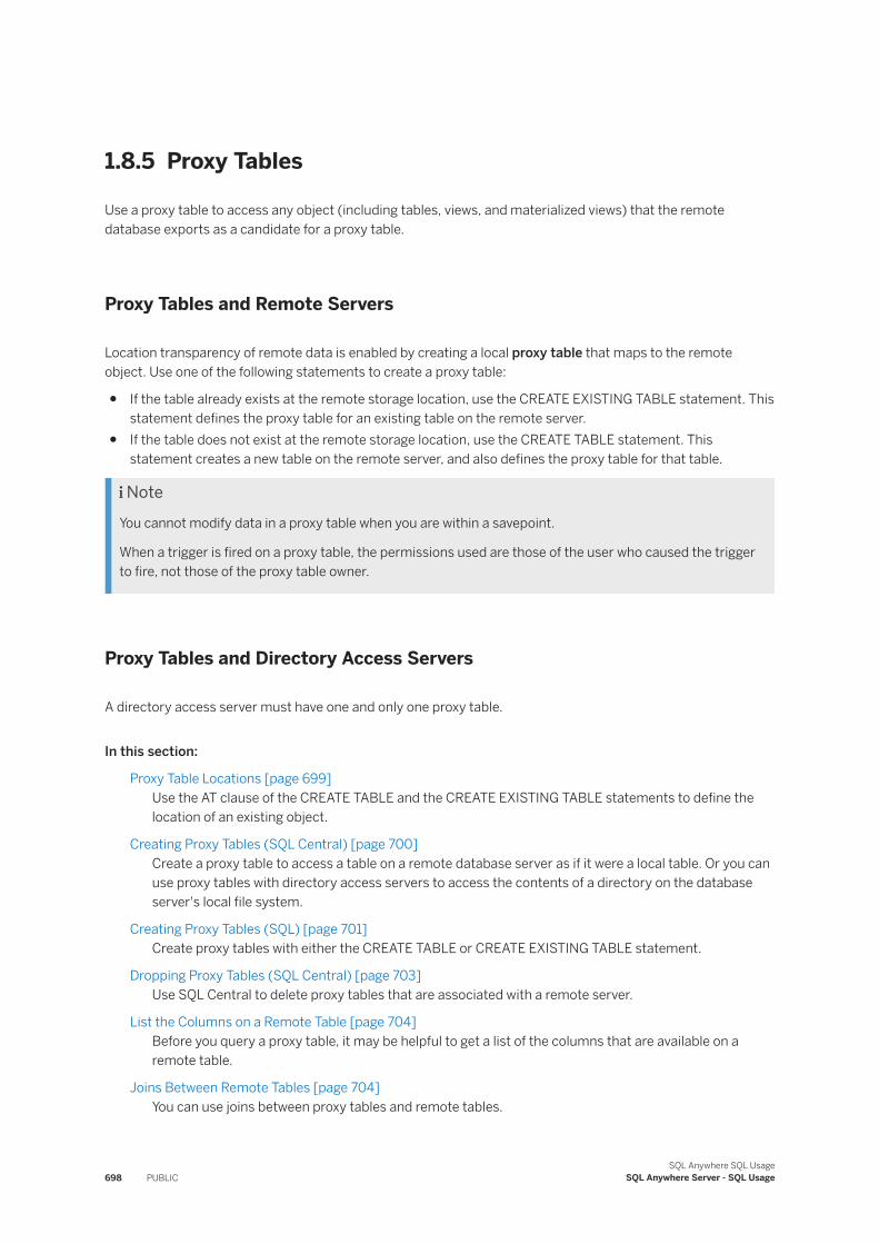
1.8.5 Proxy Tables
Use a proxy table to access any object (including tables, views, and materialized views) that the remote database exports as a candidate for a proxy table.
Proxy Tables and Remote Servers
Location transparency of remote data is enabled by creating a local proxy table that maps to the remote object. Use one of the following statements to create a proxy table:
● If the table already exists at the remote storage location, use the CREATE EXISTING TABLE statement. This statement defines the proxy table for an existing table on the remote server.
● If the table does not exist at the remote storage location, use the CREATE TABLE statement. This statement creates a new table on the remote server, and also defines the proxy table for that table.
NoteYou cannot modify data in a proxy table when you are within a savepoint.
When a trigger is fired on a proxy table, the permissions used are those of the user who caused the trigger to fire, not those of the proxy table owner.
Proxy Tables and Directory Access Servers
A directory access server must have one and only one proxy table.
In this section:
Proxy Table Locations [page 699]Use the AT clause of the CREATE TABLE and the CREATE EXISTING TABLE statements to define the location of an existing object.
Creating Proxy Tables (SQL Central) [page 700]Create a proxy table to access a table on a remote database server as if it were a local table. Or you can use proxy tables with directory access servers to access the contents of a directory on the database server's local file system.
Creating Proxy Tables (SQL) [page 701]Create proxy tables with either the CREATE TABLE or CREATE EXISTING TABLE statement.
Dropping Proxy Tables (SQL Central) [page 703]Use SQL Central to delete proxy tables that are associated with a remote server.
List the Columns on a Remote Table [page 704]Before you query a proxy table, it may be helpful to get a list of the columns that are available on a remote table.
Joins Between Remote Tables [page 704]You can use joins between proxy tables and remote tables.
698 PUBLICSQL Anywhere SQL Usage
SQL Anywhere Server - SQL Usage
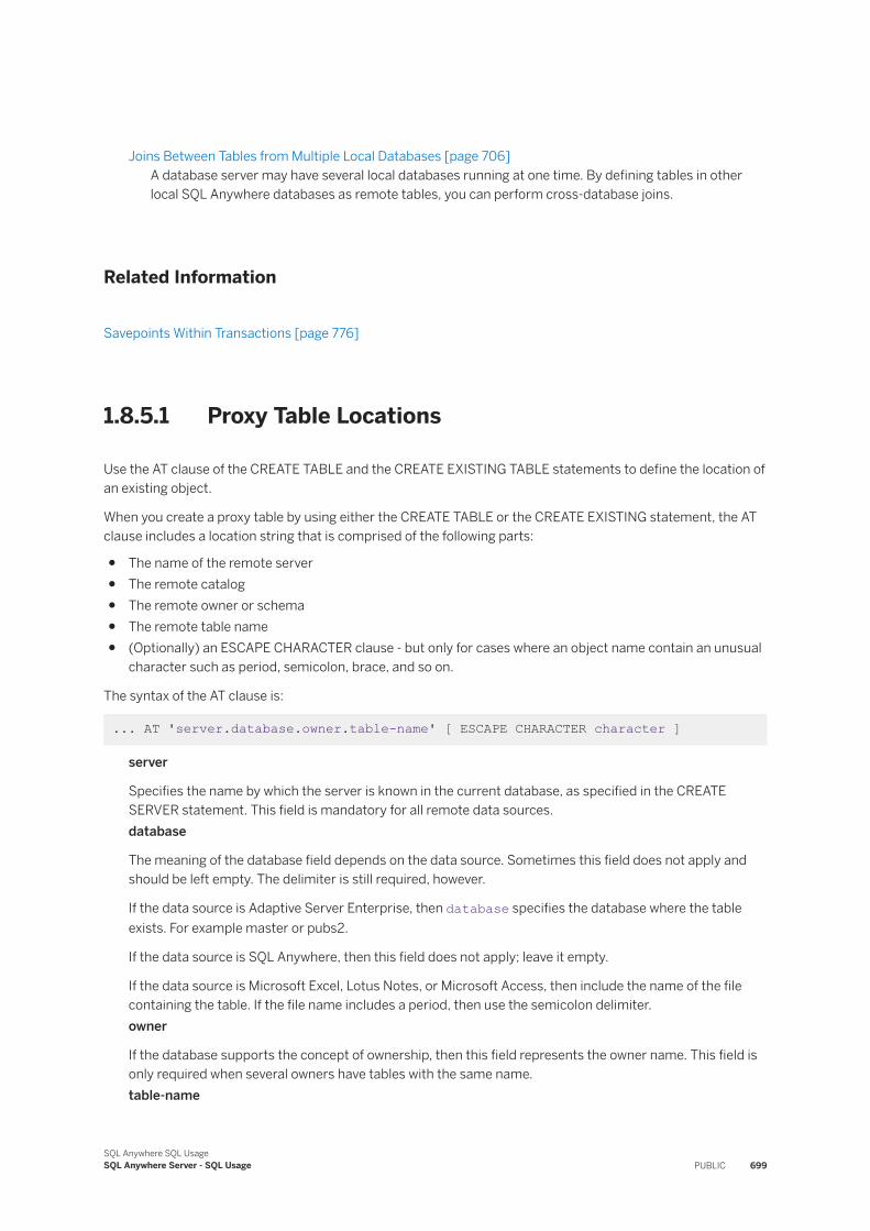
Joins Between Tables from Multiple Local Databases [page 706]A database server may have several local databases running at one time. By defining tables in other local SQL Anywhere databases as remote tables, you can perform cross-database joins.
Related Information
Savepoints Within Transactions [page 776]
1.8.5.1 Proxy Table Locations
Use the AT clause of the CREATE TABLE and the CREATE EXISTING TABLE statements to define the location of an existing object.
When you create a proxy table by using either the CREATE TABLE or the CREATE EXISTING statement, the AT clause includes a location string that is comprised of the following parts:
● The name of the remote server● The remote catalog● The remote owner or schema● The remote table name● (Optionally) an ESCAPE CHARACTER clause - but only for cases where an object name contain an unusual
character such as period, semicolon, brace, and so on.
The syntax of the AT clause is:
... AT 'server.database.owner.table-name' [ ESCAPE CHARACTER character ]
server
Specifies the name by which the server is known in the current database, as specified in the CREATE SERVER statement. This field is mandatory for all remote data sources.database
The meaning of the database field depends on the data source. Sometimes this field does not apply and should be left empty. The delimiter is still required, however.
If the data source is Adaptive Server Enterprise, then database specifies the database where the table exists. For example master or pubs2.
If the data source is SQL Anywhere, then this field does not apply; leave it empty.
If the data source is Microsoft Excel, Lotus Notes, or Microsoft Access, then include the name of the file containing the table. If the file name includes a period, then use the semicolon delimiter.owner
If the database supports the concept of ownership, then this field represents the owner name. This field is only required when several owners have tables with the same name.table-name
SQL Anywhere SQL UsageSQL Anywhere Server - SQL Usage PUBLIC 699
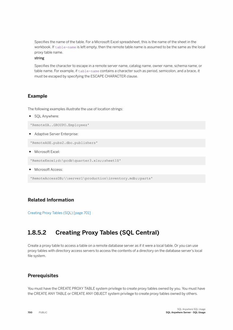
Specifies the name of the table. For a Microsoft Excel spreadsheet, this is the name of the sheet in the workbook. If table-name is left empty, then the remote table name is assumed to be the same as the local proxy table name.string
Specifies the character to escape in a remote server name, catalog name, owner name, schema name, or table name. For example, if table-name contains a character such as period, semicolon, and a brace, it must be escaped by specifying the ESCAPE CHARACTER clause.
Example
The following examples illustrate the use of location strings:
● SQL Anywhere:
'RemoteSA..GROUPO.Employees'
● Adaptive Server Enterprise:
'RemoteASE.pubs2.dbo.publishers'
● Microsoft Excel:
'RemoteExcel;d:\pcdb\quarter3.xls;;sheet1$'
● Microsoft Access:
'RemoteAccessDB;\\server1\production\inventory.mdb;;parts'
Related Information
Creating Proxy Tables (SQL) [page 701]
1.8.5.2 Creating Proxy Tables (SQL Central)
Create a proxy table to access a table on a remote database server as if it were a local table. Or you can use proxy tables with directory access servers to access the contents of a directory on the database server's local file system.
Prerequisites
You must have the CREATE PROXY TABLE system privilege to create proxy tables owned by you. You must have the CREATE ANY TABLE or CREATE ANY OBJECT system privilege to create proxy tables owned by others.
700 PUBLICSQL Anywhere SQL Usage
SQL Anywhere Server - SQL Usage
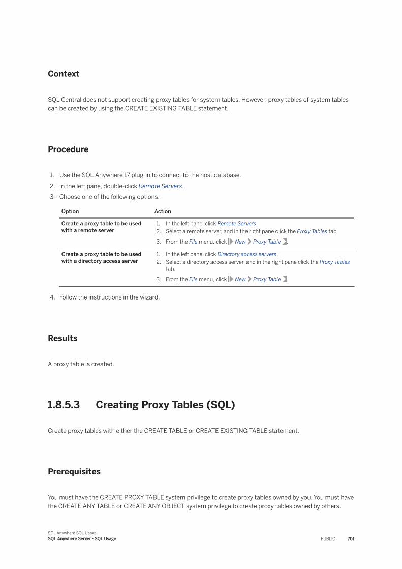
Context
SQL Central does not support creating proxy tables for system tables. However, proxy tables of system tables can be created by using the CREATE EXISTING TABLE statement.
Procedure
1. Use the SQL Anywhere 17 plug-in to connect to the host database.2. In the left pane, double-click Remote Servers.3. Choose one of the following options:
Option Action
Create a proxy table to be used with a remote server
1. In the left pane, click Remote Servers.2. Select a remote server, and in the right pane click the Proxy Tables tab.
3. From the File menu, click New Proxy Table .
Create a proxy table to be used with a directory access server
1. In the left pane, click Directory access servers.2. Select a directory access server, and in the right pane click the Proxy Tables
tab.
3. From the File menu, click New Proxy Table .
4. Follow the instructions in the wizard.
Results
A proxy table is created.
1.8.5.3 Creating Proxy Tables (SQL)
Create proxy tables with either the CREATE TABLE or CREATE EXISTING TABLE statement.
Prerequisites
You must have the CREATE PROXY TABLE system privilege to create proxy tables owned by you. You must have the CREATE ANY TABLE or CREATE ANY OBJECT system privilege to create proxy tables owned by others.
SQL Anywhere SQL UsageSQL Anywhere Server - SQL Usage PUBLIC 701
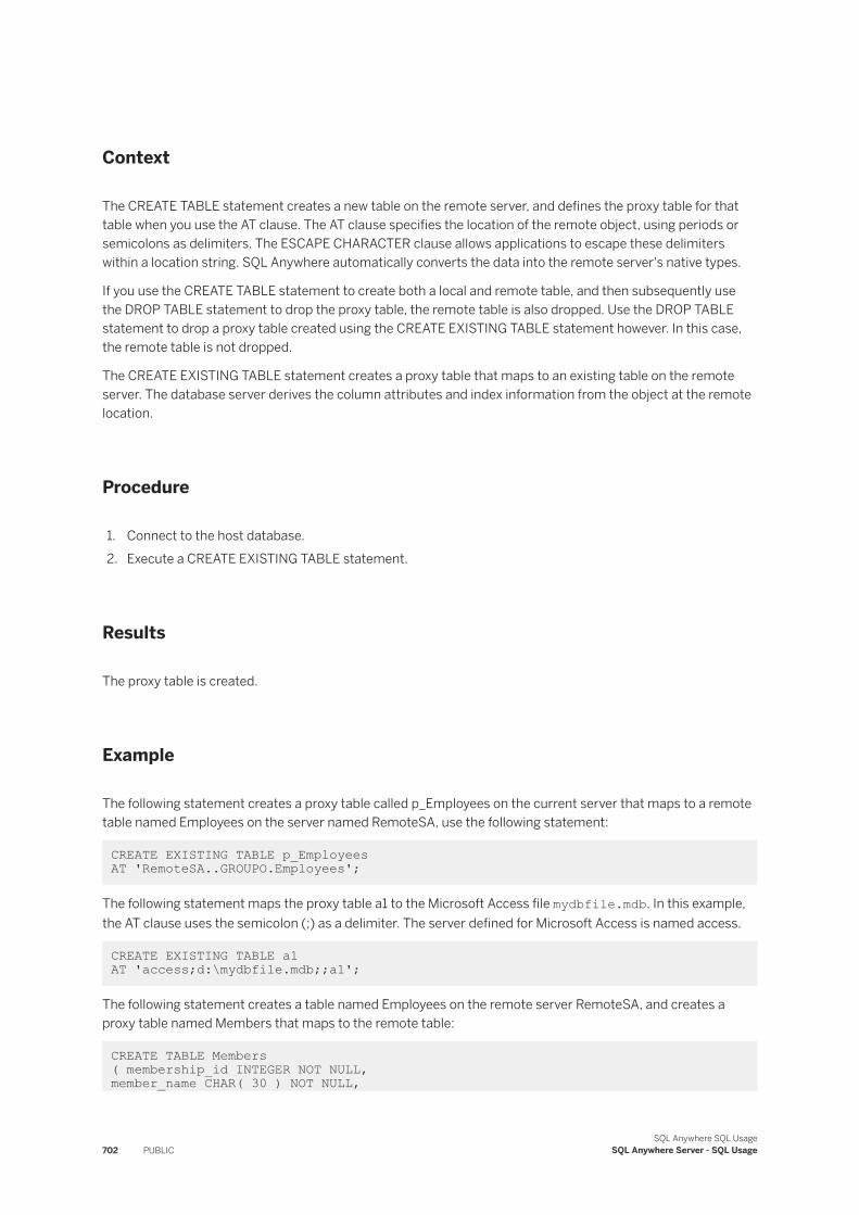
Context
The CREATE TABLE statement creates a new table on the remote server, and defines the proxy table for that table when you use the AT clause. The AT clause specifies the location of the remote object, using periods or semicolons as delimiters. The ESCAPE CHARACTER clause allows applications to escape these delimiters within a location string. SQL Anywhere automatically converts the data into the remote server's native types.
If you use the CREATE TABLE statement to create both a local and remote table, and then subsequently use the DROP TABLE statement to drop the proxy table, the remote table is also dropped. Use the DROP TABLE statement to drop a proxy table created using the CREATE EXISTING TABLE statement however. In this case, the remote table is not dropped.
The CREATE EXISTING TABLE statement creates a proxy table that maps to an existing table on the remote server. The database server derives the column attributes and index information from the object at the remote location.
Procedure
1. Connect to the host database.2. Execute a CREATE EXISTING TABLE statement.
Results
The proxy table is created.
Example
The following statement creates a proxy table called p_Employees on the current server that maps to a remote table named Employees on the server named RemoteSA, use the following statement:
CREATE EXISTING TABLE p_Employees AT 'RemoteSA..GROUPO.Employees';
The following statement maps the proxy table a1 to the Microsoft Access file mydbfile.mdb. In this example, the AT clause uses the semicolon (;) as a delimiter. The server defined for Microsoft Access is named access.
CREATE EXISTING TABLE a1 AT 'access;d:\mydbfile.mdb;;a1';
The following statement creates a table named Employees on the remote server RemoteSA, and creates a proxy table named Members that maps to the remote table:
CREATE TABLE Members ( membership_id INTEGER NOT NULL,member_name CHAR( 30 ) NOT NULL,
702 PUBLICSQL Anywhere SQL Usage
SQL Anywhere Server - SQL Usage
office_held CHAR( 20 ) NULL ) AT 'RemoteSA..GROUPO.Employees';
Related Information
Proxy Table Locations [page 699]
1.8.5.4 Dropping Proxy Tables (SQL Central)
Use SQL Central to delete proxy tables that are associated with a remote server.
Prerequisites
You must be the owner, or have the DROP ANY TABLE or DROP ANY OBJECT system privilege.
Context
Before a remote server can be dropped, you must drop all proxy tables associated with the remote server.
Procedure
1. Use the SQL Anywhere 17 plug-in to connect to the host database.2. In the left pane, double-click Remote Servers.3. In the right pane, click the Proxy Tables tab.
4. Select the proxy table, and then click Edit Delete .5. Click Yes.
Results
The proxy table is deleted.
SQL Anywhere SQL UsageSQL Anywhere Server - SQL Usage PUBLIC 703
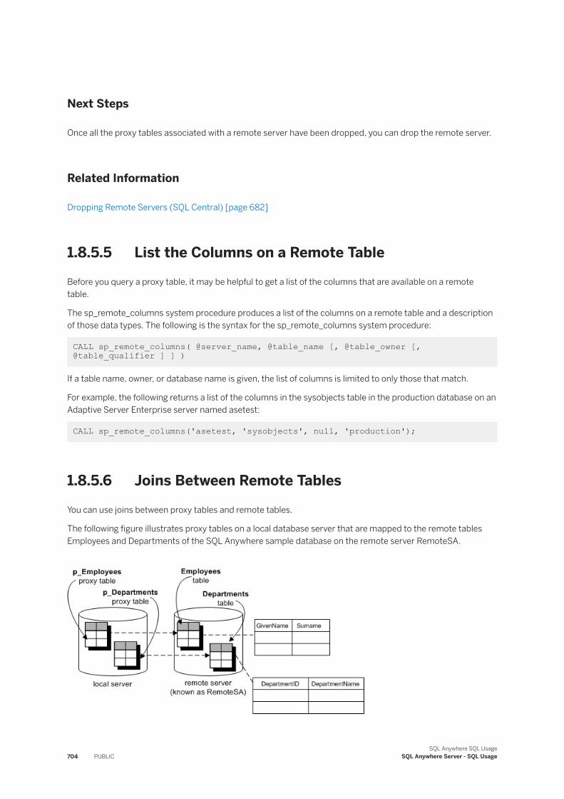
Next Steps
Once all the proxy tables associated with a remote server have been dropped, you can drop the remote server.
Related Information
Dropping Remote Servers (SQL Central) [page 682]
1.8.5.5 List the Columns on a Remote Table
Before you query a proxy table, it may be helpful to get a list of the columns that are available on a remote table.
The sp_remote_columns system procedure produces a list of the columns on a remote table and a description of those data types. The following is the syntax for the sp_remote_columns system procedure:
CALL sp_remote_columns( @server_name, @table_name [, @table_owner [, @table_qualifier ] ] )
If a table name, owner, or database name is given, the list of columns is limited to only those that match.
For example, the following returns a list of the columns in the sysobjects table in the production database on an Adaptive Server Enterprise server named asetest:
CALL sp_remote_columns('asetest, 'sysobjects', null, 'production');
1.8.5.6 Joins Between Remote Tables
You can use joins between proxy tables and remote tables.
The following figure illustrates proxy tables on a local database server that are mapped to the remote tables Employees and Departments of the SQL Anywhere sample database on the remote server RemoteSA.
704 PUBLICSQL Anywhere SQL Usage
SQL Anywhere Server - SQL Usage
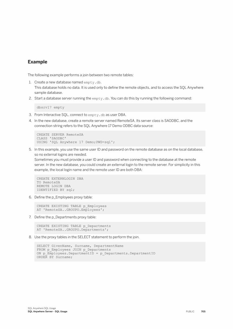
Example
The following example performs a join between two remote tables:
1. Create a new database named empty.db.This database holds no data. It is used only to define the remote objects, and to access the SQL Anywhere sample database.
2. Start a database server running the empty.db. You can do this by running the following command:
dbsrv17 empty
3. From Interactive SQL, connect to empty.db as user DBA.4. In the new database, create a remote server named RemoteSA. Its server class is SAODBC, and the
connection string refers to the SQL Anywhere 17 Demo ODBC data source:
CREATE SERVER RemoteSA CLASS 'SAODBC' USING 'SQL Anywhere 17 Demo;PWD=sql';
5. In this example, you use the same user ID and password on the remote database as on the local database, so no external logins are needed.Sometimes you must provide a user ID and password when connecting to the database at the remote server. In the new database, you could create an external login to the remote server. For simplicity in this example, the local login name and the remote user ID are both DBA:
CREATE EXTERNLOGIN DBA TO RemoteSAREMOTE LOGIN DBA IDENTIFIED BY sql;
6. Define the p_Employees proxy table:
CREATE EXISTING TABLE p_Employees AT 'RemoteSA..GROUPO.Employees';
7. Define the p_Departments proxy table:
CREATE EXISTING TABLE p_Departments AT 'RemoteSA..GROUPO.Departments';
8. Use the proxy tables in the SELECT statement to perform the join.
SELECT GivenName, Surname, DepartmentName FROM p_Employees JOIN p_DepartmentsON p_Employees.DepartmentID = p_Departments.DepartmentID ORDER BY Surname;
SQL Anywhere SQL UsageSQL Anywhere Server - SQL Usage PUBLIC 705
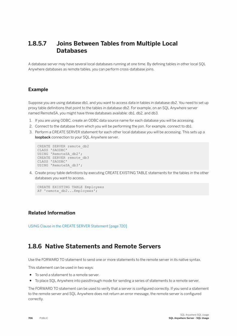
1.8.5.7 Joins Between Tables from Multiple Local Databases
A database server may have several local databases running at one time. By defining tables in other local SQL Anywhere databases as remote tables, you can perform cross-database joins.
Example
Suppose you are using database db1, and you want to access data in tables in database db2. You need to set up proxy table definitions that point to the tables in database db2. For example, on an SQL Anywhere server named RemoteSA, you might have three databases available: db1, db2, and db3.
1. If you are using ODBC, create an ODBC data source name for each database you will be accessing.2. Connect to the database from which you will be performing the join. For example, connect to db1.3. Perform a CREATE SERVER statement for each other local database you will be accessing. This sets up a
loopback connection to your SQL Anywhere server.
CREATE SERVER remote_db2 CLASS 'SAODBC'USING 'RemoteSA_db2';CREATE SERVER remote_db3CLASS 'SAODBC' USING 'RemoteSA_db3';
4. Create proxy table definitions by executing CREATE EXISTING TABLE statements for the tables in the other databases you want to access.
CREATE EXISTING TABLE Employees AT 'remote_db2...Employees';
Related Information
USING Clause in the CREATE SERVER Statement [page 720]
1.8.6 Native Statements and Remote Servers
Use the FORWARD TO statement to send one or more statements to the remote server in its native syntax.
This statement can be used in two ways:
● To send a statement to a remote server.● To place SQL Anywhere into passthrough mode for sending a series of statements to a remote server.
The FORWARD TO statement can be used to verify that a server is configured correctly. If you send a statement to the remote server and SQL Anywhere does not return an error message, the remote server is configured correctly.
706 PUBLICSQL Anywhere SQL Usage
SQL Anywhere Server - SQL Usage
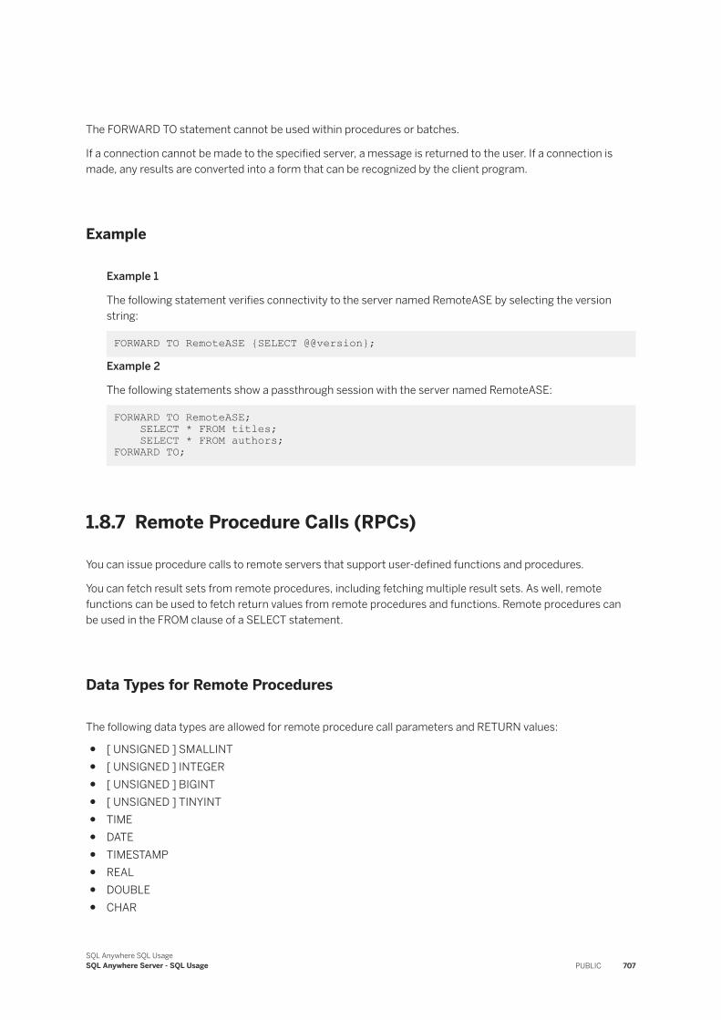
The FORWARD TO statement cannot be used within procedures or batches.
If a connection cannot be made to the specified server, a message is returned to the user. If a connection is made, any results are converted into a form that can be recognized by the client program.
Example
Example 1
The following statement verifies connectivity to the server named RemoteASE by selecting the version string:
FORWARD TO RemoteASE {SELECT @@version};
Example 2
The following statements show a passthrough session with the server named RemoteASE:
FORWARD TO RemoteASE; SELECT * FROM titles; SELECT * FROM authors; FORWARD TO;
1.8.7 Remote Procedure Calls (RPCs)
You can issue procedure calls to remote servers that support user-defined functions and procedures.
You can fetch result sets from remote procedures, including fetching multiple result sets. As well, remote functions can be used to fetch return values from remote procedures and functions. Remote procedures can be used in the FROM clause of a SELECT statement.
Data Types for Remote Procedures
The following data types are allowed for remote procedure call parameters and RETURN values:
● [ UNSIGNED ] SMALLINT● [ UNSIGNED ] INTEGER● [ UNSIGNED ] BIGINT● [ UNSIGNED ] TINYINT● TIME● DATE● TIMESTAMP● REAL● DOUBLE● CHAR
SQL Anywhere SQL UsageSQL Anywhere Server - SQL Usage PUBLIC 707
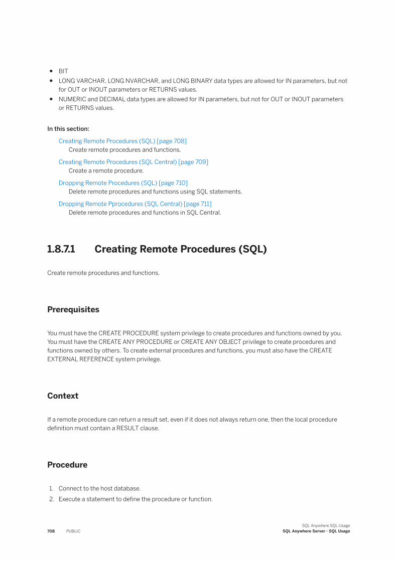
● BIT● LONG VARCHAR, LONG NVARCHAR, and LONG BINARY data types are allowed for IN parameters, but not
for OUT or INOUT parameters or RETURNS values.● NUMERIC and DECIMAL data types are allowed for IN parameters, but not for OUT or INOUT parameters
or RETURNS values.
In this section:
Creating Remote Procedures (SQL) [page 708]Create remote procedures and functions.
Creating Remote Procedures (SQL Central) [page 709]Create a remote procedure.
Dropping Remote Procedures (SQL) [page 710]Delete remote procedures and functions using SQL statements.
Dropping Remote Pprocedures (SQL Central) [page 711]Delete remote procedures and functions in SQL Central.
1.8.7.1 Creating Remote Procedures (SQL)
Create remote procedures and functions.
Prerequisites
You must have the CREATE PROCEDURE system privilege to create procedures and functions owned by you. You must have the CREATE ANY PROCEDURE or CREATE ANY OBJECT privilege to create procedures and functions owned by others. To create external procedures and functions, you must also have the CREATE EXTERNAL REFERENCE system privilege.
Context
If a remote procedure can return a result set, even if it does not always return one, then the local procedure definition must contain a RESULT clause.
Procedure
1. Connect to the host database.2. Execute a statement to define the procedure or function.
708 PUBLICSQL Anywhere SQL Usage
SQL Anywhere Server - SQL Usage
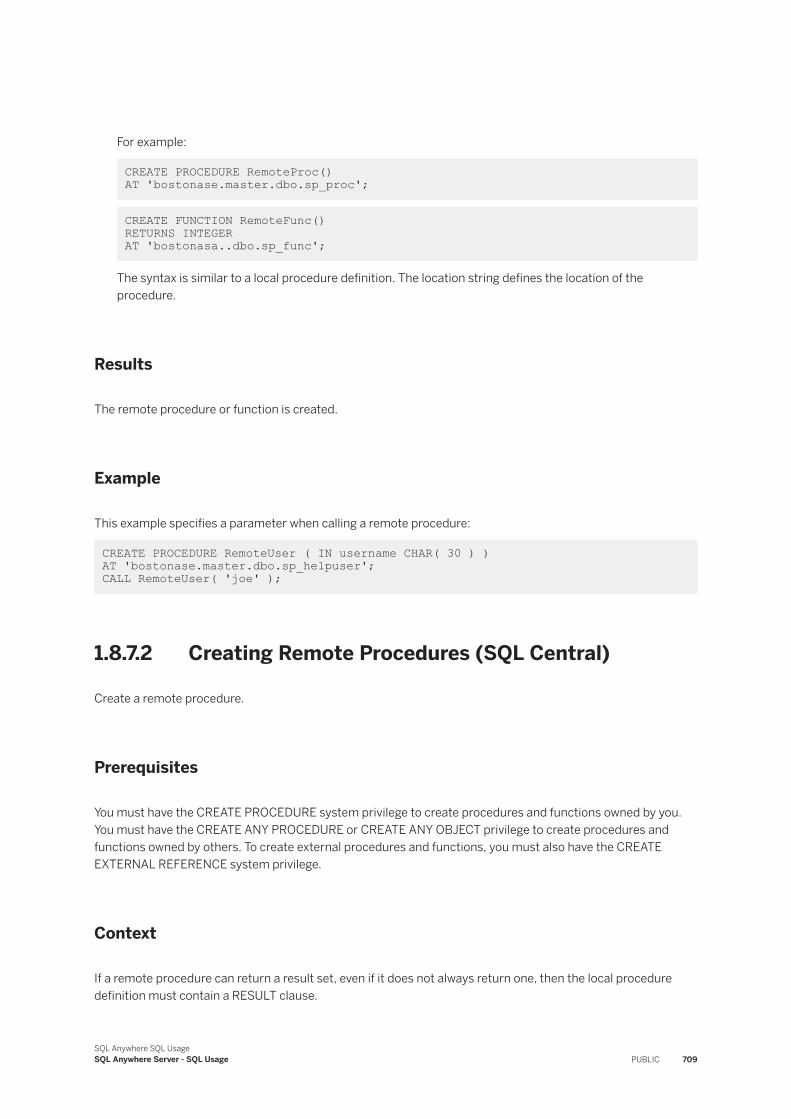
For example:
CREATE PROCEDURE RemoteProc() AT 'bostonase.master.dbo.sp_proc';
CREATE FUNCTION RemoteFunc() RETURNS INTEGER AT 'bostonasa..dbo.sp_func';
The syntax is similar to a local procedure definition. The location string defines the location of the procedure.
Results
The remote procedure or function is created.
Example
This example specifies a parameter when calling a remote procedure:
CREATE PROCEDURE RemoteUser ( IN username CHAR( 30 ) ) AT 'bostonase.master.dbo.sp_helpuser'; CALL RemoteUser( 'joe' );
1.8.7.2 Creating Remote Procedures (SQL Central)
Create a remote procedure.
Prerequisites
You must have the CREATE PROCEDURE system privilege to create procedures and functions owned by you. You must have the CREATE ANY PROCEDURE or CREATE ANY OBJECT privilege to create procedures and functions owned by others. To create external procedures and functions, you must also have the CREATE EXTERNAL REFERENCE system privilege.
Context
If a remote procedure can return a result set, even if it does not always return one, then the local procedure definition must contain a RESULT clause.
SQL Anywhere SQL UsageSQL Anywhere Server - SQL Usage PUBLIC 709
Procedure
1. Use the SQL Anywhere 17 plug-in to connect to the host database.2. In the left pane, double-click Remote Servers.3. Select the remote server, and in the right pane click the Remote Procedures tab.
4. In the File menu, click New Remote Procedure .5. Follow the instructions in the Create Remote Procedure Wizard.
Results
The remote procedure is created.
1.8.7.3 Dropping Remote Procedures (SQL)
Delete remote procedures and functions using SQL statements.
Prerequisites
You must be the owner of the procedure or function, or have either the DROP ANY PROCEDURE or DROP ANY OBJECT system privileges.
Procedure
Execute a statement to drop the procedure or function.
DROP PROCEDURE RemoteProc;
DROP FUNCTION RemoteFunc;
Results
The remote procedure or function is deleted.
710 PUBLICSQL Anywhere SQL Usage
SQL Anywhere Server - SQL Usage
1.8.7.4 Dropping Remote Pprocedures (SQL Central)
Delete remote procedures and functions in SQL Central.
Prerequisites
You must be the owner of the procedure or function, or have either the DROP ANY PROCEDURE or DROP ANY OBJECT system privileges.
Procedure
1. Use the SQL Anywhere 17 plug-in to connect to the host database.2. In the left pane, double-click Remote Servers.3. Select the remote server, and in the right pane click the Remote Procedures tab.
4. Select the remote procedure or function, and then click Edit Delete .5. Click Yes.
Results
The remote procedure is deleted.
1.8.8 Transaction Management and Remote Data
Transactions provide a way to group SQL statements so that they are treated as a unit (either all work performed by the statements is committed to the database, or none of it is).
For the most part, transaction management with remote tables is the same as transaction management for local tables in SQL Anywhere, but there are some differences.
In this section:
Remote Transaction Management and Restrictions [page 712]A multi-phase commit protocol is used for managing transactions that involve remote servers.
Related Information
Transactions and Isolation Levels [page 771]
SQL Anywhere SQL UsageSQL Anywhere Server - SQL Usage PUBLIC 711
1.8.8.1 Remote Transaction Management and Restrictions
A multi-phase commit protocol is used for managing transactions that involve remote servers.
However, when more than one remote server is involved in a transaction, there is still a chance that a distributed unit of work will be left in an undetermined state, no recovery process is included.
The general logic for managing a user transaction is as follows:
1. SQL Anywhere prefaces work to a remote server with a BEGIN TRANSACTION notification.2. When the transaction is ready to be committed, SQL Anywhere sends a PREPARE TRANSACTION
notification to each remote server that has been part of the transaction. This ensures that the remote server is ready to commit the transaction.
3. If a PREPARE TRANSACTION request fails, all remote servers are instructed to roll back the current transaction.If all PREPARE TRANSACTION requests are successful, the server sends a COMMIT TRANSACTION request to each remote server involved with the transaction.
Any statement preceded by BEGIN TRANSACTION can begin a transaction. Other statements are sent to a remote server to be executed as a single, remote unit of work.
Restrictions on Transaction Management
Restrictions on transaction management are as follows:
● Savepoints are not propagated to remote servers.● If nested BEGIN TRANSACTION and COMMIT TRANSACTION statements are included in a transaction that
involves remote servers, only the outermost set of statements is processed. The innermost set, containing the BEGIN TRANSACTION and COMMIT TRANSACTION statements, is not transmitted to remote servers.
1.8.9 Internal Operations Performed on Queries
The are several steps that are performed on all queries, both local and remote.
Query Parsing
When a statement is received from a client, the database server parses it. The database server raises an error if the statement is not a valid SQL statement.Query Normalization
Referenced objects in the query are verified and some data type compatibility is checked.
For example, consider the following query:
SELECT * FROM t1 WHERE c1 = 10;
712 PUBLICSQL Anywhere SQL Usage
SQL Anywhere Server - SQL Usage
The query normalization stage verifies that table t1 with a column c1 exists in the system tables. It also verifies that the data type of column c1 is compatible with the value 10. If the column's data type is TIMESTAMP, for example, this statement is rejected.Query Preprocessing
Query preprocessing prepares the query for optimization. It may change the representation of a statement so that the SQL statement that SQL Anywhere generates for passing to a remote server is syntactically different from the original statement, even though it is semantically equivalent.
Preprocessing performs view expansion so that a query can operate on tables referenced by the view. Expressions may be reordered and subqueries may be transformed to improve processing efficiency. For example, some subqueries may be converted into joins.
1.8.10 Other Internal Operations
In addition to internal operations performed on queries, the several internal operations performed by the database server.
In this section:
Server Capabilities [page 713]Each remote server has a set of capabilities defined for it.
Complete Passthrough of the Statement [page 714]For efficiency, SQL Anywhere passes off as much of the statement as possible to the remote server.
Partial Passthrough of the Statement [page 714]If a statement contains references to multiple servers, or uses SQL features not supported by a remote server, the query is broken into simpler parts.
1.8.10.1 Server Capabilities
Each remote server has a set of capabilities defined for it.
These capabilities are stored in the ISYSCAPABILITY system table, and are initialized during the first connection to a remote server.
The following steps depend on the type of SQL statement and the capabilities of the remote servers involved.
The generic server class ODBC relies strictly on information returned from the ODBC driver to determine these capabilities. Other server classes such as DB2ODBC have more detailed knowledge of the capabilities of a remote server type and use that knowledge to supplement what is returned from the driver.
Once a server is added to ISYSCAPABILITY, the capability information is retrieved only from the system table.
Since a remote server may not support all the features of a given SQL statement, the database server must break the statement into simpler components to the point that the query can be given to the remote server. SQL features not passed off to a remote server must be evaluated by the database server itself.
SQL Anywhere SQL UsageSQL Anywhere Server - SQL Usage PUBLIC 713
For example, a query may contain an ORDER BY statement. If a remote server cannot perform ORDER BY, the statement is sent to the remote server without it and an ORDER BY is performed on the result returned, before returning the result to the user. The user can therefore employ the full range of supported SQL.
1.8.10.2 Complete Passthrough of the Statement
For efficiency, SQL Anywhere passes off as much of the statement as possible to the remote server.
Often, this is the complete statement originally given to SQL Anywhere.
SQL Anywhere hands off the complete statement when:
● Every table in the statement resides on the same remote server.● The remote server can process all of the syntax in the statement.
In rare conditions, it may actually be more efficient to let SQL Anywhere do some of the work instead of the remote server doing it. For example, SQL Anywhere may have a better sorting algorithm. In this case, you may consider altering the capabilities of a remote server using the ALTER SERVER statement.
1.8.10.3 Partial Passthrough of the Statement
If a statement contains references to multiple servers, or uses SQL features not supported by a remote server, the query is broken into simpler parts.
SELECT
SELECT statements are broken down by removing portions that cannot be passed on and letting SQL Anywhere perform the work. For example, suppose a remote server cannot process the ATAN2 function in the following statement:
SELECT a,b,c WHERE ATAN2( b, 10 ) > 3 AND c = 10;
The statement sent to the remote server would be converted to:
SELECT a,b,c WHERE c = 10;
Then, SQL Anywhere locally applies WHERE ATAN2( b, 10 ) > 3 to the intermediate result set.
714 PUBLICSQL Anywhere SQL Usage
SQL Anywhere Server - SQL Usage
Joins
When two tables are joined, one table is selected to be the outer table. The outer table is scanned based on the WHERE conditions that apply to it. For every qualifying row found, the other table, known as the inner table, is scanned to find a row that matches the join condition.
This same algorithm is used when remote tables are referenced. Since the cost of searching a remote table is usually much higher than a local table (due to network I/O), every effort is made to make the remote table the outermost table in the join.
UPDATE and DELETE
When a qualifying row is found, if SQL Anywhere cannot pass off an UPDATE or DELETE statement entirely to a remote server, it must change the statement into a table scan containing as much of the original WHERE clause as possible, followed by a positioned UPDATE or DELETE statement that specifies WHERE CURRENT OF cursor-name.
For example, when the function ATAN2 is not supported by a remote server:
UPDATE t1 SET a = atan2( b, 10 ) WHERE b > 5;
Would be converted to the following:
SELECT a,b FROM t1 WHERE b > 5;
Each time a row is found, SQL Anywhere would calculate the new value of a and execute:
UPDATE t1 SET a = 'new value' WHERE CURRENT OF CURSOR;
If a already has a value that equals the new value, a positioned UPDATE would not be necessary, and would not be sent remotely.
To process an UPDATE or DELETE statement that requires a table scan, the remote data source must support the ability to perform a positioned UPDATE or DELETE (WHERE CURRENT OF cursor-name). Some data sources do not support this capability.
NoteTemporary tables cannot be updated. An UPDATE or DELETE cannot be performed if an intermediate temporary table is required. This occurs in queries with ORDER BY and some queries with subqueries.
SQL Anywhere SQL UsageSQL Anywhere Server - SQL Usage PUBLIC 715
1.8.11 Troubleshooting: Features Not Supported for Remote Data
Several features are not supported for remote data.
● ALTER TABLE statement on remote tables.● Triggers defined on proxy tables.● SQL Remote.● Foreign keys that refer to remote tables.● READTEXT, WRITETEXT, and TEXTPTR functions.● Positioned UPDATE and DELETE statements.● UPDATE and DELETE statements requiring an intermediate temporary table.● Backward scrolling on cursors opened against remote data. Fetch statements must be NEXT or RELATIVE
1.● Calls to functions that contain an expression that references a proxy table.● If a column on a remote table has a name that is a keyword on the remote server, you cannot access data in
that column. You can execute a CREATE EXISTING TABLE statement, and import the definition but you cannot select that column.
● When using remote data access, if you use an ODBC driver that does not support Unicode, then character set conversion is not performed on data coming from that ODBC driver.
1.8.12 Troubleshooting: Case Sensitivity and Remote Data Access
The case sensitivity setting of your SQL Anywhere database should match the settings used by any remote servers accessed.
SQL Anywhere databases are created case insensitive by default. With this configuration, unpredictable results may occur when selecting from a case-sensitive database. Different results will occur depending on whether ORDER BY or string comparisons are pushed off to a remote server, or evaluated by the local SQL Anywhere server.
1.8.13 Troubleshooting: Connectivity Tests for Remote Data Access
There are a few steps you can take to ensure that you can connect to a remote server.
● Make sure that you can connect to a remote server using a client tool such as Interactive SQL before configuring SQL Anywhere.
● Perform a simple passthrough statement to a remote server to check your connectivity and remote login configuration. For example:
FORWARD TO RemoteSA {SELECT @@version};
716 PUBLICSQL Anywhere SQL Usage
SQL Anywhere Server - SQL Usage
● Turn on remote tracing for a trace of the interactions with remote servers. For example:
SET OPTION cis_option = 7;
Once you have turned on remote tracing, the tracing information appears in the database server messages window. You can log this output to a file by specifying the -o server option when you start the database server.
1.8.14 Troubleshooting: Queries Blocked on Themselves
You must have enough threads available to support the individual tasks that are being run by a query.
Failure to provide the number of required tasks can lead to a query becoming blocked on itself.
Related Information
Transaction Blocking and Deadlock [page 793]
1.8.15 Troubleshooting: Remote Data Access Connections via ODBC
If you access remote databases via ODBC, the connection to the remote server is given a name.
You can use the DROP REMOTE CONNECTION statement to cancel a remote request.
The connections are named ASACIS_unique-database-identifier_conn-name, where conn-name is the connection ID of the local connection. The connection ID can be obtained from the sa_conn_info stored procedure.
1.8.16 Server Classes for Remote Data Access
The server class you specify in the CREATE SERVER statement determines the behavior of a remote connection.
The server classes give SQL Anywhere detailed server capability information. SQL Anywhere formats SQL statements specific to a server's capabilities.
All server classes are ODBC-based. Each server class has a set of unique characteristics that you need to know to configure the server for remote data access. You should refer to information generic to the server class category and also to the information specific to the individual server class.
SQL Anywhere SQL UsageSQL Anywhere Server - SQL Usage PUBLIC 717
The server classes include:
● ADSODBC● ASEODBC● DB2ODBC● HANAODBC● IQODBC● MIRROR● MSACCESSODBC● MSSODBC● MYSQLODBC● ODBC● ORAODBC● SAODBC● ULODBC
NoteWhen using remote data access, if you use an ODBC driver that does not support Unicode, then character set conversion is not performed on data coming from that ODBC driver.
In this section:
ODBC External Server Definitions [page 719]The most common way of defining an ODBC-based remote server is to base it on an ODBC data source. To do this, you can create a data source using the ODBC Data Source Administrator.
USING Clause in the CREATE SERVER Statement [page 720]You must issue a separate CREATE SERVER statement for each remote SQL Anywhere database you intend to access.
Server Class SAODBC [page 720]A remote server with server class SAODBC is an SQL Anywhere database server.
Server Class MIRROR [page 721]A remote server with server class MIRROR is a SQL Anywhere database server.
Server Class ULODBC [page 722]A remote server with server class ULODBC is an UltraLite database server.
Server Class ADSODBC [page 722]When you execute a CREATE TABLE statement, SQL Anywhere automatically converts the data types to the corresponding SAP Advantage Database Server data types. The following table describes the SQL Anywhere to SAP Advantage Database Server data type conversions.
Server Class ASEODBC [page 723]A remote server with server class ASEODBC is an Adaptive Server Enterprise (version 10 and later) database server.
Server Class DB2ODBC [page 726]A remote server with server class DB2ODBC is an IBM DB2 database server.
Server Class HANAODBC [page 728]A remote server with server class HANAODBC is an SAP HANA database server.
718 PUBLICSQL Anywhere SQL Usage
SQL Anywhere Server - SQL Usage
Server Class IQODBC [page 729]A remote server with server class IQODBC is an SAP IQ database server.
Server Class MSACCESSODBC [page 730]Microsoft Access databases are stored in a .mdb file. Using the ODBC manager, create an ODBC data source and map it to one of these files.
Server Class MSSODBC [page 731]The server class MSSODBC is used to access Microsoft SQL Server through one of its ODBC drivers.
Server Class MYSQLODBC [page 733]When you execute a CREATE TABLE statement, SQL Anywhere automatically converts the data types to the corresponding Oracle MySQL data types.
Server Class ODBC [page 735]ODBC data sources that do not have their own server class use ODBC server class.
Server Class ORAODBC [page 738]A remote server with server class ORAODBC is an Oracle Database version 8.0 or later.
1.8.16.1 ODBC External Server Definitions
The most common way of defining an ODBC-based remote server is to base it on an ODBC data source. To do this, you can create a data source using the ODBC Data Source Administrator.
When using remote data access, if you use an ODBC driver that does not support Unicode, then character set conversion is not performed on data coming from that ODBC drive
Once you have defined the data source, the USING clause in the CREATE SERVER statement should refer to the ODBC Data Source Name (DSN).
For example, to configure an IBM DB2 server named mydb2 whose data source name is also mydb2, use:
CREATE SERVER mydb2 CLASS 'DB2ODBC' USING 'mydb2';
The driver used must match the bitness of the database server.
On Windows, you must also define a System Data Source Name (System DSN) with a bitness matching the database server. For example, use the 32-bit ODBC Data Source Administrator to create a 32-bit System DSN. A User DSN does not have bitness.
Using Connection Strings Instead of Data Sources
An alternative, which avoids using data source names, is to supply a connection string in the USING clause of the CREATE SERVER statement. To do this, you must know the connection parameters for the ODBC driver you are using. For example, a connection to an SQL Anywhere database server may be as follows:
CREATE SERVER TestSA CLASS 'SAODBC' USING 'DRIVER=SQL Anywhere 17;HOST=myhost;Server=TestSA;DBN=sample';
SQL Anywhere SQL UsageSQL Anywhere Server - SQL Usage PUBLIC 719
This defines a connection to a database server named TestSA, running on a computer called myhost, and a database named sample using the TCP/IP protocol.
Related Information
Server Class SAODBC [page 720]Server Class ULODBC [page 722]Server Class ADSODBC [page 722]Server Class ASEODBC [page 723]Server Class DB2ODBC [page 726]Server Class HANAODBC [page 728]Server Class IQODBC [page 729]Server Class MSACCESSODBC [page 730]Server Class MSSODBC [page 731]Server Class MYSQLODBC [page 733]Server Class ODBC [page 735]Server Class ORAODBC [page 738]
1.8.16.2 USING Clause in the CREATE SERVER Statement
You must issue a separate CREATE SERVER statement for each remote SQL Anywhere database you intend to access.
For example, if an SQL Anywhere server named TestSA is running on the computer Banana and owns three databases (db1, db2, db3), you would set up the remote servers similar to this:
CREATE SERVER TestSAdb1 CLASS 'SAODBC' USING 'DRIVER=SQL Anywhere 17;HOST=Banana;Server=TestSA;DBN=db1'; CREATE SERVER TestSAdb2CLASS 'SAODBC' USING 'DRIVER=SQL Anywhere 17;HOST=Banana;Server=TestSA;DBN=db2'; CREATE SERVER TestSAdb3CLASS 'SAODBC' USING 'DRIVER=SQL Anywhere 17;HOST=Banana;Server=TestSA;DBN=db3';
If you do not specify a database name, the remote connection uses the remote SQL Anywhere server default database.
1.8.16.3 Server Class SAODBC
A remote server with server class SAODBC is an SQL Anywhere database server.
No special requirements exist for the configuration of an SQL Anywhere data source.
720 PUBLICSQL Anywhere SQL Usage
SQL Anywhere Server - SQL Usage
To access SQL Anywhere database servers that support multiple databases, create an ODBC data source name defining a connection to each database. Execute a CREATE SERVER statement for each of these ODBC data source names.
Example
Supply a connection string in the USING clause of the CREATE SERVER statement to connect to a SQL Anywhere database.
CREATE SERVER TestSA CLASS 'SAODBC' USING 'DRIVER=SQL Anywhere 17;HOST=myhost;Server=TestSA;DBN=sample';
1.8.16.4 Server Class MIRROR
A remote server with server class MIRROR is a SQL Anywhere database server.
The MIRROR server class makes a connection to a remote SQL Anywhere server via ODBC. However, when creating the remote server, the USING clause contains a mirror server name from the SYS.SYSMIRRORSERVER catalog table. The remote data access layer uses this mirror server name to build the connection string to the remote SQL Anywhere server.
Notes
If you query a proxy table mapped to a table on a remote data access mirror server, the remote data access layer looks at both the SYS.SYSMIRRORSERVER and SYS.SYSMIRRORSERVEROPTION catalog tables to determine what connection string to use to establish a connection to the SA server pointed to by the remote data access mirror server.
Example
To set up a remote data access mirror server to connect to MyMirrorServer, execute a statement similar to the following:
CREATE SERVER remote_server_name CLASS 'MIRROR' USING 'MirrorServer=MyMirrorServer';
NoteUnlike other remote data access server classes, connections to remote data mirror access servers automatically reconnect if the remote connection drops.
SQL Anywhere SQL UsageSQL Anywhere Server - SQL Usage PUBLIC 721
1.8.16.5 Server Class ULODBC
A remote server with server class ULODBC is an UltraLite database server.
Create an ODBC data source name defining a connection to the UltraLite database. Execute a CREATE SERVER statement for the ODBC data source name.
There is a one-to-one mapping between the UltraLite and SQL Anywhere data types because UltraLite supports a subset of the data types available in SQL Anywhere.
NoteYou cannot create a remote server for an UltraLite database running on macOS.
Example
Supply a connection string in the USING clause of the CREATE SERVER statement to connect to an UltraLite database.
CREATE SERVER TestUL CLASS 'ULODBC' USING 'DRIVER=UltraLite 17;UID=DBA;PWD=sql;DBF=custdb.udb'
1.8.16.6 Server Class ADSODBC
When you execute a CREATE TABLE statement, SQL Anywhere automatically converts the data types to the corresponding SAP Advantage Database Server data types. The following table describes the SQL Anywhere to SAP Advantage Database Server data type conversions.
SQL Anywhere Data TypeAdvantage Database Server Default Data Type
BIT Logical
VARBIT(n) Binary(n)
LONG VARBIT Binary(2G)
TINYINT Integer
SMALLINT Integer
INTEGER Integer
BIGINT Numeric(32)
UNSIGNED TINYINT Numeric(11)
UNSIGNED SMALLINT Numeric(11)
UNSIGNED INTEGER Numeric(11)
722 PUBLICSQL Anywhere SQL Usage
SQL Anywhere Server - SQL Usage
SQL Anywhere Data TypeAdvantage Database Server Default Data Type
UNSIGNED BIGINT Numeric(32)
CHAR(n) Character(n)
VARCHAR(n) VarChar(n)
LONG VARCHAR VarChar(65000)
NCHAR(n) NChar(n)
NVARCHAR(n) NVarChar(n)
LONG NVARCHAR NVarChar(32500)
BINARY(n) Binary(n)
VARBINARY(n) Binary(n)
LONG BINARY Binary(2G)
DECIMAL(precision, scale)
Numeric(precision+3)
NUMERIC(precision, scale)
Numeric(precision+3)
SMALLMONEY Money
MONEY Money
REAL Double
DOUBLE Double
FLOAT(n) Double
DATE Date
TIME Time
TIMESTAMP TimeStamp
TIMESTAMP WITH TIME ZONE
Char(254)
XML Binary(2G)
ST_GEOMETRY Binary(2G)
UNIQUEIDENTIFIER Binary(2G)
1.8.16.7 Server Class ASEODBC
A remote server with server class ASEODBC is an Adaptive Server Enterprise (version 10 and later) database server.
SQL Anywhere requires the installation of the Adaptive Server Enterprise ODBC driver and Open Client connectivity libraries to connect to a remote Adaptive Server Enterprise database server with class ASEODBC.
SQL Anywhere SQL UsageSQL Anywhere Server - SQL Usage PUBLIC 723
Notes
● Open Client should be version 11.1.1, EBF 7886 or later. Install Open Client and verify connectivity to the Adaptive Server Enterprise server before you install ODBC and configure SQL Anywhere.The most recent version of the SAP Adaptive Server Enterprise ODBC driver that has been tested is SDK 15.7 SP110.
● The local setting of the quoted_identifier option controls the use of quoted identifiers for Adaptive Server Enterprise. For example, if you set the quoted_identifier option to Off locally, then quoted identifiers are turned off for Adaptive Server Enterprise.
● Configure a user data source in the Configuration Manager with the following attributes:
General tab
Type any value for Data Source Name. This value is used in the USING clause of the CREATE SERVER statement.
The server name should match the name of the server in the interfaces file.Advanced tab
Click the Application Using Threads and Enable Quoted Identifiers options.Connection tab
Set the charset field to match your SQL Anywhere character set.
Set the language field to your preferred language for error messages.Performance tab
Set the Prepare Method to 2-Full.
Set the Fetch Array Size as large as possible for the best performance. This increases memory requirements since this is the number of rows that must be cached in memory. Adaptive Server Enterprise recommends using a value of 100.
Set Select Method to 0-Cursor.
Set Packet Size to as large a value as possible. Adaptive Server Enterprise recommends using a value of -1.
Set Connection Cache to 1.
Data Type Conversions: ODBC and Adaptive Server Enterprise
When you execute a CREATE TABLE statement, SQL Anywhere automatically converts the data types to the corresponding Adaptive Server Enterprise data types. The following table describes the SQL Anywhere to Adaptive Server Enterprise data type conversions.
SQL Anywhere Data Type Adaptive Server Enterprise Default Data Type
BIT bit
VARBIT(n) if (n <= 255) varbinary(n) else image
LONG VARBIT image
724 PUBLICSQL Anywhere SQL Usage
SQL Anywhere Server - SQL Usage
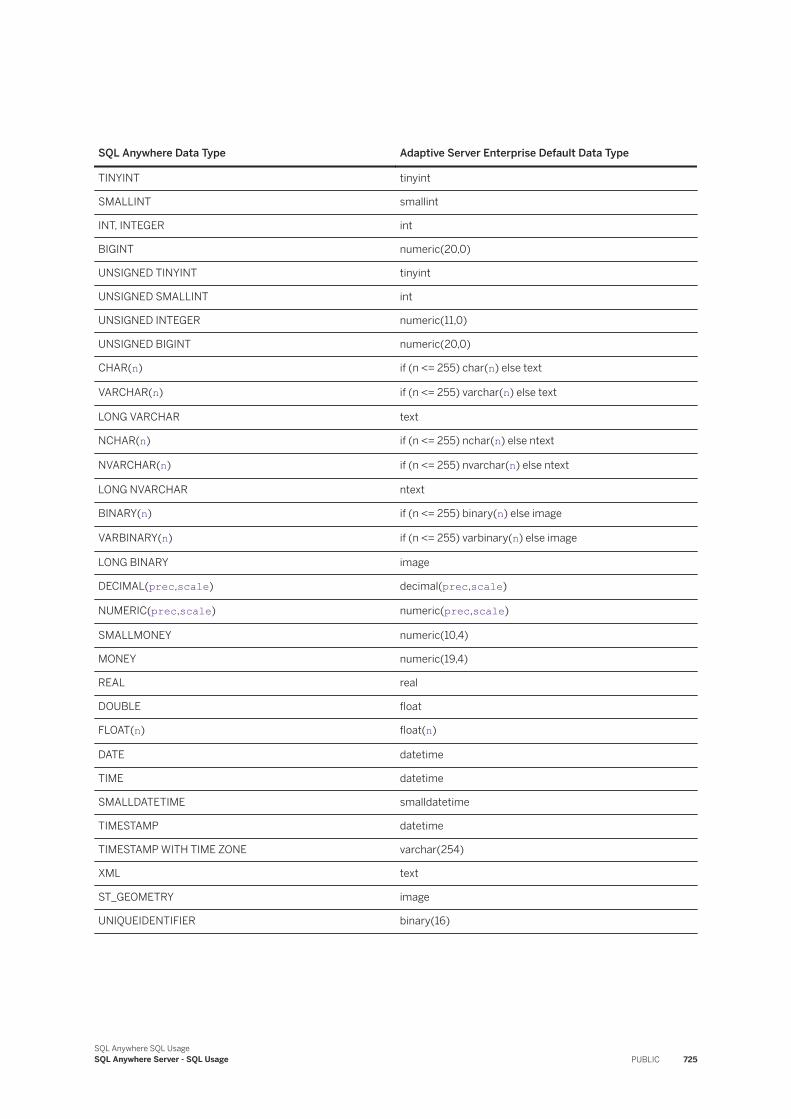
SQL Anywhere Data Type Adaptive Server Enterprise Default Data Type
TINYINT tinyint
SMALLINT smallint
INT, INTEGER int
BIGINT numeric(20,0)
UNSIGNED TINYINT tinyint
UNSIGNED SMALLINT int
UNSIGNED INTEGER numeric(11,0)
UNSIGNED BIGINT numeric(20,0)
CHAR(n) if (n <= 255) char(n) else text
VARCHAR(n) if (n <= 255) varchar(n) else text
LONG VARCHAR text
NCHAR(n) if (n <= 255) nchar(n) else ntext
NVARCHAR(n) if (n <= 255) nvarchar(n) else ntext
LONG NVARCHAR ntext
BINARY(n) if (n <= 255) binary(n) else image
VARBINARY(n) if (n <= 255) varbinary(n) else image
LONG BINARY image
DECIMAL(prec,scale) decimal(prec,scale)
NUMERIC(prec,scale) numeric(prec,scale)
SMALLMONEY numeric(10,4)
MONEY numeric(19,4)
REAL real
DOUBLE float
FLOAT(n) float(n)
DATE datetime
TIME datetime
SMALLDATETIME smalldatetime
TIMESTAMP datetime
TIMESTAMP WITH TIME ZONE varchar(254)
XML text
ST_GEOMETRY image
UNIQUEIDENTIFIER binary(16)
SQL Anywhere SQL UsageSQL Anywhere Server - SQL Usage PUBLIC 725
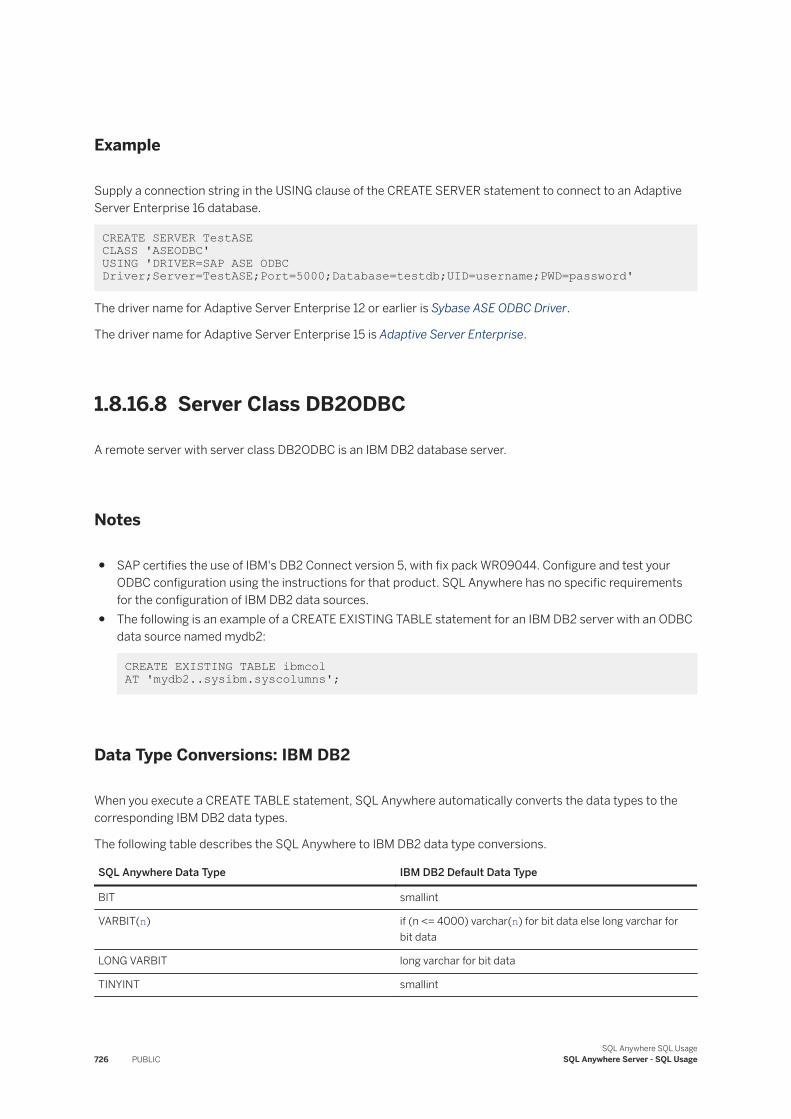
Example
Supply a connection string in the USING clause of the CREATE SERVER statement to connect to an Adaptive Server Enterprise 16 database.
CREATE SERVER TestASE CLASS 'ASEODBC' USING 'DRIVER=SAP ASE ODBC Driver;Server=TestASE;Port=5000;Database=testdb;UID=username;PWD=password'
The driver name for Adaptive Server Enterprise 12 or earlier is Sybase ASE ODBC Driver.
The driver name for Adaptive Server Enterprise 15 is Adaptive Server Enterprise.
1.8.16.8 Server Class DB2ODBC
A remote server with server class DB2ODBC is an IBM DB2 database server.
Notes
● SAP certifies the use of IBM's DB2 Connect version 5, with fix pack WR09044. Configure and test your ODBC configuration using the instructions for that product. SQL Anywhere has no specific requirements for the configuration of IBM DB2 data sources.
● The following is an example of a CREATE EXISTING TABLE statement for an IBM DB2 server with an ODBC data source named mydb2:
CREATE EXISTING TABLE ibmcol AT 'mydb2..sysibm.syscolumns';
Data Type Conversions: IBM DB2
When you execute a CREATE TABLE statement, SQL Anywhere automatically converts the data types to the corresponding IBM DB2 data types.
The following table describes the SQL Anywhere to IBM DB2 data type conversions.
SQL Anywhere Data Type IBM DB2 Default Data Type
BIT smallint
VARBIT(n) if (n <= 4000) varchar(n) for bit data else long varchar for bit data
LONG VARBIT long varchar for bit data
TINYINT smallint
726 PUBLICSQL Anywhere SQL Usage
SQL Anywhere Server - SQL Usage
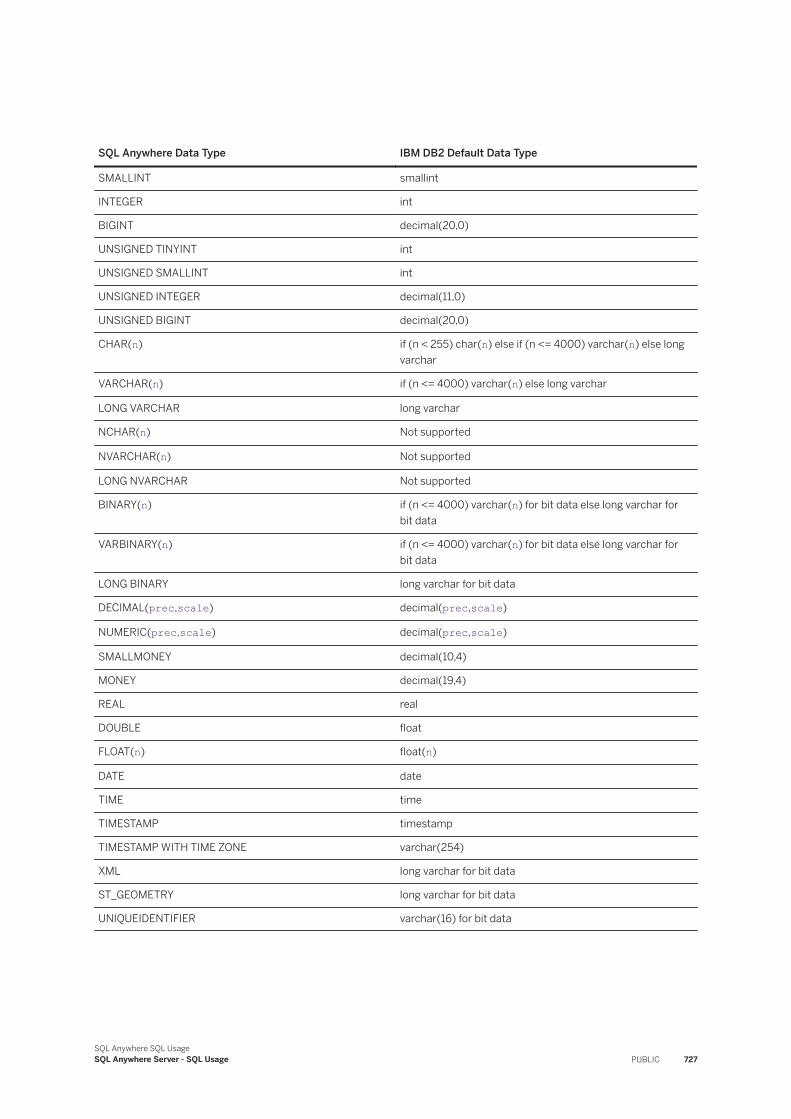
SQL Anywhere Data Type IBM DB2 Default Data Type
SMALLINT smallint
INTEGER int
BIGINT decimal(20,0)
UNSIGNED TINYINT int
UNSIGNED SMALLINT int
UNSIGNED INTEGER decimal(11,0)
UNSIGNED BIGINT decimal(20,0)
CHAR(n) if (n < 255) char(n) else if (n <= 4000) varchar(n) else long varchar
VARCHAR(n) if (n <= 4000) varchar(n) else long varchar
LONG VARCHAR long varchar
NCHAR(n) Not supported
NVARCHAR(n) Not supported
LONG NVARCHAR Not supported
BINARY(n) if (n <= 4000) varchar(n) for bit data else long varchar for bit data
VARBINARY(n) if (n <= 4000) varchar(n) for bit data else long varchar for bit data
LONG BINARY long varchar for bit data
DECIMAL(prec,scale) decimal(prec,scale)
NUMERIC(prec,scale) decimal(prec,scale)
SMALLMONEY decimal(10,4)
MONEY decimal(19,4)
REAL real
DOUBLE float
FLOAT(n) float(n)
DATE date
TIME time
TIMESTAMP timestamp
TIMESTAMP WITH TIME ZONE varchar(254)
XML long varchar for bit data
ST_GEOMETRY long varchar for bit data
UNIQUEIDENTIFIER varchar(16) for bit data
SQL Anywhere SQL UsageSQL Anywhere Server - SQL Usage PUBLIC 727
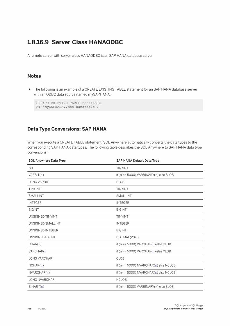
1.8.16.9 Server Class HANAODBC
A remote server with server class HANAODBC is an SAP HANA database server.
Notes
● The following is an example of a CREATE EXISTING TABLE statement for an SAP HANA database server with an ODBC data source named mySAPHANA:
CREATE EXISTING TABLE hanatable AT 'mySAPHANA..dbo.hanatable';
Data Type Conversions: SAP HANA
When you execute a CREATE TABLE statement, SQL Anywhere automatically converts the data types to the corresponding SAP HANA data types. The following table describes the SQL Anywhere to SAP HANA data type conversions.
SQL Anywhere Data Type SAP HANA Default Data Type
BIT TINYINT
VARBIT(n) if (n <= 5000) VARBINARY(n) else BLOB
LONG VARBIT BLOB
TINYINT TINYINT
SMALLINT SMALLINT
INTEGER INTEGER
BIGINT BIGINT
UNSIGNED TINYINT TINYINT
UNSIGNED SMALLINT INTEGER
UNSIGNED INTEGER BIGINT
UNSIGNED BIGINT DECIMAL(20,0)
CHAR(n) if (n <= 5000) VARCHAR(n) else CLOB
VARCHAR(n if (n <= 5000) VARCHAR(n) else CLOB
LONG VARCHAR CLOB
NCHAR(n) if (n <= 5000) NVARCHAR(n) else NCLOB
NVARCHAR(n) if (n <= 5000) NVARCHAR(n) else NCLOB
LONG NVARCHAR NCLOB
BINARY(n) if (n <= 5000) VARBINARY(n) else BLOB
728 PUBLICSQL Anywhere SQL Usage
SQL Anywhere Server - SQL Usage
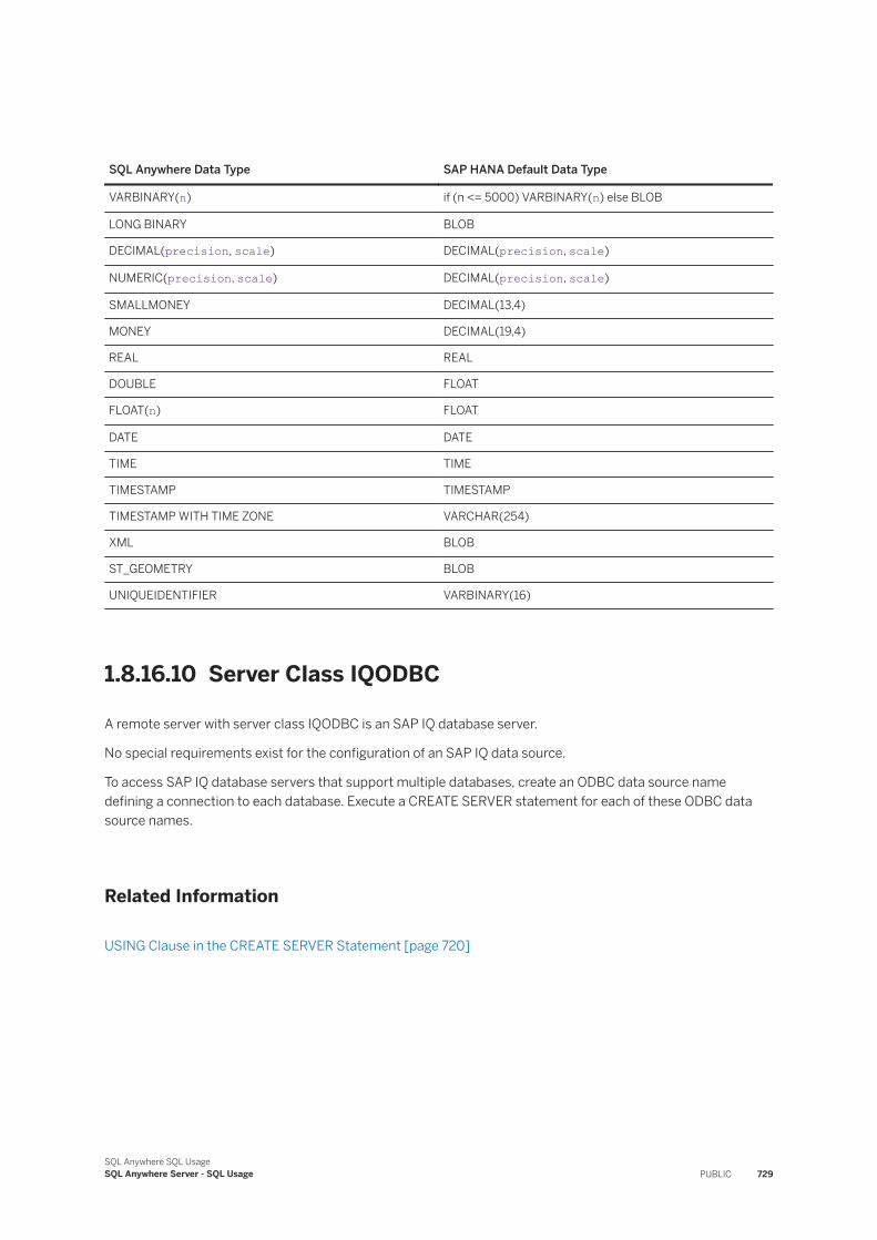
SQL Anywhere Data Type SAP HANA Default Data Type
VARBINARY(n) if (n <= 5000) VARBINARY(n) else BLOB
LONG BINARY BLOB
DECIMAL(precision, scale) DECIMAL(precision, scale)
NUMERIC(precision, scale) DECIMAL(precision, scale)
SMALLMONEY DECIMAL(13,4)
MONEY DECIMAL(19,4)
REAL REAL
DOUBLE FLOAT
FLOAT(n) FLOAT
DATE DATE
TIME TIME
TIMESTAMP TIMESTAMP
TIMESTAMP WITH TIME ZONE VARCHAR(254)
XML BLOB
ST_GEOMETRY BLOB
UNIQUEIDENTIFIER VARBINARY(16)
1.8.16.10 Server Class IQODBC
A remote server with server class IQODBC is an SAP IQ database server.
No special requirements exist for the configuration of an SAP IQ data source.
To access SAP IQ database servers that support multiple databases, create an ODBC data source name defining a connection to each database. Execute a CREATE SERVER statement for each of these ODBC data source names.
Related Information
USING Clause in the CREATE SERVER Statement [page 720]
SQL Anywhere SQL UsageSQL Anywhere Server - SQL Usage PUBLIC 729

1.8.16.11 Server Class MSACCESSODBC
Microsoft Access databases are stored in a .mdb file. Using the ODBC manager, create an ODBC data source and map it to one of these files.
A new .mdb file can be created through the ODBC manager. This database file becomes the default if you don't specify a different default when you create a table through SQL Anywhere.
Assuming an ODBC data source named access, you can use any of the following statements to access data:
● CREATE TABLE tab1 (a int, b char(10)) AT 'access...tab1';
● CREATE TABLE tab1 (a int, b char(10)) AT 'access;d:\\pcdb\\data.mdb;;tab1';
● CREATE EXISTING TABLE tab1 AT 'access;d:\\pcdb\\data.mdb;;tab1';
Microsoft Access does not support the owner name qualification; leave it empty.
Data Type Conversions: Microsoft Access
SQL Anywhere Data Type Microsoft Access Default Data Type
BIT TINYINT
VARBIT(n) if (n <= 4000) BINARY(n) else IMAGE
LONG VARBIT IMAGE
TINYINT TINYINT
SMALLINT SMALLINT
INTEGER INTEGER
BIGINT DECIMAL(19,0)
UNSIGNED TINYINT TINYINT
UNSIGNED SMALLINT INTEGER
UNSIGNED INTEGER DECIMAL(11,0)
UNSIGNED BIGINT DECIMAL(20,0)
CHAR(n) if (n < 255) CHARACTER(n) else TEXT
VARCHAR(n) if (n < 255) CHARACTER(n) else TEXT
LONG VARCHAR TEXT
NCHAR(n) Not supported
NVARCHAR(n) Not supported
LONG NVARCHAR Not supported
730 PUBLICSQL Anywhere SQL Usage
SQL Anywhere Server - SQL Usage
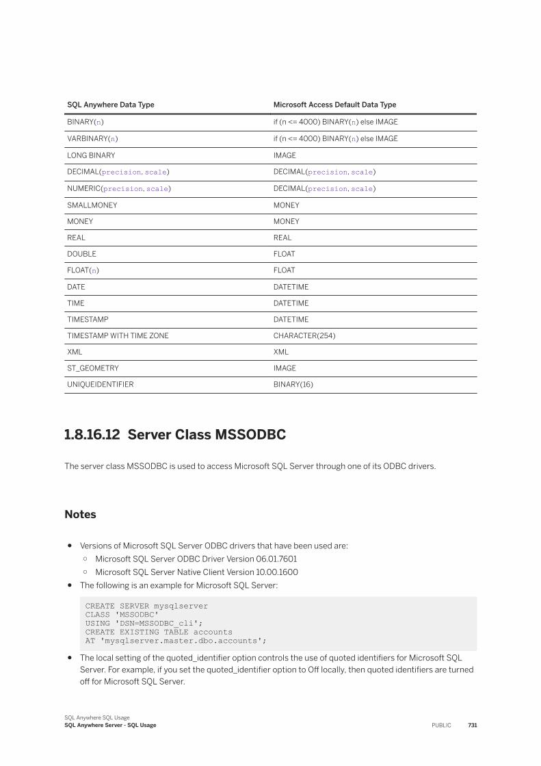
SQL Anywhere Data Type Microsoft Access Default Data Type
BINARY(n) if (n <= 4000) BINARY(n) else IMAGE
VARBINARY(n) if (n <= 4000) BINARY(n) else IMAGE
LONG BINARY IMAGE
DECIMAL(precision, scale) DECIMAL(precision, scale)
NUMERIC(precision, scale) DECIMAL(precision, scale)
SMALLMONEY MONEY
MONEY MONEY
REAL REAL
DOUBLE FLOAT
FLOAT(n) FLOAT
DATE DATETIME
TIME DATETIME
TIMESTAMP DATETIME
TIMESTAMP WITH TIME ZONE CHARACTER(254)
XML XML
ST_GEOMETRY IMAGE
UNIQUEIDENTIFIER BINARY(16)
1.8.16.12 Server Class MSSODBC
The server class MSSODBC is used to access Microsoft SQL Server through one of its ODBC drivers.
Notes
● Versions of Microsoft SQL Server ODBC drivers that have been used are:○ Microsoft SQL Server ODBC Driver Version 06.01.7601○ Microsoft SQL Server Native Client Version 10.00.1600
● The following is an example for Microsoft SQL Server:
CREATE SERVER mysqlserver CLASS 'MSSODBC'USING 'DSN=MSSODBC_cli';CREATE EXISTING TABLE accounts AT 'mysqlserver.master.dbo.accounts';
● The local setting of the quoted_identifier option controls the use of quoted identifiers for Microsoft SQL Server. For example, if you set the quoted_identifier option to Off locally, then quoted identifiers are turned off for Microsoft SQL Server.
SQL Anywhere SQL UsageSQL Anywhere Server - SQL Usage PUBLIC 731
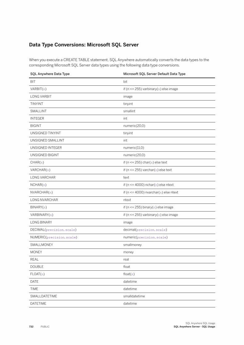
Data Type Conversions: Microsoft SQL Server
When you execute a CREATE TABLE statement, SQL Anywhere automatically converts the data types to the corresponding Microsoft SQL Server data types using the following data type conversions.
SQL Anywhere Data Type Microsoft SQL Server Default Data Type
BIT bit
VARBIT(n) if (n <= 255) varbinary(n) else image
LONG VARBIT image
TINYINT tinyint
SMALLINT smallint
INTEGER int
BIGINT numeric(20,0)
UNSIGNED TINYINT tinyint
UNSIGNED SMALLINT int
UNSIGNED INTEGER numeric(11,0)
UNSIGNED BIGINT numeric(20,0)
CHAR(n) if (n <= 255) char(n) else text
VARCHAR(n) if (n <= 255) varchar(n) else text
LONG VARCHAR text
NCHAR(n) if (n <= 4000) nchar(n) else ntext
NVARCHAR(n) if (n <= 4000) nvarchar(n) else ntext
LONG NVARCHAR ntext
BINARY(n) if (n <= 255) binary(n) else image
VARBINARY(n) if (n <= 255) varbinary(n) else image
LONG BINARY image
DECIMAL(precision, scale) decimal(precision, scale)
NUMERIC(precision, scale) numeric(precision, scale)
SMALLMONEY smallmoney
MONEY money
REAL real
DOUBLE float
FLOAT(n) float(n)
DATE datetime
TIME datetime
SMALLDATETIME smalldatetime
DATETIME datetime
732 PUBLICSQL Anywhere SQL Usage
SQL Anywhere Server - SQL Usage
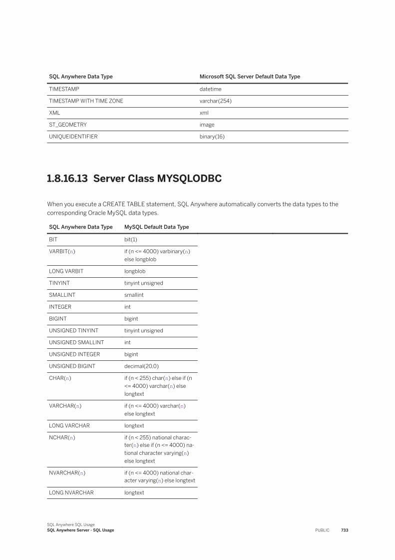
SQL Anywhere Data Type Microsoft SQL Server Default Data Type
TIMESTAMP datetime
TIMESTAMP WITH TIME ZONE varchar(254)
XML xml
ST_GEOMETRY image
UNIQUEIDENTIFIER binary(16)
1.8.16.13 Server Class MYSQLODBC
When you execute a CREATE TABLE statement, SQL Anywhere automatically converts the data types to the corresponding Oracle MySQL data types.
SQL Anywhere Data Type MySQL Default Data Type
BIT bit(1)
VARBIT(n) if (n <= 4000) varbinary(n) else longblob
LONG VARBIT longblob
TINYINT tinyint unsigned
SMALLINT smallint
INTEGER int
BIGINT bigint
UNSIGNED TINYINT tinyint unsigned
UNSIGNED SMALLINT int
UNSIGNED INTEGER bigint
UNSIGNED BIGINT decimal(20,0)
CHAR(n) if (n < 255) char(n) else if (n <= 4000) varchar(n) else longtext
VARCHAR(n) if (n <= 4000) varchar(n) else longtext
LONG VARCHAR longtext
NCHAR(n) if (n < 255) national character(n) else if (n <= 4000) national character varying(n) else longtext
NVARCHAR(n) if (n <= 4000) national character varying(n) else longtext
LONG NVARCHAR longtext
SQL Anywhere SQL UsageSQL Anywhere Server - SQL Usage PUBLIC 733
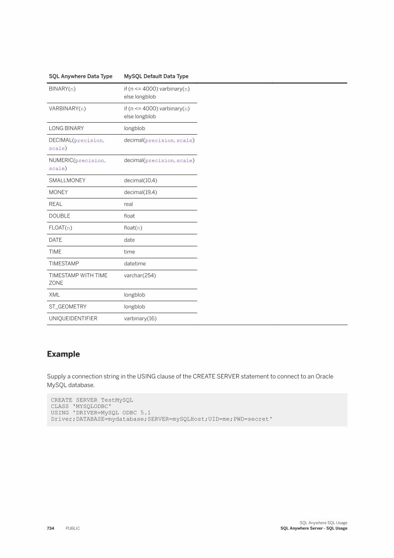
SQL Anywhere Data Type MySQL Default Data Type
BINARY(n) if (n <= 4000) varbinary(n) else longblob
VARBINARY(n) if (n <= 4000) varbinary(n) else longblob
LONG BINARY longblob
DECIMAL(precision, scale)
decimal(precision, scale)
NUMERIC(precision, scale)
decimal(precision, scale)
SMALLMONEY decimal(10,4)
MONEY decimal(19,4)
REAL real
DOUBLE float
FLOAT(n) float(n)
DATE date
TIME time
TIMESTAMP datetime
TIMESTAMP WITH TIME ZONE
varchar(254)
XML longblob
ST_GEOMETRY longblob
UNIQUEIDENTIFIER varbinary(16)
Example
Supply a connection string in the USING clause of the CREATE SERVER statement to connect to an Oracle MySQL database.
CREATE SERVER TestMySQL CLASS 'MYSQLODBC' USING 'DRIVER=MySQL ODBC 5.1 Driver;DATABASE=mydatabase;SERVER=mySQLHost;UID=me;PWD=secret'
734 PUBLICSQL Anywhere SQL Usage
SQL Anywhere Server - SQL Usage
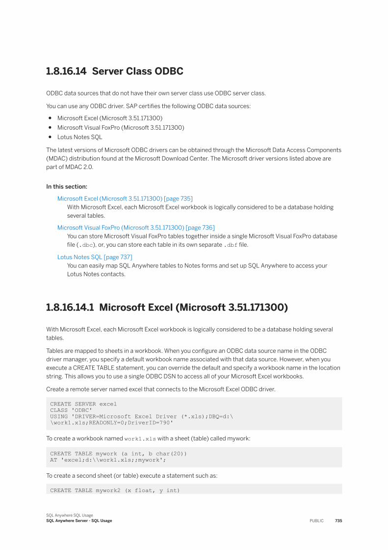
1.8.16.14 Server Class ODBC
ODBC data sources that do not have their own server class use ODBC server class.
You can use any ODBC driver. SAP certifies the following ODBC data sources:
● Microsoft Excel (Microsoft 3.51.171300)● Microsoft Visual FoxPro (Microsoft 3.51.171300)● Lotus Notes SQL
The latest versions of Microsoft ODBC drivers can be obtained through the Microsoft Data Access Components (MDAC) distribution found at the Microsoft Download Center. The Microsoft driver versions listed above are part of MDAC 2.0.
In this section:
Microsoft Excel (Microsoft 3.51.171300) [page 735]With Microsoft Excel, each Microsoft Excel workbook is logically considered to be a database holding several tables.
Microsoft Visual FoxPro (Microsoft 3.51.171300) [page 736]You can store Microsoft Visual FoxPro tables together inside a single Microsoft Visual FoxPro database file (.dbc), or, you can store each table in its own separate .dbf file.
Lotus Notes SQL [page 737]You can easily map SQL Anywhere tables to Notes forms and set up SQL Anywhere to access your Lotus Notes contacts.
1.8.16.14.1 Microsoft Excel (Microsoft 3.51.171300)
With Microsoft Excel, each Microsoft Excel workbook is logically considered to be a database holding several tables.
Tables are mapped to sheets in a workbook. When you configure an ODBC data source name in the ODBC driver manager, you specify a default workbook name associated with that data source. However, when you execute a CREATE TABLE statement, you can override the default and specify a workbook name in the location string. This allows you to use a single ODBC DSN to access all of your Microsoft Excel workbooks.
Create a remote server named excel that connects to the Microsoft Excel ODBC driver.
CREATE SERVER excel CLASS 'ODBC' USING 'DRIVER=Microsoft Excel Driver (*.xls);DBQ=d:\\work1.xls;READONLY=0;DriverID=790'
To create a workbook named work1.xls with a sheet (table) called mywork:
CREATE TABLE mywork (a int, b char(20)) AT 'excel;d:\\work1.xls;;mywork';
To create a second sheet (or table) execute a statement such as:
CREATE TABLE mywork2 (x float, y int)
SQL Anywhere SQL UsageSQL Anywhere Server - SQL Usage PUBLIC 735
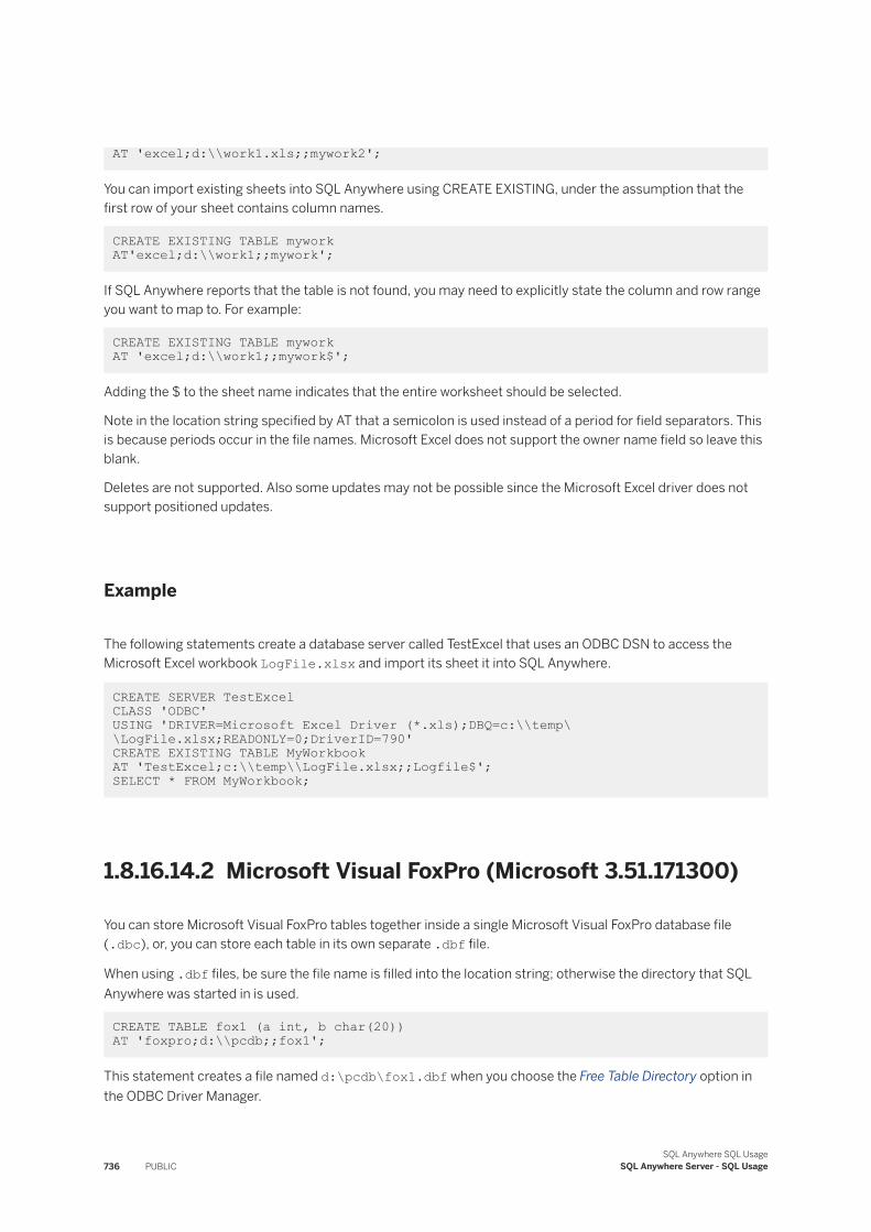
AT 'excel;d:\\work1.xls;;mywork2';
You can import existing sheets into SQL Anywhere using CREATE EXISTING, under the assumption that the first row of your sheet contains column names.
CREATE EXISTING TABLE mywork AT'excel;d:\\work1;;mywork';
If SQL Anywhere reports that the table is not found, you may need to explicitly state the column and row range you want to map to. For example:
CREATE EXISTING TABLE mywork AT 'excel;d:\\work1;;mywork$';
Adding the $ to the sheet name indicates that the entire worksheet should be selected.
Note in the location string specified by AT that a semicolon is used instead of a period for field separators. This is because periods occur in the file names. Microsoft Excel does not support the owner name field so leave this blank.
Deletes are not supported. Also some updates may not be possible since the Microsoft Excel driver does not support positioned updates.
Example
The following statements create a database server called TestExcel that uses an ODBC DSN to access the Microsoft Excel workbook LogFile.xlsx and import its sheet it into SQL Anywhere.
CREATE SERVER TestExcel CLASS 'ODBC'USING 'DRIVER=Microsoft Excel Driver (*.xls);DBQ=c:\\temp\\LogFile.xlsx;READONLY=0;DriverID=790'CREATE EXISTING TABLE MyWorkbookAT 'TestExcel;c:\\temp\\LogFile.xlsx;;Logfile$'; SELECT * FROM MyWorkbook;
1.8.16.14.2 Microsoft Visual FoxPro (Microsoft 3.51.171300)
You can store Microsoft Visual FoxPro tables together inside a single Microsoft Visual FoxPro database file (.dbc), or, you can store each table in its own separate .dbf file.
When using .dbf files, be sure the file name is filled into the location string; otherwise the directory that SQL Anywhere was started in is used.
CREATE TABLE fox1 (a int, b char(20)) AT 'foxpro;d:\\pcdb;;fox1';
This statement creates a file named d:\pcdb\fox1.dbf when you choose the Free Table Directory option in the ODBC Driver Manager.
736 PUBLICSQL Anywhere SQL Usage
SQL Anywhere Server - SQL Usage
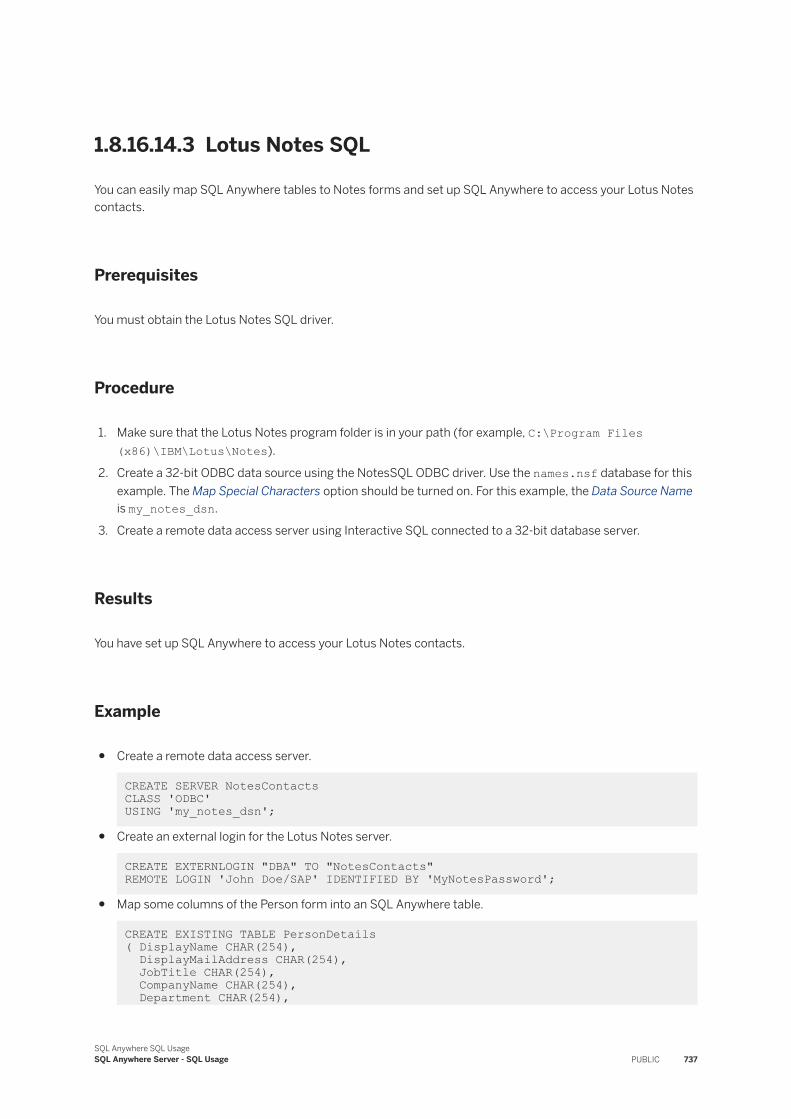
1.8.16.14.3 Lotus Notes SQL
You can easily map SQL Anywhere tables to Notes forms and set up SQL Anywhere to access your Lotus Notes contacts.
Prerequisites
You must obtain the Lotus Notes SQL driver.
Procedure
1. Make sure that the Lotus Notes program folder is in your path (for example, C:\Program Files (x86)\IBM\Lotus\Notes).
2. Create a 32-bit ODBC data source using the NotesSQL ODBC driver. Use the names.nsf database for this example. The Map Special Characters option should be turned on. For this example, the Data Source Name is my_notes_dsn.
3. Create a remote data access server using Interactive SQL connected to a 32-bit database server.
Results
You have set up SQL Anywhere to access your Lotus Notes contacts.
Example
● Create a remote data access server.
CREATE SERVER NotesContacts CLASS 'ODBC' USING 'my_notes_dsn';
● Create an external login for the Lotus Notes server.
CREATE EXTERNLOGIN "DBA" TO "NotesContacts" REMOTE LOGIN 'John Doe/SAP' IDENTIFIED BY 'MyNotesPassword';
● Map some columns of the Person form into an SQL Anywhere table.
CREATE EXISTING TABLE PersonDetails ( DisplayName CHAR(254), DisplayMailAddress CHAR(254), JobTitle CHAR(254), CompanyName CHAR(254), Department CHAR(254),
SQL Anywhere SQL UsageSQL Anywhere Server - SQL Usage PUBLIC 737
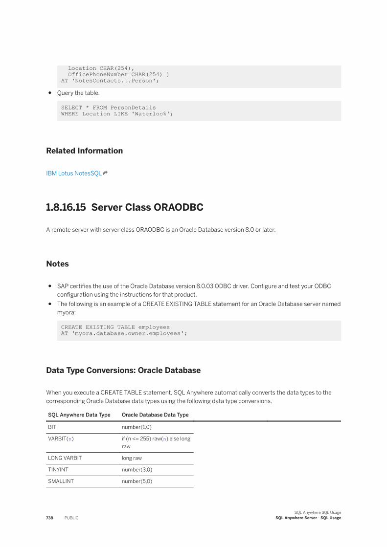
Location CHAR(254), OfficePhoneNumber CHAR(254) ) AT 'NotesContacts...Person';
● Query the table.
SELECT * FROM PersonDetails WHERE Location LIKE 'Waterloo%';
Related Information
IBM Lotus NotesSQL
1.8.16.15 Server Class ORAODBC
A remote server with server class ORAODBC is an Oracle Database version 8.0 or later.
Notes
● SAP certifies the use of the Oracle Database version 8.0.03 ODBC driver. Configure and test your ODBC configuration using the instructions for that product.
● The following is an example of a CREATE EXISTING TABLE statement for an Oracle Database server named myora:
CREATE EXISTING TABLE employees AT 'myora.database.owner.employees';
Data Type Conversions: Oracle Database
When you execute a CREATE TABLE statement, SQL Anywhere automatically converts the data types to the corresponding Oracle Database data types using the following data type conversions.
SQL Anywhere Data Type Oracle Database Data Type
BIT number(1,0)
VARBIT(n) if (n <= 255) raw(n) else long raw
LONG VARBIT long raw
TINYINT number(3,0)
SMALLINT number(5,0)
738 PUBLICSQL Anywhere SQL Usage
SQL Anywhere Server - SQL Usage
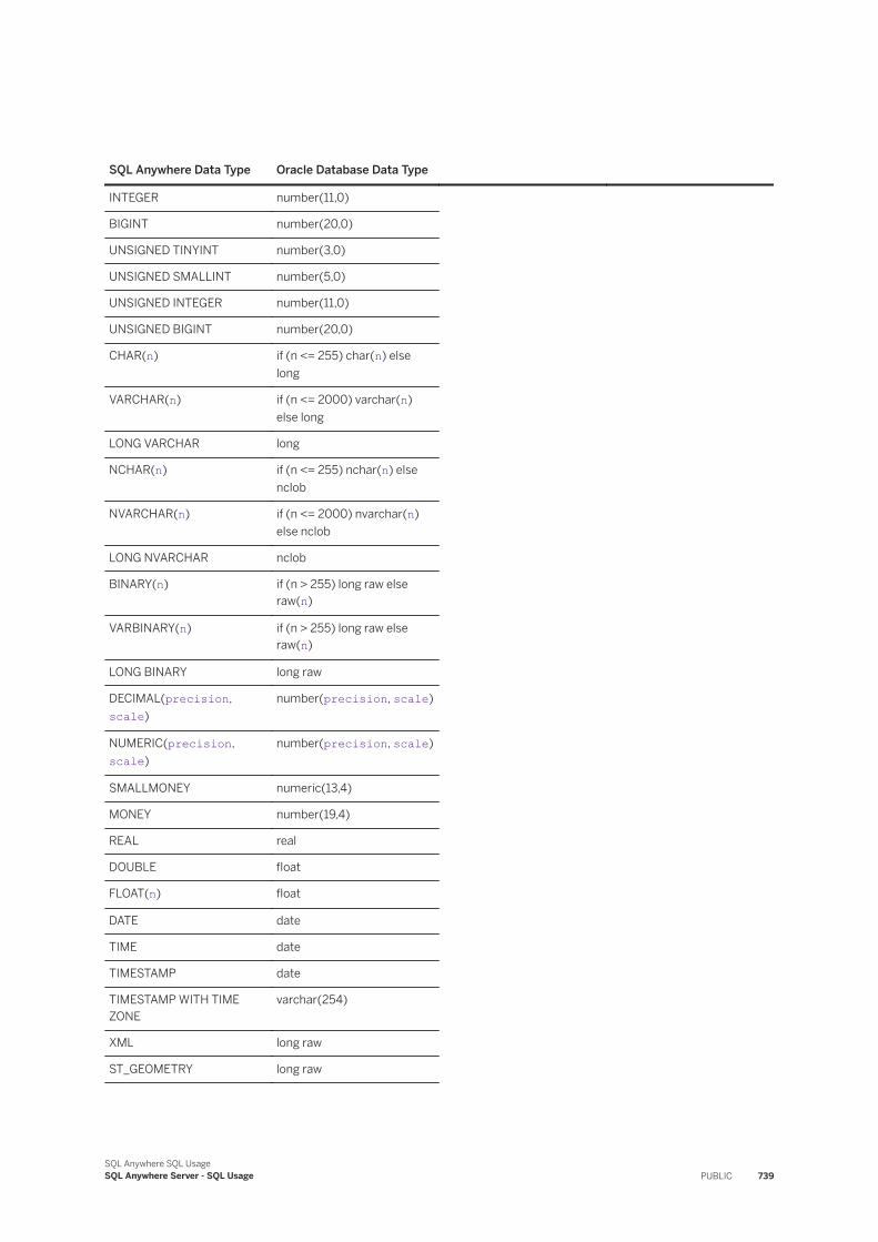
SQL Anywhere Data Type Oracle Database Data Type
INTEGER number(11,0)
BIGINT number(20,0)
UNSIGNED TINYINT number(3,0)
UNSIGNED SMALLINT number(5,0)
UNSIGNED INTEGER number(11,0)
UNSIGNED BIGINT number(20,0)
CHAR(n) if (n <= 255) char(n) else long
VARCHAR(n) if (n <= 2000) varchar(n) else long
LONG VARCHAR long
NCHAR(n) if (n <= 255) nchar(n) else nclob
NVARCHAR(n) if (n <= 2000) nvarchar(n) else nclob
LONG NVARCHAR nclob
BINARY(n) if (n > 255) long raw else raw(n)
VARBINARY(n) if (n > 255) long raw else raw(n)
LONG BINARY long raw
DECIMAL(precision, scale)
number(precision, scale)
NUMERIC(precision, scale)
number(precision, scale)
SMALLMONEY numeric(13,4)
MONEY number(19,4)
REAL real
DOUBLE float
FLOAT(n) float
DATE date
TIME date
TIMESTAMP date
TIMESTAMP WITH TIME ZONE
varchar(254)
XML long raw
ST_GEOMETRY long raw
SQL Anywhere SQL UsageSQL Anywhere Server - SQL Usage PUBLIC 739
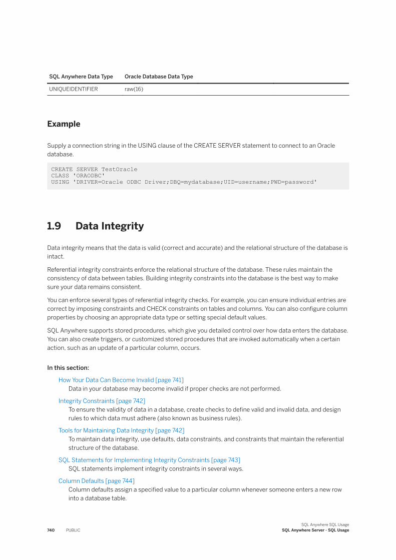
SQL Anywhere Data Type Oracle Database Data Type
UNIQUEIDENTIFIER raw(16)
Example
Supply a connection string in the USING clause of the CREATE SERVER statement to connect to an Oracle database.
CREATE SERVER TestOracle CLASS 'ORAODBC' USING 'DRIVER=Oracle ODBC Driver;DBQ=mydatabase;UID=username;PWD=password'
1.9 Data Integrity
Data integrity means that the data is valid (correct and accurate) and the relational structure of the database is intact.
Referential integrity constraints enforce the relational structure of the database. These rules maintain the consistency of data between tables. Building integrity constraints into the database is the best way to make sure your data remains consistent.
You can enforce several types of referential integrity checks. For example, you can ensure individual entries are correct by imposing constraints and CHECK constraints on tables and columns. You can also configure column properties by choosing an appropriate data type or setting special default values.
SQL Anywhere supports stored procedures, which give you detailed control over how data enters the database. You can also create triggers, or customized stored procedures that are invoked automatically when a certain action, such as an update of a particular column, occurs.
In this section:
How Your Data Can Become Invalid [page 741]Data in your database may become invalid if proper checks are not performed.
Integrity Constraints [page 742]To ensure the validity of data in a database, create checks to define valid and invalid data, and design rules to which data must adhere (also known as business rules).
Tools for Maintaining Data Integrity [page 742]To maintain data integrity, use defaults, data constraints, and constraints that maintain the referential structure of the database.
SQL Statements for Implementing Integrity Constraints [page 743]SQL statements implement integrity constraints in several ways.
Column Defaults [page 744]Column defaults assign a specified value to a particular column whenever someone enters a new row into a database table.
740 PUBLICSQL Anywhere SQL Usage
SQL Anywhere Server - SQL Usage
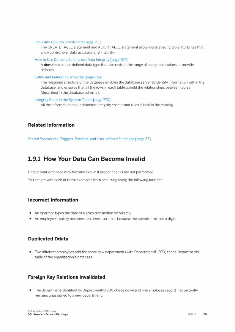
Table and Column Constraints [page 751]The CREATE TABLE statement and ALTER TABLE statement allow you to specify table attributes that allow control over data accuracy and integrity.
How to Use Domains to Improve Data Integrity [page 757]A domain is a user-defined data type that can restrict the range of acceptable values or provide defaults.
Entity and Referential Integrity [page 759]The relational structure of the database enables the database server to identify information within the database, and ensures that all the rows in each table uphold the relationships between tables (described in the database schema).
Integrity Rules in the System Tables [page 770]All the information about database integrity checks and rules is held in the catalog.
Related Information
Stored Procedures, Triggers, Batches, and User-defined Functions [page 87]
1.9.1 How Your Data Can Become Invalid
Data in your database may become invalid if proper checks are not performed.
You can prevent each of these examples from occurring using the following facilities.
Incorrect Information
● An operator types the date of a sales transaction incorrectly.● An employee's salary becomes ten times too small because the operator missed a digit.
Duplicated Ddata
● Two different employees add the same new department (with DepartmentID 200) to the Departments table of the organization's database.
Foreign Key Relations Invalidated
● The department identified by DepartmentID 300 closes down and one employee record inadvertently remains unassigned to a new department.
SQL Anywhere SQL UsageSQL Anywhere Server - SQL Usage PUBLIC 741
1.9.2 Integrity Constraints
To ensure the validity of data in a database, create checks to define valid and invalid data, and design rules to which data must adhere (also known as business rules).
Typically, business rules are implemented through check constraints, user-defined data types, and the appropriate use of transactions.
Constraints that are built into the database are more reliable than constraints that are built into client applications or that are provided as instructions to database users. Constraints built into the database become part of the definition of the database itself, and the database enforces them consistently across all applications. Setting a constraint once in the database imposes it for all subsequent interactions with the database.
In contrast, constraints built into client applications are vulnerable every time the software changes, and may need to be imposed in several applications, or in several places in a single client application.
1.9.3 Tools for Maintaining Data Integrity
To maintain data integrity, use defaults, data constraints, and constraints that maintain the referential structure of the database.
Defaults
You can assign default values to columns to make certain kinds of data entry more reliable. For example:
● A column can have a CURRENT DATE default value for recording the date of transactions with any user or client application action.
● Other types of default values allow column values to increment automatically without any specific user action other than entering a new row. With this feature, you can guarantee that items (such as purchase orders for example) are unique, sequential numbers.
Primary Keys
Primary keys guarantee that every row of a given table can be uniquely identified in the table.
Table and Column Constraints
The following constrains maintain the structure of data in the database, and define the relationship between tables in a relational database:
Referential constraints
742 PUBLICSQL Anywhere SQL Usage
SQL Anywhere Server - SQL Usage
Data integrity is also maintained using referential constraints, also called RI constraints (for referential integrity constraints). RI constraints are data rules that are set on columns and tables to control what the data can be. RI constraints define the relationship between tables in a relational database.NOT NULL constraint
A NOT NULL constraint prevents a column from containing a NULL entry.CHECK constraint
A CHECK constraint assigned to a column can ensure that every item in the column meets a particular condition. For example, you can ensure that Salary column entries fit within a specified range and are protected from user error when new values are entered.
CHECK constraints can be made on the relative values in different columns. For example, you can ensure that a DateReturned entry is later than a DateBorrowed entry in a library database.
Column constraints can be inherited from domains.
Triggers for Advanced Integrity Rules
A trigger is a procedure stored in the database and executed automatically whenever the information in a specified table changes. Triggers are a powerful mechanism for database administrators and developers to ensure that data remains reliable. You can also use triggers to maintain data integrity. Triggers can enforce more sophisticated CHECK conditions.
Related Information
Column Defaults [page 744]Primary Keys [page 25]Entity and Referential Integrity [page 759]Table and Column Constraints [page 751]Stored Procedures, Triggers, Batches, and User-defined Functions [page 87]
1.9.4 SQL Statements for Implementing Integrity Constraints
SQL statements implement integrity constraints in several ways.
CREATE TABLE statement
This statement implements integrity constraints during creation of the table.ALTER TABLE statement
This statement adds integrity constraints to an existing table, or modifies constraints for an existing table.CREATE TRIGGER statement
This statement creates triggers that enforce more complex business rules.
SQL Anywhere SQL UsageSQL Anywhere Server - SQL Usage PUBLIC 743
CREATE DOMAIN statement
This statement creates a user-defined data type. The definition of the data type can include constraints.
1.9.5 Column Defaults
Column defaults assign a specified value to a particular column whenever someone enters a new row into a database table.
The default value assigned requires no action on the part of the client application, however if the client application does specify a value for the column, the new value overrides the column default value.
Column defaults can quickly and automatically fill columns with information, such as the date or time a row is inserted, or the user ID of the person entering the information. Using column defaults encourages data integrity, but does not enforce it. Client applications can always override defaults.
When default values are defined using variables that start with @, the value used for the default is value of the variable at the moment the DML or LOAD statement is executed.
Supported Default Values
SQL supports the following default values:
● A string specified in the CREATE TABLE statement or ALTER TABLE statement.● A number specified in the CREATE TABLE statement or ALTER TABLE statement.● AUTOINCREMENT: an automatically incremented number that is one more than the previous highest value
in the column.● GLOBAL AUTOINCREMENT, which ensures unique primary keys across multiple databases.● Universally Unique Identifiers (UUIDs) generated using the NEWID function.● CURRENT DATE, TIME, or TIMESTAMP.● CURRENT SERVER DATE, CURRENT SERVER TIME, or CURRENT SERVER TIMESTAMP● The CURRENT USER of the database user.● A NULL value.● A constant expression, as long as it does not reference database objects.
In this section:
Creation of Column Defaults [page 745]You can use the CREATE TABLE statement to create column defaults at the time a table is created, or the ALTER TABLE statement to add column defaults at a later time.
Alteration of Column Defaults [page 746]You can change or remove column defaults using the same form of the ALTER TABLE statement you used to create the defaults.
Current Date and Time Defaults [page 747]For columns of DATE, TIME, or TIMESTAMP data type, you can use CURRENT DATE, CURRENT TIME, or CURRENT TIMESTAMP as a default.
744 PUBLICSQL Anywhere SQL Usage
SQL Anywhere Server - SQL Usage
The User ID Defaults [page 748]Assigning a DEFAULT USER to a column is a reliable way of identifying the person making an entry in a database.
The AUTOINCREMENT Default [page 748]The AUTOINCREMENT default is useful for numeric data fields where the value of the number itself may have no meaning.
The GLOBAL AUTOINCREMENT Default [page 749]The GLOBAL AUTOINCREMENT default is intended for use when multiple databases are used in a SQL Remote replication or MobiLink synchronization environment.
The NEWID Default [page 750]Universally Unique Identifiers (UUIDs), also known as Globally Unique Identifiers (GUIDs), can be used to identify unique rows in a table.
The NULL Default [page 750]For columns that allow NULL values, specifying a NULL default is the same as not specifying a default. If the client inserting the row does not assign a value, the row receives A NULL value.
String and Number Defaults [page 751]You can specify a specific string or number as a default value, as long as the column has a string or numeric data type.
Constant Expression Defaults [page 751]You can use a constant expression as a default value, as long as it does not reference database objects.
1.9.5.1 Creation of Column Defaults
You can use the CREATE TABLE statement to create column defaults at the time a table is created, or the ALTER TABLE statement to add column defaults at a later time.
Example
The following statement adds a default to an existing column named ID in the SalesOrders table, so that it automatically increments (unless a client application specifies a value). In the SQL Anywhere sample database, this column is already set to AUTOINCREMENT.
ALTER TABLE SalesOrders ALTER ID DEFAULT AUTOINCREMENT;
SQL Anywhere SQL UsageSQL Anywhere Server - SQL Usage PUBLIC 745
1.9.5.2 Alteration of Column Defaults
You can change or remove column defaults using the same form of the ALTER TABLE statement you used to create the defaults.
The following statement changes the default value of a column named OrderDate from its current setting to CURRENT DATE:
ALTER TABLE SalesOrders ALTER OrderDate DEFAULT CURRENT DATE;
You can remove column defaults by modifying them to be NULL. The following statement removes the default from the OrderDate column:
ALTER TABLE SalesOrders ALTER OrderDate DEFAULT NULL;
In this section:
Working with Column Defaults [page 746]Add, alter, and drop column defaults in SQL Central using the Value tab of the Column Properties window.
1.9.5.2.1 Working with Column Defaults
Add, alter, and drop column defaults in SQL Central using the Value tab of the Column Properties window.
Prerequisites
You must be the owner of the table the column belongs to, or have one of the following privileges:
● ALTER privilege on the table● ALTER ANY TABLE system privilege● ALTER ANY OBJECT system privilege
Procedure
1. In SQL Central, use the SQL Anywhere 17 plug-in to connect to the database.2. In the left pane, double-click Tables.3. Double-click the table.4. Click the Columns tab.5. Right-click the column and click Properties.
746 PUBLICSQL Anywhere SQL Usage
SQL Anywhere Server - SQL Usage
6. Click the Value tab.7. Alter the column defaults as needed.
Results
The column properties are altered.
1.9.5.3 Current Date and Time Defaults
For columns of DATE, TIME, or TIMESTAMP data type, you can use CURRENT DATE, CURRENT TIME, or CURRENT TIMESTAMP as a default.
The default you choose must be compatible with the column's data type.
Useful Examples of the CURRENT DATE Default
The CURRENT DATE default might be useful to record:
● dates of phone calls in a contacts database● dates of orders in a sales entry database● the date a patron borrows a book in a library database
CURRENT TIMESTAMP
The CURRENT TIMESTAMP default is similar to the CURRENT DATE default, but offers greater accuracy. For example, a user of a contact management application may have several interactions with a single customer in one day: the CURRENT TIMESTAMP default would be useful to distinguish these contacts.
Since it records a date and the time down to a precision of millionths of a second, you may also find CURRENT TIMESTAMP useful when the sequence of events is important in a database.
DEFAULT TIMESTAMP
DEFAULT TIMESTAMP provides a way of indicating when each row in the table was last modified. When a column is declared with DEFAULT TIMESTAMP, a default value is provided for inserts, and the value is updated with the current date and time whenever the row is updated. To provide a default value on insert, but not update the column whenever the row is updated, use DEFAULT CURRENT TIMESTAMP instead of DEFAULT TIMESTAMP.
SQL Anywhere SQL UsageSQL Anywhere Server - SQL Usage PUBLIC 747
1.9.5.4 The User ID Defaults
Assigning a DEFAULT USER to a column is a reliable way of identifying the person making an entry in a database.
This information may be required; for example, when salespeople are working on commission.
Building a user ID default into the primary key of a table is a useful technique for occasionally connected users, and helps to prevent conflicts during information updates. These users can make a copy of tables relevant to their work on a portable computer, make changes while not connected to a multi-user database, and then apply the transaction log to the server when they return.
The LAST USER special value specifies the name of the user who last modified the row. When combined with the DEFAULT TIMESTAMP, a default value of LAST USER can be used to record (in separate columns) both the user and the date and time a row was last changed.
1.9.5.5 The AUTOINCREMENT Default
The AUTOINCREMENT default is useful for numeric data fields where the value of the number itself may have no meaning.
The feature assigns each new row a unique value larger than any other value in the column. You can use AUTOINCREMENT columns to record purchase order numbers, to identify customer service calls or other entries where an identifying number is required.
AUTOINCREMENT columns are typically primary key columns or columns constrained to hold unique values.
You can retrieve the most recent value inserted into an AUTOINCREMENT column using the @@identity global variable.
AUTOINCREMENT and Negative Numbers
AUTOINCREMENT is intended to work with positive integers.
The initial AUTOINCREMENT value is set to 0 when the table is created. This value remains as the highest value assigned when inserts are done that explicitly insert negative values into the column. An insert where no value is supplied causes the AUTOINCREMENT to generate a value of 1, forcing any other generated values to be positive.
AUTOINCREMENT and the IDENTITY Column
A column with the AUTOINCREMENT default is referred to in Transact-SQL applications as an IDENTITY column.
748 PUBLICSQL Anywhere SQL Usage
SQL Anywhere Server - SQL Usage

Related Information
The GLOBAL AUTOINCREMENT Default [page 749]Use of a Sequence to Generate Unique Values [page 845]Entity Integrity [page 760]The Special IDENTITY Column [page 549]
1.9.5.6 The GLOBAL AUTOINCREMENT Default
The GLOBAL AUTOINCREMENT default is intended for use when multiple databases are used in a SQL Remote replication or MobiLink synchronization environment.
It ensures unique primary keys across multiple databases.
This option is similar to AUTOINCREMENT, except that the domain is partitioned. Each partition contains the same number of values. You assign each copy of the database a unique global database identification number. SQL Anywhere supplies default values in a database only from the partition uniquely identified by that database's number.
The partition size can be any positive integer, although the partition size is generally chosen so that the supply of numbers within any one partition will rarely, if ever, be exhausted.
If the column is of type BIGINT or UNSIGNED BIGINT, the default partition size is 232 = 4294967296; for columns of all other types, the default partition size is 216 = 65536. Since these defaults may be inappropriate, especially if your column is not of type INT or BIGINT, it is best to specify the partition size explicitly.
When using this option, the value of the public option global_database_id in each database must be set to a unique, non-negative integer. This value uniquely identifies the database and indicates from which partition default values are to be assigned. The range of allowed values is n p + 1 to (n + 1) p, where n is the value of the public option global_database_id and p is the partition size. For example, if you define the partition size to be 1000 and set global_database_id to 3, then the range is from 3001 to 4000.
If the previous value is less than (n + 1) p, the next default value is one greater than the previous largest value in column. If the column contains no values, the first default value is n p + 1. Default column values are not affected by values in the column outside the current partition; that is, by numbers less than np + 1 or greater than p(n + 1). Such values may be present if they have been replicated from another database via MobiLink synchronization.
Because the public option global_database_id cannot be set to a negative value, the values chosen are always positive. The maximum identification number is restricted only by the column data type and the partition size.
If the public option global_database_id is set to the default value of 2147483647, a NULL value is inserted into the column. If NULL values are not permitted, attempting to insert the row causes an error. This situation arises, for example, if the column is contained in the table's primary key.
NULL default values are also generated when the supply of values within the partition has been exhausted. In this case, a new value of global_database_id should be assigned to the database to allow default values to be chosen from another partition. Attempting to insert the NULL value causes an error if the column does not permit NULLs. To detect that the supply of unused values is low and handle this condition, create an event of type GlobalAutoincrement.
SQL Anywhere SQL UsageSQL Anywhere Server - SQL Usage PUBLIC 749
GLOBAL AUTOINCREMENT columns are typically primary key columns or columns constrained to hold unique values.
While using the GLOBAL AUTOINCREMENT default in other cases is possible, doing so can adversely affect database performance. For example, when the next value for each column is stored as a 64-bit signed integer, using values greater than 231 - 1 or large double or numeric values may cause wraparound to negative values.
You can retrieve the most recent value inserted into an AUTOINCREMENT column using the @@identity global variable.
Related Information
Entity Integrity [page 760]The AUTOINCREMENT Default [page 748]Use of a Sequence to Generate Unique Values [page 845]
1.9.5.7 The NEWID Default
Universally Unique Identifiers (UUIDs), also known as Globally Unique Identifiers (GUIDs), can be used to identify unique rows in a table.
The values are generated such that a value produced on one computer will not match that produced on another. They can therefore be used as keys in replication and synchronization environments.
Using UUID values as primary keys has some tradeoffs when you compare them with using GLOBAL AUTOINCREMENT values. For example:
● UUIDs can be easier to set up than GLOBAL AUTOINCREMENT, since there is no need to assign each remote database a unique database ID. There is also no need to consider the number of databases in the system or the number of rows in individual tables. The Extraction utility (dbxtract) can be used to deal with the assignment of database IDs. This isn't usually a concern for GLOBAL AUTOINCREMENT if the BIGINT data type is used, but it needs to be considered for smaller data types.
● UUID values are considerably larger than those required for GLOBAL AUTOINCREMENT, and will require more table space in both primary and foreign tables. Indexes on these columns will also be less efficient when UUIDs are used. In short, GLOBAL AUTOINCREMENT is likely to perform better.
● UUIDs have no implicit ordering. For example, if A and B are UUID values, A > B does not imply that A was generated after B, even when A and B were generated on the same computer. If you require this behavior, an additional column and index may be necessary.
1.9.5.8 The NULL Default
For columns that allow NULL values, specifying a NULL default is the same as not specifying a default. If the client inserting the row does not assign a value, the row receives A NULL value.
You can use NULL defaults when information for some columns is optional or not always available.
750 PUBLICSQL Anywhere SQL Usage
SQL Anywhere Server - SQL Usage
1.9.5.9 String and Number Defaults
You can specify a specific string or number as a default value, as long as the column has a string or numeric data type.
You must ensure that the default specified can be converted to the column's data type.
Default strings and numbers are useful when there is a typical entry for a given column. For example, if an organization has two offices, the headquarters in city_1 and a small office in city_2, you may want to set a default entry for a location column to city_1, to make data entry easier.
1.9.5.10 Constant Expression Defaults
You can use a constant expression as a default value, as long as it does not reference database objects.
For example, the following expression allows column defaults to contain the date 15 days from today:
... DEFAULT ( DATEADD( day, 15, GETDATE() ) );
1.9.6 Table and Column Constraints
The CREATE TABLE statement and ALTER TABLE statement allow you to specify table attributes that allow control over data accuracy and integrity.
Constraints allow you to place restrictions on the values that can appear in a column, or on the relationship between values in different columns. Constraints can be either table-wide constraints, or can apply to individual columns.
In this section:
CHECK Constraints on Columns [page 752]You use a CHECK condition to ensure that the values in a column satisfy certain criteria or rules.
CHECK Constraints on Tables [page 753]A CHECK condition applied as a constraint on a table typically ensures that two values in a row conform to a defined relationship.
Column CHECK Constraints That Are Inherited from Domains [page 753]You can attach CHECK constraints to domains. Columns defined on those domains inherit the CHECK constraints.
Managing Constraints [page 754]Use SQL Central to add, alter, and drop column constraints using the Constraints tab of the table or Column Properties window.
Adding a UNIQUE Constraint [page 755]Create and drop UNIQUE constraints for columns in SQL Central.
How to Alter and Drop CHECK Constraints [page 756]There are several ways to alter the existing set of CHECK constraints on a table.
SQL Anywhere SQL UsageSQL Anywhere Server - SQL Usage PUBLIC 751
1.9.6.1 CHECK Constraints on Columns
You use a CHECK condition to ensure that the values in a column satisfy certain criteria or rules.
These rules or criteria may be required to verify that the data is correct, or they may be more rigid rules that reflect organization policies and procedures. CHECK conditions on individual column values are useful when only a restricted range of values are valid for that column.
Once a CHECK condition is in place, future values are evaluated against the condition before a row is modified. When you update a value that has a check constraint, the constraints for that value and for the rest of the row are checked.
Variables are not allowed in CHECK constraints on columns. Any string starting with @ within a column CHECK constraint is replaced with the name of the column the constraint is on.
If the column data type is a domain, the column inherits any CHECK constraints defined for the domain.
NoteColumn CHECK tests fail if the condition returns a value of FALSE. If the condition returns a value of UNKNOWN, the behavior is as though it returns TRUE, and the value is allowed.
Example
Example 1
You can enforce a particular formatting requirement. For example, if a table has a column for phone numbers you may want to ensure that users enter them all in the same manner. For North American phone numbers, you could use a constraint such as:
ALTER TABLE Customers ALTER Phone CHECK ( Phone LIKE '(___) ___-____' );
Once this CHECK condition is in place, if you attempt to set a Phone value to 9835, for example, the change is not allowed.Example 2
You can ensure that the entry matches one of a limited number of values. For example, to ensure that a City column only contains one of a certain number of allowed cities (such as those cities where the organization has offices), you could use a constraint such as:
ALTER TABLE Customers ALTER City CHECK ( City IN ( 'city_1', 'city_2', 'city_3' ) );
By default, string comparisons are case insensitive unless the database is explicitly created as a case-sensitive database.Example 3
752 PUBLICSQL Anywhere SQL Usage
SQL Anywhere Server - SQL Usage
You can ensure that a date or number falls in a particular range. For example, you may require that the StartDate of an employee be between the date the organization was formed and the current date. To ensure that the StartDate falls between these two dates, use the following constraint:
ALTER TABLE Employees ALTER StartDateCHECK ( StartDate BETWEEN '1983/06/27' AND CURRENT DATE );
You can use several date formats. The YYYY/MM/DD format in this example has the virtue of always being recognized regardless of the current option settings.
Related Information
Column CHECK Constraints That Are Inherited from Domains [page 753]
1.9.6.2 CHECK Constraints on Tables
A CHECK condition applied as a constraint on a table typically ensures that two values in a row conform to a defined relationship.
When you give a name to the constraint, the constraint is held individually in the system tables, and you can replace or drop them individually. Since this is more flexible behavior, it is recommended that you either name a CHECK constraint or use an individual column constraint wherever possible.
For example, you can add a constraint on the Employees table to ensure that the TerminationDate is always later than, or equal to, the StartDate:
ALTER TABLE Employees ADD CONSTRAINT valid_term_date CHECK( TerminationDate >= StartDate );
You can specify variables within table CHECK constraints but their names must begin with @. The value used is the value of the variable at the moment the DML or LOAD statement is executed.
1.9.6.3 Column CHECK Constraints That Are Inherited from Domains
You can attach CHECK constraints to domains. Columns defined on those domains inherit the CHECK constraints.
A CHECK constraint explicitly specified for the column overrides that from the domain. For example, the CHECK clause in this domain definition requires that values inserted into columns only be positive integers.
CREATE DATATYPE positive_integer INT CHECK ( @col > 0 );
SQL Anywhere SQL UsageSQL Anywhere Server - SQL Usage PUBLIC 753
Any column defined using the positive_integer domain accepts only positive integers unless the column itself has a CHECK constraint explicitly specified. Since any variable prefixed with the @ sign is replaced by the name of the column when the CHECK constraint is evaluated, any variable name prefixed with @ could be used instead of @col.
An ALTER TABLE statement with the DELETE CHECK clause drops all CHECK constraints from the table definition, including those inherited from domains.
Any changes made to a constraint in a domain definition (after a column is defined on that domain) are not applied to the column. The column gets the constraints from the domain when it is created, but there is no further connection between the two.
Related Information
CHECK Constraints on Columns [page 752]
1.9.6.4 Managing Constraints
Use SQL Central to add, alter, and drop column constraints using the Constraints tab of the table or Column Properties window.
Prerequisites
You must be the owner of the table the column belongs to, or have one of the following privileges:
● ALTER privilege on the table● ALTER ANY TABLE system privilege● ALTER ANY OBJECT system privilege
Procedure
1. In SQL Central, use the SQL Anywhere 17 plug-in to connect to the database.2. In the left pane, double-click Tables.3. Double-click the table you want to alter.4. In the right pane, click the Constraints tab and modify an existing constraint or add a new constraint.
Results
The column constraints are displayed.
754 PUBLICSQL Anywhere SQL Usage
SQL Anywhere Server - SQL Usage
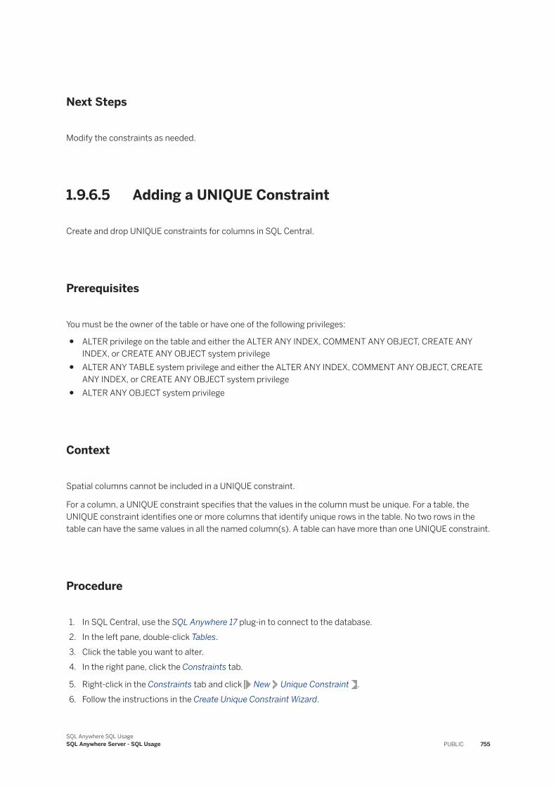
Next Steps
Modify the constraints as needed.
1.9.6.5 Adding a UNIQUE Constraint
Create and drop UNIQUE constraints for columns in SQL Central.
Prerequisites
You must be the owner of the table or have one of the following privileges:
● ALTER privilege on the table and either the ALTER ANY INDEX, COMMENT ANY OBJECT, CREATE ANY INDEX, or CREATE ANY OBJECT system privilege
● ALTER ANY TABLE system privilege and either the ALTER ANY INDEX, COMMENT ANY OBJECT, CREATE ANY INDEX, or CREATE ANY OBJECT system privilege
● ALTER ANY OBJECT system privilege
Context
Spatial columns cannot be included in a UNIQUE constraint.
For a column, a UNIQUE constraint specifies that the values in the column must be unique. For a table, the UNIQUE constraint identifies one or more columns that identify unique rows in the table. No two rows in the table can have the same values in all the named column(s). A table can have more than one UNIQUE constraint.
Procedure
1. In SQL Central, use the SQL Anywhere 17 plug-in to connect to the database.2. In the left pane, double-click Tables.3. Click the table you want to alter.4. In the right pane, click the Constraints tab.
5. Right-click in the Constraints tab and click New Unique Constraint .6. Follow the instructions in the Create Unique Constraint Wizard.
SQL Anywhere SQL UsageSQL Anywhere Server - SQL Usage PUBLIC 755
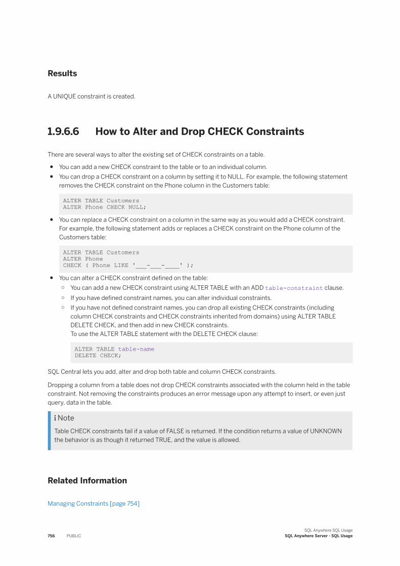
Results
A UNIQUE constraint is created.
1.9.6.6 How to Alter and Drop CHECK Constraints
There are several ways to alter the existing set of CHECK constraints on a table.
● You can add a new CHECK constraint to the table or to an individual column.● You can drop a CHECK constraint on a column by setting it to NULL. For example, the following statement
removes the CHECK constraint on the Phone column in the Customers table:
ALTER TABLE Customers ALTER Phone CHECK NULL;
● You can replace a CHECK constraint on a column in the same way as you would add a CHECK constraint. For example, the following statement adds or replaces a CHECK constraint on the Phone column of the Customers table:
ALTER TABLE Customers ALTER Phone CHECK ( Phone LIKE '___-___-____' );
● You can alter a CHECK constraint defined on the table:○ You can add a new CHECK constraint using ALTER TABLE with an ADD table-constraint clause.○ If you have defined constraint names, you can alter individual constraints.○ If you have not defined constraint names, you can drop all existing CHECK constraints (including
column CHECK constraints and CHECK constraints inherited from domains) using ALTER TABLE DELETE CHECK, and then add in new CHECK constraints.To use the ALTER TABLE statement with the DELETE CHECK clause:
ALTER TABLE table-name DELETE CHECK;
SQL Central lets you add, alter and drop both table and column CHECK constraints.
Dropping a column from a table does not drop CHECK constraints associated with the column held in the table constraint. Not removing the constraints produces an error message upon any attempt to insert, or even just query, data in the table.
NoteTable CHECK constraints fail if a value of FALSE is returned. If the condition returns a value of UNKNOWN the behavior is as though it returned TRUE, and the value is allowed.
Related Information
Managing Constraints [page 754]
756 PUBLICSQL Anywhere SQL Usage
SQL Anywhere Server - SQL Usage
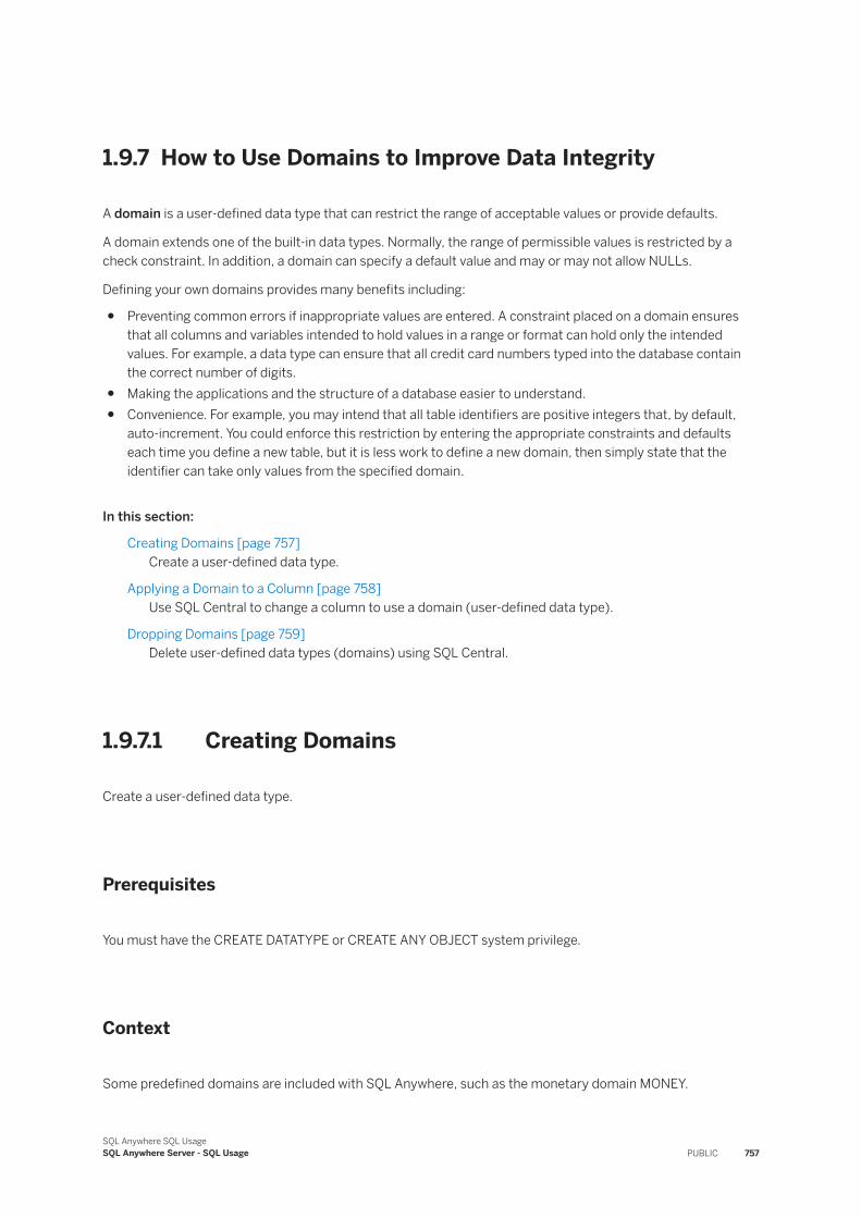
1.9.7 How to Use Domains to Improve Data Integrity
A domain is a user-defined data type that can restrict the range of acceptable values or provide defaults.
A domain extends one of the built-in data types. Normally, the range of permissible values is restricted by a check constraint. In addition, a domain can specify a default value and may or may not allow NULLs.
Defining your own domains provides many benefits including:
● Preventing common errors if inappropriate values are entered. A constraint placed on a domain ensures that all columns and variables intended to hold values in a range or format can hold only the intended values. For example, a data type can ensure that all credit card numbers typed into the database contain the correct number of digits.
● Making the applications and the structure of a database easier to understand.● Convenience. For example, you may intend that all table identifiers are positive integers that, by default,
auto-increment. You could enforce this restriction by entering the appropriate constraints and defaults each time you define a new table, but it is less work to define a new domain, then simply state that the identifier can take only values from the specified domain.
In this section:
Creating Domains [page 757]Create a user-defined data type.
Applying a Domain to a Column [page 758]Use SQL Central to change a column to use a domain (user-defined data type).
Dropping Domains [page 759]Delete user-defined data types (domains) using SQL Central.
1.9.7.1 Creating Domains
Create a user-defined data type.
Prerequisites
You must have the CREATE DATATYPE or CREATE ANY OBJECT system privilege.
Context
Some predefined domains are included with SQL Anywhere, such as the monetary domain MONEY.
SQL Anywhere SQL UsageSQL Anywhere Server - SQL Usage PUBLIC 757
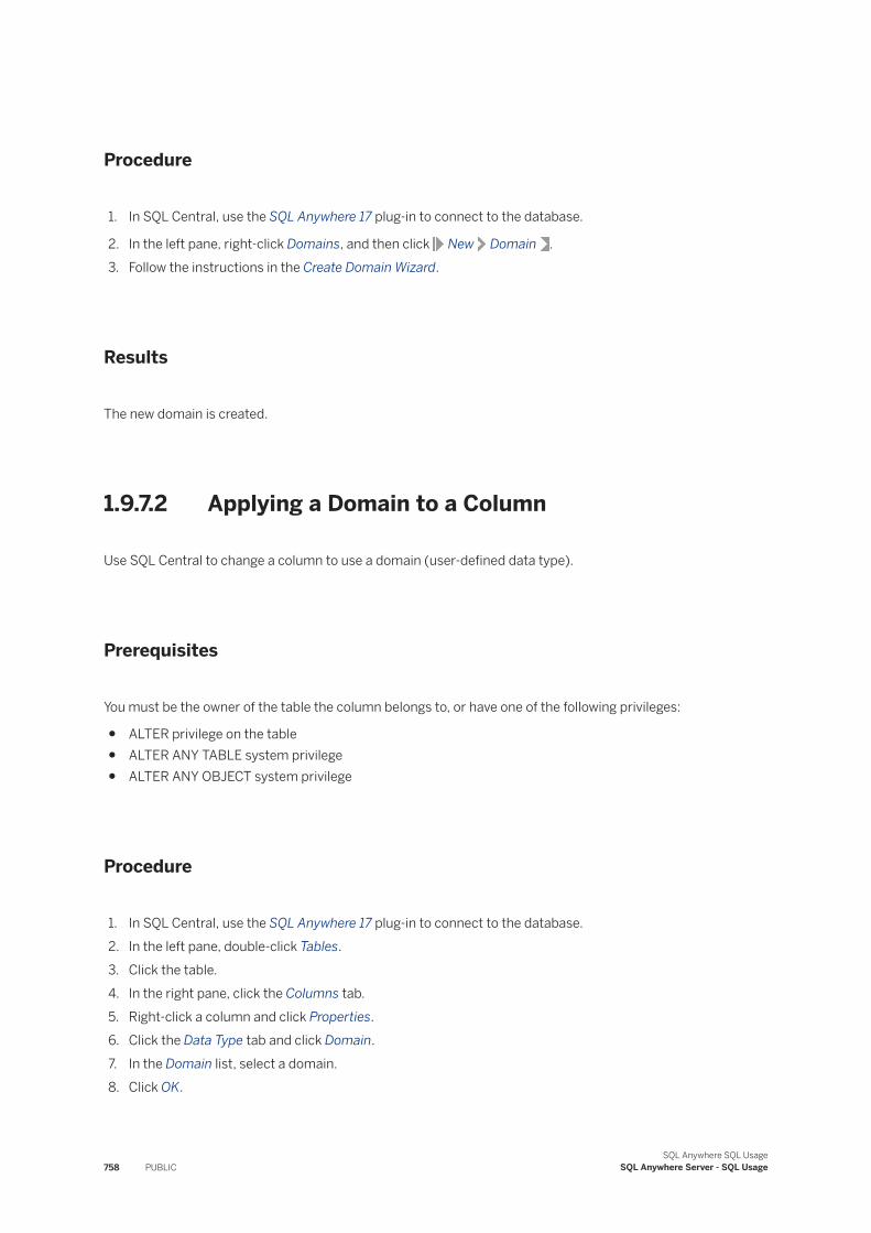
Procedure
1. In SQL Central, use the SQL Anywhere 17 plug-in to connect to the database.
2. In the left pane, right-click Domains, and then click New Domain .3. Follow the instructions in the Create Domain Wizard.
Results
The new domain is created.
1.9.7.2 Applying a Domain to a Column
Use SQL Central to change a column to use a domain (user-defined data type).
Prerequisites
You must be the owner of the table the column belongs to, or have one of the following privileges:
● ALTER privilege on the table● ALTER ANY TABLE system privilege● ALTER ANY OBJECT system privilege
Procedure
1. In SQL Central, use the SQL Anywhere 17 plug-in to connect to the database.2. In the left pane, double-click Tables.3. Click the table.4. In the right pane, click the Columns tab.5. Right-click a column and click Properties.6. Click the Data Type tab and click Domain.7. In the Domain list, select a domain.8. Click OK.
758 PUBLICSQL Anywhere SQL Usage
SQL Anywhere Server - SQL Usage
Results
The column uses the selected domain.
1.9.7.3 Dropping Domains
Delete user-defined data types (domains) using SQL Central.
Prerequisites
You must have the DROP DATATYPE or DROP ANY OBJECT system privilege.
A domain cannot be dropped if any variable or column in the database uses the domain. Drop or alter any columns or variables that use the domain before you drop the domain.
Procedure
1. In SQL Central, use the SQL Anywhere 17 plug-in to connect to the database.2. In the left pane, double-click Domains.3. In the right pane, right-click the domain and click Delete.4. Click Yes.
Results
The domain is deleted.
1.9.8 Entity and Referential Integrity
The relational structure of the database enables the database server to identify information within the database, and ensures that all the rows in each table uphold the relationships between tables (described in the database schema).
In this section:
Entity Integrity [page 760]When a user inserts or updates a row, the database server ensures that the primary key for the table is still valid: that each row in the table is uniquely identified by the primary key.
SQL Anywhere SQL UsageSQL Anywhere Server - SQL Usage PUBLIC 759
If a Client Application Breaches Entity Integrity [page 761]Entity integrity requires that each value of a primary key be unique within the table, and that no NULL values exist.
Primary Keys Enforce Entity Integrity [page 761]Once you specify the primary key for each table, maintaining entity integrity requires no further action by either client application developers or by the database administrator.
Referential Integrity [page 761]For a foreign key relationship to be valid, the entries in the foreign key must correspond to the primary key values of a row in the referenced table.
Foreign Keys Enforce Referential Integrity [page 765]You use the CREATE TABLE or ALTER TABLE statements to create foreign keys.
Loss of Referential Integrity [page 765]Your database can lose referential integrity if certain conditions are present.
If a Client Application Breaches Referential Integrity [page 765]If a client application updates or deletes a primary key value in a table, and if a foreign key references that primary key value elsewhere in the database, this can break referential integrity.
Referential Integrity Actions [page 766]Maintaining referential integrity when updating or deleting a referenced primary key can be as simple as disallowing the update or drop. Often, however, it is also possible to take a specific action on each foreign key to maintain referential integrity.
Referential Integrity Checking [page 766]For foreign keys defined to RESTRICT operations that would violate referential integrity, default checks occur at the time a statement executes.
1.9.8.1 Entity Integrity
When a user inserts or updates a row, the database server ensures that the primary key for the table is still valid: that each row in the table is uniquely identified by the primary key.
Example
Example 1
The Employees table in the SQL Anywhere sample database uses an employee ID as the primary key. When you add a new employee to the table, the database server checks that the new employee ID value is unique and is not NULL.Example 2
The SalesOrderItems table in the SQL Anywhere sample database uses two columns to define a primary key.
This table holds information about items ordered. One column contains an ID specifying an order, but there may be several items on each order, so this column by itself cannot be a primary key. An additional LineID
760 PUBLICSQL Anywhere SQL Usage
SQL Anywhere Server - SQL Usage
column identifies which line corresponds to the item. The columns ID and LineID, taken together, specify an item uniquely, and form the primary key.
1.9.8.2 If a Client Application Breaches Entity Integrity
Entity integrity requires that each value of a primary key be unique within the table, and that no NULL values exist.
If a client application attempts to insert or update a primary key value, providing values that are not unique would breach entity integrity. A breach in entity integrity prevents the new information from being added to the database, and instead sends the client application an error.
You must decide how to present an integrity breach to the user and enable them to take appropriate action. The appropriate action is usually as simple as asking the user to provide a different, unique value for the primary key.
1.9.8.3 Primary Keys Enforce Entity Integrity
Once you specify the primary key for each table, maintaining entity integrity requires no further action by either client application developers or by the database administrator.
The table owner defines the primary key for a table when they create it. If they modify the structure of a table at a later date, they can also redefine the primary key.
Related Information
Primary Keys [page 25]
1.9.8.4 Referential Integrity
For a foreign key relationship to be valid, the entries in the foreign key must correspond to the primary key values of a row in the referenced table.
Occasionally, some other unique column combination may be referenced instead of a primary key.
A foreign key is a reference to a primary key or UNIQUE constraint, usually in another table. When that primary key does not exist, the offending foreign key is called an orphan. SQL Anywhere automatically ensures that your database contains no rows that violate referential integrity. This process is referred to as verifying referential integrity. The database server verifies referential integrity by counting orphans.
When using a multi-column foreign key, you can determine what constitutes an orphaned row versus what constitutes a violation of referential integrity using the MATCH clause. The MATCH clause also allows you to specify uniqueness for the key, thereby eliminating the need to declare uniqueness separately.
SQL Anywhere SQL UsageSQL Anywhere Server - SQL Usage PUBLIC 761
The following is a list of MATCH types you can specify:
MATCH [ UNIQUE ] SIMPLE
A match occurs for a row in the foreign key table if all the column values match the corresponding column values present in a row of the primary key table. A row is orphaned in the foreign key table if at least one column value in the foreign key is NULL.
MATCH SIMPLE is the default behavior.
If the UNIQUE keyword is specified, the referencing table can have only one match for non-NULL key values.MATCH [ UNIQUE ] FULL
A match occurs for a row in the foreign key table if none of the values are NULL and the values match the corresponding column values in a row of the primary key table. A row is orphaned if all column values in the foreign key are NULL.
If the UNIQUE keyword is specified, the referencing table can have only one match for non-NULL key values.
Example
Example 1
The SQL Anywhere sample database contains an Employees table and a Departments table. The primary key for the Employees table is the employee ID, and the primary key for the Departments table is the department ID. In the Employees table, the department ID is called a foreign key for the Departments table because each department ID in the Employees table corresponds exactly to a department ID in the Departments table.
The foreign key relationship is a many-to-one relationship. Several entries in the Employees table have the same department ID entry, but the department ID is the primary key for the Departments table, and so is unique. If a foreign key could reference a column in the Departments table containing duplicate entries, or entries with a NULL value, there would be no way of knowing which row in the Departments table is the appropriate reference. This is prevented by defining the foreign key column as NOT NULL.Example 2
Suppose the database also contained an office table listing office locations. The Employees table might have a foreign key for the office table that indicates which city the employee's office is in. The database designer can choose to leave an office location unassigned at the time the employee is hired, for example, either because they haven't been assigned to an office yet, or because they don't work out of an office. In this case, the foreign key can allow NULL values, and is optional.Example 3
Execute the following statement to create a composite primary key.
CREATE TABLE pt( pk1 INT NOT NULL, pk2 INT NOT NULL, str VARCHAR(10) PRIMARY KEY ( pk1, pk2 ));
762 PUBLICSQL Anywhere SQL Usage
SQL Anywhere Server - SQL Usage
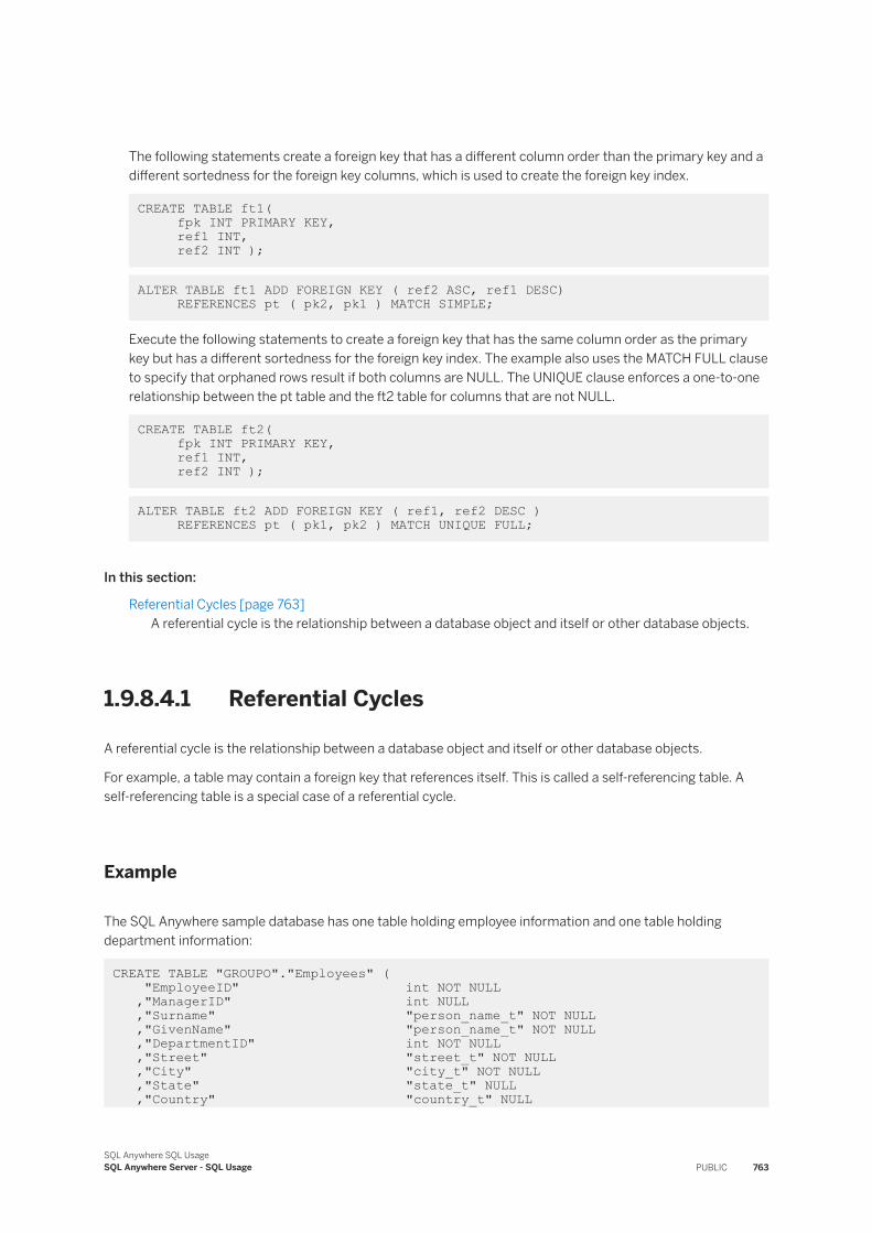
The following statements create a foreign key that has a different column order than the primary key and a different sortedness for the foreign key columns, which is used to create the foreign key index.
CREATE TABLE ft1( fpk INT PRIMARY KEY, ref1 INT, ref2 INT );
ALTER TABLE ft1 ADD FOREIGN KEY ( ref2 ASC, ref1 DESC) REFERENCES pt ( pk2, pk1 ) MATCH SIMPLE;
Execute the following statements to create a foreign key that has the same column order as the primary key but has a different sortedness for the foreign key index. The example also uses the MATCH FULL clause to specify that orphaned rows result if both columns are NULL. The UNIQUE clause enforces a one-to-one relationship between the pt table and the ft2 table for columns that are not NULL.
CREATE TABLE ft2( fpk INT PRIMARY KEY, ref1 INT, ref2 INT );
ALTER TABLE ft2 ADD FOREIGN KEY ( ref1, ref2 DESC ) REFERENCES pt ( pk1, pk2 ) MATCH UNIQUE FULL;
In this section:
Referential Cycles [page 763]A referential cycle is the relationship between a database object and itself or other database objects.
1.9.8.4.1 Referential Cycles
A referential cycle is the relationship between a database object and itself or other database objects.
For example, a table may contain a foreign key that references itself. This is called a self-referencing table. A self-referencing table is a special case of a referential cycle.
Example
The SQL Anywhere sample database has one table holding employee information and one table holding department information:
CREATE TABLE "GROUPO"."Employees" ( "EmployeeID" int NOT NULL ,"ManagerID" int NULL ,"Surname" "person_name_t" NOT NULL ,"GivenName" "person_name_t" NOT NULL ,"DepartmentID" int NOT NULL ,"Street" "street_t" NOT NULL ,"City" "city_t" NOT NULL ,"State" "state_t" NULL ,"Country" "country_t" NULL
SQL Anywhere SQL UsageSQL Anywhere Server - SQL Usage PUBLIC 763
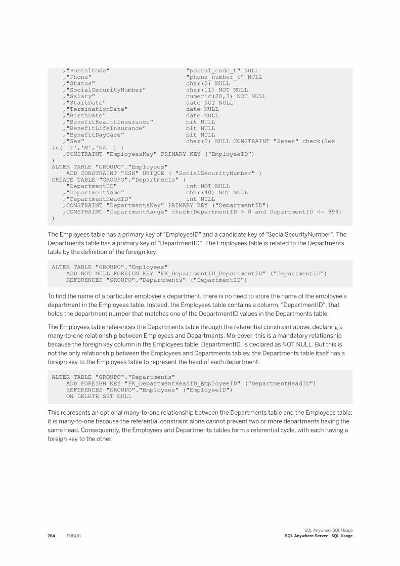
,"PostalCode" "postal_code_t" NULL ,"Phone" "phone_number_t" NULL ,"Status" char(2) NULL ,"SocialSecurityNumber" char(11) NOT NULL ,"Salary" numeric(20,3) NOT NULL ,"StartDate" date NOT NULL ,"TerminationDate" date NULL ,"BirthDate" date NULL ,"BenefitHealthInsurance" bit NULL ,"BenefitLifeInsurance" bit NULL ,"BenefitDayCare" bit NULL ,"Sex" char(2) NULL CONSTRAINT "Sexes" check(Sex in( 'F','M','NA' ) ) ,CONSTRAINT "EmployeesKey" PRIMARY KEY ("EmployeeID") )ALTER TABLE "GROUPO"."Employees" ADD CONSTRAINT "SSN" UNIQUE ( "SocialSecurityNumber" )CREATE TABLE "GROUPO"."Departments" ( "DepartmentID" int NOT NULL ,"DepartmentName" char(40) NOT NULL ,"DepartmentHeadID" int NULL ,CONSTRAINT "DepartmentsKey" PRIMARY KEY ("DepartmentID") ,CONSTRAINT "DepartmentRange" check(DepartmentID > 0 and DepartmentID <= 999))
The Employees table has a primary key of "EmployeeID" and a candidate key of "SocialSecurityNumber". The Departments table has a primary key of "DepartmentID". The Employees table is related to the Departments table by the definition of the foreign key:
ALTER TABLE "GROUPO"."Employees" ADD NOT NULL FOREIGN KEY "FK_DepartmentID_DepartmentID" ("DepartmentID") REFERENCES "GROUPO"."Departments" ("DepartmentID")
To find the name of a particular employee's department, there is no need to store the name of the employee's department in the Employees table. Instead, the Employees table contains a column, "DepartmentID", that holds the department number that matches one of the DepartmentID values in the Departments table.
The Employees table references the Departments table through the referential constraint above, declaring a many-to-one relationship between Employees and Departments. Moreover, this is a mandatory relationship because the foreign key column in the Employees table, DepartmentID, is declared as NOT NULL. But this is not the only relationship between the Employees and Departments tables; the Departments table itself has a foreign key to the Employees table to represent the head of each department:
ALTER TABLE "GROUPO"."Departments" ADD FOREIGN KEY "FK_DepartmentHeadID_EmployeeID" ("DepartmentHeadID") REFERENCES "GROUPO"."Employees" ("EmployeeID") ON DELETE SET NULL
This represents an optional many-to-one relationship between the Departments table and the Employees table; it is many-to-one because the referential constraint alone cannot prevent two or more departments having the same head. Consequently, the Employees and Departments tables form a referential cycle, with each having a foreign key to the other.
764 PUBLICSQL Anywhere SQL Usage
SQL Anywhere Server - SQL Usage
1.9.8.5 Foreign Keys Enforce Referential Integrity
You use the CREATE TABLE or ALTER TABLE statements to create foreign keys.
Once you create a foreign key, the column or columns in the key can contain only values that are present as primary key values in the table associated with the foreign key.
1.9.8.6 Loss of Referential Integrity
Your database can lose referential integrity if certain conditions are present.
● Updates or drops a primary key value. All the foreign keys referencing that primary key would become invalid.
● Adds a new row to the foreign table, and enters a value for the foreign key that has no corresponding primary key value. The database would become invalid.
SQL Anywhere provides protection against both types of integrity loss.
1.9.8.7 If a Client Application Breaches Referential Integrity
If a client application updates or deletes a primary key value in a table, and if a foreign key references that primary key value elsewhere in the database, this can break referential integrity.
Example
If the server allowed the primary key to be updated or dropped, and made no alteration to the foreign keys that referenced it, the foreign key reference would be invalid. Any attempt to use the foreign key reference, for example in a SELECT statement using a KEY JOIN clause, would fail, as no corresponding value in the referenced table exists.
While the database server handles breaches of entity integrity in a generally straightforward fashion by simply refusing to enter the data and returning an error message, potential breaches of referential integrity become more complicated. You have several options (known as referential integrity actions) available to help you maintain referential integrity.
SQL Anywhere SQL UsageSQL Anywhere Server - SQL Usage PUBLIC 765
1.9.8.8 Referential Integrity Actions
Maintaining referential integrity when updating or deleting a referenced primary key can be as simple as disallowing the update or drop. Often, however, it is also possible to take a specific action on each foreign key to maintain referential integrity.
The CREATE TABLE and ALTER TABLE statements allow database administrators and table owners to specify what action to take on foreign keys that reference a modified primary key when a breach occurs.
NoteReferential integrity actions are triggered by physical, rather than logical, updates to the unique value. For example, even in a case-insensitive database, updating the primary key value from SAMPLE-VALUE to sample-value will trigger a referential integrity action, even though the two values are logically the same.
You can specify each of the following referential integrity actions separately for updates and drops of the primary key:
RESTRICT
Generates an error and prevents the modification if an attempt to alter a referenced primary key value occurs. This is the default referential integrity action.SET NULL
Sets all foreign keys that reference the modified primary key to NULL.SET DEFAULT
Sets all foreign keys that reference the modified primary key to the default value for that column (as specified in the table definition).CASCADE
When used with ON UPDATE, this action updates all foreign keys that reference the updated primary key to the new value. When used with ON DELETE, this action deletes all rows containing foreign keys that reference the deleted primary key.
System triggers implement referential integrity actions. The trigger, defined on the primary table, is executed using the privileges of the owner of the secondary table. This behavior means that cascaded operations can take place between tables with different owners, without additional privileges having to be granted.
1.9.8.9 Referential Integrity Checking
For foreign keys defined to RESTRICT operations that would violate referential integrity, default checks occur at the time a statement executes.
If you specify a CHECK ON COMMIT clause, then the checks occur only when the transaction is committed.
766 PUBLICSQL Anywhere SQL Usage
SQL Anywhere Server - SQL Usage
Using a Database Option to Control Check Time
Setting the wait_for_commit database option controls the behavior when a foreign key is defined to restrict operations that would violate referential integrity. The CHECK ON COMMIT clause can override this option.
With the default wait_for_commit set to Off, operations that would leave the database inconsistent cannot execute. For example, an attempt to DELETE a department that still has employees in it is not allowed. The following statement gives an error:
DELETE FROM Departments WHERE DepartmentID = 200;
Setting wait_for_commit to On causes referential integrity to remain unchecked until a commit executes. If the database is in an inconsistent state, the database disallows the commit and reports an error. In this mode, a database user could drop a department with employees in it, however, the user cannot commit the change to the database until they:
● Delete or reassign the employees belonging to that department.● Insert the DepartmentID row back into the Departments table.● Roll back the transaction to undo the DELETE operation.
In this section:
Integrity Checks on INSERT [page 767]The database server performs integrity checks when executing INSERT statements.
Integrity Checks on DELETE or UPDATE [page 768]Foreign key errors can arise when performing update or delete operations.
1.9.8.9.1 Integrity Checks on INSERT
The database server performs integrity checks when executing INSERT statements.
For example, suppose you attempt to create a department, but supply a DepartmentID value that is already in use:
INSERT INTO Departments ( DepartmentID, DepartmentName, DepartmentHeadID ) VALUES ( 200, 'Eastern Sales', 902 );
The INSERT is rejected because the primary key for the table would no longer be unique. Since the DepartmentID column is a primary key, duplicate values are not permitted.
Inserting Values that Violate Relationships
The following statement inserts a new row in the SalesOrders table, but incorrectly supplies a SalesRepresentative ID that does not exist in the Employees table.
INSERT
SQL Anywhere SQL UsageSQL Anywhere Server - SQL Usage PUBLIC 767
INTO SalesOrders ( ID, CustomerID, OrderDate, SalesRepresentative) VALUES ( 2700, 186, '2000-10-19', 284 );
There is a one-to-many relationship between the Employees table and the SalesOrders table, based on the SalesRepresentative column of the SalesOrders table and the EmployeeID column of the Employees table. Only after a record in the primary table (Employees) has been entered can a corresponding record in the foreign table (SalesOrders) be inserted.
Foreign Keys
The primary key for the Employees table is the employee ID number. The sales rep ID number in the SalesRepresentative table is a foreign key for the Employees table, meaning that each sales rep number in the SalesOrders table must match the employee ID number for some employee in the Employees table.
When you try to add an order for sales rep 284 an error is raised.
There isn't an employee in the Employees table with that ID number. This prevents you from inserting orders without a valid sales representative ID.
1.9.8.9.2 Integrity Checks on DELETE or UPDATE
Foreign key errors can arise when performing update or delete operations.
For example, suppose you try to remove the R&D department from the Departments table. The DepartmentID field, being the primary key of the Departments table, constitutes the ONE side of a one-to-many relationship (the DepartmentID field of the Employees table is the corresponding foreign key, and forms the MANY side). A record on the ONE side of a relationship may not be deleted until all corresponding records on the MANY side are deleted.
Referential Integrity Error on DELETE
Suppose you attempt to delete the R&D department (DepartmentID 100) in the Departments table. An error is reported indicating that there are other records in the database that reference the R&D department, and the delete operation is not performed. To remove the R&D department, you need to first get rid of all employees in that department, as follows:
DELETE FROM Employees WHERE DepartmentID = 100;
Now that you deleted all the employees that belong to the R&D department, you can now delete the R&D department:
DELETE FROM Departments WHERE DepartmentID = 100;
768 PUBLICSQL Anywhere SQL Usage
SQL Anywhere Server - SQL Usage
Cancel these changes to the database by entering a ROLLBACK statement:
ROLLBACK;
Referential Integrity Error on UPDATE
Now, suppose you try to change the DepartmentID field from the Employees table. The DepartmentID field, being the foreign key of the Employees table, constitutes the MANY side of a one-to-many relationship (the DepartmentID field of the Departments table is the corresponding primary key, and forms the ONE side). A record on the MANY side of a relationship may not be changed unless it corresponds to a record on the ONE side. That is, unless it has a primary key to reference.
For example, the following UPDATE statement causes an integrity error:
UPDATE Employees SET DepartmentID = 600 WHERE DepartmentID = 100;
An error is raised because there is no department with a DepartmentID of 600 in the Departments table.
To change the value of the DepartmentID field in the Employees table, it must correspond to an existing value in the Departments table. For example:
UPDATE Employees SET DepartmentID = 300 WHERE DepartmentID = 100;
This statement can be executed because the DepartmentID of 300 corresponds to the existing Finance department.
Cancel these changes to the database by entering a ROLLBACK statement:
ROLLBACK;
Checking the Integrity at Commit Time
In the previous examples, the integrity of the database was checked as each statement was executed. Any operation that would result in an inconsistent database is not performed.
It is possible to configure the database so that the integrity is not checked until commit time using the wait_for_commit option. This is useful if you need to make changes that may cause temporary inconsistencies in the data while the changes are taking place. For example, suppose you want to delete the R&D department in the Employees and Departments tables. Since these tables reference each other, and since the deletions must be performed on one table at a time, there will be inconsistencies between the table during the deletion. In this case, the database cannot perform a COMMIT until the deletion finishes. Set the wait_for_commit option to On to allow data inconsistencies to exist up until a commit is performed.
You can also define foreign keys in such a way that they are automatically modified to be consistent with changes made to the primary key. In the above example, if the foreign key from Employees to Departments was
SQL Anywhere SQL UsageSQL Anywhere Server - SQL Usage PUBLIC 769
defined with ON DELETE CASCADE, then deleting the department ID would automatically delete the corresponding entries in the Employees table.
In the above cases, there is no way to have an inconsistent database committed as permanent. SQL Anywhere also supports alternative actions if changes would render the database inconsistent.
Related Information
Data Integrity [page 740]
1.9.9 Integrity Rules in the System Tables
All the information about database integrity checks and rules is held in the catalog.
System view Description
SYS.SYSCONSTRAINT Each row in the SYS.SYSCONSTRAINT system view describes a constraint in the database. The constraints currently supported include table and column checks, primary keys, foreign keys, and unique constraints.
For table and column check constraints, the actual CHECK condition is contained in the SYS.ISYSCHECK system table.
SYS.SYSCHECK Each row in the SYS.SYSCHECK system view defines a check constraint listed in the SYS.SYSCONSTRAINT system view.
SYS.SYSFKEY Each row in the SYS.SYSFKEY system view describes a foreign key, including the match type defined for the key.
SYS.SYSIDX Each row in the SYS.SYSIDX system view defines an index in the database.
SYS.SYSTRIGGER Each row in the SYS.SYSTRIGGER system view describes one trigger in the database, including triggers that are automatically created for foreign key constraints that have a referential triggered action (such as ON DELETE CASCADE).
The referential_action column holds a single character indicating whether the action is cascade (C), delete (D), set null (N), or restrict (R).
The event column holds a single character specifying the event that causes the action to occur: A=insert and delete, B=insert and update, C=update, D=delete, E=delete and update, I=insert, U=update, M=insert, delete and update.
The trigger_time column shows whether the action occurs after (A) or before (B) the triggering event.
770 PUBLICSQL Anywhere SQL Usage
SQL Anywhere Server - SQL Usage
1.10 Transactions and Isolation Levels
Transactions and isolation levels help to ensure data integrity through consistency.
The concept of consistency is best illustrated through an example:
Consistency Example
Suppose you use your database to handle financial accounts, and you want to transfer money from one client's account to another. The database is in a consistent state both before and after the money is transferred; but it is not in a consistent state after you have debited money from one account and before you have credited it to the second. During a transfer of money, the database is in a consistent state when the total amount of money in the clients' accounts is as it was before any money was transferred. When the money has been half transferred, the database is in an inconsistent state. Either both or neither of the debit and the credit must be processed.
Transactions are Logical Units of Work
A transaction is a logical unit of work. Each transaction is a sequence of logically related statements that do one task and transform the database from one consistent state into another. The nature of a consistent state depends on your database.
The statements within a transaction are treated as an indivisible unit: either all are executed or none is executed. At the end of each transaction, you commit your changes to make them permanent. If for any reason some of the statements in the transaction do not process properly, then any intermediate changes are undone, or rolled back. Another way of saying this is that transactions are atomic.
Grouping statements into transactions is key both to protecting the consistency of your data (even in the event of media or system failure), and to managing concurrent database operations. Transactions may be safely interleaved and the completion of each transaction marks a point at which the information in the database is consistent. You should design each transaction to perform a task that changes your database from one consistent state to another.
In the event of a system failure or database crash during normal operation, the database server performs automatic recovery of your data when the database is next started. The automatic recovery process recovers all completed transactions, and rolls back any transactions that were uncommitted when the failure occurred. The atomic character of transactions ensures that databases are recovered to a consistent state.
In this section:
Transactions [page 772]Commit a transaction to make changes to your database permanent.
Concurrency [page 774]Concurrency is the ability of the database server to process multiple transactions at the same time.
Savepoints Within Transactions [page 776]
SQL Anywhere SQL UsageSQL Anywhere Server - SQL Usage PUBLIC 771
You can define savepoints in a transaction to separate groups of related statements.
Isolation Levels and Consistency [page 777]You can control the degree to which the operations in one transaction are visible to the operations in other concurrent transactions by setting the isolation level.
Transaction Blocking and Deadlock [page 793]When a transaction is executed, the database server places locks on rows to prevent other transactions from interfering with the affected rows.
How Locking Works [page 796]A lock is a concurrency control mechanism that protects the integrity of data during the simultaneous execution of multiple transactions.
Guidelines for Choosing Isolation Levels [page 817]The choice of isolation level depends on the kind of task an application is performing.
Isolation Level Tutorials [page 821]Each isolation level behaves differently and which one you should use depends on your database and on the operations you are performing.
Use of a Sequence to Generate Unique Values [page 845]You can use a sequence to generate values that are unique across multiple tables or that are different from a set of natural numbers.
1.10.1 Transactions
Commit a transaction to make changes to your database permanent.
When you alter data, your alterations are recorded in the transaction log and are not made permanent until you execute the COMMIT statement.
Transactions start with one of the following events:
● The first statement following a connection to a database.● The first statement following the end of a transaction.
Transactions complete with one of the following events:
● A COMMIT statement makes the changes to the database permanent.● A ROLLBACK statement undoes all the changes made by the transaction.● A statement with a side effect of an automatic commit is executed: most data definition statements, such
as ALTER, CREATE, COMMENT, and DROP have the side effect of an automatic commit.● Disconnecting from a database causes an implicit rollback.● ODBC and JDBC have an autocommit setting that enforces a COMMIT after each statement. By default,
ODBC and JDBC require autocommit to be on, and each statement is a single transaction. To take advantage of transaction design possibilities, you should turn autocommit off.
● Setting the chained database option to Off is similar to enforcing an autocommit after each statement. By default, connections that use jConnect or Open Client applications have chained set to Off.
Determine which connections have outstanding transactions by connecting to a database using SQL Anywhere Cockpit. Inspect the CONNECTIONS page to see which connection has uncommitted operations.
772 PUBLICSQL Anywhere SQL Usage
SQL Anywhere Server - SQL Usage
Determining When a Transaction Began
The TransactionStartTime connection property returns the time that the database server first modified the database after a COMMIT or ROLLBACK. Use this property to find the start time of the earliest transaction for all active connections.
The following example uses the TransactionStartTime connection property to determine the start time of the earliest transaction of any connection to the database. It loops through all connections for the current database and returns the timestamp of the earliest connection to the database as a string. This information is useful as transactions get row and table locks and other transactions can block on table and row locks, depending on the blocking option. Long-running transactions can result in other users getting blocked or could affect performance. For example:
BEGIN DECLARE connid int; DECLARE earliest char(50); DECLARE connstart char(50); SET connid=next_connection(null); SET earliest = NULL; lp: LOOP IF connid IS NULL THEN LEAVE lp END IF; SET connstart = CONNECTION_PROPERTY('TransactionStartTime',connid); IF connstart <> '' THEN IF earliest IS NULL OR CAST(connstart AS TIMESTAMP) < CAST(earliest AS TIMESTAMP) THEN SET earliest = connstart; END IF; END IF; SET connid=next_connection(connid); END LOOP; SELECT earliest END
In this section:
Controlling How and When a Transaction Ends (SQL) [page 774]Interactive SQL provides you with two options that let you control when and how transactions end.
Related Information
Transact-SQL Compatibility [page 535]
SQL Anywhere SQL UsageSQL Anywhere Server - SQL Usage PUBLIC 773
1.10.1.1 Controlling How and When a Transaction Ends (SQL)
Interactive SQL provides you with two options that let you control when and how transactions end.
Context
By default, ODBC operates in autocommit mode. Even if you set the auto_commit option to OFF in Interactive SQL, the ODBC setting in an ODBC data source overrides the Interactive SQL setting. Change ODBC's setting by using the SQL_ATTR_AUTOCOMMIT connection attribute. ODBC autocommit is independent of the chained option.
Procedure
To control how and when a transaction ends, choose one of the following options:
Option Action
Use the auto_commit option
Automatically commit your results following every successful statement and automatically perform a ROLLBACK after each failed statement. Execute the following statement:
SET OPTION auto_commit=ON;
Use the commit_on_exit option
Control what happens to uncommitted changes when you exit Interactive SQL. If this option is set to ON (the default), then Interactive SQL performs a COMMIT; otherwise, it undoes your uncommitted changes with a ROLLBACK statement. Execute the following statement:
SET OPTION commit_on_exit={ ON | OFF }
Results
You have configured how Interactive SQL determines when and how a transaction ends.
1.10.2 Concurrency
Concurrency is the ability of the database server to process multiple transactions at the same time.
Were it not for special mechanisms within the database server, concurrent transactions could interfere with each other to produce inconsistent and incorrect information.
774 PUBLICSQL Anywhere SQL Usage
SQL Anywhere Server - SQL Usage
Who Needs to Know About Concurrency
Concurrency is a concern to all database administrators and developers. Even if you are working with a single-user database, you must be concerned with concurrency to process requests from multiple applications or even from multiple connections from a single application. These applications and connections can interfere with each other in exactly the same way as multiple users in a network setting.
Transaction Size Affects Concurrency
The way you group SQL statements into transactions can have significant effects on data integrity and on system performance. If you make a transaction too short and it does not contain an entire logical unit of work, then inconsistencies can be introduced into the database. If you write a transaction that is too long and contains several unrelated actions, then there is a greater chance that a ROLLBACK could unnecessarily undo work that could have been committed quite safely into the database.
If your transactions are long, they can lower concurrency by preventing other transactions from being processed concurrently.
There are many factors that determine the appropriate length of a transaction, depending on the type of application and the environment.
In this section:
Primary Key Generation and Concurrency [page 775]The database can automatically generate a unique number called the primary key.
1.10.2.1 Primary Key Generation and Concurrency
The database can automatically generate a unique number called the primary key.
For example, if you are building a table to store sales invoices you might prefer that the database assign unique invoice numbers automatically, rather than require sales staff to pick them.
Example
For example, invoice numbers could be obtained by adding 1 to the previous invoice number. This method does not work when there is more than one person adding invoices to the database. Two employees may decide to use the same invoice number.
There is more than one solution to the problem:
● Assign a range of invoice numbers to each person who adds new invoices.You could implement this scheme by creating a table with the columns user name and invoice number. The table would have one row for each user that adds invoices. Each time a user adds an invoice, the number in the table would be incremented and used for the new invoice. To handle all tables in the database, the table
SQL Anywhere SQL UsageSQL Anywhere Server - SQL Usage PUBLIC 775
should have three columns: table name, user name, and last key value. You should periodically verify that each person has enough numbers.
● Create a table with the columns table name and last key value.One row in the table contains the last invoice number used. The invoice number is automatically incremented every time a user adds an invoice, establishes a new connection, increments the invoice number, or immediately commits a change. Other users can access new invoice numbers because the row is instantly updated by a separate transaction.
● Use a column with a default value of NEWID with the UNIQUEIDENTIFIER binary data type to generate a universally unique identifier.You can use UUID/GUID values to uniquely identify table rows. Because the values generated on one computer do not match the values generated on another computer, the UUID/GUID values can be used as keys in replication and synchronization environments.
● Use a column with a default value of AUTOINCREMENT. For example:
CREATE TABLE Orders ( OrderID INTEGER NOT NULL DEFAULT AUTOINCREMENT, OrderDate DATE, primary key( OrderID ) );
On inserts into the table, if a value is not specified for the AUTOINCREMENT column, a unique value is generated. If a value is specified, it is used. If the value is larger than the current maximum value for the column, that value is used as a starting point for subsequent inserts. The value of the most recently inserted row in an AUTOINCREMENT column is available as the global variable @@identity.
Related Information
The NEWID Default [page 750]
1.10.3 Savepoints Within Transactions
You can define savepoints in a transaction to separate groups of related statements.
A SAVEPOINT statement defines an intermediate point during a transaction. You can undo all changes after that point using a ROLLBACK TO SAVEPOINT statement. Once a RELEASE SAVEPOINT statement has been executed or the transaction has ended, you can no longer use the savepoint. Savepoints do not have an effect on COMMITs. When a COMMIT is executed, all changes within the transaction are made permanent in the database.
No locks are released by the RELEASE SAVEPOINT or ROLLBACK TO SAVEPOINT statements: locks are released only at the end of a transaction.
Naming and Nesting Savepoints
Using named, nested savepoints, you can have many active savepoints within a transaction. Changes between a SAVEPOINT and a RELEASE SAVEPOINT can be canceled by rolling back to a previous savepoint or rolling
776 PUBLICSQL Anywhere SQL Usage
SQL Anywhere Server - SQL Usage
back the transaction itself. Changes within a transaction are not a permanent part of the database until the transaction is committed. All savepoints are released when a transaction ends.
Savepoints cannot be used in bulk operations mode. There is very little additional overhead in using savepoints.
1.10.4 Isolation Levels and Consistency
You can control the degree to which the operations in one transaction are visible to the operations in other concurrent transactions by setting the isolation level.
You do this using the isolation_level database option. The isolation levels of individual tables in a query are controlled with corresponding table hints.
The following isolation levels are provided:
This isolation level... Has these characteristics...
0 - read uncommitted ● Read permitted on row with or without write lock● No read locks are applied● No guarantee that concurrent transaction will not mod
ify row or roll back changes to row● Corresponds to table hints NOLOCK and READUNCOM
MITTED● Allow dirty reads, non-repeatable reads, and phantom
rows
1 - read committed ● Read only permitted on row with no write lock● Read lock acquired and held for read on current row
only, but released when cursor moves off the row● No guarantee that data will not change during transac
tion● Corresponds to table hint READCOMMITTED● Prevent dirty reads● Allow non-repeatable reads and phantom rows
2 - repeatable read ● Read only permitted on row with no write lock● Read lock acquired as each row in the result set is read,
and held until transaction ends● Corresponds to table hint REPEATABLEREAD● Prevent dirty reads and non-repeatable reads● Allow phantom rows
SQL Anywhere SQL UsageSQL Anywhere Server - SQL Usage PUBLIC 777
This isolation level... Has these characteristics...
3 - serializable ● Read only permitted on rows in result without write lock● Read locks acquired when cursor is opened and held
until transaction ends● Corresponds to table hints HOLDLOCK and SERIALIZA
BLE● Prevent dirty reads, non-repeatable reads, and phantom
rows
snapshot1 ● No read locks are applied● Read permitted on any row● Database snapshot of committed data is taken when
the first row is read or updated by the transaction
statement-snapshot1 ● No read locks are applied● Read permitted on any row● Database snapshot of committed data is taken when
the first row is read by the statement
readonly-statement-snapshot1 ● No read locks are applied● Read permitted on any row● Database snapshot of committed data is taken when
the first row is read by a read-only statement● Uses the isolation level (0, 1, 2, or 3) specified by the up
datable_statement_isolation option for an updatable statement
1 Snapshot isolation must be enabled for the database by setting the allow_snapshot_isolation option to On for the database.
The default isolation level is 0, except for Open Client, jConnect, and TDS connections, which have a default isolation level of 1.
Lock-based isolation levels prevent some or all interference. Level 3 provides the highest level of isolation. Lower levels allow more inconsistencies, but typically have better performance. Level 0 (read uncommitted) is the default setting.
The snapshot isolation levels prevent all interference between reads and writes. However, writes can still interfere with each other. Few inconsistencies are possible and contention performance is the same as isolation level 0. Performance not related to contention is worse because of the need to save and use row versions.
In general, each isolation level is characterized by the types of locks needed and by how locks held by other transactions are treated. At isolation level 0, the database server needs only write locks. It makes use of these locks to ensure that no two transactions make modifications that conflict. For example, a level 0 transaction acquires a write lock on a row before it updates or deletes it, and inserts any new rows with a write lock already in place.
Level 0 transactions perform no checks on the rows they are reading. For example, when a level 0 transaction reads a row, it does not check what locks may or may not have been acquired on that row by other transactions. Since no checks are needed, level 0 transactions are fast. This speed comes at the expense of
778 PUBLICSQL Anywhere SQL Usage
SQL Anywhere Server - SQL Usage
consistency. Whenever transactions read a row that is write locked by another transaction, they risk returning dirty data. At level 1, transactions check for write locks before they read a row. Although one more operation is required, these transactions are assured that all the data they read is committed.
NoteAll isolation levels guarantee that each transaction executes completely or not at all, and no updates are lost.
The isolation is between transactions only: multiple cursors within the same transaction cannot interfere with each other.
In this section:
Snapshot Isolation [page 779]Snapshot isolation is designed to improve concurrency and consistency by maintaining different versions of data.
Typical Types of Inconsistency [page 786]There are three common types of inconsistency that can occur during the execution of concurrent transactions.
How to Set the Isolation Level [page 788]Each connection to the database has its own isolation level.
Isolation Levels in ODBC-enabled Applications [page 790]ODBC applications call SQLSetConnectAttr with Attribute set to SQL_ATTR_TXN_ISOLATION and ValuePtr set according to the corresponding isolation level.
Viewing the Isolation Level [page 792]Use the CONNECTION_PROPERTY function to view the isolation level for the current connection.
Related Information
How to Enable Snapshot Isolation [page 782]
1.10.4.1 Snapshot Isolation
Snapshot isolation is designed to improve concurrency and consistency by maintaining different versions of data.
Blocks and deadlocks can occur when users are reading and writing the same data simultaneously. When you use snapshot isolation in a transaction, the database server returns a committed version of the data in response to any read requests. It does this without acquiring read locks, and prevents interference with users who are writing data.
A snapshot is a set of data that has been committed in the database. When using snapshot isolation, all queries within a transaction use the same set of data. No locks are acquired on database tables, which allows other transactions to access and modify the data without blocking. Open snapshot transactions require the
SQL Anywhere SQL UsageSQL Anywhere Server - SQL Usage PUBLIC 779
database server to keep copies of all data modified by other transactions to the database. Minimize the performance impact of snapshot transactions by limiting them to small transactions.
Three snapshot isolation levels that let you control when a snapshot is taken are supported:
snapshot
Use a snapshot of committed data from the time when the first row is read, inserted, updated, or deleted by the transaction.statement-snapshot
Use a snapshot of committed data from the time when the first row is read by the statement. Each statement within the transaction sees a snapshot of data from a different time.readonly-statement-snapshot
For read-only statements, use a snapshot of committed data from the time when the first row is read. Each read-only statement within the transaction sees a snapshot of data from a different time. For insert, update, and delete statements, use the isolation level specified by the updatable_statement_isolation option (can be one of 0 (the default), 1, 2, or 3).
You also have the option of specifying when the snapshot starts for a transaction by using the BEGIN SNAPSHOT statement.
Snapshot isolation is often useful, such as:
Applications that perform many reads and few updates
Snapshot transactions acquire write locks only for statements that modify the database. If a transaction is performing mainly read operations, then the snapshot transaction does not acquire read locks that could interfere with other users' transactions.Applications that perform long-running transactions while other users need to access data
Snapshot transactions do not acquire read locks, which makes data available to other users for reading and updating while the snapshot transaction takes place.Applications that must read a consistent set of data from the database
Because a snapshot shows a committed set of data from a specific point in time, you can use snapshot isolation to see consistent data that does not change throughout the transaction, even if other users are making changes to the data while your transaction is running.
Snapshot isolation only affects base tables and global temporary tables that are shared by all users. A read operation on any other table type never sees an old version of the data, and never initiates a snapshot. The only time where an update to another table type initiates a snapshot is if the isolation_level option is set to snapshot, and the update initiates a transaction.
The following statements cannot be executed when there are cursors opened with the WITH HOLD clause that use either statement or transaction snapshots:
● ALTER INDEX statement● ALTER TABLE statement● CREATE INDEX statement● DROP INDEX statement● REFRESH MATERIALIZED VIEW statement● REORGANIZE TABLE statement● CREATE TEXT INDEX statement● REFRESH TEXT INDEX statement
780 PUBLICSQL Anywhere SQL Usage
SQL Anywhere Server - SQL Usage
When opening cursors with the WITH HOLD clause, a snapshot of all rows committed at the snapshot start time is visible. Also visible are all modifications completed by the current connection since the start of the transaction within which the cursor was opened.
TRUNCATE TABLE is allowed only when a fast truncation is not performed because in this case, individual DELETEs are then recorded in the transaction log.
In addition, if any of these statements are performed from a non-snapshot transaction, then snapshot transactions that are already in progress that subsequently try to use the table return an error indicating that the schema has changed.
Materialized view matching avoids using a view if it was refreshed after the start of the snapshot for a transaction.
Snapshot isolation levels are supported in all programming interfaces. You can set the isolation level using the SET OPTION statement.
Row Versions
When snapshot isolation is enabled for a database, each time a row is updated, the database server adds a copy of the original row to the version stored in the temporary file. The original row version entries are stored until all the active snapshot transactions complete that might need access to the original row values. A transaction using snapshot isolation sees only committed values, so if the update to a row was not committed or rolled back before a snapshot transaction began, the snapshot transaction needs to access the original row value. This allows transactions using snapshot isolation to view data without placing any locks on the underlying tables.
The VersionStorePages database property returns the number of pages in the temporary file that are currently being used for the version store. To obtain this value, execute the following query:
SELECT DB_PROPERTY ( 'VersionStorePages' );
Old row version entries are removed when they are no longer needed. Old versions of BLOBs are stored in the original table, not the temporary file, until they are no longer required, and index entries for old row versions are stored in the original index until they are not required.
You can retrieve the amount of free space in the temporary file using the sa_disk_free_space system procedure.
If a trigger is fired that updates row values, the original values of those rows are also stored in the temporary file.
Designing your application to use shorter transactions and shorter snapshots reduces temporary file space requirements.
If you are concerned about temporary file growth, you can set up a GrowTemp system event that specifies the actions to take when the temporary file reaches a specific size.
In this section:
Understanding Snapshot Transactions [page 782]
SQL Anywhere SQL UsageSQL Anywhere Server - SQL Usage PUBLIC 781
Snapshot transactions acquire write locks on updates, but read locks are never acquired for a transaction or statement that uses a snapshot. As a result, readers never block writers and writers never block readers, but writers can block writers if they attempt to update the same rows.
How to Enable Snapshot Isolation [page 782]Snapshot isolation is enabled or disabled for a database using the allow_snapshot_isolation option.
Snapshot Isolation Example [page 783]Snapshot isolation can be used to maintain consistency without blocking.
Update Conflicts and Snapshot Isolation [page 785]With snapshot isolation, an update conflict can occur when a transaction encounters an old version of a row and tries to update or delete it.
1.10.4.1.1 Understanding Snapshot Transactions
Snapshot transactions acquire write locks on updates, but read locks are never acquired for a transaction or statement that uses a snapshot. As a result, readers never block writers and writers never block readers, but writers can block writers if they attempt to update the same rows.
With snapshot isolation a transaction does not begin with a BEGIN TRANSACTION statement. Rather, it begins with the first read, insert, update, or delete within the transaction, depending on the snapshot isolation level being used for the transaction. The following example shows when a transaction begins for snapshot isolation:
SET OPTION PUBLIC.allow_snapshot_isolation = 'On'; SET TEMPORARY OPTION isolation_level = 'snapshot'; SELECT * FROM Products; --transaction begins and the statement only --sees changes that are already committed INSERT INTO Products SELECT ID + 30, Name, Description, 'Extra large', Color, 50, UnitPrice, NULL FROM Products WHERE Name = 'Tee Shirt'; COMMIT; --transaction ends
1.10.4.1.2 How to Enable Snapshot Isolation
Snapshot isolation is enabled or disabled for a database using the allow_snapshot_isolation option.
When the option is set to On, row versions are maintained in the temporary file, and connections are allowed to use any of the snapshot isolation levels. When this option is set to Off, any attempt to use snapshot isolation results in an error.
Enabling a database to use snapshot isolation can affect performance because copies of all modified rows must be maintained, regardless of the number of transactions that use snapshot isolation.
The following statement enables snapshot isolation for a database:
SET OPTION PUBLIC.allow_snapshot_isolation = 'On';
The setting of the allow_snapshot_isolation option can be changed, even when there are users connected to the database. When you change the setting of this option from Off to On, all current transactions must
782 PUBLICSQL Anywhere SQL Usage
SQL Anywhere Server - SQL Usage
complete before new transactions can use snapshot isolation. When you change the setting of this option from On to Off, all outstanding transactions using snapshot isolation must complete before the database server stops maintaining row version information.
You can view the current snapshot isolation setting for a database by querying the value of the SnapshotIsolationState database property:
SELECT DB_PROPERTY ( 'SnapshotIsolationState' );
The SnapshotIsolationState property has one of the following values:
On
Snapshot isolation is enabled for the database.Off
Snapshot isolation is disabled for the database.in_transition_to_on
Snapshot isolation is enabled once the current transactions complete.in_transition_to_off
Snapshot isolation is disabled once the current transactions complete.
When snapshot isolation is enabled for a database, row versions must be maintained for a transaction until the transaction commits or rolls back, even if snapshots are not being used. Therefore, it is best to set the allow_snapshot_isolation option to Off if snapshot isolation is never used.
1.10.4.1.3 Snapshot Isolation Example
Snapshot isolation can be used to maintain consistency without blocking.
Example
This example uses two connections to the sample database to demonstrate this.
1. Run the following command to create an Interactive SQL connection (Connection1) to the sample database:
dbisql -c "DSN=SQL Anywhere 17 Demo;PWD=sql;ConnectionName=Connection1"
2. Run the following command to create an Interactive SQL connection (Connection2) to the sample database:
dbisql -c "DSN=SQL Anywhere 17 Demo;PWD=sql;ConnectionName=Connection2"
3. In Connection1, execute the following statement to set the isolation level to 1 (read committed).
SET OPTION isolation_level = 1;
SQL Anywhere SQL UsageSQL Anywhere Server - SQL Usage PUBLIC 783
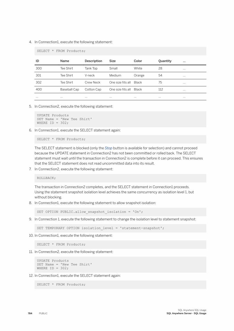
4. In Connection1, execute the following statement:
SELECT * FROM Products;
ID Name Description Size Color Quantity ...
300 Tee Shirt Tank Top Small White 28 ...
301 Tee Shirt V-neck Medium Orange 54 ...
302 Tee Shirt Crew Neck One size fits all Black 75 ...
400 Baseball Cap Cotton Cap One size fits all Black 112 ...
... ... ... ... ... ... ...
5. In Connection2, execute the following statement:
UPDATE Products SET Name = 'New Tee Shirt' WHERE ID = 302;
6. In Connection1, execute the SELECT statement again:
SELECT * FROM Products;
The SELECT statement is blocked (only the Stop button is available for selection) and cannot proceed because the UPDATE statement in Connection2 has not been committed or rolled back. The SELECT statement must wait until the transaction in Connection2 is complete before it can proceed. This ensures that the SELECT statement does not read uncommitted data into its result.
7. In Connection2, execute the following statement:
ROLLBACK;
The transaction in Connection2 completes, and the SELECT statement in Connection1 proceeds.Using the statement snapshot isolation level achieves the same concurrency as isolation level 1, but without blocking.
8. In Connection1, execute the following statement to allow snapshot isolation:
SET OPTION PUBLIC.allow_snapshot_isolation = 'On';
9. In Connection 1, execute the following statement to change the isolation level to statement snapshot:
SET TEMPORARY OPTION isolation_level = 'statement-snapshot';
10. In Connection1, execute the following statement:
SELECT * FROM Products;
11. In Connection2, execute the following statement:
UPDATE Products SET Name = 'New Tee Shirt' WHERE ID = 302;
12. In Connection1, execute the SELECT statement again:
SELECT * FROM Products;
784 PUBLICSQL Anywhere SQL Usage
SQL Anywhere Server - SQL Usage
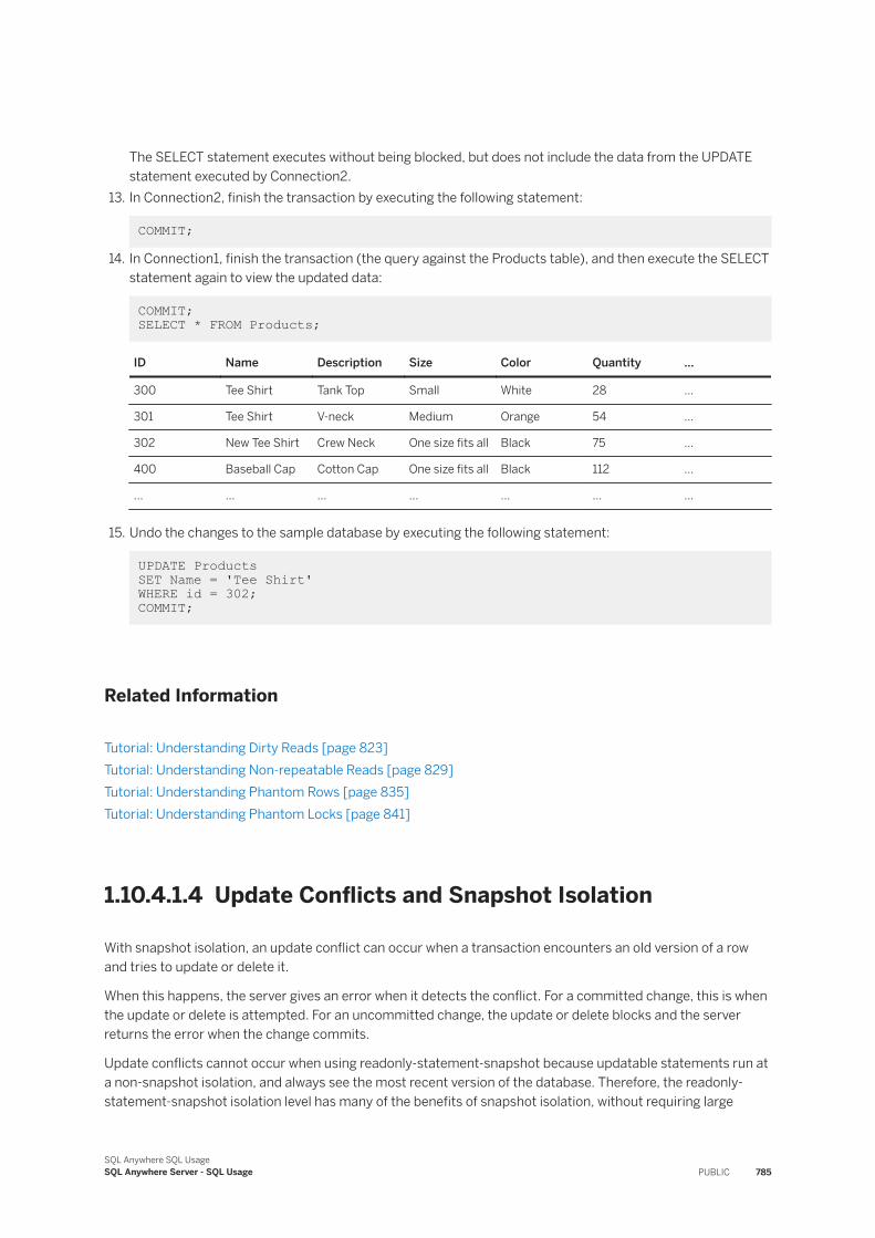
The SELECT statement executes without being blocked, but does not include the data from the UPDATE statement executed by Connection2.
13. In Connection2, finish the transaction by executing the following statement:
COMMIT;
14. In Connection1, finish the transaction (the query against the Products table), and then execute the SELECT statement again to view the updated data:
COMMIT; SELECT * FROM Products;
ID Name Description Size Color Quantity ...
300 Tee Shirt Tank Top Small White 28 ...
301 Tee Shirt V-neck Medium Orange 54 ...
302 New Tee Shirt Crew Neck One size fits all Black 75 ...
400 Baseball Cap Cotton Cap One size fits all Black 112 ...
... ... ... ... ... ... ...
15. Undo the changes to the sample database by executing the following statement:
UPDATE Products SET Name = 'Tee Shirt'WHERE id = 302; COMMIT;
Related Information
Tutorial: Understanding Dirty Reads [page 823]Tutorial: Understanding Non-repeatable Reads [page 829]Tutorial: Understanding Phantom Rows [page 835]Tutorial: Understanding Phantom Locks [page 841]
1.10.4.1.4 Update Conflicts and Snapshot Isolation
With snapshot isolation, an update conflict can occur when a transaction encounters an old version of a row and tries to update or delete it.
When this happens, the server gives an error when it detects the conflict. For a committed change, this is when the update or delete is attempted. For an uncommitted change, the update or delete blocks and the server returns the error when the change commits.
Update conflicts cannot occur when using readonly-statement-snapshot because updatable statements run at a non-snapshot isolation, and always see the most recent version of the database. Therefore, the readonly-statement-snapshot isolation level has many of the benefits of snapshot isolation, without requiring large
SQL Anywhere SQL UsageSQL Anywhere Server - SQL Usage PUBLIC 785
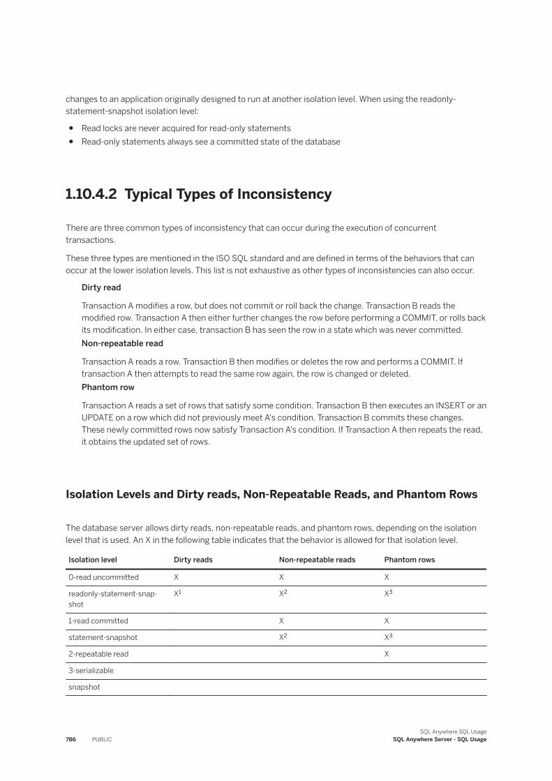
changes to an application originally designed to run at another isolation level. When using the readonly-statement-snapshot isolation level:
● Read locks are never acquired for read-only statements● Read-only statements always see a committed state of the database
1.10.4.2 Typical Types of Inconsistency
There are three common types of inconsistency that can occur during the execution of concurrent transactions.
These three types are mentioned in the ISO SQL standard and are defined in terms of the behaviors that can occur at the lower isolation levels. This list is not exhaustive as other types of inconsistencies can also occur.
Dirty read
Transaction A modifies a row, but does not commit or roll back the change. Transaction B reads the modified row. Transaction A then either further changes the row before performing a COMMIT, or rolls back its modification. In either case, transaction B has seen the row in a state which was never committed.Non-repeatable read
Transaction A reads a row. Transaction B then modifies or deletes the row and performs a COMMIT. If transaction A then attempts to read the same row again, the row is changed or deleted.Phantom row
Transaction A reads a set of rows that satisfy some condition. Transaction B then executes an INSERT or an UPDATE on a row which did not previously meet A's condition. Transaction B commits these changes. These newly committed rows now satisfy Transaction A's condition. If Transaction A then repeats the read, it obtains the updated set of rows.
Isolation Levels and Dirty reads, Non-Repeatable Reads, and Phantom Rows
The database server allows dirty reads, non-repeatable reads, and phantom rows, depending on the isolation level that is used. An X in the following table indicates that the behavior is allowed for that isolation level.
Isolation level Dirty reads Non-repeatable reads Phantom rows
0-read uncommitted X X X
readonly-statement-snapshot
X1 X2 X3
1-read committed X X
statement-snapshot X2 X3
2-repeatable read X
3-serializable
snapshot
786 PUBLICSQL Anywhere SQL Usage
SQL Anywhere Server - SQL Usage

1 Dirty reads can occur for updatable statements within a transaction if the isolation level specified by the updatable_statement_isolation option does not prevent them from occurring.
2 Non-repeatable reads can occur for statements within a transaction if the isolation level specified by the updatable_statement_isolation option does not prevent them from occurring. Non-repeatable reads can occur because each statement starts a new snapshot, so one statement may see changes that another statement does not see.
3 Phantom rows can occur for statements within a transaction if the isolation level specified by the updatable_statement_isolation option does not prevent them from occurring. Phantom rows can occur because each statement starts a new snapshot, so one statement may see changes that another statement does not see.
This table demonstrates two points:
● Each isolation level eliminates one of the three typical types of inconsistencies.● Each level eliminates the types of inconsistencies eliminated at all lower levels.● For statement snapshot isolation levels, non-repeatable reads and phantom rows can occur within a
transaction, but not within a single statement in a transaction.
The isolation levels have different names under ODBC. These names are based on the names of the inconsistencies that they prevent.
In this section:
Cursor Instability [page 787]A significant inconsistency that can occur during the execution of concurrent transactions is cursor instability.
Related Information
Isolation Levels in ODBC-enabled Applications [page 790]Tutorial: Understanding Dirty Reads [page 823]Tutorial: Understanding Non-repeatable Reads [page 829]Tutorial: Understanding Phantom Rows [page 835]
1.10.4.2.1 Cursor Instability
A significant inconsistency that can occur during the execution of concurrent transactions is cursor instability.
When this inconsistency is present, a transaction can modify a row that is being referenced by another transaction's cursor. Cursor stability ensures that applications using cursors do not introduce inconsistencies into the data in the database.
SQL Anywhere SQL UsageSQL Anywhere Server - SQL Usage PUBLIC 787
Example
Transaction A reads a row using a cursor. Transaction B modifies that row and commits. Not realizing that the row has been modified, Transaction A modifies it.
Eliminating Cursor Instability
Cursor stability is provided at isolation levels 1, 2, and 3. Cursor stability ensures that no other transactions can modify information that is contained in the present row of your cursor. The information in a row of a cursor may be the copy of information contained in a particular table or may be a combination of data from different rows of multiple tables. More than one table is likely involved whenever you use a join or sub-selection within a SELECT statement.
Cursors are used only when you are using SQL Anywhere through another application.
A related but distinct concern for applications using cursors is whether changes to underlying data are visible to the application. You can control the changes that are visible to applications by specifying the sensitivity of the cursor.
Related Information
Stored Procedures, Triggers, Batches, and User-defined Functions [page 87]
1.10.4.3 How to Set the Isolation Level
Each connection to the database has its own isolation level.
In addition, the database can store a default isolation level for each user or user-extended role. The PUBLIC setting of the isolation_level database option enables you to set a default isolation level.
You can also set the isolation level using table hints, but this is an advanced feature that is for setting the isolation level for an individual statement.
You can change the isolation level of your connection and the default level associated with your user ID using the SET OPTION statement. You can also change the isolation level for other users or groups.
Default Isolation Level
When you connect to a database, the database server determines your initial isolation level as follows:
1. A default isolation level may be set for each user and role. If a level is stored in the database for your user ID, then the database server uses it.
788 PUBLICSQL Anywhere SQL Usage
SQL Anywhere Server - SQL Usage
2. If not, the database server checks the groups to which you belong until it finds a level. If it finds no other setting first, then the database server uses the level assigned to PUBLIC.
NoteTo use snapshot isolation, you must first enable snapshot isolation for the database.
Example
Set the isolation level for the current user - Execute the SET OPTION statement. For example, the following statement sets the isolation level to 3 for the current user:
SET OPTION isolation_level = 3;
Set the isolation level for a user or for the PUBLIC role
1. Connect to the database.2. Execute the SET OPTION statement, adding the grantee name and a period before isolation_level. For
example, the following statement sets the default isolation for the PUBLIC role to 3.
SET OPTION PUBLIC.isolation_level = 3;
Set the isolation level for the current connection - Execute the SET OPTION statement using the TEMPORARY keyword. For example, the following statement sets the isolation level to 3 for the duration of the current connection:
SET TEMPORARY OPTION isolation_level = 3;
Related Information
How to Enable Snapshot Isolation [page 782]Changes to Isolation Levels Within a Transaction [page 791]
SQL Anywhere SQL UsageSQL Anywhere Server - SQL Usage PUBLIC 789
1.10.4.4 Isolation Levels in ODBC-enabled Applications
ODBC applications call SQLSetConnectAttr with Attribute set to SQL_ATTR_TXN_ISOLATION and ValuePtr set according to the corresponding isolation level.
The ValuePtr Parameter
ValuePtr Isolation Level
SQL_TXN_READ_UNCOMMITTED 0
SQL_TXN_READ_COMMITTED 1
SQL_TXN_REPEATABLE_READ 2
SQL_TXN_SERIALIZABLE 3
SA_SQL_TXN_SNAPSHOT snapshot
SA_SQL_TXN_STATEMENT_SNAPSHOT statement-snapshot
SA_SQL_TXN_READONLY_STATEMENT_SNAPSHOT readonly-statement-snapshot
Changing an Isolation Level via ODBC
You can change the isolation level of your connection via ODBC using the function SQLSetConnectAttr in the library ODBC32.dll.
The SQLSetConnectAttr function takes four parameters: the value of the ODBC connection handle, the fact that you want to set the isolation level, the value corresponding to the isolation level, and zero. The values corresponding to the isolation level appear in the table below.
String Value
SQL_TXN_ISOLATION 108
SQL_TXN_READ_UNCOMMITTED 1
SQL_TXN_READ_COMMITTED 2
SQL_TXN_REPEATABLE_READ 4
SQL_TXN_SERIALIZABLE 8
SA_SQL_TXN_SNAPSHOT 32
SA_SQL_TXN_STATEMENT_SNAPSHOT 64
SA_SQL_TXN_READONLY_STATEMENT_SNAPSHOT 128
Do not use the SET OPTION statement to change an isolation level from within an ODBC application. Since the ODBC driver does not parse the statements, execution of any statement in ODBC is not recognized by the ODBC driver. This could lead to unexpected locking behavior.
790 PUBLICSQL Anywhere SQL Usage
SQL Anywhere Server - SQL Usage
Example
The following function call sets the isolation level to statement-snapshot:
SQLSetConnectAttr (dbc, SA_SQL_ATTR_TXN_ISOLATION, (SQLPOINTER*) SA_SQL_TXN_STATEMENT_SNAPSHOT, 0);
ODBC uses the isolation feature to support assorted database lock options. For example, in PowerBuilder you can use the Lock attribute of the transaction object to set the isolation level when you connect to the database. The Lock attribute is a string, and is set as follows:
SQLCA.lock = "RU"
The Lock option is honored only at the moment the CONNECT occurs. Changes to the Lock attribute after the CONNECT have no effect on the connection.
In this section:
Changes to Isolation Levels Within a Transaction [page 791]Different isolation levels may be suitable for different parts of a single transaction.
1.10.4.4.1 Changes to Isolation Levels Within a Transaction
Different isolation levels may be suitable for different parts of a single transaction.
The database server allows you to change the isolation level of your database in the middle of a transaction.
When you change the isolation_level option in the middle of a transaction, the new setting affects only the following:
● Any cursors opened after the change● Any statements executed after the change
You may want to change the isolation level during a transaction to control the number of locks your transaction places. You may find a transaction needs to read a large table, but perform detailed work with only a few of the rows. If an inconsistency would not seriously affect your transaction, set the isolation to a low level while you scan the large table to avoid delaying the work of others.
You may also want to change the isolation level mid-transaction if, for example, just one table or group of tables requires serialized access.
In the tutorial on understanding phantom rows, you can see an example of the isolation level being changed in the middle of a transaction.
NoteYou can also set the isolation level (levels 0-3 only) by specifying a WITH table-hint clause in a FROM clause, but this is an advanced feature that you should use only when needed.
SQL Anywhere SQL UsageSQL Anywhere Server - SQL Usage PUBLIC 791
Changing Isolation Levels When Using Snapshot Isolation
When using snapshot isolation, you can change the isolation level within a transaction. This can be done by changing the setting of the isolation_level option or by using table hints that affect the isolation level in a query. You can use statement-snapshot, readonly-statement-snapshot, and isolation levels 0-3 at any time. However, you cannot use the snapshot isolation level in a transaction if it began at an isolation level other than snapshot. A transaction is initiated by an update and continues until the next COMMIT or ROLLBACK. If the first update takes place at some isolation level other than snapshot, then any statement that tries to use the snapshot isolation level before the transaction commits or rolls back returns error -1065 (SQLE_NON_SNAPSHOT_TRANSACTION). For example:
SET OPTION PUBLIC.allow_snapshot_isolation = 'On'; BEGIN TRANSACTION SET OPTION isolation_level = 3; INSERT INTO Departments ( DepartmentID, DepartmentName, DepartmentHeadID ) VALUES( 700, 'Foreign Sales', 129 ); SET TEMPORARY OPTION isolation_level = 'snapshot'; SELECT * FROM Departments;
Related Information
Tutorial: Understanding Phantom Rows [page 835]
1.10.4.5 Viewing the Isolation Level
Use the CONNECTION_PROPERTY function to view the isolation level for the current connection.
Prerequisites
You must be connected to a database.
Procedure
Execute the following statement:
SELECT CONNECTION_PROPERTY( 'isolation_level' );
792 PUBLICSQL Anywhere SQL Usage
SQL Anywhere Server - SQL Usage
Results
The isolation level for the current connection is returned.
1.10.5 Transaction Blocking and Deadlock
When a transaction is executed, the database server places locks on rows to prevent other transactions from interfering with the affected rows.
Locks control the amount and types of interference permitted.
The database server uses transaction blocking to allow transactions to execute concurrently without interference, or with limited interference. Any transaction can acquire a lock to prevent other concurrent transactions from modifying or even accessing a particular row. This transaction blocking scheme always stops some types of interference. For example, a transaction that is updating a particular row of a table always acquires a lock on that row to ensure that no other transaction can update or delete the same row at the same time.
Transaction Blocking
When a transaction attempts to perform an operation, but is prevented by a lock held by another transaction, a conflict arises and the progress of the transaction attempting to perform the operation is impeded
Sometimes a set of transactions arrive at a state where none of them can proceed.
In this section:
The Blocking Option [page 793]If two transactions have each acquired a read lock on a single row, the behavior when one of them attempts to modify that row depends on the setting of the blocking option.
Deadlocks [page 794]Transaction blocking can cause deadlock, the situation where a set of transactions arrive at a state where none of them can proceed.
1.10.5.1 The Blocking Option
If two transactions have each acquired a read lock on a single row, the behavior when one of them attempts to modify that row depends on the setting of the blocking option.
To modify the row, that transaction must block the other, yet it cannot do so while the other transaction has it blocked.
● If the blocking is option is set to On (the default), then the transaction that attempts to write waits until the other transaction releases its read lock. At that time, the write goes through.
SQL Anywhere SQL UsageSQL Anywhere Server - SQL Usage PUBLIC 793
● If the blocking option has been set to Off, then the statement that attempts to write receives an error.
When the blocking option is set to Off, the statement terminates instead of waiting and any partial changes it has made are rolled back. In this event, try executing the transaction again, later.
Blocking is more likely to occur at higher isolation levels because more locking and more checking is done. Higher isolation levels usually provide less concurrency. How much less depends on the individual natures of the concurrent transactions.
1.10.5.2 Deadlocks
Transaction blocking can cause deadlock, the situation where a set of transactions arrive at a state where none of them can proceed.
Reasons for Deadlocks
A deadlock can arise for two reasons:
A cyclical blocking conflict
Transaction A is blocked on transaction B, and transaction B is blocked on transaction A. More time will not solve the problem, and one of the transactions must be canceled, allowing the other to proceed. The same situation can arise with more than two transactions blocked in a cycle.
To eliminate a transactional deadlock, the database server selects a connection from those involved in the deadlock, rolls back the changes for the transaction that is active on that connection and returns an error. The database server selects the connection to roll back by using an internal heuristic that prefers the connection with the smallest blocking wait time left as determined by the blocking_timeout option. If all connections are set to wait forever, then the connection that caused the server to detect a deadlock is selected as the victim connection.All workers are blocked
When a transaction becomes blocked, its worker is not relinquished. For example, if the database server is configured with three workers and transactions A, B, and C are blocked on transaction D which is not currently executing a request, then a deadlock situation has arisen since there are no available workers. This situation is called thread deadlock.
Suppose that the database server has n workers. Thread deadlock occurs when n-1 workers are blocked, and the last worker is about to block. The database server's kernel cannot permit this last worker to block, since doing so would result in all workers being blocked, and the database server would hang. Instead, the database server ends the task that is about to block the last worker, rolls back the changes for the transaction active on that connection, and returns an error (SQLCODE -307, SQLSTATE 40W06).
Database servers with tens or hundreds of connections may experience thread deadlock in cases where there are many long-running requests either because of the size of the database or because of blocking. In this case, increasing the database server's multiprogramming level may be an appropriate solution. The design of your application may also cause thread deadlock because of excessive or unintentional contention. In these cases, scaling the application to larger data sets can make the problem worse, and increasing the database server's multiprogramming level may not solve the problem.
794 PUBLICSQL Anywhere SQL Usage
SQL Anywhere Server - SQL Usage
The number of database threads that the server uses depends on the individual database's setting.
In this section:
Example: Determining Who Is Blocked in a Deadlock (SQL) [page 795]Create an event that uses the sa_conn_info system procedure to determine which connections are blocked in a deadlock.
1.10.5.2.1 Example: Determining Who Is Blocked in a Deadlock (SQL)
Create an event that uses the sa_conn_info system procedure to determine which connections are blocked in a deadlock.
This procedure returns a result set consisting of a row for each connection. One column of the result set lists whether the connection is blocked, and if so which other connection it is blocked on. The result set indicates whether a connection is blocked, and the connection that is blocking it.
You can also use a deadlock event to take action when a deadlock occurs. The event handler can use the sa_report_deadlocks procedure to obtain information about the conditions that led to the deadlock. To retrieve more details about the deadlock from the database server, use the log_deadlocks option and enable the RememberLastStatement feature.
When you find that your application has frequent deadlocks, use Profiler to help diagnose the cause of the deadlocks.
Example
This example shows you how to set up a table and system event that can be used to obtain information about deadlocks when they occur.
1. Create a table to store the data returned from the sa_report_deadlocks system procedure:
CREATE TABLE DeadlockDetails( deadlockId INT PRIMARY KEY DEFAULT AUTOINCREMENT, snapshotId BIGINT, snapshotAt TIMESTAMP, waiter INTEGER, who VARCHAR(128), what LONG VARCHAR, object_id UNSIGNED BIGINT, record_id BIGINT, owner INTEGER, is_victim BIT, rollback_operation_count UNSIGNED INTEGER );
2. Create an event that fires when a deadlock occurs.This event copies the results of the sa_report_deadlocks system procedure into a table and notifies an administrator about the deadlock:
CREATE EVENT DeadlockNotification
SQL Anywhere SQL UsageSQL Anywhere Server - SQL Usage PUBLIC 795
TYPE DeadlockHANDLERBEGIN INSERT INTO DeadlockDetails WITH AUTO NAME SELECT snapshotId, snapshotAt, waiter, who, what, object_id, record_id, owner, is_victim, rollback_operation_count FROM sa_report_deadlocks (); COMMIT; CALL xp_startmail ( mail_user ='George Smith', mail_password ='mypwd' ); CALL xp_sendmail( recipient='DBAdmin', subject='Deadlock details added to the DeadlockDetails table.' ); CALL xp_stopmail ( ); END;
3. Set the log_deadlocks option to On:
SET OPTION PUBLIC.log_deadlocks = 'On';
4. Enable logging of the most-recently executed statement:
CALL sa_server_option( 'RememberLastStatement', 'YES' );
1.10.6 How Locking WorksA lock is a concurrency control mechanism that protects the integrity of data during the simultaneous execution of multiple transactions.
The database server automatically applies locks to prevent two connections from changing the same data at the same time, and to prevent other connections from reading data that is in the process of being changed. Locks improve the consistency of query result by protecting information that is in the process of being updated.
The database server places these locks automatically and needs no explicit instruction. It holds all the locks acquired by a transaction until the transaction is completed, for example by either a COMMIT or ROLLBACK statement, with a single exception.
The transaction that has access to the row is said to hold the lock. Depending on the type of lock, other transactions may have limited access to the locked row, or none at all.
In this section:
Types of Locks [page 797]To ensure database consistency and to support appropriate isolation levels between transactions, the database server uses several types of locks.
Locking Conflicts [page 804]A locking conflict occurs when one transaction attempts to acquire an exclusive lock on a row on which another transaction holds a lock, or attempts to acquire a shared lock on a row on which another transaction holds an exclusive lock.
Locks During Queries [page 805]The locks that the database server uses when a user enters a SELECT statement depend on the transaction isolation level.
Locks During Inserts [page 807]
796 PUBLICSQL Anywhere SQL Usage
SQL Anywhere Server - SQL Usage
Insert operations create new rows, and the database server utilizes various types of locks during insertions to ensure data integrity.
Locks During Updates [page 809]The database server modifies the information contained in a particular record when it is using locking.
Locks During Deletes [page 810]The DELETE operation follows almost the same steps as the INSERT operation, except in the opposite order.
Lock Duration [page 811]Locks are typically held by a transaction until it completes.
Viewing Locks (SQL Central) [page 811]Use the Locks tab in SQL Central to view the locks that are currently held in the database.
Viewing Locks (Interactive SQL) [page 812]Obtain information about locked rows to diagnose locking issues in the database.
Mutexes and Semaphores [page 813]Use mutexes and semaphores in your application logic to achieve locking behavior and control and communicate the availability of resources.
1.10.6.1 Types of Locks
To ensure database consistency and to support appropriate isolation levels between transactions, the database server uses several types of locks.
Schema Locks
Schema locks serialize changes to a database schema, and ensure that transactions using a table are not affected by schema changes initiated by other connections. For example, a transaction that is changing the structure of a table by inserting a new column can lock a table so that other transactions are not affected by the schema change. In such a case, it is essential to limit the access of other transactions to prevent errors.Row Locks
Row locks ensure consistency between concurrent transactions by allowing multiple users to access and modify a particular table at the row level. For example, a transaction can lock a particular row to prevent another transaction from changing it. The classes of row locks are read (shared) locks, write (exclusive) locks, and intent locks.Table Locks
Table locks place a lock on all the rows in a table and prevent a transaction from updating a table while another transaction is updating it. The types of table locks are read (shared) locks, write (exclusive) locks, and intent locks.Position Locks
Position locks ensure consistency within a sequential or indexed scan of a table. Transactions typically scan rows sequentially, or by using the ordering imposed by an index. In either case, a lock can be placed on the scan position. For example, placing a lock in an index can prevent another transaction from inserting a row with a specific value or range of values within that index.
SQL Anywhere SQL UsageSQL Anywhere Server - SQL Usage PUBLIC 797
Lock Duration
Locks are typically held by a transaction until it completes. This behavior prevents other transactions from making changes that would make it impossible to roll back the original transaction. At isolation level three, all locks must be held until a transaction ends to guarantee transaction serializability.
When row locks are used to implement cursor stability, they are not held until the end of a transaction. They are held for as long as the row in question is the current row of a cursor. In most cases, this amount of time is shorter than the lifetime of the transaction. When cursors are opened WITH HOLD, the locks can be held for the lifetime of the connection.
Locks can be held for the following durations:
Position
Short-term locks, such as read locks on specific rows that are used to implement cursor stability at isolation level 1.Transaction
For example, row, table, and position locks that are held until the end of a transaction.Connection
Schema locks are held beyond the end of a transaction, such as schema locks created when WITH HOLD cursors are used.
In this section:
Schema Locks [page 799]Schema locks serialize changes to a database schema, and ensure that transactions using a table are not affected by schema changes initiated by other connections.
Row Locks [page 799]Row locks prevent lost updates and other types of transaction inconsistencies.
Table Locks [page 801]Table locks prevent a transaction from updating a table while another transaction is updating it.
Position Locks [page 802]Position locks are a form of key-range locking that is designed to prevent anomalies because of the presence of phantoms or phantom rows.
Related Information
Schema Locks [page 799]Row Locks [page 799]Table Locks [page 801]Position Locks [page 802]
798 PUBLICSQL Anywhere SQL Usage
SQL Anywhere Server - SQL Usage
1.10.6.1.1 Schema Locks
Schema locks serialize changes to a database schema, and ensure that transactions using a table are not affected by schema changes initiated by other connections.
For example, a shared schema lock prevents an ALTER TABLE statement from dropping a column from a table when that table is being read by an open cursor on another connection.
There are two classes of schema locks: shared and exclusive.
Shared Locks
A shared schema lock is acquired when a transaction refers directly or indirectly to a table in the database. Shared schema locks do not conflict with each other; any number of transactions can acquire shared schema locks on the same table at the same time. The shared schema lock is held until the transaction completes via a COMMIT or ROLLBACK.
Any connection holding a shared schema lock is allowed to change table data, providing the change does not conflict with other connections. The table schema is locked in shared (read) mode.
Exclusive Locks
An exclusive schema lock is acquired when the schema of a table is modified, usually through the use of a DDL statement. The ALTER TABLE statement is one example of a DDL statement that acquires an exclusive schema lock on a table before modifying it. Only one connection can acquire an exclusive schema lock on a table at any time. All other attempts to lock the table's schema (shared or exclusive) are either blocked or fail with an error. A connection executing at isolation level 0, which is the least restrictive isolation level, is blocked from reading rows from a table whose schema has been locked in exclusive mode.
Only the connection holding the exclusive table schema lock can change the table data. The table schema is locked for the exclusive use of a single connection.
1.10.6.1.2 Row Locks
Row locks prevent lost updates and other types of transaction inconsistencies.
Row locks ensure that any row modified by a transaction cannot be modified by another transaction until the first transaction completes, either by committing the changes by issuing an implicit or explicit COMMIT statement or by aborting the changes via a ROLLBACK statement.
There are three classes of row locks: read (shared) locks, write (exclusive) locks, and intent locks. The database server acquires these locks automatically for each transaction.
SQL Anywhere SQL UsageSQL Anywhere Server - SQL Usage PUBLIC 799
Read Locks
When a transaction reads a row, the isolation level of the transaction determines if a read lock is acquired. Once a row is read locked, no other transaction can obtain a write lock on it. Acquiring a read lock ensures that a different transaction does not modify or delete a row while it is being read. Any number of transactions can acquire read locks on any row at the same time, so read locks are sometimes referred to as shared locks, or non-exclusive locks.
Read locks can be held for different durations. At isolation levels 2 and 3, any read locks acquired by a transaction are held until the transaction completes through a COMMIT or a ROLLBACK. These read locks are called long-term read locks.
For transactions executing at isolation level 1, the database server acquires a short-term read lock on the row upon which a cursor is positioned. As the application scrolls through the cursor, the short-term read lock on the previously positioned row is released, and a new short-term read lock is acquired on the subsequent row. This technique is called cursor stability. Because the application holds a read lock on the current row, another transaction cannot make changes to the row until the application moves off the row. More than one lock can be acquired if the cursor is over a query involving multiple tables. Short-term read locks are acquired only when the position within a cursor must be maintained across requests (ordinarily, these requests would be FETCH statements issued by the application). For example, short-term read locks are not acquired when processing a SELECT COUNT(*) query since a cursor opened over this statement is never positioned on a particular base table row. In this case, the database server only needs to guarantee read committed semantics; that is, that the rows processed by the statement have been committed by other transactions.
Transactions executing at isolation level 0 (read uncommitted) do not acquire long-term or short-term read locks and do not conflict with other transactions (except for exclusive schema locks). However, isolation level 0 transactions may process uncommitted changes made by other concurrent transactions. You can avoid processing uncommitted changes by using snapshot isolation.
Write Locks
A transaction acquires a write lock whenever it inserts, updates, or deletes a row. This behavior is true for transactions at all isolation levels, including isolation level 0 and snapshot isolation levels. No other transaction can obtain a read, intent, or write lock on the same row after a write lock is acquired. Write locks are also referred to as exclusive locks because only one transaction can hold an exclusive lock on a row at any time. No transaction can obtain a write lock while any other transaction holds a lock of any type on the same row. Similarly, once a transaction acquires a write lock, requests to lock the row that are made by other transactions are denied.
Intent Locks
Intent locks, also known as intent-for-update locks, indicate an intent to modify a particular row. Intent locks are acquired when a transaction:
● issues a FETCH FOR UPDATE statement● issues a SELECT...FOR UPDATE BY LOCK statement
800 PUBLICSQL Anywhere SQL Usage
SQL Anywhere Server - SQL Usage
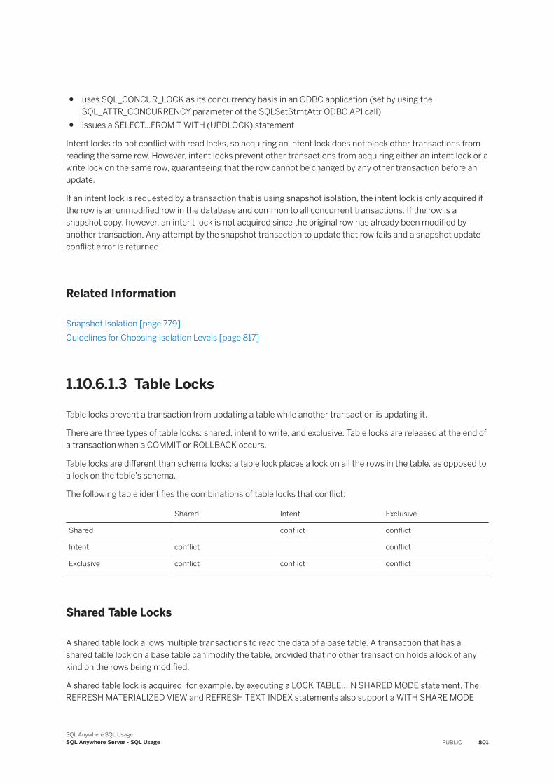
● uses SQL_CONCUR_LOCK as its concurrency basis in an ODBC application (set by using the SQL_ATTR_CONCURRENCY parameter of the SQLSetStmtAttr ODBC API call)
● issues a SELECT...FROM T WITH (UPDLOCK) statement
Intent locks do not conflict with read locks, so acquiring an intent lock does not block other transactions from reading the same row. However, intent locks prevent other transactions from acquiring either an intent lock or a write lock on the same row, guaranteeing that the row cannot be changed by any other transaction before an update.
If an intent lock is requested by a transaction that is using snapshot isolation, the intent lock is only acquired if the row is an unmodified row in the database and common to all concurrent transactions. If the row is a snapshot copy, however, an intent lock is not acquired since the original row has already been modified by another transaction. Any attempt by the snapshot transaction to update that row fails and a snapshot update conflict error is returned.
Related Information
Snapshot Isolation [page 779]Guidelines for Choosing Isolation Levels [page 817]
1.10.6.1.3 Table Locks
Table locks prevent a transaction from updating a table while another transaction is updating it.
There are three types of table locks: shared, intent to write, and exclusive. Table locks are released at the end of a transaction when a COMMIT or ROLLBACK occurs.
Table locks are different than schema locks: a table lock places a lock on all the rows in the table, as opposed to a lock on the table's schema.
The following table identifies the combinations of table locks that conflict:
Shared Intent Exclusive
Shared conflict conflict
Intent conflict conflict
Exclusive conflict conflict conflict
Shared Table Locks
A shared table lock allows multiple transactions to read the data of a base table. A transaction that has a shared table lock on a base table can modify the table, provided that no other transaction holds a lock of any kind on the rows being modified.
A shared table lock is acquired, for example, by executing a LOCK TABLE...IN SHARED MODE statement. The REFRESH MATERIALIZED VIEW and REFRESH TEXT INDEX statements also support a WITH SHARE MODE
SQL Anywhere SQL UsageSQL Anywhere Server - SQL Usage PUBLIC 801
clause that you can use to create shared table locks on the underlying tables while the refresh operation takes place.
Intent to Write Table Locks
An intent to write table lock, also known as an intent table lock, is implicitly acquired the first time a write lock on a row is acquired by a transaction. That is, an intent table lock is obtained when updating, inserting, or deleting a row. As with shared table locks, intent table locks are held until the transaction completes via a COMMIT or a ROLLBACK. Intent table locks conflict with shared and exclusive table locks, but not with other intent table locks.
Exclusive Table Locks
An exclusive table lock prevents other transactions from modifying the schema or data in a table, including inserting new data. Unlike an exclusive schema lock, transactions executing at isolation level 0 can still read the rows in a table that has an exclusive table lock on it. Only one transaction can hold an exclusive lock on any table at one time. Exclusive table locks conflict with all other table and row locks.
You acquire an exclusive table lock implicitly when using the LOAD TABLE statement.
You acquire an exclusive table lock explicitly by using the LOCK TABLE...IN EXCLUSIVE MODE statement. The REFRESH MATERIALIZED VIEW and REFRESH TEXT INDEX statements also provide a WITH EXCLUSIVE MODE clause that you can use to place exclusive table locks on the underlying tables while the refresh operation takes place.
Related Information
Schema Locks [page 799]Guidelines for Choosing Isolation Levels [page 817]
1.10.6.1.4 Position Locks
Position locks are a form of key-range locking that is designed to prevent anomalies because of the presence of phantoms or phantom rows.
Position locks are only relevant when the database server is processing transactions that are operating at isolation level 3.
Transactions that operate at isolation level 3 are serializable. A transaction's behavior at isolation level 3 should not be impacted by concurrent update activity by other transactions. In particular, at isolation level 3, transactions cannot be affected by INSERTs or UPDATEs (phantoms) that introduce rows that can affect the
802 PUBLICSQL Anywhere SQL Usage
SQL Anywhere Server - SQL Usage
result of a computation. The database server uses position locks to prevent such updates from occurring. It is this additional locking that differentiates isolation level 2 (repeatable read) from isolation level 3.
To prevent the creation of phantom rows, the database server acquires locks on positions within a physical scan of a table. For a sequential scan, the scan position is based on the row identifier of the current row. For an index scan, the scan's position is based on the current row's index key value (which can be unique or non-unique). Through locking a scan position, a transaction prevents insertions by other transactions relating to a particular range of values in that ordering of the rows. This behavior applies to INSERT statements and UPDATE statements that change the value of an indexed attribute. When a scan position is locked, an UPDATE statement is considered a request to DELETE the index entry followed immediately by an INSERT request.
There are two types of position locks supported: phantom locks and insert locks. Both types of locks are shared, in that any number of transactions can acquire the same type of lock on the same row. However, phantom and anti-phantom locks conflict.
Phantom Locks
A phantom lock, sometimes called an anti-insert lock, is placed on a scan position to prevent the subsequent creation of phantom rows by other transactions. When a phantom lock is acquired, it prevents other transactions from inserting a row into a table immediately before the row that is anti-insert locked. A phantom lock is a long-term lock that is held until the end of the transaction.
Phantom locks are acquired only by transactions operating at isolation level 3; it is the only isolation level that guarantees consistency with phantoms.
For an index scan, phantom locks are acquired on each row read through the index, and one additional phantom lock is acquired at the end of the index scan to prevent insertions into the index at the end of the satisfying index range. Phantom locks with index scans prevent phantoms from being created by the insertion of new rows to the table, or the update of an indexed value that would cause the creation of an index entry at a point covered by a phantom lock.
With a sequential scan, phantom locks are acquired on every row in a table to prevent any insertion from altering the result set. Isolation level 3 scans often have a negative effect on database concurrency. While one or more phantom locks conflict with an insert lock, and one or more read locks conflict with a write lock, no interaction exists between phantom/insert locks and read/write locks. For example, although a write lock cannot be acquired on a row that contains a read lock, it can be acquired on a row that has only a phantom lock. More options are open to the database server because of this flexible arrangement, but it means that the database server must generally take the extra precaution of acquiring a read lock when acquiring a phantom lock. Otherwise, another transaction could delete the row.
Insert Locks
An insert lock, sometimes called an anti-phantom lock, is a short-term lock that is placed on a scan position to reserve the right to insert a row. The lock is held only for the duration of the insertion itself; once the row is properly inserted within a database page, it is write-locked to ensure consistency, and then the insert lock is released. A transaction that acquires an insert lock on a row prevents other transactions from acquiring a phantom lock on the same row. Insert locks are necessary because the database server must anticipate an
SQL Anywhere SQL UsageSQL Anywhere Server - SQL Usage PUBLIC 803
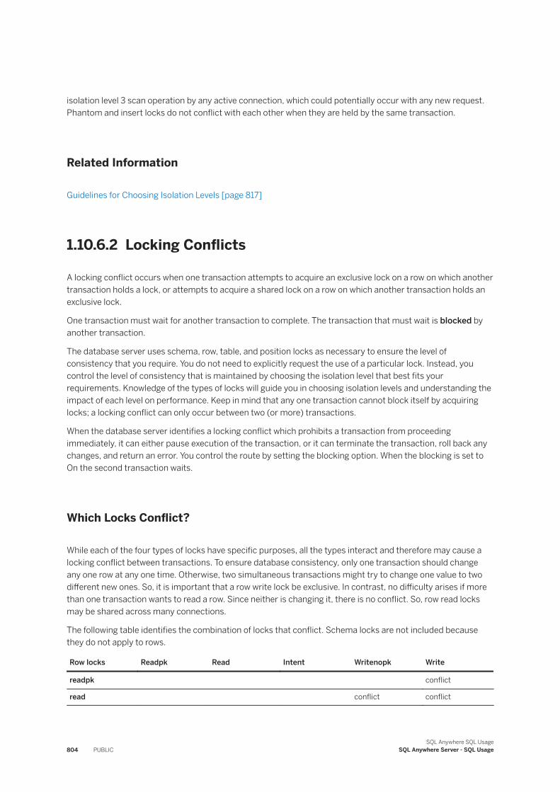
isolation level 3 scan operation by any active connection, which could potentially occur with any new request. Phantom and insert locks do not conflict with each other when they are held by the same transaction.
Related Information
Guidelines for Choosing Isolation Levels [page 817]
1.10.6.2 Locking Conflicts
A locking conflict occurs when one transaction attempts to acquire an exclusive lock on a row on which another transaction holds a lock, or attempts to acquire a shared lock on a row on which another transaction holds an exclusive lock.
One transaction must wait for another transaction to complete. The transaction that must wait is blocked by another transaction.
The database server uses schema, row, table, and position locks as necessary to ensure the level of consistency that you require. You do not need to explicitly request the use of a particular lock. Instead, you control the level of consistency that is maintained by choosing the isolation level that best fits your requirements. Knowledge of the types of locks will guide you in choosing isolation levels and understanding the impact of each level on performance. Keep in mind that any one transaction cannot block itself by acquiring locks; a locking conflict can only occur between two (or more) transactions.
When the database server identifies a locking conflict which prohibits a transaction from proceeding immediately, it can either pause execution of the transaction, or it can terminate the transaction, roll back any changes, and return an error. You control the route by setting the blocking option. When the blocking is set to On the second transaction waits.
Which Locks Conflict?
While each of the four types of locks have specific purposes, all the types interact and therefore may cause a locking conflict between transactions. To ensure database consistency, only one transaction should change any one row at any one time. Otherwise, two simultaneous transactions might try to change one value to two different new ones. So, it is important that a row write lock be exclusive. In contrast, no difficulty arises if more than one transaction wants to read a row. Since neither is changing it, there is no conflict. So, row read locks may be shared across many connections.
The following table identifies the combination of locks that conflict. Schema locks are not included because they do not apply to rows.
Row locks Readpk Read Intent Writenopk Write
readpk conflict
read conflict conflict
804 PUBLICSQL Anywhere SQL Usage
SQL Anywhere Server - SQL Usage
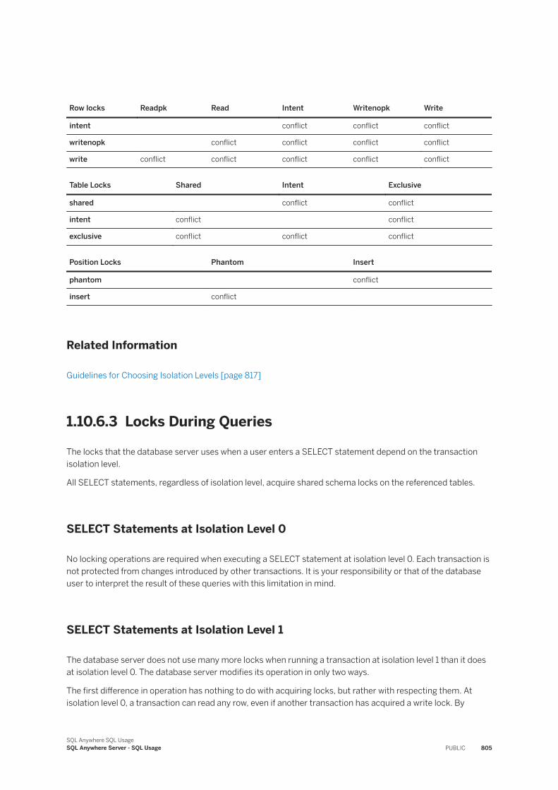
Row locks Readpk Read Intent Writenopk Write
intent conflict conflict conflict
writenopk conflict conflict conflict conflict
write conflict conflict conflict conflict conflict
Table Locks Shared Intent Exclusive
shared conflict conflict
intent conflict conflict
exclusive conflict conflict conflict
Position Locks Phantom Insert
phantom conflict
insert conflict
Related Information
Guidelines for Choosing Isolation Levels [page 817]
1.10.6.3 Locks During Queries
The locks that the database server uses when a user enters a SELECT statement depend on the transaction isolation level.
All SELECT statements, regardless of isolation level, acquire shared schema locks on the referenced tables.
SELECT Statements at Isolation Level 0
No locking operations are required when executing a SELECT statement at isolation level 0. Each transaction is not protected from changes introduced by other transactions. It is your responsibility or that of the database user to interpret the result of these queries with this limitation in mind.
SELECT Statements at Isolation Level 1
The database server does not use many more locks when running a transaction at isolation level 1 than it does at isolation level 0. The database server modifies its operation in only two ways.
The first difference in operation has nothing to do with acquiring locks, but rather with respecting them. At isolation level 0, a transaction can read any row, even if another transaction has acquired a write lock. By
SQL Anywhere SQL UsageSQL Anywhere Server - SQL Usage PUBLIC 805
contrast, before reading each row, an isolation level 1 transaction must check whether a write lock is in place. It cannot read past any write-locked rows because doing so might entail reading dirty data. The use of the READPAST hint permits the server to ignore write-locked rows, but while the transaction no longer blocks, its semantics no longer coincide with those of isolation level 1.
The second difference in operation affects cursor stability. Cursor stability is achieved by acquiring a short-term read lock on the current row of a cursor. This read lock is released when the cursor is moved. More than one row may be affected if the contents of the cursor is the result of a join. In this case, the database server acquires short-term read locks on all rows which have contributed information to the cursor's current row, and releases these locks when another row of the cursor is selected as the current row.
SELECT Statements at Isolation Level 2
At isolation level 2, the database server modifies its operation to ensure repeatable read semantics. If a SELECT statement returns values from every row in a table, then the database server acquires a read lock on each row of the table as it reads it. If, instead, the SELECT contains a WHERE clause, or another condition which restricts the rows in the result, then the database server instead reads each row, tests the values in the row against that condition, and then acquires a read lock on the row if it meets that condition. The read locks that are acquired are long-term read locks and are held until the transaction completes via an implicit or explicit COMMIT or ROLLBACK statement. As with isolation level 1, cursor stability is assured at isolation level 2, and dirty reads are not permitted.
SELECT Statements at Isolation Level 3
When operating at isolation level 3, the database server is obligated to ensure that all transaction schedules are serializable. In particular, in addition to the requirements imposed at isolation level 2, it must prevent phantom rows so that re-executing the same statement is guaranteed to return the same results in all circumstances.
To accommodate this requirement, the database server uses read locks and phantom locks. When executing a SELECT statement at isolation level 3, the database server acquires a read lock on each row that is processed during the computation of the result set. Doing so ensures that no other transactions can modify those rows until the transaction completes.
This requirement is similar to the operations that the database server performs at isolation level 2, but differs in that a lock must be acquired for each row read, whether those rows satisfy any predicates in the SELECT's WHERE, ON, or HAVING clauses. For example, if you select the names of all employees in the sales department, then the server must lock all the rows which contain information about a sales person, whether the transaction is executing at isolation level 2 or 3. At isolation level 3, however, the server must also acquire read locks on each of the rows of employees which are not in the sales department. Otherwise, another transaction could potentially transfer another employee to the sales department while the first transaction was still executing.
There are two implications when a read lock must be acquired for each row read:
● The database server may need to place many more locks than would be necessary at isolation level 2. The number of phantom locks acquired is one more than the number of read locks that are acquired for the scan. This doubling of the lock overhead adds to the execution time of the request.
● The acquisition of read locks on each row read has a negative impact on the concurrency of database update operations to the same table.
806 PUBLICSQL Anywhere SQL Usage
SQL Anywhere Server - SQL Usage
The number of phantom locks the database server acquires can vary greatly and depends upon the execution strategy chosen by the query optimizer. The SQL Anywhere query optimizer attempts to avoid sequential scans at isolation level 3 because of the potentially adverse affects on overall system concurrency, but the optimizer's ability to do so depends on the predicates in the statement and on the relevant indexes available on the referenced tables.
As an example, suppose you want to select information about the employee with Employee ID 123. As EmployeeID is the primary key of the employee table, the query optimizer will almost certainly choose an indexed strategy, using the primary key index, to locate the row efficiently. In addition, there is no danger that another transaction could change another Employee's ID to 123 because primary key values must be unique. The server can guarantee that no second employee is assigned that ID number simply by acquiring a read lock on the row containing information about employee 123.
In contrast, the database server would acquire more locks were you instead to select all the employees in the sales department. In the absence of a relevant index, the database server must read every row in the employee table and test whether each employee is in sales. If this is the case, both read and phantom locks must be acquired for each row in the table.
SELECT Statements and Snapshot Isolation
SELECT statements that execute at snapshot, statement-snapshot, or readonly-statement-snapshot do not acquire read locks. This is because each snapshot transaction (or statement) sees a snapshot of a committed state of the database at some previous point in time. The specific point in time is determined by which of the three snapshot isolation levels is being used by the statement. As such, read transactions never block update transactions and update transactions never block readers. Therefore, snapshot isolation can give considerable concurrency benefits in addition to the obvious consistency benefits. However, there is a tradeoff; snapshot isolation can be very expensive. This is because the consistency guarantee of snapshot isolation means that copies of changed rows must be saved, tracked, and (eventually) deleted for other concurrent transactions.
Related Information
Guidelines for Choosing Isolation Levels [page 817]
1.10.6.4 Locks During Inserts
Insert operations create new rows, and the database server utilizes various types of locks during insertions to ensure data integrity.
The following sequence of operations occurs for INSERT statements executing at any isolation level:
1. Acquire a shared schema lock on the table, if one is not already held.2. Acquire an intent-to-write table lock on the table, if one is not already held.3. Find an unlocked position in a page to store the new row. To minimize lock contention, the database server
does not immediately reuse space made available by deleted (but as yet uncommitted) rows. A new page may be allocated to the table (and the database file may grow) to accommodate the new row.
SQL Anywhere SQL UsageSQL Anywhere Server - SQL Usage PUBLIC 807
4. Fill the new row with any supplied values.5. Place an insert lock in the table to which the row is being added. Insert locks are exclusive, so once the
insert lock is acquired, no other isolation level 3 transaction can block the insertion by acquiring a phantom lock.
6. Write lock the new row. The insert lock is released once the write lock has been obtained.7. Insert the row into the table. Other transactions at isolation level 0 can now, for the first time, see that the
new row exists. However, these other transactions cannot modify or delete the new row because of the write lock acquired earlier.
8. Update all affected indexes and verify uniqueness where appropriate. Primary key values must be unique. Other columns may also be defined to contain only unique values, and if any such columns exist, uniqueness is verified.
9. If the table is a foreign table, acquire a shared schema lock on the primary table (if not already held), and acquire a read lock on the matching primary row in the primary table if the foreign key column values being inserted are not NULL. The database server must ensure that the primary row still exists when the inserting transaction COMMITs. It does so by acquiring a read lock on the primary row. With the read lock in place, any other transaction is still free to read that row, but none can delete or update it.If the corresponding primary row does not exist, a referential integrity constraint violation is given.
After the last step, any AFTER INSERT triggers defined on the table may fire. Processing within triggers follows the same locking behavior as for applications. Once the transaction is committed (assuming all referential integrity constraints are satisfied) or rolled back, all long-term locks are released.
Uniqueness
You can ensure that all values in a particular column, or combination of columns, are unique. The database server always performs this task by building an index for the unique column, even if you do not explicitly create one.
In particular, all primary key values must be unique. The database server automatically builds an index for the primary key of every table. Do not ask the database server to create an index on a primary key, as that index would be a redundant index.
Orphans and Referential Integrity
A foreign key is a reference to a primary key or UNIQUE constraint, usually in another table. When that primary key does not exist, the offending foreign key is called an orphan. The database server automatically ensures that your database contains no rows that violate referential integrity. This process is referred to as verifying referential integrity. The database server verifies referential integrity by counting orphans.
wait_for_commit
You can instruct the database server to delay verifying referential integrity to the end of your transaction. In this mode, you can insert a row which contains a foreign key, then subsequently insert a primary row which contains the missing primary key. Both operations must occur in the same transaction.
808 PUBLICSQL Anywhere SQL Usage
SQL Anywhere Server - SQL Usage
To request that the database server delay referential integrity checks until commit time, set the value of the option wait_for_commit to On. By default, this option is Off. To turn it on, execute the following statement:
SET OPTION wait_for_commit = On;
If the server does not find a matching primary row when a new foreign key value is inserted, and wait_for_commit is On, then the server permits the insertion as an orphan. For orphaned foreign rows, upon insertion the following series of steps occurs:
● The server acquires a shared schema lock on the primary table (if not already held). The server also acquires an intent-to-write lock on the primary table.
● The server inserts a surrogate row into the primary table. An actual row is not inserted into the primary table, but the server manufactures a unique row identifier for that row for locking, and a write lock is acquired on this surrogate row. Subsequently, the server inserts the appropriate values into the primary table's primary key index.
Before committing a transaction, the database server verifies that referential integrity is maintained by checking the number of orphans your transaction has created. At the end of every transaction, that number must be zero.
1.10.6.5 Locks During Updates
The database server modifies the information contained in a particular record when it is using locking.
As with insertions, this sequence of operations is followed for all transactions regardless of their isolation level.
1. Acquire a shared schema lock on the table, if one is not already held.2. Acquire an intent-to-write table lock for each table to be updated, if one is not already held.
1. For each table to be updated, if the table has triggers then create the temporary tables for the OLD and NEW values as required.
2. Identify candidate rows to be updated. As rows are scanned, they are locked.At isolation levels 2 and 3 the following differences occur that are different from the default locking behavior: intent-to-write row-level locks are acquired instead of read locks, and intent-to-write locks may be acquired on rows that are ultimately rejected as candidates for update.
3. For each candidate row identified in step 2.a, follow the rest of the sequence.3. Write lock the affected row.4. Update each of the affected column values as per the UPDATE statement.5. If indexed values were changed, add new index entries. The original index entries for the row remain, but
are marked as deleted. New index entries for the new values are inserted while a short-term insert lock is held. The server verifies index uniqueness where appropriate.
6. If a uniqueness violation occurred, a temporary "hold" table is created to store the old and new values of the row. The old and new values are copied to the hold table, and the base table row is deleted. Any DELETE triggers are not fired. Defer steps 7 through 9 until the end of row-by-row processing.
7. If any foreign key values in the row were altered, acquire a shared schema lock on the primary table(s) and follow the procedure for inserting new foreign key values.Similarly, follow the procedure for WAIT_FOR_COMMIT if applicable.
8. If the table is a primary table in a referential integrity relationship, and the relationship's UPDATE action is not RESTRICT, determine the affected row(s) in the foreign table(s) by first acquiring a shared schema lock on the table(s), an intent-to-write table lock on each, and acquire write locks on all the affected rows,
SQL Anywhere SQL UsageSQL Anywhere Server - SQL Usage PUBLIC 809
modifying each as appropriate. This process may cascade through a nested hierarchy of referential integrity constraints.
9. Fire AFTER ROW triggers as appropriate.
After the last step, if a hold temporary table was required, each row in the hold temporary table is now inserted into the base table (but INSERT triggers are not fired). If the row insertion succeeds, steps 7-9 above are executed and the old and new row values are copied to the OLD and NEW temporary tables to permit any AFTER STATEMENT UPDATE triggers to correctly process all of the modified rows. After all of the hold rows have been processed, the AFTER STATEMENT UPDATE triggers are fired in order. Upon COMMIT, the server verifies referential integrity by ensuring that the number of orphans produced by this transaction is 0, and release all locks.
Modifying a column value can necessitate a large number of operations. The amount of work that the database server needs to do is much less if the column being modified is not part of a primary or foreign key. It is lower still if it is not contained in an index, either explicitly or implicitly because the column has been declared as unique.
The operation of verifying referential integrity during an UPDATE operation is no less simple than when the verification is performed during an INSERT. In fact, when you change the value of a primary key, you may create orphans. When you insert the replacement value, the database server must check for orphans once more.
Related Information
Locks During Inserts [page 807]Isolation Levels and Consistency [page 777]Guidelines for Choosing Isolation Levels [page 817]
1.10.6.6 Locks During Deletes
The DELETE operation follows almost the same steps as the INSERT operation, except in the opposite order.
As with insertions and updates, this sequence of operations is followed for all transactions regardless of their isolation level.
1. Acquire a shared schema lock on the table, if one is not already held.2. Acquire an intent-to-write table lock on the table, if one is not already held.
1. Identify candidate rows to be updated. As rows are scanned, they are locked.At isolation levels 2 and 3 the following differences occur that are different from the default locking behavior: intent-to-write row-level locks are acquired instead of read locks, and intent-to-write locks may be acquired on rows that are ultimately rejected as candidates for update.
2. For each candidate row identified in step 2.a, follow the rest of the sequence.3. Write lock the row to be deleted.4. Remove the row from the table so that it is no longer visible to other transactions. The row cannot be
destroyed until the transaction is committed because doing so would remove the option of rolling back the transaction. Index entries for the deleted row are preserved, though marked as deleted, until transaction completion. This prevents other transactions from re-inserting the same row.
810 PUBLICSQL Anywhere SQL Usage
SQL Anywhere Server - SQL Usage

5. If the table is a primary table in a referential integrity relationship, and the relationship's DELETE action is not RESTRICT, determine the affected row(s) in the foreign table(s) by first acquiring a shared schema lock on the table(s), an intent-to-write table lock on each, and acquire write locks on all the affected rows, modifying each as appropriate. This process may cascade through a nested hierarchy of referential integrity constraints.
The transaction can be committed provided referential integrity is not violated by doing so. To verify referential integrity, the database server also keeps track of any orphans created as a side effect of the deletion. Upon COMMIT, the server records the operation in the transaction log file and release all locks.
Related Information
Isolation Levels and Consistency [page 777]Guidelines for Choosing Isolation Levels [page 817]
1.10.6.7 Lock Duration
Locks are typically held by a transaction until it completes.
This behavior prevents other transactions from making changes that would make it impossible to roll back the original transaction. At isolation level three, all locks must be held until a transaction ends to guarantee transaction serializability.
The only locks that are not held until the end of a transaction are cursor stability locks. These row locks are held for as long as the row in question is the current row of a cursor. In most cases, this amount of time is shorter than the lifetime of the transaction, but for WITH HOLD cursors, cursor stability locks can be held for the lifetime of the connection.
1.10.6.8 Viewing Locks (SQL Central)
Use the Locks tab in SQL Central to view the locks that are currently held in the database.
Context
The contents of locked rows can be used to diagnose a locking issue in the database.
SQL Anywhere SQL UsageSQL Anywhere Server - SQL Usage PUBLIC 811
Procedure
1. In left pane, click the database.2. Click the Locks tab in the right pane.
Results
The tab displays information about the locks.
SQL Central shows the locks present at the time that the query began.
Related Information
Schema Locks [page 799]
1.10.6.9 Viewing Locks (Interactive SQL)
Obtain information about locked rows to diagnose locking issues in the database.
Prerequisites
You must have EXECUTE privilege on sa_locks, sa_conn_info, and connection_properties. You must have the MONITOR system privilege and either the SERVER OPERATOR or the DROP CONNECTION system privilege.
Context
View the locks that your connection is holding, including information about the lock, the lock duration, and the lock type.
Procedure
1. Connect to a database in Interactive SQL.
2. Use the Locking Viewer window. Click Tools Locking Viewer .
812 PUBLICSQL Anywhere SQL Usage
SQL Anywhere Server - SQL Usage
Results
Interactive SQL shows the locks your connection is holding, the objects being locked, and the connections that are blocked as a result.
You can also view this information in the status bar. The status bar indicator displays the status information for the selected tab.
Related Information
Transaction Blocking and Deadlock [page 793]
1.10.6.10 Mutexes and Semaphores
Use mutexes and semaphores in your application logic to achieve locking behavior and control and communicate the availability of resources.
Mutexes and semaphores are locking and signaling mechanisms that control the availability or use of a shared resource such as an external library or a procedure. You can include mutexes and semaphores to achieve the type of locking behavior your application requires. Choosing whether to use mutexes or semaphores depends on the requirements of your application.
Mutexes provide the application with a concurrency control mechanism; for example, they can be used to allow only one connection at a time to execute a critical section in a stored procedure, user-defined function, trigger, or event. Mutexes can also lock an application resource that does not directly correspond to a database object. Semaphores provide support for producer/consumer application logic in the database or for access to limited application resources.
Mutexes and semaphores benefit from the same deadlock detection as database row and table locks.
UPDATE ANY MUTEX SEMAPHORE allows locking/releasing of mutexes and notifying/waiting for semaphores, CREATE ANY MUTEX SEMAPHORE is necessary to create/replace, and DROP ANY MUTEX SEMAPHORE is necessary to drop/replace. To have a finer level of control on who can update a mutex or semaphore, you can grant privileges on the objects they are used in instead. For example, you can grant EXECUTE privilege on a system procedure that contains a mutex.
More About Mutexes
A mutex is a lock and release mechanism that limits the availability of a critical section of a shared resource such as an external library or a stored procedure. Locking and unlocking a mutex is achieved by executing LOCK MUTEX and RELEASE MUTEX statements, respectively.
The scope of a mutex can be either transaction or connection. In transaction-scope mutexes, the lock is held until the end of the transaction that has locked the mutex. In connection-scope mutexes, the lock is held until a RELEASE MUTEX statement is executed by the connection or until the connection terminates.
SQL Anywhere SQL UsageSQL Anywhere Server - SQL Usage PUBLIC 813
The mode of a mutex can be either exclusive or shared. In exclusive mode, only the transaction or connection holding the lock can use the resource. In shared mode, multiple transactions or connections can lock the mutex.
You can recursively lock a mutex (that is, you can nest LOCK MUTEX statements for the same mutex inside your code). However, with connection-scope mutexes, an equal number of RELEASE MUTEX statements are required to release the mutex.
If a connection locks a mutex in shared mode, and then (recursively) locks it again in exclusive mode, then the lock remains held in exclusive mode until it is released twice, or until the end of the transaction.
Here is a simple scenario showing how you can use a mutex to protect a critical section of a stored procedure. In this scenario, the critical section can only be executed by one connection at a time (but can span multiple transactions):
1. The following statement creates a new mutex to protect the critical section:
CREATE MUTEX protect_my_cr_section SCOPE CONNECTION;
2. The following statement locks the critical section in exclusive mode so that no other connection can access it:
LOCK MUTEX protect_my_cr_section IN EXCLUSIVE MODE;
3. The following statement releases the critical section:
RELEASE MUTEX protect_my_cr_section;
4. The following statement removes the mutex when the critical section no longer needs protection:
DROP MUTEX protect_my_cr_section;
More About Semaphores
A semaphore is a signaling mechanism that uses a counter to communicate the availability of a resource. Incrementing and decrementing the semaphore counter is achieved by executing NOTIFY SEMAPHORE and WAITFOR SEMAPHORE statements, respectively. Use semaphores in a resource availability model or in a producer-consumer model. Regardless of model, a semaphore cannot go below 0. That way, the counter is used to limit the availability of the resource (a license, in this example).
The resource availability model is when a counter is used to limit the availability of a resource. For example, suppose you have a license that restricts application use to 10 users at a time. You set the semaphore counter to 10 at create time using the START WITH clause. When a user logs in, a WAITFOR SEMAPHORE statement is executed, and the count is decremented by one. If the count is 0, then the user waits for up to the specified timeout period. If the counter goes above 0 before the timeout, then they log in. If not, then the users login attempt times out. When the user logs out, a NOTIFY SEMAPHORE statement is executed, incrementing the count by one. Each time a user logs in, the count is decremented; each time they log out, the count is incremented.
The producer-consumer model is when a counter is used to signal the availability of a resource. For example, suppose there is a procedure that consumes what another procedure produces. The consumer executes a WAITFOR SEMAPHORE statement and waits for something to process. When the producer has created output, it executes a NOTIFY SEMAPHORE statement to signal that work is available. This statement increments the
814 PUBLICSQL Anywhere SQL Usage
SQL Anywhere Server - SQL Usage
counter associated with the semaphore. When the waiting consumer gets the work, the counter is decremented. In the producer-consumer model, the counter cannot go below 0, but it can go as high as the producers increment the counter.
Here is a simple scenario showing how you can use a semaphore to control the number of licenses for an application. The scenario assumes there is a total of three licenses available, and that each successful log in to the application consumes one license:
1. The following statement creates a new semaphore with the number of licenses specified as the initial count:
CREATE SEMAPHORE license_counter START WITH 3;
2. The following statement obtains a license using the license_counter semaphore:
WAITFOR SEMAPHORE license_counter;
3. The following statement releases the license:
NOTIFY SEMAPHORE license_counter INCREMENT BY 1;
4. The following statement removes the semaphore when the application no longer needs to be limited by the license:
DROP SEMAPHORE license_counter;
So, a common way to use semaphores in a producer-consumer model might look something like this:
CREATE SEMAPHORE producer_counter; CREATE SEMAPHORE consumer_counter START WITH 100;CREATE PROCEDURE DBA.MyProducer( ) BEGIN WHILE 1 = 1 LOOP WAITFOR SEMAPHORE consumer_counter; -- produce some data and put it somewhere (e.g. a table) NOTIFY SEMAPHORE producer_counter; END LOOP ENDgoCREATE PROCEDURE DBA.MyConsumer( ) BEGIN WHILE 1 = 1 LOOP WAITFOR SEMAPHORE producer_counter; -- read the next bit of data and do something with it NOTIFY SEMAPHORE consumer_counter; END LOOP ENDgo
In this example, MyProducer and MyConsumer run in different connections. MyProducer just fetches data and can get at most 100 iterations ahead of MyConsumer. If MyConsumer goes faster than MyProducer, producer_counter will eventually reach 0. At that point, MyConsumer will block until MyProducer can make more data. If MyProducer goes faster than MyConsumer, consumer_counter will eventually reach 0. At that point, MyProducer will block until MyConsumer can consume some data.
In this section:
Creating Mutexes and Semaphores (SQL Central) [page 816]Use a mutex or a semaphore within your applications to achieve locking behavior, and control and communicate the availability of resources.
SQL Anywhere SQL UsageSQL Anywhere Server - SQL Usage PUBLIC 815

1.10.6.10.1 Creating Mutexes and Semaphores (SQL Central)
Use a mutex or a semaphore within your applications to achieve locking behavior, and control and communicate the availability of resources.
Prerequisites
You must have the CREATE ANY MUTEX SEMAPHORE system privilege.
Context
Include mutexes and semaphores to achieve the type of locking behavior that your application requires.
Procedure
1. In the left pane, right-click Mutexes and Semaphores, click New, and then click either Mutex or Semaphore.2. Follow the instructions in the wizard.
Results
The mutex or semaphore is created.
Next Steps
For MUTEXES, execute LOCK MUTEX and RELEASE MUTEX statements to limit the availability of a critical section of a code or a shared resource, such as an external library or a stored procedure.
For semaphores, execute WAITFOR SEMAPHORE or NOTIFY SEMAPHORE statements to limit the availability of a resource, such as a license.
Related Information
Mutexes and Semaphores [page 813]
816 PUBLICSQL Anywhere SQL Usage
SQL Anywhere Server - SQL Usage
1.10.7 Guidelines for Choosing Isolation Levels
The choice of isolation level depends on the kind of task an application is performing.
To choose an appropriate isolation level, you must balance the need for consistency and accuracy with the need for concurrent transactions to proceed unimpeded. If a transaction involves only one or two specific values in one table, it is unlikely to interfere as much with other processes compared to one that searches many large tables and therefore may need to lock many rows or entire tables and may take a very long time to complete.
For example, if your transactions involve transferring money between bank accounts, you likely want to ensure that the information you return is correct. However, if you just want a rough estimate of the proportion of inactive accounts, then you may not care whether your transaction waits for others or not, and you may be willing to sacrifice some accuracy to avoid interfering with other users of the database.
Furthermore, a transfer may affect only the two rows which contain the two account balances, whereas all the accounts must be read to calculate the estimate. For this reason, the transfer is less likely to delay other transactions.
Four isolation levels are provided: levels 0, 1, 2, and 3. Level 3 provides complete isolation and ensures that transactions are interleaved in such a manner that the schedule is serializable.
If you have enabled snapshot isolation for a database, then three additional isolation levels are available: snapshot, statement-snapshot, and readonly-statement-snapshot.
In this section:
Choosing a Snapshot Isolation Level [page 818]Snapshot isolation offers both concurrency and consistency benefits.
Serializable Schedules [page 818]The order in which the component operations of the various transactions are interleaved is called the schedule.
Typical Transactions at Various Isolation Levels [page 819]The isolation level should be set to reflect the type of tasks the database server performs.
Concurrency Improvement at Isolation Levels 2 and 3 [page 820]Isolation levels 2 and 3 use a lot of locks. Good design is important for databases that make regular use of these isolation levels.
Tips on Reducing the Impact of Locking [page 821]To avoid placing a large number of locks that might impact the execution of other concurrent transactions, avoid running transactions at isolation level 3.
Related Information
Snapshot Isolation [page 779]
SQL Anywhere SQL UsageSQL Anywhere Server - SQL Usage PUBLIC 817
1.10.7.1 Choosing a Snapshot Isolation Level
Snapshot isolation offers both concurrency and consistency benefits.
Using snapshot isolation incurs a cost penalty since old versions of rows are saved as long as they may be needed by running transactions. Therefore, long running snapshots can require storage of many old row versions. Usually, snapshots used for statement-snapshot do not last as long as those for snapshot. Therefore, statement-snapshot may have some space advantages over snapshot at the cost of less consistency (every statement within the transaction sees the database at a different point in time).
For most purposes, the snapshot isolation level is recommended because it provides a single view of the database for the entire transaction.
The statement-snapshot isolation level provides less consistency, but may be useful when long running transactions result in too much space being used in the temporary file by the version store.
The readonly-statement-snapshot isolation level provides less consistency than statement-snapshot, but avoids the possibility of update conflicts. Therefore, it is most appropriate for porting applications originally intended to run under different isolation levels.
Related Information
Snapshot Isolation [page 779]
1.10.7.2 Serializable Schedules
The order in which the component operations of the various transactions are interleaved is called the schedule.
To process transactions concurrently, the database server must execute some component statements of one transaction, then some from other transactions, before continuing to process further operations from the first.
Applying transactions concurrently in this manner can result in many possible outcomes, including the three particular inconsistencies described in the previous section. Sometimes, the final state of the database also could have been achieved had the transactions been executed sequentially, meaning that one transaction was always completed in its entirety before the next was started. A schedule is called serializable whenever executing the transactions sequentially, in some order, could have left the database in the same state as the actual schedule.
Serializability is the commonly accepted criterion for correctness. A serializable schedule is accepted as correct because the database is not influenced by the concurrent execution of the transactions.
The isolation level affects a transaction's serializability. At isolation level 3, all schedules are serializable. The default setting is 0.
818 PUBLICSQL Anywhere SQL Usage
SQL Anywhere Server - SQL Usage
Serializable Means that Concurrency has Added No Effect
Even when transactions are executed sequentially, the final state of the database can depend upon the order in which these transactions are executed. For example, if one transaction sets a particular cell to the value 5 and another sets it to the number 6, then the final value of the cell is determined by which transaction executes last.
Knowing a schedule is serializable does not settle which order transactions would best be executed, but rather states that concurrency has added no effect. Outcomes which may be achieved by executing the set of transactions sequentially in some order are all assumed correct.
Unserializable Schedules Introduce Inconsistencies
The inconsistencies are typical of the types of problems that appear when the schedule is not serializable. In each case, the inconsistency appeared because of the way the statements were interleaved; the result produced would not be possible if all transactions were executed sequentially. For example, a dirty read can only occur if one transaction can select rows while another transaction is in the middle of inserting or updating data in the same row.
Related Information
Typical Types of Inconsistency [page 786]
1.10.7.3 Typical Transactions at Various Isolation Levels
The isolation level should be set to reflect the type of tasks the database server performs.
Use the information below to help you decide which level is best suited to each particular operation.
Typical Level 0 Transactions
Transactions that involve browsing or performing data entry may last several minutes, and read a large number of rows. If isolation level 2 or 3 is used, concurrency can suffer. Isolation level of 0 or 1 is typically used for this kind of transaction.
For example, a decision support application that reads large amounts of information from the database to produce statistical summaries may not be significantly affected if it reads a few rows that are later modified. If high isolation is required for such an application, it may acquire read locks on large amounts of data, not allowing other applications write access to it.
SQL Anywhere SQL UsageSQL Anywhere Server - SQL Usage PUBLIC 819
Typical Level 1 Transactions
Isolation level 1 is useful with cursors because this combination ensures cursor stability without greatly increasing locking requirements. The database server achieves this benefit through the early release of read locks acquired for the present row of a cursor. These locks must persist until the end of the transaction at either levels two or three to guarantee repeatable reads.
For example, a transaction that updates inventory levels through a cursor is suited to this level, because each of the adjustments to inventory levels as items are received and sold would not be lost, yet these frequent adjustments would have minimal impact on other transactions.
Typical Level 2 Transactions
At isolation level 2, rows that match your criterion cannot be changed by other transactions. You can employ this level when you must read rows more than once and rely that rows contained in your first result set won't change.
Because of the relatively large number of read locks required, you should use this isolation level with care. As with level 3 transactions, careful design of your database and indexes reduce the number of locks acquired and can improve the performance of your database.
Typical Level 3 Transactions
Isolation level 3 is appropriate for transactions that demand the most in security. The elimination of phantom rows lets you perform multi-step operations on a set of rows without fear that new rows could appear partway through your operations and corrupt the result.
However much integrity it provides, isolation level 3 should be used sparingly on large systems that are required to support a large number of concurrent transactions. The database server places more locks at this level than at any other, raising the likelihood that one transaction impedes the process of many others.
1.10.7.4 Concurrency Improvement at Isolation Levels 2 and 3
Isolation levels 2 and 3 use a lot of locks. Good design is important for databases that make regular use of these isolation levels.
When you must make use of serializable transactions, it is important that you design your database, in particular the indexes, with the business rules of your project in mind. You may also improve performance by breaking large transactions into several smaller ones, and shorten the length of time that rows are locked.
Although serializable transactions have the most potential to block other transactions, they are not necessarily less efficient. When processing these transactions, the database server can perform certain optimizations that may improve performance, in spite of the increased number of locks. For example, since all rows read must be locked whether they match the search criteria, the database server is free to combine the operation of reading rows and placing locks.
820 PUBLICSQL Anywhere SQL Usage
SQL Anywhere Server - SQL Usage
1.10.7.5 Tips on Reducing the Impact of Locking
To avoid placing a large number of locks that might impact the execution of other concurrent transactions, avoid running transactions at isolation level 3.
When the nature of an operation demands that it run at isolation level 3, you can lower its impact on concurrency by designing the query to read as few rows and index entries as possible. These steps help the level 3 transaction run more quickly and, of possibly greater importance, will reduce the number of locks it places.
When at least one operation executes at isolation level 3, you may find that adding an index improves transaction speed. An index can have two benefits:
● An index enables rows to be located in an efficient manner.● Searches that make use of the index may need fewer locks.
Related Information
How Locking Works [page 796]
1.10.8 Isolation Level Tutorials
Each isolation level behaves differently and which one you should use depends on your database and on the operations you are performing.
The following set of tutorials helps you determine which isolation levels are suitable for different tasks.
In this section:
Tutorial: Setting Up the Scenario for the Isolation Level Tutorials [page 822]Set up your database for an isolation level tutorial by opening two Interactive SQL windows to act as the Sales Manager and Accountant.
Tutorial: Understanding Dirty Reads [page 823]The following tutorial demonstrates the type of inconsistency that can occur when multiple transactions are executed concurrently: the dirty read.
Tutorial: Understanding Non-repeatable Reads [page 829]The tutorial demonstrates the type of inconsistency that can occur when multiple transactions are executed concurrently: the non-repeatable read.
Tutorial: Understanding Phantom Rows [page 835]The tutorial demonstrates the type of inconsistency that can occur when multiple transactions are executed concurrently: the phantom row.
Tutorial: Understanding Phantom Locks [page 841]Prevent phantom rows by using phantom locks.
SQL Anywhere SQL UsageSQL Anywhere Server - SQL Usage PUBLIC 821
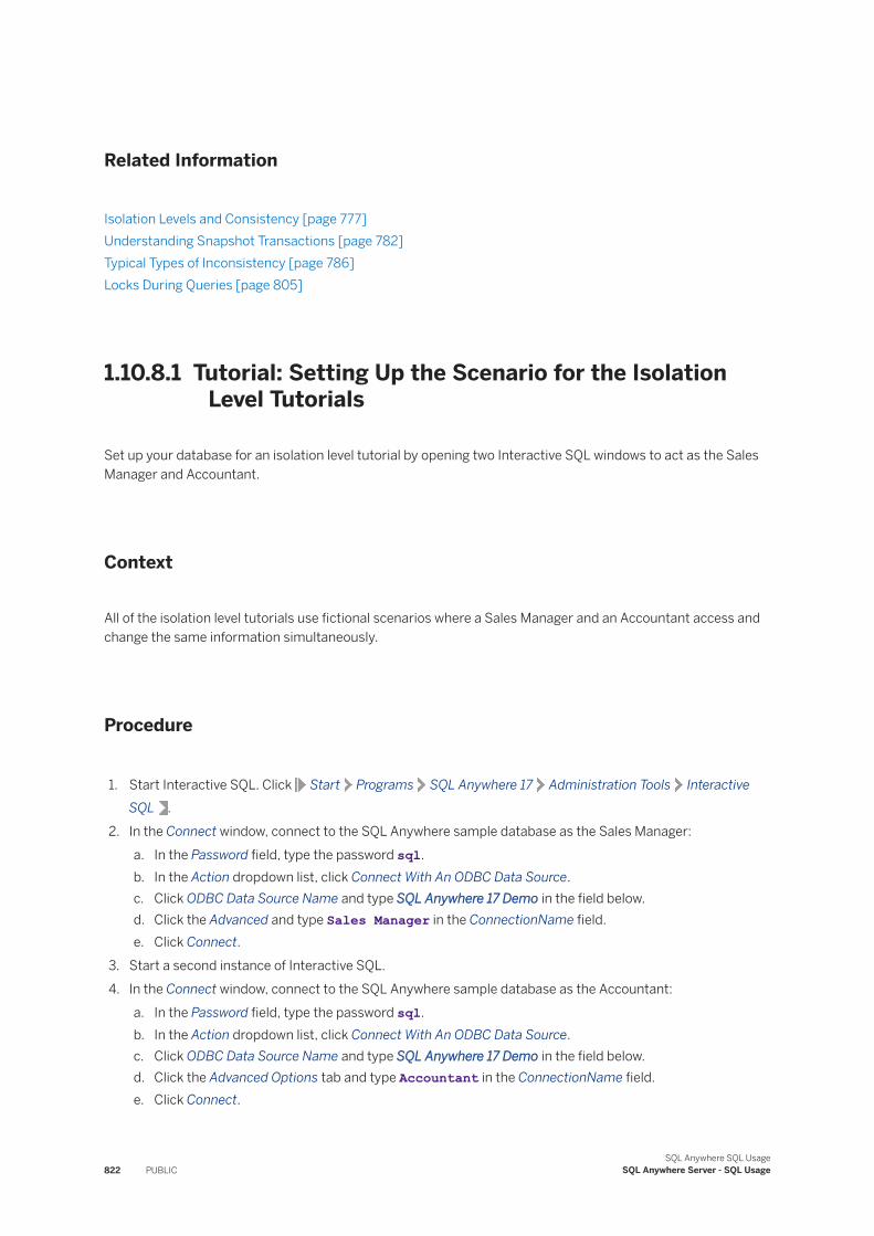
Related Information
Isolation Levels and Consistency [page 777]Understanding Snapshot Transactions [page 782]Typical Types of Inconsistency [page 786]Locks During Queries [page 805]
1.10.8.1 Tutorial: Setting Up the Scenario for the Isolation Level Tutorials
Set up your database for an isolation level tutorial by opening two Interactive SQL windows to act as the Sales Manager and Accountant.
Context
All of the isolation level tutorials use fictional scenarios where a Sales Manager and an Accountant access and change the same information simultaneously.
Procedure
1. Start Interactive SQL. Click Start Programs SQL Anywhere 17 Administration Tools Interactive SQL .
2. In the Connect window, connect to the SQL Anywhere sample database as the Sales Manager:a. In the Password field, type the password sql.b. In the Action dropdown list, click Connect With An ODBC Data Source.c. Click ODBC Data Source Name and type SQL Anywhere 17 Demo in the field below.d. Click the Advanced and type Sales Manager in the ConnectionName field.e. Click Connect.
3. Start a second instance of Interactive SQL.4. In the Connect window, connect to the SQL Anywhere sample database as the Accountant:
a. In the Password field, type the password sql.b. In the Action dropdown list, click Connect With An ODBC Data Source.c. Click ODBC Data Source Name and type SQL Anywhere 17 Demo in the field below.d. Click the Advanced Options tab and type Accountant in the ConnectionName field.e. Click Connect.
822 PUBLICSQL Anywhere SQL Usage
SQL Anywhere Server - SQL Usage
Results
You are connected to the sample database as both the Sales Manager and the Accountant.
Next Steps
Perform one of the isolation level tutorials.
Related Information
Tutorial: Understanding Dirty Reads [page 823]Tutorial: Understanding Non-repeatable Reads [page 829]Tutorial: Understanding Phantom Rows [page 835]Tutorial: Understanding Phantom Locks [page 841]
1.10.8.2 Tutorial: Understanding Dirty Reads
The following tutorial demonstrates the type of inconsistency that can occur when multiple transactions are executed concurrently: the dirty read.
Prerequisites
You must have the SELECT ANY TABLE, UPDATE ANY TABLE, and SET ANY SYSTEM OPTION system privileges.
This tutorial assumes that you have connected to the sample database as the Sales Manager and as the Accountant, as described in the tutorial "Setting up the scenario for the isolation level tutorials."
Context
In this scenario, two employees at a small merchandising company access the corporate database at the same time. The first person is the company's Sales Manager; the second is the Accountant.
The Sales Manager wants to increase the price of tee shirts sold by their firm by $0.95, but is having a little trouble with the syntax of the SQL language. At the same time, unknown to the Sales Manager, the Accountant is trying to calculate the retail value of the current inventory to include in a report needed for the next management meeting.
SQL Anywhere SQL UsageSQL Anywhere Server - SQL Usage PUBLIC 823
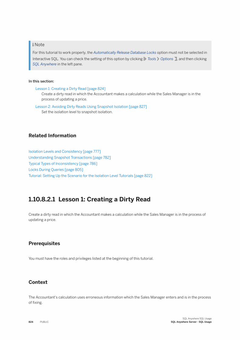
NoteFor this tutorial to work properly, the Automatically Release Database Locks option must not be selected in Interactive SQL. You can check the setting of this option by clicking Tools Options , and then clicking SQL Anywhere in the left pane.
In this section:
Lesson 1: Creating a Dirty Read [page 824]Create a dirty read in which the Accountant makes a calculation while the Sales Manager is in the process of updating a price.
Lesson 2: Avoiding Dirty Reads Using Snapshot Isolation [page 827]Set the isolation level to snapshot isolation.
Related Information
Isolation Levels and Consistency [page 777]Understanding Snapshot Transactions [page 782]Typical Types of Inconsistency [page 786]Locks During Queries [page 805]Tutorial: Setting Up the Scenario for the Isolation Level Tutorials [page 822]
1.10.8.2.1 Lesson 1: Creating a Dirty Read
Create a dirty read in which the Accountant makes a calculation while the Sales Manager is in the process of updating a price.
Prerequisites
You must have the roles and privileges listed at the beginning of this tutorial.
Context
The Accountant's calculation uses erroneous information which the Sales Manager enters and is in the process of fixing.
824 PUBLICSQL Anywhere SQL Usage
SQL Anywhere Server - SQL Usage
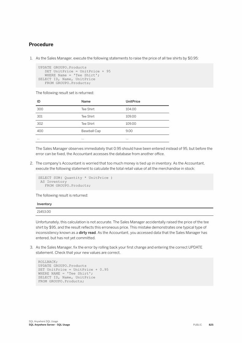
Procedure
1. As the Sales Manager, execute the following statements to raise the price of all tee shirts by $0.95:
UPDATE GROUPO.Products SET UnitPrice = UnitPrice + 95 WHERE Name = 'Tee Shirt';SELECT ID, Name, UnitPrice FROM GROUPO.Products;
The following result set is returned:
ID Name UnitPrice
300 Tee Shirt 104.00
301 Tee Shirt 109.00
302 Tee Shirt 109.00
400 Baseball Cap 9.00
... ... ...
The Sales Manager observes immediately that 0.95 should have been entered instead of 95, but before the error can be fixed, the Accountant accesses the database from another office.
2. The company's Accountant is worried that too much money is tied up in inventory. As the Accountant, execute the following statement to calculate the total retail value of all the merchandise in stock:
SELECT SUM( Quantity * UnitPrice ) AS Inventory FROM GROUPO.Products;
The following result is returned:
Inventory
21453.00
Unfortunately, this calculation is not accurate. The Sales Manager accidentally raised the price of the tee shirt by $95, and the result reflects this erroneous price. This mistake demonstrates one typical type of inconsistency known as a dirty read. As the Accountant, you accessed data that the Sales Manager has entered, but has not yet committed.
3. As the Sales Manager, fix the error by rolling back your first change and entering the correct UPDATE statement. Check that your new values are correct.
ROLLBACK; UPDATE GROUPO.ProductsSET UnitPrice = UnitPrice + 0.95WHERE NAME = 'Tee Shirt';SELECT ID, Name, UnitPrice FROM GROUPO.Products;
SQL Anywhere SQL UsageSQL Anywhere Server - SQL Usage PUBLIC 825
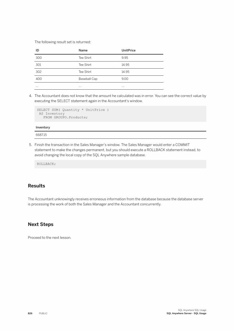
The following result set is returned:
ID Name UnitPrice
300 Tee Shirt 9.95
301 Tee Shirt 14.95
302 Tee Shirt 14.95
400 Baseball Cap 9.00
... ... ...
4. The Accountant does not know that the amount he calculated was in error. You can see the correct value by executing the SELECT statement again in the Accountant's window.
SELECT SUM( Quantity * UnitPrice ) AS Inventory FROM GROUPO.Products;
Inventory
6687.15
5. Finish the transaction in the Sales Manager's window. The Sales Manager would enter a COMMIT statement to make the changes permanent, but you should execute a ROLLBACK statement instead, to avoid changing the local copy of the SQL Anywhere sample database.
ROLLBACK;
Results
The Accountant unknowingly receives erroneous information from the database because the database server is processing the work of both the Sales Manager and the Accountant concurrently.
Next Steps
Proceed to the next lesson.
826 PUBLICSQL Anywhere SQL Usage
SQL Anywhere Server - SQL Usage
1.10.8.2.2 Lesson 2: Avoiding Dirty Reads Using Snapshot Isolation
Set the isolation level to snapshot isolation.
Prerequisites
You must have completed the previous lessons in this tutorial.
You must have the roles and privileges listed at the beginning of this tutorial.
Context
Snapshot isolation prevents dirty reads from occurring by allowing other database connections to only view committed data in response to queries.
The Accountant can use snapshot isolation to ensure that uncommitted data does not affect his queries.
Procedure
1. As the Sales Manager, execute the following statement to enable snapshot isolation for the database:
SET OPTION PUBLIC.allow_snapshot_isolation = 'ON';
2. As the Sales Manager, raise the price of all the tee shirts by $0.95:a. Execute the following statement to update the price:
UPDATE GROUPO.Products SET UnitPrice = UnitPrice + 0.95 WHERE Name = 'Tee Shirt';
b. Calculate the total retail value of all merchandise in stock using the new tee shirt price for the Sales Manager:
SELECT SUM( Quantity * UnitPrice ) AS Inventory FROM GROUPO.Products;
The following result is returned:
Inventory
6687.15
SQL Anywhere SQL UsageSQL Anywhere Server - SQL Usage PUBLIC 827
3. As the Accountant, execute the following statements to calculate the total retail value of all the merchandise in stock. Because this transaction uses the snapshot isolation level, the result is calculated only for data that has been committed to the database.
SET OPTION isolation_level = 'Snapshot'; SELECT SUM( Quantity * UnitPrice ) AS Inventory FROM GROUPO.Products;
The following result is returned:
Inventory
6538.00
4. As the Sales Manager, commit your changes to the database by executing the following statement:
COMMIT;
5. As the Accountant, execute the following statements to view the updated retail value of the current inventory:
COMMIT; SELECT SUM( Quantity * UnitPrice ) AS Inventory FROM GROUPO.Products;
The following result is returned:
Inventory
6687.15
Because the snapshot used for the Accountant's transaction began with the first read operation, you must execute a COMMIT to end the transaction and allow the Accountant to see changes made to the data after the snapshot transaction began.
6. As the Sales Manager, execute the following statement to undo the tee shirt price changes and restore the SQL Anywhere sample database to its original state:
UPDATE GROUPO.Products SET UnitPrice = UnitPrice - 0.95WHERE Name = 'Tee Shirt'; COMMIT;
Results
The Accountant successfully avoided dirty reads by enabling snapshot isolation.
Next Steps
(optional) Restore the sample database (demo.db) to its original state.
828 PUBLICSQL Anywhere SQL Usage
SQL Anywhere Server - SQL Usage
1.10.8.3 Tutorial: Understanding Non-repeatable Reads
The tutorial demonstrates the type of inconsistency that can occur when multiple transactions are executed concurrently: the non-repeatable read.
Prerequisites
You must have the SELECT ANY TABLE, UPDATE ANY TABLE, and SET ANY SYSTEM OPTION system privileges.
This tutorial assumes that you have connected to the sample database as the Sales Manager and as the Accountant.
Context
In this scenario, two employees at a small merchandising company access the corporate database at the same time. The first person is the company's Sales Manager; the second is the Accountant.
The Sales Manager wants to offer a new sales price on plastic visors. The Accountant wants to verify the prices of some items that appear on a recent order.
This example begins with both connections at isolation level 1, rather than at isolation level 0, which is the default for the SQL Anywhere sample database. By setting the isolation level to 1, you eliminate the possibility of dirty reads.
NoteFor this tutorial to work properly, the Automatically Release Database Locks option must not be selected in Interactive SQL. You can check the setting of this option by clicking Tools Options , and then clicking SQL Anywhere in the left pane.
In this section:
Lesson 1: Creating a Non-repeatable Read [page 830]Create a non-repeatable read in which the Accountant attempts to read a row being modified by the Sales Manager and gets two different results during the same transaction.
Lesson 2: Avoiding Non-repeatable Reads Using Snapshot Isolation [page 833]Use snapshot isolation to help avoid blocking.
Related Information
Isolation Levels and Consistency [page 777]Understanding Snapshot Transactions [page 782]
SQL Anywhere SQL UsageSQL Anywhere Server - SQL Usage PUBLIC 829
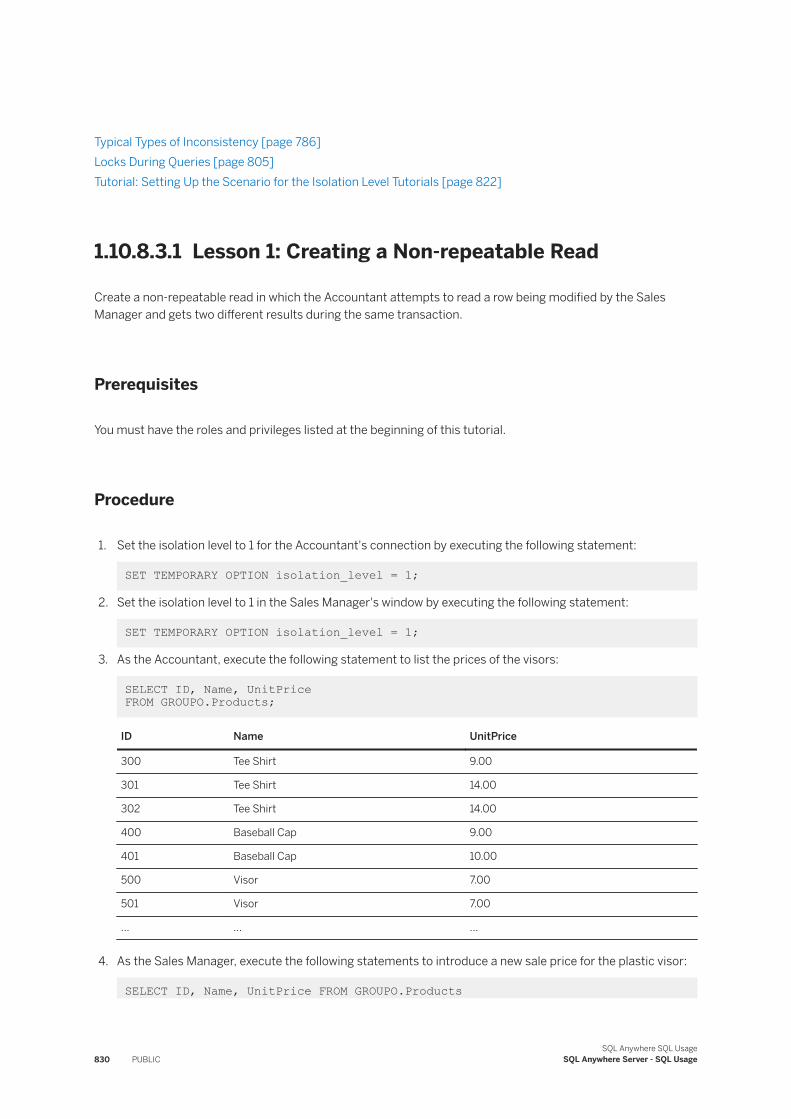
Typical Types of Inconsistency [page 786]Locks During Queries [page 805]Tutorial: Setting Up the Scenario for the Isolation Level Tutorials [page 822]
1.10.8.3.1 Lesson 1: Creating a Non-repeatable Read
Create a non-repeatable read in which the Accountant attempts to read a row being modified by the Sales Manager and gets two different results during the same transaction.
Prerequisites
You must have the roles and privileges listed at the beginning of this tutorial.
Procedure
1. Set the isolation level to 1 for the Accountant's connection by executing the following statement:
SET TEMPORARY OPTION isolation_level = 1;
2. Set the isolation level to 1 in the Sales Manager's window by executing the following statement:
SET TEMPORARY OPTION isolation_level = 1;
3. As the Accountant, execute the following statement to list the prices of the visors:
SELECT ID, Name, UnitPrice FROM GROUPO.Products;
ID Name UnitPrice
300 Tee Shirt 9.00
301 Tee Shirt 14.00
302 Tee Shirt 14.00
400 Baseball Cap 9.00
401 Baseball Cap 10.00
500 Visor 7.00
501 Visor 7.00
... ... ...
4. As the Sales Manager, execute the following statements to introduce a new sale price for the plastic visor:
SELECT ID, Name, UnitPrice FROM GROUPO.Products
830 PUBLICSQL Anywhere SQL Usage
SQL Anywhere Server - SQL Usage
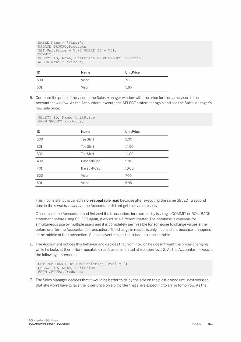
WHERE Name = 'Visor';UPDATE GROUPO.ProductsSET UnitPrice = 5.95 WHERE ID = 501;COMMIT;SELECT ID, Name, UnitPrice FROM GROUPO.Products WHERE Name = 'Visor';
ID Name UnitPrice
500 Visor 7.00
501 Visor 5.95
5. Compare the price of the visor in the Sales Manager window with the price for the same visor in the Accountant window. As the Accountant, execute the SELECT statement again and see the Sales Manager's new sale price:
SELECT ID, Name, UnitPrice FROM GROUPO.Products;
ID Name UnitPrice
300 Tee Shirt 9.00
301 Tee Shirt 14.00
302 Tee Shirt 14.00
400 Baseball Cap 9.00
401 Baseball Cap 10.00
500 Visor 7.00
501 Visor 5.95
... ... ...
This inconsistency is called a non-repeatable read because after executing the same SELECT a second time in the same transaction, the Accountant did not get the same results.
Of course, if the Accountant had finished the transaction, for example by issuing a COMMIT or ROLLBACK statement before using SELECT again, it would be a different matter. The database is available for simultaneous use by multiple users and it is completely permissible for someone to change values either before or after the Accountant's transaction. The change in results is only inconsistent because it happens in the middle of the transaction. Such an event makes the schedule unserializable.
6. The Accountant notices this behavior and decides that from now on he doesn't want the prices changing while he looks at them. Non-repeatable reads are eliminated at isolation level 2. As the Accountant, execute the following statements:
SET TEMPORARY OPTION isolation_level = 2; SELECT ID, Name, UnitPrice FROM GROUPO.Products;
7. The Sales Manager decides that it would be better to delay the sale on the plastic visor until next week so that she won't have to give the lower price on a big order that she's expecting to arrive tomorrow. As the
SQL Anywhere SQL UsageSQL Anywhere Server - SQL Usage PUBLIC 831
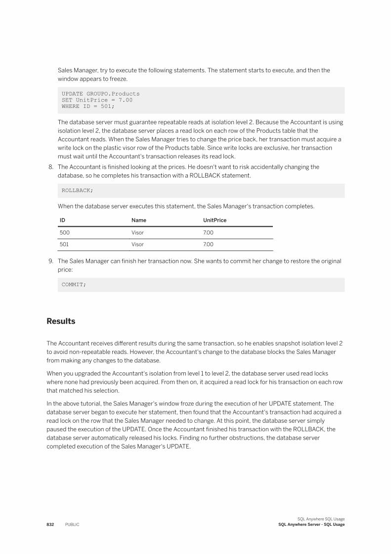
Sales Manager, try to execute the following statements. The statement starts to execute, and then the window appears to freeze.
UPDATE GROUPO.Products SET UnitPrice = 7.00 WHERE ID = 501;
The database server must guarantee repeatable reads at isolation level 2. Because the Accountant is using isolation level 2, the database server places a read lock on each row of the Products table that the Accountant reads. When the Sales Manager tries to change the price back, her transaction must acquire a write lock on the plastic visor row of the Products table. Since write locks are exclusive, her transaction must wait until the Accountant's transaction releases its read lock.
8. The Accountant is finished looking at the prices. He doesn't want to risk accidentally changing the database, so he completes his transaction with a ROLLBACK statement.
ROLLBACK;
When the database server executes this statement, the Sales Manager's transaction completes.
ID Name UnitPrice
500 Visor 7.00
501 Visor 7.00
9. The Sales Manager can finish her transaction now. She wants to commit her change to restore the original price:
COMMIT;
Results
The Accountant receives different results during the same transaction, so he enables snapshot isolation level 2 to avoid non-repeatable reads. However, the Accountant's change to the database blocks the Sales Manager from making any changes to the database.
When you upgraded the Accountant's isolation from level 1 to level 2, the database server used read locks where none had previously been acquired. From then on, it acquired a read lock for his transaction on each row that matched his selection.
In the above tutorial, the Sales Manager's window froze during the execution of her UPDATE statement. The database server began to execute her statement, then found that the Accountant's transaction had acquired a read lock on the row that the Sales Manager needed to change. At this point, the database server simply paused the execution of the UPDATE. Once the Accountant finished his transaction with the ROLLBACK, the database server automatically released his locks. Finding no further obstructions, the database server completed execution of the Sales Manager's UPDATE.
832 PUBLICSQL Anywhere SQL Usage
SQL Anywhere Server - SQL Usage
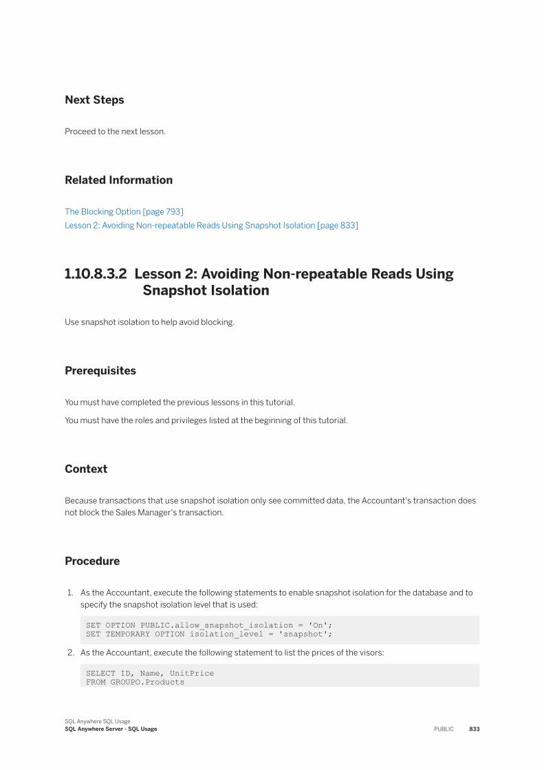
Next Steps
Proceed to the next lesson.
Related Information
The Blocking Option [page 793]Lesson 2: Avoiding Non-repeatable Reads Using Snapshot Isolation [page 833]
1.10.8.3.2 Lesson 2: Avoiding Non-repeatable Reads Using Snapshot Isolation
Use snapshot isolation to help avoid blocking.
Prerequisites
You must have completed the previous lessons in this tutorial.
You must have the roles and privileges listed at the beginning of this tutorial.
Context
Because transactions that use snapshot isolation only see committed data, the Accountant's transaction does not block the Sales Manager's transaction.
Procedure
1. As the Accountant, execute the following statements to enable snapshot isolation for the database and to specify the snapshot isolation level that is used:
SET OPTION PUBLIC.allow_snapshot_isolation = 'On'; SET TEMPORARY OPTION isolation_level = 'snapshot';
2. As the Accountant, execute the following statement to list the prices of the visors:
SELECT ID, Name, UnitPrice FROM GROUPO.Products
SQL Anywhere SQL UsageSQL Anywhere Server - SQL Usage PUBLIC 833
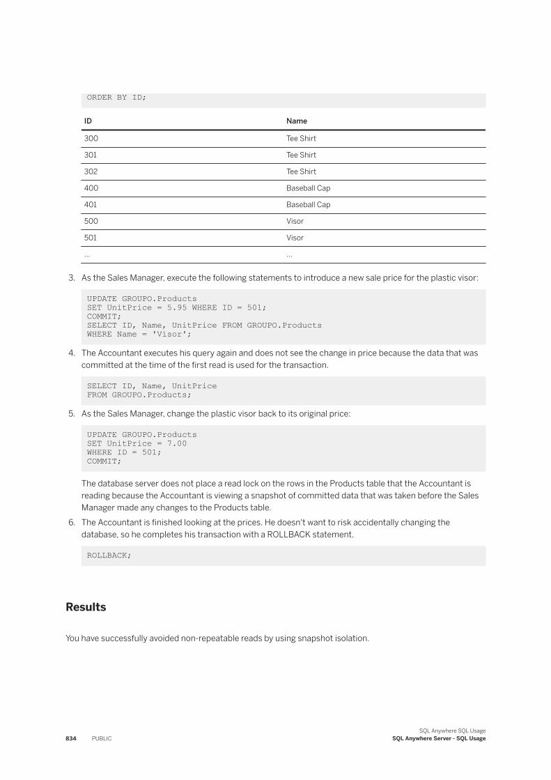
ORDER BY ID;
ID Name
300 Tee Shirt
301 Tee Shirt
302 Tee Shirt
400 Baseball Cap
401 Baseball Cap
500 Visor
501 Visor
... ...
3. As the Sales Manager, execute the following statements to introduce a new sale price for the plastic visor:
UPDATE GROUPO.Products SET UnitPrice = 5.95 WHERE ID = 501;COMMIT;SELECT ID, Name, UnitPrice FROM GROUPO.Products WHERE Name = 'Visor';
4. The Accountant executes his query again and does not see the change in price because the data that was committed at the time of the first read is used for the transaction.
SELECT ID, Name, UnitPrice FROM GROUPO.Products;
5. As the Sales Manager, change the plastic visor back to its original price:
UPDATE GROUPO.Products SET UnitPrice = 7.00WHERE ID = 501; COMMIT;
The database server does not place a read lock on the rows in the Products table that the Accountant is reading because the Accountant is viewing a snapshot of committed data that was taken before the Sales Manager made any changes to the Products table.
6. The Accountant is finished looking at the prices. He doesn't want to risk accidentally changing the database, so he completes his transaction with a ROLLBACK statement.
ROLLBACK;
Results
You have successfully avoided non-repeatable reads by using snapshot isolation.
834 PUBLICSQL Anywhere SQL Usage
SQL Anywhere Server - SQL Usage
1.10.8.4 Tutorial: Understanding Phantom Rows
The tutorial demonstrates the type of inconsistency that can occur when multiple transactions are executed concurrently: the phantom row.
Prerequisites
You must have the SELECT ANY TABLE, INSERT ANY TABLE, DELETE ANY TABLE, and SET ANY SYSTEM OPTION system privileges.
This tutorial assumes that you have connected to the sample database as the Sales Manager and as the Accountant.
Context
In this scenario, two employees at a small merchandising company access the corporate database at the same time. The first person is the company's Sales Manager; the second is the Accountant.
The Sales Manager wants to create new departments for foreign sales and major account sales. The Accountant wants to verify all the departments that exist in the company.
This example begins with both connections at isolation level 2, rather than at isolation level 0, which is the default for the SQL Anywhere sample database. By setting the isolation level to 2, you eliminate the possibility of dirty reads and non-repeatable reads.
NoteFor this tutorial to work properly, the Automatically Release Database Locks option must not be selected in Interactive SQL. You can check the setting of this option by clicking Tools Options and then clicking SQL Anywhere in the left pane.
In this section:
Lesson 1: Creating a Phantom Row [page 836]Create a phantom row by having the Sales Manager insert a row while the Accountant is reading adjacent rows, causing the new row to appear as a phantom.
Lesson 2: Avoiding Phantom Rows Using Snapshot Isolation [page 839]Use the snapshot isolation level to maintain consistency at the same level as isolation level at 3 without any sort of blocking.
Related Information
Isolation Levels and Consistency [page 777]
SQL Anywhere SQL UsageSQL Anywhere Server - SQL Usage PUBLIC 835
Understanding Snapshot Transactions [page 782]Typical Types of Inconsistency [page 786]Locks During Queries [page 805]Tutorial: Setting Up the Scenario for the Isolation Level Tutorials [page 822]
1.10.8.4.1 Lesson 1: Creating a Phantom Row
Create a phantom row by having the Sales Manager insert a row while the Accountant is reading adjacent rows, causing the new row to appear as a phantom.
Prerequisites
You must have the roles and privileges listed at the beginning of this tutorial.
Procedure
1. Set the isolation level to 2 in the Sales Manager and Accountant windows by executing the following statement in each:
SET TEMPORARY OPTION isolation_level = 2;
2. As the Accountant, execute the following statement to list all the departments:
SELECT * FROM GROUPO.Departments ORDER BY DepartmentID;
DepartmentID DepartmentName
100 R & D
200 Sales
300 Finance
400 Marketing
500 Shipping
3. The Sales Manager decides to set up a new department to focus on the foreign market. Philip Chin, who has EmployeeID 129, heads the new department. As the Sales Manager, execute the following statement to create a new entry for the new department, which appears as a new row at the bottom of the table in the Sales Manager's window:
INSERT INTO GROUPO.Departments ( DepartmentID, DepartmentName, DepartmentHeadID ) VALUES( 600, 'Foreign Sales', 129 ); COMMIT;
836 PUBLICSQL Anywhere SQL Usage
SQL Anywhere Server - SQL Usage
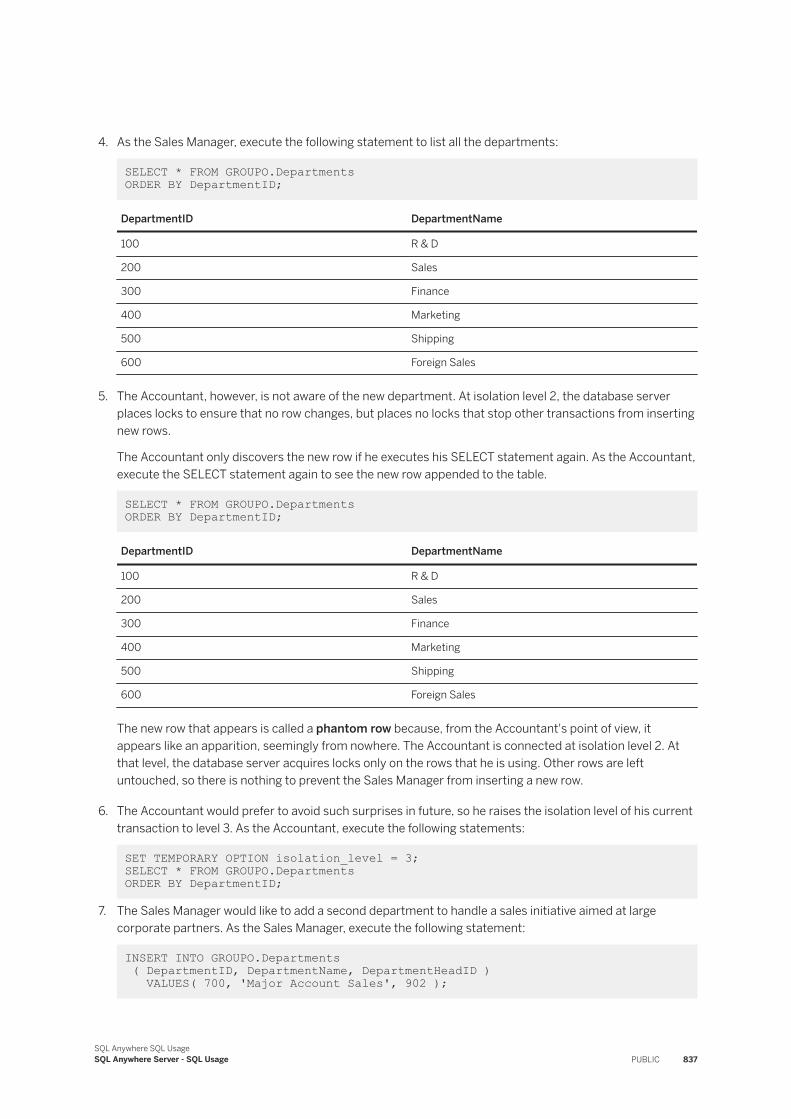
4. As the Sales Manager, execute the following statement to list all the departments:
SELECT * FROM GROUPO.Departments ORDER BY DepartmentID;
DepartmentID DepartmentName
100 R & D
200 Sales
300 Finance
400 Marketing
500 Shipping
600 Foreign Sales
5. The Accountant, however, is not aware of the new department. At isolation level 2, the database server places locks to ensure that no row changes, but places no locks that stop other transactions from inserting new rows.
The Accountant only discovers the new row if he executes his SELECT statement again. As the Accountant, execute the SELECT statement again to see the new row appended to the table.
SELECT * FROM GROUPO.Departments ORDER BY DepartmentID;
DepartmentID DepartmentName
100 R & D
200 Sales
300 Finance
400 Marketing
500 Shipping
600 Foreign Sales
The new row that appears is called a phantom row because, from the Accountant's point of view, it appears like an apparition, seemingly from nowhere. The Accountant is connected at isolation level 2. At that level, the database server acquires locks only on the rows that he is using. Other rows are left untouched, so there is nothing to prevent the Sales Manager from inserting a new row.
6. The Accountant would prefer to avoid such surprises in future, so he raises the isolation level of his current transaction to level 3. As the Accountant, execute the following statements:
SET TEMPORARY OPTION isolation_level = 3; SELECT * FROM GROUPO.Departments ORDER BY DepartmentID;
7. The Sales Manager would like to add a second department to handle a sales initiative aimed at large corporate partners. As the Sales Manager, execute the following statement:
INSERT INTO GROUPO.Departments ( DepartmentID, DepartmentName, DepartmentHeadID ) VALUES( 700, 'Major Account Sales', 902 );
SQL Anywhere SQL UsageSQL Anywhere Server - SQL Usage PUBLIC 837
The Sales Manager's window pauses during execution because the Accountant's locks block the statement. From the toolbar, click Stop to interrupt this entry.
When the Accountant raised his isolation to level 3 and again selected all rows in the Departments table, the database server placed anti-insert locks on each row in the table, and added one extra phantom lock to block inserts at the end of the table. When the Sales Manager attempted to insert a new row at the end of the table, it was this final lock that blocked her statement.
The Sales Manager's statement was blocked even though she is still connected at isolation level 2. The database server places anti-insert locks, like read locks, as demanded by the isolation level and statements of each transaction. Once placed, these locks must be respected by all other concurrent transactions.
8. To avoid changing the SQL Anywhere sample database, you should roll back the incomplete transaction that inserts the Major Account Sales department row and use a second transaction to delete the Foreign Sales department.a. As the Accountant, execute the following statements to lower the isolation level and release the row
locks, allowing the Sales Manager to undo changes to the database:
SET TEMPORARY OPTION isolation_level=1; ROLLBACK;
b. As the Sales Manager, execute the following statements to roll back the current transaction, delete the row inserted earlier, and commit this operation:
ROLLBACK; DELETE FROM GROUPO.DepartmentsWHERE DepartmentID = 600; COMMIT;
Results
The Accountant receives different results each time the SELECT statement is executed, so he enables snapshot isolation level 3 to avoid phantom rows. However, the Accountant's change to the database blocks the Sales Manager from making any changes to the database.
Next Steps
Proceed to the next lesson.
Related Information
How Locking Works [page 796]
838 PUBLICSQL Anywhere SQL Usage
SQL Anywhere Server - SQL Usage
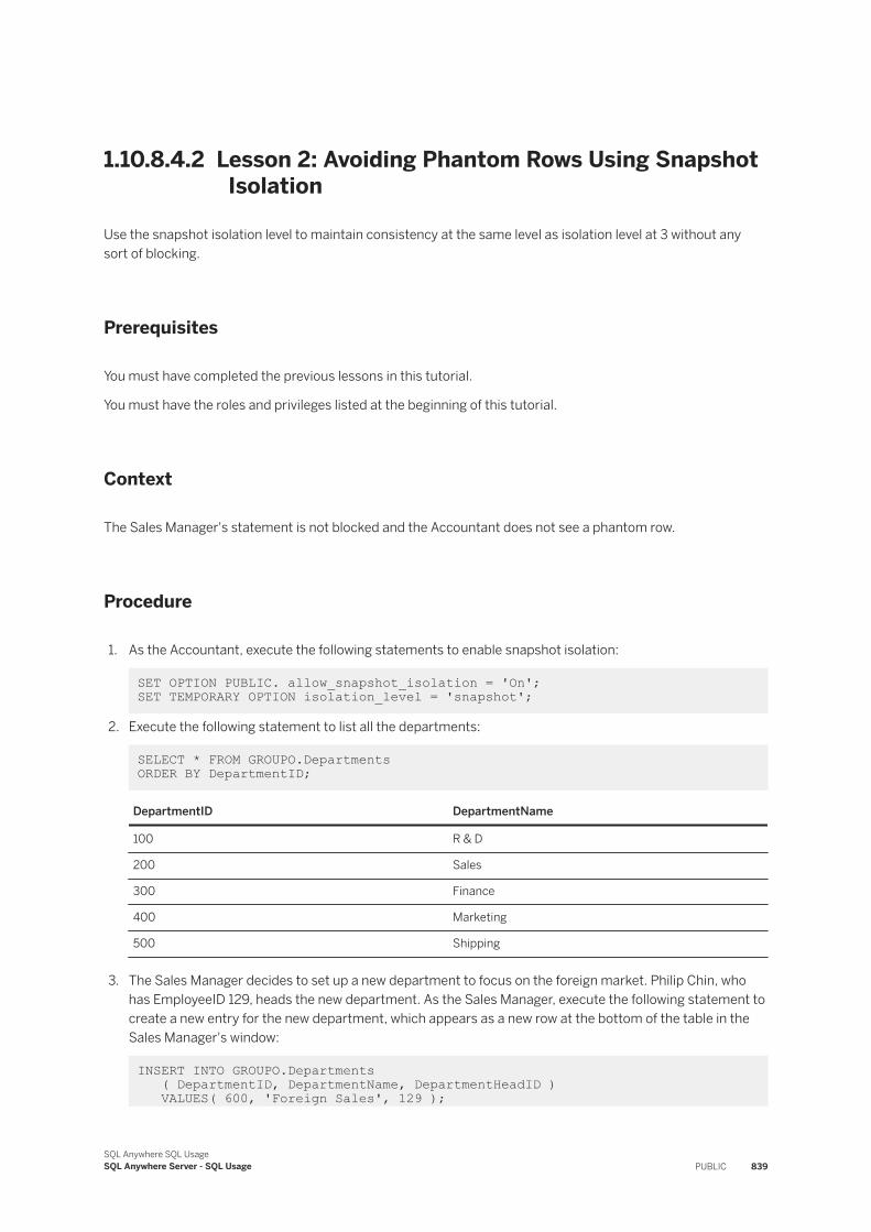
1.10.8.4.2 Lesson 2: Avoiding Phantom Rows Using Snapshot Isolation
Use the snapshot isolation level to maintain consistency at the same level as isolation level at 3 without any sort of blocking.
Prerequisites
You must have completed the previous lessons in this tutorial.
You must have the roles and privileges listed at the beginning of this tutorial.
Context
The Sales Manager's statement is not blocked and the Accountant does not see a phantom row.
Procedure
1. As the Accountant, execute the following statements to enable snapshot isolation:
SET OPTION PUBLIC. allow_snapshot_isolation = 'On'; SET TEMPORARY OPTION isolation_level = 'snapshot';
2. Execute the following statement to list all the departments:
SELECT * FROM GROUPO.Departments ORDER BY DepartmentID;
DepartmentID DepartmentName
100 R & D
200 Sales
300 Finance
400 Marketing
500 Shipping
3. The Sales Manager decides to set up a new department to focus on the foreign market. Philip Chin, who has EmployeeID 129, heads the new department. As the Sales Manager, execute the following statement to create a new entry for the new department, which appears as a new row at the bottom of the table in the Sales Manager's window:
INSERT INTO GROUPO.Departments ( DepartmentID, DepartmentName, DepartmentHeadID ) VALUES( 600, 'Foreign Sales', 129 );
SQL Anywhere SQL UsageSQL Anywhere Server - SQL Usage PUBLIC 839
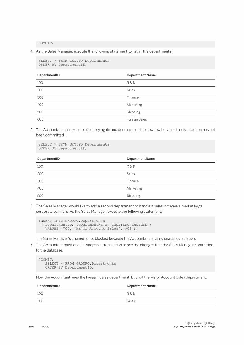
COMMIT;
4. As the Sales Manager, execute the following statement to list all the departments:
SELECT * FROM GROUPO.Departments ORDER BY DepartmentID;
DepartmentID Department Name
100 R & D
200 Sales
300 Finance
400 Marketing
500 Shipping
600 Foreign Sales
5. The Accountant can execute his query again and does not see the new row because the transaction has not been committed.
SELECT * FROM GROUPO.Departments ORDER BY DepartmentID;
DepartmentID DepartmentName
100 R & D
200 Sales
300 Finance
400 Marketing
500 Shipping
6. The Sales Manager would like to add a second department to handle a sales initiative aimed at large corporate partners. As the Sales Manager, execute the following statement:
INSERT INTO GROUPO.Departments ( DepartmentID, DepartmentName, DepartmentHeadID ) VALUES( 700, 'Major Account Sales', 902 );
The Sales Manager's change is not blocked because the Accountant is using snapshot isolation.7. The Accountant must end his snapshot transaction to see the changes that the Sales Manager committed
to the database.
COMMIT; SELECT * FROM GROUPO.Departments ORDER BY DepartmentID;
Now the Accountant sees the Foreign Sales department, but not the Major Account Sales department.
DepartmentID Department Name
100 R & D
200 Sales
840 PUBLICSQL Anywhere SQL Usage
SQL Anywhere Server - SQL Usage
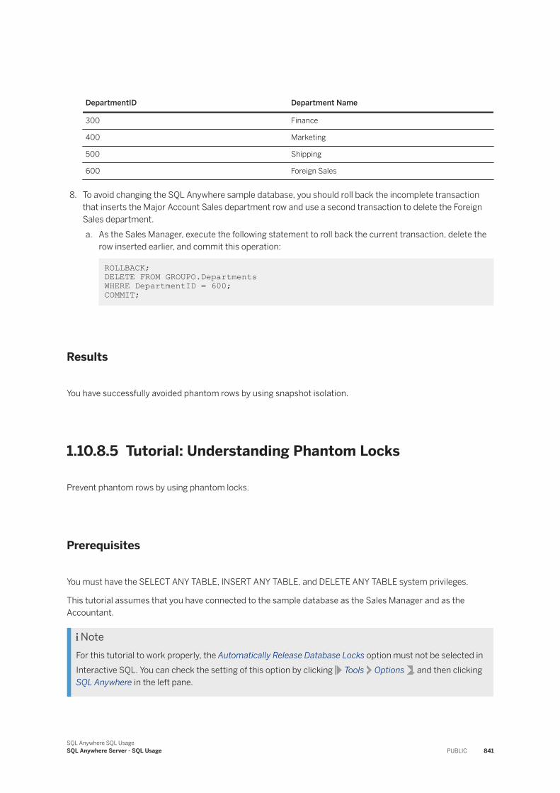
DepartmentID Department Name
300 Finance
400 Marketing
500 Shipping
600 Foreign Sales
8. To avoid changing the SQL Anywhere sample database, you should roll back the incomplete transaction that inserts the Major Account Sales department row and use a second transaction to delete the Foreign Sales department.a. As the Sales Manager, execute the following statement to roll back the current transaction, delete the
row inserted earlier, and commit this operation:
ROLLBACK; DELETE FROM GROUPO.DepartmentsWHERE DepartmentID = 600; COMMIT;
Results
You have successfully avoided phantom rows by using snapshot isolation.
1.10.8.5 Tutorial: Understanding Phantom Locks
Prevent phantom rows by using phantom locks.
Prerequisites
You must have the SELECT ANY TABLE, INSERT ANY TABLE, and DELETE ANY TABLE system privileges.
This tutorial assumes that you have connected to the sample database as the Sales Manager and as the Accountant.
NoteFor this tutorial to work properly, the Automatically Release Database Locks option must not be selected in Interactive SQL. You can check the setting of this option by clicking Tools Options , and then clicking SQL Anywhere in the left pane.
SQL Anywhere SQL UsageSQL Anywhere Server - SQL Usage PUBLIC 841
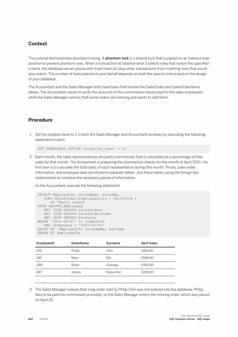
Context
This tutorial demonstrates phantom locking. A phantom lock is a shared lock that is placed on an indexed scan position to prevent phantom rows. When a transaction at isolation level 3 selects rows that match the specified criteria, the database server places anti-insert locks to stop other transactions from inserting rows that would also match. The number of locks placed on your behalf depends on both the search criteria and on the design of your database.
The Accountant and the Sales Manager both have tasks that involve the SalesOrder and SalesOrderItems tables. The Accountant needs to verify the amounts of the commission checks paid to the sales employees while the Sales Manager notices that some orders are missing and wants to add them.
Procedure
1. Set the isolation level to 2 in both the Sales Manager and Accountant windows by executing the following statement in each:
SET TEMPORARY OPTION isolation_level = 2;
2. Each month, the sales representatives are paid a commission that is calculated as a percentage of their sales for that month. The Accountant is preparing the commission checks for the month of April 2001. His first task is to calculate the total sales of each representative during this month. Prices, sales order information, and employee data are stored in separate tables. Join these tables using the foreign key relationships to combine the necessary pieces of information.
As the Accountant, execute the following statement:
SELECT EmployeeID, GivenName, Surname, SUM( SalesOrderItems.Quantity * UnitPrice ) AS "April sales"FROM GROUPO.Employees KEY JOIN GROUPO.SalesOrders KEY JOIN GROUPO.SalesOrderItems KEY JOIN GROUPO.ProductsWHERE '2001-04-01' <= OrderDate AND OrderDate < '2001-05-01'GROUP BY EmployeeID, GivenName, Surname ORDER BY EmployeeID;
EmployeeID GivenName Surname April Sales
129 Philip Chin 2160.00
195 Marc Dill 2568.00
299 Rollin Overbey 5760.00
467 James Klobucher 3228.00
... ... ... ...
3. The Sales Manager notices that a big order sold by Philip Chin was not entered into the database. Philip likes to be paid his commission promptly, so the Sales Manager enters the missing order, which was placed on April 25.
842 PUBLICSQL Anywhere SQL Usage
SQL Anywhere Server - SQL Usage
As the Sales Manager, execute the following statements. The sales order and the items are entered in separate tables because one order can contain many items. You should create the entry for the sales order before you add items to it. To maintain referential integrity, the database server allows a transaction to add items to an order only if that order already exists.
INSERT into GROUPO.SalesOrders VALUES ( 2653, 174, '2001-04-22', 'r1', 'Central', 129 );INSERT into GROUPO.SalesOrderItemsVALUES ( 2653, 1, 601, 100, '2001-04-25' ); COMMIT;
4. The Accountant has no way of knowing that the Sales Manager has just added a new order. Had the new order been entered earlier, it would have been included in the calculation of Philip Chin's April sales.
In the Accountant's window, calculate the April sales totals again. Use the same statement, and observe that Philip Chin's April sales changes to $4560.00.
EmployeeID GivenName
129 Philip
195 Marc
299 Rollin
467 James
... ...
Imagine that the Accountant now marks all orders placed in April to indicate that commission has been paid. The order that the Sales Manager just entered might be found in the second search and marked as paid, even though it was not included in Philip's total April sales.
5. At isolation level 3, the database server places anti-insert locks to ensure that no other transactions can add a row that matches the criteria of a search or select.
As the Sales Manager, execute the following statements to remove the new order:
DELETE FROM GROUPO.SalesOrderItemsWHERE ID = 2653;DELETEFROM GROUPO.SalesOrdersWHERE ID = 2653; COMMIT;
6. As the Accountant, execute the following statements:
ROLLBACK; SET TEMPORARY OPTION isolation_level = 3;
7. As the Accountant, execute the following query:
SELECT EmployeeID, GivenName, Surname, SUM( SalesOrderItems.Quantity * UnitPrice ) AS "April sales"FROM GROUPO.Employees KEY JOIN GROUPO.SalesOrders KEY JOIN GROUPO.SalesOrderItems KEY JOIN GROUPO.ProductsWHERE '2001-04-01' <= OrderDate
SQL Anywhere SQL UsageSQL Anywhere Server - SQL Usage PUBLIC 843
AND OrderDate < '2001-05-01' GROUP BY EmployeeID, GivenName, Surname;
Because you set the isolation to level 3, the database server automatically places anti-insert locks to ensure that the Sales Manager cannot insert April order items until the Accountant finishes his transaction.
8. As the Sales Manager, attempt to enter Philip Chin's missing order by executing the following statement:
INSERT INTO GROUPO.SalesOrders VALUES ( 2653, 174, '2001-04-22', 'r1','Central', 129 );
The Sales Manager's window stops responding, and the operation does not complete. On the toolbar, click interrupt the SQL statement to interrupt this entry.
9. The Sales Manager cannot enter the order in April, but you might think that they could still enter it in May.
Change the date in the statement to May 05 and try again.
INSERT INTO GROUPO.SalesOrders VALUES ( 2653, 174, '2001-05-05', 'r1', 'Central', 129 );
The Sales Manager's window stops responding again. On the toolbar, click interrupt the SQL statement to interrupt this entry. Although the database server places no more locks than necessary to prevent insertions, these locks have the potential to interfere with many transactions.
The database server places locks in table indexes. For example, it places a phantom lock in an index so a new row cannot be inserted immediately before it. However, when no suitable index is present, it must lock every row in the table. In some situations, anti-insert locks may block some insertions into a table, yet allow others.
10. To avoid changing the sample database, you should roll back the changes made to the SalesOrders table. In both the Sales Manager and Accountant windows, execute the following statement:
ROLLBACK;
11. Shut down both instances of Interactive SQL.
Results
You have completed the tutorial on understanding how phantom locks work.
Related Information
Isolation Levels and Consistency [page 777]Understanding Snapshot Transactions [page 782]Typical Types of Inconsistency [page 786]Locks During Queries [page 805]
844 PUBLICSQL Anywhere SQL Usage
SQL Anywhere Server - SQL Usage
1.10.9 Use of a Sequence to Generate Unique Values
You can use a sequence to generate values that are unique across multiple tables or that are different from a set of natural numbers.
A sequence is created using the CREATE SEQUENCE statement. Sequence values are returned as BIGINT values.
For each connection, the most recent use of the next value is saved as the current value.
When you create a sequence, its definition includes the number of sequence values the database server holds in memory. When this cache is exhausted, the sequence cache is repopulated. If the database server fails, then sequence values that were held in the cache may be skipped.
Obtaining Values in a Sequence
To return the next value in the sequence, use the following statement.
SELECT [owner.]sequence-name.NEXTVAL;
The sequence is shared by all connections, so each connection will get a unique next value.
To return the most recently supplied sequence value for the current connection, use the following statement.
SELECT [owner.]sequence-name.CURRVAL;
NEXTVAL must have been used at least once on the connection in order to return the current value.
Choosing Between Sequences and AUTOINCREMENT Values
AUTOINCREMENT Behavior Sequence Behavior
Defined for a single column in a table Stored as a database object and can be used anywhere that an expression is allowed
Column must have an integer data type or an exact numeric data type
Values can be referred to anywhere that an expression can be used and do not have to conform to default value for a column
Values can only be used for a single column in one table Values can be used across multiple tables
Values are part of the set of natural numbers (1, 2, 3, ...) Can generate values other than the set of natural numbers
Values must increment Values can increment or decrement
SQL Anywhere SQL UsageSQL Anywhere Server - SQL Usage PUBLIC 845
AUTOINCREMENT Behavior Sequence Behavior
A unique value that is one greater than the previous maximum value in the column is generated by default
The sa_reset_identity system procedure can be used to change the AUTOINCREMENT value for the next row that is inserted
Unit of increment can be specified
If the next value to be generated exceeds the maximum value that can be stored in the column, NULL is returned
Can choose to allow values to be generated after the maximum or minimum value is reached, or return an error by specifying NO CYCLE
Sequence Example
Consider a sequence that is used to generate incident numbers for a customer hotline. Suppose that customers can call in with two different types of complaints: incorrect billing or missing shipments.
CREATE SEQUENCE incidentSequence MINVALUE 1000 MAXVALUE 100000;
CREATE TABLE reportedBillingMistake( incidentID INT PRIMARY KEY DEFAULT (incidentSequence.nextval), billNumber INT, valueOnBill NUMERIC(10,2), expectedValue NUMERIC(10,2), comments LONG VARCHAR );
CREATE TABLE reportedMissingShipment( incidentID INT PRIMARY KEY DEFAULT(incidentSequence.nextval), orderNumber INT, comments LONG VARCHAR );
Using incidentSequence.nextval for the incidentID columns guarantees that incidentIDs are unique across the two tables. When a customer calls back for further inquiries and provides an incident value, there is no possibility of confusion as to whether the incident is a billing or shipping mistake.
To insert a billing mistake, the following statements would be equivalent:
INSERT INTO reportedBillingMistake VALUES( DEFAULT, 12345, 100.00, 75.00, 'Bad bill' ); INSERT INTO reportedBillingMistake SELECT incidentSequence.nextval, 12345, 100.00, 75.00, 'Bad bill';
To find the incidentID that was just inserted, the connection that performed the insert (using either of the above two statements) could execute the following statement:
SELECT incidentSequence.currval;
In this section:
Creating a Sequence [page 847]
846 PUBLICSQL Anywhere SQL Usage
SQL Anywhere Server - SQL Usage
Use SQL Central to create a sequence.
Altering a Sequence [page 848]Use SQL Central to alter a sequence.
Dropping a Sequence [page 848]Use SQL Central to drop a sequence.
Related Information
The AUTOINCREMENT Default [page 748]The GLOBAL AUTOINCREMENT Default [page 749]
1.10.9.1 Creating a Sequence
Use SQL Central to create a sequence.
Prerequisites
You must have the CREATE ANY SEQUENCE or CREATE ANY OBJECT system privilege.
Procedure
1. In SQL Central, use the SQL Anywhere 17 plug-in to connect to the database.
2. In the left pane, right-click Sequence Generators, then click New Sequence Generator .3. Follow the instructions in the Create Sequence Generator Wizard.
Results
The sequence has been created.
SQL Anywhere SQL UsageSQL Anywhere Server - SQL Usage PUBLIC 847
1.10.9.2 Altering a Sequence
Use SQL Central to alter a sequence.
Prerequisites
You must be the owner of the sequence or have one of the following privileges:
● ALTER ANY SEQUENCE system privilege● ALTER ANY OBJECT system privilege
Procedure
1. In SQL Central, use the SQL Anywhere 17 plug-in to connect to the database.2. Right-click a sequence generator and then click Properties.
On the General tab, you can change the settings for the sequence. Clicking Restart Now executes an ALTER SEQUENCE...RESTART WITH n statement, where n corresponds to the value in the Start Value field.
Results
The change takes effect immediately.
1.10.9.3 Dropping a Sequence
Use SQL Central to drop a sequence.
Prerequisites
You must be the owner of the sequence or have one of the following privileges:
● DROP ANY SEQUENCE system privilege● DROP ANY OBJECT system privilege
848 PUBLICSQL Anywhere SQL Usage
SQL Anywhere Server - SQL Usage
Procedure
1. In SQL Central, use the SQL Anywhere 17 plug-in to connect to the database.2. Right-click a sequence generator and then click Delete.
Results
The sequence is dropped from the database. When you drop a sequence, all synonyms for the name of the sequence are dropped automatically by the database server.
1.11 The SQL Anywhere Debugger
You can use the SQL Anywhere debugger to debug SQL stored procedures, triggers, event handlers, and user-defined functions you create.
You can also use the debugger to:
Debug event handlers
Event handlers are an extension of SQL stored procedures. The following information about debugging stored procedures applies equally to debugging event handlers.Browse stored procedures and classes
You can browse the source code of SQL procedures.Trace execution
Step line by line through the code of a stored procedure. You can also look up and down the stack of functions that have been called.Set breakpoints
Run the code until you hit a breakpoint, and stop at that point in the code.Set break conditions
Breakpoints include lines of code, but you can also specify conditions when the code is to break. For example, you can stop at a line the tenth time it is executed, or only if a variable has a particular value.Inspect and modify local variables
When execution is stopped at a breakpoint, you can inspect the values of local variables and alter their value.Inspect and break on expressions
When execution is stopped at a breakpoint, you can inspect the value of a wide variety of expressions.Inspect and modify row variables
Row variables are the OLD and NEW values of row-level triggers. You can inspect and modify these values.Execute queries
SQL Anywhere SQL UsageSQL Anywhere Server - SQL Usage PUBLIC 849
You can execute queries when execution is stopped at a breakpoint in a SQL procedure. This permits you to look at intermediate results held in temporary tables, check values in base tables, and to view the query execution plan.
In this section:
Requirements for Using the Debugger [page 850]There are several criteria that must be met to use the debugger. For example, only one user can use the debugger at a time.
Tutorial: Getting Started with the Debugger [page 850]Learn how to use the debugger to identify errors in stored procedures.
Breakpoints [page 856]Breakpoints control when the debugger interrupts the execution of your source code.
Variable Modification with the Debugger [page 859]The debugger lets you view and edit the behavior of your variables while it steps through your code.
Connections and Breakpoints [page 862]The Connections tab in SQL Central displays the connections to the database.
1.11.1 Requirements for Using the Debugger
There are several criteria that must be met to use the debugger. For example, only one user can use the debugger at a time.
When using the debugger over HTTP/SOAP connections, change the port timeout options on the server. For example, -xs http{TO=600;KTO=0;PORT=8081) sets the timeout to 10 minutes and turns off keep-alive timeout for port 8081. Timeout (TO) is the period of time between received packets. Keep-alive timeout (KTO) is the total time that the connection is allowed to run. When you set KTO to 0, it is equivalent to setting it to never time out.
If using a SQL Anywhere HTTP/SOAP client procedure to call into the SQL Anywhere HTTP/SOAP service you are debugging, set the client's remote_idle_timeout database option to a large value such as 150 (the default is 15 seconds) to avoid timing out during the debugging session.
1.11.2 Tutorial: Getting Started with the Debugger
Learn how to use the debugger to identify errors in stored procedures.
Prerequisites
You must have the SA_DEBUG system role.
850 PUBLICSQL Anywhere SQL Usage
SQL Anywhere Server - SQL Usage
Additionally, you must have either the EXECUTE ANY PROCEDURE system privilege or EXECUTE privilege on the system procedure debugger_tutorial. You must also have either the ALTER ANY PROCEDURE system privilege or the ALTER ANY OBJECT system privilege.
Context
The SQL Anywhere sample database, demo.db, contains a stored procedure named debugger_tutorial, which contains a deliberate error. The debugger_tutorial system procedure returns a result set that contains the name of the company that has placed the highest value of orders and the value of their orders. It computes these values by looping over the result set of a query that lists companies and orders. (This result could be achieved without adding the logic into the procedure by using a SELECT FIRST query. The procedure is used to create a convenient example.) However, the bug contained in the debugger_tutorial system procedure results in its failure to return the correct result set.
1. Lesson 1: Starting the Debugger and Finding the Bug [page 851]Start the debugger to run the debugger_tutorial stored procedure and find the bug.
2. Lesson 2: Diagnosing the Bug [page 853]Diagnose the bug in the debugger_tutorial stored procedure by setting breakpoints and then stepping through the code, watching the value of the variables as the procedure executes.
3. Lesson 3: Fixing the Bug [page 855]Fix the bug you identified in the previous lesson by initializing the Top_Value variable.
Related Information
Requirements for Using the Debugger [page 850]
1.11.2.1 Lesson 1: Starting the Debugger and Finding the Bug
Start the debugger to run the debugger_tutorial stored procedure and find the bug.
Prerequisites
You must have the roles and privileges listed at the beginning of this tutorial.
SQL Anywhere SQL UsageSQL Anywhere Server - SQL Usage PUBLIC 851
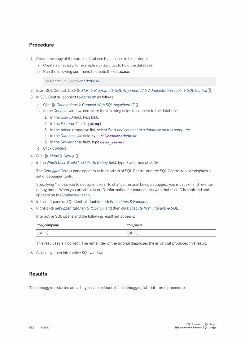
Procedure
1. Create the copy of the sample database that is used in this tutorial.a. Create a directory, for example c:\demodb, to hold the database.b. Run the following command to create the database:
newdemo c:\demodb\demo.db
2. Start SQL Central. Click Start Programs SQL Anywhere 17 Administration Tools SQL Central .3. In SQL Central, connect to demo.db as follows:
a. Click Connections Connect With SQL Anywhere 17 .b. In the Connect window, complete the following fields to connect to the database:
1. In the User ID field, type DBA.2. In the Password field, type sql.3. In the Action dropdown list, select Start and connect to a database on this computer.4. In the Database file field, type c:\demodb\demo.db.5. In the Server name field, type demo_server.
c. Click Connect.
4. Click Mode Debug .5. In the Which User Would You Like To Debug field, type * and then click OK.
The Debugger Details pane appears at the bottom of SQL Central and the SQL Central toolbar displays a set of debugger tools.
Specifying * allows you to debug all users. To change the user being debugged, you must exit and re-enter debug mode. When you provide a user ID, information for connections with that user ID is captured and appears on the Connections tab.
6. In the left pane of SQL Central, double-click Procedures & Functions.7. Right-click debugger_tutorial (GROUPO), and then click Execute from Interactive SQL.
Interactive SQL opens and the following result set appears:
top_company top_value
(NULL) (NULL)
This result set is incorrect. The remainder of the tutorial diagnoses the error that produced this result.
8. Close any open Interactive SQL windows.
Results
The debugger is started and a bug has been found in the debugger_tutorial stored procedure.
852 PUBLICSQL Anywhere SQL Usage
SQL Anywhere Server - SQL Usage

Next Steps
Proceed to the next lesson.
Task overview: Tutorial: Getting Started with the Debugger [page 850]
Next task: Lesson 2: Diagnosing the Bug [page 853]
Related Information
The SQL Anywhere Debugger [page 849]
1.11.2.2 Lesson 2: Diagnosing the Bug
Diagnose the bug in the debugger_tutorial stored procedure by setting breakpoints and then stepping through the code, watching the value of the variables as the procedure executes.
Prerequisites
You must have completed the previous lessons in this tutorial.
You must have the roles and privileges listed at the beginning of this tutorial.
Procedure
1. In the right pane of SQL Central, double-click debugger_tutorial (GROUPO).2. In the SQL tab for the debugger_tutorial (GROUPO), locate the following statement:
OPEN cursor_this_customer;
3. Add a breakpoint by clicking the vertical gray area to the left of the statement. The breakpoint appears as a red circle.
4. In the left pane, right-click debugger_tutorial (GROUPO) and click Execute from Interactive SQL.
In the right pane of SQL Central, a yellow arrow appears on top of the breakpoint.5. In the Debugger Details window, click the Local tab to display a list of local variables in the procedure, along
with their current values and data types. The Top_Company, Top_Value, This_Value, and This_Company variables are all uninitialized and are therefore NULL.
SQL Anywhere SQL UsageSQL Anywhere Server - SQL Usage PUBLIC 853
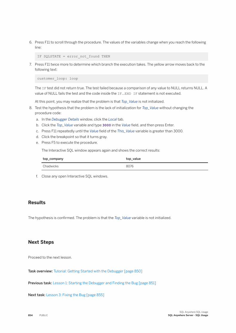
6. Press F11 to scroll through the procedure. The values of the variables change when you reach the following line:
IF SQLSTATE = error_not_found THEN
7. Press F11 twice more to determine which branch the execution takes. The yellow arrow moves back to the following text:
customer_loop: loop
The IF test did not return true. The test failed because a comparison of any value to NULL returns NULL. A value of NULL fails the test and the code inside the IF...END IF statement is not executed.
At this point, you may realize that the problem is that Top_Value is not initialized.8. Test the hypothesis that the problem is the lack of initialization for Top_Value without changing the
procedure code:a. In the Debugger Details window, click the Local tab.b. Click the Top_Value variable and type 3000 in the Value field, and then press Enter.c. Press F11 repeatedly until the Value field of the This_Value variable is greater than 3000.d. Click the breakpoint so that it turns gray.e. Press F5 to execute the procedure.
The Interactive SQL window appears again and shows the correct results:
top_company top_value
Chadwicks 8076
f. Close any open Interactive SQL windows.
Results
The hypothesis is confirmed. The problem is that the Top_Value variable is not initialized.
Next Steps
Proceed to the next lesson.
Task overview: Tutorial: Getting Started with the Debugger [page 850]
Previous task: Lesson 1: Starting the Debugger and Finding the Bug [page 851]
Next task: Lesson 3: Fixing the Bug [page 855]
854 PUBLICSQL Anywhere SQL Usage
SQL Anywhere Server - SQL Usage
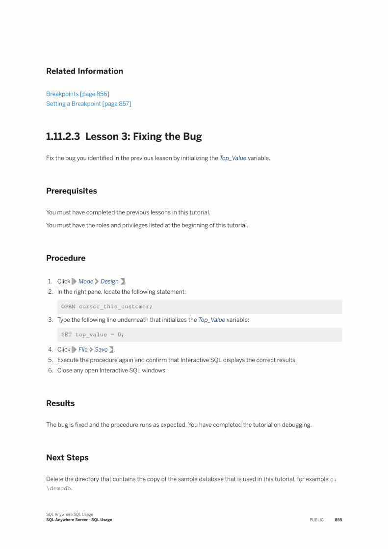
Related Information
Breakpoints [page 856]Setting a Breakpoint [page 857]
1.11.2.3 Lesson 3: Fixing the Bug
Fix the bug you identified in the previous lesson by initializing the Top_Value variable.
Prerequisites
You must have completed the previous lessons in this tutorial.
You must have the roles and privileges listed at the beginning of this tutorial.
Procedure
1. Click Mode Design .2. In the right pane, locate the following statement:
OPEN cursor_this_customer;
3. Type the following line underneath that initializes the Top_Value variable:
SET top_value = 0;
4. Click File Save .5. Execute the procedure again and confirm that Interactive SQL displays the correct results.6. Close any open Interactive SQL windows.
Results
The bug is fixed and the procedure runs as expected. You have completed the tutorial on debugging.
Next Steps
Delete the directory that contains the copy of the sample database that is used in this tutorial, for example c:\demodb.
SQL Anywhere SQL UsageSQL Anywhere Server - SQL Usage PUBLIC 855
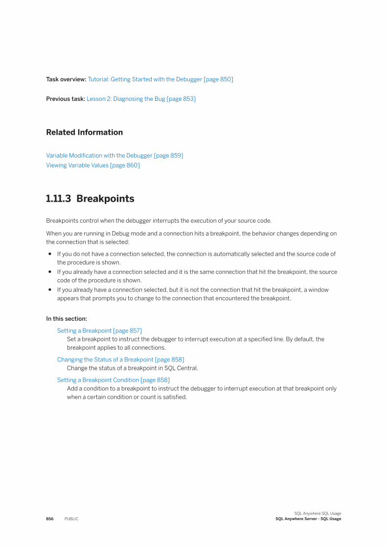
Task overview: Tutorial: Getting Started with the Debugger [page 850]
Previous task: Lesson 2: Diagnosing the Bug [page 853]
Related Information
Variable Modification with the Debugger [page 859]Viewing Variable Values [page 860]
1.11.3 Breakpoints
Breakpoints control when the debugger interrupts the execution of your source code.
When you are running in Debug mode and a connection hits a breakpoint, the behavior changes depending on the connection that is selected:
● If you do not have a connection selected, the connection is automatically selected and the source code of the procedure is shown.
● If you already have a connection selected and it is the same connection that hit the breakpoint, the source code of the procedure is shown.
● If you already have a connection selected, but it is not the connection that hit the breakpoint, a window appears that prompts you to change to the connection that encountered the breakpoint.
In this section:
Setting a Breakpoint [page 857]Set a breakpoint to instruct the debugger to interrupt execution at a specified line. By default, the breakpoint applies to all connections.
Changing the Status of a Breakpoint [page 858]Change the status of a breakpoint in SQL Central.
Setting a Breakpoint Condition [page 858]Add a condition to a breakpoint to instruct the debugger to interrupt execution at that breakpoint only when a certain condition or count is satisfied.
856 PUBLICSQL Anywhere SQL Usage
SQL Anywhere Server - SQL Usage
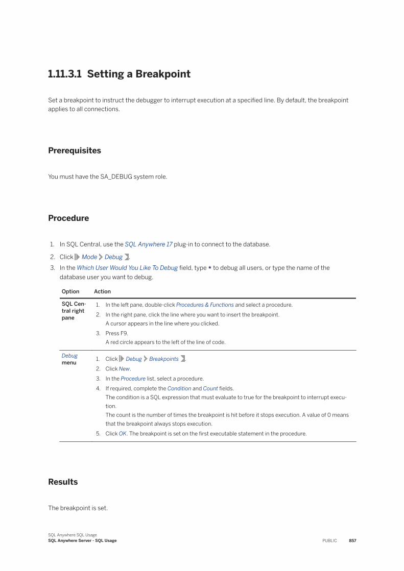
1.11.3.1 Setting a Breakpoint
Set a breakpoint to instruct the debugger to interrupt execution at a specified line. By default, the breakpoint applies to all connections.
Prerequisites
You must have the SA_DEBUG system role.
Procedure
1. In SQL Central, use the SQL Anywhere 17 plug-in to connect to the database.
2. Click Mode Debug .3. In the Which User Would You Like To Debug field, type * to debug all users, or type the name of the
database user you want to debug.
Option Action
SQL Central right pane
1. In the left pane, double-click Procedures & Functions and select a procedure.2. In the right pane, click the line where you want to insert the breakpoint.
A cursor appears in the line where you clicked.3. Press F9.
A red circle appears to the left of the line of code.
Debug menu 1. Click Debug Breakpoints .
2. Click New.3. In the Procedure list, select a procedure.4. If required, complete the Condition and Count fields.
The condition is a SQL expression that must evaluate to true for the breakpoint to interrupt execution.The count is the number of times the breakpoint is hit before it stops execution. A value of 0 means that the breakpoint always stops execution.
5. Click OK. The breakpoint is set on the first executable statement in the procedure.
Results
The breakpoint is set.
SQL Anywhere SQL UsageSQL Anywhere Server - SQL Usage PUBLIC 857
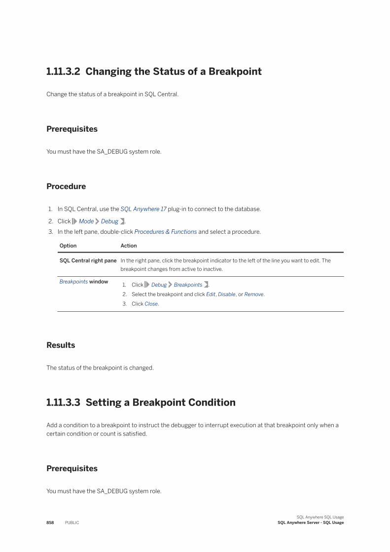
1.11.3.2 Changing the Status of a Breakpoint
Change the status of a breakpoint in SQL Central.
Prerequisites
You must have the SA_DEBUG system role.
Procedure
1. In SQL Central, use the SQL Anywhere 17 plug-in to connect to the database.
2. Click Mode Debug .3. In the left pane, double-click Procedures & Functions and select a procedure.
Option Action
SQL Central right pane In the right pane, click the breakpoint indicator to the left of the line you want to edit. The breakpoint changes from active to inactive.
Breakpoints window 1. Click Debug Breakpoints .2. Select the breakpoint and click Edit, Disable, or Remove.3. Click Close.
Results
The status of the breakpoint is changed.
1.11.3.3 Setting a Breakpoint Condition
Add a condition to a breakpoint to instruct the debugger to interrupt execution at that breakpoint only when a certain condition or count is satisfied.
Prerequisites
You must have the SA_DEBUG system role.
858 PUBLICSQL Anywhere SQL Usage
SQL Anywhere Server - SQL Usage
Context
For procedures and triggers, the condition must be a SQL search condition.
Procedure
1. In SQL Central, use the SQL Anywhere 17 plug-in to connect to the database.
2. Click Mode Debug .3. In the left pane, double-click Procedures & Functions and select a procedure.
4. Click Debug Breakpoints .5. Select the breakpoint you want to edit and then click Edit.6. In the Condition list, add a condition. For example, to set the breakpoint so that it applies only to
connections from a specific user ID, enter the following condition:
CURRENT USER='user-name'
In this condition, user-name is the user ID for which the breakpoint is to be active.
7. Click OK and then click Close.
Results
The condition is set on the breakpoint.
1.11.4 Variable Modification with the Debugger
The debugger lets you view and edit the behavior of your variables while it steps through your code.
The debugger provides a Debugger Details pane to display the different kinds of variables used in stored procedures. The Debugger Details pane appears at the bottom of SQL Central when SQL Central is running in Debug mode.
Global Variables in the Debugger
Global variables are defined by the database server and hold information about the current connection, database, and other settings.
They appear in the Debugger Details pane on the Global tab.
Row variables are used in triggers to hold the values of rows affected by the triggering statement. They appear in the Debugger Details pane on the Row tab.
SQL Anywhere SQL UsageSQL Anywhere Server - SQL Usage PUBLIC 859
Static variables are used in Java classes. They appear on the Statics tab.
In this section:
Viewing Variable Values [page 860]View variable values in SQL Central.
Displaying the Call Stack [page 861]Examine the sequence of calls that has been made when you are debugging nested procedures.
Related Information
Triggers [page 107]
1.11.4.1 Viewing Variable Values
View variable values in SQL Central.
Prerequisites
You must have the SA_DEBUG system role.
Additionally, you must have the EXECUTE ANY PROCEDURE system privilege or EXECUTE privilege on the procedure.
Procedure
1. In SQL Central, use the SQL Anywhere 17 plug-in to connect to the database.
2. Click Mode Debug .3. In the Which User Would You Like To Debug field, type * to debug all users, or type the name of the
database user you want to debug.4. In the left pane, double-click Procedures & Functions and select a procedure.5. In the right pane, click the line where you want to insert the breakpoint.
A cursor appears in the line where you clicked.6. Press F9.
A red circle appears to the left of the line of code.7. In the Debugger Details pane, click the Local tab.8. In the left pane, right-click the procedure and click Execute From Interactive SQL.
860 PUBLICSQL Anywhere SQL Usage
SQL Anywhere Server - SQL Usage
9. Click the Local tab.
Results
The variables, along with their values, are displayed.
1.11.4.2 Displaying the Call Stack
Examine the sequence of calls that has been made when you are debugging nested procedures.
Prerequisites
You must have the SA_DEBUG system role.
Additionally, you must have the EXECUTE ANY PROCEDURE system privilege or EXECUTE privilege on the procedure.
Context
You can view a listing of the procedures on the Call Stack tab.
Procedure
1. In SQL Central, use the SQL Anywhere 17 plug-in to connect to the database.
2. Click Mode Debug .3. In the Which User Would You Like To Debug field, type * to debug all users, or type the name of the
database user you want to debug.4. In the left pane, double-click Procedures & Functions and select a procedure.5. In the right pane, click the line where you want to insert the breakpoint.
A cursor appears in the line where you clicked.6. Press F9.
A red circle appears to the left of the line of code.7. In the Debugger Details pane, click the Local tab.8. In the left pane, right-click the procedure and click Execute From Interactive SQL.9. In the Debugger Details pane, click the Call Stack tab.
SQL Anywhere SQL UsageSQL Anywhere Server - SQL Usage PUBLIC 861
Results
The names of the procedures appear on the Calls Stack tab. The current procedure is shown at the top of the list. The procedure that called it is immediately below.
1.11.5 Connections and Breakpoints
The Connections tab in SQL Central displays the connections to the database.
At any time, multiple connections may be running. Some may be stopped at a breakpoint, and others may not.
To switch connections, double-click a connection on the Connections tab.
A useful technique is to set a breakpoint so that it interrupts execution for a single user ID. You can do this by setting a breakpoint condition of the following form:
CURRENT USER = 'user-name'
The SQL special value CURRENT USER holds the user ID of the connection.
Related Information
Setting a Breakpoint Condition [page 858]
862 PUBLICSQL Anywhere SQL Usage
SQL Anywhere Server - SQL Usage
Important Disclaimers and Legal Information
HyperlinksSome links are classified by an icon and/or a mouseover text. These links provide additional information.About the icons:
● Links with the icon : You are entering a Web site that is not hosted by SAP. By using such links, you agree (unless expressly stated otherwise in your agreements with SAP) to this:
● The content of the linked-to site is not SAP documentation. You may not infer any product claims against SAP based on this information.● SAP does not agree or disagree with the content on the linked-to site, nor does SAP warrant the availability and correctness. SAP shall not be liable for any
damages caused by the use of such content unless damages have been caused by SAP's gross negligence or willful misconduct.
● Links with the icon : You are leaving the documentation for that particular SAP product or service and are entering a SAP-hosted Web site. By using such links, you agree that (unless expressly stated otherwise in your agreements with SAP) you may not infer any product claims against SAP based on this information.
Videos Hosted on External PlatformsSome videos may point to third-party video hosting platforms. SAP cannot guarantee the future availability of videos stored on these platforms. Furthermore, any advertisements or other content hosted on these platforms (for example, suggested videos or by navigating to other videos hosted on the same site), are not within the control or responsibility of SAP.
Beta and Other Experimental FeaturesExperimental features are not part of the officially delivered scope that SAP guarantees for future releases. This means that experimental features may be changed by SAP at any time for any reason without notice. Experimental features are not for productive use. You may not demonstrate, test, examine, evaluate or otherwise use the experimental features in a live operating environment or with data that has not been sufficiently backed up.The purpose of experimental features is to get feedback early on, allowing customers and partners to influence the future product accordingly. By providing your feedback (e.g. in the SAP Community), you accept that intellectual property rights of the contributions or derivative works shall remain the exclusive property of SAP.
Example CodeAny software coding and/or code snippets are examples. They are not for productive use. The example code is only intended to better explain and visualize the syntax and phrasing rules. SAP does not warrant the correctness and completeness of the example code. SAP shall not be liable for errors or damages caused by the use of example code unless damages have been caused by SAP's gross negligence or willful misconduct.
Gender-Related LanguageWe try not to use gender-specific word forms and formulations. As appropriate for context and readability, SAP may use masculine word forms to refer to all genders.
SQL Anywhere SQL UsageImportant Disclaimers and Legal Information PUBLIC 863
www.sap.com/contactsap
© 2020 SAP SE or an SAP affiliate company. All rights reserved.
No part of this publication may be reproduced or transmitted in any form or for any purpose without the express permission of SAP SE or an SAP affiliate company. The information contained herein may be changed without prior notice.
Some software products marketed by SAP SE and its distributors contain proprietary software components of other software vendors. National product specifications may vary.
These materials are provided by SAP SE or an SAP affiliate company for informational purposes only, without representation or warranty of any kind, and SAP or its affiliated companies shall not be liable for errors or omissions with respect to the materials. The only warranties for SAP or SAP affiliate company products and services are those that are set forth in the express warranty statements accompanying such products and services, if any. Nothing herein should be construed as constituting an additional warranty.
SAP and other SAP products and services mentioned herein as well as their respective logos are trademarks or registered trademarks of SAP SE (or an SAP affiliate company) in Germany and other countries. All other product and service names mentioned are the trademarks of their respective companies.
Please see https://www.sap.com/about/legal/trademark.html for additional trademark information and notices.
THE BEST RUN


