Steve Vanlanduit, Mario Sorgente, Aydin R. Zadeh, Alfredo Güemes,
and Nadimul Faisal
Abstract This chapter provides an overview of the use of strain sensors forstructural health monitoring. Compared to acceleration-based sensors, strain sensorscan measure the deformation of a structure at very low frequencies (up to DC) andenable the measurement of ultrasonic responses. Many existing SHM methods makeuse of strain measurement data. Furthermore, strain sensors can be easily integratedin (aircraft) structures. This chapter discusses the working principle of traditionalstrain gauges (Sect. 8.1) and different types of optical fiber sensors (Sect. 8.2). Theinstallation requirements of strain sensors and the required hardware for reading outsensors are provided. We will also give an overview of the advantages and thelimitations of commonly used strain sensors. Finally, we will present an overview ofthe applications of strain sensors for structural health monitoring in the aeronauticsfield.
8.1 Strain Gauges
A strain gauge (or gage) is a sensing device used to determine the directions andmagnitudes of principal surface strains (ASTM E1561-93 2014) and residual stresses(ASTM E837-13a 2013) in conjuction with established algorithms. Once the surfaceon which the strain gauge is assembled is deformed, the strain gauge causes a changein length leading to a change in electrical resistance. The change in electrical
S. Vanlanduit (*)University of Antwerp, Antwerp, Belgiume-mail: [email protected]
M. Sorgente · A. R. ZadehOptics 11, Amsterdam, The Netherlands
A. GüemesTechnical University of Madrid, Madrid, Spain
resistance is measured using an electrical circuit (i.e. Wheatstone bridge), which isthen related to strain by the quantity known as the gauge factor. The stress is forceper unit of surface (i.e. pressure) that is acting on an infinitesimal area. The stress is aderived quantity that under some assumptions (e.g. single axis stress state and strainmeasured in the transverse direction) can be calculated from the strain (if theYoung’s modulus is known). In general the measured strain depends on the mechan-ical load as well as the thermal loading. When establishing the stress-strain relation-ship both contributions should be balanced. Furthermore in case of permanent orplastic deformation of a material setting up the relation between the measured strainand the stresses (including residual stress) is much more difficult (Faisal et al. 2019).
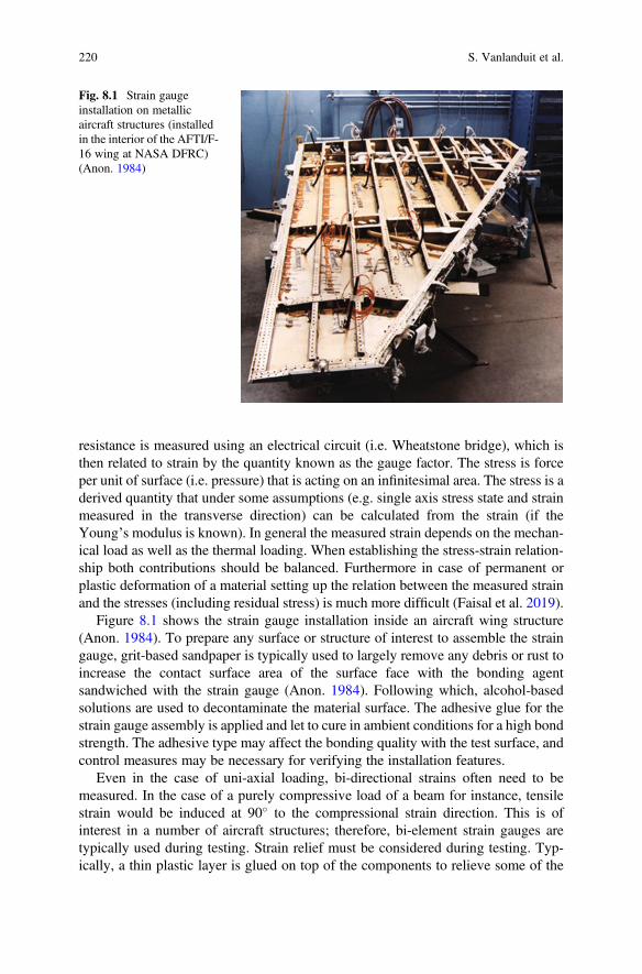
Figure 8.1 shows the strain gauge installation inside an aircraft wing structure(Anon. 1984). To prepare any surface or structure of interest to assemble the straingauge, grit-based sandpaper is typically used to largely remove any debris or rust toincrease the contact surface area of the surface face with the bonding agentsandwiched with the strain gauge (Anon. 1984). Following which, alcohol-basedsolutions are used to decontaminate the material surface. The adhesive glue for thestrain gauge assembly is applied and let to cure in ambient conditions for a high bondstrength. The adhesive type may affect the bonding quality with the test surface, andcontrol measures may be necessary for verifying the installation features.
Even in the case of uni-axial loading, bi-directional strains often need to bemeasured. In the case of a purely compressive load of a beam for instance, tensilestrain would be induced at 90� to the compressional strain direction. This is ofinterest in a number of aircraft structures; therefore, bi-element strain gauges aretypically used during testing. Strain relief must be considered during testing. Typ-ically, a thin plastic layer is glued on top of the components to relieve some of the
Fig. 8.1 Strain gaugeinstallation on metallicaircraft structures (installedin the interior of the AFTI/F-16 wing at NASA DFRC)(Anon. 1984)
220 S. Vanlanduit et al.
stress exerted. Excess plastic is then removed after the glue sets. A commerciallyavailable programmable automation controller (e.g. National Instruments, VishayPrecision Group) can be used to receive the signals created by strain gauges. Theinstrumentation includes strain indicators, signal conditioning amplifiers, and soft-ware for data recording. The strain gauge would normally come with a shorter leadcable length (e.g. recommended length of 1.5–2.5 m, (IPC/JEDEC 2005). Quarter-bridge strain gauges in a ‘three-wire connection’ are preferred over those in a ‘two-wire connection.’ The increase in the lead wire length increases the possibility oferrors due to temperature variations, lead desensitization, and lead-wire resistancechanges (ASTM E1561-93 2014). A slight change in the temperature can generate ameasurement error of several microstrain. For the extension of strain gauge cables, acareful consideration is needed when extending to long lengths because the overallresistance of the strain gauge assembly will change (Takeuchi 2012).
For aircraft SHM, the complex geometry of the structures (specimen) leads to acomplex strain analysis. Usually assumptions of a much simpler strain distributionare made in practice (e.g. by ignoring the strain in the thickness direction of a thinbeam). Due to a combination of the high sensitivity of the strain gauge measurementequipment, outdoor environment, and necessity for extremely long data cables, theraw data could feature a high noise level. To minimise the effects of such noise andallow trends to be more clearly identified, the signals (for each strain gauge) can besmoothed by averaging over a window of data points using a computational code,thereby removing localised spikes that could potentially be seen in the raw data.Despite data smoothing, there can still be a fluctuation due to the low signal-to-noiseratio, which makes it difficult to identify significant events within the test from thestrain gauge data alone.
8.2 Optical Fiber Sensors
8.2.1 Introduction
In a fiber optic sensor, light guided through the fiber core is affected by themeasurand. Optical fiber sensors (OFS) are most frequently used to measure strain,temperature, or pressure, but they can also be used as chemical sensors,vibroacoustic detectors and refractometers for cure monitoring (Lee 2003). One ofthe main advantages of the optical fiber sensor is its thinness. It usually has adiameter of 125μm, but OFS with a diameter of up to 12μm have also been reported(Malik et al. 2016). This makes it easy to integrate them in materials like compositematerials. In the last few decades, the OFS have been successfully used for damagedetection in composite materials (Kinet et al. 2014).
In composite materials, OFS are sandwiched between two composite layers(Dawood et al. 2007). This process has been successfully applied to aircraft com-ponents at Airbus (Giraldo et al. 2017).
8 Strain Monitoring 221
In metals, OFS are also being integrated in components (Saheb and Mekid 2015;He et al. 2019). In this case, fiber is inserted in a groove closed by meltingsubsequent powder layers on top of the fibers (Havermann et al. 2015). Metalmelting is usually performed by laser cladding or high-power ultrasound (He et al.2019). A metal (Grandal et al. 2018) or carbon (Nedjalkov et al. 2018) coating isapplied to protect the fibers from high temperatures during the integration process.
In other applications, the OFS is not integrated in the material under test, but thesensors are applied at the surface of the part. This can be done by using a prepregsample with an integrated optical fiber, of which the so-called fiber optic ribbon tape(FORT) is an example (Loutas et al. 2015). For aerospace applications, a specialtyaerospace-grade coated fiber Bragg gratings (FBG) sensor with an adapted bondingprocedure was developed (Goossens et al. 2019). Goossens et al. tested their sensorin in-flight conditions with realistic humidity, temperature, and pressure cycles, aswell as hydraulic fluid and fatigue loading.
Optical fiber sensors can be used in harsh environments (Mihailov 2012). Theyare immune to electromagnetic interference (Druet et al. 2018) and can be used atvery high temperatures. Silica glass allows the detection of strains in environmentsup to 1000 �C (Yu and Okabe 2017). Radiation-hardened sensors have beendeveloped for space applications (Girard et al. 2018).
Another important advantage of OFS is the fact that they can be multiplexed.Several sensors can be inscribed in one optical fiber, and these sensors can be readout using one single interrogator. The interrogator is the hardware needed to acquirethe measurand from the reflected or transmitted light that goes through the fiber.Time domain multiplexing has been used to realise up to 1000 ultra-weak FBG fordistributed temperature sensing (Wang et al. 2012) and 100s of strain sensors (Daiet al. 2009; Cranch and Nash 2001). In addition to the point sensors, also distributedfiber optics sensors based on different principles are available: Rayleigh (Froggattet al. 1998) and Brillouin scattering (Garus et al. 1996).
8.2.2 Types of Optical Fiber Sensors
Sensors vitally affect our life in multiple fields, such as IoT, structural healthmonitoring, smart structures, and digital twins. The necessity of tracking the materialbehavior has assumed a great, and not trivial importance in reducing maintenancecosts and promoting prevention over replacement. In addition, the harsher theenvironment, the more challenging the measurement. The advantages of opticalsensors come into play because of the fact that they are
• completely passive,• lightweight,• survive at critical temperature, dust, and ATEX (ATmosphere EXplosible)
environment,• immune to electromagnetic interference,
222 S. Vanlanduit et al.
• not required to have pre-amplification, and• capable of being interrogated from hundreds of meters of distance.
These features open up scenarios for more accurate, precise, and repeatablemeasurements (Pinet 2009). This study discusses some of the most common opticalsensing techniques based on the interferometry principle.
8.2.3 Interferometry
Interferometry is a technique based on the wave interference phenomenon. In classicphysics, this comes into play when two waves superimpose to generate a resultantwave of a greater (constructive interference) or lower amplitude (destructive inter-ference). The former occurs when the phase difference of the two waves is an evenmultiple of π (180�), whereas the latter happens when the difference is an oddmultiple of π. The phase differences with values between these two extremes willresult in displacement magnitudes that range between the minimum and maximumvalues. Two conditions must be met to set up an interference pattern that is stable andclear (Hariharan 2007):
1. Coherent light sources must be used, meaning they emit waves with a constantphase difference.
2. The waves should be of a single wavelength, that is, monochromatic.
Several types of interferometers are available and have a wide-spread use inoptical sensing applications. Interferometry based optical sensors can be easilyscaled up to long ranges, used in satellite imaging of surface deformation, and scaleddown to cell stiffness measurement in biological matters. Furthermore, the sensitiv-ity of these sensors can be tuned by adjusting the interferometry arm lengths of thesensor. For these reasons, the interferometry principle has become a basis fornumerous sensor designs in both academia and in the industry.
In this article, three of the most common interferometer types will be discussed,namely Mach–Zehnder, Michelson, and Fabry–Pérot.
8.2.4 Mach–Zehnder
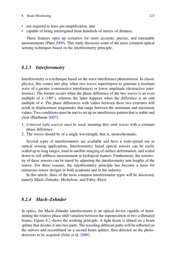
In optics, the Mach–Zehnder interferometer is an optical device capable of deter-mining the relative phase shift variation between the superposition of two collimatedbeams. Figure 8.2 shows the working principle. A light beam is shined on a beamsplitter that divides it into two parts. The traveling different paths will be reflected onthe mirrors and recombined on a second beam splitter, then directed on the photo-detectors to be acquired (Zetie et al. 2000).
8 Strain Monitoring 223
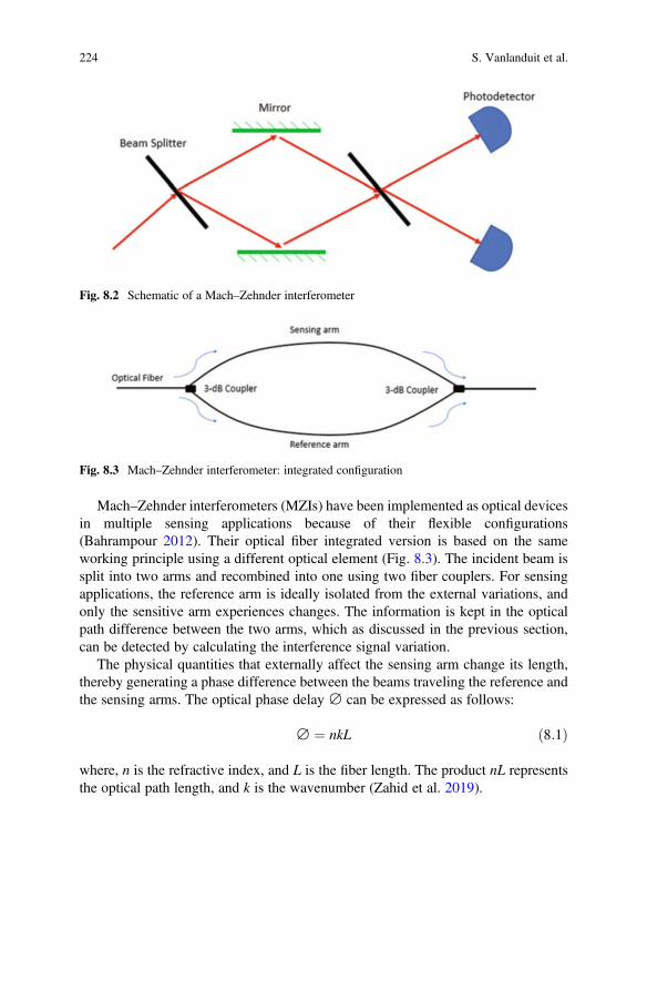
Mach–Zehnder interferometers (MZIs) have been implemented as optical devicesin multiple sensing applications because of their flexible configurations(Bahrampour 2012). Their optical fiber integrated version is based on the sameworking principle using a different optical element (Fig. 8.3). The incident beam issplit into two arms and recombined into one using two fiber couplers. For sensingapplications, the reference arm is ideally isolated from the external variations, andonly the sensitive arm experiences changes. The information is kept in the opticalpath difference between the two arms, which as discussed in the previous section,can be detected by calculating the interference signal variation.
The physical quantities that externally affect the sensing arm change its length,thereby generating a phase difference between the beams traveling the reference andthe sensing arms. The optical phase delay ∅ can be expressed as follows:
∅ ¼ nkL ð8:1Þ
where, n is the refractive index, and L is the fiber length. The product nL representsthe optical path length, and k is the wavenumber (Zahid et al. 2019).
Fig. 8.2 Schematic of a Mach–Zehnder interferometer
Similar to the Mach–Zehnder interferometer, the Michelson interferometer(MI) compares two beams reflected from two mirrors on two configuration branches.An MI is considered as half of an MZI, where the main difference is the presence oftwo reflectors.
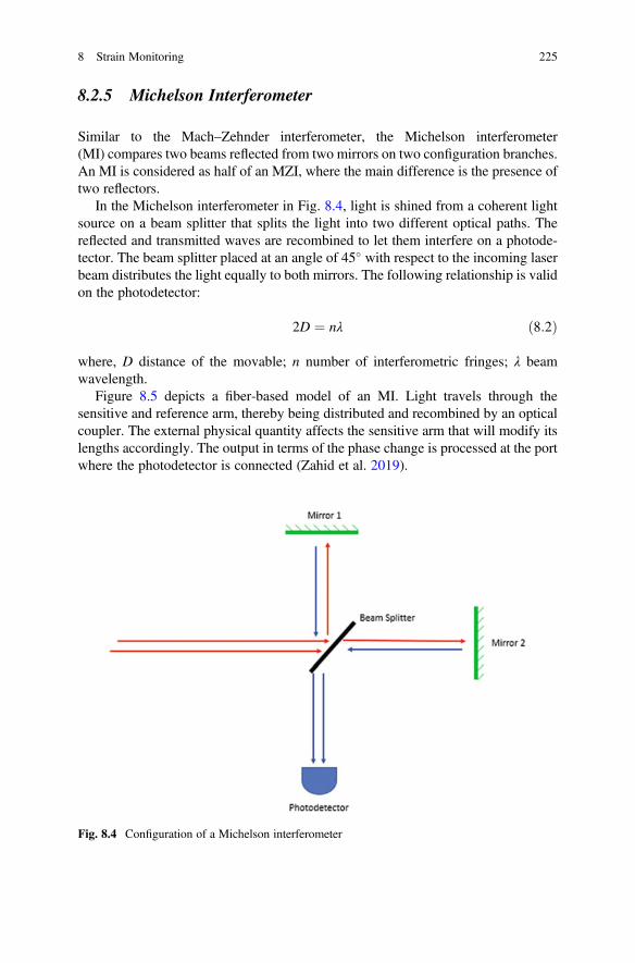
In the Michelson interferometer in Fig. 8.4, light is shined from a coherent lightsource on a beam splitter that splits the light into two different optical paths. Thereflected and transmitted waves are recombined to let them interfere on a photode-tector. The beam splitter placed at an angle of 45� with respect to the incoming laserbeam distributes the light equally to both mirrors. The following relationship is validon the photodetector:
2D ¼ nλ ð8:2Þ
where, D distance of the movable; n number of interferometric fringes; λ beamwavelength.
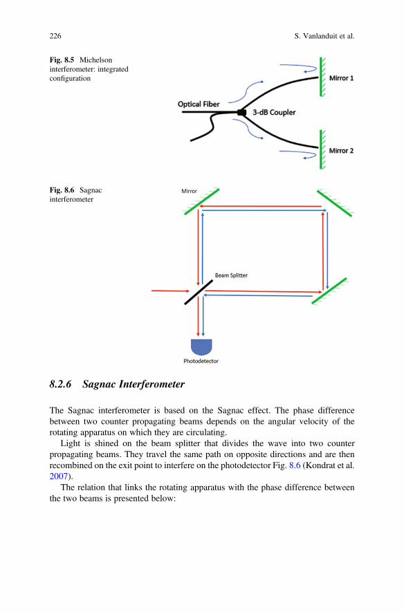
Figure 8.5 depicts a fiber-based model of an MI. Light travels through thesensitive and reference arm, thereby being distributed and recombined by an opticalcoupler. The external physical quantity affects the sensitive arm that will modify itslengths accordingly. The output in terms of the phase change is processed at the portwhere the photodetector is connected (Zahid et al. 2019).
Fig. 8.4 Configuration of a Michelson interferometer
8 Strain Monitoring 225
8.2.6 Sagnac Interferometer
The Sagnac interferometer is based on the Sagnac effect. The phase differencebetween two counter propagating beams depends on the angular velocity of therotating apparatus on which they are circulating.
Light is shined on the beam splitter that divides the wave into two counterpropagating beams. They travel the same path on opposite directions and are thenrecombined on the exit point to interfere on the photodetector Fig. 8.6 (Kondrat et al.2007).
The relation that links the rotating apparatus with the phase difference betweenthe two beams is presented below:
where, A is the unit vector perpendicular to the surface area of the apparatus; ωrot isthe angular velocity of the apparatus; λ is the light wavelength; and v is the beamspeed.
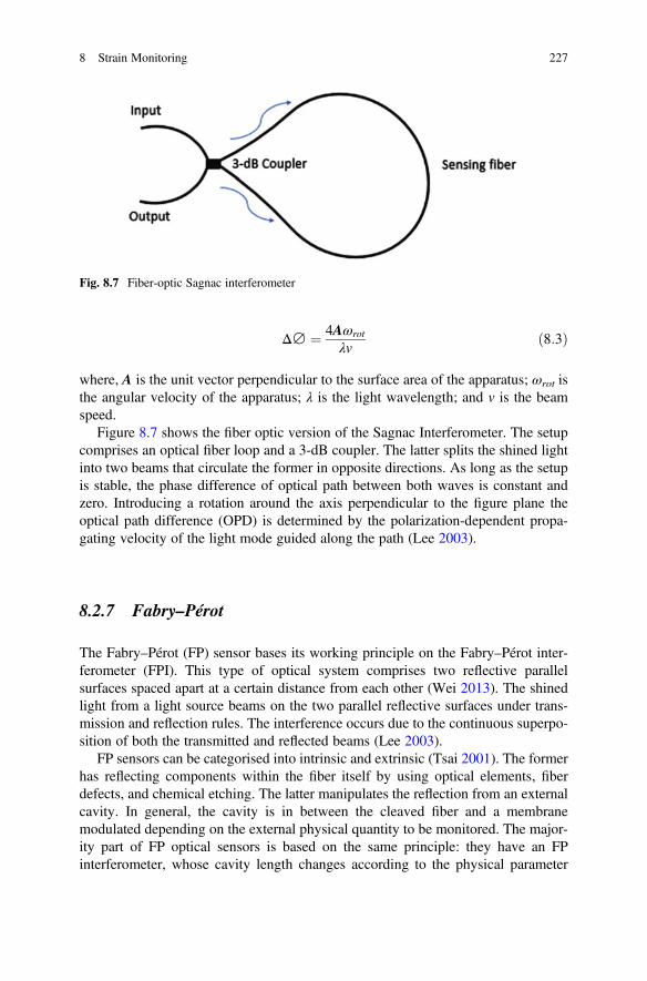
Figure 8.7 shows the fiber optic version of the Sagnac Interferometer. The setupcomprises an optical fiber loop and a 3-dB coupler. The latter splits the shined lightinto two beams that circulate the former in opposite directions. As long as the setupis stable, the phase difference of optical path between both waves is constant andzero. Introducing a rotation around the axis perpendicular to the figure plane theoptical path difference (OPD) is determined by the polarization-dependent propa-gating velocity of the light mode guided along the path (Lee 2003).
8.2.7 Fabry–Pérot
The Fabry–Pérot (FP) sensor bases its working principle on the Fabry–Pérot inter-ferometer (FPI). This type of optical system comprises two reflective parallelsurfaces spaced apart at a certain distance from each other (Wei 2013). The shinedlight from a light source beams on the two parallel reflective surfaces under trans-mission and reflection rules. The interference occurs due to the continuous superpo-sition of both the transmitted and reflected beams (Lee 2003).
FP sensors can be categorised into intrinsic and extrinsic (Tsai 2001). The formerhas reflecting components within the fiber itself by using optical elements, fiberdefects, and chemical etching. The latter manipulates the reflection from an externalcavity. In general, the cavity is in between the cleaved fiber and a membranemodulated depending on the external physical quantity to be monitored. The major-ity part of FP optical sensors is based on the same principle: they have an FPinterferometer, whose cavity length changes according to the physical parameter
Fig. 8.7 Fiber-optic Sagnac interferometer
8 Strain Monitoring 227
they are designed to measure. The cavity length is converted into the appropriate unitcorresponding to the sensor type using appropriate sensor calibration (Pinet 2009).
The FP reflection (or transmission) spectrum is described as the wavelength-dependent intensity modulation of the input light source caused by the optical phasedifference (wave imaginary part variation) between two reflected (or transmitted)beams. Constructive and destructive interference combines the maximum and min-imum peaks in the 2π modulus. The phase difference is given as follows:
Δ∅FPI ¼2πλn 2L ð8:4Þ
where, λ is the wavelength on the incident light; n is the refractive index of the cavitymode or cavity material; and L is the physical length of the cavity considering thelight traveling back and forth (Rajan 2016).
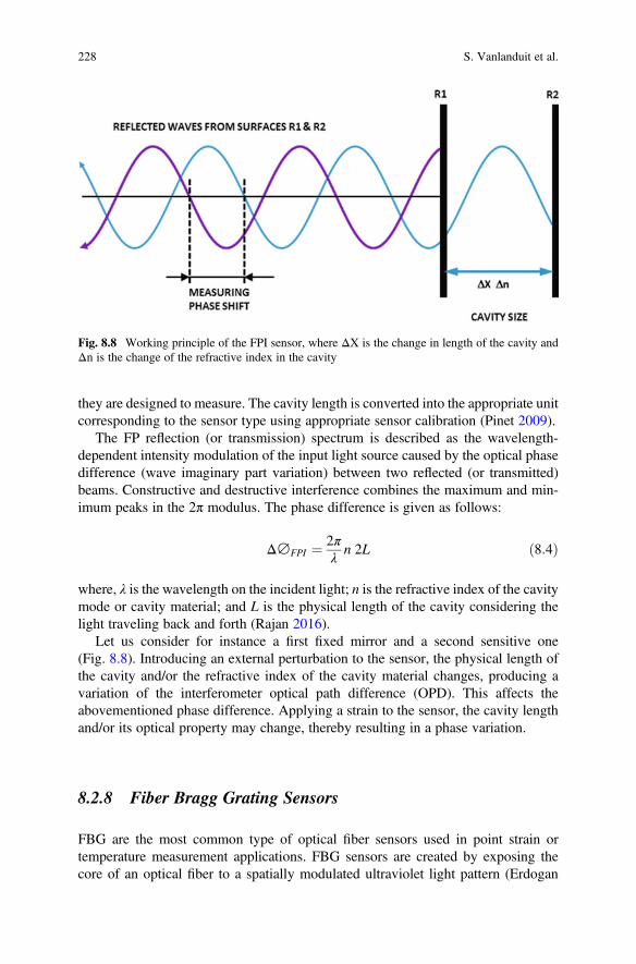
Let us consider for instance a first fixed mirror and a second sensitive one(Fig. 8.8). Introducing an external perturbation to the sensor, the physical length ofthe cavity and/or the refractive index of the cavity material changes, producing avariation of the interferometer optical path difference (OPD). This affects theabovementioned phase difference. Applying a strain to the sensor, the cavity lengthand/or its optical property may change, thereby resulting in a phase variation.
8.2.8 Fiber Bragg Grating Sensors
FBG are the most common type of optical fiber sensors used in point strain ortemperature measurement applications. FBG sensors are created by exposing thecore of an optical fiber to a spatially modulated ultraviolet light pattern (Erdogan
Fig. 8.8 Working principle of the FPI sensor, where ΔX is the change in length of the cavity andΔn is the change of the refractive index in the cavity
228 S. Vanlanduit et al.
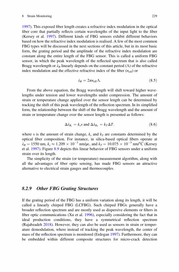
1997). This exposed fiber length creates a refractive index modulation in the opticalfiber core that partially reflects certain wavelengths of the input light to the fiber(Kersey et al. 1997). Different kinds of FBG sensors exhibit different behaviorsbased on how the refractive index modulation is realised. A few of the most commonFBG types will be discussed in the next sections of this article, but in its most basicform, the grating period and the amplitude of the refractive index modulation areconstant along the entire length of the FBG sensor. This is called a uniform FBGsensor, in which the peak wavelength of the reflected spectrum that is also calledBragg wavelength or λB linearly depends on the constant period (Λ) of the refractiveindex modulation and the effective refractive index of the fiber (neff) or
λB ¼ 2πneffΛ: ð8:5Þ
From the above equation, the Bragg wavelength will shift toward higher wave-lengths under tension and lower wavelengths under compression. The amount ofstrain or temperature change applied over the sensor length can be determined bytracking the shift of this peak wavelength of the reflection spectrum. In its simplifiedform, the relationship between the shift of the Bragg wavelength and the amount ofstrain or temperature change over the sensor length is presented as follows:
ΔλBE¼ kss and ΔλBT
¼ kTΔT: ð8:6Þ
where s is the amount of strain change, ks and kT are constants determined by theoptical fiber composition. For instance, in silica-based optical fibers operate atλB ¼ 1550 nm, ks � 1.209 � 10�3 nm/μE, and kT ¼ 10.075 � 10�3 nm/oC (Kerseyet al. 1997). Figure 8.9 depicts this linear behavior of FBG sensors under a uniformstrain over its length.
The simplicity of the strain (or temperature) measurement algorithm, along withall the advantages of fiber optic sensing, has made FBG sensors an attractivealternative to electrical strain gauges and thermocouples.
8.2.9 Other FBG Grating Structures
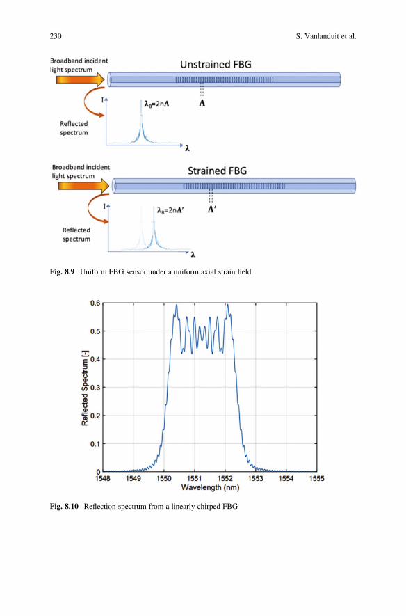
If the grating period of the FBG has a uniform variation along its length, it will becalled a linearly chirped FBG (LCFBG). Such chirped FBGs generally have abroader reflection spectrum and are mostly used as dispersive elements or filters infiber optic communications (Xu et al. 1996), especially considering the fact that inideal production conditions, they have a symmetrical reflection spectrum(Rajabzadeh 2018). However, they can also be used as sensors in strain or temper-ature demodulation, where instead of tracking the peak wavelength, the center ofmass of the reflection spectrum is monitored (Erdogan 1997). Furthermore, they canbe embedded within different composite structures for micro-crack detection
8 Strain Monitoring 229
Fig. 8.9 Uniform FBG sensor under a uniform axial strain field
Fig. 8.10 Reflection spectrum from a linearly chirped FBG
230 S. Vanlanduit et al.
applications (Takeda et al. 2013). In Fig. 8.10 an example of the reflection spectrumof such a LCFBGs is given (with 10 mm length and a linear chirp rate of dλB
dz¼
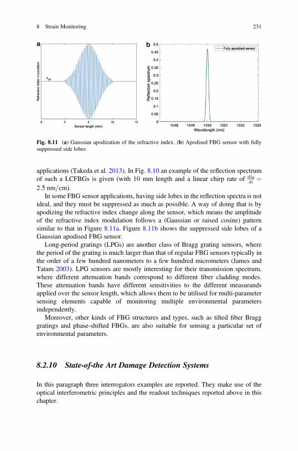
2:5 nm=cm).In some FBG sensor applications, having side lobes in the reflection spectra is not
ideal, and they must be suppressed as much as possible. A way of doing that is byapodizing the refractive index change along the sensor, which means the amplitudeof the refractive index modulation follows a (Gaussian or raised cosine) patternsimilar to that in Figure 8.11a. Figure 8.11b shows the suppressed side lobes of aGaussian apodised FBG sensor.
Long-period gratings (LPGs) are another class of Bragg grating sensors, wherethe period of the grating is much larger than that of regular FBG sensors typically inthe order of a few hundred nanometers to a few hundred micrometers (James andTatam 2003). LPG sensors are mostly interesting for their transmission spectrum,where different attenuation bands correspond to different fiber cladding modes.These attenuation bands have different sensitivities to the different measurandsapplied over the sensor length, which allows them to be utilised for multi-parametersensing elements capable of monitoring multiple environmental parametersindependently.
Moreover, other kinds of FBG structures and types, such as tilted fiber Bragggratings and phase-shifted FBGs, are also suitable for sensing a particular set ofenvironmental parameters.
8.2.10 State-of-the Art Damage Detection Systems
In this paragraph three interrogators examples are reported. They make use of theoptical interferometric principles and the readout techniques reported above in thischapter.
Fig. 8.11 (a) Gaussian apodization of the refractive index. (b) Apodised FBG sensor with fullysuppressed side lobes
8 Strain Monitoring 231
DeltaSens: Fabry Perot Interrogator
The DeltaSens interrogator from Optics11 is a high-speed interrogation unit forreading Fabry–Pérot-type sensors. Optical sensors have to be properly coupled withDeltaSens, which will then communicate the sensed physical quantities to a com-puter to allow data processing. The readout must be equipped with the opticalinterface to manipulate and interpret the light.
DeltaSens (Fig. 8.12) interrogates multiple Fabry–Pérot-type sensors in an opticalfiber network connected through standard optical splitters. The interferometer isformed by a broadband light source and a spectrometer. A spectral acquisitionarrangement acquires successive spectral responses from the optical sensor arrange-ment during successive time intervals. All connected FP cavities with differentcavity lengths result in specific footprints on the spectrometer. The spectral analysisarrangement detects a phase evolution of the periodicity throughout the successivespectral responses. The phase evolution of the periodicity provides a relativelyprecise measurement of a variation in an optical path length between the tworeflective surfaces of the Fabry–Pérot structure. A variation in a physical quantitycan cause optical path length variation. Accordingly, a relatively precise measure-ment of the physical quantity can be achieved (Grzegorz Gruca 2019).
The main application of such an interrogator is acceleration sensing using 1D and3D optical accelerometers. The distances between each sensor and to the read-outcan be kilometers (Rijnveld 2017). Further algorithms have been implemented toretrieve both the relative variation and the absolute value of the acceleration.
I4 Series: FBG Interrogators
Several methods can be used to interrogate FBG sensors, and a few of the mostcommon techniques will be discussed herein. The most straightforward approach isto use a superluminescent diode (SLD) as a light source and a spectrometer to recordthe FBG-reflected spectrum (Alves 2003). However, the wavelength resolution andthe accuracy offered by such spectrometers are usually above a few hundreds ofpicometers to a few nanometers, greatly limiting the strain and temperature resolu-tion of the FBG sensor. Another approach is to use the fiber Fabry–Pérot tunable
Fig. 8.12 DeltaSens interrogator by Optics11
232 S. Vanlanduit et al.
filter technology for a high-spatial resolution interrogation of the reflected spectrum.In this technique, a tunable laser and a high-precision synchronization system areused to scan the wavelength region of interest and sample the FBG-reflectedspectrum (Ushakov 2015).
A similar alternative method is the interrogation of FBG sensors with the semi-conductor tunable laser technology used in FAZ interrogators. This technologyoffers a sub-picometer wavelength accuracy that translates into micro-strain accu-racy for strain measurements and temperature measurement accuracy of below0.1 �C or �1 με at scanning frequencies between 1 and 8 kHz (Fig. 8.13).
The I4 series can sustain up to 30 sensing points per channel. Different channelversions are produced: 4 and 16 with a trade-off between the number of sensingpoints and the sampling frequency.
8.2.11 Acoustic Emission Interrogator (OptimAE)
Acoustic emission (AE) is a non-invasive technique that allows the detection ofdamage and crack formation in engineering structures in real time (see Chap. 7). As acrack forms in such structures, the energy release results in transient surface acousticwaves, which are also called Rayleigh waves, that propagate throughout the material(Park 2011). Electrical AE systems use piezo-electric sensors to acquire these high-frequency acoustic waves. However, piezo-electric sensors have some limitationsthat narrow down their application in harsh environments.
The OptimAE unit is the optical acoustic emission monitoring system (Fig. 8.14).The optical AE setup contains two optical fibers (i.e., one operating as a sensing armand one as a reference arm), which together form an interferometry setup. Thesensing fiber is densely coiled on a metallic mandrel and is in a direct contact withthe material surface for the optimum transmission of the surface acoustic wave to thesensor. The elastic energy of the acoustic wave stretches the fiber that changes the
differential length of the fibers on the sensing and the reference arms of theinterferometer. The resulting interferometric signal is transferred to the OptimAEreadout for signal acquisition, demodulation, and communication to the computer.The optical AE sensors can be sampled at 1 MS/s and have a spectral noise density of150 f E=
ffiffiffiffiffiffi
Hzp
(this term is the average amount of displacement noise per frequencybin which can be derived from power spectral analysis of the noise floor of the sensorresponse). They operate at a C-band wavelength range.
Performance tests showed that the optical acoustic emission sensors are a com-parable alternative with respect to existing piezoelectric ones, opening new mea-surement scenarios in harsh environment conditions and extending the benefits ofAE testing to new industries (Mario Sorgente 2020).
8.2.12 OFS Applications in Aeronautics
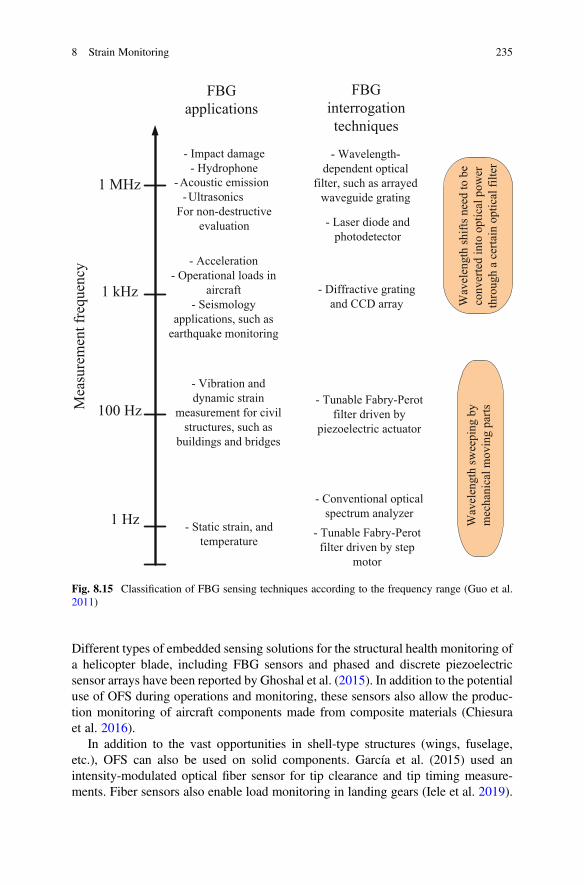
The optical fiber sensor technology and fiber Bragg gratings are evaluated as goodtools for load monitoring and damage detection of aircraft structures (Guo et al.2011; Mendoza et al. 2013) see overview in (Fig. 8.15). Di Sante gave a relativelyrecent overview of the major potential of OFS in the aeronautics industry (Di Sante2015). Real-life OFS measurement campaigns on complete aircraft have beenperformed in the literature. A real-time analysis of wing deformations with amillimeter resolution allowed load interpretation during flight manoeuvres (Wadaet al. 2019). Other researchers demonstrated the use of 780 FBG sensors to obtainout-of-plane loads and the wing deformations at various load levels (Nicolas,Sullivan and Richards 2016). OFS have also been used for wing shape deflectionmeasurements of an ultralight carbon-composite aerial vehicle (Ma and Chen 2019).
Fig. 8.14 OptimAE acoustic emission monitoring system
234 S. Vanlanduit et al.
Different types of embedded sensing solutions for the structural health monitoring ofa helicopter blade, including FBG sensors and phased and discrete piezoelectricsensor arrays have been reported by Ghoshal et al. (2015). In addition to the potentialuse of OFS during operations and monitoring, these sensors also allow the produc-tion monitoring of aircraft components made from composite materials (Chiesuraet al. 2016).
In addition to the vast opportunities in shell-type structures (wings, fuselage,etc.), OFS can also be used on solid components. García et al. (2015) used anintensity-modulated optical fiber sensor for tip clearance and tip timing measure-ments. Fiber sensors also enable load monitoring in landing gears (Iele et al. 2019).
1 Hz
100 Hz
1 kHz
1 MHz
Mea
sure
men
t fr
equen
cyFBG
applications
FBG
interrogation
techniques
- Static strain, and
temperature
- Conventional optical
spectrum analyzer
- Tunable Fabry-Perot
filter driven by step
motor
- Vibration and
dynamic strain
measurement for civil
structures, such as
buildings and bridges
- Tunable Fabry-Perot
filter driven by
piezoelectric actuator
- Acceleration
- Operational loads in
aircraft
- Seismology
applications, such as
earthquake monitoring
- Impact damage
- Hydrophone
- Acoustic emission
-Ultrasonics
For non-destructive
evaluation
Wav
elen
gth
sw
eepin
g b
y
mec
han
ical
movin
g p
arts
Wav
elen
gth
shif
ts n
eed t
o b
e
conver
ted i
nto
opti
cal
pow
er
thro
ugh a
cer
tain
opti
cal
filt
er
- Diffractive grating
and CCD array
- Laser diode and
photodetector
- Wavelength-
dependent optical
filter, such as arrayed
waveguide grating
Fig. 8.15 Classification of FBG sensing techniques according to the frequency range (Guo et al.2011)
8 Strain Monitoring 235
Limitations and Challenges of Optical Fiber Sensors
Notwithstanding their immense application potential, optical fiber sensors also facesome limitations, as is the case with any sensor type. Fiber integration is challenging,and care should be taken that debonding of the host composite material does nothappen during the integration (Wang et al. 2012). Other researchers proposed theintegration of a standard connector in the material (Sjögren 2000; Green and Shafir1999). This facilitates the test process, but has an additional effect on the componentstrength (Sjögren 2001).
Another aspect related to the sensor integration is the fact that the optical responseof the sensor might change after the embedding process (Luyckx et al. 2011). Thisgenerally does not pose any problem for the OFS operation, but in some situationslike when the integration is poorly done, peak-splitting can occur. This peak-splittingcan also occur because of a non-uniform loading (Kuang et al. 2001). In other words,a single Bragg peak will split in two separate peaks. In that case, the adapted signalprocessing algorithms should be used to consider the deformed state of the peak(Lamberti et al. 2014).
After integration in the material, the sensor is protected and can withstand highloads and temperatures. High-percentage strains can be reached in the case ofpolymer fiber (Zhou and Sim 2002; Peters 2011). However, the weakest point inthe sensor system is the ingress or egress point where the fiber leaves the material. Atthis location, care should be taken not to apply high loads. In practice, a stress-relievecover is often used to protect the fiber at the ingress/egress point. Accordingly,Missinne et al. (2017) proposed a special type of connector to detect a potentialsignal loss between the fiber and the connector.
Optical fiber sensors can be used to measure a variety of measurands (e.g., strain,pressure, temperature, etc.). However, it is not generally easy to separate thesequantities if they appear simultaneously. One possible technique for simultaneouslymeasuring strain and temperature is using so-called micro-structured optical fibers(Sonnenfeld et al. 2011).
8.3 Strain-Based SHM
Note that measuring strains is not the same as detecting damage. A local crack in astructure may significantly drop the failure loads, but until it grows toward thecatastrophic failure, it produces negligible changes in most of the structure param-eters (natural frequencies, global strain fields, etc.). The main difficulty for the SHMis identifying the ‘features’ or parameters sensitive to minor damages anddistinguishing the response from natural and environmental disturbances.
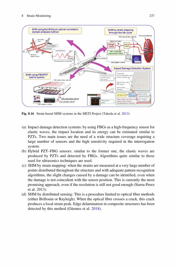
If a crack does not change the strain field at the sensor location, it would not bedetected, and the strain changes are quite small a few millimeters away from thecrack tip, providing difficulties for a global SHM system based on strain monitoring.Figure 8.16 illustrates a few existing approaches:
236 S. Vanlanduit et al.
(a) Impact damage detection systems: by using FBGs as a high-frequency sensor forelastic waves, the impact location and its energy can be estimated similar toPZTs. Two main issues are the need of a wide structure coverage requiring alarge number of sensors and the high sensitivity required in the interrogationsystem.
(b) Hybrid PZT–FBG sensors: similar to the former one, the elastic waves areproduced by PZTs and detected by FBGs. Algorithms quite similar to thoseused for ultrasonics techniques are used.
(c) SHM by strain mapping: when the strains are measured at a very large number ofpoints distributed throughout the structure and with adequate pattern recognitionalgorithms, the slight changes caused by a damage can be identified, even whenthe damage is not coincident with the sensor position. This is currently the mostpromising approach, even if the resolution is still not good enough (Sierra-Perezet al. 2013).
(d) SHM by distributed sensing: This is a procedure limited to optical fiber methods(either Brillouin or Rayleigh). When the optical fiber crosses a crack, this crackproduces a local strain peak. Edge delamination in composite structures has beendetected by this method (Güemes et al. 2018).
Fig. 8.16 Strain-based SHM systems in the METI Project (Takeda et al. 2013)
8 Strain Monitoring 237
References
Alves JA (2003) Fiber Bragg sensor interrogation system based on a CCD spectrometer.Sensors:909–913
Anon. (1984) Strain gage instrumentation installed on the interior of the AFTI/F-16 wing NASA/Dryden Flight Research Center (NASA-DFRC) (p 1/1/1984)
ASTM E1561-93 (2014) Standard practice for analysis of strain gage rosette data. ASTM Interna-tional, West Conshohocken, PA
ASTM E837-13a (2013) Standard test method for determining residual stresses by the hole-drillingstrain-gage method. ASTM International, West Conshohocken, PA
Bahrampour AR (2012) Optical fiber interferometers and theirs application. Interferometry ResAppl Sci Technol. https://doi.org/10.5772/34346
Chiesura G, Lamberti A, Yang Y et al (2016) RTM production monitoring of the A380 hinge armdroop nose mechanism: a multi-sensor approach. Sensors 16. https://doi.org/10.3390/s16060866.
Cranch GA, Nash PJ (2001) Large-scale multiplexing of interferometric fiber-optic sensors usingTDM and DWDM. J Lightwave Technol 19:687–699. https://doi.org/10.1109/50.923482
Dai Y, Liu Y, Leng J et al (2009) A novel time-division multiplexing fiber Bragg grating sensorinterrogator for structural health monitoring. Opt Lasers Eng 47:1028–1033. https://doi.org/10.1016/j.optlaseng.2009.05.012
Dawood TA, Shenoi RA, Sahin M (2007) A procedure to embed fibre Bragg grating strain sensorsinto GFRP sandwich structures. Compos A 38:217–226. https://doi.org/10.1016/j.compositesa.2006.01.028
Di Sante R (2015) Fibre optic sensors for structural health monitoring of aircraft compositestructures: recent advances and applications. Sensors (Switzerland) 15:18666–18713. https://doi.org/10.3390/s150818666
Druet T, Chapuis B, Jules M et al (2018) Passive guided waves measurements using fiber Bragggratings sensors. J Acoust Soc Am 144:1198. https://doi.org/10.1121/1.5054015.
Faisal NH et al (2019) Diametral compression test method to analyse relative surface stresses inthermally sprayed coated and uncoated circular disc specimens. Surface Coatings Technol357:497–514
Froggatt M et al (1998) High-spatial-resolution distributed strain measurement in optical fiber withRayleigh scatter. Appl Opt 37(10):1735–1740
García I, Zubia J, Durana G et al (2015) Optical fiber sensors for aircraft structural healthmonitoring. Sensors (Switzerland) 15:15494–15519. https://doi.org/10.3390/s150715494
Garus D, Krebber K, Schliep F et al (1996) Distributed sensing technique based on Brillouinoptical-fiber frequency-domain analysis. Opt Lett 21(/17):1402–1404. https://doi.org/10.1364/OL.21.001402
Ghoshal A, Ayers J, Gurvich M et al (2015) Experimental investigations in embedded sensing ofcomposite components in aerospace vehicles. Compos Part B Eng 71:52–62. https://doi.org/10.1016/j.compositesb.2014.10.050
Giraldo CM, Sagredo JZ, Gómez JS et al (2017) Demonstration and methodology of structuralmonitoring of stringer runs out composite areas by embedded optical fiber sensors and connec-tors integrated during production in a composite plant. Sensors (Basel, Switzerland) 17. https://doi.org/10.3390/s17071683.
Girard S et al (2018) Recent advances in radiation-hardened fiber-based technologies for spaceapplications. J Opt (United Kingdom) 9:20. https://doi.org/10.1088/2040-8986/aad271
Goossens S, De Pauw B, Geernaert T et al (2019) Aerospace-grade surface mounted optical fibrestrain sensor for structural health monitoring on composite structures evaluated against in-flightconditions. Smart Mater Struct 28. https://doi.org/10.1088/1361-665X/ab1458
Grandal T, Zornoza A, Fraga S et al (2018) Laser cladding-based metallic embedding technique forfiber optic sensors. J Lightwave Technol 36:1018–1025. https://doi.org/10.1109/JLT.2017.2748962.
Green AK, Shafir E (1999) Termination and connection methods for optical fibres embedded inaerospace composite components. Smart Mater Struct 8:269–273. https://doi.org/10.1088/0964-1726/8/2/013
Grzegorz Gruca NR (2019). United States Patent No. US, 10, p 255 B2Güemes A, Fernández-López A, Díaz-Maroto PF et al (2018) Structural health monitoring in
composite structures by fiber-optic sensors. Sensors 18:1094. https://doi.org/10.3390/s18041094
Guo H, Xiao G, Mrad N et al (2011) Fiber optic sensors for structural health monitoring of airplatforms. Sensors 11:3687–3705. https://doi.org/10.3390/s110403687.
Hariharan P (2007) Basics of interferometry, Academic Presse, ISBN: 978-0-12-373589-8, https://doi.org/10.1016/B978-0-12-373589-8.X5000-7.
Havermann D, Mathew J, MacPherson WN et al (2015) Temperature and strain measurements withfiber Bragg gratings embedded in stainless steel 316. J Lightwave Technol 33:2474–2479.https://doi.org/10.1109/JLT.2014.2366835.
He XL, Wang ZQ, Wang DH et al (2019) Optical fiber sensor for strain monitoring of metallicdevice produced by very high-power ultrasonic additive Manufacturing. IEEE Sensors J IEEE19:10680–10685. https://doi.org/10.1109/JSEN.2019.2928966.
Iele A et al (2019) A fiber optic sensors system for load monitoring on aircraft landing Gears. In:Kalli K, Brambilla G, OKeeffe S (eds) Opt Eng (proc SPIE) seventh European workshop onoptical fibre sensors (EWOFS 2019). SPIE-International Society, Bellingham, WA, pp98227–90010. https://doi.org/10.1117/12.2541110.
IPC/JEDEC (2005) Printed wiring board strain gage test guideline JEDEC. IPC/JEDEC-9704James SW, Tatam RP (2003) Optical fibre long-period grating sensors: characteristics and appli-
cation. Meas Sci Technol 14:R49–R61. https://doi.org/10.1088/0957-0233/14/5/201Kersey AD, Davis MA, Patrick HJ et al (1997) Fiber grating sensors. J Lightwave Technol 151442-
1463. https://doi.org/10.1109/50.618377.Kinet D, Mégret P, Goossen KW et al (2014) Fiber Bragg grating sensors toward structural health
monitoring in composite materials: challenges and solutions. Sensors (Switzerland)14:7394–7419. https://doi.org/10.3390/s140407394
Kondrat M et al (2007) A Sagnac-Michelson fibre optic interferometer: signal processing fordisturbance localization. Opto-Electronics Review 15:127–132
Kuang KSC, Kenny R, Whelan MP et al (2001) Embedded fibre Bragg grating sensors in advancedcomposite materials. Compos Sci Technol 61:1379–1387. https://doi.org/10.1016/S0266-3538(01)00037-9.
Lamberti A, Vanlanduit S, De Pauw B et al (2014) A novel fast phase correlation algorithm for peakwavelength detection of fiber Bragg grating sensors. Opt Express 22:7099–7112. https://doi.org/10.1364/OE.22.007099.
Lee B (2003) Review of the present status of optical fiber sensors. Opt Fiber Technol 9:57–79.https://doi.org/10.1016/S1068-5200(02)00527-8
Loutas TH, Charlaftis P, Airoldi A et al (2015) Reliability of strain monitoring of compositestructures via the use of optical fiber ribbon tapes for structural health monitoring purposes.Compos Struct 134:762–771. https://doi.org/10.1016/j.compstruct.2015.08.100
Luyckx G, Voet E, Lammens N et al (2011) Strain measurements of composite laminates withembedded fibre Bragg gratings: criticism and opportunities for research. Sensors 11:384–408.https://doi.org/10.3390/s110100384.
Ma Z, Chen X (2019) Fiber Bragg gratings sensors for aircraft wing shape measurement: recentapplications and technical analysis. Sensors (Switzerland) 19. https://doi.org/10.3390/s19010055
Malik SA, Wang L, Curtis PT et al (2016) Self-sensing composites: in-situ detection of fibrefracture. Sensors (Switzerland) 16:1–18. https://doi.org/10.3390/s16050615
Mario Sorgente AR (2020) Performance comparison between fiber-optic and piezoelectric acousticemission sensors.
Mendoza E et al (2013) In-flight fiber optic acoustic emission sensor (FAESense) system for the realtime detection, localization, and classification of damage in composite aircraft structures.Photon Appl Aerosp Comm Harsh Environ IV 8720:87200K. https://doi.org/10.1117/12.2018155
Missinne J, Luyckx G, Voet E et al (2017) Low-loss connection of embedded optical fiber sensorsusing a self-written waveguide. IEEE Photon Technol Lett 29:1731–1734. https://doi.org/10.1109/LPT.2017.2747630.
Nedjalkov A, Meyer J, Waltermann C et al (2018) Direct inscription and evaluation of fiber Bragggratings in carbon-coated optical sensor glass fibers for harsh environment oil and gas applica-tions. Appl Opt 57:7515–7525. https://doi.org/10.1364/AO.57.007515.
Nicolas MJ, Sullivan RW, Richards WL (2016) Large scale applications using FBG sensors:determination of in-flight loads and shape of a composite aircraft wing. Aerospace 3. https://doi.org/10.3390/aerospace3030018
Park S-JA-K (2011) Interface science and composites. Academic Press, Cambridge, MAPeters K (2011) Polymer optical fiber sensors - a review. Smart Mater Struct 20. https://doi.org/10.
1088/0964-1726/20/1/013002Pinet É (2009) Fabry-Pérot fiber-optic sensors for physical parameters. J Sens 2009:1–9. https://doi.
org/10.1155/2009/720980Rajabzadeh AA (2018) Analysis of FBG reflection spectra under anti-symmetrical strain distribu-
tions using the approximated transfer matrix model Optical sensing and detection V(p. 106800O). International Society for Optics and Photonics, Strasbourg
Rajan G (2016) Structural health monitoring of composite structures using fiber optic methods.CRC Press, Boca Raton
Rijnveld N (2017) Optical fibre interferometry – new concepts and applications. Mikroniek 18–21Saheb N, Mekid S (2015) Fiber-embedded metallic materials: from sensing towards nervous
behavior. Materials 8:7938–7961. https://doi.org/10.3390/ma8115435Sjögren A (2000) Manufacturing technique for embedding detachable fiber-optic connections in
aircraft composite components. Smart Mater Struct 9:855–858. https://doi.org/10.1088/0964-1726/9/6/316
Sjögren BA (2001) Static strength of CFRP laminates with embedded fiber-optic edge connectors.Compos A 32:189–196. https://doi.org/10.1016/S1359-835X(00)00138-X
Sonnenfeld C, Sulejmani S, Geernaert T et al (2011) Microstructured optical fiber sensors embed-ded in a laminate composite for smart material applications. Sensors 11:2566–2579. https://doi.org/10.3390/s110302566.
Takeda NA et al (2013) Outline of the Japanese National Project on Structural Health MonitoringSystem for Aircraft Composite Structures and JASTAC Project. IWSHM2013, Stanford
Takeda NA (2005) Development of smart composite structures with small-diameter fiber Bragggrating sensors for damage detection: quantitative evaluation of delamination length in CFRPlaminates using lamb wave sensing. Compos Sci Technol 2005:2575–2587
Takeuchi K (2012) Locations of strain gauges for fatigue analysis of welded joints (2). Weld Int26:655–664. https://doi.org/10.1080/09507116.2011.590680
Tsai W (2001) A novel structure for the intrinsic Fabry-Perot fiber-optic temperature sensor. JLightw Techol
Ushakov NA (2015) Utilization of NI PXIe-4844 interrogator for high resolution fiber extrinsicFabry-Perot interferometric sensing. In: 2015 International Siberian conference on control andcommunications (SIBCON). IEEE, pp 1–4
Wada D, Igawa H, Tamayama M et al (2019) Flight demonstration of aircraft wing monitoringusing optical fiber distributed sensing system. Smart Mater Struct 28. https://doi.org/10.1088/1361-665X/aae411
Wang Y, Gong J, Dong B et al (2012) A large serial time-division multiplexed Fiber Bragg gratingsensor network. J Lightwave Technol IEEE 30:2751–2756. https://doi.org/10.1109/JLT.2012.2205897.
Wei US (2013) Fiber optic interferometric devices. Springer Science, ChamXu MG, Alavie AT, Maaskant R et al (1996) Tunable fibre bandpass filter based on a linearly
chirped fibre Bragg grating for wavelength demultiplexing. Electron Lett 32:1918–1919. https://doi.org/10.1049/el:19961242
Yu F, Okabe Y (2017) Fiber-optic sensor-based remote acoustic emission measurement in a 1000�C environment. Sensors (Switzerland) 17. https://doi.org/10.3390/s17122908
Zahid MN et al (2019) Reflectometric and interferometric fiber optic sensor’s principles andapplications. Springer, Cham
Zetie KP, Adams SF, Tocknell RM (2000) How does a Mach-Zehnder interferometer work?Westminster School Phys Educ 35:46–48. https://doi.org/10.1088/0031-9120/35/1/308
Zhou G, Sim LM (2002) Damage detection and assessment in fibre-reinforced composite structureswith embedded fibre optic sensors-review. Smart Mater Struct 11:925–939. https://doi.org/10.1088/0964-1726/11/6/314
Open Access This chapter is distributed under the terms of the Creative Commons Attribution 4.0International License (http://creativecommons.org/licenses/by/4.0/), which permits use, duplica-tion, adaptation, distribution and reproduction in any medium or format, as long as you giveappropriate credit to the original author(s) and the source, a link is provided to the CreativeCommons license and any changes made are indicated.
The images or other third party material in this chapter are included in the work’s CreativeCommons license, unless indicated otherwise in the credit line; if such material is not included inthe work’s Creative Commons license and the respective action is not permitted by statutoryregulation, users will need to obtain permission from the license holder to duplicate, adapt orreproduce the material.