260
| Date post: | 08-Feb-2023 |
| Category: |
Documents |
| Upload: | khangminh22 |
| View: | 0 times |
| Download: | 0 times |


TESIS DOCTORAL
Universidad de GranadaPrograma de Doctorado en Ciencias de La Tierra
Novel technique to detect seismicsignals and its application to map
upper-mantle discontinuitiesbeneath Iberia
Anahı Luciana Bonatto
Granada 2013

TESIS DOCTORAL
Novel technique to detect seismicsignals and its application to map
upper-mantle discontinuitiesbeneath Iberia
REALIZADA POR:
Anahı Luciana Bonatto
DIRECTORES DE LA TESIS:Dr. Martin Schimmel
Dr. Jose Morales
Instituto de Ciencias de La Tierra ”Jaume Almera”-CSICInstituto Andaluz de Geofısica -UGR

Compromiso de respeto derechos de autor
La doctorando Anahı Luciana Bonatto y los directores de la tesis ”Novel
techniques to detect seismic signals and its application to map the tran-
sition zone discontinuities beneath Iberia”, garantizamos, al firmar esta
tesis doctoral, que el trabajo ha sido realizado por el doctorando bajo la
direccion de los directores de la tesis y hasta donde nuestro conocimiento
alcanza, en la realizacion del trabajo, se han respetado los derechos de
otros autores a ser citados, cuando se han utilizado sus resultados o pub-
licaciones.
Granada 15 de Septeimbre de 2013
Directores de la Tesis Doctorando
Fdo.: Dr. Martin Schimmel Fdo.: Anahı Luciana Bonatto
Dr. Jose Morales


Esta tesis esta dedicada a
Ricardo
por su apoyo incondicional

Agradecimientos
El Instituto de Ciencias de la Tierra ”Jaume Almera” -IJA- (CSIC) me
ha concedido una beca Jae-Predoc del CSIC para realizar el doctorado en
Espana. A quienes corresponda, quisiera agradecer la oportunidad que se
me ha brindado.
La realizacion de esta tesis no habrıa sido posible sin los datos pro-
porcionados por los siguientes proyectos: TopoIberia, TopoMed, Rifsis,
CGL2012-31472, P09RNM5100. Detras de estos proyectos estan los gru-
pos y personas que se encargan de la instalacion de las estaciones y de la
adquisicion de los datos. A todos ellos quiero agradecerles especialmente,
ya que realizan una ardua tarea para poner los datos a disposicion de
los investigadores. Tambien quiero agradecer al proyecto WILLAS por
compartir su base de datos, de los cuales algunos han sido utilizados en
este estudio.
A mis directores de tesis, Martin y Pepe, quiero agradecer su apoyo y el
haber confiado en mi para realizar este trabajo de investigacion. A Pepe,
quiero agradecerle especialmente por haberme acogido en el Instituto An-
daluz de Geofısica -IAG- y por poner todos sus recursos a mi disposicion.
A Martin por guiarme, por proporcionarme animo y confianza cuando el
trabajo se tornaba mas complejo y por aconsejarme tantas veces sobre
como lidiar con la polıtica cientıfica.
Quisiera agradecer tambien a la Dra. Eleonore Stutzmann por haberme
dado la oportunidad de hacer una estancia de investigacion en el Institut
de Physique du Globe de Paris y por ensenarme a trabajar con las ”fun-
ciones receptoras”. A Antonio Villasenor por haberme proporcionado su
modelo de tomografıa de onda P, que ha sido un aporte imortante para la
interpretacion de los resultados de esta tesis. A la Prof. Adriana Caldiz
le agradezco especialmente por haber corregido la escritura de la tesis.
A mis companeros del IJA y del IAG quiero agradecerles la predisposicion
para darme una mano siempre que fue necesario. A Janire por responder
todas mis preguntas, incluso hasta unos dıas antes de su defensa. A Luisa
por hacerme un lugar en su casa cuando lo necesite.
A Pocho y Adriana quisiera agradecerles y dedicarles parte de todo este
esfuerzo porque los he visto sufrir y reir conmigo desde que tengo uso de
razon y porque fueron los primeros en creer en mi. A Santi porque me
alegra el dıa con sus ocurrencias y a veces me desestructura y otras me
hace enojar. A Ricardo por ser mi companero de aventuras y por ser un
amigo incondicional.
TESIS DOCTORAL
Novel technique to detect seismicsignals and its application to map
upper-mantle discontinuitiesbeneath Iberia
PALABRAS CLAVES: Estructura interior de la Tierra,discontinuidades del manto superior, zona de transicion, deteccion de
senales sısmicas, region Ibero-Maghrebı, IberArray, TopoIberia.

Resumen
En este estudio analizamos las discontinuidades de la zona de transicion
del manto superior a 410 km y 660 km de profundidad a partir de la
deteccion de ondas sısmicas convertidas de P -a-s debajo de la region
Ibero-Magrebı. Para este proposito, usamos eventos telesismicos registra-
dos en 259 estaciones de banda ancha desplegadas mayormente por el
proyecto TopoIberia. El analisis detallado de las discontinuidades de la
zona de transicion proporciona informacion acerca de la temperatura y
composicion del manto superior a las profundidades estudiadas. Este es-
tudio anade nuevas restricciones para la mejor comprension de la compleja
y controversial region Ibero-Maghrebı.
Las ondas convertidas en las discontinuidades del manto superior llegan en
la coda de la onda P junto con otras senales y usualmente son identificadas
en los stacks de funciones receptoras. Aquı, construimos una tecnica nueva
de procesamiento, que se apoya en las funciones receptoras y que se basa
en tecnicas de correlacion cruzada y de stacking para detectar y extraer
senales de manera eficiente a partir de su coherencia, lentitud, tiempo de
viaje y polaridad. A fin de anadir consistencia y robustez a las detec-
ciones, nuestros resultados finales se basan en el analisis conjunto de las
funciones receptoras y dos funcionales diferentes de correlacion cruzada.
Esto permite evaluar errores y rellenar gaps en las observaciones cuando
alguna de las tecnicas falla inherente a las caracterısticas de la senal y
el ruido. Finalmente, la profundidad de las discontinuidades se deter-
mina utilizando correcciones de tiempo obtenidas a partir de un modelo
de velocidades 3D. Ası, presentamos mapas topograficos de las discon-
tinuidades 410-km y 660-km, que muestran variaciones en el espesor de
la zona de transicion debajo del area de estudio.
El espesor de la zona de transicion debajo de Iberia central (240-250 km)
esta dentro del promedio global; la zona de transicion es mas ancha de-
bajo del oeste de Marruecos (250-275 km), el Mar de Alboran (280-300
km) y el este de Espana (260-280); y es predominantemente fina debajo
del sur de Portugal (220-240 km), el Golfo de Cadiz (220-250 km) y el
area del Estrecho de Gibraltar (214 km). La zona de transicion mas ancha
debajo del oeste de Marruecos y el este de Espana es mayormente debido
a que la discontinuidad 660-km se encuentra a una profundidad mayor
que el promedio global, mientras que la topografıa de la discontinuidad
410-km es mas suave. Aunque, debajo del este de Espana, se aprecia una
leve depresion de la 410. Por otro lado, la profundidad de las discon-
tinuidades esta anti-correlacionada debajo del Mar de Alboran. Ademas,
encontramos una correlacion espacial entre el vulcanismo anorogenico
Neogeno y la topografıa de la 410. Todos estos resultados se discuten
con el fin de anadir nuevas restricciones a la temperatura y composicion
de las anomalıas de velocidad ssmica observadas en la zona de transicion
debajo de la controversial region Ibero-Magrebı. El ensanchamiento de
la zona de transicion del orden de 50 km -respecto al valor de referencia-
debajo del Mar de Alboran sugiere que la loza de Alboran aun esta lo su-
ficientemente frıa como para elevar la transformacion de fase α−β y para
deprimir la post-spinel. De forma similar, creemos que la loza del Tethys
debajo de Espana -estancada en la base de la zona de transicion- aun
estarıa frıa y serıa responsable de la depresion de la 660, mientras que un
proceso de conveccion de pequena escala encima de la 660 -activada por
deshidratacion de la loza- explicarıa la depresion de la 410. Por otro lado,
la zona de transicion mas ancha debajo de Marruecos es probablemente
de origen composicional. La explicacion preferida es que la depresion
de la 660 se debe a la transicion granate-a-perovskita sumado a un alto
contenido de aluminio en el granate. La zona de transicion mas angosta
debajo del Golfo de Cadiz, el Estrecho de Gibraltar y el sur de Portugal es
mayormente debido a una 410 mas profunda y pensamos que podrıa estar
causada por un manto superior de elevada temperatura, que tambien ha
sido inferido en imagenes tomograficas recientemente publicadas.
Adicionalmente, determinamos el espesor de las discontinuidades 410-km
y 660-km e investigamos su variacion espacial. Este analisis, muestra que
ambas discontinuidades presentan variaciones espaciales en su espesor.
En particular, la 660 es mas ancha debajo del Mar de Alboran y el sur de
Espana. Interpretamos la variacion espacial en el espesor de la 410 como
causada por variaciones en la concentracion de agua dentro de la zona de
transicion debajo del area de estudio. Creemos que la 660 mas ancha, de
aproximadamente 30 km, debajo del Mar de Alboran y del sur de Espana
es causada por la combinacion de gradientes de velocidades debido a las
transformaciones de fase post-spinel e ilmenita-a-perovskita.

.
Abstract
In this study, we analyze the upper-mantle transition zone discontinuities
at a depth of 410 km and 660 km as seen from seismic P -to-s wave con-
versions beneath the Ibero-Maghrebian region. For this purpose, we use
teleseismic events recorded at 259 broadband seismic stations deployed
mainly by the TopoIberia project. The detailed analysis of the transition-
zone discontinuities provides information on the temperature and compo-
sition of the upper mantle at the investigated depths. This study adds
new constraints, which would help to improve the understanding of the
complex and controversial Ibero-Maghrebian region.
The converted waves from the upper-mantle discontinuities arrive in the
P-wave coda together with other signals and are usually identified on
stacked receiver functions. Here, a new processing approach is built, which
is leaned on receiver functions and which is based on cross-correlation and
stacking techniques, to efficiently detect and extract signals by means of
their coherence, slowness, travel time and polarity. In order to add con-
sistency and robustness to the detections, our final results are based on a
joint analysis of the receiver functions and two different cross-correlation
functionals. This permits to assess errors and to bridge observation gaps
due to detection failure of any of the techniques inherent to signal and
noise characteristics. Finally, discontinuity depths are determined using
time corrections obtained from a 3D velocity model. We present topog-
raphy maps for the 410-km and 660-km discontinuities, which show vari-
ations in the transition zone thickness beneath the study area.
The transition zone thickness is about global average beneath central
Iberia (240-250 km); it is thicker beneath west Morocco (250-275 km),
the Alboran Sea (280-300 km) and east Spain (260-280); and it is pre-
dominantly thinner beneath south Portugal (220-240 km), the Strait of
Gibraltar area (214 km) and the Gulf of Cadiz (220-250 km). The thicker
transition zone beneath west Morocco and east Spain is mainly due to a
deeper 660-km discontinuity, while the topography of the 410-km discon-
tinuity is smaller. Although, beneath east Spain, the 410 is slightly de-
pressed. On the other hand, the discontinuities’ depths are anti-correlated
beneath the Alboran Sea. Additionally, we find a spatial correlation be-
tween the Neogene anorogenic volcanism and the topography of the 410-
km discontinuity. These results are discussed to add new constraints on
temperature and composition to seismic velocity anomalies observed in
the transition zone beneath the controversial Ibero-Magrhrebian region.
The transition zone thickening of about 50 km -from the reference value-
beneath the Alboran Sea suggests that the Betic-Alboran slab is still suf-
ficiently cold to elevate the α−β mineral phase transition and to depress
the post-spinel one. Similarly, the cold Tethys slab -stagnant at the base
of the transition zone- beneath east Spain is thought to be responsible for
the 660 depression, while small-scale convection above the 660 -triggered
by slab dehydration- may explain the 410 depression. On the other hand,
the thicker transition zone beneath Morocco is probably of compositional
origin. Our preferred explanation is that the 660 depression is due to
the garnet-to-perovskite transition and a high aluminum content within
garnet. The thinner transition zone beneath the Gulf of Cadiz, the Strait
of Gibraltar and the south of Portugal is mainly due to a depressed 410
and is thought to be caused by high upper-mantle temperature, which is
also inferred by recently published tomographic images.
Furthermore, we determine the widths of the 410-km and 660-km dis-
continuities and we investigate their spatial variations. This analysis has
revealed that both discontinuities present spatial thickness variations. In
particular, the 660 is thicker beneath the Alboran Sea and south Spain.
We interpret the spatial variation of the 410 width as caused by varia-
tions in the water concentration in the transition zone beneath the study
area. The thicker 660, of about 30 km, beneath the Alboran Sea and
south Spain is thought to be caused by combined velocity gradients due
to post-spinel and ilmenite-to-perovskite phase transitions.
Contents
1 General introduction 2
1.1 Motivation and organization of the thesis . . . . . . . . . . . . . . . . 4
1.2 Upper mantle . . . . . . . . . . . . . . . . . . . . . . . . . . . . . . . 8
1.2.1 Upper mantle composition . . . . . . . . . . . . . . . . . . . . 10
1.2.2 Olivine-related TZ discontinuities . . . . . . . . . . . . . . . . 12
1.2.3 Using the 410 and 660 depths to infer changes in TZ temperatures 13
1.3 Research methods . . . . . . . . . . . . . . . . . . . . . . . . . . . . . 15
1.3.1 Seismic phases . . . . . . . . . . . . . . . . . . . . . . . . . . 16
1.3.2 Spatial resolution . . . . . . . . . . . . . . . . . . . . . . . . . 16
1.3.3 Detection of P -to-s converted phases in the seismic records . . 17
1.4 The western Mediterranean and the Ibero-
Maghrebian region . . . . . . . . . . . . . . . . . . . . . . . . . . . . 19
1.4.1 Deep earthquakes beneath Granada . . . . . . . . . . . . . . . 21
1.4.2 Tomographic images of the upper mantle . . . . . . . . . . . . 22
1.4.3 A controversial geodynamic scenario in the Alboran Sea area . 24
1.4.4 Anorogenic magmatism . . . . . . . . . . . . . . . . . . . . . . 26
1.4.5 Seismic discontinuity studies . . . . . . . . . . . . . . . . . . . 28
1.5 TopoIberia data set . . . . . . . . . . . . . . . . . . . . . . . . . . . . 29
2 Methodology: detection of P -coda phases 32
2.1 Introduction . . . . . . . . . . . . . . . . . . . . . . . . . . . . . . . . 34
2.2 Method . . . . . . . . . . . . . . . . . . . . . . . . . . . . . . . . . . 34
2.2.1 Theoretical background . . . . . . . . . . . . . . . . . . . . . . 34
2.2.2 Detection of P-coda phases using cross-correlation . . . . . . . 36
2.3 Synthetic analysis . . . . . . . . . . . . . . . . . . . . . . . . . . . . . 43
i
2.3.1 Generating synthetic data . . . . . . . . . . . . . . . . . . . . 46
2.3.2 Pilot length . . . . . . . . . . . . . . . . . . . . . . . . . . . . 47
2.3.3 Noise influence . . . . . . . . . . . . . . . . . . . . . . . . . . 50
2.3.4 Robustness analysis . . . . . . . . . . . . . . . . . . . . . . . . 53
2.4 Real data examples . . . . . . . . . . . . . . . . . . . . . . . . . . . . 55
2.4.1 Processing . . . . . . . . . . . . . . . . . . . . . . . . . . . . . 57
2.4.2 Detection of P -to-s conversions at individual stations . . . . . 57
2.5 Discussion and conclusions . . . . . . . . . . . . . . . . . . . . . . . . 64
3 Data set 68
3.1 Introduction . . . . . . . . . . . . . . . . . . . . . . . . . . . . . . . . 70
3.2 Data selection . . . . . . . . . . . . . . . . . . . . . . . . . . . . . . . 71
3.3 Processing and final data set . . . . . . . . . . . . . . . . . . . . . . . 72
3.4 Building of correlograms and receiver functions . . . . . . . . . . . . 75
3.5 Data consistency . . . . . . . . . . . . . . . . . . . . . . . . . . . . . 76
3.5.1 Frequency . . . . . . . . . . . . . . . . . . . . . . . . . . . . . 77
3.5.2 Pilot length . . . . . . . . . . . . . . . . . . . . . . . . . . . . 79
3.6 Discussion and conclusions . . . . . . . . . . . . . . . . . . . . . . . . 79
4 Transition zone discontinuities beneath Iberia and Morocco 84
4.1 Introduction . . . . . . . . . . . . . . . . . . . . . . . . . . . . . . . . 86
4.2 Data and method . . . . . . . . . . . . . . . . . . . . . . . . . . . . . 86
4.2.1 Stacking of correlograms and receiver functions . . . . . . . . 87
4.2.2 Robustness analysis and quality criteria . . . . . . . . . . . . . 88
4.2.3 Integrated detections and depth conversions . . . . . . . . . . 92
4.3 Results . . . . . . . . . . . . . . . . . . . . . . . . . . . . . . . . . . . 97
4.3.1 410 and 660 discontinuities . . . . . . . . . . . . . . . . . . . . 97
4.3.2 Time corrections and the 410 and 660 absolute depths . . . . 105
4.3.3 TZ thickness . . . . . . . . . . . . . . . . . . . . . . . . . . . 105
4.3.4 Additional features in the receiver functions . . . . . . . . . . 110
4.4 Discussion . . . . . . . . . . . . . . . . . . . . . . . . . . . . . . . . . 115
4.4.1 Relation with previous works . . . . . . . . . . . . . . . . . . 115
4.4.2 Interpretation of results . . . . . . . . . . . . . . . . . . . . . 116
4.5 Summary and conclusions . . . . . . . . . . . . . . . . . . . . . . . . 130
ii
5 Discontinuity characterization 134
5.1 Introduction . . . . . . . . . . . . . . . . . . . . . . . . . . . . . . . . 136
5.2 Relative amplitudes . . . . . . . . . . . . . . . . . . . . . . . . . . . . 137
5.2.1 Processing . . . . . . . . . . . . . . . . . . . . . . . . . . . . . 137
5.2.2 Results . . . . . . . . . . . . . . . . . . . . . . . . . . . . . . . 137
5.2.3 Discussion . . . . . . . . . . . . . . . . . . . . . . . . . . . . . 139
5.3 Width of the 410 and 660 discontinuities . . . . . . . . . . . . . . . . 141
5.3.1 Methodology and processing . . . . . . . . . . . . . . . . . . . 142
5.3.2 Results . . . . . . . . . . . . . . . . . . . . . . . . . . . . . . . 151
5.3.3 Discussion . . . . . . . . . . . . . . . . . . . . . . . . . . . . . 151
5.4 Conclusions . . . . . . . . . . . . . . . . . . . . . . . . . . . . . . . . 157
Appendix A Receiver functions 159
A.1 Transmission path impulse response . . . . . . . . . . . . . . . . . . . 161
A.2 Water-level deconvolution receiver functions . . . . . . . . . . . . . . 163
Appendix B The presence of other transforming and non-transforming
phases and their geophysical implications 165
B.1 Garnet-related discontinuities near 660 km depth . . . . . . . . . . . 167
B.2 410 and 660 complexities . . . . . . . . . . . . . . . . . . . . . . . . . 168
B.3 Influence in the TZ thickness . . . . . . . . . . . . . . . . . . . . . . 170
B.4 510-km discontinuity . . . . . . . . . . . . . . . . . . . . . . . . . . . 170
Appendix C Supplementary figures for Chapter 2 173
Appendix D TopoIberia stations 191
Appendix E Supplementary figures for Chapter 4 201
References 221
iii

1General introduction
2

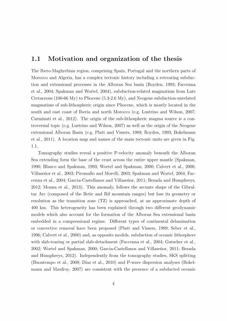
1.1 Motivation and organization of the thesis
The Ibero-Maghrebian region, comprising Spain, Portugal and the northern parts of
Morocco and Algeria, has a complex tectonic history including a retreating subduc-
tion and extensional processes in the Alboran Sea basin (Royden, 1993; Faccenna
et al., 2004; Spakman and Wortel, 2004), subduction-related magmatism from Late
Cretaceous (100-66 My) to Pliocene (5.3-2.6 My), and Neogene subduction-unrelated
magmatism of sub-lithospheric origin since Pliocene, which is mostly located in the
south and east coast of Iberia and north Morocco (e.g. Lustrino and Wilson, 2007;
Carminati et al., 2012). The origin of the sub-lithospheric magma source is a con-
troversial topic (e.g. Lustrino and Wilson, 2007) as well as the origin of the Neogene
extensional Alboran Basin (e.g. Platt and Vissers, 1989; Royden, 1993; Bokelmann
et al., 2011). A location map and names of the main tectonic units are given in Fig.
1.1.
Tomography studies reveal a positive P-velocity anomaly beneath the Alboran
Sea extending form the base of the crust across the entire upper mantle (Spakman,
1990; Blanco and Spakman, 1993; Wortel and Spakman, 2000; Calvert et al., 2000;
Villasenor et al., 2003; Piromallo and Morelli, 2003; Spakman and Wortel, 2004; Fac-
cenna et al., 2004; Garcia-Castellanos and Villasenor, 2011; Bezada and Humphreys,
2012; Monna et al., 2013). This anomaly, follows the arcuate shape of the Gibral-
tar Arc (composed of the Betic and Rif mountain ranges) but lose its geometry or
resolution as the transition zone (TZ) is approached, at an approximate depth of
400 km. This heterogeneity has been explained through two different geodynamic
models which also account for the formation of the Alboran Sea extensional basin
embedded in a compressional regime. Different types of continental delamination
or convective removal have been proposed (Platt and Vissers, 1989; Seber et al.,
1996; Calvert et al., 2000) and, as opposite models, subduction of oceanic lithosphere
with slab-tearing or partial slab-detachment (Faccenna et al., 2004; Gutscher et al.,
2002; Wortel and Spakman, 2000; Garcia-Castellanos and Villasenor, 2011; Bezada
and Humphreys, 2012). Independently from the tomography studies, SKS splitting
(Buontempo et al., 2008; Dıaz et al., 2010) and P-wave dispersion analyses (Bokel-
mann and Maufroy, 2007) are consistent with the presence of a subducted oceanic
4
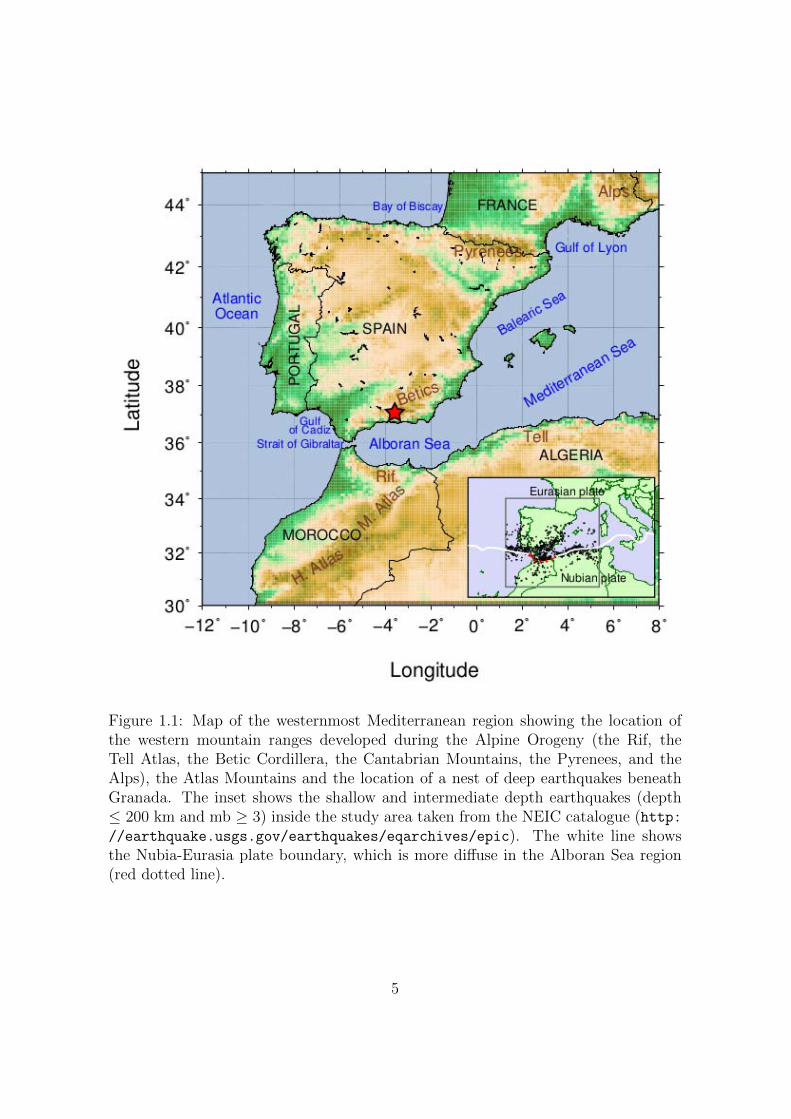
Figure 1.1: Map of the westernmost Mediterranean region showing the location ofthe western mountain ranges developed during the Alpine Orogeny (the Rif, theTell Atlas, the Betic Cordillera, the Cantabrian Mountains, the Pyrenees, and theAlps), the Atlas Mountains and the location of a nest of deep earthquakes beneathGranada. The inset shows the shallow and intermediate depth earthquakes (depth≤ 200 km and mb ≥ 3) inside the study area taken from the NEIC catalogue (http://earthquake.usgs.gov/earthquakes/eqarchives/epic). The white line showsthe Nubia-Eurasia plate boundary, which is more diffuse in the Alboran Sea region(red dotted line).
5
lithosphere (Bokelmann et al., 2011). Nevertheless, there is still room for the different
interpretations. Additionally, recent tomographic images have revealed a negative P-
velocity anomaly beneath the Gulf of Cadiz and south Portugal (Monna et al., 2013).
This anomaly extends to the base of the model reaching the upper-mantle transition
zone. The authors suggest that this negative anomaly might be related to hot mantle
temperatures and to the origin of the sub-lithospheric magma source responsible for
the anorogenic magmatism in the Mediterranean.
Indirect evidences on upper-mantle temperature, composition, position and verti-
cal extension of the heterogeneities revealed in tomographic images are needed. These
additional constrains would help the interpretation of the velocity anomalies and can
be achieved using seismic analysis. The study of the 410-km and 660-km disconti-
nuities (or TZ discontinuities) is probably one of the best approaches, since these
discontinuities are globally observed mineral phase transitions which, as function of
composition, respond with depth and thickness variations to temperature anomalies
(e.g., Helffrich, 2000). The discontinuities are not resolved with seismic tomography
and their study requires the detection and identification of seismic body waves which
directly interact with the discontinuity through a reflection and/or wave type conver-
sion (from P to S, or S to P). Reflection/conversion coefficients are typically smaller
than 5 % and the corresponding small-amplitude signals are concealed in a multitude
of other scattered waves. This makes it difficult to identify the signals on individual
records.
Upper mantle discontinuities are most commonly studied using the receiver func-
tion technique (RF) (Phinney, 1964; Vinnik, 1977; Langston, 1979; Ammon, 1991)
which enhances the P -to-s conversions and P-wave reflections from discontinuities be-
low the recording stations. In Chapter 2 we build a new processing approach which
is leaned on RFs and which is based on cross-correlation and stacking techniques;
part of this chapter has been published as a research article in the Geophysical Jour-
nal International (Bonatto et al., 2013). The instantaneous phase coherence obtained
from analytic signals forms the backbone of one of the cross-correlation approaches
and stacking used. We focus on P -to-s conversions whose detection and extraction
are based on their coherence, slowness, travel time and polarity; such conversions are
used to map the 410-km and 660-km discontinuities. In order to add consistency and
robustness to the detections, our final results are based on a joint analysis of two
different cross-correlation functionals and RFs. In addition, this approach permits to
6
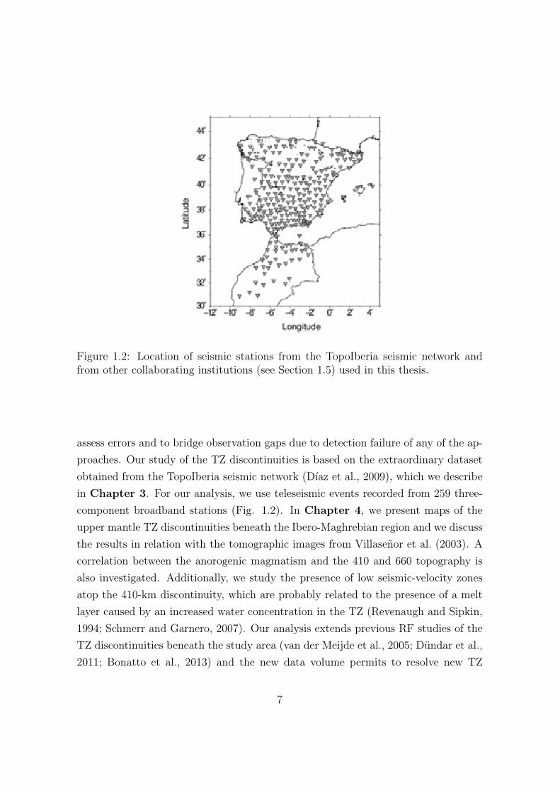
Figure 1.2: Location of seismic stations from the TopoIberia seismic network andfrom other collaborating institutions (see Section 1.5) used in this thesis.
assess errors and to bridge observation gaps due to detection failure of any of the ap-
proaches. Our study of the TZ discontinuities is based on the extraordinary dataset
obtained from the TopoIberia seismic network (Dıaz et al., 2009), which we describe
in Chapter 3. For our analysis, we use teleseismic events recorded from 259 three-
component broadband stations (Fig. 1.2). In Chapter 4, we present maps of the
upper mantle TZ discontinuities beneath the Ibero-Maghrebian region and we discuss
the results in relation with the tomographic images from Villasenor et al. (2003). A
correlation between the anorogenic magmatism and the 410 and 660 topography is
also investigated. Additionally, we study the presence of low seismic-velocity zones
atop the 410-km discontinuity, which are probably related to the presence of a melt
layer caused by an increased water concentration in the TZ (Revenaugh and Sipkin,
1994; Schmerr and Garnero, 2007). Our analysis extends previous RF studies of the
TZ discontinuities beneath the study area (van der Meijde et al., 2005; Dundar et al.,
2011; Bonatto et al., 2013) and the new data volume permits to resolve new TZ
7
topography. It is worth mentioning that the results for the Alboran Sea region and
north Morocco have been published in the Geophysical Journal International (Bon-
atto et al., 2013). The analysis for the entire Ibero-Maghrebian region is at present
part of a paper in preparation. Finally, in Chapter 5, we determine the thickness of
the 410-km and 660-km discontinuities, which provide additional information to con-
straint the mantle temperature and composition. In particular, the 410 thickness is a
very sensitive probe of mantle conditions (Katsura and Ito, 1989; Wood, 1995; Smyth
and Frost, 2002). Our results provide additional and independent constraints to aid
and strengthen the interpretation of the seismic velocity anomalies, which has direct
implications for the understanding of the geodynamic state of the western Mediter-
ranean. In what follows, we introduce different key concepts which are significant for
a better understanding of this thesis.
1.2 Upper mantle
The Earth’s upper mantle extends from the base of the crust (or Moho discontinuity)
to a depth of about 700 km (Fig. 1.3). Based upon results from seismological
research, the Earth’s upper-mantle is divided into different sections. These sections
are separated by seismic discontinuities that correspond to abrupt changes in the
seismic velocity and/or velocity gradient and/or material density (see Fig. 1.3). The
upper-mantle sections are:
• The lithosphere (or LID): the outer solid part of the Earth, including the crust
and uppermost mantle. It is a region of high seismic velocity and its thickness
varies from 50-100 km beneath oceans to 150-250 km beneath the older conti-
nental shields. The discontinuity which defines the lower limit of this layer is
known as the LAB (lithosphere-asthenosphere boundary), which corresponds
to a seismic velocity decrease with increasing depth.
• The asthenosphere (or LVZ): a weak region underlying the relatively strong
lithosphere. It is a region of diminished velocity or negative velocity gradient
proposed by Beno Gutenberg in 1959. This layer is bounded by the LAB and
by a seismic discontinuity at a depth of about 220 km -the Lehmann discon-
tinuity (Lehmann, 1959, 1961a)- which corresponds to a velocity increase with
increasing depth. The LID and the LVZ are essential to plate tectonic theory.
8
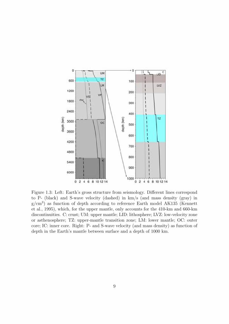
Figure 1.3: Left: Earth’s gross structure from seismology. Different lines correspondto P- (black) and S-wave velocity (dashed) in km/s (and mass density (gray) ing/cm3) as function of depth according to reference Earth model AK135 (Kennettet al., 1995), which, for the upper mantle, only accounts for the 410-km and 660-kmdiscontinuities. C: crust; UM: upper mantle; LID: lithosphere; LVZ: low-velocity zoneor asthenosphere; TZ: upper-mantle transition zone; LM: lower mantle; OC: outercore; IC: inner core. Right: P- and S-wave velocity (and mass density) as function ofdepth in the Earth’s mantle between surface and a depth of 1000 km.
9
• The region between 220 km and 410 km: limited by the Lehmann discontinuity
and the seismic discontinuity at a depth of 410 km. It is a region where the
seismic velocity gradually increases as the 410-km discontinuity is approached.
• The transition zone: a region of high seismic wave-speed gradient. It is bounded
by two seismic discontinuities at a depth of 410 km and 660 km, which corre-
spond to increases in seismic wave speed with increasing depth. This region
play an important role in the convection models of the mantle (e.g., Bercovici
and Karato, 2003). Inside this region, at an approximate depth of 510 km,
there is another seismic discontinuity, which corresponds to a velocity increase
with depth and is thought to be a regional feature.
For further details on the upper-mantle structure see Anderson (2007) [pp. 91-108]
and references therein.
The seismic discontinuities in the Earth reflect mineralogical phase transforma-
tions, changes in the chemical composition of the material, or changes in other elastic
properties of waves. Although these changes are generally referred to as discontinu-
ities, they represent regions where the physical and/or chemical properties change
very rapidly over a finite depth interval.
This thesis focuses on the discontinuities of the upper-mantle TZ. Throughout
this thesis, and whenever not specified we will use TZ to refer to the upper-mantle
transition zone which is bounded by the 410-km and 660-km discontinuities.
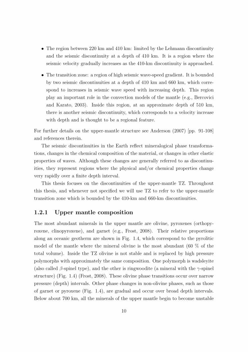
1.2.1 Upper mantle composition
The most abundant minerals in the upper mantle are olivine, pyroxenes (orthopy-
roxene, clinopyroxene), and garnet (e.g., Frost, 2008). Their relative proportions
along an oceanic geotherm are shown in Fig. 1.4, which correspond to the pyrolitic
model of the mantle where the mineral olivine is the most abundant (60 % of the
total volume). Inside the TZ olivine is not stable and is replaced by high pressure
polymorphs with approximately the same composition. One polymorph is wadsleyite
(also called β-spinel type), and the other is ringwoodite (a mineral with the γ-spinel
structure) (Fig. 1.4) (Frost, 2008). These olivine phase transitions occur over narrow
pressure (depth) intervals. Other phase changes in non-olivine phases, such as those
of garnet or pyroxene (Fig. 1.4), are gradual and occur over broad depth intervals.
Below about 700 km, all the minerals of the upper mantle begin to become unstable
10
Figure 1.4: Mineral volume fractions for the top 1000 km of a pyrolitic mantle com-position and mineral phase changes of the different mantle components (from Frost(2008)).
11
and the most abundant mineral is the silicate-perovskite that constitutes 93% of the
lower mantle (Murakami et al., 2004, 2007).
The changes in mineralogy inside the TZ yield different seismic discontinuities
that print distinctive signatures in seismic records and are detected using seismic
wave processing tools. The study of these discontinuities, their global or regional
distribution, their topography and sharpness sets boundary conditions for mantle
dynamics and petrology. Therefore, the existence of dense seismic networks such
as the TopoIberia seismic network is essential to produce more realistic and more
detailed images of the Earth’s interior.
1.2.2 Olivine-related TZ discontinuities
The seismic discontinuities in the TZ at a depth of 410 km, 510 km and 660 km are
related to mineral phase changes in the olivine((Mg,Fe)2SiO4)-system (Fig. 1.4)
(see reviews in Shearer, 2000; Helffrich, 2000).
The 410-km and 660-km discontinuities (hereafter referred to as 410 and 660,
respectively) limit the TZ. Their names came from the depths at which they are found
globally in seismology studies (e.g., Shearer, 1991, 1993; Gu and Dziewonski, 1998;
Lawrence and Shearer, 2006). In an upper mantle of pyrolitic composition, the 410 is
the result of the olivine-to-wadsleyite (or α → β) transition (at about 13-14 GPa in
Fig. 1.4) (e.g., Ringwood, 1975), while the 660 is the dissociation of ringwoodite into
perovskite+magnesiowustite (rw → pv+mw or post-spinel transition) (at about 23-
24 GPa in Fig. 1.4) (e.g., Ringwood, 1975; Ito and Takahashi, 1998). The left panel
of Fig. 1.5 illustrates these phase relations in the (Mg,Fe)2SiO4 (olivine) system
at a constant temperature of 1600◦C. The green line marks the typical Mg − Fe
proportion. Note that the phase transitions show a region of a certain width where
product and reactant coexist (e.g., dotted region in the α-β phase). Inside this
interval the mineral phase transformations progress through a zone of transitional
seismic properties interpolating those above and below the phase change (Bina and
Wood, 1987). Several seismological studies have shown that the 410 and the 660
are sharp, with a prevailing velocity increase occurring over a depth range of 10 km
or less (e.g., Paulssen, 1988; Benz and Vidale, 1993; Vidale et al., 1995; Collier and
Helffrich, 1997; Landes et al., 2006).
12
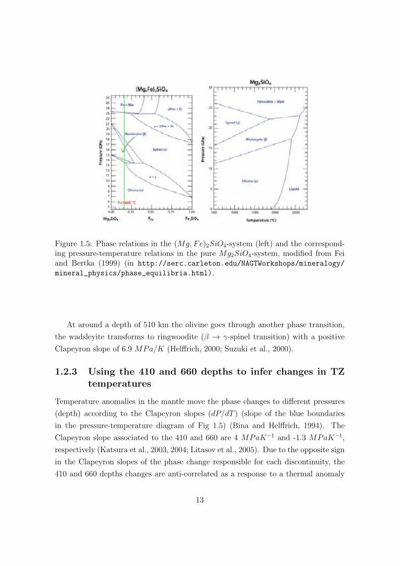
Figure 1.5: Phase relations in the (Mg,Fe)2SiO4-system (left) and the correspond-ing pressure-temperature relations in the pure Mg2SiO4-system, modified from Feiand Bertka (1999) (in http://serc.carleton.edu/NAGTWorkshops/mineralogy/
mineral_physics/phase_equilibria.html).
At around a depth of 510 km the olivine goes through another phase transition,
the wadsleyite transforms to ringwoodite (β → γ-spinel transition) with a positive
Clapeyron slope of 6.9 MPa/K (Helffrich, 2000; Suzuki et al., 2000).
1.2.3 Using the 410 and 660 depths to infer changes in TZtemperatures
Temperature anomalies in the mantle move the phase changes to different pressures
(depth) according to the Clapeyron slopes (dP/dT ) (slope of the blue boundaries
in the pressure-temperature diagram of Fig 1.5) (Bina and Helffrich, 1994). The
Clapeyron slope associated to the 410 and 660 are 4 MPaK−1 and -1.3 MPaK−1,
respectively (Katsura et al., 2003, 2004; Litasov et al., 2005). Due to the opposite sign
in the Clapeyron slopes of the phase change responsible for each discontinuity, the
410 and 660 depths changes are anti-correlated as a response to a thermal anomaly
13
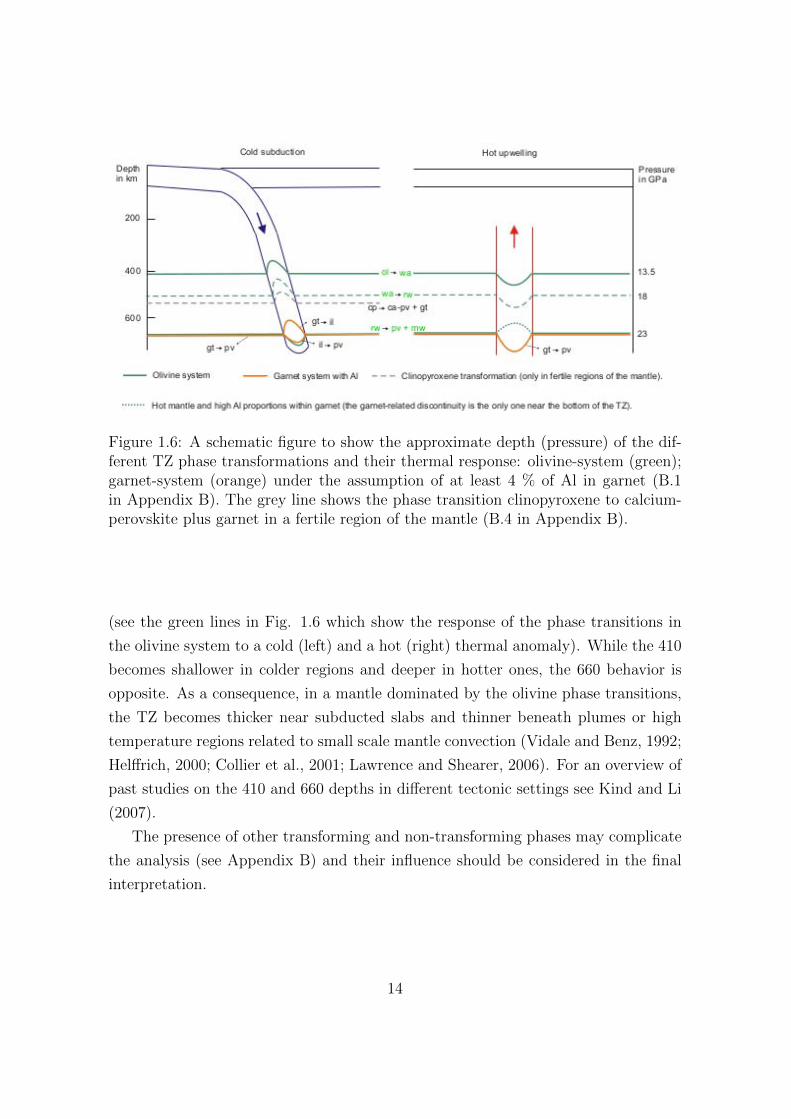
Figure 1.6: A schematic figure to show the approximate depth (pressure) of the dif-ferent TZ phase transformations and their thermal response: olivine-system (green);garnet-system (orange) under the assumption of at least 4 % of Al in garnet (B.1in Appendix B). The grey line shows the phase transition clinopyroxene to calcium-perovskite plus garnet in a fertile region of the mantle (B.4 in Appendix B).
(see the green lines in Fig. 1.6 which show the response of the phase transitions in
the olivine system to a cold (left) and a hot (right) thermal anomaly). While the 410
becomes shallower in colder regions and deeper in hotter ones, the 660 behavior is
opposite. As a consequence, in a mantle dominated by the olivine phase transitions,
the TZ becomes thicker near subducted slabs and thinner beneath plumes or high
temperature regions related to small scale mantle convection (Vidale and Benz, 1992;
Helffrich, 2000; Collier et al., 2001; Lawrence and Shearer, 2006). For an overview of
past studies on the 410 and 660 depths in different tectonic settings see Kind and Li
(2007).
The presence of other transforming and non-transforming phases may complicate
the analysis (see Appendix B) and their influence should be considered in the final
interpretation.
14
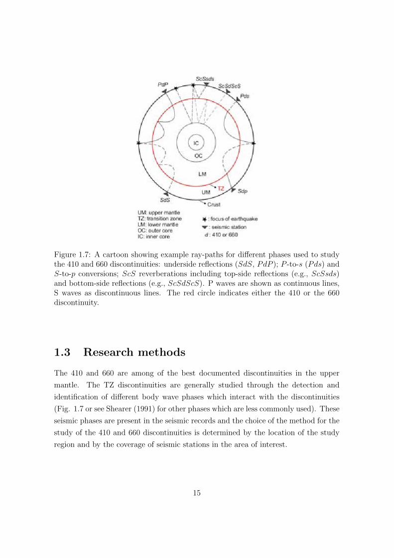
Figure 1.7: A cartoon showing example ray-paths for different phases used to studythe 410 and 660 discontinuities: underside reflections (SdS, PdP ); P -to-s (Pds) andS-to-p conversions; ScS reverberations including top-side reflections (e.g., ScSsds)and bottom-side reflections (e.g., ScSdScS). P waves are shown as continuous lines,S waves as discontinuous lines. The red circle indicates either the 410 or the 660discontinuity.
1.3 Research methods
The 410 and 660 are among of the best documented discontinuities in the upper
mantle. The TZ discontinuities are generally studied through the detection and
identification of different body wave phases which interact with the discontinuities
(Fig. 1.7 or see Shearer (1991) for other phases which are less commonly used). These
seismic phases are present in the seismic records and the choice of the method for the
study of the 410 and 660 discontinuities is determined by the location of the study
region and by the coverage of seismic stations in the area of interest.
15
1.3.1 Seismic phases
Long-period precursors to SS or PP (SdS or PdP where d is the discontinuity
depth) resulting from underside reflections at the upper-mantle discontinuities are
mostly used to map the global depth of these reflectors (because of the wide distribu-
tion of bounce points) or to study them beneath oceanic areas (e.g., Shearer, 1993;
Flanagan and Shearer, 1998, 1999; Deuss and Woodhouse, 2002; Deuss et al., 2006).
Nevertheless, SS precursors are preferred to PP because they have a better ray
coverage and less interference with other seismic phases (e.g., Shearer, 1991). Differ-
ential times between the precursors and SS (i.e. tSS-tSdS where d is the discontinuity
depth) provide a measure of the two-way S travel time between the surface and the
discontinuity. Structure near the sources and the receivers is relatively unimportant
since the SS and SdS ray paths are nearly identical except near the bounce points.
Short period P -to-s conversions have also been used in global studies (Chevrot
et al., 1999; Lawrence and Shearer, 2006; Tauzin et al., 2007). Nevertheless, owing to
the limited geographic distribution of seismometers, the P -to-s and S-to-p conversions
are mostly used to study the discontinuities beneath continents since the conversions
occur beneath the stations (e.g., Vinnik, 1977; Paulssen, 1985; Dueker and Sheehan,
1997; Li and Yuan, 2003; Shen et al., 2008; Eagar et al., 2010). The 410 and 660 are
commonly studied through detection of P -to-s conversions. Differential travel times
between P -to-s conversions and P provide a measure of the one-way S travel time
between the surface and the discontinuity. Using an adequate velocity model, this
one-way travel time can be translated to discontinuity depth.
To a lesser extent, short period ScS reverberations have also been used to study
the 410 and 660 beneath continents (e.g., Revenaugh and Jordan, 1991; Suetsugu
et al., 2004). For an overview of past studies on 410 and 660 discontinuities in
different tectonic settings and with different seismic phases see Kind and Li (2007).
1.3.2 Spatial resolution
One problem in using the SS precursors to study in detail the topography of the TZ
discontinuities is their relatively low resolution due to the long periods of these phases.
The achieved spatial resolution with the different seismic phases is controlled by the
size of the first Fresnel zone, which is frequency dependent. This zone is the area
where the elementary waves (following Huygens-Fresnel principle) that belong to the
16
same wave-front interfere with each other constructively, which in practice is defined
as the area where the travel paths differ by less than a half period (Sheriff, 1996). SS
precursors have a complex Fresnel zone with a minimax characteristic saddle shape
and with an extension larger than 1000 km (Neele et al., 1997). Therefore, these
phases are not suited to study variations in the 410 and 660 topography over small
distances. On the other hand, short period P -to-s conversions are more adequate
to exploit the high spatial resolution provided by dense seismic arrays such as the
TopoIberia seismic network (see Section 1.5 and Chapter 3). The Pds signal is formed
within the first Fresnel zone, which depends on the frequency of the signal and the
depth of the discontinuity, d. The first Fresnel zone for the P410s and P660s phases
at a depth of 410 km and 660 km, respectively, is a circular area with a radius of less
than 100 km, for frequencies larger than 0.1 Hz.
1.3.3 Detection of P -to-s converted phases in the seismicrecords
P -to-s conversions from mantle discontinuities arrive in the P -wave coda and are
difficult to observe directly on seismograms mainly because of their low amplitude.
These coda phases are commonly studied through the receiver functions (RFs) tech-
nique (Phinney, 1964; Vinnik, 1977; Langston, 1979; Ammon, 1991) which enhances
the P-wave conversions and reflections from discontinuities below the recording sta-
tions using teleseismic earthquakes. For a better understanding of RFs see Appendix
A.
Under the assumption of lateral homogeneity and considering teleseismic earth-
quakes, most of the P -wave energy arrives on the vertical (Z) component and the
SV-wave energy, such as P -to-s conversions, on the radial (R) component. To en-
hance the P-wave conversions and reflections, the RFs use the deconvolution of the
Z component from the R which is equivalent to spectral division in the frequency
domain. The division of small amplitudes (spectral holes), however, makes the spec-
tral division unstable and regularization of the deconvolution is required. A common
regularization approach is the water level technique (Clayton and Wiggins, 1976),
(see Appendix A), which nevertheless may cause artifacts. Also the presence of high
frequency noise is known to impair the deconvolution (Clayton and Wiggins, 1976)
and often handled through the multiplication of a Gaussian window during spectral
deconvolution or through the application of a low-pass filter.
17
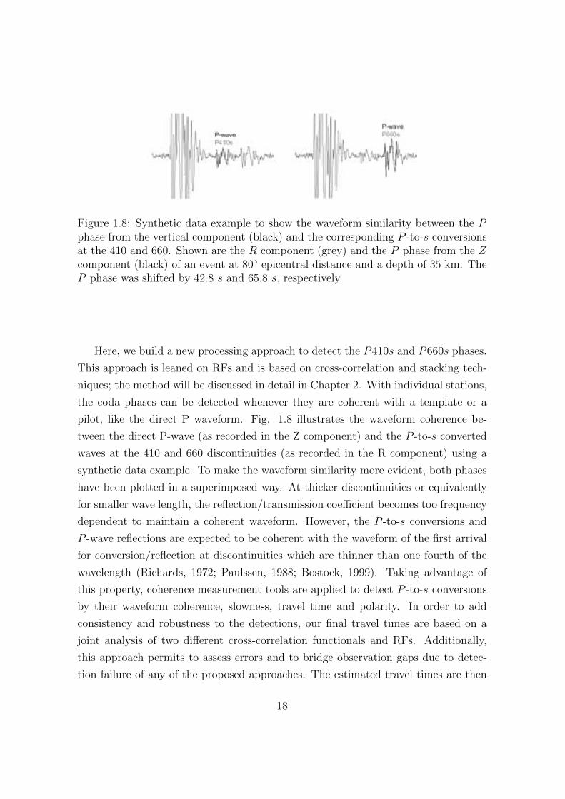
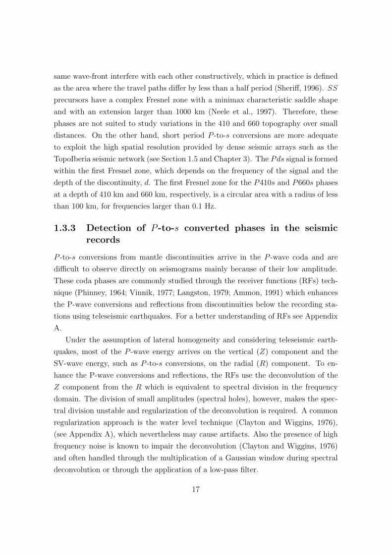
Figure 1.8: Synthetic data example to show the waveform similarity between the Pphase from the vertical component (black) and the corresponding P -to-s conversionsat the 410 and 660. Shown are the R component (grey) and the P phase from the Zcomponent (black) of an event at 80◦ epicentral distance and a depth of 35 km. TheP phase was shifted by 42.8 s and 65.8 s, respectively.
Here, we build a new processing approach to detect the P410s and P660s phases.
This approach is leaned on RFs and is based on cross-correlation and stacking tech-
niques; the method will be discussed in detail in Chapter 2. With individual stations,
the coda phases can be detected whenever they are coherent with a template or a
pilot, like the direct P waveform. Fig. 1.8 illustrates the waveform coherence be-
tween the direct P-wave (as recorded in the Z component) and the P -to-s converted
waves at the 410 and 660 discontinuities (as recorded in the R component) using a
synthetic data example. To make the waveform similarity more evident, both phases
have been plotted in a superimposed way. At thicker discontinuities or equivalently
for smaller wave length, the reflection/transmission coefficient becomes too frequency
dependent to maintain a coherent waveform. However, the P -to-s conversions and
P -wave reflections are expected to be coherent with the waveform of the first arrival
for conversion/reflection at discontinuities which are thinner than one fourth of the
wavelength (Richards, 1972; Paulssen, 1988; Bostock, 1999). Taking advantage of
this property, coherence measurement tools are applied to detect P -to-s conversions
by their waveform coherence, slowness, travel time and polarity. In order to add
consistency and robustness to the detections, our final travel times are based on a
joint analysis of two different cross-correlation functionals and RFs. Additionally,
this approach permits to assess errors and to bridge observation gaps due to detec-
tion failure of any of the proposed approaches. The estimated travel times are then
18
used to map the discontinuities.
1.4 The western Mediterranean and the Ibero-
Maghrebian region
The geodynamic evolution of the western Mediterranean during the Cenozoic is domi-
nated by the subduction of the Tethys oceanic lithosphere beneath the Eurasian plate
in a north dipping direction followed by slab retreating (or slab roll-back) and split-
ting in different directions (Royden, 1993; Lonergan and White, 1997; Faccenna et al.,
2004; Spakman and Wortel, 2004; Rosenbaum et al., 2002). One of the fragments, the
Alboran slab, retreats towards the west-southwest diverging from the Algerian slab
and the Apennines slab which undergoes south and east retreat, respectively (see
geodynamic reconstructions in: Faccenna et al., 2004; Spakman and Wortel, 2004;
Verges and Fernandez, 2012). The subduction process initiates near the Gulf of Lyon
in the Oligocene (30 My) as a consequence of the convergence of Africa with respect
to Europe, which starts in the Cretaceous between 120-83 My (Rosenbaum et al.,
2002). The current convergence rate is of 2-6 mm/y (Argus et al., 1989; Demets
et al., 1990; Stich et al., 2006; Fadil et al., 2006; Vernant et al., 2010). In the western
sector, roll-back occurs during subduction of the African paleomargin with possible
continental subduction of the Iberian paleomargin (e.g. Morales et al., 1999). The
convergence of Africa and Europe gives origin to the Alpine orogeny that forms the
westernmost mountain ranges of the Alpide belt. From west to east, this mountain
belt comprises the Rif, the Tell Atlas, the Betic Cordillera, the Cantabrian Moun-
tains, the Pyrenees, the Alps and the Apennine Mountains (some of these ranges are
depicted in Fig. 1.1 and in Fig. 1.9). The origin of the Neogene extensional Basins
(see ligth-green areas in Fig. 1.9) is attributed to the back-arc extensional processes
during the retreating of the subducted slabs (e.g. Faccenna et al., 2004; Spakman and
Wortel, 2004). Nevertheless, the nature of the Alboran Basin is in debate because
some scientists attribute its origin to a delamination process or convective removal
of an overthickened continental crust (Platt and Vissers, 1989; Calvert et al., 2000).
The Ibero-Maghrebian region, our area of interest, is located in the westernmost
end of the present location of the boundary between the Nubian and Eurasian plate
(see inset in Fig. 1.1). In the Atlantic Ocean, the plate boundary separates oceanic
lithosphere while in the Alboran Sea (western Mediterranean), the contact is not well
19
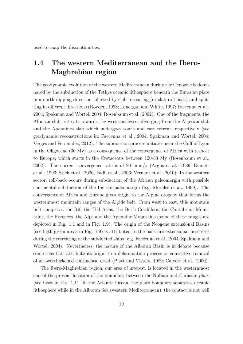
Figure 1.9: Illustrative tectonic map of the western Mediterranean (modified fromComas et al. (1999)) showing the Neogene basins (light-green areas), the location ofthe active orogenic and anorogenic volcanism (extracted from Faccenna et al. (2004))and the mountain ranges of the Alpide belt.
defined (e.g., Mezcua and Martınez-Solares, 1983; Negredo et al., 2002; Vernant et al.,
2010) and involves a continental collision. The seismic activity occurs from shallow
to intermediate depth in a diffuse band which extends to both sides of the Strait of
Gibraltar (see inset in Fig. 1.1), leading to a poorly-defined plate boundary (Mezcua
and Martınez-Solares, 1983). Neotectonic modeling of the Ibero-Maghrebian region
has also indicated a diffuse geometry of the plate boundary in this area (Negredo
et al., 2002). Earthquake activity stops at a depth of 150 km and reappears in a
small area south of Granada at a depth of about 630-660 km (red star in Fig. 1.1)
(Buforn et al., 2011; Bezada and Humphreys, 2012).
20
1.4.1 Deep earthquakes beneath Granada
The origin of the deep isolated events beneath Granada is still an open question,
mainly because the physical processes that permit the occurrence of deep earthquakes
are not well understood. Shallow earthquakes (≤ 60km) are explainable by the brittle
failure of rocks. However, increasing pressure with depth tends to inhibit fracture and
sliding, while increasing temperature promotes ductile flow. There are three primary
mechanisms proposed for the generation of deep earthquakes. Here we explain the
mechanisms of very deep earthquakes, depth ≥ 550 km; for a complete review and
bibliographic citations see Green and Houston (1995); Houston (2007):
(1) Dehydration embrittlement: refers to brittle failure assisted by high fluid pore
pressures that counteract the high normal stress due to large overburden pres-
sures. The viability of this mechanism to generate very deep earthquakes de-
pends on the availability of fluids at relevant depths. The α-to-β phase transi-
tion could carry water deeper into the mantle TZ. However, this phase transition
is capable of storing increasing amounts of water. Thus, net water would not be
released during the phase transition, and the availability of free fluid to promote
brittle fracture is questionable.
(2) Transformational faulting in metastable olivine: shear instabilities are triggered
by the heat release and sudden volume change of the olivine phase transition
to denser forms (α-to-β and α-to-γ). The shear instability requires that the
starting phase exists metastably in the stability field of the final phase, so
that the shear zone could grow aseismically. The final phase acts as a lubricant
permitting shear slip to occur. This model requires sufficiently low temperatures
inside the slab to inhibit the transformation of the low-pressure phase as the slab
gradually subducts to deeper higher pressure-temperature environs. However,
it is unclear to which extent the phase transformation inhibition is sustained in
long timescales relevant to subduction (e.g., several million years).
(3) Thermal shear instabilities: refers to shear localization produced by a positive
feedback between temperature-dependent slab rheology and shear deformation
that generates viscous heating. Under certain conditions, the feedback expo-
nentially increases the localization of shear strain, leading to apparently abrupt
failure on a shear zone. The rheological structure of a cold slab can be simply
21
explained as a weak cold core surrounded by stronger regions. The cooler slabs
are weaker and rapid deformation will focus the stress onto the strong regions.
In this model, shear instabilities can occur in the strong regions if strain rate is
large; thus earthquakes could occur in the regions surrounding the weak core.
The three mechanisms mentioned are temperature dependent. Although the mecha-
nism of deep earthquakes is still unclear, it seems that the thermal structure of the
slab is central to deep earthquake problems. Thus, constraints on the slab tempera-
ture near the hypocenter (see Chapter 4) would help to characterize the scenarios of
the different deep earthquakes.
1.4.2 Tomographic images of the upper mantle
Most tomography studies have revealed a positive P-wave velocity anomaly (or cold
anomaly) beneath the Alboran Sea and southeast Spain (see B in Fig. 1.10) which
follows the arcuate shape of the Gibraltar Arc but loses its geometry (or resolution)
at the base of the upper-mantle TZ; this anomaly plunges into the mantle to the east
(Spakman, 1990; Blanco and Spakman, 1993; Wortel and Spakman, 2000; Calvert
et al., 2000; Piromallo and Morelli, 2003; Spakman and Wortel, 2004; Faccenna et al.,
2004; Garcia-Castellanos and Villasenor, 2011; Bezada et al., 2013; Monna et al.,
2013). There is a long debate on the origin and shape of this anomaly (Platt and
Vissers, 1989; Royden, 1993; Seber et al., 1996; Wortel and Spakman, 2000; Gutscher
et al., 2002; Faccenna et al., 2004; Bokelmann et al., 2011; Verges and Fernandez,
2012) as it is an important clue to understand the regional geodynamic state of the
Ibero-Maghrebian region. The lack of consensus is in part due to the fact that the ex-
act location and shape of this anomaly differs among different author’s publications.
Furthermore, the continuity of the anomaly in depth as well as its steep dipping to
the east has been questioned and attributed to the uneven distribution of teleseismic
ray paths in the westernmost Mediterranean (Calvert et al., 2000). Recent high res-
olution images (Bezada et al., 2013) show that the positive anomaly has an arcuate
shape, it is vertically continuous, it is located beneath the western Alboran Sea and is
more than 600 km long. However, independent observations of any of these features
are still needed. The tomographic images also show a broad positive anomaly in
the TZ beneath the northern Apennines, the northwestern Mediterranean, southern
22
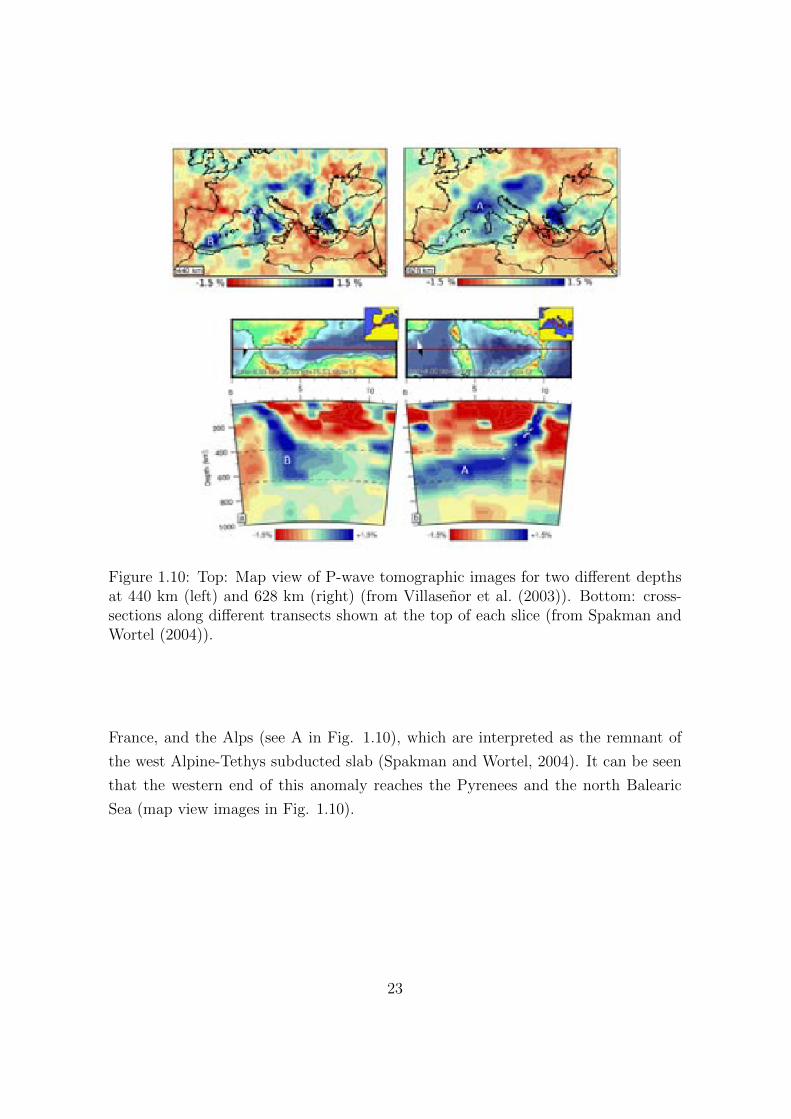
Figure 1.10: Top: Map view of P-wave tomographic images for two different depthsat 440 km (left) and 628 km (right) (from Villasenor et al. (2003)). Bottom: cross-sections along different transects shown at the top of each slice (from Spakman andWortel (2004)).
France, and the Alps (see A in Fig. 1.10), which are interpreted as the remnant of
the west Alpine-Tethys subducted slab (Spakman and Wortel, 2004). It can be seen
that the western end of this anomaly reaches the Pyrenees and the north Balearic
Sea (map view images in Fig. 1.10).
23
1.4.3 A controversial geodynamic scenario in the AlboranSea area
Although the general geodynamic scenario of the Ibero-Maghrebian region is under-
stood and is related to a subduction process which started in the Oligocene, this
particular area comprises a complex tectonic setting still controversial. The origin
of the controversy lies in the geodynamic model which best explains the existence
of an extensional basin (Alboran Sea) developed in the early Miocene (23-5.3 My)
which is embedded in a compressional regime and which is coeval with the uplift
and shortening of the Betic and Rif mountains (e.g. Platt and Vissers, 1989; Royden,
1993; Bokelmann et al., 2011). In this context, the explanations of the heterogeneity
in the Alboran Sea involve (1) different types of continental delamination or con-
vective removal (Platt and Vissers, 1989; Seber et al., 1996; Calvert et al., 2000)
or (2) retreating subduction of oceanic lithosphere with slab-tearing or partial slab-
detachment (Faccenna et al., 2004; Gutscher et al., 2002; Wortel and Spakman, 2000;
Garcia-Castellanos and Villasenor, 2011; Bezada and Humphreys, 2012).
In model (1) an over-thickened continental lithosphere is detached by convective
removal or delamination causing extension of the Alboran Basin and uplift around
the margin. Convective removal was firstly proposed by Platt and Vissers (1989) and
delamination by Seber et al. (1996). These models are also known as ’continental
models’ and are consistent with continental collision or subduction; for a schematic
explanation see Fig. 1.11 (b). Model (2) was originally proposed by Royden (1993)
arguing that the subduction of oceanic lithosphere followed by slab rollback causes the
extension within the Alboran Basin. These models, also known as ’oceanic models’,
have gained more popularity; for a schematic explanation see Fig. 1.11 (a). Several
authors reconcile both groups of models (e.g. Duggen et al., 2003; Garcia-Castellanos
and Villasenor, 2011; Bezada and Humphreys, 2012). For example, based upon re-
sults from tomography, Bezada and Humphreys (2012) proposed that the delamina-
tion event occurred as a result of subduction of the Alboran lithospheric mantle along
with the larger slab that they find presently under the westernmost Mediterranean.
Independently from the tomography studies, SKS splitting (Buontempo et al., 2008;
Dıaz et al., 2010) and P-wave dispersion analyses (Bokelmann and Maufroy, 2007)
are consistent with the presence of a subducted oceanic lithosphere. Nevertheless,
24
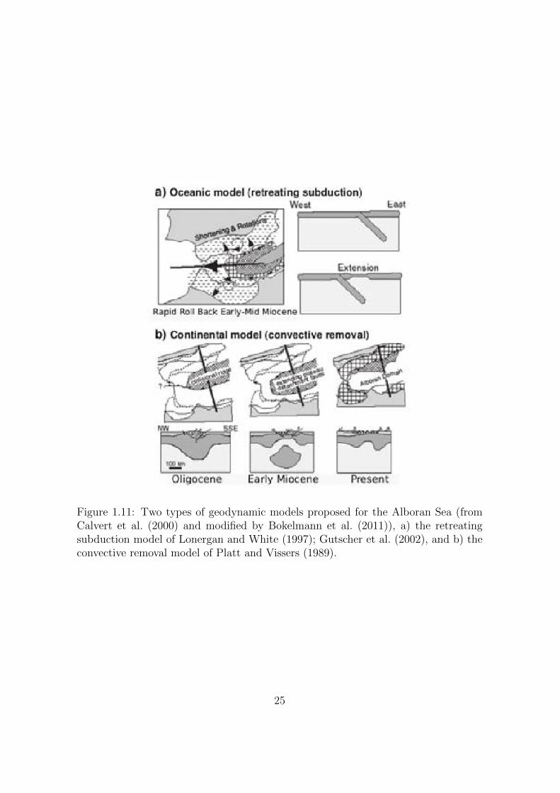
Figure 1.11: Two types of geodynamic models proposed for the Alboran Sea (fromCalvert et al. (2000) and modified by Bokelmann et al. (2011)), a) the retreatingsubduction model of Lonergan and White (1997); Gutscher et al. (2002), and b) theconvective removal model of Platt and Vissers (1989).
25
there is still room for different interpretations.
1.4.4 Anorogenic magmatism
The complexity of the region increases if the mafic Neogene subduction-unrelated
(or anorogenic) volcanism is considered (Fig. 1.9). This volcanism extends from
the eastern Atlantic Ocean to central Europe and the western Mediterranean and it
is still active in some regions (e.g. Lustrino and Wilson, 2007; Lustrino et al., 2011;
Carminati et al., 2012). Several petrological and geodynamical models have been pro-
posed in the literature to explain the deep-origin magmas (sub-lithospheric), which
are summarized in fig. 18 in Lustrino and Wilson (2007). The models require either
(i) active asthenospheric (or deeper) mantle convection (i.e., mantle plumes) or (ii)
lithospheric extension (or delamination and detachment) to induce passive, adiabatic,
decompression melting of both asthenospheric and lithospheric upper mantle. The
main difference between both models is that model (i) needs a hot buoyant, deep
mantle source. The prevalence of plume models in recent decades has been sustained
by many researchers largely on the basis of geochemical arguments (e.g., Hoernle
et al., 1995; Oyarzun et al., 1997; Macera et al., 2003; Duggen et al., 2009). Recently,
Duggen et al. (2009) reconcile both groups of models (see Fig. 1.12). In Duggen’s
model, the stem of the plume is in the Canary Islands and the mantle plume ma-
terial travels laterally along a subcontinental lithospheric corridor (i.e., at depths
that are usually occupied by continental lithospheric mantle) more than 1500 km to
the western Mediterranean, marking its route over the last 15 My through a trail of
intraplate volcanism. In this model, the anorogenic magmatism occurs in areas of
thinned lithosphere (due to delamination or other extensional processes). When the
extent of thinning lithosphere of a particular part of the corridor allowed sufficient
upwelling, decompression melting occurs as in model (ii). Nevertheless, the existence
of a physically continuous mantle source to explain the anorogenic magmatism is still
questionable because it is mainly sustained on the compositional similarity (incom-
patible trace elements and Sr-Nd-Pb isotopic composition) between the igneous rocks
of distant volcanoes (Lustrino, 2011). Recent tomography studies have revealed for
the first time a clear low P-velocity anomaly beneath the Gulf of Cadiz that reaches
the upper-mantle transition zone (TZ) in the Strait of Gibraltar (Monna et al., 2013).
26
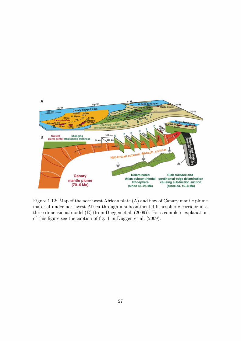
Figure 1.12: Map of the northwest African plate (A) and flow of Canary mantle plumematerial under northwest Africa through a subcontinental lithospheric corridor in athree-dimensional model (B) (from Duggen et al. (2009)). For a complete explanationof this figure see the caption of fig. 1 in Duggen et al. (2009).
27
This anomaly is interpreted as hot mantle material which is probably related to the
alkaline magmatism of western Portugal.
1.4.5 Seismic discontinuity studies
The compositional discontinuity which separates the crust from the mantle (Moho)
has been mapped in detail beneath Iberia and its surrounding waters through a com-
pilation of seismic reflection data (Dıaz et al., 2010). These data show the deepest
Moho beneath the Pyrenees (50 km) and the shallowest Moho beneath the Alboran
Sea (15-18 km), the Valencia Trough (13-15 km) and the Atlantic domain (10 km).
These results are consistent with a crustal thinning beneath the Alboran Sea, the
Valencia Trough and the Atlantic domain. Beneath Morocco the Moho depth has
been investigated through P-wave RFs analysis (Mancilla et al., 2012). The Moho
depths are consistent with a thickened crust (of about 35-44 km) beneath northwest-
ern Morocco, and with a significantly thinned crust (of about 22-30 km) beneath
northeastern Morocco. These results seem to support that the high topography in
the Middle Atlas domain is not isostatically compensated at the crustal level.
The boundary between the high-viscosity lithosphere and the low-viscosity as-
thenosphere (or LAB) defines a low-velocity zone below the Moho. This discontinu-
ity has been investigated in the Gibraltar Arc area using P-wave and S-wave RFs
(Dundar et al., 2011). The results indicate a 90-100 km thick lithosphere from the
northwest part of Africa to southern Portugal across the Atlantic, west of Gibraltar
as well as in the Betics, while it is thinner beneath the Alboran Sea (of about 60 km).
The authors attribute their results to a delamination process.
The TZ discontinuities in the Ibero-Maghrebian region have been studied through
detection of P -to-s converted waves (Chevrot et al., 1999; Tauzin et al., 2007; van der
Meijde et al., 2005; Dundar et al., 2011; Bonatto et al., 2013). Chevrot et al. (1999)
and Tauzin et al. (2007) studied the global distribution of TZ thickness (TZT), in-
cluding in their analysis a small number of Spanish stations. Van der Meijde et al.
(2005) estimated the TZT beneath 22 stations located in the entire Mediterranean
region, with 4 of them in Iberia and 2 in Africa (1 station in Melilla and the other
in Morocco). Their results indicate a thicker TZ beneath the western coast of Spain
and beneath the station in Melilla, with a maximum thickness of about 280 km. At
the stations in central Spain and Morocco, their results show an averaged TZT of
28
about 257 km. With the installation of new permanent stations and the deployment
of large seismic arrays, such as the IberArray, more data are available and it is now
possible to study the TZ discontinuities as well as the TZT in a detailed way. Dundar
et al. (2011) used 38 stations to evaluate whether the TZ presents thickness varia-
tions beneath the Alboran Sea and its surroundings. They found no hint of local
changes in the TZT. Recently, using the data from the first deployment of IberArray
(43 stations), we published the first detailed topography maps for the 410 and 660
discontinuities in the Alboran Sea area (Bonatto et al., 2013). The results are in
good agreement with van der Meijde et al. (2005); the Alboran Sea area is discussed
in Sections 4.4.2.3, 4.4.2.4 and 4.4.2.6 of Chapter 4.
1.5 TopoIberia data set
In this thesis we use the data set belonging to the TopoIberia project (http://
www.igme.es/internet/TopoIberia/default.html) (Dıaz et al., 2009). This mul-
tidisciplinary project involves more than 100 researchers from 10 different Spanish
institutions:
• Instituto de Ciencias de la Tierra ’Jaume Almera’
• Instituto Geologico y Minero de Espana
• Real Instituto y Observatorio de la Armada
• Universidad Autonoma de Barcelona
• Universidad de Barcelona
• Universidad de Cadiz
• Universidad Complutense de Madrid
• Universidad de Granada
• Universidad de Jaen
• Universidad de Oviedo
29
One of TopoIberia major aims consists of the deployment of a high resolution
multi-component seismic array called IberArray. This has been the first large-scale
dense station deployment in Europe. The multidisciplinary dense system of sta-
tion deployment (broadband seismic stations, GPS receivers and MT sensors) of
TopoIberia has been pioneered in the US by EarthScope. The seismological com-
ponent IberArray of the TopoIberia project permitted to gather continuous three-
component broadband data during more than 6 years. This technological observa-
tory platform provides us with a huge seismological database with more than 250
broadband seismic stations deployed along the Iberian Peninsula and north of Mo-
rocco. However, not all the stations were active at the same time. The installation
process was performed in three phases moving the stations from south to the north
and lasted 6 years, starting in January 2007. The stations are still recording in
north Spain. Additionally, other institutions collaborate with TopoIberia by sharing
their own data bases. In Spain these are the Instituto Geografico Nacional (IGN),
the Instituto Geologic de Catalunya (IGC), the Real Instituto y Observatorio de la
Armada (ROA), the Universidad Complutense de Madrid (UCM) and the Instituto
Andaluz de Geofısica (IAG). Furthermore, many different foreign research groups col-
laborate or share data through their projects such as WILAS, PYROPE, PICASSO
(USA, Munster, Bristol), and the Institut Scientifique, Universite Mohammed V Ra-
bat (Morocco).
Certainly, this pretentious project significantly increases the high-quality infor-
mation available for the study of geological and geophysical processes in the Iberian
Peninsula and its surroundings. Besides, it puts Spain into the leading edge of inter-
national research on basic research into orogenic processes as well as the preparation,
prevention, and mitigation of geological risk in tectonically active and highly popu-
lated areas.
30

31
2Methodology: detection of P -coda phases
32

2.1 Introduction
The TZ discontinuities are generally studied through the detection and identifica-
tion of different body wave phases present in the seismic records (Shearer, 1991,
2000). The P -to-s converted waves at the 410 and 660 arrive in the P -wave coda
together with multiply reflected and scattered waves. Coda phases are characterized
by low amplitudes and consequently are difficult to identify within the multitude of
different other phases in individual records. However, the P -to-s conversions and
P -wave reflections are expected to be coherent with the waveform of the first arrival
for conversion (or reflection) at discontinuities which are thinner than one fourth of
the wavelength (Richards, 1972; Paulssen, 1988; Bostock, 1999). At thicker disconti-
nuities or equivalently for smaller wavelength, the reflection/transmission coefficient
becomes too frequency dependent to maintain a coherent waveform. Therefore, with
individual stations, these coda signals can be detected whenever they are coherent
with the direct P waveform. Taking advantage of this property, we have applied
coherence measurement tools to detect coda signals by their waveform similarity as
function of lag time. We apply different cross-correlation techniques between compo-
nents of teleseisms recorded at individual stations. Finally, the signals are identified
by the measured travel time, slowness and polarity. In order to add consistency and
robustness to the detections, our final approach is based on a joint analysis of two
different cross-correlation functionals and RF. Furthermore, this approach permits
to assess errors and to bridge observation gaps due to detection failure of any of the
approaches.
2.2 Method
2.2.1 Theoretical background
In order to determine the waveform similarity between the coda phases and the
P phase, we apply two cross-correlation techniques which are based on different
strategies: the classical cross-correlation geometrically normalized (CCGN) and the
phase cross-correlation (PCC) presented by Schimmel (1999). To enhance coherent
34
signals and to suppress incoherent noise, we use the phase-weighted stack (PWS)
(Schimmel and Paulssen, 1997).
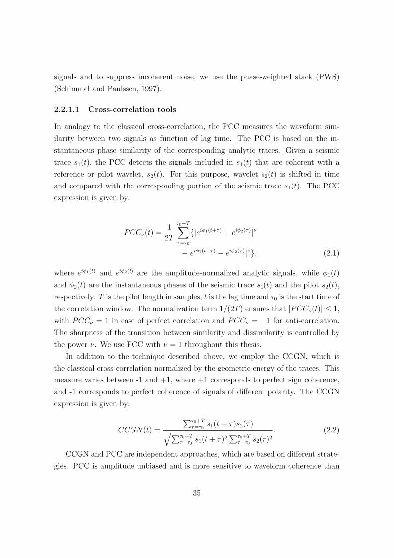
2.2.1.1 Cross-correlation tools
In analogy to the classical cross-correlation, the PCC measures the waveform sim-
ilarity between two signals as function of lag time. The PCC is based on the in-
stantaneous phase similarity of the corresponding analytic traces. Given a seismic
trace s1(t), the PCC detects the signals included in s1(t) that are coherent with a
reference or pilot wavelet, s2(t). For this purpose, wavelet s2(t) is shifted in time
and compared with the corresponding portion of the seismic trace s1(t). The PCC
expression is given by:
PCCν(t) =1
2T
τ0+T∑τ=τ0
{|eiφ1(t+τ) + eiφ2(τ)|ν
−|eiφ1(t+τ) − eiφ2(τ)|ν}, (2.1)
where eiφ1(t) and eiφ2(t) are the amplitude-normalized analytic signals, while φ1(t)
and φ2(t) are the instantaneous phases of the seismic trace s1(t) and the pilot s2(t),
respectively. T is the pilot length in samples, t is the lag time and τ0 is the start time of
the correlation window. The normalization term 1/(2T ) ensures that |PCCν(t)| ≤ 1,
with PCCν = 1 in case of perfect correlation and PCCν = −1 for anti-correlation.
The sharpness of the transition between similarity and dissimilarity is controlled by
the power ν. We use PCC with ν = 1 throughout this thesis.
In addition to the technique described above, we employ the CCGN, which is
the classical cross-correlation normalized by the geometric energy of the traces. This
measure varies between -1 and +1, where +1 corresponds to perfect sign coherence,
and -1 corresponds to perfect coherence of signals of different polarity. The CCGN
expression is given by:
CCGN(t) =
∑τ0+Tτ=τ0
s1(t+ τ)s2(τ)√∑τ0+Tτ=τ0
s1(t+ τ)2∑τ0+T
τ=τ0s2(τ)2
. (2.2)
CCGN and PCC are independent approaches, which are based on different strate-
gies. PCC is amplitude unbiased and is more sensitive to waveform coherence than
35
CCGN and, therefore, well suited for the detection of coherent weak amplitude sig-
nals. CCGN is based on the sum of signal amplitude products and is therefore less
sensitive to waveform coherence. The decreased sensitivity may favor signal detection
when there is less waveform similarity due to waveform distortion.
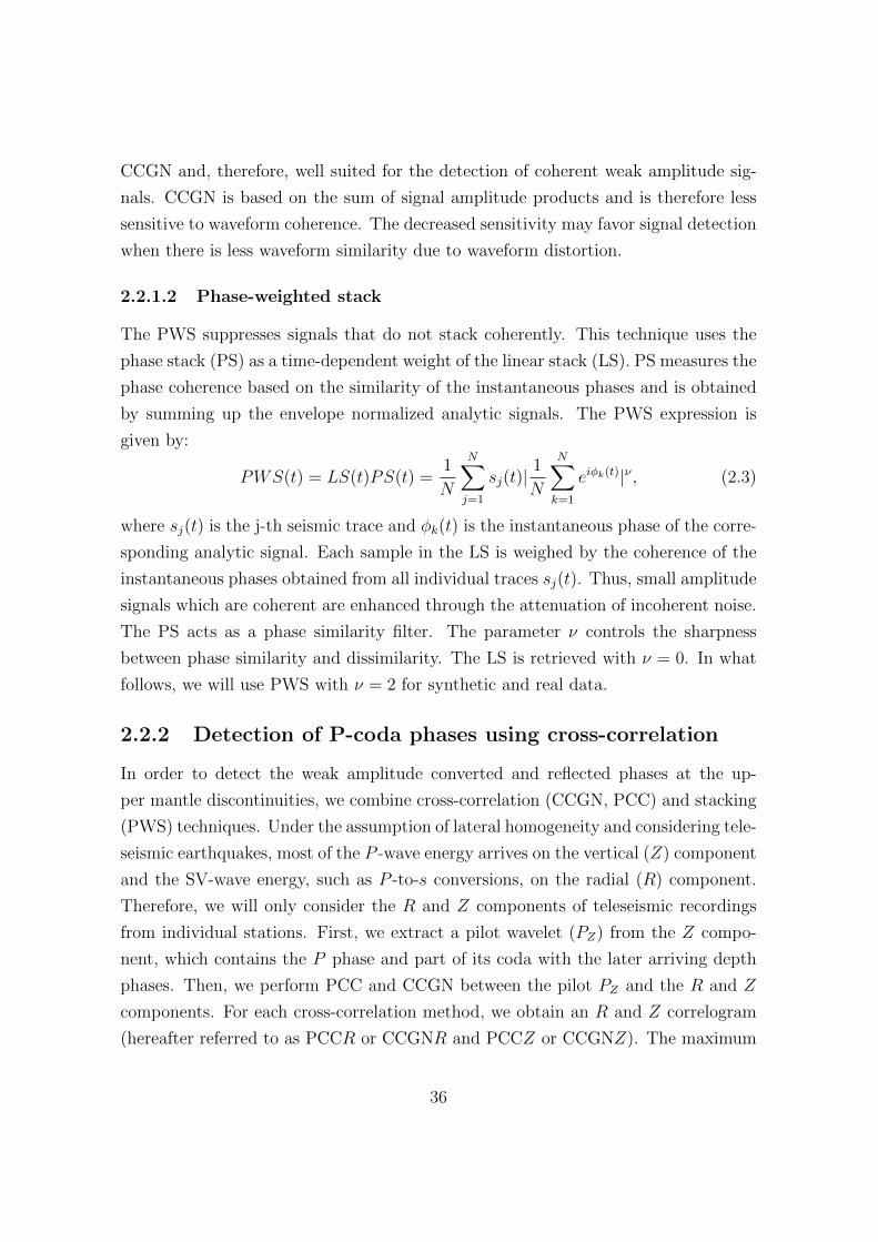
2.2.1.2 Phase-weighted stack
The PWS suppresses signals that do not stack coherently. This technique uses the
phase stack (PS) as a time-dependent weight of the linear stack (LS). PS measures the
phase coherence based on the similarity of the instantaneous phases and is obtained
by summing up the envelope normalized analytic signals. The PWS expression is
given by:
PWS(t) = LS(t)PS(t) =1
N
N∑j=1
sj(t)|1
N
N∑k=1
eiφk(t)|ν , (2.3)
where sj(t) is the j-th seismic trace and φk(t) is the instantaneous phase of the corre-
sponding analytic signal. Each sample in the LS is weighed by the coherence of the
instantaneous phases obtained from all individual traces sj(t). Thus, small amplitude
signals which are coherent are enhanced through the attenuation of incoherent noise.
The PS acts as a phase similarity filter. The parameter ν controls the sharpness
between phase similarity and dissimilarity. The LS is retrieved with ν = 0. In what
follows, we will use PWS with ν = 2 for synthetic and real data.
2.2.2 Detection of P-coda phases using cross-correlation
In order to detect the weak amplitude converted and reflected phases at the up-
per mantle discontinuities, we combine cross-correlation (CCGN, PCC) and stacking
(PWS) techniques. Under the assumption of lateral homogeneity and considering tele-
seismic earthquakes, most of the P -wave energy arrives on the vertical (Z) component
and the SV-wave energy, such as P -to-s conversions, on the radial (R) component.
Therefore, we will only consider the R and Z components of teleseismic recordings
from individual stations. First, we extract a pilot wavelet (PZ) from the Z compo-
nent, which contains the P phase and part of its coda with the later arriving depth
phases. Then, we perform PCC and CCGN between the pilot PZ and the R and Z
components. For each cross-correlation method, we obtain an R and Z correlogram
(hereafter referred to as PCCR or CCGNR and PCCZ or CCGNZ). The maximum
36
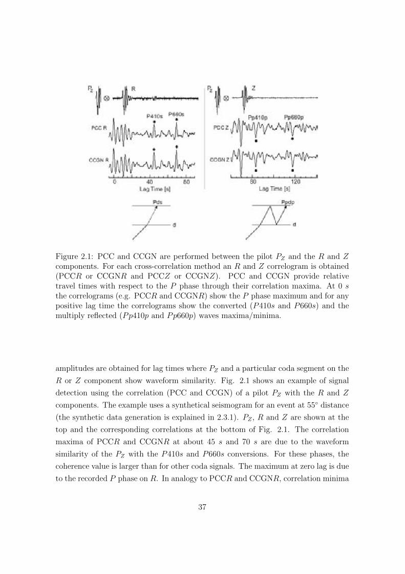
Figure 2.1: PCC and CCGN are performed between the pilot PZ and the R and Zcomponents. For each cross-correlation method an R and Z correlogram is obtained(PCCR or CCGNR and PCCZ or CCGNZ). PCC and CCGN provide relativetravel times with respect to the P phase through their correlation maxima. At 0 sthe correlograms (e.g. PCCR and CCGNR) show the P phase maximum and for anypositive lag time the correlograms show the converted (P410s and P660s) and themultiply reflected (Pp410p and Pp660p) waves maxima/minima.
amplitudes are obtained for lag times where PZ and a particular coda segment on the
R or Z component show waveform similarity. Fig. 2.1 shows an example of signal
detection using the correlation (PCC and CCGN) of a pilot PZ with the R and Z
components. The example uses a synthetical seismogram for an event at 55◦ distance
(the synthetic data generation is explained in 2.3.1). PZ , R and Z are shown at the
top and the corresponding correlations at the bottom of Fig. 2.1. The correlation
maxima of PCCR and CCGNR at about 45 s and 70 s are due to the waveform
similarity of the PZ with the P410s and P660s conversions. For these phases, the
coherence value is larger than for other coda signals. The maximum at zero lag is due
to the recorded P phase on R. In analogy to PCCR and CCGNR, correlation minima
37
on PCCZ and CCGNZ show the topside P -wave reflections Pp410p and Pp660p from
the 410 and 660 upper-mantle discontinuities. The negative correlation is due to the
polarity change of the reflections with respect to the pilot PZ . The figure shows that
PCC and CCGN provide relative travel times with respect to the P phase through
their correlation maxima and minima.
Depth phases, such as pP , sP and their near source multiples (pmP , smP ) are
included into PZ since they are similarly affected by receiver site discontinuities.
The inclusion of the depth phases aids the detection of receiver structure since their
respective lag time for the depth conversions and reflections is the same as for the
direct P -wave. This is in analogy to the teleseismic source function in RF studies.
Phases related with the source depth (such as pP , pmP , etc) may also correlate with
the P phase. However, the use of a pilot with depth phases decreases the correlation
of the depth phases with respect to a pilot which consists only of the direct P -wave.
The final stacking over different events eliminates the source signature, enhances the
signals which arrive consistently, such as near receiver conversions and reflections, and
attenuates spurious arrivals. To illustrate the source equalization, the correlograms
of four different events (same depth and different source function) have been stacked
using LS and PWS. The correlograms using PCC and CCGN and their respective
stacks are shown in Fig. 2.2. The first four lines in each panel show PCC (left)
and CCGN (right) correlograms for the different events. The last two lines show the
results when using LS and PWS to stack the correlograms. Notice that both stacking
techniques attenuate phase side lobes due to the different source functions, although
the PWS has a better signal-to-noise ratio (SNR) than the LS. This example uses
events from the same depth, which means that near source site reverberations stack
constructively due to the source equalization. However, these signals are still more
attenuated in the real data stacks due to the different source depths and source site
heterogeneities for each event.
Fig. 2.3 shows an example where the approach has been applied using teleseisms
from epicentral distances of 65◦ to 95◦ registered at the Spanish station CART (Fig.
2.3 a). Blue crosses show the piercing points as obtained from a P -to-s conversion
at a depth of 510 km to illustrate the sampled TZ by the P410s and P660s phases.
Move-out corrected radial correlograms are shown in Fig. 2.3 (b). We obtained these
correlograms using a PZ of 100 s length, a fixed relative slowness parameter of - 0.1
s/◦, and a reference distance of 80◦. Working with relative times allows us to perform
38
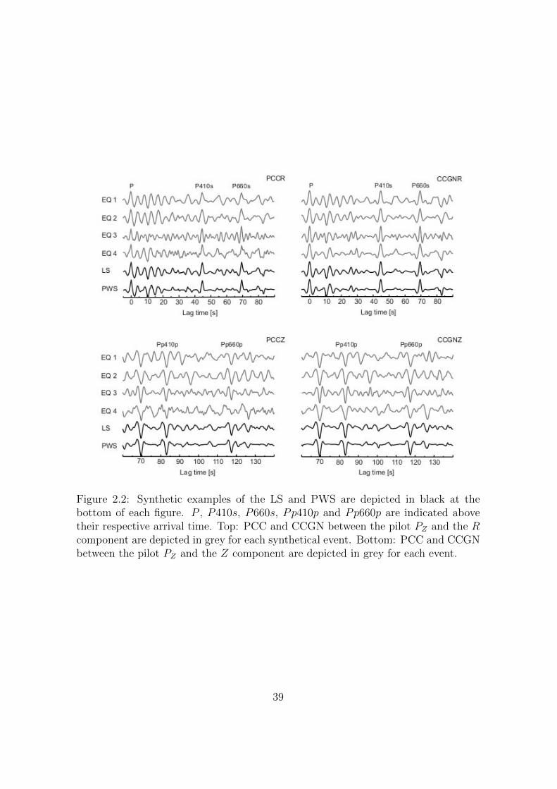
Figure 2.2: Synthetic examples of the LS and PWS are depicted in black at thebottom of each figure. P , P410s, P660s, Pp410p and Pp660p are indicated abovetheir respective arrival time. Top: PCC and CCGN between the pilot PZ and the Rcomponent are depicted in grey for each synthetical event. Bottom: PCC and CCGNbetween the pilot PZ and the Z component are depicted in grey for each event.
39
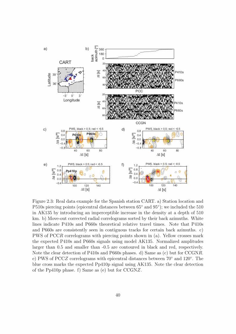
Figure 2.3: Real data example for the Spanish station CART. a) Station location andP510s piercing points (epicentral distances between 65◦ and 95◦); we included the 510in AK135 by introducing an imperceptible increase in the density at a depth of 510km. b) Move-out corrected radial correlograms sorted by their back azimuths. Whitelines indicate P410s and P660s theoretical relative travel times. Note that P410sand P660s are consistently seen in contiguous tracks for certain back azimuths. c)PWS of PCCR correlograms with piercing points shown in (a). Yellow crosses markthe expected P410s and P660s signals using model AK135. Normalized amplitudeslarger than 0.5 and smaller than -0.5 are contoured in black and red, respectively.Note the clear detection of P410s and P660s phases. d) Same as (c) but for CCGNR.e) PWS of PCCZ correlograms with epicentral distances between 70◦ and 120◦. Theblue cross marks the expected Pp410p signal using AK135. Note the clear detectionof the Pp410p phase. f) Same as (e) but for CCGNZ.
40
linear move-out corrections. P410s and P660s phases are consistently seen in the
CCGNR time-back azimuth section, while the PCCR correlograms show intermit-
tently the same phases with a lower SNR. We attribute this difference to the loss
of waveform coherence due to noise contamination. The unambiguous detection of
P410s and P660s phases is obtained in the relative time-slowness domain, where the
reference is the P phase and the stack is performed using a range of slowness val-
ues. This approach is also known as slant-stack and permits identification of phases
in time and slowness. The signals are detected with respect to the P phase, which
means that the obtained travel time and slowness values are relative values with re-
spect to the values of the P phase. The PWS of PCCR and CCGNR correlograms
from Fig. 2.3 (b) are displayed in Fig. 2.3 (c) and (d). These figures show a clear
detection of P410s and P660s phases close to the reference values of relative time
and slowness and with positive coherence value (black contours). For a reference
distance of 80◦, as the one used in the stacking of Fig. 2.3 (c), the P410s arrives at
relative time of 42.8 s and the P660s at 65.8 s, both with positive coherence value
and negative relative slowness. Fig. 2.3 (e) and (f) show the slant-stacks of PCCZ
and CCGNZ for events registered at station CART with epicentral distances between
70◦ and 120◦. These figures show a clear detection of Pp410p at expected relative
time and slowness and with negative amplitude (red contours). However, there is no
evidence for a Pp660p detection. Detection of topside reflections from the 410 and
660 is a more difficult task due to the great variability of these phases caused by the
two extra trajectories through the upper mantle and crust. Ppdp phases (where d is
the discontinuity depth) are therefore more sensitive to lateral heterogeneities than
the P phase, which can affect the waveform similarity and the travel times.
The summary of the method is as follows:
• Extract a pilot wavelet PZ from the Z component of a teleseism which contains
the P phase and part of its coda.
• Perform the cross-correlation (PCC, CCGN) between PZ and R and Z compo-
nents.
• Apply the PWS through a slant-stacking approach to detect the coda phases
by their relative travel time, polarity and slowness.
41
Relation with Receiver Functions method
Discontinuities beneath seismic stations are commonly studied through the detection
of P -to-s conversions in receiver functions (RFs). These are based on deconvolution
of the Z component from the R, which is equivalent to spectral division in the fre-
quency domain. This process removes the source wavelet and complexities, while it
enhances P -to-s conversions from the receiver site discontinuities. The division of
small amplitudes (spectral holes), however, makes the spectral division unstable and
regularization of the deconvolution is required. A common regularization approach
is the water-level technique (Clayton and Wiggins, 1976) (see Appendix A) which
nevertheless may cause artifacts. Also, the presence of high frequency noise is known
to impair the deconvolution (Clayton and Wiggins, 1976) and often handled through
the multiplication of a Gaussian window during spectral deconvolution or through
the application of a low-pass filter.
Our processing approach (presented above) is based on cross-correlation, which
is equivalent to spectral multiplication in the frequency domain, and therefore, there
is no need of regularization. However, as we suppress the amplitude information, we
only retrieve the kinematic response of the Earth while RF retrieve the dynamic re-
sponse. The RF can be expressed in terms of cross-correlation (Clayton and Wiggins,
1976; Ammon, 1991; Galetti and Curtis, 2012), its analytic expression in the spectral
domain is:
RF (w) =Z∗(w) R(w)
Z∗(w) Z(w), (2.4)
where Z∗ is the complex conjugate of Z. The numerator of equation 2.4 is the cross-
correlation between Z and R in the spectral domain, while the denominator is a
positive real number which functions as a frequency dependent normalization factor.
In our approach, we avoid division and compute only the nominator of equation 2.4
if we use the classical cross-correlation instead of the CCGN. Using equation 2.4 the
classical cross-correlation can be expressed as:
Z∗ R = {Z∗ Z} RF, (2.5)
which shows that our approach (cross-correlation between Z and R) is equivalent to a
RF which is multiplied by the auto-correlation of the source, i.e., a symmetric function
in the time domain, peaked and centered at t=0s. Thus, the cross-correlation repre-
sents the receiver site response convolved with a function that is relatively compact.
42
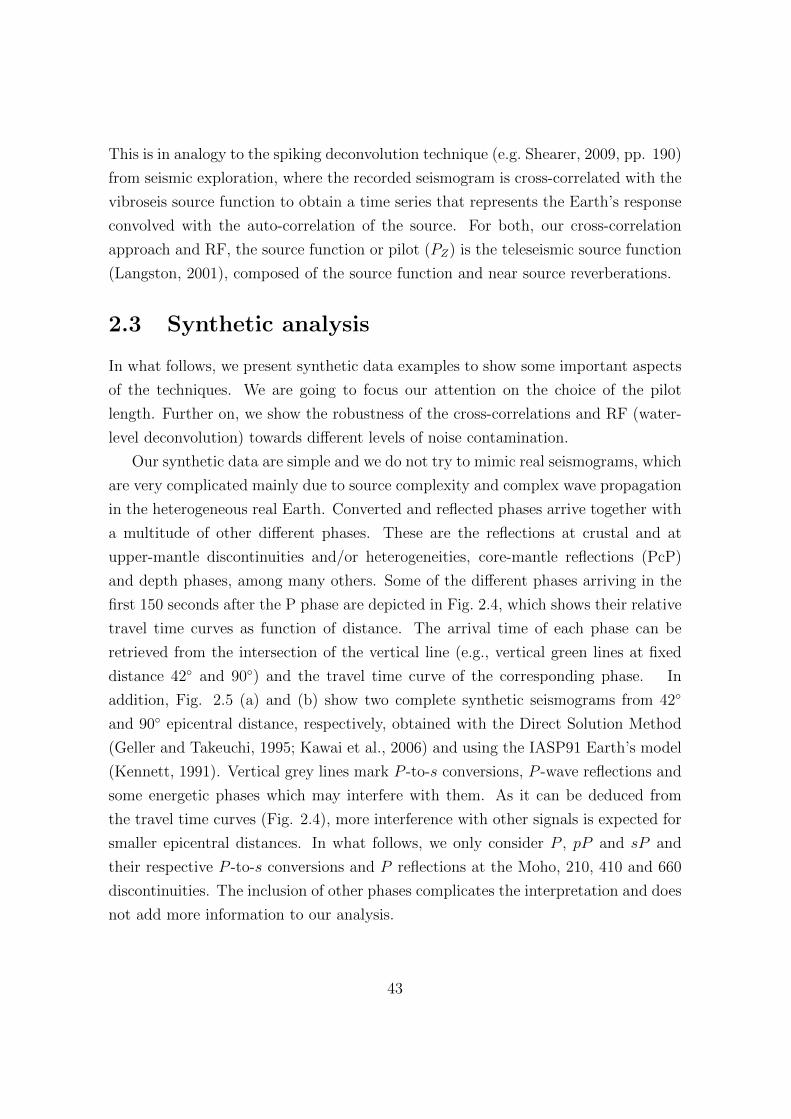
This is in analogy to the spiking deconvolution technique (e.g. Shearer, 2009, pp. 190)
from seismic exploration, where the recorded seismogram is cross-correlated with the
vibroseis source function to obtain a time series that represents the Earth’s response
convolved with the auto-correlation of the source. For both, our cross-correlation
approach and RF, the source function or pilot (PZ) is the teleseismic source function
(Langston, 2001), composed of the source function and near source reverberations.
2.3 Synthetic analysis
In what follows, we present synthetic data examples to show some important aspects
of the techniques. We are going to focus our attention on the choice of the pilot
length. Further on, we show the robustness of the cross-correlations and RF (water-
level deconvolution) towards different levels of noise contamination.
Our synthetic data are simple and we do not try to mimic real seismograms, which
are very complicated mainly due to source complexity and complex wave propagation
in the heterogeneous real Earth. Converted and reflected phases arrive together with
a multitude of other different phases. These are the reflections at crustal and at
upper-mantle discontinuities and/or heterogeneities, core-mantle reflections (PcP)
and depth phases, among many others. Some of the different phases arriving in the
first 150 seconds after the P phase are depicted in Fig. 2.4, which shows their relative
travel time curves as function of distance. The arrival time of each phase can be
retrieved from the intersection of the vertical line (e.g., vertical green lines at fixed
distance 42◦ and 90◦) and the travel time curve of the corresponding phase. In
addition, Fig. 2.5 (a) and (b) show two complete synthetic seismograms from 42◦
and 90◦ epicentral distance, respectively, obtained with the Direct Solution Method
(Geller and Takeuchi, 1995; Kawai et al., 2006) and using the IASP91 Earth’s model
(Kennett, 1991). Vertical grey lines mark P -to-s conversions, P -wave reflections and
some energetic phases which may interfere with them. As it can be deduced from
the travel time curves (Fig. 2.4), more interference with other signals is expected for
smaller epicentral distances. In what follows, we only consider P , pP and sP and
their respective P -to-s conversions and P reflections at the Moho, 210, 410 and 660
discontinuities. The inclusion of other phases complicates the interpretation and does
not add more information to our analysis.
43
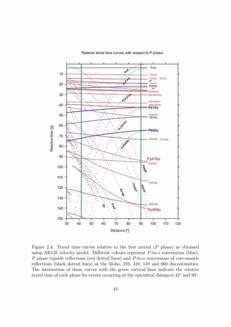
Figure 2.4: Travel time curves relative to the first arrival (P phase) as obtainedusing AK135 velocity model. Different colours represent P -to-s conversions (blue),P phase topside reflections (red dotted lines) and P -to-s conversions of core-mantlereflections (black dotted lines) at the Moho, 210, 410, 510 and 660 discontinuities.The intersection of these curves with the green vertical lines indicate the relativetravel time of each phase for events occurring at the epicentral distances 42◦ and 90◦.
44
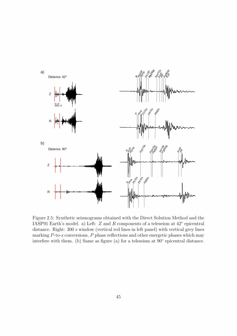
Figure 2.5: Synthetic seismograms obtained with the Direct Solution Method and theIASP91 Earth’s model. a) Left: Z and R components of a teleseism at 42◦ epicentraldistance. Right: 300 s window (vertical red lines in left panel) with vertical grey linesmarking P -to-s conversions, P phase reflections and other energetic phases which mayinterfere with them. (b) Same as figure (a) for a teleseism at 90◦ epicentral distance.
45
2.3.1 Generating synthetic data
Synthetic seismograms were generated using the WKBJ (Chapman et al., 1988) al-
gorithm and the convolutional model of the seismic trace. This algorithm provides
synthetic seismograms for body waves in a 1-D (spherical or flat) Earth using the
WKBJ approximation to solve the second order wave equation for high frequencies.
2.3.1.1 Convolutional model of the trace and Green functions
Seismic wave propagation in the Earth is approximated as linear, satisfying the prin-
ciple of superposition. This means that based on linear system theory, the wavefield
is fully characterized by the Earth’s impulse response.
The output of a linear system to an input signal is the convolution of the input
with the impulse response of the system. The impulse response of the Earth is known
as the Green function. For a lateral homogeneous Earth, with velocity and density
varying only with the Earth’s radius and as a high frequency approximation, this
Green function, g(t), is a series of impulses corresponding, in time and amplitude,
to reflection and transmission coefficients at layer boundaries. In this context, the
seismic trace, x(t), is the output of the Earth system when the input signal is the
time function of the source, s(t). The noise component, n(t), is additive. Thus,
using the convolutional model, the seismic trace can be expressed as:
x(t) = s(t) ∗ g(t) + n(t) (2.6)
2.3.1.2 WKBJ synthetic data and processing
The synthetic data was built by computing a simplified Green function of the R
and Z components with the WKBJ algorithm and using the AK135 (Kennett et al.,
1995) velocity model. To keep the seismic traces as simple as possible, our synthetic
seismograms consisted of P, pP and sP and their respective P -to-s conversions and
P reflections at the Moho, 210, 410 and 660 discontinuities. The Green functions
were computed for different source depths (0 km, 20 km and 35 km) and epicentral
distances every degree from 55◦ to 65◦, and were convolved with different source
functions for each event. The source functions were 10 to 12 seconds long and were
generated from random number sequences filtered in different frequency bands with
central frequency at 0.4 Hz (band width ∼ 0.6 Hz). Unless otherwise noted, the
46
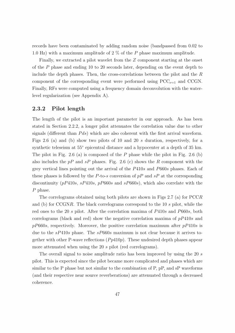
records have been contaminated by adding random noise (bandpassed from 0.02 to
1.0 Hz) with a maximum amplitude of 2 % of the P phase maximum amplitude.
Finally, we extracted a pilot wavelet from the Z component starting at the onset
of the P phase and ending 10 to 20 seconds later, depending on the event depth to
include the depth phases. Then, the cross-correlations between the pilot and the R
component of the corresponding event were performed using PCCν=1 and CCGN.
Finally, RFs were computed using a frequency domain deconvolution with the water-
level regularization (see Appendix A).
2.3.2 Pilot length
The length of the pilot is an important parameter in our approach. As has been
stated in Section 2.2.2, a longer pilot attenuates the correlation value due to other
signals (different than Pds) which are also coherent with the first arrival waveform.
Figs 2.6 (a) and (b) show two pilots of 10 and 20 s duration, respectively, for a
synthetic teleseism at 55◦ epicentral distance and a hypocenter at a depth of 35 km.
The pilot in Fig. 2.6 (a) is composed of the P phase while the pilot in Fig. 2.6 (b)
also includes the pP and sP phases. Fig. 2.6 (c) shows the R component with the
grey vertical lines pointing out the arrival of the P410s and P660s phases. Each of
these phases is followed by the P -to-s conversion of pP and sP at the corresponding
discontinuity (pP410s, sP410s, pP660s and sP660s), which also correlate with the
P phase.
The correlograms obtained using both pilots are shown in Figs 2.7 (a) for PCCR
and (b) for CCGNR. The black correlograms correspond to the 10 s pilot, while the
red ones to the 20 s pilot. After the correlation maxima of P410s and P660s, both
correlograms (black and red) show the negative correlation maxima of pP410s and
pP660s, respectively. Moreover, the positive correlation maximum after pP410s is
due to the sP410s phase. The sP660s maximum is not clear because it arrives to-
gether with other P-wave reflections (Pp410p). These undesired depth phases appear
more attenuated when using the 20 s pilot (red correlograms).
The overall signal to noise amplitude ratio has been improved by using the 20 s
pilot. This is expected since the pilot became more complicated and phases which are
similar to the P phase but not similar to the combination of P, pP, and sP waveforms
(and their respective near source reverberations) are attenuated through a decreased
coherence.
47
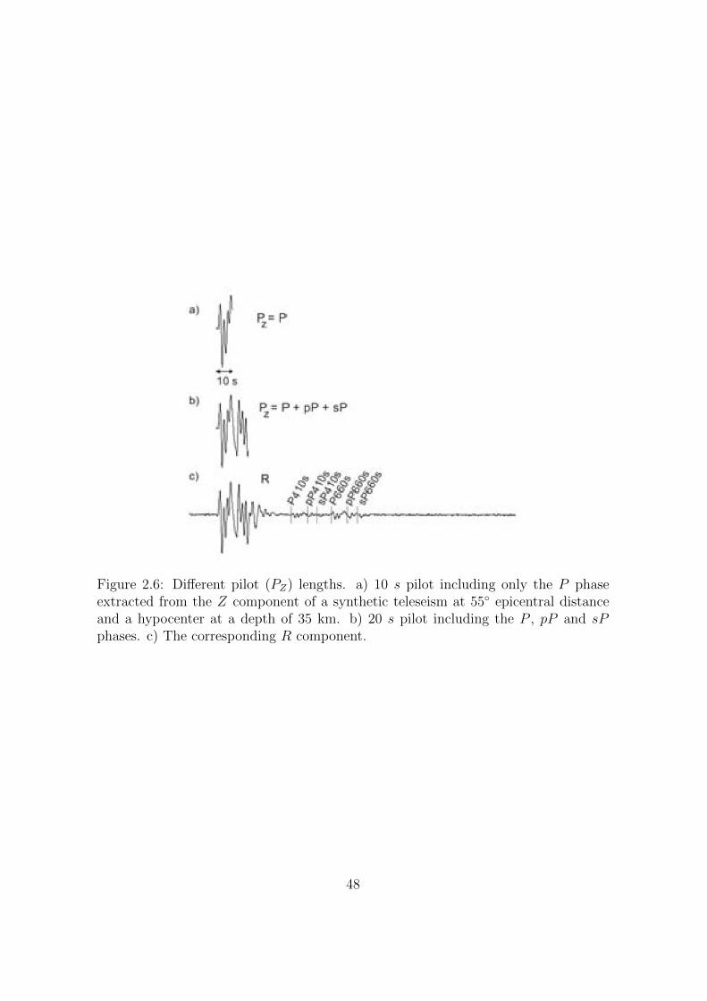
Figure 2.6: Different pilot (PZ) lengths. a) 10 s pilot including only the P phaseextracted from the Z component of a synthetic teleseism at 55◦ epicentral distanceand a hypocenter at a depth of 35 km. b) 20 s pilot including the P , pP and sPphases. c) The corresponding R component.
48
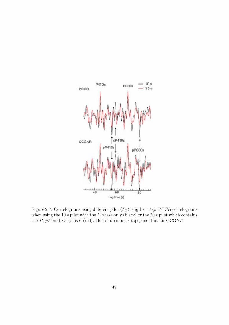
Figure 2.7: Correlograms using different pilot (PZ) lengths. Top: PCCR correlogramswhen using the 10 s pilot with the P phase only (black) or the 20 s pilot which containsthe P , pP and sP phases (red). Bottom: same as top panel but for CCGNR.
49
Figure 2.8: Synthetic seismogram contaminated with different noise levels, which weredefined as a percentage (2 %, 10 % and 15 %) of the P phase maximum amplitudein the Z component. Left: Z component. Right: R component. P410s and P660sare marked for a reference.
2.3.3 Noise influence
Ambient noise is perhaps the most disturbing component in seismograms because it
is always present and cannot be easily eliminated. Fortunately, the random waveform
nature of this noise and its relative low amplitude for strong events permit a good
performance of cross-correlations. On the other hand, noise may be amplified in
deconvolution (see equation A.5 in Appendix A). However, RFs with a good SNR
and with clear detections can be obtained by using an adequate water-level parameter
in the deconvolution. Normally, the optimum water-level parameter is achieved by
visual inspection of the resultant RF, which makes it a subjective election. In what
comes next, we are going to present synthetic seismograms contaminated with noise
of different amplitude to illustrate the PCC’s, CCGN’s and RF’s performance in the
presence of noise.
The synthetic seismograms in Fig. 2.8 have been contaminated with different
noise levels which were defined as a percentage (2 %, 10 % and 15 %) of the P phase
maximum amplitude in the Z component. From the R component (right panel), it can
be seen that P410s and P660s are obscured by the noise amplitude for increasing
noise levels (indicated at the right end of each trace). On the other hand, in the
50
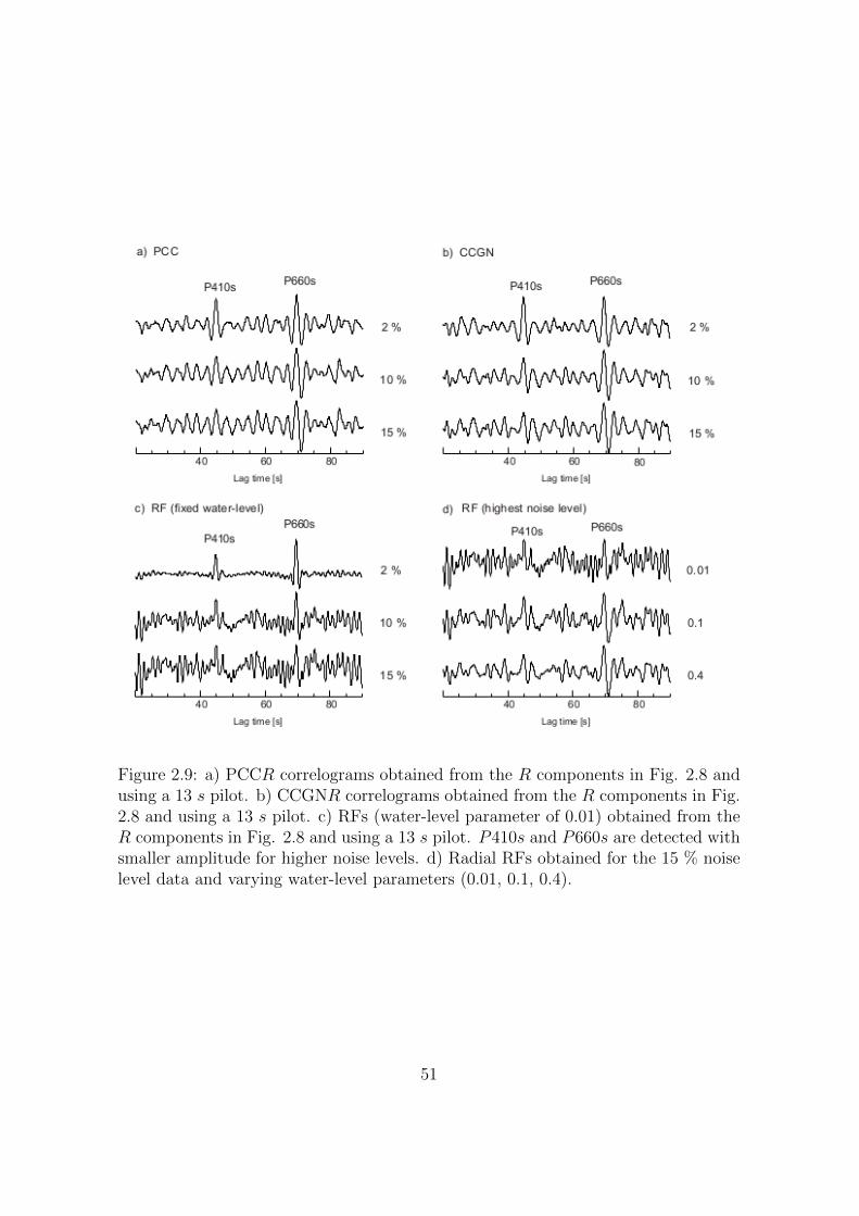
Figure 2.9: a) PCCR correlograms obtained from the R components in Fig. 2.8 andusing a 13 s pilot. b) CCGNR correlograms obtained from the R components in Fig.2.8 and using a 13 s pilot. c) RFs (water-level parameter of 0.01) obtained from theR components in Fig. 2.8 and using a 13 s pilot. P410s and P660s are detected withsmaller amplitude for higher noise levels. d) Radial RFs obtained for the 15 % noiselevel data and varying water-level parameters (0.01, 0.1, 0.4).
51
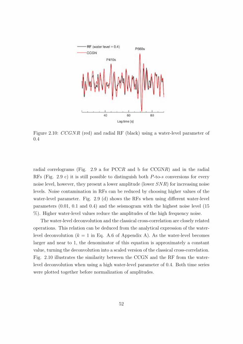
Figure 2.10: CCGNR (red) and radial RF (black) using a water-level parameter of0.4
radial correlograms (Fig. 2.9 a for PCCR and b for CCGNR) and in the radial
RFs (Fig. 2.9 c) it is still possible to distinguish both P -to-s conversions for every
noise level, however, they present a lower amplitude (lower SNR) for increasing noise
levels. Noise contamination in RFs can be reduced by choosing higher values of the
water-level parameter. Fig. 2.9 (d) shows the RFs when using different water-level
parameters (0.01, 0.1 and 0.4) and the seismogram with the highest noise level (15
%). Higher water-level values reduce the amplitudes of the high frequency noise.
The water-level deconvolution and the classical cross-correlation are closely related
operations. This relation can be deduced from the analytical expression of the water-
level deconvolution (k = 1 in Eq. A.6 of Appendix A). As the water-level becomes
larger and near to 1, the denominator of this equation is approximately a constant
value, turning the deconvolution into a scaled version of the classical cross-correlation.
Fig. 2.10 illustrates the similarity between the CCGN and the RF from the water-
level deconvolution when using a high water-level parameter of 0.4. Both time series
were plotted together before normalization of amplitudes.
52
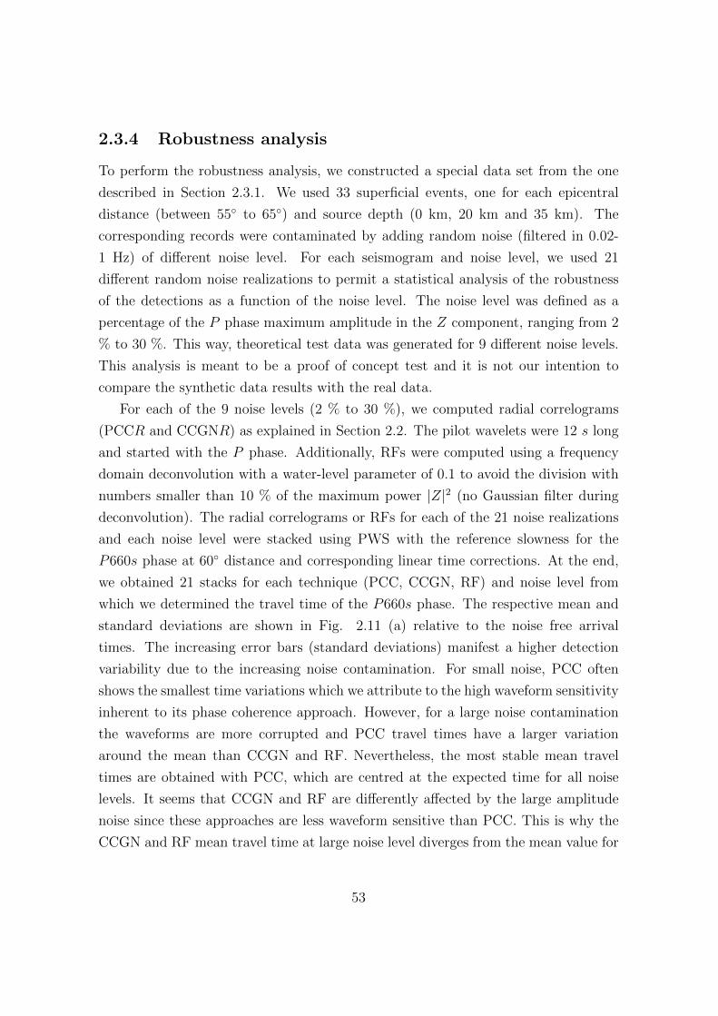
2.3.4 Robustness analysis
To perform the robustness analysis, we constructed a special data set from the one
described in Section 2.3.1. We used 33 superficial events, one for each epicentral
distance (between 55◦ to 65◦) and source depth (0 km, 20 km and 35 km). The
corresponding records were contaminated by adding random noise (filtered in 0.02-
1 Hz) of different noise level. For each seismogram and noise level, we used 21
different random noise realizations to permit a statistical analysis of the robustness
of the detections as a function of the noise level. The noise level was defined as a
percentage of the P phase maximum amplitude in the Z component, ranging from 2
% to 30 %. This way, theoretical test data was generated for 9 different noise levels.
This analysis is meant to be a proof of concept test and it is not our intention to
compare the synthetic data results with the real data.
For each of the 9 noise levels (2 % to 30 %), we computed radial correlograms
(PCCR and CCGNR) as explained in Section 2.2. The pilot wavelets were 12 s long
and started with the P phase. Additionally, RFs were computed using a frequency
domain deconvolution with a water-level parameter of 0.1 to avoid the division with
numbers smaller than 10 % of the maximum power |Z|2 (no Gaussian filter during
deconvolution). The radial correlograms or RFs for each of the 21 noise realizations
and each noise level were stacked using PWS with the reference slowness for the
P660s phase at 60◦ distance and corresponding linear time corrections. At the end,
we obtained 21 stacks for each technique (PCC, CCGN, RF) and noise level from
which we determined the travel time of the P660s phase. The respective mean and
standard deviations are shown in Fig. 2.11 (a) relative to the noise free arrival
times. The increasing error bars (standard deviations) manifest a higher detection
variability due to the increasing noise contamination. For small noise, PCC often
shows the smallest time variations which we attribute to the high waveform sensitivity
inherent to its phase coherence approach. However, for a large noise contamination
the waveforms are more corrupted and PCC travel times have a larger variation
around the mean than CCGN and RF. Nevertheless, the most stable mean travel
times are obtained with PCC, which are centred at the expected time for all noise
levels. It seems that CCGN and RF are differently affected by the large amplitude
noise since these approaches are less waveform sensitive than PCC. This is why the
CCGN and RF mean travel time at large noise level diverges from the mean value for
53
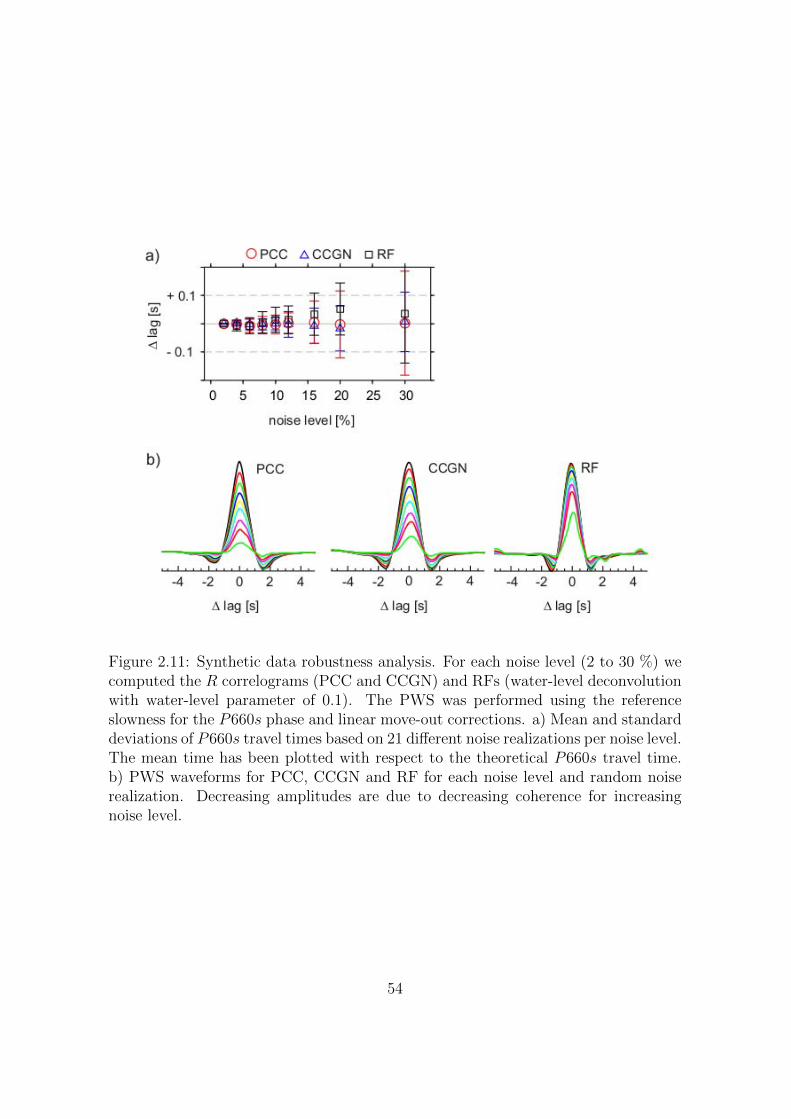
Figure 2.11: Synthetic data robustness analysis. For each noise level (2 to 30 %) wecomputed the R correlograms (PCC and CCGN) and RFs (water-level deconvolutionwith water-level parameter of 0.1). The PWS was performed using the referenceslowness for the P660s phase and linear move-out corrections. a) Mean and standarddeviations of P660s travel times based on 21 different noise realizations per noise level.The mean time has been plotted with respect to the theoretical P660s travel time.b) PWS waveforms for PCC, CCGN and RF for each noise level and random noiserealization. Decreasing amplitudes are due to decreasing coherence for increasingnoise level.
54
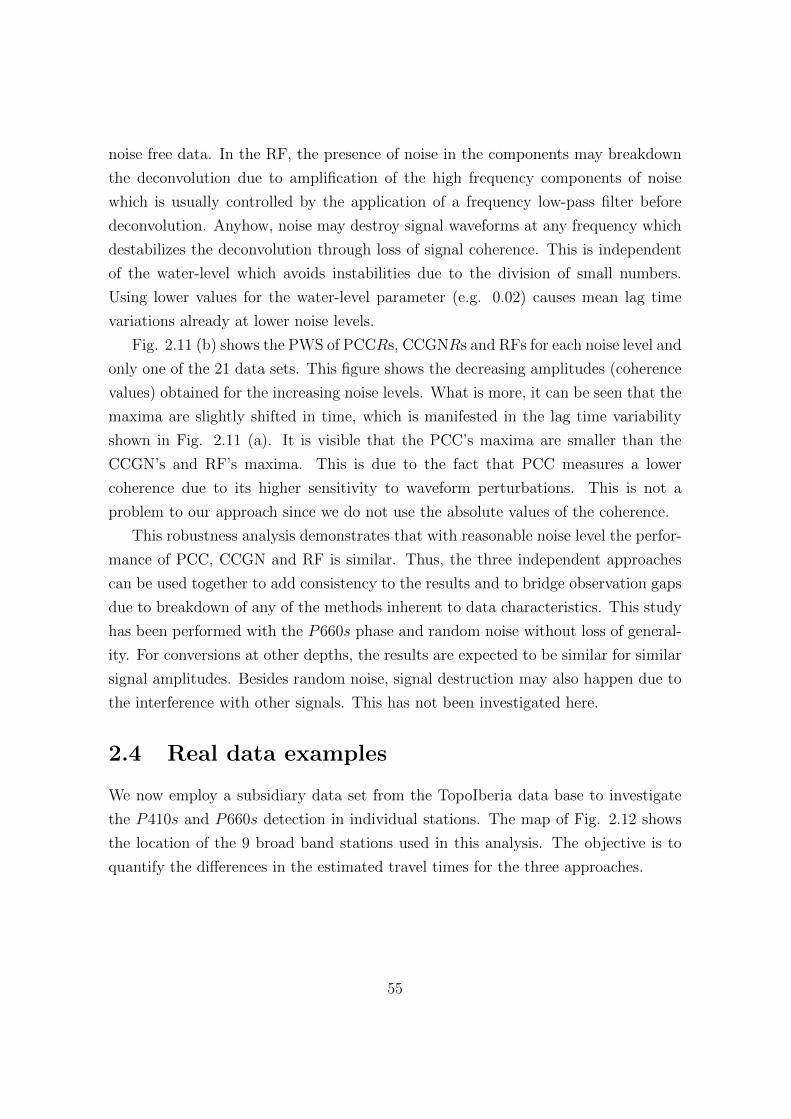
noise free data. In the RF, the presence of noise in the components may breakdown
the deconvolution due to amplification of the high frequency components of noise
which is usually controlled by the application of a frequency low-pass filter before
deconvolution. Anyhow, noise may destroy signal waveforms at any frequency which
destabilizes the deconvolution through loss of signal coherence. This is independent
of the water-level which avoids instabilities due to the division of small numbers.
Using lower values for the water-level parameter (e.g. 0.02) causes mean lag time
variations already at lower noise levels.
Fig. 2.11 (b) shows the PWS of PCCRs, CCGNRs and RFs for each noise level and
only one of the 21 data sets. This figure shows the decreasing amplitudes (coherence
values) obtained for the increasing noise levels. What is more, it can be seen that the
maxima are slightly shifted in time, which is manifested in the lag time variability
shown in Fig. 2.11 (a). It is visible that the PCC’s maxima are smaller than the
CCGN’s and RF’s maxima. This is due to the fact that PCC measures a lower
coherence due to its higher sensitivity to waveform perturbations. This is not a
problem to our approach since we do not use the absolute values of the coherence.
This robustness analysis demonstrates that with reasonable noise level the perfor-
mance of PCC, CCGN and RF is similar. Thus, the three independent approaches
can be used together to add consistency to the results and to bridge observation gaps
due to breakdown of any of the methods inherent to data characteristics. This study
has been performed with the P660s phase and random noise without loss of general-
ity. For conversions at other depths, the results are expected to be similar for similar
signal amplitudes. Besides random noise, signal destruction may also happen due to
the interference with other signals. This has not been investigated here.
2.4 Real data examples
We now employ a subsidiary data set from the TopoIberia data base to investigate
the P410s and P660s detection in individual stations. The map of Fig. 2.12 shows
the location of the 9 broad band stations used in this analysis. The objective is to
quantify the differences in the estimated travel times for the three approaches.
55
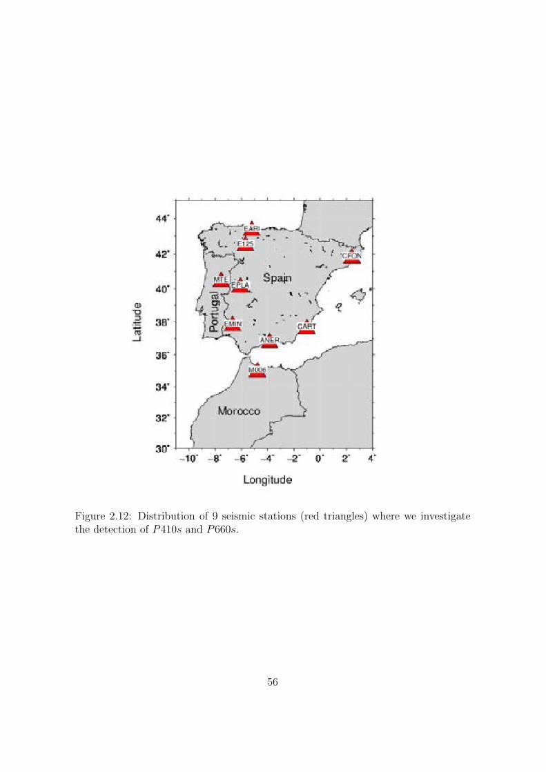
Figure 2.12: Distribution of 9 seismic stations (red triangles) where we investigatethe detection of P410s and P660s.
56
2.4.1 Processing
Based on the quality of the records, we selected for each station between 27 and
103 earthquakes for the available data from January 2007 to December 2011. The
epicentral distances are between 65◦ and 95◦ and the magnitude, mb, range is 5.1 to
7.2.
The Z and R components were bandpass filtered between 0.02 and 0.12 or 0.03 and
0.2 Hz. The choice of the frequency band for each station is based on the clarity of the
figures. From the Z components of each recorded event, we extracted a 100 s pilot,
which contains the P phase and part of its coda. Then, the cross-correlations (PCC
and CCGN) were performed between the pilot and the corresponding R component.
Additionally, RFs were computed using the water-level deconvolution with a water-
level parameter of 0.1. Two quality controls were applied over these RFs. The
RFs were discarded when the amplitudes prior to the P phase were larger than the
amplitudes after the P phase. The second condition was that the RFs must have
an amplitude maximum in the vicinity of zero seconds. After the quality control,
between 16 to 91 RFs were left for each station. For a direct comparison of the three
techniques, only data that pass the RFs quality controls were used.
Finally, the cross-correlation functions and RFs were stacked in the relative time
and slowness domain using the PWS. Further details on the processing are given in
Chapter 3, where the entire data set is being used to analyse the TZ beneath Iberia
and Morocco.
2.4.2 Detection of P -to-s conversions at individual stations
Fig. 2.13 shows the individual correlograms and RFs, which were move-out corrected
using a fixed relative slowness parameter of -0.1 s/◦ and a reference distance of 80◦,
for the stations in Fig. 2.12. Note that Fig. 2.13 continues in Appendix C. In general,
Fig. 2.13 shows that the individual RFs and CCGNRs have a better SNR than the
PCCRs. In this figure, the correlograms and RFs are arranged by increasing back
azimuth. The black amplitudes are positive and the grey ones are negative. On some
time-back azimuth sections, it is easy to distinguish the P410s and P660s phases
(e.g., ANER, CART, EMIN), which are the positive-amplitude signals close to the
theoretical travel times marked with the white lines at 42.8 s (P410s) and 65.8 s
(P660s). In other sections, it is more difficult to discriminate the P410s and P660s
57
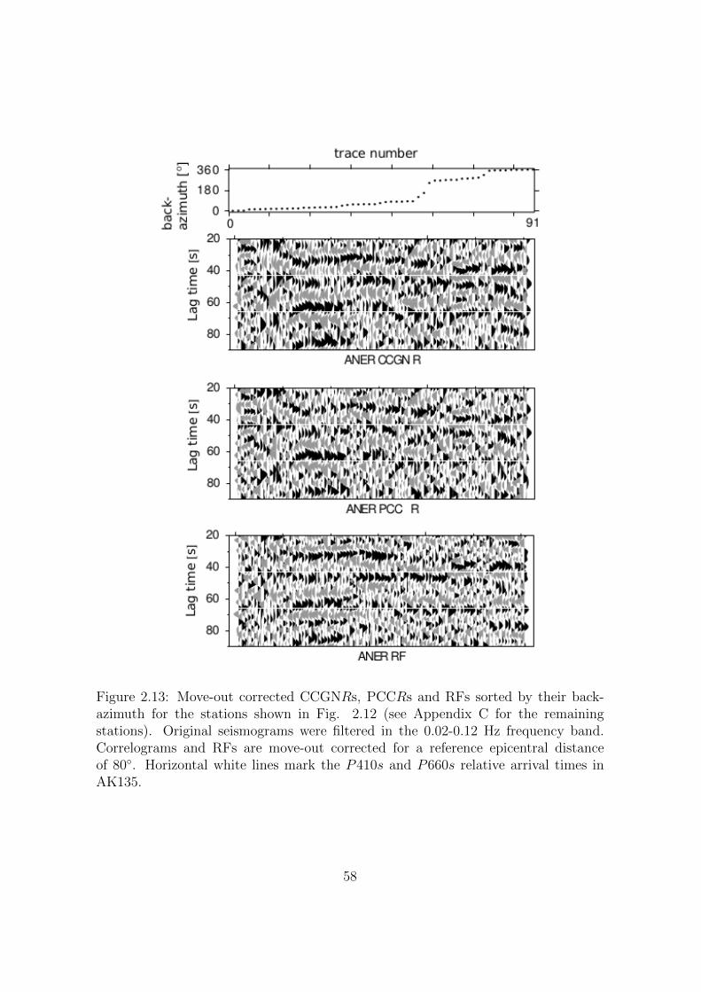
Figure 2.13: Move-out corrected CCGNRs, PCCRs and RFs sorted by their back-azimuth for the stations shown in Fig. 2.12 (see Appendix C for the remainingstations). Original seismograms were filtered in the 0.02-0.12 Hz frequency band.Correlograms and RFs are move-out corrected for a reference epicentral distanceof 80◦. Horizontal white lines mark the P410s and P660s relative arrival times inAK135.
58
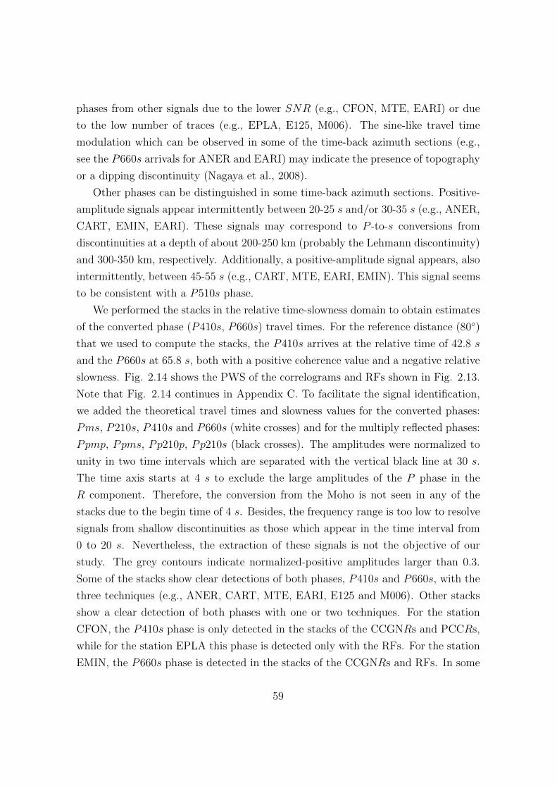
phases from other signals due to the lower SNR (e.g., CFON, MTE, EARI) or due
to the low number of traces (e.g., EPLA, E125, M006). The sine-like travel time
modulation which can be observed in some of the time-back azimuth sections (e.g.,
see the P660s arrivals for ANER and EARI) may indicate the presence of topography
or a dipping discontinuity (Nagaya et al., 2008).
Other phases can be distinguished in some time-back azimuth sections. Positive-
amplitude signals appear intermittently between 20-25 s and/or 30-35 s (e.g., ANER,
CART, EMIN, EARI). These signals may correspond to P -to-s conversions from
discontinuities at a depth of about 200-250 km (probably the Lehmann discontinuity)
and 300-350 km, respectively. Additionally, a positive-amplitude signal appears, also
intermittently, between 45-55 s (e.g., CART, MTE, EARI, EMIN). This signal seems
to be consistent with a P510s phase.
We performed the stacks in the relative time-slowness domain to obtain estimates
of the converted phase (P410s, P660s) travel times. For the reference distance (80◦)
that we used to compute the stacks, the P410s arrives at the relative time of 42.8 s
and the P660s at 65.8 s, both with a positive coherence value and a negative relative
slowness. Fig. 2.14 shows the PWS of the correlograms and RFs shown in Fig. 2.13.
Note that Fig. 2.14 continues in Appendix C. To facilitate the signal identification,
we added the theoretical travel times and slowness values for the converted phases:
Pms, P210s, P410s and P660s (white crosses) and for the multiply reflected phases:
Ppmp, Ppms, Pp210p, Pp210s (black crosses). The amplitudes were normalized to
unity in two time intervals which are separated with the vertical black line at 30 s.
The time axis starts at 4 s to exclude the large amplitudes of the P phase in the
R component. Therefore, the conversion from the Moho is not seen in any of the
stacks due to the begin time of 4 s. Besides, the frequency range is too low to resolve
signals from shallow discontinuities as those which appear in the time interval from
0 to 20 s. Nevertheless, the extraction of these signals is not the objective of our
study. The grey contours indicate normalized-positive amplitudes larger than 0.3.
Some of the stacks show clear detections of both phases, P410s and P660s, with the
three techniques (e.g., ANER, CART, MTE, EARI, E125 and M006). Other stacks
show a clear detection of both phases with one or two techniques. For the station
CFON, the P410s phase is only detected in the stacks of the CCGNRs and PCCRs,
while for the station EPLA this phase is detected only with the RFs. For the station
EMIN, the P660s phase is detected in the stacks of the CCGNRs and RFs. In some
59
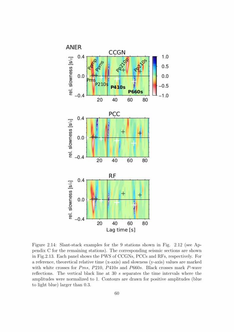
Figure 2.14: Slant-stack examples for the 9 stations shown in Fig. 2.12 (see Ap-pendix C for the remaining stations). The corresponding seismic sections are shownin Fig.2.13. Each panel shows the PWS of CCGNs, PCCs and RFs, respectively. Fora reference, theoretical relative time (x-axis) and slowness (y-axis) values are markedwith white crosses for Pms, P210, P410s and P660s. Black crosses mark P -wavereflections. The vertical black line at 30 s separates the time intervals where theamplitudes were normalized to 1. Contours are drawn for positive amplitudes (blueto light blue) larger than 0.3.
60
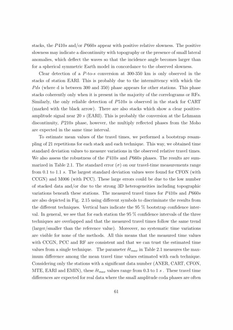
stacks, the P410s and/or P660s appear with positive relative slowness. The positive
slowness may indicate a discontinuity with topography or the presence of small lateral
anomalies, which deflect the waves so that the incidence angle becomes larger than
for a spherical symmetric Earth model in concordance to the observed slowness.
Clear detection of a P -to-s conversion at 300-350 km is only observed in the
stacks of station EARI. This is probably due to the intermittency with which the
Pds (where d is between 300 and 350) phase appears for other stations. This phase
stacks coherently only when it is present in the majority of the correlograms or RFs.
Similarly, the only reliable detection of P510s is observed in the stack for CART
(marked with the black arrow). There are also stacks which show a clear positive-
amplitude signal near 20 s (EARI). This is probably the conversion at the Lehmann
discontinuity, P210s phase, however, the multiply reflected phases from the Moho
are expected in the same time interval.
To estimate mean values of the travel times, we performed a bootstrap resam-
pling of 21 repetitions for each stack and each technique. This way, we obtained time
standard deviation values to measure variations in the observed relative travel times.
We also assess the robustness of the P410s and P660s phases. The results are sum-
marized in Table 2.1. The standard error (σ) on our travel-time measurements range
from 0.1 to 1.1 s. The largest standard deviation values were found for CFON (with
CCGN) and M006 (with PCC). These large errors could be due to the low number
of stacked data and/or due to the strong 3D heterogeneities including topographic
variations beneath these stations. The measured travel times for P410s and P660s
are also depicted in Fig. 2.15 using different symbols to discriminate the results from
the different techniques. Vertical bars indicate the 95 % bootstrap confidence inter-
val. In general, we see that for each station the 95 % confidence intervals of the three
techniques are overlapped and that the measured travel times follow the same trend
(larger/smaller than the reference value). Moreover, no systematic time variations
are visible for none of the methods. All this means that the measured time values
with CCGN, PCC and RF are consistent and that we can trust the estimated time
values from a single technique. The parameter δtmax in Table 2.1 measures the max-
imum difference among the mean travel time values estimated with each technique.
Considering only the stations with a significant data number (ANER, CART, CFON,
MTE, EARI and EMIN), these δtmax values range from 0.3 to 1 s . These travel time
differences are expected for real data where the small amplitude coda phases are often
61
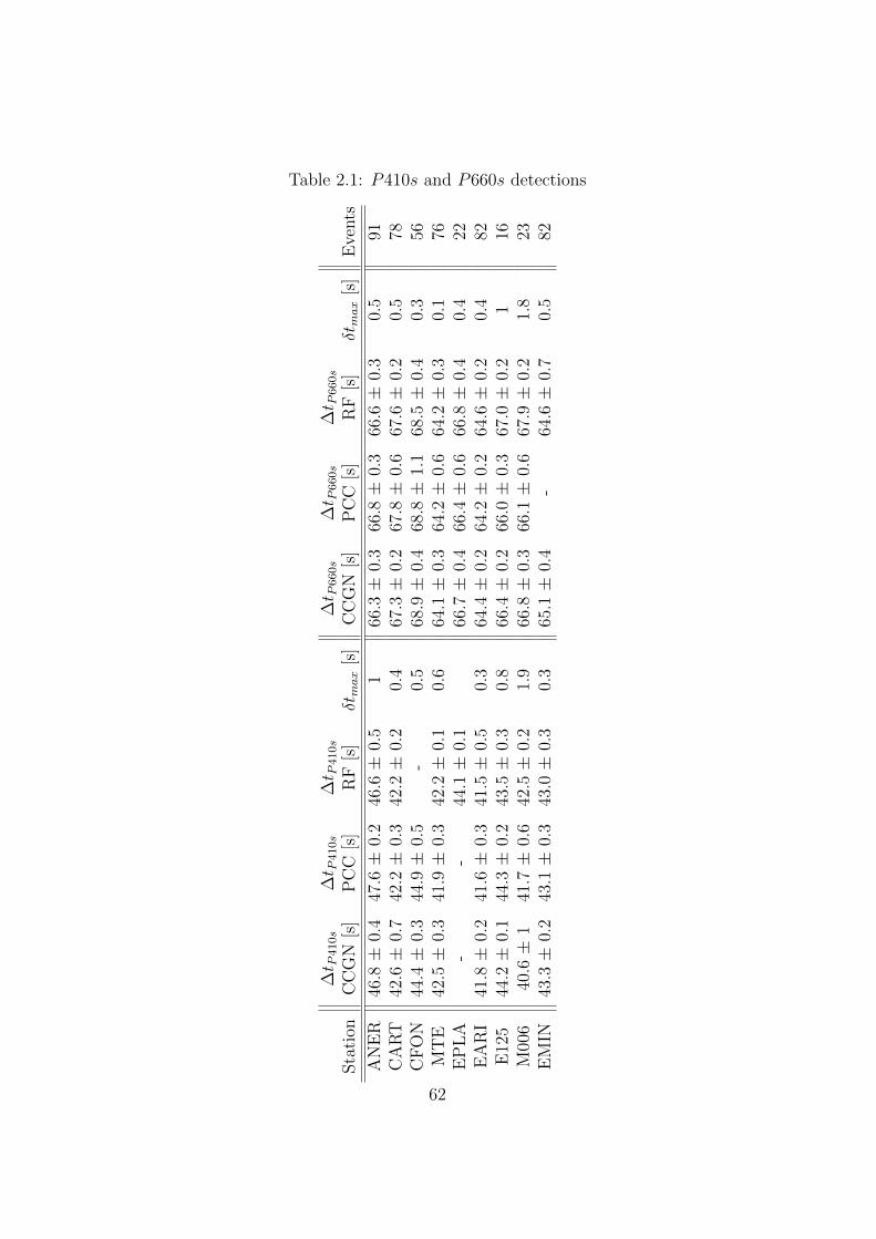
Table 2.1: P410s and P660s detections
∆t P
410s
∆t P
410s
∆t P
410s
∆t P
660s
∆t P
660s
∆t P
660s
Sta
tion
CC
GN
[s]
PC
C[s
]R
F[s
]δtmax
[s]
CC
GN
[s]
PC
C[s
]R
F[s
]δtmax
[s]
Ev e
nts
AN
ER
46.8±
0.4
47.6±
0.2
46.6±
0.5
166
.3±
0.3
66.8±
0.3
66.6±
0.3
0.5
91C
AR
T42
.6±
0.7
42.2±
0.3
42.2±
0.2
0.4
67.3±
0.2
67.8±
0.6
67.6±
0.2
0.5
78C
FO
N44
.4±
0.3
44.9±
0.5
-0.
568
.9±
0.4
68.8±
1.1
68.5±
0.4
0.3
56M
TE
42.5±
0.3
41.9±
0.3
42.2±
0.1
0.6
64.1±
0.3
64.2±
0.6
64.2±
0.3
0.1
76E
PL
A-
-44
.1±
0.1
66.7±
0.4
66.4±
0.6
66.8±
0.4
0.4
22E
AR
I41
.8±
0.2
41.6±
0.3
41.5±
0.5
0.3
64.4±
0.2
64.2±
0.2
64.6±
0.2
0.4
82E
125
44.2±
0.1
44.3±
0.2
43.5±
0.3
0.8
66.4±
0.2
66.0±
0.3
67.0±
0.2
116
M00
640
.6±
141
.7±
0.6
42.5±
0.2
1.9
66.8±
0.3
66.1±
0.6
67.9±
0.2
1.8
23E
MIN
43.3±
0.2
43.1±
0.3
43.0±
0.3
0.3
65.1±
0.4
-64
.6±
0.7
0.5
82
62
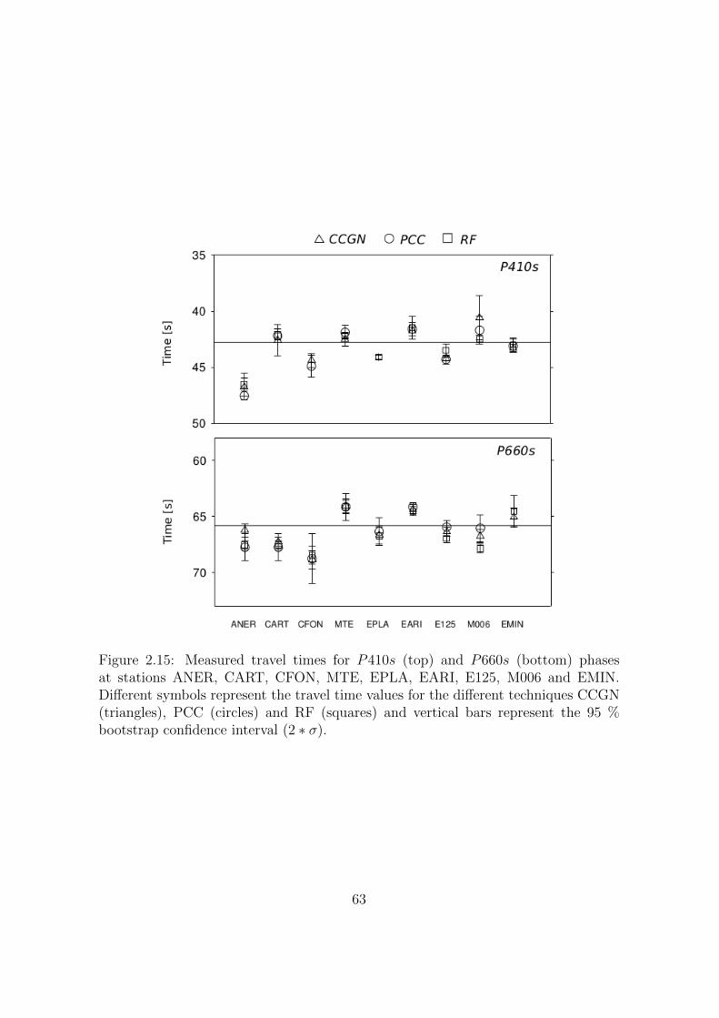
Figure 2.15: Measured travel times for P410s (top) and P660s (bottom) phasesat stations ANER, CART, CFON, MTE, EPLA, EARI, E125, M006 and EMIN.Different symbols represent the travel time values for the different techniques CCGN(triangles), PCC (circles) and RF (squares) and vertical bars represent the 95 %bootstrap confidence interval (2 ∗ σ).
63
obscured by other signals and noise, and where signals are less coherent due to the
presence of structural heterogeneities. As a consequence, the observed differences can
be attributed to the different strategies of the employed methods, which differently
handle the detection of less coherent signals. Differences in the travel time measure-
ments of the coda phases indicate data complexities and also indicate that at least
one of the approaches is less suited to accurately detect the signals due to the present
signal and noise characteristics for this detection. It is often not possible to deter-
mine which of the approaches provide the better time measurement and we therefore
understand the variations in the time measurements as an indicator of inconsisten-
cies due to data complexity. That is, the smaller the travel time variations among
the three methods, the more certain we are about having obtained a correct coda
phase detection. What is more, the mean travel time obtained from the detections
with the three techniques can stabilize against systematic and non-systematic errors.
Note that a small standard deviation of travel time measurements obtained for one
single approach cannot reveal systematic time errors due to some strange noise (e.g.,
see Fig. 2.11 at high noise level). Therefore, we propose to merge the independent
Pds (d=410 or 660) detections from each bootstrap repetition for each of the three
techniques. This way, robust mean and standard deviation values can be obtained
for the P410s and P660s travel times at each station.
2.5 Discussion and conclusions
We have presented a new processing approach based on cross-correlation and stacking
techniques to detect weak amplitude phases that arrive in the P phase coda. As cross-
correlation functional, we have used the CCGN, which is the classical approach to
measure waveform similarity and the PCC, which is based on instantaneous phase
coherence and which has not been widely explored before (Schimmel et al., 2011). We
have proposed to use these cross-correlations (PCC and CCGN) together with RFs
to stabilize the detections against errors and to bridge observation gaps. Without
noise or with low to reasonable noise level, the results of the three techniques are
similar but inherent to their different strategies the signals are detected differently.
Similar results obtained through different methods (Fig. 2.15) add robustness and
confidence to the detections and interpretations. Varying results or non-detections
are expected for more difficult data, depending on the signal and noise characteristics.
64
Therefore, the variations of the final results and the amount of approaches which lead
to an independent detection can be used as a quality indicator. Our procedure is a
step forward to stabilize against detection problems and to identify more ambiguous
detections. Another advantage is that one automatically bridges observation gaps
by one or the other method. Each difficult detection is a special case due to the
non-stationarity of signals and noise and none of the methods will lead to satisfying
detections for all cases.
PCC is amplitude unbiased and more sensitive to waveform coherence than CCGN
and RF. Coherent signals are therefore accurately detected even in the vicinity of
other larger amplitude signals which may bias the detections with CCGN (figs 3 and
4 in Schimmel (1999), fig. 1 in Schimmel et al. (2011)). Our synthetic data tests
(Fig. 2.11) show that PCC may even provide more stable results than CCGN and RF
at high noise levels. Of course, PCC fails when signals cannot be detected by their
coherence. In these cases, CCGN is usually the better approach. The water-level
deconvolution used to compute the RFs has the inconvenience that the choice of the
water-level parameter is a subjective task. However, we have used a fixed water-
level parameter of 0.1 and a quality control over the RFs amplitude, which simplify
the automatic computation of RFs. In practice, we see that the detection of P410s
and P660s in individual records is a more difficult task, which can be deduced from
the individual traces in the time-back azimuth sections (Fig. 2.13). We attribute
this complexity to the loss of waveform coherence with the reference phase, which is
particularly disadvantageous to the PCC. Nevertheless, the P410s and P660s phases
are well detected with the three techniques in the time-slowness domain. We observed
that the 95 % confidence interval of the estimated time values with each technique
are overlapped and that they follow the same trend, regardless of the technique. All
this suggests that the measured time values with CCGN, PCC and RF are consistent
and that we can rely on the estimated time values from a single technique.
Cross-correlations have been used before to detect P -to-s conversions from the
upper-mantle discontinuities (Paulssen, 1985, 1988; van der Lee et al., 1994; Schim-
mel, 1999). However, while we use a 100 s pilot wavelet, these studies used a shorter
one that comprises only the P phase or part of it, e.g. in Paulssen (1985, 1988) and
van der Lee et al. (1994) the pilots were about 5-6 s long. Besides, they normalized
the correlograms with respect to the auto-correlation maximum of the P phase, and
linear stacks were employed to identify the signals. Shearer (1991) resorted to the
65

cross-correlation between components to detect P -to-s conversions and other phases
using a global data set. For the Pds phases a 41 s reference wavelet was preferred
and correlation peaks were plotted without previous stacking. Similar to this study,
our approach can be used to detect other phases such as SdS, PdP , Sdp, etc with
an adequate definition of the pilot.
66

3Data set
68

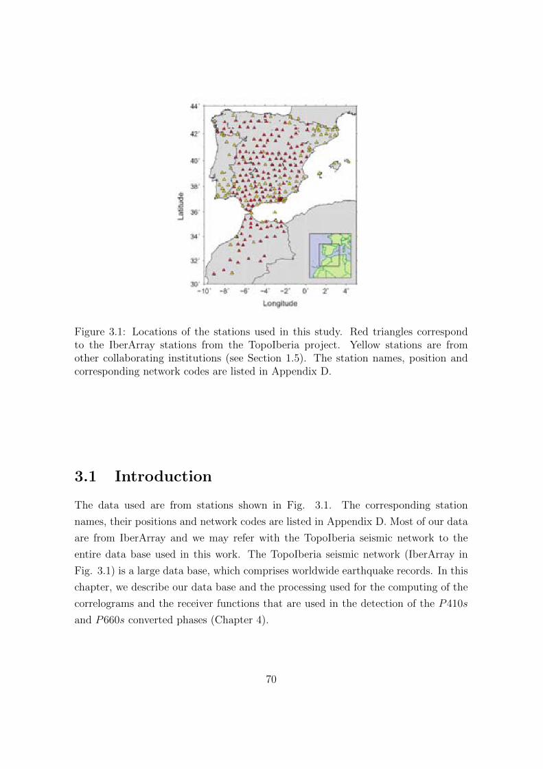
Figure 3.1: Locations of the stations used in this study. Red triangles correspondto the IberArray stations from the TopoIberia project. Yellow stations are fromother collaborating institutions (see Section 1.5). The station names, position andcorresponding network codes are listed in Appendix D.
3.1 Introduction
The data used are from stations shown in Fig. 3.1. The corresponding station
names, their positions and network codes are listed in Appendix D. Most of our data
are from IberArray and we may refer with the TopoIberia seismic network to the
entire data base used in this work. The TopoIberia seismic network (IberArray in
Fig. 3.1) is a large data base, which comprises worldwide earthquake records. In this
chapter, we describe our data base and the processing used for the computing of the
correlograms and the receiver functions that are used in the detection of the P410s
and P660s converted phases (Chapter 4).
70
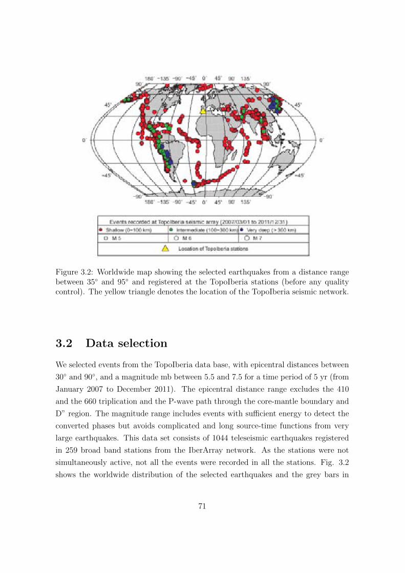
Figure 3.2: Worldwide map showing the selected earthquakes from a distance rangebetween 35◦ and 95◦ and registered at the TopoIberia stations (before any qualitycontrol). The yellow triangle denotes the location of the TopoIberia seismic network.
3.2 Data selection
We selected events from the TopoIberia data base, with epicentral distances between
30◦ and 90◦, and a magnitude mb between 5.5 and 7.5 for a time period of 5 yr (from
January 2007 to December 2011). The epicentral distance range excludes the 410
and the 660 triplication and the P-wave path through the core-mantle boundary and
D” region. The magnitude range includes events with sufficient energy to detect the
converted phases but avoids complicated and long source-time functions from very
large earthquakes. This data set consists of 1044 teleseismic earthquakes registered
in 259 broad band stations from the IberArray network. As the stations were not
simultaneously active, not all the events were recorded in all the stations. Fig. 3.2
shows the worldwide distribution of the selected earthquakes and the grey bars in
71
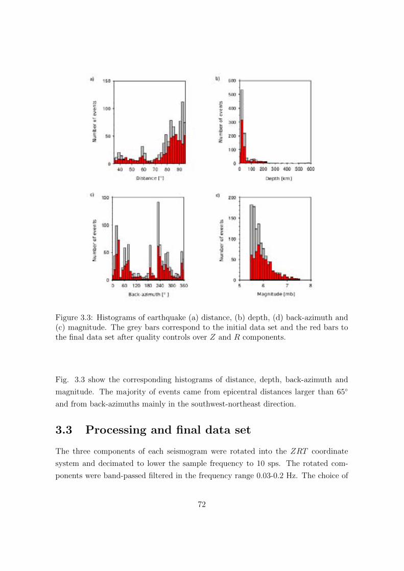
Figure 3.3: Histograms of earthquake (a) distance, (b) depth, (d) back-azimuth and(c) magnitude. The grey bars correspond to the initial data set and the red bars tothe final data set after quality controls over Z and R components.
Fig. 3.3 show the corresponding histograms of distance, depth, back-azimuth and
magnitude. The majority of events came from epicentral distances larger than 65◦
and from back-azimuths mainly in the southwest-northeast direction.
3.3 Processing and final data set
The three components of each seismogram were rotated into the ZRT coordinate
system and decimated to lower the sample frequency to 10 sps. The rotated com-
ponents were band-passed filtered in the frequency range 0.03-0.2 Hz. The choice of
72
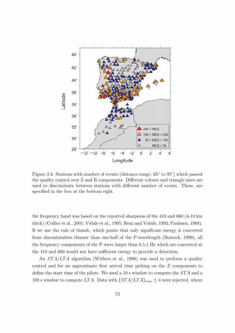
Figure 3.4: Stations with number of events (distance range: 65◦ to 95◦) which passedthe quality control over Z and R components. Different colours and triangle sizes areused to discriminate between stations with different number of events. These, arespecified in the box at the bottom right.
the frequency band was based on the reported sharpness of the 410 and 660 (4-10 km
thick) (Collier et al., 2001; Vidale et al., 1995; Benz and Vidale, 1993; Paulssen, 1988).
If we use the rule of thumb, which posits that only significant energy is converted
from discontinuities thinner than one-half of the P-wavelength (Bostock, 1999), all
the frequency components of the P-wave larger than 0.5-1 Hz which are converted at
the 410 and 660 would not have sufficient energy to provide a detection.
An STA/LTA algorithm (Withers et al., 1998) was used to perform a quality
control and for an approximate first arrival time picking on the Z components to
define the start time of the pilots. We used a 10 s window to compute the STA and a
100 s window to compute LTA. Data with {STA/LTA}max ≤ 4 were rejected, where
73
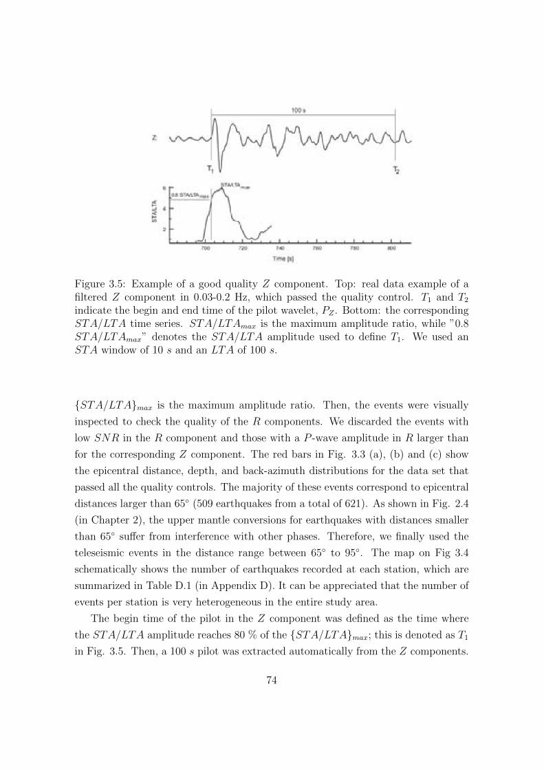
Figure 3.5: Example of a good quality Z component. Top: real data example of afiltered Z component in 0.03-0.2 Hz, which passed the quality control. T1 and T2indicate the begin and end time of the pilot wavelet, PZ . Bottom: the correspondingSTA/LTA time series. STA/LTAmax is the maximum amplitude ratio, while ”0.8STA/LTAmax” denotes the STA/LTA amplitude used to define T1. We used anSTA window of 10 s and an LTA of 100 s.
{STA/LTA}max is the maximum amplitude ratio. Then, the events were visually
inspected to check the quality of the R components. We discarded the events with
low SNR in the R component and those with a P -wave amplitude in R larger than
for the corresponding Z component. The red bars in Fig. 3.3 (a), (b) and (c) show
the epicentral distance, depth, and back-azimuth distributions for the data set that
passed all the quality controls. The majority of these events correspond to epicentral
distances larger than 65◦ (509 earthquakes from a total of 621). As shown in Fig. 2.4
(in Chapter 2), the upper mantle conversions for earthquakes with distances smaller
than 65◦ suffer from interference with other phases. Therefore, we finally used the
teleseismic events in the distance range between 65◦ to 95◦. The map on Fig 3.4
schematically shows the number of earthquakes recorded at each station, which are
summarized in Table D.1 (in Appendix D). It can be appreciated that the number of
events per station is very heterogeneous in the entire study area.
The begin time of the pilot in the Z component was defined as the time where
the STA/LTA amplitude reaches 80 % of the {STA/LTA}max; this is denoted as T1
in Fig. 3.5. Then, a 100 s pilot was extracted automatically from the Z components.
74
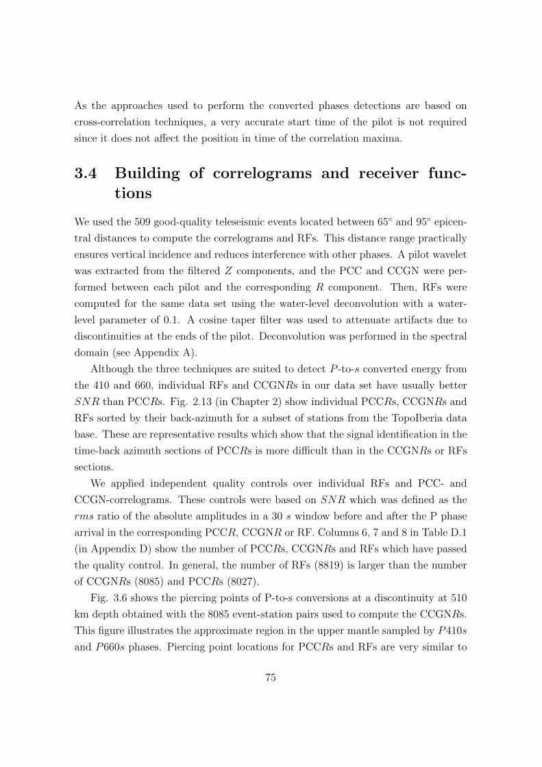
As the approaches used to perform the converted phases detections are based on
cross-correlation techniques, a very accurate start time of the pilot is not required
since it does not affect the position in time of the correlation maxima.
3.4 Building of correlograms and receiver func-
tions
We used the 509 good-quality teleseismic events located between 65◦ and 95◦ epicen-
tral distances to compute the correlograms and RFs. This distance range practically
ensures vertical incidence and reduces interference with other phases. A pilot wavelet
was extracted from the filtered Z components, and the PCC and CCGN were per-
formed between each pilot and the corresponding R component. Then, RFs were
computed for the same data set using the water-level deconvolution with a water-
level parameter of 0.1. A cosine taper filter was used to attenuate artifacts due to
discontinuities at the ends of the pilot. Deconvolution was performed in the spectral
domain (see Appendix A).
Although the three techniques are suited to detect P -to-s converted energy from
the 410 and 660, individual RFs and CCGNRs in our data set have usually better
SNR than PCCRs. Fig. 2.13 (in Chapter 2) show individual PCCRs, CCGNRs and
RFs sorted by their back-azimuth for a subset of stations from the TopoIberia data
base. These are representative results which show that the signal identification in the
time-back azimuth sections of PCCRs is more difficult than in the CCGNRs or RFs
sections.
We applied independent quality controls over individual RFs and PCC- and
CCGN-correlograms. These controls were based on SNR which was defined as the
rms ratio of the absolute amplitudes in a 30 s window before and after the P phase
arrival in the corresponding PCCR, CCGNR or RF. Columns 6, 7 and 8 in Table D.1
(in Appendix D) show the number of PCCRs, CCGNRs and RFs which have passed
the quality control. In general, the number of RFs (8819) is larger than the number
of CCGNRs (8085) and PCCRs (8027).
Fig. 3.6 shows the piercing points of P-to-s conversions at a discontinuity at 510
km depth obtained with the 8085 event-station pairs used to compute the CCGNRs.
This figure illustrates the approximate region in the upper mantle sampled by P410s
and P660s phases. Piercing point locations for PCCRs and RFs are very similar to
75
Figure 3.6: P510s piercing points (gray crosses) in the Iberian Peninsula and northMorocco for the teleseismic events located between 65◦ and 95◦ of epicentral distance.Black triangles show the station locations.
Fig. 3.6. The number of piercing points is larger in south Spain and its surroundings,
while the rest of the area presents a few less abundantly covered parts, such as the
north of Spain or the central part of Morocco, which is mostly due to the different
station deployment time during the selected time interval of the IberArray data base.
3.5 Data consistency
In this section, the whole data base is used to identify the upper-mantle conversions
on the R component arriving in the relative travel time interval between 25 s and 85
s. Additionally, the data consistency is investigated when the frequency band of the
76
filters and the pilot length change.
3.5.1 Frequency
PCC- and CCGN-correlograms and RFs were computed after filtering the whole data
set in three frequency bands with increasing frequency range (0.02-0.12 Hz, 0.03-0.2
Hz and 0.04-0.5 Hz) and using a 100 s long pilot. Linear time corrections were applied
using the reference slowness for the P510s phase at 80◦ distance and all the positive
peaks of PCCRs, CCGNRs and RFs were saved. These peaks constitute potential
detections of converted phases, since for the predicted upper-mantle conversion it
is expected that P (in the Z component) and Pds (in the R component) have the
same polarity. Fig. 3.7 shows the number of positive peaks per 1-s time interval
as function of relative time for each of the three techniques. The abscissa has been
normalized by the maximum number of peaks extracted from the highest frequency
band in the time interval 25-85 s to allow the comparison of results among the
different frequency bands. The mean value of peaks in the same interval has been
subtracted to eliminate the offset (in the abscissa) due to the increasing density of
maxima in individual PCCRs, CCGNRs and RFs for increasing frequency range.
Note that all maxima were used regardless their coherence or amplitude value. We
did not use the coherence or amplitude values because these are very similar for
all the peaks in individual PCCRs, CCGNRs and RFs. It is the relative number
of coherently stacked maxima which would provide the signal detection while the
influence of the coherence or amplitude value is smaller. This is a conclusion that
may be easily drawn from the observation of Figs 2.13 and 2.14 (in Chapter 2). In
Fig. 3.7, different line styles are used to discriminate the results from the three
frequency bands: continuous (0.02-0.12 Hz), dotted (0.03–0.2 Hz) and dotted-point
(0.04–0.5 Hz). Besides, vertical lines mark the theoretical arrival time of P410s (42.8
s) and P660s (65.8 s) at 80◦ epicentral distance for the reference model AK135.
The number of positive peaks for the three techniques shows two maxima which are
consistently seen in the three frequency bands and which correspond to the P410s
and P660s phases. For the three techniques, the number of peaks near the P410s
phase does not seem to depend much on the frequency band. Thus, the number
of potential detections of P410s in individual records does not increase or decrease
with the frequency band. On the other hand, the number of peaks for the P660s
77
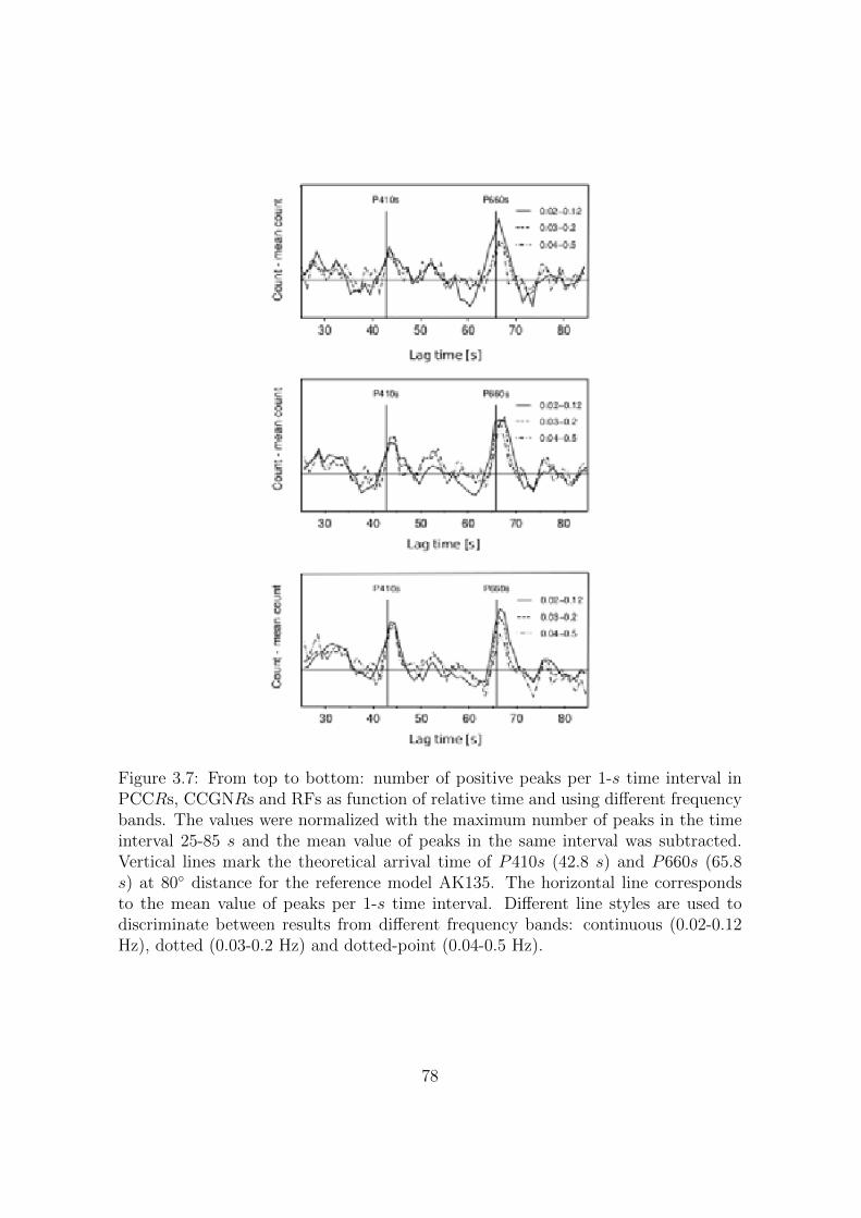
Figure 3.7: From top to bottom: number of positive peaks per 1-s time interval inPCCRs, CCGNRs and RFs as function of relative time and using different frequencybands. The values were normalized with the maximum number of peaks in the timeinterval 25-85 s and the mean value of peaks in the same interval was subtracted.Vertical lines mark the theoretical arrival time of P410s (42.8 s) and P660s (65.8s) at 80◦ distance for the reference model AK135. The horizontal line correspondsto the mean value of peaks per 1-s time interval. Different line styles are used todiscriminate between results from different frequency bands: continuous (0.02-0.12Hz), dotted (0.03-0.2 Hz) and dotted-point (0.04-0.5 Hz).
78
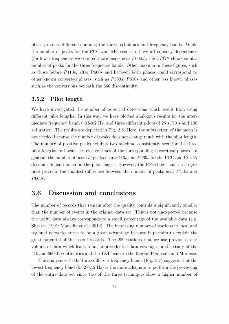
phase presents differences among the three techniques and frequency bands. While
the number of peaks for the PCC and RFs seems to have a frequency dependence
(for lower frequencies we counted more peaks near P660s), the CCGN shows similar
number of peaks for the three frequency bands. Other maxima in these figures, such
as those before P410s, after P660s and between both phases could correspond to
other known converted phases, such as P300s, P510s and other less known phases
such as the conversions beneath the 660 discontinuity.
3.5.2 Pilot length
We have investigated the number of potential detections which result from using
different pilot lengths. In this way, we have plotted analogous results for the inter-
mediate frequency band, 0.03-0.2 Hz, and three different pilots of 25 s, 50 s and 100
s duration. The results are depicted in Fig. 3.8. Here, the subtraction of the mean is
not needed because the number of peaks does not change much with the pilot length.
The number of positive peaks exhibits two maxima, consistently seen for the three
pilot lengths and near the relative times of the corresponding theoretical phases. In
general, the number of positive peaks near P410s and P660s for the PCC and CCGN
does not depend much on the pilot length. However, the RFs show that the largest
pilot presents the smallest difference between the number of peaks near P410s and
P660s.
3.6 Discussion and conclusions
The number of records that remain after the quality controls is significantly smaller
than the number of events in the original data set. This is not unexpected because
the useful data always corresponds to a small percentage of the available data (e.g.
Shearer, 1991; Mancilla et al., 2012). The increasing number of stations in local and
regional networks turns to be a great advantage because it permits to exploit the
great potential of the useful records. The 259 stations that we use provide a vast
volume of data which leads to an unprecedented data coverage for the study of the
410 and 660 discontinuities and the TZT beneath the Iberian Peninsula and Morocco.
The analysis with the three different frequency bands (Fig. 3.7) suggests that the
lowest frequency band (0.02-0.12 Hz) is the more adequate to perform the processing
of the entire data set since two of the three techniques show a higher number of
79
Figure 3.8: From top to bottom: number of positive peaks per 1-s time interval inPCCRs, CCGNRs and RFs as function of relative time as obtained when differentpilot lengths are used. The values were normalized with the maximum number ofpeaks in the time interval 25-85 s. The horizontal line corresponds to the mean valueof peaks per 1-s time interval. Different symbols are used to discriminate betweenresults from different pilot lengths: continuous (25 s), dotted (50 s) and dotted-point(100 s).
80
signals in the lower frequency band. However, the number of detections near P410s
and P660s for the three frequency bands and techniques is considerably larger than for
other time intervals. This enables us to conclude that any of the three frequency bands
proves to be a good choice. This result permits us to base our choice of frequency band
on other important aspects, such as time-slowness resolution and spatial resolution.
The higher frequency bands are more adequate to better constraint the P410s and
P660s detections in time and slowness. On the other hand, the spatial resolution is
also related to the frequency band. The spatial resolution is controlled by the size
of the first Fresnel zone. This zone comprises the area where the elementary waves
that belong to the same wave-front interfere with each other constructively, which in
practice is defined as the area where the travel paths differ by less than a half period
(Sheriff, 1996). The Pds signal is formed within the first Fresnel zone, which depends
on the frequency of the signal and the depth of the discontinuity, d. The first Fresnel
zone for the P660s phase at a depth of 660 km is a circular area with a radius of
about 100 km for the frequency band 0.03-0.2 Hz and of about 60 km for 0.04-0.5
Hz. This is so, if we consider that constructive interference occurs over travel paths
that differ by T/6 (T is the period which corresponds to the central frequency of the
frequency band). The corresponding radius of the first Fresnel zone for the P410s
phase at a depth of 410 km is about 70 km for 0.03-0.2 Hz and 50 km for 0.04-0.5
Hz. Thus, in the frequency band 0.03-0.2 Hz, the 410 (and 660) depth obtained with
a P -to-s conversion corresponds to a circular area of about 70 km (100 km) which is
also the approximate spatial resolution.
Additionally, the number of peaks near P410s and P660s for PCC and CCGN
does not show strong dependence on the pilot length choice. However, we have seen
that for the RFs the smallest differences between the number of detections near P410s
and P660s is obtained with the largest pilot. In line with this observation, in Chapter
2 we have shown that clear signal detection is obtained with a pilot sufficiently large
to contain the depth phases. Thus, we consider that the 100 s pilot is the more
adequate pilot length to perform the data processing. In general, for both analyses
(frequency and pilot length) we have seen that the number of signals near P660s is
always larger than near the P410s.
An interesting feature in Figs. 3.7 and 3.8 is the striking time shift of the number
of peaks near the P410s and P660s phases with respect to the reference values.
This is probably due to a not considered velocity structure beneath the study area.
81

Such effect can be minimized by applying time corrections based on realistic velocity
models for the study area.
82

4Transition zone discontinuities beneath
Iberia and Morocco
84

4.1 Introduction
In the general introduction of this thesis, we explained the importance of studying the
Earth’s discontinuities. They relate seismological observations to the Earth’s thermal
and chemical state with a precision that cannot be achieved by tomography studies.
In particular, the study of the TZT, and the 410 and 660 discontinuities provide
additional constraints on the upper-mantle thermal structure and composition.
Here, we map the 410 and 660 discontinuities through detection of P -to-s con-
verted phases and we estimate the TZT beneath the Ibero-Maghrebian region. Our
analysis is based on the extraordinary dataset obtained from 259 broad band sta-
tions mostly deployed by the TopoIberia project (Dıaz et al., 2009). In this study we
present the first detailed maps for the 410 and 660 discontinuities and the TZT in
the Ibero-Maghrebian region. Our analysis permits us to provide constraints on the
present-day upper-mantle thermal structure and composition beneath the study area.
We relate our results with the tomographic images by Villasenor et al. (2003) and
with the most recent tomography results by Monna et al. (2013) and Bezada et al.
(2013). We further explore evidences (independent of tomography) of the location
of the Alboran Sea slab at TZ depths and its possible relation with the occurrence
of deep localized earthquakes in this area (Buforn et al., 1995, 2011; Bezada and
Humphreys, 2012).
4.2 Data and method
Our data set has been extracted from the TopoIberia data already described in Chap-
ter 3. It is composed of 1044 events from epicentral distances between 30◦ and 90◦.
Of these, 509 events of distances between 65◦ and 95◦ have been used to carry out the
final processing. The selection of events is based on the SNR in the Z component
and on the subsequent visual check of the R component.
In order to map the 410 and 660 discontinuities in the Iberian Peninsula and
Morocco, P410s and P660s phases are detected in the seismic records using three
independent techniques (PCC, CCGN and RF) (see Bonatto et al. (2013) and Chapter
2 for further details on these techniques and for further references). The joint usage
86
of the three approaches adds consistency and robustness to our results and helps to
bridge observation gaps due to the breakdown of any of the approaches.
Correlograms and RFs are computed following the processing described in section
3.4 (Chapter 3). We analyse 8819 RFs, 8085 CCGNs and 8027 PCCs. To enhance
the weak-amplitude P -to-s conversions, we use the PWS (Schimmel and Paulssen,
1997) of correlograms (and RFs) in bins of common piercing point (CPP) areas. The
robustness of the detected signals is evaluated using a bootstrap resampling approach
(Efron and Tibshitani, 1986). Finally, robust detections are visually inspected and
converted to depth through an adequate velocity model.
4.2.1 Stacking of correlograms and receiver functions
In order to stack, the data need to be grouped into bins. The bin size is a trade
off between the number of piercing points inside the bin (larger bins contain more
piercing points increasing the SNR of the stacks) and the spatial resolution controlled
by the Fresnel zone (larger bins average the discontinuity depth over areas which can
be larger than the Fresnel zone). The piercing point density depends on the station
and event distribution and is variable over the entire study region. The variable
piercing point density implies a variable discontinuity visibility, which we account for
using adaptive bins of variable size depending on the local number of piercing points.
On the other hand, to exploit the high spatial resolution of the converted phases and
to avoid signal destruction due to destructive interference, we use bin sizes smaller
than the first Fresnel zone of the P660s phase. For the used frequency band, this
zone is a circular area with a diameter of about 2◦ (see Discussion in Chapter 3).
The bin sizes vary between 0.8◦, 1◦ and 1.6◦ width in latitude and longitude and
were located every 0.25◦ in both directions (see schematic example of the bin size
and overlap in Fig. 4.1 a). Although the grid step results in variable redundancy,
we choose to use a homogeneous grid for a better numerical treatment of the results.
Fig. 4.1 (b) shows the location of the centre of each bin. The grid is composed of
1391 bins for PCC, 1396 for CCGN and 1400 for RF. The bin size at each centre
location for the CCGN-correlograms is depicted in Fig. 4.1 (c) using different colours
to discriminate between bins of different size: blue (0.8◦ width), red (1◦ width) and
yellow (1.6◦ width). The number of piercing points per bin which equals the number
of CCGN-correlograms to be stacked for each bin is shown in Fig. 4.1 (d). This last
87
figure shows the available data density and areas where we expect a higher robustness
of results due to the higher discretization into independent data bins. The best data
coverage is in the southern Iberian region and in the Pyrenees. Analogous figures for
the PCC-correlograms and RFs are shown in Fig. 4.2. Small differences in the data
coverage are observed when comparing Fig. 4.1 (d), Fig. 4.2 (b) and Fig. 4.2 (d),
which, however, do not have a meaningful influence on the results.
For an unambiguous detection of P410s and P660s, the data are stacked per bin
using the PWS in the time-slowness domain (as shown in Figs 2.3 c and d). The
robustness of the measurements is assessed during the stacking as outlined in the
following section 4.2.2.
4.2.2 Robustness analysis and quality criteria
A bootstrapping technique (Efron and Tibshitani, 1986) of 21 repetitions has been
used to estimate the uncertainties in our relative travel time measurements, tP410s−tPand tP660s−tP . For each bin we randomly pick the same number of radial correlograms
(or RFs) and we perform the stack in the relative time and slowness domain. Finally,
we use the 21 stacks to compute mean and standard deviation values of relative travel
time and slowness for each detected signal. The signals are identified as positive or
negative maxima with amplitude larger than twice the absolute mean amplitude of
the stack in the time interval 30–80 s but we only consider the positive amplitude
signals, which correspond to the expected polarity for the P410s and P660s phases.
This has been done for each bin and processing technique (PCC, CCGN and RF) to
assess the robustness of the individual detections per bin.
In order to discard bins with ambiguous P410s and P660s detections, an auto-
matic quality control has been performed by analysing the positive amplitude maxima
in the time-slowness stacks. We discard stacks (of PCCRs, CCGNRs or RFs) without
signals inside the time intervals 36.8-48.8 s and 59.8-71.8 s, and the relative slowness
interval of ± 0.4 s/◦. These time intervals are defined as ± 5 s from the P410s
and P660s relative times in AK135 (Kennett et al., 1995) for a reference distance
of 80◦, which are 42.8 s for tP410s − tP and 65.8 s for tP660s − tP . Additionally, we
discard signals with bootstrap uncertainty larger than 1.5 s. This time uncertainty
corresponds to a depth uncertainty value of about 15 km for the 410 and 660. Fi-
nally, the number of bins with stacks that satisfy the automatic quality criterion are
88
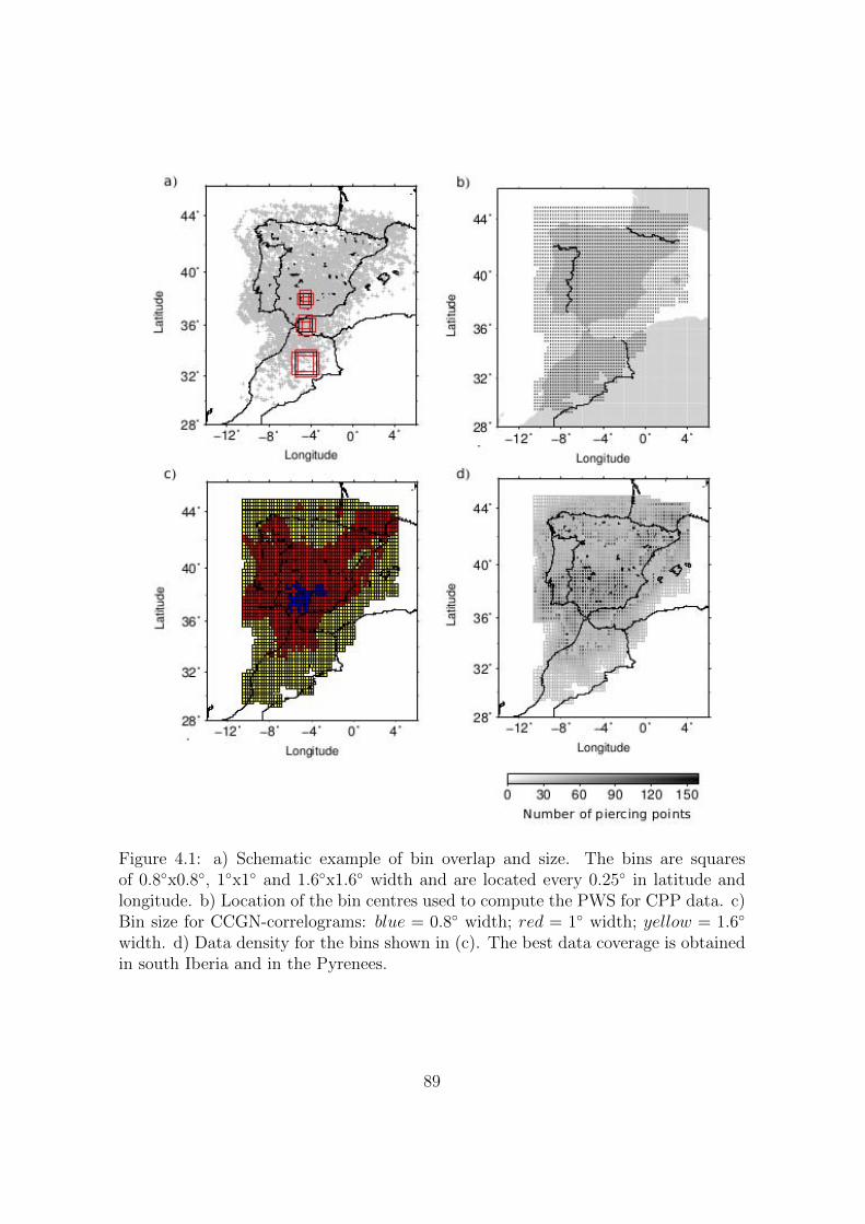
Figure 4.1: a) Schematic example of bin overlap and size. The bins are squaresof 0.8◦x0.8◦, 1◦x1◦ and 1.6◦x1.6◦ width and are located every 0.25◦ in latitude andlongitude. b) Location of the bin centres used to compute the PWS for CPP data. c)Bin size for CCGN-correlograms: blue = 0.8◦ width; red = 1◦ width; yellow = 1.6◦
width. d) Data density for the bins shown in (c). The best data coverage is obtainedin south Iberia and in the Pyrenees.
89
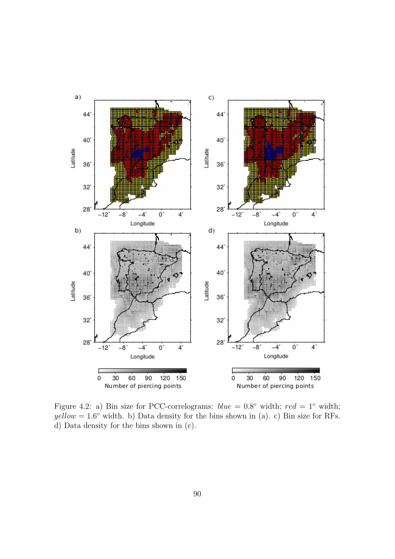
Figure 4.2: a) Bin size for PCC-correlograms: blue = 0.8◦ width; red = 1◦ width;yellow = 1.6◦ width. b) Data density for the bins shown in (a). c) Bin size for RFs.d) Data density for the bins shown in (c).
90
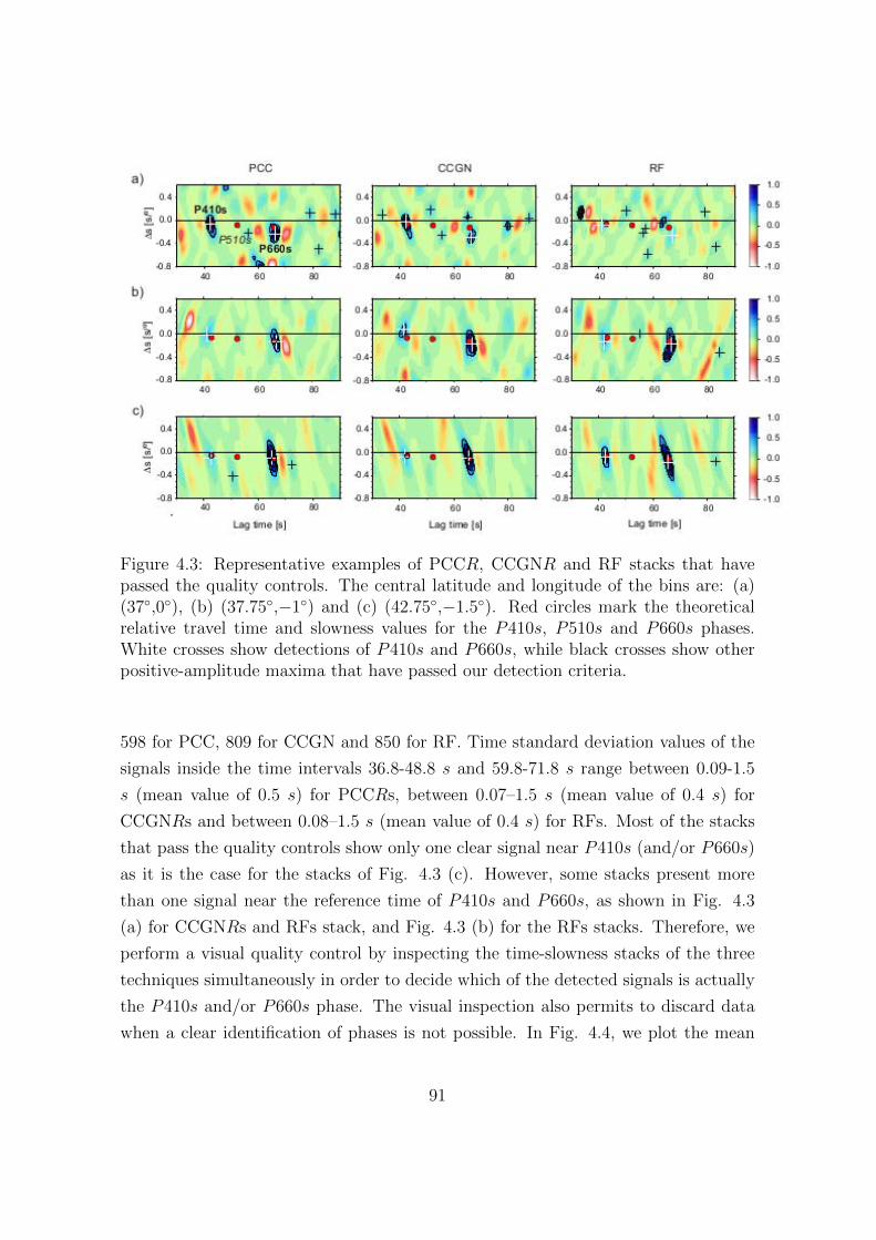
Figure 4.3: Representative examples of PCCR, CCGNR and RF stacks that havepassed the quality controls. The central latitude and longitude of the bins are: (a)(37◦,0◦), (b) (37.75◦,−1◦) and (c) (42.75◦,−1.5◦). Red circles mark the theoreticalrelative travel time and slowness values for the P410s, P510s and P660s phases.White crosses show detections of P410s and P660s, while black crosses show otherpositive-amplitude maxima that have passed our detection criteria.
598 for PCC, 809 for CCGN and 850 for RF. Time standard deviation values of the
signals inside the time intervals 36.8-48.8 s and 59.8-71.8 s range between 0.09-1.5
s (mean value of 0.5 s) for PCCRs, between 0.07–1.5 s (mean value of 0.4 s) for
CCGNRs and between 0.08–1.5 s (mean value of 0.4 s) for RFs. Most of the stacks
that pass the quality controls show only one clear signal near P410s (and/or P660s)
as it is the case for the stacks of Fig. 4.3 (c). However, some stacks present more
than one signal near the reference time of P410s and P660s, as shown in Fig. 4.3
(a) for CCGNRs and RFs stack, and Fig. 4.3 (b) for the RFs stacks. Therefore, we
perform a visual quality control by inspecting the time-slowness stacks of the three
techniques simultaneously in order to decide which of the detected signals is actually
the P410s and/or P660s phase. The visual inspection also permits to discard data
when a clear identification of phases is not possible. In Fig. 4.4, we plot the mean
91
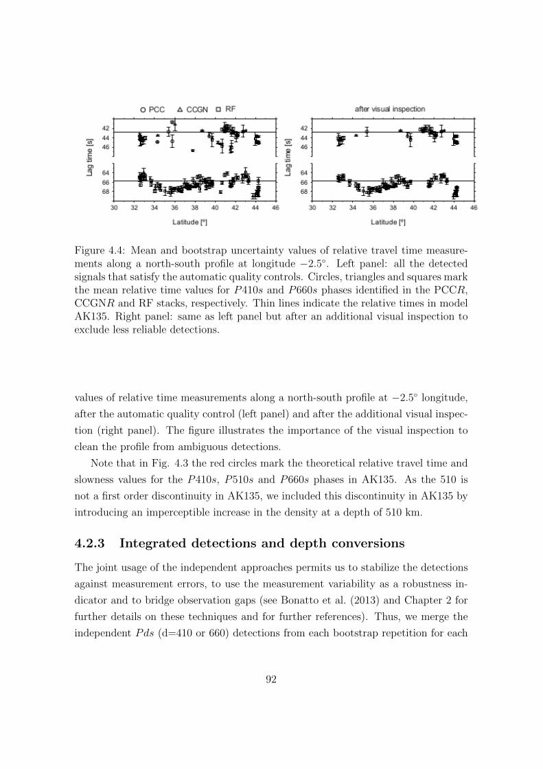
Figure 4.4: Mean and bootstrap uncertainty values of relative travel time measure-ments along a north-south profile at longitude −2.5◦. Left panel: all the detectedsignals that satisfy the automatic quality controls. Circles, triangles and squares markthe mean relative time values for P410s and P660s phases identified in the PCCR,CCGNR and RF stacks, respectively. Thin lines indicate the relative times in modelAK135. Right panel: same as left panel but after an additional visual inspection toexclude less reliable detections.
values of relative time measurements along a north-south profile at −2.5◦ longitude,
after the automatic quality control (left panel) and after the additional visual inspec-
tion (right panel). The figure illustrates the importance of the visual inspection to
clean the profile from ambiguous detections.
Note that in Fig. 4.3 the red circles mark the theoretical relative travel time and
slowness values for the P410s, P510s and P660s phases in AK135. As the 510 is
not a first order discontinuity in AK135, we included this discontinuity in AK135 by
introducing an imperceptible increase in the density at a depth of 510 km.
4.2.3 Integrated detections and depth conversions
The joint usage of the independent approaches permits us to stabilize the detections
against measurement errors, to use the measurement variability as a robustness in-
dicator and to bridge observation gaps (see Bonatto et al. (2013) and Chapter 2 for
further details on these techniques and for further references). Thus, we merge the
independent Pds (d=410 or 660) detections from each bootstrap repetition for each
92
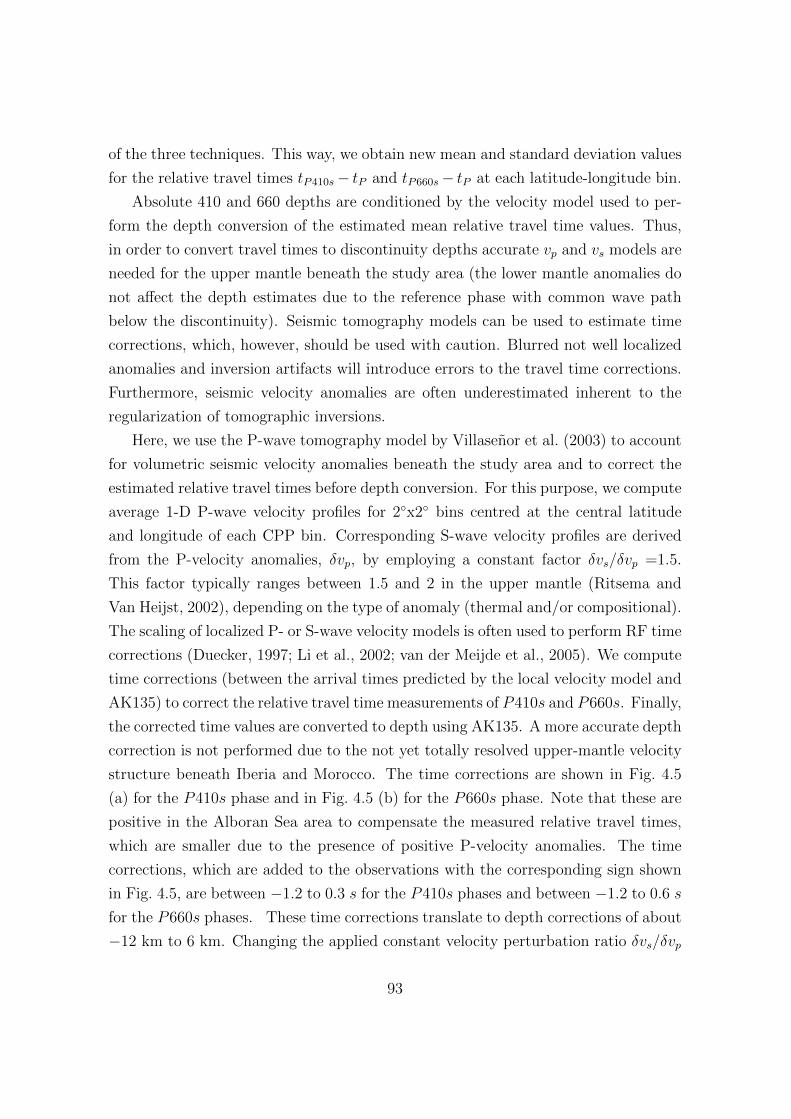
of the three techniques. This way, we obtain new mean and standard deviation values
for the relative travel times tP410s− tP and tP660s− tP at each latitude-longitude bin.
Absolute 410 and 660 depths are conditioned by the velocity model used to per-
form the depth conversion of the estimated mean relative travel time values. Thus,
in order to convert travel times to discontinuity depths accurate vp and vs models are
needed for the upper mantle beneath the study area (the lower mantle anomalies do
not affect the depth estimates due to the reference phase with common wave path
below the discontinuity). Seismic tomography models can be used to estimate time
corrections, which, however, should be used with caution. Blurred not well localized
anomalies and inversion artifacts will introduce errors to the travel time corrections.
Furthermore, seismic velocity anomalies are often underestimated inherent to the
regularization of tomographic inversions.
Here, we use the P-wave tomography model by Villasenor et al. (2003) to account
for volumetric seismic velocity anomalies beneath the study area and to correct the
estimated relative travel times before depth conversion. For this purpose, we compute
average 1-D P-wave velocity profiles for 2◦x2◦ bins centred at the central latitude
and longitude of each CPP bin. Corresponding S-wave velocity profiles are derived
from the P-velocity anomalies, δvp, by employing a constant factor δvs/δvp =1.5.
This factor typically ranges between 1.5 and 2 in the upper mantle (Ritsema and
Van Heijst, 2002), depending on the type of anomaly (thermal and/or compositional).
The scaling of localized P- or S-wave velocity models is often used to perform RF time
corrections (Duecker, 1997; Li et al., 2002; van der Meijde et al., 2005). We compute
time corrections (between the arrival times predicted by the local velocity model and
AK135) to correct the relative travel time measurements of P410s and P660s. Finally,
the corrected time values are converted to depth using AK135. A more accurate depth
correction is not performed due to the not yet totally resolved upper-mantle velocity
structure beneath Iberia and Morocco. The time corrections are shown in Fig. 4.5
(a) for the P410s phase and in Fig. 4.5 (b) for the P660s phase. Note that these are
positive in the Alboran Sea area to compensate the measured relative travel times,
which are smaller due to the presence of positive P-velocity anomalies. The time
corrections, which are added to the observations with the corresponding sign shown
in Fig. 4.5, are between −1.2 to 0.3 s for the P410s phases and between −1.2 to 0.6 s
for the P660s phases. These time corrections translate to depth corrections of about
−12 km to 6 km. Changing the applied constant velocity perturbation ratio δvs/δvp
93
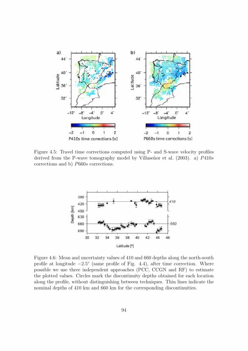
Figure 4.5: Travel time corrections computed using P- and S-wave velocity profilesderived from the P-wave tomography model by Villasenor et al. (2003). a) P410scorrections and b) P660s corrections.
Figure 4.6: Mean and uncertainty values of 410 and 660 depths along the north-southprofile at longitude −2.5◦ (same profile of Fig. 4.4), after time correction. Wherepossible we use three independent approaches (PCC, CCGN and RF) to estimatethe plotted values. Circles mark the discontinuity depths obtained for each locationalong the profile, without distinguishing between techniques. Thin lines indicate thenominal depths of 410 km and 660 km for the corresponding discontinuities.
94
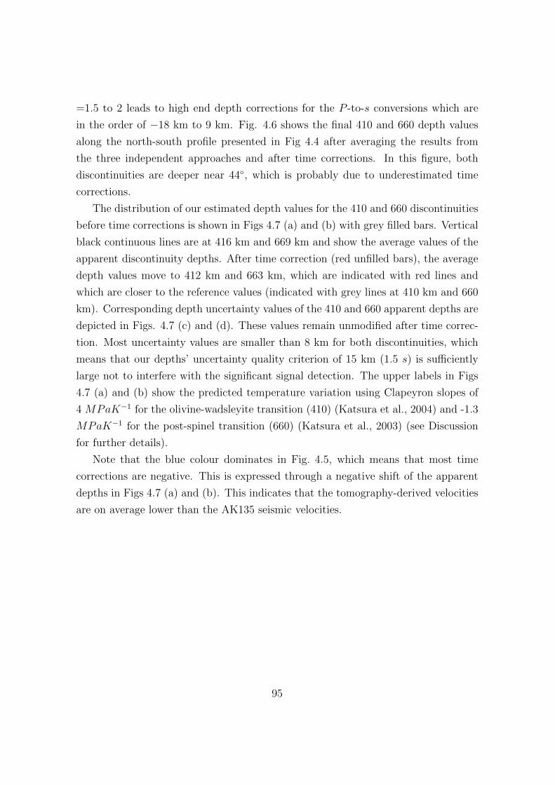
=1.5 to 2 leads to high end depth corrections for the P -to-s conversions which are
in the order of −18 km to 9 km. Fig. 4.6 shows the final 410 and 660 depth values
along the north-south profile presented in Fig 4.4 after averaging the results from
the three independent approaches and after time corrections. In this figure, both
discontinuities are deeper near 44◦, which is probably due to underestimated time
corrections.
The distribution of our estimated depth values for the 410 and 660 discontinuities
before time corrections is shown in Figs 4.7 (a) and (b) with grey filled bars. Vertical
black continuous lines are at 416 km and 669 km and show the average values of the
apparent discontinuity depths. After time correction (red unfilled bars), the average
depth values move to 412 km and 663 km, which are indicated with red lines and
which are closer to the reference values (indicated with grey lines at 410 km and 660
km). Corresponding depth uncertainty values of the 410 and 660 apparent depths are
depicted in Figs. 4.7 (c) and (d). These values remain unmodified after time correc-
tion. Most uncertainty values are smaller than 8 km for both discontinuities, which
means that our depths’ uncertainty quality criterion of 15 km (1.5 s) is sufficiently
large not to interfere with the significant signal detection. The upper labels in Figs
4.7 (a) and (b) show the predicted temperature variation using Clapeyron slopes of
4 MPaK−1 for the olivine-wadsleyite transition (410) (Katsura et al., 2004) and -1.3
MPaK−1 for the post-spinel transition (660) (Katsura et al., 2003) (see Discussion
for further details).
Note that the blue colour dominates in Fig. 4.5, which means that most time
corrections are negative. This is expressed through a negative shift of the apparent
depths in Figs 4.7 (a) and (b). This indicates that the tomography-derived velocities
are on average lower than the AK135 seismic velocities.
95
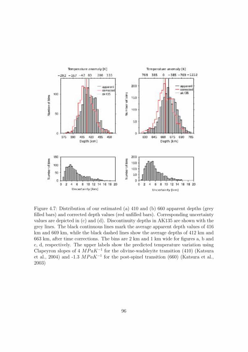
Figure 4.7: Distribution of our estimated (a) 410 and (b) 660 apparent depths (greyfilled bars) and corrected depth values (red unfilled bars). Corresponding uncertaintyvalues are depicted in (c) and (d). Discontinuity depths in AK135 are shown with thegrey lines. The black continuous lines mark the average apparent depth values of 416km and 669 km, while the black dashed lines show the average depths of 412 km and663 km, after time corrections. The bins are 2 km and 1 km wide for figures a, b andc, d, respectively. The upper labels show the predicted temperature variation usingClapeyron slopes of 4 MPaK−1 for the olivine-wadsleyite transition (410) (Katsuraet al., 2004) and -1.3 MPaK−1 for the post-spinel transition (660) (Katsura et al.,2003)
96
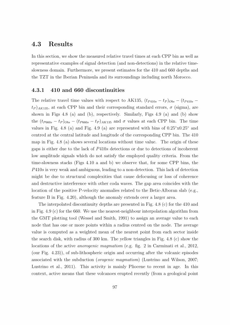
4.3 Results
In this section, we show the measured relative travel times at each CPP bin as well as
representative examples of signal detection (and non-detections) in the relative time-
slowness domain. Furthermore, we present estimates for the 410 and 660 depths and
the TZT in the Iberian Peninsula and its surroundings including north Morocco.
4.3.1 410 and 660 discontinuities
The relative travel time values with respect to AK135, (tP410s − tP )Obs − (tP410s −tP )AK135, at each CPP bin and their corresponding standard errors, σ (sigma), are
shown in Figs 4.8 (a) and (b), respectively. Similarly, Figs 4.9 (a) and (b) show
the (tP660s − tP )Obs − (tP660s − tP )AK135 and σ values at each CPP bin. The time
values in Fig. 4.8 (a) and Fig. 4.9 (a) are represented with bins of 0.25◦x0.25◦ and
centred at the central latitude and longitude of the corresponding CPP bin. The 410
map in Fig. 4.8 (a) shows several locations without time value. The origin of these
gaps is either due to the lack of P410s detections or due to detections of incoherent
low amplitude signals which do not satisfy the employed quality criteria. From the
time-slowness stacks (Figs 4.10 a and b) we observe that, for some CPP bins, the
P410s is very weak and ambiguous, leading to a non-detection. This lack of detection
might be due to structural complexities that cause defocusing or loss of coherence
and destructive interference with other coda waves. The gap area coincides with the
location of the positive P-velocity anomalies related to the Betic-Alboran slab (e.g.,
feature B in Fig. 4.20), although the anomaly extends over a larger area.
The interpolated discontinuity depths are presented in Fig. 4.8 (c) for the 410 and
in Fig. 4.9 (c) for the 660. We use the nearest-neighbour interpolation algorithm from
the GMT plotting tool (Wessel and Smith, 1991) to assign an average value to each
node that has one or more points within a radius centred on the node. The average
value is computed as a weighted mean of the nearest point from each sector inside
the search disk, with radius of 300 km. The yellow triangles in Fig. 4.8 (c) show the
locations of the active anorogenic magmatism (e.g. fig. 2 in Carminati et al., 2012,
(our Fig. 4.23)), of sub-lithospheric origin and occurring after the volcanic episodes
associated with the subduction (orogenic magmatism) (Lustrino and Wilson, 2007;
Lustrino et al., 2011). This activity is mainly Pliocene to recent in age. In this
context, active means that these volcanoes erupted recently (from a geological point
97
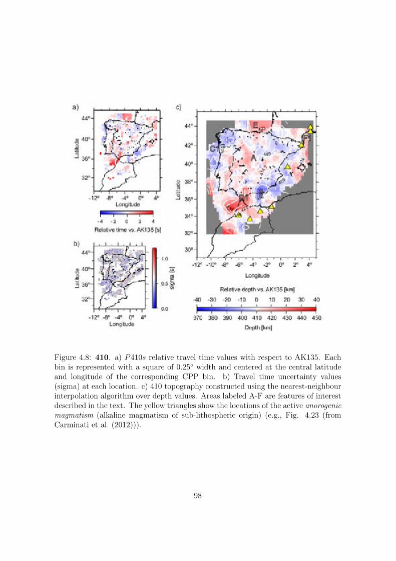
Figure 4.8: 410. a) P410s relative travel time values with respect to AK135. Eachbin is represented with a square of 0.25◦ width and centered at the central latitudeand longitude of the corresponding CPP bin. b) Travel time uncertainty values(sigma) at each location. c) 410 topography constructed using the nearest-neighbourinterpolation algorithm over depth values. Areas labeled A-F are features of interestdescribed in the text. The yellow triangles show the locations of the active anorogenicmagmatism (alkaline magmatism of sub-lithospheric origin) (e.g., Fig. 4.23 (fromCarminati et al. (2012))).
98
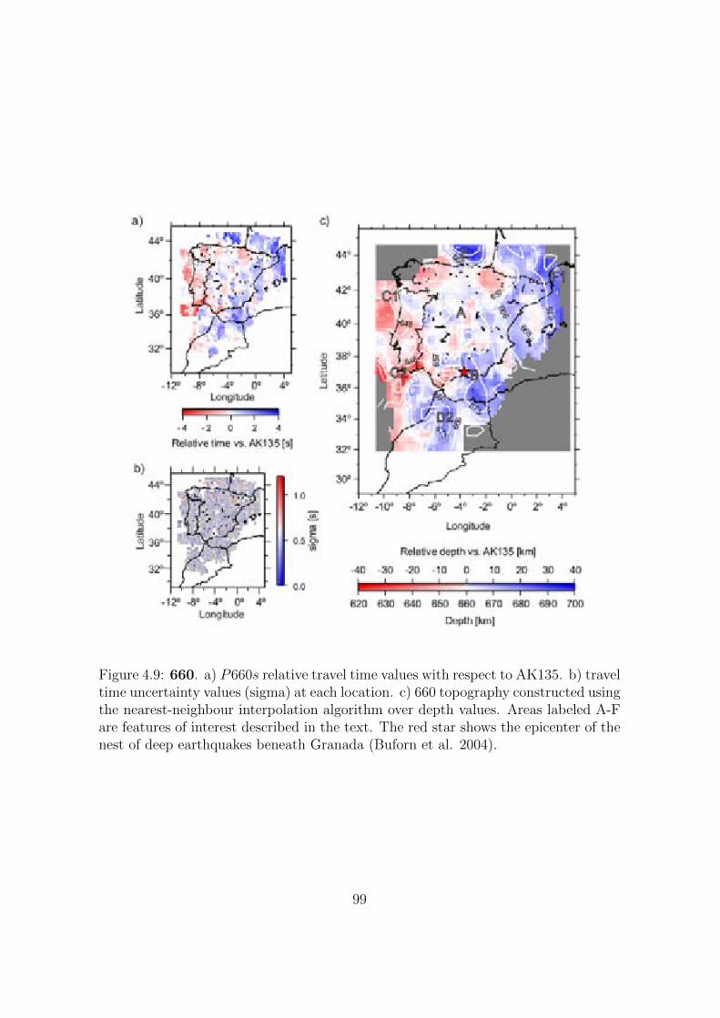
Figure 4.9: 660. a) P660s relative travel time values with respect to AK135. b) traveltime uncertainty values (sigma) at each location. c) 660 topography constructed usingthe nearest-neighbour interpolation algorithm over depth values. Areas labeled A-Fare features of interest described in the text. The red star shows the epicenter of thenest of deep earthquakes beneath Granada (Buforn et al. 2004).
99
Figure 4.10: Representative examples of ambiguous or non-detections of theP410s phase. a) From left to right: stacking of PCCRs, CCGNRs and RFs for aCPP bin located at latitude 40◦ and longitude 1◦. b) Same as (a) but for a CPP binat latitude 40◦ and longitude −3◦. Red circles mark the theoretical relative traveltime and slowness values for P410s, P510s and P660s.
of view) and could still erupt. Note, that they are all located at the border of areas
with a depressed 410. The red star in Fig. 4.9 (c) shows the epicenter of the nest
of deep earthquakes beneath Granada (Buforn et al. 2004), which coincides with a
transition from depressed to uplifted 660.
The 410 topography shows small depth variations in central Spain of about ±10
km (A in Fig. 4.8 c). In the surrounding areas we observe peak-to-peak variation of
about 60 km (excluding the extreme values in Fig. 4.7 a). The 410 is locally uplifted
by about 20 km (410 at 390 km) in the Alboran Sea and south Spain (B in Fig. 4.8 c)
and in the northwest of Spain is uplifted by about 30 km (C1 in Fig. 4.8 c). In both
areas the P410s phase is clearly detected at each CPP bin with at least two of the
three techniques, as it is shown in the stacks of Figs 4.11 (a) and (b) for the Alboran
Sea and in Fig. 4.12 for the northwest of Spain. The deepest 410 depth values are
found in the Gulf of Cadiz, the Strait of Gibraltar and the northwestern part of the
sampled Moroccan region (D1 in Fig. 4.8 c). In this area, the 410 is locally depressed
by about 30 km. Figs 4.13 (a) and (b), Fig. 4.14 and Figs 4.15 (a) and (b) show
representative examples of the detection of P410s in this area. In Fig. 4.16, we show
100
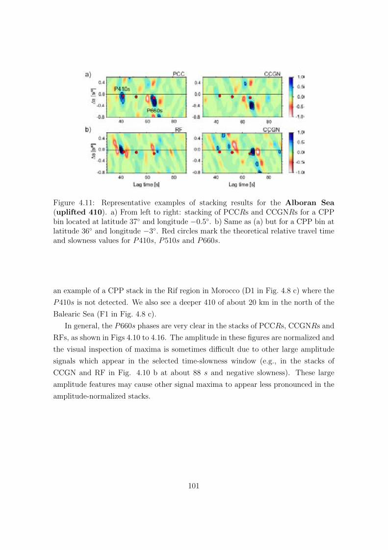
Figure 4.11: Representative examples of stacking results for the Alboran Sea(uplifted 410). a) From left to right: stacking of PCCRs and CCGNRs for a CPPbin located at latitude 37◦ and longitude −0.5◦. b) Same as (a) but for a CPP bin atlatitude 36◦ and longitude −3◦. Red circles mark the theoretical relative travel timeand slowness values for P410s, P510s and P660s.
an example of a CPP stack in the Rif region in Morocco (D1 in Fig. 4.8 c) where the
P410s is not detected. We also see a deeper 410 of about 20 km in the north of the
Balearic Sea (F1 in Fig. 4.8 c).
In general, the P660s phases are very clear in the stacks of PCCRs, CCGNRs and
RFs, as shown in Figs 4.10 to 4.16. The amplitude in these figures are normalized and
the visual inspection of maxima is sometimes difficult due to other large amplitude
signals which appear in the selected time-slowness window (e.g., in the stacks of
CCGN and RF in Fig. 4.10 b at about 88 s and negative slowness). These large
amplitude features may cause other signal maxima to appear less pronounced in the
amplitude-normalized stacks.
101
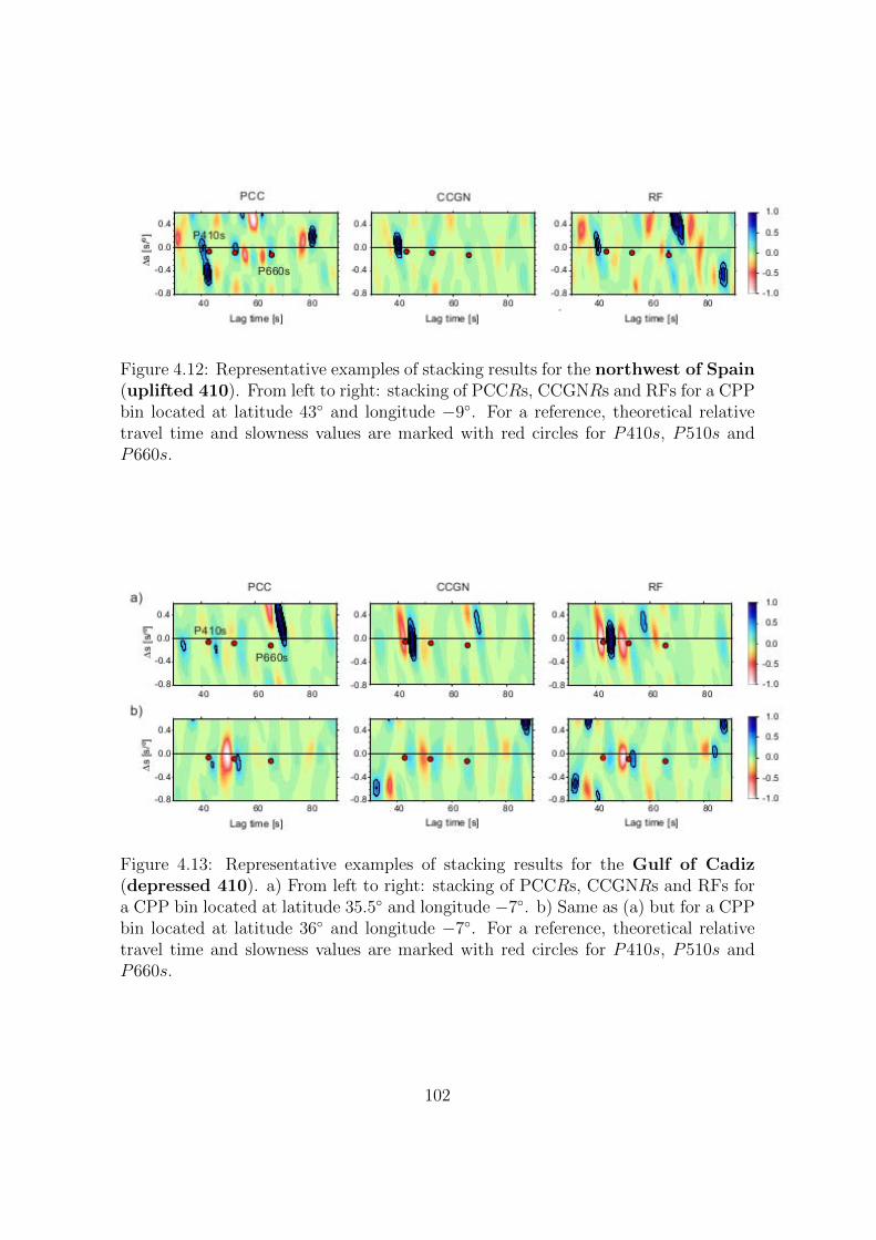
Figure 4.12: Representative examples of stacking results for the northwest of Spain(uplifted 410). From left to right: stacking of PCCRs, CCGNRs and RFs for a CPPbin located at latitude 43◦ and longitude −9◦. For a reference, theoretical relativetravel time and slowness values are marked with red circles for P410s, P510s andP660s.
Figure 4.13: Representative examples of stacking results for the Gulf of Cadiz(depressed 410). a) From left to right: stacking of PCCRs, CCGNRs and RFs fora CPP bin located at latitude 35.5◦ and longitude −7◦. b) Same as (a) but for a CPPbin located at latitude 36◦ and longitude −7◦. For a reference, theoretical relativetravel time and slowness values are marked with red circles for P410s, P510s andP660s.
102
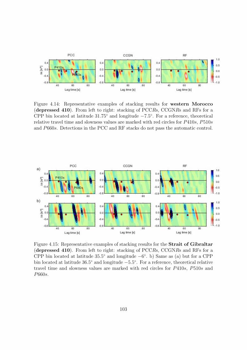
Figure 4.14: Representative examples of stacking results for western Morocco(depressed 410). From left to right: stacking of PCCRs, CCGNRs and RFs for aCPP bin located at latitude 31.75◦ and longitude −7.5◦. For a reference, theoreticalrelative travel time and slowness values are marked with red circles for P410s, P510sand P660s. Detections in the PCC and RF stacks do not pass the automatic control.
Figure 4.15: Representative examples of stacking results for the Strait of Gibraltar(depressed 410). From left to right: stacking of PCCRs, CCGNRs and RFs for aCPP bin located at latitude 35.5◦ and longitude −6◦. b) Same as (a) but for a CPPbin located at latitude 36.5◦ and longitude −5.5◦. For a reference, theoretical relativetravel time and slowness values are marked with red circles for P410s, P510s andP660s.
103
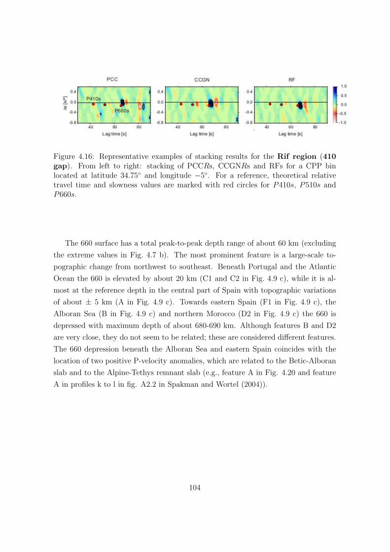
Figure 4.16: Representative examples of stacking results for the Rif region (410gap). From left to right: stacking of PCCRs, CCGNRs and RFs for a CPP binlocated at latitude 34.75◦ and longitude −5◦. For a reference, theoretical relativetravel time and slowness values are marked with red circles for P410s, P510s andP660s.
The 660 surface has a total peak-to-peak depth range of about 60 km (excluding
the extreme values in Fig. 4.7 b). The most prominent feature is a large-scale to-
pographic change from northwest to southeast. Beneath Portugal and the Atlantic
Ocean the 660 is elevated by about 20 km (C1 and C2 in Fig. 4.9 c), while it is al-
most at the reference depth in the central part of Spain with topographic variations
of about ± 5 km (A in Fig. 4.9 c). Towards eastern Spain (F1 in Fig. 4.9 c), the
Alboran Sea (B in Fig. 4.9 c) and northern Morocco (D2 in Fig. 4.9 c) the 660 is
depressed with maximum depth of about 680-690 km. Although features B and D2
are very close, they do not seem to be related; these are considered different features.
The 660 depression beneath the Alboran Sea and eastern Spain coincides with the
location of two positive P-velocity anomalies, which are related to the Betic-Alboran
slab and to the Alpine-Tethys remnant slab (e.g., feature A in Fig. 4.20 and feature
A in profiles k to l in fig. A2.2 in Spakman and Wortel (2004)).
104
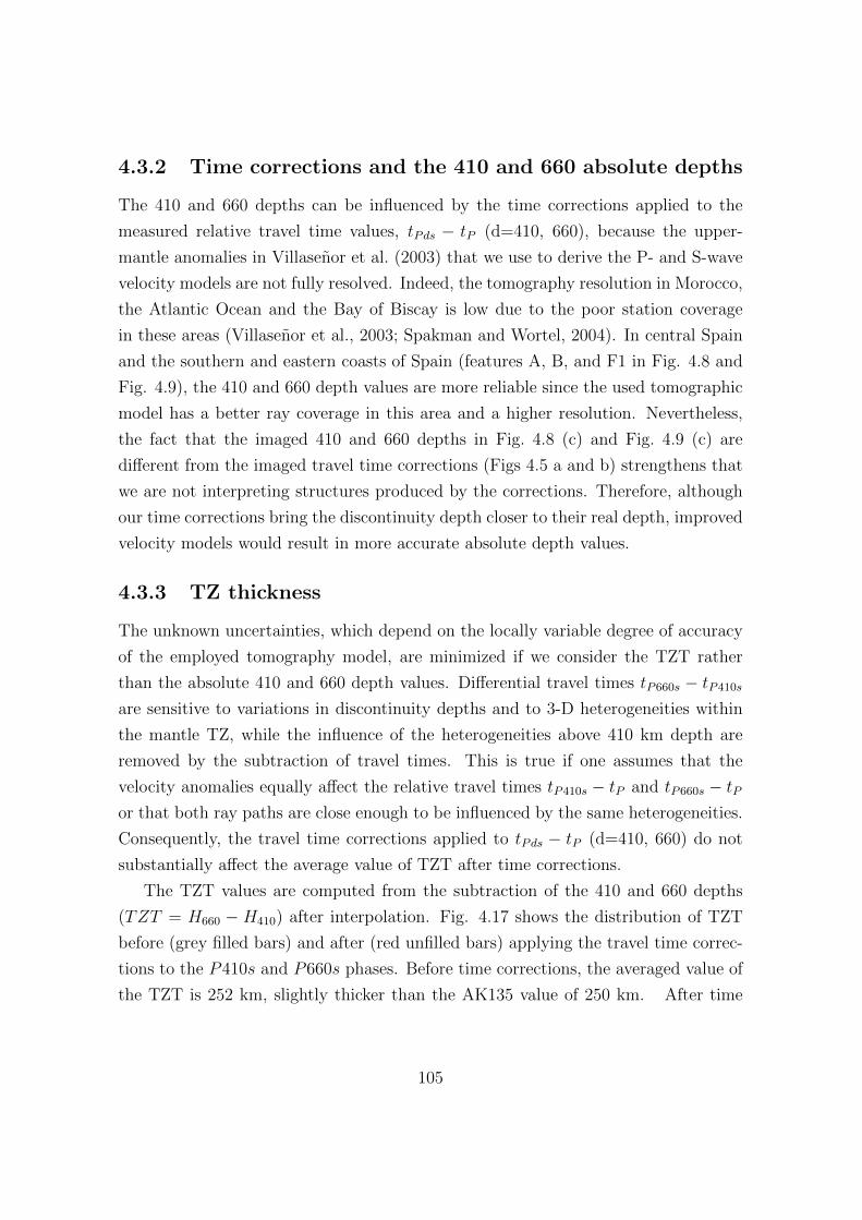
4.3.2 Time corrections and the 410 and 660 absolute depths
The 410 and 660 depths can be influenced by the time corrections applied to the
measured relative travel time values, tPds − tP (d=410, 660), because the upper-
mantle anomalies in Villasenor et al. (2003) that we use to derive the P- and S-wave
velocity models are not fully resolved. Indeed, the tomography resolution in Morocco,
the Atlantic Ocean and the Bay of Biscay is low due to the poor station coverage
in these areas (Villasenor et al., 2003; Spakman and Wortel, 2004). In central Spain
and the southern and eastern coasts of Spain (features A, B, and F1 in Fig. 4.8 and
Fig. 4.9), the 410 and 660 depth values are more reliable since the used tomographic
model has a better ray coverage in this area and a higher resolution. Nevertheless,
the fact that the imaged 410 and 660 depths in Fig. 4.8 (c) and Fig. 4.9 (c) are
different from the imaged travel time corrections (Figs 4.5 a and b) strengthens that
we are not interpreting structures produced by the corrections. Therefore, although
our time corrections bring the discontinuity depth closer to their real depth, improved
velocity models would result in more accurate absolute depth values.
4.3.3 TZ thickness
The unknown uncertainties, which depend on the locally variable degree of accuracy
of the employed tomography model, are minimized if we consider the TZT rather
than the absolute 410 and 660 depth values. Differential travel times tP660s − tP410s
are sensitive to variations in discontinuity depths and to 3-D heterogeneities within
the mantle TZ, while the influence of the heterogeneities above 410 km depth are
removed by the subtraction of travel times. This is true if one assumes that the
velocity anomalies equally affect the relative travel times tP410s − tP and tP660s − tPor that both ray paths are close enough to be influenced by the same heterogeneities.
Consequently, the travel time corrections applied to tPds − tP (d=410, 660) do not
substantially affect the average value of TZT after time corrections.
The TZT values are computed from the subtraction of the 410 and 660 depths
(TZT = H660 − H410) after interpolation. Fig. 4.17 shows the distribution of TZT
before (grey filled bars) and after (red unfilled bars) applying the travel time correc-
tions to the P410s and P660s phases. Before time corrections, the averaged value of
the TZT is 252 km, slightly thicker than the AK135 value of 250 km. After time
105
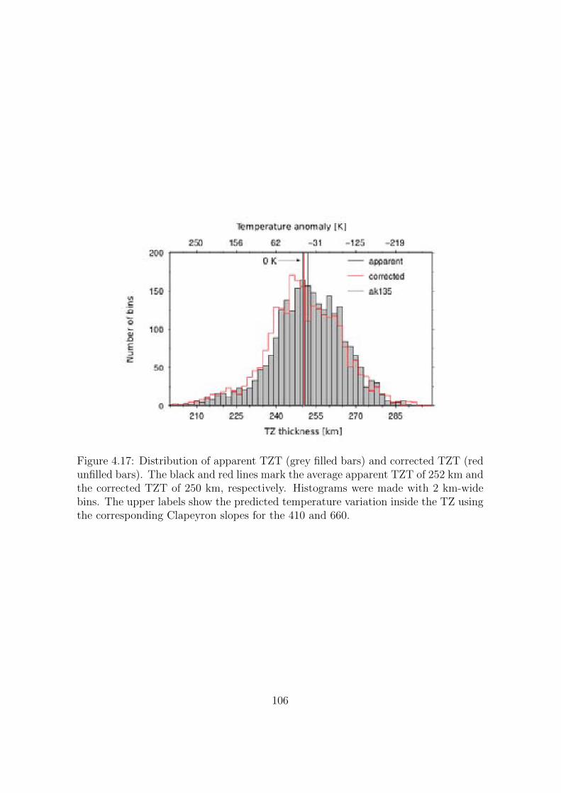
Figure 4.17: Distribution of apparent TZT (grey filled bars) and corrected TZT (redunfilled bars). The black and red lines mark the average apparent TZT of 252 km andthe corrected TZT of 250 km, respectively. Histograms were made with 2 km-widebins. The upper labels show the predicted temperature variation inside the TZ usingthe corresponding Clapeyron slopes for the 410 and 660.
106
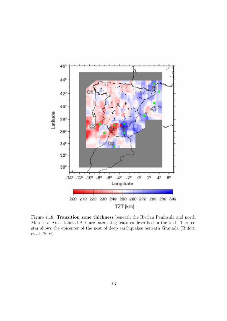
Figure 4.18: Transition zone thickness beneath the Iberian Peninsula and northMorocco. Areas labeled A-F are interesting features described in the text. The redstar shows the epicenter of the nest of deep earthquakes beneath Granada (Bufornet al. 2004).
107
corrections the averaged TZT is 250 km. Anyhow, both values are thicker than the
global RF average of 242± 2 km (Lawrence and Shearer, 2006).
The TZT is shown in Fig. 4.18. The green squares show the location of selected
bins with robust 410 and 660 depth values, where the P410s and P660s phases are
detected with at least two techniques and with small uncertainty values. These bins
are located in areas of special interest, where the TZ shows thickness values larger
or smaller than the reference thickness in AK135. The 410 and 660 depths and the
TZT for the green squares in Fig. 4.18 are listed in Table 4.1. We observe a large-
scale thickness change from southwest to the east. In the central part of Iberia, the
TZT shows variations around the mean of about ±10 km (A in Fig. 4.18). The
southwest coast of Iberia (C2 and D1 in Fig. 4.18 and Table 4.1) exhibits a thinner
TZ of about 220 km. The southern and eastern coasts of Spain are characterized
by a thicker TZ with maximum thickness of about 300 km beneath the Alboran Sea
(B in Fig. 4.18 and Table 4.1) and about 280 km beneath the Pyrenees area (F1 in
Fig. 4.18 and Table 4.1) and the south part of the Balearic Sea (see Table 4.1). In
both areas, the tomographic images (Wortel and Spakman, 2000; Villasenor et al.,
2003; Spakman and Wortel, 2004) show positive P-wave velocity anomalies related
to the Betic-Alboran slab and to the Alpine-Tethys remnant slab which lies at the
base of the TZ beneath the Pyrenees, southern France, the Alps and the northern
Italy/Adriatic region (e.g., feature A in Fig. 4.20 and feature A in profiles k to l
in fig. A2.2 in Spakman and Wortel (2004)). Beneath the Alboran Sea, the TZ is
thick due to an elevated 410 and a depressed 660 and beneath the south Balearic
Sea the TZ is thick mainly due to a depressed 660. On the other hand, beneath the
eastern Pyrenees and the northern Balearic Sea both discontinuities are depressed.
The broad extension of the thicker TZ beneath the Alboran Sea is controlled by the
extended 660 depression, while the 410 is locally elevated in the areas where the TZ
reaches the largest thickness value. A thick TZ is also visible beneath the northwest of
Morocco (D2 in Fig. 4.18 and Table 4.1), primarily due to an up to 20 km depressed
660 discontinuity. Another interesting result is that the deep earthquakes beneath
Granada coincide with a transition from thinner to thicker TZ. In this area, our
observations present a large P410s detection gap and a smaller P660s gap. Therefore,
the TZ is obtained exclusively from interpolated 410 and 660 values. Thus, although
the TZT change is a real feature, the position of the transition from thinner to thicker
108
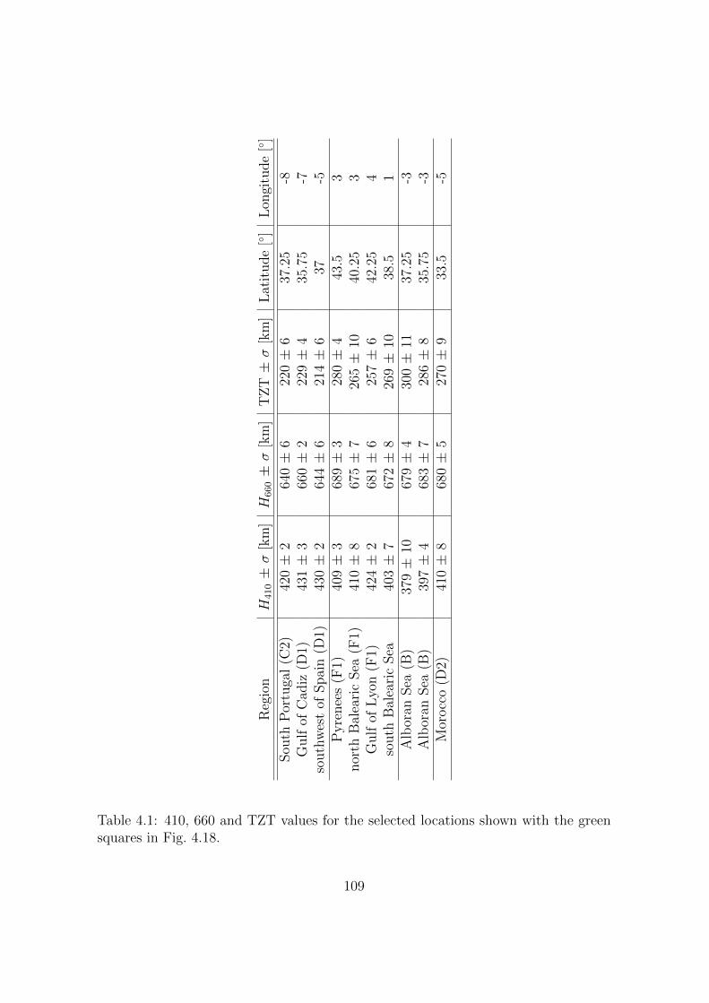
Reg
ion
H410±σ
[km
]H
660±σ
[km
]T
ZT±σ
[km
]L
atit
ude
[◦]
Lon
gitu
de
[◦]
Sou
thP
ortu
gal
(C2)
420±
264
0±
622
0±
637
.25
-8G
ulf
ofC
adiz
(D1)
431±
366
0±
222
9±
435
.75
-7so
uth
wes
tof
Spai
n(D
1)43
0±
264
4±
621
4±
637
-5P
yre
nee
s(F
1)40
9±
368
9±
328
0±
443
.53
nor
thB
alea
ric
Sea
(F1)
410±
867
5±
726
5±
1040
.25
3G
ulf
ofL
yon
(F1)
424±
268
1±
625
7±
642
.25
4so
uth
Bal
eari
cSea
403±
767
2±
826
9±
1038
.51
Alb
oran
Sea
(B)
379±
1067
9±
430
0±
1137
.25
-3A
lbor
anSea
(B)
397±
468
3±
728
6±
835
.75
-3M
orocc
o(D
2)41
0±
868
0±
527
0±
933
.5-5
Table 4.1: 410, 660 and TZT values for the selected locations shown with the greensquares in Fig. 4.18.
109
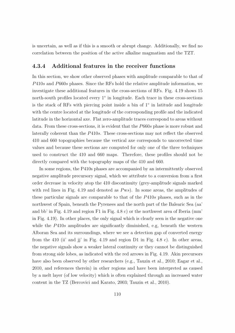
is uncertain, as well as if this is a smooth or abrupt change. Additionally, we find no
correlation between the position of the active alkaline magmatism and the TZT.
4.3.4 Additional features in the receiver functions
In this section, we show other observed phases with amplitude comparable to that of
P410s and P660s phases. Since the RFs hold the relative amplitude information, we
investigate these additional features in the cross-sections of RFs. Fig. 4.19 shows 15
north-south profiles located every 1◦ in longitude. Each trace in these cross-sections
is the stack of RFs with piercing point inside a bin of 1◦ in latitude and longitude
with the centre located at the longitude of the corresponding profile and the indicated
latitude in the horizontal axe. Flat zero-amplitude traces correspond to areas without
data. From these cross-sections, it is evident that the P660s phase is more robust and
laterally coherent than the P410s. These cross-sections may not reflect the observed
410 and 660 topographies because the vertical axe corresponds to uncorrected time
values and because these sections are computed for only one of the three techniques
used to construct the 410 and 660 maps. Therefore, these profiles should not be
directly compared with the topography maps of the 410 and 660.
In some regions, the P410s phases are accompanied by an intermittently observed
negative amplitude precursory signal, which we attribute to a conversion from a first
order decrease in velocity atop the 410 discontinuity (grey-amplitude signals marked
with red lines in Fig. 4.19 and denoted as Pws). In some areas, the amplitudes of
these particular signals are comparable to that of the P410s phases, such as in the
northwest of Spain, beneath the Pyrenees and the north part of the Balearic Sea (aa’
and bb’ in Fig. 4.19 and region F1 in Fig. 4.8 c) or the northwest area of Iberia (mm’
in Fig. 4.19). In other places, the only signal which is clearly seen is the negative one
while the P410s amplitudes are significantly diminished, e.g, beneath the western
Alboran Sea and its surroundings, where we see a detection gap of converted energy
from the 410 (ii’ and jj’ in Fig. 4.19 and region D1 in Fig. 4.8 c). In other areas,
the negative signals show a weaker lateral continuity or they cannot be distinguished
from strong side lobes, as indicated with the red arrows in Fig. 4.19. Akin precursors
have also been observed by other researchers (e.g., Tauzin et al., 2010; Eagar et al.,
2010, and references therein) in other regions and have been interpreted as caused
by a melt layer (of low velocity) which is often explained through an increased water
content in the TZ (Bercovici and Karato, 2003; Tauzin et al., 2010).
110
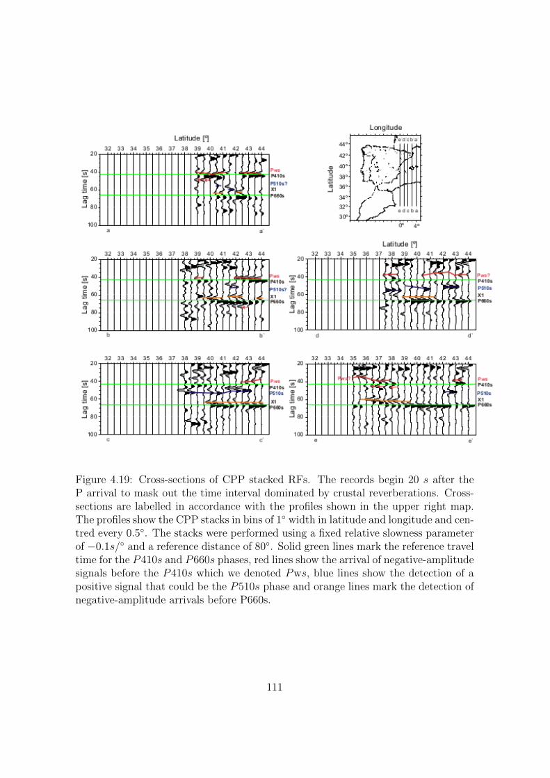
Figure 4.19: Cross-sections of CPP stacked RFs. The records begin 20 s after theP arrival to mask out the time interval dominated by crustal reverberations. Cross-sections are labelled in accordance with the profiles shown in the upper right map.The profiles show the CPP stacks in bins of 1◦ width in latitude and longitude and cen-tred every 0.5◦. The stacks were performed using a fixed relative slowness parameterof −0.1s/◦ and a reference distance of 80◦. Solid green lines mark the reference traveltime for the P410s and P660s phases, red lines show the arrival of negative-amplitudesignals before the P410s which we denoted Pws, blue lines show the detection of apositive signal that could be the P510s phase and orange lines mark the detection ofnegative-amplitude arrivals before P660s.
111
Figure 4.19 continuation
112
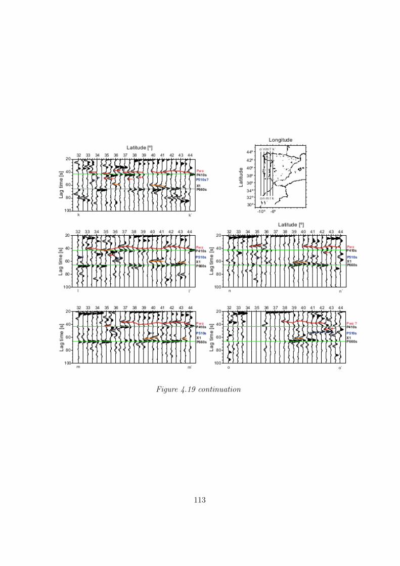
Figure 4.19 continuation
113
We also observe negative amplitude arrivals before the P660s phases, denoted as
X1 and marked with orange lines in Fig. 4.19. In some places, these negative peaks
appear to be laterally coherent. In other areas, they appear intermittently. In general,
the amplitudes of these signals are comparable to those of the P660s phases. Up to
our knowledge, there exists no known mineralogical phase change that would produce
the negative signal before P660s. Other studies have also observed similar negative
impedance features and have interpreted them as accumulated oceanic crust at the
base of the TZ (Shen and Blum, 2003; Shen et al., 2008; Eagar et al., 2010), probably
coming from crustal decoupling from the slab at TZ pressure and temperature (van
Keken et al., 1996; Karato, 1997). In subduction environments, where the slab is
stagnant at the base of the TZ and where the cold slab lies atop a warmer mantle,
the negative signals are probably associated to a decrease in velocity caused by a
positive temperature gradient (δT/δz � 0) (Bina and Kawakatsu, 2010). Depending
on the stagnation depth, the rg → pv+mw phase transition would be located below,
above or within this low-velocity layer (e.g., fig. 7 in Bina and Kawakatsu, 2010).
We also note the presence of other intermittent positive amplitude arrivals between
P410s and P660s. These are the black-amplitude signals marked with blue lines in
Fig. 4.19. These signals are less laterally coherent and are likely P -to-s conversions
at first order velocity increases within the depth range of 500-550 km and could
be signatures from the 510-km discontinuity. This discontinuity has been detected
before in global stacks of SS precursors (Shearer, 1990) and has been proposed to
be only a regional observable (Revenaugh and Jordan, 1991; Gu and Dziewonski,
1998). Deuss and Woodhouse (2001) confirmed the regional nature of the 510 with
SS precursors; they found the 510 in many regions but confirmed its absence in
others. In some regions, they found a splitting of the 510. The discontinuity at
510 km depth has been attributed to the wadsleyite-to-ringwoodite transformation
in the olivine system by Shearer (1996). However, at approximately the same depth
the dissociation of clinopyroxene to calcium-perovskite plus garnet gives origin to
an additional discontinuity in fertile regions of the mantle (see Appendix B). Thus,
if both phase transformations occur in the same region, two close signals would be
detected. The variable arrival time of the positive signals between P410s and P660s
may reflect the double origin for the 510.
Besides the TZ-related signals, we also observe laterally coherent positive signals
in the time window between 20 and 30 s, after the time interval for the crustal
114
reverberations. These features can be seen in every profile in Fig. 4.19 and are likely
to be P -to-s conversions at first order velocity increases within the depth range of
200-300 km. The Lehmann discontinuity (Lehmann, 1961b, 1964) is defined as a
positive seismic discontinuity (velocity increases downward) at about a depth of 220
km. It is thought to reveal the bottom of the asthenosphere. P -to-s conversions
at this discontinuity have been reported previously in other regions (e.g., Bostock,
1998; Li et al., 2002), but the analysis of SS precursors has been preferred to study
the Lehmann discontinuity (e.g., Shearer, 1990; Vidale and Benz, 1992; Deuss and
Woodhouse, 2002, 2004). The positive signal in the time window between 20 and
30 s is probably caused by the Lehmann discontinuity but it is not used in the
following analysis and therefore we do not further explore its origin. Studying these
discontinuities and the other discontinuities mentioned in this section is beyond the
scope of this thesis.
4.4 Discussion
4.4.1 Relation with previous works
We have used a vast volume of data thanks to the IberArray of the TopoIberia project
(Dıaz et al., 2009), which has permitted us to study in detail and with high resolution
a previously under-sampled portion of the TZ discontinuities beneath Iberia and north
Morocco. Our results locate the 410 and 660 discontinuities within the expected depth
range as obtained by global studies (Shearer, 1991; Revenaugh and Jordan, 1991;
Vidale and Benz, 1992; Shearer, 1993; Chevrot et al., 1999; Lawrence and Shearer,
2006; Tauzin et al., 2007), and are further in good agreement with a large scale
P-RF study that covered the entire Mediterranean region (van der Meijde et al.,
2005). In van der Meijde et al. (2005) two stations are located in central Spain
and north Morocco, which show the same TZT variations as observed in our study:
small thickness variations beneath central Spain (A in Fig. 4.18) and a thicker TZ
beneath Morocco (D2 and feature B in north Morocco in Fig. 4.18). In a previous
study, published as Bonatto et al. (2013) and based on fewer stations and larger
bin size and bin spacing, we observed the thickening of the TZ towards Africa as a
narrow and steep transition between the two continents and we observed a P410s
detection gap beneath the Rif. For this second study, more data were available, a
fact which has permitted us to increase the spatial resolution. Although we have
115
increased the amount of data and have improved the resolution, part of the 410
gap remains there. The thickening of the TZ towards Africa seems to be a robust
feature; we have estimated a TZT variation from 214 km to 270 km in the Strait
of Gibraltar (D1 and D2 in Fig. 4.18). This TZT variation is not seen by Dundar
et al. (2011), who studied the 410 and 660 discontinuities beneath the Alboran Sea
and close surroundings using P-RFs and the available stations before the IberArray
deployment. Their RFs are stacked for two piercing point areas, the Alboran Sea and
surrounding areas including south Spain, north Morocco, and Gulf of Cadiz and show
a good agreement between the conversions from the different RF groups, within 1 s
of the theoretically expected arrivals. Their results do not contradict the presence
of topography, which most probably is not seen due to the averaging in the large
piercing point area. Our analysis shows systematic variations for independent data
from many smaller piercing point areas and for the joint usage of three different
techniques.
4.4.2 Interpretation of results
In what follows, we discuss the TZT and the 410 and 660 topography in the study
area by proposing different possible scenarios which may explain our results. In-
terpretation of TZT (and topography of discontinuities) includes temperature and
composition of the mantle at these depths.
The tomographic images provide additional information to interpret our results.
We use the P-wave tomography of Villasenor et al. (2003), which, due to the inclusion
of regional data for Spain, is a slightly higher resolution version of the original model
in Wortel and Spakman (2000). The tomography in the western part of the study area
has a lower resolution, therefore, direct comparison of the tomographic images and our
TZT (or 410 and 660 depth values) in this area should be taken with care. To estimate
the thermal anomalies needed to explain the obtained 410 and 660 topographies, we
assume that velocity perturbations in the tomography model are thermally controlled.
To infer TZ temperatures, we consider the detected TZ discontinuities as olivine
phase transformations. Under this assumption, the 410 and 660 depth changes are
anti-correlated as a response to a thermal anomaly (due to the opposite sign in
the Clapeyron slopes of the olivine-to-wadsleyite and ringwoodite-to-perovskite +
magnesiowustite phase transformations). While the 410 becomes shallower in colder
116
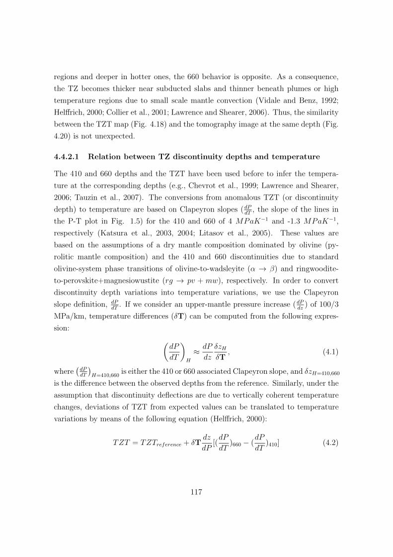
regions and deeper in hotter ones, the 660 behavior is opposite. As a consequence,
the TZ becomes thicker near subducted slabs and thinner beneath plumes or high
temperature regions due to small scale mantle convection (Vidale and Benz, 1992;
Helffrich, 2000; Collier et al., 2001; Lawrence and Shearer, 2006). Thus, the similarity
between the TZT map (Fig. 4.18) and the tomography image at the same depth (Fig.
4.20) is not unexpected.
4.4.2.1 Relation between TZ discontinuity depths and temperature
The 410 and 660 depths and the TZT have been used before to infer the tempera-
ture at the corresponding depths (e.g., Chevrot et al., 1999; Lawrence and Shearer,
2006; Tauzin et al., 2007). The conversions from anomalous TZT (or discontinuity
depth) to temperature are based on Clapeyron slopes (dPdT
, the slope of the lines in
the P-T plot in Fig. 1.5) for the 410 and 660 of 4 MPaK−1 and -1.3 MPaK−1,
respectively (Katsura et al., 2003, 2004; Litasov et al., 2005). These values are
based on the assumptions of a dry mantle composition dominated by olivine (py-
rolitic mantle composition) and the 410 and 660 discontinuities due to standard
olivine-system phase transitions of olivine-to-wadsleyite (α → β) and ringwoodite-
to-perovskite+magnesiowustite (rg → pv + mw), respectively. In order to convert
discontinuity depth variations into temperature variations, we use the Clapeyron
slope definition, dPdT
. If we consider an upper-mantle pressure increase (dPdz
) of 100/3
MPa/km, temperature differences (δT) can be computed from the following expres-
sion: (dP
dT
)H
≈ dP
dz
δzHδT
, (4.1)
where(dPdT
)H=410,660
is either the 410 or 660 associated Clapeyron slope, and δzH=410,660
is the difference between the observed depths from the reference. Similarly, under the
assumption that discontinuity deflections are due to vertically coherent temperature
changes, deviations of TZT from expected values can be translated to temperature
variations by means of the following equation (Helffrich, 2000):
TZT = TZTreference + δTdz
dP[(dP
dT)660 − (
dP
dT)410] (4.2)
117
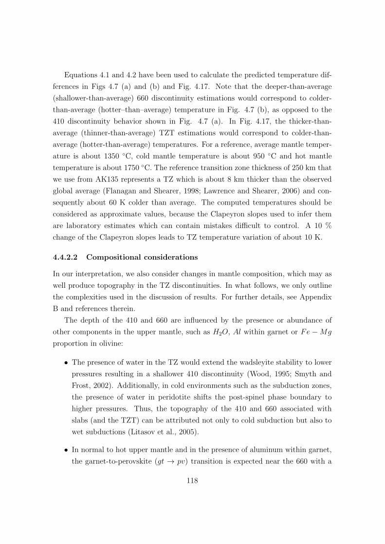
Equations 4.1 and 4.2 have been used to calculate the predicted temperature dif-
ferences in Figs 4.7 (a) and (b) and Fig. 4.17. Note that the deeper-than-average
(shallower-than-average) 660 discontinuity estimations would correspond to colder-
than-average (hotter–than–average) temperature in Fig. 4.7 (b), as opposed to the
410 discontinuity behavior shown in Fig. 4.7 (a). In Fig. 4.17, the thicker-than-
average (thinner-than-average) TZT estimations would correspond to colder-than-
average (hotter-than-average) temperatures. For a reference, average mantle temper-
ature is about 1350 ◦C, cold mantle temperature is about 950 ◦C and hot mantle
temperature is about 1750 ◦C. The reference transition zone thickness of 250 km that
we use from AK135 represents a TZ which is about 8 km thicker than the observed
global average (Flanagan and Shearer, 1998; Lawrence and Shearer, 2006) and con-
sequently about 60 K colder than average. The computed temperatures should be
considered as approximate values, because the Clapeyron slopes used to infer them
are laboratory estimates which can contain mistakes difficult to control. A 10 %
change of the Clapeyron slopes leads to TZ temperature variation of about 10 K.
4.4.2.2 Compositional considerations
In our interpretation, we also consider changes in mantle composition, which may as
well produce topography in the TZ discontinuities. In what follows, we only outline
the complexities used in the discussion of results. For further details, see Appendix
B and references therein.
The depth of the 410 and 660 are influenced by the presence or abundance of
other components in the upper mantle, such as H2O, Al within garnet or Fe −Mg
proportion in olivine:
• The presence of water in the TZ would extend the wadsleyite stability to lower
pressures resulting in a shallower 410 discontinuity (Wood, 1995; Smyth and
Frost, 2002). Additionally, in cold environments such as the subduction zones,
the presence of water in peridotite shifts the post-spinel phase boundary to
higher pressures. Thus, the topography of the 410 and 660 associated with
slabs (and the TZT) can be attributed not only to cold subduction but also to
wet subductions (Litasov et al., 2005).
• In normal to hot upper mantle and in the presence of aluminum within garnet,
the garnet-to-perovskite (gt → pv) transition is expected near the 660 with a
118
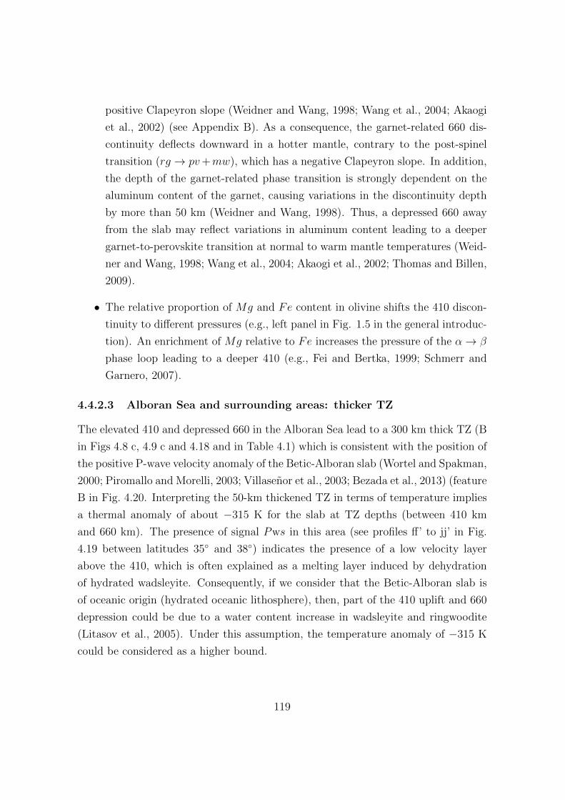
positive Clapeyron slope (Weidner and Wang, 1998; Wang et al., 2004; Akaogi
et al., 2002) (see Appendix B). As a consequence, the garnet-related 660 dis-
continuity deflects downward in a hotter mantle, contrary to the post-spinel
transition (rg → pv+mw), which has a negative Clapeyron slope. In addition,
the depth of the garnet-related phase transition is strongly dependent on the
aluminum content of the garnet, causing variations in the discontinuity depth
by more than 50 km (Weidner and Wang, 1998). Thus, a depressed 660 away
from the slab may reflect variations in aluminum content leading to a deeper
garnet-to-perovskite transition at normal to warm mantle temperatures (Weid-
ner and Wang, 1998; Wang et al., 2004; Akaogi et al., 2002; Thomas and Billen,
2009).
• The relative proportion of Mg and Fe content in olivine shifts the 410 discon-
tinuity to different pressures (e.g., left panel in Fig. 1.5 in the general introduc-
tion). An enrichment of Mg relative to Fe increases the pressure of the α→ β
phase loop leading to a deeper 410 (e.g., Fei and Bertka, 1999; Schmerr and
Garnero, 2007).
4.4.2.3 Alboran Sea and surrounding areas: thicker TZ
The elevated 410 and depressed 660 in the Alboran Sea lead to a 300 km thick TZ (B
in Figs 4.8 c, 4.9 c and 4.18 and in Table 4.1) which is consistent with the position of
the positive P-wave velocity anomaly of the Betic-Alboran slab (Wortel and Spakman,
2000; Piromallo and Morelli, 2003; Villasenor et al., 2003; Bezada et al., 2013) (feature
B in Fig. 4.20. Interpreting the 50-km thickened TZ in terms of temperature implies
a thermal anomaly of about −315 K for the slab at TZ depths (between 410 km
and 660 km). The presence of signal Pws in this area (see profiles ff’ to jj’ in Fig.
4.19 between latitudes 35◦ and 38◦) indicates the presence of a low velocity layer
above the 410, which is often explained as a melting layer induced by dehydration
of hydrated wadsleyite. Consequently, if we consider that the Betic-Alboran slab is
of oceanic origin (hydrated oceanic lithosphere), then, part of the 410 uplift and 660
depression could be due to a water content increase in wadsleyite and ringwoodite
(Litasov et al., 2005). Under this assumption, the temperature anomaly of −315 K
could be considered as a higher bound.
119
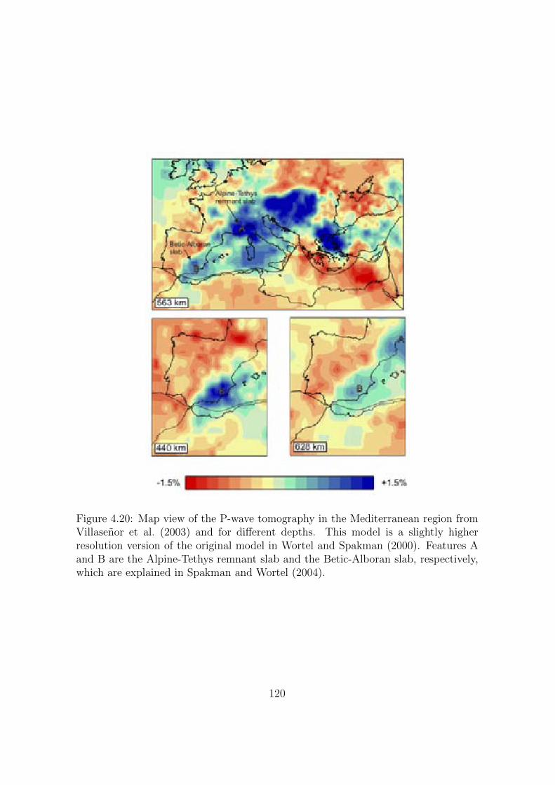
Figure 4.20: Map view of the P-wave tomography in the Mediterranean region fromVillasenor et al. (2003) and for different depths. This model is a slightly higherresolution version of the original model in Wortel and Spakman (2000). Features Aand B are the Alpine-Tethys remnant slab and the Betic-Alboran slab, respectively,which are explained in Spakman and Wortel (2004).
120
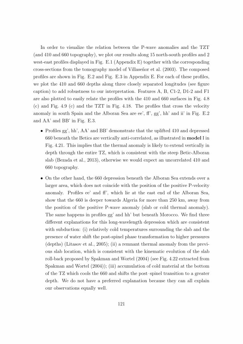
In order to visualize the relation between the P-wave anomalies and the TZT
(and 410 and 660 topography), we plot our results along 15 north-south profiles and 2
west-east profiles displayed in Fig. E.1 (Appendix E) together with the corresponding
cross-sections from the tomography model of Villasenor et al. (2003). The composed
profiles are shown in Fig. E.2 and Fig. E.3 in Appendix E. For each of these profiles,
we plot the 410 and 660 depths along three closely separated longitudes (see figure
caption) to add robustness to our interpretation. Features A, B, C1-2, D1-2 and F1
are also plotted to easily relate the profiles with the 410 and 660 surfaces in Fig. 4.8
(c) and Fig. 4.9 (c) and the TZT in Fig. 4.18. The profiles that cross the velocity
anomaly in south Spain and the Alboran Sea are ee’, ff’, gg’, hh’ and ii’ in Fig. E.2
and AA’ and BB’ in Fig. E.3.
• Profiles gg’, hh’, AA’ and BB’ demonstrate that the uplifted 410 and depressed
660 beneath the Betics are vertically anti-correlated, as illustrated in model I in
Fig. 4.21. This implies that the thermal anomaly is likely to extend vertically in
depth through the entire TZ, which is consistent with the steep Betic-Alboran
slab (Bezada et al., 2013), otherwise we would expect an uncorrelated 410 and
660 topography.
• On the other hand, the 660 depression beneath the Alboran Sea extends over a
larger area, which does not coincide with the position of the positive P-velocity
anomaly. Profiles ee’ and ff’, which lie at the east end of the Alboran Sea,
show that the 660 is deeper towards Algeria for more than 250 km, away from
the position of the positive P-wave anomaly (slab or cold thermal anomaly).
The same happens in profiles gg’ and hh’ but beneath Morocco. We find three
different explanations for this long-wavelength depression which are consistent
with subduction: (i) relatively cold temperatures surrounding the slab and the
presence of water shift the post-spinel phase transformation to higher pressures
(depths) (Litasov et al., 2005); (ii) a remnant thermal anomaly from the previ-
ous slab location, which is consistent with the kinematic evolution of the slab
roll-back proposed by Spakman and Wortel (2004) (see Fig. 4.22 extracted from
Spakman and Wortel (2004)); (iii) accumulation of cold material at the bottom
of the TZ which cools the 660 and shifts the post–spinel transition to a greater
depth. We do not have a preferred explanation because they can all explain
our observations equally well.
121
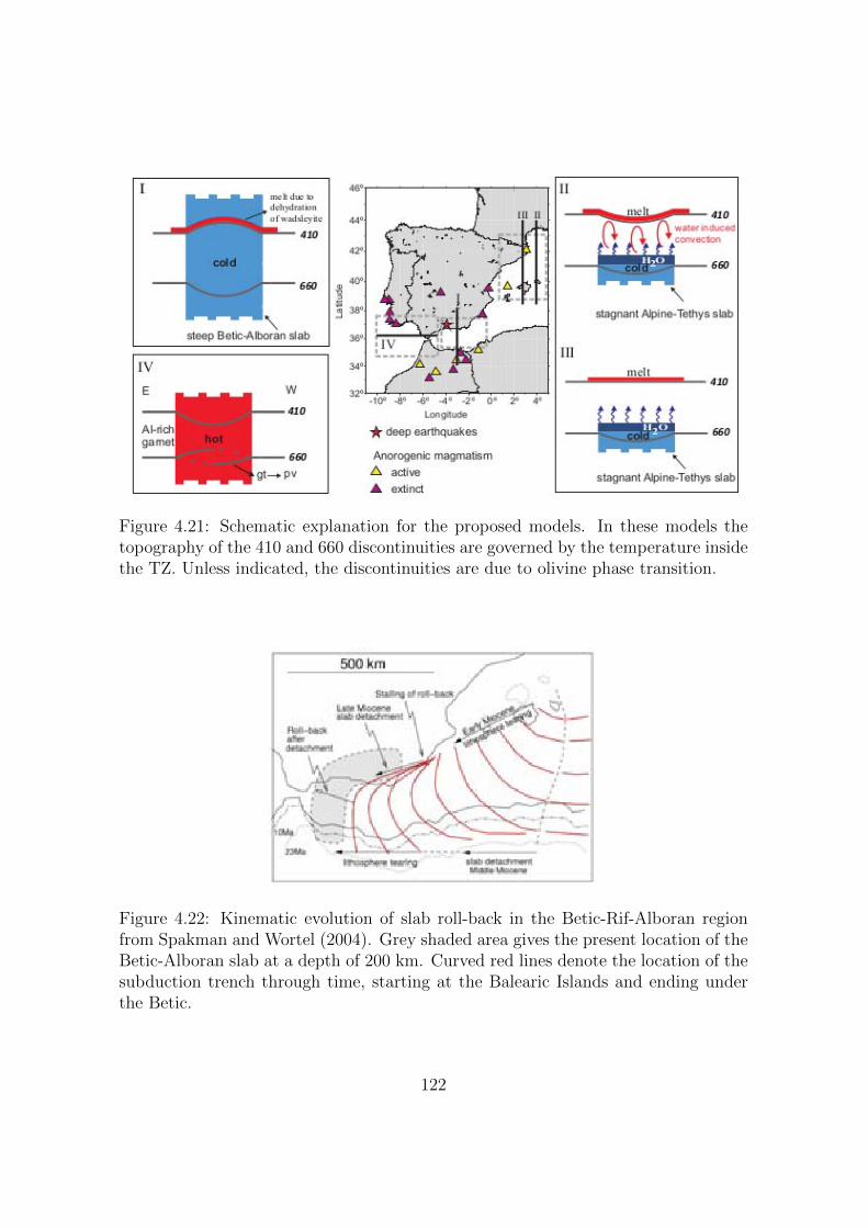
Figure 4.21: Schematic explanation for the proposed models. In these models thetopography of the 410 and 660 discontinuities are governed by the temperature insidethe TZ. Unless indicated, the discontinuities are due to olivine phase transition.
Figure 4.22: Kinematic evolution of slab roll-back in the Betic-Rif-Alboran regionfrom Spakman and Wortel (2004). Grey shaded area gives the present location of theBetic-Alboran slab at a depth of 200 km. Curved red lines denote the location of thesubduction trench through time, starting at the Balearic Islands and ending underthe Betic.
122
4.4.2.4 The area of deep earthquakes beneath Granada
Profile ii’ in Fig. E.2, which is at the western end of the slab, demonstrates that
the depression of the 660 is consistent with the seismic anomaly related with the
Betic-Alboran slab. The maximum depression of the 660 (∼ 25 km) includes an
area of isolated deep earthquakes beneath Granada (37◦N 3.7◦E approximately) with
similar focal mechanism, magnitudes (MW ) from 4 to 7 and a recurrence time of
about 20 years (Buforn et al., 2004, 2011; Bezada and Humphreys, 2012). Further-
more, Fig. 4.18 shows that the location of the nest of deep earthquakes (red star)
corresponds to a TZT change from thin to thick, which may be interpreted as a tem-
perature change. In the west-east profile BB’ in Fig. E.3 it is evident that the TZT
change fairly coincides with the western end of the Betic-Alboran slab. The thinner
TZ in this area is due to anti-correlated 410 and 660 depth changes. Using afore-
mentioned assumptions and equation 4.2 with the values in Table 4.1, we estimate a
net temperature variation of about 540 K (from about −315 K inside the cold slab
to about +225 K at the western end of the slab) over a distance of less than 250
km inside the TZ. Thus, the nest of deep earthquakes is located in an area of a high
temperature gradient inside the TZ and at the western end of the slab revealed by
the tomographic images of Villasenor et al. (2003).
4.4.2.5 Pyrenees and northeast coast of Spain
Profiles aa’, bb’ and cc’ in Fig. E.2 show that the depressed 660 (in F1) coincides with
the location of the positive P-wave anomaly related with the Alpine-Tethys remnant
slab (see also Fig. 4.20). Thus, we interpret the 20-30 km downward deflection of
the 660 as caused by the cold slab, which shifts the post-spinel transition to greater
depths. Using Equation 4.1 and the corresponding Clapeyron slope of the post-spinel
transformation, we infer a negative thermal anomaly of about 500-750 K at the 660,
which we consider as a higher bound if we assume that part of the 660 depression is
caused by the presence of water (Litasov et al., 2005), perhaps from dehydration of
the slab. In this area, the 410 is also downward deflected by about 20 km (see F1 in
Fig. 4.8 c), however, this deflection is more evident in profile aa’ of Fig. E.2, while in
bb’ the 410 is at its expected depth (see F1 in Fig. E.2). Additionally, in this area
we see a strong and clear reversed polarity signal arriving immediately before the
123
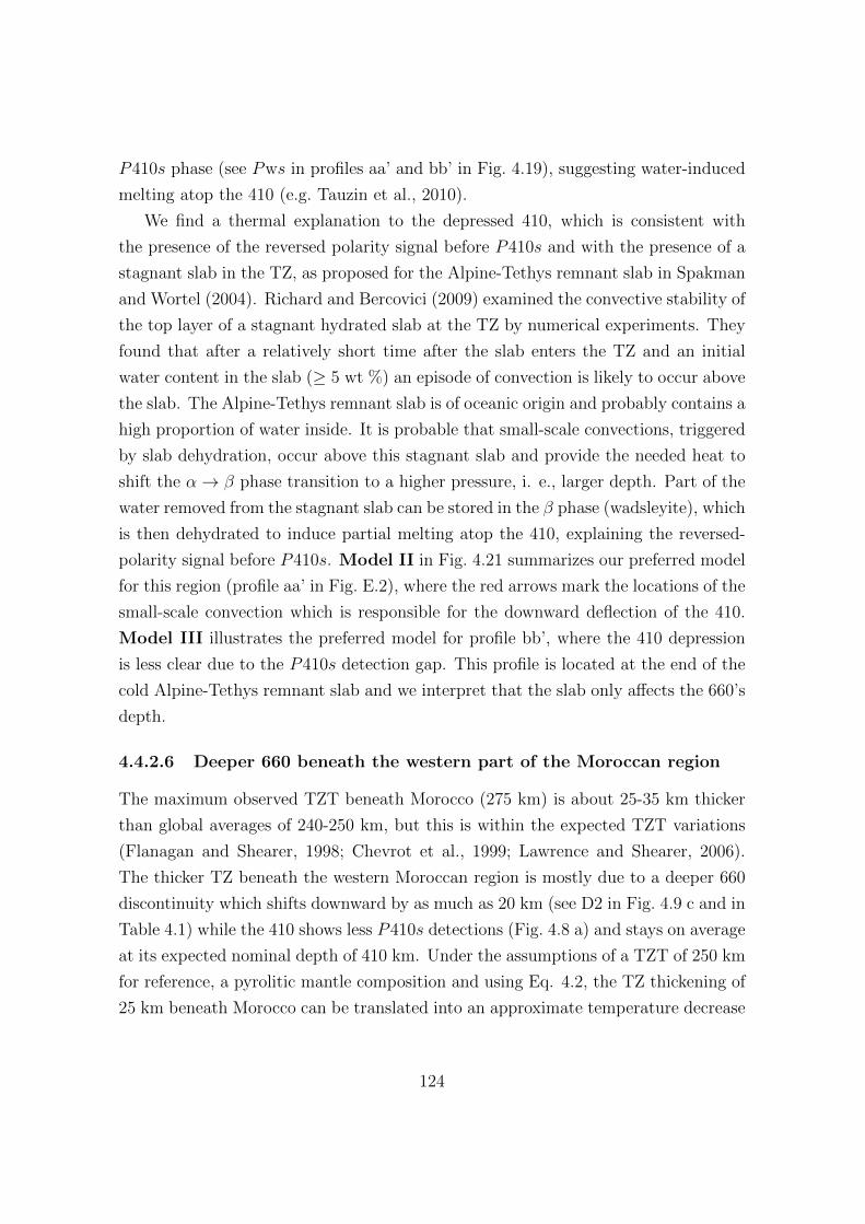
P410s phase (see Pws in profiles aa’ and bb’ in Fig. 4.19), suggesting water-induced
melting atop the 410 (e.g. Tauzin et al., 2010).
We find a thermal explanation to the depressed 410, which is consistent with
the presence of the reversed polarity signal before P410s and with the presence of a
stagnant slab in the TZ, as proposed for the Alpine-Tethys remnant slab in Spakman
and Wortel (2004). Richard and Bercovici (2009) examined the convective stability of
the top layer of a stagnant hydrated slab at the TZ by numerical experiments. They
found that after a relatively short time after the slab enters the TZ and an initial
water content in the slab (≥ 5 wt %) an episode of convection is likely to occur above
the slab. The Alpine-Tethys remnant slab is of oceanic origin and probably contains a
high proportion of water inside. It is probable that small-scale convections, triggered
by slab dehydration, occur above this stagnant slab and provide the needed heat to
shift the α→ β phase transition to a higher pressure, i. e., larger depth. Part of the
water removed from the stagnant slab can be stored in the β phase (wadsleyite), which
is then dehydrated to induce partial melting atop the 410, explaining the reversed-
polarity signal before P410s. Model II in Fig. 4.21 summarizes our preferred model
for this region (profile aa’ in Fig. E.2), where the red arrows mark the locations of the
small-scale convection which is responsible for the downward deflection of the 410.
Model III illustrates the preferred model for profile bb’, where the 410 depression
is less clear due to the P410s detection gap. This profile is located at the end of the
cold Alpine-Tethys remnant slab and we interpret that the slab only affects the 660’s
depth.
4.4.2.6 Deeper 660 beneath the western part of the Moroccan region
The maximum observed TZT beneath Morocco (275 km) is about 25-35 km thicker
than global averages of 240-250 km, but this is within the expected TZT variations
(Flanagan and Shearer, 1998; Chevrot et al., 1999; Lawrence and Shearer, 2006).
The thicker TZ beneath the western Moroccan region is mostly due to a deeper 660
discontinuity which shifts downward by as much as 20 km (see D2 in Fig. 4.9 c and in
Table 4.1) while the 410 shows less P410s detections (Fig. 4.8 a) and stays on average
at its expected nominal depth of 410 km. Under the assumptions of a TZT of 250 km
for reference, a pyrolitic mantle composition and using Eq. 4.2, the TZ thickening of
25 km beneath Morocco can be translated into an approximate temperature decrease
124
of 160 K. However, in the profiles jj’, kk’ and ll’ (in Fig. E.2) we do not find a
corresponding positive velocity anomaly in the tomographic image.
In Bonatto et al. (2013), we proposed that a plausible cause for the thickened
TZ can be (i) a not considered isothermal low-velocity anomaly (not resolved in
the tomographic images) which increases the P660s travel times and which leads to
apparent TZT thicker than expected or, alternatively, (ii) an Al-rich garnet-related
660, which in normal to hotter environments is to be expected at greater depth than
the post-spinel transition depending on the Al content (Weidner and Wang, 1998;
Wang et al., 2004).
A recent tomography study (Bezada et al., 2013), which includes more stations
in Morocco, has revealed an irregular but pronounced zone of low velocities beneath
the Middle Atlas at 50-125 km followed by a high-velocity body at a depth of about
400-500 km. This pair of anomalies has been interpreted as a drip-like delamination
of the Middle Atlas mantle lithosphere. The fast velocity anomaly inside the TZ does
not reach the 660 and consequently is discarded to depress the post-spinel transition
through its expected colder than average temperature. The high velocity anomaly
would therefore only decrease the travel time of the P660s phase, which, without the
correct travel time corrections, would lead to apparent discontinuity uplift. However,
we observe the opposite, a deeper 660. In this new context our preferred explanation
is (ii). In the absence of a hot thermal anomaly, as expected from the tomographic
images, the depth variations of the garnet-related 660 beneath Morocco can likely
be attributed to variable proportions of Al content within garnet (e.g., Thomas and
Billen, 2009), since the Al content also controls the depth of this transition.
4.4.2.7 Thinner TZ beneath Strait of Gibraltar, Gulf of Cadiz and southof Portugal
With the exception of the Spanish side of the Strait of Gibraltar, the thinner TZ in
this region is not due to anti-correlated 410 and 660 depths. The 410 is, on average,
deeper in the whole area, but the largest depressions are towards the east, beneath
the Gulf of Cadiz and the Strait of Gibraltar. On the other hand, the 660 is on
average deeper to the east and shallower to the west of the region and it has small
length-scale depth changes (see dotted circles in profiles AA’ and BB’ in Fig E.3).
In particular, near the longitude -8◦ in profile AA’ there is a 40-km jump in the 660
125
depth. Moreover, in the lower panel of this figure, the RF cross-section shows double
peaks near P660s at longitude -6◦ and -5◦.
We do not find a clear relation between the tomographic images and the thinned
TZ in profiles AA’ and BB’ (C2 and D1 in Fig. E.3) and profiles kk’, ll’, mm’, nn’ and
oo’ (C2 and D1 in Fig. E.2). In this area, the P-wave anomalies are slightly negative
indicating velocities lower than the reference model, which suggests that the mantle
is warmer than average. Recently, Monna et al. (2013) published a tomography
study which covers the Atlantic domain in the southwest Iberian margin and the
Alboran Sea. This study has a higher resolution than previous studies because it
includes data from OBS stations in the Gulf of Cadiz and the Atlantic Sea. Below
the Atlantic domain, they image a wide area of negative P-velocity anomalies, which
is attributed to the presence of a hot upper mantle and which is perhaps related with
the late Mesozoic-early Cenozoic alkaline igneous activity of sub-lithospheric origin
(e.g., Lustrino and Wilson, 2007; Grange et al., 2010, and references therein), such
as observed in south Portugal in Fig. 4.23.
The depth variability of the 660 and the double peaks near P660s suggest the
presence of multiple discontinuities near 660 km depth but, due to the used qual-
ity criteria, we have detected each time the best quality signal. The only additional
discontinuity expected in a warm to hot TZ is the garnet-to-perovskite phase transfor-
mation with a positive Clapeyron slope. In warmer to higher mantle temperatures,
this discontinuity is shifted to higher pressures (depth), which depend on the Al
proportion within garnet (Weidner and Wang, 1998). The presence of multiple dis-
continuities introduces additional complexities, which make the interpretation in this
area difficult. If the TZ temperature in this area is higher than average, then due to
the opposite sign in the Clapeyron slopes of the gt → pv and the post-spinel phase
transitions, we can attribute the deeper 660 to the garnet-related phase transition
and the shallower 660 to the post-spinel transition. In this scenario, our preferred
model for this region is model IV in Fig. 4.21, where a warm thermal anomaly
crosses the TZ causing the depression of the 410 and the uplift of the olivine-related
660 discontinuity. This results in the thinning of the TZ while the presence of Al
within garnet is responsible for the depressed 660 in such warmer environment.
126
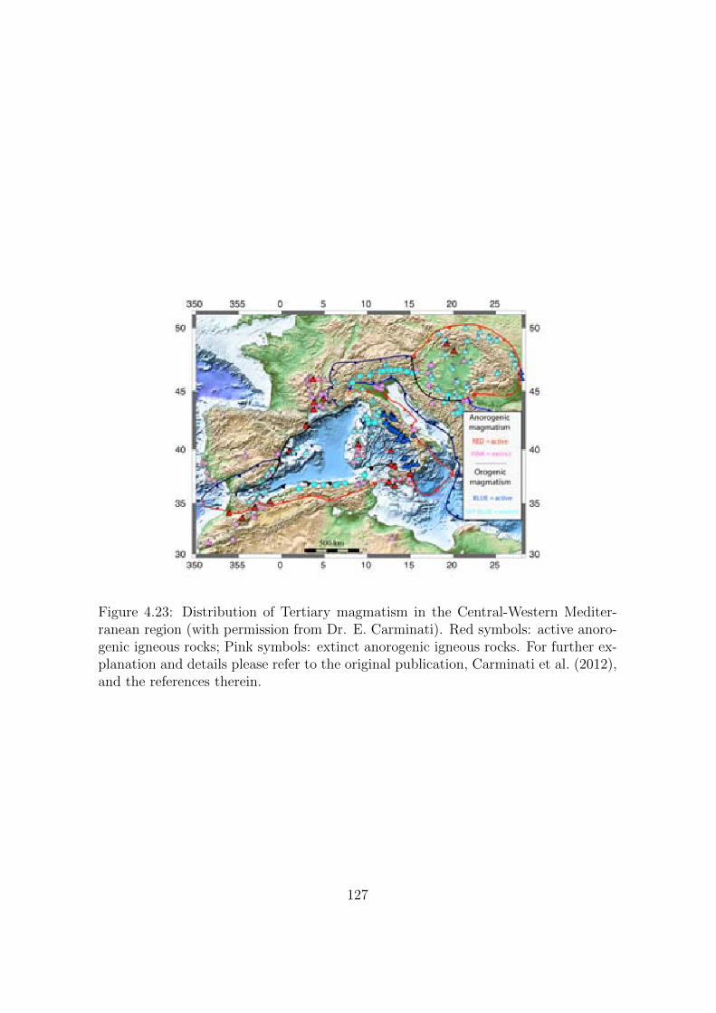
Figure 4.23: Distribution of Tertiary magmatism in the Central-Western Mediter-ranean region (with permission from Dr. E. Carminati). Red symbols: active anoro-genic igneous rocks; Pink symbols: extinct anorogenic igneous rocks. For further ex-planation and details please refer to the original publication, Carminati et al. (2012),and the references therein.
127
4.4.2.8 410 depression and anorogenic magmatism
The north of Morocco and the east coast of Spain are characterized by recent igneous
activity (∼ 10-0.01 My) of sub-lithospheric origin (yellow triangles in Fig. 4.8), which
is also found in all the Mediterranean region as shown in Fig. 4.23. This igneous
activity is also known as the Circum-Mediterranean Anorogenic Cenozoic Igneous
(CiMACI) Province (Lustrino and Wilson, 2007; Lustrino et al., 2011; Carminati
et al., 2012). Several petrological and geodynamic models have been proposed to
explain the anorogenic magmatic activity; these are summarized in fig. 18 in Lus-
trino and Wilson (2007). The models require either (i) active asthenospheric (or
deeper) mantle convection (i.e., mantle plumes) or (ii) lithospheric extension (or de-
lamination and detachment) to induce passive adiabatic decompression melting of
both asthenospheric and lithospheric upper mantle.
This active anorogenic magmatism, where active means that these volcanoes
erupted recently and could still erupt, are located at the border of areas with a
depressed 410. We do not see the same spatial correlation with the 660 topography
or with the TZT.
Our results can be explained with the mantle-plume model (model i), where the
stem of the plume is centered away from the Mediterranean, similar to the model
proposed by Duggen et al. (2009) (Fig. 1.6). The plume material would only affect
the 410 beneath north Morocco and the eastern coast of Spain. Additionally, this
model is consistent with the presence of the reversed polarity signal before P410s. The
410 depression can be attributed to a thermal anomaly of about +160 K, while the
reversed polarity signal is attributed to the effect of high temperatures on water rich
mantle silicate rocks, as has been suggested from S-RF studies in other regions (Vinnik
and Farra, 2002, 2007). Although model (i) explains the Pws phase before P410s,
the detection of this signal is not restricted to a particular tectonic environment, but
is rather attributed to a global low-velocity layer of variable thickness within the
Earth’s upper mantle (Tauzin et al., 2010). Furthermore, this plume-like model is
consistent with the thinned TZ beneath the Strait of Gibraltar, Gulf of Cadiz and
south of Portugal. In this context, the Alboran slab would be an obstacle for the
plume material, which increases the upper-mantle temperature towards the west of
the Alboran slab. This temperature increase will result in the shift of the α → β
transformation to higher pressures and to the shift of the post-spinel transition to
128
lower ones (and the garnet-related phase transition to higher pressures). The plume-
like model provides an alternative explanation (to our model II in Fig. 4.21 and
section 4.4.2.5) for the depressed 410 beneath the northeast coast of Spain, while the
explanation for the 660 deflection remains the same.
On the other hand, melt in the overlying mantle, as proposed by model (ii),
preferentially extracts Fe, leaving a Mg-enriched residue that should be transported
into the mantle transition zone (Schmerr and Garnero, 2007). In a Mg-enriched
mantle in the vicinity of the 410, the α→ β phase transition moves to higher pressures
(e.g., left panel in Fig. 1.5 in the general introduction), leading to the downward
deflection of the 410 discontinuity beneath north Morocco and the northeast coast of
Spain. This explanation is consistent with our model II for the northeast coast of
Spain. The contribution of the Mg-enriched mantle to the depth of the 410 has the
same sign as that of a higher temperature due to small scale convection above the
Alpine-Tethys remnant slab.
In conclusion, the obtained 410 and 660 topographies in this area can be explained
equally well with both models (i and ii). We have no preferred model, and yet there
is lack of evidence to suport any of them (Lustrino, 2011).
4.4.2.9 Other features and minor comments
We have recognized several anomalous features in the cross-sections of RFs and large
areas of undetected P410s phases. We discuss these particularities in more detail
below.
The negative peaks before the P410s phase, suggesting water-induced melting
atop the 410 (e.g. Tauzin et al., 2010), are present in the entire region (see Pws in
Fig. 4.19). Nevertheless, this signal is more clear, continuous and stronger in the pro-
files that cross the Alboran Sea (ff’, gg’, ii’ and jj’ in Fig. 4.19), the northeast of Spain
(aa’, bb’ and cc’ in Fig. 4.19) and the Gulf of Cadiz (AA’ and BB’ in Fig. E.3). The
first two areas coincide with the location of the Betic-Alboran slab and the Alpine-
Tethys remnant slab, respectively, which likely contribute to a water concentration
increase in the TZ. On the other hand, in the Gulf of Cadiz we have found a thinned
TZ which corresponds to a thermal anomaly of +190 K across the TZ and which
could be related to plume material that is forced to release water, because the stor-
age capacity of wadsleyite is larger than the overlying olivine (Hirschmann, 2006). In
this context, the increased water content could be responsible for a localized higher
129
amount of melting atop the 410 in the mentioned areas.
The 410 has been less well observed in the Alboran Sea area which leads to ob-
servation gaps (Fig. 4.8 a). A detection gap of converted or reflected energy from
the 410 in subduction zones has been reported in other studies too, e.g., for near
source conversions (Collier and Helffrich, 2001; Tibi and Wiens, 2005), sScS pre-
cursors (Tono et al., 2005), and SS precursors (Contenti et al., 2012). Profile AA’
and BB’ in Fig. E.3 show that the 410 gap coincides with the position of the Betic-
Alboran slab. Furthermore, we have noted that the only clear signal in this area is
the negative-amplitude signal Pws before P410s. We believe that structural com-
plexities cause the 410 observation gap due to defocusing or loss of coherence and
destructive interference with other coda waves. Furthermore, the seismic visibility of
the 410 is often decreased in subduction areas owing to its thermodynamic properties
which may lead to smaller conversions/reflections in colder-than-normal mantle and
additional discontinuity broadening in the presence of water (Collier and Helffrich,
2001).
In the north and northwest coast of Iberia the 410 and 660 depths are correlated.
Both discontinuities are deeper beneath the Bay of Biscay (feature E in Figs 4.8 and
4.9) and shallower beneath the northwest coast of Iberia (feature C1 in Figs 4.8 and
4.9). In both areas, the TZT is close to the reference value of 250 km. It is probable
that the 410 and 660 depth correlation is due to underestimated time corrections on
P410s and P660s travel times. This is expected due to the lower resolution of the
tomographic images in these areas.
4.5 Summary and conclusions
We have carried out a semiautomatic search for converted phases P410s and P660s
beneath the Iberian Peninsula and north Morocco using teleseismic data from 259
stations, most of them belonging to the IberArray of the TopoIberia project. We
have used three independent approaches (PCC, CCGN and RF) to estimate the rel-
ative travel time of converted phases and a bootstrap algorithm to estimate the time
uncertainties. The region has been divided in small areas of common piercing points
to perform the stack of correlograms and receiver functions. We have considered only
130
converted phases with stacked amplitude larger than twice the mean amplitude in the
time interval 30-80 s, and with bootstrap time-standard deviation smaller than 1.5
s. Besides, we have performed a thorough visual inspection to avoid spurious detec-
tions. Based on a body wave tomography velocity model for the study area, we have
applied time corrections to the travel times of the Pds (d=410, 660) phases. These
corrected travel times were then converted to depth obtaining the topography maps
for the 410 and 660 discontinuities and the TZT map beneath the Iberian Peninsula
and its surroundings. The main results are:
• Alboran Sea region: thicker TZ due to vertically anti-correlated 410 and 660
(locally elevated 410 and widely depressed 660).
• South Spain (Granada area): TZT variation of 86 km towards the east (from
thin to thick) coinciding with the location of the nest of deep earthquakes.
• Northeast Spain (Pyrenees and Balearic Sea): thicker TZ mainly due to a
depressed 660 while the 410 depths are unperturbed or slightly depressed.
• Northwest and central Iberia: normal TZT.
• Morocco: deeper 660 beneath the western part of the Moroccan region, leading
to a thicker TZ. The 410 is at normal depth and exhibits a detection gap beneath
the Rif area.
• Southwest Iberia and Gulf of Cadiz: thinner TZ due to a depressed 410, while
the 660 is shallower to the west and deeper to the east.
• Reversed polarity signal before P410s: observed in the entire region but more
clear, continuous and stronger in the Gulf of Cadiz, Alboran Sea and the north-
east coast of Spain.
• Spatial correlation between the location of the anorogenic magmatism and the
downward deflected 410.
In the discussion we have considered both, thermal and compositional interpreta-
tions of our results. Our main conclusions are the following:
131
• Our results are in good agreement with previous studies in the same area
(van der Meijde et al., 2005; Dundar et al., 2011). However, the large data
volume provided by the IberArray of the TopoIberia project has permitted us
to considerably increase the resolution and to resolve new TZT and topography
of discontinuities.
• Alboran Sea:
– We have found consistency between the thickened TZ beneath the Alboran
Sea and the position of a high-velocity anomaly in the tomographic images
which have been related to the Betic-Alboran slab. Our results suggest
that the slab is still cold enough to induce downward deflection of the
post-spinel transformation and uplift of the olivine-to-wadsleyite phase
transition.
– The anti-correlated depth of the 410 and 660 beneath the Alboran Sea have
provided indirect and independent (from tomography) evidences confirm-
ing the steep nature of the Betic-Alboran slab.
– The nest of deep earthquakes beneath Granada is in an area of high tem-
perature gradient inside the TZ (of about 540 K over a distance of less
than 250 km). This may further help to constrain the origin of the deep
earthquakes beneath Granada.
• The depressed 410 beneath the Balearic Sea, the presence of strong Pws phases
before P410s and the depressed 660 in the Pyrenees and Balearic Sea are con-
sistent with the presence of the Alpine-Tethys remnant slab. The cold stagnant
slab can explain the 660 depression; small-scale convection above the 660, trig-
gered by slab dehydration can explain the depressed 410; and the presence of
a water concentration increase in the TZ due to dehydration of the stagnant
slab can explain the strong reversed polarity signal before P410s. Nevertheless,
other models proposed to explain the anorogenic magmatism in the Mediter-
ranean are also consistent with our observations.
• We have proposed a compositional origin for the thickened TZ beneath the
western Moroccan region. The post-garnet transition together with an Al-rich
mantle can explain the downward deflection of the 660 beneath Morocco and
the thicker TZ in this area.
132
• The decreased visibility of the P410s phase beneath the Rif and beneath the
western end of the Alboran Sea is possibly caused by structural complexities
and/or the thermodynamic properties of the olivine-to-wadsleyite phase change
in colder-than-normal mantle.
• For the Gulf of Cadiz and the southwest coast of Portugal we have proposed a
thermally thinned TZ, which is consistent with the tomographic images from
Monna et al. (2013). Besides, a warm environment and the presence of Al
within garnet would also explain the small length-scale depth changes of the
660. We attribute the deeper 660 to the garnet-related phase transition and
the shallower 660 to the postspinel transition.
• The presence of melt atop the 410 may explain reversed polarity arrivals from
above this discontinuity. Plume material beneath the Gulf of Cadiz and sub-
ducted oceanic-lithosphere beneath the Alboran Sea and northeast Spain could
provide the higher water content to explain the stronger reversed polarity signal
in these areas.
• We have found that the spatial correlation between the active anorogenic mag-
matism and the 410 depression beneath Morocco and the northeast coast of
Spain can be explained with both groups of models proposed for the origin of
this magmatic activity. The estimated 410 depression in this area is consistent
with a plume-like model with the steam of the plume away from the Mediter-
ranean and affecting only the upper portion of the TZ or with a Mg-enriched
mantle due to decompression melting in the overlaying mantle, which shifts the
410 phase transition to higher pressures.
133
5Discontinuity characterization
134

5.1 Introduction
In this chapter, we study the amplitude of the P410s and P660s phases and the width
of the corresponding boundaries, which, together with their topography, provide an
important link between mineral physics experiments and seismic observations.
The amplitudes of the seismic phases that interact with the discontinuity (e.g.,
conversions) provide information about the contrast in velocity (v) and density (ρ)
across the boundary. Ideally, the converted phases (Pds) are primarily sensitive to S-
wave velocity variations and less sensitive to density contrasts (Ammon, 1991; Julia,
2007). But in the real Earth a number of factors influence the amplitudes of the
converted (and reflected) phases, which may lead to erroneous measurements. Such
factors are the dependence of the transmission coefficient of the converted waves on
the angle of incidence (or epicentral distance), e.g., with variations of about 10 %
every 10◦ in the AK135 model (Kennett et al., 1995); the interference with other
energetic phases; focusing or defocusing effects due to discontinuity or mantle struc-
ture; intrinsic attenuation. These complexities may affect the analysis and their
influence should be considered to constrain the discontinuities (e.g., Helffrich et al.,
2003; Chambers et al., 2005).
The width (or sharpness) of the 410 and 660 is associated to how rapidly the
mineral phase reaction responsible for the discontinuity occurs with increasing depth.
However, mantle temperature and composition (Fe-Mg partitioning in the olivine-
system and the presence of H2O or garnet) can change the characteristics of the phase
transitions, making the interpretation of the corresponding seismic discontinuities
more difficult (Katsura and Ito, 1989; Wood, 1995; Stixrude, 1997; Weidner and
Wang, 1998; Smyth and Frost, 2002; Wang et al., 2004; Litasov and Ohtani, 2005;
Wang and Niu, 2010; Schmandt, 2012). The sharpness of the 410 and 660 provides
information about the temperature and composition of the upper mantle and TZ.
Seismically, the 410 and 660 are often approximated as linear velocity gradients,
which act as low-pass filters to converted waves, attenuating the high frequency en-
ergy. The high corner frequency of these filters is related to the thickness of the
velocity jump (Richards, 1972; Paulssen, 1988; Bostock, 1999). Thus, amplitude
variations in P -to-s conversions observed with long-period (low-frequency) data can
136
be interpreted as changes in the velocity contrast, while variations observed using
short-period (high-frequency) data can be read as changes in discontinuity thickness.
In what follows, we analyse the relative amplitude of the converted phases P410s
and P660s and the 410 and 660 thickness for a subset of stations selected from the
TopoIberia data set.
5.2 Relative amplitudes
To compare the amplitudes of the converted phases between different measurements
a normalization is necessary. Therefore, we use the relative amplitudes of P410s
(P410s/P ) and P660s (P660s/P ). To investigate them, we have employed the data
from the 9 stations presented in Chapter 2 (Section 2.4).
5.2.1 Processing
The amplitude values are measured from the linear stack of RFs (already normalized),
which are previously low-pass filtered (0.02-0.12 Hz or 0.03-0.2 Hz) to avoid the
attenuating effect of the discontinuity width (Richards, 1972; Bostock, 1999). The
epicentral distance interval (from 65◦ to 95◦) used in this analysis minimizes the
interference with other phases. The RFs are stacked in the time-slowness domain
stabilizing the amplitudes and attenuating the contribution from other phases to the
conversions.
5.2.2 Results
Our measured values of relative amplitudes (or the amplitude of the conversion coef-
ficient at low frequencies) are shown in the second (P410s/P ) and third (P660s/P )
column of Table 5.1 and plotted in Fig. 5.1 (for the clarity of this figure, the large
relative amplitudes of station E125 are excluded, but they have not been excluded
from the analysis). The plotted amplitudes are mean values obtained using a boot-
strap resampling of 21 repetitions. The P410s/P values vary from 0.038 ± 0.012(2σ)
to 0.130 ± 0.022(2σ) and the P660s/P values from 0.033 ± 0.010(2σ) to 0.170 ±0.018(2σ). The largest values are for two close stations in north Spain, EARI and
E125. At 95 % confidence level (2σ), the P660s/P values for station ANER, CFON,
MTE, EARI and EMIN correspond to the predicted value for AK135 of 0.036 at 80◦
137
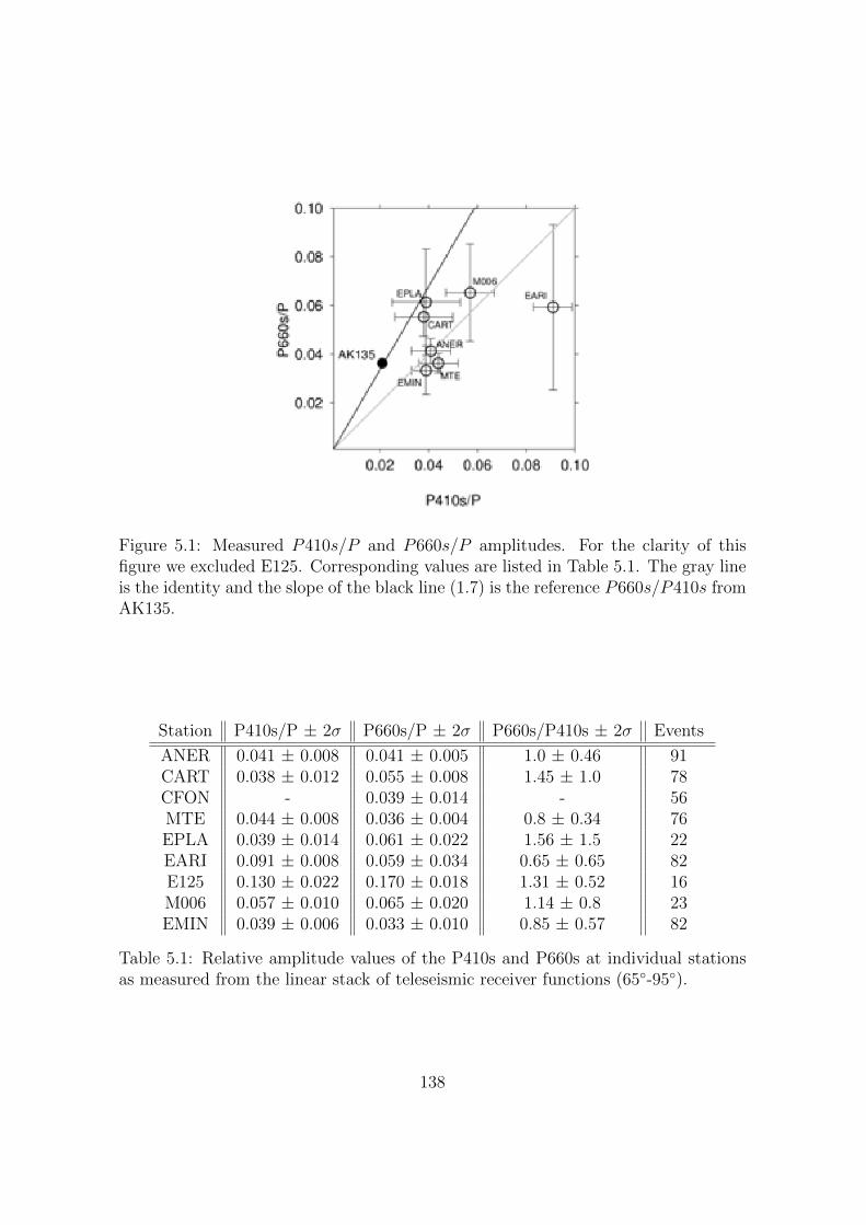
Figure 5.1: Measured P410s/P and P660s/P amplitudes. For the clarity of thisfigure we excluded E125. Corresponding values are listed in Table 5.1. The gray lineis the identity and the slope of the black line (1.7) is the reference P660s/P410s fromAK135.
Station P410s/P ± 2σ P660s/P ± 2σ P660s/P410s ± 2σ Events
ANER 0.041 ± 0.008 0.041 ± 0.005 1.0 ± 0.46 91CART 0.038 ± 0.012 0.055 ± 0.008 1.45 ± 1.0 78CFON - 0.039 ± 0.014 - 56MTE 0.044 ± 0.008 0.036 ± 0.004 0.8 ± 0.34 76EPLA 0.039 ± 0.014 0.061 ± 0.022 1.56 ± 1.5 22EARI 0.091 ± 0.008 0.059 ± 0.034 0.65 ± 0.65 82E125 0.130 ± 0.022 0.170 ± 0.018 1.31 ± 0.52 16M006 0.057 ± 0.010 0.065 ± 0.020 1.14 ± 0.8 23EMIN 0.039 ± 0.006 0.033 ± 0.010 0.85 ± 0.57 82
Table 5.1: Relative amplitude values of the P410s and P660s at individual stationsas measured from the linear stack of teleseismic receiver functions (65◦-95◦).
138
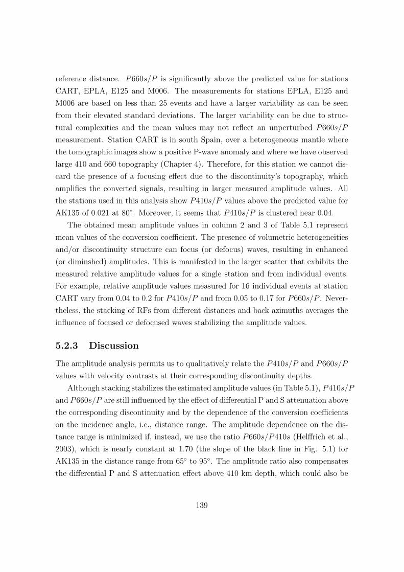
reference distance. P660s/P is significantly above the predicted value for stations
CART, EPLA, E125 and M006. The measurements for stations EPLA, E125 and
M006 are based on less than 25 events and have a larger variability as can be seen
from their elevated standard deviations. The larger variability can be due to struc-
tural complexities and the mean values may not reflect an unperturbed P660s/P
measurement. Station CART is in south Spain, over a heterogeneous mantle where
the tomographic images show a positive P-wave anomaly and where we have observed
large 410 and 660 topography (Chapter 4). Therefore, for this station we cannot dis-
card the presence of a focusing effect due to the discontinuity’s topography, which
amplifies the converted signals, resulting in larger measured amplitude values. All
the stations used in this analysis show P410s/P values above the predicted value for
AK135 of 0.021 at 80◦. Moreover, it seems that P410s/P is clustered near 0.04.
The obtained mean amplitude values in column 2 and 3 of Table 5.1 represent
mean values of the conversion coefficient. The presence of volumetric heterogeneities
and/or discontinuity structure can focus (or defocus) waves, resulting in enhanced
(or diminshed) amplitudes. This is manifested in the larger scatter that exhibits the
measured relative amplitude values for a single station and from individual events.
For example, relative amplitude values measured for 16 individual events at station
CART vary from 0.04 to 0.2 for P410s/P and from 0.05 to 0.17 for P660s/P . Never-
theless, the stacking of RFs from different distances and back azimuths averages the
influence of focused or defocused waves stabilizing the amplitude values.
5.2.3 Discussion
The amplitude analysis permits us to qualitatively relate the P410s/P and P660s/P
values with velocity contrasts at their corresponding discontinuity depths.
Although stacking stabilizes the estimated amplitude values (in Table 5.1), P410s/P
and P660s/P are still influenced by the effect of differential P and S attenuation above
the corresponding discontinuity and by the dependence of the conversion coefficients
on the incidence angle, i.e., distance range. The amplitude dependence on the dis-
tance range is minimized if, instead, we use the ratio P660s/P410s (Helffrich et al.,
2003), which is nearly constant at 1.70 (the slope of the black line in Fig. 5.1) for
AK135 in the distance range from 65◦ to 95◦. The amplitude ratio also compensates
the differential P and S attenuation effect above 410 km depth, which could also be
139
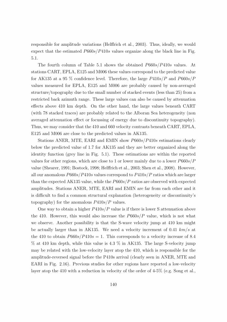
responsible for amplitude variations (Helffrich et al., 2003). Thus, ideally, we would
expect that the estimated P660s/P410s values organize along the black line in Fig.
5.1.
The fourth column of Table 5.1 shows the obtained P660s/P410s values. At
stations CART, EPLA, E125 and M006 these values correspond to the predicted value
for AK135 at a 95 % confidence level. Therefore, the large P410s/P and P660s/P
values measured for EPLA, E125 and M006 are probably caused by non-averaged
structure/topography due to the small number of stacked events (less than 25) from a
restricted back azimuth range. These large values can also be caused by attenuation
effects above 410 km depth. On the other hand, the large values beneath CART
(with 78 stacked traces) are probably related to the Alboran Sea heterogeneity (non
averaged attenuation effect or focussing of energy due to discontinuity topography).
Thus, we may consider that the 410 and 660 velocity contrasts beneath CART, EPLA,
E125 and M006 are close to the predicted values in AK135.
Stations ANER, MTE, EARI and EMIN show P660s/P410s estimations clearly
below the predicted value of 1.7 for AK135 and they are better organized along the
identity function (grey line in Fig. 5.1). These estimations are within the reported
values for other regions, which are close to 1 or lower mainly due to a lower P660s/P
value (Shearer, 1991; Bostock, 1998; Helffrich et al., 2003; Shen et al., 2008). However,
all our anomalous P660s/P410s values correspond to P410s/P ratios which are larger
than the expected AK135 value, while the P660s/P ratios are observed with expected
amplitudes. Stations ANER, MTE, EARI and EMIN are far from each other and it
is difficult to find a common structural explanation (heterogeneity or discontinuity’s
topography) for the anomalous P410s/P values.
One way to obtain a higher P410s/P value is if there is lower S attenuation above
the 410. However, this would also increase the P660s/P value, which is not what
we observe. Another possibility is that the S-wave velocity jump at 410 km might
be actually larger than in AK135. We need a velocity increment of 0.41 km/s at
the 410 to obtain P660s/P410s = 1. This corresponds to a velocity increase of 8.4
% at 410 km depth, while this value is 4.3 % in AK135. The large S-velocity jump
may be related with the low-velocity layer atop the 410, which is responsible for the
amplitude-reversed signal before the P410s arrival (clearly seen in ANER, MTE and
EARI in Fig. 2.16). Previous studies for other regions have reported a low-velocity
layer atop the 410 with a reduction in velocity of the order of 4-5% (e.g. Song et al.,
140
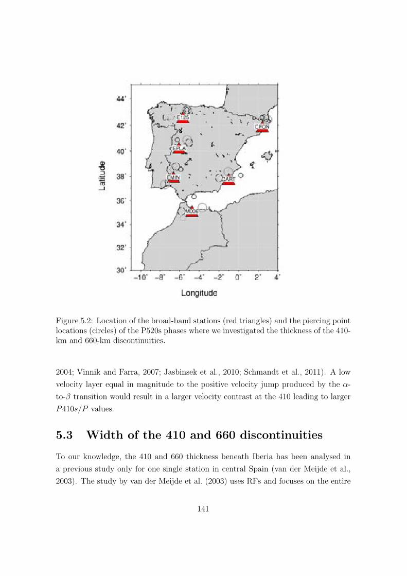
Figure 5.2: Location of the broad-band stations (red triangles) and the piercing pointlocations (circles) of the P520s phases where we investigated the thickness of the 410-km and 660-km discontinuities.
2004; Vinnik and Farra, 2007; Jasbinsek et al., 2010; Schmandt et al., 2011). A low
velocity layer equal in magnitude to the positive velocity jump produced by the α-
to-β transition would result in a larger velocity contrast at the 410 leading to larger
P410s/P values.
5.3 Width of the 410 and 660 discontinuities
To our knowledge, the 410 and 660 thickness beneath Iberia has been analysed in
a previous study only for one single station in central Spain (van der Meijde et al.,
2003). The study by van der Meijde et al. (2003) uses RFs and focuses on the entire
141
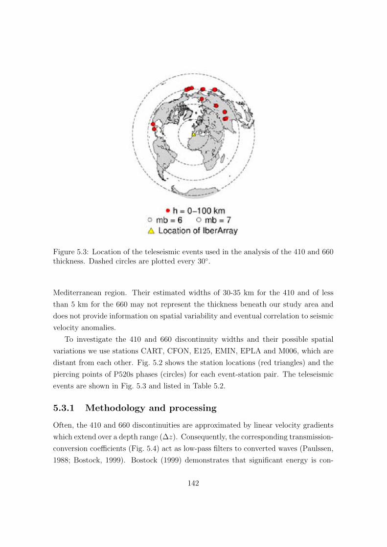
Figure 5.3: Location of the teleseismic events used in the analysis of the 410 and 660thickness. Dashed circles are plotted every 30◦.
Mediterranean region. Their estimated widths of 30-35 km for the 410 and of less
than 5 km for the 660 may not represent the thickness beneath our study area and
does not provide information on spatial variability and eventual correlation to seismic
velocity anomalies.
To investigate the 410 and 660 discontinuity widths and their possible spatial
variations we use stations CART, CFON, E125, EMIN, EPLA and M006, which are
distant from each other. Fig. 5.2 shows the station locations (red triangles) and the
piercing points of P520s phases (circles) for each event-station pair. The teleseismic
events are shown in Fig. 5.3 and listed in Table 5.2.
5.3.1 Methodology and processing
Often, the 410 and 660 discontinuities are approximated by linear velocity gradients
which extend over a depth range (∆z). Consequently, the corresponding transmission-
conversion coefficients (Fig. 5.4) act as low-pass filters to converted waves (Paulssen,
1988; Bostock, 1999). Bostock (1999) demonstrates that significant energy is con-
142
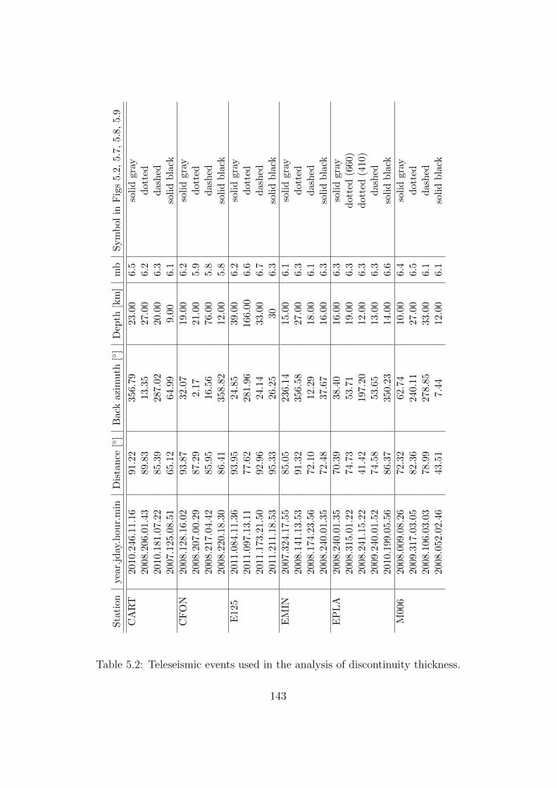
Station
year.jday.hou
r.min
Distance
[◦]
Backazim
uth
[◦]
Depth
[km]
mb
Symbolin
Figs5.2,5.7,5.8,5.9
CART
2010.246.11.16
91.22
356.79
23.00
6.5
solidgray
2008.206.01.43
89.83
13.35
27.00
6.2
dotted
2010.181.07.22
85.39
287.02
20.00
6.3
dashed
2007.125.08.51
65.12
64.99
9.00
6.1
solidblack
CFON
2008.128.16.02
93.87
32.07
19.00
6.2
solidgray
2008.207.00.29
87.29
2.17
21.00
5.9
dotted
2008.217.04.42
85.95
16.56
76.00
5.8
dashed
2008.220.18.30
86.41
358.82
12.00
5.8
solidblack
E125
2011.084.11.36
93.95
24.85
39.00
6.2
solidgray
2011.097.13.11
77.62
281.96
166.00
6.6
dotted
2011.173.21.50
92.96
24.14
33.00
6.7
dashed
2011.211.18.53
95.33
26.25
306.3
solidblack
EMIN
2007.324.17.55
85.05
236.14
15.00
6.1
solidgray
2008.141.13.53
91.32
356.58
27.00
6.3
dotted
2008.174.23.56
72.10
12.29
18.00
6.1
dashed
2008.240.01.35
72.48
37.67
16.00
6.3
solidblack
EPLA
2008.240.01.35
70.39
38.40
16.00
6.3
solidgray
2008.315.01.22
74.73
53.71
19.00
6.3
dotted
(660)
2008.241.15.22
41.42
197.20
12.00
6.3
dotted
(410)
2009.240.01.52
74.58
53.65
13.00
6.3
dashed
2010.199.05.56
86.37
350.23
14.00
6.6
solidblack
M006
2008.009.08.26
72.32
62.74
10.00
6.4
solidgray
2009.317.03.05
82.36
240.11
27.00
6.5
dotted
2008.106.03.03
78.99
278.85
33.00
6.1
dashed
2008.052.02.46
43.51
7.44
12.00
6.1
solidblack
Table 5.2: Teleseismic events used in the analysis of discontinuity thickness.
143
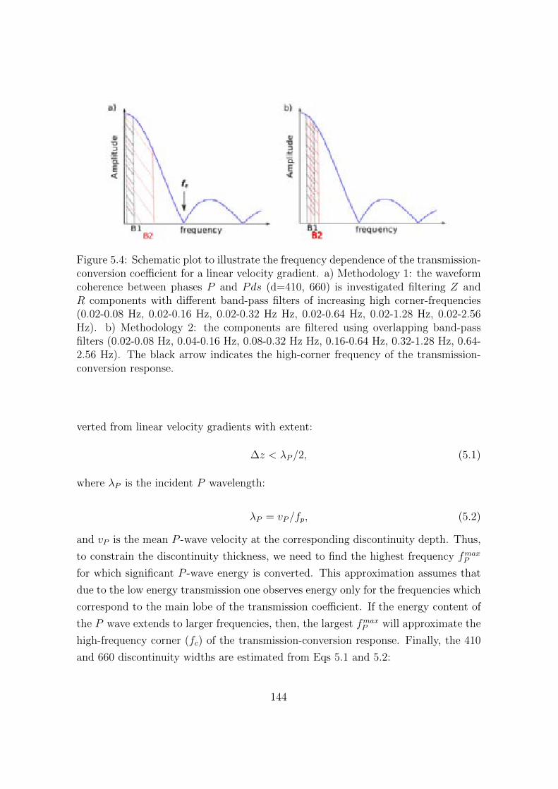
Figure 5.4: Schematic plot to illustrate the frequency dependence of the transmission-conversion coefficient for a linear velocity gradient. a) Methodology 1: the waveformcoherence between phases P and Pds (d=410, 660) is investigated filtering Z andR components with different band-pass filters of increasing high corner-frequencies(0.02-0.08 Hz, 0.02-0.16 Hz, 0.02-0.32 Hz Hz, 0.02-0.64 Hz, 0.02-1.28 Hz, 0.02-2.56Hz). b) Methodology 2: the components are filtered using overlapping band-passfilters (0.02-0.08 Hz, 0.04-0.16 Hz, 0.08-0.32 Hz Hz, 0.16-0.64 Hz, 0.32-1.28 Hz, 0.64-2.56 Hz). The black arrow indicates the high-corner frequency of the transmission-conversion response.
verted from linear velocity gradients with extent:
∆z < λP/2, (5.1)
where λP is the incident P wavelength:
λP = vP/fp, (5.2)
and vP is the mean P -wave velocity at the corresponding discontinuity depth. Thus,
to constrain the discontinuity thickness, we need to find the highest frequency fmaxP
for which significant P -wave energy is converted. This approximation assumes that
due to the low energy transmission one observes energy only for the frequencies which
correspond to the main lobe of the transmission coefficient. If the energy content of
the P wave extends to larger frequencies, then, the largest fmaxP will approximate the
high-frequency corner (fc) of the transmission-conversion response. Finally, the 410
and 660 discontinuity widths are estimated from Eqs 5.1 and 5.2:
144
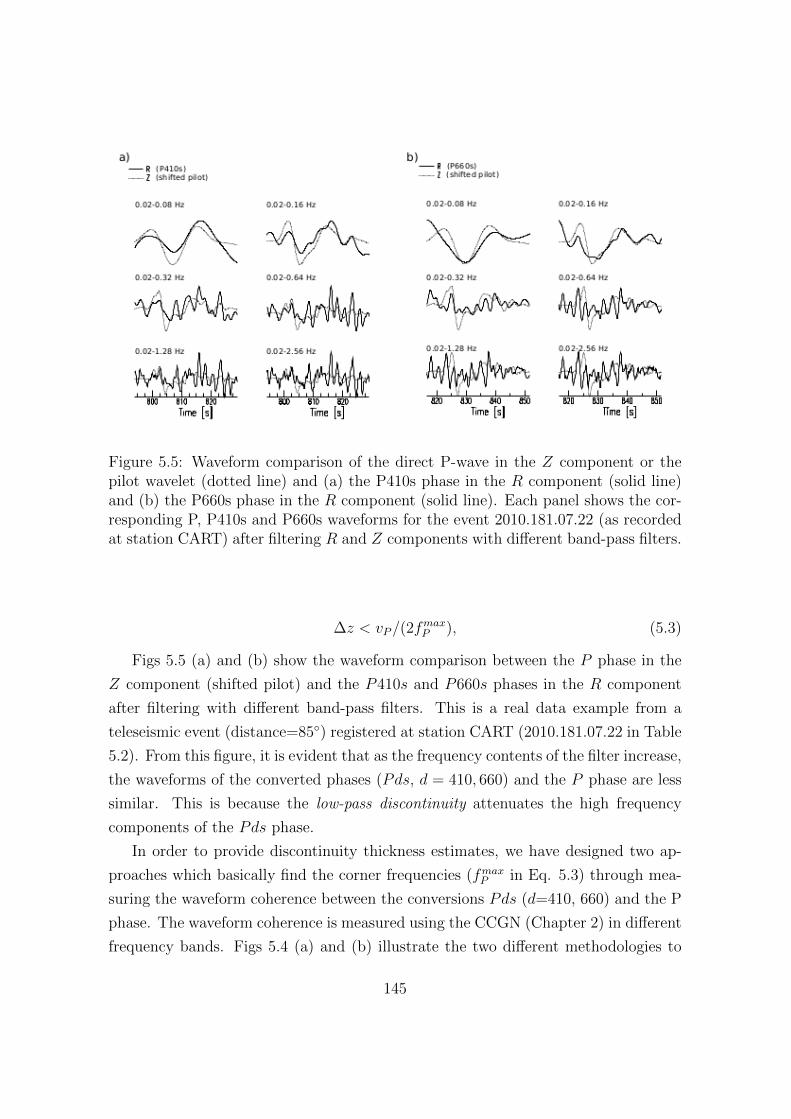
Figure 5.5: Waveform comparison of the direct P-wave in the Z component or thepilot wavelet (dotted line) and (a) the P410s phase in the R component (solid line)and (b) the P660s phase in the R component (solid line). Each panel shows the cor-responding P, P410s and P660s waveforms for the event 2010.181.07.22 (as recordedat station CART) after filtering R and Z components with different band-pass filters.
∆z < vP/(2fmaxP ), (5.3)
Figs 5.5 (a) and (b) show the waveform comparison between the P phase in the
Z component (shifted pilot) and the P410s and P660s phases in the R component
after filtering with different band-pass filters. This is a real data example from a
teleseismic event (distance=85◦) registered at station CART (2010.181.07.22 in Table
5.2). From this figure, it is evident that as the frequency contents of the filter increase,
the waveforms of the converted phases (Pds, d = 410, 660) and the P phase are less
similar. This is because the low-pass discontinuity attenuates the high frequency
components of the Pds phase.
In order to provide discontinuity thickness estimates, we have designed two ap-
proaches which basically find the corner frequencies (fmaxP in Eq. 5.3) through mea-
suring the waveform coherence between the conversions Pds (d=410, 660) and the P
phase. The waveform coherence is measured using the CCGN (Chapter 2) in different
frequency bands. Figs 5.4 (a) and (b) illustrate the two different methodologies to
145
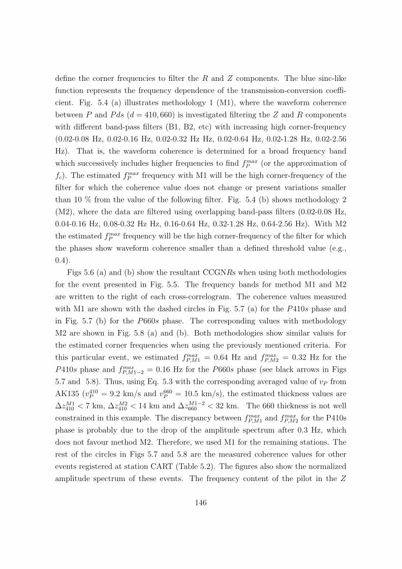
define the corner frequencies to filter the R and Z components. The blue sinc-like
function represents the frequency dependence of the transmission-conversion coeffi-
cient. Fig. 5.4 (a) illustrates methodology 1 (M1), where the waveform coherence
between P and Pds (d = 410, 660) is investigated filtering the Z and R components
with different band-pass filters (B1, B2, etc) with increasing high corner-frequency
(0.02-0.08 Hz, 0.02-0.16 Hz, 0.02-0.32 Hz Hz, 0.02-0.64 Hz, 0.02-1.28 Hz, 0.02-2.56
Hz). That is, the waveform coherence is determined for a broad frequency band
which successively includes higher frequencies to find fmaxP (or the approximation of
fc). The estimated fmaxP frequency with M1 will be the high corner-frequency of the
filter for which the coherence value does not change or present variations smaller
than 10 % from the value of the following filter. Fig. 5.4 (b) shows methodology 2
(M2), where the data are filtered using overlapping band-pass filters (0.02-0.08 Hz,
0.04-0.16 Hz, 0.08-0.32 Hz Hz, 0.16-0.64 Hz, 0.32-1.28 Hz, 0.64-2.56 Hz). With M2
the estimated fmaxP frequency will be the high corner-frequency of the filter for which
the phases show waveform coherence smaller than a defined threshold value (e.g.,
0.4).
Figs 5.6 (a) and (b) show the resultant CCGNRs when using both methodologies
for the event presented in Fig. 5.5. The frequency bands for method M1 and M2
are written to the right of each cross-correlogram. The coherence values measured
with M1 are shown with the dashed circles in Fig. 5.7 (a) for the P410s phase and
in Fig. 5.7 (b) for the P660s phase. The corresponding values with methodology
M2 are shown in Fig. 5.8 (a) and (b). Both methodologies show similar values for
the estimated corner frequencies when using the previously mentioned criteria. For
this particular event, we estimated fmaxP,M1 = 0.64 Hz and fmaxP,M2 = 0.32 Hz for the
P410s phase and fmaxP,M1−2 = 0.16 Hz for the P660s phase (see black arrows in Figs
5.7 and 5.8). Thus, using Eq. 5.3 with the corresponding averaged value of vP from
AK135 (v410P = 9.2 km/s and v660P = 10.5 km/s), the estimated thickness values are
∆zM1410 < 7 km, ∆zM2
410 < 14 km and ∆zM1−2660 < 32 km. The 660 thickness is not well
constrained in this example. The discrepancy between fmaxP,M1 and fmaxP,M2 for the P410s
phase is probably due to the drop of the amplitude spectrum after 0.3 Hz, which
does not favour method M2. Therefore, we used M1 for the remaining stations. The
rest of the circles in Figs 5.7 and 5.8 are the measured coherence values for other
events registered at station CART (Table 5.2). The figures also show the normalized
amplitude spectrum of these events. The frequency content of the pilot in the Z
146
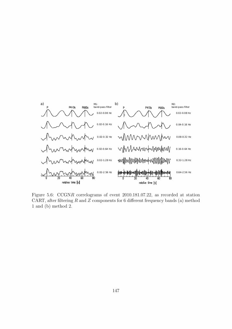
Figure 5.6: CCGNR correlograms of event 2010.181.07.22, as recorded at stationCART, after filtering R and Z components for 6 different frequency bands (a) method1 and (b) method 2.
147
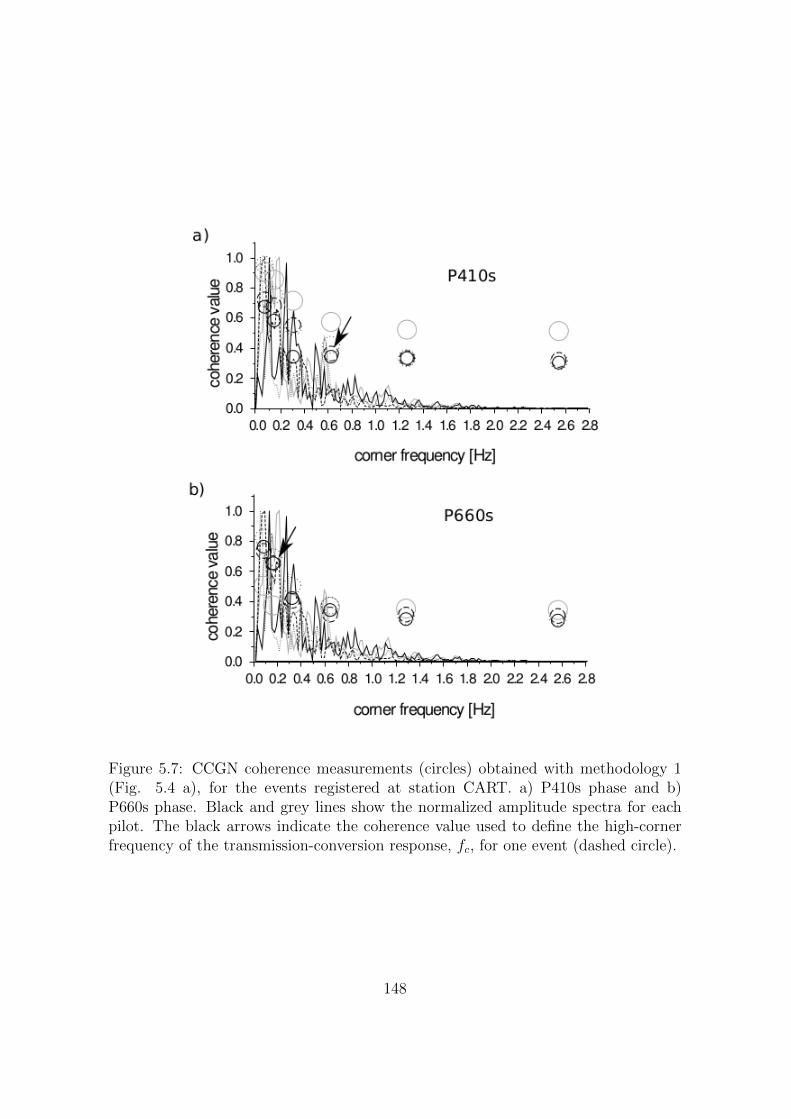
Figure 5.7: CCGN coherence measurements (circles) obtained with methodology 1(Fig. 5.4 a), for the events registered at station CART. a) P410s phase and b)P660s phase. Black and grey lines show the normalized amplitude spectra for eachpilot. The black arrows indicate the coherence value used to define the high-cornerfrequency of the transmission-conversion response, fc, for one event (dashed circle).
148

Figure 5.8: CCGN coherence measurements (circles) obtained with methodology 2(Fig. 5.4 b), for the events registered at station CART. a) P410s phase and b)P660s phase. Black and grey lines show the normalized amplitude spectra for eachpilot. The black arrows indicate the coherence value used to define the high-cornerfrequency of the transmission-conversion response, fc, for one event (dashed circle).
149
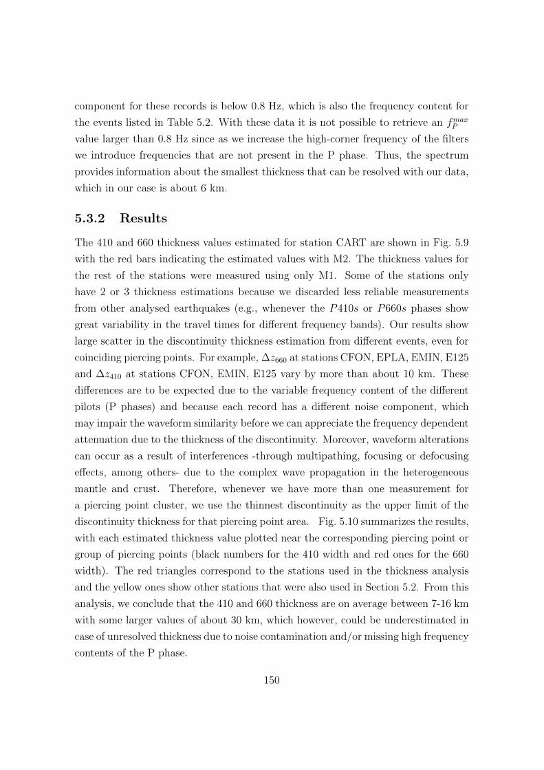
component for these records is below 0.8 Hz, which is also the frequency content for
the events listed in Table 5.2. With these data it is not possible to retrieve an fmaxP
value larger than 0.8 Hz since as we increase the high-corner frequency of the filters
we introduce frequencies that are not present in the P phase. Thus, the spectrum
provides information about the smallest thickness that can be resolved with our data,
which in our case is about 6 km.
5.3.2 Results
The 410 and 660 thickness values estimated for station CART are shown in Fig. 5.9
with the red bars indicating the estimated values with M2. The thickness values for
the rest of the stations were measured using only M1. Some of the stations only
have 2 or 3 thickness estimations because we discarded less reliable measurements
from other analysed earthquakes (e.g., whenever the P410s or P660s phases show
great variability in the travel times for different frequency bands). Our results show
large scatter in the discontinuity thickness estimation from different events, even for
coinciding piercing points. For example, ∆z660 at stations CFON, EPLA, EMIN, E125
and ∆z410 at stations CFON, EMIN, E125 vary by more than about 10 km. These
differences are to be expected due to the variable frequency content of the different
pilots (P phases) and because each record has a different noise component, which
may impair the waveform similarity before we can appreciate the frequency dependent
attenuation due to the thickness of the discontinuity. Moreover, waveform alterations
can occur as a result of interferences -through multipathing, focusing or defocusing
effects, among others- due to the complex wave propagation in the heterogeneous
mantle and crust. Therefore, whenever we have more than one measurement for
a piercing point cluster, we use the thinnest discontinuity as the upper limit of the
discontinuity thickness for that piercing point area. Fig. 5.10 summarizes the results,
with each estimated thickness value plotted near the corresponding piercing point or
group of piercing points (black numbers for the 410 width and red ones for the 660
width). The red triangles correspond to the stations used in the thickness analysis
and the yellow ones show other stations that were also used in Section 5.2. From this
analysis, we conclude that the 410 and 660 thickness are on average between 7-16 km
with some larger values of about 30 km, which however, could be underestimated in
case of unresolved thickness due to noise contamination and/or missing high frequency
contents of the P phase.
150
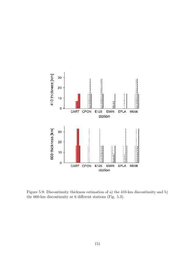
Figure 5.9: Discontinuity thickness estimation of a) the 410-km discontinuity and b)the 660-km discontinuity at 6 different stations (Fig. 5.3).
151
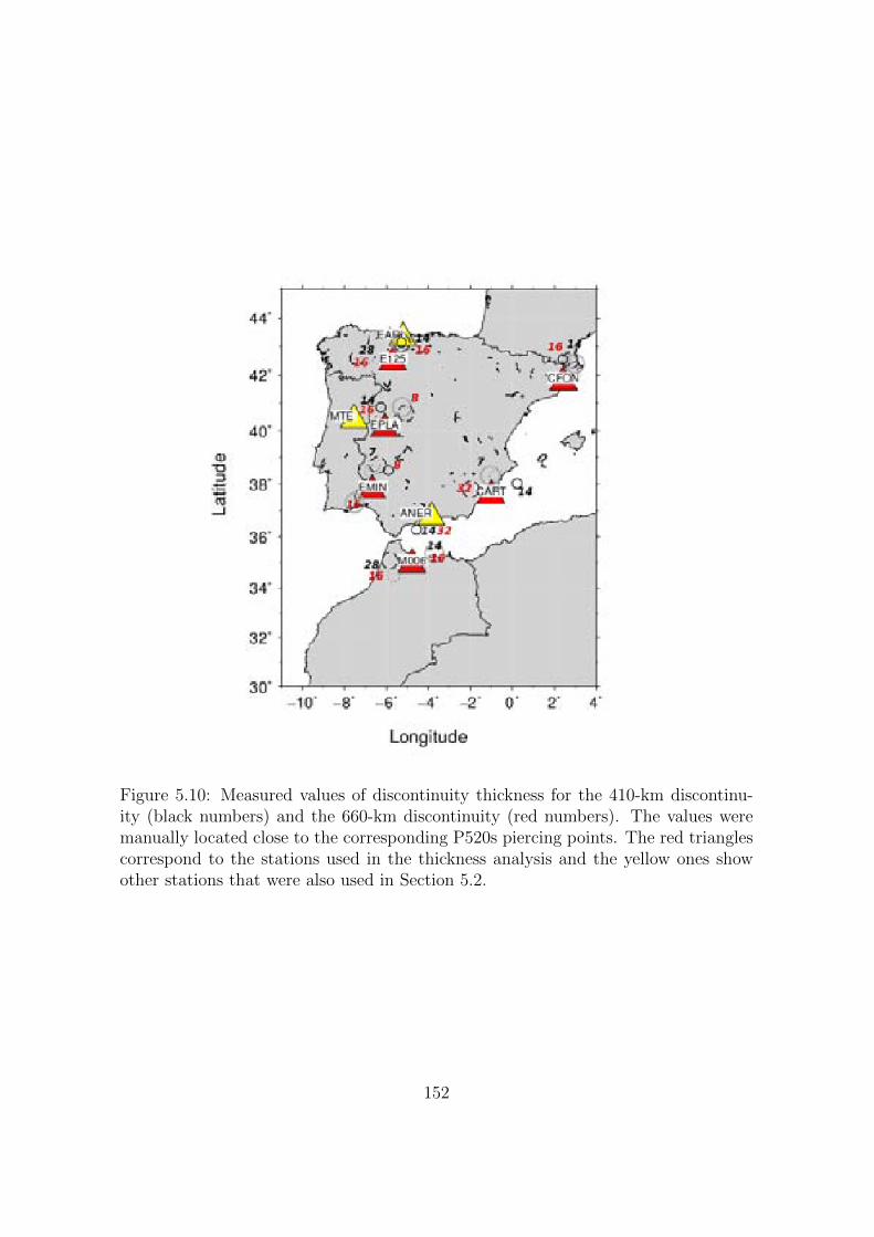
Figure 5.10: Measured values of discontinuity thickness for the 410-km discontinu-ity (black numbers) and the 660-km discontinuity (red numbers). The values weremanually located close to the corresponding P520s piercing points. The red trianglescorrespond to the stations used in the thickness analysis and the yellow ones showother stations that were also used in Section 5.2.
152
5.3.3 Discussion
5.3.3.1 Thickness constraints from mineral physics
The published depth interval for the olivine-to-wadsleyite transition (410), in dry
(Mg,Fe)2SiO4-systems and at typical TZ temperatures, ranges between 6 to 18 km
(Akaogi et al., 1989; Smyth and Frost, 2002; Frost, 2003). The transition width de-
pends on the Fe content of the olivine-system (wider for higher Fe content) (e.g.,
Katsura et al., 2004, fig. 3). For a fixed Mg-Fe partitioning, the α-to-β transforma-
tion is sharper at higher temperatures but broader at lower temperatures (Katsura
and Ito, 1989; Katsura et al., 2004) affecting the visibility of the discontinuity in sub-
duction related environments (Bina and Helffrich, 1994). For example, an increase
in T of 100 K will reduce the width of the 410 by 2-3 km (Bina and Helffrich, 1994;
Katsura and Ito, 1989). Additionally, H2O might act to broaden the transformation
interval to 22-40 km (Wood, 1995; Smyth and Frost, 2002; Frost, 2003; Litasov et al.,
2005; Katsura et al., 2004). For example, a small amount of 100 ppm of water will
broaden the transition by about 3 km (Wood, 1995; Frost, 2003). Thus, the expected
widths of the 410 range between about 4 to 40 km, depending on the composition
(Mg-Fe partitioning and H2O) and temperature of the upper mantle.
On the other hand, the pressure interval where ringwoodite and perovskite +
magnesiowustite (660) coexist is about 0.1-0.5 GPa (5-20 km) (Ito and Takahashi,
1998; Hirose, 2002; Litasov et al., 2005) and it appears to remain narrow over a broad
range of temperatures (Ito and Takahashi, 1998). Like the wadsleyite, the ringwoodite
has also enhanced water storage capacity over the upper and lower mantle mineral
assemblages (Kohlstedt et al., 1996). Although the presence of water can move the
post-spinel phase transition to higher pressures in colder environments, it does not
have an appreciable effect on the thickness of this transition (Higo et al., 2001; Litasov
and Ohtani, 2005). Therefore, the 660 must be a sharp discontinuity with a thickness
less than 20 km, if it is solely caused by the post-spinel phase transition. The garnet-
to-perovskite phase transition (Appendix B), which is also expected at the base of
the TZ, occurs in a wider pressure interval of about 1-1.5 GPa (40-60 km). However,
the effective width of these phase transitions could be narrowed by compositional
frustration of the full reaction interval in the pure-garnet system (Stixrude, 1997).
Therefore, both discontinuities would appear as sharp discontinuities unless they
153
partially overlap. In this case, it is possible to have a single and broad discontinuity
(e.g., Wang and Niu, 2010, in a subduction area in north-east China).
5.3.3.2 Thickness constraints from seismology
Seismically, the 410 and 660 discontinuities have been observed to maximum fre-
quencies of about 1 Hz leading to sharp transitions (< 10 km wide intervals) (e.g.
Paulssen, 1988; Vidale et al., 1995; Collier and Helffrich, 1997; Landes et al., 2006).
Differences with the mineral physics experiments have been attributed to: presence of
non-transforming phases (Stixrude, 1997); focusing effects which might boost the am-
plitudes of conversions (or reflections) above the corner frequency of the transmission-
conversion (or reflection) response (fc in Fig. 5.4) (Shearer, 2000); non-linear velocity
increases, predicted by models of mineral phase changes (e.g., Helffrich and Bina,
1994), where the highest-frequency reflections/conversions are determined more by
the sharpness of the steepest part of the profile than by the total layer thickness
(Shearer, 2000); gravity-driven diffusion of hydrogen, which may enrich the lower
parts of the two-phase region in wadsleyite and the upper part in olivine, thus sharp-
ening the boundary (Smyth and Frost, 2002).
Other studies have reported wider discontinuities. Beneath central Spain, for ex-
ample, van der Meijde et al. (2003) found a 410 discontinuity of about 30-35 km asso-
ciated with the presence of water in wadsleyite. In subduction related environments,
the 660 has been observed as a wide velocity gradient of about 50-70 km, which has
been associated to complex velocity structures due to the post-spinel (olivine phase
transition) and ilmenite-to-perovskite (garnet related) phase transitions (Wang and
Niu, 2010; Schmandt et al., 2011; Schmandt, 2012).
5.3.3.3 410 and 660 thickness beneath Iberia
We cannot discard a thickness underestimation with our methodology, related to un-
resolved thickness due to noise contamination and/or missing high frequency contents
of the P phase. Therefore, our estimated thickness values of 7 to 30 km, for both
discontinuities, can be considered as upper limits on the 410 and 660 velocity gradient
thickness beneath Iberia and Morocco.
We have estimated a 660 thickness of 16 km for the entire area with exception
of larger thickness values of 32 km beneath south Spain and the Alboran Sea and
smaller thickness of 8 km in the central area of Iberia. For the 410 we have estimated
154
a thickness value of 7-14 km for almost the entire study area, with exception of larger
values of 28 km in the north-west corner of Iberia and Morocco. Assuming that
our estimated values are well-constrained upper limits, it can be considered that the
observed differences in the thickness of the 410 and 660 represent spatial variations
of this parameter.
Because the post-spinel transition remains narrow over a broad range of temper-
atures (and Mg-Fe partitioning), the spatial variation in the 660 thickness might
reflect the dual origin of this discontinuity (olivine-related and the garnet-related
phase transitions). This complicates the interpretation in normal-to-cold mantle en-
vironments, because we cannot be sure to which phase transition one should attribute
the 660 width since both discontinuities may appear at similar depth (depending on
the Al contents of the garnet), although the post-spinel occurs in a thinner depth
interval than the garnet-related phase transition. The broad 660 of about 30 km co-
incides with the location of the cold Alboran slab. Other studies also reported broad
660 discontinuities in subduction related environments, explained as combined veloc-
ity gradients due to post-spinel and ilmenite-to-perovskite phase transitions (Wang
and Niu, 2010; Schmandt et al., 2011; Schmandt, 2012). Therefore, if the ilmenite-
to-perovskite phase transition is present, the 30 km thickness estimation for the 660
beneath the Alboran Sea might be due to combined velocity gradients.
In Chapter 4, it was shown the presence of a reversed-polarity signal before the
P410s (Fig. 4.19), which is attributed to partial melt atop the 410 due to high water
concentrations (e.g. Tauzin et al., 2010, and references therein). If the melt interpre-
tation of the P410s precursory signal with reverted polarity is correct, then most of
the 410 thickness is likely controlled by the increased water contents. Thus, it seems
that the spatial variation of the 410 thickness might reflect variable proportions of
water in the TZ minerals (rather than temperature variation or Fe-Mg partitioning).
Our estimated values for the width of the 410 (7-14 km) are consistent with 200 to
500 ppm of water in wadsleyite (obtained from fig. 16 in Wood and Corgne, 2007,
pp. 81).
Our estimated 660 thickness values are in good agreement with a previous RFs
study which covered the entire Mediterranean region (van der Meijde et al., 2003). In
their study, van der Meijde et al. (2003) investigate P -to-s conversions from the 660 in
the Mediterranean region. One of the stations (PAB) in van der Meijde et al. (2003)
is in central Spain. For this station, they report a sharp 660 of 5 km width. In good
155
agreement with van der Meijde et al. (2003) we have estimated a 660 of 8 km width
for station EPLA, which is close to station PAB. We have found a 410 thickness of
7-14 km in the same area, which is much thinner than the transition width reported
in van der Meijde et al. (2003) of about 30-35 km, consistent with about 700 ppm
to 1500 ppm of water in wadsleyite. Although our results are in agreement with
lower water contents, the 200 to 500 ppm water concentration in wadsleyite that we
estimate is still a considerable amount of water (see fig. 16 in Wood and Corgne,
2007, pp. 81).
5.4 Conclusions
The P410s amplitudes and the 410 widths are consistent with spatial variations in
the water concentrations in the TZ beneath Iberia. In particular, the variation of the
410 thickness (7-28 km) agrees with 200-500 ppm of water in wadsleyite. On the other
hand, to explain the anomalously high relative amplitude values of the P410s phase
(P410s/P ) we need to assume a negative velocity jump atop the 410, which increases
the total velocity jump across the 410 km depth discontinuity. The negative velocity
jump immediately above 410 km depth is consistent with the reversed-polarity signal
that we observed before P410s, which is related with partial melt atop the 410 caused
by a water concentration increase in the TZ.
The spatial variation of the 660 thickness might reflect the presence of the garnet-
related phase transition (garnet-to-perovskite or ilmenite-to-perovskite) together with
the post-spinel. This could lead to complex velocity structures which might be respon-
sible for the broader 660 in the cold Alboran Slab. The estimated relative amplitude
values of the P660s phase agree with the velocity jump in AK135 at 660 km depth.
156


AReceiver functions
158

A.1 Transmission path impulse response
The P coda consists of all type of scattered, reflected, diffracted and converted waves.
Among these coda waves, are the S waves converted from P waves at the seismic
discontinuities below the station. For a teleseismic earthquake, the near-vertically
incoming wavefield leads to a separation of the P - and SV -waves energy in the vertical
and radial components, respectively. Thus, the P -to-s conversions are detected on
the radial component. Consequently, the P coda in the radial component contains
information about the structure beneath the station. Deconvolution of the radial
component by the vertical component is used to eliminate the source influence and
to isolate the P -to-s conversions (Langston, 1979). The resultant time series is called
receiver function (RF) and can be viewed as the relative response of the Earth’s
structure (or transmission path impulse response) near the receiver. Another kind
of receiver function is the SV component deconvolved by the P component (Vinnik,
1977), obtained by rotating the radial and vertical components considering the ray
incidence angle to maximize SV - and P -wave energy.
In what follows, we explain the RF computation in more detail. The radial com-
ponent, r(t), of a teleseism can be expressed in terms of the transmission path impulse
response, h(t). Using the convolutional model of the trace (eq. 2.6), in the absence
of noise, this relation is:
r(t) = s(t) ∗ h(t), (A.1)
where s(t) is the source wavelet and ∗ denotes convolution. The source wavelet is
known as the ”teleseismic source function”, composed of the source function, near
source reverberations and the instrument response.
According to the convolution theorem, convolution in the time domain is mapped
as multiplication in the frequency domain. The frequency domain form of Eq. A.1
is:
R(w) = S(w) H(w), (A.2)
160
where the capital letters denote the Fourier transform pairs of the quantities in Eq.
A.1 and w is the angular frequency. In what comes next, we omit the frequency
argument to clarify the notation.
The objective of the RF technique is to obtain the impulse response H. This
objective can be achieved through deconvolution of the radial component R by the
source function S. The source function is an unknown parameter which is often
approximated with the recorded teleseismic P -wave source function on the vertical
component (S ≈ Z) (e.g., Bostock, 2007). Finally, an estimate of H is obtained,
which is denoted as RF.
H ≈ RF =R
Z. (A.3)
There exists a variety of deconvolution techniques to solve Eq. A.2. These tech-
niques are applied either in time or in the frequency domain (e.g. Wiener, 1964;
Clayton and Wiggins, 1976; Kikuchi and Kanamori, 1982; Gurrola et al., 1995; Bo-
stock, 1998; Ligorrıa and Ammon, 1999; Chen et al., 2010). Deconvolution in the
frequency domain (Eq. A.3) implies a spectral division. However, the division of
small amplitudes (holes in the Z amplitude spectrum) makes the spectral division in-
stable and in practice a regularization of the deconvolution is required. A commonly
used strategy in the frequency domain is the water-level method of Clayton and Wig-
gins (1976). This method fills the spectral holes in Z to prohibit instability resulting
from division by very small numbers. The approaches in the time domain are itera-
tive methods, which avoid dividing by the Z spectrum. These iterative methods were
first introduced by Kikuchi and Kanamori (1982) to estimate large-earthquake source
time functions and then adapted to estimate RFs (Ligorrıa and Ammon, 1999). The
iterative nature of these methods makes them more computation-intensive.
Both, time and frequency domain methods, have been widely used to compute
the RFs (e.g. Ammon, 1991; Kind et al., 1995; Dueker and Sheehan, 1997; Vinnik
and Farra, 2002; Dundar et al., 2011; Knapmeyer-Endrun et al., 2013) and there is
no preferred methodology. Scientists tend to favour a certain method for different
reasons and have not explored the full realm of RF deconvolution techniques.
In the following section, we will continue with the water-level deconvolution
of Clayton and Wiggins (1976) to compute the RF. We choose this deconvolution
method because it is closely related to our approach (see Section 2.2.2).
161
A.2 Water-level deconvolution receiver functions
In this section, we summarize the water-level deconvolution method from Clayton
and Wiggins (1976).
In practice, the spectral division in A.3 is obtained by:
RF =R Z∗
Z Z∗ , (A.4)
where Z∗ is the complex conjugate of Z.
Real seismograms are contaminated with noise (N = N(w)). Thus, we consider
Eq. A.2 with the noise component (R = SH +N) and replace it in Eq. A.4:
RF =S Z∗
|Z|2H +
Z∗
|Z|2N, (A.5)
where Z Z∗ was substituted by the power spectrum of the Z component, |Z|2.When the estimated source amplitude becomes small (|Z| ∼ 0), the factor mul-
tiplying H is O(1) (assuming that Z does not deviate too far from S), however, the
factor multiplying N is O(1/|Z|). Therefore, the later can destabilize the deconvo-
lution. In order to prevent the noise term from becoming too large, Clayton and
Wiggins (1976) established a minimum amplitude level for the source. The minimum
source amplitude is termed the water-level. With this change the RF becomes:
RF =SZ∗ H + Z∗N
max{|Z|2, k |Z|2max}, (A.6)
where k is the water-level parameter (0 ≤ k ≤ 1).
Because the teleseismic source function is recorded with less energy at the higher
frequencies, the source wavelet and its approximation, Z, naturally act as a low-pass
filter. Consequently, 1/Z (the operator in the deconvolution) is effectively a high-pass
filter and amplifies the unwanted high-frequency noise (Gurrola et al., 1995). The
water-level parameter attenuates the high-frequency noise by lowering the amplitude
of the high-pass filter to k|Z|max. The choice of the water-level parameter is a sub-
jective task. In practice, the water-level deconvolution is performed for a range of
k ε [0, 1] and the stability of the deconvolution is checked by comparing the impulse
response for the various water-levels. Typical values of the water-level parameter are
0.0001, 0.001, 0.01, and 0.1.
162
It is interesting to note that as k approaches unity, the RF is just a scale factor
times the cross-correlation of R and Z (Clayton and Wiggins, 1976). This makes our
approach in Section 2.2.2 closely related to the water-level deconvolution method if
we used the classical cross-correlation in our methodology.
In practice, the seismogram components are bandpass filtered prior deconvolu-
tion. The pass-band is commonly defined by the band of significant energy of the
seismogram. This filtering is performed to exclude the spurious noise information
from the RF , specially at the higher frequencies.
Another common practice is to apply a Gaussian filter (low-pass) during deconvo-
lution, which was introduced by Langston (1979). This prevents from obtaining too
much detail which is not warranted by the observations; in other words, it stabilizes
the RFs. The same result is obtained if the data is low-pass filtered prior to the
water-level deconvolution.
163
BThe presence of other transforming and
non-transforming phases and theirgeophysical implications
164

The seismic discontinuities in the TZ at 410, 510 and 660 km depth are related
to mineral phase changes in the olivine((Mg,Fe)2SiO4)-system (Fig. 1.4) (see re-
views in Shearer, 2000; Helffrich, 2000). However, there are other reactions taking
place in the TZ which involve the mineral garnet. Mineral physics experiments show
that, depending on the aluminum (Al) proportion in garnet and the temperature of
the mantle, the garnet-related phase transitions are also responsible for a number of
discontinuities near the bottom of the TZ (Weidner and Wang, 1998; Hirose, 2002;
Wang et al., 2004). Lately, several seismological studies support that garnet phase
transformations must be taken into account to interpret the results in high temper-
ature regions of the mantle (Deuss et al., 2006; Deuss, 2007; Cao et al., 2011) or in
cold subduction environments (Ai and Zheng, 2003; Schmerr and Garnero, 2007).
B.1 Garnet-related discontinuities near 660 km depth
The reactions which involve the mineral garnet (X3Y2(SiO4)3, whereX = (Ca,Mg, Fe)
and Y = (Al, Fe, Cr)) are gradual and occur over broad depth intervals. In the depth
range between 600 and 800 km, the garnet transforms to ilmenite and subsequently
to perovskite. These mineral phase transitions depend on temperature and on the
Al content of garnet (Weidner and Wang, 1998; Akaogi et al., 2002; Hirose, 2002;
Wang et al., 2004). In a pyrolite-like composition, Al proportions larger than 4 %
can be considered as high. (Weidner and Wang, 1998; Wang et al., 2006). Therefore,
assuming a high Al content:
• At low mantle temperature, the rw → pv + mw transition is preceded by the
garnet-to-ilmenite phase transition (gt → il) with a positive Clapeyron slope
and by the ilmenite-to-perovskite phase transition (il → pv) with a negative
Clapeyron slope. Because the il → pv and the rw → pv + mw (Section 1.2.2)
may only be separated by 10 km in depth, they may appear as a single seismic
discontinuity (e.g. fig. 2 in Weidner and Wang, 1998).
• In normal to hot mantle, the rw → pv + mw is followed by the garnet-to-
perovskite (gt → pv) reaction with a positive Clapeyron slope (Weidner and
Wang, 1998; Hirose, 2002).
166
• In hot mantle regions (≥ 1800◦C), if the Al proportion is very high (e.g., 5 %),
the perovskite is not stable and the amount of ringwoodite is diminished by
the transition of ringwoodite to garnet (not perovskite) plus magnesiowustite
(rw → gt + mw) (due to chemical interaction between olivine and garnet in a
pyrolit-like composition) with a negative Clapeyron slope, and is followed by
the gt→ pv transition (Weidner and Wang, 1998; Hirose, 2002).
In the extreme case of an Al-poor garnet (1 % Al or less), the garnet-related tran-
sitions are the gt→ il and the il → pv, which will occur at all mantle temperatures
(e.g., Wang et al., 2006, table 2). In this case, the perovskite-forming reactions will
be the rw → pv +mw and the il→ pv (not gt→ pv).
The orange lines in Fig. 1.6 (Chapter 1) show the response of the garnet-related
phase changes to a negative (left) and positive (right) thermal anomaly when the Al
proportion in garnet is high. The dashed-green line in the hot-mantle scheme denotes
that the rw → pv + mw might be completely removed if the Al content in this hot
mantle is high (e.g., 4-5 % (Weidner and Wang, 1998)). Indeed, in hot mantle regions
with high Al proportion, the garnet-related transitions might be more important than
the rw → pv+mw and becomes the dominant post-spinel phase transition (Weidner
and Wang, 1998; Akaogi et al., 2002; Hirose, 2002; Wang et al., 2004).
B.2 410 and 660 complexities
The presence of other transforming or non-transforming mantle components can
change the characteristics of the phase transitions and makes the interpretation of
the corresponding seismic discontinuities more difficult. The depth and width of the
phase transformations associated with the 410 and 660 are influenced by the presence
or abundance of other components in the upper mantle, such as H2O, Al, or Fe−Mg
proportion (Katsura and Ito, 1989; Wood, 1995; Weidner and Wang, 1998; Fei and
Bertka, 1999; Akaogi et al., 2002; Smyth and Frost, 2002; Wang et al., 2004; Litasov
et al., 2005; Schmerr and Garnero, 2007).
The complexities for the 410 discontinuity are as follows:
• The presence of water in the TZ would extend the wadsleyite stability to lower
pressures resulting in a shallower and broader α-to-β transition (Wood, 1995;
Smyth and Frost, 2002).
167
• The width of the 410 is found to increase with decreasing temperature (Katsura
and Ito, 1989).
• The relative proportion of Mg and Fe content in olivine shifts the 410 dis-
continuity to different pressures (see Fig. 1.5). An enrichment of Mg relative
to Fe increases the pressure of the phase loops leading to a deeper 410 (e.g.,
Fei and Bertka, 1999; Schmerr and Garnero, 2007). Besides, phase equilibrium
strongly depends on iron content, such that the transition is broadened with
iron enrichment.
In conclusion, the detailed form of the 410 may become a very sensitive probe of
mantle conditions.
The 660 is more complex because different transformations in olivine and non-
olivine components are expected at almost the same depth. These complexities are
the following:
• In cold environments, such as the subduction zones, the presence of water in
ringwoodite shifts the rw → pv + mw phase boundary to higher pressures
(Litasov et al., 2005).
• Since two phase transformations occur near 660 km (olivine- and garnet-related)
and they depend on mantle temperature and composition (Al content), multiple
discontinuities may exist near the bottom of the TZ (e.g., Wang et al., 2006,
section 6).
• In the extreme case of a hot mantle and high Al proportions within garnet, the
only discontinuity near the bottom of the TZ is the gt → pv with a positive
Clapeyron slope. The rw → pv+mw has a negative Clapeyron slope and does
occur in cold mantle regions. The 660-km discontinuity defined by these two
transitions has a minimum depth of about 640 km (for a mantle geotherm that
reaches 1900 K at 660 km depth) and is deeper in both colder and hotter mantle
(Weidner and Wang, 1998, 2000).
• The garnet-related phase transitions depend not only on temperature, such as
the rw → pv + mw reaction, but on composition as well. The depth of the
garnet-related phase transitions is strongly dependent on the Al content of the
168
garnet, which can cause variations in the discontinuity depth by more than
50 km (e.g., higher Al content leads to deeper gt → pv transition at normal
to warm mantle temperatures) (Weidner and Wang, 1998; Akaogi et al., 2002;
Wang et al., 2004).
B.3 Influence in the TZ thickness
The 410 and 660 complexities should be considered in the interpretation of the TZ
thickness:
• In cold environments, the presence of water in wadsleyite and ringwoodite shifts
the α-β phase to lower pressures and the rw → pv + mw to higher pressures.
Thus, a thicker TZ associated with slabs can be attributed not only to cold
subduction but also to wet subductions (Litasov et al., 2005).
• In a mantle with sufficient Al content within garnet, the 660 becomes deeper
in hotter regions. In combination with a deeper 410 at high temperature, the
effect of garnet is to leave the TZT in hot regions almost unaffected (Deuss
et al., 2006).
B.4 510-km discontinuity
Around 510 km depth, the olivine goes through another phase transition, the wads-
leyite transforms to ringwoodite (β → γ-spinel transition) with a positive Clapeyron
slope of 6.9 MPa/K (Helffrich, 2000; Suzuki et al., 2000). Although this is a broad
discontinuity, the presence of garnet in the mantle will reduce the transformation
interval to about 0.7 GPa (20 km) (Frost, 2003). Variations in water concentration
inside the TZ or Fe content in olivine does not affect the width of the β → γ-
spinel transition because H2O and Fe have similar solubility in both wadsleyite and
ringwoodite (Kohlstedt et al., 1996; O’Neill et al., 1993).
The presence of pyroxenes in the upper mantle leads to an additional phase tran-
sition near 510 km. Phase equilibrium experiments in pyrolitic compositions indi-
cate that diopside(CaMgSi2O6)-rich clinopyroxene is dissolved into Al-rich garnet
to form majorite garnet solid solution (gt s.s.). When the garnet phase becomes
saturated in the Ca component at approximately 17 GPa (510 km), it starts to
169
exsolve (CaSiO3)-perovskite (Ca-pv) with increasing depth in the transition zone (Ir-
ifune and Ringwood, 1987; Wood, 2000). This sequence of transitions is expressed
as cpx + gt → gts.s. → Ca − pv + gts.s. In pure diopside-rich systems the 510-km
discontinuity would correspond to the dissociation of clinopyroxene (CaMgSi2O6) to
calcium-perovskite plus garnet (cpx→ ca− pv + gt) dissociation (e.g., Akaogi et al.,
2004), which is how we referred to this transition in Fig. 1.6. This is a wide transition
(40-60 km) but most of the dissociation occurs within the first 10-20 km leading to
a seismic discontinuity with an impedance contrast of about 1 or 2 % over 25 km
(Saikia et al., 2008).
Because the Clapeyron slope of the cpx → ca − pv + gt transition is positive (4
MPa/K) (Saikia et al., 2008) and the Clapeyron slope of the β → γ-spinel transition
is also positive, both phase transitions will merge at around 540-560 km depth and
1600 K (Thomas and Billen, 2009). For other temperatures double discontinuities
are expected. However, the amount of clinopyroxene varies in the mantle. Therefore,
the presence or lack of a double discontinuity near a depth of 510 km is an indication
of the fertility of that region of the mantle.
170


CSupplementary figures for Chapter 2
172

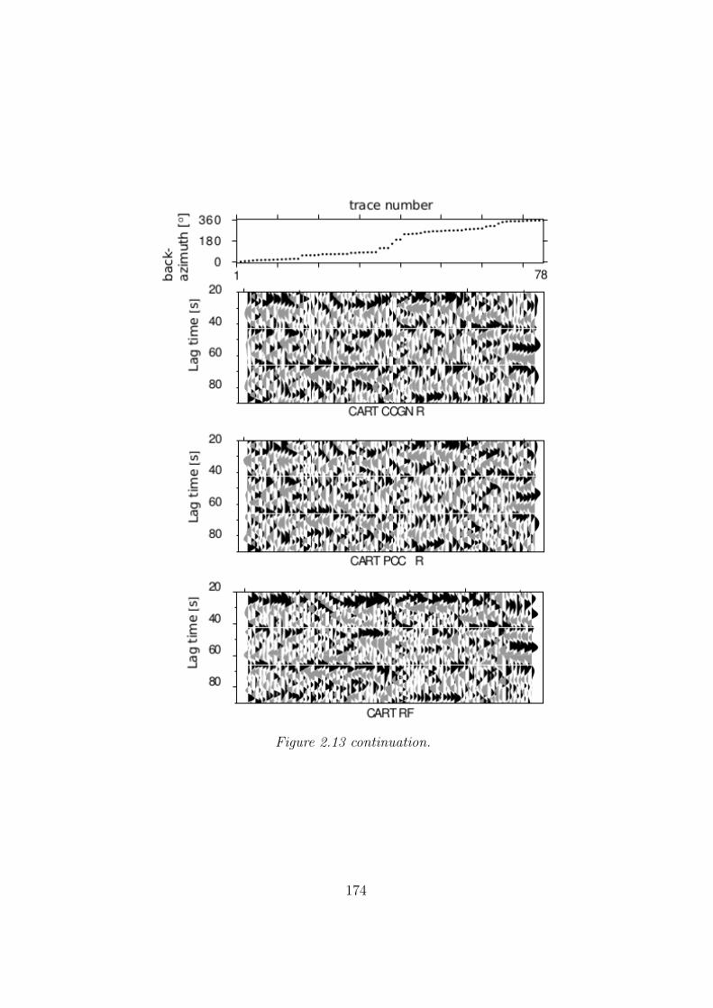
Figure 2.13 continuation.
174
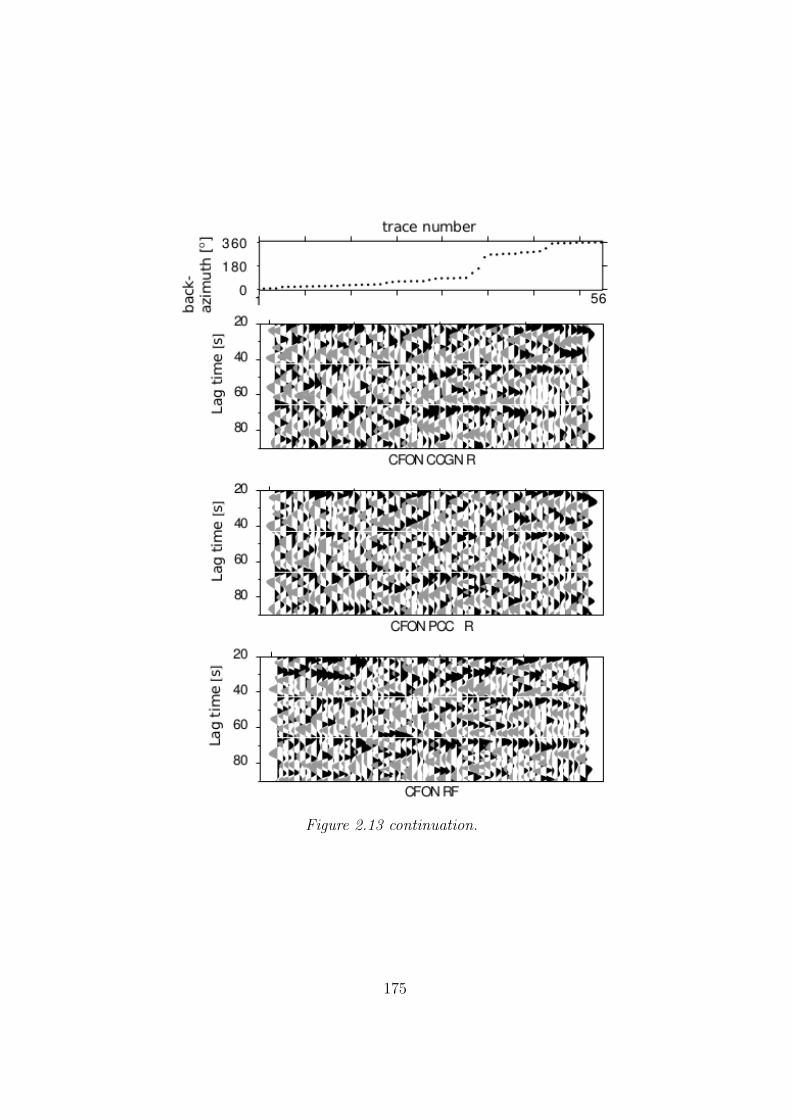
Figure 2.13 continuation.
175
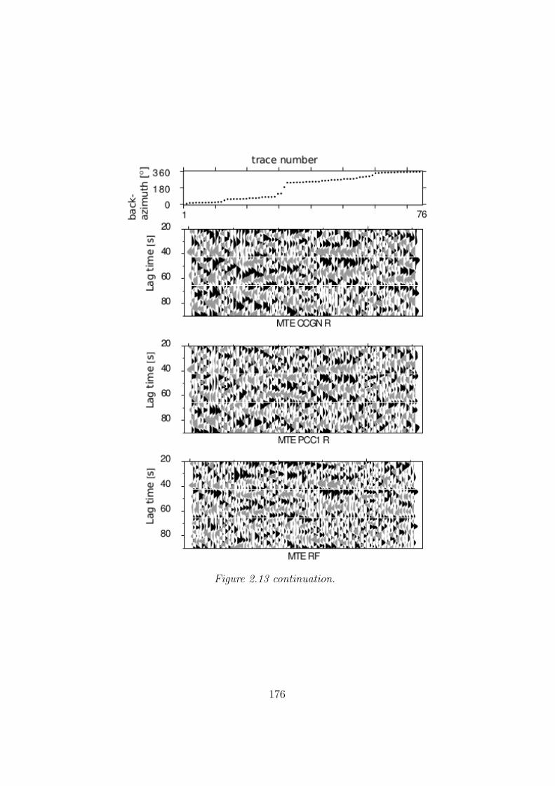
Figure 2.13 continuation.
176
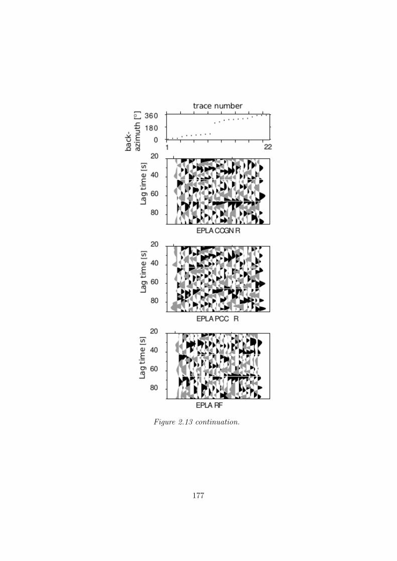
Figure 2.13 continuation.
177
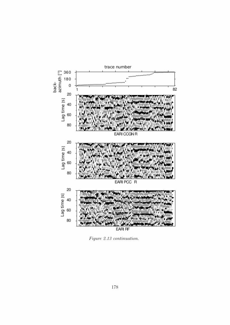
Figure 2.13 continuation.
178
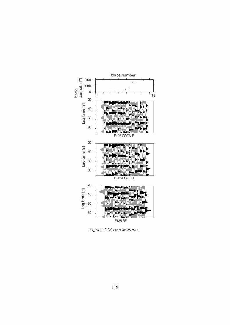
Figure 2.13 continuation.
179
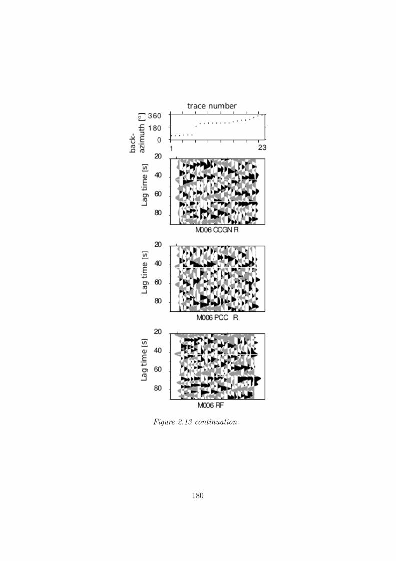
Figure 2.13 continuation.
180
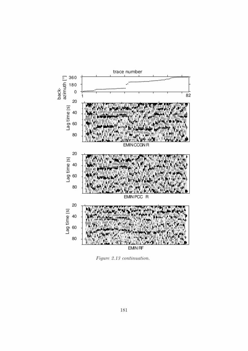
Figure 2.13 continuation.
181
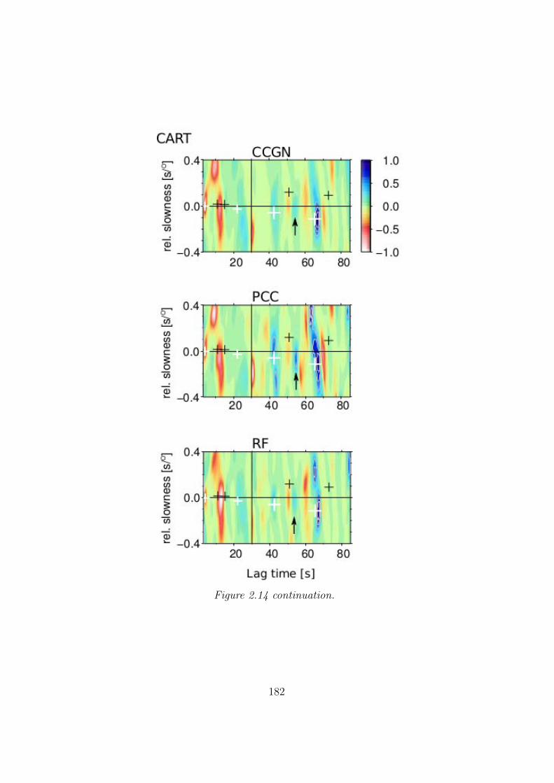
Figure 2.14 continuation.
182
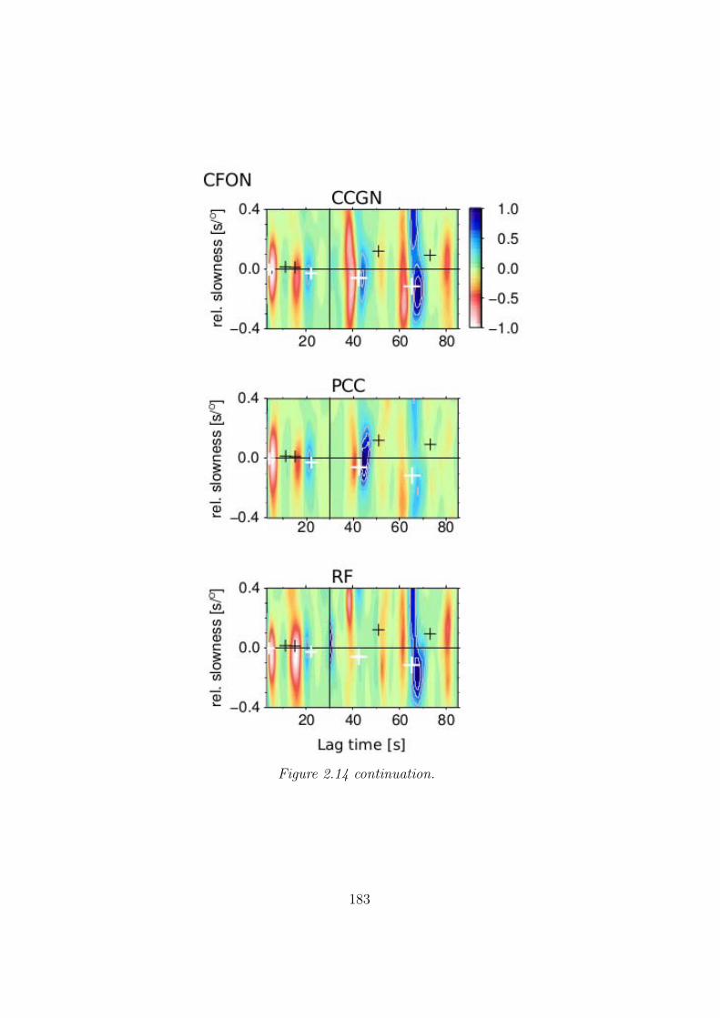
Figure 2.14 continuation.
183
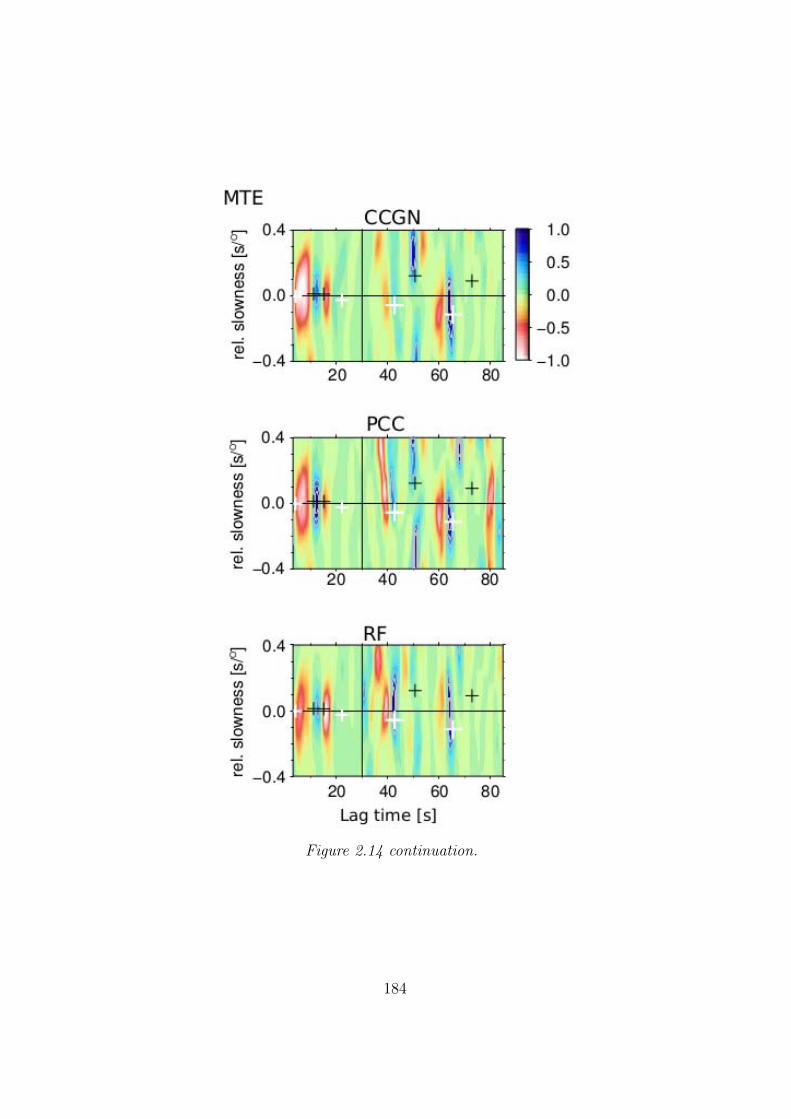
Figure 2.14 continuation.
184
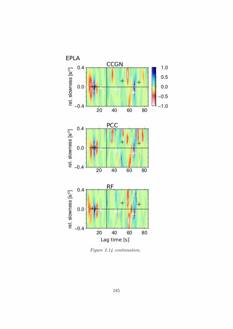
Figure 2.14 continuation.
185
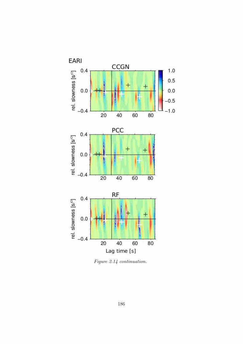
Figure 2.14 continuation.
186
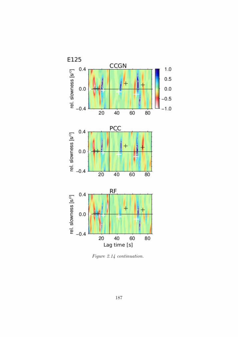
Figure 2.14 continuation.
187
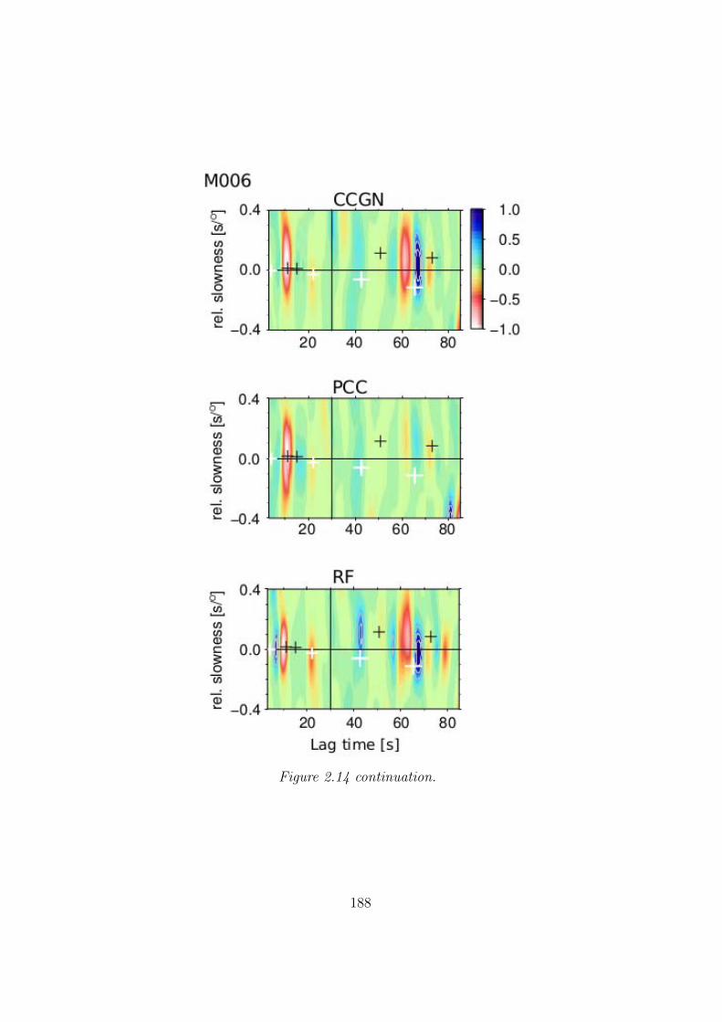
Figure 2.14 continuation.
188
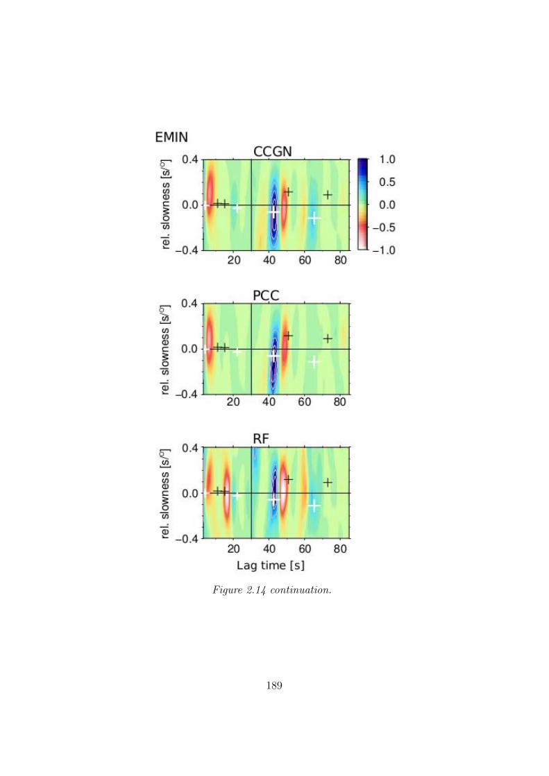
Figure 2.14 continuation.
189
DTopoIberia stations
190

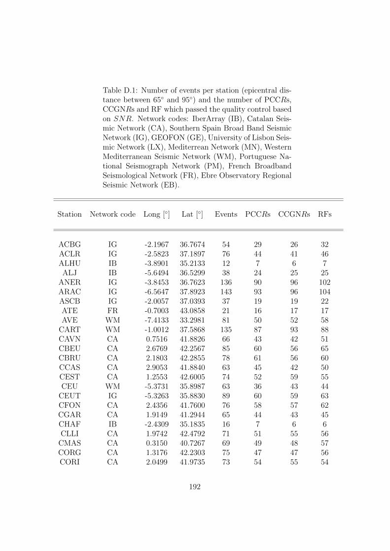
Table D.1: Number of events per station (epicentral dis-tance between 65◦ and 95◦) and the number of PCCRs,CCGNRs and RF which passed the quality control basedon SNR. Network codes: IberArray (IB), Catalan Seis-mic Network (CA), Southern Spain Broad Band SeismicNetwork (IG), GEOFON (GE), University of Lisbon Seis-mic Network (LX), Mediterrean Network (MN), WesternMediterranean Seismic Network (WM), Portuguese Na-tional Seismograph Network (PM), French BroadbandSeismological Network (FR), Ebre Observatory RegionalSeismic Network (EB).
Station Network code Long [◦] Lat [◦] Events PCCRs CCGNRs RFs
ACBG IG -2.1967 36.7674 54 29 26 32ACLR IG -2.5823 37.1897 76 44 41 46ALHU IB -3.8901 35.2133 12 7 6 7ALJ IB -5.6494 36.5299 38 24 25 25
ANER IG -3.8453 36.7623 136 90 96 102ARAC IG -6.5647 37.8923 143 93 96 104ASCB IG -2.0057 37.0393 37 19 19 22ATE FR -0.7003 43.0858 21 16 17 17AVE WM -7.4133 33.2981 81 50 52 58
CART WM -1.0012 37.5868 135 87 93 88CAVN CA 0.7516 41.8826 66 43 42 51CBEU CA 2.6769 42.2567 85 60 56 65CBRU CA 2.1803 42.2855 78 61 56 60CCAS CA 2.9053 41.8840 63 45 42 50CEST CA 1.2553 42.6005 74 52 59 55CEU WM -5.3731 35.8987 63 36 43 44
CEUT IG -5.3263 35.8830 89 60 59 63CFON CA 2.4356 41.7600 76 58 57 62CGAR CA 1.9149 41.2944 65 44 43 45CHAF IB -2.4309 35.1835 16 7 6 6CLLI CA 1.9742 42.4792 71 51 55 56
CMAS CA 0.3150 40.7267 69 49 48 57CORG CA 1.3176 42.2303 75 47 47 56CORI CA 2.0499 41.9735 73 54 55 54
192
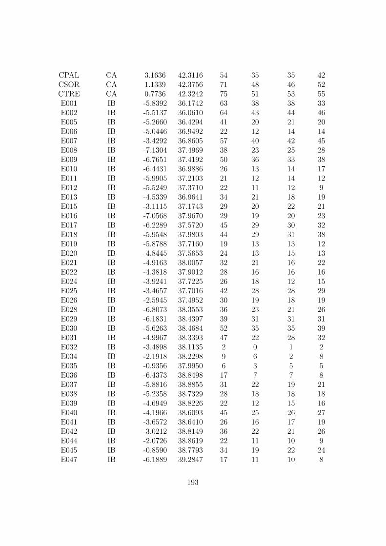
CPAL CA 3.1636 42.3116 54 35 35 42CSOR CA 1.1339 42.3756 71 48 46 52CTRE CA 0.7736 42.3242 75 51 53 55E001 IB -5.8392 36.1742 63 38 38 33E002 IB -5.5137 36.0610 64 43 44 46E005 IB -5.2660 36.4294 41 20 21 20E006 IB -5.0446 36.9492 22 12 14 14E007 IB -3.4292 36.8605 57 40 42 45E008 IB -7.1304 37.4969 38 23 25 28E009 IB -6.7651 37.4192 50 36 33 38E010 IB -6.4431 36.9886 26 13 14 17E011 IB -5.9905 37.2103 21 12 14 12E012 IB -5.5249 37.3710 22 11 12 9E013 IB -4.5339 36.9641 34 21 18 19E015 IB -3.1115 37.1743 29 20 22 21E016 IB -7.0568 37.9670 29 19 20 23E017 IB -6.2289 37.5720 45 29 30 32E018 IB -5.9548 37.9803 44 29 31 38E019 IB -5.8788 37.7160 19 13 13 12E020 IB -4.8445 37.5653 24 13 15 13E021 IB -4.9163 38.0057 32 21 16 22E022 IB -4.3818 37.9012 28 16 16 16E024 IB -3.9241 37.7225 26 18 12 15E025 IB -3.4657 37.7016 42 28 28 29E026 IB -2.5945 37.4952 30 19 18 19E028 IB -6.8073 38.3553 36 23 21 26E029 IB -6.1831 38.4397 39 31 31 31E030 IB -5.6263 38.4684 52 35 35 39E031 IB -4.9967 38.3393 47 22 28 32E032 IB -3.4898 38.1135 2 0 1 2E034 IB -2.1918 38.2298 9 6 2 8E035 IB -0.9356 37.9950 6 3 5 5E036 IB -6.4373 38.8498 17 7 7 8E037 IB -5.8816 38.8855 31 22 19 21E038 IB -5.2358 38.7329 28 18 18 18E039 IB -4.6949 38.8226 22 12 15 16E040 IB -4.1966 38.6093 45 25 26 27E041 IB -3.6572 38.6410 26 16 17 19E042 IB -3.0212 38.8149 36 22 21 26E044 IB -2.0726 38.8619 22 11 10 9E045 IB -0.8590 38.7793 34 19 22 24E047 IB -6.1889 39.2847 17 11 10 8
193
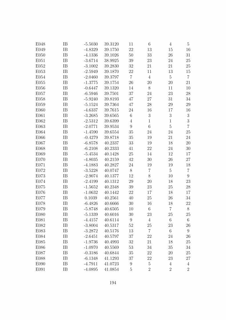
E048 IB -5.5030 39.3120 11 6 4 5E049 IB -4.8329 39.1750 22 13 15 16E050 IB -4.1336 39.1026 50 33 26 31E051 IB -3.6714 38.9925 39 23 24 25E052 IB -3.1002 39.2830 32 21 21 25E053 IB -2.5949 39.1870 22 11 13 15E054 IB -2.0460 39.3797 7 4 5 7E055 IB -1.3775 39.1754 26 20 20 21E056 IB -0.6447 39.1320 14 8 11 10E057 IB -6.5946 39.7501 37 24 23 28E058 IB -5.9240 39.8193 47 27 31 34E059 IB -5.1524 39.7364 47 28 29 29E060 IB -4.6337 39.7615 24 16 17 16E061 IB -3.2685 39.6565 6 3 3 3E062 IB -2.5312 39.6399 4 1 1 3E063 IB -2.0771 39.9534 9 6 5 7E064 IB -1.4590 39.6554 35 24 24 25E066 IB -0.4279 39.8718 35 19 21 24E067 IB -6.8578 40.2337 33 19 18 20E068 IB -6.2108 40.2333 41 22 24 30E069 IB -5.4534 40.1428 25 14 12 17E070 IB -4.8035 40.2159 42 30 26 27E071 IB -4.1883 40.2827 24 19 19 18E072 IB -3.5228 40.0747 8 7 5 7E073 IB -2.9074 40.1377 12 8 10 9E074 IB -2.4199 40.1312 29 20 18 23E075 IB -1.5652 40.2348 39 23 25 28E076 IB -1.0632 40.1442 22 17 18 17E077 IB 0.1039 40.2561 40 25 26 34E078 IB -6.4826 40.6666 30 16 18 22E079 IB -5.8748 40.6505 10 6 7 8E080 IB -5.1339 40.6016 30 23 25 25E081 IB -4.4157 40.6114 9 4 6 6E082 IB -3.8004 40.5317 52 25 23 26E083 IB -3.2872 40.5176 13 7 6 9E084 IB -2.6451 40.5797 37 22 24 26E085 IB -1.9736 40.4993 32 21 18 25E086 IB -1.0970 40.5569 53 34 35 34E087 IB -0.3186 40.6844 35 22 20 25E088 IB -6.1348 41.1293 37 22 23 27E090 IB -4.7911 41.0723 9 5 4 4E091 IB -4.0895 41.0854 5 2 2 2
194
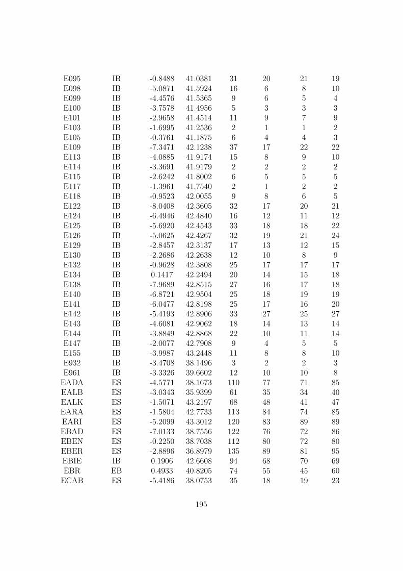
E095 IB -0.8488 41.0381 31 20 21 19E098 IB -5.0871 41.5924 16 6 8 10E099 IB -4.4576 41.5365 9 6 5 4E100 IB -3.7578 41.4956 5 3 3 3E101 IB -2.9658 41.4514 11 9 7 9E103 IB -1.6995 41.2536 2 1 1 2E105 IB -0.3761 41.1875 6 4 4 3E109 IB -7.3471 42.1238 37 17 22 22E113 IB -4.0885 41.9174 15 8 9 10E114 IB -3.3691 41.9179 2 2 2 2E115 IB -2.6242 41.8002 6 5 5 5E117 IB -1.3961 41.7540 2 1 2 2E118 IB -0.9523 42.0055 9 8 6 5E122 IB -8.0408 42.3605 32 17 20 21E124 IB -6.4946 42.4840 16 12 11 12E125 IB -5.6920 42.4543 33 18 18 22E126 IB -5.0625 42.4267 32 19 21 24E129 IB -2.8457 42.3137 17 13 12 15E130 IB -2.2686 42.2638 12 10 8 9E132 IB -0.9628 42.3808 25 17 17 17E134 IB 0.1417 42.2494 20 14 15 18E138 IB -7.9689 42.8515 27 16 17 18E140 IB -6.8721 42.9504 25 18 19 19E141 IB -6.0477 42.8198 25 17 16 20E142 IB -5.4193 42.8906 33 27 25 27E143 IB -4.6081 42.9062 18 14 13 14E144 IB -3.8849 42.8868 22 10 11 14E147 IB -2.0077 42.7908 9 4 5 5E155 IB -3.9987 43.2448 11 8 8 10E932 IB -3.4708 38.1496 3 2 2 3E961 IB -3.3326 39.6602 12 10 10 8
EADA ES -4.5771 38.1673 110 77 71 85EALB ES -3.0343 35.9399 61 35 34 40EALK ES -1.5071 43.2197 68 48 41 47EARA ES -1.5804 42.7733 113 84 74 85EARI ES -5.2099 43.3012 120 83 89 89EBAD ES -7.0133 38.7556 122 76 72 86EBEN ES -0.2250 38.7038 112 80 72 80EBER ES -2.8896 36.8979 135 89 81 95EBIE IB 0.1906 42.6608 94 68 70 69EBR EB 0.4933 40.8205 74 55 45 60
ECAB ES -5.4186 38.0753 35 18 19 23
195
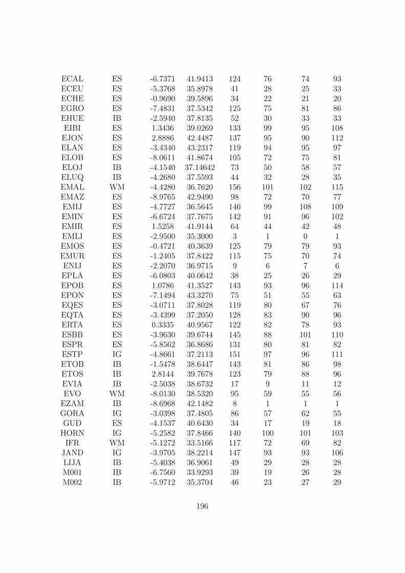
ECAL ES -6.7371 41.9413 124 76 74 93ECEU ES -5.3768 35.8978 41 28 25 33ECHE ES -0.9690 39.5896 34 22 21 20EGRO ES -7.4831 37.5342 125 75 81 86EHUE IB -2.5940 37.8135 52 30 33 33EIBI ES 1.3436 39.0269 133 99 95 108
EJON ES 2.8886 42.4487 137 95 90 112ELAN ES -3.4340 43.2317 119 94 95 97ELOB ES -8.0611 41.8674 105 72 75 81ELOJ IB -4.1540 37.14642 73 50 58 57ELUQ IB -4.2680 37.5593 44 32 28 35EMAL WM -4.4280 36.7620 156 101 102 115EMAZ ES -8.9765 42.9490 98 72 70 77EMIJ ES -4.7727 36.5645 146 99 108 109EMIN ES -6.6724 37.7675 142 91 96 102EMIR ES 1.5258 41.9144 64 44 42 48EMLI ES -2.9500 35.3000 3 1 0 1EMOS ES -0.4721 40.3639 125 79 79 93EMUR ES -1.2405 37.8422 115 75 70 74ENIJ ES -2.2070 36.9715 9 6 7 6EPLA ES -6.0803 40.0642 38 25 26 29EPOB ES 1.0786 41.3527 143 93 96 114EPON ES -7.1494 43.3270 75 51 55 63EQES ES -3.0711 37.8028 119 80 67 76EQTA ES -3.4399 37.2050 128 83 90 96ERTA ES 0.3335 40.9567 122 82 78 93ESBB ES -3.9630 39.6744 145 88 101 110ESPR ES -5.8562 36.8686 131 80 81 82ESTP IG -4.8661 37.2113 151 97 96 111ETOB IB -1.5478 38.6447 143 81 86 98ETOS IB 2.8144 39.7678 123 79 88 96EVIA IB -2.5038 38.6732 17 9 11 12EVO WM -8.0130 38.5320 95 59 55 56
EZAM IB -8.6968 42.1482 8 1 1 1GORA IG -3.0398 37.4805 86 57 62 55GUD ES -4.1537 40.6430 34 17 19 18
HORN IG -5.2582 37.8466 140 100 101 103IFR WM -5.1272 33.5166 117 72 69 82
JAND IG -3.9705 38.2214 147 93 93 106LIJA IB -5.4038 36.9061 49 29 28 28M001 IB -6.7560 33.9293 39 19 26 28M002 IB -5.9712 35.3704 46 23 27 29
196
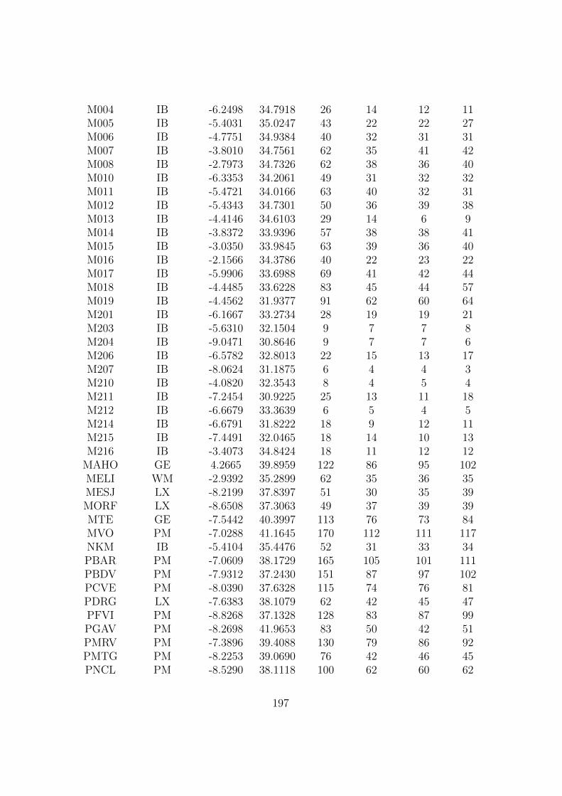
M004 IB -6.2498 34.7918 26 14 12 11M005 IB -5.4031 35.0247 43 22 22 27M006 IB -4.7751 34.9384 40 32 31 31M007 IB -3.8010 34.7561 62 35 41 42M008 IB -2.7973 34.7326 62 38 36 40M010 IB -6.3353 34.2061 49 31 32 32M011 IB -5.4721 34.0166 63 40 32 31M012 IB -5.4343 34.7301 50 36 39 38M013 IB -4.4146 34.6103 29 14 6 9M014 IB -3.8372 33.9396 57 38 38 41M015 IB -3.0350 33.9845 63 39 36 40M016 IB -2.1566 34.3786 40 22 23 22M017 IB -5.9906 33.6988 69 41 42 44M018 IB -4.4485 33.6228 83 45 44 57M019 IB -4.4562 31.9377 91 62 60 64M201 IB -6.1667 33.2734 28 19 19 21M203 IB -5.6310 32.1504 9 7 7 8M204 IB -9.0471 30.8646 9 7 7 6M206 IB -6.5782 32.8013 22 15 13 17M207 IB -8.0624 31.1875 6 4 4 3M210 IB -4.0820 32.3543 8 4 5 4M211 IB -7.2454 30.9225 25 13 11 18M212 IB -6.6679 33.3639 6 5 4 5M214 IB -6.6791 31.8222 18 9 12 11M215 IB -7.4491 32.0465 18 14 10 13M216 IB -3.4073 34.8424 18 11 12 12
MAHO GE 4.2665 39.8959 122 86 95 102MELI WM -2.9392 35.2899 62 35 36 35MESJ LX -8.2199 37.8397 51 30 35 39MORF LX -8.6508 37.3063 49 37 39 39MTE GE -7.5442 40.3997 113 76 73 84MVO PM -7.0288 41.1645 170 112 111 117NKM IB -5.4104 35.4476 52 31 33 34PBAR PM -7.0609 38.1729 165 105 101 111PBDV PM -7.9312 37.2430 151 87 97 102PCVE PM -8.0390 37.6328 115 74 76 81PDRG LX -7.6383 38.1079 62 42 45 47PFVI PM -8.8268 37.1328 128 83 87 99PGAV PM -8.2698 41.9653 83 50 42 51PMRV PM -7.3896 39.4088 130 79 86 92PMTG PM -8.2253 39.0690 76 42 46 45PNCL PM -8.5290 38.1118 100 62 60 62
197
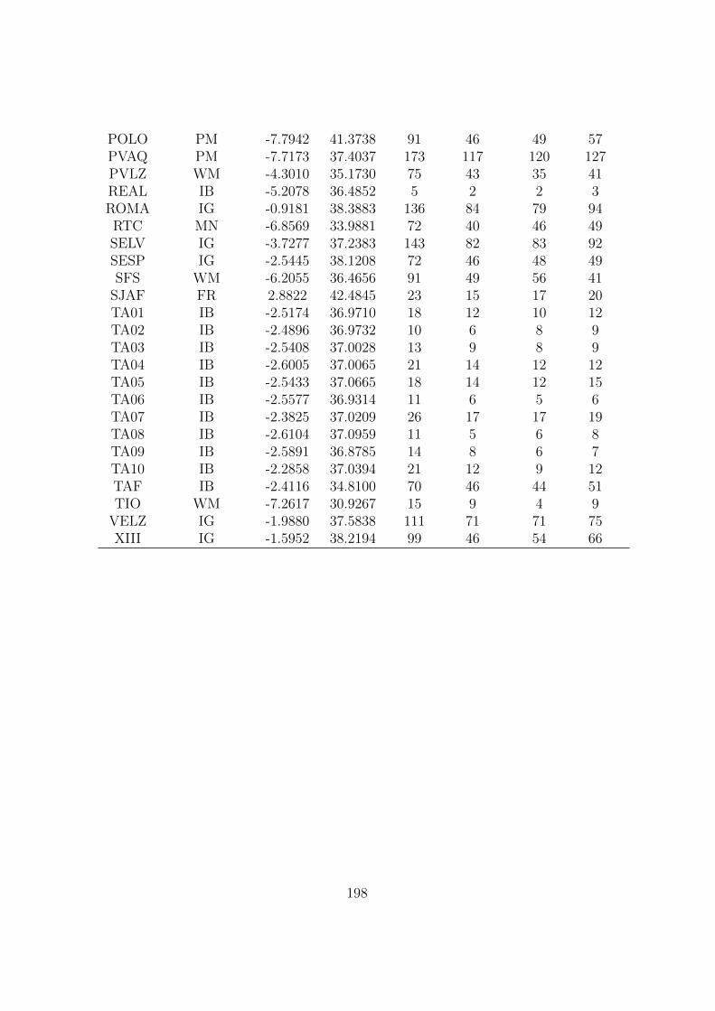
POLO PM -7.7942 41.3738 91 46 49 57PVAQ PM -7.7173 37.4037 173 117 120 127PVLZ WM -4.3010 35.1730 75 43 35 41REAL IB -5.2078 36.4852 5 2 2 3ROMA IG -0.9181 38.3883 136 84 79 94RTC MN -6.8569 33.9881 72 40 46 49SELV IG -3.7277 37.2383 143 82 83 92SESP IG -2.5445 38.1208 72 46 48 49SFS WM -6.2055 36.4656 91 49 56 41
SJAF FR 2.8822 42.4845 23 15 17 20TA01 IB -2.5174 36.9710 18 12 10 12TA02 IB -2.4896 36.9732 10 6 8 9TA03 IB -2.5408 37.0028 13 9 8 9TA04 IB -2.6005 37.0065 21 14 12 12TA05 IB -2.5433 37.0665 18 14 12 15TA06 IB -2.5577 36.9314 11 6 5 6TA07 IB -2.3825 37.0209 26 17 17 19TA08 IB -2.6104 37.0959 11 5 6 8TA09 IB -2.5891 36.8785 14 8 6 7TA10 IB -2.2858 37.0394 21 12 9 12TAF IB -2.4116 34.8100 70 46 44 51TIO WM -7.2617 30.9267 15 9 4 9
VELZ IG -1.9880 37.5838 111 71 71 75XIII IG -1.5952 38.2194 99 46 54 66
198


ESupplementary figures for Chapter 4
200

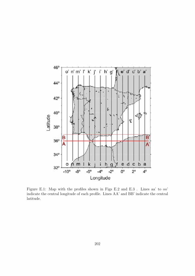
Figure E.1: Map with the profiles shown in Figs E.2 and E.3 . Lines aa’ to oo’indicate the central longitude of each profile. Lines AA’ and BB’ indicate the centrallatitude.
202
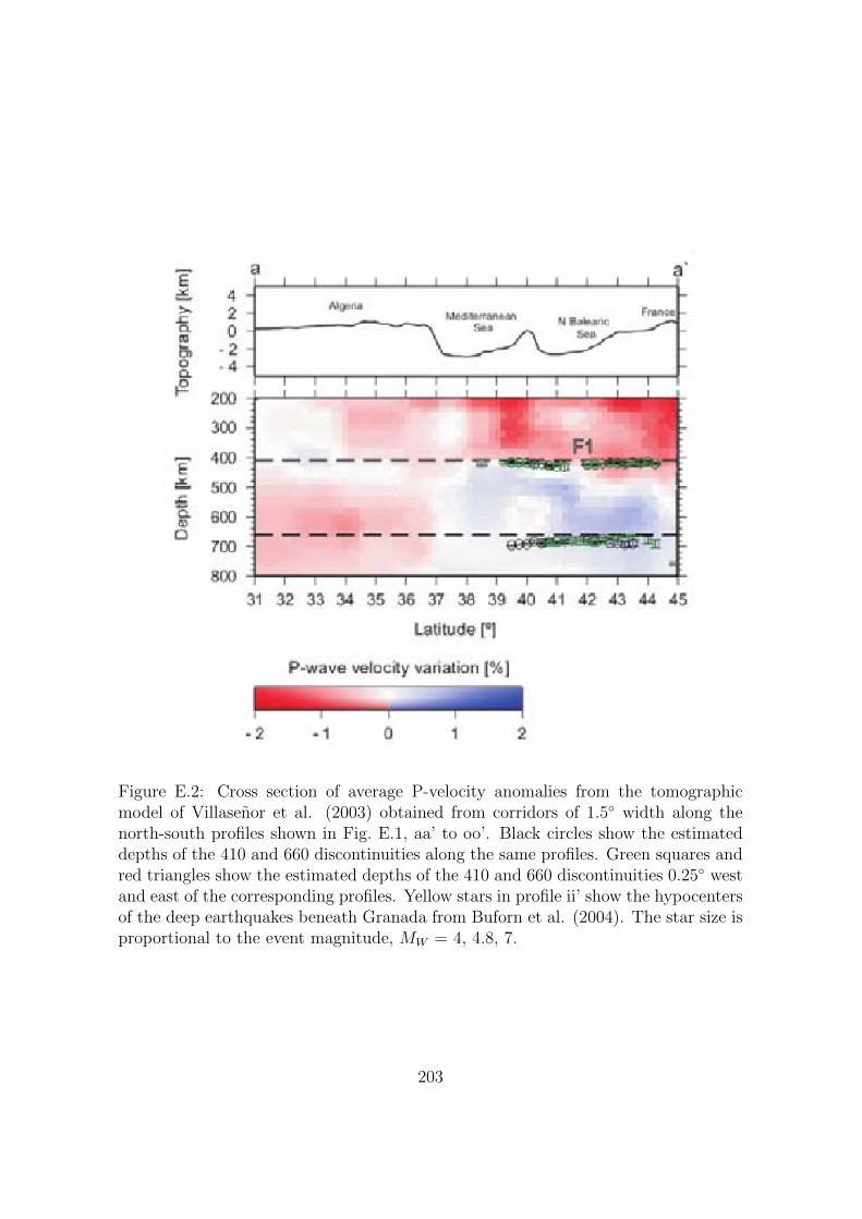
Figure E.2: Cross section of average P-velocity anomalies from the tomographicmodel of Villasenor et al. (2003) obtained from corridors of 1.5◦ width along thenorth-south profiles shown in Fig. E.1, aa’ to oo’. Black circles show the estimateddepths of the 410 and 660 discontinuities along the same profiles. Green squares andred triangles show the estimated depths of the 410 and 660 discontinuities 0.25◦ westand east of the corresponding profiles. Yellow stars in profile ii’ show the hypocentersof the deep earthquakes beneath Granada from Buforn et al. (2004). The star size isproportional to the event magnitude, MW = 4, 4.8, 7.
203
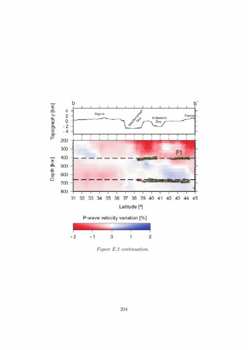
Figure E.2 continuation.
204
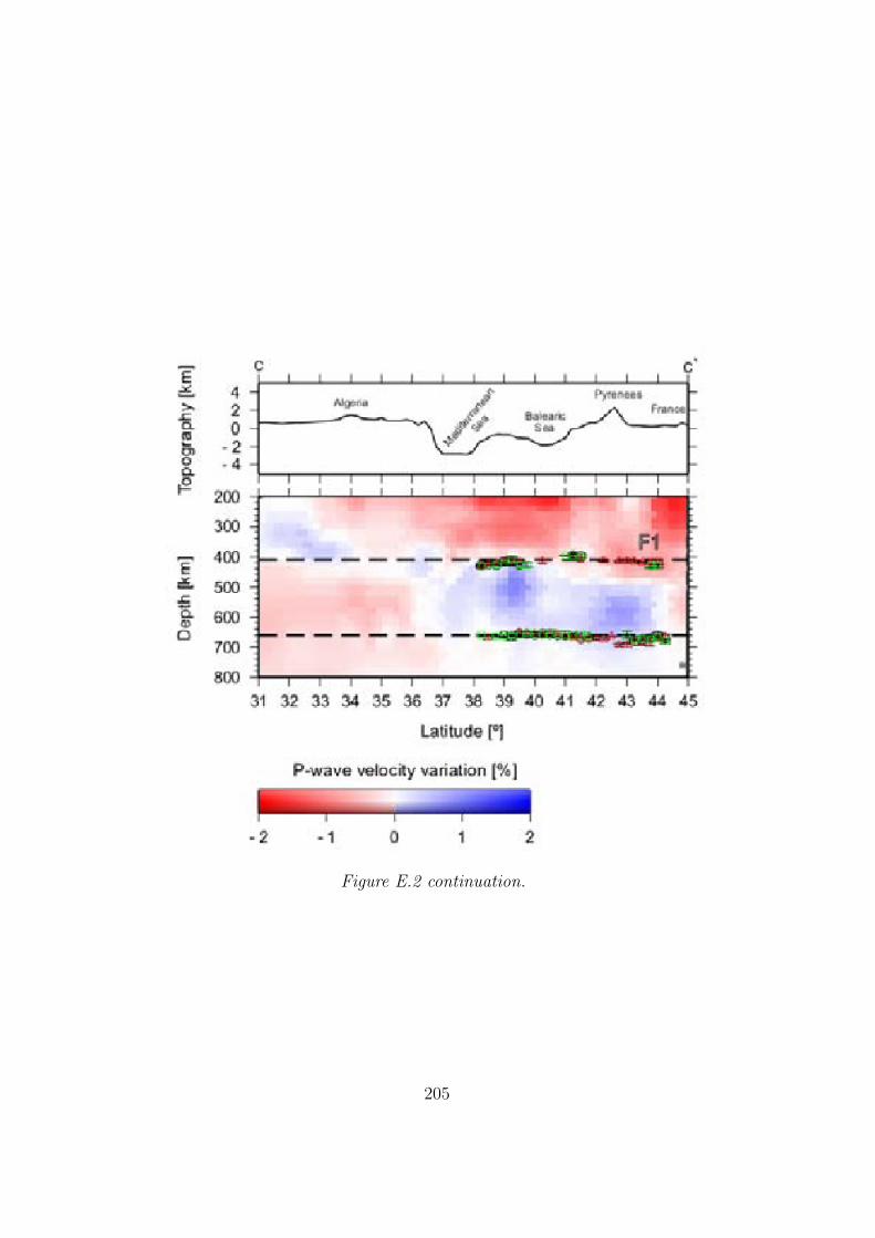
Figure E.2 continuation.
205
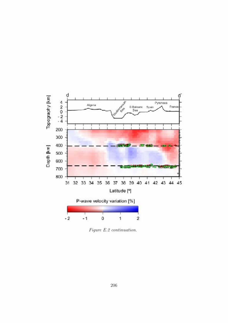
Figure E.2 continuation.
206
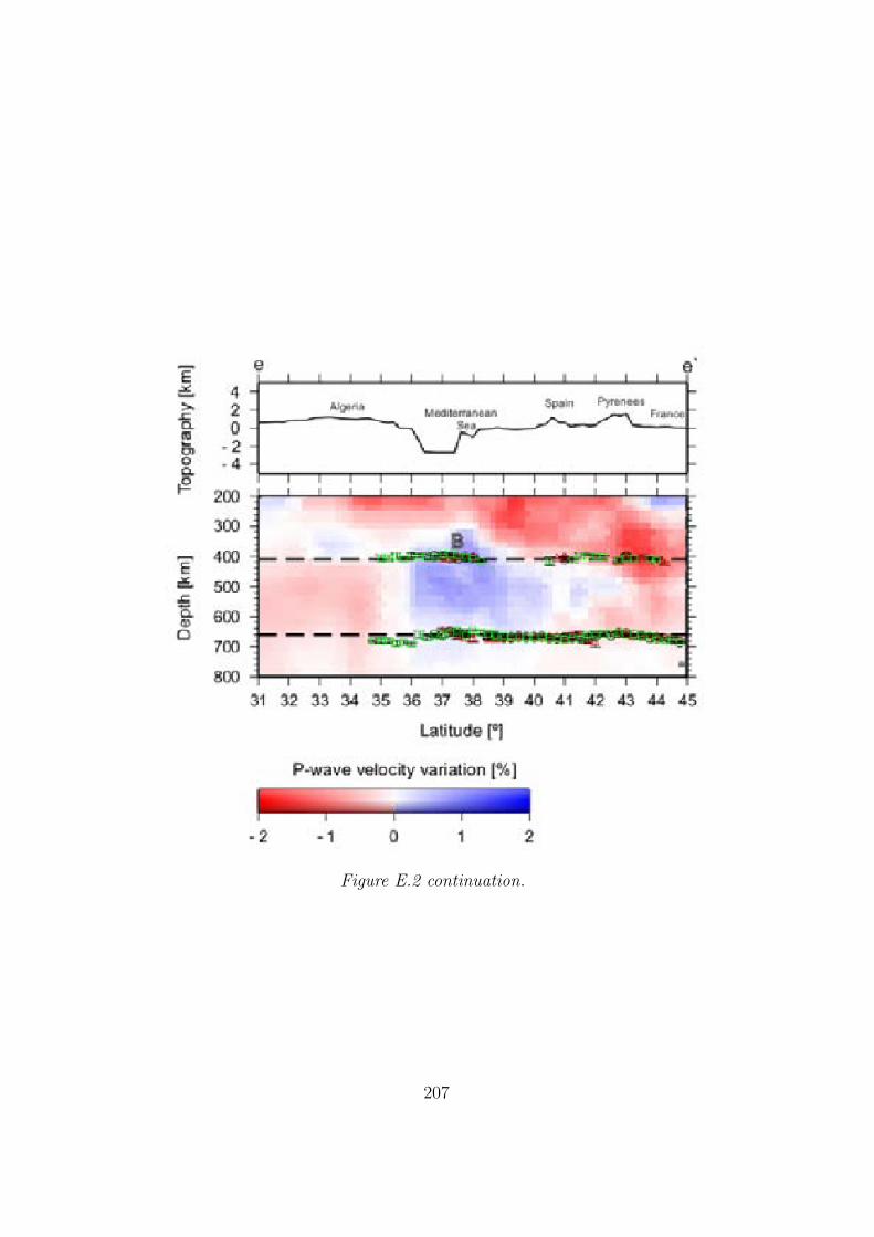
Figure E.2 continuation.
207
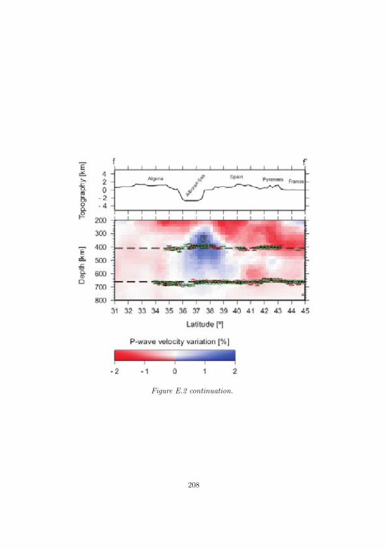
Figure E.2 continuation.
208
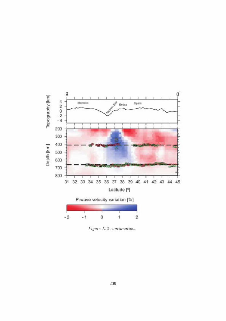
Figure E.2 continuation.
209
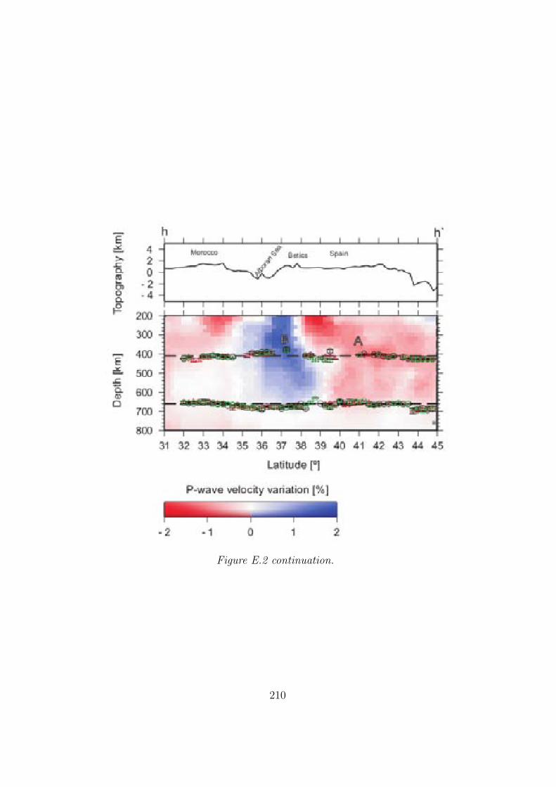
Figure E.2 continuation.
210
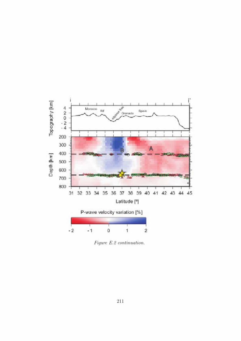
Figure E.2 continuation.
211
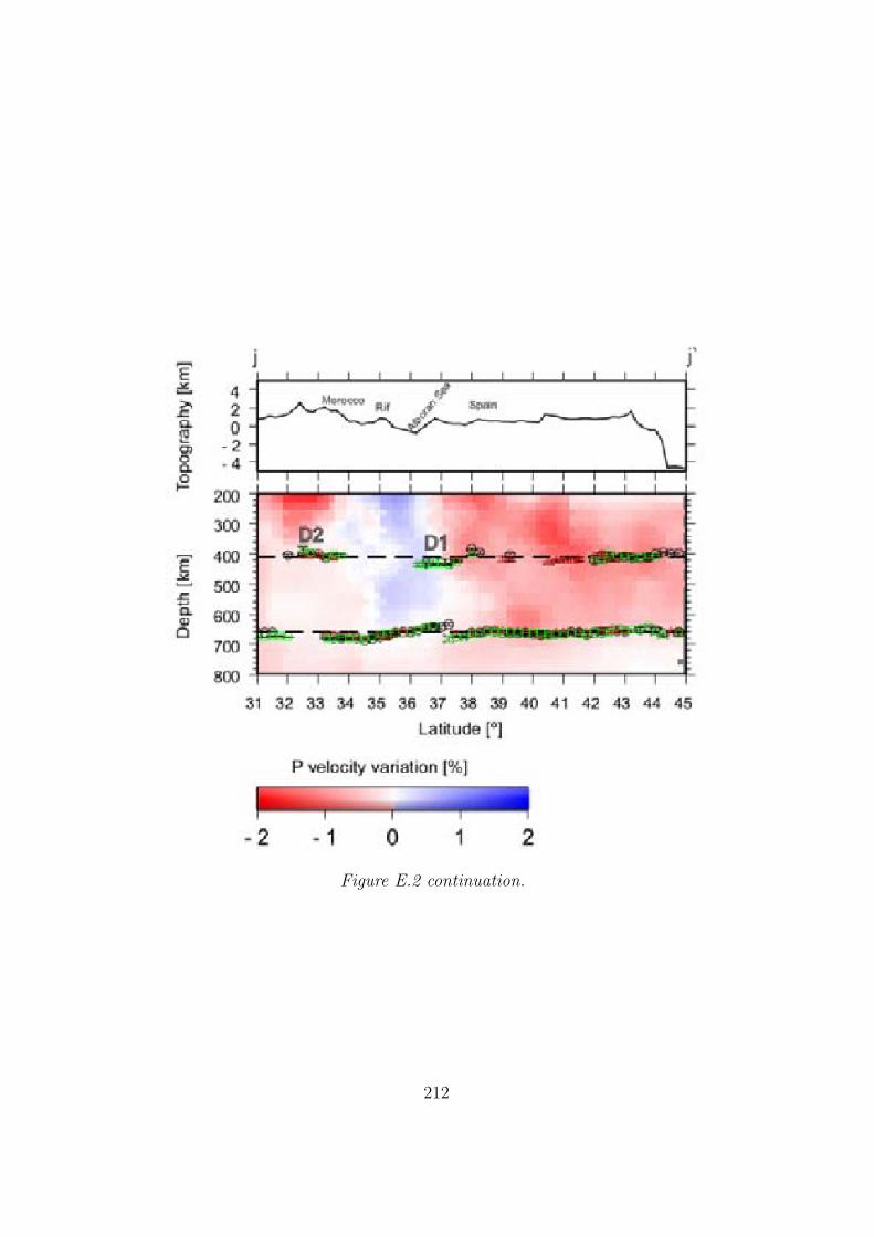
Figure E.2 continuation.
212
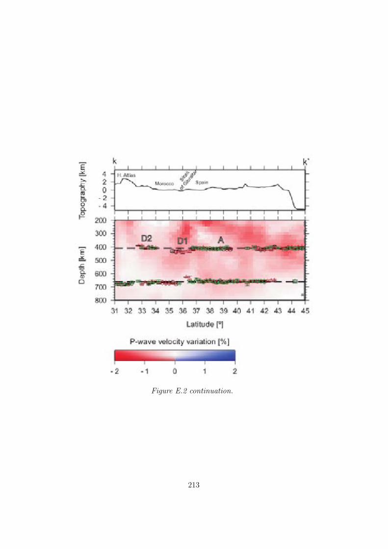
Figure E.2 continuation.
213
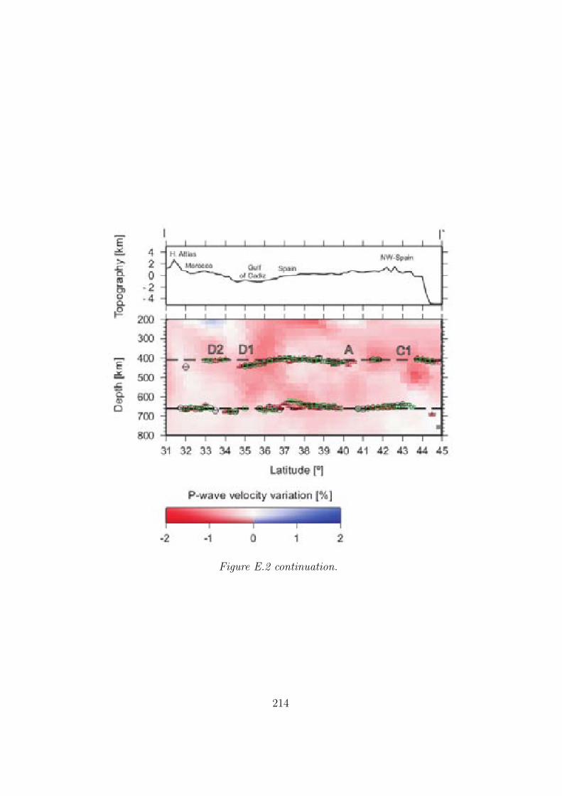
Figure E.2 continuation.
214
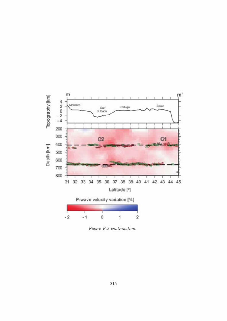
Figure E.2 continuation.
215
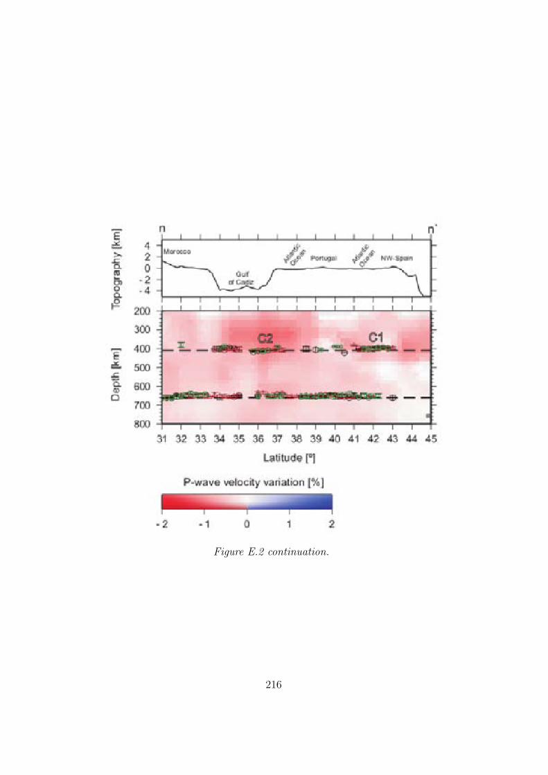
Figure E.2 continuation.
216
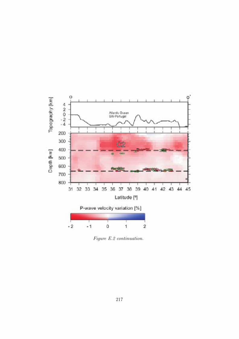
Figure E.2 continuation.
217
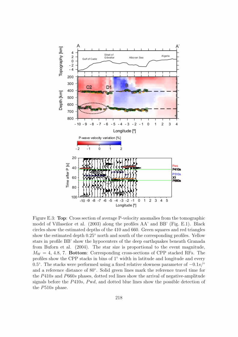
Figure E.3: Top: Cross section of average P-velocity anomalies from the tomographicmodel of Villasenor et al. (2003) along the profiles AA’ and BB’ (Fig. E.1). Blackcircles show the estimated depths of the 410 and 660. Green squares and red trianglesshow the estimated depth 0.25◦ north and south of the corresponding profiles. Yellowstars in profile BB’ show the hypocenters of the deep earthquakes beneath Granadafrom Buforn et al. (2004). The star size is proportional to the event magnitude,MW = 4, 4.8, 7. Bottom: Corresponding cross-sections of CPP stacked RFs. Theprofiles show the CPP stacks in bins of 1◦ width in latitude and longitude and every0.5◦. The stacks were performed using a fixed relative slowness parameter of −0.1s/◦
and a reference distance of 80◦. Solid green lines mark the reference travel time forthe P410s and P660s phases, dotted red lines show the arrival of negative-amplitudesignals before the P410s, Pwd, and dotted blue lines show the possible detection ofthe P510s phase.
218
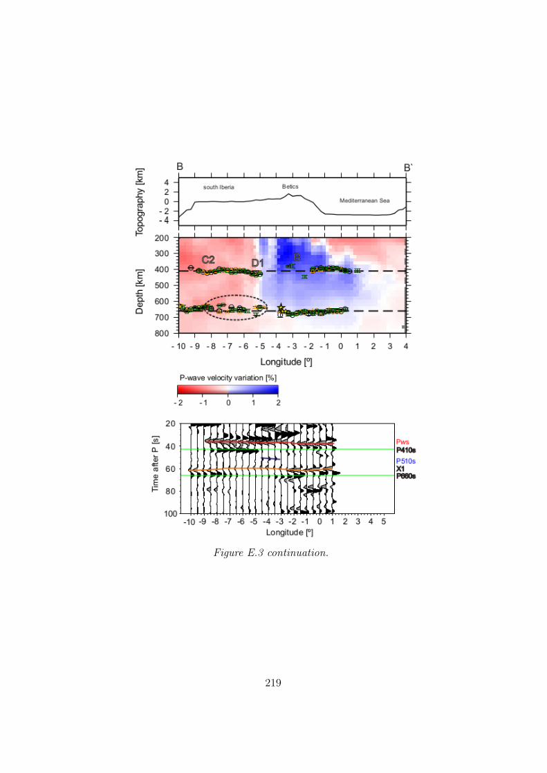
Figure E.3 continuation.
219
Bibliography
Ai, Y. and Zheng, Z. (2003). The upper mantle discontinuity structure beneath
eastern China. Geophys. Res. Lett. 30(21), 2089.
Akaogi, M., Ito, E. and Navrotsky, A. (1989). Olivine-modified spinel transitions
in the system Mg2SiO4 - Fe2SiO4: calorimetric measurements, thermochemical
calculation, and geophysical application. J. Geophys Res. 94, 15671–15685.
Akaogi, M., Tanaka, A. and Ito, E. (2002). Garnet−ilmenite−perovskite transitions in
the system Mg4 Si4 O12 − Mg3Al2 Si3O12 at high pressures and high temperatures:
phase equilibria, calorimetry and implications for mantle structure. Earth Planet.
Sci. Lett 132, 303–324.
Akaogi, M., Yano, M., Tejima, Y., Iijima, M. and Kojitani, H. (2004). High- pressure
transitions of diopside and wollanstonite: phase equilibria and thermochemistry of
CaMgSi2O6, CaSiO3 and CaSi2O5-CaTiSiO5 system. Phys. Earth planet. Inter.
143/144, 145–156.
Ammon, C. J. (1991). The isolation of receiver effects from teleseismic P waveforms.
Bull. Seism. Soc. Am. 81, 2504–2510.
Anderson, D. (2007). New Theory of the Earth pp. 91–108. Cambridge: Cambridge
University Press, second edition.
Argus, D., Gordon, R., Demets, C. and Stein, S. (1989). Plate Motion Circuit and
Tectonics of the Gloria Fault. J. Geophys. Res., 94(B5), 5585–5602.
Benz, H. M. and Vidale, J. E. (1993). Sharpness of upper-mantle discontinuities
determined from high-frequency reflections. Nature , 365(6442), 147–150.
220
Bercovici, D. and Karato, S.-I. (2003). Whole mantle convection and the transition-
zone water filter. Nature , 425, 39–44.
Bezada, M. J. and Humphreys, E. D. (2012). Contrasting rupture processes during
the April 11, 2010 deep-focus earthquake beneath Granada, Spain. Earth planet.
Sci. Lett., 353-354, 38–46.
Bezada, M. J., Humphreys, E. D., Toomey, D. R., Harnafi, M. and Davila, J. M.
(2013). Western mediterranean slab rollback revealed by upper mantle tomography.
Earth planet. Sci. Lett., 368, 51–60.
Bina, C. R. and Helffrich, G. (1994). Phase transition Clapeyron slopes and transition
zone seismic discontinuity topography. J. Geophys. Res., 99(B8), 15853–15860.
Bina, C. R. and Kawakatsu, H. (2010). Buoyancy, bending, and seismic visibility in
deep slab stagnation. Phys. Earth Planet. Int., 183, 330–340.
Bina, C. R. and Wood, B. J. (1987). Olivine-spinel transitions: Experimental and
thermodynamic constraints and implications for the nature of the 400-km seismic
discontinuity. J. Geophys. Res., 92, 4853–4866.
Blanco, M. and Spakman, W. (1993). The P–wave velocity structure of the mantle
below the Iberian Peninsula: evidence for subducted lithosphere below southern
Spain. Tectonophysics , 221, 13–34.
Bokelmann, G. and Maufroy, E. (2007). Mantle structure under Gibraltar constrained
by dispersion of body waves. Geophys. Res. Lett., 34, L22305.
Bokelmann, G., Maufroy, E., Buontempo, L., Morales, J. and Barruol, G. (2011).
Testing oceanic subduction and convective removal models for the Gibraltar arc:
Seismological constraints from dispersion and anisotropy. Tectonophysics , 502,
28–37.
Bonatto, L., Schimmel, M., Gallart, J. and Morales, J. (2013). Studying the 410-km
and 660-km discontinuities beneath Spain and Morocco through detection of P-to-s
conversions. Geophys. J. Int., 194(2), 920–935.
Bostock, M. G. (1998). Mantle stratigraphy and evolution of the Slave province. J.
Geophys. Res., 103(B9), 21183–21200.
221
Bostock, M. G. (1999). Seismic waves converted from velocity gradient anomalies in
the Earth’s upper mantle. Geophys. J. Int., 138, 747–756.
Bostock, M. G. (2007). 1.07 - Theory and Observations - Teleseismic Body-Wave
Scattering and Receiver-Side Structure. In Treatise on Geophysics, (Schubert, G.,
ed.),, pp. 219–246. Elsevier, Oxford.
Buforn, E., Bezzeghoud, M., Ud´ ias, A. and Pro, C. (2004). Seismic Sources on
the Iberia-African Plate Boundary and their Tectonic Implications. Pure appl.
geophys., 161, 623–646.
Buforn, E., Pro, C., Cesca, S., Ud´ ias, A. and del Fresno, C. (2011). The 2010
Granada, Spain deep Earthquake. Bull. Seism. Soc. Am., 101, 2418–2430.
Buforn, E., Sanz de Galdeano, C. and Ud´ ias, A. (1995). Seismotectonics of the
Ibero-Maghrebian region. Tectonophysics , 248, 247–261.
Buontempo, L., Bokelmann, G. H. R., Barruol, G. and Morales, J. (2008). Seismic
anisotropy beneath southern Iberia from SKS splitting. Earth planet. Sci. Lett.,
273, 237–250.
Calvert, A., Sandvol, E., Seber, D., Barazangi, M., Roecker, S., Mourabit, T., Vidal,
F., Alguacil, G. and Jabour, N. (2000). Geodynamic evolution of the lithosphere
and upper mantle beneath the Alboran region of the western Mediterranean: con-
straints from travel time tomography. J. Geophys. Res., 105(B5), 10871–10898.
Cao, Q., van der Hilst, R. D., de Hoop, M. V. and Shim, S.-H. (2011). Seismic
Imaging of Transition Zone Discontinuities Suggests Hot Mantle West of Hawaii.
Science , 332, 1068–1071.
Carminati, E., Lustrino, M. and Doglioni, C. (2012). Geodynamic evolution of the
central and western Mediterranean: Tectonics vs. igneous petrology constraints.
Tectonophys., 579, 173–192.
Chambers, K., Deuss, A. and Woodhouse, J. H. (2005). Reflectivity of the 410-km
discontinuity from PP and SS precursors. J. Geophys. Res., 110(B02301).
222
Chapman, C., Jen-Yi, C. and Lyness, D. G. (1988). The WKBJ seismogram approx-
imation. In Seismological Algorithms, (Doornbos, D., ed.),, pp. 47–74. Academic
Press, London.
Chen, C. W., Miller, D. E., Djikpesse, H. A., U., H. J. B. and Rondenay (2010). Array-
conditioned deconvolution of multiple-component teleseismic recordings. Geophys.
J. Int., 182, 967–976.
Chevrot, S., Vinnik, L. and Montagner, J.-P. (1999). Global scale analysis of the
mantle Pds phases. J. Geophys. Res., 104(B9), 20203–20219.
Clayton, R. W. and Wiggins, R. A. (1976). Source shape estimation and deconvolu-
tion of teleseismic body waves. J. R. Astr. Soc., 47(1), 151–177.
Collier, J. and Helffrich, G. (1997). Topography of the 410 and 660 km seismic dis-
continuities in the Izu-Bonin subduction zone. Geophys. Res. Lett., 24, 15351538.
Collier, J. D. and Helffrich, G. R. (2001). The thermal influence of the subducting slab
beneath South America from 410 and 660 km discontinuity observations. Geophys.
J. Int., 147, 319–329.
Collier, J. D., Helffrich, G. R. and Wood, B. J. (2001). Seismic discontinuities and
subduction zones. Phys. Earth Planet. Int., 127, 35–49.
Comas, M. C., Platt, J. P., Soto, J. I. and Watts, A. B. (1999). The origin and
tectonic history of the Alboran Basin: insigths from Leg 161 results. In Porc.
ODP, Sci. Results, (Zahn, R., Comas, M. C. and Klau, A., eds),, vol. 161,, pp.
555–579. Ocean Drilling Program, College Station, TX.
Contenti, S., Gu, Y. J., Okeler, A. and Sacchi, M. D. (2012). Shear wave reflectivity
imaging of the Nazca–South America subduction zone: Stagnant slab in the mantle
transition zone? Geophys. Res. Lett., 39, L02310.
Demets, C., Gordon, R., Argus, D. and Stein, S. (1990). Current Plate Motions.
Geophys. J. Int., 101, 425–478.
223
Deuss, A. (2007). Seismic observations of transition zone discontinuities beneath
hotspot locations, Vol. Special Paper 430. In Plates, Plumes, and Planetary Pro-
cesses, (G., F. and J., J., eds),, pp. 121–136. Geological Society of America, Boulder,
CO. doi:10.1130/2007.2430(07).
Deuss, A., Redfern, S. A. T., Chambers, K. and Woodhouse, J. H. (2006). The Nature
of the 660–km Discontinuity in Earth’s Mantle from Global Seismic Observations
of PP Precursors. Science , 311(5758), 198–201.
Deuss, A. and Woodhouse, J. H. (2001). Seismic Observations of splitting of the
mid-transition zone discontinuities in Erath’s mantle. Science , 294, 354–357.
Deuss, A. and Woodhouse, J. H. (2002). A systematic search for mantle discontinu-
ities using SS-precursors. Geophys. Res. Lett., 29(8), 90.1–90.4.
Deuss, A. and Woodhouse, J. H. (2004). The nature of the Lehmann discontinuity
from its seismological Clapeyron slopes. Earth planet. Sci. Lett., 225, 295–304.
Dıaz, J., Gallart, J., Villasenor, A., Mancilla, F., Pazos, A., Cordoba, D., Pulgar,
J. A., Ibarra, P. and Harnafi, M. (2010). Mantle dynamics beneath the Gibraltar
Arc (western Mediterranean) from shear wave splitting measurements on a dense
seismic array. Geophys. Res. Lett., 37, L18304.
Dıaz, J., Villasenor, A., Gallart, J., Morales, J., Pazos, A., Cordoba, D., Pulgar, J. A.,
Garcia-Lobon, J., Harnafi, M. and Group, T. S. W. (2009). The IBERARRAY
broadband seismic network: A new tool to investigate the deep structure beneath
Iberia. Orfeus Newsl., 8, 2.
Duecker, K.G. & A.F. Sheehan, . (1997). Mantle discontinuity structure from mid-
point stacks of converted P to S waves across the Yellowstone hotspot track. J.
Geophys. Res., 102, 83130–8327.
Dueker, K. and Sheehan, A. (1997). Mantle discontinuity structure from midpoint
stacks of converted P to S waves across the Yellowstone hot spot track. Geophys.
J. R. astr. Soc., 47, 151–177.
Duggen, S., Hoernle, K., van den Bogaard, P., Rupke, L. and Morgan, J. P. (2003).
Deep roots of the Messinian salinity crisis. Nature , 422, 602–606.
224
Duggen, S., Hoernle, K. A., Hauff, F., Klugel, A., Bouabdellah, M. and Thirlwall,
M. (2009). Flow of Canary mantle plume material through a subcontinental litho-
spheric corridor beneath Africa to the Mediterranean. Geology , 37(3), 283–286.
Dundar, S., Kind, R., Yuan, X., Bulut, F., Sodoudi, F., Heit, B., Kumar, P., Li, X.,
Hanka, W., Martin, R., Stiller, M., Eken, T., Bianchi, M., Buforn, E. and Davila,
J. M. (2011). Receiver function images of the base of the lithosphere in the Alboran
Sea region. Geophys. J. Int., 187, 1019–1026.
Eagar, K. C., Foucha, M. J. and James, D. E. (2010). Receiver function imaging
of upper mantle complexity beneath the Pacic Northwest, United States. Earth
Planet. Sci. Lett., 297, 140–152.
Efron, B. and Tibshitani, R. (1986). Bootstrap methods for standard errors, confi-
dence intervals, and other measures of statistical accuracy. Stat. Sci., 1, 54–77.
Faccenna, C., Piromallo, C., Crespo-Blanc, A., Jolivet, L. and Rossetti, F. (2004).
Lateral slab deformation and the origin of the western Mediterranean arcs. Tec-
tonics , 23, TC1012.
Fadil, A., Vernant, P., McClusky, S., Reilinger, R., Gomez, F., Sari, D. B., Mourabit,
T., Feigl, K. and Barazangi, M. (2006). Active tectonics of the western Mediter-
ranean: Geodetic evidence for rollback of a delaminated subcontinental lithospheric
slab beneath the Rif Mountains, Morocco. Geology , 34, 529–532.
Fei, Y. and Bertka, C. M. (1999). Phase transitions in the Earths mantle and mantle
mineralogy. In Mantle Petrology: Field Observations and High-Pressure Experi-
mentation: A Tribute to F. R. Boyd, (Fei, Y., Bertka, C. M. and Mysen, B. O.,
eds),, pp. 189–207. Geochemical Society, Special Publication No 6, Huston.
Flanagan, M. and Shearer, P. (1998). Global mapping of topography on transition
zone velocity discontinuities by stacking SS precursors. J. Geophys. Res., 103(B2),
2673–2692.
Flanagan, M. and Shearer, P. (1999). A map of topography on the 410-km disconti-
nuity from PP precursors. Geophys. Res. Lett., 26, 549–552.
225
Frost, D. (2003). The structure and sharpness of (Mg,Fe)2SiO4 phase transforma-
tions in the transition zone. Earth Planet. Sci. Lett., 216, 313–328.
Frost, D. J. (2008). The Upper Mantle and Transition Zone. Elements , 4, 171–176.
Galetti, E. and Curtis, A. (2012). Generalised receiver functions and seismic inter-
ferometry. Tectonophysics , 532-535,, 1–26.
Garcia-Castellanos, D. and Villasenor, A. (2011). Messinian salinity crisis regulated
by competing tectonics and erosion at the Gibraltar Arc. Nature , 480, 359–363.
Geller, R. J. and Takeuchi, N. (1995). A new method for computing highly accurate
DSM synthetic seismograms. Geophys. J. Int., 123, 449–470.
Grange, M., Scharer, U., Merle, R., Girardeau, J. and Cornen, G. (2010). Plume-
Lithosphere Interaction during Migration of Cretaceous Alkaline Magmatism in
SW Portugal: Evidence from U-Pb Ages and Pb-Sr-Hf Isotopes. J. Petr., 51(5),
1143–1170.
Green, H. and Houston, H. (1995). The mechanics of deep earthquakes. Annu. Rev.
Earth Planet. Sci., 23, 169–213.
Gu, Y. and Dziewonski, A. M. (1998). Global de-correlation of the topography of
transition zone discontinuities. Earth and Planetary Science Letters , 157, 57–67.
Gurrola, H., Baker, G. E. and Minster, J. B. (1995). Simultaneous time-domain
deconvolution with application to the computation of receiver functions. Geophys.
J. Int., 120, 537–543.
Gutscher, M., Malod, J., Rehault, J., Contrucci, I., Klingelhoefer, F., Mendes-Victor,
L. and Spakman, W. (2002). Evidence for active subduction beneath Gibraltar.
Geology , 30, 1071–1074.
Helffrich, G. (2000). Topography of the transition zone seismic discontinuities. Rev.
Geophys., 38(1), 141–158.
Helffrich, G., Asencio, E., Knapp, J. and Owens, T. (2003). Transition zone structure
in a tectonically inactive area: 410 and 660 km discontinuity properties under the
northern North Sea. Geophys. J. Int., 55, 193–199.
226
Helffrich, G. and Bina, C. R. (1994). Frequency dependence the visibility depths
mantle of and of seismic discontinuitie. Geophys. Res. Lett., 21(24), 2613–2616.
Higo, Y., Inoue, T., Irifune, T. and Yurimoto, H. (2001). Effect of water on the
spinelpostspinel transformation in Mg2SiO4. Geophys. Res. Lett., 28(18), 3505–
3508.
Hirose, K. (2002). Phase transitions in pyrolitic mantle around 670 km depth: Impli-
cations for upwelling of plumes from the lower mantle. J. Geophys. Res., 107(B4),
2078.
Hirschmann, M. (2006). Water, melting and the deep Earth H2O cycle. An. Rev.
Earth Planet. Sci., 34, 629–653.
Hoernle, K., Zhang, Y.-S. and Graham, D. (1995). Seismic and geochemical evidence
for large-scale mantle upwelling beneath the eastern Atlantic and western and
central Europe. Nature , 374, 34–39.
Houston, H. (2007). 4.11 - Deep Earthquakes. In Treatise on Geophysics, (Schubert,
G., ed.),, pp. 321–350. Elsevier, Oxford.
Irifune, T. and Ringwood, A. E. (1987). Phase transformations in primitive MORB
and pyrolite compositions to 25 GPa and some geophysical implications. In High-
Pressure Research in Mineral Physics: A Volume in Honor of Syun-iti Akimoto,
Geophys. Monogr. Ser., (Manghnani, M. and Syono, Y., eds),, vol. 39,, pp. 221–242.
AGU, Washington, D. C. doi:10.1029/GM039p0231.
Ito, E. and Takahashi, E. (1998). Postspinel transformations in the systemMg2SiO4−Fe2SiO4 and some geophysical implications. J. Geophys. Res., 94(B8), 10637–
10646.
Jasbinsek, J. J., Dueker, K. G. and Hansen, S. M. (2010). Characterizing the 410
km discontinuity lowvelocity layer beneath the LA RISTRA array in the North
American Southwest. Geochem. Geophys. Geosyst., 11, Q03008.
Julia, J. (2007). Constraining velocity and density contrasts across the crustmantle
boundary with receiver function amplitudes. Geophys. J. Int., 171(1), 286–301.
227
Karato, S. (1997). On the separation of crustal component from subducted oceanic
lithosphere near the 660 km discontinuity. Phys. Earth Planet. Inter., 99, 103–111.
Katsura, T. and Ito, E. (1989). The system Mg2SiO4 − Fe2SiO4 at high pressure
and temperature: precise determination of stabilities of olivine, modifed spinel and
spinel. J. Geophys. Res., 94, 15663–15670.
Katsura, T., Yamada, H., Nishikawa, O., Song, M., Kubo, A., Shinmei, T., Yokoshi,
S., Aizawa, Y., Yoshino, T., Walter, M. J. and Ito, E. (2004). Olivine-wadsleyite
transition in the system (Mg,Fe)2SiO4. J. Geophys. Res., 109, B02209.
Katsura, T., Yamada, H., Shinmei, T., Kubo, A., Ono, S., Kanzaki, M., Yoneda, A.,
Walter, M. J., Ito, E., Urakawa, S., Funakoshi, K. and Utsumi, W. (2003). Post-
spinel transition in Mg2 SiO4 determined by high P-T in situ X-ray diffractometry.
Earth Planet. Sci. Lett., 136, 11–24.
Kawai, K., Takeuchi, N. and Geller, R. J. (2006). Complete synthetic seismograms
up to 2 Hz for transversely-isotropic spherically symmetric media. Geophys. J. Int.,
164, 411–424.
Kennett, B. L. N., Engdahl, E. R. and R., B. (1995). Constraints on seismic velocities
in the Earth from traveltimes. Geophys. J. Int., 122, 108–124.
Kennett, B. L. N. & Engdahl, E. R. (1991). Traveltimes for Global Earthquake
Location and Phase Identification. Geophys. J. Int., 105, 429–465.
Kikuchi, M. and Kanamori, H. (1982). Inversion of complex body waves. Bull. Seism.
Soc. Am., 72(2), 491–506.
Kind, R., Kosarev, G. and Petersen, N. (1995). Receiver functions at the stations of
the German Regional Seismic Network (GRSN). Geophys. J. Int., 121, 191–202.
Kind, R. and Li, X. (2007). 1.17 - Deep Earth Structure - Transition Zone and
Mantle Discontinuities. In Treatise on Geophysics, (Schubert, G., ed.),, pp. 592–
611. Elsevier, Oxford.
Knapmeyer-Endrun, B., Kruger, F., Legendre, C., Geissler, W. and PASSEQ, W. G.
(2013). Tracing the influence of the Trans-European Suture Zone into the mantle
transition zone. Earth Planet. Sci. Lett., 363, 73–87.
228
Kohlstedt, D. L., Keppler, H. and Rubie, D. C. (1996). Solubility of water in the α,
β, and γ phases of (Mg,Fe)2SiO4. Contrib. Mineral. Petrol., 123, 345–357.
Landes, M., Ritter, J. R. R., OReilly, B. M., Readman, P. W. and Do, V. C. (2006). A
N-S receiver function profile across the Variscides and Caledonides in SW Ireland.
Geophys. J. Int., 166, 814–824.
Langston, C. A. (1979). Structure under Mount Rainier, Washington, inferred from
teleseismic body waves. J. Geophys. Res., 84, 4749–4762.
Langston, C. A. & Hammer, J. K. (2001). The vertical component P–wave receiver
function. Bull. seism. Soc. Am., 91(6), 1805–1819.
Lawrence, J. F. and Shearer, P. M. (2006). A global study of transition zone thickness
using receiver functions. J. Geophys. Res., 111, B06307.
Lehmann, I. (1959). Velocities of longitudinal waves in the upper part of the Earth’s
mantle. Ann. Geophys., 15, 93–113.
Lehmann, I. (1961a). S and the structure of the upper mantle. Geophys. J. R. astr.
Soc., 4, 124–138.
Lehmann, I. (1961b). S and the structure of the upper mantle. Geophysical Journal
of the Royal Astronomical Society , 4, 124–138.
Lehmann, I. (1964). On the velocity of P in the upper mantle. Bulletin Seismological
Society of America , 54, 1097–1103.
Li, A., Fischer, K. M., van der Lee, S. and Wysession, M. E. (2002). Crust and upper
mantle discontinuity structure beneath North America. J. Geophys. Res., 107, B5.
Li, X. and Yuan, X. (2003). Receiver functions in northeast China – implications for
slab penetration into the lower mantle in northwest Pacific subduction zone. Earth
Planet. Sci. Lett., 216, 679–691.
Ligorrıa, J. P. and Ammon, C. J. (1999). Iterative Deconvolution and Receiver-
Function Estimation. Bull. seism. Soc. Am., 89(5), 1395–1400.
229
Litasov, K. D. and Ohtani, E. (2005). Phase relations in hydrous MORB at 18-
28 GPa: Implications for heterogeneity of the lower mantle. Phys. Earth Planet.
Inter., 150, 239–263.
Litasov, K. D., Ohtani, E., Sano, A., Suzuki, A. and Funakoshi, K. (2005). Wet
subduction versus cold subduction. Geophys. Res. Lett., 32, L13312.
Lonergan, L. and White, N. (1997). Origin of the Betic-Rif mountain belt. Tectonics
, 16, 504–522.
Lustrino, M. (2011). What ’anorogenic’ igneous rocks can tell us about the chemical
composition of the upper mantle: case studies from the circum-Mediterranean area.
Geol. Mag., 148(2), 304–316.
Lustrino, M., Duggen, S. and Rosenberg, C. L. (2011). The Central-Western Mediter-
ranean: Anomalous igneous activity in an anomalous collisional tectonic setting.
Earth-Sciences Reviews , 104, 1–40.
Lustrino, M. and Wilson, M. (2007). The circum-Mediterranean anorogenic Cenozoic
igneous province. Earth-Science Reviews , 81, 1–65.
Macera, P., Gasperini, D., Piromallo, C., Blichert-Toft, J., Bosch, D., del Moro,
A. and Martin, S. (2003). Geodynamic implications of deep mantle upwelling in
the source of Tertiary volcanics from the Veneto region (south-eastern Alps). J.
Geodyn., 36, 563–590.
Mancilla, F., Stich, D., Morales, J., Julia, J., Diaz, J., Pazos, A., Cordoba, D., Pulgar,
J. A., Ibarra, P., Harnafi, M. and Gonzalez-Lodeiro, F. (2012). Crustal thickness
variations in northern Morocco. J. Geophys. Res., 117, B02312.
Mezcua, J. and Martınez-Solares, M. (1983). Sismicidad del area Ibero-Mogrebı.
Instituto geografico Nacional, Madrid.
Monna, S., Cimini, G. B., Montuori, C., Matias, L. M. M., Geissler, W. H. and Favali,
P. (2013). New insights from seismic tomography on the complex geodynamic
evolution of two adjacent domains: Gulf of Cadiz and Alboran Sea. J. Geophys.
Res. in press.
230
Morales, J., Serrano, I., Javajoy, A., Galindo-Zaldıvar, J., Zaho, D., Torcal, F., Vidal,
F. and Gonzalez Lodeiro, F. (1999). Active continental subduction beneath the
Betic Cordillera and the Alboran Sea. Geology 27, 735–738.
Murakami, M., Hirose, K., Kawamura, K., Sata, N. and Ohishi, Y. (2004). Post-
Perovskite phase transition in MgSiO3. Science 304, 855–858.
Murakami, M., Sinogeikiin, S., Hellwig, H., Bass, J. and Li, J. (2007). Sound velocity
of MgSiO3 perovskite to Mbar pressure. Earth planet. Sci. Lett. 256, 47–54.
Nagaya, M., Oda, H., Akazawa, H. and Ishise, M. (2008). Receiver Functions of Seis-
mic Waves in Layered Anisotropic Media: Application to the Estimate of Seismic
Anisotropy. Bull. Seism. Soc. Am. 98(6), 2990–3600.
Neele, F., De Regt, H. and VanDecar, J. (1997). Gross errors in uppermantle discon-
tinuity topography from underside reflection data. Geophys. J. Int. 129, 194–204.
Negredo, A. M., Bird, P., Sanz de Galdeano, C. and Buforn, E. (2002). Neotectonic
modelling of the Ibero-Maghrebian region. J. Geophys. Res. 107(B11), 2292.
O’Neill, H. S. C., McCammon, C. A., Canil, D., Rubie, D. C., Ross, C. R. and
Seifert, F. (1993). Mossbauer spectroscopy of mantle transition zone phases and
determination of minimum Fe3+ content. Am. Mineral 78, 456–460.
Oyarzun, R., Doblas, M., LpezRuiz, J. and Cebri, J. (1997). Opening of the central
Atlantic and asymmetric mantle upwelling phenomena: Implications for long-lived
magmatism in western North Africa and Europe. Geology 25, 727–730.
Paulssen, H. (1985). Upper Mantle Converted Waves Beneath The NARS Array.
Geophys. Res. Lett. 12(10), 709–712.
Paulssen, H. (1988). Evidence for a Sharp 670-km Discontinuity as Inferred From
P-to-s Converted Waves. J. Geophys. Res. 93(B9), 10489–10500.
Phinney, R. (1964). Structure of the Earth’s Crust from Spectral Behavior of Long–
Period Body Waves. J. Geophys. Res. 69(14), 2997–3017.
Piromallo, C. and Morelli, A. (2003). P wave tomography of the mantle under the
Alpine-Mediterranean area. J. Geophys. Res. 108(B2), 2065.
231
Platt, J. and Vissers, R. (1989). Extensional collapse of thickened continental litho-
sphere: a working hypothesis for the Alboran Sea and Gibraltar Arc. Geology 17,
540–543.
Revenaugh, J. and Jordan, T. H. (1991). Mantle layering from ScS reverberations,
2, The transition zone. J. Geophys. Res. 96(B12), 19763–19780.
Revenaugh, J. and Sipkin, S. (1994). Seismic evidence for silicate melt atop the 410
km discontinuity. Nature 369, 474–476.
Richard, G. C. and Bercovici, D. (2009). Water-induced convection in the Earth’s
mantle transition zone. J. Geophys. Res. 114, B01205.
Richards, P. (1972). Seismic waves reflected from velocity gradient anomalies within
the Earth’s upper mantle. J. Geophys. Res. 38, 517–527.
Ringwood, A. E. (1975). Composition and Petrology of the Earths Mantle. McGraw-
Hill, New York.
Ritsema, J. and Van Heijst, H. J. (2002). Constraints on the correlation of P- and
S-wave velocity heterogeneity in the mantle from P, PP, PPP and PKPab travel
times. Geophys. J. Int. 149, 482–489.
Rosenbaum, G., Lister, G. and Duboz, C. (2002). Relative motions of Africa, Iberia
and Europe during Alpine orogeny. Tectonophysics 359, 117–129.
Royden, L. (1993). Evolution of retreating subduction boundaries formed during
continental collision. Tectonics 12(3), 629–638.
Saikia, A., Frost, D. and Rubie, D. (2008). Splitting of the 520-kilometer seismic
discontinuity and chemical heterogeneity in the mantle. Science 319, 1515–1518.
Schimmel, M. (1999). Phase cross-correlations: design, comparisons and applications.
Bull. Seismol. Soc. Am. 89(5), 1366–1378.
Schimmel, M. and Paulssen, H. (1997). Noise reduction and detection of weak, co-
herent signals through phase-weighted stacks. Geophys. J. Int. 130, 497–505.
232
Schimmel, M., Stutzmann, E. and Gallart, J. (2011). Using instantaneous phase
coherence for signal extraction from ambient noise data at a local to a global scale.
Geophys. J. Int. 184, 494–506.
Schmandt, B. (2012). Mantle transition zone shear velocity gradients beneath US-
Array. Earth Planet. Sci. Lett. 355-356, 119–130.
Schmandt, B., Dueker, K. G., Hansen, S. M., Jasbinsek, J. J. and Zhang, Z. (2011).
A Sporadic Low-Velocity Layer Atop the Western Us Mantle Transition Zone and
Short-Wavelength Variations in Transition Zone Discontinuities. Geochem. Geo-
phys. Geosyst. 12, Q08014.
Schmerr, N. C. and Garnero, E. J. (2007). Upper Mantle Discontinuity Topography
from Thermal and Chemical Heterogeneity. Science 318, 623–626.
Seber, D., Barazangi, M., Ibenbrahim, A. and Demnati, A. (1996). Geophysical
evidence for lithospheric delamination beneath the Alboran Sea and Rif-Betics
mountains. Nature 379, 785–790.
Shearer, P. (1990). Seismic imaging of upper-mantle structure with new evidence for
a 520-km discontinuity. Nature 344, 121–126.
Shearer, P. M. (1991). Constraints on Upper Mantle Discontinuities From Observa-
tions of Long-Period Reflected and Converted Phases. J. Geophys. Res. 96(B11),
18147–18182.
Shearer, P. M. (1993). Global mapping of upper mantle reflectors from long-period
SS precursors. Geophys. J. Int. 115, 878–904.
Shearer, P. M. (1996). Transition zone velocity gradients and the 520 km discontinu-
ity. J. Geophys. Res. 101, 3053–3066.
Shearer, P. M. (2000). Upper mantle seismic discontinuities. In Earth’s Deep Interior:
Mineral Physics and Tomography from the Atomic to the Global Scale, Geophysical
Monographs, (Karato, S.-I., Forte, A., Liebermann, R., Masters, G. and Stixrude,
L., eds), vol. 117, pp. 115–131. AGU Washington, D. C.
Shearer, P. M. (2009). Introduction to Seismology. Second edition, Cambridge Uni-
versity Press, Cambridge.
233
Shen, X. and Blum, J. (2003). Seismic evidence for accumulated oceanic crust above
the 660-km discontinuity beneath southern Africa. Geophys. Res. Lett. 30(18),
1925.
Shen, X., Zhou, H. and Kawakatsu, H. (2008). Mapping the upper mantle discon-
tinuities beneath China with teleseismic receiver functions. Earth Planets Space
60, 713–719.
Sheriff, R. (1996). Understanding the Fresnel zone. Geophysical Corner , 1–2.
Smyth, J. R. and Frost, D. (2002). The Effect of Water on the 410-km Discontinuity:
An Experimental Study. Geophys. Res. Lett. 29.
Song, T. A., Helmberger, D. V. and Grand, S. P. (2004). Low velocity zone atop the
410 seismic discontinuity in the northwestern United States. Nature 427, 530–533.
Spakman, W. (1990). Images of the upper mantle of central Europe and the Mediter-
ranean. Terra Nova 2, 542–533.
Spakman, W. and Wortel, M. J. R. (2004). A tomographic view on western Mediter-
ranean geodynamics. In The TRANSMED Atlas–The Mediterranean Region From
Crust to Mantle, (Ziegler, P., ed.), pp. 31–52. Springer Berlin.
Stich, D., Serpelloni, E., Mancilla, F. and Morales, J. (2006). Kinematics of the
Iberia-Maghreb plate contact from seismic moment tensors and GPS observations.
Tectonophysics 426, 295–317.
Stixrude, L. (1997). Structure and sharpness of phase transitions and mantle discon-
tinuities. J. Geophys. Res. 102, 14835–14852.
Suetsugu, D., Saita, T., Takenaka, H. and Niu, F. (2004). Thickness of the mantle
transition zone beneath the South Pacific as inferred from analyses of ScS rever-
berated and Ps converted waves. Phys. Earth Planet. Int. 146, 35–46.
Suzuki, A., Ohtani, E., Morishima, H., Kubo, T., Kanbe, Y., Kondo, T., Okada, T.,
Terasaki, H., Kato, T. and Kikegawa, T. (2000). In situ determination of the phase
boundary between wadsleyite and ringwoodite in Mg2SiO2. Geophys. Res. Lett.
27, 803–806.
234
Tauzin, B., Debayle, E. and Wittlinger, G. (2007). The mantle transition zone as
seen by global Pds phases: No clear evidence for a thin transition zone beneath
hotspots. J. Geophys. Res. 113, B08309.
Tauzin, B., Debayle, E. and Wittlinger, G. (2010). Seismic evidence for a global low-
velocity layer within the Earth’s upper mantle. Nature Geoscience 3, 718–721.
Thomas, C. and Billen, M. I. (2009). Mantle transition zone structure along a profile
in the SW Pacific: thermal and compositional variations. Geophys. J. Int. 176,
113–125.
Tibi, R. and Wiens, D. A. (2005). Detailed structure and sharpness of upper mantle
discontinuities in the Tonga subduction zone from regional broadband arrays. J.
Geophys. Res. 110, B06313.
Tono, Y., Kunugi, T., Fukao, Y., Tsuboi, S., Kanjo, K. and Kasahara, K. (2005).
Mapping of the 410– and 660–km discontinuities beneath the Japanese islands. J.
Geophys. Res. 110, B03307.
van der Lee, S., Paulssen, H. and Nolet, G. (1994). Variability of P660s phases as
a consequence of topography of the 660 km discontinuity. J. Phys. Earth Planet.
Inter. 86, 147–164.
van der Meijde, M., Marone, F., Giardini, D. and van der Lee, S. (2003). Seismic
Evidence for Water Deep in Earth’s Upper Mantle. Science 300(5625), 1556–1558.
van der Meijde, M., van der Lee, S. and Giardini, D. (2005). Seismic discontinuities
in the Mediterranean mantle. J. Phys. Earth Planet. Inter. 148, 233–250.
van Keken, P. E., Karato, S. and Yuen, D. A. (1996). Rheological contol of oceanic
crust separation in the transition zone. Geophys. Res. Lett. 23, 1821–1824.
Verges, J. and Fernandez, M. (2012). Tethys-Atlantic interaction along the Iberi-
aAfrica plate boundary: The BeticRif orogenic system. Tectonophysics 579, 144–
172.
Vernant, P., Fadil, A., Mourabit, T., Ouazar, D., Koulali, A., Davila, J. M., Garate,
J., McClusky, S. and Reilinger, R. (2010). Geodetic constraints on active tectonics
235
of the Western Mediterranean: Implications for the kinematics and dynamics of
the Nubia-Eurasia plate boundary zone. J. Geodyn. 49, 123–129.
Vidale, J. E. and Benz, H. M. (1992). Upper-mantle seismic discontinuities and the
thermal structure of subduction zones. Nature 356(6371), 678–683.
Vidale, J. E., Ding, X.-Y. and Grand, S. P. (1995). The 410-km-depth discontinuity:
A sharpness estimate from near-critical reflections. Geophys. Res. Lett. 22, 2557–
2560.
Villasenor, A., Spakman, W. and Engdahl, E. R. (2003). Influence of regional travel
times in global tomographic models. Geophys. Res. Abstr. 5.
Vinnik, L. (1977). Detection of waves converted from P to SV in the mantle. J. Phys.
Earth Planet. Inter. 15, 39–45.
Vinnik, L. P. and Farra, V. (2002). Subcratonic low velocity layer and flood basalts.
Geophys. Res. Lett. 29(4), 1049.
Vinnik, L. P. and Farra, V. (2007). Low S velocity atop the 410-km discontinuity
and mantle plums. Earth Planet. Sci. Lett. 262(3-4), 398–412.
Wang, B. and Niu, F. (2010). A broad 660 km discontinuity beneath northeast
China revealed by dense regional seismic networks in China. J. Geophys. Res. 115,
B06308.
Wang, Y., Uchida, T., Zhang, J., Rivers, M. L. and Sutton, S. R. (2004). Thermal
equation of state of akimotoite MgSiO3 and effects of akimotoite–garnet transfor-
mation on seismic structure near the 660 km discontinuity. J. Phys. Earth Planet.
Inter. 143/144, 57–80.
Wang, Y., Wen, L., Weidner, D. and He, Y. (2006). SH velocity and compositional
models near the 660-km discontinuity beneath South America and northeast Asia.
J. Geophys. Res. 111, B07305.
Weidner, D. and Wang, Y. (1998). Chemical- and Clapeyron-induced buoyancy at
the 660 km discontinuity. J. geophys. Res. 103(B4), 7431–7441.
236
Weidner, D. and Wang, Y. (2000). Phase transformations: implications for mantle
structure. In Earth’s Deep Interior: Mineral Physics and Tomography from the
Atomic to the Global Scale, Geophys. Monogr. Ser., (Karato, S.-I., Forte, A.,
Liebermann, R., Masters, G. and Stixrude, L., eds), vol. 117, pp. 215–235. AGU
Washington, D. C.
Wessel, P. and Smith, W. H. F. (1991). Free software helps map and display data.
EOS Trans., AGU 72, 441.
Wiener, N. (1964). Extrapolation, interpolation, and smoothing of stationary time
series: with engineering applications. The MIT Press, Cambridge, MA.
Withers, M., Aster, R., Young, C., Beiriger, J., Harris, M., Moore, S. and Trujillo, J.
(1998). A Comparison of Select Trigger Algorithms for Automated Global Seismic
Phase and Event Detection. Bull. Seism. Soc. Am. 88(1), 95–106.
Wood, B. (1995). The effect of H2O on the 410-kilometer seismic discontinuity.
Science 268, 74–76.
Wood, B. (2000). Phase transformations and partitioning relations in peridotite under
lower mantle conditions. Earth Planet Sci. Lett. 174, 341–354.
Wood, B. and Corgne, A. (2007). 2.04 - Mineralogy of the Earth - Trace Elements
and Hydrogen in the Earth’s Transition Zone and Lower Mantle. In Treatise on
Geophysics, (Schubert, G., ed.), pp. 63–89. Elsevier Oxford.
Wortel, M. J. R. and Spakman, W. (2000). Subduction and Slab Detachment in the
Mediterranean-Carpathian Region. Science 290, 1910.
237


