arX

iv:1

411.

3913

v2 [

mat

h-ph

] 2

6 N

ov 2

014

The Bannai-Ito algebra and some applications

Hendrik De Bie

Department of Mathematical Analysis, Faculty of Engineering and Architecture, Ghent University, Galglaan 2

Galglaan 2, 9000 Ghent, Belgium

E-mail: hendrik.debie@ugent.be

Vincent X. Genest

Centre de recherches mathématiques, Université de Montréal, P.O. Box 6128, Centre-ville Station, Montréal

(QC) Canada, H3C 3J7

E-mail: vincent.genest@umontreal.ca

Satoshi Tsujimoto

Department of applied mathematics and physics, Kyoto University, Kyoto 6068501, Japan

E-mail: tujimoto@i.kyoto-u.ac.jp

Luc Vinet

Centre de recherches mathématiques, Université de Montréal, P.O. Box 6128, Centre-ville Station, Montréal

(QC) Canada, H3C 3J7

E-mail: luc.vinet@umontreal.ca

Alexei Zhedanov

Donetsk Institute for Physics and Technology, Donetsk 340114, Ukraine

E-mail: zhedanov@yahoo.com

Abstract. The Bannai-Ito algebra is presented together with some of its applications. Its relations with the

Bannai-Ito polynomials, the Racah problem for the sl−1(2) algebra, a superintegrable model with reflections and

a Dirac-Dunkl equation on the 2-sphere are surveyed.

1. Introduction

Exploration through the exact solution of models has a secular tradition in mathematical physics.

Empirically, exact solvability is possible in the presence of symmetries, which come in various

guises and which are described by a variety of mathematical structures. In many cases, exact

solutions are expressed in terms of special functions, whose properties encode the symmetries of

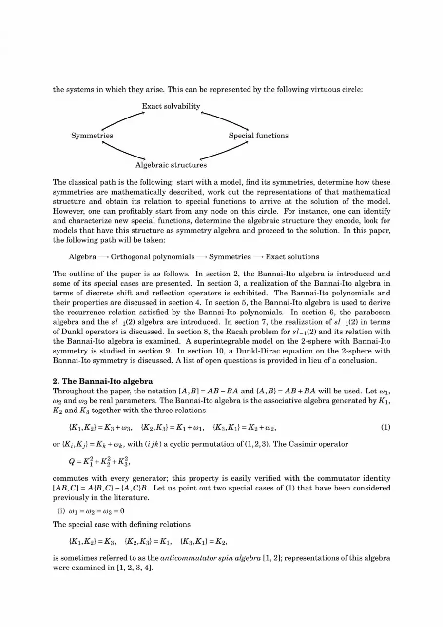
the systems in which they arise. This can be represented by the following virtuous circle:

Exact solvability

Symmetriesxx

44

Special functions''

kk

Algebraic structuresss

77

**

ff

The classical path is the following: start with a model, find its symmetries, determine how these

symmetries are mathematically described, work out the representations of that mathematical

structure and obtain its relation to special functions to arrive at the solution of the model.

However, one can profitably start from any node on this circle. For instance, one can identify

and characterize new special functions, determine the algebraic structure they encode, look for

models that have this structure as symmetry algebra and proceed to the solution. In this paper,

the following path will be taken:

Algebra−→Orthogonal polynomials−→Symmetries −→Exact solutions

The outline of the paper is as follows. In section 2, the Bannai-Ito algebra is introduced and

some of its special cases are presented. In section 3, a realization of the Bannai-Ito algebra in

terms of discrete shift and reflection operators is exhibited. The Bannai-Ito polynomials and

their properties are discussed in section 4. In section 5, the Bannai-Ito algebra is used to derive

the recurrence relation satisfied by the Bannai-Ito polynomials. In section 6, the paraboson

algebra and the sl−1(2) algebra are introduced. In section 7, the realization of sl−1(2) in terms

of Dunkl operators is discussed. In section 8, the Racah problem for sl−1(2) and its relation with

the Bannai-Ito algebra is examined. A superintegrable model on the 2-sphere with Bannai-Ito

symmetry is studied in section 9. In section 10, a Dunkl-Dirac equation on the 2-sphere with

Bannai-Ito symmetry is discussed. A list of open questions is provided in lieu of a conclusion.

2. The Bannai-Ito algebra

Throughout the paper, the notation [A,B] = AB−BA and A,B= AB+BA will be used. Let ω1,

ω2 and ω3 be real parameters. The Bannai-Ito algebra is the associative algebra generated by K1,

K2 and K3 together with the three relations

K1,K2= K3+ω3, K2,K3= K1+ω1, K3,K1= K2+ω2, (1)

or K i,K j= Kk +ωk, with (i jk) a cyclic permutation of (1,2,3). The Casimir operator

Q = K21 +K2

2 +K23 ,

commutes with every generator; this property is easily verified with the commutator identity

[AB,C] = AB,C− A,CB. Let us point out two special cases of (1) that have been considered

previously in the literature.

(i) ω1 =ω2 =ω3 = 0

The special case with defining relations

K1,K2= K3, K2,K3= K1, K3,K1= K2,

is sometimes referred to as the anticommutator spin algebra [1, 2]; representations of this algebra

were examined in [1, 2, 3, 4].

(ii) ω1 =ω2 = 0 6=ω3

In recent work on the construction of novel finite oscillator models [5, 6], E. Jafarov, N. Stoilova

and J. Van der Jeugt introduced the following extension of u(2) by an involution R (R2 = 1):

[I3,R]= 0, I1,R= 0, I2,R= 0,

[I3, I1]= iI2, [I2, I3]= iI1, [I1, I2]= i(I3+ω3R).

It is easy to check that with

K1 = iI1R, K2 = I2, K3 = I3R,

the above relations are converted into

K1,K3= K2, K2,K3= K1, K1,K2= K3+ω3.

3. A realization of the Bannai-Ito algebra with shift and reflections operators

Let T+ and R be defined as follows:

T+ f (x)= f (x+1), R f (x)= f (−x).

Consider the operator

K1 = F(x)(1−R)+G(x)(T+R −1)+h, h =ρ1 +ρ2 − r1− r2+1/2, (2)

with F(x) and G(x) given by

F(x)=(x−ρ1)(x−ρ2)

x, G(x)=

(x− r1+1/2)(x− r2+1/2)

x+1/2,

where ρ1,ρ2, r1, r2 are four real parameters. It can be shown that K1 is the most general operator

of first order in T+ and R that stabilizes the space of polynomials of a given degree [7]. That is,

for any polynomial Qn(x) of degree n, [K1Qn(x)] is also a polynomial of degree n. Introduce

K2 = 2x+1/2, (3)

which is essentially the “multiplication by x” operator and

K3 ≡ K1, K2−4(ρ1ρ2− r1r2). (4)

It is directly verified that K1, K2 and K3 satisfy the commutation relations

K1, K2= K3+ ω3, K2, K3= K1+ ω1, K3, K1= K2+ ω2, (5)

where the structure constants ω1, ω2 and ω3 read

ω1 = 4(ρ1ρ2 + r1r2), ω2 = 2(ρ21 +ρ2

2 − r21− r2

2), ω3 = 4(ρ1ρ2 − r1r2). (6)

The operators K1, K2 and K3 thus realize the Bannai-Ito algebra. In this realization, the Casimir

operator acts as a multiple of the identity; one has indeed

Q = K21 + K2

2 + K23 = 2(ρ2

1 +ρ22 + r2

1+ r22)−1/4.

4. The Bannai-Ito polynomials

Since the operator (2) preserves the space of polynomials of a given degree, it is natural to look

for its eigenpolynomials, denoted by Bn(x), and their corresponding eigenvalues λn. We use the

following notation for the generalized hypergeometric series [8]

rFs

(a1, . . .,ar

b1, . . . , bs

∣∣∣ z

)=

∞∑

k=0

(a1)k · · · (ar)k

(b1)k · · · (bs)k

zk

k!,

where (c)k = c(c+1) · · · (c+k−1), (c)0 ≡ 1 stands for the Pochhammer symbol; note that the above

series terminates if one of the a i is a negative integer. Solving the eigenvalue equation

K1Bn(x)=λnBn(x), n = 0,1,2, . . . (7)

it is found that the eigenvalues λn are given by [7]

λn = (−1)n(n+h), (8)

and that the polynomials have the expression

Bn(x)

cn

=

4F3

(− n

2, n+1

2+h, x−r1+1/2,−x−r1+1/2

1−r1−r2,ρ1−r1+ 12

,ρ2−r1+ 12

∣∣∣1)

+ ( n2

)(x−r1+ 12

)

(ρ1−r1+ 12

)(ρ2−r1+ 12

) 4F3

(1− n

2, n+1

2+h, x−r1+3/2,−x−r1+1/2

1−r1−r2,ρ1−r1+ 32,ρ2−r1+ 3

2

∣∣∣1

)n even,

4F3

(− n−1

2, n

2+h, x−r1+ 1

2,−x−r1+ 1

2

1−r1−r2,ρ1−r1+ 12,ρ2−r1+ 1

2

∣∣∣1

)

− ( n2+h)(x−r1+ 1

2)

(ρ1−r1+ 12

)(ρ2−r1+ 12

) 4F3

(− n−1

2, n+2

2+h, x−r1+ 3

2,−x−r1+ 1

2

1−r1−r2,ρ1−r1+ 32

,ρ2−r1+ 32

∣∣∣1)

n odd,

(9)

where the coefficient

c2n+p = (−1)p (1− r1− r2)n(ρ1 − r1+1/2,ρ2− r1+1/2)n+p

(n+h+1/2)n+p

, p ∈ 0,1,

ensures that the polynomials Bn(x) are monic, i.e. Bn(x) = xn +O (xn−1). The polynomials (9)

were first written down by Bannai and Ito in their classification of the orthogonal polynomials

satisfying the Leonard duality property [9, 10], i.e. polynomials pn(x) satisfying both

• A 3-term recurrence relation with respect to the degree n,

• A 3-term difference equation with respect to a variable index s.

The identification of the defining eigenvalue equation (7) of the Bannai-Ito polynomials in [7] has

allowed to develop their theory. That they obey a three-term difference equation stems from the

fact that there are grids such as

xs = (−1)s(s/2+a+1/4)−1/4,

for which operators of the form

H = A(x)R +B(x)T+R +C(x),

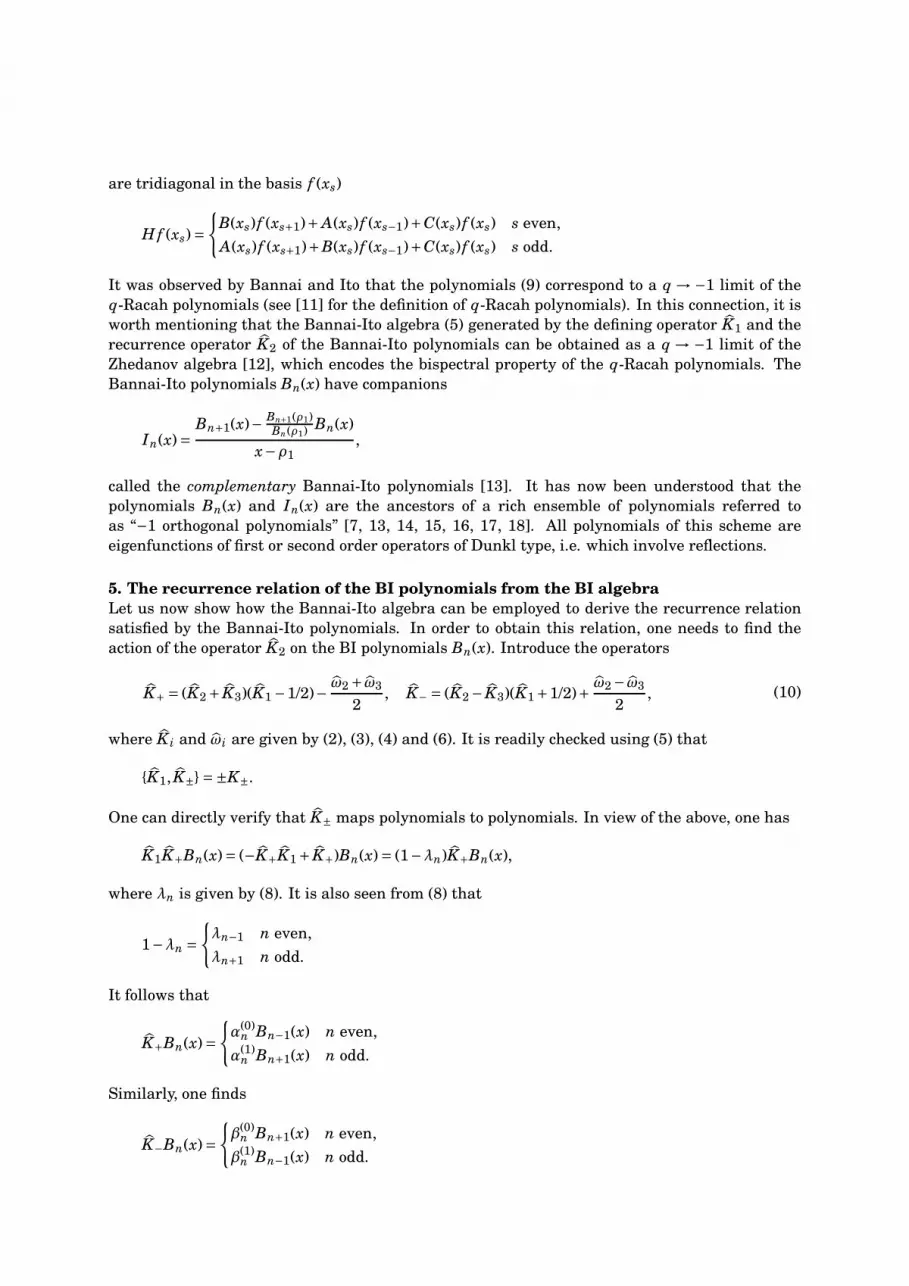
are tridiagonal in the basis f (xs)

H f (xs)=

B(xs) f (xs+1)+ A(xs) f (xs−1)+C(xs) f (xs) s even,

A(xs) f (xs+1)+B(xs) f (xs−1)+C(xs) f (xs) s odd.

It was observed by Bannai and Ito that the polynomials (9) correspond to a q →−1 limit of the

q-Racah polynomials (see [11] for the definition of q-Racah polynomials). In this connection, it is

worth mentioning that the Bannai-Ito algebra (5) generated by the defining operator K1 and the

recurrence operator K2 of the Bannai-Ito polynomials can be obtained as a q → −1 limit of the

Zhedanov algebra [12], which encodes the bispectral property of the q-Racah polynomials. The

Bannai-Ito polynomials Bn(x) have companions

In(x)=Bn+1(x)− Bn+1(ρ1)

Bn(ρ1)Bn(x)

x−ρ1

,

called the complementary Bannai-Ito polynomials [13]. It has now been understood that the

polynomials Bn(x) and In(x) are the ancestors of a rich ensemble of polynomials referred to

as “−1 orthogonal polynomials” [7, 13, 14, 15, 16, 17, 18]. All polynomials of this scheme are

eigenfunctions of first or second order operators of Dunkl type, i.e. which involve reflections.

5. The recurrence relation of the BI polynomials from the BI algebra

Let us now show how the Bannai-Ito algebra can be employed to derive the recurrence relation

satisfied by the Bannai-Ito polynomials. In order to obtain this relation, one needs to find the

action of the operator K2 on the BI polynomials Bn(x). Introduce the operators

K+ = (K2+ K3)(K1 −1/2)−ω2 + ω3

2, K− = (K2− K3)(K1+1/2)+

ω2− ω3

2, (10)

where K i and ωi are given by (2), (3), (4) and (6). It is readily checked using (5) that

K1, K±=±K±.

One can directly verify that K± maps polynomials to polynomials. In view of the above, one has

K1K+Bn(x)= (−K+K1+ K+)Bn(x)= (1−λn)K+Bn(x),

where λn is given by (8). It is also seen from (8) that

1−λn =λn−1 n even,

λn+1 n odd.

It follows that

K+Bn(x)=α(0)

n Bn−1(x) n even,

α(1)n Bn+1(x) n odd.

Similarly, one finds

K−Bn(x)=β(0)

n Bn+1(x) n even,

β(1)n Bn−1(x) n odd.

The coefficients

α(0)n =

2n( n2+ρ1 +ρ2)(r1+ r2− n

2)( n−1

2+h)

n+h− 12

, α(1)n =−4(n+h+1/2),

β(0)n = 4(n+h+1/2), β(1)

n =4(ρ1 − r1+ n

2)(ρ2 − r1+ n

2)(ρ1 − r2+ n

2)(ρ2 − r2+ n

2)

n+h−1/2,

can be obtained from the comparison of the highest order term. Introduce the operator

V = K+(K1+1/2)+ K−(K1−1/2). (11)

From the definition (10) of K±, it follows that

V = 2K2(K21 −1/4)− ω3K1− ω2/2. (12)

From (7), (11) and the actions of the operators K±, we find that V is two-diagonal

V Bn(x)=

(λn +1/2)α(0)n Bn−1(x)+ (λn −1/2)β(0)

n Bn+1(x) n even,

(λn −1/2)β(1)n Bn−1(x)+ (λn +1/2)α(1)

n Bn+1(x) n odd.(13)

From (12) and recalling the definition (3) of K2, we have also

V Bn(x)=[(λ2

n −1/4)(4x+1)− ω3λn − ω2/2]Bn(x). (14)

Upon combining (13) and (14), one finds that the Bannai-Ito polynomials satisfy the three-term

recurrence relation

xBn(x)=Bn+1(x)+ (ρ1 − An −Cn)Bn(x)+ An−1CnBn−1(x),

where

An = (n+1+2ρ1−2r1)(n+1+2ρ1−2r2)

4(n+ρ1+ρ2−r1−r2+1)n even,

(n+1+2ρ1+2ρ2−2r1−2r2)(n+1+2ρ1+2ρ2)

4(n+ρ1+ρ2−r1−r2+1)n odd,

Cn =− n(n−2r1−2r2)

4(n+ρ1+ρ2−r1−r2)n even,

− (n+2ρ2−2r2)(n+2ρ2−2r1)

4(n+ρ1+ρ2−r1−r2)n odd.

(15)

The positivity of the coefficient An−1Cn restricts the polynomials Bn(x) to being orthogonal on a

finite set of points [19].

6. The paraboson algebra and sl−1(2)

The next realization of the Bannai-Ito algebra will involve sl−1(2); this algebra, introduced in

[20], is closely related to the parabosonic oscillator.

6.1. The paraboson algebra

Let a and a† be the generators of the paraboson algebra. These generators satisfy [21]

[a,a†,a]=−2a, [a,a†,a†]= 2a†.

Setting H = 12a,a†, the above relations amount to

[H,a]=−a, [H,a†]= a†,

which correspond to the quantum mechanical equations of an oscillator.

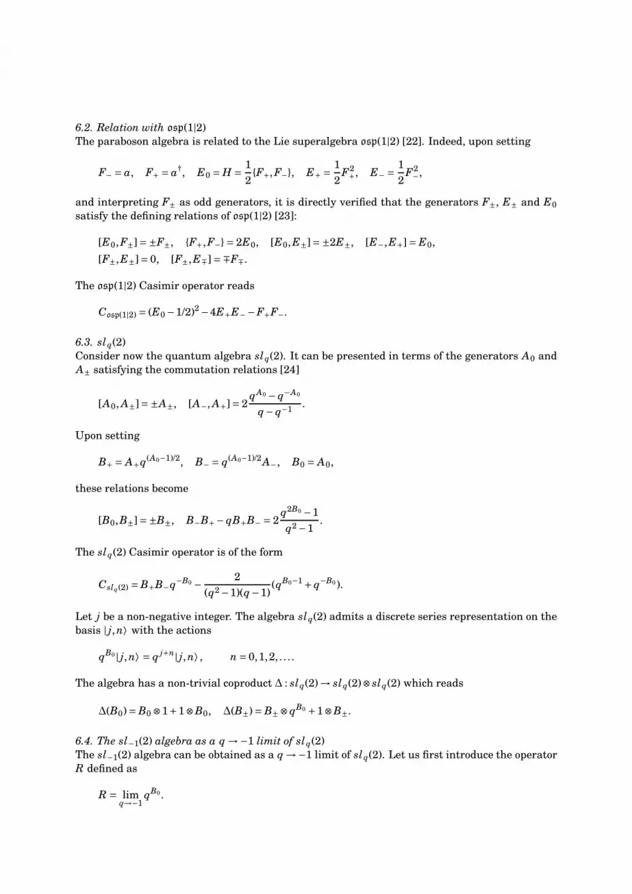
6.2. Relation with osp(1|2)

The paraboson algebra is related to the Lie superalgebra osp(1|2) [22]. Indeed, upon setting

F− = a, F+ = a†, E0 = H =1

2F+,F−, E+ =

1

2F2+, E− =

1

2F2−,

and interpreting F± as odd generators, it is directly verified that the generators F±, E± and E0

satisfy the defining relations of osp(1|2) [23]:

[E0,F±]=±F±, F+,F−= 2E0, [E0,E±]=±2E±, [E−,E+]= E0,

[F±,E±]= 0, [F±,E∓]=∓F∓.

The osp(1|2) Casimir operator reads

Cosp(1|2) = (E0−1/2)2 −4E+E−−F+F−.

6.3. slq(2)

Consider now the quantum algebra slq(2). It can be presented in terms of the generators A0 and

A± satisfying the commutation relations [24]

[A0, A±]=±A±, [A−, A+]= 2qA0 − q−A0

q− q−1.

Upon setting

B+ = A+q(A0−1)/2, B− = q(A0−1)/2A−, B0 = A0,

these relations become

[B0,B±]=±B±, B−B+− qB+B− = 2q2B0 −1

q2−1.

The slq(2) Casimir operator is of the form

Cslq(2) =B+B−q−B0 −2

(q2−1)(q−1)(qB0−1+ q−B0).

Let j be a non-negative integer. The algebra slq(2) admits a discrete series representation on the

basis | j, n⟩ with the actions

qB0 | j, n⟩ = q j+n| j, n⟩ , n =0,1,2, . . ..

The algebra has a non-trivial coproduct ∆ : slq(2)→ slq(2)⊗ slq(2) which reads

∆(B0)= B0 ⊗1+1⊗B0, ∆(B±)= B±⊗ qB0 +1⊗B±.

6.4. The sl−1(2) algebra as a q →−1 limit of slq(2)

The sl−1(2) algebra can be obtained as a q →−1 limit of slq(2). Let us first introduce the operator

R defined as

R = limq→−1

qB0 .

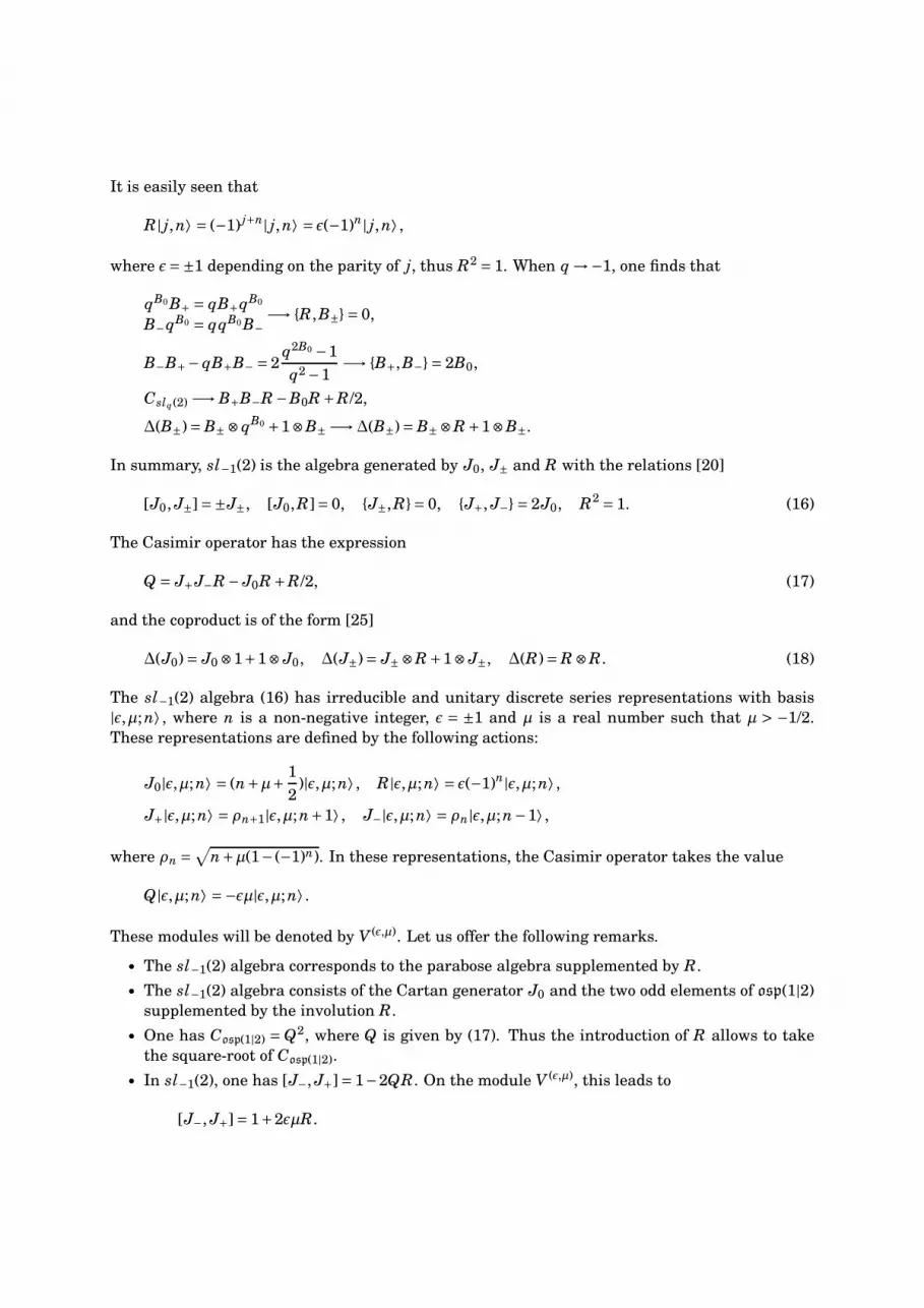
It is easily seen that

R| j, n⟩ = (−1) j+n| j, n⟩ = ǫ(−1)n| j, n⟩ ,

where ǫ=±1 depending on the parity of j, thus R2 = 1. When q →−1, one finds that

qB0 B+ = qB+qB0

B−qB0 = qqB0B−−→ R,B±= 0,

B−B+− qB+B− = 2q2B0 −1

q2 −1−→ B+,B−= 2B0,

Cslq(2) −→ B+B−R −B0R +R/2,

∆(B±)= B±⊗ qB0 +1⊗B± −→∆(B±)= B±⊗R +1⊗B±.

In summary, sl−1(2) is the algebra generated by J0, J± and R with the relations [20]

[J0, J±]=±J±, [J0,R]= 0, J±,R= 0, J+, J−= 2J0, R2 = 1. (16)

The Casimir operator has the expression

Q = J+J−R − J0R +R/2, (17)

and the coproduct is of the form [25]

∆(J0)= J0 ⊗1+1⊗ J0, ∆(J±)= J±⊗R +1⊗ J±, ∆(R)= R ⊗R. (18)

The sl−1(2) algebra (16) has irreducible and unitary discrete series representations with basis

|ǫ,µ; n⟩ , where n is a non-negative integer, ǫ = ±1 and µ is a real number such that µ > −1/2.

These representations are defined by the following actions:

J0|ǫ,µ; n⟩ = (n+µ+1

2)|ǫ,µ; n⟩ , R|ǫ,µ; n⟩ = ǫ(−1)n|ǫ,µ; n⟩ ,

J+|ǫ,µ; n⟩ = ρn+1|ǫ,µ; n+1⟩ , J−|ǫ,µ; n⟩ = ρn|ǫ,µ; n−1⟩ ,

where ρn =√

n+µ(1− (−1)n). In these representations, the Casimir operator takes the value

Q|ǫ,µ; n⟩ =−ǫµ|ǫ,µ; n⟩ .

These modules will be denoted by V (ǫ,µ). Let us offer the following remarks.

• The sl−1(2) algebra corresponds to the parabose algebra supplemented by R.

• The sl−1(2) algebra consists of the Cartan generator J0 and the two odd elements of osp(1|2)

supplemented by the involution R.

• One has Cosp(1|2) = Q2, where Q is given by (17). Thus the introduction of R allows to take

the square-root of Cosp(1|2).

• In sl−1(2), one has [J−, J+]= 1−2QR. On the module V (ǫ,µ), this leads to

[J−, J+]= 1+2ǫµR.

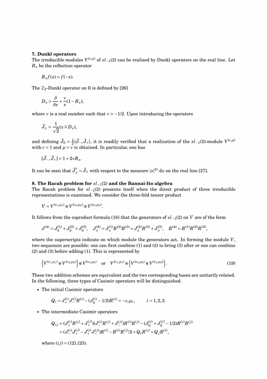
7. Dunkl operators

The irreducible modules V (ǫ,µ) of sl−1(2) can be realized by Dunkl operators on the real line. Let

Rx be the reflection operator

Rx f (x)= f (−x).

The Z2-Dunkl operator on R is defined by [26]

Dx =∂

∂x+

ν

x(1−Rx),

where ν is a real number such that ν>−1/2. Upon introducing the operators

J± =1p

2(x∓Dx),

and defining J0 = 12J−, J+, it is readily verified that a realization of the sl−1(2)-module V (ǫ,µ)

with ǫ= 1 and µ= ν is obtained. In particular, one has

[J−, J+]= 1+2νRx.

It can be seen that J†± = J∓ with respect to the measure |x|2νdx on the real line [27].

8. The Racah problem for sl−1(2) and the Bannai-Ito algebra

The Racah problem for sl−1(2) presents itself when the direct product of three irreducible

representations is examined. We consider the three-fold tensor product

V =V (ǫ1,µ1) ⊗V (ǫ2,µ2) ⊗V (ǫ3,µ3).

It follows from the coproduct formula (18) that the generators of sl−1(2) on V are of the form

J(4) = J(1)0

+ J(2)0

+ J(3)0

, J(4)± = J

(1)± R(2)R(3)+ J

(2)± R(3)+ J

(3)± , R(4) = R(1)R(2)R(3),

where the superscripts indicate on which module the generators act. In forming the module V ,

two sequences are possible: one can first combine (1) and (2) to bring (3) after or one can combine

(2) and (3) before adding (1). This is represented by

(V (ǫ1,µ1) ⊗V (ǫ2,µ2)

)⊗V (ǫ3,µ3) or V (ǫ1,µ1)⊗

(V (ǫ2,µ2) ⊗V (ǫ3,µ3)

). (19)

These two addition schemes are equivalent and the two corresponding bases are unitarily related.

In the following, three types of Casimir operators will be distinguished.

• The initial Casimir operators

Q i = J(i)+ J(i)

− R(i) − (J(i)0

−1/2)R(i) =−ǫiµi, i = 1,2,3.

• The intermediate Casimir operators

Q i j = (J(i)+ R( j)+ J

( j)+ )(J(i)

− R( j)+ J( j)− )R(i)R( j)− (J(i)

0+ J

( j)

0−1/2)R(i)R( j)

= (J(i)− J

( j)+ − J

(i)+ J( j)

− )R(i) −R(i)R( j)/2+Q iR( j)+Q jR

(i),

where (i j)= (12), (23).

• The total Casimir operator

Q4 = [J(4)+ J(4)

− − (J(4)0

−1/2)]R(4).

Let |q12, q4; m⟩ and |q23, q4; m⟩ be the orthonormal bases associated to the two coupling schemes

presented in (19). These two bases are defined by the relations

Q12|q12, q4; m⟩ = q12|q12, q4; m⟩ , Q23|q23, q4; m⟩ = q23|q23, q4; m⟩ ,

and

Q4|−, q4; m⟩ = q4|−, q4; m⟩ , J(4)0

|−, q4; m⟩ = (m+µ1 +µ2 +µ3 +3/2)|−, q4; m⟩ .

The Racah problem consists in finding the overlap coefficients

⟨q23, q4 |q12, q4⟩ ,

between the eigenbases of Q12 and Q23 with a fixed value q4 of the total Casimir operator Q4; as

these coefficients do not depend on m, we drop this label. For simplicity, let us now take

ǫ1 = ǫ2 = ǫ3 = 1.

Upon defining

K1 =−Q23, K3 =−Q12,

one finds that the intermediate Casimir operators of sl−1(2) realize the Bannai-Ito algebra [28]

K1,K3= K2+Ω2, K1,K2= K3+Ω3, K2,K3= K1+Ω1, (20)

with structure constants

Ω1 = 2(µ1µ+µ2µ3), Ω2 = 2(µ1µ3 +µ2µ), Ω3 = 2(µ1µ2+µ3µ), (21)

where µ= ǫ4µ4 =−q4. The first relation in (20) can be taken to define K2 which reads

K2 = (J(1)+ J(3)

− − J(1)− J

(3)+ )R(1)R(2)+R(1)R(3)/2−Q1R(3)−Q3R(1).

In the present realization the Casimir operator of the Bannai-Ito algebra becomes

QBI =µ21+µ2

2 +µ23 +µ2

4 −1/4.

It has been shown in section 3 that the Bannai-Ito polynomials form a basis for a representation

of the BI algebra. It is here relatively easy to construct the representation of the BI algebra on

bases of the three-fold tensor product module V with basis vectors defined as eigenvectors of Q12

or of Q23. The first step is to obtain the spectra of the intermediate Casimir operators. Simple

considerations based on the nature of the sl−1(2) representation show that the eigenvalues q12

and q23 of Q12 and Q23 take the form [29, 30, 28, 20]:

q12 = (−1)s12+1(s12+µ1 +µ2 +1/2), q23 = (−1)s23 (s23+µ2 +µ3 +1/2),

where s12, s23 = 0,1, . . ., N. The non-negative integer N is specified by

N +1=µ4−µ1 −µ2 −µ3.

Denote the eigenstates of K3 by |k⟩ and those of K1 by |s⟩ ; one has

K3|k⟩ = (−1)k(k+µ1 +µ2 +1/2)|k⟩ , K1|s⟩ = (−1)s(s+µ2+µ3 +1/2)|s⟩ .

Given the expressions (21) for the structure constants Ωk, one can proceed to determine the

(N + 1)× (N + 1) matrices that verify the anticommutation relations (20). The action of K1 on

|k⟩ is found to be [28]:

K1|k⟩ =Uk+1|k+1⟩ +Vk|k⟩ +Uk|k−1⟩ ,

with Vk =µ2+µ3 +1/2−Bk −Dk and Uk =√

Bk−1Dk where

Bk = (k+2µ2+1)(k+µ1+µ2+µ3−µ+1)

2(k+µ1+µ2+1)k even,

(k+2µ1+2µ2+1)(k+µ1+µ2+µ3+µ+1)

2(k+µ1+µ2+1)k odd,

Dk =− k(k+µ1+µ2−µ3−µ)

2(k+µ1+µ)2)n even,

− (k+2µ1)(k+µ1+µ2−µ3+µ)

2(k+µ1+µ2)n odd.

Under the identifications

ρ1 =1

2(µ2 +µ3), ρ2 =

1

2(µ1 +µ), r1 =

1

2(µ3 −µ2), r2 =

1

2(µ−µ1),

one has Bk = 2Ak, Dk = 2Ck, where Ak and Ck are the recurrence coefficients (15) of the Bannai-

Ito polynomials. Upon setting

⟨s |k⟩ = w(s)2kBk(xs), B0(xs)≡ 1,

one has on the one hand

⟨s |K1 |k ⟩ = (−1)s(s+2ρ1 +1/2) ⟨s |k⟩ ,

and on the other hand

⟨s |K1 |k ⟩ =Uk+1 ⟨s |k+1⟩ +Vk ⟨s |k⟩ +Uk−1 ⟨s |k−1⟩ .

Comparing the two RHS yields

xsBk(xs)=Bk+1(xs)+ (ρ1 − Ak −Ck)Bk(xs)+ Ak−1CkBk−1(xs),

where xs are the points of the Bannai-Ito grid

xs = (−1)s( s

2+ρ1 +1/4

)−1/4, s =0, . . . , N.

Hence the Racah coefficients of sl−1(2) are proportional to the Bannai-Ito polynomials. The

algebra (20) with structure constants (21) is invariant under the cyclic permutations of the pairs

(K i,µi). As a result, the representations in the basis where K1 is diagonal can be obtained directly.

In this basis, the operator K3 is seen to be tridiagonal, which proves again that the Bannai-Ito

polynomials possess the Leonard duality property.

9. A superintegrable model on S2 with Bannai-Ito symmetry

We shall now use the analysis of the Racah problem for sl−1(2) and its realization in terms of

Dunkl operators to obtain a superintegrable model on the two-sphere. Recall that a quantum

system in n dimensions with Hamiltonian H is maximally superintegrable it it possesses 2n−1

algebraically independent constants of motion, where one of these constants is H [31]. Let

(s1, s2, s3) ∈R and take s21+ s2

2+ s23 = 1. The standard angular momentum operators are

L1 =1

i

(s2

∂

∂s3

− s3

∂

∂s2

), L2 =

1

i

(s3

∂

∂s1

− s1

∂

∂s3

), L3 =

1

i

(s1

∂

∂s2

− s2

∂

∂s1

).

The system governed by the Hamiltonian

H = L21 +L2

2 +L23 +

µ1

s21

(µ1−R1)+µ2

s22

(µ2−R2)+µ3

s23

(µ3−R3), (22)

with µi, i = 1,2,3, real parameters such that µi >−1/2 is superintegrable [32].

(i) The operators Ri reflect the variable s i: Ri f (s i)= f (−s i).

(ii) The operators Ri commute with the Hamiltonian: [H,Ri]= 0.

(iii) If one is concerned with the presence of reflection operators in a Hamiltonian, one may

replace Ri by κi =±1. This then treats the 8 potential terms

µ1

s21

(µ1−κ1)+µ2

s22

(µ2 −κ2)+µ3

s23

(µ3 −κ3),

simultaneously much like supersymmetric partners.

(iv) Rescaling s i → rs i and taking the limit as r → ∞ gives the Hamiltonian of the Dunkl

oscillator [27, 33]

H =−[D2x1+D2

x2]+ µ2

3(x21 + x2

2),

after appropriate renormalization; see also [34, 35, 36].

It can be checked that the following three quantities commute with the Hamiltonian (22) [29, 32]:

C1 =(iL1 +µ2

s3

s2

R2−µ3

s2

s3

R3

)R2+µ2R3+µ3R2+R2R3/2,

C2 =(−iL2 +µ1

s3

s1

R1−µ3

s1

s3

R3

)R1R2+µ1R3+µ3R1+R1R3/2,

C3 =(iL3 +µ1

s2

s1

R1−µ2

s1

s2

R2

)R1+µ1R2+µ2R1+R1R2/2,

that is, [H,Ci] = 0 for i = 1,2,3. To determine the symmetry algebra generated by the above

constants of motion, let us return to the Racah problem for sl−1(2). Consider the following (gauge

transformed) parabosonic realization of sl−1(2) in the three variables s i:

J(i)± =

1p

2

[s i ∓∂si

±µi

s i

Ri

], J

(i)0

=1,

2

[−∂2

si+ s2

i +µi

s2i

(µi −Ri)

], R(i) = Ri, (23)

for i = 1,2,3. Consider also the addition of these three realizations so that

J0 = J(1)0

+ J(2)0

+ J(3)0

, J± = J(1)± R(2)R(3)+ J

(2)± R(3)+ J

(3)± , R = R(1)R(2)R(3). (24)

It is observed that in the realization (24), the total Casimir operator can be expressed in terms of

the constants of motion as follows:

Q =−C1R(1)−C2R(2)−C3R(3)+µ1R(2)R(3)+µ2R(1)R(3)+µ3R(1)R(2)+R/2,

Upon taking

Ω=QR,

one finds

Ω2 +Ω= L2

1 +L22+L2

3 + (s21 + s2

2+ s23)

(µ1

s21

(µ1−R1)+µ2

s22

(µ2−R2)+µ3

s23

(µ3−R3)

), (25)

so that H =Ω2 +Ω if s2

1+ s22 + s2

3 = 1. Assuming this constraint can be imposed, H is a quadratic

combination of QR. By construction, the intermediate Casimir operators Q i j commute with the

total Casimir operator Q and with R and hence with Ω; they thus commute with H =Ω2 +Ω and

are the constants of motion. It is indeed found that

Q12 =−C3, Q23 =−C1,

in the parabosonic realization (23). Let us return to the constraint s21+ s2

2+ s2

3= 1. Observe that

1

2(J++ J−)2 = (s1R2R3+ s2R3+ s3)2 = s2

1+ s22 + s2

3.

Because (J++ J−)2 commutes with Ω = QR, Q12 and Q23, one can impose s21 + s2

2 + s23 = 1. Since

it is already known that the intermediate Casimir operators in the addition of three sl−1(2)

representations satisfy the Bannai-Ito structure relations, the constants of motion verify

C1,C2= C3−2µ3Q+2µ1µ2,

C2,C3= C1−2µ1Q+2µ2µ3,

C3,C1= C2−2µ2Q+2µ3µ1,

and thus the symmetry algebra of the superintegrable system with Hamiltonian (22) is a central

extension (with Q begin the central operator) of the Bannai-Ito algebra. Let us note that the

relation H =Ω2+Ω relates to chiral supersymmetry since with S =Ω+1/2 one has

1

2S,S= H+1/4.

10. A Dunkl-Dirac equation on S2

Consider the Z2-Dunkl operators

D i =∂

∂xi

+µi

xi

(1−Ri), i = 1,2, . . ., n,

with µi >−1/2. The Zn2-Dunkl-Laplace operator is

~D2 =n∑

i=1

D2i .

With γn the generators of the Euclidean Clifford algebra

γm,γn= 2δnm,

the Dunkl-Dirac operator is

/D =n∑

i=1

γiD i.

Clearly, one has /D2 = ~D2. Let us consider the three-dimensional case. Introduce the Dunkl

“angular momentum” operators

J1 =1

i(x2D3 − x3D2), J2 =

1

i(x3D1− x1D3), J3 =

1

i(x1D2 − x2D1).

Their commutation relations are found to be

[Ji , Jk]= iǫ jkl Jl(1+2µl Rl). (26)

The Dunkl-Laplace equation separates in spherical coordinates; i.e. one can write

~D2 = D21 +D2

2 +D23 =Mr +

1

r2∆S2 ,

where ∆S2 is the Dunkl-Laplacian on the 2-sphere. It can be verified that [36]

~J2 = J21 + J2

2 + J23

=−∆S2 +2µ1µ2(1−R1R2)+2µ2µ3(1−R2R3)+2µ1µ3(1−R1R3)

−µ1R1−µ2R2−µ3R3+µ1 +µ2 +µ3.

(27)

In three dimensions the Euclidean Clifford algebra is realized by the Pauli matrices

σ1 =(0 1

1 0

), σ2 =

(0 −i

i 0

), σ3 =

(1 0

0 −1

),

which satisfy

σiσ j = iǫi jkσk +δi j .

Consider the following operator:

Γ= (~σ ·~J)+~µ · ~R,

with~µ ·~R =µ1R1+µ2R2+µ3R3. Using the commutation relations (26) and the expression (27) for~J2, it follows that

Γ2 +Γ=−∆S2 + (µ1 +µ2 +µ3)(µ1 +µ2 +µ3 +1).

This is reminiscent of the expression (25) for the superintegrable system with Hamiltonian (22) in

terms of the sl−1(2) Casimir operator. This justifies calling Γ a Dunkl-Dirac operator on S2 since

a quadratic expression in Γ gives ∆S2 . The symmetries of Γ can be constructed. They are found to

have the expression [37]

Mi = Ji +σi(µ jR j +µkRk +1/2), (i jk) cyclic,

and one has [Γ, Mi]= 0. It is seen that the operators

X i =σiRi i = 1,2,3

also commute with Γ. Furthermore, one has

[Mi, X i]= 0, Mi, X j= Mi, Xk= 0.

Note that Y = −iX1X2 X3 = R1R2R3 is central (like Γ). The commutation relations satisfied by

the operators Mi are

[Mi, M j]= iǫi jk

(Mk +2µk(Γ+1)Xk

)+2µiµ j[X i , X j].

This is again an extension of su(2) with reflections and central elements. Let

K i = Mi X iY = MiσiR jRk.

It is readily verified that the operators K i satisfy

K1,K2= K3+2µ3(Γ+1)Y +2µ1µ2,

K2,K3= K1+2µ1(Γ+1)Y +2µ2µ3,

K3,K1= K2+2µ3(Γ+1)Y +2µ3µ1,

showing that the Bannai-Ito algebra is a symmetry subalgebra of the Dunkl-Dirac equation on S2.

Therefore, the Bannai-Ito algebra is also a symmetry subalgebra of the Dunkl-Laplace equation.

11. Conclusion

In this paper, we have presented the Bannai-Ito algebra together with some of its applications. In

concluding this overview, we identify some open questions.

(i) Representation theory of the Bannai-Ito algebra

Finite-dimensional representations of the Bannai-Ito algebra associated to certain models

were presented. However, the complete characterization of all representations of the Bannai-

Ito algebra is not known.

(ii) Supersymmetry

The parallel with supersymmetry has been underscored at various points. One may wonder

if there is a deeper connection.

(iii) Dimensional reduction

It is well known that quantum superintegrable models can be obtained by dimensional

reduction. It would be of interest to adapt this framework in the presence of reflections

operators. Could the BI algebra can be interpreted as a W-algebra ?

(iv) Higher ranks

Of great interest is the extension of the Bannai-Ito algebra to higher ranks, in particular for

many-body applications. In this connection, it can be expected that the symmetry analysis of

higher dimensional superintegrable models or Dunkl-Dirac equations will be revealing.

Acknowledgements

V.X.G. holds an Alexander-Graham-Bell fellowship from the Natural Science and Engineering

Research Council of Canada (NSERC). The research of L.V. is supported in part by NSERC. H.

DB. and A.Z. have benefited from the hospitality of the Centre de recherches mathématiques

(CRM).

References[1] Arik M and Kayserilioglu U 2003 Int. J. Mod. Phys. A 18 5039–5046

[2] Gorodnii M and Podkolzin G 1984 Irreducible representations of a graded Lie algebra (Inst. Math. Acad. Sci.) pp

66–76 Spectral theory of operators and infinite-dimensional analysis

[3] Brown G 2013 Elec. J. Lin. Alg. 26 258–299

[4] Ostrovskii V and Sil’vestrov S 1992 Ukr. Math. J. 44 1395–1401

[5] Jafarov E I, Stoilova N I and Van der Jeugt J 2011 J. Phys. A: Math. Theor. 44 265203

[6] Jafarov E I, Stoilova N I and Van der Jeugt J 2011 J. Phys. A: Math. Theor. 44 355205

[7] Tsujimoto S, Vinet L and Zhedanov A 2012 Adv. Math. 229 2123–2158

[8] Andrews G, Askey R and Roy R 1999 Special functions (Cambridge University Press)

[9] Leonard D 1982 SIAM J. Math. Anal. 13

[10] Bannai E and Ito T 1984 Algebraic Combinatorics I: Association Schemes (Benjamin/Cummings)

[11] Koekoek R, Lesky P and Swarttouw R 2010 Hypergeometric orthogonal polynomials and their q-analogues 1st ed

(Springer) ISBN 978-3-642-05013-8

[12] Zhedanov A 1991 Theor. Math. Phys. 89 1146–1157

[13] Genest V X, Vinet L and Zhedanov A 2013 SIGMA 9 18–37

[14] Genest V X, Vinet L and Zhedanov A 2014 SIGMA 10 38–55

[15] Vinet L and Zhedanov A 2011 J. Phys. A: Math. Theor. 44 085201

[16] Vinet L and Zhedanov A 2012 Trans. Amer. Math. Soc. 364 5491–5507

[17] Tsujimoto S, Vinet L and Zhedanov A 2013 Proc. Amer. Math. Soc. 141 959–970

[18] Tsujimoto S, Vinet L and Zhedanov A 2011 J. Math. Phys. 52 103512

[19] Chihara T 2011 An Introduction to Orthogonal Polynomials (Dover Publications)

[20] Tsujimoto S, Vinet L and Zhedanov A 2011 SIGMA 7 93–105

[21] Green H S 1953 Phys. Rev. 90 270–273

[22] Ganchev A C and Palev T D 1980 J. Math. Phys. 21 797

[23] Kac V G 1977 Adv. Math. 26 8–96

[24] Vilenkin N J and Klimyk A U 1991 Representation of Lie Groups and Special Functions (Kluwer Academic

Publishers)

[25] Daskaloyannis C and Kanakoglou K 2000 J. Math. Phys. 41 652–660

[26] Dunkl C F 1989 Trans. Amer. Math. Soc. 311 167–183

[27] Genest V X, Ismail M, Vinet L and Zhedanov A 2013 J. Phys. A: Math. Theor. 46 145201

[28] Genest V X, Vinet L and Zhedanov A 2014 Proc. Am. Soc. 142 1545–1560

[29] Genest V X, Vinet L and Zhedanov A 2013 Comm. Math. Phys. (to appear)

[30] Genest V X, Vinet L and Zhedanov A 2013 J. Math. Phys. 54 023506

[31] Miller W, Post S and Winternitz P 2013 J. Phys. A: Math. Theor. 46 423001

[32] Genest V X, Vinet L and Zhedanov A 2014 J. Phys. A: Math. Theor. 47 205202

[33] Genest V X, Ismail M, Vinet L and Zhedanov A 2014 Comm. Math. Phys. 329 999–1029

[34] Genest V X, Lemay J M, Vinet L and Zhedanov A 2013 J. Phys. A: Math. Theor. 46 505204

[35] Genest V X, Vinet L and Zhedanov A 2013 J. Phys. A: Math. Theor. 46 325201

[36] Genest V X, Vinet L and Zhedanov A 2014 J. Phys.: Conf. Ser. 512 012010

[37] De Bie H, Genest V X and Vinet L 2014 In preparation