Accepted Manuscript

Variability of CO concentrations in the Venus troposphere fromVenus Express/VIRTIS using a band ratio technique

C.C.C. Tsang, F.W. Taylor, C.F. Wilson, S.J. Liddell, P.G.J. Irwin,G. Piccioni, P. Drossart, S.B. Calcutt

PII: S0019-1035(09)00010-4DOI: 10.1016/j.icarus.2009.01.001Reference: YICAR 8877

To appear in: Icarus

Received date: 5 August 2008Revised date: 4 December 2008Accepted date: 8 January 2009

Please cite this article as: C.C.C. Tsang, F.W. Taylor, C.F. Wilson, S.J. Liddell, P.G.J. Irwin,G. Piccioni, P. Drossart, S.B. Calcutt, Variability of CO concentrations in the Venus troposphere fromVenus Express/VIRTIS using a band ratio technique, Icarus (2009), doi: 10.1016/j.icarus.2009.01.001

This is a PDF file of an unedited manuscript that has been accepted for publication. As a service toour customers we are providing this early version of the manuscript. The manuscript will undergocopyediting, typesetting, and review of the resulting proof before it is published in its final form. Pleasenote that during the production process errors may be discovered which could affect the content, and alllegal disclaimers that apply to the journal pertain.

ACCEP

TED M

ANUSC

RIPT

ACCEPTED MANUSCRIPT

1

Variability of CO concentrations in the Venus troposphere from 1

Venus Express/VIRTIS using a Band Ratio Technique 2

3

C.C.C. Tsang

a

, F.W. Taylora

, C.F. Wilsona

, S.J. Liddella

,4

P.G.J. Irwina

, G. Piccionib

, P. Drossartc

, S.B. Calcutta

5

6

a

Atmospheric, Oceanic and Planetary Physics, Department of Physics, University of Oxford, Parks 7

Road, Oxford, Oxon, OX1 3PU, U.K. 8

b

INAF-IASF, Via del Fosso del Cavaliere, 100 00133 Rome, Italy 9

c

LESIA, Observatoire de Paris, CNRS, UPMC Université Paris-Diderot 10

11

12

Number of Manuscript Papers: 9 + references, figures (22 in total) 13

Number of Tables: 1 14

Number of Figures: 12 15

16

17

Proposed Running Head: 18

Band Ratio Technique of CO on Venus 19

20

21

Editorial correspondence should be directed to: 22

23

Dr Constantine C.C. Tsang 24

Atmospheric, Oceanic and Planetary Physics, Department of Physics, University of 25

Oxford, Clarendon Laboratory, Parks Road, Oxford, Oxon, OX1 3PU, Oxford, 26

United Kingdom. 27

28

Tel:(+44) 1865 272927, Fax: (+44) 1865 272923 29

Email: con@atm.ox.ac.uk 30

31

Keywords: 32

Venus, Venus Express, Dynamics, Carbon Monoxide, Troposphere 33

34

35

Abstract36

37

A fast method is presented for deriving the tropospheric CO concentrations in the Venus 38

atmosphere from near-infrared spectra using the night side 2.3 µm window. This is validated using 39

the spectral fitting techniques of Tsang et al. (2008a) to show that monitoring CO in the deep 40

atmosphere can be done quickly using large numbers of observations, with minimal effect from 41

cloud and temperature variations. The new method is applied to produce some 1,450 zonal mean 42

CO profiles using data from the first eighteen months of operation from the Visible and Infrared 43

Thermal Imaging Spectrometer infrared mapping subsystem (VIRTIS-M-IR) on Venus Express. 44

These results show many significant long and short-term variations from the mean equator-to-pole 45

ACCEP

TED M

ANUSC

RIPT

ACCEPTED MANUSCRIPT

2

increasing trend previously found from earlier Earth- and space-based observations, including a 46

possible North-South dichotomy, with interesting implications for the dynamics and chemistry of 47

the lower atmosphere of Venus. 48

49

1. Introduction 50

51

The concentration of carbon monoxide (CO) in the troposphere (surface to 40km) of Venus was 52

first proposed to be retrievable through modeling by Kamp et al. (1988). This is possible through 53

the observation of the thermal emission window at 2.3 µm, where the radiation is escaping from the 54

deep atmosphere. For a thorough review of this topic, see Taylor et al. (1997) and Tsang et al. 55

(2008b). The first measurements of CO using this window were made by Bézard et al. (1990) from 56

CFHT observations. Pollack et al. (1993) also conducted ground-based observations to measure the 57

mean abundance of CO in the troposphere. However, the first attempt to measure spatial variations 58

in CO at 35 km was by Collard et al. (1993), using 2.3 µm spectra obtained by the Near Infrared 59

Mapping Spectrometer (NIMS) on the Galileo spacecaft. 60

61

1.1 Collard et al. 1993 Method 62

63

These authors used Galileo/NIMS spectra at 2.3 µm from the fly-by of Venus in 1990. Rather than 64

using a spectral fitting technique, Collard et al. (1993) used ratios of radiances at two different 65

wavelengths. Between 2.20 and 2.30 µm, the absorption is purely due to CO2 and cloud opacity, 66

whilst at 2.30 to 2.43 µm, the absorption is due to strong vibrational-rotation CO bands as well. The 67

wavelengths chosen by the authors were 2.252 µm, outside the CO band, and 2.330 µm, with strong 68

CO absorption. A distinct correlation is observed between these two wavelengths, which is due to 69

the optical depth of the cloud layer, as one might expect. However, an off-branching set of points 70

was also seen beneath the main branch. This was interpreted as being due to the increase in the CO 71

abundance at these locations on the planet, causing the increased absorption at 2.330 µm compared 72

to the `nominal'. After drawing an arbitrary line bisecting the cloud opacity points and the points 73

due to increased CO, an enhancement was seen poleward of 47 o

N. It was thus shown that a CO 74

latitudinal gradient exists in the lower atmosphere. Extensive studies were conducted by the above 75

authors to investigate the possibility that the bifurcation was due to other effects such as variations 76

in temperature profiles, emission angles and differing cloud structures, all of which proved 77

negative. 78

79

1.2 Ground-Based Observations and Venus Express 80

81

Since the work of Collard et al. (1993), numerous ground-based studies have been conducted, most 82

notably Marcq et al. (2005, 2006), in order to confirm the existence of the trospospheric CO 83

gradient and to better elucidate its nature. Whilst their measurements were in line with the expected 84

gradients and values seen by Galileo/NIMS, they did not manage to yield information as to the 85

temporal and zonal distribution of CO at this altitude of 35 km, due to their high spectral, but 86

therefore low spatial, resolutions. Observations took on a new facet with the arrival of Venus 87

Express and its array of instruments around Venus in 2006, which allowed the possibility of 88

retrieving and thus monitoring CO in the troposphere with good spatial and temporal coverage. On 89

board was an imaging spectrometer, VIRTIS (Drossart et al. 2007, Piccioni et al. 2008). The 90

subsystems on VIRTIS, called H (high resolution spectrograph of 1 nm spectral sampling) and M-91

IR (low resolution spectral imager with 10 nm spectral sampling), are able to sample the 2.3 µm 92

thermal emission, amongst others. VIRTIS-M-IR has a spectral range from 1.01 to 5.19 µm, divided 93

into 432 discrete spectral bands (Band 0 to Band 431). 94

95

ACCEP

TED M

ANUSC

RIPT

ACCEPTED MANUSCRIPT

3

Marcq et al. (2008) were able to retrieve the abundance and the latitudinal gradient of CO using the 96

H subchannel to good precision, whilst Tsang et al. (2008a) used the M imaging channel to retrieve 97

spatial maps to look for spatial and temporal variations, without substantial loss in precision. Tsang 98

et al. (2008a) showed the latitudinal variations as expected. However, due to the complex and time 99

consuming spectral fitting of the CO 2-0 band required for the analysis, only four observations were 100

analysed. These observations, although limited in time, did show interesting and significant signs of 101

zonal and temporal variability. A faster, but still accurate, method is thus required to derive and 102

monitor variations in the CO concentration. This was the main motivation for this analysis. Section 103

2 will deal with the drawbacks of the Collard et al. (1993) method, followed by our new method, 104

with forward modeling. Section 3 contains the results and Section 4 the conclusions of this analysis. 105

106

2. Analysis 107

108

2.1 Ratio Methodology 109

110

The premise for this analysis was to repeat the experiment of Collard et al. 1993 described in 111

Section 1.1, by taking radiation emitted at 2.30µm, which should be sensitive only to cloud opacity 112

and compare it to the radiation emitted at 2.32 or 2.33 µm, which is attenuated by CO as well as 113

cloud opacity. Fig. 1 shows how synthetic spectra behave when we artificially increase the 114

abundance of CO in the deep atmosphere. We shall return to this in Section 2.2.3. 115

116

As we followed the approach mentioned above, it became clear it was not accurate enough for our 117

purpose. Fig. 2 shows the result from using the method on VIRTIS-M-IR observation; VI099_2, 118

corresponding to orbit number 99, cube 2, is used as a case study. When we plot radiances from 119

Band 135 versus Band 137, which correspond to wavelengths of 2.30 and 2.32 µm, two general 120

trends appear, which mimic the observation by Collard et al. (1993). The reasons for choosing these 121

two wavelengths will be given in Section 2.2. We then choose an arbitrary straight line to bisect the 122

points due to CO and those from cloud opacity. The displacement of the points from the straight 123

line is then plotted as a function of their latitude position, and compared with the 2.30 µm 124

radiances, which are a direct indication of cloud opacity. Firstly, we see that the displacement as a 125

function of latitude increases towards the poles. This is in line with what is expected of the CO 126

latitudinal structure (Marcq et al. 2008a, Tsang et al. 2008a). However, comparison with 2.30 µm 127

radiances also shows an anti-correlation with the cloud opacity. Clearly, this is not an accurate 128

method of retrieving CO in the lower atmosphere, as the CO abundance should be decoupled from 129

variations in the overlying cloud layers. The problem comes from the selection of the straight line, 130

which is arbitrary, and has no physical basis. Therefore, we have propose an alternative, and 131

simpler method. 132

133

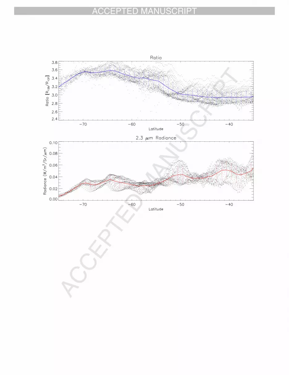
Fig. 3 shows the result of a direct division of the radiances at Band 135 with Band 137 [2.300/2.320 134

µm] using the same dataset as before. The result is a trend in the expected direction, increasing from 135

equator to pole, peaking at 65 o

S, but in this instance, there is no discernable correlation between 136

the ratio values using this division method and the 2.3 µm radiances. We then plot the zonal mean 137

value of the Band135/Band137 ratio and the 2.30 µm radiance, with their 1σ standard deviation 138

from the mean as error bars. This gives a value for the variation of the cloud opacity and CO value 139

at that latitude. We shall now present some forward modelling calculations to show that this ratio is 140

an excellent proxy for the tropospheric CO abundances. 141

142

2.2 Forward Modelling and Retrieval Comparison 143

144

ACCEP

TED M

ANUSC

RIPT

ACCEPTED MANUSCRIPT

4

A forward model was used to generate synthetic spectra between 2.18 and 2.50 µm under different 145

conditions to confirm the ratio mentioned above is indeed sensitive primarily to CO enhancements. 146

The forward model, which is described fully in Tsang et al. (2008b) and Irwin et al. (2008), uses the 147

correlated-k approach to pre-tabulate the absorption coefficient for gaseous species, which is then 148

used to calculate the transmission through the atmosphere. We use the HITEMP linelist for CO2, 149

with a collision induced absorption coefficient of 4.0x10-8

cm-1

/amagat2

in this spectral window. 150

The temperature profile has been taken from Seiff (1983), and the nominal cloud profile has been 151

taken from Pollack et al. (1993). We assume a 75% H2SO

4 to 25% H

2O concentration for the 152

sulphuric acid clouds, using Palmer and Williams (1975) for the refractive indices. We use a 10- 153

stream matrix operator model to account for multiple-scattering events in the atmosphere, with 111 154

vertical scattering layers. Using this model, a number of different tests were conducted in order to 155

show the only significant effect on the 2.30/2.32 µm radiance is the CO abundance in the 156

troposphere. 157

158

2.2.1 Changes in Cloud Profile 159

160

A major effect on the outgoing radiances at these near infrared wavelengths is due to cloud opacity, 161

which changes rapidly across the planet. We adopt the cloud model described in Pollack et al. 162

(1993). There are four different modes, with radius of 0.5, 1.0, 1.2 and 3.0 µm. We have modelled 163

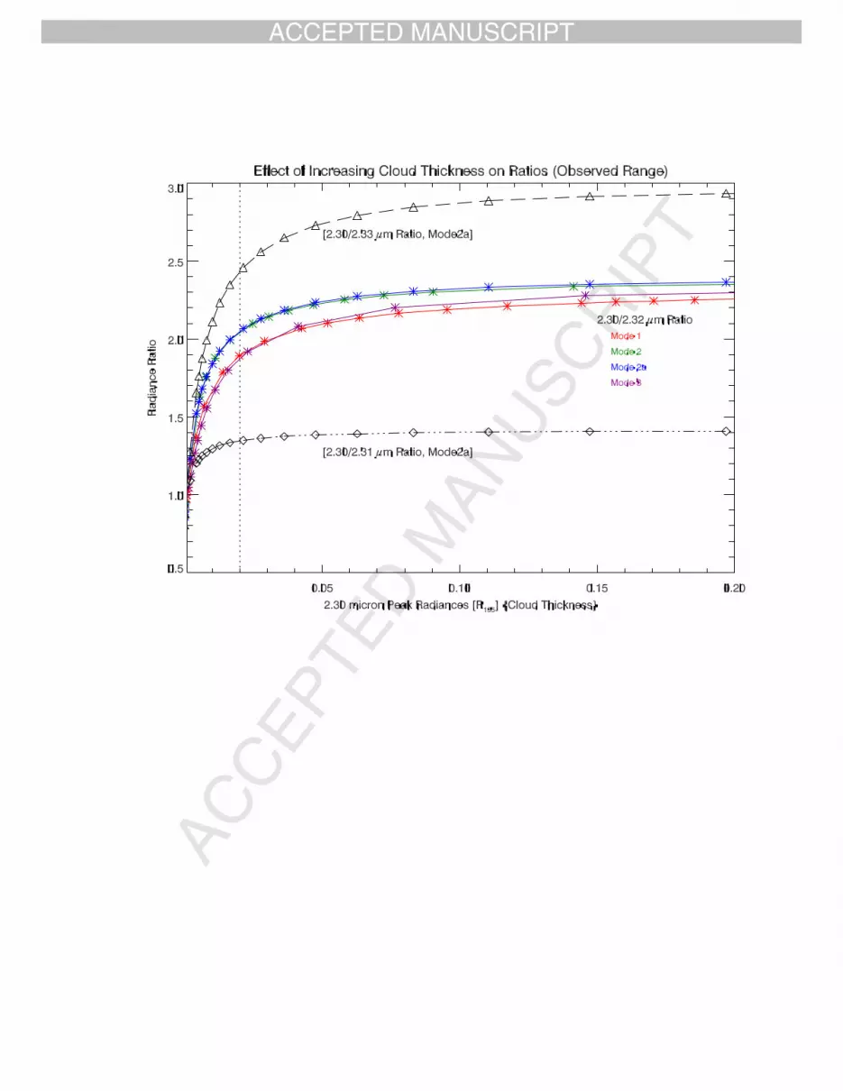
different opacities of clouds to better understand its effects on the ratio of radiances 2.30/2.32. The 164

results can be seen in Fig. 4, where the cloud opacity is plotted as a function of the 2.30 peak 165

radiances. The observed 2.3µm radiances observed by VIRTIS range from 0.001 to 0.3 W/m2

/sr/µm 166

corresponding to the darkest and brightest regions of cloud. As we increase the opacity of the 167

clouds, we see the value of the ratio remains constant (no correlation) but then moves gradually 168

such that a direct relationship between the ratio and cloud opacity occurs under extremely large 169

optical depths. However, there is little correlation in the radiance region seen from the VIRTIS-M 170

data, until the clouds are so thick that the 2.3 µm radiance is less than 0.02 W/m2

/sr/µm. In 171

radiances above this limit, there is less than a 10% error on the ratio caused by cloud opacity. We 172

shall see that this is small compared to the signal due to CO. Ultimately, the choice of the 173

wavelength pairs, in our case 2.30 and 2.32 µm, comes from a compromise between a good 174

sensitivity to CO, where the peak sensitivity occurs at 2.33 µm, and the sensitivity to the non-grey 175

absorption of H2SO

4, which increases as we increase the separation of the wavelength pairs. Indeed, 176

if we chose 2.30/2.31 µm, the relationship of this wavelength pair would be even more independent 177

of cloud opacity, but we forfeit our sensitivity to CO. The converse is true for the 2.30/2.33 µm 178

pair; and thus we arrive at the compromise wavelength pair of 2.30/2.32 µm. These alternate 179

wavelength pairs are also plotted in Fig. 4. 180

181

2.2.2 Temperature and emission angle effects 182

183

It can be seen in Tsang et al. (2008b) that the effect of idealised changes in the vertical temperature 184

profile at 30o

latitude to that at 80o

at 2.30 µm is to cause less than a 10% change in the outgoing 185

radiances. Even so, these latitudinal temperature profiles deviate from each other at heights greater 186

than ~ 45km, above the peak of the weighting function at 2.3µm. We also do not expect a 187

significantly large variation from the adiabat in this region of the atmosphere. Effects of variations 188

in the emission angle have also been tested. Fig. 5 shows the model calculations to investigate the 189

effect of changing the emission angle on the ratio. Different assumed a priori were tested: 1) the 190

nominal profile described in Section 2.2, 2) CO vertical profiles scaled by factors of one half and 191

two, 3) a cloud model with opacity 5% and 200% of the nominal Pollack et al. 1993 profile, and 4) 192

a much cooler temperature profile (from Tsang et al. 2008a) which might be more indicative of the 193

temperature structure at the polar regions. All other variables in the profiles are as the nominal 194

ACCEP

TED M

ANUSC

RIPT

ACCEPTED MANUSCRIPT

5

profile. Because Band 135 and Band 137 are close in wavelength, the variation of radiances as a 195

function of cos θ, where θ is the emission angle, is the same. The change in the ratio value as a 196

function of emission angle, from 0o

to 85o

, is less than 1% for all the profiles. It is also satisfying to 197

see that large changes in the cloud optical depth and temperature profile away from the nominal 198

case have a much smaller effect on the ratio than changes in the CO concentration. 199

200

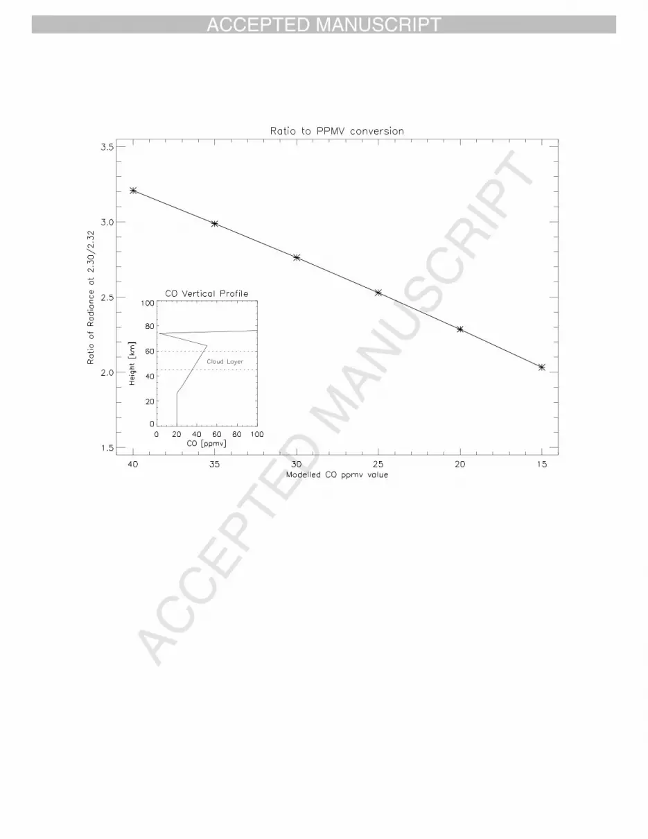
2.2.3 Conversion of Radiance Ratio to CO 201

202

Having shown that cloud opacity and mode variations, temperature and emission angle effects can 203

all be neglected as the prime cause of the trends seen in the ratio as a function of latitude, we now 204

model the remaining effect on this ratio: the CO vertical profile. Fig. 1 and 6 shows the effect of 205

changes in the vertical CO volume mixing ratio (ppmv) on the radiance in the 2.3 µm emission 206

window. The modelled concentrations are plotted against the ratio of the radiances at wavelengths 207

2.30 and 2.32 µm. The nominal vertical profile is the same as the one used in Tsang et al. 2008a and 208

is scaled from 50% to 120%, in 10% increments, yielding CO ppmv values at 35 km from 13.8 to 209

33.2. The spectra have been calculated with a Full Width Half Maximum (FHWM) of 17 nm, which 210

is the width of the spectral profile seen in flight (private comm. with B. Bézard and G. Piccioni) 211

(i.e.: spectral bin is 10nm, but the spectral resolution is 17nm). We can see from Fig. 6 a direct 212

linear correlation exists between CO abundance in ppmv in the model atmosphere and the 2.30/2.32 213

µm radiance ratio, allowing a direct conversion between the two. It should also be noted from Figs. 214

4 and 6 that the slight dependence of the ratio to cloud opacity above 0.02 W/m2

/sr/µm of ± 0.2 215

ratio units equates to a conservative error of ± 4 ppmv in the CO abundance. 216

217

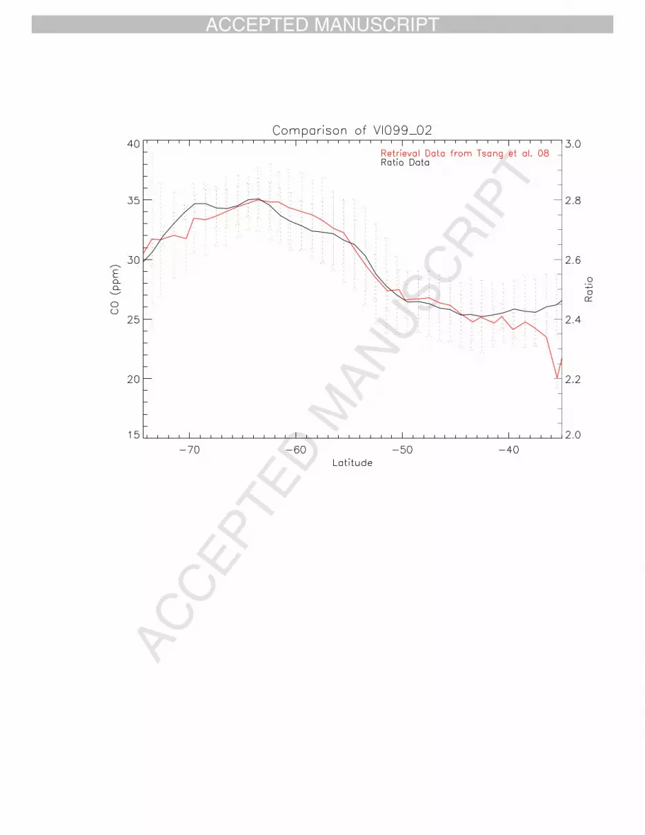
2.2.4 Comparison with Retrieval by Spectral Fitting 218

219

As a test of this conversion of radiance ratio to ppmv, we can compare, for a given observation, the 220

2.30/2.32 zonal mean ratio to that of the zonal mean retrieved through spectral fitting. The results 221

for this test case are given in Fig. 7. The spatial map of CO at 35 km for VI099_2, derived from 222

Tsang et al. (2008a), is zonally averaged to yield a latitudinal trend. This is then compared to the 223

2.30/2.32 ratio and plotted together. The agreement is extremely good, allowing a direct validation 224

of the relationship between the CO abundance (ppmv), and the radiance ratio. Examination of Fig. 7 225

shows a near perfect match between the zonal means at 40 to 55o

S, whilst the greatest difference 226

occuring at 30 and 70o

S differ by 2-3ppmv. The overlapping trends are in good agreement with the 227

modelling described in the previous section. Therefore, we can be even more confident that the 228

contrast seen in the 2.30/2.32 ratio is due primarily to CO, rather than other factors. 229

230

2.3 Wavelength Shift and Interpolation 231

232

It has been known that a slight wavelength shift is detectable from different observations, as the 233

temperature of the spectrometer changes slightly from orbit to orbit under different thermal 234

conditions (priv. comms. with G. Piccioni and P. Drossart). This effect has not been fully calibrated 235

out of the data and was studied by Bezard et al. (2008), using the 1.74 µm window, which probes at 236

a height approximately 15 km. The mean spectral shift was seen to change on the order of 4-10 nm 237

(1 bin size = 10 nm) from observation to observation. In addition, the effect was also spatially 238

dependent (i.e.: the shift was different at the edge of the detector compared to the centre). Also, the 239

spectral shift for a particular observation was slightly different depending on which wavelength 240

region was under study. Therefore, one should not rely solely on a single 2D wavelength shift 241

applied to a single observation for all wavelengths. This instrumental effect must be taken into 242

account before proceeding with the band-ratio technique. 243

244

ACCEP

TED M

ANUSC

RIPT

ACCEPTED MANUSCRIPT

6

To work out the spectral shift at 2.3 µm on a pixel-to-pixel basis, we generate a synthetic spectrum 245

using the model described by Tsang et al. 2008b, with nominal clouds and full Mie scattering with 246

assumed a priori temperature and gaseous concentrations. This spectrum is then normalised and 247

compared to the normalised spectra taken between Bands 122 and Bands 155, which covers the 2.3 248

µm window, in the image. We then use a cross-correlation algorithm (Research Systems 2000), to 249

find the wavelength shift which best matches the shift of the real spectrum to that of the reference 250

spectrum. We do this for all points on the image. We assume the spectral shift is constant in the 2.3 251

µm window, and thus the two-dimensional shift map is applied to all spectral points in this window. 252

However, since we want radiances that are exactly 2.300 and 2.320 µm (producing ratios we can 253

convert to ppmv and thus comparable from observation to observation), we also interpolate the 254

radiances to those wavelengths. All results given below have been wavelength adjusted and 255

interpolated to exactly 2.300 and 2.320 µm. 256

257

3. Results258

259

3.1 Data Set Used 260

261

The method described above has been used to analyse all VIRTIS observations with integration 262

times of 3s and greater that were obtained during Venus Express operations from the time of orbit 263

insertion (16th

April 2006) to 11th

November 2007 (Titov et al., 2006). This corresponds to some 264

1,450 spectral images, each producing a CO map and a zonal mean CO profile. Table 1 gives a 265

summary of the observations used, which includes a total of 82 Northern Hemisphere observations. 266

An observation is defined as a single 3D (two spatial, one spectral) image cube. Several 267

observations are taken during a single orbit. Refer to Titov et al., 2006 for additional clarity. 268

269

3.2 Variability 270

271

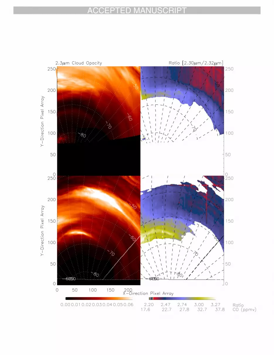
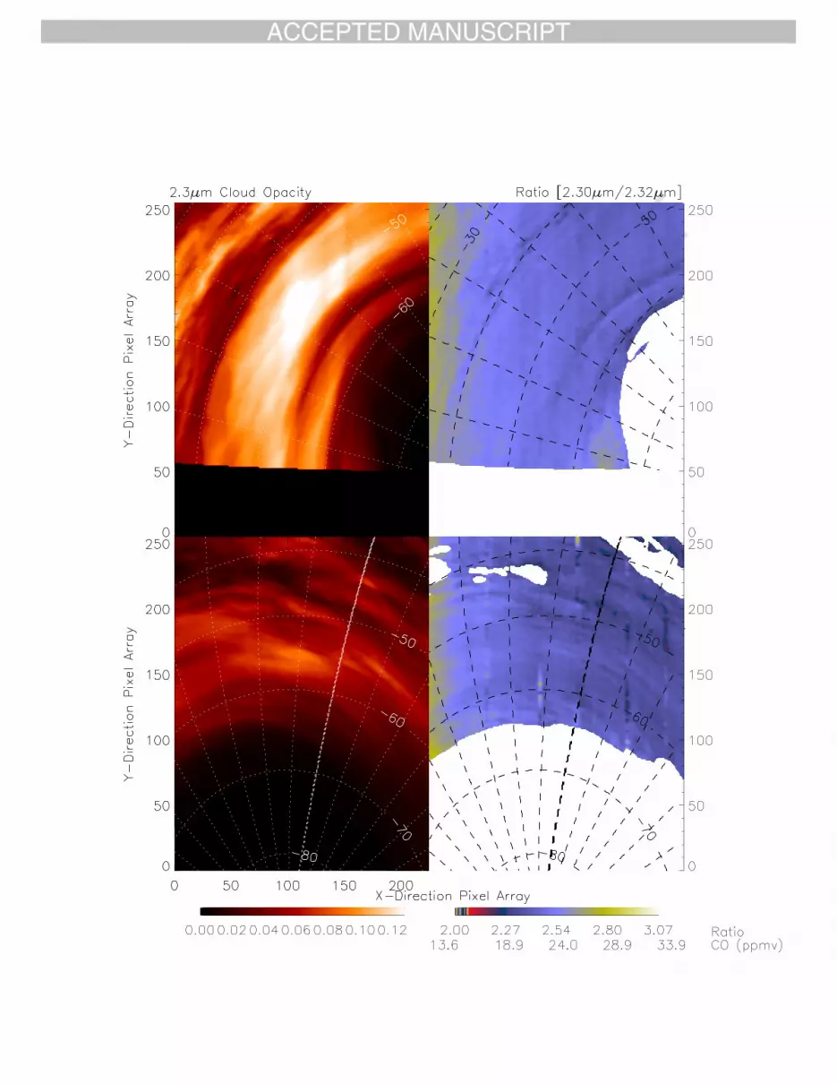
Fig. 8 shows two observations: VI0336_00, a 3.3 s exposure image cube taken on the 22nd

March 272

2007, and VI0392_05, an 8 second exposure image cube taken on the 17th May 2007. Fig. 9 shows 273

another two observations, VI0301_00 and VI0381_00, both 3.3 s exposures taken on the 15th 274

February and 6th

May 2007 respectively. All four observations are 256x256 pixels, cover the 275

Southern Hemisphere including high latitudes, and are typical of the data used in this analysis. As 276

expected from the analysis shown in Fig. 3, they all show little correlation with the 2.3 µm cloud 277

opacity variations in the mid-latitude region, all of the significant variability being due to CO. 278

However, near the pole (latitude >70 o

S) where the radiance falls below the 0.02 W/m2

/sr/µm 279

threshold at 2.3µm, indicating very thick clouds, the effect of cloud opacity becomes important. 280

281

In both of the examples shown in Fig. 8, the 2.3/2.32µm radiance ratio shows an increase in value 282

with latitude, peaking at 65 o

S, and the CO abundance rises from the equator and attains a 283

maximum value at 65 o

S of ~33 ± 4 ppmv in both observations. When the longitudinal variability 284

first noted by Tsang et al. (2008a) is taken into account, this behaviour and these values are typical 285

of those found in the low-resolution ground-based and Galileo NIMS data discussed above in the 286

introduction. However, in the long, high-resolution data set analysed here we find that examples 287

occur when the equator-to-pole gradient in CO is almost completely absent: two of these are shown 288

in Figure 9. The distribution of CO in the observation VI0301_00 has a mean value of ~24 ± 4 289

ppmv rising to 26 at 60 o

S, i.e. is essentially flat. VI0381_00 again shows a flat field for CO, and 290

has an even lower abundance of ~23 ± 4 ppmv from 40 to 65 o

S, approximately the expected value 291

at the equator. 292

293

ACCEP

TED M

ANUSC

RIPT

ACCEPTED MANUSCRIPT

7

In the past, the trend of increasing CO from equator to pole has been taken to be a characteristic 294

feature of the Venus atmosphere, related to its general circulation (see e.g. Taylor, 2006). The 295

degree of temporal variability reported here has never been seen before and so is both unexpected 296

and intriguing. The current hypothesis was that a hemispherical ‘Hadley’ circulation brings CO rich 297

air down from the mesosphere (~65km) to the troposphere (~35km) at high latitudes. However, the 298

variability seen in our new results would seem to be too large and too rapid to be consistent with 299

such a simple picture. The lack of any CO gradient, if it applied to the whole hemisphere, would 300

imply that transport in the Hadley cell had essentially ceased, while even smaller fluctuations in the 301

global-scale flux might be expected to take more than a few days. Yet the elapsed time between 302

VI0381_00 and VI0392_05, for instance, is only about 11 (Earth) days. 303

304

It seems more reasonable to speculate that the net meridional circulation on Venus is more 305

asymmetric than a simple Hadley cell, a possibility that is supported by the zonal variation that can 306

be seen in the images in Figs. 8 and 9. There may also be implications for the chemical processes 307

which lead to the destruction of CO as it descends from the main source in the mesosphere to the 308

main sink regions in the clouds and at the surface, but it may also imply that the strength of the 309

downwelling might be variable. Another possibility is that we are seeing different phases of the 310

spatial variability locked to a planetary wave feature, which prevails in the lower atmosphere, 311

moving horizontally. We thus might be seeing the maximum (Fig. 8) and minimum (Fig. 9) of the 312

wave feature at different times and locations. This possibility is difficult to investigate with the data 313

set used here, because of a lack of systematic coverage due to the operating modes of the Venus 314

Express payload (Titov et al., 2006). However, the spacecraft, and VIRTIS, are still operating at the 315

time of this writing and further investigations can be conducted to search for systematic behaviour 316

in the CO distribution. Finally, recent work by Marcq et al. (priv. comms.) using passive tracers in a 317

General Circulation Model of Venus have tentatively shown zonal variability in the CO abundances 318

at 35 km. In some of these simulations, the equator-pole gradient is much reduced and it is very 319

likely that we are observing at these locations. The processes involved to produce such a picture are 320

not fully understood, but must involve a complex interplay between the general circulation, the 321

lifetime of CO and perhaps other factors such as the topography of the surface. 322

323

3.3 Zonal mean CO profiles 324

325

The zonal means show the divergence of the CO abundance from the mean trends more clearly than 326

global maps. Fig. 10 shows the ratio of the radiances at 2.30/2.32 µm vs. latitude for four sequential 327

observations spanning three orbits, with Fig. 10 showing a further 10 observations. Fig.10 also 328

shows the 2.3µm radiances, which show large fluctuations produced by cloud opacity. These 329

fluctuations are not mimicked by the radiance ratios, again showing this method of generating the 330

CO abundance is effectively decoupled from the cloud morphology except near the poles where the 331

clouds are highly opaque. It should also be noted that the 0.02 W/m2

/sr/µm threshold at which the 332

CO retrieval becomes contaminated by cloud opacity is rarely reached in these observations. 333

334

The CO abundance shows the marked poleward increase, from 22 ppm at the equator to 30 ppm at 335

the 60 o

S, expected of tropospheric CO seen prior to the present work. Our contemporaneous 336

observations of both hemispheres show the degree of dichotomy between the hemispheres. The 337

Northern Hemisphere shows a maximum in CO abundance of 29 ± 3 ppm, whilst the Southern 338

Hemisphere reaches 32 ± 3 ppm. The degree of variability in location and magnitude of the CO 339

maximum can be seen most clearly in Fig. 11, which shows the Northern and Southern 340

Hemispheres seen in sequential observations. Over the space of two orbits, we can see the 341

maximum CO abundance in the North vary from 35 ± 3 ppm (top), to as low as 27 ± 3 ppm 342

(bottom), while a smaller variation is seen in the South. However, following on from the discussion 343

ACCEP

TED M

ANUSC

RIPT

ACCEPTED MANUSCRIPT

8

above, it is difficult to be sure at present whether there is a real North-South dichotomy, or whether 344

these results reflect the natural variability in the deep CO abundance. 345

346

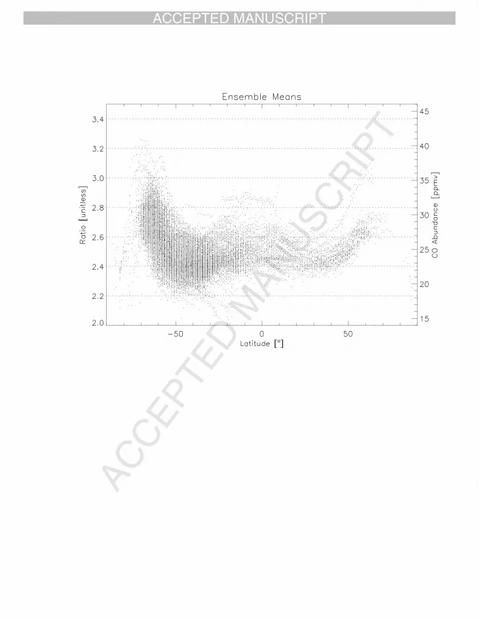
3.4 Ensemble Mean 347

348

Fig. 12 is the ensemble of the zonal mean ratios derived from all of the 1,450 CO observations in 349

Table 1. This gives a good impression of the degree of variability over the 18-month period relative 350

to the large-scale temporal mean. There are some 80+ observations of the Northern Hemisphere, 351

leaving the remaining large majority in the South. In the ensemble mean, the Southern Hemisphere 352

CO maximum peak at 65 o

S is approximately 35 ± 3 ppm, whilst the Northern Hemisphere attains 353

30 ± 3 ppm for the same latitude. This modest hemispherical asymmetry may, however, be due to 354

the less frequent sampling of the Northern Hemisphere, a consequence of the orbit of Venus 355

Express. Scrutiny of Fig. 12 shows that there was one observation of the Northern hemisphere when 356

the CO maximum was as high as the highest seen at any time in the South, suggesting that the 357

relative shortage of high values in the coverage of the North is fortuitous. 358

359

The ensemble mean also emphasizes the decrease of abundance polewards of 650

latitude in both 360

hemispheres, as was seen by Tsang et al. (2008a) and Marcq et al. (2008). However, since the 361

radiances near 2.3μm at these high latitudes are small, the contribution from the CO below the 362

clouds to the spectrum is also small and the signal-to-noise ratio correspondingly low. This makes 363

the 2.30/2.32 µm ratio more dependent on the cloud opacity than the CO mixing ratio and reduces 364

confidence in the retrievals which indicate that the polar concentrations of CO are lower than the 365

peak value of 30-35 ppm. 366

367

4. Conclusions 368

369

The first focus of this analysis was to show that the measured ratio of thermal emission from the 370

nightside of Venus in the 2.30 and 2.32 μm spectral bands can yield good estimates of the 371

abundance of tropospheric CO. Forward modelling to test the effects of changes in the temperature 372

profile and the cloud optical depth showed little detrimental effect on the CO retrieval by this 373

method. Direct comparison with CO profiles obtained from the full spectral modeling approach of 374

Tsang et al. (2008a) confirmed that the ratio method gave results which, while marginally less 375

accurate than full accurate spectral fitting retrievals, do allow large number of datasets to be 376

analyzed quickly. In addition to the interpretation to Venus Express VIRTIS data discussed here, 377

the technique is currently being applied to ground-based telescopic image cubes taken from both 378

NASA IRTF/SpeX (E. Young priv. comm.) and the Anglo-Australian Telescope (J. Bailey priv. 379

comm.). It should also be valuable for the future Japanese mission Planet-C to Venus, which will 380

fly an IR imaging camera at wavelengths sensitive to CO (Nakamura et al. 2007). 381

382

The analysis of 1,450 observations of nightside spectral cubes from VIRTIS-M on Venus Express 383

has shown significant, previously unseen temporal and spatial variations in the abundance of CO. It 384

is not clear at present whether these new data are compatible with the previously widely accepted 385

notion that Venus has a hemispherical Hadley-type circulation and that this carries CO into the 386

troposphere from the mesosphere where CO is produced in large quantities by the photolysis of 387

carbon dioxide. At the very least, such a model will need to be extensively modified to include 388

time-dependent and latitudinally-variable processes that significantly affect the production and 389

removal of carbon monoxide in Venus’ atmosphere.390

391

392

393

ACCEP

TED M

ANUSC

RIPT

ACCEPTED MANUSCRIPT

9

Acknowledgements394

395

We acknowledge the contributions in discussion with Emmanuel Marcq, Bruno Bezard, Bob 396

Carlson, Jeremy Bailey and Eliot Young. This work would not have been possible without the 397

funding from the Science Technology and Facility Council (STFC). We also thank the support of 398

ASI and CNES. 399

400

References401

402

Bezard B, de Bergh C, Crisp D, Maillard J. (1990), The deep atmosphere of Venus revealed by 403

high-resolution nightside spectra. Nature, Vol. 345, 508–511 404

405

Bezard B., Tsang C.C.C., Carlson R.W., Piccioni G., Marcq, E., and Drossart P., (2008), The water 406

vapour abundance near the surface of Venus with Venus Express/VIRTIS Observations, Journal of 407

Geophys. Res., (Submitted). 408

409

Collard A. D., Taylor F.W., Calcutt S.B., Carlson R.W., Kamp L.W., Baines K.H., Encrenaz, Th., 410

Drossart P., Lellouch E. and Bezard B., (1993), Latitudinal distribution of carbon monoxide in the 411

deep atmosphere of Venus. Planetary and Space Science, Vol. 41(7), 487–94 412

413

Drossart, P., Piccioni, G., Adriani, A., Angrilli, F., Arnold, G., Baines, K., Bellucci, G., Benkhor, J., 414

Bezard, B., Bibring, J.-P., Blanco, A., Blecka, M., Carlson, R., Coradini, A., Di Lellis, A., 415

Encrenaz, T., Erard, S., Fonti, S., Formisano, V., Fouchet, T., Garcia, R., Haus, R., Helbert, J., 416

Ignatiev, N., Irwin, P., Langevin, Y., Lebonnois, S., Lopez-Valverde, M., Luz, D., Marinangeli, L., 417

Oro¯no, V., Rodin, A., Roos-Serote, M., Saggin, B., Sanchez-Lavega, A., Stam, D., Taylor, F., 418

Titov, D., Visconti, G., Zambelli, M., Hueso, R., Tsang, C.C.C., Wilson, C. and Afanasenko, T. Z. 419

(2007), `Scientific goals for the observation of Venus by VIRTIS on ESA/Venus Express mission', 420

Planetary and Space Science, Vol 55, 1653-1672. 421

422

Irwin P.G.J., Teanby N.A., de Kok R., Fletcher L.N., Howett C.A., Tsang C.C.C., Wilson C.F., 423

Calcutt S.B., Nixon C.A., Parrish P.D., (2008), The NEMESIS planetary atmosphere radiative 424

transfer and retrieval tool, Journal of Quantitative Spectroscopy and Radiative Transfer, Vol. 109, 425

Pg 1136-1150, doi:10.1016/j.jqsrt.2007.11.006 426

427

Kamp, L., Taylor, F. and Calcutt, S. (1988), `Structure of Venus's atmosphere from modelling of 428

night-side infrared spectra.', Nature, 336, 360-362. 429

430

Marcq, E., B. Bezard, T. Encrenaz, and M. Birlan (2005), Latitudinal variations of CO and OCS in 431

the lower atmosphere of Venus from near-infrared nightside spectro-imaging, Icarus, 179, 375–386, 432

doi:10.1016/j.icarus.2005.06.018. 433

434

Marcq, E., T. Encrenaz, B. Bezard, and M. Birlan (2006), Remote sensing of Venus’ lower 435

atmosphere from ground-based IR spectroscopy: Latitudinal and vertical distribution of minor 436

species, Planet. Space Sci., 54, 1360–1370, doi:10.1016/j.pss.2006.04.024. 437

438

Marcq, E., B. Bezard, P. Drossart, and G. Piccioni (2008), A latitudinal survey of CO, OCS, H2O 439

and SO2 in the lower atmopshere of Venus: spectroscopic studies using VIRTIS-H, Journal of 440

Geophys. Res., (In Press) 441

442

Nakamura, M. and. Imamura., T. and Ueno, M. and Iwagami, N. and Satoh, T. and Watanabe, S. 443

ACCEP

TED M

ANUSC

RIPT

ACCEPTED MANUSCRIPT

10

and Taguchi, M. and Takahashi, Y. and and M. a. A. Suzuki, T. and Hashimoto, G.L. and Sakanoi, 444

T. and Okano, S. and Kasaba, Y. and Yoshida, J. and Yamada, M. and Ishii, N. and Yamada, T. and 445

Uemizu, K. and Fukuhara, T. and Oyama, K. (2007), Planet-C: Venus Climate Orbiter mission of 446

Japan, Planetary and Space Science 55, 831-1842. 447

448

Palmer, K. and Williams, D. (1975), Optical Constants of Sulfuric Acid; Application to the Clouds 449

of Venus?, Applied Optics 14(1), 208–219 450

451

Piccioni, G., Drossart P. and Suetta, E. and Cosi, M. and Ammannito, E. and Barbis, A. and Berlin, 452

R. and Boccaccini, A. and Bonello, G. and Bouyé, M. and Capaccioni, F. and Cherubini, G. and 453

Dami, M. and Dupuis, O. and Fave, A. and Filacchione, G. and Hello, Y. and Henry, F. and Hofer, 454

S. and Huntzinger, G. and Melchiorri, R. and Parisot, J. and Pasqui, C. and Peter, G. and Pompei, C. 455

and Rèess, J.M. and Semery, A. and Soufflot A. and the Venus Express/VIRTIS Team (2008). 456

VIRTIS: The Visible and Infrared Thermal Imaging Spectrometer, ESA Special Publication, SP-457

1295: 1-27. 458

459

Pollack, J., Dalton, J., Grinspoon, D., Wattson, R., Freedman, R., Crisp, D., Allen, D., Bezard, B., 460

de Bergh, C. and Giver, L. (1993), Near-Infrared Light from Venus’ Nightside: A Spectroscopic 461

Analysis.’, Icarus 103, 1–42 462

463

Research Systems (2000), IDL Reference Guide, IDL Version 5.4, September 2000 Edition, 139-464

140 465

466

Seiff A. (1983), Thermal structure of the atmosphere of Venus. In: Hunten D, Colin L, Donahue T, 467

Moroz V, editors. ‘Venus’. Tucson, AZ, University of Arizona,. p. 215–79. 468

469

Taylor, F., Crisp, D. and Bezard, B. (1997), Near-Infrared Sounding of the Lower Atmosphere of 470

Venus., in ‘Venus II: Geology, Geophysics, Atmosphere, and Solar Wind Environment.’, The 471

University of Arizona Press., Tuscon, Arizona, pp. 325–351. 472

473

Taylor, F. W. (2006). "Venus before Venus Express." Planetary and Space Science 54: 1249-1262. 474

475

Titov, D. V. and. Svedhem, H. and Koschny, D. and Hoofs, R. and Barabash, S. and Bertaux, J.-P. 476

and Drossart, P. and Formisano, V. and Hausler, B. and Korablev, O. and Markiewicz, W.J. and 477

Nevejans, D. and Patzold, M. and Piccioni, G. and Zhang, T.L. and Merritt, D. and Witasse, O. and 478

Zender, J. and Accomazzo, A. and Sweeney, M. and Trillard, D. and Janvier, M. and Clochet, A. 479

(2006). Venus Express science planning, Planetary and Space Science, Vol. 54, pp. 1279-1297 480

481

Tsang C.C.C., Irwin P.G.J., Taylor F.W., Wilson C.F., Drossart P., Piccioni G., de Kok R., Lee C., 482

Calcutt S.B. and the Venus Express/VIRTIS Team, (2008a), Tropospheric Carbon Monoxide 483

Concentrations and Variability on Venus with Venus Express/VIRTIS-M Observations, Journal of 484

Geophys. Res., (In Press), doi:10.1029/2008JE003089 485

486

Tsang C.C.C., Irwin, P.G.J., Taylor, F.W., Wilson C.F., (2008b), A Correlated-k Model of 487

Radiative Transfer in the Near Infrared Windows of Venus, Journal of Quantitative Spectroscopy 488

and Radiative Transfer, Vol. 109, Pg 1118-1135, doi:10.1016/j.jqsrt.2007.12.008489

ACCEP

TED M

ANUSC

RIPT

ACCEPTED MANUSCRIPT

11

490

Observation

Sequences

Int. Time:

3.0 s

Int. Time:

3.3 s

Int. Time:

8.0 s

Int. Time:

18.0 s

Presented Observations

MTP01 13

MTP02 13 VI060_06, VI061_06,

VI066_00, VI066_01

MTP03 133 14 VI082_03, VI082_18,

VI083_02, VI099_02

MTP04 189 6

MTP05 196 2 VI0148_15, VI0149_00,

VI0149_01, VI0149_02

MTP06 20 11

MTP07 5

MTP08 39

MTP09 70 3

MTP10 33 6

MTP11 80 59 9 VI0301_00

MTP12 83 37 6 VI0336_00, VI0336_01,

VI0336_02, VI0336_03,

VI0336_04, VI0336_05,

VI0336_08

MTP13 126 12 6

MTP14 105 15 3 VI0381_00, VI0392_05

`MTP15 3 1

MTP16 2 16

MTP17 62 9 2

MTP18 10 26 10

MTP19

MTP20 12 1 3

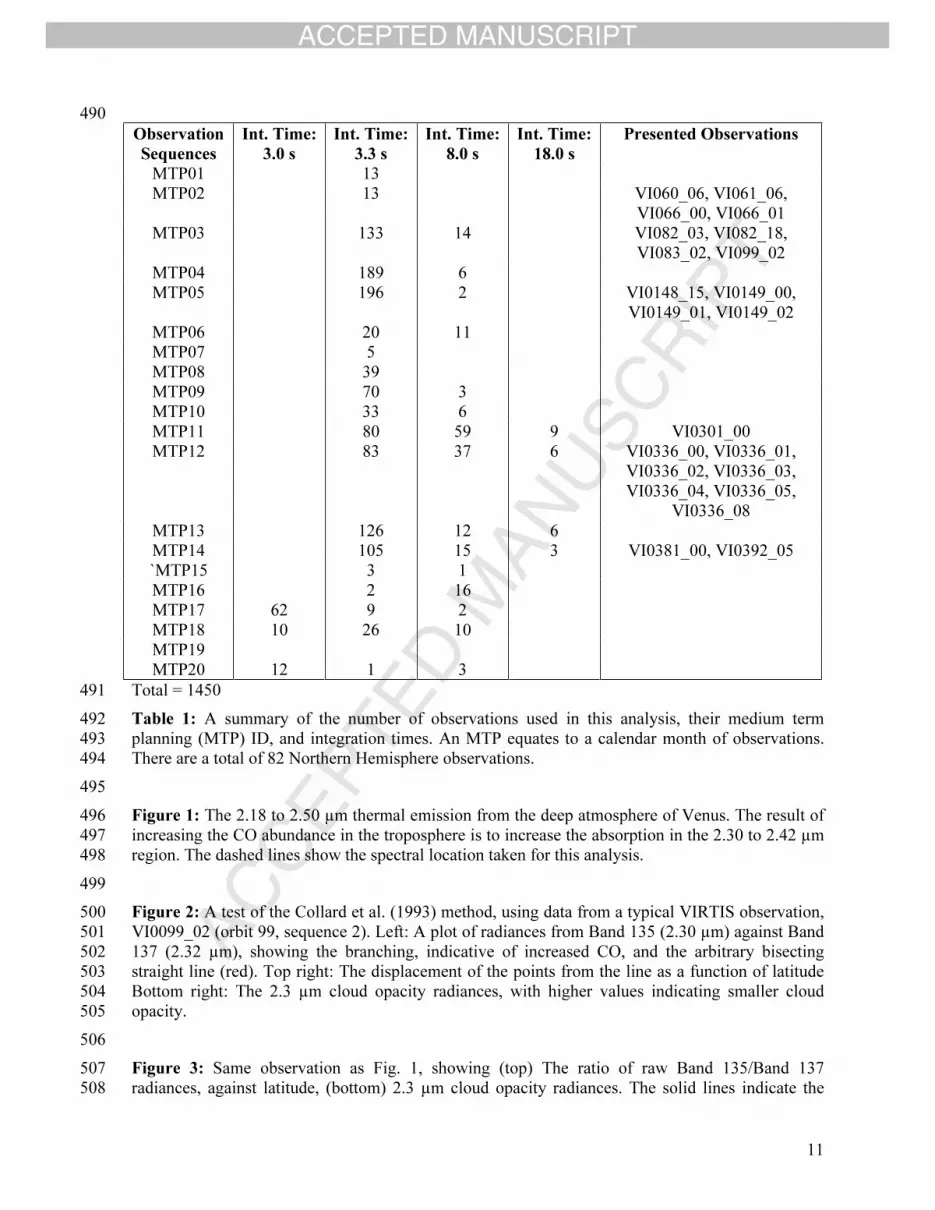
Total = 1450 491

Table 1: A summary of the number of observations used in this analysis, their medium term 492

planning (MTP) ID, and integration times. An MTP equates to a calendar month of observations. 493

There are a total of 82 Northern Hemisphere observations. 494

495

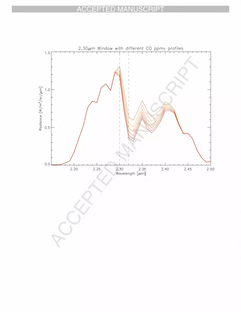
Figure 1: The 2.18 to 2.50 µm thermal emission from the deep atmosphere of Venus. The result of 496

increasing the CO abundance in the troposphere is to increase the absorption in the 2.30 to 2.42 µm 497

region. The dashed lines show the spectral location taken for this analysis. 498

499

Figure 2: A test of the Collard et al. (1993) method, using data from a typical VIRTIS observation, 500

VI0099_02 (orbit 99, sequence 2). Left: A plot of radiances from Band 135 (2.30 µm) against Band 501

137 (2.32 µm), showing the branching, indicative of increased CO, and the arbitrary bisecting 502

straight line (red). Top right: The displacement of the points from the line as a function of latitude 503

Bottom right: The 2.3 µm cloud opacity radiances, with higher values indicating smaller cloud 504

opacity. 505

506

Figure 3: Same observation as Fig. 1, showing (top) The ratio of raw Band 135/Band 137 507

radiances, against latitude, (bottom) 2.3 µm cloud opacity radiances. The solid lines indicate the 508

ACCEP

TED M

ANUSC

RIPT

ACCEPTED MANUSCRIPT

12

zonal means, whilst the error bars are the 1σ standard deviations from the zonal mean. No 509

correction for the wavelength shift has been made here. 510

511

Figure 4: The 2.30/2.32 µm wavelength pair used in this analysis as a function of cloud thickness, 512

plotted against 2.30 peak radiance (W/m2

/sr/μm), using different cloud modes in the forward model. 513

Dotted vertical line indicates approximately where the radiance ratio exceeds 10% error and 514

depends evermore strongly on the cloud thickness. The 2.30/2.33 µm and 2.30/2.31 µm wavelength 515

pairs are also plotted, using Mode2’, but are not used in the analysis. 516

517

Figure 5: The effect of emission angle on the ratio for different assumed a priori cloud, 518

temperature and CO profiles. For all assumed profiles, the effect of the emission angle is less than 519

1%. 520

521

Figure 6: The conversion profile relating the radiance ratio value, to CO concentration. (Inset) The 522

assumed CO vertical profile used to create the linear trend. 523

524

Figure 7: A comparison, using the same observation VI099_02, of the zonal mean ratio derived in 525

this analysis (black) with the zonal mean CO abundance from spectral fitting by Tsang et al. (2008) 526

(red). 527

528

Figure 8: Southern Hemisphere observations VI0336_00 (top) and VI0392_05 (bottom), with their 529

associated 2.3µm radiances (left) and the ratio at 2.30/2.32 (right). In regions where the 2.3µm 530

radiances drops below 0.02 W/m2

/sr/µm, the ratio is sensitive to cloud opacity variations and have 531

been masked out (white areas). Above this value, the ratio map is essentially free of cloud features 532

and shows the CO abundance at ~35 km. The general equator-pole increase is clear, and some 533

longitudinal variability can also be seen. 0o

longitude is marked by thick dashed line. 534

535

Figure 9: Southern Hemisphere observations VI0301_00 (top) and VI0381_00 (bottom), with their 536

associated 2.3µm radiances (left) and the ratio at 2.300/2.320 (right). In contrast to the observations 537

presented in Fig. 7, the equator–pole increase in CO is absent, showing great temporal variability in 538

the CO abundance between the two figures. Regions where the 2.3 µm radiance drops below 0.02 539

W/m2

/sr/µm have been masked white on the radiance ratios. 0o

longitude is marked by thick dashed 540

line. 541

542

Figure 10: (top) Ratio of radiances at 2.30µm/2.32µm for the observation shown, and (bottom) the 543

2.3µm radiances. It can be seen that the cloud opacity variations at 2.3µm are well decoupled from 544

the 2.30/2.32 µm ratio. It also shows the expected CO latitudinal trends. Thick lines indicate the 545

zonal mean, with thin lines showing the 1σ variance from the mean. 546

547

Figure 11: Ratio of radiances at 2.30µm/2.32µm against latitude, and the corresponding CO 548

abundance near 35 km in units of ppmv using the linear trend in Fig. 5. The trends show variations 549

in the magnitude of the CO maximum and its location in the Northern and Southern hemispheres. 550

ACCEP

TED M

ANUSC

RIPT

ACCEPTED MANUSCRIPT

13

Only zonal means are plotted to avoid confusion. CO abundances have not been plotted where the 551

corresponding 2.3 µm radiance drops below the threshold value of 0.02 W/m2

/sr/µm. 552

553

Figure 12: Ensemble zonal mean trends of CO retrieved in this study using the band ratio technique 554

from all 1450 observations. Zonal mean values have not been plotted where the corresponding 2.3 555

µm radiance drops below the threshold value of 0.02 W/m2

/sr/µm. 556

ACCEP

TED M

ANUSC

RIPT

ACCEPTED MANUSCRIPT

ACCEP

TED M

ANUSC

RIPT

ACCEPTED MANUSCRIPT

ACCEP

TED M

ANUSC

RIPT

ACCEPTED MANUSCRIPT

ACCEP

TED M

ANUSC

RIPT

ACCEPTED MANUSCRIPT

ACCEP

TED M

ANUSC

RIPT

ACCEPTED MANUSCRIPT

ACCEP

TED M

ANUSC

RIPT

ACCEPTED MANUSCRIPT

ACCEP

TED M

ANUSC

RIPT

ACCEPTED MANUSCRIPT

ACCEP

TED M

ANUSC

RIPT

ACCEPTED MANUSCRIPT

ACCEP

TED M

ANUSC

RIPT

ACCEPTED MANUSCRIPT

ACCEP

TED M

ANUSC

RIPT

ACCEPTED MANUSCRIPT

ACCEP

TED M

ANUSC

RIPT

ACCEPTED MANUSCRIPT

ACCEP

TED M

ANUSC

RIPT

ACCEPTED MANUSCRIPT