
1
11. Cost minimization
Econ 494
Spring 2013

2
Agenda
Cost minimizationPrimal approachEnvelope theorem for constrained optimizationLink to profit maximization
Readings Silberberg Chapter 8Also review constrained optimization

3
Quick optimization review
For the constrained optimization problem:
1 2
1 2 1 2,
( , ) subject to ( , ) 0x x
Max g x x c h x x
Set up the Lagrangian function:
1 2 1 2 1 2( , ) ( , ) ( , )x x g x x c h x x L
To get correct sign of l, For maximization problems, write the constraints to be non-negative
For minimization problems, write the constraints to be non-positive

4
FONC
Note that l is a choice variable, hence there are 3 FONC.If the SOSC are satisfied, you can use the IFT to solve the FONC simultaneously for x1
*, x2* and l*.
1 2
1 2 1 2 1 2, ,
( , ) ( , ) ( , )x xMax x x g x x c h x x
L
1 1 2 1 1 2 1 1 2
2 1 2 2 1 2 2 1 2
1 2 1 2
( , ) ( , ) ( , ) 0
( , ) ( , ) ( , ) 0
( , ) ( , ) 0
x x g x x h x x
x x g x x h x x
x x c h x x
L
L
L

5
SOSC
With one constraint, the SOSC require that all border-preserving principal minors be: Sign (–1)r, r = 2,…n for a maximum
starts with positive second order principal minor All minors of order r will have same sign (no need to check all)
Sign is negative for a minimum
A border-preserving principal minor of order r is the determinant of the matrix obtained by deleting n-r rows and corresponding columns – but you cannot delete the row/column with the border
11 11 11 21
2
1
12 1
21 21
1 12
21 2222
2
22 2
1 2 0
g h g h h
BH g h g h h
h h
L L
L
L L L
L L
L
See Silb table 6-1, p. 138; Chiang table 12.1, p. 362

6
Border-preserving principal minors(one constraint)
11 1 1
2
1 2
2
21 22BH
L L L
L
L
L
L L
L
11 221 2
1 2
1
2
11 12
21 2
1
2
2
First-order border preserving principal minors:
and
Second-order border preserving principal minors:
0
L L
L L L L
L
L
L L L
L L
L L
L L
n =2, r = 1 n – r =1 delete one row and column.Sign unknown
n =2, r = 2 n – r =0 delete no rows or columns.Max: >0 Min: <0

7
Question
For a profit maximization problem, what must we assume about the shape of the production function?How do you know this?
8
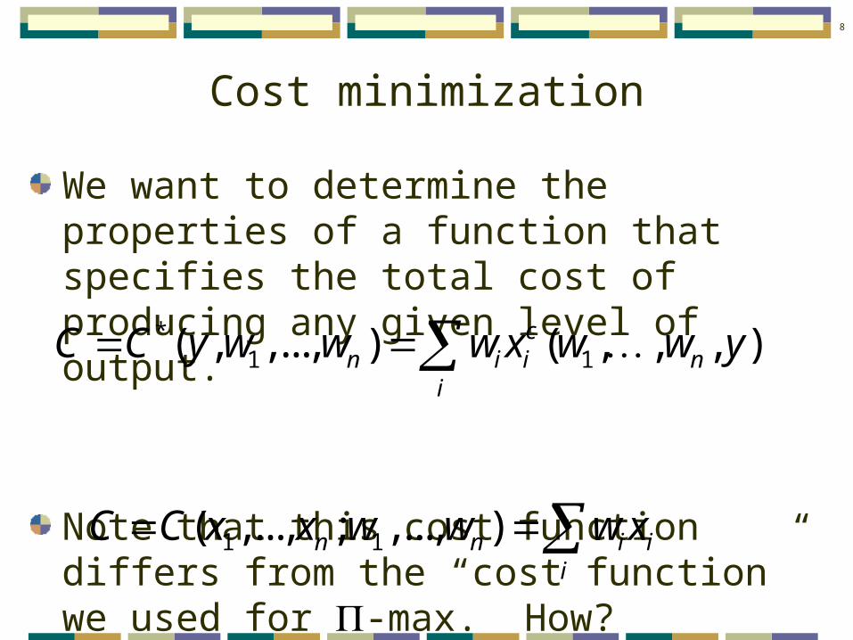
Cost minimization
We want to determine the properties of a function that specifies the total cost of producing any given level of output.
Note that this cost function differs from the “cost function” we used for P-max. How?
*1 1( , ,..., ) ( , , , )c
n i i ni
C C y w w w x w w y
1 1( ,..., ; ,..., )n n i ii
C C x x w w w x

9
Cost minimization
To assert the existence of a well-defined cost function, we need a theory of the firm.
The cost function depends upon what the firm intends to do, and the constraints they face.The production function is a constraint
We cannot directly derive the cost function from the postulate of P-max. (see Silb p. 176)Need y to enter as a parameter, not a variable

10
Cost minimization
Cost functions must be derived from a model with output y as a parameter
Clearly, in order to maximize profits, the firm must minimize the cost producing the optimal level of output.This cost min assertion is consistent with P-max
11
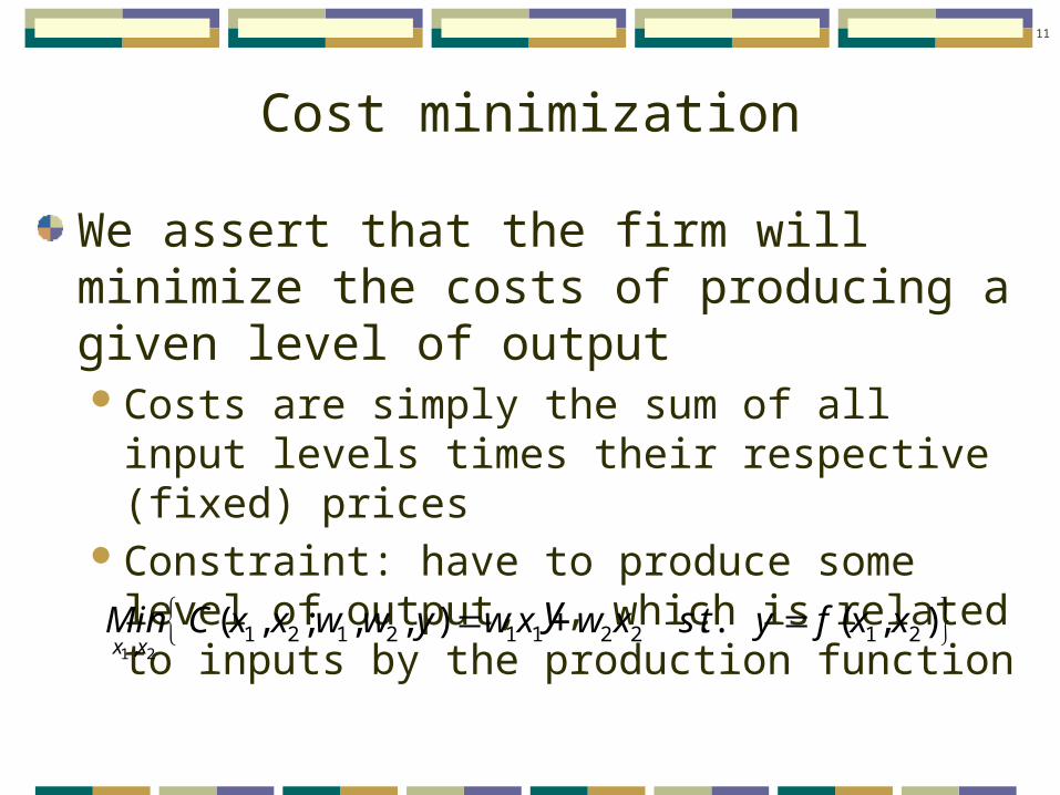
Cost minimization
We assert that the firm will minimize the costs of producing a given level of outputCosts are simply the sum of all input levels times
their respective (fixed) pricesConstraint: have to produce some level of
output, y, which is related to inputs by the production function
1 2
1 2 1 2 1 1 2 2 1 2,
( , ; , , ) . . ( , )x xMin C x x w w y w x w x s t y f x x
12
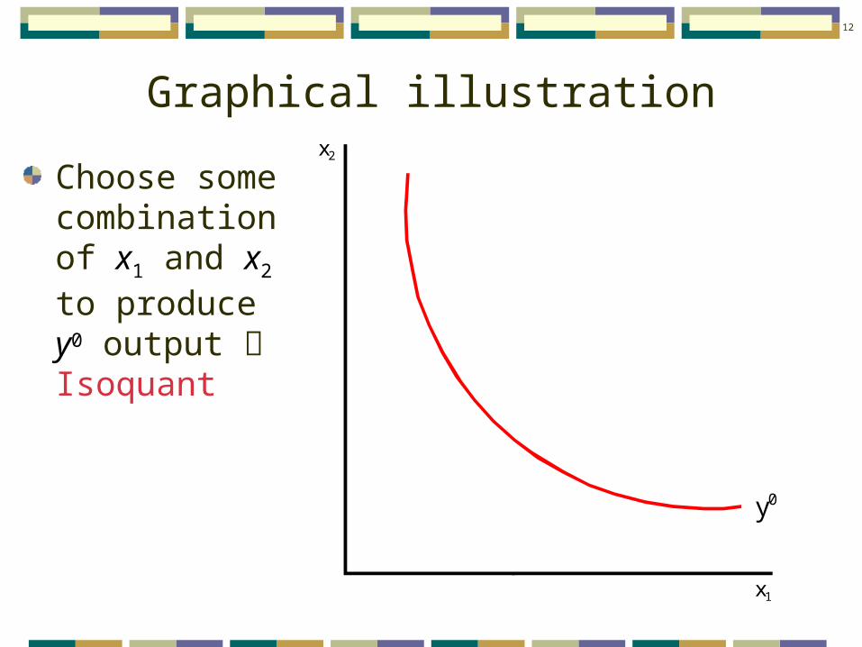
Graphical illustration
Choose some combination of x1 and x2 to produce y0 output Isoquant
x2
x1
y0

13
Graphical illustration
Choose (x1, x2) such that the firm produces y0 at least cost.
Remember w1 and w2 are fixed, as is y0
Isocost line – “same cost”There are an infinite number of isocost lines
given factor prices w1 and w2, but only one that will produce y0
0 0 01 1 2 2C w x w x

14
Graphical illustration
Cost is minimized where isocost line is tangent to isoquant
x2
x1
x20
x10
•
y0
0 0 01 1 2 2C w x w x
0
1
C
w
0
2
C
w
0 0 01 1 2 2
0 01 1
2 02
2 1
1 2
(slope)
C w x w x
C w xx
w
dx w
dx w

15
Graphical illustration
What if isocost and isoquant were not tangent?
Consider:C2 > C0 > C1
x2
x1
x20
x10
•
y0
0
1
C
w
0
2
C
w
2
1
C
w
1
1
C
w
2
2
C
w
1
2
C
w
1 1
2 2
At optimal input use:
slope of isocost slope of isoquant
w f
w f
16
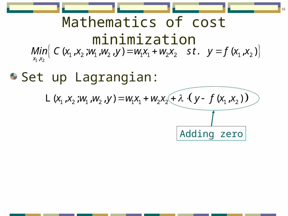
Mathematics of cost minimization
Set up Lagrangian:
1 2
1 2 1 2 1 1 2 2 1 2,
( , ; , , ) . . ( , )x xMin C x x w w y w x w x s t y f x x
1 2 1 2 1 1 2 2 1 2( , ; , , ) ( , )x x w w y w x w x y f x x L
Adding zero
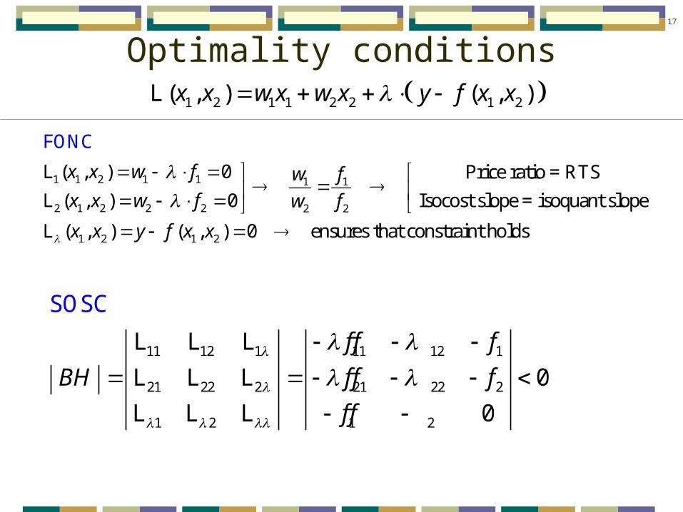
17
Optimality conditions 1 2 1 1 2 2 1 2( , ) ( , )x x w x w x y f x x L
1 1 2 1 1 1 1
2 1 2 2 2 2 2
1 2 1 2
( , ) 0 Price ratio = RTS
( , ) 0 Isocost slope = isoquant sl
FO
ope
( , ) ( , ) 0 ensures that constra
NC
int holds
x x w f w f
x x w f w f
x x y f x x
L
L
L
11 12 1 11 12 1
21 22 2 21 22 2
1 2 1 2
SOSC
0
0
f f f
BH f f f
f f
L L L
L L L
L L L

18
Evaluate SOSC
11 12 1 11 12 1
21 22 2 21 22 2
1 2 1 2
SOS
0
0
C
f f f
f f f
f f
L L L
L L L
L L L
1 111 12 1 11 12 1
2 121 22 2 21 22 2
1 2 1 2
Factor from row 1 only Factor from row 2 only
0 0
f f f f f f
f f f f f f
f f f f
1
11 12 1 11 12 1
21 22 2 21 22 2
1 2 1 2
Factor 1 from row 2 onlyFactor from column 3
0
0 0
f f f f f f
f f f f f f
f f f f

19
Evaluate SOSC (cont.)11 12 1
21 22 2
1 2
11 12 1
21 22 2
1 2
SOSC imply: 0
0
which implies: 0 since 0
0
f f f
f f f
f f
f f f
f f f
f f
11 12 12 2
21 22 2 12 2 1 1 2 21 1 22 2 11
1 2
2 212 2 1 1 22 2 11
0
2 0
f f f
f f f f f f f f f f f f f
f f
f f f f f f f
SHAPE OF PRODUCTION FUNCTION:Cost min requires quasi-concavityProfit max requires strict concavity (stronger requirement)Isoquants are convex

20
Conditional factor demands
There are 3 parameters in the FONC (y,w1,w2)
By the IFT, assuming the SOSC hold, we can solve the FONC simultaneously for the explicit choice functions: x1
c(y,w1,w2), x2c (y,w1,w2), lc (y,w1,w2)
xic are known as conditional factor demands The factor demands from a cost min problem are conditioned on the
level of output y.
To distinguish between conditional factor demands and profit-max factor demands, look at the arguments: Conditional factor demands: xi
c (y,w1,w2)
Profit max factor demands: xi* (p,w1,w2)
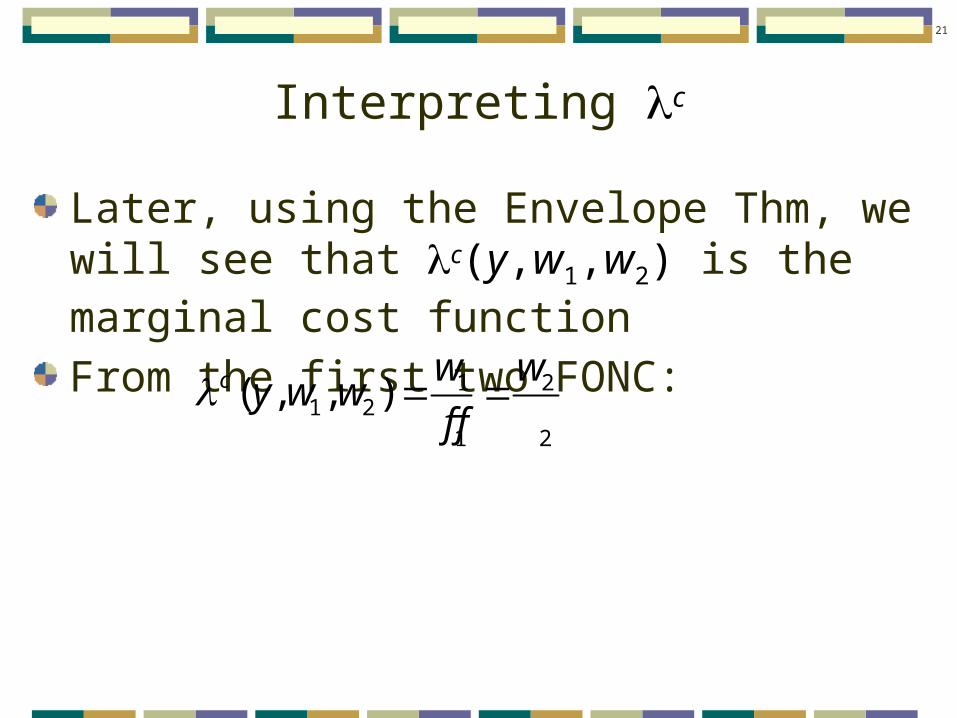
21
Interpreting lc
Later, using the Envelope Thm, we will see that lc(y,w1,w2) is the marginal cost function
From the first two FONC:1 2
1 21 2
( , , )c w wy w w
f f

22
lc(y,w1,w2) is marginal cost function
At cost min input mix, if the firm were to increase xi “a little bit” Dxi
Total cost would rise by wi×Dxi
Output would also rise by MPi×Dxi = fi×Dxii i i
i i i
w w x
f f x
Hence l represents the incremental cost of increasing output through the use of xi.
1 2
1 2
MC must be same for each inputw w
f f
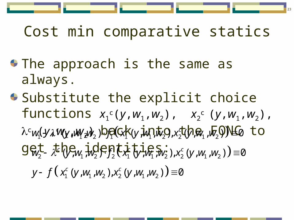
23
Cost min comparative statics
The approach is the same as always.
Substitute the explicit choice functions x1
c(y,w1,w2), x2c (y,w1,w2), lc (y,w1,w2) back into the
FONC to get the identities:
1 1 2 1 1 1 2 2 1 2
2 1 2 2 1 1 2 2 1 2
1 1 2 2 1 2
( , , ) ( , , ), ( , , ) 0
( , , ) ( , , ), ( , , ) 0
( , , ), ( , , ) 0
c c c
c c c
c c
w y w w f x y w w x y w w
w y w w f x y w w x y w w
y f x y w w x y w w
24
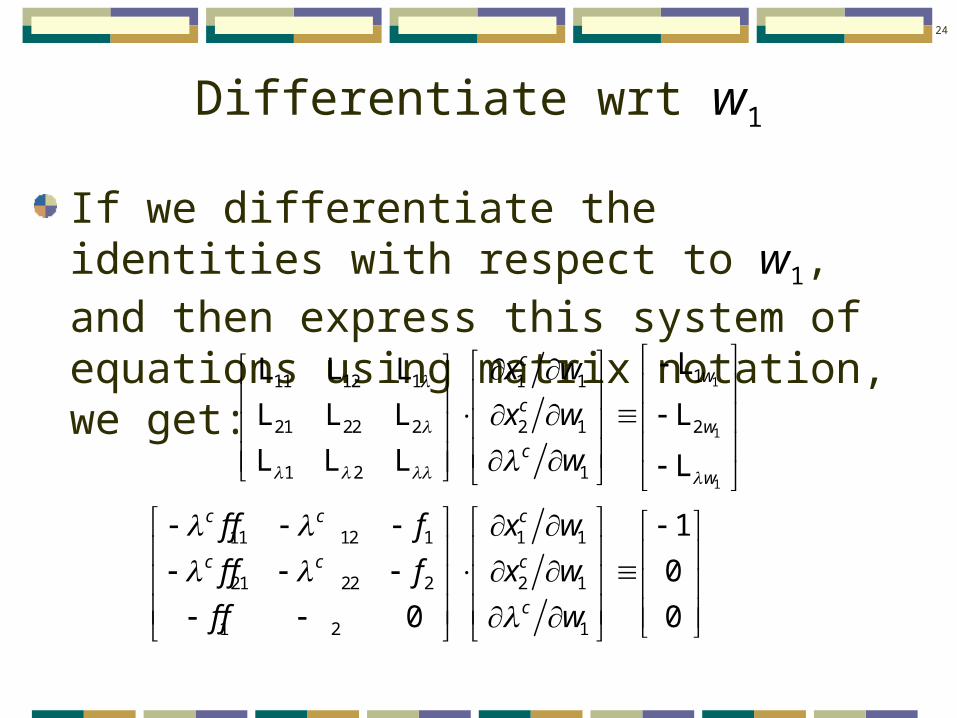
Differentiate wrt w1
If we differentiate the identities with respect to w1, and then express this system of equations using matrix notation, we get:
1
1
1
111 12 1 1 1
21 22 2 2 1 2
1 2 1
11 12 1 1 1
21 22 2 2 1
1 2 1
1
0
0 0
cw
cw
c
w
c c c
c c c
c
x w
x w
w
f f f x w
f f f x w
f f w
LL L L
L L L L
L L L L
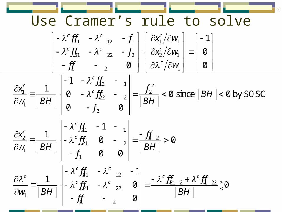
25
Use Cramer’s rule to solve11 12 1 1 1
21 22 2 2 1
1 2 1
1
0
0 0
c c c
c c c
c
f f f x w
f f f x w
f f w
12 1 21 2
22 21
2
11
0 0 since 0 by SOSC
0 0
c
cc
f fx f
f f BHw BH BH
f
11 1
2 1 221 2
11
11
0 0
0 0
c
cc
f fx f f
f fw BH BH
f
11 12
21 2 1 2221 22
11 2
11
0 0
0
c c
c c cc c
f ff f f f
f fw BH BH
f f
26
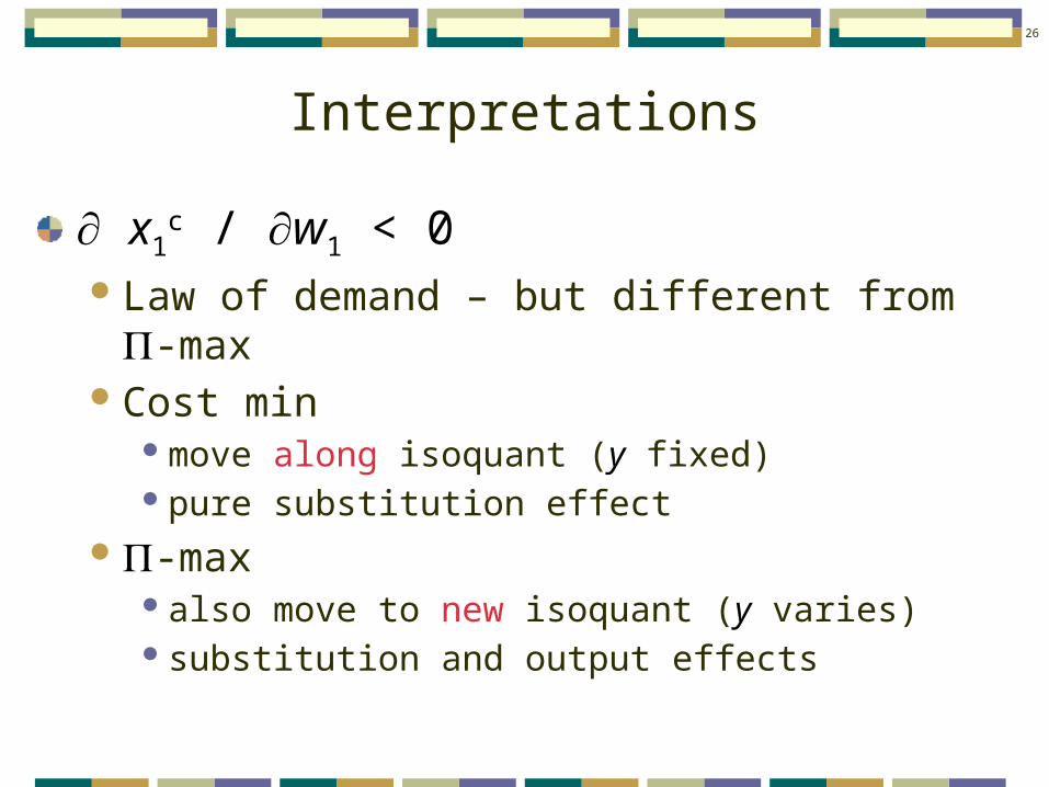
Interpretations
¶ x1c / ¶w1 < 0
Law of demand – but different from P-maxCost min
move along isoquant (y fixed)pure substitution effect
P-maxalso move to new isoquant (y varies)substitution and output effects

27
Interpretations
¶ x2c / ¶w1 > 0
The firm will use more x2 when w1 increases.
We already know that x1 will decrease when w1 increases
If output is held constant, and x1 decreases, then x2 must increase
This result will not necessarily hold if there are more than two inputs.

28
Graphical illustration (w1 increases)
x2
x1x11
x2
y0
x1
x21

29
Interpretations
¶ lc / ¶w1 indeterminateMarginal costs may increase or decrease when a
factor price increasesMay seem counter-intuitiveLater, we will show that this depends upon
whether x1 is a normal or inferior inputSee Silb fig 8-11
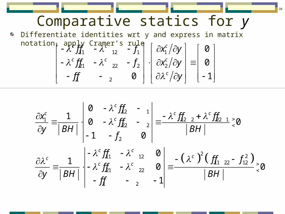
30
Comparative statics for yDifferentiate identities wrt y and express in matrix notation, apply Cramer’s rule
11 12 1 1
21 22 2 2
1 2
0
0
0 1
c c c
c c c
c
f f f x y
f f f x y
f f y
12 1
1 12 2 22 122 2
2
2 211 1211 22 12
21 22
1 2
01
0 0
1 0
01
0 0
1
c
c c cc
c ccc
c c
f fx f f f f
f fy BH BH
f
f ff f f
f fy BH BH
f f
31
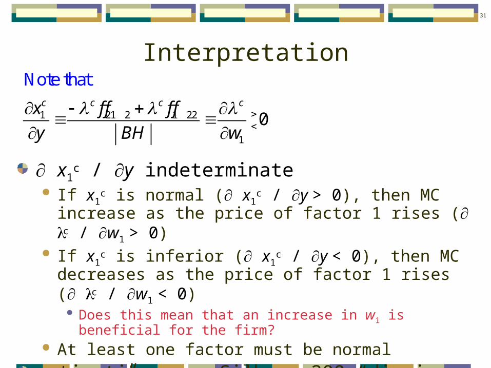
Interpretation
¶ x1c / ¶y indeterminate
If x1c is normal (¶ x1
c / ¶y > 0), then MC increase as the price of factor 1 rises (¶ lc / ¶w1 > 0)
If x1c is inferior (¶ x1
c / ¶y < 0), then MC decreases as the price of factor 1 rises (¶ lc / ¶w1 < 0)
Does this mean that an increase in w1 is beneficial for the firm? At least one factor must be normal
motivation: see Silb p. 200 “digging ditches” and Figures 8-10 and 8-11
1 21 2 1 22
1
0
Note thatc c c cx f f f f
y BH w
32
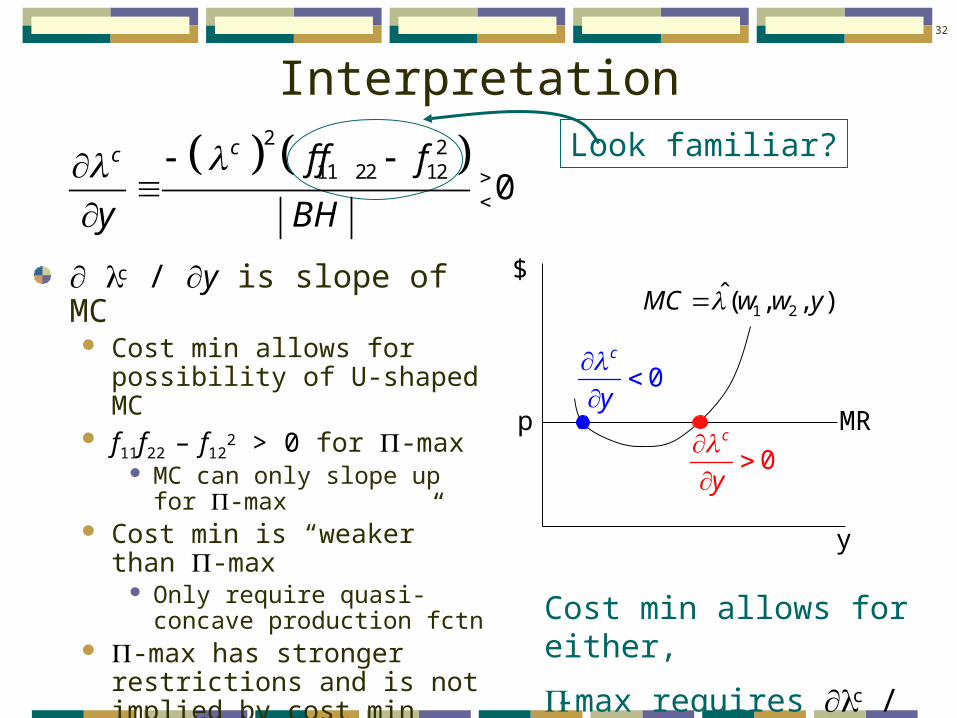
Interpretation
¶ lc / ¶y is slope of MC Cost min allows for possibility
of U-shaped MC f11f22 – f12
2 > 0 for P-max MC can only slope up for P-
max Cost min is “weaker” than P-
max Only require quasi-concave
production fctn P-max has stronger restrictions
and is not implied by cost min Requires strictly concave
production function
2 211 22 12
0cc f f f
y BH
Look familiar?
MR
$
y
1 2ˆ( , , )MC w w y
0c
y
0c
y
p
Cost min allows for either,
P-max requires ¶lc / ¶y > 0

33
Envelope Theorem forgeneral constrained problems
Consider the two-variable, one constraint problem:
1 21 2
,
1 2
( , ; )
subject to ( , ; ) 0
x xMax g x x
h x x
Form the Lagrangian:
1 2 1 2 1 2( , ; ) ( , ; ) ( , ; )x x g x x h x x L
FONC
1 1 1 2 1 1 2
2 2 1 2 2 1 2
1 2
( , ; ) ( , ; ) 0
( , ; ) ( , ; ) 0
( , ; ) 0
g x x h x x
g x x h x x
h x x
L
L
L
By the IFT, assuming the SOSC hold, we can solve the FONC simultaneously for the explicit choice functions
x1*(a), x2
*(a), l*(a)

34
Envelope Theorem for one constraint
Define the indirect objective functionSubstitute the explicit choice functions back into
the objective function to get the indirect objective function
1 2
1 2 1 2,
* *1 2
Indire
( ) ( ,
ct obje
; ) subject to ( , ; ) 0
( ( ), ( )
ctive function
; )
x xMax g x x h x x
g x x
*
*
* * * * *1 2 1 2
(1 2(
( ) ( ), ( ); ( ) ( ), ( );
( , ; )
Envelope Theorem
i
i
x
g x x h x x
x x
L

35
Proof
* ** * * * * *1 2
1 1 2 2 1 2 1 2( ) ( ( ),
Differentiate
( ); ) (
indirect objective fu
( ), ( )
nction wrt
; ) ( ( ), ( ); )x x
g x x g x x g x x
*
* ** 1 2
1 2
( )
(
Multiply by
) 0x x
h h h
* ** * * * * *1 2
1 1 2 2 1 2 1 2( ( ), ( ); ) ( ( ), ( ); ) ( ( ),
Differentiate w
( );
t
0
r :
)x x
h x x h x x h x x
* *1 2
Now consider constraint at optimal so
( ( ),
lutio
); 0
n
( )h x x
add this to above (adding zero)

36
Proof (cont)
* ** 1 2
1 2
* * * **1 2 1 2
1 2 1 2
Adding zero
( ) ( )
( )
x xh h h
x x x xg g g h h h
* **1
0 by FONC 0 b
* *1 1 2 2
O
2
y F NC
Rearran
( )
ge terms
g hx
g hx
g h
*
*
* * * * *1 2 1 2
(1 2(
( ) ( ), ( ); ( ) ( ), ( );
( , ; ) Q.E.D
Therefore:
i
i
x
g x x h x x
x x
L

37
Apply ET to cost minimization
Define the indirect cost functionWe already solved the FONC for the explicit
choice functions.Substitute these back into the objective function
to get the indirect cost function
1 2
1 2 1 2 1 1 2 21 2
,1 2
1 1 1 2 2 2 1 2
( , ; , , )*( , , )
. . ( , )
( , , ) ( , , )
x x
c c
C x x w w y w x w xC y w w Min
s t y f x x
w x y w w w x y w w

38
Envelope Theorem Results (y)
By definition, marginal cost is the change in cost when output changes: ¶C* / ¶y lc = ¶C* / ¶y must be the marginal cost function
1 2
1 21 2
1 2
( , , ) 1 2( , , )( , , )
( , , )
Using t
*( ,
he Env. Thm.
, )c
cc
c
cx x y w w
y w wx x y w wy w w
Cy w w
y y
L
1 2 1 1 1 2 2 2 1 2
1 1 2 2 1 2
Indirect cost function
Lagrangian
*( , , ) ( , , ) ( , , )
( , )
c cC y w w w x y w w w x y w w
w x w x y f x x
L

39
Envelope Theorem Results (w1)
Derivative of indirect cost function wrt an input price yields conditional factor demandShephard’s Lemma
1 2
1 2 1 2
1 2
( , , ) 1 2( , , ) ( , , )( , , )
Using
*( , , )
the Env. Thm.
c
c c
c
cx x y w wi i
x x y w w y w wi iy w w
Cx x y w w
w w
L
1 2 1 1 1 2 2 2 1 2
1 1 2 2 1 2
Indirect cost function
Lagrangian
*( , , ) ( , , ) ( , , )
( , )
c cC y w w w x y w w w x y w w
w x w x y f x x
L

40
Symmetry and reciprocity
1 2 2 1
1 1
* * 1 2
2 1
* * 1
1
Symmetry
Reciprocity
c c
w w w w
c c
w y yw
x xC C
w w
xC C
y w
0 is a normal input
0 is a inferior input
0 is a neutral input
ic ci
ii
i
xx
xy w
x

41
Conditional factor demands are HOD(0) in factor prices
Multiply factor prices in FONC by t:
1 1 2 1 1
2 1 2 2 2
11
2
2
1 1
2
2
( , ) 0
FONC
( , )
, ) 0
( ) 0
(
,
x x w f
x x w f
x x
w f
w f
y f x x
L
L
L
1 1
2 2
1 2( , ) 0
t w f
w f
y f x x
t
Clearly, the t will cancel out. Since these FONC, with prices (tw1, tw2) are identical to the FONC with prices (w1, w2), the solutions must also be the same. Thus: xi
c(tw1, tw2) = xic(w1, w2)
42
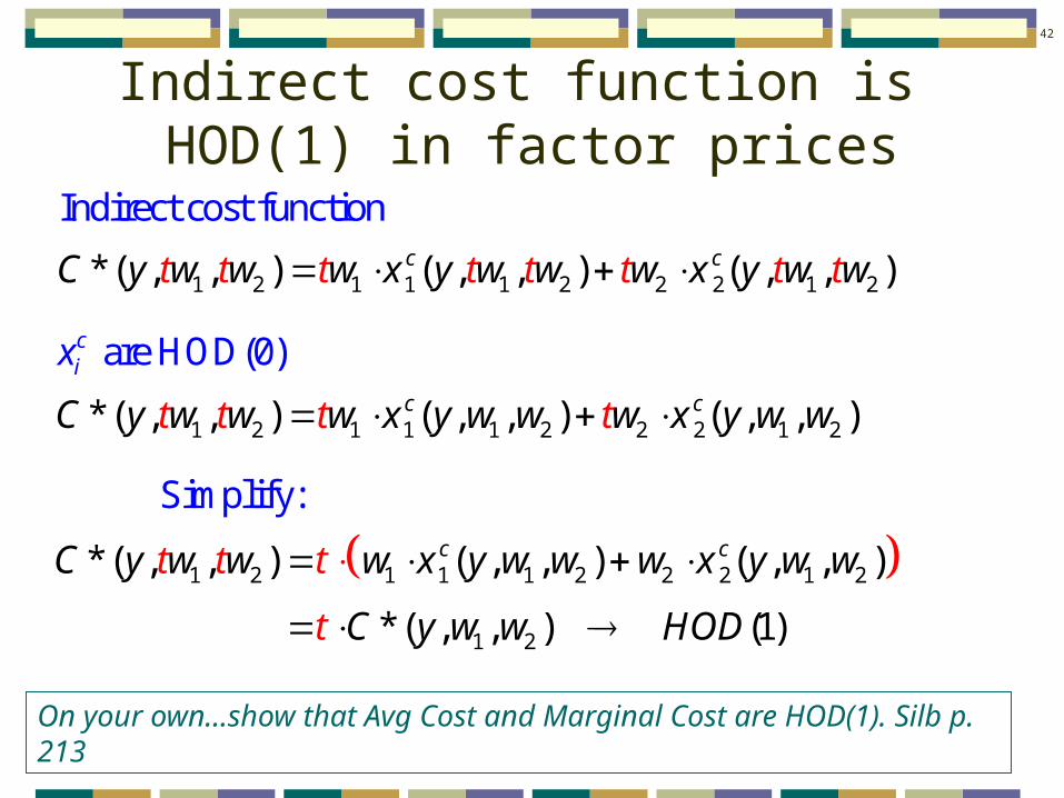
Indirect cost function is HOD(1) in factor prices
1 2 1 1 1 2 2 2 1 2*( , ,
Indirect cost functi
) ( , , ) ( , , )
onc ct t tC y w w w x y w w w x yt t t tw wt
1 2 1 1 1 2 2 2 1 2*( , , )
are HO
( , , ) ( , , )
D(0)ci
c cC y w w w x y w w w x y w wt t
x
t t
1 2 1 1 1 2 2 2 1 2
1 2
Sim
*( , , ) ( , , ) ( , ,
p
)
*( , , ) (1)
lify:c cC y w w w x y w w w x y w w
C y
t t
H
t
w Ot w D
On your own…show that Avg Cost and Marginal Cost are HOD(1). Silb p. 213
43
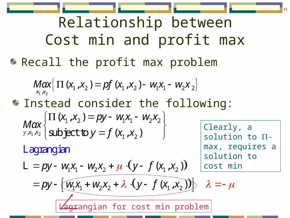
Relationship betweenCost min and profit max
Recall the profit max problem
1 2
1 2 1 2 1 1 2 2,
( , ) ( , )x x
Max x x pf x x w x w x
Instead consider the following:
1 2
1 2 1 1 2 2
, ,1 2
1 1 2 2 1 2
1 1 2 2 1 2
Lagrang
( , )
subject to ( , )
( , )
(
ian
, )
y x x
x x py w x w xMax
y f x x
py w x w x y f x x
py w x w x y f x x
L
Lagrangian for cost min problem
Clearly, a solution to P-max, requires a solution to cost min

44
Relationship between factor demands from cost min and profit max
The solutions to the profit max and cost min FONC are the factor demand functions The profit max factor demand functions:
xi*(p, w1, w2)
The conditional factor demands from cost min:xi
c(y, w1, w2)
These functions are different. As w1 increases: P-max xi
* holds w2 and p constant movement to new isoquant
Cost-min xic holds w2 and y constant
movement along isoquant
How can we tie these two demand functions together?
45
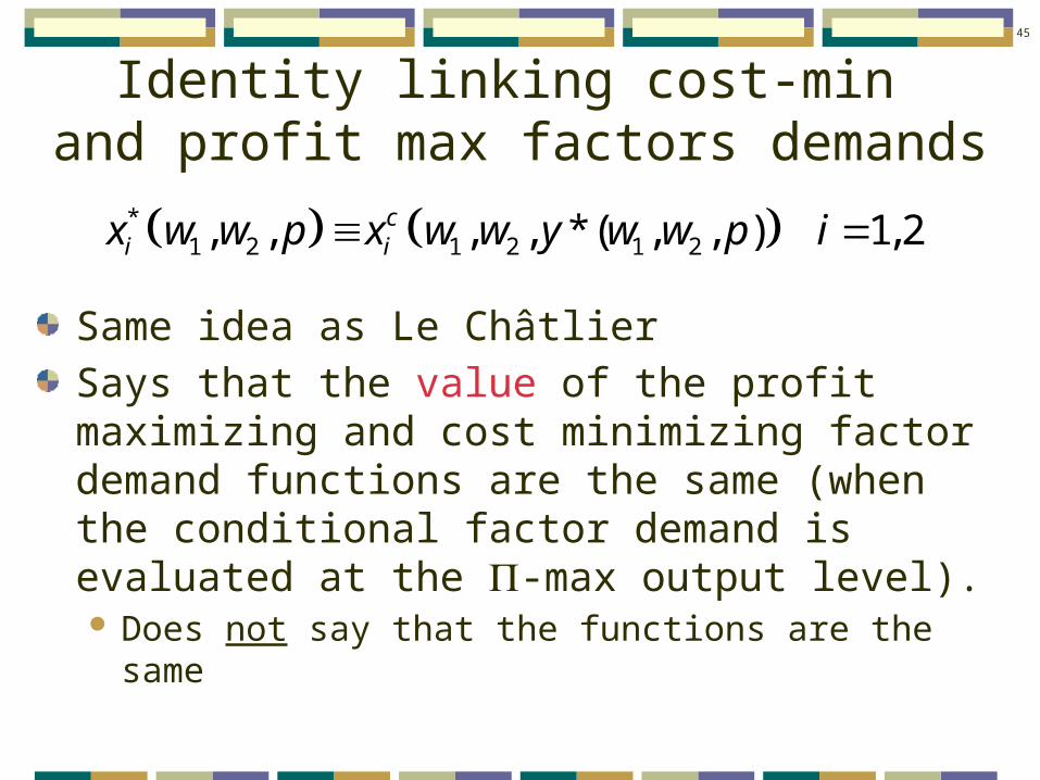
Identity linking cost-min and profit max factors demands
Same idea as Le Châtlier
Says that the value of the profit maximizing and cost minimizing factor demand functions are the same (when the conditional factor demand is evaluated at the P-max output level). Does not say that the functions are the same
*1 2 1 2 1 2, , , , *( , , ) 1, 2c
i ix w w p x w w y w w p i
46
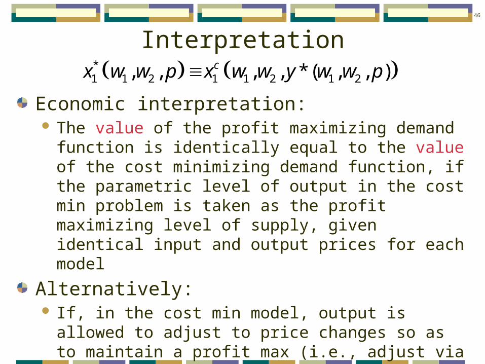
Interpretation
Economic interpretation: The value of the profit maximizing demand function is
identically equal to the value of the cost minimizing demand function, if the parametric level of output in the cost min problem is taken as the profit maximizing level of supply, given identical input and output prices for each model
Alternatively: If, in the cost min model, output is allowed to adjust to
price changes so as to maintain a profit max (i.e., adjust via profit maximizing supply response), then the value of profit max and cost min factor demands will be identical
*1 1 2 1 1 2 1 2, , , , *( , , )cx w w p x w w y w w p

47
Differentiate wrt w1
Using Young’s theorem and the Envelope theorem for the P-max model, we showed:
1 1* *1 2 11 2 2, , , , ( , , )cw w wx w p x w y w p
* *1 1 1
1 1 1
c cx x x y
w w y w
1 1
* ** *1
1w p pw
y x
w p
Now differentiate identity wrt p:
* *1 1
cx x y
p y p
48
Combine
*1
*
*1 1 1
*1 1
*
1
*
1
1
1
1 1
1 1
c c
c c
y
w x
px
x x x
w w y x x x
w wy
p
y
w
**1 1 1
*1 1 1 1 1
1 1
2* *
1
*
1 1
*1
*1
1
1
1
1
0
c c
c c
c
c
c
c
x x x
w w y x x x
w w y
x x x
x
p
x
p
y
w w y
x y
yx
y
p
py
p
<0 <0 >0 >0

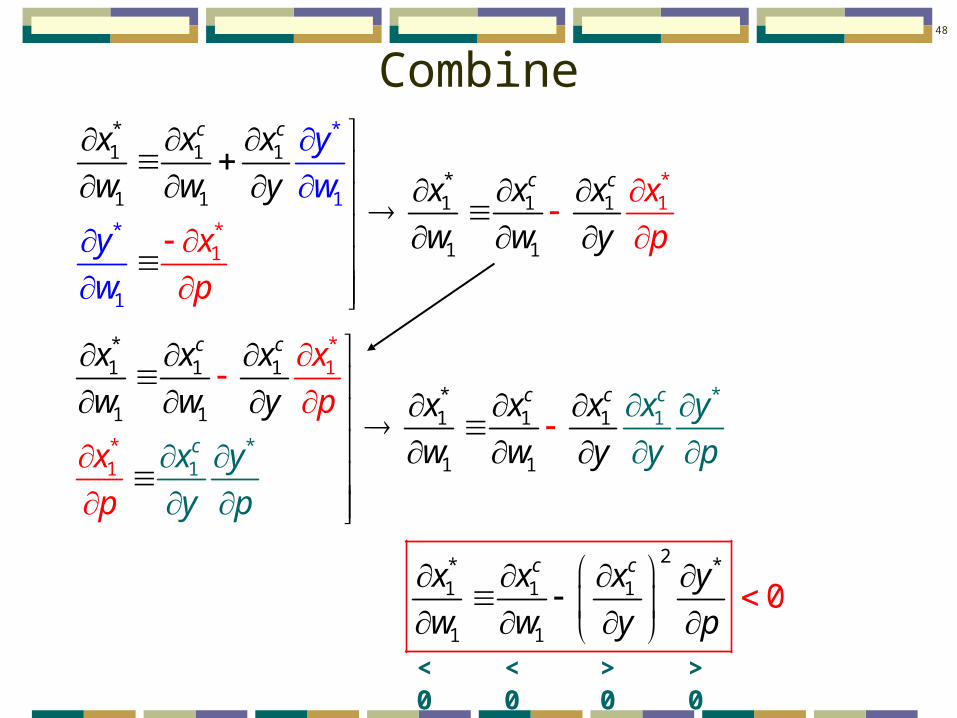
49
Interpret
x1* is more negatively sloped in own price
than x1c
Multiply last inequality by w1/x1 elasticitiesP-max factor demands are more price elastic
2* *1 1 1
1 1
* *1 1 1 1
1 1 1 1
*1 1
1 1
0
0
since negative
c c
c c
c
x x x y
w w y p
x x x x
w w w w
x x
w w

50
Graph
The cost min and profit max factor demand functions intersect
w1
x1
x1*(p, w1, w2)
x1c(y, w1 , w2)
Be careful…Note that this graph has w1 on the vertical axis, so x1
* more price elastic means x1
* is flatter than x1
c.

51
Decomposing the effect
* *1 1 1
1 1 1
R
0
ecallc cx x x y
w w y w
SUBSTITUTION EFFECTHolds output constant. movement along isoquant
OUTPUT EFFECTOutput responds to changes in w1. movement to new isoquant


