

'1 c-
3 3
A Guide to Energy Conservation and Waste Minimization:
Case Studies from Carolina Industries.
3 3 Stephen M. Poulter
June 8,1995
d
J

A Guide to Energy Conservation and Waste Minimization: Case Studies from Carolina Industries
by
Stephen M. Poulter
A project submitted to the Graduate Faculty of North Carolina Sate University in partial fulfillment of the requirements for the Degree of Masters of Integrated Manufacturing Systems Engineering
Integrated Manufacturing Systems Engineering Institute
Raleigh, North Carolina
June 8, 1995
Approved By:
James W. Leach, Ph.D., Chair of Advisory Committee Department of Mechanical and Aerospace Engineering
Herbert M. Eckerlin, Ph.D., Committee Member Department of Mechanical and Aerospace Engineering
Michael Overcash, Ph.D., Committee Member Department of Chemical Engineering
Date
Date
Date

Abstract
Poulter, Stephen Michael, A Guide to Energy Conservation and Waste Minimization:
Case Studies from Carolina Industries. (Under the direction of Dr. James W. Leach)
This report acts as a guide to assist in the identification and evaluation of energy
conservation and waste minimization opportunities. An introduction to the energy
analysis and waste minimization fields is given to show the importance of these
activities within manufacturing and their possible benefits. Methods to identify and
evaluate energy saving opportunities as well as detailed analysis of several conservation
opportunities is presented to give the user the tools to evaluate ideas for feasibility.
Waste minimization methods are also discussed to enable the reader to realize the
benefits of these activities. Case studies taken from work performed at the Energy
Analysis and Diagnostic Center at North Carolina University are presented to illustrate
how energy conservation and waste minimization activities were applied in various
North Carolina and South Carolina industries.
It should be noted that the material presented in this paper does not include a
comprehensive discussion of all possible energy saving or waste minimization
opportunities that can be found in industry. It is meant as a beginners guide for
developing a basic understanding of the fields of energy conservation and waste
minimization.
ii

Biography
Stephen Michael Poulter was born in Indiana, Pennsylvania on March 3, 1971. After
receiving most of his schooling in Indiana, he moved to Beckley, West Virginia in
1987 where he graduated from Woodrow Wilson High School in 1989.
He earned a Bachelor of Science Degree in Mechanical Engineering from
University of Kentucky in December 1993. During his undergraduate studies
completed three cooperative education rotations with General Electric Appliances
the
he
In
January, 1994, he began studies toward the fulfillment of the Master of Integrated
Manufacturing Systems Engineering at North Carolina State University. In May of
1994, he began work at the Energy Analysis and Diagnostic Center at North Carolina
State University as a research assistant and continued work with the center until
graduating in June of 1995.
iii

n 7
'1 8..
3 1
Acknowledgments
I would like to thank Dr. James Leach and Dr. Herbert Eckerlin for giving me the
opportunity to be a member of the Energy Analysis and Diagnostic Center at North
Carolina State University. Their guidance and confidence in my abilities are greatly
appreciated. I would also like to thank Stephen Terry and Adam Chmielewski, who
helped me learn about the energy assessment procedure and evaluation at the EADC,
and have answered the many questions I have thrown their way with patience.
I also want to thank my parents, Malcolm and Anne Poulter, for if it was not for their
support and belief in me, I would not have been able to achieve my goals.
Finally, I want to thank my wife Jennifer, who has patiently supported me while I
pursued my bachelors degree and masters degree.
iv

n -1 Table of Contents
J
I 3
LIST OF TABLES ..................................................................................... vii
LIST OF FIGURES .................................................................................... vii PREFACE ............................................................................................. viii
1 . INTRODUCTION TO INDUSTRIAL ENERGY CONSERVATION .................................. 1 2 . ANALYZING ENERGY CONSUMPTION .......................................................... 3
3 . ANALYZING SYSTEMS ............................................................................ 4
...
3.1 Compressed Air Systems .................................................................... 4 3.1.1 Compressed Air Leaks .................................................................. 4
Compressed Air Leaks in a North Carolina Manufacturer of Aerospace Instrumentation .................................................................................. 7
3.1.2 Compressor Intake Air ................................................................ 10
Cardboard Boxes and Displays ............................................................. 12 3.1.3 Compressor Waste Heat ............................................................... 14
Compressor Waste Heat Recovery at a North Carolina Manufacturer of Fire Protection Valves ............................................................................. 16
3.1.4 Oversized Air Compressors .......................................................... 17
Compressor Intake Air Modification at a North Carolina Manufacturer of
Oversized Compressor at a South Carolina Manufacturer of Dyed and Finished Knitted Cloth ................................................................................... 19
3.2 Waste Heat Recovery ...................................................................... 21 3.2.1 Heat Reclaim - Preheating Combustion Air ....................................... 21
Preheating Combustion Air at a North Carolina Manufacturer of Aluminum Extruded Channel ............................................................................. 26
3.2.2 Heat Containment ...................................................................... 29
3.2.2.1 Insulate Flat Surfaces .............................................................. 29 Insulating Flat Surfaces at a North Carolina Manufacturer of Clay Bricks ......... 32 3.2.2.2 Insulate Pipes ....................................................................... 37 Insulating Pipes at a South Carolina Manufacturer of Woven Narrow Fabric ..... 39
3.3 Lights ......................................................................................... 43 3.3.1 High Efficiency Lighting .............................................................. 44
V

High Efficiency Fluorescent Lights at a North Carolina Manufacturer of Folding Paper Cartons .................................................................................. 46
3.3.2 High Intensity Discharge (HID) Lighting .......................................... 49
3.3.3 Additional Lighting Suggestions ..................................................... 52 3.4 High Efficiency Motors ..................................................................... 53
High Efficiency Motors at a North Carolina Manufacturer of Injection Molded Automobile Parts .............................................................................. 56
4 . WASTE MINIMIZATION / POLLUTION PREVENTION ........................................ 58 4.1 Benefits Associated with Pollution Prevention ......................................... 58 4.2 Waste Management Hierarchy ............................................................ 59 4.3 Energy Conservation and Pollution Prevention ....................................... 63
4.4 Life Cycle Analysis ......................................................................... 63 4.5 Waste Minimization Case Studies from Carolina Industries ........................ 64
Dyed and Finished Knitted Cloth .......................................................... 65
Installing HID Lights at a South Carolina Manufacturer of Woven Narrow Fabric50
Using Waste Water Sludge as a Boiler Fuel at a South Carolina Manufacturer of
Water and Energy Conservation in a North Carolina Manufacturer of Synthetic Yarn ............................................................................................. 68 Recycling Waste Polyethylene in a North Carolina Manufacturer of Fiber Optic
Elimination of Wooden Pallet Disposal at a North Carolina Manufacturer of Air
Cables ........................................................................................... 69
Compressors ................................................................................... 70 APPENDIX A: CONVERSION FACTORS ........................................................... 72
APPENDIX €3: ADDITIONAL INFORMATION ON POLLUTION PREVENTION .................. 72 BIBLIOGRAPHY ....................................................................................... 74
vi

1
1
*- 7 1
:I II
List of Tables Table 1 : Summary of Savings Based on Leak Size .......................................... 9
Table 2: Summary of Air Leaks ................................................................ 9
Table 3: Compressor Air Calculations ......................................................... 13
Table 4: Physical Properties of Air at Atmospheric Pressure ............................. 24
Table 5: Emissivity of Various Surfaces ...................................................... 31
Table 6: Existing Kiln Heat Loss Information ............................................... 36
Table 7: Heat Loss with Additional External Insulation .................................... 36
Table 8: Combined Convection and Radiation Coefficient ................................. 38
Table 9: Exposed Steam Pipe Data ............................................................. 41
Table 10: Summary of Savings for Insulating Pipes ......................................... 42
Table 11 : Summary of Implementation Costs for Insulating Pipes ....................... 43
Table 12: Lighting Levels for Various Areas ................................................ 44
Table 13: Existing Lighting Information., .................................................... 47
Table 14: Proposed Lighting Information ..................................................... 47
Table 15: Summary of Incremental Lighting Savings ....................................... 49
Table 16: Summary of Lamp Costs ............................................................ 49
Table 17: Motor Efficiency Lookup Table .................................................... 55
Table 19: Summary of Motor Implementation Cost and Payback ........................ 57
Table 20: Waste Water Sludge Analysis Results ............................................. 66
Table 21: Wood Fuel Quantification ........................................................... 66
Table 22: Waste Water Sludge Quantification ................................................ 66
Table 18: Summary of Motor Energy and Cost Savings ................................... 57
List of Figures
Figure 1 : Metallic Radiation Recuperator .................................................... 23
Figure 2: Schematic of Proposed Stack Modifications ...................................... 27
Figure 3: Environmental Management Options Hierarchy ................................. 60
Figure 4: Source Reduction Methods .......................................................... 61
Figure 5: The Waste Minimization Assessment Procedure ............................... 62
3
vii

Preface
1 I 1
n ‘7 i l
.- 1 [I
11
The information and analysis described in this report was originated in part by the
Energy Analysis and Diagnostic Center (EADC) at North Carolina State University.
The EADC program is managed by Rutgers, the State University of New Jersey under
agreement from the US Department of Energy, which financially supports the program.
The purpose of the center is to conduct energy and waste assessments at small to
medium sized manufacturing facilities within a 150 mile radius of Raleigh, North
Carolina. Its objective is to identify, evaluate, and recommend energy conservation
and waste minimization opportunities to reduce cost. These recommendations are made
to plant personnel based on observations and measurements made during a one-day site
visit.
Under the EADC program, North Carolina State University does not prepare
engineering designs or perform services normally offered by an engineering firm,
vendor, or a manufacturer’s representative. When the need for such assistance arises,
it is suggested that the participating plant contact these specialists directly.
North Carolina State University and all technical sources referenced do not (a) make
any warranty or representation, expressed or implied, with respect to the accuracy,
completeness, or usefulness of the information, or that the use of any information,
apparatus, method, or process disclosed in this report may not infringe on privately
owned rights; (b) assume liabilities with respect to the use of, or for damages resulting
from use of, any information, apparatus, method, or process disclosed. Mention of
trade names or commercial products does not constitute endorsement or
recommendation of use.
viii

7 ‘1 1 1 1 n :I 3 3
ri a
1. Introduction to Industrial Energy Conservation
Similar to materials, labor, and capital, energy is a production factor that is required to
manufacture final goods or produce services.’ However, as companies try to increase I
their competitive edge by reducing material waste and cost, down-sizing their work
force, or reducing capital investment in such items as inventory, the potential for
saving through energy conservation is often overlooked. The reasons for this are
many, including: a basic lack of knowledge about energy conservation opportunities in
industry, more attractive investments being available, low energy costs per unit of
product, and industry being forced to invest in other areas brought on by safety and
environmental regulations .2
As industry learns to use its energy sources in a more effective and efficient manner, it
will be able to increase its productivity by reducing energy costs and therefore
improving profits. The means by which energy can be saved can be classified into
three general categories: * 1. Housekeeping Measures 2. Equipment and Process Modification 3. Integrated Operations.
The first of these, housekeeping measures, usually falls into the hands of maintenance
and production personnel. It involves the operation and upkeep of equipment in a
manner as not to be wasteful. Some examples of these types of measures are: shutting
off conveyors when not in use, lowering the operating temperature of a curing oven,
identifying and eliminating compressed air and steam leaks, and optimizing thermostat
set-points on air conditioning equipment. These type of energy conservation activities
usually involve very little investment but can result in considerable savings. The
second category, equipment and process modification, involves activities ranging from
the small retrofitting of equipment to the complete replacement of a process. An
example would be installing a duct to direct outside air to the intake of an air
compressor, or replacing a 25 year old chiller with a more efficient unit. The amount
1
"1 3 :3 '1 n n 13 II
II 3 L1
of investment involved in these type of activities can range from several hundred
dollars to several hundred thousand dollars, depending on the scale of the project, but
usually offer an attractive payback on the investment. The third category, integrated
operations, involves thoroughly examining processes, schedules, and operating
practices in order to improve their utilization. For example, it may be less expensive
to run a large piece of equipment during third shift in order to avoid high demand
charges on an electric bill.
An effective energy management policy should be developed by the company. It has
been seen in many instances that corporate programs won't survive very long if they
are not given a strong commitment from management plus the allocation of resources to
make them work. It takes the authority of management to instill the importance of the
energy conservation activities and assist in overcoming obstacles such as employee
indifferences and historic operating practices. Some basic elements to be considered in
establishing an effective energy management program are as follows:
Understanding the basic principles of energy use in the plant. Conducting comprehensive surveys to measure all energy input and output
should be identified. Creating and communicating a plan of action. Setting targets for unit energy consumption. Managing and controlling energy use against the targets.
li during a given period. Equipment associated with large energy consumption
Although no energy management program can perfectly fit the needs of all industries,
these guidelines can provide a starting point for a company to develop its own.
The sections that follow include background information that will assist the reader in
developing a greater understanding of the field of energy conservation. Methods for
identifying and evaluating certain energy conservation opportunities found in many
industrial facilities are also presented.
2
3 L _ rl S J
s n 7 n 3 :4 3 :I 3
Li
a
2. Analyzing Energy Consumption
An essential component of any energy management program is a continuous accounting
of energy use and its cost. This can best be done by keeping up-to-date records of
energy use, demand, and costs. Plots of this data will sometimes show irregularities in
energy use that should be investigated. This information will also facilitate the
comparison to the same month in consecutive years to give insight into equipment
problems. It is necessary to graph individual and total energy use and costs. Any "spikes" should be investigated and their cause explored. Through careful observation
of trends, it may be possible to catch wasteful equipment and practices before they get
out of hand.3
Electricity usually composes the largest portion of a facilities utility bill. A study of
the rate schedule and the consumption of electricity at a facility can sometimes lead to
the detection of conservation opportunities or equipment problems. The two
components of an electric bill that should be monitored are the kilowatt-hour (kWh)
usage and the kilowatt (kW) demand. The kWh usage listed on a utility bill reflects the
energy usage for the length of the billing period. Charges for this portion of the bill
are usually divided between on-peak and off-peak demand periods. The on-peak period
corresponds to a higher rate per kWh due to the large demand on the power plant in the
area during a set time period. The peak demand is determined by the highest kW load
the facility obtains over a billing period. This load represents the energy demand per
time period (usually 15, 30, or 60 minutes). The peak kW demand charge set for one
month can sometimes carry over for an entire season, or an entire billing year. For
this reason, facilities should closely monitor such activities as the start-up of large
pieces of equipment during close intervals. Some suggestions for managing utility
consumption for the avoidance of high demand charges are :2
0 A starting schedule should be prepared and adhered to, so that the whole of the plant starting load does not occur within the same period of the demand meter.
3

Maximum advantage should be taken of night usage wherever operationally possible, to accomplish such tasks as operating intermittent equipment, recharging industrial truck batteries, etc. Heavy machinery, which takes a high starting load and is used intermittently should never started twice within one recording period of the maximum demand meter. No two units of heavy machinery used only during short periods of the working day are ever used at the same time. Wherever possible, clutches are fitted so that motors are started on no load. Large production machines are scheduled as uniformly as possible among all shifts to minimize the demand charges for purchased power.
3. Analyzing Systems
The sections that follow contain methods for identifying and evaluating specific energy
conservation opportunities found in many industrial facilities. Portions of the material
presented was obtained from work performed at the Energy Analysis and Diagnostic
Center at North Carolina State University. An effort has been made to present the
reader with clear explanations of how to obtain data and information required to
analyze the system or conservation opportunity.
3.1 Compressed Air Systems
The operating costs associated with an air compressor can easily exceed its purchase
price within one year, For this reason, it is important that care is taken to operate and
maintain the entire compressor system to conserve energy. Sections 3.1.1 through
3.1.4 present descriptions of opportunities for cost savings associated with compressed
air systems.
3.1.1 Compressed Air Leaks
Leaks are an unavoidable and irritating part of most compressed air systems. Hoses
wear out, get pinched and cut by surrounding equipment, and couplings get loosened
over time. What most facilities don’t emphasize is that allowing leaks to persist is
equivalent to throwing money out the window. Others realize that letting a leak persist
is costly, but don’t have time to fix the problem. By encouraging plant personnel to
4

3 '1 c
I.. 7
7 n
3
3
report air leaks to maintenance or the appropriate supervisor as soon as they are
located, the leak can be repaired and the waste associated with supplying air to the leak
can be eliminated. The cost of an air leak over a period of time can easily pay for a
new hose or the time it takes for maintenance to install a new coupling.
Although trying to quantify the cost of an existing air leak does not solve the problem
directly, it can provide a facility with an idea of the actual cost associated with different
sized leaks. This information can be posted in the workplace to convey the importance
of fixing the leaks to plant personnel and management.
The following data is required to quantify the loss associated with compressed air
leaks:
Compressor operating pressure Inlet air temperature
4 Compressor motor efficiency 4 Average compressed air line temperature
Annual operating time of the compressor
The operating pressure can be found from a pressure gauge on the compressed air line.
Most air compressors are set to cycle so that the pressure in the receiver tank is
maintained between a low and high operating pressure. The line pressure may be kept
constant with the use of pressure regulators. Some compressors may have the ability to
display the inlet temperature on a digital display at the control panel. If the inlet
temperature is not available, a thermocouple or thermometer placed in close proximity
to the compressor intake will work. Note that the intake temperature may vary
throughout the year. This can be accounted for by estimating annual temperature
variations. The average line temperature may also vary seasonally, but can be
estimated by determining the average temperature at which the facility is conditioned.
The compressor motor efficiency can be found on the compressor motor label. (If not
available, refer to the motor efficiency lookup table, Table 17, in section 3.4 of this
5

7 [I
3
:f
I)
-1
i
report.) The annual operating hours of the compressor are usually known from the
facility operating schedule.
In order to calculate the loss due to an air leak, the volumetric flow of free air, Vf,
associated with the leak is calculated from the following relation:
where, Vf C1 P O
Cd
Ti c2
Pi TO
D
C, P, C, D2 ( I ; + 460) c2 pl J7p3iz
volumetric flow of free air, cubic feet er minute (cfm)
compressor operating pressure, psia discharge coefficient for orifice, 0.6, no units leak diameter, inches inlet temperature, O F
inlet (atmospheric) pressure, 14.7 psia average line temperature, O F
choked flow constant, 1336 ft/min.'R 85
conversion constant, 144 in 2 2 /ft
The values listed for the above variable are commonly used values. These can be
modified to more accurately model a facilities actual conditions if desired. From the
above equation, we can now calculate the power loss from each leak, L, which is the
power required to compress the volume of lost air from atmospheric pressure to the
compressor discharge pressure. It may be calculated as follows :4
L
where, L d
c2 k N
c3
= power loss, hp = = =
2 2 conversion constant, 144 in /ft specific heat ratio of air, 1.4, no units factor based on type of compressor considered: For one-stage reciprocating, N = 1 For two-stage reciprocating, N =2 For screw compressors, N = 1.25 (polytropic efficiency of 80%)
= conversion constant, 3.03 x hp.min/ft.lb
iJ 6

n 11
E, = air compressor volumetric efficiency, 85 %, no units E, = compressor motor efficiency, no units
Once these values are obtained for a certain size air leak, the energy savings for each
leak, ES, can be estimated as follows:
where, ES = H L C q ( 1 - F )
ES = annual energy savings, kWh H = annual operating time of the compressor, hr L = power loss, hp c4 = conversion factor, 0.746 kW/hp F = fraction of full power consumed when the compressor is idle,
For reciprocating compressors, F = O For screw compressors, F=0.5
The potential cost savings can be determined by multiplying the above energy savings by the average electricity cost for the facility ($/kWh). Once this information has
been calculated for various sized air leaks, the information could be displayed in a table
similar to the one shown below (Table 1).
Compressed Air Leaks in a North Carolina Manufacturer of Aerospace Instrumentation Following is the assessment recommendation developed for a North Carolina
manufacturer that uses compressed air throughout the facility for blow-off purposes at
workstations and machining centers. During the energy assessment performed by the
EADC at NCSU, 43 compressed air leaks were located using both audible recognition
and an ultrasonic leak detector. The majority of these air leaks were located at hose
couplings and on the air hoses. The savings that can be realized by this facility by
repairing all of the existing air leaks are:
Estimated Energy Savings Estimated Cost Savings = $3,233/yr Estimated Implementation Cost = $1,290 Simple Payback = 4.8 months
= 54,803 kWh/yr
7

n n
1 n 3 1 3
il 3 3
-1
Savings
Compressed air at 120 psig is generated 7 days per week 24 hours per day for a total of
8,400 annual hours using a 50 horsepower rotary screw compressor. Substantial savings can be realized if this compressed air leakage is reduced. The volumetric flow
of free air, Vf, associated with each air leak is given by:
1,336 * )(134.7 psia)(O.6)(74"F + 460) ( minoR0.5 . I\\
= D2 V f 144 7 (14.7psia)- [ 3
where,
D = leak diameter, inches
The power loss from each leak, L, is the power required to compress the volume of
lost air from atmospheric pressure to the compressor discharge pressure. It may be
calculated as follows ':
1.4-1
hp - .in)[( 134.7 pia] ft - Ib 14.7 psia
-
L = v, L 1 (0.85)(0.905)
Annual energy savings for each leak, ES, are estimated as follows:
ES =
The potential savings associated with leaks of various sizes for the operating pressure at
the subject plant are summarized in the table below. Cost savings are based on the
facility's average electricity cost of $0.059 / kWh.
8

During the audit, 43 leaks were located. The following table summarizes the total
energy savings for the leaks.
Table 2: Summary of Air Leaks
From the two tables above, the total estimated savings for repairing the air leaks are
54,797 kWNyr. At the facility's electricity cost of $0.059 / kWh, the estimated annual
cost savings are $3,233,
Implementation of this recommendation involves the repair of all leaking fittings and
holes in compressed air lines. (Each leak was marked with tape during the audit for
identification.) It is estimated that these leaks can be eliminated for an average cost of
$3O/leak or a total cost of $1,290. With an annual savings of $3,233, the simple
payback period for this recommendation is about 4.8 months.
The above example of savings associated with compressed air leaks can be realized by
identifying and repairing leaks on a regular basis. Leaks can be identified by their
9

"hiss" when other plant operations are idle. Most air leaks are found at hose couplings
that have either been loosened over time or have worn with time and use. Teflon tape
should be used to seal all threaded connections to ensure a good seal. Care should also
be taken to store hoses on wall hangers whenever possible to avoid damage from
surrounding equipment. Spring loaded hose winders can also be used to assist in
keeping hoses out of the way to avoid damage.
3.1.2 Compressor Intake Air
The electrical power consumption will be reduced if cool intake air is provided to the
compressor. Most package air compressors pull the supply air for compression
through an intake that is located very close to the motor and compression chamber.
This air is usually at an elevated temperature due to the heat generated by the
compressor and motor operation. If the intake air is ducted from a cooler location, less
electrical power will be required.
The compressor work for the usual operating conditions in manufacturing plants is
proportional to the absolute temperature of the intake air. Thus, the fractional
reduction in compressor work, WR, resulting from lowering the intake air temperature
is given by:
WR = (TI - TO)/(T, + 460)
where
TI = current annual average intake air temperature, OF TO = proposed annual average outside air temperature, OF
The annual energy savings, ES, can be estimated from the following relationship:
ES = HP x FR x LF x UF x C x H x WR / EFF where
HP = compressor horsepower rating, hp FR = horsepower reduction factor based on operating pressure, no
units LF = fraction of rated load at which compressor operates, no units
10

UF = fraction of time compressor is loaded, no units C = conversion constant, 0.746 kW/hp H = hours per year of compressor operation, h/yr WR = fractional reduction in compressor work, no units EFF = efficiency of compressor motor, no units
To obtain FR, the horsepower reduction factor, the maximum operating pressure must
be obtained from the air compressor specifications. At this operating pressure, the
compressor requires the rated horsepower for operating, but at lower operating
pressures, requires less power. The horsepower reduction factor can be obtained using
the following relation.
where,
Pdo = discharge pressure at operating pressure conditions, psia Pi = inlet pressure, psia k E = compression efficiency (0.85, average value), no units Pd, = discharge pressure at maximum pressure conditions, psia
= ratio of specific heats for air (k= 1.4), no units
Note that in order to properly compute FR, the discharge pressures must be converted
from pounds per square inch gauge (psig) to pounds per square inch absolute (psia).
This can be done by adding the atmospheric pressure (14.7 psia at sea level) to the
gauge pressure.
The load factor for the compressor can be estimated by measuring the amps the
compressor pulls during compression and dividing it by the specified rated amps for the
compressor. The usage factor can be estimated by determining the percentage of time
the compressor is operating in the loaded state. This can be obtained either by using a
stopwatch to time the cycle, or if the compressor has a control panel, by dividing the
displayed loaded hours by the displayed operating hours (loaded plus unloaded hours). d
11

Once the energy savings are estimated using the above procedure, the cost savings can
be determined by multiplying the savings by the average cost of electricity.
Some literature states that ducting cooler air to the compressor intake is beneficial only
on reciprocating compressors. It has been demonstrated, however, in an eastern North
Carolina textile plant that savings can be achieved on rotary screw compressors. This
facility used excess chiller capacity to cool the air ducted to the compressor intake.
Compressor Intake Air Modification at a North Carolina Manufacturer of Cardboard Boxes and Displays Following is the assessment recommendation developed for a North Carolina
manufacturer that uses compressed air throughout the facility for process equipment
and blow-off. During the energy assessment performed by the EADC at NCSU, the
assessment team gathered data from three operating air compressors. These
compressors were 100 hp, 60 hp, and 40 hp, and pulled the intake air for compression
from the vicinity of the motor and compression chambers. The savings that can be
realized by this facility by ducting the cooler outside air to the intake of the
compressors is:
Estimated Energy Savings Estimated Cost Savings = $1,746/yr Estimated Implementation Cost = $500 Simple Payback = 3.4 months
= 32,936 kWWyr
ed S a v w
The following example calculations are based on the 100 hp air compressor at the
facility. Calculations for the remaining air compressors can be seen in the table
following this analysis (Table 3). The average air temperature at the intake of the 100
hp compressor, as measured by the audit team, was about 103°F. Based on discussions
with plant personnel concerning temperature changes throughout the year in the
compressor location, it is estimated
95°F. The annual average outside
that the annual average intake temperature is about
temperature, obtained from the National Climactic
12

Center, is 64°F. Thus, the fractional reduction in compressor work, WR, resulting
from lowering the intake air temperature is estimated as:
WR = (95°F - 64"F)/(95"F + 460) WR = 0.056
The 100 hp compressor currently supplies a 100 psig line (114.7 psia). The design
pressure is also 100 psig. Thus, the horsepower reduction factor, FR, based on the
operating pressure and the maximum pressure is 1 .O. 1.4-1 I 1.4-1
FR = 1 .o
The compressor operates for 6,000 hours per year, and the load factor and usage factor
(LF and UF respectively), are estimated as 0.923 and 0.33, from audit measurements.
Thus, the energy savings for the 100 hp compressor, ES, is estimated as:
(100 hp)( 1 .O)( 1 .O)( 1.0)(0.746 kW / hp)(6,000 hrs / yr)(0.056) 0.917
ES =
ES = 27,334 kWh/yr
The annual cost savings, CS, are estimated as:
CS = (27,334 kWh/yr)($O.O53/kWh) CS = $1,449/yr
Table 3 shows the values used to calculate the energy savings for all of the air
compressors in the facility.
13

n cost
Implementation of this recommendation requires the purchase and installation of 6-inch
PVC pipe to connect the intake port of the compressor to the nearest outside wall. It is
estimated that 10 feet of this pipe would be sufficient to duct outside air to each of the
compressors (30 feet total for 3 compressors). The material cost for these lines i
estimated as $lO/fk for a total of $300. The labor cost for installation of the ductwork
is estimated as $200. The total implementation cost for materials and labor to make
these modifications to the compressor and building is $500. The cost savings of
$l,746/yr would pay for the implementation cost within about 3.4 months.
3 *
3.1.3 Compressor Waste Heat
Typically, much of the energy of compression is available as heat and only a small
portion is contained in the compressed air. Most package air compressor units use
n 7 J
1 11
water to remove the heat from the compressed air through a heat exchanger or direct
the air through a radiator that is cooled by a fan. Often times the heat is ducted
outdoors, but with the installation of additional ductwork, this heat could be used for
space heating during the winter months to offset the cost of heating.
The compression of air to a typical operating pressure of 100 psi results in outlet air
temperatures of 350-5000F. When this air is cooled, approximately 80% of the energy
of compression is removed and is available as heat for other purposes. For water-
cooled compressors, the overall recovery efficiency of this waste heat is approximately
55-60%.5 A fan coil can be installed to allow the hot water from the compressor to
heat the building. It is estimated that the heat energy recovered from the compressor
can be used for space heating for about five months per year, depending on the
conditions in the facility.
3
14

1
3 1 7
n 3 n 3
1
The annual energy savings, ES, associated with using the compressor waste heat for
space heating can be estimated as follows: - ES -
where,
HP = C - -
- - - - Fl
F2
- FR -
LF
HM = H = EFF =
-
HP x C x FI x F2 x FR x LF x HM x H / EFF
horsepower rating of the compressor, hp conversion factor, 2545 Btu/hp h fraction of compression energy available as heat, 0.8, no units fraction of available heat which is recoverable, 0.6 for water cooled compressors, no units horsepower reduction factor based on operating pressure, no units (see section 3.1.2) average fraction of rated load at which compressor operates, no units (see section 3.1.2) fraction of the year during which heating is required, no units annual operating time of compressor, h/yr efficiency of space heating system, no units
Values given for the factors F1 and F2 can be used as estimates if the actual values for
the compressor system are not known.
The annual cost savings, CS, can be determined using the above energy savings by
multiplying the savings by the unit cost of the energy source used for heating (Le.,
electricity, natural gas).
cs = ES x unit cost of gas
The implementation of this recommendation on a water cooled compressor involves the
purchase and installation of a fan coil, controller, and required ductwork. To
implement the idea on an air cooled compressor, a damper and additional ductwork is
required so the hot air can be directed indoors during the heating months, and outdoors
when heating is not required.
15

1
3 3 3
'J 3 3 [I
II
3 3'
Compressor Waste Heat Recovery at a North Carolina Manufacturer of Fire Protection Valves Following is the assessment recommendation developed for a North Carolina
manufacturer that operates a 200 horsepower air compressor to supply process
equipment. During the energy assessment performed by the EADC at NCSU, the
assessment team gathered data from the air compressor. The waste heat from the
compressor was being captured in hot water and dumped to the atmosphere through a cooling tower. The savings that could be obtained by using the waste heat to offset
space heating was estimated as:
Estimated Energy Savings Estimated Cost Savings = $5,307/yr Estimated Implementation Cost = $2,500 Simple Payback = 5.7 months
= 977.3 MMBtu/yr
S a v w
Compressed air is currently generated at 115 psig, which is the maximum pressure
condition for the reciprocating compressor. Thus, the compressor operates at its full
rated power of 200 hp. The compressor operates five days per week, 24 hours per day
for a total of 6,000 annual hours. From observations made during the plant audit, the
compressor operates at full-load during all hours of operation.
Therefore, the annual energy savings, ES, are estimated as:
(200 hp)(2,545 Btu! hp- h)(0.8)(0.6)(1.0)(1.0)(5/ 12)(6,000 hrs/ yr) 0.625
ES =
ES = 977.3 MMBtu/yr
The annual cost savings, CS, are estimated as:
CS = ES x unit cost of gas CS = 977.3 MMBtu/yr x $5.43/MMBtu CS = $5,307/yr
a 3 16

n n n
n n n
1 3 i 3 J
The implementation of this recommendation involves the purchase and installation of i
fan coil and controller. For a cabinet unit and controller, the estimated total
implementation cost is $2,500. The savings of $5,307/yr would pay for the
implementation cost of $2,500 in about 5.7 months.
3.1.4 Oversized Air Compressors
Industrial facilities often utilize pneumatic equipment that must remain pressurized at
times when production requirements for compressed air are minimal. For example, a
facility may operate 3 shifts per day, 5 days per week, and shut down production for
the weekend. Often times, certain HVAC equipment and process controls must have a
certain pressure in order to operate over the weekend. It is often the case that a large
compressor, sized to provide compressed air for production equipment, will be left on
during this period to supply the auxiliary equipment requirements. When this is done,
the compressor either runs at no load for a large percentage of time, or cycles on and
off, which can cause a large motor to deteriorate. As was noted earlier, the cost of
operating an air compressor can outweigh its purchase cost within a years time. By
purchasing a small compressor that will run at close to full load over the non-
production period, savings can be obtained.
The annual energy savings, ES, resulting from shutting off the large air compressor
over a period of time and maintaining line pressure with a smaller air compressor can
be calculated by subtracting the energy requirements for the small air compressor from
the energy savings obtained from shutting off the large compressor. To obtain an
estimate on these savings, the voltage, amperage, and power factor for the loaded and
unloaded states of the large compressor operation must be obtained. From these
measurements, the energy consumption can be calculated from the following
expression:
E = &H[FLPLVLA, + FuPuVuAu]
17

3
1 3
3
3 I]
13 j.
where, H = annual hours of compressor operation, hrs/yr FL = P = power factor, no units V = voltage, volts A - - amperage, amps L = loaded state of compressor operation U = unloaded state of compressor operation
percentage of time in loaded state, L (F,= 1-FL), no units
Note that most industrial compressors operate on a three phase power supply, and
voltages can exceed 240 volts. Extreme care must be taken while taking
measurements, it is recommended that a facility have an electrician or trained personnel
take the required measurements. The value for FL, the percentage of time the
compressor is in the loaded state, can be obtained by timing the compressor during the
time of low compressed air consumption over several cycles and averaging the results.
Once the energy consumption of the current compressor is obtained, the next step is to
obtain an approximation for the energy that will be consumed by a smaller air
compressor for the same period. This can be done by either totaling the volume of
compressed air required by each piece of auxiliary equipment (in cubic feet per minute,
cfm) to size the horsepower for the small compressor, or by estimating the compressor
size from the fraction of time the current compressor is operating during the non-
production period.
The estimated energy savings that can be obtained from installing a small compressor
for non-production periods is therefore: = [E~arge compressor - E s m a ~ ~ compressor]
Where the energy consumption of the small compressor is obtained by converting the
compressor horsepower into the equivalent kilowatts (1 hp = 0.746). The annual cost
savings, CS, are estimated as:
CS = ES x unit cost of electricity.
3 1
18

Oversized Compressor at a South Carolina Manufacturer of Dyed and Pinished Knitted Cloth Following is the assessment recommendation developed for a North Carolina
manufacturer that operates a 125 hp air compressor 24 hours per day, 7 days per week
to maintain pressure in the compressed air line. During the weekend, however, the compressed air demand is greatly reduced, and the compressor only supplies pressure
for dye bath controls and HVAC equipment. During the energy assessment performed
by the EADC at NCSU, the assessment team gathered data from the air compressor to
evaluate the savings that could be obtained by installing a 50 horsepower air
compressor to supply the equipment during the weekend. These savings were
estimated as:
Estimated Energy Savings = 113,168 kWh/yr. Estimated Cost Savings = $6,45O/yr. Estimated Implementation Cost = $12,000 Simple Payback = 22.3 months
The facilities two 125 hp air compressors supply approximately 1,200 cfm of
compressed air to the facility during production hours. It was estimated by the plant
engineer that the compressed air load needed to supply HVAC controls, water softener
tanks, and dye bath controls during the weekend is approximately 200 cfm. The annual
energy savings, ES, resulting from shutting off the 125 hp air compressor for a 48 hour period and maintaining line pressure with a 50 hp air compressor can be calculated by
subtracting the energy requirements for the 50 hp air compressor from the energy
savings from shutting off the 125 hp compressor. During the plant visit, measurements
were taken from the 125 hp air compressor on voltage, amperage, and power factor for
the loaded and unloaded states of compressor operation.
It is estimated that during the 48 hour weekend period, the compressor runs in the
loaded state 1/3 of the time. Therefore, the annual energy consumption of the 125 hp
air compressor during the weekend is:
19

3.2 Waste Heat Recovery
Waste heat is the "heat rejected from a process at a temperature high enough above the
ambient temperature to permit the extraction of additional heating value from ite2 This
waste heat can be categorized into three temperature ranges: the high temperature
range, above 1200"F, the medium temperature range, between 450°F and 1200"F, a
the low temperature range, below 45O0F. temperature range heat include: preheating combustion air, producing process steam,
generating electricity, or consumption in low quality processes. For the low
temperature range heat, below 450"F, the uses are more limited to space heating and
cooling, or in the use of operating a heat pump.2
The uses for the high and
3 3 n
n 3 3 3
CT 3
c9
It is important to note that the essential quality to consider in recovering waste heat is not the amount of heat, but the quality of the heat. For example, waste heat in a clean
flue gas at 900°F is more useful than the same amount of heat coming out of a dirty
flue at 350°F. The recovery of waste heat in an economical manner is dependent on
several factors:*
1. There must be a use for the waste heat within the plant or facility. 2. An adequate quantity of waste heat must be available. 3. The heat must be of adeqwte quality for the intended use. 4. The heat must be transported from the waste stream to the process or
material where it is to be used. This is a problem of heat transfer. 5 . The process must be economical (have a fairly short payback time).
The following conservation opportunities involve the reclamation of heat and the
containment of heat to obtain energy savings.
3.2.1 Heat Reclaim - Preheating Combustion Air
Many industrial curing ovens, dryers, or boilers operate by combusting a gas to
provide heat for the process. This combustion process draws air from the surrounding
area to provide oxygen in the combustion zone. Energy savings can be obtained by
preheating this incoming combustion air by drawing the air from the ceiling and d
21

n 1 1 3 II L ’1 1 1 n L ‘-1
‘1 L
3
i
ducting it around the hot exhaust stack. The energy added to the air from the stack
gases is energy that does not have to be supplied from additional combustion of fuel.
“The savings in fuel also means a decrease in combustion air, and therefore, stack
losses are decreased, not only by lowering the stack gas temperatures but also by
discharging smaller quantities of exhaust gas.”* The heat exchanger used in this type
of application is called a metallic radiation tecuperator which consists of two co
lengths of metal tubing as shown in Figure 1. Following is an explanation of how this
device works:
“The inner tube carries the hot exhaust gases, while the external annulus carries the combustion air from the atmosphere to the air inlets of the furnace burners. The hot gases are cooled by the incoming combustion air, which now carries additional energy into the combustion chamber. This particular recuperator gets its name from the fact that a substantial portion of the heat transfer from the hot gases to the surface of the inner tube takes place by The cooler air in the annulus, however, is almost transparent to infrared radiation, so that only convective heat transfer takes place to the incoming air.”2
radiative heat transfer.
The counterflow of the air streams creates for a more efficient heat transfer mechanism
as well as allowing the intake air to be drawn from the warm air supply below the
ceiling of the facility. This air is usually warmer due to stratification that occurs in
facilities with high ceilings.
The amount of heat the incoming air gains from the flue gas can be estimated from the
following relation:
Q = h A(AT)
where,
Q = heat gained by incoming combustion supply air, Btu/hr h = heat transfer coefficient, Btu/hr-ft2-”F A - - area of heat transfer, ft2 AT = temperature difference between the supply and exhaust air, O F
22

Insulation and Metal Coverin
Hot Air +
toprocess -..z
Waste Gas
/
)Tm+ Cold Inlet Air
I 1 T r
Flue Gas
Figure 1: Metallic Radiation Recuperator2
In order to obtain the values for the above equation, the area of the existing duct, as well as the temperature and velocity of the air exiting the duct must be obtained. The
area of a cylindrical duct is the circumference (c=27tr, where r is the radius) times the
length of duct to be used for heat transfer. For a rectangular duct, the area is the
perimeter times the length. The mass flow rate of the air, m, can then be calculated
with the relationship:
a
m = p x velocity x Area
The properties of the flue gas, can be estimated from Table 4 depending on the flue gas
temperature. Note that Table 4 actually gives properties of air.
23

The following conversion factors will be helpful for using the above table.
temperature: density, p: kinematic viscosity, v: thermal conductivity, k: 1 W/m K = 0.5779 Btu/(h ft OF)
K = ("F-32)/1.8 +273, and "I?= 1.8(K-273) + 32 1 kg/m3 = 0.06243 lb/ft3 1 m2/s = 10.76 ft2/s
The mass flow of exhaust must be made up by the fuel and the fresh air in the
combustion zone. The
relationship between the velocity of the intake air through the cool air inlet and the
This is very important when designing the recuperator.
intake area is:
Intake Velocity = m / (Intake Area x pintake air)
where,
Intake Area = x/4[(diameter of outer duct)* - (diameter of inner duct)' J
The heat transfer coefficient ,h, is dependent on many factors, like the materials used,
the flow rates, and the setup of the heat exchanger. It can be estimated from the
Colburn relation6.
24

1 1 n .. 1 i :I
111 :3
h = 0.023 k (Reo*8)(Pr1’3) / Dh
where,
k = thermal conductivity of air, (see Table 4) Btu/hr-ft-”F Re = Reynold’s number of the incoming air Pr = Prandtl number of air, (see Table 4) Dh = hydraulic diameter
When determining the above constants from Table 4, average the exhaust temperature
and the intake air temperature to determine an estimate for k and Pr. The Reynold’s number is given by:
Re = p x velocity x Dh / v
where,
Dh = hydraulic diameter = 4 x Area / Perimeter V = viscosity of air (see Table 4)
The perimeter is the total perimeter of both cylinders. Therefore after simplification,
D h is: -
Dh - Douter duct - Dinner duct
Once the value for the Q is obtained using the above method, the total annual energy
savings are:
ES = Q M / Efficiency of Combustion
where H is the annual hours of operation for the furnace. The cost saving, CS, are
then calculated by:
CS = ES x unit cost of fuel
Note that a professional should be contacted to design a proper system to recover heat from the flue gas. If not properly designed, the combustion zone could be starved of
oxygen, creating a very dangerous situation. It is also important to check the
temperature rating of the intake fan to insure that the fan can handle the increased air
temperature.
3 25
:1 S
1 3 7
'1 ...
. _ -1 I 11
Preheating Combustion Air at a North Carolina Manufacturer of Aluminum Extruded Channel Following is the assessment recommendation developed for a North Carolina
manufacturer that extrudes aluminum billets through dies to form channels. These
billets are heated to approximately 900°F in a gas furnace before entering the extrusion
chamber. During the energy assessment performed by the EADC at NCSU, the assessment team gathered data from the bilIet heaters and flue gas stacks to determine
the savings that could be obtained by using the stack heat to preheat incoming
combustion air for the gas furnace. These savings were estimated as:
Estimated Energy Savings = 1,592.5 MMBtu/yr. Estimated Cost Savings = $7,34l/yr. Estimated Implementation Cost = $3,000 Simple Payback Period = 4.9months
ed Savtngs
Currently, the combustion air used in the three billet heaters comes from the factory
floor and is at approximately 80°F. During combustion, the air will be heated in the
burner to around 900°F before it is used to heat billets. Because of the heat recovery
equipment installed, the air leaves the stack at around 550°F. If the combustion air
were preheated, then the amount of energy used to heat the combustion air during
burning would decrease, resulting in energy savings.
It is recommended that air from the ceiling, which is generally warmer than air at the
floor, be drawn through ductwork, which surrounds the exhaust stack, into the
combustion supply air fan. The air flowing through the duct around the outside of the
exhaust stack will gain heat from the hot exhaust gases. The incoming air duct will
completely surround the exhaust duct, like two concentric cylinders. About ten feet of
duct with a diameter of 2 feet will be required.
26

Stack Gases Incoming -
Combustion Air A- T
9 Furnace
Figure 2: Schematic of Proposed Stack Modifications
The existing exhaust duct is about one foot in diameter, therefore, a ten foot section of
this duct has an area of 31.4 ft2. The flow out of the exhaust duct is about 1,000 $me The mass of air leaving the stack is therefore:
= = 28.1 Ib/min - - 1,686.2 lb/hr
Exhaust = p x Speed x Area 0.040 Ib/ft3 x 1,OOO fpm x 0.707 ft2
This exhaust rate must be made up by fresh air. If the outer duct is two feet in diameter, the area of the intake duct is the total area of the two foot duct minus the area covered by the exhaust duct.
Intake Area = n/4 x [(2 ft)2 - (1 f02 ] - - 2.36 ft2
The velocity of the intake air can be found from the mass flow.
Mass Flow = p x Speed x Area
Speed = Mass flow / (Area x p) or,
= - - 159.0 ft/min. - - 2.65 ft/sec
1,686.2 lb/hr / (2.36 ft2 x 0.075 Ib/ft3)
27

The estimated temperature difference between the exhaust and supply air is 470°F.
The heat transfer coefficient is given by:
where, h = 0.023 k (Reo.8)(Pr"3) / Dh
k = thermal conductivity of air, 0.0152 Btu/hr-ft-"F Re = Reynold's number of the incoming air Pr = Prandtl number of air, 0.7 Dh = Hydraulic Diameter
The hydraulic diameter is calculated as:
Douter - Dinner - - Dh = 2 f t - l f t
1 ft. - - The density of air at 80°F is about 0.075 Ib/ft3 and the viscosity is about 1 . 3 3 ~ 1 0 - ~
lb/f"t-sec. Therefore, the Reynold's number is:
(0.075 Ib / tt3 )(2.65 ft / sec)(l ft)
1.33~10" Ib / ft - sec Re =
Re = 1.50 x io5
The Prandtl number for air is generally taken as 0.7. Therefore,
h = (0.0152 Btu/hr-ft2-oF)(0.023)(1.50x105)o*8 (0.71'3) / (1 ft) - - 4.3 Btu/hr-ft2-"F
The heat transfer, Q is:
Q = 4.3 Btu/hr-ft2-OF x 31.4 ft2 x 470°F = 63,194.3 Btu/hr.
The facility operates three such furnaces for 8,400 hrs/yt. The total annual energy
savings are:
Energy Savings = = 1,592.5 MMBtu/yr.
63,194.3 Btu/hr x 3 furnaces x 8,400 hrs/yr.
Cost Savings = 1,592.5 MMBtu/yr. x $4.61/MMBtu = $7,34l/yr.
28

n n I
7 . . 1
3 .3 [3
1
Implementation will require that each of the three stacks be surrounded by a 2 foot
diameter insulated duct. This duct will then feed into the combustion supply air fan. It
is important to check the temperature rating of the fan to insure that fan can handle the
increased air temperature. The total implementation cost is estimated as $3,000, which
includes materials and labor. The simple payback period is calculated to be 4.9 months.
3.2.2 Heat Containment
Another method of obtaining energy savings from systems that operate at elevated
temperatures is to use insulation. The proper amount of insulation can reduce the
amount of heat that is lost from a process, such as a curing oven, or a transport device,
such as a steam pipe. Benefits of insulating these types of surfaces are not limited to
reducing fuel consumption, but include savings due to reduced cooling load and
reduced emissions from the heat source. The following information contains methods
for estimating the energy savings due to the reduction of heat transfer. The first
section deals with flat horizontal and vertical surfaces, as may be seen on drying ovens
or kilns, and the second deals with pipes.
3.2.2.1 Insulate Flat Surfaces
To estimate the savings associated with adding insulation to flat surfaces, the current
heat loss must be estimated. The following information must be obtained:
1. internal temperature of the ovenldryer 2. external surface area of the wall 3. external temperature of the wall 4. ambient temperature of the room.
First, the value for h, the convective heat transfer coefficient, is calculated for the
horizontal walls using the following formula:6
0.516(GrL*Pr)0*25k L h -
where,
3 29

h = Convective Heat Transfer Coefficient, Btu/(h ft2 O F )
Gr, = GrashofNumber Pr = Prandtl Number of Air, (see Table 4) k L = Height of Wall, ft.
= Thermal Conductivity of Air, (see Table 4), Btu/(h ft OF)
The Grashof number is given by:
gP (Tw - T0)L3 Gr, = V L
where,
8 = Gravitational Constant, 32.2 ft/s2 P = 2 / (T, +To), " P I L = Height of Wall, ft V = Kinematic Viscosity, (see Table 4) ft2/s TO = Ambient Air Temperature, O F .
The combined heat loss due to convection and radiation is given by:
Q =A[h(T, - To) + Clew (TW4 - To4)]
where,
Q = Total Heat Transfer Rate, Btu/hr A = Surface Area, ft2 h = Convective Heat Transfer Coefficient, Btu/ft2. "Fahr C1 = Stephan-Boltzmann Constant (0.1714 x 10" Btu/hrbft2.OR4) e, = Emissivity of the surface (see Table 5 ) TW = Average Wall Temperature, OR (OR= "F+460) TO = Ambient Air Temperature, O R .
Table 5 contains emissivity values for various surfaces that may be found in industry.
These can be used to estimate the emissivity of the hot surface being examined.
The formula used to calculate the convective heat transfer coefficient for a horizontal
surface is:
0. 16(GrL * k L h -
30

In this formula, L is the Area of the ceiling divided by the Perimeter.
Table 5: Emissivity t Surface
Aluminum: Highly polished Rough plate Oxide
Highly polished Rolled plate, natural
Brass:
Chromium: Copper:
Electrolytic, polished Thick oxide coating
Pure Fe, polished Wrought Iron, polished Smooth sheet iron Rusted plate Smooth oxidized iron Strongly oxidized
Iron and Steel:
Rough red brick Stainless steels
Type 3 16, cleaned 316, repeated heating 310, furnace service Allegheny #4, polished
* When two temperatures and two emissiv
Various ~urfaces' Tempierature*. "C
230-580 26
280- 830
260-380 22
40-540
80 25
180-980 40-250
700- 1040 20
130-530 40-250
21
24 230-780 220-530
100
Emissivity *
0.04-0.06 0.055-0.07 0.63-0.26
0.03-0.04 0.06
0.08-0.26
0.02 0.78
0.05-0.37 0.28
0.69
0.95
0.55-0.60
0.78-0.82
0.91 -0.96
0.28 0.57-0.66 0.90-0.97
0.13 ~ __
es are given they correspond, first to first and second to second, and linear interpolation is suggested. 'C = 5/9("F-32)
To determine the savings that would be possible if additional insulation were added to
the surfaces, the effectiveness of the existing insulation must be determined. The
actual effective value of k, the thermal conductivity of the wall, is given by:
where, k = Thermal Conductivity of the wall, Btu*in/hr*ft*."F Q = Total Heat Transfer Rate, Btu/hr L = Wall Thickness, inches
31
n 1 I
1 3 1 ‘.. 1 3 :I 3
4
A = Area of Wall, ft2 T f = Internal Wall Temperature, O F
TW = Average External Wall Temperature, O F .
The next step is to determine the heat loss after insulation is added to determine the
energy savings. The new heat loss is:
where k,, represents the thermal conductivity an “t” is the thickness of the insulation
to be added. This can be obtained from an insulation supplier. They will be able to
assist in the determination of the proper insulation for the system. When the
differences between the heat loss for the current system and the heat loss for the
insulated system are determined and totaled, the resulting energy savings are:
The annual cost savings are: ES =
CS = ES x unit cost of fuel
(Q - Qnew) x Hours of Operation / Efficiency of Combustion.
As was stated earlier, a representative from a insulation supplier should be able to assist in the proper selection of insulation for the application.
Insulating Flat Surfaces at a North Carolina Manufacturer of Clay Bricks
Following is the assessment recommendation developed for a North Carolina
manufacturer that bakes clay bricks in long kilns. Sections of these kilns are heated to
approximately 1300°F using gas and sawdust. Although the kiln walls are made of a
three part composite construction, there remains a large unnecessary loss of heat from
the oven, and the areas surrounding the kilns are extremely hot. During the assessment
performed by the EADC at NCSU, the assessment team gathered temperature data
from the kilns to determine the savings that could be obtained by insulating sections of
the walls and roof. These savings were estimated as: - Estimated Energy Savings -
Estimated Cost Savings - Estimated Implementation Cost = Simple Payback - -
5 1,100 MMBtulyr $176,704 I yr $52,500 3.6 months
11 32

These numbers represent the savings that could be obtained from the four kilns located
at this facility. Since the fuel cost for the wood fired kilns were not quantifiable by
plant personnel, we have estimated the savings with the assumption that cost of wood
chips is approximately the same as that of natural gas.
d Savings
The amount of heat now being lost through the walls of the kilns is calculated below
based on measured surface temperatures at the kiln walls and ceilings along a 200 foot
length of the main burner section of the kiln. First, the value for h, the convective heat
transfer coefficient, is calculated for the horizontal walls using the following formula:6
0.516(GrL * Pr)0*25 k L h -
where, h = Convective Heat Transfer Coefficient, W/m2*K GrL - - Grashof Number Pr = Prandtl Number of Air = 0.702 k = Thermal Conductivity of Air6, 0.028 W/m.K L = Height of Wall, 4.3 m.
Sample calculations for Kiln 4-2 are as follows. From measurements made during the
plant visit, the average wall temperature (T,) is known to be 164°F. The Grashof
number is given by:
= 2.27~10' 89 (Tw - To )L3 Gr, = V 2
where, g = Gravitational Constant, 9.8 m/s2 b = 2 / (T,+T,), K-' L = Height of Wall, m n = Kinematic Viscosity, m2/s T O = Ambient Air Temperature, 100°F.
33

The value of h for the wall of kiln 4-2 is:
0.5 16(2.27~10" *0.702) 0*25 (0.028) 4.3
h -
h = 2.12 W/m2.K = 1.21 Btu/ft2*"F*hr
For kiln 4-2, the area of the wall is 2,800 ft2, therefore the combined heat loss due to
convection and radiation is given by:
Q =2800[1.21(164- 100)+0.1714~10-~(0.91)(623.7~ -559.74)] Q = 449,118 Btu/hr
Following a similar procedure, heat loss estimates are calculated for the ceiling of the
kiln. The formula used to calculate the convective heat transfer coefficient for a
horizontal surface is:6
0. 16(GrL* Pr)0*33 k L h -
In this formula, L is the Area of the ceiling divided by the Perimeter.
Substituting average values of the measured surface temperature of the ceiling into the
formulas, we obtain:
h = 3.17 BTU/ft2a"Fahr.
The combined heat transfer from the ceiling of Kiln 4-2 is calculated to be:
Q = 801,487 Btu/hr.
Thus based on the wall temperature measurements from the plant visit, the total heat
loss from the two walls and ceiling of Kiln 4-2 is:
Q = 2(449,118)+801,487 = 1,699,723 Btu/hr.
To determine the savings that would be possible if additional insulation were added to
the outside walls, we must first determine the effectiveness of the existing insulation.
Discussions with plant personnel revealed that the walls are made of a three part
construction, including fire brick, a loose fill cavity containing a vermiculite powder,
34

n n 1 3 1 ._ 1 3 3 3 1 :I J :.I
1 Ii a 13
and an outer red brick wall. The published values of the thermal conductivity's for
these materials at the representative temperature of the kiln wall is:
kl =fire brick = 1.39 BtuWhr.ft2."F k2..vermiculite = 0.26 Btu*in/hr.ft2*"F k3 = red brick = 4.88 Btu.in/hr*ft2.0F.
Based on the published values, the theoretical effective value of the conductivity of wall is:
AX, +Ax2 + Ax3 AX, AX, AX^ h e f t 2 - F - +-+-
Btu e in k = = 0.77
k , k2 k, The actual effective value of the thermal conductivity of the existing wall should be
higher than the theoretical value because of age cracks and possible improper
installation. The actual effective value of k can be determined from the heat loss
calculated above and the dimensions of the wall.
The actual effective value of k is given by:
where, k = Thermal Conductivity of the Wall, Btu*in/hr*ft2.0F Q = Total Heat Transfer Rate, BTU/hr L = Wall Thickness, 18 inches A = Area of Wall, ft2 Tf = Internal Wall Temperature, estimated average = 1350°F TW = Average Wall Temperature, O F .
Based on the heat losses calculated above, the actual effective value of k for the
existing insulation in the walls of Kiln 4-2 is:
k = 2.43 Btu.in/hr*f?*"F.
The value calculated for the ceiling of Kiln 4-2 is:
k = 4.04 Btu.in/hr.ft**"F.
35
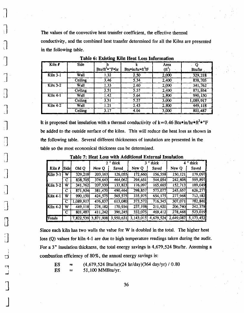
The values of the convective heat transfer coefficient, the effective thermal
conductivity, and the combined heat transfer determined for all the Kilns are presented
in the following table.
It is proposed that insulation with a thermal conductivity of k=0.46 Btu.inlhr.ft2boF
be added to the outside surface of the kilns. This will reduce the heat loss as shown in
the following table. Several different thicknesses of insulation are presented in the
table so the most economical thickness can be determined.
Table 7: Heat Loss with Additional External Insulation
Since each kiln has two walls the value for W is doubled in the total. The higher heat
loss (Q) values for kiln 4-1 are due to high temperature readings taken during the audit.
For a 3" insulation thickness, the total energy savings is 4,679,524 Btu/hr. Assuming a
combustion efficiency of 80%, the annual energy savings is:
ES = (4,679,524 Btu/hr)(24 hr/day)(364 day/yr) / 0.80 ES = 51,10OMMBtu/yr.
36

The annual cost savings based on the cost of natural gas is:
CS = (51,100 MMBtu/yr)($3.458/MMBtu) CS = $176,704
The exposed area of the main 200 foot section of the kilns is 30,000 ft2. The cost of the
insulation was based on a quote from a North Carolina insulation supplier at a price of
$0.SO/ft2 for a 3" thick insulation with a thermal conductivity of approximately 0.46
Btu@in/hr.ft2*"F. This results in an insulation cost of $15,000, and assuming labor is
2.5 times the insulation cost, the labor cost is $37,500, giving a total cost of $52,500
which will be recovered by the cost savings in 3.6 months. Since the payback period is
relatively short, insulation thicknesses greater than 3" should be considered. Also, the
existing insulation in the kilns should be inspected to determine whether it can be
repaired,
3.2.2.2 Insulate Pipes
In many industrial facilities, sections of piping leading to valves and flanges are often
found to be uninsulated. Insulating these exposed sections of steam or hot water pipes
will reduce heat loss and associated costs.
The amount of energy saved by insulating the hot pipes, ES, is calculated as follows:
ES = (UHL-IHL)/EFF
where,
UHL = heat loss from uninsulated pipe, MMBtu IHL = heat loss from insulated pipe, MMBtu EFF = efficiency of the heat supply, no units
The heat loss from the uninsulated pipes, UHL, is given by:
UHL = A H k , ( T , - T , )
37

1
Flat Plates 1.82 Horizontal Facing Upward 2.00 Horizontal Facing Downward 1.58
where,
2.13 2.40 2.70 2.99 3.30 4.00 4.79 5.70 2.35 2.65 2.97 3.26 3.59 4.31 5.12 6.04 1.85 2.09 2.36 2.63 2.93 3.61 4.38 J.27
n \- 1 -I
'1
n 1 1
J
kfi = effective heat transfer coefficient, Btu/h ft2 O F
A = area of exposed pipe, ft2 TP = surface temperature of the pipe, O F
Ts = average temperature of the surrounding air, O F
H = annual time during which pipes are heated, h/yr
(see Table 8)
Table 8 contains the values for heff for various size pipes and temperatures in a room
with an ambient temperature of 80°F.
Temperature difference from surface to room, O F I Nominal Pipe I Diameter
By covering the pipe with an inexpensive fiberglass pipe wrap, the amount of heat loss
can be reduced dramatically. The heat loss from an insulated pipe, IHL, is calculated
using the following equation:
where,
R TP = surface temperature of the pipe, O F
Ts = average temperature of the surrounding air, O F A = area of outer surface of insulation, ft2 H = annual time during which pipes are heated, Wyr
= thermal resistance of pipe insulation, hr O F ft2 / Btu
3 38
1

The average pipe insulation recommended by the EADC is a fiberglass pipe wrap with
an R value of 3 and an aluminum-vinyl outer wrap. This insulation costs
approximately $1 per square foot on average.
The total cost savings , CS, are:
CS = ES x unit cost of fuel
Note: The savings realized by not having to remove the heat from the plant by air
conditioning can also be calculated. This energy savings associated with this are:
ESz = H (UHL - IHL )/ COP
where,
H = annual hours air conditioning system is operating, h/yr UHL = heat loss from uninsulated pipe, MMBtu IHL = heat loss from insulated pipe, MMBtu COP = coefficient of performance of air conditioning system, no units
The cost savings associated with this energy savings can be calculated by multiplying
ES2 by the average cost of electricity.
Insulating Pipes at a South Carolina Manufacturer of Woven Narrow Fabric Following is the assessment recommendation developed for a South Carolina
manufacturer that weaves, dyes, and finishes narrow fabric. These narrow fabric strips
are directed through a series of steam jacket calendar drums to press and dry the fabric.
During the energy assessment performed by the EADC at NCSU, the assessment team
located and gathered data from many sections of steam piping leading to valves and
flanges that were uninsulated. This data was then used to determine the savings that
could be obtained by insulating the piping. These savings were estimated as:
Estimated Energy Savings Estimated Cost Savings = $1,717/yr Estimated Implementation Cost = $248 Simple Payback = 1.7 months
= 437 MMBtu/yr
39

n 3 n 3 J n 1 3 3
3
The first energy savings, ES1, due to a reduction in fuel needed to run the boiler is
calculated as follows:
ES1 = (UHL-IHL)/EFF
where,
UHL = heat loss from uninsulated pipe, MMBtu IHL = heat loss from insulated pipe, MMBtu EFF = efficiency of the heat supply, no units
The following equation illustrates an example heat loss calculation for a one foot
section of one inch diameter pipe found in the warehouse.
UHL = (2.38 Btu/hr ft2 "F)(0.26 ft2)(190SoF - 85"F)(6,000 hrs/yr) UHL = 0.39 MMBtu/yr
By covering this pipe with an inexpensive fiberglass pipe wrap the amount of heat loss
is reduced dramatically. The heat loss from the insulated pipe, IHL, is calculated as
follows :
IHL = - 850F (0.33 rt2)(6,000 hrs / yr) 5.68 h" F ft2 / Btu
IHL = 0.036MMBtu
Thus, ES1 for this pipe is:
ESI = (0.39 MMBtu/yr - 0.036 MMBtu/yr) / (0.8) ESl = 0.44 MMBtu/yr
Due to the fact that none of the uninsulated piping was found in air conditioned areas,
the value for ES2, the savings realized by not having to remove the heat from the plant
by air conditioning, is zero for all piping.
The total energy savings to be realized by insulating the pipe from the above example,
ES, is the sum of ESI and ES,.
40
1
ES = (0.44 MMBtu/yr) + (0 MMBtu/yr) ES = 0.44 MMBtu/yr
The total cost savings for this pipe, CS, are:
CS = CS = (0.44 MMBtu)($3.93/MMBtu) +(0 MMBtu)($l4.57/MMBtu) CS = $1.73 f yr
ES, x (unit cost of gas) + ES2 x (unit cost for electricity)
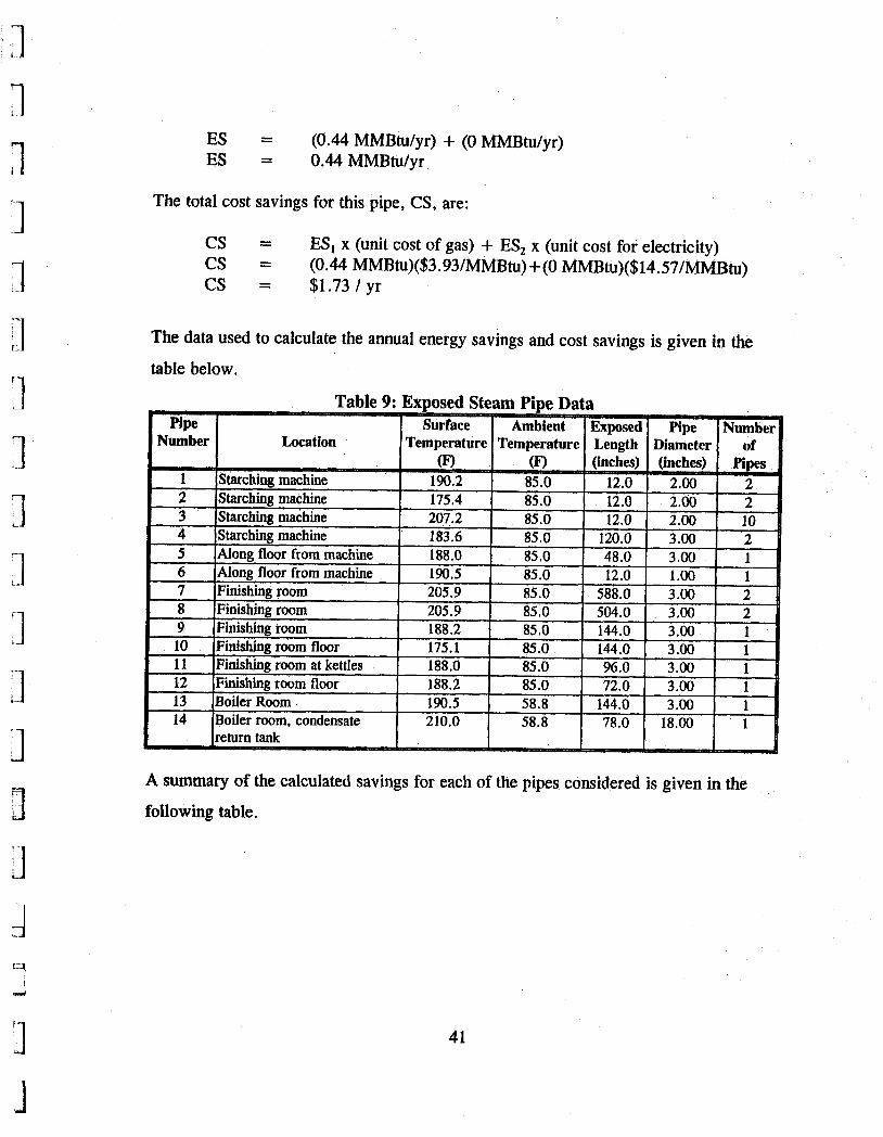
The data used to calculate the annual energy savings and cost savings is given in the
table below.
A summary of the calculated savings for each of the pipes considered is given in the
following table.
41

n 1 1 1 7 1 3 1 n 3 II il 1
:I
m
I
The estimated total annual energy savings, ES, from the table are:
The total cost savings, CS, are:
ES = 436.92 MMBtu/yr
CS = $1717.11 /yr
on Cost
The estimated total implementation cost, as shown in the following table, is $247.53.
The insulation recommended is fiberglass pipe wrap with an R value of 3 and an aluminum-vinyl outer wrap. The implementation cost is based on a material cost of
$1.00 per square foot of insulation and a labor cost of $10 per hour with each pipe
taking twenty minutes to insulate. The total cost savings of $1717 per year would pay
for the total estimated implementation cost of $247.53 within 1.7 months.
42

n
n n
n 1 7 L
1 3
q i
3.3 Lights
Industrial lighting systems pravide two visual functions to building occupants. “The
first is to provide enough light so the occupants can perceive two-dimensional words,
graphics, symbols, and other markings. The second function is the perception of the
three-dimensional items, such as equipment and furniture. ”* “The quality of lighting is
determined by a variety of factors such as glare, contrast, color, and foot-candle levels,
which are somewhat elusive or subjective and not readily measured. Only foot-candle
levels can easily be measured with a meter.”7 Careful examination of area lighting
levels with a foot-candle meter can sometimes reveal overlit areas that can be delamped
for cost savings. Many lighting handbooks provide recommended light levels that can
assist in determining if areas are overlit. Table 12 contains a list of recommended light
levels for a selection of areas.
3 43

n n 1 -3 3 1 1
-1
3 3
d
Table 12: Lighting Levels for Various Areas * Location
Private Offices Reading handwriting, fair reproductions, filing, mail sorting Reading high contrast or well-printed materials Conferring and Interviewing
Rough bench and machine work Ordinary automatic machines, rough grinding, fine buffing and polishing fine bench work, fine automatic machines, medium grinding, fine buffing and polishing Extra fine bench and machine work, fine grinding
General illumination Precision manual arc welding
Machine Shops
Welding
Storage Areas Active-medium materials Active-rough, bulky materials Inactive storage
Recommended Foot-candles
100
30 30
50 la0
500
1,000
50 1,000 1,000
20 10 5
Savings can also be obtained by replacing the current lighting system with more
efficient bulbs and ballasts, and installation of occupancy sensors or timers to reduce
the unnecessary lighting of unoccupied areas. The energy conservation opportunities
that follow discuss the savings that can be obtained through the use of high efficiency
lighting and high intensity discharge lighting.
3.3.1 High Efficiency Lighting
One of the more simple methods to obtain savings with a lighting system is to replace
existing lamps with high-efficiency (lower wattage) lamps as the existing lamps fail.
High efficiency lamps use less energy than standard lamps and provide nearly
equivalent light output.
4
3 1
44

n I n 3 n ;I
The estimated energy savings that can be realized by lreplacing all corivetitional
efficiency lamps with high efficiency lamps, are given by the following relation:
Energy Savings = Current Energy Use - Proposed Energy Use
The energy usage for a given area is calculated as follows:
Energy Use = (# fixtures) x (Wattage) x (hrs/yr)
The wattage for a fluorescent fixture is the bulb wattage plus the ballast wattage per
fixture. Since the energy savings for this recommendation are achieved on an
incremental basis as existing lamps fail, the annual savings due to replacing failed
standard lamps with higher efficiency lamps will depend on the life of the old lamps.
Assuming an even distribution of lamp life throughout the areas considered, the current
annual lamp replacement fraction, f, is given by:
f = (operating hrs/yr) / (bulb life hrs)
As an example, the value of the lamp replacement fraction, f, for an area which is
lighted for 2,000 hr/yr with lamps that have an average life of 10,000 hours, can be
estimated as follows:
f = 2,000 hrs/yr I 10,000 hrs f - - 0.20
This means that approximately 20% of the lamps in the area will fail in a given year.
The energy savings for an area in the first year would be the fraction of lamps that fail
in the first year multiplied by the difference in the total proposed and total current
electrical energy usage for all lamps in a given area. Each year, more of the original
existing lamps are also converted over to high efficiency lamps; thus, the energy
savings will increase until all of the existing lamps have been replaced. This is when
the full energy and cost savings will be realized.
The anticipated first year’s incremental cost savings, from replacement of lamps in an
area are estimated as:
Cost Savings = 0.20 x Energy Savings x Average Cost of Electricity
I 1
45

:1 1 '1 1
3
L..
I
Lj
a
The cost of implementation is based on replacement of existing lamps with
high-efficiency lamps as old lamps fail. This cost will simply be the difference
between the price of regular and high-efficiency lamps, since no additional labor costs
should be realized. The wattage of high efficiency lamps and their associated costs cajn
be obtained from any lighting supplier.
High EMciency Fluorescent Lights at a North Carolina Manufacturer of Folding Paper Cartons Following is the assessment recommendation developed for a North Carolina
manufacturer that illuminated the facility with standard fluorescent light fixtures.
During the energy assessment performed by the EADC at NCSU, the assessment team
gathered data on the number and type of lights being used. This data was then used to
determine the savings that could be obtained by installing high efficiency fluorescent
lamps as the existing lamps burn out. These savings were estimated as:
Estimated Energy Savings = 173,394 kWh/yr Estimated Cost Savings = $10,577.23/yr Estimated Implementation Cost = $2,946 Simple Payback Period = 3.3months
d Sav-
A detailed tabular breakdown of the lighting calculations for this facility is shown in
the Existing Lighting and Proposed Lighting tables which provide an area-by-area
analysis, The values given under the Existing Lighting heading are the result of a lighting survey conducted during the facility visit. Values in the Proposed Lighting
table were calculated based on replacement of all standard lamps with high efficiency
lamps.
The wattage for a fluorescent fixture is the bulb Wattage plus the ballast Wattage per
fixture. As an example, the estimated energy savings for replacing all the high output
F96T12 lamps with high efficiency lamps in the warehouse area, are given by the
following :
46

I
3 3 c
3 .-_ '1 111
11 I
Current Energy Use = 454 fixtures x 253 W/fixture x 6,000 hrs/yr - - 689,172 kWh/yr
Proposed Energy Use = 454 fixtures x 213 Wlfixture x 6,000 hrs/yr = 580,212 kWh/yr
Energy Savings = 689,172 - 580,212 = 108,960 kWh/yr
Cost Savings = 108,960 kWh/yr x $0.06l/kWh = $6,646.56/yr.
The Proposed Lighting table below describes the number and wattage of the higher
efficiency lamps. The following specifications for replacement lamps that use less
power while providing equivalent levels of illumination were gathered from
manufacturers' literature.
47

The energy savings after all the lamps have been replaced can be calculated using the
data in the Existing Lighting and the Proposed Lighting tables. From these tables the
total estimated energy savings after all the lamps have been replaced, are:
Energy Savings = 1,693,700 - 1,520,306 = 173,394 kWNyr
The anticipated annual cost savings due to replacement and removal of lamps are
estimated as:
Cost Savings = 173,394 kWh/yr x $O.O6l/kWh = $10,577.03 / yr.
Removal and replacement of lamps will save $10,577.03 per year after all high
efficiency lamps have been installed.
Initially, the annual savings due to replacing burned out standard lamps with higher
efficiency lamps will depend on the life of the old lamps. This measure is
recommended on an incremental basis (as the lamps burn out); therefore, both total and
incremental savings are given in this recommendation. As an example, the value of the
lamp replacement fraction, f, for the warehouse area, which is lighted for 6,000 hr/yr
with lamps that have an average life of 10,OOO hours, can be estimated as follows:
f = 6,000 hrslyr / 10,000 hrs f = 0.60
This means that approximately 60% of the lamps in the warehouse area will fail in a
given year. The energy savings for an area in the first year would be the fraction of
lamps that burn out in the first year multiplied by the difference in the total proposed
and total current electrical energy usage for all lamps in a given area. Each year, more
of the original existing lamps are also converted over to high efficiency lamps; thus,
the energy savings will increase until all of the existing lamps have been replaced.
This is when the full energy and cost savings will be realized. The anticipated first
year's incremental cost savings, from replacement of lamps in the warehouse area are
estimated as:
3 48
J

n n n n 3 n 1 c.
1
I
Cost Savings = 0.60 x $6,646.56 = $3,987.94
The cost of implementation is based on replacement of existing lamps with
high-efficiency lamps as old lamps burn out. This cost will simply be the difference
between the price of regular and high-efficiency lamps, since no additional labor costs
should be realized.
Table 16: Summary of Lamp Costs
Implementation Cost = 2,946 bulbs x $1.00 /bulb = $2,946
Simple Payback = Implementation Cost / Cost Savings = ($2,946) / ($10,577.03/yr) = 0.28 years = 3.3 months
3.3.2 High Intensity Discharge (HID) Lighting
Often times fluorescent lighting is installed in areas that have severe humidity or
temperature conditions that cause the lamps to fail frequently. By replacing the
49

n * _ 1 n 9 n
1 i.- 7 3 CI 1
II
3
existing fluorescent fixtures in these areas with an HID type of lighting like metal
halide fixtures, the lights can better withstand the conditions of the space.
Due to the higher light output (and highet wattage requirement) associated with HID
lights, a fewer number of these lights will have to be installed to achieve an equivalent
lighting level. In addition, the higher efficiency of the HID lighting will result in
energy savings. This savings can be estimated by calculating the current energy
consumption of the fluorescent lighting minus the proposed energy consumption of the
HID lighting. A lighting supplier can assist in determining how many HID fixtures
will be needed and their associated energy requirements.
Energy Requirement = Energy Savings = Fluorescent Energy - HID Energy Energy Cost Savings =
# fixtures x Wattdfixture x hrs/yr.
Energy Savings x Average Cost of Electricity
Additional savings can be estimated by taking into the consideration the reduction in
frequency of bulb replacement associated with HID lights. This can be obtained by
comparing the number of changes that occur with the old system versus the new system
times the cost of the lamp and the labor for changing the lamp. Note that these savings
will be incremental.
Installing HID Lights at a South Carolina Manufacturer of Woven Narrow Fabric Following is the assessment recommendation developed for a South Carolina
manufacturer that weaves, dyes, and finishes narrow fabric. The finishing room is
illuminated with fluorescent lighting, but these lamps fail frequently due the high
humidity that must be maintained in the area to reduce static electricity buildup on the
fabric during finishing. During the energy assessment performed by the EADC at
NCSU, the assessment team gathered data on the number and type of fluorescent lights
used to determine the savings that could be obtained by installing HID lighting. HID
lighting can better withstand the conditions of the space.
J 50

The savings were estimated as:
Estimated Energy Savings Estimated Cost Savings = $833/yr. Estimated Implementation Cost = $2,100 Simple Payback Period = 30.2months
= 4,320 kWh/yr.
d Savinps
During the facility assessment, it was noted that fluorescent lighting was installed in the
finishing room, where temperatures near the roof approach 120°F with high humidity.
As a result, the fluorescent fixtures fail quickly, necessitating replacement. It is
estimated that the estimated life of a fluorescent lamp is about half of the normal life,
or about 5,000 hours.
The 25 F96T12 fixtures in the finishing room can be replaced with 7, 400 Watt metal
halide fixtures, that have a life of about 20,000 hours. The energy consumed by the
fluorescent and metal halide fixtures are:
Fluorescent Energy = 25 fixtures x 172 Wjfixture x 4,000 hrs/yr. = 17,200 kWh/yr.
Metal Halide Energy = 7 x 460 W/fixture x 4,000 hrs/yr. = 12,880 kWh/yr.
Energy Savings = 17,200 - 12,880 kWh/yr = 4,320 kWh/yr.
Energy Cost Savifigs = 4,320 kWh/yr. x $O.O67/kWh = $289/yr.
The energy savings calculated is due to the increase in efficiency from standard
F96T12 lamps to metal halide fixtures.
Also, there is a cost of labor associated with replacing lamps in the fluorescent fixtures.
One metal halide lamp will last four times as long as a fluorescent lamp. The cost of
fluorescent lamps and the installation labor is estimated below.
51

I
Fluorescent Cost = = $3,000
4 changes x 50 lamps x ($10 lamp + $5 labor)
Metal Halide Cost = 7 lamps x ($30 lamp + $10 labor) = $280
Cost Difference = $2,720
This cost difference is spread out over a five year period since the area operates 4,000
hours per year. The annual cost savings are:
= $544/yr. Maintenance Savings = $2,720 1 5 years
The total cost savings are:
Total Cost Savings = Energy Cost Savings + Maintenance Savings = $289 + $5441yr. = $833/yr.
The cost to install a metal halide fixtures is estimated to be $300 each, which includes
materials and installation. For seven fixtures, this is a cost of $2,100. The simple
payback is:
Simple Payback = $2,100 I $833/yr. = 30.2 months
3.3.3 Additional Lighting Suggestions
Following are some things to be considei-ed when working with a lighting system:
When disconnecting lamps, it is important to disconnect the ballast as well as removing the lamp itself, since the ballast draws energy even when there are no lamps in the fixture.
* Typically there are two lamps per ballast in fluorescent fixtures. Lamp life ratings for fluorescent lamps are based on the assumption of 3 hours between lamp start-ups. If the time between starts is reduced to only one hour, lamp life is reduced by 25 % .
* Lamp life ratings for Mercury Vapor, Metal Halide and High Pressure Sodium ate based on the assumption of 10 hours between starts. If time between starts is reduced to 5 hours, the lamp life is reduced by 25 % .9
d
52

n 1
% - I n 1 3 i.. 1 1
3
3
3
d
The Color Rendering Index (CRI) is a scale from 0-100 on how well a given lamp renders colors. A lamp with a CRI of 100 will make objects appear as they do in sunlight. High pressure sodium lamps have a CRI of about 25 and metal halide has a CRI of about 65. It is suggested that lamps of both types be tested before committing to either lamp. Painting the ceiling of the building is an excellent way of getting more light to the production floor. A light colored ceiling will reflect light back to the floor and reduce the need for lighting fixtures.
6 Installing occupancy sensors or photosensors in certain areas of a facility can assist in using lighting only when it is necessary.
3.4 High Efficiency Motors
Standard electric motors are the workhorse of the common industrial facility. Due to
the fact that most motors are so dependable and rugged, they are often the least
understood and most unappreciated pieces of equipment in most facilities. lo
“A standard motor is a compromise between efficiency, endurance, starting torque, initial cost and othet. considerations. The emphasis, however, is in holding down the initial cost to remain competitive. Unfortunately, lower first cost usually means higher operating cost. The difference in standard and energy efficient motors can be categorized into design modification and changes in materials and/or processes. These improvements are focused on minimizing losses and better heat dissipation. Reducing bearing friction, improving winding insulation and enhanced design for better cooling are examples of the techniques used to improve a motor’s full load efficiency.” lo
By installing high efficiency motors as the standard motors currently used wear out, energy savings can be obtained. Some reasons for using energy efficient motors are: lo
0 Higher operating efficiency 6 Lower operating costs 6 Lower demand charges, now and in the future
Better power factor Lower branch circuit losses
* Lower no load losses 6 Reduced air conditioning load
Improved bearing life
The motors that are most applicable to obtain energy savings through replacement with
high efficiency motors have some of the following characteristics:
the annual hours of operation are high
3 53

1 1 1 L 1
3 n
d
the required starting torque is high, or 6 the increased power factor is needed.
Many facilities rewind motors as they wear out to avoid the cost of total replacement.
However, studies have shown that it is usually uneconomical to repair old motors.
Rewound motors are on average 4% less efficient than new standard motors.
Therefore, it is often recommend that the worn out motor be replaced with a new high
efficiency motor to obtain savings in operating costs.
Depending on the horsepower rating, operating efficiencies of high efficiency motors
may be from 1% to 10% higher than the operating efficiencies of standard motors. In
general, the larger the motor, the smaller the efficiency increase. Normally, a cost
premium (or cost differential) must be paid for the high efficiency motors. The
estimated efficiencies of standard motors, potential increase in efficiency and cost
premiums for various horsepower ratings are summarized in Table 17. This data was
obtained from averaging information from several motor manufacturers.
The annual energy savings, ES, which could be realized by installing high efficiency
motors of a given size on a replacement basis, can be estimated as follows:
ES = HP x N x H x LF x C x (l/Ec - l/Ep)
where,
HP = horsepower of motor considered, hp N = H = LF =
C = conversion constant, 0.746 kW/hp EC = estimated efficiency of existing motor, no units EP = estimated efficiency of proposed motor, no units
number of motors of a given size, no units annual operating hours of equipment driven by motor, h/yr fraction of rated load at which motor normally operates, no units (frequently estimated as 0.75, depending on application)
d
54

1 Table 17: Motor Efficiency Lookup Table
n n n 3 3 3
3
-1
10 0.850 0,909 150 15 0.860 0.915 200 20 0.870 0.922 250 25 0.880 0,929 300 30 0.890 0.930 400 40 0.900 0.934 500 50 0.905 0.937 700 w 60 0.910 0.939 800 75 0.915 0.942 900
400 0.960 0.970 7,000 500 0.960 0,970 8,000
Cost savings associated with the installation of a high efficiency motor can be obtained
by multiplying the energy savings by the average cost of electricity. Additional
information on high efficiency motors can be obtained from the Industrial
Electrotechnology Laboratory at North Carolina State University, telephone number
9 19-5 15-394 1. .
55

1 i - 1 n n 3 n 3 3 1 1 3 3
3 Ll
High Efficiency Motors at a North Carolina Manufacturer of Injection Molded Automobile Parts Following is the assessment recommendation developed for a North Carolina
manufacturer that uses various sized motors to operate injection molding machines and
pumps. During the energy assessment performed by the EADC at NCSU, the
assessment team located and gathered data from many of the motors in the facility.
This data was then used to determine the savings that could be obtained by replacing
these motors with high efficiency units once the existing motors wear out. These
savings were estimated as:
Estimated Energy Savings = 82,556 kWh/yr Estimated Cost Savings = $3,55O/yr Estimated Implementation Cost = $4,020 Simple Payback = 13.6months
Saviogs
As an example, the energy savings, ES, for the 30 hp, #16 Mold Injector Gear Pump
motor was estimated as:
ES = (30 hp)(1)(8,400 hrs/yr)(0.75)(0.746 kW/hp)(1/0.890 - U0.930) ES = 6,814 kWh/yr
Annual cost savings for the 30 hp motor, CS, are estimated as:
CS = (6,814 kWNyr)($0.043 /kWh) CS = $293 /yr
A summary of savings calculations for all of the motors considered is given in the
following table.
-Savings
The cost savings listed above are incurred gradually as the existing motors wear out
and are replaced by high efficiency motors. The total annual savings will occur after
all motors are replaced.
56

1 n
. i n n
n 3 1 3 3 1
i- 3
Table 18: Summary of Motor Energy and Cost Savings
The total implementation cost is $4,020. This cost is based on the difference betweeli
the cost for installing high efficiency motors and that for installing standard motors, for
each size shown in the table. This is based on the assumption that the standard motors
currently used will be replaced with high efficiency motors as the standard motors wear
out. The payback for individual motors of a particular size is the same as the payback
listed in the tables for all motors of that size. The total cost savings of $3,551 would
pay for the total implementation cost within about 13.6 months.
Driven Equipment
57

d
4. Waste Minimization / Pollution Prevention
In addition to the savings that can be achieved through energy conservation, facilities
are finding benefits from pollution prevention activities. Pollution Prevention can be
described as “the use of materials, processes, or practices that reduce or eliminate
creation of pollutants or wastes at the source. It includes practices that reduce
of hazardous and non-hazardous materials, energy, water, or other res
those that protect natural resources through conservation or more efficient use. ’”’ Over the past ten years, pollution prevention has grown through legislation and
necessity to provide facilities with a method for reducing costs and liability for wastes.
This field, which is sometimes referred to as waste minimization by the Environmental
Protection Agency (EPA), has enabled companies to take advantage of many benefits
through properly addressing the wastes produced in their facilities.
It is the purpose of this section to provide the reader with an overview of the field of
pollution prevention, and provide references from which further information can be
obtained on how to establish a pollution prevention program and to address the wastes
produced within the facility to obtain cost savings. The amount of literature available
on the subject of pollution prevention has gtown enormously over the past few years.
Successful case studies and methodologies for pollution prevention are abundant, and
technical assistance is readily available through local, state, and federal groups.
4.1 Benefits Associated with Pollution Prevention
Pollution prevention activities provides industry with a tool to align its economic
interests with the goals established by national environmental regulatory agencies. The
main benefits of pollution prevention activities can be summarized as:
Reduced risk of liability:
11
The cradle to grave liability associated with the production and disposal of
industrial wastes is a major incentive to eliminate or reduce the toxicity of the
pollutant. Environmental regulations require documentation of pollution prevention
’J 1- 58

‘- 1 n rl 1 n
3 m
11
3
efforts associated with various wastes. The excessive production or mishandling of
these wastes can lead to heavy fines and legal actions against those responsible.
0 Reduced operating costs:
The savings that can be obtained from pollution prevention activities include
immediate savings on materials, elimination of costs associated with docu
and reporting procedures , and anticipated savings from avoiding potential future
costs. Material cost savings can be obtained through improved operating
procedures that convert more of the raw material into finished product.
Improved Company Image:
Industries who show a commitment to reducing the impact their operations have on the environment can improve the companies image with consumers and the
community,
4.2 Waste Management Hierarchy
Although the emphasis of pollution prevention practices are focused on reduction of
waste at the source, complete elimination of waste is not always possible, and
alternative methods of dealing with the waste must be investigated. Even if processes
are modified to make better use of materials and reduce waste, some wastes are
inherently present. Figure 3 shows the preferred hierarchy for waste management.
As can be seen in this figure, source reduction is given highest priority since it is the
most ideal method of dealing with the waste, eliminating or reducing the amount
produced in the process. This basic concept was overlooked for many years while a
great deal of effort was being placed on “end-of-the-pipe” treatment. The changes
involved in source reduction activities can be broken down into product changes and
process changes, Figure 4 illustrates this and gives examples of each type of change.
a 59

n
Source Reduction (Highest Priority)
n 6 Environmentally
Friendly Design of Avoid Solvent Use New Products Modify Product to - 6 Product Changes Extend Coating Life Source Elimination
i 1
Recycling
1 Solvent Recycling
Reuse From a Spent - Reclamation Plating Bath Volatile Organic Recovery
.. 1
Treatment
J
of Organic Solvent Precipitation of Heavy Metal From a Spent Plating Bath
Stabilization Neutralization Precipitation
--+ Evaporation Incineration Scrubbhg
L1 L 1 :I 3 111
3
d
60

3
Product Changes 0 Design for Less
Environmental Impact Increased Product Life
n
Process Changes
Figure 4: Source Reduction Methods ''
Input Material Changes Material Purification Substitution of Less
3
Technology Changes Layout Changes
0 Increased Automation 0 Improved Operating
Conditions 0 Improved Equipment
New Technology
1
'_ 1
3 II 3 a 111
I I I 1 I I I
Improved Operating Practices * Operating and Maintenance
m Management Practices m Stream Segregation D Material Handling
Improvements Production Scheduling
m Inventory Control m Training I) Waste Segregation
Procedures
I
If source reduction techniques cannot eliminate all wastes, proper tecycling or reuse of
the waste should be investigated. This can range from recycling of office paper and
aluminum cans, to reuse of pallets and barrels, to the transfer of waste from one
facility to be used as a raw material in another industry. If these methods are still not
applicable to the waste stream, treatment of the waste, either on-site or off-site, should
be considered before disposal.
Figure 5 outlines a suggested procedure for developing a pollution prevention / waste
minimization program and identifying and analyzing areas prime for waste reduction.
1 I d
61

Li 1 d
Figure 5: The Waste Minimization Assessment Procedure12
The Recognized Need to Minimize Waste
PLANNING AND ORGANIZATION Get Management Commitment
0 Set Overall Assessment Program Goals
6 Collect Process and Facility Data 6 Prioritize and Select Assessment Targets 6 Select People for Assessment Teams 6 Review Data and Inspect Site
Recommended Options
IMPLEMENTATION 6 Justify projects and Obtain Funding 6 Installation (equipment) 6 Implementation (procedure) Repeat the 6 Evaluate Performance Process
t Successfully Implemented
Waste Minimization Projects Pollution prevention should be included in the corporate objectives in order for it to be
successful within a facility. As can be seen in Figure 5 , pollution prevention is a
62

n 1 3
L _ 1 3 L. 1
3
:I 3 11 g 1 -I d 1
d
continuous cycle of assessment, analysis, and implementation. The opportunities for
improvement and savings can be so great that it should not be looked at as a temporary
fix to recurring problems.
4.3 Energy Conservation and Pollutibn Prevention
Energy conservation and pollution prevention activities are complementary. Energy
reduction is most visible when production wastes are reduced. These savings in energy
are not only seen directly from the energy bills, but also through the reduced energy
required to treat and transport the wastes. However there are cases when the
modification of a production process might increase the amount of energy required,
This type of trade-off must be considered in the feasibility analysis of the pollution
prevention project.
4.4 Life Cycle Analysis
A tool that can be used to assist in the comparison of a proposed pollution prevention
process to the current process is called a Life Cycle Analysis. “The concept of life-
cycle assessment is to evaluate the environmental effects associated with any given
activity from the initial gathering of raw material from the earth until the point at which
all residuals are teturned to the earth,” which is known as ‘cradle-to-gra~e.”~ There
are three components to the life-cycle analysis: Inventory Analysis, Impact Analysis,
and Improvement Analysis. Following is a brief overview of each component.
The inventory analysis is composed of the identification of the elements in each
material and energy input and output streams, as well as the quantification of the inputs
and output^.'^ Flow diagrams can be used to map out the “cradle-to-grave” flow of
materials and energy. Once the flow is understood, quantification of “energy, raw
material requirements, atmospheric emissions, waterborne emissions, solid wastes, and
other releases for the entire life cycle of a product, package, process, material, or
activity” can be performed. l3
63
The impact analysis uses the information obtained in the inventory analysis to
determine the potential environmental effects associated with the inputs and outputs.
This part of the life-cycle analysis is one of the most challenging due: to the fact that the
methods for evaluating impacts on the environment are not completely developed.
These environmental impacts include, but are not restricted to: 14
resource depletion ecological degradation human health effects other human welfare effects (Le. loss of recreational value or scenic beauty).
This third component of the life-cycle analysis is “a systematic evaluation of the needs
and opportunities to reduce the environmental burden associated with energy and raw material use and waste emissions throughout the life cycle of a product, process, or
activity. Quantitative and qualitative measures can be utilized to measure the
improvements proposed in comparison to a current process or a competing process.
Life cycle analysis is not a tool that needs to be used to evaluate all pollution
prevention activities. It is both a complex and time consuming process of gathering
and analyzing data. Two references used to summarize this concept, the Life-Cycle
Assessment: Inventory Guidelines and Principles, and the Life Cycle Design Guidance
Manual are good sources for learning more about the life-cycle analysis tool (see
reference 13 and 14).
4.5 Waste Minimization Case Studies from Carolina Industries
The Energy Analysis and Diagnostic Center at NCSU has recently incorporated waste
minimization assessments into the energy assessment program. Due to the fact the
assessments are composed of one day site visits, the majority of the waste minimization
assessment is based on the information obtained from plant petsonnel and visual
64

n 1
IT
i 1 J c3 J 3 II 3
inspection of processes and facility activities. Following are several waste
minimization recommendations made by the EADC to North and South Carolina
manufacturers. They are intended to give insight into some of the simple activities that
facilities can perform to reduce or properly reuse wastes in order to obtain cost
savings.
Using Waste Water Sludge as a Boiler Fuel at a South Carolina Manufacturer of Dyed and Finished Knitted Cloth This facility currently produced approximately 15 tons of waste water sludge per week
from its water treatment facility and disposes of it in an industrial lined landfill. It was
recommended that if environmentally feasible, hot flue gases leaving the facilities
wood-fired boiler could be used to dry the sludge. The dried sludge could be stored in
a separate silo and fed from the silo into the wood fuel stream to the boiler. At present
plant operating conditions, the heat value from the sludge will comprise about 1.62
percent of the annual fuel input to the boiler. This recommended action will serve to
reduce waste (i.e., eliminate sludge to landfill), while simultaneously displacing some
of the wood fuel, which is now purchased at a cost of $1.276 per MMBtu.
Estimated Energy Savings Estimated Energy Cost Savings Estimated Landfill Savings = $20,80O/yr Total Savings = $24,714/yr Estimated Implementation Cost = $18,000 Simple Payback = 8.7 months
= 3,067 MMBtu/yr = $3,914/yr
After being processed in a sludge press, the waste water sludge is 20 percent solids, or
80 percent moisture. The cost to dispose of the sludge in a landfill was estimated by
plant personnel at $190 per 7 ton load (i.e., a $65 hauling fee plus a $125 landfill fee).
This yields a weekly sludge removal cost of approximately $400. Plant management is
very concerned about (1) skyrocketing landfill costs in the near-term, and/or 2) hture
regulations which may prohibit the dumping of sludge. It is clear that some
alternatives to the sludge-to-landfill procedure must be explored.
65

The EADC at NCSU collected a sample of sludge and sent it to a testing laboratory for
an ultimate analysis. The results of this analysis (given below) are on a dry, percent by
weight, basis.
Table 20: Waste Water Slude Constituent
Carbon Hydrogen Nitrogen Oxygen Ash Sulfur Moisture
Analvsis Results % by weight
50.41 % 6.95% 6.17%
21.34% 14.19% 0.94% 0%
Heating Value. Btu/lb I 9.83 1
An analysis was conducted on the annual fuel usage of the wood fired boiler. The
analysis shows that the “as received” cost of the wood fuel is $1.276 per MMBtu. Table 21: Wood Fuel Quantification
If the moisture in the sludge is removed to a reasonable level (Le., 0 to 20 percent), the
dried sludge can be used as a boiler fuel to displace some of the purchased wood fuel.
Table 22: Waste Water Sludge Ouantificatfon
As the
Sludge Generated (wet) 15 tonslweek Sludge Generated (dry) 3 tonslweek Sludge Geaerated (dry) Energy Value of Dry Sludge 3,067 MMBtu/yr
bove table indicates, this sludge has an energy value of $3,914 per year, and
would displace 1.62 percent of the wood fuel which is now purchased.
66
1 Using sludge as a boiler fuel would also eliminate the cost associated with landfilling.
Present Cost of Sludge Disposal (landfill) = $400 $/wk = $20,000 $/year
Construct a drying chamber and storage silo system which incorporates (1) traveling
grates and/or screens on which the sludge is placed, (2) an opening into the chamber
above the grate for introducing the sludge into the chamber, (3) a duct opening below
the grates for introducing the hot flue gases into the chamber, and (4) a conveyor belt
for transporting the dried sludge to the silo. A separate induced draft fan may also be
required to control the amount of flue gas to the drying chamber.
n Cost
The cost of the drying chamber, storage silo, conveyor belts, induced draft fan, and
controls is estimated at $15,000. The additional labor associated with operating this
system is estimated at $3,000 per year.
d Sav-
Energy Savings = (3,067 MMktu/yr)x($l.276/MMBtu) = $3,914/yr
Waste Minimization Savings = ($4OO/wk)x(52 wWyr) = $20,800
Total Savings = $3,914 + $20,800 = $24,714
Implementation and Annual Labor Cost = $18,000
Based on the above costs and savings, the “sludge as fuel drying system’’ will pay for
itself in approximately 8.7 months.
(Recommendation by Dr. Herbert Eckerlin)
67

n
zi a
Water and Energy Conservation id 8 North Carolina Manufacturer of Synthetic Tarn This facility currently uses two large pressurized dyebecks to dye its synthetic yarn.
The vertical dyebecks have large domed lids which have a large amount of unused
volume. It was recommended that a space filler be installed to decrease the volume of
water required to fill the tank.
Estimated Energy Savings Estimated Waste Reduction Estimated Cost Savings Estimated Implementation Cost = $10,000 Simple Payback Period
= 279 MMBtu = 896,400 gallons/yr = $5,176 /yr
= 23.2 months
d S a v w
The estimated savings of this recommendation came from two sources, the elimination of the need to buy and heat the displaced water. The cost savings associated with
reduced water consumption, RW, are estimated below. This is based on data supplied
by the plant personnel that it is possible to displace approximately 150 gallons of water
per batch and that each unit runs 9 batches per day (total of 18 batches) for 332 days
per year.
RW = 150 gallons x 18 batcheslday x 332 dayslyr RW = 896,400 gallons/yr
At a cost of $4 per 1000 gallons of water, this represents a cost savings of $3,585/yr.
The second area of savings is associated with not having to heat the water. Assuming a
temperature change of 30°F from the incoming water main to the dyebeck, a specific
heat of 1 Btu/lb"F and a boiler efficiency of 0.8, the fuel savings, FS, is:
FS = FS = 279MMBtu/yr
896,400 gallons x 8.3 Iblgallon x 1 x 30°F / 0.8
With an approximate gas cost of $5.71/MMBtu, the resulting cost savings is $1,593/yr,
for a total cost savings of $5,176/yr.
68

1 7 3 3 i3 3 3
:I
11
I] Ij
n Cost
The implementation cost was estimated from Means Mechanical Cost Data, based on
time and materials for a welding crew for 3 days per dyebeck (for 2 dyebecks). This
cost was approximately $lO,OOO, which gives a payback period of 23.2 months.
(Recommendation by Adam Chmielewski)
Recycling Waste Polyethylene in a North Carolina Manufacturer of Fiber Optic Cables This facility uses polyethylene as a cover material for fiber optic cables. The plastic is
extruded over the fibers in a continuous process. Currently, some of the extruders are operated continuously even though glass fibers may not be present, due to the extensive
setup required. These machines may operate for several hours without fibers. This
polyethylene can not be recycled in-house due to very strict quality control measures in
place. However, other manufacturers can incorporate this material into their raw
polyethylene streams, reducing their material costs. The estimated savings of
collecting and recycling the clean polyethylene covers that are not used in the process
are:
Estimated Waste Savings Estimated Cost Savings = $1,017/yr. Estimated ImpIementation Cost = $0 Simple Payback Period = instantaneous
= 65,625 lb/yr.
d S a v w
It is proposed that the waste polyethylene from the process, without fibers, be collected
and sorted by color. After accumulation of a quantity of material, another
manufacturer can pay to have the material shipped to their plant and this be
incorporated into their raw material stream. Discussions with several facilities that use
polyethylene have shown that this is often done with other sources of polyethylene.
J 3
69

i 7 n
3 1 3 3 3 3 J 3 3 3
3 J'
The only savings from this recommendation is the savings in waste disposal. From
observations made during the site visit, the amount of wasted polyethylene is estimated
as : Daily Waste Material =
= 3.125 ft3/day. 120 min. x 30 ft/min. x 0.125 in2 x 1 ft2/144 in2
Annual Waste Material = 3.125 ft3/day x 350 days/yr. = 1,093.75 ft3/yr.
The density of polyethylene is about 60 Ib/ft3.
Annual Waste Material = 1,093.75 ft3/yr. x 60 Ib/ft3 = 65,625 lb/yr. = 32.8 tons/yr.
This is the amount of material that will not have to be landfilled. The cost of landfill
space is estimated as $3l/ton. The total cost per year of landfilling the waste
polyethylene is estimated as:
Landfill Cost = 32.8 tons/yr. x $3l/ton = $1,017/yr.
Note that this cost does not include transportation costs.
The waste polyethylene without fibers is a1
the facility, and the cost to segregate further by color is assumed minimal since the
extruders produce only one color at a time. Therefore, there is no implementation cost
associated with this recommendation. All that is required is that a manufacturer that
can use recycled polyethylene be located and be willing to pay the cost to ship the
material to their plant for recycling.
(Recommendation by Stephen Terry)
segregated from the other wastes in
Elimination of Wooden Pallet Disposal at a North Carolina Manufacturer of Air Compressors This facility currently receives its incoming materials on wooden pallets of various size and quality. These pallets are then collected in large dumpsters and sent to the landfill.
70

1 n
3
By giving these pallets away instead of landfilling them, the savings that could be obtained are:
Estimated Waste Savings = 1,750,000 lb/yr. Estimated Cost Savings = $50,00O/yr. Estimated Implementation Cost = $1,000 Simple Payback Period = 0.3 months
d Savings
There are several options this facility can choose from to avoid sending the pallets to the landfill, they are:
1. Exchange the pallets with other business in the area. It is often the case where a nearby business is having to purchase pallets for shipping materials, and the facility could donate or sell the pallets to these businesses.
2. Donate pallets to an industry that chips pallets for use as fuel, mulch, compost, or animal bedding (if the pallets are not treated or contaminated).
3. Recycle pallets. There are a number of private pallet rebuilders in the state of North Carolina that will pick up used pallets at no charge and rebuild them for resale.
The facility landfills approximately 175 wooden pallets per day, 5 days per week. This
costs the facility $200 per day for removal and landfill of the pallets. Assuming
production during 50 weeks per year, the annual cost of landfilling the pallets is
$50,000 per year. Estimating the weight of the pallets at 40 pounds, this
recommendation would represent a reduction in the waste sent to landfill of about
1,750,000 lb/yr.
The most feasible alternative for removal of the pallets is to give the pallets to a
recycler. It is estimated that implementation cost for giving the wooden pallets away
would be $l,O00. This would account for the time spent locating and setting up a
contract with the recycling business. No additional costs will be incurred for storage
due to the fact that the facility is already having to store the pallets for disposal. To
assist in locating a business to recycle the pallets, a copy of the Directory of Markets
for Recyclable Materials can be obtained from the North Carolina Office of Waste
Reduction (919-571-4100) or by contacting the EADC office (919-515-1878).
71

3 3 3 n 3 3 1 3 4 2
Appendix A: Conversion Factors
temperature: K=(OF-32)/1.8+273, and OF= 1.8(K-273)+32 density, p: 1 kg/m3 = 0.06243 lb/ft3 kinematic viscosity, v : 1 m2/s = 10.76 ft2/s thermal conductivity, k: 1 W/m K = 0.5779 Btu/(h ft OF)
v Convmon Factom 1 kWh = 3,413 Btu 1 therm = 100,000Btu 1 cu. ft. natural gas = 1,000 Btu (may vary with supplier)
1 gallon No. 2 oil = 140,000 Btu (may vary with supplier) 1 kilowatt = 1.341 hp
1 hp-hr = 2,545 Btu
Appendix B: Additional Information on Pollution Prevention
d. Freeman, Harry Me, McGraw-Hill, Inc. New York. 1995. This reference handbook covers the techniques, technologies, regulations, and strategies that define pollution prevention. Pollution prevention basics as well as information on specific industries is covered form many perspectives by the 78 contributing authors. 935 pages.
Facility Pollution Prevention Guide. Office of Research and Development. Washington, DC 20460. EPA/600/R-92/088. May 1992. Abstract: "The U . S . Environmental Protection Agency developed the Facility Pollution Prevention Guide for those who are interested in and responsible for pollution prevention in industrial or service facilities. It summarizes the benefits of a company- wide pollution prevention program and suggests ways to incorporate pollution prevention in company policies and practices. 143 pages.
United States EPA.
Guides to Pollution Prevention. United States EPA. Office of Research and Development. Washington, DC 20460. EPA/625/R-92/011. October 1992. These guides are a series of manuals that describe waste minimization options for specific industries. This is a continuing series, some of the industries covered are: Paint Manufacturing, Pesticide Formulating, Commercial Printing, Fabricated Metal, Printed Circuit Board Manufacturing, Pharmaceutical, Photoprocessing, Fiberglass Reinforced and Composite Plastics, Automotive Repair, Automotive Refinishing, Marine Maintenance and Repair, Metal Casting and Heat Treating, Metal Finishing.
12

1 The US EPA guidebooks also contain contact information for local, state, and federal programs that can assist in the technical and financial aspects of pollution prevention. These guidebooks and other information on pollution prevention can be obtained from:
CERI Publications unit, US EPA 26 W. Martin Luther King Drive Cincinnati, OH 45268 (513)-569-7562
To contact the EADC at NCSU for information on Energy Conservation of Pollution Prevention, write or call:
Energy Analysis ahd Diagnostic Center North Carolina State University Box 7910, Mechanical & Aerospace Engineering Raleigh, NC 27695-7910 (919)-5 15-1 878
The following centers can assist in obtaining information on pollution prevention and waste minimization:
Department of Environmental, Health, and Natural Resources Pollution Prevention Pays Program Office of Waste Reduction 3825 Barret Drive, 3rd Floor Raleigh, NC 27611-7687 (919) 5714100 Fax: (919) 571-4135
Waste Reduction Resource Center 3825 Barret Drive, 1st Floor P.O. Box 27687 Raleigh, NC 2761 1-7687 (919) 571-4100 (800) 476-8686
E¶J
73

1 1
1 1
3 3 3 L. ’1 3 II
Bibliography
’ Hu, $. David. Handbook o f l n d u s t r i a l v Conserva b. New York: Van Nostrand Reinhold. c1983.
York, c1979.
Carolina State University, 1995.
Institute, New York, 1961.
1985.
New York, ~1985 .
Chiogioji, Melvin H. v v C o m ’ . Marcel Dekker, Inc. New
Energy Analysis and Diagnostic Center. Assessment report boilerplate. North
“Compressed Air and Gas Handbook”, Third Edition, Compressed Air and Gas
ed Air m. A Guebook Cost Savings, Talbott, E.M., 5
Ozisik, M.N. Heat: A . McGraw-Hill Book Company.
’ Avallone, E.A., Baumeister, T. -oak for Me- ’ * . McGraw-Hill Book Company. New York, c1987.
NC D m a n d Community Development. “Energy Efficient Lighting: A Manual for Conservation. ” Energy/Preventive Maintenance Cost Reduction Program. Industrial Extension Service, NCSU.
Engineering Society of North America. New York, NY. 1981.
Efficiencies and Variable Speed Drives: A Manual for Conservation. ” EnergylPreventive Maintenance Cost Reduction Program, Industrial Extension Service, NCSU.
United States EPA. Office of Research and Development. Washington, DC 20460. EPA/600/R-92/088. May 1992.
l2 “Guide to Pollution Prevention. United States EPA. Office of Research and Development, Washington, DC 20460. EPA/625/R-92/011. October 1992.
l3 “Life Cycle Assessment: Inventory Guidelines and Principles.” US EPA. Office of Research and Development. Washington, DC. February 1993. EPA/600/R- 92/245.
System.” US EPA. Office of Research and Development. Washington, DC. January 1993. EPA/6oO/R-92/226.
“Illuminating Engineering Society Handbook Reference Volume. ” Illuminating
lo NC Department of Economic and Community Development. “Electric Motor
“Facility Pollution Prevention Guide.
l4 “Life Cycle Design Guidance Manual: Environmental Requirements ahd the Product
3
3 74


