

2003-11-06Dan Ellis 1
ELEN E4810: Digital Signal Processing
Topic 8:
Filter Design: IIR
1. Filter Design Specifications
2. Analog Filter Design
3. Digital Filters from Analog Prototypes
2003-11-06Dan Ellis 2
1. Filter Design Specifications
! The filter design process:
Design ImplementAnalysis
Pro
ble
mS
olu
tion
G(z)
transferfunction
performance
constraints
• magnitude response
• phase response
• cost/complexity
• FIR/IIR
• subtype
• order
• platform
• structure
• ...

2003-11-06Dan Ellis 3
Performance Constraints
! .. in terms of magnitude response:
2003-11-06Dan Ellis 4
! “Best” filter:
! improving one usually worsens others
! But: increasing filter order (i.e. cost)
improves all three measures
Performance Constraints
smallestPassband Ripple
greatest
Minimum SB Attenuation
narrowest
Transition Band

2003-11-06Dan Ellis 5
Passband Ripple
! Assume peak passband gain = 1
then minimum passband gain =
! Or, ripple
!
1
1+"2
!
"max = 20 log10 1+#2 dB
PB rippleparameter
2003-11-06Dan Ellis 6
Stopband Ripple
! Peak passband gain is A! larger than
peak stopband gain
! Hence, minimum stopband attenuation
SB rippleparameter
!
"s
= #20 log101A
= 20 log10 A dB

2003-11-06Dan Ellis 7
Filter Type Choice: FIR vs. IIRFIR
! No feedback(just zeros)
! Always stable
! Can belinear phase
! High order(20-2000)
! Unrelated tocontinuous-time filtering
IIR
! Feedback(poles & zeros)
! May be unstable
! Difficult to controlphase
! Typ. < 1/10thorder of FIR (4-20)
! Derive fromanalog prototype
BUT
2003-11-06Dan Ellis 8
FIR vs. IIR
! If you care about computational cost" use low-complexity IIR
(computation no object " Lin Phs FIR)
! If you care about phase response" use linear-phase FIR
(phase unimportant " go with simple IIR)

2003-11-06Dan Ellis 9
IIR Filter Design
! IIR filters are directly related to
analog filters (continuous time)
! via a mapping of H(s) (CT) to H(z) (DT) that
preserves many properties
! Analog filter design is sophisticated
! signal processing research since 1940s
" Design IIR filters via analog prototype
! hence, need to learn some CT filter design
2003-11-06Dan Ellis 10
2. Analog Filter Design
! Decades of analysis of transistor-based
filters – sophisticated, well understood
! Basic choices:! ripples vs. flatness in stop and/or passband! more ripples " narrower transition band
ripplesripplesElliptical
ripplesflatChebyshev II
flatripplesChebyshev I
flatflatButterworth
SBPBFamily

2003-11-06Dan Ellis 11
CT Transfer Functions
! Analog systems: s-transform (Laplace)
Continuous-time Discrete-time
!
Has( ) = h
at( )e"stdt#
!
Hd z( ) = hd n[ ]z"n#Transform
Frequencyresponse
Pole/zerodiagram
!
Ha j"( )
!
Hd ej"( )
s-plane
Re{s}
Im{s}
j#
stable
poles
stable
polesz-plane
Re{z}
Im{z}
1
ej$
2003-11-06Dan Ellis 12
Maximally flat in pass and stop bands
! Magnitude
response (LP):
! #<<#c,
|Ha(j#)|2 "1
! # = #c,
|Ha(j#)|2 = 1/2
Butterworth Filters
!
Ha j"( )2
=1
1+ ""c
( )2N
filterorder
N
3dB point

2003-11-06Dan Ellis 13
Butterworth Filters! #>>#c, |Ha(j#)|2 "(#c/#)2%
! flat "
@ # = 0 for n = 1 .. 2N-1
!
dn
d"nHa j"( )
2
= 0
Log-log
magnitude
response
6N dB/oct
rolloff
2003-11-06Dan Ellis 14
Butterworth Filters
! How to meet design specifications?
! !
!
1
1+"p
"c( )
2N=
1
1+#2
!
1
1+"p
"c( )
2N=1
A2
!
N "1
2
log10A2#1
$ 2( )log10
%s
%p( )
Design
Equation
!
k1
="
A2#1
=“discrimination”, <<1
!
k =" p
"s=“selectivity”, < 1

2003-11-06Dan Ellis 15
Butterworth Filters
! but what is Ha(s)?
! Traditionally, look it up in a table
! calculate N " normalized filter with #c = 1
! scale all coefficients for desired #c
! In fact,
where
!
Ha j"( )2
=1
1+ ( ""c
)2N
!
Has( ) =
1
s " pi( )
i#
!
pi="
cej# N +2 i$1
2N i =1..Ns-plane
Re{s}
Im{s}
#c!
!
!
!
!
s
"c
#
$ %
&
' (
2N
= )1
2003-11-06Dan Ellis 16
Butterworth Example
!
"1dB = 20 log101
1+#2
!
"#2 = 0.259
!
"40dB = 20 log101A
!
" A =100
Design a Butterworthfilter with 1 dB cutoffat 1kHz and aminimum attenuationof 40 dB at 5 kHz
!
"s
" p
= 5
!
N " 12
log1099990.259
log10 5
# N = 4 " 3.28

2003-11-06Dan Ellis 17
Butterworth Example
! Order N = 4 will satisfy constraints;What are #c and filter coefficients?
! from a table, #-1dB = 0.845 when #c = 1
& #c = 1000/0.845 = 1.184 kHz
! from a table, get normalized coefficients forN = 4, scale by 1184
! Or, use Matlab:
[b,a] =
butter(N,Wc,’s’);
M
2003-11-06Dan Ellis 18
Chebyshev I Filter
! Equiripple in passband (flat in stopband)" minimize maximum error
!
Ha j"( )2
=1
1+#2TN2( ""p
)
!
TN"( ) =
cos N cos#1"( ) " $1
cosh N cosh#1"( ) " >1
% & '
( '
Chebyshev
polynomial
of order N

2003-11-06Dan Ellis 19
Chebyshev I Filter
! Design procedure:
! desired passband ripple " '
! min. stopband atten., #p, #s " N :
!
1
A2
=1
1+" 2TN
2(#s
# p)
=1
1+" 2 cosh N cosh$1 #s
# p( )[ ]
2
!
" N #cosh
$1 A2$1
%( )cosh
$1 &s
&p( )
1/k1, discrimination
1/k, selectivity
2003-11-06Dan Ellis 20
Chebyshev I Filter
! What is Ha(s)?
! complicated, get from a table
! .. or from Matlab cheby1(N,r,Wp,’s’)
! all-pole; can inspect them:
..like squashed-in Butterworth
2003-11-06Dan Ellis 21
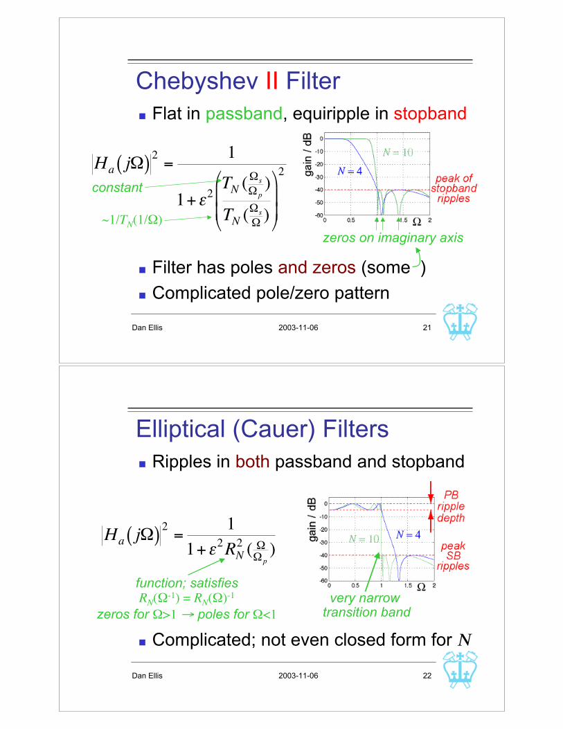
Chebyshev II Filter
! Flat in passband, equiripple in stopband
! Filter has poles and zeros (some )
! Complicated pole/zero pattern!
Ha j"( )2
=1
1+#2TN (
"s
"p
)
TN ("s
")
$
%
& &
'
(
) )
2
zeros on imaginary axis
constant
~1/TN(1/#)
2003-11-06Dan Ellis 22
Elliptical (Cauer) Filters
! Ripples in both passband and stopband
! Complicated; not even closed form for %
very narrow transition band
!
Ha j"( )2
=1
1+#2RN2( ""p
)
function; satisfiesRN(#-1) = RN(#)-1
zeros for #>1 " poles for #<1

2003-11-06Dan Ellis 23
Analog Filter Types Summary
N = 6
r = 3 dB
A = 40 dB
2003-11-06Dan Ellis 24
Analog Filter Transformations
! All filters types shown as lowpass;
other types (highpass, bandpass..)
derived via transformations
! i.e.
! General mapping of s-planeBUT keep j# " j#;
frequency response just ‘shuffled’
!
HLP
s( )
ˆ s = F"1
s( )
# HD
ˆ s ( )
Desired alternate
response; still a
rational polynomiallowpass
prototype
^

2003-11-06Dan Ellis 25
Lowpass-to-Highpass! Example transformation:
! take prototype HLP(s) polynomial
! replace s with
! simplify and rearrange" new polynomial HHP(s)
!
H HP ˆ s ( ) = HLP s( )s="p
ˆ " p
ˆ s
!
" pˆ " p
ˆ s
^
2003-11-06Dan Ellis 26
Lowpass-to-Highpass
! What happens to frequency response?
!
! Frequency axes inverted
!
s = j" # ˆ s ="p
ˆ " pj"
= j$"p
ˆ " p"( )
!
" ˆ # =$#p
ˆ # p
#
!
" =" p # ˆ " = $ ˆ " p
!
" <" p # ˆ " < $ ˆ " pLP passband HP passband
!
" >" p # ˆ " > $ ˆ " pLP stopband HP stopband
imaginary axis
stays on self...
...freq."freq.

2003-11-06Dan Ellis 27
Transformation Example
Design a Butterworth highpass filterwith PB edge -0.1dB @ 4 kHz (#p)
and SB edge -40 dB @ 1 kHz (#s)
! Lowpass prototype: make #p = 1
! Butterworth -0.1dB @ #p=1, -40dB @ #s=4
^
^
!
"#s = $( )#p
ˆ # pˆ # s
= $( )4
!
N "1
2
log10A2#1
$ 2( )log10
%s
%p( )
!
" N = 5
!
" p@# 0.1dB$1
1+ ("p
"c
)10
=10#0.1
10
!
"#c =# p /0.6866 =1.4564
2003-11-06Dan Ellis 28
Transformation Example
! LPF proto has
! Map to HPF:
!
pl
="cej# N +2l$1
2N Re{s}
Im{s}
#c!
!
!
!
!
" HLPs( ) =
#c
N
s $ pil( )
i=1
N
%
!
H HP ˆ s ( ) = HLP s( )s="p
ˆ " p
ˆ s
!
" H HP ˆ s ( ) =#c
N
#pˆ # p
ˆ s $ p
l( )l=1
N
%=
#cN
ˆ s N
# pˆ # p $ p
lˆ s ( )
l=1
N
%
N zeros@ s = 0^
new poles @ s = #p#p/pl^ ^

2003-11-06Dan Ellis 29
Transformation Example
! In Matlab:[N,Wc]=buttord(1,4,0.1,40,'s');[B,A] = butter(N, Wc, 's');[n,d] = lp2hp(B,A,2*pi*4000);
#p #s Rp Rs
2003-11-06Dan Ellis 30
3. Analog Protos " IIR Filters
! Can we map high-performance CT
filters to DT domain?
! Approach: transformation Ha(s)"G(z)
i.e.
where s = F(z) maps s-plane ( z-plane:
!
G z( ) = Has( )
s=F z( )
s-plane
Re{s}
Im{s}
z-plane
Re{z}
Im{z}
1
Ha(s0) G(z0)Every value of G(z)is a value of Ha(s)somewhere on the s-plane & vice-versa
s = F(z)

2003-11-06Dan Ellis 31
CT to DT Transformation
! Desired properties for s = F(z):
! s-plane j# axis ( z-plane unit circle
" preserves frequency response values
! s-plane LHHP ( z-plane unit circle interior
" preserves stability of poles
s-plane
Re{s}
Im{s}
j#
z-plane
Re{z}
Im{z}
1
ej$
LHHP(UCI
Im(u.c.
2003-11-06Dan Ellis 32
Bilinear Transformation
! Solution:
! Hence inverse:
! Freq. axis?
! Poles?
!
s =1" z
"1
1+ z"1
Bilinear
Transform
!
z =1+ s
1" sunique,
1:1 mapping
!
s = j" # z =1+ j"
1$ j"
|z| = 1 i.e.
on unit circle
!
s =" + j# $ z =1+"( )+ j#1%"( )% j#
!
" z2
=1+ 2# +# 2
+$2
1% 2# +# 2+$
2
)< 0
( |z| < 1

2003-11-06Dan Ellis 33
Bilinear Transformation
! How can entire half-plane fit inside u.c.?
! Highly nonuniform warping!
s-plane z-plane
2003-11-06Dan Ellis 34
Bilinear Transformation
! What is CT(DT freq. relation #($ ?
! i.e.
! infinite range of CT frequency
maps to finite DT freq. range
! nonlinear; as $ " *
!
z = ej"# s = 1$e
$ j"
1+e$ j" =
2 j sin" /2
2 cos" /2= j tan "
2u.circle
im.axis
!
" = tan #2( )
# = 2 tan$1"
!
"#<$ <#
!
"# <$ < #
!
d
d"#$% pack it all in!

2003-11-06Dan Ellis 35
Frequency Warping
! Bilinear transform makes
for all $, #
!
G ej"( ) = Ha j#( )
"=2 tan$1#
! Same gain & phase (', A...),
in same ‘order’,
but with
warped
frequency axis
2003-11-06Dan Ellis 36
Design Procedure! Obtain DT filter specs:
! general form (LP, HP...),
! ‘Warp’ frequencies to CT:
!
! Design analog filter for
! " Ha(s), CT filter polynomial
! Convert to DT domain:
! " G(z), rational polynomial in z
! Implement digital filter!
!
" p ," s,1
1+# 2, 1A
!
" p = tan# p
2
!
"s
= tan#s
2
!
" p ,"s,1
1+# 2, 1A
!
G z( ) = Has( )
s=1"z"1
1+z"1
Old-
style

2003-11-06Dan Ellis 37
Bilinear Transform Example
! DT domain requirements:Lowpass, 1 dB ripple in PB, $p = 0.4*,
SB attenuation ! 40 dB @ $s = 0.5*,
attenuation increases with frequency
SB ripples,
PB monotonic" Chebyshev I
2003-11-06Dan Ellis 38
Bilinear Transform Example
! Warp to CT domain:
! Magnitude specs:
1 dB PB ripple
40 dB SB atten.
!
" p = tan# p
2= tan 0.2$ = 0.7265 rad/sec
!
"s
= tan#s
2= tan 0.25$ =1.0 rad/sec
!
" 1
1+# 2=10
$1/20= 0.8913"# = 0.5087
!
" 1
A=10
#40 /20= 0.01" A =100

2003-11-06Dan Ellis 39
Bilinear Transform Example
! Chebyshev I design criteria:
! Design analog filter, map to DT, check:
!
N "cosh
#1 A2#1
$( )cosh
#1 %s
%p( )
= 7.09 i.e. need N = 8
>> N=8;
>> wp=0.7265;
>> [B,A]=cheby1(N,1,wp,'s');
>> [b,a] = bilinear(B,A,.5);
M
2003-11-06Dan Ellis 40
Other Filter Shapes
! Example was IIR LPF from LP prototype
! For other shapes (HPF, bandpass,...):
! Transform LP"X in CT or DT domain...
DTspecs
CTspecs
HLP(s)
HD(s)
GLP(z)
GD(z)
Bilinearwarp
Analogdesign
CTtrans
DTtrans
Bilineartransform
Bilineartransform
2003-11-06Dan Ellis 41
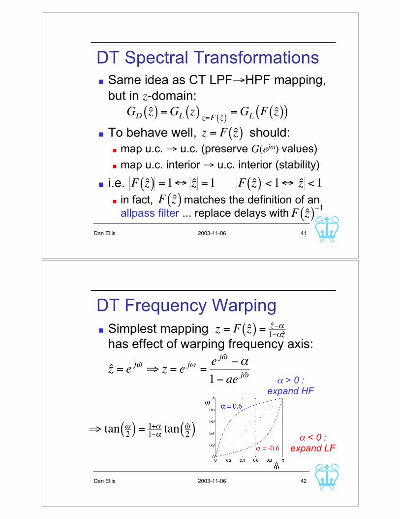
DT Spectral Transformations
! Same idea as CT LPF"HPF mapping,
but in z-domain:
! To behave well, should:
! map u.c. " u.c. (preserve G(ej$) values)
! map u.c. interior " u.c. interior (stability)
! i.e.
! in fact, matches the definition of an
allpass filter ... replace delays with
!
z = F ˆ z ( )
!
GD ˆ z ( ) = G
Lz( )
z=F ˆ z ( )= G
LF ˆ z ( )( )
!
F ˆ z ( ) =1" ˆ z =1
!
F ˆ z ( ) < 1" ˆ z < 1
!
F ˆ z ( )
!
F ˆ z ( )"1
2003-11-06Dan Ellis 42
DT Frequency Warping
! Simplest mapping
has effect of warping frequency axis:
!
z = F ˆ z ( ) = ˆ z "#1"#ˆ z
!
ˆ z = ej ˆ " # z = e
j"=
ej ˆ " $%
1$ aej ˆ "
!
" tan #2
( ) = 1+$1%$
tan ˆ # 2
( )
+ > 0 :expand HF
+ < 0 :expand LF
2003-11-06Dan Ellis 43
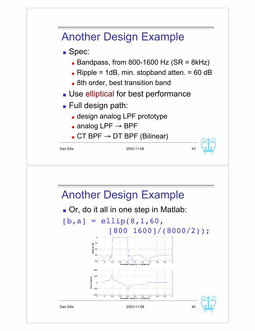
Another Design Example
! Spec:
! Bandpass, from 800-1600 Hz (SR = 8kHz)
! Ripple = 1dB, min. stopband atten. = 60 dB
! 8th order, best transition band
! Use elliptical for best performance
! Full design path:
! design analog LPF prototype
! analog LPF " BPF
! CT BPF " DT BPF (Bilinear)
2003-11-06Dan Ellis 44
Another Design Example
! Or, do it all in one step in Matlab:
[b,a] = ellip(8,1,60,
[800 1600]/(8000/2));


