

1
OPTIMIZING NETWORK LIFETIME IN SENSOR NETWORKS WITH LIMITEDRECHARGING CAPABILITIES
by
Jennifer Nichole Johnson
A Thesis Submitted to the
Office of Research and Graduate Studies
In Partial Fulfillment of the
Requirements for the Degree of
MASTER OF SCIENCE
School of Engineering and Computer ScienceEngineering Science
University of the PacificStockton, California
2014
OPTIMIZING NETWORK LIFETIME IN SENSOR NETWORKS WITH LIMITEDRECHARGING CAPABILITIES
by
Jennifer Nichole Johnson
APPROVED BY:
Thesis Advisor: Elizabeth Basha, Ph.D.
Committee Member: Carrick Detweiler, Ph.D.
Committee Member: Louise Stark, Ph.D.
Department Chairperson: Jennifer Ross, Ph.D.
Interim Dean of Graduate Studies: Bhaskara R. Jasti, Ph.D.
2

DEDICATION
I dedicate everything I have to my loving and supportive family. Without their help and
care I would have never pursued a degree in engineering nor a masters.
3

ACKNOWLEDGMENTS
I would like to thank my thesis advisor, Dr. Elizabeth Basha. For all the support she’s given
me throughout this whole process. I would also like to thank Dr. Carrick Detweiler and Dr.
Emma Bowring for being additional references to turn to. I would like to give additional
thanks to Dr. Louise Stark and Dr. Kenneth Hughes for their support and encouragement
as well.
I would also like to thank the National Science Foundation for supporting the research
(CSR #1217400 and CSR #1217428) as well as Pacific SURF and the Graduate office at
the University of the Pacific.
4

Optimizing Network Lifetime in Sensor Networks with Limited Recharging Capabilities
Abstract
by Jennifer Nichole JohnsonUniversity of the Pacific
2014
Monitoring the structural health of civil infrastructures with wireless sensor networks aids
in detecting failures early, but faces power challenges in ensuring reasonable network life-
times. Recharging select nodes with Unmanned Aerial Vehicles (UAVs) provides a solution
that currently can recharge a single node; however, questions arise on the effectiveness of
a limited recharging system, the appropriate node to recharge, and the best sink selection
algorithm for improving network lifetime given a limited recharging system. This paper
simulates such a network in order to answer those questions. This thesis first determines
whether or not recharging with a UAV is an effective method of delivering limited power to
the network. It then determines the best way to deliver that power. Finally, this thesis ex-
plores five different sink positioning algorithms to find which optimize the network lifetime
by load-balancing the energy in the network, all in combination with the added capability
of a UAV.
5

TABLE OF CONTENTS
LIST OF TABLES. . . . . . . . . . . . . . . . . . . . . . . . . . . . . . . . . . . . . . 9
LIST OF FIGURES . . . . . . . . . . . . . . . . . . . . . . . . . . . . . . . . . . . . . 10
CHAPTER
1. Introduction . . . . . . . . . . . . . . . . . . . . . . . . . . . . . . . . . . . . 12
1.1 Key Objectives . . . . . . . . . . . . . . . . . . . . . . . . . . . . . . 14
1.1.1 Setup: Limited Recharging . . . . . . . . . . . . . . . . . 15
1.1.2 Setup: Node Recharging Selection . . . . . . . . . . . . . 15
1.1.3 Setup: Energy Load-Balancing with Sink Positioning . . 16
1.2 Contributions of this Thesis . . . . . . . . . . . . . . . . . . . . . . 17
1.3 Overview of the Thesis . . . . . . . . . . . . . . . . . . . . . . . . . 17
2. Related Works . . . . . . . . . . . . . . . . . . . . . . . . . . . . . . . . . . . 19
2.1 Sink Selection and Movement Algorithms . . . . . . . . . . . . . . 20
3. The Network Model . . . . . . . . . . . . . . . . . . . . . . . . . . . . . . . 23
3.1 Network Functionality . . . . . . . . . . . . . . . . . . . . . . . . . 23
3.2 Network Assumptions . . . . . . . . . . . . . . . . . . . . . . . . . . 25
3.3 Recharging Implementation . . . . . . . . . . . . . . . . . . . . . . 26
4. The Simulation . . . . . . . . . . . . . . . . . . . . . . . . . . . . . . . . . . 28
4.1 The Simulation . . . . . . . . . . . . . . . . . . . . . . . . . . . . . 28
4.1.1 bridgeiter Function . . . . . . . . . . . . . . . . . . . . . 32
4.1.2 bridgesimfunc Function . . . . . . . . . . . . . . . . . . . 33
4.1.3 bridgesim Function . . . . . . . . . . . . . . . . . . . . . 33
6

4.1.4 Topology and Connectivity . . . . . . . . . . . . . . . . . 33
4.1.5 Main body of the Simulation . . . . . . . . . . . . . . . . 34
4.2 Routing Changes . . . . . . . . . . . . . . . . . . . . . . . . . . . . 37
4.3 Post-Processing . . . . . . . . . . . . . . . . . . . . . . . . . . . . . 39
4.4 Summary . . . . . . . . . . . . . . . . . . . . . . . . . . . . . . . . . 40
5. Sink Classifications . . . . . . . . . . . . . . . . . . . . . . . . . . . . . . . . 41
5.1 Static Sink Positioning . . . . . . . . . . . . . . . . . . . . . . . . . 42
5.2 Random Sink Movement . . . . . . . . . . . . . . . . . . . . . . . . 42
5.3 Controlled Sink Movement . . . . . . . . . . . . . . . . . . . . . . . 42
5.3.1 Circles . . . . . . . . . . . . . . . . . . . . . . . . . . . . 43
5.3.2 Linear Programming . . . . . . . . . . . . . . . . . . . . 43
5.3.3 Linear Programming: Periodic versus Exact Movement . 47
5.3.4 Linear Programming: Naivety . . . . . . . . . . . . . . . 49
5.4 Dynamic Sink Movement . . . . . . . . . . . . . . . . . . . . . . . . 50
5.5 Comparing the Algorithms . . . . . . . . . . . . . . . . . . . . . . . 52
6. Results . . . . . . . . . . . . . . . . . . . . . . . . . . . . . . . . . . . . . . . 53
6.1 Unmanned Aerial Vehicle Impact . . . . . . . . . . . . . . . . . . . 54
6.1.1 Recharging versus No Recharging . . . . . . . . . . . . . 54
6.1.2 UAV Recharge Amount . . . . . . . . . . . . . . . . . . . 55
6.2 Node Recharging Selection . . . . . . . . . . . . . . . . . . . . . . . 57
6.2.1 UAV Amount to Recharge . . . . . . . . . . . . . . . . . 58
6.2.2 Revisiting Recharge Amount . . . . . . . . . . . . . . . . 60
6.3 Sink Selection . . . . . . . . . . . . . . . . . . . . . . . . . . . . . . 62
7

6.3.1 Perimeter Walk . . . . . . . . . . . . . . . . . . . . . . . . 62
6.3.2 Linear Programming: Periodic versus Exact Movement . 64
6.3.3 Linear Programming: Naivety . . . . . . . . . . . . . . . 65
6.3.4 Comparison Between Sink Selection Algorithms . . . . 67
7. Conclusion and Future Work . . . . . . . . . . . . . . . . . . . . . . . . . . 70
7.1 Conclusion . . . . . . . . . . . . . . . . . . . . . . . . . . . . . . . . 70
7.1.1 Limited Recharging . . . . . . . . . . . . . . . . . . . . . 70
7.1.2 Node Recharging Selection . . . . . . . . . . . . . . . . . 70
7.1.3 Energy Load-Balancing with Sink Positioning . . . . . . 71
7.2 Future Work . . . . . . . . . . . . . . . . . . . . . . . . . . . . . . . 73
7.2.1 Extra Tests . . . . . . . . . . . . . . . . . . . . . . . . . . 73
7.2.2 Simulation . . . . . . . . . . . . . . . . . . . . . . . . . . 73
7.2.3 Physical Implementation of a Real Network . . . . . . . 74
7.2.4 Integer Linear and Non-Linear Programming . . . . . . . 75
References . . . . . . . . . . . . . . . . . . . . . . . . . . . . . . . . . . . . . . . . . . 77
8

LIST OF TABLES
Table Page
1. Example Linear Programming Results . . . . . . . . . . . . . . . . . . . . . 48
2. More Realistic Linear Programming Results . . . . . . . . . . . . . . . . . . 49
3. Multiple Grid Topologies: How recharging with a UAV Affects the Net-work Lifetime . . . . . . . . . . . . . . . . . . . . . . . . . . . . . . . . . . . 55
4. Static Sink: Recharging Impact at 30% . . . . . . . . . . . . . . . . . . . . . 57
5. Recharging the Sink versus Recharging the Lowest Powered Node . . . . . 58
6. Recharging the Sink versus Recharging the Lowest Powered Node: LargerGrid Sizes . . . . . . . . . . . . . . . . . . . . . . . . . . . . . . . . . . . . . 59
7. UAV Recharge Amount per Grid Topology . . . . . . . . . . . . . . . . . . 62
8. Periodic, Square Movement in an 8x8 Grid . . . . . . . . . . . . . . . . . . 63
9. Periodic vs Exact Sink LP Implementation . . . . . . . . . . . . . . . . . . 65
10. LP Approximation: Normal Rounding . . . . . . . . . . . . . . . . . . . . . 66
11. LP Approximation: Rounding Up . . . . . . . . . . . . . . . . . . . . . . . . 66
12. LP Approximation: Rounding Down . . . . . . . . . . . . . . . . . . . . . . 66
13. Policy of Sink Algorithm Choice per Grid Size . . . . . . . . . . . . . . . . 68
9

LIST OF FIGURES
Figure Page
1. Scenario showing UAV going to recharge sensors on a bridge. . . . . . . . 14
2. UAV recharging a single node. . . . . . . . . . . . . . . . . . . . . . . . . . 26
3. Simulation Flow Chart . . . . . . . . . . . . . . . . . . . . . . . . . . . . . . 30
4. Various Grid Sizes Created by the Simulation . . . . . . . . . . . . . . . . . 32
5. An Example 3 by 3 Grid Topology . . . . . . . . . . . . . . . . . . . . . . . 34
6. An Example 3 by 3 Grid Communication Connectivity . . . . . . . . . . . 35
7. An Example 7 by 8 Grid Routing Map . . . . . . . . . . . . . . . . . . . . . 36
8. Poisson Node Distribution . . . . . . . . . . . . . . . . . . . . . . . . . . . . 43
9. An Example 3 by 3 Grid Topology . . . . . . . . . . . . . . . . . . . . . . . 48
10. An Example 5 by 5 Sink Neighboorhood Problem. . . . . . . . . . . . . . . 51
11. An Example 8 by 8 Various Greedy Blocks . . . . . . . . . . . . . . . . . . 52
12. Multiple Grid Topologies with Varying Recharge Amounts: Rechargingthe Sink . . . . . . . . . . . . . . . . . . . . . . . . . . . . . . . . . . . . . . 56
13. Decreasing Impact of Recharging as the Number of Nodes in the NetworkIncrease . . . . . . . . . . . . . . . . . . . . . . . . . . . . . . . . . . . . . . 59
14. Multiple Grid Topologies with Varying Recharge Amounts: RechargingLowest Powered Node . . . . . . . . . . . . . . . . . . . . . . . . . . . . . . 61
15. Four Different Periodic Movements; Perimeter Walk, P-1 Walk, P-2 Walk,P-3 Walk . . . . . . . . . . . . . . . . . . . . . . . . . . . . . . . . . . . . . . 63
16. LP Periodic Implementation versus Exact Implementation . . . . . . . . . . 6410

17. All Five Sink Positioning Algorithms Compared . . . . . . . . . . . . . . . 67
11
12
Chapter 1: Introduction
A sensor network is made up of automated electronic nodes that sense and gather
information about the environment around it, then transmit the data to a place where it can
be processed and analyzed. Wireless sensor networks, or WSN, is a type of sensor network
where all communication along the network is transmitted wirelessly. These types of sensor
networks are used in a variety of applications from scientific surveying of the ecosystem,
wildlife observation, military tracking of enemies, and structural monitoring [7,12,19,30].
Wireless Sensor Networks provide a unique solution to the growing problem of big
data collection. It has been found that the collection and analysis of large data sets can add
more depth and insight into a topic that smaller data sets cannot provide. Using people
to collect large amounts of data is time-consuming and expensive. With the advances in
smaller and faster processors, using sensor networks provided a cheaper, faster and more
accurate alternative to gathering information that manpower can do alone.
On August 1st 2007, the I-35W Mississippi River Bridge collapsed during rush hour,
killing 13 people and injuring 175 others [1]. The collapse was caused by a lack of inspec-
tion and quality maintenance of the bridge. There are over 600,000 bridges currently in the
United States of America, [13]. Currently, most bridges are inspected manually, requiring
educated engineers to go and visually determine whether or not bridges are sound and safe
to drive over. This requires an incredible amount of manpower, time and money that the
Federal Highway Administration cannot cover. One approach to reducing manpower needs

13
is to install wireless sensor networks underneath bridges to monitor the bridge’s structural
health [22] . Wireless sensor networks can be used to detect the structural health of civil
infrastructures, such as monitoring bridges, so that engineers can quickly and easily detect
bridge fatigue before a bridge becomes in danger of falling [19].
One of the biggest challenges related to sensor networks under bridges is being able to
continually power the system. Using connected power lines increases the difficulty and cost
of setting up the system as well as introducing possible safety hazards to the general public.
Solar powered sensors would require additional cost to set up the system and, because the
sensors are underneath the bridge, it introduces problems of efficiency in collecting enough
solar energy to power the system and of continual cleanup of the solar panels.
In this thesis, we explore using WSNs to collect environmental data in areas where
power lines and other common power sources are unable to be used, such as underneath
bridges. The following research is embedded in a larger body of work looking into the
feasibility of recharging a sensor network with a unmanned aerial vehicle, or UAV. Re-
search at the University of Nebraska-Lincoln and the University of the Pacific is exploring
charging the nodes in the sensor grid with UAVs [9]. Recharging select nodes with UAVs
provides a solution that currently can recharge nodes at specified time intervals; however,
questions arise on the effectiveness of a limited recharging system, how the UAV should
use its limited recharging capability, and the best types of energy load-balancing algorithms
to be used in conjunction with the UAV.
This research focuses on the energy consumption of the network, and studies whether
or not the influence of a UAV improves upon how long a sensor network can continually
gather data from the environment. If there is no improvement, or very little, using a UAV

14
Figure 1.: Scenario showing UAV going to recharge sensors on a bridge.
becomes useless. This research also focuses on how to best utilize this limited recharging
capability by studying various ways the UAV can deliver energy, and once limited power
has been delivered by the UAV, various energy load-balancing algorithms that work best in
conjunction with recharging.
1.1 Key Objectives
Finding out if using a UAV can be a viable option for improving upon already existing
sensor networks can be broken up into three sections: studying whether limited recharging
a sensor network can improve upon the lifetime of the network, which node itself should
be recharged by the UAV, and what are the load-balancing algorithms that best support the
UAV’s recharging capabilities. A few definitions must be presented before exploring the
key parts to these questions.
First, we must define the sink in a sensor network. A sink is a special node in the
network that is designated to collect, store and transmit all of the data the network gathers.
This node simplifies the extraction of the large amount of data that the network gathers.
Another important detail in a sensor network is the cost of transmitting and receiving
wireless data. Gathering data from the environment is a low-power operation, however

15
wireless communication is a large-power operation. The energy cost of communication in
a wireless sensor network is exponentially related to the distance it has to communicate. It
is important to note that when the UAV recharges specific nodes in the network, it will pick
up the collected information from the sink, which greatly reduces the energy drain on the
sink because the sink only needs to transmit all collected data a short distance to the UAV.
1.1.1 Setup: Limited Recharging Using an unmanned aerial vehicle centers around
the idea that limited recharging to a network will improve enough to make the effort and
cost of a UAV viable. This thesis assumes that the sensor network is setup to easily support
a UAV, and recharging each node is 100 percent effective without any errors. The question
then becomes, assuming that a UAV can reliably recharge a network, does its influence of
the recharging improve the life, or uptime, of the network?
To find an answer to this question, the simulation was run with two different scenarios;
one scenario where the UAV recharges an individual node at each time unit for 25 percent
of a node’s initial energy, and another scenario where there is no UAV recharging. Then
these two scenarios will be compared to see if recharging improves the network lifetime.
This comparison will answer the question of does the UAV have any viable impact upon
the network. In addition to these experiments, we will also re-run the simulation multiple
times, each time with a different UAV recharging amounts. Using these results we will find
when the UAV has the greatest impact on the network for the lowest amount of recharge.
1.1.2 Setup: Node Recharging Selection Another important question is, taking
into account that a UAV can only recharge one node at a time, recharging which node will
impact the network lifetime the greatest?
16
Forming this experiment assumes two things. One, the sink is the most important
node in the network, if it dies then all of the data collected by the other nodes becomes
un-collectible, therefore unusable. Two, the network lifetime is defined as the time where
the first node fails, meaning when just a single node dies, the network becomes inoperable.
This makes the sink and the first node to fail the biggest points of failure in the network.
Because of these two assumptions, the two most important nodes to keep alive become
the sink and the node with the least amount of energy. We created two experiments, one
where the UAV recharges the sink and one where the UAV recharges the lowest powered
node. Once the data is collected, these scenarios were compared against one another to
determine which scenario would gain the most impact in the network.
1.1.3 Setup: Energy Load-Balancing with Sink Positioning Most network com-
munication schemes drains the power unevenly throughout the network, leaving nodes with
a large amount of power while other nodes in the network are completely drained. If a node
in the critical communication path dies before the rest, the entirety of the network cannot
serve its purpose; therefore it is extremely important to keep every node in the network
alive as long as possible.
Strategically placing the sink has been found to greatly improve upon the energy drain
in the network. Past research has proven the sink mobility, or lack thereof, in a network
can greatly impact how long a network can run for [1, 4, 5, 20, 24, 26] . There are four
major sink movements that have been studied in the focus of energy conservation in sensor
networks: a static, non-mobile sink, a random sink movement, a pre-processed controlled
sink movement, and a dynamically moving sink.

17
1.2 Contributions of this Thesis
To the best of our knowledge, no past research has been done on the effect of using
a UAV to recharge a wireless sensor network, nor has there been a comparison of sink
mobility algorithms with an added finite infusion of energy given at every time interval.
This thesis gives clear, beneficial contributions into the field of wireless sensor networks
for the following reasons.
We have simulated and analyzed the impact of using a unmanned aerial vehicle to
added finite amount of recharging to one node at every time interval. We have also gener-
alized this infusion of energy to represent any type of recharging, with the constraints that
the recharging is a finite amount delivered to one node at every time unit.
From the experiments that we conducted, we have created a policy to determine how
much the UAV should recharge for given a certain grid topology. In addition, we have ex-
plored different implementations of UAV recharging to determine which of our executions
provide the longest network lifetime.
We have compared and analyzed sink mobility algorithms to determine which pro-
vides the longest network lifetime given our network constraints and an added infusion of
finite recharging.
Lastly, we have improved and modified the wireless simulation to better reflect a WSN
with recharging capabilities.
1.3 Overview of the Thesis
The following section, Chapter 2, discusses papers with similar themes conducted in
previous research and how they relate to what this thesis is attempting to accomplish. Chap-

18
ter 3 lays out the sensor network model that was used in this thesis. It describes how the
basic functionality was laid out, why we choose this behavior, and how this functionality
impacts our results.
Chapter 4 discusses the simulation that was created to emulate a wireless sensor net-
work; how the simulation was setup, how the control parameters were chosen and why,
and what parameters were used in analysis of the findings. Chapter 5 section describes, in
depth, the five load-balancing algorithms used to determine which sink positioning algo-
rithm prolongs the network lifetime the greatest.
Chapter 6 displays the findings we collected after running the simulation. It relates the
findings to the key objectives outlined in this introduction and discusses why these findings
were important. The last section, Chapter 7, discusses the conclusions drawn from these
experiments and any future work that will be conducted, and any future improvements to
the simulation.
19
Chapter 2: Related Works
Wireless sensor networks, WSNs, has become a practical solution to many problems
in a wide variety of areas such as civil and infrastructure monitoring, environmental sur-
veying, military tracking and strategy planning, and other commercial activities. Fields
which require large amounts of detailed and accurate information are a perfect fit for the
application of wireless sensor networks.
Large civil infrastructures must be constantly maintained and monitored, which be-
comes a huge drain on manpower if gathered manually [13, 22]. With a wireless sensor
network, this data can be collected and passed on saving large amounts time and money.
Military movements in war zones must be carefully planned for the safety of person-
nel, and without information about the ground movements of the opposition many lives
can be lost [7]. In military applications, sensor networks that are placed in war zones can
endanger the life of military personnel, so the nodes must be placed quickly, and require
minimal amount of time near the nodes. For this reason, the military setup their network so
the nodes are durable, long lasting, easily deployable and cheaply made so that they can be
discarded and left where they are placed when the network has served it’s purpose. WSN’s
can provide the military with a way to gather this data to prevent this loss of life.
For environmental functions, any decisions based on protecting the habitat of animals
or plant life must be based on data that is gathered with minimal interference of people, and
wireless sensor networks can monitor wildlife without disturbing the natural ecosystem.

20
For example, in a paper done by Wen et al., the network was constructed to monitor the
population and numbers of cane-toads [12]. Because any human intrusion in the habitat of
these frogs can disturb their natural patterns, the nodes must be carefully placed, and made
to be camouflaged so as to not interfere with the frogs habitat.
Wireless sensor networks is a widely studied topic that is continually looking to im-
prove large data collection. Lots of research ranging from creating more energy efficient
and cost effective hardware communication modules [30], to improvement in software
communication protocols [17]. An example of this type of work has looked into adjust-
ing medium access control protocols as a way to boost network energy efficiency [27].
In addition, a large portion of network communication research has been spent in
data routing strategies such as multiple different dissemination protocols, tree structured
protocols and power and sink aware sensor protocols [1,2,8,15]. Network topology is also
an important discussion in the field of sensor networks. Constructing the way the nodes
in the network are physically placed can influence the network energy consumption and
performance [14, 29].
2.1 Sink Selection and Movement Algorithms
An important subset of research in the field of wireless sensor networks, or WSNs,
looks at utilizing the sink to make the network as energy efficient as possible. Such research
includes determining the best number of sinks to have in a network, the placement of these
sinks, sink communication protocols, sink mobility algorithms and how best to mobilize
the sink [1, 3, 6, 11, 16, 18, 21].
Research on sink mobility algorithms has been continually growing as an important
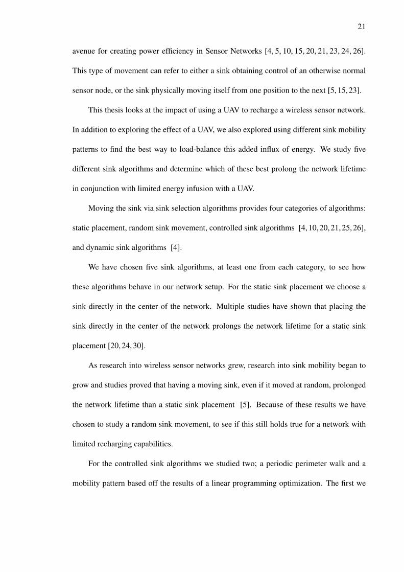
21
avenue for creating power efficiency in Sensor Networks [4, 5, 10, 15, 20, 21, 23, 24, 26].
This type of movement can refer to either a sink obtaining control of an otherwise normal
sensor node, or the sink physically moving itself from one position to the next [5, 15, 23].
This thesis looks at the impact of using a UAV to recharge a wireless sensor network.
In addition to exploring the effect of a UAV, we also explored using different sink mobility
patterns to find the best way to load-balance this added influx of energy. We study five
different sink algorithms and determine which of these best prolong the network lifetime
in conjunction with limited energy infusion with a UAV.
Moving the sink via sink selection algorithms provides four categories of algorithms:
static placement, random sink movement, controlled sink algorithms [4,10,20,21,25,26],
and dynamic sink algorithms [4].
We have chosen five sink algorithms, at least one from each category, to see how
these algorithms behave in our network setup. For the static sink placement we choose a
sink directly in the center of the network. Multiple studies have shown that placing the
sink directly in the center of the network prolongs the network lifetime for a static sink
placement [20, 24, 30].
As research into wireless sensor networks grew, research into sink mobility began to
grow and studies proved that having a moving sink, even if it moved at random, prolonged
the network lifetime than a static sink placement [5]. Because of these results we have
chosen to study a random sink movement, to see if this still holds true for a network with
limited recharging capabilities.
For the controlled sink algorithms we studied two; a periodic perimeter walk and a
mobility pattern based off the results of a linear programming optimization. The first we

22
call circles. In a paper done by Luo et al. they mathematically proved the optimal sink
mobility algorithm was a periodic perimeter walk along the outside of a circular network
[20]. They found that, for a mobile sink, the farthest away from the center of the network,
the longer the network lifetime. They compared their algorithms to a static sink and found
that it outperformed a static sink placed in the center of the network.
The second controlled sink algorithm we used was based off a linear programming
optimization. There has been extensive research into using a linear programming optimiza-
tion to prolong the network lifetime [10, 23, 26]. These papers proved that using a linear
programming optimization increased the network lifetime over a static sink.
The last algorithm that we used was called The Greedy Maximum Residual Energy
Heuristic, and represents the dynamic sink movement category. In the paper written by
Basagni et al. they showed that moving the sink to an area with the largest concentration
of energy prolong the network lifetime over a static sink [4].
We selected these algorithms as representative set covering the major areas to examine
in regards to our set of recharging questions; Section 5 describes our implementation of
these algorithms in greater detail.

23
Chapter 3: The Network Model
Every wireless sensor network purpose is unique; requiring different constraints and
considerations when setting up the network. This thesis concentrates on networks that are
used for monitoring structural healths of large objects that are unable to provide an adequate
power supply to the network. These types of constraints mold the way the network is set
up, and how it behaves. An example application of our thesis is a sensor network placed
underneath a bridge to monitor its structural health and safety.
The following will discuss three important parts of setting up our network; the basic
functionality of how our network will behave, our specific network assumptions and how
we implement the recharging ability of the Unmanned Aerial Vehicle.
3.1 Network Functionality
A sensor network must be engineered to meet all the requirements of data collection,
while being as time and cost efficient as possible. The first consideration that goes into
creating a network is the topology, or layout of the network. In this paper, we constrain our
network to be of square or rectangular size, such as to fit underneath a bridge or other man-
made structure. In addition, because the size and shape of man-made objects are limited
and known before setting up the network, we have created an equal node distribution,
geographically localized with no network holes present. These types of constraints are
realistic and feasible for the objective network we are designing for.

24
Another consideration into the setup of a network is what type of environmental data
is the network gathering. For monitoring the solidity of the infrastructure, the key data that
needs to be collected is the vibration of the structure. Testing vibration alone can determine
if there are any cracks or breaks in the foundation [19], which is the main concern in
structural safety. This type of environmental data gathering requires very little hardware,
and in terms of energy cost, is minimal compared to the wireless communication that is
needed for transmitting the data to other nodes.
In addition to this, we know that every node will collect the same amount of infor-
mation, thus any drain in the network’s energy because of environmental monitoring is the
same for every node. This thesis is only interested in the comparison in the uneven battery
drain that happens with other power hungry network functions such as communication. Be-
cause of these reasons, our testing can ignore any energy cost associated with gathering of
the environmental data, and can focus on just the communication costs. This is a realistic
assumption that can be made because of the way we are analyzing our data, however if the
power cost of monitoring data needs to be added in for future work, a quick change to our
simulation can be added in.
Communication between the nodes, however, is the largest drain of energy in our
network model. Therefore, how the nodes communicate was an important consideration
when constructing our model. To get one packet of information from one node to another is
called routing. It is possible to have each node transmit the packet of information directly
from itself to the sink, however, previous papers found that a multi-hop routing schema
was the most energy efficient in transmitting data across large distances [28]. Because
our sensor network could be widely spread out depending on the length and size of our

25
structure, we adopted this form of communication routing.
A multi-hop routing schema involves sending a communication packet directly to its
neighboring node, which will then forward that packet to its closest node until it reaches the
sink. Our simulation used an Euclidean shortest distance to determine the direct neighbor
that was closest to the sink. This communication means more wireless communication,
however because of the short distance that each communication travels, it is actually more
energy efficient [28]. To enable this communication schema in a network with a mobile
sink, all the nodes must be able to communicate bi-directionally with any of its neighbors
which is a realistic assumption given our network setup. In fact, if our network did not have
bi-directional communication, the sink mobility algorithms would not work.
3.2 Network Assumptions
In our model, we assume that all sensor nodes are homogeneous, with each having
the capability of being the sink. This is a very real and possible assumption for a network,
however if some of the nodes must be built differently from one another, three significant
changes in our model must be made. First, we must constrain the available nodes that can
be the sink in the sink algorithms we employ in the network. Second, we must change the
recharging amount we have given to the UAV. Lastly, we must re-consider the way that we
post-process the results from the sensor network to take into account this difference in node
setup.
Because this paper’s focus is on energy efficiency of sink mobility and limited recharg-
ing, we assume a simulation model where there is no packet loss in the transmission of
packets between the nodes. This is generally not true with wireless transmissions, how-

26
Figure 2.: UAV recharging a single node.
ever, our experiment is not interested in the behavior of packet loss and delay, thus we are
ignoring it. The results from this thesis can be easily tried on a sensor network with packet
loss and delay for future work if it is deemed useful.
In our simulation the battery and time measurements are not defined by real-world
units, such as watt-hours or seconds respectively, but instead as an abstract definition of
units. This abstraction can be done because of the nature of the way we are collecting and
analyzing our results. We are not looking at direct energy consumption in terms of watts,
but instead the ratio of energy loss of every node compared to another. For this abstract
approach we must make a very important network assumption when analyzing the results:
every node’s hardware is exactly alike. Each node starts out with the same amount of
energy, and each node is the same between simulations regardless of how big or small the
network will be.
3.3 Recharging Implementation
Researchers in prior work, created an unmanned aerial vehicle to wirelessly recharge
sensor nodes in a network [9]. This UAV was created to be fully automated, and not require
any manpower to control. Through inductive charging, the UAV can fly out to a remote area

27
and recharge nodes, giving a small infusion of power into the network. Figure 2. shows
this UAV inductively recharging a sensor node that was created to light an LED.
The UAV is able to transfer over 5W in flight and other prototypes can transfer up
to 15W. It is theorized that a UAV can prolong the life of an energy constrained wireless
sensor network. This work provides a solution to the problem of a lack of manpower that
would be required to recharge a wireless sensor network, however, the UAV can only hold
a limited amount of energy and is constrained to only being able to recharge one to two
nodes per flight. For the purposes of our simulation, we constrain the energy infusion from
the UAV to only be able to recharge a single node with a limited amount of energy per time
unit.

28
Chapter 4: The Simulation
To test the hypothesis and theories proposed in this body of work, we created a wire-
less sensor network simulation. This paper had looked into utilizing other types of sensor
network simulations already out there, however they were either too specific to individual
network setups, or they were overly complex and required functionality that we wanted to
leave out.
Requirements in our simulation are a way for the nodes to communicate, a way to
measure and adjust power levels in the node’s batteries, a way to choose the sink, and an
algorithm to route information between the nodes. In addition, the simulation covers all
basic functioning aspects of a sensor network and collects and saves important data to be
analyzed once the sensor network simulation has completed. This simulation also allows
measurements of many different sensor networks with varying row and column dimensions
to accurately assess how each experimental algorithm will behave across varying sized
networks.
4.1 The Simulation
Dr. Carrick Detweiler from the University of Nebraska-Lincoln and Dr. Elizabeth
Basha from the University of the Pacific created the original simulation. For this thesis,
the simulation was adjusted and manipulated to include various different sink movement
algorithms, corrections in the code to patch a few routing issues, and variables added for

29
post-processing analysis for better understanding of how the wireless sensor network per-
formed.
Coding a simulation of a wireless sensor network differs in coding for an actual wire-
less sensor network. When a physical sensor network is set up, certain aspects of the
network is realized in the hardware, but in a simulation they must be accounted for in code.
For example, in our simulation we have a function that will calculate the energy drain of
communication between the nodes. In a physical network, the energy drain is a side ef-
fect of the communication, and happens automatically. Because of this, there is additional
functionality that we have to add into the simulation that would not otherwise be needed.
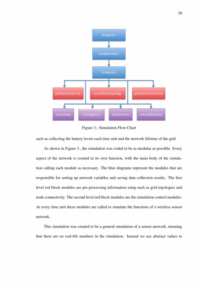
The simulation high level block diagram can be seen in Figure 3.. The first two blocks,
bridgeiter and bridgesimfun, are the top level structures that set up the simulated physical
sensor network, such as the grid topology sizes, battery unit levels and recharge amounts
by the UAV.
The block bridgesim also sets up the simulated physical aspects of our simulation,
such as outlining the physical topology of the grid and the communication connectivity
between the nodes. In Figure 3., all pre-processing modules are highlighted in the first
level red block diagrams. Bridgesim then becomes responsible for the control flow of the
simulation, which can be seen in the second level red block diagrams. Once the network is
setup, the bridgesim function loops through the life of the sensor network, represented as a
time unit, and controls the network’s functions. Some of the important functions that were
simulated are how the packets are routed through the network, how the sink moves in the
network at each time unit and the drain of the batteries as a function of the communication
between the nodes. The bridgesim function also keeps track of post-processing variables,
30
Figure 3.: Simulation Flow Chart
such as collecting the battery levels each time unit and the network lifetime of the grid.
As shown in Figure 3., the simulation was coded to be as modular as possible. Every
aspect of the network is created in its own function, with the main body of the simula-
tion calling each module as necessary. The blue diagrams represent the modules that are
responsible for setting up network variables and saving data collection results. The first
level red block modules are pre-processing information setup such as grid topologies and
node connectivity. The second level red block modules are the simulation control modules.
At every time unit these modules are called to simulate the functions of a wireless sensor
network.
This simulation was created to be a general simulation of a sensor network, meaning
that there are no real-life numbers in the simulation. Instead we use abstract values to

31
allow for comparisons within our network setup. For example, when the simulation speaks
about batteries, it is not referring to a true watt-Hour battery lifetime, instead it refers to an
abstract idea of a battery unit. All nodes have the same batteries attached to them, so the
battery can be 900 watt-Hours, or 1 watt-hour in our simulation. What is important is how
quickly the battery ratio between the nodes is drained, not the exact amount that is drained.
In this simulation, a battery unit is defined as a fraction of the total battery power that the
nodes are initialized with.
This idea of abstract generality also applies to other network specifics, such as the
network lifetime and the time as it passes through the network. We define the network
lifetime to be the time in which the first node in the network is completely drained of
battery as a ratio against how long the simulation ran for. We also define a time unit as the
time it takes for all packets to gather environmental data then send the gathered data to the
sink. After the simulation has run, the data is analyzed against other runs in the simulation
and compared as a ratio to one another.
This abstraction makes the simulation more portable to other types of sensor networks.
For example, this simulation can be applied to networks with small or large battery sizes.
It can also support networks that collect data each second or networks that collect data
every hour. In using this abstract definitions of units, we aren’t limiting our network to a
specific type network hardware, and we can generalize our findings to a much broader set
of wireless sensor networks. The following sections outline in more detail each important
aspect of the simulation, and how the control modules loop through the life of the entire
network.

32
Figure 4.: Various Grid Sizes Created by the Simulation
4.1.1 bridgeiter Function The simulation starts out in the bridgeiter function.
This module is responsible for declaring necessary network variables, including which sink
algorithm to call, if there is recharging in the network, what node the UAV will charge, the
initial battery levels of the nodes in the network, how many time units the simulation will
run for and how many nodes are in the network for that particular run.
This simulation was created to run with a flexible number of rows and columns. The
simulation can run with ten nodes in each row and ten nodes in each column or it can run it
with eight nodes in each row and one hundred nodes in each column. This function is also
responsible for running the simulation multiple times, with each simulation having various
sizes of topologies, in the form of m rows by n columns. This flexibility of the simulation
can help test the sink algorithms over multiple different types of square and rectangular
sizes to see how the algorithms change with network size. Figure 4. shows various grid
sizes that are created by the bridgeiter function. The last responsibility of this module is
to compile the data from each individual network simulation and save off the variables for
post-processing of the data collected.

33
4.1.2 bridgesimfunc Function This function was created for the sole purpose of
saving off the data of each individual run. The bridgeiter function will pass the necessary
setup variables to this function. This module then calls the main body of the network
simulation. When the simulation has finished running, this function collects all the data
created and saves it off as a unique individual run. When multiple topologies are run, this
function will save off each m row by n column as a unique data file.
4.1.3 bridgesim Function This is the main body of the entire simulation. This
function controls the behavior and flow of the network. It keeps track of vital variables
and collects data produced by the network for analysis. The beginning of this function
initializes network behavior variables and sets up the structure of the network. It then
checks to see if there is any pre-processing of network data required for the particular
sink algorithm chosen. If the sink algorithm is linear programming, or a derivation of, it
determines the sink’s path and location before the simulation begins. If it is any other type
of sink algorithm, the sink’s path and location is determined in real-time while the network
is running.
4.1.4 Topology and Connectivity In Figure 3. depicting the flow chart of the sim-
ulation, the first level red blocks getBatteryCapacity, createNodeTopology and generate-
Connectivty are all pre-processing network setup functions. getBatteryCapacity is a func-
tion to determine the initial battery levels of every node.

34
Figure 5.: An Example 3 by 3 Grid Topology
The topology function takes every node and places them in a square or rectangular
form. Using the number of nodes in a row and a number of nodes in a column, it numeri-
cally labels where every node is in the grid. Figure 5. shows an example 3 row by 3 column
square grid, and how each node is labeled in the simulation.
The connectivity function defines how the nodes are connected to one another. We
stated earlier that every node can only talk to its direct neighbors. This function implements
this constraint by creating a connectivity matrix, laying out which nodes a given node can
communicate with. At the start of the simulation, a maximum communication range is
defined as a set distance. An example 3 by 3 grid’s communication connectivity can be
seen in Figure 6., where every node can only communicate with its direct neighbors.
4.1.5 Main body of the Simulation Once any pre-processing network setup is
finished, the actual simulation of the network begins. These functions are the red and
purple block diagrams, as seen in figure 3..
The simulation is set up such that the network’s activities are conducted one time

35
Figure 6.: An Example 3 by 3 Grid Communication Connectivity
unit for each run through. The simulation will process all of the necessary actions during
each time unit, then it will move to the next time unit and process the networks activities
once again. The simulation will then loop through each time unit until it has reached its
maximum iterations.
When the simulation begins, the network chooses the sink, as determined by the sink
positioning algorithms defined by the user. This happens in the chooseSink function, which
can be seen in figure 3., in the second level red block diagrams. The different types of sink
algorithms are defined, in depth in chapter 5.
The next activity is the routing algorithm. This algorithm is handled in the function
routingFunct. It determines which path the nodes will send their data to get to the sink. An
example 7 by 8 rectangular grid can be seen in Figure 7.. This figure shows how each node
routes its packets to reach the sink.
This routing algorithm is based on the assumption that nodes cannot communicate
with anyone other than their direct neighbors so messages must move one node at a time to
the sink. Because of this, the simulation takes on a multi-hop routing function approach.
This means that the sensor network chooses its routing path by constraining the node’s pos-

36
Figure 7.: An Example 7 by 8 Grid Routing Map
sible communication partners by the ones in least distance from it, ie its direct neighbors.
Then forwards the packets of information to the sink by sending data from one neighbor to
the next until it reaches the sink.
It is important to note that this simulation assumes that every node knows where the
sink is without any cost of communication or any cost of time. This is highly unrealistic
for sink algorithms that chooses the sink in real-time while the network is running, but very
realistic if the network pre-processes the sink selection. These costs were not calculated
into our experiments, but will be followed up in future work, as discussed in chapter 7.
When the simulation was first created, the routing algorithm was not coded properly, and
these problems as well as the solutions will be discussed in section 4.2.
The next function called is the updatePower function. Once the sink and routing paths
have been chosen, this function will determine the battery drainage cost for communicating
data collected by the nodes. Our network simulates wireless transmission between the
nodes in the network. This function takes into account this cost, and considers all other
activity in the network negligible compared to the communication. Once again, because
we are looking at the ratio of battery drain along the whole of the network, and we assume
that every node has their batteries drained equally by all other sensor network activities,

37
this is a safe assumption.
Once all routing costs have been calculated and subtracted from the current battery
levels of all nodes, updatePower calculates in the cost of recharging due to the UAV. There
are three possible behaviors of the UAV, recharging the sink, recharging the lowest powered
node, and recharging nothing. The user chooses the behavior of the sink in the top level
function bridgeiter, and this function enacts the users choice here.
The last part of the simulation is to calculate the data for post-processing purposes.
The simulation calculates the node that runs out of battery first, how long it takes for this
node to die. It also keeps track of important variables at each time unit such as the battery
levels of each node and which node was the sink.
4.2 Routing Changes
When the simulation was first created and the first group of experiments run, it was
discovered that the routing function was not properly calculating the communication costs
for the entirety of the network. At first glance, the routing function seemed to work fine;
however the results showed that the energy drain on the network was independent of the
size of the network. The larger amount of nodes in the network the more communication
is required and the faster the energy drain. Therefore, a bigger grid size with the same
initialization of battery energy should lose its energy much faster than a smaller grid size.
When the routing discrepancies were found, the routing algorithm was more closely
scrutinized. The main problem laid in the way the routing costs were calculated. The
simulation was responsible for keeping track of the amount of packets it had to pass to its
neighbor nearest to the sink then subtracting the communication costs of each node from

38
its total battery charge. The inconsistency was how the simulation counted the number of
packets that each node had to pass along. In the routing function, every node’s communi-
cation cost was calculated by its receiving cost plus its sending cost. The receiving cost is
how many packets it receives from its children times the battery drain to receive a packet.
The sending cost is how many packets it forwards to the sink times the battery drain to send
a packet.
The broken routing function only counted the packets it received from its direct neigh-
bors, referred to as children, but it did not take into consideration its grandchildren or nodes
even more extended than that. Therefore, regardless of grid size, the network acted like a
small grid size where no node had any grandchildren, great-grandchildren, etc. This created
a network whose energy cost was independent of the grid size.
The problem in the routing function was that it was unable to take into account every
node’s ancestor, and therefore unable to calculate the true amount of packets needed to be
forwarded. A few algorithms were developed, attempting to process the node’s communi-
cation costs in different ways, but none that accurately calculated the packets of information
for every node. The problem in this approach was that at compilation time it was impossi-
ble to know how many nodes were connected to it when it began the cost calculation. At
this point, we realized a completely different approach was needed.
We realized we needed to construct our algorithm such that we could keep an accurate
count of any one node’s children, grandchildren and beyond. The only thing that the algo-
rithm knew at compilation time was that the outer-most perimeter nodes had no children
at all. Thus, the nodes right next to the outer-most nodes only had children nodes, but no
grandchildren nodes or more. The nodes next to those had only children and grandchil-

39
dren, but no great-grandchildren. With this understanding, we could figure out how many
ancestors each node had if we started from the leaf nodes and worked toward the sink.
The problem was we did not know which nodes were the outer-most perimeter nodes at
compilation time.
The problem then became identifying which nodes were leaf nodes, or outer-most
perimeter nodes. With this new goal in mind, we began to look at the node’s structure
in a different way. We realized that our nodes could be viewed as a tree-like hierarchal
structure, with the sink being the root node and the perimeter nodes being the leaves of the
tree.
Using this hierarchal view of our network, we could employ a Depth-First Search al-
gorithm to determine leaf nodes and their hierarchal connection to the sink, or root node.
Employing the Depth-First Search algorithm created an accurate list of how many packets
each node sends and receives regardless of the complexity, size or shape of the network.
Using the results from this algorithm, we were able to simulate the actual cost communi-
cation behavior of a wireless sensor network.
4.3 Post-Processing
When the simulation is finished, data collected during the simulation is examined. The
simulation collects many different variables; however, for the analysis of this paper the two
most important variables is the network lifetime and the sink history. The network lifetime
is determined by the time the first node in the network dies. And the sink history details
which node was the sink at every time unit in the network. Using these two variables, it
is possible to compare each experimental run against the others. The network lifetime can

40
be analyzed to show which sink algorithm provides the most energy savings while the sink
history can be analyzed to provide insight as to how the energy load is being distributed by
the sink’s movement.
4.4 Summary
We use this simulation to test our different objectives on UAV recharging and sink
mobility energy conservation. Our simulation runs through various square and rectangular
grid sizes to see the overall behavior of the network without constraining it to be any one
size. Using our network assumptions, the network communication path and cost was cal-
culated for every time unit in the life of the network. After every experiment was run, all
of the different scenarios were compared against each other to find the network layout and
behavior which provides the longest network lifetime in our network setup.
41
Chapter 5: Sink Classifications
Research into energy conservation by specific positioning of the sink can be classified
in four ways; static sink positioning, random sink movement, controlled sink movement
and dynamic sink movement. This research looked into these four different classifications
to find the best way to optimize the impact the UAV has on the network. This section will
discuss in depth the types of algorithms that have been previously implemented and how
we will adapt them to our network. In the results section, we will discuss the comparison of
these different algorithms to determine which extends the lifetime of the network longest
with the limited infusion of power from the UAV.
It is important to note when discussing sink movement, there are two possible ways
a sink can move; physically moving around the network, and algorithmically upgrading a
node’s function to temporarily become the sink. In our network, the nodes will be placed
statically on a structural surface, making it impossible for any node to physically move
around the network. Fortunately, we assume every node in our network has the exact same
hardware, and thus can have its software upgraded to act as the sink at any point in time.
Therefore, when we discuss sink ’movement’ we are not referring to a physically moving
node, but instead any node in the network temporarily becoming the sink for that time unit.
42
5.1 Static Sink Positioning
The static sink algorithm fixes the sink at a stationary location throughout the lifetime
of the sensor network. Early sensor networks used this method of sink positioning, and
a lot of research explored finding the optimal position in the network [24]. The research
conducted by Lou et al. mathematically found the optimal placement of a static sink was
in the center of the network [20]. We applied these findings to our static sink scenario.
5.2 Random Sink Movement
As research into sink positioning grew, discoveries were made that moving the sink
around greatly improved the network lifetime [1]. The work of Chatzigiannakis proved
that mobile sinks moving randomly around the network proved to have a longer network
lifetime as compared to the sink remaining motionless [5]. For this sink classification, we
used a random function to choose the placement of the sink. The sink stays at a node for
one time interval and then it uses the random function to choose the next node to become
the sink. Every time interval, the sink moves in a complete random pattern.
5.3 Controlled Sink Movement
The third sink classification that this paper looks at is controlled sink movement. As
opposed to random sink positioning, this movement is consciously controlled and planned
before the network begins operating. The following two sink algorithms are controlled sink
movements that we studied.

43
Figure 8.: Poisson Node Distribution
5.3.1 Circles In one algorithm proposed by Luo et al. [20], moving the sink in
the outermost perimeter of the network would dramatically increase the network lifetime
versus a static sink. Using multi-hop routing, moving the sink around the perimeter in the
network balanced the energy load equally across the network, thus improving the lifetime.
However, this paper assumes a Poisson Process circular distribution of nodes, as seen in
figure 8., [20], where the nodes in our network are evenly distributed in a square or rectan-
gular pattern.
In our implementation of the circular sink positioning algorithm, first we must prove
the hypothesis that walking on the outer perimeter increases the network lifetime given a
square or rectangular grid. If this holds true, then we will compare this algorithm with our
other sink movement algorithms with the added dimension of recharging from the UAV.
5.3.2 Linear Programming Another controlled sink movement that we will im-
plement is a mathematical optimization algorithm called Linear Programming Optimiza-
tion. This algorithm is one we base off of the work done by Wang et al. [26]. In this
work, the linear programming algorithm determines the optimal sink placement to maxi-
mize the network lifetime. The following section will first describe the basic idea of Linear
Programming Optimization, then we will describe how we implement this optimization in

44
conjunction with our constraints and network setup.
This optimization first starts out as a basic set of linear equations, an example can be
seen in Equations 5.1 and 5.2. With any set of linear equations there are three possible
results; no solution, a unique solution and an infinite set of solutions. Linear Programming
Optimization deals with a set of linear equations, at least one or more, that have an infinite
set of solutions. Within this set of solutions, it computes the optimal solution, given a set
of constraints.
x+2y (5.1)
−5x+ y = 7 (5.2)
For example, using the set of linear equations 5.1 and 5.2, a linear programming opti-
mization would attempt to find the optimal solution to these equations based on a given set
of constraints. Let us assume we want the value x and y be as small as possible, but at the
same time x must be greater than or equal to three and y must be greater than or equal to
four. These three statements represent constraints in the optimization. We say that we want
the minimal solution of the two equations, with constraints subject to 5.3 and 5.4.
x≥ 3 (5.3)
y≥ 4 (5.4)
The result from this optimization can be seen in equations 5.5 and 5.6. This is the
minimal solution to the set of equations 5.1 and 5.2, with x being greater than three and y

45
being greater than four.
x = 19/6 (5.5)
y = 137/6 (5.6)
We employ this same idea to our network. We first create our linear equation, denoting
it to be the time that the sink stays at any one particular node. For example, in a 3 by 3
grid size, our linear equation can be found in Equation 5.7. In this equation, t represents
the amount of time that node is the sink during the lifetime of the network. This equation
can also be simplified into Equation 5.8.
t1 + t2 + t3 + t4 + t5 + t6 + t7 + t8 + t9 (5.7)
In the Linear Programming example above, we found the minimum solution to x and
y. However, in our example, we wish to find the maximum solution to this equation by
prolonging the sink’s sojourn time at each node. In doing so, we will maximize the network
lifetime because the longer the sink stays at every node, the longer the network lifetime will
be. We call this a maximization of our linear equation. Our network linear programming
optimization algorithms can be found in the equations 5.8, 5.9 and 5.10.
Max Network Lifetime:
∑∀k∈N
tk (5.8)
Subject to:
∑∀k∈N
cki tk ≤ e0 (5.9)

46
tk ≥ 0 (5.10)
Where:
• N is the set of all nodes in the grid.
• k represents the current sink.
• i represents a general node in the grid.
• tk represents the sojourn time spent at each sink.
• cki represents the cost of one node sending and receiving data in one time interval
when the sink is at position k.
Equation 5.9 is one of our most important constraints. This equation represents the
cost of sending and receiving packets of information for each node when the sink is at po-
sition k, but not draining the battery more than its initial energy. This constraint represents
our power limitation in the network. No battery can be drained more than the power it
begins with. Our last constraint, Equation 5.10 ensures that the result does not give us a
negative value for a sink sojourn time. It is impossible to stay at a sink for negative time
values.
These set of equations and constraints represent our network setup, and attempts to
maximize the length of the network lifetime. Once this optimization has finished com-
puting, the algorithm creates a sink movement based on the results. The next two sections
describe the obstacles our network constraints have on the implementation of this optimiza-
tion, and how we overcome them.

47
5.3.3 Linear Programming: Periodic versus Exact Movement In the paper by
Wang et al [26], the authors state that applying the linear programming optimization results
could be implemented irregardless of the order in which the sink follows the optimization.
However, this paper did not consider limited recharging while implementing the optimiza-
tion.
Since the optimization we are using is a linear one, we can only account for the energy
drain as a direct results of the sink’s position, and not directly optimize for the recharging
of the UAV. Because of this, we adjusted the cost of sending and receiving messages to
reflect the variable recharge placement as an even distribution of power across all the nodes.
In doing so, we hypothesized the implementation would matter, and set to prove which
implementation of the results would be optimal for our network.
The two main implementations discussed in the paper was exact sink movement and
periodic sink movement, and we implemented both of them in our network. In exact sink
movement, the sink would directly relay the results of the linear programming optimization
into its movement. For a periodic sink movement, the sink will stay at a node for one time
unit, then move to the next. When the sink has visited all the nodes once, it will go back to
the first node again and repeat.
Take an example grid given in figure 9.. Remember, the basic linear optimization
output is a list of which nodes in the network should be the sink, and for how long. Let’s
say the results of an LP Optimization were given in Table 1..
In this example, an exact sink movement implementation would be the following. The
sink will stay at node 1 for three time units then move on to sink 2 for one time unit. It will
move to node 3 for three time units, node 4 for one time unit. The node will skip node 5,

48
Figure 9.: An Example 3 by 3 Grid Topology
Table 1.: Example Linear Programming ResultsNode Number Time units a node should be the sink
1 32 13 34 15 06 17 38 19 3

49
Table 2.: More Realistic Linear Programming ResultsNode Number Time units a node should be the sink
1 3.12 .93 2.94 1.15 0.16 1.37 3.28 .99 3.4
because the results is zero, then go to node 6 for one time unit, and so on and so forth.
For this example with a periodic sink movement, the sink will stay at node one for one
time unit, then node two for one time unit and continue around the network, staying at each
node, if the LP results did not output zero for that node. When it finishes its first round, it
will come back to node one and stay at it for one time unit. Because the optimization had
node two being the sink only once, it will now skip this node and go to node three for one
time unit. This will continue, the sink staying at a particular node for one time unit. Once
the sink leaves a node, it notifies the network that it has been there by subtracting one from
the result. It then moves onto the next node if its results have not yet reached zero.
5.3.4 Linear Programming: Naivety The type of linear programming optimiza-
tion we are implementing is a deterministic and solvable problem. However, the output
from this algorithm is a non-integer number. Table 1. results are given as integers. How-
ever, Table 2. is actually what the Linear Programming Optimization will give us.
In the setup of our network, we have constrained the sink to stay at one location
for at least one time unit. When the results comes back from the linear programming
optimization, the non-integer numbers represent a fraction of a time unit. To configure

50
the results into an implementable solution, we had to round the results to whole numbers.
There are three different types of common rounding; general Rounding, floor rounding,
which truncates the answer by rounding down, and ceiling rounding, which truncates the
answer by rounding up. To make sure we took the best rounding approach, we ran three
experiments with three different rounding techniques.
It has been said that such rounding of results of a Linear Programming Optimization is
a naive approach and does not obtain the optimal results. There is an optimization that will
provide the results as integers, however it then becomes an NP-hard problem. This means,
worst case, there is no solution. In addition, computing the answer to this optimization
requires a drastic increase in computational power. As such, we experimented with the
three types of rounding techniques to decide which type of rounding was optimal.
5.4 Dynamic Sink Movement
The previous sink algorithms are calculated based of initial known variables before the
network begins. Our last sink algorithm differs in that it uses the ever-changing network
energies to determine the next node to be the sink.
We use an algorithm developed in the work introduced by Basagni et al. [4]. This
work found a common problem in multi-hop networks called the neighborhood problem.
Nodes surrounding the sink, called ’neighbor’ nodes, become inundated with all packets
being sent to the sink. This inundation drains these nodes faster than the others farther
away from the sink. Using this information, the paper creates a heuristic called Greedy
Maximum Residual Energy (GMRE). This algorithm moves the sink to the section of nodes
with the highest energy levels in an effort to drain the nodes energy more evenly around

51
Time Unit 1 Time Unit 20
Time Unit 40 Time Unit 60
Figure 10.: An Example 5 by 5 Sink Neighboorhood Problem.
the network. Each iteration the algorithm calculates the highest energy groupings in the
network, and moves the sink to that location, knowing that the nodes around it will become
more drained than the others. In Figure 10., you can see a five by five grid over the length
of the simulation. A yellow block represents a node with over 80% charge, where green
represents a node between 80% and 50%, and blue between 50% and 30%. A red block
represents a node that is about to die.
Here we apply this heuristic to a limited recharging network, calculating the movement
of the sink based on the ever-changing energy in the network. As the network is operating
the sink polls all of the sensors energy levels and compares them in blocks. Depending on
the placement of the nodes, the blocks can vary in the amount of nodes in each block. An
example of these ”Blocks” can be seen in Figure 11.. Blocks within the network contain
9 nodes, which can be seen within the red block. Blocks near the edges of the network

52
Figure 11.: An Example 8 by 8 Various Greedy Blocks
contain 6 nodes, which can be seen within the purple block. Blocks on the corners of the
network contain 4 nodes, which can be seen within the blue block.
5.5 Comparing the Algorithms
The algorithms we tested in this thesis are all implemented on a network that has no
availability to power during the life of the network. In addition, they have not yet been
previously compared to one another. Our work implement these algorithms and apply
them to our gridded topology with an added dimension of recharging. We then compare
these algorithms to each other to determine the optimal sink positioning algorithm to use
in addition to the limited recharging of the UAV.

53
Chapter 6: Results
Given our network setup and constraints, we ran the simulation to gather data to help
us determine the answers to our key objectives. Does using an unmanned aerial vehicle
extend the network lifetime of a sensor network? We choose a UAV recharge amount of
25% with a static sink placement and looked at seven different grid topologies to under-
stand how the UAV impacts the sensor network lifetime. We determined that using a UAV
prolonged the network lifetime. We than ran simulations to determine how much the UAV
should recharge for to provide the longest network lifetime.
After determining the results to the first key objective, we then looked into the second.
Which node should the UAV recharge at every time unit? We choose two different nodes
we believed were the biggest failing points in the network, the sink and the lowest powered
node. We ran simulations with these different charging scenarios and determined which
node would provide the longer network lifetime.We determined the lowest powered node
was better to recharge so we re-ran the earlier simulation to determine how much the UAV
should recharge for with this new implementation.
Following the first two key objectives, we found out what sink positioning algorithm
would to optimize the influx of energy by the UAV. We compared five different sink algo-
rithms and found that using a UAV during the lifetime of the network is best with the static
sink algorithm for smaller grid sizes. For grids larger than the UAV can compensate for the
best sink algorithms were Greedy and Circles.

54
6.1 Unmanned Aerial Vehicle Impact
To test the viability of an unmanned aerial vehicle in a wireless sensor network, we
started with a static sink directly in the center of the network. A sink placed in the middle
of the network is the most general form of sink selection algorithm, and thus we used it
as a basis for our preliminary tests. Using this algorithm; seven sensor networks were
simulated, each with a different square and rectangular grid topologies.
6.1.1 Recharging versus No Recharging Every time unit during the simulation
we set the UAV to recharge the sink node. We chose the sink because it is the most impor-
tant node in the network, and has the greatest cost in communication per each time unit.
Every node in the network must pass on the packets of information from its neighbor nodes,
but the sink must forward all of the packets of the network to the UAV as it passes by.
We set the amount the UAV would recharge as a ratio of the initial energy of each
node. Remember that every node in the sensor network is homogeneous, and contains the
same initial energy. We began with the UAV recharging at 25% of the initial energy to
determine if the UAV had any impact on the network lifetime. We ran two simulations on
the seven grid topologies; a normal wireless sensor network with no recharging, and one
with recharging. We ran the simulation against seven grid topologies; 8 by 8, 8 by 13, 8 by
18, 11 by 18, 14 by 18, 17 by 18, and finally, 20 by 18. These grids were chosen because
the total number of nodes in these grid sizes were near 50, 100, 150, 200, 250, 300 and
350, respectively.
Table 3. reflects you can see the impact of recharging versus no recharging. The first
column represents a grid topology in terms of number of nodes in each row versus number

55
Table 3.: Multiple Grid Topologies: How recharging with a UAV Affects the NetworkLifetime
Grid Topologies Total Number of Nodes No Recharge Recharging8 by 8 64 17 668 by 13 104 11 338 by 18 144 8 20
11 by 18 198 7 1614 by 18 252 5 1517 by 18 306 5 1420 by 18 360 4 8
of nodes in each column, and the second column represents the number of nodes in the
network for this given row by column topology. The third column contains the results of
the grid simulation with no recharging, shown as the time unit at which the first node failed.
The fourth column shows the results of the simulation where the UAV recharged a single
node at every time unit. The results are displayed as the network lifetime, which is the time
unit when the first node failed.
These results show that the there is a positive impact on network lifetime when the
UAV recharges for at least twenty-five percent of each node’s initial energy. It’s also im-
portant to note that as the number of nodes increase, the impact that the UAV has on the
network decreases. This happens due to the fact that as the number of nodes increase, the
amount of communication and energy cost increases. The UAV’s recharge amount, how-
ever, stays the same. This results in a decrease the ratio of recharge to energy drain of the
network, thus impacting the network less as the network gets larger.
6.1.2 UAV Recharge Amount The next question becomes, given there is a posi-
tive impact on network lifetime when utilizing a UAV, how much does the UAV need to
recharge to become a viable option for use? Constructing a UAV takes time and resources.
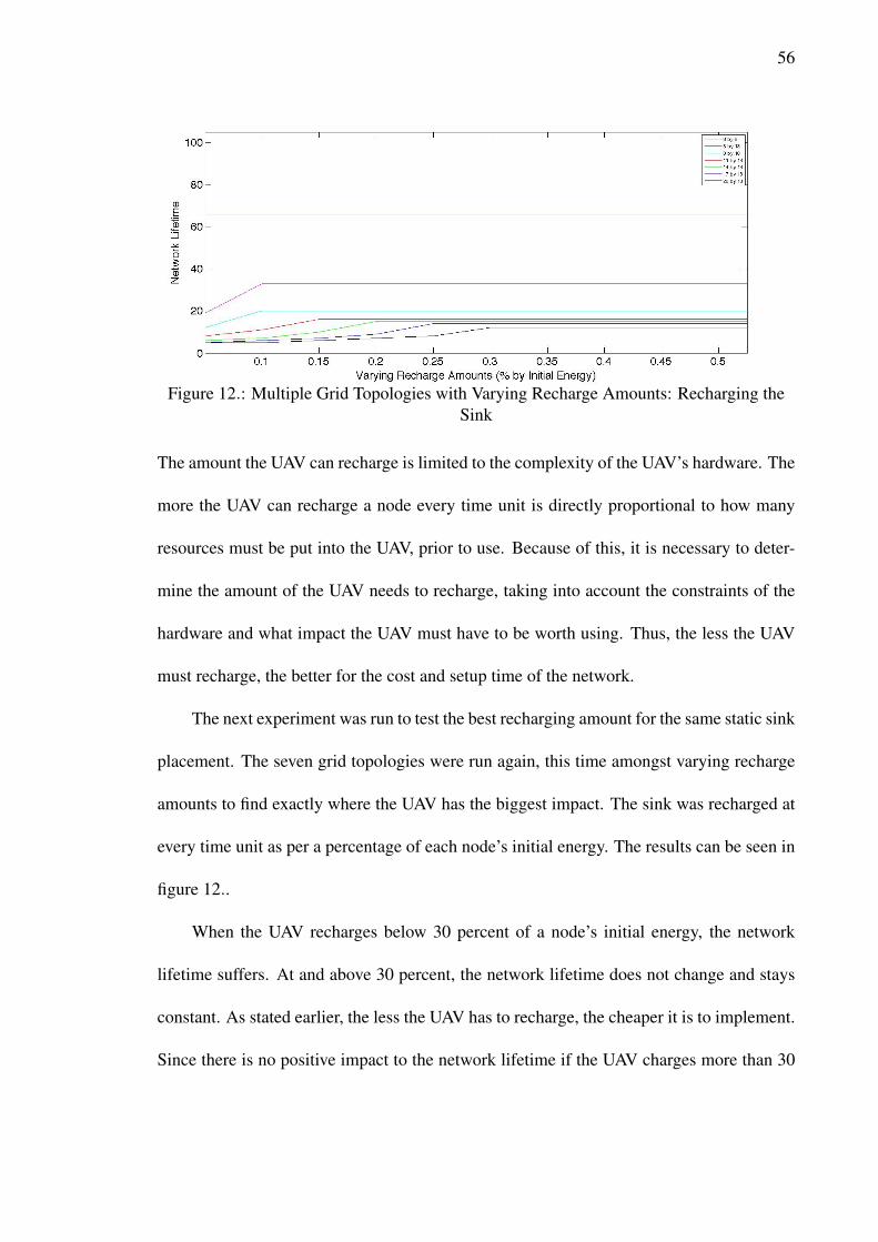
56
Figure 12.: Multiple Grid Topologies with Varying Recharge Amounts: Recharging theSink
The amount the UAV can recharge is limited to the complexity of the UAV’s hardware. The
more the UAV can recharge a node every time unit is directly proportional to how many
resources must be put into the UAV, prior to use. Because of this, it is necessary to deter-
mine the amount of the UAV needs to recharge, taking into account the constraints of the
hardware and what impact the UAV must have to be worth using. Thus, the less the UAV
must recharge, the better for the cost and setup time of the network.
The next experiment was run to test the best recharging amount for the same static sink
placement. The seven grid topologies were run again, this time amongst varying recharge
amounts to find exactly where the UAV has the biggest impact. The sink was recharged at
every time unit as per a percentage of each node’s initial energy. The results can be seen in
figure 12..
When the UAV recharges below 30 percent of a node’s initial energy, the network
lifetime suffers. At and above 30 percent, the network lifetime does not change and stays
constant. As stated earlier, the less the UAV has to recharge, the cheaper it is to implement.
Since there is no positive impact to the network lifetime if the UAV charges more than 30

57
Table 4.: Static Sink: Recharging Impact at 30%Grid Topologies Total Number of Nodes Network Lifetime
8 by 8 64 668 by 13 104 338 by 18 144 20
11 by 18 198 1614 by 18 252 1517 by 18 306 1420 by 18 360 12
percent, we decided it was the best recharge amount for the UAV.
In table 4., you can see the network lifetime as the time until the first node failed.
Again, it is important to note that as the network grows, the impact of the UAV decreases
because the ratio of energy the UAV can provide decreases.
6.2 Node Recharging Selection
The next key objective is to find out how the UAV should recharge the network. In
our results above we assumed that the sink was the best node to recharge due to its need
to communicate the entirety of the networks environmental data collection, and that if the
sink dies, the entire network becomes inoperable. Also, once the sink has received all of the
packets, it is responsible for passing along all of the information from the sensor network
to the UAV flying by. This puts a heavy burden on the sink to receive then transmit the
entirety of the network’s gathered data.
This makes recharging the sink a very logical choice for recharging selection, however
does this apply to every scenario? What if there is another node that needs the recharge
amount more than the sink? The sink might have the greatest drain on the network, however
what if there is a node that is in danger of dying more than the sink? We define the ”lowest

58
Table 5.: Recharging the Sink versus Recharging the Lowest Powered NodeGrid Topologies Total Number of Nodes Sink Recharged Lowest Powered Node Recharged
8 by 8 64 66 2008 by 13 104 33 2008 by 18 144 20 4211 by 18 198 16 2814 by 18 252 15 1917 by 18 306 14 1720 by 18 360 12 10
powered node” to be a node that has the least amount of energy left in its battery at any
given time unit. We setup our next experiment to see if recharging the lowest powered node
improved the network lifetime better than recharging the sink node.
6.2.1 UAV Amount to Recharge This experiment involved using the same seven
grid topologies. In one set of experiments, the sink was recharged at every time unit.
The second set the lowest powered node was recharged at every time unit. The previous
experiments showed that the biggest impact the UAV had was recharging was 30% of the
initial node’s energy, and thus we set this as the recharge amount. The results of this test
are shown in table 5..
The first column shows which grid topology was being tested, and the second column
shows the number of nodes in that topology. The third and fourth columns represent the
network lifetime, which is the time the first node fails. The simulation was run for a total
of 200 time units, so on simulations that had a network lifetime of 200 never had a node
die and was considered to be 100% successful for our network setup.
The results show that recharging the lowest powered node is greater in all cases but
the last grid, 20 by 18. These results also show that as the number of nodes get larger, both

59
Table 6.: Recharging the Sink versus Recharging the Lowest Powered Node: Larger GridSizes
Grid Topologies Total Number of Nodes Sink Recharged Lowest Powered Node Recharged17 by 18 306 14 1718 by 18 324 14 1319 by 18 342 14 1122 by 18 396 9 920 by 20 400 9 9
Figure 13.: Decreasing Impact of Recharging as the Number of Nodes in the NetworkIncrease
forms of recharging have less of an impact. In fact, as the number of nodes get bigger,
the impact of recharging the lowest powered node gets less effective faster than the sink
recharging impact. We found these results to be of interest to our objectives, and sought to
investigate this further. Additional experiments were done with larger grids to see if type of
recharging depends on the grid sizes of the network. We ran larger grid sizes and compared
the results to the rest of the topologies. These results can be seen in table 6..
At grid sizes between 306 nodes and 324 nodes the most effective recharging schema
with the sink versus recharging the lowest powered node switches. Below 306 nodes,
powering the lowest powered node is the best, however at grid sizes larger than 350 nodes

60
recharging the sink is a better choice. We graphed the impact of recharging the sink versus
recharging the lowest powered node versus the number of nodes in the network, as seen in
figure 13..
The y-axis is the network lifetime. The x-axis is the number of nodes in the net-
work. The results show that recharging the network drops off exponentially as a function
of the number of nodes in the network. These results also show that the lowest powered
node drops off faster than recharging the sink, and around 306 nodes, recharging the sink
becomes better than recharging the lowest powered node.
This result were not unexpected. As the number of nodes in the network become
larger, the amount of packets the sink has to forward to the UAV becomes exponentially
larger than the rest of the packets the nodes around it must pass on. As such, the sink
becomes the node that requires the most energy. At times in the network, the sink is not the
lowest powered node, however because of the large amount of communication it must pass
on and the large requirement of power to do so, it is the most needy node. After just one
time unit, passing along those packets without an infusion of energy can cause the sink to
lose power completely, making it need the energy infusion more than the lowest powered
node. For the rest of the experiments, any grid size with 324 nodes or more will have the
sink being recharged, and any nodes less than that will have the lowest powered node being
recharged.
6.2.2 Revisiting Recharge Amount Now that we have determined recharging the
lowest powered node provides the longest network lifetime, it is necessary to revisit the
question of how much should the UAV recharge to provide a positive impact, given this
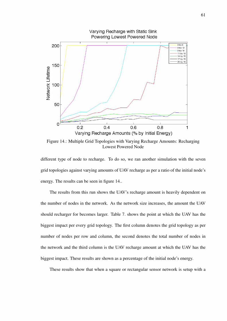
61
Figure 14.: Multiple Grid Topologies with Varying Recharge Amounts: RechargingLowest Powered Node
different type of node to recharge. To do so, we ran another simulation with the seven
grid topologies against varying amounts of UAV recharge as per a ratio of the initial node’s
energy. The results can be seen in figure 14..
The results from this run shows the UAV’s recharge amount is heavily dependent on
the number of nodes in the network. As the network size increases, the amount the UAV
should recharger for becomes larger. Table 7. shows the point at which the UAV has the
biggest impact per every grid topology. The first column denotes the grid topology as per
number of nodes per row and column, the second denotes the total number of nodes in
the network and the third column is the UAV recharge amount at which the UAV has the
biggest impact. These results are shown as a percentage of the initial node’s energy.
These results show that when a square or rectangular sensor network is setup with a

62
Table 7.: UAV Recharge Amount per Grid TopologyGrid Topologies Total Number of Nodes Node Recharged UAV Recharge Amount
8 by 8 64 Lowest Powered Node 10%8 by 13 104 Lowest Powered Node 25%8 by 18 144 Lowest Powered Node 55%11 by 18 198 Lowest Powered Node 80%14 by 18 252 Lowest Powered Node 80%17 by 18 306 Lowest Powered Node 95%20 by 18 360 Sink 30%
static sink, determining the UAV recharge amount should be a function of the number of
nodes setup in the network. When we begin to compare sink algorithms together we will
use table 7. to determine how much the UAV should recharge.
The 20 by 18 grid size is the only size that does not follow the normal progression
because the sink is being recharged, not the lowest powered node. Recharging the sink for
larger grid sizes not only saves us in computational complexity of determining the lowest
powered node, but also provides us with a UAV that is less costly.
6.3 Sink Selection
The next key objective is to determine which sink algorithm best optimizes the limited
recharging capability of the UAV. In Chapter 5, we discussed previous research that out-
lined different load balancing algorithms that strategically moved or placed the sink. For
our experiments we recreated those algorithms, adjusting for our network constraints and
grid topologies, then compared the results together to find which algorithm worked best in
conjunction to the UAV recharging.
6.3.1 Perimeter Walk As discussed in section 5.3.1, work done by Luo et al. [20],
showed that moving the sink in a periodic, circular direction increased the network lifetime.

63
Figure 15.: Four Different Periodic Movements; Perimeter Walk, P-1 Walk, P-2 Walk, P-3Walk
Table 8.: Periodic, Square Movement in an 8x8 GridCircular Path Network Lifetime
Perimeter 168P-1 122P-2 86P-3 42
They further showed that moving along the outer-most perimeter achieved the highest net-
work lifetime by load balancing the energy in the network. Before we can consider utilizing
this algorithm in our network, first we must prove that moving the sink on the outer-most
perimeter holds true for a square or rectangular grid.
We took an 8 row by 8 column topology and ran four experiments. Each experiment
involved the sink moving in a square pattern, with differing distances from the center of the
network, as seen in figure 15..
We did not implement any recharging in this network so that we could accurately
assess and compare a circular periodic movement to a square periodic movement. As you
can see in table 8., the sink that moves on the outer-most perimeter is indeed the better
sink movement. As the sink moves closer to the center of the network the lifetime becomes
smaller, which is consistent with the statements made in the paper done by Luo et al. [20].

64
6.3.2 Linear Programming: Periodic versus Exact Movement The other sink
algorithm that needed extra testing to properly apply to our network was the Linear Pro-
gramming Optimization. Because our implementation of the LP optimization was con-
strained to a naive implementation, we had to first determine which execution of the al-
gorithm provided the longest network lifetime. We ran two experiments over the seven
various grid topologies. The UAV recharge amount per each grid size was determined by
the previous results, as shown in table 7.. The results are displayed in figure 16..
Figure 16.: LP Periodic Implementation versus Exact Implementation
The results are not definitively conclusive, but the LP periodic implementation pro-
vides the longest network lifetime compared to the exact sink LP implementation for the

65
Table 9.: Periodic vs Exact Sink LP ImplementationGrid Topologies Total Number of Nodes Periodic Movement Exact Movement
8 by 8 64 200 2008 by 13 104 200 768 by 18 144 113 3411 by 18 198 95 3814 by 18 252 42 2917 by 18 306 24 3020 by 18 360 23 25
majority of the grid sizes. For grid sizes with less than 300 nodes, the periodic implemen-
tation of the LP algorithm works better. In grid sizes greater than 300, the exact movement
can be a better choice. However, there are larger grid sizes, such as 20 by 18, that do not
preform better with an exact sink movement. This can be seen in table 9.. That, and because
the change in network lifetime is at best 3 percent, we have decided to use the periodic sink
movement for all future implementations of the Linear Programming Optimization.
In the paper detailing the Linear Programming Optimization [26], it was stated that
the exact implementation and periodic implementation would provide the same results.
We believe our implementation differed from this statement because we are attempting to
balance the infusion of UAV energy into the network. Because the LP algorithm is not fully
representing our UAV recharging capabilities and our naive implementation, the results in
their paper are not perfectly comparable to the actual behavior of our network. Therefore
there is extra energy in our network, and periodic sink movement balances this energy best.
6.3.3 Linear Programming: Naivety For the second experiment on the imple-
mentation of the Linear Programming Optimization, we looked at how best to round the
non-integer results that would give us the longest network lifetime. We took various grid
topologies, with the experimentally found amount of recharging by the UAV at each time

66
Table 10.: LP Approximation: Normal RoundingGrid Topologies Number of Nodes Network Lifetime
8 by 8 64 2008 by 13 104 2008 by 18 144 101
11 by 18 198 9514 by 18 252 4217 by 18 306 3720 by 18 360 23
Table 11.: LP Approximation: Rounding UpGrid Topologies Number of Nodes Network Lifetime
8 by 8 64 2008 by 13 104 2008 by 18 144 179
11 by 18 198 4314 by 18 252 2517 by 18 306 2420 by 18 360 23
unit, delivered to the experimentally found appropriate node. We then used the periodic
sink movement. The results of these experiments can be seen below in tables 10., 11. and
12..
These results show that normal rounding operations are not the best way to approxi-
mate the Linear Programming results. When the number of nodes is small, under or around
150 nodes, using a ceiling rounding function to approximate the results is superior. How-
Table 12.: LP Approximation: Rounding DownGrid Topologies Number of Nodes Network Lifetime
8 by 8 64 2008 by 13 104 2008 by 18 144 115
11 by 18 198 9214 by 18 252 7017 by 18 306 4720 by 18 360 35

67
Figure 17.: All Five Sink Positioning Algorithms Compared
ever, this increase in network lifetime when using the ceiling method drop dramatically
after 150 nodes. When the grid is larger, over 150 nodes, using the floor rounding function
is best. In future tests, when we do a Linear Programming Optimization, we will approxi-
mate the results as per the number of nodes in the grid. If the number of nodes is less than
150, we will use the ceiling function. If it is greater than, we will use the flooring rounding
function.
6.3.4 Comparison Between Sink Selection Algorithms Once all five algorithms
had been implemented in the simulation they were run and compared against one another.
Our test setup included all the results from earlier experiments. We ran these simulations
on the seven grid topologies we had been using previously; 8 by 8, 8 by 13, 8 by 18, 11 by
18, 14 by 18, 17 by 18, and finally, 20 by 18. Table 7. outlines the amount we set the UAV
to recharge per grid size, and which node it would recharge.
The results of this experiment can be seen in figure 17. and the policy we have created

68
Table 13.: Policy of Sink Algorithm Choice per Grid SizeGrid Topologies Number of Nodes Chosen Algorithm
8 by 8 64 All 5 Equal8 by 13 104 Static Sink, Random and LP8 by 18 144 Static Sink
11 by 18 198 Static Sink14 by 18 252 Greedy17 by 18 306 Circles20 by 18 360 Greedy
to decide which sink algorithm to use per grid size can be seen in table 13.. The first grid
size, 8 by 8, never fails during the simulation, regardless of which sink algorithm is being
implemented. With such small amount of nodes, any influx in extra energy that the UAV
supplies is greater than the amount of energy that is consumed by communication and can
easily keep up with uneven draining in the network. The second grid size, 8 by 13, the
static sink, random sink and LP sink all survive the entirety of the simulation time. Again,
the UAV infuses more energy into the network, however for some sink algorithms it cannot
keep up with uneven drains in the network and dies prematurely for the Circle and Greedy
algorithms.
The 8 by 18 and 11 by 18 grid sizes all survive the entirety of the simulation with the
static sink Algorithm. This was surprising at first, because all papers on sink positioning
algorithms all say that the static sink is the poorest performing algorithm. However, with
our added dimension of recharging, the reason the static sink easily outperforms all other
algorithms, is for the exact same reason that it performs the worst without recharging. In
section 5.4, we spoke of the neighborhood problem that occurred with static sinks. In figure
10., you can see that the sink and the nodes nearest the sink die out far faster than any other
node in the network. This provides a small group of nodes that need an infusion of energy,

69
that which a UAV can provide. Other sink algorithms move the sink around, increasing this
group of nodes to such a large grouping that the UAV cannot provide support for them all.
At grid sizes larger than 200 nodes, the UAV can no longer provide enough energy
infusion to compensate for the energy drain in the network communication, thus the Static
Sink now behaves relatively as poorly as it has with no recharging. The best performing
sink positioning algorithms for the last three grid sizes are the greedy sink, circles sink
and random sink. Because the random function can provide uncertain results, and never
outperformed either that Circles or Greedy sink, we will discard it from consideration.
The greedy sink and circles sink provide very similar network lifetimes, never dif-
fering more than 16 time units. To choose an appropriate sink algorithm, it is possible to
follow table 13. exactly, or take into consideration other factors such as time/space com-
plexity or ease of implementation. These considerations are not investigated here, but have
been proposed in future work.

70
Chapter 7: Conclusion and Future Work
7.1 Conclusion
In this thesis we set out to find answers to three key objectives; does the UAV provide
enough energy infusion to increase the network lifetime of a WSN? If so, which node in
the network will optimize this limited infusion. Lastly, which sink positioning algorithm
will provide the longest network lifetime, given this added recharging capability.
7.1.1 Limited Recharging Experiments proved that the small amount of power
infusion that the UAV can provide does indeed improve the network lifetime. We also found
that when recharging the sink every time unit, the best performing amount of recharge
provided by the UAV was 30 percent of the initial energy of a node in the network. In
smaller grid sizes, using the UAV can increase the network lifetime over 24.5 percent more
than no recharging. However, as the grid sizes got bigger, the impact of a singular UAV
decreased. This is because as grid sizes get larger, the amount of energy infusion by the
UAV becomes a smaller ratio of the total energy in the network, and thus impacts it less.
7.1.2 Node Recharging Selection Once it has been determined that the UAV does
provide a positive impact on the network lifetime, this thesis then sought to determine
which node would be the best to recharge at every time unit. We found that recharging
the lowest powered node proved to increase the network lifetime over powering the sink in
71
grid sizes smaller than 306 nodes. In grid sizes larger than 306 nodes, recharging the sink
proved to perform the best. At every time unit, the sink must pass on all of the packets from
every single node. This amount of communication places a great drain on the sink. At grid
sizes that are smaller, these large amounts of packets are smaller and can be compensated
for by the UAV. However, at larger grid sizes, if the sink is not recharged at every time unit,
the sink becomes in danger of dying each time unit. From these results, for grid sizes at or
smaller than 306 nodes per grid, we powered the lowest powered node, in grid sizes larger
than this, we powered the sink.
We then revisited the question of how much the UAV should recharge to provide the
biggest impact to the network. In Table 7., you can see the point at which the UAV has
the most effect on the network. We use this table in all future experiments, determining
the UAV recharge amount as a look-up table, determined by the number of nodes in the
network.
7.1.3 Energy Load-Balancing with Sink Positioning Before we could compare
each sink positioning algorithm, we first had to show the best implementations of each
algorithm. The two algorithms in question were the Circles algorithm and the Linear Pro-
gramming Optimization.
We proved that even with a square or rectangular topology, moving the sink along the
perimeter of the network was indeed better to periodic movements closer to the center of
the network. When we implemented this algorithm in the final comparison of all five sink
positioning algorithms, we moved the sink in a periodic movement around the perimeter of
the network.

72
For the linear programming optimization, we proved that a periodic implementation
peformed better than an exact optimization for most smaller grid sizes. We found the
lifetime increase gained by the exact implementation in larger grid sizes was not large
enough to warrant the computational complexity of splitting the grid sizes up, we decided
to use the periodic sink movement for all grid sizes.
The second implementation obstacle we faced with the Linear Programming Opti-
mization was our naive approach in implementing the results. From our three naive im-
plementations we found that for grid sizes smaller than 150 nodes per grid, the ceiling
function provided the longest network lifetime. However, in grid sizes larger than that, the
flooring function proved to obtain the largest network lifetime. Because of this, we decided
to implement the ceiling function for grid sizes smaller than 150, and the flooring function
for grid sizes over 150.
When we compared all five algorithms together we found that for grid sizes under
200, the Static Sink easily outperformed all other sink algorithms, lasting the entirety of the
simulation. At larger grid sizes, however, the UAV became unable to infuse enough energy
to make up for the drain in battery by the communication, and the Static Sink preformed
poorly. At this point either the Circles Sink or the Greedy Sink output similar network
lifetimes and either can be used. To help further determine which sink algorithm to use
in larger grid sizes, it might be beneficial to consider other trade-offs, such as time/space
complexity and ease of implementation.

73
7.2 Future Work
7.2.1 Extra Tests In addition to the experiments already conducted, there are many
more aspects of UAV recharging amount versus the behavior of the grid. We’ve seen that
the UAV best recharge amount changes depending on which node is being recharged. Fu-
ture work into determining the appropriate amount of recharge for every single sink posi-
tioning algorithm may give us a more effective UAV recharge amount.
There were three types of recharging implemented in this thesis; no recharging, recharg-
ing the sink and recharging the lowest powered node. An additional node to be recharged
that was considered was the most needy node. This node is the lowest powered node after
the current time unit in question. One of the reasons why recharging the sink provides a
bigger impact at 324 nodes or greater is because the current lowest powered node is not
the node that needs the infusion the most, it is just currently the lowest powered node. For
future work, powering the most needy node may provide to be better than both powering
the sink and powering the lowest powered node.
In reviewing the findings from section 6.3.4, it would be interesting to see what the
impact of two UAV recharging at the same time would be. Would the results follow in
the same format, but double the grid sizes? Or would the impact of dual-charging change
the best performing sink algorithm? For future work, running tests that compare all five
algorithms together with multiple UAVs recharging the network.
7.2.2 Simulation All the work in this thesis is theoretical. To find answers to the
key objectives of this thesis, a simulation was created to test out different algorithms. The
simulation was built on a theoretical assumption of a perfectly functioning sensor network.

74
In this network, there was no packet loss, no delay, no errors in recharging, and nodes
that always know where the sink is located. However, in real world applications, these
assumptions are not plausible. There is always error in wireless communication, creating
information packets to be lost. In addition, not all nodes will be able to transmit messages
in the same amount of time. If a node is malfunctioning, or a node is not synchronized with
the rest, it may take longer to transmit, or it may not transmit at all. For future work of
the simulation, implementing these errors into the simulation could add an extra dimension
into determining the best sink positioning algorithms.
All of these algorithms have been compared to each other in a singular dimension of
network lifetime, however there are many other dimensions that can be used for compari-
son. In this simulation, all nodes are omnipotent, always knowing where the sink is, thus
always knowing where to send their information. When dealing with dynamic sink move-
ment, this assumption is not plausible. The Maximum Greedy Residual Energy Heuristic
picks a sink movement based upon all nodes current energy, and changes the sink accord-
ingly. Implementation of this heuristic will require each node to first transmit their energy
level, then wait for communication to where the next sink is before sending their next
packet of information. This will require extra communication that this simulation did not
account for. This would play heavily into the determination of which sink positioning al-
gorithm is better, by giving the results an extra comparison into the time of the algorithm
versus the network lifetime.
7.2.3 Physical Implementation of a Real Network Currently, a live sensor net-
work is being set up to run through the same algorithms of sink mobility and UAV recharg-

75
ing. Once run, the results from this thesis will be compared to the results of the live net-
work. In addition to finding the best sink algorithm with real-world constraints, it will also
compare how realistic the sink algorithm is to implement, run and be processed. Once these
factors has been accounted for, the simulation can be updated to provide a more realistic
view of how a wireless sensor network behaves.
Another important question that has not been answered is the reliability of the UAV.
Using a UAV to recharge a network is a complex implementation. When implemented on
a live wireless sensor network, it will most likely miss a few targets, or recharge the wrong
node, leading to a non-ideal recharging scenario. Implementing a network with a fully
autonomous UAV and testing for errors and deviations of its behavior could give a good
insight into how dependable delivering an added power infusion into the network is.
7.2.4 Integer Linear and Non-Linear Programming We found that Linear Pro-
gramming Optimization provided an extremely high network lifetime. However, the imple-
mentation of the optimization was used in a naive manner. The sink sojourn time cannot be
done in fractions, so the output of the linear programming was rounded, in multiple ways,
to the nearest integer. There is an additional Linear Programming Optimization Model
that has results in integers, taking into account the constraints of implementing it in a net-
work. However, changing the output from floats to integers makes the problem an NP hard
problem, requiring inordinately long processing times on a normal computational machine.
In addition to integer linear programming, there is also a non-linear integer program-
ming optimization. Currently, we only optimized for the sink sojourn times, but with the
added ability of recharging it is necessary to see if there is a non-deterministic choice of

76
which node to recharge. Adding the idea of which node to recharge will bring the opti-
mization from linear programming to non-linear programming. However, this also makes
the problem an NP hard problem, requiring more processing power then the lab currently
has.
For future work, the Integer Linear Program Optimization and Non-Linear Program-
ming Optimization will be parallelized and run in a cloud computation. With newer tech-
nology and services available, it is possible to ’borrow’ resources from outside providers,
making it possible to process complex algorithms across multiple cores and computers.
Creating and running this simulation in the cloud can greatly reduce the processing time
making it possible to gather a result in a reasonable amount of time.
77
References
[1] Kemal Akkaya, Mohamed Younis, and Meenakshi Bangad. Sink repositioning for
enhanced performance in wireless sensor networks. Computer Networks, 49(4):512–
534, November 2005.
[2] P. Baruah, R. Urgaonkar, and B. Krishnamachari. Learning-enforced time domain
routing to mobile sinks inwireless sensor fields. In Local Computer Networks, 2004.
29th Annual IEEE International Conference, pages 525 – 532, nov 2004.
[3] S. Basagni, A. Carosi, E. Melachrinoudis, C. Petrioli, and Z. M Wang. Protocols
and model for sink mobility in wireless sensor networks. SIGMOBILE Mob. Comput.
Commun. Rev., 10(4):28–30, October 2006. ACM ID: 1215990.
[4] Stefano Basagni, Alessio Carosi, Emanuel Melachrinoudis, Chiara Petrioli, and
Z. Wang. Controlled sink mobility for prolonging wireless sensor networks lifetime.
Wireless Networks, 14(6):831–858, 2008.
[5] Ioannis Chatzigiannakis, Athanasios Kinalis, and Sotiris Nikoletseas. Efficient data
propagation strategies in wireless sensor networks using a single mobile sink. Com-
puter Communications, 31(5):896–914, March 2008.
[6] Canfeng Chen and Jian Ma. MEMOSEN: multi-radio enabled mobile wireless sensor

78
network. In Advanced Information Networking and Applications, 2006. AINA 2006.
20th International Conference on, volume 2, page 5 pp., 2006.
[7] M.P. Durisic, Z. Tafa, G. Dimic, and V. Milutinovic. A survey of military applications
of wireless sensor networks. In Embedded Computing (MECO), 2012 Mediterranean
Conference on, pages 196–199, June 2012.
[8] M. Garcia-Luna-Aceves, J.J.; Spohn. Source-tree routing in wireless networks. In
Proceedings. Seventh International Conference, pages 273–282, nov 1999.
[9] B. Griffin and C. Detweiler. Resonant wireless power transfer to ground sensors from
a uav. In IEEE International Conference on Robotics and Automation (ICRA), 2012.
[10] P.D. Hossein Zadeh, C. Schlegel, and M.H. MacGregor. Distributed optimal dynamic
base station positioning in wireless sensor networks. Computer Networks, 56(1):34–
49, January 2012.
[11] Y.T. Hou, Yi Shi, and H.D. Sherali. Optimal base station selection for anycast routing
in wireless sensor networks. Vehicular Technology, IEEE Transactions on, 55(3):813
–821, May 2006.
[12] Wen Hu, Van Nghia Tran, N. Bulusu, Chun Tung Chou, Sanjay Jha, and A. Taylor.
The design and evaluation of a hybrid sensor network for cane-toad monitoring. In
Information Processing in Sensor Networks, 2005. IPSN 2005. Fourth International
Symposium on, pages 503–508, April 2005.
[13] Emily Kaiser. Minnesota bridge collapse. http://minnesota.publicradio.org/
collections/special/2007/bridge_collapse/. Accessed Dec. 2011.
79
[14] Gurwinder Kaur and Rachit Mohan Garg. Energy efficient topologies for wireless
sensor networks. International Journal of Distributed and Parallel Systems, 3(5),
2012.
[15] H.S. Kim, Abdelzaher, and W.H. Kwon. Minimum energy asynchronous dissemi-
nation to mobile sinks in wireless sensor networks. In Proceedings of the First In-
ternations Conference on Embedded Networked Sensor Systems, SenSys 2003, pages
193–204, nov 2003.
[16] Jinsu Kim, Junghyun Lee, and Keewook Rim. 3DE: selective cluster head selection
scheme for energy efficiency in wireless sensor networks. In Proceedings of the 2nd
International Conference on PErvasive Technologies Related to Assistive Environ-
ments, PETRA ’09, pages 33:1–33:7, Corfu, Greece, 2009. ACM.
[17] Youngmin Kim, Hyojeong Shin, and Hojung Cha. Y-MAC: an Energy-Efficient multi-
channel MAC protocol for dense wireless sensor networks. In 2008 International
Conference on Information Processing in Sensor Networks (ipsn 2008), pages 53–63,
St. Louis, MO, USA, April 2008.
[18] H. J Lee, M. Wicke, B. Kusy, O. Gnawali, and L. Guibas. Data stashing: energy-
efficient information delivery to mobile sinks through trajectory prediction. In Pro-
ceedings of the 9th ACM/IEEE International Conference on Information Processing
in Sensor Networks, page 291302, 2010.
[19] Luke S. Lee, Vistasp M. Karbhari, and Charles Sikorsky. Structural health monitor-
ing of cfrp strengthened bridge decks using ambient vibrations. Structural Health
Monitoring, 6(3):199–214, 2007.

80
[20] Jun Luo. Joint mobility and routing for lifetime elongation in wireless sensor net-
works. In INFOCOM 2005. 24th Annual Joint Conference of the IEEE Computer
and Communications Societies. Proceedings IEEE, volume 3, pages 1735– 1746, mar
2005.
[21] Mirela Marta and Mihaela Cardei. Improved sensor network lifetime with multiple
mobile sinks. Pervasive and Mobile Computing, 5(5):542–555, October 2009.
[22] Jeff Wise. Popular Mechanics. Engineers cite vibrations, wind in bay
bridge failure. http://www.popularmechanics.com/technology/engineering/
infrastructure/4335323. Accessed Dec. 2011.
[23] Ioannis Papadimitriou and Leonidas Georgiadis. maximum lifetime routing to mo-
bile sink in wireless sensor networks. In Proceedings of the 2005 International Con-
ference on Sofware, Telecommunications and Computer Networks, SoftCOM 2005,
September 2005.
[24] Ahmed Safwat, Hossam Hassanein, and Hussein Mouftah. Power-aware virtual base
stations for wireless mobile ad hoc communications. Computer Networks, 41(3):331–
346, February 2003.
[25] Dusan Stevanovic. Sink mobility in wireless sensor networks: Theoretical and prac-
tical considerations. M.Sc., York University (Canada), Canada, 2010.
[26] Z.M. Wang, S. Basagni, E. Melachrinoudis, and C. Petrioli. Exploiting sink mobility
for maximizing sensor networks lifetime. In Proceedings of the 38th Annual Hawaii

81
International Conference on System Sciences, 2005. HICSS ’05, page 287a, January
2005.
[27] D. Wei Ye; Heidemann, J.; Estrin. An energy-efficient mac protocol for wireless
sensor networks. In INFOCOM 2002. Twenty-First Annual Joint Conference of the
IEEE Computer and Communications Societies. Proceedings. IEEE, volume 3, pages
1567–1576, 2002.
[28] Elias Yaacoub and Adnan Abu-Dayya. Multihop routing for energy efciency in wire-
less sensor networks. In Dr. Mohammad Matin, editor, Wireless Sensor Networks -
Technology and Protocols”, b, pages 165–188. Springer Berlin Heidelberg, Berlin,
Heidelberg, 2012.
[29] Ziqing Zhang, Hai Zhao, Jian Zhu, and Dazhou Li. Research on wireless sensor
networks topology models. Journal of Software Engineering & Applications, 3(12),
2010.
[30] Feng Zhao and Leonidas J. Guibas. Wireless sensor networks: an information pro-
cessing approach. Morgan Kaufmann, 2004.


