
1
Research MethodResearch Method
Lecture 1 (Ch1, Lecture 1 (Ch1, Ch2)Ch2)
Simple linear Simple linear regressionregression
©
2
The goal of econometric The goal of econometric analysisanalysis
To estimate the causal effect of one variable on another
The effect of one variable on another, holding all other relevant factors constant.
Causal effect in other words is cetris paribus effect, which means “other relevant factors being constant”
3
For example consider the following model
(Crop yield)= β0+ β1(fertilizer)+u
You are interested in the causal effect of the amount of fertilizer on crop yield.
u contains all relevant factors which are unobserved by the researcher, such as the quality of land.
4
One way to obtain the causal effect is to control for all other relevant variables, like
(Crop yield)= β0+ β1(fertilizer)+ β2(land quality)+. . . . +u
In reality, we do not have all the relevant variables in the data set.
5
However, under certain conditions, even if we do not have all the relevant variables in the data, we can estimate the causal effect.
In this lecture, you will learn such conditions for the case of simple linear regression.
6
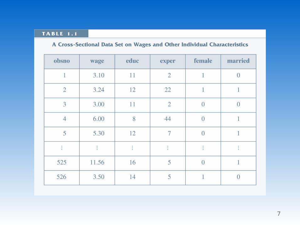
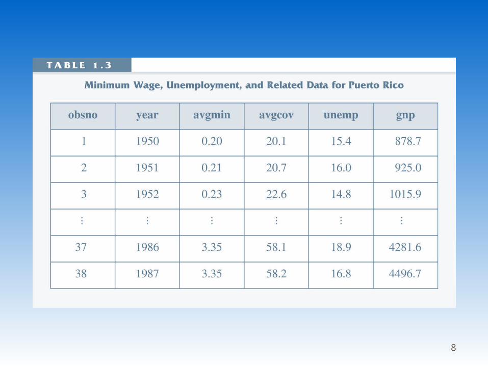
Type of data setsType of data sets
Cross sectional Time series Pooled cross sectional Panel Data
7
8
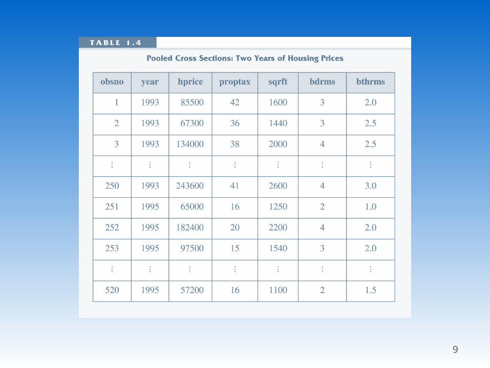
9
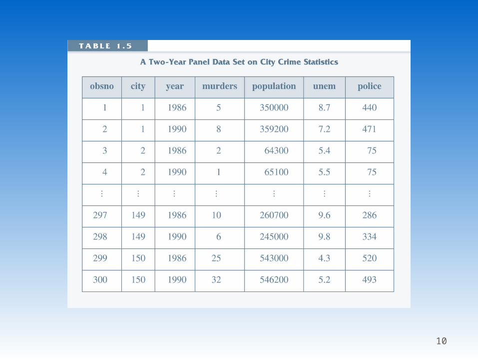
10
11
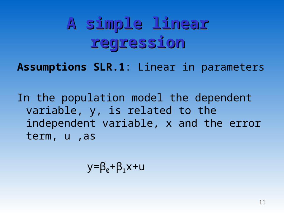
A simple linear regressionA simple linear regression
Assumptions SLR.1: Linear in parameters
In the population model the dependent variable, y, is related to the independent variable, x and the error term, u ,as
y=β0+β1x+u
12
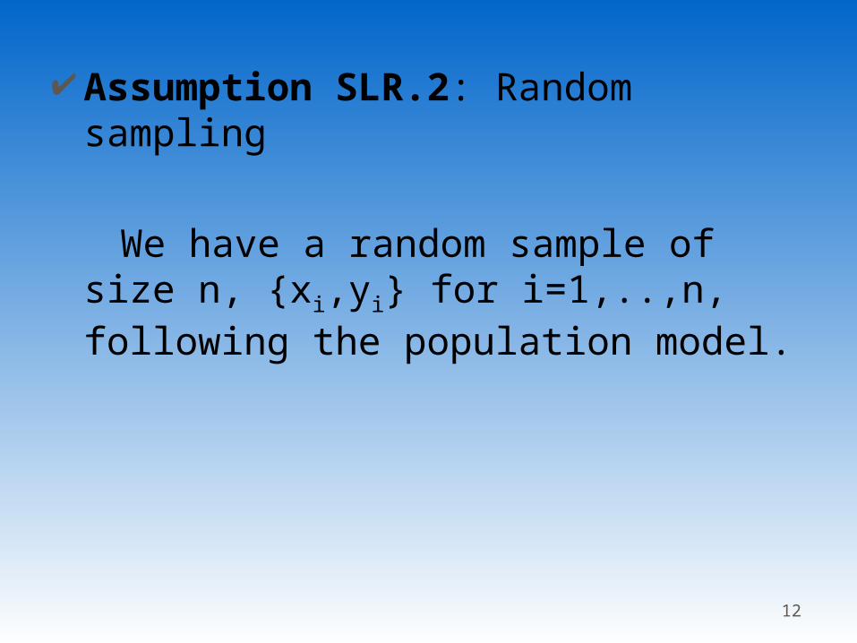
Assumption SLR.2: Random sampling
We have a random sample of size n, {xi,yi} for i=1,..,n, following the population model.
13
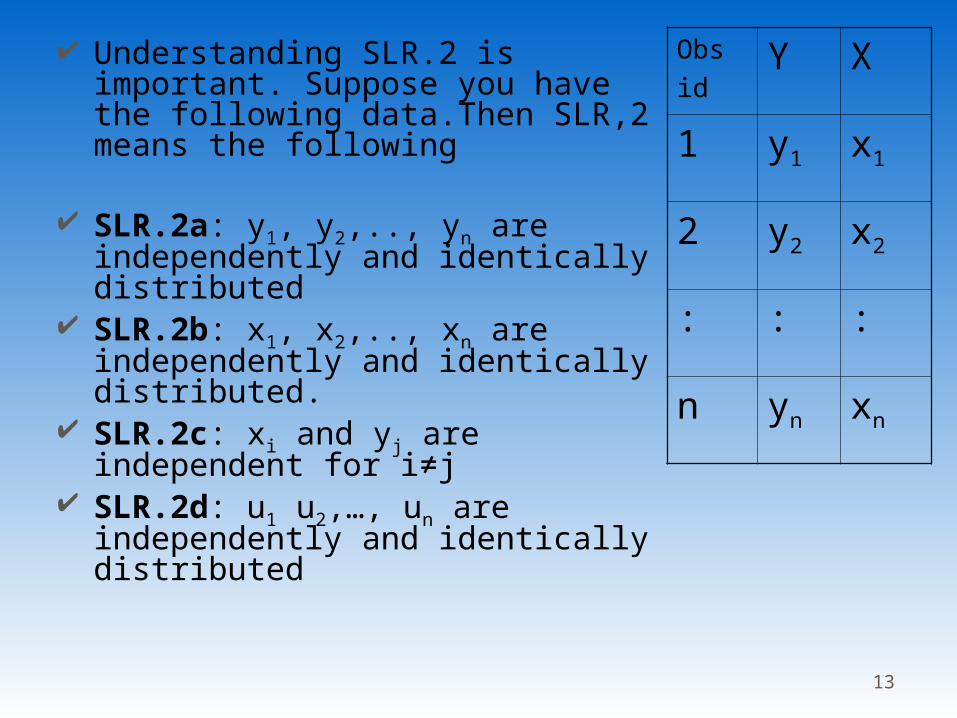
Understanding SLR.2 is important. Suppose you have the following data.Then SLR,2 means the following
SLR.2a: y1, y2,.., yn are independently and identically distributed
SLR.2b: x1, x2,.., xn are independently and identically distributed.
SLR.2c: xi and yj are independent for i≠j
SLR.2d: u1 u2,…, un are independently and identically distributed
Obs id
Y X
1 y1 x1
2 y2 x2
: : :
n yn xn
14
Assumption SLR.3
The sample outcome of x, namely, x1,x2,…,xn are not all the same value.
15
Assumption SLR.4: Zero conditional mean
Given any value of x, the expected value of u is zero, that is
E(u|x)=0
16
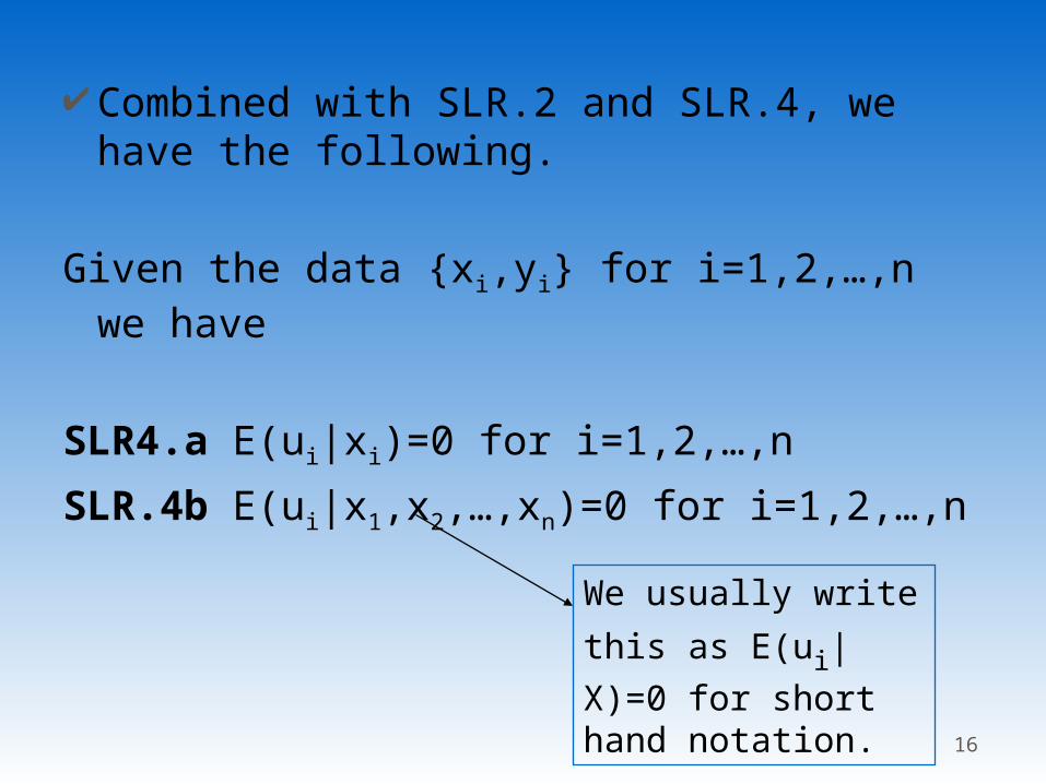
Combined with SLR.2 and SLR.4, we have the following.
Given the data {xi,yi} for i=1,2,…,n we have
SLR4.a E(ui|xi)=0 for i=1,2,…,n
SLR.4b E(ui|x1,x2,…,xn)=0 for i=1,2,…,n
We usually write this as
E(ui|X)=0 for short
hand notation.
17
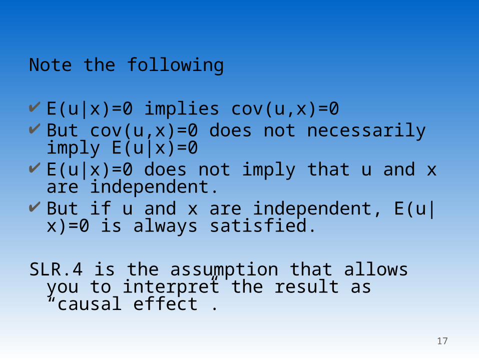
Note the following
E(u|x)=0 implies cov(u,x)=0 But cov(u,x)=0 does not necessarily imply
E(u|x)=0 E(u|x)=0 does not imply that u and x are
independent. But if u and x are independent, E(u|x)=0 is
always satisfied.
SLR.4 is the assumption that allows you to interpret the result as “causal effect”.
18
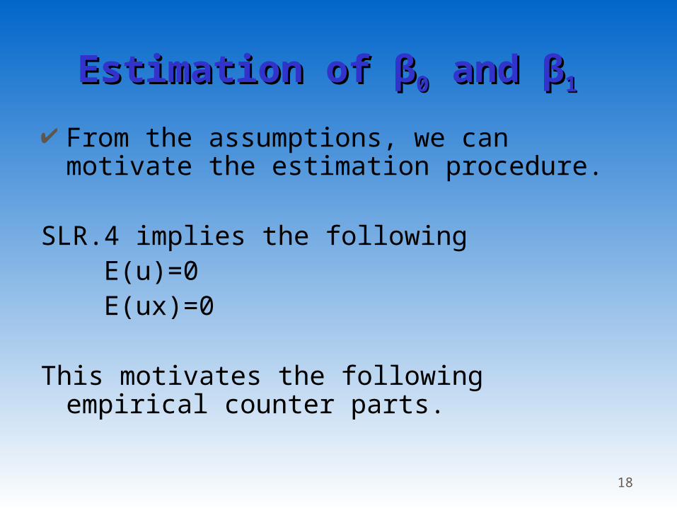
Estimation of Estimation of ββ00 and and ββ11
From the assumptions, we can motivate the estimation procedure.
SLR.4 implies the following E(u)=0 E(ux)=0
This motivates the following empirical counter parts.
19
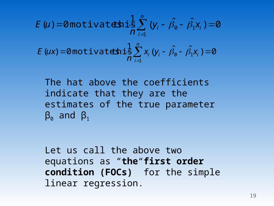
0)ˆˆ(1
: thismotivates 0)(1
10
n
iii xy
nuE
0)ˆˆ(1
: thismotivates 0)(1
10
n
iiii xyx
nuxE
The hat above the coefficients indicate that they are the estimates of the true parameter β0 and β1
Let us call the above two equations as “the first order condition (FOCs)” for the simple linear regression.
By solving FOCs for beta coefficients, we have the following estimates. (See next page)
20
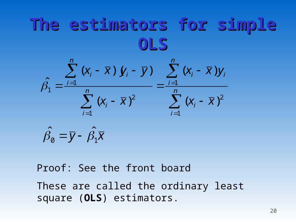
The estimators for simple The estimators for simple OLSOLS
n
ii
n
iii
n
ii
n
iii
xx
yxx
xx
yyxx
1
2
1
1
2
11
)(
)(
)(
))((̂
xy 10ˆˆ
Proof: See the front board
These are called the ordinary least square (OLS) estimators.
21
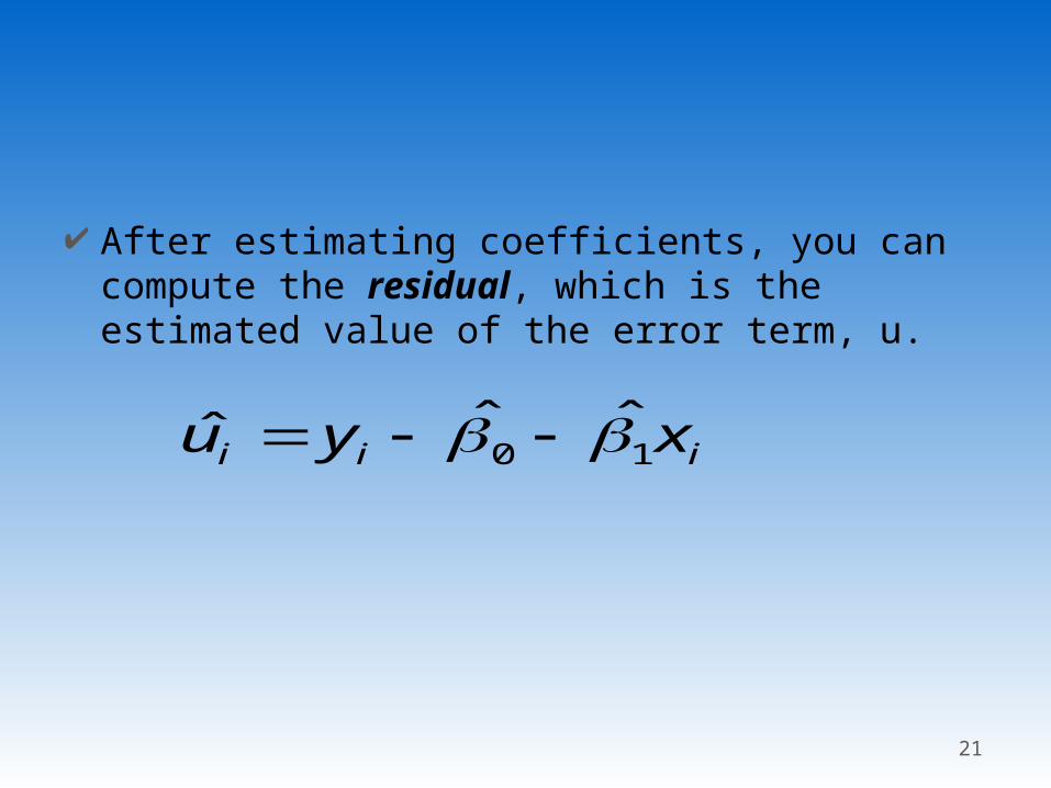
After estimating coefficients, you can compute the residual, which is the estimated value of the error term, u.
iii xyu 10ˆˆˆ
22
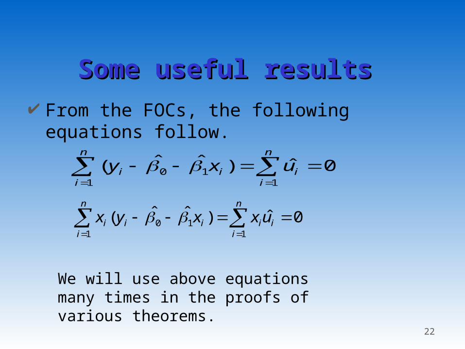
Some useful resultsSome useful results From the FOCs, the following equations
follow.
0ˆ)ˆˆ(11
10
i
n
ii
n
iiii uxxyx
0ˆ)ˆˆ(11
10
n
ii
n
iii uxy
We will use above equations many times in the proofs of various theorems.
23
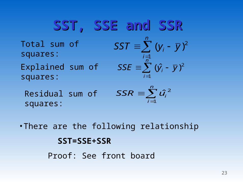
SST, SSE and SSRSST, SSE and SSR
n
ii yySST
1
2)(
n
ii yySSE
1
2)ˆ(
n
iiuSSR
1
2ˆ
Total sum of squares:
Explained sum of squares:
Residual sum of squares:
•There are the following relationship
SST=SSE+SSR
Proof: See front board
24
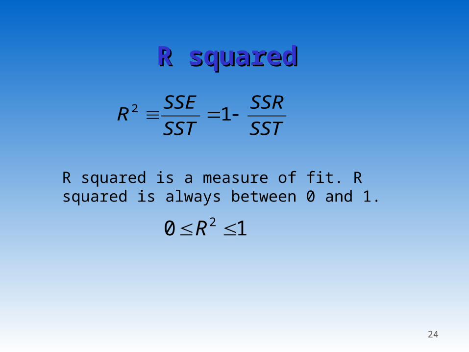
R squaredR squared
SST
SSR
SST
SSER 12
10 2 R
R squared is a measure of fit. R squared is always between 0 and 1.
25
Unit of measurements and Unit of measurements and functional formfunctional form
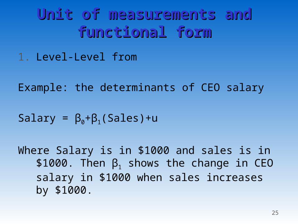
1. Level-Level from
Example: the determinants of CEO salary
Salary = β0+β1(Sales)+u
Where Salary is in $1000 and sales is in $1000. Then β1 shows the change in CEO salary in $1000 when sales increases by $1000.
26
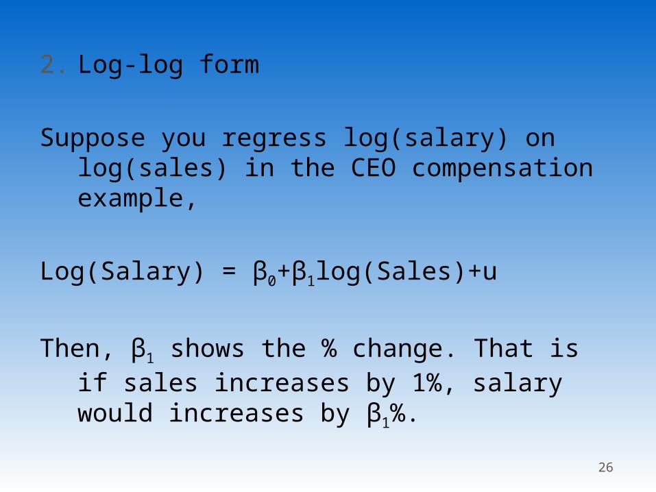
2. Log-log form
Suppose you regress log(salary) on log(sales) in the CEO compensation example,
Log(Salary) = β0+β1log(Sales)+u
Then, β1 shows the % change. That is if sales increases by 1%, salary would increases by β1%.
27
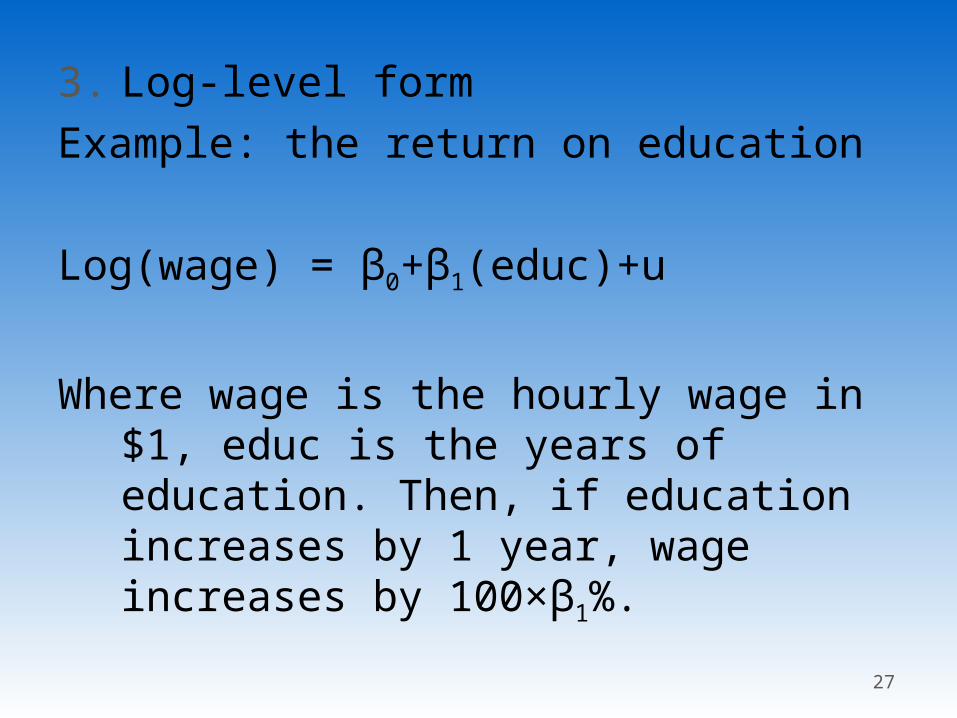
3. Log-level formExample: the return on education
Log(wage) = β0+β1(educ)+u
Where wage is the hourly wage in $1, educ is the years of education. Then, if education increases by 1 year, wage increases by 100×β1%.
28
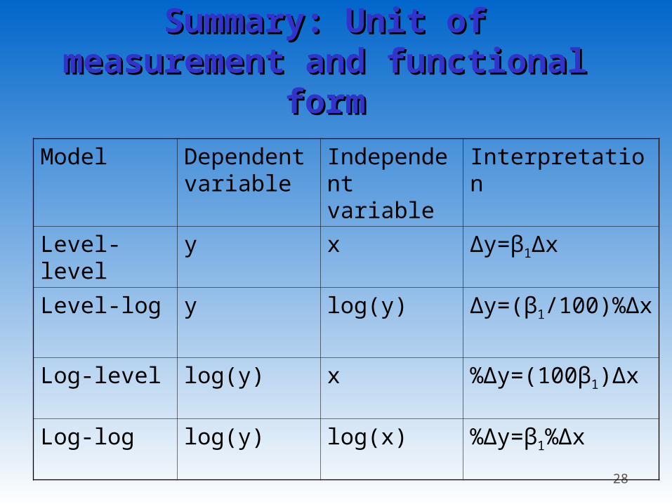
Summary: Unit of Summary: Unit of measurement and functional measurement and functional
formform
Model Dependent variable
Independent variable
Interpretation
Level-level y x ∆y=β1∆x
Level-log y log(y) ∆y=(β1/100)%∆x
Log-level log(y) x %∆y=(100β1)∆x
Log-log log(y) log(x) %∆y=β1%∆x
29
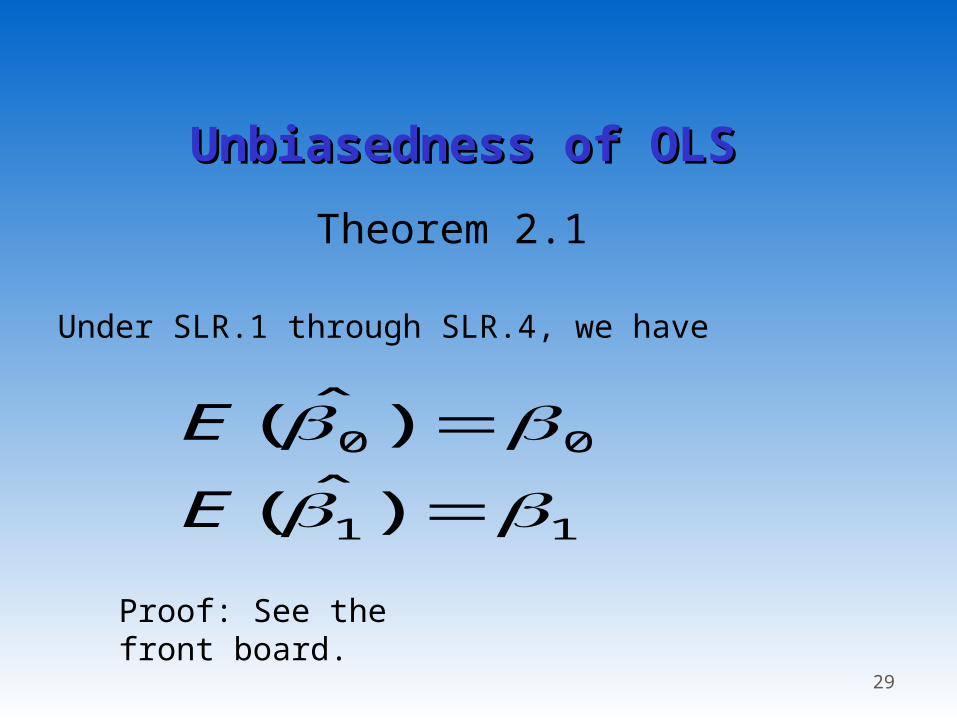
Unbiasedness of OLSUnbiasedness of OLS
Theorem 2.1
Under SLR.1 through SLR.4, we have
11
00
)ˆ(
)ˆ(
E
E
Proof: See the front board.
30
Variance of OLS Variance of OLS estimatorsestimators
First, we introduce one more assumption
Assumption SLR.5: Homoskedasticity
Var(u|x)=σ2
This means that the variance of u does not depend on the value of x.

31
Combining SLR.5 with SLR.2, we also have
MRL.4a Var(ui|X)=σ2 for i=1,…,n
where X denotes the independent variable for all the observations. That is, x1, x2,…, xn.
32
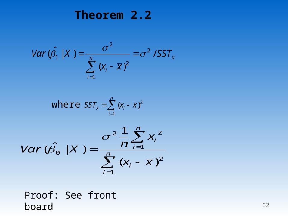
Theorem 2.2
xn
ii
SSTxx
XVar /)(
)|ˆ( 2
1
2
2
1
n
iix xxSST
1
2)(
n
ii
n
ii
xx
xn
XVar
1
2
1
22
0
)(
1
)|ˆ(
where
Proof: See front board
33
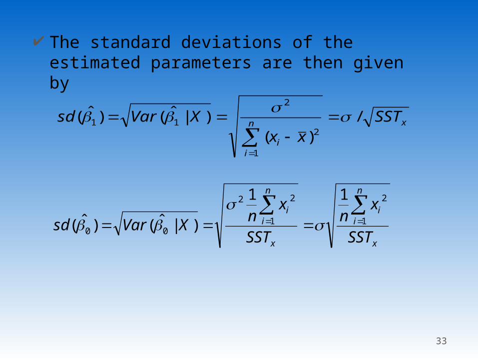
The standard deviations of the estimated parameters are then given by
xn
ii
SSTxx
XVarsd /)(
)|ˆ()ˆ(
1
2
2
11
x
n
ii
x
n
ii
SST
xn
SST
xn
XVarsd 1
2
1
22
00
11
)|ˆ()ˆ(
34
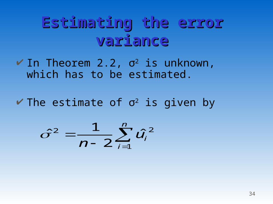
Estimating the error Estimating the error variancevariance
In Theorem 2.2, σ2 is unknown, which has to be estimated.
The estimate of σ2 is given by
n
iiun 1
22 ˆ2
1̂
35
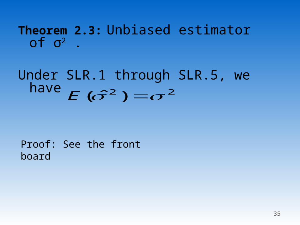
Theorem 2.3: Unbiased estimator of σ2 .
Under SLR.1 through SLR.5, we have 22 )ˆ( E
Proof: See the front board
36
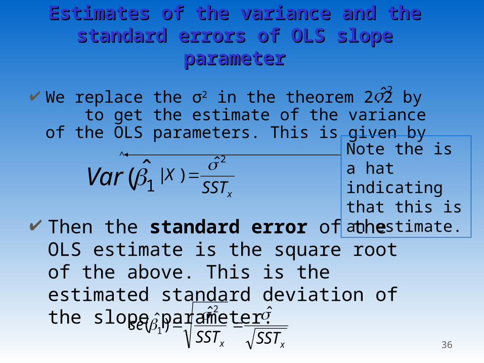
Estimates of the variance and the Estimates of the variance and the standard errors of OLS slope standard errors of OLS slope
parameterparameter
We replace the σ2 in the theorem 2.2 by to get the estimate of the variance of the OLS parameters. This is given by
xSSTXVar
2^ˆ
)|1̂(
Note the is a hat indicating that this is an estimate.
Then the standard error of the OLS estimate is the square root of the above. This is the estimated standard deviation of the slope parameter.
xx SSTSSTse
ˆˆ
)ˆ(2
1
2̂


