Download - 11 Computational Nosology and Precision Psychiatryredishlab.neuroscience.umn.edu/Papers/SFR20_11 Friston.pdf · ing or model selection ... Computational Nosology and Precision Psychiatry

11

Computational Nosology and Precision Psychiatry

A Proof of Concept

Karl J. Friston

Abstract

This chapter provides an illustrative treatment of psychiatric morbidity that offers an alternative to the standard nosological model in psychiatry. It considers what would happen if we treated diagnostic categories not as putative causes of signs and symp-toms, but as diagnostic consequences of psychopathology and pathophysiology. This reconstitution (of the standard model) opens the door to a more natural formulation of how patients present and their likely response to therapeutic interventions. The chapter describes a model that generates symptoms, signs, and diagnostic outcomes from latent psychopathological states. In turn, psychopathology is caused by pathophysiological processes that are perturbed by (etiological) causes, such as predisposing factors, life events, and therapeutic interventions. The key advantages of this nosological formula-tion include: (a) the formal integration of diagnostic (e.g., DSM) categories and latent psychopathological constructs (e.g., the dimensions of RDoC); (b) the provision of a hypothesis or model space that accommodates formal evidence-based hypothesis test-ing or model selection (using Bayesian model comparison); (c) the ability to predict therapeutic responses (using a posterior predictive density), as in precision medicine; and (d) a framework that allows one to test hypotheses about the interactions between pharmacological and psychotherapeutic interventions. These and other advantages are largely promissory at present: the purpose of this chapter is to show what might be pos-sible, through the use of idealized simulations. These simulations can be regarded as a (conceptual) prospectus that motivates a computational nosology for psychiatry.

Introduction

One of the key issues addressed by our working group at this Forum (Flagel et al., this volume) was the status of psychiatric nosology and how it might

From “Computational Psychiatry: New Perspectives on Mental Illness,” A. David Redish and Joshua A. Gordon, eds. 2016. Strüngmann Forum Reports, vol. 20,

series ed. J. Lupp. Cambridge, MA: MIT Press. ISBN 978-0-262-03542-2.

202 K. J. Friston

be informed by advances in computational neurobiology (Redish and Johnson 2007; Montague et al. 2012; Wang and Krystal 2014). In brief, our starting point was the realization that diagnostic categories are not the causes of psy-chopathology—they are (diagnostic) consequences. Although rather obvious in hindsight, this was something of a revelation, largely because it disclosed the missing link between putative causes of psychiatric illness (e.g., genetic predisposition, environmental stressors, iatrogenic) and the consequences, as observed by clinicians (e.g., symptoms, signs and, crucially, diagnostic out-come). In what follows, I briefl y rehearse the ideas—borrowed from compu-tational neurobiology—that we hope might close this gap (for full discussion, see Flagel et al., this volume). This treatment provides a technical summary of our conclusions, using an illustrative (simulated) case study of nosology, diagnosis, and prognosis.

The principal contribution of a formal or computational approach to no-sology rests on the notion of a generative model. A generative model gener-ates consequences from causes—in our case, symptoms, signs, and diagno-ses—from underlying psychopathology and pathophysiology. Generally, these models are state-space models that describe dynamics and trajectories in the space of latent (e.g., pathophysiological) states. These states are latent or hid-den from direct observation and are only expressed in terms of measurable consequences, such as symptoms and signs. The utility of a generative model lies in the ability to infer latent states from observed outcomes and, possibly more importantly, assess the evidence for one model relative to others, given a set of measurements. This is known as (Bayesian) model comparison, where the evidence is simply the probability of any sequence of observations under a particular model (Stephan et al. 2009b). To assess the evidence for a particular model, it is necessary to fi t the model to observed data, a procedure known as model inversion. This is because the mapping from causes to consequences is inverted, to infer from consequences to causes (e.g., inferring pathophysiol-ogy from symptoms). Furthermore, having inverted a model—by optimizing its parameters to maximize model evidence—one can then simulate or predict new outcomes in the future using something called the posterior predictive density. Heuristically, this is the technology behind weather forecasts, where the generative model is a detailed state-space model of meteorological dy-namics (Young 2002). So can we conceive of an equivalent meteorology for psychiatry?

In the past decade, there have been considerable advances in using state-space models of distributed neuronal processes to understand (context-sensi-tive) connectivity and functional architectures in the brain. This is known as dynamic causal modeling, which accounts for a signifi cant number of papers in the imaging neuroscience literature (Friston et al. 2003; Daunizeau et al. 2011a). In what follows, I apply exactly the same (computational neurosci-ence) principles to the problem of modeling the causes of nosological outcomes in psychiatry. Indeed, all the examples below use standard Bayesian model



Computational Nosology and Precision Psychiatry 203

inversion schemes that are available in freely available academic software: the simulations described below can be reproduced by downloading the SPM software (http://www.fi l.ion.ucl.ac.uk/spm/) and invoking the Matlab script DEM_demo_ontology.m. The dynamic causal modeling of psychopathology can, in principle, offer a number of advantages over the standard nosological model. As noted in the abstract and by Flagel et al. (this volume), these in-clude: (a) the formal integration of diagnostic (e.g., DSM) categories and latent psychopathological constructs (e.g., the dimensions of RDoC) (Stephan and Mathys 2014), (b) the provision of a hypothesis or model space that accom-modates formal evidence-based hypothesis testing (Krystal and State 2014), and (c) the ability to predict therapeutic responses (using a posterior predictive density). Crucially, by adopting a dynamic modeling approach, one can prop-erly accommodate the personal history and trajectory of individual patients in determining (and predicting) the course of their illness.

Our overall approach to nosology (and its promissory advantages) may seem rather abstract and perhaps even grandiose. This chapter should there-fore be taken as a prospectus for future discussions about nosology and the potential for individualized or precision psychiatry in the future. Its purpose is to illustrate what could be possible, in an idealized world, if we were able to use clinical data to optimize generative models of psychopathology. Whether or not this is possible with current data is an outstanding question. In short, this chapter offers a (mathematical) sketch of what a computational nosology could look like.

I begin by describing a formal model that generates symptomatic and di-agnostic outcomes from latent (pathophysiological and psychopathological) causes. This model should not be taken too seriously; it is just used to illustrate the promise of such modeling initiatives and to show how a formal approach to nosology forces one to think carefully about the known and unknown variables in psychiatric processes and how they infl uence each other. In the next section, I consider the use of ratings of symptoms and signs (and diagnosis) to estimate or infer their latent causes. This is a necessary prelude for model comparison and is discussed briefl y. Finally, prognosis and prediction are considered by using the generative model to predict the outcome of a (simulated) schizoaf-fective process and its response to treatment.

Generative Models for Psychiatric Morbidity

This section introduces the general form of generative (dynamic causal) mod-els for psychiatric morbidity and a particular example that will be used to illus-trate model inversion, model selection, and prediction in subsequent sections. As noted above, a generative model generates consequences from causes. The basic form assumed here starts with the (observable) causes of psychiat-ric illness, such as genetic or environmental predispositions, and therapeutic



204 K. J. Friston

interventions. These factors induce pathophysiological states, such as aber-rant dopamine receptor availability or glucocorticoid receptor function, to alter their trajectories (i.e., time courses or fl uctuations) over a course of weeks to months. These latent pathophysiological states then determine psychopa-thology, cast in terms of latent cognitive, emotional, or behavioral function (e.g., low mood, psychomotor poverty, thought disorder). Psychopathological states correspond to the constructs underlying things like Research Domain Criteria (RDoC) (Kaufman et al. 2015) and clinical brain profi ling (Peled 2009). Finally, psychopathological states generate measured symptoms using, for example, standardized instruments (e.g., PANSS [Kay 1990], Beck depres-sion inventory, mini mental state) or diagnostic outcomes (e.g., schizophrenia, major affective disorder, schizoaffective disorder).

Note that in this setup, a diagnosis represents an outcome, provided by a cli-nician. In other words, symptoms, signs, and diagnosis have a common cause, where the diagnostic categorization provides a useful summary outcome that integrates aspects of psychopathology which may not be covered explicitly by standardized symptom ratings or particular signs (e.g., psychomotor poverty, EEG abnormalities, abnormal dexamethasone suppression).

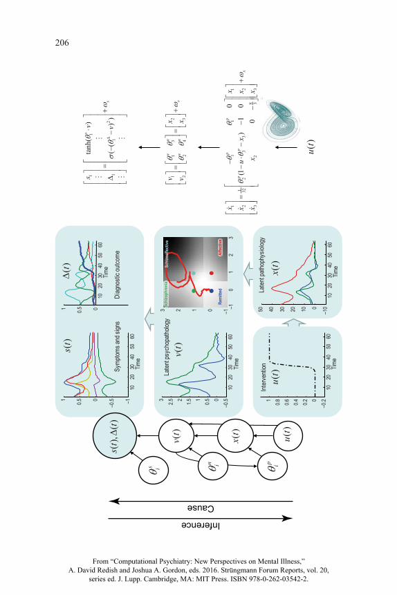
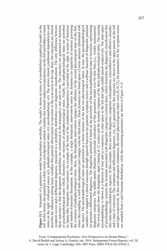
This formulation of psychiatric nosology is largely common sense and reiterates what most people would understand about psychiatric disorders. However, can this understanding be articulated formally in a way that can be used to make quantitative predictions and test competing etiological hy-potheses? This is where a formal nosology or generative model comes into play. The fi rst step is to construct a graphical model of dependencies among the variables generating measurable outcomes. Figure 11.1 (left panel) shows the graphical model that summarizes the probabilistic dependencies among etiological causes u(t), pathophysiological states x(t), psychopathology v(t), and, fi nally, symptoms and diagnosis s(t), Δ(t). In this format, the variables in white circles correspond to latent states that are hidden from direct observa-tion, while the observable outcomes are in the cyan circle.

Probabilistic dependencies are denoted by arrows that entail (time-invari-ant) parameters (θ = θs, θn, θp). This formulation clarifi es the roles of different quantities and makes their interdependencies explicit. For example, a diagnos-tic classifi cation at a particular time would be an outcome variable, whereas a patient’s drug history would be an etiological cause that infl uenced pathophys-iology. Having established the form of the graphical model, it is now necessary to specify the nature of the dependencies within and among latent variables. An example is provided in the right panel and can be described as follows.

A Generative (Dynamic Causal) Model

This example of a generative model is deliberately very simple and restricts itself to modeling a limited differential diagnosis that includes (a simulation




of) schizophrenia, affective disorder, schizoaffective disorder, and a remitted state. These diagnostic outcomes are accompanied by six symptom scores that have been normalized to lie between plus and minus one. Furthermore, only a limited number of exogenous causes and latent variables are considered: spe-cifi cally, a single therapeutic cause perturbs the evolution of three physiologi-cal states, from which two psychopathological states are derived. At any one time, the location in the psychopathological state-space determines a symptom profi le (through a linear mixture of psychopathological states that is passed through a sigmoid function). Diagnostic outcomes are, here, encoded by a probability profi le over the differential diagnosis (i.e., the relative confi dence a clinician places in the differential diagnoses). In the model, the probability of any one diagnosis corresponds to the relative proximity to a particular point in psychopathological state-space. In other words, as the disorder progresses, a trajectory is traced out in a two-dimensional psychopathological state-space, where, at any one time, the prevalent diagnosis is determined by the location to which the current state is closest. Technically, this has been modeled by a soft-max function of diagnostic potential, where diagnostic potential is the (nega-tive) Euclidean distance between the current state and the locations associated with each diagnostic category (encoded by θi

Δ, the color dots in Figure 11.1).The trajectory of psychopathology is determined by the corresponding tra-

jectory through a pathophysiological state-space which has its own dynamics. These are encoded by equations of motion or fl ow based, in this example, on a Lorenz attractor (Lorenz 1963). The Lorenz form is an arbitrary choice and could easily be replaced by other plausible equations: Moran et al. (this volume) provide an example based on normal form stochastic dynamics and indeed optimized on the basis of Bayesian model evidence (see below). Having said this, the Lorenz attractor provides a simple model of chaotic dynamics in the physical (Poland 1993) and biological (de Boer and Perelson 1991) sciences. Interestingly, it arose in the modeling of convection dynamics, which speaks to the analogy between the current modeling proposal and weather forecasting. In this setting, the ensuing dynamics can be regarded as a canonical form for nonlinear coupled processes that might underlie pathophysiology in psychosis. It has a canonical form because, as seen in Figure 11.1 (on the right), one can regard the parameters as specifying coupling coeffi cients or connections that mediate the infl uence of one physiological state on the others. Crucially, some of these connections are state dependent. This is important because it means one can model fl uctuations in pathophysiology in terms of self-organized (cha-otic) dynamics that have an underlying attracting set. In other words, we have a rough model of pathophysiological dynamics that summarize slow fl uctuations in neuronal (or hormonal) states that show homoeostatic or allostatic tenden-cies (e.g., Leyton and Vezina 2014; Misiak et al. 2014; Oglodek et al. 2014; Pettorruso et al. 2014; see also Krystal et al., this volume).

The equations in Figure 11.1 all include random fl uctuations. These fl uctua-tions render the generative model a probabilistic statement about how various



206

1020

3040

5060

–0.500.511.522.53

Laten

t psy

chop

atholo

gy

Time

–10

12

3–10123

1020

3040

5060

–1–0.500.51

Symp

toms a

nd si

gns

Time

1020

3040

5060

00.51

Diag

nosti

c outc

ome

Time

1020

3040

5060

–1001020304050

Laten

t path

ophy

siolog

y

Time

1020

3040

5060

–0.200.20.40.60.81

Interv

entio

n Time

()

ut

()

ut

()

xt

()

vt()

st

()t

()

ut()

xt()

vt

(),()

st

t

n i p is i

11

21

1

21

13

32

24

11

11

12

23

32

328

32

33

tanh(

)

((

))

0(1

)1

00

s

s

nn

vn

n

pp

pp

x

sv v

xv

xv

xx

xu

xx

xx

x

��

��

� � �

Inference

Cause



207

Figu

re 1

1.1

Sche

mat

ic o

f a g

ener

ativ

e m

odel

for p

sych

iatri

c m

orbi

dity

. The

mod

el is

show

n in

term

s of a

(pro

babi

listic

) gra

phic

al m

odel

on

the

left.

In th

is fo

rmat

, the

qua

ntiti

es in

whi

te ci

rcle

s cor

resp

ond

to ra

ndom

var

iabl

es th

at in

clud

e (un

know

n) p

aram

eter

s on

the l

eft a

nd h

idde

n or

late

nt

stat

es o

n th

e rig

ht: e

tiolo

gica

l cau

ses

u(t),

pat

hoph

ysio

logi

cal s

tate

s x(

t), p

sych

opat

holo

gy v

(t). T

he a

rrow

s de

note

con

ditio

nal d

epen

denc

ies

and

desc

ribe

the

infl u

ence

s am

ong

late

nt v

aria

bles

that

gen

erat

e ob

serv

atio

ns o

r out

com

es in

the

cyan

circ

le a

t the

top.

Her

e, th

e ou

tcom

es a

re c

linic

al

sym

ptom

sco

res

and

a di

ffere

ntia

l dia

gnos

is, m

easu

red

as a

pro

babi

lity

dist

ribut

ion

over

dia

gnos

tic c

lass

ifi ca

tions

. The

onl

y di

ffere

nce

betw

een

thes

e ou

tcom

es is

that

the

diag

nost

ic p

roba

bilit

ies

are

cons

train

ed to

the

nonn

egat

ive

and

sum

to o

ne. T

he o

utco

mes

are

gen

erat

ed a

s fu

nctio

ns

of p

sych

opat

holo

gica

l sta

tes

whi

ch, t

hem

selv

es, a

re m

ixtu

res

of p

atho

phys

iolo

gica

l sta

tes.

Fina

lly, t

he p

atho

phys

iolo

gica

l sta

tes

are

pertu

rbed

by

inpu

ts (l

ike

ther

apeu

tic in

terv

entio

ns).

An

exam

ple

of th

e fo

rm o

f the

con

ditio

nal d

epen

denc

ies

is p

rovi

ded

on th

e rig

ht, i

n te

rms

of fu

nctio

ns

and

rand

om (

Gau

ssia

n) fl

uctu

atio

ns. I

n th

is e

xam

ple,

a s

ingl

e th

erap

eutic

inte

rven

tion

ente

rs th

e dy

nam

ics

(or

equa

tions

of

mot

ion)

gov

erni

ng

the

evol

utio

n of

pat

hoph

ysio

logi

cal s

tate

s. H

ere,

the

ther

apeu

tic in

terv

entio

n ch

ange

s th

e infl u

ence

of t

he s

econ

d ph

ysio

logi

cal s

tate

on

the fi r

st,

whe

re th

is c

oupl

ing

is it

self

stat

e-de

pend

ent (

and

chan

ges w

ith th

e th

ird st

ate)

. The

se d

ynam

ics a

re b

ased

upo

n a

Lore

nz a

ttrac

tor (

illus

trate

d w

ith

the

inse

rt). T

he p

sych

opat

holo

gica

l sta

tes

are

gene

rate

d as

a li

near

mix

ture

of t

he la

st tw

o ph

ysio

logi

cal s

tate

s. In

turn

, the

psy

chop

atho

logi

cal

varia

bles

are

map

ped

to c

linic

al o

utco

mes

thro

ugh

sigm

oid

func

tions

(to

gene

rate

sym

ptom

scor

es) a

nd a

softm

ax fu

nctio

n of

dia

gnos

tic p

oten

tial

(to g

ener

ate

a di

ffere

ntia

l dia

gnos

is).

The

diag

nost

ic p

oten

tial i

s ba

sed

on th

e pr

oxim

ity o

f the

psy

chop

atho

logi

cal s

tate

to lo

catio

ns re

pres

entin

g di

agno

stic

cat

egor

ies.

The

mid

dle

pane

ls il

lust

rate

a p

artic

ular

real

izat

ion

of th

is g

ener

ativ

e m

odel

ove

r 64

time

bins

(i.e

., w

eekl

y as

sess

men

ts).

The

low

er p

anel

s sho

w th

e th

erap

eutic

inpu

t (st

artin

g at

32

wee

ks) a

nd th

e dy

nam

ic re

spon

se o

f the

thre

e pa

thop

hysi

olog

ical

stat

es. T

he e

nsui

ng

psyc

hopa

thol

ogy

is sh

own

as a

func

tion

of ti

me

and

as a

traj

ecto

ry in

stat

e-sp

ace

in th

e le

ft an

d rig

ht m

iddl

e pa

nels

resp

ectiv

ely.

The

stat

e-sp

ace

of p

sych

opat

holo

gy c

onta

ins t

he lo

catio

ns a

ssoc

iate

d w

ith d

iagn

ostic

cat

egor

ies (

colo

red

dots

), w

hich

det

erm

ine

the

diag

nost

ic c

lass

ifi ca

tion

that

til

es st

ate-

spac

e (s

hade

d gr

ay re

gion

s). I

n th

is e

xam

ple,

ther

e ar

e fo

ur d

iagn

ostic

cat

egor

ies:

schi

zoph

reni

a, sc

hizo

affe

ctiv

e an

d af

fect

ive

diso

rder

, an

d a

stat

e of

rem

issi

on. T

he sy

mpt

oms a

nd d

iffer

entia

l dia

gnos

is, s

(t), Δ

(t), g

ener

ated

by

this

traj

ecto

ry a

re sh

own

in th

e up

per p

anel

s on

the

left

and

right

resp

ectiv

ely.

In th

is a

nd su

bseq

uent

sim

ulat

ions

, the

initi

al (p

hysi

olog

ical

) sta

tes w

ere

[8,1

0,32

], th

e pa

ram

eter

s for

the

sym

ptom

scor

es

are

sam

pled

from

a u

nit G

auss

ian

dist

ribut

ion,

whi

le th

e re

mai

ning

par

amet

ers a

re sh

own

in F

igur

e 11

.4.



208 K. J. Friston

variables infl uence each other. Here, the random fl uctuations can be regarded as observation noise (when assessing symptoms) and random fl uctuations or perturbations to psychological or physiological processing (e.g., life events or drug misuse). In this chapter, these random fl uctuations are smooth processes with a Gaussian correlation function with a correlation length of half an assess-ment interval (i.e., a few days).

There is no pretence that any of these states map in a simple way onto physi-ological variables; rather, they stand in for mixtures of physiological variables that have relatively simple dynamics. The existence of mixtures is assured by technical theorems such as the center manifold theorem and the slaving prin-ciple in physics (Carr 1981; Haken 1983; Frank 2004; Davis 2006b). Basically, these theorems say that any set of coupled dynamical systems can always be described in terms of a small number of patterns (known variously as order parameters or eigenmodes), which change slowly relative to fast and noisy fl uctuations about these patterns.

Crucially, this generative model has been constructed such that the thera-peutic intervention changes the state-dependent coupling between the fi rst and second pathophysiological states (in fl uid dynamics, this control parameter is known as a Rayleigh number and refl ects the degree of turbulent fl ow). This means we could regard this intervention as pharmacotherapy that changes the coupling between different neuronal (or hormonal) systems, e.g., an infl uence of an atypical antipsychotic (Hrdlicka and Dudova 2015) on dopaminergic and serotonin receptor function responsible for monoaminergic tone in the ventral striatum and serotoninergic projections from the amygdala to the paraventricu-lar nucleus (Wieland et al. 2015; Muzerelle et al. 2016). Furthermore, I have introduced a parameter θ3

p that determines the sensitivity to the intervention that may be important in determining a patient’s responsiveness to therapy (Brennan 2014).

The middle panel of Figure 11.1 provides an illustration of how a patient might present over time under this particular model. Imagine we wanted to model (six) symptom scores and a probabilistic differential diagnosis over four diagnoses (schizophrenia, schizoaffective, affective, and remitted), when as-sessing an outpatient on a weekly basis for 64 weeks. A therapeutic interven-tion, say an atypical antipsychotic, is introduced at 32 weeks and we want to model the response. This therapeutic input is shown in the lower left panel as a dotted line and affects the evolution of physiological states according to equations of motion on the right. These equations generate chaotic fl uctuations in (three) pathological states shown on the lower right. Two of these states are then mixed to produce a trajectory in a psychopathological state-space. This trajectory is shown in the middle panel as a function of time (middle left) and as a trajectory in state-space (red line in the middle right panel). In turn, the psychopathology generates symptom scores (shown as colored lines on the up-per left) and diagnostic probabilities (shown on the upper right). The relation-ship between the continuous (dimensional) latent space of psychopathology




and the (categorical) differential diagnosis is determined by diagnostic param-eters θi

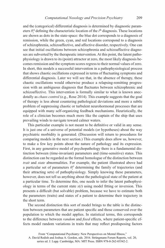
Δ defi ning the characteristic location of the ith diagnosis. These locations are shown as dots in the state-space: the blue dot corresponds to a diagnosis of remission, while the green, cyan, and red locations correspond to a diagnosis of schizophrenia, schizoaffective, and affective disorder, respectively. One can see that initial oscillations between schizophrenia and schizoaffective diagno-ses are subverted by the therapeutic intervention. At this point, the latent patho-physiology is drawn to its (point) attractor at zero, the most likely diagnosis be-comes remission and the symptom scores regress to their normal values of zero. In short, this models a successful intervention in a pathophysiological process that shows chaotic oscillations expressed in terms of fl uctuating symptoms and differential diagnosis. Later we will see that, in the absence of therapy, these chaotic oscillations would otherwise produce a relapsing-remitting progres-sion with an ambiguous diagnosis that fl uctuates between schizophrenic and schizoaffective. This intervention is formally similar to what is known anec-dotally as chaos control (e.g., Rose 2014). This example suggests that the goal of therapy is less about countering pathological deviations and more a subtle problem of suppressing chaotic or turbulent neurohormonal processes that are equipped with many self-organizing feedback mechanisms. Heuristically, the role of a clinician becomes much more like the captain of the ship that uses prevailing winds to navigate toward calmer waters.

This particular example is not meant to be defi nitive or valid in any sense. It is just one of a universe of potential models (or hypotheses) about the way psychiatric morbidity is generated. (Discussion will return to procedures for comparing models in the next section.) This example does allow us, however, to make a few key points about the nature of pathology and its expression. First, in any generative model of psychopathology there is a fundamental dis-tinction between (time-invariant) parameters and (time-sensitive) states. This distinction can be regarded as the formal homologue of the distinction between trait and state abnormalities. For example, the patient illustrated above had a particular set of parameters θi

p determining the family of trajectories (and their attracting sets) of pathophysiology. Simply knowing these parameters, however, does not tell us anything about the pathological state of the patient at a particular time. To determine this, one needs to infer the latent pathophysi-ology in terms of the current state x(t) using model fi tting or inversion. This presents a diffi cult (but solvable) problem, because we have to estimate both the parameters (traits) and states of a patient to determine their trajectory in the short term.

The second distinction this sort of model brings to the table is the distinc-tion between parameters that are patient specifi c and those conserved over the population to which the model applies. In statistical terms, this corresponds to the difference between random and fi xed effects, where patient-specifi c ef-fects model random variations in traits that may refl ect predisposing factors



210 K. J. Friston

(e.g., genetic predisposition). Conversely, other parameters may be fi xed over patients and determine the canonical form of nosology.

In the example above, this distinction is illustrated by the difference be-tween parameters that are specifi c to each patient or pathophysiology θi

p and those that are inherent in the nosology θi

n. The nosological parameters defi ne a generic mapping from pathophysiology to psychopathology that is conserved over patients. Understanding this distinction is important practically, because nosological parameters can only be estimated from group data. Examples of this are given in the next section.

Model Inversion and Selection

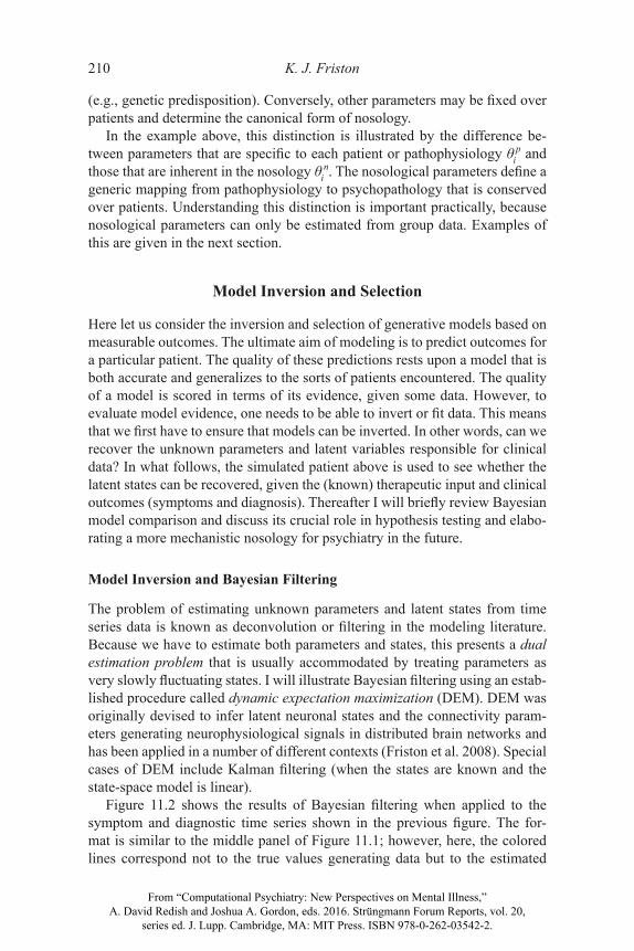
Here let us consider the inversion and selection of generative models based on measurable outcomes. The ultimate aim of modeling is to predict outcomes for a particular patient. The quality of these predictions rests upon a model that is both accurate and generalizes to the sorts of patients encountered. The quality of a model is scored in terms of its evidence, given some data. However, to evaluate model evidence, one needs to be able to invert or fi t data. This means that we fi rst have to ensure that models can be inverted. In other words, can we recover the unknown parameters and latent variables responsible for clinical data? In what follows, the simulated patient above is used to see whether the latent states can be recovered, given the (known) therapeutic input and clinical outcomes (symptoms and diagnosis). Thereafter I will briefl y review Bayesian model comparison and discuss its crucial role in hypothesis testing and elabo-rating a more mechanistic nosology for psychiatry in the future.

Model Inversion and Bayesian Filtering

The problem of estimating unknown parameters and latent states from time series data is known as deconvolution or fi ltering in the modeling literature. Because we have to estimate both parameters and states, this presents a dual estimation problem that is usually accommodated by treating parameters as very slowly fl uctuating states. I will illustrate Bayesian fi ltering using an estab-lished procedure called dynamic expectation maximization (DEM). DEM was originally devised to infer latent neuronal states and the connectivity param-eters generating neurophysiological signals in distributed brain networks and has been applied in a number of different contexts (Friston et al. 2008). Special cases of DEM include Kalman fi ltering (when the states are known and the state-space model is linear).

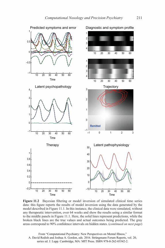
Figure 11.2 shows the results of Bayesian fi ltering when applied to the symptom and diagnostic time series shown in the previous fi gure. The for-mat is similar to the middle panel of Figure 11.1; however, here, the colored lines correspond not to the true values generating data but to the estimated




10 20 30 40 50 60–1

–0.5

0

0.5

1

Time

10 20 30 40 50 60–1

0

1

2

3

4Latent psychopathology

Time

10 20 30 40 50 60–10

0

10

20

30

40

50Latent pathophysiology

Time10 20 30 40 50 60

–0.2

0

0.2

0.4

0.6

0.8

1

Therapy

Time

Diagnostic and symptom profile

10 20 30 40 50 60

1

2

3

4

10 20 30 40 50 60

1

2

3

4

Trajectory

–1 0 1 2 3–1

0

1

2

3

Predicted symptoms and error

Figure 11.2 Bayesian fi ltering or model inversion of simulated clinical time series data: this fi gure reports the results of model inversion using the data generated by the model described in Figure 11.1. In this instance, the clinical data were simulated, without any therapeutic intervention, over 64 weeks and show the results using a similar format to the middle panels in Figure 11.1. Here, the solid lines represent predictions, while the broken black lines are the true values and actual outcomes being predicted. The gray areas correspond to 90% confi dence intervals on hidden states. (continued on next page)



212 K. J. Friston

trajectories based upon Bayesian fi ltering (as implemented with the Matlab routine spm_DEM.m). In this example, I simulated clinical progression in the absence of any therapeutic intervention (as shown by the fl at line in the lower left panel). In the absence of any check on pathophysiology, chaotic oscilla-tions of slowly increasing amplitude emerge over a period of 64 weeks. These fl uctuations are shown in terms of a trajectory in the state-space of psychopa-thology (lower right panel) and as functions of time (middle row). Here, the solid lines correspond to posterior expectations (the most likely trajectories) that are contained within 90% Bayesian confi dence intervals (gray areas). The true values are shown as dotted black lines. In this example, the true and esti-mated values were almost identical. This is because very low levels of random fl uctuations were used—with log precisions of twelve, eight, and four—to control the amplitude of random effects at the level of outcomes, psychopa-thology, and pathophysiology, respectively (see Figure 11.1). Precision is the inverse variance or amplitude.

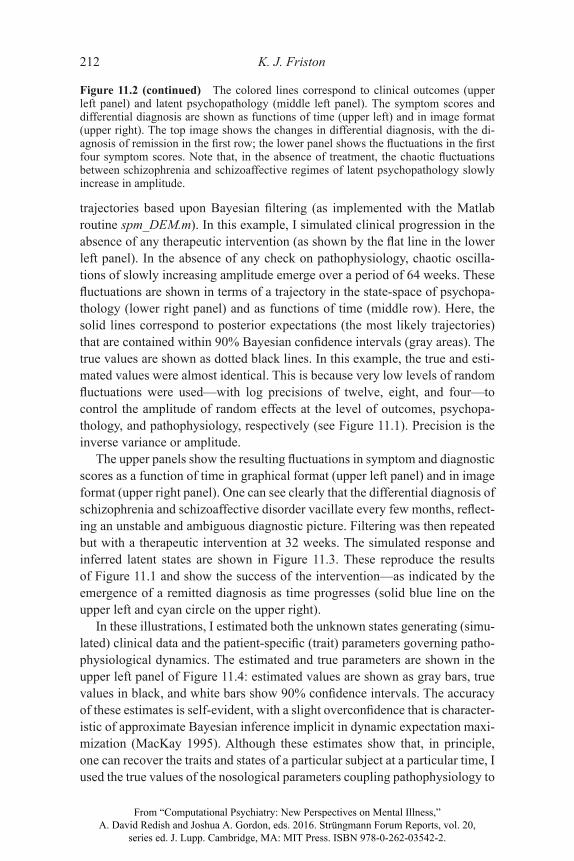
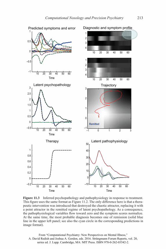
The upper panels show the resulting fl uctuations in symptom and diagnostic scores as a function of time in graphical format (upper left panel) and in image format (upper right panel). One can see clearly that the differential diagnosis of schizophrenia and schizoaffective disorder vacillate every few months, refl ect-ing an unstable and ambiguous diagnostic picture. Filtering was then repeated but with a therapeutic intervention at 32 weeks. The simulated response and inferred latent states are shown in Figure 11.3. These reproduce the results of Figure 11.1 and show the success of the intervention—as indicated by the emergence of a remitted diagnosis as time progresses (solid blue line on the upper left and cyan circle on the upper right).

In these illustrations, I estimated both the unknown states generating (simu-lated) clinical data and the patient-specifi c (trait) parameters governing patho-physiological dynamics. The estimated and true parameters are shown in the upper left panel of Figure 11.4: estimated values are shown as gray bars, true values in black, and white bars show 90% confi dence intervals. The accuracy of these estimates is self-evident, with a slight overconfi dence that is character-istic of approximate Bayesian inference implicit in dynamic expectation maxi-mization (MacKay 1995). Although these estimates show that, in principle, one can recover the traits and states of a particular subject at a particular time, I used the true values of the nosological parameters coupling pathophysiology to

Figure 11.2 (continued) The colored lines correspond to clinical outcomes (upper left panel) and latent psychopathology (middle left panel). The symptom scores and differential diagnosis are shown as functions of time (upper left) and in image format (upper right). The top image shows the changes in differential diagnosis, with the di-agnosis of remission in the fi rst row; the lower panel shows the fl uctuations in the fi rst four symptom scores. Note that, in the absence of treatment, the chaotic fl uctuations between schizophrenia and schizoaffective regimes of latent psychopathology slowly increase in amplitude.




10 20 30 40 50 60–1

–0.5

0

0.5

1Predicted symptoms and error

Time

10 20 30 40 50 60–0.5

0

0.5

1

1.5

2

2.5


Time

10 20 30 40 50 60–10

0

10

20

30

40


Time10 20 30 40 50 60

–0.2

0

0.2

0.4

0.6

0.8

1

Therapy

Time


10 20 30 40 50 60

1234

10 20 30 40 50 60

1234

Trajectory

–1 0 1 2 3–1

0

1

2

3

Figure 11.3 Inferred psychopathology and pathophysiology in response to treatment. This fi gure uses the same format as Figure 11.2. The only difference here is that a thera-peutic intervention was introduced that destroyed the chaotic attractor, replacing it with a point attractor in the remitted regime of latent psychopathology. As a consequence, the pathophysiological variables fl ow toward zero and the symptom scores normalize. At the same time, the most probable diagnosis becomes one of remission (solid blue line in the upper left panel; see also the cyan circle in the corresponding predictions in image format).



214 K. J. Friston

psychopathology (and generating clinical outcomes) during model inversion. One might ask: Can these parameters also be estimated?

To illustrate this estimation, the upper right panel of Figure 11.4 reports the estimates (and 90% confi dence intervals) based on any empirical Bayesian analysis (Kass and Steffey 1989) of eight simulated patients (using spm_dcm_peb.m). Again, the estimates are remarkably accurate, suggesting that, in prin-ciple, it is possible to recover parameters that are conserved over subjects.

0 5 10 150

0.2

0.4

0.6

0.8

1Model posterior

Model

Prob

abilit

y

1 2 3 4–0.5

0

0.5

1

1.5

2

2.5

Model

Param

eter

Model space

5 10 15

B(1,1)

B(2,1)

B(1,2)

B(2,2)

B(1,1)

B(2,1)

B(1,2)

B(2,2)

B(1,1)

1 2 3–10

0

10

20

30

40

1,3p

1,4n

Subject-specificparameters

Nosology-specificparameters

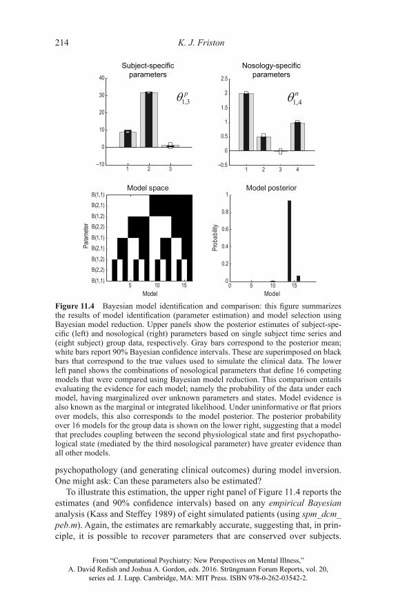
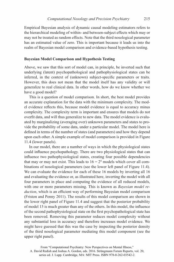
Figure 11.4 Bayesian model identifi cation and comparison: this fi gure summarizes the results of model identifi cation (parameter estimation) and model selection using Bayesian model reduction. Upper panels show the posterior estimates of subject-spe-cifi c (left) and nosological (right) parameters based on single subject time series and (eight subject) group data, respectively. Gray bars correspond to the posterior mean; white bars report 90% Bayesian confi dence intervals. These are superimposed on black bars that correspond to the true values used to simulate the clinical data. The lower left panel shows the combinations of nosological parameters that defi ne 16 competing models that were compared using Bayesian model reduction. This comparison entails evaluating the evidence for each model; namely the probability of the data under each model, having marginalized over unknown parameters and states. Model evidence is also known as the marginal or integrated likelihood. Under uninformative or fl at priors over models, this also corresponds to the model posterior. The posterior probability over 16 models for the group data is shown on the lower right, suggesting that a model that precludes coupling between the second physiological state and fi rst psychopatho-logical state (mediated by the third nosological parameter) have greater evidence than all other models.




Empirical Bayesian analysis of dynamic causal modeling estimators refers to the hierarchical modeling of within- and between-subject effects which may or may not be treated as random effects. Note that the third nosological parameter has an estimated value of zero. This is important because it leads us into the realm of Bayesian model comparison and evidence-based hypothesis testing.

Bayesian Model Comparison and Hypothesis Testing

Above, we saw that this sort of model can, in principle, be inverted such that underlying (latent) psychopathological and pathophysiological states can be inferred, in the context of (unknown) subject-specifi c parameters or traits. However, this does not mean that the model itself has any validity or will generalize to real clinical data. In other words, how do we know whether we have a good model?

This is a question of model comparison. In short, the best model provides an accurate explanation for the data with the minimum complexity. The mod-el evidence refl ects this, because model evidence is equal to accuracy minus complexity. The complexity term is important and ensures that models do not overfi t data, and will thus generalize to new data. The model evidence is evalu-ated by marginalizing (averaging over) unknown parameters and states to pro-vide the probability of some data, under a particular model. The model here is defi ned in terms of the number of states (and parameters) and how they depend upon each other. A simple example of model comparison is provided in Figure 11.4 (lower panels).

In our model, there are a number of ways in which the physiological states could infl uence psychopathology. There are two physiological states that can infl uence two pathophysiological states, creating four possible dependencies that may or may not exist. This leads to 16 = 24 models which cover all com-binations of nosological parameters (see the lower left panel of Figure 11.4). We can evaluate the evidence for each of these 16 models by inverting all 16 and evaluating the evidence or, as illustrated here, inverting the model with all four parameters in place and computing the evidence of all reduced models, with one or more parameters missing. This is known as Bayesian model re-duction, which is an effi cient way of performing Bayesian model comparison (Friston and Penny 2011). The results of this model comparison are shown in the lower right panel of Figure 11.4 and suggest that the posterior probability of model 15 is much greater than any of the others. In this model, the infl uence of the second pathophysiological state on the fi rst psychopathological state has been removed. Removing this parameter reduces model complexity without any substantial loss in accuracy and therefore increases model evidence. We might have guessed that this was the case by inspecting the posterior density of the third nosological parameter mediating this model component (see the upper right panel).



216 K. J. Friston

This is a rather trivial example of model comparison but illustrates an im-portant aspect of dynamic causal modeling; namely, the ability to test and compare different models or hypotheses. Although not illustrated here, one can imagine comparing models with different numbers of pathophysiologi-cal states and different forms of dynamics. One could even imagine compar-ing models with a different graphical structure. One interesting example here would be the modeling of psychotherapeutic interventions that might infl uence pathophysiology through experience-dependent plasticity. This would neces-sitate comparing models in which therapeutic intervention infl uenced psycho-pathology, which couples back to pathophysiology, through the parameters of its dynamics. This is illustrated by the dotted arrows in Figure 11.1.

Many other examples lend themselves to speculation: crucial examples in-volve an increasingly mechanistic interpretation of pathophysiology, in which pathophysiological states could be mapped onto neurotransmitter systems through careful (generative) modeling of electrophysiological and psycho-physical measurements (Stephan and Mathys 2014). One could also contem-plate comparing models with different sorts of inputs or causes, ranging from social or environmental perturbations (e.g., traumatic events) to genetic factors (or their proxies like family history). Questions about whether and where ge-netic polymorphisms affect pathophysiology are formalized by simply com-paring different generative models that accommodate effects on different states or parameters. For example, do models that include genetic biases on physi-ological parameters have greater evidence than models that do not?

The potential importance of model comparison should not be underesti-mated. Here I have tried to give a fl avor of its potential. It is also worth noting that this fi eld is an area of active research; fast and improved schemes for scor-ing large model spaces are continually being developed (e.g., Viceconti et al. 2015). One can construe an exploration of model space as a greedy search over competing hypotheses and a formal statement of the scientifi c process. This may be especially relevant for psychiatry, which addresses the specifi c prob-lem of integrating both physiological and psychological therapies, and points to the need for generative models that map between these two levels of descrip-tion. In the fi nal section, let us turn to the more pragmatic issue of predicting response to treatment for an individual patient.

Prediction and Personalized Psychiatry

Let us assume that we used Bayesian model comparison to optimize our gen-erative model of psychosis and prior probability distributions over its param-eters. Can we now use the model to predict the outcome of a particular inter-vention in a given patient? In the previous section, we saw how clinical data from a single subject could be used to estimate subject-specifi c parameters (traits) and states at a particular time. In fact, the parameter estimates in Figure




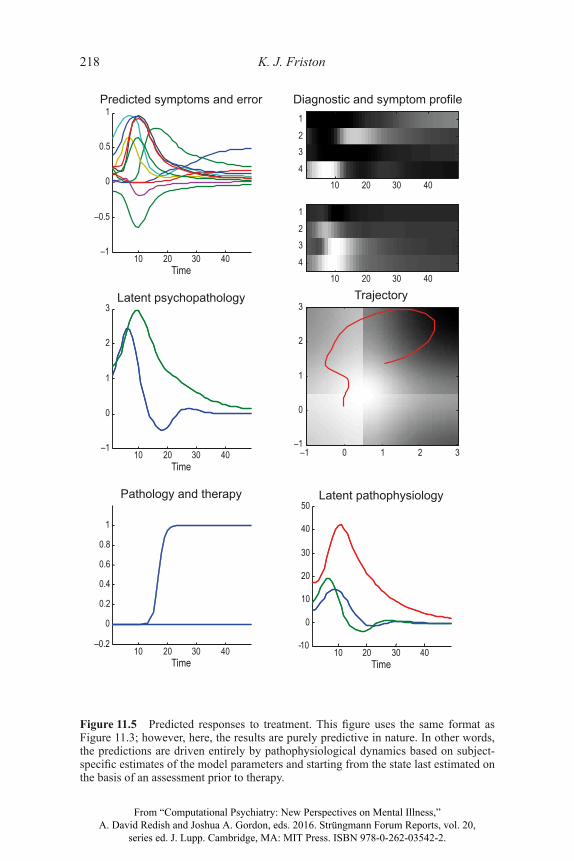
11.4 were based on the fi rst 32 weeks of data before any treatment began. This means that we now have estimates of how this particular subject would respond from any physiological state and the physiological state at the end of the period of assessment. Given these (posterior probability) estimates, there are several ways in which we can predict clinical prognosis and responses to different treatments. The simplest way would be to sample from the posterior distribution and integrate the generative model with random fl uctuations to build a probability distribution over future states. We will take a related but simpler approach and apply Bayesian fi ltering to null data with zero precision; in other words, data that has yet to be acquired. This fi nishes a predictive distri-bution over future trajectories based on the posterior estimates of the subject’s current parameters and states.

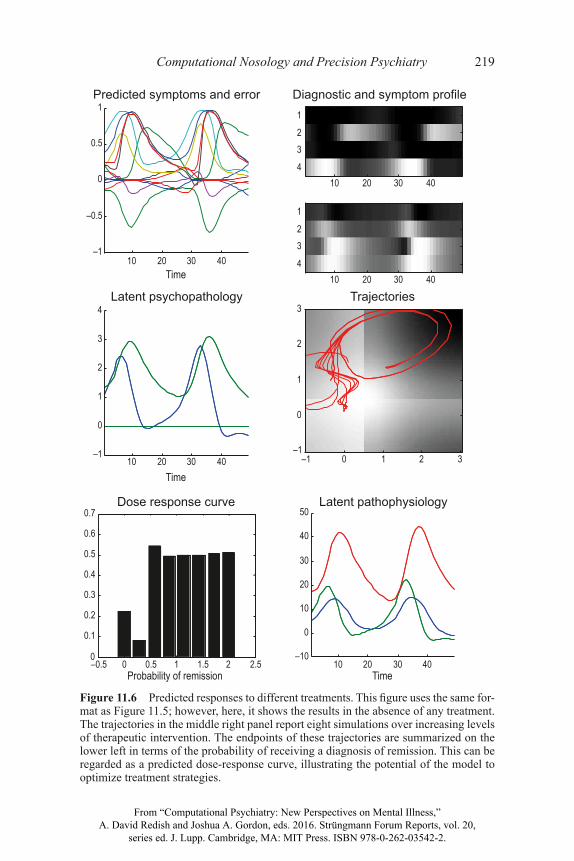
Figure 11.5 shows the results of this predictive fi ltering using the same for-mat as Figure 11.3. However, there are two crucial differences between Figures 11.5 and 11.3. First, we are starting from latent states that are posterior esti-mates of the subject’s current state and, more importantly, the trajectories are pure predictions based upon pathophysiological dynamics. One can see that the predicted response to treatment (at 16 weeks) has a similar outcome to the actual treatment (although the trajectories are not exactly the same, when comparing the predicted and actual outcomes in Figures 11.3 and 11.5, re-spectively). Figure 11.6 shows the same predictions in the absence of treat-ment, again showing the same pattern of fl uctuation between schizophrenia and schizoaffective diagnosis encountered in Figure 11.2.

The right panel of Figure 11.6 also includes trajectories with increasing levels of therapeutic intervention (ranging from 0 to 2). The fi nal outcomes of these interventions are summarized on the lower left in terms of the prob-ability of a diagnosis of remission at 48 weeks. This illustrates the potential for predictive modeling of this sort to provide dose-response relationships and ex-plore different therapeutic interventions (and combinations of interventions). In this simple example, there is a small probability that the patient would remit without treatment, which dips and then recovers to levels of around 50% with increasing levels of therapy. The apparent spontaneous recovery would not, however, be long lasting, as can be imputed from the chaotic oscillations in Figure 11.1.

Conclusion

In this chapter, I have illustrated what a computational nosology could look like using simulations of clinical trajectories, under a canonical generative model. The potential of this approach to nosological constructs can be motivated from a number of perspectives. First, it resolves the dialectic between categorical diagnostic constructs (e.g., DSM) and those based on latent dimensions of psychopathology or pathophysiology (e.g., RDoC). Both constructs play an



218 K. J. Friston

10 20 30 40–1

–0.5

0

0.5


Time

10 20 30 40–1

0

1

2


Time

10 20 30 40-10

0

10

20

30

40


Time10 20 30 40

–0.2

0

0.2

0.4

0.6

0.8

1

Pathology and therapy

Time


10 20 30 40

1

23

4

10 20 30 40

1

23

4

Trajectory

–1 0 1 2 3–1

0

1

2

3

Figure 11.5 Predicted responses to treatment. This fi gure uses the same format as Figure 11.3; however, here, the results are purely predictive in nature. In other words, the predictions are driven entirely by pathophysiological dynamics based on subject-specifi c estimates of the model parameters and starting from the state last estimated on the basis of an assessment prior to therapy.




10 20 30 40–1

–0.5

0

0.5


Time

10 20 30 40–1

0

1

2

3


Time

10 20 30 40–10

0

10

20

30

40


Time–0.5 0 0.5 1 1.5 2 2.50

0.1

0.2

0.3

0.4

0.5

0.6

0.7Dose response curve

Probability of remission


10 20 30 40

1

23

4

10 20 30 40

1

23

4

Trajectories

–1 0 1 2 3–1

0

1

2

3

Figure 11.6 Predicted responses to different treatments. This fi gure uses the same for-mat as Figure 11.5; however, here, it shows the results in the absence of any treatment. The trajectories in the middle right panel report eight simulations over increasing levels of therapeutic intervention. The endpoints of these trajectories are summarized on the lower left in terms of the probability of receiving a diagnosis of remission. This can be regarded as a predicted dose-response curve, illustrating the potential of the model to optimize treatment strategies.



220 K. J. Friston

essential role in a generative modeling framework, as diagnostic outcomes and latent causes, respectively. To harness their complementary strengths, it is only necessary to determine how one follows from the other, which is an inherent objective of model inversion and selection. Second, I have tried to emphasize the potential for an evidence-based approach to nosology that can operational-ize mechanistic hypotheses in terms of Bayesian model comparison. This pro-vides an integration of basic research and clinical studies which could, in prin-ciple, contribute synergistically to an evidenced-based nosology. Finally, I have illustrated the practical utility of using the predictions of (optimized) genera-tive models for individualized or precision psychiatry (Chekroud and Krystal 2015), in terms of providing probabilistic predictions of responses to therapy.

Although I have emphasized the provisional nature of this approach, it should be acknowledged that one could analyze existing clinical data using the model described in this chapter with existing algorithms. Indeed, there are hun-dreds of publications using dynamic causal modeling to infer the functional coupling among hidden neuronal states in the neuroimaging literature. In other words, it would be relatively simple to apply the techniques described above to existing data at the present time. The real challenge, however, lies in searching the vast model space to fi nd models that are suffi ciently comprehensive yet parsimonious to account for the diverse range of clinical measures—in a way that generalizes from patient to patient. This challenge is not necessarily insur-mountable: one might argue that if we invested the same informatics resources in psychiatry as has been invested in weather forecasting and geophysical modeling, then considerable progress could be made. Ultimately, one could imagine model-based psychiatric prognosis being received with the same con-fi dence with which we currently accept daily weather forecasts. There are, of course, differences between psychiatric and meteorological forecasting. For example, the latter must handle the “big data problem” with a relatively small model space. Conversely, psychiatry may have to contend with a “big theory problem,” with a relatively large model space but more manageable data sets.

Perhaps the more important contribution of a formal nosology is not in the pragmatic application to precision medicine (i.e., through the introduction of prognostic apps for clinicians), but in the use of Bayesian model selection to test increasingly mechanistic hypotheses and pursue a deeper understanding of pathogenesis in psychiatry. This is the way in which dynamic causal modeling has been applied in computational neuroscience and, as such, is just a formal operationalization of the scientifi c process.

Acknowledgments

KJF is funded by the Wellcome Trust. The author declares no confl icts of interest.

