

2 CHAPTER 5. GEOMETRIC ANALYSIS
modelling). In applications, there are the two principles of homogeneity and
exhaustiveness.
To sum up, gda is Benzecri’s tradition of multivariate statistics, with
the spectral theorem as the basic mathematical tool: “All in all, doing a
data analysis, in good mathematics, is simply searching eigenvectors; all the
science (or the art) of it is just to find the right matrix to diagonalize.”
(Benzecri et al, 1973, p. 289). This tradition extends the geometric ap-
proach far beyond the scaling of categorical data — a fact well perceived by
Greenacre (1981, p. 122): “The geometric approach of the French school
gives a much broader view of correspondence analysis, widening its field of
application to other types of data matrices apart from contingency tables.”
The present chapter, in the line of the book by Le Roux & Rouanet
(2004), is rooted in Benzecri’s tradition. It is devoted to individuals × vari-
ables tables — a basic data set in many research studies — by either pca
(numerical variables) or mca (categorized ones). The distinction numerical
vs categorized matters technically, but is not essential methodologically. As
Benzecri (2003, p.7) states: “One should not say: ‘Continuous numerical
magnitude’ ' ‘quantitative data’ vs ‘finite number of categories’ ' ‘qual-
itative data’. Indeed, at the level of a statistical individual, a numerical
datum is not to be taken as a rule with its full accuracy but according to its
meaningfulness; and from this point of view, there is no difference in nature
between age and (say) profession.”
The chapter is organized as follows. I describe pca and mca as gda
methods (§2). Then I introduce structuring factors and Structured Data
Analysis (§3). Last, I describe two analyses of structured individuals ×
variables tables, embedding anova techniques into the geometric framework
(§4 and §5).

5.2. PCA AND MCA AS GEOMETRIC METHODS 3
5.2 PCA and MCA as geometric methods
5.2.1 PCA: from multivariate analysis to GDA
To highlight Geometric Data Analysis, pca is a case in point on two counts:
i) pca preexisted as an established multivariate analysis procedure. ii) As
Benzecri (1992, p. 57) points out: “Unlike correspondence analysis, the
various methods derived from principal component analysis assign clearly
asymmetrical roles to the individuals and the variables”.
Letting n denote the number of individuals and p the number of variables,
the data table analyzed by pca is a n× p table with numerical entries. The
following excerpt by Kendall & Stuart (1976, p. 276) nicely describes the
two spaces involved: “We may set up a Euclidean space of p dimensions, one
for each variable, and regard each sample set . . . as determining a point in it,
so that our sample consists of a swarm of n points; or we may set up a space
of n dimensions, one for each observation, and consider each variable in it, so
that the variation is described by p vectors (lying in a p–dimensional space
embedded in a n–dimensional space).” In what follows, these spaces will be
called the “space of individuals” and the “space of variables”, respectively.
Now in conventional multivariate analysis — see, for example, Kendall &
Stuart (1976), Anderson (1958) — the space of variables is the basic one;
principal variables are sought as linear combinations of initial variables,
having the largest variances under specified constraints. On the other hand,
in pca recast as a gda method, the basic space is that of individuals (see,
for example, Lebart & Fenelon, 1971).
In pca as a gda method, the steps of pca are the following:
Step 1. The distance d(i, i′) between individuals i and i′ is defined by a
quadratic form on the difference between their description profiles, possibly
allowing for different weights on variables; see e.g. Rouanet & Le Roux
(1993), Le Roux & Rouanet (2004, p. 131).

4 CHAPTER 5. GEOMETRIC ANALYSIS
Step 2. The principal axes of the cloud are determined (by orthogonal
least squares), and a principal subspace is retained.
Step 3. The principal cloud of individuals is studied geometrically, ex-
hibiting approximate distances between individuals.
Step 4. The geometric representation of variables follows, exhibiting ap-
proximate correlations between variables. Drawing the circle of correlations
has become a tradition in pca as a gda method.
5.2.2 MCA: a GDA Method
Categorized variables are variables defined by (or encoded into) a finite set
of categories; the paradigm of the individuals × categorized variables table is
the I×Q table of a questionnaire in standard format, where for each question
q there is a set Jq of response categories — also called modalities — and
each individual i chooses for each question q one and only one category in
the set Jq. To apply the algorithm of ca to such tables, a preliminary coding
is necessary. When each question q has two categories, one of them being
distinguished as “presence of property q”, ca can immediately be applied
after logical coding : “0” (absence) vs “1” (presence); in this procedure there
is no symmetry between presence and absence. The concern for symmetry —
often a methodologically desirable requirement — naturally led to the coding
where each categorized variable q is replaced by Jq indicator variables, that
is, (0, 1) variables (also known as “dummy variables”); hence (letting J =∑q Jq) an I×J indicator matrix to which the basic ca algorithm is applied.
In this procedure, all individuals are given equal weights. In the early 1970s
in France, this variant of ca gradually became a standard for analyzing
questionnaires. The phrase “analyse des correspondances multiples” appears
for the first time in the paper by Lebart (1975), which is devoted to mca
as a method in its own right. Special mca software was soon developed and
published (see Lebart et al, 1977).
5.2. PCA AND MCA AS GEOMETRIC METHODS 5
The steps for mca parallel the ones for pca described above.
Step 1. Given two individuals i and i′ and a question q, if both individ-
uals choose the same response category, the part of distance due to question
q is zero; if individual i chooses category j and individual i′ category j′ 6= j
the part of (squared) distance due to question q is d2q(i, i
′) = 1fj
+ 1fj′
where
fj and fj′ are the proportions of individuals choosing j and j′, respectively.
The overall distance d(i, i′) is then defined by d2(i, i′) = 1Q
∑q d2
q(i, i′) (see Le
Roux & Rouanet, 2004). Once the distance between individuals is defined,
the cloud of individuals is determined.
Steps 2 and 3. They are the same as in pca.
Step 4. The cloud of categories consists of J category points.
Remark 1. (i) Only disagreements create distance between individuals.
(ii) The smaller the frequencies of disagreement categories, the greater the
distance between individuals. Property (i) is essential; property (ii), which
enhances infrequent categories, is desirable up to a certain point. Very in-
frequent categories of active questions need to be pooled with others; alter-
natively, one may attempt to put them as passive elements, while managing
to preserve the structural regularities of mca; see the paper by Benali &
Escofier (1987), reproduced in Escofier (2003), and the method of specific
mca in Le Roux (1999), Le Roux & Chiche (2004), Le Roux & Rouanet
(2004, chap. 5).
Remark 2. There is a fundamental property relating the two clouds.
Consider the subcloud of the individuals that have chosen category j, hence
the mean point of this subcloud (category mean–point); let fs denote its s–th
principal coordinate (in the cloud of individuals), and gs the s–th principal
coordinate of point j in the cloud of categories; then one has: fs = γs gs,
where γs denotes the s–th singular value of the ca of the I × J table.
This fundamental property follows from transition formulas; see Lebart et
al (1984, p. 94), Benzecri (1992, p. 410), Le Roux & Rouanet (1998, p.

6 CHAPTER 5. GEOMETRIC ANALYSIS
204). As a consequence, the derived cloud of category mean–points is in a
one–to–one correspondence with the cloud of category points, obtained by
shrinkages by scale factors γs along the principal axes s = 1, 2 . . . S.
5.2.3 A strategy for analyzing individuals × variables tables
For each table to analyze, the same strategy can be applied, with the fol-
lowing phases (phrased in terms of mca, to be adapted for pca).
Phase 1. Construction of the individuals × variables table
• Elementary statistical analyses and coding of data.
• Choice of active and supplementary individuals, of active and supple-
mentary variables, and of structuring factors (see §3).
Phase 2. Interpretation of axes
• Determine the eigenvalues, the principal coordinates and the contribu-
tions of categories to axes, and decide about how many axes to interpret.
• Interpret each of the retained axes by looking at important questions
and important categories, using the contributions of categories.
• Draw diagrams in the cloud of categories showing for each axis the
most important categories, and calculate the contributions of deviations (cf.
Le Roux & Rouanet, 1998).
Phase 3. Exploring the cloud of individuals
• Explore the cloud of individuals, in connection with the questions of
interest.
• Proceed to a Euclidean classification of individuals; interpret this clas-
sification in the framework of the geometric space.
Each step of the strategy may be more or less elaborate, according
to the questions of interest. As worked–out examples, see the Culture
Example in Le Roux & Rouanet (2004), and data sets at the web site
http://www.math-info.univ-paris5.fr/ ˜ lerb.

5.2. PCA AND MCA AS GEOMETRIC METHODS 7
5.2.4 Using GDA in survey research
In research studies, gda (pca or mca) can be used to construct geometric
models of individuals × variables tables. A typical instance is the analysis of
questionnaires, when the set of questions is sufficiently broad and at the same
time diversified enough to cover several themes of interest (among which
some balance is managed), so as to lead to meaningful multidimensional
representations.
In social sciences, the work of Bourdieu and his school is exemplary of
the “elective affinities” between the spatial conception of social space and
geometric representations, described by Bourdieu & Saint–Martin (1978)
and emphasized again by Bourdieu (2001, p.70): “Those who know the
principles of mca will grasp the affinities between mca and the thinking in
terms of field.”
For Bourdieu, mca provides a representation of the two complementary
faces of social space, namely the space of categories — in Bourdieu’s words,
the space of properties — and the space of individuals. Representing the two
spaces has become a tradition in Bourdieu’s sociology. In this connection,
the point is made by Rouanet et al (2000) that doing correspondence anal-
yses is not enough to do “analyses a la Bourdieu”, and that the following
principles should be kept in mind:
i) Representing individuals. The interest of representing the cloud of
individuals is obvious enough when the individuals are “known persons”; it is
less apparent when individuals are anonymous, as in opinion surveys. When,
however, there are factors structuring the individuals (education, age, etc.),
the interest of depicting the individuals, not as an undifferentiated collection
of points, but structured into subclouds, is soon realized and naturally leads
to analyzing subclouds of individuals. As an example, see the study of the
electorates in the French political space by Chiche et al (2002).
ii) Uniting theory and methodology. Once social spaces are constructed,
8 CHAPTER 5. GEOMETRIC ANALYSIS
the geometric model of data can lead to an explanatory use of gda, bringing
answers to the following two kinds of questions: How can individual positions
in the social space be explained by structuring factors? How can individual
positions, in turn, explain the position–takings of individuals about various
issues such as political or environmental? As examples, see the studies of the
French publishing space by Bourdieu (1999), of the field of French economists
by Lebaron (2000, 2001), and of Norwegian society by Rosenlund (2000) and
Hjellbrekke et al (2005).
5.3 Structured data analysis
5.3.1 Structuring factors
The geometric analysis of an individuals × variables table brings out the
relations between individuals and variables, but it does not take into ac-
count the structures with which the basic sets themselves may be equipped.
By structuring factors, we mean descriptors of the two basic sets that do
not serve to define the distance of the geometric space; and by structured
data, we designate data tables whose basic sets are equipped with struc-
turing factors. Clearly, structured data constitute the rule rather than the
exception, leading to questions of interest that may be central to the study
of the geometric model of data. Indeed, the set of statistical individuals aka
units may have to be built from basic structuring factors, a typical example
being the subjects×treatments design, for which a statistical unit is defined
as a pair (subject, treatment). Similarly, the set of variables may have to
be built from basic structuring factors. I will exemplify such constructions
for the individuals in the basketball study (§4), and for the variables in the
Education Progam for Gifted Youth study, in short EPGY study (§5).
In conventional statistics, there are techniques for handling structuring
factors, such as analysis of variance (anova) — including manova exten-

5.3. STRUCTURED DATA ANALYSIS 9
sions — and regression; yet, these techniques are not typically used in the
framework of gda. By structured data analysis we mean the integration of
such techniques into gda, while preserving the gda construction: see Le
Roux & Rouanet (2004, chap 6).
5.3.2 From experimental to observational data
In the experimental paradigm, there is a clear distinction between experi-
mental factors, or independent variables, and dependent variables. Statisti-
cal analysis aims at studying the effects of experimental factors on dependent
variables. When there are several dependent variables, a gda can be per-
formed on them, and the resulting space takes on the status of a “geometric
dependent variable”.
Now turning to observational data, let us consider an educational study,
for instance, where for each student, variables on various subject matters
are used as active variables to “create distance” between students and so to
construct an educational space. In addition to these variables, structuring
factors, such as identification characteristics (gender, age, etc.) may have
been recorded; their relevance is reflected in a question such as: “How are
boys and girls scattered in the educational space?”. Carrying over the ex-
perimental language, one may speak of the “effect of gender”; or one may
prefer the more neutral language of prediction, hence the question: knowing
the gender of a student (“predictor variable”), predict the position of this
student in the space (“geometric variable to be predicted”). As another
question of interest, suppose the results of students at some final exam are
available. Taking this variable as a structuring factor on the set of individu-
als, one may ask: knowing the position of a student in the space (“geometric
predictor”), predict the success of this student at the exam. The geometric
space is now the predictor, and the structuring factor the variable to be
predicted.

10 CHAPTER 5. GEOMETRIC ANALYSIS
5.3.3 Supplementary variables vs structuring factors
As a matter of fact, there is a technique in gda that handles structured data,
namely that of supplementary variables; see Benzecri (1992, p. 662), Cazes
(1982), Lebart et al (1984). Users of gda have recognized for a long time
that introducing supplementary variables amounts to doing regressions, and
they have widely used this technique, both in a predictive and explanatory
perspective. For instance, Bourdieu (1979), to build the lifestyle space of La
Distinction, puts the age, father’s profession, education level, and income as
supplementary variables, to demonstrate that differences in lifestyle can be
explained by those status variables.
The limitations of the technique of supplementary variables become ap-
parent, however, when it is realized that in the space of individuals, consid-
ering a supplementary category amounts to confining attention to the mean
point of a subcloud (fundamental property of mca), ignoring the dispersion
of the subcloud. Taking again La Distinction, this concern led Bourdieu, in
his study of the upper class, to regard the fractions of this class — “the most
powerful explanatory factor”, as he puts it — as what we call a structuring
factor in the cloud of individuals. In Diagrams 11 and 12 of La Distinction,
the subclouds corresponding to the fractions of class are stylized as contours
(for further discussion, see Rouanet et al, 2000).
To sum up, the extremely useful methodology of supplementary variables
appears as a first step toward structured data analysis; a similar case can
be made for the method of contributions of points and deviations developed
in Le Roux & Rouanet (1998).
5.3.4 Breakdown of variances
In experimental data, the relationships between factors take the form of a
factorial design, involving relations such as nesting and crossing of factors.
In observational data, even in the absence of prior design, similar relation-

5.3. STRUCTURED DATA ANALYSIS 11
ships between structuring factors may also be defined, as discussed in Le
Roux & Rouanet (1998). As in genuine experimental data, the nesting and
crossing relations generate effects of factors of the following types: main
effects, between–effects, within–effects and interaction effects. In contrast,
in observational data, the crossing relation is usually not orthogonal (as
opposed to experimental data, where orthogonality is often ensured by de-
sign), that is, structuring factors are usually correlated. As a consequence,
within–effects may differ from main effects. For instance, if social categories
and education levels are correlated factors, the effect of the education fac-
tor within social categories may be smaller, or greater, or even reversed
with respect to the main (overall) effect of the education factor (“structural
effect”).
Given a partition of a cloud of individuals, the mean points of the classes
of the partition (category mean–points) define a derived cloud, whose vari-
ance is called the between–variance of the partition. The weighted average
of the variances of subclouds is called the within–variance of the partition.
The overall variance of the cloud decomposes itself additively in between–
variance plus within–variance. Given a set of sources of variation and of
principal axes, the double breakdown of variances consists in calculating the
parts of variance of each source on each principal axis, in the line of Le
Roux & Rouanet (1984). This useful technique will be used repeatedly in
the applications presented in §4 and §5.
5.3.5 Concentration ellipses
Useful geometric summaries of clouds in a principal plane are provided by
ellipses of inertia, in the first place concentration ellipses: see Cramer, (1946,
p. 284). The concentration ellipse of a cloud is the ellipse of inertia such that
a uniform distribution over the interior of the ellipse has the same variance
as the cloud; this property leads to the ellipse with a half–axis along the s-th

12 CHAPTER 5. GEOMETRIC ANALYSIS
principal direction equal to 2 γs (i.e. twice the corresponding singular value).
For a normally–shaped cloud, the concentration ellipse contains about 86%
of the points of the cloud. Concentration ellipses are especially useful for
studying families of subclouds induced by a structuring factor or a clustering
procedure; see e.g. the EPGY study in §5.
Remark. In statistical inference, under appropriate statistical modelling,
the family of inertia ellipses also provides confidence ellipses for the true
mean points of clouds. For large n, the half–axes of the 1 − α confidence
ellipse are√
χ2α/n γs (χ2 with 2 d.f.); for instance, for α = .05, they are equal
to√
5.991/n γs, and the confidence ellipse can be obtained by shrinking
the concentration ellipse by a factor equal to 1.22/√
n. Thus the same
basic geometric construction yields descriptive summaries for subclouds and
inductive summaries for mean points. For an application, see the political
space study in Le Roux & Rouanet (2004, p.383 and 388).
In the next sections, structured individuals × variables tables are pre-
sented and analyzed in two research studies: 1) basketball (sport); 2) EPGY
(education). pca was used in the first study, mca in the second one.
Other extensive analyses of structured individuals × variables tables,
following the same overall strategy, will be found in the Racism study by
Bonnet et al (1990), in the political space study by Chiche et al (2000), and
in the Norwegian field of power study by Hjellbrekke et al (2005). The paper
by Rouanet et al (2002) shows how regression techniques can be embedded
into gda.
5.4 The basketball study
In the study by Wolff et al (1998), the judgments of basketball experts were
recorded in the activity of selecting high–level potential players. First, an
experiment was set up, where video sequences were constructed covering

5.4. THE BASKETBALL STUDY 13
typical game situations; eight young players (structuring factor P ) were
recorded in all sequences. These sequences were submitted to nine experts
(structuring factor E); each expert expressed for each player free verbal
judgments about the potentialities of this player. The compound factor
I = P ×E, made of the 8×9 = 72 (player, expert) combinations, defines the
set of statistical units, on which the expert judgments were recorded. Then,
a content analysis of the 72 records was carried out, leading to construct
11 judgment variables about the following four aspects of performance, re-
lating to upper body (four variables), lower body (four variables), global
judgment (one variable), play strategy (two variables: attack and defense),
respectively. The basic data set can be downloaded from the site http:
//math-info.univ-paris5.fr/ ˜ rouanet. Hereafter, we show how anova
techniques can be embedded into pca.
Weights were allocated to the 11 standardized variables following ex-
pert’s advice, namely 7, 3.5, 2.5 and 3 for the four aspects, respectively;
hence a total weight of 16. Then, a weighted pca was performed on the
72 × 11 table. The variance of the whole cloud is equal to 16 (sum of
weights), with 11 non-zero eigenvalues, hence the average λ = 16/11 = 1.45.
Two eigenvalues (λ1 = 9.30 and λ2 = 2.10) were found exceeding average.
Accordingly, two axes were interpreted: axis 1 was found to be related to
“dexterity”, and axis 2 to “strategy” (attack and defense).
Then from the basic cloud of 72 individual points, the cloud of the eight
mean points of players (indexed by factor P ) and the cloud of the nine mean
points of experts (factor E) were derived, and the additive cloud, i.e. the
fitted cloud without interaction was constructed. Table 5.1 shows the double
breakdown of variances, for the first two axes, according to the three sources
of variation: main effect of P , main effect of E, and interaction effect; it
also shows the variance of the additive cloud (P + E).
The table shows the large individual differences among players, the over-

14 CHAPTER 5. GEOMETRIC ANALYSIS
VariancesAxis1 Axis2
I = P × E 9.298 2.104Main P (Players) 8.913 1.731Main E (Experts) 0.051 0.124
Interaction 0.335 0.250P + E 8.964 1.855
Table 5.1: Basketball. Double breakdown of variances according to players (P ), experts(E), interaction, and additive cloud (P + E).
all homogeneity of experts, and the small interaction between players and
experts. Figure 5.1 shows the basic cloud, structured by the players mean
points, and Figure 5.2 the fitted additive cloud. In Figure 5.1, the observed
interaction effects between players and experts are reflected in the various
locations and distances of expert points with respect to player mean points.
For instance, the point of expert #6 is on the right of p1 but on the left of
p6, expert #4 is on the bottom side for most players, not for player p8, etc.
On Figure 5.2, the pattern of experts points is the same for all players; the
lines joining expert points (numbered arbitrarily from 1 to 9) exhibit the
parallelism property of the additive cloud.
Remark. Structural effect and interaction effect are two different things.
In the basketball study, the two factors players and experts are orthogonal,
therefore there is no structural effect, that is, for each axis, the sum of the
two variances of the main effects P and E is exactly the variance of the
additive cloud; on the other hand, the observed interaction effect between
the two factors is not exactly zero.
5.5 The EPGY study
The Education Program for Gifted Youth (epgy) at Stanford University
is a continuing project dedicated to developing and offering multimedia
computer–based distance–learning courses in a large variety of subjects; for
instance, in Mathematics, epgy offers a complete sequence from kinder-
garten through advanced–undergraduate (see Tock & Suppes, 2002).

5.5. THE EPGY STUDY 15
This case study, conducted by Brigitte Le Roux and Henry Rouanet in
cooperation with Patrick Suppes, deals with the detailed performances of
533 students in the third grade in the course of Mathematics, with its five
topics organized as strands, namely Integers, Fractions, Geometry, Logic and
Measurement, and for each strand, performance indicators of three types,
namely error rates, latencies (for correct answers) and numbers of exercises
(to master the concepts of the strand). The overall objective was to con-
struct a geometric space of data exhibiting the organization of individual
differences among gifted students. A specific question of interest was to
investigate the trade–off between errors and latencies. In this respect, the
body of existing knowledge about “ordinary students” appears to be of lim-
ited relevance, so the case study is really exploratory. The detailed study
can be found in Le Roux & Rouanet (2004, chapter 9) and on the Web–site
http://epgy.stanford.edu/research/GeometricDataAnalysis.pdf.
5.5.1 Data and coding
In such a study, in order to analyze the individuals × variables table, the
set of 533 students is naturally taken as the set of individuals, whereas the
set of variables is built from the two structuring factors: the set S of the five
strands and the set T of the three types of performance. Crossing the two
factors yields the compound factor S×T , which defines the set of 5×3 = 15
variables.
In the first and indispensable phase of elementary analyses and coding
of variables, we examine in detail the variables and their distributions. For
error rates, the distributions differ among the strands; they are strongly
asymmetric for Integers, Fractions and Measurement, and more bell-shaped
for Geometry and Logic. Latencies differ widely among strands. The num-
ber of exercises is a discrete variable. To cope with this heterogeneity, we
choose mca for constructing a geometric model of data. The coding of

16 CHAPTER 5. GEOMETRIC ANALYSIS
variables into small numbers of categories (2, 3 or 4) will aim to achieve
as much homogeneity as possible, as required to define a distance between
individuals.
For error rates, we start with a coding in three categories from 1 (low er-
ror rate) through 3 (high error rate), for each strand, hence 15 categories for
the five strands; now with this coding, category 3 has a frequency less than
1% for Integers and Fractions, therefore we pool this category with category
2, resulting in 13 categories. For latencies, we take, for each strand, a 4–
category coding, from 1 (short) through 4 (long); hence 4×5 = 20 categories.
For numbers of exercises, we code in two categories for Integers, Fractions,
and Measurement, and in three categories for Geometry and Logic, from 1
(small number) through 3 (large number); hence 12 categories. All in all,
we get 13 + 20 + 12 = 45 categories for 15 variables.
5.5.2 MCA and first interpretations
The basic results of mca are the following: (i) the eigenvalues; (ii) the prin-
cipal coordinates and the contributions of the 45 categories to axes (they
are given in Le Roux & Rouanet, 2004, p. 400; see also the web–site); (iii)
the principal coordinates of the 533 individuals; (iv) the geometric repre-
sentations of the two clouds (categories and individuals).
Eigenvalues and modified rates. There are J−Q = 45−15 = 30 eigenval-
ues, and the sum of eigenvalues (J−Q)/Q is equal to 2. How many axes to in-
terpret? Letting λm = 1/Q (mean eigenvalue, here .067) and λ′ = (λ−λm)2,
we have calculated modified rates by Benzecri’s formula λ′/∑
λ′, the sum
being taken over the eigenvalues greater than λm (Benzecri, 1992, p.412).
The modified rates indicate how the cloud deviates from a spherical cloud
(with all eigenvalues equal to the mean eigenvalue). As an alternative to
Benzecri’s formula — which Greenacre (1993) claims to be too optimistic
— we have also calculated modified rates using Greenacre’s formula. See

5.5. THE EPGY STUDY 17
Table 5.2. At any rate, one single axis is not sufficient. In what follows we
will concentrate on the interpretation of the first two axes.
Axis 1 Axis 2
Eigenvalues (λ) .3061 .2184
Raw rates of inertia 15.3% 10.9%Benzecri’s modified rates 63.1% 25.4%Grenacre’s modified rates 55.5% 21.8%
Table 5.2: EPGY. First two axes. Eigenvalues; raw rates and modified rates
From the basic table of the contributions of the 45 categories to axes
(not reproduced here), the contributions of the 15 variables can be obtained
by adding up their separate contributions (Table 5.3). The more compact
contributions of the three types of performance can be similarly derived, as
well as the contributions of the five strands. See Table 5.3 (contributions
greater than average are in bold).
Ctr Axis 1 Axis 2
Integers .083 .043Fraction .051 .034
Error Rate Geometry .104 .035Logic .096 .053Measuremt .098 .018
Error rate (Total) .433 .184
Integers .048 .159Fraction .043 .157
Latency Geometry .059 .123Logic .066 .131Measuremt .054 .106
Latency (Total) .271 .677
Integers .065 .022Fraction .028 .028
Exercises Geometry .023 .023Logic .097 .044Measuremt .084 .022
Exercises (Total) .296 .139
Total 1. 1.
Table 5.3: EPGY. Contributions to axes of the 15 variables (in bold: contributionsgreater than 1
15= .067), and of the three types of performance (in bold: contributions
greater than 1/3).
Making use of the S × T structure, the cloud of 45 categories can be
subdivided into subclouds. For instance, for each type of performance, we

18 CHAPTER 5. GEOMETRIC ANALYSIS
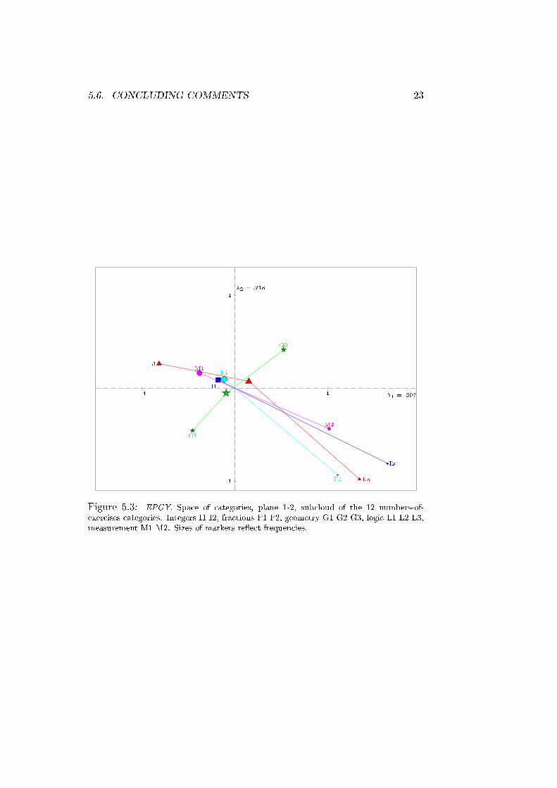
can construct and examine the corresponding subcloud. As an example,
Figure 5.3 depicts the subcloud of the 12 numbers-of-exercises categories
in plane 1-2; this figure shows for this type of performance the coherence
between strands, except for geometry.
5.5.3 Interpretation of axes
Interpretation of axis 1 (λ1 = .3061)
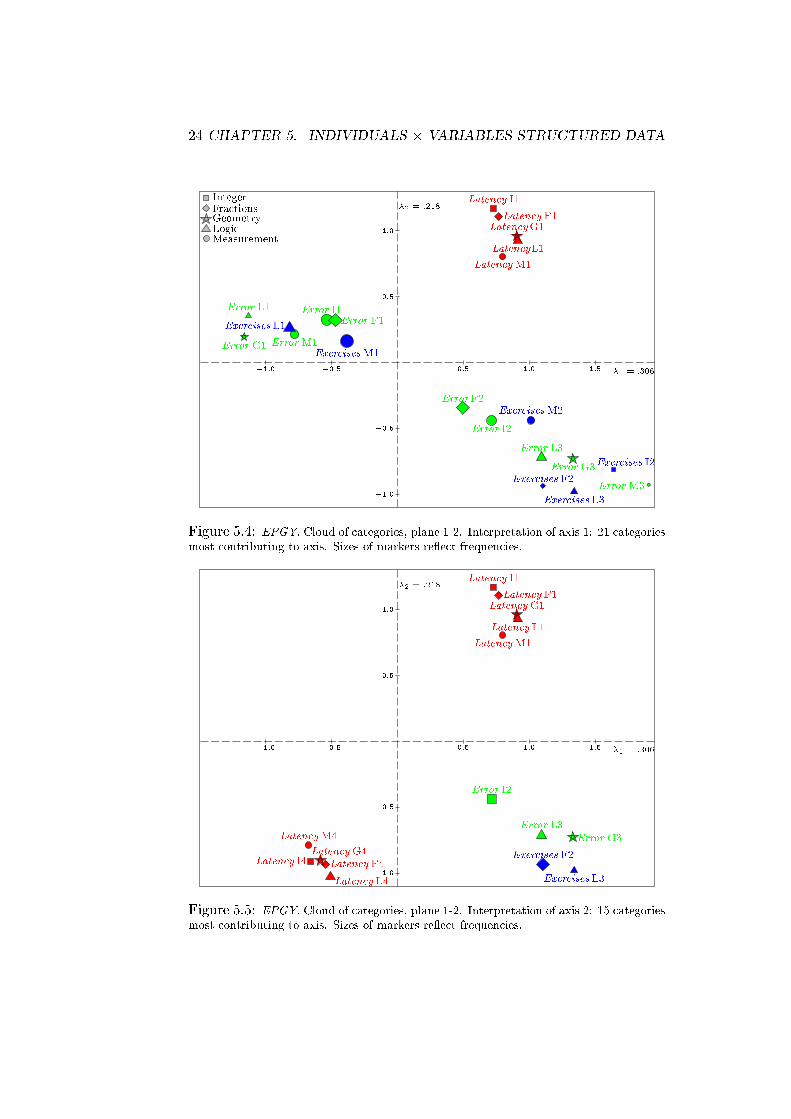
There are 20 categories whose contributions to axis 1 are greater than
average (1/Q = 1/45 = .022 = 2.2%); to which we will add the low error rate
category for Logic; the 21 categories account for 81% of the variance of axis,
on which we base the interpretation of axis 1. The opposition between high
error rates (right of axis) and low error rates (left) accounts for 35% of the
variance of axis 1 (out of the 43% accounted for by all error rate categories).
The contributions of short latency categories for the five strands are greater
than the average contribution. These five categories are located on the right
of origin (cf. Figure 5.4), exhibiting the link between high error rates and
short latencies. The opposition between low error rates and short latencies
accounts for 28% of the variance of axis 1, and the one between small and
large numbers of exercises for 24%. The opposition between the 7 categories
on the left and the 14 ones on the right accounts for 67% of the variance of
axis 1.
The first axis is the axis of error rates and numbers of exercises.
It opposes on one side low error rates and small numbers of
exercises and on the other side high error rates and large numbers
of exercises, the latter being associated with short latencies.
Interpretation of axis 2 (λ2 = .2184)
Conducting the analysis in the same way, we look for the categories most
contributing to the axis; we find 15 categories, that can be depicted again

5.5. THE EPGY STUDY 19
in plane 1-2, see Figure 5.5; the analysis leads to the conclusion:
The second axis is the axis of latencies. It opposes short latencies
and long latencies, the latter being associated with high error
rates and large numbers of exercises.
5.5.4 Cloud of individuals
The cloud of individuals (533 students) is represented on Figure 5.6; it con-
sists in 520 observed response patterns, to which we add the following four
extreme response patterns: Pattern 11111 11111 11111 (point A) (low error
rates, short latencies, small number of exercises); Pattern 11111 44444 11111
(point B) (low error rates, long latencies, small number of exercises); Pat-
tern 22332 11111 22332 (point D) (high error rates, short latencies, large
number of exercises); and Pattern 22332 44444 22332 (point C) (high error
rates, long latencies, large number of exercises). None of the 533 individuals
matches any one of these extreme patterns, which will be used as landmarks
for the cloud of individuals.
The individuals are roughly scattered inside the quadrilateral ABCD,
with a high density of points along the side AB and a low density along
the opposed side. This shows there are many students who make few errors
whatever their latencies. On the other hand, students with high error rates
are less numerous and very dispersed.
In structured individuals × variables tables, the cloud of individuals
enables one to go farther than the cloud of categories, for investigating
compound factors. As an example, let us study, for the measurement strand,
the crossing of error rates and latencies. There are 3 × 4 = 12 composite
categories, and for each of them there is associated a subcloud of individuals,
each one with its mean point. Figure 5.7 shows the 3 × 4 derived cloud
of mean points. The profiles are approximately parallel. There are few
individuals with high error rates (3) (dotted lines), whose mean points are

20 CHAPTER 5. GEOMETRIC ANALYSIS
close to side CD. As one goes down along the AB direction, latencies increase,
while error rates remain about steady; as one goes down along the AD
direction, error rates increase, while latencies remain about steady.
Axis 1 Axis 2 Plane 1-2
Between (Age×Gender) .0306 .0099 .0405
Age .0301 .0067 .0368Gender .0000 .0012 .0012
Interaction .0006 .0016 .0022
Within (Age×Gender) .2683 .2055 .4738Total variance (n = 468) .2989 .2154 .5143
Table 5.4: EPGY. Double breakdown of variances for the crossing Age × Gender.
To illustrate the study of external factors in the cloud of individuals, we
sketch the joint analysis of age and gender, allowing for missing data (57
and 46 respectively). Crossing age (in four classes) and gender (283 boys
and 204 girls) generates 4×2 = 8 classes. A large dispersion is found within
the 8 classes. In plane 1-2, the within variance is equal to .4738, and the
between–variance only .0405: see Table 5.4. The variances of the two main
effects and of the interaction between age and gender are also shown on this
table. The crossing of age and gender is nearly orthogonal, therefore there
is virtually no structural effect, that is, for each axis, the sum of the two
main effect variances is close to the difference “between–variance of crossing
minus interaction variance”.
5.5.5 Euclidean classification
Distinguishing classes of gifted students was one major objective of the
EPGY study. We have made a Euclidean classification, that is, an ascend-
ing hierarchical clustering with the inertia (Ward) criterion. The procedure
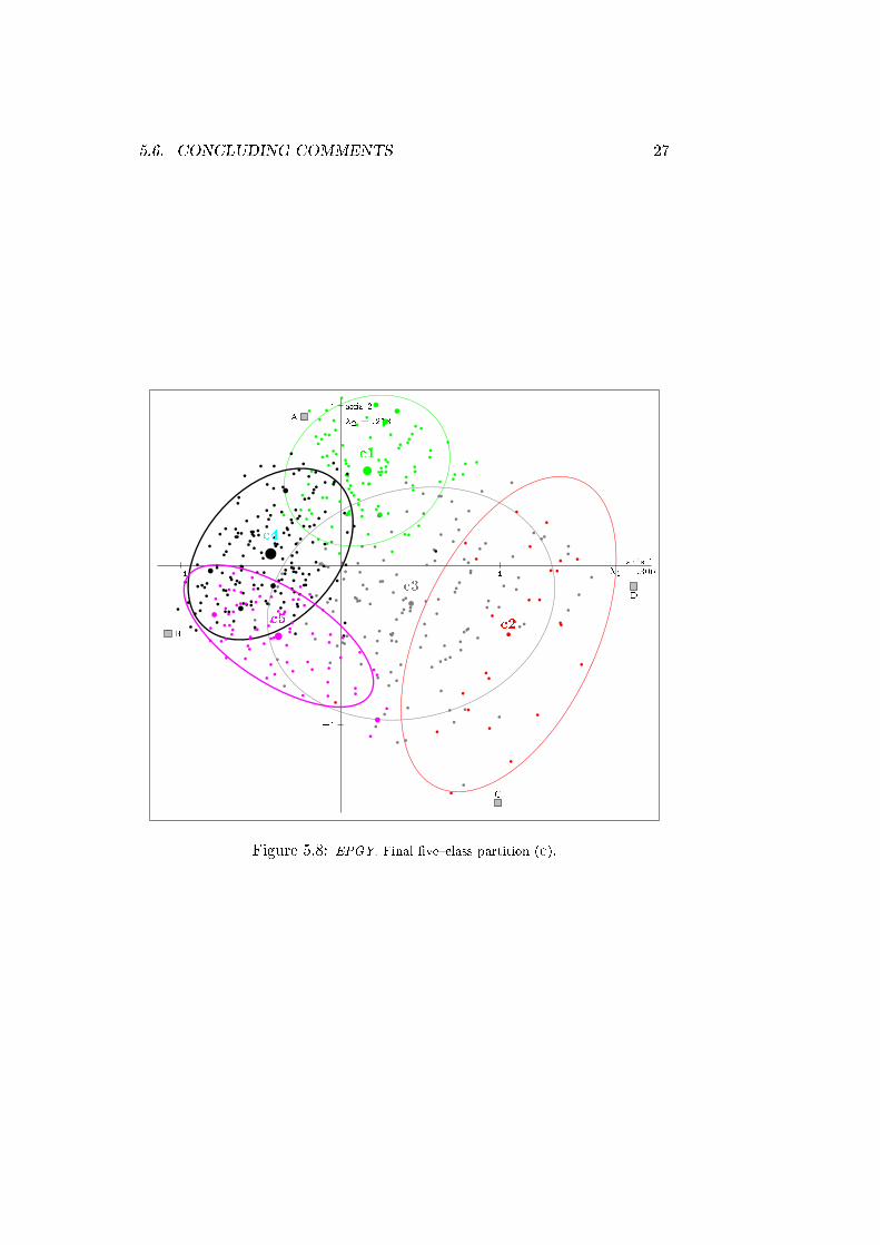
first led to a 6–class partition, from which a partition into 5 classes (c1, c2,
c3, c4, c5) was constructed and retained as a final partition. The between–
and within–variances on the first two axes of this final partition are given
in Table 5.5. A synopsis of this partition is presented on Table 5.6.

5.6. CONCLUDING COMMENTS 21
Axis 1 Axis2
Between–Variance .1964 .1277
Within–Variance .1097 .0907
Table 5.5: EPGY. Between and within variances for the five–class partition.
frequencies Error rates Latencies Exercises
c1 111 short small except in Geometry
c2 25 high rather large
c3 142 high
c4 178 low rather small
c5 77 long rather small
Table 5.6: EPGY. Synopsis of final five–class partition.
There are two compact classes of highly–performing students. One is
class c1, close to point A, with short latencies and medium error rates; the
other one is class c4, close to point B, with rather low error rates (especially
in Geometry and in Logic) and medium to long latencies.
5.5.6 Conclusion of EPGY study
The geometric study shows the homogeneity of matters (strands), except
geometry. It also shows how the differences among gifted students are artic-
ulated around two scales: that of error rates and numbers of exercises, and
that of latencies. Within the geometric frame, differentiated clusters have
been identified. The highly performing class c4, with low error rates and
(comparatively) long latencies, is of special interest, in so far its profile is
hardly reinforced by the current standards of educational testing!
5.6 Concluding comments
1. In Geometric Data Analysis, individuals×variables tables, beyond tech-
nical differences (pca vs mca), can be analyzed with a common strategy,
with the joint study of the cloud of variables (or of categories) and the cloud
of individuals.
2. Structured data arise whenever individuals or variables are described

22 CHAPTER 5. GEOMETRIC ANALYSIS
by structuring factors. A cloud of individuals with structuring factors is no
longer an undifferentiated set of points, it becomes a complex meaningful ge-
ometric object. The families of subclouds induced by structuring factors can
be studied not only for their mean points but also for their dispersions. Con-
centration ellipses can be constructed, and various effects (between, within,
interaction) investigated both geometrically and numerically.

5.6. CONCLUDING COMMENTS 23
Software Note
To carry out the analyses, we have used spss for the elementary descriptive
statistics and the data codings. Then, programs in addad format written
by B. Le Roux, P. Bonnet and J. Chiche have been used for performing pca
and mca. Finally, starting from principal coordinates calculated with ad-
dad, the exploration of clouds and the double breakdowns of variance have
been made with Eyelid. The Eyelid software, for the graphical investiga-
tion of multivariate data, was developed by Bernard, Baldy and Rouanet
(1988), it combines two original features: a Language for Interrogating Data
(“lid”), which designates relevant data sets in terms of structuring factors
and constitutes a command language for derivations, and the Visualization
(“Eye”) of the clouds designated by Eyelid requests. For illustrations of
the command language, see Bernard et al (1989) and Bonnet et al (1996).
Concentration ellipses have been determined by the ellipse program by B.
Le Roux and J. Chiche, which prepares a request file for the drawings done
by the “freeware” wgnuplot.
An extensive (though limited in data size) version of addad (association
pour le developpement et la diffusion de l’analyse des donnees) and a dos–
version of Eyelid are available on the following ftp:
ftp.math-info.univ-paris5.fr/pub/MathPsy/AGD
addad, Eyelid and ellipse programs can be downloaded from the
Brigitte Le Roux’s homepage:
http://www.math-info.univ-paris5.fr/ ˜ lerb(under the “Logiciels” heading).

24 CHAPTER 5. GEOMETRIC ANALYSIS
Acknowledgments
This chapter is part of an ongoing joint project on “the comparison of the
French and Norwegian social spaces”, headed by B. Le Roux and O. Korsnes
and funded by the Aurora-program (CNRS France and NC Norway). I thank
those who have encouraged and helped me to write this chapter, especially
my much regretted friend Werner Ackermann.

5.6. CONCLUDING COMMENTS 25
Figure 5.1: Basketball. Basic cloud, plane 1-2: 8 × 9 = 72 (player, expert)points, joined to the eight player mean points.
Figure 5.2: Basketball. Additive cloud, plane 1-2: 8×9 = 72 (player, expert)points, showing parallelism property.
Figure 5.3: EPGY. Space of categories, plane 1-2, subcloud of the 12 numbers-of-exercises categories. Integers I1 I2, fractions F1 F2, geometry G1 G2 G3, logic L1 L2 L3,measurement M1 M2. Sizes of markers reflect frequencies.
Figure 5.4: EPGY. Cloud of categories, plane 1-2. Interpretation of axis 1: 21 categoriesmost contributing to axis. Sizes of markers reflect frequencies.
Figure 5.5: EPGY. Cloud of categories, plane 1-2. Interpretation of axis 2: 15 categoriesmost contributing to axis. Sizes of markers reflect frequencies.
Figure 5.6: EPGY. Cloud of individuals with extreme (unobserved) patterns A, B, C,D.
Figure 5.7: EPGY. Space of individuals, plane 1-2. For the measurement strand: meanpoints of the 12 composite categories error×latencies. Example: Point 14 is the meanpoint of individuals with low error rates (1) and long latencies (4) for measurement.
Figure 5.8: EPGY. Final five–class partition (c).

�������������� �������������������������� �!�"�� #����$%�&�%�'�(� )�*�#��� +�����#�+,�
-/.*0&132'254768-91325470(:;+<�=?>A@�B#C5D,EF=?<HG&IKJLE*M5D?<�JNG(>A<�JN<�EO>QPQR?<H>�EOG(GAR?<TST<�=�GN>A<�U?<7B#<�PQR?<H>QPQR?<�V�=?WXCF>QYZEOGAIK[\D?<U?<^]�EO>QIKJ�_'`badcfeXgdh"iQjdk�=,ImlF<H>QJAImG\n<^B#<�=Tn<po�<�JAPHEO>AGN<�JHjL]�EO>QIKJHqT;�IKJ#YZEFIK='IK=�GN<H>A<�JNGAJ+IK=JNGAEOGAIKJNGAIKPHJ*EO>A<rEF=,EFsm@"JAIKJTCFW&lOEO>QIKEF=,Pt<uEF=,Uwv%E�@F<�JAIKEF='IK=?WX<H>A<�=,Pt<Fq7;�IKJ%YZEFIK=yx,<�sKU,JTCFWEOz,z{sKIKPHEOGAImC5=|EO>A<Zz{JN@"PQR?C5smCFMF@|EF=,U|JNC"PHIKEFs7JAPHIm<�=,Pt<�JHq�;+<yR,EFJ^PtC5EFD?GAR?CF>A<�U}JN<HlF<H>QEFs~ C\CF�"J#E ~ C5D?G#JNGAEOGAIKJNGAIKPHJ#EF=,U���<HC5Y�<HGN>QIKPro�EOGAE���=,EFsm@"JAIKJHq�+�5�O�A���Q�H���(�����|�F�X���b�Q���H���u���,�X�F�t�Q�����?��+�#�t�^����)���H�Q�O�t����� j" �_^>QD?<�U?<�J*¡"EFIK=�GAJ�¢
]#£<H>A<�JHjd¤&¢�¥O_F¦5¥�§y]�EO>QIKJ�ST<�U?<t¨w§5©\jd¤?>QEF=,Pt<Fqª3¢�YZEFIKs¬«3?®O¯d°�±{²5³?´�µf°F³5¶d·"¸¹±,º"®�»¬¯\±f¸O¼,·�½{°F{¸\¾5¿7»Àº5
�����F�����%�����+��������� ������� ����7� �
� 6 ��6,:56����"6����� ����� ������� � !"�$#&%�')(*)+-,�.�/10-/325476�8:93;<25=>6:/?2@6BA�9DC 25=�E:F:4-=>F:2@G�HI2@F:25=KJ-25=>;LF:CM.�/NF:C OPJ-=KJ-,
Q$RTSVUXWZY7[N\^]?_ ` RTa ,b ���dc�e)fXgh�>i jk��lN��mnf���� b �^#&%�'Z*no+qp)rLst _ ` _ r�uR�vDRk`5w sx3s ` aDyzRkvDR�y${<WZY7Y7R�yz|IW x v sx {<R�yM}�~�` �
r _ |�` R�y�R x { s y�vDW x�x�uRTR�y�} sx3� ~ sx)r R�ykR r vDR }�WDvD` _ r�uR�y��s��>s _ t ` R R<�NR�{ r _ �&����G<E�93G�8ZGJ-2@F:25=KJ-25=>�<93G�F7�Z�NC =>�<9k�GLG<�I�)(D�D�3% � (D%Z,
b �����X��3lI�df��D�z������� WZ` ` ,�#&%�'no:�)+-,���� .�/NF:C OPJTGB8ZG-J ��6:/3/��G�G-JT�¡ I6:C �?¢Z£?¤3FT¥Z=�/N6:¦�=>G�� I6:C ��§n£¨.�/NF:C OPJTG�8ZG-J ©X6:4-47G-J5�36:/N8ZF:/N;LG-J-,qª�s Y7_KyT\^«�~ x WDv ,
b �����X��3lI�df��D�z����#&%�'Z*)¬Z+-,$�=KJ-2@6:=�47G G<2q®q4^�GL¯n=KJ-2@6:=�47G�8ZG�Cz� .�/NF:C OPJTG 8ZG-Jk��6:/3/��G�G-JT��ª�s Y7_KyT\«�~ x WDv ,
b �����X��3lI�dfM�D�z���°#&%�'Z')¬Z+-,k©X6:4-47G-J5�36:/N8ZG</N;LG�.�/NF:C OPJ-=KJ��F:/N8Z±L6�6�²:� Q$RTSVUXWZY7[N\�«�RT[n[ZRTY ,b �����X��3lI�df^�D�z��� #5¬³Z³Z�)+-,�´ ~ w R�y r �@{<R � ~�R$`5w µ x3s ` aDyzR�vDR�yq«�W x�x�uRTR�yL¶)· ¸�R<¹ r Y7R s v t a º ,n» R
¼¨WZ~D¹ s:r¨r7½ R � W xD� RTY7R x {<R�W x {<WZY7Y7R�yz|IW x vDR x {<R sx3s ` aDyz_Ky � º s YL{<RT` W x3s:¾b ���d�dc��d���D�L¿À�>i b c�e)�IÁÃÂ����ÄÂ���Ådc�� �DÆÇgh�$#&%�'Z*Z*)+-, ¸ ½ R »�sx�È ~ sÈ R � WZY�É x)r RTYz�
Y7W È)s:r _ x�È « s:rLsÀ#5e)f���+-, É xV��F:2@FÊ.�/NF:C OPJ-=KJÊF:/N8Ë0-/�Ì<6:4-¦ F:25=>;-J�#>Í v , «�_Kv s a Í$, +-��)Î�% � �)ÎZ*�,
b ���d�dc��d�Ê�D�L¿À�>iIÏM��Â���ÅdÐ b �>iIÂ���Ådc�� �DÆBgh�I�ÒÑdlIÓ f�e<Æ ��¿Ô�7�h�I#&%�'Z*Z')+-,°» w sx3s ` aDyzRvDR�y�vDW x�x�uRTR�y$}�~�` r _KvD_ }�R x yz_ W x�x RT` ` R�y�| s Y�` R�` sx�È)sÈ R�vdw _ x)r RTY7Y7W È)s:r _ W x vDR�vDW x�x�uRTR�y#5e)f���+ \ s ~�vDRT`@�s vDRÕ`5w sx3s ` aDyzRÕvDR�y�{<WZY7Y7R�yz|IW x v sx {<R�y �qÖ¨9DC�C G<25=�/×8ZGÕAØ�G<2Ù¯�6�8Z6:C 67Ú=>GHd6�;<=>6:C 67Ú=>�<93G<�d¬���D� � �)Î�,
b ��� � �DÆ¡���>i�ÏM�ÛÂ���ÅdÐ b ���ÜÏM��Ý$c�f�� �ÃÞÕ�k#&%�'Z'ZÎ)+-, µ x3s ` aDyzR È�uRTWZ} uR r Y7_ � ~�R�vDR�yvDW x�x�uRTR�yT\M~ x R�R x3� ~ ßR r R�yz~�Y�` R�Y s {<_Kyz}�R � AËF:2Ù¯��G<¦ F:25=>�<93G-J G<2qHd;<=>G</N;LG-Jk�9D¦ F:=�/NG-J-�%��ZÎ���( � ¬:�3,
b ��Å �d��f���Åà���°#&%�'no:')+-,M��F���=KJ-25=�/N;<25=>6:/N£�©^4-=�25=>�<93G�Hd6�;<=>F:C G�8:9Bá)9ZÚ)G<¦ G</325,Xª�s Y7_KyT\ Í vD_ �r _ W x yqvDRkâ�_ x ~�_ r�#>ÍXx�È ` _Ky ½ r Y sx yz` s:r _ W x \ ��=KJ-25=�/N;<25=>6:/�#&%�'Z*�n+-, ºqW)y r W xB#5Ý$c�+ \�ã s Yz�ä s YLvhå x _ ä RTYLyz_ r a ª Y7R�y7y +-,
b ��Å �d��f���Å�����#&%�'Z'Z')+-, å x RÕY uR ä WZ` ~ r _ W x {<W x yzRTY ä s:r Y7_K{<Rhv sx y�`5w uR�vD_ r _ W x ��.�;<2@G-J�8ZG�C F��GL;L¯�G<47;L¯�G�G</BHd;<=>G</N;LG-JkHd6�;<=>F:C G-J-�3æ WZ` ,¨%P¬Î � %P¬)on�)� � ¬*�,
b ��Å �d��f���Å1���°#5¬³Z³�%P+-,M��F:/nÚ)FTÚ)G�G<2 �36:9DE:6:=�4�J-O:¦ ±L6:C =>�<93G<,Mª�s Y7_KyT\^ç s a s YLv ,b ��Å �d��f���Å����°�èÑIc�f��dÆ3éd¿�c��)Ædf��à¿À�°#&%�'no:*)+-,^» R ª�s:r Y7W x3s:r���.�;<2@G-J�8ZG�C F���GL;L¯�G<47;L¯�G
G</�Hd;<=>G</N;LG-JkHd6�;<=>F:C G-J-�Iæ WZ` ,X¬³ � ¬D%Z�D� � *)¬D,ê c°��3�����M#&%�'Z*)¬Z+-, Q$W r R yz~�Yk` R�y uRT` uRT}�R x)r y�yz~�|�|�` uRT}�R x)rLs _ Y7R�y�R x µ x3s ` aDyzR vDR�y � WZY7Y7R<�
yz|IW x v sx {<R�y �I��G-J�©XF�¯n=>G<4LJ�8ZG�Cz� .�/NF:C OPJTG�8ZG-J���6:/3/��GLG-J-�Non��' � ¬��ëÒ%��Z� � %P(:�3,ê Ó fÙlIÓ �Û���>i�ÏM�ÛÂ���ÅdÐ b �>i������d�df�� �DcdÅ¡�����ÜÂ���Ådc�� �DÆ¡gh��#5¬³Z³Z³)+-,Ç» w R�yz| s {<R
|IWZ` _ r _ � ~�R�vDR�y uRT` R�{ r RT~�YLy � Y sx�ì{ s _Ky��s ` s í3x vDR�y sx�x�uRTR�y %�'Z'Z³��N��G<E�93G�ÌL47F:/Iî;�F:=KJTG�8ZGJT;<=>G</N;LG��36:C =�25=>�<93G<�N(³��D�)ÎZ� � �)*non,
ê �Nc�ÝË����Çgh��#&%�'�)Î)+-,ËAËF:2Ù¯�G<¦ F:25=>;LF:CMAËG<2Ù¯�6�8PJÕ6&Ì HI2@F:25=KJ-25=>;-J-,�ª Y7_ x {<R r W x \ ª Y7_ x {<R r W xå x _ ä RTYLyz_ r a ª Y7R�y7y ,
jk��lN��mnf���� b �n#5¬³Z³Z�)+-,^.�/NF:C OPJTG�8ZG-J�;L6:4-47G-J5�36:/N8ZF:/N;LG-JT£�47GL;L¯�G<47;L¯�G-J�F:9�;�ïM9D4q8ZGqCz� F:/NF:C OPJTG8ZG-J�8Z6:/3/��GLG-J-, ¼¨R x�x R�yT\ ª Y7R�y7yzR�yq~ x _ ä RTYLyz_ rLs _ Y7R�y�vDR�¼¨R x�x R�y ,

¦O§ ���������� �������������������������� �!�"�� #����$%�&�%�'�(� )�*�#��� +�����#�+,�
Þ��d�����dc lI�d��¿À��#&%�'Z*�%P+-,�ª Y s { r _K{ s `�{<WZY7Y7R�yz|IW x vDR x {<R sx3s ` aDyz_Ky , É xË0-/32@G<45�N47G<25=�/nÚ�A�9DC �25=�E:F:4-=>F:2@Gk��F:2@FB#>Í v ,�æ�, º s Y x R rzr-+-�d%Z%�' � %T�)Î�,��M½ _K{ ½ R�y r RTY�\^]?_ ` RTa ,
g � ��e)e��I�d�����°�����>i¨ÏM��Â���ÅdÐ b �>i������ �T� �3�h�>i¨ÏM���3c��N�����k�>i¨Â��°�T��� e)Å � �ÇÏ��>iÂ���Ådc�� �DÆÛgh�$#5¬³Z³)(Z+-, ¸ ½ RÕQ$WZY7SqR È _ sxÔí RT`Kv1W � |IW:SqRTY sx�x W ¬³Z³Z³��� q9D4767�3GLF:/Hd6�;<=>G<25=>G-J�#�r W s |�|IR s Y +-,
� ��� �Nc�e)e�¿À�KÞÕ�n�¡ÑIÆdÅdc��)Æ��h�n#&%�'no:�)+-,k¤N¯�GM.�8:E:F:/N;LGL8 ¤N¯�GL6:4-O�6&Ì�HI2@F:25=KJ-25=>;-J-�Pæ WZ` ~�}�R¬D,X» W x vDW x \���Y7_ � x ,
ÏM��Â���ÅdÐ b �D#&%�'Z'Z')+-, µ x3s ` aDyzRMyz| uR�{<_ íI� ~�R�vdw ~ x�x ~ sÈ R^RT~3{<` _KvD_ R x \ s |�|�` _K{ s:r _ W x �s `5w uR r ~3vDRvDR�y � ~�R�y r _ W x�x3s _ Y7R�y �DAËF:2Ù¯��G<¦ F:25=>�<93G-J�� 0-/�Ì<6:4-¦ F:25=>�<93GkG<2°Hd;<=>G</N;LG-JM�9D¦ F:=�/NG-J-�3%T�)Î��Î)( � *Z��,
ÏM�ÊÂ���ÅdÐ b �>i ê Ó fÙlIÓ �Ô���°#5¬³Z³�n+-,qp |IR�{<_ í {k}�~�` r _ |�` R�{<WZY7Y7R�yz|IW x vDR x {<R sx3s ` aDyz_Ky �3�G<C �C G</3= ²ZG�¤3G<2547FZ8:=>F�.�/NF:C OPJ-=KJ���GL8Z6:¦ G</N6:/3� ¸ ½ R�y7y s ` W x _ [ZR �n�3�3�Z³ � �3%Z,
ÏM��Â���ÅdÐ b ���"Â���Ådc�� �DÆÔgh� #&%�'Z*�n+-,°» w sx3s ` aDyzR�}�~�` r _KvD_ }�R x yz_ W x�x RT` ` R�vDR�y�vDW x�x�uRTR�yy r Y7~3{ r ~�Y uRTR�y �IAËF:2Ù¯��G<¦ F:25=>�<93G-J�G<2MHd;<=>G</N;LG-J��9D¦ F:=�/NG-J-��*)(D�3( � %�*�,
ÏM�1Â���ÅdÐ b �q� Â���Ådc�� �DÆ?gh�M#&%�'Z'Z*)+-, É x)r RTY7|�Y7R r _ x�Èhs ¹DR�y�_ x â�~�` r _ |�` R � WZY7Y7R�yz|IW x �vDR x {<RÕµ x3s ` aDyz_KyT\�â�R r7½ WDvàW �¨r7½ RÕ{<W x)r Y7_ t ~ r _ W x y�W � |IWZ_ x)r y sx vàvDR ä _ s:r _ W x y , É x �=KJ-93F:C = ��F:25=>6:/À6&ÌB©XF:2@G Ú)6:4-=>;LF:C���F:2@F:�¨#>Í v�y , ºq` s yz_ ~3y�� ,°ë ��Y7RTR x3s {<Y7R�â , +-��%�'no �¬Z¬³��3pDsx «�_ R È W3\�µ�{ s vDRT}�_K{ ª Y7R�y7y ,
ÏM�ËÂ���ÅdÐ b �^� Â���Ådc�� �DÆ�gh�°#5¬³Z³�n+-,��$GL6:¦ G<254-=>;���F:2@F�.�/NF:C OPJ-=KJT£°ÌL476:¦ ©X6:4-47G-J5�36:/��8ZG</N;LG�.�/NF:C OPJ-=KJ�2@6�HI254-93;<259D47GL8���F:2@F:, «�WZYLvDY7R�{ ½)r \��k` ~nSqRTY ,
ÏM�ÛÂ���ÅdÐ b ���ÜÂ���Ådc�� �DÆØgh��#5¬³Z³�n+-, 0-/N8:=�E�=>8:93F:C�8:= ��G<47G</N;LG-JË=�/?Ú= ÌL2@GL81J-25938ZG</32>J-���� ��!#"%$ $�&'!�( )+*�,-��.'/�0 132�4�*5&3436�$'2�&�,3&�.32879�8$':�& 19;<&'� 28=�7->�.3��.3?�/�.�@-)8, =�,�*�!�4�0 ,
ÏM���3c��N���A�k��#5¬³Z³Z³)+-,���FË;<476:OZF:/N;LG��G�;L6:/N6:¦�=>�<93G�£�C G-JÇ�G�;L6:/N6:¦�=KJ-2@G-J�G</32547G�JT;<=>G</N;LGhG<2�36:C =�25=>�<93G<,qª�s Y7_KyT\ p RT~�_ ` ,
ÏM���3c��N���B�k�N#5¬³Z³�%P+-,^Í {<W x WZ}�_Ky r y sx v r7½ R$R�{<W x WZ}�_K{�WZYLvDRTY�\�¸ ½ R í RT`Kv�W � R�{<W x WZ}�_Ky r ysx v r7½ R í RT`KvhW � |IW:SqRTY¨_ x ç�Y sx {<R �� q9D4767�3GLF:/BHd6�;<=>G<25=>G-J-�I�Õ#&%P+-�3'�% � %Z%�³�,
ÏM���3c��)Æ Ï���#&%�'no(Z+-,Ø» w WZY7_ R x)rLs:r _ W x vD~×v uRT|IWZ~�_ ` ` RT}�R x)r vDRÔ{<RTY rLs _ x R�y�R x3� ~ ßR r R�y�| s Y`5w sx3s ` aDyzR�vDR�y¨{<WZY7Y7R�yz|IW x v sx {<R�yM}�~�` r _ |�` R�y ,�©X6:/�JT6:¦�¦ F:25=>6:/3�N¬D�Io:� � 'ZÎ�,
ÏM���3c��)ÆØÏ����C�Õ���� ��en��� �D�z����#&%�'non%P+-,ÃHI2@F:25=KJ-25=>�<93GÊG<2�0-/�Ì<6:4-¦ F:25=>�<93GB.M�Z�NC =>�<9k�G�G-J-,ª�s Y7_KyT\^«�~ x WDv ,
ÏM���3c��)Æ Ï��>ih¿à���df�� �DcdÅ"�h�>i��McD�3c��d�FEh��#&%�'noZo+-,&¤3GL;L¯n/3=>�<93G-J�8ZG�C FÀ8ZG-JT;<4-= �N25=>6:/J-2@F:25=KJ-25=>�<93G�£Õ¦V�G<2Ù¯�6�8ZG-JÕG<2�C 67Ú=>;<=>G<C J��36:9D4�Cz� F:/NF:C OPJTG�8ZG-J�Ú47F:/N8PJ�2@FZ±<C GLF:9Z¥Z,�ª�s Y7_KyT\«�~ x WDv ,
ÏM���3c��)Æ�Ï��>i^¿à���df�� �DcdÅ��h�>i°!àc��'G�fÙl8�H���^#&%�'Z*�n+-,$A�9DC 25=�E:F:4-=>F:2@G���G-JT;<4-= �N25=�E:G�HI2@F-�25=KJ-25=>;LF:Cd.�/NF:C OPJ-=KJT� Q$RTS��5UXWZY7[N\^]?_ ` RTa ,
Â��°�T��� e)Å � �àÏ��°#5¬³Z³Z³)+-,Xp WD{<_ s ` y r Y7~3{ r ~�Y7R�y sx vh{ ½3sx�È R3I s |�|�` an_ x�È ª _ RTY7Y7RkºqWZ~�YLvD_ RT~ w ys |�|�Y7W s { ½ksx v sx3s ` a r _K{ � Y s }�RTSqWZY7[ , ]ÊWZY7[n_ x�È | s |IRTYLy � Y7WZ} p)rLs ä sx�È RTY å x _ ä RTYLyz_ r a� WZ` ` R È R �3*)(�J¬³Z³Z³Z³�,°��4T��®X¯n=�C 6�2Ù¯�G-J-=KJ-�Ip)rLs ä sx�È RTY � Q$WZY7S s a ,
Â���Ådc�� �DÆÀgh�>i���l8�°���dÝ$c�� �?!"����ÏM��Â���ÅdÐ b �q#5¬³Z³Z³)+-, ¸ ½ R È RTWZ}�R r Y7_K{ sx3s ` a)�yz_Ky�W ��� ~�R�y r _ W x�x3s _ Y7R�yT\ r7½ R » R�y7yzW x W � ºqWZ~�YLvD_ RT~ w y »�s «�_Ky r _ x { r _ W x �qÖ¨9DC�C G<25=�/À8ZGAØ�G<2Ù¯�6�8Z6:C 67Ú=>G�Hd6�;<=>6:C 67Ú=>�<93G<�NÎ)(D�3( � %�*�,

�����F�����%�����+��������� ������� ����7� ¦ �
Â���Ådc�� �DÆÊgh�d� ÏM�ÕÂ���ÅdÐ b �d#&%�'Z'Z�)+-,�.�/NF:C OPJTG�8ZG-J�8Z6:/3/��G�G-J�¦�9DC 25=>8:=�¦ G</�J-=>6:/3/NG<C�C G-J-,ª�s Y7_KyT\^«�~ x WDv ,
Â���Ådc�� �DÆ¡gh�>i�ÏM���3c��N��� �k�>i�ÏM�Çg�cnÁ � �>i���l8�°���dÝ$c�� �Ã!"��� ÏM�ÇÂ���ÅdÐ b �#5¬³Z³)¬Z+-, ¼ uR È Y7R�y7yz_ W x R r¨sx3s ` aDyzR È�uRTWZ} uR r Y7_ � ~�R¨vDR�y�vDW x�x�uRTR�yT\�Y uR��3R<¹D_ W x yXR r yz~ ÈZÈ R�y&�r _ W x y �NAËF:2Ù¯��G<¦ F:25=>�<93G-J��ÛHd;<=>G</N;LG-J�¯n9D¦ F:=�/NG-J-� %�ÎZ³��N%�� � �n(D,
���°l8�����q� ÑNÅ������3�h���M#5¬³Z³)¬Z+-, ¸ ½ R ã$_ ÈZ½ «�_ }�R x yz_ W x3s ` _ r a�W �¨p)r ~3vDR x)r yTwdÉ x vD_ ä _Kvn�~ s `^«�_ �NRTY7R x {<R�y$_ x˪ RTY � WZY7} sx {<R�_ xÊ���dÁ w y ��ÎÕ� WZ}�|�~ r RTYz�@º s yzR�vÕâ s:r7½ RT} s:r _K{Ty� ~�Y7Y7_K{<~�` ~�} � ��� ��!#"%$ $�&'!�( )+*�,-��.'/�0 132 4�*5&3436�$'2�&�,3&�.32�7 � ,
!Ã��e)mnmÔ¿À�>iXÂ���Ådc�� �DÆ�gh�M� Þ��N�°����3������ b �X#&%�'Z'Z*)+-, µ x3s ` aDyzR�vdw ~ x R�R<¹D|IRTY r _KyzR|�Y7W � R�y7yz_ W x�x RT` ` RZ\ `5w uR ä s ` ~ s:r _ W x vDR�y� &RT~ x R�y rLs ` R x)r y s ~ t3s yz[ZR r��nt3s ` `DvDR ½3s ~ r�x _ ä R s ~ ���GÕ¤D47F:E:F:=�CN�9D¦ F:=�/3��Î�%Z�3¬*�% � �Z³Z��,

¦F¦ ���������� �������������������������� �!�"�� #����$%�&�%�'�(� )�*�#��� +�����#�+,�
������������� �� ��������� ���� � ����� �!#"
$ � ��%&����'(�� �*)���+�� ,-� � � )(�.,-��!#"
/10
,
2
�
�
3
4
+ �
/65
,
2�� 3
4 +
�
/87
,
2�
�3
4
+ �
/:9,2
�� 3
4
+
�/6;,2
��
34+
�
/8<,2 ��34
+ �
/6=,
2�
�3
4
+
�
/8> ,2�
�34
+
�
¤�ImM5D?>A<�_\q � «@? ���&A5�H��BA�DC�C�E v%EFJAIKP)PHsmC5D,ULjdz{sKEF=?< � ¢À¦\« ����GF ¥O¦/`Xz{sKE�@F<H>�jL<t¨"zf<H>AG�izfC5IK=�GAJHjIHNC5IK=?<�U�GNCZGAR?<r<�ImM5R�G*z{sKE�@F<H>�Y�<�EF=wzfC5IK=�GAJHq
JLKNM O8P
JLKNM O�Q
/10
,2 ��3
4
+ �
/65,
2 ��3
4
+ �
/87,
2 ��3
4
+ �
/:9,
2 ��3
4
+ �
/6;,
2 ��3
4
+ �
/8<,
2 ��3
4
+ �
/6=
/8>,
2 ��34
+ �
¤�ImM5D?>A<*_\q ¦\«R? ���&A5�H��BA�DC�C q3��U,U,ImGAImlF<%PHsmC5D,ULjOz{sKEF=?< � ¢À¦\« �7��SF ¥O¦)`Xz{sKE�@F<H>�j5<t¨"zf<H>AG�izfC5IK=�GAJHj,JAR?C�T+IK=?M)z{EO>QEFsKsm<�sKIKJAY z,>ACFzf<H>AG�@Fq
�����F�����%�����+��������� ������� ����7� ¦��
�� �
�
� �
���.� � ��� 2
�*) � � +�,-
� ,
� +
���
��
�
��
��
�
���
���
��������������� �!#"%$�&('�)+*�,.-0/214305(/6-�78129:30;8< 12=2>?,A@ -0BA1DCFEHG�>I=KJAL�/2@ 3:J.MN305O78PA1QC�GRB�JAS(L�1F;8=HET305 E1FUV1F;8/2< =K12=�/6-�78129:30;8< 12=2)XWYB�78129:1F;8=ZW[C�WKG�>V5 ;[-0/F78< 3:BA=+\XC?\]G�>A9:123:S^1F7K;K_a`OCb`?Gc`�d�>A@ 3:9:< /be]C?efG(e�d�>S^16-0=KJV;812S^12B�7+ghCOgiG�)�*�< j212=�305]Sk-�;8l1F;8=�;81Fm.12/F7Z5 ;816n�JA12BA/2< 12=2)
¦� ���������� �������������������������� �!�"�� #����$%�&�%�'�(� )�*�#��� +�����#�+,�
� � � � � � � � �� � � �� � � �
� � �
� � �
� � � �
� � � �
���.� � ��� 2
�*) � � +�,- ���������� ���������� �������� ��� � ��� �!"��#�� �$ � ����%�� � � � ���
&('�' )�'+*�,
&('�' )�'+*.-
&('�' )�'+ (,
&('�' )�'� /-
&('�' )�' � ,
&('�' )�' �10
&('�' )�'+!2,
&('�' )�'+! 0
&('�' )�'/$3,
&('�' )�'2$ 0
465�7�8:9<;:=2*�,465�7�8:9<;:=2 (,
465�7�8:9<;:= � ,
465�7�8:9<;:=>!2,465�7�8:9<;:=?$3,
&2@�8:' ;:A B�8:B6*.-&2@�8:' ;:A B�8:BC /-
&2@�8:' ;:A B�8:BC!2,
&2@�8:' ;:A B�8:BC! 0
&2@�8:' ;:A B�8:B6$3,
&2@�8:' ;:A B�8:B6$D-
�����������^��� E�!b"%$�&('�)�FX@ 3:J.MO305�/6-�78129:30;8< 12=2>�,A@ -0BA1ICFEHG�)�WYB�781F;8,V;81F7[-�78< 3:B(305�-�UV< =ZCHG]G�CZ/6-�78129:30;8< 12=S^3:=H7�/23:B�7K;8< LAJV78< BA9(783^-�UV< =2)�*�< j212=�305�Sk-�;8l1F;8=�;81Fm.12/F7�5 ;816n�JA12BA/2< 12=2)
I�J K L�J I L�J KM I�J KM L�J I
I�J K
L�J I
M I�J K
M L�J I
NHO?P J ��Q�R
N�STP J �[� U
&('�' )�'+*.-
&('�' )�' �10&('�' )�'+! 0
&2@�8:' ;:A B�8:BC /-
&2@�8:' ;:A B�8:BC! 0
465�7�8:9<;:=2*�,
465�7�8:9<;:=2*�V
465�7�8:9<;:=2 (,
465�7�8:9<;:=2 +V
465�7�8:9<;:= � ,
465�7�8:9<;:= � V
465�7�8:9<;:=2!2,
465�7�8:9<;:=2!"V
465�7�8:9<;:=?$3,
465�7�8:9<;:=?$WV
�����������^��� ��!b"%$�&('�)�FX@ 3:J.MO305�/6-�78129:30;8< 12=2>�,A@ -0BA1ICFEHG�)�WYB�781F;8,V;81F7[-�78< 3:B(305�-�UV< =XG�GXC�X+/6-�78129:30;8< 12=S^3:=H7�/23:B�7K;8< LAJV78< BA9(783^-�UV< =2)�*�< j212=�305�Sk-�;8l1F;8=�;81Fm.12/F7�5 ;816n�JA12BA/2< 12=2)

�����F�����%�����+��������� ������� ����7� ¦F_
� � � � � � � � �� � � �� � � �
� � �
� � �
� � � �
� � � �
� � � �
����� � ,���.� � ��� 2
����� � +�*) � � +�,- �
�
�
¤�ImM5D?>A<)_\q ©\«� ������� �� ����������� ����� � � ����!�� "$#%� &('*)�+ &-,()/.0)213�4�4��54"-)�,(�6)7��8:9�!;&-&()�,(�4" �=< � < <� �

¦F© ���������� �������������������������� �!�"�� #����$%�&�%�'�(� )�*�#��� +�����#�+,�
� � � � � � � � �� � � �� � � �
� � �
� � �
� � � �
� � � �
� � � �
����� � ,
����� � +�
�
�
�
,�,+�,
, 4
+ 4
��,
� 4
¤�ImM5D?>A<u_\q ¥�« ��������� 9�!��/)$��� � ����� � � ����!�� " < 94� !��4)���� �� ��, &('4)$.0)7!�"-��,()/.0)/� & " &-, !������ .0)7!��9 ��� � &("���� &('4)������/��.09 ��"-� &()��7!;&()�����,(� )/"0)�,-,(��,�� � !;&()/���/� )/" ��� +4!�.094� )���� ��� � &���� � " &('4) .0)7!��9 ��� � & ��� � ����� � � ����!�� ":#%� &(' � �7# )�,-,(��,%, !;&()/"=1��;8:!���� � �����0� !;&()/���/� )/"=1 � 8�� ��,$.0)7!�"-��,()/.0)/� & �
�����F�����%�����+��������� ������� ����7� ¦5¥
�� �
�
� �
� ��� � ,��� � � ��� 2
� ��� � +�*) � � +�,- �
�
�
�
���
��
��
� �
��
��������������� ��� �"!�# $�%'&)( *+-,�./1032546, +-787:9+�;8<=( <=( >?*A@CB'D3%


