
765
Geotechnical Aspects of Underground Construction in Soft Ground – Viggiani (ed) © 2012 Taylor & Francis Group, London, ISBN 978-0-415-68367-8
FEM analyses of deep excavations and earth retaining structures in soft clay
Takao Kono & Yoshimasa ShigenoTakenaka Corporation, Chiba, Japan
ABSTRACT: In recent years, an increasing amount of excavation work has come close to adjacent structures. To reduce the effects of excavations on adjacent structures, it is becoming increasingly impor-tant to predict the displacement of earth retaining walls and the retained soil movement. 2D finite element analyses were performed to simulate the behavior of an earth retaining wall. In this FEM simulation, a Mohr-Coulomb failure model was adopted to consider soil stiffness dependence on shear strain. The influence of the initial Young’s modulus and the soil stiffness dependence on confining pressure were examined. FEM calculation results were compared with the monitoring results of excavations in soft clay. Excavation depth was 17.0 m and the retaining wall was soil-cement with H-section steel. Excavation was done using a total of four levels of RC slab struts and the top down method. A good agreement was found with displacements of the retaining wall between the calculation results and observation datas using the deformation modulus at small strain Eo estimated from the results of PS logging. The analysis was effec-tive in predicting the vertical displacement of the retained soil.
condition. In Japan, to predict the behavior of adjacent structures, the FEM analysis applying displacement is generally used (AIJ 2006). With the FEM analysis applying displacement, the pre-diction accuracy is high because it uses lateral dis-placement of the wall calculated by beam-spring analysis. However, the influence of the adjacent structure cannot be considered when only the wall displacement is calculated (AIJ 2006).
In this paper, a step by step FEM analysis is per-formed to predict the wall displacement and ground movement due to excavation in soft ground. In the analysis, the elasto-plastic Mohr-Coulomb failure model is used to examine the influence of the con-stitutive model. Moreover, to examine the influence of the deformation modulus used for the analysis, the deformation modulus is set from VS derived from PS logging or N value and cohesion c.
2 OVERVIEW OF EXCAVATIONS AND GROUND CONDITIONS
2.1 Excavations
Figures 1 and 2 shows a plan and section of the excavation and soil profile of the project. The build-ing had multiple basements, and was eight stories above ground. The project excavation covered an area of 135 m × 50 m, at a depth of GL – 17.0 m. There were office buildings and shore protection next to the retaining wall, so the wall displacement caused by excavation had to be strictly controlled.
1 INTRODUCTION
Recently, excavations that are adjacent to railways and the roads have been increasing in cities. In the adjacent excavations, it is important to control the influence on the adjacent structures as much as possible. It is becoming increasingly important to estimate not only the lateral displacement of earth retaining walls but also the movement of the ground behind the retaining walls.
There are two basic approaches to predict the ground movements caused by excavation. Peck (1969), Aoki et al. (2000) and Moorman (2004) proposed prediction of settlement behind retaining walls based on measurement results. Roscoe (1970) and Aoki et al. (1990) proposed prediction forms of settlement assuming a slip surface behind the retaining wall. The method based on actual meas-urement results is a simple empirical method, and effective to understand the amount of settlement qualitatively. However, it is difficult to evaluate the influence on the adjacent structure accurately by this method. Moreover, if structures exist behind a retaining wall, it is very difficult to define a slip surface in the soil, so the method of defining a slip surface in soil is not suitable for displacement fore-casts of the adjacent structure.
In recent years, FEM analyses are used to estimate the displacement of the adjacent struc-ture. In the FEM analysis, there are two methods for analyzing. One is a step by step analysis, and another is applying displacements as a boundary

766
of the inclinometer was embedded in the mudstone by about 5 m. Because this project involved deep excavation into soft clay there was a risk of base heave. Therefore, vertical heave was measured in the center of the excavation. It was assumed at GL-60 m in the mudstone there was zero vertical displacement. The lateral displacement of, and the water pressure on the retaining wall were measured from the completion of retaining wall construction to the completion of the excavation. The vertical displacement and water pressure in the ground were measured from the second excavation to the end of the excavation work.
2.2 Ground condition
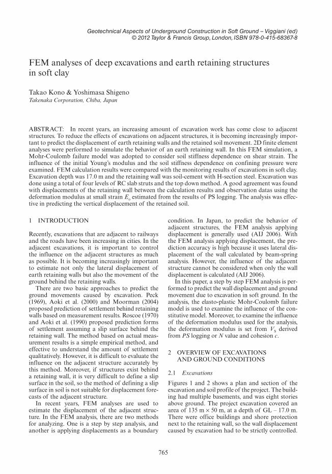
The project location was at the mouth of the Kata-bira River and the east side of the East Japan Rail-way Company’s Yokohama Station. The site was reclaimed prior to the 1930’s. The Soil profile at the site is shown in Figure 3. To the south of the site, alluvial sand exists between the soft clay and mudstone. Soft clay layers extend from the ground surface to a depth of about 35 m. The thickness of the soft clay layer is almost constant across the site.
Soil properties are shown in Table 2 and Figure 4. Natural water content wn of the soft clay ranged 70% to 100%, and was close to the liquid limit. The values of on drained shear strength were ranged 40 kpa to 70 kpa. Shear wave velocities were in the range to 100 m/s to 120 m/s in the soft clay layer and 460 m/s to 610 m/s in the mudstone. The groundwater level was 1.6 m below ground level and was GL-4.1 m in the mudstone layer.
3 MEASURED RESULTS
3.1 Lateral displacement of retaining wall
Figure 5 shows the lateral displacement of the retai-ning wall. Lateral displacement gradually increased
GL-5.2m
GL-7.3m
GL-17.0m
m9m48m05
9m
4
2m
34
m
GL-5.2m GL-7.3m
GL-7.3m
S1 w1
w2
I1
S1 differential settlement gauge
w1,w2 water level gauge
I1 Inclinometer
:
:
:
Bor.No.6
Bor.No.7
Bor.No.8
Figure 1. Plan of excavation.
w1
0 20 40 60
-Value
0
10
20
30
40
De
pth
(m)
GL-27.0m
1F-Slab
1st-GL-1.9m
2nd-GL-6.0mB1F-Slab
temp-Slab1
temp-Slab23rd-GL-10.4m
4th-GL-13.2m
GL-5.3m
5th-GL-17.0m
GL-20.0m
GL-28.0m
GL-35.0m
GL-60.0mS1
GL-40.0mI1
w2
GL-10.0m
GL-20.0m
Figure 2. Section of excavation.
Table 1. Monitoring instruments.
Items EquipmentMeasurement depth
Lateral displacement of the wall
Inclinometer GL − 0 m–GL − 40 m (@2.0 m)
Water pressure on the wall
Water-level gauge
GL − 10 m, −20 m
Vertical displacement of the ground
Differential settlementgauge
GL − 20 m, −28 m, −35 m
Water pressure in the ground
Water-level gauge
GL − 20 m, −28 m, −35 m
Excavation was done using a total of four levels of supporting struts, including two basement floors and two temporary RC slabs. The top down method was used to build these supports.
The retaining wall comprised soil cement up to 28 m, reinforced with H-section steel (H588 × 300) of 27 m length. The pitch of the H-section steel down to GL − 5 m was 1200 mm, because the lat-eral pressure that acted on the wall was lower close to ground level, and from GL − 5 m to GL − 27 m was 600 mm. Ground water was pumped from dewatering wells.
Table 1 shows the excavation monitoring equip-ment and instrument locations are shown Figures 1 and 2. The lateral displacement of the retaining wall, the water pressure that acts on the wall, the vertical displacement of the ground and water pressure in the ground were measured. Because the retaining wall was not embedded in stiff ground, the retaining wall toe was assumed to move into the excavation (Tanaka, 1994). Therefore, the bottom
767
Figure 3. Soil profile.
Table 2. Soil properties.
Soil layer
wn
(%)γ(g/m3)
c(kN/m2)
Vs
(m/sec)
Fill (B) − 1.70 − 160
Clay (Ac1) 70 1.57 45 100
Clay (Ac2) 90 1.45 65 120
Sand (Ds) − 1.82 − 460
Clay (Ka) – 1.90 − 610
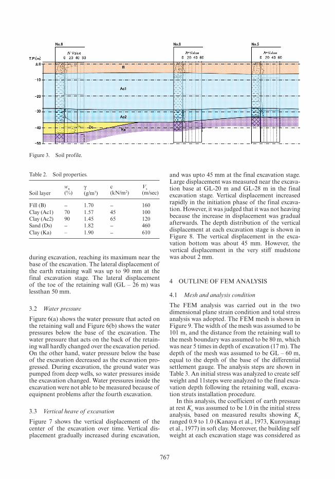
during excavation, reaching its maximum near the base of the excavation. The lateral displacement of the earth retaining wall was up to 90 mm at the final excavation stage. The lateral displacement of the toe of the retaining wall (GL – 26 m) was lessthan 50 mm.
3.2 Water pressure
Figure 6(a) shows the water pressure that acted on the retaining wall and Figure 6(b) shows the water pressures below the base of the excavation. The water pressure that acts on the back of the retain-ing wall hardly changed over the excavation period. On the other hand, water pressure below the base of the excavation decreased as the excavation pro-gressed. During excavation, the ground water was pumped from deep wells, so water pressures inside the excavation changed. Water pressures inside the excavation were not able to be measured because of equipnent problems after the fourth excavation.
3.3 Vertical heave of excavation
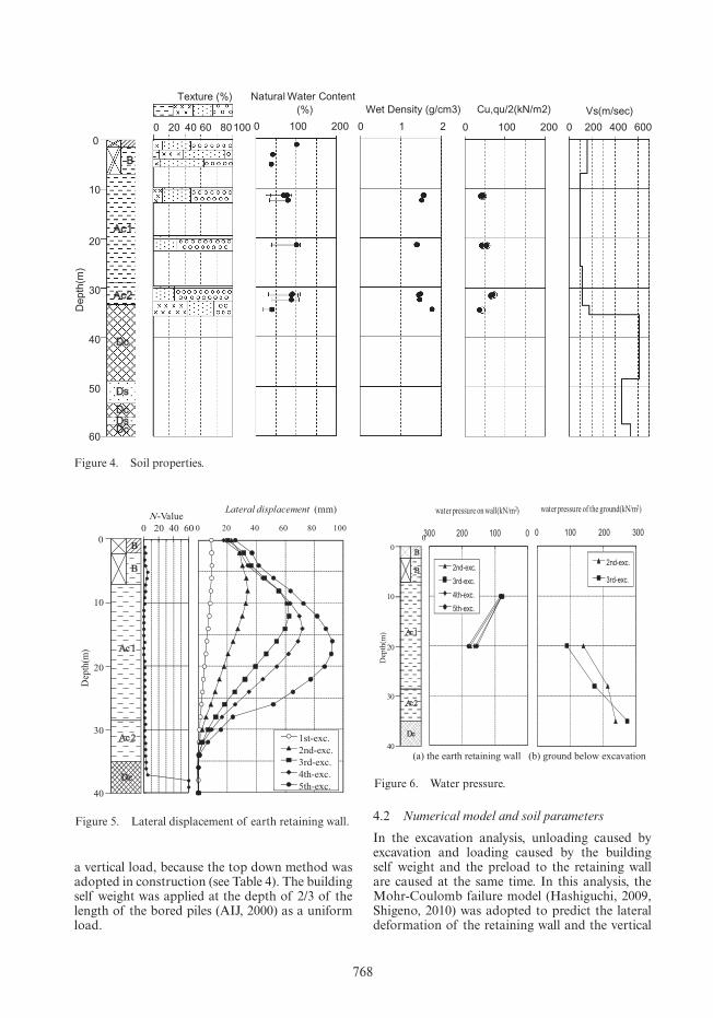
Figure 7 shows the vertical displacement of the center of the excavation over time. Vertical dis-placement gradually increased during excavation,
and was upto 45 mm at the final excavation stage. Large displacement was measured near the excava-tion base at GL-20 m and GL-28 m in the final excavation stage. Vertical displacement increased rapidly in the initiation phase of the final excava-tion. However, it was judged that it was not heaving because the increase in displacement was gradual afterwards. The depth distribution of the vertical displacement at each excavation stage is shown in Figure 8. The vertical displacement in the exca-vation bottom was about 45 mm. However, the vertical displacement in the very stiff mudstone was about 2 mm.
4 OUTLINE OF FEM ANALYSIS
4.1 Mesh and analysis condition
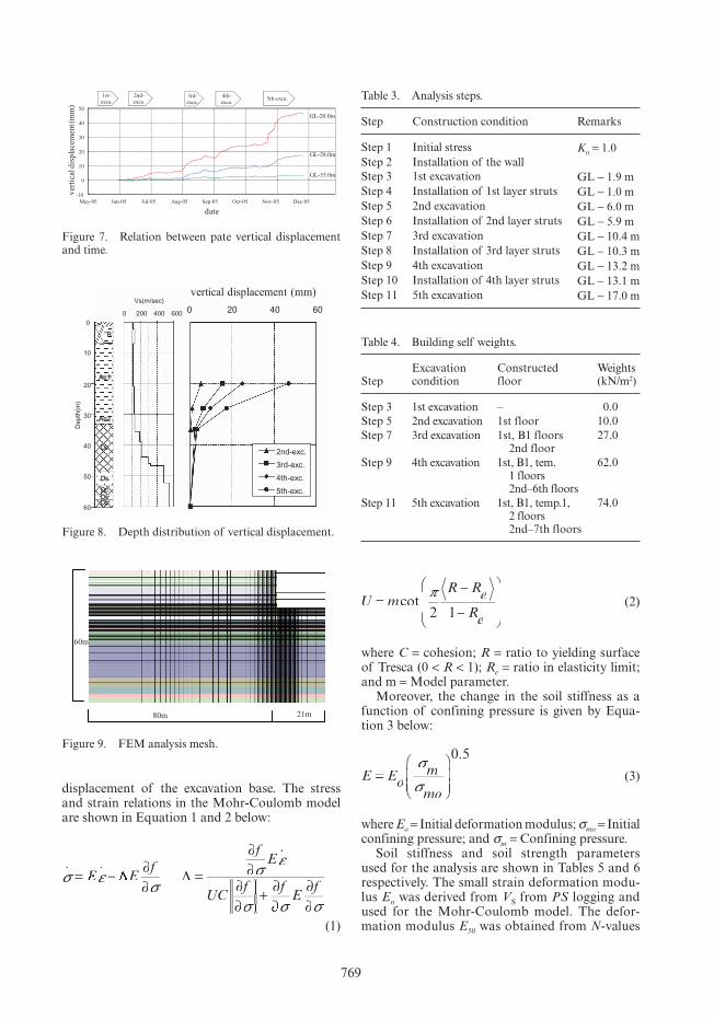
The FEM analysis was carried out in the two dimensional plane strain condition and total stress analysis was adopted. The FEM mesh is shown in Figure 9. The width of the mesh was assumed to be 101 m, and the distance from the retaining wall to the mesh boundary was assumed to be 80 m, which was near 5 times in depth of excavation (17 m). The depth of the mesh was assumed to be GL – 60 m, equal to the depth of the base of the differential settlement gauge. The analysis steps are shown in Table 3. An initial stress was analyzed to create self weight and 11steps were analyzed to the final exca-vation depth following the retaining wall, excava-tion struts installation procedure.
In this analysis, the coefficient of earth pressure at rest Ko was assumed to be 1.0 in the initial stress analysis, based on measured results showing Ko ranged 0.9 to 1.0 (Kanaya et al., 1973, Kuroyanagi et al., 1977) in soft clay. Moreover, the building self weight at each excavation stage was considered as
768
00
10
20
30
40
Dep
th(m
)
0 100 200 300
water pressure on wall(kN/m2)
2nd-exc.
3rd-exc.
4th-exc.
5th-exc.
0 100 200 300
water pressure of the ground(kN/m2)
2nd-exc.
3rd-exc.
(a) the earth retaining wall (b) ground below excavation
Figure 6. Water pressure.
0 100 200
Cu,qu/2(kN/m2)
0 1 2
Wet Density (g/cm3)
0 100 200
Natural Water Content
0 200 400 600
Vs(m/sec)
0
10
20
30
40
50
60
0 20 40 60 80100
Texture (%)
Depth
(m)
(%)
Figure 4. Soil properties.
0 20 40 60-Value
0
10
20
30
40
Dep
th(m
)
0 20 40 60 80 100
Lateral displacement (mm)
1st-exc.2nd-exc.3rd-exc.4th-exc.5th-exc.
Figure 5. Lateral displacement of earth retaining wall.
a vertical load, because the top down method was adopted in construction (see Table 4). The building self weight was applied at the depth of 2/3 of the length of the bored piles (AIJ, 2000) as a uniform load.
4.2 Numerical model and soil parameters
In the excavation analysis, unloading caused by excavation and loading caused by the building self weight and the preload to the retaining wall are caused at the same time. In this analysis, the Mohr-Coulomb failure model (Hashiguchi, 2009, Shigeno, 2010) was adopted to predict the lateral deformation of the retaining wall and the vertical
769
displacement of the excavation base. The stress and strain relations in the Mohr-Coulomb model are shown in Equation 1 and 2 below:
. .
.
σ εσ
σε
σ σ σ
= ∂∂
=
∂∂
∂∂
+ ∂∂
∂∂
Eε −εf∂
f∂E
UCf f∂ + ∂
Ef∂
Λ Λ∂E
f∂
(1)
U mR Re
Re−
⎛
⎝
⎜⎛⎛
⎜⎝⎝
⎜⎜⎞
⎠
⎟⎞⎞
⎟⎠⎠
⎟⎟cotπ2 1
(2)
where C = cohesion; R = ratio to yielding surface of Tresca (0 < R < 1); Re = ratio in elasticity limit; and m = Model parameter.
Moreover, the change in the soil stiffness as a function of confining pressure is given by Equa-tion 3 below:
E EoE m
mo
⎛
⎝⎜⎛⎛
⎜⎝⎝⎜⎜
⎞
⎠⎟⎞⎞
⎟⎠⎠⎟⎟
σmσm
0 5.
(3)
where Eo = Initial deformation modulus; σmo = Initial confining pressure; and σm = Confining pressure.
Soil stiffness and soil strength parameters used for the analysis are shown in Tables 5 and 6 respectively. The small strain deformation modu-lus Eo was derived from VS from PS logging and used for the Mohr-Coulomb model. The defor-mation modulus E50 was obtained from N-values
-10
0
10
20
30
40
50
May-05 Jun-05 Jul-05 Aug-05 Sep-05 Oct-05 Nov-05 Dec-05
verti
cal d
ispl
acem
ent (
mm
)
date
GL-20.0m
GL-28.0m
GL-35.0m
1st-exca.
2nd-exca.
3rd-exca.
4th-exca.
5th-exca.
Figure 7. Relation between pate vertical displacement and time.
0 20 40 60
vertical displacement (mm)
2nd-exc.
3rd-exc.
4th-exc.
5th-exc.
0 200 400 600
Vs(m/sec)
0
10
20
30
40
50
60
De
pth
(m)
Figure 8. Depth distribution of vertical displacement.
80m 21m
60m
Figure 9. FEM analysis mesh.
Table 3. Analysis steps.
Step Construction condition Remarks
Step 1 Initial stress Ko = 1.0
Step 2 Installation of the wall
Step 3 1st excavation GL − 1.9 m
Step 4 Installation of 1st layer struts GL − 1.0 m
Step 5 2nd excavation GL − 6.0 m
Step 6 Installation of 2nd layer struts GL − 5.9 m
Step 7 3rd excavation GL − 10.4 m
Step 8 Installation of 3rd layer struts GL − 10.3 m
Step 9 4th excavation GL − 13.2 m
Step 10 Installation of 4th layer struts GL − 13.1 m
Step 11 5th excavation GL − 17.0 m
Table 4. Building self weights.
StepExcavation condition
Constructed floor
Weights (kN/m2)
Step 3 1st excavation – 0.0
Step 5 2nd excavation 1st floor 10.0
Step 7 3rd excavation 1st, B1 floors2nd floor
27.0
Step 9 4th excavation 1st, B1, tem.1 floors2nd–6th floors
62.0
Step 11 5th excavation 1st, B1, temp.1, 2 floors2nd–7th floors
74.0

770
Table 5. Soil stiffness parameters.
Soil layerBottom depth (m) N-Value
Eo
(MN/m2)E50
(MN/m2)
Fill 7.8 4 124.0 4.2
A-Clay1 24.5 1 45.7 8.8
A-Clay2 33.2 5 61.7 15.3
D-Clay1 48.4 99 2020.0 378.0
D-Sand1 53.0 141 1090.0 395.0
D-Clay2 56.0 102 1150.0 378.0
D-Sand1 57.5 144 1090.0 403.0
D-Clay3 60.0 97 1580.0 378.0
Table 6. Soil strength parameters.
Soil layer
Bottom depth (m)
γ(kN/m3)
c(kN/m2) υ m
Fill 7.8 17.0 20.0 0.4 2000
A-Clay1 24.5 14.0 42.0 0.4 50
A-Clay2 33.2 15.0 73.0 0.4 50
D-Clay1 48.4 19.0 1800.0 0.4 65
D-Sand1 53.0 19.5 300.0 0.3 90
D-Clay2 56.0 19.0 1800.0 0.4 65
D-Sand1 57.5 19.5 300.0 0.3 90
D-Clay3 60.0 19.0 1800.0 0.4 65
0 20 40
Dep
th(m
)
displacement
1st-exc.
0 20 40 60 80
displacement(mm)
3rd-exc.
0 20 40 60 80 100
displacement(mm)
5th-exc.
GL-1.9m
GL-10.4m
GL-17.0m
0 20 40 60
displacement(mm)
2nd-exc.
GL-6.0m
GL-1.0m GL-1.0m
GL-5.9m
0 20 40 60 80 100
displacement(mm)
4th-exc.
GL-13.2m
GL-1.0m
GL-5.9m
GL-10.3m
GL-1.0m
GL-5.9m
GL-10.3m
GL-13.1m
MC-model
Elastic model
Mesuredvalue
0
10
20
30
40
Figure 10. Comparison between analytical and measured value (lateral displacement).
or cohesion c and used for elasticity analysis. The retaining wall and struts were modeled with as beams.
5 ANALYSIS RESULTS
5.1 Lateral displacement of retaining wall
Figure 10 shows a comparison between the analytical values obtained with the FEM analysis and actual measured values. The analytical values showed good agreement with the measured values at each stage of excavation though some distribution shapes were different. Displacement below the wall also corresponds well.
The result of the elastic analysis using E50 in Table 5 is shown in Figure10. The analyzed value is much higher than the measured value in the early excavation stages. However, the analytical value corresponds to the actual measurement value comparatively well in the fifth excavation
stage. It was thought that the stiffness has not decreased much because the excavation unload-ing is small in the early stages of the excavation. This leads us to conclude that to forecast the retaining wall displacement in each excavation stage, it is necessary to evaluate the soil stiff-ness corresponding to the amount of excavation unloading.
5.2 Vertical displacement of excavation base
The lateral distribution of the vertical dis-placement of the excavation base is shown in Figure 11. The depth distribution of the vertical displacement in the centre of the site is shown in Figure 12. The analytical values showed reason-able agreement with the measured values at each stage of excavation.
The result of the elasticity analysis using E50 in Table.5 is shown in Figure11. The analytical value is much larger than the actual measurement

771
value, because a reducing shiffness E was used in the analysis. It is important to adopt an appro-priate soil stiffness considering the stress strain conditions to predict the vertical displacement appropriately.
6 CONCLUSIONS
The lateral displacement of the retaining wall and the vertical displacement of soil in soft clay were evaluated by FEM analysis. In the FEM analysis, the deformation modulus at small strain Eo and
Mohr-Coulomb model was adopted. The follow-ing conclusions were mode:
1. The analytical values of maximum lateral dis-placement of the retaining wall showed good agreement with the measured values at each stage of excavation.
2. The analytical values of vertical displacement of soil showed reasonable agreement with the measured values at each stage of excavation.
3. An elastic analysis was executed for compari-son. The analytical value was much higher than the actual measurement value at the end of excavation.
4. The vertical displacement of the ground was over predicted by the elastic analysis.
5. It is necessary to evaluate the soil deformation modulus appropriately to forecast lateral and vertical displacements. It is concluded that the Mohr-Coulomb model and deformation modulus at small strain Eo are suitable for excavation analysis.
REFERENCES
AIJ 2000. Recommendations for Design of Building Foundation, pp. 230–232 (in Japanese).
Aoki M. et al. 2000. Evaluation Methods of Surface Set-tlement of Retained Side Ground Based on Measured Earth Retaining Wall Displacement (Part 1, Part 2), Summaries of Technical Papers of Annual Meeting A.I.J, pp. 537–540 (in Japanese).
Christian Moormann 2004. Analysis of Wall and Ground Movement due to Deep Excavations in Soft Soil Based on a New Worldwide Database, Soils and Foundations, Vol. 44, No. 1, pp. 87–98.
Hashguchi 2009. Elastoplasticity theory, Springer.Kanaya Y. et al. 1973. Measurement results of Lateral
Earth Pressure on RC earth retaining wall, Proc. of 7the Japan National conf. on SMFE, 499–502 (in Japanese).
Kuroyanagi M. and Inoue Y. 1975. Measurement results of Lateral Displacement and Lateral Earth Pressure on RC earth retaining wall in Soft Ground, Proc. of 9th Japan National conf. on SMFE, 785–788 (in Japanese).
Peck, R.B. 1969. Deep Excavation and Tunneling in Soft Ground. Proc. 7th International Conference on Soil Mechanics and Foundation Engineering, Mexico, State-of-the-art Vol. 7, pp. 225–290.
Roscoe 1970. The Influence of Strains in Soil Mechanics, Geotechnique, Volume 20, Issue 2, 129–170.
Shigeno Y. et al. 2010. Rebound and Settlement Analysis of the Building using Three-dimensional elasto-plastic FEM, Summaries of Technical Papers of Annual Meeting A.I.J, pp. 681–682 (in Japanese).
Tanaka H. 1994. Behavior of A Braced Excavation in Soft Clay and The Undrained Shear Strength For Pas-sive Earth Pressure, Soils and Foundations, Vol. 34, No. 1, pp. 53–64.
0
20
40
60
80
100
0 5 10 15 20 25
Vert
ical
dis
plac
emen
t(m
m)
Distance from the wall(m)
2nd-mea.3rd-mea.4th-mea.5th-mea.
2nd-cal.
3rd-cal.
4th-cal.
5th-cal.
5th-cal. elasticity analysis
maximum displacement=162mm
Figure 11. Comparison between analytical and meas-ured value (vertical displacement away from wall).
0 200 400 600
Vs(m/sec)
0
10
20
30
40
50
60
Dep
th(m
)
0 20 40 60 80
Vertical displacement(mm)
2nd-mea.3rd-mea.4th-mea.5th-mea.
2nd-cal. 3rd-cal. 4th-cal.
5th-cal.
Figure 12. Comparison between analytical and meas-ured value (vertical displacement with depth).


