

Calhoun: The NPS Institutional Archive
Faculty and Researcher Publications Faculty and Researcher Publications
2014-05-08
Probability Modeling of Autonomous
Unmanned Combat Aerial Vehicles (UCAVs)
Kress, Moshe
þÿ�2�0�0�6� ��P�r�o�b�a�b�i�l�i�t�y� �M�o�d�e�l�i�n�g� �o�f� �A�u�t�o�n�o�m�o�u�s� �U�n�m�a�n�n�e�d� �C�o�m�b�a�t� �A�e�r�i�a�l� �V�e�h�i�c�l�e�s� �(�U�C�A�V�s�) �� �(�w�i�t�h
A. Baggesen and E. Gofer), Military Operations Research, Vol. 11, No. 4, pp 5-24.
http://hdl.handle.net/10945/41144
brought to you by COREView metadata, citation and similar papers at core.ac.uk
provided by Calhoun, Institutional Archive of the Naval Postgraduate School
1
May 2006
Probability Modeling of Autonomous Unmanned Combat Aerial Vehicles (UCAVs)
by
Moshe Kress1*
Arne Baggesen2
Eylam Gofer3
1 Operations Research Dept., Naval Postgraduate School, Monterey CA. 2 MOVES Institute, Naval Postgraduate School, Monterey CA, and German Naval Office, Rostock, Germany 3 Center for Military Analyses, Haifa, Israel * To whom correspondence should be addressed. E-mail: [email protected] APPLICATION AREA: Unmanned Systems, Strike Warfare. OR METHODOLOGY: Markov Processes

2
ABSTRACT Unmanned Combat Aerial Vehicles (UCAVs) are advanced weapon systems that can
loiter autonomously in a pack over a target area, detect and acquire the targets, and
then engage them. Modeling these capabilities in a specific hostile operational setting
is necessary for addressing weapons’ design and operational issues. In this paper we
develop several analytic probability models, which range from a simple regenerative
formula to a large-scale continuous-time Markov chain, with the objective to address
the aforementioned issues. While these models capture key individual aspects of the
weapon such as detection, recognition, memory and survivability, special attention is
given to pack related aspects such as simultaneous targeting, multiple kills due to
imperfect battle damage assessment, and the effect of attack coordination. From
implementing the models we gain some insights on design and operational
considerations regarding the employment of a pack of UCAVs in a strike scenario.

3
INTRODUCTION Advances in sensors and command, control, communications, computers, intelligence,
surveillance and reconnaissance (C4ISR) technologies, coupled with operational
needs, like the war against terror, have led in recent years to the development of a new
class of weapon systems called Unmanned Combat Aerial Vehicles, or in short –
UCAVs. A UCAV is a self-propelled aerial vehicle that typically loiters over the
target area, seeking targets for engagement. UCAVs combine a unique set of
capabilities in one platform; they have an eye that senses the area and gathers target
information, a brain that processes this information, wings that move the UCAV
around and keep it aloft and a fist, in a form of a warhead. There are two major types
of UCAVs: disposable and retrievable. Disposable UCAVs are essentially precision
guided munitions (PGM), like guided missiles, where the warhead is an integral part
of the platform. Thus, a UCAV of this type can engage at most one target. Examples
of disposable UCAVs are the Israeli Harpy (Jane’s, 2000a), the German Taifun
(Jane’s, 2000b) and the US (Lockheed Martin) LOCAAS (Jane’s, 2002). Retrievable
UCAVs are larger vehicles that carry one or more munitions, which are launched
from the vehicle towards the targets in a controlled trajectory. Once the weapons are
expended, the UCAV returns to its base for refit and reload. An example of a
retrievable UCAV is the US Air force Predator that can carry a Hellfire laser-guided
missile (Airforce Technology 2005).
In this paper we focus on autonomous UCAVs, which are designed to operate as a
pack of vehicles that autonomously search, detect, acquire and attack targets. Similar
operational concepts are imbedded in the Autonomous Wide Area Search Munition
(AWASM), which is developed by Lockheed Martin for the US Air Force (Lockheed
Martin, 2004). While much attention is given to the engineering and technological
aspects of UCAV developments, there are very few studies on operational concepts
for these weapon systems and their expected effectiveness and efficiency. The wide
range of design and operational factors and capabilities of such autonomously acting
and interacting weapons will most likely lead to a wide range of engagement
performance in various scenarios. The problems are to select proper measures of
effectiveness (MOEs) for the engagement performance, map the functional relations

4
between the parameters and the MOEs, and obtain insights regarding the design of the
UCAVs and their tactical employment.
While target detection and recognition capabilities, and weapon’s accuracy and
lethality determine the effectiveness of a single vehicle, two phenomena may affect
the performance of the UCAVs as a pack: multiple acquisitions and multiple kills.
Multiple acquisitions occur when two or more UCAVs acquire, and are about to
engage, the same target. This situation, which may lead to redundancy and waste of
attack resources, is due to lack of targeting coordination among the UCAVs. Absent
multiple acquisitions, multiple kills occur when a UCAV engages a target that has
already been killed by another UCAV. This situation is due to imperfect battle
damage assessment (BDA).
The issue of coordination and cooperative control for target acquisition is addressed in
several studies. Jacques (2002) presents a simple probability model for examining
some operational aspects of employing a pack of AWASM. Other studies (e.g.,
Chandler et al, (2002), Gillen and Jacques (2002) and Richards et al (2002)) utilize
simulations for evaluating possible information sharing schemes, and develop
optimization (mixed-integer programming) models that produce task assignment rules
for target observation and classification and trajectory designs. Jeffcoat (2004) applies
Markov-chain analysis to study the effect of cueing in the case of two cooperative
searchers. The effect of BDA is analyzed in the context of Shoot-Look-Shoot models.
Aviv and Kress (1997) utilize Markov and dynamic programming models to evaluate
several shooting tactics when damage information is only partial. Manor and Kress
(1997) prove the optimality of a certain shooting tactics under conditions of
incomplete information. An optimal assignment of weapons and BDA sensors is
presented in Yost and Washburn (2000), and a general review of probability models
for evaluating Shoot-Look-Shoot models in the presence of partial damage
information is given in Glazebrook and Washburn (2004).
In this paper we develop analytic probability models for analyzing some design and
operational aspects relating to autonomous UCAVs. The models range from a simple
regenerative formula to a large scale continuous-time Markov chain. In addition to
considering individual UCAV properties – detection, recognition, memory, kill-

5
effectiveness and vulnerability – the models explicitly incorporate also the effect of
multiple acquisitions and multiple kills. Unlike simulations, a single run of each of
these models produces exact probability distributions and values for the MOEs, and
by applying these models to a set of design and operational parameters some insights
– not all intuitive – are gained. The framework of the paper The rest of the paper is
organized as follows. In Section 2 we describe the basic operational setting of the
situation we model, and in Section 3 we introduce notation and discuss the basic
assumptions. In Section 4 we address the issue of UCAV memory and answer the
question “is it an important feature?” Some transient properties of the engagement
process in the case of no situational awareness are presented in Section 5. In Section 6
we study the complete problem where both multiple acquisition and situational
awareness are considered. We formulate the continuous-time Markov model and
present the results of the analysis, along with some design and operational insights.
Summary and concluding remarks are presented in Section 7.
THE BASIC SITUATION A pack of single-weapon autonomous unmanned combat aerial vehicles (UCAV) is
launched on a mission to attack a set of homogeneous targets located on the ground or
at sea in a specific target area. Each UCAV loiters independently over the target area
searching for valuable targets. The definition of a valuable target depends on the
scenario and mission e.g., armored vehicles in tactical ground combat scenarios, air-
defense missile launchers and radar sites in suppression of air defense (SEAD)
missions, and command posts in operational-level missions. All other targets are non-
valuable. A killed valuable target becomes non-valuable.
During its mission, a UCAV can be in one of three possible situations: search, attack
or removed. A UCAV is said to be searching if it is still loitering and it has not
acquired a target for engagement yet. Once a UCAV detects a target it locks on the
target and attempts to identify if it is a valuable or non-valuable target. If the UCAV
classifies the target (correctly or incorrectly) as non-valuable, the target is rejected
(not acquired), the UCAV disengages and moves on with its search. If the UCAV
classifies a target as valuable, it acquires the target and attacks it. The randomly
distributed inter-detection time of a UCAV in a search stage is defined as the time
between two consecutive detections of targets. This time comprises the loitering time

6
from the last rejection to a new detection, and the identification time between the
moment of lock-on and the moment the UCAV identifies the target and decides to
attack (in case of acquisition) or disengage (in case of rejection). The total search time
of a UCAV is the sum of its inter-detection times. We assume that the inter-detection
times are not dependent on the classification result. The randomly distributed attack
time is measured from the moment the target is classified as valuable to the moment
the weapon hits the ground (or the surface). Figure 1 describes the aforementioned
mission time parameters.
Figure 1: UCAV Mission Timeline
Once a UCAV enters an attack stage, it is committed to attack the acquired target and
therefore cannot go back to the search stage, even if during the time of the attack
another UCAV hits the target and kills it. Thus, if several UCAVs acquire the same
target, at most one of them can be effective. We consider a UCAV that is either
disposable or carries a single missile, therefore after an attack the UCAV is removed
from further consideration in the current mission. A UCAV may fail during the search
or attack stages if it is intercepted by enemy’s air defense or it crashes due to technical
failure or accident. We assume imperfect sensitivity and specificity; therefore
identification may be subject to error. A valuable target may be identified, due to
imperfect sensitivity, as non-valuable and therefore passed over by the UCAV, and a
non-valuable target may be identified, due to imperfect specificity, as valuable and
therefore attacked by the UCAV. We assume that the nominal loitering time (e.g., due
to fuel consumption) is long compared to the minimum between the time it takes a
Detection
IdentificationRejection Acquisition
Rejection
Hit
Inter-DetectionTime
AttackTime
Detection
IdentificationRejection Acquisition
Rejection
Hit
Inter-DetectionTime
AttackTime
7
UCAV to acquire and attack a target and the time until it (possibly) fails. In other
words, a UCAV never runs out of fuel before its mission is over.
Given this combat situation, we wish to measure the effectiveness of the UCAVs,
perform sensitivity analysis, and determine tradeoffs among design and operational
parameters.
NOTATION AND BASIC ASSUMPTIONS The probabilities of correctly identifying a valuable target and correctly identifying a
non-valuable target are 1q and 2q , respectively. That is, 1q represents the sensitivity
of the UCAV’s sensor and data processing unit, and 2q their specificity. The
identification attempts are independent. The sensitivity and specificity of a UCAV
determine its BDA capabilities. BDA (battle damage assessment) refers to the ability
of a shooter to distinguish between a live valuable target and a killed one (which
becomes non-valuable). For simplicity we assume that the specificity of the UCAV
with respect to initially non-valuable targets is the same as for killed valuable targets.
The models can be easily generalized to account for target dependent specificity. An
acquired target is successfully hit and killed with probability p. To simplify the
model, and without loss of generality, we assume that the probability of a kill given a
hit is 1. We assume that the inter-detection and the attack times are exponentially
distributed random variables with parametersλ and µ , respectively. While the former
is a reasonable assumption based on the independent and memory-less nature of the
search process (see Section 4 below), the latter is an approximation, which is similar
to the exponential inter-firing assumption in stochastic duel or stochastic Lanchester
models (e.g., Kress (1991) and Kress and Talmor (1999)). The failure rate of UCAVs
is assumed to be constant and therefore the time until a UCAV fails is exponentially
distributed random variable with parameterθ . The launched pack comprises N
UCAVs. The total number of targets – valuable and non-valuable – in the target zone
at the beginning of the operation is T, out of which L targets are valuable and T-L
targets are non-valuable.
8
DOES MEMORY MATTER? Consider a single UCAV, which detects a target and decides, correctly or incorrectly,
to reject it. This event may or may not register in the UCAV’s memory. If the UCAV
remembers the rejected targets, then it would not consider any of them for future
acquisition and therefore, after a finite number of detections, the pool of potential
targets for engagement may be depleted. Absent memory, and since the detections are
independent, it is possible that the UCAV will acquire a previously rejected target.
The question is, can memory enhance (or reduce) the probability that the search
process terminates with a killed valuable target?
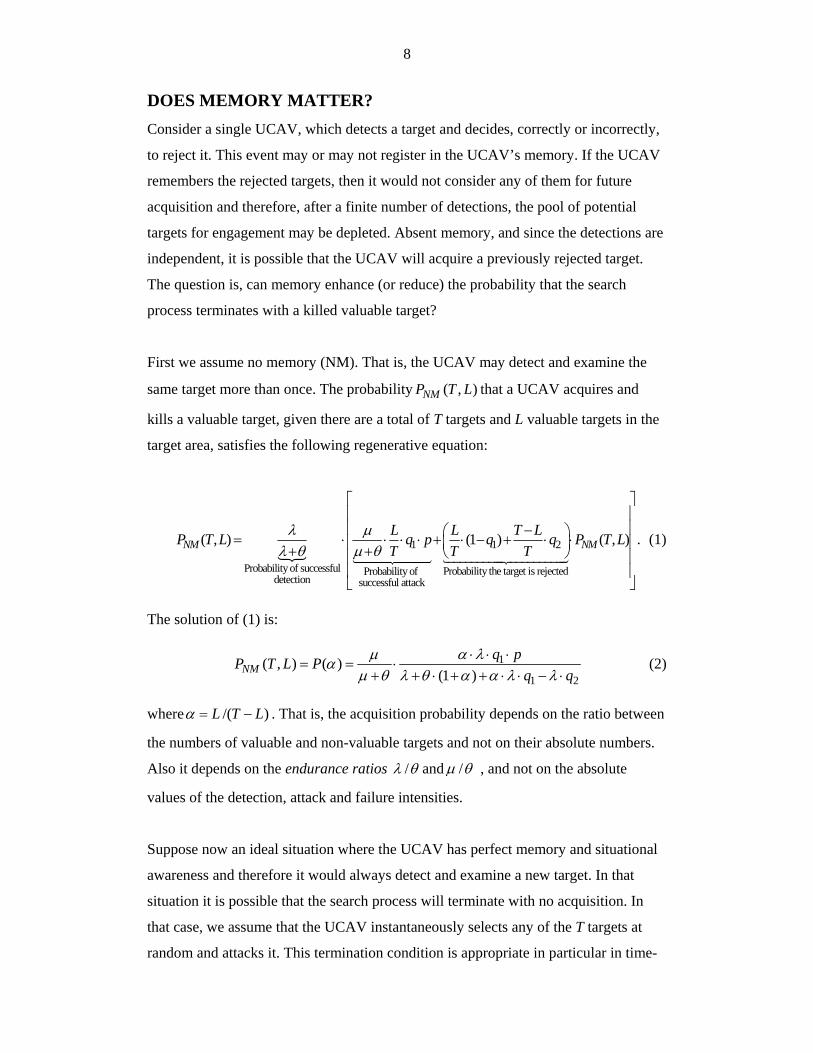
First we assume no memory (NM). That is, the UCAV may detect and examine the
same target more than once. The probability ( , )NMP T L that a UCAV acquires and
kills a valuable target, given there are a total of T targets and L valuable targets in the
target area, satisfies the following regenerative equation:
1 1 2
Probability of successful Probability the target is rejectedProbability of detection successful attack
( , ) (1 ) ( , )NM NML L T LP T L q p q q P T LT T T
λ µλ θ µ θ
⎡⎢
−⎛ ⎞= ⋅ ⋅ ⋅ ⋅ + ⋅ − + ⋅ ⋅⎜ ⎟+ + ⎝ ⎠
⎣
⎤⎥
⎢ ⎥⎢ ⎥⎢ ⎥⎢ ⎥
⎦
. (1)
The solution of (1) is:
1
1 2( , ) ( )
(1 )NMq pP T L P
q qα λµα
µ θ λ θ α α λ λ⋅ ⋅ ⋅
= = ⋅+ + ⋅ + + ⋅ ⋅ − ⋅
(2)
where /( )L T Lα = − . That is, the acquisition probability depends on the ratio between
the numbers of valuable and non-valuable targets and not on their absolute numbers.
Also it depends on the endurance ratios /λ θ and /µ θ , and not on the absolute
values of the detection, attack and failure intensities.
Suppose now an ideal situation where the UCAV has perfect memory and situational
awareness and therefore it would always detect and examine a new target. In that
situation it is possible that the search process will terminate with no acquisition. In
that case, we assume that the UCAV instantaneously selects any of the T targets at
random and attacks it. This termination condition is appropriate in particular in time-
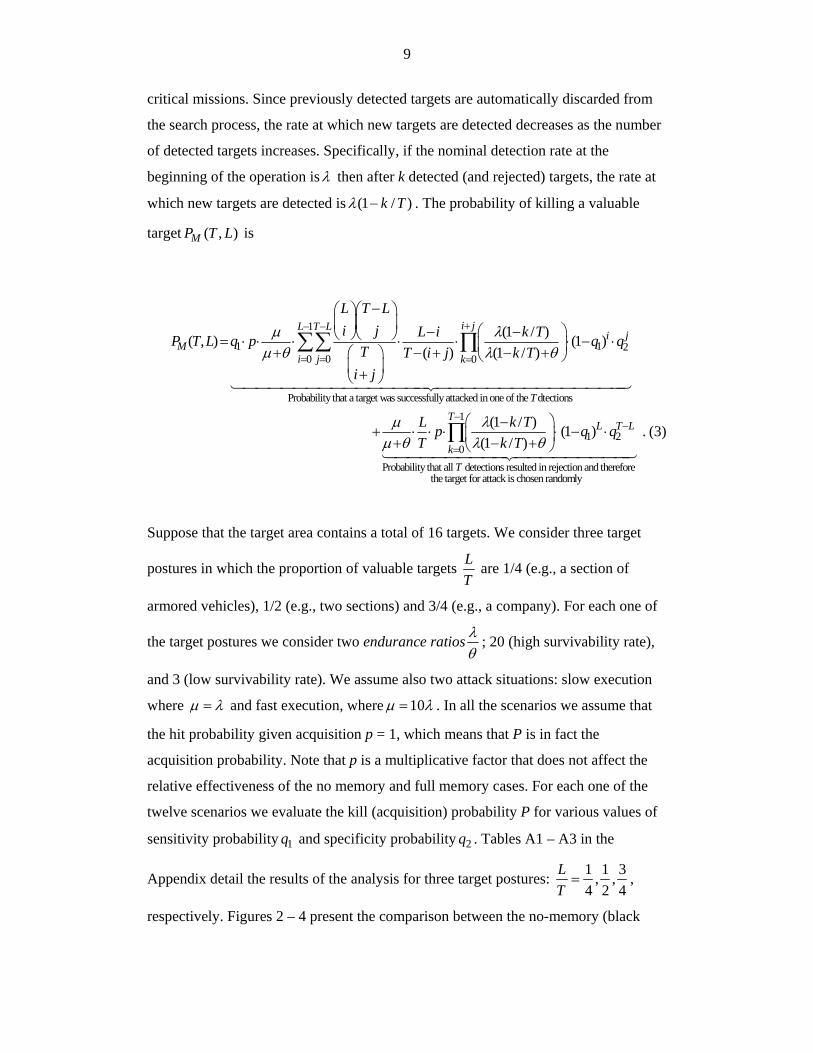
9
critical missions. Since previously detected targets are automatically discarded from
the search process, the rate at which new targets are detected decreases as the number
of detected targets increases. Specifically, if the nominal detection rate at the
beginning of the operation isλ then after k detected (and rejected) targets, the rate at
which new targets are detected is (1 / )k Tλ − . The probability of killing a valuable
target ( , )MP T L is
1
1 1 20 0 0
Probability that a target was successfully attacked in one of the dtections
(1 / )( , ) (1 )( ) (1 / )
i jL T Lji
Mi j k
T
L T Li j L i k TP T L q p q q
T T i j k Ti j
µ λµ θ λ θ
+− −
= = =
−⎛ ⎞⎛ ⎞⎜ ⎟⎜ ⎟ ⎛ ⎞− −⎝ ⎠⎝ ⎠= ⋅ ⋅ ⋅ ⋅ ⋅ ⋅ − ⋅⎜ ⎟+ − + − +⎛ ⎞ ⎝ ⎠⎜ ⎟+⎝ ⎠
∑∑ ∏
14444444 2
1
1 20
Probability that all detections resulted in rejection and thereforethe target for attack is chosen randomly
(1 / ) (1 )(1 / )
TL T L
kT
L k Tp q qT k T
µ λµ θ λ θ
−−
=
⎛ ⎞−+ ⋅ ⋅ ⋅ ⋅ − ⋅⎜ ⎟+ − +⎝ ⎠
∏
44444444 4444444444444443
14444444 244 4444444443
. (3)
Suppose that the target area contains a total of 16 targets. We consider three target
postures in which the proportion of valuable targets LT
are 1/4 (e.g., a section of
armored vehicles), 1/2 (e.g., two sections) and 3/4 (e.g., a company). For each one of
the target postures we consider two endurance ratios λθ
; 20 (high survivability rate),
and 3 (low survivability rate). We assume also two attack situations: slow execution
where µ λ= and fast execution, where 10µ λ= . In all the scenarios we assume that
the hit probability given acquisition p = 1, which means that P is in fact the
acquisition probability. Note that p is a multiplicative factor that does not affect the
relative effectiveness of the no memory and full memory cases. For each one of the
twelve scenarios we evaluate the kill (acquisition) probability P for various values of
sensitivity probability 1q and specificity probability 2q . Tables A1 – A3 in the
Appendix detail the results of the analysis for three target postures: 1 1 3, ,4 2 4
LT= ,
respectively. Figures 2 – 4 present the comparison between the no-memory (black

10
lines) and full-memory (grey lines) cases for the three target postures ( 1 1 3, ,4 2 4
LT= )
with 20λθ= and 10µ λ= .
0
0.2
0.4
0.6
0.8
1
0.0 0.1 0.2 0.3 0.4 0.5 0.6 0.7 0.8 0.9 1.0
q1
P
No Memory, q2=0.5
No Memory, q2=0.7
No Memory, q2=0.9
Full Memory, q2=0.5
Full Memory, q2=0.7
Full Memory, q2=0.9
Figure 2: Probability of Acquiring a Valuable Target, L/T = 1/4
0
0.2
0.4
0.6
0.8
1
0.0 0.1 0.2 0.3 0.4 0.5 0.6 0.7 0.8 0.9 1.0
q1
P
No Memory, q2=0.5
No Memory, q2=0.7
No Memory, q2=0.9
Full Memory, q2=0.5
Full Memory q2=0.7
Full Memory, q2=0.9
Figure 3: Probability of Acquiring a Valuable Target, L/T = 1/2

11
0
0.2
0.4
0.6
0.8
1
0.0 0.1 0.2 0.3 0.4 0.5 0.5 0.6 0.7 0.8 0.9 1.0
q1
P
No Memory, q2=0.5
No Memory, q2=0.7
No Memory, q2=0.9
Full Memory, q2=0.5
Full Memory, q2=0.7
Full Memory, q2=0.9
Figure 4: Probability of Acquiring a Valuable Target, L/T = 3/4
Clearly, P is monotonic increasing in both q1 and q2; better sensitivity and specificity
results in higher acquisition probability. While for some (relatively small) values of q1
and q2 the no-memory system outperforms the full-memory system, and for other
(relatively large) values the opposite is true, the differences between the two cases are
negligible. This conclusion is robust with respect to the detection, attack and failure
rates (see Appendix). For example, if q1 = 0.8 and q2 = 0.7 then the relative
differences between PM and PNM, over all twelve scenarios, range between 0% and
less than 3%. As shown in Tables A1-A3 in the appendix, this conclusion remains
unchanged for longer inter-detection whereλ µ= .
Based on the analysis we can conclude that, under our assumptions, memory is rather
redundant design feature in UCAVs. The processing capacity on board the UCAV
would be better utilized for other data processing or storing tasks. Note however that
this conclusion may not be true in other tactical settings such as time-critical missions
or situations where the search time is limited due to operational or logistical
constraints. From now on we assume that the UCAVs have no memory.
MULTIPLE UCAVS, NO SITUATIONAL AWARENESS In this section we explore temporal effects of the UCAVs’ target engagement process.
We assume no situational awareness, which means that any detected target is
attacked. In other words, 1 21 1q q= − = .
12
The probability that at time t of the engagement a certain UCAV is still searching
is ( )te λ θ− + . Using conditioning, we obtain that the probability the UCAV failed by
time t is:
( ) ( )( ) ( )
0 0Probability of failure during the attack stage Probability of failure
during the search stage
( ) ( )
( ) (1 )
1 (
t ts t s s
F
t t
Q t e e ds e ds
e e
λ θ µ θ λ θ
λ θ µ θ
λθ θµ θ
λθµ θ λ θ λ µ
− + − + − − +
− + − +
= − ++
−−
+ + −=
∫ ∫144444424444443 1442443
( ) ( )
( )( ) ( )
1 ) (1 ) if
1 (1 ) if .
t t
tt t
e e
e te e
λ µ λ θ
λ θλ θ λ θ
θ λ µλ θ
λθ θ λ µλ θ λ θ λ θ
− − − +
− +− + − +
⎧ ⎡ ⎤− + − ≠⎪ ⎢ ⎥
+⎢ ⎥⎪ ⎣ ⎦⎨
⎡ ⎤−⎪ − + − =⎢ ⎥⎪ + + +⎢ ⎥⎣ ⎦⎩
(4)
The probability that the UCAV has completed its mission by time t without failure is
( ) ( )( )
0
( ) ( ) ( )
2 ( )( )
( ) (1 )
1 (1 ) if
1 if ,
ts t s
A
t t t
tt
Q t e e ds
e e e
e te
λ θ µ θ
λ θ µ θ λ µ
λ θλ θ
λµµ θ
λµ λ µµ θ λ θ λ µ
λ λ µλ θ λ θ
− + − + −
− + − + − −
− +− +
= − =+
⎧ ⎛ ⎞− −− ≠⎪ ⎜ ⎟⎜ ⎟+ + −⎪ ⎝ ⎠=⎨
⎛ ⎞−⎪ − =⎜ ⎟⎪ ⎜ ⎟+ +⎝ ⎠⎩
∫
(5)
and ( )( )( )A
tQ t λµ
λ θ µ θ→∞→
+ +.
Since the UCAVs are independent, the CDF of the duration of the operation is:
( ) [ ( ) ( )]ND F AF t Q t Q t= + (6)
and the expected number of killed targets at time t is
( )1 1N
At
Q t pE LT
⎛ ⎞⎛ ⎞⎜ ⎟= − −⎜ ⎟⎜ ⎟⎝ ⎠⎝ ⎠. (7)
Consider the base case where the average detection time is 5 minutes, the average
attack time is 30 seconds and the mean time between failures (MTBF) is 100 minutes,

13
that is, 0.2, 2 and 0.01.λ µ θ= = = Figure 5 depicts the CDF of the operation
completion time for various pack sizes N.
0.0
0.2
0.4
0.6
0.8
1.0
1 4 7 10 13 16 19 22 25 28 31 34 37 40 43 46 49
Minutes
N=4
N=8
N=12
N=16
N=20
Figure 5: CDF of the Operation Completion Time for Varying N
The 90th percentiles of these CDFs are 18, 23, 26, 27 and 28 minutes for packs of 4, 8,
12, 16 and 20 UCAVs, respectively. Figures 6 and 7 present the CDF of the mission
completion time for varying detection intensities (λ ) and failure intensities (θ ),
respectively. In both cases we assume a pack of N = 8 UCAVs. The values of the
other parameters are as in the base case.
0.0
0.2
0.4
0.6
0.8
1.0
1 4 7 10 13 16 19 22 25 28 31 34 37 40 43 46 49
Minutes
λ=0.05
λ=0.1
λ=0.2
λ=1
Figure 6: CDF of the Operation Completion Time for Varying λ
The 90th percentiles of these distributions are 72, 40, 21, and 5 minutes for mean
detection times of 20, 10, 5 and one minutes, respectively.
14
0.0
0.2
0.4
0.6
0.8
1.0
1 4 7 10 13 16 19 22 25 28 31 34 37 40 43 46 49
Minutes
θ=0.005θ=0.01θ=0.02θ=0.05θ=0.1
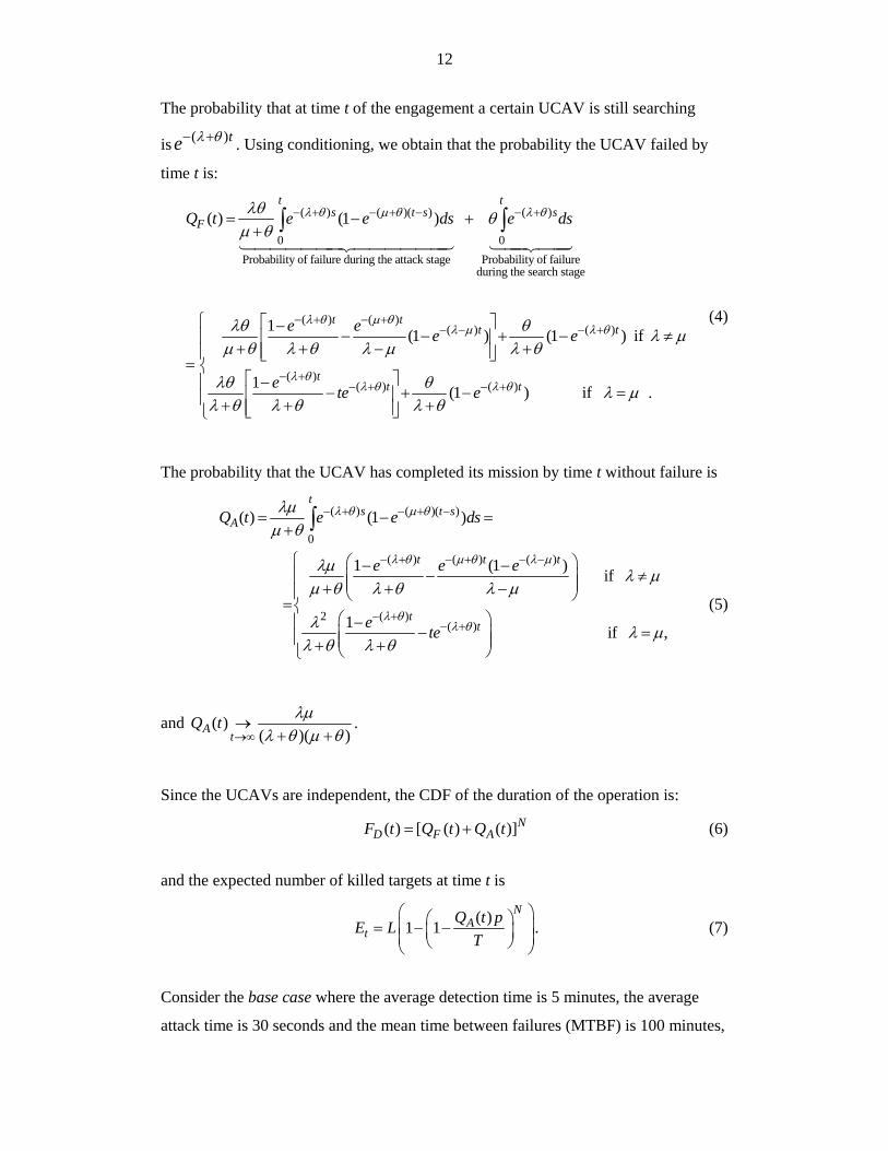
Figure 7: CDF of the Operation Completion Time for Varying θ
The 90th percentiles of the CDFs in Figure 5.3 are 22, 21, 20, 18 and 14 minutes for
mean interception times of 200, 100, 50, 20 and 10 minutes, respectively. While the
completion time of the mission is sensitive to the pack size and very sensitive to the
detection intensity, it is rather insensitive to the failure rate within the relevant range.
In other words, for the selected ranges of the time parameters, the most significant
factor is the detection time.
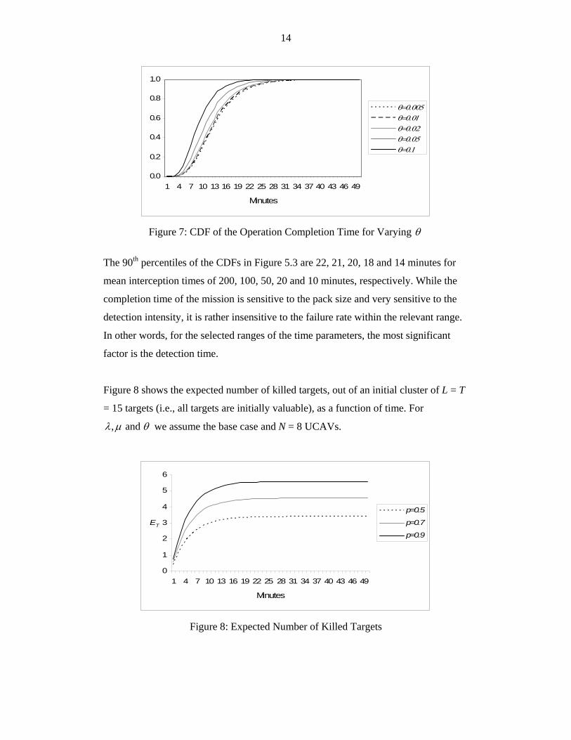
Figure 8 shows the expected number of killed targets, out of an initial cluster of L = T
= 15 targets (i.e., all targets are initially valuable), as a function of time. For
, and λ µ θ we assume the base case and N = 8 UCAVs.
0
1
2
3
4
5
6
1 4 7 10 13 16 19 22 25 28 31 34 37 40 43 46 49
Minutes
ET
p=0.5
p=0.7
p=0.9
Figure 8: Expected Number of Killed Targets

15
Absent situational awareness, the expected number of killed targets approaches
asymptotically 3.4, 4.5 and 5.6 targets for kill probabilities .5, .7 and .9, respectively.
These limit values are reached relatively fast – after about 20 minutes of operation.
Figure 5.4 can help obtain some guidelines for operating the UCAVs in case they are
not disposable and can be used in future operations. For example, it can identify a
time t* at which all searching UCAVs will be programmed to abandon their mission
and return to the home base.
MULTIPLE UCAVS WITH IMPERFECT BDA AND LIMITED
COORDINATION
Assume now that the UCAVs have limited situational awareness, that is,
1 20 , 1.q q< < Next we develop a continuous time Markov chain that represents our
combat situation.
STATES
Let n denote the number of searching UCAVs. Initially, n = N. A state in the model is
represented by ( , ; 0,..., )in m i N n= − where im indicates the number of valuable
targets that are currently under attack (but have not been hit yet) by exactly i UCAVs
each. An absorbing state in the engagement process is of the form 0(0, ,0,...,0)m ,
which means that there are no UCAVs at the search stage (n = 0) and no UCAVs at
the attack stage. The number of valuable targets killed by the UCAVs in an absorbing
state is 0L m− .
Example: let L = N = 2. There are 11 possible states: (2,2,0,0), (1,2,0,0), (1,1,1,0),
(1,1,0,0), (0,2,0,0), (0,1,1,0), (0,1,0,1), (0,1,0,0), (0,0,2,0), (0,0,1,0) and (0,0,0,0). For
example, the state (1,2,0,0) represents the situation where one UCAV is searching and
the other UCAV is removed following a failed attack (acquired a non-valuable target
or missed a valuable target or has crashed). The state (1,1,0,0) represents a similar
situation, however the removed UCAV successfully acquired and killed a valuable
target.
16
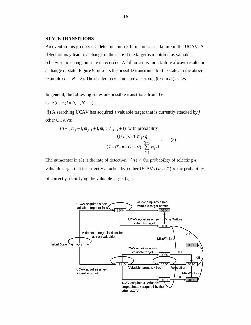
STATE TRANSITIONS
An event in this process is a detection, or a kill or a miss or a failure of the UCAV. A
detection may lead to a change in the state if the target is identified as valuable,
otherwise no change in state is recorded. A kill or a miss or a failure always results in
a change of state. Figure 9 presents the possible transitions for the states in the above
example (L = N = 2). The shaded boxes indicate absorbing (terminal) states.
In general, the following states are possible transitions from the
state ( , ; 0,..., )in m i N n= − .
(i) A searching UCAV has acquired a valuable target that is currently attacked by j
other UCAVs:
1
1
1
( 1, 1, 1, ; , 1) with probability
(1/ )
( ) ( )
j j i
jN n
ii
n m m m i j j
T n m q
n m i
λ
λ θ µ θ
+
−
=
− − + ≠ +
⋅ ⋅ ⋅
+ ⋅ + + ⋅ ⋅∑. (8)
The numerator in (8) is the rate of detection ( nλ ) × the probability of selecting a
valuable target that is currently attacked by j other UCAVs ( /jm T ) × the probability
of correctly identifying the valuable target ( 1q ).
2200
1110 1100
1200
Initial State
UCAV acquires a newvaluable target
UCAV acquires a non-valuable target or fails
A detected target is classifiedas non-valuable
0200
0110
0020
Valuable target is killed
UCAV acquires a newvaluable target
UCAV acquires a non-valuable target or fails
0010
0100
0000UCAV acquires a new
valuable target
0101UCAV acquires a valuabletarget already acquired by theother UCAV
Acquisition
Kill
Kill
Miss/Failure
Miss/Failure
Kill
Miss/Failure
Kill

17
Figure 9: The State Transitions, L = N = 2
(ii) A searching UCAV has acquired a non-valuable target or has failed (removed
prematurely):
20
1
( 1, ; 0,..., 1) with probability
(1/ ) ( ) (1 )
( ) ( )
iN n
ii
N n
ii
n m i N n
T n T m q n
n m i
λ θ
λ θ µ θ
−
=−
=
− = − +
⋅ ⋅ ⋅ − ⋅ − +
+ ⋅ + + ⋅ ⋅
∑
∑
. (9)
The numerator in (9) is the rate at which non valuable targets are acquired (= the rate
of detection ( nλ ) × the probability of selecting a non-valuable target
(0
( ) /N n
ii
T m T−
=
−∑ ) × the probability of incorrectly identifying this target as valuable
( 21 q− )) + the failure rate of searching UCAVs (= nθ ).
(iii) A UCAV is the first to kill a valuable target that is currently attacked by j
UCAVs:
1
( , 1; ; ) with probability
( ) ( )
j i
jN n
ii
n m m i j
j m p
n m i
µ
λ θ µ θ−
=
− ≠
⋅ ⋅ ⋅
+ ⋅ + + ⋅ ⋅∑. (10)
The numerator in (10) is the attack rate of a single UCAV (µ ) × the number of
UCAVs that are attacking this type of targets ( jj m⋅ ) × the kill probability of a single
UCAV (p).
(iv) A UCAV that is attacking a valuable target, which is currently attacked by j
UCAVs, is removed without completing its mission, that is, misses the target or
fails during the attack:
18
1
1
( , 1, 1; ; 1, ) with probability
( (1 ) )
( ) ( )
j j i
jN n
ii
n m m m i j j
p j m
n m i
µ θ
λ θ µ θ
−
−
=
+ − ≠ −
⋅ − + ⋅ ⋅
+ ⋅ + + ⋅ ⋅∑. (11)
The numerator in (11) is the rate of attacks that miss the target ( (1 ) jp j mµ ⋅ − ⋅ ⋅ , see
also (10) above) + the failure rate of attacking UCAVs ( jj mθ ⋅ ⋅ )).
(v) A detected target is classified as non-valuable and therefore passed over:
1 20 0
1
( , ; 0,..., ) with probability
(1/ ) [(1 ) ( )]
( ) ( )
iN n N n
i ii i
N n
ii
n m i n
T n q m q T m
n m i
λ
λ θ µ θ
− −
= =−
=
=
⋅ ⋅ ⋅ − ⋅ + ⋅ −
+ ⋅ + + ⋅ ⋅
∑ ∑
∑
. (12)
The numerator in (12) is the rate at which valuable targets are misclassified as non-
valuable (= detection rate ( nλ )×probability of selecting a valuable target
(0
/N n
ii
m T−
=∑ )× the probability for type-1 error 1(1 )q− ) + the rate at which non-
valuable targets are classified correctly as such ( 20
( ) /N n
ii
n q T m Tλ−
=⋅ ⋅ ⋅ − ∑ ).
Suppose now that the UCAVs can share information and coordinate their attacks.
Specifically, we assume that during the attack stage a UCAV sends out a signal that
marks (“highlights”) its target. The signal, which is set off when the UCAV is
removed, may be received by any searching UCAV with a fixed probability r. The
signals from the various UCAVs are independent. Thus, a searching UCAV that
detects a target that is currently attacked by j other UCAVs avoids it without further
investigation with probability1 (1 ) jr− − . Notice that if r = 1 then no incidents of
multiple acquisitions (attacks) can occur. The transition rates shown above change
only for cases (i) and (v):

19
(i) A searching UCAV has acquired a live (valuable) target that is already attacked by
j other UCAVs:
1
1
1
( 1, 1, 1, ; , 1) with probability
(1/ ) (1 )
( ) ( )
j j i
jj
N n
ii
n m m m i j j
T n m q r
n m i
λ
λ θ µ θ
+
−
=
− − + ≠ +
⋅ ⋅ ⋅ ⋅ −
+ ⋅ + + ⋅ ⋅∑. (13)
(v) A target is passed over (is valuable but recognized as being acquired by other
UCAVs or is classified as non-valuable or is non-valuable):
1 20 0
1
( , ; 0,..., ) with probability
(1/ ) [ ((1 ) (1 ) 1 (1 ) ) ( )]
( ) ( )
iN n N n
i ii i
i iN n
ii
n m i N n
T n m r q r q T m
n m i
λ
λ θ µ θ
− −
= =−
=
= −
⋅ ⋅ ⋅ − ⋅ − + − − + −
+ ⋅ + + ⋅ ⋅
∑ ∑
∑
. (14)
All other transitions ((ii) – (iv)) remain the same.
To keep the model tractable, we assume that this transfer of attack information does
not apply to non-valuable targets. Otherwise we need to keep track also of the number
of non-valuable targets that are being attacked by i UCAVs, which leads to a
considerable expansion of the state dimension. If the number of non-valuable targets
is relatively high compared to the numbers of valuable targets and UCAVs, and if the
specificity of the sensor q2 is reasonably high, then we can assume that instances of
multiple acquisitions of non-valuable targets are highly unlikely. In particular, we
assume that there are practically no incidents where a UCAV avoids acquiring a
certain non-valuable target solely because it receives a signal from another UCAV
that has already acquired (erroneously) that non-valuable target. Another assumption
that leads to the same transition probabilities is that r ≈ 0 for acquisitions of non-
valuable targets (e.g., a UCAV realizes rather quickly that it has acquired a non-
valuable target and sets the signal off immediately).
MEASURES OF EFFECTIVENESS
To evaluate the relative effects of design and operational parameters we define four
measures of effectiveness (MOE):
20
• Expected relative effectiveness (EM) is the ratio between the expected number
of killed valuable targets and their initial number. This MOE represent the
effectiveness of the attack. Formally,
[ ]L
E XEL
= (15)
where X is the number of killed valuable targets.
• Expected relative efficiency (EN) is the ratio between the expected number of
killed valuable targets and the initial number of UCAVs in the attack pack.
This MOE represent how efficient is the mission. Formally,
[ ]N
E XEN
= . (16)
• Probability of attaining the mission objective ( Pα ) is the probability that at
least a fraction α of the L valuable targets are killed. This MOE represents
tactical or operational objectives, as set by the mission commander. Clearly,
this MOE is non-trivial only if N Lα≥ . Formally,
Pr( )P X Lα α= ≥ . (17)
In addition to the three MOEs we compute also the expected duration of a mission
ETime. The results are obtained by utilizing computational procedures of absorbing
Markov chains (e.g., Minh (2000)).
ANALYSIS
The time parameters in our base case are as in Section 5: 0.2, 2 and 0.01.λ µ θ= = =
The sensitivity, specificity and kill probabilities are 1 20.7, 0.8q q= = and p = 0.8,
respectively. These values represent only a reasonable reference point for the
technical and operational parameters of UCAVs since most of these vehicles are still
in the development phase. Even if some relevant data do exist, it would be most likely
classified. Notwithstanding this limitation, the ensuing sensitivity analysis provides
insights into tradeoffs among the parameters of the vehicle and the combat scenario.
The base case scenario comprises a pack of N = 8 UCAVs that engages a total of T =
12 targets, out of which L = 8 are valuable. We first assume no coordination, that is r
= 0. The expected number of killed valuable targets is 4.32 with engagement
effectiveness and efficiency of EL = EN = 0.54. The probability of attaining the mission
objective – at least 40% of the valuable targets killed – is P0.4 = 0.77. The expected

21
duration of the operation is ETime = 30 min. If the UCAVs are fully coordinated then
EL = EN = 0.55, P0.4 = 0.78 and ETime = 30.4 min. Clearly, in the base case,
coordination has no significant effect; the changes in the MOEs values are negligible.
Next we investigate the impact of various parameters on the values of the MOEs.
(a) Detection and Attack Rates
For a fixed failure rate of 0.01θ = (base case) Figures 10 – 13 present the effect of
the detection rate ( )λ and the attack rate ( )µ on the expected relative effectiveness EN
and on the probability of attaining a mission objective of 40% killed valuable targets
P0.4. Since L = N, the expected relative effectiveness is also the expected relative
efficiency. Figures 10 and 11 apply to the case where there is no coordination among
the UCAVs (r = 0), while Figures 12 and 13 apply to the case of full coordination (r =
1).
0.5
0.6
0.1 1.5 3
λ
EN
µ=1µ=2µ=3µ=4
Figure 10: The Effect of Detection Rate on the Expected Relative Effectiveness
(Efficiency), r = 0.

22
0.7
0.8
0.9
0.1 1.5 3
λ
P0.4
µ=1µ=2µ=3µ=4
Figure 11: The Effect of Detection Rate on the Probability of Attaining 40% Killed
Valuable Targets, r = 0.
0.5
0.6
0.1 1.5 3
λ
EN
µ=1µ=2µ=3µ=4
Figure 12: The Effect of Detection Rate on the Expected Relative Effectiveness
(Efficiency), r = 1.
0.7
0.8
0.9
0.1 1.5 3
λ
P0.4
µ=1µ=2µ=3µ=4
Figure 13: The Effect of Detection Rate on the Probability of Attaining 40% Killed
Valuable Targets, r = 1.

23
In all four charts the mean detection time of a UCAV ranges between 10 minutes
( 0.1λ = ) and 20 seconds ( 3λ = ). Both MOEs – EN and P0.4 – are computed for four
mean attack times that range from 1 minute ( 1µ = ) to 25 seconds ( 4µ = ). In the case
of no coordination (r = 0), shorter attack times result in better performance of the
UCAVs with respect to both MOEs. This conclusion is quite intuitive for cases of
relatively high sensitivity, specificity and kill probability. Shorter attack times reduce
the possibility of redundant multiple attacks. The observation that higher detection
rate may be counter-effective, as displayed by the unimodal plots in Figures 10 and
11, is less intuitive. The monotonic increasing part for small values of λ represents a
race between the detection and failure processes; increasing detection rate decreases
loitering time and therefore also the chances for failure. The monotonic decreasing
part for larger values of λ is explained by exactly the same arguments used above for
explaining the positive effect of increasingµ ; shorter detection time relative to the
attack time implies more opportunities for simultaneous acquisitions that lead to
multiple attacks. The effect of θ is discussed later on. In the case of perfect
coordination (r = 1) there can be no multiple acquisitions and therefore higher
detection rate is always better. Since the attack time is very short compared to the
MTBF ( 1θ − ) of the UCAVs, perfect coordination implies that the effect of the attack
rate µ is negligible.
Note that the graphs of EN and P0.4 have similar shapes. For brevity we display from
now on mostly results regarding EN or EL.
(b) Sensitivity, Specificity and Kill Probability
An interesting question regarding the UCAV’s sensor capabilities is: which property
is more important, sensitivity or specificity? Recall that higher sensitivity means
lower probability for type I error (misclassifying a valuable target), while higher
specificity implies lower probability for type II error (misclassifying a non valuable
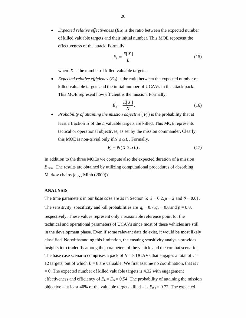
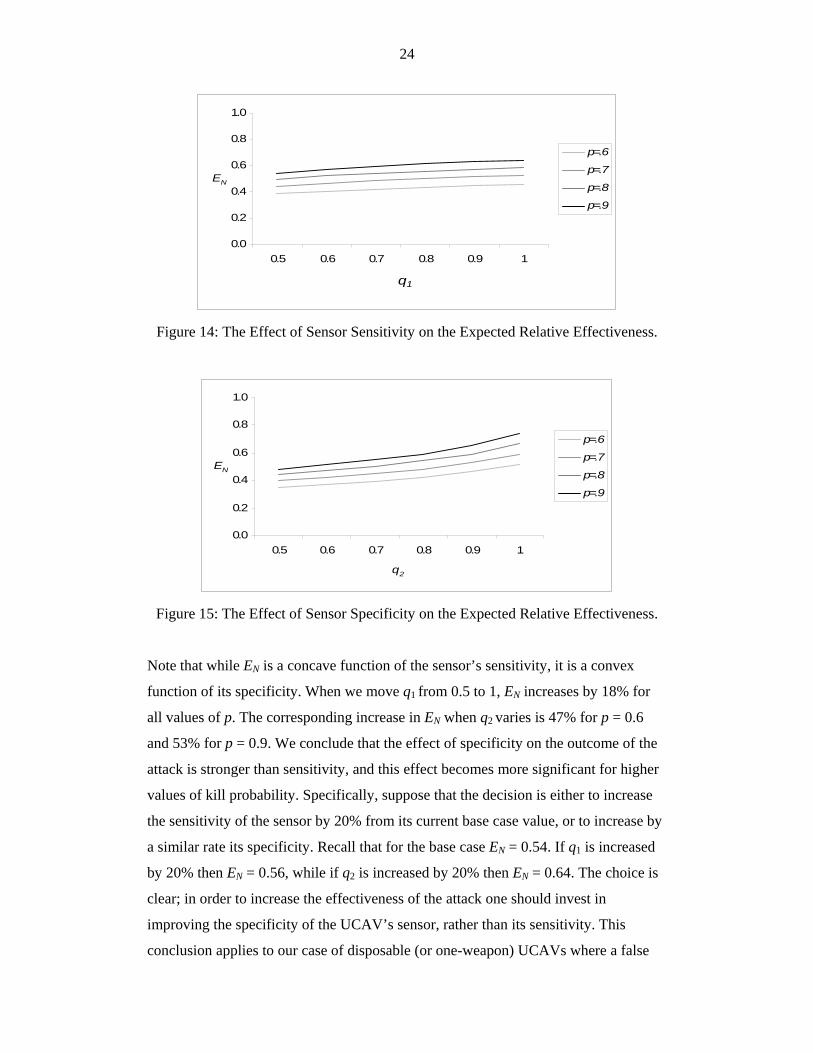
target). Figures 14 and 15 show the effect of changing the sensitivity and specificity
of the sensor, respectively. The results are displayed for 4 values of kill probability:
0.6, 0.7, 0.8 and 0.9. All other parameters are set at their base case values.
24
0.0
0.2
0.4
0.6
0.8
1.0
0.5 0.6 0.7 0.8 0.9 1
q1
EN
p=.6
p=.7
p=.8
p=.9
Figure 14: The Effect of Sensor Sensitivity on the Expected Relative Effectiveness.
0.0
0.2
0.4
0.6
0.8
1.0
0.5 0.6 0.7 0.8 0.9 1
q2
EN
p=.6
p=.7
p=.8
p=.9
Figure 15: The Effect of Sensor Specificity on the Expected Relative Effectiveness.
Note that while EN is a concave function of the sensor’s sensitivity, it is a convex
function of its specificity. When we move q1 from 0.5 to 1, EN increases by 18% for
all values of p. The corresponding increase in EN when q2 varies is 47% for p = 0.6
and 53% for p = 0.9. We conclude that the effect of specificity on the outcome of the
attack is stronger than sensitivity, and this effect becomes more significant for higher
values of kill probability. Specifically, suppose that the decision is either to increase
the sensitivity of the sensor by 20% from its current base case value, or to increase by
a similar rate its specificity. Recall that for the base case EN = 0.54. If q1 is increased
by 20% then EN = 0.56, while if q2 is increased by 20% then EN = 0.64. The choice is
clear; in order to increase the effectiveness of the attack one should invest in
improving the specificity of the UCAV’s sensor, rather than its sensitivity. This
conclusion applies to our case of disposable (or one-weapon) UCAVs where a false

25
positive error is irreversible. This may not be the case if the UCAV has multiple
weapons and the mission is not time-critical. The recommendation to invest in better
specificity is enhanced by other measures of merit such as the human and political
cost of attacking a wrong target (e.g., the bombing of the Chinese embassy in
Belgrade by NATO forces in 1999).
(c) Failure Rate and Coordination
Arguably, UCAVs’ coordination can be effective only if the attack stage is long
compared to the search stage. If it is short, then multiple acquisitions are very unlikely
and therefore there is no practical need for coordination. It is shown next that the
failure rate may affect the benefit the pack gains from coordination. Let L = 6, and
suppose that the attack time is four time shorter than the detection time, which is set at
its base case value. This situation may represent a standoff attack. The failure rate
ranges between 0 (no failure during the mission) to 0.1 (MTBF = 10 min). Figure 16
presents the expected relative effectiveness for r = 0 and r = 1. All other parameters
are set at their base case values.
0.0
0.2
0.4
0.6
0.8
1.0
0 0.1
θ
EL
No Coordination
Full Coordination
Figure 16: The Effect of Failure Rate and Coordination on the Expected Relative
Effectiveness.
As one would expect, the effectiveness of the UCAVs decreases as the failure rate
increases. Note that even in this extreme scenario, where conditions are relatively
favorable for effective coordination, the effect is minute. Moreover, while for smaller
failure rates full coordination is somewhat more effective than no coordination, the
opposite is true for larger failure rates for which coordination actually reduces the
mission effectiveness. The latter counter-intuitive observation is due to the fact that if

26
UCAVs pass over targets, they prolong their stay in the target area and therefore
increase their chances to be intercepted before staging their attack.
Another way to avoid multiple acquisitions is to employ the UCAVs sequentially
rather than simultaneously as a pack. This tactical solution to multiple acquisition
problem leads to a different Markov model that is based on the probabilities given in
(2) above. Taking once again L = 6, / 4µ λ= and the rest of the parameters at their
base case values, Figure 17 presents the value of the expected relative effectiveness
EL for three cases: No coordination, perfect coordination and sequential engagement.
These values are computed as functions of the specificity probability q2.
0.0
0.2
0.4
0.6
0.8
1.0
0.5 0.6 0.7 0.8 0.9 1
q2
EL
No Coordination
Perfect Coordination
SequentialEngagement
Figure 17: The Effect of Eliminating Multiple Acquisitions
For poor to moderate specificity the three graphs coincide. For high specificity,
eliminating multiple acquisitions, either by a design features (coordination) or tactics
(sequential engagement) has some effect. The effect is similar in both cases, with a
slight advantage to the tactical solution, which is applicable only for non time-critical
targets.
(d) Scenario Parameters
So far we have analyzed the effect of parameters that are associated with the design of
the UCAVs. Figures 18 and 19 display the effect of the scenario. Figure 18 presents
the value of EL when the number of valuable targets L and the specificity probability
q2 vary in the target area. Note that besides being a design parameter, specificity is

27
also a scenario parameter that may depend on the clutter in the target area. Figure 19
displays the combined effect of L and the number of UCAVs N. The MOE here is
P0.4, which represents a specific tactical objective.
0.0
0.2
0.4
0.6
0.8
1.0
0.5 0.56 0.61 0.67 0.72 0.78 0.83 0.89 0.94 1
q2
EL
L=2
L=4
L=6
L=8
Figure 18: The Effect of the Number of Valuable Targets
0.0
0.2
0.4
0.6
0.8
1.0
2 3 4 5 6 7 8
Number of UCAVs - N
P0.4
L=2
L=4
L=6
L=8
Figure 19: Probability of Attaining 40% Killed Valuable Targets as a Function of M
and N
From Figure 18 we see once again the effect of specificity. At low specificity, the rate
of killed valuable targets is relatively insensitive to their number. At high specificity
this rate decreases with the number of targets, as one would expect.
Figure 19 examines the impact of the number of valuable targets on the engagement
performance from another angle. For small number of UCAVs the 40% attrition
probability is very sensitive to the number of targets. This sensitivity diminishes as N
gets larger. Note that Figure 19 may be used also as a decision support tool for
28
mission planning. For example, if there are four valuable targets in the target area,
then in order to attain the mission objective – two killed targets – with probability of
at least 0.8, then the pack must contain at least seven UCAVs. This can be seen by
observing the point at which the graph corresponding to L=4 crosses the 0.8 threshold.
SUMMARY, CONCLUSIONS AND FUTURE RESEARCH In this paper we explore several design and operational aspects of employing a pack
of autonomous UCAVs against valuable targets that are imbedded among other, non-
valuable targets. Utilizing newly developed analytic probability models, we evaluate
the effect of key design and operational parameters on the performance of the pack.
First, it is shown that under reasonable assumptions memory is a redundant property.
The processing capacity in the UCAV brain should be utilized to other tasks such as
enhanced recognition capability. Second, based on a transient model, inter-temporal
behavior of the system is explored and some insights regarding mission duration and
maximum allowable loitering time are obtained. It is shown that detection rate is a
major factor in determining the duration of the operation. Finally, in Section 6 we
implement a large-scale continuous-time Markov model to analyze the effect of
weapon coordination on multiple acquisitions, and the effect of BDA on multiple
kills. The two main conclusions from the analysis are: (1) attack coordination among
UCAVs is largely an insignificant feature for the scenarios analyzed, and (2)
specificity of the UCAV’s sensor is more important than its sensitivity. The first
conclusion is true as long as the valuable targets are homogeneous. It essentially says
that the random uniform and independent selection is the right thing to do when
engaging uniform targets. If among the valuable targets there are some that are more
noticeable or attractive then targeting coordination may improve the engagement
performance. The case of non-homogeneous targets is left for future research. The
second conclusion tells us that avoiding non-valuable targets is more beneficial than
picking correctly valuable ones. This observation, which at first glance may look a
little odd, is quite logical. Type I error by a UCAV (passing over a valuable target)
can be rectified later on. Type II error (acquiring and attacking non-valuable target)
cannot.

29
The models described in this paper are limited to homogeneous targets, homogeneous
UCAVs and to the engagement rules specified. Another limitation is the assumption
that all the temporal random variables are exponential. While this assumption is
reasonable for the failure and detection processes, the attack time is probably not well
represented by a constant failure-rate (CFR) distribution. Accordingly, the models
presented in this paper may be extended to account for non-homogeneous targets,
multiple types of UCAVs and more general time CDFs (e.g., non-exponential attack
times). Another interesting and potentially important extension is to incorporate in the
models decision rules where the UCAVs manifest some level of cognitive capability.
Specifically, in reality both sensitivity and specificity probabilities may depend on the
time a UCAV spends investigating a target. This aspect is not captured in our models
and may lead to interesting optimization models.
REFERENCES Airforce Technology, 2005, “Predator RQ-1 / MQ-1 / MQ-9 Unmanned Aerial
Vehicle (UAV), USA”, http://www.airforce-technology.com/projects/predator/.
Aviv, Y., and Kress, M., 1997, “Evaluating the Effectiveness of Shoot-Look-Shoot
Tactics in the Presence of Incomplete Damage Information”, Military Operations
Research, V. 3, No. 1, pp 79-89.
Chandler, P. R., Pachter, M., Nygard, K. E., and Swaroop, D., 2002, “Cooperative
Control for Target Classification”, in R. Murphy and P. Pardalos, Ed. Cooperative
Control and Optimization, Kluwer Academic Publishers, 2002, pp 1-19.
Gillen, D., and Jacques, D. R., 2002, “Cooperative Behavior Schemes for Improving
the Effectiveness of Autonomous Wide Area Search Munitions”, Kluwer Academic
Publishers, 2002, pp 95-120.
Glazebrook, K., and Washburn, A. R., 2004, “Shoot-Look-Shoot: a Review and
Extension”, Operations Research, V. 52, pp 454-463.

30
Jacques, D. R., 2002, “Modeling Considerations for Wide Area Search Munition
Effectiveness Analysis”, Proceedings of the 2002 Winter Simulation Conference, pp
878-886.
Jane’s, 2000a, “Briefing – Autonomous Weapons”, Jane’s Defense Weekly, V. 33/6,
February 9, 2000.
Jane’s, 2000b, “Germany Funds Final Phase of TAIFUN UAV”, Jane’s Defense
Weekly, V. 33/17, April 26, 2000.
Jane’s, 2002, “Air-to-Surface Missiles”, Jane’s Air-Launched Weapons, V. 40, 23
April, 2002.
Kress, M., 1991, “A Two-on-One Stochastic Duel with Maneuvering and Fire
Allocation Tactics”, Naval Research Logistics, V. 38, No. 3, pp 303-313.
Kress, M., and Talmor, I., 1999, “A New Look at the 3:1 Rule of Combat Through
Markov Stochastic Lanchester Models”, Journal of the Operational Research
Society, V. 50, No. 7, pp 733-744.
Lockheed Martin, 2004, “Autonomous Wide Area Search Munition”, Defense Update
– International Online Defense Magazine, Issue 5, 2004, http://www.defense-
update.com/products/a/awasm.htm.
Manor, G., and Kress, M., 1997, “Optimality of the Greedy Shooting Strategy in the
Presence of Incomplete Damage Information”, Naval Research Logistics, V.
44, No. 7, pp 613-622.
Minh, D. L., 2000, Applied Probability Models, Duxbury Press, pp 98-107.
Richards, A., Bellingham, J., Tillerson, M, and How, J., 2002, “Co-ordination and
Control of Multiple UAVs”, Proceedings of the AIAA Guidance, Navigation
and Control Conference, Monterey CA.

31
Yost, K., and Washburn, A. R., 2000, “Optimizing assignment of Air-to-Ground
Assets and BDA Sensors”, Military Operations Research, V. 5, No. 2, pp 77-
91.
APPENDIX
Acquisition probabilities in the full-memory (M) and no-memory (NM) cases.
20λθ= 3λ
θ=
µ λ= 10µ λ= µ λ= 10µ λ=
q1
q2
NM M NM M NM M NM M
0.5 .22 .22 .23 .23 .11 .11 .15 .14
0.7 .30 .30 .31 .31 .14 .14 .18 .17
0.5
0.9 .48 .47 .50 .49 .18 .17 .23 .22
0.5 .28 .28 .29 .29 .15 .15 .19 .19
0.7 .37 .38 .39 .40 .18 .18 .23 .23
0.7
0.9 .56 .56 .58 .59 .23 .22 .29 .29
0.5 .33 .34 .34 .35 .18 .18 .23 .24
0.7 .43 .44 .45 .46 .22 .22 .28 .28
0.9
0.9 .61 .63 .64 .66 .27 .27 .34 .35
Table A1: Acquisition Probability – Proportion of Valuable Targets = 1/4

32
20λθ= 3λ
θ=
µ λ= 10µ λ= µ λ= 10µ λ=
q1
q2
NM M NM M NM M NM M
0.5 .43 .43 .45 .45 .23 .22 .29 .29
0.7 .53 .53 .55 .55 .26 .25 .33 .32
0.5
0.9 .68 .67 .71 .71 .30 .29 .38 .37
0.5 .51 .52 .54 .54 .28 .28 .36 .36
0.7 .61 .61 .63 .64 .31 .31 .46 .46
0.7
0.9 .74 .74 .77 .78 .36 .36 .49 .49
0.5 .57 .58 .60 .60 .33 .33 .45 .45
0.7 .68 .69 .69 .70 .36 .36 .49 .50
0.9
0.9 .79 .80 .81 .82 .41 .41 .55 .55
Tale A2: Acquisition Probability – Proportion of Valuable Targets = 1/2

33
20λθ= 3λ
θ=
µ λ= 10µ λ= µ λ= 10µ λ=
q1
q2
NM M NM M NM M NM M
0.5 .65 .65 .68 .67 .34 .33 .44 .43
0.7 .71 .71 .75 .74 .36 .35 .46 .46
0.5
0.9 .79 .79 .83 .82 .38 .38 .50 .49
0.5 .71 .72 .75 .75 .40 .40 .52 .51
0.7 .77 .77 .80 .81 .42 .42 .54 .54
0.7
0.9 .83 .83 .87 .87 .45 .44 .58 .57
0.5 .76 .76 .79 .80 .45 .45 .58 .58
0.7 .80 .81 .84 .84 .47 .47 .60 .60
0.9
0.9 .86 .86 .90 .90 .49 .49 .63 .63
Tale A3: Acquisition Probability – Proportion of Valuable Targets = 3/4


