

Risk Measures and Robustness
2016-2017 CAE Actuarial Science Research Project
Supervised by Dr. Ying Wang
Jinkai Xu Nur Amalina Abdul Razak
Charlies W. Robinson Peng Jin
Department of Mathematics
University of Illinois at Urbana-Champaign
May 20, 2017

Risk Measures and Robustness
Jinkai Xu∗, Nur Amalina Abdul Razak †, Charles W. Robinson ‡, Peng Jin §
Abstract
In this paper, we will summarize the risk measures and their robustness metrics. Simulate
and perform research on the robustness for VaR and TVaR.
Keywords: Risk measures, robustness, sensitivity, VaR, TVaR
∗Department of Statistics, University of Illinois at Urbana-Champaign, Urbana, IL 61801, USA (email:
[email protected]).†Department of Mathematics, University of Illinois at Urbana-Champaign, Urbana, IL 61801, USA (email:
[email protected]).‡Department of Mathematics, University of Illinois at Urbana-Champaign, Urbana, IL 61801, USA (email:
[email protected]).§Department of Mathematics, University of Illinois at Urbana-Champaign, Urbana, IL 61801, USA (email:
1

1 Introduction
Measuring or quantifying risk is important to understand the potential features of risk that
an institution has. It helps to analyze the efficiency of risk control measures which is sig-
nificant in the process of decision making. However, this attempt sounds controversial as it
tries to quantify the whole statistical distribution of financial loss with a single number (Kuo
et al., 2010). Currently, there are many types of risk measures that have been developed to
accommodate this situation. Most of these precedent risk measures are favored to hold the
property of coherence, but this modeling assumption is too sensitive for the tails of loss dis-
tributions and outliers. This sensitivity is known as robustness; which is an essential feature
for a risk measure, especially for regulatory purposes. Otherwise, Kuo (2013) stated that
regulatory risk measures would be unacceptable because different regulatory capital needs
are specific to each institution.
The robustness of policy rules pertains to the property of well performing across of dif-
ferent of the alternative model including integrates the misspecification errors because it has
a close correlation to ambiguity aversion and model uncertainty (Kuo et al., 2010). This is
because risk measures have two objectives: the internal objective for individual institution
risk management and the external objective for all relevant external institution regulations.
Kuo et al. (2010) signified that the difference depends on how much information is available
to tailor the risk measure. The paper also added that our current regulation has allowed the
usage of internal modeling and private data with external regulations. This has lead to two
points at issue which are unreliable data and attaining several models for the same portfo-
lio. Thus, other than having an external risk measure that demonstrates societal norms, it
should be robust along with balancing sub-additivity to allow comparisons between different
distortion functions or probability measures. For instance, Kuo (2013) implied that using the
median of a distribution would produce a better robust measurement because it considers
the size of a position and the likelihood of losses when evaluating a specific risk. In addition,
there are more concerns revolving around this topic such as robustness and conservative risk
measures are preferable by regulators of rigidness and diversification would rely upon the
tail of the distribution (Kuo et al., 2010).
2

2 Risk Measures
In this section, we will introduce various categories for risk measures. The first category
is defining the general types of risk measures and their mathematical properties that a
risk measure must satisfy. Secondly, we define distortion, spectral, entropic, generalized
quantiles and Haezendonck-Goovaerts risk measures by construction. Thirdly, there are
metrics based on statistical properties, such as those defined based on moments. One risk
measure can belong to multiple categories. For example, Tail Value-at-Risk (TVaR) is a
spectral risk measure along with being coherent and a distortion risk measure. Moreover,
risk measures are utilized both for single random variables and multivariate random variables.
The multivariate random variables contain risk measures defined with dependence structures
among random variables. Also, there are parametric risk measures, semi-parametric risk
measures and non-parametric risk measures, given the experienced data or the parameters
for certain specially distributed random variables are sufficiently provided.
Definition Let X be a random variable such that the risk measure of X, ρpXq, is a func-
tional with ρ : X Ñ p´8,8s with ρpL 8q Ă R. In actuarial science, we define a risk
measure ρ : χ Ñ p´8,8q as mapping of a random variable from the probability space to
the real line: R. Risk measures are crucial for quantifying risks and translating bulks of
data into easy-to-understand real numbers. For example, the expectation EpXq of a random
variable X is a risk measure because it gives us a estimation so we can grasp a feeling of the
uncertainty of the risk.
Risk measures are denoted as ρpXq in this paper. We can think of ρpXq as a function
that we use to derive a monetary amount to prevent the loss that may be causeds by X. In
life insurance companies, ρpXq is paramount because the company will assign the premiums
they collect to the reserve based on their estimation of ρpXq. If the monetary value of their
reserves are insufficient to cover the losses incurred, the company may go into bankruptcy.
2.1 Risk Measures by Axioms
Coherent Risk Measures A majority of the risk measures that we will discuss are coher-
ent. Artzner et al. (1999) defined that a risk measure is coherent if it satisfies the following
four properties: monotonicity, positive homogeneity, sub-additivity and translation invari-
ance.
3

The definitions of the axioms are as follows:
• Monotonicity: ρpXq ď ρpY q, if X ď Y .
• Positive Homogeneity: ρpλXq “ λρpXq, λ P p0,8q.
• Subadditivity: ρpX ` Y q ď ρpXq ` ρpY q.
• Translation Invariance: ρpX ` cq “ ρpXq ` c, c P R.
Convex Risk Measures Convex risk measures are used as a way to introduce a better
diversification benefit compared coherent risk measures. The idea of convexity is that it
takes the properties of positive homogeneity and subadditivity, and combines them to better
portay the liquidity risk of a portfolio. Due to this combination of other properties, convexity
is a weaker property than positive homogeneity and subadditivity.
Convexity:
ρpλX ` p1´ λqY q ď λρpXq ` p1´ λqρpY q for any λ P r0, 1s.
A map ρ : X Ñ R of a convex risk measure must also satisfy the properties of monotonicity
and translation invariance to be valid.
2.2 Risk Measures by Construction
2.2.1 Distortion Risk Measures
Distortion risk measures are first introduced in Yaari (1987). A distortion function g :
r0, 1s Ñ r0, 1s is a non-decreasing function with gp0q “ 0 and gp1q “ 1. For a random loss
variable X with decumulative distribution function SpXq “ 1´F pXq, we have the distortion
risk measure:
ρgpXq “
ż 8
0
g pSpxqq dx.
As the name implies, the distortion function adjusts the true probability of events by giving
more weight to higher risk events.
• Value at Risk
Definition Value at Risk (VaR) is the amount of losses at a given confidence level
α. A definition of VaR given by Linsmeier and Pearson (2000), with a probability of x
percent and a holding period of t days, an entity’s VaR is the loss that is expected to
4
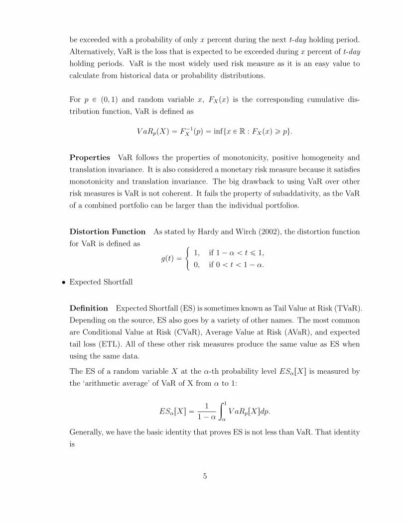
be exceeded with a probability of only x percent during the next t-day holding period.
Alternatively, VaR is the loss that is expected to be exceeded during x percent of t-day
holding periods. VaR is the most widely used risk measure as it is an easy value to
calculate from historical data or probability distributions.
For p P p0, 1q and random variable x, FXpxq is the corresponding cumulative dis-
tribution function, VaR is defined as
V aRppXq “ F´1X ppq “ inftx P R : FXpxq ě pu.
Properties VaR follows the properties of monotonicity, positive homogeneity and
translation invariance. It is also considered a monetary risk measure because it satisfies
monotonicity and translation invariance. The big drawback to using VaR over other
risk measures is VaR is not coherent. It fails the property of subaddativity, as the VaR
of a combined portfolio can be larger than the individual portfolios.
Distortion Function As stated by Hardy and Wirch (2002), the distortion function
for VaR is defined as
gptq “
#
1, if 1´ α ă t ď 1,
0, if 0 ă t ă 1´ α.
• Expected Shortfall
Definition Expected Shortfall (ES) is sometimes known as Tail Value at Risk (TVaR).
Depending on the source, ES also goes by a variety of other names. The most common
are Conditional Value at Risk (CVaR), Average Value at Risk (AVaR), and expected
tail loss (ETL). All of these other risk measures produce the same value as ES when
using the same data.
The ES of a random variable X at the α-th probability level ESαrXs is measured by
the ‘arithmetic average’ of VaR of X from α to 1:
ESαrXs “1
1´ α
ż 1
α
V aRprXsdp.
Generally, we have the basic identity that proves ES is not less than VaR. That identity
is
5
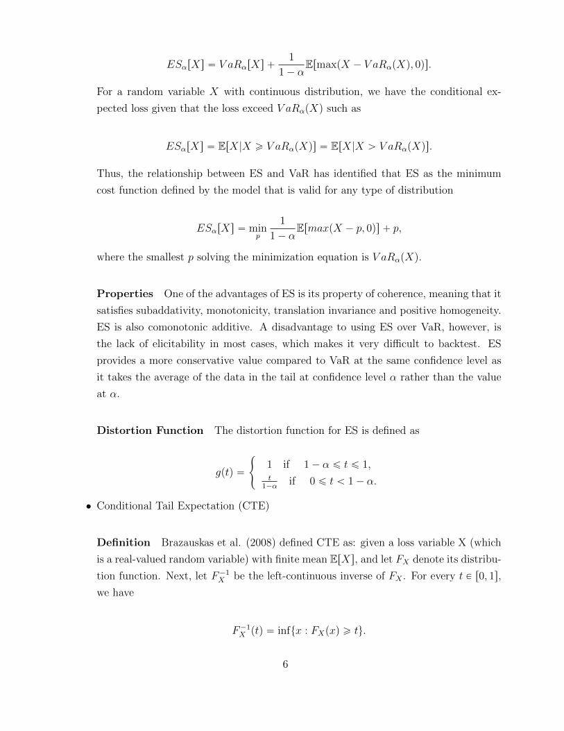
ESαrXs “ V aRαrXs `1
1´ αErmaxpX ´ V aRαpXq, 0qs.
For a random variable X with continuous distribution, we have the conditional ex-
pected loss given that the loss exceed V aRαpXq such as
ESαrXs “ ErX|X ě V aRαpXqs “ ErX|X ą V aRαpXqs.
Thus, the relationship between ES and VaR has identified that ES as the minimum
cost function defined by the model that is valid for any type of distribution
ESαrXs “ minp
1
1´ αErmaxpX ´ p, 0qs ` p,
where the smallest p solving the minimization equation is V aRαpXq.
Properties One of the advantages of ES is its property of coherence, meaning that it
satisfies subaddativity, monotonicity, translation invariance and positive homogeneity.
ES is also comonotonic additive. A disadvantage to using ES over VaR, however, is
the lack of elicitability in most cases, which makes it very difficult to backtest. ES
provides a more conservative value compared to VaR at the same confidence level as
it takes the average of the data in the tail at confidence level α rather than the value
at α.
Distortion Function The distortion function for ES is defined as
gptq “
#
1 if 1´ α ď t ď 1,t
1´αif 0 ď t ă 1´ α.
• Conditional Tail Expectation (CTE)
Definition Brazauskas et al. (2008) defined CTE as: given a loss variable X (which
is a real-valued random variable) with finite mean ErXs, and let FX denote its distribu-
tion function. Next, let F´1X be the left-continuous inverse of FX . For every t P r0, 1s,
we have
F´1X ptq “ inftx : FXpxq ě tu.
6

With these notations, CTE is defined by
CTEtpXq “ ErX|X ą F´1X ptqs.
If FX is continuous, then FXpF´1X ptqq “ t for every t P r0, 1s. In other words, at point
t, t ¨ 100% of losses are at or below t, while p1 ´ tq100% of losses are above t. In the
continuous case, CTE is defined as
CTEtpXq “1
1´ t
ż 1
t
F´1X puqdu.
Properties The main property that CTE has is that it is a coherent risk measure
only in the continuous case.
Relation to ES As noted by their definitions, ES and CTE are similar risk measures.
ES and CTE are equal to each other if the distribution is continuous and calculated
at the same value of α, otherwise they might be different. This result can be expected
as both ES and CTE calculate the expected loss in the right tail of the distribution.
In the continuous case, there is only one value for each distribution at α.
2.2.2 Spectral Risk Measures
Definition Spectral risk measures involve a weighted average of the quantiles of a loss as
stated by Adams et al. (2007). A spectral risk measure is defined as
MφpXq “ ´
ż 1
0
φppqF´1x ppqdp.
The function φ is right-continuous, non-negative and non-increasing. It is defined from
[0,1] andş1
0φppqdp “ 1. As mentioned in Acerbi (2002), an admissible risk spectrum φ P
L 1pr0, 1sq will be called the ‘risk aversion function’ of the risk measure MφpXq, where Mφ
will be called the ‘spectrum risk measure’.
Properties Spectral risk measures satisfy monotonicity, positive homogeneity and trans-
lation invariance, but also include other properties that make them robuster than other risk
measures. Those properties are law-invariance and comonotonicity as defined below:
Law-Invariance: For X and Y with cumulative distribution functions FX and FY , if FX “ FY ,
7
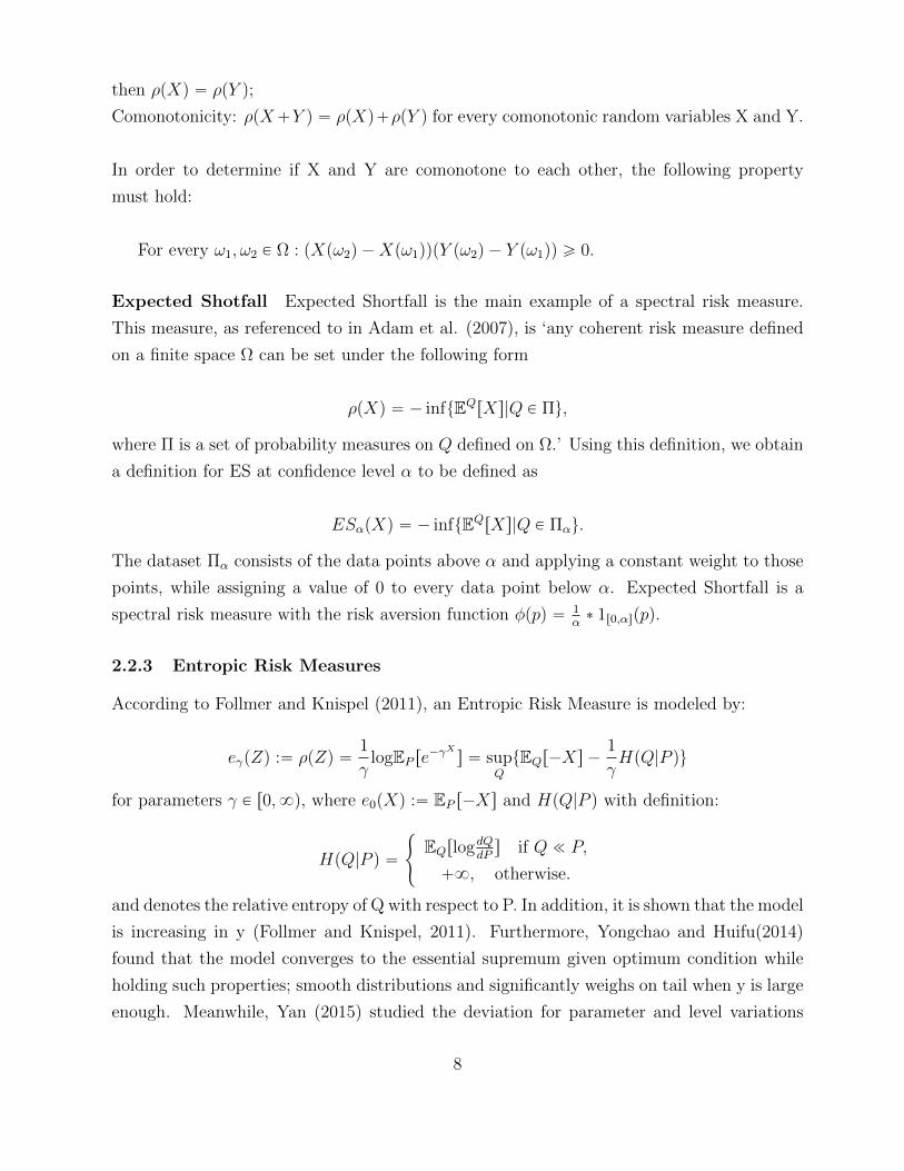
then ρpXq “ ρpY q;
Comonotonicity: ρpX`Y q “ ρpXq`ρpY q for every comonotonic random variables X and Y.
In order to determine if X and Y are comonotone to each other, the following property
must hold:
For every ω1, ω2 P Ω : pXpω2q ´Xpω1qqpY pω2q ´ Y pω1qq ě 0.
Expected Shotfall Expected Shortfall is the main example of a spectral risk measure.
This measure, as referenced to in Adam et al. (2007), is ‘any coherent risk measure defined
on a finite space Ω can be set under the following form
ρpXq “ ´ inftEQrXs|Q P Πu,
where Π is a set of probability measures on Q defined on Ω.’ Using this definition, we obtain
a definition for ES at confidence level α to be defined as
ESαpXq “ ´ inftEQrXs|Q P Παu.
The dataset Πα consists of the data points above α and applying a constant weight to those
points, while assigning a value of 0 to every data point below α. Expected Shortfall is a
spectral risk measure with the risk aversion function φppq “ 1α˚ 1r0,αsppq.
2.2.3 Entropic Risk Measures
According to Follmer and Knispel (2011), an Entropic Risk Measure is modeled by:
eγpZq :“ ρpZq “1
γlogEP re´γ
X
s “ supQtEQr´Xs ´
1
γHpQ|P qu
for parameters γ P r0,8q, where e0pXq :“ EP r´Xs and HpQ|P q with definition:
HpQ|P q “
#
EQrlogdQdPs if Q ! P,
`8, otherwise.
and denotes the relative entropy of Q with respect to P. In addition, it is shown that the model
is increasing in y (Follmer and Knispel, 2011). Furthermore, Yongchao and Huifu(2014)
found that the model converges to the essential supremum given optimum condition while
holding such properties; smooth distributions and significantly weighs on tail when y is large
enough. Meanwhile, Yan (2015) studied the deviation for parameter and level variations
8

related to its convex and coherent model; it is identified that ENT γp pXq is the convex
entropic risk measure with parameter γ as the risk aversion parameter. Let X be a random
variable on probability space pΩ, F, P q with ENT γp pXq is defined as
ENT γp pXq :“1
γlogEppe´γXq,
where Epp¨q means the mathematical expectation with respect to P and γ ą 0.
Properties of ENT pγ, pq As implied above, ENT γp pXq satisfies the convexity property
for risk measures, but it is not a coherent risk measure as it does not satisfy the property of
positive homogeneity.
CERM cppXq is the coherent entropic risk measure model with parameter c as the level.
For each c ą 0, CERM cppXq is defined as
ρcpXq :“ suptQPM1:HpQ|P qďcu
EQr´Xs, X P L8,
where M1 denotes the class of all probability measures on X with a functional ρ : X P Rwith properties monotonicity and translation invariance. Another, more concise definition
for CERM cppXq is
CERM cppXq “ inf
γą0tc
γ` ENT γp pXqu
Properties of CERM cppXq CERM c
ppXq satisfies the property of coherence and is also
law-invariant.
Entropic Value at Risk Ahmadi-Javid (2012) introduced Entropic Value-at-Risk that
shows the corresponding tightest possible upper bound derived from the Chernoff Inequality.
In this case, the Chernoff Inequality for any constant a and X P LM` is defined as
PrpX ě aq ď e´zaMXpzq, @z ą 0.
When solving the equation e´zaMXpzq “ a with respect to a for α P r0, 1s, the following
equation is obtained:
aXpα, zq :“ z´1lnpMXpzq
αq.
This is proven as one of the coherent risk measure defined by the model:
9

EV AR1´αpXq :“ infzą0taXpα, zqu “ inf
zą0tz´1lnp
MXpzq
αqu.
This definition had leading us to a preposition that this risk measure also depends on the
moment generating function. He also showed the dual representation through Donsker-
Varadhan Variational Formula which is
EV AR1´αpXq “ supQP=
EQpXq,
where = “ tQ ! P : DKLpQ||P q ď ´ln αu and DKLpQ||P q :“ş
dQdPplndQ
dPqdP is the relative
entropy of Q with respect to P. Furthermore, he demonstrated that EV aR is the upper
bound of for both V aR and CV aR at the same level of confidence which means that EV aR
is known to be as more risk averse compared to others. Through financial view, EV aR
requires a lot of resources allocation for least possible risk yet made it undesirable to be
used.
Properties Unlike other risk measures that involve VaR, EVaR is a coherent risk measure.
2.2.4 Generalized Quantiles
It is important to know the properties that the generalized quantiles of a random variable
X refers to the ‘minimizers of a piecewise-linear loss function’ (Bellini et al., 2014). The
metrics are defined as
qαpXq “ arg minxPR
tπαpX, xqu,
where παpX, xq “ αErpX ´ xq`s ` p1 ´ αqErpX ´ xq´s with x` “ maxtx, 0u and x´ “
maxt´x, 0u. Furthermore, we can identify generalized quantile as first-order condition as
any minimizer such that xα˚ P arg mintπαpX, xqu is proven to be a generalized quantile.
Here, παpX, xq satisfies the properties of finite, non-negative and convex in a closed interval.
According to Bellini et al. (2014), there are numerous generalized quantile risk measures in
the literature such as expectiles, power loss functions, Orlicz quantiles, generic loss functions
all holding similar properties: translation invariance, constancy, internality, monotonicity,
positive homogeneity and convexity. However, Orlicz quantiles lack the property of mono-
tonicity. In addition, only expectiles are a type of coherent generalized quantile due to strict
monotonicity. This type of expectiles can be written as
eαpXq ´ ErXs “2α ´ 1
1´ αErpX ´ eαpXqq
`s.
10
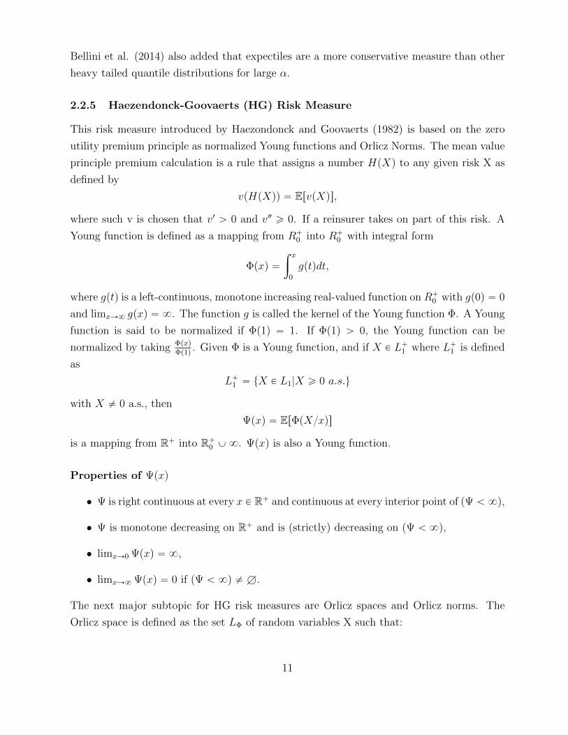
Bellini et al. (2014) also added that expectiles are a more conservative measure than other
heavy tailed quantile distributions for large α.
2.2.5 Haezendonck-Goovaerts (HG) Risk Measure
This risk measure introduced by Haezondonck and Goovaerts (1982) is based on the zero
utility premium principle as normalized Young functions and Orlicz Norms. The mean value
principle premium calculation is a rule that assigns a number HpXq to any given risk X as
defined by
vpHpXqq “ ErvpXqs,
where such v is chosen that v1 ą 0 and v2 ě 0. If a reinsurer takes on part of this risk. A
Young function is defined as a mapping from R`0 into R`0 with integral form
Φpxq “
ż x
0
gptqdt,
where gptq is a left-continuous, monotone increasing real-valued function on R`0 with gp0q “ 0
and limxÑ8 gpxq “ 8. The function g is called the kernel of the Young function Φ. A Young
function is said to be normalized if Φp1q “ 1. If Φp1q ą 0, the Young function can be
normalized by taking ΦpxqΦp1q
. Given Φ is a Young function, and if X P L`1 where L`1 is defined
as
L`1 “ tX P L1|X ě 0 a.s.u
with X ‰ 0 a.s., then
Ψpxq “ ErΦpXxqs
is a mapping from R` into R`0 Y8. Ψpxq is also a Young function.
Properties of Ψpxq
• Ψ is right continuous at every x P R` and continuous at every interior point of pΨ ă 8q,
• Ψ is monotone decreasing on R` and is (strictly) decreasing on pΨ ă 8q,
• limxÑ0 Ψpxq “ 8,
• limxÑ8 Ψpxq “ 0 if pΨ ă 8q ‰ H.
The next major subtopic for HG risk measures are Orlicz spaces and Orlicz norms. The
Orlicz space is defined as the set LΦ of random variables X such that:
11

ErΦp|X|aqs ď 1 for some a ą 0,
which is a subspace of L1. The Orlicz norm on the Orlicz space LΦ is defined to be:
||X||Φ “ infta ą 0|ErΦp|X|aqs ď 1u.
The Orlicz norm follows the properties of positive homogeneity and sub-additivity. The
norm is always greater than 0 and equals 0 if and only if X “ 0. Using the formulas of the
Young functions we can calculate the HG premium principle for bounded risks. If X P L`8
and X ‰ 0 a.s., then the equation
Ψpxq “ ErΦpXxqs “ 1
has exactly one solution denoted by HpXq with HpXq “ 0 if X “ 0 a.s. and HpXq is named
as the H-G risk measure for X.
Properties of H(X)
• HpXq “ HpY q if FX “ FY ,
• if X is a constant K a.s. then HpXq “ K,
• ErXs ď HpXq,
• HpX ` Y q ď HpXq `HpY q,
• HpaXq “ aHpXq if a P R`0 ,
• HpXq ď HpY q if X ă Y ,
• if X ď constant K a.s., then HpXq ď K,
• if Φ is strictly convex, then ErXs ă HrXs except when X “ constant a.s.
Other than being homogenous and translation invariant, it is found that HG risk measure,
with φ derived from a concave distortion function g is sub-additive (Goovaerts et al., 2012).
Also, the HG risk measure is an application of the mean value principle. Additionally,
according to Bellini and Gianin (2011), HG risk measures are not comonotonically additive
yet the simplest coherent risk measures. This type of risk measure is naturally defined on
Orlicz spaces. HG premium is identified to be finite, convex, law-invariant and coherent
(Bellini and Gianin, 2011).
12

2.3 Statistical Risk Measures
Expectation-first moment Expectation of a random variable is defined by ErXs, which
is the simplest risk measure to evaluate the average loss.
Variance and Standard Deviation-second moment Variance is usually adopted to
describe the deviation from mean, and is defined by
V arpXq “ ErpX ´ ErXsq2s
for a random variable X. Moreover, the most commonly used deviation risk measure is the
standard deviation σ, which is calculated as σpXq “a
V arpXq. Deviation measures are
used to determine how far from the mean of the data the data is distributed. Deviation is
critical in the world of finance as having the ability to predict what future gains or losses one
may have can lead to better management of wealth. In general, higher standard deviation
means more risk as the spread of potential returns is spread out more from the mean. By
Rockafellar et al. (2002), a deviation measure on L2 will mean any functional D : L2 Ñ r0,8s
satisfying the following five properties: shift invariant, normalization, positive homogeneous,
subadditivity and positivity. The additional properties are defined as below,
• Normalization: Dp0q “ 0.
• Positivity: DpXq ą 0 for nonconstant X and DpXq “ 0 for constant X.
• Shift-Invariance: DpX ` cq “ DpXqfor c P R.
Skewness-third moment The skewness of a distribution is a measure of the asymmetry
of a probability distribution about its mean. Skewness is the third standardized moment of
a distribution, and is calculated by
γ1 “ ErpX ´ µ
σ
3
qs “µ3
σ3,
where µ3 is the third centralized moment of a distribution. A skewness value of 0 means that
the distribution is perfectly symmetrical about its mean. A skewness value below 0 indicates
that the distribution has a “longer left tail”. In other words, more data lies farther out in
the left tail while a majority of the data is bunched up on the right side of the distribution.
For a skewness value above 0, the opposite is true. The right tail of the distribution has
more data farther away from the mean while a majority of the data is bunched up on the left
side of the distribution. When assessing risk measures, the skewness value can be used to
13

help determine how far away from the mean the confidence level (α) value will be. A higher
absolute value of skewness shows that there are outliers in the data set, which can affect the
difference in value between VaR and TVaR greatly.
Kurtosis-fourth moment The kurtosis of a distribution describes the shape of a curve
in terms of how the data is plotted throughout a probability distribution. Like skewness,
kurtosis is also a standardized moment with it being the fourth standardized moment and
is calculated by
γ2 “ ErpX ´ µ
σ
4
qs “µ4
σ4.
Kurtosis determines how ”narrow and tall” or ”wide and short” the distribution is. In other
words, kurtosis measures the tailed-ness of a distribution. Kurtosis is a positive value with
higher values representing greater tailed-ness. Kurtosis values for distributions are often
compared to the value for a standard normal distribution to better understand the shape of
the distribution. The kurtosis value for a standard normal distribution is 3. A value less
than this means the data is highly centered with few outliers, and therefore small tails. A
value greater than 3 means the distribution has lots of extreme outliers and data far from
the mean, resulting in heavy tails.
Semi-variance Semi-variance, like the name implies, does not compute the variance of
the whole data set that is being used. Instead, semi-variance only is the variance for a
portion of a data set. In finance and portfolio selection, the semi-variance of a data set is
typically calculated using only the data points below the mean or target return of that data
set. Semi-variance can be used by investors to determine how much downside risk they are
taking on. For a random variable X, the semi-variance is defined by
V ar`pXq “ ErpX ´ ρrXsq2`|X ą ρrXss,
where ρ is the risk measure to denote the target of the risk.
Tail-variance Like semi-variance, tail-variance (TV) does not calculate the variance of
the whole distribution, but only a part of it. In this case, tail-variance only calculates the
variance of data points located in the tail of the distribution, where the tail is defined above
a confidence level α. Furman and Landsman (2006) defined tail-variance to be
TVαpXq “ V arpX|X ą xαq “ EppX ´ ταpXqq2|X ą xαq,
14

where ταpXq “ TCEαpXq “ EpX|X ą xαq. TV is used to measure how much risk is located
within the tail itself, and to determine how spread out the data points are.
Region-variance Tail-variance as Furman and Landsman (2006) defined can be general-
ized. For a random variable X, the region-variance (RV) can be defined by
RV “ V arpX|Aq “ ErpX ´REApXqq2|X P As,
where REA is the region-expectation defined by REApXq “ ErXIAs and A is the special
region considered.
2.4 Dependence Risk Measures
2.4.1 CoVariance
Covariance is defined by
CovpX, Y q “ ErpX ´ ErXsqpY ´ ErY sqs
for two random variables X and Y to illustrate their linear dependence structure.
2.4.2 Dependence Risk Measure by comparasion with Comonotonicity and In-
dependence (Dhaene et al., 2014)
Let Xc “ pXc1, . . . , X
cdq be a random vector with the same marginal distributions as X but
with comonotonic components and Sc “řdi“1X
ci . In addition, XK “ pXK
1 , . . . , XKd q be a
random vector with the same marginal distributions as X but with comonotonic components
and SK “řdi“1X
Ki , Dhaene et al. (2014) defined
ρcpXq “V arpSq ´ V arpSKq
V arpScq ´ V arpSKq“
řdi“1
ř
jăiCovpXi, Xjqřdi“1
ř
jăiCovpXci , X
cj q
provided the convariances exist. This risk measure satisfies normalization, monotonicity,
permutation invariance and duality.
15

3 Robustness
3.1 Introduction
Generally speaking, robustness is used with risk measures to determine how well they stand
up to small or large changes in the underlying datasets. A robust model is one that unaf-
fected by outliers or small errors from the assumptions made in the model.
Developing a robust risk measure is of utmost importance to corporations, especially fi-
nancial institutions, as they use hundreds of different models and distributions. Applying
a risk measure that is not robust can lead to issues as small errors or deviations in the as-
sumptions or data could drastically affect the output data. In the aftermath of the financial
crisis, people start to realize that the robustness of the estimate is important. Consequently,
regulators and other stakeholders have started to require that the internal models used by
financial institutions are robust.
In the following discussion, we are going to exhibit different measurements of robustness
in risk measure process and their characteristics. Also, we will analysis traditional risk
measure method like VaR and TVaR in those robustness measurements.
3.2 Qualitative Robustness
Informally, qualitative robustness refers to a certain insensitivity of the sampling distribution
with respect to deviations from the theoretical distribution. We will focus on law invariant
risk estimators in this part. A risk estimator is said to be robust if a small variation in the
loss distribution results in a small change in the the risk estimation.
3.2.1 Definition
Definition 3.1. (Cont, 2010) A risk estimator ρ is qualititive robust at F if for any ε ą 0
there exist δ ą 0 and n0 ě 1 such that
G P C, dpF, Gq ď δ ñ dpρpF q, ρpGqq ď ε, @n ě n0,
where C is a fixed set of loss distributions and F P C.
The intuitive notion of robustness in this paper can now be made more precisely by adopting
this definition. With respect to the above definition, dpF, Gq ď δ indicates that the distortion
16

level of distribution is bounded in certain radius δ, meaning the variation is so small that
the value from risk function will only make a small change less than ε. However, Definition
3.1 is not widely used in either econometric or financial applications since it cannot give us
a quantitative result of robustness. Moreover, the following characteristics (a) and (b) will
also limit its application in practice:
(a) It may not be able to solve different behaviors in tail distribution.
In practice, two distributions can be rather close with respect to a distance d, but still
have completely different tail behavior. In this case, whether the risk functional is
senstive to tail behavior is determined by the metrics selected. Here we provide one
example for each case.
Example 1: Levy metric
Definition 3.2. (Kratschmer, 2012) Let Fµ and Fν be the distribution functions for
parameters µ and ν. Then, Levy metric between these two distributions can be defined
as follow:
dLevypFµ, Fνq “ inftε ą 0 : Fµpx´ εq ´ ε ď Fνpxq ď Fµpx` εq ` ε for all xu.
Intuitively, if between the graphs of Fµ and Fν one inscribes squares with sides par-
allel to the coordinate axes, then the side-length of the largest such square is equal to
dLevypFµ, Fνq.
To illustrate the point that Levy metric is insensitive in tail distribution, let M1 be
the class of all probability measures on R and recall that the Levy metric metrizes
the weak topology on M1 and that the compactly supported probability measures are
dense in M1 with respect to weak convergence. Hence, for every µ P M1 and every
ε ą 0 there exists a compactly supported ν PM1 such that dLevypFµ, Fνq ă ε. Clearly,
Fµ can have arbitrary tail behavior, whereas the tail behavior of Fν is trivial.
Example 2: Wasserstein and Lp metric To illustrate that Wasserstein metric
is sensitive to tail distribution, we can have a simple simulation example to compare
Wasserstein metric and Lp distance. The definition of Wasserstein distance is defined
by Definition 3.3 and Lp metric by Definition 3.4 as below.
Definition 3.3. (Kiesel, 2016) Let F,G be two distribution functions. The Wasser-
stein distance, WppF,Gq for two distributions is given by
WppF,Gq “
ż 1
0
|F´1puq ´G´1
puq|pdu, p ě 1.
17

Table 1: Wasserstein and Lp distance, λ=0.1
p ε Lp Distance Wasserstein Distance
p=1
0.05 0.500 0.500
0.075 0.800 0.800
0.1 1.000 1.000
p=2
0.05 0.106 0.455
0.075 0.169 1.164
0.1 0.213 1.820
p=3
0.05 0.069 0.632
0.075 0.109 2.585
0.1 0.137 5.053
p=4
0.05 0.057 1.164
0.075 0.091 7.625
0.1 0.114 18.634
Definition 3.4. (Kiesel, 2016) Lp-distance, ΘppF,Gq is defines as
ΘppF, Gq “ p
ż 8
´8
|F puq ´Gpuq|pduq1p, p ě 1.
We compare Lp distance with the Wasserstein metric for a standard normal distribution
Φ, by which we perturbate data such that there is a difference in the right tail. Thus,
let
Gpxq “ p1´ εqΦpxq ` εExppx, λq,
where Exppx, λq is an exponential distribution with parameter λ.
Example 3.1. Suppose λ=0.1, we get the values of Lp distance and Wasserstein dis-
tance in Table 1 by changing values of p from 1 to 4. As is illustrated by Figure 1 and
2, the Wasserstein distance increases in p while the Lp distance decreases. Thus, the
weighting of differences in the tail increase for the Wasserstein metric in p, while it
decreases for Lp.
In the recent years of financial crisis, it has become apparent that a misspecification
of the tail behavior of loss can largely influence the result of risk measure. As a result,
applying qualitative robustness measure without choosing specific risk functional or
metric could lead to a dramatic underestimation of the associated risk.
18

Figure 1: Lp distance as to p
Figure 2: Wasserstein distance as to p
19

(b) It is clustering all risk functional into two groups.
The qualitative robustness definition generates a sharp division of risk functionals into
the class of those that are called ‘robust’ and another class of those that are called ‘not
robust’. However, the distinction between ‘robust’ and ‘non-robust’ risk functionals is
artificial because there is actually a full continuum of possible degrees of robustness
beyond the classical concept. So labeling a risk measure as ‘robust’ or ‘non-robust’
may give a false impression.
In addition, we will introduce Theorem 3.1 which provides an equivalence between
the loss distribution set and qualitative robust for a risk measure.
Theorem 3.1. (Cont, 2010) Let ρ be a risk measure, C is a fixed set of loss dis-
tributions and F P C. If ρh is consistent with ρ at every G P C, the following are
equivalent:
(a) the restriction of ρ to C is weakly continuous at F ;
(b) ρh is qualitative-robust at F .
VaR For any function F P C where C is the set of all distributions continuous at α
if
q`F pαq “ q´F pαq, α P p0, 1q.
Then, historical V aRα is qualitative robust at F, and hence, V aRα is weakly continuous
at F by Cont (2010). By adopting Theorem 3.1, we know that V aRα is qualitative
robust.
TVaR The statistical functional of TV aR is
T pF q “ ´p1´ αq´1
ż 1
α
F´1pxqdx.
Historcial TVaR function is not weakly continuous at D “ tF P P ,ż `8
´8
|x|dF ă 8u
according to Cont (2010), and thus not qualitative robust by Theorem 3.1. However,
TVaR is robust by Wasserste distance, which has been proved by Kiesel (2016). In
summary, TVaR is generally not robust unless certain distribution distance metric is
applied. Note that fully proof that Corollary needs other definitions and Lemma from
additional references. For simplicity, we only include the conclusion that TVaR is not
weakly continuous on any distributions with finite first moment.
20
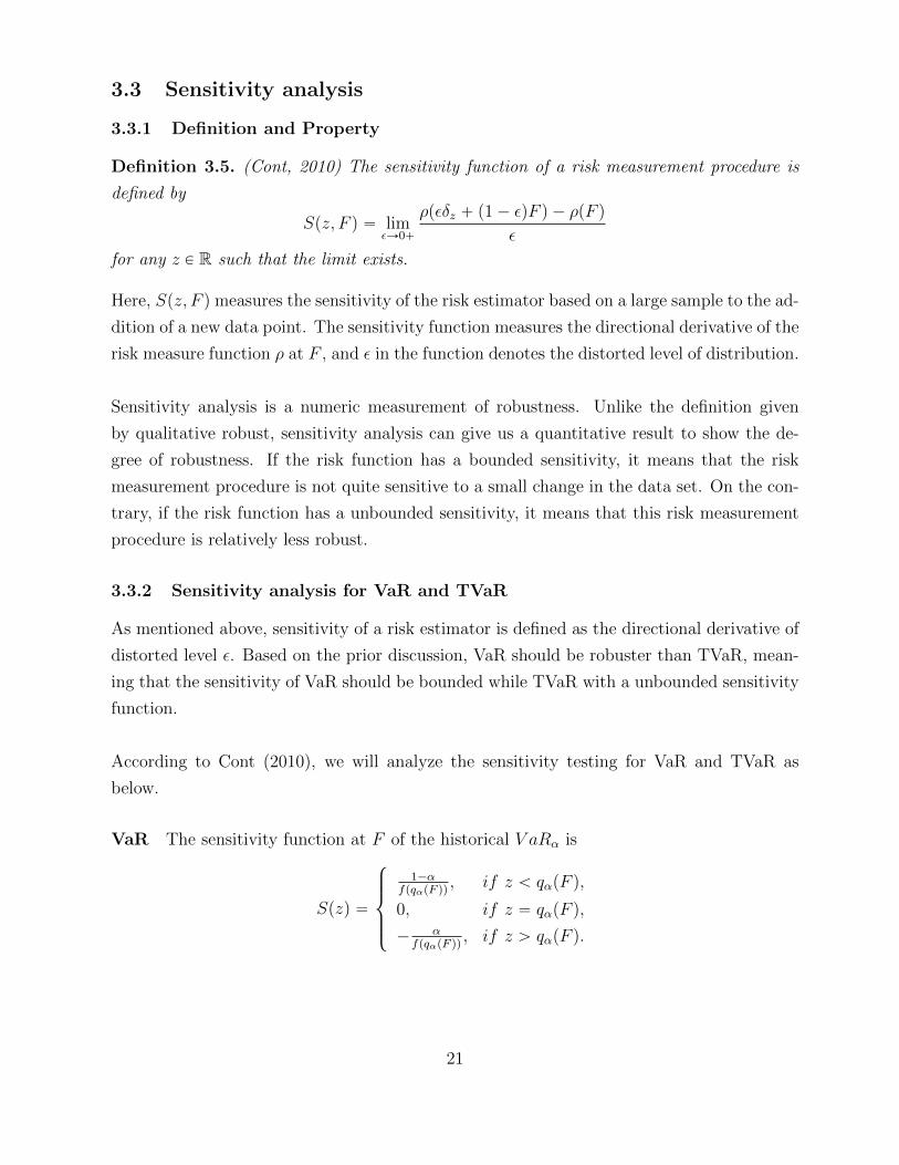
3.3 Sensitivity analysis
3.3.1 Definition and Property
Definition 3.5. (Cont, 2010) The sensitivity function of a risk measurement procedure is
defined by
Spz, F q “ limεÑ0`
ρpεδz ` p1´ εqF q ´ ρpF q
ε
for any z P R such that the limit exists.
Here, Spz, F qmeasures the sensitivity of the risk estimator based on a large sample to the ad-
dition of a new data point. The sensitivity function measures the directional derivative of the
risk measure function ρ at F , and ε in the function denotes the distorted level of distribution.
Sensitivity analysis is a numeric measurement of robustness. Unlike the definition given
by qualitative robust, sensitivity analysis can give us a quantitative result to show the de-
gree of robustness. If the risk function has a bounded sensitivity, it means that the risk
measurement procedure is not quite sensitive to a small change in the data set. On the con-
trary, if the risk function has a unbounded sensitivity, it means that this risk measurement
procedure is relatively less robust.
3.3.2 Sensitivity analysis for VaR and TVaR
As mentioned above, sensitivity of a risk estimator is defined as the directional derivative of
distorted level ε. Based on the prior discussion, VaR should be robuster than TVaR, mean-
ing that the sensitivity of VaR should be bounded while TVaR with a unbounded sensitivity
function.
According to Cont (2010), we will analyze the sensitivity testing for VaR and TVaR as
below.
VaR The sensitivity function at F of the historical V aRα is
Spzq “
$
’
’
&
’
’
%
1´αfpqαpF qq
, if z ă qαpF q,
0, if z “ qαpF q,
´ αfpqαpF qq
, if z ą qαpF q.
21

Figure 3: VaR and TVaR with 100 replications per day
TVaR The sensitivity function at F P D´ for historical TV aRα is
Spzq “
$
’
&
’
%
´ zα` 1´α
αqαpF q ´ TVaRαpF q, if z ď qαpF q,
´qαpF q ´ TVaRαpF q, if z ě qαpF q.
From these risk functions, we can see that historical VaR has a bounded sensitivity whilst
TVaR has a linear sensitivity, indicating that VaR is robuster than TVaR.
3.3.3 Numerical Example
As shown above, VaR is a robuster risk functional than TVaR. To start the simulation, we
propose an empirical investigation to show the above conclusions. More precisely, we use
historical simulation to generate random samples from a dataset of S&P 500.
Figure 3 plots the values of the historical VaR and TVaR for a total of 100 replications
per day. We can see how the overall path of historical VaR is more regular than that of
TVaR, which is more volatile. Thus, we can conclude that the historical estimator of TVaR
is less robust, confirming the insights we get above.
Furthermore, we can see how VaR and TVaR change with some small pertubation to the loss
22

Figure 4: VaR and TVaR by adding pertubation
distribution. As Figure 4 shows, if we add the pertubation in the loss distribution, TVaR
changes more than VaR, which illustrates that TVaR is more sensitive to pertubation and
thus less robust than VaR.
3.4 Score Function-Elicitability
3.4.1 Definition and Properties
Usually, risk measures are calculated based on historical or empirical data. In order to ar-
rive at the best possible point estimate, we have to make appropriate decisions concerning
models, methods and parameters. Thus, it is crucial to be able to validate and compare
competing estimation procedures.
Let P be a class of probability measures on R with the Borel sigma algebra. We consider a
functional
ν : P Ñ 2R, P ÞÑ νpP q Ă R,
where 2R denotes the power set of R.
Formally, a statistical functional is a potentially set-valued mapping from a class of probabil-
ity distributions. We want to make sure that we can find an optimal point of this function.
Here is the definition of the consistency for a scoring function.
23
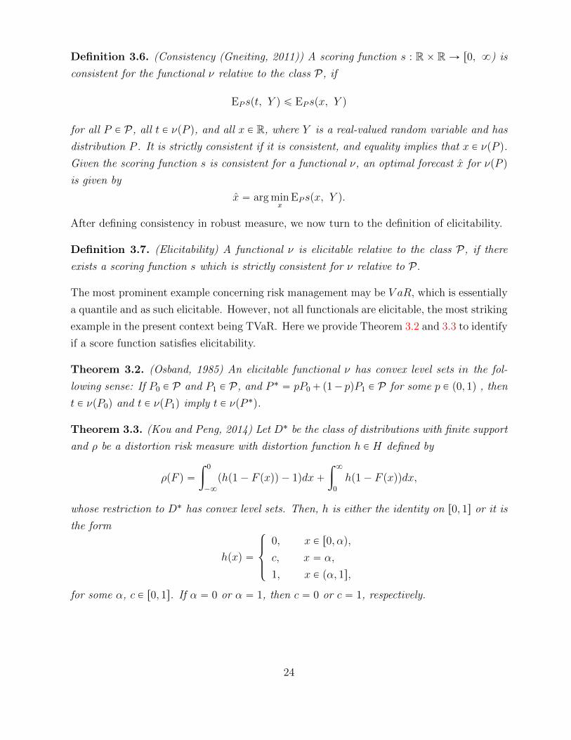
Definition 3.6. (Consistency (Gneiting, 2011)) A scoring function s : R ˆ R Ñ r0, 8) is
consistent for the functional ν relative to the class P, if
EP spt, Y q ď EP spx, Y q
for all P P P, all t P νpP q, and all x P R, where Y is a real-valued random variable and has
distribution P . It is strictly consistent if it is consistent, and equality implies that x P νpP q.
Given the scoring function s is consistent for a functional ν, an optimal forecast x for νpP q
is given by
x “ arg minx
EP spx, Y q.
After defining consistency in robust measure, we now turn to the definition of elicitability.
Definition 3.7. (Elicitability) A functional ν is elicitable relative to the class P, if there
exists a scoring function s which is strictly consistent for ν relative to P .
The most prominent example concerning risk management may be V aR, which is essentially
a quantile and as such elicitable. However, not all functionals are elicitable, the most striking
example in the present context being TVaR. Here we provide Theorem 3.2 and 3.3 to identify
if a score function satisfies elicitability.
Theorem 3.2. (Osband, 1985) An elicitable functional ν has convex level sets in the fol-
lowing sense: If P0 P P and P1 P P, and P ˚ “ pP0`p1´ pqP1 P P for some p P p0, 1q , then
t P νpP0q and t P νpP1q imply t P νpP ˚q.
Theorem 3.3. (Kou and Peng, 2014) Let D˚ be the class of distributions with finite support
and ρ be a distortion risk measure with distortion function h P H defined by
ρpF q “
ż 0
´8
php1´ F pxqq ´ 1qdx`
ż 8
0
hp1´ F pxqqdx,
whose restriction to D˚ has convex level sets. Then, h is either the identity on r0, 1s or it is
the form
hpxq “
$
’
&
’
%
0, x P r0, αq,
c, x “ α,
1, x P pα, 1s,
for some α, c P r0, 1s. If α “ 0 or α “ 1, then c “ 0 or c “ 1, respectively.
24

Table 2: Score of each estimator
Spx, yq “ px´ yq2 Spx, yq “ |x´ y| Spx, yq “ |px´ yqx|
True Estimation Score 4082.363 461.336 128.362
Mean Estimation Score 4142.571 468.947 94.387
3.4.2 Competing estimate procedures
By referring to the score ranking of scoring function, we can compare different risk estimators.
Suppose that in n estimate senarios we have point estimations xpkq1 , . . . , x
pkqn , k “ 1, . . . ,
K, and realizing observations y1, . . . , yn. The index k numbers the K competing forecast
procedures. We can rank the procedures by their average scores
spkq “1
n
nÿ
i“1
spxpkqi , yiq.
The consistency of the scoring rule for the functional ν ensures that accurate forecasts
of νpP q are rewarded. On the contrary, evaluating point forecasts with respect to some
poorly selected scoring function, which is not consistent for ν, may lead to grossly misguided
conclusions about the quality of the estimate. We will provide a small simulation study by
Example 3.2 to illustrate it.
Example 3.2. We generate a series where Yt “ Z2t and Zt is a Garch(1,1) series with
α “ 0.2, β “ 0.8 and ω “ 0.05. Here we want to estimate the value of Yt series.
Based on the generating process, the true predict level is EpYtq “ σ2t . In this simulation
study, we will compare the ‘true estimation’ and ‘mean estimation’ with score functions
of squared error Spx, yq “ px ´ yq2, absolute error Spx, yq “ |x ´ y|, and relative error
Spx, yq “ |px´ yqx| as in Figure 5.
Based on Figure 5, we can find that the true estimator fits better than the mean estimator.
However, if we choose the inappropriate score function, we may misjudge the fitted level of
each model and make a wrong decision.
The squared error score function and absolute error score function illustrates our intuition
that true estimator is a better estimator to predict the value of series. However, if we choose
Spx, yq “ |px ´ yqx| as our score function to select model, we may make a wrong decision
25

Figure 5: True Estimation and Mean Estimation
to select mean estimator as our measure function, which may lead to grossly misguided
conclusions.
3.5 Summary
To end this section, we provide Table 3 to summarize the properties of VaR and TVaR.
26
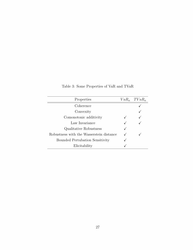
Table 3: Some Properties of VaR and TVaR
Properties V aRα TV aRα
Coherence X
Convexity X
Comonotonic additivity X X
Law Invariance X X
Qualitative Robustness X
Robustness with the Wasserstein distance X X
Bounded Pertubation Sensitivity X
Elicitability X
27

4 Robustness in Other Fields
4.1 Cyber Robustness
Cyber Robustness metrics quantify the possibility of success and time taken for an ICT sys-
tem resisting to attackers who arrange the sequence of attacks for their own privileges and
goals. The fundamental evaluation has adopted the Haruspex suite result; it is forecasting a
system through simulation of the interaction between attackers and the system which resulted
to robuster design and metrics computation. The model builds the statistical samples to ac-
cess the ICT risk by using the Monte Carlo method in the computation of probability given
their measurable parameters in the model, such as the vulnerabilities in each system module,
the attacks, and their success probability. Besides, the attacker also has been modeled as at
and included two important properties: the selection strategy of at and the look ahead, sg,
a non-negative integer presents the selection way of attacks by the attacker in its escalations.
Baiardi et al. (2016) suggested three types of metrics for this evaluation. First is by using
the security stress that calculates the probability of an attacker to reach his goal given a
time interval and number of attacks in an escalation. The probability distribution of stress
is defined by
StrSat,sgptq “ PrSuccSat,sgptq,
where PrSuccSat,sgptq is the sum for all the possible escalations of the probability each esca-
lation is successful at t. It is also identified to increases with t as larger value of t allows a
larger number of attack failures so the inverse of stress. Note that
SurSat,sgptq “ 1´ StrSat,sgptq
presents the probability that S survives to the attacks of at to reach a goal in sg. We can
also compute the stress of a set of shared mission attacker by using the model:
StrSat,sgptq “ maxtat P sa, StrSat,sgptqu,
which is the largest stress of its attackers.
Here, we have two kinds of distributions: the AvLoss measures the expected loss at the
certain time given discrete attackers corresponding rights using the first-order derivative of
stress as the probability. The average loss of for an agent with a goal is defined by the model
AvLossSsag,sgptq “
ż
t1Pt0,...,tu
StrSag,sgpt1qImpSag,g,ipt´ t
1qdt1,
28

while in general scenarios, the sum of the average losses due to each agent is
AvLossSsag,sgptq “ÿ
agiPsag
AvLossSagi,sgptq
where sag “ ta1, . . . , afu and each agent in sag has the goals in sg “ tg1, . . . , gnu.
The next one is CyV ar that assesses loss while applying the VaR model. As VaR widely
used for security investment, this metric evaluation chooses to focus on the same perspective;
it estimates the chances of losing money given the time, the confidence level, and the loss
amount. CyV ar consists of two models: for one agent with alternative goals, approximation
of largest probability loss such in the given model
CyV arSag,sgpν, tq “ maxtCyV arSag,gipν, tq, gi P sgu
and the model for numbers of agents included. Conclusively, CyV ar gives more accurate
evaluation compared than AvLoss.
4.2 Flood and Drought Risk Management
Climate change has increased the uncertainty of the likeliness of floods and droughts occur-
ring. Robustness helps to give more accurate flood risk analysis through assessing a large
range of possible floods in the analysis. Robustness in the drought risk analysis adds to a
wider definition of drought magnitude, giving us more supply reliability. It also allows us to
take into account worst-case climate change scenarios.
In conjunction to that, a system robustness analysis has been developed, by exploring the
characteristics of the event and measuring the severity and impact, to access the ability of
the system. It is important to characterize the system with resilience, the system’s ability
to recover from response to a disturbance, and resistance, the endurance ability without
responding, which both give the analysis on sensitivity of the system in detail. Researchers
have drawn the relationship between the event severity and corresponding response. In
general, the robustness model includes few important criteria in the analysis such as the
resistance threshold, the proportionality of the relationship, and the manageability of the
system.
This developed robustness model has been successfully applied in the flood risk system.
29
In the system analysis, while the protection standard is chosen as the resistance threshold, it
is found that the sudden change in river flow does not significantly contribute to the flood’s
impacts. Thus, this result has enable us to manage the impact whilst below the critical level
even for wider range of magnitudes.
Mens and Kirin (2015) demonstrated that the robustness criteria have additional value
compared to the more traditional decision making criteria, based on single-value risk, by
performing a case study on the IJssel River valley in the Netherlands. They access the flood
risk by calculating the water level probability distribution per breach location. The value is
then integrated into a fragility curve giving us the flood probability distribution of
Pk “
ż
fkphq ¨ PCkphq ¨ dh
which Pk is the flood probability of location k, fkphq is the water level probability density
function and PCkphq is the conditional probability of embankment breaching:
PCkphq “ Φpµ “ m;σ “ 0.2q.
Using the maximum flood depth maps as input for the damage model, the flood risk calcula-
tion of the IJssel valley combines flood probabilities, which is defined by a normal distribution
where PrpZ ă 0q means failure, and consequences of at each of location; the risk is known
by determining the area under the normal curve:
Flood Risk “ ErDs “ż
P pDq ¨D ¨ dD “
ż
F pDq ¨ dD,
where D is flood damage [EUR], F pDq is the probability density of the damage, P pDq is
the probability of one damage scenario and EpDq is the expected value of the damage. In
addition, the robustness analysis was completed by applying the Monte Carlo approach; it
resulted in proving that the resistance threshold is similar in all configurations, because it
does not significantly depend on assumptions about discharge variability and climate change.
Meanwhile, Mens et al. (2015) demonstrated the application of the robustness system in the
drought risk analysis on a case inspired by the Oologah reservoir in Oklahoma, United States.
In addition, they used different criteria in the analysis like Demand reduction, Hedging, and
Reservoir expansion. First, the drought volume is determined by the equation:
V olume “toffÿ
ton
pRt ´Qtq “ Ktoff.
30
Then, the impact of the event was determined in terms of change in welfare through the
willingness to pay; it was estimated by a total loss function in US Dollar that includes the
amount of available water, the baseline water use, water rate and price elasticity. Finally, the
robustness criteria was scored using the response curve. The demand reduction is preferable
over the supply increase on the supply reliability in the side of robustness. Additionally,
focusing on demand reduction allows us to deal with similar extreme conditions. Neverthe-
less, it is recommended to put the framework into testing different systems or types of floods
(Mens et al., 2015).
4.3 The Robustness of Power Grids
The significant dependency on electric power grids for electric supply in a country leads
to higher control of risk or failure limitation. According to the North American Electrical
Reliability Council (NERC), data shows that large blackouts happen more frequently than
expected due to line overloads or failure of any single transmission line. It is important to
analyze and minimize possible risk, and this could be done by a robustness metric of a power
transmission grid with respect to cascading failures (Koc et al., 2013).
A new notion of network robustness, there is only one metric to evaluate it that was in-
duced by random failures. Koc et al. (2013) confirmed that there are two important factors
in the robustness evaluation. The structure and the operative structure of a network. In
addition, the metric also depends on two main concepts: the electrical nodal robustness, and
the electrical node significance which uses an entropy-based approach and a nodal centrality
measure.
Koc et al. (2013) developed a model for each factor of the cascading effects. The line
overloads in power networks is modeled using the complex networks approach. The system
includes the power grid as a graph, the line flows across the grid analysis, and estimation of
the cascading damages which is defined with the linear equation
Pi “d
ÿ
j“1
fij “d
ÿ
j“1
bijθij
where Pi is the real power flow at node i, and d is the degree of node i. In specific, the
capacity of a line was introduced as the maximum transportable power flow by the line, Ci
which is proportional to its initial load, Lip0q, given the tolerance parameter of line i, αi,
i.e. Ci “ αiLip0q.
31

Meanwhile, Koc et al. (2013) has quantified the cascading failures by the metrics:
• Demand Survivability pDSq: The fraction of the satisfied power demand after a cas-
cading failure occurs in a network.
• Link Survivability pLSq: The fraction of lines that are still in operation after a cascad-
ing failure with definition
LS “L’
L
where L is the total number of links and L’ the number of links operational after a
cascading faliure.
• Capacity Survivability pCSq: The fraction of capacity of the operational lines after a
cascading failure with definition
CS “
řL’i“1Ci
řLj“1Cj
with C being the sum of the capacity of the links in the network and C’ the sum of
the capacity after a cascading failure.
However, operators need considerable computational power and time for large networks. The
paper introduced a robustness metric, RCF , to encounter the issue. This metric relies on
two main concepts: electrical nodal robustness and electrical node significance. First, the
electrical nodal robustness is the aggregate value that represents the ability to withstand
cascades of link overload failures as well as takes flow dynamics and topology effects on
network robustness into account with equation
Rn,i “ ´
Lÿ
i“1
αipi log pi,
where pi stands for values in the distribution under consideration. On the other side, elec-
trical node significance suggests the impact of a particular node as
δi “Pi
řNj“1 Pj
,
with Pi standing for total power distributed by node i, and N refers to the number of nodes
in the network. Finally, the computation of network robustness metric,
32

RCF “
Nÿ
i“1
Rn,iδi
was done by adding all individual contributions of each node in the network with respect to
cascading failures.
This shows how the computation does not include expensive tasks such as simulation of
cascading failures. The effectiveness of this robustness metric has been verified via ex-
perimental developed models and shown applicable on different cases including IEEE test
systems and UCTE networks. It is shown that the computation is parallel and how the
computation does not include expensive tasks such simulation of cascading failures. The
properties of RCF have allowed us to use it as a real-time measure while monitoring and
optimizing it dynamically.
4.4 Robustness Evaluation for Bio-manufacturing
Both drug development and manufacturing are dependent upon economic and regulatory
factors that can impact industry decision-making towards cost-effective and value-potential
alternatives for areas such as: bioprocess and facility design, capacity sourcing and portfolio
selection. Farid (2013) summarized systematic approaches and evaluations established at
University College London (UCL) in addressing this issue; including some techniques such
as: process economics, simulation, risk analysis, optimization, operations research and mul-
tivariate analysis. This evaluation develops a model to estimate cost of goods and other cost
metrics. The model also consolidates bioprocess economics, manufacturing logistics through
discrete-event simulations, and uncertainties through Monte Carlo simulation to assess the
robustness and assist in the decision-making process.
One of the applications of this model is a case study for a company which was required
to make a decision on a pipeline of monoclonal antibodies. The decision was either to invest
in the disposable facility, the traditional stainless-steel based one or go for a hybrid option
at the 200-L scale (Farid, 2013). It used the technique of probabilistic additive weighting
to consolidate the trade-offs and uncertainties in the input. Then, it would standardize the
financial and operational score into a common dimensionless scale that also indicates the
intrinsic risk.
The results show that the preference is for the hybrid option, followed by the disposable
and the stainless steel option for earlier stage material. While for later stage materials, the
33
relative rankings may give a different result. This is due to the former’s operational score
relying on other scores, which are very important to that stage, such as the construction
time, project throughput, and operational flexibility. In the conclusion, Farid (2013) sug-
gested that the given support tool has crystallized the trade-offs and uncertainties involved,
as well as coming up with clear financial, operational and risk metric evaluations. This has
allowed the tool being applied across different company departments during both building
and analysis.
4.5 Robust Optimization Formulations in Water Resource Sys-
tems Planning
Robust optimization (RO) formulations in the water resources planning is important stan-
dardize the uncertainty analysis as well as allowing for better evaluation and regulation of
various risks of poor system performance. These risks are solution robustness, reliability, vul-
nerability and sustainability. Previously, RO has been modeled by a single metric showing
inadequate importance compared to RO evaluation through post-processing given a wider
selection of performance metrics. The failure of the former model is the lacking of the most
basic shortcoming, which is the operational trade-off. This is proven via analysis of the
trade offs between solution robustness and its feasibility over all possible scenarios (Ray et
al., 2014).
Ray et al. (2014) has investigated the robustness of different models that have been de-
veloped over time. One of the earliest formulations of this problem was completed by Lund
and Israel in 1995. They computed the minimization of the expected total of direct and
indirect costs. In this first model, the potential water availability and usage was used as the
random input parameter with related probabilities. The model is defined in the following
two-stage stochastic nonlinear program:
minZ1 “ ccQ`ÿ
sPS
ÿ
rPR
prpsrc0Uqrs ` ctUtrs ` ηpUsrsqγs,
where Z1 is the objective function value, total cost (direct and indirect). cc is the unit capital
cost of desalination plant. Q is the capacity of desalination plant. pr is the probability of
water requirement event r. ps is the probability of supply event s. co is the amortized unit
operation and maintenance cost of desalination plant. Uqrs is the capacity of desalination
plant actually used. ct is the unit cost of water transfer. Utrs is the quantity of transfer
water purchased. Usrs is the quantity of water shortage. ηpUsrsqγ is the nonlinear cost of
34

water shortage.
Although the previous model gives the least-cost solution to the problem, it still requires
a multi-objective approach when it is high dimensional. The next model shows the multi-
objective two-stage robust optimization model (MO-RO) by Watkins and McKinney. It
defined by a model of standard deviation of possible water-related cost in the future which
has been identified as not monotonically increasing. This model has been developed to
improve the rationality of second-stage decision process making. It also offers to simultane-
ously control the sensitivity of solutions through the extension of stochastic programming
to a multi-objective optimization framework which manages to reflect risk-averse behavior
in the objective function. Therefore, the relationship between solution robustness and its
feasibility is fairly important for optimization.
Nevertheless, the second model is more vulnerable to shortage range in a specified range.
There is a newer model that consists of three alternative MO-RO formulation, that funda-
mentally penalizes the square of positive deviations from a fixed target cost. This model
gives a better result in terms of smaller standard deviation and direct cost compared to
Model 1. Besides, it can reduce the dependability on water usage during drier years by using
more excess capacity and accepting a fair amount of the expected cost.
35

5 Conclusion
In this paper, we studied the various risk measures in the literature and the robustness
metrics for VaR and TVaR. It is worth to investigate the properties of robustness metrics
for different risk measures and apply the methods in other fields to the framwork.
36
References
[1] Acerbi, C. (2002) Spectral measures of risk: A coherent representation of subjective
risk aversion. Journal of Banking & Finance. 26, 1505-1518.
[2] Adam, A., Houkari, M., and Laurent, J.P. (2008) Spectral risk measures and portfolio
selection[J]. Journal of Banking & Finance. 32(9), 1870-1882.
[3] Ahmadi-Javid, A. (2012)Entropic Value-at-Risk: a new coherent risk measure. Journal
of Optimization Theory and Applications. 155, 1105-1123.
[4] Artzner, P., Delbaen, F., Eber, J.M., and Heath, D. (1999) Coherent measures of risk.
Mathematical Finance. 9, 203-228.
[5] Baiardi, F., Tonelli, F., Bertolini, A., and Montecucco, M. (2016) Metrics for cyber
robustness.
https://www.sto.nato.int/publications/STO%20Meeting%20Proceedings/STO-MP-
IST-148/MP-IST-148-08.pdf
[6] Bellini, F., and Gianin, E.R. (2011) Haezondonck-Goovaerts risk measures and Orlicz
quantiles. Insurance: Mathematics and Economics. 51, 107-114.
[7] Bellini, F., Klar, B., Muller, A., and Gianin, E.R. (2014) Generalized quantiles as risk
measures. Insurance: Mathematics and Economics. 54, 41-48.
[8] Brazauskas, V., Jones, B.L., Puri, M. L., and Zitikis, R. (2008) Estimating conditonal
tail expectation with actuarial applications in view. Journal of Statistical Planning and
Inference. 138, 3590-3604.
[9] Cont, R., Deguest, R., and Scandolo, G. (2010) Robustness and sensitivity analysis of
risk measurement procedures. Quantitative finance. 10(6), 593-606.
[10] Dhaene, J., Linders, D., Schoutens, W., and Vyncke, D., (2014) A multivariate depen-
dence measure for aggregating risks. J. Comput. Appl. Math. 263, 78-87.
[11] Emmer, S., Kratz, M., and Tasche, D. (2013) What is the best risk measure in practice?
a comparison of standard measures. ESSEC working paper.
[12] Farid, S.S. (2013) Cost-effectiveness and robustness evaluation for bio-manufacturing.
http://www.bioprocessintl.com/upstream-processing/upstream-contract-services/cost-
effectiveness-and-robustness-evaluation-for-biomanufacturing-348549
37

[13] Follmer, H., and Knispel, T. (2011) Entropic risk measures: coherence vs. convexty,
model ambiguity, and robust large deviations. Stochastics and Dynamics. 11, 333-351.
[14] Furman, E., and Landsman, Z. (2006) Tail variance premium with applications for
elliptical portfolio of risks. ASTIN Bulletin: The Journal of IAA. 36, 433-462.
[15] Gneiting, T. (2011) Making and evaluating point forecasts. Journal of the American
Statistical Association. 106(494), 746-762.
[16] Goovaerts, M., and Haezondonck, J. (1982) A new premium calculation principle based
on Orlicz norms. Insurance: Mathematics and Economics. 1, 41-53.
[17] Goovaerts, M., Linders, D., Weert, K.V., and Tank, F. (2012) On the interplay between
distortion, mean value and Haezondonck-Goovaerts risk measures. Insurance: Mathe-
matics and Economics. 51, 10-18.
[18] Hettmansperger, T. P., and McKean, J. W. (1998) Robust nonparametric statistical
methods, Kendall’s Library of Statistics, 5, New York: John Wiley, & Sons, Inc., ISBN
0-340-54937-8, MR 1604954. 2nd ed., CRC Press, 2011.
[19] Huber, P.J. (1981) Robust Statistics. Chichester: Wiley.
[20] Kiesel, R., Rhlicke, R., and Stahl, G. (2016) The Wasserstein metric and robustness in
risk management. Risks. 4(3), 32.
[21] Koc, Y., Warnier, M., Kooij, R.E., and Brazier, F.M. (2013). An entropy-based metric
to quantify the robustness of power grids against cascading failures. Safety Science,
(59)126-134.
[22] Kou, S.(2013) Quantitative finance after the recent financial crisis.
http://ww1.math.nus.edu.sg/rsch-staffprofile/FoS Newsletter Dec2013-StevenKou.pdf
[23] Kou, S., Peng, X.H., and Heyde, C.C. (2010) Robust external risk measures. Wiley
Encyclopedia of Operations Research and Management Science.
[24] Kratschmer, V., Schied, A., and Zahle, H. (2014) Comparative and qualitative robust-
ness for law-invariant risk measures. Financ. Stoch. 18, 271-295.
[25] Linsmeier, T. J., and Pearson, N.D. (2000) Value at Risk. Financial Analysts Journal
56, 47-67.
38

[26] Liu, Y., and Xu, H. (2014) Entropic approximation for mathematical programs with
robust equilibrium constraints, SIAM J. Optim. 24, 933-958.
[27] Mens, M. J., Gilroy, K., and Williams, D. (2015) Developing system robustness analy-
sis for drought risk management: an application on a water supply reservoir. Natural
Hazards and Earth System Science. 15(8), 1933-1940.
[28] Mens, M. J., and Klijn, F. (2015) The added value of system robustness analysis for
flood risk management illustrated by a case on the IJssel River. Natural Hazards and
Earth System Science.15(2), 213-223.
[29] Ray, P.A., Watkins, D.W., Vogel, R.M., and Kirshen, P.H. (2014). Performance-based
evaluation of an improved robust optimization formulation. Journal of Water Resources
Planning and Management. 140(6), 04014006.
[30] Rockafellar, R.T., Uryasev, S.P., and Zabarankin, M. (2002) Deviation measures in risk
analysis and optimization. University of Florida, Department of Industrial and Systems
Engineering Working Paper No. 2002-7.
[31] Wang, R., and Ziegel, J. (2015) Elicitable distortion risk measures: a concise proof.
Statistics and Probability Letters. 100, 172-175.
[32] Wirch, J. L., and Hardy, M. R. (2002) Distortion risk measures: coherence and stochastic
dominance. International Congress of Insurance: Mathematics and Economics.
[33] Yaari, M.E. (1987) The dual theory of choice under risk. Econometrica. 55, 95-115.
[34] Yan., J. (2015) Deviations of convex and coherent entropic risk measures. Statistics and
Probability Letters. 100, 56-66.
[35] Ziegel, J.F. (2016) Coherence and elicitability. Mathematical Finance. 26, 901-918.
39


