

110/11/2016
36-463/663: Hierarchical
Linear Models
Lmer model selection and residuals
Brian Junker
132E Baker Hall
210/11/2016
Outline
� The London Schools Data (again!)
� A nice random-intercepts, random-slopes model
� Residuals in MLM’s
� Marginal residuals
� Conditional residuals
� Random effects residuals
� Variable selection
� Overall fit statistics
� Simulation-based methods (save for later!)
� AIC, BIC, DIC and all that
� An improved model for the London Schools data

The London Schools Data
� Student (1..1978)
� Gender (0=Female, 1=Male), per student
� VR = verbal reasoning level (High/Med/Low)
� LRT = London Reading test (at beginning of year)
� Y = end-of-year test
� School (1..38)
� School.gender (All.Boy, All.Girl, Mixed)
� School.denom (Other,CofE,RomCath,State)
310/11/2016
London Schools Data
� The dotted line is the
pooled regression
(ignoring schools)
� The solid lines are
unpooled regressions
(separate for each
school)
� The solid lines look like
a random sample of
lines, with “mean” the
solid line!
410/11/2016
Unpooled
Pooled
Note – these plots were made with an earlier version of ggplot2.
An alternative approach with the help of gridExtra is shown in the R handout.

The London Schools Data
� This suggests a model like
or, as a variance components model
� As an R model this would be
Y ~ 1 + LRT + (1 + LRT|school)
510/11/2016
The London Schools Data
> display(lmer.1
+ <- lmer(Y ~ 1 + LRT +
+ (1 + LRT|school),data=school.frame))
coef.est coef.se
(Intercept) 0.01 0.05
LRT 0.05 0.00
Error terms:
Groups Name Std.Dev. Corr
school (Int) 0.23
LRT 0.01 0.56
Residual 0.79
---
number of obs: 1978,
groups: school, 38
AIC = 4764.4, DIC = 4722.4
deviance = 4737.4
610/11/2016
Unpooled
Pooled
mlm alphas
mlm betas

710/11/2016
Residuals
� In ordinary linear regression (and glm’s) the
residuals are easy to think about:
� E[yi] = g-1(Xiβ)
� ri = yi – E[yi]
� Multi-level models pose a couple of challenges
810/11/2016
Residuals in Multi-Level Models
� Where are they?
� Level 1? Level 2? Some combination?
� What are they? The α’s are random draws, so does the following make sense?
� E[yij] = αj + αj LRTij ??
� rij = yij - E[yij] ??
Level 1
Level 2

� The variance components version of the model
could be re-expressed in matrix form as
i.e.
Laird & Ware (1982, Biometrics)
Residuals in Multi-Level Models
910/11/2016
� Given the Laird-Ware form ,
can formulate 3 different kinds of residuals:
� Marginal residuals:
� Conditional residuals:
� Random effects:
� In practice, estimate with , the MLE, and
estimate with
� Although there is only one per group, there are as
many ’s as there are observations.
� Nobre & Singer (2007, Biometrical Journal)
Residuals in Multi-Level Models
1010/11/2016

� Marginal residuals:
� Should be mean 0, but may show grouping structure
� May not be homoskedastic!
� Good for checking fixed effects, just like linear regr.
� Conditional residuals:
� Should be mean zero with no grouping structure
� Should be homoskedastic!
� Good for checking normality of ǫ, outliers
� Random effects:
� Will generally not be mean-zero
� May not be be homoskedastic!
� Good for checking normality of , outliers
Residuals in Multi-Level Models
1110/11/2016
Residuals in the London Schools Data
> str(fixef(lmer.1))
> beta0 <- fixef(lmer.1)[1]
> beta1 <- fixef(lmer.1)[2]
> str(ranef(lmer.1))
> eta <- ranef(lmer.1)$school
> attach(school.frame)
> X <- cbind(1,LRT)
> blocks <- lapply(split(X,school),
+ function(x){matrix(x,ncol=2)})
> J <- length(blocks)
> n <- dim(school.frame)[1]
> Z <- matrix(0,nrow=n,ncol=J*2)
> row <- 1
> for (j in 1:J) {
+ col <- 2*j
+ nj <- dim(blocks[[j]])[1]
+ Z[row:(row+nj-1),c(col-1,col)] <-
+ blocks[[j]]
+ row <- row + nj
+ }
> beta <- rbind(beta0,beta1)
> # so beta is a column vector
> eta <- c(t(eta))
> # so eta is a column vector
> resid.marg <- Y - X%*%beta
> resid.cond <- Y - X%*%beta - Z%*%eta
> resid.reff <- Z%*%eta
1210/11/2016

Residuals in the London Schools Data
� Marginal residuals
look pretty good…
� Conditional residuals
look pretty good
� Rand Effect residuals
look weird…
1310/11/2016
0 500 1000 1500 2000
-2-1
01
2
Index
Marg
inal R
esid
uals
0 500 1000 1500 2000
-2-1
01
2
Index
Conditio
nal R
esid
uals
0 500 1000 1500 2000
-0.5
0.0
0.5
Index
Random
Eff
ects
Residuals in the London Schools Data
� Marginal residuals
plotted by school
� No noticeable patterns
� Nice set of residuals
1410/11/2016
Residuals in the London Schools Data
1510/11/2016
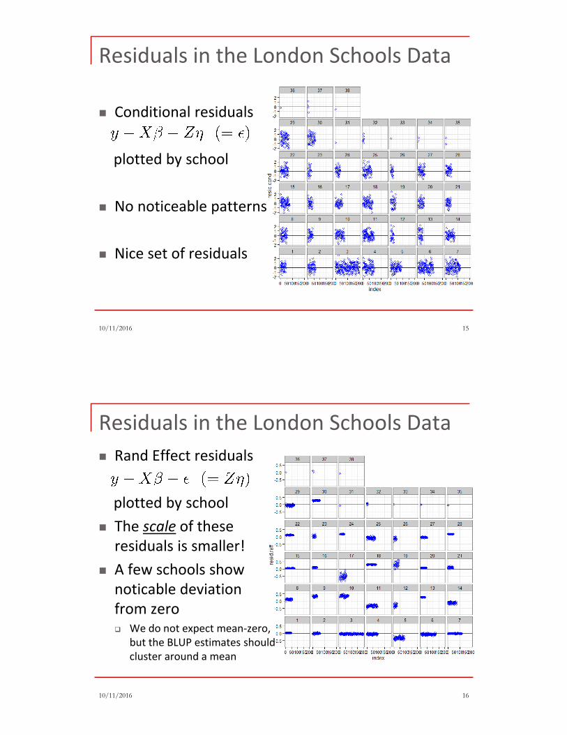
� Conditional residuals
plotted by school
� No noticeable patterns
� Nice set of residuals
Residuals in the London Schools Data
1610/11/2016
� Rand Effect residuals
plotted by school
� The scale of these
residuals is smaller!
� A few schools show
noticable deviation
from zero� We do not expect mean-zero,
but the BLUP estimates should
cluster around a mean

Standardized Residuals� We were looking at raw residuals
� You could standardize by dividing the raw
residuals by the square root of the variance
components, for example
� Quick and dirty: divide by their sample SD!
� If there are severe outliers, the sample SD will be
inflated and this won’t work well
� If we have standardized residuals, outlier
detection is a bit easier.
� There are simulation-based methods for
detecting outliers as well
1710/11/2016
1810/11/2016
Residuals: Practical Advice
� Looking at some residuals is better than looking at
none.
� In many MLM’s, marginal and conditional residuals can be
used roughly as you would with ordinary linear regression
� It is worthwhile to plot residuals again the group/cluster
indicators
� To identify and fix problems, plot residuals against other
variables (within and/or across clusters), try
transformations, etc…
� residuals(lmer.1) gives you the conditional
residuals!

The London Schools Data –
Variable Selection
� How can we improve the model?
� We have a bunch of other variables lying around:
� Unit-level (student): Gender, VR
� Group-level (school): School.denom, School.gender
� Which ones to include? Fixed effects or
random effects? Interactions? Etc.
1910/11/2016
Comparing models – Two basic tools
� Overall Fit Indices
� Likelihood ratio test / “Deviance” statistics
� AIC, BIC, DIC and all that
� Simulation-based Checks
� “Fake data” methods
� Posterior predictive checks
2010/11/2016
2110/11/2016
Overall fit indices
� Pro’s:
� Quick-and-dirty (a drop of 2 is marginally interesting, a
drop of 3 is interesting, a drop of 10 is a big deal)
� Tells you whether one model “fits better” overall than
another
� Con’s:
� Doesn’t tell whether the “best” model really fits
� If a model doesn’t fit, doesn’t tell you what went
wrong
� We will discuss these today
2210/11/2016
Simulation-based checks
� Con’s
� The method is not automatic
� You have to choose a “feature” of the data or model that you want to check
� You have to program the simulation
� Pro’s
� You can focus on particular features of the model or data that you are worried about
� You can “see” what went wrong with the model, and sometimes fix it
� We will discuss these later in the semester

2310/11/2016
Overall Fit Indices
� Basic tool: “deviance” of the model M
� Direct use: If M0 is nested in M1, then approx:
� Used to compare ordinary linear models,
generalized linear models, etc.
2410/11/2016
What if models are not nested?
� The “Chi-squared” theory for D(M) is gone.
� Other considerations (prediction accuracy, Bayesian decis. theory, …) lead to penalized deviance measures:
DP(M) = D(M) + P(#parameters)
� Three common cases (let k = #parameters)
� AIC = D(M) + 2 k
� BIC = D(M) + k log(n)
� DIC = meansim(D(M)) + 2 kD ≈ D(M) + 2 kD
� kD is estimated #parameters

2510/11/2016
Why are we fudging about k vs kD?
� In ordinary linear models (and glm’s), k = #X’s.
� What about σ? what about over-dispersion
parameter?
� In both M1 and M0, so df1 – df0 is the same either way).
� In multilevel models it’s not so clear:
� one-way ANOVA with J cells (df=J)
� fitting grand mean only (df=1)
� 1 ≤ kD≤ J, depending on size of τ
2610/11/2016
Variable Selection: Practical Advice
� Start with multilevel model that represents your
initial guesses about group structure in the data
� Do variable selection on all the fixed effects first,
using AIC or DIC (or if you prefer, BIC)
� AIC will result in bigger models that predict better
� BIC will result in smaller models that interpret better
� DIC will result in models between AIC and BIC sizes…
� Deviance/LRT only valid if models have same random
effects, and are nested
� Then go back and use AIC or DIC (or BIC) to do
selection on random effects

Digression: REML vs MLE
� In order to properly use AIC, BIC, or even LR tests,
must calculate the true maximum log-likelihood.
� By default, lmer() calculates estimates known as
“REML” estimates.
� Less biased estimates than true MLE’s, especially for
variance components
� Essentially, calculates fixed effect estimates by least-
squares, and calculates variance components from
marginal residuals
� REML estimates do not maximize the true likelihood
� For AIC, BIC, LRT, etc., need to refit using MLEs!
2710/11/2016
Digression: REML vs MLE
� Can use lmer() or update() function to get MLE fit
� lmer.1 <- lmer(Y ~ 1 + LRT + (1 + LRT|school),
data=school.frame, REML=F)
� lmer.1 <- update(lmer.1, . ~ ., REML=F)
� Can produce substantial differences in likelihood
� Use AIC(), BIC(), logLik() to extract these values directly
from fitted model
� ANOVA() always refits using MLEs so that comparisons
are valid
2810/11/2016
Not valid to compare
models with these numbers
OK to compare models
with these numbers

Back to London Schools Data> names(tmp) # main variabes in school.frame…
# [1] "Y" "LRT" "Gender" "School.gender"
# [5] "School.denom" "VR"
> lmer.2 <- update(lmer.1, . ~ . + Gender)
> anova(lmer.1,lmer.2)
# refitting model(s) with ML (instead of REML)
# Df AIC BIC logLik deviance Chisq Chi Df Pr(>Chisq)
# lmer.1 6 4749.4 4782.9 -2368.7 4737.4
# lmer.2 7 4823.3 4862.5 -2404.7 4809.3 0 1 1
# --> AIC, BIC prefer lmer.2
> lmer.3 <- update(lmer.2, . ~ . + School.gender)
> anova(lmer.2,lmer.3)
# refitting model(s) with ML (instead of REML)
# Df AIC BIC logLik deviance Chisq Chi Df Pr(>Chisq)
# lmer.2 7 4823.3 4862.5 -2404.7 4809.3
# lmer.3 9 4815.0 4865.3 -2398.5 4797.0 12.327 2 0.002105 **
# --> AIC prefers lmer.3, BIC prefers lmer.2
2910/11/2016Etc!
London Schools Data
� Tried Gender, School.gender, School.denom, and
VR stepwise as fixed effects, found only Gender
and VR reduce AIC by more than 3, so keep them.
Gender and VR.
� Trying to convert Gender and VR to random
effects does not improve AIC enough to keep
them, so the final model we obtain is
> lmer.5 <- lmer(Y ̃LRT + Gender + VR +
+ (1 + LRT | school), data=school.frame))
3010/11/2016

London Schools Data – “final” model
> display(lmer.5)
lmer(formula = Y ~ LRT + Gender +
VR + (1 + LRT | school), data =
school.frame)
coef.est coef.se
(Intercept) 0.39 0.06
LRT 0.03 0.00
Gender1 0.16 0.04
VRLow -0.92 0.07
VRMed -0.57 0.05
Error terms:
Groups Name Std.Dev. Corr
school (Intercept) 0.23
LRT 0.01 0.61
Residual 0.75
---
number of obs: 1978, groups: school,
38
AIC = 4594.6, DIC = 4521.2
deviance = 4548.9
> anova(lmer.1,lmer.5)
refitting model(s) with ML (instead
of REML)
Df AIC BIC logLik
lmer.1 6 4749.4 4782.9 -2368.7
lmer.5 9 4566.9 4617.2 -2274.4
3110/11/2016
Some Automatic & Exact Methods
� There are a number of R packages that will do
variable selection for lmer models, including:
� LMERConvenienceFunctions automates
backwards selection of fixed effects and forward
selection of random effects, using AIC, BIC, etc.
� fitLMER.fnc() is general-purpose function for this
� RLRsim provides simulation-based exact likelihood
ratio tests for random effects
� exactLRT() performs exact LRT test for true ML fits
� exactRLRT() performs exact LRT test for REML fits
3210/11/2016

Automated Variable Selection…
> library(LMERConvenienceFunctions) # for fitLMER.fnc() function...
# start with a "big fixed effects" model
> lmer.10 <- lmer(Y ~ LRT + VR + Gender + School.gender +School.denom +
+ (1+LRT|school), data=school.frame)
> bic_best.11 <- fitLMER.fnc(lmer.10,
+ ran.effects=c("(School.gender|school)",
+ "(School.denom|school)"),method="BIC")
> anova(lmer.5,lmer.10,lmer.11)
refitting model(s) with ML (instead of REML)
Data: school.frame
Models:
lmer.5: Y ~ LRT + Gender + VR + (1 + LRT | school)
lmer.11: Y ~ LRT + VR + Gender + (1 + LRT | school)
lmer.10: Y ~ LRT + VR + Gender + School.gender + School.denom + (1 + LRT |
lmer.10: school)
Df AIC BIC logLik deviance Chisq Chi Df Pr(>Chisq)
lmer.5 9 4566.9 4617.2 -2274.4 4548.9
lmer.11 9 4566.9 4617.2 -2274.4 4548.9 0 0 <2e-16 ***
lmer.10 14 4618.9 4697.2 -2295.5 4590.9 0 5 1
3310/11/2016
fitLMER.fnc:
1. Backwards elimination of F.E’s
2. Forward selection of R.E.’s
3. Backwards elimination of F.E.’s
Exact Test of Random Effect..library(RLRsim)
m0 <- lmer(Y ~ LRT + VR + Gender + (1 | school), data=school.frame)
lmer.11a <- lmer(Y ~ LRT + VR + Gender + (1|school) + (0 + LRT | school),
data=school.frame) # need indep rand effects for RLRsim...
lmer.LRT.only <- lmer(Y ~ LRT + VR + Gender + (0 + LRT | school),
data=school.frame)
formula(m0) # formula under H0: no random slopes for LRT
formula(lmer.11a) # model under HA: yes random slopes for LRT
formula(lmer.LRT.only) # model with *only* random slopes for LRT
exactRLRT(lmer.LRT.only,lmer.11a,m0)
# simulated finite sample distribution of RLRT.
#
# (p-value based on 10000 simulated values)
#
# data:
# RLRT = 6.2561, p-value = 0.0055
3410/11/2016

3510/11/2016
Summary
� The London Schools Data (again!)
� A nice random-intercepts, random-slopes model
� Residuals in MLM’s
� Marginal residuals
� Conditional residuals
� Random effects residuals
� Variable selection
� Overall fit statistics
� Simulation-based methods (save for later!)
� AIC, BIC, DIC and all that
� An improved model for the London Schools data


