

1
4. Ordered response models
4.1 General model approaches
Ordered (ordinal) dependent variables in a microeconometric analysis:
These qualitative variables have also more than two possible mutually exclusi-
ve categories which are (in contrast to multinomial variables), however, natural-
ly ordered (in the case of two categories, the variables are binary)
Examples for microeconometric analyses with ordered response models:
• Analysis of the individual satisfaction of a person with life (e.g. on a eleven-
point scale of integers from zero for “completely dissatisfied” to ten for “com-
pletely satisfied”)
• Analysis of the personal strength of agreement to a political program (e.g.
with the categories “strong disagreement”, “weak disagreement”, weak
agreement”, “strong agreement”)
• Analysis of the years of education of a person (e.g. with the categories “less
than nine years”, “between nine and 12 years”, “at least 13 years”)
• Analysis of the credit rating of firms (e.g. on a scale from D to AAA)
• Analysis of the stated importance of equity issues in international climate ne-
gotiations (e.g. on a five-point scale from “no importance” to “very high im-
portance”)
2
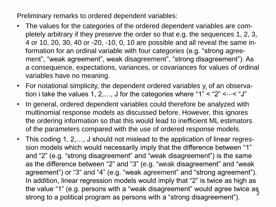
Preliminary remarks to ordered dependent variables:
• The values for the categories of the ordered dependent variables are com-
pletely arbitrary if they preserve the order so that e.g. the sequences 1, 2, 3,
4 or 10, 20, 30, 40 or -20, -10, 0, 10 are possible and all reveal the same in-
formation for an ordinal variable with four categories (e.g. “strong agree-
ment”, “weak agreement”, weak disagreement”, “strong disagreement”). As
a consequence, expectations, variances, or covariances for values of ordinal
variables have no meaning.
• For notational simplicity, the dependent ordered variables yi of an observa-
tion i take the values 1, 2,…, J for the categories where “1” < “2” <⋯< “J”
• In general, ordered dependent variables could therefore be analyzed with
multinomial response models as discussed before. However, this ignores
the ordering information so that this would lead to inefficient ML estimators
of the parameters compared with the use of ordered response models.
• This coding 1, 2,…, J should not mislead to the application of linear regres-
sion models which would necessarily imply that the difference between “1”
and “2” (e.g. “strong disagreement” and “weak disagreement”) is the same
as the difference between “2” and “3” (e.g. “weak disagreement” and “weak
agreement”) or “3” and “4” (e.g. “weak agreement” and “strong agreement”).
In addition, linear regression models would imply that “2” is twice as high as
the value “1” (e.g. persons with a “weak disagreement” would agree twice as
strong to a political program as persons with a “strong disagreement”).

3
Continuous latent variable (which sometimes can be interpreted as varying uti-
lity) in ordered response models (i = 1,…, n):
As in binary response models, xi = (xi1,…, xik)
‘ is again a vector of k explanatory
variables, β = (β1,…, βk)‘ is the corresponding k-dimensional parameter vector,
and εi is an error term. These unobservable latent variables can be related to
the observed variables yi or yij (i = 1,…, n; j = 1,…, J):
This threshold mechanism divides the latent variable yi* in J intervals by using
J + 1 threshold parameters κ0, κ1 ,…, κJ with κ0 < κ1 <⋯< κJ. According to this
mechanism, higher values of the latent variable yi* lead to higher values of the
ordered dependent variable yi with the values or intervals j = 1,…, J. It follows:
*
i i iy = β'x + ε
*
i j-1 i j
i
ij
y = j if κ < y κ
1 if y = jy =
0 otherwise
*
i 0 i 1 0 i i 1 i
*
i 1 i 2 1 i i 2 i
*
i 2 i 3 2 i i 3 i
y = 1 if κ < y κ κ - β'x < ε κ - β'x
y = 2 if κ < y κ κ - β'x < ε κ - β'x
y = 3 if κ < y κ κ - β'x < ε κ - β'x
*
i J-1 i J J-1 i i J i
y = J if κ < y κ κ - β'x < ε κ - β'x
4
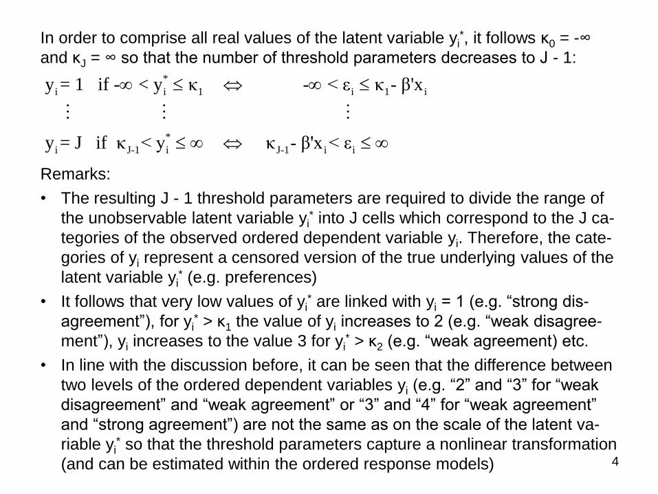
In order to comprise all real values of the latent variable yi*, it follows κ0 = -∞
and κJ = ∞ so that the number of threshold parameters decreases to J - 1:
Remarks:
• The resulting J - 1 threshold parameters are required to divide the range of
the unobservable latent variable yi* into J cells which correspond to the J ca-
tegories of the observed ordered dependent variable yi. Therefore, the cate-
gories of yi represent a censored version of the true underlying values of the
latent variable yi* (e.g. preferences)
• It follows that very low values of yi* are linked with yi = 1 (e.g. “strong dis-
agreement”), for yi* > κ1 the value of yi increases to 2 (e.g. “weak disagree-
ment”), yi increases to the value 3 for yi* > κ2 (e.g. “weak agreement) etc.
• In line with the discussion before, it can be seen that the difference between
two levels of the ordered dependent variables yi (e.g. “2” and “3” for “weak
disagreement” and “weak agreement” or “3” and “4” for “weak agreement”
and “strong agreement”) are not the same as on the scale of the latent va-
riable yi* so that the threshold parameters capture a nonlinear transformation
(and can be estimated within the ordered response models)
*
i i 1 i 1 i
*
i J-1 i J-1 i i
y = 1 if - < y κ - < ε κ - β'x
y = J if κ < y κ - β'x < ε

5
Different ordered response models result from different types of the density
function of the latent variables yi* on the basis of a distribution assumption
about εi with the distribution function Fi(εi) as discussed later. If the J - 1 thres-
hold parameters κ1, κ2 ,…, κJ-1 and the parameters in β are summarized in the
vector θ, it follows for the probability that yi takes the value j (j = 1,…, J):
On the basis of κ0 = -∞ and κJ = ∞, it follows F(-∞) = 0 and F(∞) = 1. However,
these probabilities comprise too many parameters so that not all threshold pa-
rameters are identified if a constant is included in the ordered response model.
Therefore, one parameter has to be normalized. Common approaches are to
set the first threshold parameter κ1 = 0 or to drop the constant term from xi. In
the following, we consider the second approach.
Based on the aforementioned probabilities and the binary variables yij, the ML
estimation of the k + J - 1 parameters β1,…, βk and κ1,…, κJ-1 in ordered res-
ponse models (instead of k∙(J-1) slope parameters and constants in pure multi-
nomial logit and probit models) is identical to the ML estimation in multinomial
discrete choice models. Therefore, it follows for the log-likelihood function:
ij i i i ij i i j i i j-1 ip (x , θ) = P(y = j|x , θ) = P(y = 1|x , θ) = F (κ - β'x ) - F (κ - β'x )
n J
ij ij i
i=1 j=1
logL(θ) = y logp (x , θ)

6
4.2 Ordered probit and logit models
Ordered probit models:
These ordered response models assume that the error terms εi are standard
normally distributed (as in binary probit models which are special cases of or-
dered probit models with J = 2)
Choice probabilities in ordered probit models (i = 1,…, n; j = 1,…, J):
For the specific probabilities this means:
→ As in binary probit models, the parameterization of the standard normal dis-
tribution of εi is not restrictive. In fact, the normalization of the normal distri-
bution with an expected value of zero and variance one is necessary for the
identification of the parameters in the choice probabilities
ij i i i i j i i j-1 ip (x , θ) = P(y = j|x , θ) = Φ (κ - β'x ) - Φ (κ - β'x )
i i i 1 i
i i i 2 i i 1 i
i i i 3 i i 2 i
i i i J-1 i
P(y = 1|x , θ) = Φ (κ - β'x )
P(y = 2|x , θ) = Φ (κ - β'x ) - Φ (κ - β'x )
P(y = 3|x , θ) = Φ (κ - β'x ) - Φ (κ - β'x )
P(y = J|x , θ) = 1 - Φ (κ - β'x )

7
Ordered logit models:
These ordered response models are derived in the same way as ordered probit
models and thus assume that the error terms εi are standard logistically distri-
buted (as in binary logit models which are special cases of ordered logit mo-
dels with J = 2)
Choice probabilities in ordered logit models (i = 1,…, n; j = 1,…, J):
For the specific probabilities this means:
→ In the same way as in the case of binary probit and logit models, the as-
sumptions of standard normal or standard logistic distributions of εi in order-
ed probit or ordered logit models usually lead to very similar estimation re-
sults in practice across these two types of ordered response models (see la-
ter)
ij i i i i j i i j-1 ip (x , θ) = P(y = j|x , θ) = Λ (κ - β'x ) - Λ (κ - β'x )
i i i 1 i
i i i 2 i i 1 i
i i i 3 i i 2 i
i i i J-1 i
P(y = 1|x , θ) = Λ (κ - β'x )
P(y = 2|x , θ) = Λ (κ - β'x ) - Λ (κ - β'x )
P(y = 3|x , θ) = Λ (κ - β'x ) - Λ (κ - β'x )
P(y = J|x , θ) = 1 - Λ (κ - β'x )
8
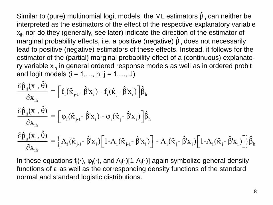
Similar to (pure) multinomial logit models, the ML estimators β h can neither be
interpreted as the estimators of the effect of the respective explanatory variable
xih nor do they (generally, see later) indicate the direction of the estimator of
marginal probability effects, i.e. a positive (negative) β h does not necessarily
lead to positive (negative) estimators of these effects. Instead, it follows for the
estimator of the (partial) marginal probability effect of a (continuous) explanato-
ry variable xih in general ordered response models as well as in ordered probit
and logit models (i = 1,…, n; j = 1,…, J):
In these equations fi(∙), φi(∙), and Λi(∙)[1-Λi(∙)] again symbolize general density
functions of εi as well as the corresponding density functions of the standard
normal and standard logistic distributions.
ij i
i j-1 i i j i h
ih
ij i
i j-1 i i j i h
ih
ij i
i j-1 i i j-1 i i j i i
ih
ˆp̂ (x , θ) ˆ ˆ ˆˆ ˆ = f (κ - β'x ) - f (κ - β'x ) βx
ˆp̂ (x , θ) ˆ ˆ ˆˆ ˆ = φ (κ - β'x ) - φ (κ - β'x ) βx
ˆp̂ (x , θ) ˆ ˆ ˆˆ ˆ ˆ = Λ (κ - β'x ) 1-Λ (κ - β'x ) - Λ (κ - β'x ) 1-Λ (x
j i hˆ ˆκ̂ - β'x ) β

9
The estimators of a discrete change of pij(xi, θ) due to a discrete change ∆xih of
a (particularly discrete) explanatory variable xih in general ordered response
models as well as in ordered probit and logit models are (i = 1,…, n; j = 1,…, J):
→ On the basis of the estimators of (partial) marginal probability effects and of
discrete probability effects, it is again possible to estimate average marginal
and discrete probability effects of an explanatory variable xih across all i as
well as marginal and discrete probability effects of xih at the mean of the ex-
planatory variables (the procedure for this estimation with STATA by consi-
dering differences of estimated probabilities is identical to the case of multi-
nomial logit models)
ij i i i ih i i
i j i h ih i j-1 i h ih i j i i j-1 i
ij i i j i h ih i
ˆ ˆ ˆˆΔp (x , θ) = P(y = j|x +Δx , θ) - P(y = j|x , θ) =
ˆ ˆ ˆ ˆ ˆ ˆ F (κ - β'x - β Δx ) - F (κ - β'x - β Δx ) - F (κ - β'x ) - F (κ - β'x )
ˆ ˆˆˆΔp (x , θ) = Φ (κ - β'x - β Δx ) - Φ (κ
j-1 i h ih
i j i i j-1 i
ij i i j i h ih i j-1 i
ˆ ˆ- β'x - β Δx ) -
ˆ ˆ Φ (κ - β'x ) - Φ (κ - β'x )
ˆ ˆ ˆˆˆΔp (x , θ) = Λ (κ - β'x - β Δx ) - Λ (κ - β'x -
h ih
i j i i j-1 i
ˆ β Δx ) -
ˆ ˆ Λ (κ - β'x ) - Λ (κ - β'x )
10
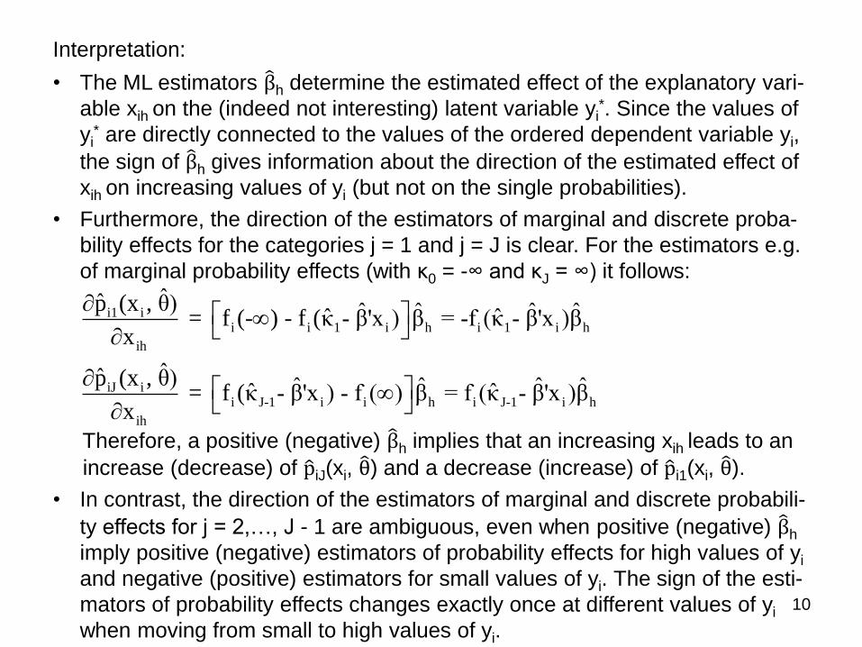
Interpretation:
• The ML estimators β h determine the estimated effect of the explanatory vari-
able xih on the (indeed not interesting) latent variable yi*. Since the values of
yi* are directly connected to the values of the ordered dependent variable yi,
the sign of β h gives information about the direction of the estimated effect of
xih on increasing values of yi (but not on the single probabilities).
• Furthermore, the direction of the estimators of marginal and discrete proba-
bility effects for the categories j = 1 and j = J is clear. For the estimators e.g.
of marginal probability effects (with κ0 = -∞ and κJ = ∞) it follows:
Therefore, a positive (negative) β h implies that an increasing xih leads to an
increase (decrease) of p iJ(xi, θ ) and a decrease (increase) of p i1(xi, θ ).
• In contrast, the direction of the estimators of marginal and discrete probabili-
ty effects for j = 2,…, J - 1 are ambiguous, even when positive (negative) β h
imply positive (negative) estimators of probability effects for high values of yi
and negative (positive) estimators for small values of yi. The sign of the esti-
mators of probability effects changes exactly once at different values of yi
when moving from small to high values of yi.
i1 ii i 1 i h i 1 i h
ih
iJ ii J-1 i i h i J-1 i h
ih
ˆp̂ (x , θ) ˆ ˆ ˆ ˆˆ ˆ = f (- ) - f (κ - β'x ) β = -f (κ - β'x )βx
ˆp̂ (x , θ) ˆ ˆ ˆ ˆˆ ˆ = f (κ - β'x ) - f ( ) β = f (κ - β'x )βx
11
---------------------------------------------------------------------------------------------------------
Example: Determinants of secondary school choice (I)
The determinants of the choice of 675 pupils in Germany between the three se-
condary school types Hauptschule, Realschule, and Gymnasium are again
analyzed. In contrast to the previous application of a (pure) multinomial logit
model, however, the natural ordering of the three categories is now used so
that the coding of 1 for “Hauptschule”, the coding of 2 for “Realschule”, and the
coding of 3 for “Gymnasium” of the dependent variable secondary school type
(schooltype) indicates this ordering. The explanatory variables are the same as
in the previous multinomial logit model analysis:
• Years of education of the mother (motheduc) as mainly interesting explana-
tory variable
• Dummy variable for labor force participation of the mother (mothinlf) that
takes the value one if the mother is employed
• Logarithm of household income (loghhincome)
• Logarithm of household size (loghhsize)
• Rank by age among the siblings (birthorder)
• Year dummies for 1995-2002
The ML estimation of the ordered probit and logit models with STATA leads to
the following results:
---------------------------------------------------------------------------------------------------------

12
---------------------------------------------------------------------------------------------------------
Example: Determinants of secondary school choice (II)
oprobit schooltype motheduc mothinlf loghhincome loghhsize birthorder year1995 year1996
year1997 year1998 year1999 year2000 year2001 year2002
Ordered probit regression Number of obs = 675
LR chi2(13) = 203.31
Prob > chi2 = 0.0000
Log likelihood = -631.18653 Pseudo R2 = 0.1387
------------------------------------------------------------------------------
schooltype | Coef. Std. Err. z P>|z| [95% Conf. Interval]
-------------+----------------------------------------------------------------
motheduc | .2731466 .0279933 9.76 0.000 .2182808 .3280124
mothinlf | -.1649158 .0993593 -1.66 0.097 -.3596565 .0298249
loghhincome | .6492508 .1049847 6.18 0.000 .4434845 .8550172
loghhsize | -.6145965 .2016538 -3.05 0.002 -1.009831 -.2193624
birthorder | -.1049289 .0576033 -1.82 0.069 -.2178293 .0079714
year1995 | .0457511 .1877388 0.24 0.807 -.3222101 .4137124
year1996 | .0898004 .1952066 0.46 0.645 -.2927974 .4723982
year1997 | -.2803249 .1982527 -1.41 0.157 -.668893 .1082432
year1998 | .0750879 .2120345 0.35 0.723 -.3404922 .4906679
year1999 | -.1605177 .2046103 -0.78 0.433 -.5615465 .240511
year2000 | .0009375 .2037127 0.00 0.996 -.3983321 .4002071
year2001 | .0330622 .1972731 0.17 0.867 -.3535859 .4197104
year2002 | -.105459 .1960686 -0.54 0.591 -.4897463 .2788283
-------------+----------------------------------------------------------------
/cut1 | 8.439737 1.061008 6.360201 10.51927
/cut2 | 9.369887 1.068849 7.274981 11.46479
------------------------------------------------------------------------------
---------------------------------------------------------------------------------------------------------
13
---------------------------------------------------------------------------------------------------------
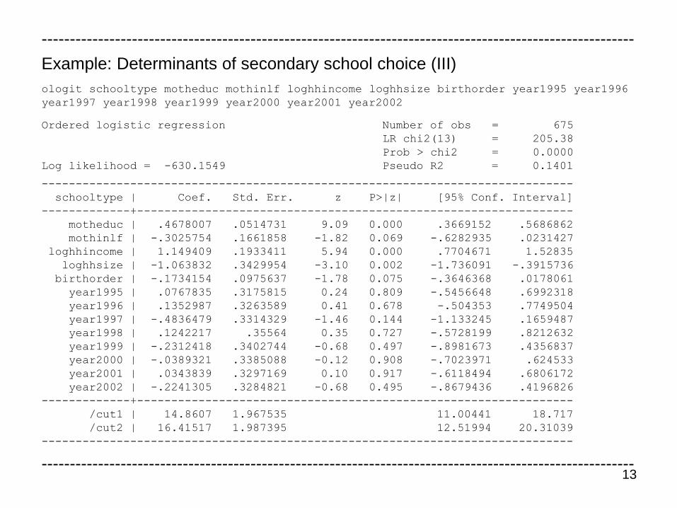
Example: Determinants of secondary school choice (III)
ologit schooltype motheduc mothinlf loghhincome loghhsize birthorder year1995 year1996
year1997 year1998 year1999 year2000 year2001 year2002
Ordered logistic regression Number of obs = 675
LR chi2(13) = 205.38
Prob > chi2 = 0.0000
Log likelihood = -630.1549 Pseudo R2 = 0.1401
------------------------------------------------------------------------------
schooltype | Coef. Std. Err. z P>|z| [95% Conf. Interval]
-------------+----------------------------------------------------------------
motheduc | .4678007 .0514731 9.09 0.000 .3669152 .5686862
mothinlf | -.3025754 .1661858 -1.82 0.069 -.6282935 .0231427
loghhincome | 1.149409 .1933411 5.94 0.000 .7704671 1.52835
loghhsize | -1.063832 .3429954 -3.10 0.002 -1.736091 -.3915736
birthorder | -.1734154 .0975637 -1.78 0.075 -.3646368 .0178061
year1995 | .0767835 .3175815 0.24 0.809 -.5456648 .6992318
year1996 | .1352987 .3263589 0.41 0.678 -.504353 .7749504
year1997 | -.4836479 .3314329 -1.46 0.144 -1.133245 .1659487
year1998 | .1242217 .35564 0.35 0.727 -.5728199 .8212632
year1999 | -.2312418 .3402744 -0.68 0.497 -.8981673 .4356837
year2000 | -.0389321 .3385088 -0.12 0.908 -.7023971 .624533
year2001 | .0343839 .3297169 0.10 0.917 -.6118494 .6806172
year2002 | -.2241305 .3284821 -0.68 0.495 -.8679436 .4196826
-------------+----------------------------------------------------------------
/cut1 | 14.8607 1.967535 11.00441 18.717
/cut2 | 16.41517 1.987395 12.51994 20.31039
------------------------------------------------------------------------------
---------------------------------------------------------------------------------------------------------
14
---------------------------------------------------------------------------------------------------------
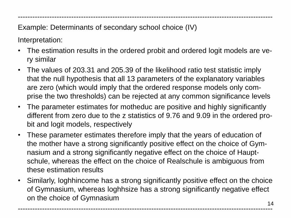
Example: Determinants of secondary school choice (IV)
Interpretation:
• The estimation results in the ordered probit and ordered logit models are ve-
ry similar
• The values of 203.31 and 205.39 of the likelihood ratio test statistic imply
that the null hypothesis that all 13 parameters of the explanatory variables
are zero (which would imply that the ordered response models only com-
prise the two thresholds) can be rejected at any common significance levels
• The parameter estimates for motheduc are positive and highly significantly
different from zero due to the z statistics of 9.76 and 9.09 in the ordered pro-
bit and logit models, respectively
• These parameter estimates therefore imply that the years of education of
the mother have a strong significantly positive effect on the choice of Gym-
nasium and a strong significantly negative effect on the choice of Haupt-
schule, whereas the effect on the choice of Realschule is ambiguous from
these estimation results
• Similarly, loghhincome has a strong significantly positive effect on the choice
of Gymnasium, whereas loghhsize has a strong significantly negative effect
on the choice of Gymnasium
---------------------------------------------------------------------------------------------------------
15
---------------------------------------------------------------------------------------------------------
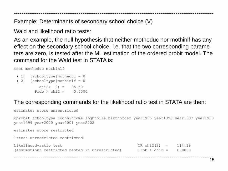
Example: Determinants of secondary school choice (V)
Wald and likelihood ratio tests:
As an example, the null hypothesis that neither motheduc nor mothinlf has any
effect on the secondary school choice, i.e. that the two corresponding parame-
ters are zero, is tested after the ML estimation of the ordered probit model. The
command for the Wald test in STATA is:
test motheduc mothinlf
( 1) [schooltype]motheduc = 0
( 2) [schooltype]mothinlf = 0
chi2( 2) = 95.50
Prob > chi2 = 0.0000
The corresponding commands for the likelihood ratio test in STATA are then:
estimates store unrestricted
oprobit schooltype loghhincome loghhsize birthorder year1995 year1996 year1997 year1998
year1999 year2000 year2001 year2002
estimates store restricted
lrtest unrestricted restricted
Likelihood-ratio test LR chi2(2) = 114.19
(Assumption: restricted nested in unrestricted) Prob > chi2 = 0.0000
---------------------------------------------------------------------------------------------------------

16
---------------------------------------------------------------------------------------------------------
Example: Determinants of secondary school choice (VI)
The estimation of the average marginal probability effects of motheduc across
all 675 pupils on the choice of Hauptschule, Realschule, and Gymnasium leads
to the following (shortened) STATA results in the ordered probit model:
margins, dydx(motheduc) predict(outcome(1))
------------------------------------------------------------------------------
| Delta-method
| dy/dx Std. Err. z P>|z| [95% Conf. Interval]
-------------+----------------------------------------------------------------
motheduc | -.0786704 .0075726 -10.39 0.000 -.0935124 -.0638283
------------------------------------------------------------------------------
margins, dydx(motheduc) predict(outcome(2))
------------------------------------------------------------------------------
| Delta-method
| dy/dx Std. Err. z P>|z| [95% Conf. Interval]
-------------+----------------------------------------------------------------
motheduc | -.007464 .0025874 -2.88 0.004 -.0125352 -.0023928
------------------------------------------------------------------------------
margins, dydx(motheduc) predict(outcome(3))
------------------------------------------------------------------------------
| Delta-method
| dy/dx Std. Err. z P>|z| [95% Conf. Interval]
-------------+----------------------------------------------------------------
motheduc | .0861344 .0073071 11.79 0.000 .0718128 .100456
------------------------------------------------------------------------------
---------------------------------------------------------------------------------------------------------

17
---------------------------------------------------------------------------------------------------------
Example: Determinants of secondary school choice (VII)
The estimation of corresponding marginal probability effects of motheduc at the
means of the explanatory variables across all 675 pupils leads to the following
(shortened) STATA results in the ordered probit model:
margins, dydx(motheduc) atmeans predict(outcome(1))
------------------------------------------------------------------------------
| Delta-method
| dy/dx Std. Err. z P>|z| [95% Conf. Interval]
-------------+----------------------------------------------------------------
motheduc | -.0859161 .0086732 -9.91 0.000 -.1029152 -.0689171
------------------------------------------------------------------------------
margins, dydx(motheduc) atmeans predict(outcome(2))
------------------------------------------------------------------------------
| Delta-method
| dy/dx Std. Err. z P>|z| [95% Conf. Interval]
-------------+----------------------------------------------------------------
motheduc | -.0199433 .0049997 -3.99 0.000 -.0297426 -.010144
------------------------------------------------------------------------------
margins, dydx(motheduc) atmeans predict(outcome(3))
------------------------------------------------------------------------------
| Delta-method
| dy/dx Std. Err. z P>|z| [95% Conf. Interval]
-------------+----------------------------------------------------------------
motheduc | .1058594 .0110476 9.58 0.000 .0842065 .1275123
------------------------------------------------------------------------------
---------------------------------------------------------------------------------------------------------

18
---------------------------------------------------------------------------------------------------------
Example: Determinants of secondary school choice (VIII)
The estimation of the average marginal probability effects of motheduc across
all 675 pupils on the choice of Hauptschule, Realschule, and Gymnasium leads
to the following (shortened) STATA results in the ordered logit model:
margins, dydx(motheduc) predict(outcome(1))
------------------------------------------------------------------------------
| Delta-method
| dy/dx Std. Err. z P>|z| [95% Conf. Interval]
-------------+----------------------------------------------------------------
motheduc | -.0795201 .0081198 -9.79 0.000 -.0954346 -.0636056
------------------------------------------------------------------------------
margins, dydx(motheduc) predict(outcome(2))
------------------------------------------------------------------------------
| Delta-method
| dy/dx Std. Err. z P>|z| [95% Conf. Interval]
-------------+----------------------------------------------------------------
motheduc | -.0082689 .0030382 -2.72 0.006 -.0142235 -.0023142
------------------------------------------------------------------------------
margins, dydx(motheduc) predict(outcome(3))
------------------------------------------------------------------------------
| Delta-method
| dy/dx Std. Err. z P>|z| [95% Conf. Interval]
-------------+----------------------------------------------------------------
motheduc | .087789 .0079214 11.08 0.000 .0722633 .1033146
------------------------------------------------------------------------------
---------------------------------------------------------------------------------------------------------
19
---------------------------------------------------------------------------------------------------------
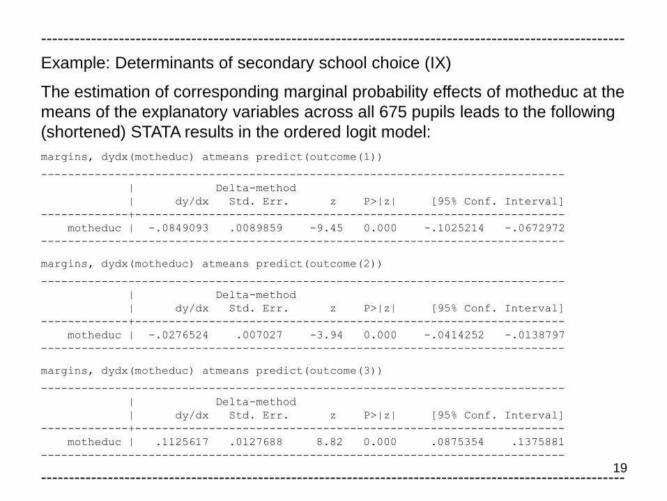
Example: Determinants of secondary school choice (IX)
The estimation of corresponding marginal probability effects of motheduc at the
means of the explanatory variables across all 675 pupils leads to the following
(shortened) STATA results in the ordered logit model:
margins, dydx(motheduc) atmeans predict(outcome(1))
------------------------------------------------------------------------------
| Delta-method
| dy/dx Std. Err. z P>|z| [95% Conf. Interval]
-------------+----------------------------------------------------------------
motheduc | -.0849093 .0089859 -9.45 0.000 -.1025214 -.0672972
------------------------------------------------------------------------------
margins, dydx(motheduc) atmeans predict(outcome(2))
------------------------------------------------------------------------------
| Delta-method
| dy/dx Std. Err. z P>|z| [95% Conf. Interval]
-------------+----------------------------------------------------------------
motheduc | -.0276524 .007027 -3.94 0.000 -.0414252 -.0138797
------------------------------------------------------------------------------
margins, dydx(motheduc) atmeans predict(outcome(3))
------------------------------------------------------------------------------
| Delta-method
| dy/dx Std. Err. z P>|z| [95% Conf. Interval]
-------------+----------------------------------------------------------------
motheduc | .1125617 .0127688 8.82 0.000 .0875354 .1375881
------------------------------------------------------------------------------
---------------------------------------------------------------------------------------------------------

20
---------------------------------------------------------------------------------------------------------
Example: Determinants of secondary school choice (X)
Interpretation:
• The estimated average marginal probability effects or marginal probability
effects at the means of the explanatory variables are very similar in the or-
dered probit and logit models, respectively, and strengthen the significantly
positive effect of the years of education of the mother on the choice of Gym-
nasium and the significantly negative effect on the choice of Hauptschule
• The estimation results particularly imply that motheduc has a significantly
negative effect on the choice of Realschule. This estimated negative effect is
stronger on the basis of the marginal probability effects at the means of the
explanatory variables than of the average marginal probability effects.
• The estimated average marginal probability effect of motheduc of -0.0075 in
the ordered probit model implies that an increase of the years of education
of the mother by one (unit) leads to an approximately estimated decrease of
the choice probability for Realschule by 0.75 percentage points, whereas the
estimated value of -0.0200 at the means of the explanatory variables implies
an approximately estimated decrease by 2.00 percentage points
• While these estimated effects are very similar to those in the multinomial lo-
git model, the estimated standard deviations are higher in the latter model
which points to efficiency losses compared to ordered response models
---------------------------------------------------------------------------------------------------------

21
---------------------------------------------------------------------------------------------------------
Example: Determinants of secondary school choice (XI)
The estimation of the average probability of the choice of Hauptschule across
all 675 pupils leads to the following STATA results in the ordered probit model:
margins, predict(outcome(1))
Predictive margins Number of obs = 675
Model VCE : OIM
Expression : Pr(schooltype==1), predict(outcome(1))
------------------------------------------------------------------------------
| Delta-method
| Margin Std. Err. z P>|z| [95% Conf. Interval]
-------------+----------------------------------------------------------------
_cons | .2931277 .015854 18.49 0.000 .2620545 .324201
------------------------------------------------------------------------------
The estimation of (average) discrete changes of probabilities due to a discrete
change of an explanatory variable requires the estimation of (average) proba-
bilities for specific values of the explanatory variable. For example, the average
change of the probability of the choice of Hauptschule across all 675 pupils due
to an increase of motheduc from the minimum value of seven years to the ma-
ximum value of 18 years of education can be estimated on the basis of the esti-
mated average probabilities at these specific values. The corresponding STATA
commands after the ML estimation of the ordered probit model are:
---------------------------------------------------------------------------------------------------------

22
---------------------------------------------------------------------------------------------------------
Example: Determinants of secondary school choice (XII)
margins, at(motheduc=7) predict(outcome(1))
Predictive margins Number of obs = 675
Model VCE : OIM
Expression : Pr(schooltype==1), predict(outcome(1))
at : motheduc = 7
------------------------------------------------------------------------------
| Delta-method
| Margin Std. Err. z P>|z| [95% Conf. Interval]
-------------+----------------------------------------------------------------
_cons | .6897138 .0423121 16.30 0.000 .6067836 .772644
------------------------------------------------------------------------------
margins, at(motheduc=18) predict(outcome(1))
Predictive margins Number of obs = 675
Model VCE : OIM
Expression : Pr(schooltype==1), predict(outcome(1))
at : motheduc = 18
------------------------------------------------------------------------------
| Delta-method
| Margin Std. Err. z P>|z| [95% Conf. Interval]
-------------+----------------------------------------------------------------
_cons | .0100681 .0052127 1.93 0.053 -.0001485 .0202848
------------------------------------------------------------------------------
The estimated average decrease of the probability of the choice of Hauptschu-
le is therefore 0.6897-0.0101=0.6796 or 67.96 percentage points for an in-
crease from seven to 18 years
---------------------------------------------------------------------------------------------------------
23
---------------------------------------------------------------------------------------------------------
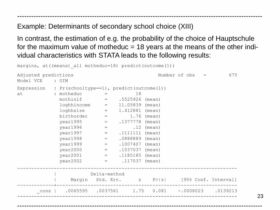
Example: Determinants of secondary school choice (XIII)
In contrast, the estimation of e.g. the probability of the choice of Hauptschule
for the maximum value of motheduc = 18 years at the means of the other indi-
vidual characteristics with STATA leads to the following results:
margins, at((means)_all motheduc=18) predict(outcome(1))
Adjusted predictions Number of obs = 675
Model VCE : OIM
Expression : Pr(schooltype==1), predict(outcome(1))
at : motheduc = 18
mothinlf = .5525926 (mean)
loghhincome = 11.05839 (mean)
loghhsize = 1.412881 (mean)
birthorder = 1.76 (mean)
year1995 = .1377778 (mean)
year1996 = .12 (mean)
year1997 = .1111111 (mean)
year1998 = .0888889 (mean)
year1999 = .1007407 (mean)
year2000 = .1037037 (mean)
year2001 = .1185185 (mean)
year2002 = .117037 (mean)
------------------------------------------------------------------------------
| Delta-method
| Margin Std. Err. z P>|z| [95% Conf. Interval]
-------------+----------------------------------------------------------------
_cons | .0065595 .0037561 1.75 0.081 -.0008023 .0139213
------------------------------------------------------------------------------
---------------------------------------------------------------------------------------------------------

24
4.3 Discussion of ordered probit and logit models
Underlying parallel regression assumption (j = 1,…, J - 1) with Fi(∙) = Φi(∙) in the
ordered probit model and Fi(∙) = Λi(∙) in the ordered logit model (i = 1,…, n):
Consequences:
• These probabilities for several categories j only differ due to different thres-
hold parameters, but not due to different parameter values
• The partial derivatives of these probabilities with respect to an arbitrary ex-
planatory variable xih are identical for all j
• With this assumption, the following dummy variables can be specified:
As a consequence, the slope parameters, but not the threshold parameters,
in ordered probit and logit models with two categories could be estimated by
binary probit or logit models with these dummy variables as dependent vari-
ables.
• This assumption is also the reason for the aforementioned property of or-
dered probit and logit models that the sign of the estimators of probability ef-
fects changes exactly once at different values of yi when moving from small
to high values of yi
*
i i i j i i j iP(y j|x , θ) = P(y κ |x , θ) = F (κ - β'x )
i
ij
i
1 if y jd =
0 if y > j

25
Latent variables in generalized ordered probit and logit models:
Here it is thus allowed that the parameter vector β changes across j. It follows
for the probabilities as discussed above with Fi(∙) = Φi(∙) in the generalized or-
dered probit model and Fi(∙) = Λi(∙) in the generalized ordered logit model:
These generalized ordered probit and logit models are clearly more flexible
than conventional ordered probit and logit models:
• For example, the partial derivatives of the probabilities with respect to an ar-
bitrary explanatory variable xih can vary across the categories j
• Furthermore, generalized ordered probit and logit models do not necessarily
imply that the sign of the estimators of probability effects changes only once
at different values of yi when moving from small to high values of yi
Statistical testing of conventional ordered probit and logit models:
• The null hypothesis of the simple ordered probit and logit models is that all
parameter vectors βj are identical across j (which implies the corresponding
single index assumption)
• This hypothesis can e.g. be tested by using a likelihood ratio test when the
generalized ordered probit or logit models are estimated (where the simple
ordered probit or logit models are the restricted models)
* '
i j i iy = β x + ε
'
i i i j j iP(y j|x , θ) = F (κ - β x )
26
Evaluation of the use of generalized ordered probit and logit models:
• These models do not ensure that the aforementioned probabilities are res-
tricted to the interval between zero and one. Due to the possibly varying βj, it
is also possible that the estimated probabilities P(yi ≤ j|xi, θ ) decrease in j for
specific values of the explanatory variables, which is, however, not logical.
• The ML estimators of the parameters (and thus e.g. estimators of marginal
probability effects) in conventional ordered probit and logit models are incon-
sistent if the single index assumption is violated so that the ML estimation of
generalized ordered probit or logit models is necessary in this case
• An alternative is the use of multinomial logit (or probit) models which also
lead to consistent ML estimators of the parameters if the single index as-
sumption is violated, although they are then inefficient
• To test the robustness of estimation results in empirical studies, it is certainly
useful to compare the parameter estimates and the estimates of probability
effects in different model approaches (e.g. binary probit and logit models, or-
dered probit and logit models, multinomial logit and probit models)
Interval data (e.g. income classes):
• For these data ordered probit and logit models can generally also be used
• The main difference to the previous analysis is that the thresholds values
(i.e. the interval bounds such as income bounds) are known so that these
threshold parameters need not to be estimated additionally


