Download - 6.046 Course Notes

6.046 Course NotesWanlin Li

Spring 2019

1 February 5• Very similar problems can have very different solutions and complexity

• Eulerian cycle (use all edges exactly once) is in P but Hamiltonian cycle is NP-complete

• Interval scheduling problem: given list of requests, find maximum number ofcompatible requests with single resource

• Greedy approach: use some strategy to select next ri• Include ri, remove all rj not compatible with ri and repeat until done

• Definition. Greedy algorithm: repeatedly make locally best choice with no look-ahead

• Possible rules for greedy: choose smallest interval, choose interval with earlieststart request, choose interval with fewest conflicts

• Rule that actually works is to select interval that finishes first

• Hybrid/exchange argument: some solution is chosen by greedy algorithm, takeoptimal solution with longest common prefix as greedy and show that if the twoare not identical, the greedy solution can be extended

• Idea to transform any optimal solution into greedy solution with no loss in qual-ity

• Can be done in O(n log n) time

• Weighted interval scheduling: want maximum value of compatible requests

• Greedy no longer appears to work, use dynamic programming instead

• Sorting by start time, O(n) subproblems because always passing a suffix

1

6.046 Notes Wanlin Li

• Dynamic programming also works in O(n log n) time with binary search for in-compatibility

• Adding complexity of multiple time slots for same class puts problem in NPclass

2 February 7: Divide and Conquer• Break problem into smaller subproblems, not necessarily a partition

• Solve each subproblem, combine subproblems into final solution

• Combination is the difficult step requiring creativity

• Runtime analysis from Master’s Theorem T (n) = aT(nb

)+ combination time

• Example. Median finding problem: given set S of n distinct numbers, find themedian

• Define rank of element x as the number of elements of S that are at most x

• Example. Rank finding problem: given set S and some index i, find the elementof rank i

• Possible solutions: sort S in O(n log n)

• Result [BFPRT ’73] in O(n) time

• Pick x ∈ S, compute L = y ∈ S|y < x and G = y ∈ S|y > x; rank of x is|L|+ 1

• If rank of x is i, return x; if rank is > i, find element of rank i in L; otherwisefind element of rank i− |L| − 1 in G

• Need to pick x optimally or worst case runtime is O(n2)

• Define x as c-balanced if maxrank(x)− 1, n− rank(x) ≤ c · n

• Then T (n) = T (cn) +O(n) and T (n) = O(n)

• Ideally would want x to be median but that is original problem

• Bootstrapping: using one rough solution to find faster algorithms

• Assume n = 10k for convenience, divide S into n5 groups of size 5 each; find

median in each group in O(n) time across all groups, recursively find median xof n

5 medians and continue as in above description

2


• Claim x is 34 -balanced, easily shown by counting; only approximate median but

still works effectively

• Runtime recurrence is T (n) = O(n) + O(n) + T(n5

)+ T

(34n)

= T(

1920n)

+ O(n)which is O(n)

• Example. Problem of integer multipication: given two n-bit numbers a, b, com-pute product ab

• Standard multiplication algorithm is Θ(n2)

• Cut each of a and b strings in half so a = 2n2 x + y and b = 2

n2w + z; then ab =

2n(xw) + 2n2 (xz + yw) + yz

• Runtime is T (n) = 4 · T(n2

)+O(n) which is still Θ(n2)

• Result [Karatsuba ’62]: compute xw, yz, (x + y)(z + w) which uses only threemultiplications and linear time addition/subtraction

• Then T (n) = 3 · T(n2

)+O(n) which is Θ

(nlog2(3)

)• Faster and more complicated algorithms exist up to O

(n log n · 2Θ(log∗ n)

)where

log∗ is number of times log must be applied to reach a value < 1

3 February 12: Fast Fourier Transform and Polynomial Mul-tiplication

• Fast Fourier Transform: shows up in numerous contexts, including signal pro-cessing, integer multiplication, multiplication of polynomials

• Evaluation of polynomial: naive calculation (assuming binary operation requiresconstant time) takesO(n2),Horner’s ruleA(x0) = a0+x0(a1+x0(a2+· · ·+xan−1))takes only O(n) which is optimal

• Addition of polynomials: ck = ak + bk, easily O(n) time

• Multiplication of polynomials: naive approach in O(n2)

• Polynomial multiplication equivalent to convolution of vectors a,b

• Vector (padded with zeros) is good representation of signal, convolution for sig-nal processing

• Example. Boxcar filter computing running average of last t signals

• Difficulty of polynomial multiplication is mostly in chosen representation of poly-nomial

3


• Another way of representating polynomials is by keeping track of roots and lead-ing coefficient

• With representation by roots, evaluation takes O(n) and multiplication takesO(n) but addition is too difficult

• Final representation of polynomial by values at x1, x2, . . . , xn

• Addition isO(n),multiplication requires computation of sufficiently many pointsbut is O(n) otherwise

• Lagrange interpolation formula gives evaluation in O(n2) time

• Each representation has flaws, but optimizing for a single operation is efficient

• Goal to find conversion between coefficient and sample representations inO(n log n)time (FFT) to take advantage of best of both worlds

• Convert coefficients to samples: given polynomial A = (a0, a1, . . . , an−1) and setof points X = x0, . . . , xm−1, compute A(x) ∀x ∈ X

• Idea to use divide and conquer

• Split A into even and odd degree coefficients, compute recursively using x2i

• Runtime T (n, |X|) = 2T(n2 , |X

2|)

+Θ(|X|) so with arbitrary choice of |X|, T (n, n)is O(n2)

• Choose |X| to be set of 2k roots of unity where k = dlog2(n)e

• This gives Θ(n log n) time algorithm

• Important part was choosing X to be collapsible, this is why even/odd coeffi-cient split worked; |X| needed to decrease as well for divide and conquer

• Discrete Fourier transform taking coefficients to sample is linear transformation

• Convert samples to coefficients: exists fixed matrix V independent of A suchthat V A = A∗

• V is Vandermonde matrix

1 x0 x2

0 . . . xn−10

1 x1 x21 . . . xn−1

1...

...... . . .

...1 xn−1 x2

n−1 . . . xn−1n−1

• Coefficients to samples is given by V ·A, fast Fourier transform gives computation

in O(n log n) time

• Claim V −1 = 1nV , computation can be done in O(n log n) because V A could be

computed in O(n log n)

4


4 February 14: Amortized Analysis Union Finding• Standard table doubling is O(1) most of the time and O(n) every once in a while

• Amortization is idea of spreading expensive cost across all cheap costs

• Aggregate method: sum costs of all steps and find average

• Accounting method: pre-pay for expensive step on each earlier step

• Union-find problem: maintain dynamic collection of pairwise disjoint sets S =S1, . . . , Sr with one representative element per set R[Si]

• Supported operations:

1. make-set(x) adding set x to collection with x as representative;2. find-set(x) returning representative of set S(x) containing element x3. union(x, y) replacing sets S(x), S(y) containing elements x, ywith S(x)∪

S(y) having single representative

• Possible representation: linked list with head of list as representative; allowsfor make set in Θ(1) time, find-set in Θ(n) time, union in Θ(n) time

• Augment linked list representation with every element pointing to head, keeptrack of tail as well; allows for find and make set in Θ(1) time by following point-ers to head, union almost works except updating pointers of S(y) takes O(n)time

• Worst case would be Ω(n) union operations taking Ω(n) time each

• Potential improvements: always concatenate smaller list into larger list by main-taing length of list; adversary could select two sets of size Ω(n) and union wouldstill take Ω(n)

• Let n be the total number of elements (number of make-set operations) and mthe total number of operations with m ≥ n; claim cost of all unions is O(n log n)and total cost is O(m+ n log n)

• Proof: focus on element u,make-set creation of S(u) results in list of size 1; whenS(u) merges with S(v), updating u’s head pointer means length of S(u) at leastdoubles

• S(u) can double at most log n times so paid cost for u is at most log n

• Total cost of unions is O(n log n) so total cost is O(m+ n log n)

• Average cost per operation is O(log n) because m ≥ n

5


• Potential method

• Union-find with forest of trees: each set is (possibly unbalanced, not necessarilybinary) tree with root as representative

• Make-set inO(1) time, find-set inO(h(S[u])) where h is height of tree, union(u, v)is O(h(S[u]) + h(S[v]))

• Tree representation differs from linked list by allowing multiple branches; atthe extreme, resembles direct access array

• Rearrange only the parts that are affected because they were moved anyway; infind-set operation, for every node that is reached reattach it to representativeelement

• Path compression/flattening the tree results in amortized cost O(log n) per op-eration

• Potential function φmapping data structure configuration to non-negative inte-ger with “make-believe cost” c = c+ ∆φ

•∑c =

∑c+ φf − φi where φf is final potential and φi is initial potential

• Select φ(DS) =∑

u log(u.size) where u.size is the size of the subtree rooted at u

• Amortized cost found to be O(log n) per operation

• Combining path compression and union by rank is O(mα(n)) where α is inverseAckermann function

5 February 21: Amortized Analysis - Competitive Analysis• Aggregate, accounting, potential

• Self-organizing list: list L of n elements with single operation of accessing ele-ment with key x costing rank(x) where rank is the index into the list

• After every access, can use transpositions of adjacent elements to reorganize listwith each transposition costing 1

• Does there exist some sequence of transpositions to minimize cost of access inon-line manner

• On-line: can only see keys one at a time, must respond immediately before seeingmore of input sequence (e.g. Tetris)

6


• Off-line: can see whole sequence of inputs in advance and make possibly betterchoices

• In worst case, adversary always picks key of last element, CA(s) = Ω(|s| · n) andany algorithm does poorly even ignoring cost of re-ordering

• Average case analysis: suppose key x is accessed with probability p(x), expectedcost of input sequence is E[CA(S)] = |S|

∑x∈L

p(x) · rankL(x) which is minimized

when L is sorted in decreasing order of p(x)

• Heuristic: keep count of number of times each element is accessed and adjust Lin decreasing order of count

• While adversary can still produce poor worst case performance, in practice thisalgorithm works well

• Move to front algorithm: after accessing x, move x to head of L

• Cost of access is rankL(x) and cost of transpositions is rankL(x)− 1

• Definition. Competitive analysis: on-line algorithm is α-competitive if thereexists a constant k such that for any sequence S of operations, CA(S) ≤ αCOPT+kwhere OPT represents the optimal off-line algorithm

• Claim move to front is 4-competitive for self-organizing lists

• Proof: let Li be MTF list after ith access and L∗i the OPT list after ith access,Ci the MTF cost for ith operation = 2 · rankLi−1(xi) − 1 and C∗i is OPT cost forith operation = rankL∗i−1

(xi)+ ti where ti is the number of transpositions in OPTalgorithm

• Amortized analysis with potential function, want lots of potential built up whenstep needed for MTF that is much more expensive than OPT

• Try potential Φi as 2 times the number of inversions betweenLi andL∗i ; 2|(x, y) :x <Li y, y <L∗i x|

• Example. Li = [E,C,A,D,B] and L∗i = [C,A,B,D,E] has 5 inversions, 5 trans-positions can make the lists equal

• If lists are the same, potential is 0; transposition changes Φ by ±2

• Once x is accessed in both Li−1 and L∗i−1, all other elements fall into 4 categories:

– A: elements before x in Li−1 and L∗i−1

– B: elements before x in Li−1 and after x in L∗i−1

7


– C: elements after x in Li−1 but before x in L∗i−1

– D: elements after x in Li−1 and L∗i−1

• r = rankLi−1(x) = |A|+ |B|+ 1, r∗ is analogous for Li−1∗ and is |A|+ |C|+ 1

• When MTF moves x to the front, Φ(Li)−Φ(Li−1) ≤ 2(|A|− |B|+ ti) because OPTcreates at most ti inversions

• Per access cost for ith access: ci is amortized cost and ci is actual cost

• ci = ci+Φ(Li)−Φ(Li−1)≤ 2r−1+2(|A|−|B|+ti) = 2r−1+2(|A|−(r−1−|A|)+ti)= 4|A|+ 1 + 2ti ≤ 4(r∗ + ti) = 4c∗i

• Examine sequence of operations CMTF =|S|∑i=1

ci =∑

(ci + Φ(Li−1) − Φ(Li)) ≤

|S|∑i=1

4c∗i + Φ(L0)− Φ(L|S|) ≤ 4COPT

6 February 26• Minimum spanning tree (MST) problem: given G = (V,E) and edge weightsw : E → R, find spanning tree T ⊆ E of minimum weight w(T ) =

∑e∈T w(e)

• Applicable to planning minimum-length networks for connecting cities

• Heuristics: avoid large weights and include small weights, some edges are in-evitable

Theorem. G = (V,E) is a connected graph with a cost function defined on itsedges. U is a proper nonempty subset of V. If (u, v) is an edge of lowest cost withu ∈ U and v ∈ (V \U), then there is an MST containing (u, v).

• Definition. Cut: partition of V into U and V \U

• Cut respects set of edges if no edge in the set crosses the cut

• If (u, v) is the unique lightest edge, (u, v) is in all MSTs

• Definition. Kruskal’s Algorithm: initially T = (V, ∅); examine edges in increas-ing weight order, arbitrarily breaking ties. If an edge connects two unconnectedcomponents, add the edge to T, and otherwise discard the edge and continue(edge forms a cycle). Terminate when all vertices are in a single connected tree.

• Implementation: use union-find data structure to maintain connected compo-nents of MST

8


• For v ∈ V, make-set(v) in Θ(|V |) times make-set time

• Sort E by weight in O(|E| log |E|)

• For edge (u, v) ∈ E, if find-set(u) 6= find-set(v), add (u, v) to T and union (u, v) inO(|E|) times sum of find-set and union times

• Overall time is O(E logE) + O(V )Θ(1) + O(E)O(α(V )) = O(E logE) + O((V +E)α(V )) = O(E log V ) because |E| < |V |2

Theorem. Given G = (V,E) a connected, undirected graph with real-valueweights on the edges and a subset A of E included in some MST for G, (U, V \U) acut of G respecting A and (u, v) a light edge crossing the cut, then edge (u, v) canbe added to A and the new edge set is still included in some MST of G.

• Definition. Prim’s Algorithm: select vertex r to start and add r to T. On eachsubsequent step, select a light edge connecting T to an isolated vertex and addthe edge (u, v) to T.

• Implementation: use min-priority queue data structure

• Put all vertices into queue with initial distance∞, extract vertex with minimumdistance and update distances of other vertices to MST

• Fibonacci heap as min-priority queue gives O(log V ) extraction, amortized O(1)decrease-key, total run time O(E + V log V )

7 February 28: Network Flows• Definition. Network: directed graph G = (V,E) with source vertex s ∈ V and

sink vertex t ∈ V and edge capacities c : E → R≥0; if edge (u, v) does not exist,c(u, v) = 0

• If vertex is not source or sink, same amount of flow enters and leaves the vertex

• Definition. Gross flow: g : E → R≥0 such that 0 ≤ g(u, v) ≤ c(u, v) for all edgesand

∑u[g(u, v)− g(v, u)] = 0 for all v 6= s, t

• Definition. Net flow: f : V × V → R such that f(u, v) ≤ c(u, v) ∀u, v ∈ V(feasibility),

∑u f(u, v) = 0 ∀v 6= s, t (flow conservation), and f(u, v) = −f(v, u)

(skew symmetry)

• Value of flow is |f | =∑

v f(s, v)

• Max flow problem: given G(V,E, s, t, c), find a flow of maximum value

9


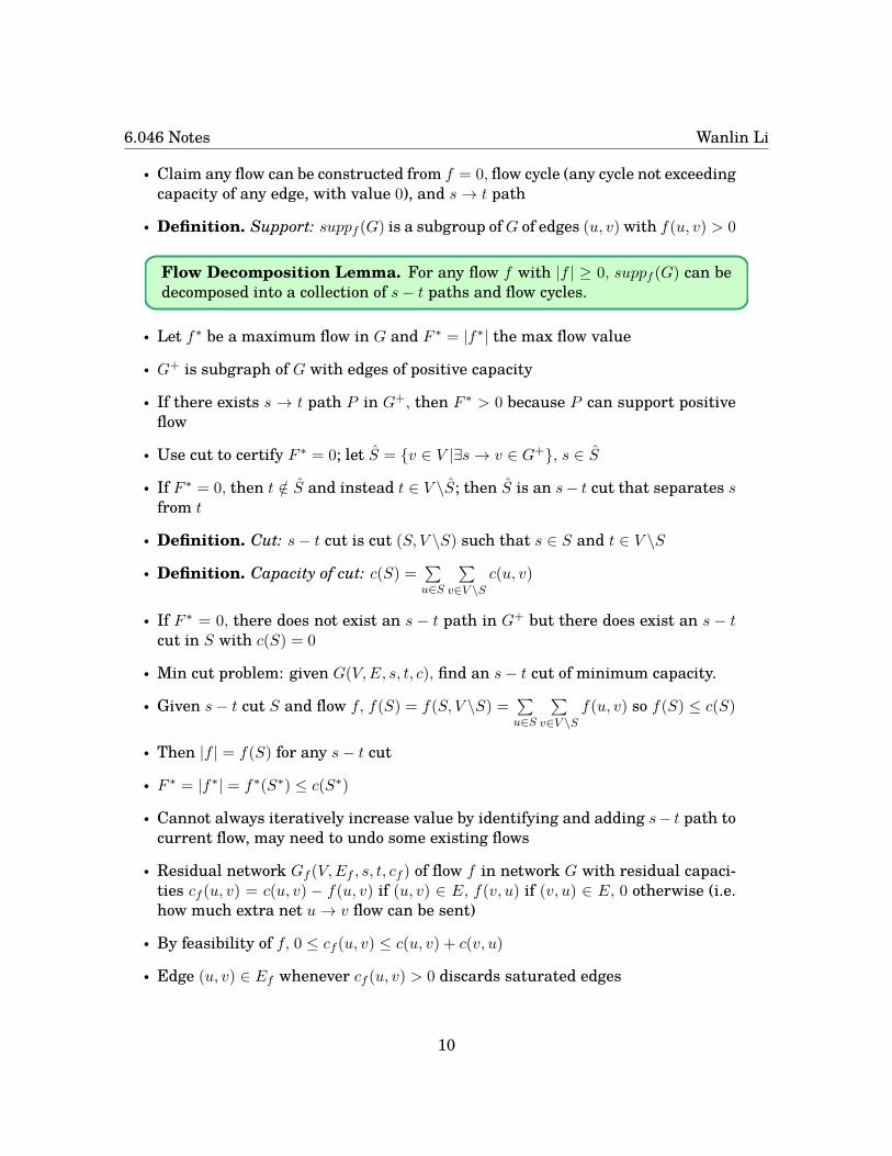
• Claim any flow can be constructed from f = 0, flow cycle (any cycle not exceedingcapacity of any edge, with value 0), and s→ t path

• Definition. Support: suppf (G) is a subgroup ofG of edges (u, v) with f(u, v) > 0

Flow Decomposition Lemma. For any flow f with |f | ≥ 0, suppf (G) can bedecomposed into a collection of s− t paths and flow cycles.

• Let f∗ be a maximum flow in G and F ∗ = |f∗| the max flow value

• G+ is subgraph of G with edges of positive capacity

• If there exists s → t path P in G+, then F ∗ > 0 because P can support positiveflow

• Use cut to certify F ∗ = 0; let S = v ∈ V |∃s→ v ∈ G+, s ∈ S

• If F ∗ = 0, then t /∈ S and instead t ∈ V \S; then S is an s− t cut that separates sfrom t

• Definition. Cut: s− t cut is cut (S, V \S) such that s ∈ S and t ∈ V \S

• Definition. Capacity of cut: c(S) =∑u∈S

∑v∈V \S

c(u, v)

• If F ∗ = 0, there does not exist an s − t path in G+ but there does exist an s − tcut in S with c(S) = 0

• Min cut problem: given G(V,E, s, t, c), find an s− t cut of minimum capacity.

• Given s− t cut S and flow f, f(S) = f(S, V \S) =∑u∈S

∑v∈V \S

f(u, v) so f(S) ≤ c(S)

• Then |f | = f(S) for any s− t cut

• F ∗ = |f∗| = f∗(S∗) ≤ c(S∗)

• Cannot always iteratively increase value by identifying and adding s− t path tocurrent flow, may need to undo some existing flows

• Residual network Gf (V,Ef , s, t, cf ) of flow f in network G with residual capaci-ties cf (u, v) = c(u, v) − f(u, v) if (u, v) ∈ E, f(v, u) if (v, u) ∈ E, 0 otherwise (i.e.how much extra net u→ v flow can be sent)

• By feasibility of f, 0 ≤ cf (u, v) ≤ c(u, v) + c(v, u)

• Edge (u, v) ∈ Ef whenever cf (u, v) > 0 discards saturated edges

10


• If f is flow in G and f ′ is flow in Gf , then f + f ′ is flow in G; reduces improvingflow f to finding nonzero flow in Gf

• If no non-zero flow in Gf , ∃s− t cut S with cf (S) = 0 (residual capacity)

• For any s − t cut S, cf (S) = c(S) − f(S) so if cf (S) = 0 then c(S) = |f |, c(S) =

|f | ≤ F ∗ ≤ c(S∗) ≤ c(S); f is max-flow and S is min s− t cut

• Max-flow min-cut Theorem: F ∗ = c(S∗)

• Max flow algorithm: augmenting path is directed s − t path in Gf , can pushadditional flow along augmenting path up to bottleneck capacity

• Total runtime O(EV C) if capacities are integers in [0, c], pseudopolynomial al-gorithm

8 March 5• Find max flow from residual network of flow, find augmenting path from s to t

in Gf (up to residual bottleneck capacity)

• Definition. Ford-Fulkerson Algorithm: start with zero flow, while augmentingpath P exists in Gf augment f along P

Max Flow Min Cut. The following are equivalent:

1. |f | = c(S) for some s− t cut S

2. f is a max flow

3. f admits no augmenting path

• Weak duality: if S∗ is minimum s − t cut and f∗ is max flow, then F ∗ = |f∗| ≤c(S∗)

• Strong duality F ∗ = c(S∗)

• Runtime of Ford-Fulkerson: each iteration/augmentation takesO(E) time, if ca-pacities are integers in [0, C] then total runtime is O(EV C) (pseudopolynomial)

• If capacities rational then runtime still finite and pseudopolynomial

• If capacities are real this could run for infinite time

Flow Integrality Theorem. If G = (V,E, s, t, c) has all capacities integral, thenthere exists a flow f such that |f | = F ∗ and both F ∗ and f are integral.

11


• Can still exist max flow that is not integral but has integral capacity

• Ford-Fulkerson picks any augmenting path, may be smarter choice

• Definition. Maximum bottleneck path: augmenting path P that maximizesbottleneck capacity cf (P )

• Maximum bottleneck path can be found inO(E log V ) time: binary search to findmaximum capacity c∗, c ≤ c∗ iff ∃s− t path in Gf after removing all edges withcf (u, v) < c

• Definition. Maximum bottleneck path algorithm: start with f(u, v) = 0 ∀u, v;while augmenting path exists, find augmenting path P with maximum bottle-neck capacity and augment flow with P

Lemma. In any graph G = (V,E, s, t, c), ther exists an s − t path in G withc(P ) = mine∈P c(e) ≥ F ∗

m where m = |E|

• Proof by flow decomposition lemma

• Corollary: MBP runs in O(m2 log n log nC) time

• Ford-Fulkerson still better when C is small

• MBP weakly polynomial time

• Definition. Edmonds-Karp algorithm: variant of Ford-Fulkerson, always chooseaugmenting path with fewest number of edges

• Edmonds-Karp runs in O(m2n) time, no dependency on edge capacities

• Applications of max flow: maximum bipartite graph matching problem (reduceto max flow), Ford-Fulkerson can give O(mn) time

9 March 7: Linear Programming• Linear programming example: how to campaign to win election based on af-

fected demographics and votes gained/lost from ads with goal to win majority ineach demographic while spending as little as possible

• Definition. Linear programming: minimize/maximize a linear objective func-tion subject to a set of linear constraints; variables as vector ~x ∈ Rm with objec-tive function ~c · ~x and constraints A~x ≤ ~b ∈ Rn where A is an n ×m constraintmatrix

12


• Standard LP form: maximize ~c · ~x subject to A · ~x ≤ ~b and ~x ≥ 0

• Transformations can change any LP to standard form, e.g. min to max by~c→ −~c

• Strict equality can be enforced using ≤ and ≥ combined, xi ∈ R can be trans-formed by x+

i ≥ 0 and x−i ≥ 0 and substituting xi = x+i − x

−i

• Geometric view: ~x is point in Rm, ~c is direction vector, want most extreme ~x indirection of~c subject to constraints which form polytope with at most n polygonalfacets

• Polytope may be unbounded (possibly no best solution) or empty (no solution, LPinfeasible)

Theorem. If the polytope is bounded, the optimal solution is a vertex of thepolytope.

• Simplex algorithm (greedy): start at any vertex in polytope, walk from vertexto vertex of feasible polytope in direction of ~c; very practical but exponential inworst-case

• Ellipsoid method: maintain ellipsoid containing optimal ~x∗, at each step cutellipsoid by hyperplane and find smaller ellipsoid containing optimal solution;geometric binary search, polynomial in worst-case and useful in theory but poorin practice

• Interior point method: start inside polytope and move vaguely in direction of ~c;polynomial in worst case and quite practical

• Simplex moves on edge of polytope, highly attuned to combinatorial structure ofconstraints

• Interior-point: moves inside polytope, ignores most combinatorial structure ofconstraints

• Integer linear programming (additional constraint that all xi are integers) isNP-complete

• Given LP in standard form: maximize ~c · ~x such that A~x ≤ ~b and ~x ≥ 0, considerdual LP min ~b · ~y such that AT~y ≥ ~c and ~y ≥ 0

• Corresponds to finding coefficients of linear constraints to sum to inequalityproving optimality of original LP

Weak LP duality. If ~x and ~y are feasible solutions to the primal and dual sys-tems, then ~c~x ≤ ~b~y.

13


Strong LP duality. If ~x∗ and ~y∗ are optimal feasible solutions to the primal anddual programs, then ~c~x∗ = ~b~y∗. Moreover, only one of the following four possibili-ties exists:

1. Both (P) and (D) have optimal solutions

2. (P) is unbounded and (D) is infeasible

3. (D) is unbounded and (P) is infeasible

4. Both (P) and (D) are infeasible

• Roles of (P) and (D) are completely symmetric

• Max flow min cut is special case of above strong duality

10 March 14• Game theory: performing thought experiments to help predict behavior of ra-

tional agent in situation of conflict

• Two player game: Aij is utility of playerR ifR plays i and C plays j; Bij is utilityof player C if R plays i and C plays j

• Definition. Two player zero sum games: A = −B where matrix A representsutility of row player and matrix B represents utility of column player

• Example. Rock paper scissors

• RPS has randomized stable outcome where each option is chosen with 13 proba-

bility

• Definition. Nash equilibrium: state of game such that no player has incen-tive to deviate from current strategy; no player can improve expected utility byunilaterally changing strategy

• Example. Testify, testify is deterministic Nash equilibrium of prisoner’s dilemmagame

Nash Equilibrium. Any game with a finite number of players and a finite num-ber of actions has a Nash equilibrium.

Min-Max Theorem. For any matrix A, if VR = maxx∈P miny∈Q xAy and VC =miny∈Q maxx∈P xAy, then VR = VC .

14


• P,Q are sets of positive vectors with sum of components equal to 1; correspondto probability distributions over rows and columns of matrix

• VR is expected utility of row player if row player goes first, VC is expected nega-tive utility of column player if column player goes first

• VR ≤ VC because VR corresponds to row player playing with handicap

• (x∗, y∗) corresponding to VR, VC is always Nash equilibrium of two-person zero-sum game described by A

• Nash equilibrium always exists for two person zero sum game

• Proof of min-max theorem by expressing VR, VC as linear program

• Need x ≥ 0 with∑xi = 1; if z = VR then for any column action j the expected

utility must be ≥ z

•∑

iAijxi ≥ z

• Want to maximize z

• By similar reasoning, VC = minu such that∑Aijyj)− u ≤ 0,

∑j yj = 1, y ≥ 0

• Observation: (R) and (C) programs are dual to each other so strong LP dualityimplies Min-Max Theorem

• C∗ = R∗ so C∗ ≥ VC ≥ VR ≥ R∗ and VC = VR

• Nash equilibrium always exists but finding it might be extremely difficult

• Simple stock market model: Xt is stock market index on day t with X0 = 0, eachday predict if Xt = Xt−1 + 1 or Xt = Xt−1 − 1

• Correct prediction gains one million, otherwise lose one million

• Given n experts, get up/down advice from each expert (not necessarily compe-tent); goal to do well when at least one expert is consistently providing decentadvice

• Define regret as number of mispredictions minus the number of mistakes of bestexpert

• Difficulty is best expert can only be identified in hindsight

• If best expert never makes a mistake, use Halving algorithm that maintainspool of trustworthy experts, at each step go with majority vote of trustworthyexperts and remove all experts that mispredicted

15


• Regret of Halving algorithm is log n

• In general setting, even best expert makesm∗mistakes; can use iterated halvingalgorithm and replenish trusted pool when emptied by putting all experts back

• Iterated halving algorithm has regret (m∗ + 1) log n

• Replenishing S fails to distinguish between very bad experts and decent experts

• Idea to use weights to capture trustworthiness of experts, start out with weightof 1 and in each round update estimate, reducing weight of expert by halvingupon each mistake

• Aggregate predictions by taking weighted majority of answers

• Weighted majority algorithm has regret of ≤ 2.4(m∗ + log n)

• Using (1 − ε)−1 as weight reduction factor instead of 2 for 0 < ε ≤ 12 , regret is

≤ (1 + ε)m∗ + 2ε log n

11 March 19: Randomized Algorithms• Randomized/probabilistic algorithm: generates random number and makes de-

cisions based on value of number; given same input, different executions mayhave different runtime or produce a different output

• Definition. Monte Carlo algorithms: always run in polynomial time with highprobability of correct output

• Definition. Las Vegas algorithms: run in expected polynomial time and alwaysgive correct output

• Matrix multiplication requires certain number of multiplications

• Matrix product verification: check if C = A×B, can multiply both sides by samerandom vector and checking agreement

• Definition. Frievald’s algorithm: choose random binary vector such that P (ri =1) = 1

2 independently; if A(Br) = Cr return yes, otherwise no

• Frievald is Monte Carlo algorithm because always time efficient but may be in-correct

• Runtime is O(n2) for three matrix vector multiplications

• Definition. Sensitivity: true positive rate

16


• Definition. Specificity: true negative rate

• Frievald has excellent sensitivity, claim C 6= AB means P (ABr 6= Cr) ≥ 12 ; let

D = C −AB with D 6= 0 so want to show there are many r with Dr 6= 0

• For any vector r with Dr = 0, ∃r′ such that Dr′ 6= 0

• Definition. Quicksort: divide and conquer algorithm with work mostly done individing step, sorts in place

• Basic, median-based pivoting, randomized quicksort (Las Vegas)

• Core quicksort: given n element array A, output sorted array

• Pick pivot element xp in A and partition into subarrays L = xi|xi < xp, G =xi|xi > xp; recursively sort subarrays

• Basic quicksort: choose pivot to be first element or last element, remove in turneach element xi from A and insert into L,E,G based on comparison to xp, canbe done in place

• Partition in Θ(n) time, worst case Θ(n2) (sorted or reverse sorted) but in practicedoes well on random inputs

• Median-based pivoting: guarantees balanced split, Θ(n log n) but loses to merge-sort in practice

• Randomized quicksort: xp chosen at random from A and new random choicemade at each recursion, expected running time O(n log n) for all input arrays

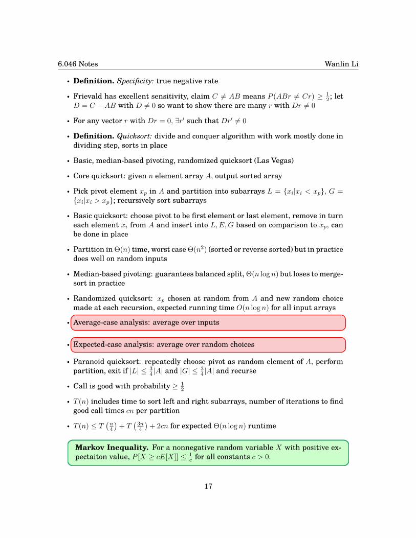
• Average-case analysis: average over inputs

• Expected-case analysis: average over random choices

• Paranoid quicksort: repeatedly choose pivot as random element of A, performpartition, exit if |L| ≤ 3

4 |A| and |G| ≤ 34 |A| and recurse

• Call is good with probability ≥ 12

• T (n) includes time to sort left and right subarrays, number of iterations to findgood call times cn per partition

• T (n) ≤ T(n4

)+ T

(3n4

)+ 2cn for expected Θ(n log n) runtime

Markov Inequality. For a nonnegative random variable X with positive ex-pectaiton value, P [X ≥ cE[X]] ≤ 1

c for all constants c > 0.

17


• Markov inequality bounds probability that random variable exceeds expectationby some proportion

• Proof by integration computation

• Markov inequality provides way to convert Las Vegas algorithm into MonteCarlo one; run Las Vegas for time cT where T is expected running time, newalgorithm completes efficiently but may not give correct answer

Chernoff Bound. For a random binary variable Y = B(n, p), P (Y ≥ E[Y ] +

r) ≤ e−2r2

n ∀r > 0 where n is the number of trials and p is the probability ofsuccess.

12 March 21: Random Walks and Markov Chain Monte CarloMethods

• Definition. Random graph walk: for undirected graph G = (V,E) and startingvertex s, start at s and repeat t times the process of randomly moving to neighborof current vertex

• If graph has non-negative edge weights, move to neighbor v′ with probabilityproportional to weight of (v, v′)

• Representation of random walk as trajectory: list of vertices visited in order ofvisiting

• Distribution: probability distribution on vertices induced by walks

• ptv is probability that walk visits vertex v at step t of walk

• Generally represent set of ptv across v as vector pt ∈ Rv where vth coordinate isptv

• Lazy random walk: allow random walk to remain at current vertex

• As t→∞, lazy walk can eliminate oscillation and lead to convergence of proba-bilities

• Given undirected graph, adjacency matrix A of G is n × n matrix Au,v = 1 if(v, u) ∈ E and 0 otherwise; degree matrixD is n×n diagonal matrix withDu,v =d(u) if u = v and 0 otherwise

• Walk matrixW = AD−1 withWu,v = 1d(v) if (v, u) ∈ E; then pt+1 = Wpt = W t+1p0

• W = PlI + (1− Pl)W for lazy random walks

18


• Many graphs converge to stationary distribution π independent of starting ver-tex

• Wπ = π or Wπ = π, represents steady state that exists whether or not walksactually converge to it

• πv = d(v)∑u∈V d(u) is a stationary distribution

Theorem. Every connected, non-bipartite, undirected graph has a stationarydistribution to which random walks in the graph are guaranteed to converge fort→∞. For lazy random walks, the graph does not have to be bipartite for this tobe true.

• For directed graphs, the graph must be strongly connected (every vertex reach-able from all other vertices) and aperiodic

• Example. Process of diffusion, self loops at end of chain

• Example. Card shuffling starting at one vertex in graph of 52! possibilities andperforming random walk

• Riffle shuffle, top to random both strongly connected, have stationary distribu-tions

• Mixing time for n cards approximately 32 log2(n) for riffle shuffle

• Problem of ranking web pages

• Count rank by making rank of page proportional to number of incoming edges(links to page); adjacency matrix times vector of all 1s

• Weight rank: weight recommendation is inverse of number of recommendationsmade by page wu =

∑v

1d(v)Au,v, WR = AD−11 = W1 where D is the outgoing

degree matrix

• Weight rank does not depend on importance of recommending page

• RecRank: RRu =∑

v∈V Au,v1

d(v)RRv, rec rank is a stationary distribution for W

• PageRank: (1 − α)W · Pr + αn1 where α is a parameter of choice and n = |V |;

stationary distribution for random process taking random step with probability(1− α) and jumps to random page with probability α

• Definition. Markov chain: process for which future staet of system dependsprobabilistically on current state of system without dependence on past states

19


• Definition. Metropolis-Hastings algorithm: states and stationary distributionare known, want to calculate transition probabilities; start at arbitrary ver-tex xt = x0, randomly pick neighbor xr as transition candidate and evaluatefr = P (xr)

P (xt); if fr ≥ 1 (trial vertex at least as probable in stationary distribution

as xt), accept trial move and let xt+1 = xr, repeat; otherwise accept trial withprobability fr, if rejected set xt+1 = xt and try again

• Metropolis-Hastings mimics random walk with appropriate stationary distribu-tion

13 April 2: Universal and Perfect Hashing• Dictionary problem: abstract data type to maintain set of keyed items subject

to insertion/deletion of item, search for key (return item with key if it exists)

• Items have distinct keys

• Easier than predecessor/successor problem solved by AVL trees or skip lists(O(log n)) or van Emde Boas (O(log log u))

• Hashing: goal of O(1) time per operation and O(n) space

• u is number of keys over all possible items, n is number of keys/items current intable and m is number of slots in table

• Hashing with chaining achieves O(1 + α) time per operation where α is loadfactor n

m

• With simple uniform hashing, probability of collision is 1m but requires assump-

tion that inputs are random, works only in average case (like basic quicksort)

• Universal hashing: choose random hash function h ∈ H where H is a universalhash family such that

Ph∈Hh(k) = h(k′) ≤ 1

m∀k 6= k′

• Then h is random, no assumption needed about input keys (like randomizedquicksort)

Theorem. For n arbitrary distinct keys and a random h ∈ H, the expected num-ber of keys colliding in a slot is at most 1 + α where α = n

m .

• Then insert, delete, search are expected to cost O(1 + α)

20


• Existence of universal hash families: e.g. all hash functions h : [u] → [n] isuniversal but useless because storing h takes logmu bits

• Definition. Dot product hash family: assume m prime (find nearby prime),assume u = mr for some integer r (round up), view keys in base m as k =〈k0, k1, . . . , kr−1〉 (cut up) and for key a = 〈a0, . . . , ar−1〉 define ha(k) = a ·k mod m(mix); then H = ha|a ∈ 0, 1, . . . , u− 1

• Storing ha requires storing just one key a

• Word RAM model: manipulatingO(1) machine words takesO(1) time and everyobject of interest (key) fits in a machine word

• Then ha(k) computation takes O(1) time

Theorem. The dot product hash family H is universal.

• Another universal hash family: choose prime p ≥ u and let hab(k) = [(ak +b) mod p] mod m, H = hab|a, b ∈ 0, 1, . . . , u− 1

• Static dictionary problem: given n keys to store in table, support search(k)

• Perfect hashing (no collisions): polynomial build time, O(1) worst case searchand O(n) worst case space

• Idea of two-level hashing: first pick h1 : 0, 1, . . . , u− 1 → 0, 1, . . . ,m− 1 froma universal hash family for m = Θ(n) (e.g. nearby prime) and hash all itemswith chaining using h1

• For each slot j ∈ 0, 1, . . . ,m−1 let lj be the number of items in slot j, pick h2,j :0, 1, . . . , u−1 → 0, 1, . . . ,mj from a universal hash family for l2j ≤ mj ≤ O(l2j )(nearby prime)

• Replace chain in slot j with hashing with chaining using h2,j

• Space is O(n+

∑m−1j=0 l2j

); if∑m−1

j=0 l2j > cn then redo first step

• Search time is O(1) for first table h1 +O(max chain size in second table)

• While h2,j(ki) = h2,j(ki′) for any i 6= i′, repick h2,j and rehash those lj items sothere are no collisions at the second level

• First and second steps are both O(n) buildtime

• Second hashing collision avoidance: expected to require at most 2 trials to reachgood h2,j so number of trials is O(log n) with high probability

21


• Chernoff bound: lj = O(log n) with high probability and each trial in O(log n)time, overall O(n log2 n) time with high probability

• Expected size of∑m−1

j=0 l2j is O(n) because m = Θ(n)

• For sufficiently large constant, by Markov inequality probability that h1 is notO(n) space is ≤ 1

2 so first step is O(n log n) with high probability

14 April 4: Streaming Algorithms• Definition. Streaming algorithms: with very limited memory (usually o(n) orO(log n)) and sequential access to data, characterize data stream; typically onlyoutput at end of input, correctness only approximate or probable

• n may refer to number of elements in stream or size of largest output of datastream

• Applications: networking (e.g. IP packet routing) to characterize network flows,identify threats; database modification and access to characterize patterns

• One pass through data stream (x1, x2, . . . , xn) with small local memory

• Exact algorithms (rare): statistics of input data stream (average, max, min, ma-jority, etc.), reservoir sampling (keep collection of elements that are uniformsample of input stream up to that point)

• Probably approximate alogirthms: number of distinct elements, additional fre-quency moments Fp =

∑mi=1(fi)

p

• Want some degree of correctness guarantee

• For simple statistics, computing average or max requires keeping partial answerwhich requires only O(log n) space and one pass

• Given input stream with majority element (occurs > n2 times): each instance of

non-majority element can be cancelled by some other element, majority elementwill remain

• Reservoir sampling: given input stream of elements xi, keep one representativeelement for output with probability 1

n but don’t know n in advance

• Solution: keep x1 in storage, when xi is read replace storage element with xiwith probability 1

i ; at each step, random sample from x1, . . . , xi is stored

• Instead of storing single element, store reservoir of k elements each with prob-ability k

n

22


• Keep first k elements, for each further element xi+1 with probability ki+1 keep it

and remove random reservoir element

• Weighted sampling: each element comes with weight wi, output according toweighted probability; keep xi with probaiblity wi∑i

j=1 wj

• Definition. Frequency moment: Fp =∑m

i=1 fpi where fi is number of times items

i appears in input stream and each xi ∈ [m]

• Frequency moments tend to be approximate rather than exact for streamingalgorithms

• Example. F0 is number of distinct elements under convention 00 = 0

• Example. F2 corresponds to size of database joins

• Probabilistic approximation: compute (ε, δ) approximation F0 to F0 such thatwith probability ≥ 1− δ, (1− ε)F0 ≤ F0 ≤ (1 + ε)F0

• Deterministic approximate algorithm and randomized exact algorithm both im-possible, δ, ε both needed for streaming algorithm

• Estimate F0 by pairwise-independent hash functions: family of hash functionsH = h : X → Y such that h(x1) and h(x2) are independent for all x1 6= x2

where randomness is over choice of hash function

• Equivalent condition: for every x1 6= x2 ∈ X, y1, y2 ∈ Y, P [h(x1) = y1 AND h(x2) =y2] = 1

|Y |2

• Many possible constructions

• H = h : [m] → [m] is pairwise independent family of hash functions, z(x) isnumber of trailing zeros of x in binary

• Algorithm: start with z = 0, for each item j, compute h(j) and test if z(h(j)) > z,set z to be z(h(j)); return 2z as estimate for F0

• With d distinct elements, Y is set of bins of elements ending with each binarystring of length log d

• With d unique elements, there is good chance one will hash to first bin (elementsending with log d zeros) making output ≥ d with good chance

• With >> d bins, good chance that no element will hash to first bin so output is< 2log(cd) = cd with good chance

• Claim for any c > 1, 1c ≤

F0F0≤ c with probability 2

c

• P (z(h(j)) ≥ r) = 12r and P (z(h(j)) ≥ r AND z(h(k)) ≥ r) = 1

22r

23


15 April 9: Dynamic Programming I• Definition. Memoization: use some form of look-up table to store previously-

solved subproblem solutions

• Iterative approach: solve subproblems in smaller-to-larger order

• Dynamic programming: essentially clever brute force solution, reduce generallyexponential problem to polynomial one through reuse of subproblem solutions

• For DP to be effective (polynomial), needed polynomial number of unique sub-problems, polynomial number of cases per subproblem, polynomial time to com-pute problem solution given subproblem solutions

• Subproblem dependency graph must be DAG

• Top down approach: corresponds to DFS of subproblem dependency graph, gen-erally larger asymptotic constants

• Bottom up approach: systematically fill subproblem solution storage in orderdictated by subproblem dependency graph, only need to consider each subprob-lem once but does not skip unnecessary subproblems

• Alternating coins game: row of n coins of value v1, . . . , vn with n even, 2 playerstake turns in which player removes first or last coin and receives correspondingvalue

• Must have one function for each player

• Optimal BST problem: given set of keys k1, . . . , kn and search probabilitiesp1, . . . , pn, construct optimal binary search tree to store keys minimizing ex-pected search costs

∑pi(d(ki) + 1) where d(ki) is depth of ki

• Enumeration of all BSTs is too large, greedy approach not guaranteed to becorrect

• Split subproblems through choice of key at root, Θ(n2) subproblems and Θ(n)per subproblem

16 April 11: Dynamic Programming II• Edit distance: given two sequences and catalog of edit functions and their as-

sociated costs (insert, delete, substitute), find minimum cost for converting onestring into the other

• Optimal alignment contains optimal subalignments e.g. prefixes X1,i → Y1,j

24


• Subproblems involve removing single character from right-hand end of one orboth strings

• Runtime Θ(mn) where m,n are lengths of sequences; mn subproblems each re-quiring O(1) time

• Knapsack problem: want to fill knapsack with goods of n types of various valueand weight, produce sack of maximal value without exceeding given weight ca-pacity W

• Subproblem structure based on smaller weight capacity

• O(nW ) runtime

• Definition. Pseudopolynomial runtime: polynomial in number of items butexponential in storage of weights/values

• General longest path in graph lacks optimal substructure but longest path inDAG has optimal substructure

• DFS can be used to sort DAG into topologically sorted order

• Topologically sort G, for each vertex v ∈ V in sorted order before s set distanceto be −∞

17 April 18• Seemingly related problems can have vastly different difficulties

• Example. Shortest path (polynomial time) vs longest path (no polynomial timealgorithm known)

• MST (given weighted graph, find spanning tre of minimum weight) vs TSP (findspanning simple cylce of minimum weight)

• Bipartite vs tripartite matching

• Optimization version of problem (MST): given weighted graph, find spanningtree of minimum weight; result is tree or report that graph is not connected

• Search version of problem: given weight graph and budgetK, find spanning treewhose weight is ≤ K or report that none exists; result is tree or report that Kis too small or that graph is not connected

• Decision version of problem: given weighted graph and budgetK, decide whetherthere exists spanning tree with weight ≤ K; result is yes or no

25


• Existence of polynomial time solution to optimization implies polynomial time tosearch; existence of polynomial time solution to search implies one for decision

• For showing intractability, generally focus on decision version because beingunsolvable in polynomial time implies the others are also unsolvable in poly-nomial time

• Decision problem π is solvable in polynomial time if there exists a polynomial-time algorithm A such that for all x, x is a yes input for π iff A(x) outputs yes

• NP: non-deterministic polynomial time captures problems with polynomiallyshort and polynomial time verifiable certificates of yes instances

• π ∈NP if there exists a polynomial-time verification algorithm Vπ and a constantc such that for all x, π(x) is yes iff there exists a certificate y such that |y| ≤ |x|cand Vπ(x, y) is yes

• Reduction: for input x, problem π1, algorithm for π2, some function R(x) suchthat A(R(x)) is solution to π1

• Polynomial time reduction from π1 to π2 useful when π2 ∈ P and want to showπ1 ∈ P or when π1 is hard and want to deduce that π2 is also hard

• Definition. Reduction: polynomial-time reduction from π1 to π2 is polynomial-time algorithm R such that if x is an input to π1, then R(x) is an input to π2 andπ1(x) is yes iff π2(R(x)) is yes

• If polynomial time reduction from π1 to π2 exists, π1 ≤p π2 (π2 at least as hardas π1)

• Definition. NP-hard: problem π such that for all π′ ∈ NP, π′ ≤p π

• Definition. NP-complete: problem π such that π ∈ NP and π is NP-hard

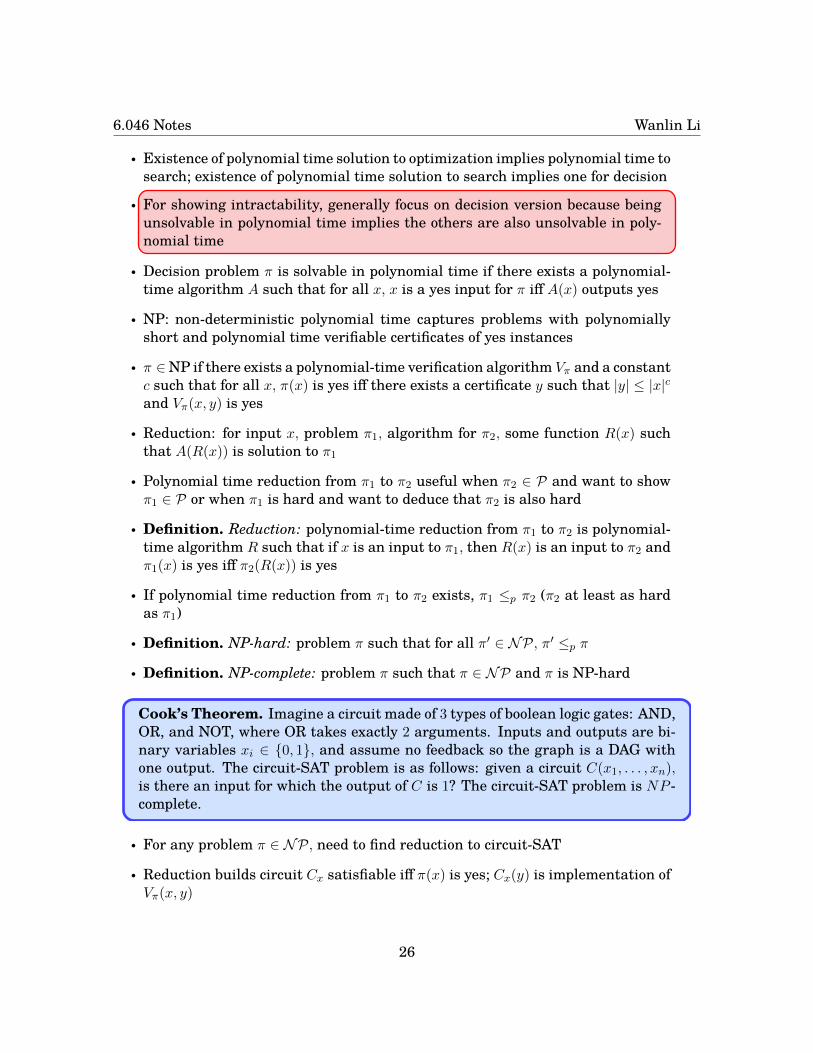
Cook’s Theorem. Imagine a circuit made of 3 types of boolean logic gates: AND,OR, and NOT, where OR takes exactly 2 arguments. Inputs and outputs are bi-nary variables xi ∈ 0, 1, and assume no feedback so the graph is a DAG withone output. The circuit-SAT problem is as follows: given a circuit C(x1, . . . , xn),is there an input for which the output of C is 1? The circuit-SAT problem is NP -complete.

• For any problem π ∈ NP, need to find reduction to circuit-SAT

• Reduction builds circuit Cx satisfiable iff π(x) is yes; Cx(y) is implementation ofVπ(x, y)

26


18 April 25

Cook’s Theorem. Circui-SAT is NP-complete.

• cSAT: given boolean circuit of AND, OR, NOT gates and no feedback, is there aset of 0, 1 input values to produce an output of 1

• Definition. SAT problem: given boolean formula, is it satisfiable? e.g. φ =(x1 ∨ x2) ∧ x3 ∧ (x3 ∨ x1 ∨ x2)

• Formulas of n boolean variables x1, . . . , xn, m boolean connectives ∧,∨, NOT,⇒,⇔, parentheses

• To show SAT is NP-hard, only need to show SAT is at least as hard as cSAT

• Given reduction, need to show circuit is satisfiable iff φ is satisfiable

• Definition. 3-SAT: given formula φ in conjunctive normal form (AND of ORs)with 3 literals per clause, is φ satisfiable?

• Example. φ = (x1 ∨ x2) ∧ x3 ∧ (x3 ∨ x1 ∨ x2) is not valid 3-SAT input because thefirst two clauses do not have three literals each

• Karp showed 3-SAT is NP-complete

• Definition. Vertex cover problem: given a graph G = (V,E) and an integer k,does there exist a subset S ⊆ V such that |S| ≤ k and every edge e ∈ E is incidentto at least one vertex in S?

• Would like to reduce 3-SAT to VC (vertex cover)

• Gadget construction: for each variable, assign gadget (subgraph ofG) represent-ing its truth value; for each clause assign gadget representing that at least oneliteral must be true, assign edges connecting these kinds of gadgets

• For each variable create edge with two vertices pxi , nxi , for each clause create3-cycle fci , sci , tci (all these vertices distinct)

• If first literal of clause ci is xj , add edge (fci , pxj ) and if first literal is xj , addedge (fci , nxj ) corresponding to positive or negative

• If clause is satisfied, at least one of its outgoing incident edges (to variable) iscovered; remaining 2 edges covered by picking two nodes from triangle

• Covering outgoing edge from variable node equivalent to satisfying correspond-ing literal in clause

27


• Exists vertex cover of size k = 2m+ n iff φ is satisfiable

• If pxi is vertex cover, set xi = 1 and otherwise xi = 0

• If ~x is a satisfying assignment and xi = 1, include pxi in VC and nxi otherwise,then pick 2 other vertices from each of the m clause gadgets to cover all edges

• Therefore VC is NP-complete

• Beyond NP-completeness: approximation algorithms, intelligent exponentialsearch, average case analysis, special input cases

19 April 30: Approximation Algorithms• Want algorithms to solve hard (NP-hard) problems using fast algorithms to ob-

tain exact solutions

• Can obtain solutions satisfying any two conditions but not all three (currently)

• Hard problems in polynomial time require approximation algorithms; optimiza-tion version of problem

• Given optimization problem of size n, c∗ is cost of optimal solution and c is costof approximate solution

• Ratio bound ρ(n) = max cc∗ ,c∗

c ≤ ρ(n) ∀n gives ρ(n)-approximation algorithm

• Approximation scheme takes ε > 0 as input and provides (1 + ε)-approximationalgorithm

• Polynomial time approximation scheme provides algorithm polynomial in n butnot necessarily in 1

ε e.g. O(n2/ε)

• Fully polyonmial time approximation scheme: provides algorithm polynomial inn and 1

ε e.g. O(nε2

)• Vertex cover optimization version: input graphG(V,E) and output set of verticesS ⊆ V such that for all edges e ∈ E, S ∩ e 6= ∅ with objective to minimize |S|

• 2-approximation algorithm for VC: pick any edge (u, v) ∈ E, add both u, v to Sand remove all edges from E incident to one of the vertices; repeat until E isempty

• Runtime O(V + E), non-deterministic (depends on order of edge selection), Salways a valid vertex cover

28


• Set cover: given set X of n points and m subsets Si of X whose union is X, findcover C ⊆ [m] such that

⋃i∈C Si = X and |C| is minimized

• Greedy algorithm: while some element is not covered, choose new set Si con-taining maximum number of uncovered elements and add i to cover

• Number of iterations is O(min(n,m)) and overall runtime is O(mnmin(m,n))

• Greedy set cover is (lnn+1)-approximation; on each iteration, 1|COPT|

of remainingelements are covered

• If t = |COPT| and Xi is set of remaining elements on each iteration i, Xi can becovered by ≤ t sets and there exists a set that covers ≥ |Xi|

t elements

• Partition problem (NP-hard): given sorted list of n positive numbers s1 ≥ · · · ≥sn, find partition of indices [n] into two setsA,B such that max

∑i∈A si,

∑j∈B sj

is minimized; find most balanced partition

• Let m =⌈

1ε

⌉− 1 so ε ≥ 1

m+1 ; find optimal partition A′, B′ for first m numberss1, . . . , sm which takes constant time wrt n

• For each successive element si, add si to partition with smaller sum

• (1 + ε)-approximation algorithm, takes O(n) time

• Greedy algorithm on vertex cover selecting vertices of maximum degree: poly-nomial time and returns valid vertex cover

• There exist inputs on which greedy vertex cover is extremely suboptimal, e.g.bipartite graph where k! vertices have degree k in the first group and secondgroup has k!

i vertices of degree i for each i; greedy may pick all vertices in secondgroup

• Linear programming relaxation for vertex cover: assign indicator xi to each ver-tex vi ∈ V

• Seek to minimize∑xi subject to 0 ≤ xi ≤ 1 (temporarily relax integer con-

straint) and xi + xj ≥ 1 for all edges (vi, vj) ∈ E

• Take x∗i = 1 iff xi ≥ 12 for 2-approximation algorithm

20 May 2: Distributed Algorithms• Computing paradigms: parallel computing (multiple processor cores), paral-

lelize task when benefit from more identical workers; distributed computing(computer networks/internet), cooperate to solve joint task even when some com-ponents are not cooperating

29


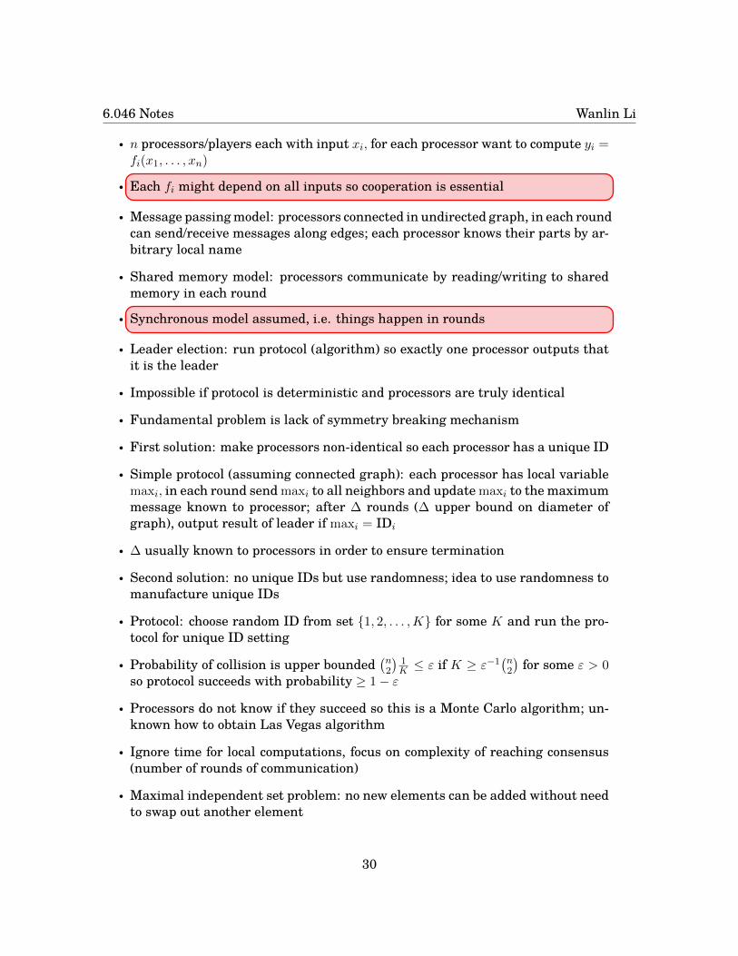
• n processors/players each with input xi, for each processor want to compute yi =fi(x1, . . . , xn)

• Each fi might depend on all inputs so cooperation is essential

• Message passing model: processors connected in undirected graph, in each roundcan send/receive messages along edges; each processor knows their parts by ar-bitrary local name

• Shared memory model: processors communicate by reading/writing to sharedmemory in each round

• Synchronous model assumed, i.e. things happen in rounds

• Leader election: run protocol (algorithm) so exactly one processor outputs thatit is the leader

• Impossible if protocol is deterministic and processors are truly identical

• Fundamental problem is lack of symmetry breaking mechanism

• First solution: make processors non-identical so each processor has a unique ID

• Simple protocol (assuming connected graph): each processor has local variablemaxi, in each round send maxi to all neighbors and update maxi to the maximummessage known to processor; after ∆ rounds (∆ upper bound on diameter ofgraph), output result of leader if maxi = IDi

• ∆ usually known to processors in order to ensure termination

• Second solution: no unique IDs but use randomness; idea to use randomness tomanufacture unique IDs

• Protocol: choose random ID from set 1, 2, . . . ,K for some K and run the pro-tocol for unique ID setting

• Probability of collision is upper bounded(n2

)1K ≤ ε if K ≥ ε−1

(n2

)for some ε > 0

so protocol succeeds with probability ≥ 1− ε

• Processors do not know if they succeed so this is a Monte Carlo algorithm; un-known how to obtain Las Vegas algorithm

• Ignore time for local computations, focus on complexity of reaching consensus(number of rounds of communication)

• Maximal independent set problem: no new elements can be added without needto swap out another element

30


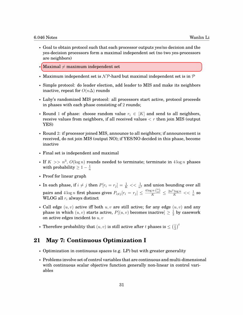
• Goal to obtain protocol such that each processor outputs yes/no decision and theyes-decision processors form a maximal independent set (no two yes-processorsare neighbors)

• Maximal 6= maximum independent set

• Maximum independent set is NP-hard but maximal independent set is in P

• Simple protocol: do leader election, add leader to MIS and make its neighborsinactive, repeat for O(n∆) rounds

• Luby’s randomized MIS protocol: all processors start active, protocol proceedsin phases with each phase consisting of 2 rounds;

• Round 1 of phase: choose random value ri ∈ [K] and send to all neighbors,receive values from neighbors, if all received values < r then join MIS (outputYES)

• Round 2: if processor joined MIS, announce to all neighbors; if announcement isreceived, do not join MIS (output NO); if YES/NO decided in this phase, becomeinactive

• Final set is independent and maximal

• If K >> n3, O(log n) rounds needed to terminate; terminate in 4 log n phaseswith probability ≥ 1− 1

n

• Proof for linear graph

• In each phase, if i 6= j then P [ri = rj ] = 1K << 1

n3 and union bounding over allpairs and 4 log n first phases gives Pi 6=j [ri = rj ] ≤

4 logn·(n2)K ≤ 2n2 logn

K << 1n so

WLOG all ri always distinct

• Call edge (u, v) active iff both u, v are still active; for any edge (u, v) and anyphase in which (u, v) starts active, P [(u, v) becomes inactive] ≥ 1

2 by caseworkon active edges incident to u, v

• Therefore probability that (u, v) is still active after t phases is ≤(

12

)t21 May 7: Continuous Optimization I• Optimization in continuous spaces (e.g. LP) but with greater generality

• Problems involve set of control variables that are continuous and multi-dimensionalwith continuous scalar objective function generally non-linear in control vari-ables

31


• Model of some type required to specify relationship between control and objec-tive

• Definition. Unconstrained minimization: given a real-valued function f : Rn →R, find its minimum, assuming it exists.

• For maximum, take min of −f ; if constraints required, minimize g(x) = f(x) +ψ(x) where ψ(x)→∞ when constraints violated and ψ(x) = 0 otherwise

• Assume f continuous and infinitely differentiable

• Definition. Gradient descent: iterative approach of locally using gradient tocontinuously attempt to make improvements by walking downhill; locally greedyapproach

• Linear expansion about current point ~x, move in opposite direction as ∇f(~x)because ∇f is direction of greatest local increase

• Algorithm: begin at some starting point ~x(0), for each i set ~x(i+1) = ~x(i)−ηi~∇f(~x(i))

• Local optimality when gradient is 0; does not improve on local optimum but canlocally perturb and continue from maximum or saddle point

• f(~x+ ~δ) ≈ f(~x) +[~∇f(~x)

]Tδ + 1

2δT∇2f(~x)δ + · · ·

• f is β-smooth if δT∇2f(~x)δ ≤ β||δ||2 for all x, δ ∈ Rn

• Plugging in choice of step gives δ = −η~∇f(~x) so f(~x + δ) ≤ f(~x) − η||~∇f(~x)||2 +βη2

2 ||~∇f(~x)||2 where first term is expected progress and second term is expectederror; if η ≈ 1

β , progress should exceed error in estimated progress (need η ≤ 2β )

• Expected minimum progress in ith step is 12β ||~∇f(~x(i))||2

• Gradient descent converges to point ~x with ~∇f(~x) = 0 (local min/max or saddle)or diverges to f(~x)→ −∞

• Local min may not be global min

• Gradient descent guaranteed to converge to global min when f is convex

• Definition. Convex function: f(λ~x + (1 − λ)~y) ≤ λf(~x) + (1 − λ)f(~y) for all0 ≤ λ ≤ 1 or equivalently, f(~x+ δ) ≥ f(~x) +

[~∇f(~x)

]Tδ for all x, δ

• Convergence analysis: how quickly gradient descent converges

32


• Let ~x∗ be the minimum of convex function f ; f(~x∗) ≥ f(~x) +[~∇f(~x)

]T(~x∗−~x) so

f(~x)− f(~x∗) ≤ −[~∇f(~x)]T (~x∗ − ~x) ≤ ||~∇f(~x)|| · ||~x∗ − ~x|| ≤ ε by Cauchy-Schwarz

• This is dependent on the unknown distance between ~x and ~x∗

• Definition. α-strong convexity: f α-strongly convex if ~yT∇2f(~x)~y ≥ α||~y||2 forall ~x, ~y ∈ Rn with α ≥ 0

• Normal convexity is α = 0

• For α-strong convex function, f(x+δ) ≥ f(x)+[~∇f(~x)

]Tδ+α

2 ||δ||2 so convergence

to minimum has f(~x)− f(~x∗) ≥ α2 ||~x− ~x

∗||2

• Within ε of optimum requires O(K log f(~x(0))−f(~x∗)

ε

)steps where K = β

α ≥ 1 isthe condition number of f

• If function not strongly convex, idea to construct new function based on f thatis α-convex by adding α||~x− ~x(0)||2 (regularization)

• New function has possibly different optimum; reduce regularization as ~x∗ is ap-proached

22 May 9: Applications of Gradient Descent• Unconstrained minimization given smooth and continuous f : Rn → R by locally

greedy gradient descent method

• Hessian matrix ∇2f(x)

• As t→∞, x(t) either diverges to −∞ or converges to critical point

• If f is convex, every critical point is a global minimum

• Convergence analysis for strongly convex function

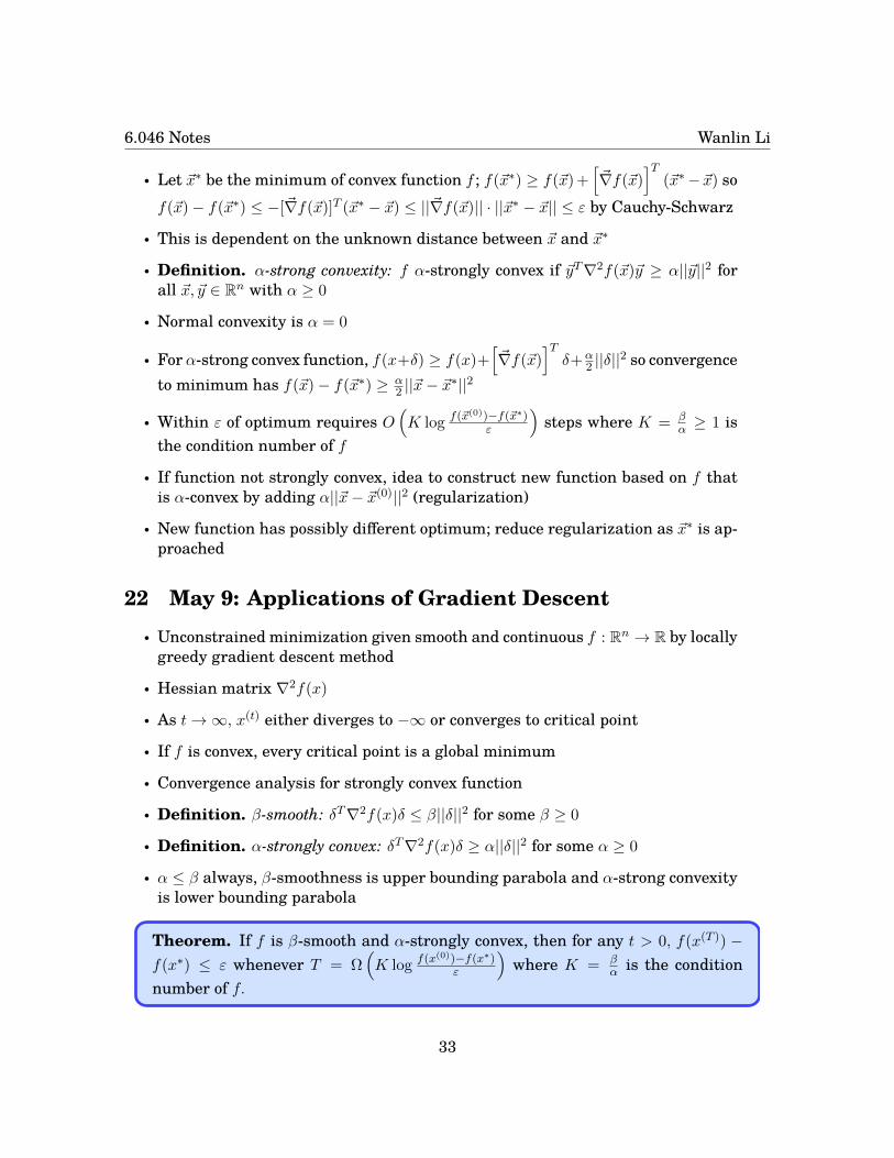
• Definition. β-smooth: δT∇2f(x)δ ≤ β||δ||2 for some β ≥ 0

• Definition. α-strongly convex: δT∇2f(x)δ ≥ α||δ||2 for some α ≥ 0

• α ≤ β always, β-smoothness is upper bounding parabola and α-strong convexityis lower bounding parabola

Theorem. If f is β-smooth and α-strongly convex, then for any t > 0, f(x(T )) −f(x∗) ≤ ε whenever T = Ω

(K log f(x(0))−f(x∗)

ε

)where K = β

α is the conditionnumber of f.

33


• Step size η ≈ 1β ; can also binary search to minimize error term

• K measures quality of local approximation of f at x

• Condition number K is main factor affecting growth of number of steps

• Key application domain of gradient descent is training machine learning models

• Linear regression as illustrative example: m data points x(1), . . . , x(m) ∈ Rn andm labels y(1), . . . , y(m) ∈ R; goal to find linear function that predicts each y(j)

given x(j)

• Popular choice for measure of best fit given by mean squared error L(w) =1m

∑Ej(w)2

• Goal to compute argument with minimum L(w)

• Gradient update takes majority vote of all data point updates

• Classic approach to solving linear system is by directly computing inverse matrixbut this is always fairly slow and numerically problematic

• Iterative approach: start with some x(0), iteratively improve solution by gradientdescent on function fA(x) = 1

2xT (ATA)x−AT bx so any critical point is a solution

• Beyond linear classifications by increasing number of dimensions, i.e. sendingx to x2 to send lines to parabolas in original space

• Deep learning: work with mapping expressed by neural network with param-eters, resulting optimization problems are highly non-convex but gradient de-scent still delivers good solutions for unknown reason

23 May 14: Quantum Computation• Represent each step of computation as n-bit binary string with transitions given

by 2n × 2n matrix

• Randomized model of computation has states as probability distributions in 2n

space, transitions are stochastic matrices

• In quantum model, universes interact and can cancel each other out

• Quantum operations must be invertible, restricts operations that can be carriedout

• Qubit: state represented as linear combinations of basis vectors over C

34


• Transition matrix is unitary, MM∗ = I to preserve lengths; state vectors havelength 1

• Quantum computing enables operations nonexistent in classical computations

• 2-qubit means n = 2

• States cannot always be separated by qubit (states of individual qubits not nec-essarily independent)

• Paradox of entanglement: measurement of first qubit can determine outcome ofsecond qubit arbitrarily far away

No-cloning Theorem. There is no quantum operation U such that (α |0〉 +β |1〉)(|0〉)→ (α |0〉+ β |1〉)(α |0〉+ β |1〉) for all α, β ∈ C.

• Can be used to design quantum money that is impossible to counterfeit or designperfectly secure protocols

• Computing XOR: given f : 0, 1 → 0, 1, compute f(0)⊕ f(1) in as few queriesas possible

• Classical model requires two queries

• Quantum query to f is given by query transformation Uf : |x y〉 → |x (y ⊕ f(x))〉for all x, y ∈ 0, 1 to ensure Uf is reversible

• Quantum algorithm to compute XOR with single query: start with |0 0〉 , flip thesecond bit, apply Hadamard gate to both bits, apply Uf , then apply Hadamardgate again to the first bit

• Hadamard gate sends |0〉 to 1√2(|0〉+ |1〉) and |1〉 to 1√

2(|0〉 − |1〉)

• This algorithm causes cancellation of undesirable states and measuring the firstqubit gives the correct answer

35