

6.11s June 2006 L3 1
6.11s Notes for Lecture 3
PM ‘Brushless DC’ Machines: Elements of Design
June 14, 2006
J.L. Kirtley Jr.
6.11s June 2006 L3 2
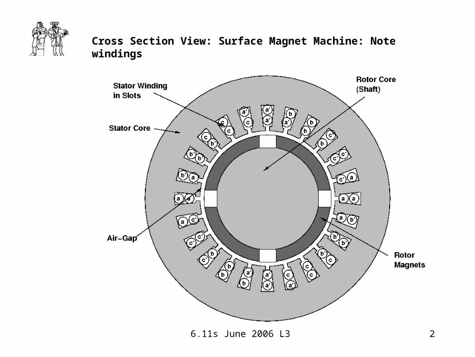
Cross Section View: Surface Magnet Machine: Note windings

6.11s June 2006 L3 3
Alternate: Surface Mount (‘Iron Free’) Armature Winding
6.11s June 2006 L3 4
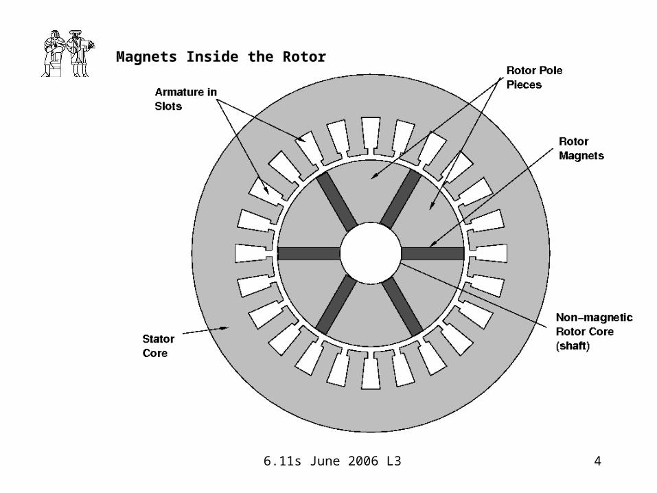
Magnets Inside the Rotor
6.11s June 2006 L3 5
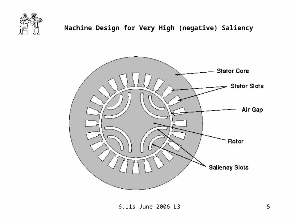
Machine Design for Very High (negative) Saliency

6.11s June 2006 L3 6
Focus on Rating:
€
P + jQ =q
2VI =
q
2
Ea
NNI
V
Ea
Ea =ωλ
N=ωφ
φ =2RlB1
pkw
Rating is number of phases times voltage times current
Internal voltage is frequency times flux
And flux is the integral of Flux density
We will consider winding factor below
6.11s June 2006 L3 7
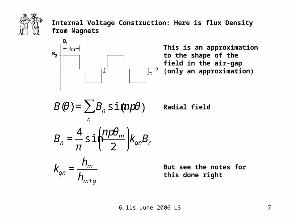
Internal Voltage Construction: Here is flux Density from Magnets
€
B(θ) = Bn sin npθ( )n
∑
Bn =4
πsin
npθm
2
⎛
⎝ ⎜
⎞
⎠ ⎟kgnBr
kgn =hm
hm+g
This is an approximation to the shape of the field in the air-gap (only an approximation)
Radial field
But see the notes for this done right

6.11s June 2006 L3 8
€
kg =Ri
p−1
Rs2p − Ri
2p
p
p+1R2
p+1 − R1p+1
( ) + Rs2p p
p−1R2
1− p − R11− p
( ) ⎛
⎝ ⎜
⎞
⎠ ⎟
Magnetic field can be found through a little field analysis
The result below is good for magnets inside and p not equal to one. See the notes for other expressions
€
kg =Rs
p−1
Rs2p − Ri
2p
p
p+1R2
p+1 − R1p+1
( ) + Ri2p p
p−1R2
1− p − R11− p
( ) ⎛
⎝ ⎜
⎞
⎠ ⎟
Stator winding outside:
Stator winding inside:
6.11s June 2006 L3 9
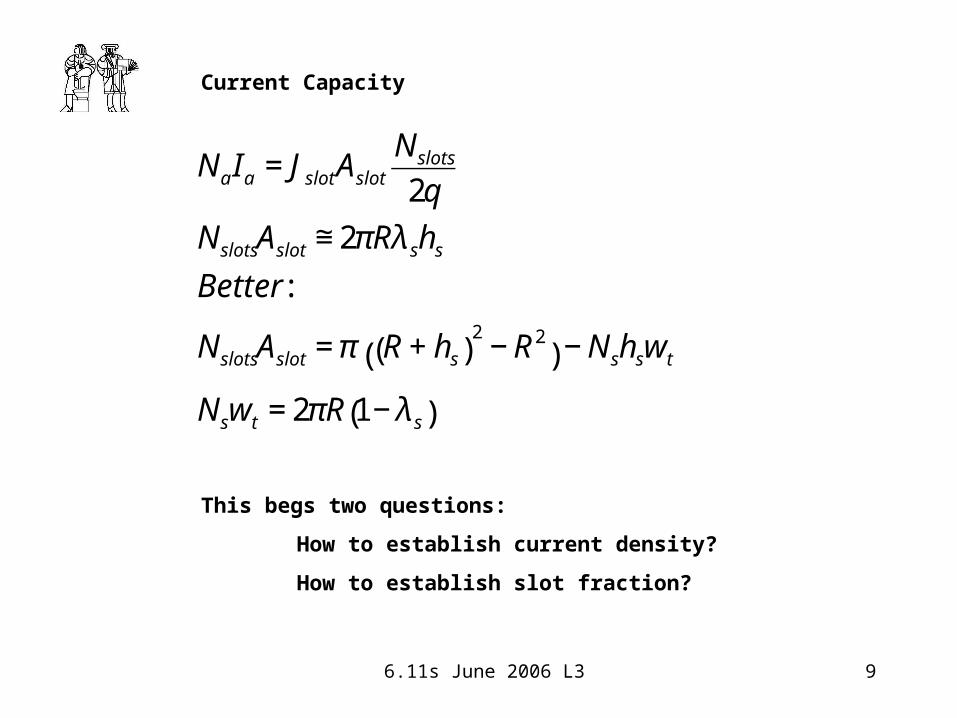
Current Capacity
€
NaIa = JslotAslot
Nslots
2q
NslotsAslot ≅ 2πRλ shs
Better :
NslotsAslot = π R + hs( )2
− R2( ) − Nshswt
Nswt = 2πR 1− λ s( )
This begs two questions:
How to establish current density?
How to establish slot fraction?

6.11s June 2006 L3 10
Voltage Ratio
€
Ea2 =V 2 + Xd Ia( )
2− 2VXd Ia cosθ
Ea2 =V 2 + Xd Ia( )
2+ 2VXd Ia sinψ
1 =V
Ea
⎛
⎝ ⎜
⎞
⎠ ⎟
2
+Xd IaEa
⎛
⎝ ⎜
⎞
⎠ ⎟
2
+ 2V
Ea
Xd IaEa
sinψ
V
Ea
= 1−Xd IaEa
cosψ ⎛
⎝ ⎜
⎞
⎠ ⎟
2
−Xd IaEa
sinψ

6.11s June 2006 L3 11
Calculation of Inductance: Start with a Full-Pitch Coil Set
This current distribution makes the flux distribution below

6.11s June 2006 L3 12
€
Br = μ0
4
π
NaIapgm
sin pθ( )
λ = lNa Br θ( )Rdθ0
π
p
∫
La = μ0
4
π
RlNa
p2gm
Ld = μ0
3
2
4
π
RlNakw2
p2gm
Ld = μ0
3
2
4
π
RlNakw2
p2(g+ hm )
Fundamental Flux Density
Flux Linkage
Idealized inductance of a full-pitch coil
Taking into account phase-phase coupling (for 3 phase machine) and winding factor
And for the PM machine the magneti is part of the magnetic gap

6.11s June 2006 L3 13
€
kw = kbkp
This is what we mean by short pitch: see the original drawing
€
λ fp = l B1 sin θ( )Rdθ0
π
p
∫ =2RlB1
p
λ sp = l B1 sin θ( )Rdθπ
2p−
α
2p
π
2p+
α
2p
∫
=2RlB1
psin
α
2
kp =λ sp
λ fp
= sinα
2

6.11s June 2006 L3 14
Breadth Factor: Coils link flux slightly out of phase
Here is a construction of the flux addition. It takes a bit of high-school like geometry to show that:
€
kb =sin
mγ
2
msinγ
2
The breadth factor is just the length of the addition of the vectors divided by the length of one times the number of vectors

6.11s June 2006 L3 15
Slot Leakage: Suppose the slot were to look like this: It actually has two coils that have Nc half turns each.
Flux linked by one coil from one driven coil is:
€
λ =℘sNc2Ia℘ s = μ0
hd
wd
+1
3
ws
hs
⎛
⎝ ⎜
⎞
⎠ ⎟
Llc = Nc2℘ s
Use top of slot dimensions for tapered slots: very small error

6.11s June 2006 L3 16
There are 2p(m-Nsp) slots with both coils in the same phase
And 2p Nsp slots with coils ineach of the different phases (in each phase)
So slot leakage is
€
Lsl = 4Llc × 2p(m − Nsp ) + Llc × 2pNsp
= Llc 8pm − 6pNsp( )
6.11s June 2006 L3 17
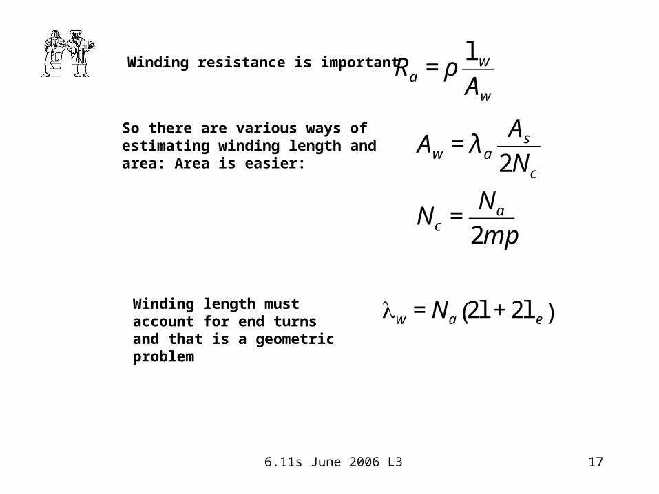
Winding resistance is important
€
Ra = ρl w
Aw
So there are various ways of estimating winding length and area: Area is easier:
€
Aw = λ a
As
2Nc
Nc =Na
2mp
€
l w = Na 2l + 2l e( )Winding length must account for end turns and that is a geometric problem

6.11s June 2006 L3 18
We have power conversion figure out
Losses are:
Armature conduction loss: I2 Ra
Core Loss
Friction, windage, etc
€
Bc = B1
R
pd c
Bt =B1
1− λ s( )
To get core loss we use the model developed earlier, depending on the species of iron and fields calculated thus:

6.11s June 2006 L3 19
The Process of design is a loop

6.11s June 2006 L3 20
There are (at least) three types of performance specifications:
Requirements are specifications that must be met
a. Rotational Speed or frequency
b. Rating
Limits are specifications that must not be exceeded
a. Tip Speed
b. Maximum operating temperature
Attributes are specifications that, all other things being equal, should be maximized or minimized
So the design process consists of meeting the requirements, observing the limits and maximizing the attributes
6.11s June 2006 L3 21
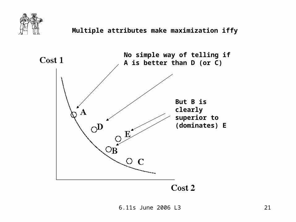
Multiple attributes make maximization iffy
No simple way of telling if A is better than D (or C)
But B is clearly superior to (dominates) E

6.11s June 2006 L3 22
Novice Design Assistant:
Is deliberately not an expert system
Uses Monte Carlo to generate randomized designs
Each variable in the design space is characterized by:
Mean Value
Standard Deviation
Maximum value (limit)
Minimum value (limit)
Setup file (msetup.m) specifies
Number of design variables
For each: the above data
Number of attributes to be returned
function file called by nda.m: called attribut.m
returns attributes and a go-no-go (limits not violated)
6.11s June 2006 L3 23
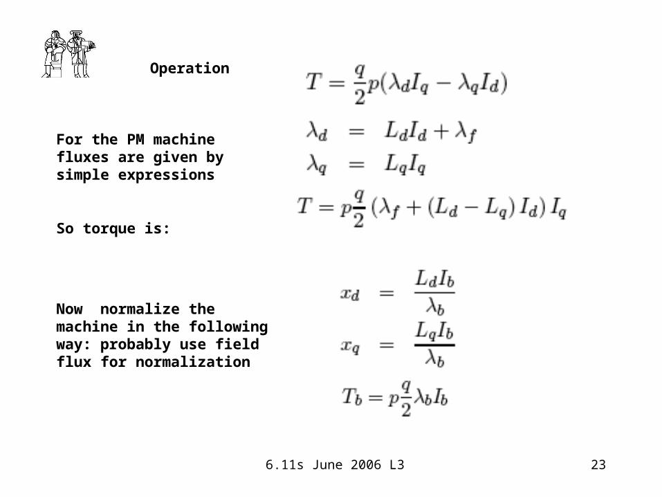
Operation
For the PM machine fluxes are given by simple expressions
So torque is:
Now normalize the machine in the following way: probably use field flux for normalization

6.11s June 2006 L3 24
Then per-unit torque is:
Per-Unit Currents to achieve the maximum torque per unit current are:
6.11s June 2006 L3 25
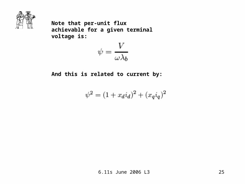
Note that per-unit flux achievable for a given terminal voltage is:
And this is related to current by:
6.11s June 2006 L3 26

6.11s June 2006 L3 27

6.11s June 2006 L3 28
Base speed

6.11s June 2006 L3 29
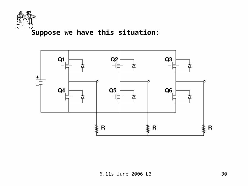
Here is your basic three phase bridge
6.11s June 2006 L3 30
Suppose we have this situation:
6.11s June 2006 L3 31
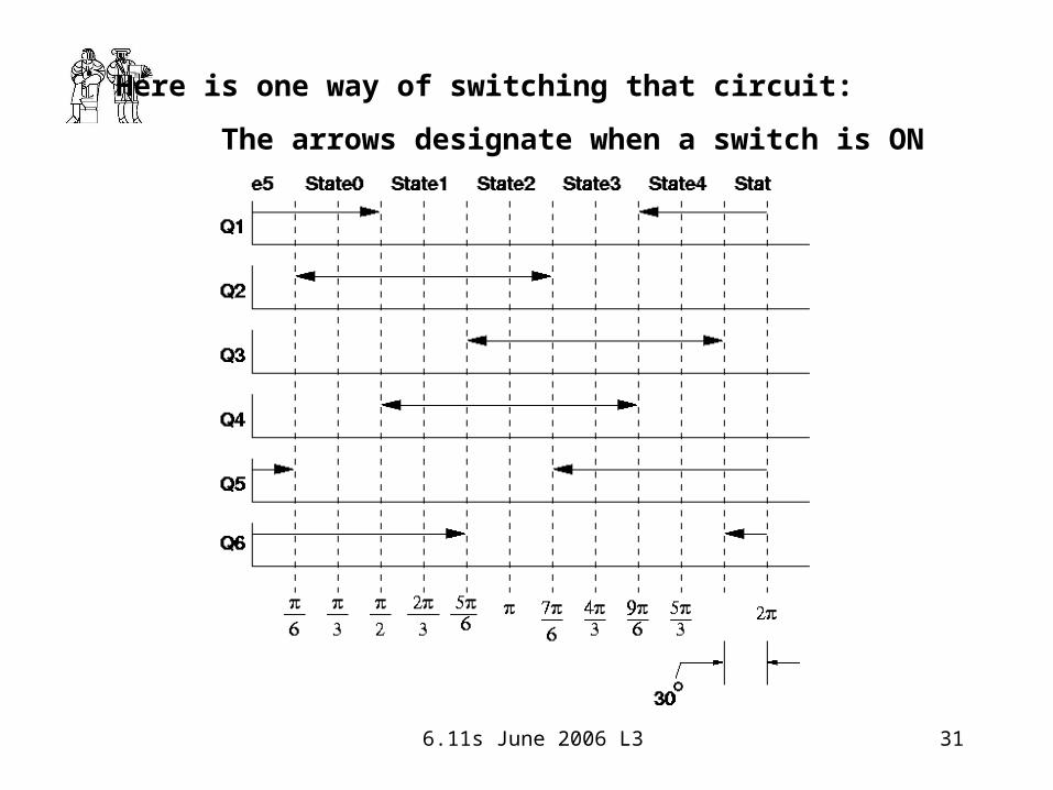
Here is one way of switching that circuit:
The arrows designate when a switch is ON

6.11s June 2006 L3 32
Here is what is on in State 0:
Va = V, Vb = V, Vc = 0 Vn = 2V/3

6.11s June 2006 L3 33
Va = 0, Vb = V, Vc = 0 Vn = V/3
Here is what is on in State 1:

6.11s June 2006 L3 34
Va = 0, Vb = V, Vc = V Vn = 2V/3
Here is what is on in State 2:
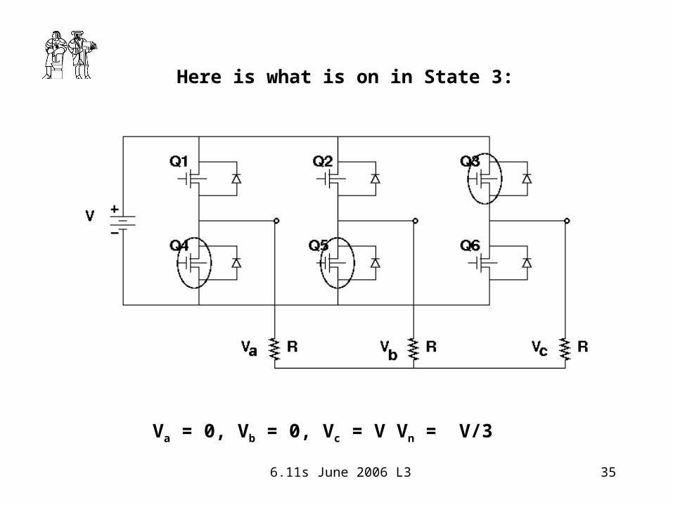
6.11s June 2006 L3 35
Va = 0, Vb = 0, Vc = V Vn = V/3
Here is what is on in State 3:

6.11s June 2006 L3 36
Va = V, Vb = 0, Vc = V Vn = 2V/3
Here is what is on in State 4:

6.11s June 2006 L3 37
Va = V, Vb = 0, Vc = 0 Vn = V/3
Here is what is on in State 5:

6.11s June 2006 L3 38
Voltages: Line-Line Voltages are well defined

6.11s June 2006 L3 39
To generate switching signals:
•Totem Pole A is High in states 0, 4 and 5
•Totem Pole B is High in states 0, 1 and 2
•Totem Pole C is High in states 2, 3 and 4
This allows us to use very simple logic:
A = S0 + S4 + S5
B = S0 + S1 + S2
C = S2 + S3 + S4

6.11s June 2006 L3 40
To generate switch signals
Note that either top or bottom switch is on in each phase
Generation of states: we will do this a bit later (see below)

6.11s June 2006 L3 41
This ‘six pulse’ switching strategy:
•Makes good use of the switching devices
•Also requires ‘shoot-through’ delays
•Has very simple logic
We propose an alternative switching strategy
•Makes minimally less effective use of switches
•Uses a little more logic
•But does not risk shoot through

6.11s June 2006 L3 42
Here is a comparison of switching strategies
180 degree six-pulse
120 degree six pulse
Give up a little timing between switch closings

6.11s June 2006 L3 43
Switches Q_1 and Q_5 are on: State0
Va = V, Vb = 0, Vc = V/2

6.11s June 2006 L3 44
Switches Q_1 and Q_6 are on: State1
Va = V, Vc = 0, Vb = V/2

6.11s June 2006 L3 45
Switches Q_2 and Q_6 are on: State2
Vb = V, Vc = 0, Va = V/2

6.11s June 2006 L3 46
Switches Q_2 and Q_4 are on: State3
Va = 0, Vb = V, Vc = V/2

6.11s June 2006 L3 47
Switches Q_3 and Q_4 are on: State4
Va = 0, Vc = V, Vb = V/2

6.11s June 2006 L3 48
Switches Q_3 and Q_5 are on: State5
Vc = V, Vb = 0, Va = V/2

6.11s June 2006 L3 49
This switching pattern results in these voltages
6.11s June 2006 L3 50
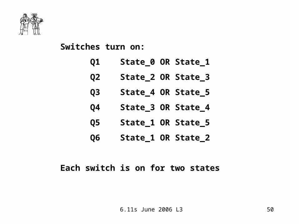
Switches turn on:
Q1 State_0 OR State_1
Q2 State_2 OR State_3
Q3 State_4 OR State_5
Q4 State_3 OR State_4
Q5 State_1 OR State_5
Q6 State_1 OR State_2
Each switch is on for two states

6.11s June 2006 L3 51
So here is how to do it
3 bit input to ‘138 selects one of 8 outputs
Active low output!
‘138 has 3 enable inputs: two low, one high

6.11s June 2006 L3 52
NAND (Not AND)
Is the same as Negative Input OR
The ‘138 output is ‘active low’:
Matching bubbles makes an OR function

6.11s June 2006 L3 53
Now we must generate six states in sequence
If we have a ‘clock’ with rising edges at the right time interval we can use a very simple finite state machine
This could be a counter, reset when it sees ‘5’

6.11s June 2006 L3 54
Here is a good counter to use: 74LS163
This is a loadable counter: don’t need that feature
Clear function is synchronous: so it clears only ON a clock edge
Part is ‘edge triggered’: changes state on a positive clock edge
P and T are enables: must pull them high

6.11s June 2006 L3 55
And here are the counter states: note how CL works

6.11s June 2006 L3 56
We already detect state 5 with the ‘138

6.11s June 2006 L3 57
The ‘138 is a simple selector: use like this:
And here are the pinouts of the ‘163 and ‘138

6.11s June 2006 L3 58
Variable Voltage: do the Pulse Width Modulation thing

6.11s June 2006 L3 59
Nomenclature: Two more views of the machine

6.11s June 2006 L3 60
This is a ‘cut’ from the radial direction (section BB)

6.11s June 2006 L3 61
Here is a cut through the machine (section AA)
Winding goes around the core: looking at 1 turn

6.11s June 2006 L3 62
Voltage is induced by motion and magnetic field
Induction is:
Voltage induction rule:
Note magnets must agree!
€
E '= E + v × B
€
V = ulB =ωRlB = Cω

6.11s June 2006 L3 63
Single Phase Equivalent Circuit of the PM machine
Ea is induced (‘speed’) voltage
Inductance and resistance are as expected
This is just one phase of three
€
Ea =ωλ 0Voltage relates to flux:

6.11s June 2006 L3 64
PM Brushless DC Motor is a synchronous PM machine with an inverter:

6.11s June 2006 L3 65
€
Ea = E cos ωt +θ( )
Eb = E cos ωt +θ −2π
3
⎛
⎝ ⎜
⎞
⎠ ⎟
Ec = E cos ωt +θ +2π
3
⎛
⎝ ⎜
⎞
⎠ ⎟
€
Ia = I1 cosωt
Ib = I1 cos ωt −2π
3
⎛
⎝ ⎜
⎞
⎠ ⎟
Ic = I1 cos ωt +2π
3
⎛
⎝ ⎜
⎞
⎠ ⎟
€
P =1
2EI1 cosθ =
1
2λ 0ωI1 cosθ
Induced voltages are:
Assume we drive with balanced currents:
Then converted power is:
Torque must be:
€
T =p
ωP =
p
2λ 0I1 cosθ

6.11s June 2006 L3 66
Now look at it from the torque point of view:
€
T = IlBR = CI

6.11s June 2006 L3 67
€
I1 =4
πsin
120o
2I0 =
4
π
3
2I0
Terminal Currents look like this:
€
T =3
2pλ 0I1 = p
3 3
πλ 0I0
So torque is, in terms of DC side current:

6.11s June 2006 L3 68
Va VbVc
Vab
0 12
Rectified back voltage is max of all six line-line voltages
<Eb>

6.11s June 2006 L3 69
€
< Eb >=3
π3
−π
6
π
6
∫ ωλ 0 cosωtdωt
=3 3
πωλ 0
Average Rectified Back Voltage is:
Power is simply:
€
Pem =3 3
πωλ 0I0 = KI0

6.11s June 2006 L3 70
So from the DC terminals this thing looks like the DC machine:
€
T = KI
Ea = Kω
K = p3 3
πλ 0

6.11s June 2006 L3 71
Magnets must match (north-north, south-south) for the two rotor disks.
Looking at them they should look like this:
End A End B
Keyway

6.11s June 2006 L3 72
Need to sense position: Use a disk that looks like this

6.11s June 2006 L3 73
Position sensor looks at the disk: 1=‘white, 0=‘black’
6.11s June 2006 L3 74
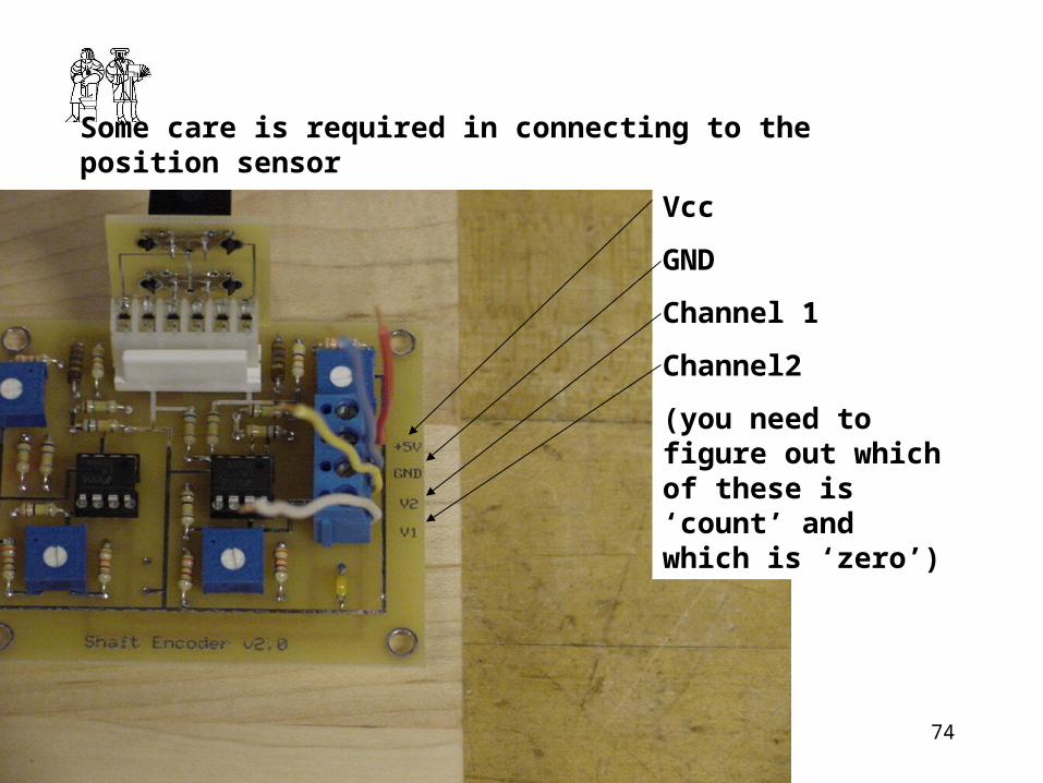
Some care is required in connecting to the position sensor
Vcc
GND
Channel 1
Channel2
(you need to figure out which of these is ‘count’ and which is ‘zero’)

6.11s June 2006 L3 75
Control Logic:
Replace open loop with position measurement

6.11s June 2006 L3 76
Why do we need to PWM only the top switches?
What happens with you turn OFF switch Q1?


