

9/7 Agenda Project 1 discussion Correlation Analysis PCA (LSI)
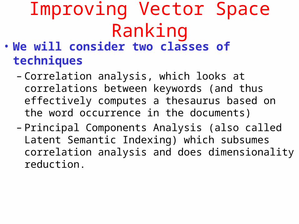
Improving Vector Space Ranking
• We will consider two classes of techniques– Correlation analysis, which looks at correlations between
keywords (and thus effectively computes a thesaurus based on the word occurrence in the documents)
– Principal Components Analysis (also called Latent Semantic Indexing) which subsumes correlation analysis and does dimensionality reduction.

Correlation/Co-occurrence analysis
Co-occurrence analysis:• Terms that are related to terms in the original query may be
added to the query.
• Two terms are related if they have high co-occurrence in documents.
Let n be the number of documents;
n1 and n2 be # documents containing terms t1 and t2,
m be the # documents having both t1 and t2
If t1 and t2 are independent
If t1 and t2 are correlated
mn
n
n
nn 21
mn
n
n
nn 21
Mea
sure
degree
of corre
lation
>> if Inversely correlated
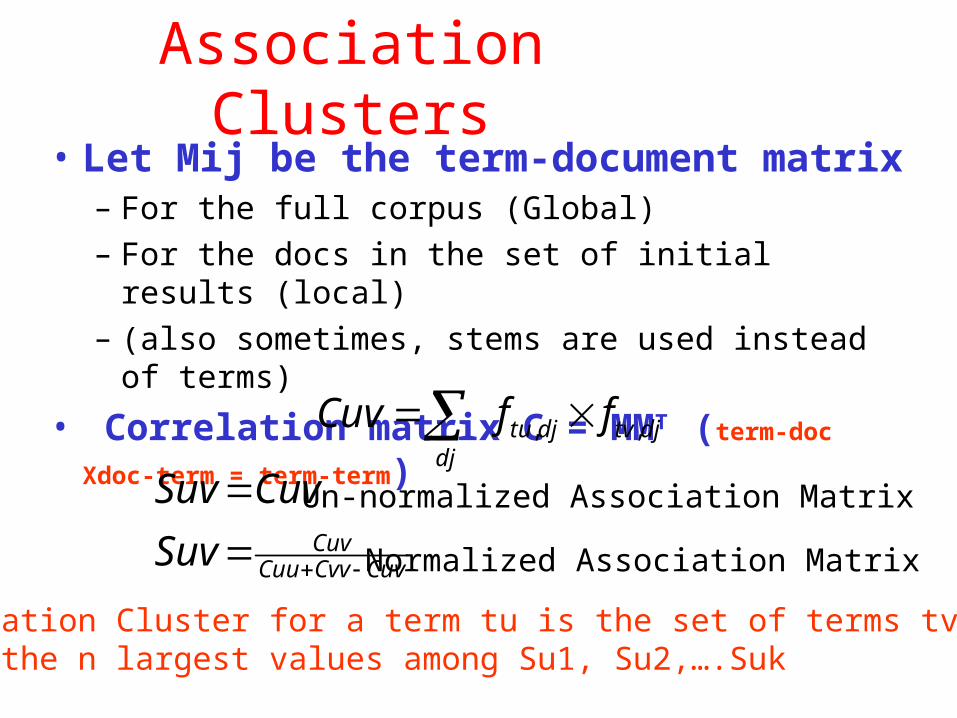
Association Clusters• Let Mij be the term-document matrix
– For the full corpus (Global)
– For the docs in the set of initial results (local)
– (also sometimes, stems are used instead of terms)
• Correlation matrix C = MMT (term-doc Xdoc-term =
term-term)
djtvdjtudj
ffCuv ,,
CuvCvvCuuCuvSuv
CuvSuv
Un-normalized Association Matrix
Normalized Association Matrix
Nth-Association Cluster for a term tu is the set of terms tv such that Suv are the n largest values among Su1, Su2,….Suk

Example
d1d2d3d4d5d6d7
K1 2 1 0 2 1 1 0
K2 0 0 1 0 2 2 5
K3 1 0 3 0 4 0 0
11 4 6
4 34 11
6 11 26
1.0 0.097 0.193
0.097 1.0 0.224
0.193 0.224 1.0
Correlatio
n
Matrix
Norm
alized
Correlation
Matrix
1th Assoc Cluster for K2 is K3
4)12(34)22(11)11(4)12(
12 ssssS

Scalar clusters
Consider the normalized association matrix S
The “association vector” of term u Au is (Su1,Su2…Suk)
To measure neighborhood-induced correlation between terms:Take the cosine-theta between the association vectors of terms u and v
Even if terms u and v have low correlations, they may be transitively correlated (e.g. a term w has high correlation with u and v).
|||| AvAuAvAuSuv
Nth-scalar Cluster for a term tu is the set of terms tv such that Suv are the n largest values among Su1, Su2,….Suk

Exampled1d2d3d4d5d6d7
K1 2 1 0 2 1 1 0
K2 0 0 1 0 2 2 5
K3 1 0 3 0 4 0 0
1.0 0.097 0.193
0.097 1.0 0.224
0.193 0.224 1.0
Normalized Correlation Matrix
AK1
USER(43): (neighborhood normatrix)
0: (COSINE-METRIC (1.0 0.09756097 0.19354838) (1.0 0.09756097 0.19354838))
0: returned 1.0
0: (COSINE-METRIC (1.0 0.09756097 0.19354838) (0.09756097 1.0 0.2244898))
0: returned 0.22647195
0: (COSINE-METRIC (1.0 0.09756097 0.19354838) (0.19354838 0.2244898 1.0))
0: returned 0.38323623
0: (COSINE-METRIC (0.09756097 1.0 0.2244898) (1.0 0.09756097 0.19354838))
0: returned 0.22647195
0: (COSINE-METRIC (0.09756097 1.0 0.2244898) (0.09756097 1.0 0.2244898))
0: returned 1.0
0: (COSINE-METRIC (0.09756097 1.0 0.2244898) (0.19354838 0.2244898 1.0))
0: returned 0.43570948
0: (COSINE-METRIC (0.19354838 0.2244898 1.0) (1.0 0.09756097 0.19354838))
0: returned 0.38323623
0: (COSINE-METRIC (0.19354838 0.2244898 1.0) (0.09756097 1.0 0.2244898))
0: returned 0.43570948
0: (COSINE-METRIC (0.19354838 0.2244898 1.0) (0.19354838 0.2244898 1.0))
0: returned 1.0
1.0 0.226 0.383
0.226 1.0 0.435
0.383 0.435 1.0
Scalar (neighborhood)Cluster Matrix
1th Scalar Cluster for K2 is still K3

Beyond Correlation analysis: PCA/LSI• Suppose I start with documents described in terms of just
two key words, u and v, but then – Add a bunch of new keywords (of the form 2u-3v; 4u-v etc), and give the
new doc-term matrix to you. Will you be able to tell that the documents are really 2-dimensional (in that there are only two independent keywords)?
– Suppose, in the above, I also add a bit of noise to each of the new terms (i.e. 2u-3v+noise; 4u-v+noise etc). Can you now discover that the documents are really 2-D?
– Suppose further, I remove the original keywords, u and v, from the doc-term matrix, and give you only the new linearly dependent keywords. Can you now tell that the documents are 2-dimensional?
• Notice that in this last case, the true dimensions of the data are not even present in the representation! You have to re-discover the true dimensions as linear combinations of the given dimensions.
added

Data Generation Models• The fact that keywords in the documents are not
actually independent, and that they have synonymy and polysemy among them, often manifests itself as if some malicious oracle mixed up the data as above.
• Need Dimensionality Reduction Techniques• If the keyword dependence is only linear (as above), a general
polynomial complexity technique called Principal Components Analysis is able to do this dimensionality reduction
• PCA applied to documents is called Latent Semantic Indexing– If the dependence is nonlinear, you need non-linear dimensionality
reduction techniques (such as neural networks); much costlier.

Visual Example
• Classify Fish– Length– Height

Better if one axis accounts for most data variationWhat should we call the red axis? Size (“factor”)

We retain 1.75/2.00 x 100 (87.5%) of the original variation.
Thus, by discarding the yellow axis we lose only 12.5% of the original information.
Reduce Dimensions
• What if we only consider “size”

If you can do it for fish, why not to docs?• We have documents as vectors in the space of terms• We want to
– “Transform” the axes so that the new axes are• “Orthonormal” (independent axes)• Can be ordered in terms of the amount of variation in the documents they
capture• Pick top K dimensions (axes) in this ordering; and use these new K
dimensions to do the vector-space similarity ranking
• Why?– Can reduce noise – Can eliminate dependent variabales– Can capture synonymy and polysemy
• How?– SVD (Singular Value Decomposition)

What happens if you multiply a vector by a matrix?
• In general, when you multiply a vector by a matrix, the vector gets “scaled” as well as “rotated” – ..except when the vector happens to be in the direction of one of the eigen
vectors of the matrix– .. in which case it only gets scaled (stretched)
• A (symmetric square) matrix has all real eigen values, and the values give an indication of the amount of stretching that is done for vectors in that direction
• The eigen vectors of the matrix define a new ortho-normal space– You can model the multiplication of a general vector by the matrix in terms of
• First decompose the general vector into its projections in the eigen vector directions– ..which means just take the dot product of the vector with the (unit) eigen vector
• Then multiply the projections by the corresponding eigen values—to get the new vector.
– This explains why power method converges to principal eigen vector.. • ..since if a vector has a non-zero projection in the principal eigen vector direction,
then repeated multiplication will keep stretching the vector in that direction, so that eventually all other directions vanish by comparison..
added

SVD, Rank and Dimensionality• Suppose we did SVD on a doc-
term matrix d-t, and took the top-k eigen values and reconstructed the matrix d-tk. We know– d-tk has rank k (since we zeroed
out all the other eigen values when we reconstructed d-tk)
– There is no k-rank matrix M such that ||d-t –M|| < ||d-t – d-tk||
• In other words d-tk is the best rank-k (dimension-k) approximation to d-t!
– This is the guarantee given by SVD!
• Rank of a matrix M is defined as the size of the largest square sub-matrix of M which has a non-zero determinant. – The rank of a matrix M is also equal
to the number of non-zero singular values it has
– Rank of M is related to the true dimensionality of M. If you add a bunch of rows to M that are linear combinations of the existing rows of M, the rank of the new matrix will still be the same as the rank of M.
• Distance between two equi-sized matrices M and M’; ||M-M’|| is defined as the sum of the squares of the differences between the corresponding entries (Sum (muv-m’uv)2)– Will be equal to zero when M = M’
Optional

a b c d e f g h IInterface 0 0 1 0 0 0 0 0 0User 0 1 1 0 1 0 0 0 0System 2 1 1 0 0 0 0 0 0Human 1 0 0 1 0 0 0 0 0Computer 0 1 0 1 0 0 0 0 0Response 0 1 0 0 1 0 0 0 0Time 0 1 0 0 1 0 0 0 0EPS 1 0 1 0 0 0 0 0 0Survey 0 1 0 0 0 0 0 0 1Trees 0 0 0 0 0 1 1 1 0Graph 0 0 0 0 0 0 1 1 1Minors 0 0 0 0 0 0 0 1 1
Terms and Docs as vectors in “factor” space
Document vector
Term vector
If terms are independent, theT-T similarity matrix would be diagonal =If it is not diagonal, we can use the correlations to add related terms to the query =But can also ask the question “Are there independent dimensions which define the space where terms & docs are vectors ?”
In addition to doc-doc similarity, We can compute term-term distance

=
=
mxnA
mxrU
rxrD
rxnVT
Terms
Documents
=
=
mxn
Âk
mxkUk
kxkDk
kxnVT
k
Terms
Documents
Singular Value DecompositionConvert doc-term
matrix into 3matricesD-F, F-F, T-F
Where DF*FF*TF’ gives theOriginal matrix back
Reduce Dimensionality:Throw out low-order
rows and columns
Recreate Matrix:Multiply to produceapproximate term-document matrix.
dtk is a k-rank matrixThat is closest to dt
dt df ff tft dfk ffktfk
t
Overview of Latent Semantic Indexing
Doc-fa
ctor
(eige
n vec
tors o
f d-t*
d-t’)
factor
-facto
r
(+ve
sqrt
of ei
gen v
alues
of
d-t*d
-t’or
d-t’*
d-t;
both
same)
(term
-facto
r)T
(eige
n vec
tors o
f d-t’
*d-t)
doc
Term Term
docdtk
dxt dxf fxf fxt dxk kxk kxt dxt

-30.8998 11.4912 1.6746 -3.1330 2.2603 -1.5582
-30.3131 10.7801 0.2064 10.3670 -3.5474 -1.6751
-18.0007 7.7138 -0.8413 -5.5394 1.8438 -2.5841
-8.3765 3.5611 -0.3232 -1.9162 0.7432 -1.3505
-52.7057 20.6051 -1.7193 -2.1159 -0.6817 2.9396
-10.8052 -21.9140 5.1744 0.3599 3.0090 0.2561
-11.5080 -28.0101 -15.8265 0.1919 1.1998 0.2137
-9.5259 -17.7666 -8.7594 2.7675 4.7017 -0.3354
-19.9219 -45.0751 4.4501 -3.1140 -7.2601 -0.3766
-14.2118 -21.8263 12.0655 2.7734 6.1728 0.5132
New document coordinates d-f*f-f
t1= databaset2=SQLt3=indext4=regressiont5=likelihoodt6=linear
u =
Columns 1 through 7
-0.3994 0.1653 0.0730 -0.2327 0.1874 -0.3249 -0.1329
-0.3918 0.1551 0.0090 0.7699 -0.2941 -0.3492 0.1193
-0.2327 0.1110 -0.0367 -0.4114 0.1528 -0.5388 0.4346
-0.1083 0.0512 -0.0141 -0.1423 0.0616 -0.2816 -0.6309
-0.6813 0.2964 -0.0750 -0.1571 -0.0565 0.6129 -0.0303
-0.1397 -0.3152 0.2256 0.0267 0.2494 0.0534 0.2735
-0.1488 -0.4029 -0.6901 0.0142 0.0995 0.0445 0.2944
-0.1231 -0.2555 -0.3819 0.2055 0.3898 -0.0699 -0.4419
-0.2575 -0.6483 0.1940 -0.2312 -0.6018 -0.0785 -0.1505
-0.1837 -0.3139 0.5261 0.2060 0.5117 0.1070 0.0291
Columns 8 through 10
-0.3190 0.6715 -0.2067
-0.0165 -0.0808 -0.0136
0.3616 -0.2800 0.2264
-0.3656 -0.5904 -0.0439
0.1173 -0.1510 0.0375
0.0070 -0.2508 -0.7916
-0.4700 -0.0391 0.1347
0.5975 0.1401 -0.0521
0.1306 0.0910 0.0765
-0.1572 -0.0242 0.4991
D-F
77.3599 0 0 0 0 0
0 69.5242 0 0 0 0
0 0 22.9342 0 0 0
0 0 0 13.4662 0 0
0 0 0 0 12.0632 0
0 0 0 0 0 4.7964
0 0 0 0 0 0
0 0 0 0 0 0
0 0 0 0 0 0
0 0 0 0 0 0
-0.7352 -0.4900 -0.2677 -0.2826 -0.1831 -0.1854
0.2788 0.2351 0.1215 -0.7417 -0.3663 -0.4097
0.0413 -0.0604 -0.0741 -0.4745 -0.0473 0.8728
0.6074 -0.7156 -0.2758 0.0815 -0.1783 -0.0671
-0.0831 0.1757 0.0060 0.3717 -0.8916 0.1704
-0.0653 -0.3976 0.9121 -0.0005 -0.0568 0.0496
F-F
T-F6 singular values
(positive sqrt of eigen values of
MM’ or M’M)Eigen vectors of MM’
(Principal document directions)
Eigen vectors of M’M(Principal term directions)
)2%(5.71
1
2
1
2
kloss n
ii
k
ii

For the database/regressionexample
t1= databaset2=SQLt3=indext4=regressiont5=likelihoodt6=linear
Suppose D1 is a newDoc containing “database”50 times and D2 contains“SQL” 50 times

LSI Ranking…• Given a query
– Either add query also as a document in the D-T matrix and do the svd OR
– Convert query vector (separately) to the LSI space– DFq*FF=q*TF
• this is the weighted query document in LSI space
– Reduce dimensionality as needed
• Do the vector-space similarity in the LSI space
TFqFFDFq
TFTFFFDFqTFq
TFFFDFqq
TFFFDFDT
I
**
'****
'**
'**

Using LSI• Can be used on the entire corpus
– First compute the SVD of the entire corpus
– Store first k columns of the df*ff matrix [df*ff]k
– Keep the tf matrix handy– When a new query q comes, take the k
columns of q*tf– Compute the vector similarity between
[q*tf]k and all rows of [df*ff]k, rank the documents and return
• Can be used as a way of clustering the results returned by normal vector space ranking– Take some top 50 or 100 of the
documents returned by some ranking (e.g. vector ranking)
– Do LSI on these documents– Take the first k columns of the
resulting [df*ff] matrix– Each row in this matrix is the
representation of the original documents in the reduced space.
– Cluster the documents in this reduced space (We will talk about clustering later)
– MANJARA did this– We will need fast SVD computation
algorithms for this. MANJARA folks developed approximate algorithms for SVD
Added based on class discussion
)'*(*)*(
)'*(*)*(
)'*'*(*)'**(
)''**(*)'**('*
)(
FFDFFFDF
DFFFFFDF
DFFFTFTFFFDF
TFFFDFTFFFDFDTDT
ncorrelatiodocdocDD
FFI

SVD Computation complexity• For an mxn matrix SVD computation is
– O( km2n+k’n3) complexity• k=4 and k’=22 for best algorithms
– Approximate algorithms that exploit the sparsity of M are available (and being developed)

Bunch of Facts about SVD• Relation between SVD and Eigen value decomposition
– Eigen value decomp is defined only for square matrices• Only square symmetric matrices have real-valued eigen values
– SVD is defined for all matrices• Given a matrix M, we consider the eigen decomposion of the correlation matrices
MMT and MTM. SVD is the eigen vectors of MMT *positive square roots of eigen values of MMT * eigen vectors of MTM
– Both MMT and MTM are symmetric (they are correlation matrices)– They both will have the same eigen values
• Unless M is symmetric, MMT and MTM are different – So, in general their eigen vectors will be different (although their eigen values are same)
– Since SVD is defined in terms of the eigen values and vectors of the “Correlation matrices” of a matrix, the eigen values will always be real valued (even if the matrix M is not symmetric).
• In general, the SVD decomposition of a matrix M equals its eigen decomposition only if M is both square and symmetric
Added based on the discussion in the classOptional


