

No. 15 | 2011
A cobweb model of financial stability in NorwayGeir Arne Dahl, Thea Birkeland Kloster, Unni Larsen, Ketil Johan Rakkestad, Rebekka Reisvaag, Bjørne Dyre Syversten and Cathrine Bolstad Træe, Norges Bank Financial Stability
Edited by Magdalena D. Riiser
Staff Memo

Staff Memos present reports and documentation written by staff members and affiliates of Norges Bank, the central bank of Norway. Views and conclusions expressed in Staff Memos should not be taken to represent the views of Norges Bank. © 2011 Norges Bank The text may be quoted or referred to, provided that due acknowledgement is given to source. References to the staff memo should read: ñDahl, Geir Arne, Thea Birkeland Kloster, Unni Larsen, Ketil Johan Rakkestad, Rebekka Reisvaag, Bjßrne Dyre Syversten and Cathrine Bolstad TrÞe (2011): ò A Cobweb Model of Financial Stability in Norwayò, edited by Magdalena D. Riiser, Norges Bank Staff Memo No. 15ñ Staff Memo inneholder utredninger og dokumentasjon skrevet av Norges Banks ansatte og andre forfattere tilknyttet Norges Bank. Synspunkter og konklusjoner i arbeidene er ikke nødvendigvis representative for Norges Banks. © 2011 Norges Bank Det kan siteres fra eller henvises til dette arbeid, gitt at forfatter og Norges Bank oppgis som kilde. ISSN 1504-2596 (online only) ISBN 978-82-7553-629-5 (online only)

1
A cobweb model of financial stability in Norway1
Geir Arne Dahl, Thea Birkeland Kloster, Unni Larsen, Ketil Johan Rakkestad,
Rebekka Reisvaag2, Bjørne Dyre Syversten and Cathrine Bolstad Træe
Edited by Magdalena D. Riiser
1. Introduction3
Central banks have been supervising financial stability for several decades now. Most central banks
publish reports providing an assessment of the financial sector and the risks to financial stability.
However, quantifying financial instability has been a challenge. A number of methods have been used to
assess financial stability.4
The first group of methods includes indicators of a specific segment of the financial system, for example
indicators of equity, debt or currency markets, or indicators based on data from balance sheets or profit
and loss accounts. The Financial Soundness Indicators that are coordinated by the IMF fall into this
group. The analyses of financial stability in Norges Bank have featured such indicators since the middle
of the 1990s. The indicators are a tool for monitoring developments in financial conditions and risks and
are widely used. However, they are often lagged or contemporaneous. The general experience is that
these indicators alone proved inadequate in signaling the recent financial crisis.
Another line of research is the development of composite financial conditions indices. As financial
stability is measured along many dimensions, these indices try to combine information on different
markets based on a set of indicators. Illing and Liu (2003) construct an index of financial stress for
Canada covering the equity markets, bond markets, foreign exchange markets and the banking sector.
Van den End (2006) builds a financial stability conditions index for the Netherlands and six OECD
countries. Hanschel and Monnin (2004) construct a stress index for the banking sector in Switzerland.
1 References to the staff memo should read: “Dahl, Geir Arne, Thea Birkeland Kloster, Unni Larsen, Ketil Johan
Rakkestad, Rebekka Reisvaag, Bjørne Dyre Syversten and Cathrine Bolstad Træe (2011): ” A Cobweb Model of Financial Stability in Norway”, edited by Magdalena D. Riiser, Norges Bank Staff Memo No. 15“ 2 Rebekka Reisvaag was employed in Norges Bank when the staff memo was written but is currently employed in
Orkla 3 The authors would like to thank Birger Vikøren, Sigbjørn Atle Berg, Ingvild Svendsen, Henrik Andersen, Per Atle
Aronsen and Haseeb Syed for valuable suggestions and comments. Thanks to Birgitte H. Molden for commenting on the household dimension and to Helle Snellingen for the language dimension 4 Galati and Moessner (2011) and Dattels, McCaughrin, Miyajima and Puig (2010) provide a detailed overview of
methods for analysing financial stability

2
Andersen (2008) presents a risk index for Norwegian banks based on data from the banks’ balance
sheets and profit and loss accounts.
Early warning indicators have also been used to analyse financial stability. Drawing on econometric
approaches, this method aims at detecting the build-up of financial imbalances. Early warning indicators
for credit and asset prices have especially performed well in terms of signaling the build-up of financial
imbalances, see Borio and Lowe (2002, 2004), Borio and Drehmann (2009) and Galati and Moessner
(2011). The extensive use of early warning indicators is motivated by the existence of endogenous
financial cycles, see Minsky (1977) and Kindleberger (1978, 2000). When times are good, asset prices
and credit tend to rise, stretching private balance sheets and contributing to the build-up of financial
imbalances. Such imbalances usually unwind in a disruptive manner when a shock occurs and threatens
financial stability. Riiser (2005, 2008 and 2010) finds that asset prices, credit and investment are useful
in predicting banking crises in Norway over a period of 150 years. VO Thi (2011) studies some other
macroeconomic indicators for Norway such as credit, house prices and GDP, and concludes that credit is
the best indicator.
Vector Autoregression Models (VARs) are another group of methods that are applied in financial
stability analyses. The VAR modelling approach studies the transmission of a shock to some financial
variables through the whole economy. A study employing VAR models has been performed by Norges
Bank, see Jacobsen, Kloster, Kvinlog and Larsen (2011).
Another group of methods employs macro stress tests. Central banks perform macro stress tests to
assess how robust the financial system is to exogenous shocks. Norges Bank semi-annually publishes
stress tests in its report Financial Stability. A virtue of Norges Bank’s stress testing framework is that it
takes into account not only the propagation of shocks from the real economy to the financial sector but
the feedback from the financial sector to the economy as well.
Achieving financial stability is a multidimensional task that is difficult to fulfil by complying with a simple
target. Acknowledging that, central banks have started to exploit new methods that reflect the various
facets of financial stability. The Bank of England has defined a list of key vulnerabilities to the UK
financial system. In the Financial Stability Review (FSR) the Bank of England highlights the change in
probability for the vulnerabilities and in their impact on the financial system compared with the
previous FSR. The International Monetary Fund (IMF) has developed a global financial stability map
(GFSM) presenting the main conditions and risks to financial stability, see Dattels et al. (2010). These are
measured by a number of indicators on a scale from 0 to 10 depending on the history of the data. The
scores are then graphically depicted as six dimensions in a cobweb-style diagram. The Reserve Bank of
New Zealand has elaborated a similar national cobweb model of financial stability, see Bedford and
Bloor (2009). In its effort to enlarge the toolkit for analysing the financial system, Norges Bank has
developed a cobweb model of financial stability for Norway.
The rest of the memo is structured as follows: Section 2 outlines the design of the cobweb model for
Norway and gives a brief description of the applied method. Section 3 describes the construction of each
3
dimension of the diagram. Section 4 summarises the performance of the cobweb model during the
periods of financial strain in Norway. Finally, Section 5 concludes.
2. Design and methodology for the cobweb model of financial stability
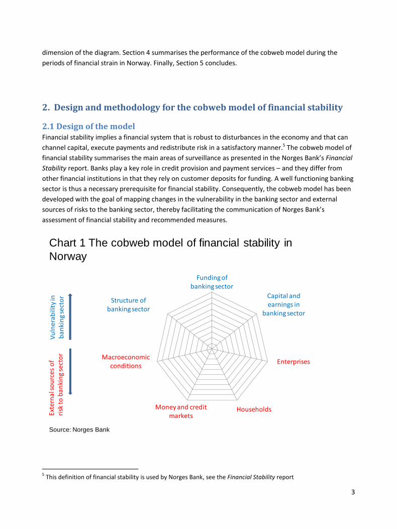
2.1 Design of the model Financial stability implies a financial system that is robust to disturbances in the economy and that can
channel capital, execute payments and redistribute risk in a satisfactory manner.5 The cobweb model of
financial stability summarises the main areas of surveillance as presented in the Norges Bank’s Financial
Stability report. Banks play a key role in credit provision and payment services – and they differ from
other financial institutions in that they rely on customer deposits for funding. A well functioning banking
sector is thus a necessary prerequisite for financial stability. Consequently, the cobweb model has been
developed with the goal of mapping changes in the vulnerability in the banking sector and external
sources of risks to the banking sector, thereby facilitating the communication of Norges Bank’s
assessment of financial stability and recommended measures.
5 This definition of financial stability is used by Norges Bank, see the Financial Stability report
Chart 1 The cobweb model of financial stability in
Norway
Structure ofbanking sector
Funding ofbanking sector
Capital and earnings in
banking sector
Enterprises
HouseholdsMoney and creditmarkets
Macroeconomicconditions
Vu
lner
abili
tyin
b
anki
ng
sect
or
Ext
ern
als
ou
rces
of
risk
to
ba
nki
ng
sect
or
Source: Norges Bank

4
The upper part of the cobweb model consists of sources of vulnerability in the banking sector (see Chart
1). High vulnerability of banks reduces their robustness to withstand shocks and hampers financial
stability. Sources of vulnerabilities are represented by three dimensions, i.e. capital and earnings,
funding and structure of the banking sector. The lower part of the model comprises external risks to the
banking sector, which include risks stemming from macroeconomic conditions, money and credit
markets, enterprises and households.
The indicators of vulnerabilities in the banking sector and external risks are assigned scores from 0 to 10.
Lower scores indicate lower level of vulnerability or risks. Moving further from the centre of the cobweb
diagram indicates higher vulnerability or risks to the banking sector.
Changes in vulnerabilities and risks to the banking sector can be abrupt or more gradual. For example,
household indebtedness tends to increase steadily over time, contributing to a permanent elevation in
risks. Money and credit markets on the other hand can experience abrupt changes.
A positive assessment of financial stability requires both a robust banking sector, i.e. that vulnerability is
low, and that there are no imminent risks to the banking sector. However, an unfavourable assessment
of the vulnerability in the banking sector might render a lower total assessment of financial stability
even in the absence of imminent risks, leading to a recommendation of measures.
2.2. Methodology Each dimension in the cobweb model is based on a number of sub-indicators. Ideally, the data series for
the sub-indicators should cover several economic and financial cycles. Preferably, the indicators should
also be based on frequently published statistics to allow regular assessments of financial stability.
Furthermore, we try to control for variations in the data which do not have implications for financial
stability, such as seasonal variations or breaks in data series. The indicators are chosen to convey the
most important and at the same time sufficient information. This has resulted in 4 to 8 sub-indicators in
each dimension.
The sub-indicators are assessed against their historical values. We start by obtaining data series for the
sub-indicators. These are subject to various transformations (see Annex A). As a first step we order the
observations into a numerical sequence. The data is then divided into 11 equally sized data subsets
(percentiles). The 11 percentiles for each sub-indicator correspond to a score between 0 and 10. The
mean and the median of each sub-indicator equal 5. This value expresses only the average value of the
sample we use and is not based on any assessment of a “normal” risk or vulnerability level. The main
indicator is constructed as an unweighted average of the underlying sub-indicators. The value of the
main indicator is rounded to the nearest whole number.
So far, each time the cobweb model has been updated, the percentile ranking has been performed on
all data observations, including the new ones. This implies that a sub-indicator’s value that is associated
with a certain score, for example 5, might change. A change in the main indicator score in the cobweb
model might thus be due to either a change in the vulnerability and risk in the banking sector or to a
5
mere change in the average value of the underlying data. Separating the effects would have required
that the percentile ranking was performed on a fixed data sample that was not extended with new
observations. However, applying this approach, new observations exceeding the outer values of the
fixed sample would not result in a change of scores, which might be a drawback especially when a crisis
unfolds.
The advantage of using percentiles is that it is a relatively simple method that does not depend on
specific distributional assumptions about the data. On the other hand, obtaining meaningful indicator
values requires sufficient long-time series for each sub-indicator covering several cycles. Applying this
method when series are characterised by tail events might be challenging. In such a case, the standard
method results in a too high proportion of extreme events. Small variations in the time series can give
too large variations in the indicator values as the data are not evenly distributed. For series where tail
events are important, such as market data etc., we use an alternative method. Instead of equally
distributing the number of observations into 11 data subsets (percentiles), we divide the series range
(the distance between the maximum and the minimum values) into a number of equal length intervals.
We also use discretion in deciding the outer boundaries for some indicators when neither of the two
methods discussed above is suitable. The latter refers mainly to some sub-indicators in banks’ capital
and earnings and the structure of the banking sector.
Problems can also arise when new observations by far surpass historical values. In such a situation, we
may not experience an increase in the score assigned to the sub-indicator as the risk or vulnerability
escalates.
Assigning weights to the sub-indicators would imply a ranking of the importance of various factors for
financial stability. As such ranking has not been undertaken, the sub-indicators are generally given equal
weights in the main indicator. How important a factor is for financial stability might change over time,
which is another argument for keeping equal weights. However, if there is an overlap of information
conveyed by the sub-indicators in the different dimensions, some factors can practically be represented
to a further extent than others.
The cobweb model is a technical tool that makes our assessment of financial stability more consistent
over time as we have to evaluate the same set of indicators. The model is also meant to reflect our best
assessment of financial stability. However, in some cases we might have information from the market
(market intelligence) that might place greater weight on certain factors or that might be inadequately
reflected in the cobweb model. In such cases, effort should be made to develop the cobweb model to
make it better reflect this kind of information. However, we might in some situations have important
information that is not easily quantifiable. In addition, sources of vulnerabilities and risks to the banking
sector may be numerous and vary over time. Moreover, we try to limit the number of sub-indicators in
the model. Therefore, our approach is to supplement the results of the model with subjective judgment
in determining the final ranking of the indicators. In such cases, the arguments for overruling the
immediate results of the model should be presented in the Financial Stability report.
6
3. Construction of the indicators This section presents the main indicators in the cobweb model and the underlying sub-indicators. The
indicators are tested against periods of financial distress in Norway. The periods are determined by
postulating that a financial crisis occurs when liquidity or solvency problems in the banking sector result
in government measures, bankruptcies or forced mergers with other financial institutions. According to
this definition, two periods are outlined, i.e. the 1988 Q2 - 1993 Q3 banking crisis in Norway and the
international financial crisis that affected Norway in 2008 Q3 - 2009 Q3. We also define a period of
financial vulnerability in 2002 Q3 – 2003 Q4. We do not define this period as a banking crisis but loan
losses, especially on loans extended to the fish farming industry, escalated and banks’ liquidity became
strained. As the period is not consistent with the definition of a banking crisis, we do not necessarily
expect that all indicators give a signal. In the charts the crises are marked in grey while the 2002 Q3 –
2003 Q4 period of financial vulnerability is marked in a slightly different colour (shade).
3.1. Capital and earnings in the banking sector
3.1.1 Sub-indicators6
Financial stability depends on how robust banks are when they are exposed to disturbances. Banks’
capital is an indicator of banks’ ability to absorb losses when times are bad. Banks’ profitability shows
whether banks have the potential to increase their capital. This part of the cobweb is designed to
measure the vulnerability regarding banks’ earnings (profitability) and capital. Profitability and capital
are interconnected as solid earnings boost banks’ capital. Five sub-indicators have been chosen for the
capital and earnings indicator. Three of them are related to earnings and two are related to capital. All
sub-indicators are given the same weight in the main indicator. This implies that sub-indicators related
to earnings make up 60 per cent of the main indicator while capital makes up 40 per cent.
Branches of foreign banks in Norway had a market share of 16 per cent in 2011 Q3.7 However, data on
capital for branches of foreign banks in Norway are insufficient and the data for total assets may vary
widely. Branches are therefore excluded from the calculation of the sub-indicators with the exception of
the sub-indicator for loan losses as a percentage of lending.
Net interest income as a percentage of average total assets
Net interest income is the most important income component for Norwegian banks. During the past
decade, net interest income has decreased sharply as a percentage of total assets. A part of the
decrease is structural and due to lower operating costs in banks driven by more automated bank
services. Moreover, over the period 1990 - 2007 the share of residential mortgage lending in banks’
portfolios has increased relative to corporate lending, contributing further to the declining trend in net
6 The sub-indicators for capital and earnings only use data for banks, i.e. excluding data for covered bond mortgage
companies 7 The market share is based on total assets
7
interest income. However, the large transfers of mortgages to covered bonds mortgage companies in
recent years imply a partial reversal of this trend.8 Because of the declining trend, the standard method
for assigning values to an indicator is not suitable. Thus, we have opted to determine the boundaries for
the indicator values subjectively. The width of the intervals is larger for higher ratios and becomes lower
for lower ratios (see Table 1). The indicator is also inversed, i.e. a lower value of net interest income as a
percentage of average total assets results in a higher indicator score, which implies higher vulnerability.
Loan losses as a percentage of gross lending to the private and municipal sector
Loan losses may have a significant negative impact on banks’ earnings and capital, as experienced under
the banking crisis in 1988–1993. Increasing loan losses are therefore an indication of higher
vulnerability. The sub-indicator is calculated based on data for all banks in Norway, i.e. including
branches of foreign banks in Norway. The standard method is applied to calculate the sub-indicator.
Pre-tax profit as a percentage of average total assets
Banks can strengthen their capital by being profitable and retaining earnings. Pre-tax profit has been
chosen as the indicator of banks’ overall earnings as after-tax profit is more volatile due to tax rules and
tax planning by banks. Banks’ profit depends on net interest income and loan losses, i.e. the first two
sub-indicators in the dimension. In addition, banks’ profit includes the effects of other operating
income, personnel expenses and other operating expenses. The standard method is applied to the sub-
indicator. The sub-indicator is inversed.
Difference between Tier 1 capital ratio and the “practiced minimum requirement”
Banks are subject to minimum capital adequacy requirements. The 2008-2009 financial crisis highlighted
the importance of banks’ capital quality. As Tier 1 capital is of higher quality than capital satisfying the
capital adequacy requirements, we employ the Tier 1 capital ratio to construct the sub-indicator.
However, Norwegian banks have been subject to stricter capital requirements than the minimum capital
adequacy requirement. We have therefore transformed the pure Tier 1 capital ratio by subtracting “the
practiced minimum requirement for Tier 1 capital”. The higher the difference between Tier 1 capital
ratio and the practiced minimum requirement, the larger banks’ buffers are and the less vulnerable the
banking sector is. Until 2008 we have set “the practiced minimum requirement” to 6 per cent, which
corresponds to the implicit minimum requirement communicated by the Financial Supervisory Authority
of Norway during the last part of this period. From 2009 “the practiced minimum requirement” is set to
8.5 per cent corresponding to the future minimum requirement for Tier 1 capital ratio of 6 per cent plus
the conservation buffer of 2.5 percentage points. An introduction of a countercyclical buffer, more
stringent capital requirements for large systemically important banks or increased requirements from
8 The interest rate on the remaining mortgage loans in the banks is on average higher than on those transferred to
the mortgage companies
Table 1 Net interest income as a percentage of average total assets
Sub-indicator value ≤ 0.9 0.91 - 1.0 1.01 - 1.1 1.11 - 1.2 1.21 - 1.4 1.41 - 1.6 1.61 - 1.8 1.81 - 2.0 2.01 - 2.5 2.51 - 3.0 > 3
Score 10 9 8 7 6 5 4 3 2 1 0

8
0
1
2
3
4
5
6
7
8
9
10
0
1
2
3
4
5
6
7
8
9
10
1988 1992 1996 2000 2004 2008
Chart 2 Capital and earnings. Main indicator.
Sources: Financial Supervisory Authority of Norway and Norges Bank
Indicator on scale 0-10. 1987Q4 - 2011Q3
0
1
2
3
4
5
6
7
8
9
10
0
1
2
3
4
5
6
7
8
9
10
1988 1992 1996 2000 2004 2008
Chart 3 Capital and earnings. Loan losses as a percentage of gross lending
Source: Norges Bank
to the private and municipal sector. Indicator on scale 0-10. 1987 - 2011
supervisors or the rating agencies might increase “the practiced minimum requirement” used in the sub-
indicator. The standard method is applied to the sub-indicator. The sub-indicator is inversed.
Equity ratio
Under Basel II and Basel III banks can use their own models to estimate credit risk and calculate the
required level of capital. The large Norwegian banks increasingly apply their own models (IRB models),
which has reduced these banks’ risk-weighted assets and facilitated compliance with capital
requirements. As a result, banks can hold less equity. Since equity is banks’ primary buffer to absorb
losses, we include the equity ratio in the set of sub-indicators. The equity ratio is defined as equity
relative to total assets. As it is not affected by the Basel II and Basel III risk weights, it represents an
alternative measure of financial strength compared to the Tier 1 capital ratio. Norwegian banks raised
equity after the 1988-1993 banking crisis but the equity ratio has decreased over the last decade. In the
present calculations of the equity ratio we do not make deductions for intangible assets etc. and we do
not include off-balance sheet items, which is an apparent shortcoming. In the future we intend to use
the Basel III leverage ratio in the sub-indicator which will correct for the aforementioned deficiencies.
The standard method is applied to the sub-indicator. The sub-indicator is inversed.
3.1.2 Performance of the indicators
The main indicator of capital and earnings in the banking sector starts just prior to the 1988-1993
banking crisis. The indicator’s value is high prior to the crisis and during the crisis (see Chart 2).
Moreover, the indicator increases somewhat prior to the period of financial vulnerability in 2002-2003
and the financial crisis in 2008 – 2009. However, the maximum values during the last two periods are
lower than the values during the banking crisis in 1988-1993.
One of the sub-indicators that varies to a large extent and that has a considerable impact on the main
indicator is loan losses as a percentage of lending. Moreover, this sub-indicator affects the development
in the sub-indicator for pre-tax profit. Consequently, we assess the signaling power of this sub-indicator
in more detail. Unfortunately, as the data series for loan losses starts in 1987, we are not able to
evaluate the early warning properties of loan losses prior to the outbreak of the 1988-1993 banking
9
crisis. The value of the sub-indicator of loan losses is high during the banking crisis (see Chart 3). The
indicator also increases somewhat prior to the period of financial vulnerability in 2002-2003. However,
the indicator does not signal the financial crisis in 2008-2009 as loan losses in Norwegian banks were
moderate over that period.
3.2 Funding
3.2.1 Sub-indicators9
The funding dimension gives an assessment of the risks to financial stability that stem from
vulnerabilities in the funding of the banking sector. If the banks’ funding structure is vulnerable, the
banking sector will be less able to absorb shocks in the money and credit markets. This could undermine
financial stability.
Funding maturity is essential for the build-up of vulnerabilities in the banking sector. Banks financing
their activities with long-term market funding and customer deposits are less vulnerable to failures in
the funding market. Banks` market claims and liquidity buffers are also important for assessing the
vulnerabilities in the funding of the banking sector. Based on these considerations, we use five sub-
indicators: the Liquidity Coverage Ratio (LCR), short-term market funding in foreign currency as a
percentage of total assets, net short-term market funding as a percentage of total assets, the net stable
funding ratio (NSFR) and the weighted average maturity of market funding. As data for the LCR and
NSFR are only available from 2010, the main indicator is based on 3 out of 5 sub-indicators prior to 2010.
Short-term market funding is defined as market funding with a maturity of less than one year. The first
three sub-indicators refer to banks’ short-term market funding.
Liquidity coverage ratio (LCR)
To reflect banks’ short-term funding risk we use the Liquidity Coverage Ratio (LCR) that is recommended
by the Basel Committee. The LCR is proposed to be implemented no later than 2015. Under the LCR
standard, each bank must have a sufficient stock of high-quality liquid assets to survive a 30-day period
of considerable market stress featuring a net outflow of customer deposits. The standard requires that
the ratio is no lower than 100 per cent. The Basel Committee has specified a number of characteristics
that an asset must meet to be eligible for inclusion in the LCR. The standard is not yet in its final form
and we use a simplified version of LCR.
LCR = Stock of high quality liquid assets Net cash outflows over a 30-day time period
9 The sub-indicator for weighted average maturity of long-term market funding uses data for banks and covered
bond mortgage companies. The other four sub-indicators use only data for banks

10
Since the LCR is not yet implemented in Norway there is no historical time series and no average
estimates to set the value of the indicator.10 Furthermore, banks need time to adjust to it. Until the
LCR is implemented we set the value between 0 and 10 based on discretion. If the LCR is very low, the
value of the indicator is set close to 10. When deciding on the score, we assess how banks are funded,
what kind of assets they hold and how close they are to complying with the LCR.
Short-term market funding in foreign currency as a percentage of total assets
Norwegian banks have a considerable share of short-term market funding in foreign currency. Market
funding in foreign currency gives banks access to more investors and enables banks to issue larger
volumes. On the other hand, a large share of short-term market funding in foreign currency may pose a
challenge in the event of financial market turmoil as a major bulk of the banks’ funding matures during a
period when the access to new funding is limited. Thus a large share of short-term market funding in
foreign currency makes the Norwegian banking sector more vulnerable to developments in these
markets. Therefore, we include the indicator in our assessment of vulnerabilities in banks’ funding. The
standard method is applied to the sub-indicator.
Net short-term market funding as a percentage of total assets
Net short-term market funding is short-term market funding less short-term high-quality liquid assets. If
a bank has a large share of short-term market funding, it can reduce the funding risk this represents by
investing in safe and liquid assets. We define short-term high-quality liquid assets as deposits in central
banks and government and government-guaranteed securities with a residual maturity of up to one
year.11 The indicator includes short-term market funding in both foreign currency and Norwegian
kroner. Market funding in foreign currency is considerable for larger banks, while smaller banks in
Norway primarily rely on NOK funding. The standard method is applied to the sub-indicator.
Net stable funding ratio (NSFR)
To reflect banks’ long-term funding risk we use the Net Stable Funding Ratio (NSFR) that is
recommended by the Basel Committee. The NSFR is proposed to be implemented no later than 2018.
NSFR is intended to eliminate funding mismatches by establishing a minimum acceptable amount of
stable funding based on the liquidity characteristics of banks` assets and activities over a one-year
horizon. The ratio is defined as “available amount of stable funding” divided by its “required amount of
stable funding”. The standard requires that the ratio be no lower than 100 per cent.
As the NSFR is not implemented yet, banks need time to adjust to it. As for the LCR indicator, we
calculate a simplified version of the NSFR and we set the value of the NSFR indicator between 0 and 10
10
In 2011 Q1 Finanstilsynet (Financial Supervisory Authority of Norway) introduced a test LCR reporting for the largest banks. In Q3 the reporting was expanded to cover all banks. We do not use Finanstilsynet’s LCR data but estimate the LCR based on available banking statistics 11
Due to roll-over at maturity, holdings of treasury bills received in exchange for covered bonds in the government swap arrangement are assumed not to be short-term high quality liquid assets if the swap agreement matures more than one year ahead

11
based on discretion. If the value is very low, then the value of the indicator is set close to 10. When
deciding on the score, we assess how banks are funded, what kind of assets they hold and how close
they are to complying with the NFSR.
Weighted average residual maturity of long-term market funding in years
Weighted average maturity of market funding is calculated based on the share of market funding in each
maturity interval. Only long-term market funding is included in this indicator. Long-term market funding
is defined as market funding with a residual maturity of more than one year. If the weighted average
maturity of a bank’s market funding is sufficiently long, the bank will be less vulnerable to turmoil in
financial markets. The alternative method is applied to the sub-indicator (see Section 2.2 and Section
3.5.2). A mid-interval (which corresponds to a score of 5) of width ±1.0 standard deviations is
constructed. The remaining data are distributed into 10 intervals of fixed and equal width. The indicator
is inversed.
3.2.2 Performance of the indicators
Due to lack of data we consider the period from 2000 Q4. As Chart 4 demonstrates, the main indicator
increases before the financial crisis of 2008-2009 but the score is generally lower than the average of 5.
As there are no data for the LCR and NFSR during that period, the indicator truly does not provide a
complete illustration of banks’ vulnerability related to funding. Moreover, the indicator is rather volatile
since it is primarily based on sub-indicators for short-term funding before 2009. However, the indicator
captures the increase in banks’ vulnerability during the financial crisis as it becomes difficult for banks to
issue debt with long maturities.
3.2.3 Further work
The net short-term market funding indicator depends heavily on changes in the largest banks’ funding
structure. Some of these balance sheet changes do not reflect actual changes in the vulnerability of the
funding structure of Norwegian banks. We are currently looking at ways to adjust for some of these
balance sheet changes, especially movements in the very short-term market funding in the largest
banks.
0
1
2
3
4
5
6
7
8
9
10
0
1
2
3
4
5
6
7
8
9
10
2000 2002 2004 2006 2008 2010
Chart 4 Funding. Main indicator 1).
Source: Norges Bank
1) The indicator is based on three out of five sub-indicators prior to 2010Q3
Indicator on scale 0-10. 2000Q4 - 2011Q3

12
We will also make adjustments in the value setting of the LCR and NSFR indicators when they are
implemented in Norwegian law.
3.3 Structure of the banking sector
3.3.1 Sub-indicators12
Large and systemically important financial institutions may increase the vulnerability of the banking
sector. Furthermore, it is important to assess how vulnerable the financial system is if the provision of a
given bank product is impeded, for example if problems in an individual bank can hinder credit
provision. Moreover, the vulnerability of the banking sector will also depend on how diversified banks’
funding sources are. It is useful to look at the diversification of the asset side of banks’ balance sheets.
The indicator of the structure of the banking sector is based on six sub-indicators, of which five are
currently in use.
In order to restrict the number of sub-indicators we have decided on two sub-indicators related to
market shares and four sub-indicators related to dispersion within the banking sector in Norway.
Market share of the largest bank in terms of total assets
The market share of the largest bank in terms of total assets reflects the bank’s total activity and
indicates whether the bank has a dominant role in the banking sector. DNB Bank is by far the largest
bank based on total assets. The larger the largest bank, and thereby the smaller the remaining banks
are, the more vulnerable the Norwegian banking sector is if this bank should run into problems. The
market share of the largest bank has increased substantially over time. Thus, the standard method is not
ideal for this sub-indicator. We have therefore determined the outer boundaries for the sub-indicator
values subjectively. A market share over 50 per cent results in an indicator value of 10, while a market
share below 10 per cent gives an indicator value of 0. The interval between these outer boundaries is
divided into 9 subintervals of equal width, e.g. a market share between 10 and 14.44 per cent produces
an indicator value of 1.
Ratio of lending to the corporate market
Lending to the corporate market is a heterogeneous and a more specialised product compared with
lending to the retail sector. In case of bank problems it is therefore more difficult to replace a bank’s
lending to the corporate market. The sub-indicator is based on the five largest banks’ lending to the
corporate market. The sub-indicator is defined as lending to the corporate market from the second,
third, fourth and fifth largest bank divided by the largest bank’s lending to this market. The higher the
ratio, the less vulnerable lending to the corporate market is. We have used discretion to determine the
12
The sub-indicators for the structure of the banking sector only use data for banks, i.e. excluding data for covered bond mortgage companies

13
outer boundaries for the indicator values. A ratio below 100 per cent results in an indicator value of 10,
while a ratio above 250 per cent gives an indicator value of 0. The outer boundaries represent the
situation when the largest bank’s lending to the corporate market is as large as the four other banks’
total lending to the same market, and respectively the situation when lending from the largest bank is
40 per cent of total lending from the four other banks. The interval between these outer boundaries is
divided into 9 subintervals of equal width, i.e. a ratio between 233⅓ and 250 per cent results in an
indicator value of 1.
The last four sub-indicators look at the dispersion within the banking sector in Norway. The first two
look at exposures to borrowers and debt funding sources, while the last two look at negative deviations
compared to the average Tier 1 capital ratio and average Liquidity Coverage Ratio respectively.
Deviations from the macro bank’s loan portfolio and deviations from the macro
bank’s debt funding structure
Banks with similar characteristics may be affected in the same way by an economic shock. A banking
sector consisting of a large number of banks with identical exposures to various categories of borrowers
may thus be vulnerable. Likewise a banking sector with many banks with identical exposures to various
debt funding sources may be vulnerable. We have constructed one sub-indicator of differences in
lending exposures and one of differences in debt funding structure based on the calculated variance
between individual banks’ exposures and the average exposures of the Norwegian banking sector.13 The
higher the variance, the more diversified the banking sector is and the lower the indicator value is. Due
to short time series for the two sub-indicators, the indicator values are currently restricted to the
interval between 4 and 6 for the sub-indicator of loan portfolio and between 3 and 7 for the sub-
indicator of funding structure. The standard method is used but restricted to the aforementioned
intervals, i.e. 4-6 and 3-7, instead of the whole interval between 0 and 10.
Semi-variance for negative deviations from banks’ average Tier 1 capital ratio
Even if the average Tier 1 capital ratio for Norwegian banks is well above the minimum requirement,
there may be individual banks which are close to the minimum requirement. To measure the negative
dispersion we single out banks with Tier 1 capital ratio below the national average and calculate the
semi-variance for these banks. A negative dispersion for a large bank will have a greater effect than the
same dispersion for a smaller bank for this sub-indicator. The larger the semi-variance, the more
vulnerable the banking sector is due to possible failures of individual banks. However, developments in
the sub-indicator during 2007-2010 have to be interpreted with caution as the introduction of Basel II
minimum capital adequacy requirements and banks’ phasing-in of IRB-models have a considerable
impact on the indicator. The standard method is applied to the sub-indicator.
13
The calculation of the variance in the sub-indicator for deviations from the macro bank’s loan portfolio is based on lending weights for each individual bank. The calculation of the variance in the sub-indicator for deviations from the macro bank’s debt funding structure is based on each bank’s weights for total debt funding, i.e. liabilities less equity

14
Semi-variance for negative deviations from the future LCR standard
Likewise we intend to measure the negative dispersion of individual banks from the future Liquidity
Coverage Ratio standard (LCR standard) by calculating the semi-variance. The Basel Committee is still
working on elaborating the LCR standard. The sub-indicator will therefore be included in the dimension
when the LCR standard is finalised and banks start reporting their LCRs.
3.3.2 Performance of the indicators
The structure indicator does not produce strong signals prior to the crises in our data set (see Chart 5).
The two semi-variance indicators might be expected to show increased vulnerability prior to crises.
However, the semi-variance for negative deviations from the future LCR is not in use yet. The two
indicators for deviations from the macro bank’s loan portfolio and debt funding structure will generally
increase during a crisis, entailing a sharp increase in the main indicator.
As the data series for many of the sub-indicators are quite short, the structure indicator covers fewer
aspects of the banking structure prior to 2005. The longest data series are for the sub-indicators for
market share of the largest bank, for the ratio of lending to the corporate market and for negative
deviations from the average Tier 1 capital ratio. The data series for the sub-indicators for diversification
of loan portfolios and funding structure are too short to give strong signals. Furthermore, the sub-
indicators in the structure dimension change quite slowly. However, the two sub-indicators for market
concentration may exhibit large shifts when mergers of large banks occur.
3.4 Macroeconomic conditions
3.4.1 Sub-indicators
Macroeconomic conditions affect borrowers’ capacity to service their debt and therefore have an
impact on financial stability. Real economic growth determines future income prospects, and hence
0
1
2
3
4
5
6
7
8
9
10
0
1
2
3
4
5
6
7
8
9
10
1992 1996 2000 2004 2008
Chart 5 Structure of the banking sector. Main indicator.
Source: Norges Bank
Indicator on scale 0-10. 1991Q4 - 2011Q3

15
borrowers’ debt servicing capacity. Growth and growth prospects can also affect how the market
perceives risk.
An ideal set of indicators should cover both cyclical as well as more structural or long-term
developments, for example a situation with growing imbalances. One or several of the indicators should
signal when a shock, given any economic imbalances, can result in a high share of loan losses in banks.
As the Norwegian economy is a small, open economy that is affected by developments abroad, we have
included sub-indicators both of domestic factors and of Norway’s trading partners. Furthermore, we use
a measure of competitiveness, the real exchange rate. The latest Norges Bank forecast for mainland GDP
is also incorporated in the dimension. As a large share of macroeconomic data is published with a lag,
this indicator provides a forward-looking element to the dimension.
The indicator describing macroeconomic conditions consists of 8 sub-indicators. With the exception of
the OECD composite leading indicator (CLI), we use the standard method when assigning values to each
of the sub-indicators.
Output gap for mainland Norway
The output gap for mainland Norway is included to take account of current economic conditions. The
gap is defined as the percentage deviation between actual and potential mainland output. The series is
calculated by Norges Bank and is published in each Monetary Policy Report. Unlike a growth rate, a gap
measure ensures that the evaluation of current developments also takes account of developments in
previous periods. The sub-indicator is inversed.
Output gap for trading partners
Global economic growth gives an impetus to growth at home. An international setback would also affect
the Norwegian economy through reduced exports. The gap captures developments for Norway’s main
trading partners and is calculated as the percentage deviation between GDP and projected potential
GDP. The sub-indicator is inversed.
Change in registered unemployment rate
The unemployment rate is an indicator of the level of activity in the economy. Furthermore, it is an
important factor in explaining household demand and problem loans for the household and the
corporate sector, see Berge and Boye (2007). The unemployment rate also affects developments in
house prices and hence collateral values.
We use the seasonally adjusted unemployment rate. The variable is available at a monthly frequency,
and we use the average of the monthly values when calculating the quarterly value. Where monthly
observations are not available, the quarterly observation is calculated using the available observations.

16
Real exchange rate in terms of relative wages
We use the real exchange rate in terms of relative wages calculated in common currency as a measure
of competitiveness. This time series is published as a percentage deviation from the mean in Norges
Bank’s Monetary Policy Report. Reduced competitiveness, either through higher relative wage growth or
an appreciation of the currency, can have adverse effects on enterprises. The exchange rate in terms of
relative wages also enters significantly in the estimated relationships for banks’ problem loans to
enterprises and bankruptcies in the stress test models at Norges Bank. As this variable is non-stationary
in the sample, we subtract a trend from the indicator using a Hodrick-Prescott filter. As the exchange
rate can be very volatile in the short-run, and a change in the exchange rate should last for some time to
affect enterprises, we use the four-quarter moving average of the deviation from trend. The indicator
captures the variation of both the exchange rate and more long-run, structural factors, considering that
we use relative wages in the calculation.
Real oil price gap
Oil prices constitute an important cyclical variable for the Norwegian economy. Activity in the petroleum
sector provides a strong impetus to the rest of the economy. Norway’s terms of trade also depend on oil
prices. A substantial portion of the petroleum revenues is invested abroad through the Government
Pension Fund Global. A certain percentage of the real return on the Fund may be spent via the annual
national budget. As the oil price has been steadily increasing, we subtract a trend from this variable
using a regression on a trend line. The sub-indicator is inversed.
Sovereign net external assets as a percentage of GDP
This indicator is included to take account of government finances in Norway. For any given shock to the
economy, the room for expansionary fiscal policy and other government measures depends on
government finances. The sub-indicator is inversed.
Forecast for GDP growth mainland Norway, average for next four quarters
This indicator covers Norges Bank’s view on future growth prospects for the mainland economy. It is
calculated as the average of projected mainland GDP growth over the next four quarters. The sub-
indicator is inversed.
OECD composite leading indicator (CLI), total OECD
Like the IMF and the Reserve Bank of New Zealand, we include a leading sub-indicator that potentially
can help us capture turning points. The OECD CLI includes a wide range of short-term indicators, such as
commodity prices, labour market data, business and consumer tendency surveys, etc. As the time series
has fat tails, we use the alternative method of equally wide intervals when assigning values to this sub-
indicator (see Section 2.2). The sub-indicator is inversed.
17
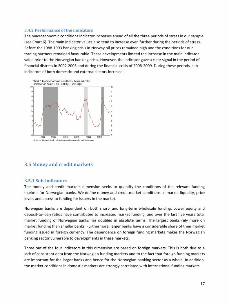
3.4.2 Performance of the indicators
The macroeconomic conditions indicator increases ahead of all the three periods of stress in our sample
(see Chart 6). The main indicator values also tend to increase even further during the periods of stress.
Before the 1988-1993 banking crisis in Norway oil prices remained high and the conditions for our
trading partners remained favourable. These developments limited the increase in the main indicator
value prior to the Norwegian banking crisis. However, the indicator gave a clear signal in the period of
financial distress in 2002-2003 and during the financial crisis of 2008-2009. During these periods, sub-
indicators of both domestic and external factors increase.
3.5 Money and credit markets
3.5.1 Sub-indicators
The money and credit markets dimension seeks to quantify the conditions of the relevant funding
markets for Norwegian banks. We define money and credit market conditions as market liquidity, price
levels and access to funding for issuers in the market.
Norwegian banks are dependent on both short- and long-term wholesale funding. Lower equity and
deposit-to-loan ratios have contributed to increased market funding, and over the last five years total
market funding of Norwegian banks has doubled in absolute terms. The largest banks rely more on
market funding than smaller banks. Furthermore, larger banks have a considerable share of their market
funding issued in foreign currency. The dependence on foreign funding markets makes the Norwegian
banking sector vulnerable to developments in these markets.
Three out of the four indicators in this dimension are based on foreign markets. This is both due to a
lack of consistent data from the Norwegian funding markets and to the fact that foreign funding markets
are important for the larger banks and hence for the Norwegian banking sector as a whole. In addition,
the market conditions in domestic markets are strongly correlated with international funding markets.
0
1
2
3
4
5
6
7
8
9
10
0
1
2
3
4
5
6
7
8
9
10
1988 1992 1996 2000 2004 2008
Chart 6 Macroeconomic conditions. Main indicator.
Sources: Norges Bank calculations and sources for sub-indicators
Indicator on scale 0-10. 1985Q1 - 2011Q3
18
The Merrill Lynch option volatility index - MOVE.
This indicator reflects uncertainty among investors in the bond market. A high degree of uncertainty will
contribute to higher costs and poorer conditions for issuers. The Move index is a yield curve weighted
index of the normalised implied volatility on one-month US Treasury options, and is hence a measure of
the expected volatility one month ahead. The options are written on futures contracts and the implied
volatilites are the weighted average of the 2-, 5-, 10-, and 30-year contracts.
Bond spreads less the CDS premium
This indicator is a measure of the market liquidity of bonds issued by European financial institutions. The
indicator is derived from the difference between the spread on bonds issued by European financial
institutions and the CDS premium on a selection of European financial institutions. The difference
between the total spread and the CDS premium expresses the residual compensation investors demand
for other types of risk than credit risk. A large part of this residual will consist of compensation for
market liquidity. The bond spread is represented by the iBoxx all financials 3-5 years index, while the
CDS premium is the iTraxx Financials index. Allthough the constituents of the two indices do not match
completely, we believe the residual to a large extent will reflect the liquidity conditions in the market for
bonds issued by financial institutions.
Spread on bonds issued by European banks
To capture the bond issuance costs of banks we use the spread on 5-year European bank bonds
represented by the option adjusted spread of the Merrill Lynch Euro Zone broad market AA Rated
financial Corporate Index. The spread index is based on spreads in the secondary market and not on
issuance in the primary market. Historically high spreads in the secondary market are associated with
periods when banks perceive market conditions to be unfavourable and bond issuance costly.
3-month NIBOR minus expected policy rate
The spread that banks demand for short-term funding in the Norwegian interbank market is expressed
by the difference between the 3-month Norwegian Interbank Offer Rate (NIBOR) and an estimate of the
expected policy rate over the same period. As seen during the financial crisis, high spread levels in the
money market indicate that banks are uncertain about their own and other banks’ future need for
liquidity. Since there is no market for overnight-indexed swaps in Norway, we estimate the expected
policy rate from the Forward-Rate-Agreement (FRA).
3.5.2 Methodology and calculation
The money and credit markets dimension applies the alternative method for calculating the sub-
indicators, (see Section 2.2). The method is based on a methodology with intervals of fixed width.
We start by calculating the standard deviation of the historical data. We then construct the mid-interval
(which corresponds to a score of 5) of width ±0.5 standard deviations. The remaining data are
distributed into 10 intervals of fixed and equal width, corresponding to indicator scores from 0 to 4 and
19
6 to 10. The size of the fixed intervals would then be the total width of the data set less one standard
deviation.
Defining a mid-interval of ±0.5 standard deviations implies imposing a wider interval for the indicator
value of 5 than would be the case with a set of strict equally sized fixed intervals. This is motivated by
the preference for a less volatile dimension and an interpretation of the score of 5 as representing
“normal” money and credit market conditions. The method implies a non-uniform distribution of the
indicator values, but follow the dynamics of the underlying market data, with the exception of more
frequent observations of 5.
Each of the four indicators is calculated using the same method, and the value of the dimension is
calculated as the average value of the four indicators.
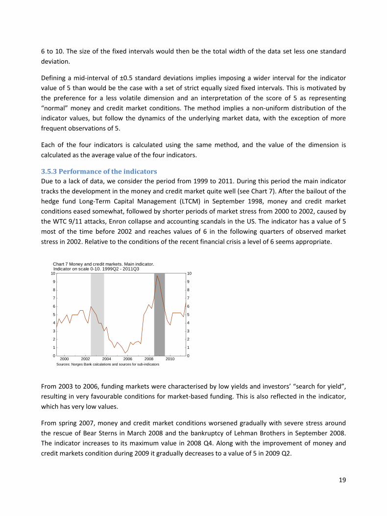
3.5.3 Performance of the indicators
Due to a lack of data, we consider the period from 1999 to 2011. During this period the main indicator
tracks the development in the money and credit market quite well (see Chart 7). After the bailout of the
hedge fund Long-Term Capital Management (LTCM) in September 1998, money and credit market
conditions eased somewhat, followed by shorter periods of market stress from 2000 to 2002, caused by
the WTC 9/11 attacks, Enron collapse and accounting scandals in the US. The indicator has a value of 5
most of the time before 2002 and reaches values of 6 in the following quarters of observed market
stress in 2002. Relative to the conditions of the recent financial crisis a level of 6 seems appropriate.
From 2003 to 2006, funding markets were characterised by low yields and investors’ “search for yield”,
resulting in very favourable conditions for market-based funding. This is also reflected in the indicator,
which has very low values.
From spring 2007, money and credit market conditions worsened gradually with severe stress around
the rescue of Bear Sterns in March 2008 and the bankruptcy of Lehman Brothers in September 2008.
The indicator increases to its maximum value in 2008 Q4. Along with the improvement of money and
credit markets condition during 2009 it gradually decreases to a value of 5 in 2009 Q2.
0
1
2
3
4
5
6
7
8
9
10
0
1
2
3
4
5
6
7
8
9
10
2000 2002 2004 2006 2008 2010
Chart 7 Money and credit markets. Main indicator.
Sources: Norges Bank calculations and sources for sub-indicators
Indicator on scale 0-10. 1999Q2 - 2011Q3

20
3.5.4 Further work
Indicators of domestic funding markets
There is a lack of consistent indicators based on data from the Norwegian funding markets. We believe
that the spread indicator based on European bank bonds is strongly correlated with domestic spreads,
and hence serves as a proxy for price movements in the Norwegian market. However, the Norwegian
bond market is small and more vulnerable to changes in market liquidity.
We are currently working on liquidity indicators for the domestic bond market at the Oslo Stock
Exchange. Liquidity indicators, such as bid-ask spreads or price impact indicators, would be a valuable
tool for assessing domestic money and credit market conditions.
The money and credit markets dimension is primarily based on price data. Data on the volumes of bond
issuance is challenging to incorporate in the indicator due to systemic and seasonal trends. Moreover,
structural changes make it difficult to interpret the data. However, information on access to the bond
market can be obtained from the liquidity survey which Norges Bank has carried out since 2007. The
survey, which covers the six largest Norwegian banks, contains both a qualitative and a quantitative
part. In the qualitative part, banks are asked to assess changes in funding conditions for different
maturities. Funding conditions comprise both market access and price movements.
We consider the implementation of a sub-indicator based on the qualitative part of the liquidity survey.
The values of such an indicator will not be a mechanical result of the survey, but will to a large extent be
set discretionally. Judgment of the survey results and of other available information will be essential in
deciding on the sub-indicator’s value.
3.6 Households
3.6.1 Sub-indicators
The household dimension gives an assessment of the risks to financial stability that stem from
imbalances in the household sector. These imbalances may at some point lead to abrupt changes in
household behavior that might impact banks negatively and undermine financial stability.
Household debt servicing affects banks’ income directly. Changes in household consumption can have a
negative effect on corporate profits and debt servicing capacity, thus affecting banks’ income indirectly.
Households are also investors and affect corporate investment opportunities and banks’ funding. The
risk to banks’ funding from changes in household investor behavior is limited and is not discussed here.
The indicators we include in the dimension reflect the build-up of imbalances in the household sector
and households’ ability to service their debt and to maintain their level of consumption in future.
The following four sub-indicators are included in the dimension: household debt burden, ratio of house
prices to disposable income, household saving ratio and the share of households with a net debt burden
above 500 per cent.

21
Household debt burden
A high household debt burden means that households are vulnerable to sudden drops in income,
increases in interest rates or changes in expectations of future income, house prices and interest rates.
The higher the debt burden, the stronger households react to unexpected shocks by adjusting
consumption and investment. It is difficult to assess when household indebtedness is too high. In spite
of numerous theoretical and empirical studies no consensus has been reached so far on either methods
or levels.
The household debt burden is defined as household loan debt as a percentage of disposable income.
The debt burden is regressed on a trend component and the residuals are used in the sub-indicator. The
measure is similar to what a Hodrick-Prescott filter with a sufficiently high lambda would produce.
Comparing to a trend means that the debt burden can increase over time without necessarily implying
the build-up of imbalances. This is consistent with falling prices on necessities (food, clothing etc) and a
lower interest rate level over the last decade. However, such an assumption will not hold over an
indefinite or a long period of time.
Ratio of house prices to disposable income
Dwellings are the largest wealth component for Norwegian households and unexpected changes in the
value of dwellings will affect household consumption and investment. Residential mortgages make up
the bulk of household debt. A change in house prices will therefore spill over to both banks’ credit risk
and households’ ability to borrow using dwellings as a collateral.
We have opted for an approach that compares house prices to household disposable income. As
Norway has experienced a substantial terms-of-trade effect over the last decade, feeding into
household disposable income, the latter has been chosen as a deflator rather than the CPI, building
costs or house rents.
The sub-indicator is based on the deviation of the house-price-to-disposable-income ratio from its
historical mean over the sample period. A positive deviation signals the build-up of imbalances in the
housing market.
Household saving ratio
A negative saving ratio is not sustainable over time. Abrupt increases in the saving ratio will lower
consumption and weaken corporate profitability, thereby increasing credit risk on banks’ lending to
firms.
The sub-indicator is calculated using an average of quarterly data from the national accounts and Norges
Bank’s calculations14 of the saving ratio based on financial accounts.15 An 8-quarter moving average is
14
Norges Bank’s calculations of the saving ratio based on the financial accounts are not public 15
As deviation between the two series has increased over time, and as it is difficult to assess which measure is the more accurate one, we have decided on the average of the two series

22
used to construct the sub-indicator. We assume that a sub-indicator between 2 and 2.5 per cent
represents a normal level and assign a score of 5 to observations in this range. A low saving ratio implies
unsustainably low savings and a build-up of imbalances. Thus, a low saving ratio implies a high sub-
indicator score. The standard method is applied to observations below 2 per cent and above 2.5 per
cent. This means that observations below 2 per cent are ranked into 5 percentiles and get a score
between 6 and 10. Observations above 2.5 per cent are ranked into 5 percentiles and get a score
between 0 and 4.
Share of households with a net debt burden above 500 per cent
Households with a high debt burden are more vulnerable to unexpected changes in economic conditions
than households with a lower debt burden. A high share of households with a high debt burden might
also signal lax lending standards in the banking sector, which might threaten financial stability.
A gross debt burden of about 500 per cent is equivalent to the requirement from Finanstilsynet
(Financial Supervisory Authority of Norway) to a maximum debt-to-income ratio on mortgage loans of
300 per cent.16 Net debt is defined as gross debt less bank deposits. The indicator is based on microdata
from the household income and tax statements in Norway.
The ratio of households with net debt burden above 500 per cent is the only annual data series in the
dimension, with observations over the period of 1987 - 2009. We construct a quarterly series by
assigning the observed annual value to all the quarters in the respective year. We use the end
observation for any consecutive quarters that we do not have data for. Unfortunately, data from the
household income and tax statements are provided with a considerable time lag of up to two years,
reducing the timeliness of the sub-indicator. However, as changes in the sub-indicator tend to be slow
and gradual, the information still has a bearing on the assessment of household risks to the banking
sector.
3.6.2 Performance of the indicators
The main indicator performs well in signaling the 1988-1993 banking crisis and the 2008-2009 financial
crisis (see Chart 8). The main indicator value increases to very high levels prior to these two crises.
However, the indicator does not seem to give signals prior to the period of financial vulnerability in 2002
– 2003 as it rises to considerably lower levels. Generally, the signals from the main indicator are broadly
produced by all sub-indicators increasing sharply prior to the distress periods.
16
Finanstilsynet issued new guidelines for prudent residential mortgage lending in March 2010. According to the guidelines, if a bank applies the debt-to-income ratio as a loan approval criterion, the mortgage loan should normally not exceed three times the household’s total gross income

23
3.7 Enterprises
3.7.1 Sub-indicators
Norwegian banks’ and mortgage companies’ lending to the corporate sector accounts for over 40
percent of their total lending. The largest corporate loan exposures are to the commercial property and
shipping industries. Developments in these industries are therefore of great importance to banks. Based
on the distribution of Norwegian banks’ lending to the corporate sector we have chosen four indicators
for the corporate sector in general, one for shipping and one for commercial property.
Norwegian companies provide annual financial statements. However, aggregated data based on annual
financial statements are not available until nine months after year-end. In order to provide more
frequently updated indicators, we use quarterly reports published by companies listed on the Oslo Børs
to calculate some of the indicators. Historically the developments of listed companies and limited
liability companies have been highly correlated. The Norwegian oil company Statoil is excluded from the
sample. Statoil accounts for about one third of all listed companies’ total assets, and it would therefore
have an excessive bearing when calculating the indicators. Moreover, Statoil’s profit is heavily correlated
with developments in oil price.
Debt servicing capacity of listed enterprises
A higher debt servicing capacity lowers the risk of bank losses. We have defined debt-servicing capacity
as operating profit before tax, depreciation and impairment losses over the previous four quarters as a
percentage of interest-bearing debt. The ratio is based on quarterly reports published by non-financial
enterprises that are constituents of the OBX index. This index consists of the 25 most traded securities
on Oslo Børs. A higher debt servicing capacity lowers the indicator value.
0
1
2
3
4
5
6
7
8
9
10
0
1
2
3
4
5
6
7
8
9
10
1980 1984 1988 1992 1996 2000 2004 2008
Chart 8 Households. Main indicator.
Sources: Norges Bank calculations and sources for sub-indicators
Indicator on scale 0-10. 1978Q4 - 2011Q3

24
Equity ratio of listed enterprises
The level of the equity ratio determines how robust companies are to a period of increased costs and/or
and reduced income. An increase in the equity ratio also reduces banks’ loan losses in the case of
default. Finally, the equity capital acts as a buffer in periods when access to funding is difficult, as
enterprises can draw on their equity capital instead of raising loans. The equity ratio is calculated as
total equity as a percentage of total assets. An increased equity ratio lowers the indicator value.
Output index
In order to obtain early signals about developments in the Norwegian economy, Norges Bank has
established a regional network of around 1500 enterprises and other organisations across the country.
The information from the survey is obtained before other official statistics are available. The contacts
are interviewed about their view of production volumes over the past three months relative to the
previous three-month period. An increase in production volumes indicates a higher potential for
earnings and thus lowers the indicator value.
Investment gap
A high degree of optimism during an upturn can drive up asset prices and investments and, in turn,
increase credit growth. This can contribute to the build-up of financial imbalances. Optimism will
diminish when the economy is exposed to disturbances. As asset prices and investments fall, debt-
servicing problems arise and bank losses increase. A negative investment gap could also constitute risk,
as lower investments may indicate weaker prospects for enterprises.
Riiser (2005, 2008 and 2010) shows that an investment gap can be useful in predicting financial
instability in Norway. The investment gap is calculated as the absolute value of the percentage deviation
from trend for mainland gross fixed investment measured as a percentage of mainland GDP. The trend is
calculated using a Hodrick-Prescott filter with Lambda equal to 400 000 and a recursive method. An
increase in the absolute value of the investment gap leads to an increased indicator value.
Real market prices for office premises in Oslo
The commercial property industry is the single largest recipient of bank loans in the business sector.
Banks’ loans to property companies are often secured against property belonging to the company. As
the property company’s earnings and the value of its property are closely related, changes in banks’
expected losses can be substantial and increase rapidly. Developments in the property industry
therefore have a considerable impact on the risk in banks’ loan portfolios.
Rent income is the main income of property companies. In theory, market prices could be viewed as the
present value of all future rent income. Market prices may therefore capture expectations on
movements in rents ahead. Market prices will also affect profitability directly through sales proceeds,
revaluations and impairment losses.

25
The indicator is based on an index for market prices for office premises in Oslo, as this segment
constitutes Norwegian banks’ largest commerical property exposure. The index is deflated by CPI. An
increase in the level of real market prices leads to an increased indicator value.
Real shipping freight rates
Shipping accounts for a large share of Norwegian banks’ corporate lending. Developments in freight
rates are important for shipping companies’ earnings, and hence their debt servicing capacity. Shipping
comprises a number of different segments. The indicator is based on the Clarksea index, which is a
weighted average for earnings in the tanker, bulk, container and gas segments. These are some of the
main segments Norwegian banks are exposed to. The index is deflated using the US CPI, and each
observation is calculated as a 12-month moving average. An increase in real freight rates leads to a
lower indicator value.
3.7.2 Performance of the indicators
The main indicator increases before all the three periods of financial stress in our sample period (see
Chart 9). From 1981 to 1990, the main indicator consists of only two sub-indicators, including market
prices for office premises. A downturn in the commercial property market was one of the reasons
behind Norwegian banks’ losses during the 1988–1993 banking crisis. The sub-indicator for the market
price of office premises reaches the maximum level of 10 in 1985. It remains at high levels almost until
the start of the banking crisis in 1988, and then gradually starts decreasing.
All of the sub-indicators are included from 2002 onwards. The main indicator signals the 2002-2003
period of financial vulnerability. Several sub-indicators are at high levels at this point but decrease
gradually in the following quarters. The exception is the equity ratio, which is at a level of 8–10
throughout the distress period.
The signals from the main indicator prior to the financial crisis in 2008–2009 differ somewhat from
earlier distress periods. Driven by the investment gap, the output index and the market price for office
premises, the indicator starts increasing a year and a half before the crisis but the values are not that
elevated. However, the largest increase takes place during the crisis period when the indicator climbs
0
1
2
3
4
5
6
7
8
9
10
0
1
2
3
4
5
6
7
8
9
10
1980 1984 1988 1992 1996 2000 2004 2008
Chart 9 Enterprises. Main indicator.
Sources: Norges Bank calculations and sources for sub-indicators
Indicator on scale 0-10. 1979Q3 - 2011Q3

26
steeply in the course of two quarters. Several sub-indicators such as enterprises’ debt servicing capacity
and equity ratio lead to the rise but shipping freight rates are by far the largest contributor. Hence,
some of the sub-indicators seem to reflect current risk, while others appear to reflect vulnerabilities
ahead of the crisis.
4. Performance of the cobweb model Most of the indicators signal the periods of financial distress. The indicators increase prior to the periods
of distress and fall as financial distress subsides. The indicators usually reach a top during these periods.
However, the household and the enterprise indicators tend to peak prior to the periods of financial
distress.17 Such early warning signals are much appreciated in deciding on the vulnerability of the
financial system. At the same time, the fact that different indicators might show movement in different
directions in the cobweb diagram between two periods, i.e. away from or towards the centre, might
pose a challenge in giving an overall assessment of financial stability.
Chart 10 shows the results of the cobweb model during the 2008-2009 financial crisis.18 The crisis
affected Norway from 2008 Q3 until 2009 Q3. In the chart, the pre-crisis period of 2007 Q3 is also
17
An exception to that observation is the enterprise indicator during the financial crisis in 2008-2009 as it reaches a peak during the distress period 18
The indicators for the different periods are calculated using the total sample until 2011 Q3. A calculation based on the sample up to the relevant period was also performed, for example a calculation for 2007 Q3 uses data only
Chart 10 The cobweb model of financial stability in
Norway during the financial crisis. 2007 Q3 – 2009 Q1
2007 Q3
2008 Q3
2008 Q4
2009 Q1
Structure ofbanking sector
Funding ofbanking sector
Capital and earnings in
banking sector
Enterprises
HouseholdsMoney and creditmarkets
Macroeconomicconditions
Vu
lner
abili
tyin
b
anki
ng
sect
or
Ext
ern
als
ou
rces
of
risk
to
ba
nki
ng
sect
or
Source: Norges Bank

27
included to enable comparisons. A score about 5 reflects the average value based on the history of the
indicator. Prior to the crisis, i.e. 2007 Q3, the vulnerability in the banking sector was over the average
due to the dimensions for banks’ capital and earnings and for the structure19 of the banking sector. It
can also be discussed whether the calibration of the indicator for banks’ funding is satisfactory. Risks in
the household sector were very high and the indicator was at its top level. As the crisis escalated,
conditions in money and credit markets worsened. The money and credit market indicator increased
from the average value of 5 prior to the crisis to its maximum value of 10 in 2008 Q4. Liquidity in
Norwegian banks became considerably strained.20 Macroeconomic conditions worsened, entailing a
rapid increase in risks from enterprises. Banks’ profits deteriorated and the difference between banks’
Tier 1 capital ratio and the “practiced minimum requirement” narrowed, implying lower capital buffers
in banks. As a result, vulnerability due to banks’ profit and capital also rose.
Generally, the model provides a good representation of the crisis-related effects on Norwegian banking
sector. Vulnerabilities and risks to the banking sector rise from around moderate to high or extreme
levels. Financial Stability report 2/07 communicated four main risks to financial stability, i.e. the risk of
an international recession, the risk of higher funding costs for banks due to turmoil in financial markets,
the risk of an abrupt rise in the saving ratio for Norwegian households as a result of high debt and the
risk of substantial optimism in the commercial property market. The model depicts the escalation of
these risks in the following periods in a satisfactory manner. However, it might be questioned whether
the initial levels of the risks in the cobweb diagram represent the same perception of risk that was
conveyed by the report. Financial Stability report 2/07 concluded that “After several years of high
earnings, banks are solid and well equipped to deal with a period of weaker results”. Compared with the
report, the model indicates somewhat higher banking sector vulnerabilities as two of the dimensions,
i.e. capital and earnings and structure of the banking sector, exceed the average value of 5.21 Thus, the
cobweb model might help us interpret the information from our analysis in a more systematic way.
An advantage of the model is that it combines both vulnerabilities in the banking sector and risks
outside the banking sector. However, vulnerability related to bank funding and risks related to
enterprises are either moderate or below the average prior to the crisis. The early warning properties of
the model are therefore yet to be tested.
until 2007 Q3. The model exhibited similar dynamics applying the two different methods, i.e. an increase in vulnerabilities and risks as the crisis unfolds. However, when using a sample up to the relevant period, some of the indicators reached very high scores early in the crisis period. The explanation is that, when using the total sample until 2011 Q3, new extreme observations are added to some of the sub-indicators in the following periods, thus changing the percentile ranking. The changes in the main indicators are therefore more gradual in this case 19
In 2007 Q4 the large banks in Norway started applying internal credit risk models in accordance with the Basel II minimum capital adequacy requirements. This has a considerable impact on the indicator for the structure of the banking sector. The indicator score is therefore rather low in 2007 Q4 compared with earlier periods. The introduction of Basel II influences the indicator in the following periods as well 20
As the series for the sub-indicators in the funding dimension are short, only 3 out of 5 sub-indicators are included in the main indicator during the financial crisis 21
However, developments in the structure dimension during that period should be interpreted with caution as banks’ adjustment to Basel II has a considerable impact on the indicator
28
5. Conclusions The cobweb model is a technical tool that incorporates both vulnerabilities in the banking sector and
external risks to the banking sector. Thus, the model helps us analyse financial stability in a more
systematic manner. As the model assigns scores to vulnerabilities and risks based on historical evidence,
it improves our perception of the state of the financial system. Coupled with a graphical presentation
along several dimensions, the model is expected to enhance communication of our assessment of
financial stability.
The cobweb model performs reasonably well during periods of financial distress. Some of the indicators
seem to signal the build-up of financial imbalances, while others are of a more contemporaneous
nature. Judgment was used to decide on the final positioning of some of the indicators. As each crisis is
different, no model can encompass all the relevant factors. In such cases, the indicators should be
evaluated with the goal of improving them. If further development of the cobweb model is neither
feasible nor appropriate, a subjective adjustment is undertaken based on other available information.
Overruling the raw outcome of the model is documented in the Financial Stability report.
The model is regularly updated and developed, so that it better captures vulnerabilities and risks to the
banking sector. As we gain experience with the model’s performance, changes in the indicators might be
considered. Banks’ funding and money and credit markets are two of the dimensions where data series
are rather short and where we are considering introducing additional indicators. Furthermore, the
indicators of banking sector vulnerabilities will have to be adapted to the introduction of Basel III capital
and liquidity requirements.
References
Andersen, Henrik (2008): “Failure Prediction of Norwegian Banks: A Logit Approach”, Norges Bank
Working Paper 2008/02
Bedford, Paul and Chris Bloor (2009): “A Cobweb Model of Financial Stability in New Zealand”, Reserve
Bank of New Zealand Discussion Paper Series No. 11
Berge, Tor Oddvar and Katrine Godding Boye (2007): “An Analysis of Banks’ Problem Loans”, Norges
Bank Economic Bulletin No.2
Borio, Claudio and Philip Lowe (2002): “Asset Prices, Financial and Monetary Stability: Exploring the
Nexus”, BIS Working Paper No. 114

29
Borio, Claudio and Philip Lowe (2004): “Securing Sustainable Price Stability: Should Credit Come Back
from the Wilderness?”, BIS Working Paper No. 157
Borio, Claudio and Mathias Drehmann (2009): “Assessing the Risk of Banking Crises – Revisited”, BIS
Quarterly Review, March 2009
Dattels, Peter, Rebecca McCaughrin, Ken Miyajima and Jaume Puig (2010): ”Can You Map Global
Financial Stability?”, IMF Working Paper No. 145
Galati, Gabriele and Richhild Moessner (2011): ”Macroprudential Policy – a Literature Review”, BIS
Working Paper No. 337
Hanschel, Elke and Pierre Monnin (2005): “Measuring and Forecasting Stress in the Banking Sector:
Evidence from Switzerland”, BIS Working Paper No. 22
Illing, Mark and Ying Liu (2003): “An Index of Financial Stress for Canada”, Bank of Canada Working
Paper No. 14
Jacobsen, Dag Henning, Thea Birkeland Kloster, Aslak Bakke Kvinlog og Unni Larsen (2011):
“Makroøkonomiske virkninger av høyere kapitalkrav for bankene”, Norges Bank Staff Memo No.14
Kindleberger, Charles P. (2000): “Manias, Panics and Crashes: a History of Financial Crises”, 4th edition
(1st edition 1978), Lohn Wiley & Sons, Inc., New York, pp. 13-15
Minsky, Hyman P. (1977): ” A Theory of Systemic Fragility” in Edvard I. Altman and Arnold W. Sametz
(ed): “Financial Crises: Institutions and Markets in a Fragile Environment”, pp. 138-152, John Wiley &
Sons, Inc., New York
Riiser, Magdalena D. (2005): “House Prices, Equity Prices, Investment and Credit – What Do They Tell Us
About Banking Crises?”, Norges Bank Economic Bulletin No.3, pp. 145-154
Riiser, Magdalena D. (2008): “Asset Prices, Investment and Credit – What Do They Tell Us About Financial Vulnerability?”, Norges Bank Economic Commentaries No.6 Riiser, Magdalena D. (2010): “Asset Prices, Investment, Credit and Financial Vulnerability”, Norges Bank Economic Commentaries No.4
Van den End, Jan Willem (2006): ”Indicator and Boundaries of Financial Stability”, De Nederlandsche
Bank Working Paper No. 97
VO Thi, Quynh Anh (2011): “Countercyclical Capital Buffer Proposal: An Analysis for Norway”, Norges
Bank Staff Memo No. 03

30
Appendices
A List of indicators in the cobweb model of financial stability in
Norway

31
Ind
ica
tors
De
fin
itio
nS
ou
rce
Sta
rt d
ate
Me
tho
d
Ca
pti
al a
nd
ea
rnin
gs
in
th
e b
an
kin
g s
ec
tor
Net
inte
rest
incom
e a
s a
perc
enta
ge o
f
ave
rage t
ota
l assets
Net
inte
rest
incom
e a
s a
perc
enta
ge o
f ave
rage t
ota
l assets
. B
ased
on n
et
inte
rest
incom
e a
nd t
ota
l assets
up t
o t
he p
resent
quart
er
in
the c
urr
ent
year.
The d
ata
series inclu
des a
ll banks e
xclu
din
g
bra
nches o
f fo
reig
n b
anks in N
orw
ay.
Inve
rsed
Norg
es B
ank (
the O
RB
OF
data
base)
1987 Q
4A
ll in
terv
als
have
been s
et
based o
n d
iscre
tion.
The w
idth
of th
e inte
rvals
is larg
er
for
hig
her
ratios a
nd b
ecom
es low
er
for
low
er
ratios.
The
inte
rvals
resultin
g in t
he d
iffere
nt
indic
ato
r
valu
es a
re:
<3,0
0,
∞>
: 0,
[2.5
1,
3.0
0]:
1,
[2.0
1,
2.5
0]:
2,
[1.8
1,
2.0
0]:
3,
[1.6
1,
1.8
0]:
4,
[1.4
1,
1.6
0]:
5,
[1.2
1,
1.4
0]:
6,
[1.1
1,
1.2
0]:
7,
[1.0
1,
1.1
0]:
8,
[0.9
1,
1.0
0]:
9 a
nd <
-∞,
0.9
0]:
10
Loan losses a
s a
perc
enta
ge o
f gro
ss
lendin
g t
o t
he p
riva
te a
nd m
unic
ipal
secto
r
Losses o
n loans t
o t
he p
riva
te a
nd m
unic
ipal secto
r as a
perc
enta
ge
of gro
ss lendin
g t
o t
his
secto
r. A
nnual series.
For
the c
urr
ent
year
loan losses u
p t
o t
he p
resent
quart
er
are
annualis
ed.
The d
ata
series inclu
des a
ll banks in N
orw
ay.
Norg
es B
ank (
the O
RB
OF
data
base)
1987
Sta
ndard
meth
od
Pre
-tax p
rofit
as a
perc
enta
ge o
f ave
rage
tota
l assets
Pre
-tax p
rofit
as a
perc
enta
ge o
f ave
rage t
ota
l assets
. B
ased o
n p
re-
tax p
rofit
and t
ota
l assets
up t
o t
he p
resent
quart
er
in t
he c
urr
ent
year.
The d
ata
series inclu
des a
ll banks e
xclu
din
g b
ranches o
f
fore
ign b
anks in N
orw
ay.
Inve
rsed
Norg
es B
ank (
the O
RB
OF
data
base)
1987 Q
4S
tandard
meth
od
Diff
ere
nce b
etw
een T
ier
1 c
apital ra
tio a
nd
the "
pra
cticed m
inim
um
requirem
ent"
The w
eig
hte
d a
vera
ge T
ier
1 c
apital ra
tio for
all
banks e
xclu
din
g
bra
nches o
f fo
reig
n b
anks in N
orw
ay m
inus t
he "
pra
cticed m
inim
um
requirem
ent"
. The "
pra
cticed m
inim
um
requirem
ent"
is s
et
at
6.0
per
cent
until 2008 Q
4,
and 8
.5 p
er
cent
there
after.
Inve
rsed
Fin
anstils
ynet
(Fin
ancia
l
Superv
isory
Auth
ority
of N
orw
ay)
and N
org
es B
ank
1991 Q
2S
tandard
meth
od
Equity r
atio
Equity a
s a
perc
enta
ge o
f banks' t
ota
l assets
. The d
ata
series
inclu
des a
ll banks e
xclu
din
g b
ranches o
f fo
reig
n b
anks in N
orw
ay.
Inve
rsed
Norg
es B
ank (
the O
RB
OF
data
base)
1987 (
yearly
data
), 1
991 Q
2
(quart
erly d
ata
)
Sta
ndard
meth
od
Fu
nd
ing
Liq
uid
ity c
ove
rage r
atio (
LC
R)
Basel III
defin
itio
n.
Inve
rsed
Norg
es B
ank (
the O
RB
OF
data
base)
2010 Q
3D
iscre
tion u
ntil B
asel III
is im
ple
mente
d
Short
-term
mark
et
fundin
g in fore
ign
curr
ency a
s a
perc
enta
ge o
f to
tal assets
Mark
et
fundin
g is d
efin
ed a
s d
eposits a
nd o
ther
debt
from
cre
dit
institu
tions (
inclu
din
g N
org
es B
ank),
bank c
ert
ificate
s,
(senio
r) b
ank
bonds,
subord
inate
d d
ebt
and d
ebt
rela
ted t
o t
he g
ove
rnm
ent
sw
ap
arr
angem
ent.
Short
-term
mark
et
fundin
g is m
ark
et
fundin
g w
ith a
resid
ual m
atu
rity
of le
ss t
han o
ne y
ear.
Only
short
-term
mark
et
fundin
g in fore
ign c
urr
ency is u
sed in t
he indic
ato
r.
Norg
es B
ank (
the O
RB
OF
data
base)
2000 Q
4S
tandard
meth
od
Net
short
-term
mark
et
fundin
g a
s a
perc
enta
ge o
f to
tal assets
Short
-term
mark
et
fundin
g less s
hort
-term
hig
h-q
ualit
y liq
uid
assets
.
See a
bove
for
a d
efin
itio
n o
f m
ark
et
fundin
g.
Only
deposits in c
entr
al
banks,
gove
rnm
ent
and g
ove
rnm
ent-
guara
nte
ed s
ecurities a
re
defin
ed a
s h
igh-q
ualit
y liq
uid
assets
. S
hort
-term
mark
et
fundin
g a
nd
assets
are
mark
et
fundin
g a
nd a
ssets
with a
resid
ual m
atu
rity
of
less t
han o
ne y
ear.
Due t
o r
oll-
ove
r at
matu
rity
, hold
ings o
f tr
easury
bill
s r
eceiv
ed in e
xchange for
cove
red b
onds in t
he g
ove
rnm
ent
sw
ap
arr
angem
ent
are
assum
ed n
ot
to b
e s
hort
-term
hig
h q
ualit
y liq
uid
assets
if th
e s
wap a
gre
em
ent
matu
res in m
ore
than o
ne y
ear.
Norg
es B
ank (
the O
RB
OF
data
base)
2000 Q
4S
tandard
meth
od
Net
Sta
ble
Fundin
g R
atio (
NS
FR
)B
asel III
defin
itio
n.
Inve
rsed
Norg
es B
ank (
the O
RB
OF
data
base)
2010 Q
3D
iscre
tion u
ntil B
asel III
is im
ple
mente
d
Weig
hte
d a
vera
ge m
atu
rity
of lo
ng-t
erm
mark
et
fundin
g in y
ears
See a
bove
for
a d
efin
itio
n o
f m
ark
et
fundin
g.
Weig
hte
d a
vera
ge
matu
rity
of lo
ng-t
erm
mark
et
fundin
g is c
alc
ula
ted b
ased o
n t
he
share
of m
ark
et
fundin
g in e
ach m
atu
rity
inte
rval. L
ong-t
erm
mark
et
fundin
g is d
efin
ed a
s m
ark
et
fundin
g w
ith a
resid
ual m
atu
rity
of m
ore
than o
ne y
ear.
The t
ime s
eries is inve
rsed.
Norg
es B
ank (
the O
RB
OF
data
base)
2000 Q
4A
ltern
ative
meth
od.
Mid
inte
rval of +
/- 1
.0 s
tdev.
The r
em
ain
ing inte
rvals
are
equally
siz
ed.

32
Ind
ica
tors
De
fin
itio
nS
ou
rce
Sta
rt d
ate
Me
tho
d
Str
uc
ture
of
the
ba
nk
ing
se
cto
r
Mark
et
share
of th
e larg
est
bank in t
erm
s
of to
tal assets
Tota
l assets
of th
e larg
est
bank in N
orw
ay d
ivid
ed b
y t
he t
ota
l
assets
of all
banks in N
orw
ay.
The s
eries is p
resente
d a
s a
perc
enta
ge.
Loans t
ransfe
rred t
o c
ove
red b
ond m
ort
gage c
om
panie
s
are
not
inclu
ded in t
he d
ata
series.
Norg
es B
ank (
the O
RB
OF
data
base)
1987 Q
1The o
ute
r boundaries for
the indic
ato
r va
lues a
re
set
based o
n d
iscre
tion.
A m
ark
et
share
ove
r 50
per
cent
results in a
n indic
ato
r va
lue o
f 10,
while
a m
ark
et
share
belo
w 1
0 p
er
cent
giv
es a
n
indic
ato
r va
lue o
f 0.
The inte
rval betw
een t
hese
oute
r boundaries is d
ivid
ed into
9 s
ubin
terv
als
of
equal w
idth
, e.g
. a m
ark
et
share
betw
een 1
0.0
0
and 1
4.4
4 p
er
cent
pro
duce a
n indic
ato
r va
lue o
f
1.
Ratio o
f le
ndin
g t
o t
he c
orp
ora
te m
ark
et
Lendin
g t
o t
he c
orp
ora
te m
ark
et
from
the s
econd,
third,
fourt
h a
nd
fifth
larg
est
bank in t
his
mark
et
div
ided b
y lendin
g t
o t
he c
orp
ora
te
mark
et
from
the larg
est
bank.
All
banks in N
orw
ay a
re e
ligib
le t
o b
e
inclu
ded in t
he s
eries.
The s
eries is p
resente
d a
s a
perc
enta
ge.
Inve
rsed
Norg
es B
ank (
the O
RB
OF
data
base)
1987 Q
1The o
ute
r boundaries for
the indic
ato
r va
lues a
re
set
based o
n d
iscre
tion.
A r
atio b
elo
w 1
00 p
er
cent
results in a
n indic
ato
r va
lue o
f 10,
while
a
ratio a
bove
250 p
er
cent
giv
es a
n indic
ato
r va
lue
of 0.
The inte
rval betw
een t
hese o
ute
r
boundaries is d
ivid
ed into
9 s
ubin
terv
als
of equal
wid
th,
e.g
. a r
atio b
etw
een 2
33
⅓ a
nd 2
50 p
er
cent
pro
duce a
n indic
ato
r va
lue o
f 1.
Devi
ations fro
m t
he m
acro
bank's
loan
port
folio
The loan p
ort
folio
of all
banks in N
orw
ay is d
ivid
ed into
seve
n
buckets
, e.g
. m
ort
gage loans,
loans t
o c
om
merc
ial pro
pert
y a
nd
ship
pin
g loans.
The loan p
ort
folio
is e
xpre
ssed a
s p
erc
enta
ge
share
s.
The v
ariance b
etw
een t
he e
xposure
s o
f th
is m
acro
bank a
nd
the e
xposure
s o
f each indiv
idual bank is c
alc
ula
ted.
The t
ota
l
lendin
g o
f each b
ank is u
sed a
s its
weig
ht
in t
he v
ariance
calc
ula
tion.
Inve
rsed
Norg
es B
ank (
the O
RB
OF
data
base)
2009 Q
2S
tandard
meth
od,
but
restr
icte
d t
o t
he inte
rval
[4,
6]
due t
o s
hort
tim
e s
eries
Devi
ations fro
m t
he m
acro
bank's
debt
fundin
g s
tructu
re
The d
ebt
fundin
g s
tructu
re o
f all
banks in N
orw
ay e
xclu
din
g
bra
nches o
f fo
reig
n b
anks is d
ivid
ed into
seve
n b
uckets
, e.g
.
secure
d d
eposits,
unsecure
d d
eposits a
nd b
onds in fore
ign
curr
ency.
The fundin
g s
tructu
re is e
xpre
ssed a
s p
erc
enta
ge s
hare
s.
The v
ariance b
etw
een t
he d
ebt
fundin
g s
tructu
re o
f th
is m
acro
bank
and t
he d
ebt
fundin
g s
tructu
re o
f each indiv
idual bank is c
alc
ula
ted.
The t
ota
l debt
fundin
g o
f each b
ank is u
sed a
s its
weig
th in t
he
variance c
alc
ula
tion.
Inve
rsed
Norg
es B
ank (
the O
RB
OF
data
base)
2005 Q
1S
tandard
meth
od,
but
restr
icte
d t
o t
he inte
rval
[3,
7]
due t
o s
hort
tim
e s
eries
Sem
i-va
riance for
negative
devi
ations fro
m
banks' a
vera
ge T
ier
1 c
apital ra
tio
The v
ariance for
banks w
ith a
low
er
Tie
r 1 c
apital ra
tio t
han t
he
national ave
rage is c
alc
ula
ted.
Hence t
he t
erm
sem
i-va
riance.
All
banks e
xclu
din
g b
ranches o
f fo
reig
n b
anks in N
orw
ay a
re
consid
ere
d.
Each b
ank's
weig
ht
in t
erm
s o
f to
tal assets
am
ong a
ll
elig
ible
banks is u
sed in t
he s
em
i-va
riance c
alc
ula
tion.
Fin
anstils
ynet
(Fin
ancia
l
Superv
isory
Auth
ority
of N
orw
ay)
and N
org
es B
ank
1991 Q
2S
tandard
meth
od
Sem
i-va
riance for
negative
devi
ations fro
m
the futu
re L
CR
-sta
ndard
The v
ariance for
banks w
ith a
low
er
LC
R-r
atio t
han t
he futu
re L
CR
-
sta
ndard
is c
alc
ula
ted.
Hence t
he t
erm
sem
i-va
riance.
All
banks
exclu
din
g b
ranches o
f fo
reig
n b
anks in N
orw
ay a
re c
onsid
ere
d.
Each
bank's
weig
ht
in t
erm
s o
f to
tal assets
am
ong a
ll elig
ible
banks is
used in t
he s
em
i-va
riance c
alc
ula
tion.
Fin
anstils
ynet
(Fin
ancia
l
Superv
isory
Auth
ority
of N
orw
ay)
and N
org
es B
ank
Not
sta
rted
Pro
bably
sta
ndard
meth
od

33
Ind
ica
tors
De
fin
itio
nS
ou
rce
Sta
rt d
ate
Me
tho
d
Ma
cro
ec
on
om
ic c
on
dit
ion
sO
utp
ut
gap for
main
land N
orw
ay
Perc
enta
ge d
evi
ation fro
m p
ote
ntial outp
ut.
Inve
rsed
Sta
tistics N
orw
ay a
nd N
org
es
Bank.
Publis
hed in M
oneta
ry P
olic
y
Report
s
1985 Q
1S
tandard
meth
od
Outp
ut
gap for
tradin
g p
art
ners
Perc
enta
ge d
evi
ation fro
m p
ote
ntial outp
ut.
Inve
rsed
IMF
, Thom
son R
eute
rs a
nd N
org
es
Bank
1994 Q
1S
tandard
meth
od
Change in r
egis
tere
d u
nem
plo
ym
ent
rate
Four-
quart
er
movi
ng a
vera
ge o
f th
e q
uart
erly c
hange in t
he
seasonally
adju
ste
d u
nem
plo
ym
ent
rate
Sta
tistics N
orw
ay
1978 Q
1S
tandard
meth
od
Real exchange r
ate
in t
erm
s o
f re
lative
wages
Devi
ation fro
m t
rend,
Hodrick-P
rescott
filt
er
with lam
bda=
400.0
00.
Four-
quart
er
movi
ng a
vera
ge
Sta
tistics N
orw
ay,
Norw
egia
n
Technic
al C
alc
ula
tion C
om
mitte
e
for
Wage S
ett
lem
ents
, M
inis
try o
f
Fin
ance a
nd N
org
es B
ank
1977 Q
4S
tandard
meth
od
Real oil
price g
ap
Oil
prices d
efla
ted b
y G
DP
defla
tor.
Devi
ation fro
m r
egre
ssio
n o
n
trend lin
e.
Inve
rsed
Thom
son R
eute
rs,
Sta
tistics
Norw
ay a
nd N
org
es B
ank
1986 Q
1S
tandard
meth
od
Sove
reig
n n
et
exte
rnal assets
as a
perc
enta
ge o
f G
DP
Devi
ation fro
m r
egre
ssio
n o
n t
rend lin
e.
Inve
rsed
Min
istr
y o
f F
inance
1985 Q
1S
tandard
meth
od
Fore
cast
for
four-
quart
er
GD
P g
row
th
main
land N
orw
ay,
ave
rage for
next
four
quart
ers
Rolli
ng s
am
ple
. In
vers
ed
Norg
es B
ank
Sta
ndard
meth
od
OE
CD
com
posite leadin
g indic
ato
r (C
LI),
tota
l O
EC
D
Inve
rsed
OE
CD
1977 Q
1A
ltern
ative
meth
od o
f equally
larg
e inte
rvals
Mo
ne
y a
nd
cre
dit
ma
rke
tsThe M
err
ill L
ynch o
ption v
ola
tilit
y index -
MO
VE
Yie
ld c
urv
e w
eig
hte
d index o
f norm
aliz
ed im
plie
d v
ola
tilit
ies d
erive
d
from
one m
onth
US
Tre
asury
options.
Ave
rage o
f daily
fig
ure
s for
the
last
month
in t
he q
uart
er
Thom
son R
eute
rs04.a
pr.
88
Altern
ative
meth
od.
Mid
inte
rval of +
/- 0
.5 s
tdev.
The r
em
ain
ing inte
rvals
are
equally
siz
ed.
Bonds s
pre
ads less t
he C
DS
-pre
miu
mB
enchm
ark
spre
ad o
f th
e iB
oxx a
ll fin
ancia
ls 3
-5 y
ears
index m
inus
the iTra
xx F
inancia
ls C
DS
index.
Ave
rage o
f daily
fig
ure
s for
the last
month
in t
he q
uart
er
Thom
son R
eute
rs a
nd N
org
es B
ank
21.jun.0
4A
ltern
ative
meth
od.
Mid
inte
rval of +
/- 0
.5 s
tdev.
The r
em
ain
ing inte
rvals
are
equally
siz
ed.
Spre
ads o
n b
onds issued b
y E
uro
pean
banks
Option a
dju
ste
d s
pre
ad o
f th
e M
err
ill L
ynch 5
-year
Euro
Zone b
road
mark
et
AA
Rate
d fin
ancia
l C
orp
ora
te Index.
Ave
rage o
f daily
fig
ure
s
for
the last
month
in t
he q
uart
er
Thom
son R
eute
rs01.jan.9
1A
ltern
ative
meth
od.
Mid
inte
rval of +
/- 0
.5 s
tdev.
The r
em
ain
ing inte
rvals
are
equally
siz
ed.
3-m
onth
NIB
OR
min
us e
xpecte
d p
olic
y
rate
Spre
ad b
etw
een t
he 3
-month
Norw
egia
n Inte
rbank O
ffer
Rate
(NIB
OR
) and e
stim
ate
s o
f th
e e
xpecte
d p
olic
y r
ate
ove
r th
e s
am
e
period.
Ave
rage o
f daily
fig
ure
s for
the last
month
in t
he q
uart
er
Norg
es B
ank
01.jan.0
7A
ltern
ative
meth
od.
Mid
inte
rval of +
/- 0
.5 s
tdev.
The r
em
ain
ing inte
rvals
are
equally
siz
ed.

34
Ind
ica
tors
De
fin
itio
nS
ou
rce
Sta
rt d
ate
Me
tho
d
Ho
us
eh
old
sH
ousehold
debt
burd
en
Debt
as a
perc
enta
ge o
f dis
posable
incom
e a
dju
ste
d for
estim
ate
d
rein
veste
d s
hare
div
idend for
2000 –
2005 a
nd r
edem
ption/r
eduction
of equity c
apital sin
ce 2
006.
The d
ebt
burd
en is r
egre
ssed o
n a
trend c
om
ponent
and t
he r
esid
uals
are
used in t
he s
ub-indic
ato
r.
Sta
tistics N
orw
ay a
nd N
org
es B
ank
1978 Q
4S
tandard
meth
od
Ratio o
f house p
rices t
o d
isposable
incom
e
Devi
ation in t
he r
atio o
f h
ouse p
rices t
o d
isposable
incom
e fro
m its
mean
Associa
tion o
f N
orw
egia
n R
eal
Esta
te A
gents
, A
ssocia
tion o
f R
eal
Esta
te A
gency F
irm
s,
Fin
n.n
o,
Econ P
öyry
, S
tatistics N
orw
ay a
nd
Norg
es B
ank
1977 Q
1S
tandard
meth
od
Household
savi
ng r
atio
The a
vera
ge o
f th
e q
uart
erly d
ata
for
the s
avi
ng r
atio fro
m t
he
national accounts
and N
org
es B
ank's
calc
ula
tions o
f th
e s
avi
ng r
atio
based o
n t
he fin
ancia
l accounts
.8-q
uart
er
movi
ng a
vera
ge.
Inve
rsed
Sta
tistics N
orw
ay a
nd N
org
es B
ank
1980 Q
1V
alu
es b
etw
een 2
and 2
.5 p
er
cent
are
assig
ned a
score
of 5.
The s
tandard
meth
od is
used for
observ
ations b
elo
w 2
and a
bove
2.5
per
cent.
Valu
es b
elo
w 2
per
cent
are
ranked into
5
perc
entile
s c
orr
espondin
g t
o t
he s
core
s o
f 6-1
0.
Valu
es a
bove
2.5
are
ranked into
5 p
erc
entile
s
corr
espondin
g t
o t
he s
core
s o
f 0-4
.
Share
of household
s w
ith a
net
debt
burd
en a
bove
500 %
Net
debt
is d
efin
ed a
s g
ross d
ebt
less b
ank d
eposits.
Net
debt
burd
en is n
et
debt
as a
perc
enta
ge o
f in
com
e a
fter
tax less inte
rest
expenditure
. O
nly
household
s w
ith incom
e a
re inclu
ded in t
he d
ata
.
Self-
em
plo
yed h
ousehold
s a
re e
xclu
ded fro
m t
he d
ata
.
Sta
tistics N
orw
ay a
nd N
org
es B
ank
1987
Sta
ndard
meth
od
En
terp
ris
es
Debt
serv
icin
g c
apacity o
f lis
ted
ente
rprises
Opera
ting p
rofit
befo
re w
rite
-offs
and w
rite
-dow
ns o
ver
the p
revi
ous
four
quart
ers
as a
perc
enta
ge o
f in
tere
st
bearing d
ebt.
Inve
rsed
Norg
es B
ank (
inte
rnally
deve
loped
data
set
for
the p
eriod 1
998
Q2–2001 Q
2)
and B
loom
berg
(data
from
2001 Q
3)
1998 Q
2S
tandard
meth
od
Equity r
atio o
f lis
ted e
nte
rprises
Equity a
s a
perc
enta
ge o
f to
tal assets
. Lis
ted e
nte
rprises a
t th
e
Oslo
Sto
ck E
xchange e
xclu
din
g S
tato
il. Inve
rsed
Sta
tistics N
orw
ay (
key fig
ure
s for
all
liste
d e
nte
rprises)
and
Blo
om
berg
(key fig
ure
s for
Sta
toil)
2002 Q
1S
tandard
meth
od
Outp
ut
index
Outp
ut
index fro
m N
org
es B
anks r
egio
nal netw
ork
. In
vers
ed
Norg
es B
ank
2002 Q
2S
tandard
meth
od
Inve
stm
ent
gap
Absolu
te v
alu
e o
f th
e p
erc
enta
ge d
evi
ation fro
m t
rend for
main
land
gro
ss fix
ed inve
stm
ent
measure
d a
s a
perc
enta
ge o
f m
ain
land G
DP
(mark
et
valu
e).
The t
rend is c
alc
ula
ted u
sin
g a
Hodrick-P
rescott
filt
er
with lam
bda e
qual to
400 0
00 a
nd a
recurs
ive m
eth
od
Sta
tistics N
orw
ay
1979 Q
3S
tandard
meth
od
Real m
ark
et
prices for
offi
ce p
rem
ises in
Oslo
Sem
i-annual data
for
mark
et
prices for
offi
ce p
rem
ises in O
slo
defla
ted b
y C
PI
OP
AK
and S
tatistics N
orw
ay
1st
half
year
1981
Sta
ndard
meth
od
Real ship
pin
g fre
ight
rate
sThe C
lark
sea index d
efla
ted b
y U
S C
PI. 1
2-m
onth
movi
ng a
vera
ge.
Inve
rsed
Cla
rkson R
esearc
h S
erv
ice L
td.
and
Thom
son R
eute
rs
Jan.
1991
Sta
ndard
meth
od

35
0
1
2
3
4
5
6
7
8
9
10
0
1
2
3
4
5
6
7
8
9
10
1988 1992 1996 2000 2004 2008
Chart 1 Capital and earnings. Main indicator.
Sources: Financial Supervisory Authority of Norway and Norges Bank
Indicator on scale 0-10. 1987Q4 - 2011Q3
0
1
2
3
4
5
6
7
8
9
10
0
1
2
3
4
5
6
7
8
9
10
1988 1992 1996 2000 2004 2008
Chart 1.1 Capital and earnings. Net interest income.
Source: Norges Bank
Indicator on scale 0-10. 1987Q4 - 2011Q3
0
1
2
3
4
5
6
7
8
9
10
0
1
2
3
4
5
6
7
8
9
10
1988 1992 1996 2000 2004 2008
Chart 1.2 Capital and earnings. Loan losses.
Source: Norges Bank
Indicator on scale 0-10. 1987 - 2011
0
1
2
3
4
5
6
7
8
9
10
0
1
2
3
4
5
6
7
8
9
10
1988 1992 1996 2000 2004 2008
Chart 1.3 Capital and earnings. Pre-tax prof it.
Source: Norges Bank
Indicator on scale 0-10. 1987Q4 - 2011Q3
0
1
2
3
4
5
6
7
8
9
10
0
1
2
3
4
5
6
7
8
9
10
1992 1996 2000 2004 2008
Chart 1.4 Capital and earnings. Tier 1 capital ratio less the practiced minimum requirement.
Sources: Financial Supervisory Authority of Norway and Norges Bank
Indicator on scale 0-10. 1991Q2 - 2011Q2
0
1
2
3
4
5
6
7
8
9
10
0
1
2
3
4
5
6
7
8
9
10
1988 1992 1996 2000 2004 2008
Chart 1.5 Capital and earnings. Equity ratio.
Source: Norges Bank
Indicator on scale 0-10. 1987Q4 - 2011Q3
B Charts of main indicators and sub-indicators22
1. Capital and earnings in the banking sector
22
In the charts the banking crisis in 1988 Q2 – 1993 Q3 and the financial crisis in 2008 Q3 – 2009 Q3 are marked in gray. The period of financial vulnerability in 2002 Q3 – 2003 Q4 is marked in a slightly different shade

36
0
1
2
3
4
5
6
7
8
9
10
0
1
2
3
4
5
6
7
8
9
10
2000 2002 2004 2006 2008 2010
Chart 2 Funding. Main indicator 1).
Source: Norges Bank
1) The indicator is based on three out of five sub-indicators prior to 2010Q3
Indicator on scale 0-10. 2000Q4 - 2011Q3
0
1
2
3
4
5
6
7
8
9
10
0
1
2
3
4
5
6
7
8
9
10
2010Q3 2010Q4 2011Q1 2011Q2 2011Q3
Chart 2.1 Funding. Banks` Liquidity Cov erage Ratio (LCR).
Source: Norges Bank
Indicator on scale 0-10. 2010Q3 - 2011Q3
0
1
2
3
4
5
6
7
8
9
10
0
1
2
3
4
5
6
7
8
9
10
2000 2002 2004 2006 2008 2010
Chart 2.2 Funding. Banks` short-term market f unding in f oreign currency 1).
Source: Norges Bank
1) As a percentage of total assets
Indicator on scale 0-10. 2000Q4 - 2011Q3
0
1
2
3
4
5
6
7
8
9
10
0
1
2
3
4
5
6
7
8
9
10
2000 2002 2004 2006 2008 2010
Chart 2.3 Funding. Banks` net short-term market f unding 1).
Source: Norges Bank
1) As a percentage of total assets
Indicator on scale 0-10. 2000Q4 - 2011Q3
0
1
2
3
4
5
6
7
8
9
10
0
1
2
3
4
5
6
7
8
9
10
2010Q3 2010Q4 2011Q1 2011Q2 2011Q3
Chart 2.4 Funding. Banks` Net Stable Funding Ratio (NSFR).
Source: Norges Bank
Indicator on scale 0-10. 2010Q3 - 2011Q3
0
1
2
3
4
5
6
7
8
9
10
0
1
2
3
4
5
6
7
8
9
10
2000 2002 2004 2006 2008 2010
Chart 2.5 Funding. Weighted residual maturity of long-term market f unding.
Source: Norges Bank
Indicator on scale 0-10. 2000Q4 - 2011Q3
2. Funding of the banking sector

37
0
1
2
3
4
5
6
7
8
9
10
0
1
2
3
4
5
6
7
8
9
10
1992 1996 2000 2004 2008
Chart 3 Structure. Main indicator.
Sources: Financial Supervisory Authority of Norway and Norges Bank
Indicator on scale 0-10. 1991Q2 - 2011Q3
0
1
2
3
4
5
6
7
8
9
10
0
1
2
3
4
5
6
7
8
9
10
1988 1992 1996 2000 2004 2008
Chart 3.1 Structure. Market share of the largest bank in Norway.
Source: Norges Bank
Indicator on scale 0-10. 1987Q1 - 2011Q3
0
1
2
3
4
5
6
7
8
9
10
0
1
2
3
4
5
6
7
8
9
10
1988 1992 1996 2000 2004 2008
Chart 3.2 Structure. Ratio of lending to the corporate sector.
Source: Norges Bank
Indicator on scale 0-10. 1987Q1 - 2011Q3
0
1
2
3
4
5
6
7
8
9
10
0
1
2
3
4
5
6
7
8
9
10
2010Q1 2011Q1
Chart 3.3 Structure. Deviations from the macro bank's loan portfolio.
Source: Norges Bank
Indicator on scale 0-10. 2009Q2 - 2011Q3
0
1
2
3
4
5
6
7
8
9
10
0
1
2
3
4
5
6
7
8
9
10
2005 2006 2007 2008 2009 2010 2011
Chart 3.4 Structure. Deviations from the macro bank's debt funding structure.
Source: Norges Bank
Indicator on scale 0-10. 2005Q1 - 2011Q3
0
1
2
3
4
5
6
7
8
9
10
0
1
2
3
4
5
6
7
8
9
10
1992 1996 2000 2004 2008
Chart 3.5 Structure. Semivariance for negative deviations from banks' average Tier 1 capital ratio.
Sources: Financial Supervisory Authority of Norway and Norges Bank
Indicator on scale 0-10. 1991Q2 - 2011Q3
3. Structure of the banking sector
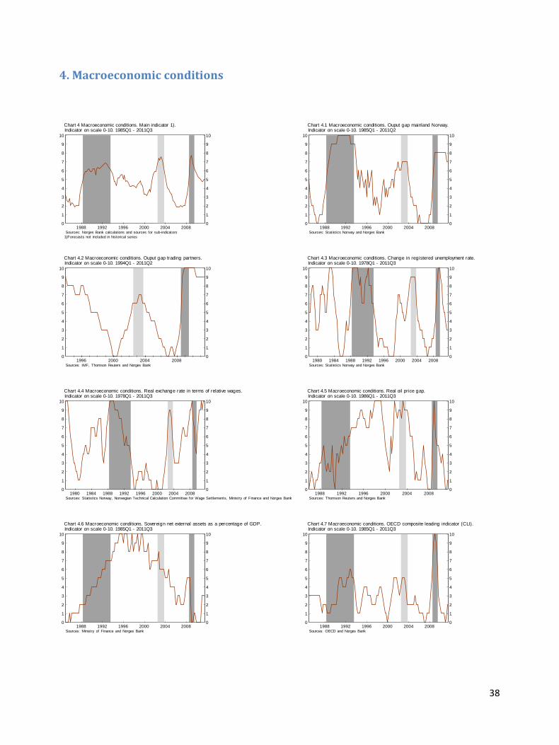
38
0
1
2
3
4
5
6
7
8
9
10
0
1
2
3
4
5
6
7
8
9
10
1988 1992 1996 2000 2004 2008
Chart 4 Macroeconomic conditions. Main indicator 1).
Sources: Norges Bank calculations and sources for sub-indicators
1)Forecasts not included in historical series
Indicator on scale 0-10. 1985Q1 - 2011Q3
0
1
2
3
4
5
6
7
8
9
10
0
1
2
3
4
5
6
7
8
9
10
1988 1992 1996 2000 2004 2008
Chart 4.1 Macroeconomic conditions. Ouput gap mainland Norway.
Sources: Statistics Norway and Norges Bank
Indicator on scale 0-10. 1985Q1 - 2011Q2
0
1
2
3
4
5
6
7
8
9
10
0
1
2
3
4
5
6
7
8
9
10
1996 2000 2004 2008
Chart 4.2 Macroeconomic conditions. Ouput gap trading partners.
Sources: IMF, Thomson Reuters and Norges Bank
Indicator on scale 0-10. 1994Q1 - 2011Q2
0
1
2
3
4
5
6
7
8
9
10
0
1
2
3
4
5
6
7
8
9
10
1980 1984 1988 1992 1996 2000 2004 2008
Chart 4.3 Macroeconomic conditions. Change in registered unemployment rate.
Sources: Statistics Norway and Norges Bank
Indicator on scale 0-10. 1978Q1 - 2011Q3
0
1
2
3
4
5
6
7
8
9
10
0
1
2
3
4
5
6
7
8
9
10
1980 1984 1988 1992 1996 2000 2004 2008
Chart 4.4 Macroeconomic conditions. Real exchange rate in terms of relative wages.
Sources: Statistics Norway, Norwegian Technical Calculation Committee for Wage Settlements, Ministry of Finance and Norges Bank
Indicator on scale 0-10. 1978Q1 - 2011Q3
0
1
2
3
4
5
6
7
8
9
10
0
1
2
3
4
5
6
7
8
9
10
1988 1992 1996 2000 2004 2008
Chart 4.5 Macroeconomic conditions. Real oil price gap.
Sources: Thomson Reuters and Norges Bank
Indicator on scale 0-10. 1986Q1 - 2011Q3
0
1
2
3
4
5
6
7
8
9
10
0
1
2
3
4
5
6
7
8
9
10
1988 1992 1996 2000 2004 2008
Chart 4.6 Macroeconomic conditions. Sovereign net external assets as a percentage of GDP.
Sources: Ministry of Finance and Norges Bank
Indicator on scale 0-10. 1985Q1 - 2011Q3
0
1
2
3
4
5
6
7
8
9
10
0
1
2
3
4
5
6
7
8
9
10
1988 1992 1996 2000 2004 2008
Chart 4.7 Macroeconomic conditions. OECD composite leading indicator (CLI).
Sources: OECD and Norges Bank
Indicator on scale 0-10. 1985Q1 - 2011Q3
4. Macroeconomic conditions
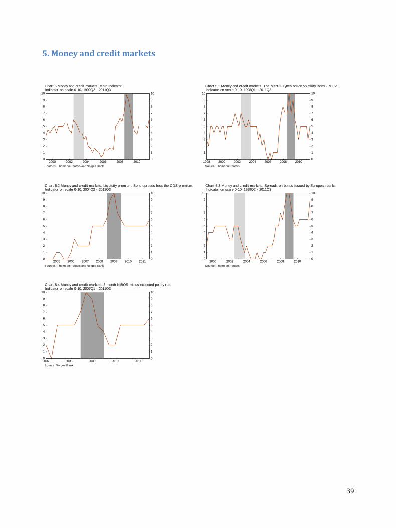
39
0
1
2
3
4
5
6
7
8
9
10
0
1
2
3
4
5
6
7
8
9
10
2000 2002 2004 2006 2008 2010
Chart 5 Money and credit markets. Main indicator.
Sources: Thomson Reuters and Norges Bank
Indicator on scale 0-10. 1999Q2 - 2011Q3
0
1
2
3
4
5
6
7
8
9
10
0
1
2
3
4
5
6
7
8
9
10
1998 2000 2002 2004 2006 2008 2010
Chart 5.1 Money and credit markets. The Merrill-Lynch option volatility index - MOVE.
Source: Thomson Reuters
Indicator on scale 0-10. 1998Q1 - 2011Q3
0
1
2
3
4
5
6
7
8
9
10
0
1
2
3
4
5
6
7
8
9
10
2005 2006 2007 2008 2009 2010 2011
Chart 5.2 Money and credit markets. Liquidity premium. Bond spreads less the CDS premium.
Sources: Thomson Reuters and Norges Bank
Indicator on scale 0-10. 2004Q2 - 2011Q3
0
1
2
3
4
5
6
7
8
9
10
0
1
2
3
4
5
6
7
8
9
10
2000 2002 2004 2006 2008 2010
Chart 5.3 Money and credit markets. Spreads on bonds issued by European banks.
Source: Thomson Reuters
Indicator on scale 0-10. 1999Q2 - 2011Q3
0
1
2
3
4
5
6
7
8
9
10
0
1
2
3
4
5
6
7
8
9
10
2007 2008 2009 2010 2011
Chart 5.4 Money and credit markets. 3 month NIBOR minus expected policy rate.
Source: Norges Bank
Indicator on scale 0-10. 2007Q1 - 2011Q3
5. Money and credit markets
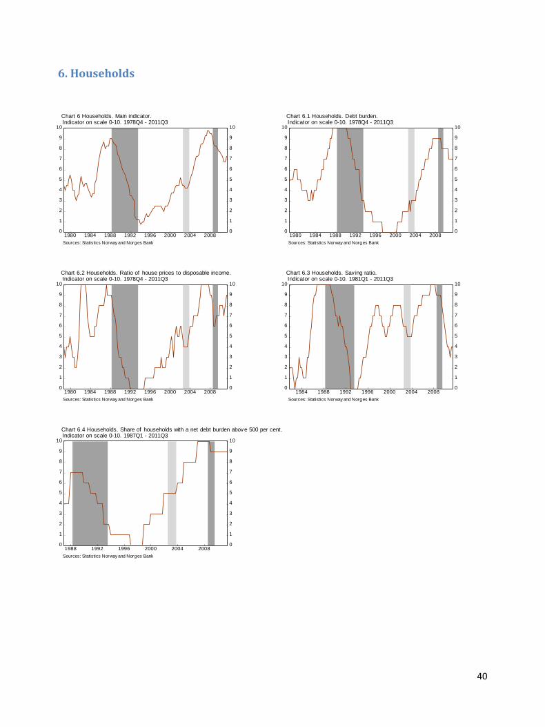
40
0
1
2
3
4
5
6
7
8
9
10
0
1
2
3
4
5
6
7
8
9
10
1980 1984 1988 1992 1996 2000 2004 2008
Chart 6 Households. Main indicator.
Sources: Statistics Norway and Norges Bank
Indicator on scale 0-10. 1978Q4 - 2011Q3
0
1
2
3
4
5
6
7
8
9
10
0
1
2
3
4
5
6
7
8
9
10
1980 1984 1988 1992 1996 2000 2004 2008
Chart 6.1 Households. Debt burden.
Sources: Statistics Norway and Norges Bank
Indicator on scale 0-10. 1978Q4 - 2011Q3
0
1
2
3
4
5
6
7
8
9
10
0
1
2
3
4
5
6
7
8
9
10
1980 1984 1988 1992 1996 2000 2004 2008
Chart 6.2 Households. Ratio of house prices to disposable income.
Sources: Statistics Norway and Norges Bank
Indicator on scale 0-10. 1978Q4 - 2011Q3
0
1
2
3
4
5
6
7
8
9
10
0
1
2
3
4
5
6
7
8
9
10
1984 1988 1992 1996 2000 2004 2008
Chart 6.3 Households. Sav ing ratio.
Sources: Statistics Norway and Norges Bank
Indicator on scale 0-10. 1981Q1 - 2011Q3
0
1
2
3
4
5
6
7
8
9
10
0
1
2
3
4
5
6
7
8
9
10
1988 1992 1996 2000 2004 2008
Chart 6.4 Households. Share of households with a net debt burden above 500 per cent.
Sources: Statistics Norway and Norges Bank
Indicator on scale 0-10. 1987Q1 - 2011Q3
6. Households
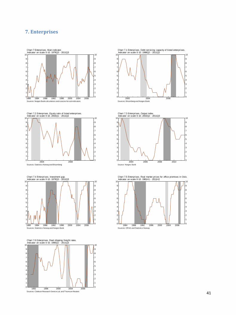
41
0
1
2
3
4
5
6
7
8
9
10
0
1
2
3
4
5
6
7
8
9
10
1980 1984 1988 1992 1996 2000 2004 2008
Chart 7 Enterprises. Main indicator.
Sources: Norges Bank calculations and sources for sub-indicators
Indicator on scale 0-10. 1979Q3 - 2011Q3
0
1
2
3
4
5
6
7
8
9
10
0
1
2
3
4
5
6
7
8
9
10
2000 2004 2008
Chart 7.1 Enterprises. Debt-servicing capacity of listed enterprises.
Sources: Bloomberg and Norges Bank
Indicator on scale 0-10. 1998Q2 - 2011Q2
0
1
2
3
4
5
6
7
8
9
10
0
1
2
3
4
5
6
7
8
9
10
2004 2008
Chart 7.2 Enterprises. Equity ratio of listed enterprises.
Sources: Statistics Norway and Bloomberg
Indicator on scale 0-10. 2002Q1 - 2011Q2
0
1
2
3
4
5
6
7
8
9
10
0
1
2
3
4
5
6
7
8
9
10
2004 2006 2008 2010
Chart 7.3 Enterprises. Output index.
Source: Norges Bank
Indicator on scale 0-10. 2002Q2 - 2011Q3
0
1
2
3
4
5
6
7
8
9
10
0
1
2
3
4
5
6
7
8
9
10
1980 1984 1988 1992 1996 2000 2004 2008
Chart 7.4 Enterprises. Investment gap.
Sources: Statistics Norway and Norges Bank
Indicator on scale 0-10. 1979Q3 - 2011Q3
0
1
2
3
4
5
6
7
8
9
10
0
1
2
3
4
5
6
7
8
9
10
1984 1988 1992 1996 2000 2004 2008
Chart 7.5 Enterprises. Real market prices for office premises in Oslo.
Sources: OPAK and Statistics Norway
Indicator on scale 0-10. 1981H1 - 2011H2
0
1
2
3
4
5
6
7
8
9
10
0
1
2
3
4
5
6
7
8
9
10
1992 1996 2000 2004 2008
Chart 7.6 Enterprises. Real shipping freight rates.
Sources: Clarkson Research Service Ltd. and Thomson Reuters
Indicator on scale 0-10. 1990Q1 - 2011Q3
7. Enterprises


![TAILS: COBWEB 1 [1]](https://static.documents.pub/doc/80x56/5681623c550346895dd27235/tails-cobweb-1-1.jpg)

