

!r:< u .-- r' lt (! ( -- . ·'· ...) ,r • ,J lv\
A MATHEMATICAL SUPPLEMENT
TO C.R. HENDERSON'S BOOK "APPLICATIONS OF LINEAR MODELS IN
ANIMAL BREEDING"
Shayle R. Searle
Professor Emeritus Department of Biometrics,
College of Agriculture & Life Sciences, Cornell University, Ithaca, N.Y., 14853
University of Guelph
1998

PREFACE
Professor Charles R. Henderson {1911-1989) of Cornell University took his only sabbatical leave
in New Zealand during 1955-6. At that time I was Research Statistician in the Herd Improvement Department of the New Zealand Dairy Board, which had sponsored Henderson's coming to New Zealand. As a result, I was lucky enough to have him as an office mate for nine months. That
was a great opportunity to get to know him well before coming to Cornell, where he was my Ph.D. advisor, 1956-8. It therefore gives me great pleasure to offer these notes on his book "Applications
of Linear Models in Animal Breeding'', published by the University of Guelph, 1984. It is referenced in this Supplement as CRH.
Those well acquainted with Professor Henderson's lectures and writings would agree that he was an enormous source of great ideas - but sometimes his conveying of them, either in lecturing
or writing, was not at the same high level as the originality of those ideas. I believe that to be
true of his book, too. My reaction to a first reading of it was that it could do with a little tidying up, especially with respect to mathematical clarity and detailed derivation of many of the formulae
quoted and used in applications. A number of professional animal breeders have told me they feel the same way.
Their encouragement flamed my own interests and this Supplement is the result. And supplement it truly is: it is not a re-writing of the book. But it is designed to be read solely in conjunction with the book. As such it pays scant attention to CRH's many arithmetical examples, except in the last dozen or so chapters, where development is given of some of the numerical equations and their solutions. This is in concert with the overall objective of this Supplement, to provide mathematical fullness for the development of many of the algebraic results which are quoted and used, often with
meager back-up. Stemming from this objective are ideas in the book which I do not like (e.g., MIVQUE and approximations thereto), or do not understand and/or which I think are wrong. At these places I have not hesitated to make personal (opinionated!) comment and to pose questions I cannot answer and problems I have been unable to solve. Hopefully, the clarity of such reactions
will prompt others to provide solutions.
To Norma Phalen I extend my sincere thanks for her typing all this algebra. Her patience is
incredible.
Finally, my heartfelt thanks go to Larry Schaeffer of the University of Guelph for supporting preparation and distribution of this Supplement, and for his help in correcting what were some of my blatant mistakes. Others undoubtedly remain. They are all mine. Corrections are eagerly
sought.
October 1998
ii
Shayle R. Searle 505 The Parkway
Ithaca, N.Y., 14850

NOTATION and LAYOUT
Chapters, paragraphs and page numbers As much as possible the notation follows that of
the book. Chapters correspond to those of CRH; and paragraphs, which are numbered, for example,
as 1.1, 1.2, 1.3, · · ·, often coincide with those of the book. Page numbers are shown, for example,
as [3) for page 3 of the book, [3, 1.2) for paragraph 1.2 on page 3 of the book, and [3, (1.3)] for
equation (1.3) on page 3 of the book.
Equation numbers Equations with decimal numbers are those of the book. Equations without
decimal numbers are mine- they are numbered consecutively, starting with (1) in each chapter.
Bold Face font To conserve time and effort, bold font has not been used for matrices and vectors,
except in places where distinction of vectors from scalars might otherwise be too confusing.
Consistency Every attempt has been made to be consistent in both notation and cross references.
But, in view of the considerable effort required for complete consistency, no excruciating endeavour
has been made in this connection.
Books Referenced by Acronym Back-up of many topics in CRH is detailed in one or more of
the following four books which are therefore frequently referenced {by acronym) in this Supplement.
LM: "Linear Models", Searle, Wiley, 1971.
MAUFS: "Matrix Algebra Useful for Statistics", Searle, Wiley, 1982.
LMFUD: "Linear Models for Unbalanced Data", Searle, Wiley, 1987.
VC: "Variance Components", Searle, Casella and McCulloch, Wiley, 1992.
iii

TABLE OF CONTENTS
CHAPTER 1. Constructing a Linear Model 1
1.1 Simple regression [3, 1.1] 1 1.2 One-way model [3, 1.2] 2 1.3 Two-trait additive genetic model [4, 1.3] 5 1.4 Two-way mixed model [5, 1.4] 6 1.5 Equivalent models [6, 1.5] 7 1.6 Example of ZGZ' = Z*G*Z~ [7] 8 1.7 Subclass means model [8, 1.6] 9 1.8 Determining possible elements in the model [8, 1.7] 9 1.9 Comments on the chapter 10
CHAPTER2. Linear Unbiased Estimation 11
2.1 Verifying estimability [11, 2.1] 12 2.1.1 Second method [12, 2.1.1] 12 2.1.2 Third method [12, 2.1.2] 12 2.1.3 Fourth Method [13, 2.1.3] 13
2.2 When is k' /3 estimable? 13
CHAPTER 3. Best Linear Unbiased Estimation 14
3.1 Introduction 14 3.2 Mixed model method for BLUE (16, 3.1] 15 3.3 Variance of BLUE [18, 3.2] 16 3.4 Cn as part of a generalized inverse 17 3.5 Generalized inverses and MMEs [19, 3.3] 18
3.5.1 First type of g-inverse [19, 3.3.1] 19 3.5.2 Second type of g-inverse [21, 3.3.2] 21
3.5.2.1 Properties of M 22 3.5.2.2 Characterizing rank properties 23 3.5.2.3 Cu as a generalized inverse 24 3.5.2.4 Extension to mixed models [22] 25 3.5.2.5 The form of the Cwmatrices 27 3.5.2.6 Example 28
3.5.3 Third type of g-inverse [22, 3.3.3.] 30 3.6 Reparameterization [23, 3.4] 31 3.7 Example [24] 31
iv

l
5.18 Prediction when R is singular [57, 5.15] 80 5.19 Another example: numeric [59, 5.16] 81 5.20 Prediction when u and e are correlated [61, 5.17] 81 5.21 Direct solution to /3 and to u + T/3 [64, 5.18] 82 5.22 Derivation of MME by maximizing f(y, w) [66, 5.19] 82
,- ... -:
CHAPTER6. G and R Known to Proportionality 83
6.1 Defining proportionality 83 6.2 BLUE and BLUP [70, 6.2] 83
CHAPTER 7. Known Functions of Fixed Effects 84
7.1 Test of estimability [75, 7.1] 84 7.2 BLUE when /3 subject to T' /3 [77, 7.2] 85 7.3 Sampling variances [79, 7.3) 86 7.4 Hypothesis testing [80, 7.4] 86
CHAPTERS. Unbiased Methods for G and R Unknown 87
8.1 Unbiased estimators [83, 8.1] 87 8.1.1 Ordinary least squares ( 0 LS) [84] 87 8.1.2 Weighted least squares (WLS) [84] 88 8.1.3 GLSE using fl-1 [84) 89 8.1.4 OLS treating u as fixed [84) 90 8.1.5 WLS using R-1 treating u as fixed 92 8.1.6 Ignoring a sub-vector of u 92
8.2 Unbiased predictors [87, 5.2] 92 8.3 Substitution of fixed values for G and R [89, 8.3] 94 8.4 Mixed model equations with estimated G and R [89, 8.4] 94 8.5 Tests of hypotheses concerning /3 [90, 8.5] 94
CHAPTER9. Biased Estimation and Prediction 95
9.1 Derivation of BLBE and BLUP [93, 9.1] 95 9.2 Use of an external estimate of /3 [95, 9.2] 98 9.3 Assumed pattern of values of /3 [96, 9.3] 99 9.4 Evaluation of bias [96, 9.4] 99 9.5 Evaluation of mean squared errors [97, 9.5] 101 9.6 Estimability in biased estimation [99, 9.6] 103 9.7 Tests of hypotheses [101, 9.7] 103 9.8 Estimation of P [102, 9.8) 103 9.9 Illustration [102, 9.9) 104
vi
11.12 Illustrations and simplified models , 11.13 An algorithm for R = R.O'; and null covariances
CHAPTER 12. REML and ML Estimation
12.1 An introduction: ML 12.1.1 A general model 12.1.2 Maximum likelihood for the general model 12.1.3 The traditional mixed model
12.1.3.1 The model 12.1.3.2 Estimation 12.1.3.3 Sampling variances
12.2 REML 12.2.1 The concept
· 12.2.2 REML for the general model 12.2.3 REML for the traditional mixed model 12.2.4 Points of interest
12.2.4.1 Differences from ML 12.2.4.2 No matrix K 12.2.4.3 Balanced data 12.2.4.4 Degrees of freedom 12.2.4.5 REML and Bayes
12.3 Practicalities of ML and REML 12.3.1 Estimating fixed effects 12.3.2 ML or REML 12.3.3 Computing
12.4 Iterative MIVQUE 12.5 An alternative algorithm for REML 12.6 ML estimation 12.7 Approximate REML 12.8 A simple result for E(residual S/S) 12.9 Biased estimation with few iterations 12.10 The problem of finding permissible estimates 12.11 Method for singular G
CHAPTER 13. Effects of Selection
13.1 Introduction 13.2 An Example of Selection 13.3 Conditional Means and Variances 13.4 BLUE and BLUP Under Selection Model
13.4.1 Equations for b 13.4.2 Equations for (3° and u0
viii
[158-175] 131 [164, 11.13J32
134
134 134 135 136 136 136 138 138 138 138 139 140 140 140 140 140 141 141 141 141 141
[177, 12.1]143 [178, 12.2]144 [179, 12.3]144 [180, 12.4]145 [180, 12.5]145 [180, 12.6]146 [182, 12.7]146 [184, 12.8]146
147
[185, 13.1] 147 [186, 13.2] 147 [188, 13.3] 148 [189, 13.4] 150
150 152

... 1
i
CHAPTER 16. The One-Way Classification 178
16.1 Estimation and tests for fixed a [223, 16.1] 178 16.2 Levels of a equally spaced (226, 16.2] 179
16.2.1 Example. 179 16.2.2 Sums of squares 180 16.2.3 Hypotheses and models 180
16.3 Biased estimation of p. + G.i [227, 16.3] 182 16.4 Model with linear trend of fixed levels of a [229, 16.6] 183 16.5 The usual one-way covariate model [230, 16.6] 183 16.6 Non-homogeneous regressions [230, 16.6] 183 16.7 The usual one-way random model [232, 16.7] 183
16.7.1 BL UPs add to zero 184 16.7.2 A property of an inverse matrix 184 16.7.3 Sampling variances 185
16.8 Finite levels of a [234, 16.8] 187 16.9 One-way random and related sires 187
CHAPTER 17. The Two-Way Classification 189
17.1 The two-way fixed model [239, 17.1] 189 17.2 BLUE for the filled subclass case [240, 17.2] 190 17.3 The fixed missing subclass case [245, 17.3] 192 17.4 A method based on assumptions "'ii = 0 if nij = 0 [247, 17.4] 192 17.5 Biased estimation by ignoring "' [249 17.5] 192 17.6 Priors on squares and products of"' [250, 17.6] 194 17.7 Priors on squares and products of a, b and "' [254, 17.7] 194 17.8 The two-way mixed model [258, 17.8] 195
CHAPTER 18. The Three-Way Classification 196
18.1 The three-way fixed model [265, 18.1] 196 18.2 The filled subclass case [266, 18.2] 196 18.3 Missing subclasses in the fixed model [2_72, 18.3] 197 18.4 The three-way mixed model [278, 18.4] 198
CHAPTER 19. Nested Classifications 199
19.1 Two-way fixed within fixed [281, 19.1] 199
19.2 Two-way random within fixed [284, 19.2] 201 19.2.1 Sires within treatments [284, 19.2.1] 202
19.3 Random within random [287, 19.3] 205
X

CHAPTER 28. Joint Cow and Sire Evaluation 238
28.1 Block diagonality of MMEs [349, 28.1] 238 28.2 Single record on single trait [351, 28.2] 238 28.3 Simple repeatability model [354, 28.3] 239 28.4 Multiple traits [356, 28.4] 239 28.5 Summary of methods [357, 28.5] 239 28.6 Genetic model to reduce the number of equations [358, 28.6] 240
28.6.1 Single record model [359, 28.6.1] 240 28.6.2 Repeated records model [361, 28.6.2] 242
CHAPTER 29. Non-Additive Genetic Merit 243
29.1 Model for genetic components [365, 29.1] 243 29.2 Single record on every animal [366, 29.2] 243 29.3 Single or no record on each animal [369, 29.3] 243 29.4 A reduced set of equations [372, 29.4] 244 29.5 Multiple or no records [375, 29.5] 244 29.6 A reduced set of equations for multiple records [377, 29.6] 244
CHAPTER 30. Line Cross and Breed Cross Analysis 245
30.1 Genetic model [351, 30.1] 245 30.2 Covariances between crosses [352, 30.2] 245 30.3 Reciprocal crosses assumed equal [384, 30.3] 245 30.4 Reciprocal crosses with maternal effects [386, 30.4] 246 30.5 Single crosses as the maternal parent [357, 30.5] 246 30.6 Breed crosses [388, 30.6] 246 30.7 Same breeds used as sire and dam [388, 30.7] 246
CHAPTER31. Maternal Effects 248
31.1 Model for maternal effects [395, 31.1] 248 31.2 Pedigrees used in the example [396, 31.1] 248 31.2 Additive and dominance maternal and direct effects [398, 31.3] 248
CHAPTER 32. Three-Way Mixed Model 249
31.2 The example [399, 32.1] 249 32.2 Estimation and prediction [400, 32.2] 249 32.3 Tests of hypotheses [401, 32.3] 250 32.4 REML estimation of EM algorithm [403, 32.4] 250
xu
'l
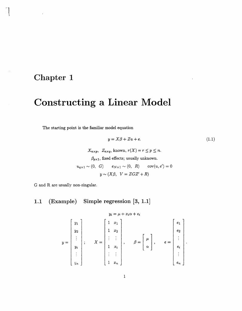
Chapter 1
Constructing a Linear Model
The starting point is the familiar model equation
y = X /3 + Zu + e.
Xnxp, Znxq, known, r(X) = r :S p :S n.
/3pxl, fixed effects; usually unknown.
Uqxl'"" (0, G) eNxl '""(0, R) cov(u, e') = 0
y'"" (X/3, V = ZGZ' + R)
G and R are usually non -singular.
1.1 (Example) Simple regression [3, 1.1)
Yi = f-L + Xia + ei
Yl 1 Xl
Y2 1 X2
y= X= fi=[:], e=
Yi 1 Xi
Yn 1 Xn
1
(1.1)
e1
e2
ei

2a
6 Mates (Dams) 6Progeny 3 Sires
--------------~Pr~<-------
---a> 1'~----
Genetic Relationships for the Matrices on [ 4] and on pages 2 and 3.

CHAPTER 1. CONSTRUCTING A LINEAR MODEL 4
and from considering the variance of any single record
u2 E - u2 - u2 = (1 - h2)u2
Y a y
and
(j2 1 = u2 - u2 = (1 - -h2)u2 e y s 4 y
Therefore
Ru2 e = A h2u2 + 1(1 - h2)u2 - Z' A Z ~h2u2 p y y s 4 y·
Thus
R = [Aph2 + 1(1- h2 )- Z' AsZ~h2Ju;;u;.
On using h2 =~'and the scaling factor of u~fu; = 16/15, along with Ap, Z and As we get
16 4 6 4 2 2 1 1 1 2 2
16 4 2 4 4 1 1 1 2 2
[ ~ 1 1 0 0 0
15 R 1 16 3 2 2 3 1 1 1 1 2 2 = - +-1-- 0 0 1 1 0 16 64 16 4 1 4 16 1 1 1
2 4 0 0 0 0 1
Sym 16 2 1 1 1 2 4
16 1 1 1 2 4
and so
16 4 6 4 2 2 1 1 1 1 1 1 2 2 2
:--·· 1 1 1 16 4 2 4 4 1 1 1 2 2 2
1 16 3 2 2 4 1 1 1 1 1 1 1 2 2 2 R = - +-1--
60 16 4 1 5 15 1 1 1 1 1 1 2 2 2 4
Sym 16 2 1 1 1 1 1 1 2 2 2 4
16 1 1 1 1 1 1 ; 2 2 2 4 4
which, as Ru:, is the third 6 x 6 matrix on [4].

> l
CHAPTER 1. CONSTRUCTING A LINEAR MODEL 6
As on [5]
[ A~1 Ag12] [ Irn Ir12l· G = var(u) = R = var(e) = Ag12 Ag22 Ir12 Ir22
1.4 Two-way mixed model [5, 1.4]
nij values
Sires Treatments ~-
j=1 j=2
i=1 2 1 3
i=2 0 2 2
i=3 3 0 3
n-j 5 3 8
Yijk = p, + tj + Si + (st)ij + eijk
y = X.B+Zu+e
Y111 1 1 1 1 81
Yn2 1 1 1 1 82
Yl21 1 1 1 1 11- 83
Y221 1 1 1 1 = tl + stn +e.
Y222 1 1 1 1
t2 st12 Y311 1 1 1 1
st22 Y312 1 1 1 1
st31 Y313 1 1 1 1
Comments
(i) Easiest to have fixed effects (e.g., treatments) indexed by i.
(ii) To develop X and Z, first write down the vectors of fixed effects, .8, and random effects, u.
l CHAPTER 1. CONSTRUCTING A LINEAR MODEL 8
For i = 1, 2, 3 and 14 = 2 Vi
1 1 0 0 1 0 0
1 1 0 0 p. 1 0 0
I:: I --; 1 0 1 0 tl 0 1 0
X(3 = X.(3. = 1 0 1 0 t2 0 1 0
1 0 0 1 t3 0 0 1
1 0 0 1 0 0 1
E(y) = X(3 = X.(3. if ai = J.L + ti.
Three unrelated cows with 3, 2 and 1 records:
Yij = J.L + Ci + ~j i = 1,2,3, n1 = 3, n2 = 2, n3 = 1
cov (Yii, Yii') = (j2 c and O"~/O"; = r, repeatability
(j2 y = 0"2 + 0"2 => 0"2 = (1 _ r) 0"2 c e e y
var(y) = ZGZ' +R
1 0 0
1 0 0
~I I~ ~I +~I, 1 0 1 1 0 0
1 0 0 (j2 = 0 1 0 0 1 1 c
0 1 0 0 0 0 0 0 0
0 1 0
0 0 1
J3 0
~I +u~I, = (j2 0 J2 c
0 0
l \
.. ,
CHAPTER 1. CONSTRUCTING A LINEAR MODEL 10
The third glibly makes the very true statement that "the most important and most difficult
aspect" is modelling; but nothing more is said.
1.9 Comments on the Chapter
In the title "Constructing a Linear Model" the all-important word is "Constructing" - and
practically nothing is said about this. What is shown is how several standard statistical models fit
into the characterization y = X (3 + Zu + e.

Chapter 2
Linear Unbiased Estimation
In [11, line 1] "linear functions of (3, say k' (3" should be "a linear function of elements of {3,
say k' (3".
For E(y) = X/3,
E(o:'y) = a'X/3
and iff a' X (3 = k' (3 then a' y is said to be an unbiased estimator of (unbiased for) k' (3.
Note: For k' and y, there are usually many vectors a'. An example of this is the following. Suppose
1 1 0
1 1 0
[= E(y) = 1 0 1
1 0 1 t2
1 0 1
with k' f3 being t1 - t2. Then
Generally speaking a'y is an unbiased estimator of k'/3 iff a' X= k'. The sufficiency part of this (if
a' X = k' then a'y is unbiased for k' (3) is always true. There are safely ignorable situations when
the necessity part is not true (see McCulloch and Searle, 1995).
11

CHAPTER 2. LINEAR UNBIASED ESTIMATION 13
2.1.3 Fourth Method [13, 2.1.3]
For (X'X)- being a generalized inverse, k'/3 is estimable if k'(X'X)-X'X = k'. This is very
practical because it does not involve rank, nor does it require finding an L or a C as in paragraphs
2.1.2 and 2.1.2, respectively.
Proof That k'(X'X)-X' X= k' =? k'/3 estimable.
k' - k'(x'x)-x'x
- a' X for a'= k'(X'X)-X'.
Hence
k'/3 = a'X/3 = E(a'y).
2.2 When is k'/3 estimable?
k' /3 is always estimable for k' = t' X for any t. This is the same algebraic relationship as E( a' y) = k' /3
but reworded in a manner that has a different emphasis; namely, for any t'. Whatever, using
k' = t' X always makes k' /3 estimable; i.e., t' X /3 is always estimable. This is a very useful fact
because it means that whenever the concern is to estimate /3, we can avoid considerations of
estimability simply by concentrating on t' X /3 - and by doing this for whatever values of t' we
desire. In particular, by letting t' be the rows of I we have every element of X {3 as being etimable,
a situation which is often described as X {3 being estimable.

l
. i
Chapter 3
Best Linear Unbiased Estimation
(BLUE)
3.1 Introduction
If a' y is to estimate k' /3 unbiasedly, we want a' X = k'; and since "best" means minimum
variance among unbiased estimators, we want to minimize a'V a subject to a' X = k'. Then we set
out to minimize
<p = a'V a + 28 ( k - X' a)
where 28 is a vector of Lagrange multipliers. 28, not just 8 is used, with benefit of hindsight, to
simplify arithmetic.
o<pfoa = 0 ~ 2Va + 2XO = 0.
o<p/88 = 0 ~ X' a = k.
These two equations constitute (3.1). From (1) get a= -v-1 XO. Using this in (2) gives
Hence
14
(1)
(2)

CHAPTER 3. BEST LINEAR UNBIASED ESTIMATION (BLUE) 16
Proof: of VV. =I.
VV. - (ZGZ' + R) V.
- RR-1 + ZGZ'R-1 - (ZGZ' + R)R-1Z(Z'R-1Z + c-1)-1Z'R-1
- I+ ZGZ'R-1 - ZG(Z'R-1Z + c-1)(Z'R-1 Z + c-1)-1 Z'R-1
- I ===? v-1 = V •.
Solving (3.4)
=.·: The second equation in (3.4) yields
Using this in the first equation of (3.4) gives
which is, from v-1 = V.,
and this reduces, as on [17], to
X'V-1 X/3° - X'V-1y
{3° - (x'v-1 x)-x'v-1y.
3.3 Variance of BLUE [18, 3.2]
Taking K' /3 estimable ~ K' = T' X for some T.
BLUE(K' /3) - K' {3°
- T' x(x'v- 1 x)-1 x'v-1y
var[BLUE(K'/3)] = T'X(X'V- 1 X)- X'v-1vv-1 X[(X'V-1 X)-]' X'T.
'i
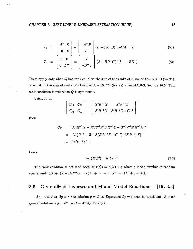
CHAPTER 3. BEST LINEAR UNBIASED ESTIMATION (BLUE) 18
(5a)
(5b)
These apply only when Q has rank equal to the sum of the ranks of A and of D-CA-B (for T1);
or equal to the sum of ranks of D and of A- BD-c (for T2) -see MAUFS, Section 10.5. This
rank condition is met when Q is symmetric.
Using T2 on
gives
Hence
X'R- 1Z lZ'R-1Z + c-1
Cn = [X' R-1 X -X' R-1 Z(Z' R-1 Z + c-1 )-1 Z' R-1 X]
= [X'{R-1 -R-1Z(Z'R-1Z+G-1)-1Z'R-1}Xr
= cx'v-1 x)-.
(3.6)
The rank condition is satisfied because r( Q) = r(X) + q where q is the number of random
effects, and r(D) + r(A- BD-1C) = r(X) + order of c-1 = r(X) + q = r(Q).
3.5 Generalized Inverses and Mixed Model Equations [19, 3.3]
AA-A= A=? Ap = z has solution p = A-z. Equations Ap = z must be consistent. A more
general solution is p = A-z + (J- A-A)t for any t.

CHAPTER 3. BEST LINEAR UNBIASED ESTIMATION (BLUE) 20
{6)
where using T2 from (5b) gives
S2 = [XiR-1XI-XiR- 1Z(Z'R-1Z+G-1)-1Z'R-1XI]- 1 (7)
It is a standard result that these two expressions for inverting a paritioned matrix are equal. To
demonstrate but one term we show that S2 = Coo for
To show this, use (7) for 821 to get
S21 (X~R-1 X1)-1 X' R-1 Z
= [X~R- 1X1- X~R-1 Z(Z'R-1 Z + c-1)-1 Z'R-1X1](X~R-1 X1)-1 X~R-1 Z
= X~R-1 Z[I- (Z'R-1Z + c-1)-1 Z'R-1X1(X~R-1XI)-1X~R-1Z]
- X~R-1 Z(Z'R-1Z + c-1)-1 (Z'R-1Z + c-1 - Z'R-1X1(X~R-1X1)-1X~R-1Z]
= X~R-1 Z(Z'R-1Z + c-1)-18!1, from (6).
Therefore (8) pre-multiplied by S21 from (7), followed by using (8a), is
S21 (X~R-1 X1)-1 + S21 (X~R-1X1)-1 X~R-1 Z S1 Z'R-1 X1(X~R-1 XI)-1
- S2 1 (X~R-1X1)-1 +X~R-1Z(Z'R-1Z +G-1 )- 1 Z'R-1X1(X~R-1X1)-1
- [S21 + X~R-1 Z(Z' R-1z + G-1)-1 Z' R-1 X1](X~R-1 X1)-1
- X~R-1X1(X~R-1X1)-1 =I
(8a)
and so Coo= S2. More easily, using regular rather than generalized inverses in T1 and T2, we show
that
CHAPTER 3. BEST LINEAR UNBIASED ESTIMATION (BLUE) 22
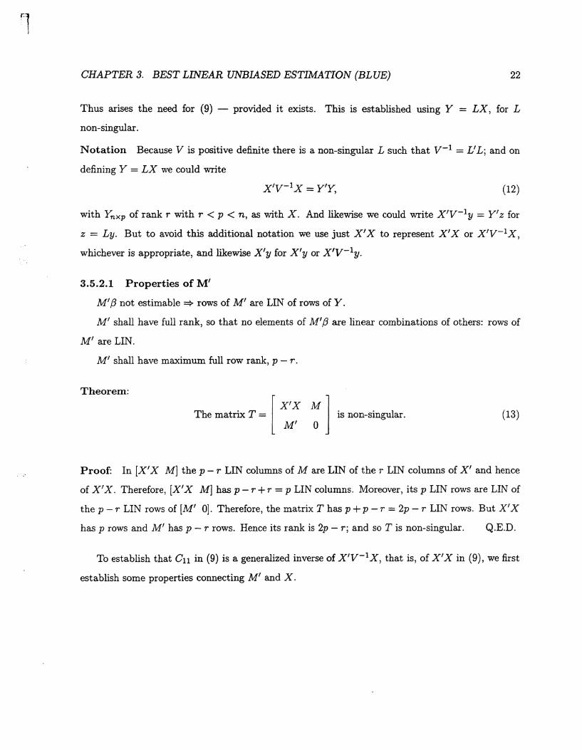
Thus arises the need for (9) - provided it exists. This is established using Y = LX, for L
non-singular.
Notation Because Vis positive definite there is a non-singular L such that v-1 = L' L; and on
defining Y = LX we could write
x'v-1 x = Y'Y, (12)
with Ynxp of rank r with r < p < n, as with X. And likewise we could write X'V- 1y = Y'z for
z = Ly. But to avoid this additional notation we use just X' X to represent X' X or X'V-1X,
whichever is appropriate, and likewise X'y for X'y or X'V- 1y.
3.5.2.1 Properties of M'
M' (3 not estimable => rows of M' are LIN of rows of Y.
M' shall have full rank, so that no elements of M' (3 are linear combinations of others: rows of
M' are LIN.
M' shall have maximum full row rank, p - r.
Theorem:
The matrix T = [ X' X M ] is non-singular. M' 0
(13)
Proof: In [X' X M] the p - r LIN columns of M are LIN of the r LIN columns of X' and hence
of X' X. Therefore, [X' X M] hasp- r + r = p LIN columns. Moreover, its p LIN rows are LIN of
the p- r LIN rows of [M' 0]. Therefore, the matrix T hasp+ p- r = 2p- r LIN rows. But X' X
hasp rows and M' hasp- r rows. Hence its rank is 2p- r; and soT is non-singular. Q.E.D.
To establish that C11 in (9) is a generalized inverse of X'V- 1 X, that is, of X' X in (9), we first
establish some properties connecting M' and X.
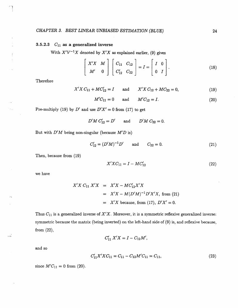
CHAPTER 3. BEST LINEAR UNBIASED ESTIMATION (BLUE)
3.5.2.3 Cu as a generalized inverse
With X'V-1 X denoted by X' X as explained earlier, (9) gives
[ X' X M l [ Cu C12] = I = [ I 0 ]· M' 0 Cb C22 0 I
Therefore
X'XCn +MC~2 =I and X'XC12 +MC22 = 0,
M'Cn =0 and M'C12 =I.
Pre-multiply (19) by D' and use D'X' = 0 from (17) to get
D'M C~2 = D' and D'M C22 = 0.
But with D' M being non-singular {because M' D is)
and
Then, because from {19)
X'XCn =I- MC~2
we have
X'XCnX'X - X'X-MCbX'X
- X'X- M(D'M)-1D'X'X, from (21)
- X'X because, from (17), D'X' = 0.
24
(18)
(19)
(20)
(21)
(22)
Thus Cn is a generalized inverse of X' X. Moreover, it is a symmetric reflexive generalized inverse:
symmetric because the matrix (being inverted) on the left-hand side of {9) is, and reflexive because,
from (22),
and so
(23)
since M'Cn = 0 from (20).

CHAPTER 3. BEST LINEAR UNBIASED ESTIMATION (BLUE) 26
And similarly
Z'XCn + ACb = 0, Z'XC12 + AC22 =I, and Z'XC13 + ACk = 0. (29)
Also, as in (20)
M'Cn = 0, M'C12 = 0, and now M'C13 =I. (30)
Then, just as in deriving (21), pre-multiply each equation in (28) by D (which is symmetric
because it is a covariance matrix) and use XD = 0 = (DX')' to get
DMCb=D DMC23 = 0 DMC33 =0. (31)
But DM = D'M =(MD)' is non-singular and so
C~3 = (DM)-1 D C23=0 and c33 = o. (32)
From the first result in (32) we see that the third equation in (30) is satisfied. And using (32) in
(28) gives
X'XCn +X'ZCb + MC~3 =I, unchanged,
X'XC12 + X'ZC22 = 0, and
X'XC13 = 0,
all with CJ.a as in (32).
We now show that (35) is true by showing that
[ X' X X' Z l [ Cn C12] [ X' X
Z'X A Cb C22 Z'X X' Z l = [ X' X X' Z ]·
A Z'X A
(33)
(34)
(35)
(36)
To do so, consider each submatrix in the product on the left-hand side of (36). First, the (1,1)
term is
(X'XC11 + X'ZC~2)X'X + (X'XC12 + X'ZC22)Z'X
= X' X CnX' X +X' ZC12X' X, using (34),
=(I- X'ZC~2 - MCb)X'X + X'ZC12X'X, using (33),
= X' X using (35).
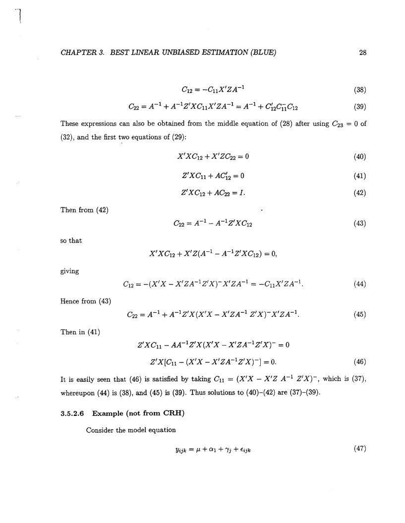
CHAPTER 3. BEST LINEAR UNBIASED ESTIMATION (BLUE) 28
(38)
(39)
These expressions can also be obtained from the middle equation of (28) after using C23 = 0 of
(32), and the first two equations of (29):
Then from ( 42)
so that
giving
Hence from (43)
Then in (41)
x' x C12 + X' zc22 = o
Z'XCn + AC~2 = 0
Z'XC12 + AC22 =I.
C A- 1 A-1Z'XC 22 = - 12
Z'XCn -AA-1Z'X(X'X -X'zA-1Z'X)- = 0
Z'X[Cn- (X' X- X'zA-1 Z'X)-] = 0.
(40)
(41)
(42)
(43)
(44)
(45)
(46)
It is easily seen that (46) is satisfied by taking C11 = (X'X- X'Z A-1 Z'X)-, which is (37),
whereupon ( 44) is (38), and ( 45) is (39). Thus solutions to ( 40)-( 42) are (37)-(39).
3.5.2.6 Example (not from CRH)
Consider the model equation
Yiik = f.L + a1 + 'Yi + €ijk (47)
J
CHAPTER 3. BEST LINEAR UNBIASED ESTIMATION (BLUE) 30
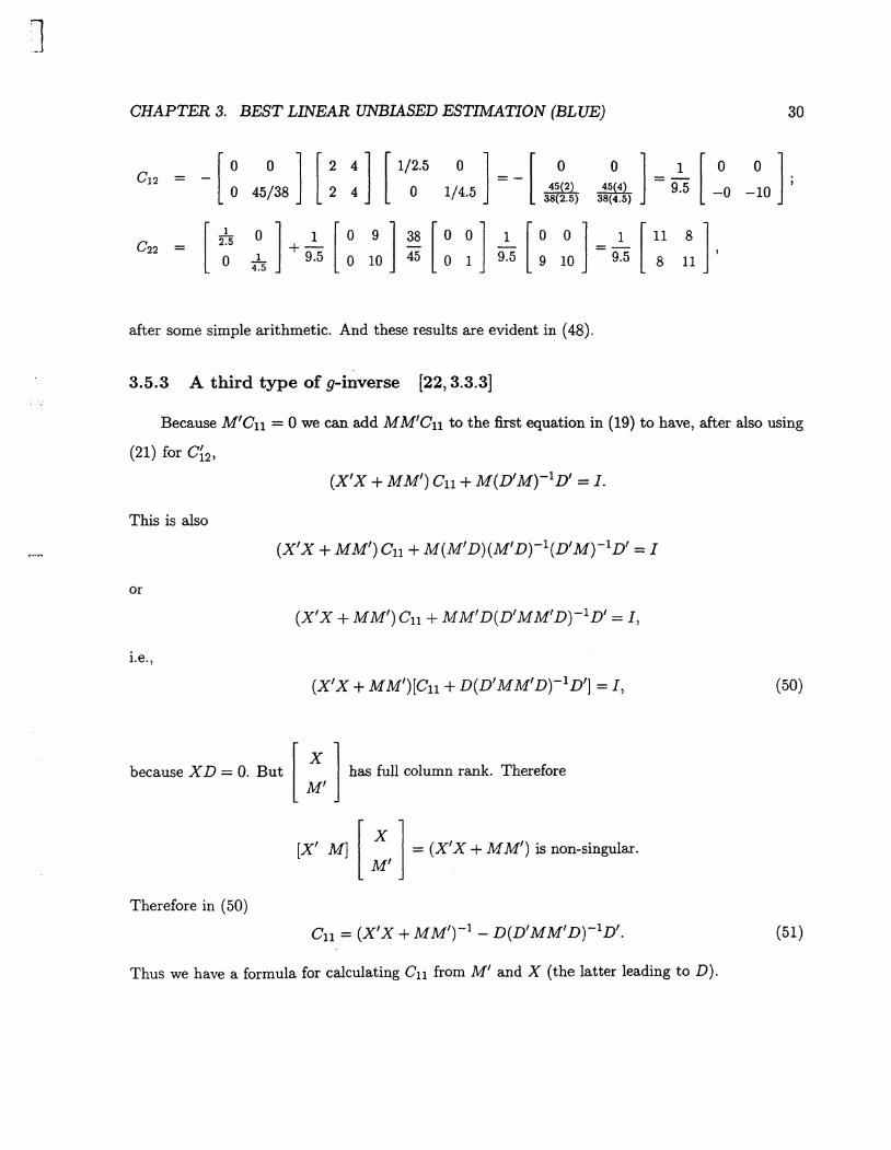
[ 0 0 l [ 2 4] [ 1/2.5 0 l [ 0 0 l 1 [ 0 0 l = - 0 45/38 2 4 0 1/4.5 =- 3!~~~g) 3!~tg) = 9.5 -0 -10 ;
[ 2\ 0 l 1 [ 0 9] 38 [ 0 0 l 1 [ 0 0 l 1 [ 11 8] = 0 4\ + 9.5 0 10 45 0 1 9.5 9 10 = 9.5 8 11 ,
after some simple arithmetic. And these results are evident in (48).
3.5.3 A third type of g-inverse [22, 3.3.3]
Because M'C11 = 0 we can add MM'Cu to the first equation in (19) to have, after also using
(21) for Cf2,
(X'X + MM') C11 + M(D'M)-1D' =I.
This is also
(X'X + MM')C11 + M(M'D)(M'D)- 1(D'M)-1D' =I
or
(X' X+ MM')C11 + MM'D(D'MM'D)- 1D' =I,
i.e.,
(X' X+ MM')[C11 + D(D'MM'D)-1D'] =I, (50)
because X D = 0. But [ ~' ] has full column rank. Therefore
[X' M] [ ~' ] = (X' X + M M') is non-singular.
Therefore in (50)
C11 =(X' X+ MM')-1 - D(D'MM'D)-1D'. (51)
Thus we have a formula for calculating Cn from M' and X (the latter leading to D).

CHAPTER 3. BEST LINEAR UNBIASED ESTIMATION (BLUE)
Then, using the first matrix on [24] as K', namely
1 2
1 2 2
K'= I~ ~ 1 I 0 ' 1 -1
-1 0
0 0 0
doing the arithmetic yields
and
as in [24].
K'K =2I3 and
22 10 12 6 161 K'x'v-1x = -1 5 -6 1 -2
-5 -1 -4 3 -8
11 -.5 -2.5
-.5 2.75 .75
-2.5 .75 2.75
K(K'K)-1 = ~K;
and
&= ~~I
32

l
Chapter 4
Hypotheses Concerning (3
4.1 Introduction
Hypotheses are described as follows.
Null
Alternative
Hbf3 = co r(H0) = m
H~{J = Ca r(Ha) =a } Full row rank r(X) > m >a.
Note that H~ = Pco can be considered a hypothesis only if H~ has full row rank, but also only if
the equations H~{J = co are consistent; which they will be, of course, if H~ has full row rank.
The last three sentences of [25] are confusing:
(i) "···the null hypothesis must be contained in the alternative hypothesis." What does this mean?
(ii) "· · · if the null is true the alternative must be true." This seems to be quite wrong. If it were
correct and the null were true, then why have the alternative if it was going to be true too?
(iii) "· · · so, we require" H~ = MH0 and Ca = Mco. This makes no sense to me.
33

~l
CHAPTER 4. HYPOTHESES CONCERNING /3 35
The first of these sums of squares, R(aiJ.L), is described as testing
J.L
0 1 0 -1 0 0 0 al
0 a2
0 0 1 -1 0 0 0 0
0 0 0 0 1 0 a3
=0. (1) 0 -1 bl
0 0 0 0 0 1 0 -1 b2
0 0 0 0 0 0 1 -1 b3
b4
This is wrong: it has 5 degrees of freedom and R(aJJ.L) has only 2 degrees of freedom because there
are three rows (factor A).
The correct hypothesis is just the first two terms in (1), namely
H: al = a3
i.e., H: a1 =a2 = a3. (2) a2 = a3
Why describe the alternative hypothesis as
0 0 0 0 1 0 0 -1
H: 0 0 0 0 0 1 0 -1 /3 = 0? (3)
0 0 0 0 0 0 1 -1
This is
and as such is no alternative to H : a1 = a2 = a3. And in terms of the last three sentences on [25]
the hypothesis of (2), taken as a null hypothesis, certainly cannot be described as "contained in"
(3) thought of as an alternative hypothesis.
Note that nothing on (26] is said about how many observations there are in each i, j cell. For
k = 1, 2, · · ·, T4.j it is only when ~j = n 'r/ i,j (i.e., only for balanced data) that (2) is the hypothesis
for R(aiJ.L). In contrast, (3) is.the hypothesis for R(bJJ.L, a) for both balanced and unbalanced data
-so long as the no-interaction model is used.

CHAPTER 4. HYPOTHESES CONCERNING /3 37
solutions to GLS equations "subject to restrictions H0/3o =co-" And here is the second confusion:
H0/3o = co starts off as being called a hypothesis and then gets called a restriction.
It seems easier to retain H as a symbol for labelling a hypothesis and to write a hypothesis as
H:K'/3 = c,
using subscripts to H, K and c (but not /3) when more than one hypothesis is being considered;
e.g.,
and
Then one can still use {3° to represent solutions to equations; in particular (with known V)
(ll)
when no hypothesis is being considered, and /38 and /3~ are solutions under hypotheses Ho and Ha,
respectively.
4.4.2 The general case
For the general hypothesis H : K' /3 = c we calculate /3~ as that value of /3 which minimizes
(y- Xf3)'V- 1(y- X/3) subject to H : K'/3 = c, i.e., which minimizes
(y- Xf3)'V- 1(y- X/3) + 2B'(K'/3- c). (12)
This, as may easily be shown, leads to equations
(13)
These are (4.4) with Kin place of Ho, and /3~ in place of /3o. These notation changes help clarify
the procedures. /3 always represents unknown parameters, except in (12) where /3 is viewed as a
mathematical variable for which one chooses as /3~ that value of {3 which minimizes (12). Thus /3~
is the solution of the GLS equations under the hypothesis H : K' /3 = c, and it is different from {3°
of (11) which applies when there is no hypothesis.
' 1
CHAPTER 4. HYPOTHESES CONCERNING {3 39
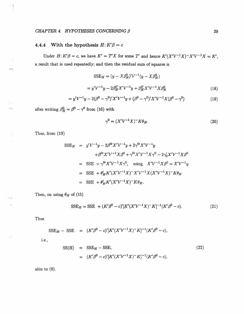
4.4.4 With the hypothesis H: K'/3 = c
Under H:K'/3 = c, we have K' = T'X for some T' and hence K'(X'v-1x)-x'v-1X = K',
a result that is used repeatedly; and then the residual sum of squares is
SSEH = (y - X {3~ )'v-1 (y -X f3Jr)
= y'V-1y- 2f3ZX'V-1y + f3ZX'V-1X~
= y'V-1y- 2(f3o- ·l)' x'v-1y + (f3o- ,oy X'v-1 X(~- ,o)
after writing f3Jr = ~ - 1° from (16) with
Thus, from (19)
SSEH = y'V-1y- 2{3°' X'V-1y + 21°' X'V-1y
+/3°' X'V-1 X {3° + ·l' X'V- 1 X 1° - 2-ybX'V-1 X {3°
= SSE + 1°' X'V- 1 X -y0, using X'V- 1 X{3° = X'V- 1y
= SSE + OnK'(X'V-1X)-X'V- 1X(X'V- 1X)-KOH
= SSE +0nK'(X'V-1X)-KOH.
Then, on using OH of (15)
Thus
i.e.,
SS(H) = SSEH- SSE,
= (K'{3°- c)'[K'(X'V-1 X)-Kr 1(K'f3°- c),
akin to (9).
(22)
(18)
(19)
(20)
(21)

CHAPTER 4. HYPOTHESES CONCERNING (3
and V = R = 5Jg. For testing H : t1 = t2 = t3 the calculations on [28] are
SSE - (y- x,tflyv-1(y- Xf3°), written as (y- Xf3o)'V-1(y- Xf3o)
= 9/4
and
SSEH = (y- x(ikyv-1(y- x(ik ), written as (y- Xf3a)'V-1(y- Xf3a)
- 146/45.
and hence the sum of squares due to His, using (22)
SS(H) = SSEH- SSE 146 9
From the calculations in [28] we also get
SSRH = f3%X'v- 1y
SSR = (3°' X'V- 1y
Thus from (25)
as in (26).
- [49/9 0 0 0](.2)[49 25 15 9]' = 492/45 =53 16 and 45
= [0 25/4 15/3 9/2](.2)[49 25 15 9]' = 125/4 + 15 + 8.1 +54!_, 20
SS(H) = 54 !_ _ 53 16 = 1 63 - 64 = 179 20 45 180 180,
4.5.3 Analysis of variance calculations
41
(26)
(27)
An alternative procedure is to use analysis of variance arithmetic (when V = )J for some
scalar .>..). This is done for two models: the full model, which has no hypothesis, and the reduced
model which is the full model reduced on incorporating the hypothesis. The model equations and

CHAPTER 4. HYPOTHESES CONCERNING {3 45
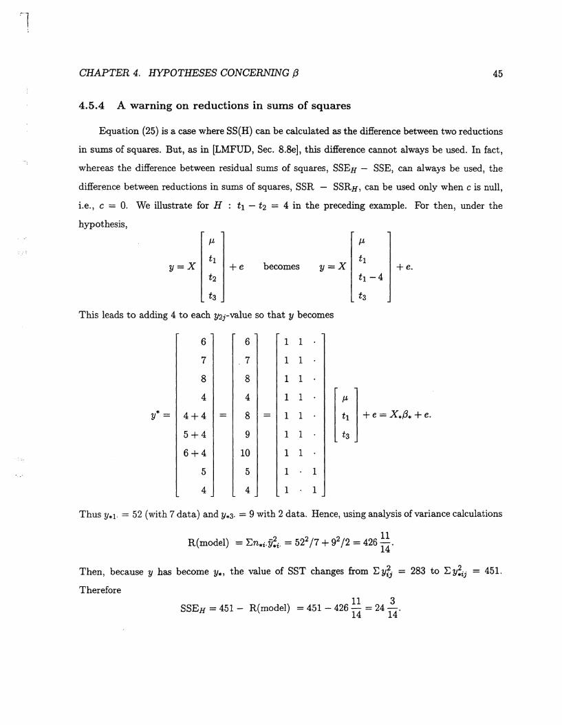
4.5.4 A warning on reductions in sums of squares
Equation (25) is a case where SS(H) can be calculated as the difference between two reductions
in sums of squares. But, as in (LMFUD, Sec. 8.8e], this difference cannot always be used. In fact,
whereas the difference between residual sums of squares, SSEH- SSE, can always be used, the
difference between reductions in sums of squares, SSR - SSRH, can be used only when c is null,
i.e., c = 0. We illustrate for H : t1 - t2 = 4 in the preceding example. For then, under the
hypothesis,
J.L J.L
y=X tl
becomes y=X tl
+e +e. t2 tl -4
t3 t3
This leads to adding 4 to each Y2J-value so that y becomes
6 6 1 1
7 7 1 1
8 8 1 1
4 4 1 1
:. ] +e ~ X,/1.+ e. y* = 4+4 = 8 = 1 1
5+4 9 1 1 t3
6+4 10 1 1
5 5 1 1
4 4 1 1
Thus y*1. =52 (with 7 data) and Y*3· = 9 with 2 data. Hence, using analysis of variance calculations
Then, because y has become y*, the value of SST changes from r, y'fJ = 283 to E YZij = 451.
Therefore 11 3
SSEH = 451- R(model) = 451- 426 14 = 24 14 .

1
CHAPTER 4. HYPOTHESES CONCERNING {3 47
And only K' and c depend on the hypothesis being tested.
In the example,
1 1 .....
1 1
1 1
1 1 9 4 3 2 0
1 1 4 4 1 X= X'X= (X'x)- = 4
1 1 3 3 1 3
1 1 2 2 1 2
1 1
1 1
1 1
And for H : t1 = t2 = ta,
,.,
K'(3 = c [ ~ 1 -1 ~1] t1
= [ ~ ]· is 1 0 t2
ta
Then the normal equations X'v-1 X[30 = X'V-1y, namely
9 4 3 2 ,_,o 49 J.Lo 0
4 4 t~ 25 tO 25/4 give (30 = 1 (28) - -
3 3 tg 15 tg 15/3
2 2 tg 9 tg 9/2
Thus
' 0- [ 25/4 -15/3]- [ 5/4] K/3- - , 25/4-9/2 7/4
CHAPTER 4. HYPOTHESES CONCERNING {3
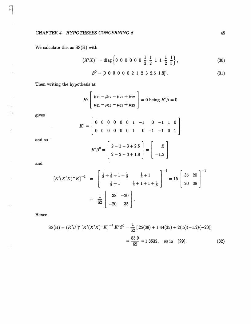
We calculate this as SS(H) with
(X'x)- = diag { o o o o o o ~ ~ 1 1 ~ ~},
rfJ = (0 0 0 0 0 0 2 1 2 3 2.5 1.8]'.
Then writing the hypothesis as
gives
and so ·
and
Hence
H: [ P.n- P-12 - Jl-21 + P-22 ] = 0 being K'f3 = 0 J.Ln - P-13 - P-21 + P-23
K' = [ 0 0 0 0 0 0 1 -1 0 -1 1 01
] 0 0 0 0 0 0 1 0 -1 -1 0
1 0 [ 2 - 1 - 3 + 2.5 ] [ .5 ] K[3 = 2-2-3+1.8 = -1.2
[ ! + ! + 1 + ! 1 + 1 ] - 1
[ 35 - 3 2 2 3 = 15
1+1 1+1+1+! w
- _!_ [ 38 -20 ] . 62 -20 35
20] -1
38
SS(H) = (K' [3°)' [K'(X'X)-K)-1 K'{3° = 612 (.25(38) + 1.44(35) + 2(.5){ -1.2)( -20)]
83.9 (2 ) = T2 = 1.3532, as in 9 .
49
(30)
(31)
(32)

CHAPTER 4. HYPOTHESES CONCERNING /3 51
LM p.278
R(J.L) - N y~. = 14(27 /14)2 - 52.0714
- 52.7917
R(J.L, c) 92 72 112
= 4.+ 4 + 6 - 52.6667
LM p. 297
R(J.L, r, c)
. {10-[3(~)+2(f)+l(¥)]}2 = 52.6667 + (32 22 12)
6- -;r+-;r+6
. ( -2.0833)2 = 52.6667 + . 2.5833 = 52.6667 + 1.6801 = 54.3468
LM p. 275
R(J.L, r, c, rc) = l:.iJniifilr
62 22 52 92 - 3 + 2 + 4 + 9 + 2 + 5 = 55.7000.
Then the sum of squares for testing interactions is
R(J.L, r, c, rc)- R(J.L, r, c) = 55.7- 54.3468 = 1.3532
as in (32); and that for testing equality of row effects in the absence of interactions is
R(riJ.L, c) = R(J.L, r, c) - R(J.L, c) = 54.3468- 52.6667 = 1.6801
as in (33). Similarly, of course, for testing equality of column effects one needs
R(ciJ.L,r) = R(J.L,r,c)- R(J.L,r) = 54.3468-52.7917 = 1.5551.

. 1 I
CHAPTER 4. HYPOTHESES CONCERNING /3 53
With {3°' = [0 0 0 0 0 0 2 1 2 3 2.5 1.8], from (31) and writing (34) as H : K' f3 = 0, we have
2 + 1 + 2-3-2.5-1.8 -2.3
2-2-3 + 1.8 = -1.2
1 - 2 - 2.5 + 1.8 -1.7
and with (X'X)--:- diag{O 0 0 0 0 0 i ! 1 1 ! !} from (30),
1 1 0 3 3
1 0 1 2 2
1 1 1 -1 -1 -1 3 185 2 1
15 -5
1 -1 -1
1 0 -1 -1 0 1 - 2 2 185 11. 15 5
-1 -1 0
0 1 -1 0 -1 1 1 11 21 -5 5 5
1 0 1 -2 -2
1 1 1 -5 5 5
-1
53 2 -3 31 -4 5
[K'(X'X)-K] - 1 1 1 = - 2 38 18 =- -4 58 -32 15 108
-3 18 33 5 -32 67

Chapter 5
Prediction of Random Variables
Many of the numerous results in this chapter are stated without derivation, probably because
their details are quite lengthy. Also, they pertain more to statistics than to animal breeding. For
these notes there are therefore two alternatives: (i) to include all those details, or (ii) to refer
the reader to the VC reference wherein Chapter 7 sets out the details in full array. Because (i)
would add considerable, solely mathematical, length to these notes and would entail little more
than copying from VC, alternative (ii) has been chosen: to give the reader specific references to
VC, at the same time emphasizing important concepts as is deemed necessary.
Notation Since in this section confusion between vectors and scalars is all too easy, bold face
font is sometimes used for vectors and matrices.
5.1 Best Prediction (BP) [33, 5.1]
Equation (5.1) gives the best predictor w = f(y) = E(wjy) of w, a scalar random variable
that is simply the univariate case of the general result for a
vector u: best predictor ft = BP(u) = E(ujy). (1)
This is VC 261, (3). Its derivation is shown on VC 262, based on minimizing not just E(w- w)2
of [33, line 2 of 5.1] but the more general quadratic E {(ii- u)'A(ii- u)} for some matrix A.
55
CHAPTER 5. PREDICTION OF RANDOM VARIABLES 57
The result is derived on VC 264.
4. Ranking predictors
A fourth result, described on [34], but not included there in the listed properties of BLP(u) is
the following. Ranking predictors of u1. ···,UN from largest to smallest, and selecting the highest
a-percentage of those predictors, maximizes E(u) for that a-percentage, if BLP(u) is used as the
predictor. VC 264-5 shows a derivation.
5.2 Best linear prediction (BLP) (34, 5.2]
Reconciling the derivation of BLP in [34-5] with that in VC Sec. 7.3 is a little tricky. The end
result is the same in both places.
The derivation in [34-5] deals with w, starts by defining w = a'y + b (linear in y), and derives
a and b by minimizing E(w- w)2• After defining
E(w) = "{, E(y) = a, Cov(y, w) = c and var(y) = V
this leads to
BLP(w) = 'Y + c'V-1(y- a)= E(w) + Cov(w, y')V-1[y- E(y)]. (3)
VC Sec. 7.3 uses u, starting with ii =a+ By (note here the use of the letters a and B from
that of a and bin w). Then a and Bare derived by minimizing E(ii- u)'A(ii- u) for positive
definite A. With definitions
E(u) = J.Lu, E(y) = py, cov( u, y') = C and var(y) = V
this yields
u = BLP(u) = P.u + cv-1(y- p.y ). (4)
This, which is (23) of VC 268, is simply the vector form of BLP(w) of (3).
Variance-covariance properties of BLP(u) come from (4) very easily. First
var(ii) = var [cv-1(y -J.Ly)] = cv-lvv-1C' = cv-1c'

n I
- '
CHAPTER 5. PREDICTION OF RANDOM VARIABLES 59
as in the last line of [35]. Now we earlier derived
var(ii) = cov(ii, u') = cv-1C'.
Hence, for w being an element of u, the ratio var(w)fcov(w, w) in (5) is unity. Thus (5) gives
Then unbiasedness of w = a' y + b gives
E(w) = E(w) = a'E(y) + b
and so
w=a'y+b - c'V-1y+E(w)-a'E(y)
= E(w) +cov(w,y')V-1[y- E(y)]
which is BLP(w) of (3). Thus the BLP maximizes the correlation between a random variable, w,
and its BLP.
5.3 Ranking
Following (5.11) is a remark about ranking. It relates to a salient problem concerning the use
of predicted values. How does the ranking on predicted values compare with the ranking on true
(realized but often unobservable) values? Henderson (1963) has shown, under certain conditions
(including normality), that the probability of predictors of 'Ui and Uj having the same pairwise
ranking as Ui and Uj is maximized. And Portnoy (1982) extends this to the usual components
of variance model for which ranking the UiS in the same order as the uis rank themselves does
maximize the probability of correctly ranking all the UiS. This is, of course, important in animal
genetics where predicting genetic merit is vital to the breeding of successive generations.
5.4 BP equals BLP under normality
Notation We revert to the norm for these notes of not using bold face for matrices and
vectors.

j ;
' . '
CHAPTER 5. PREDICTION OF RANDOM VARIABLES 61
so that y of (7) has variance
V = var(y) = ZDZ' + R. (9)
Define the function we wish to estimate (or predict, whichever word one prefers) as
f = t'X/3 + h'u (10)
for any [t' h'J ¥= 0. To have an estimator of f that is unbiased, linear (in elements of y) and "best"
we want the estimator to be
(i) linear in y: >..'y for >..' =/; 0;
(ii) unbiased: E(>..'y- f)= 0;
(iii) best: we want the error mean square, E[>..'y- (t'X/3 + h'u)]2 subject to E(>..'y- f) = 0 to
be a minimum.
In the model equation (7) we take E(u) = 0, giving E(y) = X/3 so that (ii) above gives
>..'X/3- t'X/3 = 0. We want this to be true for all /3, and so need >..'X= t'X, or
X'>..= X't.
Then, subject to (ll), we want from (iii) above to minimize
E(>..'y- t'X/3- h'u)2 = E(>..'X/3 + >..'Zu + >..'e- t'X/3- h'u)2
= E [>..'(Zu +e)- h'u] 2
= >..'V>- + h'Dh- 2>-'ZDh,
after using (8). To do this we minimize
0 = >-'V>- + h' Dh- 2>..'ZDh + 2m'(X'>..- X't)
where m' is a vector of Lagrange multipliers. Thus
(ll)
(12)
(13)
80ja>..=O gives 2V>..-2ZDh+2Xm=0 ::::} >..=-V-1Xm+V- 1ZDh, (14)

CHAPTER 5. PREDICTION OF RANDOM VARIABLES 63
and for this to be true for all k we must have >..'X = 0. This is equivalent to having t = 0 in (11);
and using this in (16) gives
This, from (10) with t = 0, is BLUP(h'u) = h' DZ'V-1(y- X(fJ), which, as in (38, line 7], is
m'C'V-1(y- X{JJ) with m' being h' and C' = DZ'.
5. 7 Using functions of y having zero expectation [38, 5.4.2]
For {3* = L'y
E(X{3*) = E(XL'y) = XL'E(y) = XL'X{3
and if
E(X{3*) = XL'X{3 is to be X{3 'V {3
then
XL'X=X.
Equations (5.19) through (5.23) of (38] are quite straightforward. The line below (5.23) deserves
support.
Proof: w is invariant to T and to (T'VT)-.
A c'v:-w = * * y*, from (5.21)
= (T'C)'(T'VT)-T'y, from earlier equations
= C'T(T'VT)-T'y. (19)
This is invariant to T because XL' X = X indicates that L' is a generalized inverse of X, say
(X' X)- X'; and then T' =I- XL' is T' =I- X(X'x)- X', invariant to (X' X)-. Then in (19)
for V = Q'Q and non-singular; and QT(T'Q'QT)-T'Q' is invariant to QT. Thus w is invariant to
T and (T'VT)-.
l
CHAPTER 5. PREDICTION OF RANDOM VARIABLES
Cov{w,w') - (K'- C'V-1 X)Cov((:/J,u') + C'V-1Cov(y,u')
= (K'- c'v-1 X)(X'v-1x)-x'v-1 zG + c'v-1 zc
- K'(x'v-1 x)-x'v-1c + c'v-1c- c'v-1 x(x'v-1 x)-x'v-1c
= K'(X'v-1x)-x'v-1c + c' PC for P = v-1 - v-1 X(X'v-1 x)-x'v-1
which is (5.26).
var(w) - var[K'{3° + C'V-1(y- X(:/J)]
var(/3°) - (X'V-1 X)-X'V-1 X(X'V-1 X)-' = (X'V-1 X)- say
cov(y, {30') - vv-1 X(X'v-1 X)-= X(X'V-1 X)-
·and on writing A = (X'V-1 X)-,
var(w) - var [CK'- C'V-1X){3° + C'V-1y] - (K' - c'v-1 X)A(K- x'v-1c) + c'v-1c + c'v-1 x A(K- x'v-1c)
+ (K' - c'v-1 X)AX'v-1c
- K'(x'v-1 x)-K + c'v-1c- c'v-1 x(x'v-1 x)-x'v-1c.
This is (5.28). Finally
. .. var(w-w) - var(w)-cov(w,w')-cov(w,w')+var(w)
- var(w)- K'(X'V-1X)-X'V-1C- C'PC
- C'V-1 X(X'v-1 X)-K- C' PC+ K'(X'V-1 X)-K + C' PC
65
_ G + K'(x'v-1 x)-K- K'(x'v-1x)-x'v-1c- c'v-1x(x'v-1x)-K- c' PC
, - which is (5.29).

CHAPTER 5. PREDICTION OF RANDOM VARIABLES
5.10 Variances from Mixed Model Equations (40, 5.7]
From (21) let
where
where
[ X'R-1X X'R-1Z l-Z'R-1X Z'R-1Z + c-1
- [ ~ :-] + [ -u-: K' X l r- [I
u = Z'R-1Z + c-1
T = X'R-1X-X'R-1Z(Z'R-1Z+G-1)-1Z'R- 1X
= X'[R-1 - R-1 Z(Z'R-1 Z + c-1)-1 Z'R-1]X.
= x'v-1x ,
using VV* = vv-1 =I of these notes for Section [3.2]. Hence
T = x'v-1x
and
[ C C l [ T- -T-X'R-1zu- l c~: c:: - -u-z'R-1xT- u-+u-z'R-1X(X'v- 1x)-x'R-1zu-
But from below (22)
67
-(X'V- 1 X)- X'V- 1 ZG l (Z' R-1 Z + c-1)-1 + GZ'V-1X(X'V- 1 X)- X'V- 1 ZG
(22a)
CHAPTER 5. PREDICTION OF RANDOM VARIABLES
var(u) = G- C22(5.38)
cov(u, u') = C'V-1cov[(y- X/P), u']
= C'v-1[1- X(X'V-1x)-X'V- 1]cov(y, u')
= GZ'V-1 [1- X(X'V- 1X)- X'V- 1]ZG
= az'v-1zG + (Z'R-1Z + a-1)-1 - C22
= G- c22(5.39)
var(u- u) = G- C22 + G- 2(G- C22) = C22(5.40)
var(w- w) = v[K'(_aO- /3) + u- u]
= v(K'j3°) + v.(u- u) + cov(K'/P, u'- u') + cov(u- u,j3°' K)
= K'CnK + C22 + K'C12 + Cf2K.(5.41)
5.11 Prediction of errors [41, 5.8]
Equation (5.18) is for scalar w with E(w) = k'/3, var(w) = v and cov(w, y') = c', giving
Adapted to vector w, k' becomes K', and c' becomes C so that
Thus the special case
w=t:=y-X/3, E(w)=O=>K'=O
gives
[41, line 4]
and then, because
69

CHAPTER 5. PREDICTION OF RANDOM VARIABLES
of (5.33). Then
ep = (I- WCW'R-1)y
var(ep- ep) = var(y- X{3°- Zu- ep)
= var(X{3 + Zu + ep- X{3°- Zu- ep)
= var[-X({3°- (3)- Z(u- u)]
= Xvar({3°- {3)X' + Z var(u- u)Z' + 2Xcov[{3°- (3, (u- u)']Z'
= XCnX' + ZC22Z' + 2XC12Z', from (5.40) and (5.37), respectively.
= WCW'. [42, line 2]
cov[(ep- ep), (K'{3°)'] - cov[{ -X({3°- {3)- Z(u- u)}, (K'{3°)']
= -Xvar({3°)K- Zcov[(u- u), {3°']K
= -XCuK- ZC12K from (5.34), (5.37)
-WC'K. [42, line 7]
cov[(ep- ep, (u- u)'] cov[{ -X({3°- {3)- Z(u- u)}, (u- u)']
- -XC12- zc22
= -we~ [42, line 8]
cov[(ep- ep, (em- em)'] - cov[(ep- ep, {~~(ep- ep)}']
= var(ep- ep)R.W1 Rpm
- WCW'R;JRpm [42, line 9]
var(em- em) = var(em) + var(em)- 2cov(em, e~)
= var(~R;iep) + Rmm- 0,
71
(23)
the zero because em is a function of ep, and hence of y; and em does not occur in y. We now need
var(ep). By definition
var(ep) = Rpp.

CHAPTER 5. PREDICTION OF RANDOM VARIABLES
This simplifies by using
and
v-1 - v-1 x(x'v-1 x)-x'v-1 - P
ZGZ' - V-R
Z(Z'R-1Z +G-1)-1 - ZG [z'R-1Z + c-1 - Z'R-1z] (Z'R-1Z +G-1)-1Z'
- ZG [1- Z'R-1Z(Z'R-1Z + c-1)-1] Z'
- ZGZ' [R-1 - R-1z(Z'R-1Z +G-1)Z'R-1] R
= ZGZ'V-1 R = (V- R)V-1 R
= R-RV-1R.
Therefore
WCW' - V(V-1 - P)V + V(P- v-1)(V- R) + (V- R)(P- v-1)V
+ (R - RV-1 R) + (V - R)(V-1 - P)(V- R)
- V- V PV + VPV- V- V P R + R + V PV- RPV- V + R
+ R- RV-1 R + V- R- R + RV-1 R- V PV- RPV + V PR- RPR,
73
and from this everything cancels except R- RPR, so leaving WCW' = R- RPR. Hence (25) is
var(ep- ep) = [I- (R- RPR)R-1]V[I- R-1(R- RPR)] + R- 2(1- (R- RPR)R-1]R
= RPVPR+R-2RPR
= RP R + R- 2RP R, because PV P = P
= R-RPR
= wcw.
Now consider the last two results preceding (42, 5.9]. From (41, last line]

CHAPTER 5. PREDICTION OF RANDOM VARIABLES
has
An alternative to (28) is
y~X.B+[Z OJ [: l +e
Applying the formula for (fJ in (27) to this set-up gives the estimator (3* as
p• ~ {[X' X~] [ v;' ~ ][ ;. l r [X' X~] [ V:' ~ ][ ~ l - (x'v-1 x)-x'v-1y - (Jo.
Likewise, applying u of (27) gives
Thus we get
and
fLn = B'v-I(y- Xf3o)
= C'Z'V-1(y- X/3°) = C'G-1u.
75
(5.47)
(5.48)
' l
--,
:. -j
CHAPTER 5. PREDICTION OF RANDOM VARIABLES 77
for
giving Wn = G-1 + c-1CTC'G-1, W12 = -G-1CT and W22 = T.
It is stated that equations (5.49) have the same solutions as (5.48) and il preceding (5.47). We
show this.
First, from the last equation of (5.49)
W22-fin = -(W12)'u
'fin - r-1TC'G- 1u = C'G-1u
which is (5.48). Then, part of the second equation of (5.49) is
Thus that second equation is
(G-1 + a-1CTC'G-1 - c-1CTC'G-1)u
- c-1u.
which, with the first equation of (5.49) constitutes the MMEs (29).
5.13 Prediction When G is Singular [43, 5.10]
Let H be a matrix we do not like, e.g., the matrix of the MMEs when G is singular. Then the
matrix in (5.50) is [ ~ ~ l H=L, ~y Now compute C, a generalized inverse of L:
LCL=L.
~l
CHAPTER 5. PREDICTION OF RANDOM VARIABLES
where there is only one record on each animal: var( a) = Au~. The MMEs have order p + n
Nevertheless, under these conditions it is suggested that equations
79
(5.57)
be used. No indication is given as to the origin of these equations, nor as to why they, of order
n + p, should be used (only?) when p + q > n; i.e., n + p > 2n- q. The equations are easily solved
Define
[ Cn C12] Cb c22
=
Vs + X(JJ = y => s = v-1(y- X,B0)
X's = o = x'v-1y- x'v-1x,a0
(x'v-1 X)/3° = x'v-1y
u GZ's=GZ'V-1(y-Xf3°).
[ v x ]- [ v-1 o l [ v-1x l x' o = o o + - I [o- x'v-1 x]-[-x'v-1 I]
[ v-1- v-1 X(X'v-1 x)-x'v-1 v-1 X(X'v-1 x)-l· (x'v-1 x)-X'v-1 -(X'v-1 x)-
Hence Cn = P and so
var(K'/3°) = var[K'(X'V-1 X)-X'V-1y]
= K'(x'v-1 x)-x'v-1vv-1 x(x'v-1 x)-K
= -K'C22K (5.59)
var(ft) - var[GZ'V-1(y- X/3°)]
= var(GZ' Py)
= GZ'PZG because PVP=P
= GZ'CuZG because Cu = P. (5.60)
cov(K' /3°, u') = cov{K'(X'V-1 X)- X'V- 1y, y'P}

:·j
CHAPTER 5. PREDICTION OF RANDOM VARIABLES 81
2 1 4 1 5
1 7 -11 -6 -17
= [ :, ][ : ~ l [I L] 4 -11 34 15 49
1 -6 15 7 22
5 -17 49 22 71
for
L= [ 3 1 4] , of order 2 x 3 has rank 2, not 3. -2 -1 -3
Finally, even after writing (30) I see no reason why X and Z being linearly dependent on R
leads to X = [ X I ] ; and Z = [ ZI ]· True, CRH says "iP' X and Z are of this nature. L'XI LZI
Then, of course
is singular.
5.19 Another Example: Numeric [59, 5.15]
5.20 Prediction When u and e Are Correlated [61, 5.17]
Derivation of (5.82) is straightforward. Verification of (5.81) is easy:
var{t) - var(Zu + e- Tu] = var(e- sa-Iu)
- R +sa-Icc-Is'- 2sc-Is' = R- sc-Is'
- B
cov(Tu, l) - cov[Tu,e'- u'G-IS'] = TS'- TGG-IS'
- TS'-TS'=O.

. 1
Chapter 6
G and R Known to Proportionality
6.1 Defining Proportionality
It is assumed that
and (6.1)
where G* and R* are taken as known, but a-; is unknown.
6.2 BLUE and BLUP [70, 6.2]
With V = V*o-;, the equations for {3° and u are precisely as previously, but with V replaced
by V*. To show that (6.6) is the same as (6.7) note that the numerator of (6.6) is
y'V-ly- /30' X'V-ly
= y'V-l(y- X/3o)
= y' R-1 [1- Z(Z' R-1z + c-1)-1 Z'R-1](y- X/3°)
= y' R-1 [(y- X {3°) - Zu], after using [41, (5.44)]
'R-1 'R-1Xf3o 'R-1zA = y y-y -y u
'R-1 f3o'x'R-I A'Z'R-1 = y y- y-u y
which is essentially the numerator of [71, (6.7)]. The remainder of Chapter 6 concerning tests of
hypotheses seems straightforward.
83

··-, '
Chapter 7
Known Functions of Fixed Effects
7.1 Tests of Estimability [75, 7.1]
For T' /3 non-estimable, T' of full row rank t < p - r, it is stated that there is always a matrix
C, of order p x ( r - t) and full column rank, such that
(7.1)
And then K' /3 is estimable if and only if
K'C = 0. (7.2)
Proof (i): If K'/3 is estimable then K'C = 0.
Estimable K' /3 means K' = Q' X for some Q'. Therefore
K'C = Q'XC = Q'O = 0, because XC= 0 from (7.1).
Proof (ii): If K'C = 0 then K' = Q'X for some Q'.
From (7.1) XC = 0 => C = (I- x-X)z, for arbitrary z. Therefore, if K'C = 0, we have
K'(I- x-X)z = 0; and letting z be in turn the columns of I gives K' = K'X- X = Q'X for
Q' = K'x-.
84
l
CHAPTER 7. KNOWN FUNCTIONS OF FIXED EFFECTS
7.3 Sampling Variances [79, 7.3]
For (7.11)
and
[ Cu C12 ] _ [ X'V-1 X T ] -c21 c22 - T' o
= [ (X'V~1X)- ~] + [ -(X'V;1x)-T] [-T'(X'v-1x)-Tt[-T'(X'v-1x)- I]
Cu = (X'v-1 x)-- (X'v-1x)-T[T'(x'v-1 x)-T]'T'(x'v-1x)-
va.r(K'{il) = K'CuK.
From (7.12) - (7.14) when c = 0
va.r(K',B0)=var[(K~ K2) ( ~~ )] =var[K~~+K2(-Tr1 T{),Bf]. Write
S' for Tr 1T{ and M for [I - S]
var(K'{il) - var{([I - S]K)',Bf}
- K'M'(W'V-1W)-MK
- K'M'(MX'V-1XM')-MK.
Question How can this be shown equal to (7.11), which is K'CuK?
7.4 Hypothesis Testing [80, 7.4]
This seems straightforward.
86
(7.6)

l l
Chapter 8
Methods for G and R Unknown
8.1 Unbiased Estimators [83, 8.1]
The last line of [83] and the first of [84] refer to G and .R, as defined in items 2 and 3 prior to
[83, 8.1].
The first line of [83, 8.1] indicates that there are many unbiased estimators of K'/3- for which
K' /3 is usually considered estimable, i.e.
K' = T'X (1)
for some T'. On [84-5] at least six such estimators are suggested. We discuss these six, using the
symbol
Var(y) = V = ZGZ' + R (2)
more than does [85-6].
8.1.1 Ordinary Least Squares (OLS) [8.4, (8.1) and (8.2)]
Solve
X'X/3° = X'y. (8.1)
Then
E(K'/3°) = K'(X'X)-X'E(y) = T'X(X' X)- X'X/3 = X/3
and
(8.2)
87

CHAPTER 8. METHODS FOR G AND R UNKNOWN 89
Comment
(i) No reason is given for defining D as the diagonal matrix of the diagonal elements of V. That
definition of D is not customary in statistics.
(ii) In place of n-1 in [84, 8.3) one usually finds v-1 with the result
Then for estimable K'/3, the best linear unbiased estimator (BLUE) is
BLUE(K'/3) = K'{fJ for K' = T'X.
This is often referred to as the generalized least squares estimator (GLSE) or weighted least squares
estimator (WLSE). An even more general form is K'(X'WX)- X'Wy for any symmetric, non
negative definite matrix W. This is discussed in Searle (1995) where, for example, it is shown to
be an unbiased estimator of estimable K'/3 if and only if X= CWX (with WX :/: 0) for some C.
8.1.3 GLSE using fl-1 (84 , (8.5) and (8.6)]
Solve
X'R- 1X(fJ = X'R-1y (8.5)
giving
(8.6)
Comment (from L.R. Schaeffer)
In animal breeding situations the cu~tomary forms of G and R are G = Au~ and R = u;I,
usually with u; » u~ and hence 1/u~ > 1/u;. This is the basis for the sentence which follows [84
(8.6)]. On the other hand, in the MMEs the a-1u; = A-1u:Ju~ - 0 as u~ - oo (or if u~ » u;) and then the MMEs- OLS, as in (84, (8.7)].

CHAPTER 8. METHODS FOR G AND R UNKNOWN 91
Then
var(K'/3° + Mu0 ) - var[K' M']CW'y]
= [K' M']CW'VWC' [::;. l (8.8)
= [K' M']CW'[R + ZGZ']WC' [ ::;. l = [K' M']CW'RWC' [::;. l + [K' M']CW'ZGZ'WC' [! l· (5)
If the second term is to simplify to M'GM as in (8.9), we must consider
(K' M')CW'Z
- [T'X M'] { [ (X';)- ~ l + [ -(X'x;-X'Z l (Z'Pz)-[-Z'X(X'X)- I]} [ ;:; l (6)
- T'X(X'X)- X'Z + [-T' X(X'X)- X'Z + M'](Z'Pz)-(Z'PZ)
- T'X(X'X)- X'Z[I- (Z'Pz)- Z'PZ] + M'(Z'Pz)- Z'PZ
M' if (Z'Pz)-z'PZ =I.
Then the second term in (5) is M'GM and (8.9) is established.
If R = u;I the first term of (8.9) is
(K' M')CW'WC [ ::;. l = [K' M']C [ ! l (8.10)
because C is a generalized inverse of W'W and to get (8.10) we take C to be symmetric and
reflexive.
l \
CHAPTER 8. METHODS FOR G AND R UNKNOWN
Z'PZu0 = Z'PZ(Z'Pz)-[Z'- Z'X(X'X)-X]y = Z'Py.
Then, since E(y) = X(3 and PX = 0, and for (Z'Pz)- = C
E(u0 ) = CZ' PX{3 = 0.
93
(8.17)
This is often described as u0 being unbiased; but note that that is not the usual statistical meaning
of unbiased. The statistical meaning is that the expected value of a parameter estimator equals
the parameter; e.g., E(/3) = {3. But in E(u0 ) = 0 the 0 is not a parameter. Maybe, if the model
includes E( u) = 0, one could call the 0 a parameter - but that is stretching things a bit.
Clearly, from (8.17)
Question
u0 = (Z'Pz)- Z'Py = CZ'Py
var(u0) CZ'PVPZC
cov(u0 , u') = CZ'PZG.
(8.18)
(8.19)
Derivation of BLUP(u) as TS-u0 of (8.21) is as follows, with P =I- X(X' X)- X' and, as in
[88, line preceding (5.18)], C = (Z'Pz)-. Hence, taking V =I,
rs-u0 GZ' P ZC( CZ' PV P ZC)-CZ' Py.
- cc-c(cc-c)-cz'Py
- cc-c(c-)CZ'Py
- cc-cz'Py
= GZ'PZ(Z'Pz)- Z'Py
= GZ'Py, because Z'PZ(Z'Pz)-z'p = Z'P(Z'P)'[Z'P(Z'P)'rz'p = Z'P
GZ'[y- X(X'X)- X'y]
- GZ'(y- X~)
- BLUP(u) with V = 1.
(7)
Note: (8.20) is for an individual Ui, whereas (8.21) is for all of the Ui together and so is (Schaeffer)
optimal; but (8.20) is not.
Chapter 9
Biased Estimation and Prediction
9.1 Derivation of BLBE and BLBP [93, 9.1]
Acronyms: BLBP: best linear biased predictor BLBE: best linear biased estimator.
For predicting k~f31 + k2f32 + m'u with a'y the mean square error of prediction is given as
MSE = a'Ra + (a'X2- k2_)f32f32(X2a- k2) + (a'Z- m')G(Z'a- m). (9.1)
It seems as if f32 is here being treated as known, although that is never explicitly stated. In
other words, f32 seems to be getting treated as a prior value of /32: see item 1 on [99].
(9.1) is not quite correct. It is, in a sense, after reading the two lines below [93, (9.1)]; i.e., after
using a' X 1 = k1 . Explanation follows.
Derivation starts with MSE = E(a'y- k~f31- k2f32- m'u)2. For convenience write
noting that each is a scalar. Then
MSE = E(a'y- s1 - s2- m 1u)2
- E[(a'y)2 +sf+ s~ + (m'u) 2 - 2(sl + s2)a'y- 2a'yu'm + 2s1s2 + 2(sl + s2)m'u]
- E(a'yy'a) +sf+ s~ + E(m'uu'm)- 2(sl + s2)a'(X1f31 + X2f12)
- 2a' ZGm + 2s1s2 + 2(sl + s2)m'O
- a'[V + (X1f31 + X2f32)(X1f31 + X2f32)']a +sf+ s~ + 2s1s2 + m'(G + O)m
- 2(sl + s2)a'(X1f31 + X2f12)- 2a'ZGm.
95

CHAPTER 9. BIASED ESTIMATION AND PREDICTION
The feature of interest is therefore 8MSE/8a. Let us label (9.1) as
MSE1 = a'Ra + [(a'X2- k2).82]2 + (a'Z- m)G(a'Z- m)'
and then using MSE2 for (1)
Then
1 a 2 aa MSE1 - Ra + (a'X2- k2).82X2fi2 + (ZGZ'a- ZGm)
- (R + ZGZ')a +a' X2/32X2fh.- k2fh.X2/32 - ZGm
= Va + X2fh.(a' X2/32)'- X2/32(k2/32)'- ZGm
- (V + X2fh./32X!;.)a- (X2/32/32k2 + ZGm).
Therefore equation (2) for MSE1 is
In contrast to this
Thus
~:a (MSE2) - ~! (MSE1) + (a'X1- kD/3lXlf3l +X2f32(a'X1- kD/31
+ (a'X2- k2)fi2Zlf3l·
Therefore for MSE2 used in (2) the equations are
97
(9.2)
.,
CHAPTER 9. BIASED ESTIMATION AND PREDICTION 99
9.3 Assumed Pattern of Values of f3 [96, 9.3]
The connection of {3 to the average values in (9.13)- (9.16) is not clear. It seems as if, given
(9.13)
then, because it is being assumed that c
2:::: aij = o j=l
we have
Hence L L CtijCtij' "'c 2 #i' _ L-j=l aij _ -1
c( c - 1) - c( c - 1) - c - 1 (9.14)
(9.15) follows similarly from r:r=l Ctij = 0. And from
dividing by rc(r- 1)(c- 1) gives [96, (9.16)]- only without the minus sign. HOW COME?
But notice: the book gives no details of the subscripts: presumably it is i =I i' and j =I j', but
nothing is said on this score.
9.4 Evaluation of Bias [96, 9.4]
It is convenient for this section and the next to use H of (9.26):
(4)
and to observe that for (9.24) and (9.25)
and S=HZ. (5)

CHAPTER 9. BIASED ESTIMATION AND PREDICTION
Comment I find all this to be unrealistic. Nowhere does there seem to be a statement
of re-estimating 132 starting from some pre-assigned value of it. And the text has some
mystifying statements: (95, line 2] has "If P were non-singular". That is impossible.
P is 132/32, the outer product of a vector with itself; that is always singular. And (95,
lines 1-2 of the paragraph preceding Section 9.2] has "/32 has a peculiar and seemingly
undesirable property, namely /32 = k/32 where k is some constant".
This does not seem to be good statistical practice.
9.5 Evaluation of Mean Squared Errors [97, 9.5]
This would seem to require evaluation of
Problem I cannot reduce !:i to be (9.28). To begin, consider
fl1 = E(CHy(CHy)'] = CH E(yy')H'C'
= CH(V + E(y)E(y')]H'C'
= CH(R + ZGZ' + (X1/31 + X2I32)(X1/31 + X2I32)']H'C'
= CHRH'C+CSGSC+ [01) +CT~][(!) +CT~r
(10)
101
after using (5) and (8). Now as part of B of (9.27) CHRH'C' is the last of the three expressions
. prior to the equal signs. And CSGSC' in fl1 is very like the second of those three expressions
except it has C3S- I whereas !:i1 has C3S. Likewise, the last term of fl1 has CT132/32T'C' wherein
CT includes C2T but in the text, the first term in (9.27) has C2T- I; and, of course, there are
( f3If32T' C )
other terms in !:i1 coming from that final product; e.g., ~ .
Problem Where do these terms C3S - I and C2T - I come from?

CHAPTER 9. BIASED ESTIMATION AND PREDICTION
= [ - f32f3~T' c~ -GS'C~
-C1Tf32f32 !32!32 - fh.f32T'C2- C2Tf32f32
-CgTf32f32- GS'C2
- which is nowhere near part of B!
9.6 Estimability in Biased Estimation [99, 9.6)
103
Lines 3-4 of [99, 9.6] suggest that if "we relax the requirement of unbiasedness is the above an
appropriate definition of estimability?"
Comment Surely if unbiasedness is relaxed then in the context of estimation there is
no linear function (i.e., linear combination of elements) of y that has expectation K' {3.
That being so, estimability becomes disconnected from unbiasedness.
[99, item 1] seems to be the first clear statement of intending to use an a priori value
of fh. for getting a better estimate. What a pity that was not stated on [93].
At [100, lines 3-4], if t~.is the a priori for tg why not estimate f..L as [1, = yg. - t~? And
at [100, bottom] why not estimate f..L + a2 + bg as Y23·?
9. 7 Tests of Hypotheses [101, 9. 7]
Comment At the bottom of [101] it seems confusing to have a C partitioned in 2 x 2
form when it applies to a matrix that is a 3 x 3 form. But presumably Cu, of order
p x p corresponds to the (X1 X2)'(X1 X2) parts of (9.32) and (9.33) and C22 to the
Z'Z part.
Typo At [101, 4 lines up] the second {3* needs no "hat".
9.8 Estimation of P [102, 9.8)
Comment I don't like P = !32!32 as part of an estimation procedure.

CHAPTER 9. BIASED ESTIMATION AND PREDICTION 105
The determinant term is
( lVI )! (IWCW'+RI)i = (1RIIWCW'R-1 +II)~ IRIICI = IRIICI IRIICI
1
( ICW'R-1W +I1) 2 - ICI , because lAB +II = IBA +II
(15)
And the exponential term is
exp-!{'y'(W'R-1W + c-1)-y- 2-y'(W' R-1y + c-1JL) + y'(R-1 - v-1)y 2
Now use
v-1 - (WCW' + R)-1
- R-1 - R-1W(W'R-1W + c-1)-1W'R-1
and for any symmetric A and vector t
Thus for the exponential term we get
exp -~ {h'- (W'R-1W + c-1)-1(W'R-1y+ c-1JL)]'(W'R-1W + c-1)
x[t- (W'R-1W + c-1)-1(W'R-1y + c-1JL)]
+ JL'c-1JL- ,a'x'v-1X,8 + 2,8'x'v-1y}. (16)
Hence by multiplying {14), (15) and {16) together we get {13) as
1r( I ) _ exp(-H·y- A-1t)'A(;- A-1t) + s] 'Y y - (27r)!{p+q)IAii ·
·v·;
CHAPTER 9. BIASED ESTIMATION AND PREDICTION 107
9.10.2 Minimum Mean Squared Error Estimation (111, 9.10.2]
Let Ay be the desired estimate. Then the mean squared error is (with A= A')
E(Ay- 7)(Ay- 'YY
= E ( Ayy' A - 'YY1 A - Ay71 + 'Y'Y1)
= E(A(W'Y + e)(W'Y + eYA- 'Y(W'Y + eYA- A(W'Y + eY'Y' + Tl]
= E(AW'Y71W 1 A+ 2AW7e1 A+ Aee1 A- 'Y'Y1W 1A-7l A- AW7'Y1 - Ae71 + 'Y'Y']
= AW(C + p.Jl)W'A+ 0 +ARA- (C + J.f.p.1)W1 A- 0- AW(C + p.J.f.1)- 0 + (C + J.I.J.I.1)
Write Q = C + p.p.1 = Q' (Recall: C = var( 'Y)]
= AWQW'A+ARA-QW'A-AWQ+Q
= A(WQW' + R)A- QW'A- AWQ + Q
= (A- (WQW' + R)-1WQr<WQW' + R)[A- (WQW1 + R)-1WQ]
+ (Q- Q'W'(WQW' + R)-1WQ]. (17)
The second term is (W'R-1W +Q-1)-1 - which is positive definite. Therefore (17) is minimized
by letting
i.e.,
Therefore
A- (WQW' + R)-1WQ = 0,
A = [R-1 - R-1 W(W' R-1 W + Q-1 )-1 W' R-1]WQ
= R-1wQ- R-1W(W'R-1W + Q-1)-1(W'R-1W + Q-1 - Q-1)Q
= R-1WQ- R-1WQ + R-1W(W'R-1W + Q-1)-1
- R-1W(W'R-1W +Q-1)-1.
(18)
(19)
This development began with defining A as symmetric. Yet neither (18) nor (19) display this
property. Nevertheless, using it, namely A= A' gives

Chapter 10
Quadratic Estimation of Variances
10.1 A general model for variances and covariances [113, 10.1)
The general mixed model as already considered has model equation
with
and
y=X/3+Zu+e
Ynxl a vector of data,
/3px 1 a vector of fixed effects,
Uqxl a vector of random effects,
Xnxp and Znxq known matrices
enxl a vector of random (residual) error terms.
Stochastic properties usually attributed toy, u and e axe
E(y) = X/3 E(u) = 0 E(e) = 0
vax(y) = V vax(u) = G vax(e) = R
and
cov( u, e') = 0.
This gives
V = ZGZ' +R.
109

CHAPTER 10. QUADRATIC ESTIMATION OF VARIANCES 111
10.1.2 Generalizing R
In (10.2) and (10.3) G is generalized through taking u' = [u]., ... , u~J, as in (1), with b being
the number of random factors. And in the generalization of R in (10.4) and (10.5) similar to that
of G, namely as
(2)
and c is the number of e-vectors. And note that i and j in (2) are not necessarily the same as i
and j in (10.2) and (10.3). They cannot be. G has order q =I: qi whereas R has order n.
10.1.3 Examples
The first example, starting at [114, bottom] is totally straightforward, except for its last line
[115, third line up]. It is not true that "G12912 does not exist." It does exist; it is null, of order
3 X 5; i.e., 03x5·
For the second example (the table at the bottom of [115]), u1 and u2 are the sire effects for
traits 1 and 2, respectively. So
u' = [u]. u~] = [un u12 u21 u22].
Z1 u 1 and Z2u2 are as shown on [116]. But we are told that sire 2 is a son of sire 1. Therefore
var(u) = [ Gngn G12912] G21921 G22922
where Gn = G22 = Ga2 = [ -~ ·~ ] , as shown.
The variance of e is given as
where [ r~1 r~2 ] is described as the variance-covariance matrix for the error terms of the two r21 r22
traits. What is this exactly? For a trait 1 observation on animal k and a trait 2 observation on the
same animal let the error terms be ~k and e2k, respectively. Then
Question On [116] the 9ii and rwterms have an asterisk. Why? Maybe as an attempt at
distinguishing between true parameters and a priori values of them.

CHAPTER 10. QUADRATIC ESTIMATION OF VARIANCES 113
are other random effects the situation will be more difficult. Also, "adjusted progeny
mean" is undefined, but may mean
(Z' R-1 z)-1 [x' R-1(y- X/3- other random effects)] .
10.5 Form of Quadratics [119, 10.5]
This section is somewhat vague. First, "full model" is undefined; apparently it is E(y) = W a.
Second, no reason is given for wanting to use OLS (ordinary least squares) for estimating /3 and
u. Third, the definition of Wi in (10.16) is unclear; and finally "reduced model" is also undefined:
it appears to be E(y) = W1a1. The only hint of (10.15) or (10.17) being pertinent to estimating
variance components is the line under (10.16), that the reduced model always includes X/3; i.e., it
is reduced only by dropping some (or none) of the ui.
10.6 Expectations of Quadratics [120, 10.6]
Matrix notes Recall that tr(ABC) = tr(CAB) = tr(BCA); and that if A2 =A it is described
as idempotent and its rank and trace are equal.
From E(y'Qy) at the bottom of [117] and top of [118], putting Q =I gives
b b
E(y'y) = L L [tr(ZiGijZj)9ij + tr(Rijrij)] + f3'X' X/3. (6) i=lj=l
This leads to E(y'y) of [120, (10.20)] only when
Gij = 0 or 9ij = 0 V' i # j
Rii = 0 or rij = 0 V i # j (7)
Rii = I and r ii = a; V i.
Then (6) becomes b
E(y'y) = :Ltr(ZiGiiZD9ii +na; +/3'X'X/3. (10.20) i=l
And, in traditional variance components models, where Gii = Iq. this becomes
b
E(y' y) = L tr( ziz:)9ii + na; + /3' X' X /3. (10.21) i=l
CHAPTER 10. QUADRATIC ESTIMATION OF VARIANCES
Therefore, using the standard results X(X'x)-X'X =X and MxX = 0,
X'W(W'W)-w' =X'
and so
Z'W(W'W)-w' = Z'X(X'X)-X'+ Z'Mx = Z'.
Hence in (8) and (10.23)
E[y'W(W'W)-W'y]
= tr[Z'W(W'W)-W'ZG] +r(W)a; + {3'X'X{3
= tr(Z'ZG) +r(W)a; + {3'X'X{3
and for G = {d Gii9ii} this is
b b
:Ltr(z:zi)9ii +r(W)a; + f3'X'X/3 = n L9ii + r(W)a; + f3'X'Xf3. i=l i=l
Note in passing that (10) and (11) easily confirm W'W(W'W)-W'W = W'W.
115
(10)
(11)
(10.24)
For the reduction for the reduced model (10.18) is (a~)'W{y = y'W1(W{W1)-W{y. Hence from
{10.23)
E[y'W1(W{WI)-W1y] b
= L tr[(W{WI)-w{ziGiiz:w1]9ii + r(WI)a; + .B'X'Wl(W{WI)-w{X,B. i=l
(10.25)
Following (10.25) we see that X "is included in W1", meaning that X is a submatrix of W1; thus
for some Wo
W1 =[X Wo]
and so from (9)
and hence
This and Gii = I reduces (10.25) to
b
:Ltr[(W{WI)-W{ZiZ~Wl]9ii + r(W1)a; + /3'X'X,B. (12) i=l

~l
........ -·
CHAPTER 10. QUADRATIC ESTIMATION OF VARIANCES
10.8 Henderson's Method 1 [122, 10.8]
and
is
and
Clarification In the fourth line of the second paragraph after (10.43) one must pre
sume that the comment "coefficient of u'f" is implicitly referring to the coefficient in
(10.41).
It seems to me in the 2-way crossed classification example on pages 123-129 that it is
a pity that there is no reference to Henderson's earlier writings (e.g., Biometrics, 1953)
nor to other people's treatment of this example. For instance in the lower part of [124]
the notation Red(ts), Red(t) and so on is not at all clear. It is well known that these
calculations are, for example,
Red(ts) = LLY'fi./~i i j
Moreover the more informative notation, based on the model equation
Yijk = f-L + ti + Sj + (ts)ij + eijk
i j i j
(13)
and then, for example
SSAB* = LL~/i/b.- L ni·Y}- Ln-jy';. + n .. fj~. i j j
and
SSA = L ~- (Yi·· - fj .. i.
117

-1
CHAPTER 10. QUADRATIC ESTIMATION OF VARIANCES 119
good idea based on P =I- X(X'X)- X' is to form the equations
{ ... z:Pzj L}=1 L uih!1 = L z:Py} i!1. (10.67)
However, the second line after these equations suggested computing b "reductions from (10.67),
and this would be Method 3." This statement gives no hint as to how the reductions would be
calculated. And it pays no heed to the kind of problem that arises in the 2-way classification:
use R(tlp) or R(t!J.L, s)? Using either (10.67) for calculating reductions in sums of squares, or
the Di-idea in (10.68) really has no appeal. Each is just an example of arbitrarily picking some
quadratics for using in the E(q) = Fu2 algorithm without any statistical criterion being applied
towards determining what quadratics to use. VC 222 addresses this serious weakness of the ANOVA
method of estimating variance components.
10.11 Henderson's Method 2 [137, 10.11]
The description given here of Method 2 is considerably different from that given in Henderson
(1953) and the extension thereof in VC 190-201.
First, notice the following omissions, presumably taken as accepted.
Also, at [137, mid-page], the (Za) = rank(Z) should be rank(Za) = rank(Z).
To involve
P* = X~Xa- X~Za(Z~Za)-1 Z~Xa = X~MXa for M =I- Za(Z~Za)-1 Za (14)
the inverse coming from (10.79) must be
Then equations {10.79) yield
(16)

. 1
j
CHAPTER 10. QUADRATIC ESTIMATION OF VARIANCES 121
and
MZa=O and
from using (14) and (19). Thus
Hence for (3' = [/3~ /3~]
y- X/3 - y- Xaf3a- Xbf3b
- -XaP;1 X~M Xb!3b + Zu +(I- XaP.-1 X~M)e (21)
If the first term of (21) can be written as JL*1 for some JL* then (21) has the correct form; it has
Zu for the random effects, the same as y, and it has e multiplied by some factor other than I. But
does JL* exist? And is the multiplying factor of e correct? [138] has no comment whatsoever about
the model for y- X/3 needing a term J.£*1, in contrast to equation (44) ·of VC 192.
The coefficient of e in (21) certainly does not seem to be in line with (10.86) of [138]. From
(21) the coefficient of a; in E(y- X/J)'Zi(Z~Zi)ZHy- X/3) would be
and there seems to be no way ofreducing this to (10.86); but see Henderson, Searle and Schaeffer
(1974).
10.12 An Unweighted Means ANOVA [139, 10.12]
A description of this method, more detailed than that on [139-141], is available in VC 219-20.
Also available there are details of using the Yates (1934) weighted means analysis of variance.
Both of these Yates' sets of calculations were designed for hypothesis testing for fixed effects
models. Using them for estimating variance components in mixed models is just another example
of using E(q) = Fo-2 to get a2 = F-1q without having any substantive statistical reason for using
Yates' sums of (or, equivalently mean) squares as elements of q. As already mentioned at the end
of Section 10.10. the weaknesses of this kind of ANOVA approach are discussed at VC 222.

l I
Chapter 11
MIVQUE of Variances and Covariances
Warning To me (and others, e.g., VC 398) MIVQUE is not a legitimate estimation procedure.
This is because MIVQUE estimators are functions of prior values of ratios a'f j a; of the variance
components being estimated. Thus people with different prior values will, from the same data, get
different estimates. This does not seem reasonable. Also, as with ANOVA estimation, there is no
protection against negative estimates.
[143, last line] might seem to imply that (11.1) yields variance components estimates. Not so,
of course. Equations (11.1) are the MMEs with solutions
BLUE(,B) = (P and BLUP(u) = u = GZ'V-1(y- X,B0 ). (1)
The thrust of this chapter is that parts of the MMEs, notably BLUP(u), can be used for calculating
MIVQUE estimates of variances and covariances of subvectors Ui of u.
11.1 The LaMotte Result for MIVQUE [144, 11.1]
The five different classes of estimators discussed by LaMotte (1973) are summarized in VC 393-4.
The estimate referred to in (11.5) is Class C4 on VC 394, described as translation invariant and
unbiased. The sentence following (11.5) indicates that the quadratic forms represented there are
used just by equating them to their expected values. That is true; but the derivation of this fact.
and of ( 11.5) itself. is not gi\'en. This we now do.
123

l
CHAPTER 11. MIVQUE OF VARIANCES AND COVARIANCE$ 125
which is the i'th term on the left-hand side of (2). Thus (2) can be described as equating the
quadratics y' PziZfFy to their expected values. With this in mind [144, 11.2] and [145, 11.3] show
how u from the MMEs can be used in calculating y' PziZfFy. Details of this are developed in
Section 11.3.
11.2 Alternatives to LaMotte quadratics [144, 11.2]
This is simple. Representing (2) as BB-2 = q with E(q) = Bu2 , then a-2 = B-1q = (HB)- 1HQ
for any non-singular H. By clever choice of Hit may be easier to compute (HB)-1Hq than B-1q,
and this is the underlying idea for introducing ft.
11.3 Quadratics equal to LaMotte's [145, 11.3]
This shows how (11.5) can be reduced to the form u'Qu which is used repeatedly in the rest of r k
the chapter. The clue to this is the generalization of V = L Viul of (6) to V = L 'VtOt for the Ots i=O i=l
being not just variances as in (16) but covariances also. To use this, recall that
I [ I I I] u = u 1 ... ui ... ub and [ I I I J e = e1 ... ej ... ec .
Then G = var(u) and R = var(e) can be partitioned respectively into b2 and c2 submatrices as in
(11.10):
(8)
with 9ji = 9ij, rji = rij and, for j < i, Gij = Gji and I4i = Rji. Now define
c:j (and Ri) as G (and R) with all submatrices null except Gij, G~i' and I4i and ~j· (9)
For example
G* _ [ Gn 0 l 11 - 0 0 and (9a)
Then
CHAPTER 11. MIVQUE OF VARIANCES AND COVARIANCES 127
Next, on defining Ci as the i'th column of G-1 (see (146], bottom) consider a-1G£iG-1 for
b = 3 and i = 2, remembering that G is symmetric;
[ 0 0 0 l [ a{ l [ C' l G-1G22G-1 = [C1 C2 C3] 0 G22 0 C2 = [0 C2G22 OJ C~ 0 0 0 ~ ~
This exemplifies (11.18) fori= 2. Similarly, fori= 2 and j = 3
a-1G2JG-1 = (C1 C2 C3] [ ~ ~ G~3] [ g~ l 0 G2J 0 C3
[ Cf l - (0 C3G2J C2G2J] g~
- C3G2JC2 + C2G~3C~
- C2G23Ca + C3G~3C2,
which exemplifies (11.19) after the correction of adding a prime to the final Ci. The same kind of
algebra applies for R.
11.3.1 A simple example
When every 9ij = 0 for i =I j
Then (11.16) is
u'[diag( Gii1gij1 )] Gti [diag( Gi,;1gij1 )]u
and G-1 di (G-1 -1) = ag .. 9·· u n ·
= u'[a null matrix except for Gi,;2Gii9i/ as the i'th block in the diagonal]u
= .,c-1 -2· ui ii 9ii Ui (12)
as in the 4'th line above (11.20) after correcting the latter to have a subscript i on the final u. After (12) the next displa:ved expression on [147] is introduced as '·an alternative is obviously"
u;G;:;- 1u;. One rna;.· well wonder why "obvious!~·"? The reason is. as discussed earlier, the usage of
these quadratics is to equate them to their expected values. so that multiplication b~· a scalar does
CHAPTER 11. MIVQUE OF VARIANCES AND COVARlANCES 129
- y'y- y'Xp0- y'(V- R)V-1(y- Xp0)
- y'y- y'xpO- y' zcz'v-1(y- Xf3°)
- y'y- y'Xp0- y'Zu.
Since a-~ can be estimated as part of MIVQUE why would one want to use the OLS residual
mean square atop [148]?
In (11.22) and (11.23) the matrix A is undefined. Presumably it is a genetic relationship matrix,
as in [5, 1.2].
11.3.3 Another computation method
A simplification of the MIVQUE equations in (2) leads to a useful computational method which
requires only the summing of squared elements of matrices. It is based on
tr(AB) = tr(BA)
and
tr(AA') - LLaij = L(every element of A) 2
i j
= sesq(A),
so defining "sesq" as "sum of elements squared". Then (2) is
{ m sesq(Z~FZj)} . . D-2 = { c sesq(Z~Py)} .. 1~ 1
(13)
11.4 Computation of missing u [149, 11.4]
This consists of but six lines of text. The reference to Chapter 5 is to [48, 5.11]
11.5 Quadratics in e with missing observations [150, 11.5]
In [150-1] note that Pis neither I- X(X' X)-X' nor v- 1 - v- 1 X(X'V- 1 X)- X'V- 1 as it has
been earlier.
11.6 Expectations of quadratics in u and e [151, 11.6]
The trace results in (11.27)-(11.29) are quite standard.
l CHAPTER 11. MIVQUE OF VARIANCES AND COVARJANCES 131
11.11 Sampling variances [156, 11.11]
Typo: In (11.49), the left-hand Q should be Qi.
Comment: A basic difficulty with this presentation is that the specific forms of the Qi and Qi in
(11.49) and (11.50) are not given. This is also true of all the Bi, Fj and Hi matrices; and, of course,
the P introduced in [157, line 2] is neither I- X(X' X)-X nor v- 1 - v-1 X(X'v- 1 X)-X'V- 1 .
Similar comments also apply to [157, 11.11.1].
In [156, lines 2 and 3 of 11.11] g and r seem to be introduced without any specific definition.
Presumably g is the vector of scalars 9ii in G = {m Gij9ii} and r has the scalars Tij of R = {m R?_jrii }. However, at [158, line before (11.59)] r is defined as the right-hand sides of the mixed
model equations.
11.12 Illustrations and simplified models [158-75, 11.12-11.16]
Much of the remainder of the chapter consists of numerical illustrations and simplifications.
[158, 11.12.1]: MIVQUE with a-;= OLS residual
Then, for approximate MIVQUE [152, 11.7], with three approximate g-inverses
[161, 11.12.2]: diagonal matrix
[162, 11.12.3]: block diagonal matrix
[163, 11.12.4]: triangular block diagonal matrix
[164, 11.13]: See Section 11.13 which follows
[165, 11.14]: illustrates a multivariate model
Two other types of MIVQUE are as follows:
[173, 11.15.1]: an estimator described as not translation invariant and (not un)biased; but the
equation given for it does not seem to coincide with any of the LaMotte equations in VC 393-4.
[174. 11.15.2]: a translation invariant and (not un)biased estimator which is Class C3 and
hence C2 on VC 394. The equha.lence of the two expressions is due to
(y- X ffl)'V- 1(y- X {3°) = (V Py)' Py = y' Py because PV P = P.

~l '
CHAPTER 11. MIVQUE OF VARIANCES AND COVARIANCES
Also from (16)
u - (Z'R-1Z+G-1)-1(Z'R-1y-Z'R-1X{fJ)
- (Z'R-1Z+G-1)-1Z'R-1(y-X[3°)
Therefore from (17)
= u~(y- X{3°)'V-1(y- X{fJ)
133
(19)
= u:(y-X{3°)' 12 [R-1 -R-1Z(Z'R-1Z+G-1u~)-1Z'R-1] (y-X{3°), from (17) O"e
Hence
= (y- X(fl)' R-1(y- X{fJ)- (y- X{fJ)'R-1 Zu, from (19)
= y' R-1y- (fY X' R-1y- y' R-1 Zu- y' R-1 X{3° + pO' X' R-1 X{fJ + p0 X' R-1 Zu
= y'R-1y- {fJ'X'R-1y- u'Z'R-1y- (fY (X'R-1y- X'R-1X{3°- X'R-1 Zu)
= y'R-1y- [{30' u1 [ ;:;=:~ l +0, from the first equation in (16).
as preceding [165, 11.14].

Chapter 12
REML and ML Estimation
12.1 An Introduction: ML
The chapter's first sentence is essentially "REML · · · can be obtained by iterating on MIVQUE".
Nothing is said about what REML is (other than what the acronym stands for), nor about its origin
and derivation (other than the standard literature reference, Patterson and Thompson, 1971). This
is an awkward start for the reader who is not conversant with at least the main underpinnings
of maximum likelihood (ML) and restricted maximum likelihood (REML) estimation of variance
components in the traditional mixed model. Some of these underpinnings are now presented, with
references to VC Chapter 6 which consists of more than twenty pages of detail about these methods
of estimation.
12.1.1 A General Model
The starting point for data vector y of order n is
y = X {3 + Zu + e, (1)
as has already been used, with {3 being a vector of fixed effects, X and Z known, u a vector
of random effects. and e a residual random error. The most general first and second moments
attributed to u and e are
u....., (0. G), e"" (0, R) and cov(u. e') = S'. (2)
134

'I
CHAPTER 12. REML AND ML ESTIMATION 136
Equating to zero expression {4), and expression {5) for t being in turn each functionally different
element of G, Rand S yields what are known as the ML equations. Their solutions are the ML
solutions; and these are all estimators if they lie in the parameter space, as discussed in [182, 12. 7].
It is not difficult to appreciate that equating to zero ( 4) and all cases of {5) usually results in
equations that are not easy to solve. Indeed, they almost always have to be solved by numerical
methods, often in the form of iterative procedures.
12.1.3 The Traditional Mixed Model
12.1.3.1 The model
The traditional mixed model is typified by its special forms of G, RandS, namely
The form of G comes from u = L uih:,1 where Ui is a qi x 1 vector of random effects having
var(ui) = a[Iqi· Then with Z = t Zih:,1 conformable for Zu (r being the number of random
effects factors)
and on defining
12.1.3.2 Estimation
v = ZGZ' + a;In = L ziz;al + a;In; i=l
Zo =In and qo =n, r
v = :Lziz;a;. i=O
(6)
(7)
V of (7) means that t of (5) takes just the values af; and oVjoat = ziz~ fori = 0, 1, ... , r.
Using this, the ML equations from (4) and (5) are
(8)
and
(9)
fori= 0. 1. .... r. as in (20) and (21) of\'C 236. Th€' notation of a dot abo\"€' 3 and\" emphasizes
that this ,.<>ctor anJ matrix haw· elements for which the !\IL equations (8) and (9) ha,·e to be soh·ed.

CHAPTER 12. REML AND ML ESTIMATION 138
12.1.3.3 Sampling variances
The large-sample asymptotic dispersion matrix of the ML estimators is
{14)
Note that this has V where the matrix on the left of (ll) has V. Derivation of (14) can be found
in VC Section 6.3a.
12.2 REML
12.2.1 The Concept
Restricted maximum likelihood (REML) estimation can be described in several different ways.
The simplest is to think of it as maximum likelihood on linear combinations k' y of the observations
in y, with k' being chosen so that k'y contains no /3. This means that k' is such that k' X= 0. Since
there are many vectors k' of this nature the method is, in fact, based on K' X = 0, where the rows of
K' are a collection of such vectors k'. Those rows are chosen to be linearly independent, and there
are as many of them as possible, namely n-p for p =rank( X). Then REML estimation is estimation
from applying maximum likelihood to K'y, where y is taken as being normally distributed, exactly
as with ML in Section 12.1.
The name 'error contrast' is sometimes associated with each row of K'y arising from the fact
that y = X /3 + Z u + e along with K' X = 0 gives K' y = K' Z u + K' e having expectation zero (and
not involving /3).
12.2.2 REML for the General Model
With
y "'N(X /3, V)
having K' X = 0 gives
K'y "'N(O, K'VK).
Therefore the likelihood function for K'y is
(15)

CHAPTER 12. REML AND ML ESTIMATION 140
which can also be expressed as
(21)
And finally the large-sample asymptotic dispersion matrix is
(22)
12.2.4 Points of interest
12.2.4.1 Differences from ML The three equivalent forms of the estimation equations for REML,
namely (19), (20) and (21), differ from those for ML, (10), (12) and (13) only by the left-hand side
of the equation having a P for REML where there is a v-1 for ML. The right-hand sides are the
same for REML and ML. And for the dispersion matrix the Pin the REML case, (22), replaces
the v-1 in the ML case, (14).
12.2.4.2 No matrix K The easiest understanding of REML stems from the concept of applying
maximum likelihood to K' y for a K' such that K' X = 0; and there are many such matrices K'.
Despite this, it is a noticeable feature of the expressions (19), (20) or (21) for calculating REML
that none of them specifically involve a K. This is because whenever K occurs it is only in the
form K(K'V K)-1 K' which, as in (17), is P = v-1 - v-1 X(X'V- 1 X)- X'v- 1.
12.2.4.3 Balanced data An interesting feature of REML for all cases of balanced data from
mixed models is that REML solutions [of equation (19) or, equivalently, (20) or (21)} are the same
as ANOVA estimators- and this is so whether normality is assumed or not (see Anderson, 1978,
pages 97-104). This is an appealing result because ANOVA estimators from balanced data have
optimal minimum variance properties. Thus there is some comfort in knowing that REML solutions
reduce to having these properties for balanced data. But this result is only for REML solutions
and not for REML estimators. The estimators are never negative whereas the solutions can be -
as can A'Y.OVA estimators.
12.2.4.4 Degrees of freedom Consider data that are a simple random sample x1, ···,In iden
tically and independent J,· distributed Af(Jl.. o-2 ). With i: = 2:, xdn. the l\11 estimator of a2 is
~,(r,- i)2 /n. whereas the RE!\IL estimator is l:,(r,- if/(n- 1). This is the simplest example
CHAPTER 12. REML AND ML ESTIMATION 142
Writing computer programs for ML or REML estimation is not, in my opinion, a task for the
amateur programmer. Some difficult questions which need to be addressed are the following, as
listed in VC Section 6.4.
(i) What method of iteration is best?
(ii) Does the choice of iterative method depend on the form of the equations used?
(iii) Is the most succinct and easily understood form of the estimation equations the best for
computational purposes?
(iv) Is convergence of the iteration always assured?
(v) If convergence is achieved, is it always at a global maximum of the likelihood and not just a
local maximum?
(vi) Do initial starting values for the iteration affect the value at which convergence is achieved?
(vii) If so, is there any particular set of starting values that always yields convergence at the global
maximum of the likelihood?
(viii) What is the cost, in terms of computer time and/or money to do the necessary computing?
(ix) The matrix V is, by definition, always non-negative definite; and usually positive definite.
The latter has been assumed. What, therefore, is to be done numerically if, at some step in
the iteration, the calculated V is not positive definite?
(x) More seriously, what is to be done if the calculated Vis singular? [Harville (1977) addresses
this concern.]
(xi) Since ML estimators. as distinct from just solutions to the estimation equations, must satisf~·
a-; > 0 and a-; 2: 0 fori = 1, · · ·, r, these conditions must be taken into account in computer
programs that are used for solving the ML equations to obtain ML estimators. Customarily,
any o} that is computed as a negative value is put equal to zero - an action which can
sometimes be interpreted as altering the model being used. It also raises the further difficult~·

.. ·.<
CHAPTER 12. REML AND ML ESTIMATION 144
In the traditional mixed model G and Rare diagonal, leading to (7). In the general model they
are not diagonal as at the bottom of [177]. But presumably the adaptation of V to (9) in Section
11.3 could be invoked to utilize the connection of REML to I-MIVQUE (iterative MIVQUE).
The paragraph preceding [175, 12.2] is a little misleading in its discussion of unbiasedness
because neither ML nor REML estimators are unbiased, and least of all when estimated values
have been calculated by iteration or other numerical procedure.
12.5 An Alternative Algorithm for REML [178, 12.2]
Equation (12.1) is (5.38) -derived in this Supplement in Section 5.10. And (12.2) is derived in
Section 5.11. Note that
C = [ g: g~~ ] here is C = [ g~~ g~~ ] in (5.33).
Typo: In [178, last line] "locks" should be "blocks".
A typical one of the first b equations of (12.5) is
which is
because E(u) = 0. Thus (12.5) represents equating these quadratic forms to their expected values,
in exactly the manner described at the end of Section 11.1.
Much of this attention to computing algorithms, at least for the traditional mixed model, seems
redundant now that SAS Proc MIXED is available.
12.6 ML Estimation [179, 12.3]
A presentation of BLUP(u) as a Bayes estimator of u is in VC Section 7.6d.
[179. penultimate line] describes Qj as quadratics. Surely, they are matrices from quadratic
forms. not the forms themselves.
l
CHAPTER 12. REML AND ML ESTIMATION 146
which is (12.7) without cr~. Probably the phrase "if a= cr~fut" in the line below (12.6) explains
the occurrence of cr~ in (12. 7) - though I doubt it.
12.9 Biased Estimation with Few Iterations [180, 12.6]
A "small simulation" cannot illustrate anything except itself.
12.10 The Problem of Finding Permissible Estimators [182, 12. 7]
This is an excellent discussion. My only criticism is in [184, line 2]: why does it "make no sense"
to add a negative value to a diagonal element of Z' R-1 Z in the MMEs? The MMEs add (cr~fu~)I
to Z' R-1 Z and neither cr~ nor u~, the true population values, are negative. But if those values
are unknown what does one do? Estimate them. a-; cannot be negative, but u~ from ANOVA (or
MIVQUE) can be. So does one use that negative value in (a-;;a-~)1? No. It may_give Vas not
n.n.d. And putting u~ to zero makes (u2fu~)I nonsense when added to Z'R-1Z. Maybe (suggests
L. Schaeffer) using IB-~1 is appropriate. I doubt it, because for negative u~ we have IB-~1 = -u~,
and that is not very reasonable.
12.11 Method for Singular G [184, 12.8]
This seems incomplete.
-)
. __ j
Chapter 13
Effects of Selection
13.1 Introduction (185, 13.1]
Easy reading.
13.2 An Example of Selection [186, 13.2]
The first 6 x 6 matrix is the variance-covariance matrix of the vector of means, the Yii· terms.
The variances are four terms of 1+15/10 = 2.5, one of 1+15/500 = 1.03 and the last is 1+15/100 = 1.15. The two covariances are cov(yn., Yn) = cov(Y2h Y22·) =a;= 1. Note that the Yij· terms
are not in lexicon order.
On [186], I have no idea how the numbers in the last two displays were derived. Scanning the
two references in the first line of [187] did not help.
The numbers in the first display of [187] are simply those on the left side of the second-to-last
display of [186].
The numbers in the second display on [187] are as follows,
0 n2 = 600
nu = 10 n12 = 500
n1. + 15 = 525
n21 = 10 n22 = 100
0 n2. + 15 = 125
14i
n31 = 10 0 0 0
n3. + 15 = 25
n41 = 10 0 0 0 0
n4. + 15 = 25

:~ J
CHAPTER 13. EFFECTS OF SELECTION
Now suppose selection on w is such that
w becomes "'N(s, Hs) "'N[d + (s- d), H8 ].
Then, on (6) and (7) being special cases of (1) and (2), respectively, with
and v2 =w,
we find from (3)
with
comparable to (4). Thus
[ y l [ X/3 + Bt l E u = But w s
for
In similar manner (3) yields
[ :z, zg ]- [ :u l Ho[B'
HsH- 1[B' B~J
B~] [ :u l H-1Hs l Hs
[ V - BHoB' ZG- BHoB~
= GZ' - BuHoB' G- BuHoB~ HsH- 1 B' HsH- 1 B~
Corrections. B~ in the (1,2) submatrix, and Bu in the (2.1) submatrix are shown in
(13.7) of [188] as B' and B, respectively.
149
(7)
(9)
(13.6)
(10)
(13.7)
CHAPTER 13. EFFECTS OF SELECTION 151
Minimizing (14) w.r.t. the Lagrange multipliers (J and IP leads to (13); and w.r.t. b yields
(V- BHoB')b- (ZG- BHoB~)m - BH-1 H,j + XO + BIP = 0
Vb- BHo(B'b- B~m)- ZGm BH-1 H,j + XO + BIP :- 0.
Substituting for B'b from (13), and for Ho from (9) gives
Vb- BH-1 (H- Hs)H- 1 H f - ZGm - BH-1 H,j + XO + BIP = 0
and this reduces to
Vb+XO+BIP= ZGm+BJ. (15)
This and the two equations in (13) have to be solved for b. They can be arrayed in matrix-vector
form as
[ ;, ~ B l [ b l [ ZGm + Bj l B' 0 ~ : = B~m:H'J '
(16)
which is (23) of Henderson (1975a).
To solve (16) observe that
[ ~v: x~ B~ ]- [ v~-1 o o l - ~ ~ + [ -v-y B) ] s- [-<;w-• r]
_ [ v-1 - v-1(x, B)s- (~:)v-1 v-1(X B)s-]
s-(~,)v-1 -s-(17)
for
(18)
Therefore, with b being the first row of (17) post-multiplied b~· the right-hand side of (16) we get
b'y = [ { v-1 - v-1)X B)S- ( ~:) v-•} (ZGm + Bf) + v-'JX B)s- ( B~m: H'j ) r Y
= (m'GZ' + j'B') [\"- 1y- v-1(X B)S- (~:) l'-1yl + [k' m'B., + j'H]S- [ ~: l v- 1y.

.l I
CHAPTER 13. EFFECTS OF SELECTION 153
But with the definitions of X., and (3., given in (23), equations (25) are precisely those of (13.8).
Thus {fJ and t0 in (19) and (21) are the same as /3 and i of (22). As a result, from the third equation
of (22)
so that
Therefore in (21)
m'GZ'V-1(y- X~- Bt0) = m'v0 . (26)
Consequently, on substituting (20) and (26) into (19)
b' y = k' ~ + ( m' Bu + f' H)t0 + m' v0, (27)
for
(28)
which is exactly (22) with second and third rows (and columns) interchanged, and with {3° and t0
replacing (but equal to) /3 and i, respectively.
Now pre-multiply each side of (28) by
P~ [ ~ and use B = ZBu +Be given below (5), i.e.,
0 I
-B~ I~ l B'- B~Z' = B~.
This changes (28) to be
Then. v.;th
X'R- 1Z Z'R- 1Z + a-1
B' R-1z- B' o- 1 e u
P' = [ ~ ~ -~u ]
0 0 I and
(29)
CHAPTER 13. EFFECTS OF SELECTION 155
En - T = (X'v-1 x)-
E12 - -(X'V-1 X)-X' R-1 RV-1 ZG = -(X'V-1 X)-X'V- 1 ZG
~2 - w-1 + w-1 z' R-1 x(x'y-1 x)-x' R-1 zw-I
- G- GZ'v-I ZG + GZ'V-1 RR-I X(X'v-I X)- X' R-I RV-I ZG
= G- cz'rv-I- v-I X(X'v-I x)-x'v-I]zG
= G-GZ'PZG
for
p = v-I - v-1 x(x'v-1 x)-x'v-I.
[X Z]E - [X En+ ZE~2 XE12 + ZE22]
= [A1 A2]
for
A1 X(X'v-Ix)-- ZGZ'v-I X(X'V- 1X)-
= (V- ZGZ')v-1 X(X'v-I X)-
= RV-I X(X'V- 1 X)-
and
A2 -X(X'V-1 X)-X'V- 1 ZG + ZG- ZGZ' PZG
= { -X(X'V-1 X)-X'V- 1 +I- (V- R)P}ZG
= RPZG.
Since (X'v- 1 X)- occurs so often we use T. as in (33). so then
' 1
CHAPTER 13. EFFECTS OF SELECTION
and
Hence
Then
A3 = B' R-1(XE' ) - B' c-1E, e 12 u 12
- B~R-1 A1 + B~G-1GZ'V-1 XT
= B' R-1 RV-1 XT + B' Z'V-1 XT e u
= (B~ + B~Z')V-1 XT
= B'v-1 XT, from (30);
~ = B~R-1 (XE12 + Z~2)- B~G-1.Ez2
- B~R-1 A2- B~G-1(G- GZ'PZG)
= B~R-1RPZG- B~(I- Z'PZG)
- B' PZG- B' + B' Z'PZG e u u
= B'PZG- B~, using (30).
r 1 [ X'R- 1Be ] M~2MiiM12 = [B'V-1XT (B PZG- Bu)J Z'R-1Be _ c-lBu ·
In making this product use
XTX'= V- VPV and ZGZ' = V -R.
This gives
M~2MliM12 = B'V-1(V- VPV)R- 1Be + B'P(V- R)R-1 Be- B'PZBu
- B~Z' R-1 Be+ B~G-1 Bu
= (B' - B~Z')R- 1 Be+ B~G- 1 Bu- B' P(Be + ZBu)
= B~R- 1 Be+B~G-1Bu-B'PB.
157
(43)
(44)
l
CHAPTER 13. EFFECTS OF SELECTION 159
Now note that {39) gives
(B~- B'PZG)Z' = B~Z'- B'P(V- R)
= B~Z'-B'+B'V-1XTX'+B'PR
and so
{3° - { TX'[I- v-1(V- R)]
+ TX'V-1B(B'PB)-[B'V-1(V- VPV)- B~Z' +B'P(V- R)- B~J}R-1y
- {TX'V-1R+TX'V-1B(B'PB)-(-B'PR)}R-1y, (49)
since B = ZBu +Be. Thus
Therefore, by making use of PVP = P and X'P = 0
var(/3°) = TX'V-1VV- 1XT+ TX'V-1B(B'PB)-B'PVPB(B'PB)-B'V-1XT
- TX'V-1VPB(B'PB)-B'V-1XT- TX'V-1B(B'PB)-B'PVV-1XT
= TX'V-1XT + TX'V- 1B(B'PB)-B'PB(B'PB)-B'V-1XT
= T + T X'V- 1 B(B' P B)-B'V-1 XT
= Cn, from {47a) and as in (13.11).
Similarly, from (13.9)
u0 = (C~2X' + C22Z' + C23B~)R-1y
= {-GZ'V- 1XTX'- (Bu -GZ'PB)(B'PB)-B'V-1XTX'
+ (G- GZ'PZG)Z' + (Bu- GZ'PB)(B'PB)-(B~- B'PZG)Z'
+ (Bu- GZ'PB)(B'PB)-B;}R-1y
= { -GZ'l'- 1(V- VPV) + GZ'[I- P(V- R)]
~ (Bu- GZ'PB)(B'PB)-[-B'V-1(V- VPV) + B~Z'- B'P(V- R) + B;]}R-1y
= {GZ' PR + (Bu- GZ'PB)(B'PB)- B'PR}R- 1y
= GZ'Py- (Bu- GZ'PB)(B'PB)- B'Py.
(50)
(51)

l i
CHAPTER 13. EFFECTS OF SELECTION 161
Therefore
as in (13.12). But
var(u0 - u) = var(u0 ) + G- 2cov(u0, u')
- C22 + 2GZ'PZG- G + 2C23B'PZG + G
-2[GZ'PZG + (Bu- GZ'PB)(B'PB)-B'PZG], (55)
after using (52) and cov(y, u') = ZG with (51). Then (55), with the help of (47e), reduces to C22
of (13.13).
13.4.6 Summary
So, in summary we have derived
and
but for
u 0 = GZ'Py+ (Bu- GZ'PB)(B'PB)-B'Py
var(/3°) = Cn, from (50),
cov[/3°, (u0 - u)'] = C12, from (54),
we ha\·e (13.15) without its -BuHoB~ term, from (52).
(49)
(51)
(13.11)
(13.12)
(13.13)
(13.14)
(13.15)

•. .:..J
CHAPTER 13. EFFECTS OF SELECTION
Then it is a standard result that
But in place of Yl we are dealing with M'y1 where [194, line 3]
Thus
But
Hence, for R12 = 0,
for k on [194, line 2].
E(y2IM'y) = X2(3 + Z2GZ~M(M'Vi1M)-1t
= X2/3 + Z2GZ~Mk
163
The sentence below [194, (13.24)] also deserves verification. With M =I and Z1 non-singular
the third equation in (13.24) is
Hence the second equation of (13.24) becomes
which, ver:v simply for Z}1 existing (which makes no sense), reduces to
Z ' p-Ix (3o z' p:-lz o Z'R-1 2 .. "22 2 + 2 .. "22 2U = 2 22 y,
which is the second equation in (13.23). But Z1 1 existing is nonsense.
The last paragraph of [194] has. for me, little practical value so far as using selection in esti-
mating J and u is concerned.

CHAPTER 13. EFFECTS OF SELECTION
_ [ X'V- 1X X'L ]- _ S- L'X L'VL -
Then the matrix is (13.35) is the same as that in (17) but with VL used for B. Thus
[ ~' ~ ~L ]--v-1 - v-1(X VL)s- [ J~ ] v-1
s- [ x' ] v-1 L'V 0 0 L'V
for Sin (57). Now with Vo as the leading term let
[ Vo X VL ]- [ An r- = X' 0 0 = A21
L'V 0 0 A31
From the definition of generalized inverse we know that
and so
[ Vo X'
L'V ~ ~L l [ ~~~ ~~~ ~~ l [ ~ ~ 0 0 A31 A32 A33 L'V 0
[ VoAn + X A21 + V LA31
X'An L'VAn
VoA12 +X A22 + V LA32 X'A12
L'VA12
VL l [ Vo 0 = X' 0 L'V
X VL l 0 0 ; 0 0
VoA13 + XA23 + V LA33] X'A13 T = T.
L'VA33
Therefore, on equating the six different (apart from transposed) submatrices
165
(57)
(58)
(59)
(60)
(61)
(VoAn +XA21 + VLA31)Vo + (VoA12 +XA22 + VLA32)X' + (VoA13 +XA23 + VLA33)L'V = Vo
(VoAn + XA21 + VLA31)X = X
(VoAn +XA21 + VLA31)VL = VL
X'AnX = 0 (62)
X'AuVL = 0
L'Vu VL = 0
~ow when Vo = V the .4wsubmatrices in (60) come from (59). But we want to show that using
those .4,;-submatrices with Vo = V5 gives (61) with \·o = \·~. Before doing that we note a correction
to. and a quer~· about. thE> expression for \~ = var(y!L'y) on [199:.

CHAPTER 13. EFFECTS OF SELECTION 167
In these terms we see that the only Awmatrices involved are An, A12 and A13· And from comparing
(60) and (59), and using (58) for s- in (59), these are
So now with
An = v-1 - v-1[X(X'V-1 X)- X'+ VL(L'VL)- L'V]V-1
A12 = v-1 x(x'v-1 x)-1
A13 - L(L'VL)-1.
Vs- V = -VLKL'V = (Vs- V)'
(66)
from (64), the effect of using Vs rather than V in (59) is to use Vs- V of (64) for Vo in (65) with
the A-matrices of (66}. In doing so observe that
L'VAn - L'- L'X(X'V-1 X)-- L' = 0, because L'X = 0
L'VA12 = L'X(X'V-1X) = 0
L'VA13 = I
Therefore we take
VoAn = (Vs - V)An = - V LK L'V Au = 0
VoA12 = (Vs- V)A12 = -VLKL'V A12 = 0
VoA13 = (Vs- V)A13 = -VLKL'VA13 = -VLK.
Hence taking the .6.s in reverse order
.6.3 = 0
.6.2 = 0
.6.1 = 0 + 0 + V L(-V LK)' + 0 + (-V LK)L'V
= -2VLKL'V
= 2(Vs- V).
.:\ 1 should be V5 - V in order to have V + .6.1 be V5 • So there is an error: either CRH's statement
[200. lines 1-2] about Cu. C12 and C13 (our An. A12. A13) is incorrect or the derivation of .6.1 is
v.Tong.

Chapter 14
Restricted Best Linear Prediction
14.1 Restricted Selection Index [203, 14.1]
Read the Kempthorne-Nordskog reference.
14.2 Restricted BLUP [204, 14.2]
Derivation of (14.2) almost assuredly proceeds in the same manner as that of (13.9) and (13.36)
and other equations in Chapter 13. But I have a question.
Question How does one utilize the restriction "expected value of C'u given a'y = 0"?
Presumably that is E(C'ula'y = 0). But, under normality,
E[C'uia'y] = C'GZ'a(a'Va)-1a'(y- X/3)
and if this is to be 0 then either we want Z' a or a' (y- X !3) to be 0, neither of which seem workable.
Moreover, if a is to be [204, line 4 of Section 14.2] "chosen so that a'y is invariant to /3," then
that means having a' X = 0; and that would seem to negate the desire of a' y predicting k' /3 + m' u
because with a' X = 0 there is no /3 in a'y.
So?
169

Chapter 15
Sampling From Finite Populations
15.1 Finite e
When the ei-population e1, e2, · · ·, et is considered finite, the sum e1 + e2 + · · · + et is fixed, because
it is the sum of the whole population. Therefore the variance of that sum is zero; i.e.,
var (t~) = 0. t=l
(1)
Assume
Then (1) is
ta2 + t(t- l)c = 0 => c = -a2 j(t- 1). (2)
Therefore for a sample of n ( < t) drawn from the population of size t the variance-covariance matrix
is -1/(f-1) ··· -1/(:-1)]
02
nxn
(15.1)
which, for Jn, an n x n matrix of ones can be written as
(tin- Jn)f(t- 1). (3)
liO

CHAPTER 15. SAMPLING FROM FINITE POPULATIONS 172
15.2 Finite u [208, 15.2]
Quite straightforward.
15.3 Infinite-by-Finite Interactions [209, 15.3)
It seems a pity that the controversy mentioned in the first line of this section is not accompanied
by literature references. Details and references therein are available as follows.
Interaction effects Interaction effects having variance I u~ summing to zero LM 401, Table 9.9 LM 401-4, Table 9.10
VC 122-3, Table 4.6 VC 123-7, Table 4.7
15.4 Finite-by-Finite Interactions [210, 15.4]
No comment.
15.5 Finite, Factorial, Mixed Models [210, 15.5]
No comment: see Searle and Fawcett (1980).
15.6 Covariance Matrices [211, 15.6]
On [212], equation (15.11) is the same nature as (15.3); (15.12) is the same as the covariances
in [210, 15.4], except for the following correction.
Correction In (15.12) the minus sign of the last -Var should be deleted: see [210, 15.4].
15.7 Estimability and Predictability [213, 15. 7]
The main paragraph on [214] concerns having a sample of two sires from a population of five
sires, but with records on only the sample of two sires. There is then a discussion of "does jJ. refer
to the mean averaged over the 2 sires in the sample or over the 5" in the population. This is then
formulated as predicting
or J.l + (8I + 82 + 83 + s4 + 8s)/5. (4)

.. ;
CHAPTER 15. SAMPLING FROM FINITE POPULATIONS 174
= (5Is- Js) 0 .1 ~1 · = -.4 .4 ~1· . [ .4 ° l [ -l [ 1.6
-.1 l [ -l
0 0 Y2· -.41la -.llg Y2· (12)
Assembling (8) - (12) into (6) gives the equations at the top of [215]. Because those equations are
of the form
[ i ~ l jJ. 81 82 sa 84 ss
= [_!!1_] [ ~1·] ' N2 Y2·
where N1 and N2 are matrices, it is clear that solutions P,, 81 and 82 will not involve sa, 84 and ss. Indeed since
[ F 0 l-1 [ p-1
L I = -LF-1 ~ l and (13) .
And then [ :: l = [N, - LT1 N,] [ ~: l = N, [ ~ ]- L [ f ]· (14)
With there being no records on sires 3, 4, and 5, it seems to me to be quite unreasonable to
consider estimating 83, 84 and 85. Their estimate from (14) will be just functions of P,, 81 and
82- without any records on 8g, 84 and 85. That being so, why worry about the prediction error
variances of such unobtainable estimates? Schaeffer rightly corrects me as follows.
"They might be progeny of 81 and 82, and therefore replacements for breeding of females- so it is not [always] unreasonable. The prediction error variances would help the decision to replace or not."
Now, on applying (13) to the equations atop [215] we get the solutions in lower [214]:
[ f l = [ 1:~ 2:: -:~ l-1 [ 1:: -:~ l [ ~~: l 0 -.4 1.4 -.4 .4
= ! [ -~~ -~ -~ l [ 1:: -:~ l [ ~l·] = ! [ ~ -~ l [ ~1·]. 9 -6 2 7 -.4 .4 y2 9 -2 2 y2.
(15)

CHAPTER 15. SAMPLING FROM FINITE POPULATIONS 176
as in (15).
Correction The 111 in [216, last line) should be lil·
15.8 BLUP When Some ui Are Finite [217, 15.8]
Comments made earlier about trying to estimate sire effects for sires with no data apply here
too, for sire effects and for interaction effects, on which there are no data. For example, in [218,
(15.15)) there is no Y4· for sire 4. What is worse is that 0 is used for the Y4· as if there is an observed
Y4· of zero. Nonsense, there is no y4 .. Its non-existence does not mean it is zero. Non-existence and
observed zero are not the same. If an animal of interest, s4 say, in [15.15), has no records but is
related to animals that do, then that animal can be predicted from its relative's records using its
relationship to those animals. For example, if s4 has no records but its sire is s2 and its maternal
grandsire is s3, then surely
The last three lines of [219) apply to the so-called 121 and 132 equations; and they relate to the
reference to 121 and 132 in the lines before [219, (15.17)).
Corrections The second i1 in [219, (15.17)) should be i2. The ll2 in [220, 2nd line)
should be Ill·
Comment The mention of BLUPs adding to zero in [219, lines 5-6, and in 7 up] is
simply part of some quite general results for the usual mixed model (with G being
block diagonal of blocks cr'f IqJ that BLUPs of random effects summed over all levels of
a factor always add to zero. See Searle (1997), and also these notes at Section [23.1].
15.9 An Easier Computational Method [220, 15.9]
Derivation of (15.18) comes from (6) with
X = 110 . Z = [ 1.5
; 3 : ]· R = 101 and G = 313 - lJ. . 12

Chapter 16
The One-Way Classification
Following Yij = 1-L + D.i + ~j of (16.1), the ~j are simply defined as having mean zero. A better
approach is to start by defining E(Yij) = 1-L + ai and then define ~j as ~j = Yij- E(Yij)· This
avoids having to specifically describe what eij consists of. It does, of course, yield (16.1). Defining
var( eij) = a-;, or describing that as a property of eij is better stated as "attributing" a variance of
a; to each eij.
16.1 Estimation and Tests for Fixed a [223, 16.1]
It would help to have at some pointy = X /3+e as the general model equation and X' X /3° = X' y
as the resulting OLS equations. Resorting to the MMEs (to which no reference is given on [223], but
see [16, (3.4)], for example) is a little cumbersome, but certainly provides uniformity of methodology.
The arithmetic in the lower half of [225] would be easier to follow (and thus be more instructive
for beginners) if fractions were retained. For example
var(K' /3°) [ 0 1 -1 0 l [ 0 k 1 [ ~ ~ 1
0 1 0 -1 ~ t -~ -~
= [ k t ~ 1 ! 1 l = _!_ [ 11 3] = [ .45833 .125] 8 8 + 4 24 3 9 .125 .375
= [ 00 11 -01 0 l [ 49°/81 [ 49/8- 16/3] 1 [ 19] [ .79167] -1 16/3 = 49/8- 13/4 = 24 69 = 2.875 .
13/4
liS

CHAPTER 16. THE ONE-WAY CLASSIFICATION 180
and it can be seen that the calculated values here are part of (16.6). The remainder of (16.6) is
derived similarly.
16.2.2 Sums of Squares
The top line of [227] merits expansion in terms of the hypotheses (called 'tests') and reductions
in sums of squares in the lower half of [226]. What is being said is as laid out in the following table.
Table A: Sums of Squares As indicated on
(227, line 1] R(·l·) Notation 4-5 R(fhiJL) - R(J.£, !31) - R(J.£) 3-4 R(fh.IJ.£, /31) - R(J.£, /31, /32) - R(J.£, {31) 2-3 R(f3aiJ.£, f3b 132) - R(J.£, f3I. /32, f3a) - R(J.£, /31, /32) 1-2 R(f34IJ.£, /31,/32, /3a) - R(J.£, {31, /32, fJa, f34) - R(J.£, f3b /32, /3a)
TOTAL = R(J.£, /31,/32, fJa, f34) - R(J.£)
Table B: Hypotheses Tested by the Sums of Squares of Table A Sum of
Squares R(f31IJ.£)
R(f32IJ.£, fJ1) R(f3aiJ.£, f3I. fJ2)
R(f34IJL, {31, /32, fJa)
Hypothesis H: fJ1 = 0, adjusted for J.£, ignoring /32, f3a and /34 H: fJ2 = 0, adjusted for J.£ and fJ1, ignoring fJa and f34 H: f33 = 0, adjusted for J.£, /31 and fJ2, ignoring /33 H: f34 = 0, adjusted for J.£, /31, 132 and fJa
The description of these in [227, lines 6-9] as linear, quadratic, cubic and quartic is misleading,
because although each sum of squares in Table B is independent of
SSE= y'y- R(J.£, fJ1, /32, /3a, {34) = y'y- [Total + R(J.£)],
those sums of squares are not independent of each other. Independent sums of squares can be
achieved by using orthogonal polynomials (see Pearson & Hartley, and Robson, 1959).
16.2.3 Hypotheses and models
The verbal descriptions shoVIrn in Table B need to be considered with care, particularly with
regard to such phrases as ••ignoring fh., /33 and {34" in the first line of the table. That means.
for instance. that R(BdJ.L) tests H: Bt = 0 in the model equation Yr; = J.l + Btx, + e1;· It is not
CHAPTER 16. THE ONE-WAY CLASSIFICATION 182
Then
Hence, using (5), the hypothesis tested by R(.Bl!J.L) in (2) is
H
H
H
and this is not H: fh = 0.
In contrast, line 3 of LMFUD Table 8.5 is for y = X1.B1 + X2.82 + e, with R(.B2I.B1) then testing
Adapted toy= p,wo + fJ1w1 + e, the hypothesis for R(.Bl!J.L) is
and
which can only be true when H: .81 = 0 is true.
Thus R(f3liiL) for Yij = p, + f3l Xi + eij tests H: !31 = 0, but for Yij = p, + !31 Xi + fhx; + eij it does
not. This principle extends to the other sums of squares in Table B.
16.3 Biased Estimation of 1-l + ai [227, 16.3]
The second line begins "Using the same data as in the previous section ... ". This seems to be
wrong. The "previous section" is 16.2, and its data is for fitting the quartic of ( 16.5) which has five
parameters, p, and four {3s. But (16.8) is six equations. Moreover, in Section 16.2 the parameters
other than J.L are {3s and both by its title and the last equation on [227] the parameters are as, not
[3s. And one might think that "previous section" could appl~· to the section two back, namely 16.1.
because its parameters are as; but only three of them. not five, as is implicit in (16.8).
Quer~· So where does the data come from?

' '..I
CHAPTER 16. THE ONE-WAY CLASSIFICATION 184
16. 7.1 BLUPs add to zero
The equation between (16.12) and (16.13) is 10E~ = 0, namely E~ = 0. This is the simplest
example of a very general result for the usual mixed model (with G being block diagonal with
blocks uf IqJ that BLUPs, for example of main effects, always add to zero; and so do BLUPs of
random interaction effects, including interactions of fixed and random factors, for which they also
add to zero over each level of the fixed effects factor. These results are derived and discussed in
Searle (1997), and in these notes at Section [23.1].
16.7.2 A property of an inverse matrix
The first line of [233] merits derivation. It concerns the inverse of the matrix on the left of (16.12)
which, in general, we write as
H= [ ~ ~ l (7)
where
N = E11i, n' = {r fli} and D = {d ~+.A} for >. = u;ju~. (8)
Then [233, line 1] states that
[0 l~]H-1 = [-1 1~]/.A. (9)
We proceed to prove this.
From (7)
H-1 = [ 1;; ~ l + [ -n'jN l (D- nn'/N)-1[-n/N I]. (10)
But a general result in matrix algebra
has the special case D -1 'D-1
(D - '/N)-1 = n-1 nn . nn + N- n'D-1n
Therefore-, -1 , _ 1 nn n.
[ D -1 'D-1 l [ ]
[0 l 0 ]H = 1 D + .T\· _ n'D-ln - t-: I · (11)
. ,.J
CHAPTER 16. THE ONE-WAY CLASSIFICATION 186
from (12). And since for random 0-i the model y = p. + 0-i + ~j has X= 1, and using Ji and Ji to
represent matrices of order 14,
Thus
- (j2/ .X"" _!!i_ e L...,ni+.X
- (j;cu, from (14).
This is the basis of the var(P,) = .079q~ result in [233, line 4].
To confirm the Method I estimation of q~ and q~ on [233, lines 8-12] we use VC section F.1b,
for which, based on the "Suppose this is 2.8" of [233, line 12].
To = y'y = 2.8(19- 5) + 210.9583 = 250.1583
TA -
T~-' =
s2 =
·2 O'e =
·2 O'a =
'Eyl./ni = 102/5 + 72/2 + 32/1 + 82/3 + 332/8 = 210.9583
y~jn. = 612/19 = 195.8421
52 + 22 + 12 + 32 + 82 = 103
250.1583- 210.9583 = 2.8 19-5
210.9583- 195.8421- (5- 1)2.8 = .288 . 19-103/19
The "Suppose this [i.e .. a-;] is 2.8" concerns me. as somewhat concocted in order to satsify the
q;fq~ = 10 of [232. two lines above (16.12)]: for note. o-;;o-~ = 2.8/.288 is nearb· 10.
ThE> last paragraph of [233] does not appeal to me: it is '"approximat<' ~IJ\'QUE"". Ugh.

n CHAPTER 16. THE ONE-WAY CLASSIFICATION
= 19J.L2 + u~ { 103 + 37~} /19 + u; = l9J.L2 + 7.395u; + u;.
188
The term in u; is as in [237 two lines below (16.18)]. The llii and llii' terms in these calculations
are elements of the relationship A-matrix given below [236, (15.14)]. And the a is the number of
sires: i = 1, 2, · · · , a.
As usual, I chose to ignore approximate MIVQUE.

Chapter 17
The Two-Way Classification
17.1 The two-way fixed model [239, 17.1]
The first word in the line before {17.3) is very important: equations {17.2) through {17.8) are
definitions. Also, the symbols Pi· and P-i in (17.3) and (17.4) are not defined. For example, is Pi·
defined as "'£j=l/-Lij/c or as "'£}=1 nij/-Lij/ni.? Presumably the former.
Using that definition, Jii. = "'£j=1 /-Lij/c, and its obvious extensions to P-i and p .. , shows how the
definitions (17.5) through (17.8) are related to the familiar overparameterized model of (17.1). For
example, (17.5) is
Row effect = Pi· - p .. = 1-£ + ai + b. + i'i· - (!-£ + a. + b. + )' .. ) = ~ - a + i'i· - )'.. ( 1)
and (17.8) is
Interaction effect = /-Lij - Jii. - P-i + p .. = 1-£ + ai + bj + /ij - (J.L + ai + b. + i'i·)
= (tij- i'i·- i'-J + )' .. ). (2)
Notice, though, that (2) is not the accepted definition of interaction as discussed, for example, in
LM page 318 and in LMFUD, page 327, equation (9). On defining (2) as
'Pij = /-Lij - Jii. - P-i + p .. = tij - i'i· - 1'-i + )' ... (3)
the definition of interaction in those references is
189

~.J
CHAPTER 17. THE TWO-WAY CLASSIFICATION 191
where W is defined as
E [ {~i··} l = W [ b l {y.;.} t
with f)i.. = 'L,;YiJ· and YI = L,iYiJ· as totals (not means, as stated in (245, line 4]) of cell means.
For example, for i = 3, from the data on [242]
:y3 .. = 61/5 + 13/1 + 61/4 = 12.2 + 13 + 15.25 = 40.45,
as in (17.22).
The logic behind (17.22) is as follows. For the overparameterized model (17.1) applied to the
breed-by-treatment data of the table on [242]
E(Yi;k) - J1- + bi + t; +Iii
E(jji;-) = J.L + bi + t; +Iii
c
- o+bo+to+ o Yii· = J.L i ; 'Yij
L Yij- = CJ1° + cbf + t~ +If j=l
r '"'- o bo to o ~ Yii· = r J.L + i + r j + !.; . i=l
On deciding to derive solutions with
J.Lo = 0, 'Yi. = 0 and
(5) and (6) reduce to
and
These are precisely (17.22). After solving them use ( 4) to obtain
o - bo to 'Yij = Yii· - i - ;
(4)
(5)
(6)
(7)
(8)
(9)
as in [245. three lines above 17.3]. Ver~· clever. And the values given by (9) will satisfy (7). For
example. from (5). with f.1. 0 = 0.
from (8).

CHAPTER 17. THE TWO-WAY CLASSIFICATION 193
then they will be found biased. But that is not logical. Biasedness is based on expected values over
the model from which estimators are derived.
In the last three lines of [249) the "suggested · · · reduction in SS" can be expressed as
R( aiJL, b) = R(JL, a, b) - R(JL, b). (10)
The question is then raised of testing this "against some denominator" , and it is suggested that if
a-; is used "the denominator is too small". But a-; here is not defined; presumably it is
, 2 y' y - R(JL, a, b, 1) Ue = N ' -s
(11)
where s is the number of filled cells. Alternatively, if "R x C for MS is used" that would be
M = R(JL, a, b, 1)- R(JL, a, b) (12)
and it is suggested that the "denominator is probably too large". The word "probably" is important
because in fact (12) is not necessarily always larger than the numerator of a-; in (11). Moreover, it
seems to me that M is not appropriate anyway. Either a-; should be used or alternatively
_ 2 y1y- R(JL, a, b) ue= N-(a+b-1)" (13)
Of these two alternatives, a-; and a-;, a-; is from the no-interaction model. Since the estimators
of JL, a and b used implicitly in (13) are from the no-interaction model it seems to me that a-; is
appropriate. This methodology is then consistent, in the sense of being a no-interaction analysis.
And within that context the F-statistic based on (10) and (13), namely
is definitely testing
F = R(alJL, b) (r -l)ui
(14)
LMFUD. both at page 106, equation (81) and in Section 9.2£, deals with this in some detail, as
does Section 7 .1g also.
!'\ote that (14). for the no-interaction model. negates [249. last line] which states that (10) is
not providing a test of rows. That statement is true if. as its context seems to impl~·. it is being

CHAPTER 17. THE TWO-WAY CLASSIFICATION 195
17.8 The two-way mixed model [258, 17.8]
An easy way of appreciating [258, (17.40)] is to think of a small example, one of just three
columns, say. Then the terms J.L + ~ + bj + /ij in the first row are
(15)
For
Then the variance-covariance matrix, C, of the three terms in (15) is
C= [ symmetric
The variance (diagonal) elements here are the var(aij) above [259, (17.42)]; and in (17.42)
r = cov( O:ij, O:ij') = cov('Yij, /ij') = -a~/ ( q - 1). (16)
(16) is not (17.42). The latter has a~ -a~j(q-1); it does not have cov(i'ij, /ij'). Frankly, (17.42)
seems strange.
The result
cov('Yij, /ij' = -a~j(q- 1)
comes from assuming
(17)
which implies
I dislike (17). It makes no sense for random )'S; and it is not functional when some cells have no
data. Wh.v not just estimate a;, a~ and r?
l
Chapter 18
The Three-Way Classification
18.1 The three-way fixed model [265, 15.1]
The definitions in [265-6, {18.3)] are similar to those in [239-240, (17.3)-(17.8)]. Akin to the
discussion in Section 17.1 of this supplement, there must be recognition that the ab-interaction
definition atop [266], namely Jli;. - Jli .. -fl.;. + jl ... , is different from the interaction definition
Jlii· - Jli'i· - flw + Jli'i'- in LMFUD, page 389, equation (17).
18.2 The filled subclass case [266, 18.2]
The whole of LMFUD Section 10.2 is devoted to multiway classifications. Many features are
illustrated with a three-factor 2 x 3 x 4 example having much easier arithmetic than the example
on [266].
The column product operation at the bottom of [267] is the Hadamard product of two columns:
{pi} · {qi} = {piqi}· See MAUFS Section 2.8n.
The last half of [271 line 5] could be stated more clearly as " ... each main effects factor and
each interaction factor is deleted in turn .... " In contemplating the whole analysis presented in
[266-267] it must be remembered that it is for all-cells-filled data, and it defines effects as adding
to zero; i.e .. the 1:-restrictions are invoked. Without these restrictions, the 2 x 3 x 4 design of the
data has the following number of parameters in the overparameterized model of [265, (8.1)].
196

CHAPTER 18. THE THREE-WAY CLASSIFICATION 198
Section 10.4, which deals with models having not all possible interactions. Procedure 3 does not
appeal, because it assumes some interaction effects are zero. And the rest of the section uses prior
values for "average sums of squares and products of interaction" -a procedure which has no appeal
for me.
18.4 The three-way mixed model [278, 18.4)
Aside from its first dozen words, [279] is somewhat mystifying - and no explanations are given.

Chapter 19
Nested Classifications
19.1 Two-way fixed within fixed (281, 19.1]
(1)
In (281, third line up] the aj bears no relation to the as in (17.18) nor those preceding (17.40).
Furthermore, in 'L-jajaij the O!j should be aij because, for example, the a multiplying a 1j does
not have to be the same as that multiplying a2j (e.g., .3au + .7al2) and because not every ti is
associated with the same number of aijS.
Note that ai defined in (282, line 2] is not the just-discussed aj at the bottom of (281]. Moreover,
in that ai = ti + 'Ejkjaij the kj should be kij, for the same reasoning as in the preceding paragraph.
To consider ai in general it is necessary to define the number of ~j terms within ti. Let that
number be Ci, so that j = 1, · · ·, Ci· Then
Ci
ai = ti + 2::::: kij~j j=l
Then the ith main effect [282, line 3] is defined as
with Ci
2::::: kij = 1. j=l
~o mention is made of normal equations. The~· are available in L!\1, Section 6.4, wherein J.L + ai
pla~·s the part of t1 and (311 the part of ai;· As in Ll\1, page 252. equation (70). a solution (the
199

~l I
CHAPTER 19. NESTED CLASSIFICATIONS
And for (282, bottom]
q = (-4.5 0 -1 l [ .1125 0 1 -1 0 .177
0
- [-4.5 - 1.5] [ .2875 .175 l-1 [ -4.5]
.175 .35278 -1.5
0 0 1 - 4·5 0 l [ 1 0 l } -1
.175 -1 -1 [ -1.5 l
- [-4.5 - 1 5] [ 4.98283 -2.47180 l [ -4.5] . -2.47180 4.06081 -1.5
- 76.64.
201
This is the numerator sum of squares - not mean square. The latter is 76.64/2 = 38.32, which
differs from the 26.70 of [282, last line] because K'(3° = (-4.5 -1.5]' and not [-3.5 - .5].
In [283, second line] "differences among a;.j' should be "differences among aij within ti". Thus
the hypothesis is
[ an - a12 0 0 0 l
H: 0 a21 - a23 0 0 = O. 0 0 a22- a23 0 0 0 0 a31- a32
The numerator sum of squares (not MS - as in [283, mid-page]) is
[ 5 - 3]' [ 2.2222 8-6 0 7-6 0 9-8 0
0 .92308
-.76923 0
0 -.76923 2.30769
0 ~ l [ ~ l = 13.24.
1.42557 1
This is a sum of squares. The corresponding mean square is not 13.24/1; degrees of freedom are
clearly 4 (not 1) and so the MS is 13.24/4 = 3.31.
Since ti is not estimable, and because t? = 0, testing
H· [ ( 4au + 5a12)/9 -(Sa31 + 2a32) J = 0 · (a21 + lOa22 + 2a23) -(Sa31 + 2a32)
is done by the calculation on (283, bottom] and [284, top].
19.2 Two-way random within fixed
Recall that M~Es are of the form
[ X'R-1X X'R- 1Z l [ {3° ]- [ X'R- 1y l Z'R- 1X Z'R- 1Z+G- 1 ii - Z'R- 1y . (2)

CHAPTER 19. NESTED CLASSIFICATIONS 203
where dashed lines in a matrix indicate partitioning to assist readability. Therefore, with u; = 40,
and with a-1 , X and Z as above, the MMEs of (5) are
[ {d5··12··13·1·8·1··5}+40Is®G-1 Z'X l [ ~ l = [ Z'y l X'Z X'X j3 X'y
(6)
in which
X'Z = [ ~ 2
3 8
And
[ Z'y l X'y = (7 . ·16 . ·I· 7 ·I· 4 ·I .. 8113 16 8]'. (8)
Assembling (4), (7) and (8) into (6) gives the 18 x 18 set of equations in [285-6, (19.1)). For example,
the leading 3 x 3 matrix on the left-hand side of (6) is
+ 40 [ -~~ -~~ -1~ l = 40 { [ 1.0
80 0 -10 20 80 .
= 40{~[-~~ -~~ -1~]}· 80 0 -10 20
The remaining 15 columns of those three rows and the first three elements in Z' y are
Hence the first three equations of (5) are as follows with, as on [286], 821, · · ·, S53, t1, t2, and t3
following 8 13 in the parameter vector:
(•o { ;0 50 -20
-~~]} 5
]) (:::) [ 7] -20 35 03x12 =
0 -10
oo-• ( [ -~ -20
-1~ l [ 10 . l )( ::: ) 7/40 ] = [ 175]
35 03x12 =
-10 20
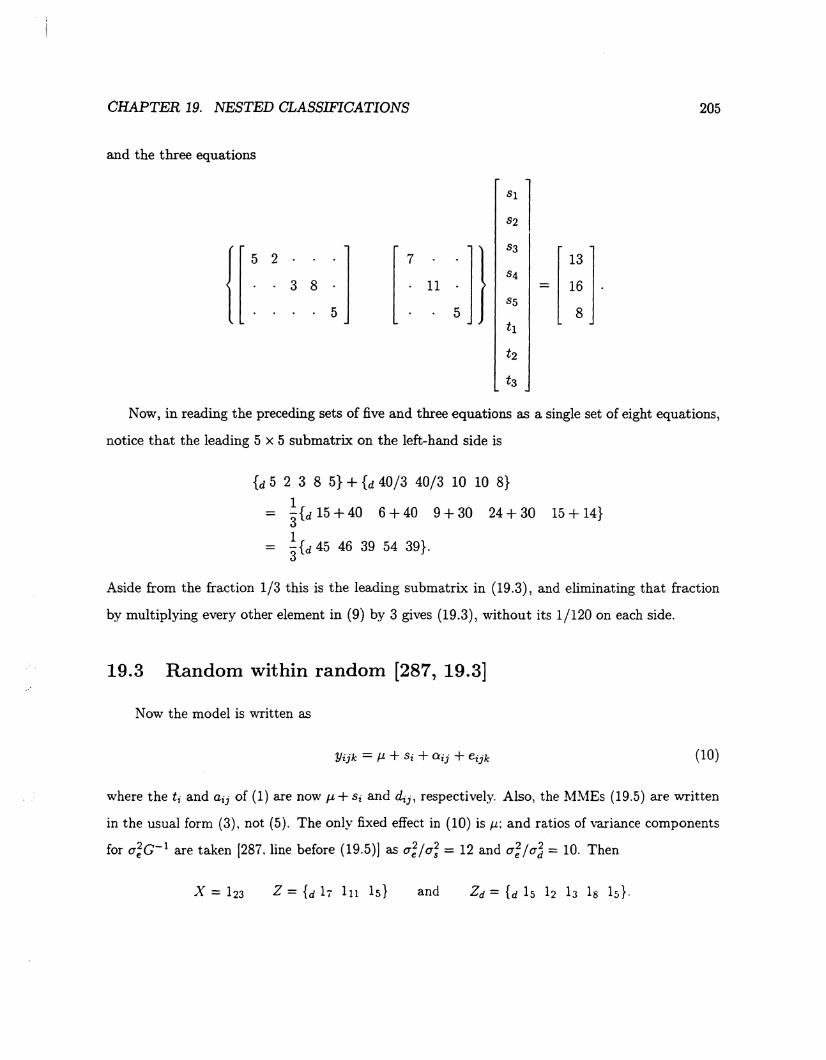
CHAPTER 19. NESTED CLASSIFICATIONS 205
and the three equations
= ss
Now, in reading the preceding sets of five and three equations as a single set of eight equations,
notice that the leading 5 x 5 submatrix on the left-hand side is
{d 5 2 3 8 5} + {d 40/3 40/3 10 10 8}
1 = 3{d15+40 6+40 9+30 24+30 15+14}
~{d 45 46 39 54 39}.
Aside from the fraction 1/3 this is the leading submatrix in (19.3), and eliminating that fraction
by multiplying every other element in (9) by 3 gives (19.3), without its 1/120 on each side.
19.3 Random within random [287, 19.3]
Now the model is written as
Yijk = f.1 + Si + O:ij + eijk (10)
where the t1 and aij of (1) are now f.1 + si and dti, respectively. Also, the MMEs (19.5) are written
in the usual form (3), not (5). The only fixed effect in (10) is J.L; and ratios of variance components
for a;c- 1 are taken [287.line before (19.5)] as a;;a; = 12 and a;;a'j = 10. Then
and

Chapter 20
Analysis of Regression Models
This is all very straightforward although it represents only a drop from the sea of books and
papers on regression.
For fitting polynomials [293] one should use orthogonal polynomials, a good description of which
is to be found in (the old, but detailed) "The Advanced Theory of Statistics" by M. G. Kendall,
1948, Volume II, pages 146-167. See also Pearson and Hartley (1954) and Robson (1959).
20i

l I
Chapter 21
Analysis of Covariance Models [295]
The analysis of covariance for the one-way classification is described with extensive detail (no
matrices) in LMFUD, Chapter 6, pages 169-211. This is, of course, not the model of CRH's Chapter
21; he considers only a numerical example of a two-way classification.
LMFUD Section 11.1 (pages 416-418) highlights some deficiencies of the traditional treatment
of analysis of covariance, and in Section 11.2 (pages 419-430) shows how the traditional fixed
effects model E(y) = X (3 of main effects and interactions can be usefully and easily extended to
E(y) = X (3 + Zb where columns of Z are columns of observed covariates, and b is the vector of
"regression" coefficients (or "slopes") multiplying those covariates. Table 11.4 of LMFUD shows
two appropriate analyses of variance based on E(y) = X(3+Zb and Table 11.5 shows the hypotheses
that can be tested from those analyses of variance. More general hypotheses are also considered;
for example, H: K'b = p and H: K' (3 = m. The important feature of this approach to analysis of
covariance is that it is directly applicable for balanced and for unbalanced data; and for as many
covariables as one wishes, necessarily fewer than N minus the rank of X.
21.1 Two-way fixed model with two covariates [295, 21.1]
LMFUD Sections 11.4 through 11.7 deal with a number of special cases of both the one-way
and two-wa~· classifications. Section 11.7 does not deal explicitly with the model of [295, 21.1]. but
LMFUD Section 11. 7a-iii can be adapted thereto. First, v.rrite /-Lij = ri + Cj + /ij in the model
208

CHAPTER 21. ANALYSIS OF COVARIANCE MODELS {295) 210
adapted to E(Yijk) = /-4.j + a1 W!ijk + a2w2ijk by replacing, for example Ei·zz with E .. w1 w1 which we
are writing as En. Thus doing this in -iii of LMFUD 452 gives, from (4)
[ :~ l = [ En E12]-l [ E1y l = [ 23.08 E21 E22 E2y 17.5 l-1 [ l 17.5 2
30.5 -12 (5)
1 [ 30.5 -17.5] [ 2] - 397.7 -17.5 23.08 -12
- [ .681 l -.784 ' (6)
exactly as in the last two elements of the solution vector in the two lines under [297, (21.2)]. The
other elements (after the zeros) are calculated from (16) of LMFUD page 422, namely
{3 =(X' X)- X'(y- Zb). (7)
In a two-way classification with-interaction model and no covariates, i.e., E(Yijk) = J.l-ij, we know
that (X'x)- X'y yields P,ij = Yij· = n~j'L-kYijk· Therefore, for E(Yijk = J.l-ijk + O!Wlijk + 02W2ijk,
(7) yields 1
P,ij = -L.k(Yijk- &IWlijk- &2W2ijk) = Yij·- &1 Wiij·- &2W2ij· nij
Thus, for example, fori= 1 and j = 1:
P,n = 20/3- .681(8/3)- ( -.784)(12/3) = 7.987,
equalling, as it should, the first element after the six zeros in the line below [297, (21.2)].
(8)
The clue to this being easier than the lengthy matrix algebra approach of MMEs (a matrix of
order 17 in [296, 21.2)] is the R in (4); as explained in LMFUD page 423, it is a matrix ofresiduals
and for the two-way crossed classification with interaction this involves just within-cell sums of
squares (and products) as in (2) and (3). For the same model without interaction the residual sums
of squares (and products) are more complicated as in the numerator of equation (51) on LMFUD
page 154.
Comment Ko indication is given as to the parameters corresponding to the 17 columns
in the matrix of [246, (21.1)]. They are for ri and c1 (each three in number), "'fi; (nine
of them) and a1 and a2.

CHAPTER 21. ANALYSIS OF COVARIANCE MODELS {295}
Note If the model is devoid of interactions Jl-ij is estimated not as Yii· but as in
equations (81) and (82) and using (76) of LMFUD pages 348-9. And Wlij· and W2ii·
have to be replaced by similar calculations.
212
21.3 Covariates all equal at the same level of a factor [300, 21.3]
The model equation is, with Wij = Wi
For this (full) model write ti + /Wi = Ti and so have
Yij = J.L + Ti + e&j·
This is a simple one-way classification with
The J.L, 'Y model equation is
and so OLS yields the standard regression results
i' =
and
"2:-niWiYi· - /:r "2:-nif}i. "2:-niWi
2:-niw; - "k (L-niwi) 2
And so after a little simplication
R(J.L, 'Y) = i'"L-niWiYi· + [J,L-niYi·
(2:-niWiYi· - 1;. L-niYi·Lniwi)2 (2:-niyi-) 2
= "L-niwl - }. (L-niwi) 2 + N
= [276- 68(34)/9]2 682 .:....._--~~---=--+-
144 -342/9 9 = 23.48 + 513.77 = 537.25
Chapter 22
Animal Model, Single Records [303]
The important aspect of the model equation
y = X {3 + Zu + Zaa + e (22.1)
is that it represents random effects other than breeding values [303, line 9]. This does not affect the
treatment of u as being random; it is just a matter of what random effects u represents.
Equations [304, (22.2)- (22.4)] flow very easily from the usual MMEs, e.g., [16, (3.4)].
22.1 Example with daughter-dam pairs [304, (22.1)]
It is a pity that no model equation is given for this example. It is clearly
(1)
where i = 1, 2 for the periods, j = 1, ... , 5 for each i, a1j is a dam j's record (made in period
l) and a2j is daughter j's record (made in period 2), the daughter of dam j. Thus dam-daughter
comparisons are confounded with periods.
Consideration of (l) reveals that X is certainl:v· as at [304, bottom]; and that u and Z do not
exist.
Error Therefore in [305. first line] it is not Z which is I, but Za = I.
The ~1MEs are therefore [304, (22.4)] without Z. and so have the form
[ X'X X
214
(2)

CHAPTER 22. ANIMAL MODEL, SINGLE RECORDS {303) 216
for .A= -10 and
p-1 = (23Is- .6Js)-1 = 213 (1s + 23 ~~(.6) Js) = 2~ (Is+ .03Js).
Therefore
[ 1 ] -1 (F- >.2 p-1 )-1 = 23Is - .6Js - 100 23 (Is+ .03Js)
[ 1 ] -1 = 23 ( 429Is - 16.8Js)
23 ( 16.8 ) = 429 Is + 429 - 5(16.8) Js
23 ( 16.8 ) = 429 Is + 345 Js · (5)
From the right-hand side of (3) we see that (W- .2XX')-1 is the part of (22.6) corresponding to
[ ~ ~ ]· Thus from (4) we similarly see that 3(F- >.2 p-1)-1 corresponds toP; and (5) gives
P = 3(F- >.2 p-1)-1 = .16084Is + .00783Js,
which has diagonal elements .16084 + .00783 = .16867 and off-diagonal elements .00783 as pre
scribed for Pin [305, line below (22.6)]. Similarly we get from (4)
Q = 3 ( -.AF-1) (F- >.2 p-1) -1
1 23 ( 16.8 ) = 30 23 (Is+ .03Js) 429 Is+ 345 Js
= ~ [], J (.o3 .03(5)(16.8) 16.8)] 143 s + s + 345 + 345
.06993Is + .0060115
which has .07594 in diagonals and .00601 in off-diagonals, just as in [305, 3rd line up]. This is
further confirmed by looking at the first row of [305, (22.6)]. It comes from (3) as
and so
_ 2X' [ P Q l = _ 2 [ 1 1 1 1 1 0 0 0 0 0 l [ P Q l . QP . 0000011111 QP
-.2l~[P Q] = -.21'[.16084h + .0078315 .0699315 + .00601J + 5]
= -.2 { [.16084 + 5(.00783)]1; [.06993 + 5(.00601 )]1~}
= ~ -.o41; - .o21;]
CHAPTER 22. ANIMAL MODEL, SINGLE RECORDS {303} 218
(8)
E(MSE)
(9)
There is no surprise in this result because in the model equation (I) 0-ij and eij are indistinguishable.
It is only the ~I5 submatrices in A that cause E(MSP) to be something other than a~+ a;.
Now as to estimation: equating (8) to (6) and (9) to (7) gives
1 A2 A2 2 5 d A2 A2 2 5 20"a +ae = . an Ga +ae = .. (10)
These clearly have solution a-; = 2.5 and <7~ = 0. CRH [306, last line first paragraph] has a-; = 2
and <7~ = .5. These satisfy the second equation in (10) but not the first. There is no non-zero
solution for <7~ only because the two mean squares are equal. Note though that, in general, with
Thus if
~ A2 + A2 = MSP 2aa O"e and
<7~ = 2(MSE- MSP) and
MSP < MSE < 2MSP
MSP > MSE
a-~ + a-; = MSE
a-; = 2MSP - MSE.
<7~ > 0 and a-; > 0
<7~ < 0 and o-; > 0
MSE > 2MSP <7~ > 0 and a-; < 0.
The calculations for MIVQUE for the unbalanced data would be illustrative if some details were
shown and not just computed results.
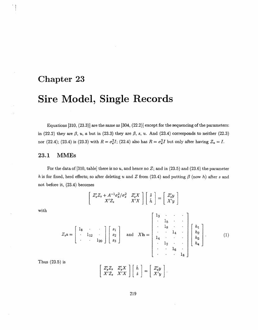
Chapter 23
Sire Model, Single Records
Equations [310, (23.3)] are the same as [304, (22.2)] except for the sequencing of the parameters:
in (22.2) they are {3, u, a but in (23.3) they are /3, s, u. And (23.4) corresponds to neither (22.3)
nor (22.4); (23.4) is (23.3) with R = O';l; (22.4) also has R = 0';1 but only after having Za =I.
23.1 MMEs
For the data of [310, table] there is no u, and hence no Z; and in (23.5) and (23.6) the parameter
his for fixed, herd effects; so after deleting u and Z from (23.4) and putting /3 (now h) after sand
not before it, (23.4) becomes
with
1s
Z,s = [ ls J [:: l 1s
112 and Xh = 14 14
12 [ ~J (1)
16 1s
Thus (23.5) is
219

CHAPTER 23. SIRE MODEL, SINGLE RECORDS 221
This result is given in Searle (1997), wherein it is also pointed out that for G_= {d o}Iq;} >.
can always be null except for a subvector 1, so leading to sums of BLUPs being zero. But when G
is not of that form, ZG>. = X7 has to be used explicitly. However, so long as X is an incidence
matrix, with no column of covariables, X1pxl = f1Nxl when there are f fixed effects factors and
so it may often be useful to take 7 = 1pxl·
In the example of this section, Z and X are given in (1) and, because in (3) any scalar emanating
from G can be ignored, we overlook the a';./12 in var(s) of [310, three lines above (23.5)], and use
[ 1 .5 .5 l
G = A = .5 1 .25 . . 5 .25 1
Then with
putting 71 = 72 = 73 = 74 = 1 gives (3) as
Therefore we want
(7)
which has solution proportional to
>-.' = [1 2 2].
Thus for BLUP(s) from (2)
X[BLUP(s)] = 1( -.036661) + 2(.453353) + 2( -.435022) = -.000001,
i.e., X[BLUP(s)] = 0, correct to five decimal places. Note in passing that (7) is
>-. = c-11.

CHAPTER 23. SIRE MODEL, SINGLE RECORDS
Note, for example: en + c12 + c13 = 0 c12 + c22 + c23 = 0. Also
r1 - 59- [3(48/7) + 5(119/15)) = -1.2381
T2 - 105- [8(119/15) + 4(74/10)) = 11.9333
ra = 150- [4(48/7) + 2(119/15) + 6(74/10) + 8(73/8)] = -10.6952;
and note that r1 + r2 + ra = 0. Then, as in LM, page 267, equation (16), for C of order 2 x 2
[ sJ.l = c-1 = [ 5.0476 -2.6666] ~1 [ - 1.2381 l
s2 r -2.6666 6.1333 11.9333
= ( 0419) [ 6.1333 2.6666] [ - 1.2381 l . 2.6666 5.0476 11.9333
= [ 1.0156] 2.3854 .
223
And s3 = 0. Notation s0 rather than sis used because the calculated values are only solutions (to
OLS equations) not estimates of s. Then, as in LMFUD page 102, equation (68)
Thus hJ. -h2 = h3 -h~ =
ho - ~2 o/ i = Yi··- Uj=11tijSj Tti-·
48/7- 3(1.0156)/7 119/15- [5(1.01561 + 8(2.3874)]/15 =
= 6.4219 6.3215 6.4450
= 9.1250. 74/10- 4(2.3874)/10 73/8-0
Arraying these in a vector [s0 ' h0 '], in keeping with the solution [311, line 7 up], gives
[s01 h01] = [1.0156 2.3874 0 6.4219 6.3215 6.4450 9.1250].
This looks very different from the [311] solution:
[10.14097 11.51238 9.125 - 2.70328 -2.80359 -2.67995 0].
But this is where estimability comes in. We are dealing with a no-interaction model, and every
difference between elements of s is estimable, as is that between elements of h. Examples follow
(to 3 decimal places).
BLUE(s1 - s2) = s2- s} = 2.387 - 1.016 = 1.371 = 11.512- 10.141 BLUE(s2- s3) = s2- s3 = 2.387-0 = 2.387 = 11.512-9.125 BLUE{Iq - h2) = h}- h2 = 6.422 - 6.322 = .100 = -2.703- 2.801 BLUE(h3- h4) = h3- h4 = 6.4450 - 9.125 = -2.680 = -2.680-0.
Chapter 24
Animal Model, Repeated Records
With c =a+ pas in (314, (24.3)] it is only the use of A-1 corresponding to a in the MMEs
(314, (24.4)] which distinguishes it, in terms of estimation, from p. Indeed, p and a are linearly
related: p = (cr;/cr~)A-1a as in (24.5).
The third equation on (315] is missing I on its left side, so that it is cr; I = .55! cr~. By considering
diagonal elements only, the first equation gives (because aii = 1 always)
cr~ = .25cr;, and and
Therefore
and - 2/ 2 - ( 2 2)/ 2 - 2 2 - 4 r- ere cry- era+ crp cry-. 5 +. -. 5.
For the example there is no u or Z. For the OLS equations
[ 1 1 1 . . . .
X'= · · · 1 1 1 · . . . . . . 1
and z' = [ ~ 1 c .
1
For the MMEs of (316, (24.8)] the 2.75 added to diagonal elements of Z~Zc is u';ju~ of [314,
(24.4)], its value being .55cr;J.2cr~ = 2.75. And the 2.2 is added to {d 3 2 2 1} in the form 2.2.4-1•
the 2.2 being cr';/cr~ = .55/.25 = 2.2.
In the solution to the MMEs below [316, (24.9)] the elements of BLUP(p) add to zero but those
of BL UP (a) do not. This is because I cr; / cr~ is diagonal but .4 -I cr; / cr~ is not (seE> these notes at
Section 23.1 ).
- "1
Chapter 25
Sire Model, Repeated Records
Typo In [321, line 4 up] the X~Xp should be z;zP. For the example on [322]
X = {d 13 16 14 13 1s 16 14}
Z' [ 1_2 1' 12 1' 1' 1' 12
{2]· = 3 2 3 3 s 1~ 13 12 1' 12 13 1
Zp will have order 31 x 14, corresponding to the 31 records and the 14 different progeny. To
write down Zp one needs to keep in mind the sequencing of the parameters in the parameter vector,
namely hyn · · · hy24 81 82 Pl · · · P14· To assist readability Zp is shown on the next page with
row and column numbers, row numbers being the records ordered by progeny within herd-year,
and the column numbers are the progeny numbers.
Note in the BLUP solution on [323] that both BLUP(8) and BLUP(p) have elements which sum
to zero.
The top of [324] has the appearance of a solution vector; but it is not. It is a vector of unknowns
which is to be premultiplied by the 9 x 9 matrix at the bottom of [323]. The solution vector is the
inverse of that matrix premultiplying the 9 x 1 vector atop [324].
In the final equation of [324] both off-diagonal terms should have two 2s, and on the right-hand
side 1.1870 should be 1.1187 (the signs are correct). The solution for 52 in that equation is then as
on [323:: 1.11870(12.26353- 5.22353) -
12.263532 - 5.223532 = ·0639 '·
226

Chapter 26
Animal Model, Multiple Traits
The algebra as presen~ed in this chapter is horrendous. Some of it can be abbreviated; and for
some of it a small example (t = 2 traits) helps understand the general case. We make use of the
direct (Kronecker) product operation that K ® L = {kijL}.
26.1 No missing data [325, (26.1)]
The model equation is, fori= 1, 2, · · ·, t
Define
Go = {m 9ij} i~=l and
Then
var {c ai} Go 0 A= G
var {c ei} = Ro0I=R
G-1 = Gal 0 A-1
R-1 = RQ1 0 I
Define
J:<>:-1 - { ij} t - { .. } t .. i) - m r i.;=l - m Pz; i,;=I·
[326: initiates notation riJ for elements of RQ 1 : \Hiting r'J = p,J makes for easier readabilit~·.
228
(26.1)
(1)
(26.3)
(26.4)
(26.5)
(26.6)
(2)

CHAPTER 26. ANIMAL MODEL, MULTIPLE TRAITS 230
26.1.2 Confirming a variance
To find var[BLUP(a)] demands knowing the variance-covariance matrix of the right-hand side
of (26.7). From (4), and then using (3), (26.3) and (26.4), this is
var(rhs)
For this
RQ 1GoRi/
var { r ~~ ;2] [ Pni P12I ] r Y1 l } I · P21I P22I Y2 . I
~ r ~; ~'] [ ::~ ::n ""w ~ ][ :: l + [ :: ]} [ :::~ :m X, X, I ~ l
r ~~ ;2] [ Pui P12I ] { [ I . ] Go 0 A [ I . ] + Ro 0 I} I · P21I P22I · I · I . I
[ Pni P12I ] [ X1 I I. ] x Pz1I Pzzi · Xz
r ~; ~2] (R;;' ® I} [(Go ® A)+ (Ro ® I)J (R;;' ®I} [ X, X, I ~ l
r 7 ~2] ((R;;'GoR;;' ® A)] + (R;;' ® I} [ X, X, I ~ ]· (6)
[ ;~~ :~ ] [ :~~ :~: ] [ :~ ;~: ] [ Pn9n + Pl2921 Pn912 + Pl2922 ] [ Pn Pl2 ]
P21911 + P22921 P21Y12 + P22922 P21 P22
[ Pn911Pll + Pl2921Pll + Pl1912P21 + Pl2922P21
P21911Pn + P22921Pl1 + P21912P21 + P22922P21
Pn9nP!2 + Pl2921Pl2 + Pn912P22 + Pl2922P22 ]
P21911Pl2 + P22921Pl2 + P21912P22 + P22922P22
[ PI!911 + 2pl!PI2912 + PI2Y22 PnP21911 + PIIP22912 + Piz92! + Pl2P22922 ] ( 7)
PliP21911 + PnP2292! + P~1Y12 + P21P22Y22 Piz9n + 2P12P22921 + P~z922
Now in (6) the matrix (7) has to be used in a direct product with A on its right: that means
each term in each sum in each element of (7) will multiplv A. And then the v.·hole matrix is to be
post-multiplied b~· a·= [ ~1 ; 2 ~ ~ ] and pre-multiplied b~· W'. Taking all this into account.
inspection of (7) reveals that the matrix multiplying 91 1 is

CHAPTER 26. ANIMAL MODEL, MULTIPLE TRAITS 232
26.1.3 Confirming a matrix
The paragraph below (26.14) leads to writing the upper right-hand 2 x 2 submatrix of what
we have in (9) as
[ X~X1PI1 X~X2P11P21 l + [ 2X~XlPllP12 X~X2(PnP22 + Pl2P21) l X2XIPnP21 X2X2P~2 ru Sym. 2X2X2P21P22 r 12
[ X!X1PI2 X1X2P12P22] + X'X X'X 2 T22· 2 1Pl2P22 2 2P22
(10)
We show that (10) is the same as that leading 2 x 2 in (9). To do this consider the coefficient of
X!X1 in (10):
c(X~X1) = PI1ru + 2PnP12r12 + PI2r22
= PI1P22~ + 2PnPI2( -p12~) + PI2Pn~
Thus
which is the coefficient of X~X1 in (9). Likewise from (10)
c(X~X2) = P11P21ru + (PnP22 + PI2)r12 + P12P22r22
= ~[PllP21P22 + (Pl1P22 + PI2)( -Pl2) + Pl2P22Pll]
= ~P12(PllP22 - PI2)
= P12,
and
c(X~X2) 2 2 2 P12r11 + P21P22r12 + P22r22
= P22~(PIIP22 - Pi2)
= P22·
And these are the coefficients in (9). Thus [9] agrees \\·ith CRH's description below [328. (26.14)].

~l
CHAPTER 26. ANIMAL MODEL, MULTIPLE TRAITS 234
Also in line three of that paragraph what is meant by "sequential"? Apparently this
means 1, or 1,2 or 1,2,3,· · · and so on. Traits may occur over time: e.g., weights at birth and
successive ages.
In [331, (26.31)] the awterms are elements of the relationship matrix A; they are not the aijS
representing animal effects in the model equations on [330]. Go in (26.31) is the same as in (26.3)
where it occurred in the form Gi ®A. But now it is
var(a) =A® Go. . (26.31)
And then
(26.32)
For the incidence matrix (26.33) the parameter vector is
And, on ordering the records by traits within animals, with zero for a missing record, they-vector
is
y = [5 3 6 2 5 7 0 3 4 2 0 OJ'
The three matrices at the bottom of [332] are, respectively,
[ 5 3 1 l-l 3 6 4 , 1 4 7
[ 0 0 0 l 0 (: ~ r and [
5-1 o o l 0 0 0 . 0 0 0
[333, (26.34)) is A®Go; and the remainder ofthe section, namely the right-hand vector, the solution
vector and the 17 x 17 matrix in (26.35) - (26.37) involve too much arithmetic for verification here.
26.3 The EM Algorithm [334, (26.3)]
This is primaril~· a section on computing, so I offer no comment.

'"\ Chapter 27
Sire Model, Multiple Traits
27.1 Only One Trait Observed on a Progeny [341, (27.1)]
Equation [341, (27.1)) is the same form as [325, (26.1)) except for {d I}{c B.i} now being
{d Zi}{c Si}
Typo The sentence in [342, line 1) is unfathomable.
var(s) = B®A=G
B = {m bij = 9ij/4} = Go/4
var( e) = D ® I = R
For fixed s GLS equations are
[ {d x;Xi/di} {d x;zij~} ] [ f!0 ] = [ {c x;Yi/~} ]· {d ZiXi/di} {d ZiZi/~} s {c Ziyi/~}
From (27.2)
The raison d 'etre for [343. (27.6)] is that "it seems logical to estimate d{ as
I (30' X' 0' Z' d _ Y Y - i i Yt - ui i Y 1
- nt - rank[Xi Zi] '
wherein 3? and u? are solutions to
235
(27.2)
(27.3)
(27.4)
(27.5)
(27.6)
(?- "") _,_,

CHAPTER 27. SIRE MODEL, MULTIPLE TRAITS 237
Then R of (27.10) for these data is
ru U 0 0
n Tl2 u 0 0
n 1 0 0 0 0 0 0 0
R= 0 0 0 0
Tl2u 0 0
n r~u 0 0
n 0 0 0 0 0 0 0 1 0 0 0 0
27.3 Relationship to Sire Model with Repeated Records on Progeny ~ [348, 27.3]
No comment.

Chapter 28
Joint Cow and Sire Evaluation
28.1 Block diagonality of MMEs [349, (28.1)]
A straightforward description.
28.2 Single Record on Single Trait [351, (28.2)]
The mid-page description on [350] applies to the animals of the example mid-page [351]. From
the genetic relationships among those animals comes A of (28.1): for example, animal 4 is the
progeny of 1 and so the relationship is .5; and animal 11 is a granddaughter of 4 (through 2) and
is also a niece of 4 (through 1) and so the relationship is .25 + .125 = .375 as seen in the second
row of (28.1). Then A-I is (28.2).
The vector mid-page [352] is sequenced in accord with the description on [350] with the herd
effects f.LI and J..L2 in amongst the ais. And (28.3) is L, say, with L = [ZI XI Z2 x2 Z3]
where Z1 = 0 is for the males a1, a4 and a5 which have no records; XI and x2 are for J..Ll and J..L2,
respectively; z2 is for the animals 2, 6, 8, 11 which have records in herd 1, and z3 is for animals 3,
7, 9 and 10 with records in herd 2.
The matrix in the MMEs of (28.4) is then L' L with 3A-1 added to all elements pertaining to
z:zi' fori, i' = 1. 2, 3. Thus the upper-most left-hand 3 X 3 is
[ 0 0 0 l [ 2 -1 -1 l [ 6 -3 -3] 0 0 0 +3 3 0 = 9 0 0 0 0 3 9
238
:l
CHAPTER 28. JOINT COW AND SIRE EVALUATION 240
28.6 Gametic model to reduce the number of equations [358, 28.6]
28.6.1 Single record model [359, {28.6.1)]
For the example the model is
OLS equations, using 12 + 22 + 12 + 32 = 15 and 1(5) + 2(3) + 1{2) + 3(8) = 37 are
15 1 2 1 3 (3 37 1 1 U} 5 2 1 U2 = 3 (2) 1 1 U3 2 3 1 U4 8
A~r~ 0 .5 .5] l !1
3 -6
-~ l 1 .5
:25 A-1 = ~ 3 9 -6 (3)
.5 .5 1 6 -6 -6 12 0 .
.5 0 .25 -4 0 0 8
To get the MMEs from (2) we therefore add to its 14 the matrix (10/4)A-1 which, with a;= 10
and a~= 4 involves (10/4)/6 = 6/12. Hence we get
1 +55 15 -30 -20
l!l 3 -6
-~ l ~ 12 12 12 12
!4 + 152 9 -6 1 + 45 -30 0 12 12
12 1 + 60 0 12
1 + 40 12
[5.5833 1.25 -2.5 -1.666]
4.75 -2.5 0 = 6 0 .
4.33
(4)
Replacing the ! 4 in (2) with (4) and then (for some reason) dividing the whole equation b:v 10 gives
[360. (28.8)j.
Question In the paragraph atop [359: there ·· are b animals with tested progen~···:
onh· c ~ b of these b parents are tested. and there arf' d tested animals with no progeny.

CHAPTER 28. JOINT COW AND SIRE EVALUATION
28.6.2 Repeated records model [361, (28.6.2)]
Items (1)- (3) on [362) are the same as (2)- (4) on (359) with a; in place of a;. The lower four diagonal elements in the matrix of [363, (28.11)] are of the form
1 ( .55) 1 ( u;) .55 n + .20 = .55 n + u~ '
242
in which n comes from Z~Zp and a;Ju; comes from R[var(p)t1 = (a;!u;) I. And diagonal elements
2 - 5 have the form
£ u; _.55 or 2- 25
UOt •
where aii is the i'th diagonal element of A-1. For example, with i = 1, n1 = 2 and, from (3),
a 11 = 11/6, 1 ( .55 11)
10.970 = .55 2 + .25 6 .
Thus the lower 8 x 5 submatrix of the matrix in (28.11) is
Comment: The elements of neither BLUP(p) nor BLUP(a) do not add to zero for the reasons
given in these notes for Section 23.1.
Chapter 29
Non-Additive Genetic Merit
29.1 Model for genetic components [365, (29.1)]
Very straightforward. The special matrix product symbol# at the bottom of [365] is defined
(as on [366]) as A# D = {aijdij}· It is the Hadamard product, more usually written as A· D or
A0D.
29.2 Single record on every animal [366, {29.2)]
This, too, is straightforward reading. One can observe that an easier-to-read form of (29.6) is
(29.6)
It is tempting to think that one could achieve some simplification of the algebra on [368] but I've
had no luck. In any case, for estimating variance components my preference would be to use ML
or REML directly.
29.3 Single or no record on each animal [369, (29.3)]
Again, the model description is straightforward and the arithmetic of the example is fairly
heft~·.
Typo In the first line. Section 28.2 should be 29.2.
2-13

Chapter 30
Line Cross and Breed Cros~ Analyses
30.1 Genetic Model [381, (30.1)]
This is the same as [365] except that although additive x additive is mentioned in [381, (30.1),
lines 2-3] of this section it is overlooked in the subsequent listing:
Var(additive x additive)= A#Ao-~ =A 0 Ao-~a·
30.2 Covariances between crosses [382, (30.2)]
My genetics fail me!
30.3 Reciprocal crosses assumed equal [384, (30.3)]
Because line crosses i x j and j x i are considered equal there are only six classes with numbers
nij + nji:
i, j = j, i 1,2 1,3 L4 2,3 2,4 3,5 5 3 2 6 3 5 4 4 2 2 3 9 9 7 4 8 6 14
Thus it is that the matrix of the OLS equations (30.1) contains the sequence of numbers in the last
line of the above table.
245

CHAPTER 30. LINE CROSS AND BREED CROSS ANALYSES 247
(3) I do not like to "pretend" about the model; see [389, 6th line up] and again on [390, top line].
(4) What is the significance of the parenthesized subscripts in r(i,j)? And what is r, anyway?

Chapter 31
Maternal Effects
31.1 Model for maternal effects [395, (31.1)]
No comment needed.
31.2 Pedigrees used in example [396, (31.2)]
Diagramming pedigrees helps derive A; each line segment represents a multiplicative .5.
31.3 Additive and Dominance Maternal and Direct Effects [398, (31.3)]
The last line, quite rightly, proclaims the example data as being inadequate for estimating
variances. But they are nevertheless too voluminous for demonstrating the arithmetic.
248
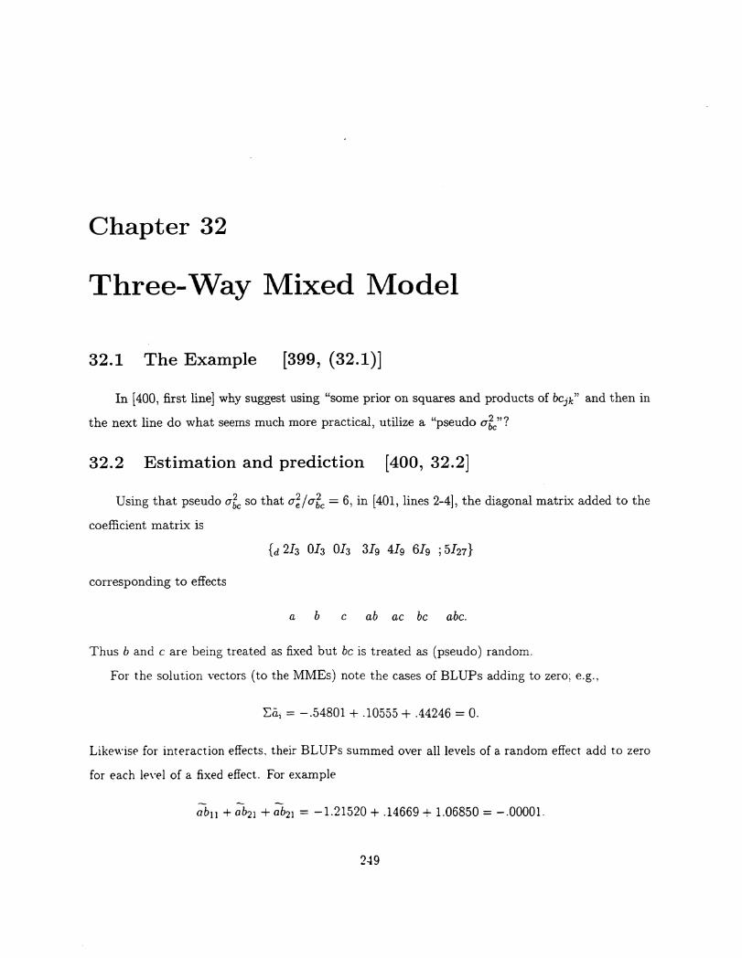
Chapter 32
Three-Way Mixed Model
32.1 The Example [399, (32.1)]
In [400, first line] why suggest using "some prior on squares and products of bcjk" and then in
the next line do what seems much more practical, utilize a "pseudo ate"?
32.2 Estimation and prediction [400, 32.2]
Using that pseudo a~c so that a;/ ate= 6, in [401, lines 2-4], the diagonal matrix added to the
coefficient matrix is
{d 21s Oh Ofs 3Jg 4Jg 6Jg ; 5h7}
corresponding to effects
a b c ab ac be abc.
Thus b and c are being treated as fixed but be is treated as (pseudo) random.
For the solution vectors (to the MMEs) note the cases of BLUPs adding to zero; e.g.,
L:a1 = -.54801 + .10555 + .44246 = o.
Likewise for interaction effects. their BLUPs summed over all levels of a random effect add to zero
for each lew! of a fixed effect. For example
abll + ab21 + ab21 = -1.21520 + .14669 + 1.06850 = -.00001.
249

CHAPTER 33. SELECTION WHEN VARIANCES ARE UNEQUAL 253
And on [410]
and [ 12 0 l R= 0 48 ®I.
A and an incidence matrix for the OLS equations are given, but for the MMEs only solutions are
given. And we note that BLUPs adding to zero does not occur, for the reasons given in these notes
at Section 23.1.

:··-"")
References (excluding those in CRR)
Anderson, R.D. (1978) Studies on the estimation of variance components. Ph.D. Thesis, Cornell
University, Ithaca, N.Y.
Hemmerle, W.J. and Hartley, H.O. (1973) Computing maximum likelihood estimates for the mixed
A.O.V. model using theW-transformation. Technometrics, 15, 819-831.
Jennrich, R.J. and Sampson, P.F. (1976) Newton-Raphson and related algorithms for maximum
likelihood estimation of variance components. Technometrics, 18, 11-17.
McCulloch, C.E. and Searle, S.R. (1995) An identity derived from unbiasedness in linear models.
The American Statistician, 49, 39-42.
Pearson, E.C. and Hartley, H.O., eds. (1954) Biometrika Tables for Statisticians, Vol. I, 3rd Ed.,
Cambridge University Press.
Robson, D.S. (1959) A simple method for constructing orthogonal polynomials when the indepen
dent variable is unequally spaced. Biometrics, 15, 187-191.
Searle, S.R. (1995) Some follow-up on Aitken's least squares equations. In Proceedings A. C. Aitken
Conference, University of Otago, Dunedin, New Zealand, 299-309.
Searle, S.R. (1997) Built-in restrictions on best linear unbiased predictors (BLUP) of random
effects in mixed models. The American Statistician, 51, 19-21.
Searle, S.R. and Fawcett, R.F. (1980) Expected mean squares in variance components models
having finite populations. Biometrics, 36, 243-254.
Searle, S.R., Speed. F.M. and Henderson, H.V. (1982) Some computational and model equivalences
in analysis of variance of unequal-subclass-numbers data. The American Statistician, 35. 16-
33.
Seber. G.A.F. (1977) Linear Regression Analysis. John Wiley & Sons, Kew York.


