

A New Parallel Algorithm for Connected Components in Dynamic Graphs Robert McColl Oded Green David Bader

Overview • The Problem
• Target Datasets
• Prior Work
• Parent-Neighbor Subgraph
• Results
• Conclusions
Problem | Datasets | Prior Work | PN Subgraph | Results | Conclusion 2

The Problem
Component Labeling • Given undirected graph G = {V,E}
§ V = set of vertices, E = set of edges (u,v) : u,v ∈ V
• Compute C(V) : Cu= Cv iff a path exists from u to v
Problem | Datasets | Prior Work | PN Subgraph | Results | Conclusion 3

The Problem
Component Labeling in a Dynamic Graph • Given same graph G = {V,E}, component labels C(V) • Maintain C(V) as edges are added and removed
§ Vertex insertion/removal handled as set of edge actions
Problem | Datasets | Prior Work | PN Subgraph | Results | Conclusion 4

The Problem
Component Labeling in a Dynamic Graph • Given same graph G = {V,E}, component labels C(V) • Maintain C(V) as edges are added and removed
§ Vertex insertion/removal handled as set of edge actions
Problem | Datasets | Prior Work | PN Subgraph | Results | Conclusion
edge inserted edge removed
5

The Problem
Component Labeling in a Dynamic Graph • Given same graph G = {V,E}, component labels C(V) • Maintain C(V) as edges are added and removed
§ Vertex insertion/removal handled as set of edge actions
Problem | Datasets | Prior Work | PN Subgraph | Results | Conclusion
edge inserted relabel purple to blue edge removed relabel blue to orange
6

The Problem
Component Labeling in a Dynamic Graph • Given same graph G = {V,E}, component labels C(V) • Maintain C(V) as edges are added and removed
§ Vertex insertion/removal handled as set of edge actions
Problem | Datasets | Prior Work | PN Subgraph | Results | Conclusion 7

The Problem: Applications • Support additional algorithms
– Centrality metrics, community detection, image processing
• Social network analysis and intelligence – Do smaller groups make contact with the big component?
• Tracking power grid issues – Will a line failure cause a blackout? Will the addition of a
new line solve it?
• Communications network tracking – Does losing a link break the connectivity of the network?
Problem | Datasets | Prior Work | PN Subgraph | Results | Conclusion 8

Massive Streaming Semantic Graphs Features • Millions to billions of vertices and edges with rich semantic information (name,
type, weight, time), possibly missing or inconsistent data • Thousands to millions of updates per second • Power-law degree distribution, sparse (d(v) ~ O(1)), low diameter
Financial • NYSE processes 1.5TB daily, maintains 8PB
Social • Facebook: 37,000 Likes and Comments per second • Twitter: 5,000 Tweets per second
Google • “Several dozen” 1PB data sets • Knowledge Graph: 500M entities, 3.5B relationships
Business • eBay: 17 trillion records, 1.5B new records per day
Problem | Datasets | Prior Work | PN Subgraph | Results | Conclusion 9

Observations and Synthetic Data Components • Generally one large component containing majority of graph
• Insertions are easy, deletions are challenging
• Deletions that actually cleave components are uncommon
• Fastest implementations of static algorithms are O(V+E) with O(V) storage
• Goal: maintain this bound, improve average-case performance
Problem | Datasets | Prior Work | PN Subgraph | Results | Conclusion
1
10
100
1000
10000
100000
1.00E+00
1.00E+01
1.00E+02
1.00E+03
1.00E+04
1.00E+05
1.00E+06
Cou
nt
Size
Components
10
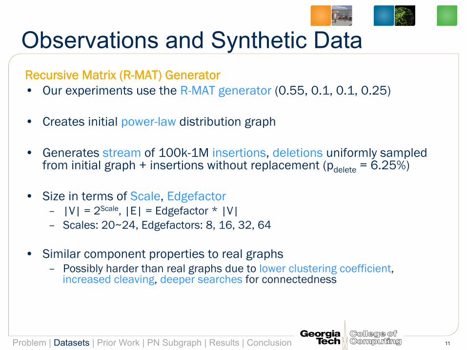
Observations and Synthetic Data Recursive Matrix (R-MAT) Generator • Our experiments use the R-MAT generator (0.55, 0.1, 0.1, 0.25)
• Creates initial power-law distribution graph
• Generates stream of 100k-1M insertions, deletions uniformly sampled from initial graph + insertions without replacement (pdelete = 6.25%)
• Size in terms of Scale, Edgefactor – |V| = 2Scale, |E| = Edgefactor * |V| – Scales: 20~24, Edgefactors: 8, 16, 32, 64
• Similar component properties to real graphs – Possibly harder than real graphs due to lower clustering coefficient,
increased cleaving, deeper searches for connectedness
Problem | Datasets | Prior Work | PN Subgraph | Results | Conclusion 11

Prior Work: Theoretical Static Parallel Algorithms • CONNECT, Hirschberg et. al. (1979)
– V ceil(V log V) or V2 processors, O(log(V2)) time • Shiloach and Vishkin (1982)
– V + 2E processors, O(log(V)) time – Implementations show good parallelism, load balance, simplicity, completes in ~d(G)/2
iterations (beneficial on graphs of interest)
Dynamic Parallel Algorithms • Shiloach and Even (1981)
– Theoretical algorithm maintaining a full BFS tree per component handling edge removal • L. Roditty and U. Zwick (2004)
– Maintain sequence of graphs per edge insertion and reachability trees • D. Eppstein et al. (1997)
– Sparsification as a technique for accelerating dynamic graph algorithms • P. Ferragina (1994)
– Use sparsification for static and dynamic algorithms • Henzinger, et. el. (1999)
– Maintain series of colored graphs or sets of spanning trees within components
Problem | Datasets | Prior Work | PN Subgraph | Results | Conclusion 12

Prior Work: Application There are plenty of theoretical approaches, so is the problem not solved? • Too expensive to compute in practice • Ignore the properties of real systems and graphs • Frequently require O(G) storage
Dynamic Parallel Algorithms • Recompute each step following Shiloach-Vishkin-based algorithm or using
repeated applications of Beamer et. al. (2012) BFS • Ediger et. al. (2011) compute triangle intersections upon delete, recompute if no
common neighbors • Our other experiments
– Spanning tree inside each component, only worry about deletions that hit the spanning tree – Keep a separate secondary spanning tree, only worry once a vertex has no edges in either
tree
Are these also not good enough? • Work well over smaller (1,000s) batches of edge updates • In practice, handle 90~99.7% of deletions, but with a batch of 100k edges at
6.25% deletes this means ~18 edges per batch that cause recompute each cycle
Problem | Datasets | Prior Work | PN Subgraph | Results | Conclusion 13

The Parent-Neighbor Subgraph Maintain one PN Subgraph per component • Select a vertex at random • Perform a breadth-first traversal of the
component • Construct a directed subgraph where
each vertex tracks its parents and neighbors
– Parents: adjacencies in previous frontier – Neighbors: adjacencies in same frontier – Record the distance to the root
• Limit the total number of PN tracked per vertex to threshPN
– Prefer parents over neighbors • This subgraph maintains various paths
back to the root – If each vertex has a path to the root
through its PN, component is connected
Problem | Datasets | Prior Work | PN Subgraph | Results | Conclusion
root
node
PN edge
non-PN edge
threshPN = 2
14

The Parent-Neighbor Subgraph In the event of an insertion • Vertices on the same frontier or
one apart, same component: – Check for opportunity to add a
parent or neighbor – Check for opportunity to replace
neighbor with parent
• Vertices are farther apart but in the same component: – Perform the same as above – The distances will now be
incorrect; however, they are still acceptable for our purposes
– Incorrect distances will eventually be cleaned up by merger or delete
Problem | Datasets | Prior Work | PN Subgraph | Results | Conclusion
root
node
PN edge
non-PN edge
insert
threshPN = 2
15
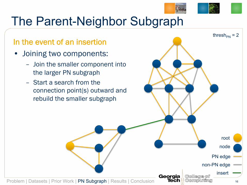
The Parent-Neighbor Subgraph In the event of an insertion • Joining two components:
– Join the smaller component into the larger PN subgraph
– Start a search from the connection point(s) outward and rebuild the smaller subgraph
Problem | Datasets | Prior Work | PN Subgraph | Results | Conclusion 16
root
node
PN edge
non-PN edge
insert
threshPN = 2
16

The Parent-Neighbor Subgraph In the event of an insertion • Joining two components:
– Join the smaller component into the larger PN subgraph
– Start a search from the connection point(s) outward and rebuild the smaller subgraph
Problem | Datasets | Prior Work | PN Subgraph | Results | Conclusion 17
root
node
PN edge
non-PN edge
insert
threshPN = 2
17

The Parent-Neighbor Subgraph In the event of a deletion Check for remaining parents or neighbors that still have parents • Have parents with paths to root:
– Do nothing • Have neighbors with paths to root:
– Change distance to indicate to children and neighbors not to depend on you
• Else (no parents or neighbors with paths to root):
– Assume components have split – Start search and relabel process down
the PN subgraph – If a node in the frontier above can be
reached, still connected. Backtrack and rebuild traversed section of PN.
– Otherwise a new PN subgraph and component is built.
Problem | Datasets | Prior Work | PN Subgraph | Results | Conclusion 18
root
node
PN edge
non-PN edge
delete
threshPN = 2
18

The Parent-Neighbor Subgraph In the event of a deletion Check for remaining parents or neighbors that still have parents • Have parents with paths to root:
– Do nothing • Have neighbors with paths to root:
– Change distance to indicate to children and neighbors not to depend on you
• Else (no parents or neighbors with paths to root):
– Assume components have split – Start search and relabel process down
the PN subgraph – If a node in the frontier above can be
reached, still connected. Backtrack and rebuild traversed section of PN.
– Otherwise a new PN subgraph and component is built.
Problem | Datasets | Prior Work | PN Subgraph | Results | Conclusion 19
root
node
PN edge
non-PN edge
delete
threshPN = 2
19

The Parent-Neighbor Subgraph Additional rules • Batch updates performed in a sequence of parallel stages
– To prevent performing duplicate work – All search and reconstruction steps are parallelized – Check to see if state already repaired before performing component
search after delete
• PN data structure maintained in arrays using in-place atomic CAS for parallel safety
• Singletons / pairs always put aside and processed in parallel
• See paper / source for specifics
Problem | Datasets | Prior Work | PN Subgraph | Results | Conclusion 20

Algorithmic Results
• Storage is still O(V) – Since threshPN is constant, Pnsubgraph = threshPN * V – threshPN doesn’t have to be very large
• Worst case update time is still O(V + E) – Performing full search and rebuild per component – Average case is generally much better – Worse case is highly unlikely
Problem | Datasets | Prior Work | PN Subgraph | Results | Conclusion 21

Algorithmic Results
Average number of unsafe deletes per 100k batch as a function of threshPN and edge factor at scale 22 • Unsafe: requires search (i.e. no remaining parents or neighbors), still
usually does not mean component was split • With graph densification, number drops significantly • threshPN = 4 good tradeoff between performance, storage
Problem | Datasets | Prior Work | PN Subgraph | Results | Conclusion
Uns
afe
Del
etes
(F
ewer
is b
ette
r)
Edgefactor
22

Algorithmic Results Average number of PN modifications per 100k batch as a function of threshPN and edge factor at scale 22 • Again, with graph
densification, number drops significantly
• Again, threshPN = 4 good tradeoff between performance, storage – Fewer modifications in
the tree = faster updates
Problem | Datasets | Prior Work | PN Subgraph | Results | Conclusion
PN
Mod
ifica
tions
P
N M
odifi
catio
ns
Edgefactor
Edgefactor
23

Performance Results
Speedup over parallel static recompute for three different graphs with 16M vertices, up to 1B edges • Ten batches of 100k updates • 64 threads • 4 x 16-core AMD Opteron 6282 SE
Problem | Datasets | Prior Work | PN Subgraph | Results | Conclusion
Speedup over sequential for multiple graphs at each size
• 1MB L2 / core • 16MB shared L3 / socket • 64 cores running at 2.6GHz • 256GB DDR3 RAM @ 1600MHz
Edgefactor
24

Performance Results
• Fraction of time during each update cycle (components + graph update) spent in the component update
• Demonstrates that the scaling of the algorithm is in line with the scaling of the data structure itself
Problem | Datasets | Prior Work | PN Subgraph | Results | Conclusion
Edgefactor
25

Conclusions New algorithm improves over prior static and dynamic options • Never requires static recompute, and in the worst case the dynamic
update is only as costly as recompute O(V + E) – Significantly better than recomputation in the average case
• Scalability is in line with the scalability of the data structure used and the static algorithm
• Storage requirement remains at O(V) – Storage can be adjusted via threshPN at possible performance costs – Likely should be tuned for graphs of other types
Future work • Apply Beamer’s BFS optimization • Try graphs of different types
Problem | Datasets | Prior Work | PN Subgraph | Results | Conclusion 26

Acknowledgment of Support
27


