

Journal of Power Electronics, Vol. 17, No. 6, pp. 1637-1649, November 2017 1637
https://doi.org/10.6113/JPE.2017.17.6.1637
ISSN(Print): 1598-2092 / ISSN(Online): 2093-4718
JPE 17-6-23
A Novel Harmonic Identification Algorithm for the Active Power Filters in Non-Ideal Voltage Source
Systems
Phonsit Santiprapan*, Kongpol Areerak†, and Kongpan Areerak*
*,†School of Electrical Engineering, Suranaree University of Technology, Nakhon Ratchasima, Thailand
Abstract
This paper describes an intensive analysis of a harmonic identification algorithm in non-ideal voltages source systems. The dq-axis Fourier with a positive sequence voltage detector (DQFP) is a novel harmonic identification algorithm for active power filters. A compensating current control system based on repetitive control is presented. A design and stability analysis of the proposed current control are also given. The aim of the paper is to achieve a robustness of the harmonic identification in a distorted and unbalanced voltage source. The proposed ideas are supported by a hardware in the loop technique based on a eZdspTM F28335 and the Simulink program. The obtained results are presented to demonstrate the performance of the harmonic identification and the control strategy for the active power filter in non-ideal systems. Key words: Active power filter (APF), DQ0-axis with a Fourier algorithm (DQF), Harmonic elimination, Positive sequence voltage detector (PSVD), Repetitive control, Three-phase four-wire system
I. INTRODUCTION
Nonlinear loads connected to an electric power system can generate harmonic into the utility source. These harmonics have numerous effects on electric power systems [1] such as motors and generators [2], [3], transformers [4], power cables [5], capacitors [6], electronic equipment, metering [7], switchgear and relaying [8] and static power converters.
In order to solve these problems, an efficient method is the active power filter (APF) [9]. The APF acts as a current source to compensate the harmonic currents at the point of common coupling (PCC). In general power systems, nonlinear loads often behave as an unbalanced condition. Therefore, an APF is a suitable structures for three-phase four-wire systems. There are many structures to solve these problems [10]. The three-leg split-capacitor topology with six IGBTs is used in this paper since this structure provides a good performance for harmonic elimination and it uses a lower number of power semiconductor devices.
In realistic conditions, the waveforms of the voltage source can be distorted and unbalanced [11]. A non-ideal voltage source causes unwanted components in the process of harmonic identification and in the control strategy. There are significant errors in the reference current calculation.
In a literature review, it was found that the positive sequence voltage detector (PSVD) was presented in 1997 by Aredes et al [12]. The PSVD is an approach to detect distorted and unbalanced voltage sources. In the conventional PSVD algorithm, analog filters (LPF or HPF) are used to obtain the fundamental component. The characteristic of an analog filter is its non-ideal response. Therefore, an analog filter is not perfect for drawing the fundamental component. In order to enhance the performance of the PSVD, the sliding window Fourier analysis (SWFA) is applied [13] in this paper. The fundamental component can be accurately calculated by using the SWFA. There are many harmonic identification techniques for calculating reference currents such as the instantaneous power theory (PQ) [14], the synchronous reference frame (SRF) or dq-axis method (DQ) [15], the synchronous detection (SD) method [16], the a-b-c reference frame method [17]. Harmonic identification techniques for non-ideal voltage source systems have been reported in previous publications. These techniques include the perfect harmonic cancellation
Manuscript received Dec. 20, 2016; accepted Jul. 21, 2017 Recommended for publication by Associate Editor Tomislav Dragicevic.
†Corresponding Author: [email protected] Tel: +66-044-224-363, Suranaree University of Technology
*School of Electrical Eng., Suranaree University of Technology, Thailand
© 2017 KIPE

1638 Journal of Power Electronics, Vol. 17, No. 6, November 2017
isu
isv
isw
iLu
iLv
iLw
icw
icv
icu
i*0
i*d
i*q
Ls
Ls
Ls
Leq
Leq
Leq
Neutral
80-120 VL-N(rm s), 50 Hz
3–single phase rectifier
isn
iLn
icn
idc,1
idv
i0v
vsu
vsv
vsw
Lc
Rc
3-phaseto
dq0-frame
V*ref
0
RC Controller
PIController
PIController
Triangular carrier
PWMGate
Signals
dq0-frameto
3-phase
RC Controller
RC Controller
ΣVdc
ΔVdc
-
Lc
××
ΣVdc
ΔVdc
-
+
2
3
++
++
- ++ δd
δq
δ0
icd
icq
ic0
uq
u0
ud
v*0,out
v*q,out
v*d,outv*
u,out
δsum
δdiff
v*v,out
v*w,out
Control strategy for active power filter (The eZdspTM F28335 board)
idc,2
vpcc,u vpcc,v vpcc,w
3-phaseto
αβ-frame
θpcc(θPLL) αβ-frame
to q-frame
vpcc,qPIController
0 -δθ
Auxiliary Current
iα,aux
iβ,auxAuxiliary
Instantaneous Powers
vpcc,α
vpcc,β
vpcc,α vpcc,β
SWFASWFA
auxpauxq
auxauxaux ppp ~ auxauxaux qqq ~
αβ-Voltage Caculation(Dual PQ Theory)
|V| Cartesian Coordinate Convertion
v’α v’
β
vpcc,u
vpcc,v
vpcc,w
ωPLL
iLα
iLβ
+-
3-phaseto
αβ0-frame
αβ-frame to dq-frame
iL0
-
+
+
iLdLdi
~Ldi
iLu
iLv
iLw
+
+
+
-
-
-
Non-Ideal Voltage Source
Part B: Positive-Sequence Voltage Detector: PSVDPart A: DQF Harmonic Detection
Part D: DC Bus Voltage Control
Part C: The Compensating Current ControlPart E: APF
1
4
5
6
7
3
2
+
-
t =0.5s t =1.5s
LLw
RLwRLwRLw
+
-
t =0.5s t =1.5s
LLv
RLvRLvRLv
+
-
t =0.5s t =1.5s
LLu
RLuRLuRLu
Fig. 1. The considered power system and control strategy.
theory [18], the fuzzy instantaneous power theory [19], the modified instantaneous power theory [20], a synchronous reference frame with a self-tuning filter [21], a modified p-q theory based method [22], the non-iterative optimized algorithm [23], [24], a synchronous reference frame based on a modified phase locked loop (PLL) [25].
In 2007, the dq-axis with Fourier (DQF) method was developed [26]. In an ideal voltage source, the reference current can be precisely calculated by this method. The DQF method provides a fast calculation time and the flexibility to operate with an APF [27], [28]. Therefore, the prominent points of the DQF and the PSVD algorithms referred to as dq-axis Fourier with a positive voltage detector (DQFP) are applied for the harmonic identification part. The reference current can be accurately achieved by the proposed harmonic identification even though the voltage source is distorted and unbalanced.
Compensating current control is an important part for the tracking performance of the compensating currents. Several strategies to control the compensating current injection can be found in previous publications such as predictive controllers [29], [30], [35], PI controllers [31], [32], the pole-zero cancellation technique [33], the sliding mode controller [34], the one cycle controller [36], repetitive controllers [37], [38], a proportional plus resonant controller [38], and a neural network [39]. Repetitive control (RT) [37], [38] is used in this paper. This controller is an excellent mechanism to track an unknown
periodic reference input. It can be operated to reduce tracking errors.
The considered power systems in the paper are non-ideal voltage source systems. For this reason, the experimental setup is not presented. However, the hardware in the loop (HIL) technique is applied to simulate the proposed harmonic identification and the overall control strategy.
This paper is structured as follows. The mathematical operations of the harmonic orders in non-ideal voltage source systems can be derived as presented in Section II. Section III describes an analysis of the harmonic orders in non-ideal voltage source systems. The principle of the DQF with the proposed PSVD is clearly explained in Section IV. In Section V, the design procedure and a stability analysis of the compensating current control system based on a RT controller are presented. Furthermore, Section VI presents the hardware in the loop technique to simulate the harmonic elimination of the considered system. Simulation results demonstrating the performance of the proposed harmonic identification and a discussion are shown in section VII. Finally, Section VIII concludes the paper.
II. ANALYSIS OF THE MAGNITUDE AND PHASE ANGLE OF THE PCC VOLTAGES IN
NON-IDEAL VOLTAGE SOURCE SYSTEMS
This section studies the effect of distorted and unbalanced

A Novel Harmonic Identification Algorithm for the Active Power Filters in … 1639
0 0.01 0.02 0.03 0.04 0.05 0.06 0.07 0.08-200
-150
-100
-50
0
50
100
150
200
-50 0 50 100 150 200 250 300 350 400 450 5000
20
40
60
80
100
120
140
160
180
200
v(V)
time(s) frequency(Hz)
phase uphase vphase w
vu
vv
vw
uvwv
uvwv~
(a)
|V|
time(s)0 0.01 0.02 0.03 0.04 0.05 0.06 0.07 0.08
0
20
40
60
80
100
120
140
160
180
200
-50 0 50 100 150 200 250 3000
20
40
60
80
100
120
140
160
180
200
173.20 174.02
frequency(Hz)
|V,ideal|
|V,dist|
|V,ideal|
|V,dist|
(b)
0 0.01 0.02 0.03 0.04 0.05 0.06 0.07 0.08-5
-4
-3
-2
-1
0
1
2
3
4
5
time(s)
θ (radian)
θ,ideal
θ,dist
(c)
Fig. 2. Condition and effect of the distorted voltage source: (a) waveforms and spectrums of the voltage source; (b) magnitude and spectrum of the PCC voltages; (c) phase angle of the PCC voltages.
voltage source systems on the control strategy performance. The magnitude and phase angle of the PCC voltages are a part of the computation for DQF harmonic identification and the compensating current control. Therefore, these effect can generate the disturbance signals that cause the control strategy to provide the inexact reference voltages of the APF
( *,outuvwv ).
A. Distorted Voltage Source
Voltage distortion is produced by the relationship between the harmonic current and the source impedance [40]. In this study, the voltage source ( uvwpccv , ) is defined as illustrated in
Fig. 2(a). uvwpccv , consists of the balanced fundamental
component ( uvwpccv , ) and the balanced harmonic components
( uvwpccv ,~ ). In the distorted voltage source condition, the
magnitudes of the PCC voltages in Fig. 2(b) have no effect on the control strategy. It can be seen that the actual magnitude
of the PCC voltages ( V ) calculated by Eq. (1) can track the
exact magnitude of the PCC voltages (*
V ). However, the
phase angle of the PCC voltages has an effect on the control strategy because the actual phase angle of the PCC voltages ( pcc ) has an error value when compared with the exact
phase angle of the PCC voltages ( *pcc ), as shown in Fig. 2(c).
The value of pcc can be calculated by Eq. (2).
21
2
,...2,1,013
,
,...2,1,023
,
2
,...2,1,013,13
,
)cos()cos(
)sin(
kkh
hpcc
kkh
hpcc
kkhkh
hpcc
thVthV
thV
V
(1)
,...2,1,013,13
,
,...2,1,013
,
,...2,1,023
,
1
)sin(
)cos()cos(
tan
kkhkh
hpcc
kkh
hpcc
kkh
hpcc
mmpcc
thV
thVthV
t
(2)
where: hwpcchvpcchupcchpcc VVVV ),(),(),(, .
B. Unbalanced Voltage Source
Malfunctions of electric power equipment and non-symmetrical loads cause an unbalanced voltage source
[41]. The voltage source ( uvwpccv , ) defined in Fig. 3(a) is
considered for this study. The amplitude of the voltage source is unbalanced. The harmonic components are neglected.
In this condition, the V calculated by Eq. (3) is an
oscillating waveform as shown in Fig. 3(b) because the
spectrum of the harmonic order appears at 100 Hz ( V~
).
This component has an effect on the control strategy.
Moreover, pcc has an error value when compared with *pcc .
From Fig. 3 (c), pcc can be derived and given in Eq. (4).
21
,,
,,
,,
22,
22,
22,
)sin()sin(
)sin()sin(
)sin()sin(
)(sin
)(sin)(sin
3
2
uwupccwpcc
wvwpccvpcc
vuvpccupcc
wwpcc
vvpccuupcc
ttVV
ttVV
ttVV
tV
tVtV
V
(3)
)sin(
)sin()sin(2
)sin(
)sin(3
tan
,
,,
,
,
1
wwpcc
vvpccuupcc
wwpcc
vvpcc
mmpcc
tV
tVtV
tV
tV
t
(4)
III. ANALYSIS OF THE HARMONIC ORDERS IN NON-IDEAL VOLTAGE SOURCE SYSTEMS
In non-ideal voltage source systems, the PCC voltages ( upccv , , vpccv , , wpccv , ) can be explained by Eq. (5). The
harmonic orders of the PCC voltages in the positive, negative and zero sequences are denoted by +m, -m and 0m, respectively. The load currents ( Lui , Lvi , Lwi ) can be
expressed by Eq. (6). The harmonic orders of the load currents in the positive, negative and zero sequences are denoted by +n, -n and 0n, respectively.

1640 Journal of Power Electronics, Vol. 17, No. 6, November 2017
0 0.01 0.02 0.03 0.04 0.05 0.06 0.07 0.08-200
-150
-100
-50
0
50
100
150
200
-50 0 50 100 150 200 250 300 350 400 450 5000
20
40
60
80
100
120
140
160
180
200
phase uphase v
phase w
time(s) frequency(Hz)
vu
vv
vw
v(V)
uvwv
(a)
|V|
time(s)0 0.01 0.02 0.03 0.04 0.05 0.06 0.07 0.08
0
20
40
60
80
100
120
140
160
180
200
-50 0 50 100 150 200 250 3000
20
40
60
80
100
120
140
160
180
200
173.20 173.73
19.97
frequency(Hz)
|V,ideal|
|V,unb|
|V,ideal|
|V,unb|
(b)
0 0.01 0.02 0.03 0.04 0.05 0.06 0.07 0.08-5
-4
-3
-2
-1
0
1
2
3
4
5
θ,ideal
time(s)
θ (radian)
θ,unb
(c)
Fig. 3. Condition and effect of the unbalanced voltage source: (a) waveforms and spectrums of the voltage source; (b) magnitude and spectrum of the PCC voltages; (c) phase angle of the PCC voltages.
)3
2sin()
3
2sin()sin(
)3
2sin()
3
2sin()sin(
)sin()sin()sin(
00,
00,
00,
mmmmmmmmmwpcc
mmmmmmmmmvpcc
mmmmmmmmmupcc
tVtVtVv
tVtVtVv
tVtVtVv
(5)
)3
2sin()
3
2sin()sin(
)3
2sin()
3
2sin()sin(
)sin()sin()sin(
00
00
00
nnnnnnnnnLw
nnnnnnnnnLv
nnnnnnnnnLu
tItItIi
tItItIi
tItItIi
(6)
The values of )(uvwLi are transformed to the dq0-axis
( Ldi , *qi , 0Li ) as shown in Eq. (7)-(9), respectively. The values
of Ldi , *qi and 0Li can be separated into the fundamental
component (DC component) ( Ldi , Lqi ) and the harmonic
components (AC component) ( Ldi~
, Lqi~
, 0
~Li ). It can be
observed in Eq. (7) and (8) that the DC components of the
load currents on the dq-axis ( Ldi , Lqi ) can be computed from
the harmonic current and voltage in the same order (m=n). On the other hand, the AC components of the load currents
on the dq-axis ( Ldi~
, Lqi~
) can be derived from the different
harmonic order (m≠n). The DC and AC components of the load current on the d-axis at the mth and nth harmonic orders
are denoted by ),( nmLdi and ),(
~nmLdi , respectively. The values of
3
4
-3
-2
-1
0
1
0.26 0.265 0.27 0.275 0.28 0.285 0.29 0.295 0.3
-2
0
2
Fig. 4. Comparison between the exact and actual load currents (without the PSVD) on the dq0-axis.
),( nmLqi and ),(
~nmLqi denote the DC and AC components of the
load current on the q-axis at the mth and nth harmonic orders. Note that the subscript "m" is the harmonic orders of the PCC voltages and that "n" is the harmonic orders of the load currents.
1 1
1 1
1),(),(
sin2
3
sin2
3
sin2
3~
mmnmn
nn
nmm
mnmnn
n
mnnm
nnmLdnmLdLd
tI
tI
Iiii
(7)
1 1
1 1
1),(),(
*
cos2
3
cos2
3
cos2
3~
mmnmn
nn
nmm
mnmnn
n
mnnm
nnmLqnmLqq
tI
tI
Iiii
(8)
nnn
nLL tIii 01
000 sin3~
(9)
In addition, the AC component of the load current on the
0-axis ( 0
~Li ) in Eq. (9) can be calculated with only the
harmonic currents. The values of Ldi and *qi are rotated
with the angular frequency of the PCC voltages ( mmpcc t ) as explained in Eq. (2) and Eq. (4).
Therefore, the calculations of Ldi and *qi cannot correct
the harmonic currents in a non-ideal voltages source. According to Fig. 4, the waveforms of the actual Ldi and
*qi are incorrect when compared with the exact Ldi and *
qi
current waveforms. The spectrum comparisons of the load
currents in Fig. 5 can express that ),( nmLdi and ),( nmLqi are
included in the DC components ( Ldi , Lqi ). The AC
components ( Ldi~
, Lqi~
) consists of ),(
~nmLdi and ),(
~nmLqi .

A Novel Harmonic Identification Algorithm for the Active Power Filters in … 1641
0 100 200 300 400 500 600 700 800 900 10000
0.5
1
1.5
2
2.5
3
3.5
4
3.65
0.14 0.25
I Ld (A
)
frequency (Hz)
0.08 0.040 100 200 300 400 500 600 700 800 900 1000
0
0.5
1
1.5
2
2.5
3
3.5
4
I* q (A
)
1.10
0.10
0.95
0.340.15
frequency (Hz)0 100 200 300 400 500 600 700 800 900 1000
0
0.5
1
1.5
2
2.5
3
3.5
4
frequency (Hz)
I L0 (A
)
0.17
1.38
0.410.16
)1,1(LqLq ii
)7,1()5,1(6
~~~LqLqLq iii
)13,1()11,1(12
~~~LqLqLq iii
)1,1(LdLd ii
)3,1(2
~~LdLd ii
)7,1()5,1(6
~~~LdLdLd iii
2
~Ldi 6
~Ldi
Ldi
Lqi6
~Lqi
12
~Lqi
)1(0
~Li
)3(0
~Li
)9(0
~Li
(a)
0 100 200 300 400 500 600 700 800 900 10000
0.5
1
1.5
2
2.5
3
3.5
4
frequency (Hz)
3.64
0.090.30
0.15 0.07
0 100 200 300 400 500 600 700 800 900 10000
0.5
1
1.5
2
2.5
3
3.5
4
1.09
0.620.77
0.340.14
frequency (Hz)
0 100 200 300 400 500 600 700 800 900 10000
0.5
1
1.5
2
2.5
3
3.5
4
frequency (Hz)
0.17
1.38
0.410.16
),Ld(),Ld(),Ld(),Ld(),Ld(Ld iiiiii 9977553311
),Ld(),Ld(),Ld(),Ld(
),Ld(),Ld(),Ld(),Ld(),Ld(Ld
iiii
iiiiii
119799757
75355313312
~~~~
~~~~~~
),Ld(),Ld(),Ld(),Ld(
),Ld(),Ld(),Ld(),Ld(),Ld(Ld
iiii
iiiiii
1593913717
115159371516
~~~~
~~~~~~
),Lq(),Lq(),Lq(),Lq(),Lq(Lq iiiiii 9977553311
),Lq(),Lq(),Lq(),Lq(),Lq(
),Lq(),Lq(),Lq(),Lq(),Lq(Lq
iiiii
iiiiii
1593913717115
15933371516
~~~~~
~~~~~~
),Lq(),Lq(),Lq(),Lq(),Lq(
),Lq(),Lq(),Lq(),Lq(),Lq(Lq
iiiii
iiiiii
2193913757175
751539313111112
~~~~~
~~~~~~
2
~Ldi 6
~Ldi
Ldi
Lqi
6
~Lqi
12
~Lqi
)1(0
~Li
)3(0
~Li
)9(0
~Li
I Ld (A
)
I* q (A
)
I L0 (A
)
(b)
0 100 200 300 400 500 600 700 800 900 10000
0.5
1
1.5
2
2.5
3
3.5
4
3.65
0.16 0.24
frequency (Hz)
0.08 0.040 100 200 300 400 500 600 700 800 900 1000
0
0.5
1
1.5
2
2.5
3
3.5
4
1.09
0.18
0.93
0.340.15
frequency (Hz)0 100 200 300 400 500 600 700 800 900 1000
0
0.5
1
1.5
2
2.5
3
3.5
4
frequency (Hz)
0.17
1.38
0.410.16
)1,1(LqLq ii
)7,1()5,1(6
~~~LqLqLq iii
)13,1()11,1(12
~~~LqLqLq iii
)1,1(LdLd ii
)3,1(2
~~LdLd ii
)7,1()5,1(6
~~~LdLdLd iii
2
~Ldi 6
~Ldi
Ldi
Lqi6
~Lqi
12
~Lqi
)1(0
~Li
)3(0
~Li
)9(0
~Li
I Ld (A
)
I* q (A
)
I L0 (A
)
(c)
Fig. 5. Spectrums of the load currents on the dq0-axis in a non-ideal voltage source: (a) exact load currents; (b) actual load currents (without the PSVD); (c) actual load currents (with the proposed PSVD).
These components are depicted in Fig. 5 (b).
As a result, the Ldi ( ),(),(
~nmLdnmLd ii ) and *
qi
( ),( nmLqi + ),(
~nmLqi ) values of the actual load currents are not
nearly the same as the exact load currents in Fig. 5 (a). However, the angular frequency of the PCC voltages
( mmpcc t ) is not used to calculate the value of 0Li in
Eq. (9). Therefore, the waveform of the actual 0Li remain
equal to the exact load current.
IV. THE DQ-AXIS FOURIER WITH A POSITIVE
VOLTAGE DETECTOR (DQFP)
The DQF algorithm as shown in Fig. 1 (Part A) can completely identify the harmonic currents. The principle of the DQF approach can be found in [26], [28]. In distorted and unbalanced voltage sources, the performance of the DQF harmonic identification has not been presented in the previous works. From section II and III, a non-ideal voltage source can provide undesirable components in terms of
Ldi and *qi . Therefore, the non-ideal voltage source must be
completely filtered out using the proposed PSVD.
The PSVD is used to detect distorted and unbalanced voltage sources. The calculation procedure of the PSVD algorithm can be summarized by the block diagram in Fig. 1 (Part B). There are seven steps for calculating the voltage source.
Step 1: Transform the PCC voltages ( uvwpccv , ) to the
-axis ( ,pccv ) by a Clark’s transformation.
Step 2: Calculate pcc by using a synchronous reference
frame phase locked loop (SRF-PLL), as shown in block number 2. The SRF-PLL was first presented in 1997 by Kaura and Blasko [42]. This algorithm can be used to
determine pcc in the distorted voltage source condition.
According to the SRF-PLL operation, the phase angle of the SRF-PLL ( PLL ) is obtained by integrating the angular
frequency ( PLL ). The value of PLL is the output of the PI
controller. This controller is used to control PLL . The
parameters of the PI controller designed by the symmetrical
optimum approach in [43] are PLLpK , = 0.54 and PLLiK , =
94.19. On the dq-axis, if PLL is identical to the angular
frequency of the PCC voltages ( pcc ), the PCC voltage on

1642 Journal of Power Electronics, Vol. 17, No. 6, November 2017
the dq-axis ( dpccv , , qpccv , ) in Eq. (10) appear as dc
components. Therefore, the reference value of the PCC
voltage on the q-axis ( *,qpccv ) is set to zero in this paper.
)sin(2
3
)cos(2
3
,
,
PLLpccmqpcc
PLLpccmdpcc
Vv
Vv
(10)
Step 3: Calculate the auxiliary currents ( auxi , , auxi , ) by Eq.
(11). The value of nI in Eq. (11) denotes the unity gain.
)cos(2
3
)sin(2
3
,
,
PLLPLLnaux
PLLPLLnaux
tIi
tIi
(11)
Step 4: Calculate the auxiliary instantaneous power ( auxp ,
auxq ) by Eq. (12):
aux
aux
pccpcc
pccpcc
aux
aux
i
i
vv
vv
q
p
,
,
,,
,,
(12)
Step 5: Determine the DC components of the auxiliary
active power ( auxp ) and the reactive power ( auxq ), as shown
in block number 5. The values of auxp and auxq from step 4 can
be separated in terms of DC ( auxp , auxq ) and AC ( auxp~ , auxq~ )
components as shown in (13) and (14), respectively. For the proposed PSVD, the HPF and LPF are replaced by the SWFA. The SWFA is used to separate the DC components
( auxp , auxq ) from the auxiliary instantaneous power
( auxp , auxq ). The Euler-Fourier formula is used to analyze
auxp and auxq . The values auxp and auxq can be described as a
periodic function ( )( snTF ) in Eq. (15). The values 0A , hA
and hB are the Fourier series coefficients. In addition,
sT is the sampling interval, n is the time index, h is the
harmonic order, and is the angular fundamental frequency
of the system.
1
1
)(cos2
3
)(cos2
3
)cos(2
3
mPLLmPLLmm
nmm
PLLmPLLmm
PLLmmaux
tV
tV
Vp
auxp
auxp~
(13)
1
1
)(sin2
3
)(sin2
3
)sin(2
3
mPLLmPLLmm
nmm
PLLmPLLmm
PLLmmaux
tV
tV
Vq
auxq
auxq~
(14)
auxaux qp ,
auxaux qp ~,~
1
0 )sin()cos(2
)(h
shshs kThBkThAA
nTF (15)
where:
),...,2,1,0(
)(sin)(2
)(cos)(2
1
1
0
0
0
0
h
TnhnTFN
B
TnhnTFN
A
s
NN
Nnsh
s
NN
Nnsh
In this case, only the 0A coefficient is calculated because the
SWFA technique is used to calculate the DC components
( auxp , auxq ). The operation of the SWFA mechanism can be
found in a previous publication [13]. Step 6: Calculate the reference voltages on the -axis
( 'v ,
'v ) by Eq. (16). This equation is verified by the dual
PQ theory [12]. In addition, if 'v and
'v are transformed
into three phases ( uvwv ' ), the values of uvwv ' can be applied for another harmonic identification.
aux
aux
auxaux
auxaux
auxaux q
p
ii
ii
iiv
v
,,
,,
2,
2,
'
' 1
(16)
Step 7: Calculate the magnitude of the PCC voltages ( V )
by using the Cartesian coordinate convention, as shown in Eq. (17).
2'2' vvV (17)
The DQF with the proposed PSVD can provide the correct
harmonic currents ( Ldi , *qi , 0Li ) in non-ideal voltages sources.
From Fig. 6, it can be seen that waveforms of the actual load currents are nearly the same as the load currents. The
spectrums of the Ldi , *qi and 0Li values calculated by the
DQF with the proposed PSVD are shown in Fig. 5(c). A spectrum comparison between the exact and actual values
A Novel Harmonic Identification Algorithm for the Active Power Filters in … 1643
3
4
-3
-2
-1
0
1
0.26 0.265 0.27 0.275 0.28 0.285 0.29 0.295 0.3
-2
0
2
Fig. 6. Comparison between the exact and actual load currents (with the proposed PSVD) on the dq0-axis.
(s)I )c(dq0
(z)U )(dq0
ZOHcc
p RsL(s)G
1(z)I*)(dq0 1z
sT(z)I )c(dq0
(z)δ )(dq0
K
(s)U )(dq0-NzzQ )(
)(zU N)(dq
0'
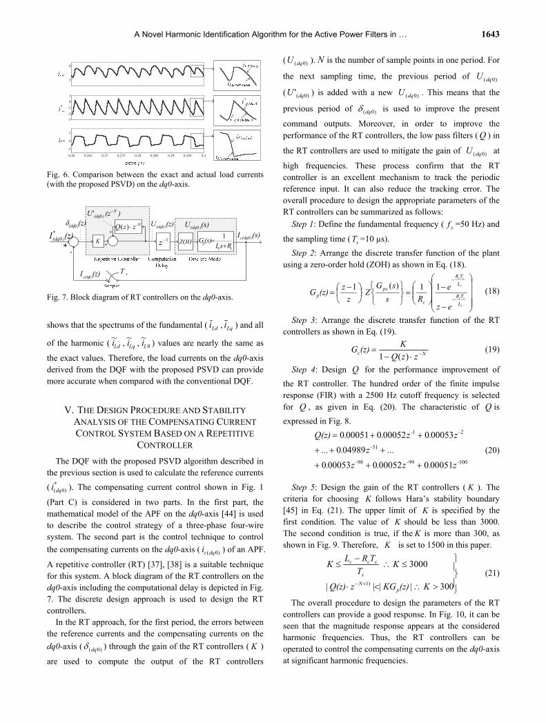
Fig. 7. Block diagram of RT controllers on the dq0-axis.
shows that the spectrums of the fundamental ( Ldi , Lqi ) and all
of the harmonic ( Ldi~
, Lqi~
, 0
~Li ) values are nearly the same as
the exact values. Therefore, the load currents on the dq0-axis derived from the DQF with the proposed PSVD can provide more accurate when compared with the conventional DQF.
V. THE DESIGN PROCEDURE AND STABILITY
ANALYSIS OF THE COMPENSATING CURRENT
CONTROL SYSTEM BASED ON A REPETITIVE
CONTROLLER
The DQF with the proposed PSVD algorithm described in the previous section is used to calculate the reference currents
( *)0(dqi ). The compensating current control shown in Fig. 1
(Part C) is considered in two parts. In the first part, the mathematical model of the APF on the dq0-axis [44] is used to describe the control strategy of a three-phase four-wire system. The second part is the control technique to control
the compensating currents on the dq0-axis ( )0(dqci ) of an APF.
A repetitive controller (RT) [37], [38] is a suitable technique for this system. A block diagram of the RT controllers on the dq0-axis including the computational delay is depicted in Fig. 7. The discrete design approach is used to design the RT controllers.
In the RT approach, for the first period, the errors between the reference currents and the compensating currents on the
dq0-axis ( )0(dq ) through the gain of the RT controllers ( K )
are used to compute the output of the RT controllers
( )0(dqU ). N is the number of sample points in one period. For
the next sampling time, the previous period of )0(dqU
( )0(' dqU ) is added with a new )0(dqU . This means that the
previous period of )0(dq is used to improve the present
command outputs. Moreover, in order to improve the performance of the RT controllers, the low pass filters ( Q ) in
the RT controllers are used to mitigate the gain of )0(dqU at
high frequencies. These process confirm that the RT controller is an excellent mechanism to track the periodic reference input. It can also reduce the tracking error. The overall procedure to design the appropriate parameters of the RT controllers can be summarized as follows:
Step 1: Define the fundamental frequency ( sf =50 Hz) and
the sampling time ( sT =10 µs).
Step 2: Arrange the discrete transfer function of the plant using a zero-order hold (ZOH) as shown in Eq. (18).
c
sc
c
sc
L
TR
L
TR
c
pcp
ez
e
Rs
sGΖ
z
z(z)G
11)(1 (18)
Step 3: Arrange the discrete transfer function of the RT controllers as shown in Eq. (19).
Nc zzQ
K(z)G
)(1
(19)
Step 4: Design Q for the performance improvement of
the RT controller. The hundred order of the finite impulse response (FIR) with a 2500 Hz cutoff frequency is selected for Q , as given in Eq. (20). The characteristic of Q is
expressed in Fig. 8.
1009998
51
21
000510000520000530
049890
000530000520000510
---
-
--
z.z.z.
...z....
z.z..Q(z)
(20)
Step 5: Design the gain of the RT controllers ( K ). The
criteria for choosing K follows Hara’s stability boundary [45] in Eq. (21). The upper limit of K is specified by the first condition. The value of K should be less than 3000. The second condition is true, if the K is more than 300, as shown in Fig. 9. Therefore, K is set to 1500 in this paper.
300 ||||
3000
)1 K(z)KGzQ(z)
KT
TRLK
pN
s
scc
(21)
The overall procedure to design the parameters of the RT controllers can provide a good response. In Fig. 10, it can be seen that the magnitude response appears at the considered harmonic frequencies. Thus, the RT controllers can be operated to control the compensating currents on the dq0-axis at significant harmonic frequencies.

1644 Journal of Power Electronics, Vol. 17, No. 6, November 2017
10-2
10-1
100
101
0
0.1
0.2
0.3
0.4
0.5
0.6
0.7
0.8
0.9
1
Frequency (kHz)
Mag
nitu
de
Magnitude ResponseLPF: Q(z)M
agni
tude
Frequency (kHz)
fc=2500 Hz
actual response
ideal response
Fig. 8. Characteristic of Q in repetitive controllers.
100
101
102
103
-20
0
20
40
60
80
100
(dB
)
(Hz)
1)( NzzQ
)(1500 zG p
)(300 zGp
)(100 zGp
Fig. 9. Criteria for choosing K.
100
101
102
103
0
50
100
150
200
250
(dB
)
(Hz)
Frequency (Hz)
Mag
nitu
de (
dB)
300 Hz
50 Hz 150 Hz 250 Hz
200 Hz100 Hz
Operational frequency range for dq-axis
Operational frequency range for 0-axis
Fig. 10. Magnitude response of repetitive controllers.
In addition, the PI controllers designed by the discrete design approach [46] are used to control the DC bus voltages.
The total ( dcV ) and different ( dcV ) DC bus voltage
control can provide good performance to regulate the
voltages to be equal to a desired operating point ( *refV ), and it
keeps the balanced voltage across the capacitors ( 1,dcC , 2,dcC ).
VI. HARDWARE IN THE LOOP TECHNIQUE
The ideas of the DQF with the proposed PSVD harmonic identification and control strategy are supported by hardware in the loop (HIL) as shown in Fig. 11. The hardware connection between the host computer and the eZdspTM
SimPowerSystemTM SIMULINK (Host)
Code Composer StudioTM
DSK v3.3 IDE
USB device
eZdspTM F28335 board (Target)
(a)
Considered power systemHost: Computer
Harmonic identification and Control strategy
for APFv*uvw,out
Real-Time Data Exchange (RTDXTM) Write
JTAG emulator
Real-Time Data Exchange (RTDXTM) Read
Vdc,1,2vpcc,uvw iL,uvw ic,uvw
Target: eZdspTM F28335 board
Code Composer StudioTM DSK v 3.3 IDE
From RTDX
To RTDX
(b)
Receive the load current, compensating current and DC
bus voltage from the considered power system in
the SPSTM SIMULINK
k=1
Calculate the reference current on dq0-axis
(i*d, i
*q, i
*0)
by using DQF method
Control the total and different DC bus voltage by using PI
controller (idv, i0v)
Control the compensating current on dq0-axis
(icd, icq, ic0) by using repetitive controller
Calculate the reference voltages of APF on dq0-axis
(v*d,out, v
*q,out, v
*0,out)
for PWM tecnique
Convert the reference voltages of APF on dq0-axis into uvw-
axis (v*
u,out, v*v,out, v
*w,out )
k=k+1
Declare the function and initial values for eZdspTM
F28335 Board.
Declare the variable and initial values for control
strategy.
Calculate the phase angle of the PCC voltage (θpcc) and the
magnitude of the PCC voltages by using PSVD
Send the v*u,out, v
*v,out and v*
w,out from the eZdspTM F28335 board to the considered power system
in the SPSTM SIMULINK
(c)
Fig. 11. HIL technique: (a) hardware connection of the HIL technique; (b) configuration of the HIL technique; (c) flowchart of the harmonic identification and control strategy.
F28335 board by a JTAG interfaced with a USB port is depicted in Fig. 11(a). The configuration of the HIL technique is shown in Fig. 11(b).
The SPSTM Simulink in the host computer works together with the CCStudioTM in the eZdspTM F28335 board. The PCC

A Novel Harmonic Identification Algorithm for the Active Power Filters in … 1645
voltages ( uvwpccv , ), the load currents ( uvwLi , ), the
compensating currents ( uvwci , ) and the DC bus voltages
( 1,dcV , 2,dcV ) are detected from the considered power system
in SPSTM Simulink. The “RTDX Write” block is used to write these data from SPSTM Simulink. Then, the “From RTDX” block is used to send these data from the host into the target. In the eZdspTM F28335 board, the data from the host are calculated by a control strategy process to obtain the
reference voltages of the APF ( *,outuvwv ). The details of the
*,outuvwv calculation can be viewed in the flowchart in Fig. 11
(c). The values of *,outuvwv are transferred into the host
computer by the “To RTDX” block. The “RTDX Read” block is used to read the data from the target into the host.
VII. RESULTS AND DISCUSSION
The performances of the novel harmonic identification and the proposed control strategy have been confirmed by the HIL technique. A performance comparison using the DQF, the DQF with the conventional PSVD and the DQF with the proposed PSVD method for harmonic identification are presented in this section.
According to Fig. 1, a non-ideal voltage source connected with a 3-single phase bridge rectifier feeding different resistor
( )(uvwLR ) and inductor ( )(uvwLL ) loads is considered. This
system can generate harmonic and unbalanced source currents. The system parameters are defined in the appendix. The performance indices for the harmonic elimination in a
three-phase four-wire system are the average THD% of the
source currents ( avTHD% ), the current unbalanced factor
( CUF% ) and the power factor after compensation ( PF ).
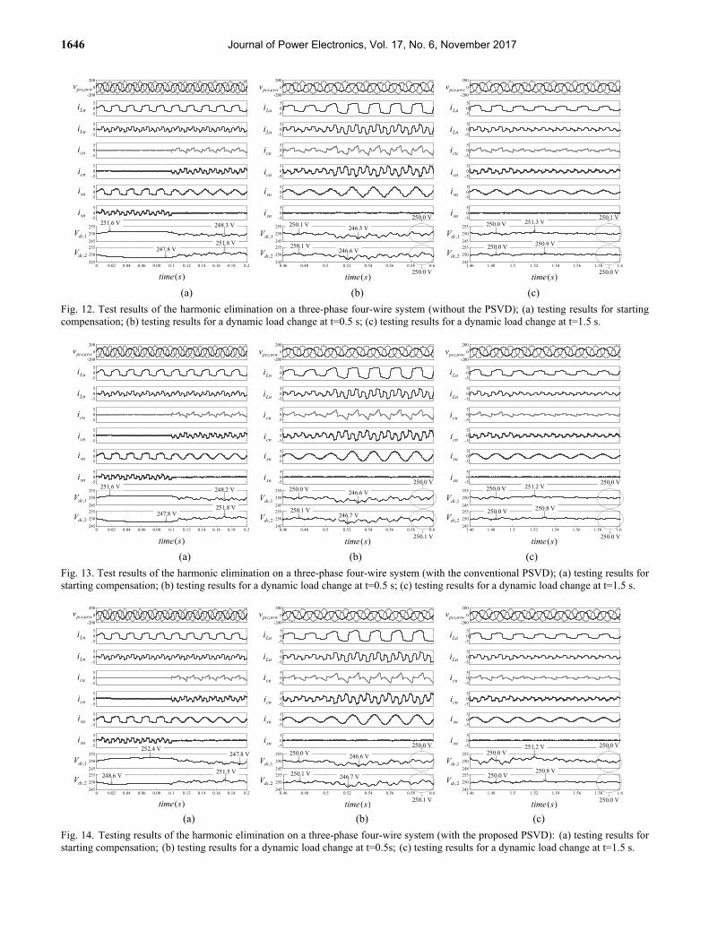
These values can satisfy IEEE std.519-2014 [1] and IEEE std.1459-2010 [11]. The results of the harmonic elimination on a three-phase four-wire system are illustrated in Fig. 12-14.
All of the testing results in terms of the avTHD% , CUF%
and PF are addressed in Table I. Before compensation at t < 0.1 s, the source currents
( uvwsi , ) are a distorted waveform and the neutral current ( sni )
appears in the neutral line. The avTHD% and CUF% are
equal to 33.53 % and 14.81 %, respectively. The
compensating currents ( uvwci , ) from the APF are injected into
the system at t = 0.1 s. From Fig. 12 (a), 13 (a) and 14 (a),
uvwsi , become more sinusoidal waveforms. For a comparison
study, the avTHD% from the DQF with the proposed PSVD
(1.41 %) is less than the DQF with the conventional PSVD (1.89 %) and the DQF (13.38 %). As a result, the DQF with the PSVD algorithm is suitable for calculating the reference
currents for an APF under non-ideal voltage source
conditions. The waveform of sni is nearly zero. This means
that these approaches can provide the balanced current
condition. The CUF% from these approaches is greatly
reduced. Moreover, the PF from these algorithms is nearly unity after compensation.
After compensation from t = 0.5 s to 1.0 s, the amplitude
of uvwLi , increases as shown in Fig. 12 (b), 13 (b) and 14 (b).
In this situation, 1,dcV and 2,dcV drop across 1,dcC and 2,dcC ,
respectively. However, the DC bus voltage control can
regulate 1,dcV and 2,dcV so that these values are equal to the
desired operating point (250 V). Waveforms of uvwsi , from
the DQF with the PSVD are more nearly sinusoidal than
uvwsi , from the DQF. The avTHD% of uvwsi , from the DQF, the
DQF with the conventional PSVD and the DQF with the proposed PSVD approaches are equal to 13.18 %, 1.70 % and 1.16 %, respectively. It can be seen in Table I that these algorithms can provide good performance in terms of
CUF% and PF .
After compensation from t = 1.5 s to 2.0 s, the amplitude
of uvwLi , decreases as shown in Fig. 12 (c), 13 (c) and 14 (c).
The values of 1,dcV and 2,dcV are greater than 250 V. After
t=1.5 s, 1,dcV and 2,dcV can track the DC bus reference voltage
even when the loads are varied. For the DQF, it can be seen
from the testing results that uvwsi , after compensation is a
nearly sinusoidal waveform. The avTHD% of this current is
equal to 13.60 %. As a result, the DQF with the proposed PSVD can provide better results when compared with the
conventional methods. The avTHD% of uvwsi , from the DQF
with the proposed PSVD is equal to 1.66 %. The value of
sni is nearly equal to zero. Therefore, the unbalanced source
current can become a balanced source current after all of the
harmonics are completely eliminated. The CUF% from the
DQF, the DQF with the conventional PSVD and the DQF with the proposed PSVD approaches are equal to 0.37 %, 0.42 % and 0.29 %, respectively. The results of the power factor correction for these approaches are equal to 0.97.
From Fig. 15, the compensating currents on the dq0-axis from the APF can track the reference currents calculated by the DQF, the DQF with the conventional PSVD and the DQF with the proposed PSVD methods. This means that the RT controllers of the three current loops with the control strategy proposed in the paper provide a good performance. However, the reference currents on the dq-axis calculated by the DQF, as shown in Fig. 15(a), are not correct when compared with the exact currents. The DQF with the PSVD can provide the reference currents on the dq-axis to track the exact currents, as shown in Fig. 15(b) and 15(c).
1646 Journal of Power Electronics, Vol. 17, No. 6, November 2017
-200
0
200
-505
-505
-505
-505
-505
-505
245
250
255
0 0.02 0.04 0.06 0.08 0.1 0.12 0.14 0.16 0.18 0.2245
250
255
-200
0
200
-505
-505
-505
-505
-505
-505
245
250
255
1.46 1.48 1.5 1.52 1.54 1.56 1.58 1.6245
250
255
-200
0
200
-505
-505
-505
-505
-505
-505
245
250
255
0.46 0.48 0.5 0.52 0.54 0.56 0.58 0.6245
250
255
uvwpccv ,
Lui
Lni
cui
cni
sui
sni
1,dcV
2,dcV
)(stime
uvwpccv ,
Lui
Lni
cui
cni
sui
sni
1,dcV
2,dcV
)(stime
uvwpccv ,
Lui
Lni
cui
cni
sui
sni
1,dcV
2,dcV
)(stime
251.6 V
247.8 V
248.3 V
251.8 V
250.1 V
250.1 V
246.5 V
246.6 V
250.0 V
250.0 V
251.3 V
250.9 V
250.0 V
250.0 V
250.1 V
250.0 V
(a) (b) (c)
Fig. 12. Test results of the harmonic elimination on a three-phase four-wire system (without the PSVD); (a) testing results for starting compensation; (b) testing results for a dynamic load change at t=0.5 s; (c) testing results for a dynamic load change at t=1.5 s.
-200
0
200
-505
-505
-505
-505
-505
-505
245
250
255
0 0.02 0.04 0.06 0.08 0.1 0.12 0.14 0.16 0.18 0.2245
250
255
-200
0
200
-505
-505
-505
-505
-505
-505
245
250
255
0.46 0.48 0.5 0.52 0.54 0.56 0.58 0.6245
250
255
-200
0
200
-505
-505
-505
-505
-505
-505
245
250
255
1.46 1.48 1.5 1.52 1.54 1.56 1.58 1.6245
250
255
uvwpccv ,
Lui
Lni
cui
cni
sui
sni
1,dcV
2,dcV
)(stime
uvwpccv ,
Lui
Lni
cui
cni
sui
sni
1,dcV
2,dcV
)(stime
uvwpccv ,
Lui
Lni
cui
cni
sui
sni
1,dcV
2,dcV
)(stime
251.6 V
247.8 V
248.2 V
251.8 V
250.0 V
250.1 V
246.6 V
246.7 V
250.0 V
250.0 V
251.2 V
250.8 V
250.0 V
250.1 V
250.0 V
250.0 V
(a) (b) (c)
Fig. 13. Test results of the harmonic elimination on a three-phase four-wire system (with the conventional PSVD); (a) testing results for starting compensation; (b) testing results for a dynamic load change at t=0.5 s; (c) testing results for a dynamic load change at t=1.5 s.
-200
0
200
-505
-505
-505
-505
-505
-505
245
250
255
0 0.02 0.04 0.06 0.08 0.1 0.12 0.14 0.16 0.18 0.2245
250
255
-200
0
200
-505
-505
-505
-505
-505
-505
245
250
255
0.46 0.48 0.5 0.52 0.54 0.56 0.58 0.6245
250
255
-200
0
200
-505
-505
-505
-505
-505
-505
248
250
252
1.46 1.48 1.5 1.52 1.54 1.56 1.58 1.6245
250
255
uvwpccv ,
Lui
Lni
cui
cni
sui
sni
1,dcV
2,dcV
)(stime
uvwpccv ,
Lui
Lni
cui
cni
sui
sni
1,dcV
2,dcV
)(stime
uvwpccv ,
Lui
Lni
cui
cni
sui
sni
1,dcV
2,dcV
)(stime
252.4 V
248.6 V
247.8 V
251.5 V
250.0 V
250.1 V
246.6 V
246.7 V
250.0 V
250.0 V
251.2 V
250.8 V
250.0 V
250.1 V
250.0 V
250.0 V
(a) (b) (c)
Fig. 14. Testing results of the harmonic elimination on a three-phase four-wire system (with the proposed PSVD): (a) testing results for starting compensation; (b) testing results for a dynamic load change at t=0.5s; (c) testing results for a dynamic load change at t=1.5 s.

A Novel Harmonic Identification Algorithm for the Active Power Filters in … 1647
TABLE I PERFORMANCE OF THE SOURCE CURRENTS BEFORE AND AFTER COMPENSATION
-1
0
1
-3
-2
-1
0
1
0.49 0.492 0.494 0.496 0.498 0.5-2
-1
0
1
2
cdi
cqi
0ci
i~Ld
i*q
iL0
iLd,ideal
i*q,ideal
iL0,ideal
icd
icq
ic0
time(s)
(a)
-1
0
1
-3
-2
-1
0
1
0.49 0.492 0.494 0.496 0.498 0.5-2
-1
0
1
2
cdi
cqi
0ci
i~Ld
i*q
iL0
iLd,ideal
i*q,ideal
iL0,ideal
icd
icq
ic0
time(s)
(b)
-1
0
1
-3
-2
-1
0
1
0.49 0.492 0.494 0.496 0.498 0.5-2
-1
0
1
2
cdi
cqi
0ci
i~Ld
i*q
iL0
iLd,ideal
i*q,ideal
iL0,ideal
icd
icq
ic0
time(s)
(c)
Fig. 15. Tracking performance of the compensating currents on the dq0-axis: (a) DQF without the PSVD; (b) DQF with the conventional PSVD; (c) DQF with the proposed PSVD.
VIII. CONCLUSIONS
The DQF with the proposed PSVD is a novel harmonic identification strategy. The proposed algorithm can be used to calculate the reference currents for the APF in a three-phase four-wire system. The magnitude and phase angle of the PCC voltages and the harmonic orders of the load currents in non-ideal voltage source systems are analyzed in this paper. A performance comparison between the DQF, the DQF with the conventional PSVD and the DQF with the proposed PSVD is carried out by the hardware in the loop technique. The testing results show that the DQF with the proposed PSVD can provide accurate reference currents. In addition, design and stability analysis of the repetitive controller are expressed in this paper. The control strategy can provide good performance of the APF. The source currents after compensation can become undistorted and balanced and the APF can improve the unity power factor at the PCC.
APPENDIX
Line voltage and frequency:
)(uvwpccv = 80-120 Vrms, sf = 50 Hz
Line impedance of the source and load:
sL = 0.1mH, eqL = 10 mH
3-single phase diode rectifiers:
LuL = 100 mH, LvL = 150 mH, LwL = 200 mH,
LuR = 15 - 45 Ω, LvR = 20 - 60 Ω, LwR = 25 - 75 Ω
DC bus voltages: *
1,dcV = 250V, *2,dcV = 250V, 1,dcC = 1,dcC = 3000 µF
Line impedance of the APF: cL = 30 mH
Switching frequency: swf = 5000 Hz
ACKNOWLEDGMENT
This work was supported by Suranaree University of Technology (SUT) and by the office of the Higher Education Commission under NRU project of Thailand. The author would like to thank Dr. Tossaporn Narongrit for providing the useful information of HIL technique.
Performance indices
The decrease of the amplitude of load currents
The considered load currents The increase of the amplitude
of load currents
Before comp.
After compensation Before comp.
After compensation Before comp.
After compensation
DQF DQF
+conv. PSVD
DQF +proposed
PSVD DQF
DQF +conv.PSVD
DQF +proposed
PSVD DQF
DQF +conv.PSVD
DQF +proposed
PSVD
avTHD% 30.95 13.60 1.83 1.66 33.53 13.38 1.89 1.41 33.84 13.18 1.70 1.16
CUF% 13.65 0.37 0.42 0.29 14.81 0.33 0.38 0.31 14.24 0.45 0.47 0.33
PF 0.86 0.97 0.97 0.97 0.83 0.97 0.97 0.97 0.80 0.98 0.98 0.98
1648 Journal of Power Electronics, Vol. 17, No. 6, November 2017
REFERENCES
[1] “IEEE recommended practices and requirements for harmonic control in electrical power systems,” IEEE Std.519-2014, 2014.
[2] A. D. Graham and E. T. Schonholder, “Line harmonics of converters with DC motor loads,” IEEE Trans. Ind. Appl., Vol. IA-19, No. 1, pp. 84-93, Jan. 1983.
[3] G. C. Jain, “The Effect of voltage waveshape on the performance of a three-phase induction motor,” IEEE Trans. Power App. Syst., Vol. 83, No. 6, pp. 561-566, Jun. 1964.
[4] “IEEE standard general requirements for liquid-immersed distribution, power, and regulating transformers,” IEEE Std. C57.12.00-1987, 1988.
[5] “IEEE recommended practice for establishing transformer capability when supplying non-sinusoidal load currents,” IEEE Std. C57.110-1986, 1988.
[6] “IEEE standard for shunt power capacitors,” IEEE Std. 18-2002, 2002.
[7] W. C. Downing, “Watthour meter accuracy on SCR controlled resistance loads,” IEEE Trans. Power App. Syst., Vol. PAS-93, No. 4, pp. 1083-1089, Jul. 1974.
[8] Power System Relaying Committee, “The impact of sine-wave distortions on protective relays,” IEEE Trans. Ind. Appl., Vol. IA-20, No. 2, pp. 335-343, Mar. 1984.
[9] L. Gyugyi, and E. C. Strycula, “Active ac power filters,” IEEE Industry Applications Annual Meeting, Vol. 19-C, pp. 529-535, 1976.
[10] D. Sreenivasarao, P. Agarwal, and B. Das, “Neutral current compensation in three-phase, four-wire systems: A review,” Electric Power Systems Research, Vol. 86, pp. 170-180, Jan. 2012.
[11] “IEEE standard definitions for the measurement of electric power quantities under sinusoidal, nonsinusoidal, balanced, or unbalanced conditions,” IEEE Std.1459-2010, 2010.
[12] M. Aredes, J. Hafner, and K. Heumann, “Three-phase four-wire shunt active filter control strategies,” IEEE Trans. Power Electron., Vol. 12, No. 2, pp. 311-318, Mar. 1997.
[13] M. EI-Habrouk and M. K. Darwish, “Design and implementation of a modified Fourier analysis harmonic current computation technique for power active filter using DSPs,” IEEE Electric Power Applications, Vol. 148, No. 1, pp. 21-28, 2001.
[14] H. Akagi, Y. Kanazawa, and A. Nabae, “Instantaneous reactive power compensators comprising switching devices without energy storage components,” IEEE Trans. Ind. Appl., Vol. IA-20, No. 3, pp. 625-630, May 1984.
[15] M. Takeda, K. Ikeda, A. Teramoto, and T. Aritsuka, “Harmonic current and reactive power compensation with an active filter,” IEEE Power Electronics Specialists Conference, Vol. 2, pp. 1174-1179, Apr. 1988.
[16] C. L. Chen, C. E. Lin, and C. L. Huang, “An active filter for unbalanced three-phase system using synchronous detection method,” IEEE Power Electronics Specialists Conference, Vol. 2, pp. 1451-1455, Jun. 1994.
[17] G. W. Chang and S. K. Chen, “An a-b-c reference frame-based control strategy for the three-phase four-wire shunt active power filter,” IEEE Conference on Harmonics and Quality of Power, Vol. 1, pp. 26-29, Oct. 2000.
[18] S. M. -R. Rafiei, H. A. Toliyat, R. Ghazi, and T. Gopalarathnam, “An optimal and flexible control strategy for active filtering and power factor correction under non-sinusoidal line voltages,” IEEE Trans. Power Del.,
Vol. 16, No. 2, Apr. 2001. [19] N. Eskandarian, Y. A. Beromi, and S. Farhangi,
“Improvement of dynamic behavior of shunt active power filter using fuzzy instantaneous power theory,” Journal of Power Electronics, Vol. 14, No. 6, pp. 1303-1313, Nov. 2014.
[20] E. Ozmedir, M. Kale, and S. Ozmedir, “A novel control method for active power filter under non-ideal mains voltage,” IEEE Conference on Control Applications, pp. 931-936, Jun. 2003.
[21] S. Biricik, S. Redif, O. C. Ozerdem, and M. Basu, “Control of the shunt Active Power Filter under non-ideal grid voltage and unbalanced load conditions,” International Universities Power Engineering Conference, Sep. 2014.
[22] M. Ucar and E. Ozdemir, "Control of a 3-phase 4-leg active power filter under non-ideal mains voltage condition," Electric Power Systems Research, Vol. 78, No. 1, pp. 58-73, Jan. 2008.
[23] P. Kanjiya, V. Khadkikar, and H. H. Zeineldin, "A Noniterative optimized algorithm for shunt active power filter under distorted and unbalanced supply voltages," IEEE Trans. Ind. Electron., Vol. 60, No. 12, pp. 5376-5390, Dec. 2012.
[24] P. Kanjiya, V. Khadkikar, and H. H. Zeineldin, “Optimal control of shunt active power filter to meet IEEE Std. 519 current harmonic constraints under nonideal supply condition,” IEEE Trans. Ind. Electron., Vol. 62, No. 2, pp. 724-734, Feb. 2015.
[25] P. Dey and S. Mekhilef, “Shunt hybrid active power filter under nonideal voltage based on fuzzy logic controller,” International Journal of Electronics, Vol. 103, No. 9, pp. 1580-1592, Feb. 2016.
[26] S. Sujitjorn, K.-L. Areerak, and T. Kulworawanichpong, “The DQ axis with Fourier (DQF) method for harmonic identification,” IEEE Trans. Power Del., Vol. 22, No. 1, pp. 737-739, Jan. 2007.
[27] K.-L. Areerak, “Harmonic detection algorithm based on DQ axis with Fourier analysis for hybrid power filters," WSEAS Trans. Power Syst., Vol. 3, No. 11, Nov. 2008.
[28] P. Santiprapan, K.-L. Areerak, and K.-N. Areerak, “The enhanced – DQF algorithm and optimal controller design for shunt active power filter,” International Review of Electrical Engineering, Vol. 10, No. 5, pp. 578-590, Sep./Oct. 2015.
[29] S. Bhattacharya, T. M. Frank, D. M. Divan, and B. Banerjee, “Parallel active filter implementation and design issues for utility interface of adjustable speed drive systems,” IEEE Industry Applications Conference, Vol. 2, pp. 1032-1039, 1996.
[30] D. G. Holmes and D. A. Martin, “Implementation of direct digital predictive current controller for single and three-phase voltage source inverters,” IEEE Industry Applications Conference, Vol. 2, pp. 906-913. 1996.
[31] X. Yuan, W. Merk, H. Stemmler, and J. Allmeling, “Stationary-frame generalized integrators for current control of active power filters with zero steady-state error for current harmonics of concern under unbalanced and distorted operating conditions,” IEEE Trans. Ind. Appl., Vol. 38, No. 2, pp. 523-532, Mar. 2002.
[32] R. Bojoi, G. Griva, V. Bostan, M. Guerriero, F. Farina, and F. Profumo, “Current control strategy for power conditioners using sinusoidal signal integrators in synchronous reference frame,” IEEE Trans. Power Electron., Vol. 20, No. 6, pp. 1402-1412, Nov. 2005.

A Novel Harmonic Identification Algorithm for the Active Power Filters in … 1649
[33] C. Lascu, L. Asiminoaei, I. Boldea, and F. Blaabjerg, “High performance current controller for selective harmonic compensation in active power filters,” IEEE Trans. Power Electron., Vol. 22, No. 5, pp. 1826-1835, Sep. 2007.
[34] B. Singh, K. Al - Haddad, and A. Chandra, “Active power filter with sliding mode control,” IEEE Trans. Ind. Appl., Vol. 144, No. 6, pp. 564-568, Nov. 1997.
[35] N. Mendalek, K. Al-Haddad, F. Fnaiech, and L. A. Dessaint, “A non-linear optimal predictive control of a shunt active power filter,” IEEE Industry Applications Conference, Vol. 1, pp. 70-77. Oct. 2002.
[36] S. Hirve, K. Chatterjee, B. G. Fernandes, M. Imayavaramban, and S. Dwari, “PLL-less active power filter based on one-cycle control for compensating unbalanced loads in three-phase four-wire system,” IEEE Trans. Power Del., Vol. 22, No. 4, pp. 2457-2465, Oct. 2007.
[37] P. Mattavelli and F. P. Marafao, “Repetitive based control for selective harmonic compensation in active power filters,” IEEE Trans. Ind. Electron., Vol. 51, No. 5, pp. 1018-1024, Oct. 2004.
[38] M. A. Abusara, S. M. Sharkh, and P. Zanchetta, “Control of grid-connected inverters using adaptive repetitive and proportional resonant schemes,” Journal of Power Electronics, Vol. 15, No. 2, pp. 518-529, Mar. 2015.
[39] P. Garanayak and G. Panda, “Harmonic elimination and reactive power compensation with a novel control algorithm based active power filter,” Journal of Power Electronics, Vol. 15, No. 6, pp. 1619-1627, Nov. 2015.
[40] V. E. Wagner, J. C. Balda, D. C. Griffith, A. McEachern, T. M. Barnes, D. P. Hartmann, D. J. Phileggi, A. E. Emannuel, W. F. Horton, W. E. Reid, R. J. Ferraro and W. T. Jewell, “Effects of harmonics on equipment,” IEEE Trans. Power Del., Vol. 8, No. 2, pp. 672-680, Apr. 1993.
[41] H. Akagi, E. H. Watanabe, and M. Aredes, Instantaneous Power Theory and Applications to Power Conditioning, John Wiley & Sons, chap. 2, 2007.
[42] V. Kaura and V. Blasko, “Operation of a phase locked loop system under distorted utility conditions,” IEEE Trans. Ind. Appl., Vol. 33, No. 1, pp. 58-63, Jan/Feb. 1997.
[43] W. Leonhard, Control of Electrical Drives, Springer Verlag, 1985.
[44] P. Santiprapan, K.-L. Areerak, and K.-N. Areerak, “Dynamic model of active power filter in three-phase four-wire system,” 11th International Conference on Electrical / Electronics, Computer, Telecommunications and Information Technology, pp. 1-5, May 2014.
[45] S. Hara, Y. Yamamoto, T. Omata, and M. Nakano, “Repetitive control system: a new type servo system for periodic exogenous signals,” IEEE Trans. Autom. Contr., Vol. 33, No. 7, pp. 659-668, Jul. 1988.
[46] P. Santiprapan, K.-L. Areerak, and K.-N. Areerak, “Dynamic model and controller design for active power filter in three-phase four-wire system,” International Journal of Control and Automation, Vol. 7, No. 9, pp. 27-44, Sep. 2014.
Phonsit Santiprapan received his B.Eng, M.Eng and Ph.D. degrees in Electrical Engineering from Suranaree University of Technology (SUT), Nakhon Ratchasima, Thailand, in 2009, 2011 and 2016, respectively. Since 2017, he has been a Lecturer in the School of Electrical Power Engineering, Mahanakorn University of
Technology (MUT), Bangkok, Thailand. His current research interests include active power filters, harmonic elimination, artificial intelligence applications, simulation and modeling.
Kongpol Areerak received his B.Eng, M.Eng and Ph.D. degrees in Electrical Engineering from Suranaree University of Technology (SUT), Nakhon Ratchasima, Thailand, in 2000, 2003 and 2007, respectively. Since 2007, he has been a Lecturer and the Head of Power Quality
Research Unit (PQRU) in the School of Electrical Engineering, SUT, where he became an Associate Professor of Electrical Engineering in 2015. His current research interests include active power filters, harmonic elimination, artificial intelligence applications, motor drives and intelligent control systems.
Kongpan Areerak received B.Eng. and M.Eng degrees from Suranaree University of Technology (SUT), Nakhon Ratchasima, Thailand, in 2000 and 2001, respectively and Ph.D. degree from the University of Nottingham, Nottingham, UK., in 2009, all in Electrical Engineering. In 2002, he was a Lecturer in the Department of Electrical
Engineering, Rangsit University, Pathum Thani, Thailand. Since 2003, he has been a Lecturer in the School of Electrical Engineering, SUT, where he became an Associate Professor of Electrical Engineering in 2015. His current research interests include system identification, artificial intelligence applications, the stability analysis of power systems with constant power loads, the modeling and control of power electronic based systems and control theory.


