

University of South FloridaScholar Commons
Graduate Theses and Dissertations Graduate School
January 2013
A Novel Method For Watermarking SequentialCircuitsMatthew LewandowskiUniversity of South Florida, [email protected]
Follow this and additional works at: http://scholarcommons.usf.edu/etd
Part of the Computer Engineering Commons
This Thesis is brought to you for free and open access by the Graduate School at Scholar Commons. It has been accepted for inclusion in GraduateTheses and Dissertations by an authorized administrator of Scholar Commons. For more information, please contact [email protected].
Scholar Commons CitationLewandowski, Matthew, "A Novel Method For Watermarking Sequential Circuits" (2013). Graduate Theses and Dissertations.http://scholarcommons.usf.edu/etd/4528

A Novel Method For Watermarking Sequential Circuits
by
Matthew Lewandowski
A thesis submitted in partial fulfillmentof the requirements for the degree of
Master of Science in Computer EngineeringDepartment of Computer Science and Engineering
College of EngineeringUniversity of South Florida
Major Professor: Srinivas Katkoori, Ph.D.Swaroop Ghosh, Ph.D.
Jay Ligatti, Ph.D.
Date of Approval:March 18, 2013
Keywords: Automata, Encoding, Intellectual Property, Finite State MachineWatermarking, Circuit Watermarking
Copyright © 2013, Matthew Lewandowski

Dedication
I would like to dedicate this work to my beloved family, parents, and siblings. To
my mother and father, Kristy and Michael Lewandowski, I cannot thank you enough for
your continued support, both emotionally and physically, throughout my many years of
academia, and the many more to come.
I also thank my siblings, Eric, Keven, and Craig for being there for me during my
times of need, and for teaching me that regardless of my handicap I can overcome any
hurdle when driven by a limitless passion. I am grateful for every lesson you have taught
me, every opportunity you have provided me with, and the many years of time you have
invested into dealing with me. I can only hope you are as proud of me as I am of you, and
I could not have accomplished the things I have today without your continued love and
support.
In addition, I dedicate this to Amanda Lewandowski. Without your continued
support both as a member of my family and as my physical therapist, I would not have
been able to regain the functionality in my hand which allowed me to complete this work.
For this time, patience, and care you put forth during my rehabilitative process, I so deeply
thank you.
Lastly, I dedicate this to my beloved grandfather and grandmother, Dean and Doris
Moon, who have continuously supported me through every life venture and taught me that
with the right mind set and attitude, I have the potential to walk among the stars.

Acknowledgments
First and foremost, I give acknowledgement with the utmost appreciation and grat-
itude to Dr. Srinivas Katkoori for providing me with the wonderful opportunity of working
on this project. I am grateful to him for letting me be his teaching assistant in the areas of
study I so passionately love, which granted me the resources to further my education and
opportunities here at the university. I also extend my appreciations and gratitude to Dr.
Swaroop Ghosh and Jay Ligatti for serving on my supervisory committee.
I would like to thank Christopher Bell and Matthew Morrison for providing me the
opportunity to work alongside them on various hardware security and quantum computing
projects. I extend thanks to Richard Meana for his sub-graph matching contributions
and involvement with this work during our senior project with Dr. Katkoori. To my
lab neighbor, Joseph Botto, I thank you for the grand idea of file hashing and continued
technical support.
To my loving friends who were there for me over my academic travels and times
of need: Christopher Bell, TracyWolf, Donald Ray, Matthew Morrison, Richard Meana,
Nicole Gonzalez, Chris Bringes, Thomas Peterson, Mary Ivory, Cybil Scott, Virginia Mau-
rer, Caitlin Snell, James Adkins, David ODonnell, Roya Kashani, Robert O’Brien, Christo-
pher Denton, Andrew Thomas, Nicholas Carter, Kristen Kluberdanz, Andrew Price, and
Benjamin Geiger.
Lastly, I want to acknowledge the wonderful faculty — and staff, current and former,
of the University of South Florida Department of Computer Science and Engineering. You
have made my academic pursuits of higher knowledge a joyful and pain free experience, and
I thank you for that. Students here are truly lucky to have faculty and staff — that are as
caring as each and every member proves.

Table of Contents
List of Tables iii
List of Figures v
Abstract vii
1 Introduction and Background 11.1 Thesis Organization 2
2 Modeling Sequential Systems 42.1 Finite State Machine Model 4
2.1.1 Asynchronous and Synchronous FSMs 42.2 Representations of FSMs 5
2.2.1 State Transition Graphs 52.2.2 State Transition Tables 62.2.3 Kiss2 6
2.3 FSM Models and Classifications 72.3.1 Moore Model 82.3.2 Mealy Model 82.3.3 Completely Specified Finite State Machine (CSFSM) 92.3.4 Incompletely Specified Finite State Machine (ISCFSM) 10
2.4 State Encoding for Sequential Circuit Optimization 112.5 Chapter Summary 12
3 Related Work 133.1 Physical Protection 13
3.1.1 Integrated Circuit Logos 133.1.2 Constraint Based Watermarking 15
3.2 Hardware Description Language Level Protection 173.3 Circuit and Model Level Protection 183.4 Sequential Circuit Watermarking Techniques 19
3.4.1 State Based Watermarking 193.4.2 Edge Based Watermarking 203.4.3 Input Output Based Watermarking 23
3.5 Motivation for This Work 253.6 Chapter Summary 29
4 State Encoding Based Watermarking 304.1 Note to Reader 304.2 Watermarking via State Encoding 314.3 Edge Creation Cost 31
i

4.4 Watermarking System: Overview 324.5 Watermark Construction Phase 33
4.5.1 Bitmap Signature Decomposition 334.5.2 File Signature Decomposition 354.5.3 Hashing Signature Decomposition 374.5.4 HSD Watermark Construction: Hash-2-K2 38
4.6 Watermark Embedding Phase 404.6.1 Embedding: Complexity 404.6.2 Brute Force Embedding Algorithm 414.6.3 Greedy Embedding Algorithm 45
4.7 Model Generation and Verification Phase 534.8 Watermark Extraction Sequence Generation 584.9 On the Tampering Hardness of State Encoding Based Watermarking 594.10 Chapter Summary 62
5 Experimental Results 655.1 Note to Reader 655.2 Xilinx Synthesis Options 655.3 Benchmark Suite 675.4 Overhead Calculations 67
5.4.1 User Encoding 685.4.2 Gray Encoding 695.4.3 Johnson Encoding 705.4.4 One-hot Encoding 715.4.5 Sequential Encoding 735.4.6 Speed1 Encoding 74
5.5 Discussion of Results 755.5.1 Synthesis Discrepancies 755.5.2 Synthesis Results 75
6 Future Work 786.1 Sequential Circuit Logic Synthesis: k3 786.2 Phantom Edges 79
6.2.1 Cost of a Phantom Edge 806.3 Watermark Extraction 806.4 Metric Stacking 81
7 Conclusions 82
References 83
Appendix A Glossary 91
Appendix B Permission of Use 97
About The Author End Page
ii

List of Tables
Table 1 Sample STT representation 6
Table 2 Metrics affected by state encoding 11
Table 3 Summary of protection techniques 26
Table 4 Summary of sequential protection techniques 28
Table 5 Xilinx synthesis results for dummy edges in Fig. 14 FSM 32
Table 6 Sample file under FSD 35
Table 7 Brute force mapping combinations 44
Table 8 Brute force cost mapping combinations 44
Table 9 Original and watermark FSM node degree values 50
Table 10 Example step-by-step greedy algorithm 52
Table 11 Embedding results, watermark (Fig. 19) has 15 states and 32 edges 52
Table 12 Time for HPC preimage attacks 61
Table 13 Time for HPC collision attacks 62
Table 14 Summary of proposed watermark construction phase methods 62
Table 15 Summary of proposed watermark embedding phase methods 63
Table 16 Summary of proposed model generation and verification methods 64
Table 17 Summary of security run-time analysis 64
Table 18 Xilinx XST optimization options 65
Table 19 Top ten largest IWLS’93 Kiss2 files 67
Table 20 Encoding schemes used 68
Table 21 Xilinx synthesis results for User & User encoded FSMs 69
Table 22 2-bit Gray encoding & Hamming distance 70
Table 23 Xilinx synthesis results for Gray & User encoded FSMs 70
Table 24 Johnson encoding 71
iii

Table 25 Xilinx synthesis results for Johnson & User encoded FSMs 71
Table 26 One-hot encoding 72
Table 27 Xilinx synthesis results for One-hot & User encoded FSMs 72
Table 28 Sequential encoding 73
Table 29 Xilinx synthesis results for Sequential & User encoded FSMs 73
Table 30 Speed1 encoding 74
Table 31 Xilinx synthesis results for Speed1 & User encoded FSMs 74
Table 32 Xilinx synthesis discrepancies for User & Sequential encoded FSMs 76
Table 33 Summary of Xilinx synthesis results 76
Table 34 Summary of performance 77
Table 35 k3 overview 78
Table 36 Xilinx synthesis results of phantom edge FSMs 80
iv

List of Figures
Figure 1 STG representation of an example FSM 6
Figure 2 Kiss2 representation of an example FSM 7
Figure 3 Moore model FSM example 8
Figure 4 Mealy model FSM example 9
Figure 5 An example of a completely specified FSM (CSFSM) 9
Figure 6 An example of an incompletely specified FSM (ICSFSM) 10
Figure 7 Sample IC logo implemented in AMI C5N that passed DRC check 15
Figure 8 Example of hierarchical watermarking 16
Figure 9 Lion FSM watermarked by HARPOON method [1] 18
Figure 10 Lion FSM utilizing state based watermarking 20
Figure 11 FSM utilizing edge based watermarking 22
Figure 12 Sample I/O signature 23
Figure 13 FSM utilizing passive I/O based watermarking 25
Figure 14 Watermarking edge creation method an illustrative watermarked FSM 31
Figure 15 High level overview of watermarking system flow 33
Figure 16 Methods of watermark construction 33
Figure 17 Sample bitmap signature 34
Figure 18 Example of FSD 36
Figure 19 Sample HSD signature prior to hashing 37
Figure 20 RIPEMD-160 Pajek netlist / STG using Gephi 38
Figure 21 Hash-2-Kiss2 watermark construction algorithm 39
Figure 22 Proposed brute force watermark embedding algorithm 42
Figure 23 Brute force cost calculation algorithm 43
Figure 24 Original and watermark FSMs for brute force embedding example 43
v

Figure 25 Original, watermark, and watermarked FSMs for brute force embedding 45
Figure 26 Greedy heuristic 46
Figure 27 Algorithm for FindMaxDegreeNode function 48
Figure 28 Algorithm for FindMinCostNode function 49
Figure 29 Algorithm for Neighbors function 50
Figure 30 Algorithm for SortDescend function 50
Figure 31 Original and watermark FSMs for greedy embedding example 51
Figure 32 Original, watermark, and watermarked FSMs for greedy embedding 51
Figure 33 Flow diagram for the custom tool “k2vhdl” 54
Figure 34 Algorithm for VertexCover 54
Figure 35 Sample VHDL signal generation for Lion.kiss2 55
Figure 36 Sample VHDL state controller for Lion.kiss2 56
Figure 37 Sample VHDL state machine for Lion.kiss2 57
Figure 38 Xilinx simulation state encoding trace 59
Figure 39 Sample VHDL synthesis options generation for Lion.kiss2 66
Figure 40 FSM with phantom edges 79
vi

Abstract
We present an Intellectual Property (IP) protection technique for sequential circuits
driven by embedding a decomposed signature into a Finite State Machine (FSM) through
the manipulation of the arbitrary state encoding of the unprotected FSM. This technique
is composed of three steps: (a) transforming the signature into a watermark graph, (b) em-
bedding watermark graphs into the original FSM’s State Transition Graph (STG) and (c)
generating models for verification and extraction. In the watermark construction process
watermark graphs are generated from signatures. The proposed methods for watermark
construction are: (1) Bitmap Signature Decomposition (BSD), (2) File Signature Decom-
position (FSD), and (3) Hashing Signature Decomposition (HSD). The HSD method is
shown to be advantageous for all signatures while providing sparse watermark FSMs with
complexity O(n2). The embedding process is related to the sub-graph matching problem.
Due to the computational complexity of the matching problem, attempts to reverse engineer
or remove the constructed watermark from the protected FSM, with only finite resources
and time, are shown to be infeasible. The proposed embedding solutions are: (1) Brute
Force and (2) Greedy Heuristic. The greedy heuristic has a computational complexity of
O(n log n), where n is the number of states in the watermark graph. The greedy heuristic
showed improvements for three of the six encoding schemes used in experimental results.
Model generation and verification utilizes design automation techniques for generating mul-
tiple representations of the original, watermark, and watermarked FSMs. Analysis of the
security provided by this method shows that a variety of attacks on the watermark and sys-
tem including: (1) data-mining hidden functionality, (2) preimage, (3) secondary preimage,
and (4) collision, can be shown to be computationally infeasible. Experimental results for
the ten largest IWLS 93 benchmarks that the proposed watermarking technique is a secure,
yet flexible, technique for protecting sequential circuit based IP cores.
vii

1 Introduction and Background
Integrated Circuit (IC) technologies have continued to rapidly evolve in size and
complexity since the beginning of their creation. Because of this constant evolution, it has
now become a common practice for companies designing Application Specific Integrated
Circuits (ASICs) to outsource part of the design process and purchase third party Intellec-
tual Property (IP) cores. These IP cores can be anything from communication to graphics
processing units, consisting of combinational or sequential sub-components. By employing
this semi-custom design approach, design houses can reduce costs that would typically be
incurred from a full-custom design approach. It also enables designers to reduce time-to-
market expectations. Under this business model, the design house will have to pay royalties
on every unit sold to the IP owner. It typically only has rights to the IP core for a limited
amount of time or design fabrication runs.
One might ponder what is to happen to the IP core that the design house physically
has once the licensing period has ended. This is where the need for further IP protection
comes into the scenario. There is currently no effective way to stop a company from further
utilizing the IP core outside of the contracted licensing period and refrain from rewarding
appropriate royalties for the further use of the design. Thus, the IP owner needs another
line of protection in the ability to thwart these potentially fraudulent actions. One common
way for IP owners to achieve this extra line of protection is through the utilization of digital
watermarking techniques. This enables an IP owner to embed a digital watermark for
the purpose of ownership verification in the event of litigation. The embedded watermark
signature can be any format of digital media ranging from images, audio, text files, and
even short length videos.
The process of watermarking electronic art consisted of the IP owners embedding
a signature, or watermark, directly into the image in a location that was only known by
the owner. This would later enable the owner a method of proving that the work, or
1

design, was his or hers if the ownership of the work ever came into question. This was
known to be the first “Electronic Water Mark” [2]. Due to technological advancements
of networks and electronic libraries [3] since this concept first appeared, this technique
would be expanded to encapsulate typography [4]. This would allow publishers, or others
sharing typographical material, a method for proving that a given document was their
IP. The concept of watermarking was extended to typography through seemingly invisible
typographical manipulations, which included the shifting of a single word a mere millimeter
to the original document.
Although digital watermarking of IP by included corporate logos in physical lay-
outs is a common today — it should be noted that they can be easily removed by etching
process. As technology complexities would continue to advance over time so too would
the spectrum of watermarking techniques and applications for which it could be used. It
was applied to ICs first by Charbon [5] through a hierarchical method, and later extended
to Field Programmable Gate Array (FPGA) technologies [6] as well as physical design
methodologies [7]. Electronic libraries report the earliest extension of this concept to se-
quential systems was by Olivera [8] where through the implementation of additional Finite
Automata and the employment of a secret input sequence to traverse into the watermark,
one could successfully embed a digital watermark into a sequential circuit.
This work presents a novel watermarking technique that can be used with sequential
systems, and their realized circuitry, by exploiting an inherent characteristic of these ma-
chines that was previously unexplored. Given an original model of a sequential system, and
the watermark signature, we determine the appropriate matching set which will minimize
overhead and properly embed the watermark signature into the original sequential system.
1.1 Thesis Organization
In Chapter 2, we present an in depth background on sequential systems. This
includes various types of FSM models and classifications, and the different methods for
representing these models. In Chapter 3 we will review related work pertaining to phys-
ical, Hardware Description Language (HDL), circuit & model level protection schemes.
Additionally, we provide detailed reviews and illustrations of the different techniques for
2

watermarking sequential circuits and discuss the motivation which led to this proposed
method.
In Chapter 4, we present the proposed method of watermarking. This chapter will
cover in depth the technical details of the proposed method. This includes the proposed
BSD, FSD, and HSD signature construction methods in sections 4.5.1 through 4.5.3. The
complexities of the embedding phase and the proposed Brute Force and Greedy solutions are
presented in sections 4.6.1 through 4.6.3. We present the custom “Hash-2-Kiss2,” “k2vhdl,”
and “k2net” tools for automation of model generation and present techniques for verifica-
tion and watermark extraction. Additionally we present an analysis of the security of the
proposed watermarking technique, showing that attacks of reverse engineering and claiming
false ownership are computationally infeasible. In Chapter 5 we describe the experimen-
tal setup, report the experimental results, and discuss advantages and disadvantages. In
Section 5.3 we cover the benchmark suite used and the pre-synthesis experimental water-
marking results. In Section 5.2 we cover the synthesis options applied to for the original
and watermarked FSM sets. In Section 5.4 we report the synthesis results and overhead
calculations for area and frequency for six different encoding schemes. In Chapters 6 and 7
we will outline directions for future work and draw conclusions, respectively.
3
2 Modeling Sequential Systems
When designing computer hardware based systems the internal subsystems can fall
into one of two categories namely, combinational and sequential. Sequential systems differ
from combination systems, in that, for a sequential system the history of input sequence may
affect the output of the system, while in a combinational system the outputs are only based
on the current input combination [9]. In this section, we focus on providing a detailed
description and background on using Finite Automata to model sequential systems and
components. More specifically this section will focus on the Finite State Machine (FSM)
model and representations.
2.1 Finite State Machine Model
As previously mentioned sequential systems are those containing memory storage
elements which can cause the system to be affected by the previous inputs to the sequential
system. An FSM model is an abstract model which can formally describe the behavior of
a sequential system, and is a 6-tuple [10], FSM < S, I, O, F, H, S0 >. Each parameter
of an FSM can be defined as follows: (S) a set of states {S0, · · · , Sk}; (I) a set inputs
{I0, · · · , Iy}; (O) a set of outputs {O0, · · · , Ox}; (F ) is a set of transitions that represent
current states and inputs mapped to next states; (H) is a set of either inputs and states
mapped to outputs S×I → O or states mapped to outputs S → O; and (S0) is the starting
state of the system. FSM models allow greater flexibility in design and enables design
automation tools to synthesize a minimal implementation.
2.1.1 Asynchronous and Synchronous FSMs
The Input/Output (I/O) behavior of an FSM can fall into two classifications namely,
asynchronous or synchronous. Asynchronous systems are those which operate independently
of clocking signals. This means that the manner in which the system will update the output
4

is based on its arrival to the next state on a transition. The way these systems handle input
combinations is also constrained to a mutually exclusive manner, such that, if the current
input is “00” the next valid input is “01” and the input “11” is not allowed. This is due to
the fact that these systems again operate independently of a clock signal, thus, by allowing
more than one input bit to change at once gives rise to the potential for race conditions. This
simply means that when exactly two inputs change at once, the signal which propagates
quickest will cause change first, i.e., in a input change from “00” to “11” possible state
transitions are also those associated with “10” and “01.”
Synchronous systems operate with a reference to a clock signal. This means that
any and all system transitions, and output changes, are performed with respect to some
property of a clock signal. This property can be either a rising or falling edge of the signal.
Synchronous machines allow for greater design flexibility because of the ability for non
mutually exclusive bit changes to occur. Thus it allows outputs and system transitions to
occur on rising or falling clock edges, removing the potential for race conditions.
2.2 Representations of FSMs
There are several ways for representing FSM models for example, graphically, or in
tabular format. The remainder of this section will describe popular representation methods
for FSMs.
2.2.1 State Transition Graphs
The graphical method of representation, the State Transition Graph (STG), utilizes
fundamental graph theory units for representing the formal FSM model. A graph consists
of vertices (nodes) and edges (links). FSM states and transitions are mapped to nodes and
edges respectively. An example of an FSM model represented in STG format is shown in
Fig. 1. In this specific example, transitions are mapped to an associated input value, while
states are mapped with an associated output value.
5

01 / - 10 / 1 01 / 1
11 / 0 00 / 1 11 / 1
st0 st1 st2 st3
0- / 1 1- / 1
0- / 111 / 0
-0 / 0
Figure 1: STG representation of an example FSM
2.2.2 State Transition Tables
This method of representing an FSM, the State Transition Table (STT), is an equiv-
alent non-graphical, method in tabular format. There are several equivalent methods for
representing an FSM through the use of the STT format. However, while the name itself
seems to imply only a table of transitions, commonly [9, 11] it is a collection of the in-
put, current state, next state, and output, or the combination of the transition and output
functions defined by the mathematical model. There are several ways for which an STT
can be expressed. To better illustrate this method of FSM representation Table 1 shows a
commonly used STT format.
Table 1: Sample STT representation
Current State (CS) Next State (NS) Output (Z)
(x = 0) (x = 1) (x = 0) (x = 1)
st0 st1 st0 0 0
st1 st0 st2 0 0
st2 st3 st1 1 0
st3 st3 st2 1 0
2.2.3 Kiss2
Lastly, with the development of synthesis and optimization tools for sequential sys-
tems, the Kiss2 format is an FSM representation and part of the Berkeley Logic Interchange
Format (BLIF) circuit description format [12]. The Kiss2 format is an adaptation of both
the mathematical model of an FSM and its associated STT representation. It utilizes a
human readible syntax to equivalently model an FSM as a 2-tuple, FSM < D, X >,
6

where (D) is a set of machine descriptors and (X) is the list of information for each row
in the corresponding STT representation. Specifically, (D) is the set of following descrip-
tors {.i, .o, .p, .s} input length, output length, number of transitions, number of states,
respectively. Additionally an optional descriptor .r, or the reset state descriptor, can also
be contained in the set (D). The parameter (X) is the set of transitions where each of the
transitions follow the format {input, current state, next state, output}. Figure 2 shows the
Kiss2 representation of the STG shown in Fig. 1.
1 #----------------------------
2 # Lion.kiss2
3 #----------------------------
4 # Machine Descriptors
5 #----------------------------
6 .i 2 # Number of Input Bits
7 .o 1 # Number of Output Bits
8 .p 11 # Number of Transitions
9 .s 4 # Number of States
10 #----------------------------
11 # Input CState NState Output
12 #----------------------------
13 -0 st0 st0 0
14 11 st0 st0 0
15 01 st0 st1 -
16 0- st1 st1 1
17 11 st1 st0 0
18 10 st1 st2 1
19 1- st2 st2 1
20 00 st2 st1 1
21 01 st2 st3 1
22 0- st3 st3 1
23 11 st3 st2 1
24 #----------------------------
Figure 2: Kiss2 representation of an example FSM
2.3 FSM Models and Classifications
Having explored the methods for representing FSMs, in the following sections we
explore the two main types of FSM models and the classification groups for which they can
7

fall into. First we define two types of models, the Moore and Mealy models. We then define
the Completely Specified Finite State Machine (CSFSM) and Incompletely Specified Finite
State Machine (ICSFSM).
2.3.1 Moore Model
The Moore Model was one of the first methods for graphically modeling sequential
systems, and was first proposed in [13]. This model has a specific constraint that pertains
to how the output of the system is to be updated. This constraint specifies that the system
output is updated after the system has arrived at the next, or destination, state during
operation after the edge input condition has been satisfied. An example Moore FSM is
shown in Fig. 3. The node labeling format for this modeling is “state encoding value /
system output value.”
st0 / 0 st1 / 0 st2 / 0 st3 / 1
0 1 0
0 11
0
Figure 3: Moore model FSM example
2.3.2 Mealy Model
The second method of modeling sequential systems is the Mealy model [14], which
operates similar to the Moore Model with the exception of its output modeling constraint.
This constraint is that the output is updated on a given edge, or transition, rather than
upon the arrival of the systems next state that is dictated by this edge. This constraint
allows for systems to drastically reduce the number of states needed to describe system
behavior and allows for greater versatility of the system design. An example Mealy FSM is
shown in Fig. 4. The edge labeling format for this modeling style is “system input value /
system output value.”
8

st0 st1 st2 st3
00 / 11 10 / 01 00 / 11
00 / 10 11 / 0010 / 10
00 / 01
11 / 00
01 / 00
Figure 4: Mealy model FSM example
2.3.3 Completely Specified Finite State Machine (CSFSM)
A CSFSM is a Mealy or Moore model which operates under the specific condition
that every single possible behavior of the system is explicitly specified by the FSM. The
use of the don’t care logic conditions in these state machines is prohibited. Figure 5, shows
an example of such a machine. It can be seen that all possible behaviors of the system
are explicitly stated in the STG. Additionally, because of the conditions in which CSFSMs
operate under, they are known to be strictly Deterministic Finite Automata (DFA). This
means that there can never be a situation in which one cannot determine the behavior that
an FSM will experience, or the resulting location of a transition.
st0 / 0 st1 / 0 st2 / 0 st3 / 1
0 1 0
0 11
01
Figure 5: An example of a completely specified FSM (CSFSM)
9

2.3.4 Incompletely Specified Finite State Machine (ISCFSM)
The ICSFSM is a classification given to a Mealy or Moore model which operates
under the specific condition where every single possible behavior of a system is not explic-
itly specified, or the system employs the use of a multi-value logic system that utilizes the
don’t care condition. The use of don’t care conditions alters the deterministic aspect of the
system to potentially non-deterministic behavior. This increases the difficulty of optimiza-
tion techniques on these machines. This is because a don’t care condition, for a single bit,
could be either a logical zero or one, and by specifying any don’t care condition to either of
these values the results produced by optimization techniques may be significantly different.
We note that the use of don’t care conditions can also apply to the use of states for edge
conditions, such that, if a given edge is triggered and the next state is a don’t care, then
the machine has now become non-deterministic. A machine is labeled as non-deterministic
when under any condition there is no way to determine what behavior the machine will ex-
hibit. In such a case, the machines operating under these conditions now becomes classified
as Non-Deterministic Finite Automata (NDFA). The FSM shown in Fig. 6 illustrates an
ICSFSM. This FSM also exemplifies non-deterministic behavior at “st3.”
st0 st1 st2 st3
00 / 11 1- / 01 00 / 1-
0- / 10 -- / --1- / --
-- / --
11 / 00
-- / --
-- / --
Figure 6: An example of an incompletely specified FSM (ICSFSM)
10

2.4 State Encoding for Sequential Circuit Optimization
Once an FSM model has been constructed, each of the states in (S) from the formal
FSM model assigned a state encoding. State encoding can be viewed as a unique identifier
for the state and can either be assigned arbitrarily [15] or intentionally [16–46]. State encod-
ing values can present themselves in either text string or binary bit sets, i.e., either “st0,”
or “00.” Intentionally assigning state encoding values for circuit optimization gives rise to
what is commonly known as the State Assignment Problem. This problem can be described
as the problem of assigning state codes such that the design metrics of the system, such as,
delay, complexity and area, power, and other metrics, can be optimized. Table 2 shows the
range of design metrics that can be optimized by the use of suitable state encoding values.
Table 2: Metrics affected by state encoding
Related Work: [16–46]
Design Metric
Area & Complexity Reduction
Built-In Self-Test (BIST)
Delay & Switching Time Reduction
Hazard & Glitch Elimination
Low-Power & Low-Leakage
Watermarking & Security
From Table 2, it can be seen that an extensive amount of work in the field of
FSM state assignment has been performed. However, while the specific techniques for
determining sets of state encoding values that can be assigned for optimization of various
design metrics, the underlying concept behind each technique is still the same. It is stated
in [11] that a good approach to handling the state assignment problem is by developing a
set of guidelines which will reduce the overall complexity of the next state equations and
yield a reduced state table. Through the use of the information provided in the STT and
the use of Karnaugh Maps [47], or other techniques, the optimal next state equations can
be produced for an FSM. This is the general idea behind most methods of state assignment
techniques.
11

2.5 Chapter Summary
There are several ways for representing FSM models which can be achieved through
the use of the STG, STT, or Kiss2 method. Each method unique in its own way, the STG
is the only visual method for representing this data. However, the non-visual methods are
amenable for easy processing by design automation tools. Recapping the types of FSMs
there exists both the asynchronous and synchronous versions of these model. In this work
all FSM models considered are synchronous machines. Additionally, there are the two main
models for FSMs the Moore and Mealy models, where the main difference lies in how the
machine updates the output. In the case of Moore model, outputs are updated upon the
arrival at the next state. On the other hand, in Mealy model, they are updated during
the transition to the next state. Further the FSMs can be either be completely specified or
incompletely specified.
12

3 Related Work
A significant amount of research has been done in the field of IP Protection and
watermarking techniques for ICs at all levels and platforms [1, 5, 7, 8, 45, 46, 48–63]. This
includes Soft IP, where designs are easily altered, and Hard IP, where designs are difficult
to alter, and range from FPGA devices to IC Layouts. In Sections 3.1 — 3.3 we illustrate
various methods for IP Protection over several different levels of the design hierarchy. In
Section 3.4, we discuss in detail the existing methods of watermarking for sequential systems.
The remainder of this chapter, will cover the main areas of IP protection currently available
to IP core owners. We will provide an overview and analysis of select methods for the
purpose of better illustrating the available protection methods.
3.1 Physical Protection
We define physical protection to be the addition of intangible elements, or function-
ality, to pre-fabrication circuit level designs for the purpose of ownership verification. These
intangible elements can range from IC company logos to specific place-and-route mapping
for standard cells. The remainder of this section will cover several methods of physical
layout protection while identifying the pitfalls as well as the advantages of employing them
for IP protection. This form of protection is typically applied to Hard IP, or an IP which
is in a format difficult to alter.
3.1.1 Integrated Circuit Logos
Physical IC layout designers have a long standing tradition of placing logos in the
fabrication ready design [64]. However, the evolution of technology, and the intricacy of
chip logos has made this a difficult process for fabrication facilities. This is due to two
facts, first, the host fabrication facility will ensure that the design intended to be fabricated
13

passes all Design Rule Checking (DRC) requirements, and second, that each fabrication
ready design follows a set of vendor-independent design rules.
For example, ON-Semiconductor’s (AMI) C5 Complementary Metal Oxide Semi-
conductor (CMOS) fabrication process family contains the N & F processes [65]. Each
of these processes has a set of DRC rules which depend specifically on the feature size
and the intended application of the technology, which may be Scalable CMOS (SC), Sub-
Mircon (SUBM), or Deep Sub-Micron (DEEP SUBM). In addition to this criteria, each sub-
process has an associated, parenthetical, labeling, i.e., AMI C5N (SCN3ME) and AMI C5F
(SCN3M) processes. These labelings denote a set of descriptors for the technologies phys-
ical design process, such that, they are Scalable CMOS (SC) developed entirely in an N
substrate (N), while providing use of three metal layers (3M), and even potentially allowing
the use of a secondary poly-silicon layer, electrode (E), for poly-capacitors. From these
notations it can be seen how quickly this system escalates out of hand even though this is
a process family of two. This system becomes even more daunting for fabrication facilities
that are required to perform in-depth verification of designs when DRC rules are violated.
Due to the potential design and fabrication issues that these logos can cause, more
and more fabrication facilities may not provide a readily available design fabrication layer
for indication of on-chip logos for the use of logos. Thus, designs must go through the
aforementioned rigorous verification process, in most cases, upon the design failing DRC due
to these logos. This is exemplified by fabrication facilities, such as the MOSIS Fabrication
Facility, that still heavily discourages the use of logos due to the potential delays they can
impose on entire fabrication runs [66]. However, even with heavy discouragement, it is
possible to construct an IC Logo that passes DRC rules. Shown in Fig. 7 is a logo that
was implemented using the ON-Scemiconductor (AMI) C5N technology, and even though
the logo is complex in design it successfully passed DRC checking. More intricate examples
can be found at [67], which can be seen as potential fabrication nightmares.
Unfortunately due to the recent increase of companies outsourcing IC fabrication,
rather than costly in-house fabrication, smaller non-spacious IC logos have the risk of be-
coming endangered. This is due to the process of how outsourcing and design fabrication
function. Under almost all conditions, the design house will provide the outsourced fab-
14

Figure 7: Sample IC logo implemented in AMI C5N that passed DRC check
rication company with a lithographic mask of the final layout. This hand off can lead to
potential theft, or counterfeiting, of the IP. This potential misuse can be in the terms of
the removal of the company logo, altering, or duplicating, the mask prior to fabrication.
However, even if companies continue to use logos, as their viable method for protection,
while continuing to outsource fabrication of their ICs, it will most likely come at a cost.
This cost is due to the lack of non-invasive methods that allow companies to verify that
their logo, still exists after an outsourced fabrication run. This means companies must use
high cost destructive methods on post-fabrication ICs to verify that the integrity of the
mask and confirm that neither the mask nor design were compromised.
3.1.2 Constraint Based Watermarking
Charbon [5] proposed the hierarchical method of watermarking through the imple-
mentation of topographical constraints through multiple signatures. This process involves
recreating the topological signatures through the floorplan and routing phase of the origi-
nal design topology. What this simply means is that the signatures are used in generating
the specific layout, and placement, of instantiated components based on these topological
signatures used as the watermark. This process relies on using a large number of partial
15

signatures rather than one signature mapped to the entire topology. This is because the
use of a single signature allows for the destruction of the watermark from the addition or
deletion of a single component that is to be used in the design layout. The process of sig-
nature identification in this technique is shown to be a complicated process. This is due to
the use of many partial signatures may have been scrambled throughout the design during
synthesis, and to identify the watermark a technique known as genome searching must be
used. This searching technique is where a best match the set of partial signatures used in
the watermark must be found in the layout. However, while this technique is non-invasive
for Soft IP it is also very costly. Additionally post-fabrication watermark verification and
extraction will require costly and invasive methods.
(a) Standard layout (b) Watermarked layout
Figure 8: Example of hierarchical watermarking
Figure 8 is an illustrative example of this scheme. The general idea is that the
topographical watermark is created from layout constraints based on the signature which
creates a specific layout from placement and routing that has a low probability of being
recreated. In Fig. 8(b) is the watermarked layout, using an arbitrary sequence the single
16
Static Random-Access Memory (SRAM) cell is adjusted a mere lambda, or grid unit. How-
ever, the probability of recreating this layout is extremely low due to design optimization
techniques and algorithms which would create a design that employs a square aspect ratio
with minimalistic amounts unused space. Shown in Fig. 8(a) is a similar layout with the
exception that it has been designed with no signature constraints that would otherwise
adjust the single SRAM cell.
3.2 Hardware Description Language Level Protection
The continued development, and advancement, of technologies eventually gave rise
to FPGA devices and advanced HDL. The HDL-based netlist could be easily used, and
re-used, for a plethora of design systems, and in a medium that was easily transferable and
editable, because of this, these formats of IP are known to be Soft IP. Due the development of
this new format, IP theft and terms of use violations for contractual agreements of licensed
Soft IP cores could occur more easily. As a result and previously mentioned, different
methods of protection have been proposed to prevent such practices. However, most of
these methods at this level of abstraction are similar in nature, which is by implementing
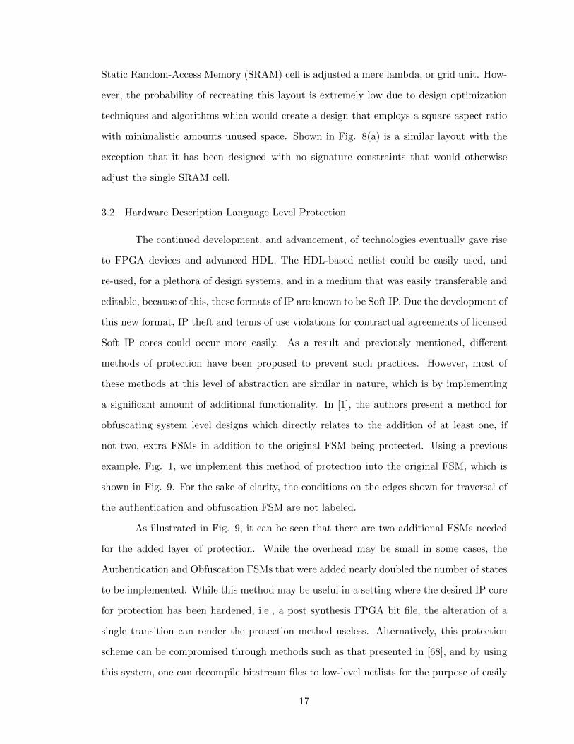
a significant amount of additional functionality. In [1], the authors present a method for
obfuscating system level designs which directly relates to the addition of at least one, if
not two, extra FSMs in addition to the original FSM being protected. Using a previous
example, Fig. 1, we implement this method of protection into the original FSM, which is
shown in Fig. 9. For the sake of clarity, the conditions on the edges shown for traversal of
the authentication and obfuscation FSM are not labeled.
As illustrated in Fig. 9, it can be seen that there are two additional FSMs needed
for the added layer of protection. While the overhead may be small in some cases, the
Authentication and Obfuscation FSMs that were added nearly doubled the number of states
to be implemented. While this method may be useful in a setting where the desired IP core
for protection has been hardened, i.e., a post synthesis FPGA bit file, the alteration of a
single transition can render the protection method useless. Alternatively, this protection
scheme can be compromised through methods such as that presented in [68], and by using
this system, one can decompile bitstream files to low-level netlists for the purpose of easily
17

01 / - 10 / 1 01 / 1
11 / 0 00 / 1 11 / 1
st0 st1 st2 st3
0- / 1 1- / 1
0- / 111 / 0-0 / 0
stA0 stA2stO2 stO1 stO0
Authentication FSM (b)
Obfuscation FSM (a)
Original (Lion) FSM (c)
stA4stA5
stA3
Figure 9: Lion FSM watermarked by HARPOON method [1]
removing and altering such security schemes. However, even though the system presented in
[68] may, or may not, be publicly available, other organizations such as [69] are beginning to
hold competitive challenges to reverse engineer the bitstream format. It should be known,
however, that for significantly complex systems, which utilize the greater portion of design
space, will further help prevent the removal of this protection scheme. For relating this type
of tampering of the protection scheme we use the idiom of “finding a needle in a hay stack,”
such that, in a significantly complex system the odds of finding a single transition in the
design are significantly low, which further helps to prevent the removal of this protection
scheme.
3.3 Circuit and Model Level Protection
Circuit level protection is employed through the utilization of the inherent char-
acteristics of a system and the behavior it experiences under given operating conditions.
This is commonly referred to as “Glitch Logic,” presented in [54], and is geared towards
exploiting inherent delay characteristics of logic circuits that would otherwise cause a glitch
in the system. Implementation of this method utilizes designs, and practices, that would
18

otherwise be considered poor due to the likelihood that a logic implementation will pro-
duce faulty, or glitched, output. Utilizing this system allows for signature logic behavior
to be produced by an otherwise hidden channel that can be activated under a given set of
operating conditions. These operating conditions are constrained by the system but can
typically be activated by simply increasing the clock speed to a set frequency outside the
operating frequency range of the design. The potential drawback of this system is that a
design house is burdened with a daunting task of intentionally implementing, what is seen
as poor design, logical hazards into the system while ensuring proper functionality under
normal operating conditions.
Model Level protection is similar to the practices detailed by the HARPOON [1]
system previously discussed in Section 3.2, and illustrated by Fig. 9. The overall goal
of this level of protection is to provide a method that can be utilized at the highest level
of abstraction, while offering protection to the IP core through all steps of any further
implementation or fabrication processes. With respect to sequential circuits, the current
methods of IP protection are detailed in Section 3.4, and are the state, edge, and I/O based
schemes of protection.
3.4 Sequential Circuit Watermarking Techniques
Several watermarking techniques for sequential systems are currently available to
IP core owners. These available watermarking techniques include state based, edge based,
and I/O based protection schemes. The remainder of this section will discuss and analyze
each of these watermarking techniques.
3.4.1 State Based Watermarking
This method of watermarking sequential systems pertains to the direct addition of
states into a sequential system. Besides watermarking states, additional states, which act as
a key-based system, are inserted to provide security between the watermark and the original
FSM. We apply this technique to the FSM shown in Fig. 1 and show the resulting FSM in
Fig. 10. We note that the labeling of edges in the watermark key FSM are intentionally
left out for the sake of clarity, such that, the key values for entering the watermark are
19

arbitrary for the purpose of the illustration of intended functionality. The watermarking
method illustrated by Fig. 10 was first introduced by Oliveira in [8]. While this method
offers an additional layer of protection, the incurred overhead of this method can escalate
rather quickly based on the complexity of the original system with respect to the key and
watermark FSMs. However, this can prove to be useful in a significantly large system.
On the other hand, when this is applied at the beginning of the modeling level before any
form of implementation, synthesis, or fabrication, this method has the potential to be easily
defeated by tampering in a design house setting.
01 / - 10 / 1 01 / 1
11 / 0 00 / 1 11 / 1
st0 st1 st2 st3
0- / 1 1- / 1
0- / 111 / 0-0 / 0
Original (Lion) FSM
01 / - 10 / 0 01 / 0
11 / 1 00 / 0 11 / 0
st0 st1 st2 st3
0- / 1 1- / 1
0- / 111 / 0-0 / 1
Watermark FSM
st0st1st2
Watermark Key FSM
Figure 10: Lion FSM utilizing state based watermarking
3.4.2 Edge Based Watermarking
Another technique for the watermarking of sequential systems is through the use of
an edge based watermarking scheme. This scheme, presented by Abdel-Hamid et al. [50],
breaks the desired signature into a bit length that matches the output length of the FSM
intended for watermarking. These output blocks are randomly paired with an input com-
20

bination that whose length matches the length of input bits used in the system. Through
the process of random start state selection, this technique evaluates its ability to add a sig-
nature edge to the selected state. This evaluation is the process of checking the randomly
generated input for the signature block against those specified by the selected state. If the
signature edge is not being utilized, this edge is simply added. Similarly, if the signature
and non-signature edge outputs match, the system utilizes the existing non-signature edge
as the signature edge. This is done to reduce the number of edges created by utilizing
inherent system functionality to reproduce the desired signature. However, if the required
signature edge is being utilized as a non-signature edge and these two edges do not contain
equivalent outputs, this method will add an input bit to the system. Upon adding the input
bit, the original non-signature transitions are extended, at the Least Significant Bit (LSB)
in a Big Endian manner, with zero and the signature edges are extended with one. However,
we note that while this work explains the manner in which this technique should operate,
it has been published various times [50–52] and each time utilizes the same example, while
each illustration used reports conflicting data in the watermarking process. This inconsis-
tency pertains to original edge I/O combinations changing throughout the example, i.e.,
I/O values of single non-signature edge were observed changing as many as three times in
a four step example.
Figure 11 illustrates an example of this protection method extended to the Lion
FSM, from Fig. 1. We note that this example has been constructed from the interpretation
of the watermark insertion algorithm presented in [51]. The desired signature “110” was
blocked appropriately to match the length of the system output and paired with random
input combinations that match the length of the initial system. In this example specifi-
cally the signature was blocked and mapped to “[00/1],[10/1],[01/0],” where the format is
“[input/signature].” For the purpose of this example, we start the technique at the starting
state and simply work our way to the end. We note that the thicker lines shown in Fig. 11
denote signature edges that were mapped within the system, in addition, edges that were
dashed indicate that they were added by the system. Shown by the watermarked FSM in
Fig. 11, it can be seen that because the watermark edge input was not being utilized, this
signature edge was simply added and the watermarking state now becomes “st1.” At “st1”
21

01 / - 10 / 1 01 / 1
11 / 0 00 / 1 11 / 1
st0 st1 st2 st3
00 / 1 10 / 1
00 / 111 / 0
Original FSM
Watermarked FSM
Watermark Sequence (Blocked) [00/1][10/1][01/0]
01 / -
10 / 1
010 / 1
11 / 0 00 / 1 11 / 1
st0 st1 st2 st3
00 / 1 10 / 1
00 / 111 / 0
00 / 1 011 / 0
Figure 11: FSM utilizing edge based watermarking
the next edge to be added in the sequence is already utilized, in addition, the signature
edge output matches that of the utilized edge and no edges need to be added, allowing us to
move to “st2.” At “st2” the signature edge and utilized edge output values do not match,
and from our interpretation, this is where the LSB of the input string is extended. The ex-
tensions that are applied to the signature edge and utilized edge are logical one and logical
zero, respectively. While unclear, this method is a low cost alternative to the previous state
based watermarking technique from Section 3.4.1.
However, because this watermarking technique directly outputs part of the signature
and alters the output of the system this allows for signature edges and utilized edges to be
differentiated between. With this in mind, once all of the signature edges have been data
mined and extracted this method is rendered useless. This is because now that an attacker
has partial blocks of the signature, regardless of what the signature may be, there is no
way to prove ownership when both parties claiming ownership know all of the additional
functionality. This is based on the fact that once all functionality has been discovered
then any desired signature can be created from the known functionality hidden or not.
However, if all edges can be completely embedded, i.e., a 100% match and no created edges,
22

then no two sequences are indistinguishable when used as signatures. This holds because
there is no secret functionality that would otherwise allow for two signatures to become
distinguishable from each other, thus this system requires at least one edge to be added.
From this however, additional functionality can be data-mined and easily removed, thus,
destroying the signature. Even if signature edges are utilized by non-signature edges along
with created edges, if the additionally created edges are removed then there is no way to
distinguish from signature and system functionality.
3.4.3 Input Output Based Watermarking
The last watermarking technique is that presented in [48], which utilizes I/O se-
quences native to the original FSM. This technique operates in a manner that utilizes
augmenting paths of state transitions to construct a resulting I/O signature, such that, a
given input sequence creates an I/O signature from the outputs of the edges traversed. How-
ever, this technique achieves this through a passive and active watermarking scheme, each
of which are applied to ICSFSMs and CSFSMs respectively. Signatures for this method are
based on binary sequences that are generated from the outputs of specific unbound input
combinations. A sample signature FSM was constructed using the signature “110,” and is
shown in Fig. 12.
wm0 wm1 wm2 wm3
-- / 1 -- / 1 -- / 0
Figure 12: Sample I/O signature
Utilizing such a signature the system algorithmically employs both a passive and
active watermarking method. The passive watermarking algorithm is based on utilization of
unbound input specifications within the original ICSFSM. These unbound edges are used in
an augmenting path algorithm which constructs the input specifications which are bound to
the I/O signature. In the event that the original FSM is a CSFSM and the passive scheme
23
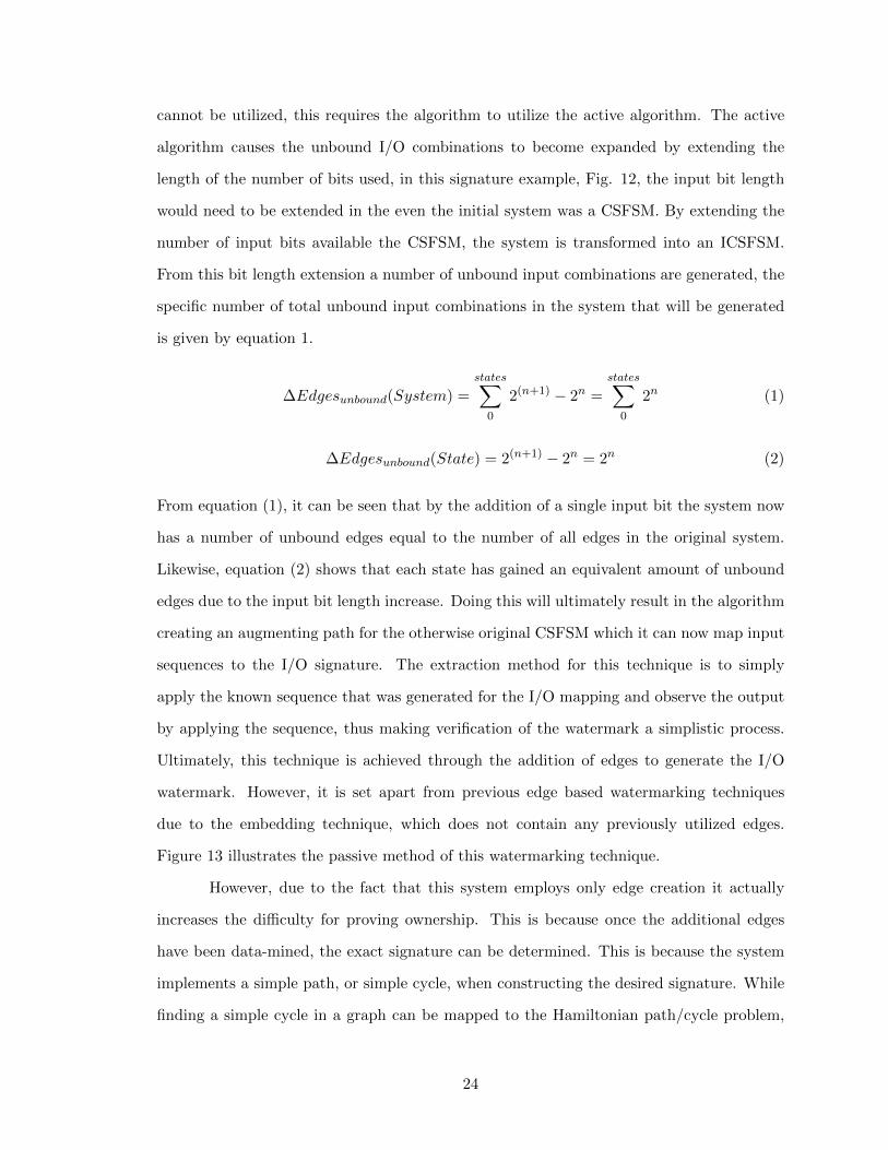
cannot be utilized, this requires the algorithm to utilize the active algorithm. The active
algorithm causes the unbound I/O combinations to become expanded by extending the
length of the number of bits used, in this signature example, Fig. 12, the input bit length
would need to be extended in the even the initial system was a CSFSM. By extending the
number of input bits available the CSFSM, the system is transformed into an ICSFSM.
From this bit length extension a number of unbound input combinations are generated, the
specific number of total unbound input combinations in the system that will be generated
is given by equation 1.
∆Edgesunbound(System) =
states∑0
2(n+1) − 2n =
states∑0
2n (1)
∆Edgesunbound(State) = 2(n+1) − 2n = 2n (2)
From equation (1), it can be seen that by the addition of a single input bit the system now
has a number of unbound edges equal to the number of all edges in the original system.
Likewise, equation (2) shows that each state has gained an equivalent amount of unbound
edges due to the input bit length increase. Doing this will ultimately result in the algorithm
creating an augmenting path for the otherwise original CSFSM which it can now map input
sequences to the I/O signature. The extraction method for this technique is to simply
apply the known sequence that was generated for the I/O mapping and observe the output
by applying the sequence, thus making verification of the watermark a simplistic process.
Ultimately, this technique is achieved through the addition of edges to generate the I/O
watermark. However, it is set apart from previous edge based watermarking techniques
due to the embedding technique, which does not contain any previously utilized edges.
Figure 13 illustrates the passive method of this watermarking technique.
However, due to the fact that this system employs only edge creation it actually
increases the difficulty for proving ownership. This is because once the additional edges
have been data-mined, the exact signature can be determined. This is because the system
implements a simple path, or simple cycle, when constructing the desired signature. While
finding a simple cycle in a graph can be mapped to the Hamiltonian path/cycle problem,
24

01 / - 10 / 1 01 / 1
11 / 0 00 / 1 11 / 1
st0 st1 st2 st3
00 / 1 10 / 1
00 / 111 / 0
Original FSM
Watermarked FSM
Watermark I/O Sequence [00/1][11/1][01/0]
01 / - 10 / 1 010 / 1
11 / 0 00 / 1 11 / 1
st0 st1 st2 st3
00 / 1 10 / 1
00 / 111 / 0
00 / 1 011 / 011 / 1
wm0 wm1 wm2 wm3
-- / 1 -- / 1 -- / 0Signature
Figure 13: FSM utilizing passive I/O based watermarking
which is known to be Non-deterministic Polynomial Complete (NP-Complete), because the
augmenting path utilizes a single state once then the watermark is easily data-mined by
finding the set of all edges not contained within the original system. From this, all possible
sequences of a given length can be computed starting from any state. This allows desired
signatures, different from the original watermark signature, to potentially be constructed.
Due to this fact, two separate parties can now claim ownership with no way to distinguish
between the “Knight Owner” and the “Knave Owner,” or simply no way to distinguish
between who is falsely claiming ownership and the real owner.
3.5 Motivation for This Work
We begin by recapping the protection methods covered in this chapter and discuss
the advantages and disadvantages of each scheme (see Table 3). It can be seen that the
majority of the protection based schemes either fall into the two categories, difficult and/or
25
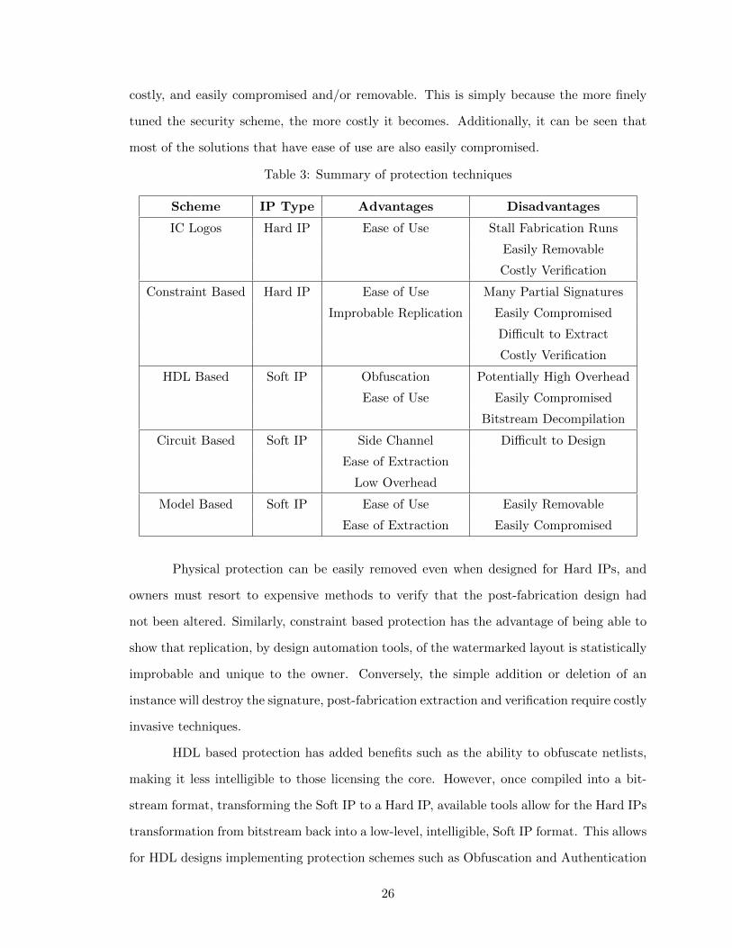
costly, and easily compromised and/or removable. This is simply because the more finely
tuned the security scheme, the more costly it becomes. Additionally, it can be seen that
most of the solutions that have ease of use are also easily compromised.
Table 3: Summary of protection techniques
Scheme IP Type Advantages Disadvantages
IC Logos Hard IP Ease of Use Stall Fabrication Runs
Easily Removable
Costly Verification
Constraint Based Hard IP Ease of Use Many Partial Signatures
Improbable Replication Easily Compromised
Difficult to Extract
Costly Verification
HDL Based Soft IP Obfuscation Potentially High Overhead
Ease of Use Easily Compromised
Bitstream Decompilation
Circuit Based Soft IP Side Channel Difficult to Design
Ease of Extraction
Low Overhead
Model Based Soft IP Ease of Use Easily Removable
Ease of Extraction Easily Compromised
Physical protection can be easily removed even when designed for Hard IPs, and
owners must resort to expensive methods to verify that the post-fabrication design had
not been altered. Similarly, constraint based protection has the advantage of being able to
show that replication, by design automation tools, of the watermarked layout is statistically
improbable and unique to the owner. Conversely, the simple addition or deletion of an
instance will destroy the signature, post-fabrication extraction and verification require costly
invasive techniques.
HDL based protection has added benefits such as the ability to obfuscate netlists,
making it less intelligible to those licensing the core. However, once compiled into a bit-
stream format, transforming the Soft IP to a Hard IP, available tools allow for the Hard IPs
transformation from bitstream back into a low-level, intelligible, Soft IP format. This allows
for HDL designs implementing protection schemes such as Obfuscation and Authentication
26

FSMs to become easily compromised and or removed. Additionally, the use of Obfuscation
and Authentication FSMs schemes have the potential to generate significant increases in
area, based on when the complexity of the protection FSMs is greater when compared to
the original system.
Circuit based protection, has extremely desirable benefits, namely, side-channel
properties and ease of extraction. Additionally, this type of protection scheme only incurs
overhead from the design practices required to implement the glitch logic. In that, altering
the design implementation practices to produce otherwise “meta-stable,” frequency range
based functionality, designs can either increase or decrease the overhead. However, while
this type of protection offers many ideal benefits, the main drawback is burdening designers
with the daunting task of designing such “meta-stable” circuitry.
Model Based protection, when simply added rather than embedded, is extremely
vulnerable to malicious parties during hand-offs in the design process, even in an in-house
design setting. This allows for IP cores to become easily compromised by removing the
protection schemes added. However, Model Based protection is among the easiest to im-
plement, similar to IC logos, protection schemes can simply be placed before or after the
original system had been designed. Alternatively, by embedding, or superimposing, water-
marks at the beginning of the design process of models the protection can be increased.
Embedding watermarks, helps deter malicious users due to the complexities involved with
differentiating between system critical components and the superimposed watermark func-
tionality.
Summarizing the watermarking techniques for sequential systems, we examine the
schemes in order as provided in Table 4. Sequential circuit protection schemes can be
generalized as one of two methods, the addition of states and the addition of edges and
input bits. However, the watermark in all cases is directly output by these schemes. This
allows the watermark to be data-mined and easily compromised in a malicious setting.
Such that, once an attacker has data-mined additional functionality implemented for the
watermark, then the secret sequence required to reproduce the IP owners signature is no
longer significant. This is due to the fact that desired signatures can be constructed by
utilizing the data-mined information.
27

Table 4: Summary of sequential protection techniques
Scheme IP Type Advantages Disadvantages
State Based Soft IP Ease of Use Potentially High Overhead
Ease of Extraction Easily Removable
Easily Compromised
Edge Based Soft IP Ease of Use Easily Removable
Lower Overhead Easily Compromised
Ease of Extraction
I/O Based Soft IP Ease of Use Easily Removable
Lower Overhead Easily Compromised
Ease of Extraction
State Based watermarking is the simplest technique among the techniques shown
in Table 4, and due to the manner in which the technique is accomplished the overhead is
likely to significantly increase overall. However, overhead assumptions can be made based
on the complexity of the additional FSMs compared to the complexity of the original system.
Additionally, data-mining the edges involved in the watermark allow this technique to be
compromised. Likewise, because of the addition of separate FSMs, during the design process
the watermark can easily be removed.
Edge Based watermarking, like State Based, can easily become compromised through
the data-mining of additional system functionality. Similarly, this is due to the fact that
the watermark is partially output by the added edges, once a malicious party data-mines
the additional edges then ownership potentially becomes indistinguishable. This is because
utilizing the outputs from the addition edges desired signatures can be constructed.
Lastly, I/O Based watermarking proves insecure as well. This is from the fact that
the watermark is solely based on the creation of additional edges for the desired sequence.
Once again, by data-mining the hidden functionality, the watermark can be obtained, com-
promised, and potentially removed. In this system the watermark can be obtained due to
the fact that the watermark signature is based on creating a simple path or cycle and em-
bedding the edges. Thus, the exact watermark signature can be found by simply traversing
the set of additional edges and observing the output.
28

3.6 Chapter Summary
Summarizing this section there are four types of IP protection commonly used: (1)
physical protection, (2) HDL protection, (3) circuit protection, and (4) model protection.
Physical protection is the use of watermark signatures and/or logos in Hard IP or fabricated
ICs. HDL protection is performed at the Soft IP level, through the alteration of hardware
netlists for obfuscation, watermarking, or authentication purposes. Circuit level protection
is at the gate level, or logic level, of design. It is performed through the use of “Glitch Logic”
where the circuity is designed using practices and constraints other than normal to create
circuits which will produce a desired glitch output at a given operating frequency. Model
level protection is the addition of structures at the highest design level and is illustrated by
the techniques presented in this work.
Additionally, there are three types of sequential watermarking techniques commonly
used: (1) state based, (2) I/O based, and (3) edge based. State based watermarking is the
process of implementing additional states in an FSM which can be used as keys and/or
entirely separate functional FSMs. Edge based watermarked is the process of embedding a
signature through the use overlapping and created edges which can be used to output part
of the signature. I/O based watermarking is the process of embedding a watermark FSM
through binding unbound input sequences of an original FSM state to a watermark FSM
state. This generates transitions based on unused input sequences to output part of the
signature.
29

4 State Encoding Based Watermarking
In this chapter, we present in detail the proposed watermarking technique that uti-
lizes the FMS’s state encoding for the purpose of permanently embedding a digital signature
into the FSM. This chapter is organized as follows. In Section 4.2 we present the concept
of watermarking via state encoding. In Section 4.4 we present an overview of the proposed
watermarking system. Section 4.3 presents experimental costs associated with proposed
edge creating techniques. In Section 4.5 we briefly detail the process of the watermark
construction phase and present the three proposed methods. In Section 4.5.1 we present
in detail the proposed method for generating watermark FSMs from bitmap signatures,
Section 4.5.2 presents in detail the proposed method for generating watermark FSMs from
file signatures, and in Section 4.5.3 we present in detail the proposed method and custom
tool for generating watermark FSMs from hash signatures. In Section 4.6 we discuss the
watermark embedding phase of the proposed system and the detailed complexities involved
in Section 4.6.1. In Section 4.6.2 we present the proposed brute force solution for wa-
termark embedding and then a greedy heuristic in Section 4.6.3. Section 4.7 details the
model generation and verification phase and presents a set of custom tools created in this
work. In Section 4.8 we detail the proposed methods for extracting the embedded water-
mark sequence. Section 4.9 details the security and computational complexities involved
for multiple forms of attacks against the proposed method.
4.1 Note to Reader
Portions of this chapter have been previously published (Lewandowski et al., 2012)[45]
and are utilized with permission of the publisher.
30

4.2 Watermarking via State Encoding
This method, as previously shown, had not been explored as a watermarking tech-
nique for FSMs. From this knowledge we developed a concept that would seamlessly in-
tegrate a new level protection into FSMs where the end user would only be impacted by
a tolerable cost. By controlling the state encoding values the watermark could be perma-
nently embedded into an FSM and later retrieved when needed. This method currently
employs edge creation methods similar to [48] and [50]. New edges created in this method
are paired with an unused state input combination, and the output is specified as a don’t
care condition. This method also utilizes transitions which are known to already provide
the desired next state transition, as in [52]. An illustrative example is shown in Fig. 14. We
note that in Fig. 14 the original edges are identified by thinner solid lines. Additionally,
the watermark edges and overlay edges are identified by thinner and thicker more closely
grouped dashed lines, respectively.
st0 st1 st2 st3
000 / 11 010 / 01 000 / 11
000 / 10 011 / 00010 / 10
000 / 01001 / -- 001 / --
100 / --
Overlay
OriginalCreated
Figure 14: Watermarking edge creation method an illustrative watermarked FSM
4.3 Edge Creation Cost
In this section we explore the costs associated with additional edges. We analyze
the expected costs of implementing these types of edges by conducting an edge creation
related synthesis experiment for the FSM shown in Fig. 14. Using the Xilinx ISE Synthesis
tool we synthesized the FSM for a varying number of dummy edges (0, 1, 2, 3, and 12) and
the results are summarized in Table 5. For more information on full extent of synthesis
options utilized see Section 5.2.
31

Table 5: Xilinx synthesis results for dummy edges in Fig. 14 FSM
Number of Dummy Edges (0) (1) (2) (3) (12)
States 4
Transitions 11 12 13 14 23
Input Bits 3 4 5 8
Output Bits 4
Encoding Gray
Implementation LUT
Registers Used 2
Look-Up Tables (LUTs) Used 4
Max. Frequency (MHz) 1075.963
For this experiment, we initially synthesized the original FSM in Fig. 14, i.e.,
without any additional dummy edges. These results are reported in column (0) in Table 5.
We then began adding the non-overlay edges from Fig. 14 one-by-one performing synthesis
after each addition. These results are reported in columns (1), (2), and (3) in Table 5. Once
we had synthesized the original FSM, the example watermarked FSM, we then examined
the synthesis results for the scenario where the number of edges added doubled the number
of edges in the original FSM. This synthesis results for this scenario are reported in Table 5
as column (12). From the data presented in Table 5 it can be seen that the Xilinx Synthesis
results, for this example, returned potentially promising implementation cost values.
4.4 Watermarking System: Overview
The watermarking system that was created utilizes a variety of tools for accom-
plishing the task at hand. At the highest level, the system has three major phases, see
Fig. 15, (a) Watermark Construction Phase, (b) Watermark Embedding Phase, and (c)
Model Generation & Verification Phase. The Watermark Construction Phase transforms
the desired signature into a graph. In the Watermark Embedding Phase the signature graph
is embedded into the FSM by overlaying it into nodes and edges of the STG representation
of the FSM. If necessary new edges are created. In the Model Generation and Verification
32

Phase, the modified FSM is converted into a testable HDL model and verified. Below we
provide more details of each phase with illustrative examples.
SignatureWatermarkConstruction
(a) Construction phase
WM GraphWatermarkEmbedding
(b) Embedding phase
WM FSM
Model
Generation
(c) Modeling phase
Figure 15: High level overview of watermarking system flow
4.5 Watermark Construction Phase
The method for constructing the watermark has continuously evolved throughout
the life of this work. We propose three techniques ranging from the utilization of bitmaps
to signature hashing. The proposed watermark construction methods are shown in Figs. 16
(a), (b), and (c). Below we propose each watermark construction method by providing
an algorithm for the technique and possible examples of signatures, decomposition, and
sequences. We also discuss advantages and disadvantages of each method.
Bitmap Decompositon
WM Construction
Signature
(a) BSD method
Signature Decompositon
WM Construction
Signature
(b) FSD method
Hash-2-Kiss2
RIPEMD-160 Hashing
Signature
(c) HSD method
Figure 16: Methods of watermark construction
4.5.1 Bitmap Signature Decomposition
BSD is the first form of watermark construction implemented in this work. BSD was
employed for the ease in constructing and verifying a proof of concept model. To illustrate
this, Fig. 17 provides a sample bitmap signature that was used in the BSD method. From
this, using the BSD method, the bitmap signature would be decomposed into a raw binary
33

format. We note that black squares in the bitmap are represented by logical ones, while
white squares are represented by logical zeros. From this simplistic binary encoding scheme
there exist a plethora of viable methods for the bitmap decomposition. Arbitrarily, we
chose the simplest method for decomposing the signature, which was a row-concatenate
based implementation. This algorithm operates by traversing the bitmap in a raster scan
fashion to yield a single binary sequence. The concatenated string is split into chunks equal
to the length of the state encoding of the FSM. If the last chunk is not appropriately sized
the remaining bits are LSB sign extended with logical zeroes until the appropriate chunk
size has been met. LSB sign extension is used as to not compromise the signature, i.e.,
while “10” and “100” are not binary equivalent, when the signature is constructed it will
simply have an extra “0” at the end of the reconstructed signature. For example, if the
signature sequence is “11110,” with a block size of three, inserting a leading zero would now
compromise the signature and generate “111|0|10” instead of the original desired signature
“11110|0|.” The worst case run-time for composing the single concatenated signature string
is O(n×m), where n is the standardized length of each row, and m is the number of rows
used total. However, because the sequence is concatenated into a single string, the worst
case run-time of chunk creation is O(x), where x is the length of the concatenated string.
This is because all of the operations for constructing the blocks are based off of constant, or
other linear time growth, operations in the code. Which overall, causes this method to entail
a worst case run-time of O(n×m), which is the time for computing single concatenated bit
string. From this, the method would prove to be rather simplistic and ideal complexity and
run-time for decomposing signatures. Unfortunately, the main drawback of this method
is the lack of signature flexibility. In addition, this method would only work under the
condition that bitmap image signatures were not artistically intricate in their design.
Figure 17: Sample bitmap signature
34

4.5.2 File Signature Decomposition
FSD operates in the same manner as BSD and the only difference is that this concept
has been extended to digital files. By transforming a file into a machine level representation
we are able to construct the raw binary representation of the signature. This enables us to
utilize any format, ranging from text files to audio clips, as a watermark signature. However
this can become a very lengthy and time consuming process due to the massive amount of
raw data. We illustrate this by presenting a small fraction of the amount of data in a sample
file in Table 6.
Table 6: Sample file under FSD
Simple VHDL File
File Size: 9.98 KB (10,222 bytes)
Row Address Column Address
0 1 · · · E F
00000000 00101101 00101101 · · · 00101101 00101101
00000010 00101101 00101101 · · · 00101101 00101101
00000020 00101101 00101101 · · · 00101101 00101101
00000030 00101101 00101101 · · · 00101101 00101101
00000040 00101101 00101101 · · · 00101101 00101101
For the sake of clarity, we note that we did not include the entirety of the files
contents, and that all of the presented row & column binary bit sets only represent about
half of a single line of text in the original file, it is also noted that for brevity we did not
include the entire column range. However, this file contains roughly 640 more row addresses
similar to those shown in Table 6. From this, it can be seen that the amount of data to
be processed, bit by bit, grows rather rapidly for what modern computer users would see
as an insignificantly sized file. Nonetheless FSD, similarly to its BSD predecessor, also
needed to employ the use of sign extension when the data at a given row address ended
before column F , or when the block size specified would create inappropriately sized chunks.
The solution for this sign extension process was performed in the same manner of BSD,
with the exception that, columns were filled with “00000000” until the appropriate size was
reached. This appropriate size for sign extension was determined simply by the number of
35

bits required to size the last chunk in the system based on the provided block size. This
process of extension, and its resulting behavior, is acceptable due to the fact that writing
zeroes to the end of the file will not actually alter or compromise a signature in most cases,
but instead, it will only slightly increase the size of the signature, further making. Whether
or not the extension of zeroes visually alters a file, in the typographical sense, depends on
whether or not a utilized text editor will show characters representing this extension. For
example, a popular open source tool Notepad++ [70] will display “NUL” characters which
represents this extension of zeroes. While the standard Windows Notepad will keep this as a
seemingly invisible alteration. From this the chunks would be computed as they were in BSD
by using the predetermined block size. Similarly the worst case run-time calculations are
also the same. However, due to file size complexities, constructed watermarks were almost
always large completely specified state machines. This left little flexibility in embedding
and resulted in high overhead. This is further illustrated by an example of FSD in Fig. 18.
It can be seen that a relatively small file, Fig. 18(a), under FSD can generate a completely
connected signature, Fig. 18(b), which can become extremely costly to implement as a
signature.
(a) Signature used in FSD (b) Corresponding STG
Figure 18: Example of FSD
36

4.5.3 Hashing Signature Decomposition
From the ideal conditions of the BSD method, and rather poor outcomes illustrated
by FSD, alternative solutions for signature decomposition were needed. Through this search
gave rise to the current decomposition method, which is known as HSD. This method
employs the external use of a secure hashing function to uniquely hash the signature intended
to be used in watermarking. We chose to utilize the secure hashing function RACE Integrity
Primitives Evaluation Message Digest 160-bit (RIPEMD-160) [71] because it is a hashing
algorithm that returns a shorter 40 character hash sequence and has been shown to be
collision free [72]. The signature chosen for illustration of this method was the Portable
Network Graphic (PNG) file shown in Fig. 19. Using the OpenSSL tool [73] and RIPEMD-
160 hash to digest this signature, the corresponding hash value was returned:
“RIPEMD160(COE-h-black.png)= 91efebee4bd48a62f338f244560b668771fa338e”
This hash, in bold, would then be transformed from its present hexadecimal format into a
decimal representation that could be further utilized in an STG format. To perform this
process we created the Hash-2-K2 program, which will automatically manipulate the hash
sequence and generate a resulting watermark STG in Kiss2 format. The benefits of this
method are that any hashing function can be used in the HSD method, while OpenSSL
offers a variety of hashing solutions, one can still obtain even greater flexibility by utilizing
a hash of choice. However, the run-time of the HSD method is solely dependent of the
hashing algorithm chosen for use, while the transformation of the hash and watermark
construction run-times are covered in Section 4.5.4, as these manipulations are performed
by the Hash-2-K2 tool.
Figure 19: Sample HSD signature prior to hashing
37
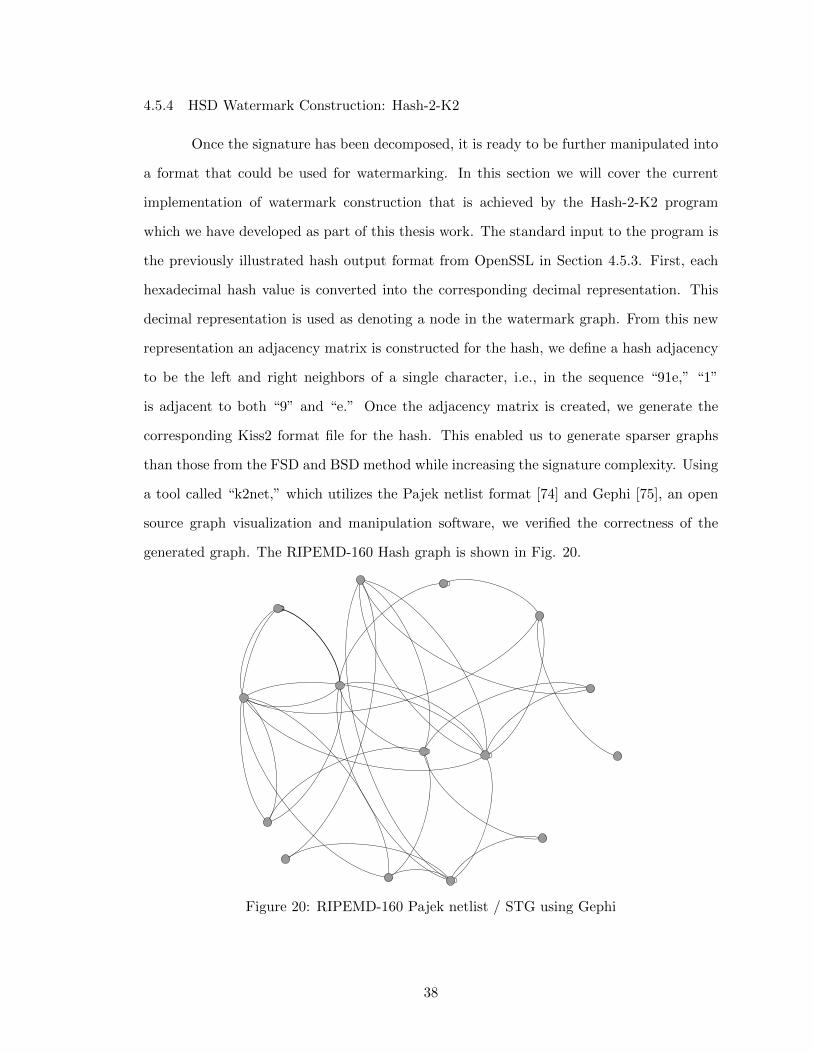
4.5.4 HSD Watermark Construction: Hash-2-K2
Once the signature has been decomposed, it is ready to be further manipulated into
a format that could be used for watermarking. In this section we will cover the current
implementation of watermark construction that is achieved by the Hash-2-K2 program
which we have developed as part of this thesis work. The standard input to the program is
the previously illustrated hash output format from OpenSSL in Section 4.5.3. First, each
hexadecimal hash value is converted into the corresponding decimal representation. This
decimal representation is used as denoting a node in the watermark graph. From this new
representation an adjacency matrix is constructed for the hash, we define a hash adjacency
to be the left and right neighbors of a single character, i.e., in the sequence “91e,” “1”
is adjacent to both “9” and “e.” Once the adjacency matrix is created, we generate the
corresponding Kiss2 format file for the hash. This enabled us to generate sparser graphs
than those from the FSD and BSD method while increasing the signature complexity. Using
a tool called “k2net,” which utilizes the Pajek netlist format [74] and Gephi [75], an open
source graph visualization and manipulation software, we verified the correctness of the
generated graph. The RIPEMD-160 Hash graph is shown in Fig. 20.
Figure 20: RIPEMD-160 Pajek netlist / STG using Gephi
38
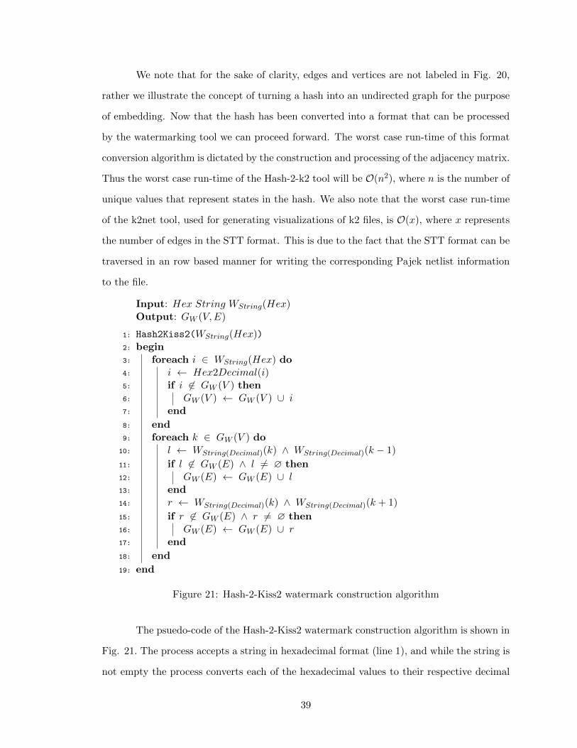
We note that for the sake of clarity, edges and vertices are not labeled in Fig. 20,
rather we illustrate the concept of turning a hash into an undirected graph for the purpose
of embedding. Now that the hash has been converted into a format that can be processed
by the watermarking tool we can proceed forward. The worst case run-time of this format
conversion algorithm is dictated by the construction and processing of the adjacency matrix.
Thus the worst case run-time of the Hash-2-k2 tool will be O(n2), where n is the number of
unique values that represent states in the hash. We also note that the worst case run-time
of the k2net tool, used for generating visualizations of k2 files, is O(x), where x represents
the number of edges in the STT format. This is due to the fact that the STT format can be
traversed in an row based manner for writing the corresponding Pajek netlist information
to the file.
Input: Hex String WString(Hex)Output: GW (V,E)
1: Hash2Kiss2(WString(Hex))2: begin3: foreach i ∈ WString(Hex) do4: i ← Hex2Decimal(i)5: if i 6∈ GW (V ) then6: GW (V ) ← GW (V ) ∪ i7: end
8: end9: foreach k ∈ GW (V ) do
10: l ← WString(Decimal)(k) ∧ WString(Decimal)(k − 1)
11: if l 6∈ GW (E) ∧ l 6= ∅ then12: GW (E) ← GW (E) ∪ l13: end14: r ← WString(Decimal)(k) ∧ WString(Decimal)(k + 1)
15: if r 6∈ GW (E) ∧ r 6= ∅ then16: GW (E) ← GW (E) ∪ r17: end
18: end
19: end
Figure 21: Hash-2-Kiss2 watermark construction algorithm
The psuedo-code of the Hash-2-Kiss2 watermark construction algorithm is shown in
Fig. 21. The process accepts a string in hexadecimal format (line 1), and while the string is
not empty the process converts each of the hexadecimal values to their respective decimal
39

value, i.e., “A” maps to “st10” (line 4). Additionally, the algorithm will only add unique
states to the graph, such that, if the hexadecimal character “A” happens to appear more
than once, then it is only added to GW (V ) once (line 5 & 6). Similarly, if there exists an
edge which connects two known states in the string and is not already an element in GW (E)
this edge is added (line 8 & 9). This prevents redundant edges from being added to the
watermark FSM and creating addition overhead in the embedding process, for example if
the sequence is “9AABC10AA,” the sequence “AA” appears twice but is only added the
first time it is found in the sequence.
4.6 Watermark Embedding Phase
The Watermark Embedding Phase is the second phase where in the original STG is
watermarked with the undirected graph of the hash signature. In this section, we cover the
complexity of the problem and proposed algorithms.
4.6.1 Embedding: Complexity
The task of embedding one graph into another is directly related to the sub-graph
isomorphism/matching problem. This sub-graph matching problem is to determine if there
exists a possible configuration of a graph, GraphA, which is contained, or can be mapped,
as a subset in another graph, GraphB. In relating this to our problem, we are seeking
a low cost configuration represented by GW (V,E) ⊂ GFSM (V,E), where GW (V,E) and
GFSM (V,E) are, respectively, the watermark and original FSM graphs. However, if an
inherent sub-graph has been found in an unaltered FSM then the watermark is lost to
the normal functionality of the machine, and an alternative signature must be sought for
use. Alternatively, if GW (V,E) 6⊂ GFSM (V,E), then an inherent isomorphic sub-graph
has not been found, and in our case the appropriate actions must be taken. However,
from this generalized overview the complexity can be derived through its matching relation
to the clique problem, where the goal is to find complete sets in which each element is
connected [76]. This is ultimately done by finding a clique of nodes in GFSM (V,E) that can
be identically, or by low cost means in our case, mapped to GW (V,E). The clique problem
40

known to be NP-Complete [77]. Thus, there is potentially no efficient solution for tackling
this problem in a reasonable amount of time.
4.6.2 Brute Force Embedding Algorithm
Determining the number of mapping combinations is specifically dependent on both
the watermark and original FSM graphs. However such a method for generating all mapping
combinations is considered to be an r-Permutation, and can be computed from equation 3,
and is specifically for situations where n choices can be mapped to r positions [78]. In our
case, we consider the number of states in the original FSM to be n choices which can be
mapped to one of r positions in the watermark, where r is the number of states in the
watermark graph.
P (n, r) =n!
(n− r)!(3)
Thus, the first, proof of concept, algorithm exhaustively checks r-Permutations by Brute
Force, and is suitable for small state machines. The algorithm employs a recursive paradigm
to generate all possible state matching combinations. Through the use of a cost calculation
function the algorithm selects the lowest cost mapping for the watermark graph to the
original FSM.
This brute force algorithm, shown by the pseudo-code in Fig. 22, accepts both
the original FSM, GFSM (V,E), and watermark graph, GW (V,E), additionally, the algo-
rithm also accepts an initial match set. The match set contains a unique permutation of
mappings, or ordered pairs, from states in the original FSM and corresponding watermark
FSM states, or GW (V )→ GFSM (V ′) ⊂ GFSM (V ), and is initially empty until the algo-
rithm first inserts a mapping (line 8). Initially, the best cost is set to the size of the edge
set, or number of edges, in the watermark graph (line 3). For each state in the original
FSM (line 4) and each state of the watermark FSM (line 5), the algorithm will add a
mapping of an original FSM state to a watermark FSM state (line 6). Once adding this
mapping, the algorithm then checks whether or not the removal of the previously mapped
watermark FSM state will cause the set of all watermark FSM states to become empty
(line 7). If this set is not empty then the algorithm will recursively call itself providing
41

Input: GFSM (V,E), GW (V,E),MatchSetOutput: Mapping of Gw(V ) to GFSM (V ′) ⊂ GFSM (V )
1: EmbedBruteForce(GFSM (V,E), GW (V,E),MatchSet)2: begin3: BestCost ← GW (E).size4: foreach k ∈ GFSM (V ) do5: foreach m ∈ GW (V ) do6: MatchSet ← MatchSet ∪ {(k,m)}7: if GW (V )− {m} 6= ∅ then8: EmbedBruteForce(GFSM (V )− {k}, GW (V )− {m},MatchSet)9: else
10: if Cost(MatchSet) < BestCost then11: BestMatch ← MatchSet12: BestCost ← Cost(MatchSet)
13: end
14: end
15: end
16: end
17: end
Figure 22: Proposed brute force watermark embedding algorithm
the current set of matches with the removal of the current original FSM state, k, and the
current watermark FSM state, m, (line 8). However, if this removal causes the set to be-
come empty, such that all watermark FSM states have been mapped, then the algorithm
will calculate the cost of the current match comparing it to the cost of the known best
cost (line 10). Figure 23 shows the pseudo-code for calculating the cost of the mapping
(line 9) in the brute force algorithm, Fig. 22. We note that M(k,m) is the relative differ-
ence between the set of edges for the mapped graph nodes GFSM (k) and GW (m), formally,
M(k,m) = {x ∈ U | x /∈ GFSM (k) ∧ x ∈ GW (m)}, where U is the set of all edges [78].
If the returned calculated cost, of the current match set, is lower than the currently known
best cost, the best match and best cost are updated.
To further illustrate the brute force embedding algorithm, we offer an example of the
algorithm embedding the watermark FSM, shown in Fig. 24(b), into the original FSM shown
in Fig. 24(a). For the sake of clarity we do not label transitions, additionally, alphabetic
state encoding values and numerical state encoding values are respectively assigned to the
original and watermark FSM. The set of mapping combinations, or simply all permutations
42

Input: MatchSetOutput: CostofMatchSetMapping
1: Cost(MatchSet)2: begin3: MapCost ← 04: foreach (k,m) ∈ MatchSet do5: M(k,m) ← {GW (m) − GFSM (k)}6: MapCost ← MapCost + M(k,m).size
7: end8: return MapCost
9: end
Figure 23: Brute force cost calculation algorithm
of the match set values, generated by the brute force algorithm is provided by Table 7. By
equation 3, for this example, the expected number of mapping combinations is 24, which is
additionally verified by Table 7.
A B
C D
(a) Original FSM
1 2
3
(b) Watermark FSM
Figure 24: Original and watermark FSMs for brute force embedding example
Each of the match sets, shown in Table 7, has its associated mapping cost calculated
and compared against the known best. These corresponding mapping costs, calculated by
the algorithm in Fig. 23, will be compared in order throughout the algorithm. Shown in
Table 8 are the map costs and actions taken by the algorithm for the corresponding range
sets in Table 7.
43

Table 7: Brute force mapping combinations
Combinatorial Ranges
[1-6] [7-12] [13-18] [19-24]
Match Sets (A,B,C) (B,A,C) (C,A,B) (D,A,B)
GFSM (A,B,C,D)→ GW (1, 2, 3) (A,B,D) (B,A,D) (C,A,D) (D,A,C)
(A,C,B) (B,C,A) (C,B,A) (D,B,A)
(A,C,D) (B,C,D) (C,B,D) (D,B,C)
(A,D,B) (B,D,A) (C,D,A) (D,C,A)
(A,D,C) (B,D,C) (C,D,B) (D,C,B)
Table 8: Brute force cost mapping combinations
Combinatorial Ranges
Cost[0] = 4 [1-6] Action [7-12] Action [13-18] Action [19-24] Action
Cost 1 Update 1 N/A 1 N/A 3 N/A
2 N/A 1 N/A 2 N/A 2 N/A
2 N/A 2 N/A 1 N/A 2 N/A
3 N/A 1 N/A 2 N/A 1 N/A
3 N/A 2 N/A 1 N/A 2 N/A
3 N/A 2 N/A 0 Update 2 N/A
Upon completion of the algorithm the map set with the lowest cost, in this example
(C,D,B) with a cost of 0, is returned. From this match set, returned by the brute force
embedding algorithm, the resulting watermarked FSM is then generated. Additionally, the
resulting watermarked FSM for this example, generated from the original and watermark
FSMs, Fig. 25(a) and Fig. 25(b), is shown by Fig. 25(c).
Run-time analysis of this algorithm shows that k! iterations will recursively call the
function EmbedBruteForce() a total of m! times during which the algorithm will construct
all combinations of possible match sets. Due to this recursive nature of the algorithm worst
case run-time complexity can be observed as O(nPm), where k and m are the number of
original states and watermarking states respectively. Alternatively, this worst case run-time
is also given by equation 3.
The drawbacks of the brute force algorithm are: (1) excessive run-time, and (2) lack
of scalability. Based on worst case run-time calculations it is apparent that this system
44

A B
C D
(a) Original FSM
1 2
3
(b) Watermark FSM
A 3(B)
1(C) 2(D)
(c) Watermarked FSM
Figure 25: Original, watermark, and watermarked FSMs for brute force embedding
will lack desired scalability due to the complexity of generating all possible permutations.
Typically brute force solutions aren’t sought out for this reason. From this, the need
arose for a more efficient algorithm that could be easily scaled for FSMs ranging in size,
with significantly lower run-time, and didn’t require the search space to be exhaustively
explored.
4.6.3 Greedy Embedding Algorithm
While it is generally known that greedy algorithms (with few exceptions, such as
Hu’s scheduling algorithm [79]), are unlikely to produce globally optimal solutions. The
proposed algorithm utilizes a node based complexity cost calculation for both watermarked
and un-watermarked states, which is used in the process of determining potential state
matches. The equations used for calculating the associated cost calculation for a single
state in either of the two machines and the cost associated with mapping a watermark state
to an original FSM state are given by equations 5 and 4 respectively. Alternatively, we note
that equation 4 is simply the degree of a node. Using these equations the algorithm first
calculates the cost of each node in the FSM and in the watermark.
Node Cost = (GFSM , Vχ) = (Vχ)in + (Vχ)out (4)
Map Cost = Node Cost(GFSM (Vχ)) − Node Cost(GW (Vχ′)) (5)
45

Through the use of this newly calculated cost information the algorithm selects and maps
the lowest cost implementation between the current watermark state and best match FSM
state. It repeats this process for each unmatched watermark node by traversing the edges
connected to the initial match while proceeding to search for the next lowest mapping. The
pseudo-code for this algorithm is shown in Fig. 26.
Input: GFSM (V,E), GW (V,E)Output: Mappings of GW (V ) to GFSM (V ′) ⊂ GFSM (V )
1: EmbedGreedy(GFSM (V,E), GW (V,E))2: begin3: n ← FindMaxDegreeNode(GFSM )4: while ∃ x ∈ GW (V ) 3 x.matched == FALSE do5: j ← FindMinCostNode(GW , n)6: MatchSet ← MatchSet ∪ {(n, j)}7: n.matched ← TRUE8: SortDescend(Neighbors(GFSM , n))9: foreach i ∈ Neighbors(GFSM , n) 3 i.matched == FALSE do
10: h ← Route(n, i)11: p ← NeighborsMatchingRoute(GW , h)12: if ∃ x ∈ p 3 x.matched == FALSE then13: k ← FindMinCostNode(i, x)14: else15: continue16: end17: MatchSet ← MatchSet ∪ {(i, k)}18: i.matched ← TRUE
19: end20: Found ← Found ∪ {(n)}21: n ← FindMaxDegreeNode(MatchSet 6∈ Found)
22: end
23: end
Figure 26: Greedy heuristic
The greedy algorithm initially accepts the original and watermark FSMs (line 1).
The algorithm begins by finding the maximum degree node in the original FSM (line 2),
by calling the FindMaxDegreeNode() function that is shown in Fig. 27. The greedy
algorithm is then run until there exists a node in the watermark FSM such that it hasn’t
been matched (line 4). Beginning the loop the algorithm finds the minimum cost node,
in the watermarking FSM, that can be paired with the recently found highest cost node
(line 5) by calling the function FindMinCostNode(). This function is shown by Fig. 28.
46

The match set is then updated (line 6) with the previously returned minimum cost node
from FindMinCostNode() and then (line 7) n is marked as being matched. Following, the
unmatched nodes are sorted in descending order first by calling the Neighbors() function
and passing the returned list to the SortDescend() function (line 8). These two functions
are shown in Fig. 29 and Fig. 30. The algorithm then checks each of the neighbors in
descending order that are still unmatched (line 9). Following this, the direction of the
edge between the unmatched neighbor and the current node determines if it is an incoming
or outgoing edge (line 10). From this direction the algorithm finds additional neighbors
matching this edge route (line 11). If there is a neighbor which matches the edge route and
is still unmatched then algorithm calls the FindMinCostNode() function and maps it to
a node on the connected path (lines 12 & 13). If there are currently no unmatched nodes
then the algorithm continues (line 15). Following this, the match set is updated (line 17),
node status flags are updated (line 18), n is added to the found match for set (line 20) and
then updated to the highest degree node that is unmatched (line 21) and the algorithm
repeats this process.
The FindMaxDegreeNode() function initially accepts a graph (line 1) and iterates
through all of the nodes which the graph contains (line 6). It calculates the degree of the
current node (line 7) and compares it against the known maximum degree (line 8). If
the degree of the node is larger than the current best the algorithm will update the max
degree and match (lines 19 & 20), however, if the degree is equal to the known max then
the algorithm switches to the cases based on the value returned from rand()%2 (line 10),
or a random number modulo 2. If the value returned is 0 then the algorithm takes no
action (line 11), otherwise the algorithm will update the match value (line 15).
The FindMinCostNode() function initially accepts two graphs as the input (line 1),
where the second graph GB is specifically the node and its edges to be mapped in GA. The
initial cost of GB(V ′) is calculated from the nodes degree x (line 6). For each state in GA
the absolute value of the cost between GB(V ′) these two is calculated (line 8), where the
absolute value is used for events where GB(V ′) is larger than GA(V ) and requires the
additions of edges. If this calculated cost is less than or equal to the known minimum
cost (line 9) then the algorithm will check if the two numbers are equal. This portion
47

Input: G(V,E)Output: Maximum Degree Node V ′ ∈ G(V )
1: FindMaxDegreeNode(G(V,E)) begin2: Degree ← 03: MaxDegree ← 04: Match ← ∅5: foreach k ∈ G(V ) do6: Degree ← (k.in + k.out)7: if Degree ≥ MaxDegree then8: if Degree == MaxDegree then9: switch (rand()%2) do
10: case 011: NULL12: end13: case 114: Match ← k15: end
16: endsw
17: else18: MaxDegree ← Degree19: Match ← k
20: end
21: end
22: end23: return Match
24: end
Figure 27: Algorithm for FindMaxDegreeNode function
of the algorithm operates the in the same manner for randomly selecting nodes as the
FindMaxDegreeNode() function.
The Neighbors() function accepts a graph and the node for which the neighborhood
is desired (line 1). The algorithm checks the set of nodes in the graph minus the center of
the neighborhood (line 4). If there is a node in the graph that is also in the sub-graph of
X, i.e., it is connected to X by an incoming or outgoing edge, then this edge is added to
the Neighborhood set (lines 5 & 6). Once the algorithm has examined all nodes not in the
neighborhood, the algorithm returns the set of nodes connected to X (line 9).
The SortDescend() function utilizes the C++ sorting function and employs the use
of a custom compare function for returning if the degree of node k is larger than the degree
48

Input: GA(V,E), GB(V ′, E)Output: Minimum Cost Node GB(V ′) ∈ GA(V )
1: FindMinCostNode(GA(V,E), GB(V ′, E))2: begin3: Cost ← 04: MinCost ← GA(E)5: Match ← ∅6: x ← (GB(V ′).in + GB(V ′).out)7: foreach k ∈ GA(V ) do8: Cost ← |x − (k.in + k.out)|9: if Cost ≤ MinCost then
10: if Cost == MinCost then11: switch (rand()%2) do12: case 013: NULL14: end15: case 116: Match ← k17: end
18: endsw
19: else20: MinCost ← Cost21: Match ← k
22: end
23: end
24: end25: return Match
26: end
Figure 28: Algorithm for FindMinCostNode function
of node j. This process is repeated for the entire match set and upon completion will return
the match set sorted where the node elements are in descending order of their degrees.
We illustrate the proposed greedy approach with an example where the original
and watermark FSMs are shown by Fig. 31(a) and Fig. 31(b). For the sake of clar-
ity, the example will be deterministic in the sense that we will simply choose nodes in a
First Come First Serve (FCFS) manner rather than the random selection employed by the
FindMaxDegreeNode() and FindMinCostNode() functions. The associated node degree
values for both the original and watermark FSMs, GFSM and GW , are given in Table 9.
Additionally, since the the complexities behind this process as significantly less than those
49

Input: G(V,E),Neighbors of Node(X)
Output: Set of G(V ′) ⊂ G(V,E)
1: Neighbors(G(V,E), X)
2: begin3: Neighborhood ← ∅4: foreach k ∈ G(V )−X do5: if k ∈ G(X,EX) then6: Neighborhood ← MatchSet ∪ {k}7: end
8: end9: return Neighborhood
10: end
Figure 29: Algorithm for Neighbors function
Input: MatchSetOutput: Sorted MatchSet
1: SortDescend(MatchSet)2: begin3: Sort(MatchSet.begin(),MatchSet.end(),
compare(k, j){return ((k.in + k.out) > (j.in + j.out)) ? 1 : 0)})4: end
Figure 30: Algorithm for SortDescend function
of the brute force approach, the step-by-step process for which the algorithm computes the
watermarked FSM is given in Table 10.
Table 9: Original and watermark FSM node degree values
GFSM GW
State Degree State Degree
A 3 1 3
B 4 2 3
C 4 3 2
D 3 - -
Upon completion of the algorithm we receive the resulting match set and additional
edges are added for connection of the watermark FSM. This can be seen by Fig. 32(c),
where due to the mappings additional edges are required from 2(C) to 1(B) and 2(C) to
3(A) for the correctness of the watermark. We note that the edges with shorter, higher
50

A B
C D
(a) Original FSM
1 2
3
(b) Watermark FSM
Figure 31: Original and watermark FSMs for greedy embedding example
frequency, dashed lines indicated edges that overlapped in the process while the longer,
lower frequency, dashed lines indicate that an edge was created. From this the cost of
this solution was one edge compared to the previous perfect match from the Brute Force
algorithm.
A B
C D
(a) Original FSM
1 2
3
(b) Watermark FSM
3(A) 1(B)
2(C) 3(D)
(c) Watermarked FSM
Figure 32: Original, watermark, and watermarked FSMs for greedy embedding
While a greedy solution, in addition with the HSD method, may produce more
desirable results there is a need for advanced solutions. This is due to the fact that the
greedy algorithm relies solely on the sparse watermark FSMs generated from the HSD
method. In addition, because the implementation is greedy globally optimal solutions will
51

Table 10: Example step-by-step greedy algorithm
Step Action Note
1 n = B FindMaxDegreeNode() returns GFSM (B)
2 j = 1 FindMinCostNode() returns GW (1)
3 MatchSet ∪ {(B, 1)} MatchSet{(B, 1)}4 i = C C connected, unmatched, highest degree
5 k = 2 FindMinCostNode() returns GW (2)
6 MatchSet ∪ {(C, 2)} MatchSet{(B, 1), (C, 2)}7 i = A A connected, unmatched, highest degree
8 k = 3 FindMinCostNode() returns GW (3)
9 MatchSet ∪ {(A, 3)} MatchSet{(B, 1), (C, 2), (A, 3)}10 Return MatchSet All nodes in GW Matched
not be produced. Further, we analyze the costs of this algorithm with the experimental
results that were gathered, which are further detailed at length in Chapter 5. Provided in
Table 11 are the results produced by this algorithm for the largest ten Kiss2 benchmark
files. The watermark used was that previously shown in Fig. 19 and Fig. 20.
Table 11: Embedding results, watermark (Fig. 19) has 15 states and 32 edges
GFSM States Edges Inputs EdgesAdded EdgesGWInputsAdded
bbara bbtas 30 268 4 20 63% 2
keyb 19 170 7 18 56% 1
kirkman 16 381 12 19 59% 1
s298 218 1096 3 21 66% 2
s820 25 232 18 16 50% 2
s832 25 245 18 16 50% 2
s1488 48 251 8 14 44% 1
s1494 48 250 8 18 56% 1
sand 23 184 11 15 47% 2
tbk 28 1569 6 13 41% 2
As shown in the table, more than half of the machines assumed more than 50% of
the watermark edges on average, and that this method is currently less than desirable due to
the fact that exemplify the algorithms performance. The benchmark “s298,” for example,
52

contains over 1000 edges in the system, however, this current greedy solution still adds 21
of the 32 edges. While it can be argued that 1000 edges over 218 states can easily allow for
this, we turn to another example, the benchmark “tbk” contains 28 states and over 1500
edges. If we were to evenly distribute these edges over 28 states then each state roughly
contains 56 edges, which contains more edges than the entirety of the watermark itself.
However, due to the creation of HSD and Hash-2-Kiss2 this algorithm has greatly reduced
the overhead incurred from methods such as FSD. In addition, this algorithm also allows
for massive scaling compared to previous implementations. However by employing a sorting
method on the Min and Max arrays for determining costs of nodes, which is comparison-
based sorting, the worst case run-times of these algorithms is known to be O(nlogn) [80].
Similarly, due to the nature of the algorithm, which implements Kruskal’s algorithm [81],
a weighted greedy algorithm for finding a minimal spanning tree in the original FSM for
which the watermark can be embedded, this run-time holds. We note that the weights in
this system are associated costs of mapping a watermark state to a state in the original
FSM.
4.7 Model Generation and Verification Phase
Once the watermark has been embedded into the original STG the model generation
phase begins. Using a custom tool we have developed, called “k2vhdl,” STGs corresponding
Very High Speed Integrated Circuit (VHSIC) HDL (VHDL-93) [82] model is automatically
generated. Figure 33 shows the system flow diagram for this tool.
The tool initially accepts a Kiss2 file and the desired Xilinx encoding scheme. The
tool first checks the Kiss2 file for states that have no accepting edges from states connected
to the starting state. This process is performed by calling a vertex cover function from the
starting state of the FSM using an adjacency matrix computed during parsing. To better
illustrate this process Fig. 34 shows the pseudo-code for the V ertexCover() function.
Following this the trimmed FSM is then passed to another custom tool, called “k2net,”
which automatically generates the Pajek netlist for viewing the FSM graph. Finally, the
VHDL file has the Xilinx Synthesis Technology (XST) scripts generated automatically which
allow for automation of the synthesis process. This function initially accepts the pre-
53

Kiss2 File
k2vhdl
Trimming
VHDL-93
k2net XST Script
Encoding
Pajek Netlist
Figure 33: Flow diagram for the custom tool “k2vhdl”
Input: AdjacencyMatrix(G(V,E)),Initial State (S0) ∈ G(V,E)
Output: Set of Reachable States (R)
1: VertexCover(AdjacencyMatrix(G(V,E)), Initial State (S0))2: begin3: Reached ← ∅4: Reached ← Reached ∪ S0
5: AdjMat ← AdjacencyMatrix(G(V,E))6: foreach k ∈ Reached do7: foreach m ∈ AdjMat.row(k) do8: if m == TRUE and m 6∈ Reached then9: Reached ← Reached ∪ m
10: end
11: end
12: end13: return Reached
14: end
Figure 34: Algorithm for VertexCover
computed adjacency matrix for the FSM and the starting state of the system (line 1).
Initially the starting state is added to the reached set (line 3) and the adjacency matrix is
copied to AdjMat (line 4). On the first iteration the outer loop of the algorithm starts with
k as the starting state (line 5), the inner loop traverses k’s adjacency matrix row (line 6)
checking to see if k is adjacent to m and has not been reached (line 7). If m is adjacent to k
and has not been previously reached then m is added to the reached set (line 8). By adding
54

adjacent nodes during the inner loop reached continues to traverse the expanded set on
the following iteration. Upon completing this process the Reached set is returned (line 12).
From the reached set the Kiss2 structure parsed removes the states not found in the reached
set.
Through the use of Xilinx Integrated Software Environment (ISE) and target plat-
form specific synthesis options, Xilinx ISE synthesis scripts, and Xilinx ISE project files, the
synthesis results can be automatically obtained through commandline usage. During this
process we are able to load, into the custom tool, an associated Xilinx synthesis script which
will place the appropriate model information into the script for quick, and automated, com-
mandline synthesis. Currently, only Xilinx VHDL compiler specific directives are generated,
in the VHDL model, that allow further specifying and controlling XST options during the
synthesis process. This allows for greater control of the synthesis process to prevent the
watermark from being compromised at any point during synthesis.
1 -- --------------------------
2 -- state encoding enabled |
3 -- --------------------------
4 -- TYPE "StateType" IS ( idle_state, state_1, state_2, .... )
5 TYPE StateType IS (st0,st1,st2,st3);
6 -- --------------------------------------------------------------
7 -- Attribute, Type, and Signal Definitions
8 -- --------------------------------------------------------------
9 ATTRIBUTE ENUM_ENCODING OF StateType : TYPE IS "00 01 10 11";
10 ATTRIBUTE SAFE_IMPLEMENTATION OF StateType : TYPE IS "yes";
11 ATTRIBUTE SAFE_RECOVERY_STATE OF StateType : TYPE IS "st0";
12 ATTRIBUTE REGISTER_POWERUP OF StateType : TYPE IS "st0";
13 SIGNAL CS : StateType;
14 ATTRIBUTE SAFE_IMPLEMENTATION OF CS : SIGNAL IS "yes";
15 ATTRIBUTE SAFE_RECOVERY_STATE OF CS : SIGNAL IS "st0";
16 SIGNAL NST : StateType;
17 ATTRIBUTE SAFE_IMPLEMENTATION OF NST : SIGNAL IS "yes";
18 ATTRIBUTE SAFE_RECOVERY_STATE OF NST : SIGNAL IS "st0";
Figure 35: Sample VHDL signal generation for Lion.kiss2
Figure 35 shows an example of the VHDL-93 code that is automatically generated
by the “k2vhdl” tool. The VHDL type StateType (line 5) shows how the FSM states
55

are specified. Following (line 9) is example of the of the User specified state encoding
allowed by Xilinx. These state encoding values, listed for the “ENUM ENCODING” at-
tribute, will specifically map to the states as they are listed in the body of the state ma-
chine process and for this example will specifically produce the state encoding mappings
of “{(st0,00),(st1,01),(st2,10),(st3,11)}”. Additionally, the attribute safe implementation is
used (line 10), which specifies that in the event of an erroneous transition the state machine
should go back to the safe recovery state. Lastly, the known starting state of the machine
is specified, such that, the system powers up in this state (line 12).
1 -- State Controller Process (Sensitive to clock and Next State Events)
2 STATE_CONTROL : PROCESS (clk, rst, NST)
3 BEGIN
4 IF(rst = ’1’) THEN
5 CS <= st0;
6 ELSIF(rising_edge(clk)) THEN
7 CS <= NST;
8 ELSE NULL;
9 END IF;
10 END PROCESS STATE_CONTROL;
Figure 36: Sample VHDL state controller for Lion.kiss2
Figure 36 shows the process for controlling state transitions within the state machine,
the process is sensitive to events on the clock, reset, and next state signals (line 2). Events
in VHDL are specifically those which cause a logical transition, i.e., logical one to zero
or vice verse. Additionally, the machine employs an asynchronous reset condition (line 4)
while only updating the state register on a rising clock edge (line 6).
Lastly, Fig. 37 shows the state machine process itself. The state machine process is
sensitive (line 2) to events on the input to the system (datai) and events on the current state
(CS) which are assigned through the state control process. An output register is initialized
to the length of the systems output as all zeroes (line 3). The state machine is based on a
case style implementation where the current state determines the case statement which will
be processed (line 5). Additionally, at each state the respective input conditions which are
mapped to transitions and output functions are checked (line 6). The order in which this
56

1 -- State Machine Process (Sensitive to datai and Current State Events)
2 STATE_MACHINE: PROCESS (datai, CS)
3 VARIABLE OREG: STD_LOGIC_VECTOR(0 downto 0) := (others => ’0’);
4 BEGIN
5 CASE CS IS
6 WHEN st0 => IF(datai = "11") THEN OREG := "0"; NST <= st0;
7 ELSIF(datai = "01") THEN NST <= st1;
8 ELSIF(datai(0) = ’0’) THEN OREG := "0"; NST <= st0;
9 ELSE NST <= st0;
10 END IF;
11 WHEN st1 => IF(datai = "11") THEN OREG := "0"; NST <= st0;
12 ELSIF(datai = "10") THEN OREG := "1"; NST <= st2;
13 ELSIF(datai(1) = ’0’) THEN OREG := "1"; NST <= st1;
14 ELSE NST <= st1;
15 END IF;
16 WHEN st2 => IF (datai = "00") THEN OREG := "1"; NST <= st1;
17 ELSIF(datai = "01") THEN OREG := "1"; NST <= st3;
18 ELSIF(datai(1) = ’1’) THEN OREG := "1"; NST <= st2;
19 ELSE NST <= st2;
20 END IF;
21 WHEN st3 => IF(datai = "11") THEN OREG := "1"; NST <= st2;
22 ELSIF(datai(1) = ’0’) THEN OREG := "1"; NST <= st3;
23 ELSE NST <= ST3;
24 END IF;
25 WHEN OTHERS => NST <= st0;
26 END CASE CS;
27 datao <= OREG;
28 END PROCESS STATE_MACHINE;
Figure 37: Sample VHDL state machine for Lion.kiss2
is done in VHDL is important, first, the completely specified input conditions are checked,
then don’t care conditions (lines 7 & 8). This is due to the fact that comparing input data to
a don’t care condition, i.e., “-0” in VHDL will always evaluate to false. Thus, the specific
positions of the input bit string which will cause a transition or output are specifically
checked (line 8). If there is an input not handled in the current state, the system remains
in the current state and the output is not affected (line 9). If there was a condition where
the output was known to be a don’t care the system holds the output (line 7). In addition
to system transitions, output updates are stored to a process variable to be updated once
the case statement has ended. This update to the register is instantaneous rather than that
57

of the signal which experiences a natural delay (line 6). Once the case statement has ended
the output register is pushed to the system output port (datao) experiencing the natural
propagation delay, known as delta delay, of the the system (line 31).
4.8 Watermark Extraction Sequence Generation
Finally once the model has been generated, we need to generate an sequence for the
watermark extraction. This is automated by a tool that checks the original hash sequence
against the newly created STG. In doing so it simply accepts the hash signature in state
form, and finds the associated input sequence for traversing to the next hash signature
state. These input pairs can either be the added dummy edges or an already specified
input combination of the state. The program simply finds the first edge input combination
that will take it to the next adjacent signature state. At synthesis level the watermark
can easily be extracted, such that, Xilinx simulation allows you to trace the state encoding
value throughout simulation. Shown in Fig. 38(a) and Fig. 38(b), is an example VHDL
simulation that traces the state encoding through the simulation. Through the use of
simulation state tracing embedded watermarks can easily be verified by simply applying
the known sequence that will reproduce the hexadecimal hashing signature that is know
represented in binary format as the state encoding.
The means of extraction during run-time or operation are generally left to the IP
owner, this is simply due to the versatility of this system, such that, additional output
logic could be generated automatically or the decision can be left to the IP owner and
the extraction techniques for which they desire. State encoding values could be output
through ports, output by seven-segment displays, stored to memory, accessed through side-
channel properties, such as power, etc. If we were to constrain the user to implement a
specific system for extracting the watermark we believe it would potentially degrade the
favorability of the system removing from the benefits due to large numbers of constraints
required for an additional layer of protection and security.
58

(a) State Trace “st0” (b) State Trace “st7”
Figure 38: Xilinx simulation state encoding trace
4.9 On the Tampering Hardness of State Encoding Based Watermarking
In this section we perform an analysis of the tampering hardness of state encoding
based watermarking. Specifically, we will focus on the complexities involved in certain
scenarios, later covered in this section, that are required in tampering the watermark. We
will refer to this scenario as the Bill and Mallory scenarios, where Bill represents the IP
core owner and Mallory represents the malicious attacker. For this section, we make this
assumption that we standardize the hashing function for this system to a hexadecimal hash
sequence generated by the RIPEMD-160 hash function, such that, we have standardized
both the length of the hash sequence and digest size to 40 and 160 respectively.
Mallory believes that Bill has watermarked his IP core and wishes to find the water-
mark Bill used. For Mallory to reverse engineer Bill’s watermark Mallory must perform the
following actions: (1) find any hidden functionality, (2) find all paths from all nodes, and
(3) perform preimage attacks on each path. Step (1) in the process requires that Mallory
formally verify the functionality of the FSM. This process requires that Mallory applies
all possible input combinations for each state O(2inputs × states) to expose any hidden
functionality. In the event that Mallory exposes hidden functionality then Mallory must
compute all paths of length 40 (the length of the RIPEMD-160 hash sequence) starting at
every in the FSM. The number of paths can be computed through the connectivity matrix
of the FSM [83]. The connectivity matrix is built by multiplying the FSM adjacency matrix
by itself x times, where x is the length of the desired path. Assuming Mallory carries out
matrix multiplication in O(n3) time, where n is the size of the n×n adjacency matrix, and
59

this process must be performed 40 times. Once Mallory has generated all paths, she must
perform a preimage attack on each path. A preimage attack is where an attacker attempts
to find the original file m for a hash sequence h that was generated by the hashing function
H [84]. The complexity of this process is determined by the digest size of the hashing
function and in the case of RIPEMD-160 is O(2160). This is now the complexity required
to attack a single path that was generated, and O(P × 2160) represents the complexity for
attacking all paths in the system.
Recent advances in High-Performance Computing (HPC) [85] show that systems can
attempt 63 billion brute force attacks on the SHA-1 hash function per second. The SHA-1
hash is similar to the RIPEMD-160 algorithm, only in that both algorithms implement the
use of a digest of 160-bits. If we neglect the finer details of these hashing functions, and their
complexities, we can assume that 63 billion attempts per second on a RIPEMD-160 hash
sequence. Additionally, we neglect the collision resistances of both algorithms, as SHA-1
has been shown to have collisions [86] while the RIPEMD-160 hash has been shown to
be collision free [72]. We examine the situation of performing exhaustive preimage attacks
under the assumption that this HPC cluster [85] can attempt the same number of attempts
on a hashing function with the same digest (RIPEMD-160). It is known that the preimage
complexity for both SHA-1 and RIPEMD-160 is 2160, or 1.5 × 1048, based on the digest
size used. We also know that the HPC cluster make 63 billion, or 6.3 × 10¹⁰, attempts
on SHA-1 per second. We can represent the time it takes for this system to complete a
preimage attack by equation 6. Where the number of unchecked sequences U in the preimage
attack is the total number of sequences minus the number of attempts per second. We
desire the point where s equates U to being zero, such as the attack has completed, which
is s = 2.3× 1037 seconds. Relating this number to functions of time Table 12 shows that
even with HPC systems a preimage attack on this system is still computationally infeasible.
UncheckedSequences(U) = (1.5× 1048)− ((6.3× 10¹⁰)s) (6)
60

Table 12: Time for HPC preimage attacks
Time Unit Equation Value
Seconds sSeconds = 1.5×1048
6.3×10102× 1037
Minutes sMinutes = sSeconds60 4× 1035
Hours sHours = sMinutes60 7× 1033
Days sDays = sHours24 3× 1032
Weeks sWeeks =sDays
7 4× 1031
Years sY ears = sWeeks52 8× 1029
Decades sDecades = sY ears10 8× 1028
Centuries sCenturies = sDecades10 8× 1027
Millenniums sMillenniums = sCenturies10 8× 1026
Alternatively, consider the scenario where Mallory discovers Bill’s signature and
corresponding hash sequence. Mallory now wishes to find an alternative signature to Bill’s
which will also produce the same hash sequence for the ability to claim false ownership of
Bill’s IP core. This type of attack is known as a secondary preimage attack and is known
to be computationally equivalent to a preimage attack [84]. Thus, both attacks are known
to be computationally infeasible.
Lastly, consider the scenario where Bill publicly discloses the signature and corre-
sponding hash sequence embedded. Mallory now wishes to use Bill’s signature find another
signature which will produce the same hash sequence. This is what is known as a collision
attack and is where an attacker attempts to find a pair or signatures which will produce
the same hash sequence [84]. Collision resistance is defined as 280, or 1.2 × 1024, for hash
functions using a 160-bit digest which is due to probabilities of random selection for data
blocks in this type of attack [84]. From this we can modify equation 6 to equation 7 and
solve for s. Table 13 shows that even though the complexity has been cut in half, the time
taken to perform a collision based attack is still computationally infeasible.
UncheckedSequences(U) = (1.2× 1024)− ((6.3× 10¹⁰)s) (7)
61

Table 13: Time for HPC collision attacks
Time Unit Equation Value
Seconds sSeconds = 1.2×1024
6.3×10102× 1013
Minutes sMinutes = sSeconds60 3× 10¹¹
Hours sHours = sMinutes60 5× 10⁹
Days sDays = sHours24 2× 10⁸
Weeks sWeeks =sDays
7 3× 10⁷
Years sY ears = sWeeks52 6× 10⁵
Decades sDecades = sY ears10 6× 10⁴
Centuries sCenturies = sDecades10 6× 10³
Millenniums sMillenniums = sCenturies10 6× 10²
4.10 Chapter Summary
Table 14 summarizes the three watermark construction methods, it is shown that
the HSD watermark construction method is the best possible implementation. While both
BSD and FSD have better time complexity, they lack the overall flexibility and low overhead
that can be observed from the sparse watermark FSMs generated by HSD.
Table 14: Summary of proposed watermark construction phase methods
Method Advantages Disadvantages
BSD Flexible for bitmaps Requires simple bitmaps
Sparse watermarks Lacks flexibility in signatures
Low complexity O(n×m)
Low overhead
FSD Flexibility in signature Requires files < 1KB
Low complexity O(n×m) Completely connected FSMs
Larger overhead
HSD Extremely flexible Higher complexity O(n2)
Secure collision free algorithm
shortest collision free hash sequence
Sparse watermark FSMs
Lowest overhead
Signature can be any possible format
62

Table 15 tabulates the advantages and disadvantages of the algorithms proposed for
the watermark embedding phase of this system. While the greedy approach provides the
desired scalability and complexity, it typically returns solutions that are not globally optimal
thus incurring higher cost. Conversely, the globally optimal solutions produced from the
brute force algorithm are ideal, but the system is not scalable for complex FSMs and incurs
extreme run-time complexities. We summarize the advantages and disadvantages of the
Table 15: Summary of proposed watermark embedding phase methods
Method Advantages Disadvantages
Brute Force Ideal for small FSMs O(nPm) complexity
Best possible matching Lacks scalability for complex systems
Greedy Scalability for complex systems Non-optimal solutions
O(n log n) complexity Higher cost implementations
methods proposed in model generation and verification phase of this system. From the
information provided in Table 16, it can be seen that these methods are advantageous in
this system but are typically limited by the capabilities of the software for which their use
relies. For example, by using the Pajek netlist format limits the functionalities that can be
taken advantage that are offered by Gephi [87]. Conversely, because the visualization tool
Gephi is still a beta version tool, support of multi-graphs (Mealy Model) FSMs is limited.
This does not allow for complete visualization of a FSM with multiple edges from a current
state to the same next sate.
Additionally, the Hash-2-Kiss2 algorithm is currently limited to only hexadecimal
hash signatures. Extraction techniques are very advantageous and the watermark is easily
verified post embedding. Additionally, the post-synthesis method implemented is extremely
flexible and can be altered to the IP owner’s choice for extracting the watermark.
Table 17 summarizes the computation complexities involved with specific attacks
that can be performed on this watermarking method. Additionally, the run-time complex-
ities involved in attacks past finding all paths of length 40 in the FSM were shown to be
computationally infeasible.
63

Table 16: Summary of proposed model generation and verification methods
Method Advantages Disadvantages
Hash-2-Kiss2 Low complexity O(n2) Limited to hexadecimal hashes
k2net Low complexity O(n) Limited by the format & software
k2vhdl Proper VHDL-93 syntax Limited to Xilinx ISE
Handles don’t cares correctly
Signal encoding flexibility
Properly generates XST scripts
Extraction Flexible extraction options
Watermark easily verified
Watermark easily extracted
Table 17: Summary of security run-time analysis
Attack Run-Time
Data-Mining Hidden Functionality O(2inputs × states)
All Paths in the FSM X O(n3)
Pre-Image Single Path O(2160)
Pre-Image All Paths O(X × 2160)
Secondary Pre-Image Single Path O(2160)
Secondary Pre-Image All Paths O(X × 2160)
Collision Single Path O(280)
Collision All Paths O(X × 280)
64

5 Experimental Results
5.1 Note to Reader
Portions of this chapter have been previously published (Lewandowski et al., 2012)[45]
and are utilized with permission of the publisher.
5.2 Xilinx Synthesis Options
All of our experiments are done with Xilinx ISE version 13.2, the synthesis options
specified are for the Xilinx Virtex5 FPGA (XUPV5-LX110T-F1136). Using the custom
k2vhdl tool, the synthesis options shown in Fig. 39 are inserted in the generated VHDL-93.
We performed simulations and obtained data for all benchmarks under the same synthesis
settings, which are listed in the VHDL code shown by Fig. 39. In the remainder of this
section explain synthesis options exercised.
Xilinx ISE offers a plethora of optimization options throughout the design process.
Table 18 shows the area and power optimization options. Further, more detailed explana-
tions of these synthesis options can be found in [88,89].
Table 18: Xilinx XST optimization options
XST Option XST Value Purpose
OPTIMIZE AREA Global Optimization {Combinatorial Logic}OPTIMIZE PRIMITIVES YES Global Optimization {Primitives}
OPT MODE AREA Global Optimization Strategy {Area}OPT LEVEL 2 High Level Optimization {Area:Speed}
POWER YES Global Optimization {Power}PWR MODE LOW Power Optimization {Macrocells}NOREDUCE [Signal] Prevents Minimization of Signal Logic
Additionally, as to not compromise the signature that was embedded the water-
marked FSMs were constrained to prevent to reduction of logic which update the output
65

1 -- --------------------------------------------------------------
2 -- Attribute Definitions
3 -- --------------------------------------------------------------
4 ATTRIBUTE OPTIMIZE OF lion : ENTITY IS "AREA";
5 ATTRIBUTE OPTIMIZE_PRIMITIVES OF lion : ENTITY IS "YES";
6 ATTRIBUTE OPT_MODE OF lion : ENTITY IS "AREA";
7 ATTRIBUTE OPT_LEVEL OF lion : ENTITY IS "2";
8 ATTRIBUTE POWER OF lion : ENTITY IS "YES";
9 ATTRIBUTE PWR_MODE OF lion : ENTITY IS "LOW";
10 ATTRIBUTE NOREDUCE OF datao : SIGNAL IS "TRUE";
11 ATTRIBUTE NOREDUCE OF svnx : SIGNAL IS "TRUE";
12 ATTRIBUTE NOREDUCE OF ansig : SIGNAL IS "TRUE";
13 ATTRIBUTE FSM_ENCODING OF lion : ENTITY IS "gray";
14 ATTRIBUTE FSM_EXTRACT OF lion : ENTITY IS "YES";
15 ATTRIBUTE SIGNAL_ENCODING OF lion : ENTITY IS "USER";
16 ATTRIBUTE REGISTER_BALANCING OF lion : ENTITY IS "YES";
17 ATTRIBUTE EQUIVALENT_REGISTER_REMOVAL OF lion : ENTITY IS "YES";
18 ATTRIBUTE BUFGCE OF lion : ENTITY IS "YES";
19 ATTRIBUTE CLOCK_SIGNAL OF clk : SIGNAL IS "YES";
20 ATTRIBUTE LUT_MAP OF lion : ENTITY IS "YES";
21 ATTRIBUTE RESOURCE_SHARING OF lion : ENTITY IS "YES";
22 ATTRIBUTE PRIORITY_EXTRACT OF lion : ENTITY IS "YES";
23 ATTRIBUTE RAM_EXTRACT OF lion : ENTITY IS "YES";
24 ATTRIBUTE ROM_EXTRACT OF lion : ENTITY IS "YES";
25 ATTRIBUTE MUX_EXTRACT OF lion : ENTITY IS "YES";
26 ATTRIBUTE SHIFT_EXTRACT OF lion : ENTITY IS "YES";
27 ATTRIBUTE SHREG_EXTRACT OF lion : ENTITY IS "YES";
28 ATTRIBUTE DECODER_EXTRACT OF lion : ENTITY IS "YES";
29 ATTRIBUTE XOR_COLLAPSE OF lion : ENTITY IS "YES";
30 ATTRIBUTE BOX_TYPE OF lion : ENTITY IS "USER_BLACK_BOX";
Figure 39: Sample VHDL synthesis options generation for Lion.kiss2
signal. Biased results have the potential to occur by only minimizing one FSM. From un-
fair minimization practices the overhead of an implementation would no longer accurately
portrayed by the results. To prevent such bias each of the benchmark files used the same
synthesis options which prevented the FSMs from having state reduction techniques per-
formed. Instead of model level reduction these synthesis options were used to attempt to
find optimal low-level hardware implementations for all benchmarks without compromising
the signature or unfairly represent overhead.
66

For the sake of clarity, we note that for “NOREDUCE” the “[Signal]” value is that of
the FSM output. By implementing this synthesis constraint, XST identifies the output node
of combinatorial feedback, preventing its removal, and ensuring its correct mapping [89].
5.3 Benchmark Suite
The benchmark suite for evaluating the proposed method is the International Work-
shop on Logic Synthesis (IWLS) ’93 benchmark suite [90,91]. It contains roughly 50 Kiss2
format files that were developed for the use with FSM optimization tools. However, the
only optimization techniques we performed were the removal of unreachable states in the
machine. Table 19 shows the ten largest state FSM benchmarks after trimming unreachable
states and their respective sizes.
Table 19: Top ten largest IWLS’93 Kiss2 files
File Number of States Number of Edges
bbara bbtas 30 268
keyb 19 170
kirkman 16 381
s298 218 1096
s820 25 232
s832 25 245
s1488 48 251
s1494 48 250
sand 23 184
tbk 28 1569
Table 20, summarizes the state encoding options used in the experiments with the
watermarked and original benchmark sets. In the last column we summarize the design
metric optimized with the given state encoding scheme. We note that only the User encoding
scheme can be employed with the watermarked FSM.
5.4 Overhead Calculations
In the following sections we provide details pertaining to each encoding scheme
and provide the calculated overhead results. Overhead calculations are computed with
67

Table 20: Encoding schemes used
Benchmark Set
State Encoding Original Watermark State Encoding Metric Notes
Gray X – Minimize Hazards & Glitches
Johnson X – FCFS Gray
One-Hot X – Speed & Power Dissipation
Sequential X – Minimized Next State Equations
Speed1 X – Speed Optimization
User X X Specified in Source by User
equations 8 and 9. Equations 10 and 11 are used for calculating overhead percentages for
the results reported in the tables comparing the watermarked and original FSM designs.
∆Area[LUT ](x′, x) = (
∑LUT[x′])/(
∑LUT[x]) (8)
∆Frequency[Max](x′, x) = (Frequency[x′])/(Frequency[x]) (9)
%Overhead[∆Area](x′, x) = 100[(∆Area[LUT ](x
′, x))− 1] (10)
%Overhead[∆Frequency](x′, x) = 100[(∆Frequency[Max](x
′, x))− 1] (11)
We note that, x′ and x represent the watermarked and original FSMs, respectively. To
provide a baseline for computing these overhead calculations, original and watermarked
designs are synthesized with the same synthesis options with the exception of state encod-
ing. All results were generated using pre-generated XST synthesis scripts through Xilinx
commandline usage of the Xilinx Tcl Shell.
5.4.1 User Encoding
Xilinx ISE Design Suite allows users to alter synthesis constraints and settings, which
allows for FSMs to implement a user specified state encoding. Using this XST command
allows us to enforce the specified state encoding after the watermark had been embedded
into the original FSMs. This user encoding is specified as a sequential state encoding that
follows the state labels from the watermarked Kiss2 file, such that, “st0” in a Kiss2 file
68

has its state encoding value strictly enforced as “...000” during synthesis. This allows us
to preserve the watermark state encoding and mappings created during the watermarking
phase from Section 4.6. Table 21 shows the baseline synthesis results of the benchmarks.
Each of the two FSMs, original and watermarked, utilize the enforced User state encoding
scheme.
Table 21: Xilinx synthesis results for User & User encoded FSMs
Un-Watermarked Watermarked Overhead (%)
File Area Frequency Area Frequency Area Frequency
LUTs MHz LUTs MHz LUTs MHz
bbara bbtas 59 328 141 354 139 8
keyb 120 348 114 313 -5 -10
kirkman 90 381 163 480 81 26
s298 360 244 514 242 43 -1
s820 90 409 384 260 327 -36
s832 101 379 349 232 246 -39
s1488 147 332 223 317 52 -5
s1494 152 369 199 340 31 -8
sand 235 282 506 215 115 -25
tbk 180 331 278 344 54 5
Average 108 -9
5.4.2 Gray Encoding
The Gray state encoding scheme operates in the same manner as binary Gray
code [92], such that, given a list of binary numbers two successive numbers are separated
at most by a Hamming Distance [93] of one. This is illustrated with a 2-bit example in
Table 22.
As illustrated, the Hamming Distance of one can be simply explained as, if two rows
are adjacent then the difference in the summation of “1s” in each of the binary strings in
the rows being compared is one. From this, Gray code can be used to avoid hazards and
logic glitches in the system by guaranteeing that only one state variable will switch [88],
69

Table 22: 2-bit Gray encoding & Hamming distance
Value Gray Value
[0] [1] [2]
0 0 0 0
1 0 0 1
3 0 1 1
2 0 1 0
maintaining a hamming distance of one, between two consecutive states. Table 23 reports
the synthesis results and calculated overhead for the watermarked and original FSMs.
Table 23: Xilinx synthesis results for Gray & User encoded FSMs
Un-Watermarked Watermarked Overhead (%)
File Area Frequency Area Frequency Area Frequency
LUTs MHz LUTs MHz LUTs MHz
bbara bbtas 54 361 141 354 161 -2
keyb 120 275 114 312 -5 13
kirkman 72 379 163 480 126 26
s298 357 235 514 241 43 2
s820 87 384 384 260 341 -32
s832 96 370 349 231 263 -37
s1488 147 344 223 316 51 -8
s1494 154 341 199 340 29 0
sand 220 280 506 214 130 -23
tbk 189 317 278 343 47 8
Average 119 -5
5.4.3 Johnson Encoding
The Johnson encoding scheme operates in a similar method to Gray, showing ben-
efit for long paths with no branching [88]. The Johnson Encoding scheme is based off of
Johnson’s original algorithm for shortest paths which operated on sparse graphs [17]. Under
these conditions it is most likely to return poor results for CSFSM. Using the FSM from
Fig. 1, and Xilinx Synthesis, Table 24 illustrates this encoding scheme.
70
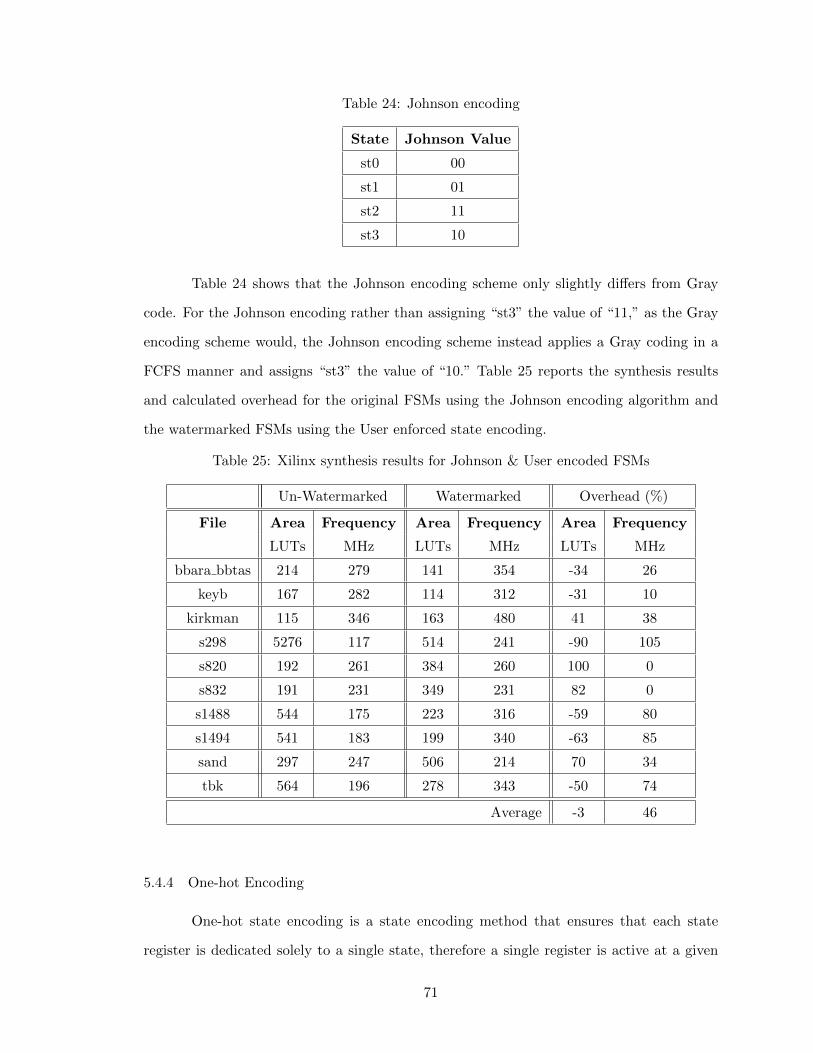
Table 24: Johnson encoding
State Johnson Value
st0 00
st1 01
st2 11
st3 10
Table 24 shows that the Johnson encoding scheme only slightly differs from Gray
code. For the Johnson encoding rather than assigning “st3” the value of “11,” as the Gray
encoding scheme would, the Johnson encoding scheme instead applies a Gray coding in a
FCFS manner and assigns “st3” the value of “10.” Table 25 reports the synthesis results
and calculated overhead for the original FSMs using the Johnson encoding algorithm and
the watermarked FSMs using the User enforced state encoding.
Table 25: Xilinx synthesis results for Johnson & User encoded FSMs
Un-Watermarked Watermarked Overhead (%)
File Area Frequency Area Frequency Area Frequency
LUTs MHz LUTs MHz LUTs MHz
bbara bbtas 214 279 141 354 -34 26
keyb 167 282 114 312 -31 10
kirkman 115 346 163 480 41 38
s298 5276 117 514 241 -90 105
s820 192 261 384 260 100 0
s832 191 231 349 231 82 0
s1488 544 175 223 316 -59 80
s1494 541 183 199 340 -63 85
sand 297 247 506 214 70 34
tbk 564 196 278 343 -50 74
Average -3 46
5.4.4 One-hot Encoding
One-hot state encoding is a state encoding method that ensures that each state
register is dedicated solely to a single state, therefore a single register is active at a given
71

time. This means that the number of registers needed is equal to the number of states in
the system and the length of the encoding string will be of the same length. Table 26 shows
an example of the One-hot encoding scheme.
Table 26: One-hot encoding
State Value One-Hot Value
st0 1000
st1 0100
st2 0010
st3 0001
Under most cases, One-hot encoding can be employed for power reduction and per-
formance improvement [88]. Table 27 reports the synthesis results and calculated overhead
for the original FSMs using the One-hot encoding algorithm and the watermarked FSMs
using the User enforced state encoding.
Table 27: Xilinx synthesis results for One-hot & User encoded FSMs
Un-Watermarked Watermarked Overhead (%)
File Area Frequency Area Frequency Area Frequency
LUTs MHz LUTs MHz LUTs MHz
bbara bbtas 195 263 141 354 -27 34
keyb 223 268 114 312 -48 16
kirkman 167 219 163 480 -2 118
s298 2384 136 514 241 -78 76
s820 211 268 384 260 81 -3
s832 226 245 349 231 54 -5
s1488 612 184 223 316 -63 71
s1494 626 158 199 340 -68 114
sand 373 191 506 214 35 73
tbk 489 198 278 343 -43 72
Average -16 57
72
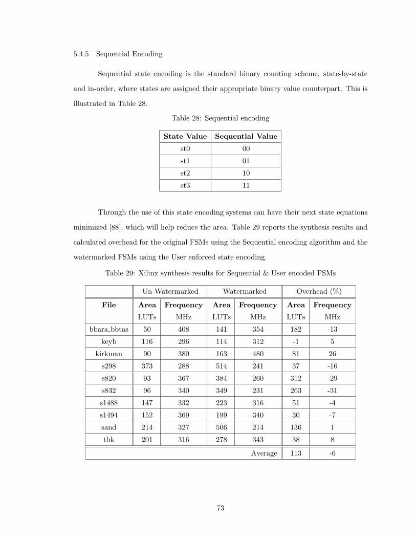
5.4.5 Sequential Encoding
Sequential state encoding is the standard binary counting scheme, state-by-state
and in-order, where states are assigned their appropriate binary value counterpart. This is
illustrated in Table 28.
Table 28: Sequential encoding
State Value Sequential Value
st0 00
st1 01
st2 10
st3 11
Through the use of this state encoding systems can have their next state equations
minimized [88], which will help reduce the area. Table 29 reports the synthesis results and
calculated overhead for the original FSMs using the Sequential encoding algorithm and the
watermarked FSMs using the User enforced state encoding.
Table 29: Xilinx synthesis results for Sequential & User encoded FSMs
Un-Watermarked Watermarked Overhead (%)
File Area Frequency Area Frequency Area Frequency
LUTs MHz LUTs MHz LUTs MHz
bbara bbtas 50 408 141 354 182 -13
keyb 116 296 114 312 -1 5
kirkman 90 380 163 480 81 26
s298 373 288 514 241 37 -16
s820 93 367 384 260 312 -29
s832 96 340 349 231 263 -31
s1488 147 332 223 316 51 -4
s1494 152 369 199 340 30 -7
sand 214 327 506 214 136 1
tbk 201 316 278 343 38 8
Average 113 -6
73

5.4.6 Speed1 Encoding
The Speed1 Encoding algorithm is designed for speed optimization [88]. The state
register size is significantly increased due to the manner in which this algorithm operates,
such that the number of bits used is FSM dependent. In general the Speed1 encoding
scheme will assign state encoding values with a length greater than the number of states in
the FSM. Using the FSM from Fig. 1, Table 30 shows this state encoding.
Table 30: Speed1 encoding
State Value Speed1 Value
st0 1000
st1 0100
st2 0010
st3 0001
It can be seen that, in this example, the Speed1 encoding scheme produces the same
encoding scheme as One-Hot but offers a different optimization metric in doing so. Table 31
reports the synthesis results and calculated overhead for the original FSMs using the Speed1
encoding algorithm and the watermarked FSMs using the User enforced state encoding.
Table 31: Xilinx synthesis results for Speed1 & User encoded FSMs
Un-Watermarked Watermarked Overhead (%)
File Area Frequency Area Frequency Area Frequency
LUTs MHz LUTs MHz LUTs MHz
bbara bbtas 458 163 141 354 -69 116
keyb 250 231 114 312 -54 35
kirkman 160 283 163 480 1 69
s298 5669 117 514 241 -90 105
s820 373 241 384 260 2 7
s832 376 195 349 231 -7 18
s1488 693 178 223 316 -67 77
s1494 706 151 199 340 -71 124
sand 397 222 506 214 27 49
tbk 866 182 278 343 -67 88
Average -40 69
74

5.5 Discussion of Results
We discuss the results gathered and evaluate the performance of our method. We
provide a summary of the watermarked and un-watermarked findings for the six state
encoding schemes. We first look at discrepancies discovered in the synthesis results.
5.5.1 Synthesis Discrepancies
The user enforced encoding scheme specified in the experiments follows a sequen-
tial encoding scheme. From the behavior of the k2vhdl tool, previously covered, during
VHDL model generation states in the Kiss2 file are written using a sequential ordering,
such that, in the body of the “state machine” VHDL process the ordering of the states
within the case statement is sequential. The User encoding scheme is specified by a list
of encoding values, i.e., {00, 10, 11, 10} will specifically map as the encoding values for
the states found in the case statement. If this case statement ordering happens to be
{st0, st3, st2, st1} then the corresponding state encoding mappings will be the set of ordered
pairs {(st0, 00), (st3, 10), (st2, 11), (st1, 10)}. With this knowledge, we expect the overhead
comparisons between User and Sequential encoding schemes to be zero in all cases. This is
based on the knowledge that Xilinx Synthesis should produce same results for the same file,
which is further supported by Xilinx guarantees that Xilinx Synthesis Technologies should
be deterministic [94].
Table 32 reports the synthesis results of benchmarks using User & Sequential state
encoding. On average there was a 3% increase in LUT usage and a 1% decrease in the
performance of the FSMs. Additionally, it can be seen that only 3 out of the 10 synthesis
results return the 0% expected overhead.
5.5.2 Synthesis Results
Table 33 summarizes the results for the six state encoding schemes. We report
minimum, maximum, and average overheads for area and frequency. Table 34 lists the
advantages and disadvantages that this method offers with respect to the encoding schemes.
75

Table 32: Xilinx synthesis discrepancies for User & Sequential encoded FSMs
Un-Watermarked Un-Watermarked Overhead (%)
File Area Frequency Area Frequency Area Frequency
LUTs MHz LUTs MHz LUTs MHz
bbara bbtas 59 328 50 409 18 -20
keyb 120 348 116 296 4 17
kirkman 90 381 90 381 0 0
s298 360 244 373 288 -4 -16
s820 90 409 93 367 -3 11
s832 101 379 96 340 5 11
s1488 147 332 147 332 0 0
s1494 152 369 152 369 0 0
sand 235 282 214 327 10 -14
tbk 180 331 201 317 -11 4
Average 3 -1
Table 33: Summary of Xilinx synthesis results
Synthesis Overhead (%)
(Min,Max,Avg) (Min,Max,Avg)
Encoding LUTs Frequency LUTs Frequency
Watermarked
User (114,514,287) (215,480,310) (–,–,–) (–,–,–)
Un-Watermarked
User (59,360,153) (244,409,340) (-5,327,109) (-38,27,-8)
Gray (54,357,150) (235,385,329) (-5,342,120) (-37,27,-5)
Johnson (115,5276,810) (118,346,232) (-90,100,-4) (0,106,47)
One-Hot (167,2384,551) (137,285,234) (-78,82,-16) (-3,119,59)
Sequential (50,373,153) (288,409,343) (-1,313,114) (-31,27,-6)
Speed1 (160,5669,995) (117,284,197) (-90,28,-40) (8,125,70)
76

Table 34: Summary of performance
Advantages Against Metrics
Johnson Minimize Hazards & Glitches
One-Hot Speed & Power Dissipation
Speed1 Speed Optimization
Disadvantages Against Metrics
User Minimized Next State Equations
Sequential Minimized Next State Equations
Gray Minimize Hazards & Glitches
77

6 Future Work
6.1 Sequential Circuit Logic Synthesis: k3
New methods for the advancement of this work are currently underway. These
methods consist of a custom tool, dubbed “k3,” that encapsulates a range of options for
the minimization and optimization of FSMs. In addition, a more intuitive sequential circuit
modeling language is being adapted from current, and newer, methods. Table 35 gives an
overview of some of the optimization techniques, options, and support for the in-progress
k3 system.
Table 35: k3 overview
Offered Minimization Techniques
Legacy & New Model Support
Trap/Dead State Removal
Unreachable State Removal
State Table Minimization
Don’t Care Collapsing & Decomposition
Clique Based Maximal Compatibility Groups
Visualization Format File Outputs
Legacy & New Model Generation
HDL & Synthesis File Generation
In addition to this new system, we will explore of new methods for the embedding
algorithm. As a greedy heuristic has proven to be a non-optimal, proof of concept, for
embedding the watermark into the original FSM. Due to the nature of the problem and
its associated complexity this can prove to be a difficult task. Currently this task is being
explored through the implementation, and construction, of a simulated annealing based
approach. However, while simulated annealing has a greater potential to produce desirable
results, alternative algorithmic solutions are to be explored. In addition to this on-going
78

work, the watermarking edge creation method is going to be further analyzed. Watermark-
ing techniques currently available, that do not implement the use of state addition, utilize
specific or unused input sequences available at a given state, we intend to explore the option
of the “phantom edge,” which is explained at length in the next section.
6.2 Phantom Edges
We define a phantom edge to be an edge in the system which does not exist, or affect
the system, in normal functionality. This is achieved through the utilization of extra input
bits that are otherwise non-functional, or non-system affecting, during normal operation.
An example of an FSM which utilizes this technique and implements these phantom edges
is shown in Fig. 40 (the phantom edges are represented by dashed lines). It can be seen
that these edges are only active in a separate mode, other than the normal, in which
system output is in no way affected. This absence of observable functionality allows for a
better disguise of internal system behavior in the event a malicious user is observing output
behavior to data mine functionality. As illustrated, the FSM utilizes modal functionality
known only to the user, we also note that the bit which will cause a modal change does not
have to be the least significant bit (LSB) or most significant bit (MSB) of the system, but
rather, it can be inserted at any location of the input bit string and, exhibiting the same
edge behavior, can achieve replication of the functionality shown.
st0 st1 st2 st3
000 / 11 010 / 01 000 / 11
000 / 10 011 / 00010 / 10
000 / 011-- / -- 1-- / --
1-- / --
Figure 40: FSM with phantom edges
Along with phantom edge creation, this method utilizes overlapping functional
edges, such that the sequence derived for recreation of the signature requires a more complex
79

interaction with the system. The idea behind this is that these edges may help obfuscate
functionality when an attacker attempts to formally verify all functionality.
6.2.1 Cost of a Phantom Edge
To further examine these phantom edges, we looked at the actual cost of the addition
of a series of phantom edges through an FSM constructed using the VHDL modeling. Table
36 shows the Xilinx Synthesis results for the series of cost experiments for phantom edges.
Table 36: Xilinx synthesis results of phantom edge FSMs
Fig. 40 FSM
Number of Phantom Edges
(0) (1) (2) (3) (12)
States 4
Transitions 11 12 13 14 23
Input Bits 3 4 5
Output Bits 4
Encoding Gray
Implementation LUT
Registers Used 2
Look-Up Tables (LUTs) Used 4 5
Max. Frequency (MHz) 1075.963
It can be seen from the results in Table 36 that, based on this particular example,
Phantom Edges can be expected to provide a low cost impact on area even though the num-
ber of edges in the system more than doubled. It can also been seen from this example that
the addition of these edges doesn’t immediately show a negative impact on the maximum
frequency for which the system can operate at either.
6.3 Watermark Extraction
Recent exploration of side-channel watermarking from [60] employ side-channel
methods for watermarking circuits. Alternative to the current watermark extraction method
which requires extra means to read the state register, the exploration of the techniques em-
80

ployed in this method may be beneficial for implementation within this system. In addition,
this method can easily be stacked with a power profiling method and phantom edges, thus
enabling the watermark to only be extracted through these hidden side-channels in the
effort to prevent the system from exhibiting behavior that exposes or outputs part of the
watermark.
6.4 Metric Stacking
The exploration of further state encoding possibilities and stacked implementations
is being looked into. This is the manner of minimizing a system and strictly enforcing the
state encoding beneficial to the system prior to watermarking. Conversely, embedding a
signature whose watermark states are strictly enforced while the remainder of states in the
FSM can have their state encoding values assigned to a given scheme for metric benefits is
being explored.
81

7 Conclusions
The proposed method of watermarking sequential circuits via state encoding is a
feasible technique that can be easily employed. The proposed methods for watermark
construction show that HSD is best implementation. It was shown to offer sparse watermark
FSMs which lower overhead and provides the greatest flexibility allowing the signature to
be a file of any format or size. Additionally, by using the RIPEMD-160 hashing function
we produce the shortest secure and collision free hash sequence known.
The proposed greedy solution for watermark embedding showed to be scalable for
FSMs of varying complexity and offered a significant decrease in run-time complexity. Scal-
ability and low run-time complexity however led to higher overhead from non-optimal so-
lutions.
Model generation and verification methods proved to be very advantageous. The
“k2net” tool, for generating visualization files, provides low run-time complexity while pro-
viding a method for visualizing the Kiss2 representations of FSMs. The “Hash-2-Kiss2”
tool, for generating watermark FSMs from hash sequences, proved to be a powerful tool
with low-run time complexity. Most importantly, the “k2vhdl” tool proved to be an ex-
tremely powerful tool for verification, synthesis, and simulation of Kiss2 FSMs. This tool
automatically generates VHDL-93 syntactically correct code, allowing for flexibility through
the ability to specify state encoding schemes to be used, and reducing complications from
don’t care statements and unspecified state behavior.
Through the use of Xilinx simulation the watermark can easily be verified. The
process of watermark extraction provides many flexible options for obtaining state encoding
values at run-time. Additionally, the watermark can be easily extracted by applying the
sequence used for verification. Lastly, the security of this method proves to be extensive.
HPC solutions that can attempt billions of brute force attacks per second can be shown to
still require a computationally infeasible amount of time.
82

References
[1] R. S. Chakraborty and S. Bhunia, “HARPOON : An Obfuscation-Based SoC DesignMethodology for Hardware Protection,” Computer-Aided Design of Integrated Circuitsand Systems, IEEE Transactions on, vol. 28, no. 10, pp. 1493–1502, 2009. [Online].Available: http://goo.gl/eizHC
[2] A. Tirkel, G. Rankin, R. van Schyndel, W. Ho, N. Mee, and C. Osborne, “ElectronicWatermark,” Digital Image Computing: Techniques and Applications, 1993., 1993.
[3] F. Lancaster, “The Evolution of Electronic Publishing,” Library Trends, vol. 43, no. 4,pp. 518–527, 1995.
[4] J. T. Brassil, S. Member, S. Low, N. F. Maxemchuk, and L. O. Gorman, “ElectronicMarking and Identification Techniques to Discourage Document Copying,” SelectedAreas in Communications, IEEE Journal on, vol. 13, no. 8, pp. 1495–1504, 1995.[Online]. Available: http://goo.gl/RLDQH
[5] E. Charbon, “Hierarchical watermarking in IC design,” Pro-ceedings of the IEEE 1998 Custom Integrated Circuits Confer-ence (Cat. No.98CH36143), pp. 295–298, 1998. [Online]. Available:http://ieeexplore.ieee.org/lpdocs/epic03/wrapper.htm?arnumber=694985
[6] J. Lach, W. Mangione-Smith, and M. Potkonjak, “FPGA fingerprinting techniquesfor protecting intellectual property,” Proceedings of the IEEE 1998 Custom IntegratedCircuits Conference (Cat. No.98CH36143), pp. 299–302, 1998. [Online]. Available:http://ieeexplore.ieee.org/lpdocs/epic03/wrapper.htm?arnumber=694986
[7] A. Oliveira, “Robust techniques for watermarking sequential cir-cuit designs,” Proceedings 1999 Design Automation Conference(Cat. No. 99CH36361), pp. 837–842, 1999. [Online]. Available:http://ieeexplore.ieee.org/lpdocs/epic03/wrapper.htm?arnumber=782155
[8] A. L. Oliveira, “Techniques for the Creation of Digital Watermarks in SequentialCircuit Designs,” Computer-Aided Design of Integrated Circuits and Systems,IEEE Transactions on, vol. 20, no. 9, pp. 1101–1117, 2001. [Online]. Available:http://goo.gl/7ihp4
[9] Z. Kohavi, “Finite state machine,” in Switching and Finite Automata Theory . TataMcGraw-Hill, 1998, p. 275.
[10] F. Vahid and T. Givargis, “State machine and concurrent process models,” in EmbeddedSystem Design, A Unified Hardware/Software Introduction. John Wiley & Sons, 2002,pp. 212–213.
[11] B. D. C. Victor P. Nelson, H. Troy Nagle and J. D. Irwin, “State assignment,” inDigital Logic Circuit Analysis & Design. Prentice-Hall, 1995, p. 605.
83

[12] U. Berkeley. (1992) Berkeley Logic Interchange Format (BLIF). [Online]. Available:http://embedded.eecs.berkeley.edu/Alumni/teh/research/papers/blif spec 92.pdf
[13] E. Moore, “Gedanken-experiments on sequential machines,” Automata Studies, Annalsof Mathematical Studies, vol. 34, pp. 129–153, 1956.
[14] G. Mealy, “A method for synthesizing sequential circuits,” The Journal of SymbolicLogic, vol. 22, no. 3, pp. 334–335, September 1957.
[15] J. L. M. Gideo Langholz, Abraham Kandel, “State assignment,” in Foundations ofDigital Logic Design. World Scientific, 1998, p. 385.
[16] G. Maki, I. Sawin, D.H., and B.-R. Jeng, “Improved state assignment selection tests,”Computers, IEEE Transactions on, vol. C-21, no. 12, pp. 1443–1449, dec. 1972.
[17] D. B. Johnson, “Efficient algorithms for shortest paths in sparse networks,”Journal of the ACM , vol. 24, no. 1, pp. 1–13, January 1977. [Online]. Available:http://dl.acm.org/citation.cfm?doid=321992.321993
[18] G. D. E. Micheli, R. Membe, and R. K. Brayton, “Optimal State Assignment forFinite State Machines,” Computer-Aided Design of Integrated Circuits and Systems,IEEE Transactions on, vol. 4, no. 3, pp. 269–285, 1985. [Online]. Available:http://goo.gl/cuu4a
[19] S. Devadas, H.-K. Ma, A. Newton, and A. Sangiovanni-Vincentelli, “MUS-TANG: State Assignment of Finite State Machines Targeting Multilevel LogicImplementations,” Computer-Aided Design of Integrated Circuits and Systems,IEEE Transactions on, vol. 7, no. 12, pp. 1290–1300, 1988. [Online]. Available:http://ieeexplore.ieee.org/stamp/stamp.jsp?tp=&arnumber=16807&isnumber=610
[20] B. Eschermann and H.-J. Wunderlich, “Optimized synthesis of self-testablefinite state machines,” [1990] Digest of Papers. Fault-Tolerant Comput-ing: 20th International Symposium, pp. 390–397, 1990. [Online]. Available:http://ieeexplore.ieee.org/lpdocs/epic03/wrapper.htm?arnumber=89393
[21] S. Robinson and J. Shen, “Evaluation and synthesis of self-monitoring statemachines,” 1990 IEEE International Conference on Computer-Aided De-sign. Digest of Technical Papers, pp. 276–279, 1990. [Online]. Available:http://ieeexplore.ieee.org/lpdocs/epic03/wrapper.htm?arnumber=129901
[22] D. J. Rosenkrantz, “Half-Hot State Assignments for Finite State Machines,”Computers, IEEE Transactions on, vol. 39, no. 5, pp. 700–702, 1990. [Online].Available: http://goo.gl/dgxLY
[23] M. Perkowski and L. Nguyen, “The encoding program for concurrent finitestate machines realized using PLD devices,” Proceedings of the 33rd MidwestSymposium on Circuits and Systems, pp. 204–207, 1990. [Online]. Available:http://ieeexplore.ieee.org/lpdocs/epic03/wrapper.htm?arnumber=140687
[24] J.-j. Yang, H. Shin, J.-w. Chow, and G. Star, “New State Assignment Algorithms forFinite State Machines Using Look Ahead,” Custom Integrated Circuits Conference,1991., Proceedings of the IEEE 1991 , pp. 11.2/1–11.2/4, 1991. [Online]. Available:http://goo.gl/6s69G
84

[25] L. Lavagno, C. Moon, R. Brayton, and A. Sangiovanni-Vincentelli, “Solving the stateassignment problem for signal transition graphs,” in Design Automation Conference,1992. Proceedings., 29th ACM/IEEE , jun 1992, pp. 568–572.
[26] G. Rietsche and F. Informatik, “State Assignment for Finite State MachinesUsing T Flip-Flops,” Design Automation Conference, 1993, with EURO-VHDL ’93.Proceedings EURO-DAC ’93., European, pp. 396–401, 1993. [Online]. Available:http://goo.gl/6khX8
[27] T.-a. Chu, N. Mani, and C. K. C. Leung, “A New State Assignment Techniquefor Asynchronous Finite State Machines,” ’Design Automation of High PerformanceVLSI Systems’, Proceedings., Third Great Lakes Symposium on, pp. 139–143, 1993.[Online]. Available: http://goo.gl/0j4H6
[28] K.-H. Wang, W.-S. Wang, T. Hwang, A. Wu, and Y.-L. Lin, “State assignment forpower and area minimization,” in Computer Design: VLSI in Computers and Proces-sors, 1994. ICCD ’94. Proceedings., IEEE International Conference on, oct 1994, pp.250–254.
[29] T.-d. Her, W. K. Tsai, F. Kurdahi, and Y. Chen, “Low-Power Driven StateAssignment of Finite State Machines,” Circuits and Systems, 1994. APCCAS ’94.,1994 IEEE Asia-Pacific Conference on, pp. 454–459, 1994. [Online]. Available:http://goo.gl/dh494
[30] E. Olson and S. Kang, “Assignment for Low-Power FSM Synthesis Using GeneticLocal Search,” Custom Integrated Circuits Conference, 1994., Proceedings of the IEEE1994 , pp. 140–143, 1994. [Online]. Available: http://goo.gl/D56EQ
[31] C. Bolchini, R. Montandon, F. Sake, D. Sciuto, and P. Milano, “A State Encodingfor Self-Checking Finite State Machines,” Design Automation Conference, 1995.Proceedings of the ASP-DAC ’95/CHDL ’95/VLSI ’95., IFIP International Conferenceon Hardware Description Languages; IFIP International Conference on Very LargeScale Integration., Asian and South Pacific, pp. 711–716, 1995. [Online]. Available:http://goo.gl/8qP7a
[32] J. Rutten and M. Berkelaar, “Improved State Assignment for Burst Mode FiniteState Machines,” Advanced Research in Asynchronous Circuits and Systems, 1997.Proceedings., Third International Symposium on, pp. 228–239, 1997. [Online].Available: http://goo.gl/oAh5V
[33] I. Ahmad and R. Ul-Mustafa, “On State Assignment of Finite State Machines UsingHypercube Embedding Approach,” Computer Design, 1999. (ICCD ’99) InternationalConference on, pp. 608–613, 1999. [Online]. Available: http://goo.gl/jAqLV
[34] P. Bacchetta, L. Daldoss, D. Sciuto, and C. Silvano, “Low-Power State AssignmentTechniques for Finite State Machines,” Circuits and Systems, 2000. Proceedings.ISCAS 2000 Geneva. The 2000 IEEE International Symposium on, vol. 2, pp.641–644, 2000. [Online]. Available: http://goo.gl/tgQWt
[35] L. Jozwiak and A. Slusarczyk, “A new state assignment method targeting fpga imple-mentations,” in Euromicro Conference, 2000. Proceedings of the 26th, vol. 1, 2000, pp.50–59.
85

[36] S. K. Kuusilinna, “Finite state machine encoding for VHDL synthesis,” Computersand Digital Techniques, IEE Proceedings -, vol. 148, no. 1, pp. 23–30, 2001. [Online].Available: http://goo.gl/wLACN
[37] M. Chyzy and W. Kosiski, “Evolutionary Algorithm for State Assignment of FiniteState Machines,” Digital System Design, 2002. Proceedings. Euromicro Symposiumon, pp. 359–362, 2002. [Online]. Available: http://goo.gl/VvY8K
[38] S. Roy, “Power conscious BIST design for sequential circuits using ghost-FSM,”Proceedings of the 7th International Conference on Properties and Applications ofDielectric Materials (Cat No 03CH37417) ATS-03 , pp. 190–195, 2003. [Online].Available: http://goo.gl/qV8eS
[39] G. Venkataraman, S. Reddy, and I. Pomeranz, “Gallop: genetic algorithm based lowpower fsm synthesis by simultaneous partitioning and state assignment,” in VLSI De-sign, 2003. Proceedings. 16th International Conference on, jan. 2003, pp. 533–538.
[40] S. Chattopadhyay, P. Yadav, and R. Singh, “Multiplexer targeted finite statemachine encoding for area and power minimization,” India Annual Conference, 2004.Proceedings of the IEEE INDICON 2004. First , pp. 12–16, 2004. [Online]. Available:http://goo.gl/3nYHA
[41] B. Tawadros and R. Guindi, “State Assignment for Low-Leakage Finite State-Machines,” The 3rd International IEEE-NEWCAS Conference, 2005., pp. 115–118, 2005. [Online]. Available:http://ieeexplore.ieee.org/lpdocs/epic03/wrapper.htm?arnumber=1496657
[42] L. Mengibar, L. Entrena, and M. Garc, “Partitioned state encoding for low power inFPGAs,” Electronics Letters, vol. 41, no. 17, pp. 18–19, 2005. [Online]. Available:http://goo.gl/E0kGx
[43] M. Damm, “State Assignment for Detecting Erroneous Transitionsin Finite State Machines,” 9th EUROMICRO Conference on Digi-tal System Design (DSD’06), pp. 483–490, 2006. [Online]. Available:http://ieeexplore.ieee.org/lpdocs/epic03/wrapper.htm?arnumber=1690077
[44] Y. Lee, K. Choi, and T. Kim, “SAT-based state encoding for peak currentMinimization,” 2009 International SoC Design Conference (ISOCC), pp. 432–435,2009. [Online]. Available: http://goo.gl/Z1kLE
[45] M. Lewandowski, R. Meana, M. Morrison, and S. Katkoori, “A novel methodfor watermarking sequential circuits,” 2012 IEEE International Symposium onHardware-Oriented Security and Trust , pp. 21–24, Jun. 2012. [Online]. Available:http://ieeexplore.ieee.org/lpdocs/epic03/wrapper.htm?arnumber=6224313
[46] L. Zhang and C.-h. Chang, “State Encoding Watermarking for Field Authenticationof Sequential Circuit Intellectual Property,” Circuits and Systems (ISCAS), 2012IEEE International Symposium on, pp. 3013–3016, 2012. [Online]. Available:http://goo.gl/R32oH
[47] M. Karnaugh, “The map method for synthesis of combinational logic circuits,” Trans.AIEE. pt I , vol. 72, no. 9, pp. 593–599, November 1953.
86

[48] I. Tomnoglu and E. Charbon, “Watermarking-Based Copyright Protection ofSequential Functions,” Custom Integrated Circuits, 1999. Proceedings of the IEEE1999 , pp. 35–38, 1999. [Online]. Available: http://goo.gl/dDx6Z
[49] A. Abdel-Hamid, S. Tahar, and E. M. Aboulhamid, “IP watermarking techniques:survey and comparison,” in System-on-Chip for Real-Time Applications, 2003. Pro-ceedings. The 3rd IEEE International Workshop on, June-2 July 2003, pp. 60–65.
[50] A. Abdel-Hamid, S. Tahar, and E. Aboulhamid, “A Tool for Automatic Watermarkingof IP Designs,” Circuits and Systems, 2004. NEWCAS 2004. The 2nd Annual IEEENortheast Workshop on, pp. 381–384, 2004. [Online]. Available: http://goo.gl/iAoNh
[51] ——, “A Public-Key Watermarking Technique for IP Designs,” Design,Automation and Test in Europe, pp. 330–335, 2005. [Online]. Available:http://ieeexplore.ieee.org/lpdocs/epic03/wrapper.htm?arnumber=1395581
[52] A. T. Abdel-Hamid, S. Tahar, and E. Aboulhamid, “Finite State Machine IPWatermarking: A Tutorial,” First NASA/ESA Conference on Adaptive Hardware andSystems (AHS’06), pp. 457–464, 2006. [Online]. Available: http://goo.gl/hZUgT
[53] S. S. P. S. Nandgawe, “Intellectual Property Protection of Sequential Circuits UsingDigital Watermarking,” Industrial and Information Systems, First InternationalConference on, no. August, pp. 8–11, 2006. [Online]. Available: http://goo.gl/ibpEU
[54] A. Stoica and S. Katkoori, “”Glitch Logic” and Applications to Computing and Infor-mation Security,” in Bio-inspired Learning and Intelligent Systems for Security, 2009.BLISS ’09. Symposium on, August 2009, pp. 107–112.
[55] A. Cui and C.-H. Chang, “Watermarking for IP Protection through TemplateSubstitution at Logic Synthesis Level,” 2007 IEEE International Symposiumon Circuits and Systems, pp. 3687–3690, May 2007. [Online]. Available:http://ieeexplore.ieee.org/lpdocs/epic03/wrapper.htm?arnumber=4253481
[56] M.-C. Lin, G.-R. Tsai, C.-R. Wu, and C.-H. Lin, “Watermarking Tech-nique for HDL-based IP Module Protection,” Third International Con-ference on Intelligent Information Hiding and Multimedia Signal Pro-cessing (IIH-MSP 2007), pp. 393–396, Nov. 2007. [Online]. Available:http://ieeexplore.ieee.org/lpdocs/epic03/wrapper.htm?arnumber=4457732
[57] R. S. Chakraborty and S. Bhunia, “Hardware protection and authenticationthrough netlist level obfuscation,” 2008 IEEE/ACM International Confer-ence on Computer-Aided Design, pp. 674–677, Nov. 2008. [Online]. Available:http://ieeexplore.ieee.org/lpdocs/epic03/wrapper.htm?arnumber=4681649
[58] A. Abdel-Hamid and S. Tahar, “Fragile IP Watermarking Techniques,” in AdaptiveHardware and Systems, 2008. AHS ’08. NASA/ESA Conference on, June 2008, pp.513–519.
[59] F. Koushanfar and W. Marsh, “Provably Secure Obfuscation of DiverseWatermarks for Sequential Circuits,” Hardware-Oriented Security and Trust (HOST),2010 IEEE International Symposium on, pp. 42–47, 2010. [Online]. Available:http://goo.gl/67KWA
87

[60] G. Becker, M. Kasper, A. Moradi, and C. Paar, “Side-channel based watermarks forintegrated circuits,” in Hardware-Oriented Security and Trust (HOST), 2010 IEEEInternational Symposium on, June 2010, pp. 30–35.
[61] A. Cui, C.-h. Chang, S. Member, and S. Tahar, “A Robust FSM WatermarkingScheme for IP Protection of Sequential Circuit Design,” Computer-Aided Design ofIntegrated Circuits and Systems, IEEE Transactions on, vol. 30, no. 5, pp. 678–690,2011. [Online]. Available: http://goo.gl/cxivz
[62] A. Cui, C.-H. Chang, and L. Zhang, “A hybrid watermarking schemefor sequential functions,” 2011 IEEE International Symposium of Cir-cuits and Systems (ISCAS), pp. 2333–2336, May 2011. [Online]. Available:http://ieeexplore.ieee.org/lpdocs/epic03/wrapper.htm?arnumber=5938070
[63] W. Xu and Y. Zhu, “A digital copyright protection scheme for soft-IP corebased on FSMs,” 2011 International Conference on Consumer Electronics,Communications and Networks (CECNet), pp. 3823–3826, Apr. 2011. [Online].Available: http://goo.gl/2DskW
[64] N. H. E. Weste and D. M. Harris, “Placing cute logos on a chip,” in CMOS VLSIDesign, A Circuits and Systems Perspective. Addison-Wesley, 2011, p. 136.
[65] MOSIS. (2010) ON Semiconductor C5 Process. USC Information Sciences Institute.[Online]. Available: http://mosis.com/vendors/view/on-semiconductor/c5
[66] ——. (2010) Mosis faqs: Design issues. USC Information Sciences Institute. [Online].Available: http://www.mosis.com/pages/Faqs/faq-design
[67] M. W. Davidson. (1995) Silicon Zoo. [Online]. Available:http://micro.magnet.fsu.edu/creatures/index.html
[68] J.-B. Note and E. Rannaud, “From the bitstream to the netlist,” in Proceedings ofthe 16th international ACM/SIGDA symposium on Field programmable gate arrays,ser. FPGA ’08. New York, NY, USA: ACM, 2008, pp. 264–264. [Online]. Available:http://doi.acm.org/10.1145/1344671.1344729
[69] Hackito-Ergo-Sum. (2010) FPGA Reverse-Engineering Challenge. [Online]. Available:http://www.hackitoergosum.org/2010/HES2010-sbourdeauducq-FPGA-Challenge.pdf
[70] D. Ho. (2011) Notepad++ a free source code editor. [Online]. Available:http://notepad-plus-plus.org/
[71] H. Dobbertin, A. Bosselaers, and B. Preneel, “RIPEMD-160: A Strength-ened Version of RIPEMD,” Proceedings of the Third International Work-shop on Fast Software Encryption, pp. 71–82, 1996. [Online]. Available:http://dl.acm.org/citation.cfm?id=647931.740583
[72] F. Mendel, N. Pramstaller, C. Rechberger, and V. Rijmen, “On the collision resistanceof ripemd-160,” in Proceedings of the 9th international conference on InformationSecurity , ser. ISC’06. Berlin, Heidelberg: Springer-Verlag, 2006, pp. 101–116.[Online]. Available: http://dx.doi.org/10.1007/11836810 8
88

[73] OpenSSL. (1999) OpenSSL Cryptography and SSL/TLS Toolkit. [Online]. Available:http://www.openssl.org/
[74] V. Batagelj and A. Mrvar, “Pajek Program for Large Network Analysis,” Connections,Journal of International Network for Social Network Analysis, vol. 21, no. 1, pp. 1–11,1998. [Online]. Available: http://vlado.fmf.uni-lj.si/pub/networks/doc/pajek.pdf
[75] M. Bastian and S. Heymann, “Gephi : An Open Source Softwarefor Exploring and Manipulating Networks,” International AAAI Confer-ence on Weblogs and Social Media, pp. 1–2, 2009. [Online]. Available:http://www.aaai.org/ocs/index.php/ICWSM/09/paper/view/154
[76] T. H. Cormen, C. E. Leiserson, R. L. Rivest, and C. Stein, in Introduction to Algo-rithms. MIT Press and McGraw-Hill, 1998.
[77] S. A. Cook, “The complexity of theorem-proving procedures,” in Proceedingsof the third annual ACM symposium on Theory of computing , ser. STOC’71. New York, NY, USA: ACM, 1971, pp. 151–158. [Online]. Available:http://doi.acm.org/10.1145/800157.805047
[78] S. S. Epp, “Basics of set theory,” in Discrete Mathematics with Applications. Thomson,2004, p. 260.
[79] G. D. Micheli, in Synthesis and Optimization of Digital Circuits. McGraw-Hill, 1994.
[80] R. Johnsonbaugh and M. Schaefer, in Algorithms. Pearson, 2004.
[81] J. B. Kruskal, “On the Shortest Spanning Subtree of a Graph and the TravelingSalesman Problem,” in American Mathematical Society , vol. 7, no. 1, February 1956,pp. 48–50. [Online]. Available: http://www.jstor.org/stable/2033241
[82] “IEEE Standard VHDL Language Reference Manual.” ANSI/IEEE Std 1076-1993 ,p. i, 1994.
[83] L.-E. Thorelli, “An algorithm for computing all paths in a graph,” BITNumerical Mathematics, vol. 6, no. 4, pp. 347–349, 1966. [Online]. Available:http://dx.doi.org/10.1007/BF01966095
[84] W. Stallings, “Requirements and security,” in Cryptography and Network Security .Prentice Hall, 1998, pp. 335–341.
[85] J. M. Gosney, “Password Cracking HPC,” in Passwords1̂2 Security Conference,December 2012, pp. 1–29. [Online]. Available: http://passwords12.at.ifi.uio.no/
[86] X. Wang, Y. L. Yin, and H. Yu. (2005) Finding Collisions in the Full SHA-1. [Online].Available: http://people.csail.mit.edu/yiqun/SHA1AttackProceedingVersion.pdf
[87] M. Bastian and S. Heymann. (2009) Comparison of Supported Graph Formats inGephi. [Online]. Available: http://gephi.org/users/supported-graph-formats/
[88] Xilinx. (2009, September) Xilinx Synthesis Tech-nology (XST) User Guide. [Online]. Available:http://www.xilinx.com/support/documentation/sw manuals/xilinx11/xst.pdf
89

[89] ——. (2009, December) Xilinx Constraints Guide. [Online]. Available:http://www.xilinx.com/support/documentation/sw manuals/xilinx11/cgd.pdf
[90] International Workshop on Logic Synthesis, IWLS’93. [Online]. Available:http://www.iwls.org
[91] K. McElvain. (1993) IWLS’93 Benchmark Set: Version 4.0, distributedas part of the IWLS’93 benchmark distribution. [Online]. Available:http://www.cbl.ncsu.edu:16080/benchmarks/LGSynth93/
[92] F. Gray, “Pulse code communication,” U.S. Patent 2,632,058 , March 1953.
[93] R. W. Hamming, “Error detecting and error correcting codes,” Bell System TechnicalJournal , vol. 29, no. 2, pp. 147–160, 1950.
[94] Xilinx. (2009, January) AR #23904 - 10.1i MAP PAR - Will the Xilinx implementationtools give the exact same results with the exact same source files, system, and softwareversion. [Online]. Available: http://www.xilinx.com/support/answers/23904.htm
90

Appendix A Glossary
3M
Terminology for the number of metal layers available in a CMOS design process. 14,91
AMI
Semiconductor and Integrated Circuit Devices corporation, formerly AMI Semicon-ductor. 14, 91
ASIC
Integrated Circuit designed using the full-custom design approach for use in a specificapplication or setting. 91
ASICs
see ASIC. 1, 91
Asynchronous
Classification of an FSM which operates independently of a clock source and is drivensolely on input sequences. 91
Big Endian
Describes a binary string where the left most bit is the MSB and the right most bitis the LSB. 91
BLIF
Format for describing circuits and systems through text to allow use in design au-tomation tools. 6, 91
BSD
Method for converting a bitmap watermarking signature into a directed graph orwatermark FSM. vii, 91
CMOS
A technology for constructing Integrated Circuits. 14, 91
CSFSM
An FSM which has all possible behavior specified. 8, 9, 91
DEEP SUBM
Manufacturing feature size for Integrated Circuit technologies. 14, 91
91

Appendix A (Continued)
DFA
Class of Finite State Machines in which all sets of input sequences result in repro-ducible behavior. 9, 91
DRC
Process in Integrated Circuit design to ensure that physical design layouts adhere tothe rules implemented for the manufacturing process being used. 14, 91
E
Terminology for the availability of a secondary polysilicon layer that can be used forpoly capacitors or transistor gates. 14, 91
FCFS
A method for processing elements, specifically, the first elements to arrive are pro-cessed first. 49, 68, 91
FPGA
Reconfigurable computing device to allow for the rapid prototyping and developmentof computer systems. 2, 91
FSD
Signature Decomposition Technique used on files for creating directed graphs or wa-termark FSMs. vii, 35, 91
FSM
Abstract modeling method of sequential circuit systems that can be mathematicaldescribed using a 6-tuple. 4, 91
Hard IP
IP in a format which is difficult to alter. 91
HDL
Language, in a human readable format, for designing and specifying the behavior ofcomputer systems. 2, 17, 53, 91
HPC
Typically a collection, or cluster, of computing resources that can be used collectivelyto achieve a single task. 60, 91
HSD
Signature Decomposition Technique used on hash sequences for creating directedgraphs or watermark FSMs. vii, 37, 91
92

Appendix A (Continued)
I/O
Describes the interfaces between user and system for communication. 4, 19, 91
IC
System of combinational or sequential logic functions manufactured on a silicon wafer.1, 2, 91
ICSFSM
An FSM which uses don’t care conditions or does not define all possible behavior. 8,10, 91
IEEE
Organization consisting of academics and industry professionals for the advancementof technology. 91
IP
Any material which an individual creates and holds the exclusive rights for. 1, 2, 91
IPC
Reusable hardware design containing logic functions that are IP for a given party. 91
ISE
Interactive software environment that has been integrated into a set of design toolsthat can otherwise be used through a commandline. 55, 91
IWLS
Annual conference held for topics relating to synthesis, optimization, and verificationof integrated circuits. 67, 91
Kiss2
Subset of the BLIF syntax used for describing sequential systems in a modified statetable format. 91
Little Endian
Describes a binary string where the right most bit is the MSB and the left most bitis the LSB. 91
LSB
Descriptor used for a position in a binary array based on whether Big or Little Endianprinciples are used. 21, 22, 91
LUT
Hardware element used as memory array which returns predefined output conditionsbased on the inputs to the device. 91
93

Appendix A (Continued)
MAX-SAT
Computationally complex problem which finds maximal group of variable configura-tions that satisfy the boolean equation in which they are used. 91
Mealy Model
Modeling for an FSM where the outputs are updated during the transition to the nextstate. 91
Moore Model
Modeling for an FSM where the outputs are updated after transitioning to the nextstate. 91
MSB
Descriptor used for a position in a binary array based on whether Big or Little Endianprinciples are used. 91
N
Terminology for Integrated Circuit Wafer Doping properties. 14, 91
NDFA
Class of Finite State Machines in which all sets of input sequences result in behaviorthat is unlikely to be reproduced or occur again. 10, 91
Netlist
Hardware device designed at the HDL or transistor level. 91
NP
Describes a set of decision based problems which have verifiable solutions in polyno-mial time. 91
NP-Complete
Describes a subset of decision based problems which have no polynomial time solu-tions. 25, 41, 91
NP-Hard
Describes a subset of computation problems which have NP-Complete decision ver-sions. 91
PNG
A raster image format that uses lossless data compression techniques. 37, 91
RIPEMD-160
160-bit cryptographic hash function. 37, 91
94

Appendix A (Continued)
SC
A method for CMOS fabrication processes that provide design abilities nearly inde-pendent of process and metric. 14, 91
SCN3M
Terminology used for describing the AMI C5F CMOS Process, Scalable CMOS, Nsubstrate, 3 Metals. 14, 91
SCN3ME
Terminology used for describing the AMI C5N CMOS Process, Scalable CMOS, Nsubstrate, 3 Metals, Electrode. 14, 91
SHA-1
160-bit bit cryptographic hash function. 60, 91
SOC
Integrated circuit which includes all necessary components for an electronic systemon a single chip. 91
SOCs
See SOC. 91
Soft IP
IP in a format which can be easily altered. 91
SRAM
Type of volatile memory that uses cross-coupled inverters to maintain the internalvalue and removes the need for this value to be refreshed. 91
State Encoding
An arbitrary or intentionally assigned binary or text string used for labeling states inan FSM. 91
STG
Graphical method for representing FSMs as a collection of nodes and edges. 5, 91
STT
Tabular, non-graphical, method for representing an FSM. 6, 91
SUBM
Manufacturing feature for Integrated Circuit technologies.. 14, 91
Synchronous
Classification on an FSM which operates on the rising or falling edge of a clock signal.91
95

Appendix A (Continued)
VHDL
Programming language for FPGA devices. 53, 91
VHDL-93
The IEEE Standard 1076, Revision 1993, version of VHDL. 53, 91
VHSIC
United States Department of Defense project which led to the development of VHDL.53, 91
Watermark
A file, video, audio, or text message used as a unique signature hidden in IP. 91
XST
A tool in the Xilinx ISE Design Suite used for the synthesis and optimization of HDLdesigns. 53, 55, 91
96
Appendix B Permission of Use
©2012 IEEE. Reprinted, with permission, from M. Lewandowski, R. Meana, M. Morri-son, S. Katkoori, ”A Novel Method for Watermarking Sequential Circuits,” 2012 IEEEInternational Symposium on Hardware-Oriented Security and Trust, June 2012.
UNIVERSITY COMMUNICATIONS & MARKETING University of South Florida • 4202 East Fowler Avenue, CGS 301 • Tampa, FL 33620-4301
(813) 974-4014 • FAX (813) 974-2888 • www.usf.edu
This letter is an electronic communication from the University of South Florida.
March 20, 2013 Matthew Lewandowski, Graduate Student, Computer Science and Engineering, University of South Florida, NarMOS Research Team Dear Matthew, You have permission to use the USF College of Engineering co-branded USF logo as an example of the capabilities of the HASH-2-K2 method detailed in your Master’s Thesis. This permission is specific to use of the logo for this purpose and does not include permission to mark any product for sale. Thank you, Anne Scott Senior Graphic Designer University Communications & Marketing University of South Florida 4202 E Fowler Ave, STOP CGS 301 Tampa, FL 33620-4301 813-974-9043 fax 813-974-2888
97

About The Author
Matthew Lewandowski will be receiving both his Bachelor’s and Master’s Degree
in Computer Engineering Spring 2013 from the University of South Florida in Tampa, FL.
Upon graduation, he will be continuing on in academia and to pursue a Doctorate Degree
Fall 2013 with USF. His goal is to become a professor in the area of CMOS-VLSI Design and
has assisted Dr. Srinivas Katkoori in teaching the course at USF over the past two years.
His research interests are Design of Secure Hardware, Design Automation, and Reversible
Logic. He is a recipient of the Design Automation Conference Young Student Scholarship
Program, and has been awarded a Best Post Award for his research at both USF’s College of
Engineering Research Day, and 9th Annual Undergraduate Research Symposium. Recently,
with his research team dubbed “NarMOS,” he was awarded First Place at NYU-Poly’s
CyberSecurity Awareness Week Embedded System Challenge. He considers his personal
achievements to be his continued success in the development of a Cadence Design Kit and
ON-Semiconductor AMI C5N Process Design Kit which are being used with the CMOS-
VLSI Design, Design Automation, and Digital Design in Nano-Scaled Technologies courses
at USF.


