
A PHARMACOKINETIC POPULATION MODEL
FOR CYCLOSPORIN A IN RENAL TRANSPLANT
RECIPIENTS
Development of a model for whole blood- and intracellular
concentrations
Trần Mạnh Trường-Sơn
Faculty of Mathemathics and Natural Sciences
Department of Pharmaceutical Biosciences
School of Pharmacy
UNIVERSITY IN OSLO
May 2009

2
AKNOWLEDGEMENT
I would like to thank my supervisor Professor Anders Åsberg for guiding me through
this past year and a half. Your knowledge and motivating skills have been an
invaluable contribution and have made this thesis possible. I would also thank Ph.D
Pål Falck for helping me getting started on this thesis.
Further I would like to thank Trúc Thanh Vân Lê for providing information regarding
the earlier model and data.
Special thanks for my classmates and friends who have supported me in frustrating
times, especially Levin Ulrich Løssfelt who I have shared both his and mine positive
and negative experiences with.
Finally I would like to thank my family, Idunn and all those who stand me close for
standing by me even though I have not been as available as normal for this last half
year. You have supported me through long days and weeks and I am forever grateful.
Oslo, May 2009
Trần Mạnh Trường-Sơn

TABLE OF CONTENT
AKNOWLEDGEMENT ...................................................................................................................... 2
TABLE OF CONTENT ........................................................................................................................ 3
ABBREVIATIONS ............................................................................................................................... 6
ABSTRACT........................................................................................................................................... 8
1. INTRODUCTION .................................................................................................................... 10
1.1 PHARMACOKINETICS .............................................................................................................. 10
1.1.1 Introduction ................................................................................................................ 10
1.1.2 Variability ................................................................................................................... 11
1.1.3 Compartmental theory ................................................................................................ 13
1.1.4 Population pharmacokinetics ..................................................................................... 13
2. PHARMACOKINETIC POPULATION MODELING ........................................................ 15
2.1 INTRODUCTION ...................................................................................................................... 15
2.1.1 Standard 2-stage approach ......................................................................................... 16
2.1.2 Naïve pooled data approach ....................................................................................... 16
2.1.3 Nonlinear mixed-effect model approach ..................................................................... 16
2.2 NONMEM ............................................................................................................................. 17
2.2.1 Background ................................................................................................................. 17
2.2.2 Modelling population PK using NONMEM ................................................................ 18
2.2.3 How to find the best model using maximum likelihood approach ............................... 20
3. CYCLOSPORIN A ................................................................................................................... 22
3.1 HISTORY ................................................................................................................................ 22
3.2 APPLICATION AND MECHANISM OF ACTION ............................................................................ 22
3.3 KNOWN PROBLEMS WITH CYCLOSPORIN A ............................................................................ 23
3.4 ADME OF CSA ..................................................................................................................... 23
4
3.4.1 Administration ............................................................................................................ 23
3.4.2 Distribution ................................................................................................................ 24
3.4.3 Metabolism ................................................................................................................. 24
3.4.4 Elimination ................................................................................................................. 25
3.5 THERAPEUTIC DRUG MONITORING ......................................................................................... 25
3.6 POPULATION KINETIC MODELS OF CSA IN LITERATURE ......................................................... 26
3.7 GOALS OF THE THESIS ........................................................................................................... 26
4. METHODS AND MATERIALS ............................................................................................ 27
4.1 MATERIALS FOR THE WHOLE BLOOD MODEL ......................................................................... 27
4.2 MATERIALS FOR THE WHOLE BLOOD MODEL AND INTRACELLULAR CONCENTRATIONS ......... 29
4.3 DEVELOPING AND BUILDING THE MODELS ............................................................................. 30
4.3.1 The whole blood model .............................................................................................. 31
4.3.2 The whole blood and intracellular model .................................................................. 31
5. RESULTS ................................................................................................................................. 35
5.1 RE-ANALYZING FOR COVARIATES FOR THE WHOLE BLOOD MODEL ....................................... 35
5.2 TESTING FOR INTEROCCACIONAL VARIABILITY ..................................................................... 37
5.3 COVARIATE ANALYSIS BASED ON VISUAL PREDICTION .......................................................... 38
5.5 COMPARING THE OLD VERSUS THE NEW MODEL .................................................................... 43
5.6 THE WHOLE BLOOD AND INTRACELLULAR CONCENTRATIONS ............................................... 44
5.6.1 Model building results ................................................................................................ 44
6. DISCUSSIONS ......................................................................................................................... 52
6.1 RE-ANALYZING FOR COVARIATES FOR CSA PLASMACONCENTRATIONS ................................ 52
6.2 TESTING FOR INTEROCCASIONAL VARIABILITY FOR THE WHOLE BLOOD MODEL ................... 54
6.3 WHOLE BLOOD AND INTRACELLULAR MODEL ....................................................................... 55
7. CONCLUSIONS ...................................................................................................................... 58

5
8. REFERENCES ......................................................................................................................... 59
9. APPENDIX ............................................................................................................................... 63
9.1 FORMULAS USED IN DEMOGRAPHICS MODEL .......................................................................... 63
9.2 PARTIAL INPUT FILE FOR WHOLE BLOOD MODEL .................................................................... 64
9.3 CONTROL FILE FOR FINAL MODEL WHOLE BLOOD .................................................................. 66
9.4 INDIVIDUAL FITTING MADE BY R FOR FINAL WHOLE BLOOD MODEL ...................................... 68
9.5 PARTIAL INPUT FILE FOR WHOLE BLOOD AND INTRACELLULAR MODEL ................................. 77
9.6 CONTROL FILE FOR FINAL MODEL WHOLE BLOOD AND INTRACELLULAR CONCENTRATIONS .. 80
9.7 DIAGNOSTIC PLOT MADE BY R FOR WHOLE BLOOD AND INTRACELLULAR MODEL ................. 82
9.8 DIVERSE FIGURES FOR WHOLE BLOOD AND INTRACELLULAR MODEL WITH A LOWER KA AND OFV
COMPARING WITH THE FINAL MODEL ................................................................................................ 85
6
ABBREVIATIONS
- 2LL minus two log likelihood,
the objective function of
NONMEM
ADME absorption, distribution,
metabolism and
elimination
ALAG absorption lagtime
AUC area under curve
BMI body mass index
BOV between occasion
variability
C0 trough concentration
Cn concentration “n” hours
post-dose
CL clearance
CsA Cyclosporine A
CYP450 cytochrom P450
DV dependent variable,
observed concentration
DVID dependent variable
identification
F bioavailability
FDA food and drug
administration (USA)
FO first-order
FOCE first-order conditional
estimation
GOF goodness of fit
ID identification
IOV interoccasional
variability
IPRED individual predicted
concentration
Ka absorption rate constant
LBM lean body mass
LN natural logarhytm
NA not applicable
NM-TRAN NONMEM-translator
NONMEM nonlinear mixed-effect
modeling
NPD naïve pooled data
OFV objective function value
P-gp P-glycoprotein
PD pharmacodynamic

7
PK pharmacokinetic
PPK population
pharmacokinetic
PRED predicted concentration
Q inter-compartmental
clearance
QOF quality of fit
RH Rikshospital University
Hospital
SD standard deviation
STS standard two-stage
TDM therapeutic drug
monitoring
TV typical value
Tx transplantation
Vc central volume
Vd distribution volume
Vp peripheral volume
WRES weighted residuals

ABSTRACT
8
ABSTRACT
Background: Cyclosporine A (CsA) has since its introduction in the 1980’s played a
substantial part of the success in solid organ transplantation. Like many other
immunosuppressive drugs, CsA has a narrow therapeutic window and a large inter-
individual variability. Drug exposure above the therapeutic window is associated with
adverse events like nephrotoxicity, infection and cancer while drug exposure below
will yield a lack of effect and increased risk for acute rejection episodes. Obtaining an
optimal drug concentration will prevent acute organ rejections and optimize survival
of the grafts and ultimately the patients.
The primary aim of this study is to implement a T-cell compartment to an already
existing whole blood model. Another goal was to further develop the basic whole
blood model after the inclusion of 20 new patients followed for at least 8 weeks, by
re-evaluating for relevant covariates and include estimation of interoccasional
variation in the model.
Methods: Data was gathered from four separate clinical trials, performed by the
department of Pharmaceutical Biosciences at the University of Oslo in co-operation
with the Medical Department at Rikshospitalet, Oslo University Hospital, for the
whole blood model. In all 70 patients and a total of 1276 whole blood samples were
included in the whole blood model.
Of the 70 patients, 20 patients also had intracellular concentrations measured. These
430 intracellular samples were included in the development of the extended model.
By using the nonlinear mixed-effect modelling program NONMEM two population
pharmacokinetic models were developed.
Results: When re-analyzing for significant covariates, many similar results as earlier
tested for the whole blood model was found. Age was a significant co-factor on the
parameters: clearance (CL), absorption (Ka) and compartmental volumes (V1), while
cytochrom P450 3A5 (CYP3A5) genotype had a significant impact on clearance. The

ABSTRACT
9
steroid dose and weight influenced the inter-compartmental clearance (Q), while BMI
had an effect on volume (V1) and absorption (Ka). Interoccasional variability was
found significant on the parameter V2, and included in the final model.
An intracellular population pharmacokinetic kinetic (PPK) model was developed for
CsA. The concentrations were homogenized to the same unit (ng/ml), by estimating
the T-lymphocyte volume, and LN-transformed because of the large concentration
range difference. The developed model predicts whole blood and intracellular
concentrations, but does not predict accurately or stable enough in its current state.
Conclusion: Two models were developed, one for whole blood concentrations and
one extended model also including intracellular concentrations of CsA. There is no
unambiguous answer if the whole blood model gave a significant improvement on the
already existing model, but the model showed somewhat improvement in the visual
plots and also included prednisolone and CYP3A5 as a covariate. Interoccasional
variability was found significant and further included for the whole blood model. The
whole blood and intracellular model is still in an early stage and needs to be further
developed, tested for covariates and interoccasional variability, and finally validated.

INTRODUCTION
10
1. INTRODUCTION
1.1 Pharmacokinetics
1.1.1 Introduction
Pharmacokinetics (PK) describes the relationship between drug concentrations
attained in different body compartments with time, during and after drug input. The
drug level-time relationship is related to adjustable elements such as route of
administration, dose, dosage form, frequency etc. Pharmacokinetics is simply put
how the body affects the drug. It differs from pharmacodynamic (PD) which says
something about the relationship between the drug concentrations effect on the body
with time. Simply put, PD is how the drug affects the body. [1]
In order to develop a PK/PD evaluation it would be ideally to take samples from the
site of action, but because of practical difficulties samples are normally acquired from
more accessible sites like blood and urine who are two of the most commonly
sampled fluids. [1]
All drugs have a therapeutic window where the drug has optimal effect and
acceptable side effects. (Figure 1) Below this range the drug exposure is too low to
give the desired effect, and above the concentration range the drug will result in
undesired adverse effects. This therapeutic window differs from drug to drug and is
individual from patient to patient. For drugs with a large therapeutic window it is
easy to stay in this window, but for drugs with a narrow therapeutic window it can be
difficult to obtain the ideal concentration where the wanted effect is achieved. [1]

INTRODUCTION
11
Figure 1. A representation of an optimal dose input so that steady state lies between the minimum
and maximum levels of the therapeutic window
1.1.2 Variability
It is often seen a difference between the expected outcome and true values in PK/PD
evaluations. This can be attributed to inter-individual variability and residual
variability. [1]
Inter-individual variability is the true biological variability that exists between
subjects. When calculating parameter values based on past experience and research,
the parameter value for a specific individual will differ from the expected value
because of true biological differences between individuals. Covariates can account
for some of this variability, and searching for these factors is an important feature of
population pharmacokinetics.
Residual variability is a common name for several variations including intra-
individual variability (variability in between the same patient), interoccasion

INTRODUCTION
12
variability (IOV) (day-to-day or week-to-week) and errors in measurement, dosage
and modeling. Because the mathematical calculations made are an oversimplification
of the reality, residual variability can arise. An increase of unexplained random
variability can cause insecurity when predicting and controlling the drug
concentrations and this can further lead to a decrease of drug safety and efficacy. It is
however important to remember that the drug response variability also applies to side
effects. [2-6]
Other variabilities in pharmacokinetics that may influence the dose concentration
relationship are:
environmental factors: smoking, diet, exposure to pollutants etc.
interactions with other drugs, co-medication
physiological factors: pregnancy
demographics: gender, age, weight etc.
genetic phenotype of polymorphism in cytochrom P450 isoforms that can
effect both metabolism and clearance of drugs
pathophysiological factors: renal- and hepatic impairment, CHD
other factors: circadian rhytm, adherence, food effect, timing of meals,
physical activity, posture and stress
We differ between two different variabilities, fixed- and random effects. Fixed effects
are properties of each individual that causes them to be different from the average,
while random effects can not be predicted. Random effect consists of inter-
individuality and residual variability. [3, 7]
It is well known that individual pharmacokinetic may vary over time. Some of the
variations can be attributed to physiological processes by means of surrogate
variables, e.g. serum creatinine, co-medications with known enzyme inhibitors etc.
Most variability in pharmacokinetic parameters within individuals are however not
predictable. It could be that the governing processes are not understood or appropriate
surrogate variables are lacking. Such apparently random intra-individual variability

INTRODUCTION
13
can be arbitrary, but practically, divided into variations interoccasion variability
(IOV) or sometimes called between-occasions variability (BOV). [8]
Neglecting IOV may result in a high incidence of statistically significant spurious
period effects and most importantly, ignoring IOV can lead to a falsely optimistic
impression of the potential value of therapeutic drug monitoring. [8]
1.1.3 Compartmental theory
Human anatomy and physiology is very complex, making it very challenging to
model how the body uses the drug. It is however possible to simplify the body into
few compartments in regards of PK modeling. [1]
A compartment is not a real physiologic or anatomic region. It represents unspecific
tissue or group of tissues that have similar blood flow and drug affinity. Within each
compartment the drug is presumed to be uniformly distributed and to reach
distribution equilibrium simultaneously. [1]
The simplest model consist of one compartment, which assumes that changes in
plasma levels of a drug reflect proportional fast changes in tissue drug level. In more
advanced multi compartment models the drug distributes into the central
compartment and one or several more tissue/peripheral compartments. The central
compartment often represents the blood, extracellular fluid and highly perfused
tissues that rapidly equilibrate with the drug. The tissue/peripheral compartment
represents tissues where the drug equilibrates to. [1]
1.1.4 Population pharmacokinetics
The main goals of population pharmacokinetic (PPK) are to quantitatively assess the
pharmacokinetic parameters, the inter-individual- and residual variability in drug
absorption, distribution, metabolism and elimination (ADME). It can be defined as
the study of variability in plasma drug concentrations between individual
representatives for the target population group receiving the drug. PPK highly
contrasts with traditional pharmacokinetics. With PPK the goal is not to homogenize

INTRODUCTION
14
and standardize the patients, whom the data was gathered from, but rather to seek as
much relevant information as possible and tailor individual dosages based on this. [3-
5]
While traditional pharmacokinetic studies rarely account for the random effects, but
rather PK-averages, population pharmacokinetics has that important feature of
quantitatively estimating the residual variability in the patient population. This may
give important information regarding drug efficacy and safety. PPK is therefore often
used in both drug development and individual dosing regimens. In drug development,
population pharmacokinetics can help designing dose guidelines. The approach is
recommended in the US Food and Drug Administration (FDA) guidance for Industry
as part of the development process. [3, 4, 9]
PPK makes it possible to collect integrated information on relatively sparse data,
dense data or from a combination of both. Data can be divided into two groups:
- Experimental data: Data collected from traditional studies, with a controlled
design and blood samples i.e. dens data.
- Observational data: Data gathered through routine clinical care or as a
supplement for traditional studies. These data are often limited, collected at
various times and unbalanced.
PPK is most valuable in situations where the drugs have a narrow therapeutic window
and shows a complex pharmacokinetic relationship. [4, 5]

PHARMACOKINETIC POPULATION MODELING
15
2. PHARMACOKINETIC POPULATION MODELING
2.1 Introduction
The requirement for population modeling has roots in the need for a system to predict
pharmacokinetic and/or pharmacodynamic parameters in new patients based on
patient-characteristics and often limited sampling. Individual predictions of drug
exposure will increase the chances of successful therapy and reduce the chances for
dose dependent side effects. [2, 10-12]
In PPK there are several parametric and nonparametric methods for estimating the
different parameters. Parametric models have a continuous parameter distribution,
and the distribution is assumed to be either normal or lognormal. It obtains means and
standard deviations (SD) of the parameters, and correlations between them.
Parametric models are able to distinguish inter- and intra-individual and assay error.
One weakness of this method is that it lacks mathematical consistency, and it makes
assumptions about the shape of the parameter distribution. [11]
Nonparametric methods makes no assumptions about the shape of the parameter
distribution, meaning that no specific parameters such as means and standard
deviations are used to describe the distribution of the parameters within a population
a priori. The shape of the distribution is instead exclusively determined from the
population raw data and can therefore detect any possible subpopulation with other
distributions. It is mathematical consistent, but it lacks a feature to distinguish the
various sources of variability. [11]
Of the most common methods for doing population pharmacokinetic analyses are the
standard 2-stage (STS) method and the nonlinear mixed-effect model approach,
which both are parametric, and the naïve pool data approach. [11, 13]

PHARMACOKINETIC POPULATION MODELING
16
2.1.1 Standard 2-stage approach
The standard 2-stage approach is traditionally used in data rich situations. It consists
of two stages where the first phase is to estimate each individual’s PK and/or PD
parameters from that individual’s dense concentration time data, using a method of
weighted nonlinear least squares.
During the second stage the populations mean and variance are derived from
individual measurements and the relationship between covariates, and the parameters
explored.
STS is easy to implement and quick to run, but gives poor prediction of parameters in
data poor situations. [4, 5, 10, 11, 14]
2.1.2 Naïve pooled data approach
In the naïve pooled data (NPD) approach, all data gathered from every individual are
considered coming from one unique individual. NPD is a general approach and can
easily deal with experimental data, non-standard data and routine pharmacokinetic
data. Parameter estimates are obtainable after a unique fitting of all data at
concurrently. [4, 10]
NPD may be a good method when inter-individual variability is small. However,
since the data is recognized as coming from one individual, imbalance and
confounding correlations may occur. Only mean parameters are given in this
approach so the inter-individual variability is lost and an imbalance in data per
individual could lead to biased estimates. [4, 10]
2.1.3 Nonlinear mixed-effect model approach
The nonlinear mixed-effect modeling considers the population sample instead of the
individual. They make foundation to estimate the distribution of parameters, the
covariates and correlation between them. Similar to the NPD approach, nonlinear
mixed-effect modeling analyzes data from all individuals simultaneously. The
PHARMACOKINETIC POPULATION MODELING
17
difference is that the variability within and between patients is kept. An advantage
compared to STS is that the nonlinear mixed-effect modeling finds the best set of
parameters and one can perform formal testing of covariates. However, the method is
slower to run and more advanced to implement compared to STS. [2, 4, 10, 11, 15,
16]
NOMEM was the first true nonlinear mixed-effect modeling program and is currently
the most used program in the pharmaceutical industry for this purpose.
2.2 NONMEM
2.2.1 Background
Shreiner et al. suggested as early as the 1970’s to use nonlinear mixed-effect
regression models to quantify inter- and intra-individual variability. The concept
further developed into a computer program, NONMEM, which was released in the
early 1980’s by Lewis Shreiner and Stuart Beal. [2]
NONMEM is a computer program written in FORTRAN77, used together with two
programs, PRED for population pharmacokinetics (PREDPP) and NONMEM
translator (NM-TRAN). Besides being the oldest, NONMEM is probably the most
widely used population analyze program today. NONMEM is validated and a well
accepted program for PK/PD analysis and allows large flexibility in the building of
models as well as in the data input.
NONMEM was the first modeling program designed to analyze large amounts of PK
data using nonlinear mixed-effect modeling.
In the NONMEM program, linearization of the model in the random effects is
effected by using the first-order (FO) Taylor series expansion with respect to the
random effect variables ηi and εij. NONMEM implements two alternative estimation
methods; the Laplacian method which uses second-order expansions about
conditional estimates of random effects, and the first-order conditional estimation

PHARMACOKINETIC POPULATION MODELING
18
(FOCE) which uses Taylor series expansion method. FOCE uses an expansion about
conditional estimates (empirical Bayesian estimates) of the inter-individual random
effects rather than about zero. [17, 18]
FOCE is the most widely used approach in PPK, and is also applied in this thesis.
2.2.2 Modelling population PK using NONMEM
NONMEM requires two specific files for modelling. Both are created by the user and
they are called the input- and control file. The input file is where the data are stored.
They are often arranged as follows: the first column is the patient ID e.g. 1, 2, 3 etc,
and in the next correlating columns are other PK data such as when the drug was
delivered (time), drug amount given, concentrations measured etc. This is also where
information about other variables (covariates) that might be relevant are included, for
example creatinine clearance, weight, height, sex etc. [7]
The other file used by NONMEM is the control file. This file describes the structural
model and states what NONMEM shall do with the input data. If it is to believe that
the model has one or several compartments, zero, first or multiple order absorption or
elimination etc. It contains the model and parameter specifications. [7]
Population modeling with NONMEM means that besides describing the PK
parameters for the population, inter-individual and residual variability also needs to
be described. The inter-individual variability () in the PK-parameters i is described
exponentially shown in equation 1 where is the individual j pharmacokinetic
parameter.
Equation 1: Pij = j * exp(ij)
Residual variability can be described by a number of different models: additive
models, proportional (CCV; Constant Coefficient of Variation) models, exponential
models, power function model, and combined additive and proportional model
(slope-intercept model).
The additive error model is described with the following equation:

PHARMACOKINETIC POPULATION MODELING
19
Equation 2: 1ˆ YY
The proportional error model is described with the following equation:
Equation 3: 11ˆ YY
The combined model describes the residual variability with the following equation:
Equation 4: 211ˆ YY
Where Y is the predicted concentration, and the randomly distributed terms 1 and
2 have zero mean and variances 1 and 2 .
Testing for covariates can be carried out using several methods. [7] Covariates are
often divided into two groups; continuous- (weight, creatinine clearance, height, age
etc.) and categorical variables (gender, diabetes, CYP-genotype etc.).
In this thesis the following methods were used: proportional, linear, power function,
mean-centered model and if/else model:
Equation 5: Linear model: valueariatevcoTV ppop 1
Equation 6: Proportional model: valueariatevcoTV ppop /
Equation 7: Power function: valueariatevcoTV ppop /2
1
Equation 8: Mean centered model:
valueariatevcomeanvalueariatevcoTV ppop 1

PHARMACOKINETIC POPULATION MODELING
20
Equation 9: IF/ELSE model:
IF (OBSERVATION.EQ.X) THEN
TVpop = p + 1
ELSE
TVpop = p + 2
ENDIF
2.2.3 How to find the best model using maximum likelihood
approach
Parameter estimation in a model is often done with the maximum likelihood approach
by minimizing the -2log likelihood (-2LL)-function:
Equation 10:
n
i i
ii
i
YYnL
12
2
2ˆ
log)2log()log(2
Where Y is the measured observation, Y is the prediction of that observation by the
model, and 2 is the variance of the model. The second part of the equation:
n
i i
ii
i
YY
12
2
2ˆ
log
is sometimes called the “extended least squares” objective
function, and from this equation the objective function value (OFV) can be obtained.
To maximize the likelihood -2LL has to be minimized. Since the first part nlog(2π) is
a constant focus has to be set on the last part of the equation.
The likelihood ratio test is a common test for statistical significance. It allows a
possibility to compare two models that are nested with each other and one can test the
significance of the parameter which differs between the two models. The difference
between -2LL values follows a chi-square distribution, with the degrees of freedom
being the difference in the number of parameters. With a probability of 0.05 and 1

PHARMACOKINETIC POPULATION MODELING
21
degree of freedom the value of the chi-distribution is 3.84. Accordingly, if the
difference in -2LL values (OFV) for two models that differ with 1 parameter exceeds
3.84, then the parameter is significant at p<0.05. [7]
It is important to remember that the model with the lowest OFV is not necessarily the
best model. OFV differs from model to model and a comparison can not be justified
when more than one/two parameters are changed at a time. Depending on the purpose
of the model, several factors should be involved in deciding which model is better;
run-time vs. visual plots vs. OFV etc.

CYCLOSPORIN A
22
3. CYCLOSPORIN A
3.1 History
Cyclosporin A is a small hydrophobic cyclic polypeptide of 11 amino acids, among
them a characteristic unsaturated C-9 amino acid, with a molecular weight of 1202.6
dalton. CsA was first discovered through screening of lower fungus extracts. Active
metabolites from the fungus Cylindrocarpon lucidum showed both mild antifungal
activity and antibody depression in mice. [19, 20]
Oral administration in mice and rats showed a strong depression of the appearance of
both direct and indirect plaque-forming cells and produced an obvious dose-
dependent, yet reversible inhibition of haemagglutinin. Skin graft rejection in mice
and graf-versus-host disease in mice and rats was considerably delayed by CsA. Soil
samples collected in Norway in March of 1970 showed that the fungus
Tolypocladium inflatum also contained CsA. This fungus was originally classified as
Trichoderma polysporurn. In 1972 CsA proved to have powerful immunosuppressive
properties. Since then much research has been performed on this drug. [19, 21]
3.2 Application and mechanism of action
Cyclosporin A was introduced to the market in the early 1980’s and has since then
been a cornerstone of solid organ transplant procedures. CsA led to for example an
improvement in transplant kidney graft outcome, and made it possible to transplant
hearts. [22-24] It has played a major part in the success of immunosuppression in the
clinical setting since its introduction. [24]
CsA acts by forming a complex with the intracellular protein cyclophilin A, a protein
localized in the cytoplasm of lymphocytes. This complex binds to and inhibits
calcineurin that will ultimately lead to interference with activation of T-cells and
production of interleukin-2. [20, 25-28]

CYCLOSPORIN A
23
CsA gives a better response to infection compared to other immunosuppressive
agents because it suppresses T-cells partially, while it to some extent spares B-
lymphocyte activity. [25, 26, 28]
3.3 Known problems with Cyclosporin A
When administrating immunosuppressive agents to patients it is important to obtain
an optimal exposure of the drug. The most important reason for this is to prevent
acute rejection, which secondarily will prolong the survival of the grafts and
ultimately, the patients. Since CsA has a narrow therapeutic window it is challenging
to keep the concentration levels within the therapeutic window.
Besides having a narrow therapeutic window CsA has a large inter-individual
variability. This is especially visible after oral administration where observations
show great variability. Below the therapeutic window there is a high risk of acute
rejection, while concentrations above the therapeutic window are associated with
minor and severe side effects such as anorexia, gastrointestinal disturbances,
nephrotoxicity, infection, hepatotoxicity, dyslipidemia, hypertension and
development of diabetes and cancer. [29-31]
There are also a wide range of drugs and other agents that interact with CsA
pharmacokinetic which can cause a decrease or increase in concentration levels. All
of these factors make it important to make a representative PPK-model to obtain an
optimal treatment. [25, 26]
3.4 ADME OF CsA
3.4.1 Administration
CsA exists in two administration forms, infusion or orally. Oral administration can
further be divided into capsules and mixture. [32]

CYCLOSPORIN A
24
The plasma peak concentration is obtained after 1-2 hours. The absorption profile is
often characterized by a lag phase followed by rapid absorption. The site of
absorption is predominately in the small intestine and due to its lipophility the
absorption is dependent of bile flow, gut motility, food and time after transplantation.
[33, 34]
Bioavailability of CsA normally ranges from 30-60 %. [32]
3.4.2 Distribution
Because CsA is highly lipophilic the distribution will to a large degree bind outside
the blood circulation. Within whole blood CsA will distribute highly to erythrocytes
41-58%, plasma proteins 33-47%, granulocytes 5-12% lymphocytes 4-9%. In plasma
approximately 90% is bound to plasma proteins, mainly lipo proteins. [32]
3.4.3 Metabolism
CsA has an extensive metabolism. It is metabolized in liver, small intestine and
kidney to approximately 30 metabolites. The reactions involved in phase 1
metabolism are oxidation, hydroxylation and demethylation. [35, 36]
Cytochrome P450 system, in particular CYP3A4 and CYP3A5 are responsible for the
Phase 1 biotransformation. CsA is also a substrate and inhibitor for the ATP-binding
cassette transporter protein, P-glycoprotein (P-gp, mdr-1/ABCB1). [37, 38] CYP-
enzymes and P-gp work together in hindering CsA to access the systemic blood
circulation. Since both systems are present in a large degree in both intestines and
liver CsA is subject to a large first pass metabolism and accordingly shows a low oral
bioavailability.
Patients with geno typical differences in CYP3A protein expression will therefore
have large variations in CsA PK. [35, 38-40]

CYCLOSPORIN A
25
3.4.4 Elimination
CsA is mainly eliminated through the biliary system. 6% of the oral dose is
eliminated renally while less than 1% excretes unchanged through the urine. [32]
Depending on the population and method used, half life varies to a great extent. Half
life varies from 6 hours for healthy volunteers to 20 hours for patients with severe
liver complications. [32]
3.5 Therapeutic drug monitoring
Due to the complex reasons for variability of CsA it is subject for therapeutic drug
monitoring (TDM) to maximize the effect of the immunosuppressive therapy.
The parameter most closely linked to the therapeutic effect and the toxic effect is
thought to be the area under the whole blood versus time curve from 0 to 12 hours
(AUC0-12). This way of measuring drug exposure is both time consuming and
expensive and is rarely done. An often used method is measuring concentrations at
trough level (C0), and/or 2 hours after dosing (C2) which is considered a better marker
for toxic effects. [41, 42]
Studies have shown that there are valid arguments for monitoring intra-lymphocytic
CsA trough levels (C0-intracellular). Since CsA’s effect is initiated by its binding to its
lymphocyte receptor, a measurement here would be “at the site of action” and a more
advantageous way to monitor. [29, 30, 43, 44]
The super CsA-study showed that by measuring the intracellular concentration, one
may potential to detect acute rejection several days earlier than possible with
traditional methods, [45] making it an attractive option to monitor CsA-
concentrations inside the T-lymphocytes as well as in whole blood concentrations.
The intracellular concentration appears to provide information about processes
important to rejection which whole blood concentrations do not provide. CsA whole
blood concentrations actually tend to be slightly higher for the rejection patients

CYCLOSPORIN A
26
during that study and did not correlate with the intracellular concentrations that were
declining days before rejection. [45]
Developing a successful PPK-model for CsA can prove useful. General dosing
regiments today is based on the physicians experience and knowledge. With a PPK-
model it will hopefully be possible to give more correct doses to each individual at an
earlier time.
3.6 Population kinetic models of CsA in literature
Through the history there have been many attempts to model the PK of CsA.
Different attempts have resulted in different conclusions. Both 1- and 2- and 3-
compartments have been used and different Erlang distribution and absorption lag-
time have given a good fit. This also applies to covariates where a wide range has
been found significant. [38, 46-51]
3.7 Goals of the thesis
The objective of this thesis is to include a T-lymphocyte compartment to the whole
blood model and continue develop the previous CsA model made by Truc van Le
[48] and Live Storhagen [49] by including 20 more patients, followed for at least 8
weeks, re-evaluate for covariates and test the model for interoccasional variation
which has not yet been tested.

METHODS AND MATERIALS
27
4. METHODS AND MATERIALS
4.1 Materials for the whole blood model
The whole blood model consists of totally 70 patients from 4 different studies. [45,
52-54]
There are differences in the amount of information gathered from each study. The
medical records included information about date, time, CsA dosage, CsA
concentration, gender, weight, serum creatinine, urea, current co-medication and
transplantation date. A full PK population design was used to allow blood samples to
be drawn at different times. [5] A total number of 1276 measured drug concentrations
were used in the model development.
All patients received renal transplantation at Rikshospitalet University hospital HF,
Oslo, Norway. CsA (Sandimmun Neoral®, Novartis Pharmaceuticals Corporation,
Switzerland) was administered orally twice daily in soft gelatin capsule formulation,
along side other routine protocol medication.
Patients 1-5, 8-11, 16-18, 20-22, 24-25, 31, 34 and 38 were from the POPDOC study.
[54]
Patient 101-120 were from the super-CsA study. [45] This was a single prospective
pilot study following patients from 0-17 weeks after transplantation, with
measurements made sporadically at trough level C0 and C2 (2 hours after CsA
administration). Nine of these 20 patients had a 12-hours pharmacokinetic profile
done once in this period. [45]
Patient 130-137 originated from the MIMPARA-study [53] which was an interaction
study between Cinacalcet and immunosuppressive drugs. Only CsA data from before
Cinacalcet was administrated was used in this model. [53]

METHODS AND MATERIALS
28
The remaining 21 patients (151-165, 167-172) were from a CsA study performed to
screen for possible age effect on PK of CsA. [52]
Whole blood samples drawn specifically for the clinical trials were analyzed for CsA
concentrations using a validated LC-MS/MS method [55], while routine clinical
follow up samples were analyzed using Cedia Cyclosporine PLUS Assay (CEDIA+)
(Cloned Enzyme Donor ImmunoAssay; Microgenetic Corporation, Fremont, CA)
method at the clinical chemistry department at Rikshospitalet. All blood
concentrations used in the development of the model were transformed to CEDIA+
equivalent concentrations. [55]
Whole blood samples for the 12-hours PK-profiling were analyzed at both the study
center, Rikshospitalet University Hospital HF and by the Department of
Pharmaceutical Biosciences, University in Oslo, while whole blood samples taken
sporadically were analyzed by Rikshospitalet University Hospital HF. Analysis
results showed that there was significant inter-laboratory variability. This may be the
result of the different analysis methods. All CsA concentrations analyzed by the
Department of Pharmaceutical Biosciences were therefore adjusted to the correct
concentration, as defined by Rikshospitalet University Hospital HF, with the
following equation:
Equation 11: RH=DPB × 0.88
Where RH is the adjusted concentration according to Rikshospitalet University
Hospital HF, and DPB is the concentration obtained from analysis performed by the
Department of Pharmaceutical Biosciences. This equation was obtained from
correlation of concentrations measured at both laboratories in the three studies. [48]
As data was gathered at various times, it was no missing data points so to speak. In
the NONMEM input file C0 levels was computed for morning doses at 06.00 hours
and at 20.00 hours for evening doses while C2 levels was coded at 08.00 hours and at
22.00 hours for evening doses.

METHODS AND MATERIALS
29
Table 1. Patient demographics whole blood
Range
Number of patients 70
Number of male/female patients 47/23
Age (years) 56.4 21-78.6
Weight (kg) 79.7 49-124
Height (m) 1.77 1.53-1.92
Body mass index (kg/m2) *
1 25.3 16.7-34.3
Lean body mass (kg) **2 53.8 75.6
Gender male 47
Gender female 23
CYP 3A5 genotype;
*1/*3 9
*3/*3 61
Time after transplantation (weeks) 5.6 1.0-17.0
Estimated creatinine clearance (ml/min) ***3 70.8 18.3-162.5
Cyclosporine A
Observed whole blood concentrations (ng/mL) 937.1 30-3240
Total number of samples 1276
Average number of samples per patients 18 *1
Estimated using BMI-formula, **2 estimated using LBM-formula, ***
3estimated using Cockgroft-
Gault equation (Formulas found in Appendix 9.1)
4.2 Materials for the whole blood model and intracellular
concentrations
Data for the combined whole blood and intracellular concentration was based on the
patients from the super-CsA study. [45] From the same patients 20 patients there was
also obtained intracellular concentrations. From these 20 patients, nine patients had a
12-hour PK-profile done once in the study period.
The intracellular samples were measured in T-lymphocytes. T-lymphocytes were
isolated from 7 ml whole blood using Prepacyte (BioE, St. Paul, MN). CsA
concentrations were measured in freshly isolated T-lymphocytes using a validated
liquid chromatography (LC) double mass spectrometry (MS/MS) method. The
intracellular levels of CsA were then related to the number of T-lymphocytes (ng/106
cells). [45]

METHODS AND MATERIALS
30
The data was computed similar to the whole blood model where C0-levels was coded
at 06.00 hours for morning doses, and at 20.00 hours for evening doses, while C2-
doses was coded at 08.00 hours for morning doses and at 22.00 hours for evening
doses.
Table 2. Patient demographics whole blood and intracellular model
Range
Number of patients 20
Number of male/female patients 13/7
Age (years) 53.6 21-74
Weight (kg) 77.9 58.5-100.5
Height (m) 1.78 1.65-1.88
Body mass index (kg/m2) *
1 24.7 19.3-32.9
Lean body mass (kg) **2 55.5 46.3-66.6
Gender male 13
Gender female 7
CYP 3A5 genotype;
*1/*3 2
*3/*3 18
Time after transplantation (weeks) 6 1.0-17.0
Estimated creatinine clearance (ml/min) ***3 76 18.3-162.5
Cyclosporine A
Observed whole blood concentrations LN (ng/mL) 6.76 3.4-8.1
Observed intracellular concentrations LN (ng/mL) 10 6.5-13.6
Total number of whole blood samples 510
Total number of intracellular samples 420
Average number of samples per patients 52 *1
Estimated using BMI-formula, **2estimated using LBM-formula, ***
3estimated using Cockgroft-
Gault equation. (Formulas found in Appendix 9.1)
4.3 Developing and building the models
All computations were done using NONMEM (version VI; GloboMax LLC,
Hanover, MD, USA). Graphical diagnostics plots were obtained from the program R
(http://www.r-project.org) and in some situations drawn using Microsoft® Office
Excel 2003 (USA) and Minitab® Statistical Software version 15.1.20.0 (State
College, Pennsylvania, USA).

METHODS AND MATERIALS
31
4.3.1 The whole blood model
For the whole blood model, there was no model development process. The model had
already been developed and undergoing clinical testing in the POPDOC-study when
this thesis was begun. The model was tested and validated to being a 2-compartment
model with lagtime. Significant covariates had already been identified, but these were
now re-validated with more patients using forward inclusion and backwards deletion
process.
Testing for interoccasional variability required a new column to be added to the data
set. This column identifies the different visits each patient had when samples were
taken. IOV was later coded in the control file by using the separate visits to equal
different etas. The BLOCK(1) option was also included. (Appendix 9.3)
It was made several attempts of modeling IOV into the model. The first attempt was
made by marking each date with a measured sample as different visits and tested on
one parameter at the time. The number of visits ranged from 22-46 for the different
patients.
NONMEM had problems with too many etas and NM-TRAN gave an error statement
when too many visits were tried estimated, accordingly it was only possible to code
the first 11 visits.
To avoid this problem every second dates (with measurements) was marked as a
different visit. For example, the first two dates with samples were marked “visit 1”
and the third and fourth samples marked “visit 2” and so on. This was done to keep
the time perspective of the samples. IOV was then tested at one parameter at the time.
4.3.2 The whole blood and intracellular model
Developing a model with both whole blood and intracellular concentrations was a
time consuming and demanding task.

METHODS AND MATERIALS
32
The first process step was to include the intracellular concentrations to the data set
including the whole blood. Then the different concentrations had to be separated
using dependent variable identification (DVID). The data are divided by
EVID/DVID, where DVID = 1 is whole blood concentrations, DVID = 2 is
intracellular concentrations. EVID = 0 is no observation, EVID = 1 is whole blood
observation and EVID = 2 is intracellular observations. Corresponding IPRED = 1 is
whole blood individual prediction and IPRED = 2 is individual intracellular
concentration predictions.
Building on the previous model the idea was to add another compartment which was
the intracellular compartment (Figure 2). Clearance (CL) and volume (V) was
parameterized and inter-compartmental rate constants were estimated by CL and V.
(Appendix 9.6)
A $DES code was added to the control file to describe the absorption and elimination
profiles for the different compartments. Previous studies on the same subjects
indicated that the absorption process in the intracellular compartment was following a
1.order reaction.

METHODS AND MATERIALS
33
Figure 2: Compartment theory for the model including whole blood and intracellular concentrations.
A 4-compartment model where the drug absorbs from the absorption compartment (1) into the central
compartment (2) and from there, it is distributed into the peripheral compartment (4) and eliminated.
The intracellular concentrations are represented in the intracellular compartment (3) where there is
equilibrium with the central compartment (2).
The whole blood concentrations were measured in ng/ml while the intracellular
concentrations were measured in ng/106 cells.
In an attempt to convert the intracellular concentrations to the same unit, an estimate
of a T-cell volume had to be made. The T-cell’s diameter was estimated to 8*10-6
m
in diameter and the volume was estimated to have a spherical shape.
Diameter: 8 μm
Equation 11: Volume = (4/3) * π * r3

METHODS AND MATERIALS
34
Similar approaches were tested to the converted concentrations without significant
luck. There were signs that NONMEM was able to predict that the observations was
independent, but because of the very large concentration differences (intracellular ≈
80000ng/ml vs. whole blood ≈ 3000ng/ml) NONMEM was not capable of reaching
concentrations that were high enough.
As a result of this the data were LN-transformed and a necessary new residual error-
code was included in the model. It was checked against both only proportional error
and additive error, and the combined proportional and additive error.

RESULTS
35
5. RESULTS
5.1 Re-analyzing for covariates for the whole blood model
The fixed effects parameters estimated for the final 2-compartment model were CL/F
(Θ1), V1/F (Θ2), Q/F (Θ3), V2/F (Θ4), Ka (Θ5), and ALAG (Θ6).
In the screening process all covariates (table 3) were tested individually on each
parameter. All the positive covariates were then double checked for significance in
the second screening (table 4). All the covariates found significant were further
included in the model (table 4) before the backwards deletion process (table 5).
Table 3. Covariates tested
Lean body mass (LBM) CYP P450 3A5 (3A5) Steroid dose (STER)
Body mass index (BMI) Height (HGT) Gender
Post transplantation TXT) Age (AGE) Diabetes
Creatinine Clearance (CRCL) Weight (WT)
Table 4. Covariates found significant during forward inclusion for the whole blood
model
Parameter Covariate Model OFV ΔOFV P
CL/F CRCL Θ1-Θ7*CRCL 14723.41 -10.7 >0.01
LBM Θ1-Θ7*(LBM-53.8) 14702.31 -31.8 >0.01
C3A5 IF (C3A5.EQ.1) THEN Θ1*Θ7
ELSE Θ1*Θ8 ENDIF 14722.24 -11.9 >0.01
BMI Θ1-Θ7*BMI 14724.21 -9.88 >0.01
AGE Θ1-Θ7*AGE/56 14722.79 -11.3 >0.01
V1/F AGE Θ2/Θ7*AGE 14712.37 -21.7 >0.01
TXT Θ2*Θ7*(TXT/5) 14702.99 -31.1 >0.01
BMI Θ2*Θ7*BMI 14699.29 -34.8 >0.01
Q AGE Θ3-Θ7*AGE 14721.85 -12.2 >0.01
WT Θ3*Θ7*WT 14710.95 -23.1 >0.01
CRCL Θ3+Θ7*CRCL 14709.53 -24.6 >0.01
STER Θ3-Θ7*(1+STER/100) 14718.7 -15.4 >0.01
V2 AGE Θ4+Θ7*(AGE-56) 14719.72 -14.4 >0.01
CRCL Θ4-Θ7*CRCL 14721.24 -12.9 >0.01
LBM Θ4+Θ7*(LBM-53.8) 14723.34 -10.8 >0.01
STER Θ4-Θ7*(1+STER/100) 14729.07 -5.02 >0.01

RESULTS
36
Ka AGE Θ5-Θ7*AGE 14710.01 -24.1 >0.01
CRCL Θ5*Θ7*CRCL 14711.12 -23 >0.01
STER Θ5-Θ7*(1+STER/100) 14724.99 -9.1 >0.01
BMI Θ5-Θ7*BMI 14700.16 -33.9 >0.01
WT Θ5-Θ7*(WT-78.5) 14717.26 -16.8 >0.01
TXT Θ5*Θ7**TXT/5 14686.4 -42.8 >0.01
ALAG AGE Θ6+Θ7*AGE 14719.06 -15 >0.01
From the early screening process many of the same covariates were found as
expected.
When all covariates from the forward-inclusion were added the OFV was 14597.34.
After the backwards deletion step, the following covariates were left in the model
(table 5).
Table 5. Covariates found significant after backwards deletion for whole blood model
Parameter Covariate Model OFV ΔOFV P
CL CRCL Θ1-Θ7*CRCL 14642.19 44.85 >0.01
C3A5 IF (C3A5.EQ.1) THEN
Θ1*Θ7 ELSE Θ1*Θ8 ENDIF 14852.22 254.88 >0.01
AGE Θ1-Θ7*AGE/56 14614.15 16.81 >0.01
V1/F AGE Θ2/Θ7*AGE 14712.37 14.97 >0.01
BMI Θ2*Θ7*BMI NA NA NA
Q WT Θ3*Θ7*WT 14710.95 18.24 >0.01
STER Θ3-Θ7*(1+STER/100) NA NA NA
Ka TXT/5 Θ5*Θ7*TXT**5 14624.7 27.36 >0.01
BMI Θ5-Θ7*BMI NA NA NA
AGE Θ5+Θ7*AGE NA NA NA
OFV in the start model was 14734.09 and dropped to 14597.34 when all the
significant covariates were added. After the backwards deletion the final model had
an OFV of 14643.28 which is a significant improvement.
When comparing the final model to the first model several similarities of significant
covariates were found. Both Truc’s model and the model used in the POPDOC-study
found these covariates to be significant in their models.

RESULTS
37
5.2 Testing for interoccacional variability
By looking at the data there is reason to suspect interoccasional variability (IOV).
After the alteration of visits (every other visits where coded as different visits) there
was a change in OFV for V2.
Table 6. OFV change after inclusion of interoccacional variability
on the different parameters
OFV ΔOFV
CL 14696.27 52.99
V1 14665.4 22.12
Q 14687.8 44.52
V2 14612.72 -30.56
Ka 14723.22 79.94
ALAG NA NA
Inclusion of OFV on the parameter V2 gave a significant reduction of OFV.
Remembering the OFV with covariates to be 14643.28, there was an OFV-change of
30.56 which makes the model with IOV significant better than the model with
covariates and the model without covariates.
RESULTS
38
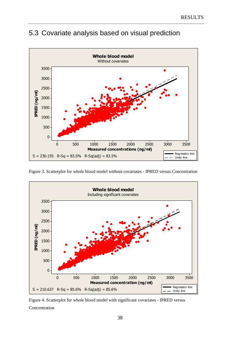
5.3 Covariate analysis based on visual prediction
3500300025002000150010005000
3500
3000
2500
2000
1500
1000
500
0
Measured concentrations (ng/ml)
IPR
ED
(n
g/
ml)
Regression line
Unity line
Whole blood modelWithout covariates
S = 230.155 R-Sq = 83.5% R-Sq(adj) = 83.5%
Figure 3. Scatterplot for whole blood model without covariates - IPRED versus Concentration
3500300025002000150010005000
3500
3000
2500
2000
1500
1000
500
0
Measured concentration (ng/ml)
IPR
ED
(n
g/
ml)
Regression line
Unity lineS = 210.637 R-Sq = 85.6% R-Sq(adj) = 85.6%
Whole blood modelIncluding significant covariates
Figure 4. Scatterplot for whole blood model with significant covariates - IPRED versus
Concentration

RESULTS
39
3500300025002000150010005000
3500
3000
2500
2000
1500
1000
500
0
Measured concentrations (ng/ml)
IPR
ED
(n
g/
ml)
Regression line
Unity line
Whole blood modelWith significant covariates and IOV
S = 206.800 R-Sq = 86.2% R-Sq(adj) = 86.2%
Figure 5. Scatterplot for whole blood model with significant covariates and interoccasional
variability - IPRED versus Concentration
The first three scatterplots (figure 3-5) show the development from the model without
covariates to the inclusion of significant covariates and finally with significant
covariates and interoccasional variability. There is a gradually improvement as seen
earlier by the decrease of OFV. The increasing R2 together with the decrease of S
show that there is a better fit and the regression line shows an improving description
of the data.

RESULTS
40
25002000150010005000
7.5
5.0
2.5
0.0
-2.5
-5.0
TIME (h)
WR
ES
Regression
Unity line
Whole blood model - Scatterplot of WRES vs. TIMEWith significant covariates and IOV
Figure 6. Whole blood model with significant covariates and IOV. Scatterplot of Wres vs. time.
180160140120100806040200
7.5
5.0
2.5
0.0
-2.5
-5.0
ID
WR
ES
Regression
Unity line
Whole blood model - Scatterplot of WRES vs. IDWith significant covariates and IOV
Figure 7. Whole blood model with significant covariates and IOV. Scatterplot of Wres vs. ID.

RESULTS
41
3500300025002000150010005000
7.5
5.0
2.5
0.0
-2.5
-5.0
IPRED
WR
ES
Regression
Unity line
Whole-blood model - Scatterplot of WRES vs. IPREDWith significant covariates and IOV
Figure 8. Whole blood model with covariates and IOV. Scatterplot Wres vs. ipred.
Figure 6-8 shows the final model with significant covariates and IOV, WRES versus
time, ID and population prediction (PRED). The weighted residuals (WRES) are
evenly distributed with time and identification (ID). WRES versus population
prediction (PRED) shows that the weighted residuals are tending towards the
negative side for the large concentration predictions implying that there is a small
over-prediction for the large concentrations.

RESULTS
42
Figure 9. Quality of fit plot, whole blood model with all significant covariates and IOV
Figure 10. Goodness of fit, whole blood model with all covariates and IOV
The remaining figures (9-10) are parts of the diagnostics plots drawn by R-script of
the final model. The figures show that POSTHOC gives an overall good prediction

RESULTS
43
for the final model. It also shows that NONMEM has small problems fitting the
concentrations on the highest and lowest end of the scale. Overall there is a good
prediction with an even spread around the regression line.
5.5 Comparing the old versus the new model
Table 7. Comparison of significant covariates from old model versus new model
Previous covariates* Current covariates
Parameter Covariates Parameter Covariates
CL Age CL Age
CRCL
Cyp3A5
V1 Age
V1 Age
Weight BMI
KA
TXT
KA
TXT
Age Age
Weight BMI
Q Weight
Steroid dose
*The last version of the model, the model used in the POPDOC-study.
Comparing the new model with the old model shows several similarities. Both
models are pretty accurate for the low to normal levels of CsA, but have some
difficulties predicting concentrations on the higher level of the scale. The covariates
found significant are majorly the same (table 7). Furthermore the scatter-plot of
weighted residuals are evenly distributed which is acceptable. The new model has
IOV included, which is expected, and this factor may be decisive of small, but
significant improvement of the model.

RESULTS
44
5.6 The whole blood and intracellular concentrations
5.6.1 Model building results
The data were LN-transformed and the necessary new error code was included in the
model. Using a proportional and an additive error code for the inter-individual
variability gave the best fit and lowest OFV.
1466
.00
1190
.20
1182
.30
1179
.40
1178
.20
986.00
842.00
674.00
458.00
218.00
2.00
14
13
12
11
10
9
8
7
6
5
TIME (h)
LN
Co
nce
ntr
ati
on
s (
LN
ng
/m
l) LNDV 1
LNDV 2
IPRE 1
IPRE 2
Variable DVID
Patient 7Comparison of observed/predicted concentrations versus time
12-hours PK
Figure 11. Patient 7, concentration vs. time. LNDV = 1 for whole blood concentrations, LNDV = 2
for intracellular concentrations and the corresponding IPRED = 1 for individual whole blood
predictions and IPRED = 2 for individual intracellular predictions. The y-scale (concentrations) is
presented on LN-scale while the x-scale is time (h). The time units are not homogenous, but rather
time measured when the different samples were taken. The graph is showing C0, C2 and 12-hours
profile data. The marked area represents the 12-hour profiles and enlarged in the figure below is the
12-hours profile for the same patient

RESULTS
45
1190
.2
1188
.2
1186
.3
1184
.3
1182
.3
1181
.3
1180
.3
1179
.8
1179
.4
1178
.8
1178
.5
1178
.2
12
11
10
9
8
7
6
5
TIME (h)
LN
co
nce
ntr
ati
on
s (
LN
ng
/m
l)
LNDV 1
LNDV 2
IPRE 1
IPRE 2
Variable DVID
Patient 7 - 12 hours profileComparison of observed/predicted concentrations versus time
Figure 12. Patient 7 – 12-hours PK-profile. For detailed description see Figure 11
2282
.00
1802
.00
1562
.00
1178
.00
914.00
554.00
441.83
435.93
434.22
266.00
50.00
12
11
10
9
8
7
6
5
4
3
TIME (h)
LN
co
nce
ntr
ati
on
s (
LN
ng
/m
l)
LNDV 1
LNDV 2
IPRE 1
IPRE 2
Variable DVID
Patient 10Comparison of observed/predicted concentrations versus time
12-hours PK
Figure 13. Patient 10 – concentrations vs. time. For detailed description see Figure 11

RESULTS
46
445.80
443.82
441.83
439.80
437.87
436.92
435.93
435.40
434.90
434.43
434.22
433.83
13
12
11
10
9
8
7
6
5
4
TIME (h)
LN
co
nce
ntr
ati
on
s (
LN
ng
/m
l)
LNDV 1
LNDV 2
IPRE 1
IPRE 2
Variable DVID
Patient 10 - 12 hours profileComparison of observed/predicted concentrations versus time
Figure 14. Patient 10 – 12-hours PK profile. For detailed description see Figure 11
1370
.00
1130
.00
866.00
650.00
386.00
170.00
36.18
30.10
27.63
26.32
2.00
14
13
12
11
10
9
8
7
6
5
TIME (h)
LN
co
nce
ntr
ati
on
s (
LN
ng
/m
l) LNDV 1
LNDV 2
IPRE 1
IPRE 2
Variable DVID
Patient 19Comparison of observed/predicted concentrations versus time
12-hours PK
Figure 15. Patient 19 – concentrations vs. time. For detailed description see Figure 11.

RESULTS
47
36.1834.1832.0730.1029.1228.1327.6327.1726.5726.3225.97
14
13
12
11
10
9
8
7
6
5
TIME (h)
LN
co
nce
ntr
ati
on
s (
LN
ng
/m
l)
LNDV 1
LNDV 2
IPRE 1
IPRE 2
Variable DVID
Patient 19 - 12 hours profileComparison of observed/predicted concentrations versus time
Figure 16. Patient 19 – 12-hours PK profile. For detailed description see Figure 11.
According to the graphical comparisons the whole blood and intracellular model is
able to tell the difference between the different observations. It seems as if it predicts
C2-levels better the trough concentrations. The model is to some degree able to
predict the large fluctuations of the observed concentrations. (Figure 11, 13 and 15)
The 12-hours profile is however rather inaccurate. (Figure 12, 14 and 16)
The absorption phase is wrongly estimated both for the whole blood and the
intracellular concentrations (Figure 12, 14, 16-19). The elimination phase is a little
over-predicted for the whole blood concentrations, and it does not match the
intracellular concentrations too well either.

RESULTS
48
121086420
40000
30000
20000
10000
0
Time (h)
Co
nce
ntr
ati
on
(n
g/
ml)
Observed
Predicted
Mean 12-hours PK with SEM-intervalIntracellular concentrations
Figure 17. Mean intracellular 12-hours profile, 12-hour profile for the mean observed and predicted
intracellular concentrations shown on a normal-scale versus a normal time-scale (h). The SEM-
interval is represented at each measurement.
121086420
150000
125000
100000
75000
50000
25000
0
Time (h)
Co
nce
ntr
ati
on
s (
ng
/m
l)
Observed
Predicted
Mean 12-hours PK with SEM-intervalWhole blood concentrations
Figure 18. Mean whole blood concentrations 12-hours profile. 12-hour profile for the mean observed
and predicted whole blood concentrations shown on a normal-scale versus a normal time-scale (h).
The variations on the predicted concentrations are represented by the SEM-interval.

RESULTS
49
121086420
1800
1600
1400
1200
1000
800
600
400
200
0
Time (h)
Co
nce
ntr
ati
on
s (
ng
/m
l)
Observed
Predicted
Mean 12-hours PK with SEM-intervalWhole blood concentrations
Reduced Y-scale
Figure 19. Mean whole blood concentrations 12-hours, DVID = 1 = Whole blood. 12-hour profile for
the mean observed and predicted whole blood concentrations shown on a reduced normal-scale
versus a normal time-scale (h). The variations on the observed concentrations are represented by the
SEM-interval.
Figure 17-19 are mean whole blood- and intracellular 12-hours PK profiles for the 9
patients. The figures confirm the earlier findings that the absorption phase is wrongly
estimated for both whole blood and intracellular measurements. The absorption phase
for whole blood predictions is too fast with a lower Tmax and a very increased Cmax,
but the elimination phase for the predicted is in the same ballpark-area as the
observed. For the intracellular 12-hours PK the absorption phase is very similar for
both the predicted and observed concentrations, with the predicted Cmax a little lower
than the observed and the Tmax a little earlier. The elimination phase is unfortunately
not similar for the predicted and observed concentrations.
The standard error of the mean (SEM) is represented as the interval for both the
observed (SEM = 3448.31) and the predicted concentrations (SEM = 2543.99) for
intracellular concentrations (figure 17). Regarding the whole blood measurements
SEMpredicted is very large (SEM = 11749.34) because of Cmax. Therefore SEM for
predicted whole blood concentrations are presented in figure 18 with a full Y-scale,

RESULTS
50
while SEM for the observed concentrations (SEM = 132.14) are presented in figure
19 with a reduced Y-scale.
14121086420
15.0
12.5
10.0
7.5
5.0
IPRE
LN
DV
1
2
DVID
Scatterplot LNDV vs. IPRED
Figure 20. Scatterplot of LNDV vs. IPRED. DVID = 1 is whole blood predictions, DVID = 2 is
intracellular predictions.
25002000150010005000
5.0
2.5
0.0
-2.5
-5.0
-7.5
TIME (h)
WR
ES
1
2
DVID
Scatterplot of WRES vs TIME
Figure 21. Scatterplot of WRES vs. time. DVID = 1 is whole blood predictions, DVID = 2 is
intracellular predictions.

RESULTS
51
20151050
5.0
2.5
0.0
-2.5
-5.0
-7.5
Identification - ID
WR
ES
1
2
DVID
Scatterplot of WRES vs ID
Figure 22. Scatterplot of WRES vs. ID. DVID = 1 is whole blood predictions, DVID = 2 is
intracellular predictions.
The scatterplot of LNDV versus IPRED (Figure 20) shows that the predictions are
still rather inaccurate. Figure 21 shows that the weighted residuals are stable over a
period of time, but the scatterplot of WRES versus ID (figure 22) shows for all
patients that the weighted residuals are negative for whole blood concentrations
which give an indication that the predictions are over-predicted.

DISCUSSIONS
52
6. DISCUSSIONS
6.1 Re-analyzing for covariates for CsA
plasmaconcentrations
As expected there were many covariates influencing different PK-parameters. During
forward inclusion several covariates showed statistical significant, but most proved
not to be significant after the backwards deletion process.
During backwards deletion (table 5) the model would not run without some
covariates. Due to the recommendation that only one or two parameters should be
changed in order to compare with the previous OFV, those covariates were kept and
marked “not applicable” (NA). [7]
Storehagen [49] and Le [48] used some of the same data for their thesis and it was
expected to find similar significant covariates. The covariate screening for their
theses included: age (years), gender (FLAG = 1 male, FLAG 2 = female), diabetes
(FLAG = 1 diabetic, FLAG 2 = non-diabetic), weight (kilos), height (centimeters),
post-transplantation (weeks), steroid dose at the pharmacokinetic day (mg), CYP3A5-
enzyme genotype (*1/x vs. *3/*3) and estimated creatinine clearance (ml/min).
The surgery performed in renal transplantation patients will most likely affect the
intestinal motility and hence absorption and bioavailability of CsA in the early post-
transplant phase. Therefore the post-transplantation time will presumably influence
the absorption constant Ka which also is found.
Patients gain up to 10% more bodyweight after transplantation and it is not surprising
that parameters like weight, lean-body-mass and body-mass-index can influence PK-
parameters like Ka, Q and distribution volume. After transplantation, patients are less
catabolic and they are able to eat more which might increase the body-fat. This is
supported by the findings of weight and weight-related (BMI) covariates influence on
Ka, Q and distribution volume.

DISCUSSIONS
53
Storehagen [49], Le [48], Falck [56] and Wu [57] have shown earlier that age has a
significant covariate for CL/F. With increasing age pharmacological changes such as
loss of liver-mass and the blood flow to liver is reduced, which influences the
metabolism and clearance of CsA. Physiological changes can also explain the
significance of age on parameters like volume and absorption. These factors
strengthen the findings in this thesis that age has a real effect on CL, V1 and Ka.
Cyclosporin A is metabolized by the cytochrom P450-system as mentioned earlier.
CYP 3A5 genotypes will most likely affect the clearance of CsA. In earlier studies
Storehagen [49] did not test this covariate because of various reasons, Le found this
covariate to be significant in a later study, but it was not included in the final model
because of clinical relevance.[48] It is therefore no surprise that this was shown to be
a significant covariate on clearance in this present version of the model.
Diabetes was tested and found non-significant in this thesis. It has been shown in
literature that diabetes may affect the absorption rate of CsA. [58] One reason why it
was not found significant in the present model may be due to the lack of detailed
description of diabetes in patients. It was only marked as FLAG = 1 diabetes and
FLAG = 2 non-diabetes. Some patients had diabetes before undergoing
transplantation and some patients developed diabetes after transplantation thus a more
detailed coding could have given a different result. This should be tested in the future
development of the model.
The covariates found to be statistical significant were mostly the same as previously
discovered by Storehagen, Le and Falck (table 7). This further supports the theory
that those covariates are statistical significant for this drug and drug model.
Overall the OFV decreased significantly during the development of the model, which
gives a strong indication that the inclusion of covariates improves the model.
However, the graphs showing concentration vs. individual predictions do not give an
unambiguous answer. There might be a slightly better population prediction with the
inclusion of covariates but this is very difficult to see from the figures. There are
minor signs indicating that the model with covariates has less spread and that the

DISCUSSIONS
54
divergence starts a little later. A more secure way of determining this is by looking at
the decrease of OFV. Along with the R2 value and S-value for the regression line for
the observation versus predictions (Figure 3-4) shows that there is an improvement of
the model.
6.2 Testing for interoccasional variability for the whole
blood model
Based on the results from the POPDOC-study there is reason to suspect significant
inter-occasional variability. [54] Due to many visits per patients the chances
increased to detect if there is something “unexplainable” that happens between
different visits. There are patients that have a variation that cannot be explained with
covariates and intra- and inter-individual variability. This gives a strong indication
that there is something more that influences patients PK-parameters.
NONMEM has a limit of etas before there is an error statement from FORTRAN.
There are ways to avoid this problem, but it requires a degree of competence in
NONMEM coding that is beyond the scope of this research group. Because of this
limitation it was only possible to code 11 visits per patients which could be a reason
why the visits were not shown more significant than when coding each measurement-
date as one separate visit. The maximum number of visits one patient had was 34
visits, thus that way of coding accounted for roughly 40% of the visits.
When coding every other date as separate visits there was an improvement (decrease)
in OFV. There was a decrease of 30.56 when including IOV to the parameter V2
(table 6), making the model significant better with IOV than without. Another
advantage of coding every other visit as one visit comparing to coding every visit as
its own, is that about 65% of the visits are included, and the time perspective is kept.
Still there are some visits that are not accounted for. A hypothesis is that coding every
visit as “its own visit” will enhance the model further. Another way to do this is by

DISCUSSIONS
55
looking at the data and picking the data where there is suspicion of IOV and code
only these visits.
Moreover there are also some covariates that are believed to influence the different
parameters e.g. diabetes. [58] Including all of these factors may improve the model
and make it even better than it is today.
From a graphical inspection it is hard to determine which model gives the best fit.
Due to a large data set there are too many observations to give an unambiguous
answer. Still, by looking again at the R2- and S-value for the regression line an
improvement is visible from the starting model without covariates to the model
including covariates and finally the model including covariates and IOV. Similarly,
by looking at the OFV the value is decreased by first including covariates and then
including IOV.
Another way to determine the best model would be a visual prediction check. [59]
One way to do this is to program R-script. There also exist different add-on programs
to NONMEM for example xPose, Wings, PsN, which gives a possibility to draw
more complex graphs. To do this it is necessary to have to have a stand-alone
NONMEM installation, which was not available. More detailed graphs would provide
an even better foundation to determine which model that had the best data fit.
6.3 Whole blood and intracellular model
The first step to overcome was to make NONMEM to differ between the whole blood
observations from the intracellular observations. This was an extremely challenging
task and was more difficult than first imagined. An unexpected hinder was the run
time the model had. In the beginning most runs used approximately 1 day. After the
transformation of intracellular concentrations from ng/106 cells to the same unit
(ng/ml), as the whole blood concentrations were measured in, there was an enormous
range from whole blood concentrations to intracellular concentrations. This large
range made data fitting nearly impossible. Finally after LN transforming the

DISCUSSIONS
56
concentrations there were difficulties finding the correct error code to include in the
model. In the end when the data fittings at last seemed promising, time was running
out.
The final model seems capable of predicting the concentrations at two different sites.
The WRES vs. time/ID shows an overall over-prediction for the intracellular
concentrations and an under-prediction for the whole blood values. The over-
prediction of whole blood concentration is largely due to the Cmax in the 12-hours PK.
The difference between predicted value and observed concentration is so high that it
will affect the mean prediction power. It seems as though the model fits the C2-levels
slightly better than the C0-concentrations, but it still has trouble fitting the large
variety of concentrations.
For the 12-hours whole blood profile it is visible that the model has large problems in
the absorption phase, which indicates that the Ka is over estimated. The elimination
however seems to be rather accurate compared to the absorption phase. It is obvious
that Ka is estimated wrongly when NONMEM predicts it to be 55 on a LN-scale. The
high Ka is the reason for the high predicted Cmax for whole blood (140000 ng/ml –
1600 ng/ml – figure 18-19). The high Cmax increases the SEM which makes the
predictive power worse as mentioned earlier.
An attempt to force/lock Ka to a lower value resulted in a more correct Cmax for
whole blood. Cmax went from 140000 ng/ml to 22000 ng/ml compared to 1600 ng/ml,
but resulted in a more identical whole blood and intracellular prediction with a lack of
concentration-variety. (Appendix 9.8) The absorption-phase is also delayed with Tmax
estimated to be approximately 1 hour later than the true value. (Figure 17-19)
The intracellular 12-hours profile has predictions in the same range as the measured
observations. The absorption phase is however slightly delayed. The absorption into
the intracellular compartment is estimated to be a 1.order reaction. This is a
reasonable assumption by looking at the measured concentrations and considering
there is a passive diffusion of CsA into T-lymphocytes and not an active transport. It
could be an idea to test other absorption-profiles to find a more fitting description.

DISCUSSIONS
57
The concentrations/LNDV vs. Ipred did not attain the desired degree of consistent
prediction. (Figure 20) The “inclusion” of the whole blood model has not been
optimal. One way to possibly improve this model is the inclusion of covariates.
However, before the covariates are tested the basic model needs to be improved,
especially the absorption rate constant, and the absorption and elimination processes.
The model is still in an early stage and needs to be further developed.
Since the model is still in a development phase it is premature to validate the model.
After further development with the inclusion of covariates and IOV the model should
be validated following FDA’s guidelines. [5] The validation process consists of
external validation (including new patients) or internal (using the existing data set). A
useful and common validation method for this data set could be cross-validation,
bootstrapping and Jackknife.
In a retrospective view it should be possible to develop a model based on the original
intracellular data. NONMEM does not understand units, meaning it only reads
numbers. Accordingly it should be possible to develop a model based on the original
data and unit (ng/106 cells). Doing this has many benefits i.e. there is no need to
transform data, future data can be measured the same way and included directly into
the model. Because the range is similar, plotting graphs will also be easier. When
both whole blood and intracellular concentrations are in the same graphs it will be
easier to interpret the plots as well.

CONCLUSIONS
58
7. CONCLUSIONS
Re-analyzing for covariates in the whole blood model was performed using the
traditional forward-inclusion criteria and the backwards-deletion process. The result
cohered with similar finding in earlier results. This substantiates earlier findings that
these covariates are relevant for this drug/model.
Interoccasional variability was included and found significant for V2. With both
covariates and IOV included, the model for whole blood has improved. The model is
accurate for low and normal concentrations, but has a tendency to over-predict
concentrations at the higher end of the scale. The predictions are however stable and
show little spread.
A model for whole blood- and intracellular concentration was initially developed
from the previous model. The model seems capable of predicting different
concentrations at different sites of measurements. There is generally a better
prediction of C2-levels compared to C0-levels. The model has however its weaknesses
however that is quite visible in the 12-hours PK. The absorption phase for both whole
blood and intracellular concentrations are not optimal and the elimination phase is
wrongly predicted. There is a need to continue working on the basic model before
covariates are to be included, IOV have to be checked and finally the model has to be
validated.
There are several reasons to continue working on this model. In theory a PPK-model
will predict concentrations more accurately and stable than in the current clinical
setting and a prediction of intracellular concentrations may prevent more rejections
from kidney transplants.

REFERENCES
59
8. REFERENCES
1. Rowland, M.a.T.N.T., Clinical pharmacokinetics: concepts and applications.
3 ed. 1995, Philadelphia: Lippincott Williams & Wilkins.
2. Atkinson, A.J., Jr. and R.L. Lalonde, Introduction of quantitative methods in
pharmacology and clinical pharmacology: a historical overview. Clin
Pharmacol Ther, 2007. 82(1): p. 3-6.
3. Ette, E.I. and P.J. Williams, Population pharmacokinetics I: background,
concepts, and models. Ann Pharmacother, 2004. 38(10): p. 1702-6.
4. Sun, H., et al., Population pharmacokinetics. A regulatory perspective. Clin
Pharmacokinet, 1999. 37(1): p. 41-58.
5. U.S. Department of Health and Human Services, F., CDER, CBER, Guidance
for Industry Population Pharmacokinetics.
http://www.fda.gov/CDER/guidance/1852fnl.pdf, 1999.
6. Sheiner, L. and J. Wakefield, Population modelling in drug development. Stat
Methods Med Res, 1999. 8(3): p. 183-93.
7. Shafer S.L, F.D., Pharmacokinetic and Pharmacodynamic Analysis with
NONMEM Basic Concepts. Fisher/Shafer NONMEM Workshop
Pharmacokinetics and Pharmacodynamics Analysis with NONMEM, Het
Pand, Ghent, Belgium, 2007.
8. Karlsson M. O, S.L.B., The importance of modeling interoccasion variability
in population pharmacokinetic analysis. Journal of pharmacokinetics and
biopharmaceutics, 1993. 21(6): p. 735.
9. Sheiner, L.B. and J.L. Steimer, Pharmacokinetic/pharmacodynamic modeling
in drug development. Annu Rev Pharmacol Toxicol, 2000. 40: p. 67-95.
10. Ette, E.I. and P.J. Williams, Population pharmacokinetics II: estimation
methods. Ann Pharmacother, 2004. 38(11): p. 1907-15.
11. Jelliffe, R., A. Schumitzky, and M. Van Guilder, Population
pharmacokinetics/pharmacodynamics modeling: parametric and
nonparametric methods. Ther Drug Monit, 2000. 22(3): p. 354-65.
12. Shaw, L.M., et al., Current opinions on therapeutic drug monitoring of
immunosuppressive drugs. Clin Ther, 1999. 21(10): p. 1632-52; discussion
1631.
13. Jelliffe, R., Goal-oriented, model-based drug regimens: setting individualized
goals for each patient. Ther Drug Monit, 2000. 22(3): p. 325-9.
14. Yafune, A. and M. Ishiguro, Bootstrap approach for constructing confidence
intervals for population pharmacokinetic parameters. II: A bootstrap
modification of standard two-stage (STS) method for phase I trial. Stat Med,
1999. 18(5): p. 601-12.
15. Sheiner, L.B. and S.L. Beal, Evaluation of methods for estimating population
pharmacokinetics parameters. I. Michaelis-Menten model: routine clinical
pharmacokinetic data. J Pharmacokinet Biopharm, 1980. 8(6): p. 553-71.

REFERENCES
60
16. Sheiner, B.L. and S.L. Beal, Evaluation of methods for estimating population
pharmacokinetic parameters. II. Biexponential model and experimental
pharmacokinetic data. J Pharmacokinet Biopharm, 1981. 9(5): p. 635-51.
17. Ette, E.I. and P.J. Williams, Population pharmacokinetics II: Estimation
methods. Annals of Pharmacotherapy, 2004. 38(11): p. 1907-1915.
18. Beal S, S.L., ed. NONMEM Users Guide - Part VII Conditional Estimation
Methods. ed. N.P. group. 1998, University of California at San Francisco. 23.
19. Borel, J.F., et al., Biological effects of cyclosporin A: a new antilymphocytic
agent. Agents Actions, 1976. 6(4): p. 468-75.
20. Tutschka, P.J., Cyclosporin A - A new outlook for Immunosupression in
Clinical Transplantation. BLUT, 1979(39): p. 81-87.
21. Stahelin, H.F., The history of cyclosporin A (Sandimmune) revisited: another
point of view. Experientia, 1996. 52(1): p. 5-13.
22. Hariharan, S., et al., Improved graft survival after renal transplantation in the
United States, 1988 to 1996. N Engl J Med, 2000. 342(9): p. 605-12.
23. E.M.T, G., Cyclosporin in cadaveric renal transplantation: one-year follow-
up of a multicentre trial. Lancet, 1983. 2(8357): p. 986-9.
24. Thorsby, E., [Transplantation medicine in Norway through 50 years]. Tidsskr
Nor Laegeforen, 2006. 126(24): p. 3305-10.
25. Rang H.P, D.M.M., Ritter J.M, Pharmacology. Vol. 4. 1999: Edinburgh:
Churchill Livingstone. 830.
26. Borel, J.F. and H.C. Gunn, Cyclosporine as a new approach to therapy of
autoimmune diseases. Ann N Y Acad Sci, 1986. 475: p. 307-19.
27. Foxwell, B.M., et al., A comparison of cyclosporine binding by cyclophilin
and calmodulin. Transplant Proc, 1989. 21(1 Pt 1): p. 873-5.
28. Resch, K. and M. Szamel, Molecular mechanisms of the immunosuppressive
action of cyclosporin A. Int J Immunopharmacol, 1997. 19(9-10): p. 579-85.
29. Barbari, A., et al., Cyclosporine lymphocyte level and lymphocyte count: new
guidelines for tailoring immunosuppressive therapy. Transplant Proc, 2003.
35(7): p. 2742-4.
30. Barbari, A., et al., Cyclosporine lymphocyte versus whole blood
pharmacokinetic monitoring: correlation with histological findings.
Transplant Proc, 2001. 33(5): p. 2782-5.
31. Borel, J.F., History of the discovery of cyclosporin and of its early
pharmacological development. Wien Klin Wochenschr, 2002. 114(12): p. 433-
7.
32. legemiddelverk, S., SPC - Sandimmun. 1994, Statens legemiddelverk -
http://www.legemiddelverket.no/custom/Preparatsok/prepSearch____80333.as
px?SearchID=9262d12e-9241-4f1f-9462-5fa361a68307: Oslo.
33. Rousseau, A., et al., Population pharmacokinetic modeling of oral cyclosporin
using NONMEM: comparison of absorption pharmacokinetic models and
design of a Bayesian estimator. Ther Drug Monit, 2004. 26(1): p. 23-30.
34. Drewe, J., C. Beglinger, and T. Kissel, The absorption site of cyclosporin in
the human gastrointestinal tract. Br J Clin Pharmacol, 1992. 33(1): p. 39-43.
35. Christians, U. and K.F. Sewing, Cyclosporin metabolism in transplant
patients. Pharmacol Ther, 1993. 57(2-3): p. 291-345.

REFERENCES
61
36. Wenger, R.M., Structures of cyclosporine and its metabolites. Transplant Proc,
1990. 22(3): p. 1104-8.
37. Lemahieu, W.P., et al., CYP3A4 and P-glycoprotein activity in healthy
controls and transplant patients on cyclosporin vs. tacrolimus vs. sirolimus.
Am J Transplant, 2004. 4(9): p. 1514-22.
38. Hesselink, D.A., et al., Population pharmacokinetics of cyclosporine in kidney
and heart transplant recipients and the influence of ethnicity and genetic
polymorphisms in the MDR-1, CYP3A4, and CYP3A5 genes. Clin Pharmacol
Ther, 2004. 76(6): p. 545-56.
39. Christians, U. and K.F. Sewing, Alternative cyclosporine metabolic pathways
and toxicity. Clin Biochem, 1995. 28(6): p. 547-59.
40. Lemahieu, W.P., et al., Alterations of CYP3A4 and P-glycoprotein activity in
vivo with time in renal graft recipients. Kidney Int, 2004. 66(1): p. 433-40.
41. Knight, S.R. and P.J. Morris, The clinical benefits of cyclosporine C2-level
monitoring: a systematic review. Transplantation, 2007. 83(12): p. 1525-35.
42. Wang, S.M., et al., Optimal C2 concentration of cyclosporin corrected with
good efficacy and safety in Asian kidney transplant recipients. Transplant
Proc, 2008. 40(7): p. 2243-4.
43. Masri, M.A., et al., Measurement of lymphocyte cyclosporine levels in
transplant patients. Transplant Proc, 1998. 30(7): p. 3561-2.
44. Barbari, A.G., et al., Cyclosporine lymphocyte maximum level: a new
alternative for cyclosporine monitoring in kidney transplantation. Exp Clin
Transplant, 2005. 3(1): p. 293-300.
45. Falck, P., et al., Declining intracellular T-lymphocyte concentration of
cyclosporine a precedes acute rejection in kidney transplant recipients.
Transplantation, 2008. 85(2): p. 179-84.
46. Fanta, S., et al., Developmental pharmacokinetics of ciclosporin--a population
pharmacokinetic study in paediatric renal transplant candidates. Br J Clin
Pharmacol, 2007. 64(6): p. 772-84.
47. Flechner, S.M., et al., The impact of body weight on cyclosporine
pharmacokinetics in renal transplant recipients. Transplantation, 1989. 47(5):
p. 806-10.
48. Le, T., A pharmacokinetic population model for Cyclosporine A in renal
transplant recipients, in Pharmaceutical Biosciences. 2008, University in
Oslo: Oslo. p. 95.
49. Storehagen, Cyclosporin A - Developement of a pharmacokinetic population
model, in Pharmaceutical Bioscience. 2007, University in Oslo: Oslo. p. 80.
50. Porta Oltra, B., et al., [Cyclosporin pharmacokinetic modeling in renal
transplant patients]. Farm Hosp, 2004. 28(1): p. 5-19.
51. Sallas, W.M., et al., A nonlinear mixed-effects pharmacokinetic model
comparing two formulations of cyclosporine in stable renal transplant
patients. J Pharmacokinet Biopharm, 1995. 23(5): p. 495-514.
52. Falck P, e.a., Reduced elimination of cyclosporine A in elderly (>65) kidney
transplant recipients. Submitted to Transplantation, 2008.

REFERENCES
62
53. Falck, P.e.a., Cinacalcet's effect on the pharmacokinetics of tacrolimus,
cyclosporine and mycophenolate in renal transplant recipients. Nephrology
Dialysis Transplantation, 2008. 23(3): p. 1048-1053.
54. Åsberg, A., Manuscript under preparation. 2009.
55. Falck, P., et al., Determination of ciclosporin A and its six main metabolites in
isolated T-lymphocytes and whole blood using liquid chromatography-tandem
mass spectrometry. J Chromatogr B Analyt Technol Biomed Life Sci, 2007.
852(1-2): p. 345-52.
56. Falck P, M.K., Le T et al., A population pharmacokinetic model of
Cycosporine A - A applicable for assisting dose management of kidney
transplant recipients
Unpublished article, 2009.
57. Wu, K.H., et al., Population pharmacokinetics of cyclosporine in clinical renal
transplant patients. Drug Metab Dispos, 2005. 33(9): p. 1268-75.
58. Mendonza, A.E., R.Y. Gohh, and F. Akhlaghi, Blood and plasma
pharmacokinetics of ciclosporin in diabetic kidney transplant recipients. Clin
Pharmacokinet, 2008. 47(11): p. 733-42.
59. Lindbom, L., P. Pihlgren, and E.N. Jonsson, PsN-Toolkit--a collection of
computer intensive statistical methods for non-linear mixed effect modeling
using NONMEM. Comput Methods Programs Biomed, 2005. 79(3): p. 241-57.
60. Hume, R., Prediction of lean body mass from height and weight. J Clin Pathol,
1966. 19(4): p. 389-91.

APPENDIX
63
9. APPENDIX
9.1 Formulas used in demographics model
Equation 12: BMI-formula:
BMI = weight (kg) / (height (m))2
Equation 13: Hume LBM-formula [60]:
(Male): L.B.M = 0.32810 W (Weight/kg) + 0.33929 H (Height/cm) – 29.5336
(Female): L.B.M = 0.29569 W (Weight/kg) + 0.41813 H (Height/cm) – 43.2933
Equation 14: Cockgroft-Gault Equation:
GFR = (140-age(years) x weight (kg)) x (0.85 for women)
72 x Serum creatinine (mg/dl)

APPENDIX
64
9.2 Partial input file for whole blood model

APPENDIX
65

APPENDIX
66
9.3 Control file for final model whole blood
$PROBLEM IOV.
$DATA valider-iov.txt
$INPUT ID AMT RATE=DROP DAT1=DROP TIME C=DV VIST WT UREA=DROP SCR=DROP
CRCL MDV SS II CMT FLAG=DROP AGE GEN HGHT TXT STER BMI C3A5 LBM
$SUBROUTINE ADVAN4
$PK
IF(C3A5.EQ.1) THEN
TVCL=THETA(1)-(THETA(8)*CRCL)-(THETA(9)*AGE/56)
ELSE
TVCL=THETA(7)-(THETA(8)*CRCL)-(THETA(9)*AGE/56)
ENDIF
TVV1=THETA(2)*THETA(10)*BMI/THETA(11)*(AGE/56)
TVQ=THETA(3)-THETA(12)*(1+STER/100)+THETA(13)*WT
TVV2=THETA(4)
TVKA=THETA(5)*THETA(14)**TXT/5*(THETA(15)*BMI)+THETA(16)*AGE/56
TVALAG=THETA(6)
IOV = ETA(1)
IF (VIST.EQ.2) IOV = ETA(2)
IF (VIST.EQ.3) IOV = ETA(3)
IF (VIST.EQ.4) IOV = ETA(4)
IF (VIST.EQ.5) IOV = ETA(5)
IF (VIST.EQ.6) IOV = ETA(6)
IF (VIST.EQ.7) IOV = ETA(7)
IF (VIST.EQ.8) IOV = ETA(8)
IF (VIST.EQ.9) IOV = ETA(9)
IF (VIST.EQ.10) IOV = ETA(10)
IF (VIST.EQ.11) IOV = ETA(11)
CL=TVCL*EXP(ETA(12)) ;Clearance (CL/F) L/hr
V1=TVV1*EXP(ETA(13)) ;Central volume (V1/F), L
Q=TVQ*EXP(ETA(14)) ;Intercompartmental clearance (Q/F)
V2=TVV2*EXP(ETA(15)+IOV) ;Peripheral volume (V2/F), L
KA=TVKA*EXP(ETA(16)) ;Absorption rate constant, 1/hr
ALAG1=TVALAG*EXP(ETA(17)) ;Absorption lag time, hr
S2=V1
K=CL/V1
K23=Q/V1
K32=Q/V2
$ERROR
IPRED=F
Y=F+F*ERR(1)+ERR(2)
$THETA (1,36.6) ;THETA(1) is POPCL/F on C3A5
$THETA (15, 21.9, 40) ;THETA(2) is POPV1/F

APPENDIX
67
$THETA (1,18.6) ;THETA(3) is POPQ/F
$THETA (1,1200) ;THETA(4) is POPV2/
$THETA (0,0.821,1) ;THETA(5) is POPKA
$THETA (0.1,0.452) ;THETA(6) is POPLAGTIME
$THETA (1, 38) ;THETA(7) is POPCL/F on C3A5
$THETA (0, 0.0047) ;THETA(8) is CRCL on CL
$THETA (0, 10.6) ;THETA(9) is AGE on CL
$THETA (0, 0.0001) ;THETA(10)is BMI on V1
$THETA (0, 0.0012) ;THETA(11)is AGE on V1
$THETA (0, 0.0001) ;THETA(12)is STER on Q
$THETA (0, 0.001) ;THETA(13)is WT on Q
$THETA (0, 0.006) ;THETA(14)is TXT on ka
$THETA (0, 265) ;THETA(15)is BMI on ka
$THETA (0, 2.1) ;THETA(16)is AGE on ka
$OMEGA BLOCK(1) 0.1
$OMEGA BLOCK SAME
$OMEGA BLOCK SAME
$OMEGA BLOCK SAME
$OMEGA BLOCK SAME
$OMEGA BLOCK SAME
$OMEGA BLOCK SAME
$OMEGA BLOCK SAME
$OMEGA BLOCK SAME
$OMEGA BLOCK SAME
$OMEGA BLOCK SAME
$OMEGA 0.04 ;IIV CL
$OMEGA 0.01 ;BSVV1/F
$OMEGA 0.01 ;BSVQ/F
$OMEGA 2.77 ;BSVV2/F
$OMEGA 0.563 ;BSVKA
$OMEGA 0.006 ;BSVALAG1
$SIGMA 0.041 ;ERRCV, Proportional error (%)
$SIGMA 388 ;ERRSD, Additive error (ug/ml)
$ESTIMATION SIG=3 METHOD=1 INTER MAXEVAL=9999 PRINT=1 POSTHOC NOABORT
$TABLE ID TIME DV IPRED MDV
NOPRINT ONEHEADER FILE=table.txt
$TABLE ID CL V1 Q V2 KA ALAG1 WT CRCL AGE GEN HGHT TXT STER BMI C3A5 LBM
FIRSTONLY NOPRINT ONEHEADER NOAPPEND FILE=etatable.txt

APPENDIX
68
9.4 Individual fitting made by R for final whole blood model
Circles: Observed concentrations; Red: Individual post hoc predicted concentrations;
Blue: Population predicted concentrations.
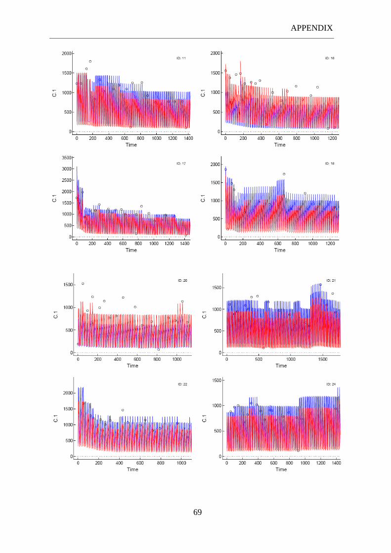
APPENDIX
69

APPENDIX
70

APPENDIX
71

APPENDIX
72

APPENDIX
73

APPENDIX
74

APPENDIX
75

APPENDIX
76

APPENDIX
77
9.5 Partial input file for whole blood and intracellular model

APPENDIX
78

APPENDIX
79

APPENDIX
80
9.6 Control file for final model whole blood and intracellular
concentrations
$PROBLEM EXAMPLE OF A THREE COMPARTMENT MODEL ABSORPTION INCLUDING
INTRACELLULAR VALUES AS METABOLITES
$INPUT ID AMT RATE=DROP DAT1=DROP TIME LNDV=DV EVID WT=DROP UREA=DROP
SCR=DROP CRCL=DROP SS=DROP II=DROP CMT DVID FLAG=DROP AGE=DROP GEN=DROP
HGHT=DROP TXT=DROP STER=DROP BMI=DROP C3A5=DROP LBM=DROP
$DATA ic.txt
$SUBROUTINES ADVAN6 TOL=4
$MODEL
COMP=(ABSORB)
COMP=(CENTRAL)
COMP=(INTRAC)
COMP=(PERIPH)
$PK
KA=THETA(1)*EXP(ETA(1))
CL2=THETA(2)
CL3=THETA(3)
CL4=THETA(4)*EXP(ETA(2))
V2=THETA(5)
V3=THETA(6)
V4=THETA(7)
K12=KA ; for matrix exponential solution
K20=CL2/V2
K23=CL3/V2
K32=CL3/V3
K24=CL4/V2
K42=CL4/V4
S2=V2
S3=V3
S4=V4
A_0(2)=0
A_0(3)=0
A_0(4)=0
$DES
DADT(1)= -KA*A(1)
DADT(2)= KA*A(1)-(A(2)*(K20+K23+K24))+A(3)*K32+A(4)*K42
DADT(3)= A(2)*K23-A(3)*K32
DADT(4)= A(2)*K24-A(4)*K42
$ERROR
PLASMA=A(2)/V2
INTRAC=A(3)/V3
IPRED=A(2)/V2
IF (DVID.EQ.2) INTRAC=A(3)/V3

APPENDIX
81
IPRED=0.001
IF(F.GT.0) IPRED=LOG(F)
W=SQRT(THETA(7)**2+THETA(8)**2/(F+0.001)**2)
IRES=DV-IPRED
IWRES = IRES/W
Y=IPRED+W*ERR(1)
$THETA
(0, 55)
(0, 3)
(0, 0.002)
(0, 0.9)
(0, 1.5)
(0, 0.006)
(0, 17.3)
(0.3)
$OMEGA
0.00136
1
$SIGMA
0.008
$ESTIMATION SIG=3 METHOD=1 INTER MAXEVAL=9999 PRINT=1 POSTHOC NOABORT
$TABLE ID TIME DV DVID IPRED MDV
NOPRINT ONEHEADER FILE=table.txt
$TABLE ID CL V1 V2 V3 KA ETA1 ETA2 ETA3 ETA4 ETA5 ETA6 ETA7 WT CRCL FLAG
AGE GEN HGHT TXT STER BMI C3A5 LBM FIRSTONLY NOPRINT ONEHEADER NOAPPEND
FILE=etatable.txt

APPENDIX
82
9.7 Diagnostic plot made by R for whole blood and
intracellular model
Circles: Observed concentrations; Red: Individual post hoc predicted concentrations;
Blue: Population predicted concentrations.
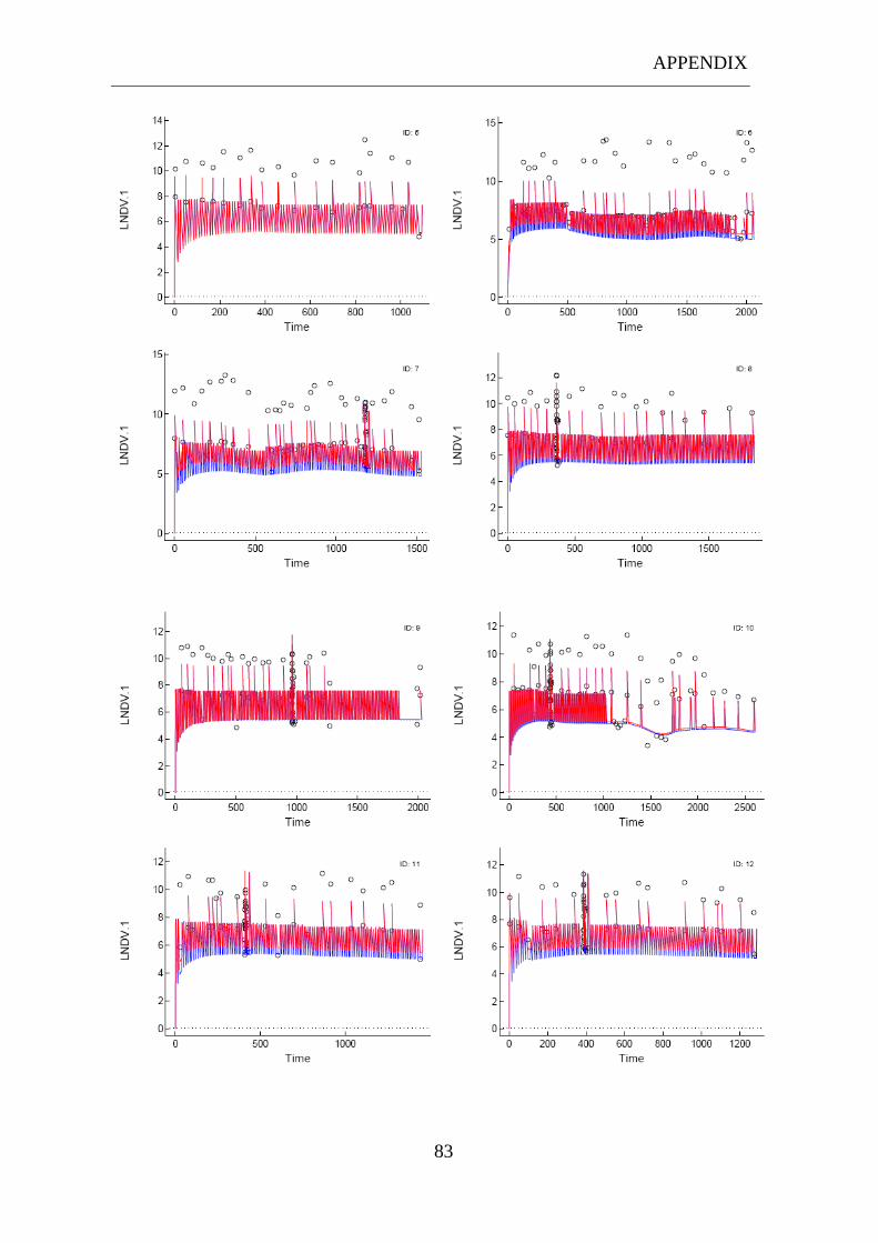
APPENDIX
83
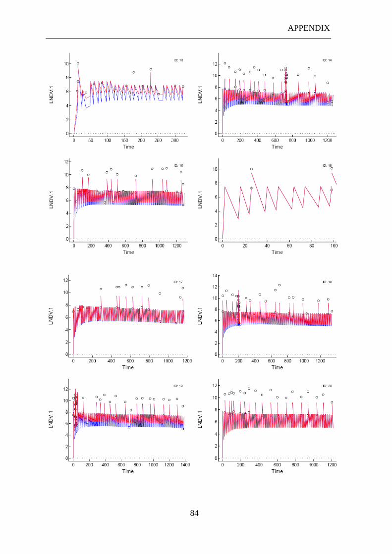
APPENDIX
84

APPENDIX
85
9.8 Diverse figures for whole blood and intracellular model
with a lower Ka and OFV comparing with the final
model
121086420
60000
50000
40000
30000
20000
10000
0
Time (h)
Co
nce
ntr
ati
on
(n
g/
ml)
Observed
Predicted
Variable
Mean 12-hours PKIntracellular concentrations

APPENDIX
86
121086420
20000
15000
10000
5000
0
Time (h)
Co
nce
ntr
ati
on
(n
g/
ml)
Observed
Predicted
Variable
Mean 12-hours PKWhole blood concentrations
121086420
2000
1500
1000
500
0
Time (h)
Co
nce
ntr
ati
on
(n
g/
ml)
Observed
Predicted
Variable
Mean 12-hours PKWhole blood concentrations
Reduced Y-scale

APPENDIX
87
1466
.00
1190
.20
1182
.30
1179
.40
1178
.20
986.00
842.00
674.00
458.00
218.00
2.00
14
13
12
11
10
9
8
7
6
5
TIME
Da
ta
LNDV 1
LNDV 2
IPRE 1
IPRE 2
Variable DVID
Patient 7
2282
.00
1802
.00
1562
.00
1178
.00
914.00
554.00
441.83
435.93
434.22
266.00
50.00
12
11
10
9
8
7
6
5
4
3
TIME
Da
ta
LNDV 1
LNDV 2
IPRE 1
IPRE 2
Variable DVID
Patient 10

APPENDIX
88
1370
.00
1130
.00
866.00
650.00
386.00
170.00
36.18
30.10
27.63
26.32
2.00
12
11
10
9
8
7
6
5
TIME
Da
ta
LNDV 1
LNDV 2
IPRE 1
IPRE 2
Variable DVID
Patient 19


