
A Salesforce-Driven Model of Consumer Choice
Bicheng Yang UBC Sauder School of Business University of British Columbia
Tat Chan
Olin Business School Washington University in St. Louis
Raphael Thomadsen Olin Business School
Washington University in St. Louis
1
A Salesforce-Driven Model of Consumer Choice
Abstract
This paper studies how salespeople affect the choices of which product consumers choose, and
from that, how a firm should set optimal commissions as a function of the appeal, substitutability
and profit margins of different products. We also examine whether firms are better off promoting
products through sales incentives or price discounts. To achieve these goals, we develop a
salesforce-driven consumer choice model to study how performance-based commissions
incentivize a salesperson’s service effort toward heterogeneous, substitutable products carried by
a firm. The model treats the selling process as a joint decision by the salesperson and the consumer.
It allows the salesperson’s efforts to vary across different transactions depending on the unique
preferences of each consumer, and incorporates the effects of commissions and other marketing
mix on the selling outcome in a unified framework. We estimate the model using data from a car
dealership. We find that the optimal commissions should be lower for popular items and for items
that are closer substitutes with other products. We also find that for the car industry we study, the
cost of selling more cars using sales incentives is cheaper than the cost of selling the same number
of cars using price discounts.
Keywords: Salesforce management, Incentives, Consumer choice, Differentiated products
2
1. Introduction
A firm’s salesforce is an important marketing tool for both B2C and B2B environments (Kotler
and Keller 2008). Data from the Bureau of Labor Statistics show that in 2012 about 14 million
people—more than 10% of the workforce—were employed in sales-related occupations. The
amount that firms spend on their salesforce is three times as high as spending on advertising
(Zoltners et al. 2008). These statistics suggest salespeople’s effort can have a significant influence
on demand; otherwise, firms would not invest as much in their salesforce.
The traditional consumer-choice literature typically assumes consumers make purchase
decisions on their own, with a focus on how a firm’s marketing mix (e.g. price promotion)
influences their decisions. In reality, consumers may not have complete market information, and
the effort from salespeople (e.g., product persuasion, recommendation, and demonstration) can
shift consumers’ product preferences and thus increase sales. We observe this impact from the
sales-management literature, which measures how performance-based commissions help increase
sales. The research focus in many of these studies is on designing the optimal compensation
structure that solves the classic principal-agent problem. The impact of commissions on consumers’
product choices, however, has not been investigated.
This paper studies how, in a market of differentiated products, commissions influence not
only the total sales but also which products consumers choose. The commissions set for selling
various products can incentivize salespeople to allocate different levels of efforts across products
and, together with other marketing mix elements that directly influence the consumer preferences,
impact the product consumers choose. To understand this deeper, we develop a model that
simultaneously incorporates the decisions of salespeople and consumers. The selling process is
structurally modeled as a joint decision that involves two sides: although the consumer makes the
3
final product choice, the salesperson’s decision of how much service effort to invest in each
product influences the consumer’s choice. This salesforce-driven consumer-choice model enables
us to infer the effects of commissions and other marketing mix elements on demand. We
empirically estimate this model from a dataset provided by a car dealership in Japan, and use the
results to investigate how commissions should be set differently across the dealer’s multiple
products. We then study the effectiveness of increasing commissions as a “push” strategy, versus
discounting prices as a “pull” strategy, to increase the sales of a product. The findings are important
for firms that sell diverse substitutable products.
Our study bridges the consumer-choice literature and the sales-management literature by
studying decisions on both sides. The majority of the sales-management literature has focused on
the salesforce productivity, and the design of the compensation structure based on aggregate sales
(see Mantrala et al. 2010 for a thorough overview). From a theoretical analysis, Basu et al. (1986)
and Rao (1990) show that a combination of salary plus nonlinear commission with respect to sales
is optimal using a common principal-agent framework that links a salesperson’s effort to total sales.
Empirically, Misra and Nair (2011) estimate a dynamic principal-agent model to estimate the
effectiveness of commissions that are combined with quotas and ceilings. They find that the
presence of ceilings on commissions demotivates effort. Chung et al. (2014) study a compensation
scheme with quotas and bonuses using a dynamic structural model as well, but include latent-class
heterogeneity and estimate the discount factors. Daljord et al. (2016) examine the implication of a
uniform compensation policy on a firm with a heterogeneous salesforce team, and suggest that
while the homogenous plan leads to a much lower profit relative to a fully heterogeneous plan, the
ability to choose salespeople mitigates the loss. A key missing component in all of these papers is
consumers, as they only look at the link between compensation and aggregate sales. Kim (2014)

4
incorporates consumers, but focuses on the impact of sales representatives on a single product (i.e.,
car radiator). Our paper extends this literature by noting the fact that there are multiple
differentiated products that can receive effort, and estimating how consumers ultimately make the
choice of which product to buy in the presence of the effort.
A stream of theoretical research has examined the incentives of salespeople when selling
multiple products. Farley (1964) assumes that a salesperson has a fixed amount of time to allocate
to selling and decides how much time to devote to each product to maximize their earnings. Sales
of each product depends on the time the salesperson allocates to that product. Farley concludes
that the salesperson’s incentives align with the firm’s incentives when commissions are set as an
equal percentage of the gross margins across all products. Weinberg (1975) extends this result to
the case in which a salesperson also controls prices. Srinivasan (1981) notes that the equal
commission policy is generally not optimal when a salesperson chooses the amount of selling time
to devote to multiple products based on both the commission they get and the disutility of working,
and he recommends setting commission rates higher for products with larger elasticities with
respect to the service time. Basu et. al. (1985) note that because these results rely on the assumption
of a deterministic relationship between sales and salesforce effort, a firm could instead more
efficiently impose requirements on final sales to maximize its profits. Lal and Srinivasan (1993)
extend Farley (1964) by modeling a stochastic selling process. They show that commissions should
be set higher for products with higher sales-effort responsiveness, lower marginal costs, and lower
uncertainty in the selling process. However, this literature still ignores the role of consumers in the
transaction outcomes.
In contrast to all of the studies above, we model the selling process as a joint decision by a
salesperson and a consumer. While the salesperson decides how much service effort to invest
5
toward each product, the consumer makes the final purchase decisions. The service effort is
valuable to consumers and helps match their heterogeneous needs with differentiated products. As
such, the likelihood of selling a product is influenced by not only the salesperson’s productivity
and commissions but also the consumer’s product preferences. Our model thus allows the
salesperson’s efforts to vary across different consumers depending on the unique product
preferences of each consumer. In that sense, our model has some similarity to Copeland and
Monnet (2003), who allow for a discrete level of high or low effort for each transaction.
Furthermore, in a unified framework our model incorporates the effect of commissions that
motivate salespeople’s effort and other marketing mix variables (e.g. price) that have a direct effect
on consumers. It helps us compare the tradeoff between increasing the commission and offering a
discounted price for a product. In that sense, our paper also contributes to the consumer choice
literature by studying how salesforce effort – in addition to other marketing mix variables – affects
purchase decisions. In fact, we show that ignoring the role of salespeople in a choice model can
create an omitted-variable problem and bias the estimation of consumers’ price sensitivity.
The estimation results show that not only do consumers have heterogeneous product
preferences but also salespeople have heterogeneous sensitivity toward commissions. Based on
the results, we use counterfactuals to illustrate how product-specific commissions should be set
differently based on how attractive the product is for consumers, how substitutable the product is
with other products, and the profit margin for the dealer. We also compare the effectiveness of
using price promotions and commission incentives to increase sales. We show that when the
commission sensitivity among salespeople (relative to the price sensitivity among consumers) is
high, increasing commissions is likely to be more profitable for the dealer. When the commission

6
sensitivity is at a moderate level, however, jointly discounting prices and increasing commissions
will be more profitable than using either discounted prices or increased commissions alone.
The rest of the paper is organized as follows: we first develop the model in section 2. Model
estimation and identification are also discussed in the section. Section 3 presents the results from
the empirical application. Finally, we conclude in section 4.
2. A Salesforce-Driven Model of Consumer Choice
To study how the service effort from salespeople influences the consumer purchase decision, we
develop a model that incorporates the decisions of both the customer and the salesperson. The
model assumes a single firm sells J differentiated products. For a salesperson s, let 𝐶𝐶(𝑠𝑠) be the
collection of all consumers who have been served by the salesperson. We assume that the matching
of the salesperson and the consumer is random so there is no selection issue.1
In period t, a unique consumer 𝑖𝑖 ∈ 𝐶𝐶(𝑠𝑠) visits the store. The consumer purchases at most
one unit of one product, and makes the purchase decision that maximizes her indirect utility. The
salesperson chooses which product he will recommend, and also how much service effort to invest
in the recommended product, to maximize his indirect utility that is a function of the commission
of any product that is sold minus the cost of his selling effort. The consumer has an initial
preference for each product, but the salesperson can demonstrate the benefits of the recommended
product to increase the consumer’s purchase utility. To make the selling efficient, before deciding
which product to recommend the salesperson talks to the consumer and obtains perfect knowledge
about the consumer’s preferences. After the salesperson exerts effort, the consumer makes the final
decision of which product she will buy, or walk away without purchase. Because the salesperson’s
1 We discuss this in more detail in Section 3.2.

7
service effort directly impacts the consumer’s decision, we call this model the salesforce-driven
consumer-choice model, in contrast to traditional choice models that ignore the influence of
salespeople.
2.1 Consumer Utility and Purchase Choice
Assuming the salesperson exerts service effort 𝑒𝑒𝑠𝑠𝑠𝑠𝑠𝑠𝑠𝑠 on product j. The consumer’s indirect utility
is specified as
𝑈𝑈𝑠𝑠𝑠𝑠𝑠𝑠𝑠𝑠 = 𝑋𝑋𝑠𝑠𝑠𝑠𝛽𝛽𝑠𝑠 + 𝛾𝛾𝑠𝑠𝑝𝑝𝑠𝑠𝑠𝑠 + 𝑒𝑒𝑠𝑠𝑠𝑠𝑠𝑠𝑠𝑠 + 𝜀𝜀𝑠𝑠𝑠𝑠𝑠𝑠 (1)2
where 𝑋𝑋𝑠𝑠𝑠𝑠 is a matrix of product characteristics and other factors that influence the demand, 𝑝𝑝𝑠𝑠𝑠𝑠
the price of the product at time 𝑡𝑡. Random coefficients 𝛽𝛽𝑠𝑠 and 𝛾𝛾𝑠𝑠 represent the individual-specific
product preferences and price sensitivity, of which the distributions are 𝐹𝐹𝛽𝛽 and 𝐹𝐹𝛾𝛾, respectively.
The utility of the no-purchase outside option is normalized as 0 0is t i tU ε= . The stochastic component
𝜀𝜀𝑠𝑠𝑠𝑠𝑠𝑠 represents the individual heterogeneous product preference, with a joint distribution 𝜺𝜺𝒊𝒊𝒊𝒊 ≡
�𝜀𝜀𝑠𝑠0𝑠𝑠, … , 𝜀𝜀𝑠𝑠𝑖𝑖𝑠𝑠�′~𝐹𝐹𝜺𝜺 . For simplicity, we assume that 𝜺𝜺𝒊𝒊𝒊𝒊 are i.i.d. across individuals; however,
within-individual product preferences are correlated in 𝐹𝐹𝜺𝜺. We assume that the service effort 𝑒𝑒𝑠𝑠𝑠𝑠𝑠𝑠𝑠𝑠
that directly shifts the purchase utility is non-negative.3 We also assume that it does not influence
the utility for other products 𝑈𝑈𝑠𝑠𝑠𝑠𝑠𝑠′𝑠𝑠 for 𝑗𝑗′ ≠ 𝑗𝑗.4 If no service effort is invested in a product, 𝑒𝑒𝑠𝑠𝑠𝑠𝑠𝑠𝑠𝑠 =
0 for that product.
2 Each consumer only appears once in our data, so i also defines the time period t. Time period appears in the subscript since prices and commissions vary over time. 3 Since 𝑒𝑒𝑠𝑠𝑠𝑠𝑠𝑠𝑠𝑠 is not observed from data, we normalize the marginal utility of the service effort for the consumer to one. Therefore, one unit of the effort is equivalent to increase the consumer utility by the monetary value of $1/-𝛾𝛾𝑠𝑠. 4 One can treat 𝑒𝑒𝑠𝑠𝑠𝑠𝑠𝑠𝑠𝑠 as services that focus on the product, such as trial use, persuasion, and explaining in detail and demonstrating product functions.
8
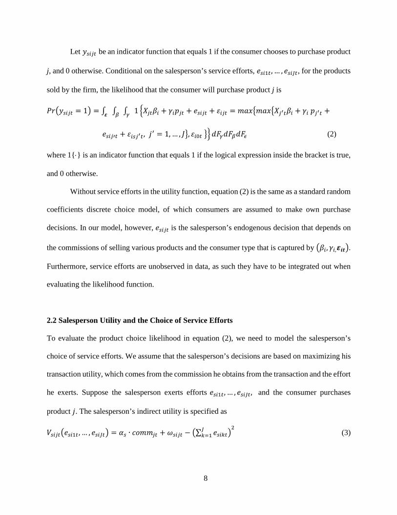
Let 𝑦𝑦𝑠𝑠𝑠𝑠𝑠𝑠𝑠𝑠 be an indicator function that equals 1 if the consumer chooses to purchase product
j, and 0 otherwise. Conditional on the salesperson’s service efforts, 𝑒𝑒𝑠𝑠𝑠𝑠1𝑠𝑠, … , 𝑒𝑒𝑠𝑠𝑠𝑠𝑖𝑖𝑠𝑠, for the products
sold by the firm, the likelihood that the consumer will purchase product j is
𝑃𝑃𝑃𝑃�𝑦𝑦𝑠𝑠𝑠𝑠𝑠𝑠𝑠𝑠 = 1� = ∫ ∫ ∫ 1 �𝑋𝑋𝑠𝑠𝑠𝑠𝛽𝛽𝑠𝑠 + 𝛾𝛾𝑠𝑠𝑝𝑝𝑠𝑠𝑠𝑠 + 𝑒𝑒𝑠𝑠𝑠𝑠𝑠𝑠𝑠𝑠 + 𝜀𝜀𝑠𝑠𝑠𝑠𝑠𝑠 = 𝑚𝑚𝑚𝑚𝑚𝑚�𝑚𝑚𝑚𝑚𝑚𝑚�𝑋𝑋𝑠𝑠′𝑠𝑠𝛽𝛽𝑠𝑠 + 𝛾𝛾𝑠𝑠 𝑝𝑝𝑠𝑠′𝑠𝑠 +𝛾𝛾𝛽𝛽𝜺𝜺
𝑒𝑒𝑠𝑠𝑠𝑠𝑠𝑠′𝑠𝑠 + 𝜀𝜀𝑠𝑠𝑠𝑠𝑠𝑠′𝑠𝑠, 𝑗𝑗′ = 1, … , 𝐽𝐽�, 𝜀𝜀𝑠𝑠0𝑠𝑠 �� 𝑑𝑑𝐹𝐹𝛾𝛾𝑑𝑑𝐹𝐹𝛽𝛽𝑑𝑑𝐹𝐹𝜖𝜖 (2)
where 1{⋅} is an indicator function that equals 1 if the logical expression inside the bracket is true,
and 0 otherwise.
Without service efforts in the utility function, equation (2) is the same as a standard random
coefficients discrete choice model, of which consumers are assumed to make own purchase
decisions. In our model, however, 𝑒𝑒𝑠𝑠𝑠𝑠𝑠𝑠𝑠𝑠 is the salesperson’s endogenous decision that depends on
the commissions of selling various products and the consumer type that is captured by �𝛽𝛽𝑠𝑠,𝛾𝛾𝑠𝑠,𝜺𝜺𝒊𝒊𝒊𝒊�.
Furthermore, service efforts are unobserved in data, as such they have to be integrated out when
evaluating the likelihood function.
2.2 Salesperson Utility and the Choice of Service Efforts
To evaluate the product choice likelihood in equation (2), we need to model the salesperson’s
choice of service efforts. We assume that the salesperson’s decisions are based on maximizing his
transaction utility, which comes from the commission he obtains from the transaction and the effort
he exerts. Suppose the salesperson exerts efforts 𝑒𝑒𝑠𝑠𝑠𝑠1𝑠𝑠, … , 𝑒𝑒𝑠𝑠𝑠𝑠𝑖𝑖𝑠𝑠, and the consumer purchases
product 𝑗𝑗. The salesperson’s indirect utility is specified as
𝑉𝑉𝑠𝑠𝑠𝑠𝑠𝑠𝑠𝑠�𝑒𝑒𝑠𝑠𝑠𝑠1𝑠𝑠, … , 𝑒𝑒𝑠𝑠𝑠𝑠𝑖𝑖𝑠𝑠� = 𝛼𝛼𝑠𝑠 ∙ 𝑐𝑐𝑐𝑐𝑚𝑚𝑚𝑚𝑠𝑠𝑠𝑠 + 𝜔𝜔𝑠𝑠𝑠𝑠𝑠𝑠𝑠𝑠 − �∑ 𝑒𝑒𝑠𝑠𝑠𝑠𝑠𝑠𝑠𝑠𝑖𝑖𝑠𝑠=1 �
2 (3)
9
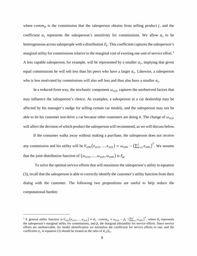
where 𝑐𝑐𝑐𝑐𝑚𝑚𝑚𝑚𝑠𝑠𝑠𝑠 is the commission that the salesperson obtains from selling product 𝑗𝑗, and the
coefficient 𝛼𝛼𝑠𝑠 represents the salesperson’s sensitivity for commissions. We allow 𝛼𝛼𝑠𝑠 to be
heterogeneous across salespeople with a distribution 𝐹𝐹𝛼𝛼. This coefficient captures the salesperson’s
marginal utility for commissions relative to the marginal cost of exerting one unit of service effort.5
A less capable salesperson, for example, will be represented by a smaller 𝛼𝛼𝑠𝑠, implying that given
equal commissions he will sell less than his peers who have a larger 𝛼𝛼𝑠𝑠. Likewise, a salesperson
who is less motivated by commissions will also sell less and thus also have a smaller 𝛼𝛼𝑠𝑠.
In a reduced-form way, the stochastic component 𝜔𝜔𝑠𝑠𝑠𝑠𝑠𝑠𝑠𝑠 captures the unobserved factors that
may influence the salesperson’s choice. As examples, a salesperson in a car dealership may be
affected by his manager’s nudge for selling certain car models, and the salesperson may not be
able to let his customer test-drive a car because other customers are doing it. The change of 𝜔𝜔𝑠𝑠𝑠𝑠𝑠𝑠𝑠𝑠
will affect the decision of which product the salesperson will recommend, as we will discuss below.
If the consumer walks away without making a purchase, the salesperson does not receive
any commission and his utility will be 𝑉𝑉𝑠𝑠𝑠𝑠0𝑠𝑠�𝑒𝑒𝑠𝑠𝑠𝑠1𝑠𝑠, … , 𝑒𝑒𝑠𝑠𝑠𝑠𝑖𝑖𝑠𝑠� = 𝜔𝜔𝑠𝑠𝑠𝑠0𝑠𝑠 − �∑ 𝑒𝑒𝑠𝑠𝑠𝑠𝑠𝑠𝑠𝑠𝑖𝑖𝑠𝑠=1 �
2. We assume
that the joint distribution function of �𝜔𝜔𝑠𝑠𝑠𝑠1𝑠𝑠, … ,𝜔𝜔𝑠𝑠𝑠𝑠𝑖𝑖𝑠𝑠,𝜔𝜔𝑠𝑠𝑠𝑠0𝑠𝑠� is 𝐹𝐹𝝎𝝎.
To solve the optimal service efforts that will maximize the salesperson’s utility in equation
(3), recall that the salesperson is able to correctly identify the customer’s utility function from their
dialog with the customer. The following two propositions are useful to help reduce the
computational burden:
5 A general utility function is 𝑉𝑉𝑠𝑠𝑠𝑠𝑠𝑠𝑠𝑠�𝑒𝑒𝑠𝑠𝑠𝑠1𝑠𝑠 , … , 𝑒𝑒𝑠𝑠𝑠𝑠𝑖𝑖𝑠𝑠� = 𝛼𝛼�𝑠𝑠 ∙ 𝑐𝑐𝑐𝑐𝑚𝑚𝑚𝑚𝑠𝑠𝑠𝑠 + 𝜔𝜔𝑠𝑠𝑠𝑠𝑠𝑠𝑠𝑠 − 𝜌𝜌�𝑠𝑠 ∙ �∑ 𝑒𝑒𝑠𝑠𝑠𝑠𝑠𝑠𝑠𝑠
𝑖𝑖𝑠𝑠=1 �
2, where 𝛼𝛼�𝑠𝑠 represents
the salesperson’s marginal utility for commissions, and 𝜌𝜌�𝑠𝑠 the marginal (dis)utility for service efforts. Since service efforts are unobservable, for model identification we normalize the coefficient for service efforts to one, and the coefficient 𝛼𝛼𝑠𝑠 in equation (3) should be treated as the ratio of 𝛼𝛼�𝑠𝑠/𝜌𝜌�𝑠𝑠.
10
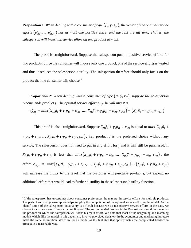
Proposition 1: When dealing with a consumer of type �𝛽𝛽𝑠𝑠, 𝛾𝛾𝑠𝑠,𝜺𝜺𝒊𝒊𝒊𝒊�, the vector of the optimal service
efforts �𝑒𝑒𝑠𝑠𝑠𝑠1𝑠𝑠∗ , … , 𝑒𝑒𝑠𝑠𝑠𝑠𝑖𝑖𝑠𝑠∗ � has at most one positive entry, and the rest are all zero. That is, the
salesperson will invest his service effort on one product at most.
The proof is straightforward. Suppose the salesperson puts in positive service efforts for
two products. Since the consumer will choose only one product, one of the service efforts is wasted
and thus it reduces the salesperson’s utility. The salesperson therefore should only focus on the
product that the consumer will choose.6
Proposition 2: When dealing with a consumer of type �𝛽𝛽𝑠𝑠, 𝛾𝛾𝑠𝑠,𝜺𝜺𝒊𝒊𝒊𝒊�, suppose the salesperson
recommends product j. The optimal service effort 𝑒𝑒𝑠𝑠𝑠𝑠𝑠𝑠𝑠𝑠∗ he will invest is
𝑒𝑒𝑠𝑠𝑠𝑠𝑠𝑠𝑠𝑠∗ = 𝑚𝑚𝑚𝑚𝑚𝑚�𝑋𝑋1𝑠𝑠𝛽𝛽𝑠𝑠 + 𝛾𝛾𝑠𝑠𝑝𝑝1𝑠𝑠 + 𝜀𝜀𝑠𝑠1𝑠𝑠, … , 𝑋𝑋𝑖𝑖𝑠𝑠𝛽𝛽𝑠𝑠 + 𝛾𝛾𝑠𝑠𝑝𝑝𝑖𝑖𝑠𝑠 + 𝜀𝜀𝑠𝑠𝑖𝑖𝑠𝑠, 𝜀𝜀𝑠𝑠𝑠𝑠0𝑠𝑠� − �𝑋𝑋𝑠𝑠𝑠𝑠𝛽𝛽𝑠𝑠 + 𝛾𝛾𝑠𝑠𝑝𝑝𝑠𝑠𝑠𝑠 + 𝜀𝜀𝑠𝑠𝑠𝑠𝑠𝑠�
This proof is also straightforward. Suppose 𝑋𝑋𝑠𝑠𝑠𝑠𝛽𝛽𝑠𝑠 + 𝛾𝛾𝑠𝑠𝑝𝑝𝑠𝑠𝑠𝑠 + 𝜀𝜀𝑠𝑠𝑠𝑠𝑠𝑠 is equal to 𝑚𝑚𝑚𝑚𝑚𝑚�𝑋𝑋1𝑠𝑠𝛽𝛽𝑠𝑠 +
𝛾𝛾𝑠𝑠𝑝𝑝1𝑠𝑠 + 𝜀𝜀𝑠𝑠1𝑠𝑠, … , 𝑋𝑋𝑖𝑖𝑠𝑠𝛽𝛽𝑠𝑠 + 𝛾𝛾𝑠𝑠𝑝𝑝𝑖𝑖𝑠𝑠 + 𝜀𝜀𝑠𝑠𝑖𝑖𝑠𝑠, 𝜀𝜀𝑠𝑠0𝑠𝑠� , i.e., product j is the preferred choice without any
service. The salesperson does not need to put in any effort for j and it will still be purchased. If
𝑋𝑋𝑠𝑠𝑠𝑠𝛽𝛽𝑠𝑠 + 𝛾𝛾𝑠𝑠𝑝𝑝𝑠𝑠𝑠𝑠 + 𝜀𝜀𝑠𝑠𝑠𝑠𝑠𝑠 is less than 𝑚𝑚𝑚𝑚𝑚𝑚�𝑋𝑋1𝑠𝑠𝛽𝛽𝑠𝑠 + 𝛾𝛾𝑠𝑠𝑝𝑝1𝑠𝑠 + 𝜀𝜀𝑠𝑠1𝑠𝑠, … , 𝑋𝑋𝑖𝑖𝑠𝑠𝛽𝛽𝑠𝑠 + 𝛾𝛾𝑠𝑠𝑝𝑝𝑖𝑖𝑠𝑠 + 𝜀𝜀𝑠𝑠𝑖𝑖𝑠𝑠, 𝜀𝜀𝑠𝑠0𝑠𝑠� , the
effort 𝑒𝑒𝑠𝑠𝑠𝑠𝑠𝑠𝑠𝑠 = 𝑚𝑚𝑚𝑚𝑚𝑚�𝑋𝑋1𝑠𝑠𝛽𝛽𝑠𝑠 + 𝛾𝛾𝑠𝑠𝑝𝑝1𝑠𝑠 + 𝜀𝜀𝑠𝑠1𝑠𝑠, … , 𝑋𝑋𝑖𝑖𝑠𝑠𝛽𝛽𝑠𝑠 + 𝛾𝛾𝑠𝑠𝑝𝑝𝑖𝑖𝑠𝑠 + 𝜀𝜀𝑠𝑠𝑖𝑖𝑠𝑠, 𝜀𝜀𝑠𝑠0𝑠𝑠� − �𝑋𝑋𝑠𝑠𝑠𝑠𝛽𝛽𝑠𝑠 + 𝛾𝛾𝑠𝑠𝑝𝑝𝑠𝑠𝑠𝑠 + 𝜀𝜀𝑠𝑠𝑠𝑠𝑠𝑠�
will increase the utility to the level that the customer will purchase product j, but expend no
additional effort that would lead to further disutility in the salesperson’s utility function.
6 If the salesperson has uncertainty about consumer preferences, he may put in service efforts for multiple products. The perfect knowledge assumption helps simplify the computation of the optimal service effort in the model. As the identification of the salesperson uncertainty is difficult because we do not observe service efforts in the data, we choose to abstract away from such complication. The recommended product in the Proposition should be treated as the product on which the salesperson will focus his main effort. We note that most of the bargaining and matching models which, like the model in this paper, also involve two-sided decisions in the economics and marketing literature make the same assumption. We view such a model as the first step that approximates the complicated transaction process in a reasonable way.
11
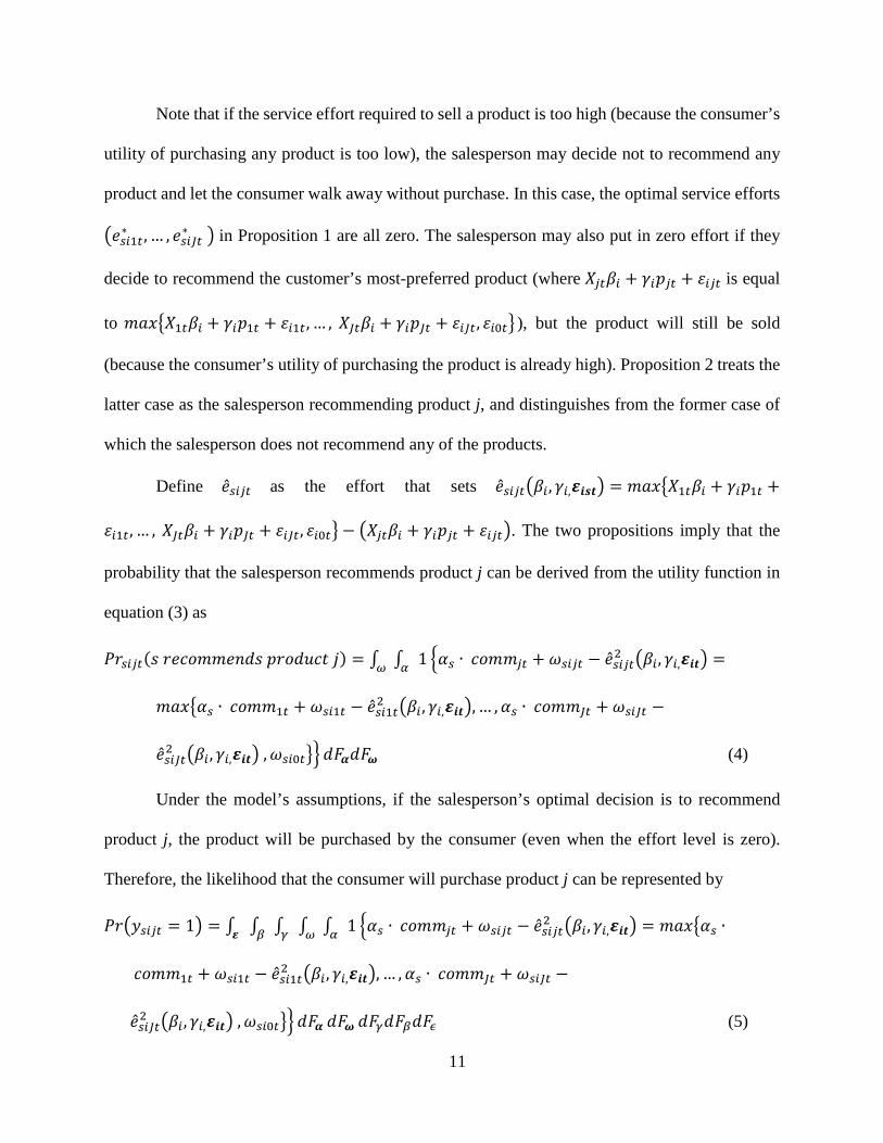
Note that if the service effort required to sell a product is too high (because the consumer’s
utility of purchasing any product is too low), the salesperson may decide not to recommend any
product and let the consumer walk away without purchase. In this case, the optimal service efforts
�𝑒𝑒𝑠𝑠𝑠𝑠1𝑠𝑠∗ , … , 𝑒𝑒𝑠𝑠𝑠𝑠𝑖𝑖𝑠𝑠∗ � in Proposition 1 are all zero. The salesperson may also put in zero effort if they
decide to recommend the customer’s most-preferred product (where 𝑋𝑋𝑠𝑠𝑠𝑠𝛽𝛽𝑠𝑠 + 𝛾𝛾𝑠𝑠𝑝𝑝𝑠𝑠𝑠𝑠 + 𝜀𝜀𝑠𝑠𝑠𝑠𝑠𝑠 is equal
to 𝑚𝑚𝑚𝑚𝑚𝑚�𝑋𝑋1𝑠𝑠𝛽𝛽𝑠𝑠 + 𝛾𝛾𝑠𝑠𝑝𝑝1𝑠𝑠 + 𝜀𝜀𝑠𝑠1𝑠𝑠, … , 𝑋𝑋𝑖𝑖𝑠𝑠𝛽𝛽𝑠𝑠 + 𝛾𝛾𝑠𝑠𝑝𝑝𝑖𝑖𝑠𝑠 + 𝜀𝜀𝑠𝑠𝑖𝑖𝑠𝑠, 𝜀𝜀𝑠𝑠0𝑠𝑠� ), but the product will still be sold
(because the consumer’s utility of purchasing the product is already high). Proposition 2 treats the
latter case as the salesperson recommending product j, and distinguishes from the former case of
which the salesperson does not recommend any of the products.
Define �̂�𝑒𝑠𝑠𝑠𝑠𝑠𝑠𝑠𝑠 as the effort that sets �̂�𝑒𝑠𝑠𝑠𝑠𝑠𝑠𝑠𝑠�𝛽𝛽𝑠𝑠, 𝛾𝛾𝑠𝑠,𝜺𝜺𝒊𝒊𝒔𝒔𝒊𝒊� = 𝑚𝑚𝑚𝑚𝑚𝑚�𝑋𝑋1𝑠𝑠𝛽𝛽𝑠𝑠 + 𝛾𝛾𝑠𝑠𝑝𝑝1𝑠𝑠 +
𝜀𝜀𝑠𝑠1𝑠𝑠, … , 𝑋𝑋𝑖𝑖𝑠𝑠𝛽𝛽𝑠𝑠 + 𝛾𝛾𝑠𝑠𝑝𝑝𝑖𝑖𝑠𝑠 + 𝜀𝜀𝑠𝑠𝑖𝑖𝑠𝑠, 𝜀𝜀𝑠𝑠0𝑠𝑠� − �𝑋𝑋𝑠𝑠𝑠𝑠𝛽𝛽𝑠𝑠 + 𝛾𝛾𝑠𝑠𝑝𝑝𝑠𝑠𝑠𝑠 + 𝜀𝜀𝑠𝑠𝑠𝑠𝑠𝑠�. The two propositions imply that the
probability that the salesperson recommends product j can be derived from the utility function in
equation (3) as
𝑃𝑃𝑃𝑃𝑠𝑠𝑠𝑠𝑠𝑠𝑠𝑠(𝑠𝑠 𝑃𝑃𝑒𝑒𝑐𝑐𝑐𝑐𝑚𝑚𝑚𝑚𝑒𝑒𝑟𝑟𝑑𝑑𝑠𝑠 𝑝𝑝𝑃𝑃𝑐𝑐𝑑𝑑𝑝𝑝𝑐𝑐𝑡𝑡 𝑗𝑗) = ∫ ∫ 1 �𝛼𝛼𝑠𝑠 ∙ 𝑐𝑐𝑐𝑐𝑚𝑚𝑚𝑚𝑠𝑠𝑠𝑠 + 𝜔𝜔𝑠𝑠𝑠𝑠𝑠𝑠𝑠𝑠 − �̂�𝑒𝑠𝑠𝑠𝑠𝑠𝑠𝑠𝑠2 �𝛽𝛽𝑠𝑠, 𝛾𝛾𝑠𝑠,𝜺𝜺𝒊𝒊𝒊𝒊� =𝛼𝛼𝜔𝜔
𝑚𝑚𝑚𝑚𝑚𝑚�𝛼𝛼𝑠𝑠 ∙ 𝑐𝑐𝑐𝑐𝑚𝑚𝑚𝑚1𝑠𝑠 + 𝜔𝜔𝑠𝑠𝑠𝑠1𝑠𝑠 − �̂�𝑒𝑠𝑠𝑠𝑠1𝑠𝑠2 �𝛽𝛽𝑠𝑠, 𝛾𝛾𝑠𝑠,𝜺𝜺𝒊𝒊𝒊𝒊�, … ,𝛼𝛼𝑠𝑠 ∙ 𝑐𝑐𝑐𝑐𝑚𝑚𝑚𝑚𝑖𝑖𝑠𝑠 + 𝜔𝜔𝑠𝑠𝑠𝑠𝑖𝑖𝑠𝑠 −
�̂�𝑒𝑠𝑠𝑠𝑠𝑖𝑖𝑠𝑠2 �𝛽𝛽𝑠𝑠, 𝛾𝛾𝑠𝑠,𝜺𝜺𝒊𝒊𝒊𝒊� ,𝜔𝜔𝑠𝑠𝑠𝑠0𝑠𝑠�� 𝑑𝑑𝐹𝐹𝜶𝜶𝑑𝑑𝐹𝐹𝝎𝝎 (4)
Under the model’s assumptions, if the salesperson’s optimal decision is to recommend
product j, the product will be purchased by the consumer (even when the effort level is zero).
Therefore, the likelihood that the consumer will purchase product j can be represented by
𝑃𝑃𝑃𝑃�𝑦𝑦𝑠𝑠𝑠𝑠𝑠𝑠𝑠𝑠 = 1� = ∫ ∫ ∫ ∫ ∫ 1 �𝛼𝛼𝑠𝑠 ∙ 𝑐𝑐𝑐𝑐𝑚𝑚𝑚𝑚𝑠𝑠𝑠𝑠 + 𝜔𝜔𝑠𝑠𝑠𝑠𝑠𝑠𝑠𝑠 − �̂�𝑒𝑠𝑠𝑠𝑠𝑠𝑠𝑠𝑠2 �𝛽𝛽𝑠𝑠,𝛾𝛾𝑠𝑠,𝜺𝜺𝒊𝒊𝒊𝒊� = 𝑚𝑚𝑚𝑚𝑚𝑚�𝛼𝛼𝑠𝑠 ∙𝛼𝛼𝜔𝜔𝛾𝛾𝛽𝛽𝜺𝜺
𝑐𝑐𝑐𝑐𝑚𝑚𝑚𝑚1𝑠𝑠 + 𝜔𝜔𝑠𝑠𝑠𝑠1𝑠𝑠 − �̂�𝑒𝑠𝑠𝑠𝑠1𝑠𝑠2 �𝛽𝛽𝑠𝑠, 𝛾𝛾𝑠𝑠,𝜺𝜺𝒊𝒊𝒊𝒊�, … ,𝛼𝛼𝑠𝑠 ∙ 𝑐𝑐𝑐𝑐𝑚𝑚𝑚𝑚𝑖𝑖𝑠𝑠 + 𝜔𝜔𝑠𝑠𝑠𝑠𝑖𝑖𝑠𝑠 −
�̂�𝑒𝑠𝑠𝑠𝑠𝑖𝑖𝑠𝑠2 �𝛽𝛽𝑠𝑠, 𝛾𝛾𝑠𝑠,𝜺𝜺𝒊𝒊𝒊𝒊� ,𝜔𝜔𝑠𝑠𝑠𝑠0𝑠𝑠�� 𝑑𝑑𝐹𝐹𝜶𝜶 𝑑𝑑𝐹𝐹𝝎𝝎 𝑑𝑑𝐹𝐹𝛾𝛾𝑑𝑑𝐹𝐹𝛽𝛽𝑑𝑑𝐹𝐹𝜖𝜖 (5)
12
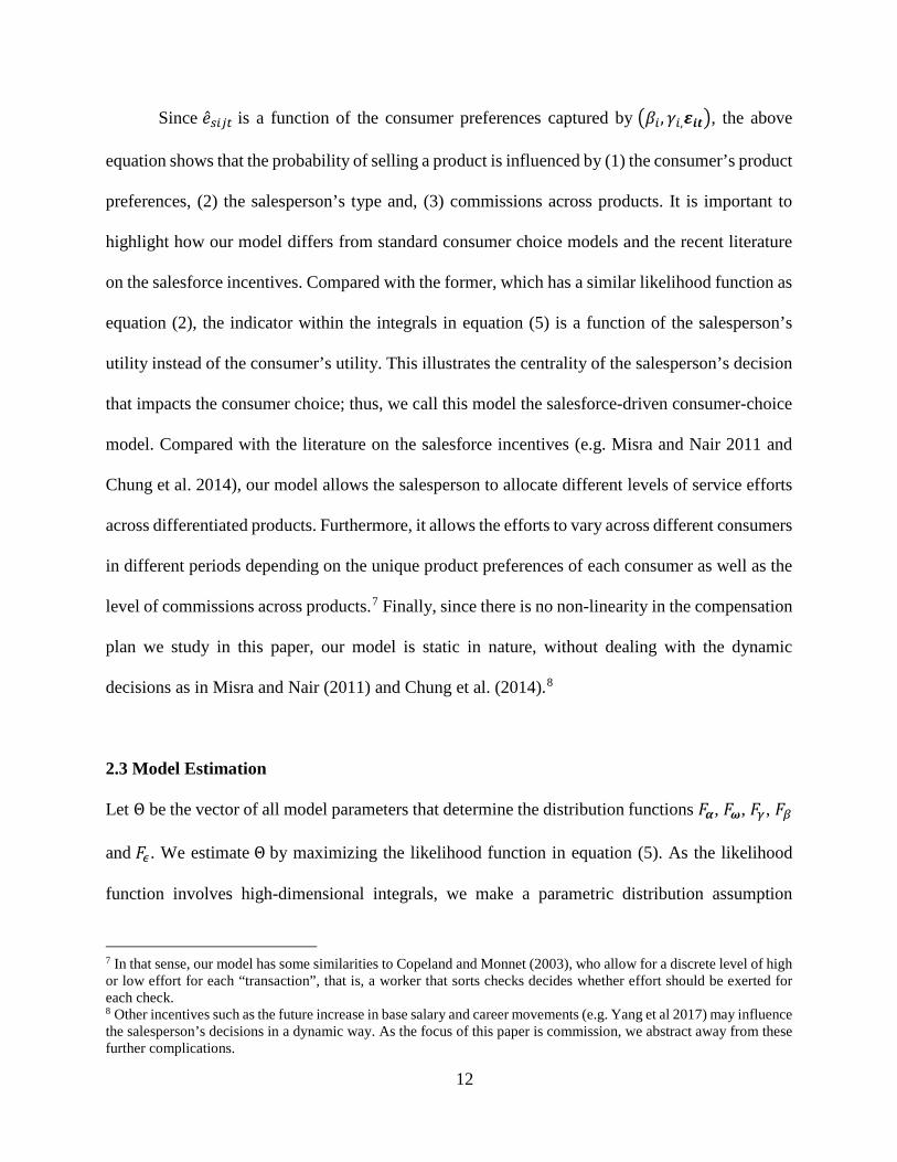
Since �̂�𝑒𝑠𝑠𝑠𝑠𝑠𝑠𝑠𝑠 is a function of the consumer preferences captured by �𝛽𝛽𝑠𝑠, 𝛾𝛾𝑠𝑠,𝜺𝜺𝒊𝒊𝒊𝒊�, the above
equation shows that the probability of selling a product is influenced by (1) the consumer’s product
preferences, (2) the salesperson’s type and, (3) commissions across products. It is important to
highlight how our model differs from standard consumer choice models and the recent literature
on the salesforce incentives. Compared with the former, which has a similar likelihood function as
equation (2), the indicator within the integrals in equation (5) is a function of the salesperson’s
utility instead of the consumer’s utility. This illustrates the centrality of the salesperson’s decision
that impacts the consumer choice; thus, we call this model the salesforce-driven consumer-choice
model. Compared with the literature on the salesforce incentives (e.g. Misra and Nair 2011 and
Chung et al. 2014), our model allows the salesperson to allocate different levels of service efforts
across differentiated products. Furthermore, it allows the efforts to vary across different consumers
in different periods depending on the unique product preferences of each consumer as well as the
level of commissions across products.7 Finally, since there is no non-linearity in the compensation
plan we study in this paper, our model is static in nature, without dealing with the dynamic
decisions as in Misra and Nair (2011) and Chung et al. (2014).8
2.3 Model Estimation
Let Θ be the vector of all model parameters that determine the distribution functions 𝐹𝐹𝜶𝜶, 𝐹𝐹𝝎𝝎, 𝐹𝐹𝛾𝛾, 𝐹𝐹𝛽𝛽
and 𝐹𝐹𝜖𝜖. We estimate Θ by maximizing the likelihood function in equation (5). As the likelihood
function involves high-dimensional integrals, we make a parametric distribution assumption
7 In that sense, our model has some similarities to Copeland and Monnet (2003), who allow for a discrete level of high or low effort for each “transaction”, that is, a worker that sorts checks decides whether effort should be exerted for each check. 8 Other incentives such as the future increase in base salary and career movements (e.g. Yang et al 2017) may influence the salesperson’s decisions in a dynamic way. As the focus of this paper is commission, we abstract away from these further complications.

13
regarding 𝐹𝐹𝝎𝝎 , and assume that 𝜔𝜔𝑠𝑠𝑠𝑠𝑠𝑠𝑠𝑠~𝐺𝐺𝑝𝑝𝑚𝑚𝐺𝐺𝑒𝑒𝐺𝐺(0,𝜃𝜃𝜔𝜔) and i.i.d. across s, i, and j. Therefore,
equation (5) can be rewritten as
𝑃𝑃𝑃𝑃�𝑦𝑦𝑠𝑠𝑠𝑠𝑠𝑠𝑠𝑠 = 1|Θ� = ∫ ∫ ∫ ∫exp�
𝛼𝛼𝑠𝑠∙ 𝑐𝑐𝑐𝑐𝑐𝑐𝑐𝑐𝑗𝑗𝑗𝑗−𝑒𝑒�𝑠𝑠𝑠𝑠𝑗𝑗𝑗𝑗2 �𝛽𝛽𝑠𝑠,𝛾𝛾𝑠𝑠,𝜺𝜺𝒊𝒊𝒊𝒊�
𝜃𝜃𝜔𝜔�
1+∑ exp�𝛼𝛼𝑠𝑠∙ 𝑐𝑐𝑐𝑐𝑐𝑐𝑐𝑐𝑙𝑙𝑗𝑗−𝑒𝑒�𝑠𝑠𝑠𝑠𝑙𝑙𝑗𝑗
2 �𝛽𝛽𝑠𝑠,𝛾𝛾𝑠𝑠,𝜺𝜺𝒊𝒊𝒊𝒊�𝜃𝜃𝜔𝜔
�𝑙𝑙
𝑑𝑑𝐹𝐹𝜶𝜶𝛼𝛼𝛾𝛾𝛽𝛽𝜺𝜺 𝑑𝑑𝐹𝐹𝛾𝛾𝑑𝑑𝐹𝐹𝛽𝛽𝑑𝑑𝐹𝐹𝜀𝜀 (6)
Next, we use a simulation method to evaluate equation (6). Conditional on a candidate Θ,
the simulation procedure is outlined below:
1. For every observation (i,t) in the data, make NS draws of (𝜺𝜺𝒊𝒊𝒊𝒊𝒔𝒔𝒊𝒊𝒔𝒔,𝛽𝛽𝑠𝑠𝑠𝑠𝑠𝑠𝑠𝑠, 𝛾𝛾𝑠𝑠𝑠𝑠𝑠𝑠𝑠𝑠) from 𝐹𝐹𝜀𝜀, 𝐹𝐹𝛽𝛽, 𝐹𝐹𝛾𝛾,
where sim = 1, …, NS. Also make NS draws of 𝛼𝛼𝑠𝑠𝑠𝑠𝑠𝑠𝑠𝑠 from 𝐹𝐹𝜶𝜶 for every salesperson. The same
𝛼𝛼𝑠𝑠𝑠𝑠𝑠𝑠𝑠𝑠 will be used for the salesperson for repeated transactions.
2. Conditional on the simulated (𝜺𝜺𝒊𝒊𝒊𝒊𝒔𝒔𝒊𝒊𝒔𝒔,𝛽𝛽𝑠𝑠𝑠𝑠𝑠𝑠𝑠𝑠, 𝛾𝛾𝑠𝑠𝑠𝑠𝑠𝑠𝑠𝑠) , calculate the effort level
�̂�𝑒𝑠𝑠𝑠𝑠𝑠𝑠𝑠𝑠�𝜺𝜺𝒊𝒊𝒊𝒊𝒔𝒔𝒊𝒊𝒔𝒔,𝛽𝛽𝑠𝑠𝑠𝑠𝑠𝑠𝑠𝑠, 𝛾𝛾𝑠𝑠𝑠𝑠𝑠𝑠𝑠𝑠� = 𝑚𝑚𝑚𝑚𝑚𝑚�𝑋𝑋1𝑠𝑠𝛽𝛽𝑠𝑠𝑠𝑠𝑠𝑠𝑠𝑠 + 𝛾𝛾𝑠𝑠𝑠𝑠𝑠𝑠𝑠𝑠𝑝𝑝1𝑠𝑠 + 𝜀𝜀𝑠𝑠𝑠𝑠𝑠𝑠𝑠𝑠𝑠𝑠𝑠𝑠, … , 𝑋𝑋𝑖𝑖𝑠𝑠𝛽𝛽𝑠𝑠𝑠𝑠𝑠𝑠𝑠𝑠 + 𝛾𝛾𝑠𝑠𝑠𝑠𝑠𝑠𝑠𝑠𝑝𝑝𝑖𝑖𝑠𝑠 +
𝜀𝜀𝑠𝑠𝑖𝑖𝑠𝑠𝑠𝑠𝑠𝑠𝑠𝑠, 𝜀𝜀𝑠𝑠0𝑠𝑠𝑠𝑠𝑠𝑠𝑠𝑠� − 𝑋𝑋𝑠𝑠𝑠𝑠𝛽𝛽𝑠𝑠𝑠𝑠𝑠𝑠𝑠𝑠 − 𝛾𝛾𝑠𝑠𝑠𝑠𝑠𝑠𝑠𝑠𝑝𝑝𝑠𝑠𝑠𝑠 − 𝜀𝜀𝑠𝑠𝑠𝑠𝑠𝑠𝑠𝑠𝑠𝑠𝑠𝑠.
3. Conditional on �̂�𝑒𝑠𝑠𝑠𝑠𝑠𝑠𝑠𝑠�𝜺𝜺𝒊𝒊𝒊𝒊𝒔𝒔𝒊𝒊𝒔𝒔,𝛽𝛽𝑠𝑠𝑠𝑠𝑠𝑠𝑠𝑠, 𝛾𝛾𝑠𝑠𝑠𝑠𝑠𝑠𝑠𝑠� and 𝛼𝛼𝑠𝑠𝑠𝑠𝑠𝑠𝑠𝑠 , calculate the likelihood 𝑃𝑃𝑃𝑃�𝑦𝑦𝑠𝑠𝑠𝑠𝑠𝑠𝑠𝑠 =
1|𝜺𝜺𝒊𝒊𝒊𝒊𝒔𝒔𝒊𝒊𝒔𝒔,𝛽𝛽𝑠𝑠𝑠𝑠𝑠𝑠𝑠𝑠, 𝛾𝛾𝑠𝑠𝑠𝑠𝑠𝑠𝑠𝑠,𝛼𝛼𝑠𝑠𝑠𝑠𝑠𝑠𝑠𝑠� in equation (6).
4. Calculate the simulated choice probability 𝑃𝑃𝑃𝑃�𝑦𝑦𝑠𝑠𝑠𝑠𝑠𝑠𝑠𝑠 = 1|Θ� = 1𝑁𝑁𝑁𝑁∑ 𝑃𝑃𝑃𝑃�𝑦𝑦𝑠𝑠𝑠𝑠𝑠𝑠𝑠𝑠 =𝑁𝑁𝑁𝑁𝑠𝑠𝑠𝑠𝑠𝑠=1
1|𝜺𝜺𝒊𝒊𝒊𝒊𝒔𝒔𝒊𝒊𝒔𝒔,𝛽𝛽𝑠𝑠𝑠𝑠𝑠𝑠𝑠𝑠, 𝛾𝛾𝑠𝑠𝑠𝑠𝑠𝑠𝑠𝑠,𝛼𝛼𝑠𝑠𝑠𝑠𝑠𝑠𝑠𝑠� .
We search for the estimate Θ� to maximize the following simulated maximum likelihood function:
𝐿𝐿 = ∑ ∑ ∑ ∑ log �𝑃𝑃𝑃𝑃�𝑦𝑦𝑠𝑠𝑠𝑠𝑠𝑠𝑠𝑠 = 1|Θ�� ∙ 𝑦𝑦𝑠𝑠𝑠𝑠𝑠𝑠𝑠𝑠𝑠𝑠𝑠𝑠s𝑠𝑠 (7)
2.4 Identification
We only observe consumers' product choice. The main identification of the commission sensitivity
(𝛼𝛼𝑠𝑠 ) among salespeople versus the price sensitivity (𝛾𝛾𝑠𝑠 ) among consumers comes from an
14
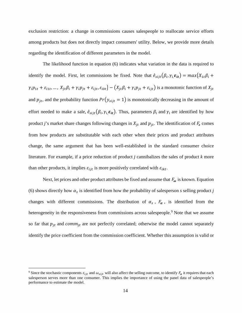
exclusion restriction: a change in commissions causes salespeople to reallocate service efforts
among products but does not directly impact consumers' utility. Below, we provide more details
regarding the identification of different parameters in the model.
The likelihood function in equation (6) indicates what variation in the data is required to
identify the model. First, let commissions be fixed. Note that �̂�𝑒𝑠𝑠𝑠𝑠𝑠𝑠𝑠𝑠�𝛽𝛽𝑠𝑠, 𝛾𝛾𝑠𝑠,𝜺𝜺𝒊𝒊𝒊𝒊� = 𝑚𝑚𝑚𝑚𝑚𝑚�𝑋𝑋1𝑠𝑠𝛽𝛽𝑠𝑠 +
𝛾𝛾𝑠𝑠𝑝𝑝1𝑠𝑠 + 𝜀𝜀𝑠𝑠1𝑠𝑠, … , 𝑋𝑋𝑖𝑖𝑠𝑠𝛽𝛽𝑠𝑠 + 𝛾𝛾𝑠𝑠𝑝𝑝𝑖𝑖𝑠𝑠 + 𝜀𝜀𝑠𝑠𝑖𝑖𝑠𝑠, 𝜀𝜀𝑠𝑠0𝑠𝑠� − �𝑋𝑋𝑠𝑠𝑠𝑠𝛽𝛽𝑠𝑠 + 𝛾𝛾𝑠𝑠𝑝𝑝𝑠𝑠𝑠𝑠 + 𝜀𝜀𝑠𝑠𝑠𝑠𝑠𝑠� is a monotonic function of 𝑋𝑋𝑠𝑠𝑠𝑠
and 𝑝𝑝𝑠𝑠𝑠𝑠, and the probability function 𝑃𝑃𝑃𝑃�𝑦𝑦𝑠𝑠𝑠𝑠𝑠𝑠𝑠𝑠 = 1� is monotonically decreasing in the amount of
effort needed to make a sale, �̂�𝑒𝑠𝑠𝑠𝑠𝑠𝑠𝑠𝑠�𝛽𝛽𝑠𝑠,𝛾𝛾𝑠𝑠,𝜺𝜺𝒊𝒊𝒊𝒊�. Thus, parameters 𝛽𝛽𝑠𝑠 and 𝛾𝛾𝑠𝑠 are identified by how
product j’s market share changes following changes in 𝑋𝑋𝑠𝑠𝑠𝑠 and 𝑝𝑝𝑠𝑠𝑠𝑠. The identification of 𝐹𝐹𝜺𝜺 comes
from how products are substitutable with each other when their prices and product attributes
change, the same argument that has been well-established in the standard consumer choice
literature. For example, if a price reduction of product j cannibalizes the sales of product k more
than other products, it implies 𝜀𝜀𝑠𝑠𝑠𝑠𝑠𝑠 is more positively correlated with 𝜀𝜀𝑠𝑠𝑠𝑠𝑠𝑠.
Next, let prices and other product attributes be fixed and assume that 𝐹𝐹𝝎𝝎 is known. Equation
(6) shows directly how 𝛼𝛼𝑠𝑠 is identified from how the probability of salesperson s selling product j
changes with different commissions. The distribution of 𝛼𝛼𝑠𝑠 , 𝐹𝐹𝜶𝜶 , is identified from the
heterogeneity in the responsiveness from commissions across salespeople.9 Note that we assume
so far that 𝑝𝑝𝑠𝑠𝑠𝑠 and 𝑐𝑐𝑐𝑐𝑚𝑚𝑚𝑚𝑠𝑠𝑠𝑠 are not perfectly correlated; otherwise the model cannot separately
identify the price coefficient from the commission coefficient. Whether this assumption is valid or
9 Since the stochastic components 𝜀𝜀𝑠𝑠𝑠𝑠𝑠𝑠 and 𝜔𝜔𝑠𝑠𝑠𝑠𝑠𝑠𝑠𝑠 will also affect the selling outcome, to identify 𝐹𝐹𝜶𝜶 it requires that each salesperson serves more than one consumer. This implies the importance of using the panel data of salespeople’s performance to estimate the model.
15
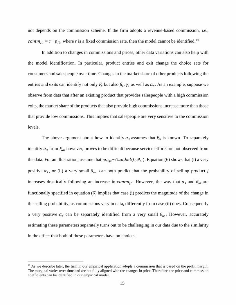
not depends on the commission scheme. If the firm adopts a revenue-based commission, i.e.,
𝑐𝑐𝑐𝑐𝑚𝑚𝑚𝑚𝑠𝑠𝑠𝑠 = 𝑃𝑃 ∙ 𝑝𝑝𝑠𝑠𝑠𝑠, where r is a fixed commission rate, then the model cannot be identified.10
In addition to changes in commissions and prices, other data variations can also help with
the model identification. In particular, product entries and exit change the choice sets for
consumers and salespeople over time. Changes in the market share of other products following the
entries and exits can identify not only 𝐹𝐹𝜀𝜀 but also 𝛽𝛽𝑠𝑠, 𝛾𝛾𝑠𝑠 as well as 𝛼𝛼𝑠𝑠. As an example, suppose we
observe from data that after an existing product that provides salespeople with a high commission
exits, the market share of the products that also provide high commissions increase more than those
that provide low commissions. This implies that salespeople are very sensitive to the commission
levels.
The above argument about how to identify 𝛼𝛼𝑠𝑠 assumes that 𝐹𝐹𝝎𝝎 is known. To separately
identify 𝛼𝛼𝑠𝑠 from 𝐹𝐹𝝎𝝎, however, proves to be difficult because service efforts are not observed from
the data. For an illustration, assume that 𝜔𝜔𝑠𝑠𝑠𝑠𝑠𝑠𝑠𝑠~𝐺𝐺𝑝𝑝𝑚𝑚𝐺𝐺𝑒𝑒𝐺𝐺(0,𝜃𝜃𝜔𝜔). Equation (6) shows that (i) a very
positive 𝛼𝛼𝑠𝑠 , or (ii) a very small 𝜃𝜃𝜔𝜔 , can both predict that the probability of selling product j
increases drastically following an increase in 𝑐𝑐𝑐𝑐𝑚𝑚𝑚𝑚𝑠𝑠𝑠𝑠 . However, the way that 𝛼𝛼𝑠𝑠 and 𝜃𝜃𝜔𝜔 are
functionally specified in equation (6) implies that case (i) predicts the magnitude of the change in
the selling probability, as commissions vary in data, differently from case (ii) does. Consequently
a very positive 𝛼𝛼𝑠𝑠 can be separately identified from a very small 𝜃𝜃𝜔𝜔 . However, accurately
estimating these parameters separately turns out to be challenging in our data due to the similarity
in the effect that both of these parameters have on choices.
10 As we describe later, the firm in our empirical application adopts a commission that is based on the profit margin. The marginal varies over time and are not fully aligned with the changes in price. Therefore, the price and commission coefficients can be identified in our empirical model.

16
We use a simulation study to further show that our model can recover the structural
parameters. We first draw the prices and commissions of four hypothetical products from a large
range over 24 months, and simulate the sales of a set of four product us different sets of parameter
values. For simplicity, we assume that each product’s utility can be summarized through a unique
brand intercept, and normalize the intercept for the fourth product as 0. For this demonstration, we
also assume that consumer heterogeneity is present only in the 𝜺𝜺 terms, and that the salesforce is
homogeneous but draws 𝝎𝝎’s for individual transactions. We further assume that the 𝜺𝜺’s are
normally distributed with mean zero, and that the covariances are all zero except for the covariance
of products 1 and 2 (Σ12) and the covariance of products 3 and 4 (Σ34). Finally, 𝜔𝜔𝑠𝑠𝑠𝑠𝑠𝑠𝑠𝑠 is assumed
to have a Gumbel distribution with 𝜃𝜃𝜔𝜔 fixed to one. We then use the simulated data to estimate the
model parameters using the likelihood function in equation (7). Table 1 presents the results for a
variety of parameters. The results show that the model is able to recover the true parameters very
well, with the price and the commission coefficients being especially close to the true values.
Table 1. Test of model performance
True 0.00 0.00 0.00 -0.80 10.00 0.50 0.70Estimated 0.00 0.01 0.00 -0.80 9.87 0.52 0.71Standard error (0.01) (0.01) (4.97E-03) (2.99E-03) (0.06) (0.01) (0.01)True 3.00 2.00 4.00 -0.70 9.00 0.70 0.50Estimated 3.07 2.08 4.06 -0.70 8.96 0.73 0.47Standard error (0.06) (0.06) (0.06) (3.47E-03) (0.05) (0.02) (0.04)True 3.00 2.00 4.00 -1.00 5.00 0.50 0.70Estimated 3.16 2.17 4.16 -1.00 4.98 0.51 0.63Standard error (0.09) (0.09) (0.09) (4.34E-03) (0.04) (0.02) (0.05)True 1.00 2.00 3.00 -0.60 7.00 0.80 0.40Estimated 0.95 1.96 2.96 -0.59 6.92 0.82 0.46Standard error (0.03) (0.03) (0.03) (3.93E-03) (0.04) (0.01) (0.02)True 3.00 0.00 4.00 -0.90 6.00 0.30 0.50Estimated 3.13 0.10 4.13 -0.90 5.93 0.15 0.42Standard error (0.09) (0.08) (0.09) (4.24E-03) (0.05) (0.07) (0.05)
𝛽𝛽1 𝛽𝛽2 𝛽𝛽3 𝛾𝛾 𝛼𝛼 Σ12 Σ34
17
3. Data and Analysis
3.1. Data Description
We estimate the model using a dataset provided by one of the largest regional chains of automobile
dealers in Japan. This dealership sells cars produced by one of the largest car manufacturers in the
world. It owns over 70 outlets and sells multiple brands produced by the same manufacturer. All
the outlets sell the same set of car models. The dataset spans two years. There are altogether 828
salespeople. The mean and standard deviation of salespeople’s tenure is 12.9 and 9.7, respectively.
59.8% of the salespeople have college degree, and all of them are male. The data are well suited
for our study because we know not only each salesperson’s transactions but also the commissions
the salespeople receive from each transaction. Furthermore, for each car we know both the selling
price and the cost borne by the dealer, which the dealer calculates based on the price it pays the
manufacturer for the car as well as administrative and inventory costs.
In each month, a salesperson receives a guaranteed base salary, which can change over
time depending on his tenure and accumulated past work performance, plus commissions from the
transactions he completes that month. The commission has a fixed and a profit-based component,
with commissions calculated as 𝑞𝑞𝑠𝑠+ 𝑃𝑃𝑠𝑠𝑠𝑠 ∙ �𝑝𝑝𝑠𝑠𝑠𝑠 − 𝑐𝑐𝑠𝑠𝑠𝑠�, where 𝑞𝑞𝑠𝑠 is a commission paid each time a
car is sold and is fixed for all car models, 𝑃𝑃𝑠𝑠𝑠𝑠 the commission rate specific for car model j, 𝑝𝑝𝑠𝑠𝑠𝑠 the
selling price, and 𝑐𝑐𝑠𝑠𝑠𝑠 the cost for the dealer (thus the commission for selling the model depends on
the margin for the dealer). The dealer determines the selling prices and commission rates of each
car model. In the data, commission rates differ across car models but remain constant over time
except for two car models. However, prices and costs fluctuate across months and do not move in
lock-step together, and have an average correlation of 0.52. Commissions make up around half of
a salesperson’s income, so the salespeople have a strong economic incentive to sell cars.
18
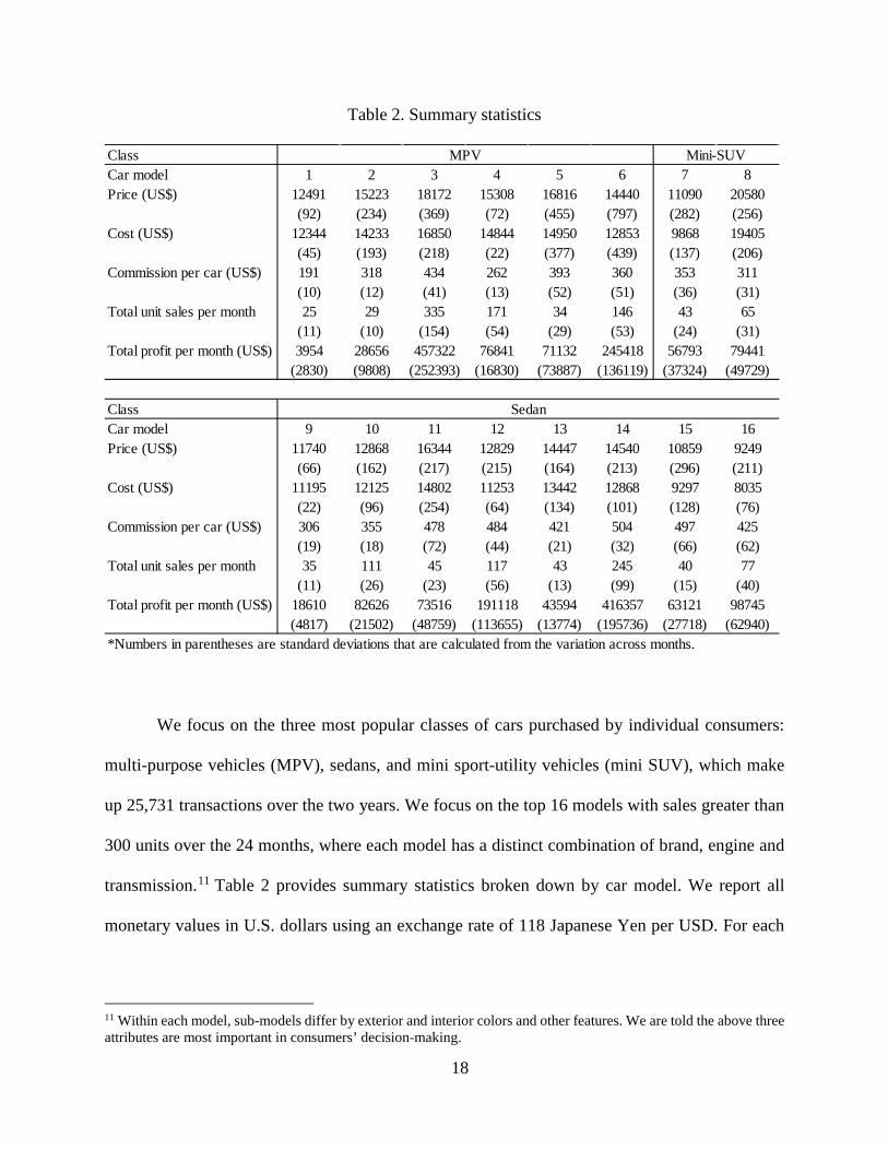
Table 2. Summary statistics
We focus on the three most popular classes of cars purchased by individual consumers:
multi-purpose vehicles (MPV), sedans, and mini sport-utility vehicles (mini SUV), which make
up 25,731 transactions over the two years. We focus on the top 16 models with sales greater than
300 units over the 24 months, where each model has a distinct combination of brand, engine and
transmission.11 Table 2 provides summary statistics broken down by car model. We report all
monetary values in U.S. dollars using an exchange rate of 118 Japanese Yen per USD. For each
11 Within each model, sub-models differ by exterior and interior colors and other features. We are told the above three attributes are most important in consumers’ decision-making.
ClassCar model 1 2 3 4 5 6 7 8Price (US$) 12491 15223 18172 15308 16816 14440 11090 20580
(92) (234) (369) (72) (455) (797) (282) (256)Cost (US$) 12344 14233 16850 14844 14950 12853 9868 19405
(45) (193) (218) (22) (377) (439) (137) (206)Commission per car (US$) 191 318 434 262 393 360 353 311
(10) (12) (41) (13) (52) (51) (36) (31)Total unit sales per month 25 29 335 171 34 146 43 65
(11) (10) (154) (54) (29) (53) (24) (31)Total profit per month (US$) 3954 28656 457322 76841 71132 245418 56793 79441
(2830) (9808) (252393) (16830) (73887) (136119) (37324) (49729)
ClassCar model 9 10 11 12 13 14 15 16Price (US$) 11740 12868 16344 12829 14447 14540 10859 9249
(66) (162) (217) (215) (164) (213) (296) (211)Cost (US$) 11195 12125 14802 11253 13442 12868 9297 8035
(22) (96) (254) (64) (134) (101) (128) (76)Commission per car (US$) 306 355 478 484 421 504 497 425
(19) (18) (72) (44) (21) (32) (66) (62)Total unit sales per month 35 111 45 117 43 245 40 77
(11) (26) (23) (56) (13) (99) (15) (40)Total profit per month (US$) 18610 82626 73516 191118 43594 416357 63121 98745
(4817) (21502) (48759) (113655) (13774) (195736) (27718) (62940)*Numbers in parentheses are standard deviations that are calculated from the variation across months.
Sedan
MPV Mini-SUV

19
car model, we present the mean and standard deviation of its price, cost and commissions on a per
unit basis, as well as the average monthly total unit sales and profit.
The standard deviations reported in the table indicate that for each car model. There are
significant fluctuations in prices and costs across months. Similarly, the range of prices and costs
across cars within each car class is also large. These suggest that the profits of selling a car for the
dealer vary across car models and months. Furthermore, the total unit sales averaged over months
range from merely 25 (model 1) to 335 (model 3), reflecting large variation in terms of the appeal
to consumers across car models. On average, the dealer pays salespeople about 30% of the margin
as commission. The commissions also fluctuate across car models and months.
Before estimating the full model, we first estimate a classic consumer choice model where
we put the commission into the customer’s utility function using the following likelihood function:
𝑃𝑃𝑃𝑃�𝑦𝑦𝑠𝑠𝑠𝑠𝑠𝑠𝑠𝑠 = 1� = ∫ ∫ 1 �𝑋𝑋𝑠𝑠𝑠𝑠β + 𝛾𝛾𝑠𝑠𝑝𝑝𝑠𝑠𝑠𝑠 + 𝛼𝛼 ∙ 𝑐𝑐𝑐𝑐𝑚𝑚𝑚𝑚𝑠𝑠𝑠𝑠𝑠𝑠 + 𝜀𝜀𝑠𝑠𝑠𝑠𝑠𝑠 = 𝑚𝑚𝑚𝑚𝑚𝑚�𝑚𝑚𝑚𝑚𝑚𝑚�𝑋𝑋𝑠𝑠′𝑠𝑠β + 𝛾𝛾𝑠𝑠𝑝𝑝𝑠𝑠′𝑠𝑠 + 𝛼𝛼 ∙𝛾𝛾𝜀𝜀
𝑐𝑐𝑐𝑐𝑚𝑚𝑚𝑚𝑠𝑠𝑠𝑠′𝑠𝑠 + 𝜀𝜀𝑠𝑠𝑠𝑠′𝑠𝑠, 𝑗𝑗′ = 1, … , 𝐽𝐽�, 𝜀𝜀𝑠𝑠0𝑠𝑠 �� 𝑑𝑑𝐹𝐹𝛾𝛾𝑑𝑑𝐹𝐹𝜀𝜀 (8)
For 𝑋𝑋𝑠𝑠𝑠𝑠, we include an indicator of the car model, and year-month indicators (23 indicators for the
24 months) to control for the seasonality. We assume that the price coefficient is distributed such
that 𝛾𝛾𝑠𝑠~𝑁𝑁�0,𝜎𝜎𝛾𝛾2� . For simplicity we assume that there is no heterogeneity in other model
parameters, and estimate a multinomial probit model, with 𝜺𝜺𝒊𝒊𝒊𝒊~N(0, Σ). The diagonal elements of
Σ are normalized to 1 and, to simplify the estimation, we assume the correlation of 𝜀𝜀𝑠𝑠𝑠𝑠𝑠𝑠 and 𝜀𝜀𝑠𝑠𝑠𝑠′𝑠𝑠 is
𝜏𝜏𝑐𝑐 for all car models j and j’ belonging to the same class c (MPV, sedan, or mini-SUV), and 0
otherwise. Note that this structure removes any IIA concerns from our model. We restrict the
covariances with each class to be non-negative (i.e., 0 < 𝜏𝜏𝑐𝑐 < 1). Consequently, all MPV car
models, for example, are closer substitutes for one another than for sedan or mini-SUV models.

20
Table 3. Results from “Consumer Choice” Models Estimation
For comparison purposes, we also estimate a standard consumer choice model without
including commissions in equation (8). The results for both models are reported in Table 3. Price
coefficients without commissions (column 1) or with commissions (column 2) are significantly
negative. However, the price coefficient in the second model is significantly more negative than
the first. To understand the reason, first notice that the coefficient for commissions is significantly
positive in the second model, indicating that commissions, like prices, can be an important factor
for car sales. Next, since the commission is calculated as 𝑞𝑞𝑠𝑠 + 𝑃𝑃𝑠𝑠𝑠𝑠 ∙ �𝑝𝑝𝑠𝑠𝑠𝑠 − 𝑐𝑐𝑠𝑠𝑠𝑠�, the commission for
a car model will decrease when the price drops. From the data, the average correlation between
the commission and the price is 0.82 across car models. Suppose there is a price promotion for a
car model. Salespeople’s incentive of investing service effort on selling the car model may
decrease because of the lower commission and, consequently, the effect of the price promotion on
sales will be diminished. Ignoring the role of salespeople’s incentives in transactions will therefore
Without commission With commission-0.288 -0.405(0.03) (0.038)0.050 0.051
(2.12E-06) (5.40E-06)0.304
(0.183)1.000 1.000
(0.003) (0.008)0.002 0.001
(0.001) (0.004)0.341 0.411
(0.001) (0.002)Car model indicators Included IncludedMonth indicators Included IncludedLoglikelihood -131464.932 -131436.723BIC 263469.723 263425.573*Prices and commissions are converted in $1,000 for estimation
Correlation: Mini- SUV
Price coefficient: mean
Price coefficient: s.d.
Commission coefficient
Correlation: MPV
Correlation: Sedan
21
bias the estimated price sensitivity of consumers towards zero. This result demonstrates the
importance of taking account of salespeople’s incentives even when the researcher’s main
objective is to understand the role of prices on sales.
3.2. Details of the Full Estimation Model
We estimate the proposed structural model described in Section 2. The specifications regarding 𝛾𝛾𝑠𝑠,
𝑋𝑋𝑠𝑠𝑠𝑠 and 𝜺𝜺𝒊𝒊𝒊𝒊 are the same as the “consumer choice” models in Table 3. For salespeople, we allow
them to be heterogeneous in the commission coefficient 𝛼𝛼𝑠𝑠. We assume that there are two latent
types of salespeople. For each type, k, we estimate the coefficient on commissions as
𝛼𝛼𝑠𝑠 = 𝑒𝑒𝑚𝑚𝑝𝑝 (𝛼𝛼𝑠𝑠,1 + 𝛼𝛼𝑠𝑠,2 ∗ 𝑡𝑡𝑒𝑒𝑟𝑟𝑝𝑝𝑃𝑃𝑒𝑒 + 𝛼𝛼𝑠𝑠,3 ∗ 𝑡𝑡𝑒𝑒𝑟𝑟𝑝𝑝𝑃𝑃𝑒𝑒2 + 𝛼𝛼𝑠𝑠,4 ∗ 𝑐𝑐𝑐𝑐𝐺𝐺𝐺𝐺𝑒𝑒𝑐𝑐𝑒𝑒) (9)12
Under this specification, salespeople are differentiated by the latent type and, within each,
differentiated by how long they have worked for the dealership (tenure, measured by months) and
their education level (college, which is equal to 1 if the salesperson has a college degree, and 0
otherwise). The heterogeneity in 𝛼𝛼 reflects the differences across salespeople in the marginal
utility for commissions and/or the marginal (dis)utility for service efforts.
We also assume that 𝜔𝜔𝑠𝑠𝑠𝑠𝑠𝑠𝑠𝑠~𝐺𝐺𝑝𝑝𝑚𝑚𝐺𝐺𝑒𝑒𝐺𝐺(0,𝜃𝜃𝜔𝜔) and is i.i.d. across s, i, and j. Therefore, the
likelihood 𝑃𝑃𝑃𝑃�𝑦𝑦𝑠𝑠𝑠𝑠𝑠𝑠𝑠𝑠 = 1� is specified as in equation (6). Given that it is difficult to identify both
𝜃𝜃𝜔𝜔 and the other parameters of the model, as we discussed in Section 2.4, we fix the value of 𝜃𝜃𝜔𝜔
to 1 when estimating the model. We then vary 𝜃𝜃𝜔𝜔 and re-estimate the model based on each unique
value to test how sensitive are other model estimates when the value of 𝜃𝜃𝜔𝜔 changes.13
12 The exponential function specification guarantees that the commission coefficient is always positive. 13 Although the likelihood function value changes (within a magnitude of .02%), parameter estimates are very similar, suggesting that our results are robust to the assumption of 𝜃𝜃𝜔𝜔 . Detailed estimation results under different 𝜃𝜃𝜔𝜔 are available from the authors upon request.
22
In the model, consumers may choose the outside no-purchase option. Those consumers are
not observed in the data; therefore, we need a proxy for the market potential. That is, the total
number of potential consumers who were served by a salesperson in each month. We use an
approach based on Albuquerque and Bronnenberg (2012), by assuming that the number of people
who consider buying a car in a given year, 𝑦𝑦, is
𝑀𝑀𝑦𝑦 = 𝑇𝑇𝑇𝑇𝑠𝑠𝑇𝑇𝑇𝑇 𝑁𝑁𝑁𝑁𝑠𝑠𝑁𝑁𝑁𝑁𝑁𝑁 𝑇𝑇𝑜𝑜 𝐻𝐻𝑇𝑇𝑁𝑁𝑠𝑠𝑁𝑁ℎ𝑇𝑇𝑇𝑇𝑜𝑜𝑠𝑠 𝑠𝑠𝑖𝑖 𝑠𝑠ℎ𝑁𝑁 𝑅𝑅𝑁𝑁𝑅𝑅𝑠𝑠𝑇𝑇𝑖𝑖𝑦𝑦7
∙ 𝑂𝑂𝑁𝑁𝑠𝑠𝑁𝑁𝑁𝑁𝑂𝑂𝑁𝑁𝑜𝑜 𝑁𝑁𝑇𝑇𝑇𝑇𝑁𝑁𝑠𝑠𝑦𝑦𝑅𝑅𝑁𝑁𝑅𝑅𝑠𝑠𝑇𝑇𝑖𝑖𝑇𝑇𝑇𝑇 𝑁𝑁𝑇𝑇𝑇𝑇𝑁𝑁𝑠𝑠𝑦𝑦
. (10)
In this formula, “7” is the average number of years between car purchases we obtain from industry
reports, and the first ratio represents the total number of potential consumers who are looking to
buy a new car in the region in the year. For the second ratio, “𝑂𝑂𝐺𝐺𝑠𝑠𝑒𝑒𝑃𝑃𝑂𝑂𝑒𝑒𝑑𝑑 𝑆𝑆𝑚𝑚𝐺𝐺𝑒𝑒𝑠𝑠𝑦𝑦” is the total
number of cars sold by the dealership in data, and “𝑅𝑅𝑒𝑒𝑐𝑐𝑖𝑖𝑐𝑐𝑟𝑟𝑚𝑚𝐺𝐺 𝑆𝑆𝑚𝑚𝐺𝐺𝑒𝑒𝑠𝑠𝑦𝑦” is the total number of cars
sold in the region during the year, which we obtain from the Japanese census data. This ratio
represents the market share of the dealer in our data. 𝑀𝑀𝑦𝑦 is thus used as a proxy for the number of
consumers who visited the dealer in the year.
We further calculate the total number of potential consumers for the dealer as 𝑀𝑀𝑠𝑠 = 𝑀𝑀𝑦𝑦 ∙
𝑂𝑂𝑁𝑁𝑠𝑠𝑁𝑁𝑁𝑁𝑂𝑂𝑁𝑁𝑜𝑜 𝑁𝑁𝑇𝑇𝑇𝑇𝑁𝑁𝑠𝑠 𝑠𝑠𝑖𝑖 𝑠𝑠𝑂𝑂𝑁𝑁𝑠𝑠𝑁𝑁𝑁𝑁𝑂𝑂𝑁𝑁𝑜𝑜 𝐴𝐴𝑖𝑖𝑖𝑖𝑁𝑁𝑇𝑇𝑇𝑇 𝑁𝑁𝑇𝑇𝑇𝑇𝑁𝑁𝑠𝑠
, where “𝑂𝑂𝐺𝐺𝑠𝑠𝑒𝑒𝑃𝑃𝑂𝑂𝑒𝑒𝑑𝑑 𝑆𝑆𝑚𝑚𝐺𝐺𝑒𝑒𝑠𝑠 𝑖𝑖𝑟𝑟 𝑚𝑚” is the average monthly sales in month m, and
“𝑂𝑂𝐺𝐺𝑠𝑠𝑒𝑒𝑃𝑃𝑂𝑂𝑒𝑒𝑑𝑑 𝐴𝐴𝑟𝑟𝑟𝑟𝑝𝑝𝑚𝑚𝐺𝐺 𝑆𝑆𝑚𝑚𝐺𝐺𝑒𝑒𝑠𝑠” is the average annual sales, both observed from the data. This way,
the number of potential consumers for the dealer is assumed to be proportional to the monthly
sales averaged across years. 14 Finally, we calculate the number of potential buyers for each
salesperson by dividing 𝑀𝑀𝑠𝑠 by the total number of salespeople employed by the dealer. In other
words, we assume that all salespeople have equal selling opportunities. Based on interviews with
14 Note that, since we include month indicators in the estimation model, our results are less sensitive to the way that we calculate the potential consumers. Suppose we over-estimate the number of potential consumers in a month. The estimated fixed effect of the month will adjust downward to reflect that the over-estimated potential consumers will walk away without purchase from the dealer.
23
the dealer, we understand that the dealer uses a territorial system: When a consumer walks into a
dealer, the salesperson who first sees her will greet her and ask some basic questions including
where she lives. The customer will then be assigned to the salesperson who is in charge of the
territory where their residence is located. If the salesperson who is in charge of the territory
happens to be not in, the person who greets the consumer will take care of her. For fairness, the
dealership assigns the territories with the goal of ensuring that each salesperson will serve the same
number of customers; therefore, the assumption of equal selling opportunities seems reasonable.
Because the territorial system is based on the residence only and not the unique type of each
consumer (i.e. 𝛽𝛽𝑠𝑠, 𝛾𝛾𝑠𝑠, and 𝜺𝜺𝒊𝒊𝒊𝒊), we further assume that there is no strategic matching between a
salesperson and a consumer.
Finally, we are concerned with the issue of price endogeneity in the model estimation. The
price of a car may be correlated with the stochastic components 𝜀𝜀’s and 𝜔𝜔’s in the model because
a consumer may negotiate price with the salesperson in the transaction process. During interviews
with the dealer, we were told that, in contrast to US practices, consumer-initiated price negotiations
are very rare in Japan. Even when price negotiations occur, salespeople cannot make the decision;
instead, they have to let the manager decide the final price. Therefore, price endogeneity is of less
concern in this study than in some other studies. However, we further address the issue of
endogeneity by adopting a control function approach, proposed in Petrin and Train (2010). We
estimate the model in two stages. In the first stage, we regress the price of every car model in each
month on product-level indicators and a set of price instruments, which include the total number
of car models in the same class and in other classes. We observe new car models enter and old car
models exit in various months, and prices of existing car models significantly fluctuate following

24
the entry and exits (as shown from the regression). Assuming the entry and exits are not correlated
to the individual 𝜀𝜀’s and 𝜔𝜔’s, these variables are valid instruments for prices.
We obtain a residual 𝜉𝜉𝑠𝑠𝑠𝑠 for each car model in each month from the price regression. In the
second stage, when estimating the proposed structural model, 𝜉𝜉𝑠𝑠𝑠𝑠 is included as an additional
covariate in the consumer utility function in equation (1). Petrin and Train (2010) show that this
method helps correct the potential endogeneity problem in discrete choice models.15
In addition to the proposed model, we also estimate three alternative models with simpler
specifications. The first (Model 1) does not account for the heterogeneity across salespeople in 𝛼𝛼𝑠𝑠
or for the potential price endogeneity. The second model (Model 2) uses the control function
approach to correct for price endogeneity, but still does not allow for the heterogeneity across
salespeople. The third model (Model 3) assumes that the heterogeneity across salespeople only
comes from the tenure and education observed from data (see equation 9) but there are no latent
type differences. Comparing the results helps us understand how each of the above components
can increase the model fit, as well as how the estimation results are robust to different model
specifications.
3.3. Estimation results
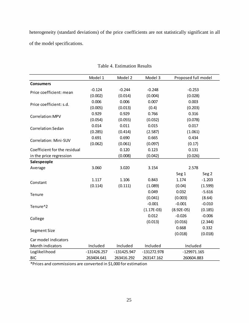
Table 4 reports the estimates from the four model specifications. All of the results show that the
mean price coefficients are negative and significant; however, after controlling for the potential
price endogeneity, the coefficients are more negative in the latter three models. The estimated
15 It may also be a concern that the cost for the dealer, 𝑐𝑐𝑠𝑠𝑠𝑠, which is the wholesale price set by the car manufacturer, may have the endogeneity issue. The wholesale price, however, is the same for every transaction in the same month t. In the model, we include the fixed effect of every car model, as well as the fixed effects for years and months. After controlling for these fixed effects, the endogeneity concern should be alleviated.
25
heterogeneity (standard deviations) of the price coefficients are not statistically significant in all
of the model specifications.
Table 4. Estimation Results
Model 1 Model 2 Model 3Consumers
-0.124 -0.244 -0.248(0.002) (0.014) (0.004)0.006 0.006 0.007
(0.005) (0.013) (0.4)0.929 0.929 0.766
(0.054) (0.055) (0.032)0.014 0.011 0.015
(0.285) (0.414) (2.587)0.691 0.690 0.665
(0.062) (0.061) (0.097)Coefficient for the residual 0.120 0.123in the price regression (0.008) (0.042)SalespeopleAverage 3.060 3.020 3.154
Seg 1 Seg 21.117 1.106 0.843 1.174 -1.203
(0.114) (0.111) (1.089) (0.04) (1.599)0.049 0.032 -5.616
(0.041) (0.003) (8.64)-0.001 -0.001 -0.010
(1.17E-03) (8.92E-05) (0.185)0.012 -0.026 -0.006
(0.013) (0.016) (2.344)0.668 0.332
(0.018) (0.018)Car model indicatorsMonth indicators Included Included IncludedLoglikelihood -131426.257 -131425.947 -131272.978BIC 263404.641 263416.292 263147.162*Prices and commissions are converted in $1,000 for estimation
260604.883
2.578
Tenure
Tenure^2
College
Segment Size
Included-129971.165
0.434(0.17)0.131
(0.026)
Constant
(0.203)
Correlation:MPV 0.316(0.078)
Correlation:Sedan 0.017(1.061)
Correlation: Mini-SUV
Proposed full model
Price coefficient: mean -0.253(0.028)
Price coefficient: s.d. 0.003

26
We next turn to how responsive salespeople are to commissions. Because the estimates of
the coefficient on commissions follows the form of equation (9), it can be hard to interpret the
overall effect of commissions on salesperson utility. For this reason, we report the commission
coefficient averaged across all salespeople (in the row labeled “Average”). The coefficients are
positive in all four models, suggesting that salespeople are fairly responsive to commission
incentives. The level of responsiveness, however, is heterogeneous across salespeople. Results
from model (3) suggest that salespeople with a higher tenure are in general more responsive to the
commission change (it takes 18 years of tenure before the coefficient reaches its maximum),
perhaps indicating that experienced workers have a higher selling ability and therefore the cost of
service effort is lower. The coefficient for College is positive but statistically insignificant.
Our proposed model allows the responsiveness to commissions to differ among salespeople
based on unobserved types. The last column in the table shows that there are two latent segments.
The majority segment (67% of salespeople) has a high sensitivity to a change in commissions.
Salespeople with a higher tenure in this segment are more responsive to commissions. The smaller
segment has a much lower commission sensitivity, which decreases over time. This may imply
that salespeople in that segment have a low selling ability and therefore the cost of service effort
is high. The decline in commission sensitivity over time perhaps reflects the increases in base
salary with tenure.16 Finally, college education does not have a significant effect for either segment.
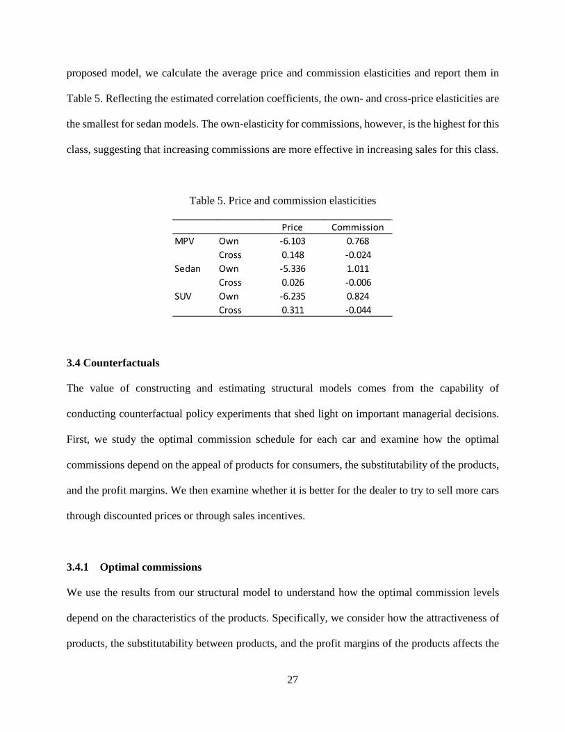
The estimated correlation coefficients of the three classes of cars have a direct effect on the
own- and cross-price elasticities, which in turn affects the way that the salespeople shift their
service efforts in response to changes in commissions. We observe high correlation in preferences
for the MPV and mini-SUV segments, but not for the sedan segment. Using the results from the
16 In Japan, the base salary largely depends on the seniority of workers and less on the work performance.
27
proposed model, we calculate the average price and commission elasticities and report them in
Table 5. Reflecting the estimated correlation coefficients, the own- and cross-price elasticities are
the smallest for sedan models. The own-elasticity for commissions, however, is the highest for this
class, suggesting that increasing commissions are more effective in increasing sales for this class.
Table 5. Price and commission elasticities
3.4 Counterfactuals
The value of constructing and estimating structural models comes from the capability of
conducting counterfactual policy experiments that shed light on important managerial decisions.
First, we study the optimal commission schedule for each car and examine how the optimal
commissions depend on the appeal of products for consumers, the substitutability of the products,
and the profit margins. We then examine whether it is better for the dealer to try to sell more cars
through discounted prices or through sales incentives.
3.4.1 Optimal commissions
We use the results from our structural model to understand how the optimal commission levels
depend on the characteristics of the products. Specifically, we consider how the attractiveness of
products, the substitutability between products, and the profit margins of the products affects the
Price CommissionMPV Own -6.103 0.768
Cross 0.148 -0.024Sedan Own -5.336 1.011
Cross 0.026 -0.006SUV Own -6.235 0.824
Cross 0.311 -0.044
28
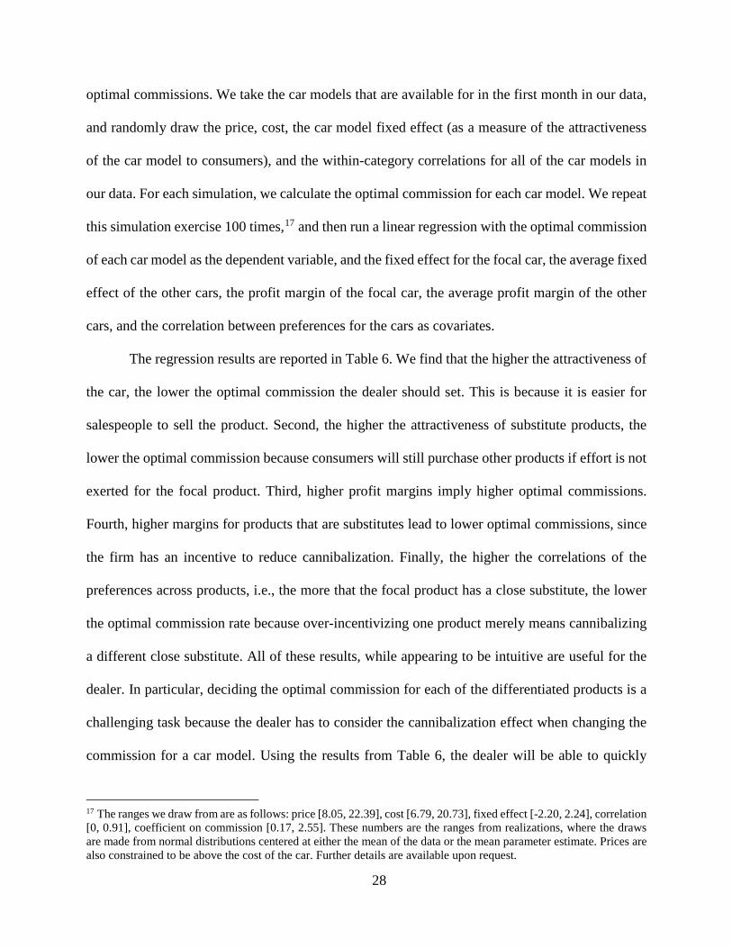
optimal commissions. We take the car models that are available for in the first month in our data,
and randomly draw the price, cost, the car model fixed effect (as a measure of the attractiveness
of the car model to consumers), and the within-category correlations for all of the car models in
our data. For each simulation, we calculate the optimal commission for each car model. We repeat
this simulation exercise 100 times,17 and then run a linear regression with the optimal commission
of each car model as the dependent variable, and the fixed effect for the focal car, the average fixed
effect of the other cars, the profit margin of the focal car, the average profit margin of the other
cars, and the correlation between preferences for the cars as covariates.
The regression results are reported in Table 6. We find that the higher the attractiveness of
the car, the lower the optimal commission the dealer should set. This is because it is easier for
salespeople to sell the product. Second, the higher the attractiveness of substitute products, the
lower the optimal commission because consumers will still purchase other products if effort is not
exerted for the focal product. Third, higher profit margins imply higher optimal commissions.
Fourth, higher margins for products that are substitutes lead to lower optimal commissions, since
the firm has an incentive to reduce cannibalization. Finally, the higher the correlations of the
preferences across products, i.e., the more that the focal product has a close substitute, the lower
the optimal commission rate because over-incentivizing one product merely means cannibalizing
a different close substitute. All of these results, while appearing to be intuitive are useful for the
dealer. In particular, deciding the optimal commission for each of the differentiated products is a
challenging task because the dealer has to consider the cannibalization effect when changing the
commission for a car model. Using the results from Table 6, the dealer will be able to quickly
17 The ranges we draw from are as follows: price [8.05, 22.39], cost [6.79, 20.73], fixed effect [-2.20, 2.24], correlation [0, 0.91], coefficient on commission [0.17, 2.55]. These numbers are the ranges from realizations, where the draws are made from normal distributions centered at either the mean of the data or the mean parameter estimate. Prices are also constrained to be above the cost of the car. Further details are available upon request.

29
calculate an approximately optimal commission level for each product, without going through the
optimization procedure that we have conducted.18
Table 6. Results from optimal commission regression
3.4.2 The profit impact of discounting prices and increasing commissions
In marketing, the use of price promotions is a popular “pull” strategy to stimulate sales. Another
strategy that is popular in many industries is to use commissions to incentivize salespeople to
invest service efforts thus help increase sales. This can be viewed as a “push” strategy. Our model
allows firms to evaluate and compare the effectiveness of the “pull” and “push” strategies within
a unified framework.
We use a counterfactual exercise as an illustration. We assume that the dealer’s goal is to
increase the sales of car model 6 in the MPV class by 50% in the first month of the data because
of the need to clear the excess inventory. The dealer can either discount the selling price of the car
model or increase the commission for salespeople who successfully sell a car.19 We calculate the
18 The high R2 from the regression indicates the predictions from the linear regression model fit well with the actual optimal commissions. 19 When the selling price drops, the commission will also decrease based on the way it is calculated. To separate the effects of the “pull” from the “push” strategy, we assume that the commission rate will be adjusted upward to make the commission remain unchanged in the first case. We also assume the selling price remains unchanged when the commission increases in the second case.
Estimate SE t pIntercept -0.74 0.27 -2.71 0.01Baseline attractiveness -0.08 0.01 -5.87 0.00Baseline attractiveness_others -0.12 0.07 -1.77 0.08Profit margin 0.61 0.01 105.05 0.00Profit margin_others -0.10 0.03 -3.80 0.00Correlation -0.04 0.02 -2.04 0.04R2 0.92
30
level of price discount and the commission increase the dealer has to offer in order to achieve the
goal. We then calculate the expected unit sales of other car models that can be affected by the sales
strategies (due to product cannibalization), and based on that calculate the total profits of the dealer.
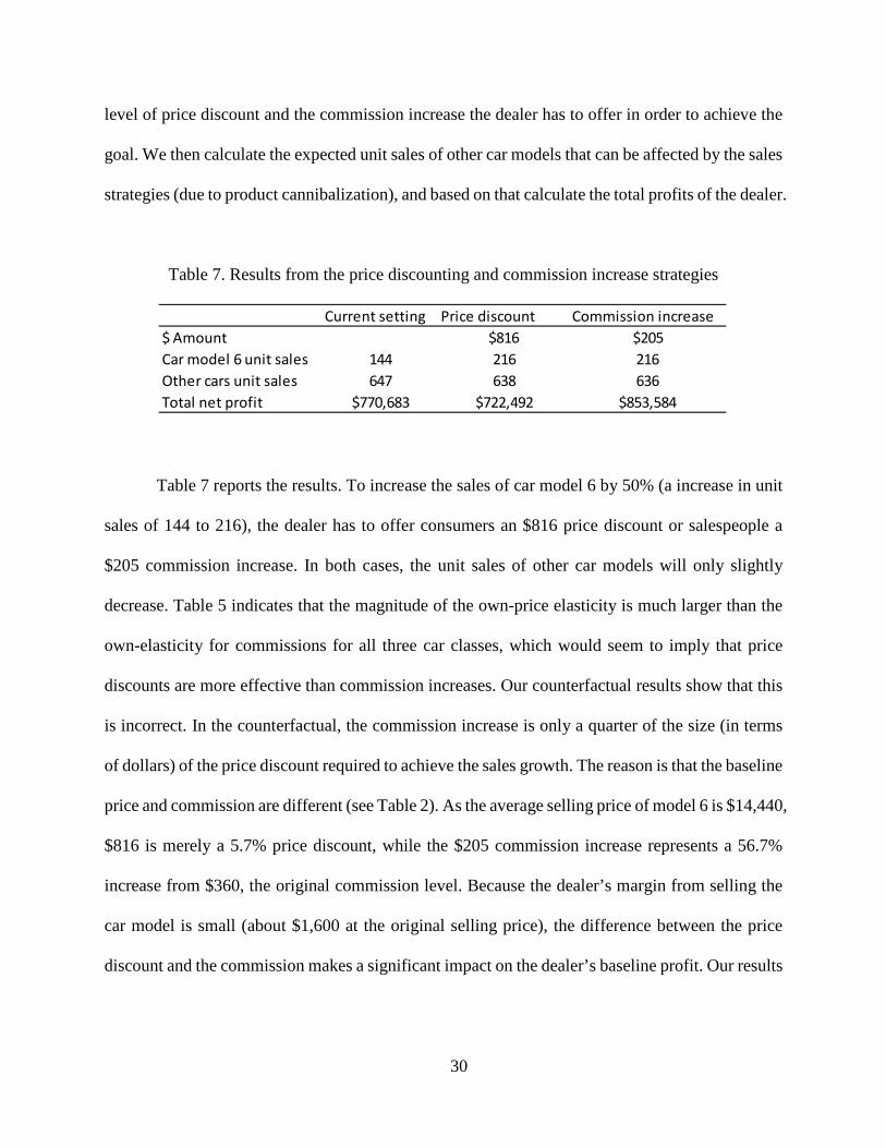
Table 7. Results from the price discounting and commission increase strategies
Table 7 reports the results. To increase the sales of car model 6 by 50% (a increase in unit
sales of 144 to 216), the dealer has to offer consumers an $816 price discount or salespeople a
$205 commission increase. In both cases, the unit sales of other car models will only slightly
decrease. Table 5 indicates that the magnitude of the own-price elasticity is much larger than the
own-elasticity for commissions for all three car classes, which would seem to imply that price
discounts are more effective than commission increases. Our counterfactual results show that this
is incorrect. In the counterfactual, the commission increase is only a quarter of the size (in terms
of dollars) of the price discount required to achieve the sales growth. The reason is that the baseline
price and commission are different (see Table 2). As the average selling price of model 6 is $14,440,
$816 is merely a 5.7% price discount, while the $205 commission increase represents a 56.7%
increase from $360, the original commission level. Because the dealer’s margin from selling the
car model is small (about $1,600 at the original selling price), the difference between the price
discount and the commission makes a significant impact on the dealer’s baseline profit. Our results
Current setting Price discount Commission increase$816 $205
Car model 6 unit sales 144 216 216647 638 636
$770,683 $722,492 $853,584
$ Amount
Other cars unit salesTotal net profit
31
show that the dealer’s profit will decrease by 6.25% for the price discount, while increase by 10.75%
for the commission increase.
Although the above counterfactual suggests that commission increases are more profitable
than price discounts, this result crucially depends on the price and commission coefficients. To
illustrate the effect across parameter values, we use further counterfactuals to investigate how a
firm’s optimal strategy may change under different commission coefficients. Specifically, we keep
the other model parameters unchanged and compare whether reducing prices or increasing
commissions is the better strategy when the commission coefficient for salespeople drops from the
average of 2.58 (see the last column of Table 4) to a lower level at 1, 0.7 or 0.5, respectively. We
again assume the dealer’s goal is to increase the sales of car model 6 by 50%, and calculate the
required price discount and commission increase for the dealer.
The results are reported in Table 8. When the commission coefficient is still high enough
(α = 1), we find that again it is more profitable for the dealer to only increase commissions ($559)
and not to cut the price. When the commission coefficient is much lower (α = 0.5), however, it is
more profitable for the dealer to only offer price discounts ($770) to consumers and not to change
commissions. This demonstrates the importance of quantifying the sensitivity of salespeople in
response to commission changes for the optimal promotion strategy. When the commission
coefficient is at the medium level (α = 0.7), it turns out to be optimal for the dealer to combine
both “pull” and “push” strategies. When there is a price discount, salespeople find it easier to sell
the car to wider audience of consumers; when the price discount is accompanied by a commission
increase, the salespeople have a greater incentive back up the sale with greater sale effort. This
result shows that when the salespeople’s sensitivity to commissions is neither too high nor too low,
the price discount and commission increase can complement the effectiveness of each other to

32
stimulate sales.20 These results also explain why car companies use both dealer cash and customer
cash, even though dealers only pass through a small fraction of the dealer cash (Busse et al. 2006).
Table 8. Optimal promotional strategies under different commission sensitivities
4. Conclusion
We develop a salesforce-driven model of consumer choice to study how performance-based
commissions incentivize a salesperson’s service effort toward heterogeneous, substitutable
products. This study bridges the gap between the consumer-choice literature and the salesforce-
management literature. In particular, the latter literature generally focuses only on how
commissions affect the performance of salespeople in terms of aggregate sales. In contrast, we
model the selling process as a joint decision by a salesperson and a consumer. The likelihood of
selling a product is influenced not only by the salesperson’s efforts induced by commissions but
also by the consumer’s innate product preferences. Our model thus allows the salesperson’s efforts
to vary across different transactions depending on the unique product preferences of each
consumer.
We estimate the model using data from a car dealership in Japan. The results show that not
only do consumers have heterogeneous product preferences but also salespeople have
heterogeneous sensitivity towards commissions. We then use counterfactuals to compare the
20 Whether it is optimal to cut prices or increase sales incentives also depends on the baseline prices and commission rates. Our key takeaway is what is optimal in our market, and understanding when one tool is likely to outweigh the other.
Price discount Commission increase$0 $559
$456 $311$770 $0
𝛼𝛼 = 1𝛼𝛼 = 0.7𝛼𝛼 = 0.5
33
effectiveness of using price promotions vs. commission incentives to increase sales. We also
illustrate how product-specific commissions should be set differently depending on the popularity
and substitutability of products.
Although our model makes significant progress toward accounting for salesforce effort in
modeling choices, it also has limitations. First, we assume that salespeople have perfect knowledge
regarding consumers’ product preferences. Future research may investigate how, when a
salesperson is uncertain of the consumer’s type, they will allocate different levels of service efforts
across differentiated products and how such uncertainty will impact the effectiveness of using
commissions as incentives. Second, if salespeople push the wrong products to consumers due to
high commissions, this can lead to increased dissatisfaction and reduced trust among consumers;
therefore, a short-term increase in profits may lead to a long-run cost for the dealer. In contrast,
price promotions directed to consumers will not have this issue. Such long term consequences have
not been studied in the paper. For simplicity our model also abstracts from how a price promotion
may act as an advertising that can attract more store visits from customers. Finally, we only study
consumer and salesforce decisions in a static framework, ignoring any dynamics that may arise if
quotas or ratcheting exist. Similarly, current performance might also affect a salesperson’s future
base salary and career movement. Therefore, the salesperson may face a dynamic optimization
problem, which is beyond the scope of the current study. We view this study as the first step in the
literature that simultaneously models the two-sided decisions in a market with differentiated
products. We hope our study will lead to more research in the future that can address the above
issues.
34
References
Albuquerque, P., & Bronnenberg, B. J. (2012). Measuring the impact of negative demand shocks
on car dealer networks. Marketing Science, 31(1), 4-23.
Basu, A. K., Lal, R., Srinivasan, V., &Staelin, R. (1985). Salesforce compensation plans: An
agency theoretic perspective. Marketing science, 4(4), 267-291.
Busse, Meghan, Jorge Silva-Risso and Florian Zettelmeyer (2006), “$1,000 Cash Back: The Pass-
Through of Auto Manufacturer Promotions,” American Economic Review, 96(4), 1253-1270.
Chung, D. J., Steenburgh, T., & Sudhir, K. (2013). Do bonuses enhance sales productivity? A
dynamic structural analysis of bonus-based compensation plans. Marketing Science, 33(2), 165-
187.
Copeland, A. M., & Monnet, C. (2003). The welfare effects of incentive schemes. Working paper.
Daljord, Ø., Misra, S., & Nair, H. S. (2016). Homogeneous Contracts for Heterogeneous Agents:
Aligning Sales Force Composition and Compensation. Journal of Marketing Research, 53(2),
161-182.
Farley, J. U. (1964). An optimal plan for salesmen's compensation. Journal of Marketing Research,
39-43.
35
Kim, T. T. (2014). When Franchisee Service Effort Affects Demand: An Application to the Car
Radiator Market and Resale Price Ceiling. Working Paper.
Kotler P., &Keller, K. (2008) Marketing Management (13th edition), Prentice Hall.
Lal, R., & Srinivasan, V. (1993). Compensation plans for single-and multi-product salesforces: An
application of the Holmstrom-Milgrom model.Management Science, 39(7), 777-793.
Mantrala, M. K., Albers, S., Caldieraro, F., Jensen, O., Joseph, K., Krafft, M., ... &Lodish, L.
(2010). Sales force modeling: State of the field and research agenda. Marketing Letters, 21(3),
255-272.
Misra, S. and Nair, H.S. (2011). A structural model of sales-force compensation dynamics:
Estimation and field implementation. Quantitative Marketing and Economics, 9(3), 211-257.
Petrin, A., & Train, K. (2010). A control function approach to endogeneity in consumer choice
models. Journal of marketing research, 47(1), 3-13.
Rao, R. C. (1990). Compensating heterogeneous salesforces: Some explicit solutions. Marketing
Science, 9(4), 319-341.
Srinivasan, V. (1981). An investigation of the equal commission rate policy for a multi-product
salesforce. Management Science, 27(7), 731-756.
36
Weinberg, C. B. (1975). An optimal commission plan for salesmen's control over
price. Management Science, 21(8), 937-943.
Yang, B., Chan, T.Y., Owan, H., Tsuru, T (2017). Incentives from compensation and career
movements. Working Paper.
Zoltners, A., Sinha, P., &Lorimer, S. (2008). Sales force effectiveness: A framework for
researchers and practitioners. Journal of Personal Selling and Sales Management 28, 115-131.


